VII International Conference on Computational PlasticityCOMPLAS 2003

E. Onate and D.R.J. Owen (Eds)c©CIMNE, Barcelona, 2003

COMPUTATIONAL MODELLING OF MOULDMANUFACTURE FOR THE LOST FOAM PROCESS

Jerzy Rojek?†, Francisco Zarate†, Carlos Agelet de Saracibar†, Michele

Chiumenti†, Miguel Cervera†, Peter M. Haigh‡, Chris Gilbourne‡ and Patrick

Verdot??

?Institute of Fundamental Technological Research (IPPT)Polish Academy of Sciences

Swietokrzyska 21, 00-049 Warszawa, Polande-mail: jrojek@ippt.gov.pl

†International Center for Numerical Methods in Engineering (CIMNE)Universidad Politecnica de Cataluna

Campus Norte UPC, 08034 Barcelona, Spaine-mail: cimne@etseccpb.upc.es, web page: http://cimne.upc.es/

‡Castings Technology International7 East Bank Road, Sheffield, UK

??Huttenes-Albertus FranceBP 30309, Z.I. de Pont Brenouille

60723 Pont Sainte Maxence, CEDEX, France

Key words: lost foam casting, mould manufacture, discrete element method

Abstract. This paper presents a numerical model of mould manufacture for the lost foamcasting process. The process of mould filling with sand and sand compaction by vibrationare modelled using spherical (in 3D) or cylindrical (in 2D) discrete elements. The motionof discrete elements is described by means of equations of rigid body dynamics. Rigidparticles interact among one another with contact forces, both in normal and tangentialdirections. Numerical simulation predicts defects of the mould due to insufficient sandcompaction around the pattern. Combining the discrete element model of sand with thefinite element model of the pattern allows us to detect possible distortion of the patternduring mould filling and compaction. Results of numerical simulation are validated bycomparison with experimental data.

1

J. Rojek et al.

1 INTRODUCTION

Lost foam casting (LFC) is a type of metal casting process that uses a sand mouldwith a polystyrene foam pattern remaining in the mould during metal pouring. The foampattern is replaced by molten metal, producing the casting. This process gives near netshape castings of high quality and definition and provides a design flexibility not givenby other casting technologies, but on the other hand the technology of LFC poses seriousdifficulties, production of a good mould being one of them.

The production of moulds for LFC process involves three steps. It is started with theplacement of the pattern in the moulding box. Next, the pattern is covered with dryand unbonded sand. Then the compaction of the sand is achieved by a vibration process.Once the compaction is complete, the mould is ready to be poured.

Vibratory compaction is one of the most important phases of the LFC process and itmay be critical to obtain a good quality cast product. Vibration should ensure uniformand proper compaction, by filling all the cavities with the sand and packing sand tomaximum density around the pattern. There is no simple relationship between sandparameters and vibration process parameters, therefore the compaction process is oftendesigned in a purely empirical trial and error manner.

Other defects occurring in the LFC process are the shape defects due to deformationof pattern under sand pressure during filling and the vibration process. This phenomenonhas also been studied in our numerical model.

2 BASIC ASSUMPTIONS OF THE NUMERICAL MODEL OF

THE MOULDING PROCESS

The objective of the computational model developed is to provide a more rational wayto design the filling and compaction process. The main physical phenomenon consideredis the flow of granular material (sand) around a rigid or deformable obstacle (mouldingbox, pattern) under gravity or vibration.

Numerical models of sand compaction adopted in the present study are based on thediscrete element method (DEM) which is widely recognized as a suitable tool to modelgranular materials [1], [2], [3], [4]. Within the DEM, it is assumed that the casting sand inthe LFC process can be represented as a collection of rigid particles (spheres or balls in 3Dand discs in 2D) interacting among themselves in the normal and tangential directions,due to friction.

The material model consisting of rigid spherical elements has been considered the mostsuitable to model the flow and re-arrangement of the sand grains induced by vibration.It would be difficult to capture properly the main characteristics of such a process usinga continuum formulation.

Obviously, it is not intended that each particle used in the DEM represents a sand grain,but it is assumed that the main characteristics of the (loose) sand behaviour during fillingand sand compaction can be macroscopically represented using the DEM. On the other

2

J. Rojek et al.

hand, it is also obvious that a large number of particles will lead to a better approximationof the results provided by the numerical method used, but a higher computational cost,in terms of computational time and computational resources, is necessary.

Different grain sizes were introduced into our computer model with the size distributionbeing a function of the sand granulometry.

To allow us to predict the cellular foam pattern deformation during mould filling andcompaction the Discrete Element Method is combined with the Finite Element Method.A general model consists of discrete elements representing sand and finite elements dis-cretising a deformable pattern.

3 DISCRETE ELEMENT METHOD FORMULATION

The DEM scheme using spherical rigid elements has been introduced by Cundall [1, 5].Our study is based on our own implementation of the DEM in the finite element explicitdynamic code Simpact [6].

3.1 Equations of motion

X

x

Y

y

Z

zt = 0

x

z

yX

0

X

u

F

T

Figure 1: Motion of a rigid particle

The translational and rotational motion of rigid spherical or cylindrical particles (Fig.1) is described by means of Newton-Euler equations of rigid body dynamics. For the i-thelement we have

miui = Fi , (1)

Iiωi = Ti , (2)

where u is the element centroid displacement in a fixed (inertial) coordinate frame X,ω – angular velocity, m – element (particle) mass, I – moment of inertia, F – resultantforce, and T – resultant moment about the central axes. Vectors F and T are sums of allforces and moments applied to the i-th element due to external load, contact interactionswith neighbouring spheres and other obstacles, as well as forces resulting from damping

3

J. Rojek et al.

in the system. The form of rotational equation (2) is valid for spheres and cylinders (in2D) and is simplified with respect to a general form for an arbitrary rigid body with therotational inertial properties represented by the second order tensor. In general case it ismore convenient to describe the rotational motion with respect to co-rotational frame x

which is embedded in each element since in this frame the tensor of inertia is constant.The tensor of inertia for a sphere or cylinder (in 2D) does not change in the fixed globalcoordinate system X, so in this case the rotational motion can be easily considered in thissystem.

Equations of motion (1) and (2) are integrated in time using a central difference scheme.Time integration operator for the translational motion at the n-th time step is as follows:

uni =

Fni

mi

, (3)

un+1/2i = u

n−1/2i + un

i ∆t , (4)

un+1i = un

i + un+1/2i ∆t . (5)

The first two steps in the integration scheme for rotational motion are identical to thosegiven by Eqs. (3) and (4):

ωni =

Tni

Ii

, (6)

ωn+1/2i = ω

n−1/2i + ω

ni ∆t . (7)

For the rotational plane (2D) motion the rotation angle θi can be obtained similarlyas displacement vector ui:

θn+1i = θn

i + ωn+1/2i ∆t . (8)

In three-dimensional motion, rotational position cannot be defined by any vector — ro-tational velocity ω cannot be integrated, cf. [7]. The rotation matrix Λi is used to definethe rotational position of the moving frame xi with respect to the inertial frame X

X = Λixi . (9)

The rotation matrix Λi is updated according to the following algorithm, cf. [7], [8]:

∆θi = ωn+1/2i ∆t , (10)

∆Λi = cos ‖∆θi‖1 +sin ‖∆θi‖

‖∆θi‖∆θi +

1 − cos ‖∆θi‖

‖∆θi‖2∆θi∆θ

Ti , (11)

Λn+1i = ∆Λi Λ

ni . (12)

4

J. Rojek et al.

Here ∆θ = {∆θx ∆θy ∆θz}T denotes the vector of incremental rotation, ∆Λ is the incre-

mental rotation matrix, and ∆θ is the skew-symmetric matrix defined as

∆θ =

0 −∆θz ∆θy

∆θz 0 −∆θx

−∆θy ∆θx 0

. (13)

It must be remarked that knowledge of the rotational configuration is not always nec-essary. If tangential forces are calculated incrementally, then knowledge of the vector ofincremental rotation ∆θ is sufficient. Then the steps (11) and (12) are not necessarywhich saves considerable computational cost of the time integration scheme.

3.2 Evaluation of contact forces

v2

w2

v1

w1

Fn

FT

Figure 2: Decomposition of the contact force

Once the contact for a pair of particles has been detected, the forces occurring at thecontact point are calculated. The interaction between the two bodies can be representedby the contact forces F1 and F2, which, by the Newton’s third law, will satisfy thefollowing relationship:

F1 = −F2 . (14)

We take F = F1 and decompose F into normal and tangential components, Fn and FT ,respectively (Fig. 2)

F = Fn + FT = Fnn + FT ,

where n is the unit vector normal to the particle surface at the contact point (this impliesthat it lies along the line connecting the centers of the two particles) and directed outwardsfrom the particle 1.

The contact forces Fn and FT are obtained using a constitutive model formulated forthe contact between two rigid spheres (Fig. 3). The contact interface in our formulationis characterized by the normal and tangential stiffness kn and kT , the Coulomb frictioncoefficient µ, and the contact damping coefficient cn.

5

J. Rojek et al.

kn

kT

cn

m

Figure 3: Model of the contact interface

The damping is used to dissipate kinetic energy and to decrease oscillations of thecontact forces. It is assumed to contribute to the normal contact force. Thus, we candecompose the normal contact force Fn to the elastic part Fne and to the damping contactforce Fnd

Fn = Fne + Fnd . (15)

The elastic part of the normal contact force Fne is proportional to the normal stiffnesskn and the penetration of the two particle surfaces urn

Fne = knurn . (16)

The penetration is calculated as

urn = d − r1 − r2 , (17)

where d is the distance of the particle centres, and r1, r2 their radii. In the formulationused in the present study no cohesion is allowed, so no tensile normal contact forces areallowed

Fne ≤ 0 . (18)

If urn < 0, the formula (16) is valid, otherwise Fne = 0.The contact damping force is assumed to be of viscous type

Fnd = cnvrn (19)

proportional to the normal relative velocity vrn of the centres of the two particles incontact

vrn = (u2 − u1) · n . (20)

The value of damping cn can be taken as a fraction of the critical damping Ccr for thesystem of two rigid bodies with masses m1 and m2, connected with a spring of the stiffnesskn (cf. [9])

Ccr = 2

√m1m2kn

m1 + m2

. (21)

6

J. Rojek et al.

urT

FT

Fn

|| ||

| |m

urT

FT

Fn

|| ||

| |m

kT

a) b)

Figure 4: Friction force vs. relative tangential displacement a) Coulomb law, b) regularized Coulomb law

The tangential reaction FT is brought about by friction opposing the relative motion atthe contact point. The relative tangential velocity at the contact point vrT is calculatedfrom the following relationship

vrT = vr − vr · n , (22)

vr = (u2 + ω2 × rc2) − (u1 + ω1 × rc1) , (23)

where u1, u2, and ω1, ω2 are the translational and rotational velocities of the particles,and rc1 and rc2 are the vectors connecting particle centres with contact points.

The relationship between the friction force ‖FT‖ and relative tangential urT displace-ment for the classical Coulomb model (for a constant normal force Fn) is shown in Fig.4a. This relationship would produce non physical oscillations of the friction force in thenumerical solution due to possible changes of the direction of sliding velocity. To preventthis the Coulomb friction model must be regularized. A possible regularization procedureinvolves decomposition of the tangential relative velocity into a reversible and irreversibleparts, vr

rT and virrT , respectively:

vrT = vrrT + vir

r . (24)

This is equivalent to formulation of the frictional contact as a problem analogous to that ofelastoplasticity, which can be seen clearly from the friction force-tangential displacementrelationship in Fig. 4b. This analogy allows us to calculate the friction force employingthe radial return algorithm analogous to that used in elastoplasticity. First a trial stateis calculated

FtrialT = Fold

T − kTvrT ∆t , (25)

and then the slip condition is checked

φtrial = ‖FtrialT ‖ − µ|Fn| . (26)

7

J. Rojek et al.

If φtrial ≤ 0, we have the case of stick contact and the friction force is assigned the trialvalue

FnewT = Ftrial

T , (27)

otherwise (slip contact) a return mapping is performed

FnewT = µ|Fn|

FtrialT

‖FtrialT ‖

. (28)

3.3 Rolling resistance

The sliding friction cannot provide any resistance to the movement of the sphere (cylin-der) rolling on a rough surface if there is no relative tangential velocity at the contactpoint (vrT = 0). The rolling resistance can be simulated numerically by applying therolling contact moment

M = a|Fn| , (29)

which appears due to the eccentricity a of the normal reaction Fn (Fig. 5).

w

Fn

-Fn

a

Figure 5: Resisting moment due to the eccentricity of the normal reaction

3.4 Background damping

A quasi-static state of equilibrium of the assembly of particles can be achieved byapplication of adequate damping. Described previously contact damping is a function ofthe relative velocity of the contacting body. It is sometimes necessary to apply damping fornon-contacting particles to dissipate their energy. There are two types of such damping,referred here as background, implemented in our formulation, one of viscous type and theother of non-viscous type. In both cases damping terms F

dampi and T

dampi are added to

equations of motion (1) and (2)

miui = Fi + Fdampi , (30)

Iiωi = Ti + Tdampi . (31)

with damping terms given by:

8

J. Rojek et al.

• for viscous dampingF

dampi = −αvtmiui , (32)

Tdampi = −αvrIiωi , (33)

• for non-viscous damping

Fdampi = −αnvt‖Fi‖

ui

‖ui‖, (34)

Tdampi = −αnvr‖Ti‖

ωi

‖ωi‖. (35)

where αvt, αvr, αnvt and αnvr are respective damping constants. It can be seen fromEqs. (32)–(35) that non-viscous like viscous damping is opposite to velocity, the differ-ence consists in the evaluation of the magnitude of damping force – viscous damping isproportional to the magnitude of velocity, while non-viscous damping is proportional tothe magnitude of resultant force and moment.

3.5 Numerical stability

Explicit integration in time yields high computational efficiency. Therefore the methodenables us to analyse large models. The known disadvantage of the explicit integrationscheme is its conditional numerical stability imposing the limitation on the time step ∆t.The time step ∆t must not be larger than a critical time step ∆tcr

∆t ≤ ∆tcr (36)

determined by the highest natural frequency of the system ωmax

∆tcr =2

ωmax

. (37)

If damping exists, the critical time increment is given by

∆tcr =2

ωmax

(√1 + ξ2 − ξ

), (38)

where ξ is the fraction of the critical damping corresponding to the highest frequencyωmax. Exact determination of the highest frequency ωmax would require a solution ofthe eigenvalue problem defined for the whole system of connected rigid particles. In anapproximate solution procedure, eigenvalue problems can be defined separately for everyrigid particle using the linearized equations of motion

miri + kiri = 0 , (39)

9

J. Rojek et al.

where

mi = {mi mi mi Ii Ii Ii}T , ri = {(ux)i (uy)i (uz)i (θx)i (θy)i (θz)i}

T , (40)

and ki is the stiffness matrix accounting for the contributions from all the penalty con-straints active for the i-th particle. Equation (40) defines the vectors mi and ri for a spher-ical particle in three-dimensional space. For a cylindrical particle in a two-dimensionalmodel the respective vectors are defined as follows:

mi = {mi mi Ii}T , ri = {(ux)i (uy)i (θz)i}

T . (41)

Equation (39) leads to an eigenproblem

kiri = λjmiri , (42)

where eigenvalues λj (j = 1, . . . , 6 in 3D case, and j = 1, 2, 3 for 2D case) are the squaredfrequencies of free vibrations:

λj = ω2j . (43)

In a 3D problem, three of six frequencies ωj are translational, and the other three –rotational.

In the algorithm implemented, a further simplification is assumed. The maximumfrequency is estimated as the maximum of natural frequencies of mass–spring systemsdefined for all the particles with one translational and one rotational degree of freedom.The translational and rotational free vibrations are governed by the following equations:

miun + knun = 0 , (44)

Iiθ + kθθ = 0 , (45)

where it is assumed that the translational motion is due to the contact interaction in thenormal direction (the spring stiffness kn represents the penalty stiffness in the normaldirection), and the rotational stiffness is due to the contact stiffness (penalty) in thetangential direction. Given the tangential penalty kT , it can be shown that the rotationalstiffness kθ can be obtained as

kθ = kT r2 , (46)

where r is the length of the vector connecting the mass centre to the contact point.The natural frequency of the translational vibrations is given by the following equation:

ωn =

√kn

mi

, (47)

while the rotational frequency ωθ can be obtained from the formula

ωθ =

√kθ

Ii

. (48)

10

J. Rojek et al.

With the rotational inertia of a sphere

I =2

5mr2 (49)

and kθ given by Eq. (46), the rotational frequency can be calculated as

ωθ =

√5kT

2mi

. (50)

If kT = kn, the rotational frequency ωθ is considerably higher than the translationalfrequency ωn obtained from Eq. (47), which results in a smaller critical time increment, cf.Eq. (37). To avoid the determination of a critical time step by the rotational frequencies,the rotational inertia terms are scaled adequately. The concept of scaling rotational inertiaterms is commonly used for shell elements, cf. [10].

3.6 Contact search algorithm

Changing contact pairs of elements during the analysis process must be automaticallydetected. The simple approach to identify interaction pairs by checking every sphereagainst every other sphere would be very inefficient, with the computational time propor-tional to n2, where n is the number of elements. In our formulation the search is based onthe quad-tree and oct-tree structures. In this case the computation time of the contactsearch is proportional to n ln n, which allows us to use it for large systems.

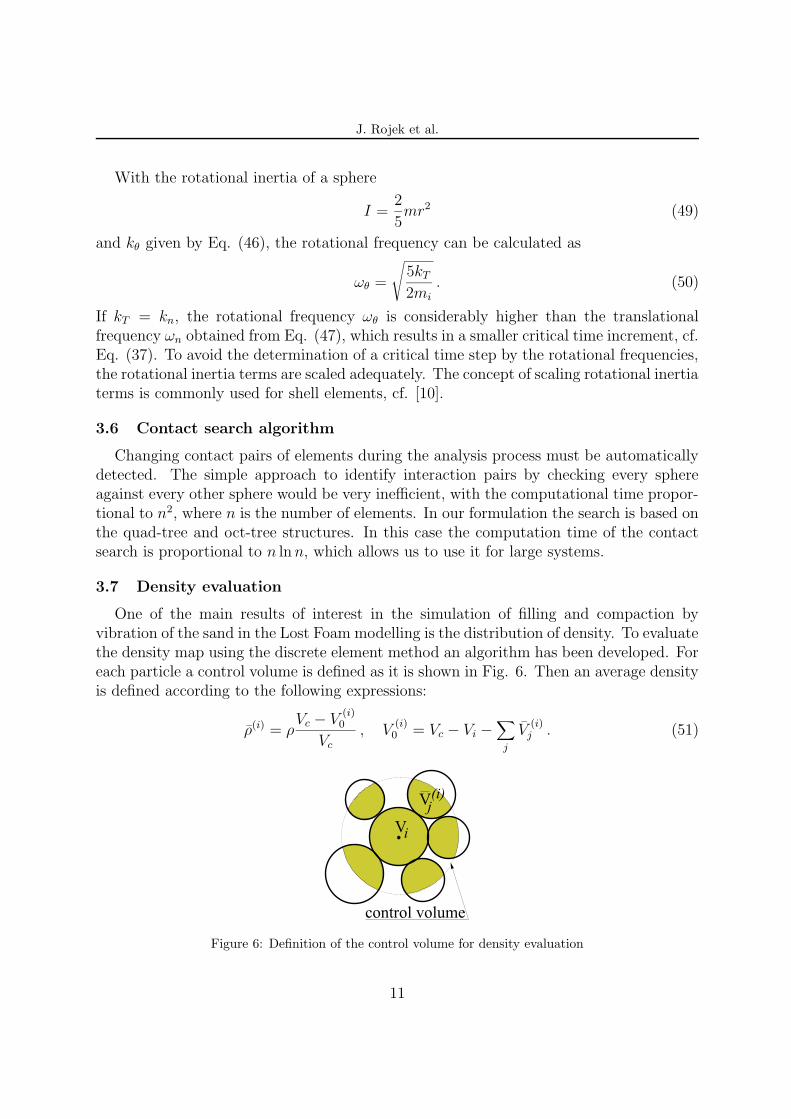
3.7 Density evaluation

One of the main results of interest in the simulation of filling and compaction byvibration of the sand in the Lost Foam modelling is the distribution of density. To evaluatethe density map using the discrete element method an algorithm has been developed. Foreach particle a control volume is defined as it is shown in Fig. 6. Then an average densityis defined according to the following expressions:

ρ(i) = ρVc − V

(i)0

Vc

, V(i)0 = Vc − Vi −

∑

j

V(i)j . (51)

control volume

V

V

i

j(i)

Figure 6: Definition of the control volume for density evaluation

11

J. Rojek et al.

In the computation of the average density associated to a particle, the intersection(common part) of the control volume with the volumes of interacting particles must becomputed. An exact analytical expression is used to compute these volumes.

3.8 Contact pressure evaluation

Contact pressure exerted by the sand on the pattern is another of the main results ofinterest in the moulding process. Figure 7 shows the scheme used to compute pressurefrom contact forces using the following formulae:

f(i)j = HjF

in , pj =

∑f(i)j

Aj

. (52)

Figure 7: Evaluation of contact forces and average contact pressure

3.9 Simulation of vibration process

In the computational simulation of the dynamics of the vibration process, the equationsof motion can be described relatively to a fixed system of reference X (cf. Fig. 8),

MX = F (53)

or alternatively, relative to a moving x system fixed to the vibrating box,

Mx = F − Ms (54)

Figure 8: Motion equations in a fixed and moving (fixed to the box) system

12

J. Rojek et al.

4 NUMERICAL EXAMPLES

The computational model developed by CIMNE has been implemented in an enhancedversion of the “in house” developed explicit dynamic computer code SIMPACT. SIMPACTis an explicit dynamic computer code mainly developed to simulate contact and impactdynamic problems. Further developments on the code have been necessary in order todeal with the computational simulation of the moulding process.

The numerical model described in the previous section has been implemented in acomputer program. Different computational simulations have been performed in order toassess the formulation developed for the sand flow and compaction by vibration withinthe lost foam technology. Here four simulation tests are considered. In the first test, therepose angle was evaluated. In the second example the flow of sand into horizontal tubeunder vibration was studied. Third example shows the possibility to study deformationof the pattern under sand pressure during mould filling and vibration. The last examplepresents possibilities of 3D simulation for a test pattern geometry. Numerical results arecompared with experimental data.

4.1 Repose angle test

Simple experiments of emptying a small hopper have been carried out to obtain therepose angle of different sand types. Experiments yielded the repose angle values rangingfrom 25◦ to 36◦. Two of the sand configurations discharged from a small hopper are shownin Fig. 9. The lowest values of repose angle, 25 − 26◦ correspond to the cerabead, anartificial sand characterized by perfectly rounded grains.

This test has been used to validate the performance of numerical model. 2D numericalmodel has been created. The sand has been represented by 10,700 particles of differentsize, their diameters ranging from 1 to 4.5 mm and size distribution according to thegranulometry of the real sand. The particle size has been scaled 4 times with respect tosand grain size.

Figure 9: Experimental repose angle, a) sand used in the foundry of Castings Technology International(England), b) artificial sand cerabead

13

J. Rojek et al.

25o

a) b)

Figure 10: Numerical simulation of the repose angle test, a) initial configuration, b) final configuration

The test has also served to assess parameters for the numerical model. Different analysishave been made using different model features. Figure 10 shows the computational resultsobtained using the following parameters: mass density ρ = 2400 kg/m3, inter-particlecontact normal and tangential stiffness kn = kT = 7·104 N/m, Coulomb friction coefficientµ = 0.8, contact damping ξ = 1.0 (equal to the critical damping), rigid wall-particlecontact characterized with kn = kT = 2 · 104 N/m, Coulomb friction coefficient µ = 0.35,contact damping ξ = 0.95, and rolling resistance parameter a was assumed 0.1 of theparticle radii. Small background damping was taken using αnvt = 0.03 and αnvr = 0.3.

The repose angle obtained, 25◦, is close to the experimental results. It agrees especiallywell with the value for the cerabead sand.

4.2 Sand flow into horizontal tubes

A metal test piece consisting of a series of three tubes of different diameters (Fig. 11)was placed in the sand box. The box was filled and vibrated in the vertical direction,with vibration frequency being 50 Hz and acceleration amplitude of 1.5 G. Migration ofthe sand into the horizontal tubes has been investigated. The results of experiments fordifferent vibration periods are shown in Fig. 12.

Numerical simulation of this test has been carried out using 2D model with the tube oflargest diameter considered only. The model employed particles of the same characteristicsas those used in the previous example. Results of numerical analysis are shown in Fig. 13.A good correlation of the numerical results with the experimental ones can be observed.

14

J. Rojek et al.

a) b)

Figure 11: Metal tubes, a) geometry definition, b) view of the tubes

6 cm

a) t = 0 s b) t=5 s

10 cm 15 cm

c) t = 20 s d) t = 40 s

Figure 12: Sand flow into horizontal tubes under vibration – experimental results

15

J. Rojek et al.

7 cm

a) t = 0 s b) t=5 s

11 cm 17 cm

c) t = 20 s d) t = 40 s

Figure 13: Sand flow into horizontal tubes under vibration – numerical results

4.3 Test with a L-shaped pattern

Distortion of a simple L-shaped pattern during filling and vibration has been studiedexperimentally and numerically. Experimental results show that the filling process distortsthe pattern (Fig. 14a) and that an area of low sand density exists below the horizontalsection. The pattern distortion although slightly reduced is still observed after vibration(Fig. 15a). During vibration the sand flows into the cavity below the horizontal part ofthe pattern.

Similar distortion of the pattern during filling and compaction has been predicted bynumerical analysis, cf. Figs. 14b and 15b. Numerical simulation has been carried outusing a 2D model of similar sand characteristics as those used in the two examples above.The pattern has been discretized with 4-node plain strain elements. Elastic propertiesof the polystyrene were characterized by Young’s modulus E = 6.4 MPa and Poissoncoefficient ν = 0.35, its density ρ = 12 kg/m3.

Figures 14 and 15 demonstrate a very good agreement of the pattern distortion obtainedin experiments and numerical simulation.

16

J. Rojek et al.

a) b)

Figure 14: Deformation of the foam pattern after mould filling, a) experiment, b) numerical simulation

a) b)

Figure 15: Deformation of the foam pattern after vibration, a) experiment, b) numerical simulation

4.4 3D test of layer-wise mould filling and compaction

Experimental study and 3D numerical analysis of mould filling and compaction havebeen carried out for a simple disc shape with a side bracket shown in Fig. 16. This designwas chosen as being able to characterise basic problems encountered in industrial LFCprocesses.

Sand was filled in layers and vibrated during filling. In order to validate the simulationof sand flow around the pattern, experimental trials were performed using coloured sandcontaining a chemical binder. Figure 17a shows a section through the sand block revealingthe test pattern and sand layers. Similar sand flow around the pattern has been obtainedin numerical simulation (Fig. 17b).

This example demonstrates the computational effectiveness of the numerical model andthe possibility to treat large models – in this case nearly 180,000 particles have been used.

17

J. Rojek et al.

a) b)

Figure 16: 3D test of moulding process, a) design of the test casting, b) the foam pattern

a) b)

Figure 17: Sand layers, a) experiment, b) numerical simulation

5 CONCLUSIONS

The following conclusions may be obtained:

• A numerical model based on the Discrete Element Method using spherical or cylin-drical rigid particles is suitable to model mould manufacture, sand filling and com-paction of sand by vibration.

• Computer implementation within the FE explicit dynamic code enables us to createa model combining the Discrete Element Method with the Finite Element Method,which gives the possibility to take into account deformation of the foam patternduring filling and vibration.

• Experimental validation tests show good correlation of numerical results with prac-tice.

• Numerical analysis can be used to find parameters characterizing mould manufactureprocess

18

J. Rojek et al.

• Computation cost time is quite expensive. Further possibilities to reduce computingincluding parallelisation of the code would be considered.

ACKNOWLEDGEMENT

Financial support of the European Commission through the Growth European ProjectGRD1-2000-25243 “Shortening Lead Times and Improving Quality by Innovative Upgrad-ing of the Lost Foam Casting Process (FOAMCAST)” is gratefully acknowledged.

19

J. Rojek et al.

REFERENCES

[1] P.A. Cundall and O.D.L. Strack. A discrete numerical method for granular assem-blies. Geotechnique, 2:47–65, 1979.

[2] C.S. Campbell. Rapid granular flows. Annual Review of Fluid Mechanics, 2:57–92,1990.

[3] Eng. Comput., 9(2), 1992. Special issue, Editor: G. Mustoe.

[4] J. Williams and R. O’Connor. Discrete element simulation and contact problem.Arch. Comp. Methods in Engineering, 6(4), 1999.

[5] P.A. Cundall. Formulation of a Three Dimensional Distinct Element Model — Part I.A Scheme to Detect and Represent Contacts in a System of Many Polyhedral Blocks.Int. J. Rock Mech., Min. Sci. & Geomech. Abstr., 25(3):107–116, 1988.

[6] J. Rojek, E. Oate, F. Zarate, and J. Miquel. Modelling of rock, soil and granularmaterials using spherical elements. In 2nd European Conference on ComputationalMechanics ECCM-2001, Cracow, 26-29 June, 2001.

[7] J. Argyris. An excursion into large rotations. Comput. Meth. Appl. Mech. Eng.,32:85–155, 1982.

[8] D.J. Benson and J.O. Hallquist. A simple rigid body algorithm for structural dy-namics programs. Int. J. Num. Meth. Eng., 12:723–749, 1986.

[9] L.M. Taylor and D.S. Preece. Simulation of blasting induced rock motion. Eng.Comput., 9(2):243–252, 1992.

[10] T.J.R. Hughes. The Finite Element Method. Linear Static and Dynamic Analysis.Prentice-Hall, 1987.

20