computational learning theory - uni-luebeck.de · c program – simulation of flips of a fair coin:...
TRANSCRIPT
Carla P. Gomes CS4700
Computational Learning Theory
Slides by Carla P. Gomes and Nathalie Japkowicz
(Reading: R&N AIMA 3rd ed., Chapter 18.5)

Carla P. Gomes CS4700
Inductive learning: given the training set, a learning algorithm generates a hypothesis. Run hypothesis on the test set. The results say something about how good our
hypothesis is. But how much do the results really tell you? Can we be certain about how the
learning algorithm generalizes? We would have to see all the examples.
Computational Learning Theory
Insight: introduce probabilities to measure degree of certainty and correctness (Valiant 1984).
Carla P. Gomes CS4700
Example: We want to use height to distinguish men and women drawing people from
the same distribution for training and testing. We can never be absolutely certain that we have learned correctly our target
(hidden) concept function. (E.g., there is a non-zero chance that, so far, we have only seen a sequence of bad examples)
E.g., relatively tall women and relatively short men… We’ll see that it’s generally highly unlikely to see a long series of bad
examples!
Computational Learning Theory

Carla P. Gomes CS4700
Aside: flipping a coin
Carla P. Gomes CS4700
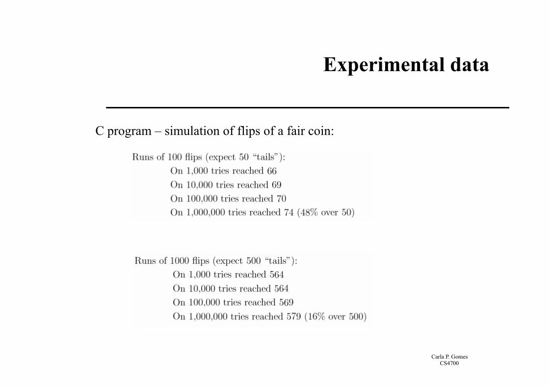
Experimental data
C program – simulation of flips of a fair coin:
Carla P. Gomes CS4700
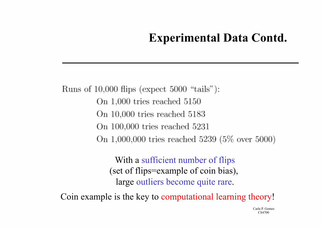
Experimental Data Contd.
Coin example is the key to computational learning theory!
With a sufficient number of flips (set of flips=example of coin bias), large outliers become quite rare.
Carla P. Gomes CS4700
Computational Learning Theory
Intersection of AI, statistics, and theory of computation. Introduce Probably Approximately Correct Learning concerning
efficient learning For our learning procedures we would like to prove that:
With high probability an (efficient) learning algorithm will find a hypothesis that is approximately identical to the hidden target concept.
Note the double “hedging” – probably and approximately.
Why do we need both levels of uncertainty (in general)?
Carla P. Gomes CS4700
Probably Approximately Correct Learning
Underlying principle:
Seriously wrong hypotheses can be found out almost certainly (with high probability) using a “small” number of examples
– Any hypothesis that is consistent with a significantly large
set of training examples is unlikely to be seriously wrong: it must be probably approximately correct.
– Any (efficient) algorithm that returns hypotheses that are PAC is called a PAC-learning algorithm
Carla P. Gomes CS4700
Probably Approximately Correct Learning
How many examples are needed to guarantee correctness?
– Sample complexity (# of examples to “guarantee” correctness) grows with the size of the Hypothesis space
– Stationarity assumption: Training set and test sets are drawn from the same distribution

Carla P. Gomes CS4700
Notations: – X: set of all possible examples – D: distribution from which examples are drawn – H: set of all possible hypotheses – N: the number of examples in the training set – f: the true function to be learned
Assume: the true function f is in H. Error of a hypothesis h wrt f :
Probability that h differs from f on a randomly picked example:
error(h) = P(h(x) ≠ f(x)| x drawn from D)
Exactly what we are trying to measure with our test set.
Notations
Carla P. Gomes CS4700
A hypothesis h is approximately correct if:
error(h) ≤ ε, where ε is a given threshold, a small constant
Goal:
Show that after seeing a small (poly) number of examples N, with high probability, all consistent hypotheses will be approximately correct. I.e, chance of “bad” hypothesis, (high error but consistent with examples) is
small (i.e, less than δ)
Approximately Correct
Carla P. Gomes CS4700
Approximately Correct
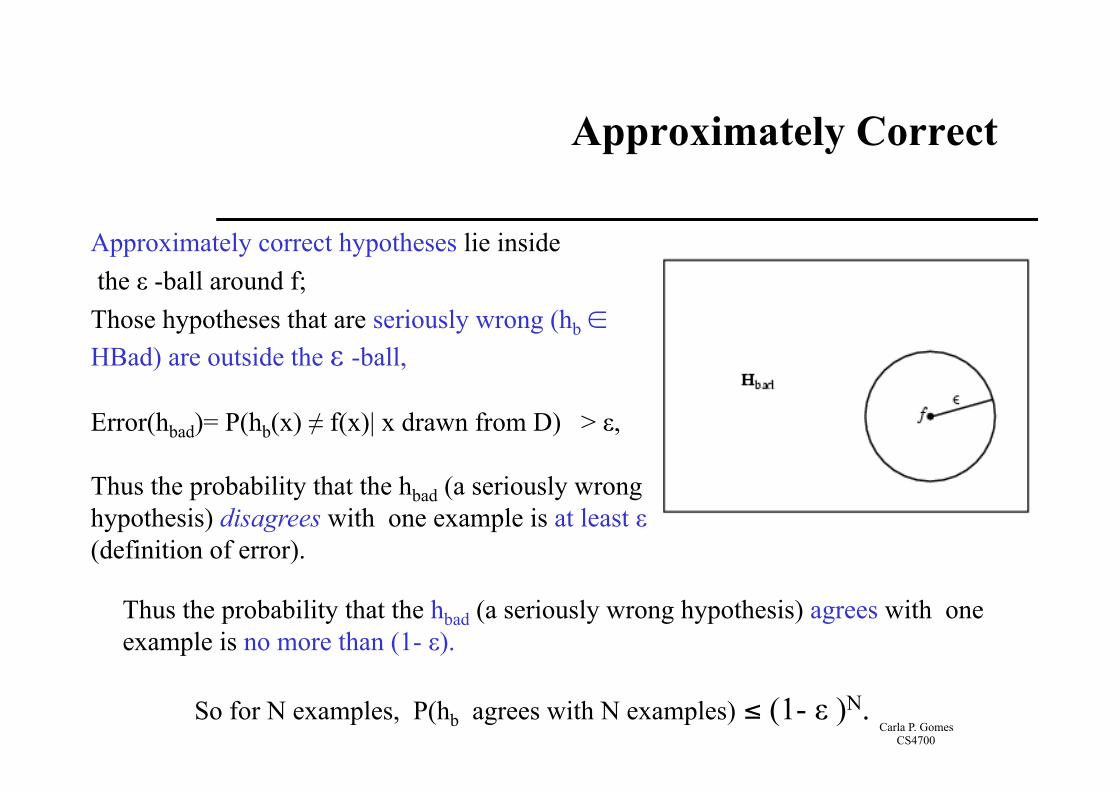
Approximately correct hypotheses lie inside the ε -ball around f; Those hypotheses that are seriously wrong (hb ∈ HBad) are outside the ε -ball, Error(hbad)= P(hb(x) ≠ f(x)| x drawn from D) > ε, Thus the probability that the hbad (a seriously wrong hypothesis) disagrees with one example is at least ε (definition of error).
Thus the probability that the hbad (a seriously wrong hypothesis) agrees with one example is no more than (1- ε).
So for N examples, P(hb agrees with N examples) ≤ (1- ε )N.
Carla P. Gomes CS4700
Approximately Correct Hypothesis
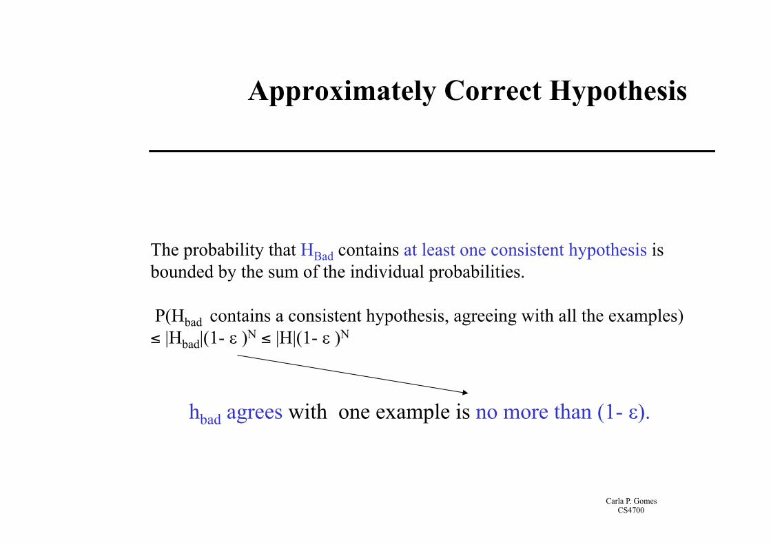
The probability that HBad contains at least one consistent hypothesis is bounded by the sum of the individual probabilities. P(Hbad contains a consistent hypothesis, agreeing with all the examples) ≤ |Hbad|(1- ε )N ≤ |H|(1- ε )N
hbad agrees with one example is no more than (1- ε).
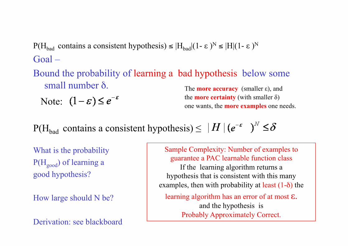
P(Hbad contains a consistent hypothesis) ≤ |Hbad|(1- ε )N ≤ |H|(1- ε )N
Goal – Bound the probability of learning a bad hypothesis below some
small number δ. What is the probability P(Hgood) of learning a good hypothesis? How large should N be? Derivation: see blackboard
Sample Complexity: Number of examples to guarantee a PAC learnable function class
If the learning algorithm returns a hypothesis that is consistent with this many
examples, then with probability at least (1-δ) the learning algorithm has an error of at most ε.
and the hypothesis is Probably Approximately Correct.
Note: The more accuracy (smaller ε), and the more certainty (with smaller δ) one wants, the more examples one needs.
P(Hbad contains a consistent hypothesis) ≤
Carla P. Gomes CS4700
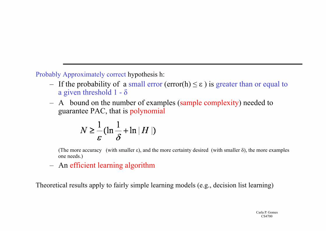
Probably Approximately correct hypothesis h: – If the probability of a small error (error(h) ≤ ε ) is greater than or equal to
a given threshold 1 - δ – A bound on the number of examples (sample complexity) needed to
guarantee PAC, that is polynomial
(The more accuracy (with smaller ε), and the more certainty desired (with smaller δ), the more examples one needs.)
– An efficient learning algorithm
Theoretical results apply to fairly simple learning models (e.g., decision list learning)
Carla P. Gomes CS4700
PAC Learning
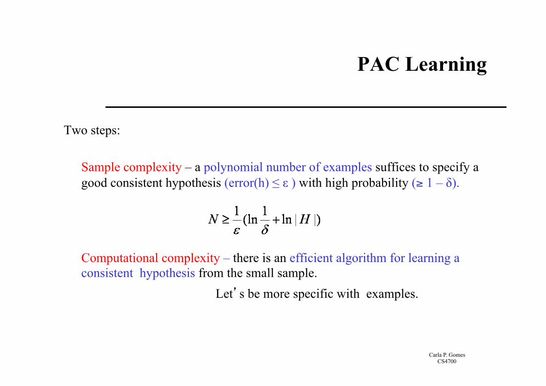
Two steps:
Sample complexity – a polynomial number of examples suffices to specify a good consistent hypothesis (error(h) ≤ ε ) with high probability (≥ 1 – δ).
Computational complexity – there is an efficient algorithm for learning a consistent hypothesis from the small sample.
Let’s be more specific with examples.
Carla P. Gomes CS4700
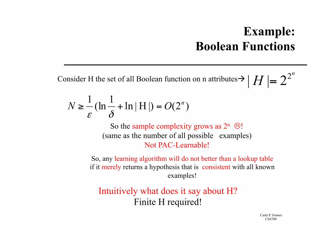
Example: Boolean Functions
Consider H the set of all Boolean function on n attributesà
)2(|)H|ln1(ln1 nON =+≥δε
n
H 22|| =
So the sample complexity grows as 2n L! (same as the number of all possible examples)
Not PAC-Learnable!
Intuitively what does it say about H? Finite H required!
So, any learning algorithm will do not better than a lookup table if it merely returns a hypothesis that is consistent with all known
examples!
Carla P. Gomes CS4700
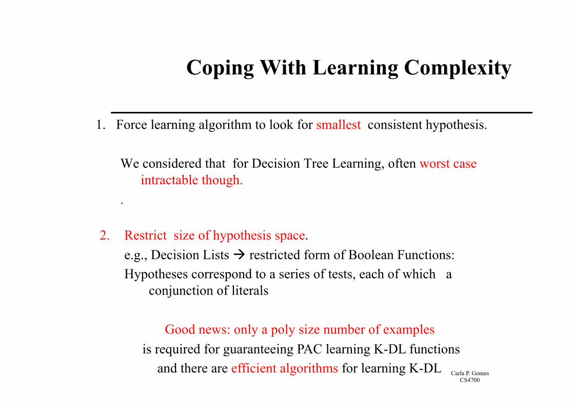
Coping With Learning Complexity
1. Force learning algorithm to look for smallest consistent hypothesis. We considered that for Decision Tree Learning, often worst case
intractable though. .
2. Restrict size of hypothesis space. e.g., Decision Lists à restricted form of Boolean Functions: Hypotheses correspond to a series of tests, each of which a
conjunction of literals
Good news: only a poly size number of examples is required for guaranteeing PAC learning K-DL functions
and there are efficient algorithms for learning K-DL

Carla P. Gomes CS4700
Decision Lists
Resemble Decision Trees, but with simpler structure: Series of tests, each test a conjunction of literals; If a test succeeds, decision list specifies value to return; If test fails, processing continues with the next test in the list.
No
Note: if we allow arbitrarily many literals per test , decision list can express all Boolean functions.
a=Patrons(x,Some) b=patrons(x,Full) c=Fri/Sat(x)
(a) (b∧c) Y Y N
Carla P. Gomes CS4700
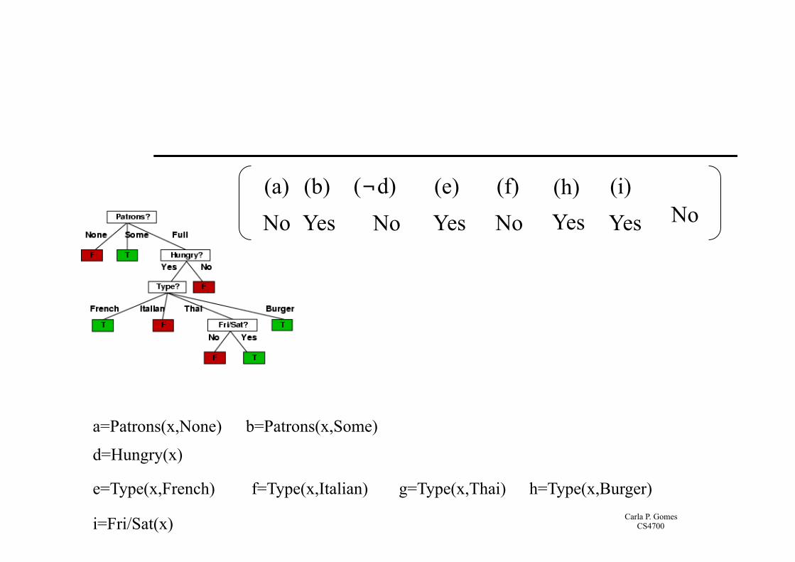
a=Patrons(x,None) b=Patrons(x,Some)
d=Hungry(x)
e=Type(x,French) f=Type(x,Italian) g=Type(x,Thai) h=Type(x,Burger)
i=Fri/Sat(x)
(a) No
(b) Yes
(¬d) No
(e) Yes
(h) Yes
(f) No
(i) Yes No
Carla P. Gomes CS4700
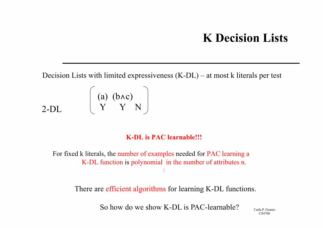
K Decision Lists
Decision Lists with limited expressiveness (K-DL) – at most k literals per test
K-DL is PAC learnable!!!
For fixed k literals, the number of examples needed for PAC learning a K-DL function is polynomial in the number of attributes n.
:
There are efficient algorithms for learning K-DL functions.
2-DL (a) (b∧c) Y Y N
So how do we show K-DL is PAC-learnable?
Carla P. Gomes CS4700
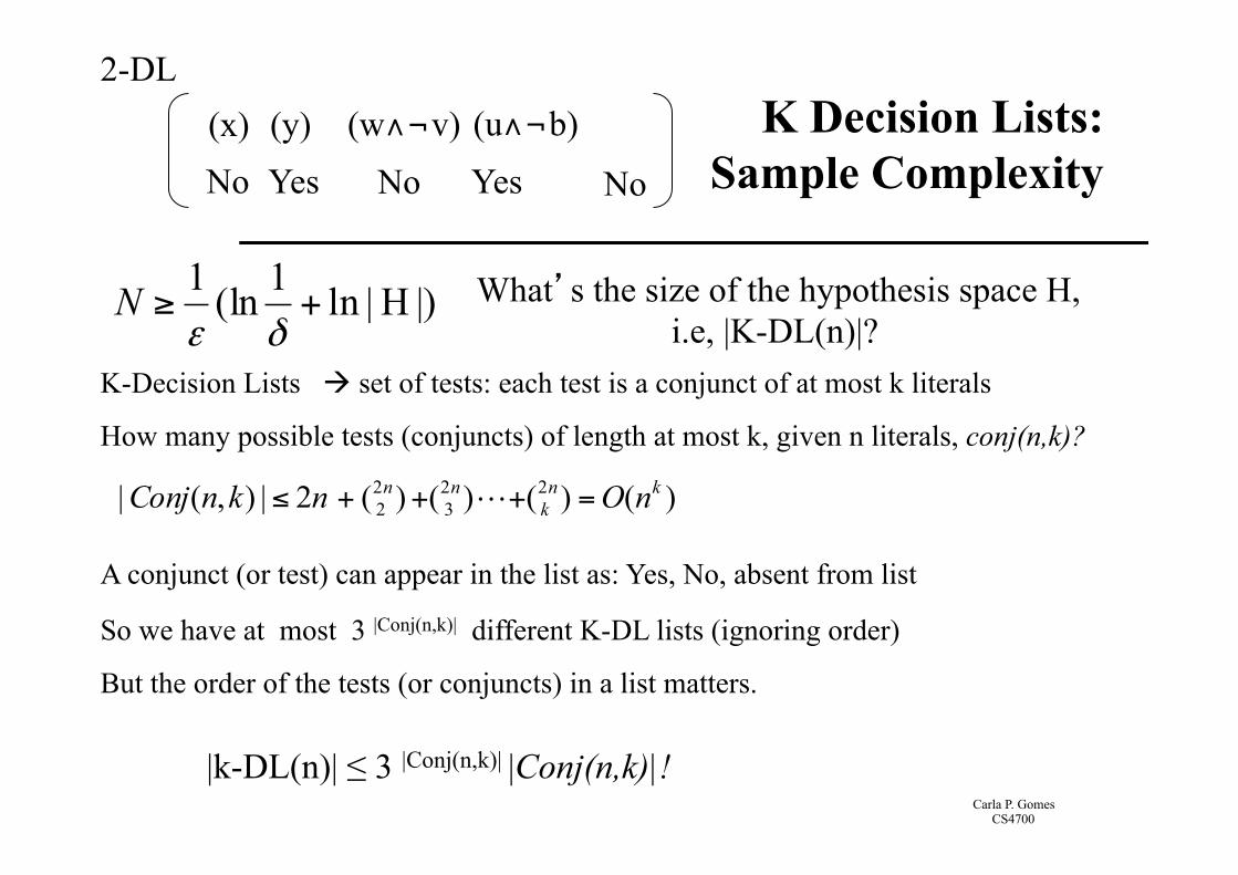
K-Decision Lists à set of tests: each test is a conjunct of at most k literals
(x) No
(y) Yes
(w∧¬v) No
(u∧¬b) Yes No
2-DL K Decision Lists:
Sample Complexity
|)H|ln1(ln1+≥
δεN What’s the size of the hypothesis space H,
i.e, |K-DL(n)|?
How many possible tests (conjuncts) of length at most k, given n literals, conj(n,k)?
)()()()(2|),(| 223
22
knk
nn nOnknConj =+++≤ !
A conjunct (or test) can appear in the list as: Yes, No, absent from list
So we have at most 3 |Conj(n,k)| different K-DL lists (ignoring order)
But the order of the tests (or conjuncts) in a list matters.
|k-DL(n)| ≤ 3 |Conj(n,k)| |Conj(n,k)|!
Carla P. Gomes CS4700
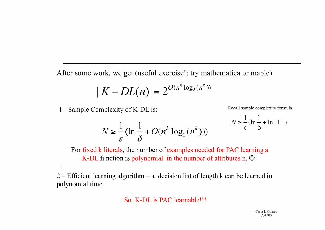
After some work, we get (useful exercise!; try mathematica or maple)
))(log( 22|)(|kk nnOnDLK =−
1 - Sample Complexity of K-DL is:
)))(log(1(ln12
kk nnON +≥δε
For fixed k literals, the number of examples needed for PAC learning a K-DL function is polynomial in the number of attributes n, J!
:
So K-DL is PAC learnable!!!
|)H|ln1(ln1+
δε≥N
Recall sample complexity formula
2 – Efficient learning algorithm – a decision list of length k can be learned in polynomial time.
Carla P. Gomes CS4700
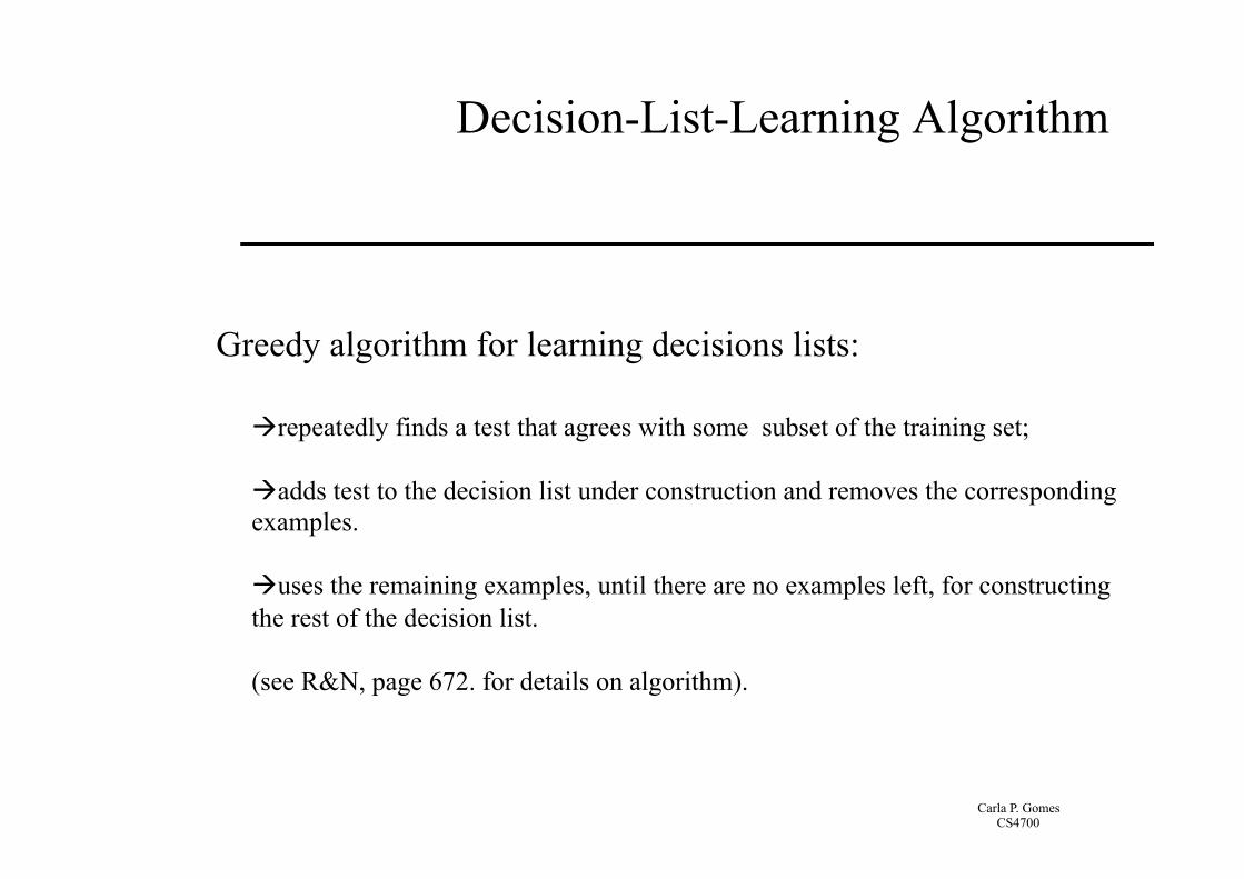
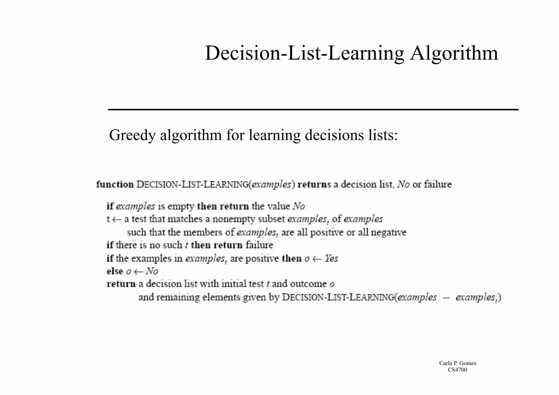
Decision-List-Learning Algorithm
àrepeatedly finds a test that agrees with some subset of the training set; à adds test to the decision list under construction and removes the corresponding examples. àuses the remaining examples, until there are no examples left, for constructing the rest of the decision list. (see R&N, page 672. for details on algorithm).
Greedy algorithm for learning decisions lists:
Carla P. Gomes CS4700
Decision-List-Learning Algorithm
Greedy algorithm for learning decisions lists:
Carla P. Gomes CS4700
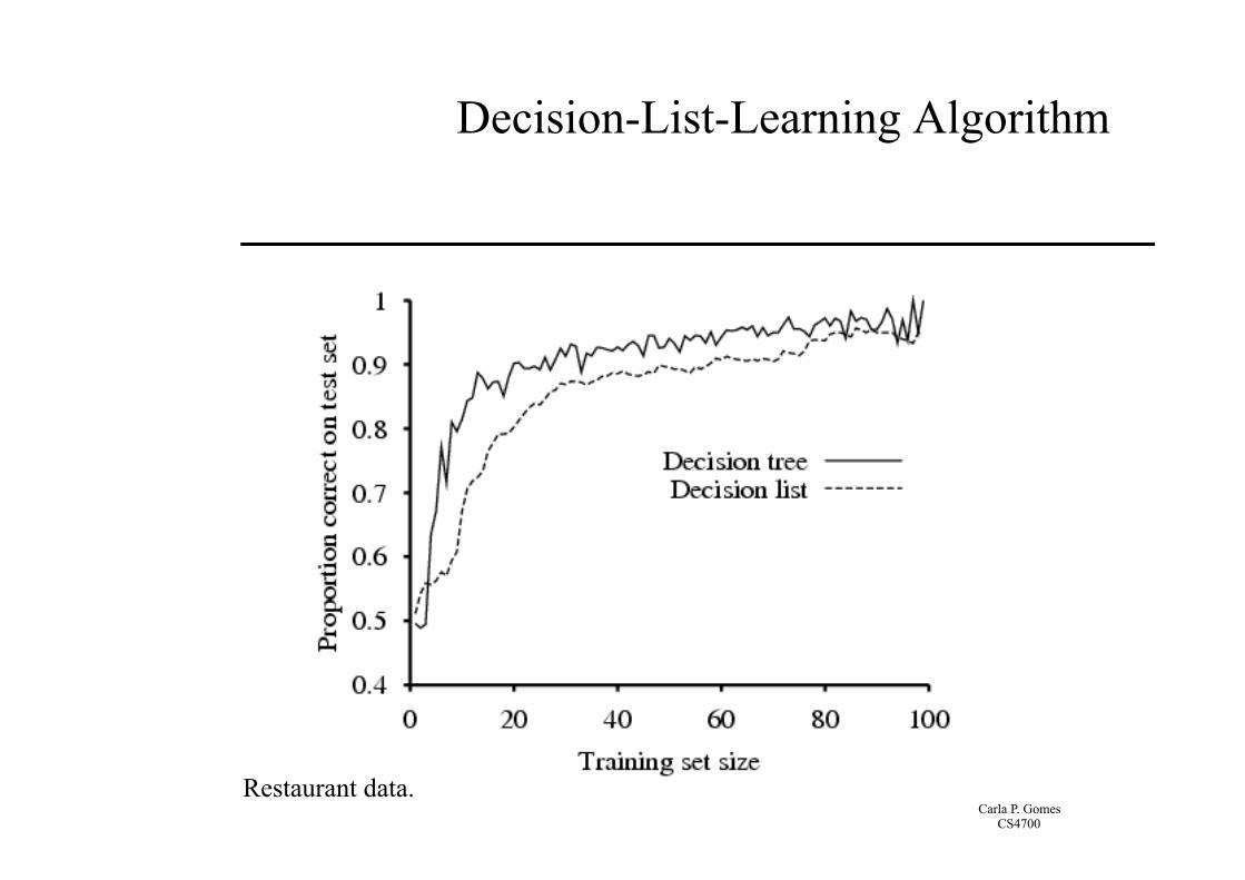
Decision-List-Learning Algorithm
Restaurant data.

Carla P. Gomes CS4700
Examples
1. H space of Boolean functions Not PAC Learnable, hypothesis space too big: need too many examples (sample complexity not polynomial)! 2. K-DL
PAC learnable 3. Conjunction of literals
PAC learnable
Carla P. Gomes CS4700
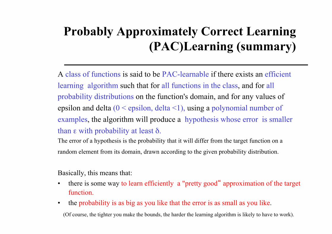
Probably Approximately Correct Learning (PAC)Learning (summary)
A class of functions is said to be PAC-learnable if there exists an efficient learning algorithm such that for all functions in the class, and for all probability distributions on the function's domain, and for any values of epsilon and delta (0 < epsilon, delta <1), using a polynomial number of examples, the algorithm will produce a hypothesis whose error is smaller than ε with probability at least δ. The error of a hypothesis is the probability that it will differ from the target function on a
random element from its domain, drawn according to the given probability distribution. Basically, this means that: • there is some way to learn efficiently a "pretty good“ approximation of the target
function. • the probability is as big as you like that the error is as small as you like. (Of course, the tighter you make the bounds, the harder the learning algorithm is likely to have to work).
Carla P. Gomes CS4700
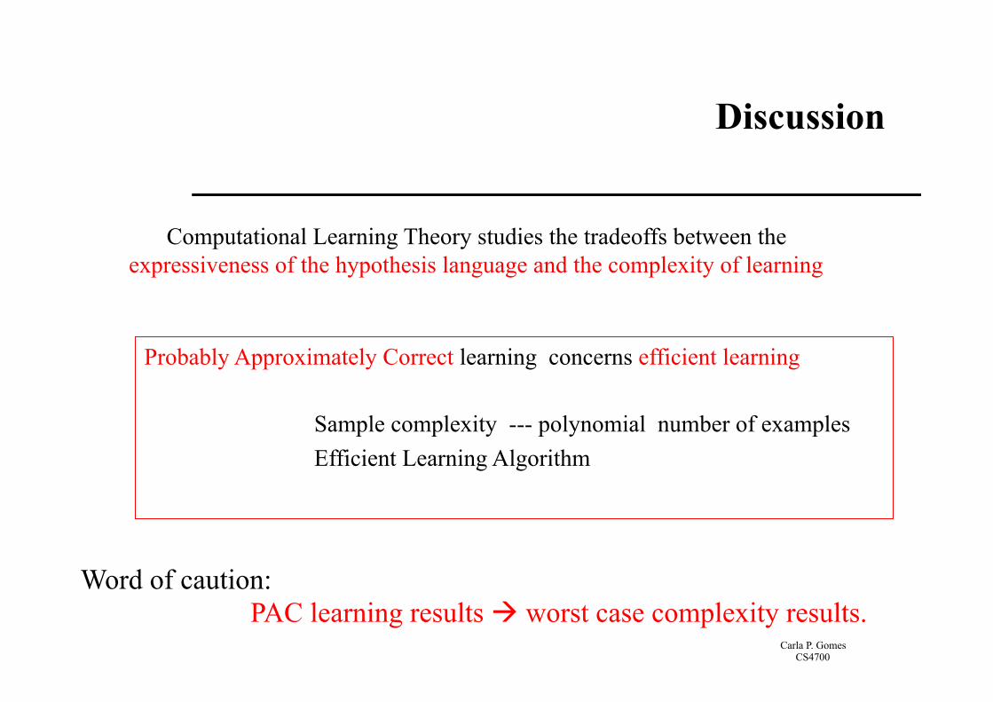
Discussion
Computational Learning Theory studies the tradeoffs between the expressiveness of the hypothesis language and the complexity of learning
Probably Approximately Correct learning concerns efficient learning
Sample complexity --- polynomial number of examples Efficient Learning Algorithm
Word of caution: PAC learning results à worst case complexity results.
Carla P. Gomes CS4700
30
Sample Complexity for Infinite Hypothesis Spaces I: VC-Dimension
• The PAC Learning framework has 2 disadvantages: – It can lead to weak bounds – Sample Complexity bound cannot be established for infinite hypothesis
spaces
• We introduce new ideas for dealing with these problems: – A set of instances S is shattered by hypothesis space H iff for every
dichotomy of S there exists some hypothesis in H consistent with this dichotomy.
Nathalie Japkowicz
Carla P. Gomes CS4700
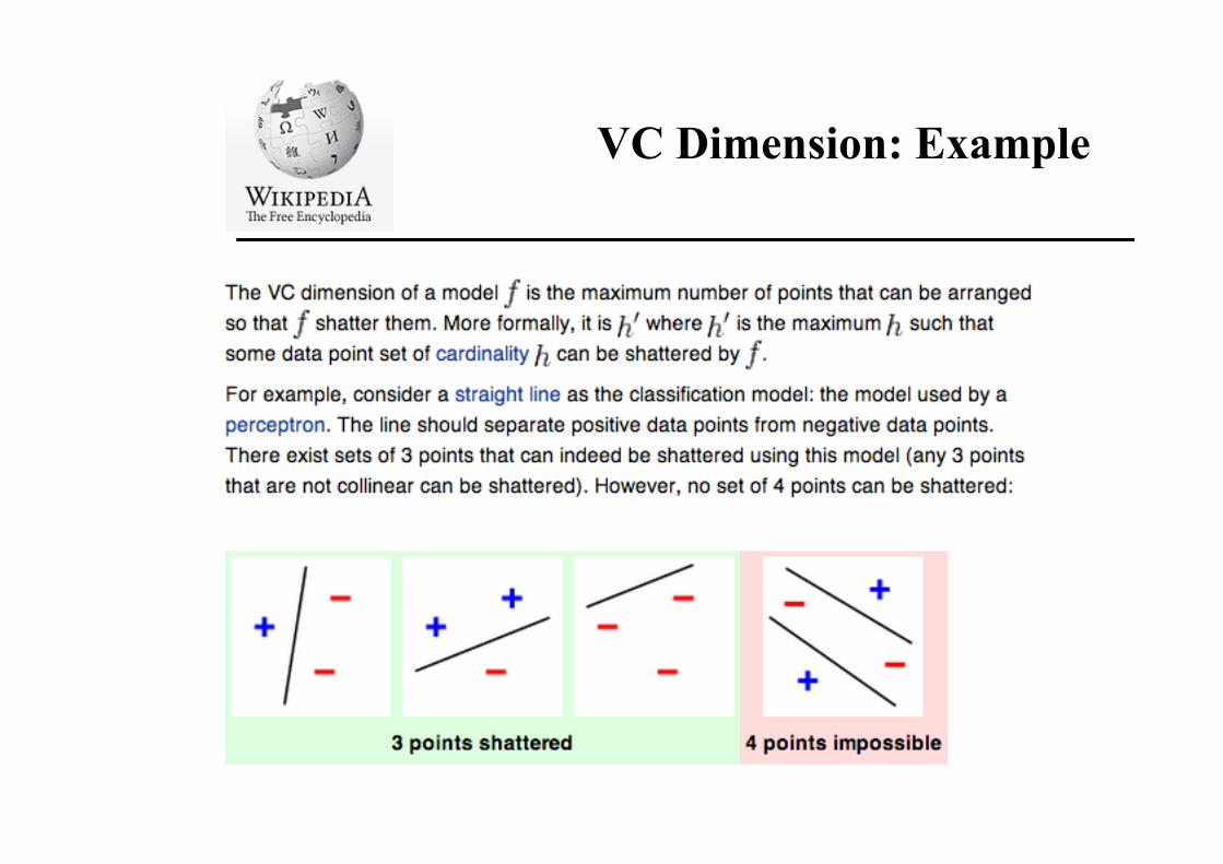
VC Dimension: Example
Carla P. Gomes CS4700
32
Sample Complexity for Infinite Hypothesis Spaces I: VC-Dimension
The Vapnik-Chervonenkis dimension, VC(H), of hypothesis space H defined over instance space X is the size of the largest finite subset of X shattered by H. If arbitrarily large finite sets of X can be shattered by H, then VC(H)=∞
Nathalie Japkowicz

Carla P. Gomes CS4700
33
VC Dimension: Example 2
• H = Axis parallel rectangles in R2
• What is the VC dimension of H • Can we PAC learn?
Carla P. Gomes CS4700
34
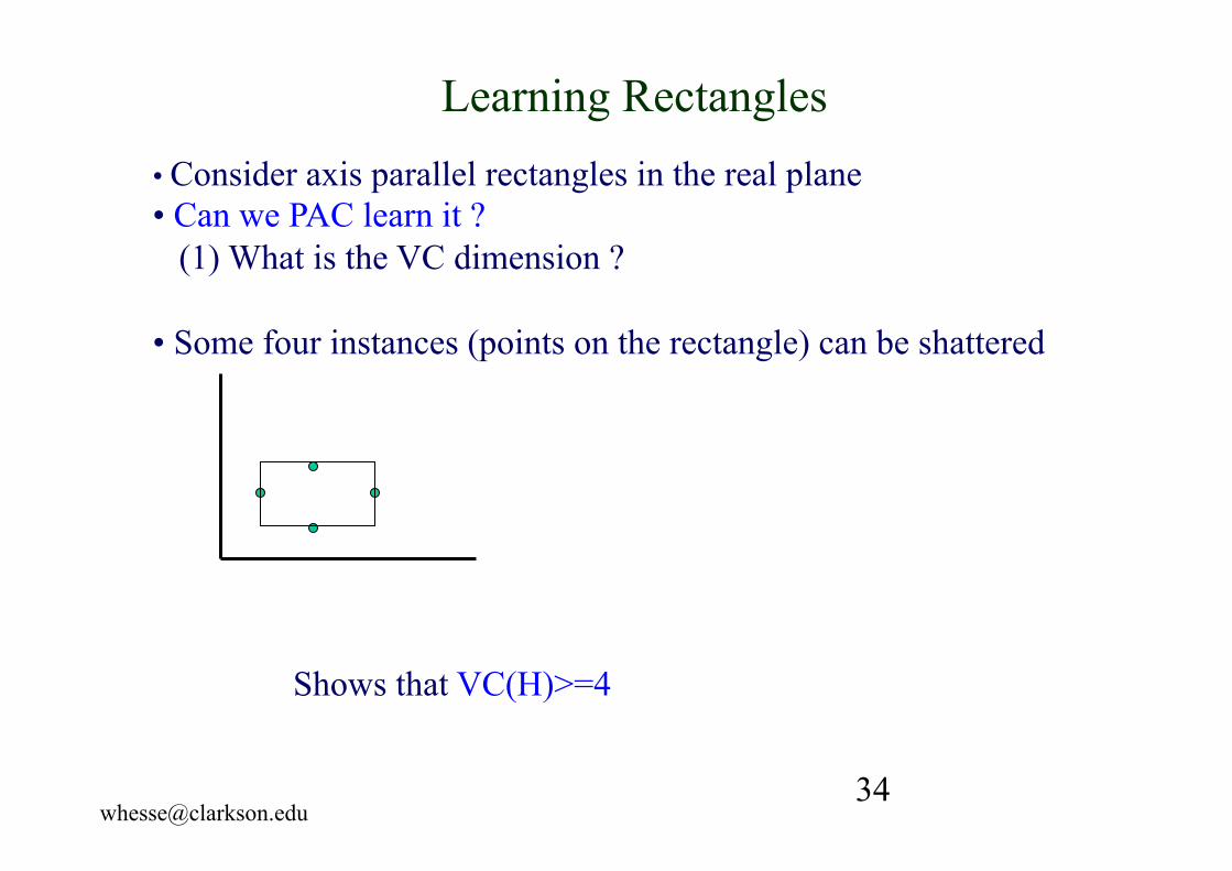
• Consider axis parallel rectangles in the real plane • Can we PAC learn it ? (1) What is the VC dimension ?
• Some four instances (points on the rectangle) can be shattered
Learning Rectangles
Shows that VC(H)>=4
Carla P. Gomes CS4700
35
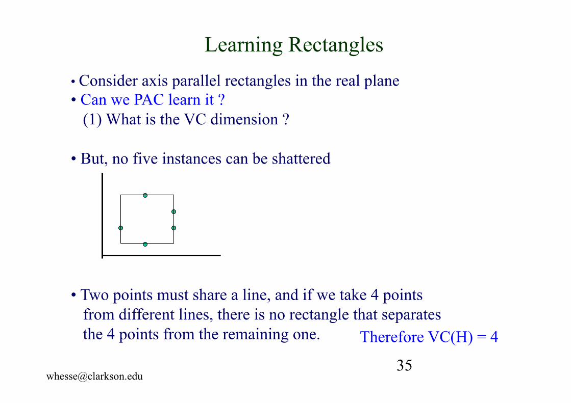
• Consider axis parallel rectangles in the real plane • Can we PAC learn it ? (1) What is the VC dimension ?
• But, no five instances can be shattered
• Two points must share a line, and if we take 4 points from different lines, there is no rectangle that separates the 4 points from the remaining one.
Learning Rectangles
Therefore VC(H) = 4
Carla P. Gomes CS4700
36
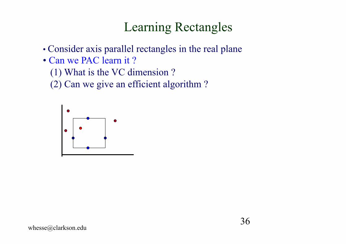
• Consider axis parallel rectangles in the real plane • Can we PAC learn it ? (1) What is the VC dimension ? (2) Can we give an efficient algorithm ?
Learning Rectangles
Carla P. Gomes CS4700
37
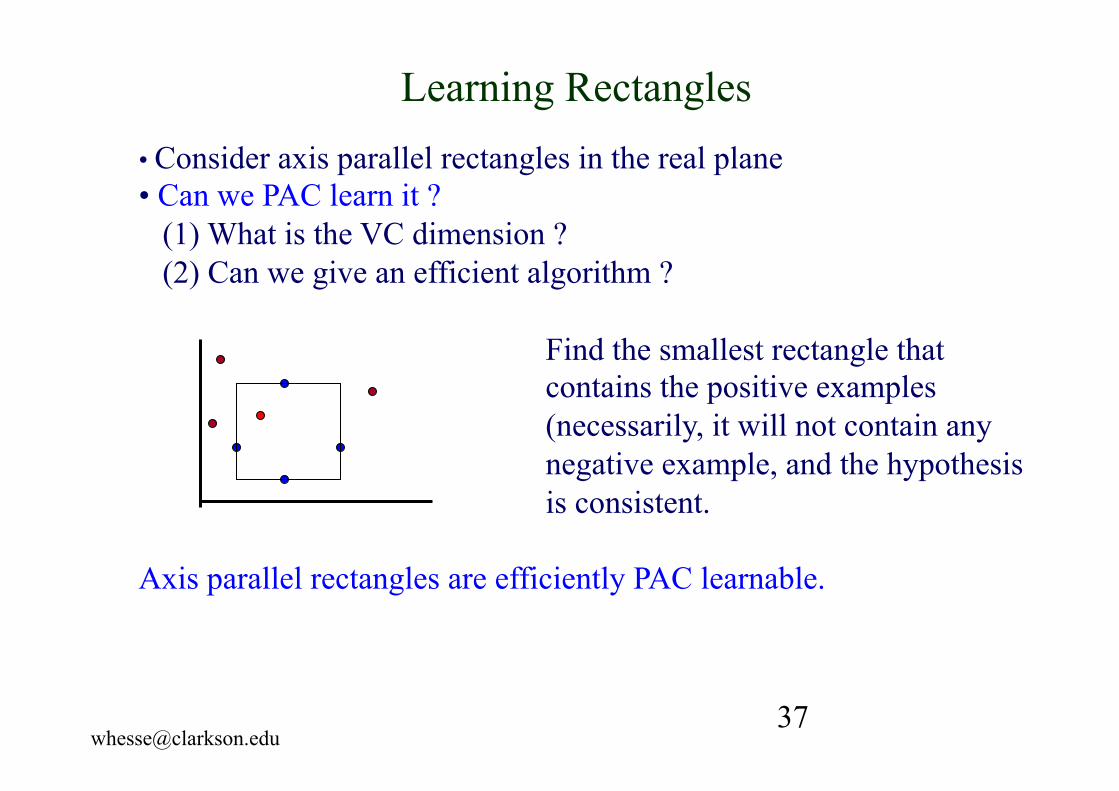
• Consider axis parallel rectangles in the real plane • Can we PAC learn it ? (1) What is the VC dimension ? (2) Can we give an efficient algorithm ? Find the smallest rectangle that contains the positive examples (necessarily, it will not contain any negative example, and the hypothesis is consistent. Axis parallel rectangles are efficiently PAC learnable.
Learning Rectangles
Carla P. Gomes CS4700
38
The Mistake Bound Model of Learning
• The Mistake Bound framework is different from the PAC framework as it considers learners that receive a sequence of training examples and that predict, upon receiving each example, what its target value is.
• The question asked in this setting is: “How many mistakes will the learner make in its predictions before it learns the target concept?”
• This question is significant in practical settings where learning must be done while the system is in actual use.
Nathalie Japkowicz

Carla P. Gomes CS4700
39
Optimal Mistake Bounds
• Definition: Let C be an arbitrary nonempty concept class. The optimal mistake bound for C, denoted Opt(C), is the minimum over all possible learning algorithms A of MA(C). Opt(C)=minA∈Learning_Algorithms MA(C)
• Proposition: For any concept class C, the optimal mistake bound is bound as follows:
VC(C) ≤ Opt(C) ≤ log2(|C|)
Nathalie Japkowicz