computational fluid dynamics the euler equationsgtryggva/cfd-course2017/lecture-10-2017.pdf ·...
TRANSCRIPT
Computational Fluid Dynamics
Computational Fluid Dynamics
http://www.nd.edu/~gtryggva/CFD-Course/
Grétar Tryggvason
Lecture 10February 27, 2017
Computational Fluid Dynamicshttp://www.nd.edu/~gtryggva/CFD-Course/
The Euler Equations
Computational Fluid Dynamics
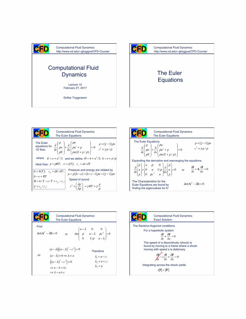
The Euler equations for 1D flow:
0)/(
2 =⎟⎟⎟
⎠
⎞
⎜⎜⎜
⎝
⎛
++
∂∂+
⎟⎟⎟
⎠
⎞
⎜⎜⎜
⎝
⎛
∂∂
ρρρρ
ρρρ
pEupu
u
xEu
t
�
E = e + u2 /2
Ideal Gas:
where
The Euler Equations
�
p = ρRT; e = e T( ); cv = de /dT
h = h T( ); cp = dh / dT;h − e = RTR = h /T − e /T = cp − cv;γ = cp / cv;
p = ρ h − e( ) = h / e −1( )ρe = γ −1( )ρeSpeed of sound
c2 = ∂p∂ρ
⎛⎝⎜
⎞⎠⎟ s
= γ RT = γ pρ
p = γ −1( )ρec2 = γ p / ρ
�
H = h + u2 /2; h = e + p /ρand we define
Pressure and energy are related by
Computational Fluid Dynamics
The Euler Equations
0)/(
2 =⎟⎟⎟
⎠
⎞
⎜⎜⎜
⎝
⎛
++
∂∂+
⎟⎟⎟
⎠
⎞
⎜⎜⎜
⎝
⎛
∂∂
ρρρρ
ρρρ
pEupu
u
xEu
t
Expanding the derivative and rearranging the equations
�
∂∂t
ρup
⎛
⎝
⎜ ⎜ ⎜
⎞
⎠
⎟ ⎟ ⎟
+u ρ 00 u 1/ρ0 ρc 2 u
⎛
⎝
⎜ ⎜ ⎜
⎞
⎠
⎟ ⎟ ⎟ ∂∂x
ρup
⎛
⎝
⎜ ⎜ ⎜
⎞
⎠
⎟ ⎟ ⎟
= 0
p = γ −1( )ρec2 = γ p / ρ
The Euler Equations
�
∂f∂t
+A ∂f∂x
= 0
�
det(AT − λI) = 0The Characteristics for the Euler Equations are found by finding the eigenvalues for AT
or
Computational Fluid Dynamics
Therefore
�
λ1 = u − c;λ2 = u + c;λ3 = u
�
detu − λ 0 0ρ u − λ ρc 2
0 1/ρ u − λ
⎛
⎝
⎜ ⎜ ⎜
⎞
⎠
⎟ ⎟ ⎟
= 0
�
det(AT − λI) = 0 or
�
u − λ( ) u − λ( )2 − c 2( ) = 0
�
u − λ( ) = 0⇒ λ = u
u − λ( )2 − c 2( ) = 0
⇒ u − λ = ±c⇒ λ = u ± c
or:
The Euler Equations
Find
Computational Fluid DynamicsExact Solution:
The Rankine-Hugoniot conditions
�
∂f∂t
+ ∂F∂x
= 0
For a hyperbolic system
The speed of a discontinuity (shock) is found by moving to a frame where a shock moving with speed s is stationary
�
s f[ ] = F[ ]�
∂f∂t
− s ∂f∂x
+ ∂F∂x
= 0
Integrating across the shock yields
0
Computational Fluid DynamicsExact Solution:
For the Euler equations:
0)/(
2 =⎟⎟⎟
⎠
⎞
⎜⎜⎜
⎝
⎛
++
∂∂+
⎟⎟⎟
⎠
⎞
⎜⎜⎜
⎝
⎛
∂∂
ρρρρ
ρρρ
pEupu
u
xEu
t
�
s ρL − ρR( ) = ρu( )L − ρu( )R( )s ρu( )L − ρu( )R( ) = ρu2 + p( )L − ρu2 + p( )R( )s ρE( )L − ρE( )R( ) = ρu(E + p /ρ)( )L − ρu(E + p /ρ)( )R( )
The Rankine-Hugoniot conditions are:
Computational Fluid Dynamics
The Shock-Tube ProblemExact Solution
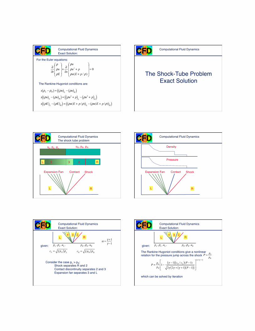
Computational Fluid DynamicsThe shock tube problem
L R
ShockContactExpansion Fan
uL, pL, ρL uR, pR, ρR
L R3 25
Computational Fluid Dynamics
L R
ShockContactExpansion Fan
Pressure
Density
Computational Fluid DynamicsExact Solution:
Consider the case pL > pR:Shock separates R and 2Contact discontinuity separates 2 and 3Expansion fan separates 3 and L
given:
�
pL , ρL , uL ,
�
pR , ρR , uR
L R234
�
α = γ +1γ −1
cR = γ pR ρRcL = γ pL ρL
Computational Fluid DynamicsExact Solution:
P =pLpR
1−γ −1( ) cR / cL( )(P −1)
2γ 2γ + γ +1( ) P −1( )( )⎡
⎣
⎢⎢
⎤
⎦
⎥⎥
2γ / γ −1( )
�
P = p2pR
The Rankine-Hugoniot conditions give a nonlinear relation for the pressure jump across the shock
which can be solved by iteration
given:
�
pL , ρL , uL ,
�
pR , ρR , uR
L R234
Computational Fluid Dynamics
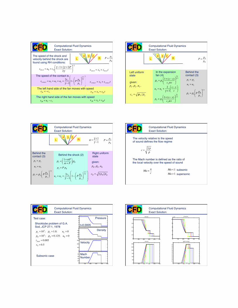
The speed of the shock and velocity behind the shock are found using RH conditions:
�
sshock = uR + cRγ −1+ γ +1( )P
2γ⎛
⎝ ⎜
⎞
⎠ ⎟ 1/ 2
�
scontact = u3 = u2 = uL + 2cLγ −1
1− P pRpL
⎛
⎝ ⎜
⎞
⎠ ⎟
γ −12γ
⎛
⎝
⎜ ⎜ ⎜
⎞
⎠
⎟ ⎟ ⎟
Exact Solution:
The speed of the contact is
The left hand side of the fan moves with speed
The right hand side of the fan moves with speed
�
sfL = −cL
s fR = u2 − c3
�
x fR = x0 + sfR t�
x fL = x0 + sfL t�
xcontact = x0 + scontact t�
xshock = x0 + sshockt
L R234
�
P = p2pR
Computational Fluid Dynamics
In the expansion fan (4)
�
p4 = p41+ (s− x)cLα t
⎛
⎝ ⎜
⎞
⎠ ⎟
2γγ −1
Exact Solution:
�
ρ4 = ρ41+ (s− x)cLα t
⎛
⎝ ⎜
⎞
⎠ ⎟
2γγ −1
�
u4 = uL + 2γ +1
s− xt
⎛ ⎝ ⎜
⎞ ⎠ ⎟
L R234
�
pL , ρL , uL ,given:
�
cL = γpL ρL
Left uniform state
Behind the contact (3)
�
p3 = p2
�
u3 = u2
�
ρ3 = ρL P pRpL
⎛
⎝ ⎜
⎞
⎠ ⎟ 1/γ
�
P = p2pR
Computational Fluid DynamicsExact Solution:
L R234
Behind the shock (2)
ρ2 =1+αPα + P
⎛⎝⎜
⎞⎠⎟ρR
u2 = uL +2cLγ −1
1− P pRpL
⎛⎝⎜
⎞⎠⎟
γ −12γ
⎛
⎝
⎜⎜
⎞
⎠
⎟⎟�
p2 = P pR
�
pR , ρR , uR
given:
Right uniform state
cR = γ pR ρR
�
α = γ +1γ −1
Behind the contact (3)
�
p3 = p2
ρ3 = ρL P pRpL
⎛⎝⎜
⎞⎠⎟
1/γ
�
u3 = u2
�
P = p2pR
Computational Fluid DynamicsExact Solution:
The velocity relative to the speed of sound defines the flow regime
c = γ pρ
�
Ma = uc
The Mach number is defined as the ratio of the local velocity over the speed of sound
�
Ma <1Ma >1
subsonicsupersonic
Computational Fluid DynamicsExact Solution:
0 100 200 300 400 5000
2
4
6
8
10x 104 pressure
0 100 200 300 400 5000
0.2
0.4
0.6
0.8
1
density
0 100 200 300 400 5000
100
200
300velocity
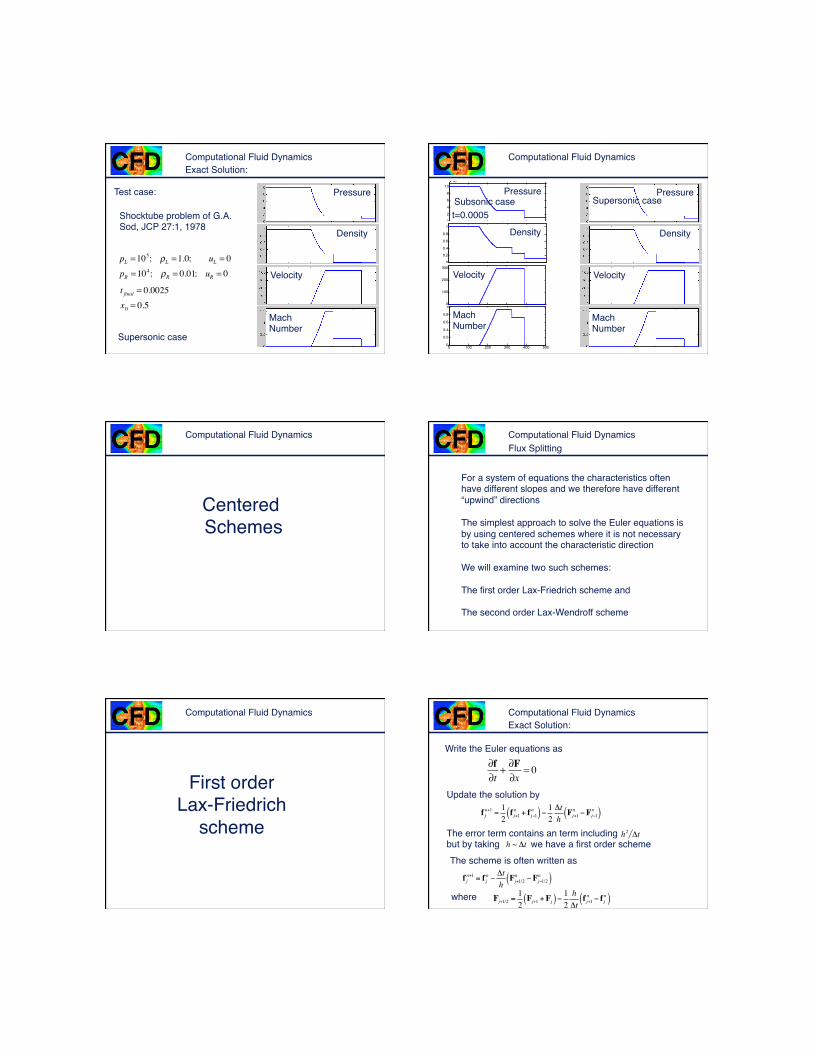
Pressure
Density
Velocity
0 100 200 300 400 5000
0.2
0.4
0.6
0.8
1Mach number
t=0.0005
Mach Number
Test case:
�
pL =105; ρL =1.0; uL = 0pR =104; ρR = 0.125; uR = 0
Shocktube problem of G.A. Sod, JCP 27:1, 1978
�
t final = 0.005x0 = 0.5
Subsonic case
Computational Fluid DynamicsExact Solution:
0 100 200 300 400 5000
0.2
0.4
0.6
0.8
1
density
0 100 200 300 400 5000
2
4
6
8
10
x 104 pressure
0 100 200 300 400 5000
50
100
150
200
250
300
velocity
0 100 200 300 400 5000
0.1
0.2
0.3
0.4
0.5
0.6
0.7
0.8
0.9
1Mach number
Computational Fluid DynamicsExact Solution:
Pressure
Density
Velocity
Mach Number
Test case:
�
pL =105; ρL =1.0; uL = 0pR =104; ρR = 0.01; uR = 0
Shocktube problem of G.A. Sod, JCP 27:1, 1978
�
t final = 0.0025x0 = 0.5
Supersonic case
Computational Fluid Dynamics
0 100 200 300 400 5000
2
4
6
8
10x 104 pressure
0 100 200 300 400 5000
0.2
0.4
0.6
0.8
1
density
0 100 200 300 400 5000
100
200
300velocity
Pressure
Density
Velocity
0 100 200 300 400 5000
0.2
0.4
0.6
0.8
1Mach number
t=0.0005
Mach Number
Pressure
Density
Velocity
Mach Number
Supersonic caseSubsonic case
Computational Fluid Dynamics
Centered Schemes
Computational Fluid Dynamics
For a system of equations the characteristics often have different slopes and we therefore have different “upwind” directions
The simplest approach to solve the Euler equations is by using centered schemes where it is not necessary to take into account the characteristic direction
We will examine two such schemes:
The first order Lax-Friedrich scheme and
The second order Lax-Wendroff scheme
Flux Splitting
Computational Fluid Dynamics
First order Lax-Friedrich
scheme
Computational Fluid DynamicsExact Solution:
�
∂f∂t
+ ∂F∂x
= 0
Write the Euler equations as
The error term contains an term includingbut by taking we have a first order scheme
Update the solution by
f jn+1 =
12f j+1n + f j−1
n( )− 12ΔthFj+1n −Fj−1
n( )
h2 Δth ~ Δt
f jn+1 = f j
n −ΔthFj+1/2n −Fj−1/2
n( )The scheme is often written as
where Fj+1/2 =12Fj+1 +Fj( )− 12
hΔtf j+1n − f j
n( )
Computational Fluid Dynamics
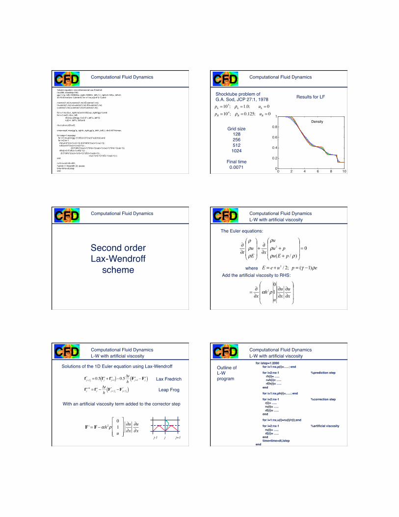
%Euler equation--one-dimensional Lax-Friedrichnx=256; maxstep=150;gg=1.4;p_left=100000;p_right=10000;r_left=1;r_right=0.125;u_left=0;xl=10.0;h=xl/(nx-1);time=0; for i=1:nx,x(i)=h*(i-1);end
r=zeros(1,nx);ru=zeros(1,nx);rE=zeros(1,nx);rn=zeros(1,nx);run=zeros(1,nx);rEn=zeros(1,nx);c=zeros(1,nx);u=zeros(1,nx);m=zeros(1,nx);
for i=1:nx,r(i)=r_right;ru(i)=0.0;rE(i)=p_right/(gg-1);endfor i=1:nx/2; r(i)=r_left; rE(i)=p_left/(gg-1)+0.5*r_left*u_left^2; ru(i)=r_left*u_left;end
rh=r;ruh=ru;rEh=rE;
cmax=sqrt( max(gg*p_right/r_right,gg*p_left/r_left) ); dt=0.45*h/cmax;
for istep=1:maxstep for i=1:nx,p(i)=(gg-1)*(rE(i)-0.5*(ru(i)*ru(i)/r(i)));end for i=2:nx-1 rh(i)=0.5*(r(i+1)+r(i-1))-(0.5*dt/h)*(ru(i+1)-ru(i-1)); ruh(i)=0.5*(ru(i+1)+ru(i-1))-...
(0.5*dt/h)*((ru(i+1)^2/r(i+1))+p(i+1)-(ru(i-1)^2/r(i-1))-p(i-1)); rEh(i)=0.5*(rE(i+1)+rE(i-1))-... (0.5*dt/h)*((ru(i+1)/r(i+1))*(rE(i+1)+p(i+1))...
-(ru(i-1)/r(i-1))*(rE(i-1)+p(i-1)) );end
r=rh;ru=ruh;rE=rEh;%plot(r,'r','linewidth',2); pausetime=time+dt,istepend
Computational Fluid Dynamics
Results for LF
0 2 4 6 8 100
0.2
0.4
0.6
0.8
1Density
Grid size128256512
1024
Final time0.0071
�
pL =105; ρL =1.0; uL = 0pR =104; ρR = 0.125; uR = 0
Shocktube problem of G.A. Sod, JCP 27:1, 1978
Computational Fluid Dynamics
Second order Lax-Wendroff
scheme
Computational Fluid Dynamics
The Euler equations:
0)/(
2 =⎟⎟⎟
⎠
⎞
⎜⎜⎜
⎝
⎛
++
∂∂+
⎟⎟⎟
⎠
⎞
⎜⎜⎜
⎝
⎛
∂∂
ρρρρ
ρρρ
pEupu
u
xEu
t
epueE ργ )1(;2/2 −=+=Add the artificial viscosity to RHS:
where
⎟⎟⎟
⎠
⎞
⎜⎜⎜
⎝
⎛
∂∂
∂∂
∂∂=
xu
xu
uh
x10
2ρα
L-W with artificial viscosity
Computational Fluid Dynamics
�
f j+ 12
* = 0.5 f jn + f j+1
n( ) − 0.5Δth F j+1n −F j
n( )f jn+1 = f j
n − ΔthF j+ 1
2
* −F j− 12*( )
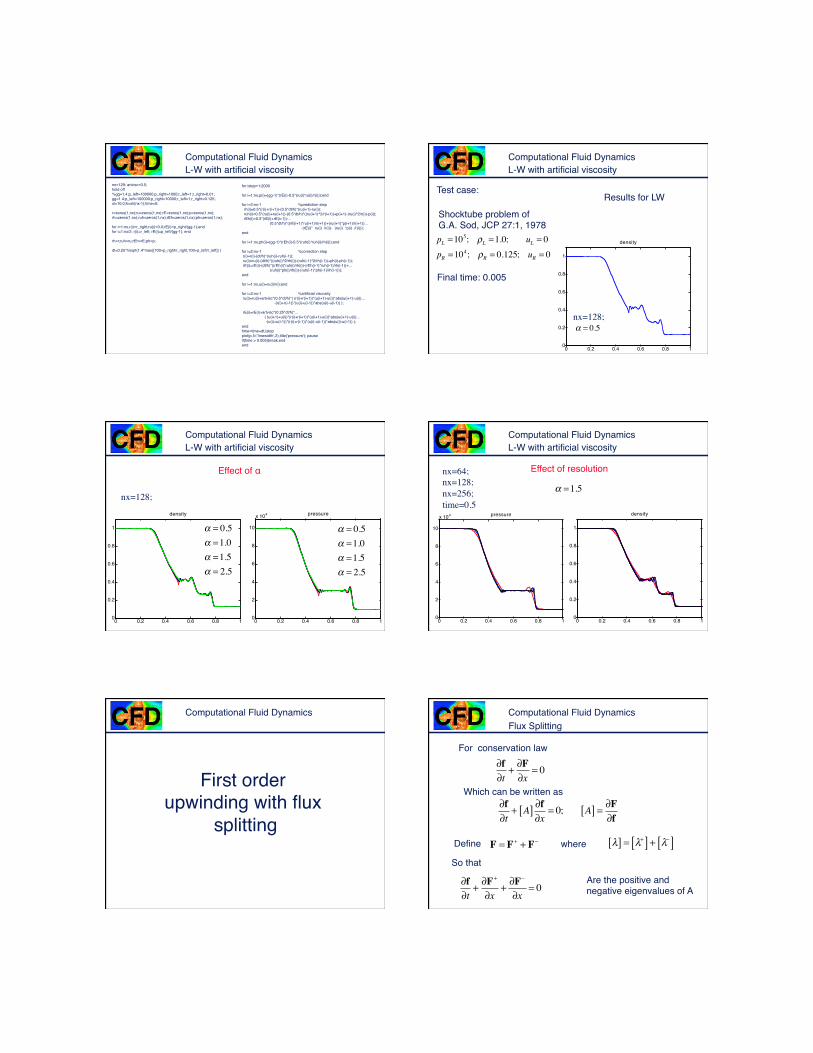
Solutions of the 1D Euler equation using Lax-Wendroff
F ' = F −αh2ρ01u
⎡
⎣
⎢⎢⎢
⎤
⎦
⎥⎥⎥
∂u∂x
∂u∂x
With an artificial viscosity term added to the corrector step
L-W with artificial viscosity
Lax Fredrich
Leap Frog
j-1 j j+1
Computational Fluid Dynamics
for istep=1:2000for i=1:nx,p(i)=…..; end
for i=2:nx-1 %prediction step rh(i)= ….. ruh(i)= ….. rEh(i)= …..end
for i=1:nx,ph(i)=…..; end
for i=2:nx-1 %correction step r(i)= ….. ru(i)= ….. rE(i)= ….. end
for i=1:nx,u(i)=ru(i)/r(i);end
for i=2:nx-1 %artificial viscosity ru(i)= ….. rE(i)= …..endtime=time+dt,istep
end
Outline of L-W program
L-W with artificial viscosity
Computational Fluid Dynamics
nx=129; artvisc=0.5;hold off%gg=1.4;p_left=100000;p_right=1000;r_left=1;r_right=0.01;gg=1.4;p_left=100000;p_right=10000;r_left=1;r_right=0.125;xl=10.0;h=xl/(nx-1);time=0;
r=zeros(1,nx);ru=zeros(1,nx);rE=zeros(1,nx);p=zeros(1,nx);rh=zeros(1,nx);ruh=zeros(1,nx);rEh=zeros(1,nx);ph=zeros(1,nx);
for i=1:nx,r(i)=r_right;ru(i)=0.0;rE(i)=p_right/(gg-1);endfor i=1:nx/2; r(i)=r_left; rE(i)=p_left/(gg-1); end
rh=r;ruh=ru;rEh=rE;ph=p;
dt=0.25*h/sqrt(1.4*max([700+p_right/r_right,700+p_left/r_left]) )
for istep=1:2000
for i=1:nx,p(i)=(gg-1)*(rE(i)-0.5*(ru(i)*ru(i)/r(i)));end
for i=2:nx-1 %prediction step rh(i)=0.5*(r(i)+r(i+1))-(0.5*dt/h)*(ru(i+1)-ru(i)); ruh(i)=0.5*(ru(i)+ru(i+1))-(0.5*dt/h)*((ru(i+1)^2/r(i+1))+p(i+1)-(ru(i)^2/r(i))-p(i)); rEh(i)=0.5*(rE(i)+rE(i+1))-...
(0.5*dt/h)*((rE(i+1)*ru(i+1)/r(i+1))+(ru(i+1)*p(i+1)/r(i+1))... -(rE(i)* ru(i) /r(i))- (ru(i) *p(i) /r(i)));
end
for i=1:nx,ph(i)=(gg-1)*(rEh(i)-0.5*(ruh(i)*ruh(i)/rh(i)));end
for i=2:nx-1 %correction step r(i)=r(i)-(dt/h)*(ruh(i)-ruh(i-1)); ru(i)=ru(i)-(dt/h)*((ruh(i)^2/rh(i))-(ruh(i-1)^2/rh(i-1))+ph(i)-ph(i-1)); rE(i)=rE(i)-(dt/h)*((rEh(i)*ruh(i)/rh(i))-(rEh(i-1)*ruh(i-1)/rh(i-1))+...
(ruh(i)*ph(i)/rh(i))-(ruh(i-1)*ph(i-1)/rh(i-1)));end
for i=1:nx,u(i)=ru(i)/r(i);end
for i=2:nx-1 %artificial viscosity ru(i)=ru(i)+artvisc*(0.5*dt/h)*( (r(i)+r(i+1))*(u(i+1)-u(i))*abs(u(i+1)-u(i))... -(r(i)+r(i-1))*(u(i)-u(i-1))*abs(u(i)-u(i-1)) );
rE(i)=rE(i)+artvisc*(0.25*dt/h)*... ( (u(i+1)+u(i))*(r(i)+r(i+1))*(u(i+1)-u(i))*abs(u(i+1)-u(i))... -(u(i)+u(i-1))*(r(i)+r(i-1))*(u(i)-u(i-1))*abs(u(i)-u(i-1)) );endtime=time+dt,istepplot(p,'b','linewidth',2),title('pressure'); pauseif(time > 0.005)break,endend
L-W with artificial viscosityComputational Fluid DynamicsL-W with artificial viscosity
Test case:
�
pL =105; ρL =1.0; uL = 0pR =104; ρR = 0.125; uR = 0
Shocktube problem of G.A. Sod, JCP 27:1, 1978
Final time: 0.005
0 0.2 0.4 0.6 0.8 10
0.2
0.4
0.6
0.8
1
density
�
α = 0.5nx=128;
Results for LW
Computational Fluid Dynamics
0 0.2 0.4 0.6 0.8 10
0.2
0.4
0.6
0.8
1
density
�
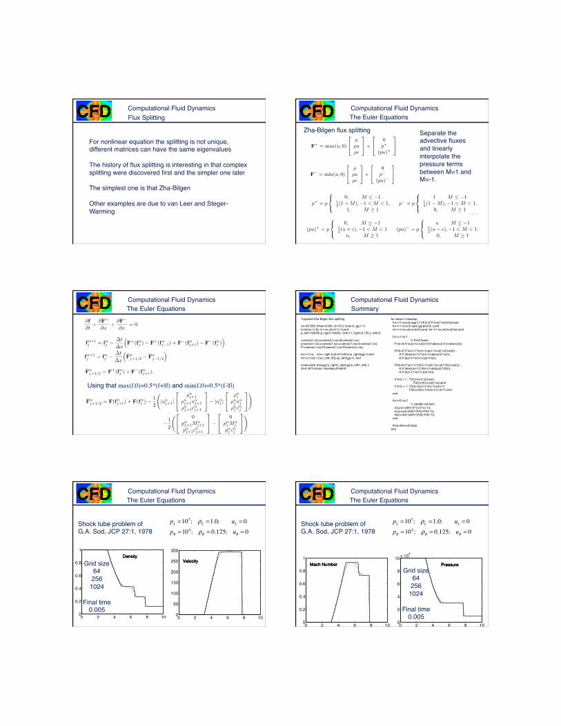
α = 0.5α =1.0α =1.5α = 2.5
nx=128;
Effect of α
0 0.2 0.4 0.6 0.8 10
2
4
6
8
10
x 104 pressure
�
α = 0.5α =1.0α =1.5α = 2.5
L-W with artificial viscosityComputational Fluid Dynamics
0 0.2 0.4 0.6 0.8 10
2
4
6
8
10
x 104 pressure
nx=64; nx=128; nx=256;time=0.5
�
α =1.5
Effect of resolution
0 0.2 0.4 0.6 0.8 10
0.2
0.4
0.6
0.8
1
density
L-W with artificial viscosity
Computational Fluid Dynamics
First order upwinding with flux
splitting
Computational Fluid Dynamics
Define
�
F = F + + F−
So that
�
∂f∂t
+ ∂F+
∂x+ ∂F−
∂x= 0
Flux Splitting
�
∂f∂t
+ ∂F∂x
= 0
For conservation law
where
Which can be written as
�
∂f∂t
+ A[ ] ∂f∂x
= 0; A[ ] = ∂F∂f
�
λ[ ] = λ+[ ] + λ−[ ]
Are the positive and negative eigenvalues of A
Computational Fluid Dynamics
For nonlinear equation the splitting is not unique, different matrices can have the same eigenvalues
The history of flux splitting is interesting in that complex splitting were discovered first and the simpler one later
The simplest one is that Zha-Bilgen
Other examples are due to van Leer and Steger-Warming
Flux SplittingComputational Fluid DynamicsThe Euler Equations
6.5. VELOCITY-PRESSURE METHOD FOR COMPRESSIBLE FLOW 55
The first part can be written as uf and it can be shown that it representsinformation carried by the flow velocity u, so the upwind direction dependsonly on the sign of u. The second part of the fluxes represents informationcarried by u±c and for supersonic flow, where the Mach number is either largerthan 1 or smaller then �1, the upwind direction again depends on the sign ofthe velocity. For �1 < M < 1, the second term is split in two and allocated tothe upwind and downwind directions as a linear function of the Mach number.Thus, following Laney (1998), the scheme is:
F+ = max(u, 0)
2
4
⇢⇢u⇢e
3
5+
2
4
0p+
(pu)+
3
5 (6.133)
and
F� = min(u, 0)
2
4
⇢⇢u⇢e
3
5+
2
4
0p�
(pu)�
3
5 , (6.134)
where we note that the first part depends only on the sign of the velocity. Thevariables in the second part are found by:
p+ = p
8
<
:
0, M �112 (1 +M),�1 < M < 1,
1, M � 1p� = p
8
<
:
1 M �112 (1�M),�1 < M < 1,
0, M � 1(6.135)
and
(pu)+ = p
8
<
:
0, M �112 (u+ c),�1 < M < 1
u, M � 1(pu)� = p
8
<
:
u M �112 (u� c),�1 < M < 1.
0, M � 1(6.136)
For M � 1, F = F+ and for M 1, F = F�, as we intended.To discretize equation (6.130) we first write
@f
@t+
@F+
@x+
@F�
@x= 0, (6.137)
and then approximate the fluxes using the first order upwind scheme:
fn+1j
= fnj
� �t
�x
⇣
F+(fnj
)� F+(fnj�1) + F�(fn
j+1)� F�(fnj
)⌘
. (6.138)
For a numerical implementation it is possible to rewrite (6.138) as
fn+1j
= fnj
� �t
�x
⇣
F̂n
j+1/2 � F̂n
j�1/2
⌘
, (6.139)
where the fluxes at the half-points are found by
F̂n
j+1/2 = F+(fnj
) + F�(fnj+1). (6.140)
Zha-Bilgen flux splitting Separate the advective fluxes and linearly interpolate the pressure terms between M=1 and M=-1.
Computational Fluid Dynamics346
The Euler Equations
56 CHAPTER 6. COMPUTATIONAL FLUID DYNAMICS
Using that max(f, 0) = 0.5(f + |f |) and min(f, 0) = 0.5(f � |f |) for any f wecan write the fluxes for �1 < M < 1 as:
F̂n
j+1/2 = F(fnj+1) + F(fn
j
)� 1
2
|un
j+1|
2
4
⇢nj+1
⇢nj+1u
n
j+1
⇢nj+1e
n
j+1
3
5� |un
j
|
2
4
⇢nj
⇢nj
un
j
⇢nj
enj
3
5
!
�1
2
2
4
0pnj+1M
n
j+1
pnj+1c
n
j+1
3
5�
2
4
0pnj
Mn
j
pnj
cnj
3
5
!
, (6.141)
and we use this form in the code shown below. Once the fluxes have been foundby (6.141), the variables are updated using (6.139).
As methods for the Euler equations are developed, new methods are oftentested using problems used to test earlier methods. Several of these tests havebeen used by so many researchers that they have become de facto standards.One such test was introduced by Sod (1978) and consists of discontinuous initialconditions with high pressure gas occupying the left half of a domain and a lowpressure gas in the right half. The solution consists of the high pressure gas ex-panding into the low pressure gas, sending a shock wave ahead and a rarifactionwave in the other direction. Thus, the solution consists of (moving from rightto left): undisturbed gas at low pressure on the right, compressed low pressuregas (separated by a shock from the undisturbed gas); expanded high pressuregas moving into the right hand side of the domain; a rarifaction fan where theinitially compressed gas expands smoothly; and finally the undisturbed highpressure gas on the left. The exact solution is easily found, as explained inchapter 15, and once the conditions in each region have been found, the timeevolution is simply given by expanding the time axis at a constant rate. A codefor this problem, using (6.141) and (6.139) is given below and sample results aregiven in figure 6.26, where we plot the density, the pressure, the velocity andthe Mach number at time 0.005. In all cases we plot results for three di↵erentresolutions. The time step must be limited by the Courant conditions, whichsay that the signal cannot travel more then one grid space in each time step, or(u+ c)�t < �t, and we take the time step to be 0.45 times the maximum step.The shock (the left most discontinuity) is captured reasonably well for the finerresolutions, but the contact discontinuity (the second density discontinuity fromthe right) is relatively smooth for all three resolutions. It is generally found thatmaintaining sharp contacts is more di�cult than keeping shocks sharp.
%project 2--upwind-Zha-Bilgen flux splitting
nx=40*256; tfinal=0.005; xl=10.0; time=0; gg=1.4;
h=xl/(nx-1);for i=1:nx,x(i)=h*(i-1);end
p_left=100000;p_right=10000;r_left=1;r_right=0.125;u_left=0;
6.5. VELOCITY-PRESSURE METHOD FOR COMPRESSIBLE FLOW 55
The first part can be written as uf and it can be shown that it representsinformation carried by the flow velocity u, so the upwind direction dependsonly on the sign of u. The second part of the fluxes represents informationcarried by u±c and for supersonic flow, where the Mach number is either largerthan 1 or smaller then �1, the upwind direction again depends on the sign ofthe velocity. For �1 < M < 1, the second term is split in two and allocated tothe upwind and downwind directions as a linear function of the Mach number.Thus, following Laney (1998), the scheme is:
F+ = max(u, 0)
2
4
⇢⇢u⇢e
3
5+
2
4
0p+
(pu)+
3
5 (6.133)
and
F� = min(u, 0)
2
4
⇢⇢u⇢e
3
5+
2
4
0p�
(pu)�
3
5 , (6.134)
where we note that the first part depends only on the sign of the velocity. Thevariables in the second part are found by:
p+ = p
8
<
:
0, M �112 (1 +M),�1 < M < 1,
1, M � 1p� = p
8
<
:
1 M �112 (1�M),�1 < M < 1,
0, M � 1(6.135)
and
(pu)+ = p
8
<
:
0, M �112 (u+ c),�1 < M < 1
u, M � 1(pu)� = p
8
<
:
u M �112 (u� c),�1 < M < 1.
0, M � 1(6.136)
For M � 1, F = F+ and for M 1, F = F�, as we intended.To discretize equation (6.130) we first write
@f
@t+
@F+
@x+
@F�
@x= 0, (6.137)
and then approximate the fluxes using the first order upwind scheme:
fn+1j
= fnj
� �t
�x
⇣
F+(fnj
)� F+(fnj�1) + F�(fn
j+1)� F�(fnj
)⌘
. (6.138)
For a numerical implementation it is possible to rewrite (6.138) as
fn+1j
= fnj
� �t
�x
⇣
F̂n
j+1/2 � F̂n
j�1/2
⌘
, (6.139)
where the fluxes at the half-points are found by
F̂n
j+1/2 = F+(fnj
) + F�(fnj+1). (6.140)
Using that max(f,0)=0.5*(f+|f|) and min(f,0)=0.5*(f-|f|)
Computational Fluid DynamicsSummary
%upwind-Zha-Bilgen flux splitting
nx=40*256; tfinal=0.005; xl=10.0; time=0; gg=1.4;h=xl/(nx-1);for i=1:nx,x(i)=h*(i-1);endp_left=100000;p_right=10000;r_left=1;r_right=0.125;u_left=0;
r=zeros(1,nx);ru=zeros(1,nx);rE=zeros(1,nx);p=zeros(1,nx);c=zeros(1,nx);u=zeros(1,nx);m=zeros(1,nx);F1=zeros(1,nx);F2=zeros(1,nx);F3=zeros(1,nx);
for i=1:nx, r(i)=r_right;ru(i)=0.0;rE(i)=p_right/(gg-1);endfor i=1:nx/2; r(i)=r_left; rE(i)=p_left/(gg-1); end
cmax=sqrt( max(gg*p_right/r_right,gg*p_left/r_left) ); dt=0.45*h/cmax; maxstep=tfinal/dt;
for istep=1:maxstep for i=1:nx,p(i)=(gg-1)*(rE(i)-0.5*(ru(i)*ru(i)/r(i)));end for i=1:nx,c(i)=sqrt( gg*p(i)/r(i) );end for i=1:nx,u(i)=ru(i)/r(i);end; for i=1:nx,m(i)=u(i)/c(i);end
for i=1:nx-1% Find fluxes
F1(i)=0.5*(ru(i+1)+ru(i))-0.5*(abs(ru(i+1))-abs(ru(i)));
F2(i)=0.5*(u(i+1)*ru(i+1)+p(i+1)+u(i)*ru(i)+p(i))... -0.5*(abs(u(i+1))*ru(i+1)-abs(u(i))*ru(i))... -0.5*(p(i+1)*m(i+1)-p(i)*m(i));
F3(i)=0.5*(u(i+1)*(rE(i+1)+p(i+1))+u(i)*(rE(i)+p(i)))... -0.5*(abs(u(i+1))*rE(i+1)-abs(u(i))*rE(i))... -0.5*(p(i+1)*c(i+1)-p(i)*c(i));
if m(i) > 1, F2(i)=ru(i)*u(i)+p(i); F3(i)=(rE(i)+p(i))*u(i);end if m(i) < -1, F2(i)=ru(i+1)*u(i+1)+p(i+1); F3(i)=(rE(i+1)+p(i+1))*u(i+1);end end
for i=2:nx-2% Update solution
r(i)=r(i)-(dt/h)*(F1(i)-F1(i-1)); ru(i)=ru(i)-(dt/h)*(F2(i)-F2(i-1)); rE(i)=rE(i)-(dt/h)*(F3(i)-F3(i-1)); end
time=time+dt,istepend
Computational Fluid Dynamics348
The Euler Equations
0 2 4 6 8 100
0.2
0.4
0.6
0.8
1
DensityDensityDensity
0 2 4 6 8 100
50
100
150
200
250
300
VelocityVelocityVelocity�
pL =105; ρL =1.0; uL = 0pR =104; ρR = 0.125; uR = 0
Shock tube problem of G.A. Sod, JCP 27:1, 1978
Grid size64256
1024
Final time0.005
Computational Fluid Dynamics349
The Euler Equations
�
pL =105; ρL =1.0; uL = 0pR =104; ρR = 0.125; uR = 0
Shock tube problem of G.A. Sod, JCP 27:1, 1978
0 2 4 6 8 100
2
4
6
8
10x 10
4
PressurePressurePressure
0 2 4 6 8 100
0.2
0.4
0.6
0.8
1
Mach NumberMach NumberMach Number
Grid size64256
1024
Final time0.005
Computational Fluid Dynamics
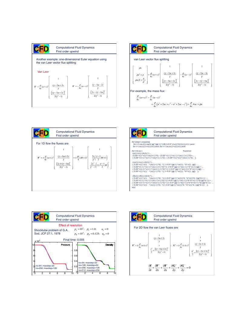
Another example: one-dimensional Euler equation using the van Leer vector flux splitting
F− = −ρ4c
(u − c)2
1
(γ −1)u − 2cγ
2c − (γ −1)u⎡⎣ ⎤⎦2
2(γ 2 −1)
⎡
⎣
⎢⎢⎢⎢⎢⎢⎢⎢⎢
⎤
⎦
⎥⎥⎥⎥⎥⎥⎥⎥⎥
F+ =ρ4c
(u + c)2
1
(γ −1)u + 2cγ
(γ −1)u + 2c⎡⎣ ⎤⎦2
2(γ 2 −1)
⎡
⎣
⎢⎢⎢⎢⎢⎢⎢⎢⎢
⎤
⎦
⎥⎥⎥⎥⎥⎥⎥⎥⎥
Van Leer
First order upwindComputational Fluid Dynamics
van Leer vector flux splitting
ρu
ρu2 + p
ρu(E +pρ
)
⎡
⎣
⎢⎢⎢⎢⎢⎢⎢
⎤
⎦
⎥⎥⎥⎥⎥⎥⎥
=ρ4c
(u + c)2
1
(γ −1)u + 2cγ
(γ −1)u + 2c⎡⎣ ⎤⎦2
2(γ 2 −1)
⎡
⎣
⎢⎢⎢⎢⎢⎢⎢⎢⎢
⎤
⎦
⎥⎥⎥⎥⎥⎥⎥⎥⎥
−ρ4c
(u − c)2
1
(γ −1)u − 2cγ
2c − (γ −1)u⎡⎣ ⎤⎦2
2(γ 2 −1)
⎡
⎣
⎢⎢⎢⎢⎢⎢⎢⎢⎢
⎤
⎦
⎥⎥⎥⎥⎥⎥⎥⎥⎥
�
ρ4c(u + c)2 − ρ
4c(u − c)2
= ρ4c
u2 + 2uc + c 2 − u2 + 2uc − c 2( ) = ρ4c4uc = ρu
For example, the mass flux:
First order upwind
Computational Fluid Dynamics
For 1D flow the fluxes are
F± = ± ρ4c(u ± c)2
1
(γ −1)u ± 2cγ
2c ± (γ −1)u[ ]22(γ 2 −1)
⎡
⎣
⎢⎢⎢⎢⎢⎢⎢⎢⎢
⎤
⎦
⎥⎥⎥⎥⎥⎥⎥⎥⎥
= ± ρc4(M ±1)2
1
2cγ
γ −12
M ±1⎛⎝⎜
⎞⎠⎟
2c2
γ 2 −11± γ −1
2M⎛
⎝⎜⎞⎠⎟2
⎡
⎣
⎢⎢⎢⎢⎢⎢⎢⎢
⎤
⎦
⎥⎥⎥⎥⎥⎥⎥⎥
First order upwindComputational Fluid Dynamics
for istep=1:maxstep for i=1:nx,c(i)=sqrt( gg*(gg-1)*(rE(i)-0.5*(ru(i)^2/r(i)))/r(i) );end for i=1:nx,u(i)=ru(i)/r(i);end; for i=1:nx,m(i)=u(i)/c(i);end for i=2:nx-1 %upwind rn(i)=r(i)-(dt/h)*(... (0.25*r(i)*c(i)*(m(i)+1)^2) - (0.25*r(i-1)*c(i-1)*(m(i-1)+1)^2)+... (-0.25*r(i+1)*c(i+1)*(m(i+1)-1)^2) - (-0.25*r(i)*c(i)*(m(i)-1)^2) ); run(i)=ru(i)-(dt/h)*(... ( 0.25*r(i)*c(i) *(m(i)+1)^2) *(( 1+0.5*(gg-1)*m(i)) *2*c(i) /gg) - ... ( 0.25*r(i-1)*c(i-1)*(m(i-1)+1)^2)*(( 1+0.5*(gg-1)*m(i-1))*2*c(i-1)/gg) + ... (-0.25*r(i+1)*c(i+1)*(m(i+1)-1)^2)*((-1+0.5*(gg-1)*m(i+1))*2*c(i+1)/gg) - ... (-0.25*r(i)*c(i) *(m(i)-1)^2) *((-1+0.5*(gg-1)*m(i)) *2*c(i) /gg) ); rEn(i)=rE(i)-(dt/h)*(... ( 0.25*r(i)*c(i) *(m(i)+1)^2) *((1+0.5*(gg-1)*m(i))^2 *2*c(i)^2 /(gg^2-1)) - ... ( 0.25*r(i-1)*c(i-1)*(m(i-1)+1)^2)*((1+0.5*(gg-1)*m(i-1))^2*2*c(i-1)^2/(gg^2-1)) + ... (-0.25*r(i+1)*c(i+1)*(m(i+1)-1)^2)*((1-0.5*(gg-1)*m(i+1))^2*2*c(i+1)^2/(gg^2-1)) - ... (-0.25*r(i)*c(i) *(m(i)-1)^2) *((1-0.5*(gg-1)*m(i))^2 *2*c(i)^2 /(gg^2-1)) ); end
First order upwind
Computational Fluid Dynamics
�
pL =105; ρL =1.0; uL = 0pR =104; ρR = 0.125; uR = 0
Shocktube problem of G.A. Sod, JCP 27:1, 1978
0 2 4 6 8 100
0.2
0.4
0.6
0.8
1 DensityDensityDensityDensityDensity
Effect of resolution
nx=64; maxstep=32nx=128; maxstep=64nx=256; maxstep=128nx=512; maxstep=256
0 2 4 6 8 100
2
4
6
8
10x 104
PressurePressure
nx=64; maxstep=32nx=256; maxstep=128
Final time: 0.005
First order upwindComputational Fluid Dynamics
For 2D flow the van Leer fluxes are
F± = ± ρ4c(u ± c)2
1(γ −1)u ± 2c
γ
vv2
2+(γ −1)u ± 2c[ ]22(γ 2 −1)
⎡
⎣
⎢⎢⎢⎢⎢⎢⎢⎢⎢⎢
⎤
⎦
⎥⎥⎥⎥⎥⎥⎥⎥⎥⎥
; G± = ± ρ4c(v ± c)2
1u
(γ −1)v ± 2cγ
u2
2+(γ −1)v ± 2c[ ]22(γ 2 −1)
⎡
⎣
⎢⎢⎢⎢⎢⎢⎢⎢⎢
⎤
⎦
⎥⎥⎥⎥⎥⎥⎥⎥⎥
First order upwind
∂f∂t
+ ∂F+
∂x+ ∂F−
∂x+ ∂G+
∂y+ ∂G−
∂y= 0
Computational Fluid Dynamics
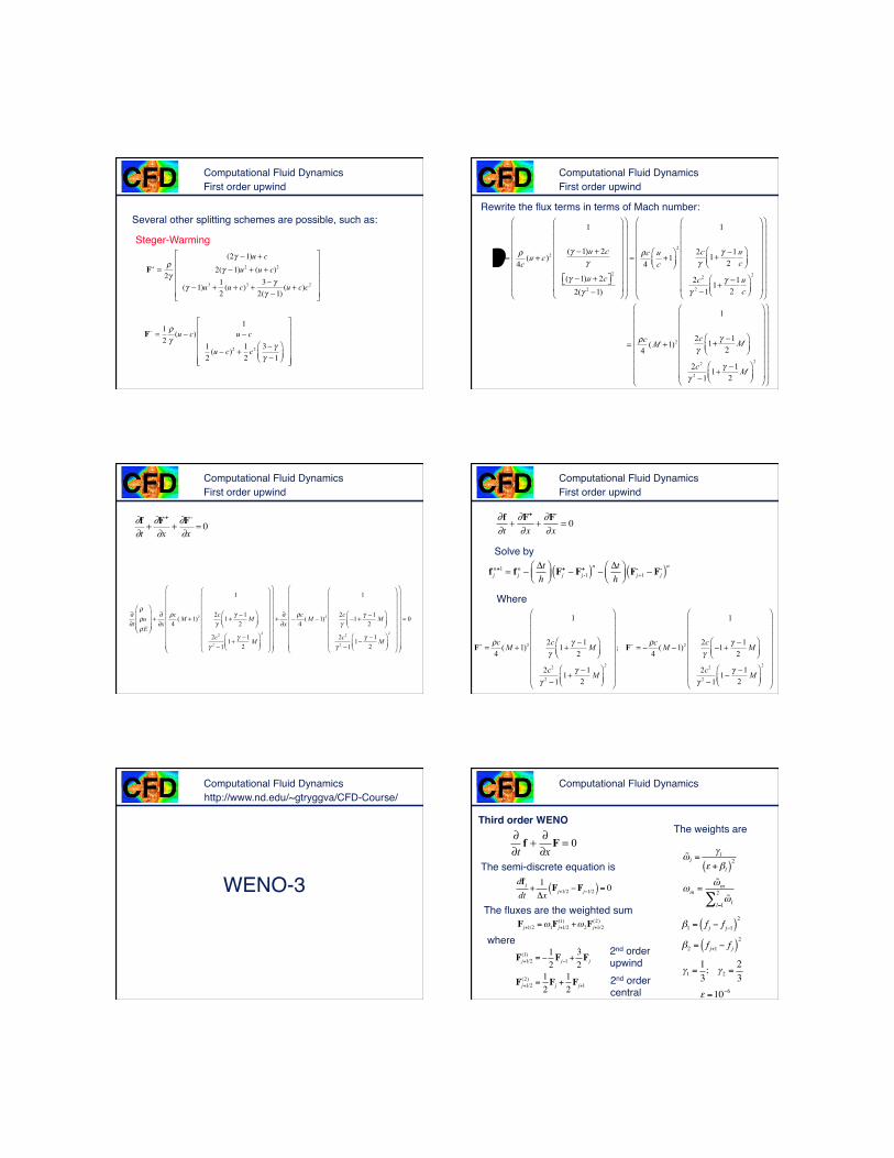
F− =12ργ(u − c)
1u − c
12(u − c)2 + 1
2c2 3− γ
γ −1⎛⎝⎜
⎞⎠⎟
⎡
⎣
⎢⎢⎢⎢⎢
⎤
⎦
⎥⎥⎥⎥⎥
F+ =ρ2γ
(2γ −1)u + c2(γ −1)u2 + (u + c)2
(γ −1)u3 + 12(u + c)3 + 3− γ
2(γ −1)(u + c)c2
⎡
⎣
⎢⎢⎢⎢⎢
⎤
⎦
⎥⎥⎥⎥⎥
Steger-Warming
Several other splitting schemes are possible, such as:
First order upwindComputational Fluid Dynamics
F+ = ρ4c(u + c )2
1
(γ −1)u + 2cγ
(γ −1)u + 2c⎡⎣ ⎤⎦2
2(γ 2 −1)
⎛
⎝
⎜⎜⎜⎜⎜⎜⎜⎜
⎞
⎠
⎟⎟⎟⎟⎟⎟⎟⎟
⎛
⎝
⎜⎜⎜⎜⎜⎜⎜⎜
⎞
⎠
⎟⎟⎟⎟⎟⎟⎟⎟
= ρc4uc+1
⎛⎝⎜
⎞⎠⎟
2
1
2cγ1+ γ −1
2uc
⎛⎝⎜
⎞⎠⎟
2c 2
γ 2 −11+ γ −1
2uc
⎛⎝⎜
⎞⎠⎟
2
⎛
⎝
⎜⎜⎜⎜⎜⎜⎜⎜
⎞
⎠
⎟⎟⎟⎟⎟⎟⎟⎟
⎛
⎝
⎜⎜⎜⎜⎜⎜⎜⎜
⎞
⎠
⎟⎟⎟⎟⎟⎟⎟⎟
= ρc4(M +1)2
1
2cγ1+ γ −1
2M⎛
⎝⎜⎞⎠⎟
2c 2
γ 2 −11+ γ −1
2M⎛
⎝⎜⎞⎠⎟
2
⎛
⎝
⎜⎜⎜⎜⎜⎜⎜⎜
⎞
⎠
⎟⎟⎟⎟⎟⎟⎟⎟
⎛
⎝
⎜⎜⎜⎜⎜⎜⎜⎜
⎞
⎠
⎟⎟⎟⎟⎟⎟⎟⎟
Rewrite the flux terms in terms of Mach number:
First order upwind
Computational Fluid Dynamics
∂∂t
ρρuρE
⎛
⎝
⎜⎜⎜
⎞
⎠
⎟⎟⎟+
∂∂x
ρc4
( M +1)2
1
2cγ
1+γ −1
2M
⎛⎝⎜
⎞⎠⎟
2c2
γ 2 −11+
γ −12
M⎛⎝⎜
⎞⎠⎟
2
⎛
⎝
⎜⎜⎜⎜⎜⎜⎜⎜
⎞
⎠
⎟⎟⎟⎟⎟⎟⎟⎟
⎛
⎝
⎜⎜⎜⎜⎜⎜⎜⎜⎜
⎞
⎠
⎟⎟⎟⎟⎟⎟⎟⎟⎟
+∂∂x
−ρc4
( M −1)2
1
2cγ
−1+γ −1
2M
⎛⎝⎜
⎞⎠⎟
2c2
γ 2 −11−
γ −12
M⎛⎝⎜
⎞⎠⎟
2
⎛
⎝
⎜⎜⎜⎜⎜⎜⎜⎜
⎞
⎠
⎟⎟⎟⎟⎟⎟⎟⎟
⎛
⎝
⎜⎜⎜⎜⎜⎜⎜⎜⎜
⎞
⎠
⎟⎟⎟⎟⎟⎟⎟⎟⎟
= 0
�
∂f∂t
+ ∂F+
∂x+ ∂F-
∂x= 0
First order upwindComputational Fluid Dynamics
∂f∂t
+∂F+
∂x+∂F-
∂x= 0
f jn+1 = f j
n −Δth
⎛⎝⎜
⎞⎠⎟Fj+ − Fj -1
+( )n − Δth
⎛⎝⎜
⎞⎠⎟Fj+1- − Fj
-( )n
F+ =ρc4
( M +1)2
1
2cγ
1+γ −1
2M
⎛⎝⎜
⎞⎠⎟
2c2
γ 2 −11+
γ −12
M⎛⎝⎜
⎞⎠⎟
2
⎛
⎝
⎜⎜⎜⎜⎜⎜⎜⎜
⎞
⎠
⎟⎟⎟⎟⎟⎟⎟⎟
; F− = −ρc4
( M −1)2
1
2cγ
−1+γ −1
2M
⎛⎝⎜
⎞⎠⎟
2c2
γ 2 −11−
γ −12
M⎛⎝⎜
⎞⎠⎟
2
⎛
⎝
⎜⎜⎜⎜⎜⎜⎜⎜
⎞
⎠
⎟⎟⎟⎟⎟⎟⎟⎟
Where
Solve by
First order upwind
Computational Fluid Dynamics
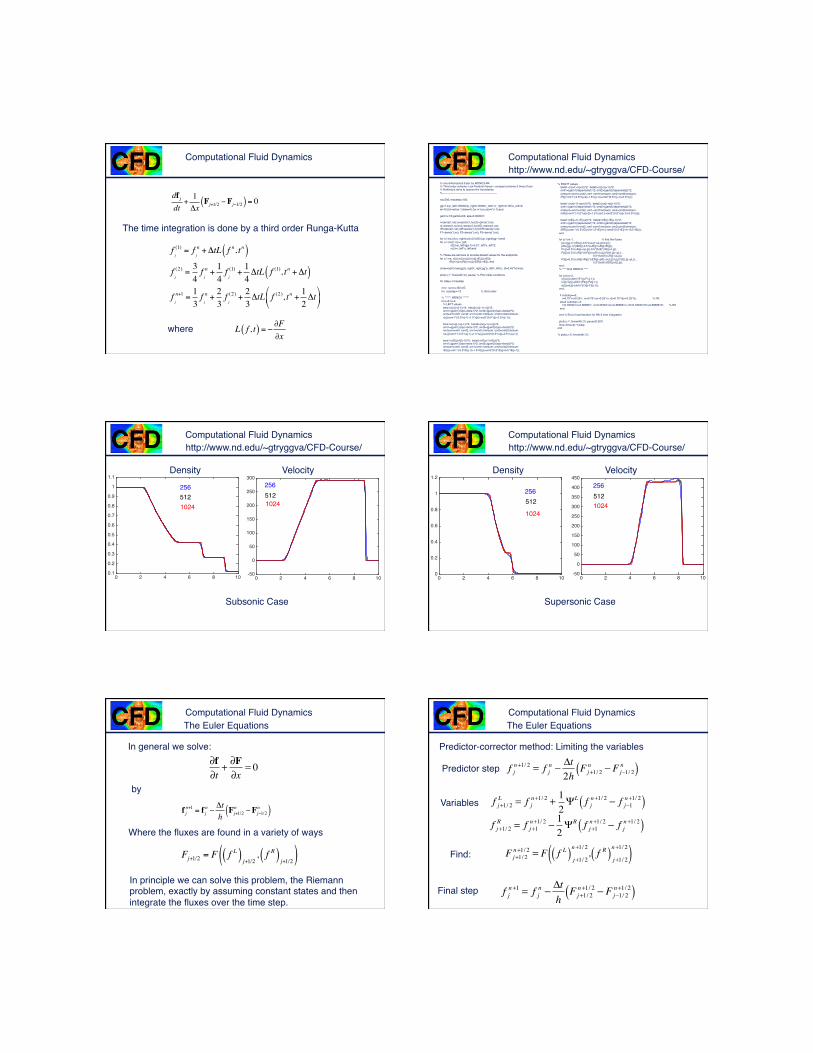
WENO-3
http://www.nd.edu/~gtryggva/CFD-Course/Computational Fluid Dynamics
df jdt
+1Δx
Fj+1/2 −Fj−1/2( ) = 0
Fj+1/2 =ω1Fj+1/2(1) +ω2Fj+1/2
(2)
!ωl =γ l
ε +βl( )2
ωm =!ωm
!ωll=1
2∑
Fj+1/2(1) = −
12Fj−1 +
32Fj
Fj+1/2(2) =
12Fj +
12Fj+1
γ1 =13; γ2 =
23
β1 = f j − f j−1( )2
β2 = f j+1 − f j( )2
ε =10−6
The semi-discrete equation is
The fluxes are the weighted sum
where
The weights are
2nd order upwind2nd order central
Third order WENO
∂∂t
f + ∂∂x
F = 0
Computational Fluid Dynamics
The time integration is done by a third order Runga-Kutta
fj
(1) = fj
n +ΔtL f n, tn( )fj
(2) =34fj
n +14fj
(1) +14ΔtL f (1), tn +Δt( )
fj
n+1 =13fj
n +23fj
(2) +23ΔtL f (2), tn + 1
2Δt
"
#$
%
&'
L f , t( ) = −∂F∂x
where
df jdt
+1Δx
Fj+1/2 −Fj−1/2( ) = 0
Computational Fluid Dynamics
% one-dimensional Euler by WENO3-RK% Third order scheme--Lax-Friedrich fluxes---compact scheme-3 times Euler% Nothing is done to account for boundaries%------------------------------------------------------------
nx=256; maxstep=150;
gg=1.4;p_left=100000;p_right=10000;r_left=1;r_right=0.125;u_left=0;xl=10.0;h=xl/(nx-1);time=0; for i=1:nx,x(i)=h*(i-1);end
gam1=1/3;gam2=2/3; eps=0.000001;
r=zeros(1,nx);ru=zeros(1,nx);rE=zeros(1,nx);rL=zeros(1,nx);ruL=zeros(1,nx);rEL=zeros(1,nx);rR=zeros(1,nx);ruR=zeros(1,nx);rER=zeros(1,nx);F1=zeros(1,nx); F2=zeros(1,nx); F3=zeros(1,nx);
for i=1:nx,r(i)=r_right;ru(i)=0.0;rE(i)=p_right/(gg-1);endfor i=1:nx/2; r(i)=r_left; rE(i)=p_left/(gg-1)+0.5*r_left*u_left^2; ru(i)=r_left*u_left;end
% These are set here to provide default values for the endpointsfor j=1:nx, rL(j)=r(j);ruL(j)=ru(j);rEL(j)=rE(j); rR(j)=r(j);ruR(j)=ru(j);rER(j)=rE(j); end
cmax=sqrt( max(gg*p_right/r_right,gg*p_left/r_left) ); dt=0.45*h/cmax;
plot(x,r,'r','linewidth',2); pause, % Plot initial conditions for istep=1:maxstep
rn=r; run=ru;rEn=rE; for substep=1:3 % third order % ****** WENO3 ****** for j=3:nx-2, % LEFT values beta1=(r(j)-r(j-1))^2; beta2=(r(j+1)-r(j))^2; omt1=(gam1)/(eps+beta1)^2; omt2=(gam2)/(eps+beta2)^2; omtsum=omt1+omt2; om1=omt1/omtsum; om2=omt2/omtsum; rL(j)=om1*(-0.5*r(j-1)+1.5*r(j))+om2*(0.5*r(j)+0.5*r(j+1));
beta1=(ru(j)-ru(j-1))^2; beta2=(ru(j+1)-ru(j))^2; omt1=(gam1)/(eps+beta1)^2; omt2=(gam2)/(eps+beta2)^2; omtsum=omt1+omt2; om1=omt1/omtsum; om2=omt2/omtsum; ruL(j)=om1*(-0.5*ru(j-1)+1.5*ru(j))+om2*(0.5*ru(j)+0.5*ru(j+1)); beta1=(rE(j)-rE(j-1))^2; beta2=(rE(j+1)-rE(j))^2; omt1=(gam1)/(eps+beta1)^2; omt2=(gam2)/(eps+beta2)^2; omtsum=omt1+omt2; om1=omt1/omtsum; om2=omt2/omtsum; rEL(j)=om1*(-0.5*rE(j-1)+1.5*rE(j))+om2*(0.5*rE(j)+0.5*rE(j+1));
http://www.nd.edu/~gtryggva/CFD-Course/% RIGHT values beta1=(r(j+1)-r(j+2))^2; beta2=(r(j)-r(j+1))^2; omt1=(gam1)/(eps+beta1)^2; omt2=(gam2)/(eps+beta2)^2; omtsum=omt1+omt2; om1=omt1/omtsum; om2=omt2/omtsum; rR(j)=om1*(-0.5*r(j+2)+1.5*r(j+1))+om2*(0.5*r(j+1)+0.5*r(j));
beta1=(ru(j+1)-ru(j+2))^2; beta2=(ru(j)-ru(j+1))^2; omt1=(gam1)/(eps+beta1)^2; omt2=(gam2)/(eps+beta2)^2; omtsum=omt1+omt2; om1=omt1/omtsum; om2=omt2/omtsum; ruR(j)=om1*(-0.5*ru(j+2)+1.5*ru(j+1))+om2*(0.5*ru(j+1)+0.5*ru(j));
beta1=(rE(j+1)-rE(j+2))^2; beta2=(rE(j)-rE(j+1))^2; omt1=(gam1)/(eps+beta1)^2; omt2=(gam2)/(eps+beta2)^2; omtsum=omt1+omt2; om1=omt1/omtsum; om2=omt2/omtsum; rER(j)=om1*(-0.5*rE(j+2)+1.5*rE(j+1))+om2*(0.5*rE(j+1)+0.5*rE(j)); end
for j=1:nx-1, % find the fluxes pL=(gg-1)*(rEL(j)-0.5*(ruL(j)*ruL(j)/rL(j))); pR=(gg-1)*(rER(j)-0.5*(ruR(j)*ruR(j)/rR(j))); F1(j)=0.5*(ruR(j)+ruL(j))-0.5*(h/dt)*(rR(j)-rL(j)); F2(j)=0.5*((ruR(j)^2/rR(j))+pR+(ruL(j)^2/rL(j))+pL)-... 0.5*(h/dt)*(ruR(j)-ruL(j)); F3(j)=0.5*((ruR(j)/rR(j))*(rER(j)+pR)+(ruL(j)/rL(j))*(rEL(j)+pL))-... 0.5*(h/dt)*(rER(j)-rEL(j)); end; % **** End WENO3 ****
for j=3:nx-2, r(j)=r(j)-(dt/h)*(F1(j)-F1(j-1)); ru(j)=ru(j)-(dt/h)*(F2(j)-F2(j-1)); rE(j)=rE(j)-(dt/h)*(F3(j)-F3(j-1)); end;
if substep==2, r=0.75*rn+0.25*r; ru=0.75*run+0.25*ru; rE=0.75*rEn+0.25*rE; % RK elseif substep==3 r=0.33334*rn+0.66666*r; ru=0.33334*run+0.66666*ru; rE=0.33334*rEn+0.66666*rE; % RK end
end % End of sub-iteration for RK-3 time integration plot(x,r,'r','linewidth',2); pause(0.001) time=time+dt; %istepend
% plot(x,r,'k','linewidth',2);
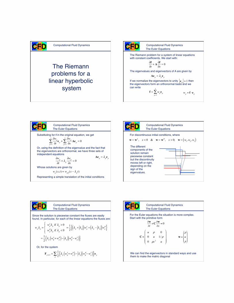
Computational Fluid Dynamics
Density Velocity
http://www.nd.edu/~gtryggva/CFD-Course/
0 2 4 6 8 100.1
0.2
0.3
0.4
0.5
0.6
0.7
0.8
0.9
1
1.1
2565121024
0 2 4 6 8 10-50
0
50
100
150
200
250
3002565121024
Subsonic Case
Computational Fluid Dynamics
Density Velocity
http://www.nd.edu/~gtryggva/CFD-Course/
0 2 4 6 8 100
0.2
0.4
0.6
0.8
1
1.2
256512
1024
0 2 4 6 8 10-50
0
50
100
150
200
250
300
350
400
4502565121024
Supersonic Case
Computational Fluid Dynamics
In general we solve:
The Euler Equations
f jn+1 = f j
n −ΔthFj+1/2n −Fj−1/2
n( )�
∂f∂t
+ ∂F∂x
= 0
by
Where the fluxes are found in a variety of ways
Fj+1/2 = F f L( ) j+1/2 , fR( ) j+1/2( )
In principle we can solve this problem, the Riemann problem, exactly by assuming constant states and then integrate the fluxes over the time step.
Computational Fluid Dynamics
�
f jn+1/ 2 = f j
n − Δt2h
Fj+1/ 2n − Fj−1/ 2
n( )
�
f jn+1 = f j
n − Δth
Fj+1/ 2n+1/ 2 − Fj−1/ 2
n+1/ 2( )�
Fj+1/ 2n+1/ 2 = F f L( ) j+1/ 2
n+1/ 2, f R( ) j+1/ 2
n+1/ 2( )
Predictor step
Variables
�
f j+1/ 2L = f j
n+1/ 2 + 12ΨL f j
n+1/ 2 − f j−1n+1/ 2( )
�
f j+1/ 2R = f j+1
n+1/ 2 − 12ΨR f j+1
n+1/ 2 − f jn+1/ 2( )
Final step
Predictor-corrector method: Limiting the variables
Find:
The Euler Equations
Computational Fluid Dynamics
The Riemann problems for a
linear hyperbolic system
Computational Fluid Dynamics369
The Riemann problem for a system of linear equations with constant coefficients. We start with:
The eigenvalues and eigenvectors of A are given by
If we normalize the eigenvectors to unity then the eigenvectors form an orthonormal basis and we can write
∂f∂t
+ A ∂f∂x
= 0
f = wp
p=1
3
∑ e p
The Euler Equations
Ae p = λpe p
e p = 1
wp = f ⋅e p
Computational Fluid Dynamics370
Substituting for f in the original equation, we get
Or, using the definition of the eigenvalue and the fact that the eigenvectors are orthonormal, we have three sets of independent equations
Whose solutions are given by
Representing a simple translation of the initial conditions
∂wp
∂tp=1
3
∑ e p +∂wp
∂xA
p=1
3
∑ e p = 0
The Euler Equations
∂wp
∂t+ λp
∂wp
∂x= 0
wp (x,t) = wp0 (x − λpt)
Ae p = λpe p
Computational Fluid Dynamics371
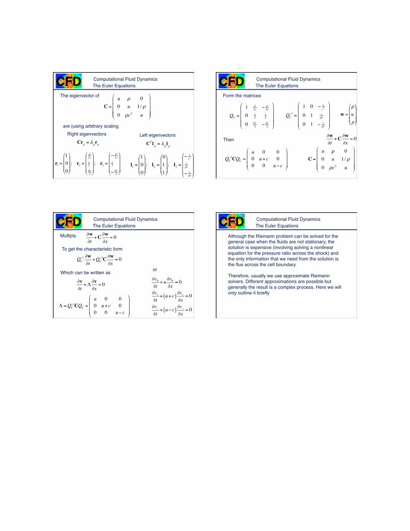
For discontinuous initial conditions, where
w = wL , x < 0 & w = wR , x > 0; w = w1,w2 ,w3( )
The Euler Equations
The different components of the solution remain piecewise constant but the discontinuity moves left or right, depending on the sign of the eigenvalues.
Computational Fluid Dynamics372
Since the solution is piecewise constant the fluxes are easily found. In particular, for each of the linear equations the fluxes are:
The Euler Equations
wpλp =wpLλp if λp > 0
wpRλp if λp < 0
⎧⎨⎪
⎩⎪= 12
λp + λp( )wpL + λp − λp( )wpR{ }= 12
λp wpLi +wp
R( )− λp wpRi −wp
L( ){ }
Fj+1/2 =12
λp wpLi +wp
R( )− λp wpRi −wp
L( ){ }e pp∑
Or, for the system
Computational Fluid Dynamics373
For the Euler equations the situation is more complex.Start with the primitive form
The Euler Equations
We can find the eigenvectors in standard ways and use them to make the matric diagonal
∂w∂t
+C∂w∂x
= 0
w =ρ
up
!
"
###
$
%
&&&
C =u ρ 00 u 1/ ρ0 ρc2 u
!
"
####
$
%
&&&&
Computational Fluid Dynamics
The eigenvector of
r1 =100
!
"
###
$
%
&&&; r2 =
ρ2c12ρc2
!
"
###
$
%
&&&; r3 =
− ρ2c
12
− ρc2
!
"
###
$
%
&&&
The Euler Equations
C =u ρ 00 u 1/ ρ0 ρc2 u
!
"
####
$
%
&&&&
are (using arbitrary scaling
l1 =100
!
"
###
$
%
&&&; l2 =
011
!
"
###
$
%
&&&; l3 =
− 1c2
1ρc
− 1ρc
!
"
###
$
%
&&&
Right eigenvectors Left eigenvectorsCrp = λprp CT l p = λpl p
Computational Fluid Dynamics
Form the matrices
QC =
1 ρ2c − ρ
2c
0 12
12
0 ρc2 − ρc
2
"
#
$$$$
%
&
''''
The Euler Equations
∂w∂t
+C∂w∂x
= 0Then
C =u ρ 00 u 1/ ρ0 ρc2 u
!
"
####
$
%
&&&&
QC−1 =
1 0 − 1c2
0 1 1ρc
0 1 − 1ρc
"
#
$$$$
%
&
''''
QC−1CQC =
u 0 00 u+ c 00 0 u− c
"
#
$$$
%
&
'''
w =ρ
up
!
"
###
$
%
&&&
Computational Fluid Dynamics
Multiply
The Euler Equations
QC−1 ∂w∂t
+QC−1C∂w
∂x= 0
Which can be written as
Λ =QC−1CQC =
u 0 00 u+ c 00 0 u− c
#
$
%%%
&
'
(((
∂w∂t
+C∂w∂x
= 0
To get the characteristic form
∂v∂t+Λ
∂v∂x
= 0∂v0∂t
+u∂v0∂x
= 0
∂v+∂t
+ u+ c( )∂v+∂x
= 0
∂v−∂t
+ u− c( )∂v−∂x
= 0
or
Computational Fluid Dynamics377
Although the Riemann problem can be solved for the general case when the fluids are not stationary, the solution is expensive (involving solving a nonlinear equation for the pressure ratio across the shock) and the only information that we need from the solution is the flux across the cell boundary.
Therefore, usually we use approximate Riemann solvers. Different approximations are possible but generally the result is a complex process. Here we will only outline it briefly
The Euler Equations