computational complexity theory lecture 2: reductions, np-completeness, cook-levin theorem indian...
TRANSCRIPT
Computational Complexity Theory
Lecture 2: Reductions, NP-completeness,
Cook-Levin theorem
Indian Institute of Science
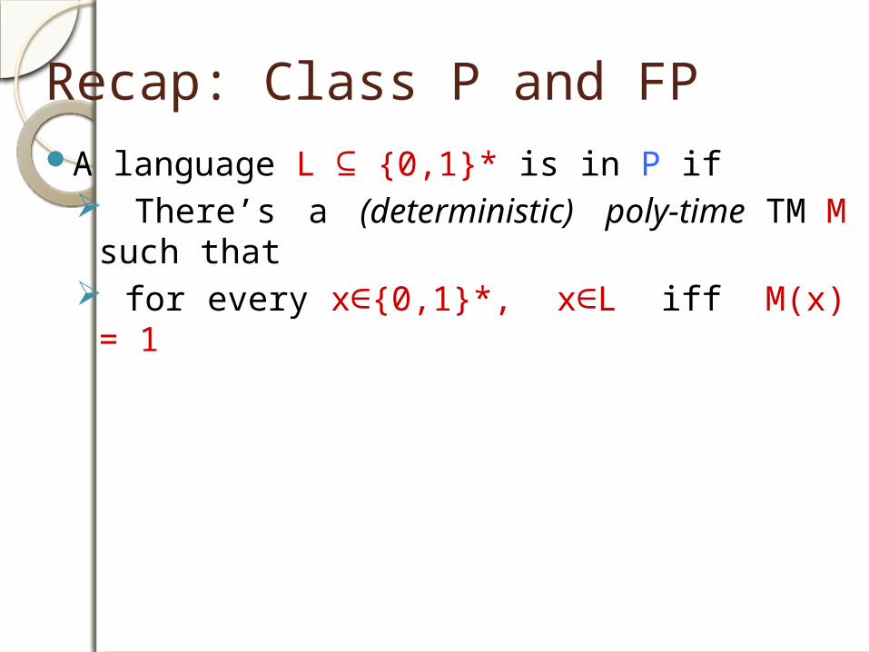
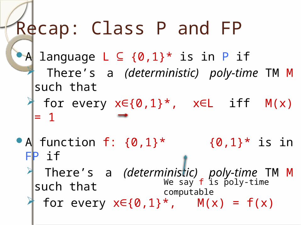
Recap: Class P and FPA language L ⊆ {0,1}* is in P if
There’s a (deterministic) poly-time TM M such that
for every x∈{0,1}*, x∈L iff M(x) = 1
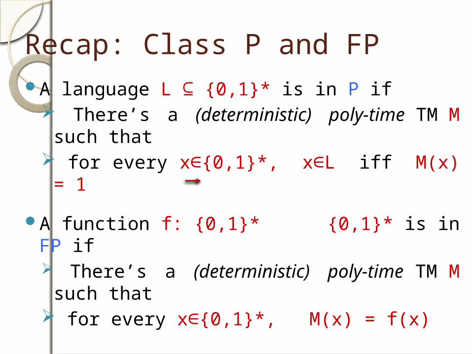
Recap: Class P and FPA language L ⊆ {0,1}* is in P if
There’s a (deterministic) poly-time TM M such that
for every x∈{0,1}*, x∈L iff M(x) = 1
A function f: {0,1}* {0,1}* is in FP if There’s a (deterministic) poly-time TM M
such that for every x∈{0,1}*, M(x) = f(x)
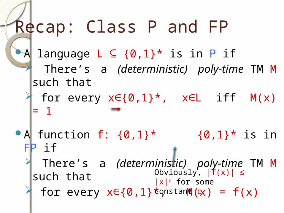
Recap: Class P and FPA language L ⊆ {0,1}* is in P if
There’s a (deterministic) poly-time TM M such that
for every x∈{0,1}*, x∈L iff M(x) = 1
A function f: {0,1}* {0,1}* is in FP if There’s a (deterministic) poly-time TM M
such that for every x∈{0,1}*, M(x) = f(x)
Obviously, |f(x)| ≤ |x|c for some constant c
Recap: Class P and FPA language L ⊆ {0,1}* is in P if
There’s a (deterministic) poly-time TM M such that
for every x∈{0,1}*, x∈L iff M(x) = 1
A function f: {0,1}* {0,1}* is in FP if There’s a (deterministic) poly-time TM M
such that for every x∈{0,1}*, M(x) = f(x)
We say f is poly-time computable
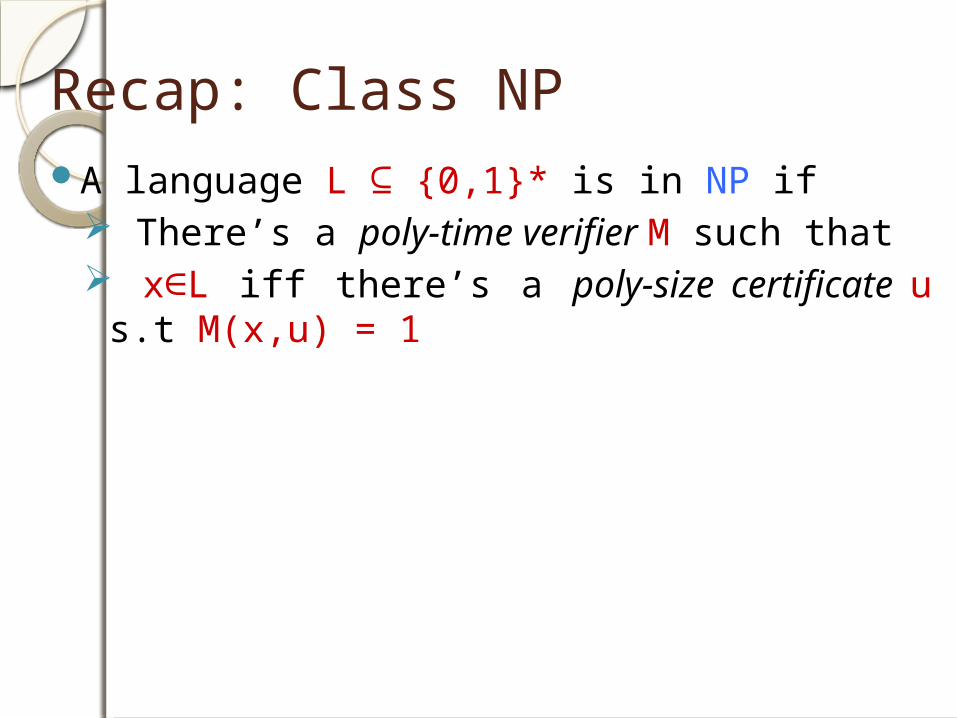
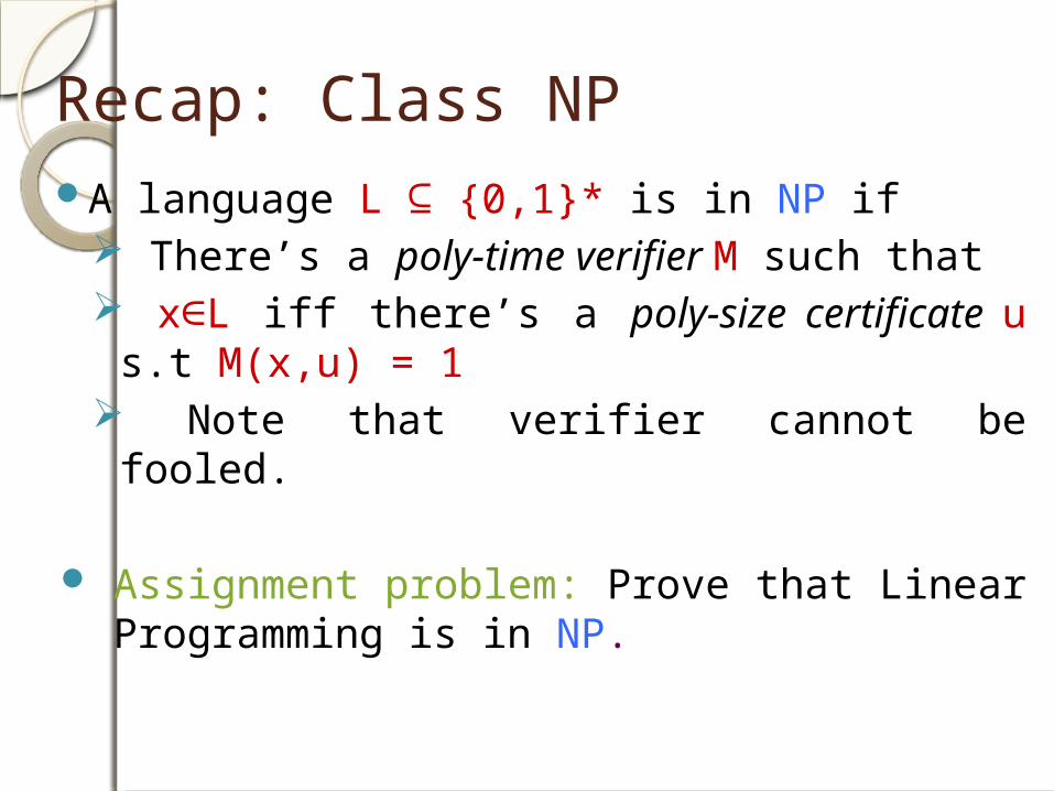
Recap: Class NPA language L ⊆ {0,1}* is in NP if
There’s a poly-time verifier M such that x∈L iff there’s a poly-size certificate u s.t
M(x,u) = 1
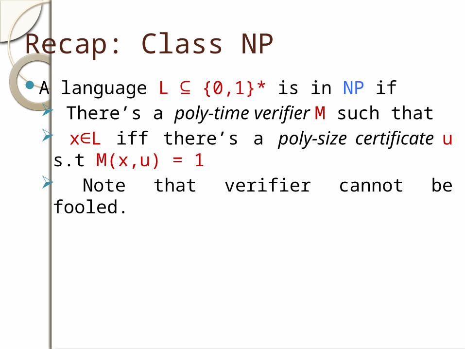
Recap: Class NPA language L ⊆ {0,1}* is in NP if
There’s a poly-time verifier M such that x∈L iff there’s a poly-size certificate u s.t
M(x,u) = 1 Note that verifier cannot be fooled.
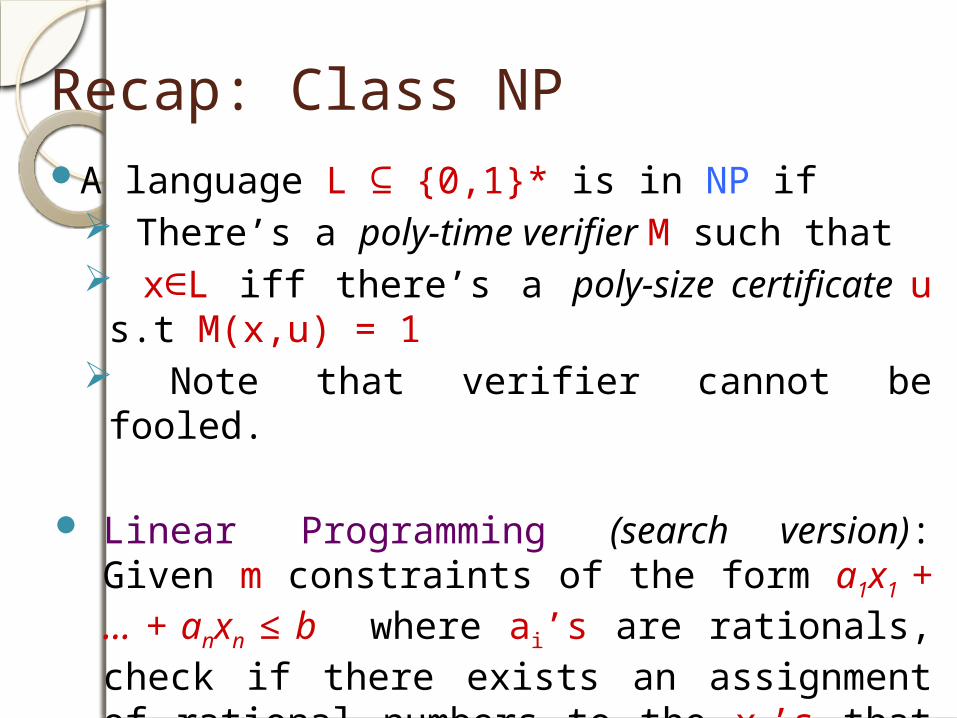
Recap: Class NPA language L ⊆ {0,1}* is in NP if
There’s a poly-time verifier M such that x∈L iff there’s a poly-size certificate u s.t
M(x,u) = 1 Note that verifier cannot be fooled.
Linear Programming (search version): Given m constraints of the form a1x1 + … + anxn ≤ b where ai’s are rationals, check if there exists an assignment of rational numbers to the xi’s that satisfy all constraints.
Recap: Class NPA language L ⊆ {0,1}* is in NP if
There’s a poly-time verifier M such that x∈L iff there’s a poly-size certificate u s.t
M(x,u) = 1 Note that verifier cannot be fooled.
Assignment problem: Prove that Linear Programming is in NP.
Nondeterministic Turing MachinesA nondeterministic Turing machine is like a
deterministic Turing machines but with two transition functions.
It is formally defined by a tuple (Γ, Q, δ0 , δ1).
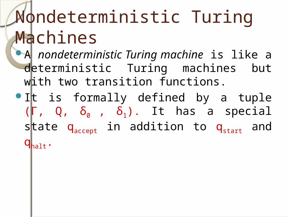
Nondeterministic Turing MachinesA nondeterministic Turing machine is like a
deterministic Turing machines but with two transition functions.
It is formally defined by a tuple (Γ, Q, δ0 , δ1). It has a special state qaccept in addition to qstart and qhalt.
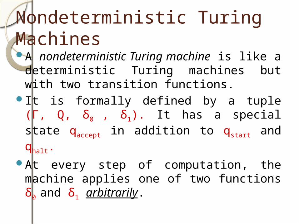
Nondeterministic Turing MachinesA nondeterministic Turing machine is like a
deterministic Turing machines but with two transition functions.
It is formally defined by a tuple (Γ, Q, δ0 , δ1). It has a special state qaccept in addition to qstart and qhalt.
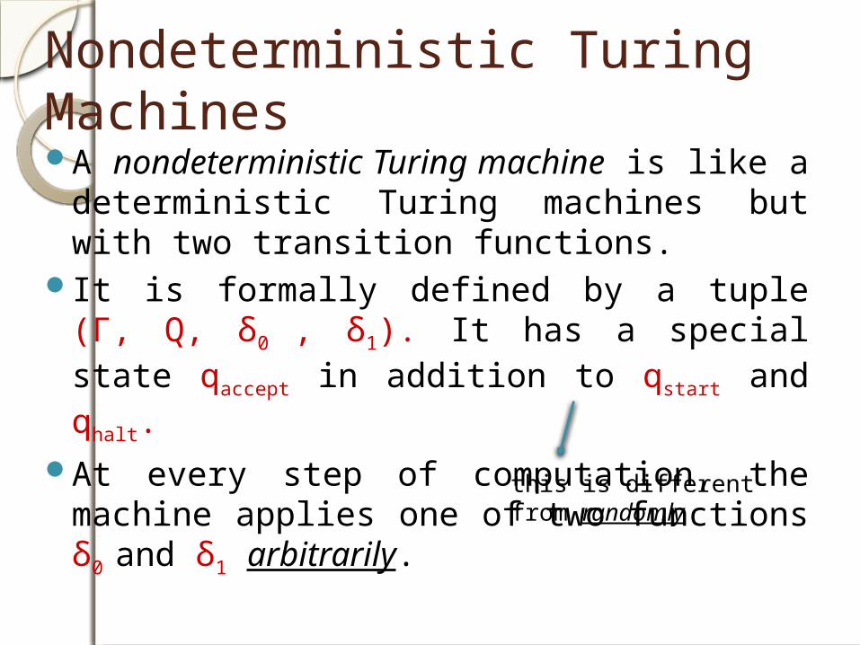
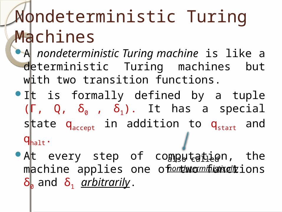
At every step of computation, the machine applies one of two functions δ0 and δ1 arbitrarily.
Nondeterministic Turing MachinesA nondeterministic Turing machine is like a
deterministic Turing machines but with two transition functions.
It is formally defined by a tuple (Γ, Q, δ0 , δ1). It has a special state qaccept in addition to qstart and qhalt.
At every step of computation, the machine applies one of two functions δ0 and δ1 arbitrarily.
this is different from randomly
Nondeterministic Turing MachinesA nondeterministic Turing machine is like a
deterministic Turing machines but with two transition functions.
It is formally defined by a tuple (Γ, Q, δ0 , δ1). It has a special state qaccept in addition to qstart and qhalt.
At every step of computation, the machine applies one of two functions δ0 and δ1 arbitrarily.
also called nondeterministically
Nondeterministic Turing MachinesA nondeterministic Turing machine is like a
deterministic Turing machines but with two transition functions.
It is formally defined by a tuple (Γ, Q, δ0 , δ1). It has a special state qaccept in addition to qstart and qhalt.
At every step of computation, the machine applies one of two functions δ0 and δ1 arbitrarily.
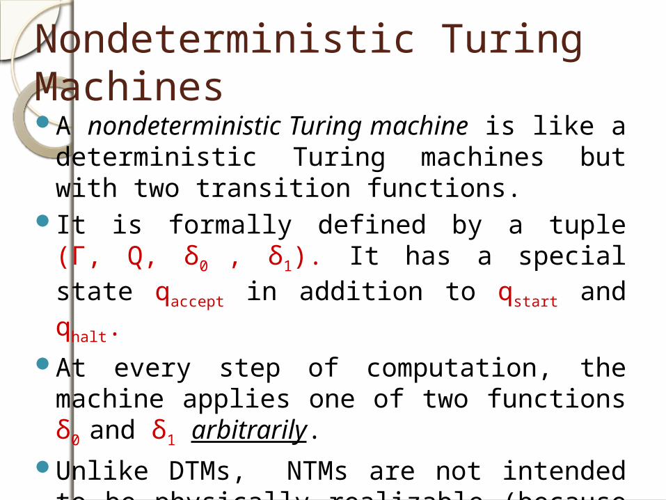
Unlike DTMs, NTMs are not intended to be physically realizable (because of the arbitrary nature of application of the transition functions).
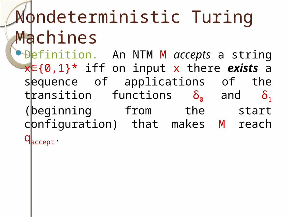
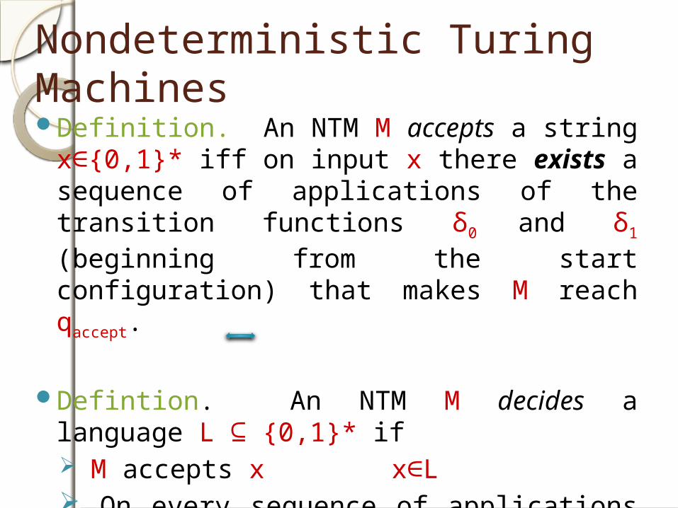
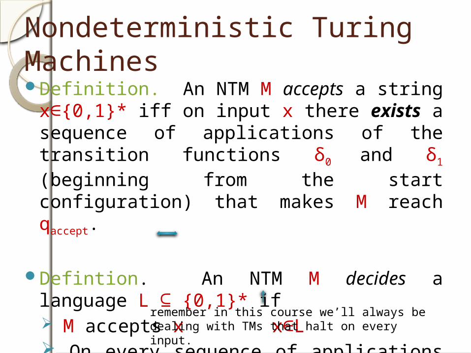
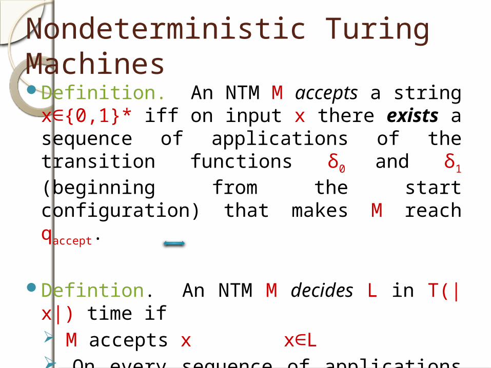
Nondeterministic Turing MachinesDefinition. An NTM M accepts a string
x∈{0,1}* iff on input x there exists a sequence of applications of the transition functions δ0 and δ1 (beginning from the start configuration) that makes M reach qaccept.
Nondeterministic Turing MachinesDefinition. An NTM M accepts a string
x∈{0,1}* iff on input x there exists a sequence of applications of the transition functions δ0 and δ1 (beginning from the start configuration) that makes M reach qaccept.
Defintion. An NTM M decides a language L ⊆ {0,1}* if M accepts x x∈L On every sequence of applications of the
transition functions on input x, M either reaches qaccept or qhalt.
remember in this course we’ll always be dealing with TMs that halt on every input.
Nondeterministic Turing MachinesDefinition. An NTM M accepts a string
x∈{0,1}* iff on input x there exists a sequence of applications of the transition functions δ0 and δ1 (beginning from the start configuration) that makes M reach qaccept.
Defintion. An NTM M decides L in T(|x|) time if M accepts x x∈L On every sequence of applications of the
transition functions on input x, M either reaches qaccept or qhalt within T(|x|) steps of computation.

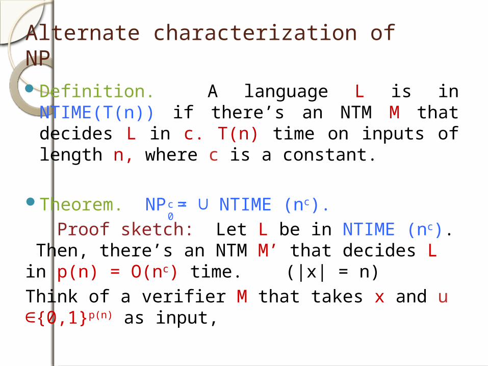
Class NTIMEDefinition. A language L is in NTIME(T(n)) if
there’s an NTM M that decides L in c. T(n) time on inputs of length n, where c is a constant.
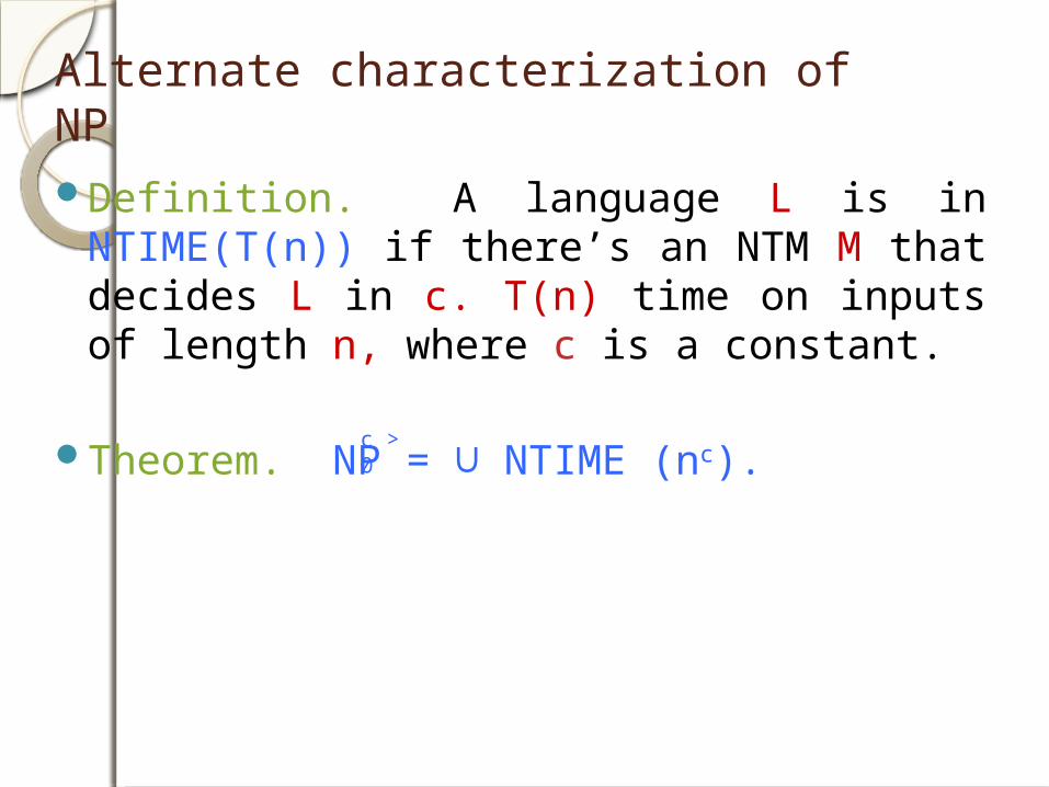
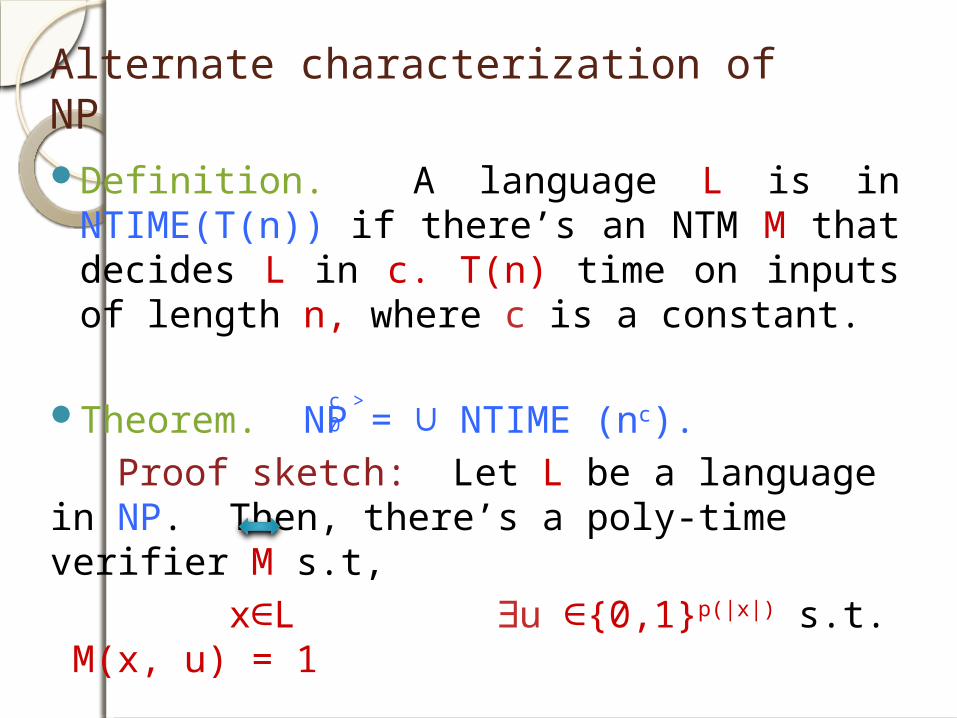
Alternate characterization of NP
Definition. A language L is in NTIME(T(n)) if there’s an NTM M that decides L in c. T(n) time on inputs of length n, where c is a constant.
Theorem. NP = ∪ NTIME (nc).c > 0
Alternate characterization of NP
Definition. A language L is in NTIME(T(n)) if there’s an NTM M that decides L in c. T(n) time on inputs of length n, where c is a constant.
Theorem. NP = ∪ NTIME (nc). Proof sketch: Let L be a language in NP. Then, there’s a poly-time verifier M s.t, x∈L ∃u ∈{0,1}p(|x|) s.t. M(x, u) = 1
c > 0
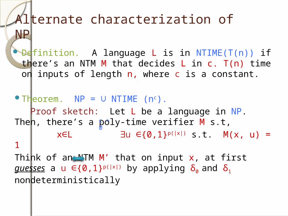
Alternate characterization of NP
Definition. A language L is in NTIME(T(n)) if there’s an NTM M that decides L in c. T(n) time on inputs of length n, where c is a constant.
Theorem. NP = ∪ NTIME (nc). Proof sketch: Let L be a language in NP. Then, there’s a poly-time verifier M s.t, x∈L ∃u ∈{0,1}p(|x|) s.t. M(x, u) = 1Think of an NTM M’ that on input x, at first guesses a u ∈{0,1}p(|x|) by applying δ0 and δ1 nondeterministically
c > 0
Alternate characterization of NP
Definition. A language L is in NTIME(T(n)) if there’s an NTM M that decides L in c. T(n) time on inputs of length n, where c is a constant.
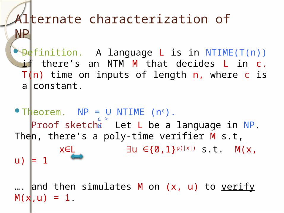
Theorem. NP = ∪ NTIME (nc). Proof sketch: Let L be a language in NP. Then, there’s a poly-time verifier M s.t, x∈L ∃u ∈{0,1}p(|x|) s.t. M(x, u) = 1
…. and then simulates M on (x, u) to verify M(x,u) = 1.
c > 0
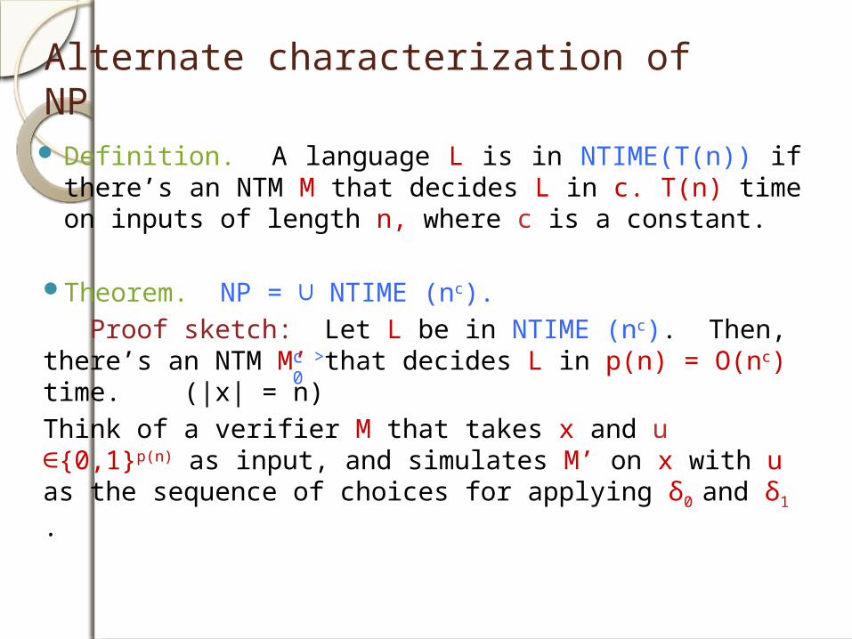
Alternate characterization of NP
Definition. A language L is in NTIME(T(n)) if there’s an NTM M that decides L in c. T(n) time on inputs of length n, where c is a constant.
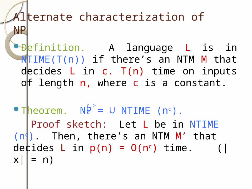
Theorem. NP = ∪ NTIME (nc). Proof sketch: Let L be in NTIME (nc). Then, there’s an NTM M’ that decides L in p(n) = O(nc) time. (|x| = n)
c > 0
Alternate characterization of NP
Definition. A language L is in NTIME(T(n)) if there’s an NTM M that decides L in c. T(n) time on inputs of length n, where c is a constant.
Theorem. NP = ∪ NTIME (nc). Proof sketch: Let L be in NTIME (nc). Then, there’s an NTM M’ that decides L in p(n) = O(nc) time. (|x| = n) Think of a verifier M that takes x and u ∈{0,1}p(n) as input,
c > 0
Alternate characterization of NP
Definition. A language L is in NTIME(T(n)) if there’s an NTM M that decides L in c. T(n) time on inputs of length n, where c is a constant.
Theorem. NP = ∪ NTIME (nc). Proof sketch: Let L be in NTIME (nc). Then, there’s an NTM M’ that decides L in p(n) = O(nc) time. (|x| = n) Think of a verifier M that takes x and u ∈{0,1}p(n) as input, and simulates M’ on x with u as the sequence of choices for applying δ0 and δ1 .
c > 0
Alternate characterization of NP
Definition. A language L is in NTIME(T(n)) if there’s an NTM M that decides L in c. T(n) time on inputs of length n, where c is a constant.
Theorem. NP = ∪ NTIME (nc). Proof sketch: (home work) Fill in the details…
c > 0
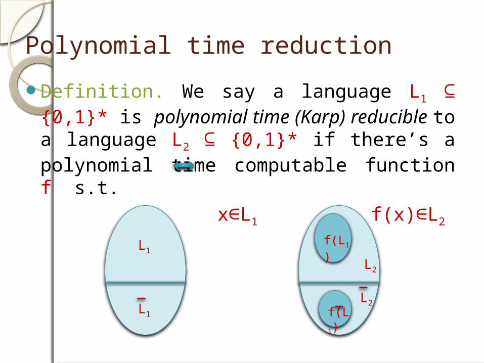
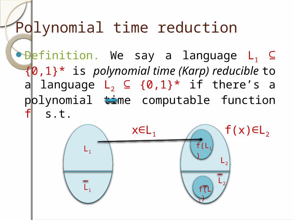
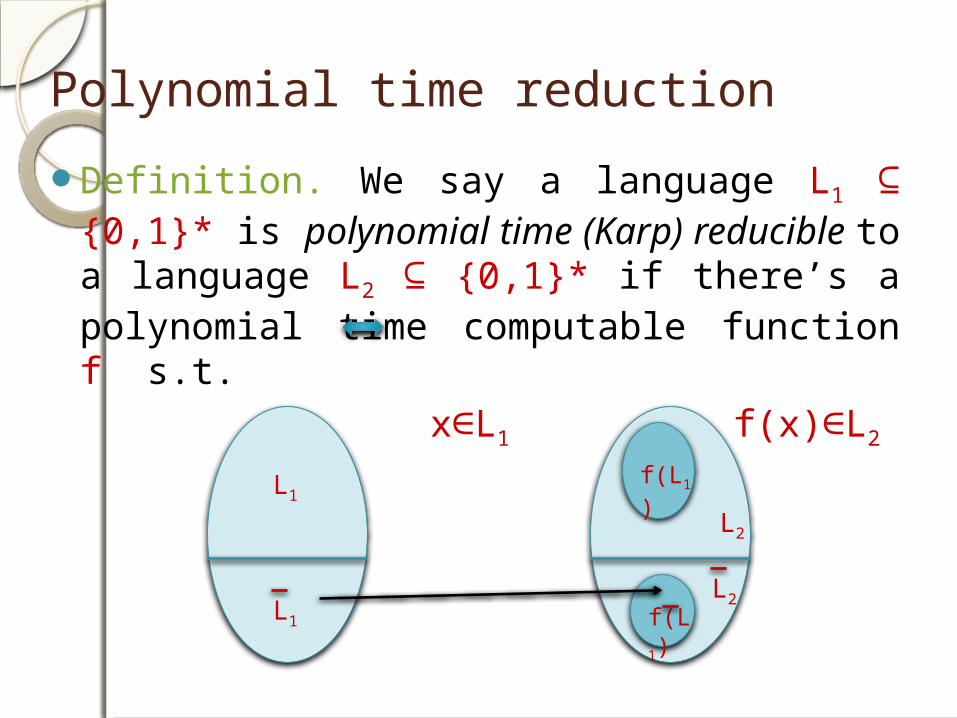
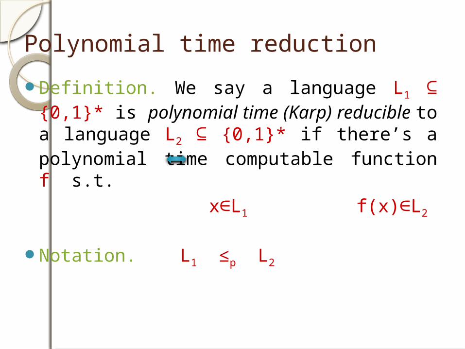
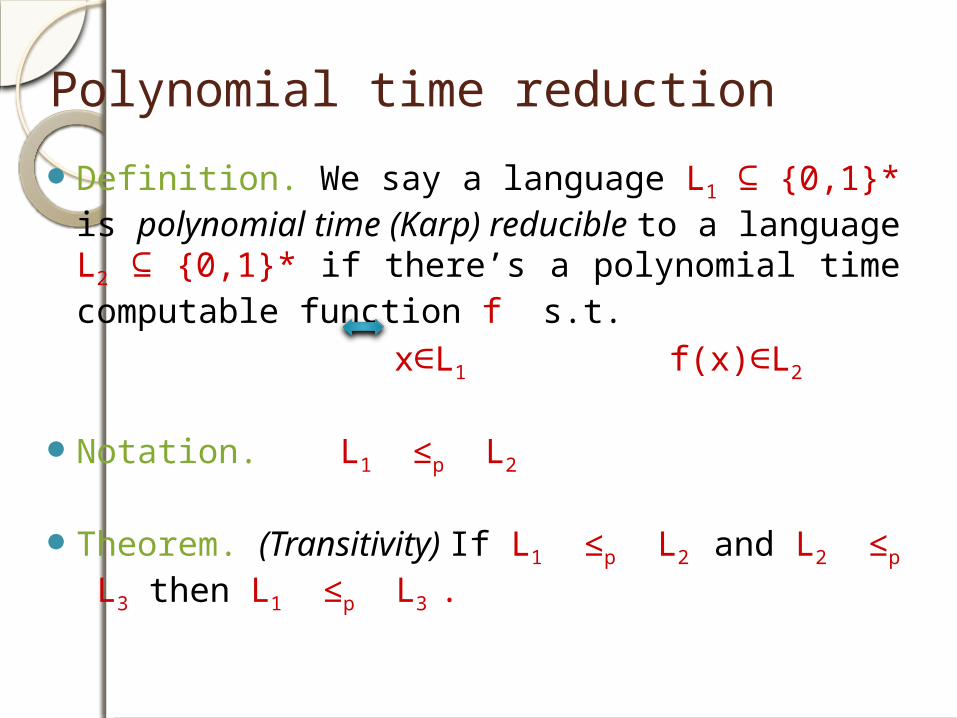
Polynomial time reductionDefinition. We say a language L1 ⊆ {0,1}*
is polynomial time (Karp) reducible to a language L2 ⊆ {0,1}* if there’s a polynomial time computable function f s.t.
x∈L1 f(x)∈L2
Polynomial time reductionDefinition. We say a language L1 ⊆ {0,1}*
is polynomial time (Karp) reducible to a language L2 ⊆ {0,1}* if there’s a polynomial time computable function f s.t.
x∈L1 f(x)∈L2
L1
L1
L2
L2
f(L1)
f(L1
)
Polynomial time reductionDefinition. We say a language L1 ⊆ {0,1}*
is polynomial time (Karp) reducible to a language L2 ⊆ {0,1}* if there’s a polynomial time computable function f s.t.
x∈L1 f(x)∈L2
L1
L1
L2
L2
f(L1)
f(L1
)
Polynomial time reductionDefinition. We say a language L1 ⊆ {0,1}*
is polynomial time (Karp) reducible to a language L2 ⊆ {0,1}* if there’s a polynomial time computable function f s.t.
x∈L1 f(x)∈L2
L1
L1
L2
L2
f(L1)
f(L1
)
Polynomial time reductionDefinition. We say a language L1 ⊆ {0,1}*
is polynomial time (Karp) reducible to a language L2 ⊆ {0,1}* if there’s a polynomial time computable function f s.t.
x∈L1 f(x)∈L2
Notation. L1 ≤p L2
Polynomial time reductionDefinition. We say a language L1 ⊆ {0,1}*
is polynomial time (Karp) reducible to a language L2 ⊆ {0,1}* if there’s a polynomial time computable function f s.t.
x∈L1 f(x)∈L2
Notation. L1 ≤p L2
Theorem. (Transitivity) If L1 ≤p L2 and L2 ≤p L3 then L1 ≤p L3 .
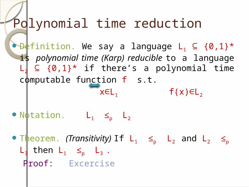
Polynomial time reductionDefinition. We say a language L1 ⊆ {0,1}* is
polynomial time (Karp) reducible to a language L2 ⊆ {0,1}* if there’s a polynomial time computable function f s.t.
x∈L1 f(x)∈L2
Notation. L1 ≤p L2
Theorem. (Transitivity) If L1 ≤p L2 and L2 ≤p L3 then L1 ≤p L3 .
Proof: Excercise
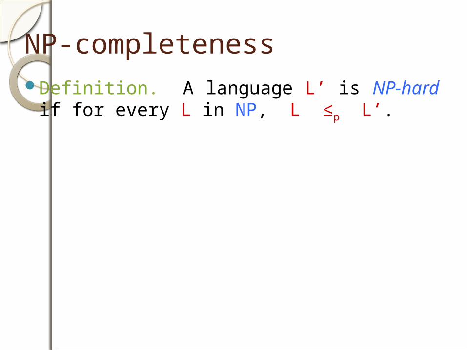
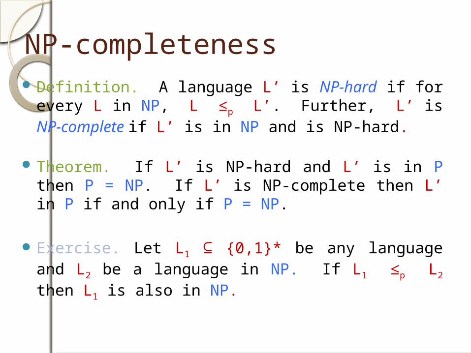
NP-completenessDefinition. A language L’ is NP-hard if for
every L in NP, L ≤p L’.
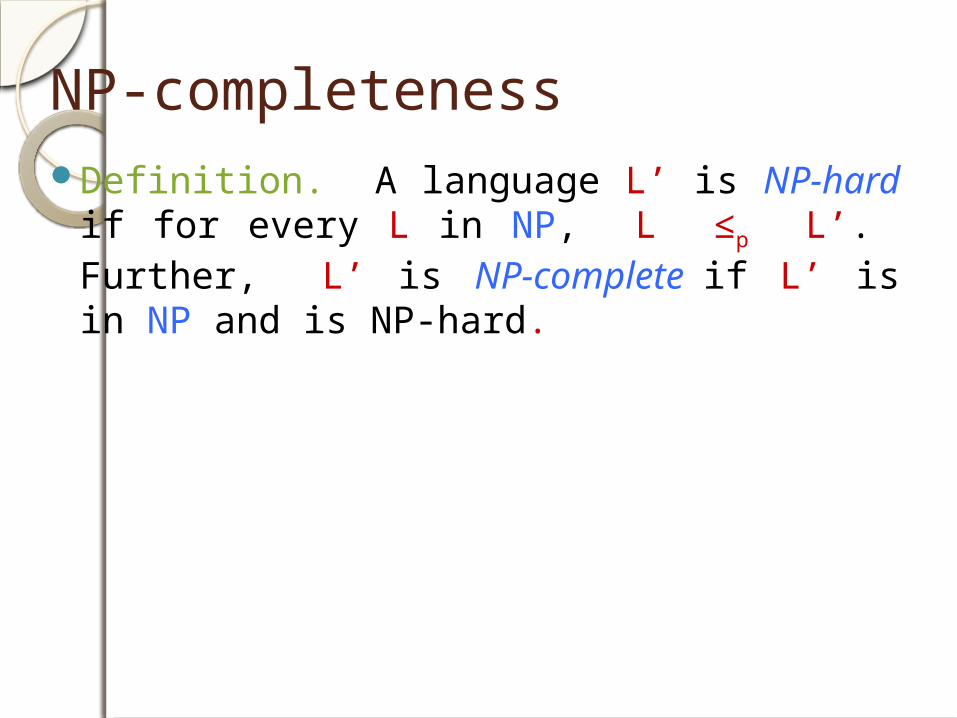
NP-completenessDefinition. A language L’ is NP-hard if for
every L in NP, L ≤p L’. Further, L’ is NP-complete if L’ is in NP and is NP-hard.
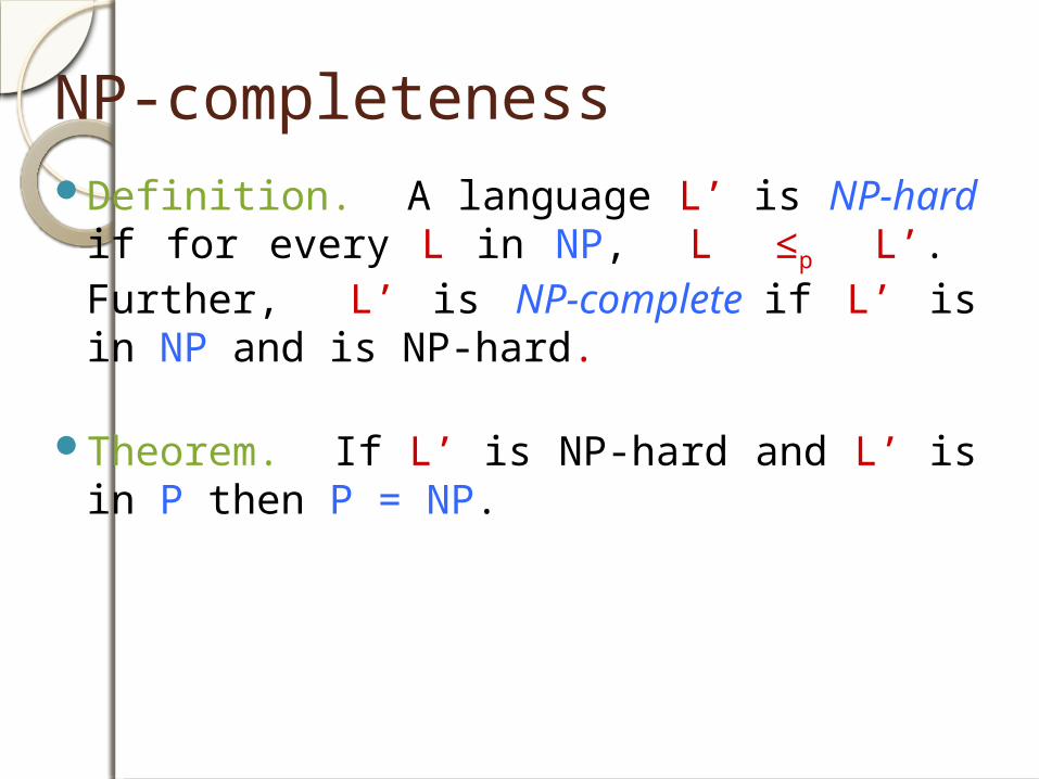
NP-completenessDefinition. A language L’ is NP-hard if for
every L in NP, L ≤p L’. Further, L’ is NP-complete if L’ is in NP and is NP-hard.
Theorem. If L’ is NP-hard and L’ is in P then P = NP.
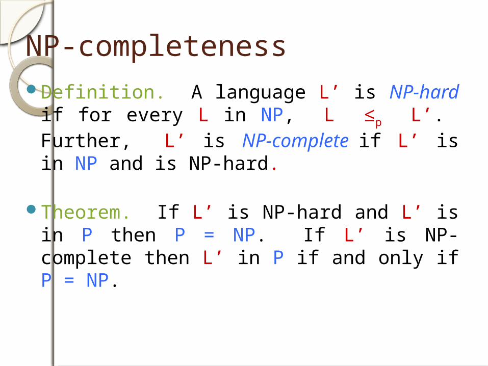
NP-completenessDefinition. A language L’ is NP-hard if for
every L in NP, L ≤p L’. Further, L’ is NP-complete if L’ is in NP and is NP-hard.
Theorem. If L’ is NP-hard and L’ is in P then P = NP. If L’ is NP-complete then L’ in P if and only if P = NP.
NP-completenessDefinition. A language L’ is NP-hard if for
every L in NP, L ≤p L’. Further, L’ is NP-complete if L’ is in NP and is NP-hard.
Theorem. If L’ is NP-hard and L’ is in P then P = NP. If L’ is NP-complete then L’ in P if and only if P = NP.
Proof. Home work
NP-completenessDefinition. A language L’ is NP-hard if for
every L in NP, L ≤p L’. Further, L’ is NP-complete if L’ is in NP and is NP-hard.
Theorem. If L’ is NP-hard and L’ is in P then P = NP. If L’ is NP-complete then L’ in P if and only if P = NP.
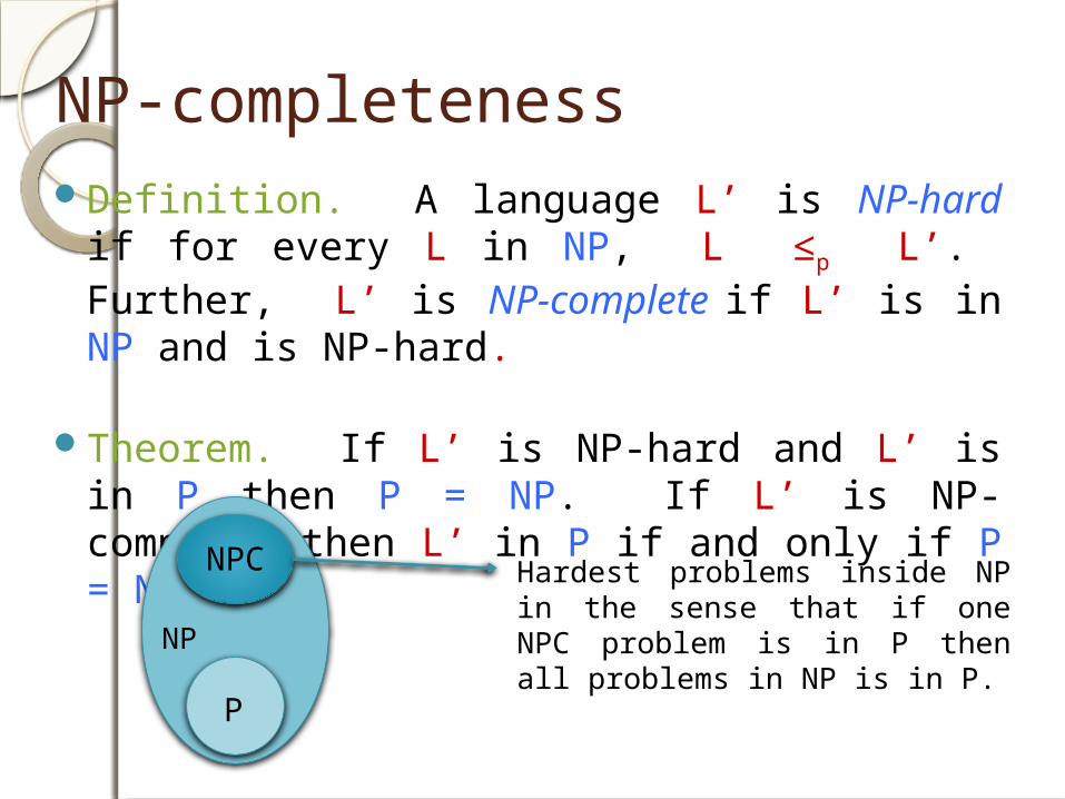
P
NPC
NP
Hardest problems inside NP in the sense that if one NPC problem is in P then all problems in NP is in P.
NP-completenessDefinition. A language L’ is NP-hard if for
every L in NP, L ≤p L’. Further, L’ is NP-complete if L’ is in NP and is NP-hard.
Theorem. If L’ is NP-hard and L’ is in P then P = NP. If L’ is NP-complete then L’ in P if and only if P = NP.
Exercise. Let L1 ⊆ {0,1}* be any language and L2 be a language in NP. If L1 ≤p L2 then L1 is also in NP.
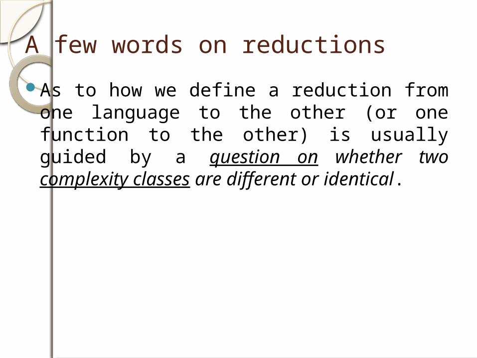
A few words on reductionsAs to how we define a reduction from one
language to the other (or one function to the other) is usually guided by a question on whether two complexity classes are different or identical.
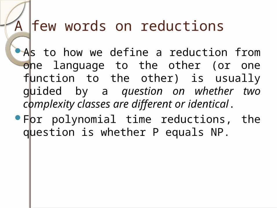
A few words on reductionsAs to how we define a reduction from one
language to the other (or one function to the other) is usually guided by a question on whether two complexity classes are different or identical.
For polynomial time reductions, the question is whether P equals NP.
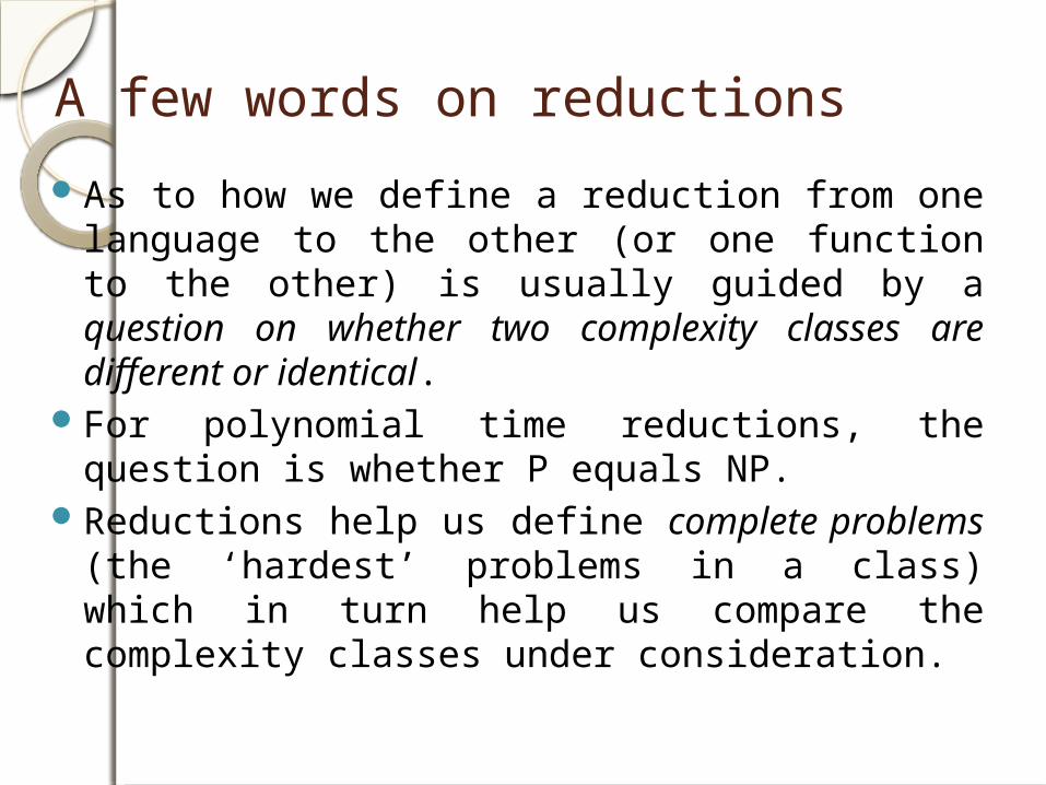
A few words on reductionsAs to how we define a reduction from one
language to the other (or one function to the other) is usually guided by a question on whether two complexity classes are different or identical.
For polynomial time reductions, the question is whether P equals NP.
Reductions help us define complete problems (the ‘hardest’ problems in a class) which in turn help us compare the complexity classes under consideration.
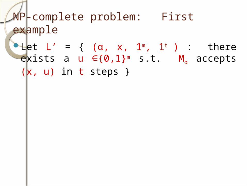
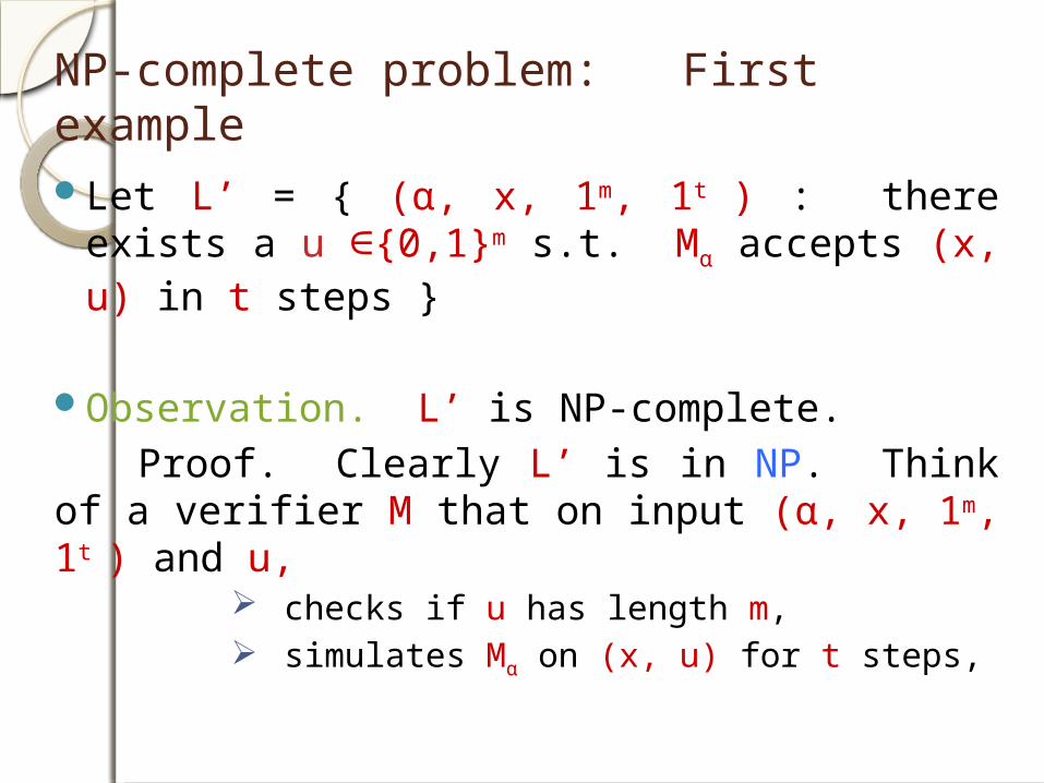
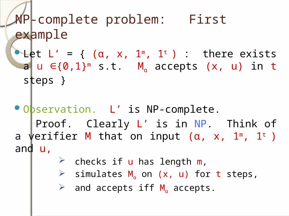
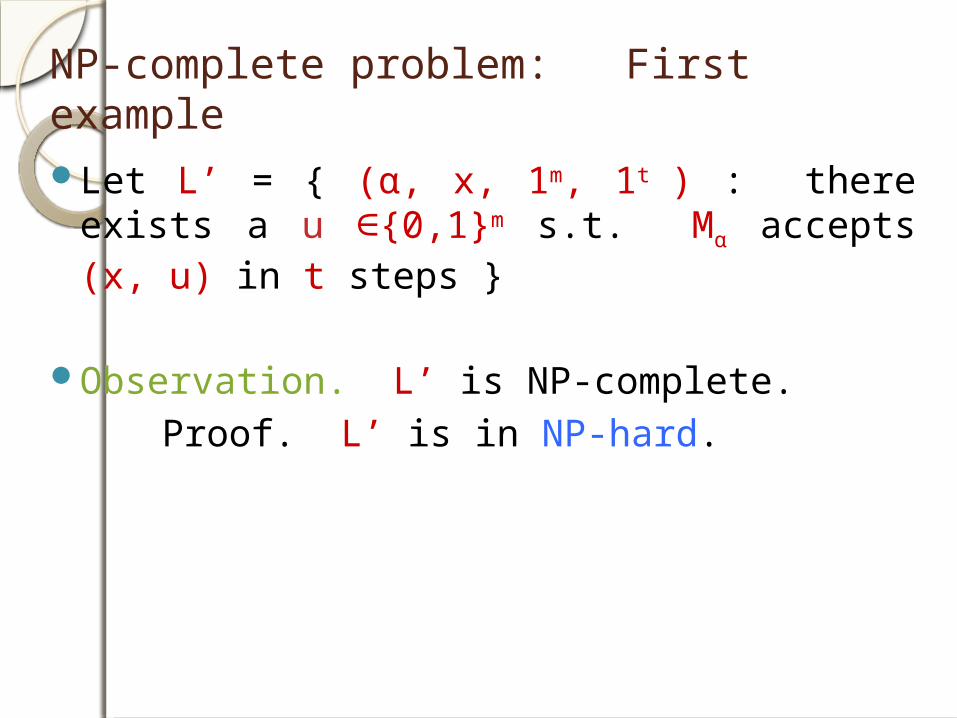
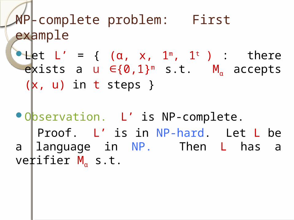
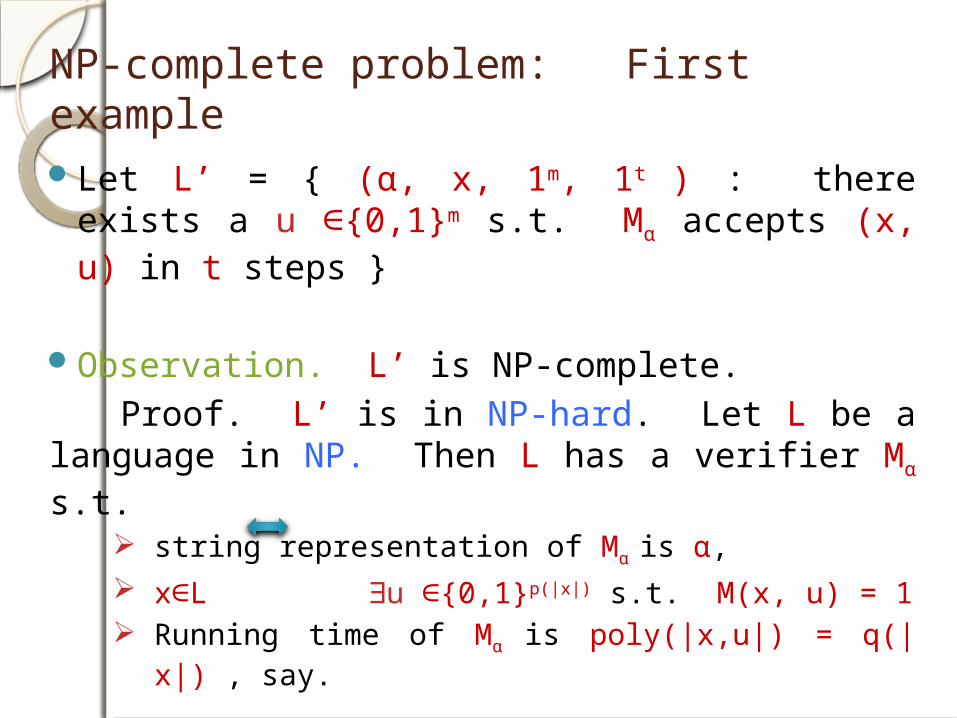
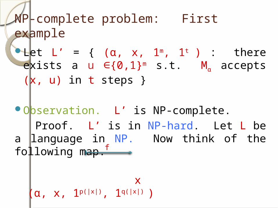
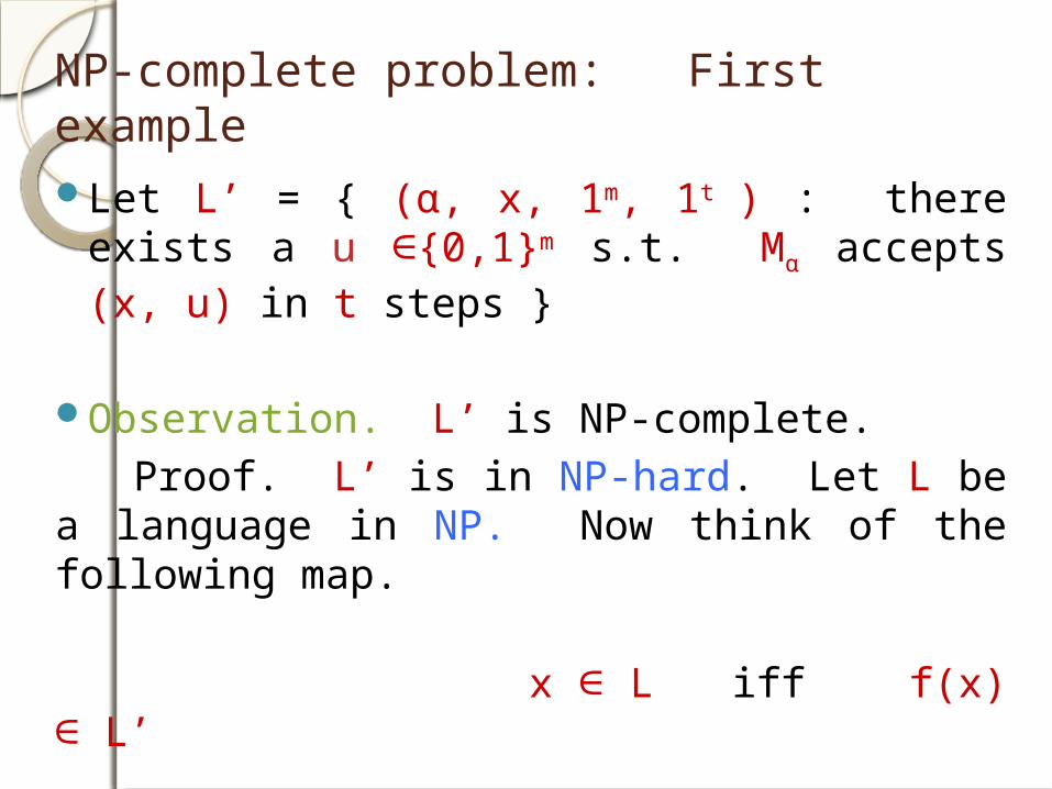
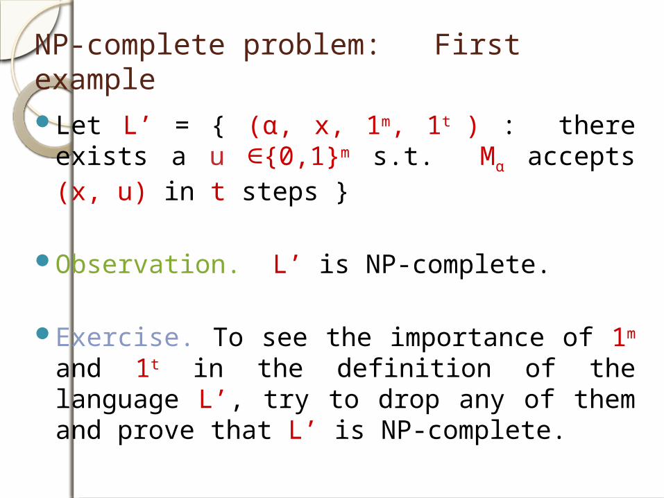
NP-complete problem: First example
Let L’ = { (α, x, 1m, 1t ) : there exists a u ∈{0,1}m s.t. Mα accepts (x, u) in t steps }
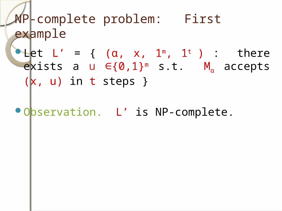
NP-complete problem: First example
Let L’ = { (α, x, 1m, 1t ) : there exists a u ∈{0,1}m s.t. Mα accepts (x, u) in t steps }
Observation. L’ is NP-complete.
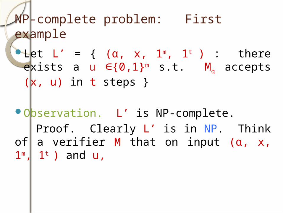
NP-complete problem: First example
Let L’ = { (α, x, 1m, 1t ) : there exists a u ∈{0,1}m s.t. Mα accepts (x, u) in t steps }
Observation. L’ is NP-complete. Proof. Clearly L’ is in NP. Think of a verifier M that on input (α, x, 1m, 1t ) and u,
NP-complete problem: First example
Let L’ = { (α, x, 1m, 1t ) : there exists a u ∈{0,1}m s.t. Mα accepts (x, u) in t steps }
Observation. L’ is NP-complete. Proof. Clearly L’ is in NP. Think of a verifier M that on input (α, x, 1m, 1t ) and u,
checks if u has length m,
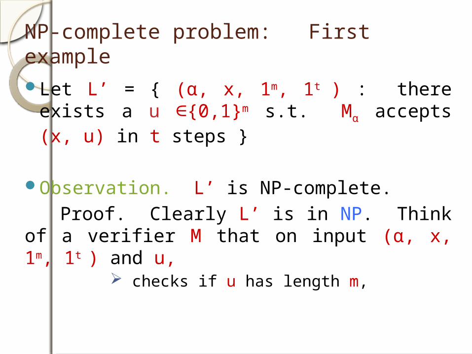
NP-complete problem: First example
Let L’ = { (α, x, 1m, 1t ) : there exists a u ∈{0,1}m s.t. Mα accepts (x, u) in t steps }
Observation. L’ is NP-complete. Proof. Clearly L’ is in NP. Think of a verifier M that on input (α, x, 1m, 1t ) and u,
checks if u has length m, simulates Mα on (x, u) for t steps,
and accepts iff Mα accepts.
NP-complete problem: First example
Let L’ = { (α, x, 1m, 1t ) : there exists a u ∈{0,1}m s.t. Mα accepts (x, u) in t steps }
Observation. L’ is NP-complete. Proof. L’ is in NP-hard.
NP-complete problem: First example
Let L’ = { (α, x, 1m, 1t ) : there exists a u ∈{0,1}m s.t. Mα accepts (x, u) in t steps }
Observation. L’ is NP-complete. Proof. L’ is in NP-hard. Let L be a language in NP. Then L has a verifier Mα s.t.
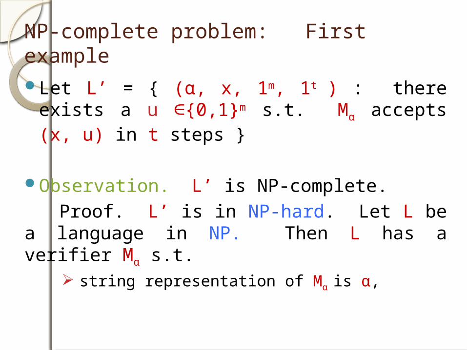
NP-complete problem: First example
Let L’ = { (α, x, 1m, 1t ) : there exists a u ∈{0,1}m s.t. Mα accepts (x, u) in t steps }
Observation. L’ is NP-complete. Proof. L’ is in NP-hard. Let L be a language in NP. Then L has a verifier Mα s.t.
string representation of Mα is α,
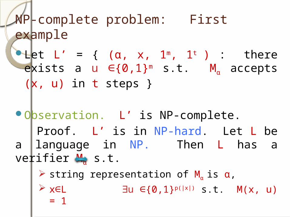
NP-complete problem: First example
Let L’ = { (α, x, 1m, 1t ) : there exists a u ∈{0,1}m s.t. Mα accepts (x, u) in t steps }
Observation. L’ is NP-complete. Proof. L’ is in NP-hard. Let L be a language in NP. Then L has a verifier Mα s.t.
string representation of Mα is α, x∈L ∃u ∈{0,1}p(|x|) s.t. M(x, u) = 1
NP-complete problem: First example
Let L’ = { (α, x, 1m, 1t ) : there exists a u ∈{0,1}m s.t. Mα accepts (x, u) in t steps }
Observation. L’ is NP-complete. Proof. L’ is in NP-hard. Let L be a language in NP. Then L has a verifier Mα s.t.
string representation of Mα is α, x∈L ∃u ∈{0,1}p(|x|) s.t. M(x, u) = 1 Running time of Mα is poly(|x,u|) = q(|x|) , say.
NP-complete problem: First example
Let L’ = { (α, x, 1m, 1t ) : there exists a u ∈{0,1}m s.t. Mα accepts (x, u) in t steps }
Observation. L’ is NP-complete. Proof. L’ is in NP-hard. Let L be a language in NP. Now think of the following map.
x (α, x, 1p(|x|), 1q(|x|) )f
NP-complete problem: First example
Let L’ = { (α, x, 1m, 1t ) : there exists a u ∈{0,1}m s.t. Mα accepts (x, u) in t steps }
Observation. L’ is NP-complete. Proof. L’ is in NP-hard. Let L be a language in NP. Now think of the following map.
x ∈ L iff f(x) ∈ L’
NP-complete problem: First example
Let L’ = { (α, x, 1m, 1t ) : there exists a u ∈{0,1}m s.t. Mα accepts (x, u) in t steps }
Observation. L’ is NP-complete.
Exercise. To see the importance of 1m and 1t in the definition of the language L’, try to drop any of them and prove that L’ is NP-complete.
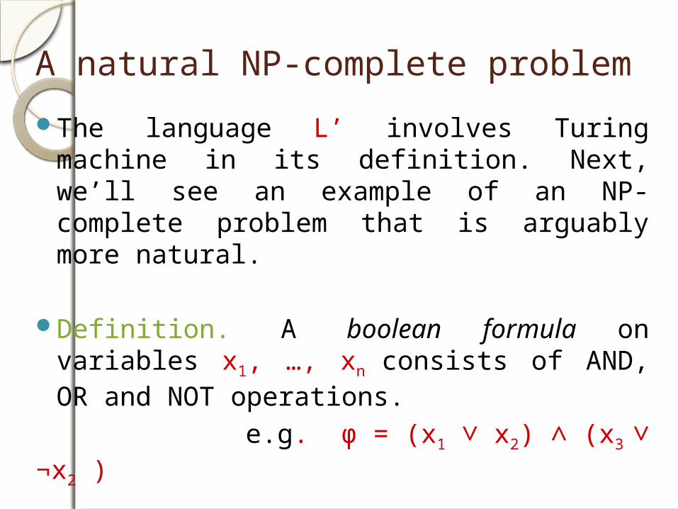
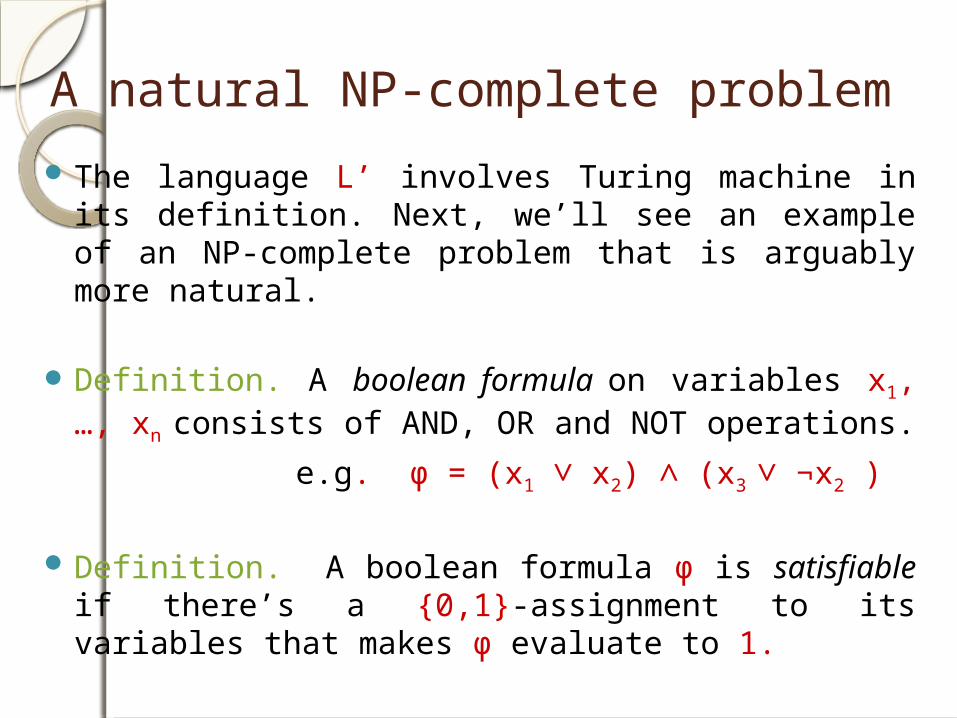
A natural NP-complete problem
The language L’ involves Turing machine in its definition. Next, we’ll see an example of an NP-complete problem that is arguably more natural.
A natural NP-complete problem
The language L’ involves Turing machine in its definition. Next, we’ll see an example of an NP-complete problem that is arguably more natural.
Definition. A boolean formula on variables x1, …, xn consists of AND, OR and NOT operations.
e.g. ϕ = (x1 ∨ x2) ∧ (x3 ∨ ¬x2 )
A natural NP-complete problem
The language L’ involves Turing machine in its definition. Next, we’ll see an example of an NP-complete problem that is arguably more natural.
Definition. A boolean formula on variables x1, …, xn consists of AND, OR and NOT operations.
e.g. ϕ = (x1 ∨ x2) ∧ (x3 ∨ ¬x2 )
Definition. A boolean formula ϕ is satisfiable if there’s a {0,1}-assignment to its variables that makes ϕ evaluate to 1.
A natural NP-complete problem
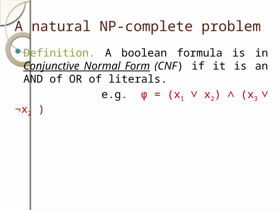
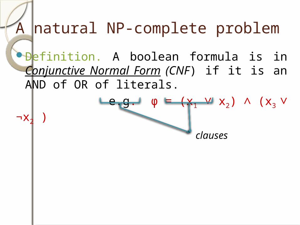
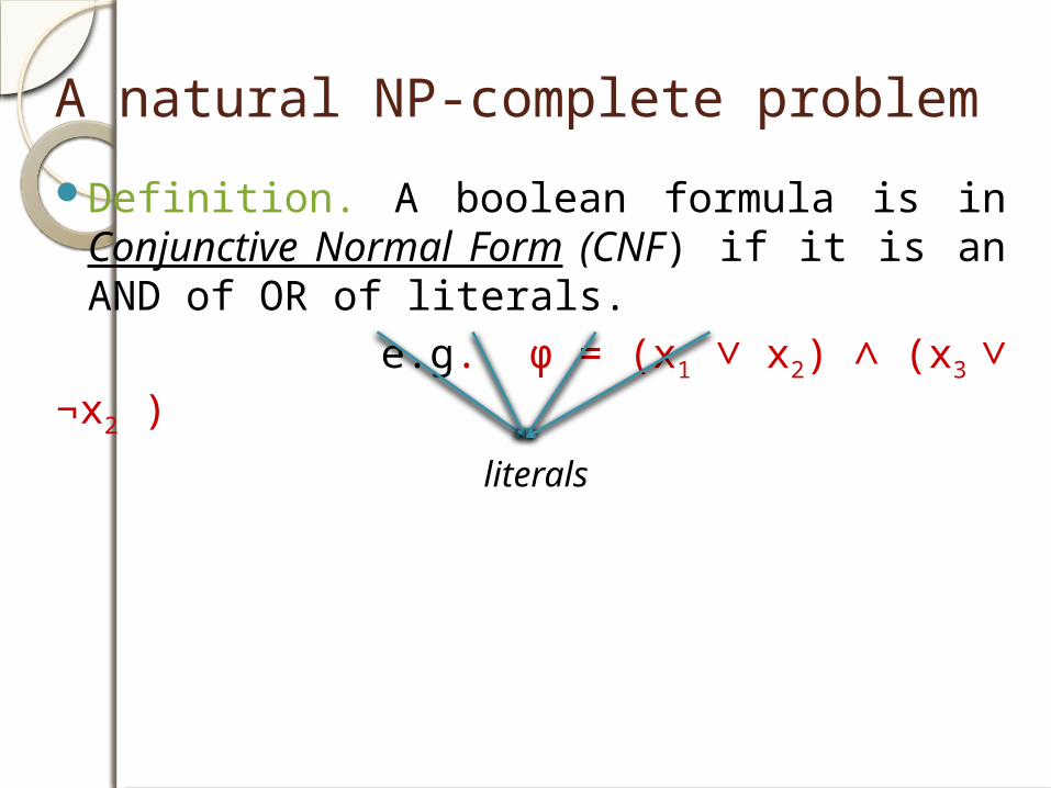
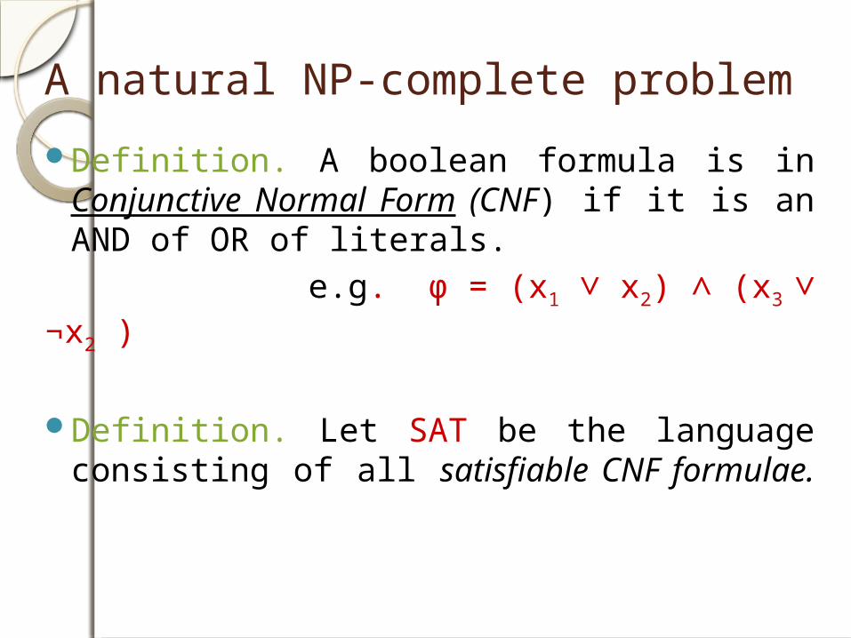
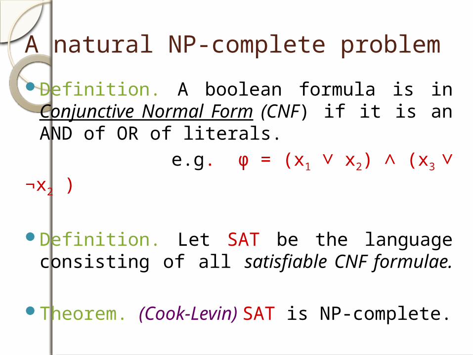
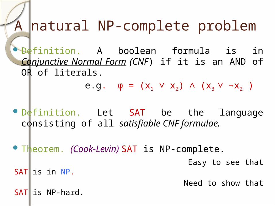
Definition. A boolean formula is in Conjunctive Normal Form (CNF) if it is an AND of OR of literals.
e.g. ϕ = (x1 ∨ x2) ∧ (x3 ∨ ¬x2 )
A natural NP-complete problem
Definition. A boolean formula is in Conjunctive Normal Form (CNF) if it is an AND of OR of literals.
e.g. ϕ = (x1 ∨ x2) ∧ (x3 ∨ ¬x2 )
clauses
A natural NP-complete problem
Definition. A boolean formula is in Conjunctive Normal Form (CNF) if it is an AND of OR of literals.
e.g. ϕ = (x1 ∨ x2) ∧ (x3 ∨ ¬x2 )
literals
A natural NP-complete problem
Definition. A boolean formula is in Conjunctive Normal Form (CNF) if it is an AND of OR of literals.
e.g. ϕ = (x1 ∨ x2) ∧ (x3 ∨ ¬x2 )
Definition. Let SAT be the language consisting of all satisfiable CNF formulae.
A natural NP-complete problem
Definition. A boolean formula is in Conjunctive Normal Form (CNF) if it is an AND of OR of literals.
e.g. ϕ = (x1 ∨ x2) ∧ (x3 ∨ ¬x2 )
Definition. Let SAT be the language consisting of all satisfiable CNF formulae.
Theorem. (Cook-Levin) SAT is NP-complete.
A natural NP-complete problem
Definition. A boolean formula is in Conjunctive Normal Form (CNF) if it is an AND of OR of literals.
e.g. ϕ = (x1 ∨ x2) ∧ (x3 ∨ ¬x2 )
Definition. Let SAT be the language consisting of all satisfiable CNF formulae.
Theorem. (Cook-Levin) SAT is NP-complete. Easy to see that SAT is in NP.
Need to show that SAT is NP-hard.
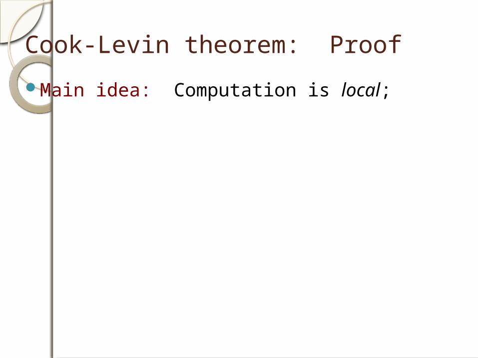
Cook-Levin theorem: ProofMain idea: Computation is local;
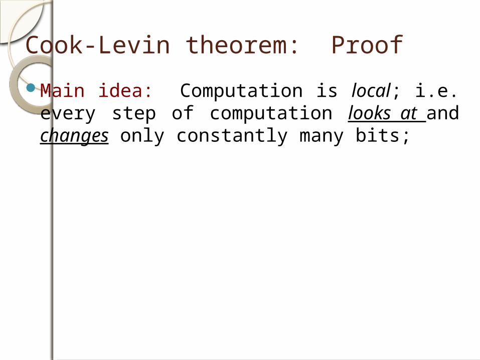
Cook-Levin theorem: ProofMain idea: Computation is local; i.e. every
step of computation looks at and changes only constantly many bits;

Cook-Levin theorem: ProofMain idea: Computation is local; i.e. every
step of computation looks at and changes only constantly many bits; and hence this step can be implemented by a small CNF formula.
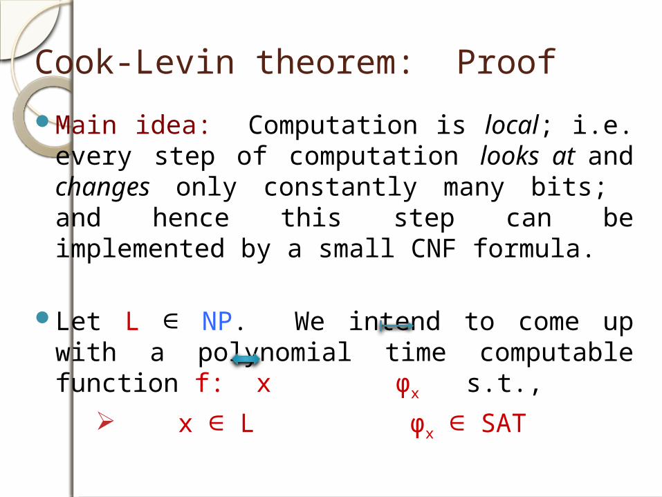
Cook-Levin theorem: ProofMain idea: Computation is local; i.e. every
step of computation looks at and changes only constantly many bits; and hence this step can be implemented by a small CNF formula.
Let L ∈ NP. We intend to come up with a polynomial time computable function f: x ϕx s.t.,
x ∈ L ϕx ∈ SAT
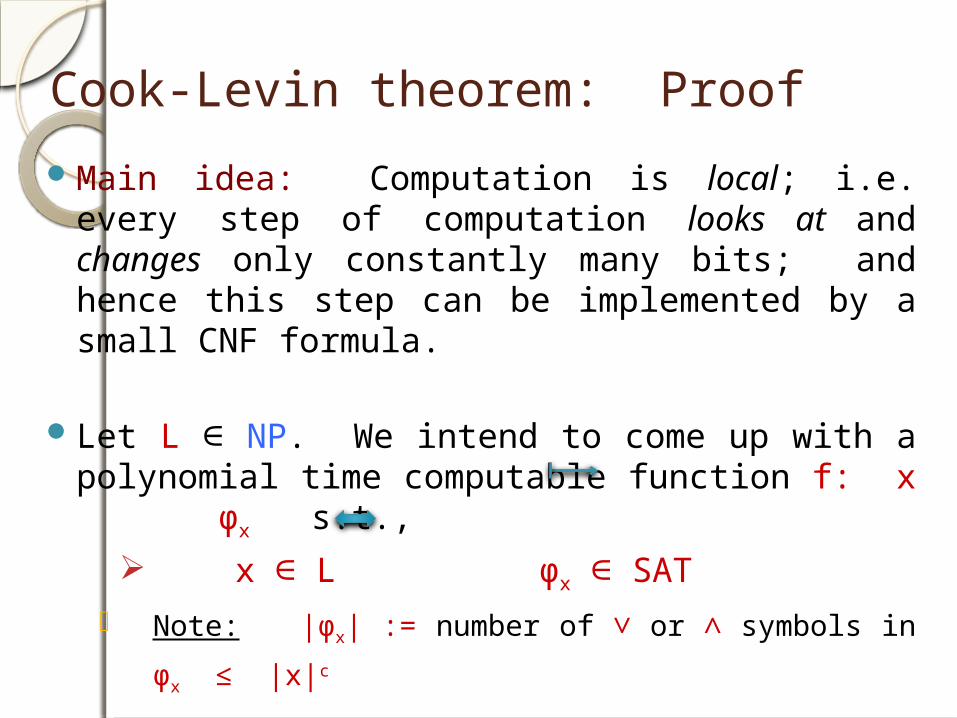
Cook-Levin theorem: ProofMain idea: Computation is local; i.e. every
step of computation looks at and changes only constantly many bits; and hence this step can be implemented by a small CNF formula.
Let L ∈ NP. We intend to come up with a polynomial time computable function f: x ϕx s.t.,
x ∈ L ϕx ∈ SAT Note: |ϕx| := number of ∨ or ∧ symbols in ϕx ≤
|x|c
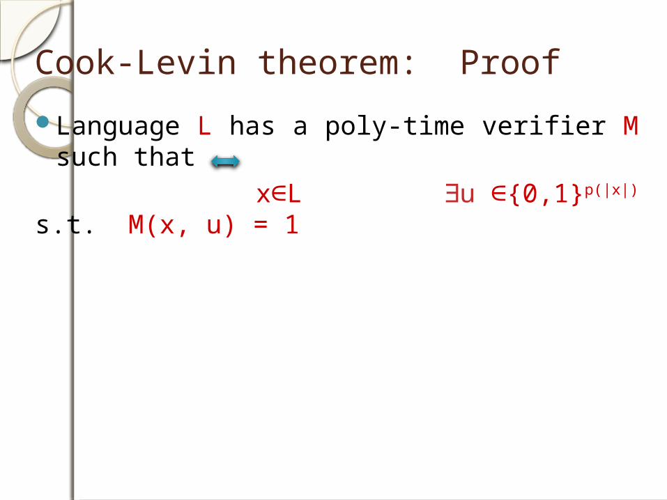
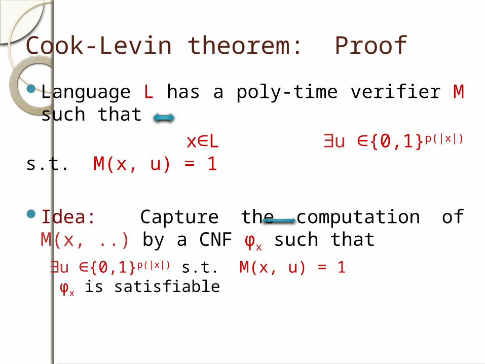
Cook-Levin theorem: ProofLanguage L has a poly-time verifier M such
that x∈L ∃u ∈{0,1}p(|x|) s.t. M(x, u) = 1
Cook-Levin theorem: ProofLanguage L has a poly-time verifier M such
that x∈L ∃u ∈{0,1}p(|x|) s.t. M(x, u) = 1
Idea: Capture the computation of M(x, ..) by a CNF ϕx such that ∃u ∈{0,1}p(|x|) s.t. M(x, u) = 1 ϕx is satisfiable
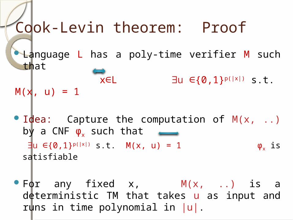
Cook-Levin theorem: ProofLanguage L has a poly-time verifier M such that x∈L ∃u ∈{0,1}p(|x|) s.t. M(x, u) = 1
Idea: Capture the computation of M(x, ..) by a CNF ϕx such that ∃u ∈{0,1}p(|x|) s.t. M(x, u) = 1 ϕx is satisfiable
For any fixed x, M(x, ..) is a deterministic TM that takes u as input and runs in time polynomial in |u|.
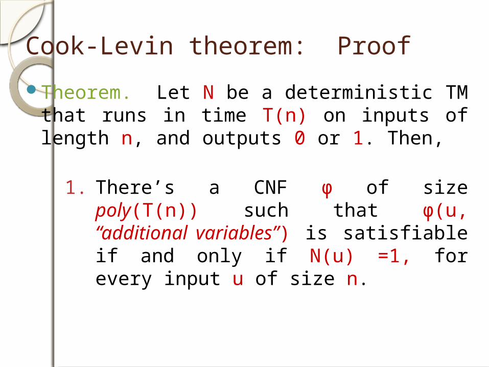
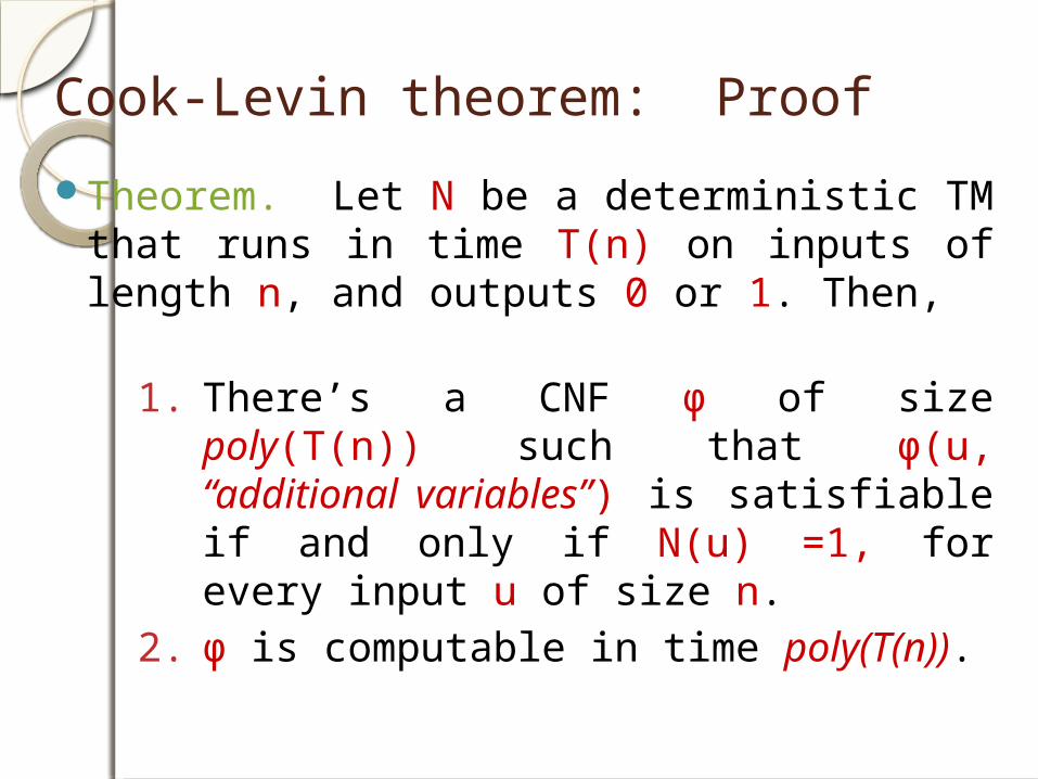
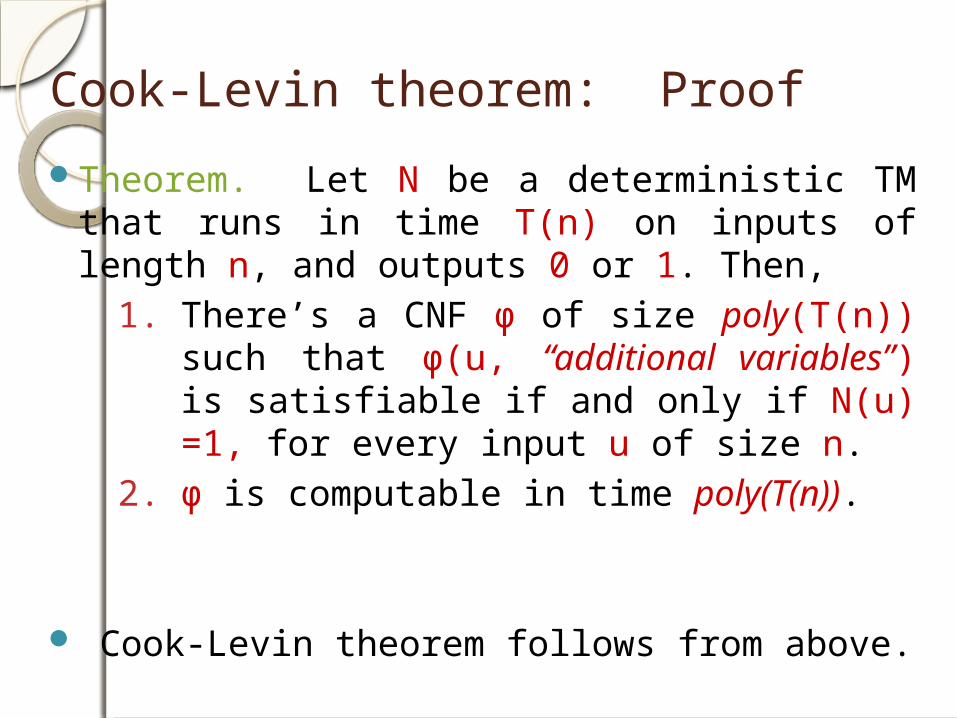
Cook-Levin theorem: ProofTheorem. Let N be a deterministic TM that
runs in time T(n) on inputs of length n, and outputs 0 or 1. Then,
Cook-Levin theorem: ProofTheorem. Let N be a deterministic TM that
runs in time T(n) on inputs of length n, and outputs 0 or 1. Then,
1. There’s a CNF ϕ of size poly(T(n)) such that ϕ(u, “additional variables”) is satisfiable if and only if N(u) =1, for every input u of size n.
Cook-Levin theorem: ProofTheorem. Let N be a deterministic TM that
runs in time T(n) on inputs of length n, and outputs 0 or 1. Then,
1. There’s a CNF ϕ of size poly(T(n)) such that ϕ(u, “additional variables”) is satisfiable if and only if N(u) =1, for every input u of size n.
2. ϕ is computable in time poly(T(n)).
Cook-Levin theorem follows from above.
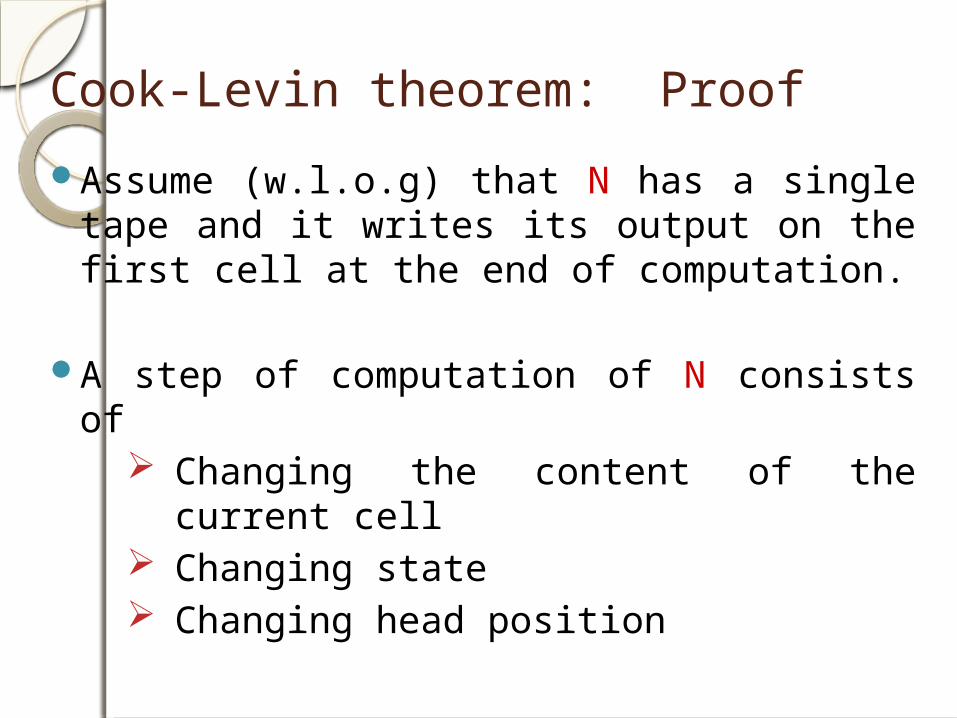
Cook-Levin theorem: ProofAssume (w.l.o.g) that N has a single tape
and it writes its output on the first cell at the end of computation.
Cook-Levin theorem: ProofAssume (w.l.o.g) that N has a single tape
and it writes its output on the first cell at the end of computation.
A step of computation of N consists of Changing the content of the current
cell Changing state Changing head position
Cook-Levin theorem: ProofAssume (w.l.o.g) that N has a single tape and it
writes its output on the first cell at the end of computation.
A step of computation of N consists of Changing the content of the current cell Changing state Changing head position
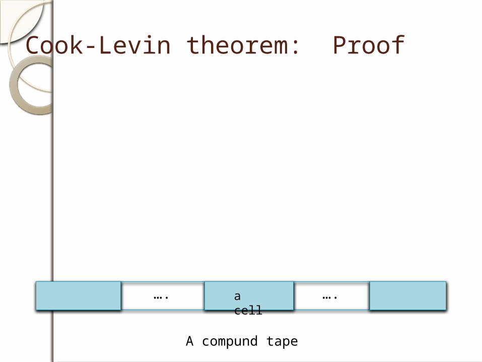
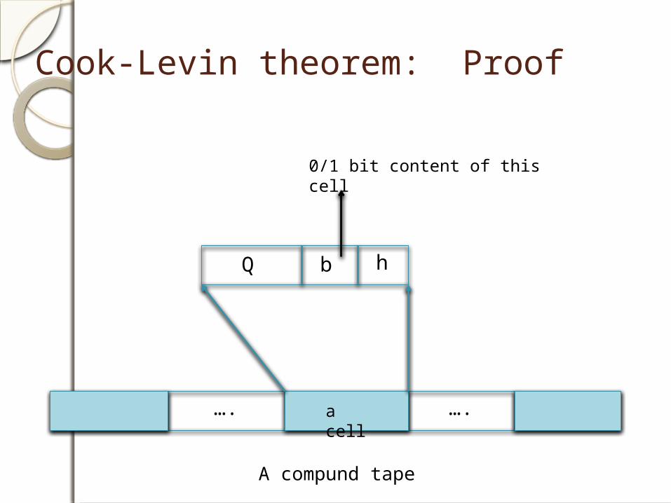
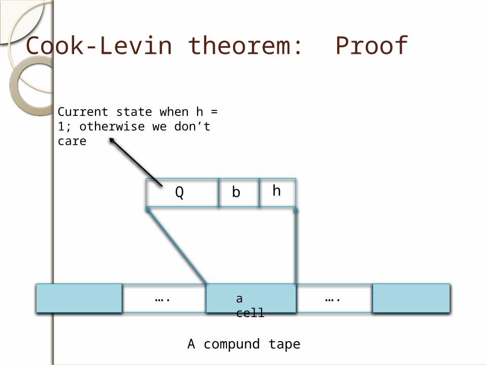
Think of a ‘compound’ tape in which every cell stores the current state and a head indicator in addition to its bit content.
Cook-Levin theorem: Proof
…. ….
A compund tape
a cell
Cook-Levin theorem: Proof
…. ….
A compund tape
a cell
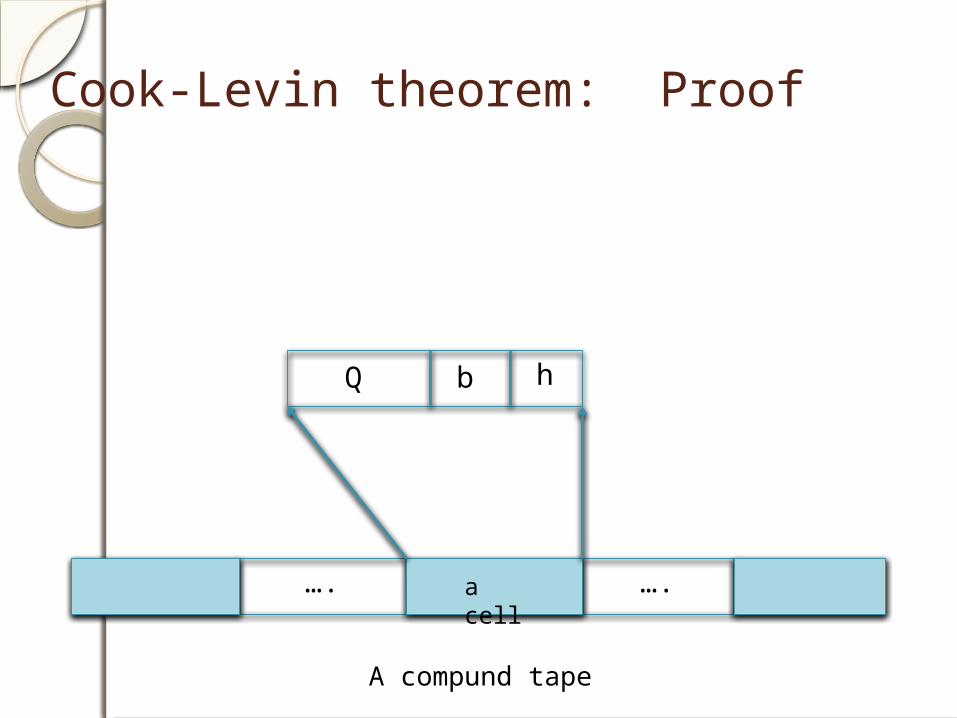
hbQ
Cook-Levin theorem: Proof
…. ….
A compund tape
a cell
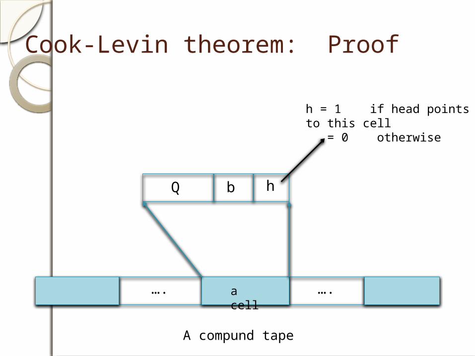
hbQ
h = 1 if head points to this cell = 0 otherwise
Cook-Levin theorem: Proof
…. ….
A compund tape
a cell
hbQ
0/1 bit content of this cell
Cook-Levin theorem: Proof
…. ….
A compund tape
a cell
hbQ
Current state when h = 1; otherwise we don’t care
Cook-Levin theorem: Proof
…. ….
A compund tape
a cell
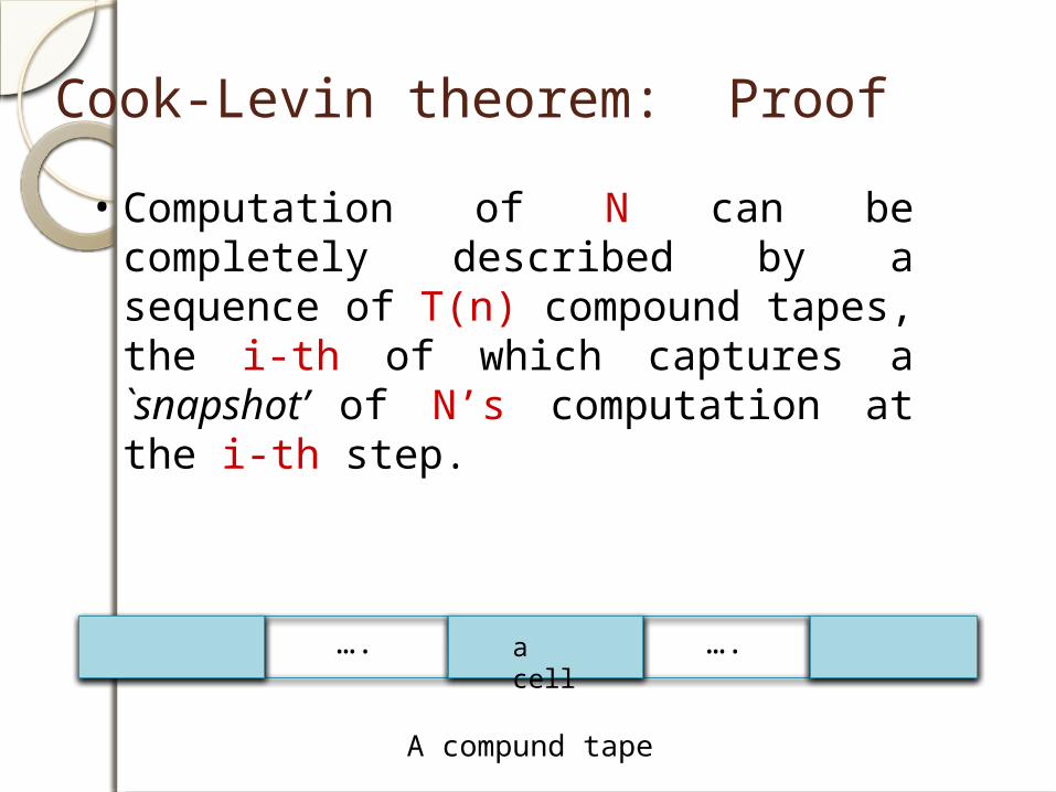
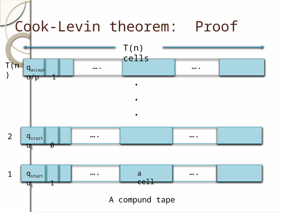
• Computation of N can be completely described by a sequence of T(n) compound tapes, the i-th of which captures a `snapshot’ of N’s computation at the i-th step.

Cook-Levin theorem: Proof
…. ….
A compund tape
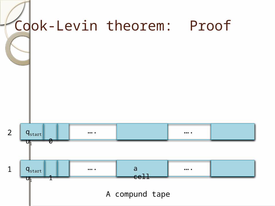
a cellqstart u1 1
1
first input bit
Cook-Levin theorem: Proof
…. ….
A compund tape
a cellqstart u1 1
1
…. ….qstart u1 0
2
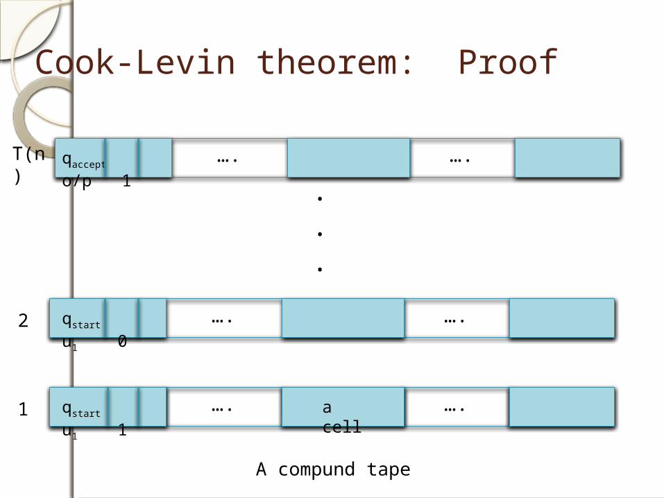
Cook-Levin theorem: Proof
…. ….
A compund tape
a cellqstart u1 1
1
…. ….qstart u1 0
2
…. ….T(n) qaccept o/p 1 .
.
.
Cook-Levin theorem: Proof
…. ….
A compund tape
a cellqstart u1 1
1
…. ….qstart u1 0
2
…. ….T(n) qaccept o/p 1 .
.
.
T(n) cells
Cook-Levin theorem: Proof
….
cell j
qi,j bi,j hi,j
i ….
• hi,j = 1 iff head points to cell j at i-th step
• bi,j = bit content of cell j at i-th step
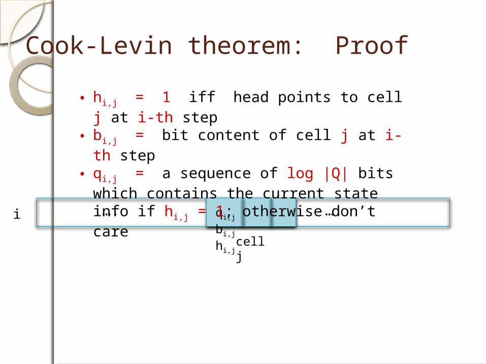
Cook-Levin theorem: Proof
….
cell j
qi,j bi,j hi,j
i ….
• hi,j = 1 iff head points to cell j at i-th step
• bi,j = bit content of cell j at i-th step• qi,j = a sequence of log |Q| bits which
contains the current state info if hi,j = 1; otherwise don’t care
Cook-Levin theorem: Proof
….
cell j
qi,j bi,j hi,j
i ….
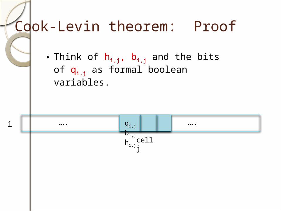
• Think of hi,j, bi,j and the bits of qi,j as formal boolean variables.
Cook-Levin theorem: Proof
….
cell j
qi,j bi,j hi,j
i ….
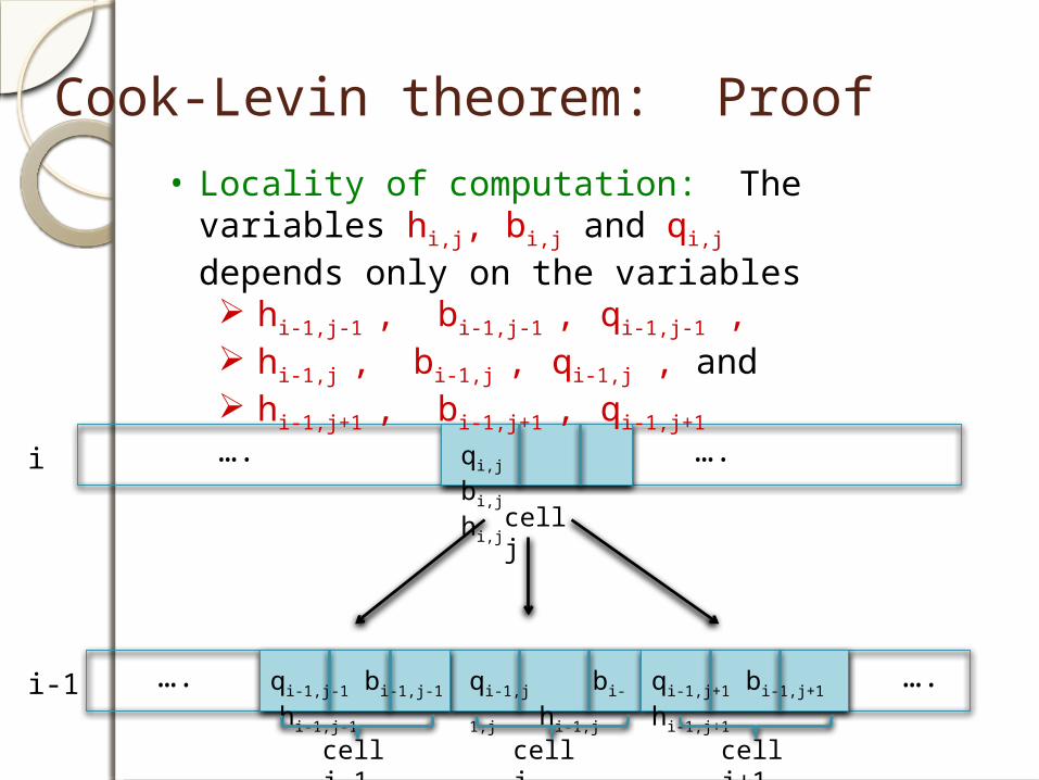
• Locality of computation: The variables hi,j, bi,j and qi,j depends only on the variables hi-1,j-1 , bi-1,j-1 , qi-1,j-1 , hi-1,j , bi-1,j , qi-1,j , and hi-1,j+1 , bi-1,j+1 , qi-1,j+1
….
cell j
qi-1,j bi-1,j hi-
1,j
i-1 …. qi-1,j-1 bi-1,j-1 hi-
1,j-1
qi-1,j+1 bi-1,j+1 hi-
1,j+1
cell j-1 cell j+1
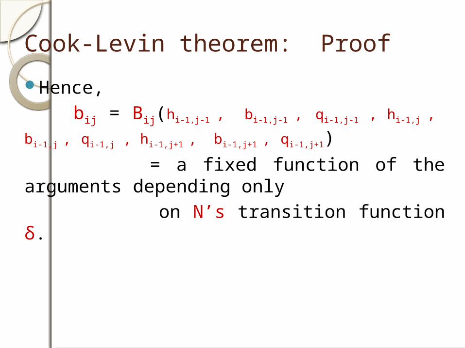
Cook-Levin theorem: ProofHence, bij = Bij(hi-1,j-1 , bi-1,j-1 , qi-1,j-1 , hi-1,j , bi-1,j , qi-1,j , hi-1,j+1 , bi-
1,j+1 , qi-1,j+1)
= a fixed function of the arguments depending only on N’s transition function δ.
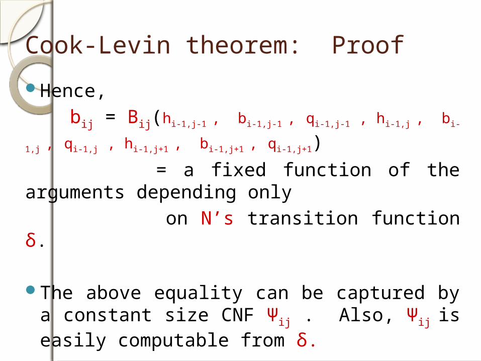
Cook-Levin theorem: ProofHence, bij = Bij(hi-1,j-1 , bi-1,j-1 , qi-1,j-1 , hi-1,j , bi-1,j , qi-1,j , hi-1,j+1 , bi-
1,j+1 , qi-1,j+1)
= a fixed function of the arguments depending only on N’s transition function δ.
The above equality can be captured by a constant size CNF Ψij . Also, Ψij is easily computable from δ.
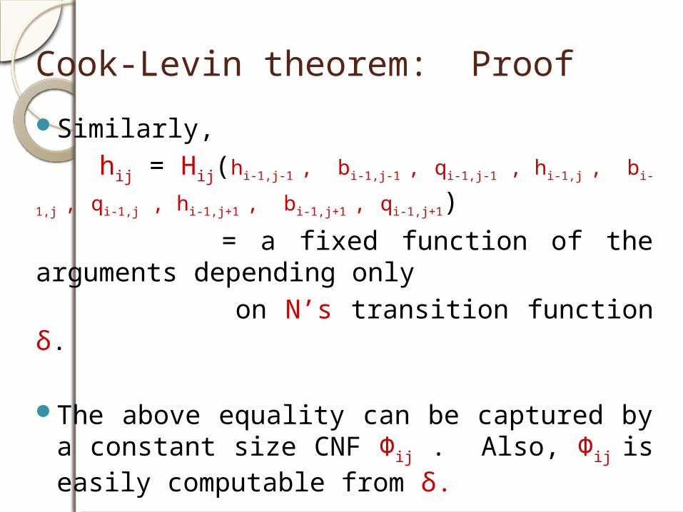
Cook-Levin theorem: ProofSimilarly, hij = Hij(hi-1,j-1 , bi-1,j-1 , qi-1,j-1 , hi-1,j , bi-1,j , qi-1,j , hi-1,j+1 , bi-
1,j+1 , qi-1,j+1)
= a fixed function of the arguments depending only on N’s transition function δ.
The above equality can be captured by a constant size CNF Φij . Also, Φij is easily computable from δ.
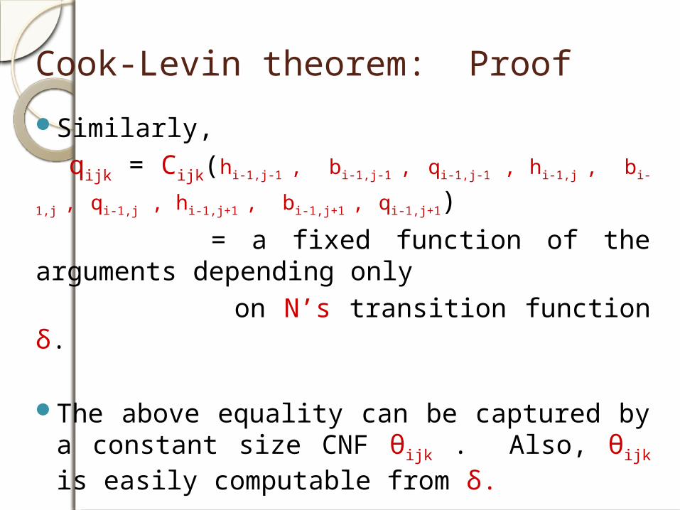
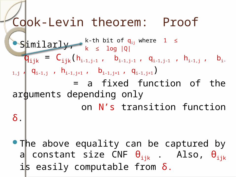
Cook-Levin theorem: ProofSimilarly, qijk = Cijk(hi-1,j-1 , bi-1,j-1 , qi-1,j-1 , hi-1,j , bi-1,j , qi-1,j , hi-1,j+1 , bi-
1,j+1 , qi-1,j+1)
= a fixed function of the arguments depending only on N’s transition function δ.
The above equality can be captured by a constant size CNF θijk . Also, θijk is easily computable from δ.
k-th bit of qij where 1 ≤ k ≤ log |Q|
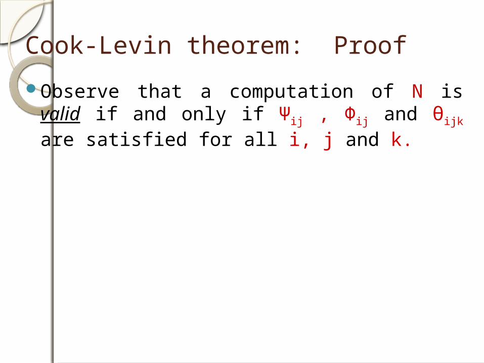
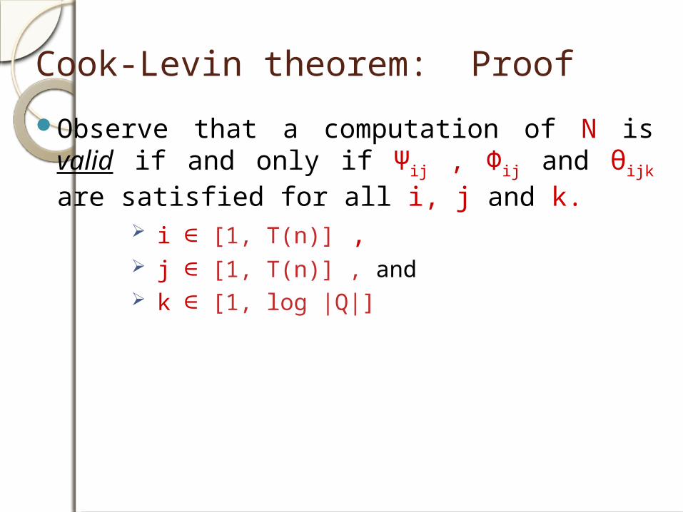
Cook-Levin theorem: ProofObserve that a computation of N is valid if
and only if Ψij , Φij and θijk are satisfied for all i, j and k.
Cook-Levin theorem: ProofObserve that a computation of N is valid if
and only if Ψij , Φij and θijk are satisfied for all i, j and k.
i ∈ [1, T(n)] , j ∈ [1, T(n)] , and k ∈ [1, log |Q|]
Cook-Levin theorem: ProofObserve that a computation of N is valid if
and only if Ψij , Φij and θijk are satisfied for all i, j and k.
Let λ be the conjunction of Ψij , Φij and θijk for all i, j and k. Size of λ is O(T(n)2).
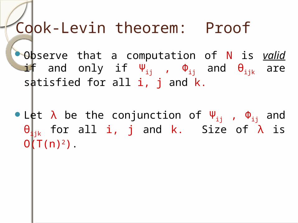
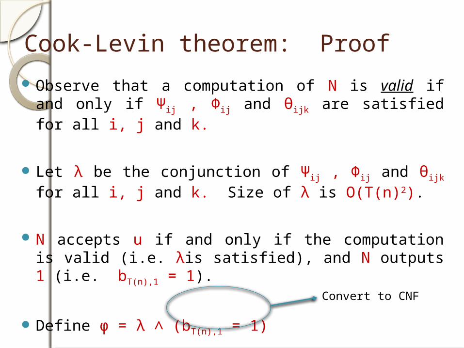
Cook-Levin theorem: ProofObserve that a computation of N is valid if and
only if Ψij , Φij and θijk are satisfied for all i, j and k.
Let λ be the conjunction of Ψij , Φij and θijk for all i, j and k. Size of λ is O(T(n)2).
N accepts u if and only if the computation is valid (i.e. λis satisfied), and N outputs 1 (i.e. bT(n),1 = 1)
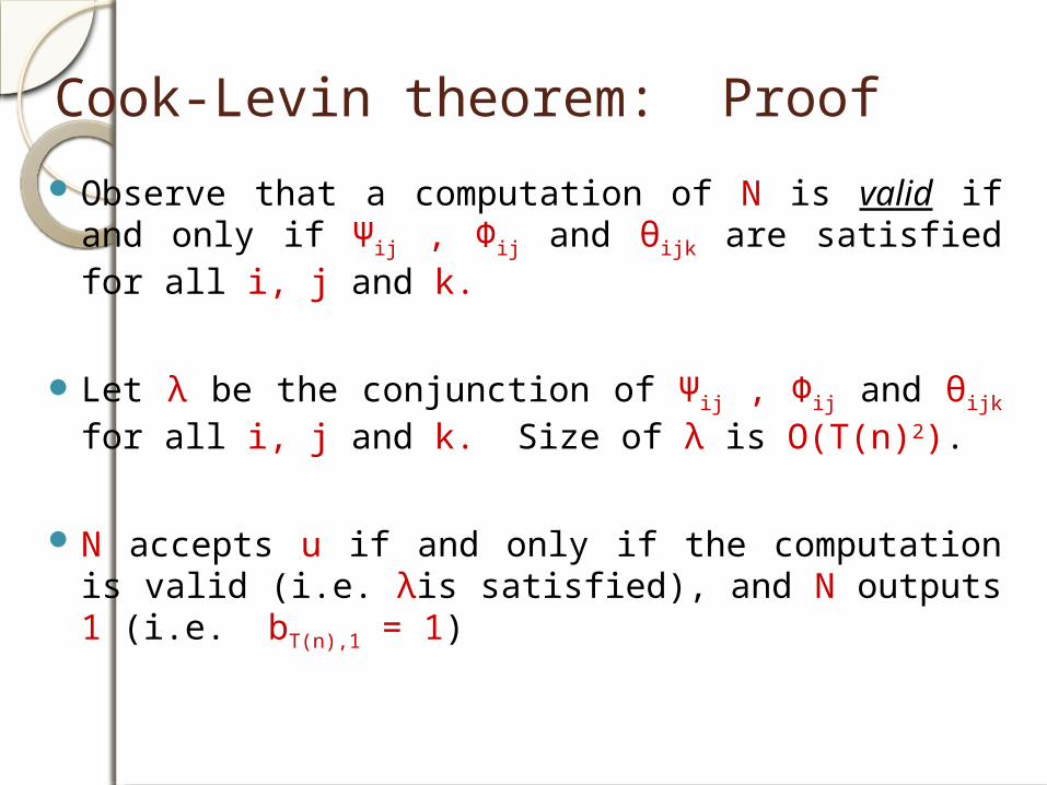
Cook-Levin theorem: ProofObserve that a computation of N is valid if and
only if Ψij , Φij and θijk are satisfied for all i, j and k.
Let λ be the conjunction of Ψij , Φij and θijk for all i, j and k. Size of λ is O(T(n)2).
N accepts u if and only if the computation is valid (i.e. λis satisfied), and N outputs 1 (i.e. bT(n),1 = 1).
Define ϕ = λ ∧ (bT(n),1 = 1)
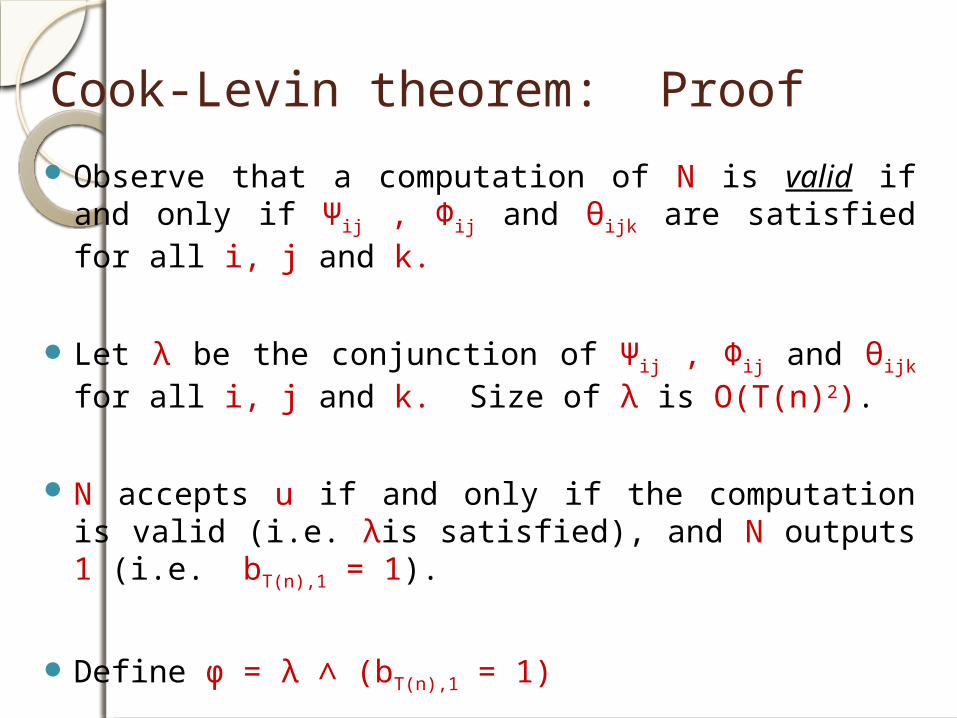
Convert to CNF
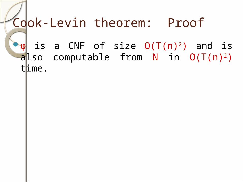
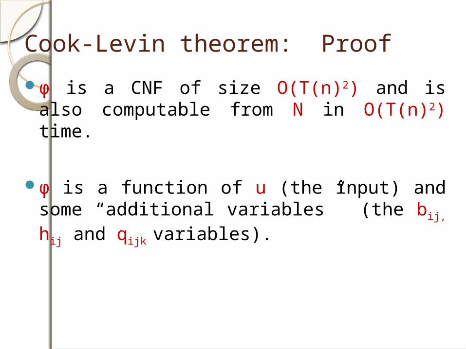
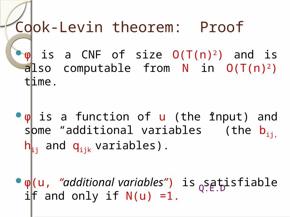
Cook-Levin theorem: Proofϕ is a CNF of size O(T(n)2) and is also
computable from N in O(T(n)2) time.
Cook-Levin theorem: Proofϕ is a CNF of size O(T(n)2) and is also
computable from N in O(T(n)2) time.
ϕ is a function of u (the input) and some “additional variables” (the bij, hij and qijk
variables).

Cook-Levin theorem: Proofϕ is a CNF of size O(T(n)2) and is also
computable from N in O(T(n)2) time.
ϕ is a function of u (the input) and some “additional variables” (the bij, hij and qijk
variables).
ϕ(u, “additional variables”) is satisfiable if and only if N(u) =1.
Cook-Levin theorem: Proofϕ is a CNF of size O(T(n)2) and is also
computable from N in O(T(n)2) time.
ϕ is a function of u (the input) and some “additional variables” (the bij, hij and qijk
variables).
ϕ(u, “additional variables”) is satisfiable if and only if N(u) =1.
Q.E.D
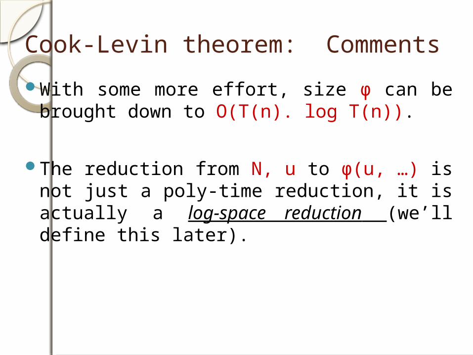
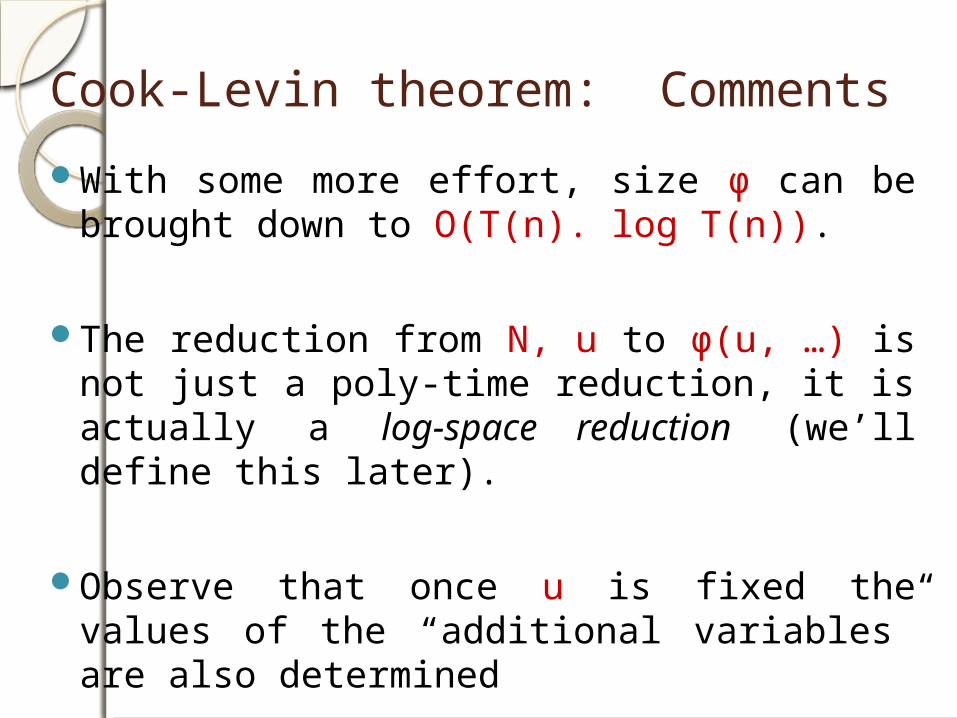
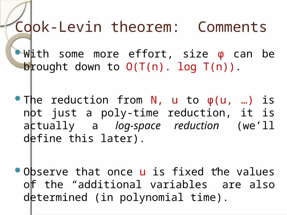
Cook-Levin theorem: Comments
With some more effort, size ϕ can be brought down to O(T(n). log T(n)).
Cook-Levin theorem: Comments
With some more effort, size ϕ can be brought down to O(T(n). log T(n)).
The reduction from N, u to ϕ(u, …) is not just a poly-time reduction, it is actually a log-space reduction (we’ll define this later).
Cook-Levin theorem: Comments
With some more effort, size ϕ can be brought down to O(T(n). log T(n)).
The reduction from N, u to ϕ(u, …) is not just a poly-time reduction, it is actually a log-space reduction (we’ll define this later).
Observe that once u is fixed the values of the “additional variables” are also determined
Cook-Levin theorem: Comments
With some more effort, size ϕ can be brought down to O(T(n). log T(n)).
The reduction from N, u to ϕ(u, …) is not just a poly-time reduction, it is actually a log-space reduction (we’ll define this later).
Observe that once u is fixed the values of the “additional variables” are also determined (in polynomial time).
Cook-Levin theorem: Comments
With some more effort, size ϕ can be brought down to O(T(n). log T(n)).
The reduction from N, u to ϕ(u, …) is not just a poly-time reduction, it is actually a log-space reduction (we’ll define this later).
Each clause of ϕ has only constantly many literals.