computational complexity of generalized quanti … ers in time and space computational complexity of...
TRANSCRIPT

Quantiers in TIME and SPACEComputational Complexity of Generalized Quantiers
in Natural Language
Jakub Szymanik


Quantiers in TIME and SPACEComputational Complexity of Generalized Quantiers
in Natural Language

ILLC Dissertation Series DS-2009-01
For further information about ILLC-publications, please contact
Institute for Logic, Language and ComputationUniversiteit van AmsterdamPlantage Muidergracht 241018 TV Amsterdam
phone: +31-20-525 6051fax: +31-20-525 5206
e-mail: [email protected]: http://www.illc.uva.nl/

Quantiers in TIME and SPACEComputational Complexity of Generalized Quantiers
in Natural Language
Academisch Proefschrift
ter verkrijging van de graad van doctor aan de
Universiteit van Amsterdam
op gezag van de Rector Magnicus
prof. dr. D.C. van den Boom
ten overstaan van een door het college voor
promoties ingestelde commissie, in het openbaar
te verdedigen in de Agnietenkapel
op vrijdag 6 maart 2009, te 14.00 uur
door
Jakub Krzysztof Szymanik
geboren te Warschau, Polen.

Promotiecommissie:
Promotores:Prof. dr. J. F. A. K. van BenthemProf. dr. M. Mostowski
Co-promotor:Dr. T. M. V. Janssen
Overige leden:Prof. dr. R. ClarkDr. P. J. E. DekkerProf. dr. J. VäänänenProf. dr. D. Westerståhl
Faculteit der Natuurwetenschappen, Wiskunde en Informatica
The investigations were supported by a Marie Curie Early Stage Research fellow-ship in the project GloRiClass (MEST-CT-2005-020841).
Copyright c© 2009 by Jakub Szymanik
Cover design by Nina Gierasimczuk.Printed and bound by Ipskamp Drukkers.
ISBN: 9789057761874

Rodzicom
v

It is the striving for truth that drives us always to advance from thesense to the reference. (Frege, 1892, p. 63)
vi

Contents
Contents vii
Acknowledgments xi
Introduction 1
1 Algorithmic Semantics 51.1 Meaning and Comprehension . . . . . . . . . . . . . . . . . . . . . 51.2 Geography of Perspectives . . . . . . . . . . . . . . . . . . . . . . 7
1.2.1 Traditional Semantics and Pragmatics . . . . . . . . . . . 71.2.2 The Dynamic Turn in Semantics . . . . . . . . . . . . . . 81.2.3 Meaning as Algorithm . . . . . . . . . . . . . . . . . . . . 10
1.3 Our Procedural Perspective on Meaning . . . . . . . . . . . . . . 151.3.1 Questions . . . . . . . . . . . . . . . . . . . . . . . . . . . 151.3.2 Methodology . . . . . . . . . . . . . . . . . . . . . . . . . 151.3.3 Psychological Motivations . . . . . . . . . . . . . . . . . . 17
1.4 Algorithms and Computations . . . . . . . . . . . . . . . . . . . . 181.4.1 What is an Algorithm? . . . . . . . . . . . . . . . . . . . 181.4.2 Turing Computability . . . . . . . . . . . . . . . . . . . . 19
1.5 Computability and Cognition . . . . . . . . . . . . . . . . . . . . 241.5.1 Computational Explanation of Cognitive Tasks . . . . . . 251.5.2 Computational Bounds on Cognition . . . . . . . . . . . . 261.5.3 Common Doubts . . . . . . . . . . . . . . . . . . . . . . . 291.5.4 Explaining the Comprehension Task . . . . . . . . . . . . 31
1.6 Finite Interpretations . . . . . . . . . . . . . . . . . . . . . . . . . 321.7 Complexity in Linguistics . . . . . . . . . . . . . . . . . . . . . . 34
1.7.1 Syntax . . . . . . . . . . . . . . . . . . . . . . . . . . . . . 341.7.2 Between Syntax and Semantics . . . . . . . . . . . . . . . 35
1.8 Classifying Meaning by Intractability . . . . . . . . . . . . . . . . 37
vii

1.8.1 Ristad's Theses . . . . . . . . . . . . . . . . . . . . . . . . 381.8.2 Descriptive Bounds on Everyday Language . . . . . . . . . 39
1.9 Summary . . . . . . . . . . . . . . . . . . . . . . . . . . . . . . . 41
2 Mathematical Prerequisites 432.1 Basic Notation . . . . . . . . . . . . . . . . . . . . . . . . . . . . 432.2 Generalized Quantier Theory . . . . . . . . . . . . . . . . . . . . 44
2.2.1 Two Equivalent Concepts of Generalized Quantiers . . . . 452.2.2 Branching Quantiers . . . . . . . . . . . . . . . . . . . . 472.2.3 Logic Enriched by Generalized Quantiers . . . . . . . . . 482.2.4 Denability of Generalized Quantiers . . . . . . . . . . . 482.2.5 Linguistic Properties of Generalized Quantiers . . . . . . 50
2.3 Computability . . . . . . . . . . . . . . . . . . . . . . . . . . . . . 542.3.1 Languages and Automata . . . . . . . . . . . . . . . . . . 542.3.2 Turing Machines . . . . . . . . . . . . . . . . . . . . . . . 602.3.3 Complexity Classes . . . . . . . . . . . . . . . . . . . . . . 612.3.4 Oracle Machines . . . . . . . . . . . . . . . . . . . . . . . 632.3.5 The Polynomial Hierarchy . . . . . . . . . . . . . . . . . . 642.3.6 The Counting Hierarchy . . . . . . . . . . . . . . . . . . . 642.3.7 Reductions and Complete Problems . . . . . . . . . . . . . 65
2.4 Descriptive Complexity Theory . . . . . . . . . . . . . . . . . . . 662.4.1 Encoding Finite Models . . . . . . . . . . . . . . . . . . . 672.4.2 Logics Capturing Complexity Classes . . . . . . . . . . . . 68
2.5 Quantiers in Finite Models . . . . . . . . . . . . . . . . . . . . . 69
3 Complexity of Polyadic Quantiers 713.1 Standard Polyadic Lifts . . . . . . . . . . . . . . . . . . . . . . . . 72
3.1.1 Iteration . . . . . . . . . . . . . . . . . . . . . . . . . . . . 733.1.2 Cumulation . . . . . . . . . . . . . . . . . . . . . . . . . . 743.1.3 Resumption . . . . . . . . . . . . . . . . . . . . . . . . . . 743.1.4 PTIME GQs are Closed under It, Cum, and Res . . . . . . 75
3.2 Branching Quantiers . . . . . . . . . . . . . . . . . . . . . . . . . 773.2.1 Henkin's Quantiers are Mighty . . . . . . . . . . . . . . . 773.2.2 Proportional Branching Quantiers are Mighty . . . . . . . 783.2.3 Branching Counting Quantiers are Mighty . . . . . . . . 793.2.4 Linguistic Remark and Branching of Dissertation . . . . . 80
3.3 Ramsey Quantiers . . . . . . . . . . . . . . . . . . . . . . . . . . 813.3.1 Ramsey Theory and Quantiers . . . . . . . . . . . . . . . 813.3.2 The Branching Reading of Hintikka's Sentence . . . . . . . 823.3.3 Clique Quantiers . . . . . . . . . . . . . . . . . . . . . . . 833.3.4 Proportional Ramsey Quantiers . . . . . . . . . . . . . . 843.3.5 Tractable Ramsey Quantiers . . . . . . . . . . . . . . . . 86
3.4 Summary . . . . . . . . . . . . . . . . . . . . . . . . . . . . . . . 89
viii

4 Complexity of Quantied Reciprocals 914.1 Reciprocal Expressions . . . . . . . . . . . . . . . . . . . . . . . . 92
4.1.1 Strong Meaning Hypothesis . . . . . . . . . . . . . . . . . 944.2 Reciprocals as Polyadic Quantiers . . . . . . . . . . . . . . . . . 96
4.2.1 Strong Reciprocal Lift . . . . . . . . . . . . . . . . . . . . 964.2.2 Intermediate Reciprocal Lift . . . . . . . . . . . . . . . . . 974.2.3 Weak Reciprocal Lift . . . . . . . . . . . . . . . . . . . . . 974.2.4 The Reciprocal Lifts in Action . . . . . . . . . . . . . . . . 98
4.3 Complexity of Strong Reciprocity . . . . . . . . . . . . . . . . . . 994.3.1 Counting Quantiers in the Antecedent . . . . . . . . . . . 994.3.2 Proportional Quantiers in the Antecedent . . . . . . . . . 1004.3.3 Tractable Strong Reciprocity . . . . . . . . . . . . . . . . . 102
4.4 Intermediate and Weak Lifts . . . . . . . . . . . . . . . . . . . . . 1034.5 A Complexity Perspective on the SMH . . . . . . . . . . . . . . . 1054.6 Summary . . . . . . . . . . . . . . . . . . . . . . . . . . . . . . . 107
5 Complexity of Collective Quantication 1095.1 Collective Quantiers . . . . . . . . . . . . . . . . . . . . . . . . . 110
5.1.1 Collective Readings in Natural Language . . . . . . . . . . 1105.1.2 Modelling Collectivity . . . . . . . . . . . . . . . . . . . . 111
5.2 Lifting First-order Determiners . . . . . . . . . . . . . . . . . . . 1135.2.1 Existential Modier . . . . . . . . . . . . . . . . . . . . . . 1135.2.2 The Neutral Modier . . . . . . . . . . . . . . . . . . . . . 1155.2.3 The Determiner Fitting Operator . . . . . . . . . . . . . . 1165.2.4 A Note on Collective Invariance Properties . . . . . . . . . 117
5.3 Second-order Generalized Quantiers . . . . . . . . . . . . . . . . 1185.3.1 Denability for SOGQs . . . . . . . . . . . . . . . . . . . . 119
5.4 Dening Collective Determiners by SOGQs . . . . . . . . . . . . . 1215.5 Collective Majority . . . . . . . . . . . . . . . . . . . . . . . . . . 123
5.5.1 An Undenability Result for SOGQ MOST . . . . . . . . 1235.5.2 Consequences of Undenability . . . . . . . . . . . . . . . 124
5.6 Summary . . . . . . . . . . . . . . . . . . . . . . . . . . . . . . . 126
6 Hintikka's Thesis Revisited 1296.1 Hintikka's Thesis . . . . . . . . . . . . . . . . . . . . . . . . . . . 1306.2 Other Hintikka-like Sentences . . . . . . . . . . . . . . . . . . . . 1326.3 Theoretical Discussion . . . . . . . . . . . . . . . . . . . . . . . . 133
6.3.1 A Remark on Possible Readings . . . . . . . . . . . . . . . 1336.3.2 Hintikka-like Sentences are Symmetric . . . . . . . . . . . 1346.3.3 Inferential Arguments . . . . . . . . . . . . . . . . . . . . 1366.3.4 Negation Normality . . . . . . . . . . . . . . . . . . . . . . 1376.3.5 Complexity Arguments . . . . . . . . . . . . . . . . . . . . 1386.3.6 Theoretical Conclusions . . . . . . . . . . . . . . . . . . . 139
ix

6.4 Empirical Evidence . . . . . . . . . . . . . . . . . . . . . . . . . . 1396.4.1 Experimental Hypotheses . . . . . . . . . . . . . . . . . . 1406.4.2 Subjects . . . . . . . . . . . . . . . . . . . . . . . . . . . . 1406.4.3 Materials . . . . . . . . . . . . . . . . . . . . . . . . . . . 1416.4.4 Experiments . . . . . . . . . . . . . . . . . . . . . . . . . . 141
6.5 Summary . . . . . . . . . . . . . . . . . . . . . . . . . . . . . . . 148
7 Comprehension of Simple Quantiers 1517.1 Motivations . . . . . . . . . . . . . . . . . . . . . . . . . . . . . . 152
7.1.1 Previous Investigations in the Area . . . . . . . . . . . . . 1527.1.2 Monadic Quantiers and Automata . . . . . . . . . . . . . 1547.1.3 The Present Experiment . . . . . . . . . . . . . . . . . . . 160
7.2 The First Study: Comparing Quantiers . . . . . . . . . . . . . . 1617.2.1 Participants . . . . . . . . . . . . . . . . . . . . . . . . . . 1617.2.2 Materials and Procedure . . . . . . . . . . . . . . . . . . . 1617.2.3 Results . . . . . . . . . . . . . . . . . . . . . . . . . . . . . 163
7.3 The Second Study: Quantiers and Ordering . . . . . . . . . . . . 1647.3.1 Participants . . . . . . . . . . . . . . . . . . . . . . . . . . 1647.3.2 Materials and Procedure . . . . . . . . . . . . . . . . . . . 1647.3.3 Results . . . . . . . . . . . . . . . . . . . . . . . . . . . . . 165
7.4 Summary . . . . . . . . . . . . . . . . . . . . . . . . . . . . . . . 166
8 Conclusions and Perspectives 1698.1 General Summary . . . . . . . . . . . . . . . . . . . . . . . . . . . 1698.2 Outline . . . . . . . . . . . . . . . . . . . . . . . . . . . . . . . . . 171
8.2.1 Dierent Complexity Measures . . . . . . . . . . . . . . . 1718.2.2 Quantiers and Games . . . . . . . . . . . . . . . . . . . . 1718.2.3 Cognitive Diculty and Complexity . . . . . . . . . . . . . 1738.2.4 Future of GQT and Beyond . . . . . . . . . . . . . . . . . 173
A English Version of the Test from Chapter 6 175
B Polish Version of the Test from Chapter 6 191
Bibliography 207
Index 224
Samenvatting 229
Abstract 231
x

Acknowledgments
It was quite a long climb. It would have never happened without the support andinspiration from many people. If I had given a full account of everyone's help Iwould have never succeed in nishing on time. Therefore, some of you will haveto forgive me for the following, only partial notes.
First of all, my parents have been a continuous source of motivation. Theywere always interested in my research and helped so much in building my con-dence, optimism and energy. I am also very grateful to the rest of my family forproviding me with many expressions of support.
I got for the rst time interested in language, logic and cognition over 10years ago thanks to Anna Wojdanowicz. She was the rst to teach me philosophyand to encourage my independent thinking. She was also the very rst critic ofmy very rst essay on language and cognition which I wrote for the PhilosophicalOlympiad. This dissertation would not come to existence without her and I wouldbe probably doing something completely dierent, presumably less fun.
I am grateful to all my friends with whom I had opportunity to discuss variousphilosophical issues in many wonderful places: climbing mountains, sailing lakesand seas, kayaking along the rivers, and bivouacking in the wildness. Let me men-tion Tomasz Adamski, Nina Gierasimczuk, Rafaª Gryko, Konrad Grzegorzewicz,Andrzej Koroluk, Maciek Malicki, Paweª Mleczko, Maciek Mostowski, MateuszOrli«ski, Jakub Pilarek, Tomasz Puczyªowski, Paweª Szewczyk, and Marcin Za-jenkowski.
It was a lucky choice for me to start studying in the inter-departmental pro-gramme at the University of Warsaw (Collegium MISH), where I had a lot offreedom to develop my interests across dierent scientic disciplines. I am indebt to my tutors in the Collegium: Jerzy Pelc and Barbara Stanosz. Their su-pervision encouraged me to use the freedom for rigorous studies in the philosophyof language and related elds (logic, linguistics, mathematics, and psychology).They had a great impact on my scientic taste. I also have grown a lot throughendless interdisciplinary discussions with my fellow students. For that, I espe-cially thank: Tadeusz Ciecierski, Nina, Justyna Grudzi«ska, Witold Kiera±, Maria
xi

Spychalska, and Marcin. The MISH Philosophical Circle was the rst playgroundfor organizing things in academia: edit books, prepare conferences, co-ordinateprojects, apply for grants, and co-operate with other people. Now, after manyyears, I know that those were all very precious experiences. I am very grateful toZbigniew Kloch who was supporting all those student initiatives.
In the second year of my studies I met the person who had the biggest impacton this thesis and my research in general. Marcin Mostowski not only taughtme logic and suggested research topic, which rst led me to MA thesis and thendirectly culminated in this dissertation, but it was also thanks to him that Istarted to be surrounded by logicians. I was lucky to learn from, study, and dis-cuss logic with: Zoa Adamowicz, Mikoªaj Boja«czyk, Cezary Cie±li«ski, MarekCzarnecki, Nina, Joanna Goli«ska-Pilarek (she was the rst to show me Hintikka'ssentence), Witek, Leszek Aleksander Koªodziejczyk, Eryk Kopczy«ski, HenrykKotlarski, Michaª Krynicki, Filip Murlak, Damian Niwi«ski, Paula Quinon, JerzyTyszkiewicz, Dominika Wojtyniak, ukasz Wojtyniak, and Konrad Zdanowski.Especially, Leszek and Konrad explained to me uncountably many things aboutlogic and inspired me with their attitude to work. I think that it is very likelythat I would have never become a scientist (although I could have easily becomea parody of a scientist) if I had not met Marcin Mostowski and his group.
Then, at the beginning of 2006, I took a great decision and came to Ams-terdam to join ILLC as a PhD student in the GLoRiClass project. I was braveenough to jump in, partially because I had met some ILLC members before atSzklarska Por¦ba Workshop on the Roots of Pragmasemantics. In connectionto this I want to thank Reinchard Blutner and Henk Zeevat for organizing theconference and giving us a chance to meet on the top of Szrenica every year. Ihad very soft landing in Amsterdam thanks to many people. First of all, theILLC sta deserve many thanks for their support and incredible ability of solvingall problems without letting me feel importunate: Marjan Veldhuisen, Ingrid vanLoon, Tanja Kassenaar, Jessica Pogorzelski, Peter van Ormondt and Karin Gi-gengack. GloRiClass coordinators: Krzysztof Apt, Paul Dekker, Benedikt Löwe,Ulle Endriss and my friends from the rst GloRiClass generation: Andreas Witzeland Daisuke Ikegami created extremely friendly atmosphere from the beginning,even though we were struggling with some problems in the project at that time.Moreover, I was introduced to ILLC and Amsterdam by many colleagues, amongothers: Tikitu de Jager (he took me on my rst tour around Amsterdam andborrowed a map which I have lost, sorry for that!), and Merlijn Sevenster (wehad discussed branching quantiers long before I arrived to Amsterdam), ReutTsarfaty, and Jelle Zuidema who were forcing me to have lunches (although itwas usually just after I had breakfast) with other ILLC members integrating mewith the Institute. Soon Amsterdam became my home when Nina, against somediculties, decided to move to the Netherlands.
Obviously, the thesis proted a lot from my Amsterdam supervisors: Johanvan Benthem and Theo Janssen. I enjoyed working with them and beneted a
xii

lot from the ways they complemented each other.Johan has been a great source of vision and inspiration. He suggested to
me plenty of problems and turned around my perspective on logic, languageand computation. I am sure that his ideas will inspire my research long aftergraduation and maybe one day I will be able to answer some of the questions hesuggested during our conversations in his oce. I have been very much motivatedby Johan's never-ceasing energy for taking new research directions and creatingfruitful academic life.
I am very gratefull to Theo for agreeing to be my daily-supervisor and takingthe most of the responsibility for my PhD research, even though my interests andplans were not exactly in line with his. My ideas were very much shaped by ourregular Monday conversations and in the process of endless rewriting to meet hisstandards and account for criticism. I learned a lot about how to write scienticpapers and prepare presentations from him. I am also very grateful for Theo'sopen-mindness in supporting my vision on complexity and cognition.
ILLC is a great place for research and Amsterdam is a beautiful place to livein. I was indeed very lucky to do my PhD here. There were many people whocontributed to the great atmosphere, on both scientic ans social levels, and alldeserve my most gratefull thanks.
Many members of the ILLC faculty have helped me in shaping my ideas: PaulDekker, Peter van Emde Boas, Dick de Jongh, Michiel van Lambalgen, Robertvan Rooij, Remko Scha, Leen Torenvliet, Jouko Väänänen, Yde Venema, andJelle Zuidema. Through the Institute I had also a great opportunity to meet andcollaborate with researchers all over the world: Denis Bonnay, Robin Clark, Janvan Eijck, Bart Geurts, Juha Kontinen, Allen Mann, Rick Nouwen, Eric Pacuit,Ramaswamy Ramanujam, Iris van Rooij, Ingmar Visser, Dag Westerståhl, YoadWinter. I especially thank Robin Clark, Paul Dekker, Jouko Väänänen, and DagWesterståhl for comments on the manuscript and being on my thesis committee.
Finally, I learned a lot through discussions and collaboration with my fellowstudents and friends. What is important I learned not only logic but also a bunchof more practical stu, like, how to play Texas Hold'em and win, how to y on aredeemer or how to say coee lter in Finish. I want to thank: Marian Couni-han, Jakub Dotlacil, Pablo Cubides Kovacsics (I admit that I have stolen a fewclimbing moves from him), Cédric Dégremont, Michael Franke, Amélie Gheer-brant, Nina, Patrick Girard, Olga Grigoriadou, Daisuke, Tikitu (thanks to himthe and a are mostly in their right places except perhaps for this chapter),Sophia Katrenko, Lauri Keskinen, Jarmo Kontinen (for the joint struggle to un-derstand computational complexity theory and a lot of other kinds of fun), LenaKurzen, Olivia Ladinig, Raul Leal Rodriguez, Michaª ukasiewicz, Stefan Minica,Petter Remen, Floris Roelofsen, Federico Sangati, Marieke Schouwstra, JonathanShaheen, Leigh Smith, Marc Staudacher, Reut, Joel and Sara Uckelman, LevanUridia, Fernando Velazquez-Quesada, Aurel Wannig, Andi, Yun Qi Xue, andJonathan Zvesper.
xiii

I am particularly in debt to Andi. First of all, since the very beginning he hasbeen a great oce-mate. Without him I would never written the thesis, simplybecause of all the computer problems I had not been able to solve by myself. Butmore importantly, I am grateful for many interesting discussions about life andlogic and all the fun we had together through the last 3 years.
I would like to express appreciations for my co-authors: Nina Gierasim-czuk, Witold Kiera±, Juha Kontinen, Marcin Mostowski, and Marcin Zajenkowskiwhose ideas directly contributed to the thesis.
Special thanks go to Nina for her incredible support. She has not only con-tributed directly to this research in almost all its stages (from being the co-authorof one of the chapters to designing the cover of this book), but rst of of all: sheis lling every day of my life with joy and love giving reasons for work. Myappreciation for her support is beyond any words that I could possibly nd.
xiv

Introduction
Everyone who has ever tried to understand, explain, and describe natural lan-guage knows how complicated it is. This dissertation is concerned with someaspects of complexity in natural language. In particular, we try to shed somelight on the interplay between complexity and expressibility.
Complexity is a very broad, although quite intuitive, notion. There are at leasttwo levels of language complexity syntactic level and semantic level. The latteris what we will consider in the thesis. Moreover, we will focus on complexity ofmeaning (semantics) of natural language quantiers. Especially, we areinterested in complexity of nding the truth-values of natural language quantiedsentences in nite situations. The general question we aim to answer is why themeanings of some sentences are more dicult than the meanings of others. Forinstance, why we will probably all agree that it is easier to evaluate sentence (1)than sentence (2) and why sentence (3) seems hard while sentence (4) soundsodd.
(1) Every book on the shelf is yellow.
(2) Most of the books on the shelf are yellow.
(3) Less than half of the members of parliament refer to each other.
(4) Some book by every author is referred to in some essay by every critic.
To discuss such dierences in a precise manner, in the dissertation we use toolsof computability theory to measure complexity. By doing it we commit ourselvesto the idea that part of a meaning can be identied with an algorithm thatchecks the truth-value of an expression. Having this in mind we formalize linguis-tic descriptions in logic. Then we use descriptive computational complexityto study properties of formalisms we have dened. Among other things we try todraw a systematic line between easy (tractable) and dicult (intractable) quanti-ers with respect to model-checking complexity. Moreover, as we are interested inthe empirical value of complexity claims we provide some linguistic case stud-ies as well as psycholinguistic empirical experiments. We apply complexityanalysis in the domain of reciprocal expressions to account for some pragmase-mantic phenomena, study various combinations of quantiers in natural language,
1

2 Introduction
and empirically investigate the comprehension of simple quantier sentences. Ourresults show that computational complexity can be very useful in investigatingnatural language semantics.
As far as our research topics and methods are concerned this work is highlyinterdisciplinary. The study can be placed within logic, natural language se-mantics, philosophy of mind and language, theoretical computer science, andcognitive science. It is an example of applying computational complexity theoryto linguistics and cognitive science. Therefore, the intended audience consistsmostly of linguists, philosophers and cognitive scientists interested in formal ap-proaches to complexity in natural language. However, we hope that also logiciansand computer scientists can nd this study a source of inspiration, not only forpossible applications, but also for developments in their research elds. The dis-sertation is intended to be self-contained, but some general background in logicand natural language semantics is assumed. Below we briey overview everychapter.
Chapter 1, Algorithmic Semantics, is a proper introduction to the thesis,where we place our study on the map of research themes. We discuss our method-ological assumptions there; in particular, we outline the idea of treating referen-tial meaning as an algorithm. We also argue that computational complexitycan be taken as a reasonable measure for the diculty of natural language ex-pressions. Moreover, we propose some hypotheses summing up our perspectiveon the role of computational complexity in linguistics and cognitive science.
Chapter 2, Mathematical Prerequisites, shows the background of the tech-nical work of the thesis. We introduce here our main logical tools: the notionsof generalized quantier theory, computability theory, and descriptive complexitytheory. The chapter may be skipped by readers with background knowledge ongeneralized quantiers and computability. For the rest of the readers it can serveas a basic reference to the mathematics used elsewhere in the dissertation.
Chapter 3, Complexity of Polyadic Quantiers, is devoted to a logical studyof the computational complexity of polyadic generalized quantiers. Wefocus here on constructions that are interesting from the semantic point of view.We prove that quantier iteration, cumulation and resumption do not carry usoutside polynomial time computability. Other polyadic quantiers often used inlinguistics, like branching and Ramsey quantiers, lead to NP-complete naturallanguage sentences. This chapter prepares the ground for the more linguisticdiscussion in the next parts of the thesis, particularly in Chapters 4 and 6.
Chapter 4, Complexity of Quantied Reciprocals, is concerned with the lin-guistic case study. We investigate the computational complexity of dierent inter-pretations of reciprocal expressions, like each other, in English. Especially,we show that Ramsey quantiers express the semantics of reciprocal sentenceswith a quantier in the antecedent. As a result we nd a computational di-chotomy between dierent interpretations of reciprocals: some of them stay inPTIME when others are NP-complete. This dichotomy is consistent with well-

Introduction 3
known semantic distinctions among dierent interpretations of each other. Wediscuss the impact of this dichotomy on the so-called Strong Meaning Hypothesisproposed as a pragmatic explanation for shifts occurring among dierent recip-rocal readings.
Chapter 5 Complexity of Collective Quantication discusses yet anotherform of quantication in natural language. We investigate logic of collectivequantiers and propose to analyze them in terms of second-order generalizedquantiers. In particular, our research shows that the widely accepted type-shifting approach to modelling collectivity in natural language is probably notexpressive enough to cover all instances. Additionally, it is also extremely complexand, as such, implausible. As a result we suggest to study algebraic (many-sorted) formalisms. Another interpretation of our results is that computationalcomplexity restricts expressibility of everyday language and as a result collectivereadings of some quantiers, e.g., proportional determiners, is not realized in thatfragment of natural language.
Chapter 6, Hintikka's Thesis Revisited, is the rst empirical fragment ofour work. We study Hintikka's well-known claim concerning the necessity of abranching interpretation for some natural language sentences, e.g., Some rel-atives of each villager and some relatives of each townsman hate each other orMost boys and most girls from my class dated each other. We argue against Hin-tikka's Thesis and propose our own reading of these sentences, which we call theconjunctional reading. Next, we show how to investigate such a problem empir-ically using insights from linguistics, logic and computability. The results of ourtests conrm that the conjunctional reading is a widely accepted interpretationfor these sentences.
Chapter 7, Processing Simple Quantiers, is about a computational seman-tics for simple (monadic) quantiers in natural language. In this case we canmodel the meaning of quantiers using nite and push-down automata. Ouraim is to show the empirical relevance of computational descriptions. We startby presenting the neurological research studying an automata-theoretic modelof simple quantier comprehension. Next we criticize the methodology ofthis research and propose a better set of hypotheses. We use these to conductour own empirical study comparing the reaction times needed for recognizing thetruth-value of sentences with simple quantiers. The results strongly conrmthe complexity predictions of the computational model for simple quantiers innatural language. Hence, this chapter directly links computational predictions tolinguistic processing.
Chapter 8, Conclusions and Perspectives, closes the dissertation with a shortsummary of results achieved from the perspective of the grand issues recognizedin the rst chapter. This is followed by a discussion of related open questionsand directions for further research. This nal discussion focuses on general looseends, as particular research questions directly implied by our technical work arediscussed at the end of the corresponding chapters.


Chapter 1
Algorithmic Semantics
1.1 Meaning and Comprehension
Meaning and Information
Natural language is arguably the most important mean we have for exchanginginformation. It inuences our everyday interactions with the external world andthose with other people. It allows information to be conveyed between speakersand hearers about the world, their beliefs, intentions and so on. To make thecommunication possible many cognitive processes have to be engaged. First ofall, a natural language expression carrying information has to be produced by aspeaker. This generation process requires the ability of producing grammaticalsequences meaning whatever a speaker intends to share with a hearer. Secondly, ahearer has to decode the information contained in an expression, i.e., a hearer hasto understand the meaning of an expression (see e.g. Kamp and Stokhof, 2008,for elaboration on information and language).
Dierent Aspects of Meaning
The comprehension process can work in many dierent ways depending on themany ways in which natural language can be used. For example, consider thefollowing sentences.
(1) Mt. Everest is the highest mountain in the world.
(2) K2 might be the most dicult mountain to climb.
If we consider the declarative use of language a speaker stating facts, likein sentence (1), or raising possibilities as in (2) then understanding may bedescribed as the ability to imagine the world satisfying the sentence and adjustone's beliefs accordingly.
5
6 Chapter 1. Algorithmic Semantics
However, there are many more possibilities. Let us consider the followingsentences.
(3) Is K2 higher than Mt. Everest?
(4) Climb K2 in winter!
To understand question (3) one has to realize what are the possible answers.On the other hand, to comprehend directive (4) we have to recognize the speaker'sintentions, i.e., realize what he wants us to do.
Moreover, there are many indirect uses of language such that their comprehen-sion depends very much on cooperation among speakers. For example considerthe following:
(5) K2 has either been climbed in winter or not.
(6) I met Alice and Bob in the Everest base camp. She climbed it in one dayand he failed.
(7) I am here right now.
When I am stating sentence (5) I do not only claim directly this obviousalternative. Rather I want to say that I actually do not know whether anyonehas in fact done it. In some other situations meaning is crucially connected to acontext. For instance, in understanding discourse and dealing with anaphora onehas to recognize the references of pronouns to the entities mentioned previouslyin a conversation. Simply consider example (6). In other cases, a hearer hasto know the context to recognize the denotation of indexical expressions, like insentence (7).
Obviously it is impossible to exhaust all the functions of language in a shortlist like the one above, and this was not our aim. We only wanted to illustratesome varieties of linguistic meaning; next we will try to identify some commonfeatures of understanding.
Basic Elements of Comprehension
What are the building-blocks of natural language comprehension? We believethat there are at least two basic processes:
• Confronting meaning with the actual world.
• Confronting meaning with knowledge and beliefs.

1.2. Geography of Perspectives 7
The rst process relates new information conveyed by the meaning of a naturallanguage expression to the actual state of aairs. In the case of declarativesentences it allows us to decide whether the new information is true, or what theworld should look like to make it true. In the case of questions we have to checkthe possible answers against the real world in order to be able to give a trueanswer. We even need to relate to the world to realize that some sentences bringindirect information. For example, to draw the intended implicatures from (5) Irst have to realize that the truth-value of the statement is independent from thefacts.
The second process, confronting meaning with knowledge, crucially determinesour belief changes triggered by the new information carried by an utterance.When we hear a declarative sentence we check whether it is consistent with ourknowledge. Sometimes we even make one step more, namely we check whetherthe implications of a sentence agree with our knowledge. Moreover, we searchthrough our knowledge to answer a question. Also processing discourse can beseen in this perspective. For example, when we deal with a sequence of twosentences, like (6), we may add the rst sentence to our knowledge and thensimply look for referents for the pronouns among the most recently added beliefs.
1.2 Geography of Perspectives
1.2.1 Traditional Semantics and Pragmatics
Formal semantics describes functions which assign some set-theoretic object inthe universe of discourse (possible worlds, models, possible interpretations oflanguage) to every well-formed expression. We say that the object is an extension(denotation) of this expression. Such an approach motivated by the work ofAlfred Tarski (1944) and successfully applied to natural language by his studentRichard Montague (1970) is often called set-theoretic (or model-theoretic)semantics. In other words, formal semantics establishes a potential link betweena well-formed natural language expression and an abstraction of the real world inthe form of a model.
Some non-linguistic aspects of the reference relation, like the inuence of thecontext or of knowledge, have been generating a lot of interest. These problem-atic cases were traditionally falling under the scope of pragmatics, however thedistinction between semantics and pragmatics has never been clear. They wereearly investigated in the philosophy of language. Let us mention only the anal-ysis given by John Langshaw Austin (1975) for performative utterances, like thefollowing:
(8) I name this mountain K2.
Additionally, recall Paul Grice's (1991) cooperative principle and conversa-tional maxims explaining indirect communication, e.g., sentence (5).

8 Chapter 1. Algorithmic Semantics
In the model-theoretic semantics there were, from the beginning, serious at-tempts to incorporate context-dependence on the agenda, e.g., by studying in-dexicals expressions (see e.g. Bar-Hillel, 1954; Montague, 1970; Kamp, 1971).One of the rst systematic accounts of context dependence within this traditionwere provided by David Kaplan and Robert Stalnaker. Kaplan (1979) pointedout that circumstances intervene into the process of determining an utterance'struth-value twice rather than only once as possible-worlds semantics appearedto suggest. He has argued that the utterance must be rst confronted with itscontext to yield an intension, which only then can be confronted with a possibleworld to yield the truth-value of the utterance with respect to the actual world.Thus, to understand an utterance such as (7) we must rst exploit the contextto unfold the indexicals I, here, and now, to reach a proposition. Then thisproposition can be evaluated in the possible worlds semantics.
Stalnaker has been one of the most inuential theorists exploring the philo-sophical aspects of possible worlds semantics. According to his view of possibleworlds, they stand for ways this world could have been, and are the maximalproperties that this world could have had. Moreover, he has used the apparatusof possible worlds semantics to explore counterfactuals, conditionals, and pre-supposition. For example, central to his account of intentionality is the view ofpropositions as sets of possible worlds (see e.g. Stalnaker, 2003). Finally, his viewof assertion as narrowing the conversational common ground to exclude situationsin which the asserted content is false was a major impetus for the recent devel-opment of belief revision a very rich theory which accounts for belief changestriggered by new information.
1.2.2 The Dynamic Turn in Semantics
The traditional model-theoretic approach has problems with combining the twobasics aspects of meaning: relation to the external world and correspondenceto knowledge. Simply put, model-theoretic semantics focuses only on the staticrelation between expressions and their denotations. This problem was recognizedvery early. For example, recall Carnap's notion of a meaning postulate, tryingto extend the inferential power of traditional semantic analysis by adding bitsof lexical awareness (see Carnap, 2007). However, in the extensional traditionthe problem has always been treated very partially and statically. Not much wasdone about changes in knowledge caused by new linguistic information before theso-called Dynamic Turn in the seventies. Around that time the real change inperspective can be observed. Since then a lot of work has been put into graspingdynamic aspects of knowledge change triggered by linguistic information (see e.g.Peregrin, 2003, for an overview). Below we briey recall three important researchaxes.

1.2. Geography of Perspectives 9
Discourse Representation
Pioneering work in the dynamic framework was Discourse Representation Theory,introduced by Hans Kamp. This is a theoretical framework for dealing withissues in the semantics and pragmatics of anaphora, tense and presuppositions.Its distinctive features are that it is a mentalist and representationalist theoryof interpretation, not only of individual sentences but of discourse as well. Inthese respects it made a clear break with classical formal semantics, but in otherrespects it continues the tradition, e.g., in its use of model-theoretic tools (seeKamp and Reyle, 1993).
Belief Revision
In the logic of belief revision, a belief state is represented by a set of sentences.The major operations of change are those consisting in the introduction or removalof a belief-representing sentence. In both cases, changes aecting other sentencesmay be needed, for instance in order to retain consistency. Rationality postulatesfor such operations have been proposed, and representation theorems have beenobtained that characterize specic types of operations in terms of these postulates.There are many technical methods of representing these processes. The logicalperspective is mostly formed around Dynamic Epistemic Logic and the algebraicperspective exploits mostly the AGM framework (see e.g. Gärdenfors, 2003; vanDitmarsch et al., 2007). Belief revision perspective can be treated as an in-depth study of the second fundamental of comprehension: knowledge-checking.However, its relationship with natural language semantics is still waiting for adevelopment.
Games and Pragmatics
The work of Stalnaker and Kaplan put pragmatic considerations into the agendaof dynamic semantics. In parallel, David Lewis also worked on these ideas, forexample formulating the analysis of counterfactual conditionals in terms of thetheory of possible worlds. However, arguably his most important input intolinguistics has given rise to game-theoretic considerations in that area. Lewis(2002) claimed that social conventions are solutions to game-theoretic coordina-tion problems, but, what is more important from our perspective, he has pointedout that the use of a language in a population relies on conventions of truthfulnessand trust among the members of the population. He has recast in this frameworknotions such as truth and analyticity, claiming that they are better understood asrelations between sentences and a language, rather than as properties of sentences.This has led directly to the development of highly formal models of communi-cation explaining Grice's principles in terms of signaling games or evolutionaryequilibria (see e.g. Benz et al., 2005). Recently language is seen as an interactionbetween speaker and hearer, as kind of a game in which by mutual interpretation

10 Chapter 1. Algorithmic Semantics
players come to an interpretation. This approach underlines Optimality Theory(see e.g. Kager, 1999) and it spans across semantics and pragmatics.
1.2.3 Meaning as Algorithm
Traditionally, in logic nite models were considered as a pathological case whileinnite universes were in the center of attention. In parallel with the DynamicTurn, researchers have started to be interested in nite interpretations. With thischange in the perspective some new philosophical dimensions have arisen. Par-ticularly, in natural language semantics the idea of treating meanings in termsof truth-conditions has naturally started to evolve towards algorithmic explana-tions. Below we briey present this evolution and in Chapter 1.6 we take a closerlook at nite interpretations in natural language semantics. This approach isparticularly important for our thesis.
Sinn und Bedeutung
This is a tradition, going back to Gottlob Frege (1892) (see also Church, 1973,1974; Dummett, 1978), of thinking about the meaning of a sentence as the modeof presenting its truth-value. In modern terms we can try to explicate the FregeanArt des Gegebenseins of a referent (the way the referent is given) by saying thatthe meaning of an expression is a procedure for nding its extension in a model.Accordingly, a sentence meaning is a procedure for nding the truth-value.1 Quot-ing Frege:
It is the striving for truth that drives us always to advance from thesense to the reference. (Frege, 1892, p. 63)
Similar ideas can be found around the same time also in the writings of otherphilosophers.
Let us quote Ludwig Wittgenstein:
To understand a proposition means to know what is the case if it istrue.2 (Wittgenstein, 1922, 4.024)
Also Kazimierz Ajdukiewicz has claimed:
1This way of interpreting Frege's Sinn is not a standard view in the philosophy of language.Although, it could help to solve some notorious puzzles of the Fregean theory of meaning, e.g.,those related to the meaning of indirect speech and discussed in the recent paper of Saul Kripke(2008).
2An even more procedural account is proposed in Philosophical Investigations whereWittgenstein asks the reader to think of language and its uses as a multiplicity of language-games. The parts of language have meaning only within these games. (Wittgenstein, 1953,23).

1.2. Geography of Perspectives 11
For two dierent persons an expression brings the same meaning,whenever it gives them the same method of deciding whether thisexpression can be applied to a given object or not.3
(Ajdukiewicz, 1931)
In model theory such procedures are often called model-checking algorithms.This approach has been adopted by many theoreticians, to dierent degrees ofexplicitness, and we can trace it back to Fregean ideas. For obvious reasons, Fregehimself could not speak about procedures or algorithms directly.
The First Explicit Formulation
Historically as far as we are aware the Fregean idea was for the rst timeexplicitly formulated in procedural terms by the Czech logician, philosopher andmathematician Pavel Tichý (1969). In the paper, which can be best summarizedby its title Intension in terms of Turing machines, he identied the meaningof an expression with a Turing machine computing its denotation. The maintechnical objective of the paper is to account for the distinction between analyticand logical truths by treating concepts as procedures.4 However, the author alsorecognized the broader application of the algorithmic idea. He noticed that:
[. . . ] the fundamental relationship between sentence and procedure isobviously of a semantic nature; namely, the purpose of sentences is torecord the outcome of various procedures. Thus e.g. the sentence Theliquid X is an acid serves to record that the outcome of a denitechemical testing procedure applied to X is positive. The present paperis an attempt to make this simple and straightforward idea the basisfor an exact semantic theory. (Tichý, 1969, p. 7)
Moreover, he directly argues for identifying meaning with an algorithm, adynamic procedure of searching for the denotation instead of a static model-theoretic entity:
For what does it mean to understand, i.e. to know the sense of anexpression? It does not mean actually to know its denotation but toknow how the denotation can be found, how to pinpoint the denota-tion of the expression among all the objects of the same type. E.g. toknow the sense of taller does not mean actually to know who is
3Dwaj ludzie rozumiej¡ pewne wyra»enie w tym samym znaczeniu, gdy rozumienie touzbraja ich obu w t¦ sam¡ metod¦ rozstrzygania, czy wyra»enie to zastosowa¢ do jakiego±przedmiotu, czy te» nie.
4The idea was for the rst time presented at the Third International Congress for Logic,Methodology and Philosophy of Science in Amsterdam (1967) under the title Analyticity interms of Turing Machines.

12 Chapter 1. Algorithmic Semantics
taller than who, but rather to know what to do whenever you want todecide whether a given individual is taller than another one. In otherwords, it does not mean to know which of the binary relations on theuniverse is the one conceived by the sense of taller, but to know amethod or procedure by means of which the relation can be identied.Thus it seems natural to conceive of concepts as procedures.
(Tichý, 1969, p. 9)
Later Tichý developed a system of intensional logic with an extensive philo-sophical justication of the Fregean idea (see Tichý, 1988).
Other Appearances of the Same Idea
Let us trace the idea of a meaning as an algorithm a little bit more as it has beengradually formulated in more recent terminology. All approaches that we brieyoutline below try to account for the very same idea. However, none of them refersto the work of Tichý.
Patrick Suppes (1982) has investigated an algebraic semantics for naturallanguage and nally came to the conclusion that the meaning of a sentence isa procedure or a collection of procedures. His motivation seems to be mainlypsychological; let us quote the author:
The basic and fundamental psychological point is that, with rare ex-ceptions, in applying a predicate to an object or judging that a relationholds between two or more objects, we do not consider properties orrelations as sets. We do not even consider them as somehow sim-ply intensional properties, but we have procedures that compute theirvalues for the object in question. Thus, if someone tells me that anobject in the distance is a cow, I have a perceptual and conceptualprocedure for making computations on the input data that reach myperipheral sensory system [. . . ] Fregean and other accounts scarcelytouch this psychological aspect of actually determining application ofa specic algorithmic procedure. (Suppes, 1982, p. 29)
He also has made a point that meaning can be treated not only in terms ofsingle procedures but as collections of those:
I have defended the thesis that the meaning of a sentence is a proce-dure or a collection of procedures and that this meaning in its mostconcrete representation is wholly private and idiosyncratic to each in-dividual. (Suppes, 1982, p. 33)
Another approach similar to Tichý's way of thinking in its direct use of au-tomata was formulated by Johan van Benthem (1986) to describe the meanings

1.2. Geography of Perspectives 13
of quantiers in natural language. Van Benthem's semantic automata recognizethe truth-value of a generalized quantier expression on a structure. We willstudy this approach in more detail in Chapter 7, where we even show that itis psychologically plausible. In particular, it correctly predicts some aspects ofthe processing of natural language quantiers, both on a cognitive and a neu-rological level. Here let us only note that the intuition behind introducing theautomata-theoretic perspective were not only technical:
An attractive, but never very central idea in modern semantics hasbeen to regard linguistic expressions as denoting certain proceduresperformed within models for the language.
(van Benthem, 1986, p. 151)
The algorithmic theory of meaning found its strongest linguistic formulationin the works of Yiannis Moschovakis (1990). He has analyzed the Fregean notionsof sense and denotation as algorithm and value, and then developed a rigorouslogical calculus of meaning and synonymy (Moschovakis, 2006). He also succeededin popularizing this idea. Reinhard Muskens (2005) has provided a similar theorybuilt on a considerably lighter formalization. All these works are mainly of alinguistic character and try to present the Fregean distinction between meaningand denotation in a strict mathematical framework, throwing some light on theclassical problems studied in the philosophy of language.
This line of research is also followed by Michiel van Lambalgen and FritzHamm (2004). They have proposed to study the meaning-as-algorithm idea inthe paradigm of logic programming. The idea was taken further in the book TheProper Treatment of Events (Lambalgen and Hamm, 2005). There the combi-nation of the event calculus (as developed in Articial Intelligence) with type freetheory and logic programming techniques is used to formulate an axiomatizedsemantic theory for a broad range of linguistic applications. The authors arguethat the proposed architecture, which sees the heart of the semantics of tenseand aspect in the notion of planning, has cognitive plausibility. The argumentproceeds via an examination of the role of time in cognitive processes.
Theories Similar in Spirit
Other advances in natural language semantics might also be viewed as incorpo-rating some procedural ideas. First of all, Montague (1970) committed himselfto the idea of intensional semantics, where the meaning of an expression can beidentied with a function choosing its denotation in every possible world. Thisfunction can be interpreted as corresponding to some model-checking procedure.Even if Montague's approach cannot be directly labeled procedural, to someextent he has motivated most of the works exploring algorithmic ideas, notablythat of Moschovakis and his followers. Moreover, the procedural spirit can be

14 Chapter 1. Algorithmic Semantics
found in the works creating the dynamic turn in linguistics, as all of them werestrongly inuenced by Montague. E.g., they adopted possible world semantics,compositionality and other tools developed by Montague.
Two other examples of procedural theories are dynamic semantics and game-theoretic semantics. Dynamic semantics (see Groenendijk and Stokhof, 1991; vanden Berg, 1996) formalizes meaning in terms of transformations between states.The idea is very simple; quoting Paul Dekker's (2008) guide to dynamic semantics:
People use language, they have cognitive states, and what languagedoes is change these states. 'Natural languages are programming lan-guages for mind', it has been said. (Dekker, 2008, p. 1)
Game-theoretic semantics (see Lorentzen, 1955; Hintikka and Sandu, 1997)sees the meaning of a sentence as a winning strategy in a game leading to itsverication. The game-theoretic semantics have initiated many advances in logicand linguistics. The game-theoretic metaphor was extended even further by Mer-lijn Sevenster (2006) who has proposed a strategic framework for evaluating somefragments of language. However, it is not completely clear how these relate tomore traditional model-checking approaches.
Considering language in a strategic paradigm as a goal-directed process ratherthan a recursive, rule-governed system (see Hintikka, 1997) may help to under-stand aspects of meaning dierent than model-checking, like inferential properties,confronting new information with knowledge and so on. For example, so-calledmodel construction games which build models for a set of formulas (see van Ben-them, 2003; Hodges, 1997) can help to understand how language users integratenew information into a consistent information state. And, at least from a logicalpoint of view, model-building games are related to Lorenzen dialogical games forproofs.
Synonymy
One of the most famous philosophical problems with meaning is concerned withthe synonymy of linguistic expressions. It is widely claimed that we do not un-derstand the meaning of meaning as long as we cannot dene synonymy (seeQuine, 1964). According to the algorithmic proposal the problem is equivalentto the question about the identity relation between algorithms. In other words,having a set A of of algorithms we search for an equivalence relation ≈ on A suchthat for every f, g ∈ A :
f ≈ g ⇐⇒ f and g realize the same algorithm.
We will see some consequences of this reformulation of the synonymy problemwhen discussing computability issues later in this chapter.

1.3. Our Procedural Perspective on Meaning 15
1.3 Our Procedural Perspective on Meaning
1.3.1 Questions
In this thesis we are mainly concerned with the rst-mentioned logical elementof natural language comprehension. Namely, we study how meaning relates tothe external world. However, as the model-theoretic perspective cannot be tornapart from knowledge representation we also sometimes (possibly between thelines) refer to the problem of the relation between meaning and knowledge, e.g.,we will speak later about referential and inferential meaning. To understand theprocesses lying behind these aspects of comprehension we need to consider, amongothers, the following questions:
• What is the meaning of a given expression?
• How do people recognize the denotations of linguistic expressions?
• Why do some sentences seem to be more dicult to understand than others?
There are many connections between these questions and this is why in tryingto answer one of them we have to take a position about the rest.
1.3.2 Methodology
Above we have discussed a certain computational approach to these problemswhich we adopt throughout the whole thesis. Therefore, we align with the dy-namic way of thinking by treating comprehension not from the static extensionalperspective but as a dynamic procedure.
The algorithmic model-checking approach to meaning seems reasonable for abig fragment of natural language in many dierent contexts. In the dissertationwe follow this philosophical line and identify the meaning of an expression withan algorithm that recognizes its extension in a given nite model. We sometimesrefer to the meaning understood in such a way as referential meaning to stressthat this is just one of the possible aspects of meaning as discussed earlier inthis chapter. Even though we see this line of thinking as another manifestationof the dynamic turn we have to restrict ourselves to studying a basic elementof comprehension, model-checking, and not pursue its more context-dependentaspects.
In other words, we say that the referential meaning of a sentence ϕ is givenby a method of establishing the truth-value of ϕ in possible situations. Suchprocedures can be described by investigating how language users look for thetruth-value of a sentence in various situations.5
5See Chapter 6 for an example of research which tries to describe referential meaning forsome class of natural language sentences.

16 Chapter 1. Algorithmic Semantics
In the thesis we do not study the algorithmic theory of meaning in itself.However, our technical work is motivated mostly by these ideas. Particularly,we are in debt to the formulations of procedural semantics which appear in theresearch of Tichý (1969) and van Benthem (1986) as we will also work mainlywith machines recognizing quantiers. Moreover, we follow Suppes (1982) andclaim that for one semantic construction6 there are many essentially dierentalgorithms. Their usefulness depends on the situation. To understand this ideabetter let us consider the following sentence:
(9) The majority of people at the party were women.
The referential meaning of sentence (9) can be expressed by a simple countingprocedure. However, in the case when there are over ve hundred people atthe party the counting procedure is not very ecient. But it may happen thatguests perform some traditional dance in pairs. Then we could apply a dierentalgorithm, for instance simply check if some woman remains without a man. Inthis case the second method would be much more ecient than the rst one.Actually, in Chapter 7 we present empirical research indicating that the samelinguistic construction can be understood by people using dierent procedureswhich are triggered by various contexts.
1.3.1. Example. Let us give one more related example capturing some of theintuitions. Imagine two people: John, who is a mathematician, and Tom, who isa geologist. They both speak English, using such expressions as: being higherthan and prime number. Both of them understand these expressions. However,only John knows the simple ancient algorithm, the Sieve of Eratosthenes, fornding all prime numbers up to a specied integer. On the other hand, only Tomunderstands the principles of using engineering instruments for measuring levels.Therefore, there are expressions such that their truth-value in certain situationscan be decided only by John or only by Tom. For example, they can both easilydecide whether the following sentences are true:
(10) 17 is a prime number.
(11) John is taller than Tom.
However, if we pick a big number or two objects whose lengths cannot becompared directly or via simple measurements, then it is very likely that onlyone of them can decide the truth-value of the sentence. For instance, John butnot Tom can decide the truth-value of the following sentence:
6We talk about constructions and not expressions to avoid misunderstandings as the sameexpression can be used for several dierent semantic constructions. For example, the expressionand can serve as a propositional connective or as an operation between noun phrases.

1.3. Our Procedural Perspective on Meaning 17
(12) 123456789 is a prime number.
Analogously, only Tom knows how to decide the truth-value of the followingstatement:
(13) Gasherbrum I is 50 meters higher than Gasherbrum II.
The point of this example is to stress that when dealing with a natural lan-guage sentence we very often want to know whether it is true or false and wemay need to use dierent meanings of it in various situations to nd out. Thislinguistic ability is based on the fact that we are continuously using various tech-niques for recognizing the extensions of natural language constructions. Thesetechniques can be identied with meanings. Moreover, learning natural languageconstructions consists essentially of collecting procedures for nding denotations(see Gierasimczuk, 2007). This way of thinking is in line with the algorithmicview of meaning.7
Summing up, what follows is the main methodological assumption of the the-sis:
Main Assumption The referential meaning of an expression χ is a collection ofalgorithms computing the extension of χ in a given nite model.
However, having model-checking algorithms for all sentences is not the onlypossible way to understand language. As we discussed, the other basic componentof language comprehension is the ability to relate it to knowledge. For example,we can also recognize some inferential relations between sentences establishingso-called inferential meaning. For instance, knowing that a sentence ψ is trueand ϕ follows from ψ we know that ϕ is true. Already Jean Piaget (2001) hasnoticed that this is a mechanism used very often to evaluate sentences. We alsostudy such situations in the thesis. One of the interesting problems which weleave open is how inferential meaning relates to belief revision.
1.3.3 Psychological Motivations
Our main aim in applying a dynamic, procedural framework is motivated by ourinterest in psycholinguistics. We share this motivation with Suppes (1982) andLambalgen and Hamm (2005). We believe that a good linguistic theory shouldgive direct input for empirical studies on language processing. Unfortunately,most of the dynamic frameworks do not make a single step in this direction.
7Notice that this way of thinking can also contribute to the philosophical idea of the divisionof linguistic labor (see Putnam, 1985). Simply, experts know more relevant meaning-algorithmsand hence understand the meaning of an expression belonging to the domain of their expertisein a more sophisticated way.

18 Chapter 1. Algorithmic Semantics
We study the computational properties of natural language to shed somelight on the cognitive processes behind language comprehension. However, as atthis stage of research we are far from formulating a satisfactory, detailed modelof comprehension, we rather focus on abstract computational properties whichdo not depend on any specic implementation. Therefore, we are not studyingconcrete procedures formalizing meaning but properties common to all possibleprocedures.
In the rest of this chapter we give an intuitive description of computations(mathematical details are presented in Section 2.3). Then we discuss the linksbetween computability theory and cognitive science as we treat comprehension asa cognitive task. Our aim is to put computational semantics in a broader contextof cognitive science.
1.4 Algorithms and Computations
1.4.1 What is an Algorithm?
We have decided to view some semantic issues from the computational perspec-tive. In this section we will then try to shed some light on what these proceduresor algorithms we are talking about really are. Actually, the issue is highly non-trivial. Even though the intuitions behind the notion of algorithm are probablymore precise than those standing behind meaning they are still far from beingcompletely clear. On the other hand, this is not a serious obstacle because weare interested rather in the inherent properties of computational problems thanin any concrete algorithmic implementations.
Euclid's method for nding the greatest common divisor for any two positiveintegers (developed around 4 BC) is commonly believed to be the rst non-trivialalgorithm. As far as etymology is concerned the word algorithm is connectedto the name of the Persian astronomer and mathematician Al-Khwarizmi. Hewrote a treatise in Arabic in 825 AD On Calculation with Hindu Numerals.It was translated into Latin in the 12th century as Algoritmi de numero Indo-rum, which title was likely intended to mean Algoritmi on the numbers of theIndians, where Algoritmi was the translator's rendition of the author's name.However, some people misunderstood the title, and treated Algoritmi as a Latinplural. This led to the word algorithm coming to mean calculation method.Coincidentally, in his treatise he introduced the decimal positional number sys-tem to the Western world and many simple algorithms for dealing with addition,substraction, multiplication and division of decimal numbers. We all learn thesealgorithms in the beginning of our education.
There is no generally accepted formal denition of algorithm yet. An infor-mal denition could be an algorithm is a mechanical procedure that calculatessomething. It is an interesting problem in the philosophical foundations of com-

1.4. Algorithms and Computations 19
puter science to come up with a reasonable and widely acceptable formal deni-tion. Actually, there is some research going in this direction and the proposedmethods for dealing with this problem are very similar to those used for solvingfoundational issues of mathematics in the beginnings of the 20th century. For ex-ample, people have suggested formalizing algorithms in set theory, rejecting theirexistence (there are no algorithms just programs) or axiomatizing their theories(see e.g. Moschovakis, 2001, for a discussion).
1.4.2 Turing Computability
Following tradition, we have decided to view computability in terms of Turingmachines (see Section 2.3.2). This decision may be justied by the followingwidely believed philosophical claim:
Church-Turing Thesis A problem has an algorithmic solution if and only if itcan be computed by a Turing machine.
The Church-Turing Thesis (Turing, 1936; Church, 1936) states that everythingthat ever might be mechanically calculated can be computed by a Turing machine.
Let us briey try to justify the Church-Turing Thesis here.8 Obviously, if aproblem is computable by some Turing machine then we can easily calculate it byfollowing the steps of this machine. But why should we believe that there are nocomputable problems beyond Turing machine computability? First of all, we donot know of any counterexample. Every function which we know how to computecan be computed by a Turing machine. Moreover, all the known methods ofconstructing computable functions from computable functions lead from Turingcomputable functions to other Turing computable functions. Additionally, theclass of all Turing computable functions is very natural in the following sense. Allattempts so far to explicate computability (many of them entirely independent)have turned out to dene exactly the same class of problems. For instance,denitions via abstract machines (Random Access Machines, quantum computers,cellular automata and genetic algorithms), formal systems (the lambda calculus,Post rewriting systems) and particular classes of function (recursive functions)are all equivalent to the denition of Turing machine computability.
Moreover, the Church-Turing Thesis is interesting because it allows us toconclude that a problem is not decidable from the proof that it is not Turingcomputable. Take the class of all functions from natural numbers to naturalnumbers. There are uncountably many such functions, but there are only count-ably many Turing machines (this follows easily from the denition, see Section2.3.2). Hence, some natural number functions must not be computable. The
8In a recent paper Mostowski (2008) gives a proof of the thesis based on the assumptionthat a nite but potentially innite world is a good mathematical model of our reality.

20 Chapter 1. Algorithmic Semantics
most famous non-computable problems are the Halting Problem (decide whetherTuring machineM will halt on input x), the decision problem for rst-order logic(i.e., the question whether a given formula ϕ is a theorem), and the Tenth HilbertProblem (the algorithmic solvability in integers of Diophantine equations).
Identity of meanings-as-algorithms
Let us relate the above arguments directly to the semantic considerations. Wehave noticed, discussing procedural approaches to meaning, that the synonymyproblem can be stated in terms of an identity criterion for algorithms.
The minimal demand on the identity relation is to identify notational variantsof the same algorithm. The widest reasonable denition will identify algorithmscomputing the same partial functions, i.e., terminating on the same inputs andgiving the same output on identical input.
Let us observe that this criterion of identity is not computable as otherwisewe could easily compute the Halting Problem. In this case, we can not nd analgorithm deciding whether two expressions have the same meaning or not.9 It ispossible only in some simple cases, for instance, when meanings can be identiedwith nite automata as in the case of Van Benthem's approach studied in Chapter7. This fact nicely matches the status of the long-standing and unsolved synonymyproblem in the philosophy of language.10
Moreover, notice that two in the above sense identical algorithms do not haveto be equally good in every sense. For instance, if we take a sentence containing nwords it is possible that one algorithm will need n2 steps to compute its referentialmeaning, when the other needs 22n
steps. Thus, the identity denition shouldprobably be enriched by a condition saying that in order for two algorithms tobe identical they not only have to compute the same partial function but alsomust be comparable with respect to their eciency. But how can we say thattwo dierent algorithms are similarly eective?
Computational Complexity
Inherent Complexity With the development of programming practice it hasbeen observed that there are computable problems for which we do not knowany eective algorithms. Some problems need too much of our computationalresources, like time or memory, to get an answer. Computational complexity the-ory, described briey in Section 2.3, investigates the amount of resources requiredfor the execution of algorithms and the inherent diculty of computational prob-lems. This means that the theory does not deal directly with concrete algorithmic
9Notice that this can cause some serious real life problems, e.g., for copyright legislation inthe domain of software.
10However, see Moschovakis (1990) for a sophisticated algorithmic theory of meaning with acomputable synonymy problem.

1.4. Algorithms and Computations 21
procedures, but instead studies the abstract computational properties of queries.These properties determine in a precise mathematical sense some properties ofall possible algorithms which can be used to solve problems. As a result, the the-ory explains why for some computable questions we cannot come up with usefulalgorithms.
Tractability and Intractability An important aspect of computational com-plexity theory is to categorize computational problems via complexity classes.In particular, we want to identify eciently solvable problems and draw a linebetween tractability and intractability. From our perspective the most importantdistinction is that between problems which can be computed in polynomial timewith respect to the size of the problem, i.e., relatively quickly, and those whichare believed to have only exponential time algorithmic solutions. The class ofproblems of the rst type is called PTIME (P for short). Problems belonging tothe second are referred to as NP-hard problems (see Section 2.3.3 for mathemat-ical details). Intuitively, a problem is NP-hard if there is no clever algorithmfor solving it. The only way to deal with it is by using brute-force methods:searching throughout all possible combinations of elements over a universe. Inother words, NP-hard problems lead to combinatorial explosion.
Notice that all complexity claims reaching out to empirical reality make senseonly under the assumption that the complexity classes dened in the theory areessentially dierent. These inequalities are sometimes extremely dicult to prove.We will discuss these, mainly technical, issues in Section 2.3.3, where we giveformal denitions. Now, let us only mention the most famous complexity problem.As we said above PTIME is the class of problems which can be computed bydeterministic Turing machines in polynomial time. Moreover, speaking precisely,NP-hard problems are problems being at least as dicult as problems belongingto the NPTIME (NP) class. This is the class of problems which can be computedby nondeterministic Turing machines in polynomial time. NP-complete problemsare NP-hard problems belonging to NPTIME, hence they are intuitively the mostdicult problems among the NPTIME problems. In particular, it is known thatP=NP if any NPTIME-complete problem is PTIME computable. Unfortunately,we do not know whether P=NP. It is the famous question worth at least the prizeof $1,000,000 oered by the Clay Institute of Mathematics for solving one of theseven greatest open mathematical problems of our time. However, the experienceand practice of computational complexity theory allows us to safely assume thatthese two classes are dierent. This is what almost all computer scientists believeand we also take it for granted.
Complexity Assumption P 6= NP .

22 Chapter 1. Algorithmic Semantics
sat-problem Before we move to more general considerations let us give someexamples. Many natural problems are computable in polynomial time, for in-stance calculating the greatest common divisor of two numbers or looking some-thing up in a dictionary. However, we will focus here on a very important NP-complete problem, the satisability problem for propositional formulae.
The problem is to decide whether a given propositional formula is not a con-tradiction. Let ϕ be a propositional formula with p1, . . . , pn distinct variables.Let us use the well-known algorithm based on truth-tables to decide whether ϕhas a satisfying valuation. How big is the truth-table for ϕ? The formula hasn distinct variables occurring in it and therefore the truth-table has 2n rows. Ifn = 10 there are 1,024 rows, for n = 20 there are already 1,048,576 rows andso on. In the worst case, to decide whether ϕ is satisable we have to check allrows. Hence, in such a case, the time needed to nd a solution is exponential withrespect to the number of dierent propositional letter of the formula. A seminalresult of computational complexity theory states that this is not a property of thetruth-table method but of the inherent complexity of the satisability problem.We have the following:
1.4.1. Theorem (Cook 1971). sat is NP-complete.
What is Tractable? To answer this question the following thesis was formu-lated, for the rst time by Jack Edmonds (1965):
Edmonds' Thesis The class of practically computable problems is identical toPTIME class, that is the class of problems which can be computed by a determin-istic Turing machine in a number of steps bounded by a polynomial function ofthe length of a query.
The thesis is accepted by most computer scientists. For example, Garey andJohnson (1979) claim:
Most exponential time algorithms are merely variations on exhaus-tive search, whereas polynomial time algorithms generally are madepossible only through the gain of some deeper insight into the na-ture of the problem. There is wide agreement that a problem has notbeen well-solved until a polynomial time algorithm is known for it.Hence, we shall refer to a problem as intractable, if it is so hard thatno polynomial time algorithm can possibly solve it.
(Garey and Johnson, 1979, p. 8)
This also justies the following denition of identity between algorithms (syn-onymy), where we do not distinguish between algorithms which dier in com-plexity up to some polynomial. According to it, we say that algorithms f and g

1.4. Algorithms and Computations 23
are identical if and only if they compute the same partial functions and moreovertheir working time on the same inputs dier at most by a polynomial function ofthat input. Notice that with such a denition we get the whole hierarchy of al-gorithms for a given expression generated by possible model-checking algorithms.This will be important for our considerations in Section 1.8.
Invariance As we said before, computational complexity theory is interestedin the inherent complexity of problems independent of particular algorithmicsolutions and their implementations. The most common model of computationused in the theory is the Turing machine. However, to justify computationalcomplexity distinctions, e.g., between tractable and intractable problems, onehas to give some argument that those distinctions are in fact independent of theparticular implementation. The situation here is very similar to assuming theChurch-Turing Thesis and the analogous arguments suggest another commonlybelieved assumption, the so-called Invariance Thesis (see e.g. Garey and Johnson,1979):
Invariance Thesis Given a reasonable encoding of the input and two reason-able machines, the complexity of computation of these machines on that inputwill dier by at most a polynomial amount.
By reasonable machine any type of deterministic Turing machine or any otherrealistic computing machine (including neural networks, often suggested as aplausible model of brain computational architecture) are meant. Notice, however,that non-deterministic Turing machines (as well as quantum computers) are notrealistic in this sense (see the argument for Theorem 2.3.13).
Assuming the Invariance Thesis we get that a task is dicult if it correspondsto a function of a high computational complexity, independent of the computa-tional devices we are working with, at least as long as they are reasonable.
Are PTIME Algorithms Always Tractable? The common belief in Ed-monds' Thesis stems from the practice of programmers. NP-hard problems oftenlead to algorithms which are not practically implementable even for inputs of notvery large size. Assuming the Church-Turing Thesis, P 6= NP , and the Invari-ance Thesis one comes to the conclusion that this has to be due to some internalproperties of these problems and not to the restrictions of the current computingtechnology. However, even with these assumptions there are still some doubts.They lead to a better understanding of the nature of computational complexityclaims and that is why we briey discuss some of them below.
First of all, in some cases the polynomial algorithm is essentially better just forvery large data. For example, not so long ago the best deterministic procedurechecking whether a given number n is prime was bounded by n
15
log log n. This

24 Chapter 1. Algorithmic Semantics
algorithm was practically used even though it is not polynomial.11 The reason
is very simple: n15
log log n > n2 for only n > eee10
, where e ≈ 2.718281 (Blass andGurevich, 2003). In other words, the polynomial algorithm is essentially betteronly for very big input.
Secondly, a polynomial algorithm might be also practically intractable.n98466506514687 is a polynomial but even for small n an algorithm of that work-
ing time would not be practical. However, many theorists believe that if we comeup with polynomial algorithms of a high degree then it is only a matter of timebefore they will be simplied. In practice, programmers implement mainly algo-rithms with time complexity not grater than n3. On the other hand, exponentialprocedures are sometimes used if they are supposed to work on small input data.Related additional diculty comes from the fact that the computational com-plexity measures do not take constants into considerations (see Denition 2.3.14)as when n increases their inuence on the complexity decreases. Then, an algo-rithm working in time n3 + 2630 is still taken as a reasonable polynomial boundof degree 3.
Finally, let us consider an even more drastic example (see Gurevich, 1995).Let g be an uncomputable function and dene f as follows:
f(x) =
1 if length of x < 29999999999999999999999999999999
g(x) otherwise.
Is f computable? For all inputs of reasonable size f is computable and hasvalue 1. It is uncomputable only for extremely big inputs. Therefore, can weintuitively claim that f is computable?
We will discuss again the pros and coins of setting the tractability borderalong PTIME computability limits in the following chapter. However, now weturn to the cognitive perspective which is more relevant for understanding thebackground of our technical work.
1.5 Computability and Cognition
Accepting Edmonds' Thesis we have to agree that problems beyond PTIME arecomputationally intractable. Our practical experience suggests that this is a rea-sonable assumption even though we raised some theoretic doubts in the previoussection. The question appears how this belief inuences cognitive science and,particularly, psycholinguistics. Below we briey review this issue.
11In 2002, Indian scientists at IIT Kanpur discovered a new deterministic algorithm known asthe AKS algorithm. The amount of time that this algorithm takes to check whether a numbern is prime depends on a polynomial function of the logarithm of n (Agrawal et al., 2004).

1.5. Computability and Cognition 25
1.5.1 Computational Explanation of Cognitive Tasks
Cognitive Tasks What is a cognitive task? Taking a very abstract perspectivewe can say that a cognitive task is an information-processing or computationaltask. Namely, the aim of a cognitive task is to transform the initial given stateof the world into some desired nal state. Therefore, cognitive tasks can beidentied with functions from possible initial states of the world into possiblenal states of the world. Notice that this understanding of cognitive tasks isvery closely related to psychological practice (see e.g. Sternberg, 2008). Firstof all, experimental psychology is naturally task oriented, because subjects aretypically studied in the context of specic experimental tasks. Furthermore, thedominant approach in cognitive psychology is to view human cognition as a formof information processing (see e.g. van Rooij, 2004).
Marr's Levels One of the primary objectives of behavioral psychology is to ex-plain human cognitive tasks understood in the very abstract way outlined above.David Marr (1983) was the rst to propose a commonly accepted general frame-work for analyzing levels of explanation in cognitive sciences. In order to focuson the understanding of specic problems, he identied three levels (ordered ac-cording to decreasing abstraction):
• computational level (problems that a cognitive ability has to overcome);
• algorithmic level (the algorithms that may be used to achieve a solution);
• implementation level (how this is actually done in neural activity).
Marr argues that the best way to achieve progress in cognitive science is bystudying descriptions at the computational level in psychological theories. Heclaims:
An algorithm is likely to be understood more readily by understand-ing the nature of the problem being solved than by examining themechanism (and the hardware) in which it is embodied.
(Marr, 1983, p. 27)
Marr's ideas in the context of computational complexity were nicely summa-rized by Frixione (2001):
The aim of a computational theory is to single out a function thatmodels the cognitive phenomenon to be studied. Within the frame-work of a computational approach, such a function must be eectivelycomputable. However, at the level of the computational theory, noassumption is made about the nature of the algorithms and their im-plementation. (Frixione, 2001, p. 381)

26 Chapter 1. Algorithmic Semantics
1.5.2 Computational Bounds on Cognition
Computable Cognition
How can we apply all the above considerations to cognitive science? First of all,we want to talk about some very general properties of cognitive tasks which can bestudied from the perspective of Marr's computational levels. As we have noticedbefore, one of the abstract computational properties of functions, independentfrom any particular implementation, is their complexity. Viewing cognitive tasksas functions we can therefore pose questions about their computational com-plexity. Notice that as we do not know the details of our cognitive hardwareor the precise algorithms implemented in the brain, the inherent perspective ofcomputational complexity theory is very well-suited for the purposes of cognitivescience.
The most common computational claim about cognition is a so-called psycho-logical version of the Church-Turing thesis.
Psychological Version of the Church-Turing Thesis The human mind canonly deal with computable problems.
In other words, cognitive tasks consist of computable functions.This claim is commonly believed. However, despite its wide acceptance, the
psychological version of the Church-Turing Thesis has its critics. The rst opposi-tion comes from researchers who believe that cognitive systems can do more thanTuring machines. In fact, we agree that there are some uncomputable problemsin the research scope of cognitive science as well. For example, the general frame-work of learning (identiability in the limit) is not computable (see Gold, 1967).Presumably, there are more cognitive tasks lying beyond Turing computability(see Kugel, 1986, for an extensive discussion). Researchers from that camp oftenargue for the possibility of hyper-computations, i.e., the realizability of super-Turing machines, like Zeno-machines (Accelerated Turing machines) that allow acountably innite number of algorithmic steps to be performed in nite time (seee.g. Syropoulos, 2008).
Some of them even misuse Gödel's theorems to claim that the human mindcannot have an algorithmic nature. J.R. Lucas (1961) has claimed:
Goedel's theorem seems to me to prove that Mechanism is false, thatis, that minds cannot be explained as machines. So also has it seemedto many other people: almost every mathematical logician I have putthe matter to has confessed to similar thoughts, but has felt reluctantto commit himself denitely until he could see the whole argument setout, with all objections fully stated and properly met. This I attemptto do. (Lucas, 1961, p. 112)

1.5. Computability and Cognition 27
Then he gives the following argument. A computer behaves according to aprogram, hence we can view it as a formal system. Applying Gödel's theorem tothis system we get a true sentence which is unprovable in the system. Thus, themachine does not know that the sentence is true while we can see that it is true.Hence, we cannot be a machine.
Lucas' argument was revived by Roger Penrose (1996) who additionally sup-ported it by claiming that the human mind can solve uncomputable problemsthanks to a specic quantum feature of the brain's neural system. Let us onlymention that Lucas' argument has been strongly criticized by logicians andphilosophers (see e.g. Benacerraf, 1967; Pudlak, 1999).
Another stream of opposition is related to practical computability. It is be-lieved that cognitive systems, being physical systems, perform their tasks undercomputational resource constraints. Therefore, the functions computed by cogni-tive systems need to be computable in realistic time and with the use of a realisticamount of memory. We agree with this objection, and will consider it in moredetail in the next section.
Tractable Cognition
What is tractable cognition? We do not know what kind of a device the humancognitive system is. Hence, it would be particularly useful to dene tractablecognition in terms of computational complexity constraints on cognitive functions,taking into account the Invariance Thesis.
As far as we are aware the version of Edmonds' Thesis for cognitive sciencewas for the rst time formulated explicitly in print12 by Frixione (2001) (see e.g.van Rooij, 2008, for a discussion):
P-cognition Thesis Human cognitive (linguistic) capacities are constrained bypolynomial time computability.
In other words, the P-cognition Thesis states that a cognitive task is (hard)easy if it corresponds to a(n) (in)tractable problem. In our psycholinguistic set-ting this means that the intractable natural language constructions are thosefor which the model-checking computational complexity goes beyond polynomialtime computability.
Let us give an argument in favor of the P-cognition Thesis. We know that abrain contains roughly 1015 synapses operating at about 10 impulses per second,giving more or less 1016 synapse operations per second (see e.g. Kandel et al.,2000). Obviously, not every cognitive capacity can claim all of the processingpower of the entire brain as there are many parallel cognitive tasks going on
12Independently, exactly the same idea was formulated in the talk of Marcin Mostowski atAlfred Tarski Centenary Conference in Warsaw on 1 June 2001 and appeared in print 3 yearslater (see Mostowski and Wojtyniak, 2004).
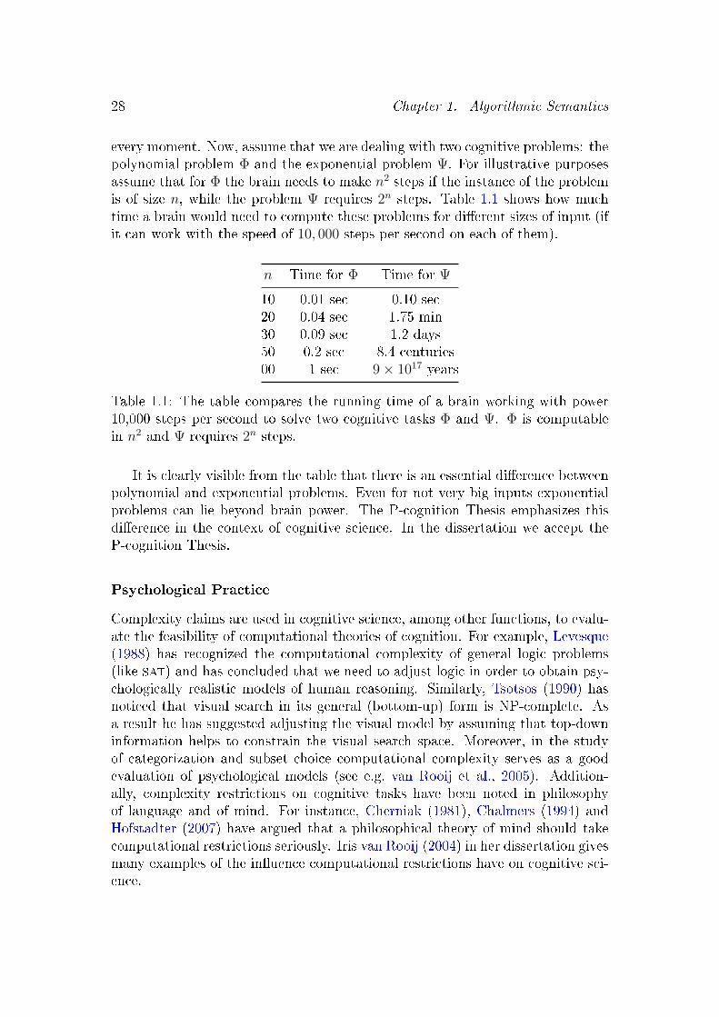
28 Chapter 1. Algorithmic Semantics
every moment. Now, assume that we are dealing with two cognitive problems: thepolynomial problem Φ and the exponential problem Ψ. For illustrative purposesassume that for Φ the brain needs to make n2 steps if the instance of the problemis of size n, while the problem Ψ requires 2n steps. Table 1.1 shows how muchtime a brain would need to compute these problems for dierent sizes of input (ifit can work with the speed of 10, 000 steps per second on each of them).
n Time for Φ Time for Ψ
10 0.01 sec 0.10 sec20 0.04 sec 1.75 min30 0.09 sec 1.2 days50 0.2 sec 8.4 centuries00 1 sec 9× 10¹⁷ years
Table 1.1: The table compares the running time of a brain working with power10,000 steps per second to solve two cognitive tasks Φ and Ψ. Φ is computablein n2 and Ψ requires 2n steps.
It is clearly visible from the table that there is an essential dierence betweenpolynomial and exponential problems. Even for not very big inputs exponentialproblems can lie beyond brain power. The P-cognition Thesis emphasizes thisdierence in the context of cognitive science. In the dissertation we accept theP-cognition Thesis.
Psychological Practice
Complexity claims are used in cognitive science, among other functions, to evalu-ate the feasibility of computational theories of cognition. For example, Levesque(1988) has recognized the computational complexity of general logic problems(like sat) and has concluded that we need to adjust logic in order to obtain psy-chologically realistic models of human reasoning. Similarly, Tsotsos (1990) hasnoticed that visual search in its general (bottom-up) form is NP-complete. Asa result he has suggested adjusting the visual model by assuming that top-downinformation helps to constrain the visual search space. Moreover, in the studyof categorization and subset choice computational complexity serves as a goodevaluation of psychological models (see e.g. van Rooij et al., 2005). Addition-ally, complexity restrictions on cognitive tasks have been noted in philosophyof language and of mind. For instance, Cherniak (1981), Chalmers (1994) andHofstadter (2007) have argued that a philosophical theory of mind should takecomputational restrictions seriously. Iris van Rooij (2004) in her dissertation givesmany examples of the inuence computational restrictions have on cognitive sci-ence.

1.5. Computability and Cognition 29
1.5.3 Common Doubts
Our experience shows that many researchers are skeptic about applicability ofcomputational complexity in cognitive science. Below we answer some commondoubts.
Limit Behavior
Computational complexity is dened in terms of limit behavior (see Section 2.3.3).In other words, a typical question of computational complexity theory is of theform:
As the size of the input increases, how do the running time and mem-ory requirements of the algorithm change?
Therefore, computational complexity theory, among other things, investigatesthe scalability of computational problems and algorithms, i.e., it measures the rateof increase in computational resources required as a problem grows. The implicitassumption here is that the size of the problem is unbounded. For example,models can be of any nite size, formulae can contain any number of distinctvariables and so on.
It is often claimed that as complexity theory deals only with relative computa-tional diculty of problems it has not much to oer for cognitive considerations.Simply put, the inputs we are dealing with in our everyday life are not of arbitrarysize. In typical situations they are even relatively small. In fact, critics claim,computational complexity does not say how dicult it is to solve a given problemfor a xed size of the input.
In general, even though computational complexity is formally dened in termsof limit behavior it can still be reasonably interpreted as saying something aboutproblem diculty on a xed model. Namely, if the computational complexityof the problem is high, then it means that there are no clever algorithms forsolving it, e.g., we have to do a complete search throughout the whole universe.Therefore, it is very likely that on a given xed model we also have to use a brute-force method and this will be again dicult (even for not so big n). For example,checking sat for a formula containing 5 variables is already quite challenging.
Moreover, even if in typical cognitive situations we are dealing with reasonablysmall inputs we have no bounds on their size. Potentially, the inputs can growwithout limit. Therefore, computational complexity makes perfect sense as adiculty measure.
Additionally, in experimental practice subjects usually do not realize the size ofthe universe in which they are supposed to solve some given problem. Therefore,it seems that they develop strategies (algorithms) for all possible universes (sizes).
However, if the size of a problem is too big subjects often start to approximatetheir solution, using heuristic methods instead of precise algorithms. But even

30 Chapter 1. Algorithmic Semantics
then we can still measure the rate of increase of the diculty (e.g. by changes inreaction time) on the interval where subjects realize their algorithmic procedures.For example, it is known that reaction time increases linearly when subjects areasked to count objects between 3 and 15. Up to 3 or 4 objects the answer is imme-diate, so-called subitizing. For tasks containing more than 15 elements subjectsstart to approximate: reaction time is constant and the number of incorrect an-swers increases dramatically (see e.g. Sternberg, 2008). Analogously, we can askhow reaction time increases when subjects are solving PTIME problems comparedto a situation when they are dealing with an NP-hard task.
There are also other experimental possibilities to observe computational com-plexity restrictions. For example, one can manipulate the universe to get a dropin the complexity and see what happens. In Chapter 7 we study the push-downrecognizable quantier most over an appropriately ordered universe, where itcould be recognized by nite automata, and we show a decrease in reaction timeto the level tting nite-automata problems. Similar methods can be used in caseof NP-hard problems by giving various certicates simplifying tasks and observingchanges in subjects' behavior.
Finally, theoretically speaking, it may be more benecial to assume that tasksare nite but that we do not know upper bounds than to try to develop a com-plexity measure up to xed size of a problem. Such a general approach worksvery well for syntax, where the assumption that language sentences can be of anylength has led to to the development of generative grammar and mathematicallinguistics (see Section 1.7.1 for a short discussion).
Summing up, various computational complexity measures seem to be a veryattractive tool for task-oriented cognitive science. At that point they are thebest established proposition for measuring the diculty of problems in precisemathematical terms. Moreover, this perspective seems promising as it was suc-cessfully applied in a few domains of psychological study which we mentionedabove. However, there is still not enough work in this direction to draw anystrong conclusions.
Last but not least, the biggest quest in applying computational complexity tocognitive science might be in discovering the right complexity measures. For sure,such measures we are using now just give a rough approximation of upper-bounddiculty.
Why Worst-case Complexity?
In our opinion the most serious criticism about the status of the P-cognitionThesis is that attacking worst-case computational complexity as a measure ofdiculty for cognitive processes. The point here is whether we really need toconsider the worst-case performance of cognitive algorithms on arbitrary inputs.It might be the case that inputs generated by nature have some special proper-ties which make problems tractable on those inputs even though in principle they

1.5. Computability and Cognition 31
might be NP-hard. It is also possible that our cognitive (linguistic) perception issimplifying things, pre-computing possible inputs. For example, it might be thecase that intractability of some problems comes from a parameter which is usu-ally very small no matter how big is the whole input. This way of thinking leadsto the consideration of so-called parametrized complexity theory (see Downeyand Fellows, 1998; Flum and Grohe, 2006) as a measure for the complexity ofcognitive processes. Iris van Rooij (2008) dwells on this subject proposing theFixed-parameter Tractability Thesis as a renement of the P-cognition Thesis.Another natural way is to turn toward so-called average-case complexity theory(see e.g. Impagliazzo, 1995; Bogdanov and Trevisan, 2006). It studies the com-putational complexity of problems on randomly generated inputs. The theory ismotivated by the fact that many NP-hard problems are in fact easily computableon most of the inputs. One potential problem with applications of this mea-sure to cognitive science is that we are unable to come up with a probabilitydistribution on the space of all possible inputs generated by the nature.
In principle, we agree that worst-case computational complexity might not bethe measure best tailored for describing the hardness of cognitive tasks. Howeverwe also think that an asymptotic analysis of cognitive capacities is the neces-sary rst step in the quest for understanding their complexity. In the book wehave tried to initiate this rst step in the domain of natural language semanticsand hope that it will be the beginning of a journey nally leading to a betterunderstanding of natural language processing.
1.5.4 Explaining the Comprehension Task
Let us summarize what we have said so far by answering to the following question:
How does computational cognition relate to our psycholinguistic per-spective?
We want to explain one of the basic components of comprehension. Usingthe algorithmic theory of meaning we can think about that component in termsof model-checking procedures. Model-checking takes a situation and a naturallanguage expression as an input and then transforms them to the output, i.e., adenotation of the expression in the world. In the paradigmatic case of sentenceswe get the truth-value. Therefore, model-checking might be treated as an exampleof a cognitive task.
Now, from the most abstract, computational level of the explanation, we areinterested in a mathematical specication of the properties of model-checking. Inparticular, we will study the computational complexity with respect to logical de-nability of a given expression. That is why we are interested in the combinationof complexity and denability. The theory which pursues the relation betweenthem is called descriptive complexity theory (see Section 2.4). Using it we willinvestigate the logical properties of natural language quantiers postulated by

32 Chapter 1. Algorithmic Semantics
some linguistic formalisms to track down the distinction between quantiers withtractable (PTIME) and intractable (NP-hard) referential meaning (the model-checking problem).
Another aspect which should be taken into account is the algorithmic level ofexplanation. Even though it is not the perspective we have explicitly taken inthe thesis, algorithmic considerations are a part of our study. We give explicitalgorithms which can be used to solve model-checking problems for example asparts of our proofs in Chapter 3. We consider concrete procedures for simplequantiers in Chapter 7 and investigate what kind of model-checking subjectsare realizing for some special sorts of sentences in Chapter 6. However, it mightbe the case that humans are actually using completely dierent algorithms. Inother words, we only claim that complexity restricts agents. Nevertheless, we donot think that humans are always using the simplest possible procedures.
As far as the implementation level is concerned we do not study neurologicalactivity when natural language is processed. However, our work was to someextent motivated by the neurological research discussed in Chapter 7. Therefore,even though we formally restrict ourselves to classical cognitive science we see apossible direct connection with neurocognitive reality.
Below we discuss more specic impacts of computational complexity on thedomain of our interest.
1.6 Finite Interpretations
The above discussion leads us to another restriction of our approach which ispartially motivated by the computational nature of our considerations.
Most of the authors considering the semantics of natural language are inter-ested only in nite universes. This is also common in papers devoted to naturallanguage quantiers; let us cite Dag Westerståhl (1984):
In general these cardinals can be innite. However, we now lay downthe following constraint:
(FIN) Only nite universes are considered.
This is a drastic restriction, no doubt. It is partly motivated bythe fact that a great deal of the interest of the present theory ofdeterminers comes from applications to natural language, where thisrestriction is reasonable. (Westerståhl, 1984, p. 154)
In typical communication situations we indeed refer to nite sets of objects.For example, the intended interpretations of the following sentences are nitesets:

1.6. Finite Interpretations 33
(14) Exactly ve of my children went to the cinema.
(15) Everyone from my family has read Alice's Adventures in Wonderland.
In many cases the restriction to nite interpretations essentially simplies ourtheoretic considerations.
First of all, there is a conceptual problem with computational complexity the-ory for an innite universe. Even though from the mathematical point of viewwe can work with innite computations, the classical study of resource boundsin such a setting does not make a lot of sense as we need innite time and in-nite memory resources. On the other hand, maybe we need only nitely manystates or loops. Hence, after all it is a matter of proposing reasonable deni-tions and nding interesting applications of innite computations in cognitivemodeling. For example, they can be useful as a framework for some cognitiveprocesses which at least in theory are supposed to continue working indenitely,like equilibrioception.
From the semantic perspective there is, however, an additional problem withinnite universes. Namely, dening an intuitive semantics for natural languagein an arbitrary universe is a very dicult task. As an example of potentialtrouble-makers we can give quantiers, like more or most. We usually reducethe problem of their meaning to a question about the relations between sets ofelements (see Section 2.2). In nite universes there is an easy and commonlyaccepted solution, which is to compare the cardinal numbers of these sets. Butextending this solution to the innite case seems to be very counterintuitive. Letus have a look at the following sentence.
(16) There are more non-primes than primes among integers.
The sentence is false if we interpret more in terms of cardinal numbers ofsets. However, intuitively we agree that the sentence is meaningful and even true.
One possible solution to this problem is to treat such quantiers as measurequantiers. In innite universes we can compare quantities by a proper measurefunctions, which are non-logical and context dependent concepts (see Krynickiand Mostowski, 1999, for more details).
Another approach to the problem can be formulated in terms of the so-calledweak semantics for second-order denable quantiers. The main idea of the weaksemantics for second-order logic is to consider structures of the form (M,K),where M is a model and K is a class of relations over the universe closed underdenability with parameters in a given language. The class K is used to inter-pret second-order quantication. Phrases like: for every relation R, there isa relation R are interpreted in (M,K) as for every relation R belonging to Kand there is a relation R belonging to K. This way of interpreting second-orderquantication essentially modies the standard semantics for second-order logic

34 Chapter 1. Algorithmic Semantics
and gives an intuitive semantics for second-order denable quantiers in arbitraryuniverses from the natural language point of view (see e.g. Mostowski, 1995).
In this dissertation we work with nite universes as we are mainly interestedin the algorithmic aspects of the semantics. However, we nd a developmenttoward covering arbitrary universes by adopting the methods outlined above anda proper complexity measure a fascinating challenge for later work.
1.7 Complexity in Linguistics
The topic of language complexity has surfaced in many dierent contexts and canbe measured in many dierent ways. We are talking only about the computa-tional and descriptive complexity of language, but there are many other aspectsof complexity, like lexical, information-theoretic (Kolmogorov complexity), struc-tural or functional. These are usually studied in less logical manner (see e.g.Miestamo et al., 2008) and we do not compare these approaches directly.
1.7.1 Syntax
Noam Chomsky has opened the door to a view of language from the computa-tional perspective (see e.g. Chomsky, 2002, 1969). In the early 1950s he capturedlanguage's recursive nature, or ability to make innite use of nite means, inWilhelm von Humboldt's famous words, inventing formal language theory. Chom-sky's complexity hierarchy of nite-state, context-free, and context-sensitive lan-guages associated with their automata counterparts (see Section 2.3.1) changedlinguistics and opened it to many interactions with computer science and cogni-tive science.
Chomsky's insight was really of the nature of computational complexity the-ory. First of all, even though the sentences we encounter are all of bounded length certainly less than 100 words long Chomsky has assumed that they mightbe arbitrarily long. Notice that this is an assumption of exactly the same sort asdiscussed in Section 1.5.3 on the limit behavior of computational claims, i.e., con-sidering inputs of arbitrary size. This assumption directly lead to the discoveryof the computational model of language generation and the complexity hierarchy.
Next, using his complexity hierarchy Chomsky asked in which complexityclass natural language lies. He has early demonstrated the inadequacy of nite-state description of natural languages and has claimed that natural languages arecontext-free (see Chomsky, 2002). This was a pathbreaking way of thinking. Firstof all, it has shown how one can mathematically measure some complexity aspectsof natural language. Then, it has given a methodological constraint on linguistictheories of syntax; they have to be able to account at least for the context-freelanguages. Actually, it has also started a long standing debate whether natural

1.7. Complexity in Linguistics 35
language is context-free or not (see e.g. Pullum and Gazdar, 1982; Shieber, 1985;Culy, 1985; Manaster-Ramer, 1987).
Chomsky himself noticed very quickly that studying whether a grammar cangenerate all strings from a given language, so-called weak generative capacity, canserve only as a kind of stress test that doesn't tell us much unless a grammarfails the test. He has claimed:
The study of generative capacity is of rather marginal linguistic inter-est. It is important only in those cases where some proposed theoryfails even in weak generative capacity that is, where there is somenatural language even the sentences of which cannot be enumerated byany grammar permitted by this theory. [. . . ] It is important to note,however that the fundamental defect of many systems is not their limi-tation in weak generative capacity but rather their many inadequaciesin strong generative capacity.13 [. . . ] Presumably, discussion of weakgenerative capacity marks only a very early and primitive stage of thestudy of generative grammar. (Chomsky, 2002, :60f)
In subsequent years this belief has led to deeper study of generative for-malisms. In particular, using computational complexity one could answer thequestion whether some proposed generative formalism is plausible in the sense ofbeing easy enough to process. To be more precise, computational complexity ofparsing and recognition has become a major topic along with the development ofcomputational linguistics. The early results achieved are summarized in a bookby Barton et al. (1987). A more recent survey is due to Pratt-Hartmann (2008).In general, the results show that even for relatively simple grammatical frame-works some problems might be intractable. For example, regular and context-freelanguages have tractable parsing and recognition problems. However, Lambekgrammars, Tree-Adjoining Grammars, Head-Driven Phrase Structure Grammar,and context-sensitive grammars give raise to intractable problems.
1.7.2 Between Syntax and Semantics
Model-theoretic Syntax
One can specify the complexity of grammars not only in terms of generativemechanisms but also via a set of general constraints to which sentences generatedby these grammars have to conform. On this view, a string (or a tree) is gram-matical if it satises these constraints. How can we dene complexity from thisperspective? The idea is to identify the complexity of a grammar with the logicalcomplexity of the formulae which express the constraints. In other words, we ask
13Chomsky uses the term strong generative capacity referring to the set of structures thatcan be generated by a grammar.

36 Chapter 1. Algorithmic Semantics
here about descriptive complexity of grammars in a similar way to how we will beasking about descriptive complexity of model-checking problems in the followingchapters.
We measure the complexity of the sentences that dene constraints by sayinghow strong a logic we need to formulate them. Particularly, we refer to fragmentsof second-order logic (see e.g. Rogers, 1983) or various extensions of modal logic(see e.g. Kracht, 2003). For illustration, the two best known results of this ap-proach are as follows. In his seminal paper Büchi (1960) showed that a languageis denable by the so-called monadic fragment of second-order logic if and onlyif it is regular. McNaughton and Papert (1971) have proven that a set of stringsis rst-order denable if and only if it is star-free. These two results have theircounterpart in modal logic: the temporal logic of strings captures star-free lan-guages and propositional dynamic logic captures regular languages (see e.g. Mossand Tiede, 2006).
Notice that it is often possible to draw conclusions about computational com-plexity from such descriptive results. It is enough to know the complexity of thecorresponding logics. For instance, we know that monadic second order logic ontrees is decidable although intractable and therefore many linguistic questionsabout parse trees which are formulated in this logic might be dicult to an-swer. Our approach to studying the complexity of semantics goes along the samedescriptive line.
Discourse Complexity
Some of the earliest research trying to combine computational complexity withsemantics can be found in Sven Ristad's book The Language Complexity Game(1993). The author carefully analyzes the comprehension of anaphoric dependen-cies in discourse. He considers a few approaches to describing the meaning ofanaphora and proves their complexity. Finally, he concludes that the problem isinherently NP-complete and that all good formalisms accounting for it should beexactly as strong.
Pratt-Hartmann (2004) has shown that dierent fragments of natural lan-guage capture various complexity classes. More precisely, he has studied thecomputational complexity of satisability problems for various fragments of nat-ural language. He has proven that the satisability problem of the syllogistic frag-ment is in PTIME as opposed to the fragment containing relative clauses which isNP-complete. He has also described fragments of language such that their compu-tational complexity is even harder (with non-copula verbs or restricted anaphora)and nally he provides the reader with an undecidable fragment containing un-restricted anaphora.
It is also worth to mention very recent paper of Pagin (2009). The authortries to explain compositionality principle in terms of computational complexity,cognitive diculty as experienced by language users during communication, and

1.8. Classifying Meaning by Intractability 37
language learnability. He argues that compositionality simplies complexity oflanguage communication.
Unfortunately as far as we are aware not much is known about the com-putational complexity of dynamic formalisms. This is suprising because complex-ity questions match the dynamic spirit perfectly and moreover can give deeperinsights into the plausibility of proposed formalisms. Some complexity results areknown for belief revision mostly showing that the logic lying behind revisionmechanisms is highly intractable (see e.g. van Benthem and Pacuit, 2006) andfor game-theoretic semantics (see e.g. Sevenster, 2006). But there are some veryinteresting questions untouched, for example: What is the complexity of a beliefrevision (game) when an intractable sentence is the input? Does model-checkingcomplexity relate to the complexity of belief revision or the corresponding gamein any way? But rst of all, there has not been much done about the complexityof this model from the agent's perspective. For example, how dicult is beliefrevision for a single agent?
The worst news is that complexity seems to be a totally open problem forformal pragmatics, even though the question of how dicult it is to solve coor-dination problems in linguistic games seems to be very basic. Probably, someresults might be achieved via translation from complexity considerations in algo-rithmic game theory (see e.g. Nisan et al., 2007). We believe that computationalcomplexity issues should be incorporated in these models to better understandtheir plausibility.
In this book we study the computational complexity of model-checking for aquantier fragment of natural language. We often evoke the descriptive perspec-tive to achieve our aims. In other words, we try to understand some aspects ofmeaning from the computational perspective. Below we say a few words on theunderlying assumptions in this enterprise, summing up the previous considera-tions on semantics, cognitive science and complexity.
1.8 Classifying Meaning by Intractability
We have argued that meaning is an algorithm. This allows us to apply com-putability considerations to linguistics. Moreover, according to what we saidabove linguistic capacities, like all cognitive processes, are bounded by computa-tional restrictions. In particular, comprehension of natural language constructionsis linked to their computational complexity. We provide some more arguments infavor of this connection throughout the dissertation. We give an example for thisdependence in Section 4.5 where we discuss the interpretation of NP-completereciprocal sentences and suggest that their meaning might be in most cases onlycomprehended by recognizing inferential properties. Then in Chapter 5 we havea look at collective quantication in natural language, where among others wecan observe how computational complexity restricts expressibility of everyday

38 Chapter 1. Algorithmic Semantics
language. In Chapters 6 and 7 we present empirical evidence supporting thestatement that computational complexity inuences the comprehension of natu-ral language. In the rst of these chapters we show that people tend to choosecomputationally simpler interpretations of so-called Hintikka-like sentences. Inthe following chapter we give empirical evidence directly linking the reactiontime needed to recognize the meaning of sentences with simple quantiers to thecomplexity of automata computing this meaning. Below we try to capture ourexperience with studying the complexity of natural language into the form of amethodological statement about the descriptive power of the linguistic formalismwhich we needed.
1.8.1 Ristad's Theses
The book of Ristad (1993) contains not only a technical contribution to thesemantic theory of anaphora but also some methodological claims on the role ofcomputational complexity in linguistics.
First of all, Ristad claims that natural language contains constructions whichsemantics is essentially NP-complete:
The second major result of this monograph is the thesis that languagecomputations are NP-complete. This complexity thesis is a substan-tive, falsiable claim about human language that is directly supportedby the quiescent state of the language complexity game.
(Ristad, 1993, p. 14)
Secondly, Ristad suggests that a good linguistic theory cannot be too strong:
The central consequence of this complexity thesis for human languageis that empirically adequate models (and theories) of language willgive rise to NP-completeness, under an appropriate idealization tounbounded inputs. If a language model is more complex than NP, sayPSPACE-hard, then our complexity thesis predicts that the systemis unnaturally powerful, perhaps because it overgeneralizes from theempirical evidence or misanalyses some linguistic phenomena.
(Ristad, 1993, p. 15)
In other words, Ristad claims that every semantic model has to be at leastNP-hard to be able to capture complex linguistic phenomena. On the otherhand, in his opinion every computationally stronger formalism is overgeneralizinglinguistic capacities. This second methodological claim can be treated as a kindof semantic Ockham's razor. Summing up, Ristad proposes NP-completeness asa kind of methodological test for plausibility of linguistic theories.

1.8. Classifying Meaning by Intractability 39
1.8.2 Descriptive Bounds on Everyday Language
We do not completely agree with Ristad but we share his intuitions. However, weprefer to restrict claims of that sort to some fragment of language as the wholeof natural language contains expressions whose complexity go beyond practicalcomputability. Nevertheless, we can see a natural intuition supporting the useof the concept of natural language excluding technical expressions. However,in this narrow sense we prefer to use the term everyday language. In a sense weunderstand everyday language here as a pre-theoretic part of natural language.
In this dissertation we study the complexity of natural language quantiersvia their denability properties. In other words, we use descriptive complexitytheory, i.e., we draw complexity conclusions on the basis of logical descriptionsof semantics. From this perspective, our experience allows us to state the follow-ing claim which resembles Ristad's thesis and was proposed by Mostowski andSzymanik (2005):
Σ11-thesis Our everyday language is semantically bounded by the properties ex-
pressible in the existential fragment of second-order logic.
In other words, we claim that everyday language can be described in the exis-tential fragment of second-order logic (see Denition 2.1.1). If some property isnot denable by any Σ1
1-formula, then it falls outside the scope of everyday lan-guage. For example, quantiers there exists, all, exactly two, at least four,every other and most belongs to everyday language. The counterexample isthe notion there exist at most countably many which is not denable by anyΣ1
1-formula. Moreover, we know from Fagin's theorem (2.4.4) that Σ11-properties
correspond to NPTIME. Hence, our thesis basically restricts the methodologicalclaim of Ristad to the realm of everyday language.
Let us give one argument in favor of accepting this methodological statement.The other one, more domain specic, will be formulated in Section 6.3.4. Theintuition is that the core sentences of everyday language are sentences whichcan be more or less eectively veriable. We argued that in the case of smallnite interpretations this means that their truth-value can be practically com-puted, directly or indirectly. Direct practical computability means that there isan algorithm which for a given nite interpretation computes the truth-value ina reasonable time. From the P-cognition Thesis it follows that the referentialmeaning of an expression which can be directly computed is in PTIME. However,as we mentioned in Section 1.3 we frequently understand sentences indirectly,evoking their inferential dependencies with other sentences. Let us consider thefollowing three sentences:
(17) There were more boys than girls at the party.
(18) At the party every girl was paired with a boy.

40 Chapter 1. Algorithmic Semantics
(19) Peter came alone to the party.
We know that sentence (17) can be inferred from sentences (18) and (19). Then wecan establish the truth-value of sentence (17) indirectly, knowing that sentences(18) and (19) are true.
The question arises: What do we mean by a tractable inferential meaning?First notice that in the case of NPTIME problems the non-deterministic be-
havior of an algorithm can be described as follows:
Firstly, choose a certicate of a size polynomially depending on thesize of input. Then apply a PTIME algorithm for nding the answer.The nondeterministic algorithm answers YES exactly when there is acerticate for which we get a positive answer.
(Garey and Johnson, 1979, p. 28)
Let us observe that in a sense such certicates are proofs. When we havea proof of a statement then we can easily check whether the sentence is true.Therefore NPTIME problems (Σ1
1-properties) are practically justiable. Let usconsider an example.
Suppose that we know that the following are true statements:
(20) Most villagers are communists.
(21) Most townsmen are capitalists.
(22) All communists and all capitalists hate each other.
From these sentences we can easily infer the NP-complete branching interpreta-tion of the following sentence (for a discussion on the computational complexityof sentences like this see Section 3.2 and Chapter 6):
(23) Most villagers and most townsmen hate each other.
Sentences (20), (21), and (22) have to be given or guessed. They are in a sensecerticates or proofs of the truth of sentence (23).
In this sense sentences with NPTIME meaning or by Fagin's theorem (seeTheorem 2.4.4) Σ1
1-expressible sentences are indirectly veriable. Moreover,NPTIME seems to capture exactly indirect veriability. This observation givesan argument for our claim everyday sentences have practically computableinferential meaning.
We assume the Σ11-thesis as a methodological principle throughout the
dissertation. We are using it to argue in favor of or against some linguisticformalizations. For instance, in Chapter 5 we study a common way of modelingcollective quantication in natural language, the so-called type-shifting approach.By using the formalism of second-order generalized quantiers, we observe that

1.9. Summary 41
a uniform treatment of collectivity via type-shifting has excessive computationalcomplexity. Therefore, we claim that either such a model cannot be plausible, andpropose turning to computationally better behaved many-sorted models or thatsome instances of collective quantication do not appear in everyday language.On the other hand, the positive use of the Σ1
1-thesis can be found in Chapter4, where we analyze the computational complexity of dierent interpretations ofEnglish reciprocal sentences with quantiers in the antecedents. We work with amodel which is expressible in the existential fragment of second-order logic andshow that it predicts some reciprocal sentences to be NP-complete. Our thesisallows us to believe that the model is plausible. Moreover, in Chapter 6 weconsider Barwise's test of negation normality and observe that it makes senseonly when assuming that everyday sentences are expressible in the existentialfragment of second order-logic (see Remark 6.3.2).
Moreover, the Σ11-thesis partially bridges the two basic comprehension mecha-
nisms formulated in Section 1.1. It explains in some cases the subtle dependencebetween the complexity of a sentence, its model-checking diculty, and its rela-tion to knowledge. It also relaxes our assumption about tractability. As a matterof fact, we found NP-complete semantic constructions in natural language. Weclaimed that such expressions are intractable for human agents but now we addone proviso: their direct model-checking can be intractable but we can still evokesome indirect mechanism making the task perfectly tractable. This puts our po-sition very close to Ristad's perspective. Additionally, it provides one idea how toconnect our investigations with dynamic formalisms describing other aspects ofmeaning. Such an integration is needed to account for the big picture of naturallanguage meaning and comprehension.
1.9 Summary
In this chapter we have discussed some motivations and philosophical assumptionslying in the background of the research presented in the next chapters. Theseassumptions do not have a direct inuence on our technical results. However,we believe that they give an additional argument for studying the computationalcomplexity of natural language expressions.
Below we summarize our assumptions:
• We mostly study a basic element of comprehension: model-checking, towhich we sometimes refer as referential meaning.
• We identify (referential) meanings (algorithms) with Turing machines (com-putable functions).
• We assume that problems are tractable if they are computable in polynomialtime. Otherwise, they are intractable.

42 Chapter 1. Algorithmic Semantics
• We assume that human cognitive (linguistic) capacities are constrained bypolynomial time computability. Therefore, if a meaning corresponds tointractable functions we believe it is too hard for direct comprehension.
• We claim that the semantics of everyday language can be adequately de-scribed in the existential fragment of second order-logic (Σ1
1-thesis).
• We restrict ourselves to nite universes.
We hope that our technical insights will give additional arguments in favor ofour assumptions.
Chapter 2
Mathematical Prerequisites
This chapter describes the notation and basic terminology from generalized quan-tier theory and computation theory. We focus only on concepts which will beexplored in the following parts of the thesis. We assume some familiarity withthe basics of rst-order and second-order logic (see e.g. Ebbinghaus et al., 1996).
2.1 Basic Notation
Let A, B be sets. We will write ∅ for the empty set, card(A) to denote thecardinality of the set A and P(B) for the power set of B. The operations ∪, ∩,−, and the relation ⊆ on sets are dened as usual. The set A×B = (a, b) | a ∈A and b ∈ B denotes the Cartesian product of A and B, where (a, b) is theordered pair. If R is a relation then by R−1 we denote its inverse. The set ofnatural numbers is denoted by ω. If k ∈ ω then Ak denotes
A× . . .× A︸ ︷︷ ︸k
.
We will write Q for the set of rational numbers. If q ∈ Q we write dqe for theceiling function of q, i.e. the smallest integer greater than q.
Let ϕ and ψ be formulae. We write ¬ϕ, ϕ ∧ ψ, ϕ ∨ ψ, ϕ =⇒ ψ, ϕ ⇐⇒ ψ,∃xϕ(x), and ∀xϕ(x) with the usual meaning. We will denote rst-order logic(elementary logic) by FO and second-order logic by SO.
Now, let us recall the denition of the hierarchy of second-order formulae.
2.1.1. Definition. The class Σ10 is identical to the class Π1
0 and both contain(all and only) the rst-order formulae. The class Σ1
n+1 is the set of formulaeof the following form: ∃P1 . . . ∃Pkψ, where ψ ∈ Π1
n. The class Π1n+1 consists of
formulae of the form: ∀P1 . . . ∀Pkψ, where ψ ∈ Σ1n. We additionally assume that
all formulae equivalent to some Σ1n (or Π1
n) formula are also in Σ1n (respectively
Π1n).
43
44 Chapter 2. Mathematical Prerequisites
In the thesis a vocabulary is a nite set consisting of relation symbols (pred-icates) with assigned arities. Let τ = R1, . . . , Rk be a vocabulary, where foreach i, ni is the arity of Ri. Then a τ -model will be a structure of the followingform: M = (M,R1, . . . , Rk), where M is the universe of model M and Ri ⊆ Mis an ni-ary relation over M , for 1 ≤ i ≤ k. If ϕ is a τ -sentence (a sentence overthe vocabulary τ) then the class of τ -models of ϕ is denoted by Mod(ϕ). We willsometimes write RM
i for relations to dierentiate them from the correspondingpredicates Ri.
2.2 Generalized Quantier Theory
Generalized quantiers are one of the basic tools of today's linguistics and theirmathematical properties have been extensively studied since the fties (see Petersand Westerståhl, 2006, for a recent overview). In its simplest form generalizedquantier theory assigns meanings to statements by dening the semantics of thequantiers occurring in them. For instance, the quantiers every, some, atleast 7, an even number of, and most build the following sentences.
(1) Every poet has low self-esteem.
(2) Some dean danced nude on the table.
(3) At least 7 grad students prepared presentations.
(4) An even number of the students saw a ghost.
(5) Most of the students think they are smart.
(6) Less than half of the students received good marks.
What is the semantics assigned to these quantiers? Formally they are treatedas relations between subsets of the universe. For instance, in sentence (1) everyis a binary relation between the set of poets and the set of people having lowself-esteem. Following the natural linguistic intuition we will say that sentence(1) is true if and only if the set of poets is included in the set of people havinglow self-esteem. Hence, the quantier every corresponds in this sense to theinclusion relation.
Let us now have a look at sentence (4). It is true if and only if the intersectionof the set of all students with the set of people who saw a ghost is of even cardi-nality. That is, this quantier says something about the parity of the intersectionof two sets.
Finally, let us consider example (5). Let us assume that the quantier mostsimply means more than half.1 Hence, sentence (5) is true if and only if the
1We would say that the stronger, but vague, meaning that seems more natural is a result ofpragmatics.

2.2. Generalized Quantier Theory 45
cardinality of the set of students who think they are smart is greater than thecardinality of the set of students who do not think they are smart. That is,the quantier most expresses that these two kinds of student exist in a specicproportion.
2.2.1 Two Equivalent Concepts of Generalized Quantiers
Frege was one of the major gures in forming the modern concept of quantica-tion. In his Begrisschrift (1879) he made a distinction between bound and freevariables and treated quantiers as well-dened, denoting entities. He thoughtof quantiers as third-order objects relations between subsets of a given xeduniverse. This way of thinking about quantiers is still current, particularly inlinguistics. However, historically speaking the notion of a generalized quantierwas formulated for the rst time in a dierent, although equivalent, way: gen-eralized quantiers were dened as classes of models closed under isomorphisms.Firstly, in a seminal paper of Andrzej Mostowski (1957) the notions of existentialand universal quantication were extended to the concept of a monadic general-ized quantier binding one variable in one formula, and later this was generalizedto arbitrary types by Per Lindström (1966). Below we give the formal denition.
2.2.1. Definition. Let t = (n1, . . . , nk) be a k-tuple of positive integers.A Lindström quantier of type t is a class Q of models of a vocabularyτt = R1, . . . , Rk, such that Ri is ni-ary for 1 ≤ i ≤ k, and Q is closed un-der isomorphisms, i.e. if M and M′ are isomorphic, then
(M ∈ Q ⇐⇒ M′ ∈ Q).
2.2.2. Definition. If in the above denition for all i: ni ≤ 1, then we say thata quantier is monadic, otherwise we call it polyadic.
2.2.3. Example. Let us explain this denition further by giving a few examples.Sentence (1) is of the form Every A is B, where A stands for poets and B forpeople having low self-esteem. As we explained above the sentence is true if andonly if A ⊆ B. Therefore, according to the denition, the quantier every is oftype (1, 1) and corresponds to the class of models (M,A,B) in which A ⊆ B.For the same reasons the quantier an even number of corresponds to the classof models in which the cardinality of A ∩ B is an even number. Finally, let usconsider the quantier most of type (1, 1). As we mentioned before the sentenceMost As are B is true if and only if card(A ∩ B) > card(A − B) and thereforethe quantier corresponds to the class of models where this inequality holds.
Therefore, formally speaking:

46 Chapter 2. Mathematical Prerequisites
∀ = (M,A) | A = M.∃ = (M,A) | A ⊆M and A 6= ∅.
Every = (M,A,B) | A,B ⊆M and A ⊆ B.Even = (M,A,B) | A,B ⊆M and card(A ∩B) is even.Most = (M,A,B) | A,B ⊆M and card(A ∩B) > card(A−B).
The rst two examples are the standard rst-order universal and existentialquantiers, both of type (1). They are classes of models with one unary predicatesuch that the extension of the predicate is equal to the whole universe in case ofthe universal quantier and is nonempty in case of the existential quantier.
Why do we assume that these classes are closed under isomorphisms? Simplyput, this guarantees that the quantiers are topic neutral. The quantier mostmeans exactly the same when applied to people as when applied to natural num-bers.
Let us now give the denition of a generalized quantier. This denitionis commonly used in linguistics as opposed to the previous one which nds itsapplications rather in logic.
2.2.4. Definition. A generalized quantier Q of type t = (n1, . . . , nk) is a func-tor assigning to every set M a k-ary relation QM between relations on M suchthat if (R1, . . . , Rk) ∈ QM then Ri is an ni-ary relation on M , for i = 1, . . . , k.Additionally, Q is preserved by bijections, i. e., if f : M −→ M ′ is a bijectionthen (R1, . . . , Rk) ∈ QM if and only if (fR1, . . . , fRk) ∈ QM ′ , for every rela-tion R1, . . . , Rk on M , where fR = (f(x1), . . . , f(xi)) | (x1, . . . , xi) ∈ R, forR ⊆M i.
In other words, a generalized quantier Q is a functional relation associatingwith each model M a relation between relations on its universe, M . Hence, if wex a model M, then we can treat a generalized quantier as a relation betweenrelations over the universe, and this is the familiar notion from natural languagesemantics.
Notice that we have the following equivalence between a Lindström quantierand a generalized quantier:
(M,R1, . . . , Rk) ∈ Q ⇐⇒ QM(R1, . . . , Rk),where Ri ⊆Mni .
For instance, in a given model M the statement MostM(A,B) says thatcard(AM ∩BM) > card(AM −BM), where AM , BM ⊆M .
2.2.5. Corollary. The denitions of a Lindström quantier (2.2.1) and a gen-eralized quantier (2.2.4) are equivalent.

2.2. Generalized Quantier Theory 47
Studying the properties of quantiers in most cases we invoke Denition 2.2.1but for descriptive purposes over some xed universe we mostly make use ofDenition 2.2.4, treating quantiers as third-order concepts (relations betweenrelations).
2.2.2 Branching Quantiers
As a matter of chronology, the idea of generalizing Frege's quantiers arose muchearlier than the work of Lindström (1966). The idea was to analyze possibledependencies between quantiers dependencies which are not allowed in thestandard linear (Fregean) interpretation of logic. Branching quantication (alsocalled partially ordered quantication, or Henkin quantication) was proposed byLeon Henkin (1961) (for a survey see Krynicki and Mostowski (1995)). Branch-ing quantication signicantly extends the expressibility of rst-order logic; forexample the so-called Ehrenfeucht sentence, which uses branching quantication,expresses innity:
∃t(∀x∃x′∀y∃y′
) [(x = y ⇐⇒ x′ = y′) ∧ x′ 6= t
].
Informally speaking, the idea of such a construction is that for dierent rowsthe values of the quantied variables are chosen independently. The semanticsof branching quantiers can be formulated mathematically in terms of Skolemfunctions. For instance, the Ehrenfeucht sentence after Skolemization has thefollowing form:
∃t∃f∃g[∀x∀y(x = y ⇐⇒ f(x) = g(y)) ∧ f(x) 6= t
].
Via simple transformations this sentence is equivalent to the following:
∃f∀x∀y[(x 6= y =⇒ f(x) 6= f(y)) ∧ (∃t∀x(f(x) 6= t))
],
and therefore, it expresses Dedekind's innity: there exists an injective functionfrom the universe to itself which is not surjective.
The idea of the independent (branching) interpretation of quantiers has givenrise to many advances in logic. Let us mention here only the logical study of(in)dependence by investigating Independence Friendly Logic (see Hintikka, 1996)and Dependence Logic (see Väänänen, 2007). It is also worth noting that Game-Theoretic Semantics (see Hintikka and Sandu, 1997) was originally designed as analternative semantics for branching quantication (Independence Friendly Logic).Now it is considered as a useful tool for studying dierent variants of indepen-dence, like imperfect information games (see Sevenster, 2006). We present com-putational complexity results for branching quantiers in Section 3.2 and discusstheir linguistic applications in Chapter 6.

48 Chapter 2. Mathematical Prerequisites
2.2.3 Logic Enriched by Generalized Quantiers
Generalized quantiers enable us to enrich the expressive power of a logic in avery controlled and minimal way. Below we dene the extension of an arbitrarylogic L by a generalized quantier Q.
2.2.6. Definition. We dene the extension, L(Q), of logic L by a quantier Qof type t = (n1, . . . , nk) in the following way:
• The formula formation rules of L-language are extended by the rule:
if for 1 ≤ i ≤ k, ϕi(xi) is a formula and xi is an ni-tuple of pairwise distinctvariables, then Q x1, . . . , xk [ϕ1(x1), . . . , ϕk(xk)] is a formula.
2.2.7. Convention. Let us observe that this denition can be modied ac-cording to common notational habits as follows. Q is treated as bindingn = max(n1, . . . , nk) variables in k formulae. For example, the quantier Everyof type (1, 1) which expresses the property ∀x[P1(x) =⇒ P2(x)] can be writtenaccording to the rst convention as:
Every xy [P1(x), P2(y)]
and according to the modied one as:
Every x [P1(x), P2(x)].
2.2.8. Definition. The satisfaction relation of L is extended by the rule:
M |= Q x1, . . . , xk [ϕ1(x1), . . . , ϕk(xk)] i (M,ϕM1 , . . . , ϕ
Mk ) ∈ Q,
where ϕMi = a ∈Mni | M |= ϕi(a).
In this dissertation we will mainly be concerned with extensions of rst-orderlogic, FO, by dierent generalized quantiers Q. Following Denition 2.2.6 suchan extension will be denoted by FO(Q).
2.2.4 Denability of Generalized Quantiers
Some generalized quantiers, like ∃≤3, ∃=3, and ∃≥3, are easily expressible inelementary logic. This is also true for many natural language determiners. Forexample, we can express the type (1, 1) quantier Some by the type (1) rst-orderexistential quantier in the following way:
Some x [A(x), B(x)] ⇐⇒ ∃x[A(x) ∧B(x)].

2.2. Generalized Quantier Theory 49
However, it is well-known that many generalized quantiers are not denable inrst-order logic. Standard application of the compactness theorem shows thatthe quantiers there exist (in)nitely many are not FO-denable. Moreover,using Ehrenfeucht-Fraïssé games it is routine to prove the following:
2.2.9. Proposition. The quantiers Most and Even are not rst-order den-able.2
Dealing with quantiers not denable in rst-order logic we will considertheir denitions in higher-order logics, for instance in fragments of second-orderlogic. To give one example here, in a model M = (M,AM , BM) the sentenceMost x [A(x), B(x)] is true if and only if the following condition holds:
∃f : (AM −BM) −→ (AM ∩BM) such that f is injective but not surjective.
In general, denability theory investigates the expressibility of quantiers invarious logics. Informally, denability of a quantier Q in a logic L means thatthere is a uniform way to express every formula of the form Q xϕ in L. Thefollowing is a precise denition.
2.2.10. Definition. Let Q be a generalized quantier of type t and L a logic.We say that the quantier Q is denable in L if there is a sentence ϕ ∈ L ofvocabulary τt such that for any τt-structure M:
M |= ϕ i M ∈ Q .
2.2.11. Definition. Let L and L′ be logics. The logic L′ is at least as strong asthe logic L (L ≤ L′) if for every sentence ϕ ∈ L over any vocabulary there existsa sentence ψ ∈ L′ over the same vocabulary such that:
|= ϕ ⇐⇒ ψ.
The logics L and L′ are equivalent (L ≡ L′) i L ≤ L′ and L′ ≤ L.
Below we assume that a logic L has the so-calledsubstitution property , i.e., thatthe logic L is closed under substituting predicates by formulas. The following factis well-known for Lindström quantiers.
2For more undenability results together with mathematical details and an introduction intoEhrenfeucht-Fraïssé techniques we suggest consulting the literature (e.g. Chapter 4 in Petersand Westerståhl, 2006).

50 Chapter 2. Mathematical Prerequisites
2.2.12. Proposition. Let Q be a generalized quantier and L a logic. Thequantier Q is denable in L i
L(Q) ≡ L.Proof The direction L ≤ L(Q) is obvious since every formula of L is also a
formula of L(Q) (see Denition 2.2.6). To show that L(Q) ≤ L we use induc-tively the fact that if ϕ is the formula which denes Q and ψ1(x1), . . . , ψk(xk) areformulae of L, then
|= Q x1, . . . , xk [ψ1(x1), . . . , ψk(xk)] ⇐⇒ ϕ(R1/ψ1, . . . , Rk/ψk),
where the formula on the right is obtained by substituting every occurrence ofRi(xi) in ϕ by ψi(xi).
2.2.5 Linguistic Properties of Generalized Quantiers
It was realized by Montague (1970) that the notion of a generalized quantier as a relation between sets can be used to model the denotations of nounphrases in natural language. Barwise and Cooper (1981) introduced the apparatusof generalized quantiers as a standard semantic toolbox and started the rigorousstudy of their properties from the linguistic perspective. Below we dene someproperties of quantiers important in linguistics which we use in our furtherresearch (see Peters and Westerståhl, 2006, for a general overview).
Boolean Combinations of Quantiers
To account for complex noun phrases, like those occurring in sentences (7)(10),we dene disjunction, conjunction, outer negation (complement) and inner nega-tion (post-complement) of generalized quantiers.
(7) At least 5 or at most 10 departments can win EU grants. (disjunction)
(8) Between 100 and 200 students started in the marathon. (conjunction)
(9) Not all students passed. (outer negation)
(10) All students did not pass. (inner negation)
2.2.13. Definition. Let Q, Q′ be generalized quantiers, both of type(n1, . . . , nk). We dene:
(Q∧Q′)M [R1, . . . , Rk] ⇐⇒ QM [R1, . . . , Rk] and Q′M [R1, . . . , Rk] (conjunction)
(Q∨Q′)M [R1, . . . , Rk] ⇐⇒ QM [R1, . . . , Rk] or Q′M [R1, . . . , Rk] (disjunction).
(¬Q)M [R1, . . . , Rk] ⇐⇒ not QM [R1, . . . , Rk] (complement)
(Q¬)M [R1, . . . , Rk] ⇐⇒ QM [R1, . . . , Rk−1,M −Rk] (post-complement)

2.2. Generalized Quantier Theory 51
Relativization of Quantiers
Every statement involving a quantier Q is about some universe M . Sometimesit is useful to dene a new quantier saying that Q restricted to some subset ofM behaves exactly as it behaves on the whole universe M . Below we give theformal denition.
2.2.14. Definition. Let Q be of type (n1, . . . , nk); then the relativization of Q,Qrel, has the type (1, n1, . . . , nk) and is dened for A ⊆ M,Ri ⊆ Mni , 1 ≤ i ≤ kas follows:
QrelM [A,R1, . . . , Rk] ⇐⇒ QA[R1 ∩ An1 , . . . , Rk ∩ Ank ].
In particular, for Q of type (1) we have:
QrelM [A,B] ⇐⇒ QA[A ∩B].
2.2.15. Example. This already shows that many natural language determinersof type (1, 1) are just relativizations of some familiar logical quantiers, e.g.:
Some = ∃rel;
Every = ∀rel.
Domain Independence
Domain independence is a property characteristic of natural language quantiers.It says that the behavior of a quantier does not change when you extend theuniverse. The formal denition follows.
2.2.16. Definition. A quantier of type (n1, . . . , nk) satises domain indepen-dence (EXT) i the following holds:
If Ri ⊆Mni , 1 ≤ i ≤ k,M ⊆M ′, then QM [R1, . . . , Rk] ⇐⇒ QM ′ [R1, . . . Rk].
Conservativity
The property which in a sense extends EXT is conservativity:
2.2.17. Definition. A type (1, 1) quantier Q is conservative (CONS) i forall M and all A,B ⊆M :
QM [A,B] ⇐⇒ QM [A,A ∩B].

52 Chapter 2. Mathematical Prerequisites
CE-quantiers
Quantiers closed under isomorphisms and satisfying CONS and EXT are knownin the literature as CE-quantiers. It has been hypothesized that all naturallanguage determiners correspond to CE-quantiers (see e.g. Barwise and Cooper,1981). From this perspective expressions like John, ∀, and only are excludedfrom the realm of natural language determiners by not being CE-quantiers. Theproper name John does not satisfy isomorphism closure, ∀ is not EXT andonly violates conservativity.
Notice that CE-quantiers of type (1, 1) over nite universes may be identiedwith pairs of natural numbers.
2.2.18. Definition. Let Q be a CE-quantier of type (1, 1). We dene a binaryrelation also denoted by Q:
Q(k,m) ⇐⇒ there is M, and A,B ⊆M such that
card(A−B) = k, card(A ∩B) = m, and QM [A,B].
2.2.19. Theorem. If Q is a CE-quantier of type (1, 1), then for all M and allA,B ⊆M we have:
QM [A,B] ⇐⇒ Q(card(A−B), card(A ∩B)).
Proof It is enough to show that whenever Q is CE, A,B ⊆ M , A′, B′ ⊆ M ′
are such that: card(A − B) = card(A′ − B′) and card(A ∩ B) = card(A′ ∩ B′),QM [A,B] ⇐⇒ QM ′ [A′, B′].
Monotonicity
One of the most striking intuitions about quantiers is that they say that somesets are large enough. Therefore, we would expect that quantiers are closedon some operations changing universe. The simplest among such operations istaking subsets and supersets. Monotonicity properties state whether a quantieris closed under these operations.
2.2.20. Definition. A quantier QM of type (n1, . . . , nk) is monotone increas-ing in the i'th argument (upward monotone) i the following holds:
If QM [R1, . . . , Rk] and Ri ⊆ R′i ⊆Mni , then
QM [R1, . . . , Ri−1, R′i, Ri+1, . . . , Rk], where 1 ≤ i ≤ k.

2.2. Generalized Quantier Theory 53
2.2.21. Definition. A quantier QM of type (n1, . . . , nk) is monotone decreas-ing in the i'th argument (downward monotone) i the following holds:
If QM [R1, . . . , Rk] and R′i ⊆ Ri ⊆Mni , then
QM [R1, . . . , Ri−1, R′i, Ri+1, . . . , Rk], where 1 ≤ i ≤ k.
In particular, for a quantier Q of type (1, 1) we can dene the following basictypes of monotonicity:
↑MON QM [A,B] and A ⊆ A′ ⊆M then QM [A′, B].
↓MON QM [A,B] and A′ ⊆ A ⊆M then QM [A′, B].
MON↑ QM [A,B] and B ⊆ B′ ⊆M then QM [A,B′].
MON↓ QM [A,B] and B′ ⊆ B ⊆M then QM [A,B′].
We also consider combinations of these basic types, for example we will write↑MON↓ for a quantier that is monotone increasing in its left argument anddecreasing in its right argument.
Upward monotonicity in the left argument is sometimes called persistence. Itis an important property for the study of noun phrases in natural language (seee.g. Peters and Westerståhl, 2006).
2.2.22. Definition. We say that a quantier is monotone if it is monotonedecreasing or increasing in any of its arguments. Otherwise, we call it non-monotone.
Obviously, monotonicity interacts in a subtle way with outer and inner nega-tions.
2.2.23. Proposition. Let Q be any type (1, 1) quantier. Q is MON↑
(1) i ¬Q is MON↓.
(2) i Q¬ is MON↓.
Q is ↑MON
(1) i ¬Q is ↓MON.
(2) i Q¬ is ↑MON.
Similarly (with reversed arrows) for the downward monotone case.

54 Chapter 2. Mathematical Prerequisites
Proof Obviously, outer negation reverses monotonicity, in any argument. In-ner negation reverses monotonicity only in the second argument, since there weare looking at complements, but not in the rst argument.
2.2.24. Example. Consider the Aristotelian square of opposition. It consists ofthe following four quantiers: Some, ¬ Some = No, Some¬ = Not all, ¬ Some¬ =All . Some is ↑MON↑. Therefore, No is ↓MON↓, Not all is ↑MON↓, and All is↓MON↑.
Moreover, Most is an example of a quantier which is not persistent but isupward monotone in its right argument (i.e., ∼MON↑). Even is non-monotone(∼MON∼).
It is not surprising that monotonicity is one of the key properties of quanti-ers, both in logic and linguistics. In model theory it contributes to denability(see e.g. Väänänen and Westerståhl, 2002), in linguistics it is used amongother applications to explain the phenomenon of negative polarity items (seee.g. Ladusaw, 1979). Moreover, there are good reasons to believe that it is acrucial feature for processing natural language quantiers, as has already beensuggested by Barwise and Cooper (1981) and empirically supported by Geurts(2003) as well as our research presented in Chapter 7. There are also strong linksbetween monotonicity and the learnability of quantiers (see e.g. Tiede, 1999;Gierasimczuk, 2009).
2.3 Computability
Throughout the thesis we use the general notions of computability theory (seee.g. Hopcroft et al., 2000; Cooper, 2003). In particular, we refer to the basicmethods and notions of complexity theory (see e.g. Papadimitriou, 1993; Kozen,2006). Below we review some of them briey to keep the thesis self-contained.
2.3.1 Languages and Automata
Formal language theory which we briey survey below is an important partof logic, computer science and linguistics (see e.g. Hopcroft et al., 2000, for acomplete treatment). Historically speaking, formal language theory forms thefoundation of modern (mathematical) linguistics and its connection with psy-cholinguistics (see e.g. Partee et al., 1990).
Languages
By an alphabet we mean any non-empty nite set of symbols. For example,A = a, b and B = 0, 1 are two dierent binary alphabets.

2.3. Computability 55
A word (string) is a nite sequence of symbols from a given alphabet, e.g.,1110001110 is a word over the alphabet B.
The empty word is a sequence without symbols. It is needed mainly for tech-nical reasons and written ε.
The length of a word is the number of symbols occurring in it. We write lh()for length, e.g., lh(111) = 3 and lh(ε) = 0.
If Γ is an alphabet, then by Γk we mean the set of all words of length k overΓ. For instance, A3 = 000, 001, 010, 011, 100, 101, 110, 111. For every alphabetΓ we have Γ0 = ε.
For any letter a and a natural number n by an we denote a string of length nconsisting only from the letter a.
The set of all words over alphabet Γ is denoted by Γ∗, e.g., 0, 1∗ =ε, 0, 1, 00, 01, 10, 11, 000, . . .. In other words, Γ∗ =
⋃n∈ω Γn. Almost always
Γ∗ is innite, except for two cases: for Γ = ∅ and Γ = ε.By xy we mean the concatenation of the word x with the word y, i.e., the new
word xy is built from x followed by y. If x = a1 . . . ai and y = b1 . . . bn, then xyis of length i+ n and xy = a1 . . . aib1 . . . bn. For instance, if x = 101 and y = 00,then xy = 10100. For any string α the following holds: εα = αε = α. Hence, ε isthe neutral element for concatenation.
Any set of words, a subset of Γ∗, will be called a language. If Γ is an alphabetand L ⊆ Γ∗, then we say that L is a language over Γ. For instance, the setL ⊆ A∗ such that L = α | the number of occurrences of b in α is even is alanguage over the alphabet A.
Finite Automata
A nite state automaton is a model of computation consisting of a nite numberof states and transitions between those states. We give a formal denition below.
2.3.1. Definition. A non-deterministic nite automaton (FA) is a tuple(A,Q, qs, F, δ), where:
• A is an input alphabet;
• Q is a nite set of states;
• qs ∈ Q is an initial state;
• F ⊆ Q is a set of accepting states;
• δ : Q× A −→ P(Q) is a transition function.

56 Chapter 2. Mathematical Prerequisites
If H = (A,Q, qs, δ, F ) is a FA such that for every a ∈ A and q ∈ Q we havecard(δ(q, a)) ≤ 1, then H is a deterministic automaton. In that case we candescribe a transition function as a partial function: δ : Q× A −→ Q.
Finite automata are often presented as graphs, where vertices (circles) sym-bolize internal states, the initial state is marked by an arrow, an accepting state isdouble circled, and arrows between nodes describe a transition function on lettersgiven by the labels of these arrows. We will give a few examples in what follows.
2.3.2. Definition. Let us rst dene the generalized transition function δ whichdescribes the behavior of an automata reading a string w from the initial state q:
δ : Q× A∗ −→ P(Q), where:
δ(q, ε) = q
and for each w ∈ A∗and a ∈ A, δ(q, wa) =⋃
q′∈δ(q,w)
δ(q′, a).
2.3.3. Definition. The language accepted (recognized) by some FA H is the setof all words over the alphabet A which are accepted by H, that is:
L(H) = w ∈ A∗ : δ(qs, w) ∩ F 6= ∅.
2.3.4. Definition. We say that a language L ⊆ A∗ is regular if and only if thereexists some FA H such that L = L(H).
The following equivalence is a well known fact.
2.3.5. Theorem. Deterministic and non-deterministic nite automata recognizethe same class of languages, i.e. regular languages.
Proof First of all notice that every deterministic FA is a non-deterministic FA.Then we have to only show that every non-deterministic FA can be simulated bysome deterministic FA. The proof goes through the so-called subset construction.It involves constructing all subsets of the set of states of the non-deterministic FAand using them as states of a new, deterministic FA. The new transition functionis dened naturally (see Hopcroft et al., 2000, for details). Notice that in theworst case the new deterministic automaton can have 2n states, where n is thenumber of states of the corresponding non-deterministic automaton.

2.3. Computability 57
2.3.6. Example. Let us give a few simple examples of regular languages togetherwith the corresponding accepting automata.
Let A = a, b and consider the language L1 = A∗. L1 = L(H1), whereH1 = (Q1, q1, F1, δ1) such that: Q1 = q1, F1 = q1, δ1(q1, a) = q1 andδ1(q1, b) = q1. The automaton is shown in Figure 2.1.
q1
a, b
Figure 2.1: Finite automaton recognizing language L1 = A∗.
Now let L2 = ∅; then L2 = L(H2), where H2 = (Q2, q2, F2, δ2) such that:Q2 = q2, F2 = ∅, δ2(q2, a) = q2 and δ2(q2, b) = q2. The automaton is depictedin Figure 2.2
q2
a, b
Figure 2.2: Finite automaton recognizing language L2 = ∅.
Finally, let L3 = ε. L3 = L(H3), where H3 = (Q3, q0, F3, δ3) such that:Q3 = q0, q1, F3 = q0, δ3(q0, i) = q1 and δ3(q1, i) = q1, for i = a, b.
The nite automaton accepting this language is presented in Figure 2.3.
q0 q1
a
ba, b
Figure 2.3: Finite automaton recognizing language L3 = ε.
Beyond Finite Automata
It is well-known that not every formal language is regular, i.e., recognized by anite automata. For example, the language Lab = anbn : n ≥ 1 cannot be

58 Chapter 2. Mathematical Prerequisites
recognized by any nite automaton. Why is that? Strings from that languagecan be arbitrary long and to recognize them a machine needs to count whetherthe number of letters a is equal to the number of letters b. A string from Lab
can start with any number of letters a so the corresponding machine needs to beable to memorize an arbitrarily large natural number. To do this a machine hasto be equipped with an unbounded internal memory. However, a nite automatonwith k states can remember only numbers smaller than k. This claim is preciselyformulated in the following lemma which implies that the language Lab is notregular.
2.3.7. Theorem (Pumping Lemma for Regular Languages). For anyinnite regular language L ⊆ A∗ there exists a natural number n such that forevery word α ∈ L, if lh(α) ≥ n, then there are x, y, z ∈ A∗ such that:
(1) α = xyz;
(2) y 6= ε;
(3) lh(xz) ≤ n;
(4) For every k ≥ 0 the string xykz is in L.
Push-down Automata
To account for languages which are not regular we need to extend the concept ofa nite automaton. A push-down automaton (PDA) is a nite automaton thatcan make use of a stack (internal memory). The denition follows.
2.3.8. Definition. A non-deterministic push-down automaton (PDA) is a tuple(A,Γ,#, Q, qs, F, δ), where:
• A is an input alphabet;
• Γ is a stack alphabet;
• # 6∈ Γ is a stack initial symbol, empty stack consists only from it;
• Q is a nite set of states;
• qs ∈ Q is an initial state;
• F ⊆ Q is a set of accepting states;
• δ : Q × (A ∪ ε) × Γ −→ P(Q × Γ∗) is a transition function. We de-
note a single transition by: (q, a, n)H−→ (p, γ), if (p, γ) ∈ δ(q, a, n), where
q, p ∈ Q, a ∈ A, n ∈ Γ, γ ∈ Γ∗.

2.3. Computability 59
If H = (A,Γ,#, Q, qs, qa, δ) is a PDA and for every a ∈ A, q ∈ Q andγ ∈ Γ card(δ(q, a, γ)) ≤ 1 and δ(q, ε, γ) = ∅, then H is a deterministic push-downautomaton (DPDA).
The language recognized by a PDA H is the set of strings accepted by H.A string w is accepted by H if and only if starting in the initial state q0 withthe empty stack and reading the string w, the automaton H terminates in anaccepting state p ∈ F .
2.3.9. Definition. We say that a language L ⊆ A∗ is context-free if and onlyif there is a PDA H such that L = L(H).
Observe that (non-deterministic) PDAs accept a larger class of languages thanDPDAs. For instance, the language consisting of palindromes is context-free butcannot be recognized by any DPDA as a machine needs to guess which is themiddle letter of every string.
2.3.10. Example. Obviously, the class of all context-free languages is largerthan the class of all regular languages. For instance, the language Lab = anbn :n ≥ 1, which we argued to be non-regular, is context-free. To show this we willconstruct a PDA H such that Lab = L(H). H recognizes Lab reading every stringfrom left to right and pushes every occurrences of the letter a to the top of thestack. After nding the rst occurrence of the letter b the automaton H popsan a o the stack when reading each b. H accepts a string if after processingall of it the stack is empty.
Formally, let H = (A,Γ,#, Q, qs, F, δ), where A = a, b = Γ,Q = qs, q1, q2, qa, F = qa and the transition function is specied in the fol-lowing way:
• (qs, a,#)H−→ (qs,#a);
• (qs, a, a)H−→ (qs, aa);
• (qs, b, a)H−→ (q1, ε);
• (qs, b,#)H−→ (q2, ε);
• (q1, ε,#)H−→ (qa, ε);
• (q1, b, a)H−→ (q1, ε);
• (q1, b, b)H−→ (q2, ε);
• (q1, a, b)H−→ (q2, ε);

60 Chapter 2. Mathematical Prerequisites
• (q1, b,#)H−→ (q2, ε);
• (q1, a,#)H−→ (q2, ε).
Context-free languages also have restricted description power. For example,the language Labc = akbkck : k ≥ 1 is not context-free. This fact follows fromthe extended version of the pumping lemma.
2.3.11. Theorem (Pumping Lemma for Context-free Languages).For every context-free language L ⊆ A∗ there is a natural number k such that foreach w ∈ L, if lh(w) ≥ k, then there are β1, β2, γ1, γ2, η such that:
• γ1 6= ε or γ2 6= ε;
• w = β1γ1ηγ2β2;
• for every m ∈ ω: β1γm1 ηγ
m2 β2 ∈ L.
Extending push-down automata with more memory (e.g., one additionalstack) we reach the realm of Turing machines.
2.3.2 Turing Machines
The basic device of computation in this thesis is a multi-tape Turing (1936)machine. Most of the particulars of Turing machines are not of direct interest tous. Nevertheless, we recall the basic idea. Amulti-tape Turing machine consists ofa read-only input tape, a read and write working tape, and a write-only output tape.Every tape is divided into cells scanned by the read-write head of the machine.Each cell contains a symbol from some nite alphabet. The tapes are assumedto be arbitrarily extendable to the right. At any time the machine is in one ofa nite number of states. The actions of a Turing machine are determined by anite programme which determines, according to the current conguration (i.e.,the state of the machine and the symbols in the cells being scanned) which actionshould be executed next. A computation of a Turing machine consists thus of aseries of successive congurations. A Turing machine is deterministic if its statetransitions are uniquely dened, otherwise it is non-deterministic. Therefore, adeterministic Turing machine has a single computation path (for any particularinput) and a non-deterministic Turing machine has a computation tree. A Turingmachine accepts an input if its computation on that inputs halts after nite timein an accepting state. It rejects an input if it halts in a rejecting state.
2.3.12. Definition. Let Γ be some nite alphabet and L ⊆ Γ∗ a language. Wesay that a deterministic Turing machine, M , decides L if for every x ∈ Γ∗ M haltsin the accepting state on x whenever x ∈ L and in the rejecting state, otherwise.

2.3. Computability 61
A non-deterministic Turing machine, M , recognizes L if for every x ∈ L thereis a computation of M which halts in the accepting state and there is no suchcomputation for any x 6∈ L.
It is important to notice that non-deterministic Turing machines recognize thesame class of languages as deterministic ones. This means that for every problemwhich can be recognized by a non-deterministic Turing machine there exists adeterministic Turing machine deciding it.
2.3.13. Theorem. If there is a non-deterministic Turing machine N recognizinga language L, then there exists a deterministic Turing machine M for languageL.
Proof The basic idea for simulating N is as follows. Machine M considers allcomputation paths of N and simulates N on each of them. If N would halt ona given computation path in an accepting state then M also accepts. Otherwise,M moves to consider the next computation path of N . M rejects the input ifmachine N would not halt in an accepting state at any computation path.
However, the length of an accepting computation of the deterministic Turingmachine is, in general, exponential in the length of the shortest accepting com-putation of the non-deterministic Turing machines as a deterministic machinehas to simulate all possible computation paths of a non-deterministic machine.3
The question whether this simulation can be done without exponential growth incomputation time leads us to computational complexity theory.
2.3.3 Complexity Classes
Let us start our complexity considerations with the notation used for comparingthe growth rates of functions.
2.3.14. Definition. Let f, g : ω −→ ω be any functions. We say that f = O(g)if there exists a constant c > 0 such that f(n) ≤ cg(n) for almost all (i.e., all butnitely many) n.
Let f : ω −→ ω be a natural number function. TIME(f) is the class oflanguages (problems) which can be recognized by a deterministic Turing machinein time bounded by f with respect to the length of the input. In other words,
3In general, the simulation outlined above leads to a deterministic Turing machine workingin time O(cf(n)), where f(n) is the time used by a non-deterministic Turing machine solvingthe problem and c > 1 is a constant depending on that machine (see e.g. Papadimitriou, 1993,page 49 for details).

62 Chapter 2. Mathematical Prerequisites
L ∈ TIME(f) if there exists a deterministic Turing machine such that for everyx ∈ L, the computation path ofM on x is shorter than f(n), where n is the lengthof x. TIME(f) is called a deterministic computational complexity class. A non-deterministic complexity class, NTIME(f), is the class of languages L for whichthere exists a non-deterministic Turing machine M such that for every x ∈ L allbranches in the computation tree of M on x are bounded by f(n) and moreoverM decides L. One way of thinking about a non-deterministic Turing machinebounded by f is that it rst guesses the right answer and then deterministicallyin a time bounded by f checks if the guess is correct.
SPACE(f) is the class of languages which can be recognized by a deterministicmachine using at most f(n) cells of the working-tape. NSPACE(f) is denedanalogously.
Below we dene the most important and well-known complexity classes, i.e.,the sets of languages of related complexity. In other words, we can say that a com-plexity class is the set of problems that can be solved by a Turing machine usingO(f(n)) of time or space resource, where n is the size of the input. To estimatethese resources mathematically natural functions have been chosen, like logarith-mic, polynomial and exponential functions. It is well known that polynomialfunctions grow faster than any logarithmic functions and exponential functionsdominate polynomial functions. Therefore, it is commonly believed that problemsbelonging to logarithmic classes need essentially less resources to be solved thanproblems from the polynomial classes and likewise that polynomial problems areeasier than exponential problems.
2.3.15. Definition.
• LOGSPACE =⋃
k∈ω SPACE(k log n)
• NLOGSPACE =⋃
k∈ω NSPACE(k log n)
• PTIME =⋃
k∈ω TIME(nk)
• NP =⋃
k∈ω NTIME(nk)
• PSPACE =⋃
k∈ω SPACE(nk)
• NPSPACE =⋃
k∈ω NSPACE(nk)
• EXPTIME =⋃
k∈ω TIME(kn)
• NEXPTIME =⋃
k∈ω NTIME(kn)

2.3. Computability 63
If L ∈ NP, then we say that L is decidable (computable, solvable) in non-deterministic polynomial time and likewise for other complexity classes.
It is obvious that for any pair of the complexity classes presented above, thelower one includes the upper one. However, when it comes to the strictness ofthese inclusions not much is known. One instance that has been proven is forLOGSPACE and PSPACE (see e.g. Papadimitriou, 1993, for so-called HierarchyTheorems).
The complexity class of all regular languages, i.e., languages recognized bynite automata, is sometimes referred to as REG and equals SPACE(O(1)), thedecision problems that can be solved in constant space (the space used is inde-pendent of the input size). The complexity class of all languages recognized bypush-down automata (i.e. context-free languages) is contained in LOGSPACE.
The question whether PTIME is strictly contained in NP is the famous Millen-nium Problem one of the most fundamental problems in theoretical computerscience, and in mathematics in general. The importance of this problem reacheswell outside the theoretical sciences as the problems in NP are usually takento be intractable or not eciently computable as opposed to the problems in Pwhich are conceived of as eciently solvable. In the thesis we take this distinctionfor granted and investigate semantic constructions in natural language from thatperspective (see Chapter 1 for a discussion of this claim).
Moreover, it was shown by Walter Savitch (1970) that if a nondeterministicTuring machine can solve a problem using f(n) space, an ordinary deterministicTuring machine can solve the same problem in the square of the space. Although itseems that nondeterminism may produce exponential gains in time, this theoremshows that it has a markedly more limited eect on space requirements.
2.3.16. Theorem (Savitch (1970)). For any function f(n) ≥ log(n):
NSPACE(f(n)) ⊆ SPACE(f(n)2).
2.3.17. Corollary. PSPACE = NPSPACE
2.3.18. Definition. For any computation class C we will denote by co-C theclass of complements of languages in C.
Every deterministic complexity class coincides with its complement. It isenough to change accepting states into rejecting states to get a machine computingthe complement L from a deterministic machine deciding L itself. However, it isunknown whether NP = co-NP. This is very important questions, as P = NPwould imply that NP = co-NP.
2.3.4 Oracle Machines
An oracle machine can be described as a Turing machine with a black box, calledan oracle, which is able to decide certain decision problems in a single step. More

64 Chapter 2. Mathematical Prerequisites
precisely, an oracle machine has a separate write-only oracle tape for writing downqueries for the oracle. In a single step, the oracle computes the query, erases itsinput, and writes its output to the tape.
2.3.19. Definition. If B and C are complexity classes, then B relativized to C,BC , is the class of languages recognized by oracle machines which obey the boundsdening B and use an oracle for problems belonging to C.
2.3.5 The Polynomial Hierarchy
The Polynomial Hierarchy, PH, is a very well-known hierarchy of classes aboveNP. It is usually dened inductively using oracle machines and relativization (seee.g. Papadimitriou, 1993) as below.
2.3.20. Definition.
(1) ΣP1 = NP;
(2) ΣPn+1 = NPΣP
n ;
(3) ΠPn = co-ΣP
n ;
(4) PH =⋃
i≥1 ΣPi .
It is known that PH ⊆ PSPACE (see e.g. Papadimitriou, 1993).
2.3.6 The Counting Hierarchy
The polynomial hierarchy dened above is an oracle hierarchy with NP as thebuilding block. If we replace NP by probabilistic polynomial time, PP, in thedenition of PH, then we arrive at a class called the counting hierarchy, CH. Theclass PP consists of languages L for which there is a polynomial time boundednondeterministic Turing machine M such that, for all inputs x, x ∈ L i morethan half of the computations of M on input x end up accepting. In other words,a language L belongs to the class PP i it is accepted with a probability morethan one-half by some nondeterministic Turing machine in polynomial time.
The counting hierarchy can be dened now as follows, in terms of oracle Turingmachines:
2.3.21. Definition.
(1) C0P = PTIME;
(2) Ck+1P = PPCkP ;

2.3. Computability 65
(3) CH =⋃
k∈NCkP .
It is known that the polynomial hierarchy, PH, is contained in the secondlevel C2P of the counting hierarchy CH (see Toda, 1991). The question whetherCH ⊆ PH is still open. However, it is widely believed that this is not the case.Under this assumption we will deliver in Chapter 5 an argument for restrictionson the type-shifting strategy in modeling the meanings of collective determinersin natural language.
2.3.7 Reductions and Complete Problems
The intuition that some problems are more dicult than others is formalized incomplexity theory by the notion of a reduction. We will use only polynomial timemany-one (Karp (1972)) reductions.
2.3.22. Definition. We say that a function f : A −→ A is a polynomial timecomputable function i there exits a deterministic Turing machine computingf(w) for every w ∈ A in polynomial time.
2.3.23. Definition. A problem L ⊆ Γ∗ is polynomial reducible to a problemL′ ⊆ Γ∗ if there is a polynomial time computable function f : Γ∗ −→ Γ∗ fromstrings to strings, such that
w ∈ L ⇐⇒ f(w) ∈ L′.
We will call such function f a polynomial time reduction of L to L′.
2.3.24. Definition. A language L is complete for a complexity class C if L ∈ Cand every language in C is reducible to L.
Intuitively, if L is complete for a complexity class C then it is among the hard-est problems in this class. The theory of complete problems was initiated witha seminal result of Cook (1971), who proved that the satisability problem forpropositional formulae, sat , is complete for NP. Many other now famous prob-lems were then proven NP-complete by Karp (1972) including some versions ofsatisability, like 3sat (the restriction of sat to formulae in conjunctional normalform such that every clause contains 3 literals), as well as some graph problems,e.g. clique, which we dene below. The book of Garey and Johnson (1979)contains a list of NP-complete languages.
2.3.25. Example. Let us give an example of a polynomial reduction. We willprove that the problem clique is NP-complete by reducing 3sat to it. Wewill dene other versions of the clique problem and use them to prove somecomplexity results for quantiers in Chapter 3.

66 Chapter 2. Mathematical Prerequisites
2.3.26. Definition. Let G = (V,E) be a graph and take a set Cl ⊆ V . We saythat Cl is a clique if there is (i, j) ∈ E for every i, j ∈ Cl.
2.3.27. Definition. The problem clique can be formulated now as follows.Given a graph G = (V,E) and a natural number k, determine whether there is aclique in G of cardinality at least k.
2.3.28. Theorem. clique is NP-complete.
Proof First we have to show that clique belongs to NP. Once we have locatedk or more vertices which form a clique, it is trivial to verify that they do, this iswhy the clique problem is in NP.
To show NP-hardness we will reduce 3sat to clique. Assume that our inputis a set of clauses in the form of 3sat:Z = (`11 ∨ `12 ∨ `13), . . . , (`m1 ∨ `m2 ∨ `m3 ), where `ji is a literal. We construct (G, k)such that:
• k = m;
• G = (V,E), where:
V = vij | i = 1, . . . ,m; j = 1, 2, 3;
E = (vij, v`k) | i 6= `; `ji 6= ¬`k`.
To complete the proof it suces to observe that in graph G there is a clique ofcardinality k if and only if the set Z is satisable (see e.g. Papadimitriou, 1993).
2.4 Descriptive Complexity Theory
Classical descriptive complexity deals with the relationship between logical den-ability and computational complexity. The main idea is to treat classes of nitemodels over a xed vocabulary as computational problems. In such a settingrather than the computational complexity of a given class of models we are deal-ing with its descriptive complexity, i.e., the question how dicult it is to describethe class using some logic. This section very briey explains the fundamentals ofdescriptive complexity as a subeld of nite model theory. More details may befound in the books of Immerman (1998), Ebbinghaus and Flum (2005), Libkin(2004), and Grädel et al. (2007).

2.4. Descriptive Complexity Theory 67
2.4.1 Encoding Finite Models
M is a nite model when its universe, M , is nite. A widely studied class ofnite models are graphs, i.e., structures of the form G = (V,E), where the niteuniverse V is called the set of vertices (nodes) of the graph and a binary relationE ⊆ V 2 is the set of edges of the graph.
Notice that in a linguistic context it makes sense to restrict ourselves to nitemodels as in a typical communication situation we refer to relatively small nitesets of objects. We have discussed this assumption further in Section 1.6.
Let K be a class of nite models over some xed vocabulary τ . We want totreat K as a problem (language) over the vocabulary τ . To do this we need to codeτ -models as nite strings. We can assume that the universe of a model M ∈ Kconsists of natural numbers: M = 1, . . . , n. A natural way of encoding a modelM (up to isomorphism) is by listing its universe,M , and storing the interpretationof the symbols in τ by writing down their truth-values on all tuples of objectsfrom M .
2.4.1. Definition. Let τ = R1, . . . , Rk be a relational vocabulary and M aτ -model of the following form: M = (M,R1, . . . , Rk), where M = 1, . . . , n isthe universe of model M and Ri ⊆M is an ni-ary relation over M , for 1 ≤ i ≤ k.We dene a binary encoding for τ -models. The code for M is a word over 0, 1,#of length O((card(M))c), where c is the maximal arity of the predicates in τ (orc = 1 if there are no predicates).
The code has the followning form:
n#R1# . . .#Rn, where:
• n is the part coding the universe of the model and consists of n 1s.
• Ri the code for the ni-ary relation Ri is an nni-bit string whose j-thbit is 1 i the j-th tuple in Mni (ordered lexicographically) is in Ri.
• # is a separating symbol.4
2.4.2. Example. Let us give an example of a binary code corresponding to amodel. Consider vocabulary σ = P,R, where P is a unary predicate andR a binary relation. Take the σ-model M = (M,PM , RM), where the universeM = 1, 2, 3, the unary relation PM ⊆M is equal to 2 and the binary relationRM ⊆M2 consists of the pairs (2, 2) and (3, 2). Notice, that we can think aboutsuch models as graphs in which some nodes are colored by P .
Let us construct the code step by step:
4See also Denition 2.1 of (Immerman, 1998) for a binary coding without separating symbol.

68 Chapter 2. Mathematical Prerequisites
• n consists of three 1s as there are three elements in M .
• PM is the string of length three with 1s in places corresponding to theelements from M belonging to PM . Hence PM = 010 as PM = 2.
• RM is obtained by writing down all 32 = 9 binary strings of elements fromM in lexicographical order and substituting 1 in places corresponding tothe pairs belonging to RM and 0 in all other places. As a result RM =000010010.
Adding all together the code for M is 111#010#000010010.
2.4.2 Logics Capturing Complexity Classes
Now we can formulate the central denition of descriptive complexity theory.
2.4.3. Definition. Let L be a logic and C a complexity class. We say that Lcaptures C, if for any vocabulary τ and any class of τ -models the following holds:
K is in C if and only if K is denable by an L-sentence.
The following are two classical results of descriptive complexity theory:
2.4.4. Theorem (Fagin (1974)). Σ11 captures NP.
2.4.5. Theorem (Stockmeyer (1976)). For any m, Σ1m captures ΣP
m.
Fagin's theorem establishes a correspondence between existential second orderlogic and NP. Stockmeyer's extends it for the hierarchy of secondorder formulaeand the polynomial hierarchy. There are many other logical characterizations ofcomplexity classes known (see e.g. Immerman, 1998), for instance that rst-orderlogic is contained in LOGSPACE (see Immerman, 1998, Theorem 3.1). One of thefamous results is the characterization of PTIME over ordered graph structures interms of xed-point logic, due to Immerman (1982) and Vardi (1982). Namely,in the presence of a linear ordering of the universe it is possible to use tuplesof nodes to build a model of a Turing machine inside the graph and imitate thepolynomial time property by a suitable xed point sentence (e.g. see Immerman,1998). One of the most important open problems is the question what logic Lcaptures PTIME on graphs if we do not have an ordering of the vertices. KnowingL one could try to show that L 6= Σ1
1, from which it would follow P 6= NP.Kontinen and Niemistö (2006) showed that the extension of rst-order logic
by second-order majority quantiers of all arities (see Section 5.3 for a denition)

2.5. Quantiers in Finite Models 69
describes exactly problems in the counting hierarchy. We will investigate thelinguistic consequences of that claim in Chapter 5.
Let us now dene one of the crucial concepts of descriptive complexity whichwe use throughout the thesis.
2.4.6. Definition. If every L-denable class K is in C then we say that modelchecking (data complexity) for L is in C.
2.4.7. Remark. In the computational literature many other complexity mea-sures besides model-checking are considered, most notably the so-called expres-sion complexity and combined complexity introduced by Vardi (1982). The maindierence between them and model-checking is as follows. In the latter our inputis a model and we measure complexity with respect to the size of its universe. Forexpression complexity a formula from some set is xed as an input and we measureits complexity given as a function of the length of the expression in dierentmodels. Expression complexity is sometimes referred to as a measure for succinct-ness of a language. There is a great dierence between those two measures, forexample Σ1
1 expression complexity is NEXPTIME, but its model-checking is NP-complete (see e.g. Gottlob et al., 1999, for a systematic comparison). The thirdpossibility is given by combined complexity: both a formula and a structure aregiven as an input and the complexity is dened with respect to their combinedsize. In this thesis we investigate model-checking complexity for quantiers.
2.5 Quantiers in Finite Models
Below we review some recent work in the eld of generalized quantiers on nitemodels. For more detailed discussion of this subject we refer to the survey ofMakowsky and Pnueli (1995) and the paper of Väänänen (1997a).
Recall Denition 2.2.1, which says that generalized quantiers are simplyclasses of models. Finite models can be encoded as nite strings over some vocab-ulary (recall Denition 2.4.1). Therefore, generalized quantiers can be treatedas classes of such nite strings, i.e., languages. Now we can easily t the notionsinto the descriptive complexity paradigm.
2.5.1. Definition. By the complexity of a quantier Q we mean the computa-tional complexity of the corresponding class of nite models.
2.5.2. Example. Consider a quantier of type (1, 2): a class of nite coloredgraphs of the form M = (M,AM , RM). Let us take a model of this form, M,and a quantier Q. Our computational problem is to decide whether M ∈ Q; orequivalently, to solve the query whether M |= Q[A,R].

70 Chapter 2. Mathematical Prerequisites
This can simply be viewed as the model-checking problem for quanti-ers. These notions can easily be generalized to quantiers of arbitrary types(n1, . . . , nk) by considering classes of models of the form M = (M,R1, . . . , Rk),where Ri ⊆Mni , for i = 1, . . . , k.
Generalized quantiers in nite models were considered from the point of viewof computational complexity for the rst time by Blass and Gurevich (1986). Theyinvestigated various forms of branching (Henkin) quantiers (see Section 2.2.2)dening NP or NLOGSPACE complete graph problems. They introduced thefollowing terminology.
2.5.3. Definition. We say that quantier Q is NP-hard if the correspondingclass of nite models is NP-hard. Q is mighty (NP-complete) if the correspondingclass belongs to NP and is NP-hard.
In the previous chapter we mentioned that one of the fundamental problemsof descriptive complexity theory is to nd a logic which expresses exactly thepolynomial time queries on unordered structures. Studying the computationalcomplexity of quantiers can contribute to this question. For instance, Hellaet al. (1996) have proven that there is a representation of PTIME queries interms of xed-point logic enriched by the quantier Even, which holds on a ran-domly chosen nite structure with a probability approaching one as the size ofthe structure increases. However, Hella (1996) has shown that on unordered -nite models, PTIME is not the extension of xed-point logic by nitely manygeneralized quantiers.
Recently there has been some interest in studying the computational com-plexity of generalized quantiers in natural language. For example, Mostowskiand Wojtyniak (2004) have observed that some natural language sentences, like(4), when assuming their branching interpretation, are mighty.
(4) Some relative of each villager and some relative of each townsman hate eachother.
Sevenster (2006) has extended this results and proved that proportional branchingquantiers, like those possibly occurring in sentence (5), are also NP-complete.
(5) Most villagers and most townsmen hate each other.
We will overview these results in Chapter 3.In the thesis we pursue the subject of the computational complexity of natural
language quantier constructions further. We prove some new results and studythe role of descriptive computational complexity in natural language semantics.

Chapter 3
Complexity of Polyadic Quantiers
In this chapter we focus on the computational complexity of some polyadic quan-tiers. In what follows we oer rather mathematical considerations, which willbe applied to linguistics in the following parts of the dissertation. Particularly,Chapter 4 on quantied reciprocal sentences and Chapter 6 on combinations ofquantiers in natural language make use of the facts discussed below.
Firstly, we will study iteration, cumulation and resumption lifts turningmonadic quantiers into polyadic ones. These lifts are widely used in linguisticsto model the meanings of complex noun phrases. We observe that they do notincrease computational complexity when applied to simple determiners. Moreprecisely, PTIME quantiers are closed under application of these lifts. Most ofthe natural language determiners correspond to monadic quantiers computablein polynomial time. Thus this observation suggests that typically polyadic quan-tiers in natural language are tractable.
Next, we move to a short discussion of the branching operation. This polyadiclift can produce intractable semantic constructions from simple determiners.In particular, when applied to proportional determiners it gives NP-completepolyadic quantiers.
There has been a lot of discussion between linguists and philosophers whethercertain natural language sentences combining a few quantiers can in fact beinterpreted as branching sentences. We will come back to this issue in detail inChapter 6, which is devoted to Hintikka's Thesis. Now it is enough to say thatthis claim is controversial and such sentences are at least ambiguous between abranching reading and other interpretations.
Therefore, in the last section of this chapter motivated by the search fornon-controversial NP-complete semantic constructions in natural language weinvestigate the so-called Ramsey quantiers. We outline some links between themand branching quantiers. Then we prove that some Ramsey quantiers, e.g. theproportional, dene NP-complete classes of nite models. Moreover, we observethat so-called bounded Ramsey quantiers are PTIME computable.
71

72 Chapter 3. Complexity of Polyadic Quantiers
After this we make the claim that Ramsey quantiers have a natural applica-tion in linguistics. They are the interpretations of natural language expressionssuch as each other and one another. We discuss the details of this approachin the following chapter, which is devoted to reciprocal expressions in English.
Some of the results presented in this chapter were published in the Proceed-ings of the Amsterdam Colloquium (see Szymanik, 2007b) and Lecture Notes inComputer Science (Szymanik, 2008).
3.1 Standard Polyadic Lifts
Monadic generalized quantiers provide the most straightforward way to givethe semantics for noun phrases in natural language. For example, consider thefollowing sentence:
(1) Some logicians smoke.
It consists of a noun phrase Some logicians followed by the intransitive verbsmoke. The noun phrase is built from the determiner Some and the nounlogicians. In a given model the noun and the verb denote subsets of the universe.Hence, the determiner stands for a quantier denoting a binary relation betweenthe subsets. In other words, with varying universes, the determiner some is atype (1, 1) generalized quantier.
Most research in generalized quantier theory has been directed towardsmonadic quantication in natural language. The recent monograph on the sub-ject by Peters and Westerståhl (2006) bears witness to this tendency, leaving morethan 90% of its volume to discussion of monadic quantiers. Some researchers,e.g., Landman (2000), claim even that polyadic generalized quantiers do notoccur in natural language, at all. However, it is indisputable that sentences cancombine several noun phrases with verbs denoting not only sets but also binary orternary relations. In such cases the meanings can be given by polyadic quantiers.
This perspective on quantiers is captured by the denition of generalizedquantiers, Denition 2.2.4 from the Mathematical Prerequisites chapter. Recallthat we say that a generalized quantier Q of type t = (n1, . . . , nk) is a functorassigning to every set M a k-ary relation QM between relations on M such that if(R1, . . . , Rk) ∈ QM then Ri is an ni-ary relation on M , for i = 1, . . . , k. Addition-ally, Q is preserved by bijections. If for all i the relation Ri is unary, i.e. it denotesa subset of the universe, then we say that the quantier is monadic. Otherwise,it is polyadic.
One way to deal with polyadic quantication in natural language is to deneit in terms of monadic quantiers using Boolean combinations (see Section 2.2.5)and so-called polyadic lifts. Below we introduce some well-known lifts: iteration,cumulation, resumption and branching (see e.g. van Benthem, 1989). We observe

3.1. Standard Polyadic Lifts 73
that the rst three do not increase the computational complexity of quantiers,as opposed to branching which does.
3.1.1 Iteration
The Fregean nesting of rst-order quantiers, e.g., ∀∃, can be applied to anygeneralized quantier by means of iteration.
3.1.1. Example. Iteration may be used to express the meaning of the followingsentence in terms of its constituents.
(2) Most logicians criticized some papers.
The sentence is true (under one interpretation) i there is a set containing mostlogicians such that every logician from that set criticized at least one paper, orequivalently:
It(Most, Some)[Logicians, Papers, Criticized].
However, similar sentences sometimes correspond to lifts other than iteration.We will introduce another possibility in Section 3.1.2. But rst we dene iterationprecisely.
3.1.2. Definition. Let Q and Q′ be generalized quantiers of type (1, 1). LetA,B be subsets of the universe and R a binary relation over the universe. Sup-pressing the universe, we will dene the iteration operator as follows:
It(Q,Q′)[A,B,R] ⇐⇒ Q[A, a | Q′(B,R(a))],
where R(a) = b | R(a, b).
Therefore, the iteration operator produces polyadic quantiers of type (1, 1,2) from two monadic quantiers of type (1, 1). The denition can be extendedto cover iteration of monadic quantiers with an arbitrary number of arguments(see e.g. Peters and Westerståhl, 2006, page 347).
Notice that the iteration operator is not symmetric, i.e., it is not thecase that for any two quantiers Q and Q′ we have It(Q,Q′)[A,B,R] ⇐⇒It(Q′,Q)[B,A,R−1]. (For example, consider the unary quantiers Q = ∀ andQ′ = ∃.) The interesting open problem is to nd a complete characterization ofthose quantiers which are order independent or, in other words, for which theequivalence is true. Partial solutions to this problem are discussed in (Peters andWesterståhl, 2006, pages 348350).
The observation that quantiers are order dependent will play a crucial rolewhen we discuss possible readings of determiner combinations and scope domi-nance between them in Chapter 6.

74 Chapter 3. Complexity of Polyadic Quantiers
3.1.2 Cumulation
Consider the following sentence:
(3) Eighty professors taught sixty courses at ESSLLI'08.
The analysis of this sentence by iteration of the quantiers eighty and sixtyimplies that there were 80× 60 = 4800 courses at ESSLLI. Therefore, obviouslythis is not the meaning we would like to account for. This sentence presumablymeans neither that each professor taught 60 courses (It(80, 60)) nor that eachcourse was taught by 80 professors (It(60, 80)). In fact, this sentence is an exampleof so-called cumulative quantication, saying that each of the professors taughtat least one course and each of the courses was taught by at least one professor.Cumulation is easily denable in terms of iteration and the existential quantieras follows.
3.1.3. Definition. Let Q and Q′ be generalized quantiers of type (1, 1). A,Bare subsets of the universe and R is a binary relation over the universe. Suppress-ing the universe we will dene the cumulation operator as follows:
Cum(Q,Q′)[A,B,R] ⇐⇒ It(Q, Some)[A,B,R] ∧ It(Q′, Some)[B,A,R−1].
3.1.3 Resumption
The next lift we are about to introduce resumption (vectorization) hasfound many applications in theoretical computer science (see e.g. Makowsky andPnueli, 1995; Ebbinghaus and Flum, 2005). The idea here is to lift a monadicquantier in such a way as to allow quantication over tuples. This is linguisticallymotivated when ordinary natural language quantiers are applied to pairs ofobjects rather than individuals. For example, this is useful in certain cases ofadverbial quantication (see e.g. Peters and Westerståhl, 2006, Chapter 10.2).
Below we give a formal denition of the resumption operator.
3.1.4. Definition. Let Q be any monadic quantier with n arguments, U auniverse, and R1, . . . , Rn ⊆ Uk for k ≥ 1. We dene the resumption operator asfollows:
Resk(Q)U [R1, . . . , Rn] ⇐⇒ (Q)Uk [R1, . . . , Rn].
That is, Resk(Q) is just Q applied to a universe, Uk, containing k-tuples. Inparticular, Res1(Q) = Q. Clearly, one can use Res2(Most) to express the meaningof sentence (4).
(4) Most twins never separate.

3.1. Standard Polyadic Lifts 75
3.1.4 PTIME GQs are Closed under It, Cum, and Res
When studying the computational complexity of quantiers a natural problemarises in the context of these lifts. Do they increase complexity? Is it the casethat together with the growth of the universe the complexity of deciding whetherquantier sentences holds increases dramatically? For example, is it possible thattwo tractable determiners can be turned into an intractable quantier?
Sevenster (2006) claims that if quantiers are denable in the Presburgerarithmetic of addition, then the computational complexity of their Boolean com-binations, iteration, cumulation, and resumption stay in LOGSPACE.1 We do notknow whether all natural language determiners are denable in the arithmetic ofaddition.
Therefore, we do not want to restrict ourselves to this class of quantiers.Hence, we show that PTIME computable quantiers are closed under Booleancombinations and the three lifts dened above. As in the dissertation we areinterested in the strategies people may use to comprehend quantiers we show adirect construction of the relevant procedures. In other words, we show how toconstruct a polynomial model-checker for our polyadic quantiers from PTIMETuring machines computing monadic determiners.
3.1.5. Proposition. Let Q and Q′ be monadic quantiers computable in poly-nomial time with respect to the size of a universe. Then the quantiers: (1)¬Q; (2) Q¬; (3) Q∧Q′; (4) It(Q,Q′); (5) Cum(Q,Q′); (6) Res(Q) are PTIMEcomputable.
Proof Let us assume that there are Turing machines M and M ′ computingquantiers Q and Q′, respectively. Moreover M and M ′ work in polynomial timewith respect to any nite universe U .
(1) A Turing machine computing ¬Q is like M . The only dierence is that wechange accepting states into rejecting states and vice versa. In other words,we accept ¬Q whenever M rejects Q and reject whenever M accepts. Theworking time of a so-dened new Turing machine is exactly the same asthe working time of machine M . Hence, the outer negation of PTIMEquantiers can be recognized in polynomial time.
(2) Recall that on a given universe U we have the following equivalence:(Q¬)U [R1, . . . , Rk] ⇐⇒ QU [R1, . . . , Rk−1, U − Rk]. Therefore, for the in-ner negation of a quantier it suces to compute U −Rk and then use thepolynomial Turing machine M on the input QU [R1, . . . , Rk−1, U −Rk].
(3) To compute Q∧Q′ we have to rst compute Q using M and then Q′ usingM ′. If both machines halt in an accepting state then we accept. Otherwise,
1Moreover, he conjectures that the circuit complexity class ThC0 (see e.g. Chapter 5.4Immerman, 1998, for denition) is also closed under taking these operations on quantiers.

76 Chapter 3. Complexity of Polyadic Quantiers
we reject. This procedure is polynomial, because the sum of the polynomialbounds on working time of M and M ′ is also polynomial.
(4) Recall that It(Q,Q′)[A,B,R] ⇐⇒ Q[A,A′], where A′ = a|Q′(B,R(a)),for R(a) = b|R(a, b). Notice that for every a from the universe, R(a) is amonadic predicate. Having this in mind we construct in polynomial timeA′. To do this we execute the following procedure for every element fromthe universe. We initialize A′ = ∅. Then we repeat for each a from theuniverse the following: Firstly we compute R(a). Then using the polynomialmachine M ′ we compute Q′[B,R(a)]. If the machine accepts, then we add ato A′. Having constructed A′ in polynomial time we just use the polynomialmachine M to compute Q[A,A′].
(5) Notice that cumulation is dened in terms of iteration and existential quan-tier (see Denition 3.1.3). Therefore, this point follows from the previousone.
(6) To compute Resk(Q) over the model M = 1, . . . , n, R1, . . . , Rnfor a xed k, we just use the machine M with the following inputnk#R1# . . .#Rn instead of n#R1# . . .#Rn. Recall Denition 2.4.1.
Let us give an informal argument that the above proposition holds for all gen-eralized quantiers not only for monadic ones. Notice that the Boolean operationsas well as iteration and cumulation are denable in rst-order logic. Recall thatthe model-checking problem for rst-order sentences is in LOGSPACE ⊆ PTIME(see Section 2.4). Let A be a set of generalized quantiers of any type from a givencomplexity class C. Then the complexity of model-checking for sentences fromFO(A) is in LOGSPACEC (deterministic logarithmic space with an oracle fromC, see Section 2.3.4). One simply uses a LOGSPACE Turing machine to decidethe rst-order sentences, evoking the oracle when a quantier from A appears.Therefore, the complexity of Boolean combinations, iteration and cumulation ofPTIME generalized quantiers has to be in LOGSPACEPTIME = PTIME.
The case of the resumption operation is slightly more complicated. Resump-tion is not denable in rst-order logic for all generalized quantiers (see Hellaet al., 1997; Luosto, 1999). However, notice that our arguments given in point (6)of the proof do not make use of any assumption about the arity of Ri. Therefore,the same proof works for resumption of polyadic quantiers. The above consid-erations allow us to formulate the following theorem which is the generalizationof the previous proposition.
3.1.6. Theorem. Let Q and Q′ be generalized quantiers computable in poly-nomial time with respect to the size of a universe. Then the quantiers: (1)

3.2. Branching Quantiers 77
¬Q; (2) Q¬; (3) Q∧Q′; (4) It(Q,Q′); (5) Cum(Q,Q′); (6) Res(Q) are PTIMEcomputable.
We have argued that PTIME quantiers are closed under Boolean operationsas well as under the polyadic lifts occurring frequently in natural language. Inother words, these operations do not increase the complexity of quantier seman-tics. As we can safely assume that most of the simple determiners in naturallanguage are PTIME computable then the semantics of the polyadic quantiersstudied above is tractable. This seems to be good news for the theory of nat-ural language processing. Unfortunately, not all natural language lifts behaveso nicely from a computational perspective. In the next section we show thatbranching can produce NP-complete quantier constructions from simple deter-miners. Speaking in the terminology of Blass and Gurevich (1986), introduced inDenition 2.5.3, some branching quantiers are mighty.
3.2 Branching Quantiers
Branching quantiers are a very well-known example of polyadic generalized quan-tiers. We introduced them in Section 2.2.2 and below we study their computa-tional complexity.
3.2.1 Henkin's Quantiers are Mighty
The famous linguistic application of branching quantiers is for the study ofsentences like:
(7) Some relative of each villager and some relative of each townsman hate eachother.
(8) Some book by every author is referred to in some essay by every critic.
(9) Every writer likes a book of his almost as much as every critic dislikes somebook he has reviewed.
According to Jaakko Hintikka (1973), to express the meaning of such sentenceswe need branching quantiers. In particular the interpretation of sentence (7) isexpressed as follows:
(10)
(∀x∃y∀z∃w
)[(V (x) ∧ T (z)) =⇒ (R(x, y) ∧R(z, w) ∧H(y, w))],
where unary predicates V and T denote the set of villagers and the set of towns-men, respectively. The binary predicate symbol R(x, y) denotes the relation xand y are relatives and H(x, y) the relation x and y hate each other.

78 Chapter 3. Complexity of Polyadic Quantiers
The polyadic generalized quantier Z of type (2, 2), called Hintikka's form,can be used to express the prex some relative of each . . . and some relative ofeach . . . . A formula Zxy [ϕ(x, y), ψ(x, y)] can be interpreted in a second-orderlanguage as:
∃A∃B[∀x∃y(A(y) ∧ ϕ(x, y)) ∧ ∀x∃y(B(y) ∧ ϕ(x, y))
∧ ∀x∀y(A(x) ∧B(y) =⇒ ψ(x, y))].
We will discuss Hintikka's claim and the role of branching quantiers in Chap-ter 6. Now we only state that the problem of recognizing the truth-value of for-mula (10) in a nite model is NP-complete (Mostowski and Wojtyniak, 2004). Inother words:
3.2.1. Theorem. The quantier Z is mighty.
Therefore, branching as opposed to iteration, cumulation, and resumption substantially eects computational complexity.
3.2.2 Proportional Branching Quantiers are Mighty
Not only the universal and existential quantiers can be branched. The procedureof branching works in a very similar way for other quantiers. Below we dene thebranching operation for arbitrary monotone increasing generalized quantiers.
3.2.2. Definition. Let Q and Q′ be both MON↑ quantiers of type (1, 1). De-ne the branching of quantier symbols Q and Q′ as the type (1, 1, 2) quantiersymbol Br(Q,Q′). A structure M = (M,A,B,R) ∈ Br(Q,Q′) if the followingholds:
∃X ⊆ A ∃Y ⊆ B[(X,A) ∈ Q∧ (Y,B) ∈ Q′ ∧ X × Y ⊆ R].
The branching operation can also be dened for monotone decreasing quanti-ers as well as for pairs of non-monotone quantiers (see e.g. Sher, 1990).
The branching lift can be used to account for some interpretations of propor-tional sentences like the following:
(11) Most villagers and most townsmen hate each other.
(12) One third of all villagers and half of all townsmen hate each other.
We will discuss these examples in Section 6 of the thesis. Now we will onlyconsider their computational complexity.
It has been shown by Merlijn Sevenster (2006) that the problem of recognizingthe truth-value of formula (11) in nite models is NP-complete. Actually, it canalso be proven that all proportional branching sentences, like (12), dene an NP-complete class of nite models. In other words the following holds.

3.2. Branching Quantiers 79
3.2.3. Theorem. Let Q and Q′ be proportional quantiers, then the quantierBr(Q,Q′) is mighty.
By proportional branching sentences (e.g. (12)), we mean the branching inter-pretations of sentences containing proportional quantiers, i.e., quantiers sayingthat some fraction of a universe has a given property (see also Denition 4.3.3),for example most, less than half, and many (although only under some in-terpretations). Therefore, the above result gives another example of a polyadicquantier construction in natural language which has an intractable reading.
3.2.3 Branching Counting Quantiers are Mighty
Below we will briey discuss the complexity of branching readings of sentences,which plays an important role in our empirical studies described in Chapter 6.Consider sentences like:
(13) More than 5 villagers and more than 3 townsmen hate each other.
Their branching readings have the following form:
(14)
(More than k x : V (x)More than m y : T (y)
)H(x, y),
where k,m are any integers. Notice that for xed k and m the above sentence isequivalent to the following rst-order formula and hence PTIME computable.
∃x1 . . . ∃xk+1∃y1 . . . ∃xm+1
[ ∧1≤i<j≤k+1
xi 6= xj ∧∧
1≤i<j≤m+1
yi 6= yj
∧∧
1≤i≤k+1
V (xi) ∧∧
1≤j≤m+1
T (yj) ∧∧
1≤i≤k+11≤j≤m+1
H(xi, yj)].
However, the general schema, for unbounded k andm, denes an NP-completeproblem. Let us formulate the idea precisely. We start by dening the countingquantier C≥A of type (1) which says that the number of elements satisfying agiven formula in a model M is greater than the cardinality of a set A ⊆M . Alter-natively we could introduce a two-sorted variant of nite structures, augmentedby an innite number sort. Then we can dene counting quantiers in such away that the numeric constants in a quantier refer to the number domain (seee.g. Otto, 1997; Grädel and Gurevich, 1998).
3.2.4. Definition. Let M = (M,A, . . .). We dene the counting quantier oftype (1) as follows:
M |= C≥Ax ϕ(x) ⇐⇒ card(ϕM,x) ≥ card(A).

80 Chapter 3. Complexity of Polyadic Quantiers
Now, we consider the computational complexity of the branching countingquantier: Br(C≥A,C≥B).
We identify models of the form M = (M,A,B, V, T,H) with colored undi-rected graphs. M ∈ Br(C≥A,C≥B) if and only if there exists two sets of verticesV ′ ⊆ V and T ′ ⊆ T such that card(V ′) ≥ card(A), card(T ′) ≥ card(B) andV ′ × T ′ ⊆ H. Then we show that a generalized version of the balanced com-plete bipartite graph problem (BCBG) is equivalent to our problem. Weneed the following notions.
3.2.5. Definition. A graph G = (V,E) is bipartite if there exists a partitionV1, V2 of its vertices (i.e., V1 ∪V2 = V and V1 ∩V2 = ∅) such that E ⊆ V1×V2.
3.2.6. Definition. BCBG is the following problem. Given a bipartite graphG = (V,E) and integer k we must determine whether there exist sets W1,W2
both of size at least k such that W1 ×W2 ⊆ E.
BCBG is an NP-complete problem, as was noticed by Garey and Johnson(1979, p. 196, problem GT24). We need a slightly dierent version of BCBG withtwo parameters k1 and k2 constraining the size of sets W1 and W2, respectively.Also this variant is clearly NP-complete as it has k1 = k2 = k as a special case.Now we can state the following.
3.2.7. Proposition. The quantier Br(C≥A,C≥B) is mighty.
Proof Let us take a colored bipartite graph model G = (V,A,B,E), suchthat V = V1 ∪ V2 and E ⊆ V1 × V2. Notice that G ∈ Br(C≥A,C≥B) if and only ifgraph G and integers card(A) and card(B) are in BCBG.
This constitutes another class of branching mighty quantiers.
3.2.4 Linguistic Remark and Branching of Dissertation
There is one linguistic proviso concerning all these examples. Namely, they areambiguous. Moreover, such sentences can hardly be found in a linguistic corpus(see Sevenster, 2006, footnote 8 p. 140). In Chapter 6 we continue that topic andwe show that their readings vary between easy (PTIME) and dicult (branching)interpretations. Additionally, we argue that the non-branching reading is thedominant one.
On the other hand, this proviso motivates us to look for mighty natural lan-guage quantiers which not only occur frequently in everyday English but arealso one of the sources of its complexity. Chapter 4 of the dissertation is devotedto presenting the so-called reciprocal expressions, which are a common elementof everyday English. They can be interpreted by so-called Ramsey quantiersand as a result they give rise to examples of uncontroversial NP-complete natu-ral language constructions. The rest of this chapter is devoted to studying thecomputational complexity of Ramsey quantiers.

3.3. Ramsey Quantiers 81
3.3 Ramsey Quantiers
3.3.1 Ramsey Theory and Quantiers
Essentially all of the proofs of NP-completeness for branching quantiers arebased on a kind of Ramsey property which is expressible by means of branching(see the following Section 3.3.2 for an example). Some Ramsey properties havebeen considered in the literature as generalized quantiers since the seventies (seee.g. Hella et al., 1997; Luosto, 1999; Magidor and Malitz, 1977; Paris and Harring-ton, 1977; Schmerl and Simpson, 1982). Comparisons of Henkin quantiers withRamsey quantiers can be found in (Mostowski, 1991; Krynicki and Mostowski,1995).
Informally speaking Ramsey (1929) Theorems state the following:2
The Innite Ramsey Theorem general schema For each coloring ofthe set Uk for a large innite set U there is a large set A ⊆ U such that Ak
are of the same colour.
The Finite Ramsey Theorem general schemaWhen coloring a su-ciently large complete nite graph, one will nd a large homogeneous subset, i.e.,a complete subgraph with all edges of the same colour, of arbitrary large nitecardinality.
For suitable explications of what large set means we obtain various Ramseyproperties. In the case U = ω the countable Ramsey Theorem takes large setas meaning an innite set. When dealing with models for Peano Arithmeticit is sometimes interpreted as co-nal set (see e.g. Macintyre, 1980) or setof cardinality greater than the minimal element of this set (see e.g. Paris andHarrington, 1977). Other known explications for large set are set of cardinalityat least κ (see e.g. Magidor and Malitz, 1977), and set of cardinality at leastf(n), where f is a function from natural numbers to natural numbers on auniverse with n elements (see e.g. Hella et al., 1997). We will adopt this lastinterpretation in our work.
A related concept is that of the Ramsey number, R(r, s), i.e., the size of thesmallest complete graph for which when the edges are colored, e.g., red or blue,there exists either a complete subgraph on r vertices which is entirely blue, or acomplete subgraph on s vertices which is entirely red. Here R(r, s) signies aninteger that depends on both r and s. The existence of such number is guaranteedby the Finite Ramsey Theorem.
The high complexity of Ramsey type questions was observed very early. Thefollowing quotation from Paul Erdös has become a part of mathematical folklore:
2More details may be found in the monograph on Ramsey Theory by Graham et al. (1990).

82 Chapter 3. Complexity of Polyadic Quantiers
Imagine an alien force, vastly more powerful than us landing on Earthand demanding the value of R(5, 5) or they will destroy our planet.In that case, we should marshal all our computers and all our math-ematicians and attempt to nd the value. But suppose, instead, thatthey asked for R(6, 6), we should attempt to destroy the aliens.3
(see e.g. Spencer, 1987)
The question of how hard it is to compute R(r, s) is not very interesting forcomplexity theory, since R(r, s) might be exponentially large compared to r and s.However, consider a similar problem, called arrowing. Let F → (G,H) meanthat for every way of coloring the edges of F red and blue, F will contain eithera red G or a blue H. The arrowing problem is to decide whether F → (G,H),for given nite graphs F , G, and H. Arrowing was proven to be complete forthe second level of the polynomial hierarchy by Marcus Schaefer (2001).
In the next section we study the computational complexity of quantiers ex-pressing some Ramsey properties on nite models. In the following chapter of thedissertation we argue that such quantiers are one of the sources of complexityin natural language.
We identify models of the form M = (M,R), where R ⊆ M2, with graphs. IfR is symmetric then we are obviously dealing with undirected graphs. Otherwise,our models become directed graphs. In what follows we will restrict ourselves toundirected graphs.
Let us start with the general denition of Ramsey quantiers.
3.3.1. Definition. A Ramsey quantier R is a generalized quantier of type (2),binding two variables, such that M |= Rxy ϕ(x, y) exactly when there is A ⊆ M(large relative to the size of M) such that for each a, b ∈ A, M |= ϕ(a, b).
We study the computational complexity of various Ramsey quantiers deter-mined by suitable explications of the phrase large relative to the universe.
3.3.2 The Branching Reading of Hintikka's Sentence
We start by giving some connections between Ramsey quantiers and branch-ing quantiers. One of the possible explications of the phrase large relative tothe universe can be extracted from the meaning of the branching interpretationof Hintikka's sentence, (7) (see Mostowski and Wojtyniak, 2004). Let us con-sider models of the form M = (M,E, . . .), where E is an equivalence relation.Being a large set in this case means having nonempty intersection with eachE-equivalence class (compare with the quantier Z from Section 3.2). We denethe corresponding Ramsey quantier, Re.
3Currently the number R(19, 19) is known (Luo et al., 2002). It is equal to178,859,075,135,299.

3.3. Ramsey Quantiers 83
3.3.2. Definition. M |= Rexy ϕ(x, y) means that there is a set A ⊆ M suchthat ∀a ∈M ∃b ∈ A E(a, b) and for each a, b ∈ A, M |= ϕ(a, b).
It is argued by Mostowski and Wojtyniak (2004) that the computational com-plexity of the branching reading of Hintikka's sentence can be reduced to that ofthe quantier Re and then the following is proven:
3.3.3. Theorem. The quantier Re is mighty.
This gives one example of a mighty Ramsey quantier which arises whenstudying natural language semantics. Below we give more such Ramsey quanti-ers.
3.3.3 Clique Quantiers
Let us start with simple Ramsey quantiers expressing the clique problem.
3.3.4. Definition. Dene for every k ∈ ω the Ramsey quantier Rk in thefollowing way. M |= Rkxy ϕ(x, y) i there is A ⊆ M such that card(A) ≥ k andfor all a, b ∈ A, M |= ϕ(a, b).
Notice that for a xed k the sentence Rkxy ϕ(x, y) is equivalent to the followingrst-order formula:
∃x1 . . . ∃xk
[ ∧1≤i<j≤k
xi 6= xj ∧∧
1≤i≤k1≤j≤k
ϕ(xi, xj)].
Therefore, we can decide whether some model M belongs to the class cor-responding to a Ramsey quantier Rk in LOGSPACE. In other words, modelchecking for Rk is like solving the clique problem for M and k. A brute forcealgorithm to nd a clique in a graph is to examine each subgraph with at least kvertices and check if it forms a clique. This means that for every xed k the com-putational complexity of Rk is in PTIME. However, in general for unboundedk this is a well-known NP-complete problem (see Garey and Johnson, 1979,problem GT19) (see also Theorem 2.3.28 for the proof). Below we dene theRamsey counting quantier corresponding to the general clique problem.
3.3.5. Definition. Let us consider models of the form M = (M,A, . . .). Wedene the Ramsey counting quantier, RA, as follows: M |= RAxy ϕ(x, y) i thereis X ⊆M such that card(X) ≥ card(A) and for all a, b ∈ X, M |= ϕ(a, b).4
The Ramsey quantier RA expresses the general clique problem and as aresult it inherits its complexity.
4Compare this denition with Denition 3.2.4.

84 Chapter 3. Complexity of Polyadic Quantiers
3.3.6. Proposition. The Ramsey quantier RA is mighty.
Proof Let as take any model M = (M,A, . . .). We have to decide whetherM |= RAxy ϕ(x, y). This is equivalent to the clique problem for M and card(A).Therefore, the Ramsey quantier RA denes an NP-complete class of nitemodels.
Below we extend this observation to cover cases where the size of a clique issupposed to be relative to the size of the universe.
3.3.4 Proportional Ramsey Quantiers
Let us start with a precise denition of large relative to the universe.
3.3.7. Definition. For any rational number q between 0 and 1 we say that theset A ⊆ U is q-large relative to U if and only if
card(A)
card(U)≥ q.
In this sense q determines the proportional Ramsey quantier Rq.
3.3.8. Definition. M |= Rqxy ϕ(x, y) i there is a q-large (relative to M)A ⊆M such that for all a, b ∈ A, M |= ϕ(a, b).
We will prove that for every rational number 0 < q < 1 the correspondingRamsey quantier Rq denes an NP-complete class of nite models.5
3.3.9. Theorem. For every rational number q, such that 0 < q < 1, the corre-sponding Ramsey quantier Rq is mighty.
To prove this theorem we will dene the corresponding clique problem andshow its NP-completeness.
3.3.10. Definition. Let q be a rational number, such that 0 < q < 1, andG = (V,E) an undirected graph. We dene the problem clique≥q as a decisionproblem whether in graph G at least a fraction q of the vertices form a completesubgraph.
5The following result was obtained in co-operation with Marcin Mostowski (see Mostowskiand Szymanik, 2007).

3.3. Ramsey Quantiers 85
Now we can state the following lemma.
3.3.11. Lemma. For any rational number q between 0 and 1 the problemclique≥q is NP-complete.
Proof The problem clique≥q is obviously in NP as it might be easily veriedin polynomial time by a nondeterministic Turing machine. The machine simplyguesses a set A ⊆ V and then it can easily check in polynomial time whether Asatises card(A)
card(V )≥ q and that the graph restricted to A is complete. Therefore, it
suces to prove hardness.To prove this we will polynomially reduce the problem clique to the problem
clique≥q. Recall that the standard clique problem is to decide for a graph Gand an integer k > 0, if G contains a complete subgraph of size at least k (seeExample 2.3.25).
Let G = (V,E) and k ∈ ω be an instance of clique. Assume thatcard(V ) = n. Now we construct from G in polynomial time a graph G′ = (V ′, E ′)belonging to clique≥q.
Let m = d qn−k1−q
e, where dpe is the ceiling function of p. Then we take G′
consisting of G and a complete graph of m vertices, Km. Every vertex from thecopy of G is connected to all nodes in Km and there are no other extra edges.Hence, card(V ′) = n + m and card(Cl′) = card(Cl) + m, where Cl and Cl′ arethe largest clique in G and G′, respectively. We claim that the graph G has aclique of size k i graph G′ has a q-large clique.
For proving our claim we need the following:
k +m = dq(n+m)eProof:
(≥) : m =
⌈qn− k
1− q
⌉. Hence, m ≥
⌈qn− k
1− q
⌉.
Now, m ≥ qn− k
1− q,then (1− q)m ≥ qn− k.
Therefore, k +m ≥ dq(n+m)e.
(≤) : Notice that m(1− q) = (1− q)
⌈qn− k
1− q
⌉≤ (1− q)
(qn− k
1− q+ 1
).
(1− q)
(qn− k
1− q+ 1
)= qn− k + 1− q < qn− k + 1.
So m(1− q) < qn− k + 1 and m(1− q) + k − 1 < qn.
Hence, k +m− 1 < q(n+m) ≤ dq(n+m)e and k +m− 1 < dq(n+m)e.Therefore, k +m ≤ dq(n+m)e.

86 Chapter 3. Complexity of Polyadic Quantiers
Therefore, the following are equivalent:
(1) In G there is a clique of size at least k;
(2) card(Cl) ≥ k;
(3) card(Cl′) ≥ k +m;
(4) card(Cl′) ≥ dq(n+m)e;
(5) card(Cl′) ≥ q(n+m);
(6) card(Cl′)card(V ′)
≥ q(n+m)n+m
(7) The clique Cl′ is q-large in G′.
Hence, we have shown that the problem clique≥q is NP-complete.
Theorem 3.3.9 follows directly from the lemma. It suces to notice that forany rational number q between 0 and 1: M |= Rqxy ϕ(x, y) i there is a q-largeA ⊆ M such that for all a, b ∈ A, M |= ϕ(a, b). Therefore, given a model Mthe model checking procedure for the query M |= Rqxy ϕ(x, y) is equivalent todeciding whether there is a q-large A ⊆M complete with respect to the relationbeing dened by the formula ϕ. From our lemma this problem is NP-completefor ϕ being of the form R(x, y).
3.3.5 Tractable Ramsey Quantiers
We have shown some examples of NP-complete Ramsey quantiers. In this sectionwe will describe a class of Ramsey quantiers computable in polynomial time.
Let us start with considering an arbitrary function f : ω −→ ω.
3.3.12. Definition. We say that a set A ⊆ U is f -large relatively to U i
card(A) ≥ f(card(U)).
Then we dene Ramsey quantiers corresponding to the notion of f -large.
3.3.13. Definition. We dene Rf as follows M |= Rfxy ϕ(x, y) i there is anf -large set A ⊆M such that for each a, b ∈ A, M |= ϕ(a, b).
Notice that the above denition is very general and covers all previously de-ned Ramsey quantiers. For example, we can reformulate Theorem 3.3.9 in thefollowing way:

3.3. Ramsey Quantiers 87
3.3.14. Corollary. Let f(n) = drne, for some rational number r such that0 < r < 1. Then the quantier Rf is mighty.
Let us put some further restrictions on the class of functions we are interestedin. First of all, as we will consider f -large subsets of the universe we can assumethat for all n ∈ ω, f(n) ≤ n+1. In that setting the quantier Rf says about a setA that it has at least f(n) elements, where n is the cardinality of the universe.We allow the function to be equal to n + 1 just for technical reasons as in thiscase the corresponding quantier has to be always false.
Our crucial notion goes back to a paper of Väänänen (1997b).
3.3.15. Definition. We say that a function f is bounded if
∃m∀n[f(n) < m ∨ n−m < f(n)].
Otherwise, f is unbounded.
Typical bounded functions are: f(n) = 1 and f(n) = n. The rst one isbounded from above by 2 as for every n we have f(n) = 1 < 2. The second oneis bounded below by 1, for every n, n − 1 < n. Unbounded functions are forexample: dn
2e, d
√ne, dlog ne. We illustrate the situation in Figure 3.1.
n
f(n)
f(n) = d√ne
f(n) = n
f(n) = 1
Figure 3.1: The functions f(n) = 1 and f(n) = n are bounded. The functiond√ne is unbounded.
In what follows we will show that Ramsey quantiers corresponding to thebounded polynomial time computable functions are in PTIME.
3.3.16. Theorem. If f is PTIME computable and bounded, then the Ramseyquantier Rf is PTIME computable.

88 Chapter 3. Complexity of Polyadic Quantiers
Proof Assume that f is PTIME computable and bounded. Then thereexists a number m such that for every n the following disjunction holds[f(n) < m or n−m < f(n)].
Let us x a graph model G = (V,E), where card(V ) = n.In the rst case assume that f(n) < m. First observe that if there exists a
clique of size greater than f(n) then there has to be also a clique of size exactlyf(n). Thus to decide whether G ∈ Rf it is enough to check if there is a cliqueof size f(n) in G. We know that f(n) < m. Hence we only need to examine allsubgraphs up to m vertices. For each of them we can check in polynomial timewhether it forms a clique. Hence, it is enough to observe that the number of allsubgraphs of size between 1 up to m is bounded by a polynomial. In fact this isthe case as the number of k-combinations from a set is smaller than the numberof permutations with repetitions of length k from that set. Therefore, we have:(
n
1
)+
(n
2
)+ . . .+
(n
m
)≤ n1 + n2 + . . .+ nm ≤ m(nm).
Let us consider the second case; assume that n−m < f(n). This time we haveto only check large subgraphs; to be precise, we need to examine all subgraphscontaining from n down to n−m vertices. Again, the number of such subgraphsis bounded by a polynomial for xed m. We use the following well known equality(
nn−k
)=
(nk
)to show that we have to inspect only a polynomial number of subsets:
(n
n
)+
(n
n− 1
)+ . . .+
(n
n−m
)=
(n
n
)+
(n
1
)+ . . .+
(n
m
)≤ 1 + n1 + n2 + . . .+ nm ≤ m(nm).
Therefore, in every case when f is bounded and computable in a polynomialtime we simply run the two algorithms given above. This model-checkingprocedure for Rf simply tests the clique property on all subgraphs up to melements and from n to n−m elements, where m is xed and independent of thesize of a universe. Therefore, it is bounded by a polynomial.
The property of boundedness plays also a crucial role in the denability ofpolyadic lifts. Hella et al. (1997) showed that the Ramseycation of Q is denablein FO(Q) if and only if Q is bounded. They also obtained similar results forbranching and resumption (see Hella et al., 1997, for details).
Moreover, in a similar way, dening joint boundness for pairs of quantiersQf and Qg (see Hella et al., 1997, page 321), one can notice that Br(Qf ,Qg)is denable in FO(Qf ,Qg) (see Hella et al., 1997, Theorem 3.12) and thereforePTIME computable for polynomial functions f and g.
Actually, the above theorems follow from a more general observation. Letus consider a property Q (corresponding to boundness) such that Q(X) i there

3.4. Summary 89
existsm such thatX diers from the universe or empty set on at mostm elements.Now observe that second-order quantication restricted to Q is denable in rst-order logic with m+ 1 parameters. We simply have the following equivalence:
∃XQ(X) ⇐⇒ ∀t1 . . . ∀tm∀tm+1
[( ∧1≤i<j≤m+1
X(ti) =⇒∨
1≤i<j≤m+1
ti = tj)∨
( ∧1≤i<j≤m+1
¬X(ti) =⇒∨
1≤i<j≤m+1
ti = tj)].
This formula says that X has a property Q if and only if X consists of atmost m elements or X diers from the universe on at most m elements. Notice,that this argument works also for innite sets.
3.4 Summary
In this chapter we have investigated the computational complexity of polyadicquantiers, preparing the ground for the linguistic discussion in the followingparts of the thesis. We have shown that some polyadic constructions do notincrease computational complexity, while others such as branching quantiersand Ramsey quantiers might be NP-complete. In particular we have observedthe following:
• PTIME quantiers are closed under Boolean operations, iteration, cumula-tion, and resumption.
• When branching PTIME quantiers we may arrive at NP-complete polyadicquantiers, e.g. branching proportional quantiers are mighty.
• Ramsey counting quantiers are mighty.
• Proportional Ramsey quantiers are mighty.
• Bounded Ramsey quantiers (and branching quantiers) are PTIME com-putable.
In the next chapter we apply Ramsey quantiers to the study of reciprocalexpressions in English. Namely, we dene so-called reciprocal lifts which turnmonadic quantiers into Ramsey quantiers.
As far as future work is concerned the following seem to be the most intriguingquestions.
We have shown that proportional Ramsey quantiers dene NP-completeclasses of nite models. On the other hand, we also observed that bounded Ram-sey quantiers are in PTIME. It is an open problem where the precise border liesbetween tractable and mighty Ramsey quantiers.

90 Chapter 3. Complexity of Polyadic Quantiers
3.4.1. Question. Can we prove under some complexity assumptions that thePTIME Ramsey quantiers are exactly the bounded Ramsey quantiers?
3.4.2. Question. Is it the case that for every function f from some class wehave a duality theorem, i.e., Rf is either PTIME computable or NP-complete?
The proper class of functions can be most likely obtained by a combinationof unboundness together with some conditions on growth-rate.
Last, but not least, there is the question of possible applications.
3.4.3. Question. Do dierences in computational complexity of polyadic quan-tiers play any role in natural language interpretation?
In the next Chapter we will argue that they do.

Chapter 4
Complexity of Quantied Reciprocals
The reciprocal expressions each other and one another are common elements ofeveryday English. Therefore, it is not surprising that they have been extensivelystudied in the formal semantics of natural language. There are two main ap-proaches to reciprocals in the literature. The long trend of analyzing reciprocalsas anaphoric noun phrases with the addition of plural semantics culminates ina paper of Beck (2000). A dierent tendency recently represented by Sabatoand Winter (2005) is to analyze reciprocals as polyadic quantiers.
In this chapter we study the computational complexity of quantied reciprocalsentences. We ally ourselves to the second tradition and treat reciprocal sentencesas examples of a natural language semantic construction that can be analyzed interms of so-called polyadic lifts of simple generalized quantiers (see Chapter 3of the thesis).
First, we propose new polyadic lifts expressing various possible meanings ofreciprocal sentences with quantied antecedents, i.e., sentences where each otherrefers in a co-reference to the quantied noun phrase (see Dalrymple et al., 1998,Chapter 7). In other words, we will consider quantied reciprocal sentences, likeFive professors discuss with each other, where reciprocal phrase each otherrefers to quantied noun phrase, in this case ve professors. All these lifts aredenable in the existential fragment of second-order logic. Therefore, according tothe Σ1
1-thesis formulated in Section 1.8 the model we investigate seems plausible.Then we study the computational complexity of reciprocal lifts with respect
to the quantiers in the antecedents. Using results from the previous chapter (onthe computational complexity of Ramsey quantiers) we observe a computationaldichotomy between dierent interpretations of reciprocity. Namely, we treat re-ciprocal expressions as polyadic lifts turning monadic quantiers into Ramsey-likequantiers. Dierences in computational complexity beetween various interpre-tations of reciprocal expressions give an additional argument for the robustness ofthe semantic distinctions established between reciprocal meanings (see Dalrympleet al., 1998).
91

92 Chapter 4. Complexity of Quantied Reciprocals
In particular, we give a sucient condition for a generalized quantier to makeits strong reciprocal interpretation PTIME computable. Moreover, we presentNP-complete natural language quantier constructions which occur frequently ineveryday English. For instance, strong interpretations of reciprocal sentences withcounting and proportional quantiers in the antecedents are intractable. As faras we are aware, all other known NP-complete quantier constructions are basedon ambiguous and articial branching operations (see Section 3.2 and Chapter 6for more discussion).
Finally, we investigate the cognitive status of the so-called Strong MeaningHypothesis proposed by Dalrymple et al. (1998). We argue that if one assumessome kind of algorithmic theory of meaning as we do in Chapter 1, then theshifts between dierent interpretations of reciprocal sentences, predicted by theStrong Meaning Hypothesis, have to be extended by accommodating the possibleinuence of dierences in computational complexity between various readings ofreciprocity.
The considerations of this chapter are based on papers from the AmsterdamColloquium 2007 (see Szymanik, 2007b), Lecture Notes in Computer Science (Szy-manik, 2008), and results proven in Chapter 3 of the thesis.
4.1 Reciprocal Expressions
We start by recalling examples of reciprocal sentences, versions of which can befound in ordinary (spoken and written) English (see footnote 1 in Dalrympleet al., 1998). Let us rst consider sentences (1)(3).
(1) At least 4 members of parliament refer to each other indirectly.
(2) Most Boston pitchers sat alongside each other.
(3) Some Pirates were staring at each other in surprise.
The possible interpretations of reciprocity exhibit a wide range of variation.For example, sentence (1) implies that there is a subset of parliament membersof cardinality at least 4 such that each parliament member in that subset refersto each of the other parliament members in that subset. However, the reciprocalsin sentences (2) and (3) have dierent meanings. Sentence (2) states that eachpitcher from a set containing most of the pitchers is directly or indirectly in therelation of sitting alongside with each of the other pitchers from that set. Sentence(3) says that there was a group of pirates such that every pirate belonging to thegroup stared at some other pirate from the group. Typical models satisfying (1)(3) are illustrated in Figure 4.1. Following Dalrymple et al. (1998) we will callthe illustrated reciprocal meanings strong, intermediate, and weak, respectively.
In general, according to Dalrymple et al. (1998) there are 2 parameters charac-terizing variations of reciprocity. The rst one relates to how the scope relation,

4.1. Reciprocal Expressions 93
Figure 4.1: On the left is a typical model satisfying sentence (1) under the so-called strong reciprocal interpretation. Each element is related to each of theother elements. In the middle is an example of a model satisfying sentence (2)in a context with at most 9 pitchers. This is the intermediate reciprocal inter-pretation. Each element in the witness set of the quantier Most is related toeach other element in that set by a chain of relations. On the right, a modelsatisfying sentence (3), assuming the so-called weak reciprocal interpretation. Foreach element there exists a dierent related element.
R, should cover the domain, A, (in our case restricted by a quantier in theantecedent). We have 3 possibilities:
FUL Each pair of elements from A participates in R directly.
LIN Each pair of elements from A participates in R directly or indirectly.
TOT Each element in A participates directly with at least one element in R.
The second parameter determines whether the relation R between individualsin A is the extension of the reciprocal's scope (R), or is obtained from the exten-sion by ignoring the direction in which the scope relation holds (R∨ = R ∪R−1).
By combining these two parameters Dalrymple et al. (1998) gets six possiblemeanings for reciprocals. We have already encountered three of them: strongreciprocity, FUL(R); intermediate reciprocity, LIN(R); and weak reciprocity,TOT(R). There are three new logical possibilities: strong alternative reciprocity,FUL(R∨); intermediate alternative reciprocity, LIN(R∨); and weak alternativereciprocity, TOT(R∨). Among these, two interpretations are linguistically at-tested: intermediate alternative reciprocity is exhibited by sentence (4) and weakalternative reciprocity occurs in sentence (5) (see Figure 4.2 for typical models).
(4) Most stones are arranged on top of each other.
(5) All planks were stacked on top of each other.
If we do not put any restrictions on the scope of the relation R, then strongerreciprocal interpretations imply weaker ones as it is depicted in the left part ofFigure 4.3. However, assuming certain properties of the relation some of the possi-ble denitions become equivalent. For example, if the relation in question is sym-metric, then obviously alternative versions reduce to their normal counterparts

94 Chapter 4. Complexity of Quantied Reciprocals
Figure 4.2: On the left is a typical model satisfying sentence (4) under the so-called intermediate alternative reciprocal interpretation. Ignoring the directionof arrows, every element in the witness set of the quantier Most is connecteddirectly or indirectly. On the right is an example of a model satisfying sentence (5)under the so-called weak alternative reciprocal reading. Each element participateswith some other element in the relation as the rst or as the second argument,but not necessarily in both roles.
and we have only three dierent reciprocal interpretations: FUL(R) = FUL(R∨),LIN(R) = LIN(R∨), and TOT (R) = TOT (R∨). If the relation R is transitive,then FUL(R) = LIN(R) and the classication of dierent reciprocal meaningscollapses to the one depicted in Figure 4.3 on the right.
FUL(R)
LIN(R) FUL(R∨)
TOT(R) LIN(R∨)
TOT(R∨)
FUL(R)=LIN(R)
TOT(R) FUL(R∨)
TOT(R∨)
LIN(R)
Figure 4.3: On the left, inferential dependencies between the six interpretations ofreciprocity. On the right, the situation when the reciprocal relation is transitive.In these diagrams implications are represented by arrows.
4.1.1 Strong Meaning Hypothesis
In an attempt to explain variations in the literal meaning of the reciprocal expres-sions Dalrymple et al. (1998) proposed the Strong Meaning Hypothesis (SMH).

4.1. Reciprocal Expressions 95
According to this principle, the reading associated with the reciprocal in a givensentence is the strongest available reading which is consistent with the proper-ties of reciprocal relation and with relevant information supplied by the context.Sabato and Winter (2005) proposed a considerably simpler system in which re-ciprocal meanings are derived directly from semantic restrictions using the SMH.
4.1.1. Example. Let us give one of the examples described by Dalrymple et al.(1998) of using SMH to derive proper interpretation of reciprocal statements.Consider the following sentence:
(6) The children followed each other.
This sentence can be interpreted in many ways depending on what is permittedby the context. First, consider:
(7) The children followed each other into the church.
The relation following into the church is asymmetric and intransitive disallowingstrong (alternative) reciprocal interpretation. Moreover, the intermediate inter-pretation is impossible since children who go into the church rst cannot evenindirectly be said to follow children who go into the church later. Additionally,if the group of children is nite then the weak reading is excluded as it is notpossible for each child to be a follower; simply put, someone must be the rst togo into the church. This analyzes leaves 2 possibilities: the alternative interme-diate reading and the weak alternative interpretation. The rst suggested thatchildren entered in one group while the later allows more than one group. As thealternative intermediate reading implies the alternative weak reading then SMHpredicts that the sentence has the rst meaning, assuming that the context doesnot supply additional information that the children enter the church in multiplegroups. However, when you consider the similar sentence:
(8) The children followed each other around the Maypole.
Then unlike in the context described above, the path traversed by the children iscircular. Hence, the intermediate reading appears as one of the possible interpre-tations. This is logically strongest possibility and according to SMH it properlydescribes the meaning of that sentence.
Our results show that the various meanings assigned to reciprocals with quan-tied antecedents dier drastically in their computational complexity. This factcan be treated as a suggestion to improve the SMH by taking into an accountcomplexity constraints. We elaborate on this in the last section of this chapter,before we draw some conclusions.

96 Chapter 4. Complexity of Quantied Reciprocals
4.2 Reciprocals as Polyadic Quantiers
Monadic generalized quantiers provide the most straightforward way to denethe semantics of noun phrases in natural language (see Peters and Westerståhl,2006, for a recent overview; also consult Section 2.2.). Sentences with reciprocalexpressions transform such monadic quantiers into polyadic ones. We will ana-lyze reciprocal expressions in that spirit by dening appropriate lifts on monadicquantiers. These lifts are denable in existential second-order logic.
For the sake of simplicity we will restrict ourselves to reciprocal sentences withright monotone increasing quantiers in their antecedents. Recall from Section2.2.5 that a quantier Q of type (1, 1) is monotone increasing in its right argumentwhenever: if QM [A,B] and B ⊆ B′ ⊆M , then QM [A,B′]. The lifts dened belowcan be extended to cover also sentences with decreasing and non-monotone quan-tiers, for example by following the strategy of bounded composition suggestedby Dalrymple et al. (1998) or the determiner tting operator proposed by Ben-Aviand Winter (2003). The situation is here analogous to problems with collectivelifts for non-increasing quantiers, discussed in Section 5.2.3 of this dissertation.
4.2.1 Strong Reciprocal Lift
In order to dene the meaning of strong reciprocity we make use of the well-known operation on quantiers called Ramseycation (see e.g. Hella et al., 1997,and Section 3.3 of this thesis).
4.2.1. Definition. Let Q be a right monotone increasing quantier of type(1, 1). We dene:
RamS(Q)[A,R] ⇐⇒ ∃X ⊆ A[Q(A,X) ∧ ∀x, y ∈ X(x 6= y =⇒ R(x, y))].
We will call the result of such lifting a Ramsey quantier.1 It says that thereexists a subset X of the domain A, restricted by a quantier Q, such that everytwo elements from X are directly related via the reciprocal relation R.
In the same way we can also easily account for alternative strong reciprocity:
4.2.2. Definition.
RamS∨(Q)[A,R] ⇐⇒
∃X ⊆ A[Q(A,X) ∧ ∀x, y ∈ X(x 6= y =⇒ (R(x, y) ∨R(y, x)))].
This expresses an analogous condition to the one before, but this time it is enoughfor the elements of X to be related either by R or by R−1.
1Notice that in the previous chapter we dened Ramsey quantiers to be of type (2) (seeDenition 3.3.1). Hence, to be precise the result of the Ramseycation gives the relativized (seeSection 2.2.5) Ramsey quantier.

4.2. Reciprocals as Polyadic Quantiers 97
4.2.2 Intermediate Reciprocal Lift
In a similar way we dene more lifts to express intermediate reciprocity and itsalternative version.
4.2.3. Definition.
RamI(Q)[A,R] ⇐⇒ ∃X ⊆ A[Q(A,X) ∧ ∀x, y ∈ X(x 6= y =⇒ ∃ sequence z1, . . . , z` ∈ X such that
(z1 = x ∧R(z1, z2) ∧ . . . ∧R(z`−1, z`) ∧ z` = y)].
This condition guarantees that there exists a subset X of domain A which isconnected with respect to R, i.e. any two elements from X are in the relationdirectly or indirectly.
4.2.4. Definition.
RamI∨(Q)[A,R] ⇐⇒ ∃X ⊆ A[Q(A,X) ∧ ∀x, y ∈ X
(x 6= y =⇒ ∃ sequence z1, . . . , z` ∈ X such that
(z1 = x ∧ (R(z1, z2) ∨R(z2, z1)) ∧ . . .∧ (R(z`−1, z`) ∨R(z`, z`−1)) ∧ z` = y)].
In other words, RamI∨ says that any two elements from X are in the relation
R∨ directly or indirectly. The property of graph connectedness is not elemen-tary expressible; we need a universal monadic second-order formula. Hence fromthe denability point of view RamI (RamI
∨) seems more complicated than RamS
(RamS∨). However, as we will see, this is not the case from the computational
complexity point of view.
4.2.3 Weak Reciprocal Lift
For weak reciprocity we take the following lifts.
4.2.5. Definition.
RamW(Q)[A,R] ⇐⇒ ∃X ⊆ A[Q(A,X) ∧ ∀x ∈ X ∃y ∈ X(x 6= y ∧ R(x, y))].

98 Chapter 4. Complexity of Quantied Reciprocals
4.2.6. Definition.
RamW∨(Q)[A,R] ⇐⇒ ∃X ⊆ A[Q(A,X) ∧ ∀x ∈ X∃y ∈ X
(x 6= y ∧ (R(x, y) ∨R(y, x))].
The weak lifts say that there exists a subset X of the domain A such that forevery element from this subset there exists another element in the subset relatedby R (or R∨ in the case of the alternative lift).
4.2.4 The Reciprocal Lifts in Action
All reciprocal lifts produce polyadic quantiers of type (1, 2). We will call the val-ues of these lifts (alternative) strong, (alternative) intermediate and (alternative)weak reciprocity, respectively.
4.2.7. Remark. Before we continue with an example, notice that all these liftscan be dened analogously for unary quantiers, just as for type (1, 1). Simplyreplace condition Q(A,X) by Q(X) in the denitions.
4.2.8. Example. The linguistic application of reciprocal lifts is straightforward.For example, using them we can account for the meanings of the reciprocal sen-tences (1)(5) discussed in Section 4.1. Below we recall these sentences one byone. Each sentence is associated with a meaning representation expressed interms of reciprocal lifts and quantiers corresponding to the simple determinersoccurring in these sentences.
(1) At least 4 parliament members refer to each other indirectly.
(9) RamS(At least 4)[MP, Refer-indirectly].
(2) Most Boston pitchers sat alongside each other.
(10) RamI(Most)[Pitcher, Sit-next-to].
(3) Some pirates were staring at each other in surprise.
(11) RamW(Some)[Pirate, Staring-at].
(4) Most stones are arranged on top of each other.
(12) RamI∨(Most)[Stones, Arranged-on-top-of].
(5) All planks were stacked on top of each other.
(13) RamW∨(All)[Planks, Stack-on-top-of].

4.3. Complexity of Strong Reciprocity 99
It is easy to see that our formulae express the appropriate reciprocal mean-ings of these sentences, i.e. (alternative) strong, (alternative) intermediate and(alternative) weak reciprocity, respectively. They are true in the correspondingmodels depicted in Figures 4.1 and 4.2.
4.3 Complexity of Strong Reciprocity
In this section we investigate the computational complexity of quantied strongreciprocal sentences. In other words, we are interested in how dicult it is toevaluate the truth-value of such sentences in nite models. Studying this problemwe make direct use of facts proven in Section 3.3 and we refer to the methodsof descriptive complexity theory introduced in Section 2.4 of the MathematicalPrerequisites chapter.
Recall that we identify models of the form M = (M,A,R), where A ⊆ U andR ⊆ U2, with colored graphs and that we consider only monotone increasing quan-tiers. Hence, in graph-theoretical terms we can say that M |= RamS(Q)[A,R]if and only if there is a subgraph in A complete with respect to R, of a sizebounded below by the quantier Q. R is the extension of a reciprocal relation.If R is symmetric then we are dealing with undirected graphs. In such casesRamS and RamS
∨ are equivalent. Otherwise, if the reciprocal relation R is notsymmetric, our models become directed graphs.
In what follows we will restrict ourselves to undirected graphs. We show thatcertain strong reciprocal quantied sentences interpreted in such graphs are NP-complete. Notice that undirected graphs are a special case of directed graphs;then our NP-complete sentences are also intractable over directed graphs.
4.3.1 Counting Quantiers in the Antecedent
To decide whether in some model M sentence RamS(At least k)[A,R] is true wehave to solve the clique problem for M and k. Recall from Section 3.3.3 that abrute force algorithm to nd a clique in a graph is to examine each subgraph withat least k vertices and check if it forms a clique. This means that for every xedk the computational complexity of RamS(At least k) is in PTIME. For instance,RamS(At least 5) is computable in polynomial time. In general, notice that thestrong reciprocal sentence RamS(∃≥k)[A,R] is equivalent to the following rst-order formula:
∃x1 . . . ∃xk
[ ∧1≤i<j≤k
xi 6= xj ∧∧
1≤i≤k
A(xi) ∧∧
1≤i≤k1≤j≤k
R(xi, xj)].
However, when we consider natural language semantics from a proceduralpoint of view it is natural to assume that people have one quantier concept

100 Chapter 4. Complexity of Quantied Reciprocals
At least k, for every natural number k, rather than the innite set of conceptsAt least 1, At least 2, . . . . It seems reasonable to suppose that we learn one mentalalgorithm to understand each of the counting quantiers At least k, At most k, andExactly k, no matter which natural number k actually is. Mathematically, we canaccount for this idea by introducing counting quantiers. Recall from Denition3.2.4 that the counting quantier C≥A says that the number of elements satisfyingsome property is greater than or equal to the cardinality of the set A. In otherwords, the idea here is that determiners like At least k express a relation betweenthe number of elements satisfying a certain property and the cardinality of someprototypical set A. For instance, the determiner At least k corresponds to thequantier C≥A such that card(A) = k. Therefore, the determiners At least 1,At least 2, At least 3, . . . are interpreted by one counting quantier C≥A theset A just has to be chosen dierently in every case.
The quantier RamS(C≥A) expresses the general schema for a reciprocal sen-
tence with a counting quantier in the antecedent. Such a general pattern denesan NP-complete problem.
4.3.1. Proposition. The quantier RamS(C≥A) is mighty.
Proof This fact is equivalent to proposition 3.3.6 from the previous chapter,where we observed that the so-called Ramsey counting quantier, RA, is mighty.
4.3.2. Corollary. The quantier RamS∨(C≥A) is mighty.
These results indicate that even though in a given situation checking the truth-value of a sentence with a xed number, such as (1), is tractable, the generalschema characterizing strong reciprocal sentences with counting quantiers isNP-complete.
4.3.2 Proportional Quantiers in the Antecedent
We can give another example of a family of strong reciprocal sentences which areintractable. Let us consider the following sentences:
(14) Most members of parliament refer to each other.
(15) At least one third of the members of parliament refer to each other.
(16) At least q × 100% of the members of parliament refer to each other.
We will call these sentences strong reciprocal sentences with proportional quan-tiers. Their general form is given by the sentence schema (16), where q can beinterpreted as any rational number between 0 and 1. These sentences say that

4.3. Complexity of Strong Reciprocity 101
with respect to the reciprocal relation, R, there is a complete subset Cl ⊆ A,where A is the set of all parliament members, such that card(Cl) ≥ q × card(A).
Recall that for any rational number 0 < q < 1 we say that a set A ⊆ U isq-large relative to U if and only if card(A)
card(U)≥ q (see Denition 3.3.7). In this sense
q determines a proportional quantier Qq of type (1, 1) as follows.
4.3.3. Definition.
M |= Qq[A,B] icard(A ∩B)
card(A)≥ q.
4.3.4. Example. Let us give two examples of proportional quantiers.
M |= Most[A,B] icard(A ∩B)
card(A)>
1
2.
M |= At least one third [A,B] icard(A ∩B)
card(A)≥ 1
3.
The strong reciprocal lift of a proportional quantier, RamS(Qq), is of type(1, 2) and obviously might be used to express the meaning of sentences like(14)(16). We will call quantiers of the form RamS(Qq) proportional Ramseyquantiers. Notice that a quantier RamS(Qq) is simply a relativization (see3.3.9 for a denition) of the mighty proportional Ramsey quantier Rq dened inChapter 3.3.4. Therefore, it inherits the computational complexity of Rq.
4.3.5. Proposition. If q is a rational number and 0 < q < 1, then the quantierRamS(Qq) is mighty.
Proof Notice that RamS(Qq) = Rrelq and see the proof of Theorem 3.3.9 in the
previous chapter.
4.3.6. Corollary. If q is a rational number and 0 < q < 1, then the quantierRamS
∨(Qq) is mighty.
Therefore, strong reciprocal sentences with proportional quantiers in theantecedent, like (14) or (15), are intractable (NP-complete).

102 Chapter 4. Complexity of Quantied Reciprocals
4.3.3 Tractable Strong Reciprocity
Our examples show that the strong interpretation of some reciprocal sentences isintractable. In this section we will describe a class of unary monadic quantiersfor which the strong reciprocal interpretation is tractable (PTIME computable).
Following Väänänen (1997b) we will identify monotone simple unary quan-tiers with number-theoretic functions, f : ω → ω, such that for all n ∈ ω,f(n) ≤ n + 1. In that setting the quantier Qf (corresponding to f) says ofa set A that it has at least f(n) elements, where n is the cardinality of theuniverse.
4.3.7. Definition. Given f : ω → ω, we dene:
(Qf )M [A] ⇐⇒ card(A) ≥ f(card(M)).
4.3.8. Example.
• ∃ = (Qf )M , where f(card(M)) ≥ 1.
• ∀ = (Qg)M , where g(card(M)) = card(M).
• Most = (Qh)M , where h(card(M)) > card(M)2
.
Notice that having a monotone increasing quantier we can easily nd thefunction corresponding to it.
4.3.9. Definition. Let Q be a monotone increasing quantier of type (1). De-ne:
f(n) =
least k such that:∃U∃A ⊆ U [card(U) = n ∧ card(A) = k ∧ QU(A)] if such a k existsn+ 1 otherwise.
4.3.10. Proposition. If Q is a monotone increasing quantier of type (1) andfunction f is dened according to Denition 4.3.9 then
Q = Qf .
Proof The equality follows directly from the denitions.
In the previous Chapter we have shown that for every PTIME computableand bounded (see Denition 3.3.15) function, f , the Ramsey quantier Rf isalso PTIME computable (see Theorem 3.3.16). The strong reciprocal lift aswe mentioned produces Ramsey quantiers from simple determiners. Hence,RamS(Qf ) corresponds to Rf . Therefore, we can claim that polynomial com-putable bounded quantiers are closed under the strong reciprocal lift.

4.4. Intermediate and Weak Lifts 103
4.3.11. Proposition. If a monotone increasing quantier Qf is PTIME com-putable and bounded, then the reciprocal quantier RamS(Qf ) is PTIME com-putable.
Proof See the proof of Theorem 3.3.16 from the previous chapter.
4.3.12. Remark. Notice that it does not matter whether we consider undirectedor directed graphs, as in both cases checking whether a given subgraph is completecan be done in polynomial time. Therefore, the result holds for RamS
∨(Qf ) aswell.
4.3.13. Corollary. If a monotone increasing quantier Qf is PTIME com-putable and bounded, then the quantier RamS
∨(Qf ) is PTIME computable.
4.3.14. Remark. Moreover, notice, that the relativization, Qrelf , of Qf is the
right monotone type (1, 1) quantier:
(Qrelf )M [A,B] ⇐⇒ card(A ∩B) ≥ f(card(A)).
Thus, the restriction to unary quantiers is not essential and the result may beeasily translated for type (1, 1) determiners.
What are the possible conclusions from Proposition 4.3.11? We have shownthat not all strong reciprocal sentences are intractable. As long as a quantierin the antecedent is bounded the procedure of checking the logical value of thesentence is practically computable. For example, the quantiers Some and All arerelativizations of the PTIME computable bounded quantiers ∃ and ∀. Therefore,the following strong reciprocal sentences are tractable:
(17) Some members of parliament refer to each other indirectly.
(18) All members of parliament refer to each other indirectly.
4.4 Intermediate and Weak Lifts
Below we show that intermediate and weak reciprocal sentences as opposed tostrong reciprocal sentences are tractable, if the determiners occurring in theirantecedents are practically computable.
Analogous to the case of strong reciprocity, we can also express the meaningsof intermediate and weak reciprocal lifts in graph-theoretical terms. We say thatM |= RamI(Q)[A,R] if and only if there is a connected subgraph in A of a sizebounded from below by the quantier Q. M |= RamW(Q)[A,R] if and only ifthere is a subgraph in A of the proper size without isolated vertices. All threeare with respect to the reciprocal relation R, either symmetric or asymmetric.
We prove that the class of PTIME quantiers is closed under the (alternative)intermediate lift and the (alternative) weak lift.

104 Chapter 4. Complexity of Quantied Reciprocals
4.4.1. Proposition. If a monotone increasing quantier Q is PTIME com-putable, then the quantier RamI(Q) is PTIME computable.
Proof Let G = (V,A,E) be a directed colored graph-model. To checkwhether G ∈ RamI(Q) compute all connected components of the subgraphdetermined by A. For example, you can use a breadth-rst search algorithmthat begins at some node and explores all the connected neighboring vertices.Then for each of those nearest nodes, it explores their unexplored connectedneighbor vertices, and so on, until it nds the full connected subgraph. Next, itchooses a node which does not belong to this subgraph and starts searching forthe connected subgraph containing it. Since in the worst case this breadth-rstsearch has to go through all paths to all possible vertices, the time complexity ofthe breadth-rst search on the whole G is O(card(V ) + card(E)). Moreover, thenumber of the components in A is bounded by card(A). Having all connectedcomponents it is enough to check whether there is a component C of the propersize, i.e., does Q[A,C] hold for some connected component C? This can bechecked in polynomial time as Q is a PTIME computable quantier. Hence,RamI(Q) is in PTIME.
4.4.2. Corollary. If a monotone increasing quantier Q is PTIME com-putable, then the quantier RamI
∨(Q) is PTIME computable.
The next proposition follows immediately.
4.4.3. Proposition. If a monotone increasing quantier Q is PTIME com-putable, then the quantier RamW(Q) is PTIME computable.
Proof To check whether a given graph-model G = (V,A,E) is in RamW(Q),compute all connected components C1, . . . , Ct of the A-subgraph. TakeX = C1 ∪ . . . ∪ Ct and check whether Q[A,X]. From the assumption this can bedone in polynomial time. Therefore, RamW(Q) is in PTIME.
4.4.4. Corollary. If a monotone increasing quantier Q is PTIME com-putable, then the quantier RamW
∨(Q) is PTIME computable.
These results show that the intermediate and weak reciprocal lifts do notincrease the computational complexity of quantier sentences in such a drasticway as may happen in the case of strong reciprocal lifts. In other words, in manycontexts the intermediate and weak interpretations are relatively easy, as opposedto the strong reciprocal reading. For instance, the sentences (2), (3), (4), and(5) we discussed in the introduction are tractable. Hence from a computational

4.5. A Complexity Perspective on the SMH 105
complexity perspective the intermediate and reciprocal lifts behave similar toiteration, cumulation and resumption (discussed in Chapter 3).
In the next section we discuss the potential inuence of computational com-plexity on the shifts in meaning of reciprocal sentences predicted by the StrongMeaning Hypothesis.
4.5 A Complexity Perspective on the SMH
Dalrymple et al. (1998) proposed a pragmatic principle, the Strong Meaning Hy-pothesis, to predict the proper reading of sentences containing reciprocal expres-sions. According to the SMH the reciprocal expression is interpreted as havingthe logically strongest truth conditions that are consistent with the given context.Therefore, if it is only consistent with the specied facts, a statement containingeach other will be interpreted as a strong reciprocal sentence. Otherwise, the in-terpretation will shift toward the logically weaker intermediate or weak readings,depending on context (see Section 4.1.1).
The SMH is quite an eective pragmatic principle (see Dalrymple et al., 1998).We will discuss the shifts the SMH predicts from a computational complexitypoint of view, referring to the results provided in the previous sections.
Let us rst think about the meaning of a sentence in the intensional way,identifying the meaning of an expression with an algorithm recognizing its deno-tation in a nite model.2 Such algorithms can be described by investigating howlanguage users evaluate the truth-value of sentences in various situations. On thecognitive level this means that subjects have to be equipped with mental devicesto deal with the meanings of expressions. Moreover, it is cognitively plausible toassume that we have a single mental device to deal with most instances of thesame semantic construction. For example, we believe that there is one mental al-gorithm to deal with the counting quantier, At least k, in most possible contexts,no matter what natural number k is. Thus, in the case of logical expressions likequantiers, the analogy between meanings and algorithms seems uncontroversial.
However, notice that some sentences, being intractable, are too complex toidentify their truth-value directly by investigating a model. The experience ofprogramming suggests that we can claim a sentence to be dicult when it can-not be computed in polynomial time. Despite the fact that some sentences aresometimes3 too hard for comprehension, we can nd their inferential relations
2We have argued for this approach in Chapter 1. Now we only recall that it goes back toFrege (1892) and exists in the linguistic literature at dierent levels of transparency (see e.g.Moschovakis, 2006).
3The fact that the general problem is hard does not show that all instances normally encoun-tered are hard. It is the matter for empirical study to provide us with data about the inuenceof computational complexity on our everyday linguistic experience. However, we believe thatit is reasonable to expect that this happens at least in some situations. We refer the reader toSection 1.5.3 for a more substantial discussion.

106 Chapter 4. Complexity of Quantied Reciprocals
with relatively easier sentences. See Section 1.8 for more discussion on indirectverication.
According to the SMH any reciprocal sentence, if it is only possible, shouldbe interpreted as a strong reciprocal sentence. We have shown that the stronginterpretation of sentences with quantied antecedents is sometimes intractablebut the intermediate and weak reading are always easy to comprehend. In otherwords, it is reasonable to suspect that in some linguistic situations the strongreciprocal interpretation is cognitively much more dicult than the intermediateor the weak interpretation. This prediction makes sense under the assumptionthat P 6= NP and that the human mind is bounded by computational restrictions.We omit a discussion here but see Chapter 1. We only recall that computationalrestrictions for cognitive abilities are widely treated in the literature (see e.g.Cherniak, 1981; Chalmers, 1994; Mostowski and Wojtyniak, 2004; Levesque, 1988;Mostowski and Szymanik, 2005). Frixione (2001) explicitly formulates the so-called P-cognition Thesis:
P-cognition Thesis Human cognitive (linguistic) capacities are constrained bypolynomial time computability.
What happens if a subject is supposed to deal with a sentence too hard fordirect comprehension? One possibility suggested in Section 1.8 is that thesubject will try to establish the truth-value of a sentence indirectly, by shiftingto an accessible inferential meaning. That will be, depending on the context,the intermediate or the weak interpretation, both being entailed by the stronginterpretation.
Summing up, our descriptive complexity perspective on reciprocity shows thatit might not always be possible to interpret a reciprocal sentence in the strongway, as the SMH suggests. If the sentence in question would be intractable underthe strong reciprocal interpretation then people will turn to tractable readings,like intermediate and weak reciprocity. Our observations give a cognitively rea-sonable argument for some shifts to occur, even though they are not predicted bythe SMH. For example, the SMH assumes that the following sentence should beinterpreted as a strong reciprocal statement.
(19) Most members of parliament refer to each other indirectly.
However, we know that this sentence is intractable. Therefore, if the set of parlia-ment members is large enough then the statement is intractable under the stronginterpretation. This gives a perfect reason to switch to weaker interpretations.

4.6. Summary 107
4.6 Summary
By investigating reciprocal expressions in a computational paradigm we founddierences in computational complexity between various interpretations of recip-rocal sentences with quantied antecedents. In particular, we have shown that:
• There exist non-branching natural language constructions whose semanticsis intractable. For instance, strong reciprocal sentences with proportionalquantiers in the antecedent, e.g. sentence (14), are NP-complete.
• For PTIME computable quantiers the intermediate and weak reciprocalinterpretations (see e.g. sentences (2) and (3)) are PTIME computable.
• If we additionally assume that a quantier is bounded, like Some and All,then also the strong reciprocal interpretation stays in PTIME, e.g. sentences(17) and (18).
Therefore, we argue that:
• The semantic distinctions of Dalrymple et al. (1998) seem solid from acomputational complexity perspective.
• The Strong Meaning Hypothesis should be improved to account for shiftsin meaning triggered by the computational complexity of sentences.
Many questions arise which are to be answered in future work. Here we willmention only a few of them:
4.6.1. Question. Among the reciprocal sentences we found NP-complete con-structions. For example, we have shown that the strong reciprocal interpretationsof proportional quantiers are NP-complete. On the other hand, we also provedthat the strong reciprocal interpretations of bounded quantiers are PTIME com-putable. It is an open problem where the precise border is between those naturallanguage quantiers for which Ramseycation is in PTIME and those for whichit is NP-complete. Is it the case that for every quantier, Q, RamS(Q) is eitherPTIME computable or NP-complete? We stated this question already in theprevious chapter.
4.6.2. Question. There is a vast literature on the denability of polyadic lifts ofgeneralized quantiers (e.g. Väänänen, 1997b; Hella et al., 1997). We introducedsome new linguistically relevant lifts, the weak and intermediate reciprocal lifts.The next step is to study their denability. For example, we would like to knowhow the denability questions for RamS(Qf ), RamI(Qf ), and RamW(Qf ) dependon the properties of f . Another interesting point is to link our operators withother polyadic lifts, like branching.

108 Chapter 4. Complexity of Quantied Reciprocals
4.6.3. Question. We could empirically compare the dierences in shifts fromthe strong interpretation of reciprocal sentences with bounded and proportionalquantiers in antecedents. Our approach predicts that subjects will shift to easierinterpretations more frequently in the case of sentences with proportional quan-tiers. Can we prove it empirically?

Chapter 5
Complexity of Collective Quantication
Most of the eorts in generalized quantier theory focus on distributive readingsof natural language determiners. In contrast as properties of plural objectsare becoming more and more important in many areas (e.g. in game-theoreticalinvestigations, where groups of agents act in concert) this chapter is devotedto collective readings of quantiers. We focus mainly on denability issues, butwe also discuss some connections with computational complexity.
For many years the common strategy in formalizing collective quanticationhas been to dene the meanings of collective determiners, quantifying over col-lections, using certain type-shifting operations. These type-shifting operations,i.e., lifts, dene the collective interpretations of determiners systematically fromthe standard meanings of quantiers. We discuss the existential modier, neutralmodier, and determiner tting operators as examples of collective lifts consid-ered in the literature. Then we show that all these lifts turn out to be denablein second-order logic.
Next, we turn to a discussion of so-called second order generalized quantiers an extension of Lindström quantiers to second-order structures. We showpossible applications of these quantiers in capturing the semantics of collectivedeterminers in natural language. We also observe that using second-order gener-alized quantiers is an alternative to the type-shifting approach.
Then we study the collective reading of the proportional quantier most.We dene a second-order generalized quantier corresponding to this reading andshow that it is probably not denable in second-order logic. If it were denablethen the polynomial hierarchy in computational complexity theory would collapse;this is very unlikely and commonly believed to be false, although no proof isknown.
Therefore, probably there is no second-order denable lift expressing the col-lective meaning of the quantier most. This is clearly a restriction of the type-shifting approach. One possible alternative would be to use second-order gener-alized quantiers in the study of collective semantics. However, we notice that
109

110 Chapter 5. Complexity of Collective Quantication
the computational complexity of such approach is excessive and hence it is not aplausible model (according to the Σ1
1-thesis formulated in Section 1.8) of collec-tive quantication in natural language. Hence, we suggest to turn in the directionof another well-known way of studying collective quantication, the many-sorted(algebraic) tradition. This tradition seems to overcome the weak points of thehigher-order approach.
Another interpretation of our results might be that computational complexityrestricts the expressive power of everyday language (see discussion in Section1.8). Namely, even though natural language can in principle realize collectiveproportional quantiers its everyday fragment does not contain such constructionsdue to their high complexity.
The main observations of this chapter are the result of joint work with JuhaKontinen (see Kontinen and Szymanik, 2008).
5.1 Collective Quantiers
5.1.1 Collective Readings in Natural Language
Already Bertrand Russell (1903) noticed that natural language contains quanti-cation not only over objects, but also over collections of objects. The notion of acollective reading is a semantic one as opposed to the grammatical notion ofplurality and it applies to the meanings of certain occurrences of plural nounphrases. The phenomenon is illustrated by the following sentences, discussed inletters between Frege and Russel in 1902 (see Frege, 1980):
(1) Bunsen and Kircho laid the foundations of spectral theory.
(2) The Romans conquered Gaul.
Sentence (1) does not say that Bunsen laid the foundations of spectral theoryand that Kircho did also, even though they both contributed. It rather saysthat they did it together, that spectral theory was a result of a group (team)activity by Kircho and Bunsen. Similarly, sentence (2) claims that the Romansconquered Gaul together. For a contrast in meaning compare sentence (1) to (3)and sentence (2) to (4).
(3) Armstrong and Aldrin walked on the moon.
(4) Six hundred tourists visited the Colosseum.
Sentence (3) says that Armstrong walked on the moon and Aldrin walked onthe moon. Similarly, sentence (4) is still true if six hundred tourists visited theColosseum separately.
Notice that not all plural noun phrases are read collectively. Let us considerthe following sentences:

5.1. Collective Quantiers 111
(5) Some boys like to sing.
(6) All boys like to sing.
(7) ∃≥2x[Boy(x) ∧ Sing(x)].
(8) ∀x[Boy(x) =⇒ Sing(x)].
The interpretations of sentences (5)(6) can be expressed using standard rst-order distributive quantiers, by formulae (7) and (8) respectively.
Therefore, linguistic theory should determine what triggers collective readings.In fact this is to a large degree determined by a context. Noun phrases which canbe read collectively may also be read distributively. Compare sentence (1) withproposition (9):
(1) Bunsen and Kircho laid the foundations of spectral theory.
(9) Cocke, Younger and Kasami discovered (independently) the algorithmwhich determines whether a string can be generated by a given context-free grammar.
However, there are so-called collective properties which entail some sort ofcollective reading; for example the phrases emphasized in the following sentencesusually trigger a collective reading:
(10) All the Knights but King Arthur met in secret.
(11) Most climbers are friends.
(12) John and Mary love each other.
(13) The samurai were twelve in number.
(14) Many girls gathered.
(15) Soldiers surrounded the Alamo.
(16) Tikitu and Samson lifted the table.
5.1.2 Modelling Collectivity
The Algebraic Approach
When we have decided that a noun phrase has a collective reading the questionarises how we should model collective quantication in formal semantics. Manyauthors have proposed dierent mathematical accounts of collectivity in language(see Lønning, 1997, for an overview and references). According to many, a goodsemantic theory for collectives should obey the following intuitive principles:

112 Chapter 5. Complexity of Collective Quantication
Atomicity Each collection is constituted by all the individuals it contains.
Completeness Collections may be combined into new collections.
Atoms Individuals are collections consisting of only a single member.
Among structures satisfying these requirements are many-sorted (algebraic)models, e.g. complete atomic join semilattices (see Link, 1983). The idea oftenattributed to Frege and Le±niewski (see e.g. Lønning, 1997, pages 10281029) is roughly to replace the domain of discourse, which consists of entities, with astructure containing also collections of entities. The intuition lying behind thisway of thinking is as follows.
Consider the following question and two possible answers to it:
(17) Who played the game?
(18) John did.
(19) The girls did.
Both answers, (18) and (19), are possible. It suggests that a plural nounphrase like the girls should denote an object of the same type as John, anda verb phrase like played the game should have one denotation which includesboth individuals and collections. The algebraic approach to collectives satisesthis intuition. One of the advantage of this algebraic perspective is that it uniesthe view on collective predication and predication involving mass nouns (see e.g.Lønning, 1997, Chapter 4.6).
Algebraic models come with formal languages, like many sorted rst-orderlogic, i.e. a rst-order language for plurals. The rst sort corresponds to entitiesand the second one to collections. Such logics usually contain a pluralizationoperator turning individuals into collections (see e.g. Lønning, 1997, for moredetails). A similar approach is also adopted in Discourse Representation The-ory to account not only for the meaning of collective quantication but also foranaphoric links (see Kamp and Reyle, 1993, Chapter 4).
The Higher-order Approach
From the extensional perspective all that can be modeled within algebraic modelscan be done in type theory as well (see e.g. van der Does, 1992). This tradition,starting with the works of Bartsch (1973) and Bennett (1974), uses extensionaltype-theory with two basic types: e (entities) and t (truth values), and compoundtypes: αβ (functions mapping type α objects onto type β objects). Togetherwith the idea of type-shifting, introduced independently by van Benthem (1983)(see also van Benthem, 1995) and Partee and Rooth (1983), this gives a way tomodel collectivity in natural language. The strategy introduced by Scha (1981)

5.2. Lifting First-order Determiners 113
and later advocated and developed by van der Does (1992, 1993) and Winter(2001) is to lift rst-order generalized quantiers to a second-order setting.In type-theoretical terms the trick is to shift determiners of type ((et)((et)t))(corresponding to relations between sets), related to the distributive readingsof quantiers, into determiners of type ((et)(((et)t)t)) (relations between setsand collections of sets) which can be used to formalize the collective readings ofquantiers.
In the next section we describe the type-shifting approach to collectivity in amore systematic and detailed way. Then we introduce second-order generalizedquantiers, and show that the type theoretic approach can be redened in termsof second-order generalized quantiers. The idea of type-shifting turns out to bevery closely related to the notion of denability which is central in generalizedquantier theory.
5.2 Lifting First-order Determiners
5.2.1 Existential Modier
Let us consider the following sentences involving collective quantication:
(20) At least ve people lifted the table.
(21) Some students played poker together.
(22) All combinations of cards are losing in some situations.
The distributive reading of sentence (20) claims that the total number ofstudents who lifted the table on their own is at least ve. This statement can beformalized in elementary logic by formula (23):
(23) ∃≥5x[People(x) ∧ Lift-the-table(x)].
The collective interpretation of sentence (20) claims that there was a collectionof at least ve students who jointly lifted the table. This can be formalized byshifting formula (23) to the second-order formula (24), where the predicate Lifthas been shifted from individuals to sets:
(24) ∃X[Card(X) = 5 ∧X ⊆ People ∧ Lift-the-table(X)].
In a similar way, by lifting the corresponding rst-order determiners, we canexpress the collective readings of sentences (21)(22) as follows:
(25) ∃X[X ⊆ Students ∧ Play-poker(X)].
(26) ∀X[X ⊆ Cards =⇒ Lose-in-some-situation(X)].

114 Chapter 5. Complexity of Collective Quantication
All the above examples can be described in terms of a uniform procedure ofturning a determiner of type ((et)((et)t)) into a determiner of type ((et)(((et)t)t))by means of a type-shifting operator introduced by van der Does (1992) and calledthe existential modier, (·)EM .
5.2.1. Definition. Let us x a universe of discourse U and take any X ⊆ Uand Y ⊆ P(U). Dene the existential lift, QEM , of a type (1, 1) quantier Q inthe following way:
QEM [X, Y ] is true ⇐⇒ ∃Z ⊆ X[Q(X,Z) ∧ Z ∈ Y ].
One can observe that the collective readings of sentences (20)(22) discussedabove agree with the interpretation predicted by the existential modier.
We can now ask about the monotonicity of collective quantication denedvia the existential lift. First of all, notice that the existential lift works properlyonly for right monotone increasing quantiers. For instance, the sentence:
(27) No students met yesterday at the coee shop.
with the ↓MON↓ quantier No gets a strange interpretation under the existentialmodier.
The existential modier predicts that this sentence is true if and only if theempty set of students met yesterday at the coee shop, which is clearly notwhat sentence (27) claims. This is because NoEM is ↑MON↑ but the collectiveinterpretation of No should remain ↓MON↓, as sentence (27) entails both (28)and (29):
(28) No left-wing students met yesterday at the coee shop.
(29) No students met yesterday at the Che Guevara coee shop.
This is the so-called van Benthem problem for plural quantication (see vanBenthem, 1986, pages 5253): any general existential lift, like (·)EM , will be prob-lematic as it turns any ((et)((et)t)) determiner into a ((et)(((et)t)t)) determinerthat is upward monotone in the right argument. Obviously, this is problematicwith non-upward monotone determiners.
5.2.2. Example. Consider the following sentence with a non-monotone quanti-er and the reading obtained by applying the existential lift:
(30) Exactly 5 students drank a whole keg of beer together.
(31) (∃=5)EM [Student,Drink-a-whole-keg-of-beer].

5.2. Lifting First-order Determiners 115
Formula (31) is true if and only if the following holds:
∃A ⊆ Student[card(A) = 5 ∧Drink-a-whole-keg-of-beer(A)].
This would yield truth as the logical value of sentence (30) even if there wereactually six students drinking a keg of beer together. Therefore, it fails to takeinto account the total number of students who drank a keg of beer.
5.2.2 The Neutral Modier
Aiming to solve problems with the collective reading of downward monotonequantiers, like in sentence (27), van der Does (1992) proposed the so-calledneutral modier, (·)N .
5.2.3. Definition. Let U be a universe, X ⊆ U , Y ⊆ P(U), and Q a type (1, 1)quantier. We dene the neutral modier:
QN [X, Y ] is true ⇐⇒ Q[X,
⋃(Y ∩ P(X))
].
The neutral modier can easily account for sentences with downward mono-tone quantiers, like proposition (27). But what about non-monotone quantiers,for example sentence (30)? Now we can express its meaning in the following way:
(32) (∃=5)N [Student,Drink-a-whole-keg-of-beer].
This analysis requires that the total number of students in sets of students thatdrank a keg of beer together is ve. Formula (32) is true whenever:
card(x|∃A ⊆ Student[x ∈ A ∧Drink-a-whole-keg-of-beer(A)]
)= 5.
However, it does not require that there was one set of ve students who drank awhole keg of beer together: in a situation where there were two groups of students,containing three and two members, sentence (30) would be true according toformula (32). Again, this is not something we would expect, because the collectivereading triggered by together suggests that we are talking about one group ofstudents.
In general, the following is true about monotonicity preservation under theneutral lift (see Ben-Avi and Winter, 2003, Fact 7):
5.2.4. Fact. Let Q be a distributive determiner. If Q belongs to one of theclasses ↑MON↑, ↓MON↓, MON↑, MON↓, then the collective determiner QN be-longs to the same class. Moreover, if Q is conservative and ∼MON (MON∼),then QN is also ∼MON (MON∼).

116 Chapter 5. Complexity of Collective Quantication
5.2.3 The Determiner Fitting Operator
To overcome problems with non-monotone quantiers Winter (2001) combinedthe existential and the neutral modiers into one type-shifting operator calleddfit, abbreviating determiner tting. The (·)dfit operator turns a determiner oftype ((et)((et)t)) into a determiner of type (((et)t)(((et)t)t)).
5.2.5. Definition. For all X, Y ⊆ P(U) and a type (1, 1) quantier Q we denethe determiner tting operator:
Qdfit[X, Y ] is true
⇐⇒Q
[⋃X,
⋃(X ∩ Y )
]∧
[X ∩ Y = ∅ ∨ ∃W ∈ (X ∩ Y ) Q
(⋃X,W
)].
Using dt we get the following interpretation of sentence (30):
(33) (∃=5)dfit[Student,Drink-a-whole-keg-of-beer].
Formula (33) assigns a satisfactory meaning to sentence (30). It says thatexactly ve students participated in sets of students drinking a whole keg of beertogether and moreover that there was a set of 5 students who drank a keg of beertogether. It is true if and only if:
card(x ∈ A|A ⊆ Student ∧Drink-a-whole-keg-of-beer(A)
)= 5
∧ ∃W ⊆ Student[Drink-a-whole-keg-of-beer(W ) ∧ card(W ) = 5].
Moreover, notice that the determiner tting operator will assign the propermeaning also to downward and upward monotone sentences, like:
(27) No students met yesterday at the coee shop.
(34) Less than 5 students ate pizza together.
(35) More than 5 students ate pizza together.
For sentence (27) the determiner tting operator does not predict that theempty set of students met at the coee shop as the existential modier does. Itsimply does not demand existence of a witness set in cases when the intersection ofarguments is empty. For the downward monotone sentence (34) the rst conjunctof the determiner tting lift counts the number of students in the appropriatecollections and guarantees that they contain not more than ve students. In thecase of the upward monotone sentence (35) the second conjunct of dt claimsexistence of the witness set. Table 5.1 adapted from (Ben-Avi and Winter, 2004)sums up the monotonicity behavior of determiner tting.

5.2. Lifting First-order Determiners 117
Monotonicity of Q Monotonicity of Qdfit Example
↑MON↑ ↑MON↑ Some↓MON↓ ↓MON↓ Less than ve↓MON↑ ∼MON↑ All↑MON↓ ∼MON↓ Not all∼MON∼ ∼MON∼ Exactly ve∼MON↓ ∼MON↓ Not all and less than ve∼MON↑ ∼MON↑ Most↓MON∼ ∼MON∼ All or less than ve↑MON∼ ∼MON∼ Some but not all
Table 5.1: Monotonicity under the determiner tting operator.
5.2.4 A Note on Collective Invariance Properties
We have briey discussed the monotonicity properties of every lift (for moredetails see Ben-Avi and Winter, 2003, 2004). What about other invariance prop-erties (see Section 2.2.5) in the collective setting?
Let us for example consider conservativity. Recall from Section 2.2.5 that adistributive determiner of type (1, 1) is conservative if and only if the followingholds for all M and all A,B ⊆M :
QM [A,B] ⇐⇒ QM [A,A ∩B].
In that sense every collective quantier QEM trivially does not satisfy conserva-tivity, as for every X, Y the intersection X ∩ P(Y ) = ∅. Therefore, for every ZZ 6∈ X ∩ P(Y ).
In the case of the neutral lift and determiner tting we can conclude the samebecause of a similar diculty.
5.2.6. Fact. For every Q the collective quantiers QEM , QN , and Qdfit are notconservative.
The failure of this classical invariance is for technical reasons but still wefeel that in the intuitive sense the collective quantiers dened by these liftssatisfy conservativity. To account for this intuition let us simply reformulate theconservativity property in the collective setting (see also Chapter 5 in van derDoes, 1992).
5.2.7. Definition. We say that a collective determiner Q of type ((et)(((et)t)t))satises collective conservativity i the following holds for allM and all A,B ⊆M :
QM [A,B] ⇐⇒ QM [A,P(A) ∩B].

118 Chapter 5. Complexity of Collective Quantication
Do lifted quantiers satisfy collective conservativity? The following fact givesa positive answer to this question.
5.2.8. Fact. For every Q the collective quantiers QEM , QN , and Qdfit satisfycollective conservativity.
Notice that collective conservativity is satised by our lifts no matter whetherthe distributed quantier itself satises it. Therefore, it is fair to say that con-servativity is incorporated into these lifts. We personally doubt that this is adesirable property of collective modelling.
Below we introduce an alternative method of grasping collectivity by means ofextending Lindström quantiers to second-order structures. Among other thingsour approach does not arbitrarily decide the invariance properties of collectivedeterminers.
5.3 Second-order Generalized Quantiers
Second-order generalized quantiers (SOGQs) were rst dened and applied inthe context of descriptive complexity theory by Burtschick and Vollmer (1998).The general notion of a second-order generalized quantier was later formulatedby Andersson (2002). The following denition of second-order generalized quan-tiers is a straightforward generalization from the rst-order case (see Deni-tion 2.2.1). However, note that the types of second-order generalized quan-tiers are more complicated than the types of rst-order generalized quanti-ers, since predicate variables can have dierent arities. Let t = (s1, . . . , sw),where si = (`i1, . . . , `
iri), be a tuple of tuples of positive integers. A second
order structure of type t is a structure of the form (M,P1, . . . , Pw), wherePi ⊆ P(M `i
1)× · · · × P(M `iri ). Below, we write f [A] for the image of A under
the function f .
5.3.1. Definition. A second-order generalized quantier Q of type t isa class of structures of type t such that Q is closed under isomor-phisms: If (M,P1, . . . , Pw) ∈ Q and f : M → N is a bijection suchthat Si = (f [A1], . . . , f [Ari
]) | (A1, . . . , Ari) ∈ Pi, for 1 ≤ i ≤ w, then
(N,S1, . . . , Sw) ∈ Q.
5.3.2. Convention. In what follows, second-order quantiers are denoted Q,whereas rst-order quantiers are denoted Q.
5.3.3. Example. The following examples show that second-order generalizedquantiers are a natural extension of the rst-order case. While Lindström quan-tiers are classes of rst-order structures (a universe and its subsets), second-order

5.3. Second-order Generalized Quantiers 119
generalized quantiers are classes of second-order structures consisting not onlyof a universe and its subsets, but also of collections of these subsets.
∃2 = (M,P ) | P ⊆ P(M) and P 6= ∅.Even = (M,P ) | P ⊆ P(M) and card(P ) is even.Even′ = (M,P ) | P ⊆ P(M) and ∀X ∈ P (card(X) is even).Most = (M,P, S) | P, S ⊆ P(M) and card(P ∩ S) > card(P − S).
The rst quantier is the unary second-order existential quantier. The typeof ∃2 is ((1)), i.e., it applies to one formula binding one unary second-order vari-able. The type of the quantier Even is also ((1)) and it expresses that a formulaholds for an even number of subsets of the universe. On the other hand, thequantier Even′ expresses that all the subsets satisfying a formula have an evennumber of elements. The type of the quantier Most is ((1), (1)) and it is thesecond-order analogue of the quantier Most.
Examples of linguistic applications of second-order generalized quantiers aregiven in the next section. However, already now we can notice that one canthink about second-order generalized quantiers as relations between collectionsof subsets of some xed universe. Therefore, also from the descriptive perspec-tive taken in linguistics the notion of second-order generalized quantiers is astraightforward generalization of Lindström quantiers.
5.3.4. Convention. Throughout the text we will write Most, Even, Some forLindström quantiers and Most, Even, Some for the corresponding second-order generalized quantiers.
5.3.1 Denability for SOGQs
5.3.5. Definition. As in the rst-order case, we dene the extension, FO(Q),of FO by a second-order generalized quantier Q of type t = (s1, . . . , sw), wheresi = (`i1, . . . , `
iri), in the following way:
• Second order variables are introduced to the FO language.
• The formula formation rules of FO-language are extended by the rule:
if for 1 ≤ i ≤ w, ϕi(X i) is a formula and X i = (X1,i, . . . , Xri,i) is a tu-ple of pairwise distinct predicate variables, such that arity(Xj,i) = `ij, for1 ≤ j ≤ ri, then
QX1, . . . , Xw
[ϕ1(X1), . . . , ϕw(Xw)
]is a formula.

120 Chapter 5. Complexity of Collective Quantication
• The satisfaction relation of FO is extended by the rule:
M |= QX1, . . . , Xw
[ϕ1, . . . , ϕw
]i (M,ϕM
1 , . . . , ϕMw ) ∈ Q,
where ϕMi =
R ∈ P(M `i
1)× · · · × P(M `iri ) | M |= ϕi(R)
.
The notion of denability for second-order generalized quantiers can be for-mulated as in the case of Lindström quantiers (see Denition 2.2.10; see alsoKontinen (2004) for technical details). However, things are not completely analo-gous to the rst-order case. With second-order generalized quantiers the equiv-alence of two logics L(Q) ≡ L does not imply that the quantier Q is denablein the logic L (see the next paragraph for an example). The converse implicationis still valid.
5.3.6. Proposition (Kontinen (2004)). Let Q be a second-order generalizedquantier and L a logic. If the quantier Q is denable in L then
L(Q) ≡ L.
Proof The idea and the proof is analogous to the rst-order case (see proof ofthe Proposition 2.2.12). Here we substitute second-order predicates by formulaehaving free second-order variables.
Kontinen (2002) has shown that the extension L∗ of rst-order logic by allLindström quantiers cannot dene the monadic second-order existential quan-tier, ∃2. In other words, the logic L∗, in which all properties of rst-orderstructures can be dened, cannot express in a uniform way that a collection ofsubsets of the universe is non-empty. This result also explains why we cannotadd the second implication to the previous proposition. Namely, even thoughL∗ ≡ L∗(∃2) the quantier ∃2 is not denable in L∗.
Moreover, this observation can be used to argue for the fact that rst-ordergeneralized quantiers alone are not adequate for formalizing all natural languagequantication. For example, as the quantier ∃2 is not denable in L∗, the logicL∗ cannot express the collective reading of sentences like:
(36) Some students gathered to play poker.
Therefore, we need to extend logic beyond L∗ to capture the semantics of collectivequantiers in natural language.
Last but not least, let us notice that natural invariance properties for SOGQshave not been investigated. Studying invariance properties in the context of clas-sical generalized quantier theory led to many denability results of mathematical

5.4. Dening Collective Determiners by SOGQs 121
and linguistic value. In the case of SOGQs these questions are still waiting forsystematic research.
In the next section we will show how to model collectivity by adding second-order generalized quantiers to elementary logic.
5.4 Dening Collective Determiners by SOGQs
In this section we show that collective determiners can be easily identied withcertain second-order generalized quantiers. Thereby, we explain the notion ofsecond-order generalized quantiers a little bit more this time with linguisticexamples. We also observe that the second-order generalized quantiers corre-sponding to lifted rst-order determiners are denable in second-order logic.
Recall that the determiner tting operator turns a rst-order quantier oftype (1, 1) directly into a second-order quantier of type ((1), (1)). Nevertheless,at rst sight, there seems to be a problem with identifying collective determinerswith second-order generalized quantiers, as the existential and neutral modi-ers produce collective noun phrases of a mixed type ((et)(((et)t)t)), while ourDenition 5.3.1 talks only about quantiers of uniform types. However, this isnot a problem since it is straightforward to extend the denition to allow alsoquantiers with mixed types. Below we dene examples of second-order general-ized quantiers of mixed types which formalize collective determiners in naturallanguage.
5.4.1. Definition. Denote by SomeEM the following quantier of type (1, (1))(M,P,G) | P ⊆M ; G ⊆ P(M) : ∃Y ⊆ P (Y 6= ∅ and P ∈ G)
.
Obviously, we can now express the collective meaning of sentence (21), re-peated here as sentence (37), by formula (38).
(37) Some students played poker together.
(38) SomeEM x,X[Student(x),Played-poker(X)].
Analogously, we can dene the corresponding second-order quantier appear-ing in sentence (20), here as (39).
(39) At least ve people lifted the table.
5.4.2. Definition. We take fiveEM to be the second order-quantier of type(1, (1)) denoting the class:
(M,P,G) | P ⊆M ; G ⊆ P(M) : ∃Y ⊆ P (card(Y ) = 5 and P ∈ G).

122 Chapter 5. Complexity of Collective Quantication
Now we can formalize the collective meaning of (39) by:
(40) fiveEMx,X[Student(x),Lifted-the-table(X)].
These simple examples show that it is straightforward to associate a mixedsecond-order generalized quantier with every lifted determiner. Also, it is easyto see that for any rst-order quantier Q the lifted second-order quantiersQEM , Qdfit and QN can be uniformly expressed in second-order logic assumingthe quantier Q is also available. In fact, all the lifts discussed in Section 5.2,and, as far as we know, all those proposed in the literature, are denable insecond-order logic. This observation can be stated as follows.
5.4.3. Theorem. Let Q be a Lindström quantier denable in second-orderlogic. Then the second-order quantiers QEM , Qdfit and QN are denable insecond-order logic, too.
Proof Let us consider the case of QEM . Let ψ(x) and φ(Y ) be formulae. Wewant to express QEM x, Y [ψ(x), φ(Y )] in second-order logic. By the assumption,the quantier Q can be dened by some sentence θ ∈ SO[P1, P2]. We can nowuse the following formula:
∃Z[∀x(Z(x) =⇒ ψ(x)) ∧ (θ(P1/ψ(x), P2/Z) ∧ φ(Y/Z)].
The other lifts can be dened analogously.
For example, SomeEM ,MostN ,Alldfit are all denable in second-order logic.Let us notice that the above theorem can be easily generalized to cover not
only the three lifts we've discussed but all possible collective operators denablein second-order logic. Namely, using the same idea for the proof we can show thefollowing:
5.4.4. Theorem. Let us assume that the lift (·)∗ and a Lindström quantierQ are both denable in second-order logic. Then the second-order generalizedquantier Q∗ is also denable in second-order logic.
These theorems show that in the case of natural language determiners which are obviously denable in second-order logic the type-shifting strategycannot take us outside second-order logic. In the next section we show that it isvery unlikely that all collective determiners in natural language can be denedin second-order logic. Our argument is based on the close connection betweensecond-order generalized quantiers and certain complexity classes in computa-tional complexity theory.

5.5. Collective Majority 123
5.5 Collective Majority
5.5.1 An Undenability Result for SOGQ MOST
Consider the following sentences:
(41) In the preop most poker hands have no chance against an Ace and a Two.
(42) Most of the PhD students played Hold'em together.
These sentences can be read collectively. For example, sentence (42) can be for-malized using the second-order generalized quantier Most (dened in Example5.3.3) by the following formula:
(43) MostX, Y [PhD-Students(X),Played-Hold'em(Y )].
Above we assume that the predicates PhD-Students and Play-Hold'em areinterpreted as collections of sets of atomic entities of the universe. Obviously, thisis just one possible way of interpreting sentence (42). In general, we are awarethat when it comes to proportional determiners, like most, it seems dicult tond contexts where they are denitely read collectively (see e.g. Lønning, 1997,p. 1016). On the other hand, we can not totally exclude the possibility thatsentences (41)(42) can be used in a setting where only a collective reading ispossible. Anyway, it seems that Most is needed in the formalization, assumingthat PhD-Students and Play-Hold'em are interpreted as collective predicates.
For the sake of argument, let us assume that our interpretation of sentence(42) is correct. We claim that the lifts discussed above do not give the intendedmeaning when applied to the rst-order quantier Most. Using them we couldonly obtain a reading saying something like there was a group of students, con-taining most of the students, such that students from that group played Hold'emtogether. But what we are trying to account for is the meaning where both ar-guments are read collectively and which can be expressed as follows most groupsof students played Hold'em together.
We shall next show that it is unlikely that any lift which can be dened insecond-order logic can do the job. More precisely, we show (Theorem 5.5.1 below)that if the quantier Most can be lifted from the rst-order Most using a liftwhich is denable in second-order logic then something unexpected happens incomputational complexity. This result indicates that the type-shifting strategyused to dene collective determiners in the literature is probably not generalenough to cover all collective quantication in natural language.
Let us start by discussing the complexity theoretic side of our argument.Recall that second-order logic corresponds in complexity theory to the polynomialhierarchy, PH, (see Theorem 2.4.5 in the Prerequisites chapter, and Section 2.3.5).

124 Chapter 5. Complexity of Collective Quantication
The polynomial hierarchy is an oracle hierarchy with NP as the building block.If we replace NP by probabilistic polynomial time (PP) in the denition of PH,then we arrive at a class called the counting hierarchy, CH, (see Section 2.3.6).
Now, we can turn to the theorem which is fundamental for our argumentation.
5.5.1. Theorem. If the quantier Most is denable in second-order logic, thenCH = PH and CH collapses to its second level.
Proof The proof is based on the observation in Kontinen and Niemistö (2006)that already the extension of rst-order logic by the unary second-order majorityquantier, MostI , of type ((1)), can dene complete problems for each levelof the counting hierarchy. The unary second-order majority quantier is easilydenable in terms of the quantier Most:
MostI [X]ψ ⇐⇒ MostX,X[X = X,ψ].
Hence, the logic FO(Most) can dene complete problems for each level ofthe counting hierarchy. On the other hand, if the quantier Most weredenable in second-order logic, then by Proposition 5.3.6 we would have thatFO(Most) ≤ SO and therefore SO would contain complete problems for eachlevel of the counting hierarchy. This would imply that CH = PH and furthermorethat CH ⊆ PH ⊆ C2P (see Toda, 1991).
5.5.2. Corollary. The type-shifting strategy is probably not general enough tocover all collective quantication in natural language.
The following conjecture is a natural consequence of the theorem.
5.5.3. Conjecture. The quantierMost is not denable in second-order logic.
5.5.2 Consequences of Undenability
Does SO Capture Natural Language?
Therefore, it is very likely that second-order logic is not expressive enough tocapture natural language semantics. Recall that apart from second-order logic,collective quantication in natural language is also not expressible in L∗ rst-order logic enriched by all Lindström quantiers (see Kontinen, 2002, and Section5.3.1). Then we have to look for alternative tools. As we have shown, the nat-ural extension of rst-order generalized quantiers beyond elementary structuresleads to the notion of second-order generalized quantiers. We have outlined howone can account for collectivity using second-order generalized quantiers. Thequestion arises what kind of insight into language can be obtained by introduc-ing second-order generalized quantiers into semantics. For example, are there

5.5. Collective Majority 125
any new interesting generalizations or simplications available in the theory? Wecan already notice that the van Benthem problem would disappear simply be-cause we would not try to describe semantics of collective quantiers in terms ofsome uniform operation but we would rather dene separate second-order gener-alized quantiers corresponding to their rst-order counterparts. Moreover, withSOGQs we do not restrict ourselves to interpretations with already xed invari-ance properties (see Section 5.2.4). We can enjoy the same freedom we have indistributive generalized quantier theory.
Are Many-sorted Models More Plausible?
Theorem 5.5.1 also shows that the computational complexity of some collectivesentences can be enormous when analyzed via second-order logic. In other words,such an approach to collective quantication violates the methodological Σ1
1-thesisfrom Section 1.8. However, notice that all these claims are valid only if werestrict a semantic theory to universes containing nothing more than entities. Butwhen we are dealing with collective sentences in our everyday communication werather tend to interpret them in the universe which contains groups of peopleand combinations of cards as well as people and cards themselves. Theorem5.5.1 explains this in terms of complexity it would be too complicated tounderstand language, thinking about the world as containing only individualobjects. From this point of view many-sorted approaches to natural languagesemantics seem to be closer to linguistic reality and our observation can be treatedas an argument in favor of them. In the light of Theorem 5.5.1 we are inclined tobelieve that this approach is much more plausible than higher-order approaches.It would be interesting to design psychological experiments throwing light on themental representation of collective quantication. We conjecture that the resultsof such experiments will show that subjects use some kind of many-sorted logicalrepresentation to comprehend collective interpretations of sentences. Experimentscan also help to identify gaps in the semantic theory of collectives and motivateand direct the research eort to ll them in.
Does SOGQ MOST Belong to Everyday Language?
Last but not least, let us give an alternative interpretation of our result. Aswe mentioned, the collective meaning of proportional quantiers like most innatural language is marginal at best. It is not completely clear that one can ndsituations where sentences like (42) have to be read collectively in the suggestedway. It might be the case that everyday language does not realize proportionalcollective quantication, at all, among other reasons due to its extremely highcomputational complexity. Therefore, we can also argue that from a linguisticpoint of view there is no need to extend the higher-order approach to proportionalquantiers. Honestly, this is what we would expect, e.g. formulating Σ1
1-thesisin Section 1.8, but at that point we can not exclude that possibility. However,

126 Chapter 5. Complexity of Collective Quantication
if there are no such sentences in everyday English then we would say that wehave just encountered an example where computational complexity restricts theexpressibility of everyday language.
5.6 Summary
In this chapter we have studied the higher-order approach for collective determin-ers in natural language. In particular, we have considered type-shifting operators:the existential modier, the neutral modier and the determiner tting operator.The research part of this chapter can be summed up in the following way:
• We observed that all these collective lifts are denable in second-order logic.
• Then we introduced second-order generalized quantiers and proposed themas a tool for modeling collective quantication in natural language.
• Using second-order generalized quantiers we considered the collective read-ing of majority quantiers and proved that it is likely not denable insecond-order logic due to its computational complexity. Hence, the type-shifting approach to collectivity in natural language does not obey the Σ1
1-thesis formulated in Section 1.8.
• Therefore, the collective reading of quantier most probably cannot beexpressed using the type-shifting strategy applied to rst-order quantiers.
• In other words, the type-shifting strategy is not general enough to cover allinstances of collective quantication in natural language.
• We see a viable alternative in many-sorted (algebraic) approaches whichseem to be much easier from the computational complexity point of viewand as a result much more psychologically plausible as a model of processingfor collective determiners.
• Another possibility is that the collective reading of proportional quantiersis not realized in everyday language and therefore there is no need for seman-tic theory to account for it. In that case we would say that computationalcomplexity restricts everyday language expressibility.
Moreover, some natural research problems have appeared in this chapter. Letus mention a few of them:
5.6.1. Question. Does everyday language contain collective interpretations ofproportional quantiers?

5.6. Summary 127
5.6.2. Question. What is the exact computational complexity of many-sortedapproaches to collectivity in natural language?
5.6.3. Question. What are the natural invariance properties for collective quan-tication? We noted in Section 5.2.4 that the standard denitions do not have towork properly in the collective context. After formulating empirically convincinginvariance properties for collective quantiers one may want to revise existingtheories.
5.6.4. Question. Moreover, the behavior of SOGQs under dierent invarianceproperties has not been studied enough. It might be that under some structuralproperties denability questions among SOGQs might be easier to solve. Obvi-ously, studying denability questions for SOGQs is a natural enterprise from theperspective of collective semantics for natural language.
5.6.5. Question. Finally, is there a purely semantic proof that the quantierMost is not denable in second-order logic?


Chapter 6
Hintikka's Thesis Revisited
This chapter is devoted to an investigation of potentially branched combinationsof quantiers in natural language. However, as opposed to the previous chap-ters we do not stay in the safe domain of theoretical discussion but confront ourclaims with empirical reality. In this way we are aiming to establish the refer-ential meaning of some controversial sentences. As we have shown in Section3.2, branching interpretations of some natural language sentences are intractable.Therefore, our quest in this chapter is to check whether in everyday language theintractable meaning of branching sentences is in fact realized.
We start by discussing the thesis formulated by Hintikka (1973) that cer-tain natural language sentences require non-linear quantication to express theirmeaning. We also sum up arguments in favor and against this thesis which haveappeared in the literature.
Then, we propose a novel alternative reading for Hintikka-like sentences, theso-called conjunctional reading. This reading is expressible by linear formulae andtractable. We compare the conjunctional reading to other possible interpretationsand argue that it is the best representation for the meaning of Hintikka-likesentences.
Next, we describe the empirical support for the conjunctional reading. Thebasic assumption here is that a criterion for adequacy of a meaning representationis compatibility with sentence truth-conditions. This can be established by ob-serving the linguistic behavior of language users. We report on our experimentsshowing that people tend to interpret sentences similar to Hintikka's sentence ina way consistent with the conjunctional interpretation.
This chapter is based on joint work with Nina Gierasimczuk (see Gierasimczukand Szymanik, 2006, 2007, 2008).
129

130 Chapter 6. Hintikka's Thesis Revisited
6.1 Hintikka's Thesis
Jaakko Hintikka (1973) claims that the following sentences essentially requirenon-linear quantication for expressing their meaning.
(1) Some relative of each villager and some relative of each townsman hate eachother.
(2) Some book by every author is referred to in some essay by every critic.
(3) Every writer likes a book of his almost as much as every critic dislikes somebook he has reviewed.
Throughout the chapter we will refer to sentence (1) as Hintikka's sentence.According to Hintikka its interpretation is expressed using Henkin's quantier(see Section 3.2 for an exposition on branching quantiers) as follows:
(4)
(∀x∃y∀z∃w
) [(V (x) ∧ T (z)) =⇒ (R(x, y) ∧R(z, w) ∧H(y, w))
],
where unary predicates V and T denote the set of villagers and the set of towns-men, respectively. The binary predicate symbol R(x, y) denotes the symmetricrelation x and y are relatives and H(x, y) the relation x and y hate eachother. Informally speaking, the idea of such constructions is that for dierentrows the values of the quantied variables are chosen independently. Accordingto Henkin's semantics for branching quantiers, formula (4) is equivalent to thefollowing existential second-order sentence:
∃f∃g∀x∀z[(V (x) ∧ T (z)) =⇒ (R(x, f(x)) ∧R(z, g(z)) ∧H(f(x), g(z))
].
Functions f and g (so-called Skolem functions) choose relatives for every villagerand every townsman, respectively. As you can see, the value of f (g) is determinedonly by the choice of a certain villager (townsman). In other words, to satisfy theformula relatives have to be chosen independently.1 This second-order formula isequivalent to the following sentence with quantication over sets:
∃A∃B∀x∀z[(V (x) ∧ T (z)) =⇒ (∃y ∈ A R(x, y) ∧ ∃w ∈ B R(z, w)
∧ ∀y ∈ A∀w ∈ B H(y, w))].
The existential second-order sentence is not equivalent to any rst-order sen-tence (see the Barwise-Kunen Theorem in (Barwise, 1979)). Not only universaland existential quantiers can be branched; the procedure of branching works in
1The idea of branching is more visible in the case of simpler quantier prexes, like insentence (5) discussed in Section 6.3.2.

6.1. Hintikka's Thesis 131
a very similar way for other quantiers (see Denition 3.2.2). Some examples motivated by linguistics are discussed in the next section of this chapter.
The reading of Hintikka's sentence given by formula (4) is called the strongreading. However, it can also be assigned weak readings, i.e., linear representa-tions which are expressible in elementary logic. Let us consider the followingcandidates:
(5) ∀x∃y∀z∃w[(V (x) ∧ T (z)) =⇒ (R(x, y) ∧R(z, w) ∧H(y, w))
]∧ ∀z∃w∀x∃y
[(V (x) ∧ T (z)) =⇒ (R(x, y) ∧R(z, w) ∧H(y, w))
].
(6) ∀x∃y∀z∃w[(V (x) ∧ T (z)) =⇒ (R(x, y) ∧R(z, w) ∧H(y, w))
].
(7) ∀x∀z∃y∃w[(V (x) ∧ T (z)) =⇒ (R(x, y) ∧R(z, w) ∧H(y, w))
].
In all these formulae the choice of the second relative depends on the one thathas been previously selected. To see the dierence between the above readingsand the branching reading consider a second-order formula equivalent to sentence(6):
∃f∃g∀x∀z[(V (x) ∧ T (z)) =⇒ (R(x, f(x)) ∧R(z, g(x, z)) ∧H(f(x), g(x, z)))
].
It is enough to compare the choice functions in this formula with those in theexistential second-order formula corresponding to sentence (4) to see the dier-ence in the structure of dependencies required in both readings. Of course, thedependencies in sentences (5) and (7) are analogous to (6). As a result all theweak readings are implied by the strong reading, (4) (where both relatives haveto be chosen independently), which is of course the reason for the names. For-mulae (5)-(7) are also ordered according to the entailment relation which holdsbetween them. Obviously, formula (5) implies formula (6), which implies formula(7). Therefore, formula (5) is the strongest among the weak readings.
By Hintikka's Thesis we mean the following statement:
Hintikka's Thesis Sentences like Hintikka's sentence have no adequate linearreading. In particular, Hintikka's sentence should be assigned the strong readingand not any of the weak readings.
6.1.1. Remark. Let us stress one point here. Of course, every branching quan-tier can be expressed by some single generalized quantier, so in the sense ofdenability Hintikka's thesis cannot be right. However, the syntax of branch-ing quantication has a particular simplicity and elegance that gets lost whentranslated into the language of generalized quantiers. The procedure of branch-ing does not employ new quantiers. Instead it enriches the accessible syntacticmeans of arranging existing quantiers, at the same time increasing their expres-sive power. Therefore, the general question is as follows: are there sentences with

132 Chapter 6. Hintikka's Thesis Revisited
simple determiners such that non-linear combinations of quantiers correspondingto the determiners are essential to account for the meanings of those sentences?The armative answer to this question suggested by Hintikka claims theexistence of sentences with quantied noun phrases which are interpreted scopeindependently. We show that for sentences similar to those proposed by Hintikkathe claim is not true.
Because of its many philosophical and linguistic consequences Hintikka's claimhas sparked lively controversy (see e.g. Jackendo, 1972; Gabbay and Moravcsik,1974; Guenthner and Hoepelman, 1976; Hintikka, 1976; Stenius, 1976; Barwise,1979; Bellert, 1989; May, 1989; Sher, 1990; Mostowski, 1994; Liu, 1996; Beghelliet al., 1997; Janssen, 2002; Mostowski and Wojtyniak, 2004; Szymanik, 2005;Schlenker, 2006; Janssen and Dechesne, 2006; Gierasimczuk and Szymanik, 2006,2007, 2008). Related discussion on the ambiguity of sentences with multiple quan-tiers has been vivid in the more philosophically oriented tradition (see Kempsonand Cormack, 1981a; Tennant, 1981; Kempson and Cormack, 1981b; Bach, 1982;Kempson and Cormack, 1982; May, 1985; Jaszczolt, 2002). In the present studysome of the arguments presented in the discussion are analyzed and criticallydiscussed. In particular, we propose to allow interpreting Hintikka's sentence bythe rst-order formula (5):
∀x∃y∀z∃w[(V (x) ∧ T (z)) =⇒ (R(x, y) ∧R(z, w) ∧H(y, w))
]∧ ∀z∃w∀x∃y
[(V (x) ∧ T (z)) =⇒ (R(x, y) ∧R(z, w) ∧H(y, w))
].
In the rest of this chapter we will refer to this reading as the conjunctionalreading of Hintikka's sentence.
Our proposal seems to be very intuitive as we show in the next section and it is also consistent with human linguistic behavior. The latter fact issupported by empirical data, which we will present in Section 6.4.
Last but not least, it is worth noticing that our proposition is reminis-cent of the linguistic representation of reciprocals. For example, accordingto the seminal paper on each other by Heim et al. (1991), Hintikka's sen-tence has the following structure: EACH[[QP and QP] ][V the other]; thatis, each simply quanties over the two conjuncts, which turns the sentenceinto [QP1 V the other and QP2 V the other], where the other picks up theother quantiers anaphorically. This already resembles our conjunctional repre-sentation. See Chapter 4 for more discussion of reciprocity.
Our conclusion is that Hintikka-like sentences allow linear reading. This ofcourse clearly contradicts Hintikka's thesis.
6.2 Other Hintikka-like Sentences
Before we move on to the central problem let us consider more sentences withcombinations of at least two determiners such that their branching interpreta-

6.3. Theoretical Discussion 133
tion is not equivalent to any linear reading. They all fall into the scope of ourdiscussion, and we will call them Hintikka-like sentences.
Interesting examples of Hintikka-like sentences were given by Jon Barwise(1979).
(8) Most villagers and most townsmen hate each other.
(9) One third of the villagers and half of the townsmen hate each other.
These sentences seem to be more frequent in our communication and more naturalthan Hintikka's examples, even though their adequate meaning representation isno less controversial.
Many more examples have been given to justify the existence of non-linearsemantic structures in natural language; see e.g. sentences (10)(12).
(10) I told many of the men three of the stories. (Jackendo, 1972)
(11) A majority of the students read two of those books. (Liu, 1996)
(12) We have been ghting for many years for human rights in China. I recountthe story of our failures and successes, and say: Whenever a representativefrom each country fought for the release of at least one dissident from eachprison, our campaign was a success. (Schlenker, 2006)
6.3 Theoretical Discussion
6.3.1 A Remark on Possible Readings
Let us start with the following remark.It was observed by Mostowski (1994) that from Hintikka's sentence we can
infer that:
(13) Each villager has a relative.
This sentence has obviously the following reading: ∀x[V (x) =⇒ ∃yR(x, y)]. Itcan be false in a model with an empty town, if there is a villager without arelative. However, the strong reading of Hintikka's sentence (see formula (4)) having the form of an implication with a universally quantied antecedent is true in every model with an empty town. Hence, this reading of (13) is notlogically implied by the proposed readings of Hintikka's sentence.
Therefore, the branching meaning of Hintikka's sentence should be correctedto the following formula with restricted quantiers:
(14)(∀x : V (x))(∃y : R(x, y))(∀z : T (z))(∃w : R(z, w))
H(y, w),

134 Chapter 6. Hintikka's Thesis Revisited
which is equivalent to:
∃A∃B[∀x(V (x) =⇒ ∃y ∈ A R(x, y)) ∧ ∀z(T (z) =⇒ ∃w ∈ B R(z, w))
∧ ∀y ∈ A∀w ∈ B H(y, w)].
Observe that similar reasoning can be used to argue for restricting the quan-tiers in formulae expressing the dierent possible meanings of all our sentences.However, applying these corrections uniformly would not change the main pointof our discussion. We still would have to choose between the same number ofpossible readings, the only dierence being the restricted quantiers. Therefore,for simplicity we will forego these corrections. From now on we will assume thatall predicates in our formulae have non-empty denotation.
6.3.2 Hintikka-like Sentences are Symmetric
It has been observed that we have the strong linguistic intuition that the twofollowing versions of Hintikka's sentence are equivalent (Hintikka, 1973):
(1) Some relative of each villager and some relative of each townsman hate eachother.
(15) Some relative of each townsman and some relative of each villager hate eachother.
However, if we assume that formula (6), repeated here:
∀x∃y∀z∃w[(V (x) ∧ T (z)) =⇒ (R(x, y) ∧R(z, w) ∧H(y, w))].
is an adequate reading of sentence (1), then we have to analogously assume thatan adequate reading of sentence (15) is represented by the formula:
(16) ∀z∃w∀x∃y[(V (x) ∧ T (z)) =⇒ (R(x, y) ∧R(z, w) ∧H(y, w))].
However, (6) and (16) are not logically equivalent, therefore it would be wrongto treat them as correct interpretations of sentences (1) or (15). Therefore, wehave to reject readings (6) and (16) from the set of possible alternatives.
Notice that a similar argument works when we consider other Hintikka-likesentences. For instance, it is enough to observe that the following sentences arealso equivalent:
(8) Most villagers and most townsmen hate each other.
(17) Most townsmen and most villagers hate each other.
However, the possible linear reading of (8):

6.3. Theoretical Discussion 135
(18) Most x [V (x),Most y (T (y), H(x, y))]
is not equivalent to an analogous reading of (17). Hence, the linear reading (18)cannot be the proper interpretation.
In general, we are dealing here with the fact that the iteration operator (recallDenition 3.1.2) is not symmetric (see Section 3.1.1).
One of the empirical tests we conducted was aimed at checking whether peoplereally perceive such pairs of sentences as equivalent. The results that we describestrongly suggest that this is the case. Therefore, the argument from symmetry isalso cognitively convincing (see Section 6.4.4 for a description of the experimentand Section 6.4.4 for our empirical results).
In spite of this observation we cannot conclude the validity of Hintikka's Thesisso easily. First we have to consider the remaining weak candidates, formulae (5)and (7):
(5) ∀x∃y∀z∃w[(V (x) ∧ T (z)) =⇒ (R(x, y) ∧R(z, w) ∧H(y, w))
]∧ ∀z∃w∀x∃y
[(V (x) ∧ T (z)) =⇒ (R(x, y) ∧R(z, w) ∧H(y, w))
],
(7) ∀x∀z∃y∃w[(V (x) ∧ T (z)) =⇒ (R(x, y) ∧R(z, w) ∧H(y, w))
].
Hintikka does not consider them at all, and other authors focus only on formula(7) (see e.g. Barwise, 1979; Mostowski and Wojtyniak, 2004)..
Also for dierent Hintikka-like sentences we still have to dierentiate betweensome possibilities. As an alternative for formula (18) we can consider not onlythe branching reading (19) (equivalent to (20)) :
(19)
(Most x : V (x)Most y : T (y)
)H(x, y).
(20) ∃A∃B[Most x (V (x), A(x))∧Most y (T (y), B(y))∧∀x ∈ A ∀y ∈ B H(x, y))
].
but also the conjunctional meaning:
(21) Most x[V (x),Most y(T (y), H(x, y))
]∧Most y
[T (y),Most x(V (x), H(y, x))
].
Notice that for proportional sentences, e.g., (8), there is no interpretation corre-sponding to the weakest reading of Hintikka's sentence, formula (7), as propor-tional sentences contain only two simple determiners, and not four as the originalHintikka's sentence. This very fact already indicates that the conjunctional form as a uniform representation of all Hintikka-like sentences should be preferredover the weakest reading. Moreover, we report on another argument against theweakest reading (7) in the next section.
To sum up, the symmetricity argument rules out readings with asymmet-ric scope dependencies. At this point the adequacy of the weakest reading isalso controversial since it is not uniform - it cannot be extended to proportional

136 Chapter 6. Hintikka's Thesis Revisited
sentences. Our space of possibilities contains now: the branching and the con-junctional reading. In the next section we give additional possible reasons toreject the weakest reading of Hintikka's sentence. However, we do not take thisargument as deciding. We tend to reject the weakest reading as a non-uniforminterpretation.
6.3.3 Inferential Arguments
Let us move now to Mostowski's (1994) argument against the weakest reading ofHintikka-like sentences.
Let us consider the following reasoning:
Some relative of each villager and some relative of each townsman hate each other.Mark is a villager.Some relative of Mark and some relative of each townsman hate each other.
In other words, if we assume that Mark is a villager, then we have to agreethat Hintikka's sentence implies that some relative of Mark and some relative ofeach townsman hate each other.
If we interpret Hintikka's sentence as having the weakest meaning (7):
∀x∀z∃y∃w[(V (x) ∧ T (z)) =⇒ (R(x, y) ∧R(z, w) ∧H(y, w))],
then we have to agree that the following sentence is true in Figure 6.1.
(22) Some relative of Mark and some relative of each townsman hate each other.
Mark
Figure 6.1: Relatives of Mark are on the left, on the right are two town families.
Mostowski (1994) observed that this is a dubious consequence of assigningthe weakest interpretation to Hintikka's sentence. He claims that sentence (22)intuitively has the following reading:
(23) ∃x[R(Mark, x) ∧ ∀y(T (y) =⇒ ∃z(R(y, z) ∧H(x, z)))].
6.3. Theoretical Discussion 137
The above formula (23) is false in the model illustrated in Figure 6.1. Therefore,it cannot be implied by the weakest reading of Hintikka's sentence which is truein the model. However, it is implied by the strong reading which is also false inthe model. Hence, Mostowski concludes that Hintikka's sentence cannot have theweakest reading (7).
If we share Mostowski's intuition, then we can conclude from this argumentthat the weakest reading, (7), should be eliminated from the set of possible alter-natives. Otherwise, we can refer to the non-uniformity problem. Then we are leftwith two propositions: the branching and the conjunctional interpretation. Bothof them have the desired inference properties.
6.3.4 Negation Normality
Jon Barwise (1979) in his paper on Hintikka's Thesis refers to the notion ofnegation normality in a defense of the statement that the proper interpretationof Hintikka's sentence is an elementary formula. He observes that the negationsof some simple quantier sentences, i.e., sentences without sentential connectivesother than not before a verb, can easily be formulated as simple quantiersentences. In some other cases this is impossible. Namely, the only way to negatesome simple sentences is by prexing them with the phrase it is not the casethat or an equivalent expression of a theoretical character.
Sentences of the rst kind are called negation normal. For example, sentence:
(24) Everyone owns a car.
can be negated normally as follows:
(25) Someone doesn't own a car.
Therefore, this sentence is negation normal. As an example of statement whichis not negation normal consider the following (see Barwise, 1979):
(26) The richer the country, the more powerful its ruler.
It seems that the most ecient way to negate it is as follows:
(27) It is not the case that the richer the country, the more powerful its ruler.
Barwise proposed to treat negation normality as a test for rst-order denabil-ity with respect to sentences with combinations of elementary quantiers. Thisproposal is based on the following theorem.
6.3.1. Theorem. If ϕ is a sentence denable in Σ11, the existential fragment of
second-order logic, and its negation is logically equivalent to a Σ11-sentence, then
ϕ is logically equivalent to some rst-order sentence.

138 Chapter 6. Hintikka's Thesis Revisited
Barwise claims that the results of the negation normality test suggest thatpeople tend to nd Hintikka's sentence to be negation normal, and hence denablein elementary logic. According to him people tend to agree that the negation ofHintikka's sentence can be formulated as follows:
(28) There is a villager and a townsmen that have no relatives that hate eachother.
6.3.2. Remark. Notice that the test works only on the assumption that simpleeveryday sentences are semantically bounded by existential second-order proper-ties; that is, exactly when we accept the Σ1
1-Thesis formulated in Section 1.8.
Barwise's claim excludes the branching reading of Hintikka's sentence but isconsistent with the conjunctional interpretation. Therefore, in the case of Hin-tikka's sentence we are left with only one possible reading: the conjunctionalreading at least as far as we are convinced by by the non-uniformity argu-ment Mostowski's and Barwise's arguments. However, in the case of proportionalsentences we still have to choose between the branching and the conjunctionalinterpretation.
6.3.5 Complexity Arguments
Mostowski and Wojtyniak (2004) claim that native speakers' inclination towarda rst-order reading of Hintikka's sentence can be explained by means of compu-tational complexity theory. The authors prove that the problem of recognizingthe truth-value of the branching reading of Hintikka's sentence in nite models isan NPTIME-complete problem. It can also be shown that proportional branch-ing sentences dene an NP-complete class of nite models (see Sevenster, 2006).See Section 3.2 for a discussion of the computational complexity of branchingquantiers.
Assuming that the class of practically computable problems is identical withthe PTIME class (i.e., the tractable version of the Church-Turing Thesis; see Ed-monds, 1965) they claim that the human mind is not equipped with mechanismsfor recognizing NP-complete problems.2 In other words, in many situations analgorithm for checking the truth-value of the strong reading of Hintikka's sentenceis intractable. According to Mostowski and Wojtyniak (2004) native speakers canonly choose between meanings which are practically computable.
6.3.3. Remark. Notice that the argument is similar to the discussion fromChapter 4 where we were considering dierent interpretations of reciprocal sen-tences. According to the Strong Meaning Hypothesis the reading associated with
2This statement can be given independent psychological support (see e.g. Frixione, 2001).We discus an inuence of computational complexity on cognitive abilities in Chapter 1.

6.4. Empirical Evidence 139
the reciprocal in a given sentence is the strongest available reading which is con-sistent with the context (see Section 4.1.1). However, we have shown that insome cases the strong interpretation of reciprocal sentences is intractable andsuggested in Section 4.5 that in such situations interpretation will shift to aweaker (tractable) inferential meaning.
The conjunctional reading is PTIME computable and therefore even tak-ing into account computational restrictions can reasonably be proposed as ameaning representation.
6.3.6 Theoretical Conclusions
We discussed possible obstacles against various interpretations of Hintikka-likesentences. Our conjunctional version for Hintikka-like sentences seems to be veryacceptable according to all mentioned properties. It is the only reading satisfyingall the following properties:
• symmetry;
• uniformity for all Hintikka-like sentences;
• passing Mostowski's inferential test;
• being negation normal for Hintikka's sentence;
• having truth-value practically computable in nite models.
In the case of Hintikka's sentence the conjunctional reading is arguably theonly possibility. In general, for proportional sentences it competes only with theintractable branching reading. The next section is devoted to empirical argumentsthat the conjunctional reading is consistent with the interpretations people mostoften assign to Hintikka-like sentences.
6.4 Empirical Evidence
Many authors taking part in the dispute on the proper logical interpretationof Hintikka-like sentences have argued not only from their own linguistic in-tuitions but also from the universal agreement of native speakers. For instance,Barwise claims that:
In our experience, there is almost universal agreement rejecting Hin-tikka's claim for a branching reading. (Barwise, 1979, p. 51)
However, none of the authors have given real empirical data to support theirclaims. We confronted this abstract discussion with linguistic reality throughexperiments.

140 Chapter 6. Hintikka's Thesis Revisited
6.4.1 Experimental Hypotheses
Our hypotheses are as follows:
1. Hypothesis. People treat Hintikka-like sentences as symmetric sentences.
This was theoretically justied in the paper of Hintikka (1973) and discussed inSection 6.3.2. To be more precise we predict that subjects will treat sentenceslike (29) and (30) as equivalent.
(29) More than 3 villagers and more than 5 townsmen hate each other.
(30) More than 5 townsmen and more than 3 villagers hate each other.
2. Hypothesis. In an experimental context people assign to Hintikka-like sen-tences meanings which are best represented by the conjunctional formulae.
We predict that subjects will tend to interpret Hintikka-like sentences in theconjunctional way, i.e. they will accept the sentence when confronted with amodel that satises its conjunctional interpretation. Arguments for that weregiven throughout the previous section and were summed up in Section 6.3.6.
In addition we conduct a cross-linguistic comparison. We predict that thecomprehension of Hintikka-like sentences is similar in English and Polish inboth languages native speakers allow the conjunctional reading.
6.4.2 Subjects
Subjects were native speakers of English and native speakers of Polish who vol-unteered to take part in the experiment. They were undergraduate students incomputer science at Stanford University and in philosophy at Warsaw University.They all had elementary training in logic so they could understand the instruc-tions and knew the simple logical quantiers. The last version of the experiment,the one we are reporting on here, was conducted on thirty-two computer sciencestudents and ninety philosophy students. However, in the process of devisingthe experiment we tested fragments of it on many more subjects, getting par-tial results on which we reported for example at the Logic Colloquium 2006 (seeGierasimczuk and Szymanik, 2006, 2007).
The choice of students with some background in logic was made so that oursubjects could be trusted to understand instructions which assume some famil-iarity with concepts of validity and truth. In that manner, we could formulatethe task using such phrases as one sentence implies the other, inference patternis valid, and sentence is a true description of the picture.

6.4. Empirical Evidence 141
6.4.3 Materials
It was suggested by Barwise and Cooper (1981) and empirically veried by Geurtsand van der Silk (2005) that the monotonicity of quantiers inuences how di-cult they are to comprehend. Moreover, our results from Chapter 7 also suggestthis dependency (see Section 7.4). In particular, sentences containing downwardmonotone quantiers are more dicult to reason with than sentences containingonly upward monotone quantiers.3 Therefore, in the experiment as we areinterested rather in combinations of quantiers than in simple determiners weused only monotone increasing quantiers of the form More than n and theircombinations in simple grammatical sentences. We used determiners, that are rel-atively easy to process, because we wanted our subjects to focus on combinationsof quantiers and not on individual ones.
In our tasks the quantiers referred to the shape of geometrical objects (circlesand squares). The sentences were Hintikka-like sentences (for the whole test inEnglish see Appendix A and in Polish Appendix B). All sentences were checkedfor grammaticality by native speakers.
6.4.4 Experiments
The study was conducted in two languages and consists of two parts. It was apen and paper study. There were no time limits and it took 20 minutes onaverage for all students to nish the test. Below we present descriptions of eachpart of the English version of the test. The Polish test was analogous (compareAppendices A and B).
Experiment I: Are Hintikka-like Sentences Symmetric?
The rst part of the test was designed to check whether subjects treat Hintikka-like sentences as symmetric (see Section 6.3.2 for a discussion).
Let us recall the notion of symmetry for our sentences. Let Q1,Q2
be quantiers and ψ a quantier-free formula. We will say that sentenceϕ := Q1x Q2y ψ(x, y) is symmetric if and only if it is equivalent toϕ′ := Q2y Q1x ψ(x, y). In other words, switching the whole quantier phrase(determiner + noun) does not change its meaning.
We checked whether subjects treat sentences with switched quantier prexesas equivalent. We presented subjects with sentence pairs ϕ, ϕ′ and asked whetherthe rst sentence implies the second sentence. There were 20 tasks. Ten of themwere valid inference patterns based on the symmetry. The rest were llers. Sixwere invalid patterns similar to the symmetric case. In three we changed the
3A quantier QM is upward monotone (increasing) i the following holds: if QM (A) andmoreover A ⊆ B ⊆ M then QM (B). The downward monotone (decreasing) quantiers aredened analogously as being closed on taking subsets. See Section 2.2.5.

142 Chapter 6. Hintikka's Thesis Revisited
nouns following the quantiers, i.e. we had ϕ := Q1x Q2y ψ(x, y) and ϕ′ :=Q1y Q2x ψ(x, y). In the second three we switched the determiners and not thewhole quantier phrases, i.e. ϕ := Q1x Q2y ψ(x, y) and ϕ′ := Q2x Q1y ψ(x, y).Four of the tasks were simple valid and invalid inferences with the quantiersmore than, all, and some.
We constructed our sentences using nonexistent nouns to eliminate any prag-matic inuence on subjects' answers. For example, in the English version of thetest we quantied over non-existing nouns proposed by Soja et al. (1991): mells,stads, blickets, frobs, wozzles, eems, coodles, dos, tannins, tches, and tul-vers. In Polish we came up with the following nouns: strzew, memniak, balbasz,protoro»ec, melarek, kr¦towiec, stular, wachlacz, sut, bubrak, wypsztyk. Oursubjects were informed during testing that they are not supposed to know themeaning of the common nouns occurring in the sentences. Therefore, subjectswere aware that they have to judge an inference according to its logical form andnot by semantic content or pragmatic knowledge.
Figure 6.2 gives examples of each type of task in English.
More than 12 eems and more than 13 coodles hate each other.More than 13 coodles and more than 12 eems hate each other.
VALID NOT VALID
More than 20 wozzles and more than 35 tches hate each other.More than 20 tches and more than 35 wozzles hate each other.
VALID NOT VALID
More than 105 wozzles and more than 68 coodles hate each other.More than 68 wozzles and more than 105 coodles hate each other.
VALID NOT VALID
Some tulvers are mells.Some mells are tulvers.
VALID NOT VALID
Figure 6.2: 4 tasks from the rst experiment: symmetry pattern, two invalidpatterns and a simple inference.
We excluded the possibility of interpreting the sentences as being about the

6.4. Empirical Evidence 143
relations between objects of the same kind (e.g. 68 coodles hate each other)by explicitly telling the subjects that in this setting the relation can occur onlybetween objects from two dierent groups.
Results We got 90% correct answers in the group consisting of philosophyundergraduates at Warsaw University and 93% correct answers among StanfordUniversity computer science students, where by correct we mean here correctaccording to our prediction about symmetricity. In simple inferences we got 83%(χ2=153.4, df=1, p < 0.001) and 97% (χ2=110.63, df=1, p < 0.001), respectively.In valid symmetricity tasks the result was: 94% (χ2=709.33, df=1, p < 0.001) and98% (χ2=286.90, df=1, p < 0.001), and in invalid symmetricity inferences: 86%(χ2=286.02, df=1, p < 0.001) and 93% (χ2=138.38, df=1, p < 0.001) (see Figure6.3). This is a statistically signicant result for both groups. Therefore, our rsthypothesis that people treat Hintikka-like sentences as symmetric sentences was conrmed.
50
60
70
80
90
100
simple valid invalid
English
Polish
Figure 6.3: Percentage of correct answers in the rst test.
Moreover, additional analysis reveals that with respect to the simple inferences45 philosophy (50%) and 28 computer science (88%) students answered correctlyall questions. Focusing on the proper symmetricity tasks, 71 subjects among thephilosophers (79%, χ2 = 30.04, p<0.001, df=1) and 29 computer scientists (91%,χ2 = 21.13, p<0.001, df=1) recognized correctly all valid and invalid reasoningwith a combination of two quantiers (see Table 6.1 for summary of the results).
Discussion Let us shortly justify our statistical analysis of the results. We wereonly interested in the frequency of correct answers among all answers to the tasksbased on the valid symmetric inference pattern (simple inferences and inferencesbased on the logically invalid schema were treated as llers) and that is why we

144 Chapter 6. Hintikka's Thesis Revisited
Groups Polish Americanphilosophers computer scientists
number of subjects 90 32simple inferences correct 83% 97%
symmetricity inferences correct 94% 98%invalid inferences correct 86% 93%
all simple inferences correct 45 (50%) 28 (88%)all symmetricity items correct 71 (79%) 29 (91%)
Table 6.1: Percentage of correct answers in the rst test.
used χ2 to analyze our data and not a statistical model, like MANOVA, in whichthe observed variance is partitioned into components due to dierent independent(explanatory) variables (e.g. 2 groups of subjects, 4 types of tasks). We did notanalyze the data with MANOVA because the assumptions were violated (seee.g. Ferguson and Takane, 1990). According to our hypothesis we had expectedthat the number of answers valid will dominate. In other words, the normalityassumption of MANOVA was not satised, i.e., the distribution of the answersis not normal but skewed (-4.728) towards validity. That is another reason touse non-parametric test like χ2. Additionally, the conditions (within-subject) foreach kind of tasks were dierent (the number of problems varied between 10, 4, 3,3) and the groups were not equal (90 philosophers, 32 computer scientists) whatalso indicates the use of non-parametric statistical model.
However, we did compare between-subjects the performance of two unequalgroups (philosophers vs computer scientists) with respect to the three tests andfound no statistically signicant dierences. To be more precise, there was no dif-ference neither in the task based on valid symmetric inference schema (χ2=6.583,df=6, p=0.361), in the simple inferences (χ2=8.214, df=4, p=0.084), nor in in-valid inference patterns (χ2=3.888, df=4, p=0.421).
Experiment II: Branching vs. Conjunctional Interpretation
The second questionnaire was the main part of the experiment, designed to dis-cover whether people agree with the conjunctional reading of Hintikka-like sen-tences. Subjects were presented with nine non-equivalent Hintikka-like sentences.Every sentence was paired with a model. All but two sentences were accom-panied by a picture satisfying the conjunctional reading but not the branchingreading. The remaining two control tasks consisted of pictures in which the as-sociated sentences were false, regardless of which of the possible interpretationswas chosen.
Every illustration was black and white and showed irregularly distributedsquares and circles. Some objects of dierent shapes were connected with each

6.4. Empirical Evidence 145
other by lines. The number of objects in the pictures varied between 9 and 13and the number of lines was between 3 and 15. Moreover, the number of objectsin pictures where the sentences were false was similar to the number of objectsin the rest of the test items. Almost all subjects solved these tasks according toour predictions (90% correct answers).
The sentences were of the following form, where 1 ≤ n,m ≤ 3:
(31) More than n squares and more than m circles are connected by lines.
(32) Wi¦cej ni» n kwadraty i wi¦cej ni» m koªa s¡ poª¡czone liniami.
Notice that the Hintikka-like sentences discussed in Chapter 6.1 as well as theitems in the symmetricity test contain the phrase each other. However, wedecided not to use this phrase in the sentences tested in the main part of theexperiments. This was because our previous experiments (Gierasimczuk andSzymanik, 2006, 2007) indicated that the occurrence of reciprocal expressionsin these sentences made people interpret them as statements about the existenceof lines between gures of the same geometrical shape. This surely is not theinterpretation we wanted to test.
In the rst the the usage of the phrase each other was meant for makinghating relation symmetric. In the case of this experiment the relation beingconnected by a line is already symmetric in itself. Moreover, interviews withnative speakers suggest that in the context of the relation being connected bylines omitting each other leads to more natural sentences. Additionally, in thePolish version of the sentences there is no possible phrase corresponding to eachother. This is a grammatical dierence between Polish and English Hintikka-likesentences. Even though we assert the possibility of the inuence that reciprocalscan have on the interpretation of the Hintikka-like sentences (see e.g. Dalrympleet al., 1998) this discussion falls outside the scope of the chapter.
Figures 6.4 and 6.5 show two examples of our tasks. In the rst picture theconjunctional reading is true and the branching reading is false. In the secondpicture the associated sentence is false, regardless of interpretation. The subjectswere asked to decide if the sentence is a true description of the picture.
6.4.1. Remark. Let us give here a short explanation why we did not show pic-tures with a branching interpretation. The theoretical arguments given in Section6.1 justify the following opposition: either Hintikka-like sentences are interpretedin the conjunctional or in the branching way. We want empirical evidence foracceptability of the conjunctional reading. In principle we have to compare thiswith the branching meaning. Notice however, that the branching reading impliesthe conjunctional reading so it is impossible to achieve consistent results rejectingbranching readings and conrming conjunctional reading at least as long assubjects recognize the inference relations between branching and conjunctionalreadings, and in our experience most of them do (see Gierasimczuk and Szymanik,

146 Chapter 6. Hintikka's Thesis Revisited
More than 1 square and more than 2 circles are connected by lines.
TRUE FALSE
Figure 6.4: Conjunctional task from the second part of the experiment.
2006, 2007). Therefore, we want to prove that people accept the conjunctionalreading and not that they reject the branching one. In other words, we are look-ing for the weakest (theoretically justied) meaning people are ready to accept.To do this it is sucient to have tasks with pictures for which the conjunctionalreading is true, but the branching reading is false. As long as subjects acceptthem we know that they agree with the conjunctional reading and there is noneed to confront them with the branching pictures. Of course this does not meanthat people in principle reject the branching reading (but see the computationalcomplexity argument from Section 6.3.5).
Results We got the following results.4 94% (χ2=444.19, df=1, p < 0.001) of theanswers of the philosophy students and 96% (χ2=187.61, df=1, p < 0.001) of theanswers of the computer science students were conjunctional, i.e., true when thepicture represented a model for a conjunctional reading of the sentence. Whenit comes to 2 sentences that were false in the pictures no matter how subjectsinterpreted them we got the following results 92% (χ2=136.94, df=1, p < 0.001)and 96% (χ2=50.77, df=1, p < 0.001) (see Figure 6.6). All these dierences arestatistically signicant. Therefore, our second hypothesis that in an empirical
4We used non-parametric statistical test χ2 because of the analogous reasons like thoseexplained when discussing the rst experiment.

6.4. Empirical Evidence 147
More than 3 circles and more than 2 squares are connected by lines.
TRUE FALSE
Figure 6.5: An example of a false task from the second part of the experiment.
context people can assign to Hintikka-like sentences meanings which are bestrepresented by the conjunctional formulae was conrmed.
Additonally, analysis of the individual subjects' preferences revealed whatfollows. 85 (94%, χ2 = 71.11, p<0.001, df=1) philosophers and 31 (97%, χ2 =28.12, p<0.001, df=1) computer scientists agreed on the conjunctional readingin more than half of the cases. Moreover, 67 (74%, χ2 = 21.51, p<0.001, df=1)philosophers and 28 (88%, χ2 = 18, p<0.001, df=1) computer scientists choseconjunctional readings in all tasks (see Table 6.2 for presentation of all data).
Groups Polish Americanphilosophers computer scientists
number of subjects 90 32conjunctional answers 94% 95%
recognized falsity 92% 96%most conjunctional answers 85 (94%) 31 (97%)only conjunctional answers 67 (74%) 28 (88%)
Table 6.2: Results of the second test.

148 Chapter 6. Hintikka's Thesis Revisited
50
60
70
80
90
100
valid invalid
English
Polish
Figure 6.6: Percentage results of the second test.
Moreover, we did not observe any dierences between our two subject groupsneither in judging obviously false situations (χ2=0.188, df=1, p=0.664) nor in theconjunctional preferences (χ2=3.900, df=7, p=0.791). Therefore, we concludethat with respect to interpretation of quantier combinations in Hintikka-likesentences there is no dierence between English and Polish.
6.5 Summary
Conclusions
We argue that Hintikka-like sentences have readings expressible by linear formulaethat satisfy all conditions which caused the introduction of branching interpreta-tion, despite what Hintikka (1973) and many of his followers have claimed. Thereasons for treating such natural language sentences as having Fregean (linear)readings are twofold.
In Section 6.1 we discussed theoretical arguments. We can sum up them asfollows.
• For Hintikka's sentence we should focus on four possibilities: a branchingreading (4), and three weak readings: (5), (6), (7).
• Hintikka's argument from symmetricity given in Section 6.3.2, together withthe results of our rst experiment, allows us to reject asymmetric formulae.A similar argument leads to rejecting the linear readings of other Hintikka-like sentences.
• What about the weakest reading? It does not exist for some Hintikka-likesentences so it cannot be viewed as a universal reading for all of them.

6.5. Summary 149
Moreover, the inferential argument from Section 6.3.3 suggests that theweakest meaning is also not an appropriate reading of Hintikka's sentence.
• Therefore, there are only two alternatives we have to choose between theconjunctional (5) and the branching readings (4).
In section 6.4 we discussed our empirical results. They indicate that peopleinterpret Hintikka-like sentences in accordance with the conjunctional reading, atleast in an experimental context. Moreover, we observed no statistically signi-cant dierences in preferences of native English and native Polish subjects.
Additionally, our experimental arguments can be supported by the followingobservations.
• The argument by Barwise from negation normality, discussed in Section6.3.4, agrees with our empirical results.
• Branching readings being NP-complete can be too dicult for lan-guage users. Conjunctional readings being PTIME computable are mucheasier in this sense.
Hence, even though we in principle agree that Hintikka-like sentences areambiguous between all proposed readings, our experiments and theoretical con-siderations convince us that in some situations the proper reading of Hintikka-likesentences can be given by conjunctional formulae. This clearly contradicts Hin-tikka's thesis.
Perspectives
We have tested one of the best known among non-Fregean combinations of quan-tiers, the so-called Hintikka-like sentences. As a result we came up with ar-guments that those sentences can be interpreted in natural language by Fregeancombinations of quantiers. However, there is still some research to be done here.
6.5.1. Question. One can nd and describe linguistic situations in whichHintikka-like sentences demand a branching analysis. For example, the workof Schlenker (2006) goes in this direction (recall example 12).
6.5.2. Question. Moreover, it is interesting to ask which determiners allow abranching interpretation at all (see e.g. Beghelli et al., 1997).
6.5.3. Question. Finally, we did not discuss the interplay of our propositionwith a collective reading of noun phrases (see e.g. Lønning, 1997, and Chapter 5)and dierent interpretations of reciprocal expressions (see Dalrymple et al., 1998,and Chapter 4).

150 Chapter 6. Hintikka's Thesis Revisited
As to the empirical work, we nd a continuation toward covering other quanti-er combinations exciting and challenging. Some ideas we discussed in the contextof Hintikka-like sentences, such as inferential meaning, negation normality, andcomputational complexity perspective, seem universal and potentially useful forstudying other quantier combinations. For instance, they can be used to inves-tigate the empirical reality of the inuence of computational complexity on theStrong Meaning Hypothesis in the domain of reciprocal expressions discussed inChapter 4.

Chapter 7
Comprehension of Simple Quantiers
In this chapter we step back from complex quantiers to consider a simpler case.We are interested here in quantiers binding two unary variable (monadic quan-tiers of type (1, 1)). As we will see their meanings can be explained in terms ofnite-state and push-down automata. Therefore, from the computational com-plexity perspective we are very low in the hierarchy of computational problems(see Section 2.3.3).
Restricting ourselves to tractable natural language constructions we will beable to directly argue for the relevance of computational complexity theory forcognitive science. Actually, we will empirically show that more complex quanti-ers are more dicult to comprehend. What do we mean by that?
In this chapter we compare the time needed for understanding dierent typesof quantier. Our results are consistent with an automata-theoretic model ofprocessing monadic quantiers in natural language which has been posited byseveral linguists and logicians. We show that the distinction between quantiersrecognized by nite automata and push-down automata is psychologically rele-vant. Moreover, our results point out the inuence of computational resourceson the complexity of cognitive tasks as discussed in Chapter 1. Additionally,our research claries the recent neuropsychological research on quantier com-prehension. In particular, we directly consider the computational properties ofquantiers and not their logical denability. We also throw more light on theinvolvement of working memory by comparing comprehension of quantiers overdiscourse universes with randomly placed objects and those where objects areordered in some specic way, simplifying the computational task with respect tomemory resources.
This chapter is based on the paper (Szymanik, 2007a) and joint work withMarcin Zajenkowski (see Szymanik and Zajenkowski, 2008).
151

152 Chapter 7. Comprehension of Simple Quantiers
7.1 Motivations
One of the primary objectives of cognitive sciences is to explain human informa-tion processing. As we have mentioned in Chapter 1 we are mainly concernedwith the computational level (see Marr, 1983) of this task. Cognitive science hasput a lot of eort into investigating the computational level of linguistic compe-tence (see e.g. Isac and Reiss, 2008; Sun, 2008). Today computational restrictionsare taken very seriously when discussing cognitive capacities (see Chapter 1 formore discussion). Unfortunately, there are not many empirical studies directlylinking the complexity predictions of computational models with psychologicalreality. The present research aims at increasing our empirical evidence in favorof this connection.
We are concerned here with the very basic linguistic ability of understandingsentences, and consistently identify meaning with a computing procedure (seeChapter 1). In particular, we are dealing here with the capacity of recognizingthe truth-value of sentences with simple quantiers (like some, an even numberof, more than 7, less than half) in nite situations illustrated in pictures.We show that a simple computational model describing the processing of suchsentences presented in Section 7.1.2 is psychologically plausible with respectto reaction time predictions.
Our research was motivated among other things by a recent neuropsy-chological investigation into the same problem and, accordingly, by some problemswith the interpretation of its results. We discuss these matters in the next sec-tion before we provide readers with some mathematical details of the automata-theoretic model of quantier processing we are working with. Sections 7.2 and7.3 present our empirical studies of some predictions that can be drawn from thatmodel. We end with a summary and an outline of future work. The basic notionsof mathematical linguistics and automata theory we are using can be found inSection 2.3.1 of the Prerequisites chapter.
7.1.1 Previous Investigations in the Area
Quantiers have been widely treated from the perspective of cognitive psychol-ogy (see e.g. Sanford et al., 1994). However, the research presented by McMil-lan et al. (2005) was the rst attempt to investigate the neural basis of naturallanguage quantiers (see also Mcmillan et al. (2006) for evidence on quantiercomprehension in patients with focal neurodegenerative disease, and Clark andGrossman (2007); Troiani et al. (2009) for a more general discussion). This pa-per was devoted to a study of brain activity during comprehension of sentenceswith quantiers. Using neuroimaging methods (BOLD fMRI) the authors exam-ined the pattern of neuroanatomical recruitment while subjects were judging thetruth-value of statements containing natural language quantiers. According tothe authors their results verify a particular computational model of natural lan-

7.1. Motivations 153
guage quantier comprehension posited by several linguists and logicians (see e.g.van Benthem, 1986). We have challenged this statement by invoking the compu-tational dierence between rst-order quantiers and divisibility quantiers (seeSzymanik, 2007a). The starting point of the recent research is this very criticism.Let us have a closer look at it.
McMillan et al. (2005) were considering the following two standard types ofquantiers: rst-order and higher-order quantiers. First-order quantiers arethose denable in rst-order predicate calculus, which is the logic containing onlyquantiers ∃ and ∀ binding individual variables. In the research, the followingrst-order quantiers were used: all, some, and at least 3. Higher-orderquantiers are those not denable in rst-order logic, for example most, everyother. The subjects taking part in the experiment were presented with thefollowing higher-order quantiers: less than half of, an even number of, anodd number of.
The expressive power of higher-order quantiers is much greater than theexpressibility of rst-order quantiers. This dierence in expressive power cor-responds to a dierence in the computational resources required to check thetruth-value of a sentence with those quantiers.
In particular, to recognize rst-order quantiers we only need computabilitymodels which do not use any form of internal memory (data storage). Intuitively,to check whether sentence (1) is true we do not have to involve short-term memory(working memory capacity) (see e.g. Baddeley, 2007, for a psychological model).
(1) All sentences in this chapter are correct.
It suces to read the sentences from this chapter one by one. If we nd anincorrect one, then we know that the statement is false. Otherwise, if we read theentire chapter without nding any incorrect sentence, then statement (1) is true(see Figure 7.2 for an illustration of a relevant automaton). We can proceed in asimilar way for other rst-order quantiers. Formally, it has been proved by vanBenthem (1986) that all rst-order quantiers can be computed by such simpledevices as nite automata (see Theorem 7.1.8 in Section 7.1.2, which contains themathematical details of the correspondence between quantiers and automata).
However, for recognizing some higher-order quantiers, like less than half ormost, we need computability models making use of internal memory. Intuitively,to check whether sentence (2) is true we must identify the number of correctsentences and hold it in working memory to compare with the number of incorrectsentences.
(2) Most of the sentences in this chapter are correct.
Mathematically speaking, such an algorithm can be realized by a push-downautomaton (see Theorem 7.1.10 in the next section).

154 Chapter 7. Comprehension of Simple Quantiers
From this perspective, McMillan et al. (2005) have hypothesized that all quan-tiers recruit the right inferior parietal cortex, which is associated with numeros-ity. Taking the distinction between the complexity of rst-order and higher-orderquantiers for granted, they also predicted that only higher-order quantiers re-cruit the prefrontal cortex, which is associated with executive resources, like work-ing memory. In other words, they believe that computational complexity dier-ences between rst-order and higher-order quantiers are also reected in brainactivity during processing quantier sentences (McMillan et al., 2005, p. 1730).This hypothesis was conrmed.
In our view the authors' interpretation of their results is not convincing. Theirexperimental design may not provide the best means of dierentiating betweenthe neural bases of the various kinds of quantiers. The main point of criticismis that the distinction between rst-order and higher-order quantiers does notcoincide with the computational resources required to compute the meaning ofquantiers. There is a proper subclass of higher-order quantiers, namely divis-ibility quantiers, which corresponds with respect to memory resources tothe same computational model as rst-order quantiers.
McMillan et al. (2005) suggest that their study honours a distinction in com-plexity between classes of rst-order and higher-order quantiers. They also claimthat:
higher-order quantiers can only be simulated by a more complexcomputing device a push-down automaton which is equippedwith a simple working memory device.
(McMillan et al., 2005, p. 1730)
Unfortunately, this is not true. In fact, most of the quantiers identied inthe research as higher-order quantiers can be recognized by nite automata. Aswe will see in the next section both an even number and an odd number arequantiers recognized by two-state nite automata with a transition from therst state to the second and vice versa.
7.1.2 Monadic Quantiers and Automata
In what follows we give a short description of the relevant mathematical results.We assume familiarity with the basic terminology of automata theory which wesurveyed in Section 2.3.1.
Monadic Generalized Quantiers
In this chapter we are concerned with generalized quantier theory restricted toits simplest form. We want to assign a meaning for sentences like the following:
(3) All poets have low self-esteem.

7.1. Motivations 155
(4) Some dean danced nude on the table.
(5) At least 7 grad students prepared presentations.
(6) An even number of the students saw a ghost.
(7) Most of the students think they are smart.
(8) Less than half of the students received good marks.
We have explained in detail the semantics assigned to these quantiers inSection 2.2, where we also formally dened the notion of a generalized quantier.Below we give a formal denition of monadic generalized quantiers of type (1, 1).These are the quantiers we are working with in this chapter.
7.1.1. Definition. A monadic generalized quantier of type (1, 1) is a class Qof models of the form M = (M,A,B), where A and B are subsets of the universeM . Additionally, Q is closed under isomorphisms.
Representation of Finite Models
Having a quantied sentence and a model we would like to know how to computethe truth-value of this sentence in that model. The rst step is to represent nitesituations (models) as strings over some nite alphabet. In other words, we needto encode our nite models in a linear form. Here is the idea for doing it.
We restrict ourselves to nite models of the form M = (M,A,B). For instance,let us consider the model from Figure 7.1. We list all elements of the model insome order, e.g., c1, . . . , c5. Then we replace every element in that sequence withone of the symbols from alphabet Γ = aAB, aAB, aAB, aAB, according to theconstituents to which it belongs. This means that we put the string of lettersaAB in place of element c1 as it belongs to the complement of the set A (denotedas A) and to the complement of the set B. We write aAB for element c2 becauseit belongs to the set A and to the complement of the set B, and so on. As aresult, in our example, we get the word αM = aABaABaABaABaAB. The word αM
corresponds to the model in which: c1 ∈ AB, c2 ∈ ABc3 ∈ AB, c4 ∈ AB, c5 ∈ AB.Hence, it uniquely (up to isomorphism) describes the model from Figure 7.1.
7.1.2. Definition. The class Q corresponding to a quantier is represented bythe set of words (language) LQ describing all elements (models) of the class.
We can extend this idea of coding to generalized quantiers of any type (seee.g. Mostowski, 1998). For a monadic quantier binding n variables we will ingeneral need an alphabet consisting of 2n letters, one letter for every constituent.However, if we restrict ourselves to so-called CE-quantiers of type (1, 1), i.e., sat-isfying isomorphism closure, extension (domain independence) and conservativity

156 Chapter 7. Comprehension of Simple Quantiers
U A B
S0
S1 S2S3c1
c2c3
c4
c5
Figure 7.1: This model is uniquely described by αM = aABaABaABaABaAB.
(see Section 2.2.5) which arguably cover all determiners in natural language then we would need only two letters, one for the elements belonging to therst argument but not the second one and the other for the elements in the in-tersection of the arguments. This observation follows from Theorem 2.2.19. Itsuggests that this coding is a quite psychologically plausible representation incase of CE-quantiers.
Quantier Automata
Having these denitions we would like to know what kind of automata correspondto particular quantiers.
Aristotelian Quantiers The Aristotelian quantiers all, some, no, andnot all, are rst-order denable. They need nite automata with a xed numberof states. Let us consider an example.
7.1.3. Example. All As are B is true if and only if A ⊆ B. In other words, thesentence is true as long as there is no element belonging to A but not B. Havingrepresentation αM of a nite model M over alphabet Γ we can easily recognizewhether M satises sentence All As are B. The following nite automaton fromFigure 7.2 does the job. The automaton gets αM as its input. It inspects the
q0 q1
Γ− aAB
aAB
Γ
Figure 7.2: Finite automaton recognizing LAll

7.1. Motivations 157
word letter by letter starting in the accepting state. As long as it does not ndletter aAB it stays in the accepting state, because this means that there was noelement belonging to A but not to B. If it nds such an element (letter), then italready knows that the sentence is false and moves to the rejecting state, whereit stays no matter what happens next.
In other words, the quantier All corresponds to the following regular lan-guage:
LAll = α ∈ Γ∗ : #aAB(α) = 0,
where #c(α) is the number of occurrences of the letter c in the word α.
Cardinal Quantiers Cardinal quantiers, e.g., at least 3, at most 7, andbetween 8 and 11, like the Aristotelian quantiers are also rst-order den-able. However, the number of states of a nite automaton recognizing a cardinalquantier increases in proportion to the number that needs to be represented.
7.1.4. Example. Consider for example the following automaton forAt least three As are B:
q0 q1 q2 q3
Γ− aAB Γ− aAB Γ− aAB Γ
aAB aAB aAB
Figure 7.3: Finite automaton recognizing LAt least three
This automaton needs four states and it corresponds to the language:
LAt least three = α ∈ Γ∗ : #aAB(α) ≥ 3.
Furthermore, to recognize at least 8 we would need nine states and so on.
Parity Quantiers
7.1.5. Example. What about the quantier an even number of? It corre-sponds to the following regular language:
LEven = α ∈ Γ∗ : #aAB(α) is even .
The nite automaton from Figure 7.4 checks whether the number of occurrencesof the letter aAB in the string coding a given model is of even parity. It needs toremember whether it is in the even state (q0) or the odd state (q1) and loopsbetween these states.

158 Chapter 7. Comprehension of Simple Quantiers
q0 q1
Γ− aAB
aAB
aAB
Γ− aAB
Figure 7.4: Finite automaton recognizing LEven
Proportional Quantiers
7.1.6. Example. Finally, let us have a look at the quantier most. The sen-tence Most As are B is true if and only if card(A∩B) > card(A−B). Therefore,the quantier corresponds to the following context-free language:
LMost = α ∈ Γ∗ : #aAB(α) > #aAB(α).
There is no nite automaton recognizing all such languages. As models might beof arbitrary nite cardinality so also the length of the coding strings is unbounded.In such a case it is impossible to compute most having only a xed nite numberof states as we are not able to predict how many states are needed (see Section2.3.1 for mathematical justication). To give a computational device for thisproblem, some kind of internal memory, which allows the automaton to compareany number of occurrences of the symbols aAB and aAB, is needed. A Push-downautomata is a computational model that can achieve this by implementing theidea of a stack (the particular push-down automaton needed for recognizing LMost
is similar to the automaton for the language L described in Section 2.3.1).
Characterization The examples considered above already give us the avor ofwhat is going on. Below we give a general answer to the question about computingdevices recognizing particular quantiers. We start by saying what it means thata class of monadic quantiers is recognized by a class of devices.
7.1.7. Definition. Let D be a class of recognizing devices, Ω a class of monadicquantiers. We say that D accepts Ω if and only if for every monadic quantierQ:
Q ∈ Ω ⇐⇒ there is a device A ∈ D such that A accepts LQ.
Now we are ready to state the relevant results. Quantiers denable in rst-order logic, FO, can be recognized by acyclic nite automata, which are a propersubclass of the class of all nite automata (van Benthem, 1986).

7.1. Motivations 159
7.1.8. Theorem. A quantier Q is rst-order denable i LQ is accepted by anacyclic nite automaton.
A less well-known result due to Mostowski (1998) says that exactly the quanti-ers denable in divisibility logic, FO(Dn) (i.e. rst-order logic enriched by allquantiers divisible by n, for n ≥ 2), are recognized by nite automata (FAs).
7.1.9. Theorem. A monadic quantier Q is denable in divisibility logic i LQ
is accepted by a nite automaton.
For instance, the quantier D2 can be used to express the natural language quan-tier an even number of. An example of a quantier falling outside the scope ofdivisibility logic is most. Hence, it cannot be recognized by a nite automaton.
A partial characterization of the quantiers recognized by push-down au-tomata is also known. For example, quantiers of type (1) expressible in thearithmetic of addition (additive quantiers, semi-linear quantiers), so-calledPresburger Arithmetic (PrA), are recognized by push-down automata (PDA) (vanBenthem, 1986).
7.1.10. Theorem. A quantier Q of type (1) is denable in PrA i LQ is ac-cepted by a push-down automaton.
More results on push-down automata and quantiers can be found in a surveyby Mostowski (1998), where the class of quantiers recognized by deterministicpush-down automata is characterized. This class seems particularly interestingfrom a cognitive point of view.
Obviously, the semantics of many natural language quantier expressions can-not be modeled by such a simple device as a PDA. Just think about sentence (9)whose meaning cannot be computed by any push-down automaton (it correspondsto the language Labc from Section 2.3.1).1 This fact follows from the PumpingLemma for context-free languages (see Theorem 2.3.11).
(9) An equal number of logicians, philosophers, and linguists climbed K2.
There are of course much more complex expressions in natural language, likethose discussed in the previous sections of the thesis.
To sum up, rst-order and higher-order quantiers do not always dier withrespect to memory requirements. For example, an even number of is a higher-order quantier that can still be recognized by a nite automaton. Therefore,dierences in processing cannot be explained based solely on denability proper-ties, as those are not ne-grained enough. A more careful perspective takinginto account all the results we've mentioned, which are summed up in Table 7.1 will have to be applied to investigate quantier comprehension. In what fol-lows we present research exploring the subject empirically with respect to thecomputational model described in this section.
1At least without assuming any additional invariance properties for the quantier in question.

160 Chapter 7. Comprehension of Simple Quantiers
Denability Examples Recognized by
FO all cars, some students, at least 3 balls acyclic FAFO(Dn) an even number of balls FAPrA most lawyers, less than half of the students PDA
Table 7.1: Quantiers, denability, and complexity of automata.
7.1.3 The Present Experiment
Our experiment consists of two separate studies. The rst study, described inSection 7.2, compares the reaction times needed for the comprehension of dif-ferent types of quantiers. In particular, it improves upon the hypothesis ofMcMillan et al. (2005) by taking directly into account the predictions of compu-tational model and not only denability considerations. Additionally, we comparetwo classes of quantiers inside the rst-order group: Aristotelian and cardinalquantiers.
The second study described in Section 7.3 dwells more on the engagementof working memory in quantier comprehension by using ordered and randomdistributions of the objects in pictures presented to participants.
General Idea of the First Study: Comparing Quantiers
First, we compared reaction time with respect to the following classes of quanti-ers: those recognized by an acyclic FA (rst-order), those recognized by an FA(parity), and those recognized by a PDA. McMillan et al. (2005) did not reportany data on dierences between rst-order and parity quantiers.
We predict that reaction time will increase along with the computationalpower needed to recognize quantiers. Hence, parity quantiers (even, odd) willtake more time than rst order-quantiers (all, some) but not as long as propor-tional quantiers (less than half, more than half) (see Denition 4.3.3).
Moreover, we have additionally compared the Aristotelian quantiers withcardinal quantiers of higher rank, for instance less than 8. In the study ofMcMillan et al. (2005) only one cardinal quantier of relatively small rank wastaken into consideration, namely at least 3. We predict that the complexityof the mental processing of cardinal quantiers depends on the number of statesin the relevant automaton. Therefore, cardinal quantiers of high rank shouldbe more dicult than Aristotelian quantiers. Additionally, we suggest that thenumber of states in an automaton (size of memory needed) inuences comprehen-sion more directly than the use of loops. Hence, we hypothesize that the reactiontime for the comprehension of cardinal quantiers of higher rank is between thatfor parity and proportional quantiers.

7.2. The First Study: Comparing Quantiers 161
General Idea of the Second Study: Quantiers and Ordering
There are many possible ways of verifying the role of working memory capacityin natural language quantier processing. One way we have taken into accountis as follows.
In the rst study, sentences with pictures were presented to subjects, whohad to decide whether the sentence was true. The array elements were randomlygenerated. However, the ordering of elements can be treated as an additionalindependent variable in investigating the role of working memory. For example,consider the following sentence:
(10) Most As are B.
Although checking the truth-value of sentence (10) over an arbitrary universeneeds a use of working memory, if the elements of a universe are ordered in pairs(a, b) such that a ∈ A, b ∈ B, then we can easily check it without using workingmemory. It suces to go through the universe and check whether there exists anelement a not paired with any b. This can be done by a nite automaton.
We have compared reaction times while subjects are judging the truth-valueof statements containing proportional quantiers, like sentence (10), over orderedand arbitrary universes. We predict that when dealing with an ordered universeworking memory is not activated as opposed to when the elements are placedin an arbitrary way. As a result reaction time over ordered universes should bemuch shorter.
7.2 The First Study: Comparing Quantiers
7.2.1 Participants
Forty native Polish-speaking adults took part in this study. They were volunteersfrom the University of Warsaw undergraduate population. 19 of them were maleand 21 were female. The mean age was 21.42 years (SD = 3.22) with a range of1830 years. Each subject was tested individually and was given a small nancialreward for participation in the study.
7.2.2 Materials and Procedure
The task consisted of eighty grammatically simple propositions in Polish contain-ing a quantier that probed a color feature of cars on display. For example:
(11) Some cars are red.
(12) Less than half of the cars are blue.

162 Chapter 7. Comprehension of Simple Quantiers
Eighty color pictures presenting a car park with cars were constructed to accom-pany the propositions. The colors of the cars were red, blue, green, yellow, purpleand black. Each picture contained fteen objects in two colors (see Figure 7.5).
Figure 7.5: An example of a stimulus used in the rst study.
Eight dierent quantiers divided into four groups were used in the study.The rst group of quantiers were rst-order Aristotelian quantiers (all, some);the second were parity quantiers (odd, even); the third were rst-order cardinalquantiers of relatively high rank (less than 8, more than 7); and the fourth wereproportional quantiers (less than half, more than half) (see Table 7.2). Eachquantier was presented in 10 trials. Hence, there were in total 80 tasks in thestudy. The sentence matched the picture in half of the trials. Propositions withless than 8, more than 7, less than half, more than half were accompaniedwith a quantity of target items near the criterion for validating or falsifying theproposition. Therefore, these tasks required a precise judgment (e.g. seven targetobjects and fteen in total) for less than half). Debrieng following the exper-iment revealed that none of the participants had been aware that each pictureconsisted of fteen objects.
The experiment was divided into two parts: a short practice session followedimmediately by the experimental session. Each quantier problem was givenone 15.5 s event. In the event the proposition and a stimulus array containing15 randomly distributed cars were presented for 15000 ms followed by a blankscreen for 500 ms. Subjects were asked to decide if the proposition was true ofthe presented picture. They responded by pressing the key P if true and thekey F if false. The letters refer to the rst letters of the Polish words for trueand false.
The experiment was performed on a PC computer running E-Prime ver-sion 1.1.

7.2. The First Study: Comparing Quantiers 163
7.2.3 Results
Analysis of Accuracy
As we expected the tasks were quite simple for our subjects and they made onlya few mistakes. The percentage of correct answers for each group of quantiersis presented in Table 7.2.
Quantier group Examples Percent
Aristotelian FO all, some 99Parity odd, even 91
Cardinal FO less than 8, more than 7 92Proportional less than half, more than half 85
Table 7.2: The percentage of correct answers for each group of quantiers.
Comparison of Reaction Times
To examine the dierences in means we used a repeated measures analysis of vari-ance with type of quantier (4 levels) as the within-subject factor. The assump-tion of normality was veried by the Shapiro-Wilk test. Because the Mauchly'stest showed violation of sphericity, Greenhouse-Geiser adjustment was applied.Moreover, polynomial contrast analysis was performed for the within-subject fac-tor. SPSS 14 was used for the analysis.
Table 7.3 presents mean (M) and standard deviation (SD) of the reaction timein milliseconds for each type of quantier.
Group Quantiers M SD
Aristotelian FO all, some 2257.50 471.95Parity even, odd 5751.66 1240.41
Cardinal FO less than 8, more than 7 6035.55 1071.89Proportional less than half, more than half 7273.46 1410.48
Table 7.3: Mean (M) and standard deviation (SD) of the reaction time in mil-liseconds for each type of quantier.
We found out that the increase in reaction time was determined by the quantiertype (F (2.4, 94.3) = 341.24, p < 0.001, η2=0.90). Pairwise comparisons amongmeans indicated that all four types of quantiers diered signicantly from one

164 Chapter 7. Comprehension of Simple Quantiers
another (p < 0.05). Polynomial contrast analysis showed the best t for a lin-ear trend (F (1, 39) = 580.77, p < 0.001). The mean reaction time increased asfollows: Aristotelian quantiers, parity quantiers, cardinal quantiers, propor-tional quantiers (see Figure 7.6).
Figure 7.6: Average reaction times in each type of quantiers in the rst study.
7.3 The Second Study: Quantiers and Ordering
7.3.1 Participants
Thirty native Polish-speaking adults took part in the second study. They wereundergraduate students from two Warsaw universities. 12 were male and 18 werefemale. The mean age was 23.4 years (SD = 2.51) with a range of 2028 years.Each subject was tested individually.
7.3.2 Materials and Procedure
In the task, we used sixteen grammatically simple propositions in Polish contain-ing proportional quantiers that probed a color feature of cars on a display (e.g.More than half of the cars are blue). Color pictures presenting a car park witheleven cars were constructed to accompany the propositions. As in the rst study,the colors used for the cars were: red, blue, green, yellow, purple and black. Eachpicture contained objects in two colors.

7.3. The Second Study: Quantiers and Ordering 165
Two dierent proportional quantiers (less than half, more than half) werepresented to each subject in 8 trials. Each type of sentence matched the picturein half of the trials. Moreover, each quantier was accompanied by four picturespresenting cars ordered in two rows with respect to their colors (see Figure 7.7)and four pictures presenting two rows of randomly distributed cars. The rest ofthe procedure was the same as in the rst study.
Figure 7.7: An example of a stimulus used in the second study. A case when carsare ordered.
7.3.3 Results
Analysis of Accuracy
The behavioral data showed higher accuracy of subjects' judgments for ordereduniverses (90% correct) than for unordered universes (79% correct) (see Ta-ble 7.4).
Comparison of Reaction Times
Since there were only two types of situations (random and ordered) in the study,a paired-samples t-test was used to analyze dierences in the reaction times.Proportional quantiers over randomized universes (M=6185.93; SD=1759.09)were processed signicantly longer than these over ordered models (M=4239.00;SD=1578.26) (t(29) = 5.87 p < 0.001; d = 1.16).
Table 7.4 summarizes the results of this study.

166 Chapter 7. Comprehension of Simple Quantiers
Situation Accuracy M SD
Randomized 79% 6185.93 1759.09Ordered 90% 4239.000 1578.27
Table 7.4: Accuracy, mean (M) and standard deviation (SD) of the reactiontime in milliseconds for proportional quantiers over randomized and ordereduniverses.
7.4 Summary
Conclusions
We have been studying the comprehension of natural language quantiers fromthe perspective of simple, automata-theoretic computational models. Our investi-gation is a continuation of previous studies. In particular, it enriches and explainssome data obtained by McMillan et al. (2005) with respect to reaction times. Ourresults support the following conclusions:
• The automata-theoretic model described in Section 7.1.2 correctly predictsthat quantiers computable by nite automata are easier to understandthan quantiers recognized by push-down automata. It improves the resultsof McMillan et al. (2005), which compared only rst-order quantiers withhigher-order quantiers, putting in one group quantiers recognized by niteautomata and those recognized by push-down automata.
• We have observed a signicant dierence in reaction time between Aris-totelian and divisible quantiers, even though they are both recognized bynite automata. This dierence may be accounted for by observing thatthe class of Aristotelian quantiers is recognized by acyclic nite automata,whereas in the case of divisible quantiers we need loops. Therefore, loopsare another example of a computational resource having an inuence on thecomplexity of cognitive tasks.
• We have shown that processing rst-order cardinal quantiers of high ranktakes more time than comprehension of parity quantiers. This suggeststhat the number of states in the relevant automaton plays an important rolewhen judging the diculty of a natural language construction. Arguably,the number of states required inuences hardness more than the necessityof using cycles in the computation.
• Decreased reaction time in the case of proportional quantiers over ordereduniverses supports the ndings of McMillan et al. (2005), who attributedthe hardness of these quantiers to the necessity of using working memory.

7.4. Summary 167
• Last but not least, our research provides direct evidence for the claim thathuman linguistic abilities are constrained by computational resources (in-ternal memory, number of states, loops).
Perspectives
There are many questions we leave for further research. Below we list a few ofthem.
7.4.1. Question. Our experimental setting can be used for neuropsychologicalstudies extending the one by McMillan et al. (2005). On the basis of our researchand the ndings of McMillan et al. (2005) we predict that comprehension of par-ity quantiers but not rst-order quantiers depends on executive resourcesthat are mediated by the dorsolateral prefrontal cortex. This would correspondto the dierence between acyclic nite automata and nite automata. Moreover,we expect that only quantiers recognized by PDAs but not FAs activate workingmemory (inferior frontal cortex). Additionally, the inferior frontal cortex shouldnot be activated when judging the truth-value of sentences with proportionalquantiers over ordered universes. Are these predictions correct? Further stud-ies answering this question would contribute to extending our understanding ofsimple quantier comprehension on Marr's implementation level.
7.4.2. Question. What about the algorithmic level of explanation? It would begood to describe the procedures actually used by our subjects to deal with com-prehension. In principle it is possible to try to extract real algorithms by lettingsubjects manipulate the elements, tracking their behavior and then drawing someconclusions about their strategies. This is one of the possible future directions toenrich our experiments.
7.4.3. Question. Before starting any neuropsychological experiments it wouldbe useful to measure memory involvement for dierent types of quantiers usingsome more classical methods known from cognitive psychology, like a dual-taskparadigm combining a memory span measure with a concurrent processing task.Will these methods conrm working memory engagement according to the pre-dictions?
7.4.4. Question. We nd it interesting to explore the dierences in compre-hension of Aristotelian and cardinal quantiers in more detail, both from theempirical and theoretical points of view. This would provide us with an oppor-tunity to better understand the connection between the number of states as apart of computational models and the real cognitive capacities described by thesemodels. How does the number of states in the minimal automaton inuence thediculty of the quantier?

168 Chapter 7. Comprehension of Simple Quantiers
7.4.5. Question. It has been observed by Geurts (2003) that monotonicityplays a crucial role in reasoning with quantiers (see also Geurts and van der Silk,2005). Upward monotone quantiers are easier than downward monotone oneswith respect to reasoning. It is a matter of empirical testing to check whether thesame holds for comprehension. Our study was not designed to explore this pos-sibility. However, we compaired pairs of quantiers with respect to monotonicityin the right argument and observed the following. In the case of the Aristotelianquantiers all and some monotonicity inuences reaction time for comprehen-sion in a way close to being signicant. Parity quantiers are non-monotone, butwe have observed that odd is more dicult. For cardinal rst-order quantierswe have a signicant result: the decreasing quantier less than 8 is more dicultthan its increasing counterpart. Unfortunately, we did not observe any statisticaldependencies between proportional quantiers of dierent monotonicity. What isthe role of monotonicity in quantier comprehension?
7.4.6. Question. Finally, the automata-theoretic model can be extended forother notions than simple quantiers. For example as was already suggestedby van Benthem (1987) by considering richer data structures it can accountfor conditionals, comparatives, compound expressions in natural language, andnon-elementary combinations of quantiers (like branching); also it can form alink with learnability theory (see e.g. Gierasimczuk, 2007) and others. Are suchpossible extensions of any value for cognitive science?

Chapter 8
Conclusions and Perspectives
8.1 General Summary
In the thesis we have pursued the topic of the computational complexity of naturallanguage quantier constructions. Our perspective combined logical research withlinguistic insights and an empirical, cognitive foundation.
In Chapter 1 we discussed computational semantics as a part of the DynamicTurn in the philosophy of language. In particular, we gave a short history and ar-gued for identifying a basic element of meaning confronting it with the actualworld with algorithms. Assuming the procedural theory of meaning allowsus to view natural language comprehension in a broader perspective of cognitivescience. Moreover, it suggests that we should look for theoretical constraintsin computational complexity theory. Aiming for that general perspective we re-called the three levels of explanation in cognitive psychology proposed by Marr:computational, algorithmic, and neurological. Next, we noticed that studying thecomputational complexity of natural language constructions can contribute to thecomputational level of explanation. Among other possibilities, as computationalcomplexity theory deals with abstract, inherent, and hardware-independent prop-erties of information processing tasks it can be used for explaining the cognitivediculty of human performance. Following the literature, we proposed treatingproblems computable in polynomial time as easy (tractable) and problems notcomputable in polynomial time (NP-hard) as dicult (intractable). Our techni-cal work, in the following chapters, was mostly devoted to drawing tractabilitydistinctions between the meanings of various natural language quantier con-structions, and evaluating the plausibility of the proposal.
Additionally, assuming the distinction between tractable and intractable andfollowing Ristad (1993), we have argued in Section 1.8 that a good semantictheory of the everyday fragment of natural language should be expressible inthe existential fragment of second-order logic. Simply put, its descriptive powershould be high enough to account for the exibility of everyday language, but,on the other hand, a theory can not be too strong or it will overgeneralize the
169

170 Chapter 8. Conclusions and Perspectives
linguistic data and need to postulate implausible linguistic mechanisms.Let us briey review how our technical results throw light on these grand
issues identied in Chapter 1.In Chapters 3 and 5 we studied the logical and computational structures of
existing linguistic theories and obtained some new complexity results. In Chap-ter 3 we studied polyadic quantiers in natural language. We showed that themost common operations creating polyadic quantiers in everyday language Boolean operations, iteration, cumulation, and resumption do not lead outsidethe tractable class of semantic constructions. On the other hand, more sophis-ticated polyadic lifts playing an important role in linguistics branching andRamseycation can produce expressions with intractable referential meanings.In Chapters 4, 5, and 6 we investigated fragments of natural language seman-tics, drawing some linguistic conclusions from complexity observations. First ofall, our results show that computational complexity might be a factor constrain-ing the expressive power of everyday language. For example, it might be the casethat collective quantication in natural language cannot really express all possiblefacts about collections. The interpretation process has to be restricted by someother linguistic factors to keep its complexity reasonable. On the other hand, wehave shown that linguistic theories have to take computational complexity intoaccount as long as they want to serve as an input for plausible cognitive theories.
Additionally, in Chapter 4 we studied some linguistic cases where model-checking is intractable and the inferential aspect of comprehension comes intothe game. This was the case with the dierent readings of reciprocal expres-sions which are connected by inferential properties. Our results suggest that thetwo basic aspects of meaning, model-theoretic and inferential, as identied inChapter 1, are strongly linked and that their interaction might be triggered bycomputational complexity eects. This shows how computational complexity caninuence pragmatics.
Finally, in Chapter 7 we described an empirical study supporting the compu-tational complexity perspective on meaning. These observations directly linkedcomplexity to diculty for natural language. They also show the strength ofthe procedural approach to semantics with respect to formulating interesting hy-potheses of psychological relevance. This clear link between algorithmic semanticsand cognitive science makes a dynamic approach to meaning extremely attractiveand proves its relevance.
In general, our research has explored the advantages of identifying meaningwith an algorithm. We have shown the fruitfulness of this approach for linguisticsand cognitive science.
There are of course many related issues waiting for an explanation. We havediscussed some open questions following directly from our work at the end of eachchapter. Below we review some more general questions and directions for futureresearch. This may help in forming a better picture of the research endeavor thisdissertation is a part of.

8.2. Outline 171
8.2 Outline
8.2.1 Dierent Complexity Measures
Recall that in Chapter 3 we showed that proportional Ramsey quantiers de-ne NP-complete classes of nite models. On the other hand, we have also ob-served that bounded Ramsey quantiers are in PTIME. It is an open problemwhere the precise border lies between tractable and mighty Ramsey quantiers.As we already noted in Section 3.4 the above open problem directs us towardsparametrized complexity theory. In general the following question arises:
8.2.1. Question. What is the parametrized complexity of iteration, cumulation,resumption, branching, and Ramseycation (the operations studied in Chapter3)?
Using parametrized complexity can help us to nd the boundary betweentractable and mighty Ramsey quantiers. Moreover, it can answer some doubtsabout worst-case complexity as a measure of linguistic diculty (see Section1.5.3). We can already notice that also from the parametrized complexity per-spective the clique problem is believed to be intractable. Therefore, our generalclaims about the intractability of strong reciprocity would probably be preservedunder this measure.
Broadly speaking we would like to study the complexity of natural languagesemantics from various perspectives. Therefore, we ask:
8.2.2. Question. What is the complexity of quantiers under dierent mea-sures, like parametrized, circuit, and average-case complexity?
Sevenster (2006) has already noted that it would be interesting to characterizethe circuit complexity of quantiers. The other interesting measure would beaverage-case complexity. It could help to answer questions like the following:How dicult is it to compute quantiers on average (random) graphs? Herethe situation might be dierent than for worst-case complexity. For instance,the clique problem (the strong interpretation of reciprocal expressions) can besolved on average in sub-exponential time on random graphs. Therefore, fromthis perspective Ramsey quantiers can become almost tractable in most cases.
8.2.2 Quantiers and Games
We have motivated our interest in the computational complexity of quantiersby the insight it gives into the possibilities for processing natural language deter-miners. However, besides studying various measures of complexity we can alsoinvestigate the properties of evaluation games for quantiers. In the case of ex-istential and universal quantiers and their combinations such games have beenextensively studied (see e.g. Hintikka and Sandu, 1997). However, the issue has

172 Chapter 8. Conclusions and Perspectives
never been satisfactory worked out for a wider class of generalized quantiers,including polyadic constructions (see e.g. Clark, 2007).
8.2.3. Remark. Our suggestion for future work is to identify simple quantierswith games and then investigate combinations of these games coinciding withpolyadic lifts on simple quantiers.
There is already some work in that direction. For instance, Peter Aczel (1975) for-mulated a game-theoretical interpretation for innite strings of monotone quan-tiers, more than 30 years ago. Recently, similar ideas were proposed by vanBenthem (2002, 2003). He considered a so-called game logic which encodes the al-gebra of game operations. In particular, he has shown that the algebra of sequen-tial operations, like choice, dual and composition, coincides with the evaluationgames for rst-order logic (see van Benthem, 2003). Recently, van Benthem et al.(2007) have extended this idea and proposed a complete logic, which they callConcurrent Dynamic Game Logic, to formalize simultaneous games. This logic with the product operator representing parallel games has applications instudying the branching operation. An immediate open question stemming fromthat research is as follows:
8.2.4. Question. Does concurrent dynamic logic coincide with evaluationgames for rst-order logic extended by all Henkin quantiers (see van Benthemet al., 2007)?
Studying the game algebra corresponding to polyadic combination of quantierscan help to understand the structure of natural operations creating complexgames for compound quantier expression out of simple ones. This fresh per-spective might be valuable for solving some of the notoriously dicult problemsof compositionality.
Moreover, games might be useful for formulating an intuitive semantics forsecond-order denable quantiers in arbitrary weak models (see Section 1.6).In a nite universe second-order denable quantiers correspond to alternatingcomputing (see Theorem 2.4.5) which is similar to game-theoretical semantics.Maybe this idea can be naturally extended to the case of innite weak models.
Additionally, one can think about using generalized quantiers to dene solu-tion concepts in games. For example, we can express the existence of an extremeNash equilibrium in a game using a rst-order formula.
8.2.5. Question. What about branching quantiers? Can they account for theexistence of mixed equilibria in non-determined games? Maybe studying othergeneralized quantiers in that context can lead to conceptually new game solu-tions. If we enrich rst-order logic with generalized quantiers we can count, ortalk about proportions. Does this give rise to any interesting game concepts?
8.2. Outline 173
8.2.3 Cognitive Diculty and Complexity
We need to investigate the interplay between cognitive diculty and computa-tional complexity in more detail. Do the dierences in computational complexityreally play an important role in natural language processing as our data fromChapter 7 suggests? Can we show empirically the inuence of computationalcomplexity on the diculty of other cognitive tasks? For example:
8.2.6. Question. Can we design experiments conrming our speculations fromSection 4.5, i.e., that shifts in reciprocal meaning are sometimes triggered by thecomputational complexity of sentences?
8.2.7. Question. Is there an empirical way to prove the implausibility of thehigher-order approach to collective quantication studied in Chapter 5?
Moreover, it is very important to extend the complexity explanation beyond therst level of Marr's hierarchy (described in Section 1.5.1). We should not onlystudy the abstract computational properties of natural language constructionsbut also try to grasp the procedures really used by humans to deal with the com-prehension of natural language. It would in principle be possible to extract realstrategies by letting subjects manipulate the elements, tracking their behaviorand then drawing some conclusions about their strategies. This is one of thepossible directions for enriching our experiments from Chapter 7. Obviously, themost ambitious question is to describe comprehension at the neural implementa-tion level using a brain scanning technique. Hopefully, at some point there willbe enough cognitive data to start broad fMRI studies of the problem.
8.2.4 Future of GQT and Beyond
Finally, we would like to share one general impression on the state of the artin generalized quantier theory. Recently, Peters and Westerståhl (2006) havepublished an excellent monograph in the eld. The book focuses on denabilityquestions and their relevance for linguistics. It gives the impression that theresearch eld is almost complete and there are not so many interesting openquestions. In fact, one can observe decreasing interest in generalized quantiertheory since the eighties. On the other hand, the above-mentioned handbookcontains no chapter that deals with computational complexity issues, collectivequantication or cognitive science. It was already noticed in the review by vanBenthem (2007) that classical generalized quantier theory as presented in thebook considers logic and language, but misses out on computation, which shouldbe the third pillar.
We hope that our dissertation may be seen as laying the groundwork forstrengthening generalized quantier theory with the computational pillar, whichmight help to revive the eld. We have tried to convey a general message that

174 Chapter 8. Conclusions and Perspectives
there is still a lot to do in the eld of generalized quantiers. We have mainlyfocused on complexity questions and their interplay with cognitive science butthere are many more possibilities. For instance, the problem of investigating theinvariance properties of collective quantiers (second-order generalized quanti-ers), as we have mentioned in Chapter 5, is not only very classical in spirit butalso potentially would have a large impact on linguistics and theoretical com-puter science. Other examples of interesting research directions which can betaken in the context of generalized quantiers include game-theoretical analysis,learnability theory for quantiers and its connections with invariance propertieslike monotonicity.
Last but not least, it is necessary to extend the computational complexityanalysis to dierent natural language constructions as well as quantiers; forinstance, exploiting the automata approach involving richer data structures, aswas already proposed in the eighties (see e.g. van Benthem, 1987). Moreover, wehave argued in the rst chapter that it would be natural to treat dynamic theoriesof language, like belief-revision, theories of context-dependence, signalling games,and discourse representation theories, with a computational complexity analysis.Presumably we need a new model of computation which is better conceptual t tothe task of describing communication in language. One obvious candidate wouldbe a model based on games, which have already been embraced by computerscientists as a rich model of computations.
Summing up, a fresh computational approach is needed to evaluate the cog-nitive plausibility of dynamic theories. And, if necessary, this can lead to morenatural reformulations. Moreover, complexity analysis can be a rst step towardsconnecting linguistic theories of communication with cognitive science. After all,the ability to use language is one of many human cognitive processes and as suchshould not be analyzed in isolation.

Appendix A
English Version of the Test from Chapter 6
FIRST TEST
Instruction: Over the next pages you will nd 20 tasks. Each task representssome inference. Your aim is to decide whether this inference is valid.
In other words, each task consists of 2 sentences with a horizontal line betweenthem. You must decide whether a sentence above the line implies a sentence belowthe line.
If you think that inference pattern is valid (second sentence is implied by therst one) encircle: VALID, otherwise encircle: NOT VALID.
Example 1:
At least 5 mells are stads.At least 3 mells are stads.
VALID NOT VALID
Example 2:
At most 5 blickets are frobs.At most 3 blickets are frobs.
VALID NOT VALID
175

176 Appendix A. English Version of the Test from Chapter 6
More than 6 eems are tulvers.More than 5 eems are tulvers.
VALID NOT VALID
More than 12 eems and more than 13 coodles hate each other.More than 13 coodles and more than 12 eems hate each other.
VALID NOT VALID
More than 16 stads and more than 9 blickets hate each other.More than 9 blickets and more than 16 stads hate each other.
VALID NOT VALID
More than 16 mells and more than 25 blickets hate each other.More than 25 blickets and more than 16 mells hate each other.
VALID NOT VALID
More than 10 mells are eems.More than 11 mells are eems.
VALID NOT VALID

177
More than 9 frobs and more than 8 coodles hate each other.More than 8 coodles and more than 9 frobs hate each other.
VALID NOT VALID
More than 20 wozzles and more than 35 tches hate each other.More than 20 tches and more than 35 wozzles hate each other.
VALID NOT VALID
All wozzles are eems.All eems are wozzles.
VALID NOT VALID
More than 100 wozzles and more than 150 stads hate each other.More than 150 stads and more than 100 wozzles hate each other.
VALID NOT VALID
More than 105 wozzles and more than 68 coodles hate each other.More than 68 wozzles and more than 105 coodles hate each other.
VALID NOT VALID

178 Appendix A. English Version of the Test from Chapter 6
More than 6 dos and more than 5 tches hate each other.More than 5 tches and more than 6 dos hate each other.
VALID NOT VALID
More than 47 stads and more than 55 tannins hate each other.More than 47 tannins and more than 55 stads hate each other.
VALID NOT VALID
More than 58 frobs and more than 49 tannins hate each other.More than 49 frobs and more than 58 tannins hate each other.
VALID NOT VALID
More than 7 coodles and more than 6 dos hate each other.More than 6 dos and more than 7 coodles hate each other.
VALID NOT VALID
Some tulvers are mells.Some mells are tulvers.
VALID NOT VALID

179
More than 99 coodles and more than 68 tulvers hate each other.More than 68 tulvers and more than 99 coodles hate each other.
VALID NOT VALID
More than 7 tannins and more than 8 tches hate each other.More than 8 tches and more than 7 tannins hate each other.
VALID NOT VALID
More than 19 frobs and more than 11 eems hate each other.More than 11 eems and more than 19 frobs hate each other.
VALID NOT VALID
More than 159 stads and more than 25 tches hate each other.More than 159 tches and more than 25 stads hate each other.
VALID NOT VALID
More than 8 frobs and more than 27 dos hate each other.More than 27 frobs and more than 8 dos hate each other.
VALID NOT VALID

180 Appendix A. English Version of the Test from Chapter 6
SECOND TEST
Instruction: Over the next few pages you will nd 9 tasks to solve. Eachtask consists of a picture. Above every picture there is exactly one sentence.Encircle TRUE if and only if the sentence is a true description of the picture.Otherwise, encircle FALSE.

181
More than 1 square and more than 2 circles are connected by lines.
TRUE FALSE

182 Appendix A. English Version of the Test from Chapter 6
More than 3 circles and more than 2 squares are connected by lines.
TRUE FALSE

183
More than 1 square and more than 1 circle are connected by lines.
TRUE FALSE

184 Appendix A. English Version of the Test from Chapter 6
More than 3 circles and more than 1 square are connected by lines.
TRUE FALSE

185
More than 3 circles and more than 3 squares are connected by lines.
TRUE FALSE

186 Appendix A. English Version of the Test from Chapter 6
More than 2 circles and more than 3 squares are connected by lines.
TRUE FALSE

187
More than 1 circle and more than 3 squares are connected by lines.
TRUE FALSE

188 Appendix A. English Version of the Test from Chapter 6
More than 2 squares and more than 1 circle are connected by lines.
TRUE FALSE

189
More than 2 circles and more than 2 squares are connected by lines.
TRUE FALSE


Appendix B
Polish Version of the Test from Chapter 6
PIERWSZY TEST
Instrukcja: Na nast¦pnych stronach znajduje si¦ 20 zada«. W ka»dym za-daniu przedstawione jest pewne wnioskowanie. Twoim celem jest stwierdzi¢, czyjest to wnioskowanie poprawne. Innymi sªowy, ka»de zadanie skªada si¦ z 2 zda«oddzielonych od siebie poziom¡ lini¡. Musisz zdecydowa¢ czy zdanie znajduj¡cesi¦ pod lini¡ wynika ze zdania znajduj¡cego si¦ nad lini¡.
Je±li uwa»asz, »e wnioskowanie jest poprawne (drugie zdanie wynika z pierw-szego) zakre±l: POPRAWNE, w przeciwnym przypadku zakre±l: NIE PO-PRAWNE.
Przykªad 1:
Co najmniej 5 strzew jest kr¦towcami.Co najmniej 3 strzewa s¡ kr¦towcami.
POPRAWNE NIE POPRAWNE
Przykªad 2:
Co najwy»ej 5 memniaków jest stularami.Co najwy»ej 3 balbasze s¡ stularami.
POPRAWNE NIE POPRAWNE
191

192 Appendix B. Polish Version of the Test from Chapter 6
Wi¦cej ni» 6 protoro»ców jest wypsztykami.Wi¦cej ni» 5 protoro»ców jest wypsztykami.
POPRAWNE NIE POPRAWNE
Wi¦cej ni» 12 protoro»ców i wi¦cej ni» 13 melarków nienawidzi si¦ wzajemnie.Wi¦cej ni» 13 melarków i wi¦cej ni» 12 protoro»ców nienawidzi si¦ wzajemnie.
POPRAWNE NIE POPRAWNE
Wi¦cej ni» 16 kr¦towców i wi¦cej ni» 9 memniaków nienawidzi si¦ wzajemnie.Wi¦cej ni» 9 memniaków i wi¦cej ni» 16 kr¦towców nienawidzi si¦ wzajemnie.
POPRAWNE NIE POPRAWNE
Wi¦cej ni» 16 strzew i wi¦cej ni» 25 memniaków nienawidzi si¦ wzajemnie.Wi¦cej ni» 25 memniaków i wi¦cej ni» 16 strzew nienawidzi si¦ wzajemnie.
POPRAWNE NIE POPRAWNE
Wi¦cej ni» 10 strzew jest protoro»cami.Wi¦cej ni» 11 strzew jest protoro»cami.
POPRAWNE NIE POPRAWNE

193
Wi¦cej ni» 9 stularów i wi¦cej ni» 8 melarków nienawidzi si¦ wzajemnie.Wi¦cej ni» 8 melarków i wi¦cej ni» 9 stularów nienawidzi si¦ wzajemnie.
POPRAWNE NIE POPRAWNE
Wi¦cej ni» 20 wachlaczy i wi¦cej ni» 35 sutów nienawidzi si¦ wzajemnie.Wi¦cej ni» 20 sutów i wi¦cej ni» 35 wachlaczy nienawidzi si¦ wzajemnie.
POPRAWNE NIE POPRAWNE
Wszystkie wachlacze s¡ protoro»cami.Wszystkie protoro»ce s¡ wachlaczami.
POPRAWNE NIE POPRAWNE
Wi¦cej ni» 100 wachlaczy i wi¦cej ni» 150 kr¦towców nienawidzi si¦ wzajemnie.Wi¦cej ni» 150 kr¦towców i wi¦cej ni» 100 wachlaczy nienawidzi si¦ wzajemnie.
POPRAWNE NIE POPRAWNE
Wi¦cej ni» 105 wachlaczy i wi¦cej ni» 68 melarków nienawidzi si¦ wzajemnie.Wi¦cej ni» 68 wachlaczy i wi¦cej ni» 105 melarków nienawidzi si¦ wzajemnie.
POPRAWNE NIE POPRAWNE
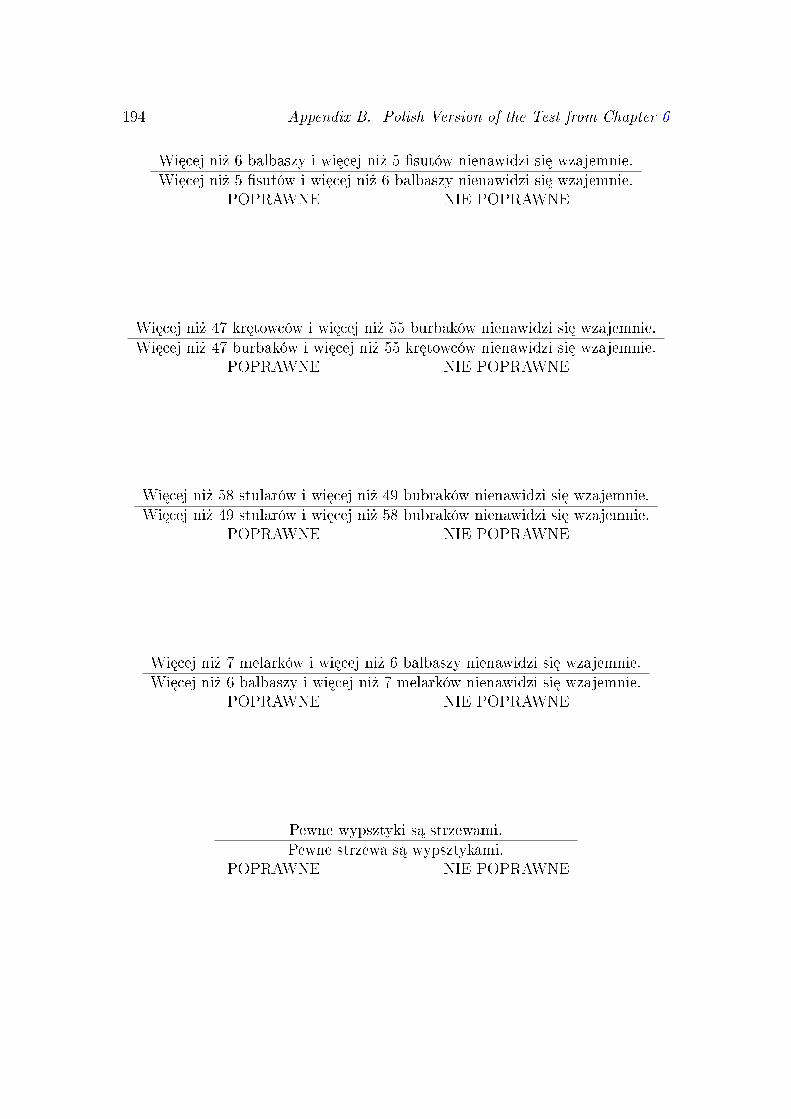
194 Appendix B. Polish Version of the Test from Chapter 6
Wi¦cej ni» 6 balbaszy i wi¦cej ni» 5 sutów nienawidzi si¦ wzajemnie.Wi¦cej ni» 5 sutów i wi¦cej ni» 6 balbaszy nienawidzi si¦ wzajemnie.
POPRAWNE NIE POPRAWNE
Wi¦cej ni» 47 kr¦towców i wi¦cej ni» 55 burbaków nienawidzi si¦ wzajemnie.Wi¦cej ni» 47 burbaków i wi¦cej ni» 55 kr¦towców nienawidzi si¦ wzajemnie.
POPRAWNE NIE POPRAWNE
Wi¦cej ni» 58 stularów i wi¦cej ni» 49 bubraków nienawidzi si¦ wzajemnie.Wi¦cej ni» 49 stularów i wi¦cej ni» 58 bubraków nienawidzi si¦ wzajemnie.
POPRAWNE NIE POPRAWNE
Wi¦cej ni» 7 melarków i wi¦cej ni» 6 balbaszy nienawidzi si¦ wzajemnie.Wi¦cej ni» 6 balbaszy i wi¦cej ni» 7 melarków nienawidzi si¦ wzajemnie.
POPRAWNE NIE POPRAWNE
Pewne wypsztyki s¡ strzewami.Pewne strzewa s¡ wypsztykami.
POPRAWNE NIE POPRAWNE

195
Wi¦cej ni» 99 melarków i wi¦cej ni» 68 wypsztyków nienawidzi si¦ wzajemnie.Wi¦cej ni» 68 wypsztyków i wi¦cej ni» 99 melarków nienawidzi si¦ wzajemnie.
POPRAWNE NIE POPRAWNE
Wi¦cej ni» 7 burbaków i wi¦cej ni» 8 sutów nienawidzi si¦ wzajemnie.Wi¦cej ni» 8 sutów i wi¦cej ni» 7 burbaków nienawidzi si¦ wzajemnie.
POPRAWNE NIE POPRAWNE
Wi¦cej ni» 19 stularów i wi¦cej ni» 11 protoro»ców nienawidzi si¦ wzajemnie.Wi¦cej ni» 11 protoro»ców i wi¦cej ni» 19 stularów nienawidzi si¦ wzajemnie.
POPRAWNE NIE POPRAWNE
Wi¦cej ni» 159 kr¦towców i wi¦cej ni» 25 sutów nienawidzi si¦ wzajemnie.Wi¦cej ni» 159 sutów i wi¦cej ni» 25 kr¦towców nienawidzi si¦ wzajemnie.
POPRAWNE NIE POPRAWNE
Wi¦cej ni» 8 stularów i wi¦cej ni» 27 balbaszy nienawidzi si¦ wzajemnie.Wi¦cej ni» 27 stularów i wi¦cej ni» 8 balbaszy nienawidzi si¦ wzajemnie.
POPRAWNE NIE POPRAWNE

196 Appendix B. Polish Version of the Test from Chapter 6
DRUGI TEST
Instrukcja: Na nast¦pnych stronach znajdziesz 9 zada«. Na ka»de zadanieskªada si¦ obrazek. Nad ka»dym obrazkiem jest jedno zdanie. Zakre±l PRAWDAgdy zdanie prawdziwe opisuje obrazek. W przeciwnym przypadku zakre±l FASZ.

197
Wi¦cej ni» 1 kwadrat i wi¦cej ni» 2 koªa s¡ poª¡czone liniami.
PRAWDA FASZ

198 Appendix B. Polish Version of the Test from Chapter 6
Wi¦cej ni» 3 koªa i wi¦cej ni» 2 kwadraty s¡ poª¡czone liniami.
PRAWDA FASZ
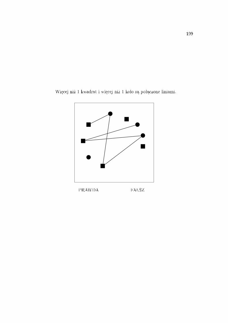
199
Wi¦cej ni» 1 kwadrat i wi¦cej ni» 1 koªo s¡ poª¡czone liniami.
PRAWDA FASZ

200 Appendix B. Polish Version of the Test from Chapter 6
Wi¦cej ni» 3 koªa i wi¦cej ni» 1 kwadrat s¡ poª¡czone liniami.
PRAWDA FASZ

201
Wi¦cej ni» 3 koªa i wi¦cej ni» 3 kwadraty s¡ poª¡czone liniami.
PRAWDA FASZ

202 Appendix B. Polish Version of the Test from Chapter 6
Wi¦cej ni» 2 koªa i wi¦cej ni» 3 kwadraty s¡ poª¡czone liniami.
PRAWDA FASZ

203
Wi¦cej ni» 1 koªo i wi¦cej ni» 3 kwadraty s¡ poª¡czone liniami.
PRAWDA FASZ

204 Appendix B. Polish Version of the Test from Chapter 6
Wi¦cej ni» 2 kwadraty i wiecej ni» 1 koªo s¡ poª¡czone liniami.
PRAWDA FASZ

205
Wi¦cej ni» 2 koªa i wi¦cej ni» 2 kwadraty s¡ poª¡czone liniami.
PRAWDA FASZ


Bibliography
Aczel, P. (1975). Quantiers, games and inductive denitions. In Kanger, S.,editor, Proceedings of the Third Scandinavian Logic Symposium, volume 82 ofStudies in Logic and Foundations of Mathematics, pages 114. Elsevier.
Agrawal, M., Kayal, N., and Saxena, N. (2004). Primes in P. Annals of Mathe-matics, 160(2):781793.
Ajdukiewicz, K. (1931). O znaczeniu wyra»e«. In Ksi¦ga Pami¡tkowa PolskiegoTowarzystwa Filozocznego we Lwowie. PTF, Lviv.
Andersson, A. (2002). On second-order generalized quantiers and nite struc-tures. Annals of Pure and Applied Logic, 115(13):132.
Austin, J. (1975). How to do things with words. The William James Lecturesdelivered at Harvard University in 1955. Cambridge, Harvard UP.
Bach, K. (1982). Semantic nonspecicity and mixed quantiers. Linguistics andPhilosophy, 4(4):593605.
Baddeley, A. (2007). Working Memory, Thought, and Action. Oxford PsychologySeries. Oxford University Press, USA, 1st edition.
Bar-Hillel, Y. (1954). Indexical expressions. Mind, 63:359379.
Barton, E. G., Berwick, R., and Ristad, E. S. (1987). Computational Complexityand Natural Language. Bradford Books. The MIT Press.
Bartsch, R. (1973). The semantics and syntax of number and numbers. In Kim-ball, J. P., editor, Syntax and Semantics 2, pages 5193. Seminar Press, NewYork.
Barwise, J. (1979). On branching quantiers in English. Journal of PhilosophicalLogic, 8:4780.
207

208 BIBLIOGRAPHY
Barwise, J. and Cooper, R. (1981). Generalized quantiers and natural language.Linguistics and Philosophy, 4:159219.
Beck, S. (2000). The semantics of dierent: Comparison operator and relationaladjective. Linguistics and Philosophy, 23(2):101139.
Beghelli, F., Ben-Shalom, D., and Szabolcsi, A. (1997). Variation, distributivity,and the illusion of branching. In Szabolcsi, A., editor, Ways of Scope Tak-ing, volume 65 of Studies in Linguistic and Philosophy, pages 2969. KluwerAcademic Publisher.
Bellert, I. (1989). Feature System for Quantication Structures in Natural Lan-guage. Foris Publications, Dordrecht.
Ben-Avi, G. and Winter, Y. (2003). Monotonicity and collective quantication.Journal of Logic, Language and Information, 12(2):127151.
Ben-Avi, G. and Winter, Y. (2004). A characterization of monotonicity withcollective quantiers. Electronic Notes in Theoretical Computer Science, 53:2133.
Benacerraf, P. (1967). God, the devil, and Gödel. The Monist, 51:932.
Bennett, M. R. (1974). Some extensions of a Montague fragment of English. PhDthesis, University of California, Los Angeles.
van Benthem (2007). Review of Stanley Peters and Dag Westerståhl 'Quantiersin Language and Logic'. Notre Dame Philosophical Reviews.
van Benthem and Pacuit, E. (2006). The tree of knowledge in action: Towards acommon perspective. In Governatori, G., Hodkinson, I. M., and Venema, Y.,editors, Advances in Modal Logic, pages 87106. College Publications.
van Benthem, J. (1983). The semantics of variety in categorial grammar. Re-port 8329, Department of Mathematics, Simon Fraser University. Publishedin Buszkowski, W., Marciszewski, W., and van Benthem, J. (Eds.) (1988). Cat-egorial grammar, linguistic and literary studies in Eastern Europe Volume 25.Amsterdam: John Benjamins, pp. 3755.
van Benthem, J. (1986). Essays in logical semantics. Reidel.
van Benthem, J. (1987). Towards a computational semantics. In Gärdenfors, P.,editor, Generalized Quantiers, pages 3171. Reidel Publishing Company.
van Benthem, J. (1989). Polyadic quantiers. Linguistics and Philosophy,12(4):437464.

BIBLIOGRAPHY 209
van Benthem, J. (1995). Language in action. MIT Press, Cambridge, MA.
van Benthem, J. (2002). Extensive games as process models. Journal of Logic,Language and Information, 11(3):289313.
van Benthem, J. (2003). Logic games are complete for game logics. Studia Logica,75(2):183203.
van Benthem, J., Ghosh, S., and Liu, F. (2007). Modelling simultaneous gameswith concurrent dynamic logic. In van Benthem, J., Ju, S., and Veltman,F., editors, A Meeting of the Minds-Proceedings of the Workshop on Logic,Rationality and Interaction, Beijing.
Benz, A., Jager, G., and van Rooij, R., editors (2005). Game Theory and Pragmat-ics. Palgrave Studies in Pragmatics, Language & Cognition. Palgrave Macmil-lan.
van den Berg, M. (1996). Dynamic generalized quantiers. In van der Does,J. and van Eijck, J., editors, Quantiers, Logic, and Language, CSLI LectureNotes, pages 6394. Stanford University, California.
Blass, A. and Gurevich, Y. (1986). Henkin quantiers and complete problems.Annals of Pure and Applied Logic, 32:116.
Blass, A. and Gurevich, Y. (2003). Algorithms: A quest for absolute denitions.Bulletin of European Association for Theoretical Computer Science, 81:195225.
Bogdanov, A. and Trevisan, L. (2006). Average-case complexity. FoundationalTrends in Theoretical Computer Science, 2(1):1106.
Büchi, J. (1960). Weak second-order arithmetic and nite automata. Zeitschriftfür Mathematische Logik und Grudlagen der Mathematik, 6:6692.
Burtschick, H. J. and Vollmer, H. (1998). Lindström quantiers and leaf lan-guage denability. International Journal of Foundations of Computer Science,9(3):277294.
Carnap, R. (2007). Meaning And Necessity - A Study In Semantics And ModalLogic. Clarke Press.
Chalmers, D. (1994). A computational foundation for the study of cognition. See:http://consc.net/papers/computation.html.
Cherniak, C. (1981). Minimal rationality. Mind, 90(358):161183.
Chomsky, N. (1969). Aspects of the Theory of Syntax. The MIT Press.

210 BIBLIOGRAPHY
Chomsky, N. (2002). Syntactic Structures. Walter de Gruyter, 2nd edition.
Church, A. (1936). An unsolvable problem of elementary number theory. Amer-ican Journal of Mathematics, 58(2):345363.
Church, A. (1973). Outline of a revised formulation of the logic of sense anddenotation (part i). Noûs, 7(1):2433.
Church, A. (1974). Outline of a revised formulation of the logic of sense anddenotation (part ii). Noûs, 8(2):135156.
Clark, R. (2007). Games, quantiers and pronouns. In Pietarinen, A. V., ed-itor, Game Theory and Linguistic Meaning, Current Research in the Seman-tics/Pragmatics Interface, pages 207228. Elsevier Science.
Clark, R. and Grossman, M. (2007). Number sense and quantier interpretation.Topoi, 26(1):5162.
Cook, S. A. (1971). The complexity of theorem-proving procedures. In STOC'71: Proceedings of the third annual ACM symposium on Theory of Computing,pages 151158, New York, NY, USA. ACM Press.
Cooper, B. S. (2003). Computability Theory. Chapman Hall/Crc MathematicsSeries. Chapman & Hall/CRC.
Culy, C. (1985). The complexity of the vocabulary of Bambara. Linguistics andPhilosophy, 8(3):345351.
Dalrymple, M., Kanazawa, M., Kim, Y., Mchombo, S., and Peters, S. (1998). Re-ciprocal expressions and the concept of reciprocity. Linguistics and Philosophy,21:159210.
Dekker, P. (2008). A guide to dynamic semantics. Preprint series PP-2008-42, In-stitute for Logic, Language and Information. Manuscript available at http://www.illc.uva.nl/Publications/ResearchReports/PP-2008-42.text.pdf.
van Ditmarsch, H., van der Hoek, W., and Kooi, B. (2007). Dynamic EpistemicLogic. (Synthese Library). Springer, 1st edition.
van der Does, J. (1992). Applied quantier logics. Collectives and naked innitives.PhD thesis, Universiteit van Amsterdam.
van der Does, J. (1993). Sums and quantiers. Linguistics and Philosophy,16(5):509550.
Downey, R. G. and Fellows, M. R. (1998). Parameterized Complexity. Monographsin Computer Science. Springer.

BIBLIOGRAPHY 211
Dummett, M. (1978). Truth and Other Enigmas. Harvard University Press.
Ebbinghaus, H.-D. and Flum, J. (2005). Finite Model Theory. Springer Mono-graphs in Mathematics. Springer.
Ebbinghaus, H. D., Flum, J., and Thomas, W. (1996). Mathematical Logic.Undergraduate Texts in Mathematics. Springer.
Edmonds, J. (1965). Paths, trees, and owers. Canadian Journal of Mathematics,17:449467.
Fagin, R. (1974). Generalized rst-order spectra an polynomial time recognizablesets. In Karp, R., editor, Complexity of Computation, volume 7 of SIAMAMSProceedings, pages 4373. American Mathematical Society.
Ferguson, G. A. and Takane, Y. (1990). Statistical Analysis in Psychology andEducation. McGraw-Hill Education.
Flum, J. and Grohe, M. (2006). Parameterized Complexity Theory. Texts inTheoretical Computer Science. An EATCS Series. Springer, 1st edition.
Frege, G. (1879). Begrisschrift: eine der arithmetischen nachgebildete Formel-sprache des reinen Denkens. Halle.
Frege, G. (1892). Über Sinn und Bedeutung. Zeitschrift für Philosophie undphilosophische Kritik, 100:2550.
Frege, G. (1980). Philosophical and Mathematical Correspondence of GottlobFrege. University Of Chicago Press.
Frixione, M. (2001). Tractable competence. Minds and Machines, 11(3):379397.
Gabbay, D. M. and Moravcsik, J. M. E. (1974). Branching quantiers, Englishand Montague grammar. Theoretical Linguistics, 1:140157.
Gärdenfors, P. (2003). Belief Revision. Cambridge Tracts in Theoretical Com-puter Science. Cambridge University Press.
Garey, M. R. and Johnson, D. S. (1979). Computers and Intractability. W. H.Freeman and Co., San Francisco.
Geurts, B. (2003). Reasoning with quantiers. Cognition, 86(3):223251.
Geurts, B. and van der Silk, F. (2005). Monotonicity and processing load. Journalof Semantics, 22:97117.

212 BIBLIOGRAPHY
Gierasimczuk, N. (2007). The problem of learning the semantics of quantiers.In Ten Cate, B. and Zeevat, H., editors, Logic, Language, and Computation,6th International Tbilisi Symposium on Logic, Language, and Computation,TbiLLC 2005, volume 4363 of Lecture Notes in Computer Science, pages 117126, Batumi, Georgia. Springer.
Gierasimczuk, N. (2009). Identication through inductive verication. Applica-tion to monotone quantiers. In Bosch, P., Gabelaia, D., and Lang, J., edi-tors, Logic, Language, and Computation, 7th International Tbilisi Symposiumon Logic, Language, and Computation, TbiLLC 2007, volume 5422 of LectureNotes on Articial Inteligence, pages 193205, Tbilisi, Georgia. Springer.
Gierasimczuk, N. and Szymanik, J. (2006). Hintikka's thesis revisited. Pre-publications series PP-2006-35, Institute for Logic, Language and Informa-tion. Manuscript avaiable at: http://www.illc.uva.nl/Publications/
ResearchReports/PP-2006-35.text-Dec-2006.pdf.
Gierasimczuk, N. and Szymanik, J. (2007). Hintikka's thesis revisited. The Bul-letin of Symbolic Logic, 17:273273.
Gierasimczuk, N. and Szymanik, J. (2008). Interpreting quantier combi-nations. Hintikka's thesis revisited. Prepublications series PP-2006-35 au-gust 2008, Institute for Logic, Language and Information. Manuscriptavaiable at: http://www.illc.uva.nl/Publications/ResearchReports/
PP-2006-35.text-Aug-2008.pdf.
Gold, E. M. (1967). Language identication in the limit. Information and Control,10:447474.
Gottlob, G., Leone, N., and Veith, H. (1999). Succinctness as a source of com-plexity in logical formalisms. Annals of Pure and Applied Logic, pages 231260.
Grädel, E. and Gurevich, Y. (1998). Metanite model theory. Information andComputation, 140(1):2681.
Grädel, E., Kolaitis, P. G., Libkin, L., Marx, M., Spencer, J., Vardi, M. Y., Ven-ema, Y., and Weinstein, S. (2007). Finite Model Theory and Its Applications.Texts in Theoretical Computer Science. An EATCS Series. Springer.
Graham, R. L., Rothschild, B. L., and Spencer, J. H. (1990). Ramsey Theory.John Wiley & Sons, New York.
Grice, P. (1991). Studies in the Way of Words. Harvard University Press.
Groenendijk, J. and Stokhof, M. (1991). Dynamic predicate logic. Linguisticsand Philosophy, 14(1):39100.

BIBLIOGRAPHY 213
Guenthner, F. and Hoepelman, J. P. (1976). A note on the representation ofbranching quantiers. Theoretical Linguistics, 3:285289.
Gurevich, Y. (1995). The Value, if any, of Decidability. Bulletin of EuropeanAssociation for Theoretical Computer Science, pages 129135.
Hamm, F. and Lambalgen, M. (2004). Moschovaki's notion of meaning as appliedto linguistics. In Baaz, M., Friedman, S., Krajicek, J., and Peters, A. K.,editors, ASL Lecture Notes in Logic, Logic Colloqium'01, pages 167183. A. K.Peters Publishers.
Heim, I., Lasnik, H., and May, R. (1991). Reciprocity and plurality. LinguisticInquiry, 22(1):63101.
Hella, L. (1996). Logical hierarchies in PTIME. Information and Computation,129(1):119.
Hella, L., Kolaitis, P. G., and Luosto, K. (1996). Almost everywhere equivalenceof logics in nite model theory. Bulletin of Symbolic Logic, 2(4):422443.
Hella, L., Väänänen, J., and Westerståhl, D. (1997). Denability of polyadiclifts of generalized quantiers. Journal of Logic, Language and Information,6(3):305335.
Henkin, L. (1961). Some remarks on innitely long formulas. In Innistic Methods,pages 167183. Pergamon Press.
Hintikka, J. (1973). Quantiers vs. quantication theory. Dialectica, 27:329358.
Hintikka, J. (1976). Partially ordered quantiers vs. partially ordered ideas. Di-alectica, 30:8999.
Hintikka, J. (1996). Principles of Mathematics Revisited. Cambridge UniversityPress.
Hintikka, J. (1997). Paradigms for Language Theory and Other Essays. JaakkoHintikka Selected Papers. Springer, 1st edition.
Hintikka, J. and Sandu, G. (1997). Game-theoretical semantics. In van Benthem,J. and ter Meulen, A., editors, Handbook of Logic and Language, pages 361410.Elsevier, Amsterdam.
Hodges, W. (1997). Compositional semantics for a language of imperfect informa-tion. Journal of the Interest Group in Pure and Applied Logics, 5 (4):539563.
Hofstadter, D. (2007). Gödel, Escher, Bach. Tusquets, 3rd edition.

214 BIBLIOGRAPHY
Hopcroft, J. E., Motwani, R., and Ullman, J. D. (2000). Introduction to AutomataTheory, Languages, and Computation. Addison Wesley, 2nd edition.
Immerman, N. (1982). Relational queries computable in polynomial time (ex-tended abstract). In STOC '82: Proceedings of the fourteenth annual ACMsymposium on Theory of computing, pages 147152, New York, NY, USA.ACM.
Immerman, N. (1998). Descriptive Complexity. Texts in Computer Science.Springer.
Impagliazzo, R. (1995). A personal view of average-case complexity. In SCT '95:Proceedings of the 10th Annual Structure in Complexity Theory Conference(SCT'95), Washington, DC, USA. IEEE Computer Society.
Isac, D. and Reiss, C. (2008). I-Language: An Introduction to Linguistics asCognitive Science. Core Linguistics. Oxford University Press, USA.
Jackendo, R. (1972). Semantic Interpretation and Generative Grammar. MITPress, Cambridge, Massachuset.
Janssen, T. (2002). Independent choices and the interpretation of IF-logic. Jour-nal of Logic, Language and Information, 11:367387.
Janssen, T. and Dechesne, F. (2006). Signalling in IF games: a tricky business. InJohan van Benthem, Gerhard Heinzmann, M. R. and Visser, H., editors, Theage of alternative logics. Assessing philosophy of logic and mathematics today,volume 3 of Logic, epistemology, and the unity of science, chapter 15, pages221241. Springer, Dordrecht, the Netherlands.
Jaszczolt, K. (2002). Semantics and Pragmatics: Meaning in Language and Dis-course. Longman Linguistics Library. Longman.
Kager, R. (1999). Optimality Theory. Cambridge Textbooks in Linguistics. Cam-bridge University Press.
Kamp, H. (1971). Formal properties of 'now'. Theoria, 37:227273.
Kamp, H. and Reyle, U. (1993). From Discourse to Logic: Introduction to Model-theoretic Semantics of Natural Language, Formal Logic and Discourse Repre-sentation Theory. Studies in Linguistics and Philosophy. Springer.
Kamp, H. and Stokhof, M. (2008). Information in natural language. In vanBenthem, J. and Adriaans, P., editors, Philosophy of Information, Handbookof the Philosophy of Science. North-Holland.

BIBLIOGRAPHY 215
Kandel, E. R., Schwartz, J. H., and Jessell, T. M. (2000). Principles of NeuralScience. McGraw-Hill Medical.
Kaplan, D. (1979). On the logic of demonstratives. Journal of PhilosophicalLogic, 8(1):8198.
Karp, R. M. (1972). Reducibility among combinatorial problems. In Miller, R. E.and Thatcher, J. W., editors, Complexity of Computer Computations, pages85103. Plenum Press.
Kempson, R. M. and Cormack, A. (1981a). Ambiguity and quantication. Lin-guistics and Philosophy, 4(2):259309.
Kempson, R. M. and Cormack, A. (1981b). On 'formal games and forms forgames'. Linguistics and Philosophy, 4(3):431435.
Kempson, R. M. and Cormack, A. (1982). Quantication and pragmatics. Lin-guistics and Philosophy, 4(4):607618.
Kontinen, J. (2002). Second-order generalized quantiers and natural language.In Nissim, M., editor, Proceedings of the Seventh ESSLLI Student Session,pages 107118. Elsevier.
Kontinen, J. (2004). Denability of second order generalized quantiers. PhDthesis, Helsinki University.
Kontinen, J. and Niemistö, H. (2006). Extensions of MSO and the monadic count-ing hierarchy. Manuscript available at http://www.helsinki.fi/~jkontine/.
Kontinen, J. and Szymanik, J. (2008). A remark on collective quantication.Journal of Logic, Language and Information, 17(2):131140.
Kozen, D. C. (2006). Theory of Computation: Classical and Contemporary Ap-proaches. Texts in Computer Science. Springer.
Kracht, M. (2003). The Mathematics of Language, volume 63 of Studies in Gen-erative Grammar. Walter de Gruyter.
Kripke, S. (2008). Frege's theory of sense and reference: Some exegetical notes.Theoria, 74(3):181218.
Krynicki, M. and Mostowski, M. (1995). Henkin quantiers. In Krynicki, M.,Mostowski, M., and Szczerba, L., editors, Quantiers: Logics, Models andComputation, pages 193263. Kluwer Academic Publishers.
Krynicki, M. and Mostowski, M. (1999). Ambigous quantiers. In Orªowska, E.,editor, Logic at work, pages 548565. Heidelberg.

216 BIBLIOGRAPHY
Kugel, P. (1986). Thinking may be more than computing. Cognition, 22(2):137198.
Ladusaw, W. (1979). Polarity Sensitivity as Inherent Scope Relations. PhD thesis,University of Texas, Austin.
Lambalgen, M. V. and Hamm, F. (2005). The Proper Treatment of Events. Ex-plorations in Semantics. Wiley-Blackwell.
Landman, F. (2000). Against binary quantiers. In Events and Plurality, Studiesin Linguistic and Philosophy, pages 310349. Kluwer Academic Publisher.
Levesque, H. J. (1988). Logic and the complexity of reasoning. Journal of Philo-sophical Logic, 17(4):355389.
Lewis, D. (2002). Convention: A Philosophical Study. Wiley-Blackwell.
Libkin, L. (2004). Elements of Finite Model Theory. Texts in Theoretical Com-puter Science. An EATCS Series. Springer.
Lindström, P. (1966). First order predicate logic with generalized quantiers.Theoria, 32:186195.
Link, G. (1983). The logical analysis of plurals and mass terms: A lattice-theoretical approach. In Bäuerle, R., Schwarze, C., and von Stechow, A., ed-itors, Meaning, Use, and Interpretation of language, pages 302323. Gruyter,Berlin.
Liu, F.-H. (1996). Branching quantication and scope independence. In van derDoes, J. and van Eijck, J., editors, Quantiers, Logic and Language, pages155168. Center for the Study of Language and Information.
Lønning, J. T. (1997). Plurals and collectivity. In van Benthem, J. and ter Meulen,A., editors, Handbook of Logic and Language, pages 10091053. Elsevier.
Lorentzen, P. (1955). Einführung in die Operative Logik und Mathematik.Springer, Berlin.
Lucas, J. R. (1961). Minds, machines and Gödel. Philosophy, 36(137):112127.
Luo, H., Su, W., and Li, Z. (2002). The properties of self-complementary graphsand new lower bounds for diagonal Ramsey numbers. Australasian Journal ofCombinatorics, 25:103116.
Luosto, K. (1999). Ramsey theory is needed for solving denability problems ofgeneralized quantiers. In Lecture Notes in Computer Science, volume 1754,pages 121134.

BIBLIOGRAPHY 217
Macintyre, A. (1980). Ramsey quantiers in arithmetic. In Pacholski, L., Wierze-jewski, J., and Wilkie, A. J., editors, Model theory of algebra and arithmetics,volume 834 of Lecture Notes in Mathematics, pages 186210. SpringerVerlag.
Magidor, M. and Malitz, J. I. (1977). Compact extensions of L(Q). Annals ofMathematical Logic, 11:217261.
Makowsky, J. and Pnueli, Y. (1995). Computable quantiers and logics over -nite structures. In Krynicki, M., Mostowski, M., and Szczerba, L., editors,Quantiers: Logics, Models and Computation, pages 313357. Kluwer Aca-demic Publishers.
Manaster-Ramer, A. (1987). Dutch as a formal language. Linguistics and Phi-losophy, 10(2):221246.
Marr, D. (1983). Vision: A Computational Investigation into the Human Repre-sentation and Processing Visual Information. W.H. Freeman, San Francisco.
May, R. (1985). Logical Form: Its Structure and Derivation. Linguistic InquiryMonographs. The MIT Press.
May, R. (1989). Interpreting logical form. Linguistics and Philosophy, 12(4):387435.
McMillan, C. T., Clark, R., Moore, P., Devita, C., and Grossman, M. (2005). Neu-ral basis for generalized quantier comprehension. Neuropsychologia, 43:17291737.
Mcmillan, C. T., Clark, R., Moore, P., and Grossman, M. (2006). Quantierscomprehension in corticobasal degeneration. Brain and Cognition, 65:250260.
McNaughton, R. and Papert, S. A. (1971). Counter-Free Automata. M.I.T.Research Monograph no. 65. The MIT Press.
Miestamo, M., Sinnemäki, K., and Karlsson, F., editors (2008). Language Com-plexity: Typology, contact, change. Studies in Language Companion Series.John Benjamins Publishing Company.
Montague, R. (1970). Pragmatics and intensional logic. Dialectica, 24(4):277302.
Moschovakis, Y. (1990). Sense and denotation as algorithm and value. In Oikko-nen, J. and Väänänen, J., editors, Lecture Notes in Logic 2, pages 210249.Springer.
Moschovakis, Y. (2001). What is an algorithm? In Enquist, B. and Schmid, W.,editors, Mathematics unlimited 2001 and beyond, pages 919936. Springer.

218 BIBLIOGRAPHY
Moschovakis, Y. (2006). A logical calculus of meaning and synonymy. Linguisticsand Philosophy, 29(1):2789.
Moss, L. and Tiede, H. J. (2006). Applications of modal logic in linguistics. InBlackburn, P., van Benthem, J. F. A. K., and Wolter, F., editors, Handbookof Modal Logic, Studies in Logic and Practical Reasoning, pages 10311077.Elsevier Science.
Mostowski, A. (1957). On a generalization of quantiers. Fundamenta Mathe-maticae, 44:1236.
Mostowski, M. (1991). Arithmetic with the Henkin quantier and its general-izations. In Gaillard, F. and Richard, D., editors, Seminaire du LaboratoireLogique, Algorithmique et Informatique Clermontois, volume II, pages 125.
Mostowski, M. (1994). Kwantykatory rozgaª¦zione a problem formy logicznej.In Omyªa, M., editor, Nauka i j¦zyk, pages 201242. Biblioteka My±li Semioty-cznej.
Mostowski, M. (1995). Quantiers denable by second order means. In Krynicki,M., Mostowski, M., and Szczerba, L., editors, Quantiers: Logics, Models andComputation, pages 181214. Kluwer Academic Publishers.
Mostowski, M. (1998). Computational semantics for monadic quantiers. Journalof Applied Non-Classical Logics, 8:107121.
Mostowski, M. (2008). Potential innity and the Church Thesis. FundamentaInformaticae, 81(1-3):241248.
Mostowski, M. and Szymanik, J. (2005). Semantical bounds for everydaylanguage. Semiotica, to appear. See also ILLC Preprint Series, PP-2006-40; Manuscript avaiable at: http://www.illc.uva.nl/Publications/
ResearchReports/PP-2006-40.text.pdf.
Mostowski, M. and Szymanik, J. (2007). Computational complexity of someRamsey quantiers in nite models. The Bulletin of Symbolic Logic, 13:281282.
Mostowski, M. and Wojtyniak, D. (2004). Computational complexity of the se-mantics of some natural language constructions. Annals of Pure and AppliedLogic, 127(1-3):219227.
Muskens, R. (2005). Sense and the computation of reference. Linguistics andPhilosophy, 28(4):473504.
Nisan, N., Roughgarden, T., Tardos, E., and Vazirani, V., editors (2007). Algo-rithmic Game Theory. Cambridge University Press.

BIBLIOGRAPHY 219
Otto, M. (1997). Bounded Variable Logics and Counting. A study in Finite Mod-els., volume 9 of Lecture Notes in Logic. Springer-Verlag.
Pagin, P. (2009). Communication and the complexity of semantics. In Hinzen,W., Machery, E., and Werning, M., editors, Oxford Handbook of Composition-ality. Forthcoming; Manuscript available at http://people.su.se/~ppagin/pagineng.htm.
Papadimitriou, C. H. (1993). Computational Complexity. Addison Wesley.
Paris, J. and Harrington, L. (1977). A mathematical incompleteness in PeanoArithmetics. In Barwise, J., editor, Handbook for mathematical logic, pages11331142. NorthHolland.
Partee, B. and Rooth, M. (1983). Generalized conjunction and type ambiguity.In Bäuerle, R., Schwarze, C., and von Stechow, A., editors, Meaning, use, andinterpretation of language, pages 361383. Gruyter, Berlin.
Partee, B. H., ter Meulen, A. G., and Wall, R. (1990). Mathematical Methods inLinguistics. Studies in Linguistics and Philosophy. Springer.
Penrose, R. (1996). Shadows of the Mind : A Search for the Missing Science ofConsciousness. Oxford University Press, USA.
Peregrin, J. (2003). Meaning: The Dynamic Turn. Elsevier Science.
Peters, S. and Westerståhl, D. (2006). Quantiers in Language and Logic. Claren-don Press, Oxford.
Piaget, J. (2001). Psychology of Intelligence. Routledge Classics. Routledge, 1stedition.
Pratt-Hartmann, I. (2004). Fragments of language. Journal of Logic, Languageand Information, 13(2):207223.
Pratt-Hartmann, I. (2008). Computational complexity in natural language. InClark, A., Fox, C., and Lappin, S., editors, Computational Linguistics and Nat-ural Language Processing Handbook. Blackwell. Forthcoming; Manuscript ava-iable at: http://www.cs.man.ac.uk/~ipratt/papers/nat_lang/handbook.
ps.
Pudlak, P. (1999). A note on applicability of the incompleteness theorem tohuman mind. Annals of Pure and Applied Logic, 96(1-3):335342.
Pullum, G. K. and Gazdar, G. (1982). Natural languages and context-free lan-guages. Linguistics and Philosophy, 4(4):471504.

220 BIBLIOGRAPHY
Putnam, H. (1975/1985). The meaning of 'meaning'. In Philosophical Papers.Mind, Language and Reality., volume 2, pages 215271. Cambridge UniversityPress.
Quine, W. V. (1964). Word and Object. Studies in Communication. The MITPress.
Ramsey, F. (1929). On a problem of formal logic. In Proceedings of the LondonMathematical Society, volume 30 of 2, pages 338384.
Ristad, E. S. (1993). The Language Complexity Game. Articial Intelligence. TheMIT Press.
Rogers, J. (1983). A descriptive approach to language-theoretic complexity. Stud-ies in Logic, Language and Information. CSLI Publications, Stanford, CA.
van Rooij, I. (2004). Tractable cognition: Complexity theory in cognitive psychol-ogy. PhD thesis, University of Victoria, BC, Canada.
van Rooij, I. (2008). The tractable cognition thesis. Cognitive Science: A Multi-disciplinary Journal, 32(6):939984.
van Rooij, I., Stege, U., and Kadlec, H. (2005). Sources of complexity in subsetchoice. Journal of Mathematical Psychology, 49(2):160187.
Russell, B. (1903). The Principles of Mathematics. Cambridge University Press,Cambridge.
Sabato, S. and Winter, Y. (2005). From semantic restrictions to reciprocal mean-ings. In Proceedings of FG-MOL 2005. CSLI Publications.
Sanford, A. J., Moxey, L. M., and Paterson, K. (1994). Psychological studies ofquantiers. Journal of Semantics, 11(3):153170.
Savitch, W. (1970). Relationship between nondeterministic and deterministictape classes. Journal of Computer and System Sciences, 4:177192.
Scha, R. (1981). Distributive, collective and cumulative quantication. In Groe-nendijk, J. A. G., Janssen, T. M. V., and Stokhof, M. B. J., editors, Formalmethods in the study of language, Part 2, pages 483512. Mathematisch Cen-trum, Amsterdam.
Schaefer, M. (2001). Graph Ramsey theory and the polynomial hierarchy. Journalof Computer and System Sciences, 62:290322.
Schlenker, P. (2006). Scopal independence: A note on branching and wide scopereadings of indenites and disjunctions. Journal of Semantics, 23(3):281314.

BIBLIOGRAPHY 221
Schmerl, J. H. and Simpson, S. G. (1982). On the role of Ramsey Quantiers inFirst Order Arithmetic. Journal of Symbolic Logic, 47:423435.
Sevenster, M. (2006). Branches of imperfect information: logic, games, and com-putation. PhD thesis, Universiteit van Amsterdam.
Sher, G. (1990). Ways of branching quantiers. Linguistics and Philosophy,13:393442.
Shieber, S. M. (1985). Evidence against the context-freeness of natural language.Linguistics and Philosophy, 8(3):333343.
Soja, N., Carey, S., and Spelke, E. (1991). Ontological categories guide youngchildren's induction of word meaning: Object terms and substance terms. Cog-nition, 38:179211.
Spencer, J. H. (1987). Ten lectures on the probabilistic methods. Society forIndustrial and Applied Mathematics.
Stalnaker, R. C. (2003). Ways a World Might Be: Metaphysical and Anti-Metaphysical Essays. Oxford University Press, USA.
Stenius, E. (1976). Comments on Jaakko Hintikka's paper Quantiers vs. quan-tication theory. Dialectica, 30:6788.
Sternberg, R. J. (2008). Cognitive Psychology. Wadsworth Publishing, 5th edition.
Stockmeyer, L. J. (1976). The polynomial-time hierarchy. Theoretical ComputerScience, 3(1).
Sun, R., editor (2008). The Cambridge Handbook of Computational Psychology.Cambridge University Press, 1st edition.
Suppes, P. (1982). Variable-free semantics with remark on procedural exten-sions. In Simon and Scholes, editors, Language, Mind and Brain, pages 2134.Hillsdale, Erlbaum.
Syropoulos, A. (2008). Hypercomputation: Computing Beyond the Church-TuringBarrier. Monographs in Computer Science. Springer, 1st edition.
Szymanik, J. (2005). Problemy z form¡ logiczn¡. Studia Semiotyczne, 25:187200.
Szymanik, J. (2007a). A comment on a neuroimaging study of natural languagequantier comprehension. Neuropsychologia, 45(9):21582160.
Szymanik, J. (2007b). A strong meaning hypothesis from a computational per-spective. In Aloni, M., Dekker, P., and Roelofsen, F., editors, Proceedings of theSixteenth Amsterdam Colloquium, pages 211216. University of Amsterdam.

222 BIBLIOGRAPHY
Szymanik, J. (2008). The computational complexity of quantied reciprocals. InBosch, P., Gabelaia, D., and Lang, J., editors, Logic, Language, and Computa-tion, 7th International Tbilisi Symposium on Logic, Language, and Computa-tion, TbiLLC 2007, volume 5422 of Lecture Notes in Computer Science, pages139152, Tbilisi, Georgia. Springer.
Szymanik, J. and Zajenkowski, M. (2008). Comprehension of simplequantiers. Empirical evaluation of a computational model. Prepubli-cations series PP-2008-49, Institute for Logic, Language and Informa-tion. Manuscript available at http://www.illc.uva.nl/Publications/
ResearchReports/PP-2008-49.text.pdf.
Tarski, A. (1944). The semantic conception of truth: and the foundations ofsemantics. Philosophy and Phenomenological Research, 4(3):341376.
Tennant, N. (1981). Formal games and forms for games. Linguistics and Philos-ophy, 4(2):311320.
Tichý, P. (1969). Intension in terms of Turing machines. Studia Logica, 24(1):721.
Tichý, P. (1988). The Foundations of Frege's Logic. De Gruyter, Berlin.
Tiede, H. J. (1999). Identiability in the limit of context-free generalized quan-tiers. Journal of Language and Computation, 1:93102.
Toda, S. (1991). PP is as hard as the polynomial-time hierarchy. SIAM Journalon Computing, 20(5):865877.
Troiani, V., Peelle, J., Clark, R., and Grossman, M. (2009). Is it logical to counton quantiers? Dissociable neural networks underlying numerical and logicalquantiers. Neuropsychologia, 47(1):104111.
Tsotsos, J. (1990). Analyzing vision at the complexity level. Behavioral and BrainSciences, 13(3):423469.
Turing, A. (1936). On computable numbers, with an application to the Entschei-dungsproblem. Proceedings of the London Mathematical Society, 42(2):230265.
Väänänen, J. (1997a). Generalized quantiers, an introduction. In ESSLLI: Euro-pean Summer School in Logic, Language, and Information, ESSLLI Workshop,volume 1754 of Lecture Notes in Computer Science, pages 117. Springer.
Väänänen, J. (1997b). Unary quantiers on nite models. Journal of Logic,Language and Information, 6(3):275304.

BIBLIOGRAPHY 223
Väänänen, J. (2007). Dependence Logic A New Approach to IndependenceFriendly Logic. London Mathematical Society Student Texts. Cambridge Uni-versity Press.
Väänänen, J. and Westerståhl, D. (2002). On the expressive power of monotonenatural language quantiers over nite models. Journal of Philosophical Logic,31:327358.
Vardi, M. Y. (1982). The complexity of relational query languages (extendedabstract). In STOC '82: Proceedings of the fourteenth annual ACM symposiumon Theory of computing, pages 137146, New York, NY, USA. ACM Press.
Westerståhl, D. (1984). Some results on quantiers. Notre Dame Journal ofFormal Logic, 25:152169.
Winter, Y. (2001). Flexibility principles in Boolean semantics. The MIT Press,London.
Wittgenstein, L. (1922). Tractatus Logico Philosophicus. Routledge Classics.Routledge.
Wittgenstein, L. (1953). Philosophical Investigations. Blackwell Publishing, In-corporated, 50th anniversary commemorative edition edition.

Index
Σ11-thesis, 3941, 91, 125, 138
3sat, 65arrowing, 82
Aczel, P., 172Ajdukiewicz, K., 10Al-Khwarizmi, 18algorithm, 1825Andersson, A., 118arithmetic of addition, see Presburger
ArithmeticAustin, J.L., 7
Büchi, J.R., 36balanced complete bipartite
graph, 80Bartsch, R., 112Barwise and Cooper (1981), 50, 54, 141Barwise, J., 133, 137, 138belief revision, 8, 9, 17, 37Bennett, M.R., 112van Benthem problem, 114van Benthem, J., 12, 16, 20, 112, 153,
158, 159, 172, 173bijection, 46Blass and Gurevich (1986), 70Burtschick and Vollmer (1998), 118
Carnap, R., 8categorization, 28Chalmers, D., 28
Cherniak, Ch., 28Chomsky, N., 34, 35Church-Turing Thesis, 19, 23
Psychological Version, 26Clark, R., 152clique≥q, 84clique, 65, 83, 99co-NP, 63cognitive task, 25collective lifts
determiner tting operator, 116existential modier, 113neutral modier, 115
collective properties, 111combined complexity, 69complexity class, 61
captured by logic, 68relativized, 64
compositionality, 172comprehension, 6, 15, 18, 31computational complexity, 2025, 29
average-case, 31, 171circuit, 171parametrized, 31, 171worst-case, 30
Concurrent Dynamic Game Logic, 172context-dependence, 8context-free language, 59, 63Cook, S., 22, 65
224

INDEX 225
Counting Hierarchy, 64, 124
data complexity, see model-checkingDependence Logic, 47descriptive complexity, 66discourse, 36
Representation Theory, 9division of linguistic labor, 17van der Does, J., 113115Dynamic Epistemic Logic, 9
Edmonds, J., 22Thesis, 22, 24
Ehrenfeucht sentence, 47Erdös, P., 81Euclid, 18everyday language, 39expression complexity, 69EXPTIME, 62
f-large, 86Fagin's Theorem, 39, 40, 68nite automata, 56, 159
acyclic, 158deterministic, 56nondeterministic, 55
Fixed-Parameter Tractability Thesis,31
Frege, G., 10, 12, 13, 45, 47, 73, 110Frixione, M., 25, 27
Gödel, K., 26games, 9
algebra, 172and quantiers, 171dialogical, 14Ehrenfeucht-Fraïssé, 49equilibria, 172evolutionary, 9
language, 10model constructions, 14signalling, 9
Garey and Johnson (1979), 22, 65, 80generative capacity
strong, 35weak, 35
Geurts, B., 54, 141graph, 67
bipartite, 80Grice, P., 7
conversational principles, 9
Hamm, F., 13, 17Hella, L., 70Henkin, L., 47hierarchy of second-order formulae, 43Hintikka's sentence, 82, 130, 132
conjunctional reading, 132strong reading, 131weak readings, 131
Hintikka's Thesis, 131Hintikka, J., 130Hofstadter, D., 28van Humboldt, W., 34
Independence Friendly Logic, 47intractability, 21, 23Invariance Thesis, 23, 27isomorphism, 45
Kamp, H., 9Kaplan, D., 8, 9Karp, R., 65Kolmogorov complexity, 34Kontinen, and Niemistö, (2006), 68, 124Kontinen, J., 120Kripke, S., 10
van Lambalgen, M., 13, 17Landman, F., 72learning theory, 26, 54, 168, 174Levesque, H., 28Lewis, D., 9Lindström, P., 45, 47logic
equivalent, 49extended by quantier, 48rst-order, 43

226 INDEX
second-order, 43LOGSPACE, 62Lorenzen, P., 14Lucas, J.R., 26
Makowsky and Pnueli (1995), 69Marr, D., 25
levels of explanation, 25, 173McMillan et al. (2005), 152McNaughton and Papert, 36meaning, 5, 6
as algorithm, 1015, 17, 20inferential, 17referential, 15, 17, 129synonymy, 14, 20, 22
model, 44nite, 32, 67encoding, 67
weak, 33, 172model-checking, 11, 69model-theoretic syntax, 35Montague, R., 7, 13, 50Moschovakis, Y., 13, 20Mostowski and Wojtyniak (2004), 70,
78, 83, 138Mostowski, M., 39, 45, 133, 136, 159Muskens, R., 13
negation normal sentence, 137neural networks, 23NEXPTIME, 62NLOGSPACE, 62NP, 62NP-complete, 21NP-hard, 21NPSPACE, 62
P-cognition Thesis, 27, 31, 39, 106P=NP, 21, 63Partee and Rooth (1983), 112Penrose, R., 27Peters and Westerståhl (2006), 72, 173Piaget, J., 17Polynomial Hierarchy, 64, 123
polynomial timecomputable function, 65many-one reduction, 65
PP, 64pragmatics, 7, 9, 37Pratt-Hartmann, I., 35, 36Presburger Arithmetic, 159PSPACE, 62PTIME, 21, 62Pumping Lemma
context-free languages, 60regular languages, 58
push-down automata, 159deterministic, 59nondeterministic, 58
q-large, 84quantier
additive, see semi-linearAristotelian, 156automata, 156Boolean combinations, 50, 75bounded, 87branching, 47, 70, 77, 82, 88, 130counting, 79proportional, 78
cardinal, 157CE, 52clique, 83collective reading, 110complexity, 69conservativity, 51, 117collective, 118
cumulation, 74, 75denability, 48, 49, 119distributive reading, 110divisibility, 157, 159domain independent, 51rst-order, 153generalized, 4446, 69satisfaction relation, 48second-order, 118
Henkin, see branching

INDEX 227
higher-order, 153iteration, 73, 75, 135Lindström, 45, 46measure, 33mighty, 70monadic, 45, 154monotonicity, 52, 141NP-complete, see mightyNP-hard, 70partially ordered, see branchingpersistence, 53polyadic, 45, 72polyadic lift, 72proportional, 79, 101, 135, 158Ramsey, 81, 96counting, 83, 100proportional, 84, 101
relativization, 51, 101, 103resumption, 74, 75, 88second-order denable, 33, 172semi-linear, 159topic neutral, 46vectorization, see resumption
Ramsey Theory, 81reciprocal expressions, 91, 145, 149
intermediate alternative reading, 93intermediate reading, 92, 93strong alternative reading, 93strong reading, 92, 93weak alternative reading, 93weak reading, 92, 93
reciprocal lift, 98intermediate, 97strong, 96weak, 97
regular language, 56, 63Ristad, S., 36, 38van Rooij, I., 28, 31Russell, B., 110
sat, 21, 65satisability, 21
Savitch, W., 63Scha, R., 112Schlenker, P., 149semantics, 7
construction, 16dynamic, 14dynamic turn, 8game-theoretic, 14, 37, 47, 172intensional, 13
Sevenster, M., 14, 70, 78, 171Skolem function, 130Stalnaker, R., 8, 9Stockmeyer's Theorem, 68Strong Meaning Hypothesis, 94, 105subset choice, 28substitution property, 49Suppes, P., 12, 16, 17
Tarski, A., 7Tichý, P., 11, 12, 16tractability, 21, 23Tsotsos, J., 28Turing machine, 11, 19, 26, 60
oracle, 63type-theory, 112
understanding, see comprehension
Väänänen, J., 69, 87, 102Vardi, M., 69visual search, 28
Westerståhl, D., 32Winter, Y., 113, 116Wittgenstein, L., 10working memory, 153


Samenvatting
In deze dissertatie bestuderen we de complexiteit van gegeneraliseerde kwantorenin de natuurlijke taal. We doen dit vanuit een interdisciplinair perspectief: wecombineren lososche inzichten met theoretische informatica, experimentele cog-nitiewetenschap en met theorieën uit de linguïstiek.
In het hoofdstuk 1 beargumenteren we dat een deel van de betekenis van eenzin - de zogenaamde referentiële betekenis (model-checking) - beschreven moetworden met algoritmen. We bespreken ook de inbreng van complexiteitstheo-rie voor de analyse van cognitieve taken. We beargumenteren dat alleen dieproblemen die berekend kunnen worden in polynomiale tijd, cognitief bruikbaarcognitively tractable zijn. Ook verdedigen we dat semantische theorieën van dealledaagse natuurlijke taal geformuleerd kunnen worden in het existentiële frag-ment van de tweede-orde logica.
Hoofdstuk 2 bevat een overzicht van de basisnoties van de theorie van gegen-eraliseerde kwantoren, berekenbaarheids-theorie, en van de beschrijvende com-plexiteitstheorie.
We beargumenteren in het hoofdstuk 3 dat PTIME kwantoren gesloten zijnonder iteratie (iteration), cumulatie (cumulation) en resumptie (resumption).Vervolgens bespreken we de NP-volledigheid van vertakkende kwantoren (branch-ing quantiers). We laten zien dat sommige Ramsey-kwantoren NP-volledigeklassen van eindige modellen deniëren, terwijl andere alleen PTIME klassendenieren. We geven ook een voorwaarde voor een Ramsey kwantor om bereken-baar te zijn in polynomiale tijd. We beëindigen het hoofdstuk met een vraagbetreende het verschil in de complexiteit van verschillende Ramsey kwantoren.
Het hoofdstuk 4 bevat een onderzoek naar de rekenkundige complexiteit vanpolyadic lifts die verschillende lezingen uitdrukken van wederkerige zinnen (re-ciprocal sentences) met gekwanticeerde antecedenten. We laten een dichotomiezien tussen deze twee lezingen. De sterke wederkerige lezing kan namelijk NP-complete constructies creëren, terwijl de zwakke, bemiddeld wederkerige lezingendit niet kunnen. We beargumenteren dat dit verschil verdisconteerd moet worden
229

230 Samenvatting
in de bekende 'Strong Meaning Hypothesis' (Sterke Betekenis Hypothese).De denieerbaarheid en de complexiteit van de type-schifting approach van
collectieve kwanticatie in de natuurlijke taal staat centraal in het hoofdstuk 5.We laten zien dat onder redelijke aannamen over de complexiteit, de kwanti-catie niet algemeen genoeg is om de semantiek van alle collectieve kwantoren inde natuurlijke taal te omvatten. De type-shifting approach kan de tweede-ordelogica niet overschrijden, terwijl sommige collectieve kwantoren kunnen niet inde tweede-orde logica worden uitgedrukt.
Vervolgens verdedigen we dat algebraïsche many-sorted formalismen die be-trekking hebben op collectiviteit (collectivity) geschikter zijn dan de type-shiftingbenadering om collectieve kwanticatie in de natuurlijke taal te denieren. Hetkan zo zijn dat sommige collectieve kwantoren niet in de natuurlijke taal aan-wezig zijn, omdat ze een te grote complexiteit hebben. Ten slotte introducerenwe zogenaamde tweede-orde gegeneraliseerde kwantoren in het onderzoek naar decollectieve semantiek.
Het hoofdstuk 6 handelt over de stelling van Hintikka, welke zegt dat zin-nen zoals de meeste jongens en de meeste meisjes haten elkaar niet uitgedruktkunnen worden door lineaire eerste orde formules, en dat vertakte kwanticatie(branching quantication) noodzakelijk is. We bespreken verschillende lezingenvan zulke zinnen en beargumenteren dat ze de lezing hebben die wel uitgedruktkan worden door lineaire formules, in tegenstelling tot wat Hintikka beweert. Wepresenteren empirisch bewijs ter ondersteuning van deze theoretische overwegin-gen.
In het hoofdstuk 7 bespreken we de semantiek van monadische kwantorenin de natuurlijke taal. Deze kan worden uitgedrukt in zogenaamde 'nite-state'en 'push-down' automata. We presenteren en bekritiseren vervolgens het neu-rologisch onderzoek dat zich baseert op dit model. Bouwend op deze discussievoltrekken we een experiment, dat empirisch bewijs levert dat de voorspellingenvan het rekenkundige model bevestigt. We laten zien dat de verschillen in detijd die een mens nodig heeft om zinnen met monadische kwantoren te begrijpen,consistent is met de verschillen in complexiteit die door het model voorspeldworden.
In het laatste hoofdstuk, 8, bespreken we een paar algemene, open vragen enmogelijke richtingen van verder onderzoek; met name het gebruik van verschil-lende maten van complexiteit, het betrekken van de speltheorie, et cetera.
Samenvattend; we onderzoeken, vanuit verschillende perspectieven, de gevol-gen van het analyseren van betekenis als een algoritme, en het toepassen vancomplexiteitanalyse van semantische vraagstukken. We hopen dat dit onderzoekde vruchtbaarheid van een abstracte en complexiteitstheoretische benadering vande linguïstiek en cognitiewetenschap laat zien.

Abstract
In the dissertation we study the complexity of generalized quantiers in naturallanguage. Our perspective is interdisciplinary: we combine philosophical insightswith theoretical computer science, experimental cognitive science and linguistictheories.
In Chapter 1 we argue for identifying a part of meaning, the so-called ref-erential meaning (model-checking), with algorithms. Moreover, we discuss theinuence of computational complexity theory on cognitive tasks. We give somearguments to treat as cognitively tractable only those problems which can becomputed in polynomial time. Additionally, we suggest that plausible semantictheories of the everyday fragment of natural language can be formulated in theexistential fragment of second-order logic.
In Chapter 2 we give an overview of the basic notions of generalized quantiertheory, computability theory, and descriptive complexity theory.
In Chapter 3 we prove that PTIME quantiers are closed under iteration,cumulation and resumption. Next, we discuss the NP-completeness of branchingquantiers. Finally, we show that some Ramsey quantiers dene NP-completeclasses of nite models while others stay in PTIME. We also give a sucientcondition for a Ramsey quantier to be computable in polynomial time. We endthis chapter with a question about the complexity dichotomy between Ramseyquantiers.
In Chapter 4 we investigate the computational complexity of polyadic liftsexpressing various readings of reciprocal sentences with quantied antecedents.We show a dichotomy between these readings: the strong reciprocal reading cancreate NP-complete constructions, while the weak and the intermediate reciprocalreadings do not. Additionally, we argue that this dierence should be acknowl-edged in the Strong Meaning Hypothesis.
In Chapter 5 we study the denability and complexity of the type-shiftingapproach to collective quantication in natural language. We show that underreasonable complexity assumptions it is not general enough to cover the semantics
231

232 Abstract
of all collective quantiers in natural language. The type-shifting approach cannotlead outside second-order logic and arguably some collective quantiers are notexpressible in second-order logic. As a result, we argue that algebraic (many-sorted) formalisms dealing with collectivity are more plausible than the type-shifting approach . Moreover, we suggest that some collective quantiers mightnot be realized in everyday language due to their high computational complexity.Additionally, we introduce the so-called second-order generalized quantiers tothe study of collective semantics.
In Chapter 6 we study the statement known as Hintikka's thesis: that thesemantics of sentences like Most boys and most girls hate each other is notexpressible by linear formulae and one needs to use branching quantication. Wediscuss possible readings of such sentences and come to the conclusion that theyare expressible by linear formulae, as opposed to what Hintikka states. Next, wepropose empirical evidence conrming our theoretical predictions that these sen-tences are sometimes interpreted by people as having the conjunctional reading.
In Chapter 7 we discuss a computational semantics for monadic quantiersin natural language. We recall that it can be expressed in terms of nite-stateand push-down automata. Then we present and criticize the neurological re-search building on this model. The discussion leads to a new experimental set-upwhich provides empirical evidence conrming the complexity predictions of thecomputational model. We show that the dierences in reaction time needed forcomprehension of sentences with monadic quantiers are consistent with the com-plexity dierences predicted by the model.
In Chapter 8 we discuss some general open questions and possible directionsfor future research, e.g., using dierent measures of complexity, involving game-theory and so on.
In general, our research explores, from dierent perspectives, the advantagesof identifying meaning with algorithms and applying computational complexityanalysis to semantic issues. It shows the fruitfulness of such an abstract compu-tational approach for linguistics and cognitive science.

Titles in the ILLC Dissertation Series:
ILLC DS-2001-01: Maria AloniQuantication under Conceptual Covers
ILLC DS-2001-02: Alexander van den BoschRationality in Discovery - a study of Logic, Cognition, Computation and Neu-ropharmacology
ILLC DS-2001-03: Erik de HaasLogics For OO Information Systems: a Semantic Study of Object Orientationfrom a Categorial Substructural Perspective
ILLC DS-2001-04: Rosalie IemhoProvability Logic and Admissible Rules
ILLC DS-2001-05: Eva HooglandDenability and Interpolation: Model-theoretic investigations
ILLC DS-2001-06: Ronald de WolfQuantum Computing and Communication Complexity
ILLC DS-2001-07: Katsumi SasakiLogics and Provability
ILLC DS-2001-08: Allard TammingaBelief Dynamics. (Epistemo)logical Investigations
ILLC DS-2001-09: Gwen KerdilesSaying It with Pictures: a Logical Landscape of Conceptual Graphs
ILLC DS-2001-10: Marc PaulyLogic for Social Software
ILLC DS-2002-01: Nikos MassiosDecision-Theoretic Robotic Surveillance
ILLC DS-2002-02: Marco AielloSpatial Reasoning: Theory and Practice
ILLC DS-2002-03: Yuri EngelhardtThe Language of Graphics
ILLC DS-2002-04: Willem Klaas van DamOn Quantum Computation Theory
ILLC DS-2002-05: Rosella GennariMapping Inferences: Constraint Propagation and Diamond Satisfaction
ILLC DS-2002-06: Ivar VermeulenA Logical Approach to Competition in Industries
ILLC DS-2003-01: Barteld KooiKnowledge, chance, and change
ILLC DS-2003-02: Elisabeth Catherine BrouwerImagining Metaphors: Cognitive Representation in Interpretation and Under-standing
ILLC DS-2003-03: Juan HeguiabehereBuilding Logic Toolboxes
ILLC DS-2003-04: Christof MonzFrom Document Retrieval to Question Answering
ILLC DS-2004-01: Hein Philipp RöhrigQuantum Query Complexity and Distributed Computing
ILLC DS-2004-02: Sebastian BrandRule-based Constraint Propagation: Theory and Applications
ILLC DS-2004-03: Boudewijn de BruinExplaining Games. On the Logic of Game Theoretic Explanations
ILLC DS-2005-01: Balder David ten CateModel theory for extended modal languages
ILLC DS-2005-02: Willem-Jan van HoeveOperations Research Techniques in Constraint Programming
ILLC DS-2005-03: Rosja MastopWhat can you do? Imperative mood in Semantic Theory
ILLC DS-2005-04: Anna PilatovaA User's Guide to Proper names: Their Pragmatics and Semanics
ILLC DS-2005-05: Sieuwert van OtterlooA Strategic Analysis of Multi-agent Protocols
ILLC DS-2006-01: Troy LeeKolmogorov complexity and formula size lower bounds
ILLC DS-2006-02: Nick BezhanishviliLattices of intermediate and cylindric modal logics
ILLC DS-2006-03: Clemens KupkeFinitary coalgebraic logics

ILLC DS-2006-04: Robert palekQuantum Algorithms, Lower Bounds, and Time-Space Tradeos
ILLC DS-2006-05: Aline HoninghThe Origin and Well-Formedness of Tonal Pitch Structures
ILLC DS-2006-06: Merlijn SevensterBranches of imperfect information: logic, games, and computation
ILLC DS-2006-07: Marie NilsenovaRises and Falls. Studies in the Semantics and Pragmatics of Intonation
ILLC DS-2006-08: Darko SarenacProducts of Topological Modal Logics
ILLC DS-2007-01: Rudi CilibrasiStatistical Inference Through Data Compression
ILLC DS-2007-02: Neta SpiroWhat contributes to the perception of musical phrases in western classicalmusic?
ILLC DS-2007-03: Darrin HindsillIt's a Process and an Event: Perspectives in Event Semantics
ILLC DS-2007-04: Katrin SchulzMinimal Models in Semantics and Pragmatics: Free Choice, Exhaustivity, andConditionals
ILLC DS-2007-05: Yoav SeginerLearning Syntactic Structure
ILLC DS-2008-01: Stephanie WehnerCryptography in a Quantum World
ILLC DS-2008-02: Fenrong LiuChanging for the Better: Preference Dynamics and Agent Diversity
ILLC DS-2008-03: Olivier RoyThinking before Acting: Intentions, Logic, Rational Choice
ILLC DS-2008-04: Patrick GirardModal Logic for Belief and Preference Change
ILLC DS-2008-05: Erik RietveldUnreective Action: A Philosophical Contribution to Integrative Neuroscience

ILLC DS-2008-06: Falk UngerNoise in Quantum and Classical Computation and Non-locality
ILLC DS-2008-07: Steven de RooijMinimum Description Length Model Selection: Problems and Extensions
ILLC DS-2008-08: Fabrice NauzeModality in Typological Perspective
ILLC DS-2008-09: Floris RoelofsenAnaphora Resolved
ILLC DS-2008-10: Marian CounihanLooking for logic in all the wrong places: an investigation of language, literacyand logic in reasoning