computational complexity and combinatorial optimization · plan of the course 1. problems:...
TRANSCRIPT
Computational complexity and combinatorial optimization
Jerome Lang
IRIT – CNRS and Universite Paul Sabatier
31062 Toulouse Cedex, France
Plan of the course
1. Problems: decision, search and optimization.
2. Complexity classes, reductions, and completeness.
3. Above NP and coNP
4. Complexity classes for function and optimization problems
5. Approximation
6. Compact representation and compilation
Parts of this course are based on the following books:
• G. Ausiello, P. Crescenzi, G. Gambosi, V. Kann, A. Marchetti-Spaccamela andM. Protasi, Complexity and approximation. Combinatorial optimization
problems and their approximability properties. Springer, 1999.
• C. Papadimitriou, Computational complexity. Addison-Wesley, 1994.
and on the following paper:
• A. Darwiche and P. Marquis. A knowledge compilation map. Journal of
Artificial Intelligence Research 17 (2002), 229-264.
1. Problems: decision, search and optimization
Problems: decision, search and optimization
Computer programming: designing algorithms for the solution of problems.
Which problems?
• decision problems
• search (or function) problems
• optimization problems
1. Problems: decision, search and optimization
Decision problems
A decision problem is a pair P = 〈IP ,YP 〉 where
• IP set of problem instances
• YP ⊆ IP set of positive instances
NP = IP \YP set of negative instances
A decision problem is usually identified with the language YP of positive instances.
Algorithm for a decision problem:
A decision problem P is solved by an algorithm A if A halts for every instance
x ∈ IP , and returns YES if and only if x ∈ YP . We also say that the set (or the
language) YP is recognized by A .
1. Problems: decision, search and optimization
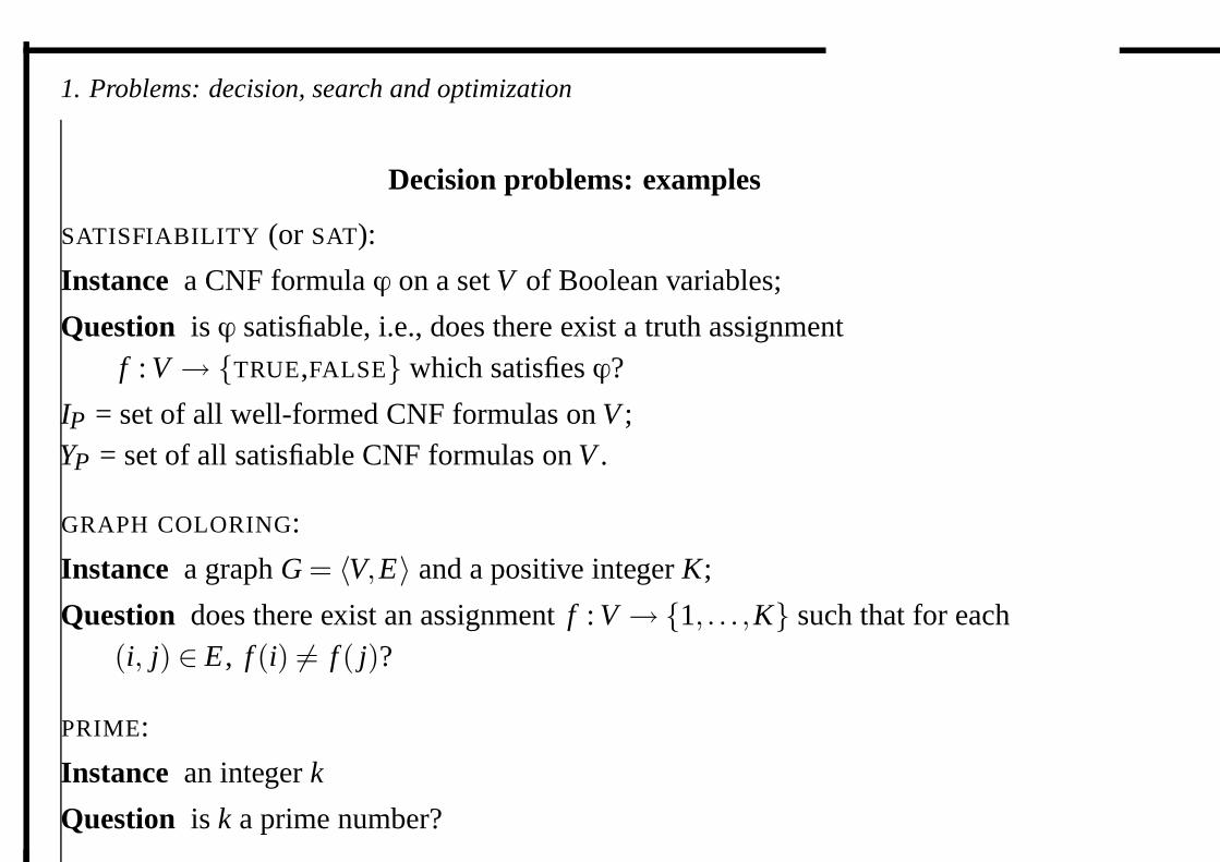
Decision problems: examples
SATISFIABILITY (or SAT):
Instance a CNF formula ϕ on a set V of Boolean variables;
Question is ϕ satisfiable, i.e., does there exist a truth assignmentf : V → {TRUE,FALSE} which satisfies ϕ?
IP = set of all well-formed CNF formulas on V ;YP = set of all satisfiable CNF formulas on V .
GRAPH COLORING:
Instance a graph G = 〈V,E〉 and a positive integer K;
Question does there exist an assignment f : V →{1, . . . ,K} such that for each(i, j) ∈ E , f (i) �= f ( j)?
PRIME:
Instance an integer k
Question is k a prime number?
1. Problems: decision, search and optimization
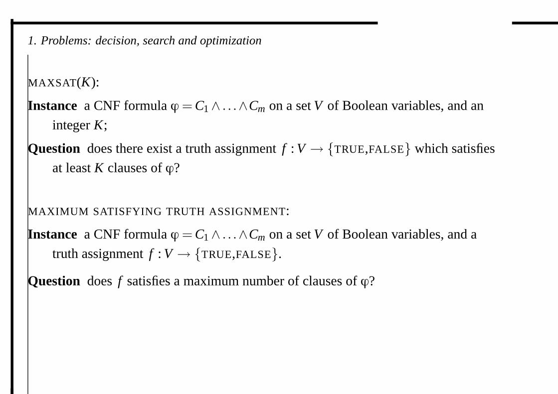
MAXSAT(K):
Instance a CNF formula ϕ = C1∧ . . .∧Cm on a set V of Boolean variables, and an
integer K;
Question does there exist a truth assignment f : V → {TRUE,FALSE} which satisfies
at least K clauses of ϕ?
MAXIMUM SATISFYING TRUTH ASSIGNMENT:
Instance a CNF formula ϕ = C1∧ . . .∧Cm on a set V of Boolean variables, and a
truth assignment f : V → {TRUE,FALSE}.Question does f satisfies a maximum number of clauses of ϕ?
1. Problems: decision, search and optimization
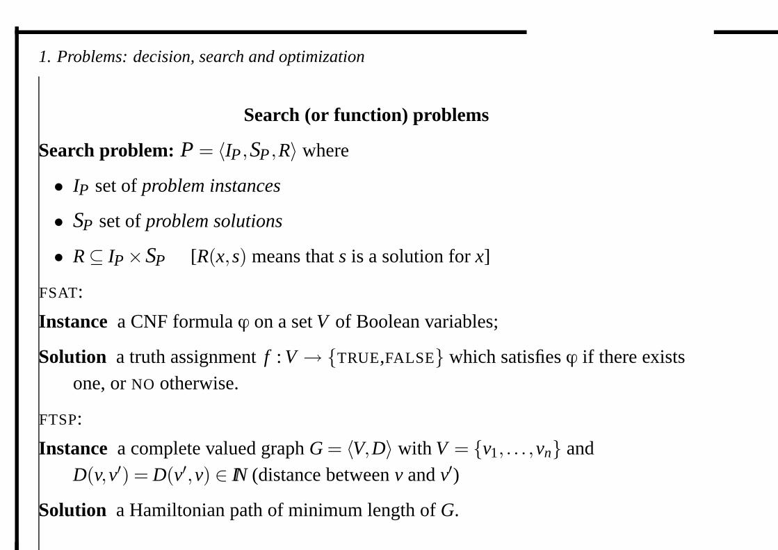
Search (or function) problems
Search problem: P = 〈IP ,SP ,R〉 where
• IP set of problem instances
• SP set of problem solutions
• R⊆ IP ×SP [R(x,s) means that s is a solution for x]
FSAT:
Instance a CNF formula ϕ on a set V of Boolean variables;
Solution a truth assignment f : V → {TRUE,FALSE} which satisfies ϕ if there existsone, or NO otherwise.
FTSP:
Instance a complete valued graph G = 〈V,D〉 with V = {v1, . . . ,vn} andD(v,v′) = D(v′,v) ∈ IN (distance between v and v′)
Solution a Hamiltonian path of minimum length of G.
1. Problems: decision, search and optimization
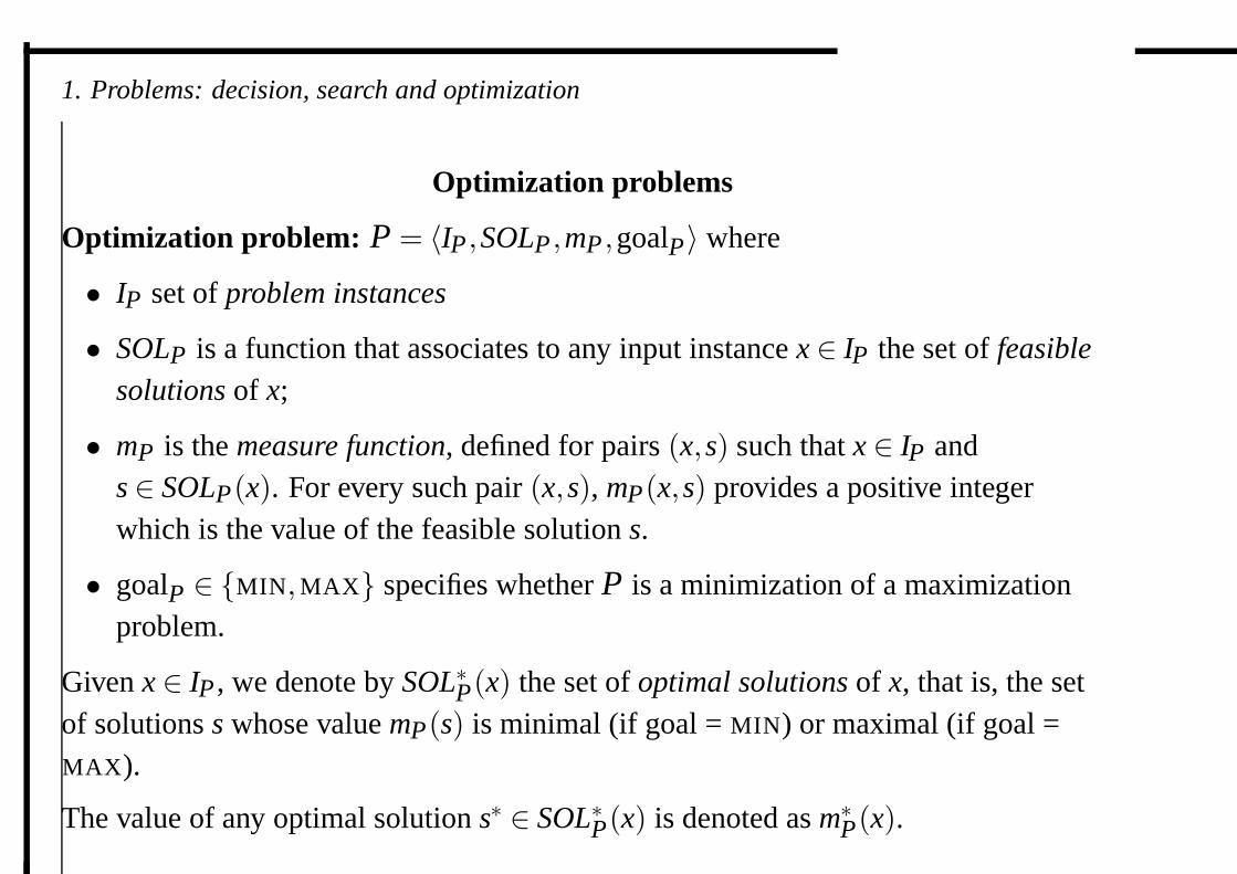
Optimization problems
Optimization problem: P = 〈IP ,SOLP ,mP ,goalP 〉 where
• IP set of problem instances
• SOLP is a function that associates to any input instance x ∈ IP the set of feasible
solutions of x;
• mP is the measure function, defined for pairs (x,s) such that x ∈ IP ands ∈ SOLP (x). For every such pair (x,s), mP (x,s) provides a positive integerwhich is the value of the feasible solution s.
• goalP ∈ {MIN,MAX} specifies whether P is a minimization of a maximizationproblem.
Given x ∈ IP , we denote by SOL∗P (x) the set of optimal solutions of x, that is, the setof solutions s whose value mP (s) is minimal (if goal = MIN) or maximal (if goal =MAX).
The value of any optimal solution s∗ ∈ SOL∗P (x) is denoted as m∗P (x).
1. Problems: decision, search and optimization
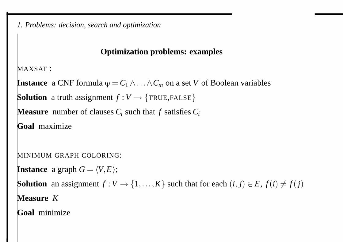
Optimization problems: examples
MAXSAT :
Instance a CNF formula ϕ = C1∧ . . .∧Cm on a set V of Boolean variables
Solution a truth assignment f : V → {TRUE,FALSE}Measure number of clauses Ci such that f satisfies Ci
Goal maximize
MINIMUM GRAPH COLORING:
Instance a graph G = 〈V,E〉;Solution an assignment f : V → {1, . . . ,K} such that for each (i, j) ∈ E , f (i) �= f ( j)
Measure K
Goal minimize
1. Problems: decision, search and optimization
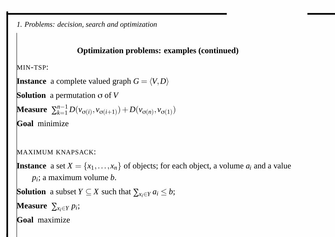
Optimization problems: examples (continued)
MIN-TSP:
Instance a complete valued graph G = 〈V,D〉Solution a permutation σ of V
Measure ∑n−1k=1 D(vσ(i),vσ(i+1))+D(vσ(n),vσ(1))
Goal minimize
MAXIMUM KNAPSACK:
Instance a set X = {x1, . . . ,xn} of objects; for each object, a volume ai and a value
pi; a maximum volume b.
Solution a subset Y ⊆ X such that ∑xi∈Y ai ≤ b;
Measure ∑xi∈Y pi;
Goal maximize
2. Complexity classes, reduction, and completeness
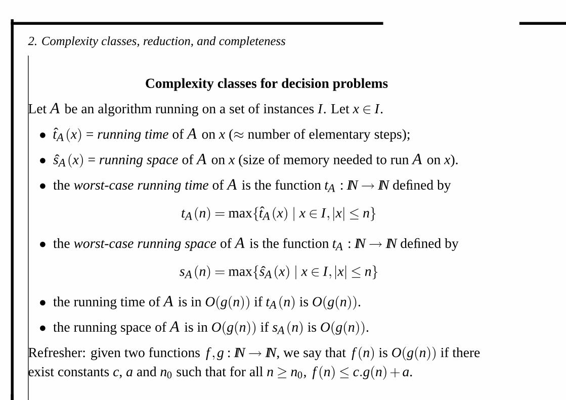
Complexity classes for decision problems
Let A be an algorithm running on a set of instances I. Let x ∈ I.
• tA(x) = running time of A on x (≈ number of elementary steps);
• sA(x) = running space of A on x (size of memory needed to run A on x).
• the worst-case running time of A is the function tA : IN→ IN defined by
tA(n) = max{tA(x) | x ∈ I, |x| ≤ n}
• the worst-case running space of A is the function tA : IN→ IN defined by
sA(n) = max{sA(x) | x ∈ I, |x| ≤ n}
• the running time of A is in O(g(n)) if tA(n) is O(g(n)).
• the running space of A is in O(g(n)) if sA(n) is O(g(n)).
Refresher: given two functions f ,g : IN→ IN, we say that f (n) is O(g(n)) if thereexist constants c, a and n0 such that for all n≥ n0, f (n)≤ c.g(n)+a.
2. Complexity classes, reduction, and completeness
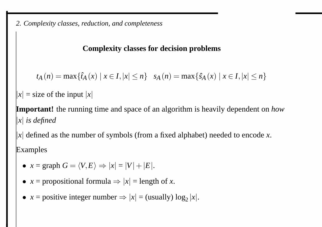
Complexity classes for decision problems
tA(n) = max{tA(x) | x ∈ I, |x| ≤ n} sA(n) = max{sA(x) | x ∈ I, |x| ≤ n}
|x| = size of the input |x|Important! the running time and space of an algorithm is heavily dependent on how
|x| is defined
|x| defined as the number of symbols (from a fixed alphabet) needed to encode x.
Examples
• x = graph G = 〈V,E〉 ⇒ |x| = |V |+ |E|.• x = propositional formula⇒ |x| = length of x.
• x = positive integer number⇒ |x| = (usually) log2 |x|.
2. Complexity classes, reduction, and completeness
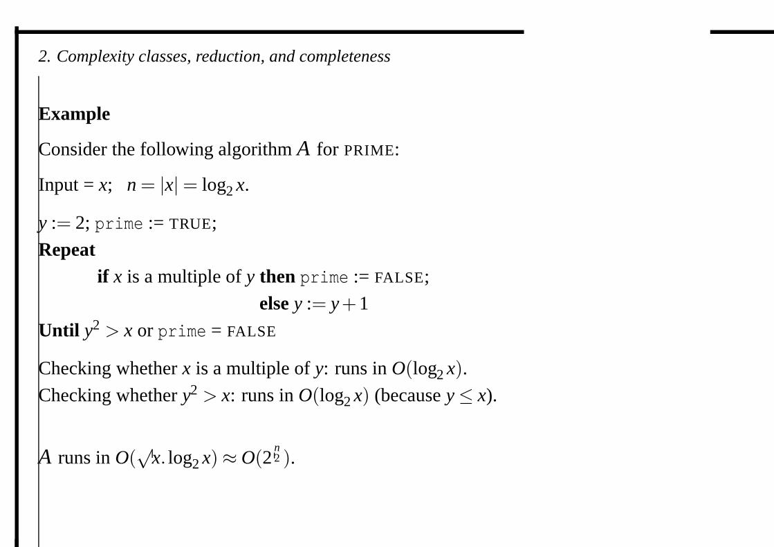
Example
Consider the following algorithm A for PRIME:
Input = x; n = |x|= log2 x.
y := 2; prime := TRUE;
Repeatif x is a multiple of y then prime := FALSE;
else y := y+1
Until y2 > x or prime = FALSE
Checking whether x is a multiple of y: runs in O(log2 x).Checking whether y2 > x: runs in O(log2 x) (because y≤ x).
A runs in O(√
x. log2 x)≈ O(2n2 ).
2. Complexity classes, reduction, and completeness
Complexity classes for decision problems
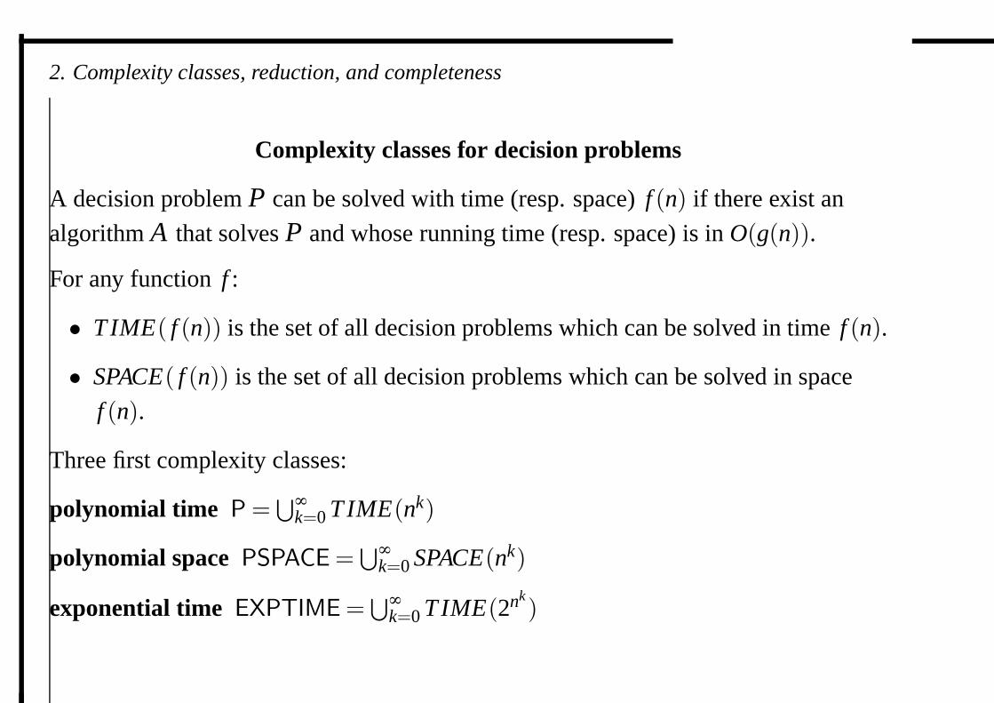
A decision problem P can be solved with time (resp. space) f (n) if there exist an
algorithm A that solves P and whose running time (resp. space) is in O(g(n)).
For any function f :
• TIME( f (n)) is the set of all decision problems which can be solved in time f (n).
• SPACE( f (n)) is the set of all decision problems which can be solved in space
f (n).
Three first complexity classes:
polynomial time P =⋃∞
k=0 TIME(nk)
polynomial space PSPACE =⋃∞
k=0 SPACE(nk)
exponential time EXPTIME =⋃∞
k=0 TIME(2nk)
2. Complexity classes, reduction, and completeness
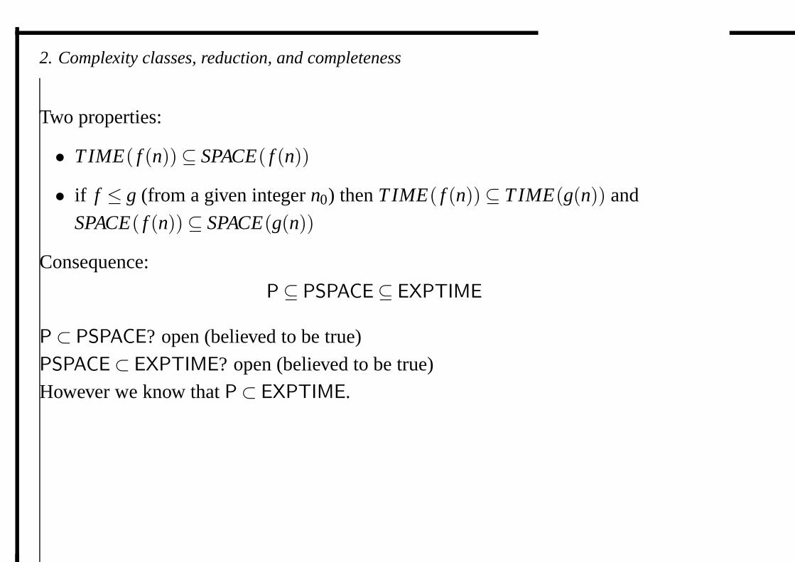
Two properties:
• TIME( f (n))⊆ SPACE( f (n))
• if f ≤ g (from a given integer n0) then TIME( f (n))⊆ TIME(g(n)) and
SPACE( f (n))⊆ SPACE(g(n))
Consequence:
P⊆ PSPACE⊆ EXPTIME
P⊂ PSPACE? open (believed to be true)
PSPACE⊂ EXPTIME? open (believed to be true)
However we know that P⊂ EXPTIME.
2. Complexity classes, reduction, and completeness
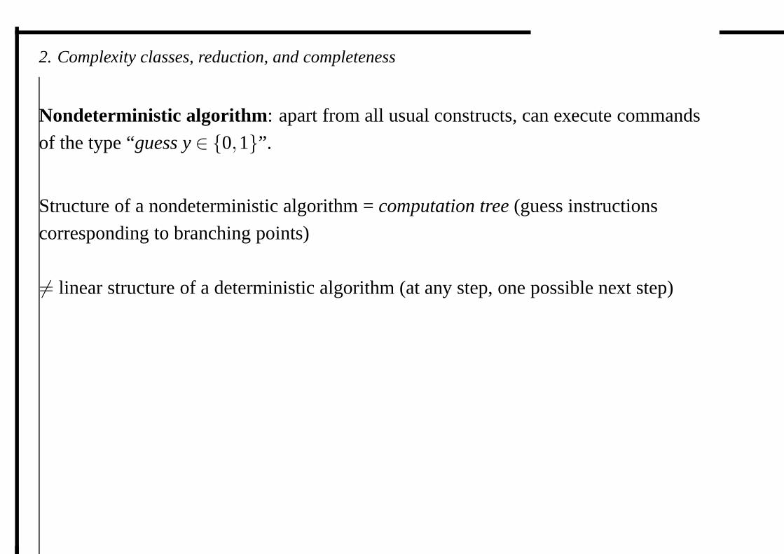
Nondeterministic algorithm: apart from all usual constructs, can execute commands
of the type “guess y ∈ {0,1}”.
Structure of a nondeterministic algorithm = computation tree (guess instructions
corresponding to branching points)
�= linear structure of a deterministic algorithm (at any step, one possible next step)
2. Complexity classes, reduction, and completeness
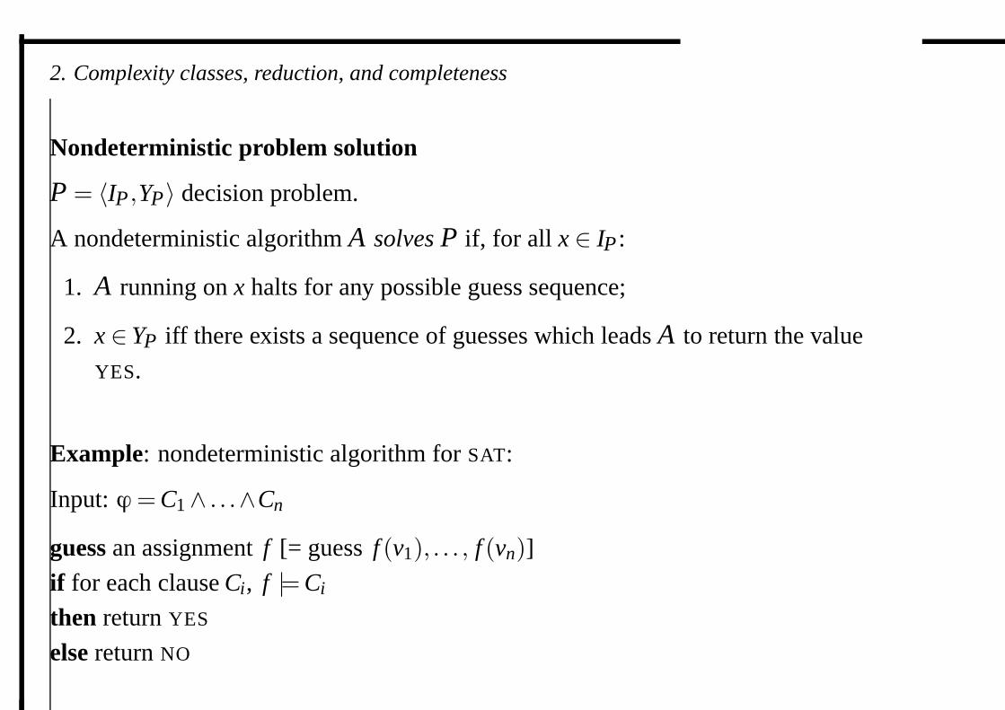
Nondeterministic problem solution
P = 〈IP ,YP 〉 decision problem.
A nondeterministic algorithm A solves P if, for all x ∈ IP :
1. A running on x halts for any possible guess sequence;
2. x ∈ YP iff there exists a sequence of guesses which leads A to return the value
YES.
Example: nondeterministic algorithm for SAT:
Input: ϕ = C1∧ . . .∧Cn
guess an assignment f [= guess f (v1), . . . , f (vn)]if for each clause Ci, f |= Ci
then return YES
else return NO
2. Complexity classes, reduction, and completeness
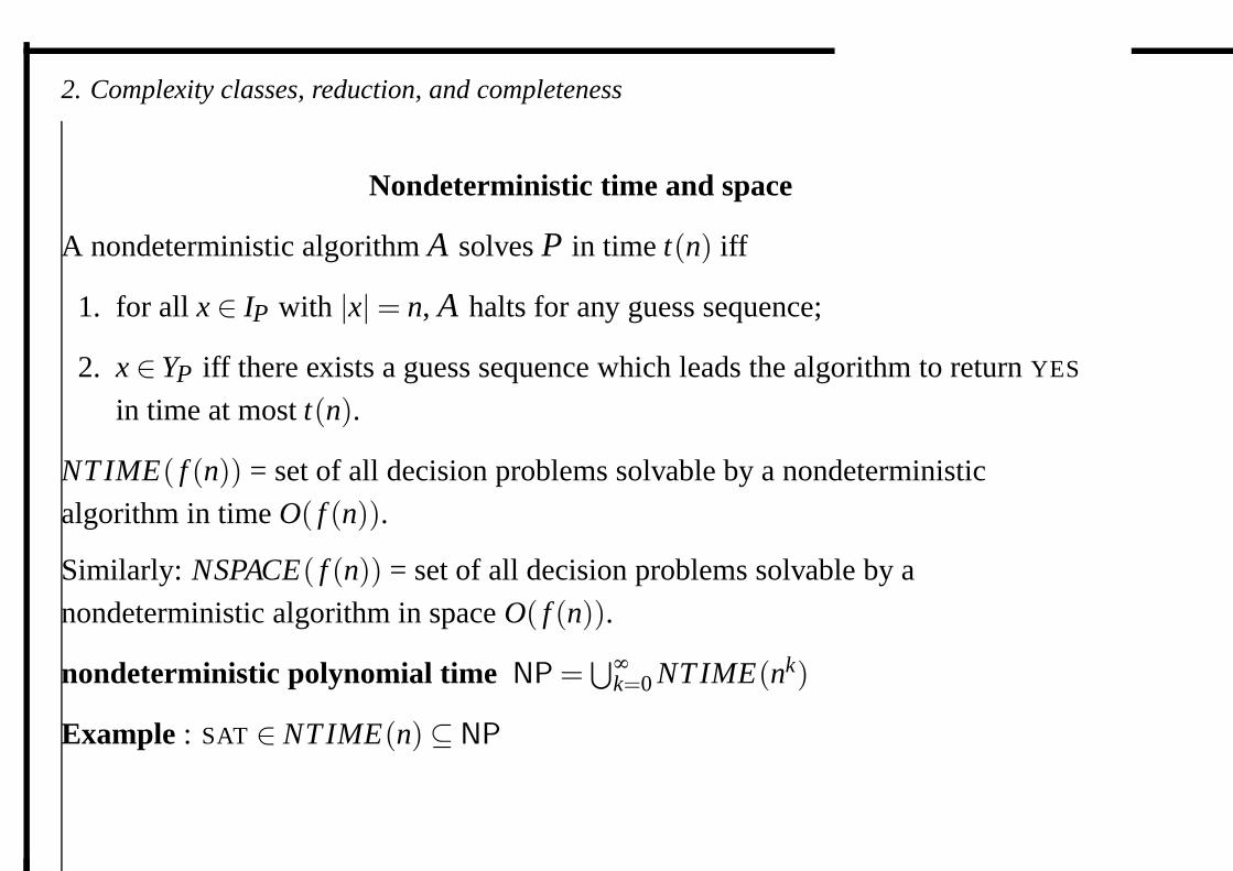
Nondeterministic time and space
A nondeterministic algorithm A solves P in time t(n) iff
1. for all x ∈ IP with |x|= n, A halts for any guess sequence;
2. x ∈ YP iff there exists a guess sequence which leads the algorithm to return YES
in time at most t(n).
NTIME( f (n)) = set of all decision problems solvable by a nondeterministic
algorithm in time O( f (n)).
Similarly: NSPACE( f (n)) = set of all decision problems solvable by a
nondeterministic algorithm in space O( f (n)).
nondeterministic polynomial time NP =⋃∞
k=0 NTIME(nk)
Example : SAT ∈ NTIME(n)⊆ NP
2. Complexity classes, reduction, and completeness
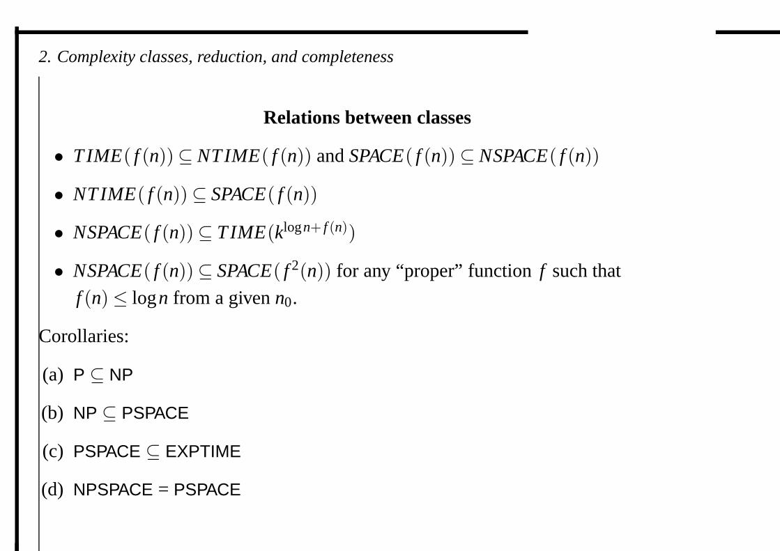
Relations between classes
• TIME( f (n))⊆ NTIME( f (n)) and SPACE( f (n))⊆ NSPACE( f (n))
• NTIME( f (n))⊆ SPACE( f (n))
• NSPACE( f (n))⊆ TIME(klogn+ f (n))
• NSPACE( f (n))⊆ SPACE( f 2(n)) for any “proper” function f such that
f (n)≤ logn from a given n0.
Corollaries:
(a) P ⊆ NP
(b) NP ⊆ PSPACE
(c) PSPACE ⊆ EXPTIME
(d) NPSPACE = PSPACE
2. Complexity classes, reduction, and completeness
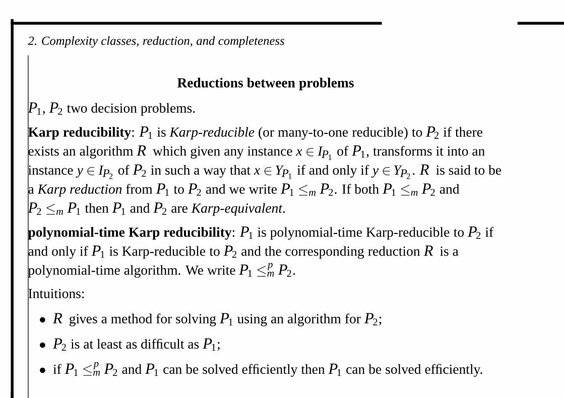
Reductions between problems
P1, P2 two decision problems.
Karp reducibility: P1 is Karp-reducible (or many-to-one reducible) to P2 if thereexists an algorithm R which given any instance x ∈ IP1 of P1, transforms it into aninstance y ∈ IP2 of P2 in such a way that x ∈ YP1 if and only if y ∈ YP2 . R is said to bea Karp reduction from P1 to P2 and we write P1 ≤m P2. If both P1 ≤m P2 andP2 ≤m P1 then P1 and P2 are Karp-equivalent.
polynomial-time Karp reducibility: P1 is polynomial-time Karp-reducible to P2 ifand only if P1 is Karp-reducible to P2 and the corresponding reduction R is apolynomial-time algorithm. We write P1 ≤p
m P2.
Intuitions:
• R gives a method for solving P1 using an algorithm for P2;
• P2 is at least as difficult as P1;
• if P1 ≤pm P2 and P1 can be solved efficiently then P1 can be solved efficiently.
2. Complexity classes, reduction, and completeness
Reductions between problems
Karp reducibility applies only to decision problems.
Oracles: let P = 〈IP ,SP ,R〉 be a function problem. An oracle for P is an abstractdevice which, for any x ∈ IP , returns a value f (x) ∈ SP in just one computation step.
Turing reducibility: let P1, P2 two function problems. P1 is Turing-reducible to P2
if there exists an algorithm R for P1 which queries an oracle for P2. R is said to be aTuring reduction from P1 to P2. We write P1 ≤T P2.
Karp-reducibility is a particular case of Turing-reducibility: case where
• P1 and P2 are decision problems (seen as particular cases of function problems);
• the oracle for P2 is queried just once;
• R returns the value answered by the oracle.
In general: Karp-reducibility is weaker than Turing-reducibility.
polynomial-time Turing reducibility: P1 ≤pT P2 iff P1 ≤T P2 and the corresponding
reduction R is polynomial-time computable with respect to the size of the input.
2. Complexity classes, reduction, and completeness
Closure and completeness
A complexity class C is closed with respect to a reducibility ≤r if for any pair of
decision problems P1 and P2 such that P1 ≤r P2, P2 ∈C implies P1 ∈C.
=⇒ P, NP, PSPACE and EXPTIME are all closed under ≤pm.
For any complexity class C, a decision problem P is C-complete with respect to a
reducibility ≤r if for any other decision problem P ′ ∈C we have P ′ ≤r P .
2. Complexity classes, reduction, and completeness
NP-completeness
In particular: a decision problem P is NP-complete (implicitly: for ≤pm) if P ∈ NP
and for any decision problem P ′ ∈ NP, we have P ′ ≤pm P .
Examples: SAT is NP-complete (Cook, 1971).
NP closed with respect to ≤pm
and P ⊆ NP
⇒ P = NP if and only if at least one NP-complete-problem is in P.
P⊂ NP? open (believed to be true)
Thousands of known NP-complete problems
Cf. book by Garey and Johnson, Computers and Intractability: A Guide to the Theory
of NP-completeness, Freeman, 1979.
2. Complexity classes, reduction, and completeness
Pseudopolynomial algorithms and strong NP-completeness
Consider a decision problem P = 〈IP ,YP 〉 involving positive integer numbers. Let
max(x) denote the highest number appearing in instance x ∈ IP . (Note that max(x)can be exponential in |x|.)An algorithm A for P is pseudopolynomial if it is polynomial in |x| and in max(x).
P is strongly NP-complete if it is still NP-complete when the integers numbers
appearing in the instances are encoded in unary notation.
Examples
• MAXSAT(K) is strongly NP-complete
• KNAPSACK(K) is not strongly NP-complete (unless P = NP).
If P is strongly NP-complete, then there exists no pseudopolynomial algorithm that
solves it, unless P = NP.
2. Complexity classes, reduction, and completeness
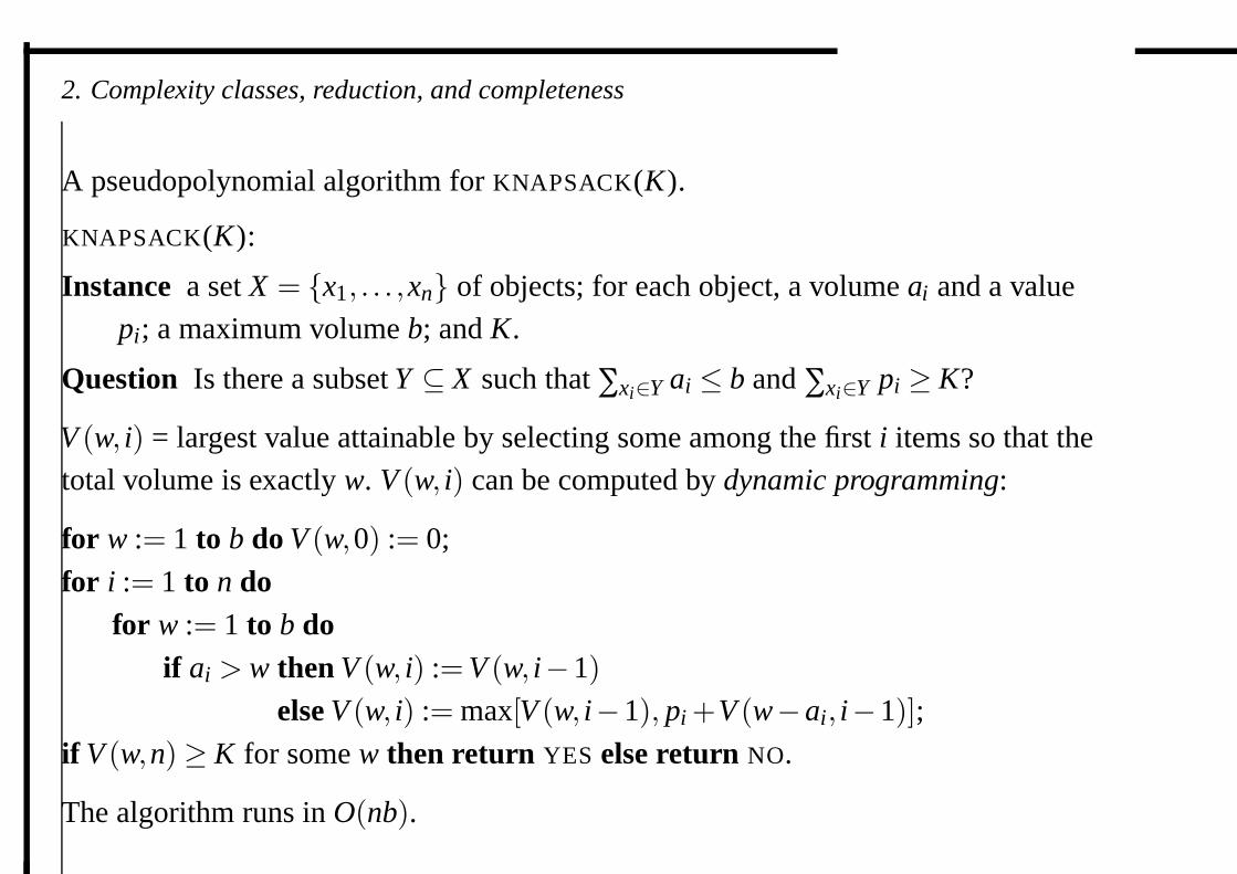
A pseudopolynomial algorithm for KNAPSACK(K).
KNAPSACK(K):
Instance a set X = {x1, . . . ,xn} of objects; for each object, a volume ai and a value
pi; a maximum volume b; and K.
Question Is there a subset Y ⊆ X such that ∑xi∈Y ai ≤ b and ∑xi∈Y pi ≥ K?
V (w, i) = largest value attainable by selecting some among the first i items so that the
total volume is exactly w. V (w, i) can be computed by dynamic programming:
for w := 1 to b do V (w,0) := 0;
for i := 1 to n dofor w := 1 to b do
if ai > w then V (w, i) := V (w, i−1)else V (w, i) := max[V (w, i−1), pi +V (w−ai, i−1)];
if V (w,n)≥ K for some w then return YES else return NO.
The algorithm runs in O(nb).
2. Complexity classes, reduction, and completeness
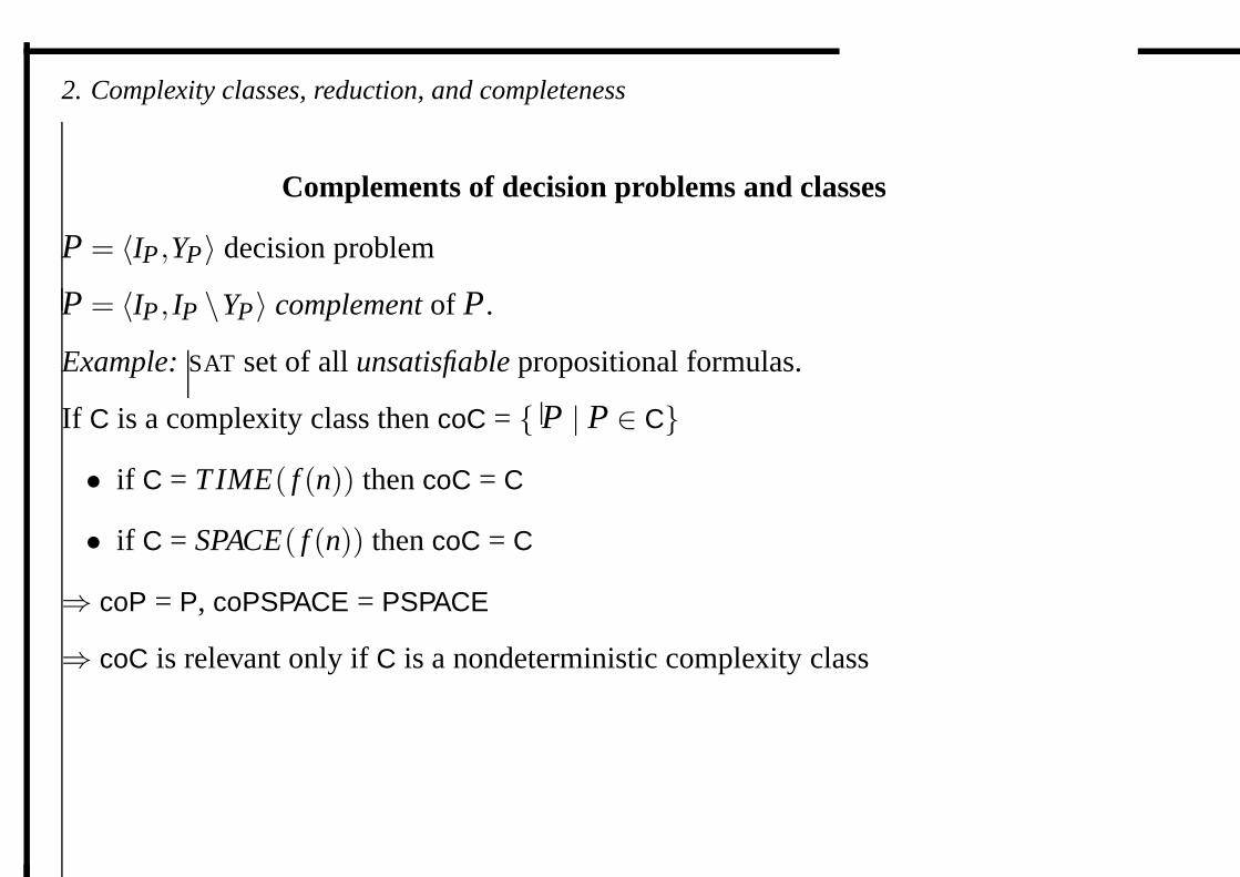
Complements of decision problems and classes
P = 〈IP ,YP 〉 decision problem
P = 〈IP , IP \YP 〉 complement of P .
Example: SAT set of all unsatisfiable propositional formulas.
If C is a complexity class then coC = { P | P ∈ C}• if C = TIME( f (n)) then coC = C
• if C = SPACE( f (n)) then coC = C
⇒ coP = P, coPSPACE = PSPACE
⇒ coC is relevant only if C is a nondeterministic complexity class
2. Complexity classes, reduction, and completeness
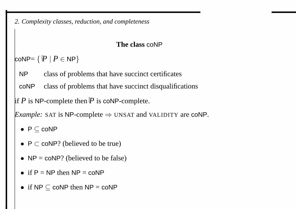
The class coNP
coNP= { P | P ∈ NP}NP class of problems that have succinct certificates
coNP class of problems that have succinct disqualifications
if P is NP-complete then P is coNP-complete.
Example: SAT is NP-complete⇒ UNSAT and VALIDITY are coNP.
• P ⊆ coNP
• P ⊂ coNP? (believed to be true)
• NP = coNP? (believed to be false)
• if P = NP then NP = coNP
• if NP ⊆ coNP then NP = coNP
3. Above NP and coNP
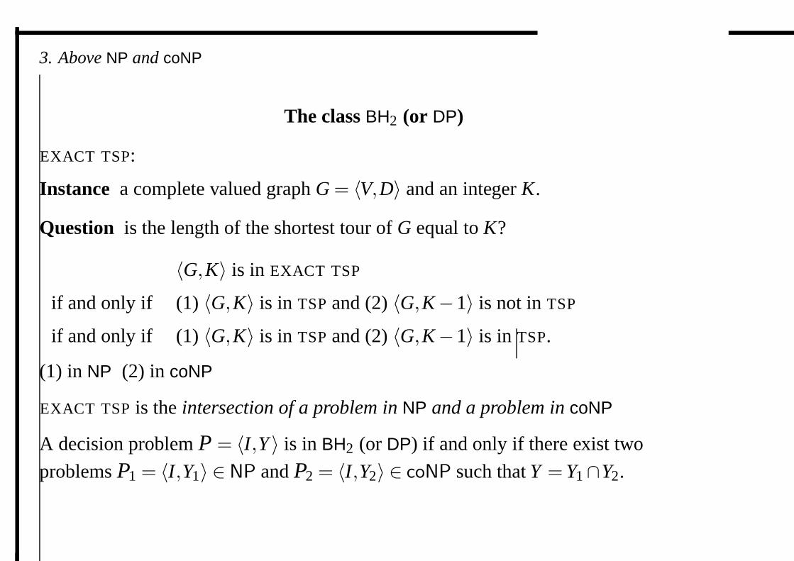
The class BH2 (or DP)
EXACT TSP:
Instance a complete valued graph G = 〈V,D〉 and an integer K.
Question is the length of the shortest tour of G equal to K?
〈G,K〉 is in EXACT TSP
if and only if (1) 〈G,K〉 is in TSP and (2) 〈G,K−1〉 is not in TSP
if and only if (1) 〈G,K〉 is in TSP and (2) 〈G,K−1〉 is in TSP.
(1) in NP (2) in coNP
EXACT TSP is the intersection of a problem in NP and a problem in coNP
A decision problem P = 〈I,Y 〉 is in BH2 (or DP) if and only if there exist two
problems P1 = 〈I,Y1〉 ∈ NP and P2 = 〈I,Y2〉 ∈ coNP such that Y = Y1∩Y2.
3. Above NP and coNP
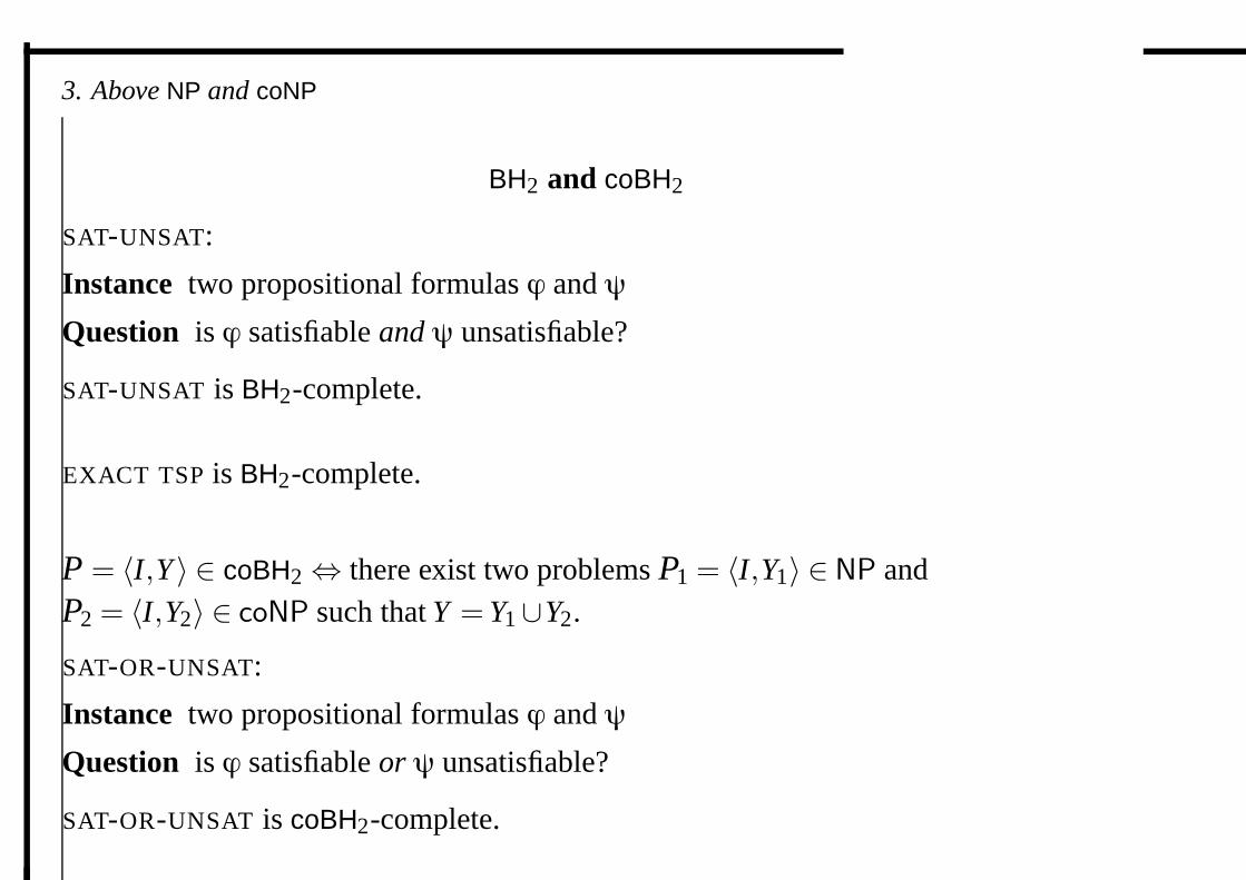
BH2 and coBH2
SAT-UNSAT:
Instance two propositional formulas ϕ and ψ
Question is ϕ satisfiable and ψ unsatisfiable?
SAT-UNSAT is BH2-complete.
EXACT TSP is BH2-complete.
P = 〈I,Y 〉 ∈ coBH2⇔ there exist two problems P1 = 〈I,Y1〉 ∈ NP andP2 = 〈I,Y2〉 ∈ coNP such that Y = Y1∪Y2.
SAT-OR-UNSAT:
Instance two propositional formulas ϕ and ψ
Question is ϕ satisfiable or ψ unsatisfiable?
SAT-OR-UNSAT is coBH2-complete.
3. Above NP and coNP
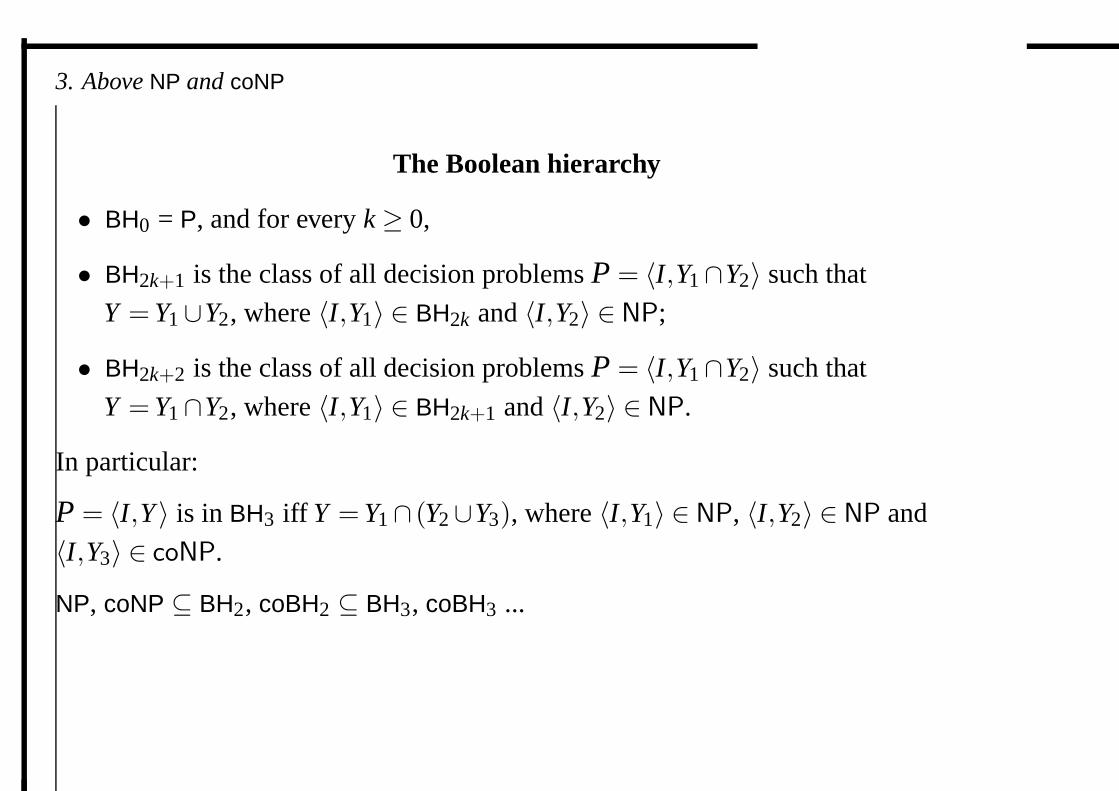
The Boolean hierarchy
• BH0 = P, and for every k ≥ 0,
• BH2k+1 is the class of all decision problems P = 〈I,Y1∩Y2〉 such that
Y = Y1∪Y2, where 〈I,Y1〉 ∈ BH2k and 〈I,Y2〉 ∈ NP;
• BH2k+2 is the class of all decision problems P = 〈I,Y1∩Y2〉 such that
Y = Y1∩Y2, where 〈I,Y1〉 ∈ BH2k+1 and 〈I,Y2〉 ∈ NP.
In particular:
P = 〈I,Y 〉 is in BH3 iff Y = Y1∩ (Y2∪Y3), where 〈I,Y1〉 ∈ NP, 〈I,Y2〉 ∈ NP and
〈I,Y3〉 ∈ coNP.
NP, coNP ⊆ BH2, coBH2 ⊆ BH3, coBH3 ...
3. Above NP and coNP
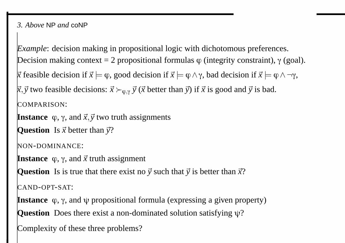
Example: decision making in propositional logic with dichotomous preferences.Decision making context = 2 propositional formulas ϕ (integrity constraint), γ (goal).
�x feasible decision if�x |= ϕ, good decision if�x |= ϕ∧ γ, bad decision if�x |= ϕ∧¬γ,�x,�y two feasible decisions: �x�ϕ,γ�y (�x better than�y) if�x is good and�y is bad.
COMPARISON:
Instance ϕ, γ, and�x,�y two truth assignments
Question Is�x better than�y?
NON-DOMINANCE:
Instance ϕ, γ, and�x truth assignment
Question Is is true that there exist no�y such that�y is better than�x?
CAND-OPT-SAT:
Instance ϕ, γ, and ψ propositional formula (expressing a given property)
Question Does there exist a non-dominated solution satisfying ψ?
Complexity of these three problems?
3. Above NP and coNP
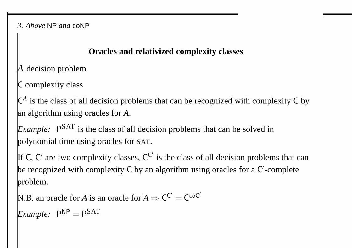
Oracles and relativized complexity classes
A decision problem
C complexity class
CA is the class of all decision problems that can be recognized with complexity C by
an algorithm using oracles for A.
Example: PSAT is the class of all decision problems that can be solved in
polynomial time using oracles for SAT.
If C, C′ are two complexity classes, CC′ is the class of all decision problems that can
be recognized with complexity C by an algorithm using oracles for a C′-complete
problem.
N.B. an oracle for A is an oracle for A⇒ CC′ = CcoC′
Example: PNP = PSAT
3. Above NP and coNP
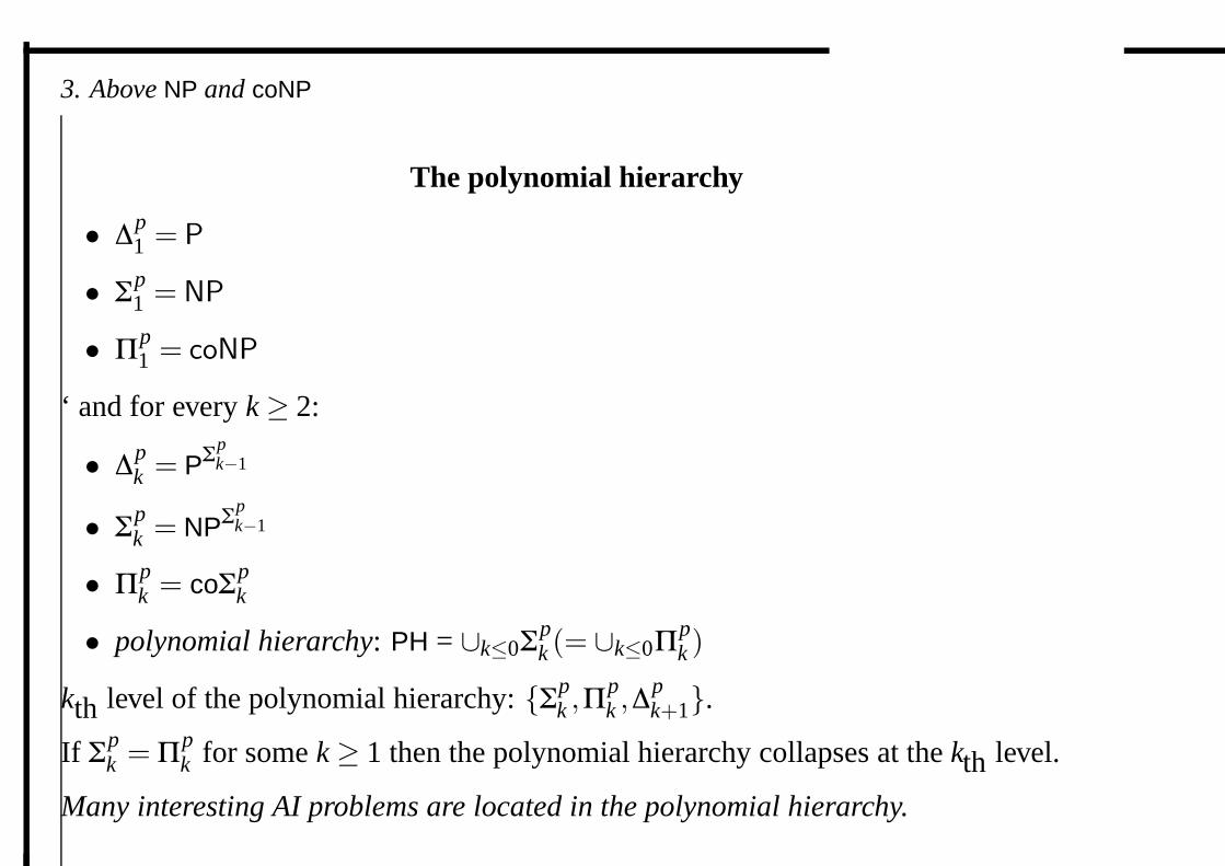
The polynomial hierarchy
• ∆p1 = P
• Σp1 = NP
• Πp1 = coNP
‘ and for every k ≥ 2:
• ∆pk = PΣp
k−1
• Σpk = NPΣp
k−1
• Πpk = coΣp
k
• polynomial hierarchy: PH = ∪k≤0Σpk (= ∪k≤0Π
pk )
kth level of the polynomial hierarchy: {Σpk ,Πp
k ,∆pk+1}.
If Σpk = Πp
k for some k ≥ 1 then the polynomial hierarchy collapses at the kth level.
Many interesting AI problems are located in the polynomial hierarchy.
3. Above NP and coNP
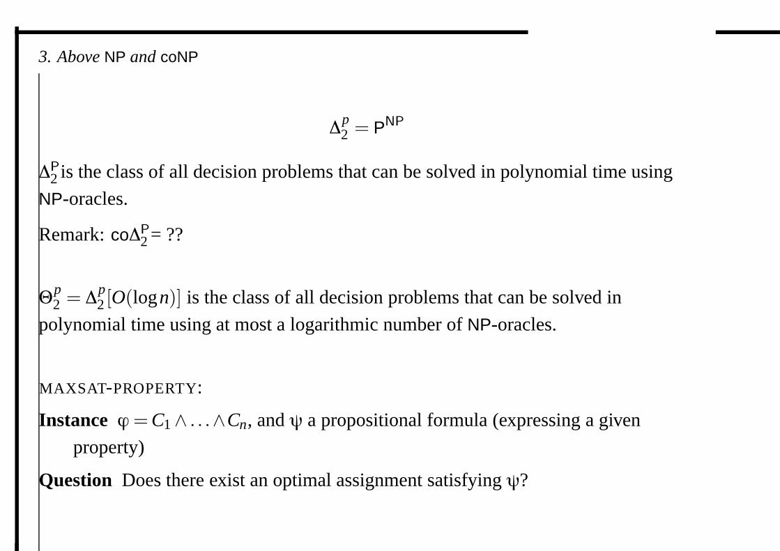
∆p2 = PNP
∆P2 is the class of all decision problems that can be solved in polynomial time using
NP-oracles.
Remark: co∆P2 = ??
Θp2 = ∆p
2 [O(logn)] is the class of all decision problems that can be solved in
polynomial time using at most a logarithmic number of NP-oracles.
MAXSAT-PROPERTY:
Instance ϕ = C1∧ . . .∧Cn, and ψ a propositional formula (expressing a given
property)
Question Does there exist an optimal assignment satisfying ψ?
3. Above NP and coNP
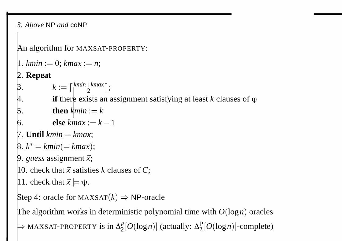
An algorithm for MAXSAT-PROPERTY:
1. kmin := 0; kmax := n;
2. Repeat3. k := � kmin+kmax
2 �;4. if there exists an assignment satisfying at least k clauses of ϕ
5. then kmin := k
6. else kmax := k−1
7. Until kmin = kmax;
8. k∗ = kmin(= kmax);9. guess assignment�x;
10. check that�x satisfies k clauses of C;
11. check that�x |= ψ.
Step 4: oracle for MAXSAT(k)⇒ NP-oracle
The algorithm works in deterministic polynomial time with O(logn) oracles
⇒ MAXSAT-PROPERTY is in ∆p2 [O(logn)] (actually: ∆P
2 [O(logn)]-complete)
3. Above NP and coNP
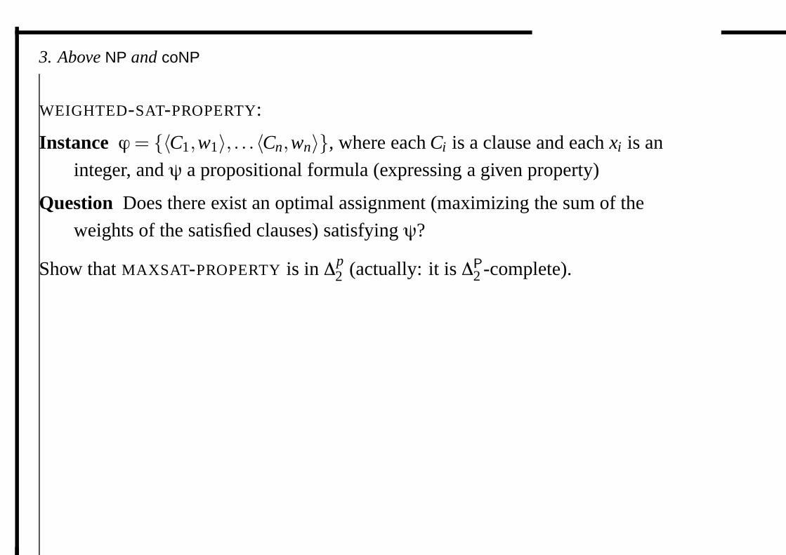
WEIGHTED-SAT-PROPERTY:
Instance ϕ = {〈C1,w1〉, . . .〈Cn,wn〉}, where each Ci is a clause and each xi is an
integer, and ψ a propositional formula (expressing a given property)
Question Does there exist an optimal assignment (maximizing the sum of the
weights of the satisfied clauses) satisfying ψ?
Show that MAXSAT-PROPERTY is in ∆p2 (actually: it is ∆P
2 -complete).
3. Above NP and coNP
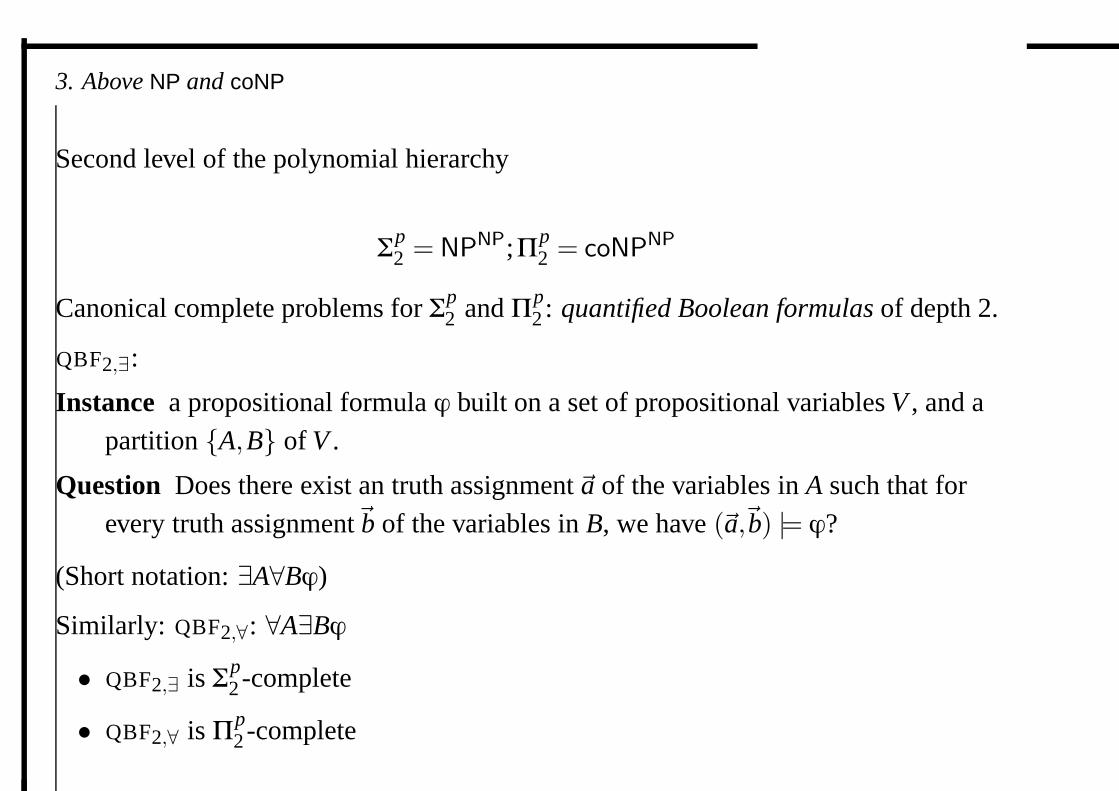
Second level of the polynomial hierarchy
Σp2 = NPNP;Πp
2 = coNPNP
Canonical complete problems for Σp2 and Πp
2 : quantified Boolean formulas of depth 2.
QBF2,∃:
Instance a propositional formula ϕ built on a set of propositional variables V , and apartition {A,B} of V .
Question Does there exist an truth assignment �a of the variables in A such that forevery truth assignment�b of the variables in B, we have (�a,�b) |= ϕ?
(Short notation: ∃A∀Bϕ)
Similarly: QBF2,∀: ∀A∃Bϕ• QBF2,∃ is Σp
2 -complete
• QBF2,∀ is Πp2 -complete
3. Above NP and coNP
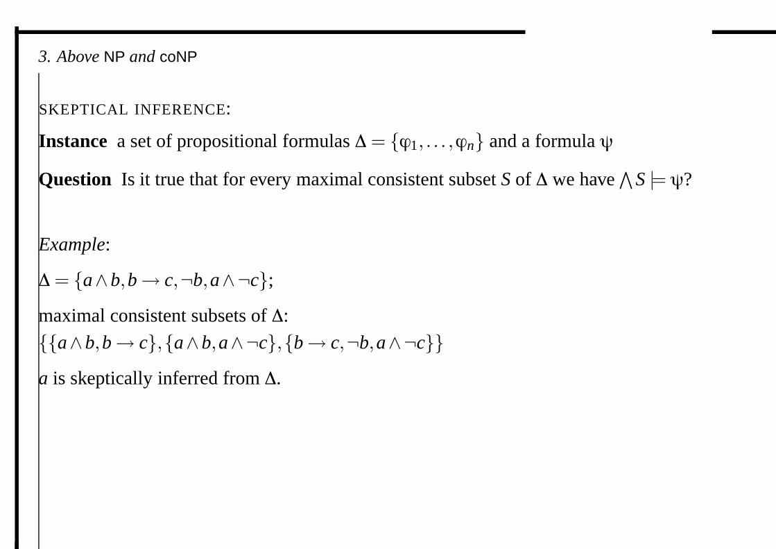
SKEPTICAL INFERENCE:
Instance a set of propositional formulas ∆ = {ϕ1, . . . ,ϕn} and a formula ψ
Question Is it true that for every maximal consistent subset S of ∆ we have∧
S |= ψ?
Example:
∆ = {a∧b,b→ c,¬b,a∧¬c};maximal consistent subsets of ∆:
{{a∧b,b→ c},{a∧b,a∧¬c},{b→ c,¬b,a∧¬c}}a is skeptically inferred from ∆.
3. Above NP and coNP
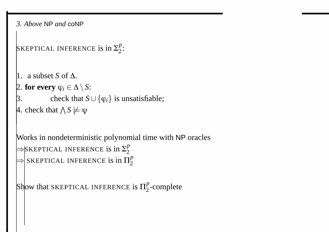
SKEPTICAL INFERENCE is in Σp2 :
1. a subset S of ∆.
2. for every ϕi ∈ ∆\S:
3. check that S∪{ϕi} is unsatisfiable;
4. check that∧
S �|= ψ
Works in nondeterministic polynomial time with NP oracles
⇒SKEPTICAL INFERENCE is in Σp2
⇒ SKEPTICAL INFERENCE is in Πp2
Show that SKEPTICAL INFERENCE is Πp2 -complete
3. Above NP and coNP
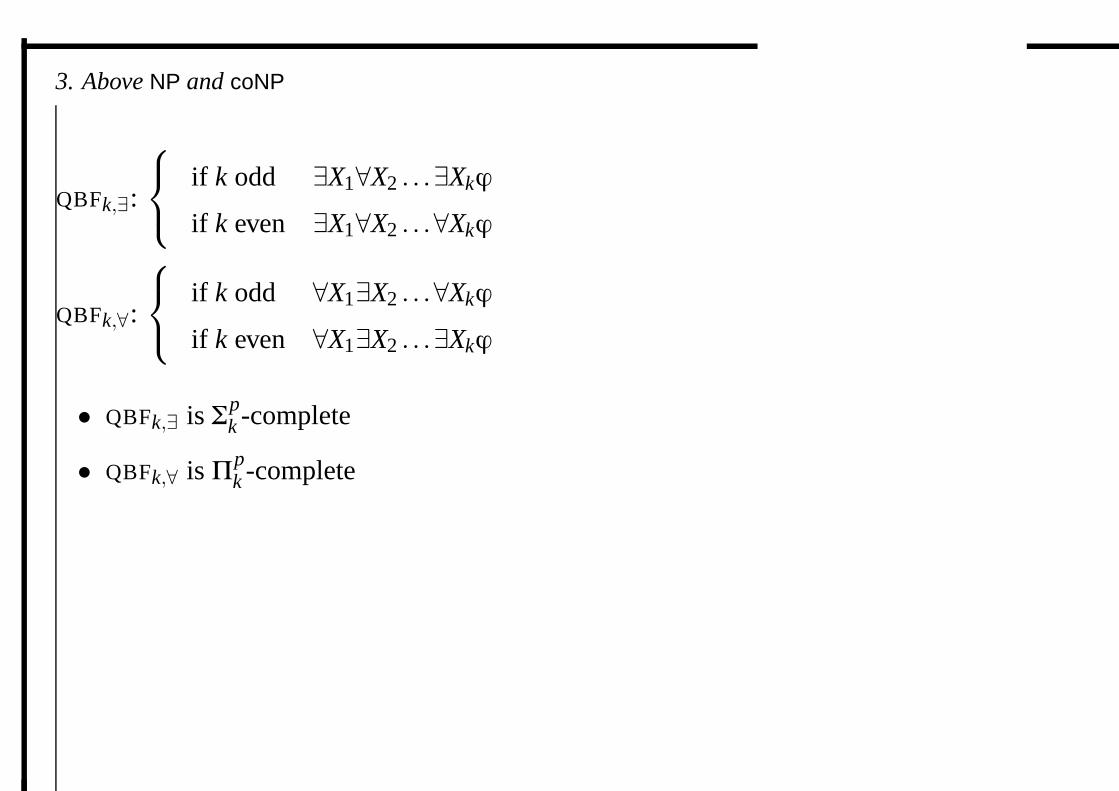
QBFk,∃:
if k odd ∃X1∀X2 . . .∃Xkϕ
if k even ∃X1∀X2 . . .∀Xkϕ
QBFk,∀:
if k odd ∀X1∃X2 . . .∀Xkϕ
if k even ∀X1∃X2 . . .∃Xkϕ
• QBFk,∃ is Σpk -complete
• QBFk,∀ is Πpk -complete
3. Above NP and coNP
Polynomial space
PSPACE = class of all decision problems that can be solved in deterministic time
using a polynomial amount of space.
QBF = set of all QBFk,∃ and QBFk,∀ for k ∈ IN
QBF is PSPACE-complete
PH ⊆ PSPACE
PH = PSPACE? open (believed to be false)
4. Complexity classes for function and optimization problems
FP and FNP
P = 〈IP ,SP ,R〉 function (search) problem
Solving P : establish, given an x, whether there exists a s such that R(x,s) holds, and
if so, give one possible value for that s.
• P is in FP if and only if there is a deterministic polynomial time algorithm that,
given x, can find some s such that R(x,s) holds, or return NO otherwise.
• P is in FNP if and only if there is a deterministic polynomial time algorithm that,
given x and s, can determine whether R(x,s) holds.
Decision problem PD induced by a function problem P : PD = 〈IP ,YP 〉 with
YP = {x | R(x,s) holds for some s}
FP = FNP if and only if P = NP.
4. Complexity classes for function and optimization problems
P is always at least as hard as PD. Can P be significantly harder than PD?
Sometimes no:
FSAT can be solved in polynomial time iff SAT can be solved in polynomial time
⇒ obvious
⇐ let ϕ built on variables {x1, . . . ,xn}.1 if ϕ is unsatisfiable
2 then return NO
3 else for i := 1 to n do4 if ϕxi:=TRUE is satisfiable
5 then f (xi) := TRUE; ϕ := ϕ∧ xi
6 else f (xi) := FALSE; ϕ := ϕ∧¬xi
7 end
If ϕ is satisfiable then the assignment f returned by the algorithm satisfies ϕ
4. Complexity classes for function and optimization problems
P is always at least as hard as PD. Can P be significantly harder than PD?
Sometimes yes:
ANOTHER HAMILTONIAN CYCLE:
Instance a graph G that possesses a Hamiltonian cycle, and a Hamiltonian cycle C
for G.
Question does G have another Hamiltonian cycle?
A cubic graph is a graph G = 〈V,E〉 where each vertex has degree 3.
Proposition (Papadimitriou, 93): given a cubic graph G, and two vertices i, j of G,
the number of Hamiltonian cycles using (i, j) is even.
Corollary: if we know a Hamiltonian cycle for a cubic graph, there must be another
one.
• ANOTHER HAMILTONIAN CYCLE IN CUBIC GRAPHS can be solved in unit time!
• F-ANOTHER HAMILTONIAN CYCLE IN CUBIC GRAPHS is not known to be in P.
4. Complexity classes for function and optimization problems
A function problem P = 〈IP ,SP ,R〉 is total iff for every x ∈ IP there exists an s ∈ SP
such that R(x,s) holds.
TFNP ⊆ FNP is the class of all total function problems that are in FNP
Example: F-ANOTHER HAMILTONIAN CYCLE IN CUBIC GRAPHS is in TFNP.
4. Complexity classes for function and optimization problems
NPO
An optimization problem P = 〈I,SOL,m,goal〉 is in NPO if and only if
1. the set of instances I is recognizable in polynomial time;
2. there exists a polynomial q such that for any x ∈ I:
• for any s ∈ SOL(x), |s| ≤ q(|x|);• for any s such that |s| ≤ q(|x|), it is decidable in polynomial time whether
s ∈ SOL(x);
3. m is computable in polynomial time.
Example: MAXSAT is in NPO
4. Complexity classes for function and optimization problems
P = 〈I,SOL,m,goal〉 optimization problem �→ three induced problems:
Constructive problem PC given an instance x ∈ I, derive an optimal solution
s∗(x) ∈ SOL∗(x) and its measure m∗(x).
Evaluation problem PE given an instance x ∈ I, derive the value m∗(x).
Decision problem PD given an instance x ∈ I and a positive integer K, decide
whether m∗(x)≥ K (if goal = MAX) or whether m∗(x)≤ K (if goal = MIN).
Underlying language of P :
• {(x,K) | x ∈ I and m∗(x)≥ K} if goal = MAX
• {(x,K) | x ∈ I and m∗(x)≤ K} if goal = MIN
For any optimization problem P in NPO, the corresponding decision problem PD
belongs to NP.
4. Complexity classes for function and optimization problems
PO
An optimization problem belongs to PO if it is in NPO and there exists a
polynomial-time algorithm A that, for any instance x ∈ I, returns an optimal solution
s ∈ SOL∗(x), together with its value m∗(x).
Example: MINIMUM PATH is in PO.
4. Complexity classes for function and optimization problems
An optimization problem P is NP-hard if for every decision problem P ′ ∈ NP, we
have P ′ ≤pT SOL∗P , that is, P ′ can be solved in polynomial time by an algorithm using
an oracle that, for any instance x ∈ IP , returns an optimal solution s∗(x) of x together
with its value m∗P (x).
Results:
1. For any problem P ∈ NPO: if the underlying language of P is NP-complete,
then P is NP-hard.
2. If P�= NP then PO�= NPO.
Example: MAXSAT is NP-hard.
4. Complexity classes for function and optimization problems
P = 〈I,SOL,m,goal〉 optimization problem
PC induced constructive problem; PE induced evaluation problem; PD induced
decision problem .
• For any P ∈ NPO we have PD ≡pT PE ≤p
T PC
• Let P ∈ NPO. If PD is NP-complete, then PC ≤pT PD
⇒ when the decision problem PD is NP-complete then the constructive, evaluation,
and decision problems are equivalent.
Question: is there an NPO problem P whose corresponding constructive problem is
harder than the evaluation problem PE? open (believed to be true).
5. Approximation
Approximation
When facing a NP-hard optimization problem: try to find a polynomial approximation
algorithm.
Given an optimization problem P = 〈I,SOL,m,goal〉, an algorithm A is an
approximation algorithm for P if, for any instance x ∈ I, it returns an approximate
solution, that is, a feasible solution A(x) ∈ SOL(x).
Two criteria for evaluating the quality of an approximation algorithm A :
• the complexity of A .
• the quality of the approximate solution returned by A :
– absolute approximation;
– relative approximation;
– differential approximation.
5. Approximation
Absolute approximation P optimization problem; x ∈ I; s ∈ SOL(x).
The absolute error of s with respect ot x is defined as
D(x,s) = |m∗(x)−m(x,s)|
An approximation algorithm A for P is an absolute approximation algorithm if
there exists a constant k such that for every instance x of P , D(x,A(x))≤ k.
Polynomial-time absolute approximation algorithms for NP-hard opmtimization
problems are rare.
5. Approximation
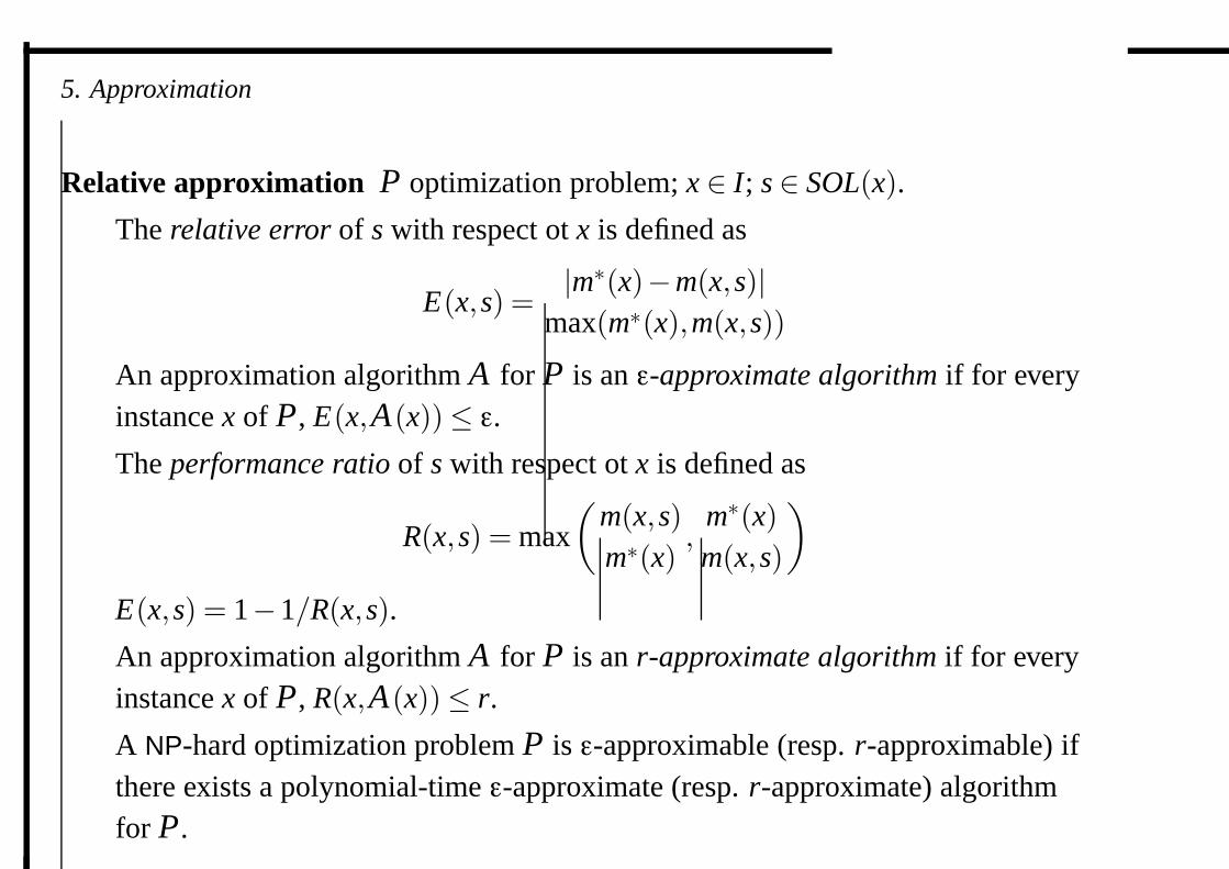
Relative approximation P optimization problem; x ∈ I; s ∈ SOL(x).
The relative error of s with respect ot x is defined as
E(x,s) =|m∗(x)−m(x,s)|
max(m∗(x),m(x,s))
An approximation algorithm A for P is an ε-approximate algorithm if for everyinstance x of P , E(x,A(x))≤ ε.
The performance ratio of s with respect ot x is defined as
R(x,s) = max
(m(x,s)m∗(x)
,m∗(x)m(x,s)
)
E(x,s) = 1−1/R(x,s).
An approximation algorithm A for P is an r-approximate algorithm if for everyinstance x of P , R(x,A(x))≤ r.
A NP-hard optimization problem P is ε-approximable (resp. r-approximable) ifthere exists a polynomial-time ε-approximate (resp. r-approximate) algorithmfor P .
5. Approximation
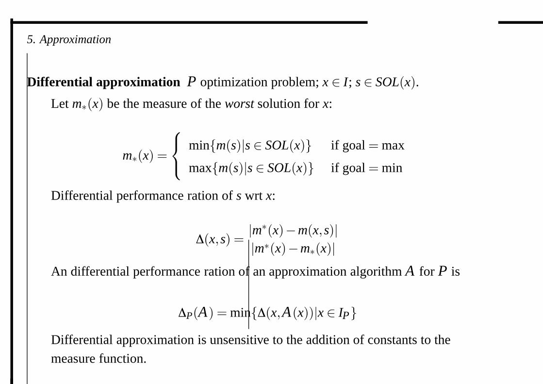
Differential approximation P optimization problem; x ∈ I; s ∈ SOL(x).
Let m∗(x) be the measure of the worst solution for x:
m∗(x) =
min{m(s)|s ∈ SOL(x)} if goal = max
max{m(s)|s ∈ SOL(x)} if goal = min
Differential performance ration of s wrt x:
∆(x,s) =|m∗(x)−m(x,s)||m∗(x)−m∗(x)|
An differential performance ration of an approximation algorithm A for P is
∆P(A) = min{∆(x,A(x))|x ∈ IP}Differential approximation is unsensitive to the addition of constants to the
measure function.
5. Approximation
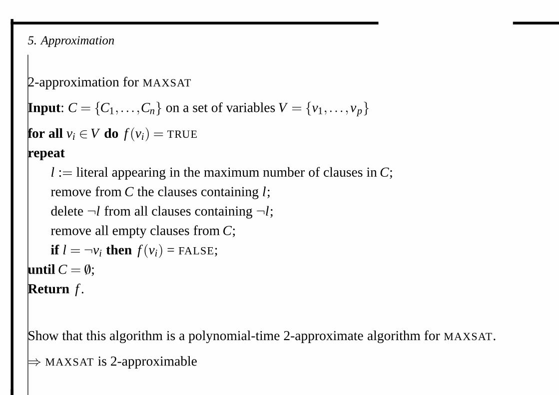
2-approximation for MAXSAT
Input: C = {C1, . . . ,Cn} on a set of variables V = {v1, . . . ,vp}for all vi ∈V do f (vi) = TRUE
repeatl := literal appearing in the maximum number of clauses in C;
remove from C the clauses containing l;
delete ¬l from all clauses containing ¬l;
remove all empty clauses from C;
if l = ¬vi then f (vi) = FALSE;
until C = /0;
Return f .
Show that this algorithm is a polynomial-time 2-approximate algorithm for MAXSAT.
⇒ MAXSAT is 2-approximable
5. Approximation
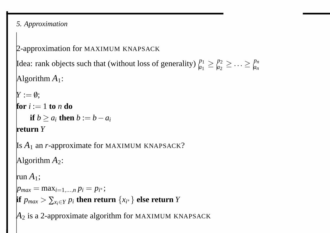
2-approximation for MAXIMUM KNAPSACK
Idea: rank objects such that (without loss of generality) p1a1≥ p2
a2≥ . . .≥ pn
an
Algorithm A1:
Y := /0;
for i := 1 to n doif b≥ ai then b := b−ai
return Y
Is A1 an r-approximate for MAXIMUM KNAPSACK?
Algorithm A2:
run A1;
pmax = maxi=1,...,n pi = pi∗ ;
if pmax > ∑xi∈Y pi then return {xi∗} else return Y
A2 is a 2-approximate algorithm for MAXIMUM KNAPSACK
5. Approximation
APX
APX is the class of all NPO problems P such that there exists a polynomial-time
r-approximate algorithm for P , for some r ≥ 1.
Example
MAXSAT and MAXIMUM KNAPSACK are 2-approximable
⇒ MAXSAT and MAXIMUM KNAPSACK are in APX.
5. Approximation
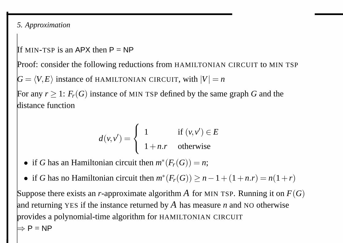
If MIN-TSP is an APX then P = NP
Proof: consider the following reductions from HAMILTONIAN CIRCUIT to MIN TSP
G = 〈V,E〉 instance of HAMILTONIAN CIRCUIT, with |V |= n
For any r ≥ 1: Fr(G) instance of MIN TSP defined by the same graph G and thedistance function
d(v,v′) =
1 if (v,v′) ∈ E
1+n.r otherwise
• if G has an Hamiltonian circuit then m∗(Fr(G)) = n;
• if G has no Hamiltonian circuit then m∗(Fr(G))≥ n−1+(1+n.r) = n(1+ r)
Suppose there exists an r-approximate algorithm A for MIN TSP. Running it on F(G)and returning YES if the instance returned by A has measure n and NO otherwiseprovides a polynomial-time algorithm for HAMILTONIAN CIRCUIT
⇒ P = NP
5. Approximation
Generalization: the “gap technique”
Given some NPO minimization problem P, if there exists a constant k such that it is
NP-hard to decide whether m∗(x)≤ k, then P is not approximable for r < k+1k , unless
P = NP.
5. Approximation
Polynomial-time approximation schemes
Let P be an optimization problem in NPO. A is a polynomial-time approximation
scheme (PTAS) for P if for any instance x of P and any r > 1, A applied to input
(x,r) returns an r-approximate solution of x in time polynomial in |x|.
Example: PTAS for MIN PARTITION
MINIMUM PARTITION:
Instance a collection of objects X = {x1, . . . ,xn} with associated integer weights
a1, . . . ,an;
Solution a partition of X into two sets Y and Z;
Measure max(∑xi∈Y ai,∑xi∈Z ai)
Goal minimize
5. Approximation
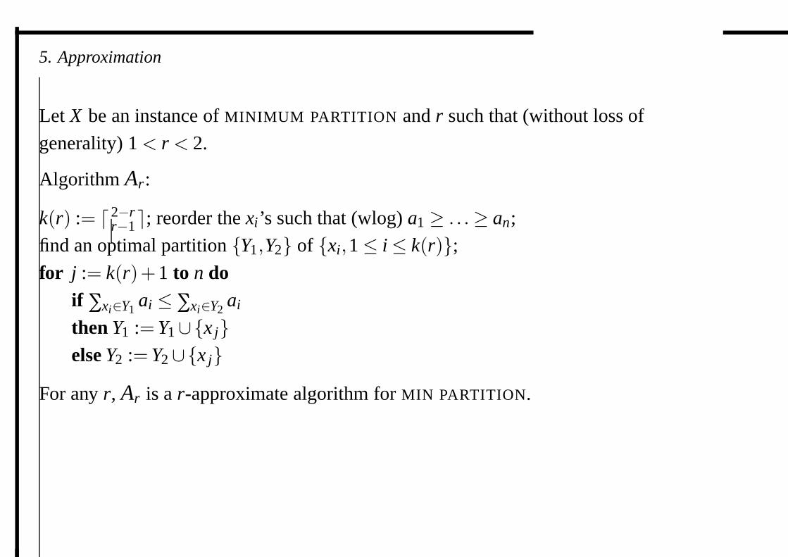
Let X be an instance of MINIMUM PARTITION and r such that (without loss of
generality) 1 < r < 2.
Algorithm Ar:
k(r) := � 2−rr−1�; reorder the xi’s such that (wlog) a1 ≥ . . .≥ an;
find an optimal partition {Y1,Y2} of {xi,1≤ i≤ k(r)};for j := k(r)+1 to n do
if ∑xi∈Y1ai ≤ ∑xi∈Y2
ai
then Y1 := Y1∪{x j}else Y2 := Y2∪{x j}
For any r, Ar is a r-approximate algorithm for MIN PARTITION.
5. Approximation
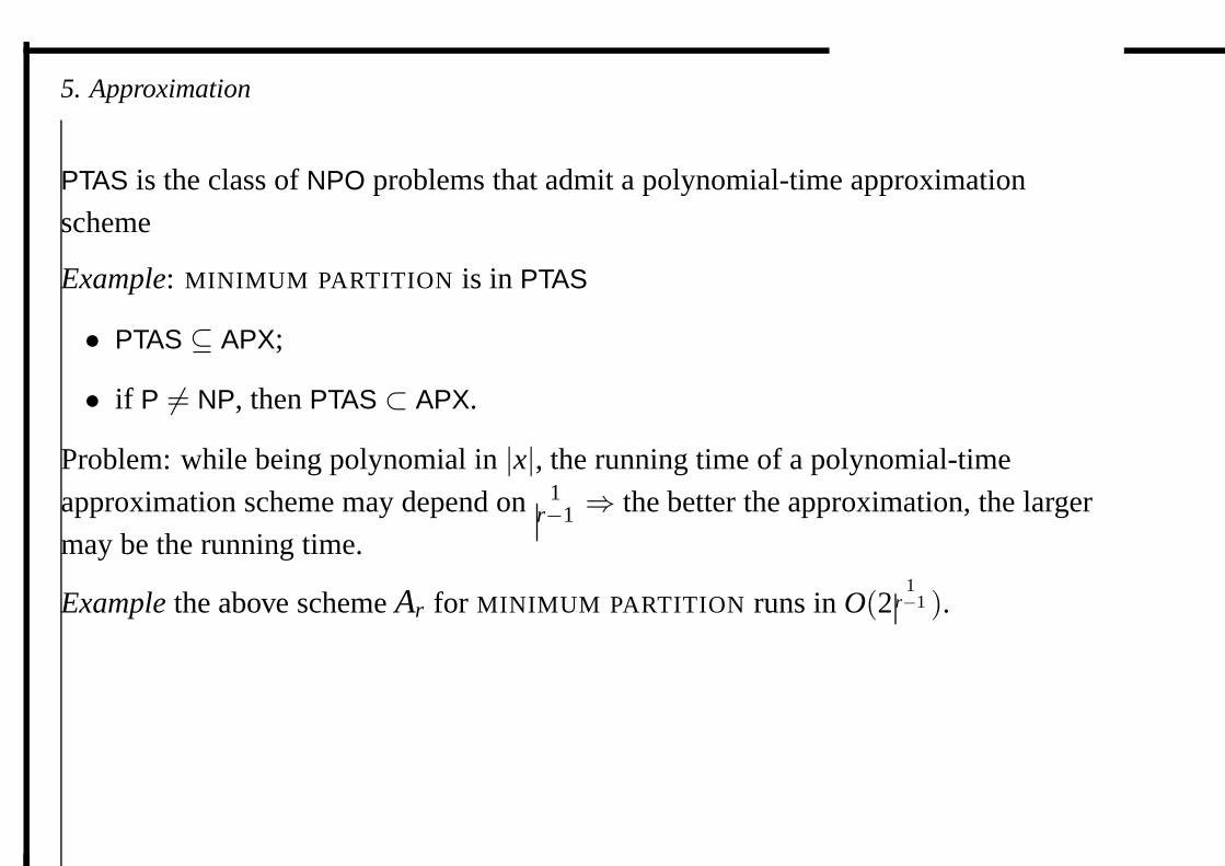
PTAS is the class of NPO problems that admit a polynomial-time approximation
scheme
Example: MINIMUM PARTITION is in PTAS
• PTAS ⊆ APX;
• if P �= NP, then PTAS ⊂ APX.
Problem: while being polynomial in |x|, the running time of a polynomial-time
approximation scheme may depend on 1r−1 ⇒ the better the approximation, the larger
may be the running time.
Example the above scheme Ar for MINIMUM PARTITION runs in O(21
r−1 ).
5. Approximation
Fully polynomial-time approximation schemes
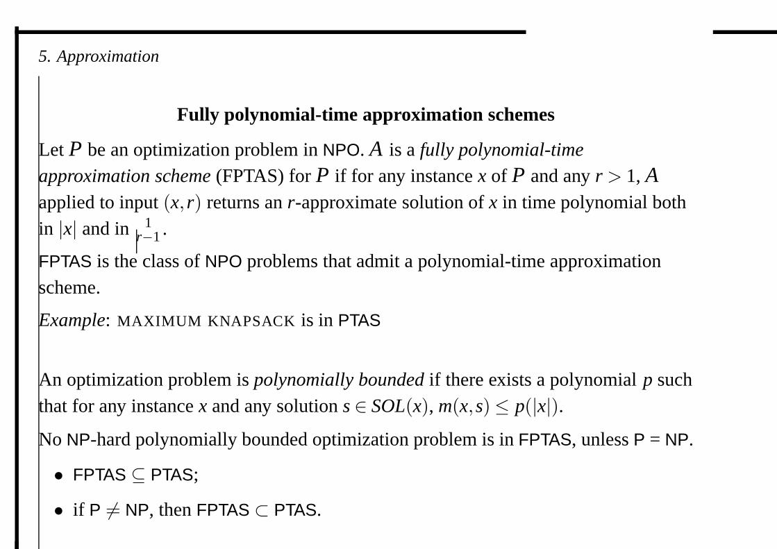
Let P be an optimization problem in NPO. A is a fully polynomial-time
approximation scheme (FPTAS) for P if for any instance x of P and any r > 1, Aapplied to input (x,r) returns an r-approximate solution of x in time polynomial bothin |x| and in 1
r−1 .
FPTAS is the class of NPO problems that admit a polynomial-time approximationscheme.
Example: MAXIMUM KNAPSACK is in PTAS
An optimization problem is polynomially bounded if there exists a polynomial p suchthat for any instance x and any solution s ∈ SOL(x), m(x,s)≤ p(|x|).No NP-hard polynomially bounded optimization problem is in FPTAS, unless P = NP.
• FPTAS ⊆ PTAS;
• if P �= NP, then FPTAS ⊂ PTAS.
5. Compact representation and compilation
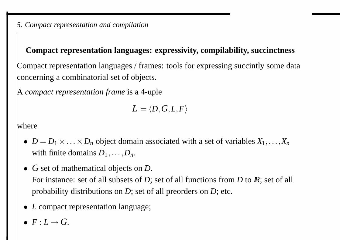
Compact representation languages: expressivity, compilability, succinctness
Compact representation languages / frames: tools for expressing succintly some dataconcerning a combinatorial set of objects.
A compact representation frame is a 4-uple
L = 〈D,G ,L,F〉where
• D = D1× . . .×Dn object domain associated with a set of variables X1, . . . ,Xn
with finite domains D1, . . . ,Dn.
• G set of mathematical objects on D.For instance: set of all subsets of D; set of all functions from D to IR; set of allprobability distributions on D; set of all preorders on D; etc.
• L compact representation language;
• F : L→ G .
5. Compact representation and compilation
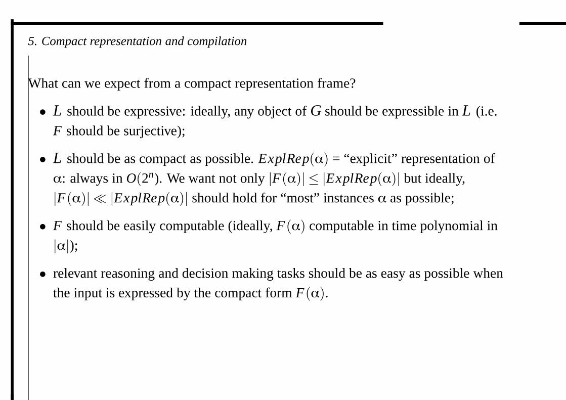
What can we expect from a compact representation frame?
• L should be expressive: ideally, any object of G should be expressible in L (i.e.
F should be surjective);
• L should be as compact as possible. ExplRep(α) = “explicit” representation of
α: always in O(2n). We want not only |F(α)| ≤ |ExplRep(α)| but ideally,
|F(α)| � |ExplRep(α)| should hold for “most” instances α as possible;
• F should be easily computable (ideally, F(α) computable in time polynomial in
|α|);• relevant reasoning and decision making tasks should be as easy as possible when
the input is expressed by the compact form F(α).
5. Compact representation and compilation
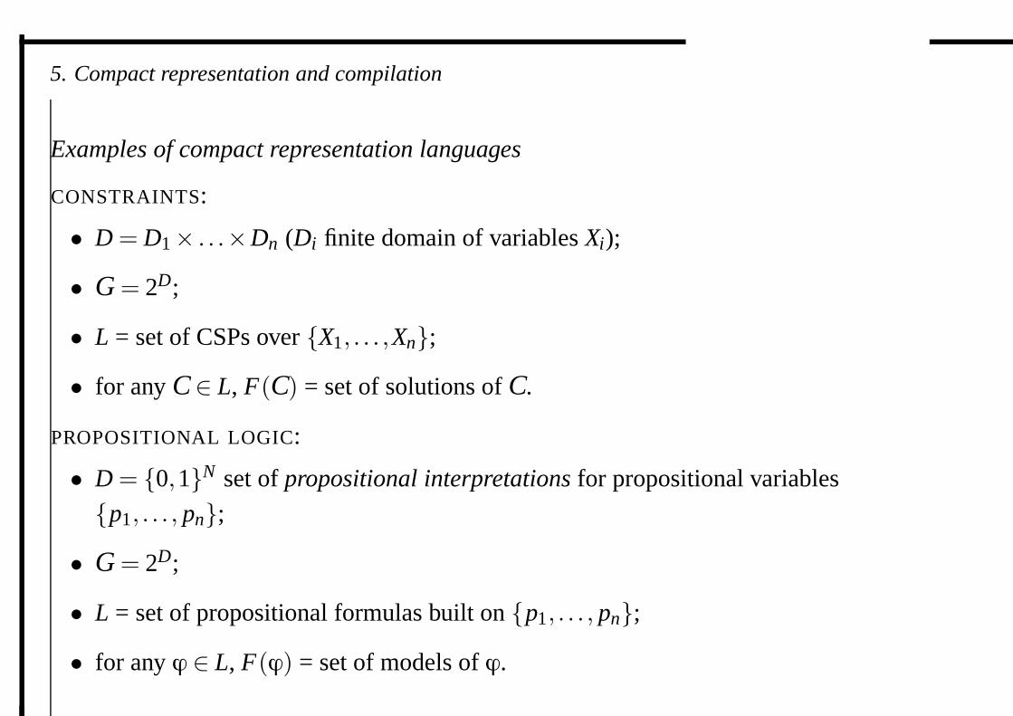
Examples of compact representation languages
CONSTRAINTS:
• D = D1× . . .×Dn (Di finite domain of variables Xi);
• G = 2D;
• L = set of CSPs over {X1, . . . ,Xn};• for any C ∈ L, F(C ) = set of solutions of C .
PROPOSITIONAL LOGIC:
• D = {0,1}N set of propositional interpretations for propositional variables
{p1, . . . , pn};• G = 2D;
• L = set of propositional formulas built on {p1, . . . , pn};• for any ϕ ∈ L, F(ϕ) = set of models of ϕ.
5. Compact representation and compilation
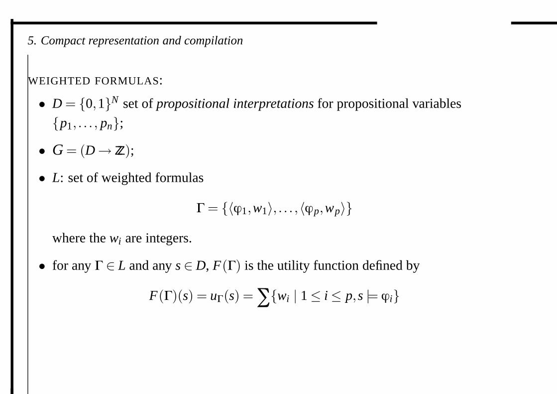
WEIGHTED FORMULAS:
• D = {0,1}N set of propositional interpretations for propositional variables
{p1, . . . , pn};• G = (D→ ZZ);
• L: set of weighted formulas
Γ = {〈ϕ1,w1〉, . . . ,〈ϕp,wp〉}
where the wi are integers.
• for any Γ ∈ L and any s ∈ D, F(Γ) is the utility function defined by
F(Γ)(s) = uΓ(s) =∑{wi | 1≤ i≤ p,s |= ϕi}
5. Compact representation and compilation
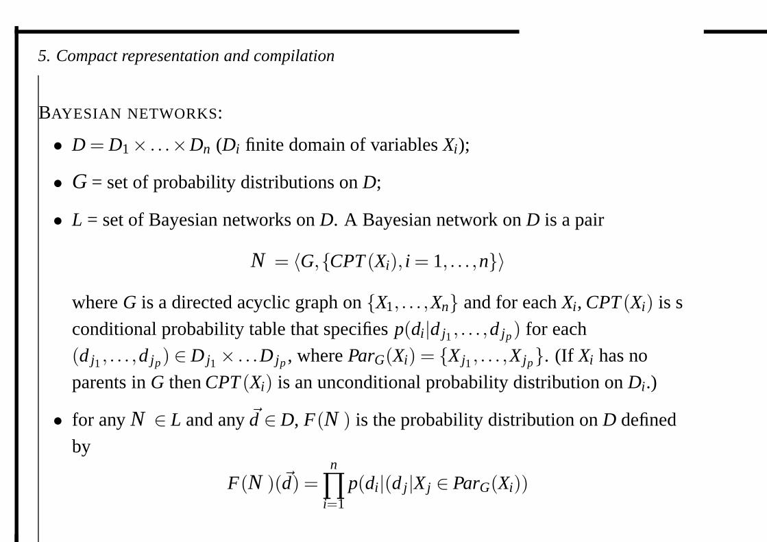
BAYESIAN NETWORKS:
• D = D1× . . .×Dn (Di finite domain of variables Xi);
• G = set of probability distributions on D;
• L = set of Bayesian networks on D. A Bayesian network on D is a pair
N = 〈G,{CPT (Xi), i = 1, . . . ,n}〉
where G is a directed acyclic graph on {X1, . . . ,Xn} and for each Xi, CPT (Xi) is s
conditional probability table that specifies p(di|d j1 , . . . ,d jp) for each
(d j1 , . . . ,d jp) ∈ Dj1 × . . .Djp , where ParG(Xi) = {Xj1 , . . . ,Xjp}. (If Xi has no
parents in G then CPT (Xi) is an unconditional probability distribution on Di.)
• for any N ∈ L and any �d ∈D, F(N ) is the probability distribution on D defined
by
F(N )(�d) =n
∏i=1
p(di|(d j|Xj ∈ ParG(Xi))
5. Compact representation and compilation
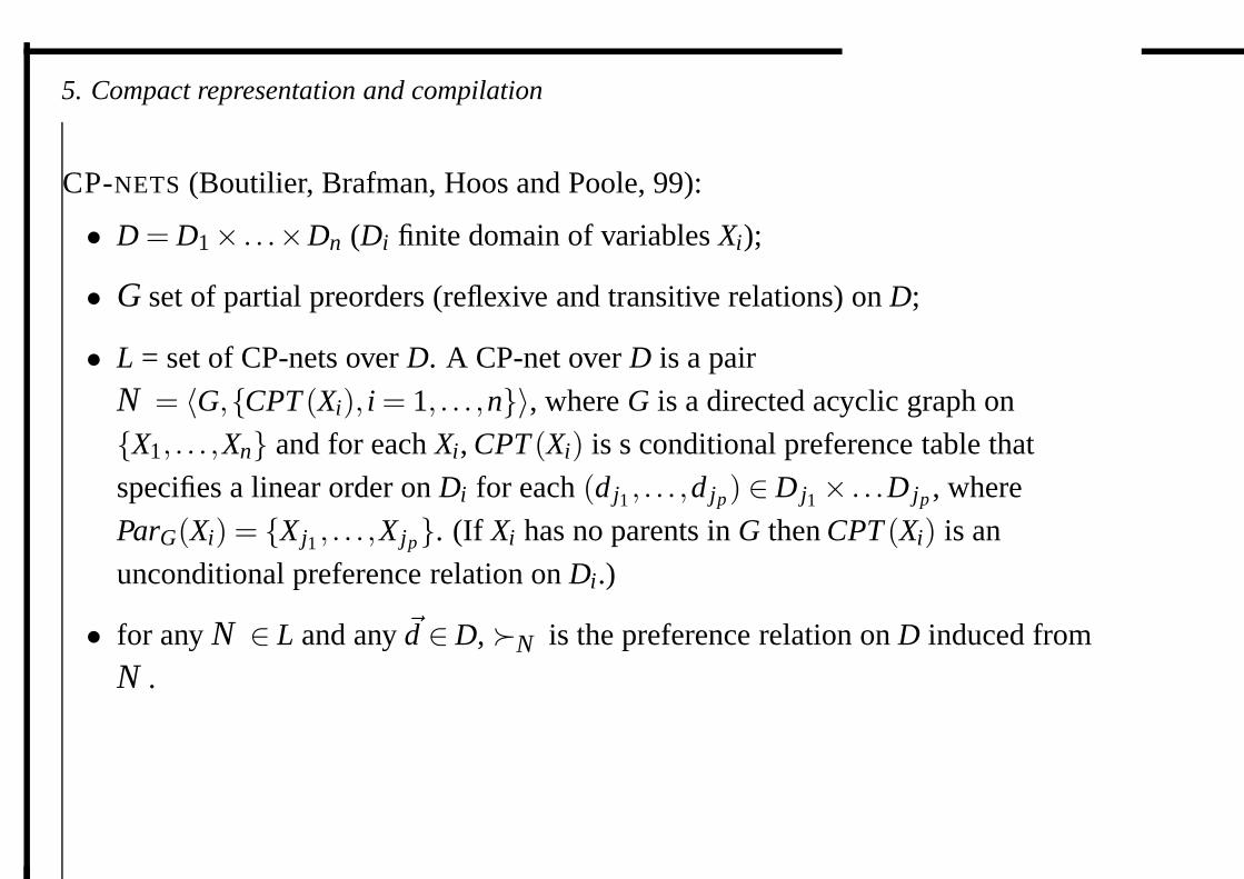
CP-NETS (Boutilier, Brafman, Hoos and Poole, 99):
• D = D1× . . .×Dn (Di finite domain of variables Xi);
• G set of partial preorders (reflexive and transitive relations) on D;
• L = set of CP-nets over D. A CP-net over D is a pair
N = 〈G,{CPT (Xi), i = 1, . . . ,n}〉, where G is a directed acyclic graph on
{X1, . . . ,Xn} and for each Xi, CPT (Xi) is s conditional preference table that
specifies a linear order on Di for each (dj1 , . . . ,d jp) ∈ Dj1 × . . .Djp , where
ParG(Xi) = {Xj1 , . . . ,Xjp}. (If Xi has no parents in G then CPT (Xi) is an
unconditional preference relation on Di.)
• for any N ∈ L and any �d ∈D, �N is the preference relation on D induced from
N .
CP-nets: example
X Y Z
x� xx : y� y
x : y� y
x∨ y : z� z
¬(x∨ y) : z� z
x : y� y
∣∣∣∣∣∣if X = x
then Y = y preferred to Y = y
everything else (z) being equal (ceteris paribus)
xyz� xyz; xyz� xyz;
xyz� xyz; xyz� xyz
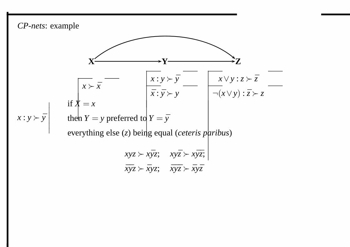
CP-nets: example
X Y Z
x� xx : y� y
x : y� y
x∨ y : z� z
¬(x∨ y) : z� z
�X : xyz� xyz, xyz� xyz, xyz� xyz, xyz� xyz
�Y : xyz� xyz, xyz� xyz, xyz� xyz, xyz� xyz
�Z : xyz� xyz, xyz� xyz, xyz� xyz, xyz� xyz
�C = transitive closure of �X ∪ �Y ∪ �Z
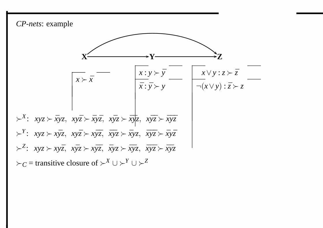
CP-nets: example
X Y Z
x� xx : y� y
x : y� y
x∨ y : z� z
¬(x∨ y) : z� z
�: xyz↗↘
xyz
xyz
↘↗
xyz→ xyz→ xyz→ xyz→ xyz
5. Compact representation and compilation
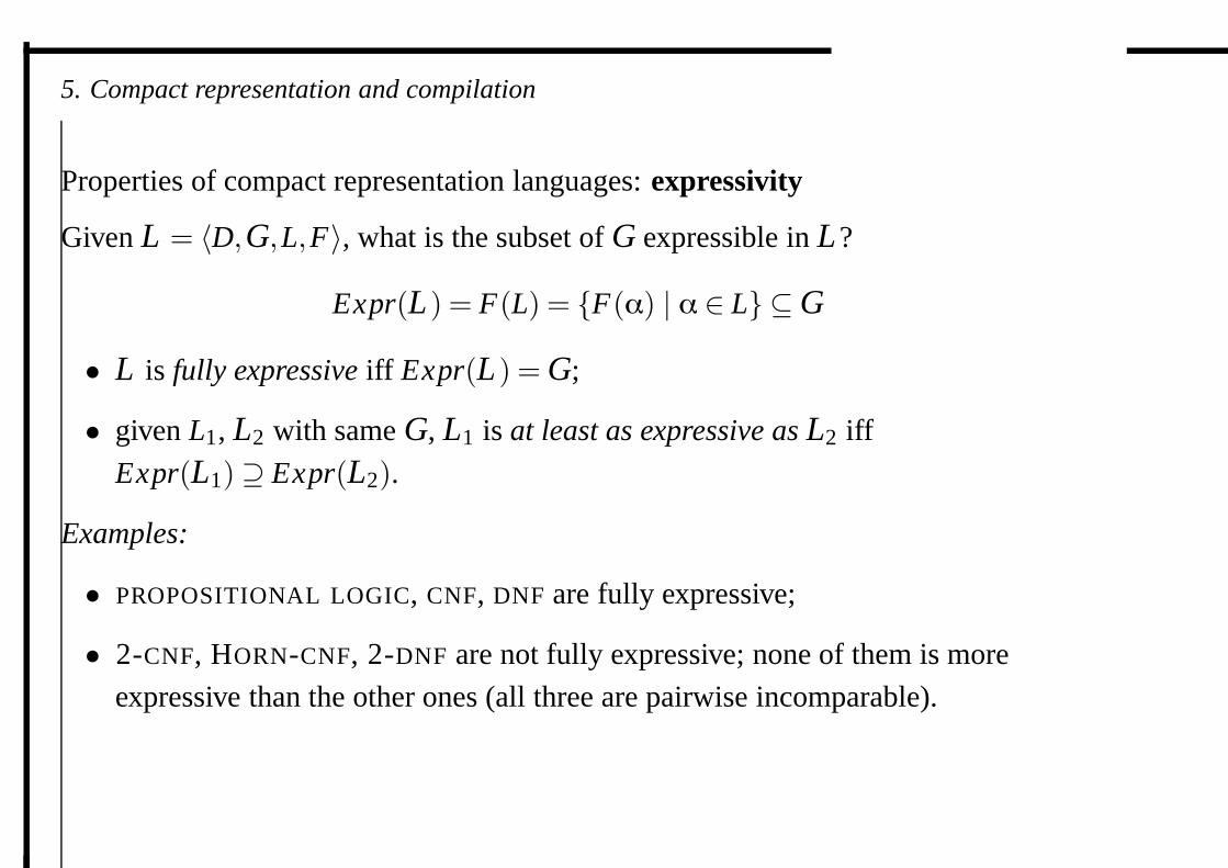
Properties of compact representation languages: expressivity
Given L = 〈D,G ,L,F〉, what is the subset of G expressible in L?
Expr(L) = F(L) = {F(α) | α ∈ L} ⊆ G
• L is fully expressive iff Expr(L) = G ;
• given L1, L2 with same G , L1 is at least as expressive as L2 iff
Expr(L1)⊇ Expr(L2).
Examples:
• PROPOSITIONAL LOGIC, CNF, DNF are fully expressive;
• 2-CNF, HORN-CNF, 2-DNF are not fully expressive; none of them is more
expressive than the other ones (all three are pairwise incomparable).
5. Compact representation and compilation
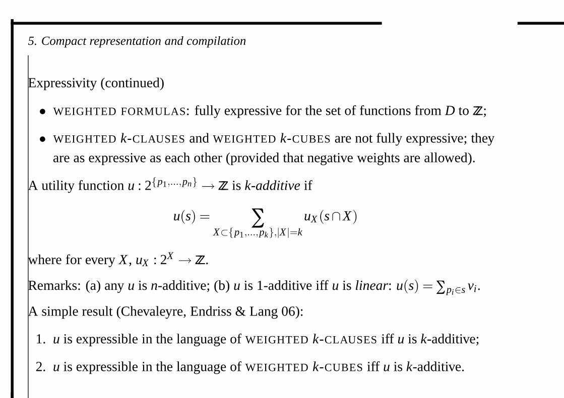
Expressivity (continued)
• WEIGHTED FORMULAS: fully expressive for the set of functions from D to ZZ;
• WEIGHTED k-CLAUSES and WEIGHTED k-CUBES are not fully expressive; they
are as expressive as each other (provided that negative weights are allowed).
A utility function u : 2{p1,...,pn} → ZZ is k-additive if
u(s) = ∑X⊂{p1,...,pk},|X |=k
uX (s∩X)
where for every X , uX : 2X → ZZ.
Remarks: (a) any u is n-additive; (b) u is 1-additive iff u is linear: u(s) =∑pi∈s vi.
A simple result (Chevaleyre, Endriss & Lang 06):
1. u is expressible in the language of WEIGHTED k-CLAUSES iff u is k-additive;
2. u is expressible in the language of WEIGHTED k-CUBES iff u is k-additive.
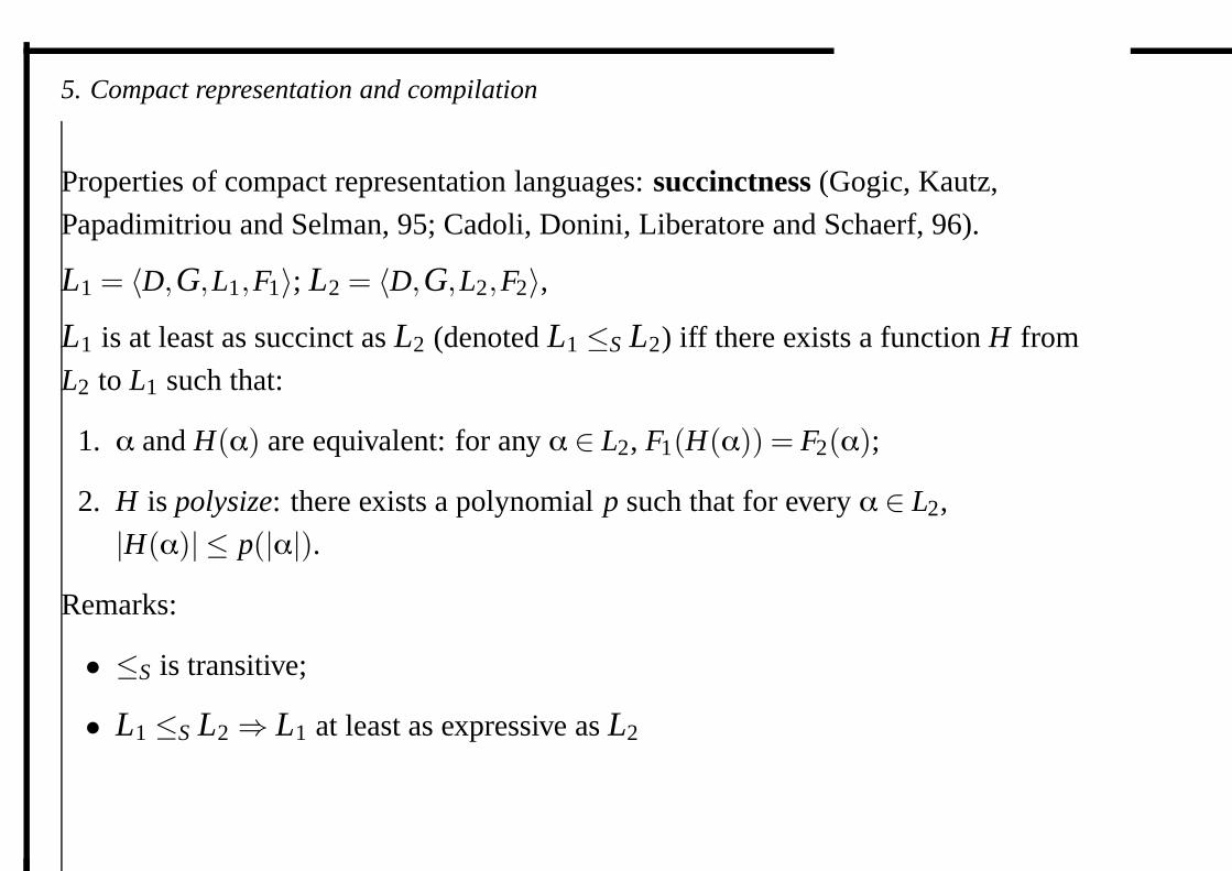
5. Compact representation and compilation
Properties of compact representation languages: succinctness (Gogic, Kautz,
Papadimitriou and Selman, 95; Cadoli, Donini, Liberatore and Schaerf, 96).
L1 = 〈D,G ,L1,F1〉; L2 = 〈D,G ,L2,F2〉,L1 is at least as succinct as L2 (denoted L1 ≤S L2) iff there exists a function H from
L2 to L1 such that:
1. α and H(α) are equivalent: for any α ∈ L2, F1(H(α)) = F2(α);
2. H is polysize: there exists a polynomial p such that for every α ∈ L2,
|H(α)| ≤ p(|α|).Remarks:
• ≤S is transitive;
• L1 ≤S L2 ⇒ L1 at least as expressive as L2
5. Compact representation and compilation
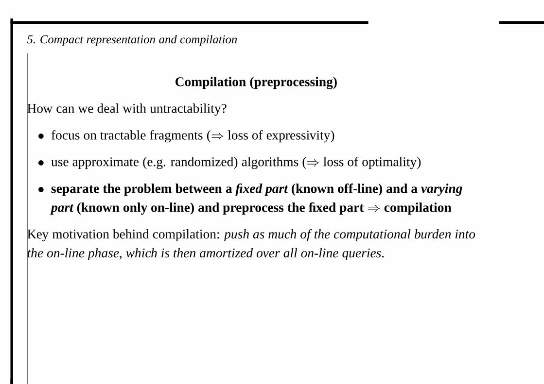
Compilation (preprocessing)
How can we deal with untractability?
• focus on tractable fragments (⇒ loss of expressivity)
• use approximate (e.g. randomized) algorithms (⇒ loss of optimality)
• separate the problem between a fixed part (known off-line) and a varyingpart (known only on-line) and preprocess the fixed part⇒ compilation
Key motivation behind compilation: push as much of the computational burden into
the on-line phase, which is then amortized over all on-line queries.
5. Compact representation and compilation
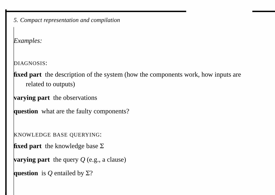
Examples:
DIAGNOSIS:
fixed part the description of the system (how the components work, how inputs are
related to outputs)
varying part the observations
question what are the faulty components?
KNOWLEDGE BASE QUERYING:
fixed part the knowledge base Σ
varying part the query Q (e.g., a clause)
question is Q entailed by Σ?
5. Compact representation and compilation
Knowledge compilation (Darwiche and Marquis, 02)
The rest of this talk is based on the following paper:
A. Darwiche and P. Marquis. A knowledge compilation map. Journal of Artificial
Intelligence Research 17 (2002), 229-264.
Propositional reasoning is intractable⇒ proprocessing (when possible) is a goodidea.
Problem: find an efficient target language into which the propositional knowledgebase Σ will be compiled.
Criteria for evaluating a target language:
1. its succinctness;
2. the class of queries that can be answered in polynomial time;
3. the class of transformations that can be applied to the representation inpolynomial time.
5. Compact representation and compilation
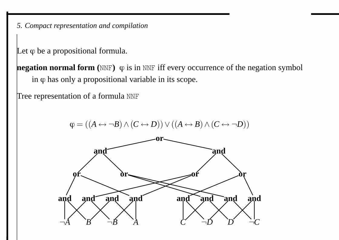
Let ϕ be a propositional formula.
negation normal form (NNF) ϕ is in NNF iff every occurrence of the negation symbol
in ϕ has only a propositional variable in its scope.
Tree representation of a formula NNF
ϕ = ((A↔¬B)∧ (C↔ D))∨ ((A↔ B)∧ (C↔¬D))
or
and and
or or or or
and and and and and and and and
¬A B ¬B A C ¬D D ¬C
5. Compact representation and compilation
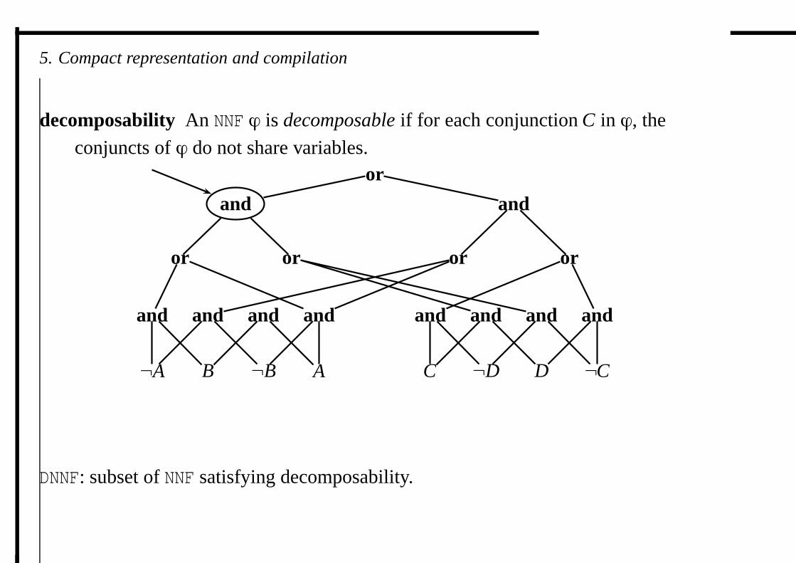
decomposability An NNF ϕ is decomposable if for each conjunction C in ϕ, the
conjuncts of ϕ do not share variables.or
and and
or or or or
and and and and and and and and
¬A B ¬B A C ¬D D ¬C
DNNF: subset of NNF satisfying decomposability.
5. Compact representation and compilation
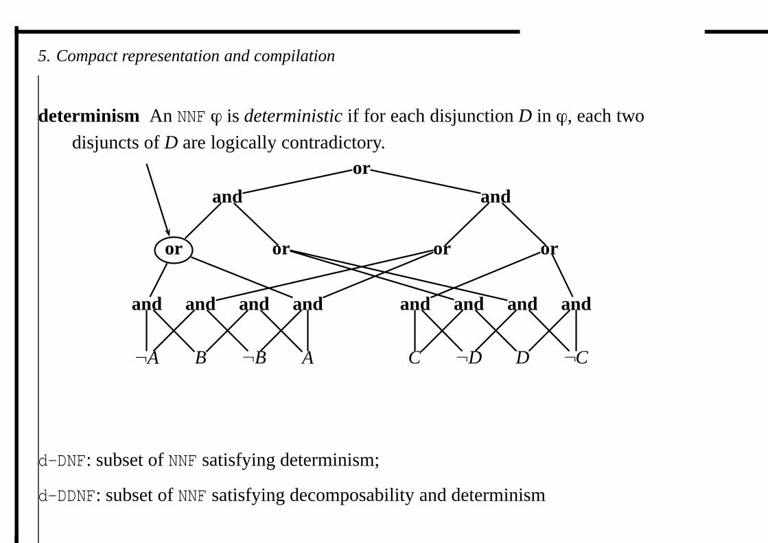
determinism An NNF ϕ is deterministic if for each disjunction D in ϕ, each two
disjuncts of D are logically contradictory.or
and and
or or or or
and and and and and and and and
¬A B ¬B A C ¬D D ¬C
d-DNF: subset of NNF satisfying determinism;
d-DDNF: subset of NNF satisfying decomposability and determinism
5. Compact representation and compilation
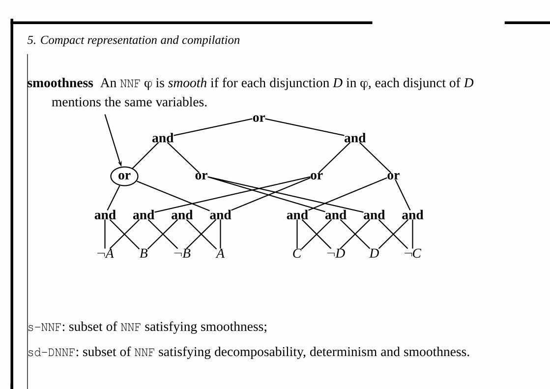
smoothness An NNF ϕ is smooth if for each disjunction D in ϕ, each disjunct of D
mentions the same variables.or
and and
or or or or
and and and and and and and and
¬A B ¬B A C ¬D D ¬C
s-NNF: subset of NNF satisfying smoothness;
sd-DNNF: subset of NNF satisfying decomposability, determinism and smoothness.
5. Compact representation and compilation
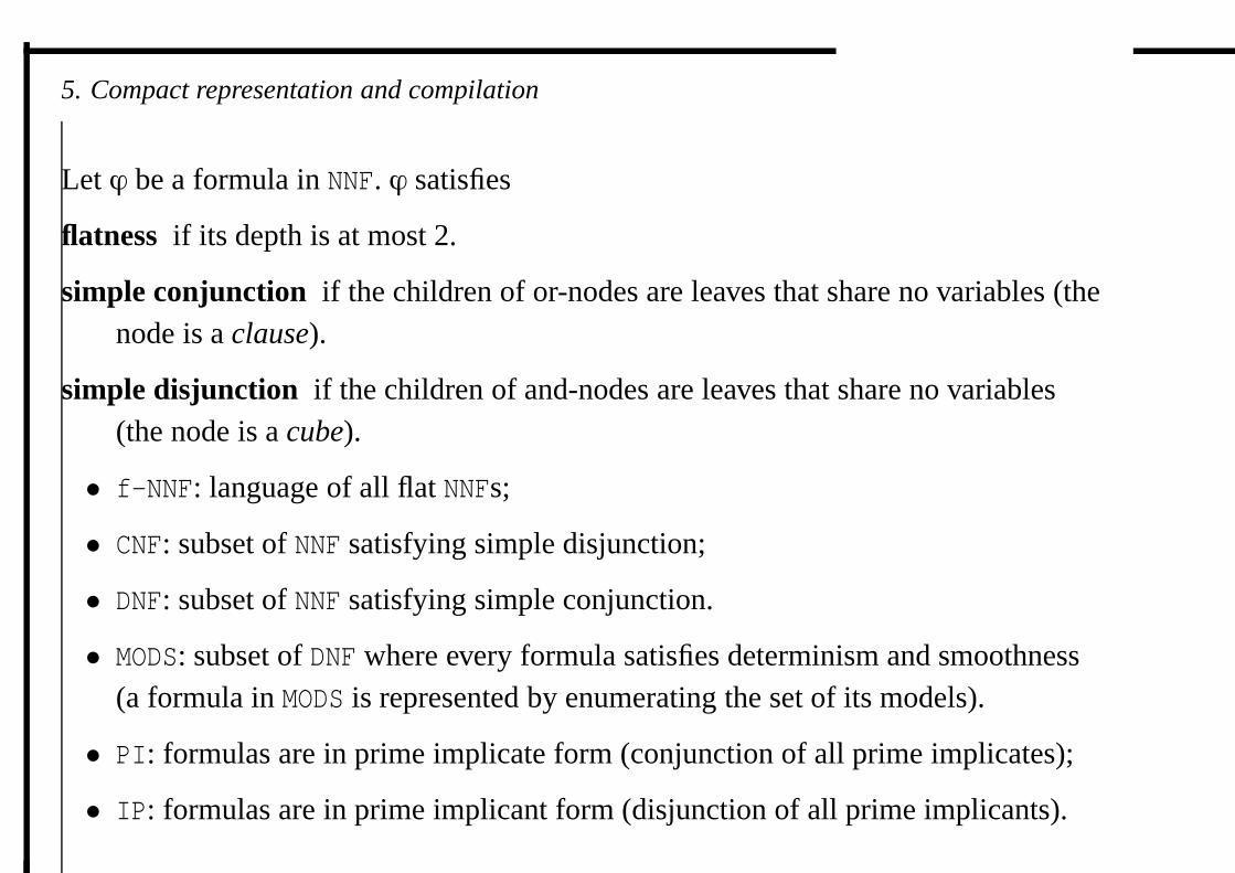
Let ϕ be a formula in NNF. ϕ satisfies
flatness if its depth is at most 2.
simple conjunction if the children of or-nodes are leaves that share no variables (thenode is a clause).
simple disjunction if the children of and-nodes are leaves that share no variables(the node is a cube).
• f-NNF: language of all flat NNFs;
• CNF: subset of NNF satisfying simple disjunction;
• DNF: subset of NNF satisfying simple conjunction.
• MODS: subset of DNF where every formula satisfies determinism and smoothness(a formula in MODS is represented by enumerating the set of its models).
• PI: formulas are in prime implicate form (conjunction of all prime implicates);
• IP: formulas are in prime implicant form (disjunction of all prime implicants).
5. Compact representation and compilation
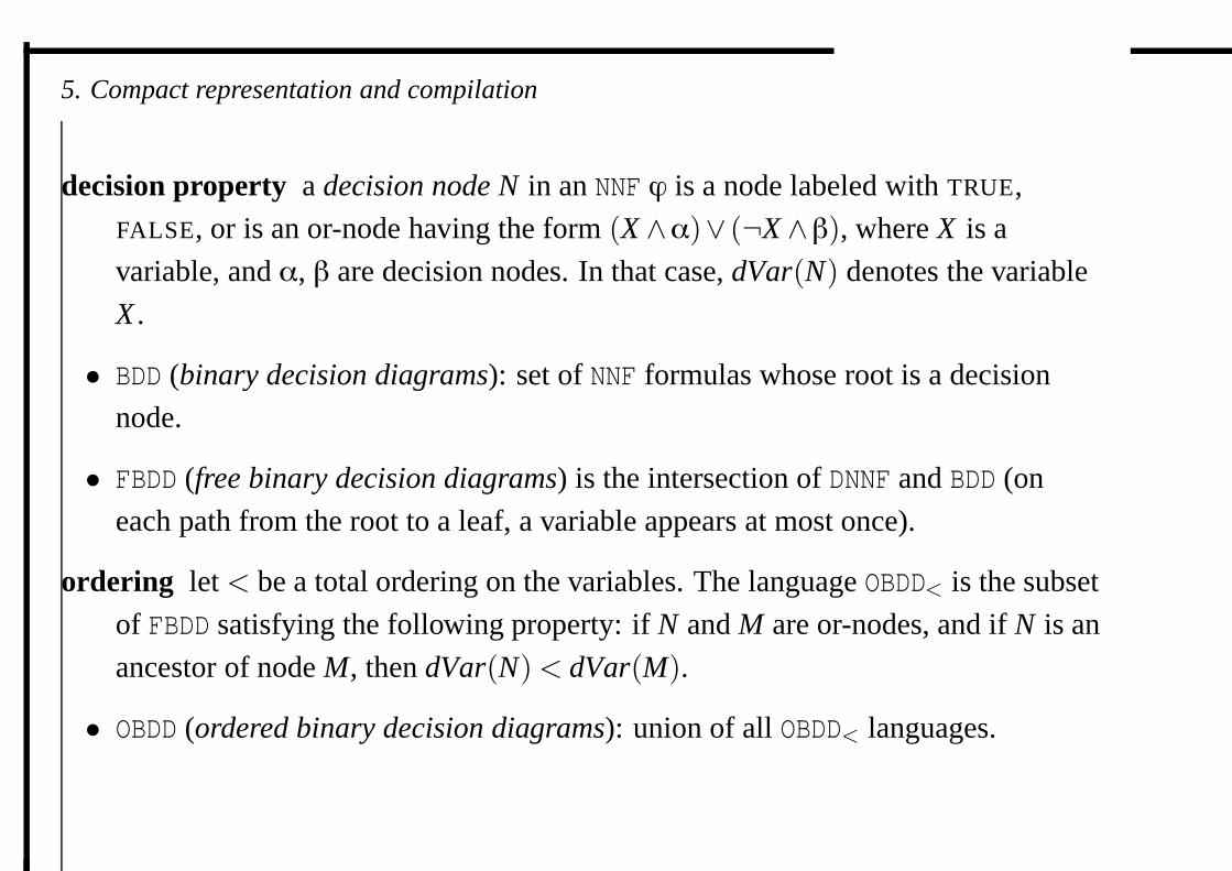
decision property a decision node N in an NNF ϕ is a node labeled with TRUE,
FALSE, or is an or-node having the form (X ∧α)∨ (¬X ∧β), where X is a
variable, and α, β are decision nodes. In that case, dVar(N) denotes the variable
X .
• BDD (binary decision diagrams): set of NNF formulas whose root is a decision
node.
• FBDD (free binary decision diagrams) is the intersection of DNNF and BDD (on
each path from the root to a leaf, a variable appears at most once).
ordering let < be a total ordering on the variables. The language OBDD< is the subset
of FBDD satisfying the following property: if N and M are or-nodes, and if N is an
ancestor of node M, then dVar(N) < dVar(M).
• OBDD (ordered binary decision diagrams): union of all OBDD< languages.
5. Compact representation and compilation
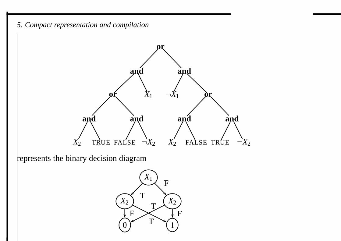
or
and and
or X1 ¬X1 or
and and and and
X2 TRUE FALSE ¬X2 X2 FALSE TRUE ¬X2
represents the binary decision diagram
X1
X2 X2
0 1
T
F
FT
TF
5. Compact representation and compilation
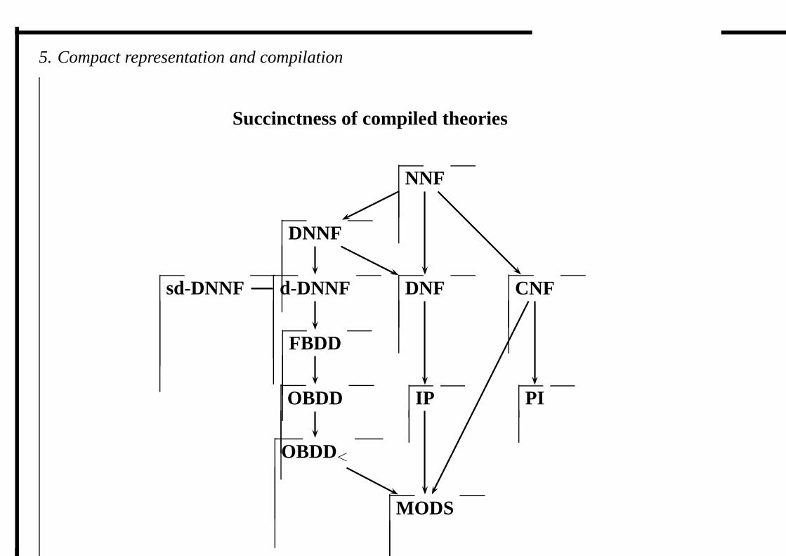
Succinctness of compiled theories
MODS
OBDD<
OBDD
FBDD
d-DNNF
DNNF
sd-DNNF
NNF
IP
DNF
PI
CNF
5. Compact representation and compilation
An example of proof:
Proposition: CNF and DNF are not at least as succinct as OBDD.
Sketch of proof: On =⊕n
i=0 xi parity function. On has a linear-size OBDD
representation but any CNF and any DNF representation of On is exponentially large.
5. Compact representation and compilation
Another example of proof:
Proposition: DNNF is not at least as succinct as CNF, unless the polynomial hierarchy
collapses at the second level.
Sketch of proof: consequence of these two lemmas:
Lemma 1 (Cadoli and Donini, 97; Selman and Kautz, 96). If there exists a polysize
compilation function F mapping CNF formulas to propositional formulas such that (a)
for any clause C and for any CNF α, α |= C iff F(α) |= C, and (b) checking whether
F(α) |= C is in P, then the polynomial hierarchy collapses at the second level.
Lemma 2 (Darwiche 99): clausal entailment in DNNF is in P.
5. Compact representation and compilation
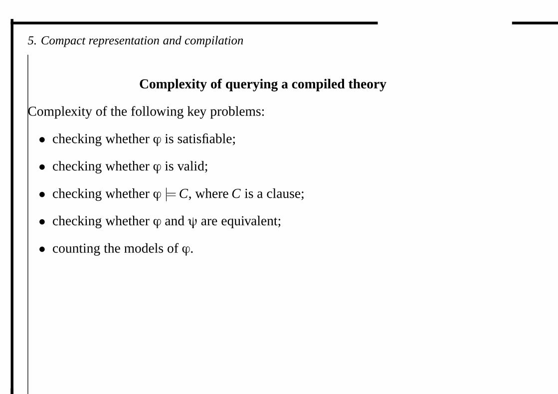
Complexity of querying a compiled theory
Complexity of the following key problems:
• checking whether ϕ is satisfiable;
• checking whether ϕ is valid;
• checking whether ϕ |= C, where C is a clause;
• checking whether ϕ and ψ are equivalent;
• counting the models of ϕ.
5. Compact representation and compilation
MODS
OBDD<
OBDD
FBDD
d-DNNF
DNNF
sd-DNNF
NNF
IP
DNF
PI
CNF
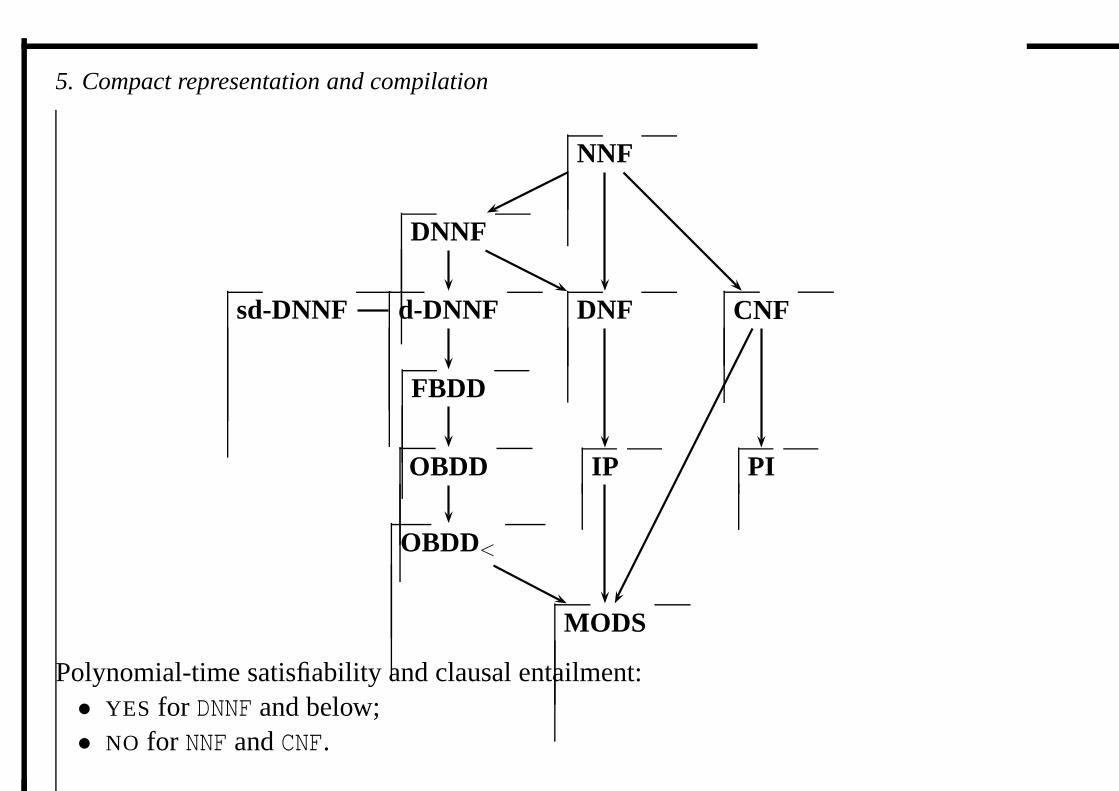
Polynomial-time satisfiability and clausal entailment:• YES for DNNF and below;• NO for NNF and CNF.
5. Compact representation and compilation
MODS
OBDD<
OBDD
FBDD
d-DNNF
DNNF
sd-DNNF
NNF
IP
DNF
PI
CNF
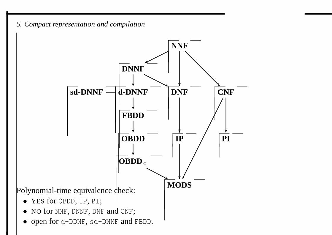
Polynomial-time equivalence check:• YES for OBDD, IP, PI;• NO for NNF, DNNF, DNF and CNF;• open for d-DDNF, sd-DNNF and FBDD.
5. Compact representation and compilation
MODS
OBDD<
OBDD
FBDD
d-DNNF
DNNF
sd-DNNF
NNF
IP
DNF
PI
CNF
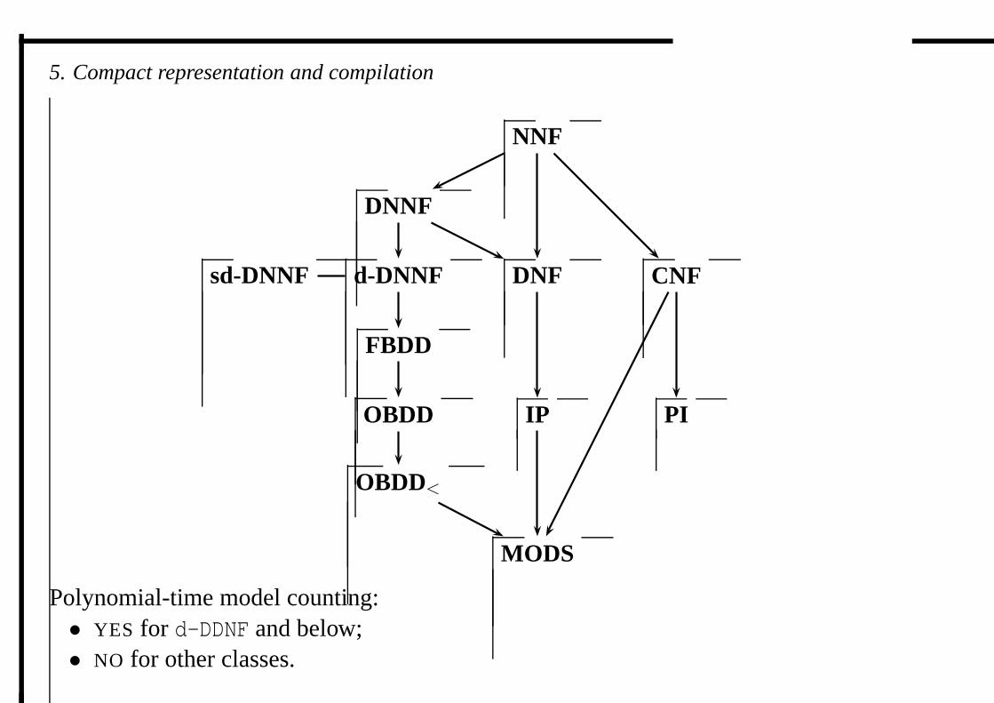
Polynomial-time model counting:• YES for d-DDNF and below;• NO for other classes.
5. Compact representation and compilation
Complexity of transforming a compiled theory
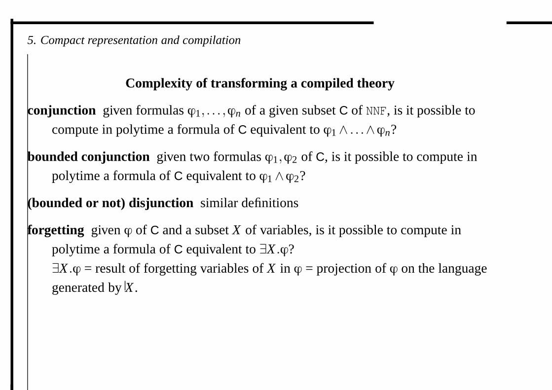
conjunction given formulas ϕ1, . . . ,ϕn of a given subset C of NNF, is it possible to
compute in polytime a formula of C equivalent to ϕ1∧ . . .∧ϕn?
bounded conjunction given two formulas ϕ1,ϕ2 of C, is it possible to compute in
polytime a formula of C equivalent to ϕ1∧ϕ2?
(bounded or not) disjunction similar definitions
forgetting given ϕ of C and a subset X of variables, is it possible to compute in
polytime a formula of C equivalent to ∃X .ϕ?
∃X .ϕ = result of forgetting variables of X in ϕ = projection of ϕ on the language
generated by X .
5. Compact representation and compilation
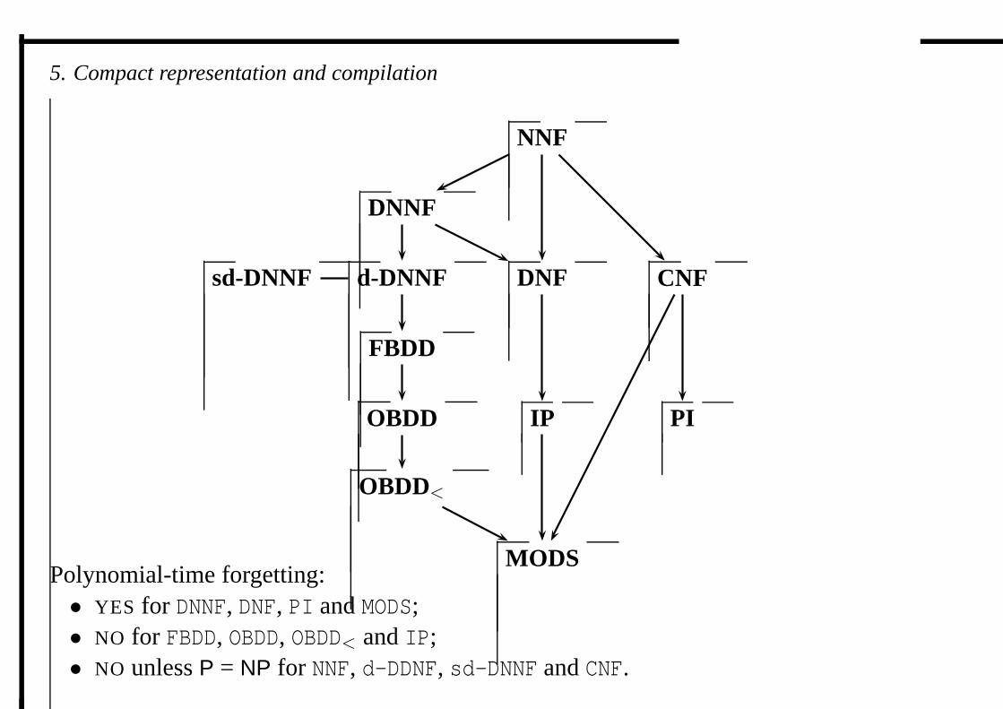
MODS
OBDD<
OBDD
FBDD
d-DNNF
DNNF
sd-DNNF
NNF
IP
DNF
PI
CNF
Polynomial-time forgetting:• YES for DNNF, DNF, PI and MODS;• NO for FBDD, OBDD, OBDD< and IP;• NO unless P = NP for NNF, d-DDNF, sd-DNNF and CNF.