compressing fingerprint templates by solving the k-node ... · compressing fingerprint templates by...
TRANSCRIPT
Compressing Fingerprint Templates by Solving thek-Node Minimum Label Spanning Arborescence
Problem by Branch-and-Price
DIPLOMARBEIT
zur Erlangung des akademischen Grades
Diplom-Ingenieurin
im Rahmen des Studiums
Software Engineering / Internet Computing (066/937)
eingereicht von
Corinna Thoni, BSc.
Matrikelnummer 9826437
an derFakultat fur Informatik der Technischen Universitat WienInstitut fur Computergrafik und Algorithmen
Betreuung:Univ.-Prof. Dipl.-Ing. Dr. techn. Gunther RaidlUniv.Ass. Mag. Dipl.-Ing. Andreas Chwatal
Wien, 05.02.2010(Unterschrift Verfasserin) (Unterschrift Betreuer)
Technische Universitat WienA-1040 Wien Karlsplatz 13 Tel. +43/(0)1/58801-0 http://www.tuwien.ac.at

Compressing Fingerprint Templates by Solving
the k-Node Minimum Label Spanning
Arborescence Problem by Branch-and-Price
MASTER’S THESIS
written at the
Institute for Computer Graphics and Algorithms
Vienna University of Technology
under supervision of
Univ.-Prof. Dipl.-Ing. Dr. techn. Gunther Raidl
Univ.Ass. Mag. Dipl.-Ing. Andreas Chwatal
by
Corinna Thoni, BSc.
Software Engineering / Internet Computing (066/937), 9826437
Vienna, 05.02.2010

Abstract
This thesis deals with the development of exact algorithms based on mathematical programmingtechniques for the solution of a combinatorial optimization problem which emerged in the contextof a new compression model recently developed at the Algorithms and Data Structures Group ofthe Institute of Computer Graphics and Algorithms at the Vienna University of Technology. Thiscompression model is particularly suited for small sets of unordered and multidimensional datahaving its application background in the field of biometrics. More precisely, fingerprint data givenas a set of characteristic points and associated properties should be compressed in order to be usedas an additional security feature for e.g. passports by embedding the data into passport imagesby watermarking techniques.
The considered model is based on the well known Minimum Label Spanning Tree Problem(MLST) with the objective to find a small set of labels, associated to the edges of the graph,inducing a valid spanning tree. Based on this solution an encoding of the considered points beingmore compact than their trivial representation can be derived. So far, heuristic and exact algo-rithms have been developed, all of them requiring a time-consuming preprocessing step. The goalof this work is to develop an improved exact algorithm carrying out the tasks of the preprocessingalgorithm during the execution of the exact methods in an profitable way.
Within this thesis the problem is solved by mixed integer programming techniques. For thispurpose a new flow formulation is presented which can be directly solved by linear programmingbased branch-and-bound, or alternatively by branch-and-price, being the main approach of thisthesis. Branch-and-price works by starting with a restricted model, and then iteratively addingnew variables potentially improving the objective function value. These variables are determinedwithin the pricing problem which has to be solved frequently during the overall solution process.For this purpose specialized data structures and algorithms, based on a k-d tree are used, with theintention to exploit possible structures of the input data. Within this tree, improving variables canbe found by various traversing and bounding techniques. These algorithms can also be adaptedin order to work as an alternative to the existing preprocessing.
All algorithms have been implemented and comprehensively tested. For the existing ap-proaches, the new methods reduced the preprocessing run times with a factor of 50 and usenow 2% of the original run times. With the presented branch-and-price approach it is possible tosolve a greater amount of test instances to optimality than previously. Generally, for most modelparameters the branch-and-price approach outperforms the previous exact method.
i
Zusammenfassung
Diese Diplomarbeit beschaftigt sich mit der Entwicklung von exakten Algorithmen, welche aufmathematischer Programmierung basieren. Ziel ist die Losung eines kombinatorischen Optimie-rungsproblems, welches im Kontext eines neuen Komprimierungsverfahren auftritt, das kurzlichvom Arbeitsbereich fur Algorithmen und Datenstrukturen des Institut fur Computergraphik undAlgorithmen an der Technischen Universitat Wien entwickelt wurde. Dieses Komprimierungsver-fahren ist insbesondere geeignet fur kleine Mengen von ungeordneten und multidimensionalenDaten, wobei biometrische Applikationen den Anwendungshintergrund bilden. Insbesondere sol-len Fingerabdruckdaten, sogenannte Minutien, gegeben als Menge charakteristischer Punkte mitzugeordneten Eigenschaften, komprimiert werden, um als zusatzliches Sicherheitsmerkmal fur z.B.Reisepasse verwendet werden zu konnen, indem die Daten als Wasserzeichen in das Passbild ein-gebettet werden.
Das betrachtete Modell basiert auf dem bekannten Minimum Label Spanning Tree Problem(MLST). Das Ziel des Problems ist es, eine kleine Menge an Labels zu finden, welche den Kantendes Graphen zugeordnet sind und so einen gultigen Spannbaum induzieren. Basierend auf dieserLosung kann eine Kodierung der betrachteten Punkte abgeleitet werden, welche kompakter als ihretriviale Darstellung ist. Bislang wurden Heuristiken und ein exaktes Verfahren entwickelt, welchealle einen laufzeitintensiven Preprocessing-Schritt voraussetzen. Das Ziel dieser Arbeit ist es, einenverbesserten exakten Algorithmus zu entwickeln, welcher die Aufgaben des Preprocessing-Schrittsin einer vorteilhaften Weise wahrend der Ausfuhrung der exakten Methode erledigt.
In dieser Arbeit wurde das Problem mit Mixed Integer Programmierungstechniken gelost. Zudiesem Zweck wird eine neue Flußnetzwerk Formulierung vorgestellt, welche direkt mittels Branch-and-Bound, basierend auf Linearer Programmierung, gelost werden kann. Alternativ dazu gelingtdie Losung auch mittels Branch-and-Price, welches den Hauptansatz darstellt. Branch-and-Pricebeginnt mit einem reduzierten Problem und fugt dann schrittweise neue Variablen, welche denZielfunktionswert verbessern konnen, diesem reduzierten Problem hinzu. Diese Variablen werdenmittels des Pricing Problems bestimmt, welches oftmals wahrend des Losungsvorgangs berechnetwerden muss. Zu diesem Zweck wurden spezialisierte, auf einem k-d Tree basierende Datenstruk-turen und Algorithmen entwickelt, welche mogliche Strukturen der Eingabedaten in geschickterWeise ausnutzen. Mittels verschiedener Traversierungs- und Boundingtechniken konnen aus dieserBaumdatenstruktur verbessernde Variablen effizient extrahiert werden. Weiters konnen die entwi-ckelten Algorithmen zu einer Alternative fur den Preprocessing-Schritt adaptiert werden.
Alle Algorithmen wurden implementiert und umfangreich getestet. Fur die bestehenden Ansatzewurde die Zeit, die fur den ursprunglichen Vorberechnungsschritt gebraucht wurde, um Faktor 50reduziert, die Laufzeiten sinken auf 2% der ursprunglichen Zeit. Mit dem vorgestellten Branch-and-Price Verfahren ist es moglich eine großere Anzahl an Testinstanzen optimal zu losen alsbisher. Fur die meisten Modellparameter ubertrifft der Branch-and-Price Ansatz die bisherigeexakte Methode.
ii

Acknowledgements
Ich mochte allen Personen danken, die mir den Abschluß dieser Diplomarbeit ermoglicht haben.Ich danke meinen Eltern Robert und Johanna sowie meinem Bruder Rudolf, die viel Geduld undVerstandnis fur mich aufgebracht und mich immer wieder zum Weitermachen motiviert haben.Ich danke Dieter, der mich in Allem unterstutzt und bekraftigt hat.Danke an Andreas Chwatal, dessen exzellente fachliche Kompetenz und unendliche Geduld dieseArbeit moglich gemacht haben. Danke an Gunther Raidl fur die großartigen Ideen und die vieleUnterstutzung. Danke an den gesamten Fachbereich fur Algorithmen und Datenstrukturen fur diegute technische Infrastruktur.
iii

Erklarung zur Verfassung
Hiermit erklare ich, dass ich diese Arbeit selbstandig verfasst habe, dass ich die verwendeten Quel-len und Hilfsmittel vollstandig angegeben habe und dass ich die Stellen der Arbeit, einschließlichTabellen, Karten und Abbildungen, die anderen Werken oder dem Internet im Wortlaut oder demSinn nach entnommen sind, auf jeden Fall unter Angabe der Quelle als Entlehnung kenntlich ge-macht habe.
Wien, 05.02.2010
iv
Contents
Abstract . . . . . . . . . . . . . . . . . . . . . . . . . . . . . . . . . . . . . . . . . . . . . iZusammenfassung . . . . . . . . . . . . . . . . . . . . . . . . . . . . . . . . . . . . . . . iiAcknowledgements . . . . . . . . . . . . . . . . . . . . . . . . . . . . . . . . . . . . . . . iii
1 Introduction 11.1 Biometric Background . . . . . . . . . . . . . . . . . . . . . . . . . . . . . . . . . . 2
1.1.1 Dactyloscopy . . . . . . . . . . . . . . . . . . . . . . . . . . . . . . . . . . . 31.1.2 Digital Watermarking, Steganography and Compression . . . . . . . . . . . 4
1.2 Previous Work . . . . . . . . . . . . . . . . . . . . . . . . . . . . . . . . . . . . . . 51.2.1 The Compression Model . . . . . . . . . . . . . . . . . . . . . . . . . . . . . 51.2.2 Determining the Codebook . . . . . . . . . . . . . . . . . . . . . . . . . . . 6
1.3 Contributions of this Thesis . . . . . . . . . . . . . . . . . . . . . . . . . . . . . . . 7
2 Graph Theory and Algorithmic Geometry Essentials 92.1 Graph Theory Basics . . . . . . . . . . . . . . . . . . . . . . . . . . . . . . . . . . . 9
2.1.1 Minimum Label Spanning Tree (MLST) . . . . . . . . . . . . . . . . . . . . 102.1.2 k-Cardinality Tree (k-CT) . . . . . . . . . . . . . . . . . . . . . . . . . . . . 102.1.3 k-node Minimum Label Spanning Arborescence (k-MLSA) . . . . . . . . . . 112.1.4 Flow networks . . . . . . . . . . . . . . . . . . . . . . . . . . . . . . . . . . 11
2.2 Algorithmic Graph Theory Essentials . . . . . . . . . . . . . . . . . . . . . . . . . . 122.3 Algorithmic Geometry . . . . . . . . . . . . . . . . . . . . . . . . . . . . . . . . . . 12
2.3.1 Binary Search Tree . . . . . . . . . . . . . . . . . . . . . . . . . . . . . . . . 122.3.2 2-d Tree and k-d Tree . . . . . . . . . . . . . . . . . . . . . . . . . . . . . . 12
3 Optimization Theory Essentials 153.1 History and Trivia . . . . . . . . . . . . . . . . . . . . . . . . . . . . . . . . . . . . 153.2 Introduction to Linear Optimization . . . . . . . . . . . . . . . . . . . . . . . . . . 16
3.2.1 Linear Programs . . . . . . . . . . . . . . . . . . . . . . . . . . . . . . . . . 163.2.2 Duality . . . . . . . . . . . . . . . . . . . . . . . . . . . . . . . . . . . . . . 173.2.3 Polyhedral Theory, Solvability and Degeneration . . . . . . . . . . . . . . . 18
3.2.3.1 Farkas’ Lemma . . . . . . . . . . . . . . . . . . . . . . . . . . . . . 193.2.4 Solution Methods for Linear Programs . . . . . . . . . . . . . . . . . . . . . 19
3.2.4.1 Geometric Method . . . . . . . . . . . . . . . . . . . . . . . . . . . 203.2.4.2 Simplex Algorithm . . . . . . . . . . . . . . . . . . . . . . . . . . . 203.2.4.3 Nonlinear Optimization Techniques . . . . . . . . . . . . . . . . . 21
3.3 Integer Optimization . . . . . . . . . . . . . . . . . . . . . . . . . . . . . . . . . . . 213.3.1 Introduction . . . . . . . . . . . . . . . . . . . . . . . . . . . . . . . . . . . 213.3.2 Relaxation . . . . . . . . . . . . . . . . . . . . . . . . . . . . . . . . . . . . 223.3.3 Exact Solution Methods for Integer Programs . . . . . . . . . . . . . . . . . 23
3.3.3.1 Branch-and-Bound . . . . . . . . . . . . . . . . . . . . . . . . . . . 233.3.3.2 Cutting Planes . . . . . . . . . . . . . . . . . . . . . . . . . . . . . 243.3.3.3 Branch-and-Cut . . . . . . . . . . . . . . . . . . . . . . . . . . . . 243.3.3.4 Column Generation . . . . . . . . . . . . . . . . . . . . . . . . . . 25
v
Contents Contents
3.3.3.5 Branch-and-Price . . . . . . . . . . . . . . . . . . . . . . . . . . . 273.3.3.6 Branch-and-Cut-and-Price . . . . . . . . . . . . . . . . . . . . . . 28
3.4 Advanced Topics in Column Generation . . . . . . . . . . . . . . . . . . . . . . . . 283.4.1 Problem Formulation and Block Diagonal Structure . . . . . . . . . . . . . 283.4.2 Decomposition, Reformulation, Convexification, Discretization . . . . . . . 293.4.3 Set Covering, Set Partitioning and Set Packing Principles . . . . . . . . . . 293.4.4 The Restricted Master Problem (RMP) . . . . . . . . . . . . . . . . . . . . 31
3.4.4.1 Deducing an Initial Basis for the RMP . . . . . . . . . . . . . . . 313.4.5 Solution Methods for the RMP . . . . . . . . . . . . . . . . . . . . . . . . . 323.4.6 The Pricing Problem - Pricing Strategies . . . . . . . . . . . . . . . . . . . 32
3.4.6.1 Pricing Integer Programs . . . . . . . . . . . . . . . . . . . . . . . 333.4.7 The Tailing Off Effect . . . . . . . . . . . . . . . . . . . . . . . . . . . . . . 333.4.8 Integer Solutions . . . . . . . . . . . . . . . . . . . . . . . . . . . . . . . . . 34
3.4.8.1 Branch-and-Price and Branching Schemes . . . . . . . . . . . . . . 35
4 Formal Problem Definition 374.1 Compression Model . . . . . . . . . . . . . . . . . . . . . . . . . . . . . . . . . . . . 374.2 Previous Approach . . . . . . . . . . . . . . . . . . . . . . . . . . . . . . . . . . . . 38
4.2.1 Standard Template Arcs and Dominance . . . . . . . . . . . . . . . . . . . . 394.2.2 Preprocessing . . . . . . . . . . . . . . . . . . . . . . . . . . . . . . . . . . . 404.2.3 Solving the k-Node Minimum Label Arborescence Problem . . . . . . . . . 404.2.4 Directed Cut Formulation for Branch-and-Cut . . . . . . . . . . . . . . . . 41
5 Branch-and-Price 435.1 Formulating the k-MLSA for Branch-and-Price . . . . . . . . . . . . . . . . . . . . 435.2 Single Commodity Flow Formulation (SCF) for k-MLSA . . . . . . . . . . . . . . . 44
5.2.1 Node-Label Constraints . . . . . . . . . . . . . . . . . . . . . . . . . . . . . 455.3 Multi Commodity Flow Formulation (MCF) for k-MLSA . . . . . . . . . . . . . . 465.4 Branch-and-Price . . . . . . . . . . . . . . . . . . . . . . . . . . . . . . . . . . . . . 465.5 Pricing Problem . . . . . . . . . . . . . . . . . . . . . . . . . . . . . . . . . . . . . 475.6 Determining a Starting Solution . . . . . . . . . . . . . . . . . . . . . . . . . . . . 48
5.6.1 Trivial Starting Solution . . . . . . . . . . . . . . . . . . . . . . . . . . . . . 485.6.2 Farkas Pricing . . . . . . . . . . . . . . . . . . . . . . . . . . . . . . . . . . 48
5.7 Pricing Methods . . . . . . . . . . . . . . . . . . . . . . . . . . . . . . . . . . . . . 485.7.1 Standard and Multiple Pricing . . . . . . . . . . . . . . . . . . . . . . . . . 495.7.2 Allowing Variable Duplicates . . . . . . . . . . . . . . . . . . . . . . . . . . 495.7.3 Algorithms . . . . . . . . . . . . . . . . . . . . . . . . . . . . . . . . . . . . 49
6 Solving the Pricing Problem 516.1 Basic Ideas . . . . . . . . . . . . . . . . . . . . . . . . . . . . . . . . . . . . . . . . 51
6.1.1 Segmenting the Area by Means of a k-d Tree . . . . . . . . . . . . . . . . . 516.1.2 Extracting Template Vectors by Bounding . . . . . . . . . . . . . . . . . . . 536.1.3 Using the Segmentation as an Alternative to Preprocessing . . . . . . . . . 54
6.2 Segmentation Trees . . . . . . . . . . . . . . . . . . . . . . . . . . . . . . . . . . . . 556.3 Region Abstraction . . . . . . . . . . . . . . . . . . . . . . . . . . . . . . . . . . . . 556.4 The Static Segmentation Tree . . . . . . . . . . . . . . . . . . . . . . . . . . . . . . 56
6.4.1 Construction Main Algorithm . . . . . . . . . . . . . . . . . . . . . . . . . . 576.4.2 Static Insert Algorithm . . . . . . . . . . . . . . . . . . . . . . . . . . . . . 57
6.4.2.1 Algorithms . . . . . . . . . . . . . . . . . . . . . . . . . . . . . . . 616.4.3 Traversing the Static Segmentation Tree (Searching τ∗) . . . . . . . . . . . 64
6.4.3.1 Determining the Standard Template Arc . . . . . . . . . . . . . . 666.4.4 Upper Bounds for the Static Segmentation Tree . . . . . . . . . . . . . . . . 666.4.5 Simulating StaticTreeSearch-τ∗ . . . . . . . . . . . . . . . . . . . . . . . 66
6.5 The Dynamic Segmentation Tree . . . . . . . . . . . . . . . . . . . . . . . . . . . . 66
vi
Contents Contents
6.5.0.1 Algorithms . . . . . . . . . . . . . . . . . . . . . . . . . . . . . . . 686.5.1 Checking for Overlaps . . . . . . . . . . . . . . . . . . . . . . . . . . . . . . 706.5.2 Simulating DynamicInsertAndSearch-τ∗ . . . . . . . . . . . . . . . . . . . 72
6.6 Pricing Algorithms . . . . . . . . . . . . . . . . . . . . . . . . . . . . . . . . . . . . 736.6.0.1 Outlook . . . . . . . . . . . . . . . . . . . . . . . . . . . . . . . . . 74
7 Extracting T c from the Segmentation Tree 757.1 Overview . . . . . . . . . . . . . . . . . . . . . . . . . . . . . . . . . . . . . . . . . 75
7.1.0.2 Domination of Template Arc defining Bound Sets . . . . . . . . . 767.1.0.3 Domination of Subtrees . . . . . . . . . . . . . . . . . . . . . . . . 76
7.2 Traversing the Static Segmentation Tree . . . . . . . . . . . . . . . . . . . . . . . . 797.2.1 Best First Search for Determining T c . . . . . . . . . . . . . . . . . . . . . 797.2.2 UB-Driven Traversing for Determining T c . . . . . . . . . . . . . . . . . . . 807.2.3 Advanced Bounding Traversal for Determining T c . . . . . . . . . . . . . . 81
7.3 Traversing the Dynamic Segmentation Tree . . . . . . . . . . . . . . . . . . . . . . 817.3.1 UB-Driven Traversing for the Dynamic Segmentation Tree . . . . . . . . . 81
7.4 A Non-Dominated Segmentation Tree . . . . . . . . . . . . . . . . . . . . . . . . . 82
8 Implementation 858.1 Branch-and-Price Framework . . . . . . . . . . . . . . . . . . . . . . . . . . . . . . 858.2 Implementing SCF and MCF formulation in SCIP . . . . . . . . . . . . . . . . . . . 86
8.2.1 SCIP Plugins . . . . . . . . . . . . . . . . . . . . . . . . . . . . . . . . . . . 868.2.2 Module Structure . . . . . . . . . . . . . . . . . . . . . . . . . . . . . . . . . 87
9 Experimental Results 899.1 Input Data Files . . . . . . . . . . . . . . . . . . . . . . . . . . . . . . . . . . . . . 899.2 Static and Dynamic Segmentation . . . . . . . . . . . . . . . . . . . . . . . . . . . 91
9.2.1 Implications for the Pricing Algorithms . . . . . . . . . . . . . . . . . . . . 969.2.2 Implications for the Determination of T c . . . . . . . . . . . . . . . . . . . . 96
9.2.2.1 Memory Usage of the Segmentation Tree . . . . . . . . . . . . . . 1009.2.3 Simulating the Pricing Problem . . . . . . . . . . . . . . . . . . . . . . . . . 100
9.3 Branch-and-Price Results for Fraunhofer Data . . . . . . . . . . . . . . . . . . . . . 1009.3.1 Tested Parameters and Limits . . . . . . . . . . . . . . . . . . . . . . . . . . 1019.3.2 Branch-and-Cut Reference Run Times . . . . . . . . . . . . . . . . . . . . . 1019.3.3 Complete SCF and MCF Formulation . . . . . . . . . . . . . . . . . . . . . 1029.3.4 Static Tree Pricing Algorithm for SCF . . . . . . . . . . . . . . . . . . . . . 102
9.3.4.1 Results . . . . . . . . . . . . . . . . . . . . . . . . . . . . . . . . . 1049.3.5 Dynamic Tree Pricing Algorithm for SCF . . . . . . . . . . . . . . . . . . . 106
9.3.5.1 Results . . . . . . . . . . . . . . . . . . . . . . . . . . . . . . . . . 1069.3.6 Summary for Pricing Algorithms with Fraunhofer Data Tests . . . . . . . . 113
9.4 Percentage of Priced Variables . . . . . . . . . . . . . . . . . . . . . . . . . . . . . 1149.5 Branch-and-Price Results for NIST Data . . . . . . . . . . . . . . . . . . . . . . . . 116
9.5.1 Results . . . . . . . . . . . . . . . . . . . . . . . . . . . . . . . . . . . . . . 1179.6 Branch-and-Price Summary . . . . . . . . . . . . . . . . . . . . . . . . . . . . . . . 117
10 Conclusions 11910.1 Further Work . . . . . . . . . . . . . . . . . . . . . . . . . . . . . . . . . . . . . . . 121
Appendix 122
vii

Contents Contents
viii
Chapter 1
Introduction
The main goal of this diploma thesis is the compression of fingerprint data in such a way thatadditional encoded information can be stored in images by watermarking techniques. Applicationbackground is the use of such watermarks on identification cards and passports, to enhance thesecurity of the stored images (for example a fingerprint image) by embedding additional com-pressed information. In the case of identification cards and passports, only a very limited amountof storage is at disposal for this task, which implies the need of a compact representation and agood compression mechanism, that is capable of compressing as much data as much as possible ina reasonable amount of time, without loosing too much precision.
Various methods for compressing fingerprint data were analysed in the course of a researchproject at the Institute of Computer Graphics and Algorithms (Algorithms and Data StructuresGroup) at the Vienna University of Technology. The performance and compression ratios of theapproaches have been evaluated. While investigating common standard compression techniquesthe view fell upon dictionary based techniques. Thus, a special tree based compression model hasbeen developed in order to extract a dictionary from the fingerprint data and represent the featuresof a fingerprint through this dictionary. To name a few details, the extraction of the dictionaryrevealed itself to be accomplished through various approaches, which again are classified into twomain categories: algorithms that find approximate solutions for the dictionary and algorithmsproviding optimal dictionaries. Normally the former ones perform very fast but the quality ofthe result might not be sufficiently high, whereas the latter supply optimal results but requiresignificant computational effort. Amongst approximating algorithms heuristics and memetic algo-rithms have been evaluated. While developing an exact algorithm (e.g. branch-and-cut) this classof problem solving approaches was found to have great potential. This thesis pursues the ideas andmodelling approaches developed in [ChwRai09, Dietzel08]. In particular elaborate combinatorialoptimization techniques are investigated and applied to the given problem. The main contributionis the development of a branch-and-price approach, and algorithms for solving the correspondingpricing problem.
The following sections give an overview of the application background where the problememerges, which approaches were already examined and how the task is approached.
The document is segmented into two main parts: The first part includes a short introduction tothe topic (chapter 1) and covers the underlying theory. Chapter 2 is concerned with graph theoryand geometric algorithms, whereas chapter 3 covers linear and integer optimization and introducesthe central topics column generation and branch-and-price. The following chapter 4 contains adetailed formal problem definition. The second part is concerned with specific algorithms andtheir evaluation: It is structured into chapter 5, which explains the branch-and-price approachincluding the formulation as a flow network, and chapter 6, which describes developed conceptsand algorithms for solving the arising pricing problem. Chapter 7 introduces an alternative for the
1
1.1. Biometric Background Chapter 1. Introduction
intermediate step, called preprocessing, needed in all previously developed solution approaches.It is followed by chapter 8, where the implementation is outlined as well as architectural details,used programming language and the framework integrated for the solution of our problem. Thechapter 9 lists test methods as well as experimental results, and is followed by the chapter 10,where final conclusions are drawn. The appendix summarizes some often used terms and namingconventions and includes additional tables for experimental results.
1.1 Biometric Background
The central problem of this thesis comes from the field of biometric data processing. The term bio-metrics (Greek: Bio life, Metron measure) collects many procedures of measuring and analyzinghumans based on one or more physical and behavioral traits. Of the many fields of which biomet-rics is comprised in this diploma thesis the procedures of biometric recognition processing are ofinterest. The origins of biometrics are located in forensic sciences, dactyloscopy and cryptography.In the past decades, with the progression of information technology, the interest and distributionof biometric applications ever increased, since cataloguing and analyzing huge amounts of databecame only possible with recent technology.
Biometric recognition bases upon several traits and characteristics of the human body andbehaviour, named biometric identifiers. According to [MalJai05] these identifiers are categorizedinto physiological (fingerprints, iris, retina, vene structure, DNA, teeth alignment, hand, palmand face geometry) and behavioral (written signature, gait, voice, typing rhythm). In [Jain08],the author describes several properties that such a trait must suffice, in order to be used as abiometric identifier:
• Universality : The characteristic is found on every individual to be verified.• Uniqueness: The characteristic is sufficiently different across the individuals.• Permanence: The characteristic remains constant over time, and depends not on age or
measure datum.• Measurability : The characteristic is acquirable with a suited device, without incommoding
the providing person. Digitalizing and further processing must be possible.• Performance: Accuracy and resource consumption for acquiring and processing should have
acceptable time, computation and hardware effort.• Acceptability : Persons should be willing to present their biometric trait to the system.• Circumvention: The characteristic should not be easily imitated, reproduced or acquired.
One main application for biometric recognition is the authentication of a person, for whichfollowing scenarios exist (from [Jain08]):
• Verification: A person claims an identity through a user name, key or PIN and provides theappropriate biometric trait for the system. The system validates the person by matching thecaptured biometric data with the samples stored in its database in a one-to-one comparison.
• Identification: A person provides only the biometric trait(s) for the system, for which thenthe system searches in the database of templates in order to find a possible match. Thecomparison is one-to-many and has the advantage that the person does not have to claiman identity.
Verification is accompanied by ID-cards, tokens, keys, passwords and user names, whereas iden-tification is only established with biometrics. It lies at hand that biometric applications preferstable, unique, physiological characteristics for their recognition process.
When realizing such a biometric recognition system, several components are necessary: First asensor produces a digital sample image for further processing. The sensor depends on the selectedcharacteristic and ranges from a simple video camera or recorder to a highly sophisticated eyescanner. Specialized algorithms extract the appropriate traits and construct an internal model.
2
1.1. Biometric Background Chapter 1. Introduction
Then a comparison algorithm matches the extracted traits with templates from a database andreturns a score for the match of a template and the sample.
Biometric traits are used ever increasingly in governmental, forensic and commercial applica-tions. In [Jain08], the authors give an overview of some of the uses:
• Government : National ID card, drivers licence, voter registration, welfare disbursement,border crossing, asylum seekers, and more.
• Forensics: corpse identification, criminal investigation, parenthood determination, missingchildren, and other applications from this field.
• Commercial : ATM, access control of all kinds (security doors, season tickets, casino visitors),computer login, mobile phone, e-commerce, internet banking, smart cards, and many more.
The basic subject of this thesis are fingerprints, which will be regarded more thoroughly in thenext section. Fingerprints suffice all properties listed above [Jain08]. They are efficiently collectedwith affordable hardware requirements, easily digitalised and processable and do not require hugestorage. Fingerprints are easily “at hand”, unique, and in the use do not incommode users.
1.1.1 Dactyloscopy
Dactyloscopy, the science of analysing fingerprints, has enormous popularity in forensic applica-tions. With the advent of computerization automated fingerprint cataloguing, identification andprocessing became well-investigated and many industrial applications, such as security systems,started to use and research the uniqueness, portability, simplicity of use of biometric data.
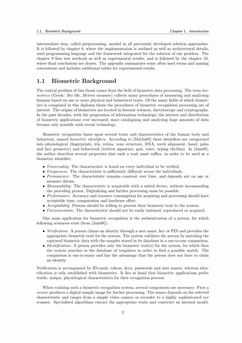
(a) Minutiae types [BasSchu05]. (b) Minutiae schema [webWong]. (c) Extracted minutiae [Jain08].
Figure 1.1: Fingerprint minutiae in dactyloscopy.
Fingerprints are catalogued with various methods. Of these, applications broadly use theminutiae representation, which is a schematic description of special features in a fingerprint likebifurcations, whorls, crossovers, and many others, as listed in figure 1.1a. Such minutiae areextracted out of a scanned fingerprint image by specialized algorithms. A minutiae data setconsists of usually 15-80 minutiae per fingerprint. A formal representation of one minutia consistsof [BasSchu05]:
• Type of the minutia: crossover, whorl, bifurcation, ridge ending, and others (see figure 1.1a).• Position (x, y) coordinates based on an imaginary zero point (see figure 1.1b).• Local orientation θ of the minutia.• Reliability rθ of orientation data1.
1This datum is only used in representations extracting ridge orientation information. The value is the higher ifthe orientation is similar to the orientation of marks in the vicinity.
3
1.1. Biometric Background Chapter 1. Introduction
The processing of most biometric applications is based upon this minutiae representation. Theminutiae data itself is extracted and compared efficiently and has many uses. Of these the mostcommon are database searches for matching fingerprints, or in general person identification, suchas in crime reconnaissance, person tracking, or access limitation with security door scanners. Fur-ther applications can be found in cryptographic context, where fingerprints are used as additionalidentification feature on important documents of various sorts, to secure and guarantee provenanceof the documents themselves and to impede theft, falsification and prevent abuse. Since nowadaysmany documents provide facilities for digital storage, like microchips, magnet strips and so on,there are many concerns to enhance the security of the stored data. For this purpose, besidesencryption watermarking is a commonly used technique. Since the considered devices have strongstorage limitations, the interest for compression comes now into play.
Furthermore it has to be mentioned, that scanning and decomposing fingerprints is not thetask of the fingerprint minutiae compression project and can be performed by highly specializedalgorithms. Starting point for the work are data sets of already extracted minutiae which are thenfurther processed for the intended use as a watermark. Digital watermarks and compression basicsare presented in the following section.
1.1.2 Digital Watermarking, Steganography and Compression
Watermarking is a technique old as humankind. With the advent of information technology theconcept of embedding information about provenience and ownership in digital media was adapted.A digital watermark is additional information interwoven in digital media files (audio, video, im-ages, text, database records, geodata) in such a way that media and watermark information cannotbe separated again. According to [Fraun08] digital watermarks are independent from data formatand remain intact after modification of the medium, for example format conversion, compression,scaling and clipping, since the watermark is not embedded into some data format dependent metaheader but into the data itself. Also the technique discerns from copy protection mechanismsand encryption methods since copying and displaying of content is not impeded. For that reasonwatermarks are called non restrictive.
Besides visible watermarks, which mostly consist of company logos and author names, there alsoexist invisible watermarks, whereby the main aim is to maintain data integrity. After signing, theoriginal content appears not to be altered and enables the following security objectives [Fraun08]:
• Copyright protection for creators, authors and ownership holders. Unambiguous identifica-tion of media through an ID, for example the ISBN embedded as watermark in an e-book.
• Integrity protection against manipulation and alteration of content. Tracking of data flowthrough transaction numbers and purchaser ID, for example color laser printouts.
• Authenticity protection for definite identification of the origin (cryptographic applications).• Other objectives are: marketing and advertising, additional services as lyrics in audio files,
partial encryption for preventing previews.
Watermarks can be engineered in such a way that any alteration of the signed content de-stroys or damages the signature and the manipulation can be reconstructed. These techniquesrelate to steganography, the science of concealing information in content. Key features of digitalwatermarks are perceptibility, transparency, robustness against alterations, capacity (the amountof information to be embedded), security (manipulation of the key and watermark renders uselessthe original data), performance of embedding and retrieving (reading/playback in real time).Steganographic embedding of information is technically realized by replacing bits or greater sec-tions of the carrier medium, mostly irrelevant or redundant, with some value calculated out of theinformation part. Methods altering single bits at appropriate locations are substitution methodswhereas greater portion altering methods perform domain transformation, with the result thatthe embedded parts are more robust against manipulation and alteration, but require more space.
4
1.2. Previous Work Chapter 1. Introduction
In the course of the research project on fingerprint minutiae compression a very sophisticatedmechanism in the fashion of domain transformation was developed, which also suffices the stor-age requirements of small devices. Since our storage capabilities are limited, data compression isapplied. Data compression is the process of replacing original data with a representation of thedata using fewer storage consumption on a digital medium. Compression mechanisms are dividedinto lossless and lossy, whereby the former ones make it possible to reconstruct the original datafrom the compressed data, whereas the latter do not permit this and information is lost after thecompression process. In the present case a lossless compression is main target.
The following section summarizes the precedent work for minutiae compression. This sectiongives an overview about the compression model as well as problem solution strategies which havebeen already investigated in the course of this project.
1.2 Previous Work
In the course of the research project [ChwRai09] and [Dietzel08] analyzed quite a number of con-ventional standard compression algorithms for their performance and efficiency when set at workto compress minutiae data. A comprehensive introduction to data compression can be found in[Sayood06].
Amongst the examined algorithms is arithmetic coding and Huffman coding. Further on dic-tionary based algorithms originating from image, audio and video compression were tested. Thesealgorithms identify redundant structures and condense them into a dictionary, in order to expressinformation to be encoded through this dictionary. Mostly these standard algorithms performvery badly and were found not to be suited for the task. Investigation of the steganographic back-ground and compression technologies in relation to fingerprint minutiae compression are describedin [ChwRai09, Dietzel08]. Here their results are not presented further, and can be looked up inthe named documents.
1.2.1 The Compression Model
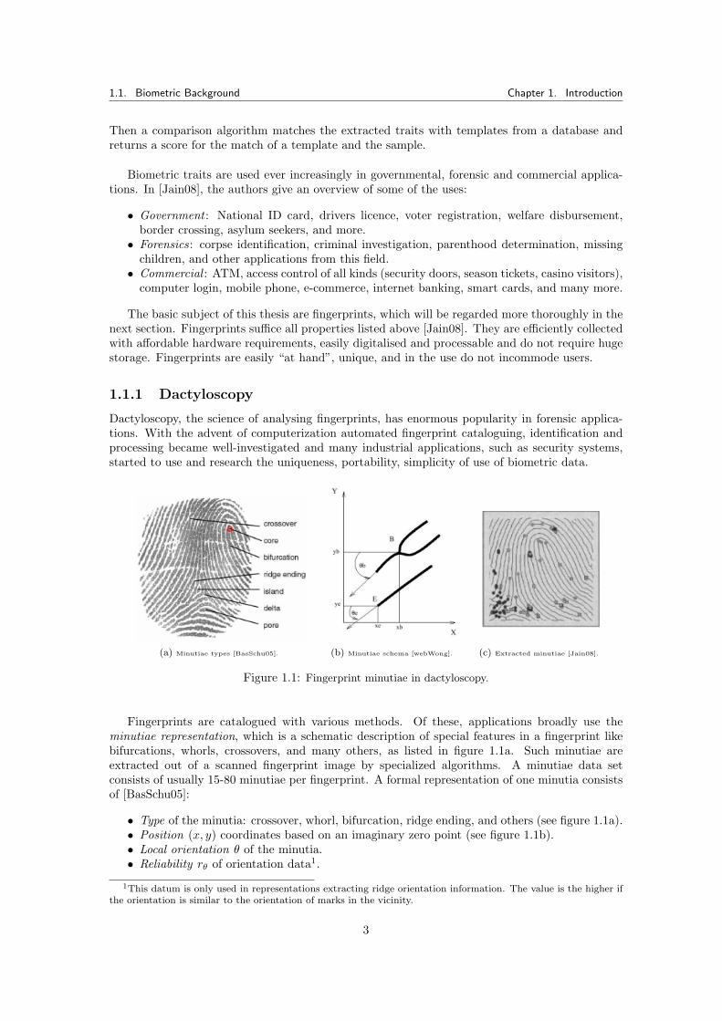
The dictionary based coder approach named above is then pursued in the following way: Havingin mind the construction of a minimal dictionary or codebook for a compact representation ofminutiae information, the naturally contained structures and redundancies in minutiae data ledto the development of a graph based encoding model as a basis for the compression mechanism.Out of this graph model the compression algorithm extracts the dictionary in form of so calledtemplate vectors and afterward expresses the minutiae from the input data by a reference tothe appropriate codebook entry. The codebook or dictionary is schematized in figure 1.2. Theauthors of [ChwRai09] emphasize that “our approach follows this general idea of using a dictionaryor codebook but its determination as well as its usage is very different to the existing methods.”
Figure 1.2: Encoding of points via adirected spanning tree using a code-book of template arcs, correction vec-tors are neglected. Image creditsto [ChwRai09].
Presumed we have extracted fingerprint minutiae from a fingertip scan, we take now a closerlook at these minutiae. As described in section 1.1.1 a minutia can be seen as a four dimensionalvector consisting of position as x, y coordinates, type t and orientation θ. Let us denote such
5
1.2. Previous Work Chapter 1. Introduction
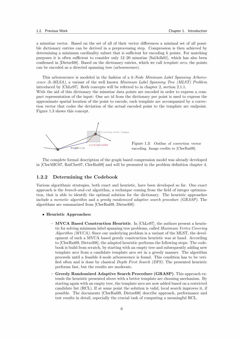
a minutiae vector. Based on the set of all of their vector differences a minimal set of all possi-ble dictionary entries can be derived in a preprocessing step. Compression is then achieved bydetermining a minimum cardinality subset that is sufficient for encoding k points. For matchingpurposes it is often sufficient to consider only 12–20 minutiae [SalAdh01], which has also beenconfirmed in [Dietzel08]. Based on the dictionary entries, which we call template arcs, the pointscan be encoded as a directed spanning tree (arborescence).
This arborescence is modeled in the fashion of a k-Node Minimum Label Spanning Arbores-cence (k-MLSA), a variant of the well known Minimum Label Spanning Tree (MLST) Problemintroduced by [ChLe97]. Both concepts will be referred to in chapter 2, section 2.1.1.With the aid of this dictionary the minutiae data points are encoded in order to express a com-pact representation of the input: One arc id from the dictionary per point is used to express theapproximate spatial location of the point to encode, each template arc accompanied by a correc-tion vector that codes the deviation of the actual encoded point to the template arc endpoint.Figure 1.3 shows this concept.
Figure 1.3: Outline of correction vector
encoding. Image credits to [ChwRai09].
The complete formal description of the graph based compression model was already developedin [ChwMIC07, RaiChw07, ChwRai09] and will be presented in the problem definition chapter 4.
1.2.2 Determining the Codebook
Various algorithmic strategies, both exact and heuristic, have been developed so far. One exactapproach is the branch-and-cut algorithm, a technique coming from the field of integer optimiza-tion, that is able to identify the optimal solution for the dictionary. The heuristic approachesinclude a memetic algorithm and a greedy randomized adaptive search procedure (GRASP). Thealgorithms are summarized from [ChwRai09, Dietzel08]:
• Heuristic Approaches:
– MVCA Based Construction Heuristic. In [ChLe97], the authors present a heuris-tic for solving minimum label spanning tree problems, called Maximum Vertex CoveringAlgorithm (MVCA). Since our underlying problem is a variant of the MLST, the devel-opment of such a MVCA based greedy construction heuristic was at hand. Accordingto [ChwRai09, Dietzel08], the adapted heuristic performs the following steps: The code-book is build from scratch, by starting with an empty tree and subsequently adding newtemplate arcs from a candidate template arcs set in a greedy manner. The algorithmproceeds until a feasible k-node arborescence is found. This condition has to be veri-fied often and is done by classical Depth First Search (DFS). The presented heuristicperforms fast, but the results are moderate.
– Greedy Randomized Adaptive Search Procedure (GRASP). This approach ex-tends the heuristic presented above with a better template arc choosing mechanism. Bystarting again with an empty tree, the template arcs are now added based on a restrictedcandidate list (RCL). If at some point the solution is valid, local search improves it, ifpossible. The documents [ChwRai09, Dietzel08] describe approach, performance andtest results in detail, especially the crucial task of computing a meaningful RCL.
6
1.3. Contributions of this Thesis Chapter 1. Introduction
• Memetic Algorithm (MA). These algorithms come from the field of genetic algorithmsand are a combination of evolutionary, population based algorithms and local improvementstrategies like individual learning. Like heuristics, this type of algorithms also yield ap-proximate solutions, but tend not to get stuck in local optima. Following the conceptspresented by [XiGolWas05] a memetic algorithm for the k-MLSA was developed and pre-sented in [ChwRai09]. According to the evolutionary background the algorithm produces aninitial population of feasible solutions, which is then modified by selection, recombinationand mutation - imitating biological evolution. An iteration produces an offspring solutionfrom recombined parent solutions, and performs tournament selection and local improve-ment steps. Redundant arcs in the arborescence must be handled. After a huge, predefinednumber of iterations or a fixed number of steps in which no improvement is achieved, the bestsolution is chosen from the population. The document [ChwRai09] shows detailed results,i.e. good solutions are achieved very quickly for the most of the test cases.
• Branch-and-Cut Approach. Following a very different approach from the field of combi-natorial optimization, an optimal solution for the k-MLSA was also attempted. The authorsof [ChwRai09] modelled and formulated the problem as an integer linear program (ILP)based on cycle elimination and connectivity inequalities. Shortly outlined, since the theo-retical background will be presented later in chapter 3, the branch-and-cut method beginswith an incomplete model and derives the solution by iteratively adding further constraintson demand.
Main drawback of these methods is the need for an intermediate step. All solution proceduresfor the k-MLSA problem employ a preprocessing step, a precalculation of a candidate template arcsset, out of which then the actual minimal template codebook is determined by the actual algorithm.
Having now summarized all previous work, it is now time to come to the actual main subjectof this diploma thesis. The task is now to follow on the exact problem solution of the k-MLSAwith further techniques coming from the field of integer programming.
1.3 Contributions of this Thesis
This section gives an overview of the attempted task. Some terms and concepts are used straight-forwardly and will be explained more in detail in the theory chapters 2 and 3.
As named several times, fingerprint minutiae compression is now attempted by integer linearprogramming. The main disadvantage of the presented approaches was already marked, it liesin the preprocessing step. This step precalculates the set of candidate template arcs, called T c.Out of this set, in all previously presented strategies, the solution to the k-MLSA, the actualminimal template codebook is determined. This preprocessing step is imminent for all presentedsolution strategies. At the present time this step is realized by restricted enumeration. As thename implies, enumeration examines the whole multitude of possible candidate template arcs setpermutations. Although the search was restricted somewhat to promising areas, the number ofpotential sets to examine is still huge. In practice, the preprocessing step consumes a relativelybig amount of processing time, particularly for large input parameters2 δ.
In the following this weak point shall be removed: Consequently our goal is to skip this pre-processing step and incorporate it into the linear program part. To do so, the focus shifts fromthe tree to the candidate template arcs themselves as central point. Their number in practice isagain very huge.
2This parameter will be addressed in the problem definition chapter 4.
7
1.3. Contributions of this Thesis Chapter 1. Introduction
The idea is now not to generate all possible candidate template arcs in advance, and thensolve the resulting (large) integer linear program, but to start with a very small set of candi-date template arcs, and then create new template arcs on demand during the solution of theILP. Such approaches are called column generation, as new variables (and therefore columns inthe coefficient matrix of the integer linear program) are generated continuously. Combined withbranch-and-bound we obtain an approach called branch-and-price.
To realize this, the original formulation from the branch-and-cut approach must be altered andadapted accordingly. Since the original formulation has an exponential number of involved restric-tions, we need a formulation consisting of a moderate amount of restrictions, but having insteada huge amount of variables. This task is realized by formulating the integer program in terms ofa single and a multi commodity flow network. The resulting mixed integer program is then solvedby branch-and-price. In other words the creation of candidate template arcs is incorporated intothe integer program itself by creating new template arcs on demand.
So, the first step is to reformulate the original integer linear program so that it can be solvedby our chosen approach. We have to set up the mixed integer program and solve it by branch-and-price. For the solution of huge sized integer programs there exist a lot of commercial andnon-commercial frameworks, one of which will be selected for this task. The chosen frameworkwill be described in the implementation chapter 8.
Branch-and-price starts with a small set of template arcs and then iteratively adds new tem-plate arcs potentially improving the objective function value. These variables are determinedwithin a special step, the pricing problem. The solution of the pricing problem depends on inter-mediate solution values of our newly formulated integer program. Also some special structures ofthe input data are exploited.
In the course of the problem analysis a very promising approach to solve the pricing problemwas developed, and realized with the aid of a very common and efficient geometric algorithm, ak-d tree. The development of efficient data structures and corresponding algorithms based on sucha k-d tree is the second important contribution of this thesis. Here, efficiency is very crucial, asthe pricing problem needs to be solved numerous times.
To solve the overall problem, the pricing problem solver is finally integrated in the branch-and-price framework, which then is tested thoroughly for its overall performance, speed and correctness.
Outlook
The following two chapters introduce theory prerequisites for the understanding of the problemdefinition and solution approach. When we look at the tasks, we identify two main theory sub-jects: Since the underlying compression model is a graph and the MLST solution bases on graphtheoretical ideas, an overview of these graph theoretical basics as well as flow networks mustbe accounted (section 2.1). Also the solution of the pricing problem requires methods from itssubarea of algorithmic geometry, the most important being the well known k-d tree, addressedin section 2.3. Furthermore, to complete the branch-and-price part, a deeper understanding ofoptimization theory is needed. Since this area is very vast, the chapter 3 concerning theory fromthis field focuses on linear and integer programming basics, but emphasizes the subjects columngeneration and branch-and-price, which are regarded more thoroughly in section 3.4.
8

Chapter 2
Graph Theory and AlgorithmicGeometry Essentials
This chapter is dedicated to shortly outline and recapitulate the most important graph theorydetails and geometric algorithms, which are needed for the problem definition and solution, sub-ject in chapters 4 until 7. Here the basics utilized for the construction of the minimum labelspanning tree based compression model are summarized. Network flow problems are basis for theformulation of the mixed integer program in order to be solved by branch-and-price. Moreoverthe background of the solution strategy used in the arising pricing problem is regarded: The usedk-d tree has its roots in binary search trees, which have a widespread application spectrum andcome from the field of algorithmic geometry. How all these dissimilar topics are finally tied to-gether will become clear in chapter 5.
Most graph theory concepts are summarized from the reference books [Sedgew01, CormLei07],which are recommended for further inquiries. Reference for multi-dimensional binary search trees(commonly known as k-d trees) is [Bentley75]. Sources for minimum label spanning trees are[ChLe97], [XiGolWas05] and [Kru98].
2.1 Graph Theory Basics
A graph is a tuple G = (V,E) and consists of a set of vertices or nodes V = {v1, v2, . . . , vn}, n ∈ Nand a set of edges E = {e1, e2, . . . , em}, m ∈ N, which are elements from V × V . An edge eijconnects two nodes vi and vj . An edge is directed if a direction is endowed, the set of edges thenis called A = {aij | aij = (vi, vj), vi, vj ∈ V }. Here aij 6= aji, with aij = (vi, vj) and aji = (vj , vi).The set of edges in an undirected graph is E = {eij | eij = {vi, vj}, vi, vj ∈ V ∧ vi 6= vj}. Herefollows eij = eji. Undirected graphs contain no directed edges. Directed graphs (digraphs) containonly directed edges. Mixed graphs contain both. Edges eij in undirected graphs are called inci-dent with the nodes vi and vj , the nodes vi and vj themselves are called adjacent. In directedgraphs adjacency of vj to vi is only implied when an edge aij exists. A loop is an edge eii thatconnects the same vertex at its endpoints. Multi-edged graphs contain multiple edges connectingthe same endpoints, a simple graph contains no multi-edges. Complete undirected graphs contain(|V |
2
)edges and all nodes vi 6= vj with vi, vj ∈ V are adjacent. In undirected graphs for each node
v the degree δ(v) is defined as the number of adjacent edges. In directed graphs the in-degreeδ−(v) is the number of incoming edges and the out-degree δ+(v) the number of outgoing edges.Nodes or edges can be endowed (depending on the modeled problem) with weights and thus forma weighted graph, with “labels” or “colours”, forming a labeled or coloured graph.
A path denotes a p-sized sequence of vertices, such that from each vertex exists an edge tothe next vertex in the sequence. Graphs are connected, if every point is reachable through a path,
9
2.1. Graph Theory Basics Chapter 2. Graph Theory and Algorithmic Geometry Essentials
else unconnected. A cycle exists, if the starting point can be reached through a path. A graphcontaining no cycles is called acyclic. A tree is a connected, undirected graph containing no cycles,where the removal of an edge renders it unconnected. A tree contains n vertices and n− 1 edges.Vertices in a tree with δ(v) = 1 are called leafs, nodes with greater degree are intermediate nodes.
A subgraph G′ of G has V ′ ⊆ V and E′ ⊆ E, the edges in E′ connecting only vertices in V ′. Aspanning tree is a subgraph of some graph containing all vertices, but being a tree. An arborescenceis a spanning tree on a directed graph, where exist (directed) paths from the root node to everyother node. A minimum spanning tree (MST) is a spanning tree with minimal weight edges. Tosolve the MST problem Kruskal and Prim developed their eponymous algorithms which nowadaysevery student learns in her first algorithmic lessons.
2.1.1 Minimum Label Spanning Tree (MLST)
The MLST problem was first introduced by [ChLe97], where the authors also showed it to beNP -hard. Following definition was found in literature:
Definition 1 (Minimum Label Spanning Tree Problem). “Let G = (V,E) be a con-nected undirected graph and c : E −→ N be an edge labeling/coloring function. AK-colored spanning tree (V, T ) is a spanning tree of G such that the number of usedcolors | {c(e) | e ∈ T} | does not exceed K. A minimum label spanning tree is a K-colored spanning tree with minimum K.” [Kru98].
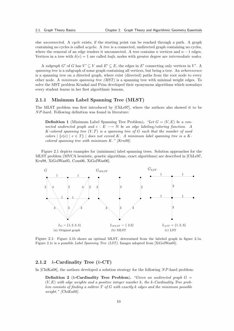
Figure 2.1 depicts examples for (minimum) label spanning trees. Solution approaches for theMLST problem (MVCA heuristic, genetic algorithms, exact algorithms) are described in [ChLe97,Kru98, XiGolWas05, Cons06, XiGolWas06].
1 1
1 1
2 24 42
3 3 3
G
LG = {1, 2, 3, 4}(a) Original graph
2 22
3 3 3
GMLST
LMLST = { 2,3}(b) MLST
1 1
1 1
2
3
GLST
LLST = {1, 2, 3}(c) LST
Figure 2.1: Figure 2.1b shows an optimal MLST, determined from the labeled graph in figure 2.1a.Figure 2.1c is a possible Label Spanning Tree (LST). Images adopted from [XiGolWas05].
2.1.2 k-Cardinality Tree (k-CT)
In [ChiKa08], the authors developed a solution strategy for the following NP -hard problem:
Definition 2 (k-Cardinality Tree Problem). “Given an undirected graph G =(V,E) with edge weights and a positive integer number k, the k-Cardinality Tree prob-lem consists of finding a subtree T of G with exactly k edges and the minimum possibleweight.” [ChiKa08].
10
2.1. Graph Theory Basics Chapter 2. Graph Theory and Algorithmic Geometry Essentials
The problem was solved by an exact algorithm: After transforming the k-CT problem into ak-cardinality arborescence problem, the formulation as an integer linear program using directedcuts was implemented in a branch-and-cut framework.
2.1.3 k-node Minimum Label Spanning Arborescence (k-MLSA)
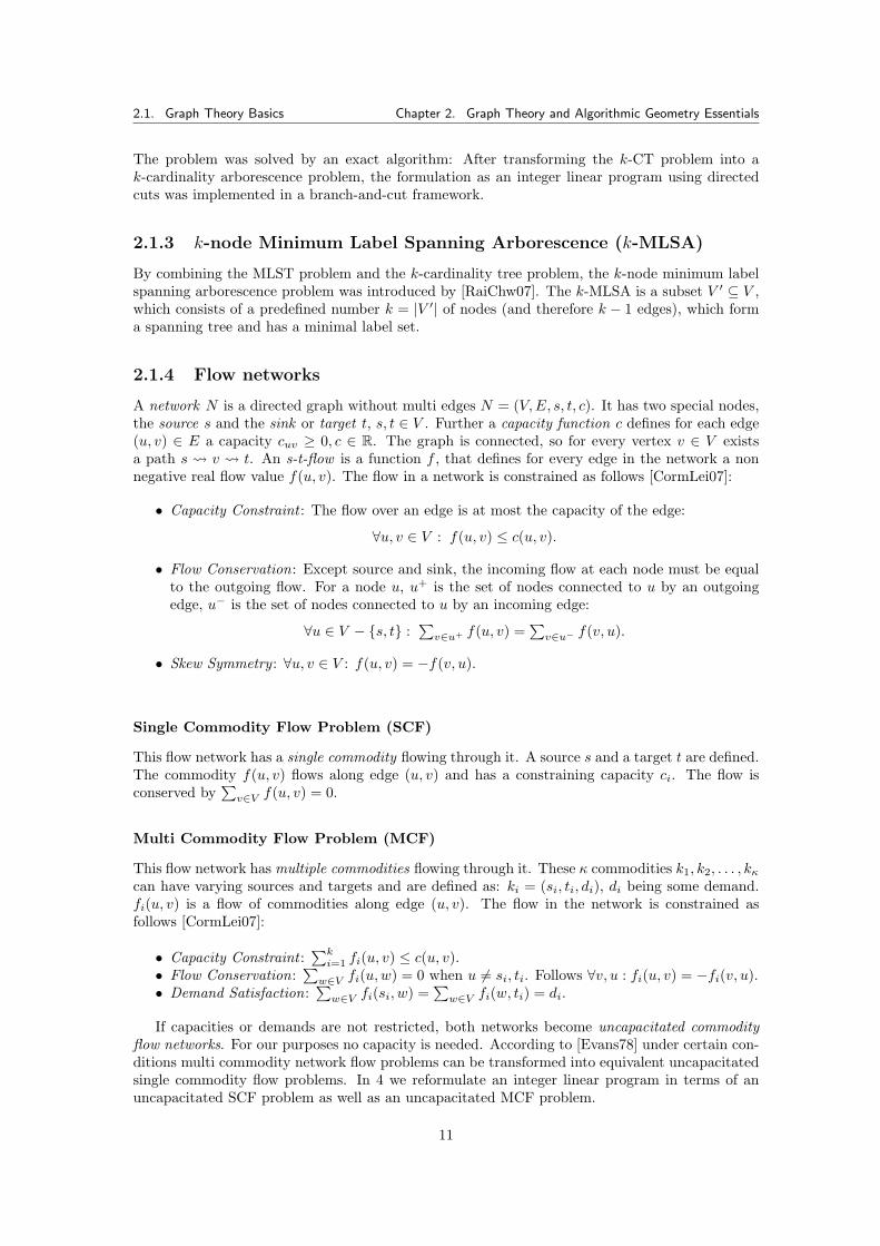
By combining the MLST problem and the k-cardinality tree problem, the k-node minimum labelspanning arborescence problem was introduced by [RaiChw07]. The k-MLSA is a subset V ′ ⊆ V ,which consists of a predefined number k = |V ′| of nodes (and therefore k − 1 edges), which forma spanning tree and has a minimal label set.
2.1.4 Flow networks
A network N is a directed graph without multi edges N = (V,E, s, t, c). It has two special nodes,the source s and the sink or target t, s, t ∈ V . Further a capacity function c defines for each edge(u, v) ∈ E a capacity cuv ≥ 0, c ∈ R. The graph is connected, so for every vertex v ∈ V existsa path s v t. An s-t-flow is a function f , that defines for every edge in the network a nonnegative real flow value f(u, v). The flow in a network is constrained as follows [CormLei07]:
• Capacity Constraint : The flow over an edge is at most the capacity of the edge:
∀u, v ∈ V : f(u, v) ≤ c(u, v).
• Flow Conservation: Except source and sink, the incoming flow at each node must be equalto the outgoing flow. For a node u, u+ is the set of nodes connected to u by an outgoingedge, u− is the set of nodes connected to u by an incoming edge:
∀u ∈ V − {s, t} :∑v∈u+ f(u, v) =
∑v∈u− f(v, u).
• Skew Symmetry : ∀u, v ∈ V : f(u, v) = −f(v, u).
Single Commodity Flow Problem (SCF)
This flow network has a single commodity flowing through it. A source s and a target t are defined.The commodity f(u, v) flows along edge (u, v) and has a constraining capacity ci. The flow isconserved by
∑v∈V f(u, v) = 0.
Multi Commodity Flow Problem (MCF)
This flow network has multiple commodities flowing through it. These κ commodities k1, k2, . . . , kκcan have varying sources and targets and are defined as: ki = (si, ti, di), di being some demand.fi(u, v) is a flow of commodities along edge (u, v). The flow in the network is constrained asfollows [CormLei07]:
• Capacity Constraint :∑ki=1 fi(u, v) ≤ c(u, v).
• Flow Conservation:∑w∈V fi(u,w) = 0 when u 6= si, ti. Follows ∀v, u : fi(u, v) = −fi(v, u).
• Demand Satisfaction:∑w∈V fi(si, w) =
∑w∈V fi(w, ti) = di.
If capacities or demands are not restricted, both networks become uncapacitated commodityflow networks. For our purposes no capacity is needed. According to [Evans78] under certain con-ditions multi commodity network flow problems can be transformed into equivalent uncapacitatedsingle commodity flow problems. In 4 we reformulate an integer linear program in terms of anuncapacitated SCF problem as well as an uncapacitated MCF problem.
11
2.2. Algorithmic Graph Theory Essentials Chapter 2. Graph Theory and Algorithmic Geometry Essentials
2.2 Algorithmic Graph Theory Essentials
A tree is a common data structure that organizes data in a set of linked nodes. Searching andinserting in such data structures can be done very efficiently. If the tree is balanced both operationsperform with logarithmic complexity. The hierarchical tree structure is expressed by predecessornode (parent, supernode) and successor node (children, subnode). The number of successors andpredecessors can be arbitrary. A tree has one root node that has no predecessors. A leaf is a nodethat has no successors. Intermediate nodes link the root and leafs together by having successorsand a predecessor. A subtree is a subset of the tree. The edges are directed from predecessor tosuccessor. The tree height denotes the length of the path from root node to the furthest leaf. Thedepth of node n is the length of the path from the root node to node n. All nodes at this depthare denoted with a level, the root node having level 0. A tree is complete if all levels, includingthe leaf level are fully occupied with data. A tree is balanced if each subtree of a node has anequal or almost equally big number of nodes. Multiple balancing schemes exist (AVL-Tree, B-Tree,Red-Black Tree, B*-Tree and more), that differ in their definition of “equal”, number of nodes,effort for re-balancing and construction, storage consumption.
2.3 Algorithmic Geometry
Algorithmic geometry is a subarea of computational geometry. Computational geometry concernsall fields, where algorithmic problems are stated in geometrical terms. Algorithmic geometry isthe subarea concerning geometric problems modeled through discrete entities.
2.3.1 Binary Search Tree
In a binary search tree each node has at most two successors left and right. It is commonly usedto structure one-dimensional data for efficient search operations, based on a key. All data with akey less than the actual node key is located in the left subtree, the other data in the right subtree.Searching in a binary tree with n nodes has complexity O(log n). A complete binary tree has2level − 1 nodes.
2.3.2 2-d Tree and k-d Tree
A 2-d tree is a binary tree, that operates on two-dimensional data points subdividing the plane intosubplanes with alternating x and y coordinates, which act also as keys. The subdivision is doneby means of the coordinates of the points. The alternating dimension, upon which the splittingis based, is called discriminator (disc) and often implemented as an incrementing number. Theactual dimension where the split occurs is extracted by a modulo operation.
A k-d tree expands the 2-d tree concept to k-dimensional space Rk. The space is then subdi-vided sequentially for every dimension d = 1, 2, . . . , k. The run time complexity of building such atree is limited to O (n log n), the complexity for a search is O(n1− 1
k +R). The variable R indicatesthe number of points in range when searching [Bentley75]. When regarding the dimensionality k,building has complexity O (k · n log n) and searching O(k · n1− 1
k +R).
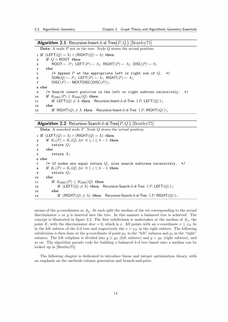
Figures 2.2 and 2.3 illustrate 2-d trees as well as k-d trees. As the insertion of further dimen-sions greater than 2 is simple, the pseudo code for inserting into a k-d tree (algorithm 2.1) andsearching it (algorithm 2.2) are listed in generalized form. These algorithms were originally devel-oped by [Bentley75], but were made recursive as we will later use these versions of the algorithms.Searching for a key works very similar to insertion, as can be seen in both listings.
12
2.3. Algorithmic Geometry Chapter 2. Graph Theory and Algorithmic Geometry Essentials
A
B
C
D
E
F
G
H
I
x
y
Ax = {A, G,F, B,E, H, C, D, I}Ay = {D,A, C, B, E, F, I,H, G}
(a) Points
A
B
C
D
E
F
G
H
I
x
y
Ax1 = {A, G,F, B,E, H, C, D, I}
(b) 1st split at disc = 0
A
B
C
D
E
F
G
H
I
x
y
Ay2 = {A, B, F , G} Ay3 = {D,C, I, H}
(c) 2nd split at disc = 1
A
B
C
D
E
F
G
H
I
x
y
Ax4 = {G}Ax7 = {D,C}Ax5 = {A, B}Ax6 = {H}
(d) 3rd split at disc = 2
A
B
C
D
E
F
G
H
I
x
y
(e) Splitting completed
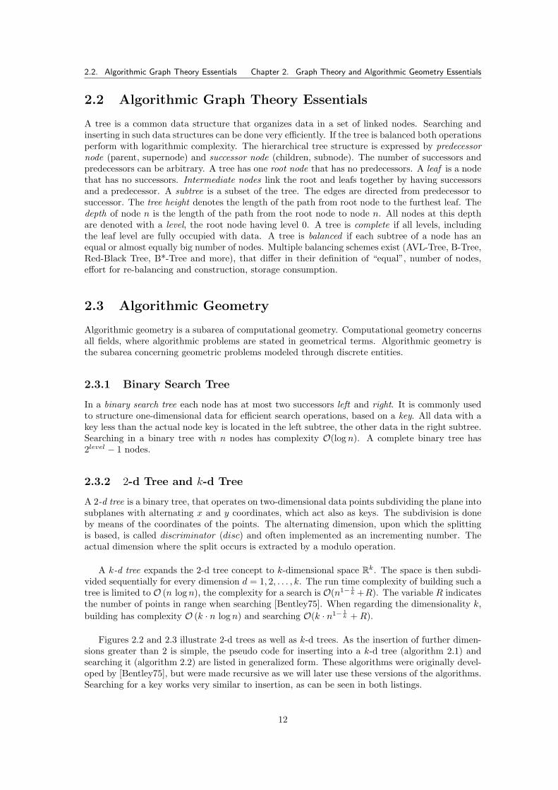
Figure 2.2: Construction of a balanced 2-d tree. The rounding median depends on the implementation.Here the median is round-up.
E
F I
HGB D
CA
x
y y
x x x x
y y
≤ >
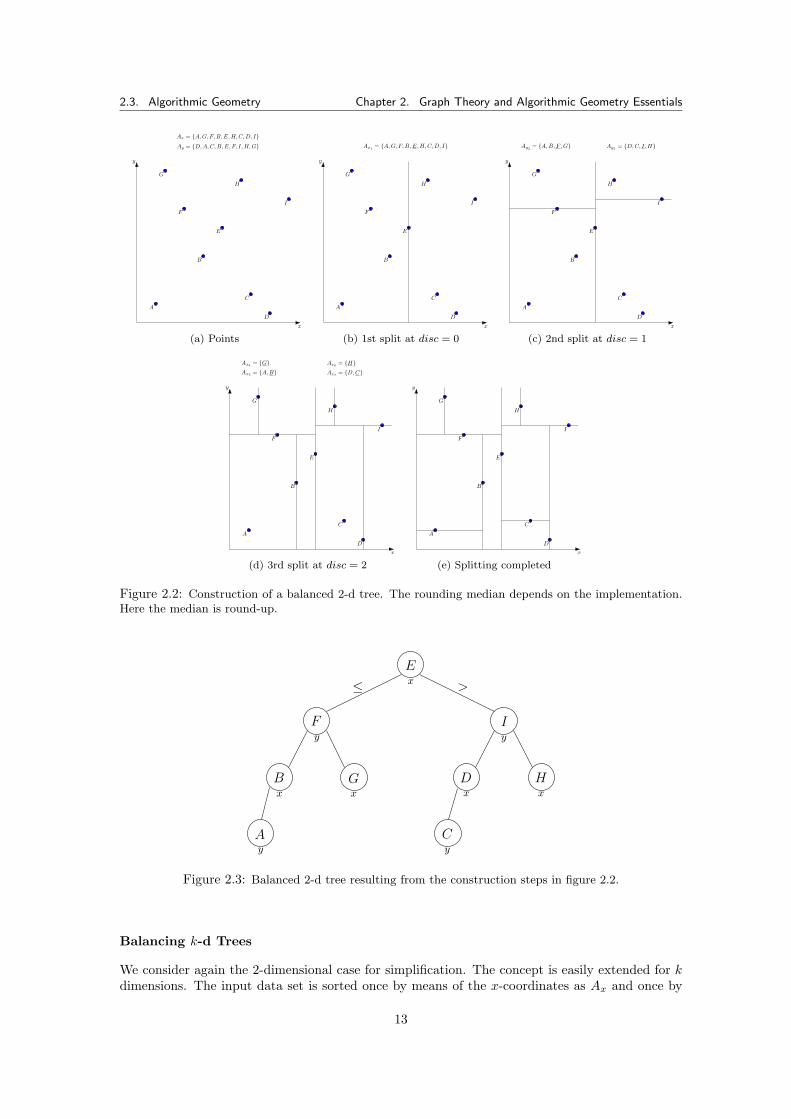
Figure 2.3: Balanced 2-d tree resulting from the construction steps in figure 2.2.
Balancing k-d Trees
We consider again the 2-dimensional case for simplification. The concept is easily extended for kdimensions. The input data set is sorted once by means of the x-coordinates as Ax and once by
13
2.3. Algorithmic Geometry Chapter 2. Graph Theory and Algorithmic Geometry Essentials
Algorithm 2.1: Recursive-Insert-k-d-Tree(P,Q ) [Bentley75]Data: A node P not in the tree. Node Q stores the actual position.
if (LEFT(Q) = Λ) ∧ (RIGHT(Q) = Λ) then1
if Q = ROOT then2
ROOT← P; LEFT(P )← Λ; RIGHT(P )← Λ; DISC(P )← 0;3
else4
/* Append P at the appropriate left or right son of Q. */5
SON(Q)← P; LEFT(P )← Λ; RIGHT(P )← Λ;6
DISC(P )← NEXTDISC(DISC(P ));7
else8
/* Search insert position in the left or right subtree recursively. */9
if KDISC(P ) ≤ KDISC(Q) then10
if LEFT(Q) 6= Λ then Recursive-Insert-k-d-Tree (P, LEFT(Q) );11
else12
if RIGHT(Q) 6= Λ then Recursive-Insert-k-d-Tree (P, RIGHT(Q) );13
Algorithm 2.2: Recursive-Search-k-d-Tree(P,Q ) [Bentley75]Data: A searched node P . Node Q stores the actual position.
if (LEFT(Q) = Λ) ∧ (RIGHT(Q) = Λ) then1
if Ki(P ) = Ki(Q) for 0 ≤ i ≤ k − 1 then2
return Q;3
else4
return Λ;5
else6
/* If nodes are equal return Q, else search subtrees recursively. */7
if Ki(P ) = Ki(Q) for 0 ≤ i ≤ k − 1 then8
return Q;9
else10
if KDISC(P ) ≤ KDISC(Q) then11
if (LEFT(Q) 6= Λ) then Recursive-Search-k-d-Tree (P, LEFT(Q) );12
else13
if (RIGHT(Q) 6= Λ) then Recursive-Search-k-d-Tree (P, RIGHT(Q) );14
means of the y-coordinates as Ay. At each split the median of the set corresponding to the actualdiscriminator x or y is inserted into the tree. In this manner a balanced tree is achieved. Theconcept is illustrated in figure 2.2. The first subdivision is undertaken at the median of Ax, thepoint E, with the discriminator disc = 0, which is x. All points with an x-coordinate x ≤ xE liein the left subtree of the 2-d tree and respectively the x > xE in the right subtree. The followingsubdivision is then done at the y-coordinate of point pF in the “left” subarea and pI in the “right”subarea. The left subplane is divided into y ≤ yF (left subtree) and y > yF (right subtree), andso on. The algorithm pseudo code for building a balanced k-d tree based onto a median can belooked up in [Bentley75].
The following chapter is dedicated to introduce linear and integer optimization theory, withan emphasis on the methods column generation and branch-and-price.
14
Chapter 3
Optimization Theory Essentials
In this chapter a brief introduction to the topic of linear and integer optimization is given. Thetheoretical knowledge is needed later in chapter 4 and the following practice chapters. All topicsare explained as short as possible, since the area of optimization theory is very huge. This chapteris divided into two main parts, i.e. linear and integer linear optimization. The first part concerninglinear optimization will serve as an introduction to optimization theory in general and present theconcepts: history and trivia, modeling linear programs and their standard form, solvability, dualityas well as some general solution methods. The passages concerning integer programming explainwhat distinguishes integer from linear programming, give a classification of integer programs andsummarize some of the known solution strategies. The part concerning advanced topics coversmore in detail topics immanent for column generation. It encompasses the detailed solution processas well as arising topics like the pricing problem and the tailing off effect.Mainly, the more general introductory parts linear and integer optimization adhere to [Wol98]and [Van98], which are the main reference books on this subject. Trivia are from [webDesSoum98].[BoydVan04] is a source for nonlinear optimization. Sources for the second part concerning columngeneration were mostly [DesLu05], with [Luebbe01] being the related dissertation of one of theauthors of the former work. Additional literature in this part is [VanWol96, Vanbk94, NemWol88,GuzRal07, webTrick97, Schrij99].
3.1 History and Trivia
The first concepts of linear optimization, also called linear programming, date back to the year 1939.The roots lie in the linear inequalities theory. First mathematical models were presented by LeonidW. Kantorovitch. The first formalizations were given by George Dantzig in the 1940ies. At thetime of the Second World War the issue was at first held secret due to the advantage in planning warresource allocation. Later industry and production planning became aware of the potential of thesemethods and since then the field of linear optimization was ever researched. A mighty instrumentto solve linear programs proved to be the Simplex algorithm created by George B. Dantzig in 1947,and with it many before calculation intensive problems suddenly were computable in significantlyshorter time and were proved to produce optimal results.Many real world applications seemed to have some additional properties. Very common in realworld applications were problems of integer nature, e.g. they needed integer or binary values intheir results like the following, very frequent problems:
• Scheduling of train, aeroplane, bus timetables.• Personnel, task and machine scheduling.• Resource planning, raw material needs and production planning.• Route planning, networking.
In such problems, entities like personnel and resources cannot be separated or fractionated torational or real values but have to be assigned entirely, e.g. one or more machines or workers to
15
3.2. Introduction to Linear Optimization Chapter 3. Optimization Theory Essentials
a specified task regardless of some “optimal” value of 0.73 or 78. Some well known problem for-
mulations for the applications listed above are Scheduling Problem, Resource Allocation Problem,Cutting Stock and Bin Packing.Problems of these nature are subject of integer optimization, which evolved on the basis of linearoptimization. Also these problems showed not to be as easy to solve like standard linear problems,because of a “combinatorial explosion” [Wol98], page 8, based on the optimal result to be a largeset of feasible solutions. As example the author names the Traveling Salesman Problem (TSP).Looking at an entity with 1000 cities, the solution space has 9.33 · 10157 feasible tours.So a multitude of techniques began to evolve around the fields of combinatorial optimization andinteger programming which will be explored further in the following.
3.2 Introduction to Linear Optimization
In order to solve a problem with linear optimization, it has first to be analysed and formulatedin a mathematical way. The according formulation is called linear program (LP) and represents amodel of a real world problem. When we analyze such problems many different goals arise:
• Minimize manufacturing costs for prescribed outputs.• Minimize overall production cost and/or time of products depending on varying resources.• Maximize profit for varying products, producible with a limited stock of raw materials.• Maximize output of products, which can be assembled on production lines with predefined
time windows and resources.
These goals are limited by factors like raw materials, resources, production cost, processing timeor market limits, which also have to be embedded into the model. The formulation in the mostcases is the most intensive task in the entire solution process.
Linear programming is a subarea of convex optimization and basis for numerous solutiontechniques in nonlinear as well as integer optimization. Linear programs are usually interpretedas general polyhedra, and many ideas, concepts and proofs are based onto polyhedral theory.
3.2.1 Linear Programs
In order to formalize the concept of a linear program (LP), we introduce some terms and notions.First we introduce the variables xi, i = 1, 2, . . . , n, which will hold the values that are yet to bedecided in an optimal way. These variables are called decision variables. For linear optimization,their values lie in R. In the majority of cases they are endowed with some cost variables, whichwe denote with ci, i = 1, 2, . . . , n, ci ∈ R.
The linear objective function is composed of these variables and has the form
max z∗ = c1x1 + c2x2 + · · ·+ cnxn, (3.1)
where z∗ is the objective value. The objective function also encodes the goal striven for: Theobjective value can either be maximized (problems concerning maximal profit or workload, andsuchlike) or minimized (problems concerning minimal resources or personnel, or similar).
In addition to the objective function the requirements for a problem have to be formulated.This is done through equality and inequality constraints. These constraints, also called restrictions,express limitations onto a problem (e.g. disposition hours of machines, production plan changedelay, sales limits, and so on), expressed in variables aij . Explicit inequalities whose goal is toprohibit negative numbers are called non negativity constraints.
16
3.2. Introduction to Linear Optimization Chapter 3. Optimization Theory Essentials
All constraints form a set of restrictions:
a11x1 + a12x2 + · · ·+ a1nxn ≤ b1a21x1 + a22x2 + · · ·+ a2nxn ≤ b2
...am1x1 + am2x2 + · · ·+ amnxn ≤ bm
x1, x2, . . . , xn ≥ 0
(3.2)
By summarizing we obtain a linear program:
maxn∑j=1
cjxj
s.t.n∑j=1
aijxj ≤ bi i = 1, 2, . . . ,m
xj ≥ 0 j = 1, 2, . . . , n.
(3.3)
The above linear program (3.3) models a problem already in standard form. In this form thelinear objective function is to be maximized and the problem constraints are in terms of ≤. Everyalternative linear program formulation (minimization problems, constraints with ≥ or = opera-tors, negative variables constraints) can be converted into an equivalent formulation in standardform. In few words, a linear program is concerned with optimizing an objective function subjectto linear (equality and inequality) constraints.
To render the notation more intuitive it became common to use the canonical matrix form.The matrix A denotes the n ·m matrix of constraint parameters aij , c> the n-dimensional (row)vector, b the m-dimensional (column) vector, x the n-dimensional column vector of variables1:
max c>xs.t. Ax ≤ b
x ≥ 0(3.4)
A shortened expression is common in literature, used by [Wol98], page 3: max{cx : Ax ≤ b, x ≥ 0}.
3.2.2 Duality
Each linear program in standard form, called primal problem, can be converted into a dual problem.The according dual problem for the linear program in (3.4) is:
min b>y
s.t. A>y ≥ cy ≥ 0
(3.5)
Here, y denotes the dual variables. The author of [Van98] formulates, that “taking the dual of thedual returns us to the primal” problem. Another fundamental idea of duality theory is that everyfeasible solution of an LP embodies also a bound on the optimal value of the objective functionof the dual. The most essential theorems of duality theory are the weak duality theorem and thestrong duality theorem [Van98], presented in the following.
1Common notation: A ∈ Rm×n, b ∈ Rm and c ∈ Rn
17
3.2. Introduction to Linear Optimization Chapter 3. Optimization Theory Essentials
Definition 3 (Weak Duality Theorem). “If (x1, x2, . . . , xn) is feasible for the pri-mal and (y1, y2, . . . , ym) is feasible for the dual, then:∑
j cjxj ≤∑i biyi, or in condensed form: c>x∗ ≤ b>y∗.”[Van98].
Definition 4 (Strong Duality Theorem). “If the primal problem has an opti-mal solution x∗ = (x∗1, x
∗2, . . . , x
∗n) then the dual also has an optimal solution y∗ =
(y∗1 , y∗2 , . . . , y
∗m) such that:∑
j cjx∗j =
∑i biy
∗i , or in condensed form: c>x∗ = b>y∗.”[Van98].
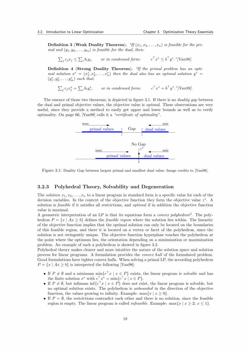
The essence of those two theorems, is depicted in figure 3.1. If there is no duality gap betweenthe dual and primal objective values, the objective value is optimal. These observations are veryuseful, since they provide a method to easily get upper and lower bounds as well as to verifyoptimality. On page 66, [Van98] calls it a “certificate of optimality”.
Gap
No Gap
max min
max min
dual valuesprimal values
primal values dual values
z∗
Figure 3.1: Duality Gap between largest primal and smallest dual value. Image credits to [Van98].
3.2.3 Polyhedral Theory, Solvability and Degeneration
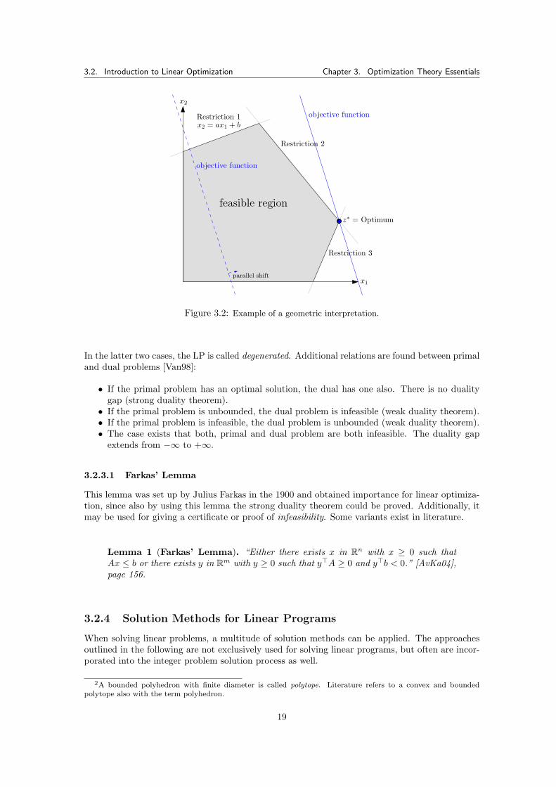
The solution x1, x2, . . . , xn to a linear program in standard form is a specific value for each of thedecision variables. In the context of the objective function they form the objective value z∗. Asolution is feasible if it satisfies all restrictions, and optimal if in addition the objective functionvalue is maximal.A geometric interpretation of an LP is that its equations form a convex polyhedron2. The poly-hedron P = {x | Ax ≥ b} defines the feasible region where the solution lies within. The linearityof the objective function implies that the optimal solution can only be located on the boundariesof this feasible region, and there it is located on a vertex or facet of the polyhedron, since thesolution is not stringently unique. The objective function hyperplane touches the polyhedron atthe point where the optimum lies, the orientation depending on a minimization or maximizationproblem. An example of such a polyhedron is showed in figure 3.2.Polyhedral theory makes clearer and more intuitive the nature of the solution space and solutionprocess for linear programs. A formulation provides the convex hull of the formulated problem.Good formulations have tighter convex hulls. When solving a primal LP, the according polyhedronP = {x | Ax ≥ b} is interpreted the following [Van98]:
• If P 6= ∅ and a minimum min{c>x | x ∈ P} exists, the linear program is solvable and hasthe finite solution x∗ with c>x∗ = min{c>x | x ∈ P}.
• If P 6= ∅, but infimum inf{c>x | x ∈ P} does not exist, the linear program is solvable, butno optimal solution exists. The polyhedron is unbounded in the direction of the objectivefunction, the values growing to infinity. Example: max{x | x ≥ 0}.
• If P = ∅, the restrictions contradict each other and there is no solution, since the feasibleregion is empty. The linear program is called infeasible. Example: max{x | x ≥ 2; x ≤ 1}.
18
3.2. Introduction to Linear Optimization Chapter 3. Optimization Theory Essentials
Restriction 1
Restriction 2
Restriction 3
z∗ = Optimum
objective function
parallel shift
objective function
feasible region
x1
x2
x2 = ax1 + b
Figure 3.2: Example of a geometric interpretation.
In the latter two cases, the LP is called degenerated. Additional relations are found between primaland dual problems [Van98]:
• If the primal problem has an optimal solution, the dual has one also. There is no dualitygap (strong duality theorem).
• If the primal problem is unbounded, the dual problem is infeasible (weak duality theorem).• If the primal problem is infeasible, the dual problem is unbounded (weak duality theorem).• The case exists that both, primal and dual problem are both infeasible. The duality gap
extends from −∞ to +∞.
3.2.3.1 Farkas’ Lemma
This lemma was set up by Julius Farkas in the 1900 and obtained importance for linear optimiza-tion, since also by using this lemma the strong duality theorem could be proved. Additionally, itmay be used for giving a certificate or proof of infeasibility. Some variants exist in literature.
Lemma 1 (Farkas’ Lemma). “Either there exists x in Rn with x ≥ 0 such thatAx ≤ b or there exists y in Rm with y ≥ 0 such that y>A ≥ 0 and y>b < 0.” [AvKa04],page 156.
3.2.4 Solution Methods for Linear Programs
When solving linear problems, a multitude of solution methods can be applied. The approachesoutlined in the following are not exclusively used for solving linear programs, but often are incor-porated into the integer problem solution process as well.
2A bounded polyhedron with finite diameter is called polytope. Literature refers to a convex and boundedpolytope also with the term polyhedron.
19
3.2. Introduction to Linear Optimization Chapter 3. Optimization Theory Essentials
3.2.4.1 Geometric Method
The geometric interpretation of an LP was already presented in section 3.2.3 and constitutes aquick and easy way of getting solutions for small linear programs. But only small problems withfew variables are solved by such graphical methods. With increasing dimensions or when havinga somewhat greater quantity of restrictions and variables they become very unhandy and theprecision in the most of cases is very inaccurate.
3.2.4.2 Simplex Algorithm
Inspired by this geometric interpretation G. Dantzig created the Simplex algorithm. Fundamen-tally, this algorithm searches the vertices of the polytope described by the problem constraints,starting by a feasible solution. The algorithm proceeds along the edges of the polytope havinggreater reduced costs, thus improving the objective function, and advances until the optimum isfound or unboundedness is asserted. The Simplex algorithm is called an edge following methodand constitutes of the following steps:
1. Check for infeasibility.2. Convert LP into augmented form: Introduce non-negative slack variables in order to replace
inequality with equality constraints. In this manner a block matrix form is achieved whichconstitutes the Simplex tableau.
3. Determine a feasible starting solution. The slack variables become basic, the main variablesbecome non-basic3.
4. While basis solution is not optimal do:
(a) Determine entering basic variable: Select a nonbasic variable, having maximal reducedcost. This variable is called pivot element.
(b) Determine leaving basic variable: Select the basic variable which will be dropped inorder to obtain an improving adjacent edge. This is performed via the ratio test.
(c) Transform the Simplex tableau into canonical form by pivoting the entering variable.The leaving variable becomes nonbasic and the entering variable becomes basic. Thisoperation is called pivot.
(d) Terminate if unboundedness or cycling (a previous state is revisited) is detected.
Since the Simplex algorithm considers only adjacent edges, in each iteration only one substi-tution of basic for a non-basic variables is performed. Dantzig designated the entering variable asthe one having maximal reduced cost, but over time alternative strategies were developed.Polyheder theory shows us that if an optimal solution exists at the edge of the polytope the Sim-plex algorithm always brings forth this optimal solution, or the problem is infeasible or unbounded.In special cases a degeneration in the Simplex tableau happens, in particular the occurrence ofcycles. This can be avoided through Bland’s rule, which performs the selection of pivot elements ina special way. The worst case complexity is exponential in problem size, but almost never 2n stepsare required. In practice the Simplex algorithm turned out to be very applicable and efficient.At the present time commercial and free software is able to solve systems with some millions ofvariables and restrictions.
Variants and improvements The selection of the pivot element influences highly the numberof iterations as well as the numerical stability especially when having degenerated tableau’s. Thusa good pivot element selection strategy is required. There exist a lot of methods for selectingpivot elements, or pivot columns and rows: Dantzigs approach (maximal reduced cost) resultedto be relatively calculation intensive. One prevalent selection strategy is steepest edge pricing,which selects column and row that together yield greatest overall improvement for the objective.It is computation intensive, but the number of iterations is significantly decreased. Devex pricingis an approximation of steepest edge pricing in combination with a normalization of the values
3Besides this approach, other more sophisticated methods exist
20
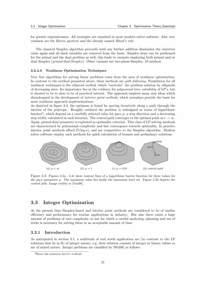
3.3. Integer Optimization Chapter 3. Optimization Theory Essentials
for greater expressiveness. All strategies are standard in most modern solver software. Also verycommon are the Harris quotient and the already named Bland’s rule.
The classical Simplex algorithm proceeds until any further addition diminishes the objectivevalue again and all slack variables are removed from the basis. Simplex steps can be performedfor the primal and the dual problem as well, this leads to variants employing both primal and/ordual Simplex (primal-dual-Simplex ). Other variants are two-phase-Simplex, M -method.
3.2.4.3 Nonlinear Optimization Techniques
Very fast algorithms for solving linear problems come from the area of nonlinear optimization.In contrast to the method presented above, these methods are path following. Foundation for allnonlinear techniques is the ellipsoid method, which “encircles” the problem solution by ellipsoidsof decreasing sizes. Its importance lies in the evidence for polynomial time solvability of LP’s, butit showed to be to slow to be of practical interest. The approach inspired many new ideas whichdisembogued in the development of interior point methods, which nowadays provide the basis formost nonlinear approach implementations.As depicted in figure 3.3, the optimum is found by moving iteratively along a path through theinterior of the polytope. Roughly outlined the problem is redesigned in terms of logarithmicbarriers4, which depend on a carefully selected value for pace µ, a step direction and a decreasingstep width, calculated in each iteration. The central path converges to the optimal point as t→∞.Again, primal-dual symmetry is exploited as optimality criterion. This class of LP solving methodsare characterized by polynomial complexity and fast convergence towards optimality. In practiceinterior point methods afford O (log n), and are competitive to the Simplex algorithm. Modernsolver software employ such methods for quick calculation of bounds and preliminary solutions.
(a) µ =∞ (b) µ = 1 (c) µ = 0.01 (d) central path
Figure 3.3: Figures 3.3a - 3.3c show contour lines of a logarithmic barrier function for three values forthe pace parameter µ. The maximum value lies inside the innermost level set. Figure 3.3d depicts thecentral path. Image credits to [Van98].
3.3 Integer Optimization
At the present time Simplex-based and interior point methods are considered to be of similarefficiency and performance for routine applications in industry. But also there exists a hugeamount of problems of vast complexity or size for which a careful analyzing, planning and use oftricks is necessary for solving them in an acceptable amount of time.
3.3.1 Introduction
As anticipated in section 3.1, a multitude of real world application are (in contrast to the LPsolutions that lie in R) of integer nature, e.g. their solution consists of integer or binary values orare of mixed nature. Integer problems are classified by [Wol98] as follows:
4Hence the synonym barrier methods.
21
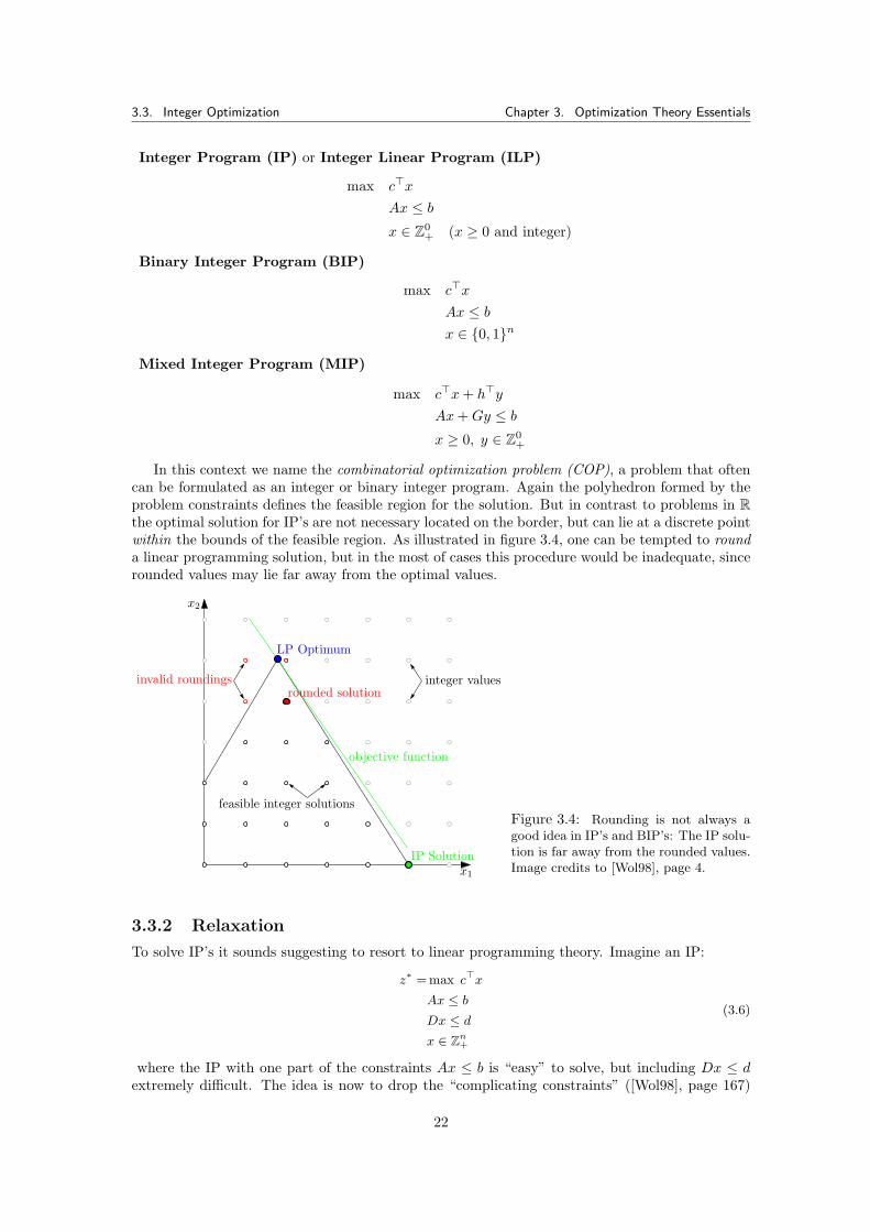
3.3. Integer Optimization Chapter 3. Optimization Theory Essentials
Integer Program (IP) or Integer Linear Program (ILP)
max c>xAx ≤ bx ∈ Z0
+ (x ≥ 0 and integer)
Binary Integer Program (BIP)
max c>xAx ≤ bx ∈ {0, 1}n
Mixed Integer Program (MIP)
max c>x+ h>yAx+Gy ≤ bx ≥ 0, y ∈ Z0
+
In this context we name the combinatorial optimization problem (COP), a problem that oftencan be formulated as an integer or binary integer program. Again the polyhedron formed by theproblem constraints defines the feasible region for the solution. But in contrast to problems in Rthe optimal solution for IP’s are not necessary located on the border, but can lie at a discrete pointwithin the bounds of the feasible region. As illustrated in figure 3.4, one can be tempted to rounda linear programming solution, but in the most of cases this procedure would be inadequate, sincerounded values may lie far away from the optimal values.
x1
x2
objective function
integer values
feasible integer solutions
IP Solution
rounded solutioninvalid roundings
LP Optimum
Figure 3.4: Rounding is not always agood idea in IP’s and BIP’s: The IP solu-tion is far away from the rounded values.Image credits to [Wol98], page 4.
3.3.2 Relaxation
To solve IP’s it sounds suggesting to resort to linear programming theory. Imagine an IP:
z∗ = max c>x
Ax ≤ bDx ≤ dx ∈ Zn+
(3.6)
where the IP with one part of the constraints Ax ≤ b is “easy” to solve, but including Dx ≤ dextremely difficult. The idea is now to drop the “complicating constraints” ([Wol98], page 167)
22
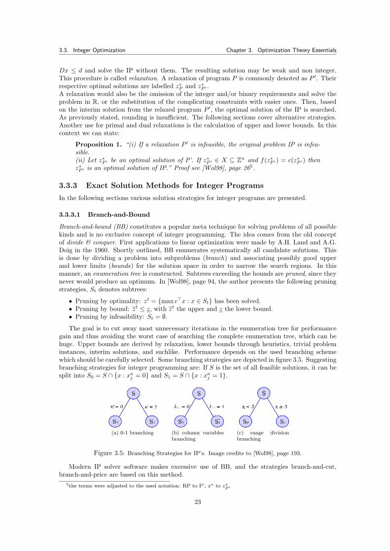
3.3. Integer Optimization Chapter 3. Optimization Theory Essentials
Dx ≤ d and solve the IP without them. The resulting solution may be weak and non integer.This procedure is called relaxation. A relaxation of program P is commonly denoted as P ′. Theirrespective optimal solutions are labelled z∗P and z∗P ′ .A relaxation would also be the omission of the integer and/or binary requirements and solve theproblem in R, or the substitution of the complicating constraints with easier ones. Then, basedon the interim solution from the relaxed program P ′, the optimal solution of the IP is searched.As previously stated, rounding is insufficient. The following sections cover alternative strategies.Another use for primal and dual relaxations is the calculation of upper and lower bounds. In thiscontext we can state:
Proposition 1. “(i) If a relaxation P ′ is infeasible, the original problem IP is infea-sible.(ii) Let z∗P ′ be an optimal solution of P’. If z∗P ′ ∈ X ⊆ Zn and f(z∗P ′) = c(z∗P ′) thenz∗P ′ is an optimal solution of IP.” Proof see [Wol98], page 265.
3.3.3 Exact Solution Methods for Integer Programs
In the following sections various solution strategies for integer programs are presented.
3.3.3.1 Branch-and-Bound
Branch-and-bound (BB) constitutes a popular meta technique for solving problems of all possiblekinds and is no exclusive concept of integer programming. The idea comes from the old conceptof divide & conquer. First applications to linear optimization were made by A.H. Land and A.G.Doig in the 1960. Shortly outlined, BB enumerates systematically all candidate solutions. Thisis done by dividing a problem into subproblems (branch) and associating possibly good upperand lower limits (bounds) for the solution space in order to narrow the search regions. In thismanner, an enumeration tree is constructed. Subtrees exceeding the bounds are pruned, since theynever would produce an optimum. In [Wol98], page 94, the author presents the following pruningstrategies, St denotes subtrees:
• Pruning by optimality: zt = {max c>x : x ∈ St} has been solved.• Pruning by bound: zt ≤ z, with zt the upper and z the lower bound.• Pruning by infeasibility: St = ∅.The goal is to cut away most unnecessary iterations in the enumeration tree for performance
gain and thus avoiding the worst case of searching the complete enumeration tree, which can behuge. Upper bounds are derived by relaxation, lower bounds through heuristics, trivial probleminstances, interim solutions, and suchlike. Performance depends on the used branching schemewhich should be carefully selected. Some branching strategies are depicted in figure 3.5. Suggestingbranching strategies for integer programming are: If S is the set of all feasible solutions, it can besplit into S0 = S ∩ {x : xκj = 0} and S1 = S ∩ {x : xκj = 1}.
(a) 0-1 branching (b) column variablesbranching
(c) range divisionbranching
Figure 3.5: Branching Strategies for IP’s. Image credits to [Wol98], page 193.
Modern IP solver software makes excessive use of BB, and the strategies branch-and-cut,branch-and-price are based on this method.
5the terms were adjusted to the used notation: RP to P’, x∗ to z∗P ′
23
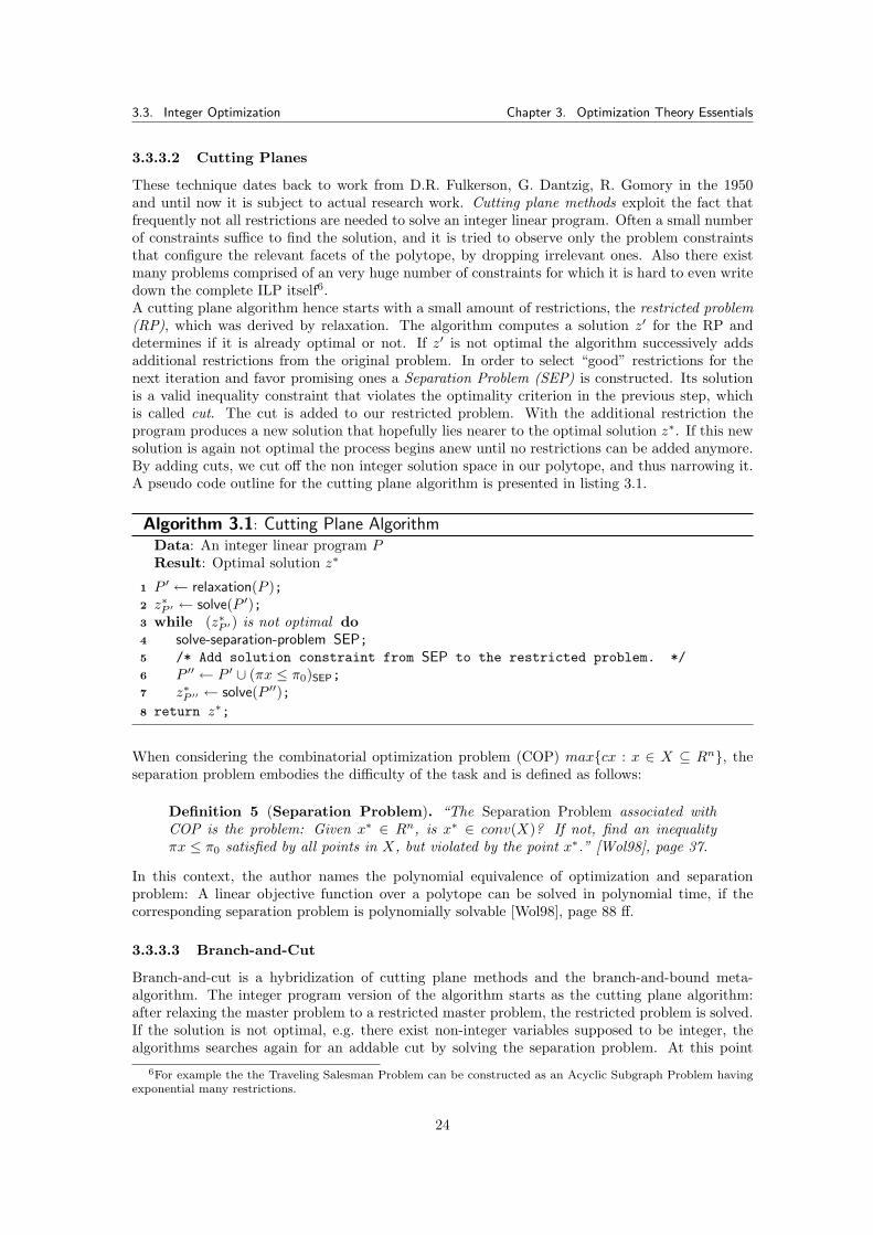
3.3. Integer Optimization Chapter 3. Optimization Theory Essentials
3.3.3.2 Cutting Planes
These technique dates back to work from D.R. Fulkerson, G. Dantzig, R. Gomory in the 1950and until now it is subject to actual research work. Cutting plane methods exploit the fact thatfrequently not all restrictions are needed to solve an integer linear program. Often a small numberof constraints suffice to find the solution, and it is tried to observe only the problem constraintsthat configure the relevant facets of the polytope, by dropping irrelevant ones. Also there existmany problems comprised of an very huge number of constraints for which it is hard to even writedown the complete ILP itself6.A cutting plane algorithm hence starts with a small amount of restrictions, the restricted problem(RP), which was derived by relaxation. The algorithm computes a solution z′ for the RP anddetermines if it is already optimal or not. If z′ is not optimal the algorithm successively addsadditional restrictions from the original problem. In order to select “good” restrictions for thenext iteration and favor promising ones a Separation Problem (SEP) is constructed. Its solutionis a valid inequality constraint that violates the optimality criterion in the previous step, whichis called cut. The cut is added to our restricted problem. With the additional restriction theprogram produces a new solution that hopefully lies nearer to the optimal solution z∗. If this newsolution is again not optimal the process begins anew until no restrictions can be added anymore.By adding cuts, we cut off the non integer solution space in our polytope, and thus narrowing it.A pseudo code outline for the cutting plane algorithm is presented in listing 3.1.
Algorithm 3.1: Cutting Plane AlgorithmData: An integer linear program PResult: Optimal solution z∗
P ′ ← relaxation(P );1
z∗P ′ ← solve(P ′);2
while (z∗P ′) is not optimal do3
solve-separation-problem SEP;4
/* Add solution constraint from SEP to the restricted problem. */5
P ′′ ← P ′ ∪ (πx ≤ π0)SEP;6
z∗P ′′ ← solve(P ′′);7
return z∗;8
When considering the combinatorial optimization problem (COP) max{cx : x ∈ X ⊆ Rn}, theseparation problem embodies the difficulty of the task and is defined as follows:
Definition 5 (Separation Problem). “The Separation Problem associated withCOP is the problem: Given x∗ ∈ Rn, is x∗ ∈ conv(X)? If not, find an inequalityπx ≤ π0 satisfied by all points in X, but violated by the point x∗.” [Wol98], page 37.
In this context, the author names the polynomial equivalence of optimization and separationproblem: A linear objective function over a polytope can be solved in polynomial time, if thecorresponding separation problem is polynomially solvable [Wol98], page 88 ff.
3.3.3.3 Branch-and-Cut
Branch-and-cut is a hybridization of cutting plane methods and the branch-and-bound meta-algorithm. The integer program version of the algorithm starts as the cutting plane algorithm:after relaxing the master problem to a restricted master problem, the restricted problem is solved.If the solution is not optimal, e.g. there exist non-integer variables supposed to be integer, thealgorithms searches again for an addable cut by solving the separation problem. At this point
6For example the the Traveling Salesman Problem can be constructed as an Acyclic Subgraph Problem havingexponential many restrictions.
24
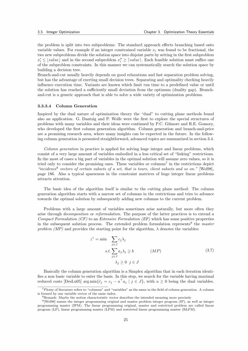
3.3. Integer Optimization Chapter 3. Optimization Theory Essentials
the problem is split into two subproblems: The standard approach effects branching based ontovariable values. For example if an integer constrained variable xi was found to be fractional, thetwo new subproblems divide the solution space into disjoint parts by setting in the first subproblemx′i ≤ bvaluec and in the second subproblem x′′i ≥ dvaluee. Each feasible solution must suffice oneof the subproblem constraints. In this manner we can systematically search the solution space bybuilding a decision tree.Branch-and-cut usually heavily depends on good relaxations and fast separation problem solving,but has the advantage of exerting small decision trees. Separating and optimality checking heavilyinfluence execution time. Variants are known which limit run time to a predefined value or untilthe solution has reached a sufficiently small deviation from the optimum (duality gap). Branch-and-cut is a generic approach that is able to solve a wide variety of optimization problems.
3.3.3.4 Column Generation
Inspired by the dual nature of optimization theory the “dual” to cutting plane methods foundalso an application. G. Dantzig and P. Wolfe were the first to explore the special structures ofproblems with many variables and their ideas were continued by P.C. Gilmore and R.E. Gomory,who developed the first column generation algorithm. Column generation and branch-and-priceare a promising research area, where many insights can be expected in the future. In the follow-ing column generation is presented straightforward, advanced topics are summarized in section 3.4.
Column generation in practice is applied for solving huge integer and linear problems, whichconsist of a very large amount of variables embodied in a less critical set of “linking” restrictions.In the most of cases a big part of variables in the optimal solution will assume zero values, so it istried only to consider the promising ones. These variables or columns7 in the restrictions depict“incidence8 vectors of certain subsets of a set, that is tours, client subsets and so on.” [Wol98],page 186. Also a typical sparseness in the constraint matrices of huge integer linear problemsattracts attention.
The basic idea of the algorithm itself is similar to the cutting plane method: The columngeneration algorithm starts with a narrow set of columns in the restrictions and tries to advancetowards the optimal solution by subsequently adding new columns to the current problem.
Problems with a large amount of variables sometimes arise naturally, but more often theyarise through decomposition or reformulation. The purpose of the latter practices is to extend aCompact Formulation (CF) to an Extensive Formulation (EF) which has some positive propertiesin the subsequent solution process. The extended problem formulation represents9 the masterproblem (MP) and provides the starting point for the algorithm, λ denotes the variables:
z∗ = min∑j∈J
cjλj
s.t.∑j∈J
ajλj ≥ b (MP )
λj ≥ 0 j ∈ J
(3.7)
Basically the column generation algorithm is a Simplex algorithm that in each iteration identi-fies a non basic variable to enter the basis. In this step, we search for the variable having maximalreduced costs [DesLu05] arg min{cj = cj − u>aj | j ∈ J}, with u ≥ 0 being the dual variables.
7Plenty of literature refers to “columns” and “variables” as the same in the field of column generation. A columnis formed by one variable vector of the same index.
8Remark: Maybe the notion characteristic vector describes the intended meaning more precisely9[Wol98] names the integer programming original and master problem integer program (IP), as well as integer
programming master (IPM). The linear programming original, master and restricted problem are called linearprogram (LP), linear programming master (LPM) and restricted linear programming master (RLPM).
25
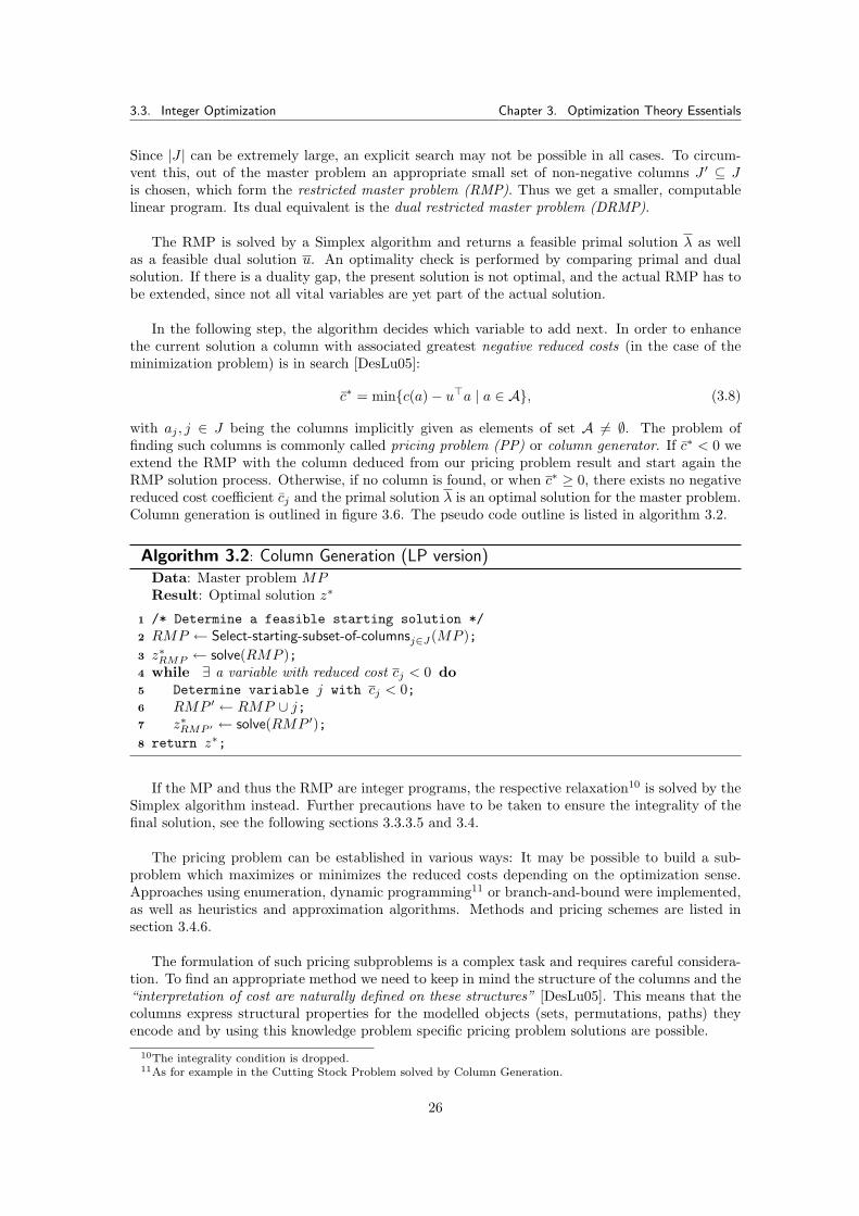
3.3. Integer Optimization Chapter 3. Optimization Theory Essentials
Since |J | can be extremely large, an explicit search may not be possible in all cases. To circum-vent this, out of the master problem an appropriate small set of non-negative columns J ′ ⊆ Jis chosen, which form the restricted master problem (RMP). Thus we get a smaller, computablelinear program. Its dual equivalent is the dual restricted master problem (DRMP).
The RMP is solved by a Simplex algorithm and returns a feasible primal solution λ as wellas a feasible dual solution u. An optimality check is performed by comparing primal and dualsolution. If there is a duality gap, the present solution is not optimal, and the actual RMP has tobe extended, since not all vital variables are yet part of the actual solution.
In the following step, the algorithm decides which variable to add next. In order to enhancethe current solution a column with associated greatest negative reduced costs (in the case of theminimization problem) is in search [DesLu05]:
c∗ = min{c(a)− u>a | a ∈ A}, (3.8)
with aj , j ∈ J being the columns implicitly given as elements of set A 6= ∅. The problem offinding such columns is commonly called pricing problem (PP) or column generator. If c∗ < 0 weextend the RMP with the column deduced from our pricing problem result and start again theRMP solution process. Otherwise, if no column is found, or when c∗ ≥ 0, there exists no negativereduced cost coefficient cj and the primal solution λ is an optimal solution for the master problem.Column generation is outlined in figure 3.6. The pseudo code outline is listed in algorithm 3.2.
Algorithm 3.2: Column Generation (LP version)Data: Master problem MPResult: Optimal solution z∗
/* Determine a feasible starting solution */1
RMP ← Select-starting-subset-of-columnsj∈J(MP );2
z∗RMP ← solve(RMP );3
while ∃ a variable with reduced cost cj < 0 do4
Determine variable j with cj < 0;5
RMP ′ ← RMP ∪ j;6
z∗RMP ′ ← solve(RMP ′);7
return z∗;8
If the MP and thus the RMP are integer programs, the respective relaxation10 is solved by theSimplex algorithm instead. Further precautions have to be taken to ensure the integrality of thefinal solution, see the following sections 3.3.3.5 and 3.4.
The pricing problem can be established in various ways: It may be possible to build a sub-problem which maximizes or minimizes the reduced costs depending on the optimization sense.Approaches using enumeration, dynamic programming11 or branch-and-bound were implemented,as well as heuristics and approximation algorithms. Methods and pricing schemes are listed insection 3.4.6.
The formulation of such pricing subproblems is a complex task and requires careful considera-tion. To find an appropriate method we need to keep in mind the structure of the columns and the“interpretation of cost are naturally defined on these structures” [DesLu05]. This means that thecolumns express structural properties for the modelled objects (sets, permutations, paths) theyencode and by using this knowledge problem specific pricing problem solutions are possible.
10The integrality condition is dropped.11As for example in the Cutting Stock Problem solved by Column Generation.
26

3.3. Integer Optimization Chapter 3. Optimization Theory Essentials
Figure 3.6: Column generation flowchart.
3.3.3.5 Branch-and-Price
Branch-and-price works similar to branch-and-cut. Accordingly, branch-and-price is a combinationof column generation and branch-and-bound and mainly used for solving huge integer programs.
The algorithm derives again a restricted master problem, and generates new columns, if theinterim solution is fractional, or until an optimal integer solution is achieved. While having frac-tional intermediate solutions, these values are used as bounds and the actual problem is split intotwo subproblems with some branching schema dividing the solution space into two complementarysubspaces. Various branching schemes exist, for example rounding of some fractional variable upin one subproblem and down in the second one, or setting binary variables to 0, respective 1 inthe corresponding subproblems. Thus for all variables found in the meantime, a decision tree is
27
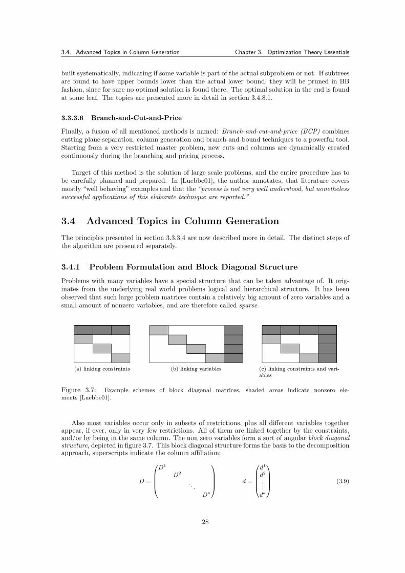
3.4. Advanced Topics in Column Generation Chapter 3. Optimization Theory Essentials
built systematically, indicating if some variable is part of the actual subproblem or not. If subtreesare found to have upper bounds lower than the actual lower bound, they will be pruned in BBfashion, since for sure no optimal solution is found there. The optimal solution in the end is foundat some leaf. The topics are presented more in detail in section 3.4.8.1.
3.3.3.6 Branch-and-Cut-and-Price
Finally, a fusion of all mentioned methods is named: Branch-and-cut-and-price (BCP) combinescutting plane separation, column generation and branch-and-bound techniques to a powerful tool.Starting from a very restricted master problem, new cuts and columns are dynamically createdcontinuously during the branching and pricing process.
Target of this method is the solution of large scale problems, and the entire procedure has tobe carefully planned and prepared. In [Luebbe01], the author annotates, that literature coversmostly “well behaving” examples and that the “process is not very well understood, but nonethelesssuccessful applications of this elaborate technique are reported.”
3.4 Advanced Topics in Column Generation
The principles presented in section 3.3.3.4 are now described more in detail. The distinct steps ofthe algorithm are presented separately.
3.4.1 Problem Formulation and Block Diagonal Structure
Problems with many variables have a special structure that can be taken advantage of. It orig-inates from the underlying real world problems logical and hierarchical structure. It has beenobserved that such large problem matrices contain a relatively big amount of zero variables and asmall amount of nonzero variables, and are therefore called sparse.
(a) linking constraints (b) linking variables (c) linking constraints and vari-ables
Figure 3.7: Example schemes of block diagonal matrices, shaded areas indicate nonzero ele-ments [Luebbe01].
Also most variables occur only in subsets of restrictions, plus all different variables togetherappear, if ever, only in very few restrictions. All of them are linked together by the constraints,and/or by being in the same column. The non zero variables form a sort of angular block diagonalstructure, depicted in figure 3.7. This block diagonal structure forms the basis to the decompositionapproach, superscripts indicate the column affiliation:
D =
0BBB@D1
D2
. . .
Dκ
1CCCA d =
0BBB@d1
d2
...dκ
1CCCA (3.9)
28
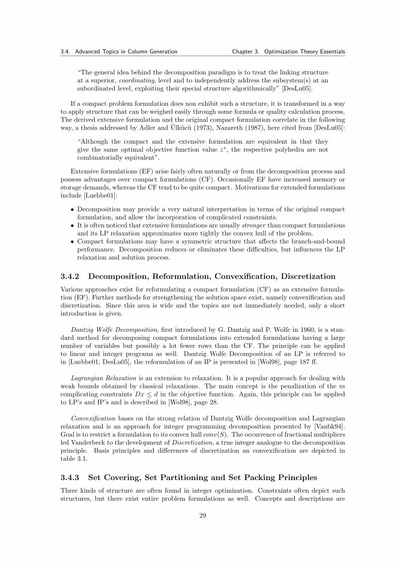
3.4. Advanced Topics in Column Generation Chapter 3. Optimization Theory Essentials
“The general idea behind the decomposition paradigm is to treat the linking structureat a superior, coordinating, level and to independently address the subsystem(s) at ansubordinated level, exploiting their special structure algorithmically” [DesLu05].
If a compact problem formulation does non exhibit such a structure, it is transformed in a wayto apply structure that can be weighed easily through some formula or quality calculation process.The derived extensive formulation and the original compact formulation correlate in the followingway, a thesis addressed by Adler and Ulkucu (1973), Nazareth (1987), here cited from [DesLu05]:
“Although the compact and the extensive formulation are equivalent in that theygive the same optimal objective function value z∗, the respective polyhedra are notcombinatorially equivalent”.
Extensive formulations (EF) arise fairly often naturally or from the decomposition process andpossess advantages over compact formulations (CF). Occasionally EF have increased memory orstorage demands, whereas the CF tend to be quite compact. Motivations for extended formulationsinclude [Luebbe01]:
• Decomposition may provide a very natural interpretation in terms of the original compactformulation, and allow the incorporation of complicated constraints.
• It is often noticed that extensive formulations are usually stronger than compact formulationsand its LP relaxation approximates more tightly the convex hull of the problem.
• Compact formulations may have a symmetric structure that affects the branch-and-boundperformance. Decomposition reduces or eliminates these difficulties, but influences the LPrelaxation and solution process.
3.4.2 Decomposition, Reformulation, Convexification, Discretization
Various approaches exist for reformulating a compact formulation (CF) as an extensive formula-tion (EF). Further methods for strengthening the solution space exist, namely convexification anddiscretization. Since this area is wide and the topics are not immediately needed, only a shortintroduction is given.
Dantzig Wolfe Decomposition, first introduced by G. Dantzig and P. Wolfe in 1960, is a stan-dard method for decomposing compact formulations into extended formulations having a largenumber of variables but possibly a lot fewer rows than the CF. The principle can be appliedto linear and integer programs as well. Dantzig Wolfe Decomposition of an LP is referred toin [Luebbe01, DesLu05], the reformulation of an IP is presented in [Wol98], page 187 ff.
Lagrangian Relaxation is an extension to relaxation. It is a popular approach for dealing withweak bounds obtained by classical relaxations. The main concept is the penalization of the mcomplicating constraints Dx ≤ d in the objective function. Again, this principle can be appliedto LP’s and IP’s and is described in [Wol98], page 28.
Convexification bases on the strong relation of Dantzig Wolfe decomposition and Lagrangianrelaxation and is an approach for integer programming decomposition presented by [Vanbk94].Goal is to restrict a formulation to its convex hull conv(S). The occurrence of fractional multipliersled Vanderbeck to the development of Discretization, a true integer analogue to the decompositionprinciple. Basis principles and differences of discretization an convexification are depicted intable 3.1.
3.4.3 Set Covering, Set Partitioning and Set Packing Principles
Three kinds of structure are often found in integer optimization. Constraints often depict suchstructures, but there exist entire problem formulations as well. Concepts and descriptions are
29
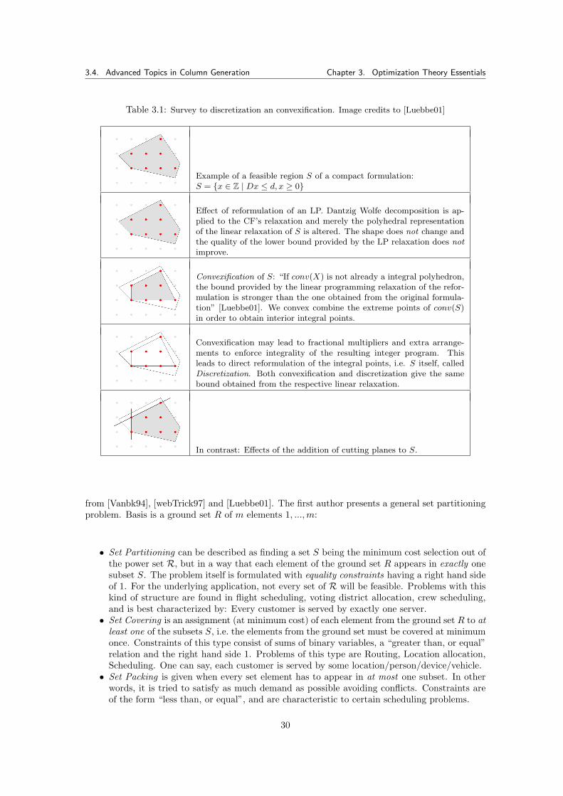
3.4. Advanced Topics in Column Generation Chapter 3. Optimization Theory Essentials
Table 3.1: Survey to discretization an convexification. Image credits to [Luebbe01]
Example of a feasible region S of a compact formulation:S = {x ∈ Z | Dx ≤ d, x ≥ 0}
Effect of reformulation of an LP. Dantzig Wolfe decomposition is ap-plied to the CF’s relaxation and merely the polyhedral representationof the linear relaxation of S is altered. The shape does not change andthe quality of the lower bound provided by the LP relaxation does notimprove.
Convexification of S: “If conv(X) is not already a integral polyhedron,the bound provided by the linear programming relaxation of the refor-mulation is stronger than the one obtained from the original formula-tion” [Luebbe01]. We convex combine the extreme points of conv(S)in order to obtain interior integral points.
Convexification may lead to fractional multipliers and extra arrange-ments to enforce integrality of the resulting integer program. Thisleads to direct reformulation of the integral points, i.e. S itself, calledDiscretization. Both convexification and discretization give the samebound obtained from the respective linear relaxation.
In contrast: Effects of the addition of cutting planes to S.
from [Vanbk94], [webTrick97] and [Luebbe01]. The first author presents a general set partitioningproblem. Basis is a ground set R of m elements 1, ...,m:
• Set Partitioning can be described as finding a set S being the minimum cost selection out ofthe power set R, but in a way that each element of the ground set R appears in exactly onesubset S. The problem itself is formulated with equality constraints having a right hand sideof 1. For the underlying application, not every set of R will be feasible. Problems with thiskind of structure are found in flight scheduling, voting district allocation, crew scheduling,and is best characterized by: Every customer is served by exactly one server.
• Set Covering is an assignment (at minimum cost) of each element from the ground set R to atleast one of the subsets S, i.e. the elements from the ground set must be covered at minimumonce. Constraints of this type consist of sums of binary variables, a “greater than, or equal”relation and the right hand side 1. Problems of this type are Routing, Location allocation,Scheduling. One can say, each customer is served by some location/person/device/vehicle.
• Set Packing is given when every set element has to appear in at most one subset. In otherwords, it is tried to satisfy as much demand as possible avoiding conflicts. Constraints areof the form “less than, or equal”, and are characteristic to certain scheduling problems.
30
3.4. Advanced Topics in Column Generation Chapter 3. Optimization Theory Essentials
3.4.4 The Restricted Master Problem (RMP)
As already stated, the Restricted Master Problem (RMP) consists of a manageable subset ofcolumns selected from the master problem, where the size of the latter would exceed either timeor memory at disposal when explicitly searching through the huge number of candidates. TheRMP serves as starting point for the subsequent pricing problem iteration process, where RMPitself is consecutively expanded by adding the improving columns from the pricing subproblemoutcomes. Any master program narrowed by omitting columns is called restricted. In the corre-sponding dual therefore the according rows are omitted.The actual purpose of the RMP is to make available the dual variables needed in the pricingprocess and for the algorithm termination control, since the stopping criterion would be equalingdual and primal objective values. The additional task of the RMP is to combine the subproblemssolutions in order to get primal feasible solutions. At all times, in the RMP is gathered all relevantinformation from already solved subproblems, which consists in a column subset, that was foundto improve the objective value. Figure 3.8 outlines the information flow between MP and RMP(s).
Figure 3.8: “Information flowbetween master program andsubproblem(s).” Image creditsto [Luebbe01].
In [DesLu05], the authors describe column generation as a method that works toward dualfeasibility by maintaining primal feasibility. It is important to keep in mind that dual valuesinfluence the selection of new variables and therefore must be monitored and analyzed carefully.However, since an initial set of columns for a RMP does not come up by itself, it has to be deducedsomehow.
3.4.4.1 Deducing an Initial Basis for the RMP
Independently from the used solution method, the RMP has to be initialized. The most commonmethods for solving the RMP, the Simplex algorithm, requires a good initial basis, since it is ofcrucial importance for the whole procedure. The author of [Luebbe01] names following approachesfor deriving a starting basis:
• The traditional approach is to employ preprocessed values from a two-phase-Simplex.• When performing an artificial start, a set of artificial variables is introduced, as many as
constraints in the RMP. They are combined with some large penalty constant, in order to beeliminated in the latter solution process. The artificial columns form a feasible basis matrixwhich variables one by one exit the basis until all artificial variables are swapped out and afeasible solution is yielded.
• Often primal heuristics are applied, but in most cases they are problem specific.• Sometimes, a warm start from primal solutions obtained in earlier, similar runs, is performed.• A trivial initialization with a set of 0, the unit basis is often encountered.
In the most of the cases software solvers utilize general methods, since they will not knowbeforehand or even detect the particular problem structure. Good starting sets reduce the headingin effect, meaning that they produce little irrelevant columns for the latter solution process, asfor example the artificial start. Bad ones may “lead the algorithm astray” [DesLu05]. The authorconcludes that best results are obtained with estimates of primal and dual solutions.
31
3.4. Advanced Topics in Column Generation Chapter 3. Optimization Theory Essentials
3.4.5 Solution Methods for the RMP
Although the Simplex algorithm is the dominant solution method for column generation problems,other approaches can be employed as well. Alongside primal-, dual-, and primal-dual-Simplex alsospecifically tailored algorithms for particular characteristics of the underlying linear program cometo use. Nonlinear approaches like the barrier/interior point method (see section 3.2.4.3) as wellas approximating approaches are very popular. Some of them are shortly outlined in the fol-lowing [Luebbe01]: The sprint method divides the linear program into working sets, which aresolved independently from each other. By combining the best results for each working set a so-lution to the main problem is approximated. The related sifting method combines interior pointmethods with a Simplex algorithm, the latter making a great progress for column selection in thebeginning, whereas the interior point method then calculates or approximates the few remainingcolumns. When no exact solution is needed, the volume algorithm deduces quickly primal anddual solution approximates. Another approximating algorithm is dual coordinate search, which isespecially designed for solving binary integer programs. It tries solving a RMP without relaxationand incorporates cost function information in combination with Lagrangian methods. The ana-lytic center cutting plane method uses “central prices” and is based onto logarithmic barriers.
Generally the methods may perform very differently in varying problem types and the bestpractice has to be carefully selected, since there exists no formula that indicates the quality of asolution method. Additionally all kinds of heuristics for improving dual variables can be employedthroughout the entire process.Traditionally Simplex, sprint/sifting and interior point method perform very well in the most cases.If the aim is maximal efficiency the adaption of specialized methods should be considered. Maindecision parameters for method choice are: efficiency, performance and speed of the algorithm,needed accuracy of the solution, problem peculiarities, available analytic and implementationskills, available industrial solver software.
3.4.6 The Pricing Problem - Pricing Strategies
The purpose of the pricing step is, as presented in 3.3.3.4, either to determine a column to be addedto the restricted master problem, i.e. to select a new variable to enter the basis or to bring theevidence that no such one exists. The author of [Luebbe01] distinguishes between pricing schemeand pricing rules, the former representing the “(sub)set of non-basic variables to consider”, andthe latter being a “criterion according to which a column is selected from the chosen (sub)set”.The most known such scheme-rule pair is the Dantzig approach: Choose among all the columnsthe one with the most negative reduced cost coefficient c∗ = min{ckq − u>akq − vk | k ∈ K, q ∈ Qk},(u, v)> being dual solutions for the RMP [Luebbe01], u being the dual variables for the so calledlinking or joint constraints.
Depending, if all variables, a subset of variables, or multiple considering of variables occurs,the according pricing schemes are called full, partial and multiple pricing.
For the pricing of linear programs following schemes exist: For (small) problems with somespecial structural properties, it is possible to determine the pricing variables by enumeration ordynamic programming12. In the majority of cases such methods are problem specific and poorlygeneralizable. An option would be to encode the pricing problem into an optimization problem asabove. The formulation of a single pricing subproblem is
c∗ = min{(c> − u>A)x | Dx ≤ d, x ≥ 0} [Luebbe01]. (3.10)
When selecting columns there has to be taken into account that some columns could be re-dundant or dominated by other ones: The concepts dominance and redundance state a condition(in this case of the dual constraints) called strength.
12As in the parade example cutting stock problem.
32
3.4. Advanced Topics in Column Generation Chapter 3. Optimization Theory Essentials
Definition 6 (Dominance). “A column k of model [M] is dominated if there ex-ists another column l ∈ Q, such that the reduced cost of k, ck is greater or equal tothat of l, cl, for all dual values (π, µ, ν) ∈ Rn+ × R1
− × R1+. On the other hand a col-
umn k is undominated if for all columns q ∈ Q, there exists a set of dual values(π, µ, ν) ∈ Rn+ × R1
− × R1+ for which ck < cq.” [Vanbk94], page 80.
Definition 7 (Redundance). “A column as is called redundant if the correspond-ing constraint is redundant for the dual problem. That is: as =
∑r⊂s arλr and cs ≥∑
r⊂r crλr. A column is strictly redundant if (above) holds with strict inequality.” [Vanbk94]
A strategy to handle dominated columns is: If a dominated column is discovered after the pric-ing step, replace this column by the dominant one in a post-processing step. Remove redundantconstraints in the dual problem.
On page 56 in [Luebbe01] are summarized a variety of alternative pricing rules for LP’s:
• Steepest-edge pricing eliminates the greedy character of the Dantzig pricing (choose a di-rection of steepest gradient) by taking into account in the pricing process all the edges andtheir directions.
• Deepest-cut pricing tries to cut away as much as possible from the dual solution space.• Lambda pricing selects columns by normalizing the reduced cost.• Lagrangian pricing exploits the original formulation by taking into account variable interac-
tions, then falls back to the local reduced cost criterion. The method is mostly not applicablein complex programs but may perform well in problems with certain structures, for examplevehicle routing.
Some additional pricing problem considerations are annotated: Whenever pricing is utilized, ithas to be considered that every column with negative reduced costs improves the objective function,and therefore not all pricing problem solutions are finally required in the optimal problem solution.Also a pricing problem can be approached by approximation, since except for the final value noexact values are needed in the RMP. According to a many reports in literature (see [Vanbk94]and [Luebbe01] for references) the column generation algorithm may spend more than 90% ofCPU time in pricing problems. Thus, this bottleneck has to be taken into account with carefulplanning since a slow pricing problem increases the execution time significantly.
3.4.6.1 Pricing Integer Programs
In integer problems, pricing is a little bit trickier. In fact, if the original compact formulationis an IP, the resulting pricing problem is one too, which has to be taken into account. Possiblearrangements would be:
• Get lower and upper bounds through approximations and relaxations with a small dualitygap between them. Use branch-and-price and divide and conquer solution space.
• Penalize the violation of integrality constraints, i.e. try to construct columns with integralcoefficients, for example the penalty function method.
• Divide the problem into smaller subproblems, that are solved integrally and independentfrom each other, and adjoin the partial solutions together to form an ultimate integralsolution. This strategy may involve structural characteristics of the problem itself.
3.4.7 The Tailing Off Effect
The convergence in IP column generation was also observed. Despite the algorithm is consideredto be finite13, sometimes it exhibits a very poor convergence behaviour, depicted in figure 3.9.
13Presupposed it does not cycle.
33
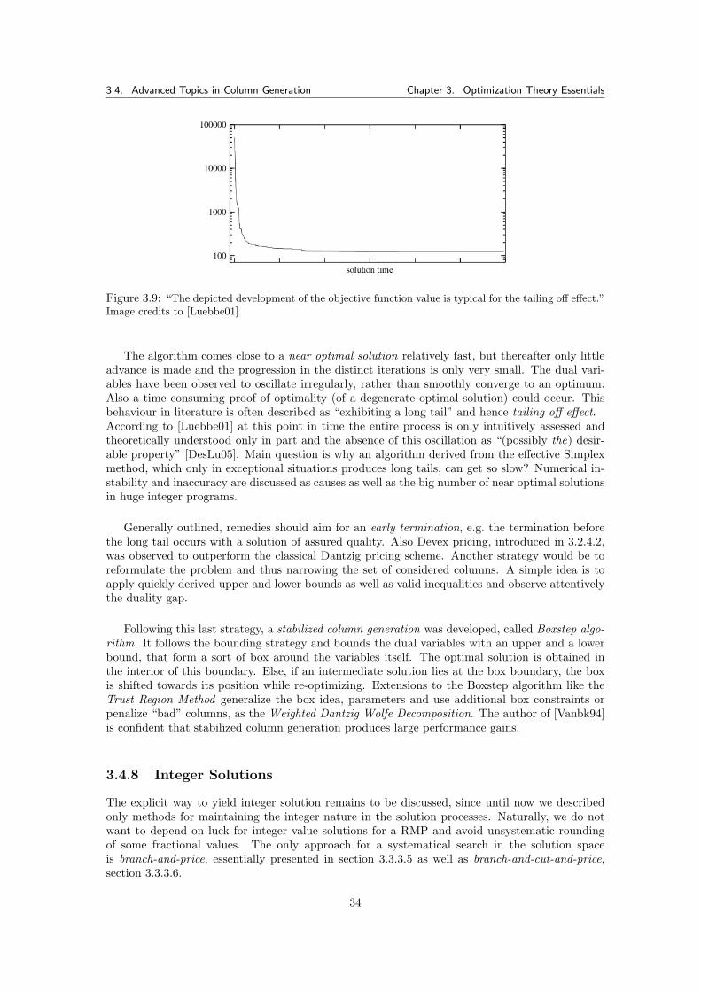
3.4. Advanced Topics in Column Generation Chapter 3. Optimization Theory Essentials
Figure 3.9: “The depicted development of the objective function value is typical for the tailing off effect.”Image credits to [Luebbe01].
The algorithm comes close to a near optimal solution relatively fast, but thereafter only littleadvance is made and the progression in the distinct iterations is only very small. The dual vari-ables have been observed to oscillate irregularly, rather than smoothly converge to an optimum.Also a time consuming proof of optimality (of a degenerate optimal solution) could occur. Thisbehaviour in literature is often described as “exhibiting a long tail” and hence tailing off effect.According to [Luebbe01] at this point in time the entire process is only intuitively assessed andtheoretically understood only in part and the absence of this oscillation as “(possibly the) desir-able property” [DesLu05]. Main question is why an algorithm derived from the effective Simplexmethod, which only in exceptional situations produces long tails, can get so slow? Numerical in-stability and inaccuracy are discussed as causes as well as the big number of near optimal solutionsin huge integer programs.
Generally outlined, remedies should aim for an early termination, e.g. the termination beforethe long tail occurs with a solution of assured quality. Also Devex pricing, introduced in 3.2.4.2,was observed to outperform the classical Dantzig pricing scheme. Another strategy would be toreformulate the problem and thus narrowing the set of considered columns. A simple idea is toapply quickly derived upper and lower bounds as well as valid inequalities and observe attentivelythe duality gap.
Following this last strategy, a stabilized column generation was developed, called Boxstep algo-rithm. It follows the bounding strategy and bounds the dual variables with an upper and a lowerbound, that form a sort of box around the variables itself. The optimal solution is obtained inthe interior of this boundary. Else, if an intermediate solution lies at the box boundary, the boxis shifted towards its position while re-optimizing. Extensions to the Boxstep algorithm like theTrust Region Method generalize the box idea, parameters and use additional box constraints orpenalize “bad” columns, as the Weighted Dantzig Wolfe Decomposition. The author of [Vanbk94]is confident that stabilized column generation produces large performance gains.
3.4.8 Integer Solutions
The explicit way to yield integer solution remains to be discussed, since until now we describedonly methods for maintaining the integer nature in the solution processes. Naturally, we do notwant to depend on luck for integer value solutions for a RMP and avoid unsystematic roundingof some fractional values. The only approach for a systematical search in the solution spaceis branch-and-price, essentially presented in section 3.3.3.5 as well as branch-and-cut-and-price,section 3.3.3.6.
34
3.4. Advanced Topics in Column Generation Chapter 3. Optimization Theory Essentials
3.4.8.1 Branch-and-Price and Branching Schemes
The method was introduced by [NemWol88]. In [VanWol96], the author refers to it as integerprogramming column generation. Further literature is [Wol98] and [Vanbk94].
As already mentioned in subsection 3.3.3.5, branch-and-price builds a BB decision tree, whereat each node the relaxation of the examined problem is solved. At each node the algorithmsubdivides the solution space in a treelike fashion and excludes from search the subtrees whereno optimal solution will be obtained for certain. This is done by means of bounds: If subtree S1
has an upper bound inferior to a lower bound of another subtree S2, it will for certain not yield asolution better than S2 and can be pruned.One crucial point in context of IP is how the problem is divided into subproblems, e.g. the usedbranching scheme. When having fractional intermediate solutions the subproblems can be builtas follows:
• A standard branching schema is to split the solution space into two complementary sub-spaces, one having x′i ≤ bvaluec and the other x′′i ≥ dvaluee.
• A very common branching scheme in binary integer programs (0-1 column generation) is:When having a fractional binary variable, the subproblems are constructed by dividing thesolution space into one containing the respective variable x′i ≥ 1 and one not containing itx′i ≤ 0. Here it has to be ensured, that variables already set to 0 are not branched on againin the subsequent process. Unfortunately such a strategy branches very asymmetrically.Moreover, since constraints have to be added to the original problem, the original problemstructure could be altered or become unsolvable. In [Vanbk94] this scheme is presented asvariable fixing branching scheme.
• Both, [VanWol96], page 157 and [DesLu05] present the branching scheme developed by Ryanand Foster in 1981. If λ is a fractional solution, there exists a pair of rows r, s ∈ {1, . . . ,m}such that 0 <
∑j∈J′ arjasjλj < 1. We branch by setting once
∑j∈J′ arjasjλj = 0 and
remove all columns with ar = as = 1 by adding a subproblem constraint xr + xs ≤ 1. Theother branch is formed
∑j∈J′ arjasjλj = 1 and remove all columns with ar + as = 1 by
adding a subproblem constraint xr = xs.
Good and valid branching schemes partition the solution space in a way so that the currentfractional solution is excluded. It leaves integer solutions intact and ensures the finiteness of thealgorithm [DesLu05]. A general advice is to branch on meaningful sets of variables and makeimportant decisions in the beginning of the branching process. Also a somewhat balanced treeshould result from branching process, which is achieved by subdividing into branches of possiblysimilar sizes. The algorithm should be prevented to branch on variables already branched uponbefore. Note that bad branching and poor planning can lead to highly unbalanced trees and amultiplication of the tailing off effect.
We shift again to branch-and-price in general: Into its procedures, a rich reservoir of fine tuningcan still be embedded:
“All strategies from standard branch-and-bound apply, including depth first search forearly integer solutions, heuristic fathoming of nodes, rounding and (temporary) fixingof variables, pre- and post processing, and many more.” [DesLu05].
One big difference between IP and LP is that LP can be solved mostly in polynomial time (in P)whereas IP are mostlyNP-hard. Since fast solution methods exist to deal even with comparativelyvast problems, column generation for LP is deployed chiefly in especially huge problems, wheresolvability by use of the Simplex algorithm is not possible anymore. Column generation has theadvantage of being especially designed for and applicable to big problems.
35

3.4. Advanced Topics in Column Generation Chapter 3. Optimization Theory Essentials
36
Chapter 4
Formal Problem Definition
Having summarized all theoretical prerequisites in the previous chapters, we proceed with theactual problem. Starting from the fingerprint minutiae data points, the process of encoding thisdata into a tree-like structure is described more in detail now. The goal is to compress this set.The result must be calculated efficiently in a reasonable amount of time. Further data processingof the compressed data should be possible.First the tree based compression model is formally presented, including the central concept ofthe codebook and a description of the solution. It follows the formulation as a k-node mini-mum label spanning arborescence (k-MLSA), out of which the actual codebook is determined.Since we discuss optimal solution strategies, we present an integer linear program for k-MLSA,that [ChwRai09] solves by branch-and-cut. This ILP is the basis for the flow network formulationthat will be solved by branch-and-price. All definitions adhere to [ChwRai09], who establishedthe model solved by branch-and-cut.
4.1 Compression Model
In [ChwRai09], the authors define the n raw minutiae as d-dimensional points, forming a set V ={v1, . . . , vn}. These points lie in a discrete domain D = {0, . . . , v1−1}×· · ·×{0, . . . , vd−1},D ⊆ Nd,whose limits, denoted by v1, . . . , vd ∈ N, encode the individual sizes of each of the d dimensions1.
As further input, a small parameter δ ∈ D′ is specified, with D′ = {0, . . . , δ1 − 1} × · · · ×{0, . . . , δd − 1}, and D′ ⊆ D. This is the domain of the correction vector, defined later. In ourscenario, we constrain δ to δ < v
2 .
Onto the points V we define a complete directed graph G = (V,A), V being the node set andA being the arc set A = {(i, j) | i, j ∈ V, i 6= j}. Each arc in this graph represents the relativegeometric positions of the n points, meaning that each arcs end point encodes the relative positionto the start point. As described in section 1.2.1 and in [ChwRai09], we extract out of this graph kof the n points, and k−1 specially selected arcs, which form an outgoing arborescence. Again, eacharc in the arborescence encodes the relative positions of the points. The compression correlateswith k in the following way: If k = n = |V |, a lossless compression is achieved. For any lowervalue of k a lossy compression is obtained.
Here a small set of specially selected template arcs comes into play. In order to achieve com-pression, we express each arc from the arborescence with an appropriate template arc ID, insteadof storing each tree arc vector in full length for all d dimensions. We select for each tree arc onetemplate arc, which resembles the tree arc the most and replace in the encoding the tree arc witha reference to the template arc. Since a small deviation from the tree arcs end point can occur we
1In our case the data is 4-dimensional, and hence d = 4.
37
4.2. Previous Approach Chapter 4. Formal Problem Definition
further need a correction vector from the small domain D′, to encode this deviation. Correctionvectors were already introduced in section 1.2.1, figure 1.3.
In the end, all k nodes from the arborescence are connected to the root node by k − 1 arcs,where each of these arcs is represented by its most similar template arc and an additional cor-rection vector. The set of involved template arcs is called codebook or dictionary, depicted infigure 1.2. Compression is achieved either by minimizing the size of the codebook of templatearcs, or by minimizing the correction vector domain, or by a combination of both alternatives.In this thesis, we concentrate on the first strategy, and enable compression by a small codebook,which size we consequently are going to minimize. An alternative would be to fix the size of thecodebook to some prespecified value and minimize the domain of the correction vector.
In [ChwRai09], the solution to our problem is defined more formally. It consists of:
• A codebook of template arcs T = (t1, . . . , tm) ∈ Dm of arbitrary, but minimal size m.• A rooted, outgoing tree GT = (VT , AT ) with VT ⊆ V and AT ⊆ A, connecting |VT | = k
nodes, in which each tree arc (i, j) ∈ AT has an associated template arc index κi,j ∈{1, . . . ,m} and a correction vector δi,j ∈ D′.
For two points vi and vj , connected by a tree arc (i, j) ∈ AT , the following condition must hold:
vj =(vi + tκi,j + δi,j
)mod v ∀ (i, j) ∈ AT . [ChwRai09] (4.1)
The points to be encoded are transformed into the finite domain by a modulo operation in orderto eliminate negative values and gain a finite ring, where domain borders must not be explicitlyconsidered. The point vj is calculated by adding to vi the corresponding template arc and correc-tion vector.
Having finally a codebook and a k-node tree, we store this tree and the template arc set ascompressed information. We traverse the tree by depth first search and save our path as a bitsequence. Each time a new arc is traversed to reach an unvisited node we add 1 to our bit sequence.When following such a new arc, we save a reference to its representing template arc and associate acorrection vector. In the case we have to backtrack along one arc, we write 0. Thus, our encodingfinally contains the number of nodes k, the size of the codebook m, the domain limits v, theposition of the root node where the path begins, a bit sequence that encodes the tree structure,the codebook of template arcs, and finally the remaining tree information. This tree informationis a list of arcs, encoded by an index representing a template arc, the respective correction vectorand the values of dimension values that were not considered for compression. Thus, we enablea good compression of the input data. Our goal is to calculate a minimal codebook, containingm template arcs, which is able to feasibly encode the input data set w.r.t. the correction vectordomain. In the following we describe the steps for obtaining this smallest possible codebook. Thesesteps will be improved in the further process, since branch-and-price needs not to precalculate theset of specially selected template arcs anymore.
4.2 Previous Approach: Selection of Candidate TemplateArcs and Solving the k-MLSA Problem
In order to find a minimal codebook, the branch-and-cut approach requires an intermediate step.We mentioned the need for a set of specially chosen template arcs. This set is the set of candidatetemplate arcs T c, actually determined by preprocessing. Most part of this section was adoptedfrom [ChwRai09], who formally introduced all terms and definitions.
38
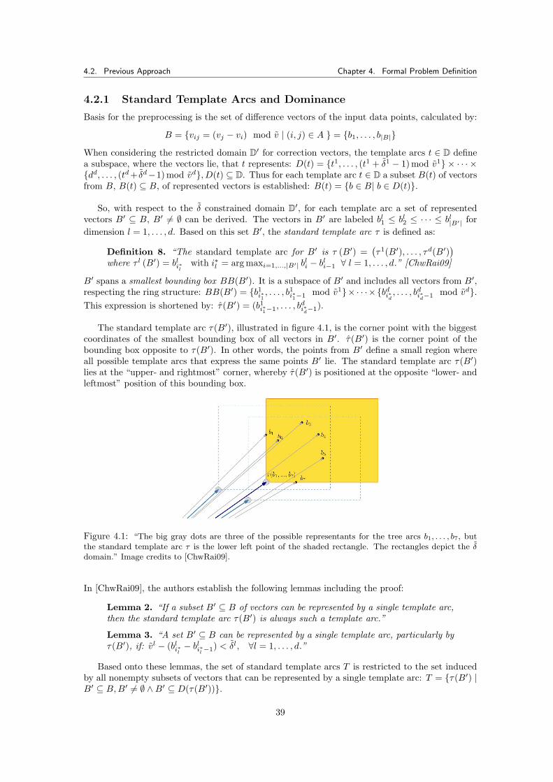
4.2. Previous Approach Chapter 4. Formal Problem Definition
4.2.1 Standard Template Arcs and Dominance
Basis for the preprocessing is the set of difference vectors of the input data points, calculated by:
B = {vij = (vj − vi) mod v | (i, j) ∈ A } = {b1, . . . , b|B|}When considering the restricted domain D′ for correction vectors, the template arcs t ∈ D definea subspace, where the vectors lie, that t represents: D(t) = {t1, . . . , (t1 + δ1 − 1) mod v1} × · · · ×{dd, . . . , (td+ δd−1) mod vd}, D(t) ⊆ D. Thus for each template arc t ∈ D a subset B(t) of vectorsfrom B, B(t) ⊆ B, of represented vectors is established: B(t) = {b ∈ B| b ∈ D(t)}.
So, with respect to the δ constrained domain D′, for each template arc a set of representedvectors B′ ⊆ B, B′ 6= ∅ can be derived. The vectors in B′ are labeled bl1 ≤ bl2 ≤ · · · ≤ bl|B′| fordimension l = 1, . . . , d. Based on this set B′, the standard template arc τ is defined as:
Definition 8. “The standard template arc for B′ is τ (B′) =(τ1(B′), . . . , τd(B′)
)where τ l (B′) = bli∗l
with i∗l = arg maxi=1,...,|B′| bli − bli−1 ∀ l = 1, . . . , d.” [ChwRai09]
B′ spans a smallest bounding box BB(B′). It is a subspace of B′ and includes all vectors from B′,respecting the ring structure: BB(B′) = {b1i∗1 , . . . , b1i∗1−1 mod v1}× · · ·×{bdi∗d , . . . , b
di∗d−1 mod vd}.
This expression is shortened by: τ(B′) = (b1i∗1−1, . . . , bdi∗d−1).
The standard template arc τ(B′), illustrated in figure 4.1, is the corner point with the biggestcoordinates of the smallest bounding box of all vectors in B′. τ(B′) is the corner point of thebounding box opposite to τ(B′). In other words, the points from B′ define a small region whereall possible template arcs that express the same points B′ lie. The standard template arc τ(B′)lies at the “upper- and rightmost” corner, whereby τ(B′) is positioned at the opposite “lower- andleftmost” position of this bounding box.
Figure 4.1: “The big gray dots are three of the possible representants for the tree arcs b1, . . . , b7, butthe standard template arc τ is the lower left point of the shaded rectangle. The rectangles depict the δdomain.” Image credits to [ChwRai09].
In [ChwRai09], the authors establish the following lemmas including the proof:
Lemma 2. “If a subset B′ ⊆ B of vectors can be represented by a single template arc,then the standard template arc τ(B′) is always such a template arc.”
Lemma 3. “A set B′ ⊆ B can be represented by a single template arc, particularly byτ(B′), if: vl − (bli∗l − b
li∗l−1) < δl, ∀l = 1, . . . , d.”
Based onto these lemmas, the set of standard template arcs T is restricted to the set inducedby all nonempty subsets of vectors that can be represented by a single template arc: T = {τ(B′) |B′ ⊆ B,B′ 6= ∅ ∧B′ ⊆ D(τ(B′))}.
39
4.2. Previous Approach Chapter 4. Formal Problem Definition
Definition 9 (Domination of Template Arcs). “Let t′ = τ (B′) and t′′ = τ (B′′),B′ ⊆ B, B′′ ⊆ B. The standard template arc t′ dominates t′′ if and only if B′′ ⊂ B′.”[ChwRai09].
By introducing this concept of domination, the set T is restricted further by discarding alldominated vectors. The resulting set of all non-dominated template arcs is the set of candidatetemplate arcs T c. It is determined in the next step, the preprocessing.
4.2.2 Preprocessing
So, the aim of the preprocessing is to provide this set of candidate template arcs T c. This set T c
is derived out of the set of difference vectors B, from which all possible subsets B′ are derived. Acandidate template arc depends on the correction vector domain δ, which induces the set BB(B′)for each tested vector. So, the check b ∈ BB(B′), with b ∈ B, is performed. The standard tem-plate arc τ(B′) is derived from the bounding box BB(B′).
The algorithm partitions B into three disjoint index sets. The first set contains differencevectors b which are part of the currently considered bounding box BB(B′). The second holds allvectors that until now were actively excluded from being part of BB(B′). The third consists of allvectors to be yet considered. When regarding a current vector and no further addable representedvectors can be found, it is added to the solution set T c. If there exist still representable vectors,branching occurs and by recursive calls these further vectors are identified. For each vector it hasto be determined if it is dominated by another vector, or if in turn dominates others, by constantlyupdating the set of currently found T c. In this manner a restricted enumeration is performed.This algorithm has the complexity O(d · |B|3d) [ChwRai09] and in practice turns out to be thebottleneck of the codebook determination.
The set T c is smaller than the set of all possible template arcs and generated to contain thevectors of the optimal solution. A lower bound for the size of T c is 1, which means, that onlyone single template arc suffices to represent all vectors b ∈ B. As upper bound [ChwRai09]give O(|B|d), and construct a worst case example consisting of a regular grid of non-dominatedtemplate arcs, which in practice should never occur. The authors expect that |T c| � Θ(|B|d).
4.2.3 Solving the k-Node Minimum Label Arborescence Problem
Having now T c available, we proceed by determining the actual minimal codebook subset. Forthis, the graph G is extended by assigning to each arc (i, j) ∈ A all template arcs T c(ai,j) ⊆ T c
that are able to represent it w.r.t. equation (4.1). The next step is to extract a minimal subsetT ⊆ T c, where T must enable a feasible minimal tree encoding.
This problem of finding the minimal codebook is modeled as a variant of the Minimum La-bel Spanning Tree Problem, presented in section 2.1.1. With the use of a MLST we search fora minimum set of labels describing a spanning tree out of an undirected graph. Consequently,we define the arcs from T c as labels. In contrast to the MLST problem we have to consider acomplete directed graph, and allow multiple labels for the arcs. Further we only need a subset ofk nodes to form our spanning tree. For matching purposes, a k of 12–20 minutiae is consideredas sufficient by [SalAdh01]. For modeling k, additionally we use a k-cardinality tree (see section2.1.2), whereby we need only k − 1 edges. The resulting problem is the k-node Minimum LabelSpanning Arborescence Problem (k-MLSA).
Existing algorithms to the k-MLSA problem include heuristics, a memetic algorithm and anexact branch-and-cut approach. Focusing on the latter method, a few details from the entireprocess are summarized straightforwardly. First a directed cut formulation is established. This
40
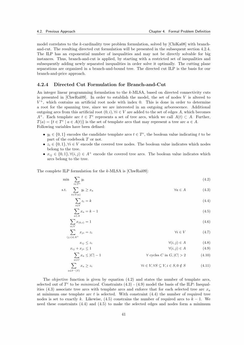
4.2. Previous Approach Chapter 4. Formal Problem Definition
model correlates to the k-cardinality tree problem formulation, solved by [ChiKa08] with branch-and-cut. The resulting directed cut formulation will be presented in the subsequent section 4.2.4.The ILP has an exponential number of inequalities and may not be directly solvable for biginstances. Thus, branch-and-cut is applied, by starting with a restricted set of inequalities andsubsequently adding newly separated inequalities in order solve it optimally. The cutting planeseparations are organized in a branch-and-bound tree. The directed cut ILP is the basis for ourbranch-and-price approach.
4.2.4 Directed Cut Formulation for Branch-and-Cut
An integer linear programming formulation to the k-MLSA, based on directed connectivity cutsis presented in [ChwRai09]. In order to establish the model, the set of nodes V is altered toV +, which contains an artificial root node with index 0. This is done in order to determinea root for the spanning tree, since we are interested in an outgoing arborescence. Additionaloutgoing arcs from this artificial root (0, i),∀i ∈ V are added to the set of edges A, which becomesA+. Each template arc t ∈ T c represents a set of tree arcs, which we call A(t) ⊂ A. Further,T (a) = {t ∈ T c | a ∈ A(t)} is the set of template arcs that may represent a tree arc a ∈ A.Following variables have been defined:
• yt ∈ {0, 1} encodes the candidate template arcs t ∈ T c, the boolean value indicating t to bepart of the codebook T or not.
• zi ∈ {0, 1},∀i ∈ V encode the covered tree nodes. The boolean value indicates which nodesbelong to the tree.
• xij ∈ {0, 1},∀(i, j) ∈ A+ encode the covered tree arcs. The boolean value indicates whicharcs belong to the tree.
The complete ILP formulation for the k-MLSA is [ChwRai09]:
minXt∈Tc
yt (4.2)
s.t.Xt∈T (a)
yt ≥ xa ∀a ∈ A (4.3)
Xi∈V
zi = k (4.4)
Xa∈A
xa = k − 1 (4.5)
Xi∈V
x(0,i) = 1 (4.6)
X(j,i)∈A+
xji = zi ∀i ∈ V (4.7)
xij ≤ zi ∀(i, j) ∈ A (4.8)
xij + xji ≤ 1 ∀(i, j) ∈ A (4.9)Xa∈C
xa ≤ |C| − 1 ∀ cycles C in G, |C| > 2 (4.10)
Xa∈δ−(S)
xa ≥ zi ∀i ∈ V, ∀S ⊆ V, i ∈ S, 0 /∈ S (4.11)
The objective function is given by equation (4.2) and states the number of template arcs,selected out of T c to be minimized. Constraints (4.3) - (4.9) model the basis of the ILP: Inequal-ities (4.3) associate tree arcs with template arcs and enforce that for each selected tree arc xaat minimum one template arc t is selected. With constraint (4.4) the number of required treenodes is set to exactly k. Likewise, (4.5) constrains the number of required arcs to k − 1. Weneed these constraints (4.4) and (4.5) to make the selected edges and nodes form a minimum
41
4.2. Previous Approach Chapter 4. Formal Problem Definition
spanning tree2. Next, we integrate the artificial root into the spanning tree, but again setting byequation (4.6) the number of outgoing arcs from this root node to some arbitrary tree node toone. Equation (4.7) defines for each node v ∈ V , that selected nodes can only have indegree 1, orelse 0, if they are not selected. Further we must associate selected arcs and involved nodes: Byconstraints (4.8) we select only arcs, when their source node is selected.
Inequalities (4.9) are part of the cycle elimination constraints: These inequalities forbid anycycle of length 2. In order to also forbid cycles of greater length (|C| > 2), the inequalities (4.10)are added. The number of these cycle elimination inequalities is exponential, and therefore re-quires to be separated by cutting planes.
The directed connectivity constraints in (4.11) were introduced for strengthening reasons andare not immediately necessary: The constraints model a path from the artificial root node to anyof the selected nodes in V . The node set S has the ingoing cut δ−(S). Their number is alsoexponential.
The branch-and-cut algorithm starts with restrictions (4.2)–(4.9) and then successively sepa-rates and adds cycle elimination constraints as well as connectivity constraints.
Outlook
Having now defined all terms and prerequisites, the task is now to attempt the optimal problemsolution with the aid of column generation techniques. Starting from this directed cut formulation,we proceed by formulating this ILP in such a way that it can be solved by branch-and-price. Thefollowing chapter 5 describes how this formulation is done.
2A spanning tree has n nodes and n− 1 edges, in our case k = n.
42
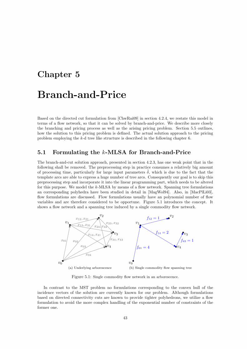
Chapter 5
Branch-and-Price
Based on the directed cut formulation from [ChwRai09] in section 4.2.4, we restate this model interms of a flow network, so that it can be solved by branch-and-price. We describe more closelythe branching and pricing process as well as the arising pricing problem. Section 5.5 outlines,how the solution to this pricing problem is defined. The actual solution approach to the pricingproblem employing the k-d tree like structure is described in the following chapter 6.
5.1 Formulating the k-MLSA for Branch-and-Price
The branch-and-cut solution approach, presented in section 4.2.3, has one weak point that in thefollowing shall be removed. The preprocessing step in practice consumes a relatively big amountof processing time, particularly for large input parameters δ, which is due to the fact that thetemplate arcs are able to express a huge number of tree arcs. Consequently our goal is to skip thispreprocessing step and incorporate it into the linear programming part, which needs to be alteredfor this purpose. We model the k-MLSA by means of a flow network. Spanning tree formulationsan corresponding polyhedra have been studied in detail in [MagWol94]. Also, in [MacPlLi03],flow formulations are discussed. Flow formulations usually have an polynomial number of flowvariables and are therefore considered to be opportune. Figure 5.1 introduces the concept. Itshows a flow network and a spanning tree induced by a single commodity flow network.
v1
v2
v3
v0
v4
x01 x02
x03
x04
x12, x21
x23, x32
x34, x43
x13, x31 x24, x42
x14, x41
(a) Underlying arborescence
v1
v2
v3
v0
f01 = 4
f12 = 1
f14 = 2
v4
f43 = 1
(b) Single commodity flow spanning tree
Figure 5.1: Single commodity flow network in an arborescence.
In contrast to the MST problem no formulations corresponding to the convex hull of theincidence vectors of the solution are currently known for our problem. Although formulationsbased on directed connectivity cuts are known to provide tighter polyhedrons, we utilize a flowformulation to avoid the more complex handling of the exponential number of constraints of theformer one.
43
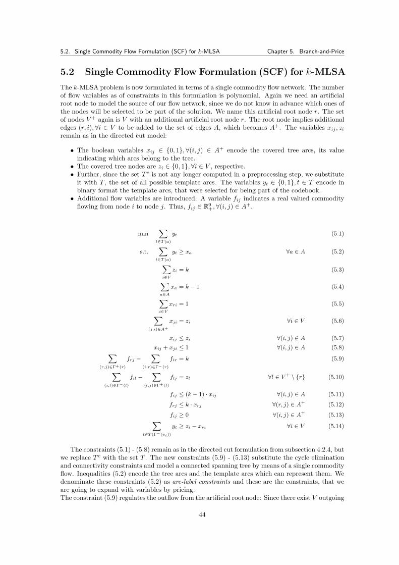
5.2. Single Commodity Flow Formulation (SCF) for k-MLSA Chapter 5. Branch-and-Price
5.2 Single Commodity Flow Formulation (SCF) for k-MLSA
The k-MLSA problem is now formulated in terms of a single commodity flow network. The numberof flow variables as of constraints in this formulation is polynomial. Again we need an artificialroot node to model the source of our flow network, since we do not know in advance which ones ofthe nodes will be selected to be part of the solution. We name this artificial root node r. The setof nodes V + again is V with an additional artificial root node r. The root node implies additionaledges (r, i),∀i ∈ V to be added to the set of edges A, which becomes A+. The variables xij , ziremain as in the directed cut model:
• The boolean variables xij ∈ {0, 1},∀(i, j) ∈ A+ encode the covered tree arcs, its valueindicating which arcs belong to the tree.
• The covered tree nodes are zi ∈ {0, 1},∀i ∈ V , respective.• Further, since the set T c is not any longer computed in a preprocessing step, we substitute
it with T , the set of all possible template arcs. The variables yt ∈ {0, 1}, t ∈ T encode inbinary format the template arcs, that were selected for being part of the codebook.
• Additional flow variables are introduced. A variable fij indicates a real valued commodityflowing from node i to node j. Thus, fij ∈ R0
+,∀(i, j) ∈ A+.
minXt∈T (a)
yt (5.1)
s.t.Xt∈T (a)
yt ≥ xa ∀a ∈ A (5.2)
Xi∈V
zi = k (5.3)
Xa∈A
xa = k − 1 (5.4)
Xi∈V
xri = 1 (5.5)
X(j,i)∈A+
xji = zi ∀i ∈ V (5.6)
xij ≤ zi ∀(i, j) ∈ A (5.7)
xij + xji ≤ 1 ∀(i, j) ∈ A (5.8)X(r,j)∈Γ+(r)
frj −X
(i,r)∈Γ−(r)
fir = k (5.9)
X(i,l)∈Γ−(l)
fil −X
(l,j)∈Γ+(l)
flj = zl ∀l ∈ V + \ {r} (5.10)
fij ≤ (k − 1) · xij ∀(i, j) ∈ A (5.11)
frj ≤ k · xrj ∀(r, j) ∈ A+ (5.12)
fij ≥ 0 ∀(i, j) ∈ A+ (5.13)Xt∈T (Γ−(vi))
yt ≥ zi − xri ∀i ∈ V (5.14)
The constraints (5.1) - (5.8) remain as in the directed cut formulation from subsection 4.2.4, butwe replace T c with the set T . The new constraints (5.9) - (5.13) substitute the cycle eliminationand connectivity constraints and model a connected spanning tree by means of a single commodityflow. Inequalities (5.2) encode the tree arcs and the template arcs which can represent them. Wedenominate these constraints (5.2) as arc-label constraints and these are the constraints, that weare going to expand with variables by pricing.The constraint (5.9) regulates the outflow from the artificial root node: Since there exist V outgoing
44
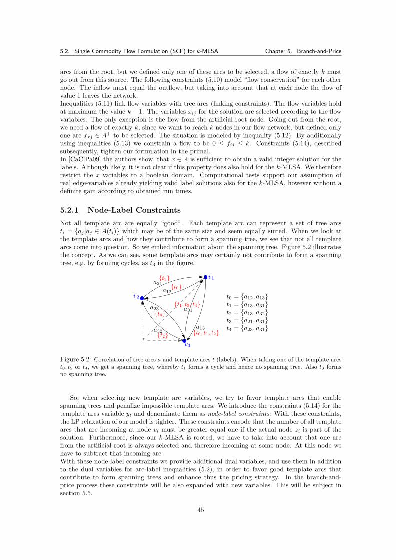
5.2. Single Commodity Flow Formulation (SCF) for k-MLSA Chapter 5. Branch-and-Price
arcs from the root, but we defined only one of these arcs to be selected, a flow of exactly k mustgo out from this source. The following constraints (5.10) model “flow conservation” for each othernode. The inflow must equal the outflow, but taking into account that at each node the flow ofvalue 1 leaves the network.Inequalities (5.11) link flow variables with tree arcs (linking constraints). The flow variables holdat maximum the value k − 1. The variables xij for the solution are selected according to the flowvariables. The only exception is the flow from the artificial root node. Going out from the root,we need a flow of exactly k, since we want to reach k nodes in our flow network, but defined onlyone arc xrj ∈ A+ to be selected. The situation is modeled by inequality (5.12). By additionallyusing inequalities (5.13) we constrain a flow to be 0 ≤ fij ≤ k. Constraints (5.14), describedsubsequently, tighten our formulation in the primal.In [CaClPa09] the authors show, that x ∈ R is sufficient to obtain a valid integer solution for thelabels. Although likely, it is not clear if this property does also hold for the k-MLSA. We thereforerestrict the x variables to a boolean domain. Computational tests support our assumption ofreal edge-variables already yielding valid label solutions also for the k-MLSA, however without adefinite gain according to obtained run times.
5.2.1 Node-Label Constraints
Not all template arc are equally “good”. Each template arc can represent a set of tree arcsti = {aj |aj ∈ A(ti)} which may be of the same size and seem equally suited. When we look atthe template arcs and how they contribute to form a spanning tree, we see that not all templatearcs come into question. So we embed information about the spanning tree. Figure 5.2 illustratesthe concept. As we can see, some template arcs may certainly not contribute to form a spanningtree, e.g. by forming cycles, as t3 in the figure.
r
v1
v2
v3
a12
a21
a13
a31
a32
a23
t0 = {a12, a13}{t0}
{t4}
{t2}
{t3}
{t0, t1, t2}
{t1, t3, t4} t1 = {a13, a31}t2 = {a13, a32}t3 = {a21, a31}t4 = {a23, a31}
Figure 5.2: Correlation of tree arcs a and template arcs t (labels). When taking one of the template arcst0, t2 or t4, we get a spanning tree, whereby t1 forms a cycle and hence no spanning tree. Also t3 formsno spanning tree.
So, when selecting new template arc variables, we try to favor template arcs that enablespanning trees and penalize impossible template arcs. We introduce the constraints (5.14) for thetemplate arcs variable yt and denominate them as node-label constraints. With these constraints,the LP relaxation of our model is tighter. These constraints encode that the number of all templatearcs that are incoming at node vi must be greater equal one if the actual node zi is part of thesolution. Furthermore, since our k-MLSA is rooted, we have to take into account that one arcfrom the artificial root is always selected and therefore incoming at some node. At this node wehave to subtract that incoming arc.With these node-label constraints we provide additional dual variables, and use them in additionto the dual variables for arc-label inequalities (5.2), in order to favor good template arcs thatcontribute to form spanning trees and enhance thus the pricing strategy. In the branch-and-price process these constraints will be also expanded with new variables. This will be subject insection 5.5.
45
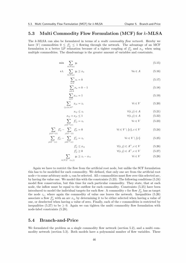
5.3. Multi Commodity Flow Formulation (MCF) for k-MLSA Chapter 5. Branch-and-Price
5.3 Multi Commodity Flow Formulation (MCF) for k-MLSA
The k-MLSA can also be formulated in terms of a multi commodity flow network. Hereby wehave |V | commodities 0 ≤ f cij ≤ 1 flowing through the network. The advantage of an MCFformulation is a better LP relaxation because of a tighter coupling of f cij and xij when usingmultiple commodities. The disadvantage is the greater amount of variables and constraints.
minXt∈T (a)
yt (5.15)
s.t.Xt∈T (a)
yt ≥ xa ∀a ∈ A (5.16)
Xi∈V
zi = k (5.17)
Xa∈A
xa = k − 1 (5.18)
Xi∈V
xri = 1 (5.19)
X(j,i)∈A+
xji = zi ∀i ∈ V (5.20)
xij ≤ zi ∀(i, j) ∈ A (5.21)
xij + xji ≤ 1 ∀(i, j) ∈ A (5.22)Xj∈Γ+(r)
fcrj = zc ∀c ∈ V (5.23)
Xj∈Γ+(i)
fcij −X
j∈Γ−(i)
fcji = 0 ∀i ∈ V \ {c}, c ∈ V (5.24)
Xj∈Γ−(c)
fcjc −X
j∈Γ+(c)
fccj = zc ∀c ∈ V \ {r} (5.25)
fcij ≤ xij ∀(i, j) ∈ A+, c ∈ V (5.26)
fcij ≥ 0 ∀(i, j) ∈ A+, c ∈ V (5.27)Xt∈T (Γ−(vi))
yt ≥ zi − xri ∀i ∈ V (5.28)
Again we have to restrict the flow from the artificial root node, but unlike the SCF formulationthis has to be modelled for each commodity. We defined, that only one arc from the artificial rootnode r to some arbitrary node zi can be selected. All c commodities must flow over this selected arc,by having the value one. We model this with the constraints (5.23). The following conditions (5.24)model flow conservation, but this time for each particular commodity. They state, that at eachnode, the inflow must be equal to the outflow for each commodity. Constraints (5.25) have beenintroduced to model the individual targets for each flow: A commodity c for flow f cjc has as targetthe node zc, where again the commodity of value one leaves the network. Inequalities (5.26)associate a flow f cij with an arc xij by determining it to be either selected when having a value ofone, or deselected when having a value of zero. Finally, each of the c commodities is restricted byinequalities (5.27) to be ≥ 0. Again we can tighten the multi commodity flow formulation withnode-label constraints (5.28).
5.4 Branch-and-Price
We formulated the problem as a single commodity flow network (section 5.2), and a multi com-modity network (section 5.3). Both models have a polynomial number of flow variables. These
46
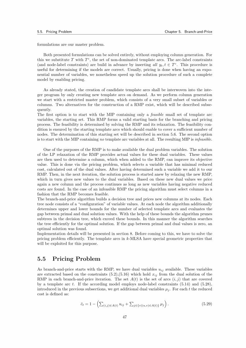
5.5. Pricing Problem Chapter 5. Branch-and-Price
formulations are our master problem.
Both presented formulations can be solved entirely, without employing column generation. Forthis we substitute T with T c, the set of non-dominated template arcs. The arc-label constraints(and node-label constraints) are build in advance by inserting all yt, t ∈ T c. This procedure isuseful for determining if the models are correct. Usually, pricing is done when having an expo-nential number of variables, we nonetheless speed up the solution procedure of such a completemodel by enabling pricing.
As already stated, the creation of candidate template arcs shall be interwoven into the inte-ger program by only creating new template arcs on demand. As we perform column generationwe start with a restricted master problem, which consists of a very small subset of variables orcolumns. Two alternatives for the construction of a RMP exist, which will be described subse-quently.The first option is to start with the MIP containing only a feasible small set of template arcvariables, the starting set. This RMP forms a valid starting basis for the branching and pricingprocess. The feasibility is determined by solving the RMP and its relaxation. The feasibility con-dition is ensured by the starting template arcs which should enable to cover a sufficient number ofnodes. The determination of this starting set will be described in section 5.6. The second optionis to start with the MIP containing no template arc variables at all. The resulting MIP is infeasible.
One of the purposes of the RMP is to make available the dual problem variables. The solutionof the LP relaxation of the RMP provides actual values for these dual variables. These valuesare then used to determine a column, which when added to the RMP, can improve its objectivevalue. This is done via the pricing problem, which selects a variable that has minimal reducedcost, calculated out of the dual values. After having determined such a variable we add it to ourRMP. Then, in the next iteration, the solution process is started anew by relaxing the new RMP,which in turn gives new values to the dual variables. Based on these new dual values we priceagain a new column and the process continues as long as new variables having negative reducedcosts are found. In the case of an infeasible RMP the pricing algorithm must select columns in afashion that the RMP becomes feasible.The branch-and-price algorithm builds a decision tree and prices new columns at its nodes. Eachtree node consists of a “configuration” of variable values. At each node the algorithm additionallydetermines upper and lower bounds for the number of selected template arcs and evaluates thegap between primal and dual solution values. With the help of these bounds the algorithm prunessubtrees in the decision tree, which exceed these bounds. In this manner the algorithm searchesthe tree efficiently for the optimal solution. If the gap between primal and dual values is zero, anoptimal solution was found.Implementation details will be presented in section 8. Before coming to this, we have to solve thepricing problem efficiently. The template arcs in k-MLSA have special geometric properties thatwill be exploited for this purpose.
5.5 Pricing Problem
As branch-and-price starts with the RMP, we have dual variables uij available. These variablesare extracted based on the constraints (5.2),(5.16) which hold xij from the dual solution of theRMP in each branch-and-price iteration. The set A(t) is the set of arcs (i, j) that are coveredby a template arc t. If the according model employs node-label constraints (5.14) and (5.28),introduced in the previous subsections, we get additional dual variables µj . For each t the reducedcost is defined as:
ct = 1−(∑
(i,j)∈A(t) uij +∑j∈{v|(u,v)∈A(t)} µj
). (5.29)
47
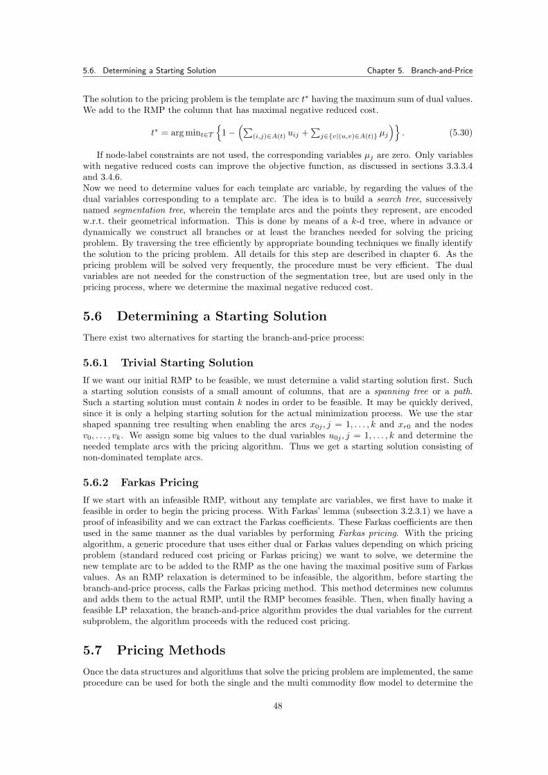
5.6. Determining a Starting Solution Chapter 5. Branch-and-Price
The solution to the pricing problem is the template arc t∗ having the maximum sum of dual values.We add to the RMP the column that has maximal negative reduced cost.
t∗ = arg mint∈T{
1−(∑
(i,j)∈A(t) uij +∑j∈{v|(u,v)∈A(t)} µj
)}. (5.30)
If node-label constraints are not used, the corresponding variables µj are zero. Only variableswith negative reduced costs can improve the objective function, as discussed in sections 3.3.3.4and 3.4.6.Now we need to determine values for each template arc variable, by regarding the values of thedual variables corresponding to a template arc. The idea is to build a search tree, successivelynamed segmentation tree, wherein the template arcs and the points they represent, are encodedw.r.t. their geometrical information. This is done by means of a k-d tree, where in advance ordynamically we construct all branches or at least the branches needed for solving the pricingproblem. By traversing the tree efficiently by appropriate bounding techniques we finally identifythe solution to the pricing problem. All details for this step are described in chapter 6. As thepricing problem will be solved very frequently, the procedure must be very efficient. The dualvariables are not needed for the construction of the segmentation tree, but are used only in thepricing process, where we determine the maximal negative reduced cost.
5.6 Determining a Starting Solution
There exist two alternatives for starting the branch-and-price process:
5.6.1 Trivial Starting Solution
If we want our initial RMP to be feasible, we must determine a valid starting solution first. Sucha starting solution consists of a small amount of columns, that are a spanning tree or a path.Such a starting solution must contain k nodes in order to be feasible. It may be quickly derived,since it is only a helping starting solution for the actual minimization process. We use the starshaped spanning tree resulting when enabling the arcs x0j , j = 1, . . . , k and xr0 and the nodesv0, . . . , vk. We assign some big values to the dual variables u0j , j = 1, . . . , k and determine theneeded template arcs with the pricing algorithm. Thus we get a starting solution consisting ofnon-dominated template arcs.
5.6.2 Farkas Pricing
If we start with an infeasible RMP, without any template arc variables, we first have to make itfeasible in order to begin the pricing process. With Farkas’ lemma (subsection 3.2.3.1) we have aproof of infeasibility and we can extract the Farkas coefficients. These Farkas coefficients are thenused in the same manner as the dual variables by performing Farkas pricing. With the pricingalgorithm, a generic procedure that uses either dual or Farkas values depending on which pricingproblem (standard reduced cost pricing or Farkas pricing) we want to solve, we determine thenew template arc to be added to the RMP as the one having the maximal positive sum of Farkasvalues. As an RMP relaxation is determined to be infeasible, the algorithm, before starting thebranch-and-price process, calls the Farkas pricing method. This method determines new columnsand adds them to the actual RMP, until the RMP becomes feasible. Then, when finally having afeasible LP relaxation, the branch-and-price algorithm provides the dual variables for the currentsubproblem, the algorithm proceeds with the reduced cost pricing.
5.7 Pricing Methods
Once the data structures and algorithms that solve the pricing problem are implemented, the sameprocedure can be used for both the single and the multi commodity flow model to determine the
48
5.7. Pricing Methods Chapter 5. Branch-and-Price
variable that is added to the RMP. The same algorithm enables Farkas pricing and determinescolumns that make some previously infeasible LP feasible. Subsequently we summarize sometopics, which adhere to the branch-and-price process.
5.7.1 Standard and Multiple Pricing
We have two alternatives when adding columns. When performing standard pricing we determinein each pricing iteration the column having maximal reduced cost and add it to our RMP. Afterresolving the RMP relaxation we proceed in the same manner in the next pricing iteration untilno further variable having negative reduced cost can be found. At the next branch-and-boundnode, the algorithm proceeds in the same manner.
When doing multiple pricing, we determine all columns with negative reduced cost in onepricing iteration, and add them all to our RMP in one step. Only after all these variables wereadded, the RMP is relaxed and solved anew, before proceeding with the next pricing iteration.This is done in each branch-and-bound node, until no variables having reduced costs are foundanymore.
5.7.2 Allowing Variable Duplicates
In the course of the branching and pricing process it may happen that some variables are foundtwice, or even more times in subsequent pricing iterations. When enabling such variable dupli-cates the algorithm may spend a lot of time with finding the same variable again and again. Suchsituations may occur due to the fact that the solution of the dual problem is not unique.
Adding duplicates each time they are found, makes the number of variables and thus the MIPvery huge. The algorithm may spend much time with the pricing of plenty of duplicates. Althoughthe problem is still solvable prevented this behaviour. Accordingly, each time we search for a newvariable, we check if we already have found this variable and add another variable, if existing, withinferior reduced cost instead. This topic is also covered in chapter 9.
5.7.3 Algorithms
The overall branch-and-price algorithm is described by listing 5.1. This algorithm only outlinesthe procedure, which we will perform with the aid of a branch-and-price framework. We embed theparts for loading the model and implement the routines relevant to the pricing problem. Furtherwe influence the solution process by selecting traversing strategy and according branching rules.
At line 1 the algorithm initializes the branch-and-bound tree and codebook. The variable z∗
will save the best solution. At line 2, the algorithm loads the desired formulation, either the SCF orMCF model, determines a starting solution and adds it to the RMP. Naturally, when employinga Farkas pricer, the step for determining a starting solution is omitted. Line 3 generates newsubproblems for the branch-and-bound process, and adds them to the branch-and-bound tree asnodes. Then, after having selected the next node and thus the subproblem to process (line 5), thepricer adds new variables tnew to the RMP as long as it finds some and relaxes/solves anew theRMP. While processing the nodes the algorithm descends into the tree by a traversing strategy(DFS or BFS) and selects the node to be processed next with the aid of a branching rule. Whiledoing so, the algorithm determines the optimal solution by evaluating at each subproblem nodethe objective value, upper and lower bounds and dual gap. The solution strategy of the pricer ispresented in the next chapter 6. In section 6.6, the instances for the abstract pricer algorithmsare described.
49
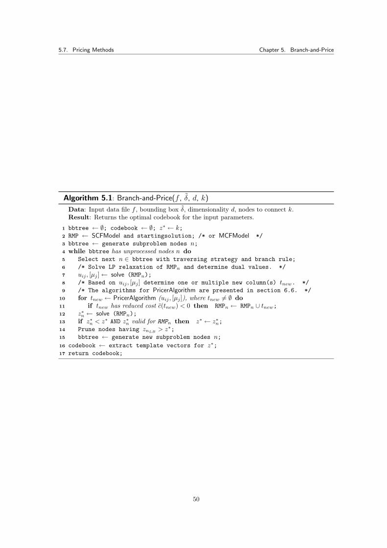
5.7. Pricing Methods Chapter 5. Branch-and-Price
Algorithm 5.1: Branch-and-Price(f , δ, d, k)
Data: Input data file f , bounding box δ, dimensionality d, nodes to connect k.Result: Returns the optimal codebook for the input parameters.
bbtree ← ∅; codebook ← ∅; z∗ ← k;1
RMP ← SCFModel and startingsolution; /* or MCFModel */2
bbtree ← generate subproblem nodes n;3
while bbtree has unprocessed nodes n do4
Select next n ∈ bbtree with traversing strategy and branch rule;5
/* Solve LP relaxation of RMPn and determine dual values. */6
uij , [µj ]← solve (RMPn);7
/* Based on uij , [µj ] determine one or multiple new column(s) tnew. */8
/* The algorithms for PricerAlgorithm are presented in section 6.6. */9
for tnew ← PricerAlgorithm (uij , [µj ]), where tnew 6= ∅ do10
if tnew has reduced cost c(tnew) < 0 then RMPn ← RMPn ∪ tnew;11
z∗n ← solve (RMPn);12
if z∗n < z∗ AND z∗n valid for RMPn then z∗ ← z∗n;13
Prune nodes having znLB > z∗;14
bbtree ← generate new subproblem nodes n;15
codebook ← extract template vectors for z∗;16
return codebook;17
50
Chapter 6
Solving the Pricing Problem
This chapter describes the solution approach for the pricing problem in detail. First, we presentthe overall principle and proceed with defining a region abstraction, upon which the k-d-tree likestructure is based on. In the following, we denominate this tree as segmentation tree. This chapterdescribes construction and management of this data structure and how we extract data from it.By traversing the segmentation tree systematically, we search for a node corresponding to thesolution to the pricing problem.
6.1 Basic Ideas
The role of the pricing problem can be illustrated as follows. Imagine a rectangle of size δ definedby each point b ∈ B in a finite 2-dimensional domain. This bounding box, with the point b at itsupper, rightmost corner, defines an area in which a template arc, able to express this point, canlie. So by having such a rectangle for each bi, these rectangles overlap. This results in areas wheremultiple rectangles overlap each other. These overlapping areas define template arcs, where morethan one element b can be expressed and therefore corresponds to a template arc, which is able toexpress all points bi associated with each one of the rectangles out of which the area was formed.In the two-dimensional case, the pricing problem can be illustrated as follows. If the boundingboxes are considered as transparent grey-shaded rectangles with a grey-tone corresponding to thevalue of the associated dual variable, overlapping regions imply darker areas. Our goal is to findthe darkest areas.
6.1.1 Segmenting the Area by Means of a k-d Tree
Input to the k-d tree are the difference vectors bi ∈ B. In order to retain the meaning of k in the(usually so called) k-d tree naming, it must be annotated that we denote the dimensionality byd. As we defined k being the size of the subset of nodes from V forming the k-MLSA we mustpay attention to not confuse both terms. Further input is the correction vector domain (δ1, . . . , δd).
The basic idea for the solution of the pricing problem is to segment the finite domain D intosubspaces in the fashion of a k-d tree. The division into subspaces is done by means of the pointsbi and the corner points of the δ sized bounding box defined by each bi:
(b1i , b2i , . . . , b
di ), (b
1i − δ1, b2i , . . . , b
di ), (b
1i , b
2i − δ2, . . . , bdi ), . . . , (b
1i − δ1, b2i − δ2, . . . , bdi − δd).
The segmentation is done along the (d − 1)-hyperplanes of the bounding boxes. Each point biimplicitly defines 2d corner points that represent the limits of the bounding box for each bi. Allrelevant coordinate information is contained in the two points (b1i , b
2i , . . . , b
di ) and (b1i − δ1, b2i −
δ2, . . . , bdi − δd). Having such bi, where each one defines a bounding box, we want to identify theareas where more bounding boxes overlap. We want to divide the finite domain D in a fashion,
51
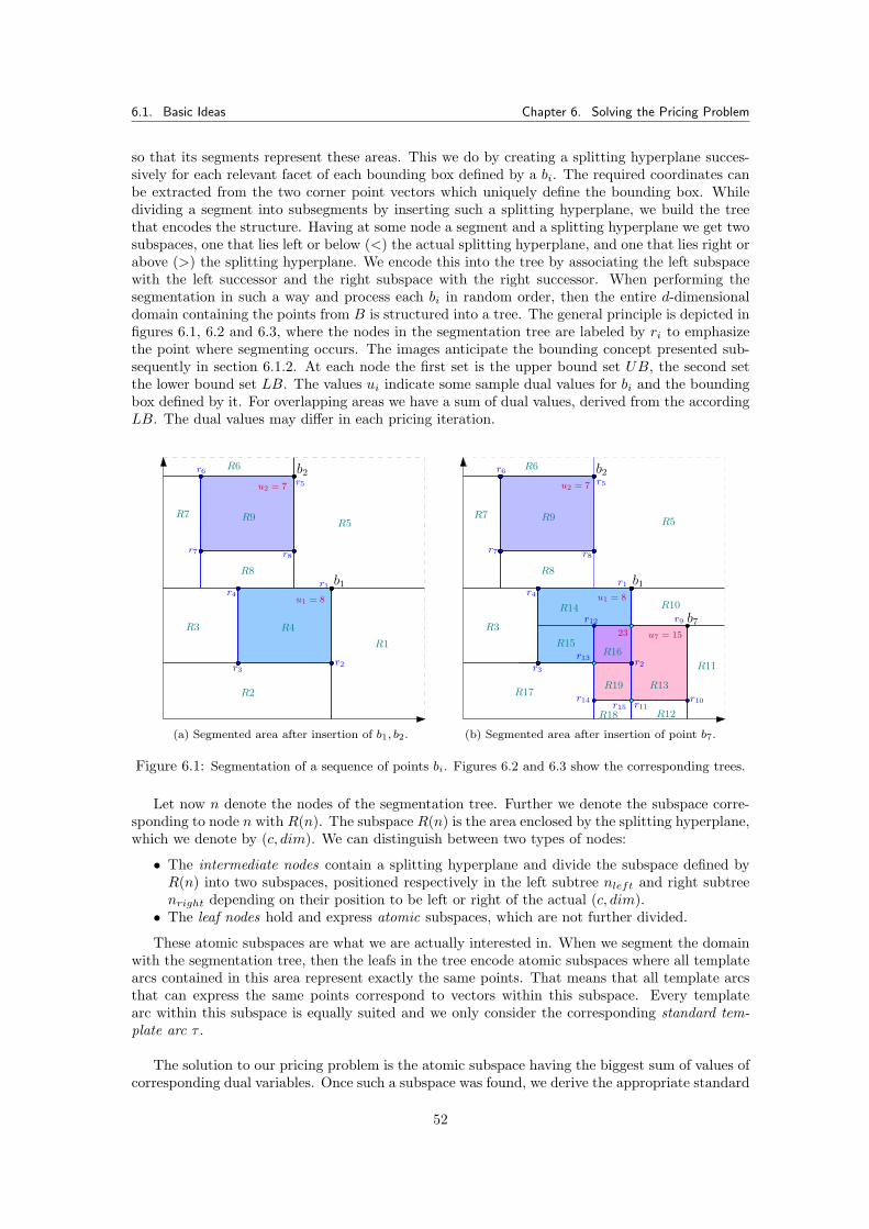
6.1. Basic Ideas Chapter 6. Solving the Pricing Problem
so that its segments represent these areas. This we do by creating a splitting hyperplane succes-sively for each relevant facet of each bounding box defined by a bi. The required coordinates canbe extracted from the two corner point vectors which uniquely define the bounding box. Whiledividing a segment into subsegments by inserting such a splitting hyperplane, we build the treethat encodes the structure. Having at some node a segment and a splitting hyperplane we get twosubspaces, one that lies left or below (<) the actual splitting hyperplane, and one that lies right orabove (>) the splitting hyperplane. We encode this into the tree by associating the left subspacewith the left successor and the right subspace with the right successor. When performing thesegmentation in such a way and process each bi in random order, then the entire d-dimensionaldomain containing the points from B is structured into a tree. The general principle is depicted infigures 6.1, 6.2 and 6.3, where the nodes in the segmentation tree are labeled by ri to emphasizethe point where segmenting occurs. The images anticipate the bounding concept presented sub-sequently in section 6.1.2. At each node the first set is the upper bound set UB, the second setthe lower bound set LB. The values ui indicate some sample dual values for bi and the boundingbox defined by it. For overlapping areas we have a sum of dual values, derived from the accordingLB. The dual values may differ in each pricing iteration.
r1
r2r3
r4
b1
b2r5
r6
r7 r8
u1 = 8
u2 = 7
R1
R2
R3 R4
R5
R6
R7
R8
R9
(a) Segmented area after insertion of b1, b2.
r1
r2r3
r4
b1
b2r5
r6
r7 r8
u1 = 8
u2 = 7
R3
R5
R6
R7
R8
R9
23 u7 = 15
b7r9
r10r11
r12
r13
r14r15
R10
R11
R12
R13
R14
R15R16
R17
R18
R19
(b) Segmented area after insertion of point b7.
Figure 6.1: Segmentation of a sequence of points bi. Figures 6.2 and 6.3 show the corresponding trees.
Let now n denote the nodes of the segmentation tree. Further we denote the subspace corre-sponding to node n with R(n). The subspace R(n) is the area enclosed by the splitting hyperplane,which we denote by (c, dim). We can distinguish between two types of nodes:
• The intermediate nodes contain a splitting hyperplane and divide the subspace defined byR(n) into two subspaces, positioned respectively in the left subtree nleft and right subtreenright depending on their position to be left or right of the actual (c, dim).
• The leaf nodes hold and express atomic subspaces, which are not further divided.
These atomic subspaces are what we are actually interested in. When we segment the domainwith the segmentation tree, then the leafs in the tree encode atomic subspaces where all templatearcs contained in this area represent exactly the same points. That means that all template arcsthat can express the same points correspond to vectors within this subspace. Every templatearc within this subspace is equally suited and we only consider the corresponding standard tem-plate arc τ .
The solution to our pricing problem is the atomic subspace having the biggest sum of values ofcorresponding dual variables. Once such a subspace was found, we derive the appropriate standard
52
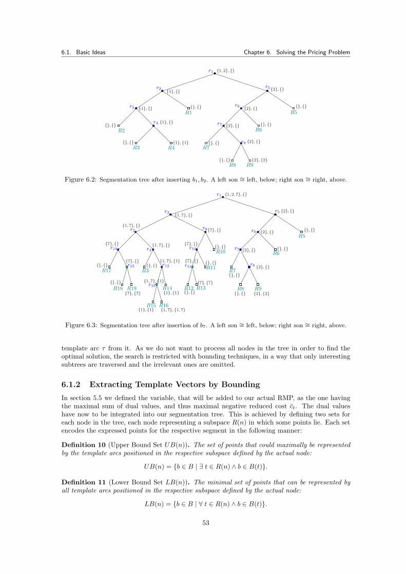
6.1. Basic Ideas Chapter 6. Solving the Pricing Problem
r1
r2
R1r3
R2
r4
R3 R4
r5
R5r6
R6r7
R7r8
R8 R9
{1, 2}, {}
{2}, {}
{2}, {}
{2}, {}
{2}, {2}
{2}, {}
{}, {}
{}, {}
{}, {}
{}, {}
{}, {}
{1}, {}
{1}, {1}
{1}, {}
{}, {}
{}, {}
{1}, {}
Figure 6.2: Segmentation tree after inserting b1, b2. A left son ∼= left, below; right son ∼= right, above.
r1
r2
r3
r4
R3
r5
R5r6
R6r7
R7r8
R8 R9
{1, 2, 7}, {}
{2}, {}
{2}, {}
{2}, {}
{2}, {2}
{2}, {}
{}, {}
{}, {}
{}, {}
{}, {}
{7}, {}
{1, 7}, {}
{1, 7}, {1}
{1, 7}, {}
{7}, {}
{}, {}
{1, 7}, {}
r9
R10r10
R11r11
R12 R13{7}, {7}
r12
R14r13
R15 R16
r14
R17r15
R18 R19
{}, {}
{}, {}
{7}, {7}
{7}, {}
{1}, {1} {1, 7}, {1, 7}
{1, 7}, {1}
{1}, {1} {}, {}
{}, {}
{}, {}{7}, {}
{7}, {}
Figure 6.3: Segmentation tree after insertion of b7. A left son ∼= left, below; right son ∼= right, above.
template arc τ from it. As we do not want to process all nodes in the tree in order to find theoptimal solution, the search is restricted with bounding techniques, in a way that only interestingsubtrees are traversed and the irrelevant ones are omitted.
6.1.2 Extracting Template Vectors by Bounding
In section 5.5 we defined the variable, that will be added to our actual RMP, as the one havingthe maximal sum of dual values, and thus maximal negative reduced cost ct. The dual valueshave now to be integrated into our segmentation tree. This is achieved by defining two sets foreach node in the tree, each node representing a subspace R(n) in which some points lie. Each setencodes the expressed points for the respective segment in the following manner:
Definition 10 (Upper Bound Set UB(n)). The set of points that could maximally be representedby the template arcs positioned in the respective subspace defined by the actual node:
UB(n) = {b ∈ B | ∃ t ∈ R(n) ∧ b ∈ B(t)}.
Definition 11 (Lower Bound Set LB(n)). The minimal set of points that can be represented byall template arcs positioned in the respective subspace defined by the actual node:
LB(n) = {b ∈ B | ∀ t ∈ R(n) ∧ b ∈ B(t)}.
53
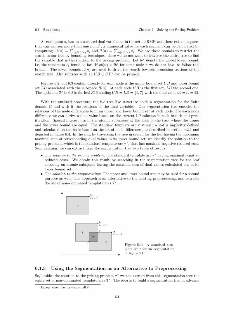
6.1. Basic Ideas Chapter 6. Solving the Pricing Problem
As each point bi has an associated dual variable ui in the actual RMP, and there exist subspacesthat can express more than one point1, a numerical value for each segment can be calculated bycomputing ub(n) =
∑i∈UB(n) ui and lb(n) =
∑i∈LB(n) ui. We use these bounds to restrict the
search in our tree by bounding techniques, since we do not want to traverse the entire tree to findthe variable that is the solution to the pricing problem. Let lb∗ denote the global lower bound,i.e. the maximum ct found so far. If ub(n) < lb∗ for some node n we do not have to follow thisbranch. The lower bounds lb(n) are used to drive the search towards promising sections of thesearch tree. Also subtrees with an UB ⊂ UB∗ can be pruned.
Figures 6.2 and 6.3 contain already for each node n the upper bound set UB and lower boundset LB associated with the subspace R(n). At each node UB is the first set, LB the second one.The optimum lb∗ in 6.3 is the leaf R16 holding UB = LB = {1, 7} with the dual value ub = lb = 23.
With the outlined procedure, the k-d tree like structure holds a segmentation for the finitedomain D and with it the relations of the dual variables. Our segmentation tree encodes therelations of the node differences bi in an upper and lower bound set at each node. For each nodedifference we can derive a dual value based on the current LP solution in each branch-and-priceiteration. Special interest lies in the atomic subspaces at the leafs of the tree, where the upperand the lower bound are equal. The standard template arc τ at such a leaf is implicitly definedand calculated on the basis based on the set of node differences, as described in section 4.2.1 anddepicted in figure 6.4. In the end, by traversing the tree in search for the leaf having the maximummaximal sum of corresponding dual values in its lower bound set, we identify the solution to thepricing problem, which is the standard template arc τ∗, that has maximal negative reduced cost.Summarizing, we can extract from the segmentation tree two types of results:
• The solution to the pricing problem: The standard template arc τ∗ having maximal negativereduced costs. We obtain this result by searching in the segmentation tree for the leafencoding an atomic subspace, having the maximal sum of dual values calculated out of itslower bound set.
• The solution to the preprocessing : The upper and lower bound sets may be used for a secondpurpose as well. The approach is an alternative to the existing preprocessing, and extractsthe set of non-dominated template arcs T c.
u2 = 7
u1 = 8
u7 = 15
7
8
15
τ
23
τ
b2
b1
b7
Figure 6.4: A standard tem-plate arc τ for the segmentationin figure 6.1b.
6.1.3 Using the Segmentation as an Alternative to Preprocessing
So, besides the solution to the pricing problem τ∗ we can extract from this segmentation tree theentire set of non-dominated template arcs T c. The idea is to build a segmentation tree in advance
1Except when having very small δ.
54
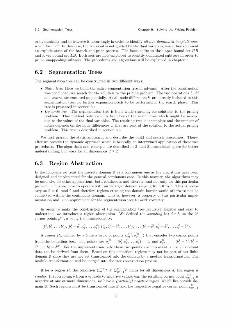
6.2. Segmentation Trees Chapter 6. Solving the Pricing Problem
or dynamically and to traverse it accordingly in order to identify all non-dominated template arcs,which form T c. In this case, the traversal is not guided by the dual variables, since they representan explicit state of the branch-and-price process. The focus shifts to the upper bound set UBand lower bound set LB. Both sets are now employed to identify dominated subtrees in order toprune unappealing subtrees. The procedures and algorithms will be explained in chapter 7.
6.2 Segmentation Trees
The segmentation tree can be constructed in two different ways:
• Static tree: Here we build the entire segmentation tree in advance. After the constructionwas concluded, we search for the solution to the pricing problem. The two operations buildand search are executed sequentially. As all node differences bi are already included in thissegmentation tree, no further expansion needs to be performed in the search phase. Thistree is presented in section 6.4.
• Dynamic tree: The segmentation tree is built while searching for solutions to the pricingproblem. This method only expands branches of the search tree which might be neededdue to the values of the dual variables. The resulting tree is incomplete and the number ofnodes depends on the node differences bi that are part of the solution to the actual pricingproblem. This tree is described in section 6.5.
We first present the static approach, and describe the build and search procedures. There-after we present the dynamic approach which is basically an intertwined application of these twoprocedures. The algorithms and concepts are described in 2- and 3-dimensional space for betterunderstanding, but work for all dimensions d ≥ 2.
6.3 Region Abstraction
In the following we treat the discrete domain D as a continuous one as the algorithms have beendesigned and implemented for the general continuous case. In this manner, the algorithms maybe used also for other applications, both continuous and discrete, and not only for this particularproblem. Thus we have to operate with an enlarged domain ranging from 0 to v. This is neces-sary as v = 0 mod v and therefore regions crossing the domain border would otherwise not beconnected within the continuous domain. This is, however, a property of this particular imple-mentation and is no requirement for the segmentation tree to work correctly.
In order to make the construction of the segmentation tree recursive, flexible and easy tounderstand, we introduce a region abstraction. We defined the bounding box for bi as the 2d
corner points p(i), d being the dimensionality:
(b1i , b2i , . . . , b
di ), (b
1i − δ1, b2i , . . . , b
di ), (b
1i , b
2i − δ2, . . . , bdi ), . . . , (b
1i − δ1, b2i − δ2, . . . , bdi − δd).
A region Ri, defined by a bi, is a tuple of points 〈p(i)0 , p
(i)
2d−1〉 that encodes two corner points
from the bounding box. The points are p(i)0 = (b1i , b
2i , . . . , b
di ) = bi and p
(i)
2d−1= (b1i − δ1, b2i −
δ2, . . . , bdi − δd). For the implementation only these two points are important, since all relevantdata can be derived from them. Based on this definition, regions may not be part of our finitedomain D since they are not yet transformed into the domain by a modulo transformation. Themodulo transformation will be merged into the tree construction process.
If for a region Ri the condition (p(i)0 )d ≥ (p(i)
2d−1)d holds for all dimensions d, the region is
regular. If subtracting δ from a bi leads to negative values, e.g. the resulting corner point p(i)
2d−1is
negative at one or more dimensions, we have a (partially) negative region, which lies outside do-main D. Such regions must be transformed into D and the respective negative corner point p(i)
2d−1
55
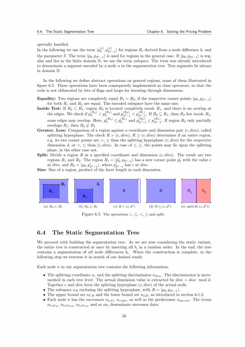
6.4. The Static Segmentation Tree Chapter 6. Solving the Pricing Problem
specially handled.In the following we use the term 〈p(i)
0 , p(i)
2d−1〉 for regions Ri derived from a node difference bi and
the parameter δ. The term 〈p0, p2d−1〉 is used for regions in the general case. If 〈p0, p2d−1〉 is reg-ular and lies in the finite domain D, we use the term subspace. The term was already introducedto denominate a segment encoded by a node n in the segmentation tree. Tree segments lie alwaysin domain D.
In the following we define abstract operations on general regions, some of them illustrated infigure 6.5. These operations have been consequently implemented as class operators, so that thecode is not obfuscated by lots of flags and loops for iterating through dimensions.
Equality: Two regions are completely equal R1 = R2, if the respective corner points 〈p0, p2d−1〉for both R1 and R2 are equal. The encoded subspace have the same size.
Inside Test: If R2 ⊂ R1, region R2 is located completely inside R1, and there is no overlap atthe edges. We check if p(R2)
0 < p(R1)0 and p(R2)
2d−1< p
(R1)
2d−1. If R2 ⊆ R1, then R2 lies inside R1,
some edges may overlap. Here, p(R2)0 ≤ p(R1)
0 and p(R2)
2d−1≤ p(R1)
2d−1. If region R2 only partially
overlaps R1, then R2 6⊂ R1.Greater, Less: Comparison of a region against a coordinate and dimension pair (c, dim), called
splitting hyperplane: The check R > (c, dim), R ≥ (c, dim) determines if an entire region,e.g. its two corner points are >, ≥ than the splitting hyperplane (c, dim) for the respectivedimension d, or <, ≤ than (c, dim). In case of ≤,≥, the points may lie upon the splittingplane, in the other case not.
Split: Divide a region R at a specified coordinate and dimension (c, dim). The result are tworegions R1 and R2. The region R1 = 〈p′0, p2d−1〉 has a new corner point p′0 with the value cat dim, and R2 = 〈p0, p
′2d−1〉, where p′2d−1 has c at dim.
Size: Size of a region, product of the facet length in each dimension.
(a) R2 ⊂ R1 (b) R2 ⊆ R1 (c) R < (c, d1) (d) R ≤ (c, d1) (e) split(R, (c, d1))
Figure 6.5: The operations ⊂, ⊆, <, ≤ and split.
6.4 The Static Segmentation Tree
We proceed with building the segmentation tree. As we are now considering the static variant,the entire tree is constructed at once by inserting all bi in a random order. In the end, the treecontains a segmentation of all node differences bi. When the construction is complete, in thefollowing step we traverse it in search of our desired result.
Each node n in our segmentation tree contains the following information:
• The splitting coordinate nc and the splitting discriminator ndisc. The discriminator is incre-mented in each tree level. The actual dimension value is extracted by dim = disc mod d.Together c and dim form the splitting hyperplane (c, dim) of the actual node.
• The subspace nR enclosing the splitting hyperplane, with R = 〈p0, p2d−1〉.• The upper bound set nUB and the lower bound set nLB , as introduced in section 6.1.2.• Each node n has the successors nleft, nright, as well as the predecessor nparent. The termsnleftR , nleftUB , nleftLB and so on, denominate successor data.
56

6.4. The Static Segmentation Tree Chapter 6. Solving the Pricing Problem
6.4.1 Construction Main Algorithm
The main construction algorithm is outlined in pseudo code 6.1. Input to the algorithm are theset of fingerprint minutiae data points vi ∈ V and the parameter δ. For the input parameter δ ≤ v
2must hold, checked at line 1. At line 2, the algorithm calculates out of the input data points theset of node differences bi by bi = (vj − vi) mod v | vi, vj ∈ V, i 6= j.
The node differences bi define our working domain D = {0, . . . , v1 − 1} × · · · × {0, . . . , vd − 1}with the resolution v1, . . . , vd ∈ N. We encode this domain into the tree root and generatea root node nroot, containing the regular subspace Rroot defined by p
(root)0 = (0, . . . , 0) and
p(root)
2d−1= (v1, . . . , vd). Further, for this root node, we set disc to the value for the first dimension
to be segmented dstart, which normally is d1. Yet, at this point we neither set the actual splittingcoordinate, left and right successor nor the bound sets UB and LB. The root node has no parent.These initialization steps are encoded in listing 6.1 at lines 2-6. The dimension where we startsegmenting, assigned in line 6, may be customized by adding an additional input parameter.
The following steps are performed for each bi ∈ B: We create out of each bi a region Riwith size δ (line 9) which may be negative, since it is not yet modulo calculated. We insertthem into the tree in random order by calling algorithm StaticInsert(Ri, nroot) at line 10. Theparameter n is a pointer to the node, where we insert Ri, in this case the root node. StaticInsertsegments the domain sequentially for each bi in a recursive way and is described in the followingsubsection 6.4.2. When the segmentation of the finite domain was finished, the algorithm searchesfor τ∗ with algorithm StaticTreeSearch-τ∗ (line 11). This algorithm is subject of section 6.4.3.
Algorithm 6.1: StaticSegmentation(V , δ).
Data: A set of normalized data points V , delta domain δ.
if δ ≤ v2 then1
B = {(vj − vi) mod v | vi, vj ∈ V, i 6= j};2
/* Initialize static segmentation tree t. */3
Rroot ← 〈(0, . . . , 0), (v1, . . . , vd)〉;4
nroot ← Rroot ;5
dstart ← d1;6
/* Build the static segmentation tree. */7
forall bi ∈ B do8
Ri ← (bi, δ);9
StaticInsert (Ri, nroot);10
Extract τ∗ with the algorithm StaticTreeSearch-τ∗ in section 6.4.3;11
6.4.2 Static Insert Algorithm
Input to the algorithm StaticInsert is a region Ri derived from a bi and the pointer to theactual node position n. In the first iteration call this node position pointer is the tree root nroot.At this first call, the tree contains only the root node, which encodes the region encompassed atthis point, namely the entire domain defined by the input data points.
First, we compare the new region Ri to be inserted to this root node subspace Rroot. As wemerge the modulo transformation into the tree construction process, we designed a region Ri tobe constructed from a node difference bi by subtracting δ. Thus, it may happen that the cor-responding δ-sized bounding box is negative and reaches outside Rroot and thus lies outside ourdomain. When this happens bdi − δd < 0 for one or more dimensions. For identifying such cases weperform an inside/outside test and thus determine if the new region Ri lies inside or (partially)
57
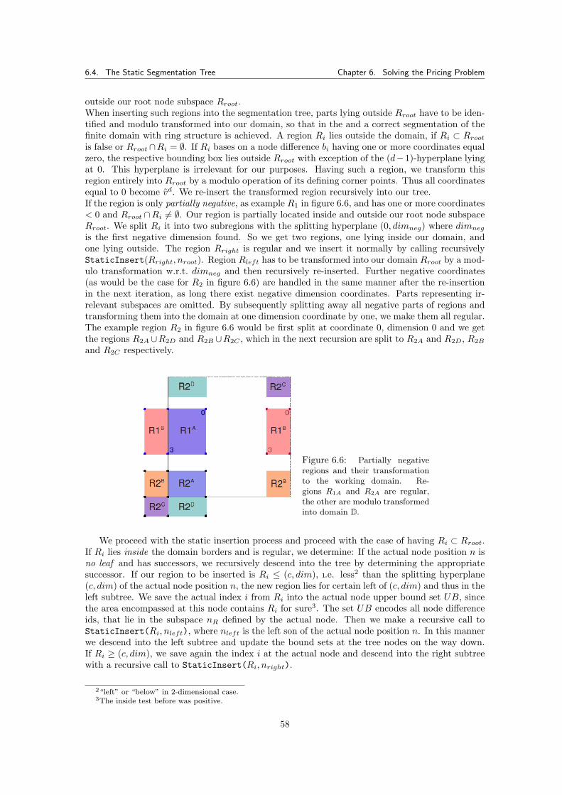
6.4. The Static Segmentation Tree Chapter 6. Solving the Pricing Problem
outside our root node subspace Rroot.When inserting such regions into the segmentation tree, parts lying outside Rroot have to be iden-tified and modulo transformed into our domain, so that in the and a correct segmentation of thefinite domain with ring structure is achieved. A region Ri lies outside the domain, if Ri ⊂ Rrootis false or Rroot∩Ri = ∅. If Ri bases on a node difference bi having one or more coordinates equalzero, the respective bounding box lies outside Rroot with exception of the (d−1)-hyperplane lyingat 0. This hyperplane is irrelevant for our purposes. Having such a region, we transform thisregion entirely into Rroot by a modulo operation of its defining corner points. Thus all coordinatesequal to 0 become vd. We re-insert the transformed region recursively into our tree.If the region is only partially negative, as example R1 in figure 6.6, and has one or more coordinates< 0 and Rroot ∩Ri 6= ∅. Our region is partially located inside and outside our root node subspaceRroot. We split Ri it into two subregions with the splitting hyperplane (0, dimneg) where dimneg
is the first negative dimension found. So we get two regions, one lying inside our domain, andone lying outside. The region Rright is regular and we insert it normally by calling recursivelyStaticInsert(Rright, nroot). Region Rleft has to be transformed into our domain Rroot by a mod-ulo transformation w.r.t. dimneg and then recursively re-inserted. Further negative coordinates(as would be the case for R2 in figure 6.6) are handled in the same manner after the re-insertionin the next iteration, as long there exist negative dimension coordinates. Parts representing ir-relevant subspaces are omitted. By subsequently splitting away all negative parts of regions andtransforming them into the domain at one dimension coordinate by one, we make them all regular.The example region R2 in figure 6.6 would be first split at coordinate 0, dimension 0 and we getthe regions R2A∪R2D and R2B ∪R2C , which in the next recursion are split to R2A and R2D, R2B
and R2C respectively.
Figure 6.6: Partially negativeregions and their transformationto the working domain. Re-gions R1A and R2A are regular,the other are modulo transformedinto domain D.
We proceed with the static insertion process and proceed with the case of having Ri ⊂ Rroot.If Ri lies inside the domain borders and is regular, we determine: If the actual node position n isno leaf and has successors, we recursively descend into the tree by determining the appropriatesuccessor. If our region to be inserted is Ri ≤ (c, dim), ı.e. less2 than the splitting hyperplane(c, dim) of the actual node position n, the new region lies for certain left of (c, dim) and thus in theleft subtree. We save the actual index i from Ri into the actual node upper bound set UB, sincethe area encompassed at this node contains Ri for sure3. The set UB encodes all node differenceids, that lie in the subspace nR defined by the actual node. Then we make a recursive call toStaticInsert(Ri, nleft), where nleft is the left son of the actual node position n. In this mannerwe descend into the left subtree and update the bound sets at the tree nodes on the way down.If Ri ≥ (c, dim), we save again the index i at the actual node and descend into the right subtreewith a recursive call to StaticInsert(Ri, nright).
2“left” or “below” in 2-dimensional case.3The inside test before was positive.
58
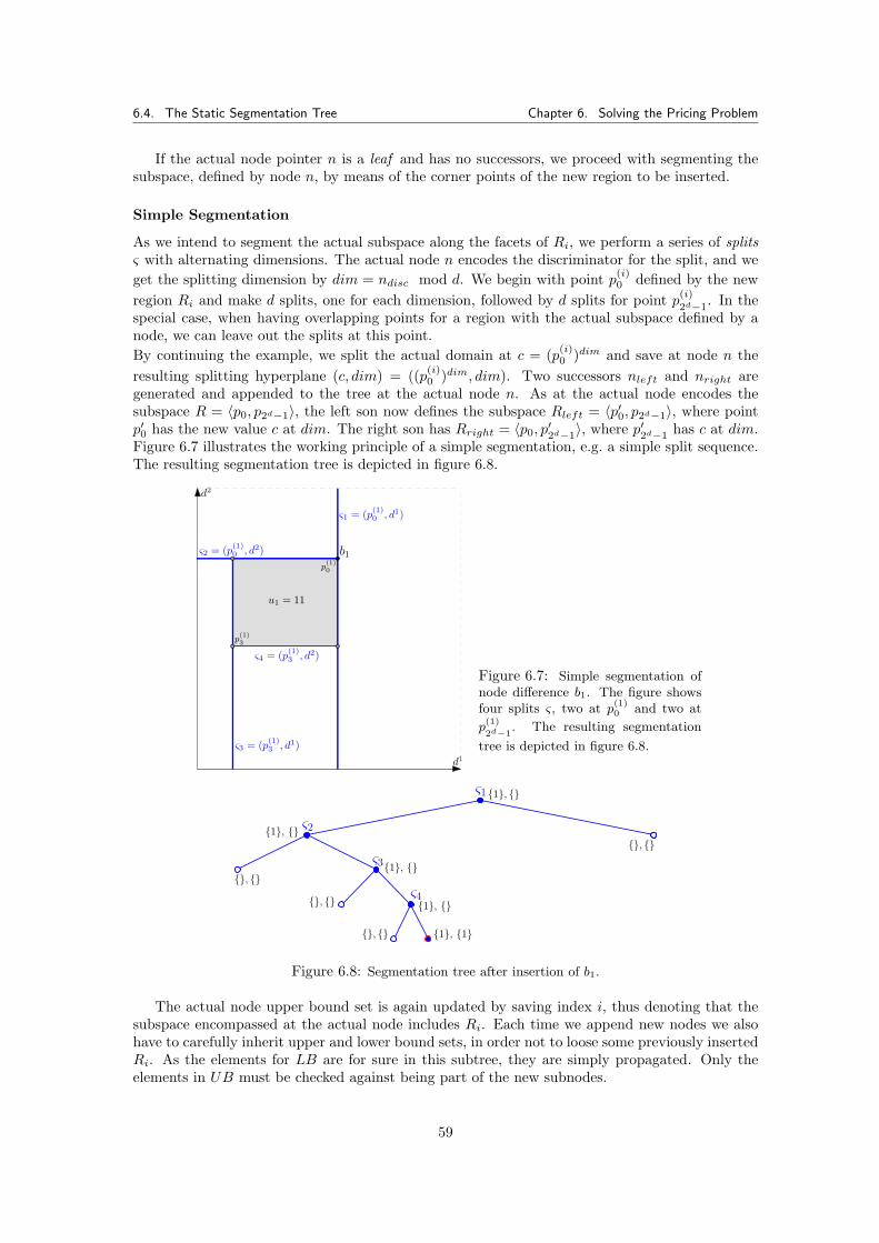
6.4. The Static Segmentation Tree Chapter 6. Solving the Pricing Problem
If the actual node pointer n is a leaf and has no successors, we proceed with segmenting thesubspace, defined by node n, by means of the corner points of the new region to be inserted.
Simple Segmentation
As we intend to segment the actual subspace along the facets of Ri, we perform a series of splitsς with alternating dimensions. The actual node n encodes the discriminator for the split, and weget the splitting dimension by dim = ndisc mod d. We begin with point p(i)
0 defined by the newregion Ri and make d splits, one for each dimension, followed by d splits for point p(i)
2d−1. In the
special case, when having overlapping points for a region with the actual subspace defined by anode, we can leave out the splits at this point.By continuing the example, we split the actual domain at c = (p(i)
0 )dim and save at node n theresulting splitting hyperplane (c, dim) = ((p(i)
0 )dim, dim). Two successors nleft and nright aregenerated and appended to the tree at the actual node n. As at the actual node encodes thesubspace R = 〈p0, p2d−1〉, the left son now defines the subspace Rleft = 〈p′0, p2d−1〉, where pointp′0 has the new value c at dim. The right son has Rright = 〈p0, p
′2d−1〉, where p′2d−1 has c at dim.
Figure 6.7 illustrates the working principle of a simple segmentation, e.g. a simple split sequence.The resulting segmentation tree is depicted in figure 6.8.
u1 = 11
p(1)0
p(1)3
b1
ς1 = (p(1)0 , d1)
ς2 = (p(1)0 , d2)
ς4 = (p(1)3 , d2)
ς3 = (p(1)3 , d1)
d1
d2
Figure 6.7: Simple segmentation ofnode difference b1. The figure showsfour splits ς, two at p
(1)0 and two at
p(1)
2d−1. The resulting segmentation
tree is depicted in figure 6.8.
ς1
ς2
ς3
ς4
{1}, {1}
{1}, {}
{1}, {}
{1}, {}
{1}, {}
{}, {}
{}, {}{}, {}
{}, {}
Figure 6.8: Segmentation tree after insertion of b1.
The actual node upper bound set is again updated by saving index i, thus denoting that thesubspace encompassed at the actual node includes Ri. Each time we append new nodes we alsohave to carefully inherit upper and lower bound sets, in order not to loose some previously insertedRi. As the elements for LB are for sure in this subtree, they are simply propagated. Only theelements in UB must be checked against being part of the new subnodes.
59
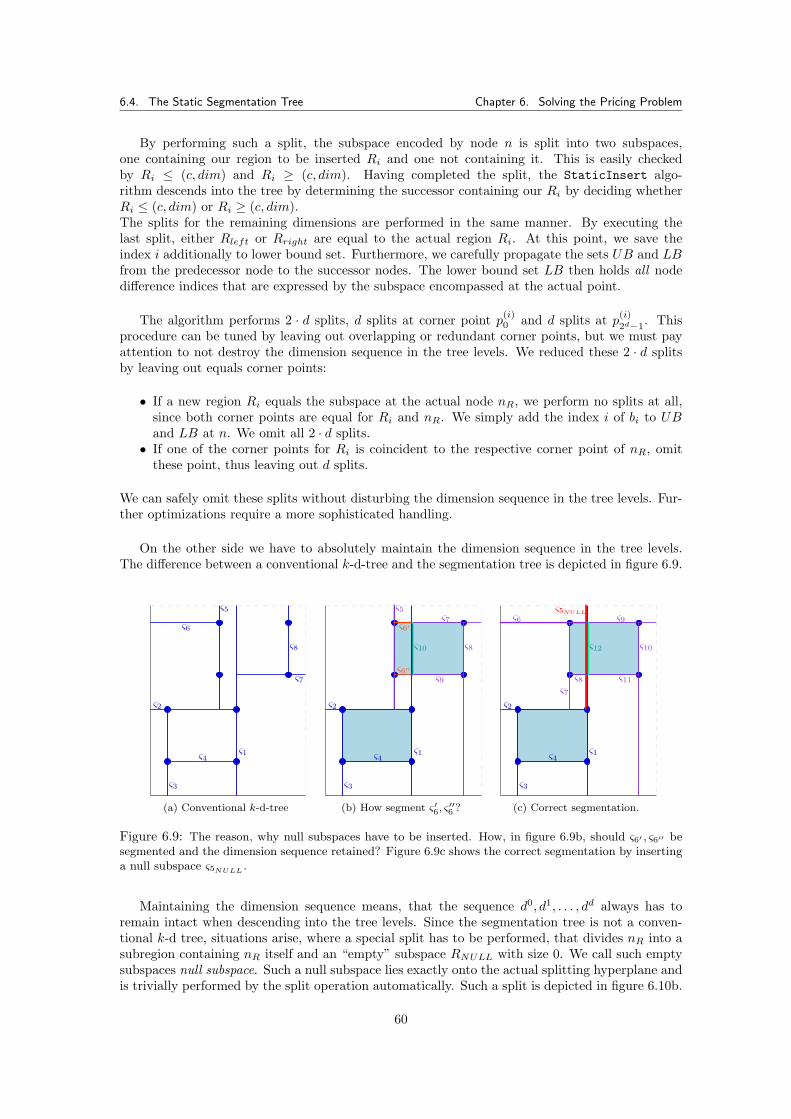
6.4. The Static Segmentation Tree Chapter 6. Solving the Pricing Problem
By performing such a split, the subspace encoded by node n is split into two subspaces,one containing our region to be inserted Ri and one not containing it. This is easily checkedby Ri ≤ (c, dim) and Ri ≥ (c, dim). Having completed the split, the StaticInsert algo-rithm descends into the tree by determining the successor containing our Ri by deciding whetherRi ≤ (c, dim) or Ri ≥ (c, dim).The splits for the remaining dimensions are performed in the same manner. By executing thelast split, either Rleft or Rright are equal to the actual region Ri. At this point, we save theindex i additionally to lower bound set. Furthermore, we carefully propagate the sets UB and LBfrom the predecessor node to the successor nodes. The lower bound set LB then holds all nodedifference indices that are expressed by the subspace encompassed at the actual point.
The algorithm performs 2 · d splits, d splits at corner point p(i)0 and d splits at p(i)
2d−1. This
procedure can be tuned by leaving out overlapping or redundant corner points, but we must payattention to not destroy the dimension sequence in the tree levels. We reduced these 2 · d splitsby leaving out equals corner points:
• If a new region Ri equals the subspace at the actual node nR, we perform no splits at all,since both corner points are equal for Ri and nR. We simply add the index i of bi to UBand LB at n. We omit all 2 · d splits.
• If one of the corner points for Ri is coincident to the respective corner point of nR, omitthese point, thus leaving out d splits.
We can safely omit these splits without disturbing the dimension sequence in the tree levels. Fur-ther optimizations require a more sophisticated handling.
On the other side we have to absolutely maintain the dimension sequence in the tree levels.The difference between a conventional k-d-tree and the segmentation tree is depicted in figure 6.9.
ς1
ς2
ς3
ς4
ς5
ς6
ς7
ς8
(a) Conventional k-d-tree
ς1
ς2
ς3
ς5
ς9
ς8
ς6′
ς6′′
ς7
ς10
ς4
(b) How segment ς′6, ς′′6 ?
ς1
ς2
ς3
ς11
ς10
ς9
ς12
ς4
ς5NULLς6
ς7
ς8
(c) Correct segmentation.
Figure 6.9: The reason, why null subspaces have to be inserted. How, in figure 6.9b, should ς6′ , ς6′′ besegmented and the dimension sequence retained? Figure 6.9c shows the correct segmentation by insertinga null subspace ς5NULL .
Maintaining the dimension sequence means, that the sequence d0, d1, . . . , dd always has toremain intact when descending into the tree levels. Since the segmentation tree is not a conven-tional k-d tree, situations arise, where a special split has to be performed, that divides nR into asubregion containing nR itself and an “empty” subspace RNULL with size 0. We call such emptysubspaces null subspace. Such a null subspace lies exactly onto the actual splitting hyperplane andis trivially performed by the split operation automatically. Such a split is depicted in figure 6.10b.
60
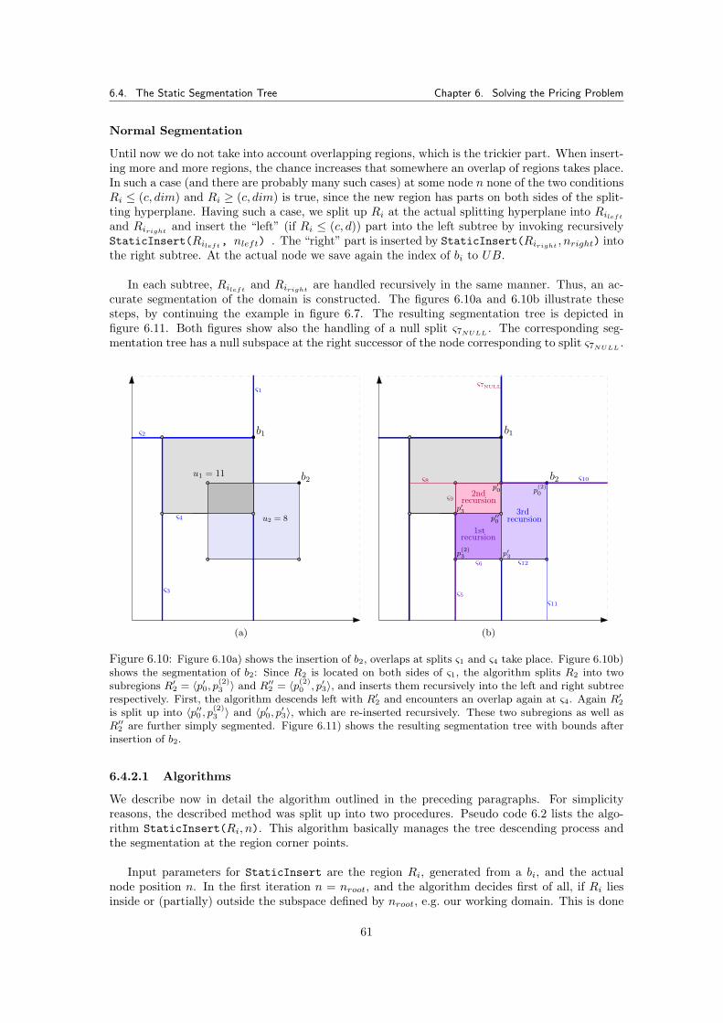
6.4. The Static Segmentation Tree Chapter 6. Solving the Pricing Problem
Normal Segmentation
Until now we do not take into account overlapping regions, which is the trickier part. When insert-ing more and more regions, the chance increases that somewhere an overlap of regions takes place.In such a case (and there are probably many such cases) at some node n none of the two conditionsRi ≤ (c, dim) and Ri ≥ (c, dim) is true, since the new region has parts on both sides of the split-ting hyperplane. Having such a case, we split up Ri at the actual splitting hyperplane into Rileftand Riright and insert the “left” (if Ri ≤ (c, d)) part into the left subtree by invoking recursivelyStaticInsert(Rileft, nleft) . The “right” part is inserted by StaticInsert(Riright , nright) intothe right subtree. At the actual node we save again the index of bi to UB.
In each subtree, Rileft and Riright are handled recursively in the same manner. Thus, an ac-curate segmentation of the domain is constructed. The figures 6.10a and 6.10b illustrate thesesteps, by continuing the example in figure 6.7. The resulting segmentation tree is depicted infigure 6.11. Both figures show also the handling of a null split ς7NULL . The corresponding seg-mentation tree has a null subspace at the right successor of the node corresponding to split ς7NULL .
u1 = 11
u2 = 8
b1
b2
ς1
ς2
ς3
ς4
(a)
b1
ς6
ς8
ς7NULL
b2
ς5
3rdrecursion
recursion2nd
1strecursion
p(2)0
p′3
p′0
p′3
p(2)3
p′′0
ς9
ς11
ς10
ς12
(b)
Figure 6.10: Figure 6.10a) shows the insertion of b2, overlaps at splits ς1 and ς4 take place. Figure 6.10b)shows the segmentation of b2: Since R2 is located on both sides of ς1, the algorithm splits R2 into twosubregions R′2 = 〈p′0, p(2)
3 〉 and R′′2 = 〈p(2)0 , p′3〉, and inserts them recursively into the left and right subtree
respectively. First, the algorithm descends left with R′2 and encounters an overlap again at ς4. Again R′2is split up into 〈p′′0 , p(2)
3 〉 and 〈p′0, p′3〉, which are re-inserted recursively. These two subregions as well asR′′2 are further simply segmented. Figure 6.11) shows the resulting segmentation tree with bounds afterinsertion of b2.
6.4.2.1 Algorithms
We describe now in detail the algorithm outlined in the preceding paragraphs. For simplicityreasons, the described method was split up into two procedures. Pseudo code 6.2 lists the algo-rithm StaticInsert(Ri, n). This algorithm basically manages the tree descending process andthe segmentation at the region corner points.
Input parameters for StaticInsert are the region Ri, generated from a bi, and the actualnode position n. In the first iteration n = nroot, and the algorithm decides first of all, if Ri liesinside or (partially) outside the subspace defined by nroot, e.g. our working domain. This is done
61
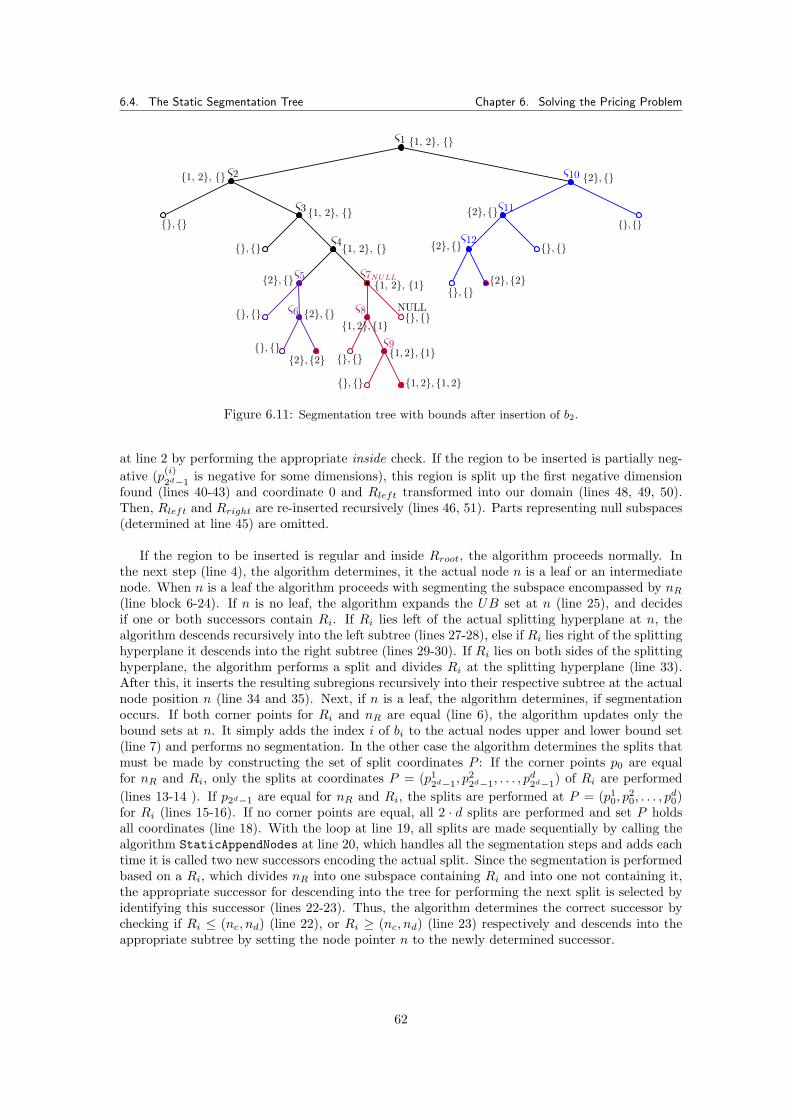
6.4. The Static Segmentation Tree Chapter 6. Solving the Pricing Problem
ς1
ς2
ς3
ς4
{1, 2}, {1}
{1, 2}, {}
{1, 2}, {}
{1, 2}, {}{}, {}
{}, {}{1, 2}, {}
{2}, {}
{2}, {}
{2}, {}
{2}, {2}
{}, {}
{}, {}
{}, {}
{1, 2}, {1, 2}
{1, 2}, {1}
{}, {}NULL
{1, 2}, {1}
{}, {}
{}, {}
{2}, {}
{2}, {}
{}, {}
{}, {}{2}, {2}
ς10
ς11
ς12
ς7NULL
ς8
ς9
ς5
ς6
Figure 6.11: Segmentation tree with bounds after insertion of b2.
at line 2 by performing the appropriate inside check. If the region to be inserted is partially neg-ative (p(i)
2d−1is negative for some dimensions), this region is split up the first negative dimension
found (lines 40-43) and coordinate 0 and Rleft transformed into our domain (lines 48, 49, 50).Then, Rleft and Rright are re-inserted recursively (lines 46, 51). Parts representing null subspaces(determined at line 45) are omitted.
If the region to be inserted is regular and inside Rroot, the algorithm proceeds normally. Inthe next step (line 4), the algorithm determines, it the actual node n is a leaf or an intermediatenode. When n is a leaf the algorithm proceeds with segmenting the subspace encompassed by nR(line block 6-24). If n is no leaf, the algorithm expands the UB set at n (line 25), and decidesif one or both successors contain Ri. If Ri lies left of the actual splitting hyperplane at n, thealgorithm descends recursively into the left subtree (lines 27-28), else if Ri lies right of the splittinghyperplane it descends into the right subtree (lines 29-30). If Ri lies on both sides of the splittinghyperplane, the algorithm performs a split and divides Ri at the splitting hyperplane (line 33).After this, it inserts the resulting subregions recursively into their respective subtree at the actualnode position n (line 34 and 35). Next, if n is a leaf, the algorithm determines, if segmentationoccurs. If both corner points for Ri and nR are equal (line 6), the algorithm updates only thebound sets at n. It simply adds the index i of bi to the actual nodes upper and lower bound set(line 7) and performs no segmentation. In the other case the algorithm determines the splits thatmust be made by constructing the set of split coordinates P : If the corner points p0 are equalfor nR and Ri, only the splits at coordinates P = (p1
2d−1, p22d−1, . . . , p
d2d−1) of Ri are performed
(lines 13-14 ). If p2d−1 are equal for nR and Ri, the splits are performed at P = (p10, p
20, . . . , p
d0)
for Ri (lines 15-16). If no corner points are equal, all 2 · d splits are performed and set P holdsall coordinates (line 18). With the loop at line 19, all splits are made sequentially by calling thealgorithm StaticAppendNodes at line 20, which handles all the segmentation steps and adds eachtime it is called two new successors encoding the actual split. Since the segmentation is performedbased on a Ri, which divides nR into one subspace containing Ri and into one not containing it,the appropriate successor for descending into the tree for performing the next split is selected byidentifying this successor (lines 22-23). Thus, the algorithm determines the correct successor bychecking if Ri ≤ (nc, nd) (line 22), or Ri ≥ (nc, nd) (line 23) respectively and descends into theappropriate subtree by setting the node pointer n to the newly determined successor.
62
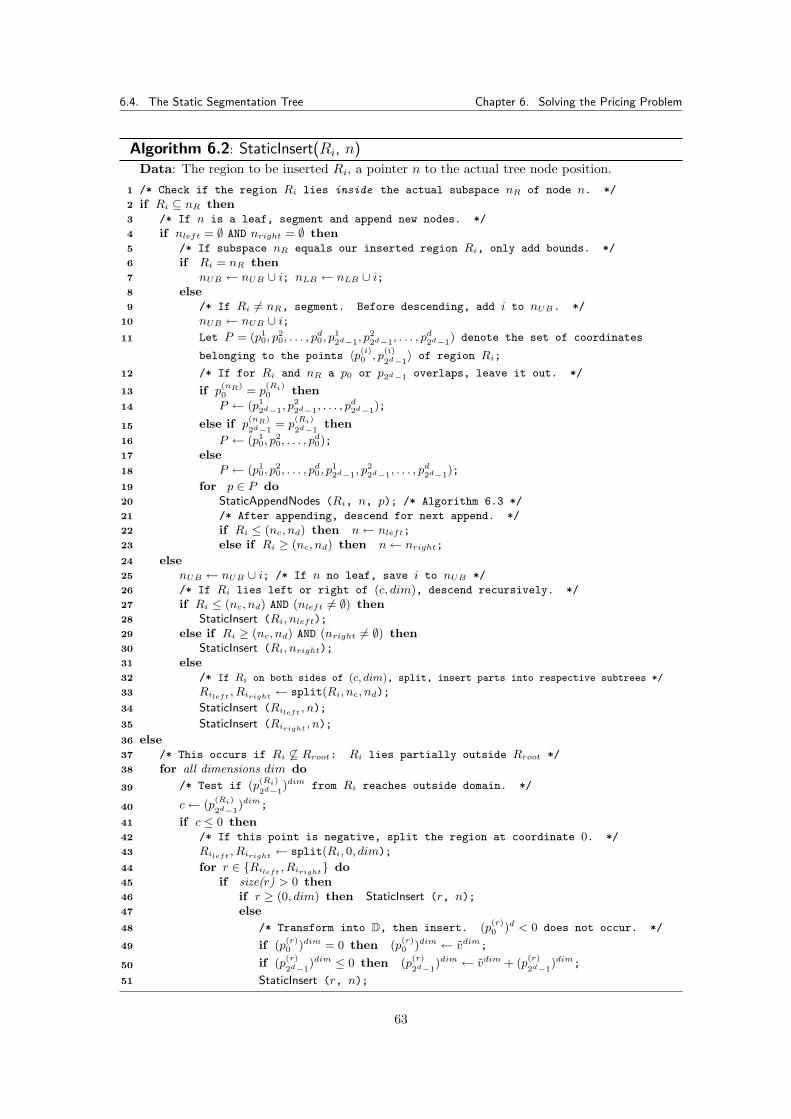
6.4. The Static Segmentation Tree Chapter 6. Solving the Pricing Problem
Algorithm 6.2: StaticInsert(Ri, n)Data: The region to be inserted Ri, a pointer n to the actual tree node position.
/* Check if the region Ri lies inside the actual subspace nR of node n. */1
if Ri ⊆ nR then2
/* If n is a leaf, segment and append new nodes. */3
if nleft = ∅ AND nright = ∅ then4
/* If subspace nR equals our inserted region Ri, only add bounds. */5
if Ri = nR then6
nUB ← nUB ∪ i; nLB ← nLB ∪ i;7
else8
/* If Ri 6= nR, segment. Before descending, add i to nUB. */9
nUB ← nUB ∪ i;10
Let P = (p10, p
20, . . . , p
d0, p
12d−1, p
22d−1, . . . , p
d2d−1) denote the set of coordinates11
belonging to the points 〈p(i)0 , p
(i)
2d−1〉 of region Ri;
/* If for Ri and nR a p0 or p2d−1 overlaps, leave it out. */12
if p(nR)0 = p
(Ri)0 then13
P ← (p12d−1, p
22d−1, . . . , p
d2d−1);14
else if p(nR)
2d−1= p
(Ri)
2d−1then15
P ← (p10, p
20, . . . , p
d0);16
else17
P ← (p10, p
20, . . . , p
d0, p
12d−1, p
22d−1, . . . , p
d2d−1);18
for p ∈ P do19
StaticAppendNodes (Ri, n, p); /* Algorithm 6.3 */20
/* After appending, descend for next append. */21
if Ri ≤ (nc, nd) then n← nleft;22
else if Ri ≥ (nc, nd) then n← nright;23
else24
nUB ← nUB ∪ i; /* If n no leaf, save i to nUB */25
/* If Ri lies left or right of (c, dim), descend recursively. */26
if Ri ≤ (nc, nd) AND (nleft 6= ∅) then27
StaticInsert (Ri, nleft);28
else if Ri ≥ (nc, nd) AND (nright 6= ∅) then29
StaticInsert (Ri, nright);30
else31
/* If Ri on both sides of (c, dim), split, insert parts into respective subtrees */32
Rileft , Riright ← split(Ri, nc, nd);33
StaticInsert (Rileft , n);34
StaticInsert (Riright , n);35
else36
/* This occurs if Ri 6⊆ Rroot: Ri lies partially outside Rroot */37
for all dimensions dim do38
/* Test if (p(Ri)
2d−1)dim from Ri reaches outside domain. */39
c← (p(Ri)
2d−1)dim;40
if c ≤ 0 then41
/* If this point is negative, split the region at coordinate 0. */42
Rileft , Riright ← split(Ri, 0, dim);43
for r ∈ {Rileft , Riright} do44
if size(r) > 0 then45
if r ≥ (0, dim) then StaticInsert (r, n);46
else47
/* Transform into D, then insert. (p(r)0 )d < 0 does not occur. */48
if (p(r)0 )dim = 0 then (p
(r)0 )dim ← vdim;49
if (p(r)
2d−1)dim ≤ 0 then (p
(r)
2d−1)dim ← vdim + (p
(r)
2d−1)dim;50
StaticInsert (r, n);51
63
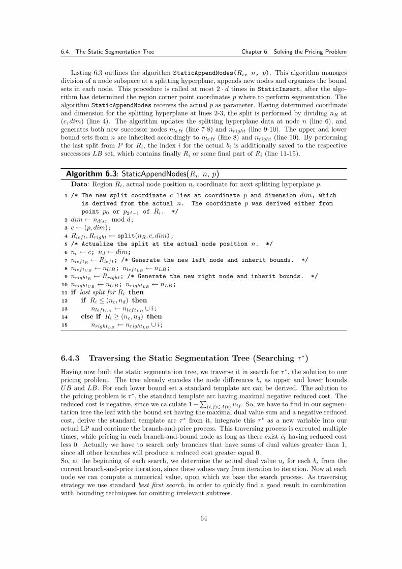
6.4. The Static Segmentation Tree Chapter 6. Solving the Pricing Problem
Listing 6.3 outlines the algorithm StaticAppendNodes(Ri, n, p). This algorithm managesdivision of a node subspace at a splitting hyperplane, appends new nodes and organizes the boundsets in each node. This procedure is called at most 2 · d times in StaticInsert, after the algo-rithm has determined the region corner point coordinates p where to perform segmentation. Thealgorithm StaticAppendNodes receives the actual p as parameter. Having determined coordinateand dimension for the splitting hyperplane at lines 2-3, the split is performed by dividing nR at(c, dim) (line 4). The algorithm updates the splitting hyperplane data at node n (line 6), andgenerates both new successor nodes nleft (line 7-8) and nright (line 9-10). The upper and lowerbound sets from n are inherited accordingly to nleft (line 8) and nright (line 10). By performingthe last split from P for Ri, the index i for the actual bi is additionally saved to the respectivesuccessors LB set, which contains finally Ri or some final part of Ri (line 11-15).
Algorithm 6.3: StaticAppendNodes(Ri, n, p)Data: Region Ri, actual node position n, coordinate for next splitting hyperplane p.
/* The new split coordinate c lies at coordinate p and dimension dim, which1
is derived from the actual n. The coordinate p was derived either frompoint p0 or p2d−1 of Ri. */
dim← ndisc mod d;2
c← (p, dim);3
Rleft, Rright ← split(nR, c, dim);4
/* Actualize the split at the actual node position n. */5
nc ← c; nd ← dim;6
nleftR ← Rleft; /* Generate the new left node and inherit bounds. */7
nleftUB ← nUB; nleftLB ← nLB;8
nrightR ← Rright; /* Generate the new right node and inherit bounds. */9
nrightUB ← nUB; nrightLB ← nLB;10
if last split for Ri then11
if Ri ≤ (nc, nd) then12
nleftLB ← nleftLB ∪ i;13
else if Ri ≥ (nc, nd) then14
nrightLB ← nrightLB ∪ i;15
6.4.3 Traversing the Static Segmentation Tree (Searching τ ∗)
Having now built the static segmentation tree, we traverse it in search for τ∗, the solution to ourpricing problem. The tree already encodes the node differences bi as upper and lower boundsUB and LB. For each lower bound set a standard template arc can be derived. The solution tothe pricing problem is τ∗, the standard template arc having maximal negative reduced cost. Thereduced cost is negative, since we calculate 1−∑(i,j)∈A(t) uij . So, we have to find in our segmen-tation tree the leaf with the bound set having the maximal dual value sum and a negative reducedcost, derive the standard template arc τ∗ from it, integrate this τ∗ as a new variable into ouractual LP and continue the branch-and-price process. This traversing process is executed multipletimes, while pricing in each branch-and-bound node as long as there exist ct having reduced costless 0. Actually we have to search only branches that have sums of dual values greater than 1,since all other branches will produce a reduced cost greater equal 0.So, at the beginning of each search, we determine the actual dual value ui for each bi from thecurrent branch-and-price iteration, since these values vary from iteration to iteration. Now at eachnode we can compute a numerical value, upon which we base the search process. As traversingstrategy we use standard best first search, in order to quickly find a good result in combinationwith bounding techniques for omitting irrelevant subtrees.
64
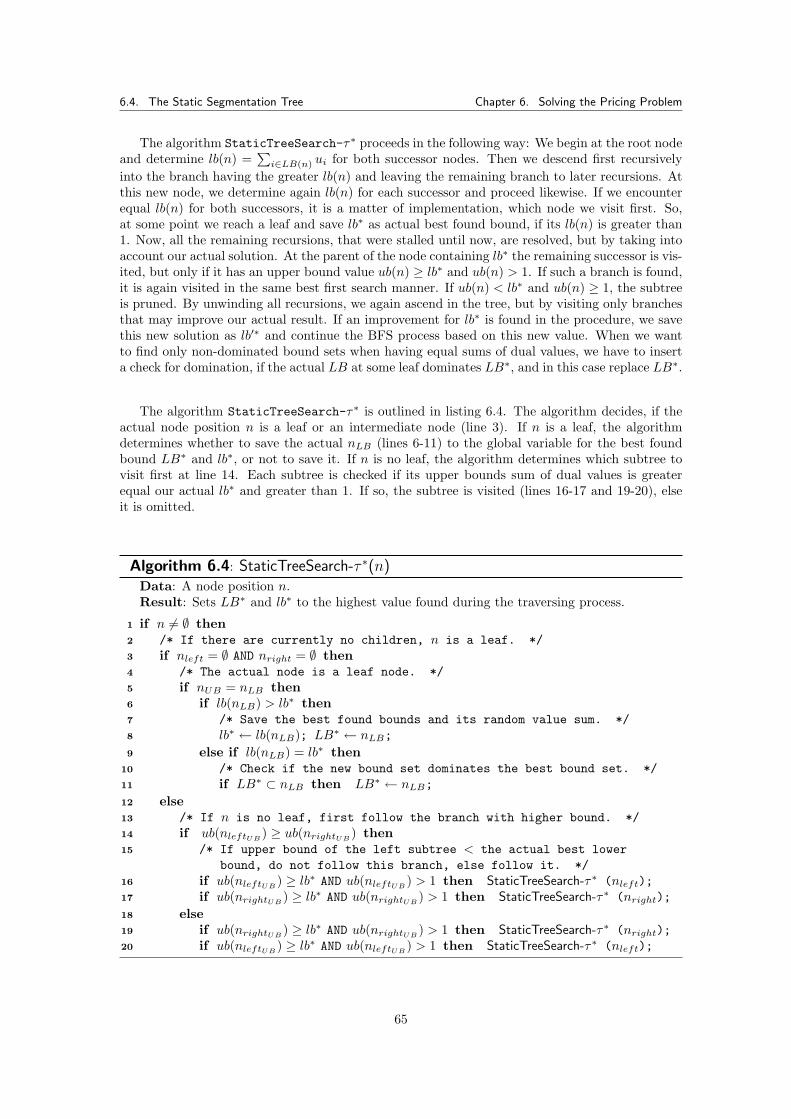
6.4. The Static Segmentation Tree Chapter 6. Solving the Pricing Problem
The algorithm StaticTreeSearch-τ∗ proceeds in the following way: We begin at the root nodeand determine lb(n) =
∑i∈LB(n) ui for both successor nodes. Then we descend first recursively
into the branch having the greater lb(n) and leaving the remaining branch to later recursions. Atthis new node, we determine again lb(n) for each successor and proceed likewise. If we encounterequal lb(n) for both successors, it is a matter of implementation, which node we visit first. So,at some point we reach a leaf and save lb∗ as actual best found bound, if its lb(n) is greater than1. Now, all the remaining recursions, that were stalled until now, are resolved, but by taking intoaccount our actual solution. At the parent of the node containing lb∗ the remaining successor is vis-ited, but only if it has an upper bound value ub(n) ≥ lb∗ and ub(n) > 1. If such a branch is found,it is again visited in the same best first search manner. If ub(n) < lb∗ and ub(n) ≥ 1, the subtreeis pruned. By unwinding all recursions, we again ascend in the tree, but by visiting only branchesthat may improve our actual result. If an improvement for lb∗ is found in the procedure, we savethis new solution as lb′∗ and continue the BFS process based on this new value. When we wantto find only non-dominated bound sets when having equal sums of dual values, we have to inserta check for domination, if the actual LB at some leaf dominates LB∗, and in this case replace LB∗.
The algorithm StaticTreeSearch-τ∗ is outlined in listing 6.4. The algorithm decides, if theactual node position n is a leaf or an intermediate node (line 3). If n is a leaf, the algorithmdetermines whether to save the actual nLB (lines 6-11) to the global variable for the best foundbound LB∗ and lb∗, or not to save it. If n is no leaf, the algorithm determines which subtree tovisit first at line 14. Each subtree is checked if its upper bounds sum of dual values is greaterequal our actual lb∗ and greater than 1. If so, the subtree is visited (lines 16-17 and 19-20), elseit is omitted.
Algorithm 6.4: StaticTreeSearch-τ ∗(n)Data: A node position n.Result: Sets LB∗ and lb∗ to the highest value found during the traversing process.
if n 6= ∅ then1
/* If there are currently no children, n is a leaf. */2
if nleft = ∅ AND nright = ∅ then3
/* The actual node is a leaf node. */4
if nUB = nLB then5
if lb(nLB) > lb∗ then6
/* Save the best found bounds and its random value sum. */7
lb∗ ← lb(nLB); LB∗ ← nLB;8
else if lb(nLB) = lb∗ then9
/* Check if the new bound set dominates the best bound set. */10
if LB∗ ⊂ nLB then LB∗ ← nLB;11
else12
/* If n is no leaf, first follow the branch with higher bound. */13
if ub(nleftUB ) ≥ ub(nrightUB ) then14
/* If upper bound of the left subtree < the actual best lower15
bound, do not follow this branch, else follow it. */if ub(nleftUB ) ≥ lb∗ AND ub(nleftUB ) > 1 then StaticTreeSearch-τ∗ (nleft);16
if ub(nrightUB ) ≥ lb∗ AND ub(nrightUB ) > 1 then StaticTreeSearch-τ∗ (nright);17
else18
if ub(nrightUB ) ≥ lb∗ AND ub(nrightUB ) > 1 then StaticTreeSearch-τ∗ (nright);19
if ub(nleftUB ) ≥ lb∗ AND ub(nleftUB ) > 1 then StaticTreeSearch-τ∗ (nleft);20
65
6.5. The Dynamic Segmentation Tree Chapter 6. Solving the Pricing Problem
6.4.3.1 Determining the Standard Template Arc
Once we have determined LB∗, we have to compute τ∗. The standard template arc τ is determinedout of the bound set LB∗ as described in section 4.2.1. For bound sets with size 1, the bi is thestandard template arc. For |LB∗| > 1, we save the first element from this set as reference anddetermine separately for each dimension dim, if the remaining bi have an according dimensioncoordinate less than the first element. Here we have to take into account the ring structure.This means that if we have a bound set that encodes bi crossing the domain border, which reachagain into the domain D at the opposite side of the domain border, we save the greater coordinate.From these domain crossing coordinates, in turn we want the smallest value. The correct procedurefor this is important. The segmentation tree does not encode information about template arcsencoding areas crossing domain borders. Although a τ may have two “parts” in the tree by crossingthe domain border, both having the same bound set LB. The tree segments these two parts intwo separate subtrees, one positioned somewhere wide left in the tree, the other wide right. Itis irrelevant, which one of these two parts is finally found by StaticTreeSearch-τ∗, since thecorrect standard template arc will be derived out of it.
6.4.4 Upper Bounds for the Static Segmentation Tree
Since the segmentation tree bases on a k-d-tree, building has complexity O (k · n log n). Searchingone element has complexity O(k · n1− 1
k + R). The worst case for the number of nodes in thesegmentation tree would be a segmentation of D into v subspaces of size 1. Such a case wouldrequire O (v2
)nodes and thus at most a storage requirement quadratic in v. In our scenario such
a case should never occur and thus the effective number of nodes is significantly lower.
6.4.5 Simulating StaticTreeSearch-τ ∗
We verify the algorithm StaticTreeSearch-τ∗ by simulating 1000 test iterations, based on ran-dom values. For this test we additionally need the set of non-dominated template arcs T c. Firstwe construct the entire static tree. Then, we start the simulation iterations, and in each iterationwe assign new random values in [1, 100] to each bi. We determine from T c the template arc τ∗T chaving maximal sum of random values. Then we traverse the static tree and get the templatearc τ∗seg. Then we determine, if τ∗T c = τ∗seg and also their random value sums are equal. By anextensive series of computation tests we showed the method to work correctly.
6.5 The Dynamic Segmentation Tree
Basically, the dynamic segmentation tree works similar to the static version, but in the dynamicversion we build the segmentation tree gradually, and enlarge it only when coming to a leaf that is“incomplete” and has to be expanded further. Thus we combine the two algorithms StaticInsertand StaticTreeSearch-τ∗ into one procedure.
We begin again by creating a root node, but this time we initialize UB with all node differencesbi. The next step is to start the recursive search process. Since there are no successor nodes forthe root node, the algorithm proceeds with the first segmentation. For this we have to select anelement from UB, that has not yet been segmented. So we regard only elements from UB \ LB,which are the elements not segmented until yet. In the first insert iteration, this non symmetricdifference set is naturally UB, since LB is empty. As soon we we segment some bi, the sets LBare filled gradually. Since the sole elements bi in this set allow no selection based on a numericalvalue, at this point we already need the current dual values uij or uij+µj respectively, which werepreviously derived from the current subproblem. Then we select the node difference bi having thehighest dual value, since this is the node difference that most likely leads fast to the greatest sumof dual values for the lower bound set lb∗. We continue by segmenting the respective Ri for this bi.
66
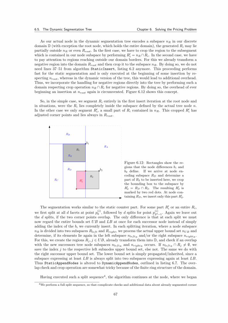
6.5. The Dynamic Segmentation Tree Chapter 6. Solving the Pricing Problem
As our actual node in the dynamic segmentation tree encodes a subspace nR in our discretedomain D (with exception the root node, which holds the entire domain), the generated Ri may liepartially outside nR or even Rroot. In the first case, we have to crop the region to the subsegmentwhich is contained in our node subspace by performing R′i = nR ∩Ri. In the second case, we haveto pay attention to regions reaching outside our domain borders. For this we already transform anegative region into the domain Rroot and then crop it to the subspace nR. By doing so, we do notneed lines 37–51 from algorithm StaticInsert, listing 6.2 anymore. This proceeding performsfast for the static segmentation and is only executed at the beginning of some insertion by re-specting nroot, whereas in the dynamic version of the tree, this would lead to additional overhead.Thus, we incorporate the handling for negative regions directly into the tree by performing such adomain respecting crop operation nR ∩Ri for negative regions. By doing so, the overhead of everbeginning an insertion at nroot again is circumvented. Figure 6.12 shows this concept.
So, in the simple case, we segment Ri entirely in the first insert iteration at the root node andin situations, were the Ri lies completely inside the subspace defined by the actual tree node n.In the other case we only segment R′i, a small part of Ri contained in nR. This cropped R′i hasadjusted corner points and lies always in Rroot.
RA
RB
RC
RD
RE
b1
b2
R1
R2
R′2
Figure 6.12: Rectangles show the re-gions that the node differences b1 andb2 define. If we arrive at node en-coding subspace RD and determine apart of R2 to be inserted here, we cropthe bounding box to the subspace byR′2 = RD ∩ R2. The resulting R′2 ismarked by two red dots. At node con-tainingRD, we insert only this partR′2.
The segmentation works similar to the static counter part. For some part R′i or an entire Ri,we first split at all d facets at point p(i)
0 , followed by d splits for point p(i)
2d−1. Again we leave out
the d splits, if the two corner points overlap. The only difference is that at each split we mustnow regard the entire bounds set UB and LB at once for each successor node instead of simplyadding the index of the bi we currently insert. In each splitting iteration, where a node subspacenR is divided into two subspaces Rleft and Rright, we process the actual upper bound set nUB anddetermine, if its elements lie again in the left subspace nleftR and/or the right subspace nrightR .For this, we create the regions Rj , j ∈ UB, already transform them into D, and check if an overlapwith the new successors tree node subspaces nleftR and nrightR occurs. If nleftR ∩ Rj 6= ∅, wesave the index j to the respective left subnodes upper bound set, else not. The same we do withthe right successor upper bound set. The lower bound set is simply propagated/inherited, since asubspace expressing at least LB is always split into two subspaces expressing again at least LB.Thus StaticAppendNodes is altered to DynamicAppendNodes, outlined in listing 6.7. The over-lap check and crop operation are somewhat tricky because of the finite ring structure of the domain.
Having executed such a split sequence4, the algorithm continues at the node, where we began
4We perform a full split sequence, so that complicate checks and additional data about already segmented corner
67
6.5. The Dynamic Segmentation Tree Chapter 6. Solving the Pricing Problem
the splitting. Here new successors have taken their place, including a fully processed upper andlower bound set. So, we can descend into the tree, but in direction of the greatest sum of dualvalues, which must not necessarily be the subtree where bi was just segmented. As example: nis a leaf and has UB = {b1, b2, b3}, LB = ∅. Here, b1, b2, b3 have to be segmented. Dual valuesare u1 = 9, u2 = 6, u3 = 5. The algorithm segments b1, since u1 is greatest and produces for nthe successors nleftUB = {b1} and nrightUB = {b2, b3}. In the left subtree at some point there isa LB = {b1}. The right subtree is yet empty. As the dual value sum for the left subtree is lessthan in the right subtree, the algorithm chooses nright for descending and finds a leaf, which isconsequently segmented again.
As we employ the best first search strategy, at some point, we reach a leaf where UB = LB.Here no more bi have to be segmented, since UB ∩ LB = ∅. We save the actual LB and lb∗, andthe algorithms proceeds with unwrapping the recursions. Hopefully, a lot of subtrees have nowa sum of upper bound dual values less lb∗ and less 1 and are omitted. If UB has a sum of dualvalues greater equal lb∗, this subtree must be searched. Maybe, there will be found some betterlb∗, which we save and take as new global bound. If non-dominated bound sets are preferred, weadd again a domination check. By proceeding thus, the procedure omits irrelevant subtrees byleaving them unconstructed. It expands new nodes only at the points determined to be relevantfor the pricing problem. In the end, LB∗ contains the optimum bound set out of which the stan-dard template arc τ∗ is determined. Its dual sum is lb∗. This is the solution to our pricing problem.
6.5.0.1 Algorithms
The pseudo code of DynamicInsertAndSearch-τ∗ is outlined in listing 6.5. Algorithm 6.6 showsDynamicInsertNode. The altered DynamicAppendNodes is outlined in listing 6.7.
The algorithm DynamicInsertAndSearch-τ∗, listing 6.5, is divided again into two main blocks,one concerning the case for the actual node position n being a leaf (lines 2-28), the other performingthe recursive BFS search (line 29-40). If n is a leaf and has empty UB and LB, this leaf is irrelevant(lines 4-5). If UB > 0 and LB empty, the algorithm determines at line 8 the element that must besegmented next, generates the according Ri (line 9), transforms and crops Ri to R′i (line 11) andinserts it (line 12). The search is continued by a recursive call to DynamicInsertAndSearch-τ∗ atline 13. If at n, the UB and LB are equal and not empty, the actual nlb is evaluated against lb∗
and 1 and saved, if greater (line 15-18). If upper and lower bound set are not equal the algorithmcalculates the symmetric difference set Φ (line 23), and determines from this set Φ the region Rito be segmented next (lines 24-26). Follow the calls to the algorithms for segmenting (line 27) anddescending further (line 28).
The algorithm DynamicInsertNode, listing 6.6 takes as parameters the region Ri to be insertedand an actual node position n. First of all, the algorithm performs at line 1 the check if Ri lies inour actual node subspace nR. Again, the algorithm differentiates between n being a leaf node andand n being an intermediate node. In case n is no leaf, the algorithm recursively descends into thetree and determines the appropriate position for segmenting Ri with lines 19-25. Having foundthis position, the upper bound set is expanded by i and the segmenting process is performed as inStaticInsert with lines 3-17. The algorithm DynamicAppendNodes at line 15 appends to n thenew nodes nleft and nright containing the newly segmented subspaces for Ri.
The algorithm DynamicAppendNodes, listing 6.7, is basically similar to the static version. First,the algorithm determines the next splitting hyperplane (lines 1-2), splits up nR at this splittinghyperplane (line 3), and generates the new nodes nleft and nright (lines 6-7). In the dynamicversion, the actual bound set nUB has to be specially handled: With lines 9-14, the algorithm
points/dimensions can be omitted. We exclude from segmentation only overlapping corner points and equal regions.
68
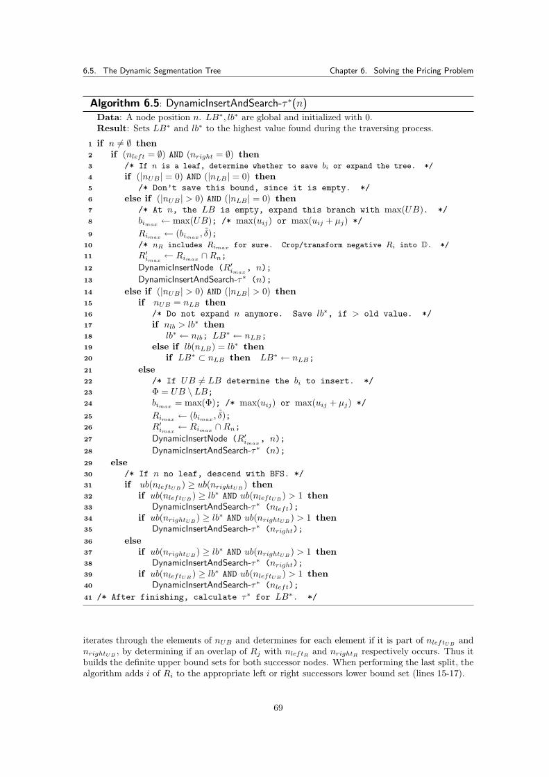
6.5. The Dynamic Segmentation Tree Chapter 6. Solving the Pricing Problem
Algorithm 6.5: DynamicInsertAndSearch-τ ∗(n)Data: A node position n. LB∗, lb∗ are global and initialized with 0.Result: Sets LB∗ and lb∗ to the highest value found during the traversing process.
if n 6= ∅ then1
if (nleft = ∅) AND (nright = ∅) then2
/* If n is a leaf, determine whether to save bi or expand the tree. */3
if (|nUB | = 0) AND (|nLB | = 0) then4
/* Don’t save this bound, since it is empty. */5
else if (|nUB | > 0) AND (|nLB | = 0) then6
/* At n, the LB is empty, expand this branch with max(UB). */7
bimax ← max(UB); /* max(uij) or max(uij + µj) */8
Rimax ← (bimax , δ);9
/* nR includes Rimax for sure. Crop/transform negative Ri into D. */10
R′imax ← Rimax ∩Rn;11
DynamicInsertNode (R′imax, n);12
DynamicInsertAndSearch-τ∗ (n);13
else if (|nUB | > 0) AND (|nLB | > 0) then14
if nUB = nLB then15
/* Do not expand n anymore. Save lb∗, if > old value. */16
if nlb > lb∗ then17
lb∗ ← nlb; LB∗ ← nLB;18
else if lb(nLB) = lb∗ then19
if LB∗ ⊂ nLB then LB∗ ← nLB;20
else21
/* If UB 6= LB determine the bi to insert. */22
Φ = UB \ LB;23
bimax = max(Φ); /* max(uij) or max(uij + µj) */24
Rimax ← (bimax , δ);25
R′imax ← Rimax ∩Rn;26
DynamicInsertNode (R′imax, n);27
DynamicInsertAndSearch-τ∗ (n);28
else29
/* If n no leaf, descend with BFS. */30
if ub(nleftUB ) ≥ ub(nrightUB ) then31
if ub(nleftUB ) ≥ lb∗ AND ub(nleftUB ) > 1 then32
DynamicInsertAndSearch-τ∗ (nleft);33
if ub(nrightUB ) ≥ lb∗ AND ub(nrightUB ) > 1 then34
DynamicInsertAndSearch-τ∗ (nright);35
else36
if ub(nrightUB ) ≥ lb∗ AND ub(nrightUB ) > 1 then37
DynamicInsertAndSearch-τ∗ (nright);38
if ub(nleftUB ) ≥ lb∗ AND ub(nleftUB ) > 1 then39
DynamicInsertAndSearch-τ∗ (nleft);40
/* After finishing, calculate τ∗ for LB∗. */41
iterates through the elements of nUB and determines for each element if it is part of nleftUB andnrightUB , by determining if an overlap of Rj with nleftR and nrightR respectively occurs. Thus itbuilds the definite upper bound sets for both successor nodes. When performing the last split, thealgorithm adds i of Ri to the appropriate left or right successors lower bound set (lines 15-17).
69
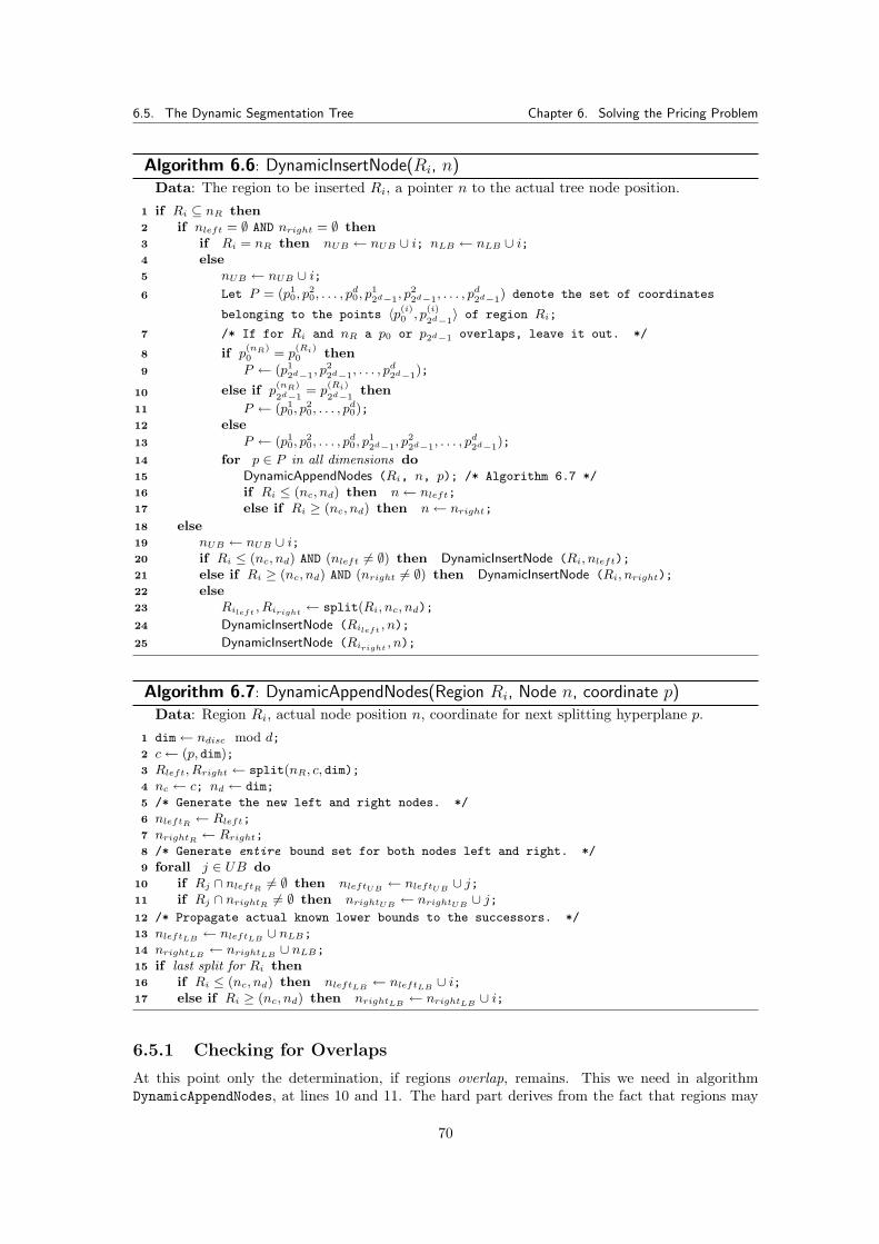
6.5. The Dynamic Segmentation Tree Chapter 6. Solving the Pricing Problem
Algorithm 6.6: DynamicInsertNode(Ri, n)Data: The region to be inserted Ri, a pointer n to the actual tree node position.
if Ri ⊆ nR then1
if nleft = ∅ AND nright = ∅ then2
if Ri = nR then nUB ← nUB ∪ i; nLB ← nLB ∪ i;3
else4
nUB ← nUB ∪ i;5
Let P = (p10, p
20, . . . , p
d0, p
12d−1, p
22d−1, . . . , p
d2d−1) denote the set of coordinates6
belonging to the points 〈p(i)0 , p
(i)
2d−1〉 of region Ri;
/* If for Ri and nR a p0 or p2d−1 overlaps, leave it out. */7
if p(nR)0 = p
(Ri)0 then8
P ← (p12d−1, p
22d−1, . . . , p
d2d−1);9
else if p(nR)
2d−1= p
(Ri)
2d−1then10
P ← (p10, p
20, . . . , p
d0);11
else12
P ← (p10, p
20, . . . , p
d0, p
12d−1, p
22d−1, . . . , p
d2d−1);13
for p ∈ P in all dimensions do14
DynamicAppendNodes (Ri, n, p); /* Algorithm 6.7 */15
if Ri ≤ (nc, nd) then n← nleft;16
else if Ri ≥ (nc, nd) then n← nright;17
else18
nUB ← nUB ∪ i;19
if Ri ≤ (nc, nd) AND (nleft 6= ∅) then DynamicInsertNode (Ri, nleft);20
else if Ri ≥ (nc, nd) AND (nright 6= ∅) then DynamicInsertNode (Ri, nright);21
else22
Rileft , Riright ← split(Ri, nc, nd);23
DynamicInsertNode (Rileft , n);24
DynamicInsertNode (Riright , n);25
Algorithm 6.7: DynamicAppendNodes(Region Ri, Node n, coordinate p)Data: Region Ri, actual node position n, coordinate for next splitting hyperplane p.
dim← ndisc mod d;1
c← (p, dim);2
Rleft, Rright ← split(nR, c, dim);3
nc ← c; nd ← dim;4
/* Generate the new left and right nodes. */5
nleftR ← Rleft;6
nrightR ← Rright;7
/* Generate entire bound set for both nodes left and right. */8
forall j ∈ UB do9
if Rj ∩ nleftR 6= ∅ then nleftUB ← nleftUB ∪ j;10
if Rj ∩ nrightR 6= ∅ then nrightUB ← nrightUB ∪ j;11
/* Propagate actual known lower bounds to the successors. */12
nleftLB ← nleftLB ∪ nLB;13
nrightLB ← nrightLB ∪ nLB;14
if last split for Ri then15
if Ri ≤ (nc, nd) then nleftLB ← nleftLB ∪ i;16
else if Ri ≥ (nc, nd) then nrightLB ← nrightLB ∪ i;17
6.5.1 Checking for Overlaps
At this point only the determination, if regions overlap, remains. This we need in algorithmDynamicAppendNodes, at lines 10 and 11. The hard part derives from the fact that regions may
70
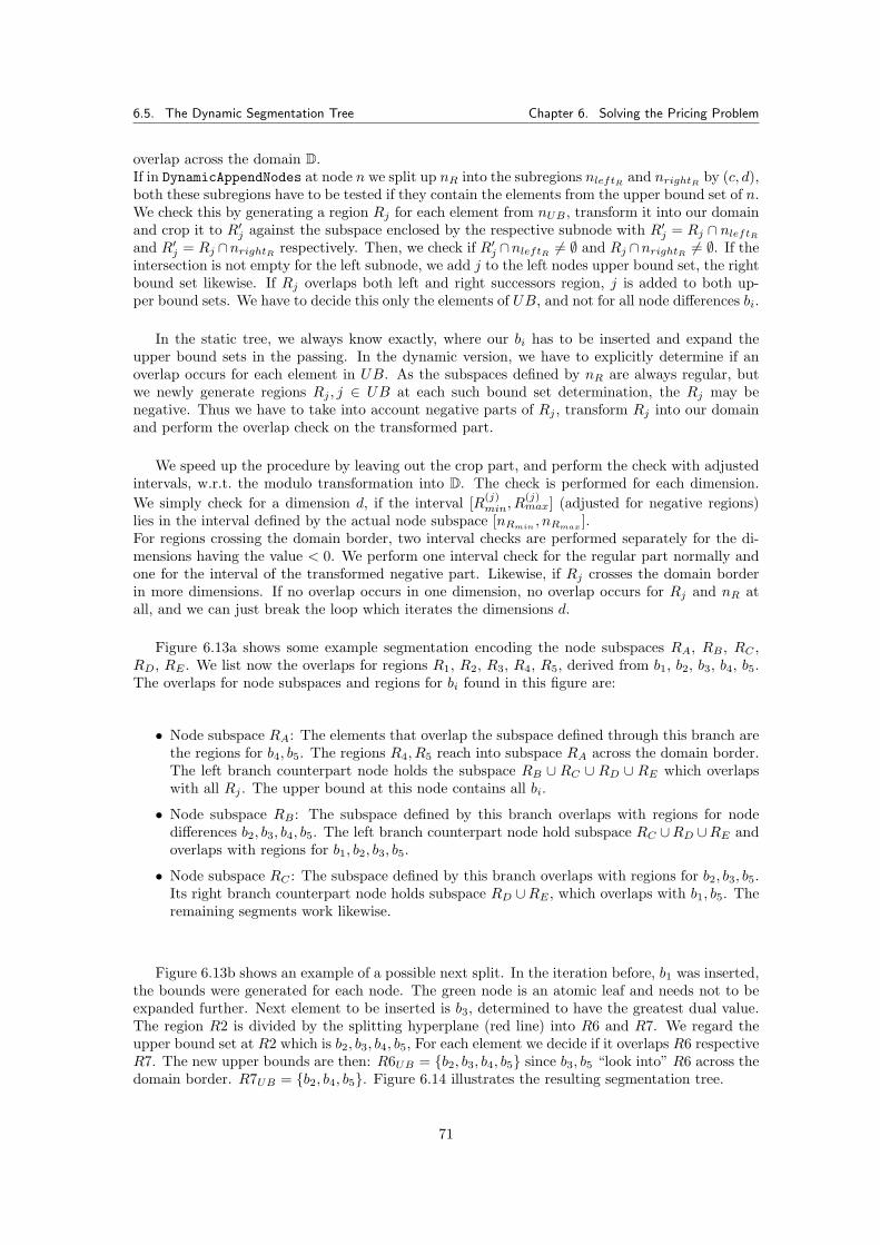
6.5. The Dynamic Segmentation Tree Chapter 6. Solving the Pricing Problem
overlap across the domain D.If in DynamicAppendNodes at node n we split up nR into the subregions nleftR and nrightR by (c, d),both these subregions have to be tested if they contain the elements from the upper bound set of n.We check this by generating a region Rj for each element from nUB , transform it into our domainand crop it to R′j against the subspace enclosed by the respective subnode with R′j = Rj ∩ nleftRand R′j = Rj ∩nrightR respectively. Then, we check if R′j ∩nleftR 6= ∅ and Rj ∩nrightR 6= ∅. If theintersection is not empty for the left subnode, we add j to the left nodes upper bound set, the rightbound set likewise. If Rj overlaps both left and right successors region, j is added to both up-per bound sets. We have to decide this only the elements of UB, and not for all node differences bi.
In the static tree, we always know exactly, where our bi has to be inserted and expand theupper bound sets in the passing. In the dynamic version, we have to explicitly determine if anoverlap occurs for each element in UB. As the subspaces defined by nR are always regular, butwe newly generate regions Rj , j ∈ UB at each such bound set determination, the Rj may benegative. Thus we have to take into account negative parts of Rj , transform Rj into our domainand perform the overlap check on the transformed part.
We speed up the procedure by leaving out the crop part, and perform the check with adjustedintervals, w.r.t. the modulo transformation into D. The check is performed for each dimension.We simply check for a dimension d, if the interval [R(j)
min, R(j)max] (adjusted for negative regions)
lies in the interval defined by the actual node subspace [nRmin , nRmax ].For regions crossing the domain border, two interval checks are performed separately for the di-mensions having the value < 0. We perform one interval check for the regular part normally andone for the interval of the transformed negative part. Likewise, if Rj crosses the domain borderin more dimensions. If no overlap occurs in one dimension, no overlap occurs for Rj and nR atall, and we can just break the loop which iterates the dimensions d.
Figure 6.13a shows some example segmentation encoding the node subspaces RA, RB , RC ,RD, RE . We list now the overlaps for regions R1, R2, R3, R4, R5, derived from b1, b2, b3, b4, b5.The overlaps for node subspaces and regions for bi found in this figure are:
• Node subspace RA: The elements that overlap the subspace defined through this branch arethe regions for b4, b5. The regions R4, R5 reach into subspace RA across the domain border.The left branch counterpart node holds the subspace RB ∪ RC ∪ RD ∪ RE which overlapswith all Rj . The upper bound at this node contains all bi.
• Node subspace RB : The subspace defined by this branch overlaps with regions for nodedifferences b2, b3, b4, b5. The left branch counterpart node hold subspace RC ∪RD ∪RE andoverlaps with regions for b1, b2, b3, b5.
• Node subspace RC : The subspace defined by this branch overlaps with regions for b2, b3, b5.Its right branch counterpart node holds subspace RD ∪RE , which overlaps with b1, b5. Theremaining segments work likewise.
Figure 6.13b shows an example of a possible next split. In the iteration before, b1 was inserted,the bounds were generated for each node. The green node is an atomic leaf and needs not to beexpanded further. Next element to be inserted is b3, determined to have the greatest dual value.The region R2 is divided by the splitting hyperplane (red line) into R6 and R7. We regard theupper bound set at R2 which is b2, b3, b4, b5, For each element we decide if it overlaps R6 respectiveR7. The new upper bounds are then: R6UB = {b2, b3, b4, b5} since b3, b5 “look into” R6 across thedomain border. R7UB = {b2, b4, b5}. Figure 6.14 illustrates the resulting segmentation tree.
71
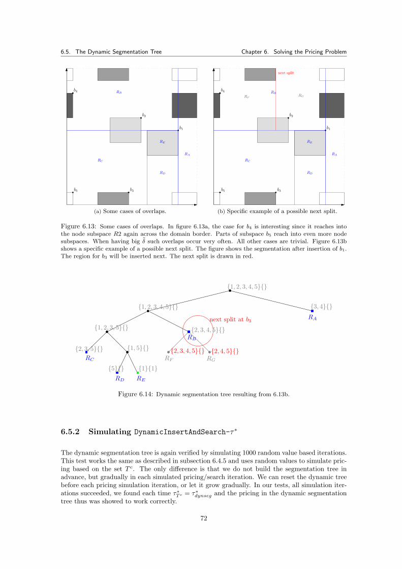
6.5. The Dynamic Segmentation Tree Chapter 6. Solving the Pricing Problem
RA
RB
RC
RD
RE
b1
b2
b3
b4
b5
(a) Some cases of overlaps.
RA
RB
RC
RD
RE
b1
b2
b3
b4
b5
next split
RFRG
(b) Specific example of a possible next split.
Figure 6.13: Some cases of overlaps. In figure 6.13a, the case for b4 is interesting since it reaches intothe node subspace R2 again across the domain border. Parts of subspace b5 reach into even more nodesubspaces. When having big δ such overlaps occur very often. All other cases are trivial. Figure 6.13bshows a specific example of a possible next split. The figure shows the segmentation after insertion of b1.The region for b3 will be inserted next. The next split is drawn in red.
RA
RB
RERD
RC
{1, 2, 3, 4, 5}{}
{3, 4}{}{1, 2, 3, 4, 5}{}
{2, 3, 4, 5}{}
{1, 5}{}
{1}{1}
{2, 3, 5}{}
{1, 2, 3, 5}{}
{5}{}
next split at b3
{2, 4, 5}{}{2, 3, 4, 5}{}RF RG
Figure 6.14: Dynamic segmentation tree resulting from 6.13b.
6.5.2 Simulating DynamicInsertAndSearch-τ ∗
The dynamic segmentation tree is again verified by simulating 1000 random value based iterations.This test works the same as described in subsection 6.4.5 and uses random values to simulate pric-ing based on the set T c. The only difference is that we do not build the segmentation tree inadvance, but gradually in each simulated pricing/search iteration. We can reset the dynamic treebefore each pricing simulation iteration, or let it grow gradually. In our tests, all simulation iter-ations succeeded, we found each time τ∗T c = τ∗dynseg and the pricing in the dynamic segmentationtree thus was showed to work correctly.
72
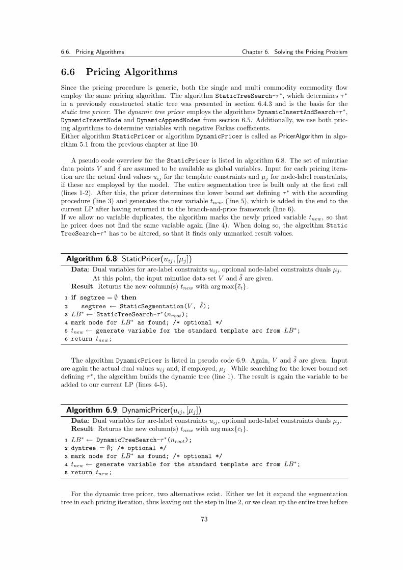
6.6. Pricing Algorithms Chapter 6. Solving the Pricing Problem
6.6 Pricing Algorithms
Since the pricing procedure is generic, both the single and multi commodity commodity flowemploy the same pricing algorithm. The algorithm StaticTreeSearch-τ∗, which determines τ∗
in a previously constructed static tree was presented in section 6.4.3 and is the basis for thestatic tree pricer. The dynamic tree pricer employs the algorithms DynamicInsertAndSearch-τ∗,DynamicInsertNode and DynamicAppendNodes from section 6.5. Additionally, we use both pric-ing algorithms to determine variables with negative Farkas coefficients.Either algorithm StaticPricer or algorithm DynamicPricer is called as PricerAlgorithm in algo-rithm 5.1 from the previous chapter at line 10.
A pseudo code overview for the StaticPricer is listed in algorithm 6.8. The set of minutiaedata points V and δ are assumed to be available as global variables. Input for each pricing itera-tion are the actual dual values uij for the template constraints and µj for node-label constraints,if these are employed by the model. The entire segmentation tree is built only at the first call(lines 1-2). After this, the pricer determines the lower bound set defining τ∗ with the accordingprocedure (line 3) and generates the new variable tnew (line 5), which is added in the end to thecurrent LP after having returned it to the branch-and-price framework (line 6).If we allow no variable duplicates, the algorithm marks the newly priced variable tnew, so thathe pricer does not find the same variable again (line 4). When doing so, the algorithm StaticTreeSearch-τ∗ has to be altered, so that it finds only unmarked result values.
Algorithm 6.8: StaticPricer(uij, [µj])Data: Dual variables for arc-label constraints uij , optional node-label constraints duals µj .
At this point, the input minutiae data set V and δ are given.Result: Returns the new column(s) tnew with arg max{ct}.if segtree = ∅ then1
segtree ← StaticSegmentation(V , δ);2
LB∗ ← StaticTreeSearch-τ∗(nroot);3
mark node for LB∗ as found; /* optional */4
tnew ← generate variable for the standard template arc from LB∗;5
return tnew;6
The algorithm DynamicPricer is listed in pseudo code 6.9. Again, V and δ are given. Inputare again the actual dual values uij and, if employed, µj . While searching for the lower bound setdefining τ∗, the algorithm builds the dynamic tree (line 1). The result is again the variable to beadded to our current LP (lines 4-5).
Algorithm 6.9: DynamicPricer(uij, [µj])Data: Dual variables for arc-label constraints uij , optional node-label constraints duals µj .Result: Returns the new column(s) tnew with arg max{ct}.LB∗ ← DynamicTreeSearch-τ∗(nroot);1
dyntree = ∅; /* optional */2
mark node for LB∗ as found; /* optional */3
tnew ← generate variable for the standard template arc from LB∗;4
return tnew;5
For the dynamic tree pricer, two alternatives exist. Either we let it expand the segmentationtree in each pricing iteration, thus leaving out the step in line 2, or we clean up the entire tree before
73

6.6. Pricing Algorithms Chapter 6. Solving the Pricing Problem
each pricing iteration (line 2) and let it build in each such pricing iteration only the tree segmentsthat are needed to solve the actual pricing problem. Again, variable duplicates may be excludedfrom search by marking found tnew. The according parts in DynamicInsertAndSearch-τ∗ haveto be altered.
6.6.0.1 Outlook
The following chapter 7 describes how to extract the set of candidate template arcs T c out of thepresented segmentation tree, and regards the static as well es dynamic version. Thus, we createan alternative to the preprocessing method from [ChwRai09]. The framework, where branch-and-price is implemented, as well as implementation details, will be subject in chapter 8.
74
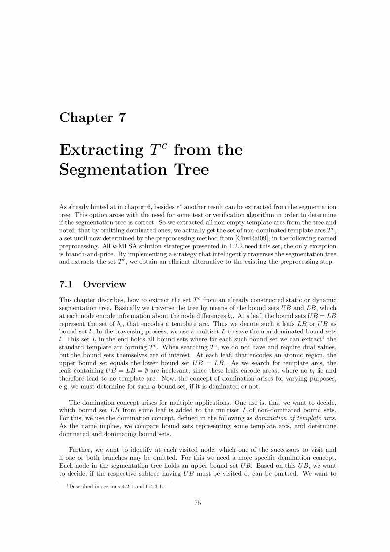
Chapter 7
Extracting T c from theSegmentation Tree
As already hinted at in chapter 6, besides τ∗ another result can be extracted from the segmentationtree. This option arose with the need for some test or verification algorithm in order to determineif the segmentation tree is correct. So we extracted all non empty template arcs from the tree andnoted, that by omitting dominated ones, we actually get the set of non-dominated template arcs T c,a set until now determined by the preprocessing method from [ChwRai09], in the following namedpreprocessing. All k-MLSA solution strategies presented in 1.2.2 need this set, the only exceptionis branch-and-price. By implementing a strategy that intelligently traverses the segmentation treeand extracts the set T c, we obtain an efficient alternative to the existing the preprocessing step.
7.1 Overview
This chapter describes, how to extract the set T c from an already constructed static or dynamicsegmentation tree. Basically we traverse the tree by means of the bound sets UB and LB, whichat each node encode information about the node differences bi. At a leaf, the bound sets UB = LBrepresent the set of bi, that encodes a template arc. Thus we denote such a leafs LB or UB asbound set l. In the traversing process, we use a multiset L to save the non-dominated bound setsl. This set L in the end holds all bound sets where for each such bound set we can extract1 thestandard template arc forming T c. When searching T c, we do not have and require dual values,but the bound sets themselves are of interest. At each leaf, that encodes an atomic region, theupper bound set equals the lower bound set UB = LB. As we search for template arcs, theleafs containing UB = LB = ∅ are irrelevant, since these leafs encode areas, where no bi lie andtherefore lead to no template arc. Now, the concept of domination arises for varying purposes,e.g. we must determine for such a bound set, if it is dominated or not.
The domination concept arises for multiple applications. One use is, that we want to decide,which bound set LB from some leaf is added to the multiset L of non-dominated bound sets.For this, we use the domination concept, defined in the following as domination of template arcs.As the name implies, we compare bound sets representing some template arcs, and determinedominated and dominating bound sets.
Further, we want to identify at each visited node, which one of the successors to visit andif one or both branches may be omitted. For this we need a more specific domination concept.Each node in the segmentation tree holds an upper bound set UB. Based on this UB, we wantto decide, if the respective subtree having UB must be visited or can be omitted. We want to
1Described in sections 4.2.1 and 6.4.3.1.
75
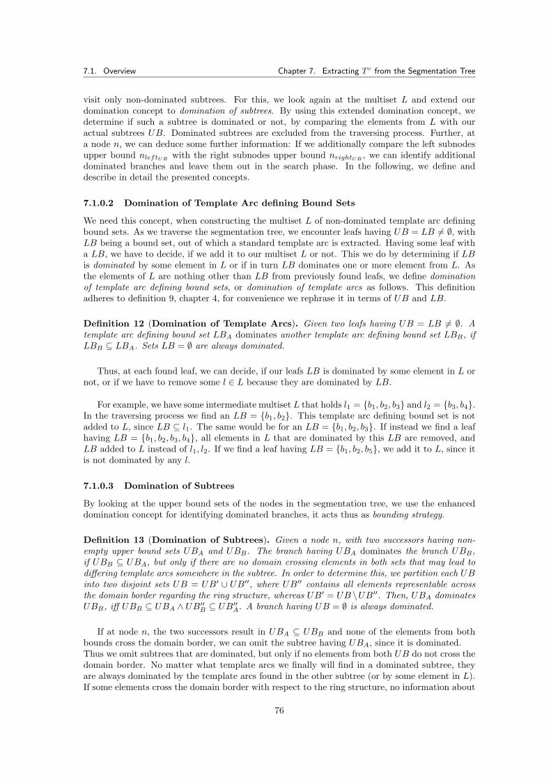
7.1. Overview Chapter 7. Extracting T c from the Segmentation Tree
visit only non-dominated subtrees. For this, we look again at the multiset L and extend ourdomination concept to domination of subtrees. By using this extended domination concept, wedetermine if such a subtree is dominated or not, by comparing the elements from L with ouractual subtrees UB. Dominated subtrees are excluded from the traversing process. Further, ata node n, we can deduce some further information: If we additionally compare the left subnodesupper bound nleftUB with the right subnodes upper bound nrightUB , we can identify additionaldominated branches and leave them out in the search phase. In the following, we define anddescribe in detail the presented concepts.
7.1.0.2 Domination of Template Arc defining Bound Sets
We need this concept, when constructing the multiset L of non-dominated template arc definingbound sets. As we traverse the segmentation tree, we encounter leafs having UB = LB 6= ∅, withLB being a bound set, out of which a standard template arc is extracted. Having some leaf witha LB, we have to decide, if we add it to our multiset L or not. This we do by determining if LBis dominated by some element in L or if in turn LB dominates one or more element from L. Asthe elements of L are nothing other than LB from previously found leafs, we define dominationof template arc defining bound sets, or domination of template arcs as follows. This definitionadheres to definition 9, chapter 4, for convenience we rephrase it in terms of UB and LB.
Definition 12 (Domination of Template Arcs). Given two leafs having UB = LB 6= ∅. Atemplate arc defining bound set LBA dominates another template arc defining bound set LBB, ifLBB ⊆ LBA. Sets LB = ∅ are always dominated.
Thus, at each found leaf, we can decide, if our leafs LB is dominated by some element in L ornot, or if we have to remove some l ∈ L because they are dominated by LB.
For example, we have some intermediate multiset L that holds l1 = {b1, b2, b3} and l2 = {b3, b4}.In the traversing process we find an LB = {b1, b2}. This template arc defining bound set is notadded to L, since LB ⊆ l1. The same would be for an LB = {b1, b2, b3}. If instead we find a leafhaving LB = {b1, b2, b3, b4}, all elements in L that are dominated by this LB are removed, andLB added to L instead of l1, l2. If we find a leaf having LB = {b1, b2, b5}, we add it to L, since itis not dominated by any l.
7.1.0.3 Domination of Subtrees
By looking at the upper bound sets of the nodes in the segmentation tree, we use the enhanceddomination concept for identifying dominated branches, it acts thus as bounding strategy.
Definition 13 (Domination of Subtrees). Given a node n, with two successors having non-empty upper bound sets UBA and UBB. The branch having UBA dominates the branch UBB,if UBB ⊆ UBA, but only if there are no domain crossing elements in both sets that may lead todiffering template arcs somewhere in the subtree. In order to determine this, we partition each UBinto two disjoint sets UB = UB′ ∪ UB′′, where UB′′ contains all elements representable acrossthe domain border regarding the ring structure, whereas UB′ = UB \UB′′. Then, UBA dominatesUBB, iff UBB ⊆ UBA ∧ UB′′B ⊆ UB′′A. A branch having UB = ∅ is always dominated.
If at node n, the two successors result in UBA ⊆ UBB and none of the elements from bothbounds cross the domain border, we can omit the subtree having UBA, since it is dominated.Thus we omit subtrees that are dominated, but only if no elements from both UB do not cross thedomain border. No matter what template arcs we finally will find in a dominated subtree, theyare always dominated by the template arcs found in the other subtree (or by some element in L).If some elements cross the domain border with respect to the ring structure, no information about
76
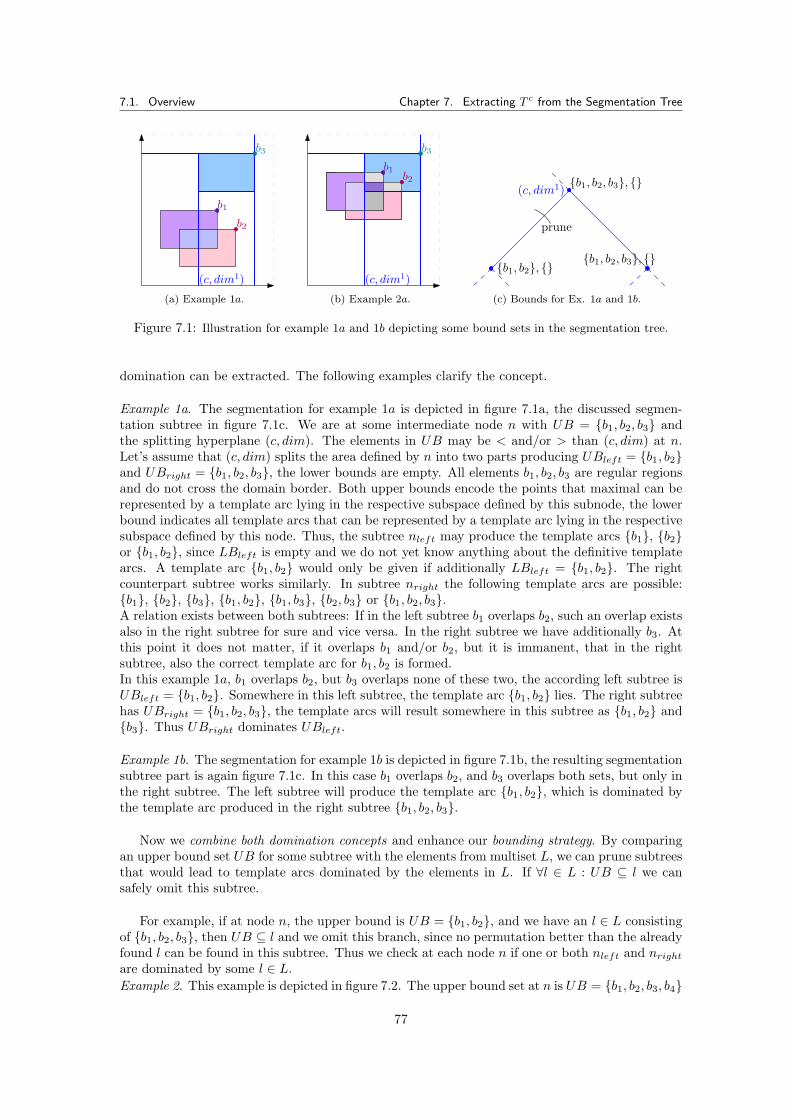
7.1. Overview Chapter 7. Extracting T c from the Segmentation Tree
b3
b2
b1
(c, dim1)
(a) Example 1a.
b3
(c, dim1)
b1b2
(b) Example 2a.
(c, dim1){b1, b2, b3}, {}
{b1, b2}, {}{b1, b2, b3}, {}
prune
(c) Bounds for Ex. 1a and 1b.
Figure 7.1: Illustration for example 1a and 1b depicting some bound sets in the segmentation tree.
domination can be extracted. The following examples clarify the concept.
Example 1a. The segmentation for example 1a is depicted in figure 7.1a, the discussed segmen-tation subtree in figure 7.1c. We are at some intermediate node n with UB = {b1, b2, b3} andthe splitting hyperplane (c, dim). The elements in UB may be < and/or > than (c, dim) at n.Let’s assume that (c, dim) splits the area defined by n into two parts producing UBleft = {b1, b2}and UBright = {b1, b2, b3}, the lower bounds are empty. All elements b1, b2, b3 are regular regionsand do not cross the domain border. Both upper bounds encode the points that maximal can berepresented by a template arc lying in the respective subspace defined by this subnode, the lowerbound indicates all template arcs that can be represented by a template arc lying in the respectivesubspace defined by this node. Thus, the subtree nleft may produce the template arcs {b1}, {b2}or {b1, b2}, since LBleft is empty and we do not yet know anything about the definitive templatearcs. A template arc {b1, b2} would only be given if additionally LBleft = {b1, b2}. The rightcounterpart subtree works similarly. In subtree nright the following template arcs are possible:{b1}, {b2}, {b3}, {b1, b2}, {b1, b3}, {b2, b3} or {b1, b2, b3}.A relation exists between both subtrees: If in the left subtree b1 overlaps b2, such an overlap existsalso in the right subtree for sure and vice versa. In the right subtree we have additionally b3. Atthis point it does not matter, if it overlaps b1 and/or b2, but it is immanent, that in the rightsubtree, also the correct template arc for b1, b2 is formed.In this example 1a, b1 overlaps b2, but b3 overlaps none of these two, the according left subtree isUBleft = {b1, b2}. Somewhere in this left subtree, the template arc {b1, b2} lies. The right subtreehas UBright = {b1, b2, b3}, the template arcs will result somewhere in this subtree as {b1, b2} and{b3}. Thus UBright dominates UBleft.
Example 1b. The segmentation for example 1b is depicted in figure 7.1b, the resulting segmentationsubtree part is again figure 7.1c. In this case b1 overlaps b2, and b3 overlaps both sets, but only inthe right subtree. The left subtree will produce the template arc {b1, b2}, which is dominated bythe template arc produced in the right subtree {b1, b2, b3}.
Now we combine both domination concepts and enhance our bounding strategy. By comparingan upper bound set UB for some subtree with the elements from multiset L, we can prune subtreesthat would lead to template arcs dominated by the elements in L. If ∀l ∈ L : UB ⊆ l we cansafely omit this subtree.
For example, if at node n, the upper bound is UB = {b1, b2}, and we have an l ∈ L consistingof {b1, b2, b3}, then UB ⊆ l and we omit this branch, since no permutation better than the alreadyfound l can be found in this subtree. Thus we check at each node n if one or both nleft and nrightare dominated by some l ∈ L.Example 2. This example is depicted in figure 7.2. The upper bound set at n is UB = {b1, b2, b3, b4}
77
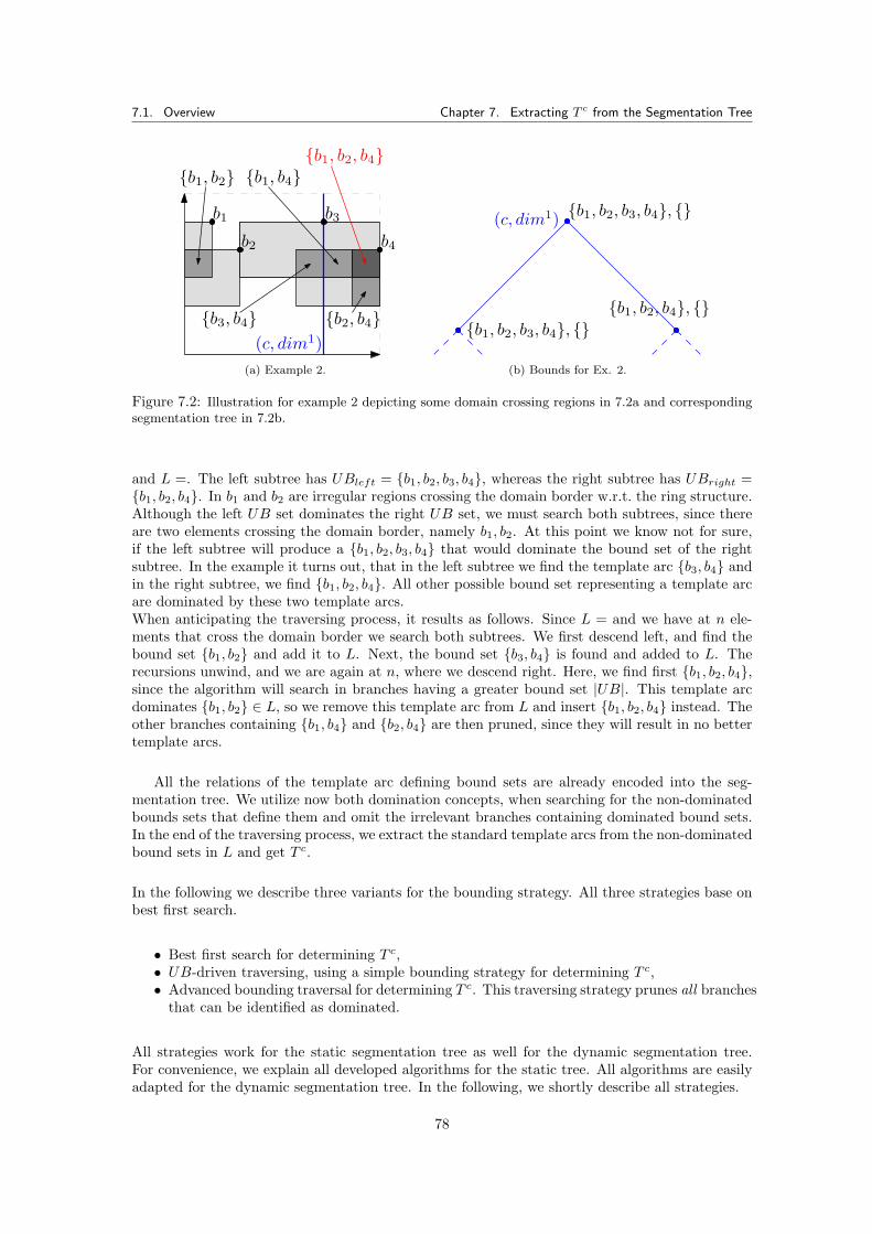
7.1. Overview Chapter 7. Extracting T c from the Segmentation Tree
(c, dim1)
b1
b2
b3
b4
{b1, b2}
{b3, b4}
{b1, b2, b4}
{b2, b4}
{b1, b4}
(a) Example 2.
(c, dim1) {b1, b2, b3, b4}, {}
{b1, b2, b3, b4}, {}{b1, b2, b4}, {}
(b) Bounds for Ex. 2.
Figure 7.2: Illustration for example 2 depicting some domain crossing regions in 7.2a and correspondingsegmentation tree in 7.2b.
and L =. The left subtree has UBleft = {b1, b2, b3, b4}, whereas the right subtree has UBright ={b1, b2, b4}. In b1 and b2 are irregular regions crossing the domain border w.r.t. the ring structure.Although the left UB set dominates the right UB set, we must search both subtrees, since thereare two elements crossing the domain border, namely b1, b2. At this point we know not for sure,if the left subtree will produce a {b1, b2, b3, b4} that would dominate the bound set of the rightsubtree. In the example it turns out, that in the left subtree we find the template arc {b3, b4} andin the right subtree, we find {b1, b2, b4}. All other possible bound set representing a template arcare dominated by these two template arcs.When anticipating the traversing process, it results as follows. Since L = and we have at n ele-ments that cross the domain border we search both subtrees. We first descend left, and find thebound set {b1, b2} and add it to L. Next, the bound set {b3, b4} is found and added to L. Therecursions unwind, and we are again at n, where we descend right. Here, we find first {b1, b2, b4},since the algorithm will search in branches having a greater bound set |UB|. This template arcdominates {b1, b2} ∈ L, so we remove this template arc from L and insert {b1, b2, b4} instead. Theother branches containing {b1, b4} and {b2, b4} are then pruned, since they will result in no bettertemplate arcs.
All the relations of the template arc defining bound sets are already encoded into the seg-mentation tree. We utilize now both domination concepts, when searching for the non-dominatedbounds sets that define them and omit the irrelevant branches containing dominated bound sets.In the end of the traversing process, we extract the standard template arcs from the non-dominatedbound sets in L and get T c.
In the following we describe three variants for the bounding strategy. All three strategies base onbest first search.
• Best first search for determining T c,• UB-driven traversing, using a simple bounding strategy for determining T c,• Advanced bounding traversal for determining T c. This traversing strategy prunes all branches
that can be identified as dominated.
All strategies work for the static segmentation tree as well for the dynamic segmentation tree.For convenience, we explain all developed algorithms for the static tree. All algorithms are easilyadapted for the dynamic segmentation tree. In the following, we shortly describe all strategies.
78
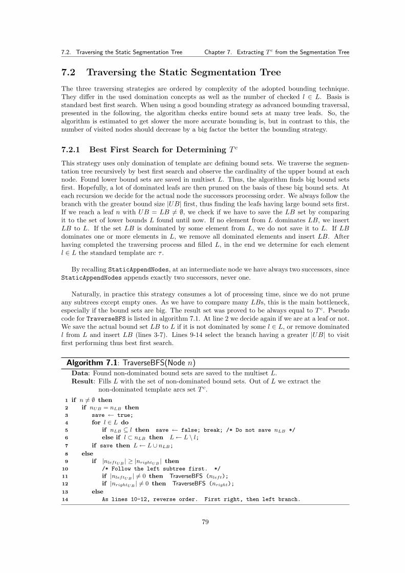
7.2. Traversing the Static Segmentation Tree Chapter 7. Extracting T c from the Segmentation Tree
7.2 Traversing the Static Segmentation Tree
The three traversing strategies are ordered by complexity of the adopted bounding technique.They differ in the used domination concepts as well as the number of checked l ∈ L. Basis isstandard best first search. When using a good bounding strategy as advanced bounding traversal,presented in the following, the algorithm checks entire bound sets at many tree leafs. So, thealgorithm is estimated to get slower the more accurate bounding is, but in contrast to this, thenumber of visited nodes should decrease by a big factor the better the bounding strategy.
7.2.1 Best First Search for Determining T c
This strategy uses only domination of template arc defining bound sets. We traverse the segmen-tation tree recursively by best first search and observe the cardinality of the upper bound at eachnode. Found lower bound sets are saved in multiset L. Thus, the algorithm finds big bound setsfirst. Hopefully, a lot of dominated leafs are then pruned on the basis of these big bound sets. Ateach recursion we decide for the actual node the successors processing order. We always follow thebranch with the greater bound size |UB| first, thus finding the leafs having large bound sets first.If we reach a leaf n with UB = LB 6= ∅, we check if we have to save the LB set by comparingit to the set of lower bounds L found until now. If no element from L dominates LB, we insertLB to L. If the set LB is dominated by some element from L, we do not save it to L. If LBdominates one or more elements in L, we remove all dominated elements and insert LB. Afterhaving completed the traversing process and filled L, in the end we determine for each elementl ∈ L the standard template arc τ .
By recalling StaticAppendNodes, at an intermediate node we have always two successors, sinceStaticAppendNodes appends exactly two successors, never one.
Naturally, in practice this strategy consumes a lot of processing time, since we do not pruneany subtrees except empty ones. As we have to compare many LBs, this is the main bottleneck,especially if the bound sets are big. The result set was proved to be always equal to T c. Pseudocode for TraverseBFS is listed in algorithm 7.1. At line 2 we decide again if we are at a leaf or not.We save the actual bound set LB to L if it is not dominated by some l ∈ L, or remove dominatedl from L and insert LB (lines 3-7). Lines 9-14 select the branch having a greater |UB| to visitfirst performing thus best first search.
Algorithm 7.1: TraverseBFS(Node n)Data: Found non-dominated bound sets are saved to the multiset L.Result: Fills L with the set of non-dominated bound sets. Out of L we extract the
non-dominated template arcs set T c.
if n 6= ∅ then1
if nUB = nLB then2
save ← true;3
for l ∈ L do4
if nLB ⊆ l then save ← false; break; /* Do not save nLB */5
else if l ⊂ nLB then L← L \ l;6
if save then L← L ∪ nLB;7
else8
if |nleftUB | ≥ |nrightUB | then9
/* Follow the left subtree first. */10
if |nleftUB | 6= 0 then TraverseBFS (nleft);11
if |nrightUB | 6= 0 then TraverseBFS (nright);12
else13
As lines 10-12, reverse order. First right, then left branch.14
79
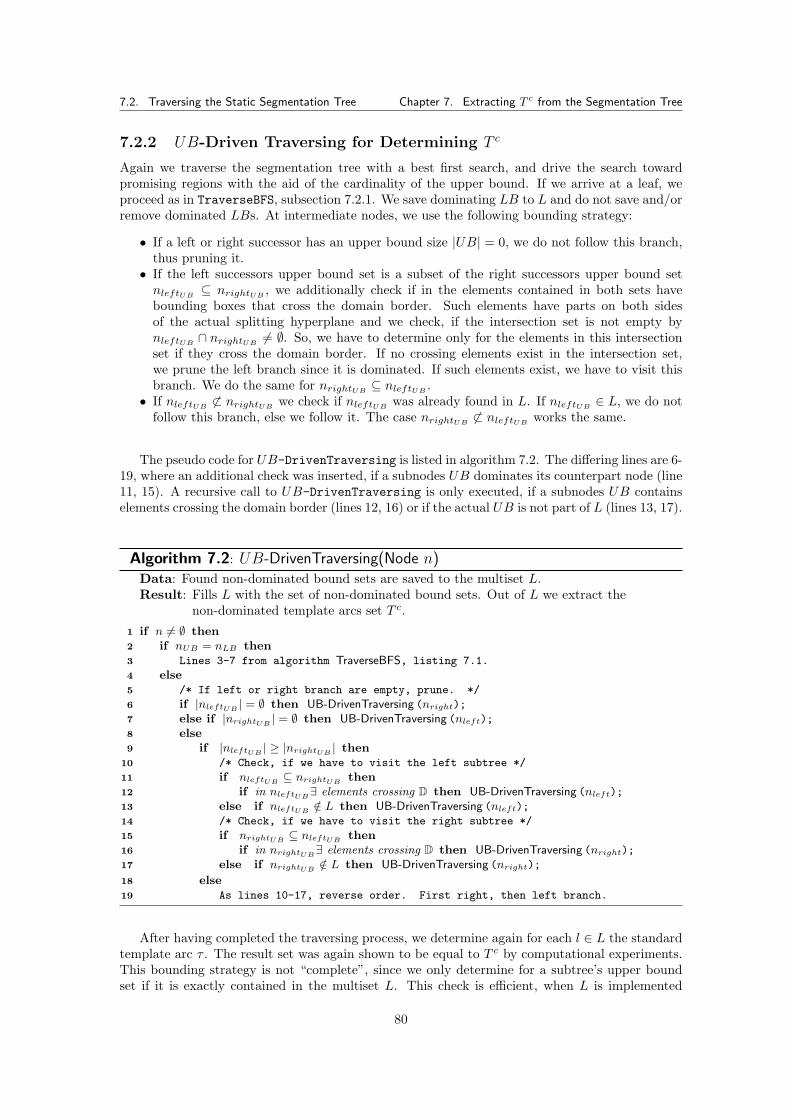
7.2. Traversing the Static Segmentation Tree Chapter 7. Extracting T c from the Segmentation Tree
7.2.2 UB-Driven Traversing for Determining T c
Again we traverse the segmentation tree with a best first search, and drive the search towardpromising regions with the aid of the cardinality of the upper bound. If we arrive at a leaf, weproceed as in TraverseBFS, subsection 7.2.1. We save dominating LB to L and do not save and/orremove dominated LBs. At intermediate nodes, we use the following bounding strategy:
• If a left or right successor has an upper bound size |UB| = 0, we do not follow this branch,thus pruning it.
• If the left successors upper bound set is a subset of the right successors upper bound setnleftUB ⊆ nrightUB , we additionally check if in the elements contained in both sets havebounding boxes that cross the domain border. Such elements have parts on both sidesof the actual splitting hyperplane and we check, if the intersection set is not empty bynleftUB ∩ nrightUB 6= ∅. So, we have to determine only for the elements in this intersectionset if they cross the domain border. If no crossing elements exist in the intersection set,we prune the left branch since it is dominated. If such elements exist, we have to visit thisbranch. We do the same for nrightUB ⊆ nleftUB .
• If nleftUB 6⊂ nrightUB we check if nleftUB was already found in L. If nleftUB ∈ L, we do notfollow this branch, else we follow it. The case nrightUB 6⊂ nleftUB works the same.
The pseudo code for UB-DrivenTraversing is listed in algorithm 7.2. The differing lines are 6-19, where an additional check was inserted, if a subnodes UB dominates its counterpart node (line11, 15). A recursive call to UB-DrivenTraversing is only executed, if a subnodes UB containselements crossing the domain border (lines 12, 16) or if the actual UB is not part of L (lines 13, 17).
Algorithm 7.2: UB-DrivenTraversing(Node n)Data: Found non-dominated bound sets are saved to the multiset L.Result: Fills L with the set of non-dominated bound sets. Out of L we extract the
non-dominated template arcs set T c.
if n 6= ∅ then1
if nUB = nLB then2
Lines 3-7 from algorithm TraverseBFS, listing 7.1.3
else4
/* If left or right branch are empty, prune. */5
if |nleftUB | = ∅ then UB-DrivenTraversing (nright);6
else if |nrightUB | = ∅ then UB-DrivenTraversing (nleft);7
else8
if |nleftUB | ≥ |nrightUB | then9
/* Check, if we have to visit the left subtree */10
if nleftUB ⊆ nrightUB then11
if in nleftUB∃ elements crossing D then UB-DrivenTraversing (nleft);12
else if nleftUB /∈ L then UB-DrivenTraversing (nleft);13
/* Check, if we have to visit the right subtree */14
if nrightUB ⊆ nleftUB then15
if in nrightUB∃ elements crossing D then UB-DrivenTraversing (nright);16
else if nrightUB /∈ L then UB-DrivenTraversing (nright);17
else18
As lines 10-17, reverse order. First right, then left branch.19
After having completed the traversing process, we determine again for each l ∈ L the standardtemplate arc τ . The result set was again shown to be equal to T c by computational experiments.This bounding strategy is not “complete”, since we only determine for a subtree’s upper boundset if it is exactly contained in the multiset L. This check is efficient, when L is implemented
80
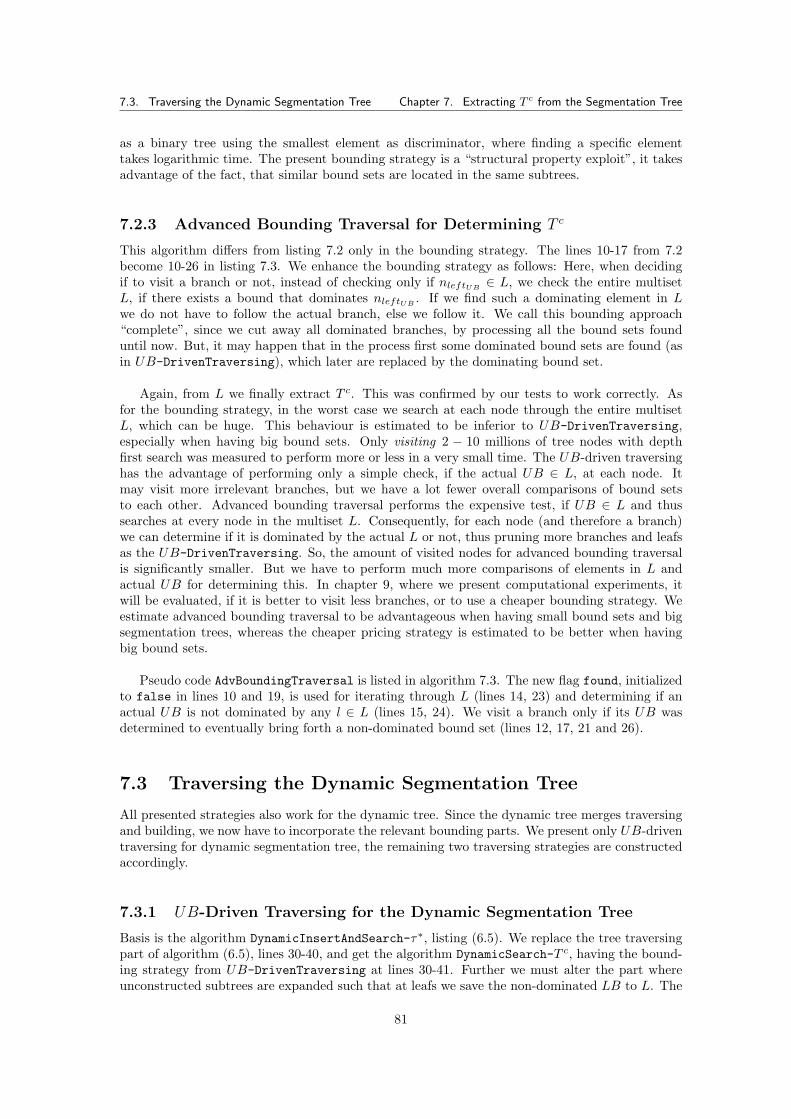
7.3. Traversing the Dynamic Segmentation Tree Chapter 7. Extracting T c from the Segmentation Tree
as a binary tree using the smallest element as discriminator, where finding a specific elementtakes logarithmic time. The present bounding strategy is a “structural property exploit”, it takesadvantage of the fact, that similar bound sets are located in the same subtrees.
7.2.3 Advanced Bounding Traversal for Determining T c
This algorithm differs from listing 7.2 only in the bounding strategy. The lines 10-17 from 7.2become 10-26 in listing 7.3. We enhance the bounding strategy as follows: Here, when decidingif to visit a branch or not, instead of checking only if nleftUB ∈ L, we check the entire multisetL, if there exists a bound that dominates nleftUB . If we find such a dominating element in Lwe do not have to follow the actual branch, else we follow it. We call this bounding approach“complete”, since we cut away all dominated branches, by processing all the bound sets founduntil now. But, it may happen that in the process first some dominated bound sets are found (asin UB-DrivenTraversing), which later are replaced by the dominating bound set.
Again, from L we finally extract T c. This was confirmed by our tests to work correctly. Asfor the bounding strategy, in the worst case we search at each node through the entire multisetL, which can be huge. This behaviour is estimated to be inferior to UB-DrivenTraversing,especially when having big bound sets. Only visiting 2 − 10 millions of tree nodes with depthfirst search was measured to perform more or less in a very small time. The UB-driven traversinghas the advantage of performing only a simple check, if the actual UB ∈ L, at each node. Itmay visit more irrelevant branches, but we have a lot fewer overall comparisons of bound setsto each other. Advanced bounding traversal performs the expensive test, if UB ∈ L and thussearches at every node in the multiset L. Consequently, for each node (and therefore a branch)we can determine if it is dominated by the actual L or not, thus pruning more branches and leafsas the UB-DrivenTraversing. So, the amount of visited nodes for advanced bounding traversalis significantly smaller. But we have to perform much more comparisons of elements in L andactual UB for determining this. In chapter 9, where we present computational experiments, itwill be evaluated, if it is better to visit less branches, or to use a cheaper bounding strategy. Weestimate advanced bounding traversal to be advantageous when having small bound sets and bigsegmentation trees, whereas the cheaper pricing strategy is estimated to be better when havingbig bound sets.
Pseudo code AdvBoundingTraversal is listed in algorithm 7.3. The new flag found, initializedto false in lines 10 and 19, is used for iterating through L (lines 14, 23) and determining if anactual UB is not dominated by any l ∈ L (lines 15, 24). We visit a branch only if its UB wasdetermined to eventually bring forth a non-dominated bound set (lines 12, 17, 21 and 26).
7.3 Traversing the Dynamic Segmentation Tree
All presented strategies also work for the dynamic tree. Since the dynamic tree merges traversingand building, we now have to incorporate the relevant bounding parts. We present only UB-driventraversing for dynamic segmentation tree, the remaining two traversing strategies are constructedaccordingly.
7.3.1 UB-Driven Traversing for the Dynamic Segmentation Tree
Basis is the algorithm DynamicInsertAndSearch-τ∗, listing (6.5). We replace the tree traversingpart of algorithm (6.5), lines 30-40, and get the algorithm DynamicSearch-T c, having the bound-ing strategy from UB-DrivenTraversing at lines 30-41. Further we must alter the part whereunconstructed subtrees are expanded such that at leafs we save the non-dominated LB to L. The
81
7.4. A Non-Dominated Segmentation Tree Chapter 7. Extracting T c from the Segmentation Tree
Algorithm 7.3: AdvBoundingTraversal(Node n)Data: Found non-dominated bound sets are saved to the multiset L.Result: Fills L with the set of non-dominated bound sets. Out of L we extract T c.
if n 6= ∅ then1
if nUB = nLB then2
Lines 3-7 from algorithm TraverseBFS, listing 7.1.3
else4
if |nleftUB | = ∅ then AdvBoundingTraversal (nright);5
else if |nrightUB | = ∅ then AdvBoundingTraversal (nleft);6
else7
if |nleftUB | ≥ |nrightUB | then8
/* Check if we have to follow the left subtree */9
found ← false;10
if nleftUB ⊆ nrightUB then11
if in nleftUB∃ elements crossing D then AdvBoundingTraversal (nleft);12
else13
forall ∀l ∈ L do14
if nleftUB ⊆ l then found ← true; break;15
/* nleftUB was already found, prune this branch. */16
if ¬ found then AdvBoundingTraversal (nleft);17
/* Check if we have to follow the right subtree */18
found ← false;19
if nrightUB ⊆ nleftUB then20
if in nrightUB∃ elem. crossing D then AdvBoundingTraversal (nright);21
else22
forall ∀l ∈ L do23
if nrightUB ⊆ l then found ← true; break;24
/* nrightUB was already found, prune this branch. */25
if ¬ found then AdvBoundingTraversal (nleft);26
else27
As lines 9-26, reverse order. First right, then left branch.28
according new lines are 15-20 in DynamicSearch-T c replacing lines 15-20 from DynamicInsert-AndSearch-τ∗. Additionally, at incomplete nodes having UB 6= LB, we replace the lines 8 and 24from DynamicInsertAndSearch-τ∗, where we select the best bi from the set Φ = UB \ LB, thatwere not yet segmented. Since we have no dual values and each bi must be segmented anyway(since we search T c), in DynamicSearch-T c at lines 8 and 23 we simply segment the first elementfrom Φ. The resulting algorithm DynamicSearch-T c is listed in pseudo code 7.4. The algorithmsDynamicAppendNodes (listing 6.7) and DynamicInsertNode (listing 6.6) remain unchanged.
7.4 A Non-Dominated Segmentation Tree
At this point the question, if a segmentation tree containing only non-dominated branches can bebuilt, remains as future work. The non-dominated segmentation tree would be built by insertingall bi sequentially into an empty tree. But at the moment it is unclear, if for each inserted bi canbe decided based on the incomplete construction status, if a subtree containing bi can be definitelyidentified as as dominated a priori (and thus must be built) or not.
An algorithm sketch mainly based on checking overlaps of bi at the nodes n was developed.We only outline the algorithm, since the work was not yet finished. Basis is again the algorithmStaticInsert, listing (6.2). By inserting bi ∈ B one by one, we construct only non-dominatedbranches, and mark the dominated ones with a flag. If a bi generates no new non-dominated
82
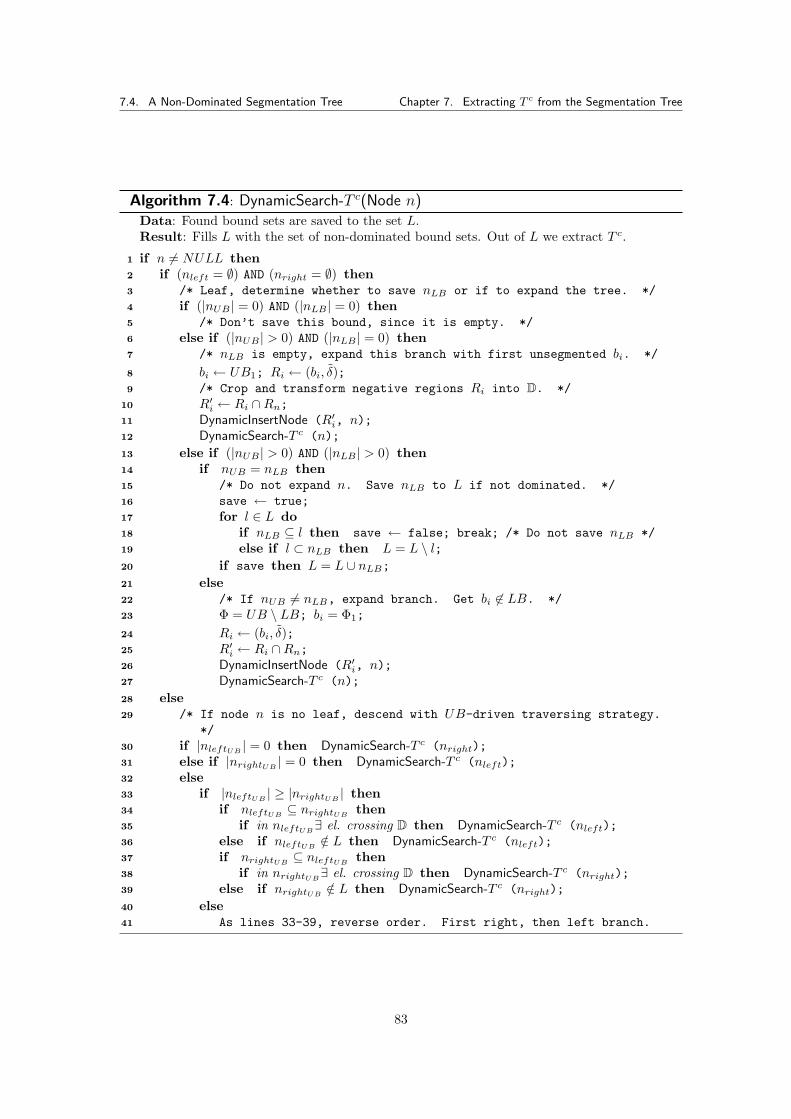
7.4. A Non-Dominated Segmentation Tree Chapter 7. Extracting T c from the Segmentation Tree
Algorithm 7.4: DynamicSearch-T c(Node n)Data: Found bound sets are saved to the set L.Result: Fills L with the set of non-dominated bound sets. Out of L we extract T c.
if n 6= NULL then1
if (nleft = ∅) AND (nright = ∅) then2
/* Leaf, determine whether to save nLB or if to expand the tree. */3
if (|nUB | = 0) AND (|nLB | = 0) then4
/* Don’t save this bound, since it is empty. */5
else if (|nUB | > 0) AND (|nLB | = 0) then6
/* nLB is empty, expand this branch with first unsegmented bi. */7
bi ← UB1; Ri ← (bi, δ);8
/* Crop and transform negative regions Ri into D. */9
R′i ← Ri ∩Rn;10
DynamicInsertNode (R′i, n);11
DynamicSearch-T c (n);12
else if (|nUB | > 0) AND (|nLB | > 0) then13
if nUB = nLB then14
/* Do not expand n. Save nLB to L if not dominated. */15
save ← true;16
for l ∈ L do17
if nLB ⊆ l then save ← false; break; /* Do not save nLB */18
else if l ⊂ nLB then L = L \ l;19
if save then L = L ∪ nLB;20
else21
/* If nUB 6= nLB, expand branch. Get bi 6∈ LB. */22
Φ = UB \ LB; bi = Φ1;23
Ri ← (bi, δ);24
R′i ← Ri ∩Rn;25
DynamicInsertNode (R′i, n);26
DynamicSearch-T c (n);27
else28
/* If node n is no leaf, descend with UB-driven traversing strategy.29
*/if |nleftUB | = 0 then DynamicSearch-T c (nright);30
else if |nrightUB | = 0 then DynamicSearch-T c (nleft);31
else32
if |nleftUB | ≥ |nrightUB | then33
if nleftUB ⊆ nrightUB then34
if in nleftUB∃ el. crossing D then DynamicSearch-T c (nleft);35
else if nleftUB /∈ L then DynamicSearch-T c (nleft);36
if nrightUB ⊆ nleftUB then37
if in nrightUB∃ el. crossing D then DynamicSearch-T c (nright);38
else if nrightUB /∈ L then DynamicSearch-T c (nright);39
else40
As lines 33-39, reverse order. First right, then left branch.41
83

7.4. A Non-Dominated Segmentation Tree Chapter 7. Extracting T c from the Segmentation Tree
template arc at some dominated branch, we only add its index to the actual upper bound set.A dominated branch is unmarked and expanded, if a new bi comes across, that generates a newtemplate arc somewhere in this subtree. Having such a case, elements from the dominated branch,that were not yet segmented, must be re-segmented.
If such a tree can be built, it is an improvement for both the search for T c and the pricingproblem. In both cases, performance may be improved by only creating the (hopefully muchsmaller) non-dominated branches instead of a full segmentation tree.
84
Chapter 8
Implementation
This chapter summarizes all implementation specific details. Basis for our implementation is theframework where [ChwRai09] and [Dietzel08] implemented all previous solution strategies. Allalgorithms have been integrated into this existing framework.
The algorithms have been implemented in C++, compiled and linked with g++-4.1. The ex-isting code makes use of the following libraries: The Standard Template Library (STL) fromSilicon Graphics (SGI), the Library of Efficient Data types and Algorithms (LEDA) fromAlgorithmic Solutions GmbH 1 which collects a variety of algorithms for graph theory and compu-tational geometry, the library Boost which extends C++, and ILOG CPLEX c© 11.2, an optimizationsoftware package for solving (among other) linear and integer programs. CPLEX is a state of theart commercial solver software that is able to solve linear and integer programs with millions ofvariables by using linear and non-linear methods.
8.1 Branch-and-Price Framework
A specialized branch-and-price framework has been integrated into the existing code. Our choicefell upon Solving Constraint Integer Programs (SCIP) [SCIP] developed by the Division Sci-entific Computing, Department Optimization at the Konrad-Zuse-Zentrum fur Informationstech-nik Berlin in cooperation with TU Braunschweig, TU Darmstadt and Siemens AG. We usedSCIP 1.2.0.This framework implements and provides most algorithms, tools and diagnostics that we needfor branch-and-price. SCIP is highly flexible, implemented in C and provides C++ wrapper classeswhich we used for integrating it into the existing code. Most of its features are realized witheasily extensible plugins, and include all sorts of constraint handlers, presolvers, branching rules,relaxators and primal heuristics. Interfaces for implementing variable pricers and cut separatorsexist. SCIP provides facility for constraint integer programming and branch-and-cut-and-price.The authors note that “SCIP is currently one of the fastest non-commercial mixed integer pro-gramming solvers on the market”.
An introduction to SCIP is [Schwa08]. A detailed description to the framework is [AcBeKoWo08]and [Achter07], who developed the original framework. The used documentation [Pfe07, Ber07,Ach07, Wolt07, Ach07-2] as well as implementation examples can be found at the website [SCIP].SCIP also includes the open LP solver SoPlex which is, compared to other freeware solvers, veryfast, but unfortunately not competitive enough for our purposes. As SCIP integrates support andinterfaces for other solvers, we chose ILOG CPLEX c© 11.2 as LP solver.
1Originally by Max Planck Institute for Informatics Saarbrucken.
85
8.2. Implementing SCF and MCF formulation in SCIP Chapter 8. Implementation
8.2 Implementing SCF and MCF formulation in SCIP
SCIP saves variables and constraints by the data types SCIP VAR* and SCIP CONS*, managed in anarbitrary container. The SCF and MCF formulations are loaded into the framework with providedinterface functions. Each problem was initialized with SCIPcreateProb, the objective sense setby SCIPsetObjsense to SCIP OBJSENSE MINIMIZE. Our solution was constrained to be integralby SCIPsetObjIntegral and to be less than k by SCIPsetObjlimit.
All variables were created by SCIPcreateVar (where we can specify name, variable type, limits,coefficients and so on) and added to the problem by SCIPaddVar. The variables were assembledinto constraints by using SCIPcreateConsLinear and SCIPaddCons. For each constraint a lot ofparameters can be specified: We defined all constraints to be part of the initial LP and disabledseparating in the solving process. Enforcing of constraint was enabled, since we have no redundantconstraints. Feasibility checking for each constraint in each branch-and-bound node was enabled.Additionally we defined constraints to be valid globally, rather than locally at some node. The arc-label constraints and node-label constraints2 were set to be modifiable, this is needed for pricing.The option for dynamic constraints (needed when cuts are separated as constraints) was disabled.The flags for a constraint to be removable from the relaxation was disabled and the option, ifconstraints may stick at the BB node where they were added, was enabled.
Our pricer classes inherit from the C++ wrapper object interface scip::ObjPricer, and thusimplement the virtual functions scip init, scip redcost and scip farkas. By providing thesefunctions, SCIP is able to call back the according user implemented methods from an arbitrarybranch-and-bound node or state. SCIP is notified about own pricers by SCIPincludeObjPricerand SCIPactivatePricer, after having constructed the pricer object.
We started the solution process by SCIPsolve. SCIP uses presolvers and relaxators for eachnode to determine feasibility and objective function values, saves actual bounds and in the pro-cess calls our functions scip redcost and scip farkas respectively. Dual variables are providedby the framework through the constraint handler by using SCIPgetDualsolLinear. Farkas co-efficients are extracted by SCIPgetDualfarkasLinear. Finally, we added the determined col-umn to the according constraints in the global model by first doing SCIPcreateVar and thenSCIPaddPricedVar.
8.2.1 SCIP Plugins
The solution process depends heavily on the plugins, that were defined3 before loading the model.In the following we only name the plugins that have been used. A detailed plugin description wouldget to long and can be looked up in the SCIP documentation, or in [Achter07, AcBeKoWo08].
Constraint handlers influence the way the constraints are relaxed and checked for validity. Weused SCIPincludeConshdlrLinear. The framework is able to transform constraints into a tighterform. In our case some constraints were tightened automatically by enabling ConshdlrIntegral,ConshdlrVarbound and ConshdlrSetppc. Many more constraint handlers exist.As we perform branch-and-price, [SCIP] recommends to deactivate some presolver plugins, mainlyPresolDualfix. We deactivated all presolvers, including PresolBoundshift, PresolImplics,PresolInttobinary, PresolProbing and PresolTrivial.
The branch-and-bound traversing mode is selected by NodeselBfs or NodeselDfs, wherebyBFS needs a good node selection strategy as well as good branching strategy, which are the
2Constraints (5.2) and (5.14) in the SCF model 5.2, constraints (5.16) and (5.28) in MCF model 5.3.3All the plugins described in the following are enabled by using the function SCIPincludeXXX, with XXX the
plugin name. If plugins are not included such, they are not used by SCIP.
86
8.2. Implementing SCF and MCF formulation in SCIP Chapter 8. Implementation
main bottleneck. DFS produces a much greater amount of BB nodes, but in our tests no sig-nificant run time difference were evaluated. Branch-and-bound nodes are selected automaticallyby the plugins NodeselEstimate, NodeselHybridestim and NodeselRestartdfs. Providedbranch rules are BranchruleAllfullstrong, BranchruleFullstrong, BranchruleInference,BranchruleMostinf, BranchruleLeastinf, BranchrulePscost, BranchruleRandom andBranchruleRelpscost, which heavily impact on the running time. The document [Ach07]describes these plugins and their working principle. We let SCIP determine by its own anappropriate branching rule.
We do not separate any constraints, in this case [SCIP] recommends to not include any sep-arator plugins. Furthermore, many heuristics plugins are at disposal, which we do not list here,since they were not included.
8.2.2 Module Structure
Figures 8.2 and 8.1 outline all implemented modules and how they work together. The remainingframework is described in [Dietzel08].
Figure 8.1 shows all classes relevant to segmentation and traversing. Basically we distinguisha static segmentation, implemented in Segmentation, and a dynamic segmentation, implementedin SegmentationDyn.
The static algorithms presented in chapters 6 and 7 have been implemented as functions inthe class SegTree, which manages nodes of the type SegNode. Basically, each node contains theactual upper and a lower bound set, the splitting coordinate, the split discriminator and a flagif the actual node contains a null subspace. The tree may may be traversed by TraverseBFS,UB-Driven Traversing or AdvBoundingTraversal, when determining T c. All such traversingalgorithms implement an interface Traverser. The τ∗ is determined by PricingTraverser (algo-rithm 6.4). The according StaticTreePricer from figure 8.2 uses this class in combination withSegTree.
The dynamic version is realized by the classes DynTree and DynNode. Here the traversing andgeneration of new nodes is done by PreprocExpander (for getting T c) and PricingExpander, allimplementing the abstract class Expander. The according DynamicTreePricer from figure 8.2uses PricingExpander, which searches in a DynTree.
The classes SimulatePricingTraverser and SimulPricingExpander simulate the pricingproblem based on random values as described in sections 6.4.5 and 6.5.2. The Comparer de-termines if single template arcs or entire sets T c equal, by comparing coordinates, expressed nodedifferences and sums of dual/random values for equality. The remaining classes are containers forT c, result set of template arcs and node differences and implement some conversion functionality,as well es template arc determination. Further classes draw 2-dimensional segmentation treeseither as bitmap (BMP) or scalable vector graphic (SVG).
Figure 8.2 shows the classes used to realize branch-and-price. The class BranchPrice loadsthe appropriate model, each one implementing the abstract class Model. Both, the SCF andMCF model may be solved entirely with CompleteSCFModel and CompleteMCFModel. In theclasses SCFModel and MCFModel we load only an RMP, including either a starting solution orFarkas priced values, and expand the RMP by performing branch-and-price. In the SCF case, theSCFPricer prices a new variable by using either StaticTreePricer, DynamicTreePricer or thetesting pricer TcPricer. Pricing for MCF works accordingly.
87
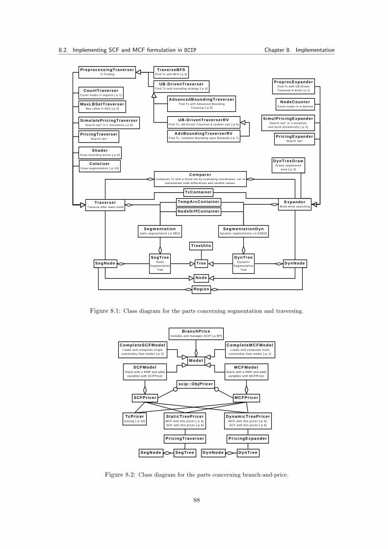
8.2. Implementing SCF and MCF formulation in SCIP Chapter 8. Implementation
Segmenta t ionstatic segmentation [-a SEG]
Segmenta t ionDyndynamic segmentation [-a DSEG]
Region
Node
TreeSegNode
SegTreeStatic
Segmentat ionTree
DynNode
DynTreeDynamic
Segmentat ionTree
TraverserTraverse after static build
ComparerCompares Tc with a found set by evaluating coordinates, set of
represented node differences and random values.
ColorizerDraw segmentat ion [-p 10]
ShaderDraw bounding boxes [-p 9]
NodeDif fConta iner
TcContainer
TempArcContainer ExpanderBuild while searching
NodeCounterCount nodes in a dyntree
PreprocExpanderFind Tc with UB-DrivenTraversal & build [-p 1]
SimulPr ic ingExpanderSearch tau* in n iterations
and bui ld dynamical ly [-p 2]
CountTraverserCount nodes in segtree [-p 1]
MaxLBSetTraverserMax LBset in SEG [-p 2]
UB-DrivenTraverserFind Tc with bounding strategy [-p 4]
TraverseBFSFind Tc with BFS [-p 3]
AdvancedBoundingTraverserFind Tc with Advanced Bounding
Traversal [-p 5]
UB-DrivenTraverserRVFind Tc, UB-Driven Traversal & random vals [-p 6]
SimulatePr ic ingTraverserSearch tau* in n interations [-p 8]
AdvBoundingTraverserRVFind Tc, complete Bounding upon Randvals [-p 7]
PreprocessingTraverserTc Finding
DynTreeDrawDraws segmented
area [-p 3]
PricingTraverserSearch tau*
PricingExpanderSearch tau*
TreeUti ls
Figure 8.1: Class diagram for the parts concerning segmentation and traversing.
scip::ObjPricer
MCFPricerSCFPricer
BranchPriceIncludes and manages SCIP [-a BP]
Mode l
CompleteSCFModelLoads and computes single
commodity f low model [ -p 2]
CompleteMCFModelLoads and computes mult i
commodity f low model [ -p 1]
MCFModelStarts with a RMP and adds
variables with MCFPricer
SCFModelStarts with a RMP and adds
variables with SCFPricer
Stat icTreePricerMCF with this pricer [-p 3],SCF with this pricer [-p 6]
DynamicTreePricerMCF with this pricer [-p 5],SCF with this pricer [-p 8]
TcPricertest ing [-p 10]
PricingTraverser Pric ingExpander
SegTreeSegNode DynNode DynTree
Figure 8.2: Class diagram for the parts concerning branch-and-price.
88
Chapter 9
Experimental Results
In this chapter we present the computational results for the algorithms presented in the previouschapters. Here, input data for the computational experiments is described. First, we evaluaterun times and visited nodes for the algorithms that replace the preprocessing by [ChwRai09].Then, computational results for the algorithms that solve the pricing problem are presented. TheSCF and MCF formulation are compared, as well as pricer alternatives (static versus dynamic).Additionally, we evaluate how the run times differ when using node-label constraints and whennot using them, as well as runs employing starting solutions versus Farkas pricer runs. All testruns have been executed on the following machines running Linux:
• G1: Grid of Dual Core AMDTMOpteronTM270, 1.993 GHz processor, 8 GB RAM, amd64.• L1: IntelTMPentiumTMM processor 1.73GHz, 1 GB RAM, ix86.• O1: AMDTMOpteronTM2.4 GHz processor, 4 GB RAM, amd64.
9.1 Input Data Files
Test data are 20 files provided by the Fraunhofer Institute [Fraun] in binary format (‘fhg’),and selected 15 files from the U.S. National Institute of Standards and Technology (NIST) dataset [NIST]. Table 9.1 lists files and amount of contained minutiae data points |V |, as well as thenumber of implied node differences is |B|. We name the Fraunhofer test set ‘fhg’, the second testset ‘nist’.
All fhg and nist data is 4-dimensional and have varying numbers of minutiae data points.The files are multiple scans of four different fingers of two persons, indicated in the name byP (person), F (finger), R (release). The used forensic algorithm extracted a different numberof minutiae in the different scans. In the Fraunhofer templates the minimum number of datapoints is min(|V |) = 15, the maximum max(|V |) = 40. These sets have an average number ofavg(|V |) = 30.75 data points. Here, the domain has an average of vavg = (286, 383, 358, 2)>, thesmallest domain vmin = (129, 191, 252, 2)> and the maximal vmax = (224, 287, 312, 2)>.The NIST templates data points are a subset of a large test set. We selected 5 instances fromthe templates classified as good, bad and ugly. The NIST data points range from min(|V |) = 72to max(|V |) = 120, with an average of avg(|V |) = 96.47 data points. The average domain isvavg = (3993, 3368, 359, 2)>, the minimal domain is vmin = (2936, 2281, 359, 2)>, the maximumvmax = (3293, 2788, 353, 2)>.
Table 9.2 shows for which of the selected δ the set T c is already available by the applicationof the preprocessing method from [ChwRai09]. We used these files to verify our segmentationtree results and for simulating the pricing problem. We point out that when counting nodes ina big segmentation tree (2–10 millions of nodes) the run time is always very small and the runstake 0.02–3.00 seconds. When running the actual tests, deviations of some milliseconds occur,
89
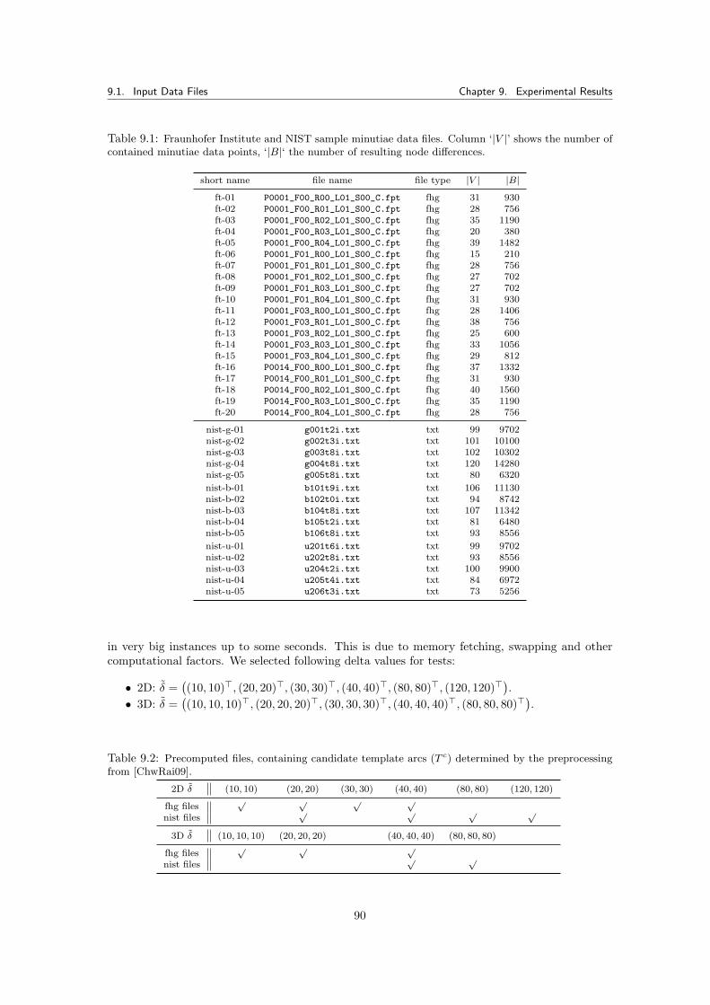
9.1. Input Data Files Chapter 9. Experimental Results
Table 9.1: Fraunhofer Institute and NIST sample minutiae data files. Column ‘|V |’ shows the number ofcontained minutiae data points, ‘|B|‘ the number of resulting node differences.
short name file name file type |V | |B|ft-01 P0001_F00_R00_L01_S00_C.fpt fhg 31 930ft-02 P0001_F00_R01_L01_S00_C.fpt fhg 28 756ft-03 P0001_F00_R02_L01_S00_C.fpt fhg 35 1190ft-04 P0001_F00_R03_L01_S00_C.fpt fhg 20 380ft-05 P0001_F00_R04_L01_S00_C.fpt fhg 39 1482ft-06 P0001_F01_R00_L01_S00_C.fpt fhg 15 210ft-07 P0001_F01_R01_L01_S00_C.fpt fhg 28 756ft-08 P0001_F01_R02_L01_S00_C.fpt fhg 27 702ft-09 P0001_F01_R03_L01_S00_C.fpt fhg 27 702ft-10 P0001_F01_R04_L01_S00_C.fpt fhg 31 930ft-11 P0001_F03_R00_L01_S00_C.fpt fhg 28 1406ft-12 P0001_F03_R01_L01_S00_C.fpt fhg 38 756ft-13 P0001_F03_R02_L01_S00_C.fpt fhg 25 600ft-14 P0001_F03_R03_L01_S00_C.fpt fhg 33 1056ft-15 P0001_F03_R04_L01_S00_C.fpt fhg 29 812ft-16 P0014_F00_R00_L01_S00_C.fpt fhg 37 1332ft-17 P0014_F00_R01_L01_S00_C.fpt fhg 31 930ft-18 P0014_F00_R02_L01_S00_C.fpt fhg 40 1560ft-19 P0014_F00_R03_L01_S00_C.fpt fhg 35 1190ft-20 P0014_F00_R04_L01_S00_C.fpt fhg 28 756
nist-g-01 g001t2i.txt txt 99 9702nist-g-02 g002t3i.txt txt 101 10100nist-g-03 g003t8i.txt txt 102 10302nist-g-04 g004t8i.txt txt 120 14280nist-g-05 g005t8i.txt txt 80 6320
nist-b-01 b101t9i.txt txt 106 11130nist-b-02 b102t0i.txt txt 94 8742nist-b-03 b104t8i.txt txt 107 11342nist-b-04 b105t2i.txt txt 81 6480nist-b-05 b106t8i.txt txt 93 8556
nist-u-01 u201t6i.txt txt 99 9702nist-u-02 u202t8i.txt txt 93 8556nist-u-03 u204t2i.txt txt 100 9900nist-u-04 u205t4i.txt txt 84 6972nist-u-05 u206t3i.txt txt 73 5256
in very big instances up to some seconds. This is due to memory fetching, swapping and othercomputational factors. We selected following delta values for tests:
• 2D: δ =((10, 10)>, (20, 20)>, (30, 30)>, (40, 40)>, (80, 80)>, (120, 120)>
).
• 3D: δ =((10, 10, 10)>, (20, 20, 20)>, (30, 30, 30)>, (40, 40, 40)>, (80, 80, 80)>
).
Table 9.2: Precomputed files, containing candidate template arcs (T c) determined by the preprocessingfrom [ChwRai09].
2D δ (10, 10) (20, 20) (30, 30) (40, 40) (80, 80) (120, 120)
fhg files√ √ √ √
nist files√ √ √ √
3D δ (10, 10, 10) (20, 20, 20) (40, 40, 40) (80, 80, 80)
fhg files√ √ √
nist files√ √
90
9.2. Static and Dynamic Segmentation Chapter 9. Experimental Results
9.2 Static and Dynamic Segmentation
The verification of the correctness of the segmentation tree has been done by performing thefollowing steps:
• We compared the running times of the static segmentation build procedure, presented insection 6.4.1 and 6.4.2 and tested its correctness by extracting T c, which then was comparedto the set T c from the preprocessing by [ChwRai09].
• We compared the running times of the strategies that determine T c from chapter 7, namelyUB-driven traversing (section 7.2.2), advanced bounding traversal (section 7.2.3), and bestfirst search (section 7.2.1), in order to determine the quickest way for getting T c. Also, weexamined the overall number of created nodes as well as the percentage of visited nodes foreach traversing strategy. The conclusion is that UB-driven traversing performs best.
• We checked the dynamic segmentation, presented in 6.5, for correctness by extracting againT c with the algorithm UB-driven traversing for dynamic trees, namely DynamicSearch-T c
(section 7.3.1), and compared the set to the set T c extracted by the previous preprocessing.• We simulated the pricing problem for both the static and dynamic variant in order to de-
termine, if both strategies to find τ∗, presented in section 6.4.3 and 6.5, find the correct τ∗
in each simulated pricing iteration, and if they are quick enough for being used in the pricerroutine.
This data is summarized in the following tables. The tests have been run on grid G1. Ta-bles 9.3, 9.4 and 9.5, 9.6 show the run times of the static and dynamic segmentation in compar-ison to the run times of the preprocessing from [ChwRai09], once for 2-dimensional and once for3-dimensional parameters δ. For each δ the number of found candidate template arcs is listed(column ‘|T c|’), followed by static tree building time in seconds (column ‘b[s]’). As during thetests UB-driven traversing was found to be the quickest variant for determining T c, in these ta-bles we compare its traversing time and total time for building and traversing with the dynamicversion total run time. The super-column ‘static/UBD’ lists static segmentation tree data, andcolumn ‘dyn’ dynamic segmentation tree data. The columns ‘t[s]’ list run times in seconds neededfor traversing the static tree with UBD, the columns ‘tot[s]’ list total run time in seconds fordetermining T c with UBD. The last column ‘PP’ in each δ block is the run time in seconds ofthe preprocessing by [ChwRai09]. Note that these run times have been determined on machine O1and we used them, since a new series of tests would take too long.
Tables 1, 2 (2-dimensional δ) and 3, 4 (3-dimensional δ) in the appendix list the run times ofall three strategies that find T c as well as the amount of visited nodes in the static tree, or creatednodes for the dynamic tree. Examined strategies are:• UB-driven traversing for determining T c in a static tree. Column ‘UBD’ lists run times.• Advanced bounding traversal for determining T c in a static tree. Column ‘ABT’.• Best first search for determining T c in a static tree. Column ‘BFS’ lists run times.
These tests have been run on grid G1. We compare this data again to the dynamic segmentation.The respective columns are again entitled ‘static’ for the static tree and ‘dyn’ for the dynamictree. For ‘static’, the column ‘|n|’ lists the total amount of nodes contained in the static tree.This tree size is later used as basis for the computation of the percentage of visited nodes. Thecolumns ‘UBD’, ‘ABT’ and ‘BFS’ list the run times of each traversing strategy in seconds. Foreach traversing strategy the respective amount of visited nodes is listed in the columns called‘%n’. For the dynamic version ‘dyn’ we listed in column ‘|n|’ the overall amount of producednodes when searching for T c, and how they correlate with the number of nodes in a static tree.The column ‘%n’ indicates the percentage, which the dynamic tree is smaller than the static tree.The amount of nodes in the dynamic tree is the smallest number of nodes needed for findingT c. When searching only for τ∗ in the dynamic tree, the number of nodes decreases massively,especially when emptying the tree before each pricing iteration. In contrast, when searching τ∗ inthe static tree, the number of nodes remains equal, since this tree is always built completely. Inthe following we aggregate the gained insights, subdivided into the main topics.
91
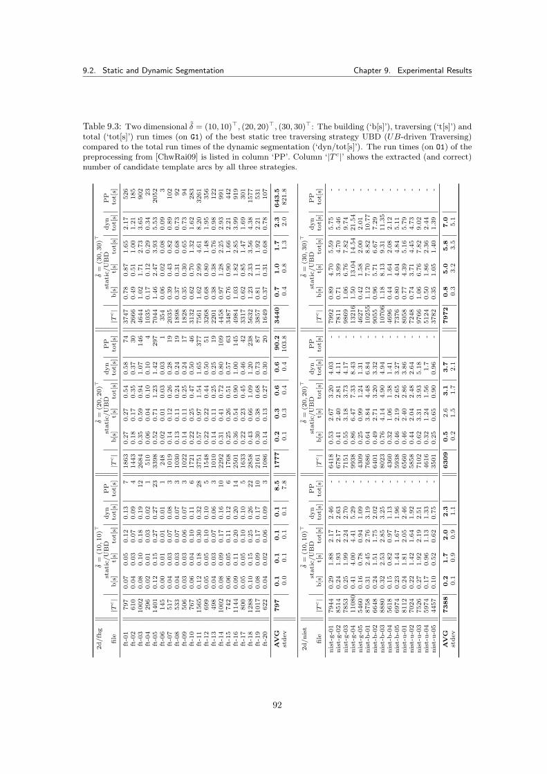
9.2. Static and Dynamic Segmentation Chapter 9. Experimental Results
Table 9.3: Two dimensional δ = (10, 10)>, (20, 20)>, (30, 30)>: The building (‘b[s]’), traversing (‘t[s]’) andtotal (‘tot[s]’) run times (on G1) of the best static tree traversing strategy UBD (UB-driven Traversing)compared to the total run times of the dynamic segmentation (‘dyn/tot[s]’). The run times (on O1) of thepreprocessing from [ChwRai09] is listed in column ‘PP’. Column ‘|T c|’ shows the extracted (and correct)number of candidate template arcs by all three strategies.
2d/fh
gδ
=(1
0,10)>
δ=
(20,20)>
δ=
(30,30)>
stati
c/U
BD
dyn
PP
stati
c/U
BD
dyn
PP
stati
c/U
BD
dyn
PP
file
|Tc|
b[s
]t[
s]to
t[s]
tot[
s]to
t[s]
|Tc|
b[s
]t[
s]to
t[s]
tot[
s]to
t[s]
|Tc|
b[s
]t[
s]to
t[s]
tot[
s]to
t[s]
ft-0
1797
0.0
70.0
50.1
20.1
37
1863
0.2
70.2
70.5
40.5
874
3747
0.7
80.8
71.6
52.1
7526
ft-0
2610
0.0
40.0
30.0
70.0
94
1443
0.1
80.1
70.3
50.3
730
2666
0.4
90.5
11.0
01.2
1185
ft-0
31002
0.0
80.1
00.1
80.1
912
2684
0.3
50.5
90.9
41.0
7146
4644
1.0
21.7
12.7
33.6
5902
ft-0
4296
0.0
20.0
10.0
30.0
21
510
0.0
60.0
40.1
00.1
04
1035
0.1
70.1
20.2
90.3
423
ft-0
51401
0.1
20.1
50.2
70.2
723
3398
0.5
20.7
11.2
31.4
2297
7044
1.4
62.4
73.9
35.5
32052
ft-0
6145
0.0
00.0
10.0
10.0
11
248
0.0
20.0
10.0
30.0
31
354
0.0
60.0
20.0
80.0
93
ft-0
7517
0.0
40.0
30.0
70.0
83
1019
0.1
40.1
20.2
60.2
819
2035
0.3
90.4
30.8
20.8
9102
ft-0
8533
0.0
40.0
30.0
70.0
73
1030
0.1
30.1
10.2
40.2
419
1898
0.3
70.3
10.6
80.7
392
ft-0
9506
0.0
30.0
30.0
60.0
73
1022
0.1
40.1
10.2
50.2
417
1828
0.3
50.3
00.6
50.7
394
ft-1
0767
0.0
60.0
40.1
00.1
16
1721
0.2
20.2
50.4
70.5
046
3132
0.6
20.7
01.3
21.6
2283
ft-1
11565
0.1
20.1
80.3
00.3
228
3751
0.5
70.9
71.5
41.6
5377
7561
1.6
22.9
94.6
18.2
03261
ft-1
2699
0.0
50.0
50.1
00.1
05
1548
0.2
20.2
20.4
40.5
051
3268
0.6
80.8
01.4
81.9
5356
ft-1
3498
0.0
40.0
30.0
70.0
63
1010
0.1
40.1
10.2
50.2
519
2201
0.3
80.3
80.7
60.9
8122
ft-1
41002
0.0
80.0
90.1
70.1
610
2292
0.3
10.4
10.7
20.8
0109
4458
0.9
71.2
82.2
52.9
3991
ft-1
5742
0.0
60.0
50.1
10.1
26
1768
0.2
50.2
60.5
10.5
763
3487
0.7
60.9
01.6
62.2
1442
ft-1
61144
0.0
90.1
10.2
00.2
014
2501
0.3
60.5
40.9
01.0
0145
4984
1.0
31.8
22.8
53.9
9919
ft-1
7800
0.0
50.0
50.1
00.1
05
1633
0.2
20.2
30.4
50.4
642
3317
0.6
20.8
51.4
71.6
9301
ft-1
81288
0.1
00.1
50.2
50.2
622
2858
0.4
30.6
61.0
91.2
0238
5632
1.2
32.3
33.5
64.3
81577
ft-1
91017
0.0
80.0
90.1
70.1
710
2161
0.3
00.3
80.6
80.7
387
3857
0.8
11.1
11.9
22.2
1531
ft-2
0622
0.0
40.0
20.0
60.0
93
1086
0.1
40.1
30.2
70.3
020
1649
0.3
70.3
10.6
80.7
8107
AV
G797
0.1
0.1
0.1
0.1
8.5
1777
0.2
0.3
0.6
0.6
90.2
3440
0.7
1.0
1.7
2.3
643.5
stdev
0.0
0.1
0.1
0.1
7.8
0.1
0.3
0.4
0.4
103.8
0.4
0.8
1.3
2.0
821.8
2d/nis
tδ
=(1
0,10)>
δ=
(20,20)>
δ=
(30,30)>
stati
c/U
BD
dyn
PP
stati
c/U
BD
dyn
PP
stati
c/U
BD
dyn
PP
file
|Tc|
b[s
]t[
s]to
t[s]
tot[
s]to
t[s]
|Tc|
b[s
]t[
s]to
t[s]
tot[
s]to
t[s]
|Tc|
b[s
]t[
s]to
t[s]
tot[
s]to
t[s]
nis
t-g-0
17944
0.2
91.8
82.1
72.4
6-
6418
0.5
32.6
73.2
04.0
3-
7992
0.8
94.7
05.5
95.7
5-
nis
t-g-0
28514
0.2
41.9
32.1
72.6
3-
6787
0.4
12.4
02.8
14.1
1-
7811
0.7
13.9
94.7
05.4
6-
nis
t-g-0
37853
0.2
51.9
92.2
42.7
0-
7151
0.5
53.1
83.7
34.1
7-
9869
1.0
66.7
67.8
29.7
4-
nis
t-g-0
411080
0.4
14.0
04.4
15.2
9-
9938
0.8
66.4
77.3
38.4
3-
13216
1.5
013.0
414.5
421.5
4-
nis
t-g-0
55460
0.1
60.7
80.9
41.0
9-
4309
0.2
50.9
91.2
41.3
1-
4627
0.4
21.5
82.0
02.0
1-
nis
t-b-0
18758
0.3
12.4
52.7
63.1
9-
7686
0.6
43.8
44.4
86.8
4-
10255
1.1
27.7
08.8
210.7
7-
nis
t-b-0
26648
0.2
41.5
11.7
52.0
2-
6401
0.4
92.7
13.2
03.3
2-
9055
0.9
65.7
16.6
77.2
9-
nis
t-b-0
38880
0.3
22.5
32.8
53.2
5-
8023
0.7
64.1
44.9
04.9
4-
10706
1.1
88.1
39.3
111.3
5-
nis
t-b-0
45618
0.1
50.8
20.9
71.1
3-
4360
0.3
21.0
61.3
81.4
1-
4696
0.4
41.6
42.0
82.1
2-
nis
t-b-0
56974
0.2
31.4
41.6
71.9
6-
5938
0.4
62.1
92.6
53.2
7-
7376
0.8
04.0
44.8
45.1
1-
nis
t-u-0
18112
0.2
41.8
12.0
52.4
6-
6560
0.4
62.4
02.8
63.8
6-
8058
0.7
74.3
95.1
65.7
9-
nis
t-u-0
27024
0.2
21.4
21.6
41.9
2-
5858
0.4
42.0
42.4
82.6
4-
7248
0.7
43.7
14.4
54.7
3-
nis
t-u-0
37526
0.2
71.9
22.1
92.5
1-
7102
0.6
23.3
13.9
35.1
8-
9766
1.0
66.7
67.8
29.0
2-
nis
t-u-0
45974
0.1
70.9
61.1
31.3
3-
4616
0.3
21.2
41.5
61.7
-5124
0.5
01.8
62.3
62.4
4-
nis
t-u-0
54457
0.1
00.5
20.6
20.7
5-
3501
0.2
50.6
50.9
00.9
6-
3782
0.3
51.0
51.4
01.3
9-
AV
G7388
0.2
1.7
2.0
2.3
6309
0.5
2.6
3.1
3.7
7972
0.8
5.0
5.8
7.0
stdev
0.1
0.9
0.9
1.1
0.2
1.5
1.7
2.1
0.3
3.2
3.5
5.1
92
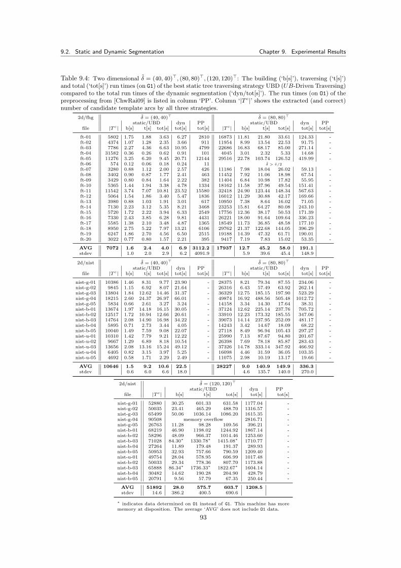
9.2. Static and Dynamic Segmentation Chapter 9. Experimental Results
Table 9.4: Two dimensional δ = (40, 40)>, (80, 80)>, (120, 120)>: The building (‘b[s]’), traversing (‘t[s]’)and total (‘tot[s]’) run times (on G1) of the best static tree traversing strategy UBD (UB-Driven Traversing)compared to the total run times of the dynamic segmentation (‘dyn/tot[s]’). The run times (on O1) of thepreprocessing from [ChwRai09] is listed in column ‘PP’. Column ‘|T c|’ shows the extracted (and correct)number of candidate template arcs by all three strategies.
2d/fhg δ = (40, 40)> δ = (80, 80)>
static/UBD dyn PP static/UBD dyn PPfile |T c| b[s] t[s] tot[s] tot[s] tot[s] |T c| b[s] t[s] tot[s] tot[s] tot[s]
ft-01 5802 1.75 1.88 3.63 6.27 2810 16873 11.81 21.80 33.61 124.33 -ft-02 4374 1.07 1.28 2.35 3.66 911 11954 8.99 13.54 22.53 91.75 -ft-03 7786 2.27 4.36 6.63 10.95 4799 22686 16.83 68.17 85.00 271.14 -ft-04 31582 0.36 0.26 0.62 0.91 101 4045 3.01 2.32 5.33 14.68 -ft-05 11276 3.25 6.20 9.45 20.71 12144 29516 22.78 103.74 126.52 419.99 -ft-06 574 0.12 0.06 0.18 0.24 11 δ > v/2
ft-07 3280 0.88 1.12 2.00 2.57 426 11186 7.98 18.04 26.02 59.13 -ft-08 3402 0.90 0.87 1.77 2.41 463 11452 7.92 11.06 18.98 67.54 -ft-09 3429 0.80 0.84 1.64 2.22 382 11404 6.84 10.98 17.82 55.95 -ft-10 5365 1.44 1.94 3.38 4.78 1334 18162 11.58 37.96 49.54 151.41 -ft-11 11542 3.74 7.07 10.81 23.52 15580 32418 24.90 123.44 148.34 567.63 -ft-12 5064 1.54 1.86 3.40 5.47 1836 16012 11.29 30.88 42.17 169.66 -ft-13 3980 0.88 1.03 1.91 3.01 617 10950 7.38 8.64 16.02 71.05 -ft-14 7130 2.23 3.12 5.35 8.21 3468 23253 15.81 64.27 80.08 243.10 -ft-15 5720 1.72 2.22 3.94 6.33 2549 17756 12.36 38.17 50.53 171.39 -ft-16 7330 2.43 3.85 6.28 9.81 4431 26221 18.00 91.64 109.64 336.23 -ft-17 5585 1.38 2.10 3.48 4.87 1365 18549 11.73 36.85 48.58 177.10 -ft-18 8950 2.75 5.22 7.97 13.21 6106 29762 21.37 122.68 144.05 396.29 -ft-19 6247 1.86 2.70 4.56 6.50 2515 19188 14.39 47.32 61.71 190.01 -ft-20 3022 0.77 0.80 1.57 2.21 395 9417 7.19 7.83 15.02 53.35 -
AVG 7072 1.6 2.4 4.0 6.9 3112.2 17937 12.7 45.2 58.0 191.1stdev 1.0 2.0 2.9 6.2 4091.9 5.9 39.6 45.4 148.9
2d/nist δ = (40, 40)> δ = (80, 80)>
static/UBD dyn PP static/UBD dyn PPfile |T c| b[s] t[s] tot[s] tot[s] tot[s] |T c| b[s] t[s] tot[s] tot[s] tot[s]
nist-g-01 10386 1.46 8.31 9.77 23.90 - 28375 8.21 79.34 87.55 234.06 -nist-g-02 9845 1.15 6.92 8.07 21.64 - 26316 6.43 57.49 63.92 262.14 -nist-g-03 13804 1.84 12.62 14.46 31.37 - 36329 12.75 185.15 197.90 523.29 -nist-g-04 18215 2.60 24.37 26.97 66.01 - 49874 16.92 488.56 505.48 1012.72 -nist-g-05 5834 0.66 2.61 3.27 3.24 - 14158 3.34 14.30 17.64 38.31 -nist-b-01 13674 1.97 14.18 16.15 30.05 - 37124 12.62 225.14 237.76 705.72 -nist-b-02 12517 1.72 10.94 12.66 20.61 - 33910 12.23 173.32 185.55 347.06 -nist-b-03 14764 2.08 14.90 16.98 34.22 - 39073 14.14 237.95 252.09 481.17 -nist-b-04 5895 0.71 2.73 3.44 4.05 - 14243 3.42 14.67 18.09 68.22 -nist-b-05 10040 1.49 7.59 9.08 22.07 - 27118 8.49 96.94 105.43 297.27 -nist-u-01 10310 1.42 7.79 9.21 12.22 - 25990 7.13 87.67 94.80 201.67 -nist-u-02 9667 1.29 6.89 8.18 10.54 - 26398 7.69 78.18 85.87 283.43 -nist-u-03 13656 2.08 13.16 15.24 49.12 - 37326 14.78 333.14 347.92 466.92 -nist-u-04 6405 0.82 3.15 3.97 5.25 - 16098 4.46 31.59 36.05 103.35 -nist-u-05 4692 0.58 1.71 2.29 2.49 - 11075 2.98 10.19 13.17 19.66 -
AVG 10646 1.5 9.2 10.6 22.5 28227 9.0 140.9 149.9 336.3stdev 0.6 6.0 6.6 18.0 4.6 135.7 140.0 270.0
2d/nist δ = (120, 120)>
static/UBD dyn PPfile |T c| b[s] t[s] tot[s] tot[s] tot[s]
nist-g-01 52880 30.25 601.33 631.58 1177.04 -nist-g-02 50035 23.41 465.29 488.70 1316.57 -nist-g-03 65499 50.06 1036.14 1086.20 1615.35 -nist-g-04 90508 memory overflow 2816.71 -nist-g-05 26763 11.28 98.28 109.56 396.21 -nist-b-01 68219 46.90 1198.02 1244.92 1867.14 -nist-b-02 58296 48.09 966.37 1014.46 1253.60 -nist-b-03 71028 84.30∗ 1330.78∗ 1415.08∗ 1710.77 -nist-b-04 27264 11.89 179.48 191.37 289.93 -nist-b-05 50953 32.93 757.66 790.59 1209.40 -nist-u-01 49754 28.04 578.95 606.99 1017.48 -nist-b-02 50033 29.34 778.36 807.70 1173.88 -nist-b-03 65888 86.34∗ 1736.33∗ 1822.67∗ 1604.14 -nist-b-04 30482 14.62 190.28 204.90 428.79 -nist-b-05 20791 9.56 57.79 67.35 250.44 -
AVG 51892 28.0 575.7 603.7 1208.5stdev 14.6 386.2 400.5 690.6
∗ indicates data determined on O1 instead of G1. This machine has morememory at disposition. The average ‘AVG’ does not include O1 data.
93
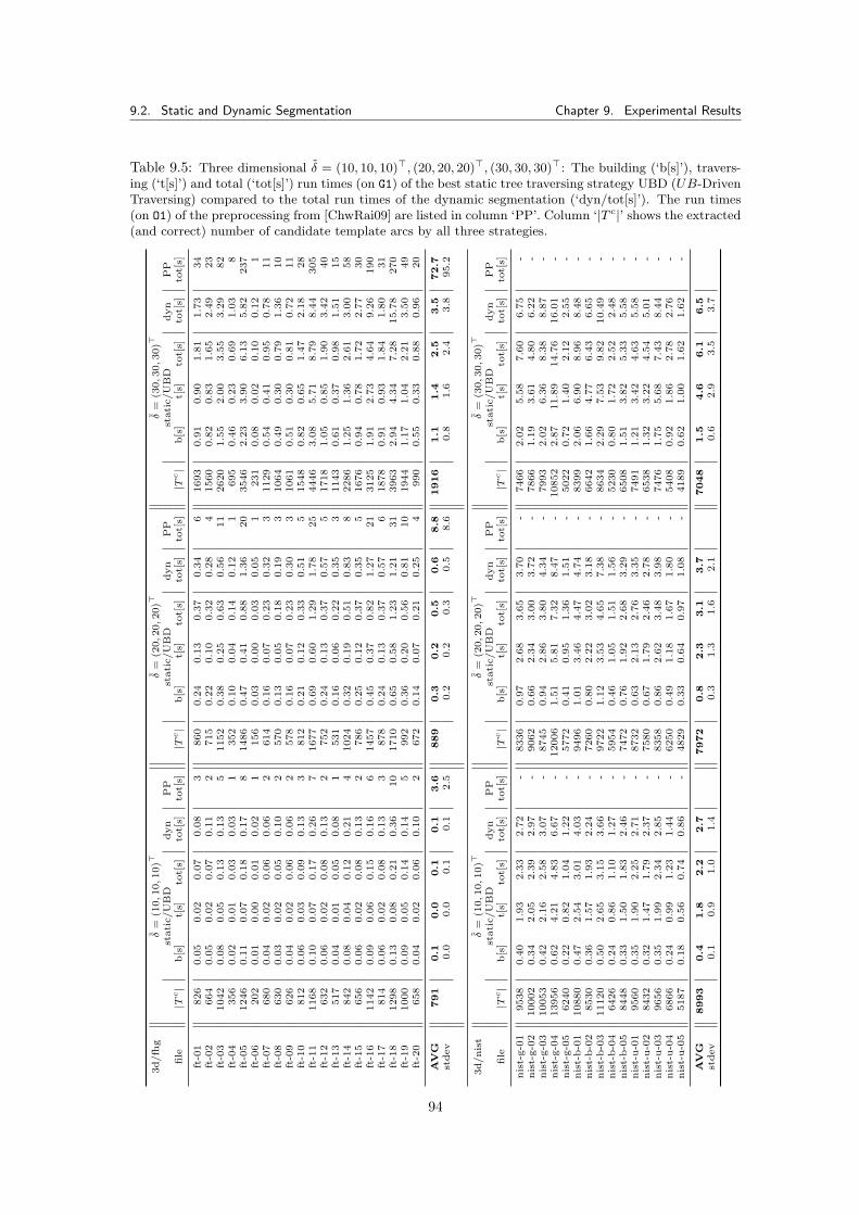
9.2. Static and Dynamic Segmentation Chapter 9. Experimental Results
Table 9.5: Three dimensional δ = (10, 10, 10)>, (20, 20, 20)>, (30, 30, 30)>: The building (‘b[s]’), travers-ing (‘t[s]’) and total (‘tot[s]’) run times (on G1) of the best static tree traversing strategy UBD (UB-DrivenTraversing) compared to the total run times of the dynamic segmentation (‘dyn/tot[s]’). The run times(on O1) of the preprocessing from [ChwRai09] are listed in column ‘PP’. Column ‘|T c|’ shows the extracted(and correct) number of candidate template arcs by all three strategies.
3d/fh
gδ
=(1
0,10,10)>
δ=
(20,20,20)>
δ=
(30,30,30)>
stati
c/U
BD
dyn
PP
stati
c/U
BD
dyn
PP
stati
c/U
BD
dyn
PP
file
|Tc|
b[s
]t[
s]to
t[s]
tot[
s]to
t[s]
|Tc|
b[s
]t[
s]to
t[s]
tot[
s]to
t[s]
|Tc|
b[s
]t[
s]to
t[s]
tot[
s]to
t[s]
ft-0
1826
0.0
50.0
20.0
70.0
83
860
0.2
40.1
30.3
70.3
46
1693
0.9
10.9
01.8
11.7
334
ft-0
2664
0.0
50.0
20.0
70.1
12
715
0.2
20.1
00.3
20.2
84
1560
0.8
20.8
31.6
52.4
923
ft-0
31042
0.0
80.0
50.1
30.1
35
1152
0.3
80.2
50.6
30.5
611
2620
1.5
52.0
03.5
53.2
982
ft-0
4356
0.0
20.0
10.0
30.0
31
352
0.1
00.0
40.1
40.1
21
695
0.4
60.2
30.6
91.0
38
ft-0
51246
0.1
10.0
70.1
80.1
78
1486
0.4
70.4
10.8
81.3
620
3546
2.2
33.9
06.1
35.8
2237
ft-0
6202
0.0
10.0
00.0
10.0
21
156
0.0
30.0
00.0
30.0
51
231
0.0
80.0
20.1
00.1
21
ft-0
7680
0.0
40.0
20.0
60.0
62
614
0.1
60.0
70.2
30.3
23
1129
0.5
40.4
10.9
50.7
811
ft-0
8630
0.0
30.0
20.0
50.1
02
570
0.1
30.0
50.1
80.1
93
1064
0.4
90.3
00.7
91.3
610
ft-0
9626
0.0
40.0
20.0
60.0
62
578
0.1
60.0
70.2
30.3
03
1061
0.5
10.3
00.8
10.7
211
ft-1
0812
0.0
60.0
30.0
90.1
33
812
0.2
10.1
20.3
30.5
15
1548
0.8
20.6
51.4
72.1
828
ft-1
11168
0.1
00.0
70.1
70.2
67
1677
0.6
90.6
01.2
91.7
825
4446
3.0
85.7
18.7
98.4
4305
ft-1
2632
0.0
60.0
20.0
80.1
32
752
0.2
40.1
30.3
70.5
75
1718
1.0
50.8
51.9
03.4
240
ft-1
3517
0.0
40.0
10.0
50.0
81
531
0.1
60.0
60.2
20.3
53
1143
0.6
10.3
70.9
81.5
115
ft-1
4842
0.0
80.0
40.1
20.2
14
1024
0.3
20.1
90.5
10.8
38
2286
1.2
51.3
62.6
13.0
058
ft-1
5656
0.0
60.0
20.0
80.1
32
786
0.2
50.1
20.3
70.3
55
1676
0.9
40.7
81.7
22.7
730
ft-1
61142
0.0
90.0
60.1
50.1
66
1457
0.4
50.3
70.8
21.2
721
3125
1.9
12.7
34.6
49.2
6190
ft-1
7814
0.0
60.0
20.0
80.1
33
878
0.2
40.1
30.3
70.5
76
1878
0.9
10.9
31.8
41.8
031
ft-1
81298
0.1
30.0
80.2
10.3
610
1710
0.6
50.5
81.2
31.2
131
3963
2.9
44.3
47.2
815.7
8270
ft-1
91000
0.0
90.0
50.1
40.1
45
992
0.3
60.2
00.5
60.8
110
1944
1.1
71.0
42.2
13.5
049
ft-2
0658
0.0
40.0
20.0
60.1
02
672
0.1
40.0
70.2
10.2
54
990
0.5
50.3
30.8
80.9
620
AV
G791
0.1
0.0
0.1
0.1
3.6
889
0.3
0.2
0.5
0.6
8.8
1916
1.1
1.4
2.5
3.5
72.7
stdev
0.0
0.0
0.1
0.1
2.5
0.2
0.2
0.3
0.5
8.6
0.8
1.6
2.4
3.8
95.2
3d/nis
tδ
=(1
0,10,10)>
δ=
(20,20,20)>
δ=
(30,30,30)>
stati
c/U
BD
dyn
PP
stati
c/U
BD
dyn
PP
stati
c/U
BD
dyn
PP
file
|Tc|
b[s
]t[
s]to
t[s]
tot[
s]to
t[s]
|Tc|
b[s
]t[
s]to
t[s]
tot[
s]to
t[s]
|Tc|
b[s
]t[
s]to
t[s]
tot[
s]to
t[s]
nis
t-g-0
19538
0.4
01.9
32.3
32.7
2-
8336
0.9
72.6
83.6
53.7
0-
7466
2.0
25.5
87.6
06.7
5-
nis
t-g-0
210002
0.3
42.0
52.3
92.9
7-
9062
0.6
62.3
43.0
03.7
2-
7866
1.1
93.6
14.8
06.2
2-
nis
t-g-0
310053
0.4
22.1
62.5
83.0
7-
8745
0.9
42.8
63.8
04.3
4-
7993
2.0
26.3
68.3
88.8
7-
nis
t-g-0
413956
0.6
24.2
14.8
36.6
7-
12006
1.5
15.8
17.3
28.4
7-
10852
2.8
711.8
914.7
616.0
1-
nis
t-g-0
56240
0.2
20.8
21.0
41.2
2-
5772
0.4
10.9
51.3
61.5
1-
5022
0.7
21.4
02.1
22.5
5-
nis
t-b-0
110880
0.4
72.5
43.0
14.0
3-
9496
1.0
13.4
64.4
74.7
4-
8399
2.0
66.9
08.9
68.4
8-
nis
t-b-0
28530
0.3
61.5
71.9
32.2
4-
7260
0.8
02.2
23.0
23.1
8-
6642
1.6
64.7
76.4
36.6
5-
nis
t-b-0
311120
0.5
02.6
53.1
53.6
6-
9722
1.1
23.5
34.6
57.3
8-
8634
2.2
97.5
39.8
210.4
9-
nis
t-b-0
46426
0.2
40.8
61.1
01.2
7-
5954
0.4
61.0
51.5
11.5
6-
5230
0.8
01.7
22.5
22.4
8-
nis
t-b-0
58448
0.3
31.5
01.8
32.4
6-
7472
0.7
61.9
22.6
83.2
9-
6508
1.5
13.8
25.3
35.5
8-
nis
t-u-0
19560
0.3
51.9
02.2
52.7
1-
8732
0.6
32.1
32.7
63.3
5-
7491
1.2
13.4
24.6
35.5
8-
nis
t-u-0
28432
0.3
21.4
71.7
92.3
7-
7580
0.6
71.7
92.4
62.7
8-
6538
1.3
23.2
24.5
45.0
1-
nis
t-u-0
39656
0.3
51.9
92.3
42.8
5-
8358
0.8
62.6
23.4
83.9
8-
7476
1.7
55.6
87.4
38.4
4-
nis
t-u-0
46866
0.2
40.9
91.2
31.4
4-
6250
0.4
91.1
81.6
71.8
0-
5408
0.9
21.8
62.7
82.7
6-
nis
t-u-0
55187
0.1
80.5
60.7
40.8
6-
4829
0.3
30.6
40.9
71.0
8-
4189
0.6
21.0
01.6
21.6
2-
AV
G8993
0.4
1.8
2.2
2.7
7972
0.8
2.3
3.1
3.7
7048
1.5
4.6
6.1
6.5
stdev
0.1
0.9
1.0
1.4
0.3
1.3
1.6
2.1
0.6
2.9
3.5
3.7
94
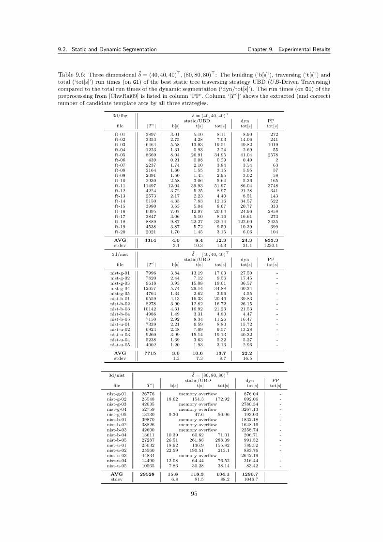
9.2. Static and Dynamic Segmentation Chapter 9. Experimental Results
Table 9.6: Three dimensional δ = (40, 40, 40)>, (80, 80, 80)>: The building (‘b[s]’), traversing (‘t[s]’) andtotal (‘tot[s]’) run times (on G1) of the best static tree traversing strategy UBD (UB-Driven Traversing)compared to the total run times of the dynamic segmentation (‘dyn/tot[s]’). The run times (on O1) of thepreprocessing from [ChwRai09] is listed in column ‘PP’. Column ‘|T c|’ shows the extracted (and correct)number of candidate template arcs by all three strategies.
3d/fhg δ = (40, 40, 40)>
static/UBD dyn PPfile |T c| b[s] t[s] tot[s] tot[s] tot[s]
ft-01 3897 3.01 5.10 8.11 8.90 272ft-02 3353 2.75 4.28 7.03 14.06 241ft-03 6464 5.58 13.93 19.51 49.82 1019ft-04 1223 1.31 0.93 2.24 2.69 55ft-05 8669 8.04 26.91 34.95 41.04 2578ft-06 439 0.21 0.08 0.29 0.40 2ft-07 2237 1.74 2.10 3.84 3.54 63ft-08 2164 1.60 1.55 3.15 5.95 57ft-09 2091 1.50 1.45 2.95 3.02 58ft-10 2930 2.58 3.06 5.64 5.36 165ft-11 11497 12.04 39.93 51.97 86.04 3748ft-12 4224 3.72 5.25 8.97 21.28 341ft-13 2573 2.17 2.23 4.40 8.51 143ft-14 5150 4.33 7.83 12.16 34.57 522ft-15 3980 3.63 5.04 8.67 20.77 333ft-16 6095 7.07 12.97 20.04 24.96 2858ft-17 3847 3.06 5.10 8.16 16.61 273ft-18 8889 9.87 22.27 32.14 122.60 3435ft-19 4538 3.87 5.72 9.59 10.39 399ft-20 2021 1.70 1.45 3.15 6.06 104
AVG 4314 4.0 8.4 12.3 24.3 833.3stdev 3.1 10.3 13.3 31.1 1230.1
3d/nist δ = (40, 40, 40)>
static/UBD dyn PPfile |T c| b[s] t[s] tot[s] tot[s] tot[s]
nist-g-01 7996 3.84 13.19 17.03 27.50 -nist-g-02 7820 2.44 7.12 9.56 17.45 -nist-g-03 9618 3.93 15.08 19.01 36.57 -nist-g-04 12657 5.74 29.14 34.88 60.34 -nist-g-05 4764 1.34 2.62 3.96 4.55 -nist-b-01 9559 4.13 16.33 20.46 39.83 -nist-b-02 8278 3.90 12.82 16.72 26.15 -nist-b-03 10142 4.31 16.92 21.23 21.53 -nist-b-04 4986 1.49 3.31 4.80 4.47 -nist-b-05 7150 2.92 8.34 11.26 16.47 -nist-u-01 7339 2.21 6.59 8.80 15.72 -nist-u-02 6924 2.48 7.09 9.57 13.28 -nist-u-03 9260 3.99 15.14 19.13 40.32 -nist-u-04 5238 1.69 3.63 5.32 5.27 -nist-u-05 4002 1.20 1.93 3.13 2.96 -
AVG 7715 3.0 10.6 13.7 22.2stdev 1.3 7.3 8.7 16.5
3d/nist δ = (80, 80, 80)>
static/UBD dyn PPfile |T c| b[s] t[s] tot[s] tot[s] tot[s]
nist-g-01 26776 memory overflow 876.04 -nist-g-02 25548 18.62 154.3 172.92 692.06 -nist-g-03 42035 memory overflow 2780.34 -nist-g-04 52759 memory overflow 3267.13 -nist-g-05 13130 9.36 47.6 56.96 193.03 -nist-b-01 39870 memory overflow 1832.18 -nist-b-02 38826 memory overflow 1648.16 -nist-b-03 42600 memory overflow 2258.74 -nist-b-04 13611 10.39 60.62 71.01 206.71 -nist-b-05 27287 26.51 261.88 288.39 991.52 -nist-u-01 25032 18.92 136.9 155.82 789.52 -nist-u-02 25560 22.59 190.51 213.1 883.76 -nist-u-03 44834 memory overflow 2642.19 -nist-u-04 14490 12.08 64.44 76.52 216.44 -nist-u-05 10565 7.86 30.28 38.14 83.42 -
AVG 29528 15.8 118.3 134.1 1290.7stdev 6.8 81.5 88.2 1046.7
95
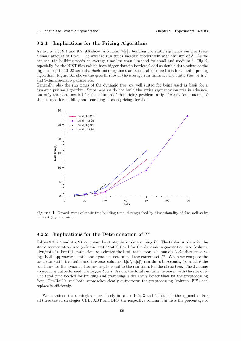
9.2. Static and Dynamic Segmentation Chapter 9. Experimental Results
9.2.1 Implications for the Pricing Algorithms
As tables 9.3, 9.4 and 9.5, 9.6 show in column ‘b[s]’, building the static segmentation tree takesa small amount of time. The average run times increase moderately with the size of δ. As wecan see, the building needs an average time less than 1 second for small and medium δ. Big δ,especially for the NIST files (which have bigger domain borders v and as double data points as thefhg files) up to 10–28 seconds. Such building times are acceptable to be basis for a static pricingalgorithm. Figure 9.1 shows the growth rate of the average run times for the static tree with 2-and 3-dimensional δ parameters.Generally, also the run times of the dynamic tree are well suited for being used as basis for adynamic pricing algorithm. Since here we do not build the entire segmentation tree in advance,but only the parts needed for the solution of the pricing problem, a significantly less amount oftime is used for building and searching in each pricing iteration.
build
tim
e[s]
0
5
10
15
20
25
30
delta0 20 40 60 80 100 120
build_fhg-2d
build_nist-2d
build_fhg-3d
build_nist-3d
Figure 9.1: Growth rates of static tree building time, distinguished by dimensionality of δ as well as bydata set (fhg and nist).
9.2.2 Implications for the Determination of T c
Tables 9.3, 9.4 and 9.5, 9.6 compare the strategies for determining T c. The tables list data for thestatic segmentation tree (column ‘static/tot[s]’) and for the dynamic segmentation tree (column‘dyn/tot[s]’). For this evaluation, we selected the best static approach, namely UB-driven travers-ing. Both approaches, static and dynamic, determined the correct set T c. When we compare thetotal (for static tree build and traverse, columns ‘b[s]’, ‘t[s]’) run times in seconds, for small δ therun times for the dynamic tree are nearly equal to the run times for the static tree. The dynamicapproach is outperformed, the bigger δ gets. Again, the total run time increases with the size of δ.The total time needed for building and traversing is decisively better than for the preprocessingfrom [ChwRai09] and both approaches clearly outperform the preprocessing (column ‘PP’) andreplace it efficiently.
We examined the strategies more closely in tables 1, 2, 3 and 4, listed in the appendix. Forall three tested strategies UBD, ABT and BFS, the respective column ‘%n’ lists the percentage of
96
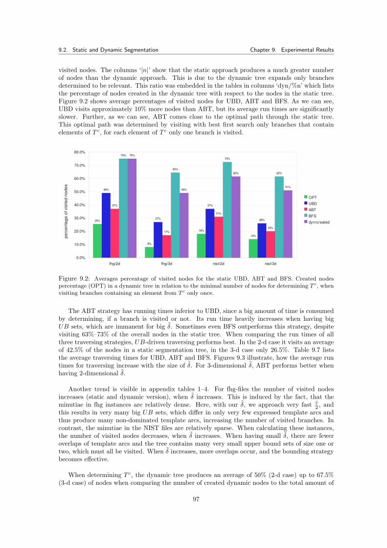
9.2. Static and Dynamic Segmentation Chapter 9. Experimental Results
visited nodes. The columns ‘|n|’ show that the static approach produces a much greater numberof nodes than the dynamic approach. This is due to the dynamic tree expands only branchesdetermined to be relevant. This ratio was embedded in the tables in columns ‘dyn/%n’ which liststhe percentage of nodes created in the dynamic tree with respect to the nodes in the static tree.Figure 9.2 shows average percentages of visited nodes for UBD, ABT and BFS. As we can see,UBD visits approximately 10% more nodes than ABT, but its average run times are significantlyslower. Further, as we can see, ABT comes close to the optimal path through the static tree.This optimal path was determined by visiting with best first search only branches that containelements of T c, for each element of T c only one branch is visited.Sheet1_2
Page 1
fhg/2d fhg/3d nist/2d nist/3d
0.0%
10.0%
20.0%
30.0%
40.0%
50.0%
60.0%
70.0%
80.0%
25%
8%
18%
14%
49%
27%
37%
26%
37%
17%
31%
20%
75%
65%
73%
62%
75%
49%
62%
51%
OPT
UBD
ABT
BFS
dyn/created
perc
enta
ge o
f vis
ited
node
s
Figure 9.2: Averages percentage of visited nodes for the static UBD, ABT and BFS. Created nodespercentage (OPT) in a dynamic tree in relation to the minimal number of nodes for determining T c, whenvisiting branches containing an element from T c only once.
The ABT strategy has running times inferior to UBD, since a big amount of time is consumedby determining, if a branch is visited or not. Its run time heavily increases when having bigUB sets, which are immanent for big δ. Sometimes even BFS outperforms this strategy, despitevisiting 63%–73% of the overall nodes in the static tree. When comparing the run times of allthree traversing strategies, UB-driven traversing performs best. In the 2-d case it visits an averageof 42.5% of the nodes in a static segmentation tree, in the 3-d case only 26.5%. Table 9.7 liststhe average traversing times for UBD, ABT and BFS. Figures 9.3 illustrate, how the average runtimes for traversing increase with the size of δ. For 3-dimensional δ, ABT performs better whenhaving 2-dimensional δ.
Another trend is visible in appendix tables 1–4. For fhg-files the number of visited nodesincreases (static and dynamic version), when δ increases. This is induced by the fact, that theminutiae in fhg instances are relatively dense. Here, with our δ, we approach very fast v
2 , andthis results in very many big UB sets, which differ in only very few expressed template arcs andthus produce many non-dominated template arcs, increasing the number of visited branches. Incontrast, the minutiae in the NIST files are relatively sparse. When calculating these instances,the number of visited nodes decreases, when δ increases. When having small δ, there are feweroverlaps of template arcs and the tree contains many very small upper bound sets of size one ortwo, which must all be visited. When δ increases, more overlaps occur, and the bounding strategybecomes effective.
When determining T c, the dynamic tree produces an average of 50% (2-d case) up to 67.5%(3-d case) of nodes when comparing the number of created dynamic nodes to the total amount of
97
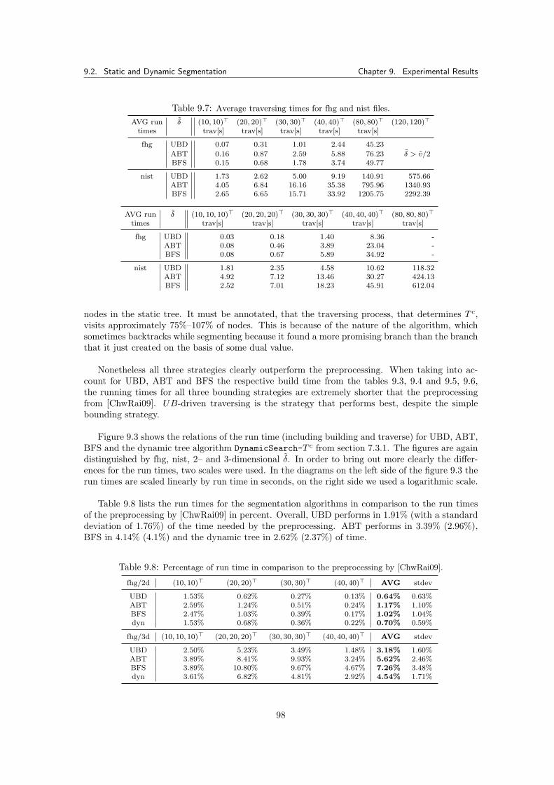
9.2. Static and Dynamic Segmentation Chapter 9. Experimental Results
Table 9.7: Average traversing times for fhg and nist files.
AVG run δ (10, 10)> (20, 20)> (30, 30)> (40, 40)> (80, 80)> (120, 120)>times trav[s] trav[s] trav[s] trav[s] trav[s]
fhg UBD 0.07 0.31 1.01 2.44 45.23
ABT 0.16 0.87 2.59 5.88 76.23 δ > v/2BFS 0.15 0.68 1.78 3.74 49.77
nist UBD 1.73 2.62 5.00 9.19 140.91 575.66ABT 4.05 6.84 16.16 35.38 795.96 1340.93BFS 2.65 6.65 15.71 33.92 1205.75 2292.39
AVG run δ (10, 10, 10)> (20, 20, 20)> (30, 30, 30)> (40, 40, 40)> (80, 80, 80)>times trav[s] trav[s] trav[s] trav[s] trav[s]
fhg UBD 0.03 0.18 1.40 8.36 -ABT 0.08 0.46 3.89 23.04 -BFS 0.08 0.67 5.89 34.92 -
nist UBD 1.81 2.35 4.58 10.62 118.32ABT 4.92 7.12 13.46 30.27 424.13BFS 2.52 7.01 18.23 45.91 612.04
nodes in the static tree. It must be annotated, that the traversing process, that determines T c,visits approximately 75%–107% of nodes. This is because of the nature of the algorithm, whichsometimes backtracks while segmenting because it found a more promising branch than the branchthat it just created on the basis of some dual value.
Nonetheless all three strategies clearly outperform the preprocessing. When taking into ac-count for UBD, ABT and BFS the respective build time from the tables 9.3, 9.4 and 9.5, 9.6,the running times for all three bounding strategies are extremely shorter that the preprocessingfrom [ChwRai09]. UB-driven traversing is the strategy that performs best, despite the simplebounding strategy.
Figure 9.3 shows the relations of the run time (including building and traverse) for UBD, ABT,BFS and the dynamic tree algorithm DynamicSearch-T c from section 7.3.1. The figures are againdistinguished by fhg, nist, 2– and 3-dimensional δ. In order to bring out more clearly the differ-ences for the run times, two scales were used. In the diagrams on the left side of the figure 9.3 therun times are scaled linearly by run time in seconds, on the right side we used a logarithmic scale.
Table 9.8 lists the run times for the segmentation algorithms in comparison to the run timesof the preprocessing by [ChwRai09] in percent. Overall, UBD performs in 1.91% (with a standarddeviation of 1.76%) of the time needed by the preprocessing. ABT performs in 3.39% (2.96%),BFS in 4.14% (4.1%) and the dynamic tree in 2.62% (2.37%) of time.
Table 9.8: Percentage of run time in comparison to the preprocessing by [ChwRai09].
fhg/2d (10, 10)> (20, 20)> (30, 30)> (40, 40)> AVG stdev
UBD 1.53% 0.62% 0.27% 0.13% 0.64% 0.63%ABT 2.59% 1.24% 0.51% 0.24% 1.17% 1.10%BFS 2.47% 1.03% 0.39% 0.17% 1.02% 1.04%dyn 1.53% 0.68% 0.36% 0.22% 0.70% 0.59%
fhg/3d (10, 10, 10)> (20, 20, 20)> (30, 30, 30)> (40, 40, 40)> AVG stdev
UBD 2.50% 5.23% 3.49% 1.48% 3.18% 1.60%ABT 3.89% 8.41% 9.93% 3.24% 5.62% 2.46%BFS 3.89% 10.80% 9.67% 4.67% 7.26% 3.48%dyn 3.61% 6.82% 4.81% 2.92% 4.54% 1.71%
98
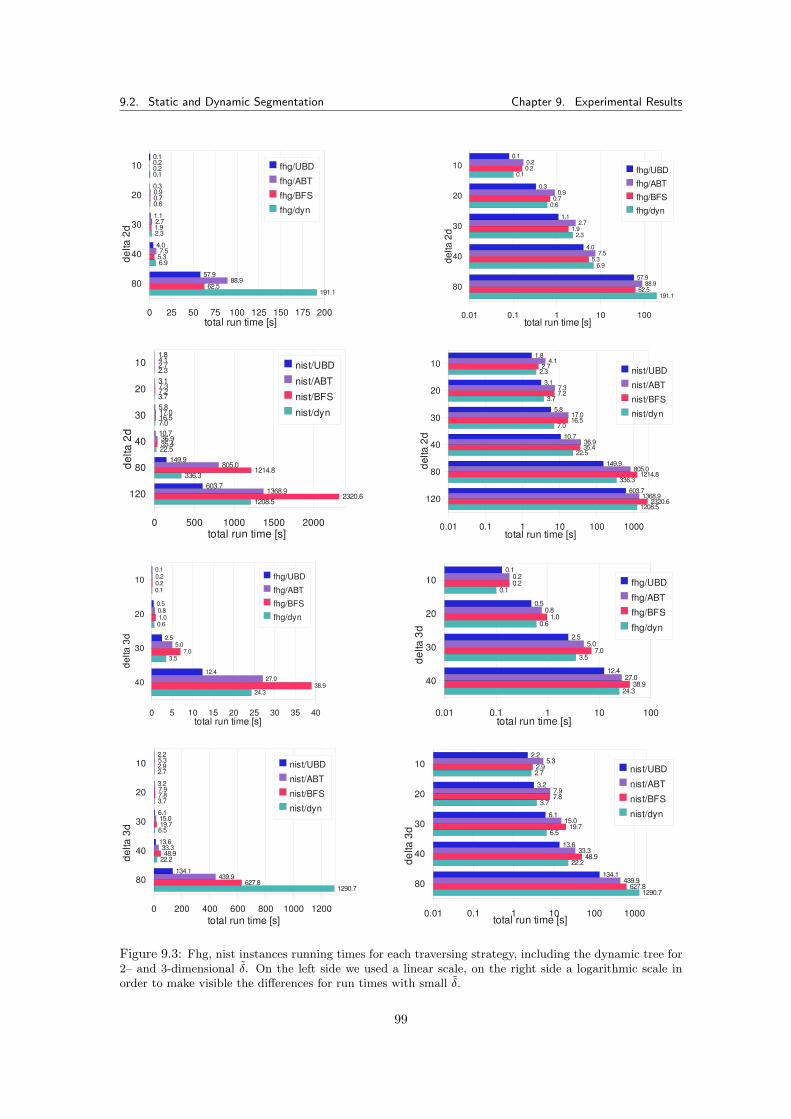
9.2. Static and Dynamic Segmentation Chapter 9. Experimental Results
Sheet1
Page 1
10
20
30
40
80
0 25 50 75 100 125 150 175 200
0.1
0.3
1.1
4.0
57.9
0.2
0.9
2.7
7.5
88.9
0.2
0.7
1.9
5.3
62.5
0.1
0.6
2.3
6.9
191.1
fhg/UBD
fhg/ABT
fhg/BFS
fhg/dyn
total run time [s]
delta
2d
Sheet1
Page 1
10
20
30
40
80
0.01 0.1 1 10 100
0.1
0.3
1.1
4.0
57.9
0.2
0.9
2.7
7.5
88.9
0.2
0.7
1.9
5.3
62.5
0.1
0.6
2.3
6.9
191.1
fhg/UBD
fhg/ABT
fhg/BFS
fhg/dyn
total run time [s]
delta
2d
Sheet1
Page 1
10
20
30
40
80
120
0 500 1000 1500 2000
1.8
3.1
5.8
10.7
149.9
603.7
4.1
7.3
17.0
36.9
805.0
1368.9
2.7
7.2
16.5
35.4
1214.8
2320.6
2.3
3.7
7.0
22.5
336.3
1208.5
nist/UBD
nist/ABT
nist/BFS
nist/dyn
total run time [s]
delta
2d
Sheet1
Page 1
10
20
30
40
80
120
0.01 0.1 1 10 100 1000
1.8
3.1
5.8
10.7
149.9
603.7
4.1
7.3
17.0
36.9
805.0
1368.9
2.7
7.2
16.5
35.4
1214.8
2320.6
2.3
3.7
7.0
22.5
336.3
1208.5
nist/UBD
nist/ABT
nist/BFS
nist/dyn
total run time [s]
delta
2d
Sheet1
Page 1
10
20
30
40
0 5 10 15 20 25 30 35 40
0.1
0.5
2.5
12.4
0.2
0.8
5.0
27.0
0.2
1.0
7.0
38.9
0.1
0.6
3.5
24.3
fhg/UBD
fhg/ABT
fhg/BFS
fhg/dyn
total run time [s]
delta
3d
Sheet1
Page 1
10
20
30
40
0.01 0.1 1 10 100
0.1
0.5
2.5
12.4
0.2
0.8
5.0
27.0
0.2
1.0
7.0
38.9
0.1
0.6
3.5
24.3
fhg/UBD
fhg/ABT
fhg/BFS
fhg/dyn
total run time [s]
delta
3d
Sheet1
Page 1
10
20
30
40
80
0 200 400 600 800 1000 1200
2.2
3.2
6.1
13.6
134.1
5.3
7.9
15.0
33.3
439.9
2.9
7.8
19.7
48.9
627.8
2.7
3.7
6.5
22.2
1290.7
nist/UBD
nist/ABT
nist/BFS
nist/dyn
total run time [s]
delta
3d
Sheet1
Page 1
10
20
30
40
80
0.01 0.1 1 10 100 1000
2.2
3.2
6.1
13.6
134.1
5.3
7.9
15.0
33.3
439.9
2.9
7.8
19.7
48.9
627.8
2.7
3.7
6.5
22.2
1290.7
nist/UBD
nist/ABT
nist/BFS
nist/dyn
total run time [s]
delta
3d
Figure 9.3: Fhg, nist instances running times for each traversing strategy, including the dynamic tree for2– and 3-dimensional δ. On the left side we used a linear scale, on the right side a logarithmic scale inorder to make visible the differences for run times with small δ.
99
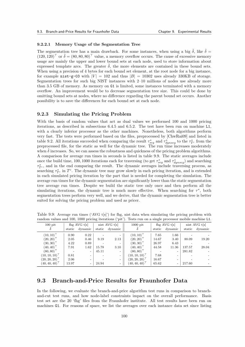
9.3. Branch-and-Price Results for Fraunhofer Data Chapter 9. Experimental Results
9.2.2.1 Memory Usage of the Segmentation Tree
The segmentation tree has a main drawback. For some instances, when using a big δ, like δ =(120, 120)> or δ = (80, 80, 80)> value, a memory overflow occurs. The cause of excessive memoryusage are mainly the upper and lower bound sets at each node, used to store information aboutexpressed template arcs. The greater δ, the more elements are contained in these bound sets.When using a precision of 4 bytes for each bound set element, at the root node for a big instance,for example nist-g-03 with |V | = 102 and thus |B| = 10302 uses already 330KB of storage.Segmentation trees for such big NIST instances with 2–10 millions of nodes use already morethan 3.5 GB of memory. As memory on G1 is limited, some instances terminated with a memoryoverflow. An improvement would be to decrease segmentation tree size. This could be done byomitting bound sets at nodes, where no difference regarding the parent bound set occurs. Anotherpossibility is to save the differences for each bound set at each node.
9.2.3 Simulating the Pricing Problem
With the basis of random values that act as dual values we performed 100 and 1000 pricingiterations, as described in subsections 6.4.5 and 6.5.2. The test have been run on machine L1,with a clearly inferior processor as the other machines. Nonetheless, both algorithms performvery fast. The tests were performed based on the files, preprocessed by [ChwRai09] and listed intable 9.2. All iterations succeeded when comparing the result τ∗seg and τ∗dynseg to the τ∗T c from thepreprocessed file, for the static as well for the dynamic tree. The run time increases moderatelywhen δ increases. So, we can assess the robustness and quickness of the pricing problem algorithms.A comparison for average run times in seconds is listed in table 9.9. The static averages includeonce the build time, 100, 1000 iterations each for traversing (to get τ∗seg and τ∗dynseg) and searchingτ∗T c , and in the end comparing the result. The dynamic averages include traversing process, assearching τ∗T c in T c. The dynamic tree may grow slowly in each pricing iteration, and is extendedin each simulated pricing iteration by the part that is needed for completing the simulation. Theaverage run times for the dynamic segmentation are significantly lower than the static segmentationtree average run times. Despite we build the static tree only once and then perform all thesimulating iterations, the dynamic tree is much more effective. When searching for τ∗, bothsegmentation trees perform very well, and we derive, that the dynamic segmentation tree is bettersuited for solving the pricing problem and used as pricer.
Table 9.9: Average run times (‘AVG t[s]’) for fhg, nist data when simulating the pricing problem withrandom values and 100, 1000 pricing iterations (‘pit’). Tests run on a single processor mobile machine L1.
100 pit fhg AVG t[s] nist AVG t[s] 1000 pit fhg AVG t[s] nist AVG t[s]
δ static dynamic static dynamic δ static dynamic static dynamic
(10, 10)> 0.90 0.22 - - (10, 10)> 7.65 1.66 - -(20, 20)> 2.05 0.46 9.19 2.13 (20, 20)> 14.67 3.40 88.09 19.20(30, 30)> 4.22 0.89 - - (30, 30)> 26.97 6.43 - -(40, 40)> 7.91 1.62 15.78 3.10 (40, 40)> 44.58 11.36 137.57 28.04(80, 80)> - - 45.11 - (80, 80)> - - 281.82 -
(10, 10, 10)> 0.81 - - - (10, 10, 10)> 7.68 - - -(20, 20, 20)> 2.06 - - - (20, 20, 20)> 16.67 - - -(40, 40, 40)> 13.97 - 24.94 - (40, 40, 40)> 65.62 - 217.60 -
9.3 Branch-and-Price Results for Fraunhofer Data
In the following, we evaluate the branch-and-price algorithm test runs in comparison to branch-and-cut test runs, and how node-label constraints impact on the overall performance. Basistest set are the 20 ‘fhg’ files from the Fraunhofer institute. All test results have been run onmachines G1. For reasons of space, we list the averages over each instance data set since listing
100
9.3. Branch-and-Price Results for Fraunhofer Data Chapter 9. Experimental Results
results on instance level would require too much space. In the following we list experimentalresults separated by solution approach.
9.3.1 Tested Parameters and Limits
For branch-and-price and branch-and-cut tests we need a small, a middle and a big value fork. As we first run tests with fhg-files, the selected values for k are k = 10, 20,max{26, . . . , 30}.Tested values for δ are δ = (10, 10)>, (20, 20)>, (30, 30)>, (40, 40)>, (80, 80)>, (10, 10, 10)>,(30, 30, 30)>, (40, 40, 40)> and (80, 80, 80)>. The small δ values (10,20) generate small bound-ing boxes, the other middle (30,40) and big (80) bounding boxes. For the instance ft-06 thebig δ = (80, 80)>, (80, 80, 80)> value exceeds the guideline δ < v
2 . Instances ft-04, ft-06 andft-13 have a smaller number of data points than max{26, . . . , 30}, so they are omitted whenaveraging. For parameter δ = (80, 80, 80)> some sets T c are not calculable neither with prepro-cessing by [ChwRai09] nor with a static tree pricing algorithm and become only computable withbranch-and-price using a dynamic tree pricing algorithm. The solution approaches presented inthe following in sections 9.3.2, 9.3.3 and 9.3.4 do not include this parameter value δ = (80, 80, 80)>,the averages for the approach in section 9.3.5 do include it. Tables 9.11, 9.12, 9.13, 9.14 and 9.15summarize average data for all tested solution approaches. In the following we describe the tablesand the tested approaches in detail.In preliminary tests we determined for fhg instances an algorithm run time limit of 14400 seconds,which are 4 hours. For these instances, we will not let branch-and-price tests run longer than thisvalue. Also a limit of 26000 for pricing iterations was established and we end a test run if it exceedsthis pricing iteration limit. We needed these limits, especially when allowing variable duplicates,to break the execution at some time point to prevent the tailing off effect (section 3.4.7).
9.3.2 Branch-and-Cut Reference Run Times
Basis for comparison are test runs with the branch-and-cut algorithm employing the directed cutmodel. This algorithm has been implemented by [ChwRai09], where a profound analysis of itcan be found. We introduced the model shortly in section 4.2.4. All tests have been re-run onmachines G1 for better comparison of the run times. Parameters and time limit have been set asdescribed in the previous section.Tables 9.11, 9.12, 9.13, 9.14 and 9.15 list in rows ‘BC/UBD’ and ‘BC/PP’ run time data for branch-and-cut tests. Rows ‘BC/UBD’ lists average algorithm run time in seconds (column ‘alg[s]’).Column ‘tot[s]’ shows average total run time in seconds when UB-driven traversing for a statictree (the fastest algorithm for determining T c) is used for the preprocessing step. Rows ‘BC/PP’lists average run times1 with preprocessing by [ChwRai09]. Columns ‘mi’ show the amount of in-stances that are missing because of either exceeding the time or pricing iterations limit or becauseof memory usage. Tables 6 and 7 in the appendix show the standard deviations for ‘BC/UBD’,standard deviations for ‘BC/PP’ are much higher.
The branch-and-cut algorithm failed to complete two instances with 2-dimensional δ withinthe time limit. For 3-dimensional δ all test runs have been completed, except all δ = (80, 80, 80)>
data for which no T c could be determined. As we can see in these tables, branch-and-cut usingUB-driven traversing for determining T c outperforms branch-and-cut using the preprocessingby [ChwRai09]. Branch-and-cut works extremely good for 3-dimensional δ. For small δ branch-and-cut run times improve with increasing k. When δ gets bigger than (30, 30)>, (30, 30, 30)>
the opposite effect is noted. When regarding the compression rate in practical application, resultsets having a small number of template arcs are favorable. This implies a big δ and therefore abig number of candidate template arcs T c. Based on experimental data, [ChwRai09] derived thatbranch-and-cut works better with small sets T c and big sets T c have a disadvantageous effect.This disadvantage is remedied by branch-and-price, since here we do not need the set T c anymore.
1Note that these preprocessing run times have been determined on machine O1.
101
9.3. Branch-and-Price Results for Fraunhofer Data Chapter 9. Experimental Results
In the following we use the ‘BC/UBD’ run times as reference. The branch-and-cut result valuesfor m, the minimal number of template arcs needed for encoding a template of size k, were used fordetermining correctness of branch-and-price. The minimal codebook sizes for tested parametersare summarized in table 5 in the appendix.
9.3.3 Complete SCF and MCF Formulation
As the single and multi commodity flow model presented in chapter 5 can be solved entirely withT replaced by T c, extracted with UB-driven traversing from a static segmentation tree. Testshave been run for determining if the models are correct. Parameters k and δ have been set asdiscussed in section 9.3.1.Tables 9.11, 9.12, 9.13, 9.14 and 9.15 summarize data for a single commodity flow formulationsolved entirely. The tables list in row ‘SCF/com’ average algorithm run times in seconds (column‘alg[s]’) and total run times including initialization step (column ‘tot[s]’) in seconds for the sin-gle commodity flow formulation. Column ‘bbn’ shows the average amount of branch-and-boundnodes. Averages for the multi commodity flow formulation are listed in rows ‘MCF/com’. Col-umn ‘mi’ lists again the amount of instances that failed to be calculated within the time limit.Tables 6 and 7 in the appendix show the standard deviations for ‘SCF/com’, standard deviationfor ‘MCF/com’ is very high and has an average of 7199.
With the SCF and MCF solved entirely, all codebooks have been determined correctly. Aswith branch-and-cut here also no data could be collected for all δ = (80, 80, 80)> because theset T c is not computable (memory usage) for this parameter value. For the MCF, already with2-dimensional δ many instances surpass the time limit. For the tested parameters δ = (10, 10)>,(20, 20)>, (40, 40)>, (80, 80)>, already 36% of the instances failed to be calculated within the timelimit. With 3-dimensional δ even more instances are missing and hence they are not listed. Wededuce that the SCF outperforms the MCF. Further experiments with pricing algorithms haveshown, that the multi commodity flow formulation is not competitive enough for our purposes.The algorithms work, but run times for many instances lie wide beyond our time limit. In thefollowing we will concentrate on the single commodity flow formulation.When comparing the appropriate values (rows ‘SCF/com’) with the corresponding branch-and-cutvalues (columns ‘BC/UBD’), the SCF performs relatively good, despite the weaker LP relaxation.For the SCF model, the average amount of branch-and-bound nodes (searched with BFS) is 862(standard deviation 1218). The strength of the SCF can already be seen in these tests. As the sizeof T c increases with increasing δ the run times also increase with branch-and-cut. With the SCFmodel the opposite effect occurs. Also, for small and middle δ the amount of possible solutionsis very high and there exist many template arcs with the same size. This induces large plateausof equally good solutions and the algorithm spends most of the time for determining if the foundsolution is optimal. When δ gets bigger the amount of expressed points for each template arcincreases the optimal solution becomes unambiguous and is found very fast. Thus, the run timesfor (40, 40)>, k = 10 and (80, 80)>, k = 30 are relatively small. Because of this characteristic alsovery many branch-and-bound nodes (1 − 38507) are created for small and middle 2-dimensionalδ, whereas very few nodes (1 − 18) are needed when δ is big. Further effect can be seen for 3-dimensional and small δ where the amount of branch-and-bound nodes gets tinier when comparedto 2-dimensional data.
9.3.4 Static Tree Pricing Algorithm for SCF
The static tree pricing algorithm was presented in section 6.4.3 and listed as pseudo code insection 6.6. Limits and parameters k and δ have been set as described in section 9.3.1. Forthe tests a huge amount of pricing possibilities arise, the main test subject was the impact onperformance when using node-label constraints:
• We test how the static tree pricing algorithm performs when the SCF model uses only arc-label constraints and the pricing bases on the dual variables uij . In contrast to it we test the
102
9.3. Branch-and-Price Results for Fraunhofer Data Chapter 9. Experimental Results
performance, when the model additionally includes node-label constraints combined with theaccording pricing strategy described in section 5.5 based on the dual variables uij and µj .
• How do run times differ, when either a starting solution (star shaped spanning tree) or aFarkas pricing algorithm for determining a starting solution is used instead.
• How are run times affected, when pricing is restricted only to non-dominated template arcsor dominated arcs are allowed as well.
• How does the algorithm perform when only one arc with negative reduced cost per pricingstep is determined, confronted to pricing all arcs with reduced cost < 0 in one pricing step.
• How does disabling or enabling variable duplicates perform. For the former, in each pricingstep we check if we already have found the actual template arc. If the actual arc was alreadypriced, we add another variable, if existing, with equal or inferior reduced cost instead.When doing this the problem turns out to be efficiently solved. The counterpart is to allowequal template arcs to be multiply priced.
• For the branch-and-bound decision tree we determine how depth first search (DFS) and bestfirst search (BFS) perform.
• How does using continuous values for arcs variables xij affect performance.
All the presented options may be combined. As listing each such test combination would take toomuch space, we present the fastest variants. All tested variants determined the correct minimalcodebook. Test runs using DFS for the branch-and-bound tree have been showed not to be com-petitive for our purposes. So for all presented test runs BFS has been used. Also tests with apricing algorithm that allows variable duplicates could not reach not in the least the run times ofthe pricing algorithm that does not permit variable duplicates and marks the found variable aftereach pricing iteration and hence is not listed here.
Tables 9.11, 9.12, 9.13, 9.14 and 9.15 show test data for the static tree pricing algorithm basedon a SCF model. As already described, in these tables columns ‘alg[s]’ lists average algorithm runtime in seconds as well as average total run time (columns ‘tot[s]’) in seconds. Columns ‘pit’ showsthe average amount of pricing iterations, columns ‘pvar’ the average number of priced variables.Columns ‘bbn’ shows the average amount of nodes created in the branch-and-bound decision tree.Rows ‘BP/static’ shows data for a static tree pricing algorithm in standard configuration that em-ploys only arc-label constraints, uses a starting solution, determines in each pricing iteration onlyone arc with maximal negative reduced cost and allows no variable duplicates. The branch-and-bound decision tree uses BFS and we restricted the search to non-dominated template arcs. Forrows ‘BP/static/nlc’ additionally node-label constraints have been used. For rows ‘BP/static/fark’and ‘BP/static/nlc/fark’ a starting solution determined with Farkas pricing algorithm has beenused instead of a star shaped spanning tree. Rows ‘BP/static/dom’ and ‘BP/static/nlc/dom’ showdata for static tree pricing algorithms that allow dominated template arcs to be priced. The sys-tematic should be clear for ‘BP/static/nlc/fark/dom’. Rows ‘BP/static/allarcs’ lists run times fora static tree pricing algorithm that prices all arcs with reduced costs < 0 in one pricing iteration.Rows ‘BP/static/nlc/cont’ show average run times of the static tree pricing algorithm using anSCF, where arcs variables xij have been implemented as continuous values. This approach was con-sidered because of the following. As described in [CaClPa09] it is possible to solve the MLST formu-lated as a flow network formulations with real valued arcs variables x. The result values for x maybe fractional, but the results for the labels are correct. We assumed that this may be the case alsofor our extended variant (selected nodes, directed). Computational tests support this assumption,and codebooks were determined correctly. Averages for the runs (rows ‘BP/static/nlc/cont’) arepresented in tables 9.11–9.15. Tables 6 and 7 in the appendix show in row ‘BP/static/[AVG]’ thestandard deviation as an average over ‘BP/static/[fark,dom,nlc,nlc/fark,nlc/dom,nlc/fark/dom]’since values for these static tree pricing algorithm variants are very similar.
In test runs employing only arc-label constraints and 2-dimensional δ one value (ft-19, δ =(20, 20)>, k = 20)) exceeds the pricing iterations limit2. The same test runs employing additionally
2When more elaborate tests are done, time and pricing iterations limit should be increased.
103
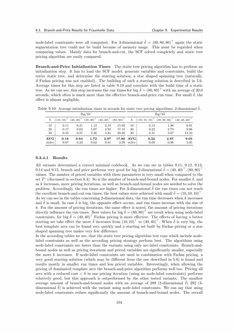
9.3. Branch-and-Price Results for Fraunhofer Data Chapter 9. Experimental Results
node-label constraints were all computed. For 3-dimensional δ = (80, 80, 80)> again the staticsegmentation tree could not be build because of memory usage. This must be regarded whencomparing values. Mainly data for branch-and-cut, the SCF solved completely and static treepricing algorithm are easily compared.
Branch-and-Price Initialization Times The static tree pricing algorithm has to perform aninitialization step. It has to load the SCF model, generate variables and constraints, build theentire static tree, and determine the starting solution, a star shaped spanning tree (naturally,if Farkas pricing was not enabled). The building of such a starting solution is described in 5.6.Average times for this step are listed in table 9.10 and correlate with the build time of a statictree. As we can see, this step increases the run times for big δ = (80, 80)> with an average of 20.0seconds, which often is much more than the effective branch-and-price run time. For small δ, theeffect is almost negligible.
Table 9.10: Average initialization times in seconds for static tree pricing algorithms, 2-dimensional δ.
fhg/2d
k (10, 10)> (20, 20)> (30, 30)> (40, 40)> (80, 80)>
10 0.11 0.41 1.12 2.19 15.9220 0.17 0.63 1.67 2.92 17.4430 0.25 0.87 2.36 3.81 20.05
AVG 0.18 0.64 1.72 2.97 17.80stdev 0.07 0.23 0.62 0.81 2.09
fhg/3d
k (10, 10, 10)> (30, 30, 30)> (40, 40, 40)>
10 0.13 1.96 6.0120 0.22 2.79 9.0630 0.31 3.87 12.10
AVG 0.22 2.87 9.05stdev 0.09 0.96 3.05
9.3.4.1 Results
All variants determined a correct minimal codebook. As we can see in tables 9.11, 9.12, 9.13,9.14 and 9.15, branch and price performs very good for big 2-dimensional δ = (40, 40)>, (80, 80)>
values. The number of priced variables with these parameters is very small when compared to theset T c (discussed in section 9.4). So is the number of branch-and-bound nodes. For smaller δ, andas k increases, more pricing iterations, as well as branch-and-bound nodes are needed to solve theproblem. Accordingly, the run times are higher. For 3-dimensional δ the run times can not reachthe excellent branch-and-cut run times, the best values were achieved with small δ = (10, 10, 10)>.As we can see in the tables concerning 2-dimensional data, the run time decreases when k increasesand δ is small. In case δ is big, the opposite effect occurs, and run times increase with the size ofk. For the amount of pricing iterations, the same effect is noted, the amount of pricing iterationsdirectly influence the run times. Best values for big δ = (80, 80)> are result when using node-labelconstraints, for big δ = (40, 40)> Farkas pricing is more effective. The effects of having a betterstarting set take effect the more δ increases from (10, 10)> to (40, 40)>. When δ is very big, thebest template arcs can be found very quickly and a starting set built by Farkas pricing or a starshaped spanning tree makes very few difference.In the according tables we see, that the static tree pricing algorithm test runs which include node-label constraints as well as the according pricing strategy perform best. The algorithms usingnode-label constraints are faster than the variants using only arc-label constraints. Branch-and-bound nodes as well as pricing iterations and priced variables are significantly smaller, especiallythe more k increases. If node-label constraints are used in combination with Farkas pricing, avery good starting solution (which may be different from the one described in 5.6) is found andresults mostly in smaller run times and less priced variables. Interestingly, when allowing thepricing of dominated template arcs the branch-and-price algorithm performs well too. Pricing allarcs with a reduced cost < 0 in one pricing iteration (using no node-label constraints) performsrelatively good, but this approach is outperformed by the other tested variants. The smallestaverage amount of branch-and-bound nodes with an average of 289 (2-dimensional δ) 292 (3-dimensional δ) is achieved with the variant using node-label constraints. We can say that usingnode-label constraints reduce significantly the amount of branch-and-bound nodes. The overall
104
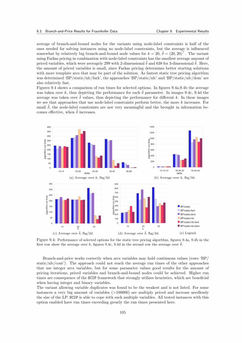
9.3. Branch-and-Price Results for Fraunhofer Data Chapter 9. Experimental Results
average of branch-and-bound nodes for the variants using node-label constraints is half of theones needed for solving instances using no node-label constraints, but the average is influencedsomewhat by relatively big branch-and-bound node values for k = 20, δ = (20, 20)>. The variantusing Farkas pricing in combination with node-label constraints has the smallest average amount ofpriced variables, which were averagely 299 with 2-dimensional δ and 638 for 3-dimensional δ. Here,the amount of priced variables is small, since Farkas pricing determines better starting solutionswith more template arcs that may be part of the solution. As fastest static tree pricing algorithmwas determined ‘BP/static/nlc/fark’, the approaches ‘BP/static/nlc’ and ‘BP/static/nlc/dom’ arealso relatively fast.Figures 9.4 shows a comparison of run times for selected options. In figures 9.4a,9.4b the averagewas taken over k, thus depicting the performance for each δ parameter. In images 9.4c, 9.4d theaverage was taken over δ values, thus depicting the performance for different k. In these imageswe see that approaches that use node-label constraints perform better, the more k increases. Forsmall δ, the node-label constraints are not very meaningful and the brought in information be-comes effective, when δ increases.
Sheet1
Page 1
10,10 20,20 30,30 40,40 80,80
0
50
100
150
200
250
300
350
400
450
delta
algo
rithm
run
time
(a) Average over k, fhg/2d.
Sheet1
Page 1
10,10,10 30,30,30 40,40,40
0
200
400
600
800
1000
1200
1400
delta
algo
rithm
run
time
(b) Average over k, fhg/3d.Sheet1
Page 1
10 20 30
0
50
100
150
200
250
300
350
k
algo
rithm
run
time
(c) Average over δ, fhg/2d.
Sheet1
Page 1
10 20 30
0
100
200
300
400
500
600
700
800
900
k
algo
rithm
run
time BP/static
BP/static/fark
BP/static/dom
BP/static/nlc
BP/static/nlc/fark
BP/static/nlc/dom
(d) Average over δ, fhg/3d.
Sheet1
Page 1
BP/static
BP/static/fark
BP/static/dom
BP/static/nlc
BP/static/nlc/fark
BP/static/nlc/dom
(e) Legend.
Figure 9.4: Performance of selected options for the static tree pricing algorithm, figures 9.4a, 9.4b in thefirst row show the average over k, figures 9.4c, 9.4d in the second row the average over δ.
Branch-and-price works correctly when arcs variables may hold continuous values (rows ‘BP/static/nlc/cont’). The approach could not reach the average run times of the other approachesthat use integer arcs variables, but for some parameter values good results for the amount ofpricing iterations, priced variables and branch-and-bound nodes could be achieved. Higher runtimes are consequence of the SCIP framework that strongly utilizes heuristics, which are beneficialwhen having integer and binary variables.The variant allowing variable duplicates was found to be the weakest and is not listed. For someinstances a very big amount of variables (>100000) are multiply priced and increase needlesslythe size of the LP. SCIP is able to cope with such multiple variables. All tested instances with thisoption enabled have run times exceeding greatly the run times presented here.
105
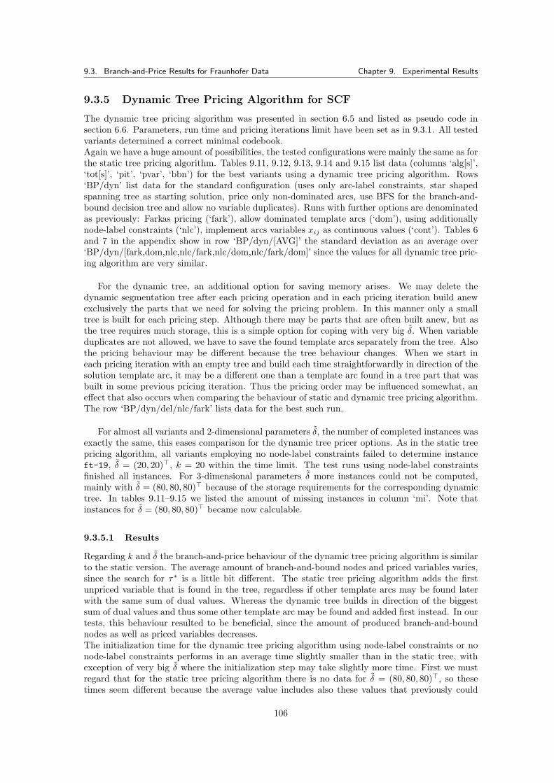
9.3. Branch-and-Price Results for Fraunhofer Data Chapter 9. Experimental Results
9.3.5 Dynamic Tree Pricing Algorithm for SCF
The dynamic tree pricing algorithm was presented in section 6.5 and listed as pseudo code insection 6.6. Parameters, run time and pricing iterations limit have been set as in 9.3.1. All testedvariants determined a correct minimal codebook.Again we have a huge amount of possibilities, the tested configurations were mainly the same as forthe static tree pricing algorithm. Tables 9.11, 9.12, 9.13, 9.14 and 9.15 list data (columns ‘alg[s]’,‘tot[s]’, ‘pit’, ‘pvar’, ‘bbn’) for the best variants using a dynamic tree pricing algorithm. Rows‘BP/dyn’ list data for the standard configuration (uses only arc-label constraints, star shapedspanning tree as starting solution, price only non-dominated arcs, use BFS for the branch-and-bound decision tree and allow no variable duplicates). Runs with further options are denominatedas previously: Farkas pricing (‘fark’), allow dominated template arcs (‘dom’), using additionallynode-label constraints (‘nlc’), implement arcs variables xij as continuous values (‘cont’). Tables 6and 7 in the appendix show in row ‘BP/dyn/[AVG]’ the standard deviation as an average over‘BP/dyn/[fark,dom,nlc,nlc/fark,nlc/dom,nlc/fark/dom]’ since the values for all dynamic tree pric-ing algorithm are very similar.
For the dynamic tree, an additional option for saving memory arises. We may delete thedynamic segmentation tree after each pricing operation and in each pricing iteration build anewexclusively the parts that we need for solving the pricing problem. In this manner only a smalltree is built for each pricing step. Although there may be parts that are often built anew, but asthe tree requires much storage, this is a simple option for coping with very big δ. When variableduplicates are not allowed, we have to save the found template arcs separately from the tree. Alsothe pricing behaviour may be different because the tree behaviour changes. When we start ineach pricing iteration with an empty tree and build each time straightforwardly in direction of thesolution template arc, it may be a different one than a template arc found in a tree part that wasbuilt in some previous pricing iteration. Thus the pricing order may be influenced somewhat, aneffect that also occurs when comparing the behaviour of static and dynamic tree pricing algorithm.The row ‘BP/dyn/del/nlc/fark’ lists data for the best such run.
For almost all variants and 2-dimensional parameters δ, the number of completed instances wasexactly the same, this eases comparison for the dynamic tree pricer options. As in the static treepricing algorithm, all variants employing no node-label constraints failed to determine instanceft-19, δ = (20, 20)>, k = 20 within the time limit. The test runs using node-label constraintsfinished all instances. For 3-dimensional parameters δ more instances could not be computed,mainly with δ = (80, 80, 80)> because of the storage requirements for the corresponding dynamictree. In tables 9.11–9.15 we listed the amount of missing instances in column ‘mi’. Note thatinstances for δ = (80, 80, 80)> became now calculable.
9.3.5.1 Results
Regarding k and δ the branch-and-price behaviour of the dynamic tree pricing algorithm is similarto the static version. The average amount of branch-and-bound nodes and priced variables varies,since the search for τ∗ is a little bit different. The static tree pricing algorithm adds the firstunpriced variable that is found in the tree, regardless if other template arcs may be found laterwith the same sum of dual values. Whereas the dynamic tree builds in direction of the biggestsum of dual values and thus some other template arc may be found and added first instead. In ourtests, this behaviour resulted to be beneficial, since the amount of produced branch-and-boundnodes as well as priced variables decreases.The initialization time for the dynamic tree pricing algorithm using node-label constraints or nonode-label constraints performs in an average time slightly smaller than in the static tree, withexception of very big δ where the initialization step may take slightly more time. First we mustregard that for the static tree pricing algorithm there is no data for δ = (80, 80, 80)>, so thesetimes seem different because the average value includes also these values that previously could
106
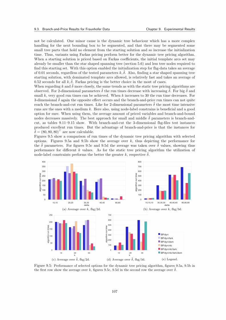
9.3. Branch-and-Price Results for Fraunhofer Data Chapter 9. Experimental Results
not be calculated. One minor cause is the dynamic tree behaviour which has a more complexhandling for the next bounding box to be segmented, and that there may be segmented somesmall tree parts that hold no element from the starting solution and so increase the initializationtime. Thus, variants using Farkas pricing perform better for the dynamic tree pricing algorithm.When a starting solution is priced based on Farkas coefficients, the initial template arcs set mayalready be smaller than the star shaped spanning tree (section 5.6) and less tree nodes required tofind this starting set. With this option enabled the initialization step for fhg-data takes an averageof 0.01 seconds, regardless of the tested parameters k, δ. Also, finding a star shaped spanning treestarting solution, with dominated template arcs allowed, is relatively fast and takes an average of0.52 seconds for all k, δ. Farkas pricing is the better choice in the most of cases.When regarding k and δ more closely, the same trends as with the static tree pricing algorithms areobserved. For 2-dimensional parameters δ the run times decrease with increasing δ. For big δ andsmall k, very good run times can be achieved. When k increases to 30 the run time decreases. For3-dimensional δ again the opposite effect occurs and the branch-and-price run times can not quitereach the branch-and-cut run times. Like for 2-dimensional parameters δ the most time intensiveruns are the ones with a medium k. Here also, using node-label constrains is beneficial and a goodoption for sure. When using them, the average amount of priced variables and branch-and-boundnodes decreases massively. The best approach for small and middle δ parameters is branch-and-cut, as tables 9.11–9.15 show. With branch-and-cut the 3-dimensional fhg-files test instancesproduced excellent run times. But the advantage of branch-and-price is that the instances forδ = (80, 80, 80)> are now calculable.Figures 9.5 show a comparison of run times of the dynamic tree pricing algorithm with selectedoptions. Figures 9.5a and 9.5b show the average over k, thus depicting the performance forthe δ parameters. For figures 9.5c and 9.5d the average was taken over δ values, showing thusperformance for different k values. As for the static tree pricing algorithm the utilization ofnode-label constraints performs the better the greater k, respective δ.Sheet1
Page 1
10,10 20,20 30,30 40,40 80,80
0
50
100
150
200
250
300
350
400
delta
algo
rithm
run
time
(a) Average over k, fhg/2d.
Sheet1
Page 1
10,10,10 30,30,30 40,40,40 80,80,80
0
100
200
300
400
500
600
700
800
delta
algo
rithm
run
time
(b) Average over k, fhg/3d.Sheet1
Page 1
10 20 30
0
50
100
150
200
250
k
algo
rithm
run
times
(c) Average over δ, fhg/2d.
Sheet1
Page 1
10 20 30
0
100
200
300
400
500
600
700
k
algo
rithm
run
time
(d) Average over δ, fhg/3d.
Sheet1
Page 1
BP/dyn
BP/dyn/fark
BP/dyn/dom
BP/dyn/nlc
BP/dyn/nlc/fark
BP/dyn/nlc/fark/dom
(e) Legend.
Figure 9.5: Performance of selected options for the dynamic tree pricing algorithm, figures 9.5a, 9.5b inthe first row show the average over k, figures 9.5c, 9.5d in the second row the average over δ.
107

9.3. Branch-and-Price Results for Fraunhofer Data Chapter 9. Experimental Results
Table 9.11: Average algorithm run time (column ‘alg[s]’), total run time (column ‘tot[s]’), pricing it-erations (column ‘pit’), priced variables (column ‘pvar’) and branch-and-bound nodes (column ‘bbn’).Parameter δ 2-dimensional. Rows description in sections 9.3.2–9.3.5.
fhg/2d (10, 10)> (20, 20)> (30, 30)>k options alg[s] tot[s] pit pvar bbn alg[s] tot[s] pit pvar bbn alg[s] tot[s] pit pvar bbn
10 BC/UBD 149.5 149.6 - - - 715.8 716.4 - - - 120.4 122.2 - - -BC/PP 149.5 158.0 - - - 715.8 806.0 - - - 120.4 763.9 - - -SCF/com 438.4 438.7 - - 1286 479.1 480.0 - - 1081 37.9 40.6 - - 23MCF/com 10564.6 n/a - - - 9496.5 n/a - - - n/a n/a - - -BP/sta 477.6 477.7 2057 491 1566 558.1 558.5 2704 960 1744 24.5 25.6 211 186 25BP/sta/fark 383.7 383.7 1853 499 1357 659.9 660.2 3129 968 2163 19.2 20.0 159 138 22BP/sta/dom 494.0 494.2 1962 539 1423 629.1 629.5 3077 1004 2072 35.4 36.5 286 257 29BP/sta/nlc 457.7 457.8 1757 471 1286 539.9 540.3 1790 1009 781 15.2 16.3 112 99 12BP/sta/nlc/fark 506.8 506.9 1977 548 1433 509.4 509.7 1732 915 818 16.9 17.7 124 113 12BP/sta/nlc/dom 492.1 492.2 1926 543 1384 568.5 568.9 1953 1031 921 32.0 33.0 255 230 26BP/sta/nlc/cont 571.0 571.1 2492 582 1910 810.3 810.7 2354 1226 1127 245.4 246.6 1136 693 442BP/sta/allarcs 587.7 587.8 1593 2953 1565 782.3 782.8 1694 6183 1544 47.4 48.4 54 6749 35BP/dyn 407.6 407.6 1747 508 1240 579.6 579.7 2975 1116 1859 11.8 12.0 147 131 16BP/dyn/fark 398.7 398.7 2102 504 1602 575.6 575.6 2952 910 2044 13.4 13.4 149 129 22BP/dyn/dom 444.5 444.5 1837 550 1288 487.5 487.5 2658 989 1669 17.3 17.3 206 182 23BP/dyn/nlc 403.3 403.4 1547 461 1086 522.2 522.3 1847 996 851 13.8 14.0 155 139 16BP/dyn/nlc/fark 479.4 479.4 2034 511 1526 543.5 543.5 2056 999 1058 10.6 10.6 85 76 10BP/dyn/nlc/fark/dom 408.5 408.5 1607 496 1114 538.7 538.7 2070 1040 1031 11.1 11.1 113 100 13BP/dyn/nlc/cont 980.3 980.3 3652 645 3007 714.4 714.5 2257 1185 1071 602.9 603.1 1881 773 1108BP/dyn/del/nlc/fark 591.3 591.3 2008 539 1472 544.2 544.2 1658 892 767 9.7 9.7 52 47 6
20 BC/UBD 51.4 51.5 - - - 387.6 388.1 - - - 309.6 311.4 - - -BC/PP 51.4 60.2 - - - 387.6 482.5 - - - 309.6 986.7 - - -SCF/com 129.7 130.0 - - 334 408.7 409.7 - - 1432 681.3 684.2 - - 1854MCF/com 7178.6 n/a - - - 3391.8 n/a - - - n/a n/a - - -BP/sta 156.0 156.2 804 307 496 200.3 200.9 1186 645 541 511.7 513.3 2835 1217 1618BP/sta/fark 178.3 178.4 910 299 616 90.3 90.6 766 368 401 540.4 541.2 2997 1118 1881BP/sta/dom 161.0 161.2 914 329 585 182.2 182.8 1443 683 761 506.8 508.2 2831 1208 1622BP/sta/nlc 154.2 154.4 679 258 421 628.3 629.0 2116 935 1180 284.4 286.1 1052 877 175BP/sta/nlc/fark 155.5 155.6 757 274 488 574.3 574.5 2103 633 1474 259.3 260.1 1096 941 158BP/sta/nlc/dom 158.5 158.7 720 280 440 495.4 496.0 1746 591 1156 301.6 303.0 1093 959 134BP/sta/nlc/cont 222.7 223.0 991 353 637 258.3 259.0 1497 571 925 1088.2 1089.9 1841 1268 573BP/sta/allarcs 258.5 258.6 646 1767 585 864.9 865.8 2119 3859 1961 879.8 881.3 1745 7527 1582BP/dyn 162.3 162.4 862 315 547 139.4 139.5 1028 585 445 394.2 394.5 2699 1333 1366BP/dyn/fark 188.7 188.7 1034 369 671 165.7 165.7 1123 547 579 302.3 302.3 2297 1000 1299BP/dyn/dom 174.0 174.0 1024 329 694 113.1 113.2 1081 656 426 419.4 419.4 3450 1594 1856BP/dyn/nlc 158.4 158.5 751 284 467 544.9 545.1 1948 806 1142 252.3 252.8 1080 930 150BP/dyn/nlc/fark 115.3 115.3 613 235 384 226.5 226.5 1197 467 733 219.5 219.5 1002 841 163BP/dyn/nlc/fark/dom 146.3 146.3 729 254 481 248.4 248.4 1351 571 784 183.0 183.0 906 767 142BP/dyn/nlc/cont 168.3 168.3 842 311 531 339.8 340.0 1972 661 1311 673.7 674.2 1527 1104 423BP/dyn/del/nlc/fark 168.6 168.6 755 291 469 477.1 477.1 1753 740 1016 134.8 134.9 644 547 99
30 BC/UBD 27.8 28.0 - - - 153.6 154.2 - - - 354.5 356.5 - - -BC/PP 27.8 37.5 - - - 153.6 258.3 - - - 354.5 1102.8 - - -SCF/complete 91.7 92.0 - - 208 220.9 221.9 - - 350 165.6 168.6 - - 496MCF/com 5646.4 n/a - - - 6139.4 n/a - - - n/a n/a - - -BP/sta 100.0 100.2 572 260 311 227.7 228.6 1178 600 577 296.2 298.4 1895 1168 727BP/sta/fark 66.6 66.6 425 252 183 250.7 251.0 1312 654 663 226.4 227.2 1599 856 746BP/sta/dom 61.6 61.9 381 213 167 268.3 269.0 1421 662 758 214.5 216.2 1557 821 735BP/sta/nlc 37.7 38.0 226 143 83 107.6 108.6 611 444 167 78.8 81.2 545 391 153BP/sta/nlc/fark 52.9 53.0 313 170 151 45.9 46.2 371 284 92 61.2 62.0 468 336 135BP/sta/nlc/dom 43.5 43.8 275 169 106 153.0 153.8 919 520 399 71.6 73.4 517 403 113BP/sta/nlc/cont 83.7 84.0 481 207 274 155.5 156.6 697 391 306 39.8 42.3 476 268 207BP/sta/allarcs 98.8 98.9 251 1433 193 524.9 526.0 968 4883 832 400.6 402.7 1090 9621 958BP/dyn 71.6 71.7 440 237 203 166.8 167.0 1138 688 450 185.7 186.2 1789 984 805BP/dyn/fark 63.9 63.9 419 227 201 318.4 318.4 1764 628 1141 126.4 126.4 1400 661 742BP/dyn/dom 62.3 62.3 410 227 183 237.4 237.5 1571 839 732 221.3 221.4 1706 1037 669BP/dyn/nlc 38.6 38.7 252 162 90 73.8 74.1 487 313 174 32.7 33.6 380 278 101BP/dyn/nlc/fark 48.6 48.6 281 156 133 113.3 113.3 792 396 402 26.4 26.4 298 182 119BP/dyn/nlc/fark/dom 39.3 39.3 243 168 85 42.0 42.0 386 296 94 28.8 28.8 321 216 108BP/dyn/nlc/cont 126.3 126.5 666 217 448 186.7 187.0 978 439 539 15.0 15.9 348 177 170BP/dyn/del/nlc/fark 67.0 67.0 327 179 156 48.4 48.5 331 236 99 52.3 52.3 366 273 96
108
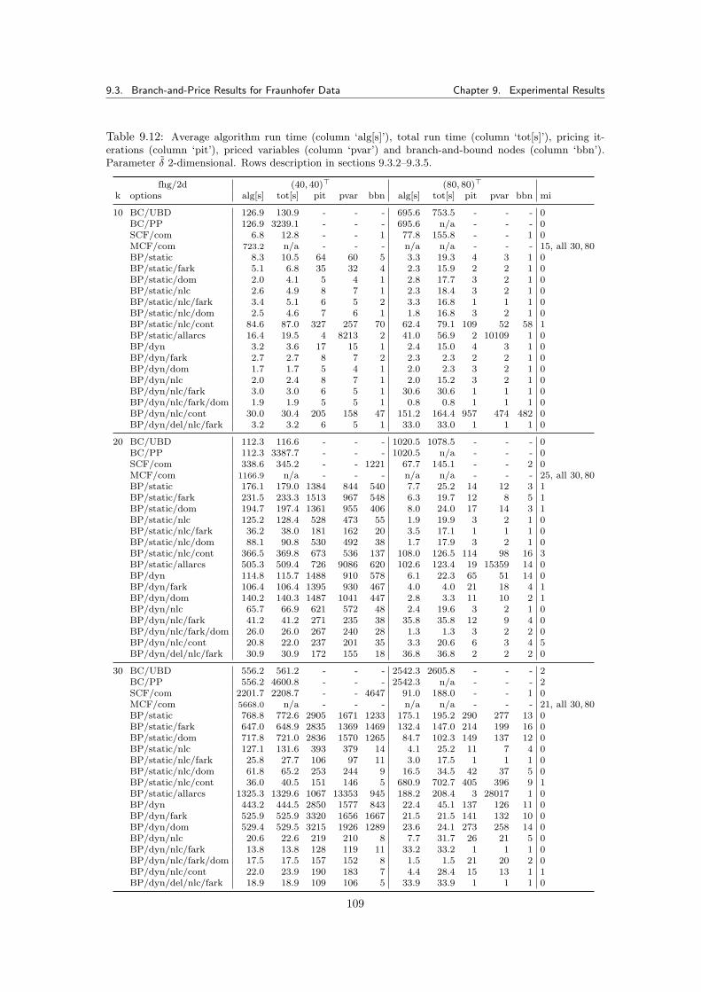
9.3. Branch-and-Price Results for Fraunhofer Data Chapter 9. Experimental Results
Table 9.12: Average algorithm run time (column ‘alg[s]’), total run time (column ‘tot[s]’), pricing it-erations (column ‘pit’), priced variables (column ‘pvar’) and branch-and-bound nodes (column ‘bbn’).Parameter δ 2-dimensional. Rows description in sections 9.3.2–9.3.5.
fhg/2d (40, 40)> (80, 80)>k options alg[s] tot[s] pit pvar bbn alg[s] tot[s] pit pvar bbn mi
10 BC/UBD 126.9 130.9 - - - 695.6 753.5 - - - 0BC/PP 126.9 3239.1 - - - 695.6 n/a - - - 0SCF/com 6.8 12.8 - - 1 77.8 155.8 - - 1 0MCF/com 723.2 n/a - - - n/a n/a - - - 15, all 30, 80BP/static 8.3 10.5 64 60 5 3.3 19.3 4 3 1 0BP/static/fark 5.1 6.8 35 32 4 2.3 15.9 2 2 1 0BP/static/dom 2.0 4.1 5 4 1 2.8 17.7 3 2 1 0BP/static/nlc 2.6 4.9 8 7 1 2.3 18.4 3 2 1 0BP/static/nlc/fark 3.4 5.1 6 5 2 3.3 16.8 1 1 1 0BP/static/nlc/dom 2.5 4.6 7 6 1 1.8 16.8 3 2 1 0BP/static/nlc/cont 84.6 87.0 327 257 70 62.4 79.1 109 52 58 1BP/static/allarcs 16.4 19.5 4 8213 2 41.0 56.9 2 10109 1 0BP/dyn 3.2 3.6 17 15 1 2.4 15.0 4 3 1 0BP/dyn/fark 2.7 2.7 8 7 2 2.3 2.3 2 2 1 0BP/dyn/dom 1.7 1.7 5 4 1 2.0 2.3 3 2 1 0BP/dyn/nlc 2.0 2.4 8 7 1 2.0 15.2 3 2 1 0BP/dyn/nlc/fark 3.0 3.0 6 5 1 30.6 30.6 1 1 1 0BP/dyn/nlc/fark/dom 1.9 1.9 5 5 1 0.8 0.8 1 1 1 0BP/dyn/nlc/cont 30.0 30.4 205 158 47 151.2 164.4 957 474 482 0BP/dyn/del/nlc/fark 3.2 3.2 6 5 1 33.0 33.0 1 1 1 0
20 BC/UBD 112.3 116.6 - - - 1020.5 1078.5 - - - 0BC/PP 112.3 3387.7 - - - 1020.5 n/a - - - 0SCF/com 338.6 345.2 - - 1221 67.7 145.1 - - 2 0MCF/com 1166.9 n/a - - - n/a n/a - - - 25, all 30, 80BP/static 176.1 179.0 1384 844 540 7.7 25.2 14 12 3 1BP/static/fark 231.5 233.3 1513 967 548 6.3 19.7 12 8 5 1BP/static/dom 194.7 197.4 1361 955 406 8.0 24.0 17 14 3 1BP/static/nlc 125.2 128.4 528 473 55 1.9 19.9 3 2 1 0BP/static/nlc/fark 36.2 38.0 181 162 20 3.5 17.1 1 1 1 0BP/static/nlc/dom 88.1 90.8 530 492 38 1.7 17.9 3 2 1 0BP/static/nlc/cont 366.5 369.8 673 536 137 108.0 126.5 114 98 16 3BP/static/allarcs 505.3 509.4 726 9086 620 102.6 123.4 19 15359 14 0BP/dyn 114.8 115.7 1488 910 578 6.1 22.3 65 51 14 0BP/dyn/fark 106.4 106.4 1395 930 467 4.0 4.0 21 18 4 1BP/dyn/dom 140.2 140.3 1487 1041 447 2.8 3.3 11 10 2 1BP/dyn/nlc 65.7 66.9 621 572 48 2.4 19.6 3 2 1 0BP/dyn/nlc/fark 41.2 41.2 271 235 38 35.8 35.8 12 9 4 0BP/dyn/nlc/fark/dom 26.0 26.0 267 240 28 1.3 1.3 3 2 2 0BP/dyn/nlc/cont 20.8 22.0 237 201 35 3.3 20.6 6 3 4 5BP/dyn/del/nlc/fark 30.9 30.9 172 155 18 36.8 36.8 2 2 2 0
30 BC/UBD 556.2 561.2 - - - 2542.3 2605.8 - - - 2BC/PP 556.2 4600.8 - - - 2542.3 n/a - - - 2SCF/com 2201.7 2208.7 - - 4647 91.0 188.0 - - 1 0MCF/com 5668.0 n/a - - - n/a n/a - - - 21, all 30, 80BP/static 768.8 772.6 2905 1671 1233 175.1 195.2 290 277 13 0BP/static/fark 647.0 648.9 2835 1369 1469 132.4 147.0 214 199 16 0BP/static/dom 717.8 721.0 2836 1570 1265 84.7 102.3 149 137 12 0BP/static/nlc 127.1 131.6 393 379 14 4.1 25.2 11 7 4 0BP/static/nlc/fark 25.8 27.7 106 97 11 3.0 17.5 1 1 1 0BP/static/nlc/dom 61.8 65.2 253 244 9 16.5 34.5 42 37 5 0BP/static/nlc/cont 36.0 40.5 151 146 5 680.9 702.7 405 396 9 1BP/static/allarcs 1325.3 1329.6 1067 13353 945 188.2 208.4 3 28017 1 0BP/dyn 443.2 444.5 2850 1577 843 22.4 45.1 137 126 11 0BP/dyn/fark 525.9 525.9 3320 1656 1667 21.5 21.5 141 132 10 0BP/dyn/dom 529.4 529.5 3215 1926 1289 23.6 24.1 273 258 14 0BP/dyn/nlc 20.6 22.6 219 210 8 7.7 31.7 26 21 5 0BP/dyn/nlc/fark 13.8 13.8 128 119 11 33.2 33.2 1 1 1 0BP/dyn/nlc/fark/dom 17.5 17.5 157 152 8 1.5 1.5 21 20 2 0BP/dyn/nlc/cont 22.0 23.9 190 183 7 4.4 28.4 15 13 1 1BP/dyn/del/nlc/fark 18.9 18.9 109 106 5 33.9 33.9 1 1 1 0
109
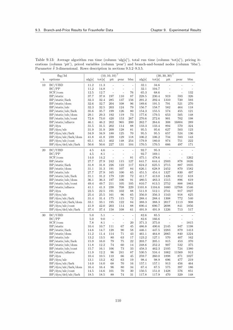
9.3. Branch-and-Price Results for Fraunhofer Data Chapter 9. Experimental Results
Table 9.13: Average algorithm run time (column ‘alg[s]’), total run time (column ‘tot[s]’), pricing it-erations (column ‘pit’), priced variables (column ‘pvar’) and branch-and-bound nodes (column ‘bbn’).Parameter δ 3-dimensional. Rows description in sections 9.3.2–9.3.5.
fhg/3d (10, 10, 10)> (30, 30, 30)>k options alg[s] tot[s] pit pvar bbn alg[s] tot[s] pit pvar bbn
10 BC/UBD 11.2 11.3 - - - 32.1 34.6 - - -BC/PP 11.2 14.8 - - - 32.1 104.7 - - -SCF/com 12.5 12.7 - - 76 65.3 68.6 - - 132BP/static 37.7 37.8 197 110 87 228.5 230.4 919 593 326BP/static/fark 32.3 32.4 285 137 156 291.2 292.4 1310 720 593BP/static/dom 32.6 32.7 204 108 96 189.6 191.5 791 521 270BP/static/nlc 32.3 32.5 203 124 79 156.7 158.7 582 464 118BP/static/nlc/fark 35.6 35.7 199 126 80 154.3 155.5 574 455 121BP/static/nlc/dom 29.1 29.3 192 119 73 177.6 179.5 653 505 148BP/static/nlc/cont 72.8 73.0 420 153 267 270.6 272.6 901 702 198BP/static/allarcs 46.1 46.2 202 965 200 262.7 264.6 308 16804 289BP/dyn 31.5 31.5 202 114 88 133.3 133.4 894 570 324BP/dyn/nlc 31.9 31.9 209 128 81 95.5 95.6 627 503 123BP/dyn/nlc/fark 34.9 34.9 188 125 70 95.5 95.5 657 524 136BP/dyn/nlc/fark/dom 41.8 41.8 239 129 118 106.2 106.2 734 593 143BP/dyn/nlc/cont 65.1 65.1 402 148 254 179.9 180.0 974 751 222BP/dyn/del/nlc/fark 50.6 50.6 227 131 104 170.5 170.5 666 497 171
20 BC/UBD 4.5 4.6 - - - 92.7 95.3 - - -BC/PP 4.5 8.1 - - - 92.7 169.1 - - -SCF/com 14.0 14.2 - - 81 475.1 478.6 - - 1262BP/static 27.7 27.9 242 115 127 641.7 644.4 2503 878 1626BP/static/fark 31.8 31.8 226 122 117 624.2 625.5 2715 887 1835BP/static/dom 31.1 31.3 191 107 84 626.1 628.9 2452 870 1582BP/static/nlc 27.7 27.9 165 100 65 451.5 454.4 1327 830 497BP/static/nlc/fark 31.1 31.2 179 120 72 411.7 413.0 1426 812 618BP/static/nlc/dom 36.1 36.3 197 106 91 480.5 483.3 1515 896 619BP/static/nlc/cont 49.4 49.7 211 105 105 810.7 813.5 2752 888 1863BP/static/allarcs 41.1 41.3 238 708 229 1101.8 1104.6 1660 12768 1546BP/dyn 22.5 22.5 191 102 88 511.9 512.1 2741 917 1827BP/dyn/nlc 25.4 25.5 161 96 65 356.0 356.3 1543 918 625BP/dyn/nlc/fark 31.4 31.4 175 115 72 288.4 288.4 1308 772 540BP/dyn/nlc/fark/dom 33.1 33.1 195 122 84 388.3 388.3 2017 1113 908BP/dyn/nlc/cont 41.9 42.0 203 114 88 690.4 690.7 2698 841 1856BP/dyn/del/nlc/fark 37.4 37.4 158 108 61 491.9 491.9 1226 713 517
30 BC/UBD 5.0 5.1 - - - 82.6 85.5 - - -BC/PP 5.0 9.0 - - - 82.6 166.6 - - -SCF/com 7.8 8.1 - - 20 371.3 375.0 - - 1815BP/static 10.4 10.7 111 67 45 486.8 490.6 2145 947 1198BP/static/fark 14.6 14.7 128 90 58 446.1 447.5 2283 879 1413BP/static/dom 11.2 11.4 114 71 43 461.1 464.8 2065 840 1224BP/static/nlc 13.2 13.5 80 63 17 123.2 127.1 570 407 162BP/static/nlc/fark 15.9 16.0 79 75 22 203.7 205.1 815 453 370BP/static/nlc/dom 11.8 12.2 74 60 14 248.6 252.2 907 532 375BP/static/nlc/cont 15.7 16.1 106 73 33 458.3 462.3 2105 724 1380BP/static/allarcs 11.9 12.2 96 241 87 530.5 534.4 1062 11569 913BP/dyn 10.4 10.5 110 66 45 259.7 260.0 1898 871 1027BP/dyn/nlc 13.1 13.2 82 63 19 98.4 98.9 696 477 219BP/dyn/nlc/fark 14.0 14.0 68 70 16 157.1 157.1 913 456 464BP/dyn/nlc/fark/dom 16.4 16.4 96 80 34 67.4 67.5 575 397 186BP/dyn/nlc/cont 14.5 14.6 101 70 30 150.5 151.0 1428 576 851BP/dyn/del/nlc/fark 18.5 18.5 88 74 31 117.8 117.9 470 329 148
110
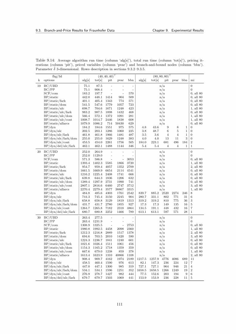
9.3. Branch-and-Price Results for Fraunhofer Data Chapter 9. Experimental Results
Table 9.14: Average algorithm run time (column ‘alg[s]’), total run time (column ‘tot[s]’), pricing it-erations (column ‘pit’), priced variables (column ‘pvar’) and branch-and-bound nodes (column ‘bbn’).Parameter δ 3-dimensional. Rows description in sections 9.3.2–9.3.5.
fhg/3d (40, 40, 40)> (80, 80, 80)>k options alg[s] tot[s] pit pvar bbn alg[s] tot[s] pit pvar bbn mi
10 BC/UBD 75.1 87.5 - - - n/a 0BC/PP 75.1 908.4 - - - n/a 0SCF/com 183.2 197.7 - - 570 n/a 0, all 80BP/static 442.0 448.1 1414 904 509 n/a 0, all 80BP/static/fark 401.1 405.4 1343 774 571 n/a 0, all 80BP/static/dom 541.5 547.6 1779 1057 723 n/a 0, all 80BP/static/nlc 698.7 704.6 1671 1248 423 n/a 1, all 80BP/static/nlc/fark 983.2 987.5 1898 1432 468 n/a 0, all 80BP/static/nlc/dom 566.4 572.1 1372 1091 281 n/a 1, all 80BP/static/nlc/cont 1008.7 1014.7 2446 1838 608 n/a 1, all 80BP/static/allarcs 1079.9 1086.2 714 50430 629 n/a 0, all 80BP/dyn 184.2 184.6 1551 975 575 4.8 43.6 9 8 1 0BP/dyn/nlc 202.5 203.1 1286 1060 225 3.8 48.7 6 5 1 0BP/dyn/nlc/fark 461.8 461.8 1966 1481 487 3.5 3.6 4 4 1 0BP/dyn/nlc/fark/dom 255.0 255.0 1629 1248 383 4.0 4.0 13 11 3 0BP/dyn/nlc/cont 453.5 454.0 2261 1756 505 184.0 223.1 681 496 184 2BP/dyn/del/nlc/fark 462.1 462.1 1488 1144 346 5.4 5.4 4 4 1 1
20 BC/UBD 252.0 264.9 - - - n/a 0BC/PP 252.0 1129.0 - - - n/a 0SCF/com 571.3 586.8 - - 3053 n/a 0, all 80BP/static 1393.4 1402.3 5585 1866 3720 n/a 1, all 80BP/static/fark 954.7 959.4 4057 1352 2709 n/a 2, all 80BP/static/dom 1661.5 1669.9 6654 2114 4541 n/a 0, all 80BP/static/nlc 1216.2 1225.4 2408 1741 666 n/a 0, all 80BP/static/nlc/fark 639.8 644.3 1836 1206 632 n/a 0, all 80BP/static/nlc/dom 1289.4 1297.9 2731 1990 741 n/a 0, all 80BP/static/nlc/cont 2807.1 2816.6 6460 2747 3712 n/a 3, all 80BP/static/allarcs 2270.4 2279.4 3577 38867 3315 n/a 1, all 80BP/dyn 484.8 485.6 4303 1761 2542 839.7 885.2 2520 2274 246 8BP/dyn/nlc 744.3 745.4 3150 2245 904 280.7 331.1 802 771 31 6BP/dyn/nlc/fark 658.8 658.8 3129 1819 1313 319.2 319.2 810 775 36 3BP/dyn/nlc/fark/dom 431.7 431.7 2780 1855 927 17.3 17.3 149 135 16 5BP/dyn/nlc/cont 1264.7 1265.8 7182 2318 4864 134.5 191.1 448 432 16 7BP/dyn/del/nlc/fark 680.7 680.8 2252 1466 789 613.1 613.1 597 571 28 1
30 BC/UBD 263.4 277.5 - - - n/a 0BC/PP 263.4 1231.9 - - - n/a 0SCF/com 1308.9 1325.5 - - 2753 n/a 0, all 80BP/static 1980.8 1992.5 4458 2098 2360 n/a 1, all 80BP/static/fark 1212.3 1216.8 2889 1517 1378 n/a 2, all 80BP/static/dom 694.6 703.5 2010 1420 590 n/a 3, all 80BP/static/nlc 1224.3 1236.7 1841 1240 601 n/a 0, all 80BP/static/nlc/fark 1021.6 1026.4 1511 1061 456 n/a 0, all 80BP/static/nlc/dom 1154.3 1165.2 1718 1359 359 n/a 0, all 80BP/static/nlc/cont 667.6 679.0 1238 859 378 n/a 1, all 80BP/static/allarcs 1613.4 1623.9 1310 40866 1108 n/a 2, all 80BP/dyn 908.4 909.7 4162 1974 2189 1217.5 1257.9 4776 4086 689 11BP/dyn/nlc 458.5 460.4 1590 976 613 82.1 147.3 236 224 12 7BP/dyn/nlc/fark 447.0 447.1 1300 985 319 727.1 727.1 964 946 21 4BP/dyn/nlc/fark/dom 534.1 534.1 1596 1251 352 1658.5 1658.5 1266 1249 19 2BP/dyn/nlc/cont 276.9 278.7 1427 982 444 77.5 152.6 203 194 9 6BP/dyn/del/nlc/fark 679.7 679.7 1503 1069 441 153.9 153.9 236 228 11 5
111

9.3. Branch-and-Price Results for Fraunhofer Data Chapter 9. Experimental Results
Table 9.15: Averages over k, δ for the tested algorithms branch-and-cut (row ‘BC’), SCF and MCFsolved entirely (rows ‘SCF/com’ and ‘MCF/com’), branch-and-price using a static tree pricing algorithm(all rows ‘BP/static’) and a dynamic tree pricing algorithm (rows ‘BP/dyn’).
AVG over k, δ
fhg/2d alg[s] tot[s] pit pvar bbn mi
BC/UBD 488.3 501.6 - - - 2
BC/PP 488.3 1323.6 - - - 2, PP t[s] for (80, 80)>
SCF/com 362.5 381.4 - - 862 0
MCF/com 5552.8 n/a - - - 61, all (30, 30)>, (80, 80)>
BP/static 246.1 250.7 1207 580 627 1BP/static/fark 229.3 232.7 1184 515 672 1BP/static/dom 237.5 241.7 1216 560 656 1BP/static/nlc 171.1 176.0 656 366 289 0BP/static/nlc/fark 150.5 153.9 616 299 320 0BP/static/nlc/dom 165.9 170.2 683 367 315 0BP/static/nlc/cont 320.9 325.9 916 470 446 5BP/static/allarcs 441.6 446.6 799 8607 723 0BP/dyn 180.7 184.4 1159 572 559 1BP/dyn/fark 187.7 187.7 1209 515 697 1BP/dyn/dom 191.8 191.9 1263 643 620 1BP/dyn/nlc 142.7 146.7 622 346 276 0BP/dyn/nlc/fark 129.4 129.4 585 282 306 0BP/dyn/nlc/fark/dom 113.0 113.0 545 289 260 0BP/dyn/nlc/cont 269.3 273.3 1049 436 612 6BP/dyn/del/nlc/fark 150.0 150.0 546 268 281 0
fhg/3d alg[s] tot[s] pit pvar bbn mi
BC/UBD 90.9 96.2 - - - 0, all (80, 80, 80)>.
BC/PP 90.9 415.7 - - - 0, all (80, 80, 80)>.
SCF/com 334.4 340.8 - - 1085 0, all (80, 80, 80)>.
BP/static 583.2 587.2 1953 842 1111 2, all (80, 80, 80)>.
BP/static/fark 445.4 447.3 1693 720 981 4, all (80, 80, 80)>.
BP/static/dom 472.1 475.7 1807 790 1017 3, all (80, 80, 80)>.
BP/static/nlc 438.2 442.3 983 691 292 1, all (80, 80, 80)>.
BP/static/nlc/fark 388.5 390.5 946 638 315 0, all (80, 80, 80)>.
BP/static/nlc/dom 443.7 447.6 1040 740 300 1, all (80, 80, 80)>.
BP/static/nlc/cont 684.6 688.6 1849 899 949 5, all (80, 80, 80)>.
BP/static/allarcs 773.1 777.0 1018 19247 924 3, all (80, 80, 80)>.BP/dyn 384.1 394.7 1946 1143 803 19BP/dyn/nlc 199.3 213.1 866 622 243 13BP/dyn/nlc/fark 269.9 269.9 957 673 290 7BP/dyn/nlc/fark/dom 296.2 296.2 941 682 264 7BP/dyn/nlc/cont 294.5 309.1 1501 723 777 15BP/dyn/del/nlc/fark 290.1 290.1 743 528 221 7
112
9.3. Branch-and-Price Results for Fraunhofer Data Chapter 9. Experimental Results
The overall average run times for branch-and-price using a dynamic tree pricing algorithm aresmaller than the ones determined with a static tree pricing algorithm, so it is the better option. Weconclude that the best pricing strategy for branch-and-price is a dynamic tree pricing algorithmusing node-label constraints and Farkas pricing. Also allowing the pricing of dominated templatearcs has good run times.
Finally, we shortly analyze the variant that deletes the dynamic tree after each pricing iteration.Naturally, all runs that delete the tree have run times inferior the the original variants. Focuswas the applicability to the bigger data sets, for example the nist data set. As these instanceshave many more data points and bigger domain sizes, building an entire segmentation tree isextremely memory intensive, up to the extent that for very big δ no segmentation tree can bebuilt because of a memory overflow. Thus we tested, how much slower the versions are that deletethe dynamic tree in each pricing iteration. For all such variants, the memory usage for big δ isgenerally very good. The overall run time average increases especially when the deletion is oftenperformed (many pricing iterations). When δ is small this variant has good run times since theaccording dynamic tree has few levels. If δ gets bigger, many nodes have to be created and deletedagain for each pricing iteration, thus slowing down the algorithm. When we compare for the bestvariant ‘BP/dyn/deltree/nlc/fark’ (listed in the results tables) the run times for both versions,the one that deletes the dynamic tree and the other being standard dynamic tree pricing withoutdeletion process, can be said: The version that deletes the tree performs in an average 110.2%of the time needed by the original version, needs 83.6% of the amount pricing iterations, prices83.4% of the variables and creates 84.2% of the branch-and-bound nodes. The different pricingbehaviour (described in section 9.3.5) is beneficial. For the variant ‘BP/dyn/deltree’ that uses noadditional options, the version that deletes the tree has run times that take 239.8% of the runtime (pit: 97.0%, pvar: 102.1%, bbn: 92.7%) for the respective version that does not delete thetree, with ‘BP/dyn/deltree/nlc’ run times need 173.4% (pit: 108.9%, pvar: 107.6%, bbn; 111.4%)of the time needed by ‘BP/dyn/nlc’.The best option for big instances is to use node-label constraints in combination with Farkaspricing. If memory has to be saved starting in each pricing iteration with an empty dynamic treeis an option.
9.3.6 Summary for Pricing Algorithms with Fraunhofer Data Tests
Table 9.15 lists total average run times for all tested variants. In tables 9.11, 9.12, 9.13, 9.14we saw that the strength of branch-and-price are big δ values. The algorithm is very fast for2-dimensional such parameters, when run times are compared to the ones of the branch-and-cutalgorithm. When k increases, the run times for small δ values diminish, and increase somewhatfor middle and big δ. In comparison to branch-and-cut for most middle, big and very big δ a hugeimprovement is achieved. For 3-dimensional δ parameters, the run times can not reach branch-and-cut run times, but are relatively good. The same characteristics for k and δ are seen with3-dimensional δ parameters.
The comparison of average values for 3-dimensional data was not as easy as for 2-dimensionaldata since some test instances were not calculated (mostly from (80, 80, 80)>, for smaller δ almostno instance is missing) either because of a memory overflow or because of surpassing our pricingiterations or time limit. For a more profound analysis, these limits as well memory size have tobe increased. Another option would be to decrease the size of the segmentation trees in order tofind a solution more quickly. The variants that delete the dynamic tree after each pricing iterationwould surely need a bigger time limit to complete all test instance runs. When regarding theamount of calculated instances the dynamic tree pricing algorithm ‘BP/dyn/nlc/fark/(dom)’ isthe best. Big 3-dimensional δ were only calculable with this algorithm.
As for node-label constraints, when added to the problem, a huge run time improvement canbe noted for all δ in combination with all k, except k = 20, δ = (20, 20)>. The improvement
113
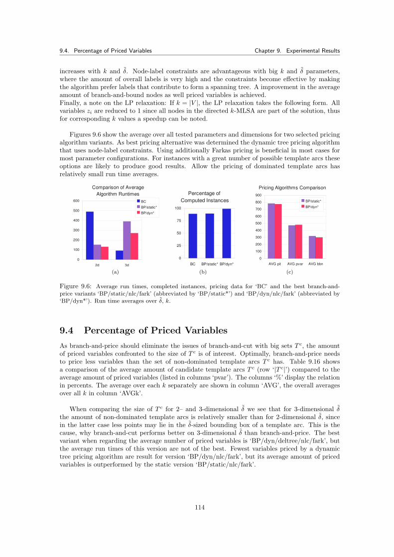
9.4. Percentage of Priced Variables Chapter 9. Experimental Results
increases with k and δ. Node-label constraints are advantageous with big k and δ parameters,where the amount of overall labels is very high and the constraints become effective by makingthe algorithm prefer labels that contribute to form a spanning tree. A improvement in the averageamount of branch-and-bound nodes as well priced variables is achieved.Finally, a note on the LP relaxation: If k = |V |, the LP relaxation takes the following form. Allvariables zi are reduced to 1 since all nodes in the directed k-MLSA are part of the solution, thusfor corresponding k values a speedup can be noted.
Figures 9.6 show the average over all tested parameters and dimensions for two selected pricingalgorithm variants. As best pricing alternative was determined the dynamic tree pricing algorithmthat uses node-label constraints. Using additionally Farkas pricing is beneficial in most cases formost parameter configurations. For instances with a great number of possible template arcs theseoptions are likely to produce good results. Allow the pricing of dominated template arcs hasrelatively small run time averages. Sheet1
Page 1
2d 3d
0
100
200
300
400
500
600
Comparison of AverageAlgorithm Runtimes
BC
BP/static*
BP/dyn*
(a)
Sheet1
Page 1
BC BP/static* BP/dyn*
0
25
50
75
100
Percentage of Computed Instances
(b)
Sheet1
Page 1
AVG pit AVG pvar AVG bbn
0
100
200
300
400
500
600
700
800
900
Pricing Algorithms Comparison
BP/static*
BP/dyn*
(c)
Figure 9.6: Average run times, completed instances, pricing data for ‘BC’ and the best branch-and-price variants ‘BP/static/nlc/fark’ (abbreviated by ‘BP/static*’) and ‘BP/dyn/nlc/fark’ (abbreviated by‘BP/dyn*’). Run time averages over δ, k.
9.4 Percentage of Priced Variables
As branch-and-price should eliminate the issues of branch-and-cut with big sets T c, the amountof priced variables confronted to the size of T c is of interest. Optimally, branch-and-price needsto price less variables than the set of non-dominated template arcs T c has. Table 9.16 showsa comparison of the average amount of candidate template arcs T c (row ‘|T c|’) compared to theaverage amount of priced variables (listed in columns ‘pvar’). The columns ‘%’ display the relationin percents. The average over each k separately are shown in column ‘AVG’, the overall averagesover all k in column ‘AVGk’.
When comparing the size of T c for 2– and 3-dimensional δ we see that for 3-dimensional δthe amount of non-dominated template arcs is relatively smaller than for 2-dimensional δ, sincein the latter case less points may lie in the δ-sized bounding box of a template arc. This is thecause, why branch-and-cut performs better on 3-dimensional δ than branch-and-price. The bestvariant when regarding the average number of priced variables is ‘BP/dyn/deltree/nlc/fark’, butthe average run times of this version are not of the best. Fewest variables priced by a dynamictree pricing algorithm are result for version ‘BP/dyn/nlc/fark’, but its average amount of pricedvariables is outperformed by the static version ‘BP/static/nlc/fark’.
114
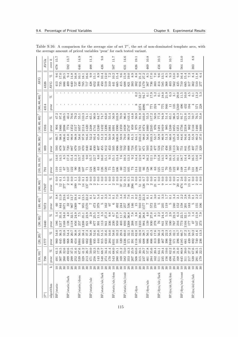
9.4. Percentage of Priced Variables Chapter 9. Experimental Results
Table 9.16: A comparison for the average size of set T c, the set of non-dominated template arcs, withthe average amount of priced variables ‘pvar’ for each tested variant.
(10,1
0)>
(20,2
0)>
(30,3
0)>
(40,4
0)>
(80,8
0)>
(10,1
0,1
0)>
(30,3
0,3
0)>
(40,4
0,4
0)>
(80,8
0,8
0)>
AV
G
|Tc|
798
1777
3440
7072
17937
791
889
1916
4314
4326
AV
Gk
alg
ori
thm
kpvar
%pvar
%pvar
%pvar
%pvar
%pvar
%pvar
%pvar
%pvar
%A
VG
%overk
BP
/st
ati
c10
491
61.5
960
54.0
186
5.4
60
0.8
30.0
110
14.0
593
66.7
904
47.2
--
413
9.6
678
15.7
20
307
38.5
645
36.3
1217
35.4
844
11.9
12
0.1
115
14.5
878
98.8
1866
97.4
--
735
17.0
30
260
32.6
600
33.8
1168
34.0
1671
23.6
277
1.5
67
8.5
947
106.6
2098
109.5
--
886
20.5
BP
/st
ati
c/fa
rk10
499
62.6
968
54.4
138
4.0
32
0.5
20.0
137
17.3
720
81.0
774
40.4
--
409
9.4
592
13.7
20
299
37.5
368
20.7
1118
32.5
967
13.7
80.0
122
15.4
887
99.8
1352
70.6
--
640
14.8
30
252
31.6
654
36.8
856
24.9
1369
19.4
199
1.1
90
11.3
879
98.9
1517
79.2
--
727
16.8
BP
/st
ati
c/d
om
10
539
67.6
1004
56.5
257
7.5
40.1
20.0
108
13.7
521
58.6
1057
55.1
--
436
10.1
646
14.9
20
329
41.2
683
38.4
1208
35.1
955
13.5
14
0.1
107
13.6
870
97.9
2114
110.3
--
785
18.1
30
213
26.7
662
37.3
821
23.9
1570
22.2
137
0.8
71
9.0
840
94.6
1420
74.1
--
717
16.6
BP
/st
ati
c/n
lc10
471
59.0
1009
56.8
99
2.9
70.1
20.0
124
15.7
464
52.2
1248
65.1
--
428
9.9
488
11.3
20
258
32.3
935
52.6
877
25.5
473
6.7
20.0
100
12.7
830
93.4
1741
90.9
--
652
15.1
30
143
17.9
444
25.0
391
11.4
379
5.4
70.0
63
8.0
407
45.8
1240
64.7
--
384
8.9
BP
/sta
tic/
nlc
/far
k10
548
68.7
915
51.5
113
3.3
50.1
10.0
126
16.0
455
51.2
1432
74.7
--
450
10.4
426
9.8
20
274
34.4
633
35.6
941
27.3
162
2.3
10.0
120
15.1
812
91.3
1206
63.0
--
519
12.0
30
170
21.4
284
16.0
336
9.8
97
1.4
10.0
75
9.5
453
50.9
1061
55.4
--
310
7.2
BP
/sta
tic/
nlc
/dom
10
543
68.0
1031
58.0
230
6.7
60.1
20.0
119
15.1
505
56.8
1091
56.9
--
441
10.2
507
11.7
20
280
35.1
591
33.2
959
27.9
492
7.0
20.0
106
13.4
896
100.8
1990
103.9
--
665
15.4
30
169
21.2
520
29.3
403
11.7
244
3.4
37
0.2
60
7.6
532
59.9
1359
70.9
--
415
9.6
BP
/sta
tic/
nlc
/con
t10
582
73.0
1226
69.0
693
20.2
257
3.6
52
0.3
153
19.3
702
79.0
1838
96.0
--
688
15.9
631
14.6
20
353
44.3
571
32.1
1268
36.8
536
7.6
98
0.5
105
13.3
888
99.9
2747
143.4
--
821
19.0
30
207
25.9
391
22.0
268
7.8
146
2.1
396
2.2
73
9.2
724
81.5
859
44.8
--
383
8.9
BP
/d
yn
10
508
63.6
1116
62.8
131
3.8
15
0.2
30.0
114
14.4
570
64.1
975
50.9
80.2
382
8.8
826
19.1
20
315
39.5
585
32.9
1333
38.8
910
12.9
51
0.3
102
12.9
917
103.2
1761
91.9
2274
52.7
916
21.2
30
237
29.7
688
38.7
984
28.6
1577
22.3
126
0.7
66
8.3
871
98.0
1974
103.0
4086
94.7
1179
27.2
BP
/d
yn
/n
lc10
461
57.8
996
56.1
139
4.0
70.1
20.0
128
16.2
503
56.6
1060
55.3
50.1
367
8.5
469
10.8
20
284
35.6
806
45.3
930
27.0
572
8.1
20.0
96
12.1
918
103.3
2245
117.2
771
17.9
736
17.0
30
162
20.4
313
17.6
278
8.1
210
3.0
21
0.1
63
7.9
477
53.7
976
50.9
224
5.2
303
7.0
BP
/d
yn
/n
lc/fa
rk10
511
64.1
999
56.2
76
2.2
50.1
10.0
125
15.8
524
58.9
1481
77.3
40.1
414
9.6
456
10.5
20
235
29.4
467
26.3
841
24.4
235
3.3
90.0
115
14.5
772
86.9
1819
94.9
775
18.0
585
13.5
30
156
19.6
396
22.3
182
5.3
119
1.7
10.0
70
8.9
456
51.3
985
51.4
946
21.9
368
8.5
BP
/dyn
/nlc
/far
k/do
m10
496
62.2
1040
58.5
100
2.9
50.1
10.0
129
16.3
593
66.8
1248
65.1
11
0.3
403
9.3
463
10.7
20
254
31.9
571
32.1
767
22.3
240
3.4
20.0
122
15.5
1113
125.3
1855
96.8
135
3.1
562
13.0
30
168
21.0
296
16.7
216
6.3
152
2.1
20
0.1
80
10.1
397
44.6
1251
65.3
1249
29.0
425
9.8
BP
/d
yn
/n
lc/co
nt
10
645
80.8
1185
66.7
773
22.5
158
2.2
474
2.6
148
18.7
751
84.6
1756
91.7
496
11.5
710
16.4
564
13.0
20
311
39.0
661
37.2
1104
32.1
201
2.8
30.0
114
14.4
841
94.6
2318
121.0
432
10.0
665
15.4
30
217
27.2
439
24.7
177
5.2
183
2.6
13
0.1
70
8.9
576
64.8
982
51.3
194
4.5
317
7.3
BP
/dyn
/del
/nlc
/far
k10
539
67.6
892
50.2
47
1.4
50.1
10.0
131
16.5
497
55.9
1144
59.7
40.1
362
8.4
383
8.9
20
291
36.5
740
41.6
547
15.9
155
2.2
20.0
108
13.6
713
80.2
1466
76.5
571
13.2
510
11.8
30
179
22.5
236
13.3
273
7.9
106
1.5
10.0
74
9.3
329
37.0
1069
55.8
228
5.3
277
6.4
115
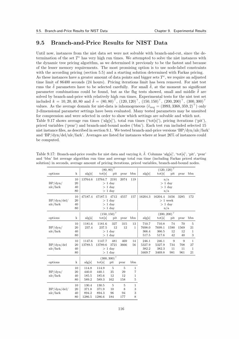
9.5. Branch-and-Price Results for NIST Data Chapter 9. Experimental Results
9.5 Branch-and-Price Results for NIST Data
Until now, instances from the nist data set were not solvable with branch-and-cut, since the de-termination of the set T c has very high run times. We attempted to solve the nist instances withthe dynamic tree pricing algorithm, as we determined it previously to be the fastest and becauseof the lesser memory requirements. The most promising option is to use node-label constraintswith the according pricing (section 5.5) and a starting solution determined with Farkas pricing.As these instances have a greater amount of data points and bigger sets T c, we require an adjustedtime limit of 86400 seconds (24 hours). Pricing iterations limit has been removed. For nist testruns the δ parameters have to be selected carefully. For small δ, at the moment no significantparameter combinations could be found, but as the fhg tests showed, small and middle δ aresolved by branch-and-price with relatively high run times. Experimental tests for the nist test setincluded k = 10, 20, 40, 80 and δ = (80, 80)>, (120, 120)>, (150, 150)>, (200, 200)>, (300, 300)>
values. As the average domain for nist-data is inhomogeneous (vavg = (3993, 3368, 359, 2)>) only2-dimensional parameter settings have been evaluated. Many tested parameters may be unsuitedfor compression and were selected in order to show which settings are solvable and which not.Table 9.17 shows average run times (‘alg[s]’), total run times (‘tot[s]’), pricing iterations (‘pit’),priced variables (‘pvar’) and branch-and-bound nodes (‘bbn’). Each test run included selected 15nist instance files, as described in section 9.1. We tested branch-and-price versions ‘BP/dyn/nlc/fark’and ‘BP/dyn/del/nlc/fark’. Averages are listed for instances where at least 26% of instances couldbe computed.
Table 9.17: Branch-and-price results for nist data and varying k, δ. Columns ‘alg[s]’, ‘tot[s]’, ‘pit’, ‘pvar’and ‘bbn’ list average algorithm run time and average total run time (including Farkas priced startingsolution) in seconds, average amount of pricing iterations, priced variables, branch-and-bound nodes.
(80, 80)> (120, 120)>options k alg[s] tot[s] pit pvar bbn alg[s] tot[s] pit pvar bbn
10 13764.6 13764.7 2191 2074 119 n/aBP/dyn/ 20 > 1 day > 1 daynlc/fark 40 > 1 day > 1 day
80 > 1 day n/a
10 47187.4 47187.5 4712 4557 157 16204.3 16204.4 3456 3285 172BP/dyn/del/ 20 > 1 day > 1 weeknlc/fark 40 > 1 day > 1 day
80 > 1 day n/a
(150, 150)> (200, 200)>options k alg[s] tot[s] pit pvar bbn alg[s] tot[s] pit pvar bbn
10 1181.6 1181.6 327 315 13 710.7 710.8 74 70 5BP/dyn/ 20 237.4 237.5 12 12 1 7698.0 7699.1 1590 1569 21nlc/fark 40 > 1 day 366.4 366.5 12 12 1
80 > 1 day 517.5 517.6 42 40 3
10 1147.6 1147.7 481 469 14 246.1 246.1 9 9 1BP/dyn/del 20 13789.5 13789.6 3721 3666 56 5327.9 5327.9 734 708 27nlc/fark 40 > 1 day 382.2 382.3 11 11 1
80 > 1 day 3469.7 3469.8 981 961 21
(300, 300)>options k alg[s] tot[s] pit pvar bbn
10 114.8 114.9 5 5 1BP/dyn/ 20 440.0 440.1 35 29 7nlc/fark 40 185.5 185.6 12 12 1
80 589.2 589.3 162 158 5
10 130.4 130.5 5 5 1BP/dyn/del/ 20 371.8 371.9 10 8 3nlc/fark 40 894.2 894.3 96 94 3
80 1286.5 1286.6 184 177 8
116
9.6. Branch-and-Price Summary Chapter 9. Experimental Results
9.5.1 Results
For very big δ = (150, 150)>, (200, 200)>, (300, 300)> almost all instances were solved relativelyfast and are computed within some hundred seconds. Small k = 10, 20, relevant to compression,have good results. The bigger k and the smaller δ, the less instances could be completed withinthe time limit. Instances with very many data points are amongst the solved instances and thesize of |V | does not influence solvability.
Generally, the tailing off effect becomes extremely visible for this data set. For instances, whereafter 24 hours no result could be determined, no result will be computed even after 1 week. Fork and δ, the behaviour of branch-and-price is very similar to the one determined with fhg-data.For big δ = (150, 150)>, (200, 200)>, (300, 300)> test parameters, the absolute compression ratesrange between 91–96% because the codebook size for such parameters is one or two. Combinedwith small k almost all instances could be computed. The bigger k and the smaller δ, the moreinstances exceed the time limit.We expect that smaller δ, more suited for compression, become solvable with fine tuning of theSCIP framework, for example by enabling a setting with an emphasis on feasibility. The testedparameters cover solution possibilities of branch-and-price with nist data and indicates the mag-nitude of the resulting run times.
9.6 Branch-and-Price Summary
All developed static and dynamic segmentation tree algorithms UB-driven traversing, advancedbounding traversal, best first search, are a massive improvement for the branch-and-cut prepro-cessing strep. All variants greatly outperform the preprocessing from [ChwRai09]. The run timesfor determining T c with the best variant UB-driven traversing are reduced to 1.91% of the pre-vious preprocessing, and is considered to be very beneficial, despite a high memory usage. Animprovement for this memory usage would be not to save the upper and lower bound set at eachnode, to either leave out equal bound sets for predecessor and successor nodes or to save only thedifferences between predecessor and successor.
All presented run times for branch-and-price are the total time needed by SCIP for determiningthe solution and determine that no better solution can be found in the branch-and-bound decisiontree. It lies in the nature of our problem, that more than one combination of template arcs maybe an optimal solution. As the possibilities for combinations are high we have as consequencelarge plateaus of equally good solutions. The times needed by SCIP to find the first best solutionsmay be relatively small, the most of time is needed to determine that the actual found solution isminimal. SCIP may find many more optimal solution possibilities in the branching and boundingprocess. If the result codebook size is already one, which is often the case with big δ, there is noneed to further determine optimality and the branch-and-price process can be terminated earlier.
The best pricing algorithm was determined to be the dynamic tree pricing algorithm. Bestrun time results have been achieved with this pricing algorithm when combined with node-labelconstraints and the according pricing as well with Farkas pricing. For this, the average amount ofbranch-and-bound nodes was smallest as well as the average number of priced variables.As for branch-and-cut run times, the time for searching T c must be added, we added the fast UB-driven traversing times. Even when regarding the new, better preprocessing times for branch-and-cut, there are parameter combinations for which branch-and-price outperforms branch-and-cut,despite the directed cut model used by branch-and-cut has the better LP relaxation.As the Farkas pricing algorithm showed beneficial effects when compared to the star shaped span-ning tree starting solution, we expect that branch-and-price would receive a speed up, if an evenbetter starting solution determined with some heuristic performs better.
117

9.6. Branch-and-Price Summary Chapter 9. Experimental Results
Another characteristic for our problem is that the solution is ambiguous. Thus, much needlesspricing is done. A further consequence of this ambiguity were the template arcs duplicates, whichwe reduced by not pricing same template arcs again. For branch-and-price we saw that the morethe correction vector domain δ increases, the more the optimal solution becomes unambiguous andis found very fast. For such big δ values, branch-and-price greatly outperforms branch-and-cutand the run times for big δ are good and we can calculate the solution for an fhg instance in acouple of seconds. Good results have been determined with small and big k. When δ and k havemiddle values, branch-and-price performs not so well.
The disadvantage when pricing non-dominated template arcs is again ambiguous optimum inthe tree, searched by regarding the sums of dual values. Many branches having sums of dualvalues equal to our actual found value have to be searched, since one element in such a branchmay dominate the actual one. As one or more dual values in such a template arc defining boundset may be 0, which is the case very often, dominated and non-dominated bound sets have oftenthe same sum of dual values and must be checked for dominance. This may occur also for differingbound sets, so we find often sets with equal sums of dual values so we can not unambiguouslydecide which one to price. Much time for searching would be saved if these sums of dual valueswould be unambiguous. Branch-and-price would be extremely faster with an unique templatearc for each pricing iteration. The effect is the main slowing cause for small and middle δ: Heremany template arcs have same sums of dual values and many tree branches must be searched. Ifδ increases, the more the template arcs have unambiguous sums of dual values.
The NIST test set, which was not calculable with branch-and-cut, becomes now computable forselected parameter values with branch-and-price and a dynamic tree pricing algorithm. Althoughmost working parameters may be inappropriate for compression, this is a strong indication that abranch-and-cut-and-price algorithm may be able to solve these instances.
When regarding the application results, the codebooks with a small amount of template arcsare favorable, since thus higher compression rates are result. This implies big δ and thus big T c.If |T c| is big, branch-and-cut performs not so well and is outperformed by branch-and-price, sinceit effectively bypasses the need for this preprocessed set T c. Thus, with small δ, branch-and-priceworks rather not so good as for big δ it performs very well. Table 5 in the appendix lists anoverview of the minimal codebooks.
118
Chapter 10
Conclusions
This thesis investigates compression of fingerprint minutiae data for watermarking. It representsa continuation of the work of [ChwRai09] who analyzed various algorithms, both approximatingand exact, for compressing such fingerprint templates.In general a fingerprint template is an unordered set of d-dimensional data points. All approachesbased on an encoding of k of these data points as a directed spanning tree for the modeling ofwhich [ChwRai09] developed the k-MLSA. By means of this arborescence, in the end a minimalset of labels or template arcs is extracted, which are used in combination with a correction vectorto encode the data points in order to achieve compression. As exact method [ChwRai09] analyzedbranch-and-cut. The k-MLSA approach outperforms several well known compression techniqueson the tested data sets and for reasonably large values of k (k ≥ 20) (in order to keep small the falsenon-match-rates) the authors achieve good average absolute compression ratios. So, this methodis suitable for watermarking fingerprint minutiae with its compressed data. Main drawback of alldeveloped methods was the need for a run time intensive preprocessing step for the determinationof candidate template arcs.
In this thesis we analyzed another exact algorithm and developed branch-and-price for solvingthe k-MLSA. As in branch-and-price we start with a small MIP and add variables or columnson demand. For this approach, no preprocessing is needed anymore. Yet, with branch-and-pricearises the pricing problem, the solution of which was one of the main topics. We developed a staticas well as a dynamic k-d tree based segmentation algorithm. At each node we associate an upperand lower bound with the help of which we build and extract the solution to the pricing problemefficiently, by searching the maximal sum of dual values for each such bound set.
By developing these segmentation algorithms an efficient alternative to the preprocessingby [ChwRai09], which determines also the candidate template arcs set, was discovered. The boundsets at each node are vital for this approach and with these bounds we conduct the search processfor searching T c, the set of non-dominated candidate template arcs. If an element from this set isfound, in the tree represented by a non-dominated bound set, we extract the according templatearc from it and save it. We developed three traversing strategies for the static tree (UB-driventraversing, advanced bounding traversal, best first search) and one for the dynamic tree (dynamicUB-driven traversing). All variants determined the correct set T c. The best variant for searchingthe candidate template arcs set resulted to be a static segmentation tree and using UB-driventraversing. This algorithm takes an average of 1.91% of the time needed by the previous prepro-cessing step and speeds up the process with a factor of 50. As all developed variants are very fastin comparison to the preprocessing, both static and dynamic tree, combined with an arbitrarytraversing strategy, are a great improvement for the preprocessing step. The only disadvantagefor the segmentation trees is a high memory usage for the upper and lower bound sets. Very nicevisualizations can be extracted from the segmentation trees, some are presented in the appendix.
119
Chapter 10. Conclusions
Next, for solving branch-and-price, the k-MLSA was modeled as a flow network. The the-sis presents a single commodity flow and a multi commodity flow formulation. Solvability andefficiency of these two k-MLSA formulations have been investigated. Branch-and-price has beenrealized by employing a non-commercial framework for solving constraint integer problems, namelySCIP in combination with the commercial state of the art solver ILOG CPLEX.
For both models, a static tree pricing algorithm and a dynamic tree pricing algorithm havebeen developed. The behaviour of both pricing algorithms can be directed by using multiple op-tions. All options have been tested extensively. The multi commodity flow formulation resultedto be not competitive to the single commodity flow formulation.
When regarding the new preprocessing times for branch-and-cut, determined now with UB-driven traversing, for many parameter configurations branch-and-price outperforms branch-and-cut, despite for the latter a directed cut model was used which has the better LP relaxation. Ourproblem has the property, that more than one combination of template arcs may be an optimalsolution. As the possibilities for combinations are high, large plateaus of equally good solutionsare consequence. Another characteristic for our problem is that the solution is ambiguous andmuch pricing is done needlessly.
Generally branch-and-price performs best when the correction vector domain δ is big. Whenusing such big δ = (40, 40)>,(80, 80)> values ( 1
4 - 110 of domain border) the amount of optimal
solutions becomes small and branch-and-price greatly outperforms branch-and-cut. The run timeaverages are very low and we can calculate the solution for a smaller fhg-instance (from [Fraun])in a couple of seconds. Good results were determined with small and big k. When δ and k havemiddle values of 20, branch-and-price can not reach branch-and-cut run times. For 3-dimensionalδ, branch-and-cut performed extremely good and with branch-and-price run times twice as highcould be achieved.
As best pricing algorithm the dynamic tree pricing algorithm was determined. For this pricingalgorithm the average run times for tested instances were smallest. Best results were determinedwith this algorithm when the corresponding single commodity flow formulation employs addition-ally node-label constraints, and the pricing algorithm uses the according pricing strategy. Here,the average amount of branch-and-bound nodes was smallest as well as the average number ofpriced variables. When Farkas pricing is used for determining a good starting solution the runtimes may improve. The main disadvantage when pricing non-dominated template arcs is againthe ambiguity for the optimum template arcs, determined based on the sums of dual values. Asone or more template arc’s dual values may be 0, which occurs very often, the according non-dominated template arc encoding bound set may have an equal sum of dual values as a dominatedbound set sum and we have to check for dominance. This may occur also for differing bound sets.As we may have many sets in the segmentation tree with equal sums of dual values, we may notunambiguously decide which one to price. Branch-and-price would be extremely faster with anunique template arc for each pricing iteration. The effect is the main slowing factor for small andmiddle δ: Here many template arcs have same sums of dual values and many tree branches mustbe searched. If δ increases, the more the template arcs have unambiguous sums of dual values.Nonetheless, when allowing dominated template arcs to be priced, branch-and-price performs wellalso and computes a correct codebook.
The nist-testset (from [NIST]) was not computable with branch-and-cut because of a higheramount of possible template arcs. Branch-and-price performs good, but only for well-chosen δvalues. Now, with such carefully selected parameters we can compute solutions for these instances.
For test runs, were branch-and-cut data can be computed, the following results are summarized.When comparing the amount of priced variables to the set of non-dominated candidate templatearcs, branch-and-price performs very good and prices an amount being only 12.8% (average over all
120
10.1. Further Work Chapter 10. Conclusions
tested fhg-instances and parameters) of the size determined by preprocessing. When consideringthe time limit set branch-and-cut completes 88.6% of the test instances, whereas with the bestdynamic tree pricing algorithm we can compute 98.6% . Branch-and-price performs very good formost model parameters and the run time averages are smaller than with branch-and-cut.
10.1 Further Work
As future work remains branch-and-cut-and-price. It has to be evaluated, if such an approachperforms quicker and faster and more efficiently that branch-and-price.As for the segmentation trees the memory consumption is very high, especially when using thestatic variant in combination with very big δ, a further improvement would be to reduce thesize of the segmentation trees, by building only non-dominated branches. Another possibility forreducing segmentation tree size would be not to save upper and lower bound set at each node, byeither interleave sets that do not change from predecessor node to successor nodes or to save onlythe difference to the predecessor node.
121

10.1. Further Work Chapter 10. Conclusions
122
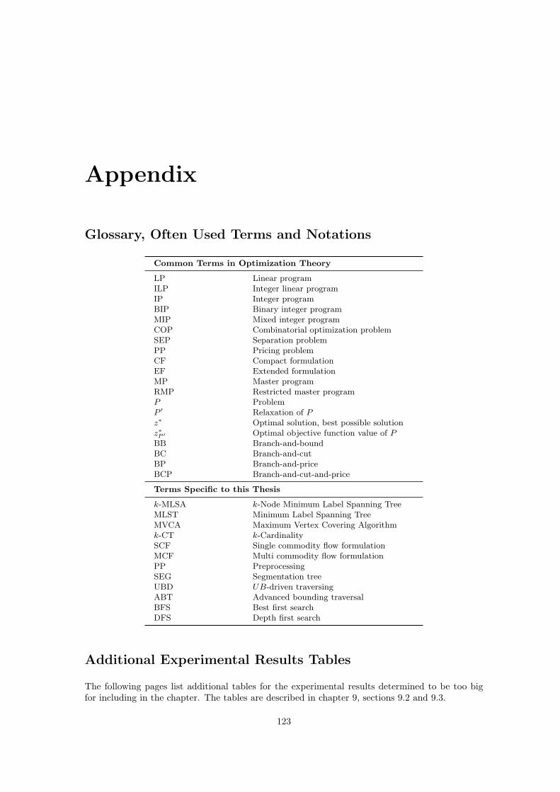
Appendix
Glossary, Often Used Terms and Notations
Common Terms in Optimization Theory
LP Linear programILP Integer linear programIP Integer programBIP Binary integer programMIP Mixed integer programCOP Combinatorial optimization problemSEP Separation problemPP Pricing problemCF Compact formulationEF Extended formulationMP Master programRMP Restricted master programP ProblemP ′ Relaxation of Pz∗ Optimal solution, best possible solutionz∗P ′ Optimal objective function value of PBB Branch-and-boundBC Branch-and-cutBP Branch-and-priceBCP Branch-and-cut-and-price
Terms Specific to this Thesis
k-MLSA k-Node Minimum Label Spanning TreeMLST Minimum Label Spanning TreeMVCA Maximum Vertex Covering Algorithmk-CT k-CardinalitySCF Single commodity flow formulationMCF Multi commodity flow formulationPP PreprocessingSEG Segmentation treeUBD UB-driven traversingABT Advanced bounding traversalBFS Best first searchDFS Depth first search
Additional Experimental Results Tables
The following pages list additional tables for the experimental results determined to be too bigfor including in the chapter. The tables are described in chapter 9, sections 9.2 and 9.3.
123
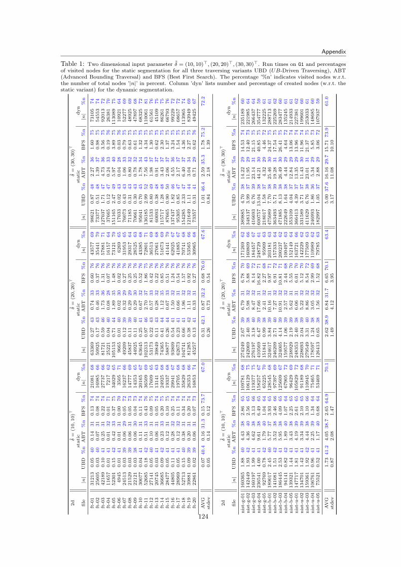
Appendix
Table 1: Two dimensional input parameter δ = (10, 10)>, (20, 20)>, (30, 30)>. Run times on G1 and percentagesof visited nodes for the static segmentation for all three traversing variants UBD (UB-Driven Traversing), ABT(Advanced Bounding Traversal) and BFS (Best First Search). The percentage ’%n’ indicates visited nodes w.r.t.the number of total nodes ’|n|’ in percent. Column ’dyn’ lists number and percentage of created nodes (w.r.t. thestatic variant) for the dynamic segmentation.
2d
δ=
(10,10)>
δ=
(20,20)>
δ=
(30,30)>
stati
cdyn
stati
cdyn
stati
cdyn
file
|n|
UB
D%
nA
BT
%n
BF
S%
n|n|
%n
|n|
UB
D%
nA
BT
%n
BF
S%
n|n|
%n
|n|
UB
D%
nA
BT
%n
BF
S%
n|n|
%n
ft-0
131213
0.0
540
0.1
431
0.1
374
21081
68
63369
0.2
743
0.7
433
0.6
076
43577
69
98621
0.8
748
2.2
736
1.6
075
73105
74
ft-0
225605
0.0
340
0.0
731
0.0
874
16985
66
50925
0.1
743
0.4
633
0.3
776
35441
70
73377
0.5
148
1.3
937
0.9
875
54553
74
ft-0
342189
0.1
041
0.2
531
0.2
274
27737
66
81721
0.5
946
1.7
336
1.3
176
57881
71
127037
1.7
147
4.7
336
3.5
675
92013
72
ft-0
411657
0.0
141
0.0
132
0.0
171
7217
62
25221
0.0
440
0.0
828
0.0
776
16157
64
37665
0.1
247
0.2
433
0.1
976
26381
70
ft-0
552301
0.1
542
0.4
233
0.3
775
34029
65
105153
0.7
144
1.8
935
1.4
876
73121
70
151165
2.4
749
5.9
740
3.8
975
113089
75
ft-0
64945
0.0
141
0.0
131
0.0
070
3505
71
9665
0.0
140
0.0
230
0.0
276
6269
65
17033
0.0
243
0.0
428
0.0
376
10921
64
ft-0
724513
0.0
339
0.0
629
0.0
572
16237
66
49209
0.1
239
0.3
229
0.2
776
31953
65
76073
0.4
343
1.0
633
0.7
975
52277
69
ft-0
821529
0.0
339
0.0
631
0.0
573
14777
69
45837
0.1
139
0.2
929
0.2
576
29317
64
71185
0.3
143
0.8
032
0.6
375
48925
69
ft-0
922121
0.0
338
0.0
630
0.0
473
14353
65
44925
0.1
140
0.2
930
0.2
576
28525
63
70661
0.3
043
0.7
832
0.6
175
47897
68
ft-1
030077
0.0
441
0.1
131
0.1
174
20165
67
63645
0.2
541
0.6
732
0.5
276
43385
68
95041
0.7
045
1.7
834
1.3
275
68325
72
ft-1
152685
0.1
842
0.5
133
0.4
376
36509
69
102313
0.9
746
2.7
037
1.8
675
72801
71
136185
2.9
952
7.5
643
4.3
475
110061
81
ft-1
227141
0.0
540
0.1
031
0.0
975
17609
65
53173
0.2
243
0.5
733
0.4
276
36513
69
81533
0.8
049
1.9
837
1.3
075
61561
76
ft-1
320745
0.0
341
0.0
631
0.0
574
13141
63
39849
0.1
143
0.2
832
0.2
276
27061
68
60093
0.3
848
0.9
137
0.6
275
45109
75
ft-1
436685
0.0
942
0.2
333
0.2
075
24925
68
74365
0.4
144
1.1
235
0.8
576
51673
69
115717
1.2
848
3.4
337
2.3
075
86261
75
ft-1
528477
0.0
541
0.1
231
0.1
075
19337
68
58877
0.2
644
0.6
733
0.5
176
41441
70
87665
0.9
050
2.0
637
1.3
775
66793
76
ft-1
644805
0.1
141
0.2
832
0.2
574
29941
67
93809
0.5
441
1.5
032
1.2
476
62925
67
137437
1.8
246
4.5
536
3.2
475
99229
72
ft-1
728969
0.0
541
0.1
232
0.1
174
19705
68
62673
0.2
341
0.6
631
0.5
476
41885
67
95305
0.8
547
2.1
737
1.5
475
68657
72
ft-1
852713
0.1
540
0.3
831
0.3
474
35829
68
104741
0.6
641
1.9
632
1.5
776
70741
68
154285
2.3
347
6.4
037
4.3
675
113965
74
ft-1
939881
0.0
939
0.2
031
0.2
074
26353
66
81285
0.3
842
1.1
132
0.9
276
53565
66
121649
1.1
144
3.0
434
2.2
775
83949
69
ft-2
022861
0.0
239
0.0
631
0.0
773
16853
74
45257
0.1
341
0.3
331
0.2
776
30965
68
73357
0.3
141
0.7
129
0.6
276
49425
67
AV
G0.0
740.4
0.1
631.3
0.1
573.7
67.0
0.3
142.1
0.8
732.2
0.6
876.0
67.6
1.0
146.4
2.5
935.3
1.7
875.2
72.2
stdev
0.0
50.1
40.1
20.2
60.7
30.5
40.8
42.1
81.3
9
2d
δ=
(10,10)>
δ=
(20,20)>
δ=
(30,30)>
stati
cdyn
stati
cdyn
stati
cdyn
file
|n|
UB
D%
nA
BT
%n
BF
S%
n|n|
%n
|n|
UB
D%
nA
BT
%n
BF
S%
n|n|
%n
|n|
UB
D%
nA
BT
%n
BF
S%
n|n|
%n
nis
t-g-0
1160365
1.8
840
4.4
338
2.8
665
109781
68
274249
2.6
739
6.7
931
6.7
870
171269
62
389885
4.7
038
14.2
229
14.5
374
235189
60
nis
t-g-0
2142449
1.9
342
4.3
640
2.5
665
106129
75
242069
2.4
038
5.9
832
5.8
869
160809
66
348137
3.9
937
11.9
529
12.4
073
221985
64
nis
t-g-0
3160197
1.9
941
4.6
238
3.1
366
119377
75
276197
3.1
840
8.4
732
8.1
472
184457
67
416693
6.7
639
23.1
431
21.1
575
266437
64
nis
t-g-0
4236541
4.0
041
9.6
138
6.4
965
158257
67
410569
6.4
739
17.6
631
16.8
271
248729
61
600757
13.0
438
44.2
130
40.8
575
354777
59
nis
t-g-0
592769
0.7
842
1.7
940
1.0
464
65225
70
151841
0.9
938
2.4
132
2.2
768
95909
63
218017
1.5
837
4.3
229
4.4
672
132225
61
nis
t-b-0
1189017
2.4
540
5.7
737
3.9
365
128545
68
324617
3.8
439
10.1
631
9.9
771
203181
63
475089
7.7
038
25.4
630
24.3
775
288713
61
nis
t-b-0
2141081
1.5
142
3.5
238
2.4
666
97397
69
246209
2.7
140
7.2
732
6.9
172
157333
64
363493
5.7
139
19.2
831
17.5
475
225269
62
nis
t-b-0
3186445
2.5
341
5.9
538
4.0
965
125609
67
324005
4.1
439
10.9
132
10.8
171
200237
62
471885
8.1
338
26.4
930
26.4
175
283477
60
nis
t-b-0
494141
0.8
242
1.8
940
1.0
764
67905
72
159577
1.0
639
2.5
732
2.4
468
100497
63
222649
1.6
438
4.4
429
4.6
472
135245
61
nis
t-b-0
5139321
1.4
441
3.4
338
2.2
565
96429
69
238929
2.1
939
5.6
231
5.5
570
152149
64
353109
4.0
437
12.8
429
13.0
674
214933
61
nis
t-u-0
1147717
1.8
141
4.1
939
2.6
165
105829
72
248353
2.4
038
6.0
631
6.0
170
163721
66
366413
4.3
937
13.3
529
13.9
674
227381
62
nis
t-u-0
2134701
1.4
241
3.3
439
2.1
065
91189
68
228693
2.0
439
5.2
232
5.1
270
142229
62
331589
3.7
137
11.4
330
11.9
674
199601
60
nis
t-u-0
3159361
1.9
242
4.4
438
3.1
066
110945
70
279549
3.3
140
8.8
632
8.5
472
177509
63
411629
6.7
638
23.0
131
21.3
775
253033
61
nis
t-u-0
4106761
0.9
641
2.2
539
1.3
464
75465
71
178597
1.2
438
3.0
532
2.9
969
110989
62
246993
1.8
636
5.3
429
5.8
573
148685
60
nis
t-u-0
575521
0.5
241
1.1
740
0.6
864
53469
71
126413
0.6
538
1.5
632
1.5
268
79785
63
182997
1.0
537
2.8
829
3.0
672
107937
59
AV
G1.7
341.2
4.0
538.7
2.6
564.9
70.1
2.6
238.9
6.8
431.7
6.6
570.1
63.4
5.0
037.6
16.1
629.7
15.7
173.9
61.0
stdev
0.8
72.0
81.4
71.4
94.1
23.9
53.1
711.0
810.1
0
124
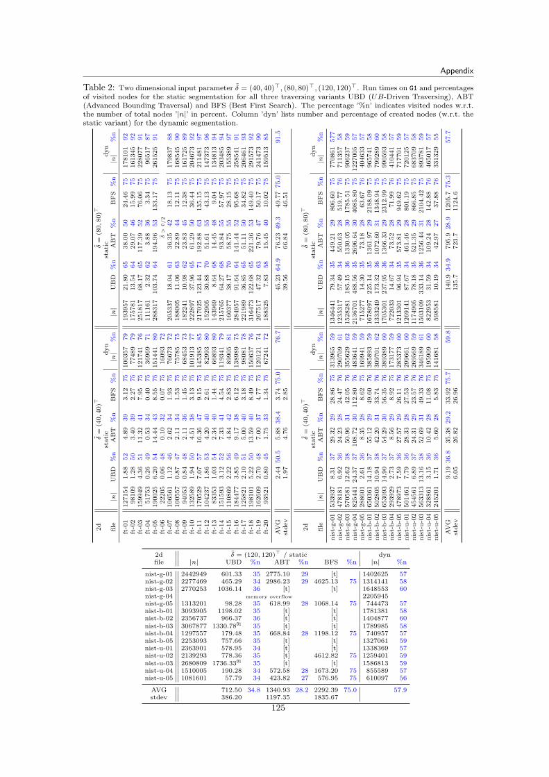
Appendix
Table 2: Two dimensional input parameter δ = (40, 40)>, (80, 80)>, (120, 120)>. Run times on G1 and percentagesof visited nodes for the static segmentation for all three traversing variants UBD (UB-Driven Traversing), ABT(Advanced Bounding Traversal) and BFS (Best First Search). The percentage ’%n’ indicates visited nodes w.r.t.the number of total nodes ’|n|’ in percent. Column ’dyn’ lists number and percentage of created nodes (w.r.t. thestatic variant) for the dynamic segmentation.
2d
δ=
(40,40)>
δ=
(80,80)>
stati
cdyn
stati
cdyn
file
|n|
UB
D%
nA
BT
%n
BF
S%
n|n|
%n
|n|
UB
D%
nA
BT
%n
BF
S%
n|n|
%n
ft-0
1127154
1.8
852
4.8
939
3.1
275
100357
79
193957
21.8
065
38.0
050
24.4
675
178101
92
ft-0
298109
1.2
850
3.4
039
2.2
775
77489
79
175781
13.5
464
29.0
746
15.9
975
161345
92
ft-0
3159949
4.3
651
11.3
241
7.9
575
121741
76
251817
68.1
765
117.3
952
76.0
675
228077
91
ft-0
451753
0.2
649
0.5
334
0.4
075
36969
71
111161
2.3
262
3.8
836
3.3
475
96517
87
ft-0
5190025
6.2
054
14.4
443
8.5
575
151441
80
288317
103.7
464
194.9
653
133.1
775
261525
91
ft-0
622205
0.0
648
0.1
032
0.0
775
16093
72
δ>v/2
ft-0
7106561
1.1
246
2.6
234
1.9
375
76673
72
205337
18.0
461
36.3
542
18.1
375
179837
88
ft-0
8100557
0.8
747
2.1
134
1.5
375
75785
75
188005
11.0
663
22.8
944
12.1
175
168545
90
ft-0
994053
0.8
448
2.1
136
1.4
575
68453
73
182241
10.9
862
23.8
345
12.3
875
161725
89
ft-1
0132589
1.9
450
4.5
138
3.1
375
101913
77
222897
37.9
665
61.2
950
36.4
475
204673
92
ft-1
1170529
7.0
757
16.3
647
9.1
575
145385
85
217025
123.4
471
192.8
863
135.1
575
211481
97
ft-1
2104237
1.8
653
4.2
040
2.6
175
82993
80
152905
30.8
870
51.6
155
43.1
375
147373
96
ft-1
383353
1.0
354
2.3
440
1.4
475
66893
80
143969
8.6
468
14.4
548
9.0
475
134813
94
ft-1
4151593
3.1
252
7.3
341
4.5
475
119341
79
215765
64.2
768
93.8
455
57.9
775
203485
94
ft-1
5110869
2.2
256
4.8
442
2.8
375
89905
81
160377
38.1
770
58.7
555
28.1
575
155389
97
ft-1
6184477
3.8
549
9.1
738
6.1
275
138989
75
284957
91.6
464
141.4
452
95.6
875
258541
91
ft-1
7125821
2.1
051
5.0
040
3.1
875
98081
78
221989
36.8
565
51.1
150
34.8
275
206461
93
ft-1
8198101
5.2
250
13.5
940
8.4
975
150637
76
316473
122.6
865
221.3
653
149.4
075
291573
92
ft-1
9162609
2.7
048
7.0
037
4.7
775
120121
74
267517
47.3
263
79.7
647
50.1
775
241473
90
ft-2
093521
0.8
045
1.7
533
1.3
475
67241
72
188325
7.8
358
15.4
540
10.0
275
159513
85
AV
G2.4
450.5
5.8
838.4
3.7
475.0
76.7
45.2
364.9
76.2
349.3
49.7
775.0
91.5
stdev
1.9
74.7
62.8
539.5
666.8
446.5
1
2d
δ=
(40,40)>
δ=
(80,80)>
stati
cdyn
stati
cdyn
file
|n|
UB
D%
nA
BT
%n
BF
S%
n|n|
%n
|n|
UB
D%
nA
BT
%n
BF
S%
n|n|
%n
nis
t-g-0
1533937
8.3
137
29.3
229
28.8
675
313965
59
1346441
79.3
435
449.2
129
806.6
075
770861
577
nis
t-g-0
2478181
6.9
236
24.2
328
24.4
776
290709
61
1235317
57.4
934
550.6
328
519.7
776
711357
58
nis
t-g-0
3570581
12.6
238
50.9
631
42.0
576
355629
62
1528281
185.1
536
1330.0
530
1785.5
175
906237
59
nis
t-g-0
4825441
24.3
737
108.7
230
112.8
076
483641
59
2136701
488.5
635
2696.6
430
4085.8
075
1227005
57
nis
t-g-0
5288601
2.6
136
8.3
528
8.6
275
169941
59
715277
14.3
035
73.1
828
63.6
776
404633
57
nis
t-b-0
1650361
14.1
837
55.1
229
49.6
076
385893
59
1678097
225.1
435
1361.9
729
2188.0
975
965741
58
nis
t-b-0
2502805
10.9
438
42.2
031
33.7
476
309701
62
1333249
173.3
236
1072.6
031
1348.9
475
799289
60
nis
t-b-0
3653093
14.9
037
54.2
930
56.3
576
389389
60
1705301
237.9
536
1366.3
329
2312.9
975
990593
58
nis
t-b-0
4293929
2.7
337
8.5
629
8.9
275
173177
59
722033
14.6
734
73.5
228
71.9
976
410441
57
nis
t-b-0
5478973
7.5
936
27.5
729
26.1
176
285373
60
1213301
96.9
435
573.8
129
949.6
275
717701
59
nis
t-u-0
1501461
7.7
936
28.3
328
27.5
376
299661
60
1269141
87.6
734
461.4
628
801.1
975
720125
57
nis
t-u-0
2454561
6.8
937
24.3
129
23.5
776
269569
59
1174905
78.1
835
521.3
529
866.8
575
683709
58
nis
t-u-0
3563313
13.1
638
52.6
931
49.3
376
346189
61
1503109
333.1
436
1256.4
431
2104.4
275
893781
59
nis
t-u-0
4328861
3.1
536
10.4
228
11.0
875
195909
60
822953
31.5
934
109.2
428
142.8
876
465017
57
nis
t-u-0
5245201
1.7
136
5.6
028
5.8
375
141681
58
598581
10.1
934
42.9
727
37.8
876
331329
55
AV
G9.1
936.8
35.3
829.2
33.9
275.7
59.8
140.9
34.9
795.9
28.9
1205.7
75.3
57.7
stdev
6.0
526.8
226.9
6135.7
723.7
1124.6
2d δ = (120, 120)> / static dynfile |n| UBD %n ABT %n BFS %n |n| %n
nist-g-01 2442949 601.33 35 2775.10 29 [t] 1402625 57nist-g-02 2277469 465.29 34 2986.23 29 4625.13 75 1314141 58nist-g-03 2770253 1036.14 36 [t] [t] 1648553 60nist-g-04 memory overflow 2205945nist-g-05 1313201 98.28 35 618.99 28 1068.14 75 744473 57nist-b-01 3093905 1198.02 35 [t] [t] 1781381 58nist-b-02 2356737 966.37 36 [t] [t] 1404877 60nist-b-03 3067877 1330.78O1 35 [t] [t] 1789985 58nist-b-04 1297557 179.48 35 668.84 28 1198.12 75 740957 57nist-b-05 2253093 757.66 35 [t] [t] 1327061 59nist-u-01 2363901 578.95 34 [t] [t] 1338369 57nist-u-02 2139293 778.36 35 [t] 4612.82 75 1259401 59nist-u-03 2680809 1736.33O1 35 [t] [t] 1586813 59nist-u-04 1510005 190.28 34 572.58 28 1673.20 75 855589 57nist-u-05 1081601 57.79 34 423.82 27 576.95 75 610097 56
AVG 712.50 34.8 1340.93 28.2 2292.39 75.0 57.9stdev 386.20 1197.35 1835.67
125
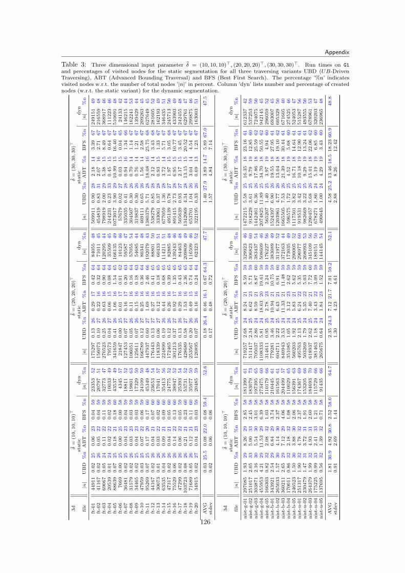
Appendix
Table 3: Three dimensional input parameter δ = (10, 10, 10)>, (20, 20, 20)>, (30, 30, 30)>. Run times on G1
and percentages of visited nodes for the static segmentation for all three traversing variants UBD (UB-DrivenTraversing), ABT (Advanced Bounding Traversal) and BFS (Best First Search). The percentage ’%n’ indicatesvisited nodes w.r.t. the number of total nodes ’|n|’ in percent. Column ’dyn’ lists number and percentage of creatednodes (w.r.t. the static variant) for the dynamic segmentation.
3d
δ=
(10,10,10)>
δ=
(20,20,20)>
δ=
(30,30,30)>
stati
cdyn
stati
cdyn
stati
cdyn
file
|n|
UB
D%
nA
BT
%n
BF
S%
n|n|
%n
|n|
UB
D%
nA
BT
%n
BF
S%
n|n|
%n
|n|
UB
D%
nA
BT
%n
BF
S%
n|n|
%n
ft-0
144911
0.0
225
0.0
623
0.0
459
23353
52
175297
0.1
326
0.2
917
0.4
264
84055
48
509911
0.9
028
2.1
814
3.3
967
249151
49
ft-0
241167
0.0
226
0.0
522
0.0
459
20797
51
156073
0.1
027
0.2
216
0.3
264
71011
45
454819
0.8
331
2.0
716
2.7
167
216559
48
ft-0
369067
0.0
524
0.1
122
0.1
159
32773
47
270523
0.2
526
0.6
316
0.9
064
120295
44
798919
2.0
029
5.3
815
8.4
967
368917
46
ft-0
420539
0.0
124
0.0
222
0.0
259
10033
49
79573
0.0
427
0.0
615
0.0
864
35509
45
244231
0.2
333
0.4
515
0.6
467
111223
46
ft-0
588639
0.0
725
0.1
821
0.1
860
43537
49
341659
0.4
126
1.0
616
1.5
465
166135
49
1073017
3.9
029
10.9
915
16.4
067
510691
48
ft-0
67669
0.0
025
0.0
025
0.0
058
4345
57
21847
0.0
025
0.0
117
0.0
162
10123
46
57679
0.0
227
0.0
315
0.0
465
24133
42
ft-0
736481
0.0
225
0.0
423
0.0
459
18811
52
127453
0.0
727
0.1
617
0.2
063
59587
47
335035
0.4
128
0.9
416
1.3
466
146215
44
ft-0
831579
0.0
226
0.0
323
0.0
359
19801
63
106051
0.0
526
0.1
116
0.1
664
57055
54
304507
0.3
026
0.7
014
1.1
467
162241
53
ft-0
934465
0.0
225
0.0
423
0.0
359
17329
50
125611
0.0
726
0.1
516
0.1
863
54685
44
319837
0.3
026
0.7
614
1.2
167
139429
44
ft-1
047959
0.0
325
0.0
722
0.0
659
24109
50
166789
0.1
227
0.2
516
0.3
664
80341
48
469111
0.6
526
1.5
614
2.5
867
209263
45
ft-1
195269
0.0
725
0.1
720
0.1
760
45349
48
447937
0.6
027
1.6
916
2.4
666
192079
43
1380379
5.7
128
18.0
816
25.7
568
627649
45
ft-1
244167
0.0
226
0.0
421
0.0
760
23653
54
176443
0.1
327
0.2
716
0.4
165
88801
50
538279
0.8
528
2.1
214
3.4
368
281605
52
ft-1
330073
0.0
126
0.0
322
0.0
260
17041
57
118339
0.0
627
0.1
215
0.1
865
60433
51
333061
0.3
728
0.9
315
1.3
367
162193
49
ft-1
463535
0.0
426
0.0
921
0.0
960
35413
56
224899
0.1
926
0.4
416
0.6
865
114211
51
677059
1.3
628
3.7
214
5.7
167
346435
51
ft-1
547317
0.0
226
0.0
421
0.0
560
24775
52
172465
0.1
226
0.2
616
0.3
965
82885
48
495139
0.7
827
1.9
715
3.0
568
245713
50
ft-1
675529
0.0
626
0.1
422
0.1
360
38947
52
301213
0.3
727
0.9
217
1.3
565
139243
46
891415
2.7
328
6.9
515
10.7
767
433903
49
ft-1
747299
0.0
226
0.0
622
0.0
559
25393
54
176335
0.1
326
0.2
916
0.4
365
84463
48
505639
0.9
327
2.1
715
3.4
567
242455
48
ft-1
8103723
0.0
826
0.2
121
0.2
360
53731
52
428689
0.5
827
1.5
316
2.3
665
209809
49
1342069
4.3
428
13.1
515
20.5
267
629761
47
ft-1
971689
0.0
526
0.1
221
0.1
160
35977
50
253567
0.2
026
0.4
915
0.7
464
116509
46
653701
1.0
426
3.0
414
4.5
467
299875
46
ft-2
034915
0.0
227
0.0
423
0.0
359
20485
59
120895
0.0
726
0.1
616
0.2
464
62323
52
322195
0.3
326
0.6
913
1.2
367
163003
51
AV
G0.0
325.5
0.0
822.0
0.0
859.4
52.6
0.1
826.4
0.4
616.1
0.6
764.3
47.7
1.4
027.9
3.8
914.7
5.8
967.0
47.5
stdev
0.0
20.0
60.0
60.1
70.4
80.7
21.5
74.8
47.1
4
3d
δ=
(10,10,10)>
δ=
(20,20,20)>
δ=
(30,30,30)>
stati
cdyn
stati
cdyn
stati
cdyn
file
|n|
UB
D%
nA
BT
%n
BF
S%
n|n|
%n
|n|
UB
D%
nA
BT
%n
BF
S%
n|n|
%n
|n|
UB
D%
nA
BT
%n
BF
S%
n|n|
%n
nis
t-g-0
1297085
1.9
329
8.2
629
2.8
558
181399
61
719257
2.6
824
8.2
421
8.5
959
329923
46
1472215
5.5
825
16.3
518
23.1
661
612337
42
nis
t-g-0
2251017
2.0
533
5.0
033
2.4
558
183079
73
511417
2.3
425
6.6
223
5.7
159
306823
60
918229
3.6
125
9.7
919
12.8
560
537253
59
nis
t-g-0
3303871
2.1
630
5.5
430
3.0
158
197395
65
705037
2.8
624
8.5
921
8.8
760
383437
54
1442461
6.3
626
17.8
618
25.5
962
724075
50
nis
t-g-0
4455953
4.2
129
11.5
329
6.3
958
273475
60
1108333
5.8
124
18.6
320
19.6
159
508609
46
2074825
11.8
925
34.7
018
50.5
562
942145
45
nis
t-g-0
5166303
0.8
232
2.0
832
1.0
358
110179
66
314611
0.9
525
2.7
823
2.2
459
176227
56
565207
1.4
025
3.9
719
4.9
460
296059
52
nis
t-b-0
1343921
2.5
429
6.8
429
3.7
458
210445
61
779281
3.4
624
10.9
421
10.7
559
383089
49
1524397
6.9
026
19.5
518
27.9
561
693007
45
nis
t-b-0
2265033
1.5
730
4.1
430
2.3
758
161563
61
604711
2.2
225
6.4
321
6.9
160
311977
52
1203961
4.7
726
13.0
418
19.1
062
605329
50
nis
t-b-0
3360211
2.6
529
7.1
229
4.0
658
204499
57
840943
3.5
324
11.3
321
11.4
859
372163
44
1665505
7.5
326
21.3
918
30.4
461
671605
40
nis
t-b-0
4170011
0.8
632
2.1
832
1.0
858
110029
65
351085
1.0
524
3.1
223
2.6
259
173035
49
596575
1.7
225
4.5
219
5.6
860
274525
46
nis
t-b-0
5246523
1.5
030
3.8
830
2.0
658
156391
63
560203
1.9
224
5.8
321
5.6
259
290005
52
1117501
3.8
225
16.7
118
14.6
461
524053
47
nis
t-u-0
1251317
1.9
032
4.7
832
2.3
758
174367
69
495763
2.1
325
6.2
422
5.3
559
296977
60
919531
3.4
225
10.1
819
12.9
061
515287
56
nis
t-u-0
2230479
1.4
731
3.7
231
1.9
158
153205
66
503269
1.7
924
5.3
522
5.0
359
268093
53
982669
3.2
225
9.2
919
13.2
461
493555
50
nis
t-u-0
3264379
1.9
932
4.9
331
2.6
058
184693
70
618937
2.6
225
7.4
021
7.7
260
345109
56
1290457
5.6
826
15.0
118
22.0
662
678961
53
nis
t-u-0
4175225
0.9
933
2.4
133
1.2
158
115729
66
381463
1.1
824
3.4
322
3.0
959
189151
50
678271
1.8
624
5.1
919
6.8
560
320203
47
nis
t-u-0
5137695
0.5
632
1.3
932
0.7
158
91435
66
265675
0.6
424
1.8
423
1.5
259
144145
54
490645
1.0
024
4.2
919
3.4
360
236965
48
AV
G1.8
130.9
4.9
230.8
2.5
258.0
64.7
2.3
524.3
7.1
221.7
7.0
159.2
52.1
4.5
825.2
13.4
618.5
18.2
360.9
48.8
stdev
0.9
12.6
91.4
41.3
04.2
34.6
12.8
88.2
612.4
2
126
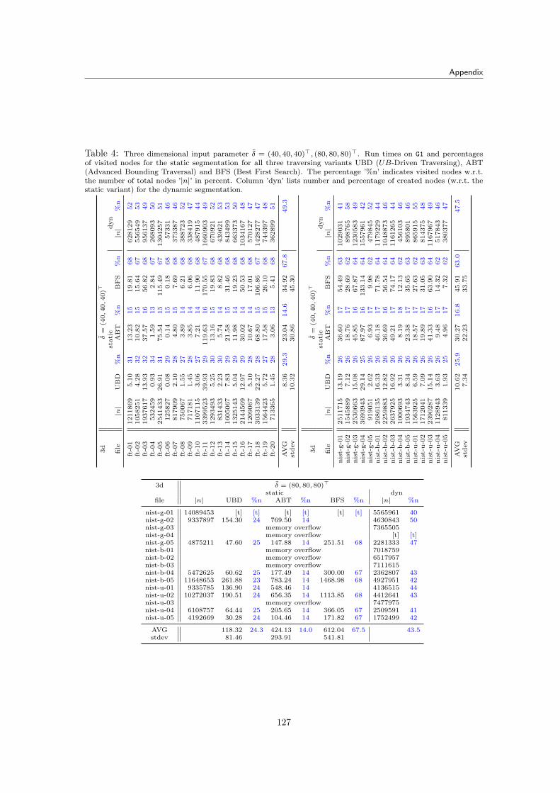
Appendix
Table 4: Three dimensional input parameter δ = (40, 40, 40)>, (80, 80, 80)>. Run times on G1 and percentagesof visited nodes for the static segmentation for all three traversing variants UBD (UB-Driven Traversing), ABT(Advanced Bounding Traversal) and BFS (Best First Search). The percentage ’%n’ indicates visited nodes w.r.t.the number of total nodes ’|n|’ in percent. Column ’dyn’ lists number and percentage of created nodes (w.r.t. thestatic variant) for the dynamic segmentation.
3d
δ=
(40,40,40)>
stati
cdyn
file
|n|
UB
D%
nA
BT
%n
BF
S%
n|n|
%n
ft-0
11211869
5.1
031
13.2
315
19.8
168
628129
52
ft-0
21058251
4.2
832
10.8
215
15.6
467
556549
53
ft-0
31937617
13.9
332
37.5
716
56.8
268
956137
49
ft-0
4532459
0.9
334
1.5
913
2.8
467
268093
50
ft-0
52541433
26.9
131
75.5
415
115.4
967
1304257
51
ft-0
6125827
0.0
829
0.1
415
0.1
868
57331
46
ft-0
7817909
2.1
028
4.8
015
7.6
968
373387
46
ft-0
8750067
1.5
527
3.8
914
6.2
168
388723
52
ft-0
9717181
1.4
528
3.8
514
6.0
668
338419
47
ft-1
01107115
3.0
627
7.2
114
11.9
068
487915
44
ft-1
13399523
39.9
329
119.6
316
170.5
567
1660903
49
ft-1
21293493
5.2
530
13.1
615
19.8
368
670921
52
ft-1
3831433
2.2
330
5.7
414
8.8
268
439621
53
ft-1
41605067
7.8
329
21.5
815
31.4
668
843499
53
ft-1
51325143
5.0
429
11.9
814
19.2
368
663373
50
ft-1
62144569
12.9
729
30.0
214
50.5
368
1034167
48
ft-1
71209067
5.1
028
10.6
714
17.0
168
570127
47
ft-1
83033139
22.2
728
68.8
015
106.8
667
1428277
47
ft-1
91564423
5.7
227
17.5
815
26.1
068
744397
48
ft-2
0713365
1.4
528
3.0
613
5.4
168
362899
51
AV
G8.3
629.3
23.0
414.6
34.9
267.8
49.3
stdev
10.3
230.8
645.3
0
3d
δ=
(40,40,40)>
stati
cdyn
file
|n|
UB
D%
nA
BT
%n
BF
S%
n|n|
%n
nis
t-g-0
12511715
13.1
926
36.6
017
54.4
963
1029031
41
nis
t-g-0
21545889
7.1
226
18.7
617
28.6
962
898765
58
nis
t-g-0
32530663
15.0
826
45.8
516
67.8
764
1230583
49
nis
t-g-0
43693943
29.1
425
87.9
716
133.1
464
1557961
42
nis
t-g-0
5919051
2.6
226
6.9
317
9.9
862
479845
52
nis
t-b-0
12686135
16.3
326
46.1
817
71.7
864
1179229
44
nis
t-b-0
22259883
12.8
226
36.6
916
56.5
464
1048873
46
nis
t-b-0
32637925
16.9
226
49.2
117
74.1
764
1161265
44
nis
t-b-0
41000693
3.3
126
8.1
918
12.1
362
456103
46
nis
t-b-0
51934743
8.3
426
23.3
817
35.6
563
895801
46
nis
t-u-0
11563925
6.5
926
18.5
717
27.6
362
865915
55
nis
t-u-0
21712041
7.0
926
19.8
917
31.0
563
814375
48
nis
t-u-0
32390287
15.1
426
41.3
316
63.9
064
1167967
49
nis
t-u-0
41128943
3.6
326
9.4
817
14.3
262
517843
46
nis
t-u-0
5811339
1.9
325
4.9
617
7.3
262
380377
47
AV
G10.6
225.9
30.2
716.8
45.9
163.0
47.5
stdev
7.3
422.2
333.7
5
3d δ = (80, 80, 80)>
static dynfile |n| UBD %n ABT %n BFS %n |n| %n
nist-g-01 14089453 [t] [t] [t] [t] [t] [t] 5565961 40nist-g-02 9337897 154.30 24 769.50 14 4630843 50nist-g-03 memory overflow 7365505nist-g-04 memory overflow [t] [t]nist-g-05 4875211 47.60 25 147.88 14 251.51 68 2281333 47nist-b-01 memory overflow 7018759nist-b-02 memory overflow 6517957nist-b-03 memory overflow 7111615nist-b-04 5472625 60.62 25 177.49 14 300.00 67 2362807 43nist-b-05 11648653 261.88 23 783.24 14 1468.98 68 4927951 42nist-u-01 9335785 136.90 24 548.46 14 4136515 44nist-u-02 10272037 190.51 24 656.35 14 1113.85 68 4412641 43nist-u-03 memory overflow 7477975nist-u-04 6108757 64.44 25 205.65 14 366.05 67 2509591 41nist-u-05 4192669 30.28 24 104.46 14 171.82 67 1752499 42
AVG 118.32 24.3 424.13 14.0 612.04 67.5 43.5stdev 81.46 293.91 541.81
127
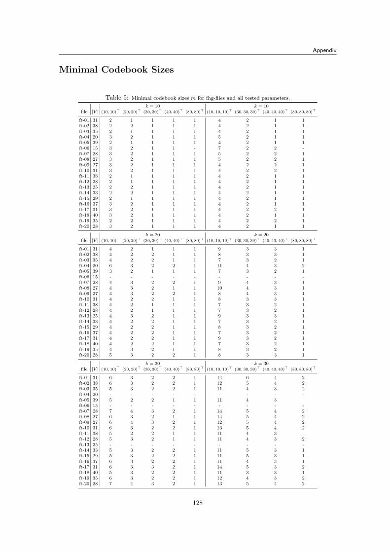
Appendix
Minimal Codebook Sizes
Table 5: Minimal codebook sizes m for fhg-files and all tested parameters.
k = 10 k = 10file |V | (10, 10)> (20, 20)> (30, 30)> (40, 40)> (80, 80)> (10, 10, 10)> (30, 30, 30)> (40, 40, 40)> (80, 80, 80)>
ft-01 31 2 1 1 1 1 4 2 1 1ft-02 38 2 2 1 1 1 4 2 1 1ft-03 35 2 1 1 1 1 4 2 1 1ft-04 20 3 2 1 1 1 5 2 1 1ft-05 39 2 1 1 1 1 4 2 1 1ft-06 15 3 2 1 1 - 7 2 2 -ft-07 28 3 2 1 1 1 5 2 2 1ft-08 27 3 2 1 1 1 5 2 2 1ft-09 27 3 2 1 1 1 4 2 2 1ft-10 31 3 2 1 1 1 4 2 2 1ft-11 38 2 1 1 1 1 4 2 1 1ft-12 28 2 1 1 1 1 4 2 1 1ft-13 25 2 2 1 1 1 4 2 1 1ft-14 33 2 2 1 1 1 4 2 1 1ft-15 29 2 1 1 1 1 4 2 1 1ft-16 37 3 2 1 1 1 4 2 1 1ft-17 31 3 2 1 1 1 4 2 2 1ft-18 40 3 2 1 1 1 4 2 1 1ft-19 35 2 2 1 1 1 4 2 2 1ft-20 28 3 2 1 1 1 4 2 1 1
k = 20 k = 20file |V | (10, 10)> (20, 20)> (30, 30)> (40, 40)> (80, 80)> (10, 10, 10)> (30, 30, 30)> (40, 40, 40)> (80, 80, 80)>
ft-01 31 4 2 1 1 1 9 3 3 1ft-02 38 4 2 2 1 1 8 3 3 1ft-03 35 4 2 2 1 1 7 3 2 1ft-04 20 6 3 2 2 1 11 4 3 2ft-05 39 3 2 1 1 1 7 3 2 1ft-06 15 - - - - - - - - -ft-07 28 4 3 2 2 1 9 4 3 1ft-08 27 4 3 2 1 1 10 4 3 1ft-09 27 4 3 2 2 1 8 4 3 1ft-10 31 4 2 2 1 1 8 3 3 1ft-11 38 4 2 1 1 1 7 3 2 1ft-12 28 4 2 1 1 1 7 3 2 1ft-13 25 4 3 2 1 1 9 3 3 1ft-14 33 4 2 2 1 1 7 3 2 1ft-15 29 4 2 2 1 1 8 3 2 1ft-16 37 4 2 2 1 1 7 3 2 1ft-17 31 4 2 2 1 1 9 3 2 1ft-18 40 4 2 2 1 1 7 3 2 1ft-19 35 4 3 2 1 1 8 3 2 1ft-20 28 5 3 2 2 1 8 3 3 1
k = 30 k = 30file |V | (10, 10)> (20, 20)> (30, 30)> (40, 40)> (80, 80)> (10, 10, 10)> (30, 30, 30)> (40, 40, 40)> (80, 80, 80)>
ft-01 31 6 3 2 2 1 14 6 4 2ft-02 38 6 3 2 2 1 12 5 4 2ft-03 35 5 3 2 2 1 11 4 3 2ft-04 20 - - - - - - - - -ft-05 39 5 2 2 1 1 11 4 3ft-06 15 - - - - - - - - -ft-07 28 7 4 3 2 1 14 5 4 2ft-08 27 6 3 2 1 1 14 5 4 2ft-09 27 6 4 3 2 1 12 5 4 2ft-10 31 6 3 2 2 1 13 5 4 2ft-11 38 5 2 2 1 1 11 4 3ft-12 28 5 3 2 1 1 11 4 3 2ft-13 25 - - - - - - - - -ft-14 33 5 3 2 2 1 11 5 3 1ft-15 29 5 3 2 2 1 11 5 3 1ft-16 37 6 3 2 2 1 11 4 3 1ft-17 31 6 3 3 2 1 14 5 3 2ft-18 40 5 3 2 2 1 11 3 3 1ft-19 35 6 3 2 2 1 12 4 3 2ft-20 28 7 4 3 2 1 13 5 4 2
128
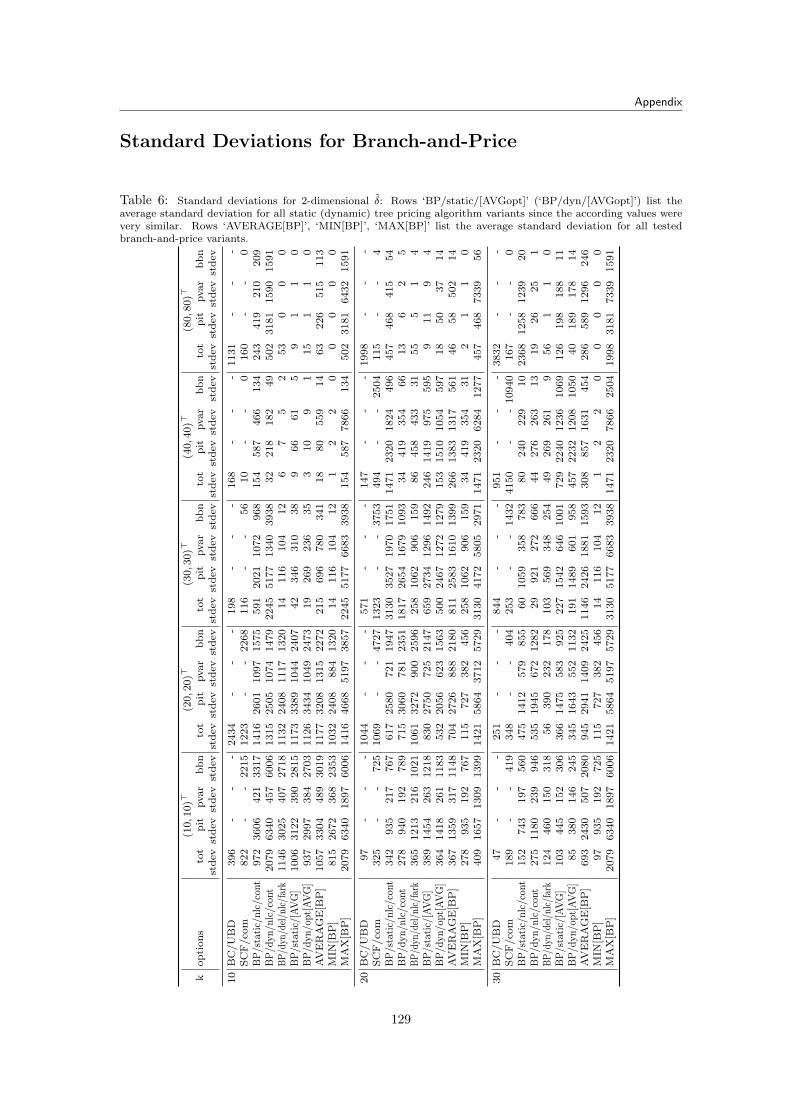
Appendix
Standard Deviations for Branch-and-Price
Table 6: Standard deviations for 2-dimensional δ: Rows ‘BP/static/[AVGopt]’ (‘BP/dyn/[AVGopt]’) list theaverage standard deviation for all static (dynamic) tree pricing algorithm variants since the according values werevery similar. Rows ‘AVERAGE[BP]’, ‘MIN[BP]’, ‘MAX[BP]’ list the average standard deviation for all testedbranch-and-price variants.
(10,1
0)>
(20,2
0)>
(30,3
0)>
(40,4
0)>
(80,8
0)>
kop
tion
sto
tp
itpvar
bb
nto
tp
itpvar
bb
nto
tp
itpvar
bb
nto
tp
itpvar
bb
nto
tp
itpvar
bb
nst
dev
std
evst
dev
std
evst
dev
std
evst
dev
std
evst
dev
std
evst
dev
std
evst
dev
std
evst
dev
std
evst
dev
std
evst
dev
std
ev
10
BC
/U
BD
396
--
-2434
--
-198
--
-168
--
-1131
--
-S
CF
/co
m822
--
2215
1223
--
2268
116
--
56
10
--
0160
--
0B
P/s
tati
c/n
lc/c
ont
972
3606
421
3317
1416
2601
1097
1575
591
2021
1072
968
154
587
466
134
243
419
210
209
BP
/dyn
/nlc
/con
t2079
6340
457
6006
1315
2505
1074
1479
2245
5177
1340
3938
32
218
182
49
502
3181
1590
1591
BP
/dyn
/del
/nlc
/far
k1146
3025
407
2718
1132
2408
1117
1320
14
116
104
12
67
52
53
00
0B
P/s
tati
c/[A
VG
]1006
3122
390
2815
1173
3389
1044
2407
42
346
310
38
966
61
59
11
0B
P/d
yn
/op
t[A
VG
]937
2997
384
2703
1126
3434
1049
2473
19
269
236
35
310
91
15
11
0A
VE
RA
GE
[BP
]1057
3304
489
3019
1177
3208
1315
2272
215
696
780
341
18
80
559
14
63
226
515
113
MIN
[BP
]815
2672
368
2353
1032
2408
884
1320
14
116
104
12
12
20
00
00
MA
X[B
P]
2079
6340
1897
6006
1416
4668
5197
3857
2245
5177
6683
3938
154
587
7866
134
502
3181
6432
1591
20
BC
/U
BD
97
--
-1044
--
-571
--
-147
--
-1998
--
-S
CF
/co
m325
--
725
1069
--
4727
1323
--
3753
494
--
2504
115
--
4B
P/s
tati
c/n
lc/c
ont
342
935
217
767
617
2580
721
1947
3130
3527
1970
1751
1471
2320
1824
496
457
468
415
54
BP
/dyn
/nlc
/con
t278
940
192
789
715
3060
781
2351
1817
2654
1679
1093
34
419
354
66
13
62
5B
P/d
yn/d
el/n
lc/f
ark
365
1213
216
1021
1061
3272
900
2596
258
1062
906
159
86
458
433
31
55
51
4B
P/s
tati
c/[A
VG
]389
1454
263
1218
830
2750
725
2147
659
2734
1296
1492
246
1419
975
595
911
94
BP
/dyn
/op
t[A
VG
]364
1418
261
1183
532
2056
623
1563
500
2467
1272
1279
153
1510
1054
597
18
50
37
14
AV
ER
AG
E[B
P]
367
1359
317
1148
704
2726
888
2180
811
2583
1610
1399
266
1383
1317
561
46
58
502
14
MIN
[BP
]278
935
192
767
115
727
382
456
258
1062
906
159
34
419
354
31
21
10
MA
X[B
P]
409
1657
1309
1399
1421
5864
3712
5729
3130
4172
5805
2971
1471
2320
6284
1277
457
468
7339
56
30
BC
/U
BD
47
--
-251
--
-844
--
-951
--
-3832
--
-S
CF
/co
m189
--
419
348
--
404
253
--
1432
4150
--
10940
167
--
0B
P/s
tati
c/n
lc/c
ont
152
743
197
560
475
1412
579
855
60
1059
358
783
80
240
229
10
2368
1258
1239
20
BP
/dyn
/nlc
/con
t275
1180
239
946
535
1945
672
1282
29
921
272
666
44
276
263
13
19
26
25
1B
P/d
yn/d
el/n
lc/f
ark
124
460
150
318
56
390
232
178
103
569
348
254
49
269
261
956
11
0B
P/s
tati
c/[A
VG
]103
445
152
306
366
1475
583
925
227
1542
646
1001
729
2240
1236
1069
126
198
188
11
BP
/dyn
/op
t[A
VG
]85
380
146
245
345
1643
552
1132
191
1489
601
958
457
2232
1208
1050
40
189
178
14
AV
ER
AG
E[B
P]
693
2430
507
2080
945
2941
1409
2425
1146
2426
1881
1593
308
857
1631
454
286
589
1296
246
MIN
[BP
]97
935
192
725
115
727
382
456
14
116
104
12
12
20
00
00
MA
X[B
P]
2079
6340
1897
6006
1421
5864
5197
5729
3130
5177
6683
3938
1471
2320
7866
2504
1998
3181
7339
1591
129
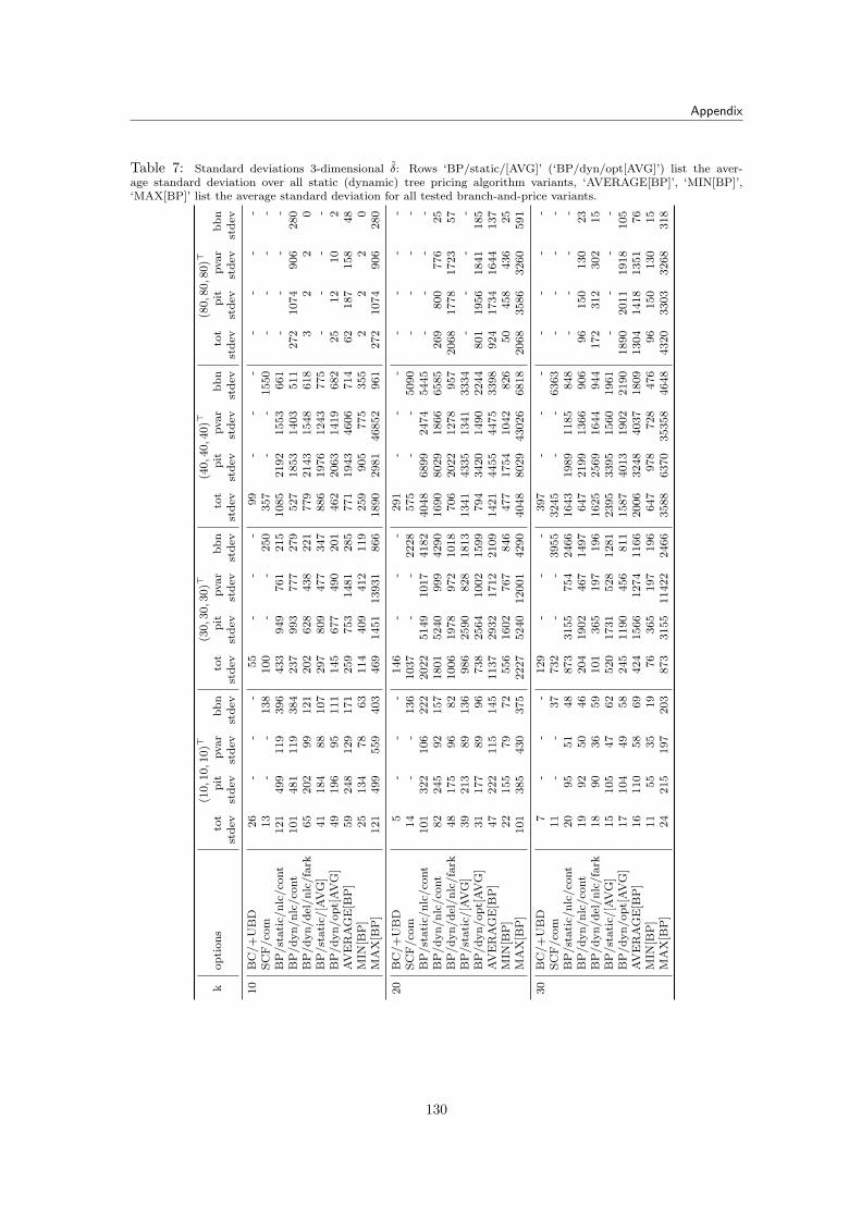
Appendix
Table 7: Standard deviations 3-dimensional δ: Rows ‘BP/static/[AVG]’ (‘BP/dyn/opt[AVG]’) list the aver-age standard deviation over all static (dynamic) tree pricing algorithm variants, ‘AVERAGE[BP]’, ‘MIN[BP]’,‘MAX[BP]’ list the average standard deviation for all tested branch-and-price variants.
(10,1
0,1
0)>
(30,3
0,3
0)>
(40,4
0,4
0)>
(80,8
0,8
0)>
kop
tion
sto
tp
itpvar
bb
nto
tp
itpvar
bb
nto
tp
itpvar
bb
nto
tp
itpvar
bb
nst
dev
std
evst
dev
std
evst
dev
std
evst
dev
std
evst
dev
std
evst
dev
std
evst
dev
std
evst
dev
std
ev
10
BC
/+
UB
D26
--
-55
--
-99
--
--
--
-S
CF
/co
m13
--
138
100
--
250
357
--
1550
--
--
BP
/st
ati
c/n
lc/co
nt
121
499
119
396
433
949
761
215
1085
2192
1553
661
--
--
BP
/d
yn
/n
lc/co
nt
101
481
119
384
237
993
777
279
527
1853
1403
511
272
1074
906
280
BP
/d
yn
/d
el/n
lc/fa
rk65
202
99
121
202
628
438
221
779
2143
1548
618
32
20
BP
/st
ati
c/[A
VG
]41
184
88
107
297
809
477
347
886
1976
1243
775
--
--
BP
/d
yn
/op
t[A
VG
]49
196
95
111
145
677
490
201
462
2063
1419
682
25
12
10
2A
VE
RA
GE
[BP
]59
248
129
171
259
753
1481
285
771
1943
4606
714
62
187
158
48
MIN
[BP
]25
134
78
63
114
409
412
119
259
905
775
355
22
20
MA
X[B
P]
121
499
559
403
469
1451
13931
866
1890
2981
46852
961
272
1074
906
280
20
BC
/+
UB
D5
--
-146
--
-291
--
--
--
-S
CF
/co
m14
--
136
1037
--
2228
575
--
5090
--
--
BP
/st
ati
c/n
lc/co
nt
101
322
106
222
2022
5149
1017
4182
4048
6899
2474
5445
--
--
BP
/d
yn
/n
lc/co
nt
82
245
92
157
1801
5240
999
4290
1690
8029
1866
6585
269
800
776
25
BP
/d
yn
/d
el/n
lc/fa
rk48
175
96
82
1006
1978
972
1018
706
2022
1278
957
2068
1778
1723
57
BP
/st
ati
c/[A
VG
]39
213
89
136
986
2590
828
1813
1341
4335
1341
3334
--
--
BP
/d
yn
/op
t[A
VG
]31
177
89
96
738
2564
1002
1599
794
3420
1490
2244
801
1956
1841
185
AV
ER
AG
E[B
P]
47
222
115
145
1137
2932
1712
2109
1421
4455
4475
3398
924
1734
1644
137
MIN
[BP
]22
155
79
72
556
1602
767
846
477
1754
1042
826
50
458
436
25
MA
X[B
P]
101
385
430
375
2227
5240
12001
4290
4048
8029
43026
6818
2068
3586
3260
591
30
BC
/+
UB
D7
--
-129
--
-397
--
--
--
-S
CF
/co
m11
--
37
732
--
3955
3245
--
6363
--
--
BP
/st
ati
c/n
lc/co
nt
20
95
51
48
873
3155
754
2466
1643
1989
1185
848
--
--
BP
/d
yn
/n
lc/co
nt
19
92
50
46
204
1902
467
1497
647
2199
1366
906
96
150
130
23
BP
/d
yn
/d
el/n
lc/fa
rk18
90
36
59
101
365
197
196
1625
2569
1644
944
172
312
302
15
BP
/st
ati
c/[A
VG
]15
105
47
62
520
1731
528
1281
2395
3395
1560
1961
--
--
BP
/d
yn
/op
t[A
VG
]17
104
49
58
245
1190
456
811
1587
4013
1902
2190
1890
2011
1918
105
AV
ER
AG
E[B
P]
16
110
58
69
424
1566
1274
1166
2006
3248
4037
1809
1304
1418
1351
76
MIN
[BP
]11
55
35
19
76
365
197
196
647
978
728
476
96
150
130
15
MA
X[B
P]
24
215
197
203
873
3155
11422
2466
3588
6370
35358
4648
4320
3303
3268
318
130
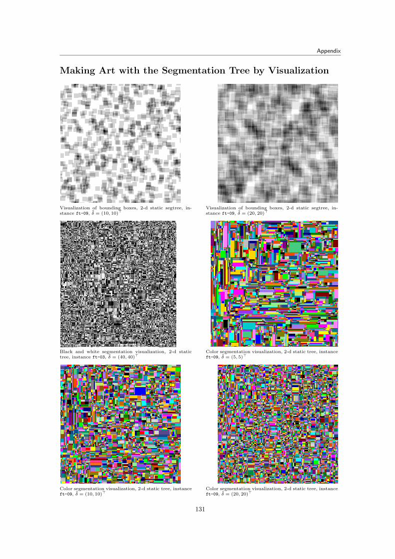
Appendix
Making Art with the Segmentation Tree by Visualization
Visualization of bounding boxes, 2-d static segtree, in-stance ft-09, δ = (10, 10)>
Visualization of bounding boxes, 2-d static segtree, in-stance ft-09, δ = (20, 20)>
Black and white segmentation visualization, 2-d statictree, instance ft-03, δ = (40, 40)>
Color segmentation visualization, 2-d static tree, instanceft-09, δ = (5, 5)>
Color segmentation visualization, 2-d static tree, instanceft-09, δ = (10, 10)>
Color segmentation visualization, 2-d static tree, instanceft-09, δ = (20, 20)>
131
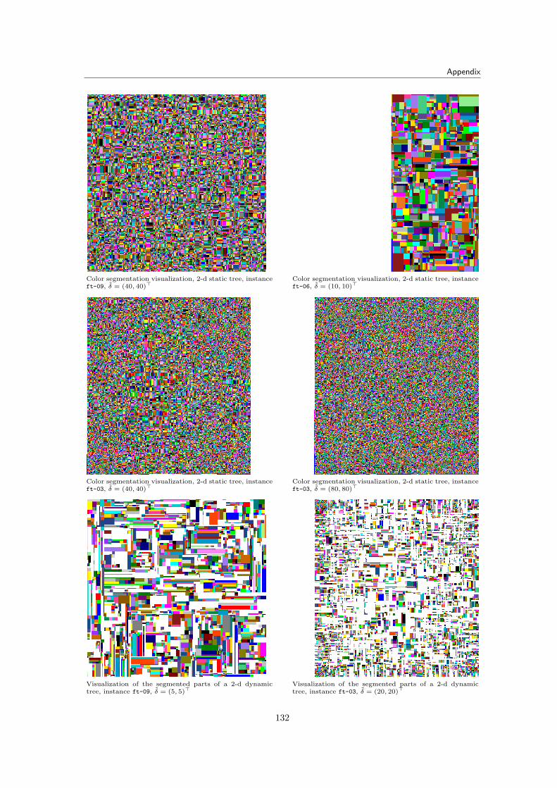
Appendix
Color segmentation visualization, 2-d static tree, instanceft-09, δ = (40, 40)>
Color segmentation visualization, 2-d static tree, instanceft-06, δ = (10, 10)>
Color segmentation visualization, 2-d static tree, instanceft-03, δ = (40, 40)>
Color segmentation visualization, 2-d static tree, instanceft-03, δ = (80, 80)>
Visualization of the segmented parts of a 2-d dynamictree, instance ft-09, δ = (5, 5)>
Visualization of the segmented parts of a 2-d dynamictree, instance ft-03, δ = (20, 20)>
132
List of Algorithms
2.1 Recursive-Insert-k-d-Tree(P,Q ) [Bentley75] . . . . . . . . . . . . . . . . . . . . . . . 142.2 Recursive-Search-k-d-Tree(P,Q ) [Bentley75] . . . . . . . . . . . . . . . . . . . . . . 143.1 Cutting Plane Algorithm . . . . . . . . . . . . . . . . . . . . . . . . . . . . . . . . . 243.2 Column Generation (LP version) . . . . . . . . . . . . . . . . . . . . . . . . . . . . . 265.1 Branch-and-Price(f , δ, d, k) . . . . . . . . . . . . . . . . . . . . . . . . . . . . . . . 506.1 StaticSegmentation(V , δ). . . . . . . . . . . . . . . . . . . . . . . . . . . . . . . . . . 576.2 StaticInsert(Ri, n) . . . . . . . . . . . . . . . . . . . . . . . . . . . . . . . . . . . . . 636.3 StaticAppendNodes(Ri, n, p) . . . . . . . . . . . . . . . . . . . . . . . . . . . . . . . 646.4 StaticTreeSearch-τ∗(n) . . . . . . . . . . . . . . . . . . . . . . . . . . . . . . . . . . 656.5 DynamicInsertAndSearch-τ∗(n) . . . . . . . . . . . . . . . . . . . . . . . . . . . . . 696.6 DynamicInsertNode(Ri, n) . . . . . . . . . . . . . . . . . . . . . . . . . . . . . . . . 706.7 DynamicAppendNodes(Region Ri, Node n, coordinate p) . . . . . . . . . . . . . . . 706.8 StaticPricer(uij , [µj ]) . . . . . . . . . . . . . . . . . . . . . . . . . . . . . . . . . . . 736.9 DynamicPricer(uij , [µj ]) . . . . . . . . . . . . . . . . . . . . . . . . . . . . . . . . . . 737.1 TraverseBFS(Node n) . . . . . . . . . . . . . . . . . . . . . . . . . . . . . . . . . . . 797.2 UB-DrivenTraversing(Node n) . . . . . . . . . . . . . . . . . . . . . . . . . . . . . . 807.3 AdvBoundingTraversal(Node n) . . . . . . . . . . . . . . . . . . . . . . . . . . . . . 827.4 DynamicSearch-T c(Node n) . . . . . . . . . . . . . . . . . . . . . . . . . . . . . . . . 83
133

List of Algorithms
134
List of Figures
1.1 Fingerprint minutiae in dactyloscopy. . . . . . . . . . . . . . . . . . . . . . . . . . . . 31.2 Encoding of points via a directed spanning tree using a codebook of template arcs, cor-
rection vectors are neglected. Image credits to [ChwRai09]. . . . . . . . . . . . . . . . . 51.3 Outline of correction vector encoding. Image credits to [ChwRai09]. . . . . . . . . . . . 6
2.1 Figure 2.1b shows an optimal MLST, determined from the labeled graph in figure 2.1a.
Figure 2.1c is a possible Label Spanning Tree (LST). Images adopted from [XiGolWas05]. 102.2 Construction of a balanced 2-d tree. The rounding median depends on the implementation.
Here the median is round-up. . . . . . . . . . . . . . . . . . . . . . . . . . . . . . . . 132.3 Balanced 2-d tree resulting from the construction steps in figure 2.2. . . . . . . . . . . . 13
3.1 Duality Gap between largest primal and smallest dual value. Image credits to [Van98]. . . 183.2 Example of a geometric interpretation. . . . . . . . . . . . . . . . . . . . . . . . . . . 193.3 Figures 3.3a - 3.3c show contour lines of a logarithmic barrier function for three values for
the pace parameter µ. The maximum value lies inside the innermost level set. Figure 3.3d
depicts the central path. Image credits to [Van98]. . . . . . . . . . . . . . . . . . . . . . 213.4 Rounding is not always a good idea in IP’s and BIP’s: The IP solution is far away from
the rounded values. Image credits to [Wol98], page 4. . . . . . . . . . . . . . . . . . . . 223.5 Branching Strategies for IP’s. Image credits to [Wol98], page 193. . . . . . . . . . . . . 233.6 Column generation flowchart. . . . . . . . . . . . . . . . . . . . . . . . . . . . . . . . 273.7 Example schemes of block diagonal matrices, shaded areas indicate nonzero elements [Luebbe01]. 283.8 “Information flow between master program and subproblem(s).” Image credits to [Luebbe01]. 313.9 “The depicted development of the objective function value is typical for the tailing off
effect.” Image credits to [Luebbe01]. . . . . . . . . . . . . . . . . . . . . . . . . . . . . 34
4.1 “The big gray dots are three of the possible representants for the tree arcs b1, . . . , b7, but
the standard template arc τ is the lower left point of the shaded rectangle. The rectangles
depict the δ domain.” Image credits to [ChwRai09]. . . . . . . . . . . . . . . . . . . . . 39
5.1 Single commodity flow network in an arborescence. . . . . . . . . . . . . . . . . . . . . 435.2 Correlation of tree arcs a and template arcs t (labels). When taking one of the template
arcs t0, t2 or t4, we get a spanning tree, whereby t1 forms a cycle and hence no spanning
tree. Also t3 forms no spanning tree. . . . . . . . . . . . . . . . . . . . . . . . . . . . 45
6.1 Segmentation of a sequence of points bi. Figures 6.2 and 6.3 show the corresponding trees. 526.2 Segmentation tree after inserting b1, b2. A left son ∼= left, below; right son ∼= right, above. 536.3 Segmentation tree after insertion of b7. A left son ∼= left, below; right son ∼= right, above. 536.4 A standard template arc τ for the segmentation in figure 6.1b. . . . . . . . . . . . . . . 546.5 The operations ⊂, ⊆, <, ≤ and split. . . . . . . . . . . . . . . . . . . . . . . . . . . . 566.6 Partially negative regions and their transformation to the working domain. Regions R1A
and R2A are regular, the other are modulo transformed into domain D. . . . . . . . . . . 586.7 Simple segmentation of node difference b1. The figure shows four splits ς, two at p
(1)0 and
two at p(1)
2d−1. The resulting segmentation tree is depicted in figure 6.8. . . . . . . . . . . 59
135
List of Figures
6.8 Segmentation tree after insertion of b1. . . . . . . . . . . . . . . . . . . . . . . . . . . 596.9 The reason, why null subspaces have to be inserted. How, in figure 6.9b, should ς6′ , ς6′′ be
segmented and the dimension sequence retained? Figure 6.9c shows the correct segmen-
tation by inserting a null subspace ς5NULL . . . . . . . . . . . . . . . . . . . . . . . . . 606.10 Figure 6.10a) shows the insertion of b2, overlaps at splits ς1 and ς4 take place. Figure 6.10b)
shows the segmentation of b2: Since R2 is located on both sides of ς1, the algorithm splits
R2 into two subregions R′2 = 〈p′0, p(2)3 〉 and R′′2 = 〈p(2)
0 , p′3〉, and inserts them recursively
into the left and right subtree respectively. First, the algorithm descends left with R′2and encounters an overlap again at ς4. Again R′2 is split up into 〈p′′0 , p(2)
3 〉 and 〈p′0, p′3〉,which are re-inserted recursively. These two subregions as well as R′′2 are further simply
segmented. Figure 6.11) shows the resulting segmentation tree with bounds after insertion
of b2. . . . . . . . . . . . . . . . . . . . . . . . . . . . . . . . . . . . . . . . . . . . . 616.11 Segmentation tree with bounds after insertion of b2. . . . . . . . . . . . . . . . . . . . . 626.12 Rectangles show the regions that the node differences b1 and b2 define. If we arrive at
node encoding subspace RD and determine a part of R2 to be inserted here, we crop the
bounding box to the subspace by R′2 = RD ∩ R2. The resulting R′2 is marked by two red
dots. At node containing RD, we insert only this part R′2. . . . . . . . . . . . . . . . . 676.13 Some cases of overlaps. In figure 6.13a, the case for b4 is interesting since it reaches into
the node subspace R2 again across the domain border. Parts of subspace b5 reach into
even more node subspaces. When having big δ such overlaps occur very often. All other
cases are trivial. Figure 6.13b shows a specific example of a possible next split. The figure
shows the segmentation after insertion of b1. The region for b3 will be inserted next. The
next split is drawn in red. . . . . . . . . . . . . . . . . . . . . . . . . . . . . . . . . . 726.14 Dynamic segmentation tree resulting from 6.13b. . . . . . . . . . . . . . . . . . . . . . 72
7.1 Illustration for example 1a and 1b depicting some bound sets in the segmentation tree. . 777.2 Illustration for example 2 depicting some domain crossing regions in 7.2a and correspond-
ing segmentation tree in 7.2b. . . . . . . . . . . . . . . . . . . . . . . . . . . . . . . . 78
8.1 Class diagram for the parts concerning segmentation and traversing. . . . . . . . . . . . 888.2 Class diagram for the parts concerning branch-and-price. . . . . . . . . . . . . . . . . . 88
9.1 Growth rates of static tree building time, distinguished by dimensionality of δ as well as
by data set (fhg and nist). . . . . . . . . . . . . . . . . . . . . . . . . . . . . . . . . . 969.2 Averages percentage of visited nodes for the static UBD, ABT and BFS. Created nodes
percentage (OPT) in a dynamic tree in relation to the minimal number of nodes for
determining T c, when visiting branches containing an element from T c only once. . . . . 979.3 Fhg, nist instances running times for each traversing strategy, including the dynamic tree
for 2– and 3-dimensional δ. On the left side we used a linear scale, on the right side a
logarithmic scale in order to make visible the differences for run times with small δ. . . . 999.4 Performance of selected options for the static tree pricing algorithm, figures 9.4a, 9.4b in
the first row show the average over k, figures 9.4c, 9.4d in the second row the average over δ.1059.5 Performance of selected options for the dynamic tree pricing algorithm, figures 9.5a, 9.5b
in the first row show the average over k, figures 9.5c, 9.5d in the second row the average
over δ. . . . . . . . . . . . . . . . . . . . . . . . . . . . . . . . . . . . . . . . . . . . 1079.6 Average run times, completed instances, pricing data for ‘BC’ and the best branch-and-
price variants ‘BP/static/nlc/fark’ (abbreviated by ‘BP/static*’) and ‘BP/dyn/nlc/fark’
(abbreviated by ‘BP/dyn*’). Run time averages over δ, k. . . . . . . . . . . . . . . . . 114
136
List of Tables
3.1 Survey to discretization an convexification. Image credits to [Luebbe01] . . . . . . . . . 30
9.1 Fraunhofer Institute and NIST sample minutiae data files. Column ‘|V |’ shows the number
of contained minutiae data points, ‘|B|‘ the number of resulting node differences. . . . . 909.2 Precomputed files, containing candidate template arcs (T c) determined by the preprocess-
ing from [ChwRai09]. . . . . . . . . . . . . . . . . . . . . . . . . . . . . . . . . . . . 909.3 Two dimensional δ = (10, 10)>, (20, 20)>, (30, 30)>: The building (‘b[s]’), traversing (‘t[s]’)
and total (‘tot[s]’) run times (on G1) of the best static tree traversing strategy UBD
(UB-driven Traversing) compared to the total run times of the dynamic segmentation
(‘dyn/tot[s]’). The run times (on O1) of the preprocessing from [ChwRai09] is listed in col-
umn ‘PP’. Column ‘|T c|’ shows the extracted (and correct) number of candidate template
arcs by all three strategies. . . . . . . . . . . . . . . . . . . . . . . . . . . . . . . . . . 929.4 Two dimensional δ = (40, 40)>, (80, 80)>, (120, 120)>: The building (‘b[s]’), traversing
(‘t[s]’) and total (‘tot[s]’) run times (on G1) of the best static tree traversing strategy UBD
(UB-Driven Traversing) compared to the total run times of the dynamic segmentation
(‘dyn/tot[s]’). The run times (on O1) of the preprocessing from [ChwRai09] is listed in col-
umn ‘PP’. Column ‘|T c|’ shows the extracted (and correct) number of candidate template
arcs by all three strategies. . . . . . . . . . . . . . . . . . . . . . . . . . . . . . . . . . 939.5 Three dimensional δ = (10, 10, 10)>, (20, 20, 20)>, (30, 30, 30)>: The building (‘b[s]’), travers-
ing (‘t[s]’) and total (‘tot[s]’) run times (on G1) of the best static tree traversing strategy
UBD (UB-Driven Traversing) compared to the total run times of the dynamic segmenta-
tion (‘dyn/tot[s]’). The run times (on O1) of the preprocessing from [ChwRai09] are listed
in column ‘PP’. Column ‘|T c|’ shows the extracted (and correct) number of candidate
template arcs by all three strategies. . . . . . . . . . . . . . . . . . . . . . . . . . . . . 949.6 Three dimensional δ = (40, 40, 40)>, (80, 80, 80)>: The building (‘b[s]’), traversing (‘t[s]’)
and total (‘tot[s]’) run times (on G1) of the best static tree traversing strategy UBD
(UB-Driven Traversing) compared to the total run times of the dynamic segmentation
(‘dyn/tot[s]’). The run times (on O1) of the preprocessing from [ChwRai09] is listed in col-
umn ‘PP’. Column ‘|T c|’ shows the extracted (and correct) number of candidate template
arcs by all three strategies. . . . . . . . . . . . . . . . . . . . . . . . . . . . . . . . . . 959.7 Average traversing times for fhg and nist files. . . . . . . . . . . . . . . . . . . . . . . . 989.8 Percentage of run time in comparison to the preprocessing by [ChwRai09]. . . . . . . . . 989.9 Average run times (‘AVG t[s]’) for fhg, nist data when simulating the pricing problem with
random values and 100, 1000 pricing iterations (‘pit’). Tests run on a single processor
mobile machine L1. . . . . . . . . . . . . . . . . . . . . . . . . . . . . . . . . . . . . . 1009.10 Average initialization times in seconds for static tree pricing algorithms, 2-dimensional δ. 1049.11 Average algorithm run time (column ‘alg[s]’), total run time (column ‘tot[s]’), pricing
iterations (column ‘pit’), priced variables (column ‘pvar’) and branch-and-bound nodes
(column ‘bbn’). Parameter δ 2-dimensional. Rows description in sections 9.3.2–9.3.5. . . 1089.12 Average algorithm run time (column ‘alg[s]’), total run time (column ‘tot[s]’), pricing
iterations (column ‘pit’), priced variables (column ‘pvar’) and branch-and-bound nodes
(column ‘bbn’). Parameter δ 2-dimensional. Rows description in sections 9.3.2–9.3.5. . . 109
137
List of Tables
9.13 Average algorithm run time (column ‘alg[s]’), total run time (column ‘tot[s]’), pricing
iterations (column ‘pit’), priced variables (column ‘pvar’) and branch-and-bound nodes
(column ‘bbn’). Parameter δ 3-dimensional. Rows description in sections 9.3.2–9.3.5. . . 1109.14 Average algorithm run time (column ‘alg[s]’), total run time (column ‘tot[s]’), pricing
iterations (column ‘pit’), priced variables (column ‘pvar’) and branch-and-bound nodes
(column ‘bbn’). Parameter δ 3-dimensional. Rows description in sections 9.3.2–9.3.5. . . 1119.15 Averages over k, δ for the tested algorithms branch-and-cut (row ‘BC’), SCF and MCF
solved entirely (rows ‘SCF/com’ and ‘MCF/com’), branch-and-price using a static tree
pricing algorithm (all rows ‘BP/static’) and a dynamic tree pricing algorithm (rows ‘BP/dyn’).1129.16 A comparison for the average size of set T c, the set of non-dominated template arcs, with
the average amount of priced variables ‘pvar’ for each tested variant. . . . . . . . . . . . 1159.17 Branch-and-price results for nist data and varying k, δ. Columns ‘alg[s]’, ‘tot[s]’, ‘pit’,
‘pvar’ and ‘bbn’ list average algorithm run time and average total run time (including
Farkas priced starting solution) in seconds, average amount of pricing iterations, priced
variables, branch-and-bound nodes. . . . . . . . . . . . . . . . . . . . . . . . . . . . . 116
1 Two dimensional input parameter δ = (10, 10)>, (20, 20)>, (30, 30)>. Run times on G1 and per-
centages of visited nodes for the static segmentation for all three traversing variants UBD (UB-
Driven Traversing), ABT (Advanced Bounding Traversal) and BFS (Best First Search). The
percentage ’%n’ indicates visited nodes w.r.t. the number of total nodes ’|n|’ in percent. Column
’dyn’ lists number and percentage of created nodes (w.r.t. the static variant) for the dynamic
segmentation. . . . . . . . . . . . . . . . . . . . . . . . . . . . . . . . . . . . . . . . . 1242 Two dimensional input parameter δ = (40, 40)>, (80, 80)>, (120, 120)>. Run times on G1 and
percentages of visited nodes for the static segmentation for all three traversing variants UBD
(UB-Driven Traversing), ABT (Advanced Bounding Traversal) and BFS (Best First Search). The
percentage ’%n’ indicates visited nodes w.r.t. the number of total nodes ’|n|’ in percent. Column
’dyn’ lists number and percentage of created nodes (w.r.t. the static variant) for the dynamic
segmentation. . . . . . . . . . . . . . . . . . . . . . . . . . . . . . . . . . . . . . . . . 1253 Three dimensional input parameter δ = (10, 10, 10)>, (20, 20, 20)>, (30, 30, 30)>. Run times on G1
and percentages of visited nodes for the static segmentation for all three traversing variants UBD
(UB-Driven Traversing), ABT (Advanced Bounding Traversal) and BFS (Best First Search). The
percentage ’%n’ indicates visited nodes w.r.t. the number of total nodes ’|n|’ in percent. Column
’dyn’ lists number and percentage of created nodes (w.r.t. the static variant) for the dynamic
segmentation. . . . . . . . . . . . . . . . . . . . . . . . . . . . . . . . . . . . . . . . . 1264 Three dimensional input parameter δ = (40, 40, 40)>, (80, 80, 80)>. Run times on G1 and percent-
ages of visited nodes for the static segmentation for all three traversing variants UBD (UB-Driven
Traversing), ABT (Advanced Bounding Traversal) and BFS (Best First Search). The percentage
’%n’ indicates visited nodes w.r.t. the number of total nodes ’|n|’ in percent. Column ’dyn’ lists
number and percentage of created nodes (w.r.t. the static variant) for the dynamic segmentation. 1275 Minimal codebook sizes m for fhg-files and all tested parameters. . . . . . . . . . . . . . . . 1286 Standard deviations for 2-dimensional δ: Rows ‘BP/static/[AVGopt]’ (‘BP/dyn/[AVGopt]’) list
the average standard deviation for all static (dynamic) tree pricing algorithm variants since the
according values were very similar. Rows ‘AVERAGE[BP]’, ‘MIN[BP]’, ‘MAX[BP]’ list the average
standard deviation for all tested branch-and-price variants. . . . . . . . . . . . . . . . . . . 1297 Standard deviations 3-dimensional δ: Rows ‘BP/static/[AVG]’ (‘BP/dyn/opt[AVG]’) list the aver-
age standard deviation over all static (dynamic) tree pricing algorithm variants, ‘AVERAGE[BP]’,
‘MIN[BP]’, ‘MAX[BP]’ list the average standard deviation for all tested branch-and-price variants. 130
138
Bibliography
[Jain08] Jain, Anil K. [Hrsg.]; Flynn, Patrick; Ross, Arun A. (Eds.): Handbook of biometrics, NewYork, NY : Springer Science + Business Media, (2008). ISBN: 978-0-387-71040-2.
[Heum06] Heumann, Bjorn: Whitepaper Biometrie, http://www.biometrie-online.de, http://www.heumann-webdesign.de/pages/biometrie/Whitepaper_Biometrie.pdf, (2006).
[BasSchu05] Basler, Georg; Schutt, Andreas: Fingerabdrucksysteme, Humboldt Uni-versitat, Institut fur Informatik, http://www2.informatik.hu-berlin.de/Forschung_Lehre/algorithmenII/Lehre/SS2004/Biometrie/04Fingerprint/fingerabdrucksysteme.pdf, Technical Report, (2005).
[MalJai05] Maltoni, Davide; Jain, Anil K.; Maio, Dario; Prabhakar, Salil: Handbook of fingerprintrecognition, Edition 2, New York, NY [u.a.], Springer, (2005). ISBN 0-387-95431-7.
[JaRoPr01] Jain, Anil K.; Ross, Arun; Prabhakar, Salil: Fingerprint Matching using minutiaeand texture features In: International Conference on Image Processing (ICIP), pp. 282-285,(2001).
[webWong] Wong, Kevin: Fingerprint identification,http://www.lems.brown.edu/vision/courses/computer-vision-2002/projects/Wong/mid.htm, (2002).
[Seitz05] Seitz, Juergen: Digital Watermarking for Digital Media, Hershey, Pa. : InformationScience Publ., (2005). ISBN 1-591-40518-1.
[Fraun08] Mediensicherheit, http://watermarking.sit.fraunhofer.de, (Februar 2008).
[Sayood06] Sayood, K.: Introduction to Data Compression, 3rd edition, Morgan Kaufmann Pub-lishers Inc., San Mateo, (2006).
[ChwRai09] Chwatal, Andreas M.; Raidl, Gunther R.; Oberlechner, Karin: Solving a k-Node Min-imum Label Spanning Arborescence Problem to Compress Fingerprint Templates, In: Journalof Mathematical Modelling and Algorithms (JMMA), Springer Netherlands, Vol. 8, No. 3,pp. 293-334, (August 2009).
[ChwRai07] Chwatal, Andreas M.; Raidl, Gunther R.: Applying branch-and-cut for compressingfingerprint templates, short abstract, In: Proceedingsof the European Conference on Opera-tional Research (EURO) XXII, Prague, (2007).
[RaiChw07] Raidl, Gunther; Chwatal, Andreas: Fingerprint Template Compression by Solvinga Minimum Label k-Node Subtree Problem, In: Simos, E. (editor), Numerical Analysis andApplied Mathematics, AIP Conference Proceedings, Vol. 936, pp. 444-447. American Instituteof Physics, New York, (2007).
[ChwMIC07] Chwatal, Andreas M.; Raidl, Gunther R.; Dietzel, Olivia: Compressing FingerprintTemplates by Solving an Extended Minimum Label Spanning Tree Problem, In: Proceedings ofMIC 2007, the 7th Metaheuristics International Conference, pp. 105/1-3, Montreal, Canada,(2007).
139
Bibliography
[Dietzel08] Dietzel, Olivia: Combinatorial Optimization for the Compression of Biometric Tem-plates, Master’s thesis, Vienna University of Technology, Institute for Computer Graphicsand Algorithms, Supervised by G. Raidl and A. Chwatal, (May 2008).
[SalAdh01] Saleh, A.; Adhami, R.: Curvature-based matching approach for automatic fingerprintidentification, In: Proceedings of the Southeastern Symposium on System Theory, pp. 171175,(2001).
[CormLei07] Cormen, Th. H.; Leiserson, Ch. E. (Editors); Rivest, R.; Stein, C.: Algorithmen -Eine Einfuhrung, 2. Auflage, Oldenbourg, Munchen, Wien, (2007). ISBN: 978-3-486-58262-8.
[CormLei01] Cormen, Th. H.; Leiserson, Ch. E. (Editors); Rivest, R.; Stein, C.: Introduction toAlgorithms, 2nd edition, MIT Press, Cambridge, (2001). ISBN: 0-07-013151-1.
[Sedgew01] Sedgewick, Robert: Algorithms in C, 3rd edition, Addison-Wesley Professional,(2001).
[Math99] Stocker, Prof. Dr. Horst (Hrsg.): Taschenbuch mathematischer Formeln und modernerVerfahren, 4., korrigierte Auflage, Verlag Harri Deutsch, Frankfurt am Main, Thun, (1999).
[webCaldwell05] Caldwell, Chris K.: Graph Theory Tutorials,http://www.utm.edu/departments/math/graph/, (2005).
[Evans78] Evans, James R.: On equivalent representations of certain multicommodity networks assingle commodity flow problems, Springer Berlin / Heidelberg, Mathematical Programming,Vol. 15, No. 1, pp. 92-99, (December 1978).
[Ev78] Evans, J.: A single commodity transform for certain multi commodity networks, OperationsResearch, Vol. 26, No. 4, pp. 673-680, (1978).
[Bentley75] Bentley, Jon Louis: Multidimensional Binary Search Trees Used for AssociativeSearching, Communications of the ACM, Vol. 18, No. 9, pp. 509-517, (September 1975).
[webGraphAlgo] Emden-Weinert, Thomas; Hougardy, Stefan; Kreuter, Bernd; Promel, HansJurgen; Steger, Angelika: Einfuhrung in Graphen und Algorithmen, http://www2.informatik.hu-berlin.de/alkox/lehre/skripte/ga/, Online Skriptum von MatroidsMatheplanet, (1996).
[ChiKa08] Chimani, M.; Kandyba, M.; Ljubic I.; Mutzel, P.: Obtaining Optimal k-Cardinality Trees Fast, Proceedings of Workshop on Algorithm Engineering and Experiments(ALENEX’08), San Francisco, (2008). http://ls11-www.cs.uni-dortmund.de/people/kandyba/kcard.html.
[ChLe97] Chang, Ruay-Shiung; Leu, Shing-Jiuan: The Minimum Labeling Spanning Trees, In:Information Processing Letters Vol. 63, No. 5, pp. 277-282, (1997).
[Kru98] Krumke, Sven O.; Wirth, Hans Christoph: On The Minimum Label Spanning Tree Prob-lem, In: Information Processing Letters, Vol. 66, No. 2, pp. 81-85, (1998).
[XiGolWas05] Xiong, Yupei; Golden, Bruce; Wasil, Edward: A One-Parameter Genetic Algorithmfor the Minimum Labeling Spanning Tree Problem, In: IEEE Transactions on EvolutionaryComputation, Vol. 9, No. 1, pp. 55-60, (February 2005).
[Xioung05] Xiong, Yupei: The Minimum Label Spanning Tree Problem and some Variants, Dis-sertation, Faculty of the Graduate School of the University of Maryland, (2005).
[Cons06] Consoli, S.; Moreno Jose, A.; Mladenovic, N.; Darby-Dowman, K.: Constructive Heuris-tics for the Minimum Labelling Spanning Tree Problem: a preliminary comparison, DEIOCTechnical Report, September 2006.
140
Bibliography
[XiGolWas06] Xiong, Yupei; Golden, Bruce; Wasil, Edward: The Minimum Label Spanning TreeProblem: Some Genetic Algorithm Approaches, Lunteren Conference on the Mathematics ofOperations Research, The Netherlands, (January 2006).
[Wol98] Wolsey, Laurence A.: Integer Programming, New York, NY, Wiley, John Wiley & Sons,Chichester, (1998). ISBN: 978-0-471-28366-9.
[Van98] Vanderbei, Robert J.: Linear Programming: Foundations and extensions, Boston, Mass.,Kluver, (1998). ISBN: 0-7923-8141-6.
[webDesSoum98] Desrosiers, Jacques; Soumis, Franois: Column Generation, http://www.gerad.ca/~gencol/gceng.html, http://www.gerad.ca/~gencol/Column/, Team GENeration deCOLonnes, Various Universities, Online since 1998.
[BoydVan04] Boyd, Stephen; Vandenberghe, Lieven: Convex Optimization, Cambridge Univ.Press, (2004). ISBN: 0-521-83378-7.
[DesLu05] Lubbecke, Marco E.; Desrosiers, Jacques: Selected Topics in Column Generation, In:Operations Research, Vol 53, pp. 1007-1023, (November, December 2005).
[Luebbe01] Lubbecke, Marco; Zimmermann, Prof. Dr. Uwe T.; Desrosiers, Prof. Dr. Jacques;Fekete, Prof. Dr. Sandor P.: Engine Scheduling by Column Generation, Dissertation, Fach-bereich f ur Mathematik und Informatik der Technischen Universitat Braunschweig, (Juli2001).
[VanWol96] Vanderbeck, Francois; Wolsey, Laurence A.: An Exact Algorithm for IP ColumnGeneration, Elsevier Science, Operations Research Letters, Vol. 19, Iss. 4, pp. 151 - 159,(November 1996).
[GuzRal07] Guzelsoy, Menal; Ralphs, Ted K.: Duality for Mixed-Integer Linear Programs, Tech-nical Report, COR@L Lab, Industrial and Systems Engineering, Lehigh University, (2007).
[webTrick97] Trick, Michael A.: A Tutorial on Integer Programming, http://mat.gsia.cmu.edu/orclass/integer/integer.html, (1998).
[Vanbk94] Vanderbeck, Francois; (Wolsey, L.A.): Decomposition and Column Generation for In-teger Programs, PhD Thesis, Universite catholique de Louvain (UCL), http://www.math.u-bordeaux.fr/~fv/publications.html, (1994).
[NemWol88] Wolsey, Laurence A., Nemhauser, George L.: Integer and Combinatorial Optimiza-tion Wiley, New York, (1988).
[Schrij99] Schrijver, Alexander: Theory of Linear and Integer Programming, Wiley InterscienceSeries in Discrete Mathematics and Optimization, Chichester, (1999).
[AvKa04] Avis, David; Kaluzny, Bohdan: Solving Inequalities and Proving Farkass Lemma MadeEasy, Amer. Math. Monthly, The Mathematical Association of America, Vol. 111, No. 2, pp.152-157. (2004).
[MacPlLi03] Maculan, Nelson; Plateau, Gerard; Lisser, Abdel: Integer Linear Models with a Poly-nomial Number of Variables and Constraints for some Classical Combinatorial OptimizationProblems, Pesquisa Operacional, Vol. 23, No. 1, pp. 161-168, (2003).
[MagWol94] Magnanti, Thomas L.; Wolsey Laurence A.: Optimal Trees, Handbooks in OperationsResearch and Management Science, Volume entitled Networks, OR 209-94, (1994).
[CaClPa09] Captivo M. Eugnia; Clmaco, Joo C.N.; Pascoal, Marta M.B.; A mixed integer linearformulation for the minimum label spanning tree problem Computers & Operations Research36, pp. 3082–3085, (2009).
141
Bibliography
[Schwa08] Schwarz, Cornelius: An Introduction to SCIP, Univerity of Bayreuth, http://scip.zib.de/download/files/scip_intro_01.pdf (2008).
[Pfe07] Pfetsch, Marc: Introduction to SCIP, DFG Research Center Matheion and Zuse In-stitute Berlin, SCIP Workshop 2007, Berlin, http://scip.zib.de/download/slides/SCIP-introduction.pdf (2007).
[Ber07] Berthold, Timo: Primal Heuristics in SCIP, DFG Research Center Matheion and ZuseInstitute Berlin, SCIP Workshop 2007, Berlin, http://scip.zib.de/download/slides/SCIP-primalHeuristics.pdf (2007).
[Ach07] Achterberg, Tobias: Branching - SCIP Workshop at ZIB, DFG Research Center Matheionand Zuse Institute Berlin, SCIP Workshop 2007, Berlin, http://scip.zib.de/download/slides/SCIP-branching.ppt (2007).
[Wolt07] Wolter, Kati: Cutting Plane Separators in SCIP, DFG Research Center Matheionand Zuse Institute Berlin, SCIP Workshop 2007, Berlin, http://scip.zib.de/download/slides/SCIP-cuttingPlanes.pdf (2007).
[Ach07-2] Achterberg, Tobias: Conflict Analysis - SCIP Workshop at ZIB, DFG Research CenterMatheion and Zuse Institute Berlin, SCIP Workshop 2007, Berlin, http://scip.zib.de/download/slides/SCIP-conflictAnalysis.ppt (2007).
[Achter07] Achterberg, Tobias: Constraint Integer Programming, Ph.D. thesis, Technische Uni-versitat Berlin, http://opus.kobv.de/tuberlin/volltexte/2007/1611/ (July 2007).
[AcBeKoWo08] Achterberg, Tobias; Berthold, Timo; Koch, Thorsten; Wolter, Kati: ConstraintInteger Programming: a New Approach to Integrate CP and MIP, Integration of AI and ORTechniques in Constraint Programming for Combinatorial Optimization Problems CPAIO2008, LNCS 5015, (2008).
[Achter04] Achterberg, Tobias: SCIP - a framework to integrate Constraint and Mixed IntegerProgramming, Technical Report ZR-04-19, Zuse Institute Berlin ZIB, http://www.zib.de/Publications/abstracts/ZR-04-19/ (June 2004).
[NIST] Garris, M.D.; McCabe, R.M.: NIST special database 27: fingerprint minutiae from latentand matching tenprint images, Technical Report, U.S. National Institute of Standards andTechnology, http://www.nist.gov. (2000).
[ILOG] ILOG Concert Technology, CPLEX: ILOG, http://www.ilog.com, Version 11.0, (2009).
[OptOn] Optimization Online,http://www.optimization-online.org,Optimization Online, supported by the Mathematical Programming Society and by the Op-timization Technology Center, Since 2000.
[Fraun] Fraunhofer Gesellschaft zur Forderung der angewandten Forschung.http://www.fraunhofer.de.
[SCIP] Framework for Solving Constraint Integer Programs (SCIP), From website of ZIB, Konrad-Zuse-Zentrum fur Informationstechnik Berlin, Department Scientific Computing, DepartmentOptimization, http://scip.zib.de.
[ZIBOpt] ZIB Optimization Suite Website, Konrad-Zuse-Zentrum fur Informationstechnik Berlin,Department Scientific Computing, Department Optimization, http://zibopt.zib.de.
142