Algorithmica (2013) 67:125–141DOI 10.1007/s00453-013-9794-z

Compressed Directed Acyclic Word Graphwith Application in Local Alignment

Huy Hoang Do · Wing Kin Sung

Received: 26 November 2011 / Accepted: 1 May 2013 / Published online: 10 May 2013© Springer Science+Business Media New York 2013

Abstract Suffix tree, suffix array, and directed acyclic word graph (DAWG) are data-structures for indexing a text. Although they enable efficient pattern matching, theirdata-structures require O(n logn) bits, which make them impractical to index longtext like human genome. Recently, the development of compressed data-structures al-low us to simulate suffix tree and suffix array using O(n) bits. However, there is stillno O(n)-bit data-structure for DAWG with full functionality. This work introducesan n(Hk(S)+ 2H ∗

0 (TS))+ o(n)-bit compressed data-structure for simulating DAWG(where Hk(S) and H ∗

0 (TS) are the empirical entropies of the reversed sequence andthe reversed suffix tree topology, respectively.) Besides, we also propose an appli-cation of DAWG to improve the time complexity for the local alignment problem.In this application, the previously proposed solutions using BWT (a version of com-pressed suffix array) run in O(n2m) worst case time and O(n0.628m) average casetime where n and m are the lengths of the database and the query, respectively. Us-ing compressed DAWG proposed in this paper, the problem can be solved in O(nm)

worst case time and the same average case time.

Keywords Directed acyclic word graph · Compression · Suffix tree · Suffix array ·Local alignment

1 Introduction

Text indexing is well-studied in the literature. In text indexing, a given input text isindexed as a data-structure to facilitate efficient pattern searching. Once the text is

H.H. Do (�) · W.K. SungNational University of Singapore, COM 1, 13 Computing Drive, Singapore 117417, Singaporee-mail: hoang@comp.nus.edu.sg

W.K. Sunge-mail: ksung@comp.nus.edu.sg

126 Algorithmica (2013) 67:125–141

indexed, many string related problems can be solved efficiently. For example, com-puting the number of occurrences of a string, finding the longest repeated substring,finding repetitions in a text, searching for a square, computing the longest commonsubstring of a finite set of strings, on-line substring matching, and approximate stringmatching [10, 23, 28]. Those solutions find applications in many research areas in-cluding compression algorithms [17, 26], information retrieval [5, 11], text database[2] and biological sequence database [14, 16].

Among all text indexing data-structures, suffix tree [29] and suffix array [21] arethe most popular structures. Both suffix tree and suffix array index all possible suf-fixes of the text. Another variant is directed acyclic word graph (DAWG) [4]. Thisdata-structure uses a directed acyclic graph to model all possible substrings of thetext.

However, all above data-structures require O(n logn)-bit space, where n is thelength of the text. When the text is long (e.g. human genome whose length is 3 bil-lions basepairs), those data-structures become impractical since they consume toomuch memory. Recently, due to the advance in compression methods, many suc-cinct and compressed versions of suffix tree and suffix array were proposed [13, 25].Nevertheless, works on DAWG data structures [4, 6, 12] still focus on explicit con-struction of DAWG and its variants. They not only require much memory but alsocannot return the locations of the indexed sub-string. Recently, Li et al. [18] have in-dependently presented a DAWG by mapping its nodes to ranges of the reversed suffixarray. However, their version can only perform forward enumeration of the nodes ofthe DAWG. A practical, full functional and small data structure for DAWG is stillneeded.

In this paper, we propose a compressed data-structure for DAWG which requiresonly O(n) bits. More precisely, it takes n(Hk(S)+2H ∗

0 (TS))+o(n) bit-space, whereHk(S) and H ∗

0 (TS) are the empirical entropies of the reversed input sequence andthe suffix tree topology of the reversed sequence, respectively. Our data-structuresupports navigation of the DAWG in constant time and decodes each of the locationsof the substrings represented in some node in O(logn) time.

In addition, this paper also describes one problem which can be solved more ef-ficiently by using the DAWG than suffix tree. This application is called local align-ment; the input is a database S of total length n and a query sequence P of length m.Our aim is to find the best local alignment between the pattern P and the databaseS which maximizes the number of matches. This problem can be solved in Θ(nm)

time by the Smith-Waterman algorithm [27]. However, when the database S is knownin advance, we can improve the running time. There are two groups of methods (see[28] for a detailed survey of the methods). One group is heuristics like Oasis[22]and CPS-tree[30] which do not provide any bound. Second group includes Navarroet al.’s method[24] and Lam et. al. method[15] which can guarantee some averagetime bound. Specifically, the previously proposed solution in [15] built suffix trie orBurrow Wheeler Transform (BWT) data-structures for S. Then, the best local align-ment between P and S can be computed in O(n2m) worst case time and O(n0.628m)

expected time for the edit distance function or a scoring function similar to BLAST[1]. We show that, by building the compressed DAWG for S instead of suffix trie, theworst case time can be improved to O(nm) while the expected time and space remainthe same.

Algorithmica (2013) 67:125–141 127

The rest of the paper is organized as follows. In Sect. 2, we review existing data-structures. Section 3 describes how to simulate the DAWG. Section 4 shows the ap-plication of the DAWG in the local alignment problem.

2 Basic Concepts and Definitions

Let Σ be a finite alphabet and Σ∗ be the set of all strings over Σ . The empty stringis denoted by ε. If S = xyz for strings x, y, z ∈ Σ∗, then x, y, and z are denoted asprefix, substring, and suffix, respectively, of S. For any S ∈ Σ∗, let |S| be the lengthof S.

2.1 Suffix Array and Suffix Tree

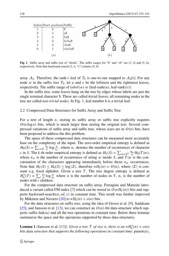
Consider a string S with a special terminating character $. The suffix array AS is anarray of the lexically sorted suffixes of S. i.e. AS[i] is the i-th lexically smallest suffixof S. Any substring x of S can be represented by a pair of indexes (st, ed), calledsuffix range, such that AS[st] and AS[ed] are respectively the lexically smallest andlargest suffixes which have x as their prefix. This implies that x occurs at positionsAS[st], AS[st + 1], . . . , AS[ed] in S. See Fig. 1(a) for an example.

The operation lookup(i) returns AS[i]. Consider a suffix range (st, ed) in AS forsome string P [1..m], the operation backward-search(st, ed, c) returns another suffixrange (st′, ed′) for the string cP [1..m]. (Note that (st′, ed′) is empty i.e. st′ < ed′ ifcP [1..m] is not a substring of S.)

For a string S with the special terminating character $, the suffix tree TS of thestring S is a tree whose edges are labeled with strings such that every suffix of S

corresponds to exactly one path from the tree’s root to a leaf. Figure 1(b) shows anexample suffix tree for cbcba$. For every node u in the suffix tree TS , the string onthe path from the root to u is called the path label of the node u, denoted as label(u).

In this work, we require the following operations on the suffix tree:

– parent(u): return the parent node of node u.– leaf-rank(u): returns the number of leaves less than or equal to u in preorder se-

quence.– leaf-select(i): returns the leaf of the suffix tree which has rank i.– leftmost-leaf(u): returns the leftmost child leaf of the subtree rooted at u.– rightmost-leaf(u): returns the rightmost child leaf of the subtree rooted at u.– lca(u, v): returns the lowest common ancestor of two leaves u and v.– depth(u): returns the depth of u. (i.e. the number of nodes from u to the root minus

one).– level-ancestor(u, d): returns the ancestor of u with depth d .– suffix-link(u) returns a node v such that label(v) equals the string label(u) with

the first character removed.

Suffix tree and suffix array are closely related. If the children of each node in thesuffix tree TS are ordered lexically according to the labels of the edges, the suffixescorresponding to the leaves of TS are ordered exactly the same as that of the suffix

128 Algorithmica (2013) 67:125–141

Fig. 1 Suffix array and suffix tree of “cbcba”. The suffix ranges for “b” and “cb” are (3, 4) and (5, 6),respectively. Note that backward-search (3, 4, “c”) returns (5, 6)

array AS . Therefore, the rank-i leaf of TS is one-to-one mapped to AS[i]. For anynode w in the suffix tree TS , let u and v be the leftmost and the rightmost leaves,respectively. The suffix range of label(w) is (leaf-rank(u), leaf-rank(v)).

In the suffix tree, some leaves hang on the tree by edges whose labels are just thesingle terminal character $. These are called trivial leaves; all remaining nodes in thetree are called non-trivial nodes. In Fig. 1, leaf number 6 is a trivial leaf.

2.2 Compressed Data-Structures for Suffix Array and Suffix Tree

For a text of length n, storing its suffix array or suffix tree explicitly requiresO(n logn) bits, which is much larger than storing the original text. Several com-pressed variations of suffix array and suffix tree, whose sizes are in O(n) bits, havebeen proposed to address the this problem.

The space of these compressed data structures can be measured more accuratelybase on the complexity of the input. The zero-order empirical entropy is defined asH0(S) = ∑

c∈Σnc

nlog n

nc, where nc denotes the number of occurrences of character

c in S. The k-th order empirical entropy is defined as Hk(S) = ∑w∈Σk

nw

nH0(T |w),

where nw is the number of occurrences of string w inside S, and T |w is the con-catenation of the characters appearing immediately before those nw occurrences.Note that Hk(S) ≤ H0(S) ≤ log |Σ |, therefore nHk(n) = O(n), where |Σ | is con-stant e.g. fixed alphabet. Given a tree T , The tree degree entropy is defined asH ∗

0 (T ) = ∑i

ni

nlog n

niwhere n is the number of nodes in T , ni is the number of

nodes with i children.For the compressed data structure on suffix array, Ferragina and Manzini intro-

duced a variant called FM-index [7] which can be stored in O(nHk(n)) bits and sup-ports backward-search(st, ed, c) in constant time. This result was further improvedby Mäkinen and Navarro [20] to nHk(n) + o(n) bits.

For the data structures on suffix tree, using the idea of Grossi et al. [9], Sadakane[25], and Jansson et al. [13], we can construct an O(n)-bit data-structure which sup-ports suffix-link(u) and all the tree operations in constant time. Below three lemmassummarize the space and the operations supported by these data-structures.

Lemma 1 (Jansson et al. [13]) Given a tree T of size n, there is an nH ∗0 (n) + o(n)

bits data structure that supports the following operations in constant time: parent(u),

Algorithmica (2013) 67:125–141 129

leaf-rank(u), leaf-select(i), leftmost-leaf(u), rightmost-leaf(u) and lca(u, v), depth(u)

and level-ancestor(u, d).

Lemma 2 (Mäkinen and Navarro [20]) Given the nHk(n) + o(n) bit FM-index ofthe sequence S, for every suffix range (st, ed) of the suffix array and every characterc, the operation backward-search(st, ed, c) runs in constant time; and the operationlookup(i) runs in O(logn) time.

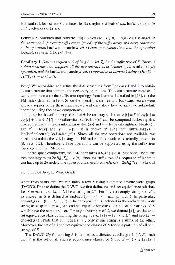
Corollary 1 Given a sequence S of length n, let TS be the suffix tree of S. There isa data structure that supports all the tree operations in Lemma 1, the suffix-link(u)

operation, and the backward-search(st, ed, c) operation in Lemma 2 using n(Hk(S)+2H ∗(TS)) + o(n) bits.

Proof We recombine and refine the data structures from Lemmas 1 and 2 to obtaina data structure that supports the necessary operations. The data structure consists oftwo components: (i) the suffix tree topology from Lemma 1 detailed in [13], (ii) theFM-index detailed in [20]. Since the operations on tree and backward-search werealready supported by these lemmas, we will only show how to simulate suffix-linkoperation using these two components.

Let AS be the suffix array of S. Let Ψ be an array such that Ψ [i] = i′ if AS[i′] =AS[i] + 1 and Ψ [i] = 0 otherwise. suffix-link(u) can be computed following thisprocedure: Let x = leaf-rank(leftmost-leaf(u)) and y = leaf-rank(rightmost-leaf(u)).Let x′ = Ψ [x] and y′ = Ψ [y]. It is shown in [25] that suffix-link(u) =lca(leaf-select(x′), leaf-select(y′)). Since, all the tree operations are available, weneed to simulate the Ψ [i] using the FM-index. This result was actually proven in[8, Sect. 3.2]. Therefore, all the operations can be supported using the suffix treetopology and the FM-index.

For the space complexity, the FM-index takes nHk(n)+o(n) bit-space. The suffixtree topology takes 2nH ∗

0 (TS) + o(n), since the suffix tree of a sequence of length n

can have up to 2n nodes. The space bound therefore is nHk(n)+2nH ∗0 (TS)+o(n). �

2.3 Directed Acyclic Word Graph

Apart from suffix tree, we can index a text S using a directed acyclic word graph(DAWG). Prior to define the DAWG, we first define the end-set equivalence relation.Let S = a1a2 . . . an (ai ∈ Σ ) be a string in Σ∗. For any non-empty string y ∈ Σ∗,its end-set in S is defined as end-setS(y) = {i | y = ai−|y|+1 . . . ai}. In particular,end-setS(ε) = {0,1,2, . . . , n}. (The zero position is included in the end-set of emptystring as a special case.) An end-set equivalence class is a set of substrings of S

which have the same end-set. For any substring x of S, we denote [x]S as the end-set equivalence class containing the string x, i.e., [x]S = {y | y ∈ Σ∗, end-setS(x) =end-setS(y)}. Note that [x]S equals [y]S only if one string is a suffix of the other.Moreover, the set of all end-set equivalence classes of S forms a partition of all sub-strings of S.

The DAWG DS for a string S is defined as a directed acyclic graph (V ,E) suchthat V is the set of all end-set equivalence classes of S and E = {([x]S, [xa]S) |

130 Algorithmica (2013) 67:125–141

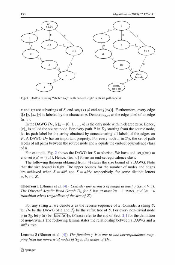
Fig. 2 DAWG of string “abcbc” (left: with end-set, right: with set path labels)

x and xa are substrings of S, end-setS(x) �= end-setS(xa)}. Furthermore, every edge([x]S, [xa]S) is labeled by the character a. Denote c(u,v) as the edge label of an edge(u, v).

In the DAWG DS , [ε]S = {0,1, . . . , n} is the only node with in-degree zero. Hence,[ε]S is called the source node. For every path P in DS starting from the source node,let its path label be the string obtained by concatenating all labels of the edges onP . A DAWG DS has an important property: For every node u in DS , the set of pathlabels of all paths between the source node and u equals the end-set equivalence classof u.

For example, Fig. 2 shows the DAWG for S = abcbc. We have end-setS(bc) =end-setS(c) = {3,5}. Hence, {bc,c} forms an end-set equivalence class.

The following theorem obtained from [4] states the size bound of a DAWG. Notethat the size bound is tight. The upper bounds for the number of nodes and edgesare achieved when S = abn and S = abnc respectively, for some distinct lettersa, b, c ∈ Σ .

Theorem 1 (Blumer et al. [4]) Consider any string S of length at least 3 (i.e. n ≥ 3).The Directed Acyclic Word Graph DS for S has at most 2n − 1 states, and 3n − 4transition edges (regardless of the size of Σ ).

For any string x, we denote x as the reverse sequence of x. Consider a string S,let DS be the DAWG of S and TS be the suffix tree of S. For every non-trivial nodeu in TS , let γ (u) be [label(u)]S . (Please refer to the end of Sect. 2.1 for the definitionof non-trivial.) The following lemma states the relationship between a DAWG and asuffix tree.

Lemma 3 (Blumer et al. [4]) The function γ is a one-to-one correspondence map-ping from the non-trivial nodes of TS to the nodes of DS .

Algorithmica (2013) 67:125–141 131

For example, for the suffix tree in Fig. 1(b) and the DAWG in Fig. 2, the internalnode of the suffix tree with path label “cb” maps to node [cb]S = [bc]S = {bc, c} inthe DAWG. In fact, every non-trivial node in the suffix tree maps to a node in theDAWG, and vice versa. Precisely, the root of the suffix tree maps to the source nodeof the DAWG, the internal node with path label “b” maps to node {“b”}, the internalnode with path label “cb” maps to node {“bc”, “c”}, leaf 5 maps to node {“a”}, leaf4 maps to node {“ab”}, leaf 2 maps to node {“abcb”, “bcb”, “cb”}, leaf 3 maps tonode {“abc”}, and leaf 1 maps to node {“abcbc”, “bcbc”, “cbc”}.

3 Simulating DAWG

Consider a sequence S of length n, this section describes an O(n)-bit data-structurefor the DAWG DS which supports the following four operations to navigate in thegraph in constant time:

– Get-Source(): returns the source node of DS ;– Find-Child(u, c): returns the child v of u in DS s.t. (u, v) is labeled by c.– Parent-Count(u): returns the number of parents of u in DS .– Extract-Parent(u, i): returns the i-th parent where 1 ≤ i ≤ Parent-Count(u).

We also support two operations which help to extract the substring information ofeach node. The first operation, denoted End-Set-Count(u), returns the number ofmembers of the end-set at node u in constant time. The second operation, denotedExtract-End-Point(u, i), returns the i-th end point in the set in O(logn) time.

To support the operations, we can store the nodes and the edges of DS directly.However, such a data-structure requires O(n logn)-bit space. Instead, this sectionshows that, given the FM-index of S and the compressed topology of the suffix treeof S (summarized in Corollary 1), we can simulate the DAWG DS and support alloperations efficiently with O(n) bits space.

First, we analyse the space complexity. Both the FM-index of S and the com-pressed suffix tree TS can be stored in nHk(S) + H ∗

0 (TS) + o(n) bits.Next, we describe how to represent the nodes in the DAWG DS . Lemma 3 implies

that each non-trivial node u in TS is one-to-one corresponding to a node γ (u) in DS .Hence, in our simulation, the non-trivial node u in TS represents the node γ (u) in DS .

Below four subsections describe how can we support the following opera-tions: Get-Source(), End-Set-Count(u), Extract-End-Point(u, i), Find-Child(u, c),Parent-Count(u) and Extract-Parent(u, i) . The implementation details is shown inListings 1, 2 3 and 4.

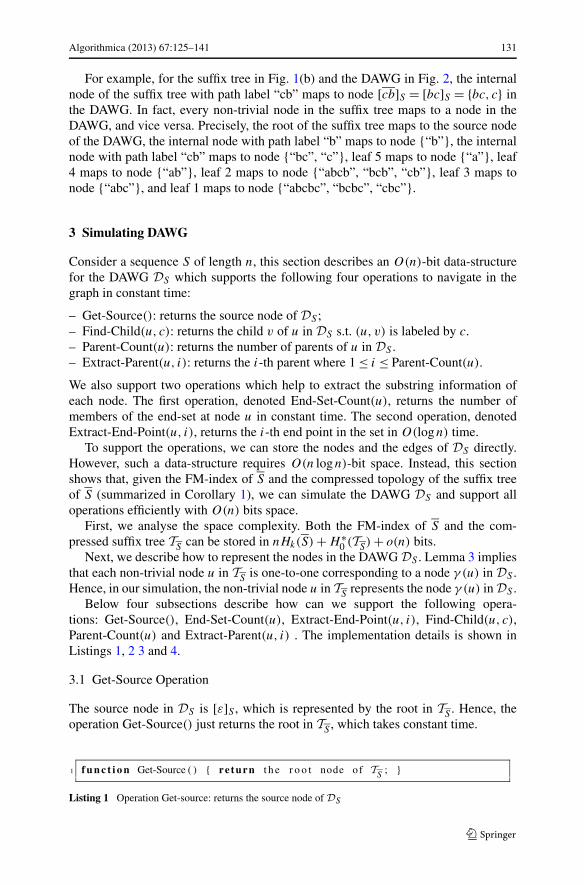
3.1 Get-Source Operation

The source node in DS is [ε]S , which is represented by the root in TS . Hence, theoperation Get-Source() just returns the root in TS , which takes constant time.

1 f u n c t i o n Get-Source ( ) { re turn t h e r o o t node of TS

; }

Listing 1 Operation Get-source: returns the source node of DS

132 Algorithmica (2013) 67:125–141

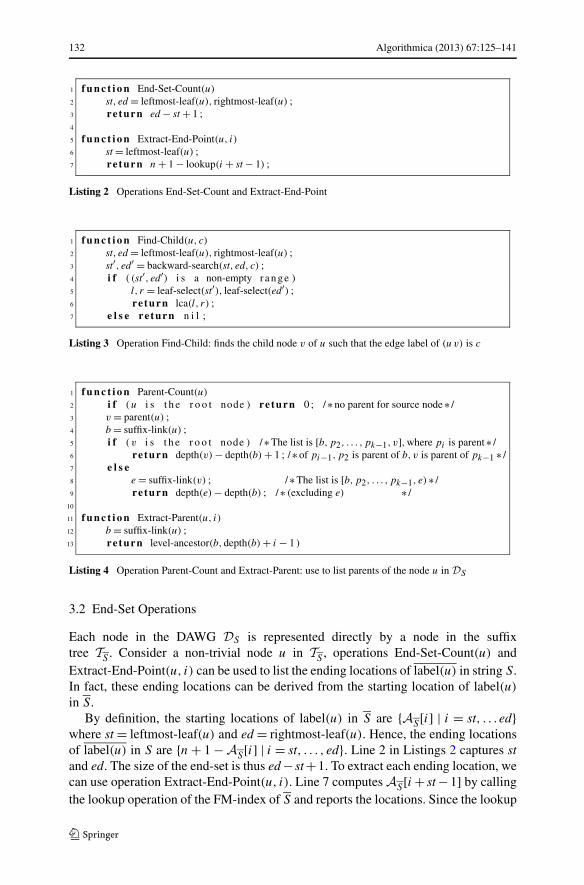
1 f u n c t i o n End-Set-Count(u)

2 st, ed = leftmost-leaf(u), rightmost-leaf(u) ;3 re turn ed − st + 1 ;4

5 f u n c t i o n Extract-End-Point(u, i)

6 st = leftmost-leaf(u) ;7 re turn n + 1 − lookup(i + st − 1) ;

Listing 2 Operations End-Set-Count and Extract-End-Point

1 f u n c t i o n Find-Child(u, c)

2 st, ed = leftmost-leaf(u), rightmost-leaf(u) ;3 st′, ed′ = backward-search(st, ed, c) ;4 i f ( (st′, ed′) i s a non-empty r a n g e )5 l, r = leaf-select(st′), leaf-select(ed′) ;6 re turn lca(l, r) ;7 e l s e re turn n i l ;

Listing 3 Operation Find-Child: finds the child node v of u such that the edge label of (uv) is c

1 f u n c t i o n Parent-Count(u)

2 i f ( u i s t h e r o o t node ) re turn 0 ; /∗ no parent for source node ∗ /3 v = parent(u) ;4 b = suffix-link(u) ;5 i f ( v i s t h e r o o t node ) /∗ The list is [b,p2, . . . , pk−1, v],where pi is parent ∗ /6 re turn depth(v) − depth(b) + 1 ; /∗ of pi−1,p2 is parent of b, v is parent of pk−1 ∗ /7 e l s e8 e = suffix-link(v) ; /∗The list is [b,p2, . . . , pk−1, e)∗ /9 re turn depth(e) − depth(b) ; /∗ (excluding e) ∗ /

10

11 f u n c t i o n Extract-Parent(u, i)

12 b = suffix-link(u) ;13 re turn level-ancestor(b,depth(b) + i − 1 )

Listing 4 Operation Parent-Count and Extract-Parent: use to list parents of the node u in DS

3.2 End-Set Operations

Each node in the DAWG DS is represented directly by a node in the suffixtree TS . Consider a non-trivial node u in TS , operations End-Set-Count(u) andExtract-End-Point(u, i) can be used to list the ending locations of label(u) in string S.In fact, these ending locations can be derived from the starting location of label(u)

in S.By definition, the starting locations of label(u) in S are {AS[i] | i = st, . . . ed}

where st = leftmost-leaf(u) and ed = rightmost-leaf(u). Hence, the ending locationsof label(u) in S are {n + 1 − AS[i] | i = st, . . . , ed}. Line 2 in Listings 2 captures stand ed. The size of the end-set is thus ed − st +1. To extract each ending location, wecan use operation Extract-End-Point(u, i). Line 7 computes AS[i + st − 1] by callingthe lookup operation of the FM-index of S and reports the locations. Since the lookup

Algorithmica (2013) 67:125–141 133

operation in FM-index takes O(logn) time, the cost of extracting each end point isO(logn) time.

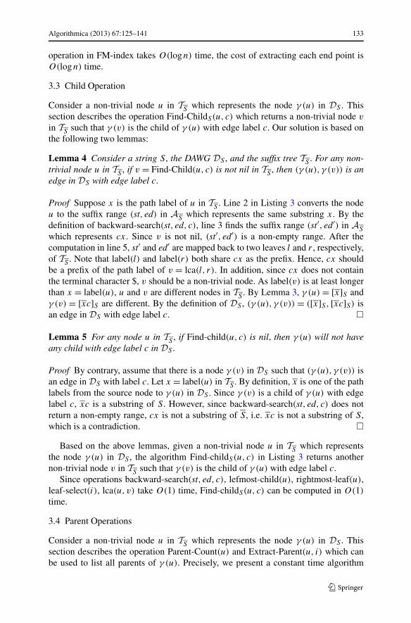
3.3 Child Operation

Consider a non-trivial node u in TS which represents the node γ (u) in DS . Thissection describes the operation Find-ChildS(u, c) which returns a non-trivial node v

in TS such that γ (v) is the child of γ (u) with edge label c. Our solution is based onthe following two lemmas:

Lemma 4 Consider a string S, the DAWG DS , and the suffix tree TS . For any non-trivial node u in TS , if v = Find-Child(u, c) is not nil in TS , then (γ (u), γ (v)) is anedge in DS with edge label c.

Proof Suppose x is the path label of u in TS . Line 2 in Listing 3 converts the nodeu to the suffix range (st, ed) in AS which represents the same substring x. By thedefinition of backward-search(st, ed, c), line 3 finds the suffix range (st′, ed′) in AS

which represents cx. Since v is not nil, (st′, ed′) is a non-empty range. After thecomputation in line 5, st′ and ed′ are mapped back to two leaves l and r , respectively,of TS . Note that label(l) and label(r) both share cx as the prefix. Hence, cx shouldbe a prefix of the path label of v = lca(l, r). In addition, since cx does not containthe terminal character $, v should be a non-trivial node. As label(v) is at least longerthan x = label(u), u and v are different nodes in TS . By Lemma 3, γ (u) = [x]S andγ (v) = [xc]S are different. By the definition of DS , (γ (u), γ (v)) = ([x]S, [xc]S) isan edge in DS with edge label c. �

Lemma 5 For any node u in TS , if Find-child(u, c) is nil, then γ (u) will not haveany child with edge label c in DS .

Proof By contrary, assume that there is a node γ (v) in DS such that (γ (u), γ (v)) isan edge in DS with label c. Let x = label(u) in TS . By definition, x is one of the pathlabels from the source node to γ (u) in DS . Since γ (v) is a child of γ (u) with edgelabel c, xc is a substring of S. However, since backward-search(st, ed, c) does notreturn a non-empty range, cx is not a substring of S, i.e. xc is not a substring of S,which is a contradiction. �

Based on the above lemmas, given a non-trivial node u in TS which representsthe node γ (u) in DS , the algorithm Find-childS(u, c) in Listing 3 returns anothernon-trivial node v in TS such that γ (v) is the child of γ (u) with edge label c.

Since operations backward-search(st, ed, c), lefmost-child(u), rightmost-leaf(u),leaf-select(i), lca(u, v) take O(1) time, Find-childS(u, c) can be computed in O(1)

time.

3.4 Parent Operations

Consider a non-trivial node u in TS which represents the node γ (u) in DS . Thissection describes the operation Parent-Count(u) and Extract-Parent(u, i) which canbe used to list all parents of γ (u). Precisely, we present a constant time algorithm

134 Algorithmica (2013) 67:125–141

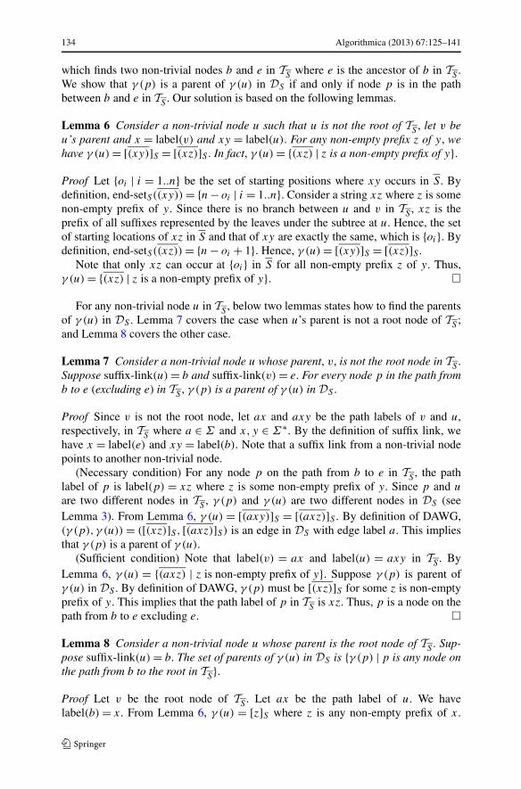
which finds two non-trivial nodes b and e in TS where e is the ancestor of b in TS .We show that γ (p) is a parent of γ (u) in DS if and only if node p is in the pathbetween b and e in TS . Our solution is based on the following lemmas.

Lemma 6 Consider a non-trivial node u such that u is not the root of TS , let v beu’s parent and x = label(v) and xy = label(u). For any non-empty prefix z of y, wehave γ (u) = [(xy)]S = [(xz)]S . In fact, γ (u) = {(xz) | z is a non-empty prefix of y}.

Proof Let {oi | i = 1..n} be the set of starting positions where xy occurs in S. Bydefinition, end-setS((xy)) = {n − oi | i = 1..n}. Consider a string xz where z is somenon-empty prefix of y. Since there is no branch between u and v in TS , xz is theprefix of all suffixes represented by the leaves under the subtree at u. Hence, the setof starting locations of xz in S and that of xy are exactly the same, which is {oi}. Bydefinition, end-setS((xz)) = {n − oi + 1}. Hence, γ (u) = [(xy)]S = [(xz)]S .

Note that only xz can occur at {oi} in S for all non-empty prefix z of y. Thus,γ (u) = {(xz) | z is a non-empty prefix of y}. �

For any non-trivial node u in TS , below two lemmas states how to find the parentsof γ (u) in DS . Lemma 7 covers the case when u’s parent is not a root node of TS ;and Lemma 8 covers the other case.

Lemma 7 Consider a non-trivial node u whose parent, v, is not the root node in TS .Suppose suffix-link(u) = b and suffix-link(v) = e. For every node p in the path fromb to e (excluding e) in TS , γ (p) is a parent of γ (u) in DS .

Proof Since v is not the root node, let ax and axy be the path labels of v and u,respectively, in TS where a ∈ Σ and x, y ∈ Σ∗. By the definition of suffix link, wehave x = label(e) and xy = label(b). Note that a suffix link from a non-trivial nodepoints to another non-trivial node.

(Necessary condition) For any node p on the path from b to e in TS , the pathlabel of p is label(p) = xz where z is some non-empty prefix of y. Since p and u

are two different nodes in TS , γ (p) and γ (u) are two different nodes in DS (seeLemma 3). From Lemma 6, γ (u) = [(axy)]S = [(axz)]S . By definition of DAWG,(γ (p), γ (u)) = ([(xz)]S, [(axz)]S) is an edge in DS with edge label a. This impliesthat γ (p) is a parent of γ (u).

(Sufficient condition) Note that label(v) = ax and label(u) = axy in TS . ByLemma 6, γ (u) = {(axz) | z is non-empty prefix of y}. Suppose γ (p) is parent ofγ (u) in DS . By definition of DAWG, γ (p) must be [(xz)]S for some z is non-emptyprefix of y. This implies that the path label of p in TS is xz. Thus, p is a node on thepath from b to e excluding e. �

Lemma 8 Consider a non-trivial node u whose parent is the root node of TS . Sup-pose suffix-link(u) = b. The set of parents of γ (u) in DS is {γ (p) | p is any node onthe path from b to the root in TS}.

Proof Let v be the root node of TS . Let ax be the path label of u. We havelabel(b) = x. From Lemma 6, γ (u) = [z]S where z is any non-empty prefix of x.

Algorithmica (2013) 67:125–141 135

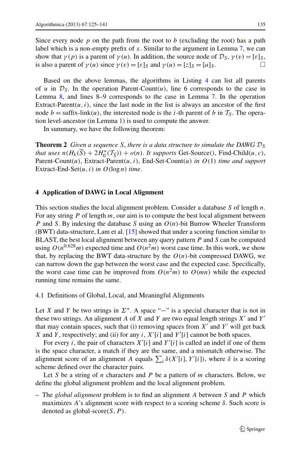
Since every node p on the path from the root to b (excluding the root) has a pathlabel which is a non-empty prefix of x. Similar to the argument in Lemma 7, we canshow that γ (p) is a parent of γ (u). In addition, the source node of DS , γ (v) = [ε]S ,is also a parent of γ (u) since γ (v) = [ε]S and γ (u) = [z]S = [a]S . �

Based on the above lemmas, the algorithms in Listing 4 can list all parentsof u in DS . In the operation Parent-Count(u), line 6 corresponds to the case inLemma 8, and lines 8–9 corresponds to the case in Lemma 7. In the operationExtract-Parent(u, i), since the last node in the list is always an ancestor of the firstnode b = suffix-link(u), the interested node is the i-th parent of b in TS . The opera-tion level-ancestor (in Lemma 1) is used to compute the answer.

In summary, we have the following theorem:

Theorem 2 Given a sequence S, there is a data structure to simulate the DAWG DS

that uses n(Hk(S) + 2H ∗0 (TS)) + o(n). It supports Get-Source(), Find-Child(u, c),

Parent-Count(u), Extract-Parent(u, i), End-Set-Count(u) in O(1) time and supportExtract-End-Set(u, i) in O(logn) time.

4 Application of DAWG in Local Alignment

This section studies the local alignment problem. Consider a database S of length n.For any string P of length m, our aim is to compute the best local alignment betweenP and S. By indexing the database S using an O(n)-bit Burrow Wheeler Transform(BWT) data-structure, Lam et al. [15] showed that under a scoring function similar toBLAST, the best local alignment between any query pattern P and S can be computedusing O(n0.628m) expected time and O(n2m) worst case time. In this work, we showthat, by replacing the BWT data-structure by the O(n)-bit compressed DAWG, wecan narrow down the gap between the worst case and the expected case. Specifically,the worst case time can be improved from O(n2m) to O(mn) while the expectedrunning time remains the same.

4.1 Definitions of Global, Local, and Meaningful Alignments

Let X and Y be two strings in Σ∗. A space “−” is a special character that is not inthese two strings. An alignment A of X and Y are two equal length strings X′ and Y ′that may contain spaces, such that (i) removing spaces from X′ and Y ′ will get backX and Y , respectively; and (ii) for any i, X′[i] and Y ′[i] cannot be both spaces.

For every i, the pair of characters X′[i] and Y ′[i] is called an indel if one of themis the space character, a match if they are the same, and a mismatch otherwise. Thealignment score of an alignment A equals

∑i δ(X

′[i], Y ′[i]), where δ is a scoringscheme defined over the character pairs.

Let S be a string of n characters and P be a pattern of m characters. Below, wedefine the global alignment problem and the local alignment problem.

– The global alignment problem is to find an alignment A between S and P whichmaximizes A’s alignment score with respect to a scoring scheme δ. Such score isdenoted as global-score(S,P ).

136 Algorithmica (2013) 67:125–141

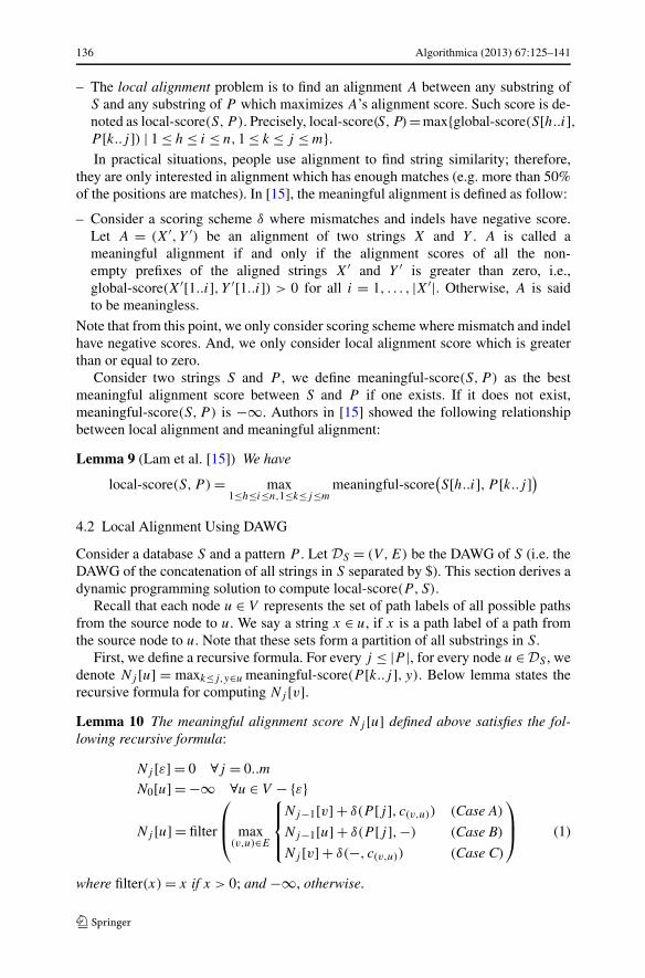
– The local alignment problem is to find an alignment A between any substring ofS and any substring of P which maximizes A’s alignment score. Such score is de-noted as local-score(S,P ). Precisely, local-score(S,P)=max{global-score(S[h..i],P [k..j ]) | 1 ≤ h ≤ i ≤ n,1 ≤ k ≤ j ≤ m}.In practical situations, people use alignment to find string similarity; therefore,

they are only interested in alignment which has enough matches (e.g. more than 50%of the positions are matches). In [15], the meaningful alignment is defined as follow:

– Consider a scoring scheme δ where mismatches and indels have negative score.Let A = (X′, Y ′) be an alignment of two strings X and Y . A is called ameaningful alignment if and only if the alignment scores of all the non-empty prefixes of the aligned strings X′ and Y ′ is greater than zero, i.e.,global-score(X′[1..i], Y ′[1..i]) > 0 for all i = 1, . . . , |X′|. Otherwise, A is saidto be meaningless.

Note that from this point, we only consider scoring scheme where mismatch and indelhave negative scores. And, we only consider local alignment score which is greaterthan or equal to zero.

Consider two strings S and P , we define meaningful-score(S,P ) as the bestmeaningful alignment score between S and P if one exists. If it does not exist,meaningful-score(S,P ) is −∞. Authors in [15] showed the following relationshipbetween local alignment and meaningful alignment:

Lemma 9 (Lam et al. [15]) We have

local-score(S,P ) = max1≤h≤i≤n,1≤k≤j≤m

meaningful-score(S[h..i],P [k..j ])

4.2 Local Alignment Using DAWG

Consider a database S and a pattern P . Let DS = (V ,E) be the DAWG of S (i.e. theDAWG of the concatenation of all strings in S separated by $). This section derives adynamic programming solution to compute local-score(P,S).

Recall that each node u ∈ V represents the set of path labels of all possible pathsfrom the source node to u. We say a string x ∈ u, if x is a path label of a path fromthe source node to u. Note that these sets form a partition of all substrings in S.

First, we define a recursive formula. For every j ≤ |P |, for every node u ∈ DS , wedenote Nj [u] = maxk≤j,y∈u meaningful-score(P [k..j ], y). Below lemma states therecursive formula for computing Nj [v].Lemma 10 The meaningful alignment score Nj [u] defined above satisfies the fol-lowing recursive formula:

Nj [ε] = 0 ∀j = 0..m

N0[u] = −∞ ∀u ∈ V − {ε}

Nj [u] = filter

⎛

⎜⎝ max

(v,u)∈E

⎧⎪⎨

⎪⎩

Nj−1[v] + δ(P [j ], c(v,u)) (Case A)

Nj−1[u] + δ(P [j ],−) (Case B)

Nj [v] + δ(−, c(v,u)) (Case C)

⎞

⎟⎠ (1)

where filter(x) = x if x > 0; and −∞, otherwise.

Algorithmica (2013) 67:125–141 137

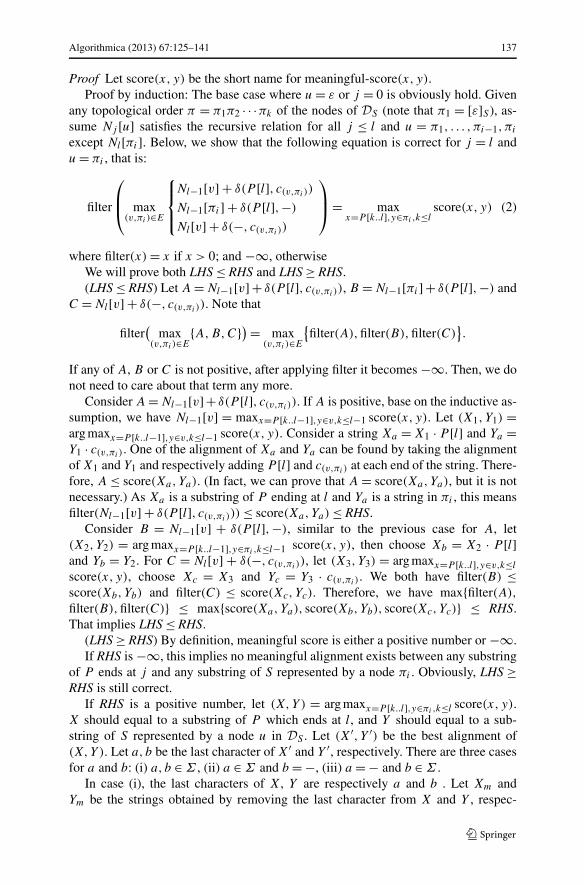
Proof Let score(x, y) be the short name for meaningful-score(x, y).Proof by induction: The base case where u = ε or j = 0 is obviously hold. Given

any topological order π = π1π2 · · ·πk of the nodes of DS (note that π1 = [ε]S ), as-sume Nj [u] satisfies the recursive relation for all j ≤ l and u = π1, . . . , πi−1,πi

except Nl[πi]. Below, we show that the following equation is correct for j = l andu = πi , that is:

filter

⎛

⎜⎝ max

(v,πi )∈E

⎧⎪⎨

⎪⎩

Nl−1[v] + δ(P [l], c(v,πi ))

Nl−1[πi] + δ(P [l],−)

Nl[v] + δ(−, c(v,πi ))

⎞

⎟⎠ = max

x=P [k..l],y∈πi ,k≤lscore(x, y) (2)

where filter(x) = x if x > 0; and −∞, otherwiseWe will prove both LHS ≤ RHS and LHS ≥ RHS.(LHS ≤ RHS) Let A = Nl−1[v] + δ(P [l], c(v,πi )), B = Nl−1[πi] + δ(P [l],−) and

C = Nl[v] + δ(−, c(v,πi )). Note that

filter(

max(v,πi )∈E

{A,B,C}) = max(v,πi )∈E

{filter(A),filter(B),filter(C)

}.

If any of A, B or C is not positive, after applying filter it becomes −∞. Then, we donot need to care about that term any more.

Consider A = Nl−1[v]+ δ(P [l], c(v,πi )). If A is positive, base on the inductive as-sumption, we have Nl−1[v] = maxx=P [k..l−1],y∈v,k≤l−1 score(x, y). Let (X1, Y1) =arg maxx=P [k..l−1],y∈v,k≤l−1 score(x, y). Consider a string Xa = X1 · P [l] and Ya =Y1 · c(v,πi ). One of the alignment of Xa and Ya can be found by taking the alignmentof X1 and Y1 and respectively adding P [l] and c(v,πi ) at each end of the string. There-fore, A ≤ score(Xa,Ya). (In fact, we can prove that A = score(Xa,Ya), but it is notnecessary.) As Xa is a substring of P ending at l and Ya is a string in πi , this meansfilter(Nl−1[v] + δ(P [l], c(v,πi ))) ≤ score(Xa,Ya) ≤ RHS.

Consider B = Nl−1[v] + δ(P [l],−), similar to the previous case for A, let(X2, Y2) = arg maxx=P [k..l−1],y∈πi ,k≤l−1 score(x, y), then choose Xb = X2 · P [l]and Yb = Y2. For C = Nl[v] + δ(−, c(v,πi )), let (X3, Y3) = arg maxx=P [k..l],y∈v,k≤l

score(x, y), choose Xc = X3 and Yc = Y3 · c(v,πi ). We both have filter(B) ≤score(Xb,Yb) and filter(C) ≤ score(Xc,Yc). Therefore, we have max{filter(A),

filter(B),filter(C)} ≤ max{score(Xa,Ya), score(Xb,Yb), score(Xc,Yc)} ≤ RHS.That implies LHS ≤ RHS.

(LHS ≥ RHS) By definition, meaningful score is either a positive number or −∞.If RHS is −∞, this implies no meaningful alignment exists between any substring

of P ends at j and any substring of S represented by a node πi . Obviously, LHS ≥RHS is still correct.

If RHS is a positive number, let (X,Y ) = arg maxx=P [k..l],y∈πi ,k≤l score(x, y).X should equal to a substring of P which ends at l, and Y should equal to a sub-string of S represented by a node u in DS . Let (X′, Y ′) be the best alignment of(X,Y ). Let a, b be the last character of X′ and Y ′, respectively. There are three casesfor a and b: (i) a, b ∈ Σ , (ii) a ∈ Σ and b = −, (iii) a = − and b ∈ Σ .

In case (i), the last characters of X, Y are respectively a and b . Let Xm andYm be the strings obtained by removing the last character from X and Y , respec-

138 Algorithmica (2013) 67:125–141

1 I n i t i a l i z e N0[u] f o r a l l u

2 f o r ( j = 1 t o m )3 /∗ u s i n g f o r m u l a from Lemma 10 ∗ /4 foreach ( p o s i t i v e e n t r y Nj−1[v] and edge (v,u) )5 Update Nj [u] = max{Nj [u],Nj−1[v] + δ(P [j ], c(v,u))} ( Case A )6 Update Nj [v] = max{Nj [v],Nj−1[v] + δ(P [j ],−)} ( Case B )7 foreach ( positive entry Nj [v] i n any topo . o r d e r o f v and edge (v,u) )8 Update Nj [u] = max{Nj [u],Nj [v] + δ(−, c(v,u))} ( Case C )

Listing 5 Complete algorithm

tively. Xm should equal to a substring ends at l; and Ym should equal to a path la-bel of a parent node of πi . In this case, we have score(Xm,Ym) ≥ score(X,Y ) −δ(a, b). As, Nl−1[v] = maxx=P [k..l−1],y∈v score(x, y), Nl−1[v] ≥ score(Xm,Ym).Hence, LHS ≥ score(Xm,Ym) + δ(a, b) ≥ score(X,Y ). Similarly, we can also proveLHS ≥ score(X,Y ) in cases (ii) and (iii). �

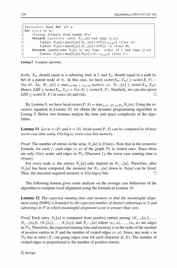
By Lemma 9, we have local-score(P,S) = maxj=1..|P |,u∈DSNj [u]. Using the re-

cursive equation in Lemma 10, we obtain the dynamic programming algorithm inListing 5. Below two lemmas analyse the time and space complexity of the algo-rithm.

Lemma 11 Let m = |P | and n = |S|. local-score(P,S) can be computed in O(mn)

worst case time using O(n logn) worst case bits memory.

Proof The number of entries in the array Nj [u] is O(mn). Note that in the recursiveformula, for each j , each edge (v,u) of the graph DS is visited once. Since thereare only O(n) nodes and edges in DS (Theorem 1), the worst case running time isO(mn).

For every node u, the entries Nj [u] only depend on Nj−1[u]. Therefore, afterNj [u] has been computed, the memory for Nj−2[u] down to N0[u] can be freed.Thus, the maximal required memory is O(n logn) bits. �

The following lemma gives some analysis on the average case behaviour of thealgorithm to compute local alignment using the formula in Lemma 10.

Lemma 12 The expected running time and memory to find the meaningful align-ment using DAWG is bounded by the expected number of distinct substrings in S andsubstrings in P in which meaningful alignment score is greater than zero.

Proof Each entry Nj [u] is computed from positive entries among (Nj−1[v1], . . . ,Nj−1[vk]), (Nj [v1], . . . ,Nj [vk]) and Nj−1[u] where (v1, u), . . . , (vk, u) are edgesin DS . Therefore, the expected running time and memory is in the order of the numberof positive entries in N and the number of visited edges (v,u). Since, any node v inDS has at most |Σ | out-going edges (one for each character in Σ ). The number ofvisited edges is proportional to the number of positive entries.

Algorithmica (2013) 67:125–141 139

Consider a positive entry Nj [u], since

Nj [u] = maxk≤j,y∈u

meaningful-score(P [k..j ], y)

.

It is obviously that each positive entry corresponds to distinct substring y in S and asubstring x in P in which meaningful alignment score is greater than zero. �

From the above lemma, the problem of estimating the average running time be-comes the problem of estimating the number of substring pairs which have positivemeaningful score. We do not notice any direct result on this bound; however, thereare a few results on measuring the average number of pairs of strings which haveHamming distance within certain bound.

For example, Baeza-Yates and Gonnet [3] analysed the all-against-all alignmentproblem (set of strings against themselves) on suffix tree. The core of the analysis isto measure the average number of comparisons for searching a random string over atrie allowing errors. This yields an O(nαm logn) bound on our problem where α is aconstant which is less than one. Maaß [19] analysed the time for searching a patternon a trie of n random strings allowing at most D Hamming’s errors. In the case whereD is less than (σ − 1)/σ logσ n where σ = |Σ |, the average number of comparisonis sub-linear (o(n)). We can use this result to obtain a bound of sub-quadratic o(nm)

on the average case where match is 1 and mismatch is less than or equal to −1.Lam et al. [15] studied a specific case of allowing Hamming errors where match is 1and mismatch is −3. This score roughly approximates the score used by BLAST.They proved that the running time is bound by O(n0.628m). Their experiments alsosuggested that in scoring model with gap penalty (gap score is −3), the expectedrunning time is also roughly O(n0.628m).

Lemma 13 The expected running time to find the meaningful alignment using DAWGis at least as good as the expected running time of BWT-SW [15]. (i.e. O(n0.628m) fortheir alignment score.)

Proof In the algorithm BWT-SW, the string S is organized in a suffix trie TS . Thealignment process computes and keeps the meaningful alignment scores between pathlabel of nodes of TS and substrings of the pattern string P . Note that each nodeof the DAWG DS can be seen as the combination of multiple nodes of the suffixtrie TS . Therefore, each entry computed in BWT-SW can be mapped to an entry ofNj [u]. (Multiple entries in BWT-SW can be mapped to the same entry Nj [u] in ouralgorithm.) The expected asymptotic running time of our algorithm is thus boundedby that of BWT-SW. �

For simplicity, the above discussion only focuses on computing the maximumalignment score, i.e., the entry Nj [u] which is the maximum. In real-life, we mayalso want to recover the regions in S containing the alignments represented by Nj [u].In this case, the value of Nj [u] is not enough. We need to compute two more num-bers Ij,u and Lj,u such that meaningful-score(P [Ij,u..j ], S′) = Nj [u] where S′ is alength-Lj,u substring belongs to u. Then, using the operations End-Set-Count(u) and

140 Algorithmica (2013) 67:125–141

Extract-End-Point(u, i), we can enumerate all alignments represented by Nj [u], i.e.,{(P [Ij,u..j ], S[q − Lj,u..q]) | q ∈ end-setS(u)}.

Ij,u and Lj,u can be computed by dynamic programming along with Nj [u]. Forthe base cases, we have Ij,ε equals j and Lj,ε equals −1. Then, depend on the out-come of Eq. (1), Ij,u and Lj,u can be updated using the following equations:

Ij,u =

⎧⎪⎨

⎪⎩

Ij−1,v if (A) happens

Ij−1,u if (B) happens

Ij,v if (C) happens

Lj,u =

⎧⎪⎨

⎪⎩

Lj−1,v + 1 if (A) happens

Lj−1,u if (B) happens

Ij,v + 1 if (C) happens

For time and space complexities, note that Lj,u and Ij,u can be computed usingthe same time and space complexities as Nj [u]. After that, all alignments representedby Nj [u] can be reported using O(occ logn) time, where occ is the number of suchalignments.

References

1. Altschul, S., Gish, W., Miller, W., Myers, E., Lipman, D.: Basic local alignment search tool. J. Mol.Biol. 215(3), 403–410 (1990)

2. Appel, A., Jacobson, G.: The world’s fastest scrabble program. Commun. ACM 31(5), 572–578(1988)

3. Baeza-Yates, R., Gonnet, G.: A fast algorithm on average for all-against-all sequence matching. In:Proceedings of the String Processing and Information Retrieval Symposium, pp. 16–23 (1999)

4. Blumer, A., Blumer, J., Haussler, D., Ehrenfeucht, A., Chen, M., Seiferas, J.: The smallest automatonrecognizing the subwords of a text. Theor. Comput. Sci. 40, 31–55 (1985)

5. Chim, H., Deng, X.: A new suffix tree similarity measure for document clustering. In: Proceedings ofthe 16th Conference on World Wide Web, pp. 121–130 (2007)

6. Crochemore, M., Vérin, R.: On compact directed acyclic word graphs. In: Structures in Logic andComputer Science, vol. 1261, pp. 192–211 (1997)

7. Ferragina, P., Manzini, G.: Indexing compressed text. J. ACM 52(4), 552–581 (2005)8. Golynski, A., Munro, J.I., Rao, S.S.: Rank/select operations on large alphabets: a tool for text in-

dexing. In: Proceedings of the Seventeenth Annual ACM-SIAM Symposium on Discrete Algorithm,pp. 368–373 (2006)

9. Grossi, R., Gupta, A., Vitter, J.: High-order entropy-compressed text indexes. In: Proceedings of theFourteenth Annual ACM-SIAM Symposium on Discrete Algorithms, pp. 841–850 (2003)

10. Gusfield, D.: Algorithms on Strings, Trees, and Sequences: Computer Science and ComputationalBiology. Cambridge University Press, Cambridge (1997)

11. Huang, J., Powers, D.: Suffix tree based approach for Chinese information retrieval. In: Eighth Inter-national Conference on Intelligent Systems Design and Applications, pp. 393–397 (2008)

12. Inenaga, S., Takeda, M.: Sparse compact directed acyclic word graphs. In: Proceedings of PragueStringology Conference, pp. 197–211 (2006)

13. Jansson, J., Sadakane, K., Sung, W.: Ultra-succinct representation of ordered trees with applications.J. Comput. Syst. Sci. 78(2), 619–631 (2012)

14. Kurtz, S., Choudhuri, J.V., Ohlebusch, E., Schleiermacher, C., Stoye, J., Giegerich, R.: Reputer: themanifold applications of repeat analysis on a genomic scale. Nucleic Acids Res. 29, 4633–4642(2001)

15. Lam, T.W., Sung, W.K., Tam, S.L., Wong, C.K., Yiu, S.M.: Compressed indexing and local alignmentof DNA. Bioinformatics 24(6), 791–797 (2008)

16. Langmead, B., Trapnell, C., Pop, M., Salzberg, S.: Ultrafast and memory-efficient alignment of shortDNA sequences to the human genome. Genome Biol. 10, R25 (2009)

17. Larsson, N.: Extended application of suffix trees to data compression. In: Proceedings of the IEEEData Compression Conference, pp. 190–199 (1996)

Algorithmica (2013) 67:125–141 141

18. Li, H., Durbin, R.: Fast and accurate long-read alignment with burrows-wheeler transform. Bioinfor-matics 26(5), 589–595 (2010)

19. Maaß, M.: Average-case analysis of approximate trie search. Algorithmica 46(3), 469–491 (2006)20. Mäkinen, V., Navarro, G.: Implicit compression boosting with applications to self-indexing. In: Pro-

ceedings of the String Processing and Information Retrieval Symposium, pp. 229–241 (2007)21. Manber, U., Myers, G.: Suffix arrays: a new method for on-line string searches. SIAM J. Comput. 22,

935–948 (1993)22. Meek, C., Patel, J., Kasetty, S.: Oasis: an online and accurate technique for local-alignment searches

on biological sequences. In: Proceedings of the 29th International Conference on Very Large DataBases, pp. 910–921 (2003)

23. Navarro, G.: A guided tour to approximate string matching. ACM Comput. Surv. 33, 31–88 (2001)24. Navarro, G., Baeza-Yates, R.: A hybrid indexing method for approximate string matching. J. Discrete

Algorithms 1, 205–239 (2000)25. Sadakane, K.: Compressed suffix trees with full functionality. Theory Comput. Syst. 41, 589–607

(2007)26. Senft, M.: Suffix tree based data compression. In: Proceedings of the 31st Conference on Current

Trends in Theory and Practice of Computer, pp. 350–359 (2005)27. Smith, T.F., Waterman, M.S.: Identification of common molecular subsequences. J. Mol. Biol. 147,

195–197 (1981)28. Sung, W.-K.: Indexed approximate string matching. In: Encyclopedia of Algorithms, pp. 408–410

(2008)29. Weiner, P.: Linear pattern matching algorithms. In: IEEE 14th Annual Symposium on Switching and

Automata Theory, pp. 1–11 (1973)30. Wong, S., Sung, W., Wong, L.: CPS-tree: a compact partitioned suffix tree for disk-based indexing

on large genome sequences. In: IEEE 23rd International Conference on Data Engineering, pp. 1350–1354 (2007)