comprehensive carbon accounting for identification of sustainable biomass feedstocks

www.theicct.org

JANUARY 2014WHITE PAPER

[email protected]

BEIJING | BERLIN | BRUSSELS | SAN FRANCISCO | WASHINGTON

COMPREHENSIVE CARBON ACCOUNTING FOR IDENTIFICATION OF SUSTAINABLE BIOMASS FEEDSTOCKSAnil Baral and Chris Malins

ACKNOWLEDGMENTSWe acknowledge the valuable feedback provided by external reviewers Dr. Michael Wang (Argonne National Laboratory) and Bart Dehue (Vattenfall). We also thank Dr. Nic Lutsey and Fanta Kamakate for their guidance and constructive feedback.

For additional information: 1225 I Street NW Suite 900 Washington DC 20005 +1 202 534 [email protected]

www.theicct.org

© 2013 International Council on Clean Transportation

Funding for this work was generously provided by the ClimateWorks Foundation.

http://www.theicct.org

i

TABLE OF CONTENTS

Executive Summary .....................................................................................................1

Results .......................................................................................................................................................... 2

Recommendations................................................................................................................................... 3

1. Introduction .......................................................................................................................... 5

1.1 Rationale .............................................................................................................................................. 8

1.2 Objectives ...........................................................................................................................................12

1.3 Scope of the study ..........................................................................................................................12

2. Carbon questions and policy implications in biomass use .......................................... 14

2.1 System boundary and scope of carbon accounting ..........................................................14

2.1.1 Soil carbon and nutrients ....................................................................................................14

2.1.2 Incorporating emissions from indirect land use change (iLUC) ........................14

2.1.3 “Rational expectations” approach .................................................................................15

2.2 Temporal impact of carbon ........................................................................................................16

2.2.1 Carbon payback period .....................................................................................................17

2.2.2 Carbon discounting ............................................................................................................18

2.2.3 Time-integrated carbon accounting of biogenic emissions ...............................19

3. Environmental impact ........................................................................................................22

4. Analytical approach ..........................................................................................................24

4.1 Methodology ....................................................................................................................................24

4.1.1 Biomass cultivation .............................................................................................................24

4.1.2 Biomass harvest and transport ......................................................................................25

4.1.3 Bioenergy production and transport ..........................................................................25

4.1.4 Calculating payback periods ..........................................................................................25

4.2 Biomass scenarios, data sources, and assumptions .........................................................27

4.2.1 Short-rotation temperate forestry ...............................................................................27

4.2.2 Stump removal....................................................................................................................27

4.2.3 Slash removal ......................................................................................................................28

4.2.4 Reduced-impact logging (Brazil) ................................................................................28

4.2.5 Forest thinning ...................................................................................................................29

4.2.6 Switchgrass ......................................................................................................................... 30

4.2.7 Corn stover .......................................................................................................................... 30

4.2.8 Willow .....................................................................................................................................31

4.2.9 Miscanthus.............................................................................................................................31

4.2.10 “Rational expectation” scenario ..................................................................................31

5. Results .................................................................................................................................32

5.1 CO2 emission profiles of biomass feedstock harvesting and use pathways ............32

5.1.1 Emission profile for short-rotation forestry ...............................................................32

5.1.2 Emission profile for dedicated energy crops ...........................................................34

5.1.3 Emission profile for selective logging .........................................................................35

5.2 Payback periods, carbon intensities, and carbon savings for biomass feedstock harvesting and use pathways ...................................................................................................36

5.3 Impact of carbon discounting and time-integrated impact of biogenic emissions (GWPbio factor) ................................................................................................................................41

6. Discussion .......................................................................................................................... 44

6.1 Assessment of biomass pathways for energy and biofuel production .................... 44

6.2 Reducing environmental impacts: Biomass cascading use and waste hierarchy 47

7. Policy implications and recommendations ....................................................................49

References .................................................................................................................................51

Appendix A: Brief overview of environmental impacts .................................................... 61

A.1. Impact of whole-tree and slash removal .............................................................................61

A.2. Stump removal ..............................................................................................................................62

A.3 Reduced-impact logging ...........................................................................................................63

A.4 Impact of agricultural residue removal ............................................................................... 64

A.5 SRWC and perennial grasses .................................................................................................. 66

A.6 Forest thinning ..............................................................................................................................67

Appendix B: Other emission profiles ...................................................................................69

Appendix C: Data and assumptions ....................................................................................73

1

CARBON ACCOUNTING FOR IDENTIFICATION OF SUSTAINABLE BIOMASS FEEDSTOCKS

EXECUTIVE SUMMARYBioenergy is incentivized by government policies that are intended to mitigate climate change, improve energy security, and boost rural economies. Biofuels derived from sustainable feedstocks through advanced processing pathways can offer substantial climate change and oil use reduction benefits. However, some studies have questioned the benefit of bioenergy, raising important issues about the carbon debt incurred by biomass harvesting and about the indirect effects of expanding bioenergy demand.

Ensuring that bioenergy pathways result in climate benefits requires life cycle analysis (LCA). The carbon footprint of bioenergy use is often sensitive to the time scale over which emissions are assessed, because different biomass pathways have radically different carbon recycling characteristics. For annual crops, biogenic carbon is cycled annually—sequestered through photosynthesis, then emitted in combustion. In the case of longer cycles such as those in forestry systems, biomass could take many years to regrow. To provide accurate guidance on the climate implications of bioenergy use, an LCA must reflect all substantial carbon sinks and sources in a given biofuel pathway. This should include soil and biomass carbon stock changes due to land use change, harvesting, and cultivation. Ignoring important emissions sources and sinks may result in over- or under-estimation of the impact of bioenergy. For instance, the carbon accounting scheme used in the European Union Emission Trading Scheme (ETS) has been criticized for treating all bioenergy as carbon-neutral, even though LCA suggests that some bioenergy pathways could result in carbon emissions exceeding those from fossil fuel use.

This study estimates the carbon impacts of bioenergy from 10 biomass feedstock harvesting pathways each feeding into three different bioenergy production pathways, for a total of 30 pathways assessed. We also consider a further 12 sensitivity cases. The biomass harvesting pathways include forestry [short-rotation forestry, reduced-impact logging (RIL), forest thinning, forest residues], an agricultural residue, and dedicated energy crops. The climate implications of RIL for bioenergy have not been studied before. The three bioenergy production pathways are electricity generation, biochemical ethanol production, and thermochemical ethanol production.

This study improves on previous analyses by assessing a broad set of pathways by comprehensively accounting for all major carbon sources and sinks—in particular, soil carbon and nutrient losses from residue harvesting. We calculate carbon payback times, carbon intensities (based on a 30-year amortization), and hence carbon savings relative to counterfactuals in which we assume direct one-to-one displacement of fossil fuels on an energy basis (coal or gasoline as appropriate). Ultimately our aim is to give an indication of the types of pathways likely to have systematically smaller or larger climate impacts.

Responding to concern about carbon payback periods, this paper considers novel approaches to accounting for the temporal character of bioenergy emissions. If biogenic carbon emissions are not resequestered for many years, the carbon dioxide released by harvest and combustion will temporarily contribute to radiative forcing (and hence global warming) just as fossil carbon would. This temporary radiative forcing from bio-genic carbon can be modeled by calculating a “global warming potential” (GWPbio) for a given cycle of carbon emission and sequestration. This compares the warming impact from the temporary emission of a quantity of biogenic carbon dioxide to the warming impact over 100 years of emitting the same quantity of fossil carbon dioxide. The longer the biogenic carbon is resident in the atmosphere, the higher its GWPbio factor will be.

2

ICCT WHITE PAPER

Including these GWPbio factors in LCA can have a significant effect on the result. We compare the results of accounting for GWPbio to the implications of applying a discount rate to the accounted value of carbon emissions—a technique that was discussed but discarded for the U.S. Renewable Fuel Standard (RFS).

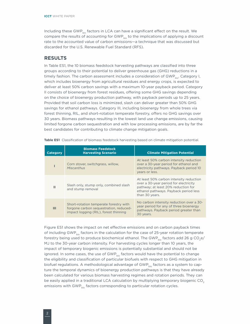
RESULTSIn Table ES1, the 10 biomass feedstock harvesting pathways are classified into three groups according to their potential to deliver greenhouse gas (GHG) reductions in a timely fashion. The carbon assessment includes a consideration of GWPbio. Category I, which includes bioenergy from agricultural residues and energy crops, is expected to deliver at least 50% carbon savings with a maximum 10-year payback period. Category II consists of bioenergy from forest residues, offering some GHG savings depending on the choice of bioenergy production pathway, with payback periods up to 25 years. Provided that soil carbon loss is minimized, slash can deliver greater than 50% GHG savings for ethanol pathways. Category III, including bioenergy from whole trees via forest thinning, RIL, and short-rotation temperate forestry, offers no GHG savings over 30 years. Biomass pathways resulting in the lowest land use change emissions, causing limited forgone carbon sequestration and with low processing emissions, are by far the best candidates for contributing to climate change mitigation goals.

Table ES1 Classification of biomass feedstock harvesting based on climate mitigation potential.

CategoryBiomass Feedstock Harvesting Scenario Climate Mitigation Potential

I Corn stover, switchgrass, willow, Miscanthus

At least 50% carbon intensity reduction over a 30-year period for ethanol and electricity pathways. Payback period 10 years or less.

II Slash only, stump only, combined slash and stump removal

At least 50% carbon intensity reduction over a 30-year period for electricity pathway; at least 20% reduction for ethanol pathways. Payback period less than 30 years.

IIIShort-rotation temperate forestry with forgone carbon sequestration, reduced-impact logging (RIL), forest thinning

No carbon intensity reduction over a 30-year period for any of three bioenergy pathways. Payback period greater than 30 years.

Figure ES1 shows the impact on net effective emissions and on carbon payback times of including GWPbio factors in the calculation for the case of 25-year rotation temperate forestry being used to produce biochemical ethanol. The GWPbio factors add 26 g CO2e/MJ to the 30-year carbon intensity. For harvesting cycles longer than 10 years, the impact of temporary biogenic emissions is potentially substantial and should not be ignored. In some cases, the use of GWPbio factors would have the potential to change the eligibility and classification of particular biofuels with respect to GHG mitigation in biofuel regulations. A methodological advantage of GWPbio factors as a system to cap-ture the temporal dynamics of bioenergy production pathways is that they have already been calculated for various biomass harvesting regimes and rotation periods. They can be easily applied in a traditional LCA calculation by multiplying temporary biogenic CO2 emissions with GWPbio factors corresponding to particular rotation cycles.

3


CO

2e (

tonn

es/h

a)

Savings (0% discounting) Savings (GWPbio factor)

50 100 150 200 250 300 350 400

Year

0-500

-300

-100

0

100

300

500

700

Figure ES1. Impact of accounting methods on carbon savings and payback periods for biochemical ethanol production from short-rotation temperate forestry with forgone sequestration.

Although we have captured a broad range of bioenergy pathways in this study, there are still several pathways of interest that we have not been able to cover, including biomass from managed forests and short-rotation forests in tropical and semitropical regions, such as Eucalyptus in Brazil.

More generally, it is important to recognize that managed forests are complex systems that produce a variety of products including timber, pulpwood, and material for bioenergy. Analyzing managed forestry as a holistic system may offer useful insights about opportunities to implement different harvesting models for bioenergy than have been examined here, potentially with strong GHG reduction potential, and constitutes an important area for future research.

RECOMMENDATIONSOur study has the following implications for policymaking in the biofuel and biomass energy space.

1. Bioenergy from agricultural residues and dedicated energy crops can deliver GHG savings and contribute to climate change mitigation. This result is broadly consistent with the conclusions of previous studies, even though our analysis is more comprehensive by including previously overlooked emis-sions such as soil carbon loss from residue harvest. Agricultural residues and dedicated energy crops should be given priority as bioenergy feedstocks in research and development.

2. Consistent with earlier studies, we find that pathways based on whole-tree logging in forests offer little or no climate mitigation over 50 years. We also show that

4

ICCT WHITE PAPER

reduced impact logging does not deliver GHG savings within 50 years. These bioenergy feedstocks are not good candidates from a climate policy point of view.

3. Comprehensive carbon accounting for bioenergy systems is important to avoid perverse impacts from biomass and biofuel policies. Any international framework for carbon accounting that replaces the Kyoto Protocol should adopt a more sophisticated and comprehensive accounting of the life cycle emissions of bioenergy use.

4. Although various national and regional bioenergy policies [e.g., the Renewable Energy Directive (RED) and Fuel Quality Directive (FQD) in Europe, RFS2 in the United States, and the Low Carbon Fuel Standard (LCFS) in California] already include life cycle accounting of bioenergy, there is room for improvement in ac-counting for key carbon emissions sources. In particular, this includes improving (or introducing) accounting for soil carbon losses and the GHG costs of nutrient replacement after residue removal, which could be major emissions sources for cellulosic biofuel feedstocks.

5. For longer harvesting cycles (>10 years), consideration of GWPbio factors could be introduced to LCA to reduce the risk of mischaracterization of climate change mitigation potential. The framework of GWPbio factors could be easily applied in the existing LCA framework used by RFS2, RED/FQD, and LCFS.

5


1. INTRODUCTION Bioenergy is the renewable energy derived from biomass. It includes heat and electricity from direct biomass combustion, as well as biofuels and biogases from thermochemical or biochemical conversion. In recent years, the use of biomass for energy and fuel has become a major policy strategy for many countries around the globe, with the aims of combatting climate change, improving energy security, and boosting rural economies.

Figure 1 shows that the use of biofuel for transport has rapidly increased in the past decade, led by support in the United States, the European Union, and Brazil. Likewise, the direct use of biomass for electricity has been increasing steadily worldwide in the past 5 years. As of 2011, there were 2000 biomass power plants in operation in 40 countries, with installed capacity of 22.5 GW; Europe alone had 1000 such plants (Price, 2011). The total primary bioenergy use in 2012, including biomass used for cooking, was 50 EJ (50 × 1018 J) (IEA, 2012).

0

5

10

15

20

25

30

35

40

45

50

55

60

2001 2002 2003 2004 2005 2006 2007 2008 2009 2010 2011

Bio

fuel

(10

6 t

onn

es o

f o

il eq

uiva

lent

)

North America South and Central America Europe and Eurasia

Africa Asia Pacific Total World

Figure 1. Global biofuel production, 2001 to 2011 (Source: BP Statistical Review of World Energy, 2013)1

With respect to biomass use for electricity, many states in the United States have renewable portfolio standards, which require electric utilities to provide a certain frac-

1 Retrieved from http://www.bp.com/statisticalreview

6

ICCT WHITE PAPER

tion of electricity from renewable sources including biomass. In the European Union, the Renewable Energy Directive (RED) requires that 20% of energy used in all sectors be renewable by 2020, and bioenergy including biomass electricity is expected to represent a substantial portion of the renewable energy supply.

Concomitant growth is taking place in the biofuel sector. A recent report from Navigant Research predicts that worldwide biofuel production will grow from 33.6 billion gallons per year in 2013 to 61.6 billion gallons per year in 2023 (Navigant Research, 2013). Already 52 countries have instituted biofuel polices that set targets or mandates for biofuels. The United States has one of the most ambitious biofuel mandates. Under the most recent Renewable Fuel Standard (RFS2), the United States needs to use 36 billion gallons of biofuel by 2022, with 16 billion gallons of cellulosic biofuels required to come from cel-lulosic biomass (although this target currently looks like it may need to be revised down).

In South America, Argentina and Brazil have 5% and 20% ethanol mandates in place, respectively. For diesel-fueled vehicles, Brazil has a 5% biodiesel mandate and Argentina has a 7% mandate. In the Asia Pacific region, China intends to move to 10% biofuel blending by 2020, with some provinces already requiring 10% ethanol blends. India requires 5% ethanol blending and aims to move to 20% biofuel blending by 2017. Bio-diesel mandates in the region range from 1% to 5%, with Malaysia and Thailand requiring 5% biodiesel. In Africa, several countries have implemented ethanol mandates, including Nigeria, Ethiopia, South Africa, Kenya, and Mozambique (Lane, 2012). However, it is not clear that all of these countries will achieve the required mandates by the target dates.

Dedicatedpower plant

Lignocellulosicfeedstocks

Co-generation

Electricity

Heat

Electricity

Electricity

Co-firing atpower plant

Figure 2. Conversion of biomass to electricity.

Biomass can be used either to produce electricity and heat (biopower) or to produce biofuels through thermochemical and biochemical conversion. For heat and electricity, biomass feedstocks can be co-fired with coal in existing coal power plants in ratios up to 30% without major modifications to the existing plant (Fig. 2). Alternatively, lignocel-lulosic biomass can be combusted in dedicated biomass power plants or can be used for co-generation of heat and electricity (combined heat and power (CHP)). By minimizing energy wastage, CHP can have a higher energy conversion efficiency: up to 90%, versus 33% for conventional coal power plants.

Unlike biomass use for heat and electricity, the production of liquid fuels from lignocel-lulosic biomass requires additional processing steps. Several technology pathways have been identified for liquid fuel production from lignocellulosic biomass. Primarily, liquid biofuels are produced via biochemical and thermochemical conversions.

In biochemical conversion, biomass is pretreated with acids, ammonia, or heat and pres-sure. This is followed by the hydrolysis of cellulose into sugars, which are subsequently

7


fermented to alcohols—primarily ethanol, although more complex molecules such as butanol can be produced (Fig. 3). Lignin, which is obtained as a by-product during hy-drolysis, can be burned to produce heat and electricity for onsite energy consumption, with any excess electricity sold to grid. This excess electricity can generate GHG credits for biochemical conversion. Most biochemical conversion technologies to produce cellulosic ethanol are still in the research and development or demonstration phases, but an increasing number of commercial-scale plants are expected to come online soon.

EnzymatichydrolysisPretreatment Ethanol FermentationLignocellulosic

feedstocks

Figure 3. Biochemical conversion to cellulosic alcohol.

Thermochemical conversions (Fig. 4) start with either pyrolysis or gasification. In gasification, feedstock is heated to temperatures on the order of 1000°C in the presence of limited amounts of oxygen and/or steam to produce “syngas,” a mixture primarily consisting of carbon monoxide and hydrogen, both of which are energy carriers. Py-rolysis processes use temperatures from 250 to 600°C in the absence of oxygen, which results in a less complete molecular breakdown than gasification and produces solids (charcoal), liquids (pyrolysis oils), and pyrolysis gases, including syngas. The amounts of pyrolysis oils and pyrolysis gas produced depend on how pyrolysis is done. For example, flash pyrolysis (in which heating occurs for a very short period of time) produces more oils and less pyrolysis gas. Pyrolysis oils can then be upgraded using hydrotreatment and hydrocracking to produce gasoline- and diesel-like fuels.

Syngas from gasification, or potentially also from pyrolysis, can be directly combusted to produce electricity or can be used for hydrogen production. (Hydrogen yields can be maximized by subjecting syngas to a water-gas shift reaction and hydrogen separation, effectively converting carbon monoxide molecules into hydrogen molecules.) Another option is to produce Fischer-Tropsch (F-T) diesel and gasoline from syngas. The Fischer-Tropsch process was originally used to produce diesel from coal and later from natural gas, and can produce a high-quality “drop-in” hydrocarbon fuel compatible with existing vehicle engines and infrastructure. Alternatively, by using catalytic or enzymatic pro-cesses, syngas can be converted to ethanol. Like biochemical conversion technologies, thermochemical conversion technologies are still in the research and development or demonstration phases, with few commercial-scale plants under construction.

Thermochemical conversion technologies are attractive because they can in principle provide a broader suite of fuels that include hydrogen, electricity, diesel, gasoline, methanol, and bio-oils (Fig. 4) and are usually feedstock-agnostic.

8

ICCT WHITE PAPER

Lignocellulosicfeedstocks

F-T diesel and F-T gasoline

Syngas Electricity

Hydrogen

Pyrolysis oil

Methanol, ethanol, methane,dimethyl ether

Renewablediesel andgasoline

Pyrolysis

Gasification

F-T process

Combustion

Separationand water-gasshift reaction

Catalyticprocesses

Hydrotreatingand

hydrocracking

Figure 4. Thermochemical conversion of biomass.

1.1 RATIONALE For many countries, a primary objective of bioenergy/biofuels policy is to regulate GHG emissions; therefore, any assessment of the success of a given policy depends on evaluating the carbon intensity of bioenergy. In particular, life cycle analysis (LCA) has been used to estimate “cradle-to-grave” GHG emissions in liquid fuel regulations such as RED and the Fuel Quality Directive (FQD) in the European Union, RFS2 in the United States, and the Low Carbon Fuel Standard (LCFS) in California.

The concept of LCA was introduced in the 1970s, but LCA was not widely used until the 1990s. With growing attention to climate change, GHG emissions became the central focus of most LCAs, particularly so for studies focusing on biomass, bioenergy, and biofuels. Despite the availability of various life cycle assessment tools for bioenergy, the question of whether bioenergy pathways deliver carbon savings remains controversial in many cases. Some policies such as the European Emissions Trading Scheme (EU ETS) assume that bioenergy is “carbon-neutral” at the point of use. This convention is inher-ited from the Kyoto treaty, where emissions from combustion of biomass are ignored in the industrial sector, on the basis that changes in carbon stocks should be accounted for in the land use, land use change, and forestry sectors. Although this is consistent with Kyoto national accounting rules, the consequence is that in principle under the ETS a clearly environmentally destructive practice (such as clear-cutting natural forest for bioenergy use) could be treated as carbon-neutral, even though in reality it might release more carbon than would coal combustion.

9


LIFE CYCLE ANALYSIS In the context of CO2 accounting for bioenergy, life cycle analysis (LCA) is an analytical framework used to quantify the carbon emissions resulting from a given biomass energy pathway. This normally includes assessing the emissions from cultivating feedstock, processing it, and transporting it to the point of distribution or use. Depending on the system boundary used for the analysis, it can also include emissions due to land use change and changes in ecosystem carbon storage. In RFS2 and LCFS, the system boundary for carbon accounting of biofuels from crops has been expanded to include indirect land use change (iLUC) emissions (EPA, 2010).

LCA is a more sophisticated method of carbon accounting than the carbon account-ing incorporated in “Land use, land use change and forestry” (LULUCF) under the Kyoto Protocol, and can be applied at the project level rather than at the national level. LCA aims to account for all the emissions associated with producing a given product, provided they lie within the defined system boundary of the analysis. Ideally, the system boundary should include all of the major emissions sources from cradle to grave. Although this offers many advantages over the accounting under Kyoto, it is still a common practice to treat tailpipe or smokestack emissions as carbon-neutral (i.e., partial carbon neutrality) by assuming that they must be offset by carbon sequestra-tion during feedstock growth.

Carbon intensities and percent GHG reductions calculated on the basis of LCA are widely used in existing regulations such as LCFS, RFS2, and RED/FQD. In LCA, upfront emissions such as those from land use change (direct and indirect) and plant construction2 are often amortized over the project period (if included in the scope of the analysis); therefore, the fact that biofuel is reported as having lower GHG emissions than petroleum fuel does not necessarily mean that GHG savings are realized im-mediately. Rather, over the entire amortized period (e.g., for RFS2, EPA amortizes over an assumed project period of 30 years for biofuel production), biofuel substitution for petroleum fuel will result in GHG reductions.

Even with a solid LCA methodology, misleading results may still occur if there are important emissions outside the system boundary of the analysis, or if the harvest of biomass results in a substantial carbon debt. To give a simple example of the latter, imagine that a 500-year-old tree is felled and burned for bioenergy. Ignoring combustion emissions and considering only the emissions from the process of cutting the tree down, transporting it to a processing facility, and turning it into biofuels, it would be possible to assign relatively low life cycle emissions to the process. However, it will take hundreds of years for a replacement tree to grow to the same size, and in the interim period the effect would have been to increase atmospheric carbon. In that interim period, this could be worse for the climate than if coal had been burned instead. Given that climate change mitigation policy is designed to reduce emissions with a clear focus on the short to medium term, felling old-growth trees should not be regarded as an attractive bioenergy pathway, even though an assumption of carbon neutrality—or an LCA that did not consider the timing of carbon emissions and sequestra-tion—would suggest that such tree felling delivered substantial carbon savings.

2 If included. Plant construction is not currently considered in any regulatory LCA for biofuels.

10

ICCT WHITE PAPER

It is important to consider the temporal aspect of emissions from cultivating, harvest, and processing of feedstock, especially when considering the potentially lengthy regrowth periods inherent in forestry-based energy pathways. One way to do this is through the calculation of a carbon payback period. The carbon payback period for a bioenergy pathway is the number of years it will take until the initial emissions caused by biomass harvest and combustion are recouped by new biomass growth and use. In the case of our 500-year-old tree, it could take several hundred years to regrow the lost biomass, but for other pathways such as energy crops, the payback time could be very short. Depending on the policy time horizon, the importance of the payback period can vary. Achieving swift GHG reductions is more important when considering a policy horizon of 30 years than when considering a horizon of 100 years.

Another approach to time accounting that has been proposed as a way to represent the temporal aspect of bioenergy emissions when formulating policy is physical car-bon discounting. This is analogous to financial discounting, and would involve valuing emissions (and emissions savings) occurring earlier more than emissions (and emis-sions savings) occurring later. For a 2% discount rate, you would put 2% less “value” on any carbon emissions a year later relative to emissions a year before. Over the longer term, the value assigned to emissions would become relatively negligible—for instance, 1 tonne of carbon emitted (or sequestered) in 2100 would be worth only 0.17 tonnes of carbon emitted in 2013. This was discussed in the context of RFS2 but has not been included in any regulation so far. The main issues have been a lack of consensus on dis-count rates and whether there is any analytical justification for discounting a physical quantity in the same way as we discount money in cost-benefit analysis.

A third approach to considering the climate change implications of upfront carbon emissions from biomass is suggested by Cherubini et al. (2011) and Guest et al. (2013). Cherubini et al. showed that even if biogenic CO2 (CO2 from biomass combustion or decay) is eventually sequestered completely, it still contributes to climate change while it is resident in the atmosphere. They assessed the global warming potential of a temporary increase in atmospheric CO2 due to biomass combustion and/or decay to give a GWPbio index for any given biomass harvesting cycle. This measures the time-integrated impact of biogenic CO2 and allows the climate impact of temporary carbon emissions to be quantitatively compared to the climate impact of other GHG emissions. Because the GWPbio index can be directly applied as a correction factor to biogenic CO2 emissions, there is a possibility of using these indices in LCA to estimate an adjusted carbon intensity of biofuels and bioenergy, or to calculate adjusted pay-back periods (payback periods for neutralizing the climate effect of biomass combus-tion, not just for resequestering the carbon).

11


TIME SCALE FOR EMISSIONS SAVINGSSeveral time scales are often quoted as important for climate mitigation. In policy terms, 2050 is often put forward as a target year for substantial decarbonization of the economy. In that context, bioenergy policy would ideally deliver substantial net savings in advance of 2050. In the calculation of global warming potential (relevant when we calculate GWPbio), a 100-year period is normal, although 20- and 500-year GWPs are also sometimes quoted. Dehue (2013) argued that we can take 2100 as a target year for delivering decarboniza-tion. In that case, a bioenergy model that started delivering significant emissions reduction during the period 2070 to 2100 might be considered acceptable.

In this analysis, we follow the treatment of EPA and the California Air Resources Board in the RFS and LCFS, respectively, by focusing on carbon savings in a 30-year time frame. Such a time frame is broadly consistent with a policy imperative to deliver carbon savings by 2050 (it would match perfectly for a batch of biofuel produced in 2020). All the carbon savings quoted here will be amortized over 30 years; thus, pathways that have a carbon payback less than 30 years will have positive carbon savings, and carbon payback periods of more than 30 years are expressed as negative carbon savings.

More broadly, the question of the targeted time scale for carbon reductions is an important one for public policy, and a different interpretation would affect our conclusions about which biofuel pathways have significant climate mitigation potential. In the very long run (hundreds or thousands of years), the amount of carbon dioxide released and not resequestered will be the dominant effect. In that case, if we believe that biomass harvesting creates an opportunity for future carbon sequestration (which could sometimes be contentious, e.g., rainforest loss), then in the very long term it could be argued that biomass use for energy is almost always preferable to coal use—but looking this far out is highly uncer-tain, and climate change mitigation efforts are not currently focused on such very long time scales.

The choice of a system boundary and the scope of modeling (both temporal and spatial) can have a substantial impact on the results of LCA. In the case of crop-based biofuels, it is relatively well established that market-mediated indirect land use change (iLUC) effects due to increasing demand (e.g., Lapola et al., 2010; Searchinger et al., 2008) are important and should be considered when evaluating biofuel pathways. Similarly, expansion of forestry and/or energy crops could cause iLUC (for instance, if food crops are displaced by energy crops, resulting in expansion elsewhere to make up the deficit). On the other side of the coin, the expectation of increasing biomass demand could also affect forest management decisions. Sedjo (2011) argued that “rational expectations”3 for future bioenergy demand and supply will inform present management decisions, which could lead to increased carbon sequestration in advance of biomass being harvested for bioenergy. Sedjo argued that this provides a further carbon offset in addition to the displacement of fossil fuel use. With these potentially significant emissions sources and sinks, it is important to consider

3 In economics, the theory of rational expectations states that on average, agents’ predictions of the future are correct. In this case, it means that the forestry industry would be expected to anticipate and prepare for increased biomass energy demand.

12

ICCT WHITE PAPER

the full scope and temporal effects of bioenergy to make an informed determination of what constitutes an effective bioenergy policy. Carbon accounting of a bioenergy system is complex, and any effort to quantify carbon intensities for regulatory frameworks will always require some level of simplification, but it may still be possible to develop reporting systems within policy that can capture the important temporal nuances of carbon flows.

1.2 OBJECTIVESPolicy that is informed by these intricacies of carbon accounting, rather than simply ignoring them, can identify better alternatives to fossil fuels and achieve climate change mitigation in more cost-effective ways. In this context, the primary objectives of this study are as follows:

» Explore various carbon accounting questions and methods outside the scope of traditional LCA, and use these methods to evaluate the carbon intensity of example pathways.

» Compare and contrast various biomass feedstock harvesting pathways including forest biomass, forest residues, agricultural residues, and dedicated energy crops for energy on the basis of their payback periods and carbon intensities estimated using expanded LCA, and illustrate the impact of carbon discounting and GWPbio factors on the calculated carbon mitigation potential of these feedstock harvesting pathways.

» Discuss how these extended LCA techniques could be incorporated in policy to help target support to the most beneficial bioenergy pathways.

Given the uncertainties in traditional LCA, above- and below-ground biomass carbon loss, soil carbon loss and sequestration, biomass yields, and market-mediated effects (such as iLUC and rational expectations–driven management change), we do not claim to be calculating definitive estimates for the absolute carbon intensities and payback periods for given pathways. Rather, we aim to provide an indication of which feedstock harvesting patterns may have systematically lower or higher climate impacts, and to advance the discussion of how carbon emissions from bioenergy should be handled in bioenergy support policy.

1.3 SCOPE OF THE STUDYThis study analyzes a range of biomass pathways, considering differing biomass feedstocks and forest harvesting intensities, in an effort to estimate carbon intensities and payback periods and to identify the pathways for bioenergy use with the potential to deliver short- to medium-term climate change mitigation. The primary focus is on comparing forest biomass harvesting strategies that are mentioned in the literature as likely sources of biomass to meet future energy demand. These include slash harvesting, stump harvesting, forest thinning, and reduced-impact logging (RIL) (see Appendix A). For comparison, other dedicated energy crops for cellulosic feedstock are also analyzed using the same methodology. This paper does not consider bioenergy pathways that directly involve conversion of high–carbon stock and/or high-biodiversity ecosystems such as tropical rainforests and peatlands, as it is already well understood that the land use change emissions inherent in such pathways are detrimental to climate change mitigation goals (Fargione, Hill, Tilman, Polasky, & Hawthorne, 2008). In addition, a simple scenario incorporating the idea of rational expectations (Sedjo, 2011) is included to explore how improved forest management plans implemented in response to bioen-ergy demand could deliver increased benefits.

13


We consider three biomass energy production pathways: (i) electricity generation (biopower), (ii) cellulosic ethanol from biochemical processing, and (iii) cellulosic ethanol from thermochemical processing. Doing so gives some indication of the spectrum of possible GHG emissions from bioenergy from a given feedstock. As well as the process used, the fuel displaced is crucial in assessing percentage carbon savings or carbon payback periods. Here, we consider gasoline displacement for ethanol and coal displacement for biopower. In both cases, we assume one-to-one displacement by energy content.

In the near term, it is likely that co-firing with coal will be the predominant use of biomass for electricity, primarily because it can be used in existing coal power plants without major modifications. Moreover, there are efficiency advantages; efficiencies ranging from 35% to 45% [on a lower heating value (LHV) basis] have been reported for co-firing (IEA, 2007), whereas the efficiencies of dedicated electricity-only biomass power plants are typically in the upper 20s on a LHV basis (McHale & Associates, 2010). Nonetheless, considering the increasing worldwide policy emphasis on greening the electric grid, co-firing may be a transitional phase toward 100% biopower as efficiencies of dedicated biomass power plants improve. In Europe in particular, dedicated biomass-only CHP is likely to become increasingly cost-competitive, with much better thermal efficiencies. In the case of dedicated biomass plants, it might be more appropriate to consider displacement of grid electricity rather than coal only. The appropriate local comparator will depend on the policy environment, and it may be important to consider whether other renewables should be considered as part of the counterfactual.

It is possible to identify other alternative scenarios for fossil energy displacement not considered in this study, with implications for the carbon savings delivered. For instance, if biomass were sent to new purpose-built CHP plants that would displace existing coal power generation capacity, the savings would be higher than presented herein. On the other hand, if biomass power generation were to displace gas CHP or even other re-newables instead of coal, the picture would be much less favorable to biomass. For this reason, we acknowledge that the 1:1 coal displacement assumed in this study represents the best-case scenario for biopower.

Note also that the assumption that 1 MJ of biomass energy will displace 1 MJ of fossil energy may not always be true. For instance, it has been shown that biofuel mandates are likely to result in a “fossil fuel rebound” (Rajagopal, Hochman, & Zilberman, 2011) and that the global reduction in fossil fuel use may only be around two-thirds of the increase in biofuel use for some policies. Taking such issues into account would give a different answer again, but we have not considered their effects in this paper.

In reality, bioenergy pathways will be embraced by the market only if they are economi-cally viable. The economic appeal of a given pathway will depend on harvest costs, transport costs, the value of feedstock for alternative uses, and production costs. It is beyond the scope of this study to attempt a comparison of the economic viability of the pathways considered, and inclusion here should not be taken to imply that a given pathway is economically appealing. For example, although we have considered short-rotation temperate forestry, it is likely that roundwood prices for timber will generally ex-ceed bioenergy feedstock prices, restricting any demand for whole trees for bioenergy.

14

ICCT WHITE PAPER

2. CARBON QUESTIONS AND POLICY IMPLICATIONS IN BIOMASS USE

2.1 SYSTEM BOUNDARY AND SCOPE OF CARBON ACCOUNTING

2.1.1 Soil carbon and nutrientsSoil is a major carbon sink. Globally, 2500 gigatonnes (Gt) of carbon are stored in soil. When land use change occurs, soil carbon is bound to be affected through processes such as soil erosion, oxidation, and carbon sequestration. Usually, changes in soil carbon stock are accounted for in LCA of food and energy crops, but they are often ignored with respect to agricultural and forest residues. Empirical and modeling studies have shown that soil carbon loss occurs when residues are removed (Eggleston, Buendia, Miwa, Ngara, & Tanabe, 2006; Petersen, Knudsen, Hermansen, & Halberg, 2013; Smith et al., 2012; Strömgren, Egnell, & Olsson, 2013). Likewise, when residues are removed, nutrients that would otherwise be recycled back to soil would no longer be available. This necessitates the use of additional nutrients through the application of chemical fer-tilizers, manure, or nutrient-rich biomass in order to maintain soil productivity, and there are GHG emissions associated with these inputs. The GHG costs of nutrient replacement are usually calculated on the basis of 1:1 nutrient replacement (the GREET model; see below). That is, for every kilogram of N removed, 1 kg of N is supplied in the form of a chemical fertilizer or manure. To properly assess the climate mitigation potential of residue use for bioenergy, in addition to GHG emissions from nutrient replacement, GHG emissions from soil carbon loss must be recognized and accounted for in LCA.

2.1.2 Incorporating emissions from indirect land use change (iLUC)Depending on the scope of modeling, outcomes of carbon accounting can vary. One obvious example is the difference in carbon intensity estimates obtained for crop-based biofuels when market-mediated land use impacts (i.e., iLUC) are considered using consequential LCA, as compared to the results when iLUC emissions are ignored by attributional LCA frameworks.4

As an example of market-mediated iLUC, if corn grown on existing land is diverted to biofuel production, then corn for livestock may have to come from cultivating ad-ditional land. The present status of this additional land could vary widely: abandoned agricultural land, grassland, forest, etc. Converting any of these land types to corn production would entail CO2 emissions due to above- and below-ground C loss and forgone carbon sequestration. In general, the largest carbon loss will come from converting forest; in some cases, converting grassland may result in limited carbon stock changes. The net carbon impact of the land use changes driven by increased bioenergy demand can be estimated with computational modeling approaches. For instance, economic modeling by Searchinger et al. (2008) using the Food and Agricultural Policy Research Institute (FAPRI) model suggested that when iLUC GHG emissions are included, the use of corn ethanol in the United States would double GHG emissions over 30 years when compared to combustion of the equivalent amount of gasoline. Subsequent estimates of iLUC for corn ethanol have tended to be lower. iLUC emissions have been incorporated into RFS2 by using the FAPRI model and the Forest

4 Attributional LCA assesses the average emissions and impacts directly associated with the life cycle of a product or service whereas consequential LCA assesses the total emissions and impact across the whole system (direct and indirect) due to a marginal change in the output of a product or service.

15


and Agricultural Sector Optimization Model (FASOM) to undertake consequential LCA of the land use impacts of biofuel expansion. EPA (2010) used the FASOM and FAPRI models to estimate that production of ethanol from corn and switchgrass would cause land use emissions of 30.3 g CO2e/MJ and 14.2 g CO2e/MJ, respectively. For corn ethanol, the iLUC emissions in the model occur in the United States, but also in Brazil and Argentina as a result of a decline in U.S. corn (and other) exports relative to the baseline. Similarly, Taheripour, Tyner, and Wang (2011) used the Global Trade Analysis Project (GTAP) model to estimate that switchgrass and Miscanthus production would cause increases in land use by 0.15 ha and 0.06 ha per thousand gallons of ethanol produced, respectively, with corresponding land use emissions of 2.36 g CO2e/MJ for switchgrass ethanol. For comparison, the total land use for switchgrass in the EPA analysis is approximately 0.38 ha per thousand gallons (Taheripour et al., 2011). LCA studies of biofuels that ignore such indirect effects may come to misleading conclu-sions about the efficacy of biofuels for climate change mitigation.

Although it is generally recognized that iLUC emissions are likely to be substantial for energy crops grown on arable land, for forestry and agricultural residues there may be little or no iLUC because their harvest does not usually affect the existing use of land. Even so, in the case where a residue has an existing use, its diversion to fuel production will still cause an indirect effect potentially associated with indirect emissions increases even without causing land use change. Where indirect emissions have been estimated, they can be included in carbon intensity calculations along with “direct” emissions. EPA also used iLUC emissions as part of the upfront emissions to calculate payback periods: 14 years for corn ethanol from a natural gas–fired dry mill (EPA, 2010).

2.1.3 “Rational expectations” approachThe discussion of iLUC emissions has largely focused on “negative” land use changes, where market-mediated effects are expected to cause increases in emissions. However, in some cases, market-mediated effects could also drive increases in carbon sequestration. Sedjo (2011) argued that when a managed forest system is analyzed as a whole and future “rational expectations” are taken into account, we can expect to see increases in carbon sequestration occurring in advance of bioenergy harvest. This contrasts with the view that carbon resequestration in forests will only start after an initial biomass harvest event. Sedjo argued that the rational expectation of future demand for bioenergy will influence current management practices. For example, in anticipation of future demand for bioen-ergy, forest productivity could be raised or more trees could be planted, either of which could increase total carbon stock in the forest before harvest of biomass for timber and energy commences. In other words, carbon sequestration during this period can offset part of the future global warming impact from combustion emissions. The importance of rational expectations can be realized from systems that can induce positive land use effects by sequestering additional carbon. There is also the possibility of “positive” iLUC, such as the conversion of grassland or marginal land to managed forests, which would generally increase the landscape carbon stock prior to bioenergy harvest.

In making investments in forestry, it is a common practice to consider future market expectations in current management decisions. Intertemporal management decisions are made over a span of decades, which can be incorporated in dynamic optimization models to capture the impacts of changes in forest management. The use of the rational expectations approach can be found in forestry projection models (Shongen et al., 1999) and in the FASOM model (Alig et al., 1997; Burton et al., 1994).

16

ICCT WHITE PAPER

Sedjo argued that studies that ignore these preemptive management changes are likely to come to misleading conclusions. Citing the Manomet study (Walker et al., 2010) as an example that overlooks the possibility of an increase in carbon stock from improved forest management, Sedjo pointed out that payback periods would have been less than 10 to 20 years for various bioenergy scenarios had they considered the improved forest manage-ment practices. Although the carbon accounting approach used in the Manomet study is correct under the conditions set forth in the study, it is fair to ask whether assumptions like these would give a correct picture of the likely evolution of forestry practices in the context of bioenergy targets. Of course, not all possible responses to expectations of increased bioenergy demand would increase carbon sequestration. An alternative view for at least some forestry systems is that because total area is primarily driven by timber prices (rather than prices for the pulpwood likely to be harvested for energy), bioenergy demand would indeed result in increased harvest rather than increased plantation area.

Two main points can be drawn from Sedjo’s argument. First, because the future expectations of bioenergy use inform present management decisions, and investment in forestry management must occur well before the actual use, it is important to consider whether expectations of future bioenergy demand will increase short-term carbon sequestration and thus provide a carbon offsetting mechanism. Second, carbon accounting for single stands of managed forest (as opposed to accounting at the landscape level) could well give different results due to differences in a system boundary. Just as an iLUC model captures economy-wide effects, a landscape forestry model incorporates the management interlinkages among different parcels of forests. That said, in the real world, the flow of management information from one forestry site to another may be more restricted than assumed by idealized landscape models, and hence landscape forestry modeling may give an indication of the maximum level of potential additional carbon offsets.

Although forest bioenergy pathways have not been analyzed in the U.S. regulations, we note that carbon emissions from land use calculated by EPA using the FAPRI and FASOM models for the RFS2 regulations do allow for future expectations to influence current management decisions for the agricultural sector. The basic framework of dynamic iLUC modeling may therefore be well suited to a more detailed consideration of these types of effects.

The pre-harvest carbon sequestration suggested by the rational expectations approach would have potentially significant bearing on carbon payback times and on the time-integrated GWP of biogenic CO2, which are discussed in more detail below. Developing a more sophisticated understanding of how different forestry management systems may respond to increasing bioenergy demand is an important area for additional research.

2.2 TEMPORAL IMPACT OF CARBONTraditional LCA tends not to consider the time profile of emissions. In regulatory LCA for biofuel policy in the European Union and the United States, all emissions are amortized over 20 or 30 years (respectively), and early emissions and sequestrations are treated the same as later ones. However, given that CO2 even temporarily resident in the atmosphere contributes to cumulative global warming, the temporal aspect of carbon accounting for bioenergy could be important, especially for longer rotation systems.

The temporal aspect of carbon accounting has been addressed in the literature in several different ways. Here we consider the carbon payback period (discussed above),

17


carbon discounting, and time-integrated accounting of biogenic carbon. The concept behind carbon discounting is to value early carbon savings more highly than later carbon savings, recognizing that earlier emissions reductions will have more impact on short- to medium-term warming. Time-integrated accounting of biogenic carbon is based on the recognition that even CO2 that is only temporarily resident in the atmo-sphere will have a measurable warming impact, and that this impact can be modeled as a “global warming potential” in much the same way that the warming impact of non-CO2 greenhouse gases (GHGs) is often quantified. We next discuss these three key concepts and their policy implications in more detail.

-1,000,000

-800,000

-600,000

-400,000

-200,000

0

200,000

400,000

600,000

800,000

2022 2030 2040 2050

GH

G E

mis

sio

ns (

gC

O2-

eq/m

mB

tu)

2005 Gasoline Baseline

Corn Ethanol Lifecycle GHG Emissions (2022 Average NG Dry Mill)

Cumulative Net Corn Ethanol Life Cycle GHG Emissions

Year 0 Land Use• Clearing with fire• Biomass decay• Soil carbon emissions• Foregone forest sequestration

Years 1-19 Land Use• Soil carbon emissions• Foregone forest sequestration

Years 20-79 Land Use• Foregone forest sequestration

Payback~14years

Figure 5. An illustration of payback period based on initial carbon loss followed by carbon offset from biofuel use (EPA, 2010).

2.2.1 Carbon payback periodOften, bioenergy production results in one-time upfront GHG emissions due to land clearing and biomass removal (directly or through market-mediated indirect effects) or soil carbon change, which is then followed by successive biomass harvests for energy displacement that result in ongoing carbon savings. The carbon payback period is the time that it takes for the ongoing carbon savings from displacing fossil fuel use to move the system from being a net emitter of carbon to a net sequester of carbon. The shorter the payback period, the quicker we realize net carbon reductions and contribute to climate change mitigation. Although percent carbon savings calculated for a given amortization period indicate whether carbon savings are realized in that period, this approach does not pinpoint exactly when those savings start to occur. For example, carbon savings calculated for a 30-year amortization of emissions do not exactly tell whether the carbon savings are attained in the first 10 or 20 years. The carbon payback period can provide this time specificity.

A typical approach to calculating the payback period involves dividing the net initial GHG emissions by annual GHG offset (Fargione et al., 2008). As an illustration, Fig. 5 shows the time trajectory of carbon emissions as calculated by EPA for a corn ethanol pathway in which initial land use change emissions are followed by ongoing fossil fuel displacement. At the 14th year, the carbon debt is paid off as cumulative carbon offset from annual gasoline displacement equals the upfront emissions. In some LCAs, because biomass combustion emissions are ignored, it would be possible to assign a

18

ICCT WHITE PAPER

carbon savings value to a pathway that will not actually deliver net carbon sequestra-tion for tens or even hundreds of years, and comparing life cycle GHG emissions of bioenergy to fossil fuels on the basis of such an analysis could give the false impres-sion that the bioenergy pathway will offer immediate GHG reductions. From a climate change perspective, there may be an imperative to reduce GHG emissions in the short term in order to meet targets, and hence the issue of carbon payback period has considerable policy relevance.

Depending on the characteristics of land cleared, type of biomass grown, and biofuel production and use pathway selected, payback periods can range anywhere from no time at all (no upfront carbon debt) to several hundred years. For example, Fargione et al. (2008) found payback periods of less than 1 year for cases that involve convert-ing marginal and abandoned land to prairie for cellulosic ethanol production. This is because the initial carbon loss is small or negative (i.e., a carbon credit) for these cases, whereas the carbon offsets from fossil fuel substitution are relatively large. On the other hand, biofuels obtained by clearing land with substantial above- and below-ground biomass and soil carbon have very long payback periods (>300 years). Examples of the longest payback periods include palm biodiesel from peatland forest in Southeast Asia and soy biodiesel from tropical rainforest in Brazil. In cases where the initial carbon stock of land being converted is relatively small and soil is managed responsibly, payback periods become shorter. For example, Gelfand et al. (2011) found that converting conservation reserve program (CRP) lands to cropland for corn etha-nol and soybean biodiesel would incur carbon payback periods of 29 to 40 years for no-till farming, versus 89 to 123 years for till farming.

2.2.2 Carbon discountingCarbon payback periods are easy to calculate and give an indication of how quickly we can begin to mitigate climate change, but they do not distinguish the climate impact of GHG emissions in the first year from those in the nth year. Given that climate change is a cumulative effect, earlier GHG emissions will have more climate impact than later ones. Similarly, earlier emission reductions will buy society more time to avoid severe climate change impacts. Quoting a carbon payback period implies that a bioenergy system becomes carbon-neutral at that point, but there may still have been a net warming effect due to the increase in atmospheric concentrations of GHGs in the interim period. We might also have other reasons to want a metric to value more highly the emissions savings in earlier years than in the later years; for instance, earlier savings may be considered to have more certainty or lower risk. One way to address this issue is to use a discounting method to discount CO2 emissions released in the nth year.

Discounting is frequently used in cost-benefit analysis to calculate the net present value of a project. Because there is a risk associated with future returns, and given the expectation of inflation, it is normal to give a future dollar less value in calculations than a current dollar. The “net present value” of an investment may be calculated by summing up the discounted future returns. A similar discounting approach has been applied in various studies to assign a net present value to carbon (Guo, Hepburn, Tol, & Anthoff, 2006; Valatin, 2010).

Valuing carbon can inform policy by allowing us to compare the merits of different GHG reduction strategies over time. Monetary discounting of carbon can be used in cost-benefit analysis of a program or policy by assigning a dollar value to CO2 emissions. CO2 emissions can be monetized by linking them to climate change and estimating social cost of carbon (SCC) from damages to human health, infrastructure, and the

19


environment (EPA, 2010). We can also monetize carbon by estimating marginal abate-ment costs or by equating the cost of carbon with the amount of carbon tax required to meet a given climate goal (Valatin, 2010). After monetization, the value of future carbon emissions can be discounted to find the net present value of carbon in monetary terms. Assumed discount rates can have a large impact on such calculations. For example, according to EPA (2010), the SCC could vary from $5/tonne CO2 at 5% discount rate to $34/tonne CO2 at 3% discount rate.

Because policies dealing with bioenergy and biofuels, such as RFS2, directly regulate the physical flux of CO2 rather than a monetized impact, an approach that discounts future physical CO2 emissions has also been discussed (ICF, 2009). In an opinion survey of experts conducted for RFS2, experts agreed that CO2 emissions exert different impacts depending on the background GHG levels or other biochemical factors, and therefore that GHG emissions at different times have different implications (ICF, 2009). However, there is no agreement on whether physical carbon discounting is justifiable. Some experts argued that discounting should not be applied to physical GHG emissions at all; others argued that if GHG emissions were considered as a proxy for damages caused by climate impacts, it would be appropriate to physically discount GHG emissions. However, the respondents concurred that discounting should not be applied if it is assumed that GHG emissions cause constant marginal damages (ICF, 2009).

None of the biofuel policies that exist today have used physical carbon discounting. However, while developing the RFS2 policy, EPA did consider whether to discount future physical CO2 emissions using discount rates of 3% and 5%. In the impact analysis of RFS2, EPA carried out sensitivity analysis using 0%, 3%, and 5% discount rates to calculate payback periods for corn ethanol. With no discounting, corn ethanol could pay its carbon debt in 14 years, but the payback period increases to about 18 and 20 years at 3% and 5% discount rates, respectively. Over 20 years, corn ethanol would yield a net 8% reduction in GHG emissions with no discount, whereas applying a 5% discount rate would eliminate the savings in that time frame (EPA, 2010). Because land use change emissions generally happen at the start of a bioenergy cycle, carbon discounting invari-ably increases payback periods.

Carbon discounting (monetary or physical) has its own limitations; the principle of physical carbon discounting in particular has been heavily contested, and if carbon discounting were to be applied, there is no consensus on the appropriate discount rate (Valatin, 2010). It is a common practice to use a constant discount rate, but it has also been suggested that a declining discount rate could be more appealing (Groom, Hepburn, Koundouri, & Pearce, 2005).

In the final RFS2 analysis, EPA did not discount emissions, given a lack of consensus that it would be appropriate and also taking into account that the relatively shorter project time horizon (30 years) meant that the choice of discount rate would not strongly affect the analysis (Regulation of Fuels, 2010).

2.2.3 Time-integrated carbon accounting of biogenic emissionsBiogenic CO2 emissions from biomass combustion, soil carbon loss, and forest residue decomposition stay in the atmosphere for some time before they are removed by vegetative regrowth, oceans, and terrestrial systems. In doing so, they contribute to radiative forcing and hence global warming, even if the CO2 is sequestered in later years. For crops with short regrowth periods, such as annual crops and short-rotation woody

20

ICCT WHITE PAPER

crops, the climate impact of this temporary increase in atmospheric CO2 will generally be negligible because of short duration in the atmosphere. But for longer-rotation forestry systems, the global warming potential of biogenic CO2 emissions from biomass harvest and use can be substantial, as they have a higher atmospheric residence time. This is an important issue to be considered when formulating policies that have a primary objective of mitigating climate change impacts.

GLOBAL WARMING POTENTIAL (GWP)The global warming potential of a GHG is a measure of its radiative forcing effect over a given number of years relative to that of CO2 (which is assigned a GWP of 1). In the case of calculating a GWP for “temporary” atmospheric residence of biogenic carbon, this requires comparing the warming effect of a given number of years of increased atmospheric CO2 to the warming effect of a “permanent” increase in atmospheric CO2. The calculation of GWP is always done for a specific time scale, normally 20, 100, or 500 years. In biofuel LCA, it is normal to use the 100-year GWP values (GWP100).

One suggested approach to deal with this situation is to develop a way to calculate GWP for temporary biogenic emissions, which we normally consider zero, and adjust the overall life cycle GHG emissions and payback period accordingly (Cherubini et al., 2011).Cherubini et al. (2011) have made an important contribution by developing an analytical approach that formulates CO2 impulse response functions for the atmospheric decay of biogenic CO2 and calculating the GWPbio index. The GWPbio index is calculated as the ratio of the absolute global warming potential (AGWP) of a temporary increase in atmospheric concentrations of biogenic CO2 to the AGWP of a permanent5 increase in atmospheric concentrations of CO2 based on integration up to the defined time horizon. The IPCC considers three time horizons of 20, 100, and 500 years, but in LCA the time horizon of 100 years is normally used. The calculation used is

GWPbio = AGWPbioCO2

AGWPCO2

= C0 ∫0 αCO2

y(t)dtTH

C0 ∫0 αCO2 f(t)dtTH

(1)

where C0 is the pulse emission of biogenic CO2 to the atmosphere, f(t) is the decay func-tion representing the atmospheric concentration for biogenic CO2 after a pulse emission, y(t) is the impulse response function taken from the climate cycle model, and αCO2 is the radiative efficiency of CO2.

Cherubini et al. (2011) considered a simple scenario in which forest biomass is harvested for energy production, followed by forest regrowth. There is a one-time pulse of CO2 emissions from biomass combustion. Changes in soil C and CO2 emissions from litter and root decomposition are ignored. Biogenic CO2 is removed from the atmosphere by three sinks: vegetative regrowth on the site from which biomass was removed, the terrestrial

5 CO2 is not truly permanently resident in the atmosphere, as there are various mechanisms such as ocean absorption that remove CO2 from the atmosphere over time. When we say “permanent” in this context, we really mean that there is no additional mechanism (such as expected forest regrowth) that will remove the CO2 more quickly than would normally be the case.

21


biosphere, and the oceans. For a case where biogenic CO2 released from harvested biomass is not sequestered by forest regrowth—for instance, if a forest is clear-cut and is neither naturally nor artificially replanted—the impact of biogenic CO2 on the climate is exactly the same as for fossil fuel CO2. GWPbio is a function of rotation period (i.e., time between biomass harvests) and hence can be used for both annual and perennial systems. Each rotation period has its own GWPbio value and varies depending on the time horizon considered (Cherubini, 2011). The 20-year GWPbio will always be higher than the 100- or 500-year factor, as shown in Table 1.

The GWPbio index can be used directly in LCA as a correcting factor by multiplying biogenic CO2 emissions with the appropriate GWPbio index when estimating carbon intensities or carbon payback periods. Estimates of GWPbio factors for various rotation cycles and time horizons are shown Table 1. GWPbio values for short-rotation systems (20 years) are quite small; for annual crops, it ranges from 0 to 0.02 for the three time horizons. As the rotation period increases to 50 years, GWPbio becomes equal to 0.21 for a 100-year time horizon. Hence, for a forest with 50-year rotation, one unit of biogenic CO2 emissions contributes global warming potential equal to one-fifth of the GWP of one unit of anthropogenic CO2. These factors show that bioenergy systems with longer rotations offer less climate change mitigation than would be indicated by traditional LCA without any consideration of temporal dynamics, at least in the case that there is no additional carbon sequestration in advance of the first harvest.

Table 1. GWPbio index for different time horizons.

Rotation period (years)

GWPbio index

20 years 100 years 500 years

1 0.02 0 0

10 0.22 0.04 0.01

20 0.47 0.08 0.02

30 0.68 0.12 0.02

50 0.87 0.21 0.04

80 0.94 0.34 0.06

100 0.96 0.43 0.08

22

ICCT WHITE PAPER

3. ENVIRONMENTAL IMPACTHarvesting biomass for energy can have a number of impacts, including soil carbon loss, loss of soil nutrients and fertility, increased use of fertilizers (leading to increased nitrogen and phosphorus loadings in surface water), and biodiversity loss. The bulk of the literature on the environmental impact of forest biomass, short-rotation woody crops/coppice (SRWC), and perennial grasses focuses on above- and below-ground biomass carbon, soil carbon, and nutrients.

Although there is an adequate level of understanding of the impact of conventional logging and whole-tree harvesting on above-ground biomass and carbon, there is a great deal of uncertainty in below-ground carbon impact estimates, primarily with respect to soil carbon. The IPCC (Eggleston et al., 2006) has developed a methodol-ogy for estimating above- and below-ground biomass on the basis of root/shoot ratios for various forest systems and land uses, but it is not clear how biomass harvesting and subsequent replanting affect soil carbon. This is especially true for short-rotation forestry because of the added complexity of assessing dead root decomposition and new root growth from replantation.

Soil carbon estimates in the literature vary for several reasons. Some studies analyze surface soil carbon (Karhu et al., 2011); other studies look into mineral soil at various depths ranging from 10 cm to 1 m (Johnson & Curtis, 2001; Keenan, Messier, & Kimmins, 1994; Laiho et al., 2003). Carbon gain or loss at various depths may differ significantly; hence, estimates based on analysis of the first 10 cm of soil may differ from estimates based on 1 m of soil depth. Also, variation arises from differences in time scale and rotation period across studies; soil carbon analysis may take place immediately or within a few years after harvest, or after 15 or 25 years. Therefore, it is not surprising to see contradictory estimates for soil carbon loss or gain among field-based studies with actual soil measurement as well as modeling studies. More long-term research is required to develop a full understanding of the extent of soil carbon loss from biomass harvest, especially because soil is a major carbon sink. Without such analysis, soil carbon change estimates remain rather uncertain.

It has been well established that the removal of biomass, irrespective of harvesting method and feedstock type, always results in loss of macronutrients (N, P, K, Ca, Mg) and micronutrients (Cu, Zn, Fe, Mn, etc.) (Jacobson, Kukkola, Mälkönen, & Tveite, 2000; Olsson, Staaf, Lundkvist, Bengtsson, & Kaj, 1996; Proe, Cameron, Dutch, & Christodoulou, 1996; Smith, Dyck, Beets, Hodgkiss, & Lowe, 1994; Smith et al., 1994). Hence, unless soil receives nutrients via nitrogen fixation, atmospheric deposition, or other mechanisms, biomass removal requires additional use of chemical fertilizers, organic manure, or ash to replenish the lost nutrients if soil quality and biomass productivity are to be maintained. Use of chemical fertilizers has its own environmental consequences, such as increased GHG emissions from manufacture and N2O emissions from use, as well as increased eutrophication and acidification from runoff.

Few studies have considered the likely impact of biomass harvesting on water, which could be particularly important for SRWC and perennial grasses. The available literature indicates an increase in sedimentation and nutrient levels in the catchment area due to forest management activities such as site preparation and harvesting, but how these increased levels of nutrients affect aquatic species has not been studied in greater detail. In contrast, converting intensive agriculture to short-rotation forestry or perennial

23


grass plantations usually results in reduced water impact from less mechanization and reduced use of pesticides and fertilizers. For example, Joslin and Schoenholtz (1997) observed elevated soil erosion and higher N and P concentrations in surface runoff from intensively managed plots than in runoff from short-rotation plots.

Studies of the biodiversity impact of biomass harvest tend to focus on a select group of species. For example, there are quantitative studies focusing on the impact of forest residue removal on biodiversity of saproxylic species and microarthropods (Bird & Chatarpaul, 1986; Victorsson & Jonsell, 2013b) and the impact of selective logging on vertebrates (Bicknell & Peres, 2010). Studies on stump and slash removal have shown declines in abundance of saproxylic species, microarthopods, and plant species, par-ticularly those dependent on residues for habitat such as fungi, lichens, and bryophytes (Walmsley & Godbold, 2010). These studies imply that removing all forest residues may not be desirable and that a certain portion of residues should be left behind to ensure that adequate species abundance and diversity can be maintained. There could poten-tially be wider and cascading impacts on biodiversity beyond what has been observed in these studies, as various species are interdependent on each other. Adoption of best harvesting practices should allow biodiversity to be protected.

Biodiversity impact is also determined by the type of land being converted to energy crops. Usually, conversion of natural and less intensively managed land to energy crops would have an adverse impact on biodiversity, whereas converting intensively managed land and marginal land (which have little biodiversity value) to SRWC and perennial grasses would have an overall positive impact on species richness and abundance by providing shelter, food, and breeding habitat.

In Appendix A, we describe some examples of climate-related and non–climate-related environmental impacts of biomass harvesting, including biodiversity, noted in the literature. A comprehensive assessment of environmental impacts is beyond the scope of this study.

24

ICCT WHITE PAPER

4. ANALYTICAL APPROACH

4.1 METHODOLOGYTo compare different biomass feedstock harvesting pathways for energy use, we calculated full life cycle GHG emissions from biomass production to bioenergy use with a spreadsheet model. The input data come from publicly available sources, including the GREET model.6 Three biomass energy production pathways were analyzed: (i) electricity generation (biopower); (ii) cellulosic ethanol from biochemical processing; and (iii) cellulosic ethanol from thermochemical processing. The system boundary for bioenergy systems analyzed in this study is depicted in Fig. 6.

GHG emissions analyzed include above- and below-ground carbon loss from biomass and soil due to land use change (and soil carbon sequestration in some cases), iLUC emissions, GHG emissions from fertilizer use, emissions from fuel use in site preparation, biomass harvest and transport, biomass processing, and biofuel transport and use. Data sources and assumptions are discussed below. The main parametric data used in this study are provided in Appendix C, Tables C1 and C2. Land use (and land use change) is a fundamental question in understanding the carbon intensity of bioenergy production pathways. Sometimes, there are both direct land use change effects and displacement effects (iLUC) for the same pathway. For instance, introducing SRWC on cropland would cause iLUC but may also directly increase the carbon sequestration of that area of land.

4.1.1 Biomass cultivationData on above-ground carbon loss and soil carbon loss specific to biomass feedstock harvesting were obtained from published literature. Below-ground biomass loss due to land use change was estimated from root/shoot ratios (Eggleston et al., 2006). For forest biomass, including residue removal, soil carbon and below-ground carbon losses were assumed to occur with the first harvest only, with no further losses occurring in subsequent harvests as the system reaches a new equilibrium. Biomass harvesting results in the loss of nutrients that otherwise would have been recycled back to the soil as plants die.

Farming and harvest

CO2Sequestration

LUCCO2e

Transport

CO2e

CO2e(fertilizer+ fuel)

Fossil CO2e Electricityproduction

Biofuelproduction

Biogenic CO2e

Use (fossil fuel

displacement)

Use (petroleum

displacement)

Biogenic +fossil CO2e

Biogenic CO2e

Transport

Fossil CO2eIndirect landuse change

Figure 6. System boundary for bioenergy systems analyzed in this study.

6 Data were obtained from the latest GREET model version (GREET 1 2012 rev2) available at http://greet.es.anl.gov.

http://greet.es.anl.gov/

25


To avoid depletion of nutrients in soil and to maintain biomass productivity, nutrients must be replaced, normally in the form of inorganic fertilizers or organic manure. Data on fertilizer requirements were collected from GREET and other published sources (EPA, 2010). In general, these fertilizer requirements are based on the expectation that soil provides a part of nutrient requirements and the rest come from fertilizers or residues. Even when the lost nutrients from biomass harvest are replaced by fertilizers or residues on a 1:1 basis, plants still need to rely on nutrient supply from the soil; because of nutri-ent loss from volatilization, leaching, immobilization, etc., not all nutrients in fertilizers or residues become available to plants. As a result, there may still be a possibility of long-term soil nutrient depletion due to biomass cultivation and removal, even if these fertilization rates were implemented. Globally, it has been shown that nutrient levels in soil are declining (Tan, Lal, & Wiebe, 2005).

To provide perspective, we also performed a sensitivity analysis that involves fertilizer requirements calculated using fertilizer use efficiency values, such that additional nutrients will also be supplied to compensate for losses from volatilization, leaching, etc., and hence allow nutrient levels in the soil to remain the same. As provided in Han et al. (2011), we used efficiencies of 33%, 20%, and 60%, respectively, for nitrogen, phospho-rus, and potassium fertilizer use. GHG emissions from fertilizer production and use (e.g., N2O emissions) were obtained from GREET.

GHG emissions data for site preparation for short-rotation forestry were obtained from Whittaker, Mortimer, Murphy, and Matthews (2011). For forest and agriculture residues, which are defined as residues left behind during timber or main crop harvesting, no site preparation GHG emissions were allocated. For perennial grass and SRWC, site preparation and establishment GHG emissions were based on GREET. Indirect land use change GHG emissions for switchgrass were obtained from Dunn, Mueller, Kwon, and Wang (2013).

4.1.2 Biomass harvest and transportFor biomass harvest and transport, generic GHG emissions for woody and herbaceous biomass pathways are available in GREET. These values are similar to the estimates of GHG emissions from forest biomass harvest and transport reported by Gustavsson, Eriksson, and Sathre (2011). We applied GREET emission factors as appropriate, depend-ing on whether the biomass in question is considered woody or herbaceous.

4.1.3 Bioenergy production and transportIn the case of electricity generation, chipped/baled biomass was assumed to be dried naturally and co-fired at a coal power plant. For bioethanol production via biochemical and thermochemical (gasification) routes, process emissions obtained from GREET model (GREET 1 2012 rev2) were used. The GREET model provides process GHG emis-sions for corn stover, Miscanthus, switchgrass, willow, and forest residues.

4.1.4 Calculating payback periodsEmissions over the life cycle of bioenergy systems are summed to calculate carbon intensities and thence percentage emissions reductions. For carbon payback periods, emissions from land use are categorized as upfront carbon debt, which is paid off by carbon sequestered during plant growth and emissions avoided by fossil fuel displace-ment. Carbon emissions and sequestration in a bioenergy scenario were compared to carbon emissions and sequestration in the business-as-usual (BAU) scenario (i.e.,

26

ICCT WHITE PAPER

counterfactual fossil energy scenario) to estimate net carbon savings from using bio-mass for bioenergy. In general, the following equation characterizes how payback period is calculated for annual crops or harvests (we assume that net annual sequestration balances combustion emissions):

Tpayback = CLUC

Cavoided – CNL

(2)

where Tpayback is the payback period in years, CLUC is the upfront carbon debt from land use change, Cavoided is the average CO2e emission avoided per year through fossil fuel substitution, and CNL is the average emission incurred per year due to feedstock produc-tion, transport, processing, and use (non–land use emissions). This equation is valid for a case when no discount rate is applied to the “value” of carbon. When discounting is applied, the calculation is a little more complicated.

For rotational forestry where biomass harvest and emissions occur at long time intervals, the payback period is characterized by the time at which cumulative net CO2 emissions become zero—that is, the time at which the cumulative emissions from biomass produc-tion and processing including initial land use change in a bioenergy scenario become equal to the cumulative emissions from fossil energy use in the BAU scenario. The payback time is then defined as T such that

∫0 (CLUC(t) + CNL(t))dt = ∫0 Cavoided(t)dtT T (3)

If carbon discounting is used, this equation becomes

∫0 (CLUC(t) + CNL(t))(1-D)tdt = ∫0 Cavoided(t) (1-D)tdtT T (4)

for a discount rate D.

As discussed earlier, carbon payback period and carbon intensities were calculated given three temporal emissions treatments: without discounting future CO2 emissions, using 2% carbon discounting,7 and taking into account the global warming impact of biogenic emissions via the use of GWPbio factors. GWPbio factors are specific to rotation periods. Although the most accurate characterization of the impact of temporary carbon release would be given by analyzing each pathway specifically, for this study we consider it adequate to use the generic GWPbio factors provided by Cherubini et al. (2011). We used the GWPbio factors corresponding to a 100-year time horizon, as this is the GWP time horizon used in most biofuel LCAs and matches our treatment of non-CO2 GHGs.

For electricity production, biomass is assumed to be co-fired at a coal power plant. Hence, the CI of biomass is compared with the CI of coal to calculate GHG savings for using biomass for electricity. We take the CI of coal to be 94.6 g CO2e/MJ, which represents a typical U.S. value. Clearly, changing the reference fuels would affect the estimates. A full consideration of the electricity likely to be displaced in a given world region by increased bioelectricity generation is beyond the scope of this study. We note, however, that depending on the assumptions made about efficiency of electricity generation and the nature of displaced electricity, there would be scenarios where use of biomass for transport fuel may be expected to provide the largest carbon benefits, and the use of the comparators outlined above should not be taken to imply that electricity generation will offer the best carbon outcome in all or even most cases.

7 EPA considered 0%, 2%, and 3% discount rates in the impact assessment of RFS2.

27


4.2 BIOMASS SCENARIOS, DATA SOURCES, AND ASSUMPTIONSThis study analyzes biomass feedstock harvesting pathways in five categories:

1. Short-rotation forestry, which involves whole-tree removal.

2. Forest residues (stump and slash). These have already been harvested in Sweden and Finland for bioenergy.

3. Agricultural residues. These are generally viewed as a sustainable supply of biomass. Corn stover in particular has been investigated extensively. However, most studies have ignored the implications of corn stover harvest for soil carbon loss (Sheehan et al., 2003; Spatari, Zhang, & MacLean, 2005).

4. Forest management practices such as forest thinning and RIL. These are used to improve the value of merchantable timber and reduce the risk of fire (thinning) or to harvest timber without seriously affecting biodiversity (RIL). It has been suggested that biomass obtained from forest thinning and RIL could be used for bioenergy (Clark, Sessions, Krankina, & Maness, 2011; Sasaki et al., 2009), but their potential for climate change mitigation is not well understood.

5. Dedicated energy crops: willow, switchgrass, and Miscanthus. These are analyzed primarily as reference biomass feedstocks for comparison.

4.2.1 Short-rotation temperate forestryIn this scenario, a growing even-aged forest stand in a temperate region is considered. This forest stand is assumed to have been previously “abandoned,” meaning that it is assumed that the stand is not currently being harvested for timber or wood. The trees are harvested (whole-tree removal) for bioenergy,8 followed by tree planting, forest regrowth, and harvesting again in a further 25 years. The whole-tree removal considered in this study assumes that both the stem and slash are used for bioenergy.

In this scenario, initial harvest constitutes a land use change where abandoned forest is converted to short-rotation forestry. Because the abandoned forest stand is young and growing, in the BAU case we assume that the forest would have continued to grow, sequestering more carbon. As a result, converting to short-rotation forestry will involve forgone carbon sequestration. For initial carbon loss, below-ground biomass carbon loss, and first-harvest biomass yield, data pertaining to temperate forests are used (Eggleston et al., 2006; Nave, Vance, Swanston, & Curtis, 2010). For subsequent harvests, no further loss of soil carbon or below-ground biomass carbon biomass is assumed, as the system is expected to reach a new equilibrium (with lower overall carbon stock than in the initial state).

For a sensitivity analysis, the payback period is also calculated assuming that the forest stand was initially in carbon equilibrium and that therefore there would be no forgone sequestration.

4.2.2 Stump removalThis scenario involves harvesting the stumps left behind by existing timber harvest operations. In the case of pine, spruce, or birch, stumps and coarse roots constitute about 20% of tree biomass (Marklund, 1988; Petersson & Ståhl, 2006). Stump removal for bioenergy has gained attention in Sweden and Finland in the past decade. Stump removal was modeled after field experiments in Sweden (Strömgren et al., 2013). The

8 In the graphs below, the initial land use change always happens in year 0.

28

ICCT WHITE PAPER

sites contained pine and spruce trees about 25 years old grown on previously clear-cut mature coniferous forest sites. Hence, this scenario is based on stump removal in a short-rotation (25 years) forest planted during 1983. Strömgren et al. (2013) reported harvestable stump amounts as well as soil carbon loss for stem-only harvesting, stem and stump harvesting, and whole-tree harvesting (stem, stump and slash). A total of 42.5 tonnes of stump is available for harvest every 25 years. Soil carbon loss attributed to stump removal was estimated from the difference in soil carbon between stem-only plots and stem and stump removal plots. The soil carbon loss of 6 tonnes C/ha between these plots has been observed, and it is statistically significant. We assign 3 tonnes of soil C to stem removal. The measured soil carbon loss represents the carbon loss 25 years after harvest from only the top 20 cm of soil (organic plus mineral layers) and hence is a conservative estimate. In the counterfactual scenario, only part of the carbon in stumps is assumed to be released back to the atmosphere through decomposition (in the short term). Decomposition rates of forest residues vary by tree species, climate, residue diameter, etc. We assume that 30% of stump biomass will remain intact at 25 years (according to Melin et al., 2009). We treat the amount of carbon that would be left unreleased at 25 years as forgone carbon sequestration when calculating the carbon intensity of the bioenergy from stump pathways.

4.2.3 Slash removalSlash, also commonly known as logging residue, can be an energy source. Slash consists of branches, leaves, and treetops, which are usually left behind in conventional logging. Slash constitutes about 40% of above-ground tree biomass. As in stump removal, the slash removal scenario was modeled after Strömgren et al. (2013). The average harvest-able slash from pine and spruce plantations is 40.4 tonnes/ha. Leaves were not collected as part of the slash in the experiment carried out by Strömgren et al. (2013). There is no definitive evidence that slash removal leads to soil carbon loss. While modeling studies (Aber, Botkin, & Melillo, 1978, Agren & Hyvönen, 2003) predict that there will be soil carbon loss following slash removal, no statistically significant carbon loss due to slash removal has been observed in long-term empirical studies (Olsson et al., 1996, Bjorkroth, 1993). One explanation given is that an appreciable soil carbon loss from conventional logging may mask an additional carbon loss from slash removal (Olsson et al., 1996). In the absence of conclusive evidence, we assume no soil carbon loss for slash removal, however for a sensitivity analysis, we consider a loss of 3 tonnes C/ha based on the range suggested by Strömgren et al. (2013). In the slash removal scenario, slash is re-moved every 25 years, at the same time as trees are harvested for timber. The literature shows that not all slash is decomposed at 25 years; reported decomposition rates range from 75% to 98% (Hyvönen et al., 2000; Repo et al., 2012) for spruce and pine in north-ern European countries. We assume that 10% of slash would remain undecomposed in the field, and we treat this as forgone carbon sequestration when calculating the carbon intensity of the bioenergy from slash pathways.

4.2.4 Reduced-impact logging (Brazil)Reduced-impact logging (RIL) is a selective logging system whereby a few good-quality trees are removed as merchantable timber from a natural forest stand. The main purpose of RIL is to minimize the biodiversity impact while getting economic benefits from timber harvest. The practice of RIL has been growing in recent years in countries such as Brazil. It has been suggested that timber harvest using RIL would be more cost-effective than conventional logging because of the best harvesting practices that must be adhered to in RIL (Holmes et al., 2002). Nonetheless, we note that the price of

29


biomass from RIL (especially with a focus on merchantable timber) may be higher than bioenergy companies are willing to pay. For the purpose of this analysis, it is assumed that the whole removed trees are used for bioenergy, which would be more economi-cally attractive than harvesting only the stem. RIL was modeled after the study by Mazzei et al. (2010), which assumed harvest for timber rather than harvest for bioenergy. That study was based on field experiments in the eastern Amazon forest in Brazil, which analyzes above-ground biomass loss in the first 4 years after the harvest. On average, 21.4 tonnes of tree biomass is removed per hectare (which corresponds to about six trees per hectare). Soil carbon loss is not modeled because of insufficient data in the literature. As only a few trees per hectare are harvested, and given the longer harvest period of 40 years assumed, it is likely that soil C loss will be limited immediately after the harvest and be recovered later as the forest regrows. Hence, we believe that the exclusion of soil carbon is an acceptable approximation. Harvesting is assumed to occur at year 0 and then every 40 years, and not all of the original above-ground biomass will be recovered by the second harvest, as it takes longer than 40 years to recover the original biomass (Mazzei et al., 2010). We assume that 80% of the original above-ground biomass will be restored at the second harvest (after 40 years) and that average overall carbon storage will remain at the same level in the subsequent rotations. Generally, RIL is preceded by construction of access roads. In this study, GHG emissions associated with the construction of access roads are ignored, but in reality the emissions associated with road building and the related increase in human accessibility could be important. As a sensitivity analysis, the impact of removing only 0.8 trees per hectare was assessed according to Medjibe, Putz, Starkey, Ndouna, and Memiaghe (2011).

4.2.5 Forest thinningForest thinning is used in young and growing forests to prevent forest fires and/or to encourage the growth of high-quality merchantable timber by cutting down smaller trees. In thinning it is a common practice to leave the cut trees on the ground; however, with growing energy demand, young trees can instead be removed (along with the understory9) for biomass energy. Carbon fluxes and storage due to forest thinning are estimated from the study of Clark et al. (2011), which is based on modeling of eastern and western Oregon standalone forests in the United States. Clark et al. (2011) modeled three forest thinning scenarios: light thinning, break-even thinning, and heavy thinning. Light thinning involves removal of the fewest trees, starting first with trees with a diameter at breast height (DBH) of 0 to 6 inches and increasing in 1-inch intervals until “fuel”10 reduction goals are met. In this case, the sale value of harvested biomass may not be adequate to cover the cost of harvest, collection, and transport. A more intensive regime of break-even thinning may therefore be preferred, in which larger trees are also removed to make biomass harvesting economically viable. Even so, usually this would still only involve removal of trees less than 20-inch DBH. In heavy thinning, most trees in a stand are removed, leaving behind only a small number of large trees—for example, removing 40 to 100 trees per acre (Tappeiner, Huffman, Marshall, Spies, & Bailey, 1997).

Break-even thinning may be a more realistic scenario for bioenergy for economic reasons, although given the lower willingness to pay for biomass relative to timber, it is still unclear whether this scenario is likely to be seen in practice. We modeled a break-

9 Understory is the vegetation that grows below a forest’s canopy.10 The term “fuel” is used here in the context of fuel for forest fires; it refers to dead biomass, herbs and shrubs,

litter, twigs and branches, small trees, and larger trees (canopy fuels). A fuel reduction goal may target a reduction in some combination of these materials.

30

ICCT WHITE PAPER

even thinning scenario in Oregon forest with thinning occurring every 50 years. After the first thinning, the system equilibrates to a new equilibrium state of lower carbon stock. No further loss in time-averaged carbon stock is assumed in subsequent thinning. The BAU scenario is no thinning at all. The difference in above- and below-ground carbon stock between the bioenergy and BAU scenarios at 50 years provides the carbon debt, which is treated as an upfront loss in this study. Because of a lack of soil C loss data for thinning, soil carbon loss was not incorporated. Given low-intensity harvesting, soil carbon loss will be either small or none over a 50-year period relative to the clear-cutting scenarios included in this study. As a sensitivity case, a scenario where thinning for fire prevention already occurs in the BAU scenario is also analyzed.

4.2.6 SwitchgrassSwitchgrass is a widely studied energy crop for biofuel production. Following the impact assessment of RFS2 carried out by EPA (2010), it is assumed that switchgrass is mainly grown on existing agricultural lands, displacing a wide variety of crops and uses. This leads to iLUC emissions. The land use change emissions value of 2.8 g CO2/MJ for cellulos-ic ethanol, which is based on GTAP modeling (Dunn, Mueller, Kwon, & Wang, 2013), is used as part of GHG emissions calculations. This value also captures soil carbon sequestration contributed by switchgrass plantations. Switchgrass establishment involves site prepara-tion and seeding. Fertilizers are applied in all years but the first year. Emissions associated with irrigation are not included. Switchgrass is harvested every year until 15 years, at which point the switchgrass plantation is reestablished with renewed site preparation and seeding. The switchgrass yield is 12 tonnes/ha (Dunn et al., 2013).

A scenario involving switchgrass plantation on “abandoned” land was also modeled to assess the impact of lower switchgrass yield but without iLUC. For this scenario, a biomass yield of 5.6 tonnes/ha was used, which represents the U.S. average yield as estimated by Thomson et al. (2009). Converting existing cropland or abandoned land to switchgrass leads to soil carbon sequestration at an assumed rate of 1.4 tonnes CO2 ha−1 year−1 until 15 years, beyond which no further soil carbon gain is assumed. Beyond that point, it is assumed that soil carbon lost from reestablishment is subsequently offset by soil carbon sequestration, so that on average the system has achieved a new equilibrium.

4.2.7 Corn stoverCorn stover has emerged as a potentially important agricultural residue for bioenergy and has been extensively studied from a life cycle perspective (EPA, 2010; Sheehan et al., 2003; Wang, 2012). The key question for corn stover removal is how much stover can be sustainably removed without adversely affecting soil fertility and causing soil carbon loss. Estimates for corn stover removal rates vary widely in the literature, with a suggested range of 15% to 80%. For this study, we used the corn stover removal rate of 1.79 tonnes/ha reported by Muth and Bryden (2013). This represents 40% of the average residue yield for no tillage. The Muth and Bryden (2013) data are a recent estimate derived from rigorous integrated environmental process modeling of sustainable corn stover removal rates, considering climate and soil data and crop management practices. According to Muth and Bryden, corn stover harvesting is economically viable only when corn stover yields exceed 2.25 tonnes/ha. Hence, it was assumed that corn stover harvesting occurs only on cropland with stover yields greater than 2.25 tonnes/ha. Even with sustainable levels of corn stover removal, some soil carbon loss will still occur. A field-based study that examined the impact of agricultural residue removal over a 30-year period in several U.S. and Canadian sites suggests that on average, agricultural residue removal reduces soil

31


carbon by 2.35 tonnes C/ha (Smith et al., 2012). This soil carbon loss was incorporated in our corn stover analysis. In the BAU scenario, stover removal does not occur.

4.2.8 WillowWillow as short-rotation coppice has gained much attention in the United States and Europe as a feedstock for bioenergy. In this study, we model short-rotation willow cop-pice grown on cropland under the U.K. conditions (Brandão, Milà i Canals, & Clift, 2011). Although there could be some variability due to climate conditions and land manage-ment, the results from the U.K. analysis should be at least indicative for the United States and the rest of Europe. In the first year, after land preparation, willow cuttings are planted to propagate willow. It takes about 1 year to fully establish a plantation, and it is harvested every 3 years afterward. In the 16th year, land is cleared again and new willow cuttings are planted to start another rotation. An average yield of 9.5 dry tonnes ha−1 year−1 (Brandão et al., 2011) was used.

In the BAU scenario, the cropland becomes set-aside land. Although replacing cropland with willow coppice increases soil C at the rate of 0.14 tonnes C ha−1 year−1 (Dawson & Smith, 2007), the increase in soil carbon in the set-aside land (BAU scenario) would be even higher at 0.32 tonnes C ha−1 year−1. There is therefore a net soil carbon loss in the form of forgone soil carbon sequestration (Dawson & Smith, 2007).

4.2.9 MiscanthusMiscanthus (M. x giganteus) is a fast-growing perennial grass hybrid originally from Africa (M. sacchariflorus) and Asia (M. sinensis). It has been commercially grown in the European Union, mostly in the United Kingdom, for animal bedding, paper, biopolymer, and electricity and power, and has been considered for bioenergy plantations in the United States. Miscanthus is vegetatively propagated using a rhizome and takes a year to establish. The first harvest occurs in 3 years, after which Miscanthus is harvested annually. A Miscanthus plantation can last for 20 years before replanting is required. In this analysis, the yield of 8.5 tonnes/ha in the European Union was used (Scurlock, 1999), which should be a reasonable estimate for commercial-scale production over large areas. Soil carbon sequestration specific to U.K. cropland was assumed (Brandão et al., 2011). As in the case of willow, in the BAU scenario the cropland becomes set-aside land.

4.2.10 “Rational expectation” scenarioFor the sake of illustration, the short-rotation temperate forestry scenario discussed ear-lier was modified using simple hypothetical assumptions regarding forest management to capture the possible impact of forestry management having a rational expectation of increased bioenergy demand in 25 years. This scenario assumes that improved forest management will be implemented now in response to expected bioenergy demand in the future, leading to an overall increase in carbon stock. Forest management plans implemented are (i) use of better forest management practices and additional fertilizers, leading to an increase in forest biomass yield by 25% in the existing forest stand, and (ii) conversion of an additional hectare of marginal land for short-rotation forestry such that overall biomass supply increases without displacing existing crops or uses of land (hence, no iLUC emissions occur). Everything else remains the same as in the short-rotation forestry scenario. In year 0, the existing forest stand is harvested for bioenergy, followed by tree planting and use of improved forest management practices. At the same time, an additional hectare of abandoned land is brought into cultivation to grow trees as an energy crop. Biomass is harvested from both stands every 25 years.

32

ICCT WHITE PAPER

5. RESULTSFor each of the three bioenergy pathways—biopower (co-firing), gasoline substitution by biochemical ethanol, and gasoline substitution by thermochemical ethanol—we calculated the carbon payback period, carbon intensity on a 30-year amortization basis, and percent-age carbon saving (if any) relative to the different fossil fuel comparators.11 To illustrate the time profile of emissions for each pathway, we also graphed the change in emissions over time for each pathway with a series of CO2 emission profiles. In addition, we show the impact on selected pathways of 2% discounting and the use of GWPbio factors, respectively.

5.1 CO2 EMISSION PROFILES OF BIOMASS FEEDSTOCK HARVESTING AND USE PATHWAYS

We present several representative CO2e emission profiles—for short-rotation forestry, dedicated energy crops, and selective logging—as illustrations of various emissions impacts and what they mean for the carbon payback period. The emission profiles for the other pathways are provided in Appendix B. These emission profiles provide the basis for calculating carbon intensities, savings, and payback periods (see below). CO2e emissions and carbon sequestration from bioenergy or biofuel can be approximated as occurring in pulses at various stages of the life cycle of a plantation or forest stand. For instance, when a forest stand is first harvested for bioenergy, the combustion of biomass and the disturbance of soil carbon result in an initial carbon emissions pulse, but as the trees grow back each summer, this can be treated as a smaller pulse of carbon seques-tration. The net CO2 impact of a biofuel production system therefore changes over time as this balance of emission and sequestration changes.

5.1.1 Emission profile for short-rotation forestryFigure 7 shows the emission profile of the pathway in which short-rotation forestry is used as feedstock for biochemical ethanol production, displacing gasoline. This scenario assumes that an existing forest stand not currently being harvested for timber is clear-cut for biomass and replaced with short-rotation forestry on a 25-year cycle.

-400.0

-300.0

-200.0

-100.0

0.0

100.0

200.0

300.0

400.0

500.0

600.0

0 25 50 75 100 125 150 175 200

CO

2e (

tonn

es/h

a)

Year

Gasoline emissions Savings Bioenergy emissions

Figure 7. CO2e emission profile for short-rotation temperate forest.

11 A 30-year amortization is used in biofuel LCA regulations in the United States.

33


Here, the bioenergy emissions line reflects all biogenic emissions from biomass harvest (above- and below-ground carbon loss) and combustion; forgone carbon sequestration; emissions from site preparation, fertilizer application, transport, and fuel production; and carbon sequestration by regrowing trees. The initial pulse of biogenic CO2e emissions at year 0 includes not only the combustion emissions from cellulosic ethanol, but additional emissions due to land use change and forgone carbon sequestration, which add up to a carbon debt several times the avoided gasoline emissions in the first year. Afterward, as newly planted trees (which have similar characteristics to the trees harvested) grow, carbon is sequestered, causing the cumulative biogenic CO2e emissions to gradually decline until the next harvest cycle, at which time biogenic CO2 is released again when biomass is harvested, processed into biofuel, and used to replace gasoline. After the first harvest, the system is assumed to reach a new equilibrium with lower carbon stock. Because the system has already been disturbed, the second harvest does not result in such large losses of additional soil and biomass carbon; now, the amount of biogenic carbon emitted by harvest and combustion is exactly the amount of carbon sequestered since the first harvest.12

The gasoline emissions line shows CO2e emissions from gasoline use in the BAU scenario (counterfactual scenario) that would be avoided if biochemical ethanol is used. The difference between bioenergy emissions and gasoline emissions provides the cumulative CO2e emission saving.13 At year 0, after the initial harvest, there is a net debt (green line) of 327 tonnes CO2/ha to be paid off (Fig. 7). Until the cumulative gasoline emissions in the BAU scenario exceed the cumulative biogenic emissions in the biomass energy scenario, the system is in carbon deficit and atmospheric CO2 content is increased rather than decreased. The point in time where the cumulative CO2 saving crosses the x axis (year) represents the carbon payback period. For the short-rotation temperate forestry example, the carbon payback period is 116 years (Fig. 7). This carbon payback occurs in the fifth rotation. Thenceforth, the carbon savings progressively increase.

CO

2e (

tonn

es/h

a)

Year


0 25 50 75 100 125 150 175 200-400

-200

0

200

400

600

800

Figure 8. CO2e emission profile of short-rotation forestry taking rational expectations into account.

12 It is assumed that the harvest cycle and intensity are planned to achieve this result.13 As noted above, this assumes that every megajoule of biomass energy displaces a full megajoule of fossil

energy, ignoring any possible “fossil rebound.”

34

ICCT WHITE PAPER

Note that in short-rotation forestry, and also in selective logging scenarios (Fig. 10), the net savings can become positive during a regrowth period, yet the system can return to a net carbon debt at the next harvest. This can happen because the amount of carbon offset by gasoline displacement after a harvest is generally less than the amount of carbon sequestered between harvests. There are two main reasons for this: (i) Some portion of biomass is lost during harvest, transport, and storage; and (ii) there will be emissions during harvesting, transport, and biomass processing to biofuels. The payback period reported in this study refers to the first instance when carbon savings become positive.

A sensitivity case examining the implication of rational expectations in forest manage-ment strategies as applied to the short-rotation temperate forest scenario is shown in Fig. 8. As described above, in this scenario we assume that forest biomass yield increases by 25% and that the expectation of expanding bioenergy demand causes additional marginal land to be brought into forestry cultivation before harvesting. These measures increase the overall forest biomass carbon stock, resulting in a reduc-tion of the payback period from 116 years to 90 years. The benefit of additional carbon sequestration in marginal land before biomass harvest is that the biogenic CO2 emis-sions from the combustion of the additional biomass can be practically considered as zero because this additional sequestration would not happen in the BAU scenario. For the same reason, in terms of GWPbio factors, biogenic emissions from this additional biomass grown in marginal land would be negative, which implies that additional carbon sequestration offers carbon mitigation benefits prior to biomass use, lowering the overall climate impact.

5.1.2 Emission profile for dedicated energy cropsFigure 9 shows an example of the CO2 emission profile for a dedicated energy crop with short harvesting cycles and soil carbon sequestration—in this case, switchgrass grown on cropland in the United States. Here, bioenergy emissions in year 0 are small, mainly from site preparation and fertilizer use. In year 1, the bioenergy emissions are more than offset by soil carbon sequestration and by GHG emissions avoided as a result of gasoline displacement. Net positive savings are realized in year 1 (i.e., there is a 1-year payback period). Similar results are seen for willow and Miscanthus on abandoned land (see Appendix B). As a sensitivity case, emission profiles and payback period for switchgrass grown on abandoned land (with a lower yield) are also shown in Appendix B; the results are similar.

35


CO

2e (

tonn

es/h

a)

Year


-100.0

0.0

100.0

200.0

300.0

400.0

500.0

600.0

0 10 20 30 40 50

Figure 9. CO2e emission profiles for switchgrass grown on cropland in the United States.

CO

2e (

tonn

es/h

a)

Year


-200.0

-100.0

0.0

100.0

200.0

300.0

400.0

0 25 50 75 100 125 150 175 200

Figure 10. CO2e emission profiles for reduced-impact logging.

5.1.3 Emission profile for selective loggingThe CO2 emission profile for RIL in the Amazon forest is shown in Fig. 10. Because only a few trees are harvested (6 trees per hectare) and used for ethanol production, and because above-ground carbon loss due to tree damage during felling and skidding is substantial, bioenergy emissions in year 0 are high with a substantial carbon debt. The carbon offset from gasoline displacement is small relative to the carbon debt; as a result, there is a longer carbon payback period of 358 years. A sensitivity case where even fewer trees are harvested (RIL in Gabon, Africa) shows an indefinite payback period (in reality, the carbon dynamics would eventually diverge from what we have modeled and the carbon debt would presumably be paid off at some point) (see Appendix B).

36

ICCT WHITE PAPER

5.2 PAYBACK PERIODS, CARBON INTENSITIES, AND CARBON SAVINGS FOR BIOMASS FEEDSTOCK HARVESTING AND USE PATHWAYS

To better understand the carbon mitigation potential of various biomass pathways, we estimate the carbon payback period, carbon intensity, and percentage CO2 reductions for each case. Table 2 summarizes carbon payback periods for various feedstock harvesting scenarios and energy uses. In addition to payback periods, carbon intensi-ties (CIs) amortized over a 30-year period and the corresponding carbon savings are provided. The choice of 30-year amortized savings is based on the life cycle accounting convention in U.S. biofuel regulations, and reflects the policy imperative to deliver GHG reductions in the near to medium term to mitigate climate change this century.

The analysis indicates that corn stover and dedicated energy crops have short carbon payback periods (less than 10 years) for all three bioenergy pathways (Table 2). This is because initial carbon debts are relatively small and are quickly offset by fossil fuel substitution in a few years. In the case of switchgrass and Miscanthus, soil carbon sequestration also helps to repay the carbon debt quickly.

As Table 2 shows, the forest residues we have considered have carbon payback periods of 0 to 25 years for all three bioenergy pathways. Biomass co-firing to replace coal allows immediate carbon payback. A number of studies (Lamers, Junginger, Dymond, & Faaij, 2013; Repo et al., 2012; Repo, Tuomi, & Liski, 2011; Zanchi, Pena, & Bird, 2012) have investigated payback periods (or carbon parity) for forest residues as an energy source; payback periods in the range of 0 to 44 years were estimated, depending on the type of baseline electricity displaced (coal, natural gas, or oil) and the fate of residues in the BAU scenario. Note that these studies did not include any assessment of soil carbon change. Generally, payback periods were short if the BAU scenario included an assump-tion that residues were to be burned unproductively at the factory or roadside (Lamers & Junginger, 2013), but longer if residues were assumed to be left to decompose. These earlier studies did not estimate payback periods for biofuel pathways.

On the other hand, whole-tree harvesting (in the form of short-rotation forestry with forgone sequestration, RIL, or forest thinning) has long payback periods ranging from 44 years to indefinite.

37


Table 2. Comparison of carbon mitigation potential of various biomass feedstock harvesting scenarios analyzed in this study.

Biomass feedstock harvesting scenario

Sho

rt-r

ota

tio

n te

mp

erat

e fo

rest

, fo

rgo

ne c

arb

on

seq

uest

rati

on

Sho

rt-r

ota

tio

n te

mp

erat

e fo

rest

w

itho

ut f

org

one

car

bo

n se

que

stra

tio

n

Rat

iona

l exp

ecta

tio

n, s

hort

-ro

tati

on

tem

per

ate

fore

st

Stum

p h

arve

st

Slas

h ha

rves

t

Slas

h p

lus

stum

p h

arve

st

Red

uced

-im

pac

t lo

gg

ing

in A

maz

on

fore

st (

6 t

rees

/ha)

Red

uced

-im

pac

t lo

gg

ing

in A

maz

on

fore

st (

0.8

tre

es/h

a)

Fore

st t

hinn

ing

wit

h b

reak

-eve

n ha

rves

t

Co

rn s

tove

r

Swit

chg

rass

on

agri

cult

ural

land

Swit

chg

rass

on

aban

do

ned

land

Mis

cant

hus

Will

ow

Payback period (years)

Ethanol, biochemical 116 42 90 25 0 25 358 ∞ 327 7 1 2 2 1

Ethanol, thermo-chemical 121 45 94 25 0 25 839 ∞ 343 8 1 2 2 1

Biopower 44 15 36 0 0 0 64 113 131 3 1 1 1 1

Carbon intensity (30-year average)

Gasoline (g CO2e/MJ) 93

Ethanol, biochemical (g CO2e/MJ) 281 164 257 70 32 59 284 413 496 30 19 3 -2 6

Ethanol, thermo-chemical (g CO2e/MJ) 300 178 291 71 33 60 304 436 522 42 26 10 6 15

Biopower (g CO2e/MJ biomass) 124 74 116 25 9 21 126 180 215 17 12 4 2 7

Coal (g CO2e/MJ) 94.6

Percent carbon reduction (30-year average)

Ethanol, biochemical –203 –76 –177 25 66 36 –206 –344 –434 68 80 97 102 94

Ethanol, thermochemical –223 –92 –214 23 65 35 –227 –370 –462 55 72 89 94 84

Biopower –31 22 –22 73 91 78 –33 –90 –127 82 88 96 98 93

Note: Percent carbon savings of biofuels and biopower (co-firing) are estimated against the carbon intensities of gasoline and coal as shown in Table 2 Color coding: green, <10 years, at least 50% carbon savings, and CIs corresponding to at least 50% reductions; orange, <30 years, at least 20% C saving for ethanol pathways and 50% for electricity, and CIs corresponding to at least 20% C savings for ethanol pathways and 50% for electricity; red, >30 years, no carbon savings for 30-year amortization, and CIs greater than comparators.

Because forest thinning is practiced in young and growing forest, thinning is expected to lead after 50 years to lower carbon stock relative to unthinned forest stands (based on the model by Clark et al., 2011). In our counterfactual scenario, the forest continues to grow and sequester more carbon. An alternative counterfactual would give a different result. Because of the substantial forgone carbon sequestration and relatively small amounts of forest biomass harvested (44 tonnes/ha for 50 years), it takes 327 years to pay back the carbon debt for a biochemical ethanol route and 131 years for an electricity route in the case of forest thinning. However, if we assume that thinning already occurs in the BAU scenario, and if it is a matter of collecting some additional biomass in addition to the already thinned biomass, the payback period reduces to less than 10 years with appreciable carbon savings.

Note that because potential GHG emission reduction from possible forest fire prevention is not considered in this study, inclusion of prevented GHG emissions may lower the

38

ICCT WHITE PAPER

payback period for the forest thinning scenario. Even so, Hudiburg, Law, Wirth, and Luyssaert (2011) showed that forest thinning as a fire prevention measure combined with bioenergy production may still increase carbon emissions 14% (405 Tg C) over a 20-year period. These results suggest that whole-tree harvesting approaches for biomass production are undesirable as climate change mitigation strategies, unless trees can be planted on low-carbon stock land specifically for that purpose.

Given our fossil fuel displacement assumptions (coal for biomass co-firing vs. gasoline for the liquid fuel pathways), carbon offsets from substituting gasoline are lower than the carbon offsets from substituting coal in electricity production, and hence the payback periods for the two bioethanol pathways are longer than for the biopower route in all scenarios. For example, in the case of temperate short-rotation forest with forgone sequestration, the payback periods for biochemical and thermochemical ethanol production are 116 and 121 years, versus a payback period of only 44 years when that biomass is used to produce electricity.

This result holds only if our assumptions about coal substitution are correct. However, fossil fuel displacement is sensitive to several issues that we have not considered here. For instance, if biomass electricity preferentially displaced low-carbon grid electricity or renewable electricity, the savings would be less. There is also the question of “fossil fuel rebound,” as noted earlier. This is the expectation that within some policy frameworks, an increase in the supply of renewable energy could allow fossil fuel prices to fall, thus increasing overall energy use. Providing a definitive verdict on whether using biomass for heat and power or for biofuel delivers greater carbon benefits is beyond the scope of this paper.

Corresponding to the long payback periods, short-rotation temperate forest harvest-ing and selective logging pathways are associated with high carbon intensities. For biochemical ethanol production, ethanol from forest thinning has a 30-year average CI of 496 g CO2e/MJ, whereas ethanol from short-rotation forestry has a CI of 281 g CO2e/MJ. For comparison, the carbon intensity of gasoline in the United States is “only” 93 g CO2e/MJ. In contrast, the agricultural residue and energy crop pathways (corn stover, switchgrass, Miscanthus, and willow) have CIs ranging from –2 to 42 g CO2e/MJ for the two ethanol production technologies.

Even with iLUC emissions, switchgrass delivers substantial carbon savings. This is somewhat attributable to high yields of switchgrass (12 tonnes ha−1 year−1) (Dunn et al., 2013), which reduces both direct and indirect emissions. If typical average switchgrass yields were lower, as suggested by Thomson et al. (2009), we might expect both direct and indirect emissions to be somewhat higher on a g CO2e/MJ basis.

In this study, other dedicated energy crops (willow and Miscanthus) are assumed to be grown in abandoned land with no iLUC emissions occurring. Still, it can be surmised by analogy to the switchgrass pathway that even if Miscanthus and willow were grown in cropland, we could hope for low carbon intensities and short payback periods, provided good yields can be achieved. Using similar reasoning, EPA argued that the iLUC impacts of Miscanthus would be similar to or smaller than those of switchgrass and concluded that Miscanthus should qualify as cellulosic biofuel by meeting the 60% GHG reduction thresh-old without requiring a new LCA analysis to be undertaken (Regulation of Fuels, 2010).

Forest residue conversion gives higher intensities in the range of 32 to 71 g CO2e/MJ for ethanol pathways. The higher carbon intensities of forest residues, particularly

39


stumps, are attributed to significant soil carbon loss during their harvest and to the fact that not all residues will be decomposed in the BAU scenario within the 30-year term horizon of the carbon intensity calculation. Stumps have higher carbon intensities than slash because stump removal involves soil carbon loss. In addition, in the counterfactual scenario about 30% of the stumps would still remain undecomposed at 25 years after stem harvest, compared to only 10% for slash.14 Hence, stump harvesting involves higher forgone carbon sequestration (over the 30-year time scale), increasing its GHG emis-sions. This suggests that the carbon mitigation potential of residues will become better in the long run. The same conclusion has been reached by Repo et al. (2012). As in other cases, producing electricity from forest residues results in more GHG savings, ranging from 73 to 91%.

Percentage carbon reductions are calculated from the difference between the carbon intensity of the bioenergy pathway and that of the fossil fuel being displaced. From a policy point of view, the key question for a given bioenergy pathway is whether it delivers carbon savings for all energy pathways, some, or none, and how large those savings are. With this in mind, the bioenergy pathways examined here can be grouped into three categories.

» Category I: Feedstocks where biochemical ethanol and biopower pathways offer at least 50% carbon reductions for a 30-year amortization. This includes corn stover, switchgrass, Miscanthus, and willow.

» Category II: Feedstocks where the electricity pathway offers appreciable carbon reductions and ethanol pathways offer some carbon reductions for 30-year amortization relative to the fossil fuel alternatives. This includes stump removal, slash removal, and slash plus stump removal. Provided that soil carbon loss is minimized, slash can offer more than 50% GHG savings for ethanol pathways.

» Category III: Pathways that offer no carbon reductions (or savings) given a 30-year amortization (rather, GHG emissions increase over that time period) for all three bioenergy conversion routes. This includes short-rotation temperate forestry, RIL, and forest thinning.

14 We take the 25-year decomposition values available in the literature as a proxy for the 30-year decomposition rate (as we amortize over 30 years). This is likely to introduce a slight underestimation of decomposition.

40

ICCT WHITE PAPER

Table 3. Sensitivity analysis: Carbon mitigation potential of selected biomass feedstock harvesting scenarios under soil nutrient–neutral system.


Sho

rt-r

ota

tio

n te

mp

erat

e fo

rest

, fo

rgo

ne c

arb

on

seq

uest

rati

on

Sho

rt-r

ota

tio

n te

mp

erat

e fo

rest

wit

hout

fo

rgo

ne c

arb

on

seq

uest

rati

on

Rat

iona

l exp

ecta

tio

n, s

hort

-ro

tati

on

tem

per

ate

fore

st

Red

uced

-im

pac

t lo

gg

ing

in

Am

azo

n fo

rest

(6

tre

es/h

a)

Red

uced

-im

pac

t lo

gg

ing

A

maz

on

fore

st (

0.8

tre

es/h

a)

Fore

st t

hinn

ing

wit

h b

reak

-eve

n ha

rves

t

Swit

chg

rass

on

agri

cult

ural

land

Swit

chg

rass

on

aban

do

ned

land

Mis

cant

hus

Will

ow


Ethanol, biochemical 119 44 139 598 ∞ 337 1 3 2 1

Ethanol, thermochemical 143 46 143 ∞ ∞ 389 1 3 2 1


Gasoline (g CO2e/MJ) 93

Ethanol, biochemical (g CO2e/MJ) 288 171 266 292 420 503 35 18 3 14

Ethanol, thermochemical (g CO2e/MJ)

307 186 300 312 445 529 41 25 10 24


Ethanol, biochemical –211 –84 –186 –214 –352 –442 63 80 97 85

Ethanol, thermochemical –231 –100 –223 –236 –379 –470 56 73 89 75

PERCENT SAVINGS VERSUS TONNES SAVEDHigher percent carbon savings (or carbon intensities) for one fuel pathway over another do not necessarily mean that it would offer higher savings in tonnes. The magnitude of carbon savings depends not only on the carbon intensity of a particular pathway and the CI of the fuel it displaces, but also on total amounts of fuel produced per tonne of biomass, as explained earlier. For example, dedicated energy crops have slightly better percent carbon savings for ethanol production via the biochemical pathway than for electricity production. But the tonnes of carbon saved from electricity production outweigh the carbon tonnes saved from ethanol production and use. For Miscanthus, the carbon savings are 102% for biochemical ethanol and 98% for electricity, but the amount of saved carbon over a 30-year period for ethanol is only 135 tonnes/ha versus 300 tonnes/ha for electricity.

As a sensitivity case, we also analyzed bioenergy systems involving a soil nutrient–neutral system wherein all nutrients removed by biomass harvest would be replaced by fertilizers so that soil nutrients would not get progressively depleted. Under such a scenario, fertilizer requirements and hence GHG emissions increased, but they did not affect the overall classification of feedstocks analyzed here, except in few cases

41


(although percentage savings would decrease and carbon intensities would increase; see Table 3). For example, consideration of a soil nutrient–neutral system in the switch-grass scenario increased the carbon intensity of switchgrass ethanol from 19 g CO2e/MJ to 35 g CO2e/MJ.

5.3 IMPACT OF CARBON DISCOUNTING AND TIME-INTEGRATED IMPACT OF BIOGENIC EMISSIONS (GWPBIO FACTOR)

Here, we illustrate the impact of carbon discounting and GWPbio factors on the climate change mitigation potential of bioenergy systems. For comparison, payback periods, carbon intensities, and carbon savings for biochemical ethanol without carbon discount-ing, with 2% carbon discounting, and GWPbio factor are summarized in Table 4.

The primary impact of carbon discounting is to make bioenergy pathways with high carbon intensities and long payback periods look even worse. For forest residues, agricultural residues, and short-rotation energy crops, 2% discounting has little or no impact on carbon payback periods. For example, in the case of short-rotation forestry with forgone sequestration, 2% carbon discounting increased the payback period from 116 years to indefinite for the biochemical ethanol route (Table 4) by reducing the accounted value of long-term carbon savings. By reducing the accounted value of emissions later in the 30-year amortization period, discounting normally leads to a decrease in the absolute calculated carbon intensity of bioenergy. However, there is a similar decrease in the reported CI of the fossil fuel displaced as well, so that the amount of saved carbon is generally reduced by discounting. There is also the possibility that in a case where carbon sequestration in later years is very substantial, the CI of bioenergy may increase relative to the case with no discounting.

42

ICCT WHITE PAPER

Table 4. Summary of carbon payback periods, carbon intensities, and carbon savings under different accounting methods for the biochemical ethanol pathway.


Sho

rt-r

ota

tio

n te

mp

erat

e fo

rest

, fo

rgo

ne c

arb

on

seq

uest

rati

on

Sho

rt-r

ota

tio

n te

mp

erat

e fo

rest

w

itho

ut f

org

one

car

bo

n se

que

stra

tio

n

Rat

iona

l exp

ecta

tio

n, s

hort

-ro

tati

on

tem

per

ate

fore

st

Stum

p h

arve

st

Slas

h ha

rves

t

Slas

h p

lus

stum

p h

arve

st

Red

uced

-im

pac

t lo

gg

ing

in A

maz

on

fore

st (

6 t

rees

/ha)

Red

uced

-im

pac

t lo

gg

ing

Am

azo

n fo

rest

(0

.8 t

rees

/ha)

Fore

st t

hinn

ing

wit

h b

reak

-eve

n ha

rves

t

Co

rn s

tove

r

Swit

chg

rass

on

agri

cult

ural

land

Swit

chg

rass

on

aban

do

ned

land

Mis

cant

hus

Will

ow


No discount 116 42 90 25 0 25 358 ∞ 327 7 1 2 2 1

2% discount ∞ ∞ ∞ 25 0 25 ∞ ∞ ∞ 8 1 2 2 1

GWPbio factor 147 47 97 25 0 25 ∞ ∞ 644 7 1 2 2 1


No discount 281 164 257 70 32 59 284 413 496 30 19 3 -2 6

GWPbio factor 307 190 278 73 33 61 334 457 550 30 19 3 2 6


No discount –203 –76 –177 25 66 36 –206 –344 –434 68 80 97 102 94

GWPbio factor –231 –104 –199 21 65 34 –259 –392 –492 68 80 97 102 93

Note: For forest residues, GWPbio factors are applied to only that fraction of biomass that would remain undecomposed in the BAU scenario but is used in the bioenergy scenario. This is because the rest of the biomass would decompose anyway in the BAU scenario. Hence, the impacts are less than expected.

Physical carbon discounting is controversial because it is not clear that it has a good scientific justification. Hence, we have provided only payback periods for 2% carbon discounting in Table 4 for illustration. Using GWPbio factors to account for the climate impact of temporary biogenic CO2 release offers a more systematic way to consider the temporal profile of emissions in bioenergy systems. Similarly to discounting, consideration of GWPbio factors to account for the climate impact of biogenic emis-sions has the most impact on pathways that already have longer payback periods and higher carbon intensities.

Figure 11 provides a comparison of carbon savings without carbon discounting, with 2% carbon discounting, and with the use of GWPbio factors. As seen from Fig. 11, the impact of GWPbio factors is less pronounced than when applying 2% carbon discount-ing. For short-rotation temperate forestry, incorporation of GWPbio factors increased the payback period to 147 years from 116, years whereas the carbon intensity increased from 281 g CO2e/MJ of ethanol to 307 g CO2e/MJ of ethanol. Because the GWPbio fac-tor is a function of rotation length, with long-rotation bioenergy systems having higher GWPbio factors, the adjusted emissions obtained by multiplying the biogenic emission intensity with GWPbio factors are higher for relatively longer-rotation systems such as RIL, where harvesting is done every 30 to 50 years.

43


For annual energy crops or short-rotation coppice such as willow, where harvesting is done frequently, GWPbio factors are negligible, which suggests that consideration of the climate impact of biogenic emissions would not affect the payback periods.

CO

2e (

tonn

es/h

a)

Year

0 50 100 150 200 250 300 350 400

Savings (0% discounting) Savings (2% discounting) Savings (GWPbio factor)

-300

-500

-100

0

100

300

500

700

Figure 11. Impact of carbon discounting and GWPbio factors on carbon savings for short-rotation forestry (biochemical ethanol pathway).

44

ICCT WHITE PAPER

6. DISCUSSION

6.1 ASSESSMENT OF BIOMASS PATHWAYS FOR ENERGY AND BIOFUEL PRODUCTION

Table 5 provides an overview of the relative carbon benefits of various feedstock harvest-ing pathways for bioenergy. The most promising feedstocks, identified as category I in Table 5, offer at least 50% carbon savings within a time period of 30 years for all biochemical and electricity pathways and have payback periods of less than 10 years. The least promising feedstocks, identified as category III, offer no carbon savings within a 30-year period for any energy pathway and have payback periods of more than 30 years.

Table 5. Carbon savings for various fuel pathways.

Category Feedstock Harvesting Scenario GHG Mitigation Potential

I Corn stover, switchgrass, willow, Miscanthus

At least 50% GHG reduction over a 30-year period for ethanol and electricity pathways. Payback period 10 years or less.

II Forest residues

At least 50% GHG reduction over a 30-year period for electricity pathway and 20% reduction for ethanol pathways. Payback period less than 30 years for all three pathways.

IIIShort-rotation temperate forestry with forgone carbon sequestration, RIL, forest thinning

No GHG reduction over a 30-year period for any of the three bioenergy pathways. Payback period greater than 30 years.

Overall, agricultural residues and energy crops (short-rotation coppice and perennial grasses) grown on existing cropland or abandoned land look likely to provide substantial carbon mitigation in the near term.

Despite the wealth of biomass studies in the literature, there still exist uncertainties regarding key questions such as soil carbon loss at plantation establishment and harvest, carbon sequestration rates, and biomass yields. As an example, there is a wide range of reported switchgrass yields (1 to 22 dry tonnes/ha) depending on climate, rainfall, soil characteristics, fertilizer use, and species (Boe et al., 2009; Heaton, Dohleman, & Long, 2008; Kindred, Sylvester-Bradley, Garstang, Weightman, & Kilpatrick, 2008; McLaughlin & Adams Kszos, 2005; Mulkey, Owens, & Lee, 2008). Reported soil carbon sequestration for switchgrass varies from 0.4 to 3.2 tonnes C ha−1 year−1 (Bransby, McLaughlin, & Par-rish, 1998; Liebig, Schmer, Vogel, & Mitchell, 2008). Considering these uncertainties, this study does not aim to provide a single accurate estimate of carbon payback periods and carbon intensities for any given bioenergy pathway, but rather to assess the impact of different carbon accounting techniques and to identify which types of biomass energy pathways are likely to offer significant potential benefits, and which pathways look unlikely to deliver carbon benefits on an acceptable time scale. We nonetheless provide a snapshot of uncertainties in Table 6 by carrying out a sensitivity analysis assuming different yields and carbon loss or gain from biomass cultivation and harvest. Data and assumptions used for the sensitivity analysis are given in Appendix C, Table C.

Table 6 shows a possible range of emissions and savings for various feedstock-to-bioenergy pathways. Despite a wide range of carbon intensities and GHG savings for a

45


given feedstock, they would most likely fall in the same category as shown in Table 5. For example, dedicated energy feedstocks and agriculture residue would still deliver more than 60% savings. Under a very optimistic scenario, slash ethanol could potentially deliver about 80% savings.

Table 6. Possible ranges of carbon intensities and percent GHG savings obtained from sensitivity analysis for selected feedstock harvesting pathways.

Biochemical Ethanol Electricity

Carbon intensity

(gCO2e/MJ)GHG savings

(%)

Carbon intensity

(gCO2e/MJ biomass)

GHG savings (%)

Short-rotation temperate forestry 138 to 291 –213 to -48 63 to 128 -35 to 34

Slash 18 to 59 36 to 81 3 to 21 78 to 97

RIL (Brazil) 227 to 341 –268 to -145 101 to 150 –58 to –7

Forest thinning 396 to 595 –541 to -327 173 to 257 –172 to –83

Corn stover 6 to 35 63 to 93 6 to 19 80 to 94

Switchgrass in abandoned land –30 to 15 83 to 133 –12 to 10 89 to 112

Miscanthus in abandoned land –22.7 to 13.6 85 to 124 –8 to 9 90 to 109

Willow in abandoned land –3 to 20 79 to 103 3 to 13 86 to 97

There is an important caveat with respect to growing dedicated energy crops on abandoned land. Our results reflect the case that abandoned land would revert to grassland, with relatively limited carbon sequestration. In biomes where abandoned land may revert to a higher-carbon state, such as “mixed land” or forest, which would be likely in northern Europe or the southeastern United States, then forgone carbon sequestration could reduce carbon benefits appreciably. Policymakers should therefore recognize that the climate benefits of incentivizing the conversion of abandoned land to bioenergy cultivation are sensitive to local conditions.

Given ambitious bioenergy targets, a major expansion of short-rotation coppice and perennial grasses is possible in the coming decades. As these crops may require sub-stantial fertilizer application to replenish harvested nutrients, the potential for impact on surface waters through eutrophication cannot be ignored. Such impacts could be moderated by increased adoption of better fertilizer management techniques, such as precision farming using Geographic Information System (GIS) technology.

While slash seems promising provided that soil carbon loss is minimized, stumps may not offer substantial carbon mitigation potential. Moreover, the magnitude of carbon reduction in tonnes would be limited, as the supply of slash and stumps is limited by the rate of conventional logging. For example, in this study the amount of stump and slash removed per hectare of forestry is 82.9 dry tonnes every 25 years or 3.3 tonnes/year. This compares to an assumed yield of switchgrass of 12 dry tonnes/year.

46

ICCT WHITE PAPER

Harvesting abandoned forest or natural forest and converting it to short-rotation for-estry for bioenergy does not deliver carbon mitigation benefits in the short to medium term, and will have negative impacts from a biodiversity point of view. However, if forest thinning already occurs in the BAU scenario, and if it is a matter of collecting some ad-ditional biomass in addition to the already thinned biomass, the payback period reduces to less than 15 years with appreciable carbon savings. As the sensitivity analysis involv-ing the rational expectation approach shows, incorporation of better forest management practices in response to future energy demand could increase overall carbon stock, but even assuming a management response to expected demand, we still found payback periods well in excess of 30 years for the example considered in this study.

Even though forest thinning15 (particularly in a case where thinning has not been practiced before) and RIL involve much lower tree removal rates and are preferable to conventional rotational forestry for maintaining biodiversity, this study suggests that adopting these management practices for bioenergy production is unlikely to meet carbon reduction objec-tives. For the three cases of selective logging analyzed here, carbon savings are not realized for at least 200 years for ethanol pathways, and (depending on how biomass is processed to fuels) the carbon debt may never be paid in some cases. There are two primary reasons for this: (i) Tree damage due to felling and skidding is substantial in relation to the biomass being removed, with accompanying above-ground carbon loss, and (ii) forgone carbon sequestration is high in the case of forest thinning when applied to a growing forest.

There is some possibility that a thinning regime that successfully reduces the incidence of forest fire could deliver additional carbon benefits, but these have not been quanti-fied with certainty. Overall, these selective logging models should not be considered as potential biomass feedstock (except when thinning already occurs anyway) under biofuel/bioenergy regulations, and decisions on forest thinning should not be based on bioenergy production potential.

Because atmospheric heating is cumulative, even temporary increases in atmospheric CO2 to be resequestered by biomass regrowth later should not be considered climate-neutral. The longer it takes to sequester biogenic emissions, the higher the impact. In this study, the best biomass pathways are already the ones with higher harvesting frequency (shorter rotations); for these, the consideration of GWPbio factors will have minimal impact on carbon reduction potential. On the other hand, for the forestry biomass pathways that have longer rotation periods, the consideration of GWPbio factors reduces their effectiveness in carbon reduction even further. The impact of GWPbio should be considered whenever assessing the climate efficacy of biomass production models with long rotational periods. Carbon discounting similarly reduces the appeal of long-rotation systems, as it reduces the accounted value of future carbon sequestration. The use of GWPbio factors has the potential to change the eligibility and classification of particular biofuels based on GHG mitigation in different regulations.

Adoption of any of these bioenergy pathways will have some impact on biodiversity. For example, converting existing cropland to dedicated energy crops may provide habitat and food to several species while at the same time affecting habitat of other species, but overall a conversion from intensive food crops to dedicated energy crops should increase biodiversity (provided that indirect biodiversity impacts are limited). Studies show that removal of forest residues may affect the habitat of fungi, mosses, bryo-

15 Mentioned as one potential biomass source for renewable fuel in the RFS2 Final Rule (EPA, 2010).

47


phytes, and insects, including saproxylic species (Victorsson & Jonsell, 2013a; Walmsley & Godbold, 2010). Saproxylic beetles are listed as endangered in Europe. The impact on fungivores and predatory invertebrates, which play an important role in nutrient cycling and maintenance of productivity, is a special cause for concern (Bengtsson, Persson, & Lundkvist, 1997). It is also important to recognize that in any ecosystem, impacts on one species may translate indirectly into impacts on other species along food chains. A large-scale forest residue harvest can be expected to have a negative impact on the biodiversity of plants and insects that are supported by forest residues.

To sum up, this analysis of 10 different biomass feedstock harvesting scenarios suggests that only those that entail minimal land use change emissions and limited forgone carbon sequestration, and hence small carbon debts, are the most promising candidates for efficient climate change mitigation. Belonging to this group are agricultural residues and high-yielding dedicated energy crops grown either on existing intensively managed cropland or on abandoned land.

6.2 REDUCING ENVIRONMENTAL IMPACTS: BIOMASS CASCADING USE AND WASTE HIERARCHY

Biomass can be used for a variety of purposes, including furniture and building materials, manufacture of bioplastics, and production of specialty chemicals, as well as combustion for energy. This study shows that the carbon mitigation potential of harvesting tree biomass for bioenergy purposes is generally rather limited because of the carbon debts incurred when forestry systems are used to provide biomass for energy. However, in many cases it is possible to reuse and recycle biomass through its life cycle before eventually recovering the embedded energy. This type of arrangement increases resource use efficiency, as the same material can be put to use for a variety of purposes while reducing overall environmental impacts. One obvious example is the use of timber for furniture and other construction materials before using it for bioenergy at the end of life. This concept is captured in biomass cascading use (Keegan, Kretschmer, Elbersen, & Panoutsou, 2013) and waste hierarchy (Fig. 12). The idea of the waste hierarchy is to create a low-waste society by waste minimization, emphasis on recycling and reuse, and recovery of energy from waste before final disposal.

PreventionIf you can’t prevent, then...

Prepare for reuseIf you can’t prepare for reuse, then...

RecycleIf you can’t prepare for recycle, then...

Recover other value (e.g. energy)If you can’t recover value, then...

DisposalLandfill if no alternative available.

Figure 12. The Waste Hierarchy Framework (adopted from Scottish Environment Protection Agency16).

16 Obtained from http://www.sepa.org.uk/waste/moving_towards_zero_waste/waste_hierarchy.aspx

48

ICCT WHITE PAPER

Similar to the waste hierarchy, biomass cascading envisions multiple use of biomass in a linear system where biomass progresses through reuse, recycling, and finally energy recovery. The underlying premise is to optimize the benefits of biomass (environmental, economic, and social) to the society through efficient resource allocation (Keegan et al., 2013). Currently, most wood biomass is used for construction and furniture. In Europe, for example, about 60% of wood harvested is used for material (Jering et al., 2010). With demand for other uses expected to grow17 and limits on the availability of land and hence on the supply of “new” biomass, there is a need to make sure that demand for biomass does not grow beyond its sustainable limits. Adopting cascading biomass use can help to reduce competition for biomass by allocating it efficiently, thereby reducing GHG emissions and other environmental impacts. For example, a review by Caurus, Raschika, and Piotrowski (2010) found that on average, additional GHG reductions of 10 to 20 tonnes/ha are possible for cascading biomass use as compared to using biomass only for energy or material.

17 For example, it is expected that annual bioplastics use in the European Union will grow to 0.77 million tonnes by 2020 from 0.26 million tonnes in 2008–2009 (even in the absence of incentives) and will grow to 2.5 million tonnes if appropriate support mechanisms are provided, as mentioned in Keegan et al. (2013).

49


7. POLICY IMPLICATIONS AND RECOMMENDATIONS

This study identifies agricultural residue and dedicated energy crops as feedstocks that can potentially deliver large GHG savings within short time frames (less than 10 years) and can contribute to climate change mitigation, provided that adequate environmental safeguards are in place. Shorter payback periods mean shorter delays in achieving GHG savings. This is important in making meaningful contributions toward keeping global warming within 2°C. An argument has been made that GHG savings from bioenergy systems must be realized well before 2100, preferably within the next two or three decades if they are to support this goal (Dehue, 2013).

On forestry residues, given the harvesting models considered here neither stump removal nor combined slash and stump removal from forests for biofuels will not offer substantial GHG benefits in the short run, largely because of carbon losses early in the life cycle of any such bioenergy project. However, if only slash is harvested and soil carbon loss is minimized, it may offer substantial percentage GHG reductions. Likewise, if the project is carried over a longer duration, forest residue harvesting will start to deliver more substantial GHG savings.

Biomass feedstock from whole-tree logging—even with the use of reduced-impact log-ging or forest thinning, which are more appealing than clear cutting from a biodiversity point of view—looks generally unlikely to offer useful climate change mitigation poten-tial, with payback periods in excess of 100 years for the biofuel pathways considered here. That said, there will be some specific cases, such as when forest thinning is already practiced without an outlet for the harvested material, where the use of forest biomass for bioenergy could still be appropriate. Still, we believe that agricultural residues and dedicated energy crops should be given a priority in future bioenergy/climate policy and in research and development funding.

From a policy perspective, comprehensive carbon accounting is important in designing effective policies and achieving the desired outcomes from bioenergy deployment. Simpler carbon accounting schemes (such as the carbon neutrality assumed in the ETS system) are easy to implement but run the risk of overvaluing the benefits of biomass, leading to misincentivization. For example, ignoring the land use change emissions in the short-rotation temperate forestry scenario considered here could make it look very attractive for bioenergy, even though this pathway would not deliver net climate ben-efits for decades. . Although various national and regional bioenergy policies (e.g., RED and FQD in Europe, RFS in the United States, and LCFS in California) already include life cycle accounting of bioenergy, there is room for improvement in accounting for key carbon emissions sources. In particular, this includes improving (or introducing) ac-counting for soil carbon losses and the GHG costs of nutrient replacement after residue removal, which could be major emissions sources for cellulosic biofuel feedstocks.

In addition to considering land use change emissions, it is important to consider the time profile of biogenic carbon emissions and resequestration when considering systems with harvest cycles longer than a few years. Because the majority of biomass used for producing biofuels today is from annual or perennial crops with shorter har-vesting periods, incorporation of GWPbio factors in the current biofuel policies would have a negligible effect. However, dealing with forestry systems introduces temporal challenges not present when conducting life cycle assessment of crop-based fuels,

50

ICCT WHITE PAPER

and policy needs to be able to flex to reflect that. We have shown that if the climate impacts of biogenic CO2 are treated in the same way as direct land use changes and amortized, many forestry biomass pathways look unappealing from a carbon perspec-tive. If more forest biomass from relatively longer-rotation forestry is used for biofuel as well as electricity, consideration of GWPbio (or a comparable analytical tool) will be important for two reasons. First, it captures the real but previously overlooked impact of temporary biogenic emissions. Second, it reduces the risk of mischaracterizing a higher-carbon biomass pathway as a climate-beneficial biomass pathway, thereby reducing the risk of a policy failure. GWPbio factors could be relatively easily applied in the existing LCA framework by multiplying temporary biogenic CO2 emissions with GWPbio factors corresponding to particular rotation cycles.

For forest carbon accounting, the use of dynamic optimization models that incorpo-rate ideas such as the impact of future “rational expectations” on current management practices, and that consider carbon implications at a landscape level rather than on a plot-by-plot basis, may provide more comprehensive understanding of carbon fluxes and hence may help inform bioenergy policy. Even though at the single-plot level this study shows limited potential for forestry bioenergy, there may well be options for management of the broader forestry system that could indeed supply biomass for energy without compromising ongoing carbon sequestration. Further studies are warranted to determine the suitability and applicability of these ideas in policy devel-opment and implementation.

Inevitably, simplifications in models and assumptions (as, indeed, we have made herein) will be necessary to make this type of carbon accounting practical for policy purposes. The standard for an effective policy framework should be that in general it withholds support from pathways delivering little or no carbon benefit, while channeling additional investment to pathways with clear benefits.

Other research areas not addressed in this study can be important from bioenergy and climate policy perspectives. One such area is a more holistic analysis of forest manage-ment practices. Biomass from managed forests can be used for a range of purposes such as timber, energy, pulp, and paper, and it is normal for commercial forestry to be managed so as to yield multiple products. Analyzing managed forests as a whole system could provide additional beneficial insights with regard to the potentials for climate change mitigation (the rational expectations approach is a first step in this direction) and therefore is a suitable candidate for future studies. Other biomass feedstock pathways that can be of interest for future research include managed short-rotation forestry in tropical semitropical and tropical countries, such as Eucalyptus in Brazil. Also, the climate mitigation potential of using forest residues for bioenergy is highly sensitive to soil carbon loss and residue decomposition rates, and there is a shortage of empirical studies to confidently estimate the magnitude of carbon losses. More empirical studies on soil carbon loss from residue harvest and decomposition rates, preferably across a variety of regions and forest types, would go a long way toward enhancing our understanding of the potential magnitude of climate benefits that could be derived from forest residues.

51


REFERENCESAlig, R., Adams, D., McCarl, B., Callaway, J., & Winnett, S. (1997). Assessing effects of

mitigation strategies for global climate change with an intertemporal model of the U.S. forest and agriculture sectors. Environmental and Resource Economics, 9, 259–274.

Andrews, S. S. (2006). Crop residue removal for biomass energy production: Effects on soils and recommendations. White paper, USDA Natural Resources Conservation Service.

Bengtsson, J., Persson, T., & Lundkvist, H. (1997). Long-term effects of logging residue addition and removal on macroarthropods and enchytraeids. Journal of Applied Ecology, 34, 1014–1022.

Bicknell, J., & Peres, C. A. (2010). Vertebrate population responses to reduced impact logging in a Neotropical forest. Forest Ecology and Management, 259, 2267–2275.

Bird, G., & Chatarpaul, L. (1986). Effect of whole tree and conventional forest harvest on soil microarthropods. Canadian Journal of Zoology, 64, 1986–1993.

Blanco-Canqui, H. (2010). Energy crops and their implications on soil and environment. Agronomy Journal, 102(2), 403-419.

Boe, A., Owens, V., Gonzalez Hernandez, J., Stein, J., Lee, D. K., & Koo, B. C. (2009). Morphology and biomass production of prairie cordgrass on marginal lands. GCB Bioenergy, 1, 240–250.

Brandão, M., Milà i Canals, L., & Clift, R. (2011). Soil organic carbon changes in the cultiva-tion of energy crops: Implications for GHG balances and soil quality for use in LCA. Biomass and Bioenergy, 35, 2323–2336.

Bransby, D., McLaughlin, S., & Parrish, D. (1998). A review of carbon and nitrogen bal-ances in switchgrass grown for energy. Biomass and Bioenergy, 14, 379–384.

Brissette, J. C., Frank, R. M. Jr., Stone, T. L., & Skratt, T. A. (1999). Precommercial thinning in a northern conifer stand: 18-year results. Forestry Chronicle, 75, 967–972.

Bulmer, C. E., & Centre, P. F. (1998). Impacts of blading and burning site preparation on soil properties and site productivity in the sub-boreal spruce zone of central British Columbia. Victoria: Pacific Forestry Centre.

Burgess, D., Baldock, J., Wetzell, S., & Brand, D. (1995). Scarification, fertilization and herbi-cide treatment effects on planted conifers and soil fertility. Plant and Soil, 168, 513–522.

Burgess, M., Mehuys, G., & Madramootoo, C. (2002). Decomposition of grain corn residues (Zea mays L.): A litterbag study under three tillage systems. Canadian Journal of Soil Science, 82, 127–138.

Burton, D., McCarl, B., Adams, D., Alig, R., Callaway, J., & Winnett, S. (1994, March). An exploratory study of the economic impacts of climate change on southern forests. Paper presented at the Southern Forest Economics Workshop, Savannah, GA.

Caurus, M., Raschika, A., & Piotrowski, S. (2010). The development of instruments to support the material use of renewable raw materials in Germany (summary). Market volumes, structure and trends—policy instruments to support the industrial material use of renewable raw materials. Hürth: nova Institut für politische und ökologische Innovation GmbH.

Cedergreen, N., & Streibig, J. C. (2005). The toxicity of herbicides to nontarget aquatic plants and algae: assessment of predictive factors and hazard. Pest Management Science, 61, 1152–1160.

http://dx.doi.org/10.1007/BF02441399

http://dx.doi.org/10.1007/BF02441399

http://dx.doi.org/10.1007/BF02441399

52

ICCT WHITE PAPER

Cherubini, F., Peters, G. P., Berntsen, T., Strømman, A. H., & Hertwich, E. (2011). CO2 emis-sions from biomass combustion for bioenergy: Atmospheric decay and contribution to global warming. GCB Bioenergy, 3, 413–426.

Clark, J., Sessions, J., Krankina, O., & Maness, T. (2011). Impacts of thinning on carbon stores in the PNW: A plot level analysis. Corvallis, OR: Oregon State University College of Forestry.

Cleary, M., Arhipova, N., Morrison, D., Thomsen, I., Sturrock, R., Vasaitis, R., … Stenlid, J. (2013). Stump removal to control root disease in Canada and Scandinavia: A synthesis of results from long-term trials. Forest Ecology and Management, 290, 5-14.

Coates, A., & Say, A. (1999). Ecological assessment of short rotation coppice. Harwell Laboratory, Energy Technology Support Unit.

Croke, J., & Hairsine, P. (2006). Sediment delivery in managed forests: A review. Environ-mental Reviews, 14, 59–87.

Dawson, J. J., & Smith, P. (2007). Carbon losses from soil and its consequences for landuse management. Science of the Total Environment, 382, 165–190.

Dehue, B. (2013). Implications of a ‘carbon debt’ on bioenergy’s potential to mitigate climate change. Biofuels, Bioproducts and Biorefining, 7, 228–234.

Doerr, J. G., & Sandburg, N. H. (1986). Notes: Effects of precommercial thinning on understory vegetation and deer habitat utilization on big level island in southeast Alaska. Forest Science, 32, 1092–1095.

Dowell, R. C., Gibbins, D., Rhoads, J. L., & Pallardy, S. G. (2009). Biomass production physiology and soil carbon dynamics in short rotation grown populus deltoids and p. deltoids, p. nigra hybrids. Forest Ecology and Management, 257, 134–142.

Dunn, J. B., Mueller, S., Kwon, H. Y., & Wang, M. Q. (2013). Land-use change and green-house gas emissions from corn and cellulosic ethanol. Biotechnology for Biofuels, 6, 51.

Edmonds, R. L. (1991). Organic matter decomposition in western United States forests. In Proceedings: Management and Productivity of Western Montane Forest Soils, A. E. Harvey & L. F. Neuenschwander, Eds., USDA For. Ser. Gen. Tech. Rep. INT280, pp. 116–128.

Edwards, C. A., & Pimentel, D. (1989). Impact of herbicides on soil ecosystems. Critical Reviews in Plant Sciences, 8, 221–257.

Eggleston, S., Buendia, L., Miwa, K., Ngara, T., & Tanabe, K. (2006). IPCC guidelines for national greenhouse gas inventories. Hayama, Japan: Institute for Global Environmen-tal Strategies.

EPA (2010, February). Renewable fuel standard program (RFS2) regulatory impact analysis (Tech. Rep. No. EPA420R10006). Washington, DC: Assessment and Standards Division Office of Transportation and Air Quality Assessment and Standards Division Office of Transportation and Air Quality, U.S. Environmental Protection Agency.

Eriksson, L. N., & Gustavsson, L. (2008). Biofuels from stumps and small roundwood—costs and CO2 benefits. Biomass and Bioenergy, 32, 897–902.

European Commission (1992). Council directive 92/43/EEC of 21 May 1992 on the conser-vation of natural habitats and of wild fauna and flora. Brussels: European Commission.

Fargione, J., Hill, J., Tilman, D., Polasky, S., & Hawthorne, P. (2008). Land clearing and the biofuel carbon debt. Science, 319, 1235–1238.

53


Franzluebbers, A. (2002). Water infiltration and soil structure related to organic matter and its stratification with depth. Soil and Tillage Research, 66, 197–205.

Gelfand, I., Zenone, T., Jasrotia, P., Chen, J., Hamilton, S. K., & Robertson, G. P. (2011). Carbon debt of conservation reserve program (CRP) grasslands converted to bioenergy production. Proceedings of the National Academy of Sciences, U.S.A., 108, 13864–13869.

Glynn, P. W., Howard, L., Corcoran, E., & Freay, A. D. (1984). The occurrence and toxicity of herbicides in reef building corals. Marine Pollution Bulletin, 15, 370–374.

Graham, R. T., McCaffrey, S., & Jain, T. B. (2004). Science basis for changing forest structure to modify wildfire behavior and severity (Gen. Tech. Rep. RMRS-GTR-120, U.S. Department of Agriculture); www.fs.fed.us/rm/pubs/rmrs_gtr120.html.

Grigal, D. F., & Berguson, W. E. (1998). Soil carbon changes associated with short rotation systems. Biomass and Bioenergy, 14, 371–377.

Groom, B., Hepburn, C., Koundouri, P., & Pearce, D. (2005). Declining discount rates: the long and the short of it. Environmental and Resource Economics, 32, 445–493.

Guest, G., Cherubini, F., & Strømman, A. H. (2013). The role of forest residues in the accounting for the global warming potential of bioenergy. GCB Bioenergy, 5(4), 459-466.

Guo, J., Hepburn, C. J., Tol, R. S., & Anthoff, D. (2006). Discounting and the social cost of carbon: a closer look at uncertainty. Environmental Science & Policy, 9, 205–216.

Gustavsson, L., Eriksson, L., & Sathre, R. (2011). Costs and CO2 benefits of recovering, refining and transporting logging residues for fossil fuel replacement. Applied Energy, 88, 192–197.

Han, F. X., King, R. L., Lindner, J. S., Yu, T. Y., Durbha, S. S., Younan, N. H., . . . Plodinec, M. J. (2011). Nutrient fertilizer requirements for sustainable biomass supply to meet us bioenergy goal. Biomass and Bioenergy, 35, 253–262.

Hardcastle, P., Calder, I., Dingwall, C., Garret, W., McChesney, I., Matthew, J., & Savill, P. (2006). A review of the potential impacts of short rotation forestry. Forestry Commis-sion & LTS International. Retrieved from http://www.forestry.gov.uk/pdf/SRFFinalRe-port27Feb.pdf/$FILE/SRFFinalReport27Feb.pdf.

Heaton, E. A., Dohleman, F. G., & Long, S. P. (2008). Meeting US biofuel goals with less land: the potential of Miscanthus. Global Change Biology, 14, 2000–2014.

Hendrickson, O., Chatarpaul, L., & Burgess, D. (1989). Nutrient cycling following whole tree and conventional harvest in northern mixed forest. Canadian Journal of Forest Research, 19, 725–735.

Holmes, T. P., Blate, G. M., Zweede, J. C., Pereira, R., Barreto, P., Boltz, F., & Bauch, R. (2002). Financial and ecological indicators of reduced impact logging performance in the eastern Amazon. Forest Ecology and Management, 163, 93–110.

Homyack, J. A. (2003). Effects of precommercial thinning on snowshoe hares, small mammals, and forest structure in Northern Maine. Unpublished doctoral dissertation, University of Maine.

Homyack, J. A., Harrison, D. J., & Krohn, W. B. (2004). Structural differences between pre commercially thinned and unthinned conifer stands. Forest Ecology and Management, 194, 131–143.

54

ICCT WHITE PAPER

Hudiburg, T. W., Law, B. E., Wirth, C., & Luyssaert, S. (2011). Regional carbon dioxide implications of forest bioenergy production. Nature Climate Change, 1, 419–423.

Huntington, T., & Ryan, D. (1990). Whole tree harvesting effects on soil nitrogen and carbon. Forest Ecology and Management, 31, 193–204.

Hyvönen, R., Olsson, B. A., Lundkvist, H., & Staaf, H. (2000). Decomposition and nutrient release from Picea abies (L.) Karst. and Pinus sylvestris L. logging residues. Forest Ecology and Management, 126, 97–112.

ICF (2009, July). Lifecycle greenhouse gas emissions due to increased biofuel produc-tion: Methods and approaches to account for lifecycle greenhouse gas emissions from biofuels production over time (Peer Review Report). Retrieved from http://www.epa.gov/omswww/renewablefuels/rfs2-peer-review-emissions.pdf

IEA (2007, January). Biomass for power generation and CHP. IEA Energy Technology Essentials, www.iea.org/techno/essentials3.pdf.

IEA (2012). Technology roadmap: Bioenergy for heat and power. International Energy Agency.

Jacobson, S., Kukkola, M., Mälkönen, E., & Tveite, B. (2000). Impact of whole tree har-vesting and compensatory fertilization on growth of coniferous thinning stands. Forest Ecology and Management, 129, 41–51.

Jering, A., Günther, J., Raschka, A., Carus, M., Piotrowski, S., Scholz, L., & Vollmer, G. (2010). Use of renewable raw materials with special emphasis on chemical industry. ETC/SCP working paper, European Topic Centre on Sustainable Consumption and Production, Copenhagen.

Johnson, D. W., & Curtis, P. S. (2001). Effects of forest management on soil C and N storage: Meta analysis. Forest Ecology and Management, 140, 227–238.

Jonsell, M., Hansson, J., & Wedmo, L. (2007). Diversity of saproxylic beetle species in logging residues in Sweden–comparisons between tree species and diameters. Biological Conservation, 138, 89–99.

Joslin, J., & Schoenholtz, S. (1997). Measuring the environmental effects of converting crop land to short rotation woody crops: A research approach. Biomass and Bioen-ergy, 13, 301–311.

Kadam, K. L., & McMillan, J. D. (2003). Availability of corn stover as a sustainable feed-stock for bioethanol production. Bioresource Technology, 88, 17–25.

Karhu, K., Wall, A., Vanhala, P., Liski, J., Esala, M., & Regina, K. (2011). Effects of afforesta-tion and deforestation on boreal soil carbon stocks—comparison of measured C stocks with Yasso07 model results. Geoderma, 164, 33–45.

Karjalainen, T., Asikainen, A., Ilavsky, J., Zamboni, R., Hotari, K. E., & Röser, D. (2004). Estimation of energy wood potential in Europe. Working paper, Finnish Forest Re-search Institute.

Kätterer, T., Andrén, O., & Persson, J. (2004). The impact of altered management on long-term agricultural soil carbon stocks–a Swedish case study. Nutrient Cycling in Agroecosystems, 70, 179–188.

Keegan, D., Kretschmer, B., Elbersen, B., & Panoutsou, C. (2013). Cascading use: A systematic approach to biomass beyond the energy sector. Biofuels, Bioproducts and Biorefining, 7, 193–206.

http://www.iea.org/techno/essentials3.pdf

55


Keenan, R. J., Messier, C., & Kimmins, J. P. (1994). Effects of clearcutting and soil mixing on soil properties and understorey biomass in western red cedar and western hemlock forests on northern Vancouver Island, Canada. Forest Ecology and Management, 68, 251–261.

Ker, M. (1987). Effects of spacing on balsam fir: 25-year results from the green river spacing trials. In Proceedings of the Precommercial Thinning Workshop, Fredericton, New Brunswick: Canadian Forest Service, Maritimes Region (pp. 58–75).

Kindred, D., Sylvester-Bradley, R., Garstang, J., Weightman, R., & Kilpatrick, J. (2008). Anticipated and potential improvements in land productivity and increased agricultural inputs with intensification. Cambridge: ADAS Ltd.; www.globalbioenergy.org/bioener-gyinfo/background/detail/pt/c/7553.

Klockow, P. A., D’Amato, A. W., & Bradford, J. B. (2013). Impacts of postharvest slash and live tree retention on biomass and nutrient stocks in Populus tremuloides michx dominated forests, Northern Minnesota, USA. Forest Ecology and Manage-ment, 291, 278–288.

Kumar, A., Flynn, P. C., & Sokhansanj, S. (2005). Feedstock availability and power costs associated with using BC’s beetle infested pine. Kingston, Ontario: BIOCAP Canada Foundation.

Laiho, R., Sanchez, F., Tiarks, A., Dougherty, P. M., & Trettin, C. C. (2003). Impacts of intensive forestry on early rotation trends in site carbon pools in the southeastern US. Forest Ecology and Management, 174, 177–189.

Lal, R. (2005). Forest soils and carbon sequestration. Forest Ecology and Management, 220, 242–258.

Lal, R. (2008). Crop residues as soil amendments and feedstock for bioethanol produc-tion. Waste Management, 28, 747–758.

Lamers, P., & Junginger, M. (2013). The ‘debt’ is in the detail: A synthesis of recent temporal forest carbon analyses on woody biomass for energy. Biofuels, Bioproducts and Biorefining, 7(4), 373-385.

Lamers, P., Junginger, M., Dymond, C. C., & Faaij, A. P. C. (2013). Damaged forests provide an opportunity to mitigate climate change. GCB Bioenergy 10.1111/gcbb.12055 (2013).

Lane, J. (2012, November 22). Biofuels mandates around the world: 2012. Biofuel Digest.

Lapola, D. M., Schaldach, R., Alcamo, J., Bondeau, A., Koch, J., Koelking, C., & Priess. J. A. (2010). Indirect landuse changes can overcome carbon savings from biofuels in Brazil. Proceedings of the National Academy of Sciences, U.S.A., 107, 3388–3393.

Lautenschlager, R., & Sullivan, T. P. (2002). Effects of herbicide treatments on biotic components in regenerating northern forests. Forestry Chronicle, 78, 695–731.

Liebig, M. A., Schmer, M. R., Vogel, K. P., & Mitchell, R. B. (2008). Soil carbon storage by switchgrass grown for bioenergy. BioEnergy Research, 1, 215–222.

Lindgren, P. M., & Sullivan, T. P. (2001). Influence of alternative vegetation management treatments on conifer plantation attributes: Abundance, species diversity, and struc-tural diversity. Forest Ecology and Management, 142, 163–182.

Lindstrom, M. (1986). Effects of residue harvesting on water runoff, soil erosion and nutrient loss. Agriculture, Ecosystems & Environment, 16, 103–112.

56

ICCT WHITE PAPER

Lindstrom, M., & Holt, R. (1983). Crop residue removal: The effects on soil erosion and nutrient loss. Special publication, University of Georgia, Agriculture Experiment Stations.

MacKenzie, M., Schmidt, M., & Bedford, L. (2005). Soil microclimate and nitrogen availability 10 years after mechanical site preparation in northern British Columbia. Canadian Journal of Forest Research, 35, 1854–1866.

Marklund, L. (1988). Biomassafunktioner för tall, gran och björk i sverige [Biomass func-tions for pine, spruce and birch in Sweden]. Umeå: Swedish University of Agricultural Sciences.

Mason, D. (1996). Responses of Venezuelan understory birds to selective logging, enrich-ment strips, and vine cutting. Biotropica, 28 (3), 296–309.

Mazzei, L., Sist, P., Ruschel, A., Putz, F. E., Marco, P., Pena, W., & Ferreira, J. E. R. (2010). Aboveground biomass dynamics after reduced impact logging in the eastern Amazon. Forest Ecology and Management, 259, 367–373.

McAloon, A., Taylor, F., Yee, W., Ibsen, K., & Wooley, R. (2000). Determining the cost of producing ethanol from corn starch and lignocellulosic feedstocks. Golden, CO: National Renewable Energy Laboratory.

McHale & Associates Inc. (2010, September). Biomass technology review. Report pre-pared for Biomass Power Association; www.usabiomass.org/docs/2010_10_20_Bio-mass_Technology_Review_Rev_1.pdf.

McHale, M. R., Burns, D. A., Lawrence, G. B., & Murdoch, P. S. (2007). Factors controlling soil water and stream water aluminum concentrations after a clear-cut in a forested watershed with calcium poor soils. Biogeochemistry, 84, 311–331.

McLaughlin, S. B., & Adams Kszos, L. (2005). Development of switchgrass (Panicum virgatum) as a bioenergy feedstock in the United States. Biomass and Bioenergy, 28, 515–535.

Medjibe, V. P., Putz, F. E., Starkey, M. P., Ndouna, A. A., & Memiaghe, H. R. (2011). Impacts of selective logging on aboveground forest biomass in the Monts de Cristal in Gabon. Forest Ecology and Management, 262, 1799–1806.

Melin, Y., Petersson, H., & Nordfjell, T. (2009). Decomposition of stump and root systems of Norway spruce in Sweden—a modelling approach. Forest Ecology and Management, 257, 1445–1451.

Merino, A., Balboa, M., Rodríguez Soalleiro, R., & González, J. (2005). Nutrient exports under different harvesting regimes in Fast growing forest plantations in southern Europe. Forest Ecology and Management, 207, 325–339.

Morrison, D., & Mallett, K. (1996). Silvicultural management of Armillaria root disease in western Canadian forests. Canadian Journal of Plant Pathology, 18, 194–199.

Mubarak, A., Rosenani, A., Anuar, A., & Zauyah, S. (2002). Decomposition and nutrient re lease of maize stover and groundnut haulm under tropical field conditions of Malaysia. Communications in Soil Science and Plant Analysis, 33, 609–622.

Mulkey, V. R., Owens, V. N., & Lee, D. K. (2008). Management of warm-season grass mixtures for biomass production in South Dakota USA. Bioresource Technology, 99, 609–617.

Muth, D., & Bryden, K. (2013). An integrated model for assessment of sustainable agricultural residue removal limits for bioenergy systems. Environmental Modelling & Software, 39, 50–69

http://www.usabiomass.org/docs/2010_10_20_Biomass_Technology_Review_Rev_1.pdf

http://www.usabiomass.org/docs/2010_10_20_Biomass_Technology_Review_Rev_1.pdf

57


Muth D., Jr., Bryden, K., & Nelson, R. (2013). Sustainable agricultural residue removal for bioenergy: A spatially comprehensive us national assessment. Applied Energy, 102, 403–417

Nave, L. E., Vance, E. D., Swanston, C. W., & Curtis, P. S. (2010). Harvest impacts on soil carbon storage in temperate forests. Forest Ecology and Management, 259, 857–866.

Navigant Research (2013). Global Biofuels Production Will Reach Nearly 62 Billion Gallons by 2023. Retrieved from http://www.navigantresearch.com/newsroom/global-biofuels-production-will-reach-nearly-62-billion-gallons-by-2023

Neal, C., Reynolds, B., Adamson, J. K., Stevens, P. A., Neal, M., Harrow, M., & Hill, S. (1999). Analysis of the impacts of major anion variations on surface water acidity particularly with regard to conifer harvesting: case studies from Wales and Northern England. Hydrology and Earth System Sciences, 2(2/3), 303-322.

Nelson, R. G. (2002). Resource assessment and removal analysis for corn stover and wheat straw in the eastern and Midwestern United States—rainfall and wind induced soil erosion methodology. Biomass and Bioenergy, 22, 349–363.

Nyland, R. D. (1996). Silviculture: Concepts and applications. New York: McGraw-Hill.

Olsson, B. A., Staaf, H., Lundkvist, H., Bengtsson, J., & Kaj, R. (1996). Carbon and nitrogen in coniferous forest soils after clear-felling and harvests of different intensity. Forest Ecology and Management, 82, 19–32.

Panoutsou, C., & Labalette, F. (2006). Cereals straw for bioenergy and competitive uses. In Proceedings of the Cereals Straw Resources for Bioenergy in the European Union, Pamplona, Spain, pp. 18–19.

Paracchini, M. L., Petersen, J. E., Hoogeveen, Y., Bamps, C., Burfiled, I., & van Swaay, C. (2008). High nature value farmland in Europe. An estimate of the distribution patterns on the basis of land cover and biodiversity data. Office for Official Publications of the European Communities, Luxemburg.

Pedroli, B., Elbersen, B., Frederiksen, P., Grandin, U., Heikkilä, R., Krogh, P. H., … Spijker, J. (2013). Is energy cropping in Europe compatible with biodiversity? Opportunities and threats to biodiversity from land based production of biomass for bioenergy purposes. Biomass and Bioenergy, 55, 73-86.

Petersen, B. M., Knudsen, M. T., Hermansen, J. E., & Halberg, N. (2013). An approach to include soil carbon changes in life cycle assessments. Journal of Cleaner Production, 52, 217–224.

Petersson, H., & Ståhl, G. (2006). Functions for belowground biomass of pinus sylvestris, picea abies, betula pendula and betula pubescens in Sweden. Scandinavian Journal of Forest Research, 21 (S7), 84–93.

Pietz, P. J., & Tester, J. R. (1983). Habitat selection by snowshoe hares in north central Minnesota. Journal of Wildlife Management, 47 686–,696.

Pothier, D. (2002). Twenty year results of precommercial thinning in a balsam fir stand. Forest Ecology and Management, 168, 177–186.

Price, T. (2011, September 13). Power generation from biomass booms worldwide. Renewable Energy Magazine. Retrieved from http://www.renewableenergymagazine.com/article/power-generation-from-biomass-booms-worldwide

Proe, M., Cameron, A., Dutch, J., & Christodoulou, X. (1996). The effect of whole tree harvesting on the growth of second rotation Sitka spruce. Forestry, 69, 389–401.

http://www.researchgate.net/journal/0959-6526_Journal_of_Cleaner_Production

58

ICCT WHITE PAPER

Proe, M. F., & Dutch, J. (1994). Impact of whole tree harvesting on second rotation growth of Sitka spruce: The first 10 years. Forest Ecology and Management, 66, 39–54.

Putz, F., Sist, P., Fredericksen, T., & Dykstra, D. (2008). Reduced impact logging: chal-lenges and opportunities. Forest Ecology and Management, 256, 1427–1433.

Rajagopal, D., Hochman, G., & Zilberman, D. (2011). Indirect fuel use change (IFUC) and the lifecycle environmental impact of biofuel policies. Energy Policy, 39, 228–233.

Regulation of Fuels and Fuel Additives: Changes to Renewable Fuel Standard Program; Final Rule. 40 CFR Part 80 (2010).

Rendón-Carmona, H., Martínez-Yrízar, A., Balvanera, P., & Pérez-Salicrup, D. (2009). Selective cutting of woody species in a Mexican tropical dry forest: Incompatibility between use and conservation. Forest Ecology and Management, 257, 567–579.

Repo, A., Känkänen, R., Tuovinen, J. P., Antikainen, R., Tuomi, M., Vanhala, P., & Liski, J. (2012). Forest bioenergy climate impact can be improved by allocating forest residue removal. GCB Bioenergy, 4, 202–212.

Repo, A., Tuomi, M., & Liski, J. (2011). Indirect carbon dioxide emissions from producing bioenergy from forest harvest residues. GCB Bioenergy, 3, 107–115.

Reynolds, B., Stevens, P., Hughes, S., Parkinson, J., & Weatherley, N. (1995). Stream chemistry impacts of conifer harvesting in welsh catchments. Water, Air, and Soil Pollution, 79, 147–170.

Rytter, R. M. (2012). The potential of willow and poplar plantations as carbon sinks in Sweden. Biomass and Bioenergy, 36, 86–95

Saffih-Hdadi, K., & Mary, B. (2008). Modeling consequences of straw residues export on soil organic carbon. Soil Biology and Biochemistry, 40, 594–607.

Sasaki, N., Knorr, W., Foster, D. R., Etoh, H., Ninomiya, H., Chay, S., . . . Sun, S. (2009). Woody biomass and bioenergy potentials in southeast Asia between 1990 and 2020. Applied Energy, 86, S140–S150.

Schmidt, M., Macdonald, S., & Rothwell, R. (1996). Impacts of harvesting and mechani-cal site preparation on soil chemical properties of mixed wood boreal forest sites in Alberta. Canadian Journal of Soil Science, 76, 531–540.

Scurlock, J. M. O. (1999). Miscanthus: A review of European experience with a novel energy crop. Environmental Sciences Division, Oak Ridge National Laboratory; https://bioenergy.ornl.gov/reports/miscanthus/toc.html.

Searchinger, T., Heimlich, R., Houghton, R. A., Dong, F., Elobeid, A., Fabiosa, J., … Yu, T. H. (2008). Use of us croplands for biofuels increases greenhouse gases through emissions from land use change. Science, 319, 1238–1240.

Sedjo, R. (2011). Carbon neutrality and bioenergy: A zero sum game? Resources for the Future Discussion Paper (1115). Retrieved from www.rff.org/documents/RFF-DP-11-15.pdf

Sheehan, J., Aden, A., Paustian, K., Killian, K., Brenner, J., Walsh, M., & Nelson, R. (2003). Energy and environmental aspects of using corn stover for fuel ethanol. Journal of Industrial Ecology, 7, 117–146.

Shongen, B., Mendelsohn, R., & Sedjo, R. (1999). Forest management, conservation and global timber markets. American Journal of Agricultural Economics, 81, 1–13.

59


Simard, S. W., Jones, M. D., Durall, D. M., Hope, G. D., Stathers, R. J., Sorensen, N. S., & Zimonick, B. J. (2003). Chemical and mechanical site preparation: Effects on pinus contorta growth, physiology, and microsite quality on grassy, steep forest sites in British Columbia. Canadian Journal of Forest Research, 33, 1495–1515.

Simmons, R. P. (2007). The effects of precommercial thinning and mid-story control on the flora and fauna of young longleaf pine plantations. PhD dissertation, University of Georgia, Athens, GA.

Sist, P., & Ferreira, F. N. (2007). Sustainability of reduced impact logging in the eastern Amazon. Forest Ecology and Management, 243, 199–209.

Smith, C., Dyck, W., Beets, P., Hodgkiss, P., & Lowe, A. (1994). Nutrition and productivity of pinus radiate following harvest disturbance and fertilization of coastal sand dunes. Forest Ecology and Management, 66, 5–38.

Smith, R. B., & Wass, E. (1991). Impacts of two stumping operations on site productivity in interior British Columbia. Victoria, BC Pacific Forestry Centre.

Smith, W., Grant, B., Campbell, C., McConkey, B., Desjardins, R., Kröbel, R., & Malhi, S. (2012). Crop residue removal effects on soil carbon: Measured and intermodel com-parisons. Agriculture, Ecosystems & Environment, 161, 27–38.

Spatari, S., Zhang, Y., & MacLean, H. L. (2005). Lifecycle assessment of switchgrass and corn stover derived ethanol fueled automobiles. Environmental Science & Technology, 39, 9750–9758.

Stevens, P., & Hornung, M. (1990). Effect of harvest intensity and ground flora establish-ment on inorganic N leaching from a Sitka spruce plantation in north wales, UK. Biogeochemistry, 10, 53–65.

Stevens, P., Norris, D., Williams, T., Hughes, S., Durrant, D., Anderson, M., . . . Woods, C. (1995). Nutrient losses after clear felling in beddgelert forest: a comparison of the effects of conventional and whole tree harvest on soil water chemistry. Forestry, 68, 115–131.

Strömgren, M., Egnell, G., & Olsson, B. A. (2013). Carbon stocks in four forest stands in Sweden 25 years after harvesting of slash and stumps. Forest Ecology and Manage-ment, 290, 59-66

Sullivan, T., & Sullivan, D. (1988). Influence of stand thinning on snowshoe hare popula-tion dynamics and feeding damage in lodge pole pine forest. Journal of Applied Ecology, 25, 791–805.

Sundman, V., Huhta, V., & Niemelä, S. (1978). Biological changes in northern spruce forest soil after clear-cutting. Soil Biology and Biochemistry, 10, 393–397.

Swedish Forest Agency (2009). Stubbskörd–kunskapssammanställningoch skogs-styrelsens rekommendationer. Jönköping: Skogsstyrelsen Förlag.

Taheripour, F., Tyner, W., & Wang, M. (2011). Global land use changes due to the US cel-lulosic biofuel program simulated with the GTAP model. Argonne National Laboratory, http://greet.es.anl.gov/files/luc_ethanol.

Tan, Z. X., Lal, R., & Wiebe, K. D. (2005). Global soil nutrient depletion and yield reduc-tion. Journal of Sustainable Agriculture, 26, 123–146.

Tappeiner, J. C., Huffman, D., Marshall, D., Spies, T. A., & Bailey, J. D. (1997). Density, ages, and growth rates in old growth and young growth forests in coastal Oregon. Canadian Journal of Forest Research, 27, 638–648.

http://greet

60

ICCT WHITE PAPER

The Finnish Forest Research Institute (2008). Effect of stump harvesting on forest damages and saproxylic species. Metla Project. 2008;3478:2007-2011. Retrieved from www.metla.fi/hanke/3478/index-en.htm

Thomson, A. M., Izarrualde, R. C., West, T. O., Parrish, D. J., Tyler, D. D., & Williams, J. R. (2009). Simulating Potential Switchgrass Production in the United States. www.pnl.gov/main/publications/external/technical.../PNNL-19072.pdf.

Thornley, P., Upham, P., & Tomei, J. (2009). Sustainability constraints on UK bioenergy development. Energy Policy, 37, 5623–5635.

Valatin, G. (2010). Forestry carbon: Valuation, discounting and risk management. Forest Research discussion paper. Roslin, Scotland.

Van der Sluis, E., Shane, R., & Stearns, L. (2007). Local biomass feedstocks availability for fueling ethanol production. Paper presented at the Biofuels, Food and Feed Tradeoffs Conference, April 12–13, 2007, St, Louis, Missouri. Retrieved from http://ageconsearch.umn.edu/bitstream/48778/2/364-Van%2520der%2520Sluis%2520Biofuels2.pdf

Victorsson, J., & Jonsell, M. (2013a). Ecological traps and habitat loss, stump extraction and its effects on saproxylic beetles. Forest Ecology and Management, 290, 22 –29.

Victorsson, J., & Jonsell, M. (2013b). Effects of stump extraction on saproxylic beetle diversity in Swedish clear-cuts. Insect Conservation and Diversity, 6 (4), 483–493

Walker, T., Cardellichio, P., Colnes, A., Gunn, J., Kittler, B., Perschel, B., … Saah, D. (2010). Massachusetts Biomass Sustainability and Carbon Policy Study: Report to the Commonwealth of Massachusetts Department of Energy Resources. Brunswick, ME: Manomet Center for Conservation Sciences.

Walmsley, J., & Godbold, D. (2010). Stump harvesting for bioenergy: A review of the environmental impacts. Forestry, 83, 17–38.

Wang, M. (2012). The greenhouse gases, regulated emissions, and energy use in trans-portation (GREET) model: 2012rev2. Center for Transportation Research, Argonne National Laboratory.

Whittaker, C., Mortimer, N., Murphy, R., & Matthews, R. (2011). Energy and greenhouse gas balance of the use of forest residues for bioenergy production in the UK. Biomass and Bioenergy, 35, 4581–4594.

Woodcock, J., Ryder, J. P., Lautenschlager, R., & Bell, F. W. (1997). Indirect effects of conifer release alternatives on songbird populations in northwestern Ontario. Forestry Chronicle, 73, 107–112.

Woodward, S., Stenlid, J., Karjalainen, R., Hüttermann, A., et al. (1998). Heterobasidion annosum: Biology, ecology, impact and control. Wallingford: CAB International.

Zabowski, D., Chambreau, D., Rotramel, N., & Thies, W. (2008). Long term effects of stump removal to control root rot on forest soil bulk density, soil carbon and nitrogen content. Forest Ecology and Management, 255, 720–727.

Zanchi, G., Pena, N., & Bird, N. (2012). Is woody bioenergy carbon neutral? A comparative assessment of emissions from consumption of woody bioenergy and fossil fuel. GCB Bioenergy, 4, 761–772.

http://www.metla.fi/hanke/3478/index-en.htm

61


APPENDIX A: BRIEF OVERVIEW OF ENVIRONMENTAL IMPACTS

A.1. IMPACT OF WHOLE-TREE AND SLASH REMOVALIn conventional logging, only the stem is harvested; the resulting forest residues are left on the site. In recent years, interest in whole-tree removal—in which branches, leaves, and treetops are harvested in addition to the stem—has grown as a way of meeting energy demand. Tree branches, leaves, and treetops together are known as slash. Whole-tree removal typically does not imply the removal of stump. There are two ways in which biomass harvested in whole-tree removal can be used: (i) Both the stem and slash are used for energy, and (ii) the stem is diverted to timber products while slash is used for energy. The whole-tree removal scenario considered in this study assumes the first alternative.

Relative to conventional logging, whole-tree removal has been shown to reduce forest productivity (Jacobson et al., 2000; Merino, Balboa, Rodríguez Soalleiro, & González, 2005; Proe & Dutch, 1994; Smith et al., 1994). In one case, residue removal reduced second-rotation mean tree volume by 32% after 17 years (Olsson et al., 1996). Because slash has higher content of nutrients (K, N, P, Ca) than the stem, removal of slash along with the stem in whole-tree removal means that nutrients that would otherwise be recycled back to the soil as a result of slash decomposition will no longer be available. Substantially higher carbon stocks and nutrient stocks (with the exception of N) were found to be present in post-harvest woody debris (coarse and fine) for stem-only removal than for whole-tree removal (Klockow, D’Amato, & Bradford, 2013).

When slash is not removed, more nutrients are available for future forest growth. The fact that whole-tree removal removes more nutrients than conventional stem-only harvest is exemplified by the results of Proe and Dutch (1994). In their study, trees planted in a plot after whole-tree harvesting turned out to have 50 kg less N, 5 kg less P, and 20 kg less K per hectare than trees planted on the plot after conventional stem-only harvest. This indicates that soil in whole-tree harvest has low concentrations of nutrients mainly due to slash removal. This is consistent with the finding of Stevens and Hornung (1990) that inorganic nitrogen in soil in conventional harvesting plots was higher than in whole-tree harvesting plots after 4 years of harvest.

In addition to nutrients, slash provides an important habitat for several forest spe-cies including soil microarthopods such as Oppiella nova, Charnobates cuspidatus, Achipteria catskillensis sp., and Galumna sp. Hence, the removal of slash will likely affect microarthropod populations, but it is not clear whether it will threaten them. Impact of slash removal on biodiversity and soil chemistry can be inferred from studies that compare whole-tree harvesting and stem only removal (conventional logging). Bird and Chatarpaul (1986) found that slash removal after stem harvesting alone could contribute to a loss of soil microarthropod population by 12% in a mixed conifer hardwood forest after 17 months of harvest. Although faunal population may revert to the precutting level upon revegetation, it takes 10 to 13 years for stabilization of soil faunal population density at the original level (Sundman, Huhta, & Niemelä, 1978).

There is no concurring evidence of soil carbon loss after slash removal. Hendrickson, Chatarpaul, and Burgess (1989) and Smith et al. (1994) noted soil carbon loss after forest residue removal, whereas Huntington and Ryan (1990) and Olsson et al. (1996) did not

62

ICCT WHITE PAPER

observe such a soil carbon loss in the forest. One reason could be the timing of data collection after harvest. Immediately after harvesting, carbon is lost but is recovered as forest regrows. For repeated harvesting, it is likely that slash removal will result in more soil carbon loss.

The overall impact of whole-tree removal on biodiversity is largely determined by whether the existing forest is a natural forest or a managed timber plantation. Clear cutting of a natural forest will have a severe impact on biodiversity as it removes the habitat for many wild vertebrate and invertebrate species, whereas such an impact will be limited in timber plantations because clear cutting already occurs there at regular intervals.

In the absence of better forest management practices, forest harvesting whether conventional logging or whole tree removal can lead to an increase in sediment, dis-solved organic carbon, nitrogen and other nutrients in the nearby rivers, streams, and lakes mainly due to disturbances to soil during site preparation and biomass harvesting (Croke & Hairsine, 2006; McHale, Burns, Lawrence, & Murdoch, 2007; Neal et al., 1998; Reynolds, Stevens, Hughes, Parkinson, & Weatherley, 1995; Stevens et al., 1995). This can have adverse impacts on aquatic communities such as eutrophication from increased nitrogen and phosphorus loadings to streams and lakes.

A.2. STUMP REMOVALAfter clear-cutting trees for timber or bioenergy, stumps are left behind because trees are usually cut above the root collar (the area where the tree trunk joins the root). In old times, stumps were used to make the horns of sledges, ship parts, and tar. Recently, there is a growing interest in stump harvesting, especially in Sweden and Finland, as a source of biomass energy. According to Karjalainen et al. (2004), as much as 9 million m3/year (about 5 million tonnes/year) of stump is potentially available for harvesting in Europe, with 1 ha of land providing 100 to 250 MWh equivalent of stump (Eriksson & Gustavsson, 2008; Kumar, Flynn, & Sokhansanj, 2005).

Stumps left after clear cutting are an important breeding ground for saproxylic insects18 such as beetles. Stumps are also an important habitat for several other species. Stump removal reduces the available amount of breeding substrate (Jonsell, Hansson, & Wedmo, 2007; Walmsley & Godbold, 2010). When stumps are removed, they are usually stored on a cleared site for few years before they are transported to a biofuel production site. During this period, volatile chemicals released from stumps attract breeding beetles. When stumps are processed for biofuels, their offspring are killed; as a result, the removed stumps constitute an ecological trap. In a study of boreal forests in Sweden, Victorsson and Jonsell (2013a) found that removing 76% of stump resulted in a decline of beetle density by 70%. In addition, the trap effect presented by storage of stumps caused 5 to 23% of beetles produced at the stump extraction site to be killed when the pile of stumps is removed. Saproxylic beetles provide valuable ecosystem services by assisting in deadwood decay and nutrient recycling. Saproxylic beetle species are listed as endangered, so large-scale stump removal is a cause of concern. The existing Swedish guideline suggests that at least 15 to 25% of stump volume should not be harvested (Swedish Forest Agency, 2009) by leaving behind some stumps intact. In terms of flora, a review by Walmsley and Godbold (2010) reveals that stump harvest causes a significant decline in species richness of bryophytes, lichens, and fungi.

18 Saproxylic insects refer to a diverse and functionally dominant group of insects, which are dependent on deadwood and old trees, at least during some stages of their life cycles. Examples are longhorn beetles and hoverflies.

63


The impact of stump removal on saproxylic species notwithstanding, studies have shown that stump removal has a beneficial value as well. Each year Denmark and Sweden lose millions of dollars from wood decay caused by root rot fungi (Woodward et al., 1998). In Canada, substantial damage to conifer trees due to root rot fungi has been observed (Morrison & Mallett, 1996). These fungi include Armillaria spp., Heterobasidion spp., Phellinus sulphurascens, and P. sulphurascens. Stumps provide a suitable habitat for fungi inoculum, which remain viable even after decades of timber harvest and pose a threat to trees stands in subsequent rotations. Stump removal can be one strategy to reduce the infection of root rot fungi and it is even suggested that it should become a routine practice in forest management as a general principle (Cleary et al., 2013). If such a recommendation was adopted, bioenergy would provide a useful market for stumps and could help encourage implementation of the practice. However, in the case of pine forest stands, a concern has been raised about the possibility of increase in pine weevil infestations of pine seedlings planted near the sites where pine stumps are stored (The Finish Forest Research Institute, 2008).

Because stump removal is carried out by mechanically uprooting stump and roots from the ground using an excavator fitted with a stump removal head, stump removal causes severe soil disturbances affecting soil chemical and physical properties. A decline in organic matter (Edmonds, 1991) and soil nutrients has been recorded (Bulmer & Centre, 1998; Burgess, Baldock, Wetzell, & Brand, 1995; MacKenzie, Schmidt, & Bedford, 2005; Schmidt, Macdonald, & Rothwell, 1996; Simard et al., 2003). It has been stipulated that above-ground productivity could decline in the long term as a result of soil disturbance (Smith & Wass, 1991) and nutrient loss. A study looking into a longer-term impact of stump removal (22 to 29 years) on Douglas fir stands in Oregon and Washington found a 20% decline of mineral soil nitrogen (Zabowski, Chambreau, Rotramel, & Thies, 2008). In addition to nutrient loss, a decline in soil carbon loss has also been reported in the literature. Strömgren, Egnell, and Olsson (2013) found that stump removal led to a loss of soil carbon relative to a control site without stump removal.

A.3 REDUCED-IMPACT LOGGINGReduced-impact logging (RIL) is defined as “intensively planned and carefully controlled implementation of harvesting operations to minimize the impact on forest stands and soils, usually in individual tree selection cutting.”19 It involves removing relatively few trees per hectare (less than one-third of basal area). Tree felling is carried out by certified supervisors and workers who follow standard procedures to minimize damage to forest stands. These include building access roads in advance of harvesting, cutting climbers if required, executing a plan that includes tree marking, planning felling direc-tion, minimizing the number of extraction trials, etc.

RIL is associated with lower biodiversity impact than conventional logging. RIL al-lows relatively faster regeneration of forest with minimal impact on biodiversity. It is estimated that switching to RIL from conventional logging in all tropical forests officially designated for logging would reduce GHG emissions by 0.16 billion tonnes/year (Putz, Sist, Fredericksen, & Dykstra, 2008).

The impact of RIL depends on the intensity of tree removal (off-take) and the extent to which the specified procedure for RIL is followed. Because RIL involves light removal

19 http://www.fao.org/docrep/005/AC805E/ac805e0f.htm

http://www.fao.org/docrep/005/AC805E/ac805e0f.htm

64

ICCT WHITE PAPER

of trees, faunal species loss is expected to be less than in conventional logging, which is associated with high faunal (i.e., animal species) loss (Mason, 1996). Bicknell and Peres (2010), in their study of RIL in Amazonian forests, found that overall vertebrate abundance was not negatively affected as opposed to conventional logging. Of the 15 different vertebrate species analyzed, only large frugivores were less prevalent in the RIL site, whereas small frugivores,20 granivores,21 folivores,22 and insectivores23 were either slightly more abundant or about the same as in undisturbed sites.

Relative to undisturbed forests, RIL may lead to reduced in canopy cover, increased soil compaction, loss of deep-rooted perennial tress and shrubs, invasion of environmental weeds, and slightly increased GHG emissions. One immediate effect of RIL is the reduc-tion on above-ground carbon, mainly due to tree removal and tree damages during felling and skidding, although carbon is recovered gradually over time. RIL that removes three trees per hectare in Amazon forest can restore above-ground biomass at the pre-cutting level in about 13 years, whereas removal of six trees per hectare requires about 50 years (Mazzei et al., 2010). Although RIL is designed to reduce tree and soil damages, it does not guarantee sustainable yields. A study on Amazon forest has shown that RIL alone is not sufficient to achieve sustainable forest management. More sophisti-cated silvicultural systems need to be implemented to ensure that the forest will still be sustainably managed on a long-term basis (Sist & Ferreira, 2007).

There are no studies on the impact of RIL on soil carbon. In the short term, RIL reduces the abundance of tree species being harvested, but harvesting operations also cause damage to nonharvested species via biophysical changes such as soil compaction and biomass removal, which in turn affect recruitment of species new to the area (Rendón-Carmona, Martínez-Yrízar, Balvanera, & Pérez-Salicrup, 2009). If trees are harvested frequently by RIL in a short period of time, species richness declines at each cut and the abundance pattern changes. Hence, sufficient time should be allowed between cuts to maintain species richness and biodiversity (Rendón-Carmona et al., 2009).

A.4 IMPACT OF AGRICULTURAL RESIDUE REMOVALWorldwide agricultural residue production is estimated to be 4 billion tonnes/year (Lal, 2008) with cereals accounting for 75% of total production. Agricultural residue plays an important role in nutrient recycling, erosion control, carbon sequestration, water conservation, and maintenance of soil biodiversity. Hence, removal of agricultural residue for bioenergy and biofuel will come with some environmental consequences. In Asia and sub-Saharan Africa soil degradation has become a chronic problem due to removal of agricultural residues for a variety of purposes such as fuel, fodder and construction materials (Lal, 2008).

Crop residues are rich in nutrients such as N, K, and Ca (Burgess, Mehuys, & Madramootoo, 2002; Mubarak, Rosenani, Anuar, & Zauyah, 2002). When residues are left in the field, it returns the nutrients to soil through biomass decomposition by microorganisms, humifica-tion, and nutrient transformation. These nutrients are important in maintaining soil pro-ductivity. When residues are removed for energy, the lost nutrients must be compensated

20 A frugivore is a fruit eater or animal for which fruits constitute a preferred food. Examples include orangutans, fruit bats, hornbills, and toucans.

21 A granivore feeds on grains and seeds. Examples include parrots, pigeons, and rats.22 A folivore is an animal that feeds on leaves. Examples include sloths, koalas, and colbine monkeys.23 An insectivore feeds primarily on insects. Examples include shrews, moles, and hedgehogs.

65


through use of extra inorganic fertilizers or organic sources such as mulch so that crop productivity is maintained. Inorganic fertilizer production is an energy-intensive process and causes large GHG emissions. Residue retention may increase soil organic carbon (SOC); conversely, removing it may result in a loss of SOC. On average, residue removal was found to cause a decline in soil C in the top 20 cm of soil by 3.3%, which amounts to 2.4 tonnes C/ha, and the impact of removal on SOC is likely to be observed after a long duration (Smith et al., 2012). In another modeling study of straw removal (Saffih-Hdadi & Mary, 2008), it was estimated that SOC loss could range from 2.5% to 10.9%, with soil quality, productivity, and climate mostly determining the degree of SOC loss.

By providing a protective cover, agricultural residues reduce the impact of wind, rain-drops, and runoff, thereby minimizing soil erosion. Residues improve water infiltration. Hence, agricultural residue removal increases the risk of soil erosion through which soil carbon and nutrients will be lost. Even a 20 to 30% removal of agricultural residue has been found to cause soil erosion (Lindstrom, 1986; Lindstrom & Holt, 1983; McAloon, Taylor, Yee, Ibsen, & Wooley, 2000; Nelson, 2002) and decline in soil organic carbon. Soil erosion reduces crop yield and decreases input efficiency. Agricultural residue retention at the level of 4-6 tonnes/ha appreciably reduces the impact of water and rain, runoff, and hence soil erosion (Lal, 2008).

Soil contributes to water conservation by minimizing agricultural runoff and evaporation and direct insolation. Exposed soil loses more water through evaporation than unexposed soil. Agricultural residues suppress the growth of weed, which means that fewer chemicals have to be used in the field. Aside from embodied GHG emissions associated with weed chemicals, they are toxic to freshwater, marine, and soil organisms (Cedergreen & Streibig, 2005; Edwards & Pimentel, 1989; Glynn, Howard, Corcoran, & Freay, 1984).

Agricultural residues are an important source of food, energy, and habitat for soil flora and fauna (Franzluebbers, 2002). They are essential in maintaining soil biodiversity and species activity. For example, the retention of residue increases earthworm activities, which play an important role in bioturbation of soil, thereby improving soil porosity and aggregation (Franzluebbers, 2002). In addition, to realize the full benefits of no-till farming, it is required to retain agricultural residues in the field.

For the above-mentioned reasons, the critical question is: What is the sustainable rate of residue removal? (Lal, 2008) argued that agricultural residue should not be removed at all, considering the longer-term value provided in terms of soil carbon sequestration and improved soil quality. On the other hand, some studies suggest that it is possible to determine an acceptable level of agricultural residue removal that would not seriously affect soil quality and soil erosion. In the literature, residue removal rates in the range of 15 to 60% have been considered sustainable for various cereal crops considering environmental and soil erosion/fertility constraints (Andrews, 2006; Kadam & McMillan, 2003; Kätterer, Andrén, & Persson, 2004; Panoutsou & Labalette, 2006; Van der Sluis, Shane, & Stearns, 2007), with even higher removal rates possible for no-till agriculture. For example, Andrews (2006) and Kadam and McMillan (2003) suggested that 70% of corn stover can be sustainable for no-till agriculture. However, a new study that used a sophisticated and integrated modeling of corn stover removal considering climate, management practices, and soil data found a sustainable removal rate to be 15% conven-tional tillage and 40% for no tillage (Muth, Bryden, & Nelson, 2013). Overall, a balance is necessary between the rate of residue removal and the preservation of ecological services it provides.

66

ICCT WHITE PAPER

A.5 SRWC AND PERENNIAL GRASSESShort-rotation woody crops/coppice (SRWC) and fast-growing perennial grasses are usually referred to as dedicated energy crops because they have been extensively studied and targeted for bioenergy. SRWC includes fast-growing and high-yielding tree species such as willow, poplar, and sycamore, which are harvested in short intervals of 3 to 15 years for bioenergy. Among perennial grasses, Miscanthus, switchgrass, napier grass, giant reed, and others have received attention for bioenergy.

The overall environmental impact of dedicated energy crops is largely determined by the land types used to grow energy crops. If existing land with both high carbon stock and high biodiversity—such as tropical rainforest, peatland forest, and natural grassland—is used for energy crops, environmental damages will be enormous. On the other hand, if they are grown in the existing cropland, marginal land, and set-aside land, there can be net benefits provided that indirect effects are small. The indirect effects are particularly important for dedicated energy crops grown in land with existing uses, such as cropland.

SRWC and perennial grasses provide net soil carbon gain if grown in marginal land, abandoned land, or cropland. For poplar plantations in the United States, a model predicted an increase in soil organic carbon (SOC) after initial loss from grassland conversion at a rate of 11.5 tonnes C ha−1 year−1 (Grigal & Berguson, 1998). Likewise, willow, poplar, and Miscanthus all have positive impacts on soil carbon. Rytter (2012), using field production data and modeling for litter and root decomposition, estimated that willow and poplar increase SOC by 0.42 tonnes C ha−1 year−1 and 0.52 tonnes C ha−1 year−1, respectively. Dawson and Smith (2007) estimated that willow and Miscanthus plantations in the United Kingdom can sequester 0.09 to 0.18 tonnes C ha−1 year−1 and 0.62 tonnes C ha−1 year−1 in soil, respectively. By contrast, Dowell, Gibbins, Rhoads, and Pallardy (2009) found a loss of soil carbon in the initial 5 years of poplar plantation, mainly due to the loss of soil carbon from pasture land conversion to SRWC, but con-cluded that lost SOC would be recovered in the long term as poplar rotation continues to add carbon to the soil.

There are no comprehensive studies to quantify biodiversity impact from land use conversion to energy crops. Most studies provide a qualitative description of what is likely to happen based on intuition. For example, Pedroli et al. (2013) hypothesized that converting sensitive areas such as peatland and wetlands to energy crops would result in soil and water ecosystem alterations that would threaten biodiversity.

Conversion to energy crops will have varying impacts on biodiversity, depending on how intensively managed the agricultural land is (Pedroli et al., 2013). If intensively managed agricultural land is converted to energy crops, there may not be any impact on biodiversity, because biodiversity values will have already disappeared with the excep-tion of common farmland birds and mammals. However, if energy crops are perennial, biodiversity may be improved by providing shelterbelts and wildlife corridors. Relative to intensively managed farmland, short-rotation forestry (8 to 20 years) can support a diverse group of invertebrates. The same applies to abundance and species richness of birds and mammals, as short-rotation forestry provides a suitable habitat and availability of forage (Hardcastle et al., 2006). However, for species dependent on mature trees and dead wood, short-rotation forestry is less likely to offer a benefit. Perennial grasses such as switchgrass help biodiversity of quails, pheasants, and rabbits (Blanco-Canqui, 2010). Because SRWC is less diverse than native forests, it has been argued that its develop-

67


ment should not come at the expense of existing native forests (Thornley, Upham, & Tomei, 2009). SRWC also contributes to lower GHG emissions because it involves less mechanization and fewer agricultural inputs than do annual crops.

For conversion to SRWC of medium-intensity agricultural land that includes grasslands, short-term set-aside land, and extensively grown feed and food crops (which have certain biodiversity values as they support farmland birds and mammals), effects on biodiversity can be negative or positive depending on the species. Improvement in water availability and soil quality that comes with switching to perennial crops may improve biodiversity (Coates & Say, 1999).

For conversion of low-intensity agricultural land that includes agroforestry, permanent grassland, long-term set-aside, fallow or marginal land, and low–grazing intensity grass-land, effects on biodiversity can be substantial. In Europe, many of these land use types belong to categories such as High Nature Value farmland or agricultural Annex I habitats of the EU Habitat Directive (European Commission, 1992; Paracchini et al., 2008), which are known for high biodiversity value. Converting low-intensity agricultural land to energy crops leads to a loss of farmland habitat and change in landscape structures. It also entails more inputs and mechanization, which in turn affects biodiversity and increases GHG emissions. The only case where conversion of such lands seems desirable is when their biodiversity is likely to be diminished in any case, such as by abandonment.

Fertilizer and pesticide use and soil erosion are the primary causes of water pollution. Because fertilizers and pesticides are applied in smaller amounts for dedicated energy crops than for annual food crops, growing energy crops in intensively agricultural lands will directly reduce fertilizer and pesticide loadings in the water. Joslin and Schoenholtz (1997) observed elevated soil erosion and higher N and P concentrations in surface runoff from intensively managed plots than from short-rotation plots in the initial 3 months of the first growing season. However, if the crops displaced because of switch-ing to an energy crop such as SRWC must be grown elsewhere, then there may not be systemwide net reductions in impact because fertilizer will still be used in growing those displaced crops. Dedicated energy crops such as switchgrass have extensive root systems that bind soil strongly, and soil is disturbed less frequently in site preparation; as a result, soil erosion is low relative to intensively managed agricultural land.

In the case of energy crops grown in less intensively managed land, switching to dedi-cated energy crops will likely increase fertilizer use and hence increase N and P loadings in the water, in turn increasing the likelihood of eutrophication and other toxic impacts.

A.6 FOREST THINNINGThe practice of forest thinning is intended to reduce the risks of fire, pest attack, and diseases, to improve timber production, and to improve or control the habitat for certain plants and animals (Nyland, 1996; Graham, McCaffrey, & Jain, 2004). There are two types of forest thinning for managed forests: precommercial thinning and commercial thin-ning. Precommercial thinning involves cutting down small trees with diameter less than 4.5 inches in dense and immature stands (about 15 years) to stimulate the growth of remaining crop trees. Precommercial thinning has been shown to increase stem diameter (Brissette, Frank, Stone, & Skratt, 1999; Pothier, 2002), crown size (Lindgren & Sullivan, 2001), and merchantable volume of wood (Ker, 1987), and to reduce mortality of crop trees (Brissette et al., 1999).

68

ICCT WHITE PAPER

Commercial thinning is the same as precommercial thinning, except that a number of merchantable trees are also cut down and harvested; these are sold as pulpwood, fuel wood, or sawlogs. Commercial thinning can be viewed as intermediate harvesting of immature forests, usually with stand age of 35 to 45 years.

Thinning reduces the fuel ladder, thereby minimizing the risk of fires. Because these small trees have little or no market value, they are usually left on the site after cutting. With increasing bioenergy demand spurred by bioenergy regulations, the collection and chipping of thinning debris may become economically viable.

Studies on whether thinning is beneficial in terms of carbon in the event of a fire have yielded conflicting results; some studies show an increase in carbon stock in thinned stands relative to unthinned stands, whereas others show a decrease in carbon stocks at landscape level. Clark et al. (2011), for example, modeled the western U.S. forests and found that thinning of various intensities would lead to overall loss in carbon stock when compared to unthinned forest stands. Hudiburg et al. (2011) estimated an increase in carbon emissions of 46 Tg C over a 20-year period for a thinning strategy as fire protection for the U.S. west coast forests (California, Oregon, and Washington) when compared to BAU management practices. This thinning strategy involved removing fuel ladder material only in fire-prone areas, whereas a thinning strategy that involved removing small trees for bioenergy and fire protection in all forest stands (irrespective of fire risks) led to an estimated increase of 405 Tg C during the next 20 years with respect to BAU management practices.

The literature on impact of forest thinning on biodiversity is sparse, especially from a quantitative perspective. Thinning leads to changes in forest structure, including hori-zontal structure, overstory structure, understory structure,24 herbaceous ground cover (Homyack, Harrison, & Krohn, 2004), understory size, and ground-level herbaceous vegetation. Because forest wildlife is sensitive to forest structure, some degree of impact on wildlife species can be expected from forest thinning, both negative and positive. For example, forest understory is an important habitat for several songbirds, providing for-age as well as nesting and perching substrates. For small herbivores, it provides thermal cover and protection against predators (Pietz & Tester, 1983). Moreover, ungulates25 forage on forest understory (Doerr & Sandburg, 1986; Lautenschlager & Sullivan, 2002). Overall, wildlife species that are suited to dense early successional forest are likely to be affected (Sullivan & Sullivan, 1988; Woodcock, Ryder, Lautenschlager, & Bell, 1997), whereas wildlife species that are suited to mature forest stands are likely to benefit from thinning (Homyack, 2003).

Simmons (2007) observed that precommercial thinning of longleaf pine stand in South Carolina had a modest and short-lived positive impact on avian and mammal abun-dance, whereas there was no change in abundance of reptiles and amphibians. Forest thinning also led to an increase in herbaceous cover.

Overall, forest thinning will have some impact on biodiversity, but the extent of damage may not be sufficient to threaten biodiversity.

24 The overstory is a small subset of trees extending higher than the general level of the forest canopy; the understory consists of plant life growing below the forest canopy without penetrating it.

25 Ungulates are mammals with hooves (enlarged toenails) such as deer, wild boar, and rhinoceros.

69


APPENDIX B: OTHER EMISSION PROFILES

CO

2e (

tonn

es/h

a)


-20

0

20

40

60

80

100

120

0 25 50 75 100 125 150 175 200

Year

Figure B1. Emission profile for stump removal. Stumps are harvested after stems are removed for timber. Because timber is harvested every 25 years, bioenergy emissions and displacement of gasoline emissions from stump use occur at year 0 and every 25 years thereafter. The initial carbon debt is from the soil carbon loss and foregone carbon sequestration that is paid at 25 years when harvested stump is used for ethanol via biochemical conversion.

0

50

100

150

200

250

0 25 50 75 100 125 150 175 200

CO

2e (

tonn

es/h

a)


Year

Figure B2. Emission profile for slash removal. Slash is harvested after stems are removed for timber. Because timber is harvested every 25 years, bioenergy emissions and displacement of gasoline emissions from slash use for ethanol occur at year 0 and every 25 years thereafter.

70

ICCT WHITE PAPER

0 25 50 75 100 125 150 175 200-200

-100

0

100

200

300

400

500

600

CO

2e (

tonn

es/h

a)


Year

Figure B3. Emission profile for temperate short-rotation forestry with no forgone carbon sequestration, which is counted as part of carbon debt. Without forgone carbon sequestration, the initial carbon emissions from harvest are lower than in the scenario with forgone carbon sequestration, although the same amount of biomass is harvested; there is less initial carbon debt, and it is paid earlier (in 42 years).

0 25 50 75 100 125 150 175 200-40

-30

-20

-10

0

10

20

30

40

50

60

70

80

CO

2e (

tonn

es/h

a)


Year

Figure B4. Emission profile for RIL with 0.8 trees removal per hectare. In this example, emissions occur at year 0 and every 40 years as biomass is harvested and used for ethanol via biochemical conversion. Because of less avoided carbon from gasoline displacement, and relatively higher carbon debt, the carbon debt is never paid back.

71


0 25 50 75 125100 150 175 200-250

-200

-150

-100

-50

0

50

100

150

200

250

CO

2e (

tonn

es/h

a)


Year

Figure B5. Emission profile for forest thinning. In this example, emissions occur at year 0 and every 50 years as biomass is harvested and used for ethanol via biochemical conversion. Because of less avoided carbon from gasoline displacement, and relatively higher carbon debt, the carbon debt is paid at 327 years.

-50

0

50

100

150

200

0 10 20 30 40 50

CO

2e (

tonn

es/h

a)


Year

Figure B6. Emission profile for Miscanthus. Because Miscanthus has small carbon debt from above-ground carbon loss from converting abandoned land to Miscanthus plantation, this debt is paid within a year as Miscanthus sequesters carbon above and below ground.

72

ICCT WHITE PAPER

-50

0

50

100

150

200

250

300

350

400

0 10 20 30 40 50

CO

2e (

tonn

es/h

a)


Year

Figure B7. Emission profile for willow. Because willow has small carbon debt from above-ground carbon loss from converting abandoned land to willow plantation, this debt is paid within a year as willow sequesters carbon above and below ground. Because harvesting occurs every 3 years, pulses of gasoline emissions and bioenergy emissions are seen at 3-year intervals.

-20

0

20

40

60

80

100

0 10 20 30 40 50

CO

2e (

tonn

es/h

a)


Year

Figure B8. Emission profile for corn stover. Because corn has a small carbon debt from soil carbon loss, this debt is paid within 10 years as stover is harvested annually and used for producing ethanol via biochemical conversion.

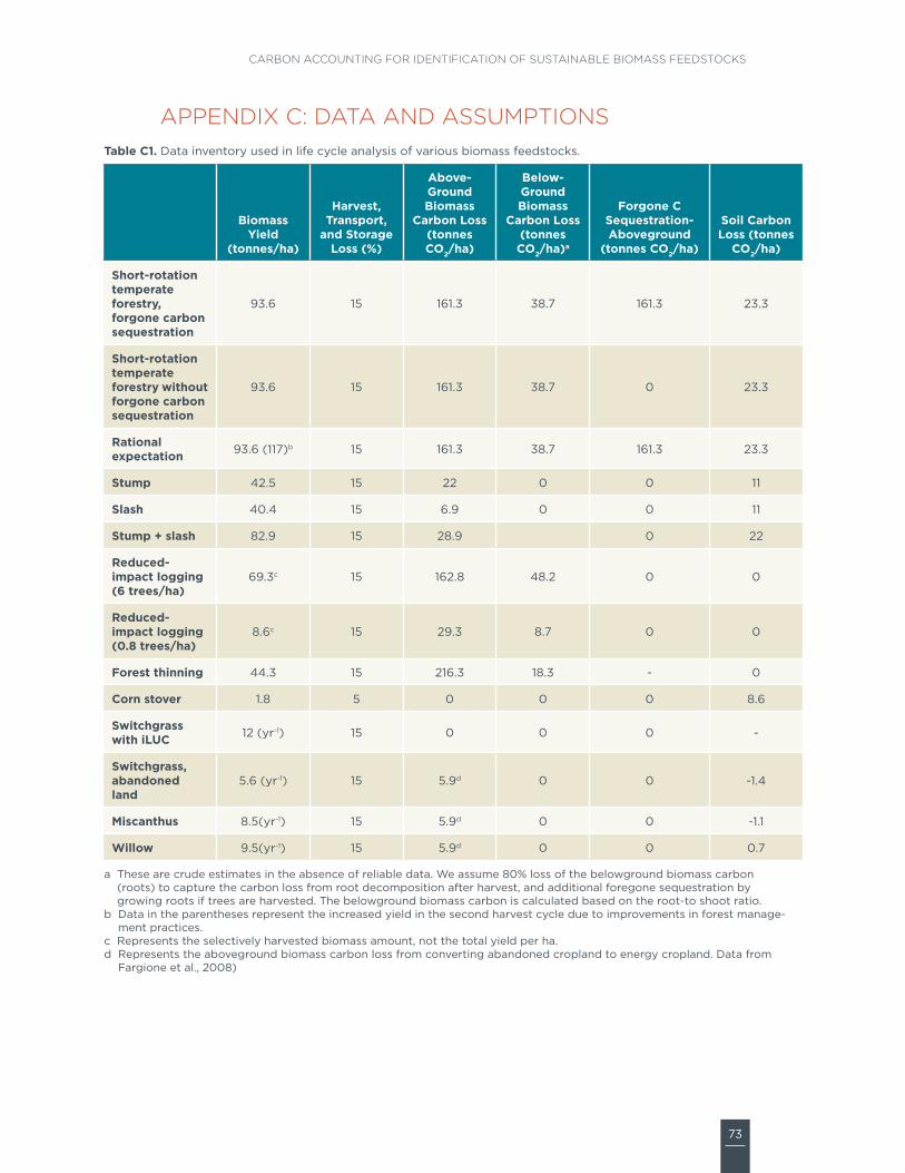
73


APPENDIX C: DATA AND ASSUMPTIONS Table C1. Data inventory used in life cycle analysis of various biomass feedstocks.

Biomass Yield

(tonnes/ha)

Harvest, Transport,

and Storage Loss (%)

Above-Ground Biomass

Carbon Loss (tonnes CO2/ha)

Below-Ground Biomass

Carbon Loss (tonnes CO2/ha)a

Forgone C Sequestration-Aboveground

(tonnes CO2/ha)

Soil Carbon Loss (tonnes

CO2/ha)

Short-rotation temperate forestry, forgone carbon sequestration

93.6 15 161.3 38.7 161.3 23.3

Short-rotation temperate forestry without forgone carbon sequestration

93.6 15 161.3 38.7 0 23.3

Rational expectation 93.6 (117)b 15 161.3 38.7 161.3 23.3

Stump 42.5 15 22 0 0 11

Slash 40.4 15 6.9 0 0 11

Stump + slash 82.9 15 28.9 0 22

Reduced-impact logging (6 trees/ha)

69.3c 15 162.8 48.2 0 0

Reduced-impact logging (0.8 trees/ha)

8.6c 15 29.3 8.7 0 0

Forest thinning 44.3 15 216.3 18.3 - 0

Corn stover 1.8 5 0 0 0 8.6

Switchgrass with iLUC 12 (yr-1) 15 0 0 0 -

Switchgrass, abandoned land

5.6 (yr-1) 15 5.9d 0 0 -1.4

Miscanthus 8.5(yr-1) 15 5.9d 0 0 -1.1

Willow 9.5(yr-1) 15 5.9d 0 0 0.7

a These are crude estimates in the absence of reliable data. We assume 80% loss of the belowground biomass carbon (roots) to capture the carbon loss from root decomposition after harvest, and additional foregone sequestration by growing roots if trees are harvested. The belowground biomass carbon is calculated based on the root-to shoot ratio.

b Data in the parentheses represent the increased yield in the second harvest cycle due to improvements in forest manage-ment practices.

c Represents the selectively harvested biomass amount, not the total yield per ha. d Represents the aboveground biomass carbon loss from converting abandoned cropland to energy cropland. Data from

Fargione et al., 2008)

74

ICCT WHITE PAPER

Table C2. Data inventory used in the life cycle analysis of various biomass feedstocks.

Indirect Land Use Change (g

CO2/MJ Ethanol)

Soil Carbon Sequestration (tonnes Co2 ha–1 year –1)

N (tonnes/dry tonne)

P2O5 (tonnes/dry

tonne)

K2O (tonnes/d

tonne)

Harvesting Cycle

(Years)

Short-rotation temperate forestry with forgone carbon sequestration

0 0 4.0 0.3 0.6 25

Short-rotation temperate forestry without forgone carbon sequestration

0 0 4.0 0.3 0.6 25

Rational expectation 0 0 4.0 0.3 0.6 25

Stump 0 0 0.8 0.2 0.6 25

Slash 0 0 3.7 0.5 1.5 25

Stump + slash 0 0 2.3 0.4 1.0 25

Reduced-impact logging (6 trees/ha)

0 0 4.0 0.3 0.6 40

Reduced-impact logging (0.8 trees/ha)

0 0 4.0 0.3 0.6 40

Forest thinning 0 0 4.0 0.3 0.6 50

Corn stover 0 0 8.5 2.2 13.2 1

Switchgrass with iLUC 2.8 - 7.6 3.1 3.1 1

Switchgrass, abandoned land 0 1.4 7.6 3.1 3.1 1

Miscanthus 0 1.1 7.1 0.9 9.4 1

Willow 0 -0.7a 2.9 0.1 0.1 3

a Although willow increases soil carbon, it will still be less than in the reference scenario, hence a negative value (Brandão, 2011).

75


Table C3. Data and assumptions used in sensitivity analysis.

High Emissions Default (Main Case) Low Emissions

Short-rotation forestry

Forgone carbon sequestration, 161.3 tonnes CO2/ha; soil carbon loss, 20% more, biomass yield, 20% less

Forgone carbon sequestration, 161.3 tonnes CO2/ha; soil carbon loss, 23.3 tonnes CO2/ha; biomass yield, 93.6 tonnes/ha

No forgone sequestration; soil carbon loss, 20% less; biomass yield, 20% more

Forest thinning

Above-ground biomass carbon loss including forgone carbon sequestration, 20% more; below-ground biomass carbon loss, 20% more

Above-ground biomass carbon loss including forgone carbon sequestration, 216.3 tonnes CO2/ha; below-ground biomass carbon loss, 18.3 tonnes CO2/ha

Above-ground carbon loss including forgone carbon sequestration, 20% less; below-ground biomass carbon loss, 20% less

RIL, Brazil

Above-ground biomass loss from harvest, 20% more CO2/ha; below-ground biomass carbon loss, 20% more

Above-ground biomass loss from harvest, 162.8 tonnes CO2/ha; below-ground biomass carbon loss, 48.2 tonnes CO2/ha

Above-ground biomass loss from harvest, 20% less; below-ground biomass carbon loss, 20% less

Corn stoverHarvested biomass, same; soil carbon loss, 20% more

Harvested biomass, 1.8 tonnes/ha; soil carbon loss, 8.6 CO2 tonnes ha−1

Harvested biomass, 30% more; soil carbon loss, 20% less

Switchgrass in abandoned land

Biomass yield, 3 tonnes ha−1 year−1; soil carbon sequestration, 1.0 tonnes CO2 ha−1 year−1

Biomass yield, 5.6 tonnes ha−1 year−1; carbon sequestration, 1.4 tonnes CO2 ha−1 year−1

Biomass yield, 14 tonnes ha−1 year−1; carbon sequestration, 11.7 tonnes CO2 ha−1 year−1

Miscanthus in abandoned land


Biomass yield, 8.5 tonnes ha−1 year−1; soil carbon sequestration, 1.1

tonnes CO2 ha−1 year−1


Willow in abandoned land

Biomass yield, 4 tonnes/ha; soil carbon sequestration,-0.7 tonnes CO2 ha−1 year−1

Biomass yield, 9.5 tonnes/ha; soil carbon sequestration, -0.7 tonnes CO2 ha−1 year−1

Biomass yield, 12 tonnes/ha; soil carbon sequestration, 0.7 tonnes CO2 ha−1 year−1

Slash

Biomass yield, 20% less; soil carbon loss, 3 tonnes C/ha; 15% of material undecomposed at 25 years in BAU scenario

Biomass yield, 40.4 tonnes/ha; no soil carbon loss; 10% of material undecomposed at 25 years in BAU scenario

Biomass yield, 40.4 tonnes/ha; no soil carbon loss; all material decomposed after 25 years in BAU scenario

comprehensive carbon accounting for identification of sustainable biomass feedstocks

Documents

carbon questions

soil carbon

carbon discounting

scope of carbon accounting

temporal impact of carbon

carbon payback period

biomass use

valuable feedback