complexity classes for optimization problemshome.in.tum.de/~kugele/files/jobsis_alt.pdf · jobsis...
TRANSCRIPT
JoBSIS – Binntal 2004 Complexity Classes for Optimization Problems – p. 2/67
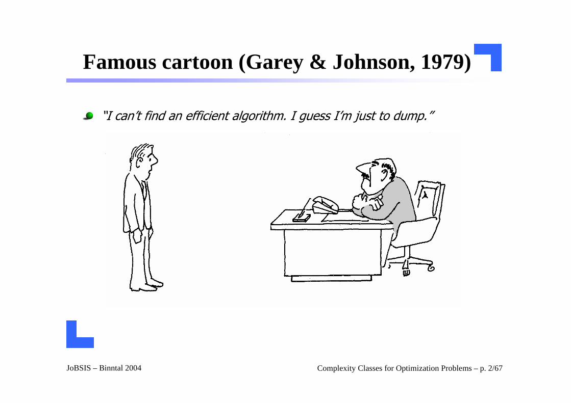
Famous cartoon (Garey & Johnson, 1979)
“I can’t find an efficient algorithm. I guess I’m just to dump.”
JoBSIS – Binntal 2004 Complexity Classes for Optimization Problems – p. 3/67
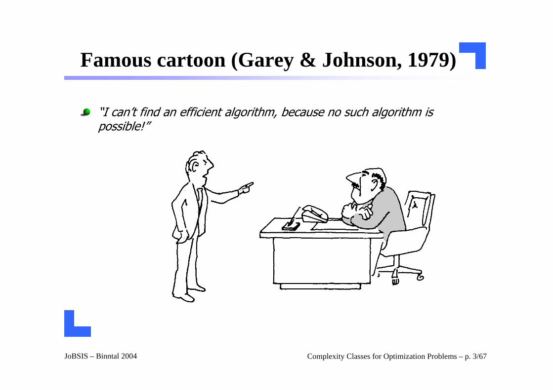
Famous cartoon (Garey & Johnson, 1979)
“I can’t find an efficient algorithm, because no such algorithm is possible!”
JoBSIS – Binntal 2004 Complexity Classes for Optimization Problems – p. 4/67
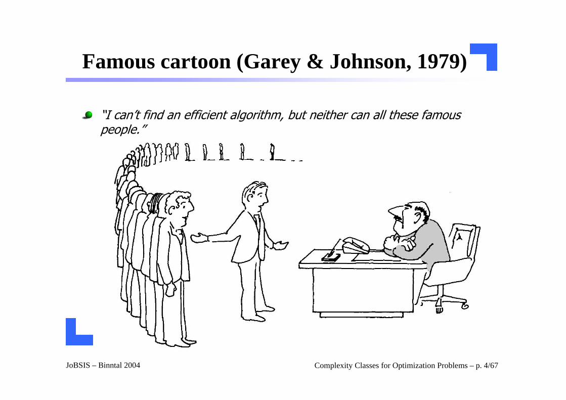
Famous cartoon (Garey & Johnson, 1979)
“I can’t find an efficient algorithm, but neither can all these famous people.”
JoBSIS – Binntal 2004 Complexity Classes for Optimization Problems – p. 5/67
Why using Approximation?
We are not able to solve NP-complete problems efficiently, that is, there is no known way to solve them in polynomial time unless P = NP.Why not looking for a approximate solution?
JoBSIS – Binntal 2004 Complexity Classes for Optimization Problems – p. 6/67
Two Basic principles
Algorithm designGreedy approachLocal searchLinear programming (LP)Dynamic programming (DP)Randomized algorithms
Complexity ClassesThat’s what we are dealing with today
JoBSIS – Binntal 2004 Complexity Classes for Optimization Problems – p. 7/67
Agenda
IntroductionOptimization problemErrors, approximation algorithmClasses
NPO
APX
PTAS
FPTAS
F-APX
OutlookAP-ReductionsMax-SNP
JoBSIS – Binntal 2004 Complexity Classes for Optimization Problems – p. 8/67
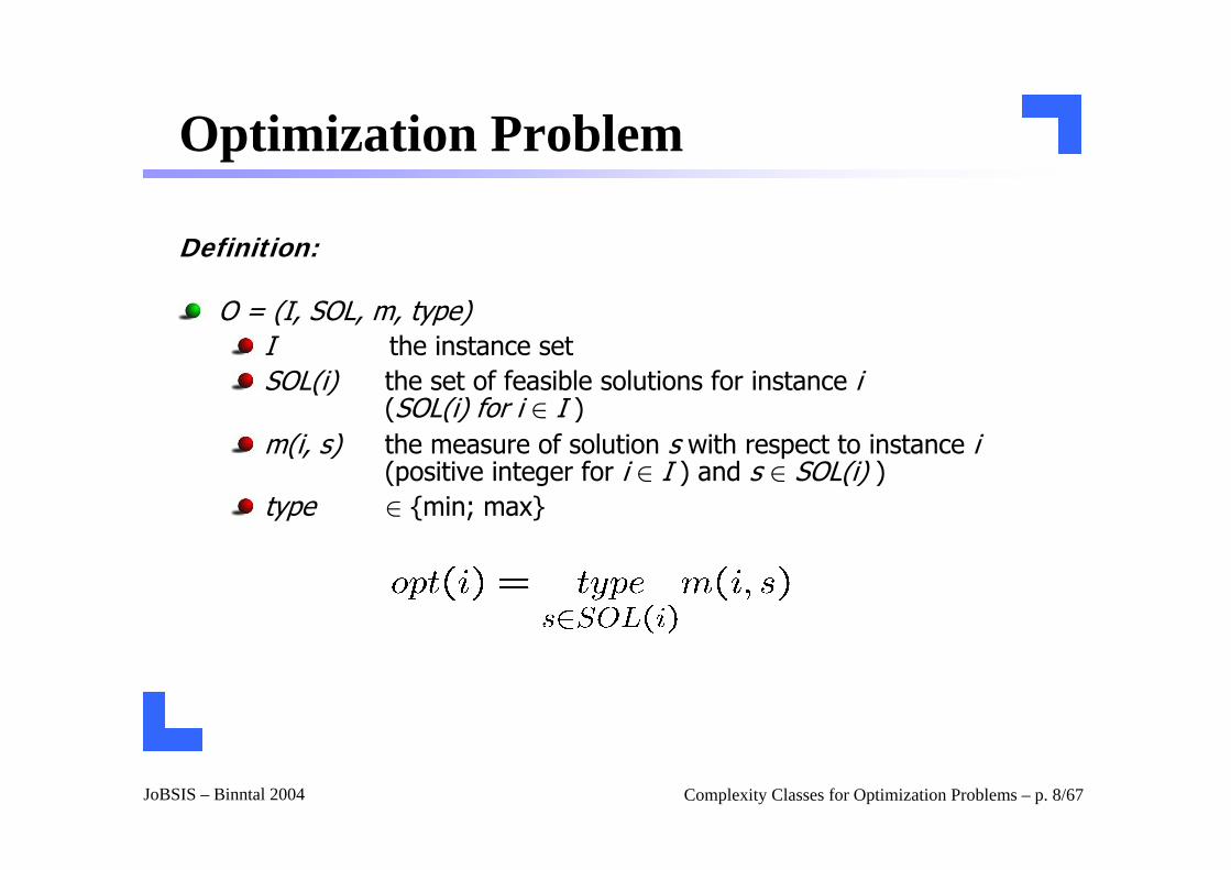
Optimization Problem
Definition:
O = (I, SOL, m, type)I the instance setSOL(i) the set of feasible solutions for instance i
(SOL(i) for i ∈ I )m(i, s) the measure of solution s with respect to instance i
(positive integer for i ∈ I ) and s ∈ SOL(i) )type ∈ {min; max}
JoBSIS – Binntal 2004 Complexity Classes for Optimization Problems – p. 9/67
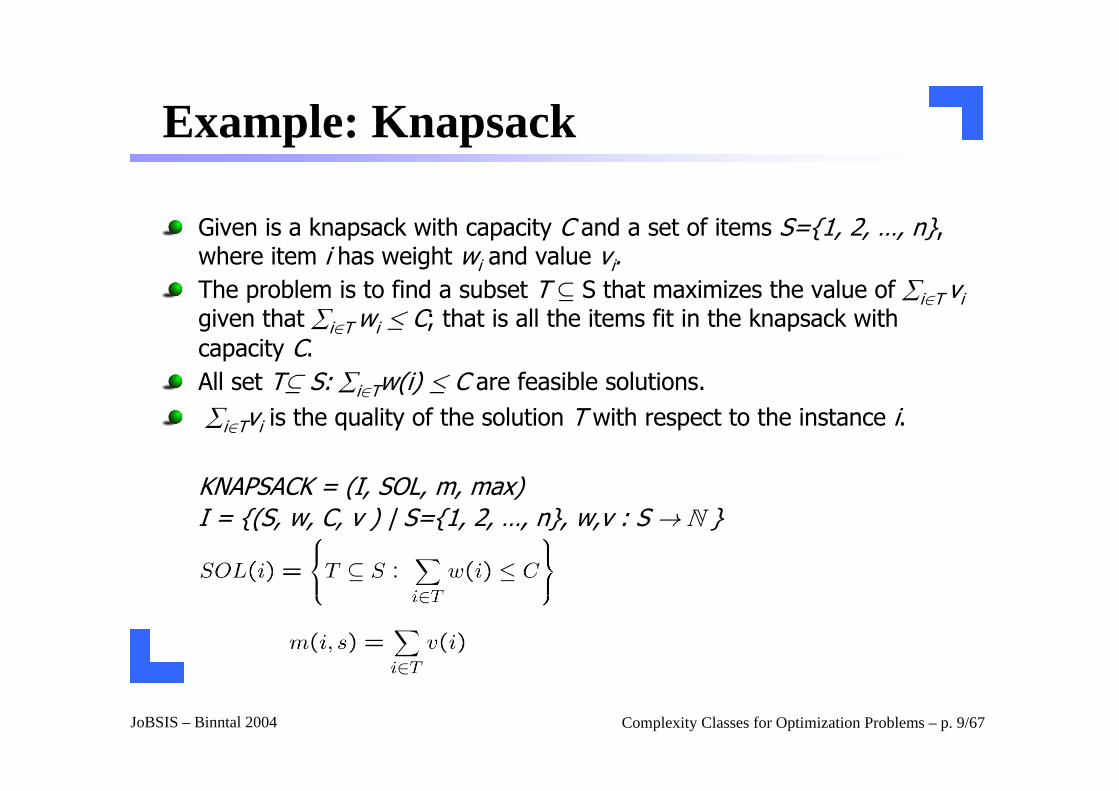
Example: Knapsack
Given is a knapsack with capacity C and a set of items S={1, 2, …, n}, where item i has weight wi and value vi.The problem is to find a subset T ⊆ S that maximizes the value of ∑i∈T vigiven that ∑i∈T wi · C; that is all the items fit in the knapsack with capacity C.All set T⊆ S: ∑i∈Tw(i) · C are feasible solutions.∑i∈Tvi is the quality of the solution T with respect to the instance i.
KNAPSACK = (I, SOL, m, max)I = {(S, w, C, v ) | S={1, 2, …, n}, w,v : S → N }
JoBSIS – Binntal 2004 Complexity Classes for Optimization Problems – p. 10/67
Agenda
IntroductionOptimization problemErrors, approximation algorithmsClasses
NPO
APX
PTAS
FPTAS
F-APX
OutlookAP-ReductionsMax-SNP
JoBSIS – Binntal 2004 Complexity Classes for Optimization Problems – p. 11/67
Approximation Algorithm
Definition:
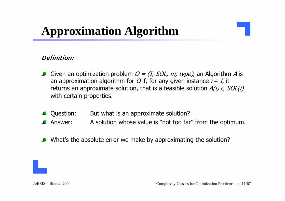
Given an optimization problem O = (I, SOL, m, type), an Algorithm A is an approximation algorithm for O if, for any given instance i ∈ I, it returns an approximate solution, that is a feasible solution A(i) ∈ SOL(i) with certain properties.
Question: But what is an approximate solution?Answer: A solution whose value is “not too far” from the optimum.
What’s the absolute error we make by approximating the solution?
JoBSIS – Binntal 2004 Complexity Classes for Optimization Problems – p. 12/67
Absolute error
Definition:
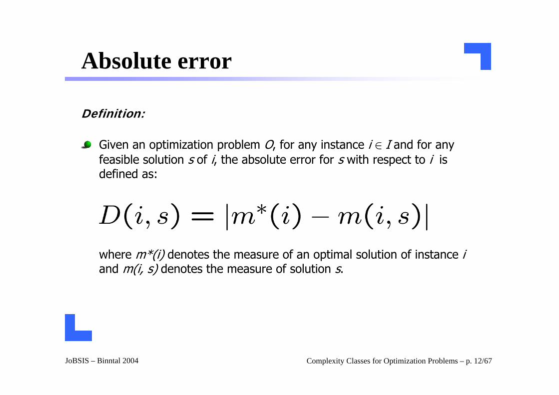
Given an optimization problem O, for any instance i ∈ I and for any feasible solution s of i, the absolute error for s with respect to i is defined as:
where m*(i) denotes the measure of an optimal solution of instance iand m(i, s) denotes the measure of solution s.
JoBSIS – Binntal 2004 Complexity Classes for Optimization Problems – p. 13/67
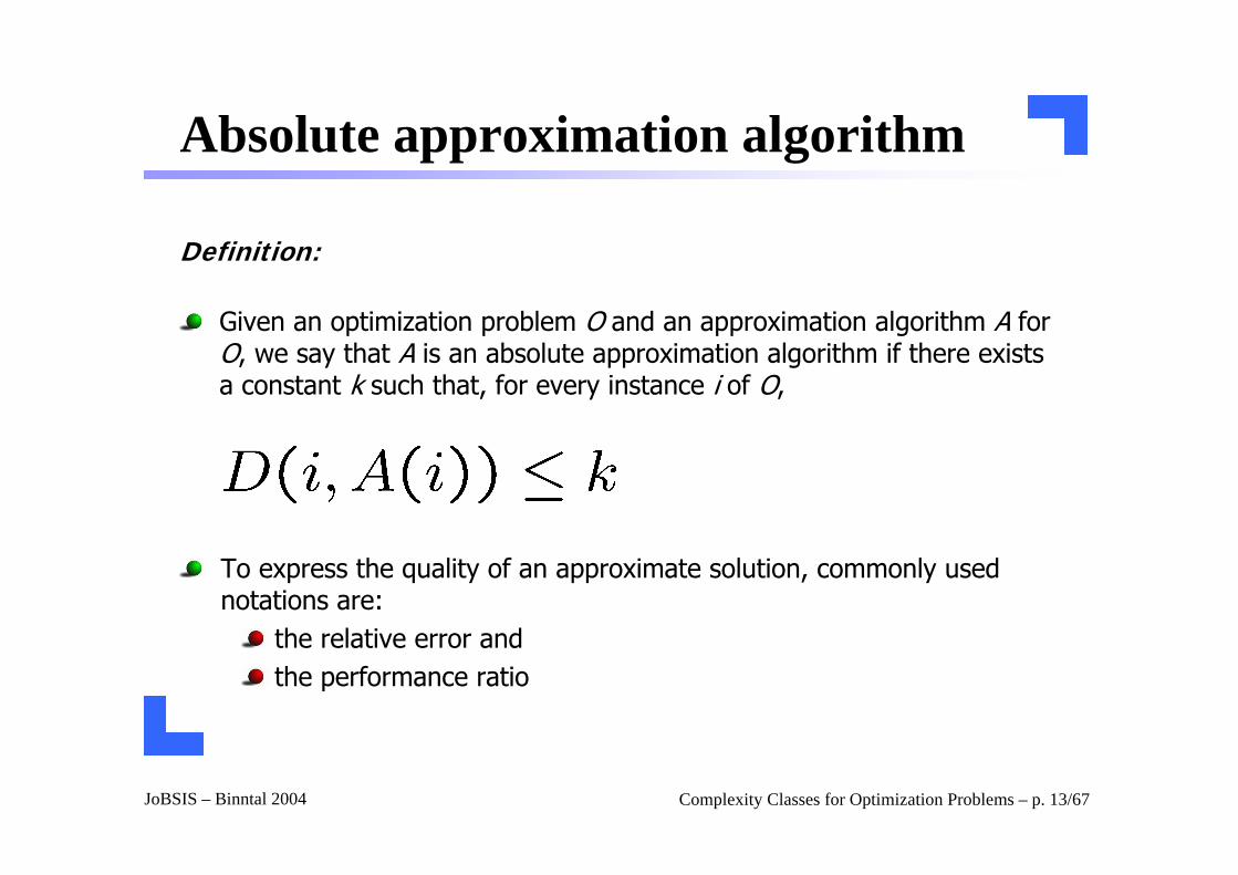
Absolute approximation algorithm
Definition:
Given an optimization problem O and an approximation algorithm A for O, we say that A is an absolute approximation algorithm if there exists a constant k such that, for every instance i of O,
To express the quality of an approximate solution, commonly usednotations are:
the relative error andthe performance ratio
JoBSIS – Binntal 2004 Complexity Classes for Optimization Problems – p. 14/67
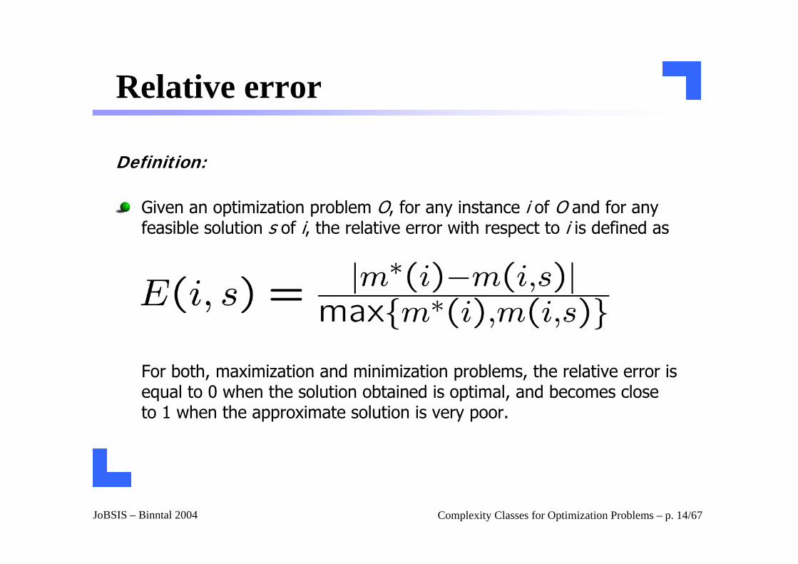
Relative error
Definition:
Given an optimization problem O, for any instance i of O and for any feasible solution s of i, the relative error with respect to i is defined as
For both, maximization and minimization problems, the relative error is equal to 0 when the solution obtained is optimal, and becomes close to 1 when the approximate solution is very poor.
JoBSIS – Binntal 2004 Complexity Classes for Optimization Problems – p. 15/67
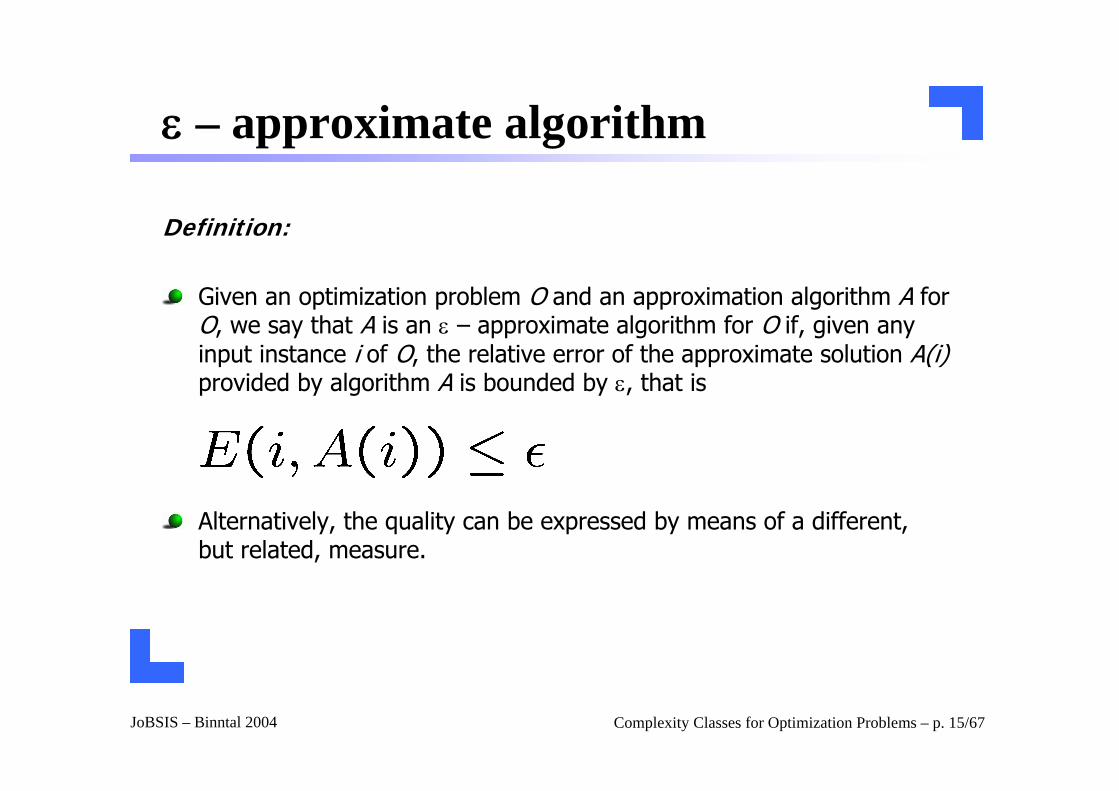
ε – approximate algorithm
Definition:
Given an optimization problem O and an approximation algorithm A for O, we say that A is an ε – approximate algorithm for O if, given any input instance i of O, the relative error of the approximate solution A(i)provided by algorithm A is bounded by ε, that is
Alternatively, the quality can be expressed by means of a different, but related, measure.
JoBSIS – Binntal 2004 Complexity Classes for Optimization Problems – p. 16/67
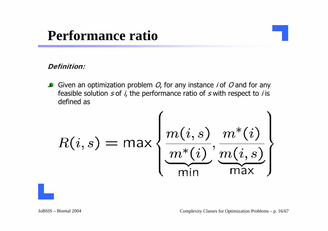
Performance ratio
Definition:
Given an optimization problem O, for any instance i of O and for any feasible solution s of i, the performance ratio of s with respect to i is defined as
JoBSIS – Binntal 2004 Complexity Classes for Optimization Problems – p. 17/67
Performance ratio (cont.)
For both, minimization and maximization, the value of the performance ratio is equal to 1 in the case of an optimal solution, and can assume arbitrarily large values in the case of an poor approximate resolution.
JoBSIS – Binntal 2004 Complexity Classes for Optimization Problems – p. 18/67
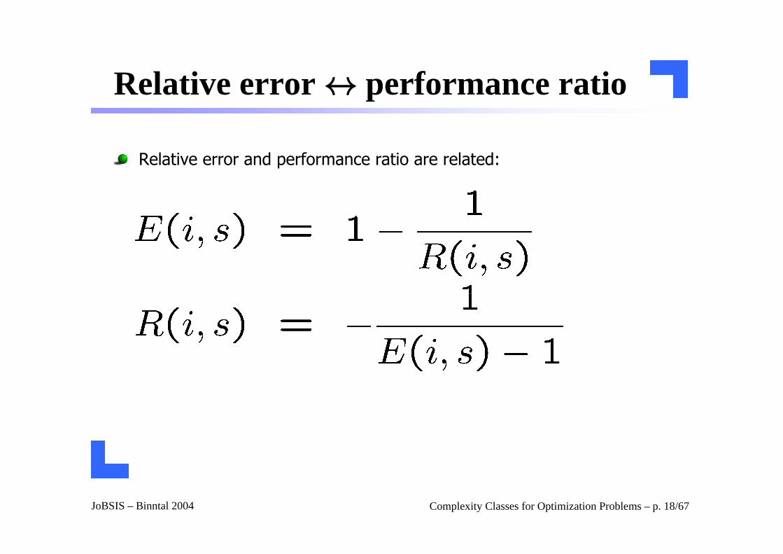
Relative error ↔ performance ratio
Relative error and performance ratio are related:
JoBSIS – Binntal 2004 Complexity Classes for Optimization Problems – p. 19/67
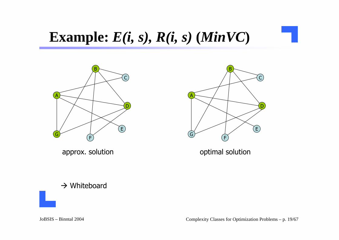
Example: E(i, s), R(i, s) (MinVC)
A
B
C
D
E
FG
A
B
C
D
E
FG
Whiteboard
approx. solution optimal solution
JoBSIS – Binntal 2004 Complexity Classes for Optimization Problems – p. 20/67
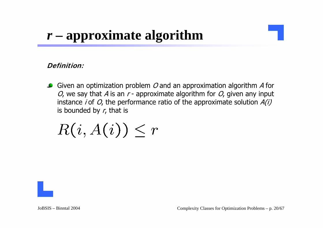
r – approximate algorithm
Definition:
Given an optimization problem O and an approximation algorithm A for O, we say that A is an r - approximate algorithm for O, given any input instance i of O, the performance ratio of the approximate solution A(i)is bounded by r, that is
JoBSIS – Binntal 2004 Complexity Classes for Optimization Problems – p. 21/67
Agenda
IntroductionOptimization problemErrors, approximation algorithmClasses
NPO
APX
PTAS
FPTAS
F-APX
OutlookAP-ReductionsMax-SNP
JoBSIS – Binntal 2004 Complexity Classes for Optimization Problems – p. 22/67
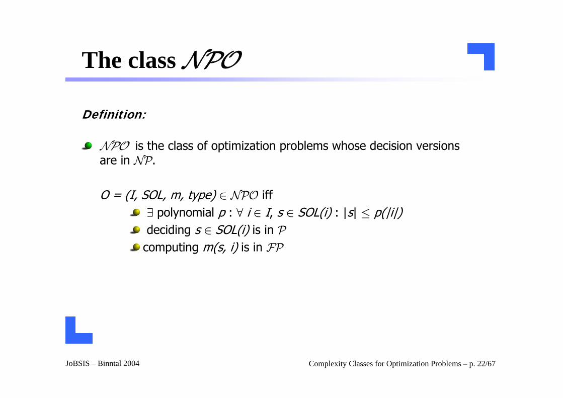
The class NPO
Definition:
NPO is the class of optimization problems whose decision versions are in NP.
O = (I, SOL, m, type) ∈ NPO iff∃ polynomial p : ∀ i ∈ I, s ∈ SOL(i) : |s| · p(|i|)deciding s ∈ SOL(i) is in P
computing m(s, i) is in FP
JoBSIS – Binntal 2004 Complexity Classes for Optimization Problems – p. 23/67
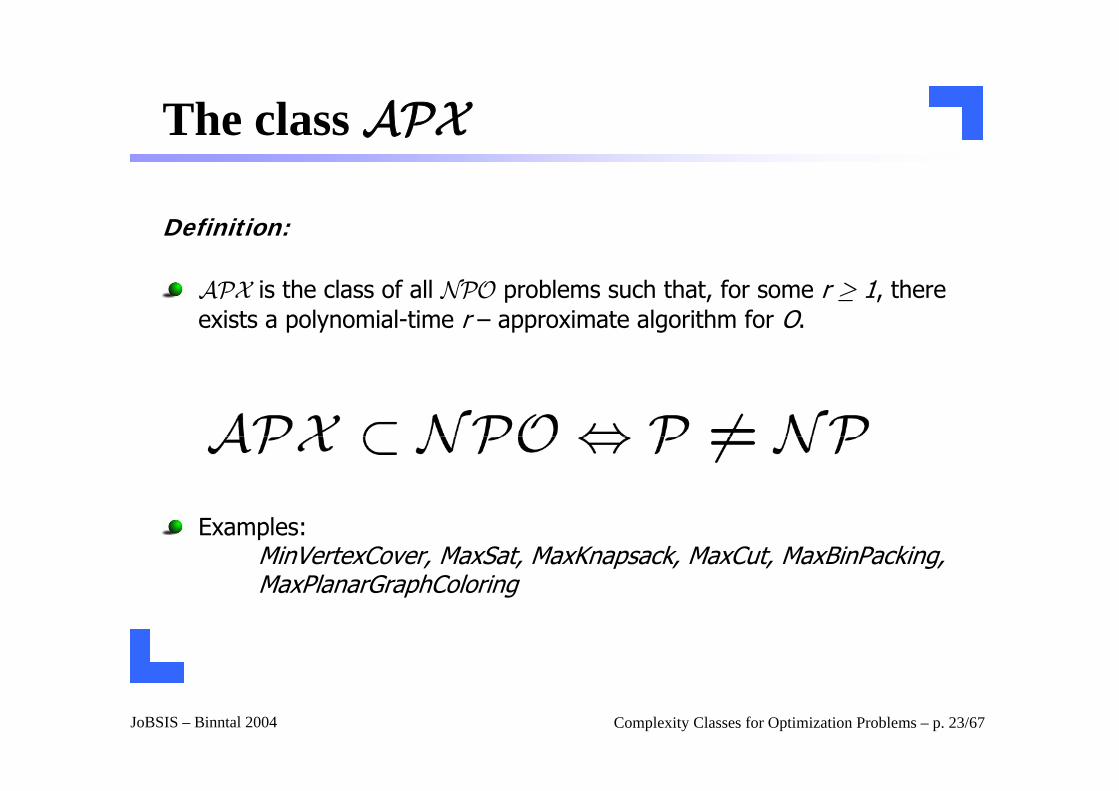
The class APX
Definition:
APX is the class of all NPO problems such that, for some r ≥ 1, there exists a polynomial-time r – approximate algorithm for O.
Examples: MinVertexCover, MaxSat, MaxKnapsack, MaxCut, MaxBinPacking, MaxPlanarGraphColoring
JoBSIS – Binntal 2004 Complexity Classes for Optimization Problems – p. 24/67
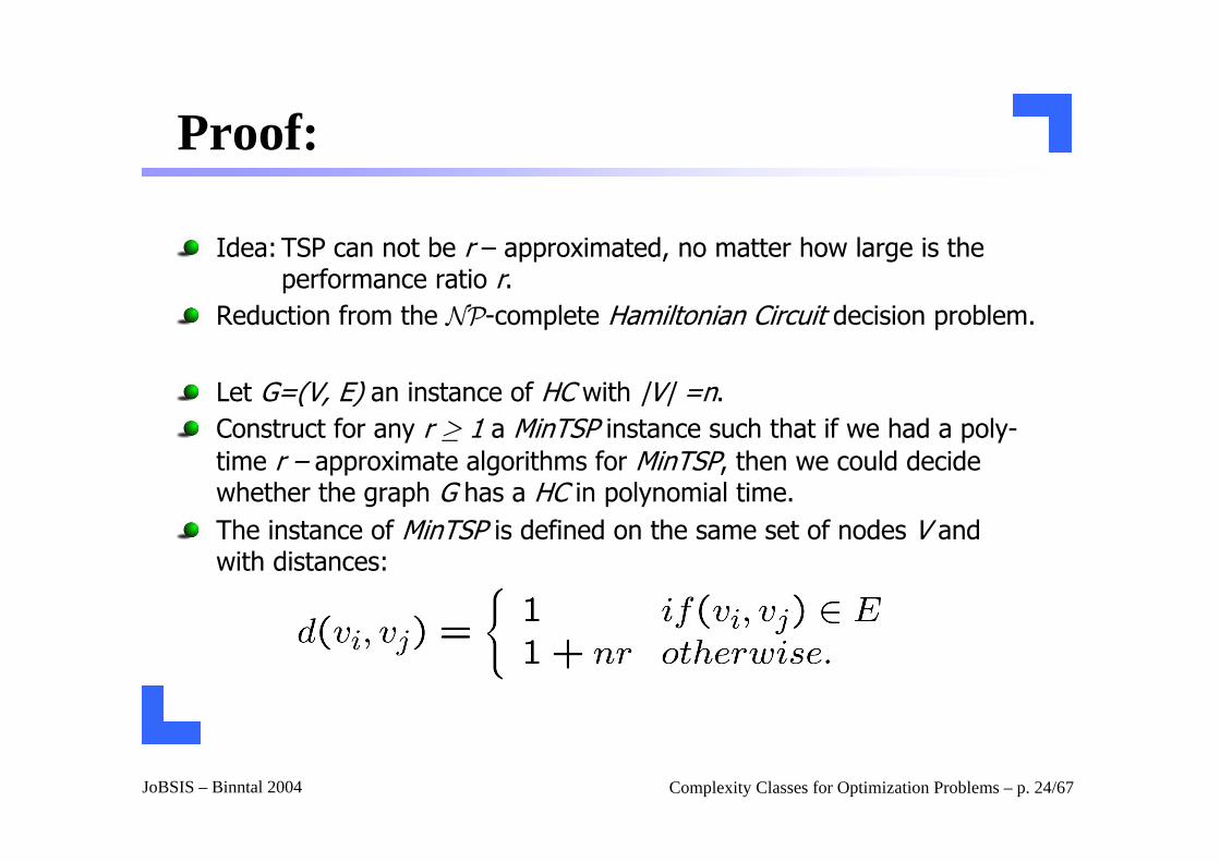
Proof:
Idea: TSP can not be r – approximated, no matter how large is the performance ratio r.
Reduction from the NP-complete Hamiltonian Circuit decision problem.
Let G=(V, E) an instance of HC with |V| =n.Construct for any r ≥ 1 a MinTSP instance such that if we had a poly-time r – approximate algorithms for MinTSP, then we could decide whether the graph G has a HC in polynomial time.The instance of MinTSP is defined on the same set of nodes V and with distances:
JoBSIS – Binntal 2004 Complexity Classes for Optimization Problems – p. 25/67
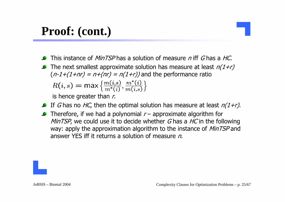
Proof: (cont.)
This instance of MinTSP has a solution of measure n iff G has a HC.The next smallest approximate solution has measure at least n(1+r)(n-1+(1+nr) = n+(nr) = n(1+r)) and the performance ratio
is hence greater than r.If G has no HC, then the optimal solution has measure at least n(1+r).Therefore, if we had a polynomial r – approximate algorithm for MinTSP, we could use it to decide whether G has a HC in the following way: apply the approximation algorithm to the instance of MinTSP and answer YES iff it returns a solution of measure n.
JoBSIS – Binntal 2004 Complexity Classes for Optimization Problems – p. 26/67
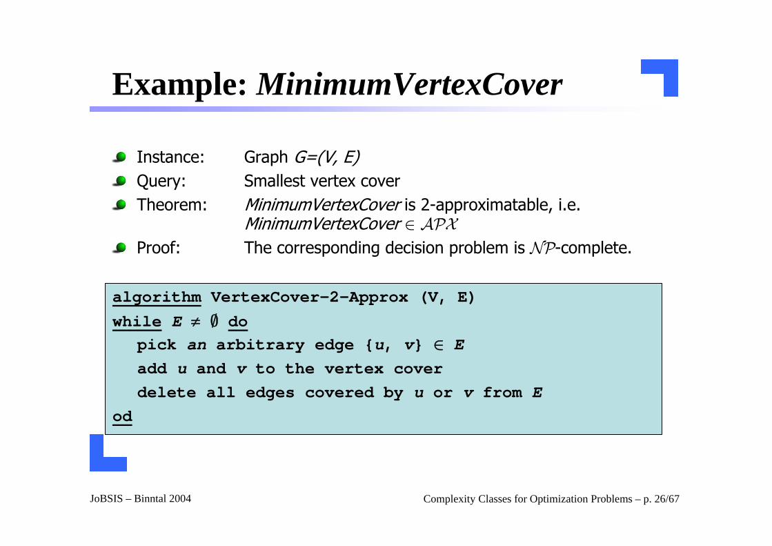
Example: MinimumVertexCover
Instance: Graph G=(V, E)Query: Smallest vertex coverTheorem: MinimumVertexCover is 2-approximatable, i.e.
MinimumVertexCover ∈ APX
Proof: The corresponding decision problem is NP-complete.
algorithm VertexCover-2-Approx (V, E)
while E ≠ ∅ dopick an arbitrary edge {u, v} ∈ Eadd u and v to the vertex coverdelete all edges covered by u or v from E
od
JoBSIS – Binntal 2004 Complexity Classes for Optimization Problems – p. 27/67
Example: MinimumVertexCover (cont.)
A
B
C
D
E
FG
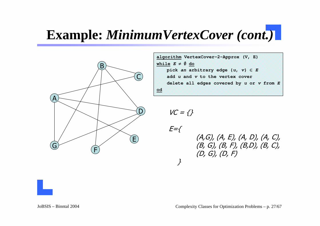
algorithm VertexCover-2-Approx (V, E)
while E ≠ ∅ dopick an arbitrary edge {u, v} ∈ Eadd u and v to the vertex coverdelete all edges covered by u or v from E
od
VC = {}
E={(A,G), (A, E), (A, D), (A, C), (B, G), (B, F), (B,D), (B, C),(D, G), (D, F)
}
JoBSIS – Binntal 2004 Complexity Classes for Optimization Problems – p. 28/67
Example: MinimumVertexCover (cont.)
A
B
C
D
E
FG
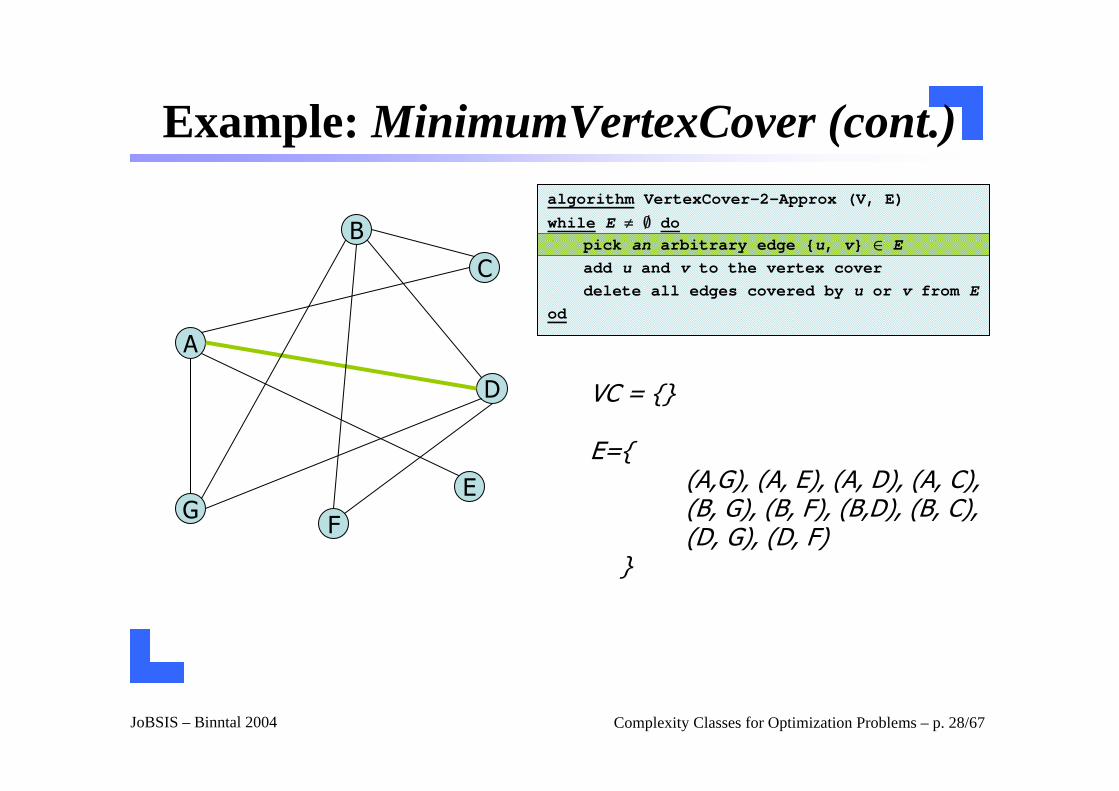
algorithm VertexCover-2-Approx (V, E)
while E ≠ ∅ dopick an arbitrary edge {u, v} ∈ Eadd u and v to the vertex coverdelete all edges covered by u or v from E
od
VC = {}
E={(A,G), (A, E), (A, D), (A, C), (B, G), (B, F), (B,D), (B, C),(D, G), (D, F)
}
JoBSIS – Binntal 2004 Complexity Classes for Optimization Problems – p. 29/67
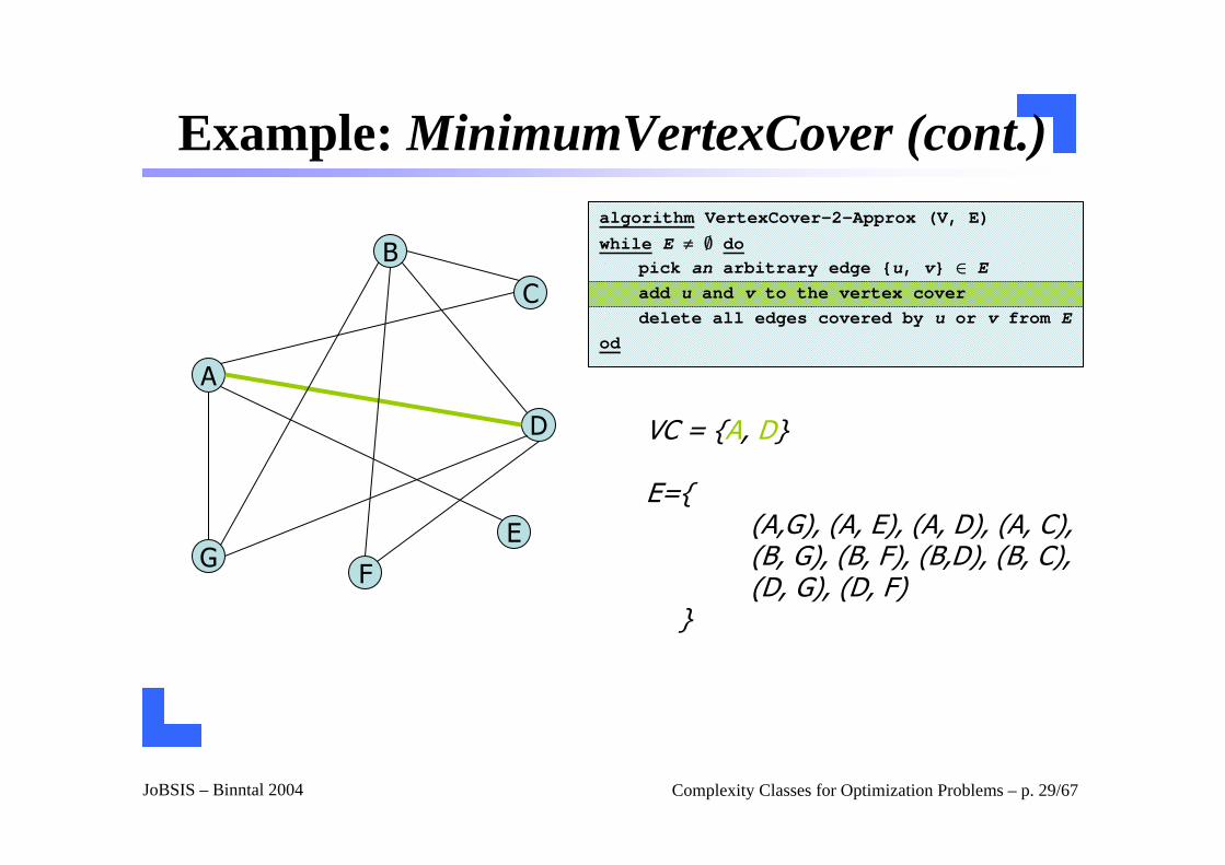
Example: MinimumVertexCover (cont.)
A
B
C
D
E
FG
algorithm VertexCover-2-Approx (V, E)
while E ≠ ∅ dopick an arbitrary edge {u, v} ∈ Eadd u and v to the vertex coverdelete all edges covered by u or v from E
od
VC = {A, D}
E={(A,G), (A, E), (A, D), (A, C), (B, G), (B, F), (B,D), (B, C),(D, G), (D, F)
}
JoBSIS – Binntal 2004 Complexity Classes for Optimization Problems – p. 30/67
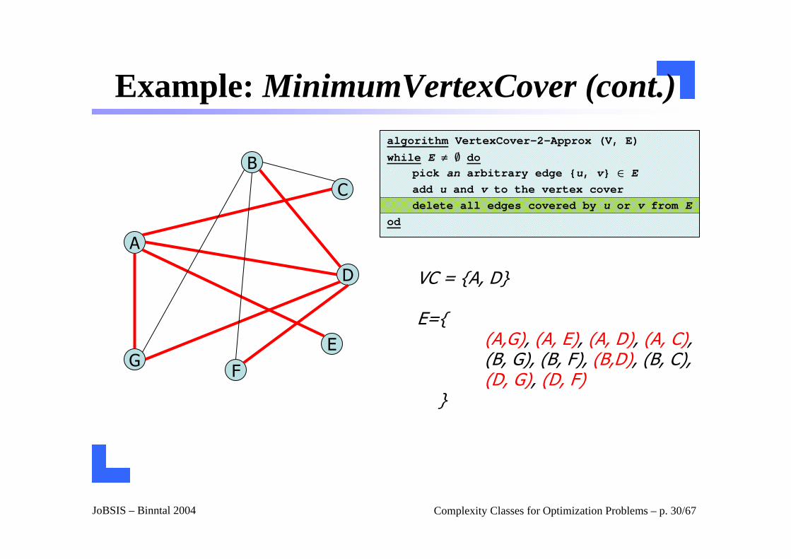
Example: MinimumVertexCover (cont.)
A
B
C
D
E
FG
algorithm VertexCover-2-Approx (V, E)
while E ≠ ∅ dopick an arbitrary edge {u, v} ∈ Eadd u and v to the vertex coverdelete all edges covered by u or v from E
od
VC = {A, D}
E={(A,G), (A, E), (A, D), (A, C), (B, G), (B, F), (B,D), (B, C),(D, G), (D, F)
}
JoBSIS – Binntal 2004 Complexity Classes for Optimization Problems – p. 31/67
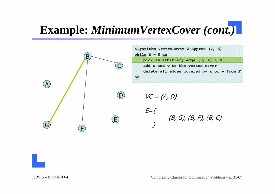
Example: MinimumVertexCover (cont.)
A
B
C
D
E
FG
algorithm VertexCover-2-Approx (V, E)
while E ≠ ∅ dopick an arbitrary edge {u, v} ∈ Eadd u and v to the vertex coverdelete all edges covered by u or v from E
od
VC = {A, D}
E={(B, G), (B, F), (B, C)
}
JoBSIS – Binntal 2004 Complexity Classes for Optimization Problems – p. 32/67
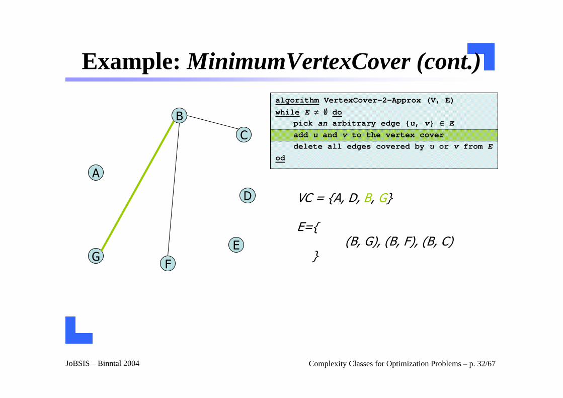
Example: MinimumVertexCover (cont.)
A
B
C
D
E
FG
algorithm VertexCover-2-Approx (V, E)
while E ≠ ∅ dopick an arbitrary edge {u, v} ∈ Eadd u and v to the vertex coverdelete all edges covered by u or v from E
od
VC = {A, D, B, G}
E={(B, G), (B, F), (B, C)
}
JoBSIS – Binntal 2004 Complexity Classes for Optimization Problems – p. 33/67
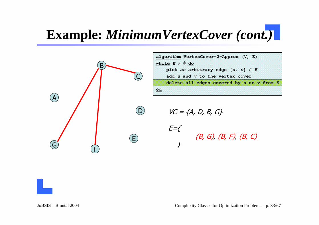
Example: MinimumVertexCover (cont.)
A
B
C
D
E
FG
algorithm VertexCover-2-Approx (V, E)
while E ≠ ∅ dopick an arbitrary edge {u, v} ∈ Eadd u and v to the vertex coverdelete all edges covered by u or v from E
od
VC = {A, D, B, G}
E={(B, G), (B, F), (B, C)
}
JoBSIS – Binntal 2004 Complexity Classes for Optimization Problems – p. 34/67
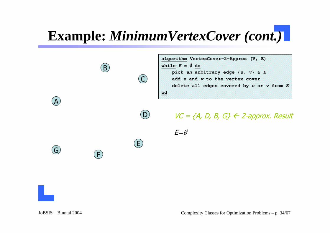
Example: MinimumVertexCover (cont.)
A
B
C
D
E
FG
algorithm VertexCover-2-Approx (V, E)
while E ≠ ∅ dopick an arbitrary edge {u, v} ∈ Eadd u and v to the vertex coverdelete all edges covered by u or v from E
od
VC = {A, D, B, G} 2-approx. Result
E=∅
JoBSIS – Binntal 2004 Complexity Classes for Optimization Problems – p. 35/67
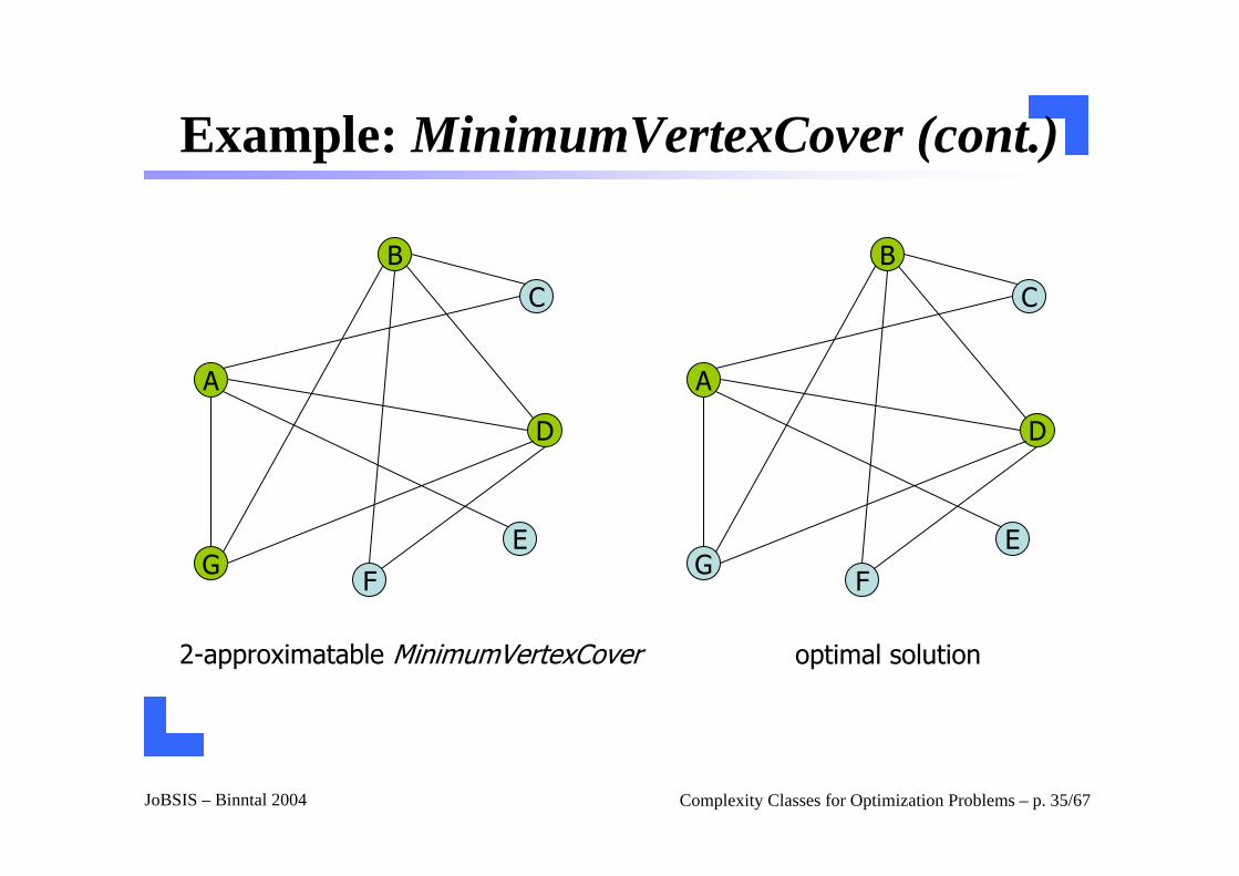
Example: MinimumVertexCover (cont.)
A
B
C
D
E
FG
A
B
C
D
E
FG
2-approximatable MinimumVertexCover optimal solution
JoBSIS – Binntal 2004 Complexity Classes for Optimization Problems – p. 36/67
Example: MinimumVertexCover (cont.)
The result is a vertex cover but is its size maximum twice the optimum?
Yes. No two edges chosen by the algorithm have shared nodes. Hence, a vertex cover of only those edges has to contain at least either of them, i.e. be at least half of the size of the found vertex cover.
JoBSIS – Binntal 2004 Complexity Classes for Optimization Problems – p. 37/67
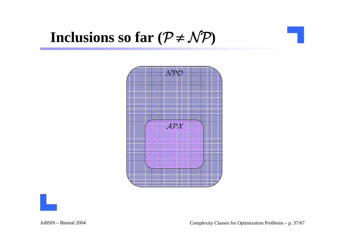
Inclusions so far (P ≠ NP)
NPO
APX
JoBSIS – Binntal 2004 Complexity Classes for Optimization Problems – p. 38/67
Limits to approximability: The gap technique
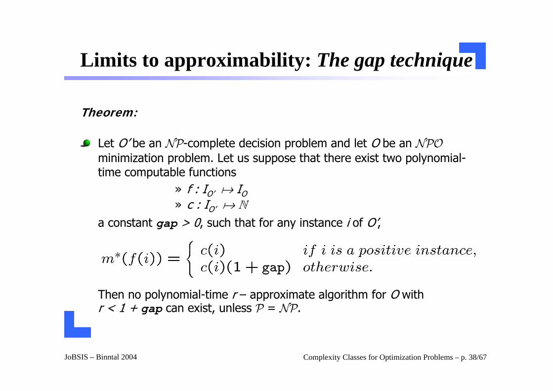
Theorem:
Let O’ be an NP-complete decision problem and let O be an NPOminimization problem. Let us suppose that there exist two polynomial-time computable functions
» f : IO’ a IO» c : IO’ a N
a constant gap > 0, such that for any instance i of O’,
Then no polynomial-time r – approximate algorithm for O with r < 1 + gap can exist, unless P = NP.
JoBSIS – Binntal 2004 Complexity Classes for Optimization Problems – p. 39/67
Proof: The gap technique
Whiteboard
JoBSIS – Binntal 2004 Complexity Classes for Optimization Problems – p. 40/67
Example: The gap technique (I)
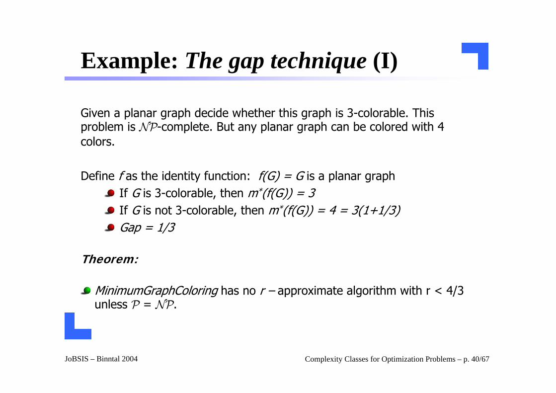
Given a planar graph decide whether this graph is 3-colorable. This problem is NP-complete. But any planar graph can be colored with 4 colors.
Define f as the identity function: f(G) = G is a planar graphIf G is 3-colorable, then m*(f(G)) = 3If G is not 3-colorable, then m*(f(G)) = 4 = 3(1+1/3)Gap = 1/3
Theorem:
MinimumGraphColoring has no r – approximate algorithm with r < 4/3 unless P = NP.
JoBSIS – Binntal 2004 Complexity Classes for Optimization Problems – p. 41/67
Example: The gap technique (II)
Whiteboard (MinimumBinPacking)
JoBSIS – Binntal 2004 Complexity Classes for Optimization Problems – p. 42/67
Polynomial-time approximation schemes
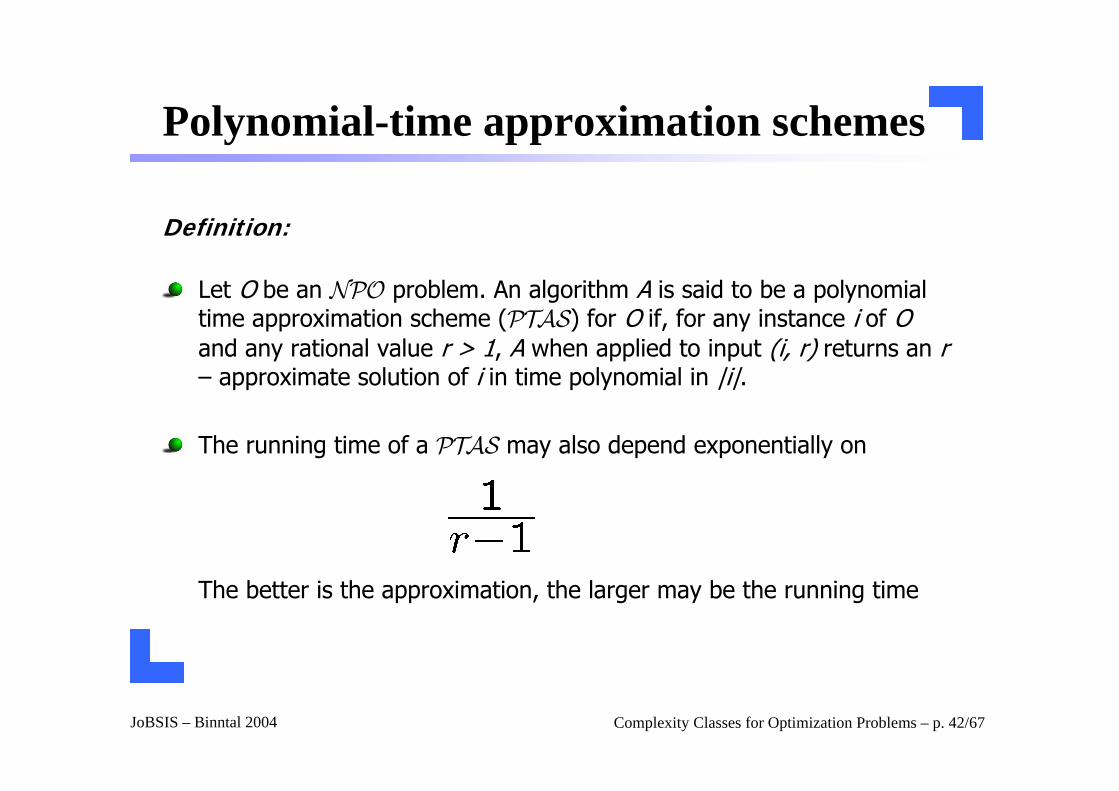
Definition:
Let O be an NPO problem. An algorithm A is said to be a polynomial time approximation scheme (PTAS) for O if, for any instance i of Oand any rational value r > 1, A when applied to input (i, r) returns an r – approximate solution of i in time polynomial in |i|.
The running time of a PTAS may also depend exponentially on
The better is the approximation, the larger may be the running time
JoBSIS – Binntal 2004 Complexity Classes for Optimization Problems – p. 43/67
The class PTAS
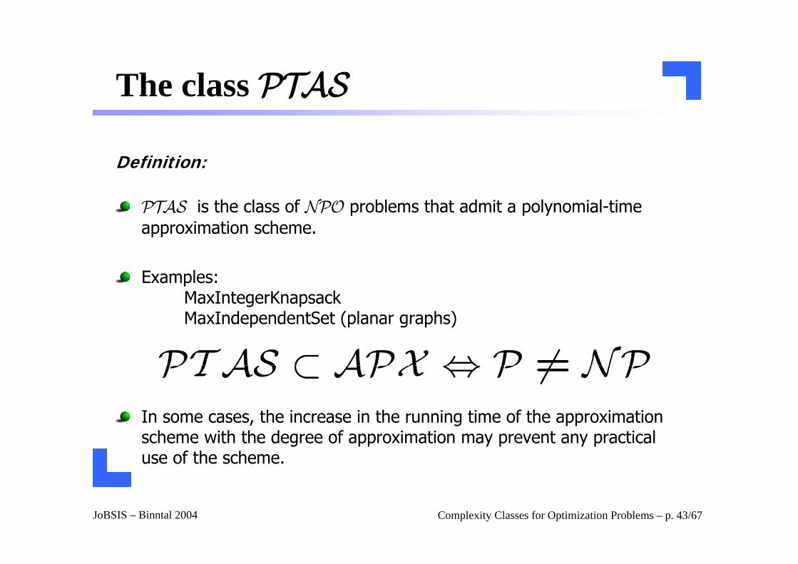
Definition:
PTAS is the class of NPO problems that admit a polynomial-time approximation scheme.
Examples:MaxIntegerKnapsackMaxIndependentSet (planar graphs)
In some cases, the increase in the running time of the approximation scheme with the degree of approximation may prevent any practical use of the scheme.
JoBSIS – Binntal 2004 Complexity Classes for Optimization Problems – p. 44/67
Proof:
Already done. MinimumBinPacking – Example
MinimumBinPacking has no r – approximate algorithm with r < 3/2 unless P = NP.
Therefore, unless P = NP, MinimumBinPacking does not admit a PTAS.
JoBSIS – Binntal 2004 Complexity Classes for Optimization Problems – p. 45/67
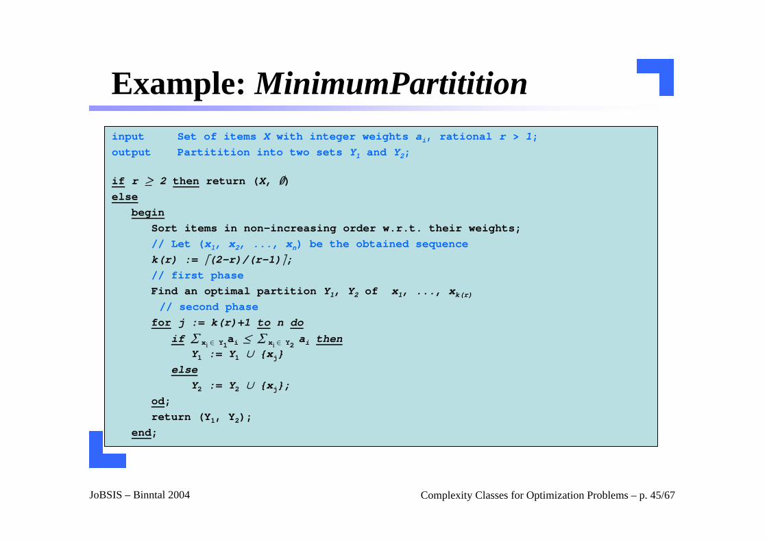
Example: MinimumPartititioninput Set of items X with integer weights ai, rational r > 1;output Partitition into two sets Y1 and Y2;
if r ≥ 2 then return (X, ∅)else
beginSort items in non-increasing order w.r.t. their weights;// Let (x1, x2, ..., xn) be the obtained sequencek(r) := d(2-r)/(r-1)e;// first phaseFind an optimal partition Y1, Y2 of x1, ..., xk(r)// second phase
for j := k(r)+1 to n do
if ∑ xi ∈ Y1ai · ∑ xi ∈ Y2
ai thenY1 := Y1 ∪ {xj}
elseY2 := Y2 ∪ {xj};
od;return (Y1, Y2);
end;
JoBSIS – Binntal 2004 Complexity Classes for Optimization Problems – p. 46/67
Proof:
Whiteboard
JoBSIS – Binntal 2004 Complexity Classes for Optimization Problems – p. 47/67
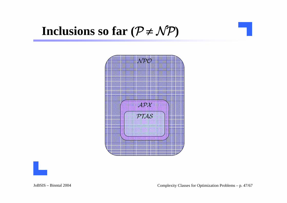
Inclusions so far (P ≠ NP)
NPO
APX
PTAS
JoBSIS – Binntal 2004 Complexity Classes for Optimization Problems – p. 48/67
Fully polynomial-time approximation scheme
A much better situation would arise when the running time is polynomial both in the size of the input and in the inverse of the performance ratio
Definition:
Let O be an NPO problem. An algorithms is said to be a fully polynomial time approximation scheme (FPTAS) for O if, for any instance i of O and for any rational value r > 1, A with input (i, r)returns an r – approximate solution of i in time polynomial both in |i|and 1/(r-1).
JoBSIS – Binntal 2004 Complexity Classes for Optimization Problems – p. 49/67
The class FPTAS
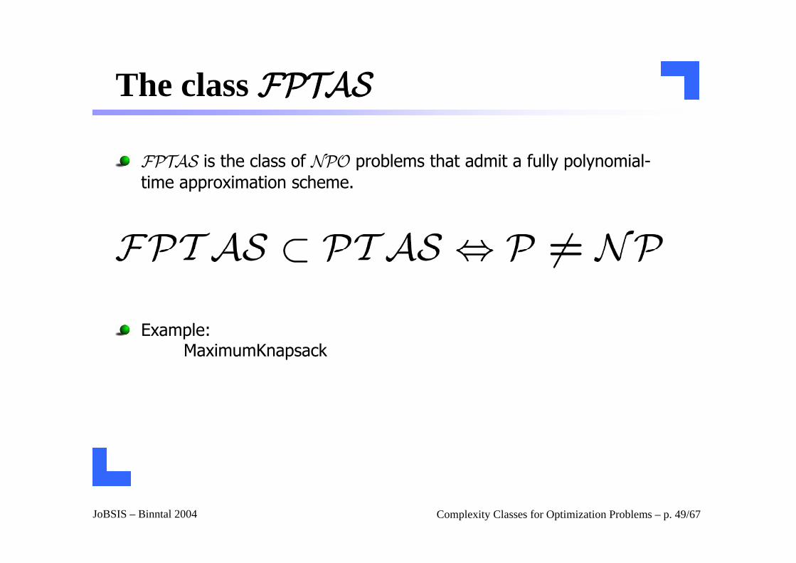
FPTAS is the class of NPO problems that admit a fully polynomial-time approximation scheme.
Example:MaximumKnapsack
JoBSIS – Binntal 2004 Complexity Classes for Optimization Problems – p. 50/67
Proof: (Example)
Hint:MaximumIndependentSetpolynomially bounded
JoBSIS – Binntal 2004 Complexity Classes for Optimization Problems – p. 51/67
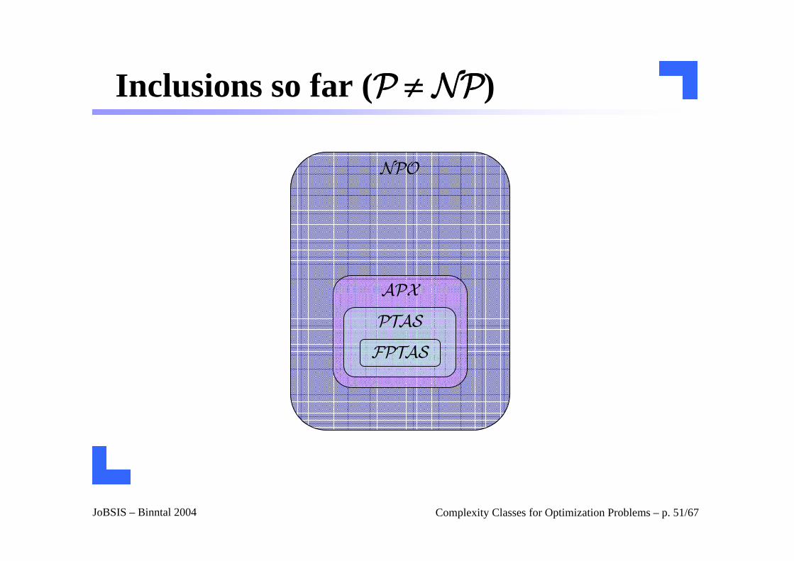
Inclusions so far (P ≠ NP)
NPO
APX
PTAS
FPTAS
JoBSIS – Binntal 2004 Complexity Classes for Optimization Problems – p. 52/67
F - APX
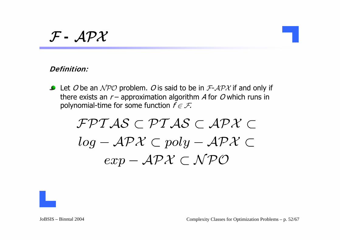
Definition:
Let O be an NPO problem. O is said to be in F-APX if and only if there exists an r – approximation algorithm A for O which runs in polynomial-time for some function f ∈ F.
JoBSIS – Binntal 2004 Complexity Classes for Optimization Problems – p. 53/67
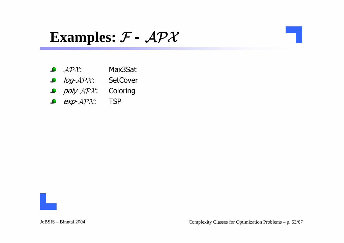
Examples: F - APX
APX: Max3Satlog-APX: SetCoverpoly-APX: Coloringexp-APX: TSP
JoBSIS – Binntal 2004 Complexity Classes for Optimization Problems – p. 54/67
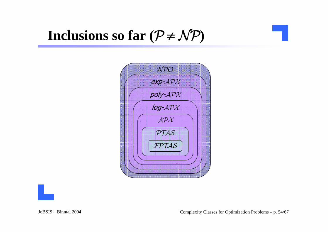
Inclusions so far (P ≠ NP)
NPO
exp-APX
poly-APX
log-APX
APX
PTAS
FPTAS
JoBSIS – Binntal 2004 Complexity Classes for Optimization Problems – p. 55/67
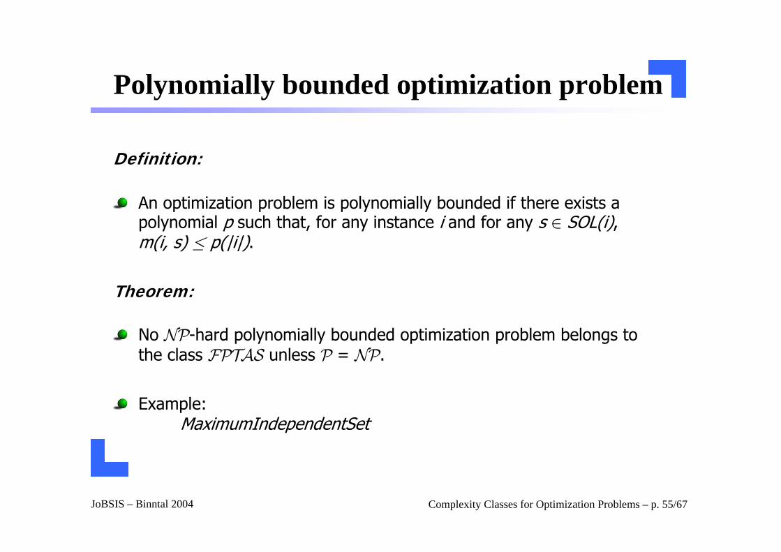
Polynomially bounded optimization problem
Definition:
An optimization problem is polynomially bounded if there exists a polynomial p such that, for any instance i and for any s ∈ SOL(i), m(i, s) · p(|i|).
Theorem:
No NP-hard polynomially bounded optimization problem belongs to the class FPTAS unless P = NP.
Example:MaximumIndependentSet

JoBSIS – Binntal 2004 Complexity Classes for Optimization Problems – p. 56/67
Proof:
Whiteboard
JoBSIS – Binntal 2004 Complexity Classes for Optimization Problems – p. 57/67
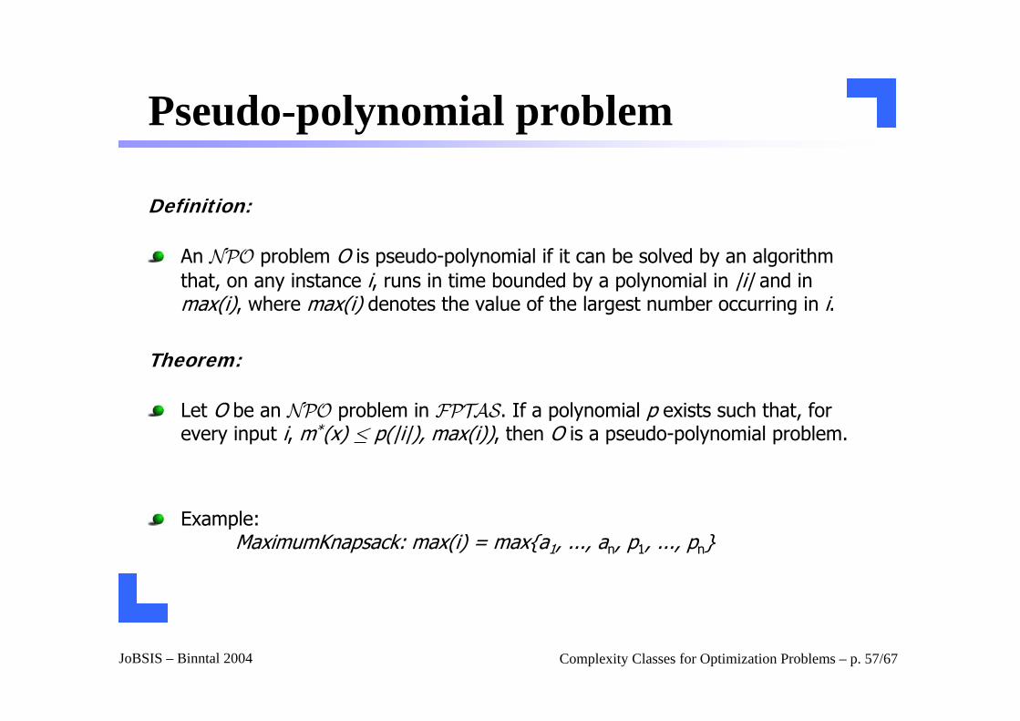
Pseudo-polynomial problem
Definition:
An NPO problem O is pseudo-polynomial if it can be solved by an algorithm that, on any instance i, runs in time bounded by a polynomial in |i| and in max(i), where max(i) denotes the value of the largest number occurring in i.
Theorem:
Let O be an NPO problem in FPTAS. If a polynomial p exists such that, for every input i, m*(x) · p(|i|), max(i)), then O is a pseudo-polynomial problem.
Example:MaximumKnapsack: max(i) = max{a1, ..., an, p1, ..., pn}
JoBSIS – Binntal 2004 Complexity Classes for Optimization Problems – p. 58/67
Strongly NP-hard problem
Definition:
An NPO problem O is said to be strongly NP-hard if a polynomial pexists such that O max, p is NP-hard.
Let O be an NPO problem and let p be a polynomial. We denote by O max, p the problem obtained by restricting O to only those instances iwhich max(i) · p(|i|).
The computation hardness does not depend on the values of the numbers included in its instances.
JoBSIS – Binntal 2004 Complexity Classes for Optimization Problems – p. 59/67
Strongly NP-hard problem (cont.)
Theorem:
If P ≠ NP, then no strongly NP-hard problem can be pseudo-polynomial.
Proof: Whiteboard
From the last two the theorems, the following result can be derived.
Let O be a strongly NP-hard problem that admits a polynomial p such that m*(i) · p(|i|, max(i)), for every input i. If P ≠ NP, then O does not belong to the class FPTAS.
JoBSIS – Binntal 2004 Complexity Classes for Optimization Problems – p. 60/67
Negative Results for the class FPTAS
The class of combinatorial problems in PTAS that admit a FPTAS is drastically reduced of those problems, whose value of the optimal measure is polynomially bounded with respect to the length of the instance.
No NP-hard polynomially bounded optimization problem belongs to the class FPTAS unless P = NP.
No NP-hard problem that admits a polynomial p such that m*(i) ·p(|i|, max(i)), for every input i belongs to the class FPTAS unless P = NP.
JoBSIS – Binntal 2004 Complexity Classes for Optimization Problems – p. 61/67
Agenda
IntroductionOptimization problemErrors, approximation algorithmClasses
NPO
APX
PTAS
FPTAS
F-APX
OutlookAP-ReductionsMax-SNP
JoBSIS – Binntal 2004 Complexity Classes for Optimization Problems – p. 62/67
Approximation Preserving Reductions
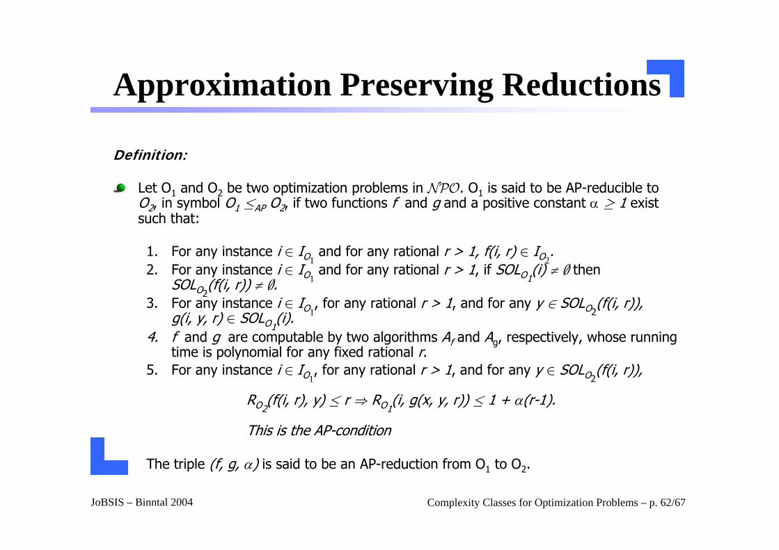
Definition:
Let O1 and O2 be two optimization problems in NPO. O1 is said to be AP-reducible toO2, in symbol O1 ·AP O2, if two functions f and g and a positive constant α ≥ 1 exist such that:
1. For any instance i ∈ IO1and for any rational r > 1, f(i, r) ∈ IO2
.2. For any instance i ∈ IO1
and for any rational r > 1, if SOLO1(i) ≠ ∅ then
SOLO2(f(i, r)) ≠ ∅.
3. For any instance i ∈ IO1, for any rational r > 1, and for any y ∈ SOLO2
(f(i, r)),g(i, y, r) ∈ SOLO1
(i).4. f and g are computable by two algorithms Af and Ag, respectively, whose running
time is polynomial for any fixed rational r.5. For any instance i ∈ IO1
, for any rational r > 1, and for any y ∈ SOLO2(f(i, r)),
RO2(f(i, r), y) · r ⇒ RO1
(i, g(x, y, r)) · 1 + α(r-1).
This is the AP-condition
The triple (f, g, α) is said to be an AP-reduction from O1 to O2.
JoBSIS – Binntal 2004 Complexity Classes for Optimization Problems – p. 63/67
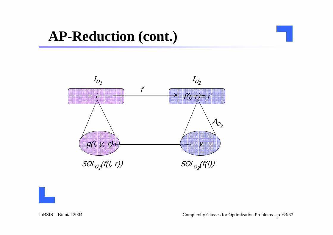
AP-Reduction (cont.)
i f(i, r)= i’
IO1IO2
SOLO2(f(i))
g(i, y, r) y
SOLO1(f(i, r))
f
AO2
JoBSIS – Binntal 2004 Complexity Classes for Optimization Problems – p. 64/67
AP-Reduction (cont.)
Lemma:
Let O1 ·AP O2 and O2 ∈ APX (respectively, O2 ∈ PTAS), then O1 ∈ APX (respectively, O1 ∈ PTAS).
Proof: Whiteboard
Example:MaximumClique ·AP MaximumIndependentSet
JoBSIS – Binntal 2004 Complexity Classes for Optimization Problems – p. 65/67
Fagin’s Theorem (1974)
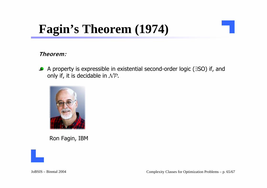
Theorem:
A property is expressible in existential second-order logic (∃SO) if, and only if, it is decidable in NP.
Ron Fagin, IBM
JoBSIS – Binntal 2004 Complexity Classes for Optimization Problems – p. 66/67
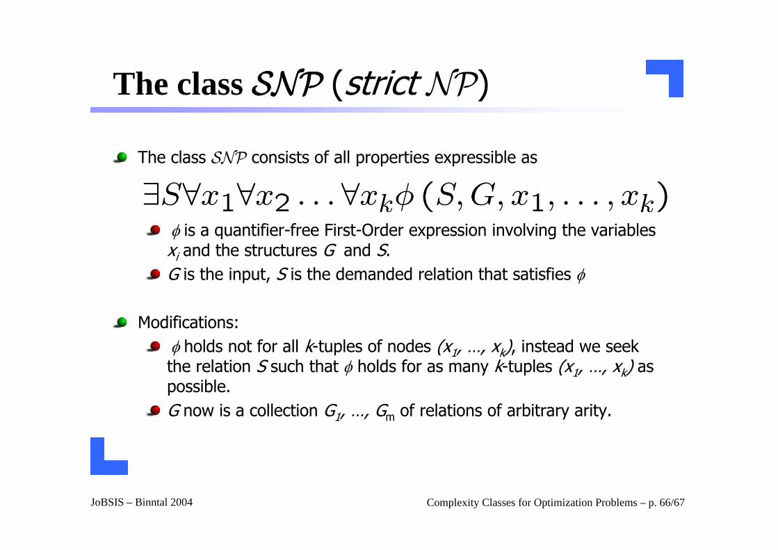
The class SNP (strict NP)
The class SNP consists of all properties expressible as
φ is a quantifier-free First-Order expression involving the variables xi and the structures G and S.G is the input, S is the demanded relation that satisfies φ
Modifications:φ holds not for all k-tuples of nodes (x1, …, xk), instead we seek the relation S such that φ holds for as many k-tuples (x1, …, xk) as possible.G now is a collection G1, …, Gm of relations of arbitrary arity.
JoBSIS – Binntal 2004 Complexity Classes for Optimization Problems – p. 67/67
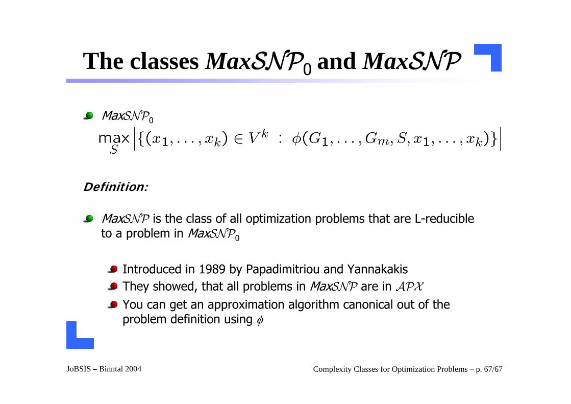
The classes MaxSNP0 and MaxSNP
MaxSNP0
Definition:
MaxSNP is the class of all optimization problems that are L-reducible to a problem in MaxSNP0
Introduced in 1989 by Papadimitriou and YannakakisThey showed, that all problems in MaxSNP are in APX
You can get an approximation algorithm canonical out of the problem definition using φ