SQLComplete Tips & Secrets for ProfessionalsComplete

SQLTips & Secrets

for Professionals

DisclaimerThis is an unocial free book created for educational purposes and is

not aliated with ocial SQL group(s) or company(s).All trademarks and registered trademarks are

the property of their respective owners

GoalKicker.comFree Programming Books

100+ pagesof professional hints and tricks

ContentsAbout 1 ...................................................................................................................................................................................

Chapter 1: Getting started with SQL 2 ................................................................................................................... Section 1.1: Overview 2 ......................................................................................................................................................

Chapter 2: SELECT 2 ........................................................................................................................................................ Section 2.1: Using the wildcard character to select all columns in a query. 3 ............................................................ Section 2.2: SELECT Using Column Aliases 4 ................................................................................................................. Section 2.3: Select Individual Columns 6 ........................................................................................................................ Section 2.4: Selecting specified number of records 7 ................................................................................................... Section 2.5: Selecting with Condition 8 ........................................................................................................................... Section 2.6: Selecting with CASE 9 .................................................................................................................................. Section 2.7: Select columns which are named after reserved keywords 9 ................................................................ Section 2.8: Selecting with table alias 9 ......................................................................................................................... Section 2.9: Selecting with more than 1 condition. 10 ................................................................................................... Section 2.10: Selecting without Locking the table 11 .................................................................................................... Section 2.11: Selecting with Aggregate functions 11 ..................................................................................................... Section 2.12: Select with condition of multiple values from column 12 ...................................................................... Section 2.13: Get aggregated result for row groups 12 ................................................................................................ Section 2.14: Selection with sorted Results 12 ............................................................................................................... Section 2.15: Selecting with null 13 .................................................................................................................................. Section 2.16: Select distinct (unique values only) 13 ..................................................................................................... Section 2.17: Select rows from multiple tables 13 .........................................................................................................

Chapter 3: JOIN 14 ............................................................................................................................................................ Section 3.1: Self Join 14 .................................................................................................................................................... Section 3.2: Dierences between inner/outer joins 15 ................................................................................................. Section 3.3: JOIN Terminology: Inner, Outer, Semi, Anti... 18 ........................................................................................ Section 3.4: Left Outer Join 26 ........................................................................................................................................ Section 3.5: Implicit Join 27 ............................................................................................................................................. Section 3.6: CROSS JOIN 28 ............................................................................................................................................ Section 3.7: CROSS APPLY & LATERAL JOIN 28 ............................................................................................................ Section 3.8: FULL JOIN 30 ............................................................................................................................................... Section 3.9: Recursive JOINs 31 ...................................................................................................................................... Section 3.10: Basic explicit inner join 31 .......................................................................................................................... Section 3.11: Joining on a Subquery 31 ...........................................................................................................................

Chapter 4: Example Databases and Tables 32 ................................................................................................. Section 4.1: Auto Shop Database 32 ............................................................................................................................... Section 4.2: Library Database 34 .................................................................................................................................... Section 4.3: Countries Table 36 .......................................................................................................................................

Chapter 5: UPDATE 37 .................................................................................................................................................... Section 5.1: UPDATE with data from another table 37 ................................................................................................. Section 5.2: Modifying existing values 38 ...................................................................................................................... Section 5.3: Updating Specified Rows 38 ....................................................................................................................... Section 5.4: Updating All Rows 38 .................................................................................................................................. Section 5.5: Capturing Updated records 39 ..................................................................................................................

Chapter 6: Indexes 39 ...................................................................................................................................................... Section 6.1: Sorted Index 39 ............................................................................................................................................. Section 6.2: Partial or Filtered Index 39 .......................................................................................................................... Section 6.3: Creating an Index 39 ...................................................................................................................................

Section 6.4: Dropping an Index, or Disabling and Rebuilding it 40 ............................................................................. Section 6.5: Clustered, Unique, and Sorted Indexes 40 ................................................................................................. Section 6.6: Rebuild index 41 ........................................................................................................................................... Section 6.7: Inserting with a Unique Index 41 ................................................................................................................

Chapter 7: CREATE TABLE 41 ...................................................................................................................................... Section 7.1: Create Table From Select 41 ....................................................................................................................... Section 7.2: Create a New Table 42 ................................................................................................................................ Section 7.3: CREATE TABLE With FOREIGN KEY 42 ...................................................................................................... Section 7.4: Duplicate a table 43 ..................................................................................................................................... Section 7.5: Create a Temporary or In-Memory Table 43 ...........................................................................................

Chapter 8: UNION / UNION ALL 44 .......................................................................................................................... Section 8.1: Basic UNION ALL query 44 .......................................................................................................................... Section 8.2: Simple explanation and Example 45 .........................................................................................................

Chapter 9: ALTER TABLE 45 ......................................................................................................................................... Section 9.1: Add Column(s) 45 ......................................................................................................................................... Section 9.2: Drop Column 46 ........................................................................................................................................... Section 9.3: Add Primary Key 46 .................................................................................................................................... Section 9.4: Alter Column 46 ........................................................................................................................................... Section 9.5: Drop Constraint 46 ......................................................................................................................................

Chapter 10: CASE 46 ......................................................................................................................................................... Section 10.1: Use CASE to COUNT the number of rows in a column match a condition. 46 ..................................... Section 10.2: Searched CASE in SELECT (Matches a boolean expression) 47 ........................................................... Section 10.3: CASE in a clause ORDER BY 48 ................................................................................................................. Section 10.4: Shorthand CASE in SELECT 48 .................................................................................................................. Section 10.5: Using CASE in UPDATE 49 ......................................................................................................................... Section 10.6: CASE use for NULL values ??ordered last 49 .......................................................................................... Section 10.7: CASE in ORDER BY clause to sort records by lowest value of 2 columns 49 ......................................

Chapter 11: INSERT 50 ..................................................................................................................................................... Section 11.1: INSERT data from another table using SELECT 50 .................................................................................. Section 11.2: Insert New Row 50 ...................................................................................................................................... Section 11.3: Insert Only Specified Columns 50 .............................................................................................................. Section 11.4: Insert multiple rows at once 51 ..................................................................................................................

Chapter 12: Primary Keys 51 ....................................................................................................................................... Section 12.1: Creating a Primary Key 51 ......................................................................................................................... Section 12.2: Using Auto Increment 51 ...........................................................................................................................

Chapter 13: ORDER BY 52 .............................................................................................................................................. Section 13.1: Sorting by column number (instead of name) 52 ................................................................................... Section 13.2: Use ORDER BY with TOP to return the top x rows based on a column's value 52 .............................. Section 13.3: Customizeed sorting order 53 ................................................................................................................... Section 13.4: Order by Alias 54 ........................................................................................................................................ Section 13.5: Sorting by multiple columns 54 .................................................................................................................

Chapter 14: GROUP BY 54 ............................................................................................................................................. Section 14.1: Basic GROUP BY example 55 ..................................................................................................................... Section 14.2: Filter GROUP BY results using a HAVING clause 55 ................................................................................ Section 14.3: USE GROUP BY to COUNT the number of rows for each unique entry in a given column

56 ................................................................................................................................................................................ Section 14.4: ROLAP aggregation (Data Mining) 57 .....................................................................................................

Chapter 15: Filter results using WHERE and HAVING 58 ................................................................................ Section 15.1: Use BETWEEN to Filter Results 58 .............................................................................................................

Section 15.2: Use HAVING with Aggregate Functions 59 .............................................................................................. Section 15.3: WHERE clause with NULL/NOT NULL values 59 ..................................................................................... Section 15.4: Equality 60 ................................................................................................................................................... Section 15.5: The WHERE clause only returns rows that match its criteria 60 ........................................................... Section 15.6: AND and OR 60 ........................................................................................................................................... Section 15.7: Use IN to return rows with a value contained in a list 61 ....................................................................... Section 15.8: Use LIKE to find matching strings and substrings 61 ............................................................................. Section 15.9: Where EXISTS 62 ........................................................................................................................................ Section 15.10: Use HAVING to check for multiple conditions in a group 62 ................................................................

Chapter 16: Window Functions 62 ............................................................................................................................. Section 16.1: Setting up a flag if other rows have a common property 62 ................................................................. Section 16.2: Finding "out-of-sequence" records using the LAG() function 63 .......................................................... Section 16.3: Getting a running total 64 .......................................................................................................................... Section 16.4: Adding the total rows selected to every row 64 ..................................................................................... Section 16.5: Getting the N most recent rows over multiple grouping 64 ...................................................................

Chapter 17: Common Table Expressions 65 ......................................................................................................... Section 17.1: generating values 65 .................................................................................................................................. Section 17.2: recursively enumerating a subtree 65 ..................................................................................................... Section 17.3: Temporary query 66 .................................................................................................................................. Section 17.4: recursively going up in a tree 66 ............................................................................................................... Section 17.5: Recursively generate dates, extended to include team rostering as example 67 .............................. Section 17.6: Oracle CONNECT BY functionality with recursive CTEs 67 ....................................................................

Chapter 18: Views 69 ........................................................................................................................................................ Section 18.1: Simple views 69 ........................................................................................................................................... Section 18.2: Complex views 69 .......................................................................................................................................

Chapter 19: LIKE operator 69 ...................................................................................................................................... Section 19.1: Match open-ended pattern 69 ................................................................................................................... Section 19.2: Single character match 70 ........................................................................................................................ Section 19.3: ESCAPE statement in the LIKE-query 71 .................................................................................................. Section 19.4: Search for a range of characters 71 ........................................................................................................ Section 19.5: Match by range or set 71 .......................................................................................................................... Section 19.6: Wildcard characters 72 ..............................................................................................................................

Chapter 20: Functions (Aggregate) 72 ................................................................................................................... Section 20.1: Conditional aggregation 73 ...................................................................................................................... Section 20.2: List Concatenation 73 ............................................................................................................................... Section 20.3: SUM 75 ........................................................................................................................................................ Section 20.4: AVG() 75 ..................................................................................................................................................... Section 20.5: Count 75 ..................................................................................................................................................... Section 20.6: Min 76 .......................................................................................................................................................... Section 20.7: Max 76 .........................................................................................................................................................

Chapter 21: DELETE 77 .................................................................................................................................................... Section 21.1: DELETE all rows 77 ...................................................................................................................................... Section 21.2: DELETE certain rows with WHERE 77 ....................................................................................................... Section 21.3: TRUNCATE clause 77 ................................................................................................................................. Section 21.4: DELETE certain rows based upon comparisons with other tables 77 ..................................................

Chapter 22: String Functions 78 ................................................................................................................................ Section 22.1: Concatenate 78 .......................................................................................................................................... Section 22.2: Length 79 .................................................................................................................................................... Section 22.3: Trim empty spaces 79 ...............................................................................................................................

Section 22.4: Upper & lower case 80 .............................................................................................................................. Section 22.5: Split 80 ........................................................................................................................................................ Section 22.6: Replace 80 .................................................................................................................................................. Section 22.7: REGEXP 80 .................................................................................................................................................. Section 22.8: Substring 80 ............................................................................................................................................... Section 22.9: Stu 81 ........................................................................................................................................................ Section 22.10: LEFT - RIGHT 81 ....................................................................................................................................... Section 22.11: REVERSE 81 ............................................................................................................................................... Section 22.12: REPLICATE 81 ........................................................................................................................................... Section 22.13: Replace function in sql Select and Update query 81 ........................................................................... Section 22.14: INSTR 82 .................................................................................................................................................... Section 22.15: PARSENAME 82 .........................................................................................................................................

Chapter 23: Data Types 83 ........................................................................................................................................... Section 23.1: DECIMAL and NUMERIC 83 ........................................................................................................................ Section 23.2: FLOAT and REAL 83 .................................................................................................................................. Section 23.3: Integers 83 .................................................................................................................................................. Section 23.4: MONEY and SMALLMONEY 83 .................................................................................................................. Section 23.5: BINARY and VARBINARY 83 ..................................................................................................................... Section 23.6: CHAR and VARCHAR 84 ............................................................................................................................ Section 23.7: NCHAR and NVARCHAR 84 ...................................................................................................................... Section 23.8: UNIQUEIDENTIFIER 84 ..............................................................................................................................

Chapter 24: AND & OR Operators 84 ..................................................................................................................... Section 24.1: AND OR Example 85 ..................................................................................................................................

Chapter 25: Triggers 85 ................................................................................................................................................. Section 25.1: CREATE TRIGGER 85 .................................................................................................................................. Section 25.2: Use Trigger to manage a "Recycle Bin" for deleted items 85 ..............................................................

Chapter 26: TRUNCATE 85 ............................................................................................................................................ Section 26.1: Removing all rows from the Employee table 86 .....................................................................................

Chapter 27: MERGE 86 .................................................................................................................................................... Section 27.1: MERGE to make Target match Source 86 ............................................................................................... Section 27.2: MySQL: counting users by name 86 ........................................................................................................ Section 27.3: PostgreSQL: counting users by name 87 ................................................................................................

Chapter 28: Foreign Keys 87 ....................................................................................................................................... Section 28.1: Foreign Keys explained 87 ........................................................................................................................ Section 28.2: Creating a table with a foreign key 88 ....................................................................................................

Chapter 29: Finding Duplicates on a Column Subset with Detail 88 ....................................................... Section 29.1: Students with same name and date of birth 88 ......................................................................................

Chapter 30: Sequence 89 .............................................................................................................................................. Section 30.1: Create Sequence 89 ................................................................................................................................... Section 30.2: Using Sequences 89 ..................................................................................................................................

Chapter 31: Comments 89 ............................................................................................................................................. Section 31.1: Single-line comments 89 ............................................................................................................................ Section 31.2: Multi-line comments 89 ..............................................................................................................................

Chapter 32: Subqueries 89 ............................................................................................................................................ Section 32.1: Subquery in FROM clause 90 .................................................................................................................... Section 32.2: Subquery in SELECT clause 90 ................................................................................................................. Section 32.3: Subquery in WHERE clause 90 ................................................................................................................. Section 32.4: Correlated Subqueries 90 ......................................................................................................................... Section 32.5: Filter query results using query on dierent table 90 ...........................................................................

Section 32.6: Subqueries in FROM clause 91 ................................................................................................................. Section 32.7: Subqueries in WHERE clause 91 ...............................................................................................................

Chapter 33: Execution blocks 91 ................................................................................................................................ Section 33.1: Using BEGIN ... END 91 ................................................................................................................................

Chapter 34: Stored Procedures 91 .......................................................................................................................... Section 34.1: Create and call a stored procedure 91 ....................................................................................................

Chapter 35: DROP Table 92 ......................................................................................................................................... Section 35.1: Check for existence before dropping 92 .................................................................................................. Section 35.2: Simple drop 92 ...........................................................................................................................................

Chapter 36: Row number 92 ........................................................................................................................................ Section 36.1: Delete All But Last Record (1 to Many Table) 92 ..................................................................................... Section 36.2: Row numbers without partitions 92 ......................................................................................................... Section 36.3: Row numbers with partitions 93 ...............................................................................................................

Chapter 37: Transactions 93 ....................................................................................................................................... Section 37.1: Simple Transaction 93 ................................................................................................................................ Section 37.2: Rollback Transaction 93 ...........................................................................................................................

Chapter 38: CREATE FUNCTION 93 ........................................................................................................................... Section 38.1: Create a new Function 93 ..........................................................................................................................

Chapter 39: SQL Group By vs Distinct 94 .............................................................................................................. Section 39.1: Dierence between GROUP BY and DISTINCT 94 ..................................................................................

Chapter 40: Table Design 94 ...................................................................................................................................... Section 40.1: Properties of a well designed table. 94 ....................................................................................................

Chapter 41: cross apply, outer apply 95 ............................................................................................................... Section 41.1: CROSS APPLY and OUTER APPLY basics 95 ............................................................................................

Chapter 42: Synonyms 97 ............................................................................................................................................ Section 42.1: Create Synonym 97 ....................................................................................................................................

Chapter 43: CREATE Database 97 ............................................................................................................................ Section 43.1: CREATE Database 97 .................................................................................................................................

Chapter 44: SKIP TAKE (Pagination) 97 ................................................................................................................ Section 44.1: Limiting amount of results 97 .................................................................................................................... Section 44.2: Skipping then taking some results (Pagination) 98 ............................................................................... Section 44.3: Skipping some rows from result 98 .........................................................................................................

Chapter 45: EXPLAIN and DESCRIBE 99 ................................................................................................................ Section 45.1: EXPLAIN Select query 99 ........................................................................................................................... Section 45.2: DESCRIBE tablename; 99 ..........................................................................................................................

Chapter 46: Information Schema 99 ...................................................................................................................... Section 46.1: Basic Information Schema Search 99 ......................................................................................................

Chapter 47: IN clause 100 ............................................................................................................................................. Section 47.1: Simple IN clause 100 .................................................................................................................................. Section 47.2: Using IN clause with a subquery 100 .......................................................................................................

Chapter 48: NULL 100 ..................................................................................................................................................... Section 48.1: Filtering for NULL in queries 100 .............................................................................................................. Section 48.2: Nullable columns in tables 100 ................................................................................................................ Section 48.3: Updating fields to NULL 101 ..................................................................................................................... Section 48.4: Inserting rows with NULL fields 101 .........................................................................................................

Chapter 49: SQL Injection 101 .................................................................................................................................... Section 49.1: SQL injection sample 101 ..........................................................................................................................

Section 49.2: simple injection sample 102 .....................................................................................................................

Chapter 50: Cascading Delete 103 ........................................................................................................................... Section 50.1: ON DELETE CASCADE 103 .........................................................................................................................

Chapter 51: Order of Execution 104 ......................................................................................................................... Section 51.1: Logical Order of Query Processing in SQL 104 ........................................................................................

Chapter 52: DROP or DELETE Database 105 ....................................................................................................... Section 52.1: DROP Database 105 ..................................................................................................................................

Chapter 53: EXCEPT 105 ................................................................................................................................................. Section 53.1: Select dataset except where values are in this other dataset 105 ........................................................

Chapter 54: TRY/CATCH 105 ....................................................................................................................................... Section 54.1: Transaction In a TRY/CATCH 105 ............................................................................................................

Chapter 55: XML 106 ........................................................................................................................................................ Section 55.1: Query from XML Data Type 106 ...............................................................................................................

Chapter 56: GRANT and REVOKE 107 ..................................................................................................................... Section 56.1: Grant/revoke privileges 107 ......................................................................................................................

Chapter 57: Functions (Scalar/Single Row) 107 ................................................................................................ Section 57.1: Date And Time 107 ..................................................................................................................................... Section 57.2: Character modifications 108 .................................................................................................................... Section 57.3: Configuration and Conversion Function 108 .......................................................................................... Section 57.4: Logical and Mathmetical Function 109 ...................................................................................................

Chapter 58: EXISTS CLAUSE 110 ................................................................................................................................ Section 58.1: EXISTS CLAUSE 110 ....................................................................................................................................

Chapter 59: Materialized Views 111 ......................................................................................................................... Section 59.1: PostgreSQL example 111 ..........................................................................................................................

Chapter 60: Functions (Analytic) 112 ...................................................................................................................... Section 60.1: LAG and LEAD 112 ..................................................................................................................................... Section 60.2: PERCENTILE_DISC and PERCENTILE_CONT 112 .................................................................................. Section 60.3: FIRST_VALUE 113 ..................................................................................................................................... Section 60.4: LAST_VALUE 114 ...................................................................................................................................... Section 60.5: PERCENT_RANK and CUME_DIST 114 ...................................................................................................

Chapter 61: Identifier 115 .............................................................................................................................................. Section 61.1: Unquoted identifiers 115 ............................................................................................................................

Chapter 62: Clean Code in SQL 115 .......................................................................................................................... Section 62.1: Formatting and Spelling of Keywords and Names 115 ......................................................................... Section 62.2: Indenting 116 ............................................................................................................................................. Section 62.3: SELECT * 117 ............................................................................................................................................... Section 62.4: Joins 117 .....................................................................................................................................................

Credits 119 ............................................................................................................................................................................

You may also like 123 ......................................................................................................................................................

Complete SQL Tips & Secrets for Professionals 1

About

Please feel free to share this PDF with anyone for free,latest version of this book can be downloaded from:

http://GoalKicker.com/SQLBook

Important notice:These Complete SQL Tips & Secrets for Professionals series are compiled from

Stack Overflow Documentation via Archive.org, the content is written by thebeautiful people at Stack Overflow, text content is released under Creative

Commons BY-SA, see credits at the end of this book whom contributed to thevarious chapters. Images may be copyright of their respective owners unless

otherwise specified

This book creation is not affiliated with SQL group(s) nor Stack Overflow, and allterms and trademarks belong to their respective company owners

The information presented in this book is not guaranteed to be correct noraccurate, use at your own risk

Send feedback and corrections to web@petercv.com

Complete SQL Tips & Secrets for Professionals 2

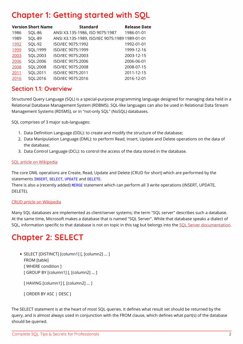
Chapter 1: Getting started with SQLVersion Short Name Standard Release Date1986 SQL-86 ANSI X3.135-1986, ISO 9075:1987 1986-01-011989 SQL-89 ANSI X3.135-1989, ISO/IEC 9075:1989 1989-01-011992 SQL-92 ISO/IEC 9075:1992 1992-01-011999 SQL:1999 ISO/IEC 9075:1999 1999-12-162003 SQL:2003 ISO/IEC 9075:2003 2003-12-152006 SQL:2006 ISO/IEC 9075:2006 2006-06-012008 SQL:2008 ISO/IEC 9075:2008 2008-07-152011 SQL:2011 ISO/IEC 9075:2011 2011-12-152016 SQL:2016 ISO/IEC 9075:2016 2016-12-01

Section 1.1: OverviewStructured Query Language (SQL) is a special-purpose programming language designed for managing data held in aRelational Database Management System (RDBMS). SQL-like languages can also be used in Relational Data StreamManagement Systems (RDSMS), or in "not-only SQL" (NoSQL) databases.

SQL comprises of 3 major sub-languages:

Data Definition Language (DDL): to create and modify the structure of the database;1.Data Manipulation Language (DML): to perform Read, Insert, Update and Delete operations on the data of2.the database;Data Control Language (DCL): to control the access of the data stored in the database.3.

SQL article on Wikipedia

The core DML operations are Create, Read, Update and Delete (CRUD for short) which are performed by thestatements INSERT, SELECT, UPDATE and DELETE.There is also a (recently added) MERGE statement which can perform all 3 write operations (INSERT, UPDATE,DELETE).

CRUD article on Wikipedia

Many SQL databases are implemented as client/server systems; the term "SQL server" describes such a database.At the same time, Microsoft makes a database that is named "SQL Server". While that database speaks a dialect ofSQL, information specific to that database is not on topic in this tag but belongs into the SQL Server documentation.

Chapter 2: SELECT

SELECT [DISTINCT] [column1] [, [column2] ... ]FROM [table][ WHERE condition ][ GROUP BY [column1] [, [column2] ... ]

[ HAVING [column1] [, [column2] ... ]

[ ORDER BY ASC | DESC ]

The SELECT statement is at the heart of most SQL queries. It defines what result set should be returned by thequery, and is almost always used in conjunction with the FROM clause, which defines what part(s) of the databaseshould be queried.

Complete SQL Tips & Secrets for Professionals 3

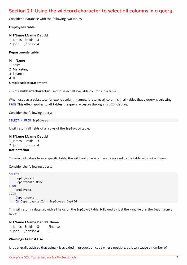
Section 2.1: Using the wildcard character to select all columns in a query.Consider a database with the following two tables.

Employees table:

Id FName LName DeptId1 James Smith 32 John Johnson 4

Departments table:

Id Name1 Sales2 Marketing3 Finance4 ITSimple select statement

* is the wildcard character used to select all available columns in a table.

When used as a substitute for explicit column names, it returns all columns in all tables that a query is selectingFROM. This effect applies to all tables the query accesses through its JOIN clauses.

Consider the following query:

SELECT * FROM Employees

It will return all fields of all rows of the Employees table:

Id FName LName DeptId1 James Smith 32 John Johnson 4Dot notation

To select all values from a specific table, the wildcard character can be applied to the table with dot notation.

Consider the following query:

SELECT Employees.*, Departments.NameFROM EmployeesJOIN Departments ON Departments.Id = Employees.DeptId

This will return a data set with all fields on the Employee table, followed by just the Name field in the Departmentstable:

Id FName LName DeptId Name1 James Smith 3 Finance2 John Johnson 4 IT

Warnings Against Use

It is generally advised that using * is avoided in production code where possible, as it can cause a number of

Complete SQL Tips & Secrets for Professionals 4

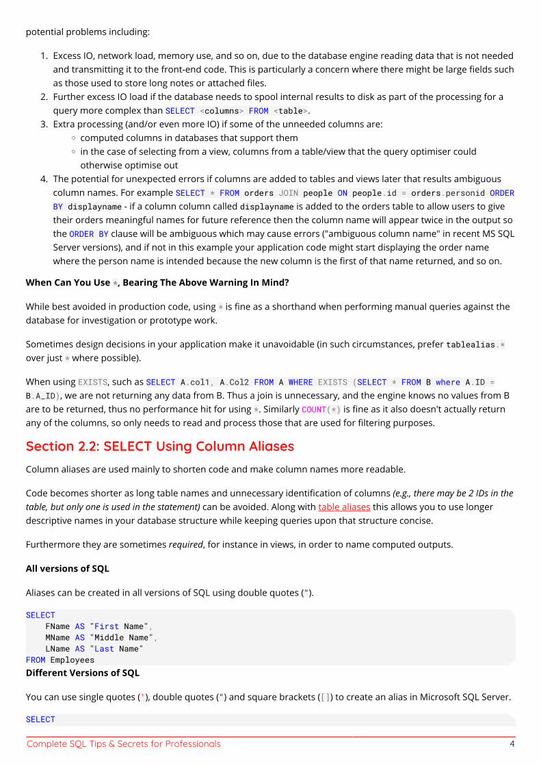
potential problems including:

Excess IO, network load, memory use, and so on, due to the database engine reading data that is not needed1.and transmitting it to the front-end code. This is particularly a concern where there might be large fields suchas those used to store long notes or attached files.Further excess IO load if the database needs to spool internal results to disk as part of the processing for a2.query more complex than SELECT <columns> FROM <table>.Extra processing (and/or even more IO) if some of the unneeded columns are:3.

computed columns in databases that support themin the case of selecting from a view, columns from a table/view that the query optimiser couldotherwise optimise out

The potential for unexpected errors if columns are added to tables and views later that results ambiguous4.column names. For example SELECT * FROM orders JOIN people ON people.id = orders.personid ORDERBY displayname - if a column column called displayname is added to the orders table to allow users to givetheir orders meaningful names for future reference then the column name will appear twice in the output sothe ORDER BY clause will be ambiguous which may cause errors ("ambiguous column name" in recent MS SQLServer versions), and if not in this example your application code might start displaying the order namewhere the person name is intended because the new column is the first of that name returned, and so on.

When Can You Use *, Bearing The Above Warning In Mind?

While best avoided in production code, using * is fine as a shorthand when performing manual queries against thedatabase for investigation or prototype work.

Sometimes design decisions in your application make it unavoidable (in such circumstances, prefer tablealias.*over just * where possible).

When using EXISTS, such as SELECT A.col1, A.Col2 FROM A WHERE EXISTS (SELECT * FROM B where A.ID =B.A_ID), we are not returning any data from B. Thus a join is unnecessary, and the engine knows no values from Bare to be returned, thus no performance hit for using *. Similarly COUNT(*) is fine as it also doesn't actually returnany of the columns, so only needs to read and process those that are used for filtering purposes.

Section 2.2: SELECT Using Column AliasesColumn aliases are used mainly to shorten code and make column names more readable.

Code becomes shorter as long table names and unnecessary identification of columns (e.g., there may be 2 IDs in thetable, but only one is used in the statement) can be avoided. Along with table aliases this allows you to use longerdescriptive names in your database structure while keeping queries upon that structure concise.

Furthermore they are sometimes required, for instance in views, in order to name computed outputs.

All versions of SQL

Aliases can be created in all versions of SQL using double quotes (").

SELECT FName AS "First Name", MName AS "Middle Name", LName AS "Last Name"FROM Employees Different Versions of SQL

You can use single quotes ('), double quotes (") and square brackets ([]) to create an alias in Microsoft SQL Server.

SELECT

Complete SQL Tips & Secrets for Professionals 5

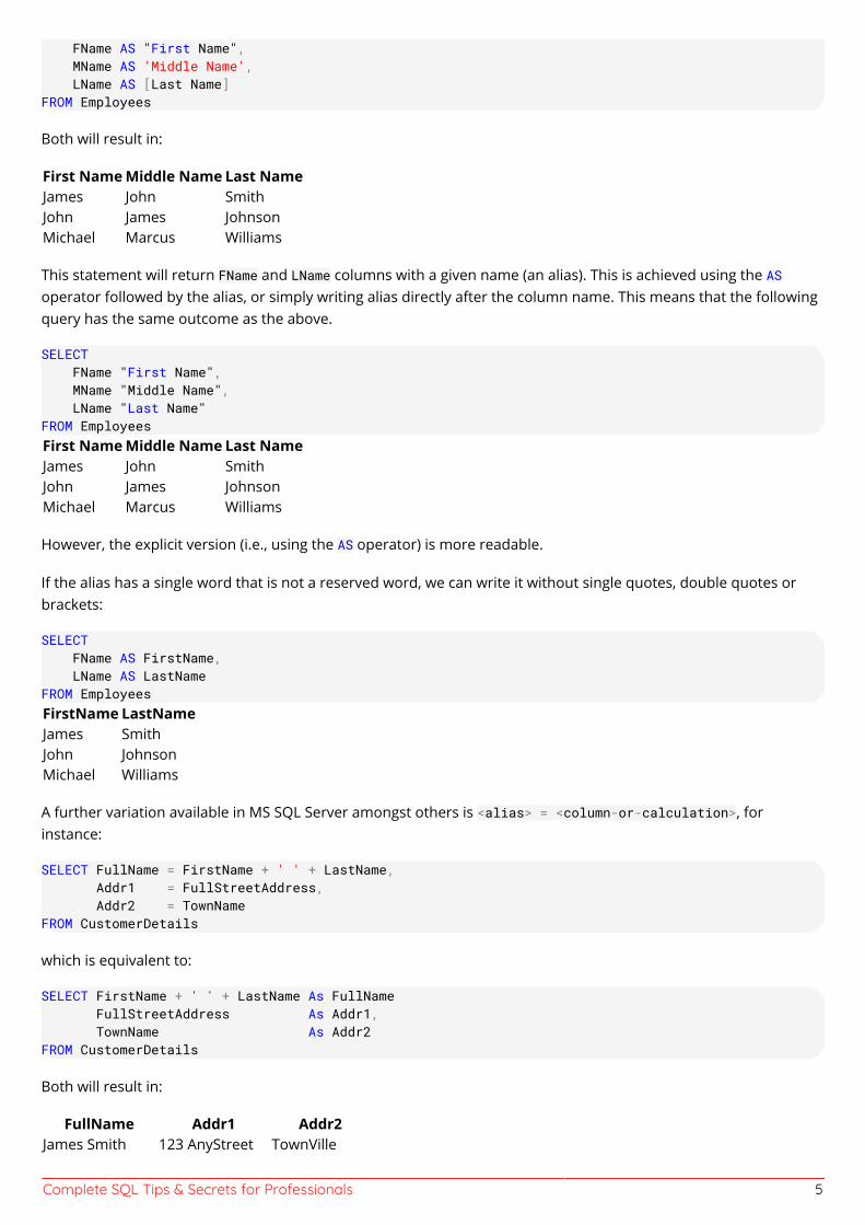
FName AS "First Name", MName AS 'Middle Name', LName AS [Last Name]FROM Employees

Both will result in:

First Name Middle Name Last NameJames John SmithJohn James JohnsonMichael Marcus Williams

This statement will return FName and LName columns with a given name (an alias). This is achieved using the ASoperator followed by the alias, or simply writing alias directly after the column name. This means that the followingquery has the same outcome as the above.

SELECT FName "First Name", MName "Middle Name", LName "Last Name"FROM EmployeesFirst Name Middle Name Last NameJames John SmithJohn James JohnsonMichael Marcus Williams

However, the explicit version (i.e., using the AS operator) is more readable.

If the alias has a single word that is not a reserved word, we can write it without single quotes, double quotes orbrackets:

SELECT FName AS FirstName, LName AS LastNameFROM Employees FirstName LastNameJames SmithJohn JohnsonMichael Williams

A further variation available in MS SQL Server amongst others is <alias> = <column-or-calculation>, forinstance:

SELECT FullName = FirstName + ' ' + LastName, Addr1 = FullStreetAddress, Addr2 = TownNameFROM CustomerDetails

which is equivalent to:

SELECT FirstName + ' ' + LastName As FullName FullStreetAddress As Addr1, TownName As Addr2FROM CustomerDetails

Both will result in:

FullName Addr1 Addr2James Smith 123 AnyStreet TownVille

Complete SQL Tips & Secrets for Professionals 6

John Johnson 668 MyRoad AnytownMichael Williams 999 High End Dr Williamsburgh

Some find using = instead of As easier to read, though many recommend against this format, mainly because it isnot standard so not widely supported by all databases. It may cause confusion with other uses of the = character.

All Versions of SQL

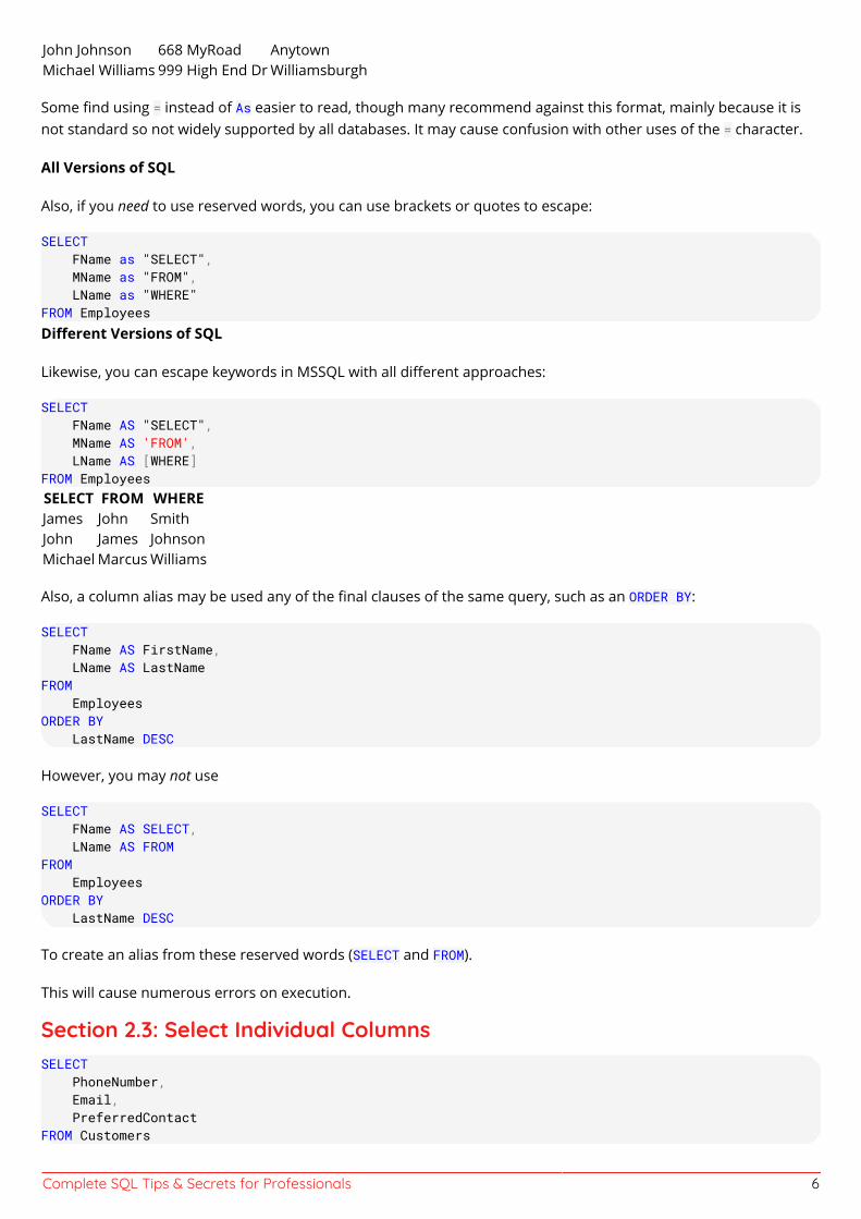
Also, if you need to use reserved words, you can use brackets or quotes to escape:

SELECT FName as "SELECT", MName as "FROM", LName as "WHERE"FROM EmployeesDifferent Versions of SQL

Likewise, you can escape keywords in MSSQL with all different approaches:

SELECT FName AS "SELECT", MName AS 'FROM', LName AS [WHERE]FROM Employees SELECT FROM WHEREJames John SmithJohn James JohnsonMichael Marcus Williams

Also, a column alias may be used any of the final clauses of the same query, such as an ORDER BY:

SELECT FName AS FirstName, LName AS LastNameFROM EmployeesORDER BY LastName DESC

However, you may not use

SELECT FName AS SELECT, LName AS FROMFROM EmployeesORDER BY LastName DESC

To create an alias from these reserved words (SELECT and FROM).

This will cause numerous errors on execution.

Section 2.3: Select Individual ColumnsSELECT PhoneNumber, Email, PreferredContactFROM Customers

Complete SQL Tips & Secrets for Professionals 7

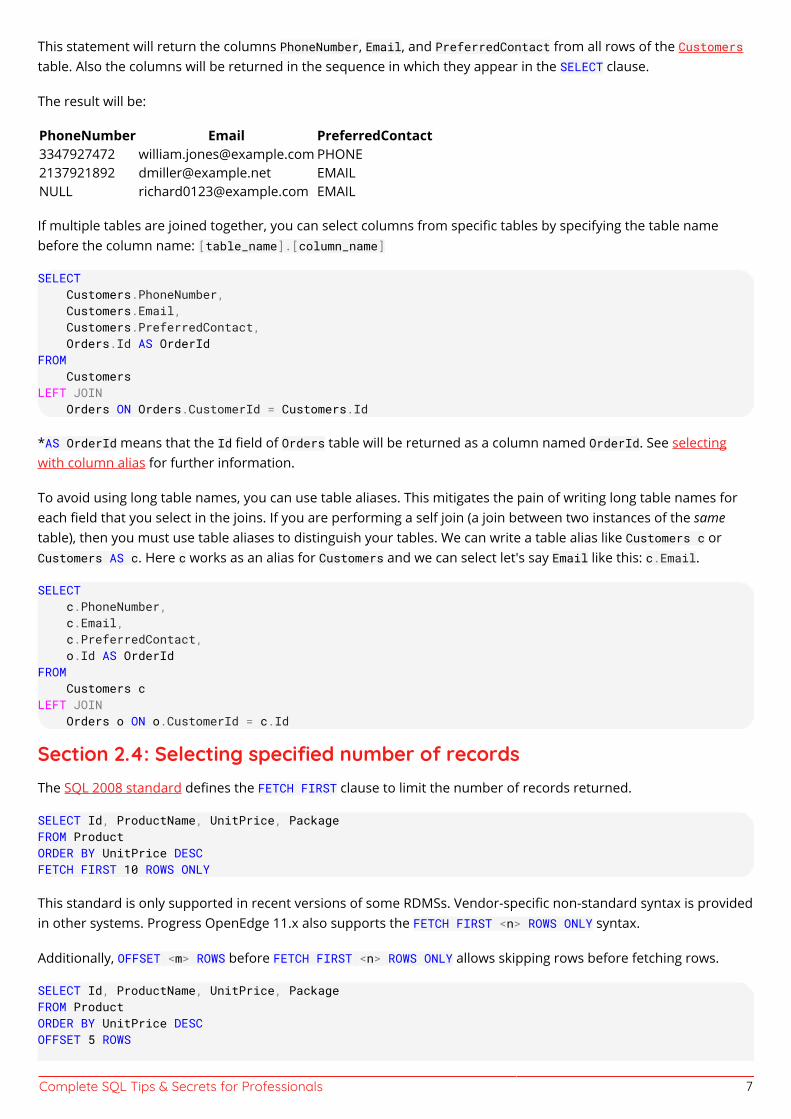
This statement will return the columns PhoneNumber, Email, and PreferredContact from all rows of the Customerstable. Also the columns will be returned in the sequence in which they appear in the SELECT clause.

The result will be:

PhoneNumber Email PreferredContact3347927472 william.jones@example.com PHONE2137921892 dmiller@example.net EMAILNULL richard0123@example.com EMAIL

If multiple tables are joined together, you can select columns from specific tables by specifying the table namebefore the column name: [table_name].[column_name]

SELECT Customers.PhoneNumber, Customers.Email, Customers.PreferredContact, Orders.Id AS OrderIdFROM CustomersLEFT JOIN Orders ON Orders.CustomerId = Customers.Id

*AS OrderId means that the Id field of Orders table will be returned as a column named OrderId. See selectingwith column alias for further information.

To avoid using long table names, you can use table aliases. This mitigates the pain of writing long table names foreach field that you select in the joins. If you are performing a self join (a join between two instances of the sametable), then you must use table aliases to distinguish your tables. We can write a table alias like Customers c orCustomers AS c. Here c works as an alias for Customers and we can select let's say Email like this: c.Email.

SELECT c.PhoneNumber, c.Email, c.PreferredContact, o.Id AS OrderIdFROM Customers cLEFT JOIN Orders o ON o.CustomerId = c.Id

Section 2.4: Selecting specified number of recordsThe SQL 2008 standard defines the FETCH FIRST clause to limit the number of records returned.

SELECT Id, ProductName, UnitPrice, PackageFROM ProductORDER BY UnitPrice DESCFETCH FIRST 10 ROWS ONLY

This standard is only supported in recent versions of some RDMSs. Vendor-specific non-standard syntax is providedin other systems. Progress OpenEdge 11.x also supports the FETCH FIRST <n> ROWS ONLY syntax.

Additionally, OFFSET <m> ROWS before FETCH FIRST <n> ROWS ONLY allows skipping rows before fetching rows.

SELECT Id, ProductName, UnitPrice, PackageFROM ProductORDER BY UnitPrice DESCOFFSET 5 ROWS

Complete SQL Tips & Secrets for Professionals 8

FETCH FIRST 10 ROWS ONLY

The following query is supported in SQL Server and MS Access:

SELECT TOP 10 Id, ProductName, UnitPrice, PackageFROM ProductORDER BY UnitPrice DESC

To do the same in MySQL or PostgreSQL the LIMIT keyword must be used:

SELECT Id, ProductName, UnitPrice, PackageFROM ProductORDER BY UnitPrice DESCLIMIT 10

In Oracle the same can be done with ROWNUM:

SELECT Id, ProductName, UnitPrice, PackageFROM ProductWHERE ROWNUM <= 10ORDER BY UnitPrice DESC

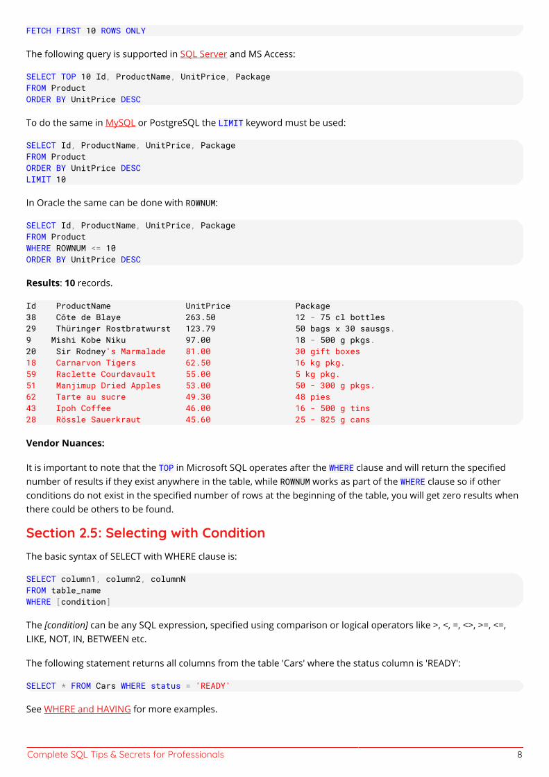
Results: 10 records.

Id ProductName UnitPrice Package38 Côte de Blaye 263.50 12 - 75 cl bottles29 Thüringer Rostbratwurst 123.79 50 bags x 30 sausgs.9 Mishi Kobe Niku 97.00 18 - 500 g pkgs.20 Sir Rodney's Marmalade 81.00 30 gift boxes18 Carnarvon Tigers 62.50 16 kg pkg.59 Raclette Courdavault 55.00 5 kg pkg.51 Manjimup Dried Apples 53.00 50 - 300 g pkgs.62 Tarte au sucre 49.30 48 pies43 Ipoh Coffee 46.00 16 - 500 g tins28 Rössle Sauerkraut 45.60 25 - 825 g cans

Vendor Nuances:

It is important to note that the TOP in Microsoft SQL operates after the WHERE clause and will return the specifiednumber of results if they exist anywhere in the table, while ROWNUM works as part of the WHERE clause so if otherconditions do not exist in the specified number of rows at the beginning of the table, you will get zero results whenthere could be others to be found.

Section 2.5: Selecting with ConditionThe basic syntax of SELECT with WHERE clause is:

SELECT column1, column2, columnNFROM table_nameWHERE [condition]

The [condition] can be any SQL expression, specified using comparison or logical operators like >, <, =, <>, >=, <=,LIKE, NOT, IN, BETWEEN etc.

The following statement returns all columns from the table 'Cars' where the status column is 'READY':

SELECT * FROM Cars WHERE status = 'READY'

See WHERE and HAVING for more examples.

Complete SQL Tips & Secrets for Professionals 9

Section 2.6: Selecting with CASEWhen results need to have some logic applied 'on the fly' one can use CASE statement to implement it.

SELECT CASE WHEN Col1 < 50 THEN 'under' ELSE 'over' END thresholdFROM TableName

also can be chained

SELECT CASE WHEN Col1 < 50 THEN 'under' WHEN Col1 > 50 AND Col1 <100 THEN 'between' ELSE 'over' END thresholdFROM TableName

one also can have CASE inside another CASE statement

SELECT CASE WHEN Col1 < 50 THEN 'under' ELSE CASE WHEN Col1 > 50 AND Col1 <100 THEN Col1 ELSE 'over' END END thresholdFROM TableName

Section 2.7: Select columns which are named after reserved keywordsWhen a column name matches a reserved keyword, standard SQL requires that you enclose it in double quotationmarks:

SELECT "ORDER", IDFROM ORDERS

Note that it makes the column name case-sensitive.

Some DBMSes have proprietary ways of quoting names. For example, SQL Server uses square brackets for thispurpose:

SELECT [Order], IDFROM ORDERS

while MySQL (and MariaDB) by default use backticks:

SELECT `Order`, idFROM orders

Section 2.8: Selecting with table aliasSELECT e.Fname, e.LNameFROM Employees e

The Employees table is given the alias 'e' directly after the table name. This helps remove ambiguity in scenarioswhere multiple tables have the same field name and you need to be specific as to which table you want to returndata from.

Complete SQL Tips & Secrets for Professionals 10

SELECT e.Fname, e.LName, m.Fname AS ManagerFirstNameFROM Employees e JOIN Managers m ON e.ManagerId = m.Id

Note that once you define an alias, you can't use the canonical table name anymore. i.e.,

SELECT e.Fname, Employees.LName, m.Fname AS ManagerFirstNameFROM Employees eJOIN Managers m ON e.ManagerId = m.Id

would throw an error.

It is worth noting table aliases -- more formally 'range variables' -- were introduced into the SQL language to solvethe problem of duplicate columns caused by INNER JOIN. The 1992 SQL standard corrected this earlier design flawby introducing NATURAL JOIN (implemented in mySQL, PostgreSQL and Oracle but not yet in SQL Server), the resultof which never has duplicate column names. The above example is interesting in that the tables are joined oncolumns with different names (Id and ManagerId) but are not supposed to be joined on the columns with the samename (LName, FName), requiring the renaming of the columns to be performed before the join:

SELECT Fname, LName, ManagerFirstNameFROM Employees NATURAL JOIN ( SELECT Id AS ManagerId, Fname AS ManagerFirstName FROM Managers ) m;

Note that although an alias/range variable must be declared for the dervied table (otherwise SQL will throw anerror), it never makes sense to actually use it in the query.

Section 2.9: Selecting with more than 1 condition.The AND keyword is used to add more conditions to the query.

Name Age GenderSam 18 MJohn 21 MBob 22 MMary 23 FSELECT name FROM persons WHERE gender = 'M' AND age > 20;

This will return:

NameJohnBob

using OR keyword

SELECT name FROM persons WHERE gender = 'M' OR age < 20;

This will return:

nameSamJohnBob

These keywords can be combined to allow for more complex criteria combinations:

SELECT name

Complete SQL Tips & Secrets for Professionals 11

FROM personsWHERE (gender = 'M' AND age < 20) OR (gender = 'F' AND age > 20);

This will return:

nameSamMary

Section 2.10: Selecting without Locking the tableSometimes when tables are used mostly (or only) for reads, indexing does not help anymore and every little bitcounts, one might use selects without LOCK to improve performance.

SQL Server

SELECT * FROM TableName WITH (nolock)

MySQL

SET SESSION TRANSACTION ISOLATION LEVEL READ UNCOMMITTED;SELECT * FROM TableName;SET SESSION TRANSACTION ISOLATION LEVEL REPEATABLE READ;

Oracle

SET TRANSACTION ISOLATION LEVEL READ UNCOMMITTED;SELECT * FROM TableName;

DB2

SELECT * FROM TableName WITH UR;

where UR stands for "uncommitted read".

If used on table that has record modifications going on might have unpredictable results.

Section 2.11: Selecting with Aggregate functionsAverageThe AVG() aggregate function will return the average of values selected.SELECT AVG(Salary) FROM EmployeesAggregate functions can also be combined with the where clause.SELECT AVG(Salary) FROM Employees where DepartmentId = 1Aggregate functions can also be combined with group by clause.

If employee is categorized with multiple department and we want to find avg salary for every department then wecan use following query.

SELECT AVG(Salary) FROM Employees GROUP BY DepartmentIdMinimumThe MIN() aggregate function will return the minimum of values selected.SELECT MIN(Salary) FROM EmployeesMaximumThe MAX() aggregate function will return the maximum of values selected.SELECT MAX(Salary) FROM EmployeesCount

Complete SQL Tips & Secrets for Professionals 12

The COUNT() aggregate function will return the count of values selected.SELECT Count(*) FROM EmployeesIt can also be combined with where conditions to get the count of rows that satisfy specific conditions.SELECT Count(*) FROM Employees where ManagerId IS NOT NULLSpecific columns can also be specified to get the number of values in the column. Note that NULL values are notcounted.Select Count(ManagerId) from EmployeesCount can also be combined with the distinct keyword for a distinct count.Select Count(DISTINCT DepartmentId) from EmployeesSumThe SUM() aggregate function returns the sum of the values selected for all rows.SELECT SUM(Salary) FROM Employees

Section 2.12: Select with condition of multiple values from columnSELECT * FROM Cars WHERE status IN ( 'Waiting', 'Working' )

This is semantically equivalent to

SELECT * FROM Cars WHERE ( status = 'Waiting' OR status = 'Working' )

i.e. value IN ( <value list> ) is a shorthand for disjunction (logical OR).

Section 2.13: Get aggregated result for row groupsCounting rows based on a specific column value:

SELECT category, COUNT(*) AS item_countFROM itemGROUP BY category;

Getting average income by department:

SELECT department, AVG(income)FROM employeesGROUP BY department;

The important thing is to select only columns specified in the GROUP BY clause or used with aggregate functions.

There WHERE clause can also be used with GROUP BY, but WHERE filters out records before any grouping is done:

SELECT department, AVG(income)FROM employeesWHERE department <> 'ACCOUNTING'GROUP BY department;

If you need to filter the results after the grouping has been done, e.g, to see only departments whose averageincome is larger than 1000, you need to use the HAVING clause:

SELECT department, AVG(income)FROM employeesWHERE department <> 'ACCOUNTING'GROUP BY departmentHAVING avg(income) > 1000;

Section 2.14: Selection with sorted ResultsSELECT * FROM Employees ORDER BY LName

This statement will return all the columns from the table Employees.

Complete SQL Tips & Secrets for Professionals 13

Id FName LName PhoneNumber2 John Johnson 24681012141 James Smith 12345678903 Michael Williams 1357911131SELECT * FROM Employees ORDER BY LName DESC

Or

SELECT * FROM Employees ORDER BY LName ASC

This statement changes the sorting direction.

One may also specify multiple sorting columns. For example:

SELECT * FROM Employees ORDER BY LName ASC, FName ASC

This example will sort the results first by LName and then, for records that have the same LName, sort by FName. Thiswill give you a result similar to what you would find in a telephone book.

In order to save retyping the column name in the ORDER BY clause, it is possible to use instead the column'snumber. Note that column numbers start from 1.

SELECT Id, FName, LName, PhoneNumber FROM Employees ORDER BY 3

You may also embed a CASE statement in the ORDER BY clause.

SELECT Id, FName, LName, PhoneNumber FROM Employees ORDER BY CASE WHEN LName='Jones` THEN 0 ELSE 1END ASC

This will sort your results to have all records with the LName of "Jones" at the top.

Section 2.15: Selecting with nullSELECT Name FROM Customers WHERE PhoneNumber IS NULL

Selection with nulls take a different syntax. Don't use =, use IS NULL or IS NOT NULL instead.

Section 2.16: Select distinct (unique values only)SELECT DISTINCT ContinentCodeFROM Countries;

This query will return all DISTINCT (unique, different) values from ContinentCode column from Countries table

ContinentCodeOCEUASNAAF

SQLFiddle Demo

Section 2.17: Select rows from multiple tablesSELECT *FROM table1, table2SELECT

Complete SQL Tips & Secrets for Professionals 14

table1.column1, table1.column2, table2.column1FROM table1, table2

This is called cross product in SQL it is same as cross product in sets

These statements return the selected columns from multiple tables in one query.

There is no specific relationship between the columns returned from each table.

Chapter 3: JOIN[ { INNER | { { LEFT | RIGHT | FULL } [ OUTER ] } } ] JOIN

JOIN is a method of combining (joining) information from two tables. The result is a stitched set of columns fromboth tables, defined by the join type (INNER/OUTER/CROSS and LEFT/RIGHT/FULL, explained below) and join criteria(how rows from both tables relate).

A table may be joined to itself or to any other table. If information from more than two tables needs to be accessed,multiple joins can be specified in a FROM clause.

Section 3.1: Self JoinA table may be joined to itself, with different rows matching each other by some condition. In this use case, aliasesmust be used in order to distinguish the two occurrences of the table.

In the below example, for each Employee in the example database Employees table, a record is returned containingthe employee's first name together with the corresponding first name of the employee's manager. Since managersare also employees, the table is joined with itself:

SELECT e.FName AS "Employee", m.FName AS "Manager"FROM Employees eJOIN Employees m ON e.ManagerId = m.Id

This query will return the following data:

Employee ManagerJohn JamesMichael JamesJohnathon JohnSo how does this work?

The original table contains these records:

Id FName LName PhoneNumber ManagerId DepartmentId Salary HireDate1 James Smith 1234567890 NULL 1 1000 01-01-20022 John Johnson 2468101214 1 1 400 23-03-20053 Michael Williams 1357911131 1 2 600 12-05-20094 Johnathon Smith 1212121212 2 1 500 24-07-2016

Complete SQL Tips & Secrets for Professionals 15

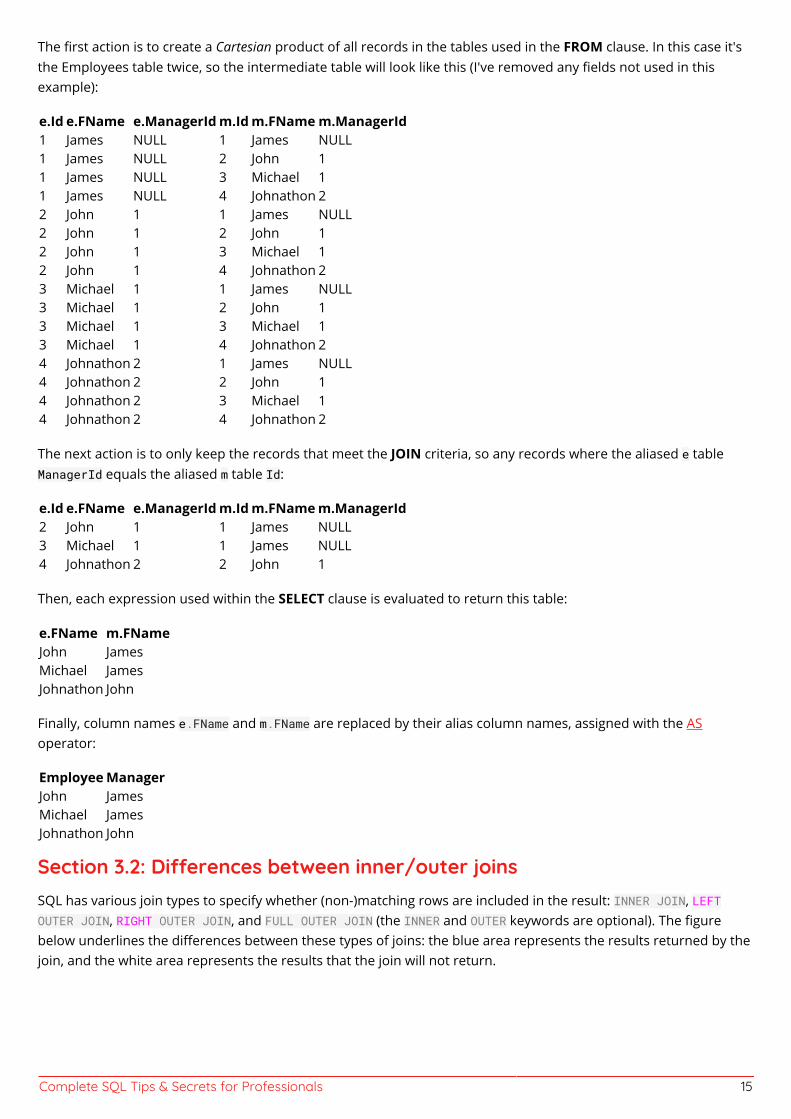
The first action is to create a Cartesian product of all records in the tables used in the FROM clause. In this case it'sthe Employees table twice, so the intermediate table will look like this (I've removed any fields not used in thisexample):

e.Id e.FName e.ManagerId m.Id m.FName m.ManagerId1 James NULL 1 James NULL1 James NULL 2 John 11 James NULL 3 Michael 11 James NULL 4 Johnathon 22 John 1 1 James NULL2 John 1 2 John 12 John 1 3 Michael 12 John 1 4 Johnathon 23 Michael 1 1 James NULL3 Michael 1 2 John 13 Michael 1 3 Michael 13 Michael 1 4 Johnathon 24 Johnathon 2 1 James NULL4 Johnathon 2 2 John 14 Johnathon 2 3 Michael 14 Johnathon 2 4 Johnathon 2

The next action is to only keep the records that meet the JOIN criteria, so any records where the aliased e tableManagerId equals the aliased m table Id:

e.Id e.FName e.ManagerId m.Id m.FName m.ManagerId2 John 1 1 James NULL3 Michael 1 1 James NULL4 Johnathon 2 2 John 1

Then, each expression used within the SELECT clause is evaluated to return this table:

e.FName m.FNameJohn JamesMichael JamesJohnathon John

Finally, column names e.FName and m.FName are replaced by their alias column names, assigned with the ASoperator:

Employee ManagerJohn JamesMichael JamesJohnathon John

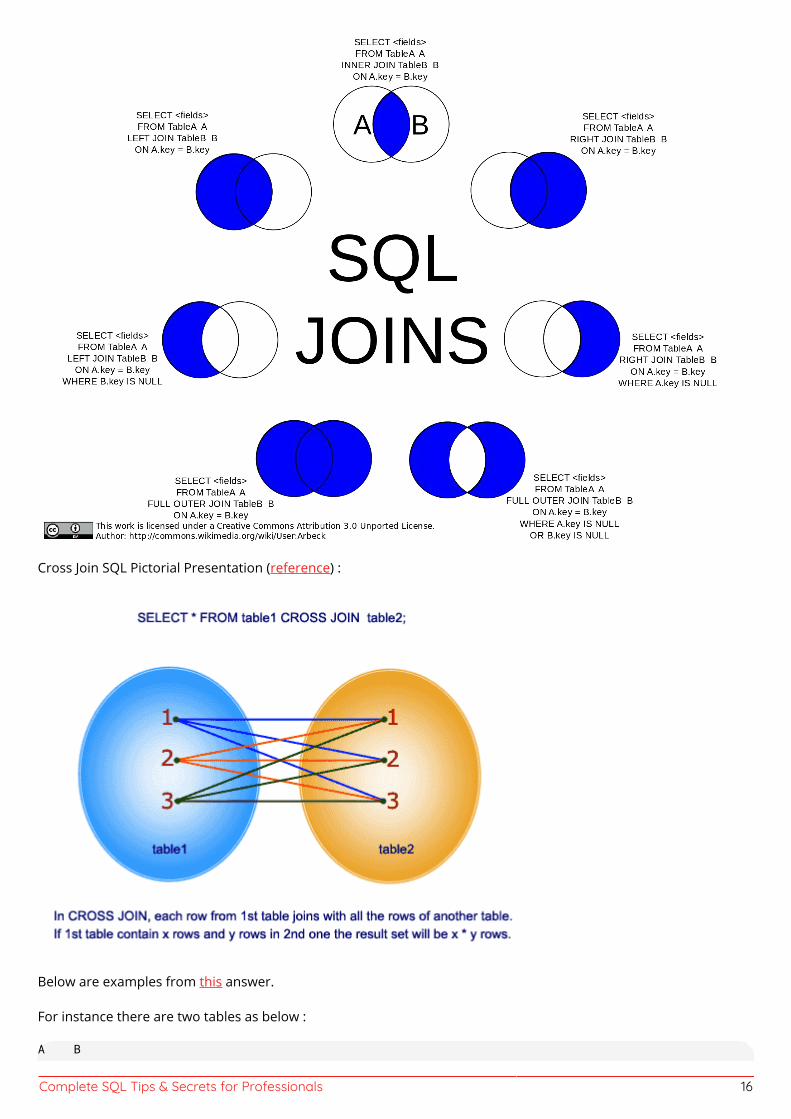
Section 3.2: Dierences between inner/outer joinsSQL has various join types to specify whether (non-)matching rows are included in the result: INNER JOIN, LEFTOUTER JOIN, RIGHT OUTER JOIN, and FULL OUTER JOIN (the INNER and OUTER keywords are optional). The figurebelow underlines the differences between these types of joins: the blue area represents the results returned by thejoin, and the white area represents the results that the join will not return.

Complete SQL Tips & Secrets for Professionals 16

Cross Join SQL Pictorial Presentation (reference) :

Below are examples from this answer.

For instance there are two tables as below :

A B

Complete SQL Tips & Secrets for Professionals 17

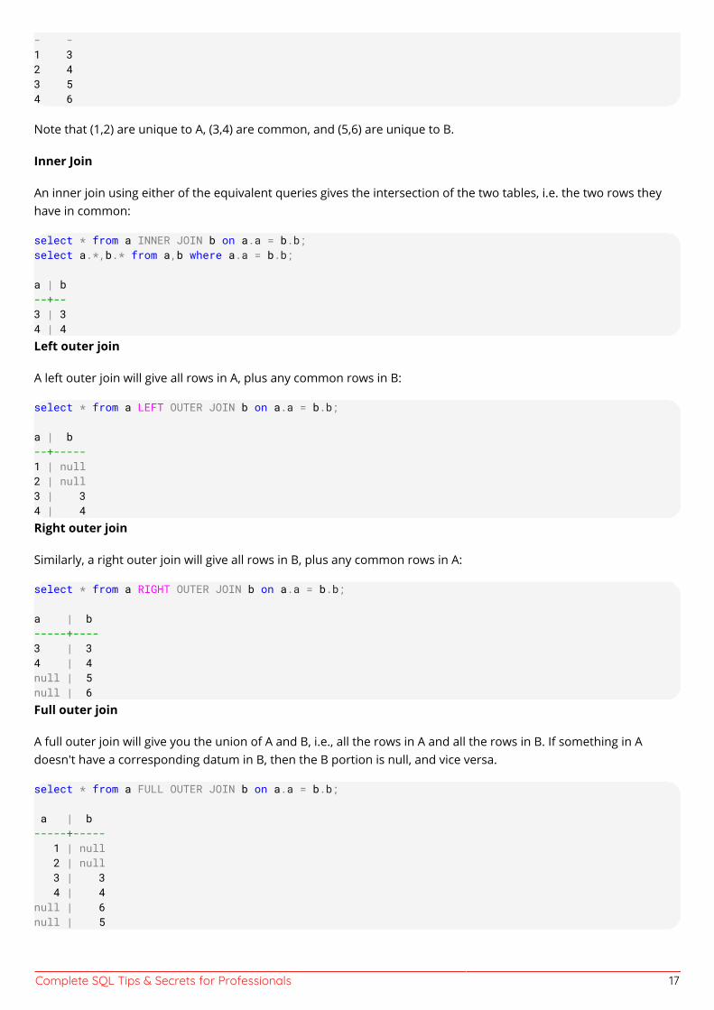
- -1 32 43 54 6

Note that (1,2) are unique to A, (3,4) are common, and (5,6) are unique to B.

Inner Join

An inner join using either of the equivalent queries gives the intersection of the two tables, i.e. the two rows theyhave in common:

select * from a INNER JOIN b on a.a = b.b;select a.*,b.* from a,b where a.a = b.b;

a | b--+--3 | 34 | 4Left outer join

A left outer join will give all rows in A, plus any common rows in B:

select * from a LEFT OUTER JOIN b on a.a = b.b;

a | b--+-----1 | null2 | null3 | 34 | 4Right outer join

Similarly, a right outer join will give all rows in B, plus any common rows in A:

select * from a RIGHT OUTER JOIN b on a.a = b.b;

a | b-----+----3 | 34 | 4null | 5null | 6Full outer join

A full outer join will give you the union of A and B, i.e., all the rows in A and all the rows in B. If something in Adoesn't have a corresponding datum in B, then the B portion is null, and vice versa.

select * from a FULL OUTER JOIN b on a.a = b.b;

a | b-----+----- 1 | null 2 | null 3 | 3 4 | 4null | 6null | 5

Complete SQL Tips & Secrets for Professionals 18

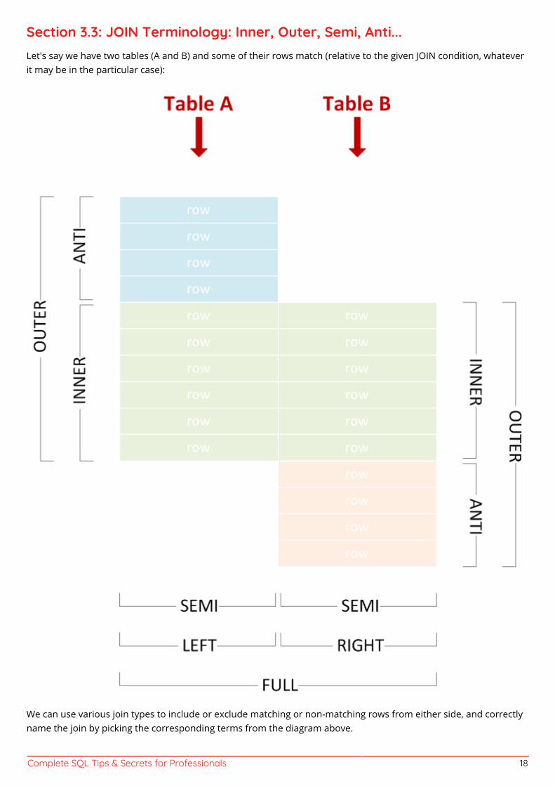
Section 3.3: JOIN Terminology: Inner, Outer, Semi, Anti...Let's say we have two tables (A and B) and some of their rows match (relative to the given JOIN condition, whateverit may be in the particular case):

We can use various join types to include or exclude matching or non-matching rows from either side, and correctlyname the join by picking the corresponding terms from the diagram above.

Complete SQL Tips & Secrets for Professionals 19

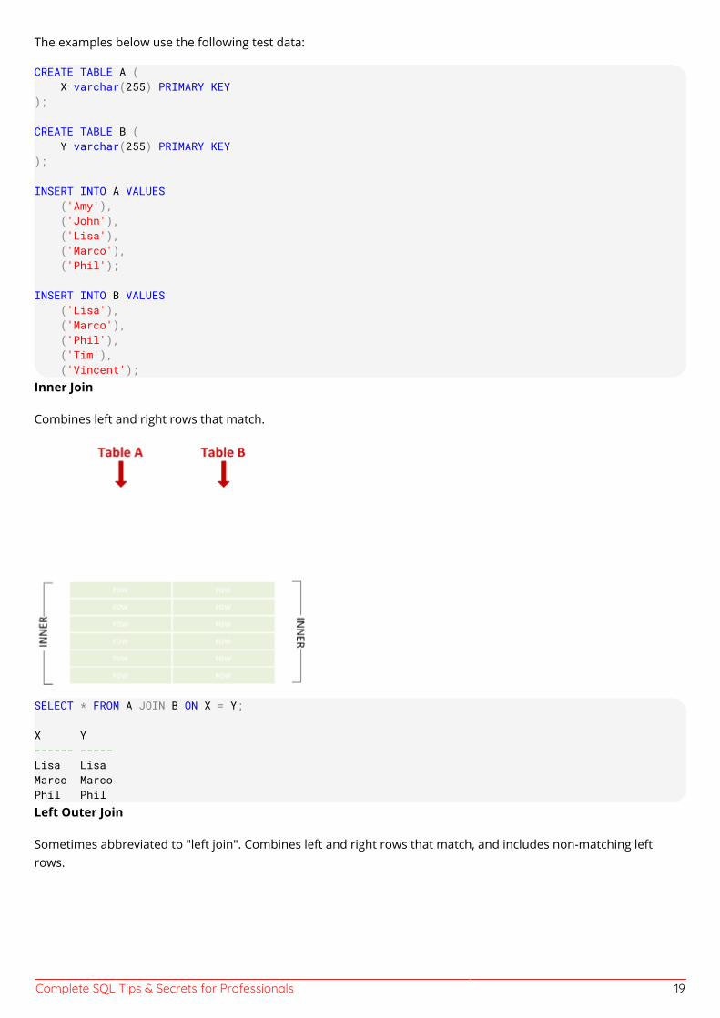
The examples below use the following test data:

CREATE TABLE A ( X varchar(255) PRIMARY KEY);

CREATE TABLE B ( Y varchar(255) PRIMARY KEY);

INSERT INTO A VALUES ('Amy'), ('John'), ('Lisa'), ('Marco'), ('Phil');

INSERT INTO B VALUES ('Lisa'), ('Marco'), ('Phil'), ('Tim'), ('Vincent');Inner Join

Combines left and right rows that match.

SELECT * FROM A JOIN B ON X = Y;

X Y------ -----Lisa LisaMarco MarcoPhil PhilLeft Outer Join

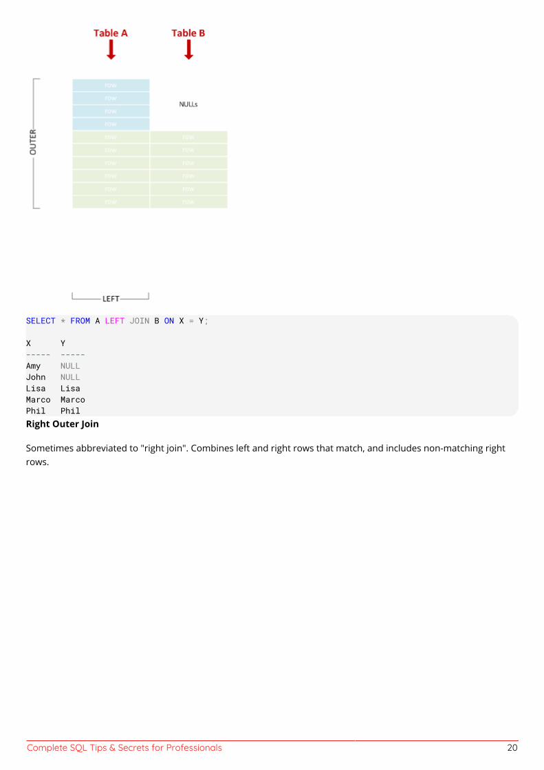
Sometimes abbreviated to "left join". Combines left and right rows that match, and includes non-matching leftrows.

Complete SQL Tips & Secrets for Professionals 20

SELECT * FROM A LEFT JOIN B ON X = Y;

X Y----- -----Amy NULLJohn NULLLisa LisaMarco MarcoPhil PhilRight Outer Join

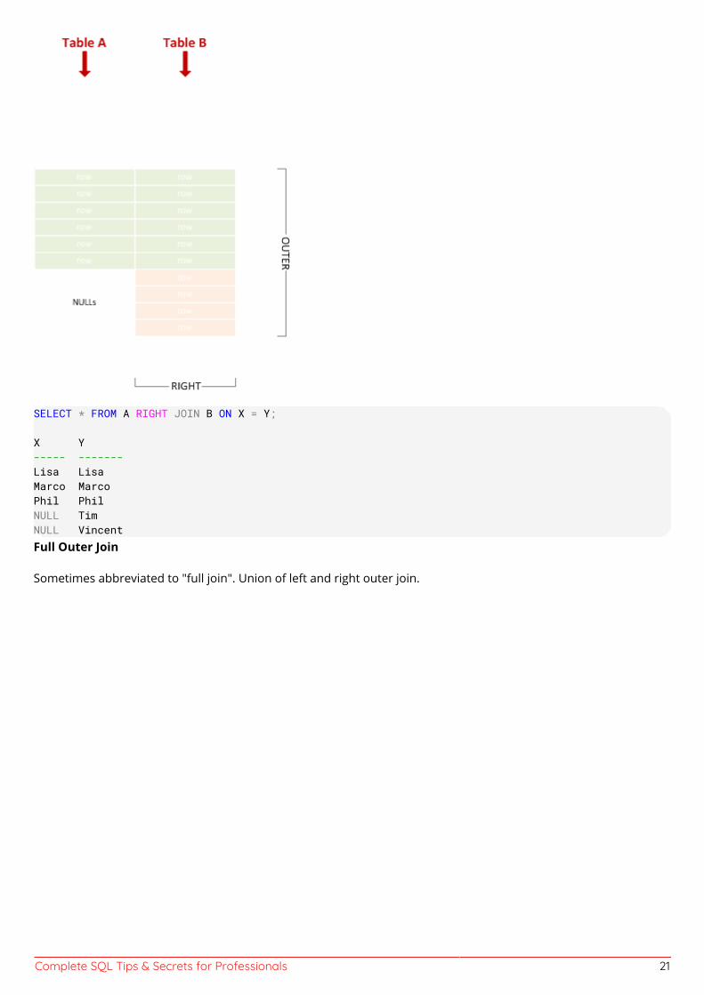
Sometimes abbreviated to "right join". Combines left and right rows that match, and includes non-matching rightrows.

Complete SQL Tips & Secrets for Professionals 21

SELECT * FROM A RIGHT JOIN B ON X = Y;

X Y----- -------Lisa LisaMarco MarcoPhil PhilNULL TimNULL VincentFull Outer Join

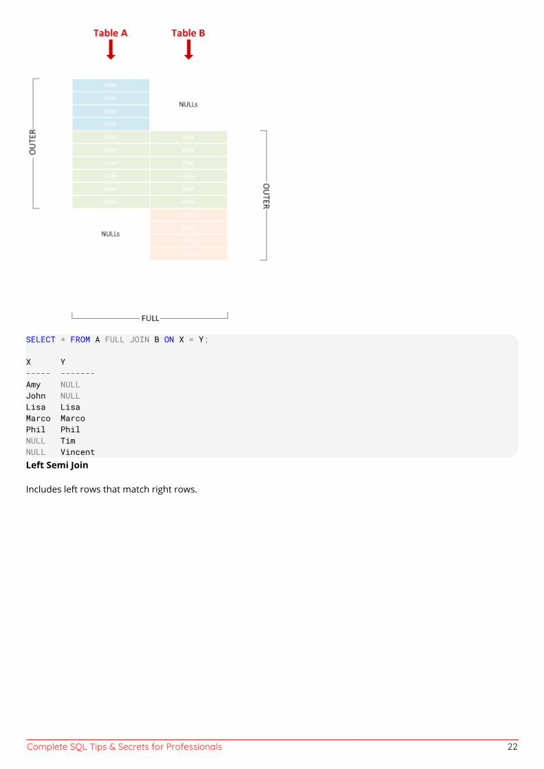
Sometimes abbreviated to "full join". Union of left and right outer join.

Complete SQL Tips & Secrets for Professionals 22

SELECT * FROM A FULL JOIN B ON X = Y;

X Y----- -------Amy NULLJohn NULLLisa LisaMarco MarcoPhil PhilNULL TimNULL VincentLeft Semi Join

Includes left rows that match right rows.

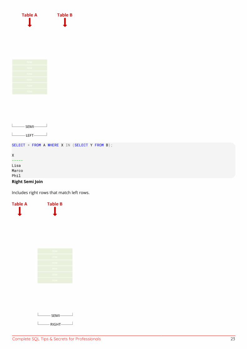
Complete SQL Tips & Secrets for Professionals 23

SELECT * FROM A WHERE X IN (SELECT Y FROM B);

X-----LisaMarcoPhilRight Semi Join

Includes right rows that match left rows.

Complete SQL Tips & Secrets for Professionals 24

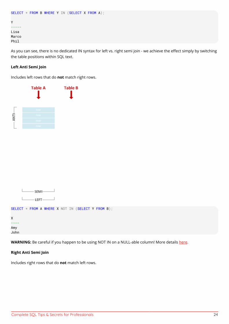
SELECT * FROM B WHERE Y IN (SELECT X FROM A);

Y-----LisaMarcoPhil

As you can see, there is no dedicated IN syntax for left vs. right semi join - we achieve the effect simply by switchingthe table positions within SQL text.

Left Anti Semi Join

Includes left rows that do not match right rows.

SELECT * FROM A WHERE X NOT IN (SELECT Y FROM B);

X----AmyJohn

WARNING: Be careful if you happen to be using NOT IN on a NULL-able column! More details here.

Right Anti Semi Join

Includes right rows that do not match left rows.

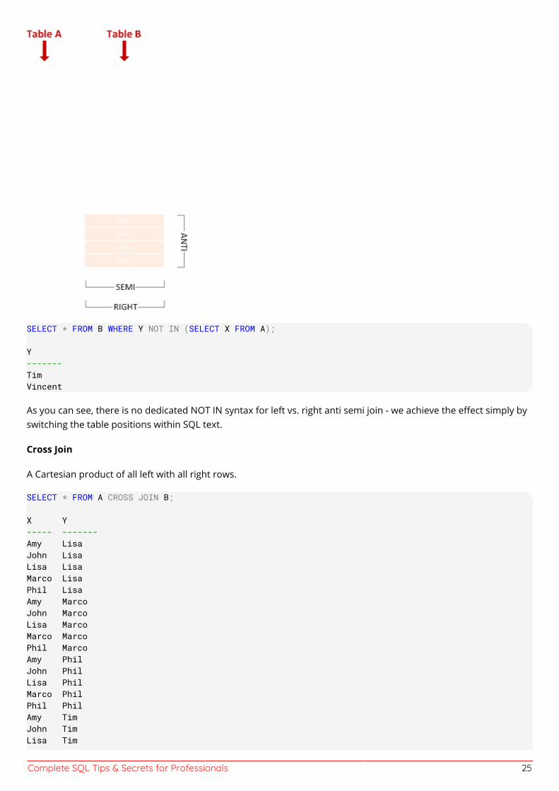
Complete SQL Tips & Secrets for Professionals 25

SELECT * FROM B WHERE Y NOT IN (SELECT X FROM A);

Y-------TimVincent

As you can see, there is no dedicated NOT IN syntax for left vs. right anti semi join - we achieve the effect simply byswitching the table positions within SQL text.

Cross Join

A Cartesian product of all left with all right rows.

SELECT * FROM A CROSS JOIN B;

X Y----- -------Amy LisaJohn LisaLisa LisaMarco LisaPhil LisaAmy MarcoJohn MarcoLisa MarcoMarco MarcoPhil MarcoAmy PhilJohn PhilLisa PhilMarco PhilPhil PhilAmy TimJohn TimLisa Tim

Complete SQL Tips & Secrets for Professionals 26

Marco TimPhil TimAmy VincentJohn VincentLisa VincentMarco VincentPhil Vincent

Cross join is equivalent to an inner join with join condition which always matches, so the following query wouldhave returned the same result:

SELECT * FROM A JOIN B ON 1 = 1;Self-Join

This simply denotes a table joining with itself. A self-join can be any of the join types discussed above. For example,this is a an inner self-join:

SELECT * FROM A A1 JOIN A A2 ON LEN(A1.X) < LEN(A2.X);

X X---- -----Amy JohnAmy LisaAmy MarcoJohn MarcoLisa MarcoPhil MarcoAmy Phil

Section 3.4: Left Outer JoinA Left Outer Join (also known as a Left Join or Outer Join) is a Join that ensures all rows from the left table arerepresented; if no matching row from the right table exists, its corresponding fields are NULL.

The following example will select all departments and the first name of employees that work in that department.Departments with no employees are still returned in the results, but will have NULL for the employee name:

SELECT Departments.Name, Employees.FNameFROM DepartmentsLEFT OUTER JOIN EmployeesON Departments.Id = Employees.DepartmentId

This would return the following from the example database:

Departments.Name Employees.FNameHR JamesHR JohnHR JohnathonSales MichaelTech NULLSo how does this work?

There are two tables in the FROM clause:

Id FName LName PhoneNumber ManagerId DepartmentId Salary HireDate1 James Smith 1234567890 NULL 1 1000 01-01-20022 John Johnson 2468101214 1 1 400 23-03-20053 Michael Williams 1357911131 1 2 600 12-05-20094 Johnathon Smith 1212121212 2 1 500 24-07-2016

Complete SQL Tips & Secrets for Professionals 27

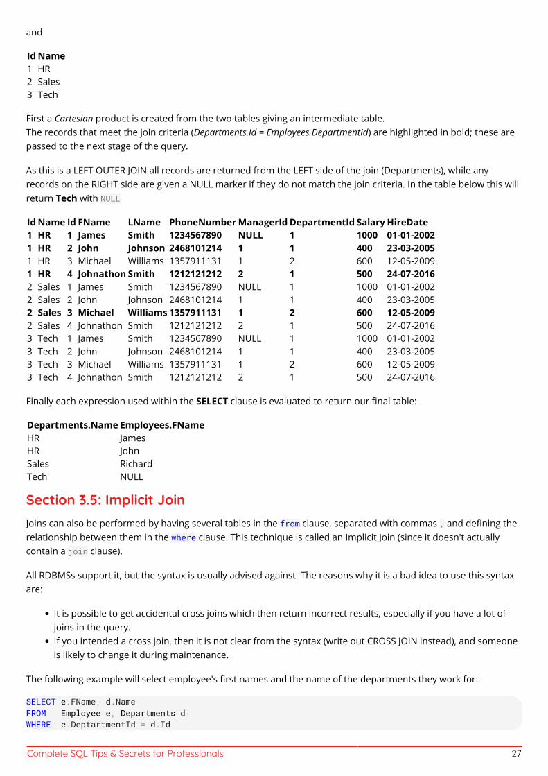
and

Id Name1 HR2 Sales3 Tech

First a Cartesian product is created from the two tables giving an intermediate table.The records that meet the join criteria (Departments.Id = Employees.DepartmentId) are highlighted in bold; these arepassed to the next stage of the query.

As this is a LEFT OUTER JOIN all records are returned from the LEFT side of the join (Departments), while anyrecords on the RIGHT side are given a NULL marker if they do not match the join criteria. In the table below this willreturn Tech with NULL

Id Name Id FName LName PhoneNumber ManagerId DepartmentId Salary HireDate1 HR 1 James Smith 1234567890 NULL 1 1000 01-01-20021 HR 2 John Johnson 2468101214 1 1 400 23-03-20051 HR 3 Michael Williams 1357911131 1 2 600 12-05-20091 HR 4 Johnathon Smith 1212121212 2 1 500 24-07-20162 Sales 1 James Smith 1234567890 NULL 1 1000 01-01-20022 Sales 2 John Johnson 2468101214 1 1 400 23-03-20052 Sales 3 Michael Williams 1357911131 1 2 600 12-05-20092 Sales 4 Johnathon Smith 1212121212 2 1 500 24-07-20163 Tech 1 James Smith 1234567890 NULL 1 1000 01-01-20023 Tech 2 John Johnson 2468101214 1 1 400 23-03-20053 Tech 3 Michael Williams 1357911131 1 2 600 12-05-20093 Tech 4 Johnathon Smith 1212121212 2 1 500 24-07-2016

Finally each expression used within the SELECT clause is evaluated to return our final table:

Departments.Name Employees.FNameHR JamesHR JohnSales RichardTech NULL

Section 3.5: Implicit JoinJoins can also be performed by having several tables in the from clause, separated with commas , and defining therelationship between them in the where clause. This technique is called an Implicit Join (since it doesn't actuallycontain a join clause).

All RDBMSs support it, but the syntax is usually advised against. The reasons why it is a bad idea to use this syntaxare:

It is possible to get accidental cross joins which then return incorrect results, especially if you have a lot ofjoins in the query.If you intended a cross join, then it is not clear from the syntax (write out CROSS JOIN instead), and someoneis likely to change it during maintenance.

The following example will select employee's first names and the name of the departments they work for:

SELECT e.FName, d.NameFROM Employee e, Departments dWHERE e.DeptartmentId = d.Id

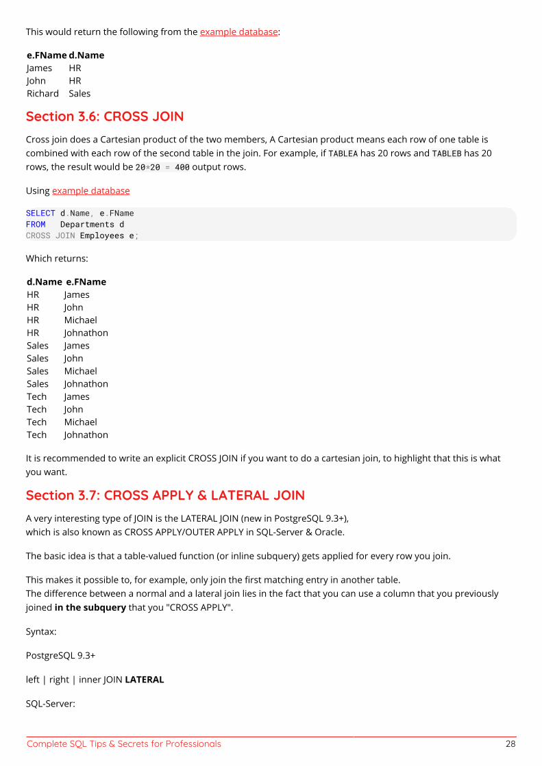
Complete SQL Tips & Secrets for Professionals 28

This would return the following from the example database:

e.FName d.NameJames HRJohn HRRichard Sales

Section 3.6: CROSS JOINCross join does a Cartesian product of the two members, A Cartesian product means each row of one table iscombined with each row of the second table in the join. For example, if TABLEA has 20 rows and TABLEB has 20rows, the result would be 20*20 = 400 output rows.

Using example database

SELECT d.Name, e.FNameFROM Departments dCROSS JOIN Employees e;

Which returns:

d.Name e.FNameHR JamesHR JohnHR MichaelHR JohnathonSales JamesSales JohnSales MichaelSales JohnathonTech JamesTech JohnTech MichaelTech Johnathon

It is recommended to write an explicit CROSS JOIN if you want to do a cartesian join, to highlight that this is whatyou want.

Section 3.7: CROSS APPLY & LATERAL JOINA very interesting type of JOIN is the LATERAL JOIN (new in PostgreSQL 9.3+),which is also known as CROSS APPLY/OUTER APPLY in SQL-Server & Oracle.

The basic idea is that a table-valued function (or inline subquery) gets applied for every row you join.

This makes it possible to, for example, only join the first matching entry in another table.The difference between a normal and a lateral join lies in the fact that you can use a column that you previouslyjoined in the subquery that you "CROSS APPLY".

Syntax:

PostgreSQL 9.3+

left | right | inner JOIN LATERAL

SQL-Server:

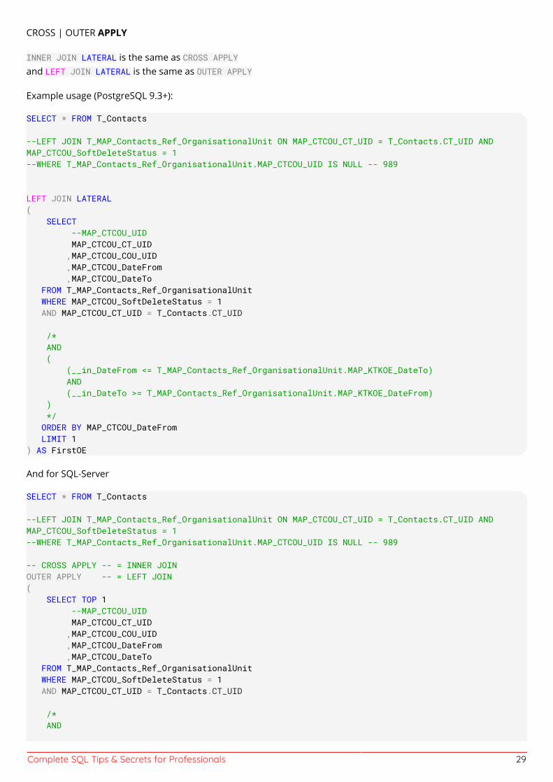
Complete SQL Tips & Secrets for Professionals 29

CROSS | OUTER APPLY

INNER JOIN LATERAL is the same as CROSS APPLYand LEFT JOIN LATERAL is the same as OUTER APPLY

Example usage (PostgreSQL 9.3+):

SELECT * FROM T_Contacts

--LEFT JOIN T_MAP_Contacts_Ref_OrganisationalUnit ON MAP_CTCOU_CT_UID = T_Contacts.CT_UID ANDMAP_CTCOU_SoftDeleteStatus = 1--WHERE T_MAP_Contacts_Ref_OrganisationalUnit.MAP_CTCOU_UID IS NULL -- 989

LEFT JOIN LATERAL( SELECT --MAP_CTCOU_UID MAP_CTCOU_CT_UID ,MAP_CTCOU_COU_UID ,MAP_CTCOU_DateFrom ,MAP_CTCOU_DateTo FROM T_MAP_Contacts_Ref_OrganisationalUnit WHERE MAP_CTCOU_SoftDeleteStatus = 1 AND MAP_CTCOU_CT_UID = T_Contacts.CT_UID

/* AND ( (__in_DateFrom <= T_MAP_Contacts_Ref_OrganisationalUnit.MAP_KTKOE_DateTo) AND (__in_DateTo >= T_MAP_Contacts_Ref_OrganisationalUnit.MAP_KTKOE_DateFrom) ) */ ORDER BY MAP_CTCOU_DateFrom LIMIT 1) AS FirstOE

And for SQL-Server

SELECT * FROM T_Contacts

--LEFT JOIN T_MAP_Contacts_Ref_OrganisationalUnit ON MAP_CTCOU_CT_UID = T_Contacts.CT_UID ANDMAP_CTCOU_SoftDeleteStatus = 1--WHERE T_MAP_Contacts_Ref_OrganisationalUnit.MAP_CTCOU_UID IS NULL -- 989

-- CROSS APPLY -- = INNER JOINOUTER APPLY -- = LEFT JOIN( SELECT TOP 1 --MAP_CTCOU_UID MAP_CTCOU_CT_UID ,MAP_CTCOU_COU_UID ,MAP_CTCOU_DateFrom ,MAP_CTCOU_DateTo FROM T_MAP_Contacts_Ref_OrganisationalUnit WHERE MAP_CTCOU_SoftDeleteStatus = 1 AND MAP_CTCOU_CT_UID = T_Contacts.CT_UID

/* AND

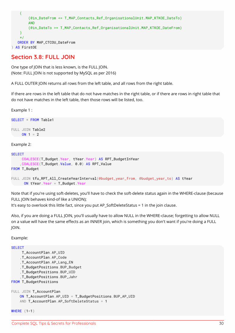
Complete SQL Tips & Secrets for Professionals 30

( (@in_DateFrom <= T_MAP_Contacts_Ref_OrganisationalUnit.MAP_KTKOE_DateTo) AND (@in_DateTo >= T_MAP_Contacts_Ref_OrganisationalUnit.MAP_KTKOE_DateFrom) ) */ ORDER BY MAP_CTCOU_DateFrom) AS FirstOE

Section 3.8: FULL JOINOne type of JOIN that is less known, is the FULL JOIN.(Note: FULL JOIN is not supported by MySQL as per 2016)

A FULL OUTER JOIN returns all rows from the left table, and all rows from the right table.

If there are rows in the left table that do not have matches in the right table, or if there are rows in right table thatdo not have matches in the left table, then those rows will be listed, too.

Example 1 :

SELECT * FROM Table1

FULL JOIN Table2 ON 1 = 2

Example 2:

SELECT COALESCE(T_Budget.Year, tYear.Year) AS RPT_BudgetInYear ,COALESCE(T_Budget.Value, 0.0) AS RPT_ValueFROM T_Budget

FULL JOIN tfu_RPT_All_CreateYearInterval(@budget_year_from, @budget_year_to) AS tYear ON tYear.Year = T_Budget.Year

Note that if you're using soft-deletes, you'll have to check the soft-delete status again in the WHERE-clause (becauseFULL JOIN behaves kind-of like a UNION);It's easy to overlook this little fact, since you put AP_SoftDeleteStatus = 1 in the join clause.

Also, if you are doing a FULL JOIN, you'll usually have to allow NULL in the WHERE-clause; forgetting to allow NULLon a value will have the same effects as an INNER join, which is something you don't want if you're doing a FULLJOIN.

Example:

SELECT T_AccountPlan.AP_UID ,T_AccountPlan.AP_Code ,T_AccountPlan.AP_Lang_EN ,T_BudgetPositions.BUP_Budget ,T_BudgetPositions.BUP_UID ,T_BudgetPositions.BUP_JahrFROM T_BudgetPositions

FULL JOIN T_AccountPlan ON T_AccountPlan.AP_UID = T_BudgetPositions.BUP_AP_UID AND T_AccountPlan.AP_SoftDeleteStatus = 1

WHERE (1=1)

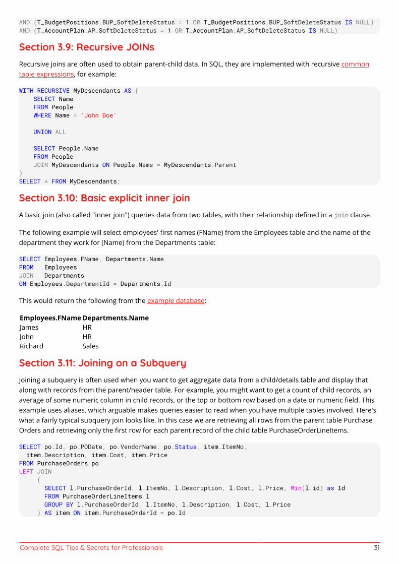
Complete SQL Tips & Secrets for Professionals 31

AND (T_BudgetPositions.BUP_SoftDeleteStatus = 1 OR T_BudgetPositions.BUP_SoftDeleteStatus IS NULL)AND (T_AccountPlan.AP_SoftDeleteStatus = 1 OR T_AccountPlan.AP_SoftDeleteStatus IS NULL)

Section 3.9: Recursive JOINsRecursive joins are often used to obtain parent-child data. In SQL, they are implemented with recursive commontable expressions, for example:

WITH RECURSIVE MyDescendants AS ( SELECT Name FROM People WHERE Name = 'John Doe'

UNION ALL

SELECT People.Name FROM People JOIN MyDescendants ON People.Name = MyDescendants.Parent)SELECT * FROM MyDescendants;

Section 3.10: Basic explicit inner joinA basic join (also called "inner join") queries data from two tables, with their relationship defined in a join clause.

The following example will select employees' first names (FName) from the Employees table and the name of thedepartment they work for (Name) from the Departments table:

SELECT Employees.FName, Departments.NameFROM EmployeesJOIN DepartmentsON Employees.DepartmentId = Departments.Id

This would return the following from the example database:

Employees.FName Departments.NameJames HRJohn HRRichard Sales

Section 3.11: Joining on a SubqueryJoining a subquery is often used when you want to get aggregate data from a child/details table and display thatalong with records from the parent/header table. For example, you might want to get a count of child records, anaverage of some numeric column in child records, or the top or bottom row based on a date or numeric field. Thisexample uses aliases, which arguable makes queries easier to read when you have multiple tables involved. Here'swhat a fairly typical subquery join looks like. In this case we are retrieving all rows from the parent table PurchaseOrders and retrieving only the first row for each parent record of the child table PurchaseOrderLineItems.

SELECT po.Id, po.PODate, po.VendorName, po.Status, item.ItemNo, item.Description, item.Cost, item.PriceFROM PurchaseOrders poLEFT JOIN ( SELECT l.PurchaseOrderId, l.ItemNo, l.Description, l.Cost, l.Price, Min(l.id) as Id FROM PurchaseOrderLineItems l GROUP BY l.PurchaseOrderId, l.ItemNo, l.Description, l.Cost, l.Price ) AS item ON item.PurchaseOrderId = po.Id

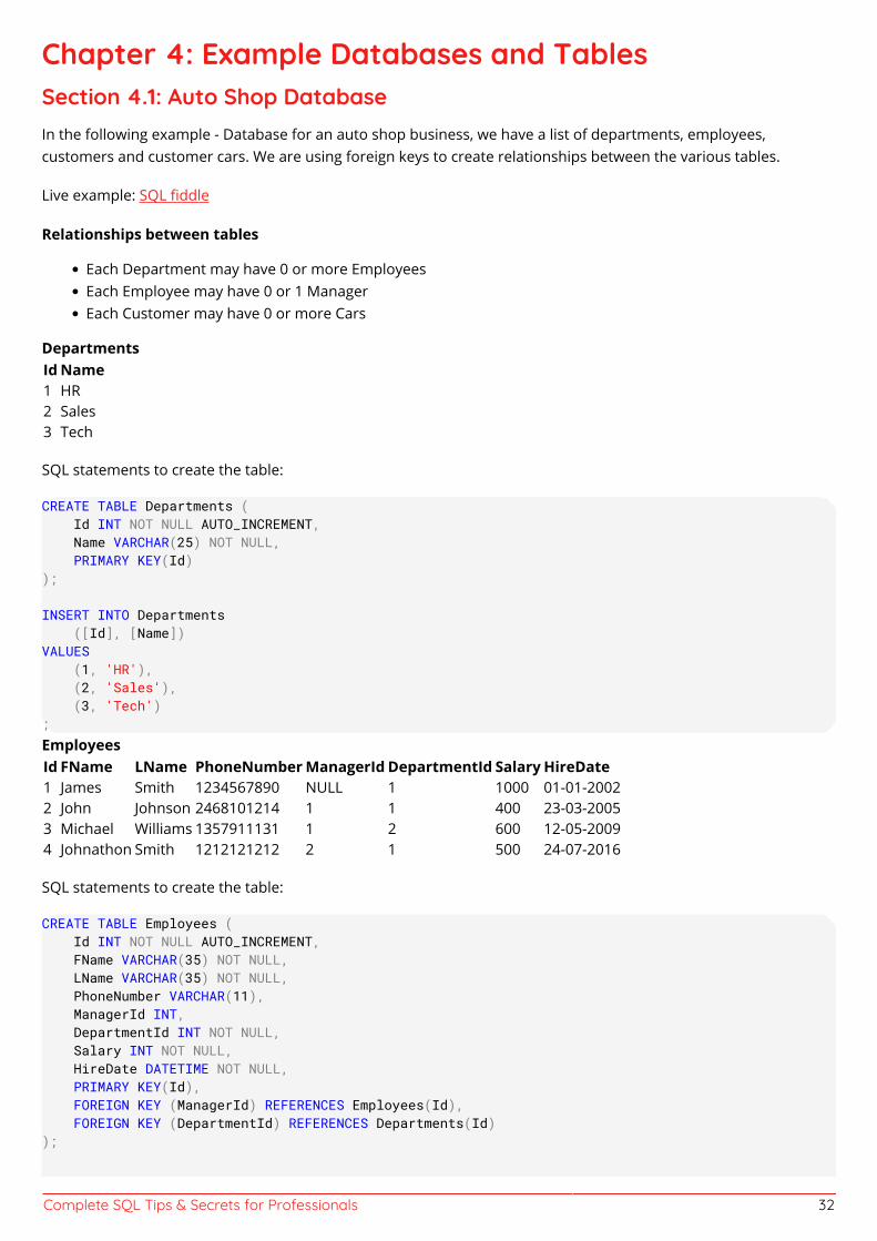
Complete SQL Tips & Secrets for Professionals 32

Chapter 4: Example Databases and TablesSection 4.1: Auto Shop DatabaseIn the following example - Database for an auto shop business, we have a list of departments, employees,customers and customer cars. We are using foreign keys to create relationships between the various tables.

Live example: SQL fiddle

Relationships between tables

Each Department may have 0 or more EmployeesEach Employee may have 0 or 1 ManagerEach Customer may have 0 or more Cars

DepartmentsId Name1 HR2 Sales3 Tech

SQL statements to create the table:

CREATE TABLE Departments ( Id INT NOT NULL AUTO_INCREMENT, Name VARCHAR(25) NOT NULL, PRIMARY KEY(Id));

INSERT INTO Departments ([Id], [Name])VALUES (1, 'HR'), (2, 'Sales'), (3, 'Tech');EmployeesId FName LName PhoneNumber ManagerId DepartmentId Salary HireDate1 James Smith 1234567890 NULL 1 1000 01-01-20022 John Johnson 2468101214 1 1 400 23-03-20053 Michael Williams 1357911131 1 2 600 12-05-20094 Johnathon Smith 1212121212 2 1 500 24-07-2016

SQL statements to create the table:

CREATE TABLE Employees ( Id INT NOT NULL AUTO_INCREMENT, FName VARCHAR(35) NOT NULL, LName VARCHAR(35) NOT NULL, PhoneNumber VARCHAR(11), ManagerId INT, DepartmentId INT NOT NULL, Salary INT NOT NULL, HireDate DATETIME NOT NULL, PRIMARY KEY(Id), FOREIGN KEY (ManagerId) REFERENCES Employees(Id), FOREIGN KEY (DepartmentId) REFERENCES Departments(Id));

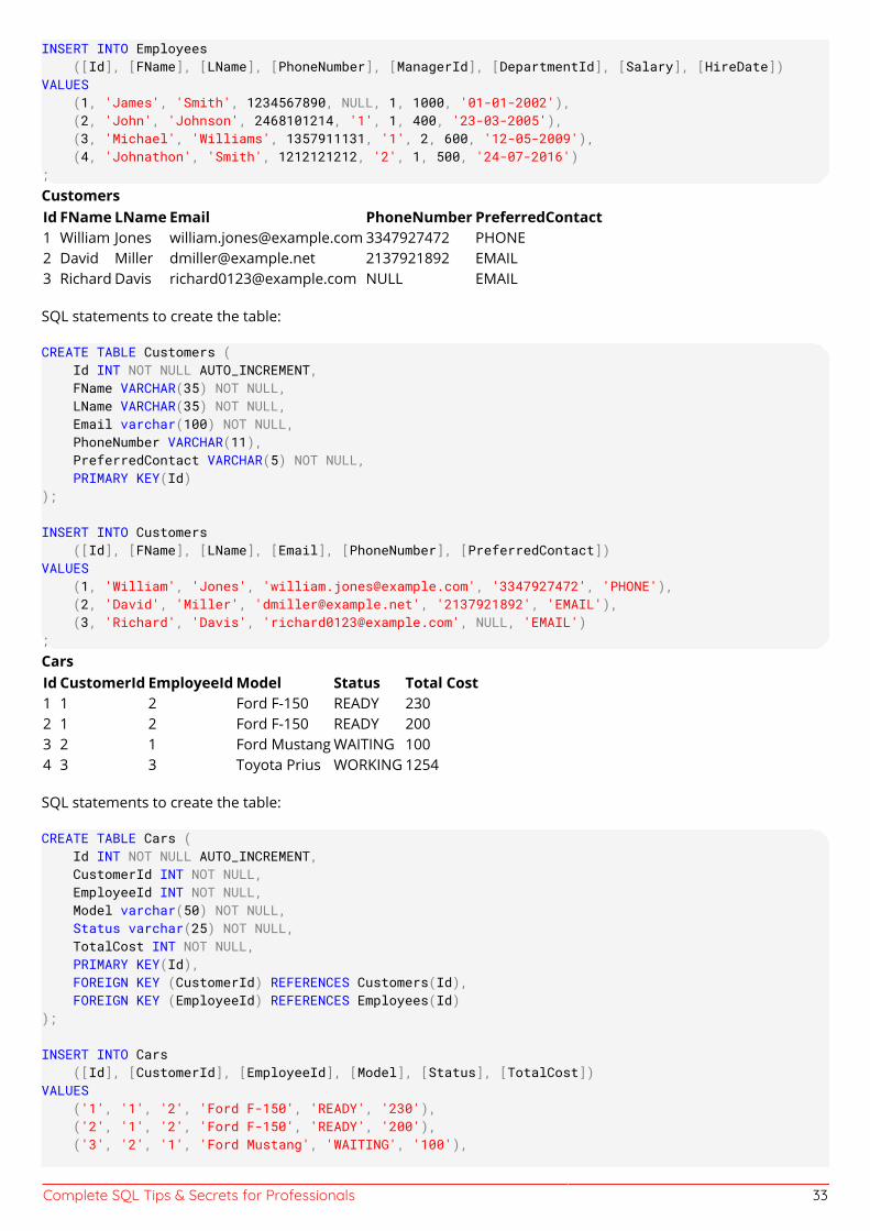
Complete SQL Tips & Secrets for Professionals 33

INSERT INTO Employees ([Id], [FName], [LName], [PhoneNumber], [ManagerId], [DepartmentId], [Salary], [HireDate])VALUES (1, 'James', 'Smith', 1234567890, NULL, 1, 1000, '01-01-2002'), (2, 'John', 'Johnson', 2468101214, '1', 1, 400, '23-03-2005'), (3, 'Michael', 'Williams', 1357911131, '1', 2, 600, '12-05-2009'), (4, 'Johnathon', 'Smith', 1212121212, '2', 1, 500, '24-07-2016');CustomersId FName LName Email PhoneNumber PreferredContact1 William Jones william.jones@example.com 3347927472 PHONE2 David Miller dmiller@example.net 2137921892 EMAIL3 Richard Davis richard0123@example.com NULL EMAIL

SQL statements to create the table:

CREATE TABLE Customers ( Id INT NOT NULL AUTO_INCREMENT, FName VARCHAR(35) NOT NULL, LName VARCHAR(35) NOT NULL, Email varchar(100) NOT NULL, PhoneNumber VARCHAR(11), PreferredContact VARCHAR(5) NOT NULL, PRIMARY KEY(Id));

INSERT INTO Customers ([Id], [FName], [LName], [Email], [PhoneNumber], [PreferredContact])VALUES (1, 'William', 'Jones', 'william.jones@example.com', '3347927472', 'PHONE'), (2, 'David', 'Miller', 'dmiller@example.net', '2137921892', 'EMAIL'), (3, 'Richard', 'Davis', 'richard0123@example.com', NULL, 'EMAIL');CarsId CustomerId EmployeeId Model Status Total Cost1 1 2 Ford F-150 READY 2302 1 2 Ford F-150 READY 2003 2 1 Ford Mustang WAITING 1004 3 3 Toyota Prius WORKING 1254

SQL statements to create the table:

CREATE TABLE Cars ( Id INT NOT NULL AUTO_INCREMENT, CustomerId INT NOT NULL, EmployeeId INT NOT NULL, Model varchar(50) NOT NULL, Status varchar(25) NOT NULL, TotalCost INT NOT NULL, PRIMARY KEY(Id), FOREIGN KEY (CustomerId) REFERENCES Customers(Id), FOREIGN KEY (EmployeeId) REFERENCES Employees(Id));

INSERT INTO Cars ([Id], [CustomerId], [EmployeeId], [Model], [Status], [TotalCost])VALUES ('1', '1', '2', 'Ford F-150', 'READY', '230'), ('2', '1', '2', 'Ford F-150', 'READY', '200'), ('3', '2', '1', 'Ford Mustang', 'WAITING', '100'),

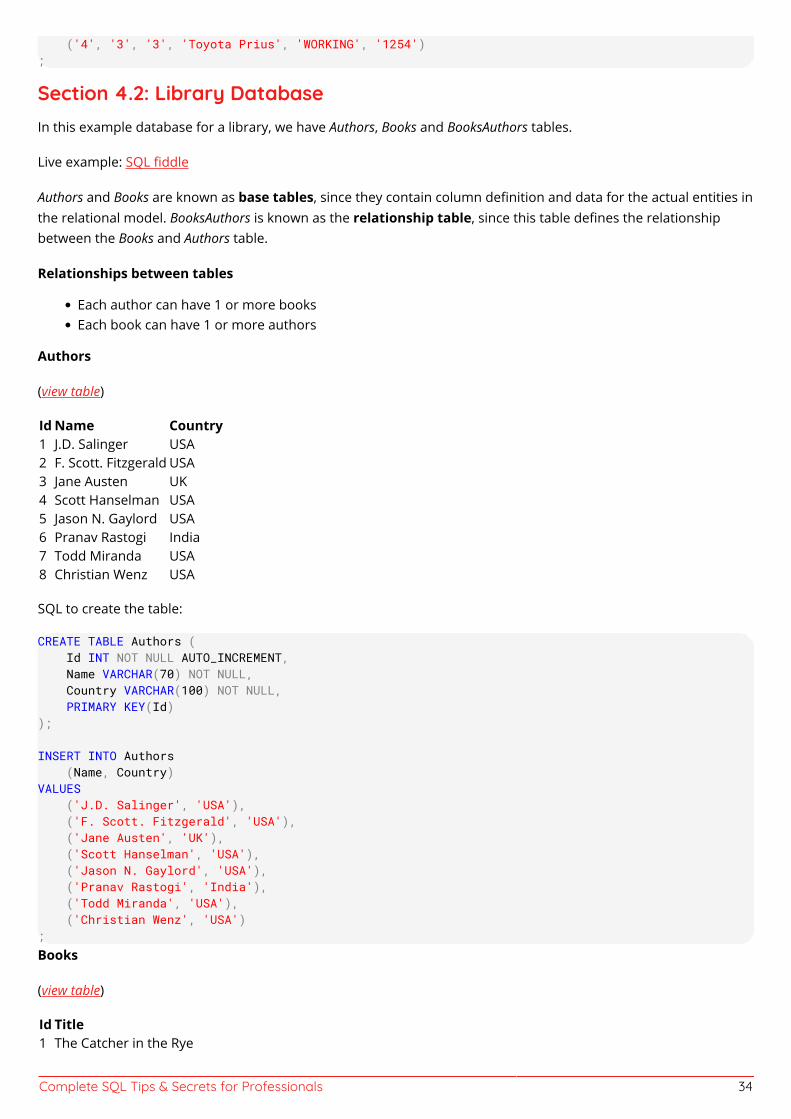
Complete SQL Tips & Secrets for Professionals 34

('4', '3', '3', 'Toyota Prius', 'WORKING', '1254');

Section 4.2: Library DatabaseIn this example database for a library, we have Authors, Books and BooksAuthors tables.

Live example: SQL fiddle

Authors and Books are known as base tables, since they contain column definition and data for the actual entities inthe relational model. BooksAuthors is known as the relationship table, since this table defines the relationshipbetween the Books and Authors table.

Relationships between tables

Each author can have 1 or more booksEach book can have 1 or more authors

Authors

(view table)

Id Name Country1 J.D. Salinger USA2 F. Scott. Fitzgerald USA3 Jane Austen UK4 Scott Hanselman USA5 Jason N. Gaylord USA6 Pranav Rastogi India7 Todd Miranda USA8 Christian Wenz USA

SQL to create the table:

CREATE TABLE Authors ( Id INT NOT NULL AUTO_INCREMENT, Name VARCHAR(70) NOT NULL, Country VARCHAR(100) NOT NULL, PRIMARY KEY(Id));

INSERT INTO Authors (Name, Country)VALUES ('J.D. Salinger', 'USA'), ('F. Scott. Fitzgerald', 'USA'), ('Jane Austen', 'UK'), ('Scott Hanselman', 'USA'), ('Jason N. Gaylord', 'USA'), ('Pranav Rastogi', 'India'), ('Todd Miranda', 'USA'), ('Christian Wenz', 'USA');Books

(view table)

Id Title1 The Catcher in the Rye

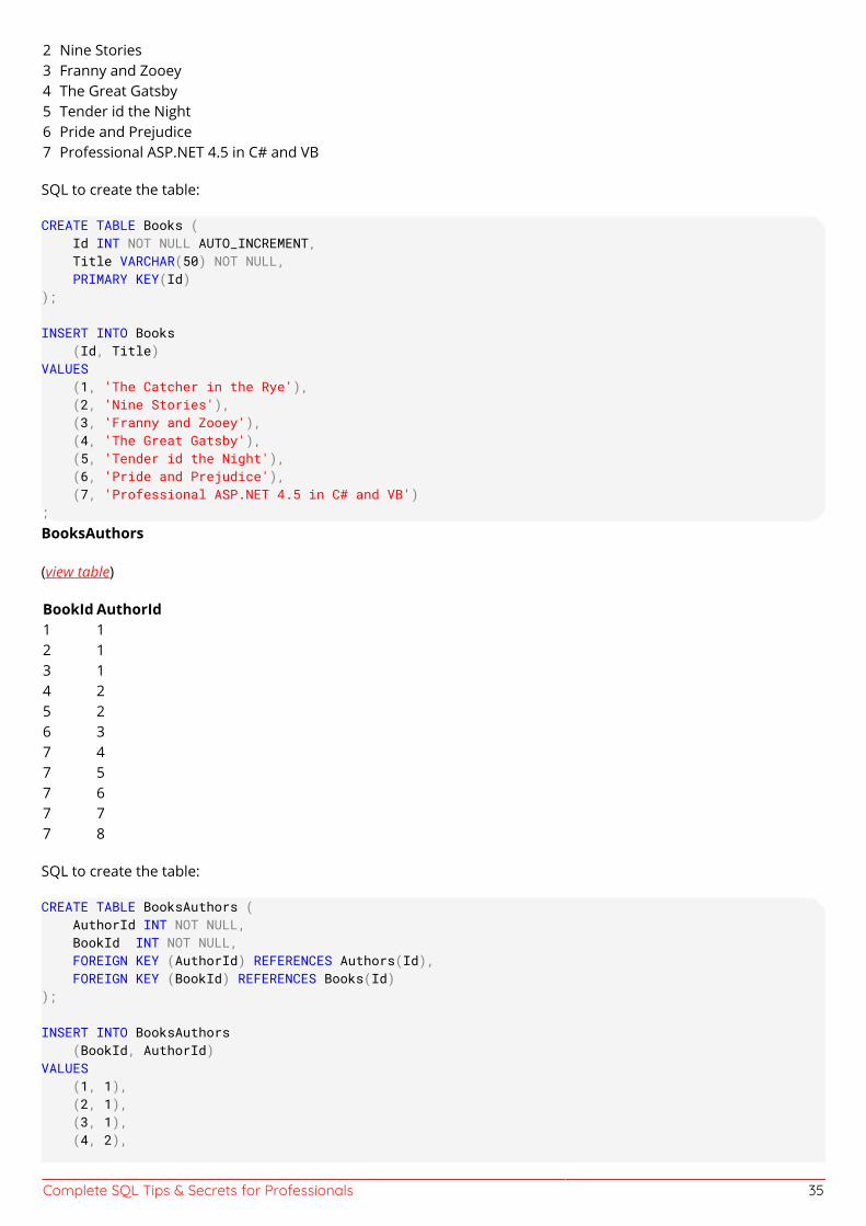
Complete SQL Tips & Secrets for Professionals 35

2 Nine Stories3 Franny and Zooey4 The Great Gatsby5 Tender id the Night6 Pride and Prejudice7 Professional ASP.NET 4.5 in C# and VB

SQL to create the table:

CREATE TABLE Books ( Id INT NOT NULL AUTO_INCREMENT, Title VARCHAR(50) NOT NULL, PRIMARY KEY(Id));

INSERT INTO Books (Id, Title)VALUES (1, 'The Catcher in the Rye'), (2, 'Nine Stories'), (3, 'Franny and Zooey'), (4, 'The Great Gatsby'), (5, 'Tender id the Night'), (6, 'Pride and Prejudice'), (7, 'Professional ASP.NET 4.5 in C# and VB');BooksAuthors

(view table)

BookId AuthorId1 12 13 14 25 26 37 47 57 67 77 8

SQL to create the table:

CREATE TABLE BooksAuthors ( AuthorId INT NOT NULL, BookId INT NOT NULL, FOREIGN KEY (AuthorId) REFERENCES Authors(Id), FOREIGN KEY (BookId) REFERENCES Books(Id));

INSERT INTO BooksAuthors (BookId, AuthorId)VALUES (1, 1), (2, 1), (3, 1), (4, 2),

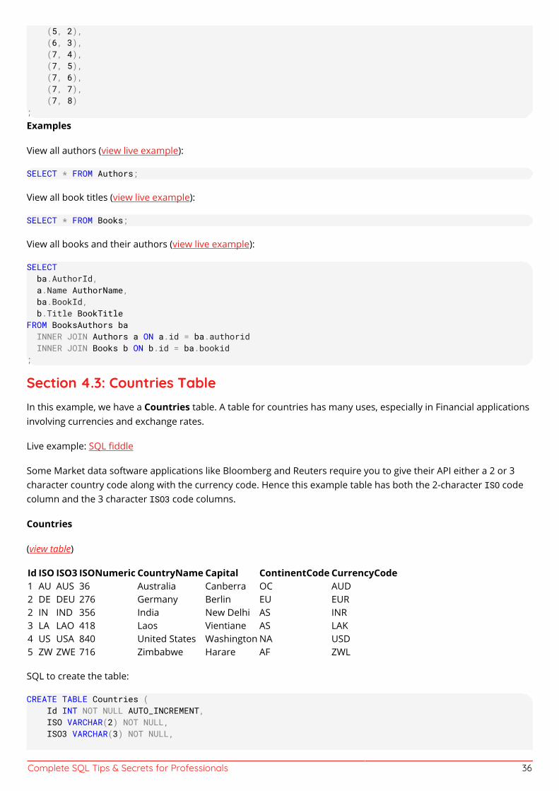
Complete SQL Tips & Secrets for Professionals 36

(5, 2), (6, 3), (7, 4), (7, 5), (7, 6), (7, 7), (7, 8);Examples

View all authors (view live example):

SELECT * FROM Authors;

View all book titles (view live example):

SELECT * FROM Books;

View all books and their authors (view live example):

SELECT ba.AuthorId, a.Name AuthorName, ba.BookId, b.Title BookTitleFROM BooksAuthors ba INNER JOIN Authors a ON a.id = ba.authorid INNER JOIN Books b ON b.id = ba.bookid;

Section 4.3: Countries TableIn this example, we have a Countries table. A table for countries has many uses, especially in Financial applicationsinvolving currencies and exchange rates.

Live example: SQL fiddle

Some Market data software applications like Bloomberg and Reuters require you to give their API either a 2 or 3character country code along with the currency code. Hence this example table has both the 2-character ISO codecolumn and the 3 character ISO3 code columns.

Countries

(view table)

Id ISO ISO3 ISONumeric CountryName Capital ContinentCode CurrencyCode1 AU AUS 36 Australia Canberra OC AUD2 DE DEU 276 Germany Berlin EU EUR2 IN IND 356 India New Delhi AS INR3 LA LAO 418 Laos Vientiane AS LAK4 US USA 840 United States Washington NA USD5 ZW ZWE 716 Zimbabwe Harare AF ZWL

SQL to create the table:

CREATE TABLE Countries ( Id INT NOT NULL AUTO_INCREMENT, ISO VARCHAR(2) NOT NULL, ISO3 VARCHAR(3) NOT NULL,

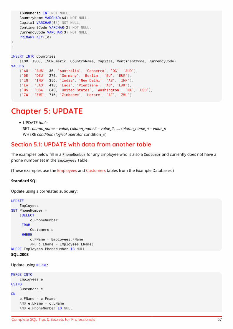
Complete SQL Tips & Secrets for Professionals 37

ISONumeric INT NOT NULL, CountryName VARCHAR(64) NOT NULL, Capital VARCHAR(64) NOT NULL, ContinentCode VARCHAR(2) NOT NULL, CurrencyCode VARCHAR(3) NOT NULL, PRIMARY KEY(Id));

INSERT INTO Countries (ISO, ISO3, ISONumeric, CountryName, Capital, ContinentCode, CurrencyCode)VALUES ('AU', 'AUS', 36, 'Australia', 'Canberra', 'OC', 'AUD'), ('DE', 'DEU', 276, 'Germany', 'Berlin', 'EU', 'EUR'), ('IN', 'IND', 356, 'India', 'New Delhi', 'AS', 'INR'), ('LA', 'LAO', 418, 'Laos', 'Vientiane', 'AS', 'LAK'), ('US', 'USA', 840, 'United States', 'Washington', 'NA', 'USD'), ('ZW', 'ZWE', 716, 'Zimbabwe', 'Harare', 'AF', 'ZWL');

Chapter 5: UPDATEUPDATE tableSET column_name = value, column_name2 = value_2, ..., column_name_n = value_nWHERE condition (logical operator condition_n)

Section 5.1: UPDATE with data from another tableThe examples below fill in a PhoneNumber for any Employee who is also a Customer and currently does not have aphone number set in the Employees Table.

(These examples use the Employees and Customers tables from the Example Databases.)

Standard SQL

Update using a correlated subquery:

UPDATE EmployeesSET PhoneNumber = (SELECT c.PhoneNumber FROM Customers c WHERE c.FName = Employees.FName AND c.LName = Employees.LName)WHERE Employees.PhoneNumber IS NULLSQL:2003

Update using MERGE:

MERGE INTO Employees eUSING Customers cON e.FName = c.Fname AND e.LName = c.LName AND e.PhoneNumber IS NULL

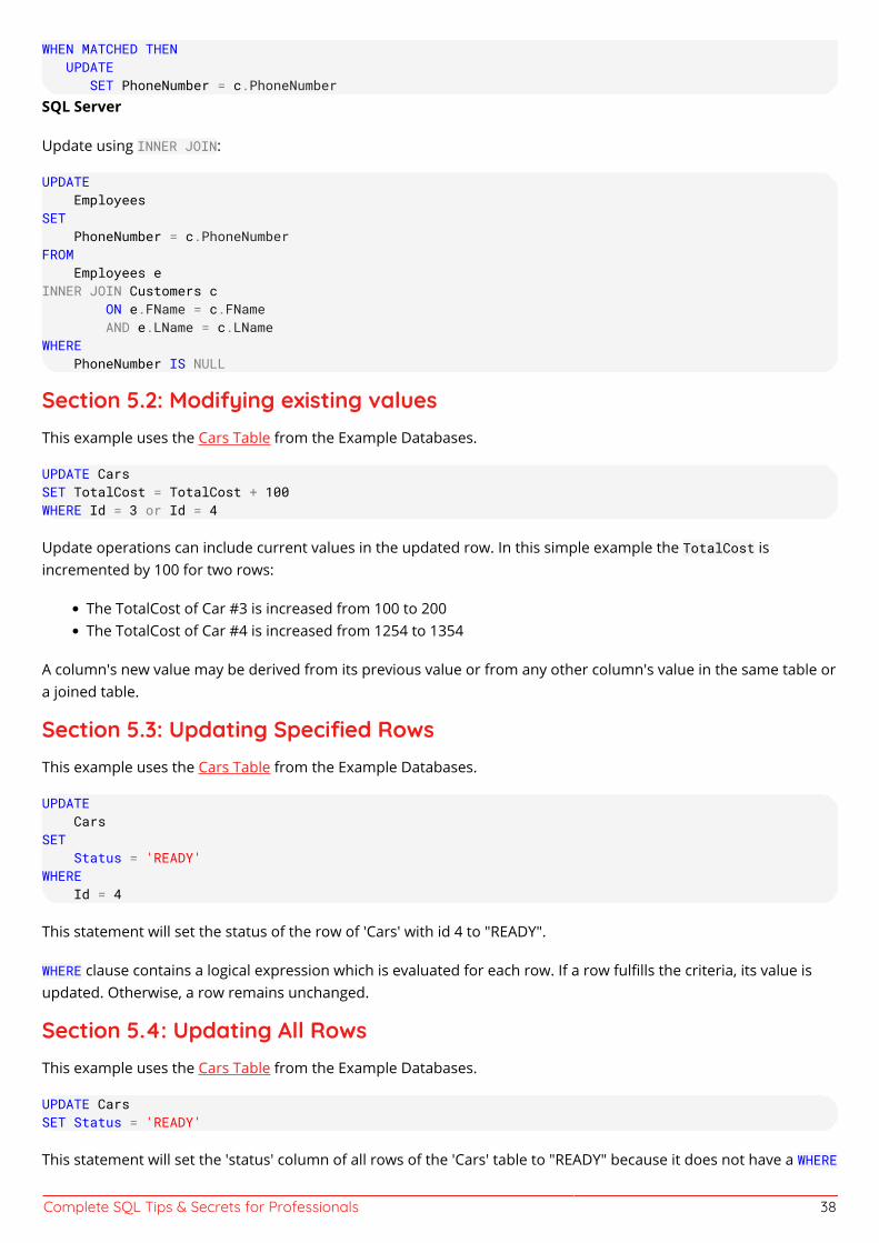
Complete SQL Tips & Secrets for Professionals 38

WHEN MATCHED THEN UPDATE SET PhoneNumber = c.PhoneNumberSQL Server

Update using INNER JOIN:

UPDATE EmployeesSET PhoneNumber = c.PhoneNumberFROM Employees eINNER JOIN Customers c ON e.FName = c.FName AND e.LName = c.LNameWHERE PhoneNumber IS NULL

Section 5.2: Modifying existing valuesThis example uses the Cars Table from the Example Databases.

UPDATE CarsSET TotalCost = TotalCost + 100WHERE Id = 3 or Id = 4

Update operations can include current values in the updated row. In this simple example the TotalCost isincremented by 100 for two rows:

The TotalCost of Car #3 is increased from 100 to 200The TotalCost of Car #4 is increased from 1254 to 1354

A column's new value may be derived from its previous value or from any other column's value in the same table ora joined table.

Section 5.3: Updating Specified RowsThis example uses the Cars Table from the Example Databases.

UPDATE CarsSET Status = 'READY'WHERE Id = 4

This statement will set the status of the row of 'Cars' with id 4 to "READY".

WHERE clause contains a logical expression which is evaluated for each row. If a row fulfills the criteria, its value isupdated. Otherwise, a row remains unchanged.

Section 5.4: Updating All RowsThis example uses the Cars Table from the Example Databases.

UPDATE CarsSET Status = 'READY'

This statement will set the 'status' column of all rows of the 'Cars' table to "READY" because it does not have a WHERE

Complete SQL Tips & Secrets for Professionals 39

clause to filter the set of rows.

Section 5.5: Capturing Updated recordsSometimes one wants to capture the records that have just been updated.

CREATE TABLE #TempUpdated(ID INT)

Update TableName SET Col1 = 42 OUTPUT inserted.ID INTO #TempUpdated WHERE Id > 50

Chapter 6: IndexesIndexes are a data structure that contains pointers to the contents of a table arranged in a specific order, to helpthe database optimize queries. They are similar to the index of book, where the pages (rows of the table) areindexed by their page number.

Several types of indexes exist, and can be created on a table. When an index exists on the columns used in aquery's WHERE clause, JOIN clause, or ORDER BY clause, it can substantially improve query performance.

Section 6.1: Sorted IndexIf you use an index that is sorted the way you would retrieve it, the SELECT statement would not do additionalsorting when in retrieval.

CREATE INDEX ix_scoreboard_score ON scoreboard (score DESC);

When you execute the query

SELECT * FROM scoreboard ORDER BY score DESC;

The database system would not do additional sorting, since it can do an index-lookup in that order.

Section 6.2: Partial or Filtered IndexSQL Server and SQLite allow to create indexes that contain not only a subset of columns, but also a subset of rows.

Consider a constant growing amount of orders with order_state_id equal to finished (2), and a stable amount oforders with order_state_id equal to started (1).

If your business make use of queries like this:

SELECT id, comment FROM orders WHERE order_state_id = 1 AND product_id = @some_value;

Partial indexing allows you to limit the index, including only the unfinished orders:

CREATE INDEX Started_Orders ON orders(product_id) WHERE order_state_id = 1;

This index will be smaller than an unfiltered index, which saves space and reduces the cost of updating the index.

Section 6.3: Creating an IndexCREATE INDEX ix_cars_employee_id ON Cars (EmployeeId);

Complete SQL Tips & Secrets for Professionals 40

This will create an index for the column EmployeeId in the table Cars. This index will improve the speed of queriesasking the server to sort or select by values in EmployeeId, such as the following:

SELECT * FROM Cars WHERE EmployeeId = 1

The index can contain more than 1 column, as in the following;

CREATE INDEX ix_cars_e_c_o_ids ON Cars (EmployeeId, CarId, OwnerId);

In this case, the index would be useful for queries asking to sort or select by all included columns, if the set ofconditions is ordered in the same way. That means that when retrieving the data, it can find the rows to retrieveusing the index, instead of looking through the full table.

For example, the following case would utilize the second index;

SELECT * FROM Cars WHERE EmployeeId = 1 Order by CarId DESC

If the order differs, however, the index does not have the same advantages, as in the following;

SELECT * FROM Cars WHERE OwnerId = 17 Order by CarId DESC

The index is not as helpful because the database must retrieve the entire index, across all values of EmployeeId andCarID, in order to find which items have OwnerId = 17.

(The index may still be used; it may be the case that the query optimizer finds that retrieving the index and filteringon the OwnerId, then retrieving only the needed rows is faster than retrieving the full table, especially if the table islarge.)

Section 6.4: Dropping an Index, or Disabling and Rebuilding itDROP INDEX ix_cars_employee_id ON Cars;

We can use command DROP to delete our index. In this example we will DROP the index called ix_cars_employee_id onthe table Cars.

This deletes the index entirely, and if the index is clustered, will remove any clustering. It cannot be rebuilt withoutrecreating the index, which can be slow and computationally expensive. As an alternative, the index can bedisabled:

ALTER INDEX ix_cars_employee_id ON Cars DISABLE;

This allows the table to retain the structure, along with the metadata about the index.

Critically, this retains the index statistics, so that it is possible to easily evaluate the change. If warranted, the indexcan then later be rebuilt, instead of being recreated completely;

ALTER INDEX ix_cars_employee_id ON Cars REBUILD;

Section 6.5: Clustered, Unique, and Sorted IndexesIndexes can have several characteristics that can be set either at creation, or by altering existing indexes.

CREATE CLUSTERED INDEX ix_clust_employee_id ON Employees(EmployeeId, Email);

The above SQL statement creates a new clustered index on Employees. Clustered indexes are indexes that dictatethe actual structure of the table; the table itself is sorted to match the structure of the index. That means there canbe at most one clustered index on a table. If a clustered index already exists on the table, the above statement willfail. (Tables with no clustered indexes are also called heaps.)

Complete SQL Tips & Secrets for Professionals 41

CREATE UNIQUE INDEX uq_customers_email ON Customers(Email);

This will create an unique index for the column Email in the table Customers. This index, along with speeding upqueries like a normal index, will also force every email address in that column to be unique. If a row is inserted orupdated with a non-unique Email value, the insertion or update will, by default, fail.

CREATE UNIQUE INDEX ix_eid_desc ON Customers(EmployeeID);

This creates an index on Customers which also creates a table constraint that the EmployeeID must be unique.(This will fail if the column is not currently unique - in this case, if there are employees who share an ID.)

CREATE INDEX ix_eid_desc ON Customers(EmployeeID Desc);

This creates an index that is sorted in descending order. By default, indexes (in MSSQL server, at least) areascending, but that can be changed.

Section 6.6: Rebuild indexOver the course of time B-Tree indexes may become fragmented because of updating/deleting/inserting data. InSQLServer terminology we can have internal (index page which is half empty ) and external (logical page orderdoesn't correspond physical order). Rebuilding index is very similar to dropping and re-creating it.

We can re-build an index with

ALTER INDEX index_name REBUILD;

By default rebuilding index is offline operation which locks the table and prevents DML against it , but many RDBMSallow online rebuilding. Also, some DB vendors offer alternatives to index rebuilding such as REORGANIZE(SQLServer) or COALESCE/SHRINK SPACE(Oracle).

Section 6.7: Inserting with a Unique IndexUPDATE Customers SET Email = "richard0123@example.com" WHERE id = 1;

This will fail if an unique index is set on the Email column of Customers. However, alternate behavior can be definedfor this case:

UPDATE Customers SET Email = "richard0123@example.com" WHERE id = 1 ON DUPLICATE KEY;

Chapter 7: CREATE TABLECREATE TABLE tableName( [ColumnName1] [datatype1] [, [ColumnName2] [datatype2] ...] )

Parameter DetailstableName The name of the table

columns Contains an 'enumeration' of all the columns that the table have. See Create a New Table for moredetails.

The CREATE TABLE statement is used create a new table in the database. A table definition consists of a list ofcolumns, their types, and any integrity constraints.

Section 7.1: Create Table From SelectYou may want to create a duplicate of a table:

CREATE TABLE ClonedEmployees AS SELECT * FROM Employees;

You can use any of the other features of a SELECT statement to modify the data before passing it to the new table.The columns of the new table are automatically created according to the selected rows.

Complete SQL Tips & Secrets for Professionals 42

CREATE TABLE ModifiedEmployees ASSELECT Id, CONCAT(FName," ",LName) AS FullName FROM EmployeesWHERE Id > 10;

Section 7.2: Create a New TableA basic Employees table, containing an ID, and the employee's first and last name along with their phone numbercan be created using

CREATE TABLE Employees( Id int identity(1,1) primary key not null, FName varchar(20) not null, LName varchar(20) not null, PhoneNumber varchar(10) not null);

This example is specific to Transact-SQL

CREATE TABLE creates a new table in the database, followed by the table name, Employees

This is then followed by the list of column names and their properties, such as the ID

Id int identity(1,1) not nullValue Meaning

Id the column's name.int is the data type.

identity(1,1) states that column will have auto generated values starting at 1 and incrementing by 1 for each newrow.

primary key states that all values in this column will have unique valuesnot null states that this column cannot have null values

Section 7.3: CREATE TABLE With FOREIGN KEYBelow you could find the table Employees with a reference to the table Cities.

CREATE TABLE Cities( CityID INT IDENTITY(1,1) NOT NULL, Name VARCHAR(20) NOT NULL, Zip VARCHAR(10) NOT NULL);

CREATE TABLE Employees( EmployeeID INT IDENTITY (1,1) NOT NULL, FirstName VARCHAR(20) NOT NULL, LastName VARCHAR(20) NOT NULL, PhoneNumber VARCHAR(10) NOT NULL, CityID INT FOREIGN KEY REFERENCES Cities(CityID));

Here could you find a database diagram.

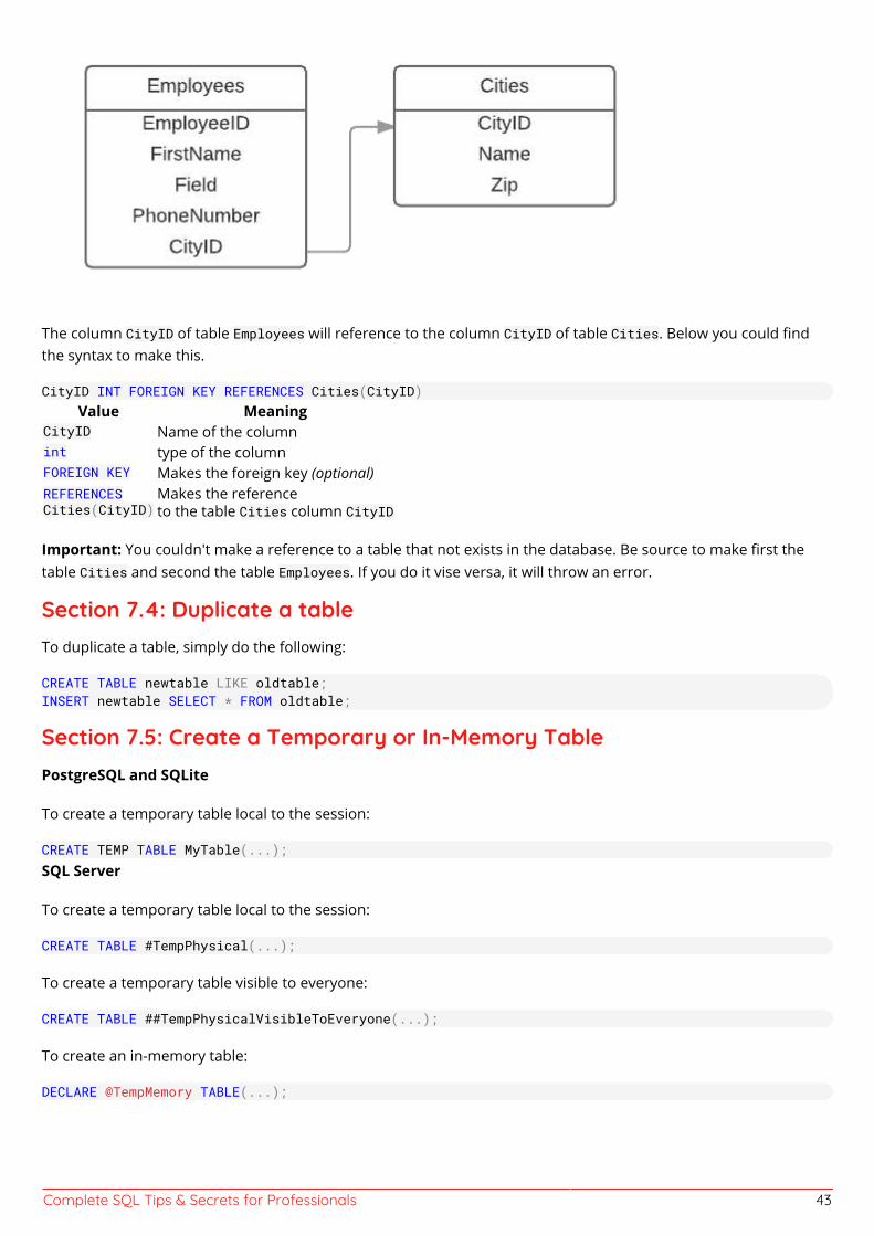
Complete SQL Tips & Secrets for Professionals 43

The column CityID of table Employees will reference to the column CityID of table Cities. Below you could findthe syntax to make this.

CityID INT FOREIGN KEY REFERENCES Cities(CityID)Value Meaning

CityID Name of the columnint type of the columnFOREIGN KEY Makes the foreign key (optional)REFERENCESCities(CityID)

Makes the referenceto the table Cities column CityID

Important: You couldn't make a reference to a table that not exists in the database. Be source to make first thetable Cities and second the table Employees. If you do it vise versa, it will throw an error.

Section 7.4: Duplicate a tableTo duplicate a table, simply do the following:

CREATE TABLE newtable LIKE oldtable;INSERT newtable SELECT * FROM oldtable;

Section 7.5: Create a Temporary or In-Memory TablePostgreSQL and SQLite

To create a temporary table local to the session:

CREATE TEMP TABLE MyTable(...);SQL Server

To create a temporary table local to the session:

CREATE TABLE #TempPhysical(...);

To create a temporary table visible to everyone:

CREATE TABLE ##TempPhysicalVisibleToEveryone(...);

To create an in-memory table:

DECLARE @TempMemory TABLE(...);

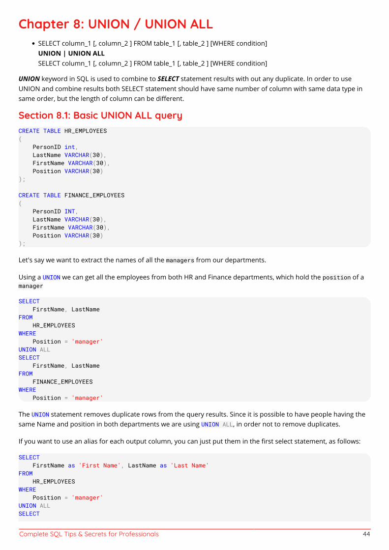
Complete SQL Tips & Secrets for Professionals 44

Chapter 8: UNION / UNION ALLSELECT column_1 [, column_2 ] FROM table_1 [, table_2 ] [WHERE condition]UNION | UNION ALLSELECT column_1 [, column_2 ] FROM table_1 [, table_2 ] [WHERE condition]

UNION keyword in SQL is used to combine to SELECT statement results with out any duplicate. In order to useUNION and combine results both SELECT statement should have same number of column with same data type insame order, but the length of column can be different.

Section 8.1: Basic UNION ALL queryCREATE TABLE HR_EMPLOYEES( PersonID int, LastName VARCHAR(30), FirstName VARCHAR(30), Position VARCHAR(30));

CREATE TABLE FINANCE_EMPLOYEES( PersonID INT, LastName VARCHAR(30), FirstName VARCHAR(30), Position VARCHAR(30));

Let's say we want to extract the names of all the managers from our departments.

Using a UNION we can get all the employees from both HR and Finance departments, which hold the position of amanager

SELECT FirstName, LastName FROM HR_EMPLOYEES WHERE Position = 'manager' UNION ALL SELECT FirstName, LastName FROM FINANCE_EMPLOYEES WHERE Position = 'manager'

The UNION statement removes duplicate rows from the query results. Since it is possible to have people having thesame Name and position in both departments we are using UNION ALL, in order not to remove duplicates.

If you want to use an alias for each output column, you can just put them in the first select statement, as follows:

SELECT FirstName as 'First Name', LastName as 'Last Name'FROM HR_EMPLOYEES WHERE Position = 'manager' UNION ALL SELECT

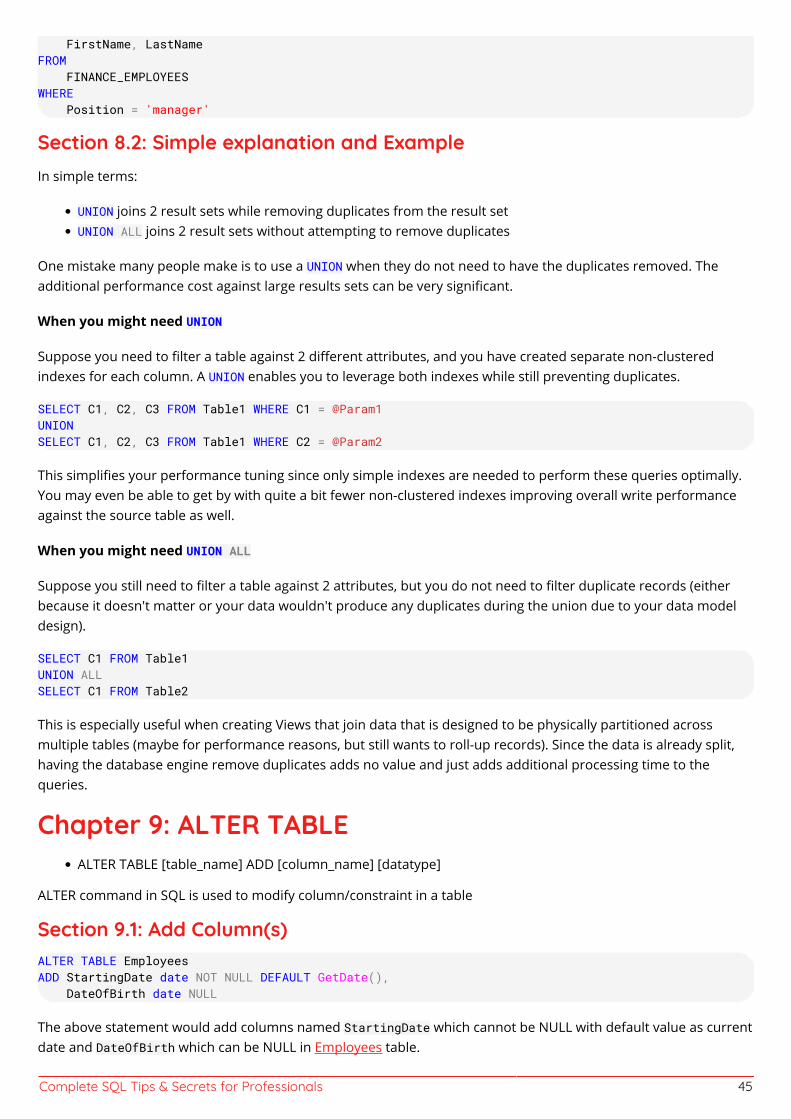
Complete SQL Tips & Secrets for Professionals 45

FirstName, LastName FROM FINANCE_EMPLOYEES WHERE Position = 'manager'

Section 8.2: Simple explanation and ExampleIn simple terms:

UNION joins 2 result sets while removing duplicates from the result setUNION ALL joins 2 result sets without attempting to remove duplicates

One mistake many people make is to use a UNION when they do not need to have the duplicates removed. Theadditional performance cost against large results sets can be very significant.

When you might need UNION

Suppose you need to filter a table against 2 different attributes, and you have created separate non-clusteredindexes for each column. A UNION enables you to leverage both indexes while still preventing duplicates.

SELECT C1, C2, C3 FROM Table1 WHERE C1 = @Param1UNIONSELECT C1, C2, C3 FROM Table1 WHERE C2 = @Param2

This simplifies your performance tuning since only simple indexes are needed to perform these queries optimally.You may even be able to get by with quite a bit fewer non-clustered indexes improving overall write performanceagainst the source table as well.

When you might need UNION ALL

Suppose you still need to filter a table against 2 attributes, but you do not need to filter duplicate records (eitherbecause it doesn't matter or your data wouldn't produce any duplicates during the union due to your data modeldesign).

SELECT C1 FROM Table1UNION ALLSELECT C1 FROM Table2

This is especially useful when creating Views that join data that is designed to be physically partitioned acrossmultiple tables (maybe for performance reasons, but still wants to roll-up records). Since the data is already split,having the database engine remove duplicates adds no value and just adds additional processing time to thequeries.

Chapter 9: ALTER TABLEALTER TABLE [table_name] ADD [column_name] [datatype]

ALTER command in SQL is used to modify column/constraint in a table

Section 9.1: Add Column(s)ALTER TABLE EmployeesADD StartingDate date NOT NULL DEFAULT GetDate(), DateOfBirth date NULL

The above statement would add columns named StartingDate which cannot be NULL with default value as currentdate and DateOfBirth which can be NULL in Employees table.

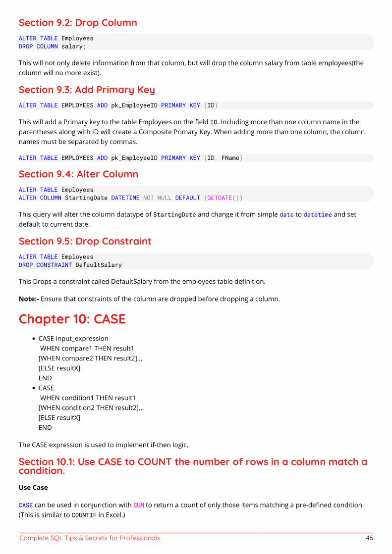
Complete SQL Tips & Secrets for Professionals 46

Section 9.2: Drop ColumnALTER TABLE EmployeesDROP COLUMN salary;

This will not only delete information from that column, but will drop the column salary from table employees(thecolumn will no more exist).

Section 9.3: Add Primary KeyALTER TABLE EMPLOYEES ADD pk_EmployeeID PRIMARY KEY (ID)

This will add a Primary key to the table Employees on the field ID. Including more than one column name in theparentheses along with ID will create a Composite Primary Key. When adding more than one column, the columnnames must be separated by commas.

ALTER TABLE EMPLOYEES ADD pk_EmployeeID PRIMARY KEY (ID, FName)

Section 9.4: Alter ColumnALTER TABLE EmployeesALTER COLUMN StartingDate DATETIME NOT NULL DEFAULT (GETDATE())

This query will alter the column datatype of StartingDate and change it from simple date to datetime and setdefault to current date.

Section 9.5: Drop ConstraintALTER TABLE EmployeesDROP CONSTRAINT DefaultSalary

This Drops a constraint called DefaultSalary from the employees table definition.

Note:- Ensure that constraints of the column are dropped before dropping a column.

Chapter 10: CASECASE input_expression WHEN compare1 THEN result1[WHEN compare2 THEN result2]...[ELSE resultX]ENDCASE WHEN condition1 THEN result1[WHEN condition2 THEN result2]...[ELSE resultX]END

The CASE expression is used to implement if-then logic.

Section 10.1: Use CASE to COUNT the number of rows in a column match acondition.Use Case

CASE can be used in conjunction with SUM to return a count of only those items matching a pre-defined condition.(This is similar to COUNTIF in Excel.)

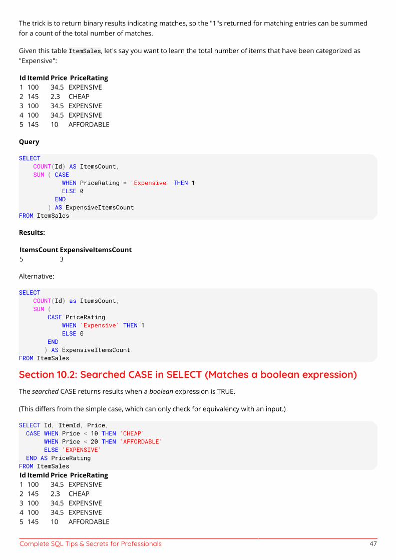
Complete SQL Tips & Secrets for Professionals 47

The trick is to return binary results indicating matches, so the "1"s returned for matching entries can be summedfor a count of the total number of matches.

Given this table ItemSales, let's say you want to learn the total number of items that have been categorized as"Expensive":

Id ItemId Price PriceRating1 100 34.5 EXPENSIVE2 145 2.3 CHEAP3 100 34.5 EXPENSIVE4 100 34.5 EXPENSIVE5 145 10 AFFORDABLE

Query

SELECT COUNT(Id) AS ItemsCount, SUM ( CASE WHEN PriceRating = 'Expensive' THEN 1 ELSE 0 END ) AS ExpensiveItemsCountFROM ItemSales

Results:

ItemsCount ExpensiveItemsCount5 3

Alternative:

SELECT COUNT(Id) as ItemsCount, SUM ( CASE PriceRating WHEN 'Expensive' THEN 1 ELSE 0 END ) AS ExpensiveItemsCountFROM ItemSales

Section 10.2: Searched CASE in SELECT (Matches a boolean expression)The searched CASE returns results when a boolean expression is TRUE.

(This differs from the simple case, which can only check for equivalency with an input.)

SELECT Id, ItemId, Price, CASE WHEN Price < 10 THEN 'CHEAP' WHEN Price < 20 THEN 'AFFORDABLE' ELSE 'EXPENSIVE' END AS PriceRatingFROM ItemSalesId ItemId Price PriceRating1 100 34.5 EXPENSIVE2 145 2.3 CHEAP3 100 34.5 EXPENSIVE4 100 34.5 EXPENSIVE5 145 10 AFFORDABLE

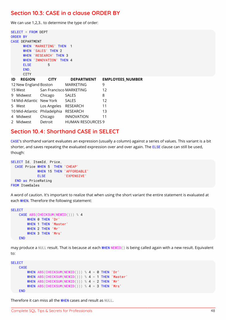
Complete SQL Tips & Secrets for Professionals 48

Section 10.3: CASE in a clause ORDER BYWe can use 1,2,3.. to determine the type of order:

SELECT * FROM DEPTORDER BYCASE DEPARTMENT WHEN 'MARKETING' THEN 1 WHEN 'SALES' THEN 2 WHEN 'RESEARCH' THEN 3 WHEN 'INNOVATION' THEN 4 ELSE 5 END, CITYID REGION CITY DEPARTMENT EMPLOYEES_NUMBER12 New England Boston MARKETING 915 West San Francisco MARKETING 129 Midwest Chicago SALES 814 Mid-Atlantic New York SALES 125 West Los Angeles RESEARCH 1110 Mid-Atlantic Philadelphia RESEARCH 134 Midwest Chicago INNOVATION 112 Midwest Detroit HUMAN RESOURCES 9

Section 10.4: Shorthand CASE in SELECTCASE's shorthand variant evaluates an expression (usually a column) against a series of values. This variant is a bitshorter, and saves repeating the evaluated expression over and over again. The ELSE clause can still be used,though:

SELECT Id, ItemId, Price, CASE Price WHEN 5 THEN 'CHEAP' WHEN 15 THEN 'AFFORDABLE' ELSE 'EXPENSIVE' END as PriceRatingFROM ItemSales

A word of caution. It's important to realize that when using the short variant the entire statement is evaluated ateach WHEN. Therefore the following statement:

SELECT CASE ABS(CHECKSUM(NEWID())) % 4 WHEN 0 THEN 'Dr' WHEN 1 THEN 'Master' WHEN 2 THEN 'Mr' WHEN 3 THEN 'Mrs' END

may produce a NULL result. That is because at each WHEN NEWID() is being called again with a new result. Equivalentto:

SELECT CASE WHEN ABS(CHECKSUM(NEWID())) % 4 = 0 THEN 'Dr' WHEN ABS(CHECKSUM(NEWID())) % 4 = 1 THEN 'Master' WHEN ABS(CHECKSUM(NEWID())) % 4 = 2 THEN 'Mr' WHEN ABS(CHECKSUM(NEWID())) % 4 = 3 THEN 'Mrs' END

Therefore it can miss all the WHEN cases and result as NULL.

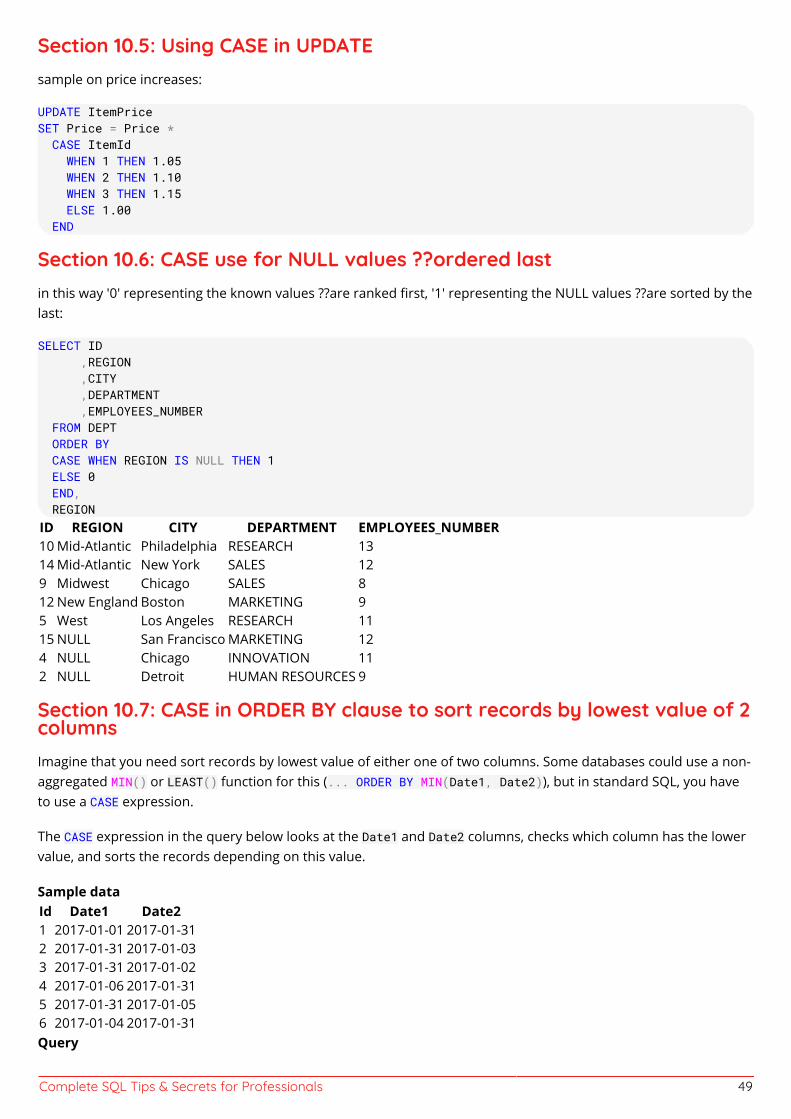
Complete SQL Tips & Secrets for Professionals 49

Section 10.5: Using CASE in UPDATEsample on price increases:

UPDATE ItemPriceSET Price = Price * CASE ItemId WHEN 1 THEN 1.05 WHEN 2 THEN 1.10 WHEN 3 THEN 1.15 ELSE 1.00 END

Section 10.6: CASE use for NULL values ??ordered lastin this way '0' representing the known values ??are ranked first, '1' representing the NULL values ??are sorted by thelast:

SELECT ID ,REGION ,CITY ,DEPARTMENT ,EMPLOYEES_NUMBER FROM DEPT ORDER BY CASE WHEN REGION IS NULL THEN 1 ELSE 0 END, REGIONID REGION CITY DEPARTMENT EMPLOYEES_NUMBER10 Mid-Atlantic Philadelphia RESEARCH 1314 Mid-Atlantic New York SALES 129 Midwest Chicago SALES 812 New England Boston MARKETING 95 West Los Angeles RESEARCH 1115 NULL San Francisco MARKETING 124 NULL Chicago INNOVATION 112 NULL Detroit HUMAN RESOURCES 9

Section 10.7: CASE in ORDER BY clause to sort records by lowest value of 2columnsImagine that you need sort records by lowest value of either one of two columns. Some databases could use a non-aggregated MIN() or LEAST() function for this (... ORDER BY MIN(Date1, Date2)), but in standard SQL, you haveto use a CASE expression.

The CASE expression in the query below looks at the Date1 and Date2 columns, checks which column has the lowervalue, and sorts the records depending on this value.

Sample dataId Date1 Date21 2017-01-01 2017-01-312 2017-01-31 2017-01-033 2017-01-31 2017-01-024 2017-01-06 2017-01-315 2017-01-31 2017-01-056 2017-01-04 2017-01-31Query

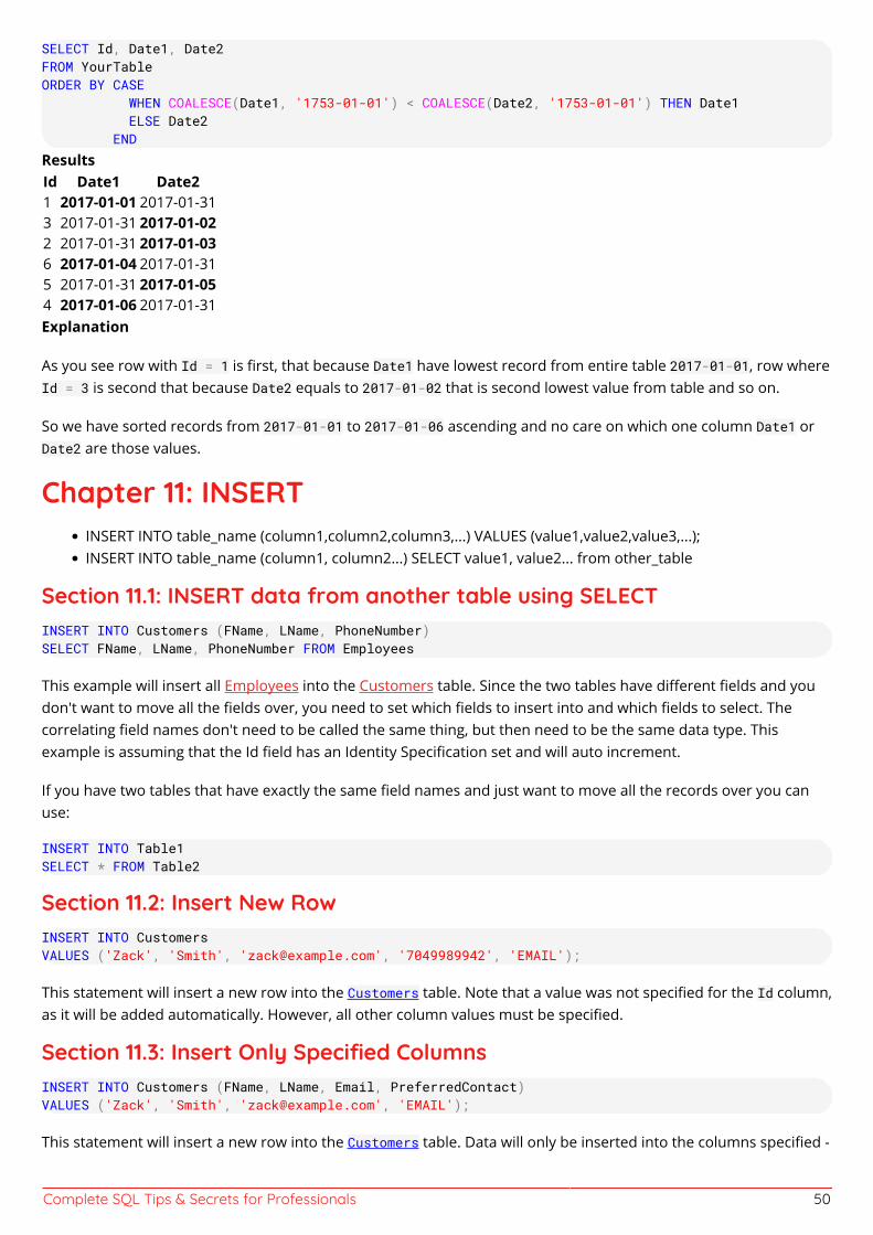
Complete SQL Tips & Secrets for Professionals 50

SELECT Id, Date1, Date2FROM YourTableORDER BY CASE WHEN COALESCE(Date1, '1753-01-01') < COALESCE(Date2, '1753-01-01') THEN Date1 ELSE Date2 ENDResultsId Date1 Date21 2017-01-01 2017-01-313 2017-01-31 2017-01-022 2017-01-31 2017-01-036 2017-01-04 2017-01-315 2017-01-31 2017-01-054 2017-01-06 2017-01-31Explanation

As you see row with Id = 1 is first, that because Date1 have lowest record from entire table 2017-01-01, row whereId = 3 is second that because Date2 equals to 2017-01-02 that is second lowest value from table and so on.

So we have sorted records from 2017-01-01 to 2017-01-06 ascending and no care on which one column Date1 orDate2 are those values.

Chapter 11: INSERTINSERT INTO table_name (column1,column2,column3,...) VALUES (value1,value2,value3,...);INSERT INTO table_name (column1, column2...) SELECT value1, value2... from other_table

Section 11.1: INSERT data from another table using SELECTINSERT INTO Customers (FName, LName, PhoneNumber)SELECT FName, LName, PhoneNumber FROM Employees

This example will insert all Employees into the Customers table. Since the two tables have different fields and youdon't want to move all the fields over, you need to set which fields to insert into and which fields to select. Thecorrelating field names don't need to be called the same thing, but then need to be the same data type. Thisexample is assuming that the Id field has an Identity Specification set and will auto increment.

If you have two tables that have exactly the same field names and just want to move all the records over you canuse:

INSERT INTO Table1SELECT * FROM Table2

Section 11.2: Insert New RowINSERT INTO CustomersVALUES ('Zack', 'Smith', 'zack@example.com', '7049989942', 'EMAIL');

This statement will insert a new row into the Customers table. Note that a value was not specified for the Id column,as it will be added automatically. However, all other column values must be specified.

Section 11.3: Insert Only Specified ColumnsINSERT INTO Customers (FName, LName, Email, PreferredContact)VALUES ('Zack', 'Smith', 'zack@example.com', 'EMAIL');

This statement will insert a new row into the Customers table. Data will only be inserted into the columns specified -

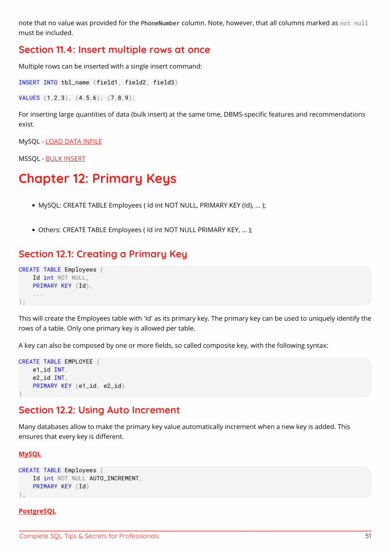
Complete SQL Tips & Secrets for Professionals 51

note that no value was provided for the PhoneNumber column. Note, however, that all columns marked as not nullmust be included.

Section 11.4: Insert multiple rows at onceMultiple rows can be inserted with a single insert command:

INSERT INTO tbl_name (field1, field2, field3)

VALUES (1,2,3), (4,5,6), (7,8,9);

For inserting large quantities of data (bulk insert) at the same time, DBMS-specific features and recommendationsexist.

MySQL - LOAD DATA INFILE

MSSQL - BULK INSERT

Chapter 12: Primary Keys

MySQL: CREATE TABLE Employees ( Id int NOT NULL, PRIMARY KEY (Id), ... );

Others: CREATE TABLE Employees ( Id int NOT NULL PRIMARY KEY, ... );

Section 12.1: Creating a Primary KeyCREATE TABLE Employees ( Id int NOT NULL, PRIMARY KEY (Id), ...);

This will create the Employees table with 'Id' as its primary key. The primary key can be used to uniquely identify therows of a table. Only one primary key is allowed per table.

A key can also be composed by one or more fields, so called composite key, with the following syntax:

CREATE TABLE EMPLOYEE ( e1_id INT, e2_id INT, PRIMARY KEY (e1_id, e2_id))

Section 12.2: Using Auto IncrementMany databases allow to make the primary key value automatically increment when a new key is added. Thisensures that every key is different.

MySQL

CREATE TABLE Employees ( Id int NOT NULL AUTO_INCREMENT, PRIMARY KEY (Id));

PostgreSQL

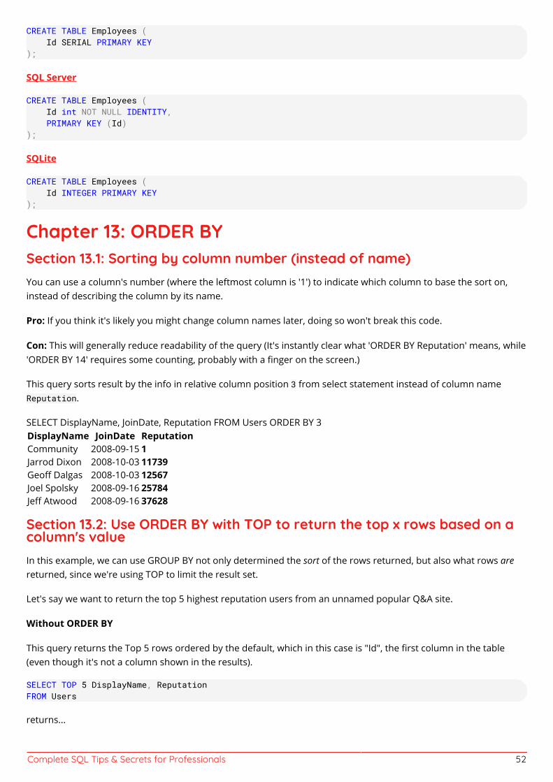
Complete SQL Tips & Secrets for Professionals 52

CREATE TABLE Employees ( Id SERIAL PRIMARY KEY);

SQL Server

CREATE TABLE Employees ( Id int NOT NULL IDENTITY, PRIMARY KEY (Id));

SQLite

CREATE TABLE Employees ( Id INTEGER PRIMARY KEY );

Chapter 13: ORDER BYSection 13.1: Sorting by column number (instead of name)You can use a column's number (where the leftmost column is '1') to indicate which column to base the sort on,instead of describing the column by its name.

Pro: If you think it's likely you might change column names later, doing so won't break this code.

Con: This will generally reduce readability of the query (It's instantly clear what 'ORDER BY Reputation' means, while'ORDER BY 14' requires some counting, probably with a finger on the screen.)

This query sorts result by the info in relative column position 3 from select statement instead of column nameReputation.

SELECT DisplayName, JoinDate, Reputation FROM Users ORDER BY 3DisplayName JoinDate ReputationCommunity 2008-09-15 1Jarrod Dixon 2008-10-03 11739Geoff Dalgas 2008-10-03 12567Joel Spolsky 2008-09-16 25784Jeff Atwood 2008-09-16 37628

Section 13.2: Use ORDER BY with TOP to return the top x rows based on acolumn's valueIn this example, we can use GROUP BY not only determined the sort of the rows returned, but also what rows arereturned, since we're using TOP to limit the result set.

Let's say we want to return the top 5 highest reputation users from an unnamed popular Q&A site.

Without ORDER BY

This query returns the Top 5 rows ordered by the default, which in this case is "Id", the first column in the table(even though it's not a column shown in the results).

SELECT TOP 5 DisplayName, ReputationFROM Users

returns...

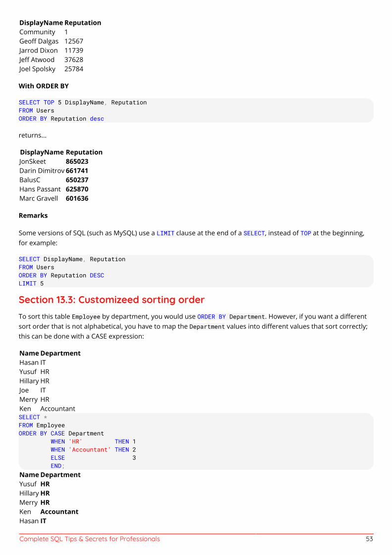
Complete SQL Tips & Secrets for Professionals 53

DisplayName ReputationCommunity 1Geoff Dalgas 12567Jarrod Dixon 11739Jeff Atwood 37628Joel Spolsky 25784

With ORDER BY

SELECT TOP 5 DisplayName, ReputationFROM UsersORDER BY Reputation desc

returns...

DisplayName ReputationJonSkeet 865023Darin Dimitrov 661741BalusC 650237Hans Passant 625870Marc Gravell 601636

Remarks

Some versions of SQL (such as MySQL) use a LIMIT clause at the end of a SELECT, instead of TOP at the beginning,for example:

SELECT DisplayName, ReputationFROM UsersORDER BY Reputation DESCLIMIT 5

Section 13.3: Customizeed sorting orderTo sort this table Employee by department, you would use ORDER BY Department. However, if you want a differentsort order that is not alphabetical, you have to map the Department values into different values that sort correctly;this can be done with a CASE expression:

Name DepartmentHasan ITYusuf HRHillary HRJoe ITMerry HRKen AccountantSELECT *FROM EmployeeORDER BY CASE Department WHEN 'HR' THEN 1 WHEN 'Accountant' THEN 2 ELSE 3 END;Name DepartmentYusuf HRHillary HRMerry HRKen AccountantHasan IT

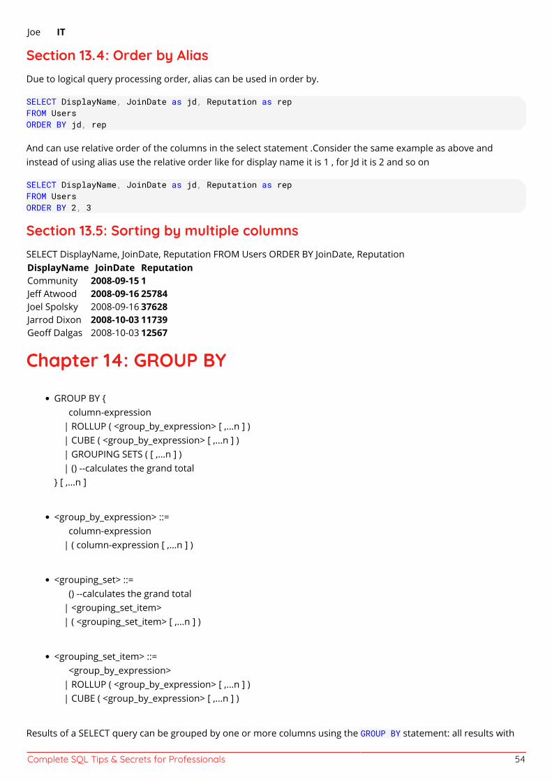
Complete SQL Tips & Secrets for Professionals 54

Joe IT

Section 13.4: Order by AliasDue to logical query processing order, alias can be used in order by.

SELECT DisplayName, JoinDate as jd, Reputation as repFROM UsersORDER BY jd, rep

And can use relative order of the columns in the select statement .Consider the same example as above andinstead of using alias use the relative order like for display name it is 1 , for Jd it is 2 and so on

SELECT DisplayName, JoinDate as jd, Reputation as repFROM UsersORDER BY 2, 3

Section 13.5: Sorting by multiple columnsSELECT DisplayName, JoinDate, Reputation FROM Users ORDER BY JoinDate, ReputationDisplayName JoinDate ReputationCommunity 2008-09-15 1Jeff Atwood 2008-09-16 25784Joel Spolsky 2008-09-16 37628Jarrod Dixon 2008-10-03 11739Geoff Dalgas 2008-10-03 12567

Chapter 14: GROUP BY

GROUP BY { column-expression | ROLLUP ( <group_by_expression> [ ,...n ] ) | CUBE ( <group_by_expression> [ ,...n ] ) | GROUPING SETS ( [ ,...n ] ) | () --calculates the grand total} [ ,...n ]

<group_by_expression> ::= column-expression | ( column-expression [ ,...n ] )

<grouping_set> ::= () --calculates the grand total | <grouping_set_item> | ( <grouping_set_item> [ ,...n ] )

<grouping_set_item> ::= <group_by_expression> | ROLLUP ( <group_by_expression> [ ,...n ] ) | CUBE ( <group_by_expression> [ ,...n ] )

Results of a SELECT query can be grouped by one or more columns using the GROUP BY statement: all results with

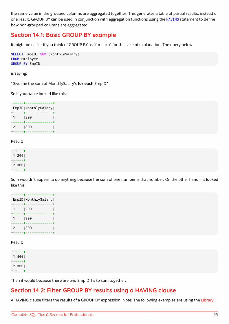
Complete SQL Tips & Secrets for Professionals 55

the same value in the grouped columns are aggregated together. This generates a table of partial results, instead ofone result. GROUP BY can be used in conjunction with aggregation functions using the HAVING statement to definehow non-grouped columns are aggregated.

Section 14.1: Basic GROUP BY exampleIt might be easier if you think of GROUP BY as "for each" for the sake of explanation. The query below:

SELECT EmpID, SUM (MonthlySalary)FROM EmployeeGROUP BY EmpID

is saying:

"Give me the sum of MonthlySalary's for each EmpID"

So if your table looked like this:

+-----+-------------+|EmpID|MonthlySalary|+-----+-------------+|1 |200 |+-----+-------------+|2 |300 |+-----+-------------+

Result:

+-+---+|1|200|+-+---+|2|300|+-+---+

Sum wouldn't appear to do anything because the sum of one number is that number. On the other hand if it lookedlike this:

+-----+-------------+|EmpID|MonthlySalary|+-----+-------------+|1 |200 |+-----+-------------+|1 |300 |+-----+-------------+|2 |300 |+-----+-------------+

Result:

+-+---+|1|500|+-+---+|2|300|+-+---+

Then it would because there are two EmpID 1's to sum together.

Section 14.2: Filter GROUP BY results using a HAVING clauseA HAVING clause filters the results of a GROUP BY expression. Note: The following examples are using the Library

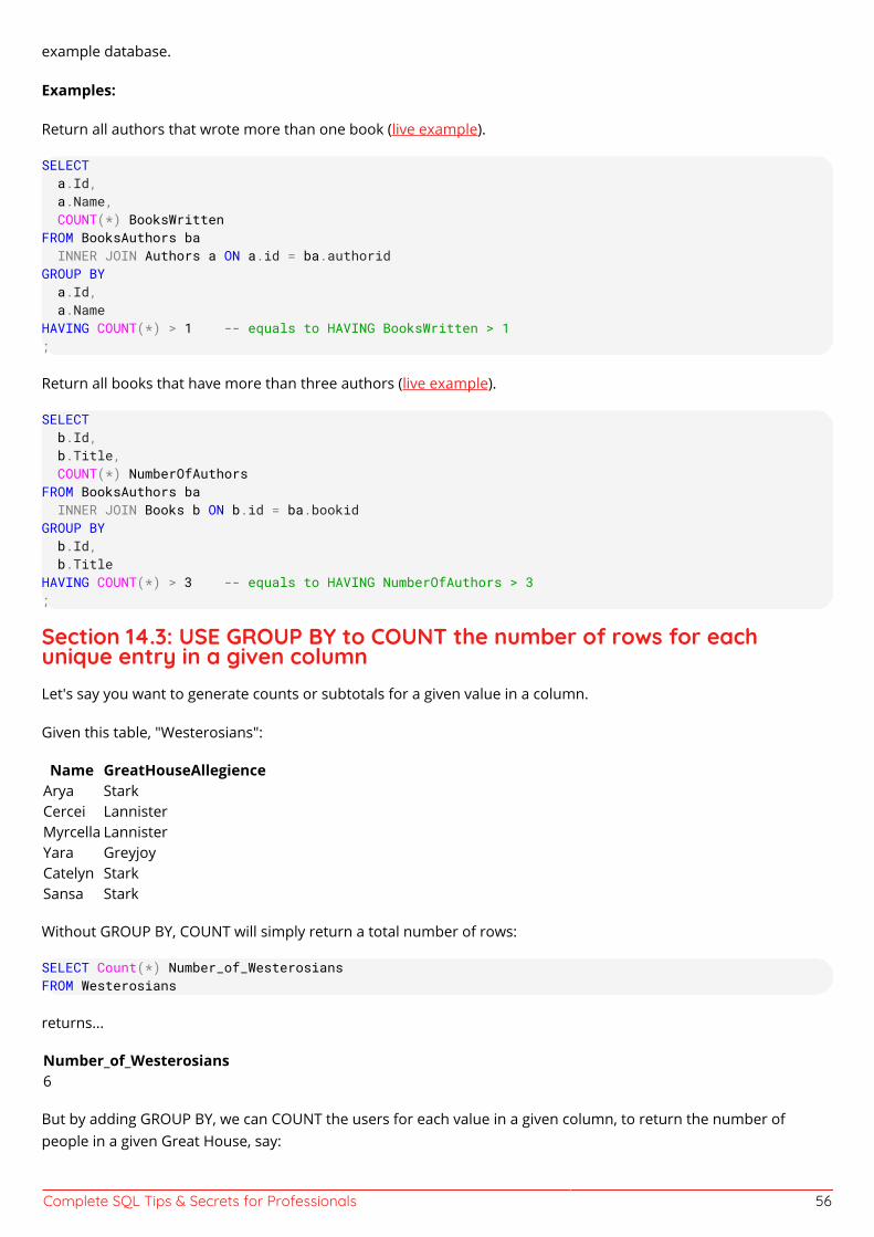
Complete SQL Tips & Secrets for Professionals 56

example database.

Examples:

Return all authors that wrote more than one book (live example).

SELECT a.Id, a.Name, COUNT(*) BooksWrittenFROM BooksAuthors ba INNER JOIN Authors a ON a.id = ba.authoridGROUP BY a.Id, a.NameHAVING COUNT(*) > 1 -- equals to HAVING BooksWritten > 1;

Return all books that have more than three authors (live example).

SELECT b.Id, b.Title, COUNT(*) NumberOfAuthorsFROM BooksAuthors ba INNER JOIN Books b ON b.id = ba.bookidGROUP BY b.Id, b.TitleHAVING COUNT(*) > 3 -- equals to HAVING NumberOfAuthors > 3;

Section 14.3: USE GROUP BY to COUNT the number of rows for eachunique entry in a given columnLet's say you want to generate counts or subtotals for a given value in a column.

Given this table, "Westerosians":

Name GreatHouseAllegienceArya StarkCercei LannisterMyrcella LannisterYara GreyjoyCatelyn StarkSansa Stark

Without GROUP BY, COUNT will simply return a total number of rows:

SELECT Count(*) Number_of_WesterosiansFROM Westerosians

returns...

Number_of_Westerosians6

But by adding GROUP BY, we can COUNT the users for each value in a given column, to return the number ofpeople in a given Great House, say:

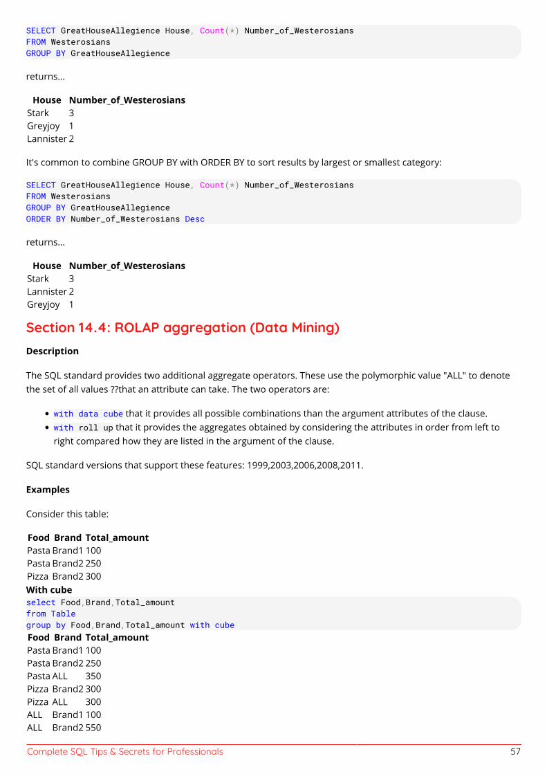
Complete SQL Tips & Secrets for Professionals 57

SELECT GreatHouseAllegience House, Count(*) Number_of_WesterosiansFROM WesterosiansGROUP BY GreatHouseAllegience

returns...

House Number_of_WesterosiansStark 3Greyjoy 1Lannister 2

It's common to combine GROUP BY with ORDER BY to sort results by largest or smallest category:

SELECT GreatHouseAllegience House, Count(*) Number_of_WesterosiansFROM WesterosiansGROUP BY GreatHouseAllegienceORDER BY Number_of_Westerosians Desc

returns...

House Number_of_WesterosiansStark 3Lannister 2Greyjoy 1

Section 14.4: ROLAP aggregation (Data Mining)Description

The SQL standard provides two additional aggregate operators. These use the polymorphic value "ALL" to denotethe set of all values ??that an attribute can take. The two operators are:

with data cube that it provides all possible combinations than the argument attributes of the clause.with roll up that it provides the aggregates obtained by considering the attributes in order from left toright compared how they are listed in the argument of the clause.

SQL standard versions that support these features: 1999,2003,2006,2008,2011.

Examples

Consider this table:

Food Brand Total_amountPasta Brand1 100Pasta Brand2 250Pizza Brand2 300With cubeselect Food,Brand,Total_amountfrom Tablegroup by Food,Brand,Total_amount with cubeFood Brand Total_amountPasta Brand1 100Pasta Brand2 250Pasta ALL 350Pizza Brand2 300Pizza ALL 300ALL Brand1 100ALL Brand2 550

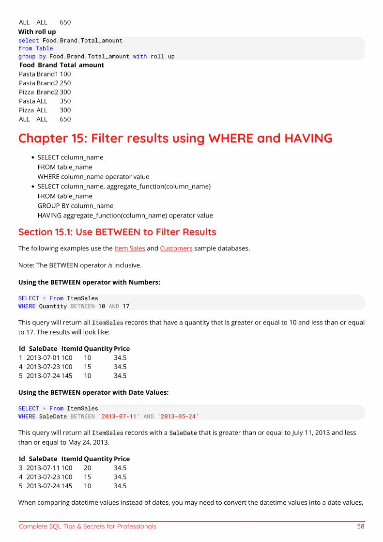
Complete SQL Tips & Secrets for Professionals 58

ALL ALL 650With roll upselect Food,Brand,Total_amountfrom Tablegroup by Food,Brand,Total_amount with roll upFood Brand Total_amountPasta Brand1 100Pasta Brand2 250Pizza Brand2 300Pasta ALL 350Pizza ALL 300ALL ALL 650

Chapter 15: Filter results using WHERE and HAVINGSELECT column_nameFROM table_nameWHERE column_name operator valueSELECT column_name, aggregate_function(column_name)FROM table_nameGROUP BY column_nameHAVING aggregate_function(column_name) operator value

Section 15.1: Use BETWEEN to Filter ResultsThe following examples use the Item Sales and Customers sample databases.

Note: The BETWEEN operator is inclusive.

Using the BETWEEN operator with Numbers:

SELECT * From ItemSalesWHERE Quantity BETWEEN 10 AND 17

This query will return all ItemSales records that have a quantity that is greater or equal to 10 and less than or equalto 17. The results will look like:

Id SaleDate ItemId Quantity Price1 2013-07-01 100 10 34.54 2013-07-23 100 15 34.55 2013-07-24 145 10 34.5

Using the BETWEEN operator with Date Values:

SELECT * From ItemSalesWHERE SaleDate BETWEEN '2013-07-11' AND '2013-05-24'

This query will return all ItemSales records with a SaleDate that is greater than or equal to July 11, 2013 and lessthan or equal to May 24, 2013.

Id SaleDate ItemId Quantity Price3 2013-07-11 100 20 34.54 2013-07-23 100 15 34.55 2013-07-24 145 10 34.5

When comparing datetime values instead of dates, you may need to convert the datetime values into a date values,

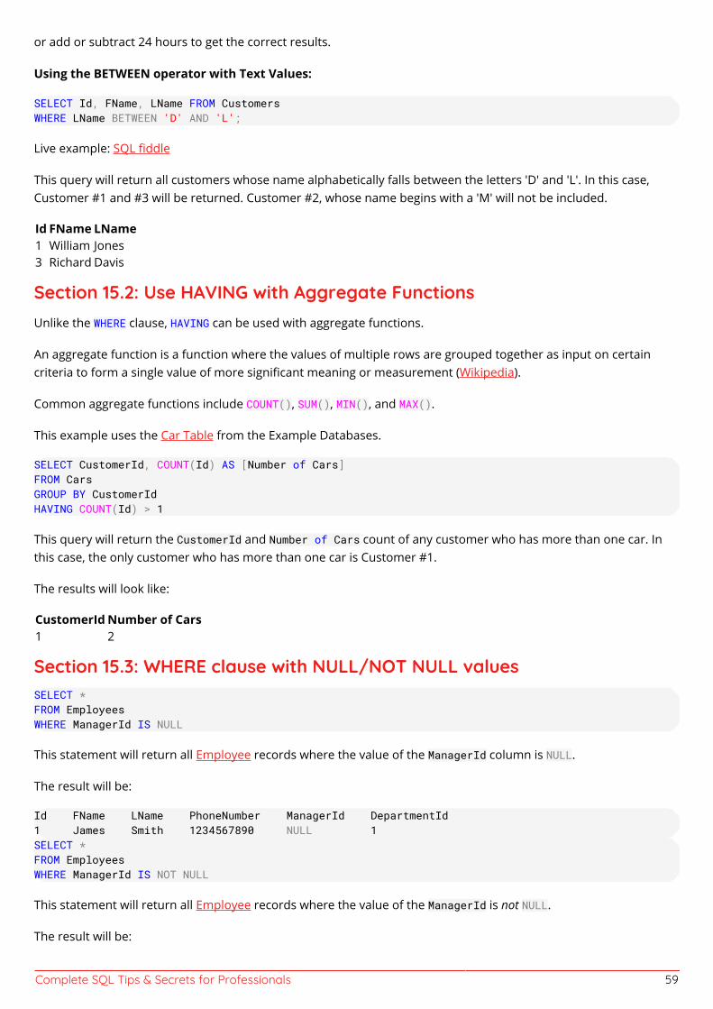
Complete SQL Tips & Secrets for Professionals 59

or add or subtract 24 hours to get the correct results.

Using the BETWEEN operator with Text Values:

SELECT Id, FName, LName FROM CustomersWHERE LName BETWEEN 'D' AND 'L';

Live example: SQL fiddle

This query will return all customers whose name alphabetically falls between the letters 'D' and 'L'. In this case,Customer #1 and #3 will be returned. Customer #2, whose name begins with a 'M' will not be included.

Id FName LName1 William Jones3 Richard Davis

Section 15.2: Use HAVING with Aggregate FunctionsUnlike the WHERE clause, HAVING can be used with aggregate functions.

An aggregate function is a function where the values of multiple rows are grouped together as input on certaincriteria to form a single value of more significant meaning or measurement (Wikipedia).

Common aggregate functions include COUNT(), SUM(), MIN(), and MAX().

This example uses the Car Table from the Example Databases.

SELECT CustomerId, COUNT(Id) AS [Number of Cars]FROM CarsGROUP BY CustomerIdHAVING COUNT(Id) > 1

This query will return the CustomerId and Number of Cars count of any customer who has more than one car. Inthis case, the only customer who has more than one car is Customer #1.

The results will look like:

CustomerId Number of Cars1 2

Section 15.3: WHERE clause with NULL/NOT NULL valuesSELECT *FROM EmployeesWHERE ManagerId IS NULL

This statement will return all Employee records where the value of the ManagerId column is NULL.

The result will be:

Id FName LName PhoneNumber ManagerId DepartmentId1 James Smith 1234567890 NULL 1SELECT *FROM EmployeesWHERE ManagerId IS NOT NULL

This statement will return all Employee records where the value of the ManagerId is not NULL.

The result will be:

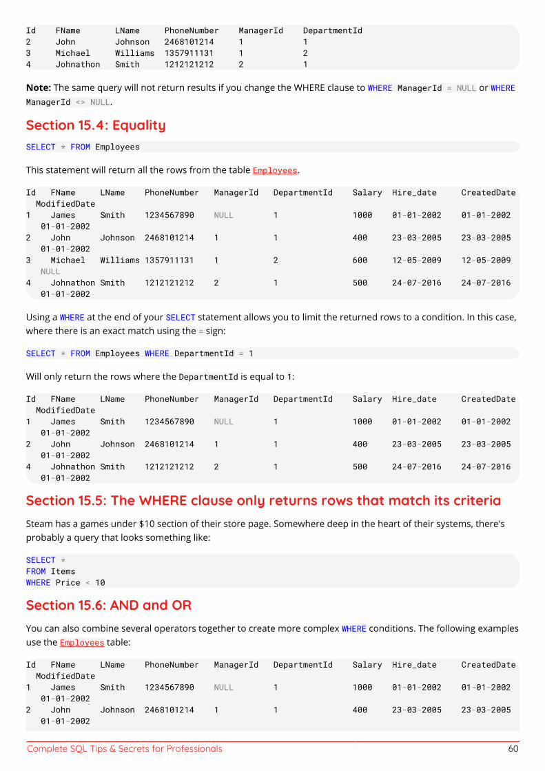
Complete SQL Tips & Secrets for Professionals 60

Id FName LName PhoneNumber ManagerId DepartmentId2 John Johnson 2468101214 1 13 Michael Williams 1357911131 1 24 Johnathon Smith 1212121212 2 1

Note: The same query will not return results if you change the WHERE clause to WHERE ManagerId = NULL or WHEREManagerId <> NULL.

Section 15.4: EqualitySELECT * FROM Employees

This statement will return all the rows from the table Employees.

Id FName LName PhoneNumber ManagerId DepartmentId Salary Hire_date CreatedDate ModifiedDate1 James Smith 1234567890 NULL 1 1000 01-01-2002 01-01-2002 01-01-20022 John Johnson 2468101214 1 1 400 23-03-2005 23-03-2005 01-01-20023 Michael Williams 1357911131 1 2 600 12-05-2009 12-05-2009 NULL4 Johnathon Smith 1212121212 2 1 500 24-07-2016 24-07-2016 01-01-2002

Using a WHERE at the end of your SELECT statement allows you to limit the returned rows to a condition. In this case,where there is an exact match using the = sign:

SELECT * FROM Employees WHERE DepartmentId = 1

Will only return the rows where the DepartmentId is equal to 1:

Id FName LName PhoneNumber ManagerId DepartmentId Salary Hire_date CreatedDate ModifiedDate1 James Smith 1234567890 NULL 1 1000 01-01-2002 01-01-2002 01-01-20022 John Johnson 2468101214 1 1 400 23-03-2005 23-03-2005 01-01-20024 Johnathon Smith 1212121212 2 1 500 24-07-2016 24-07-2016 01-01-2002

Section 15.5: The WHERE clause only returns rows that match its criteriaSteam has a games under $10 section of their store page. Somewhere deep in the heart of their systems, there'sprobably a query that looks something like:

SELECT *FROM ItemsWHERE Price < 10

Section 15.6: AND and ORYou can also combine several operators together to create more complex WHERE conditions. The following examplesuse the Employees table:

Id FName LName PhoneNumber ManagerId DepartmentId Salary Hire_date CreatedDate ModifiedDate1 James Smith 1234567890 NULL 1 1000 01-01-2002 01-01-2002 01-01-20022 John Johnson 2468101214 1 1 400 23-03-2005 23-03-2005 01-01-2002

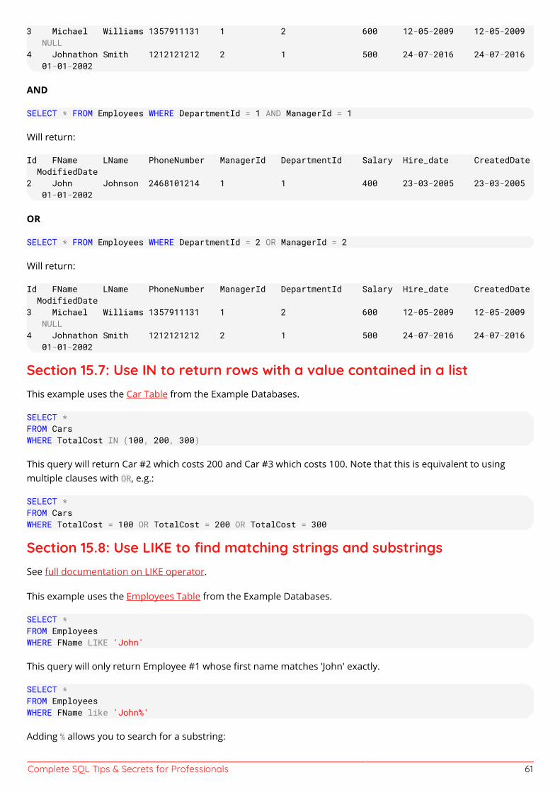
Complete SQL Tips & Secrets for Professionals 61

3 Michael Williams 1357911131 1 2 600 12-05-2009 12-05-2009 NULL4 Johnathon Smith 1212121212 2 1 500 24-07-2016 24-07-2016 01-01-2002

AND

SELECT * FROM Employees WHERE DepartmentId = 1 AND ManagerId = 1

Will return:

Id FName LName PhoneNumber ManagerId DepartmentId Salary Hire_date CreatedDate ModifiedDate2 John Johnson 2468101214 1 1 400 23-03-2005 23-03-2005 01-01-2002

OR

SELECT * FROM Employees WHERE DepartmentId = 2 OR ManagerId = 2

Will return:

Id FName LName PhoneNumber ManagerId DepartmentId Salary Hire_date CreatedDate ModifiedDate3 Michael Williams 1357911131 1 2 600 12-05-2009 12-05-2009 NULL4 Johnathon Smith 1212121212 2 1 500 24-07-2016 24-07-2016 01-01-2002

Section 15.7: Use IN to return rows with a value contained in a listThis example uses the Car Table from the Example Databases.

SELECT *FROM CarsWHERE TotalCost IN (100, 200, 300)

This query will return Car #2 which costs 200 and Car #3 which costs 100. Note that this is equivalent to usingmultiple clauses with OR, e.g.:

SELECT *FROM CarsWHERE TotalCost = 100 OR TotalCost = 200 OR TotalCost = 300

Section 15.8: Use LIKE to find matching strings and substringsSee full documentation on LIKE operator.

This example uses the Employees Table from the Example Databases.

SELECT *FROM EmployeesWHERE FName LIKE 'John'

This query will only return Employee #1 whose first name matches 'John' exactly.

SELECT *FROM EmployeesWHERE FName like 'John%'

Adding % allows you to search for a substring:

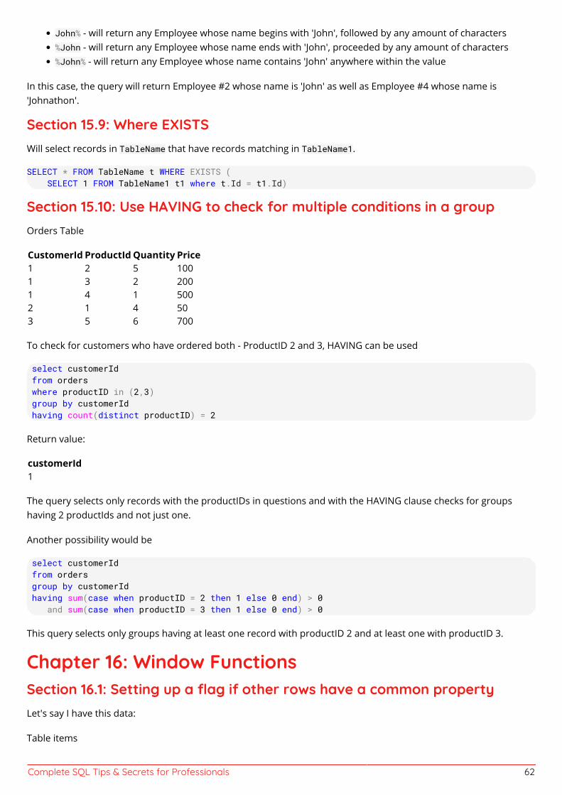
Complete SQL Tips & Secrets for Professionals 62

John% - will return any Employee whose name begins with 'John', followed by any amount of characters%John - will return any Employee whose name ends with 'John', proceeded by any amount of characters%John% - will return any Employee whose name contains 'John' anywhere within the value

In this case, the query will return Employee #2 whose name is 'John' as well as Employee #4 whose name is'Johnathon'.

Section 15.9: Where EXISTSWill select records in TableName that have records matching in TableName1.

SELECT * FROM TableName t WHERE EXISTS ( SELECT 1 FROM TableName1 t1 where t.Id = t1.Id)

Section 15.10: Use HAVING to check for multiple conditions in a groupOrders Table

CustomerId ProductId Quantity Price1 2 5 1001 3 2 2001 4 1 5002 1 4 503 5 6 700

To check for customers who have ordered both - ProductID 2 and 3, HAVING can be used

select customerId from orders where productID in (2,3) group by customerId having count(distinct productID) = 2

Return value:

customerId1

The query selects only records with the productIDs in questions and with the HAVING clause checks for groupshaving 2 productIds and not just one.

Another possibility would be

select customerId from orders group by customerId having sum(case when productID = 2 then 1 else 0 end) > 0 and sum(case when productID = 3 then 1 else 0 end) > 0

This query selects only groups having at least one record with productID 2 and at least one with productID 3.

Chapter 16: Window FunctionsSection 16.1: Setting up a flag if other rows have a common propertyLet's say I have this data:

Table items

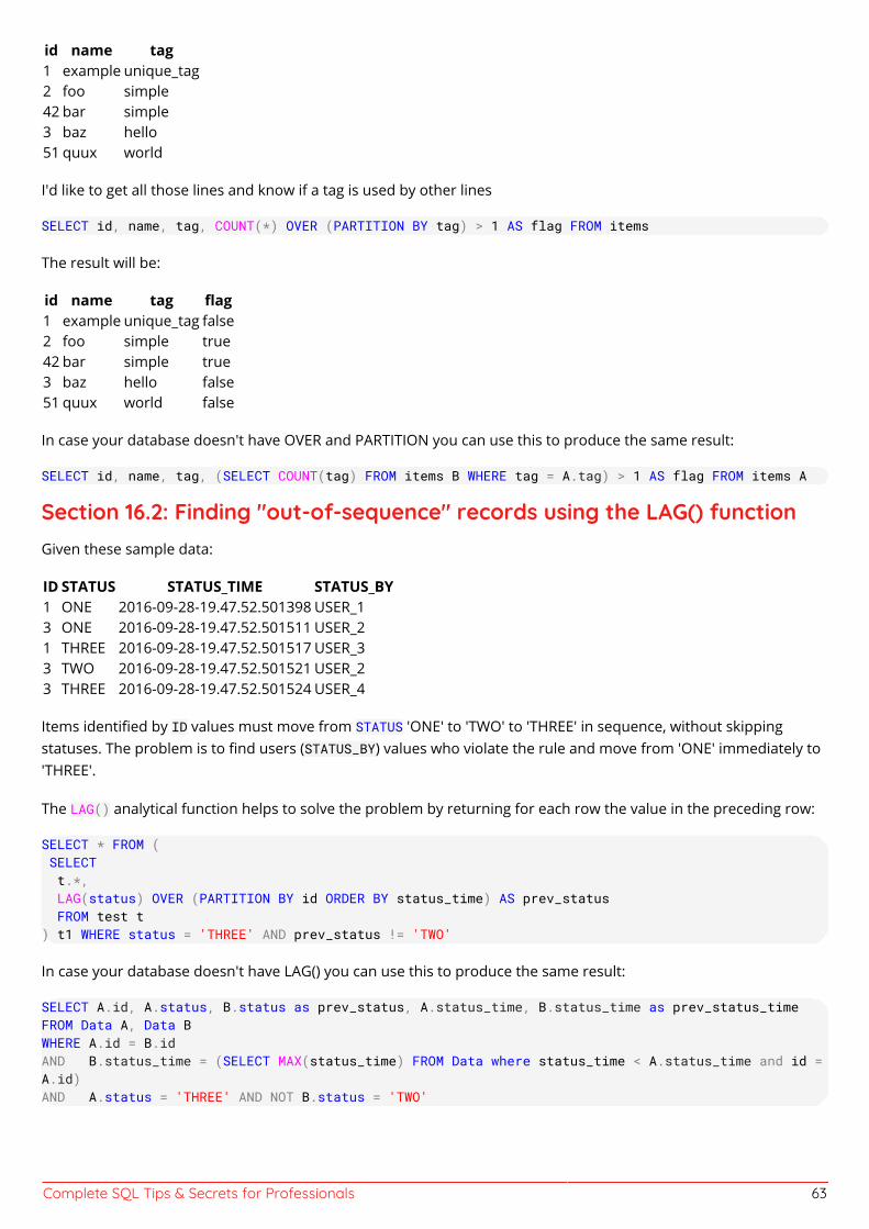
Complete SQL Tips & Secrets for Professionals 63

id name tag1 example unique_tag2 foo simple42 bar simple3 baz hello51 quux world

I'd like to get all those lines and know if a tag is used by other lines

SELECT id, name, tag, COUNT(*) OVER (PARTITION BY tag) > 1 AS flag FROM items

The result will be:

id name tag flag1 example unique_tag false2 foo simple true42 bar simple true3 baz hello false51 quux world false

In case your database doesn't have OVER and PARTITION you can use this to produce the same result:

SELECT id, name, tag, (SELECT COUNT(tag) FROM items B WHERE tag = A.tag) > 1 AS flag FROM items A

Section 16.2: Finding "out-of-sequence" records using the LAG() functionGiven these sample data:

ID STATUS STATUS_TIME STATUS_BY1 ONE 2016-09-28-19.47.52.501398 USER_13 ONE 2016-09-28-19.47.52.501511 USER_21 THREE 2016-09-28-19.47.52.501517 USER_33 TWO 2016-09-28-19.47.52.501521 USER_23 THREE 2016-09-28-19.47.52.501524 USER_4

Items identified by ID values must move from STATUS 'ONE' to 'TWO' to 'THREE' in sequence, without skippingstatuses. The problem is to find users (STATUS_BY) values who violate the rule and move from 'ONE' immediately to'THREE'.

The LAG() analytical function helps to solve the problem by returning for each row the value in the preceding row:

SELECT * FROM ( SELECT t.*, LAG(status) OVER (PARTITION BY id ORDER BY status_time) AS prev_status FROM test t) t1 WHERE status = 'THREE' AND prev_status != 'TWO'

In case your database doesn't have LAG() you can use this to produce the same result:

SELECT A.id, A.status, B.status as prev_status, A.status_time, B.status_time as prev_status_timeFROM Data A, Data BWHERE A.id = B.idAND B.status_time = (SELECT MAX(status_time) FROM Data where status_time < A.status_time and id =A.id)AND A.status = 'THREE' AND NOT B.status = 'TWO'

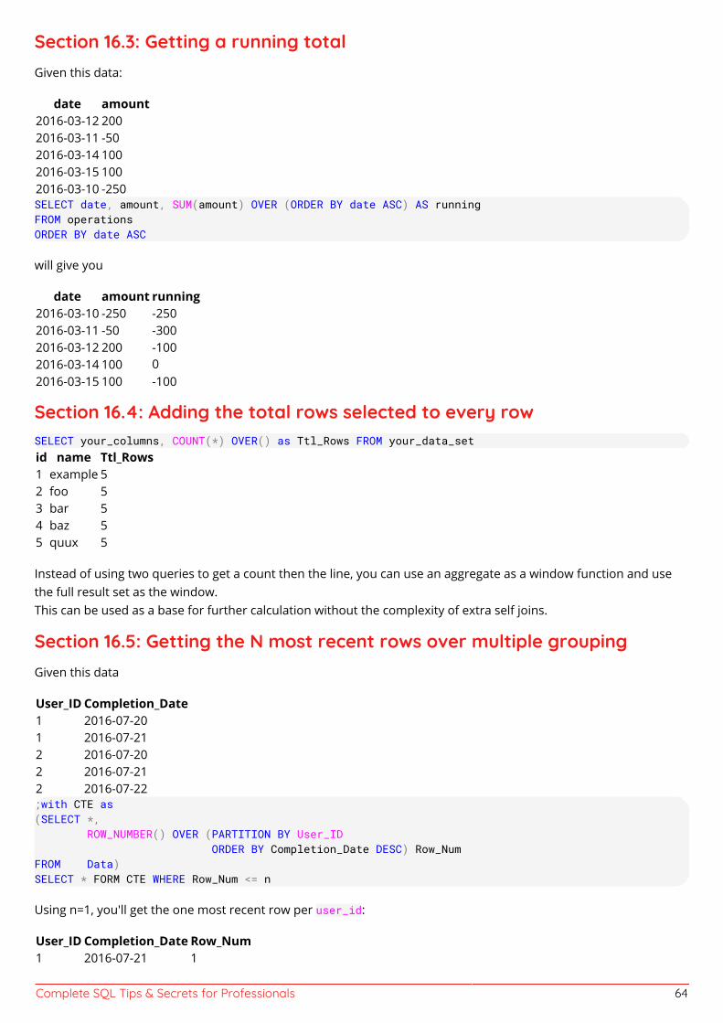
Complete SQL Tips & Secrets for Professionals 64

Section 16.3: Getting a running totalGiven this data:

date amount2016-03-12 2002016-03-11 -502016-03-14 1002016-03-15 1002016-03-10 -250SELECT date, amount, SUM(amount) OVER (ORDER BY date ASC) AS runningFROM operationsORDER BY date ASC

will give you

date amount running2016-03-10 -250 -2502016-03-11 -50 -3002016-03-12 200 -1002016-03-14 100 02016-03-15 100 -100

Section 16.4: Adding the total rows selected to every rowSELECT your_columns, COUNT(*) OVER() as Ttl_Rows FROM your_data_setid name Ttl_Rows1 example 52 foo 53 bar 54 baz 55 quux 5

Instead of using two queries to get a count then the line, you can use an aggregate as a window function and usethe full result set as the window.This can be used as a base for further calculation without the complexity of extra self joins.

Section 16.5: Getting the N most recent rows over multiple groupingGiven this data

User_ID Completion_Date1 2016-07-201 2016-07-212 2016-07-202 2016-07-212 2016-07-22;with CTE as(SELECT *, ROW_NUMBER() OVER (PARTITION BY User_ID ORDER BY Completion_Date DESC) Row_NumFROM Data)SELECT * FORM CTE WHERE Row_Num <= n

Using n=1, you'll get the one most recent row per user_id:

User_ID Completion_Date Row_Num1 2016-07-21 1

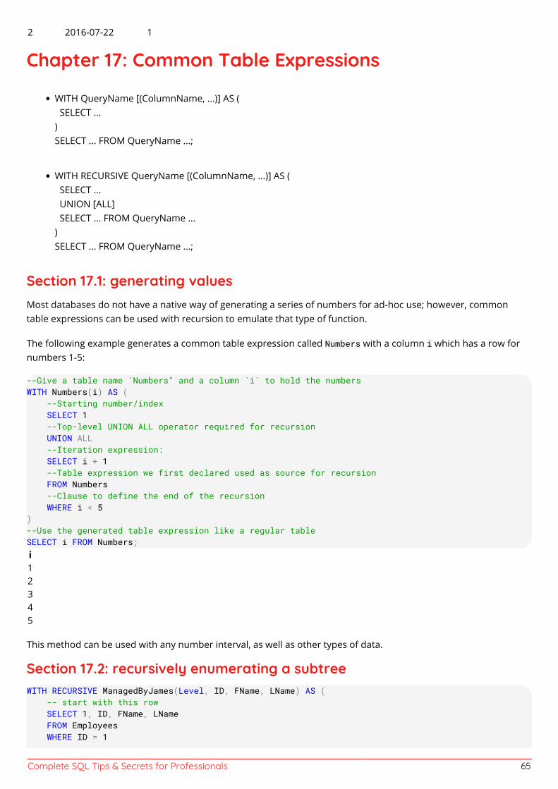
Complete SQL Tips & Secrets for Professionals 65

2 2016-07-22 1

Chapter 17: Common Table Expressions

WITH QueryName [(ColumnName, ...)] AS ( SELECT ...)SELECT ... FROM QueryName ...;

WITH RECURSIVE QueryName [(ColumnName, ...)] AS ( SELECT ... UNION [ALL] SELECT ... FROM QueryName ...)SELECT ... FROM QueryName ...;

Section 17.1: generating valuesMost databases do not have a native way of generating a series of numbers for ad-hoc use; however, commontable expressions can be used with recursion to emulate that type of function.

The following example generates a common table expression called Numbers with a column i which has a row fornumbers 1-5:

--Give a table name `Numbers" and a column `i` to hold the numbersWITH Numbers(i) AS ( --Starting number/index SELECT 1 --Top-level UNION ALL operator required for recursion UNION ALL --Iteration expression: SELECT i + 1 --Table expression we first declared used as source for recursion FROM Numbers --Clause to define the end of the recursion WHERE i < 5)--Use the generated table expression like a regular tableSELECT i FROM Numbers;i12345

This method can be used with any number interval, as well as other types of data.

Section 17.2: recursively enumerating a subtreeWITH RECURSIVE ManagedByJames(Level, ID, FName, LName) AS ( -- start with this row SELECT 1, ID, FName, LName FROM Employees WHERE ID = 1

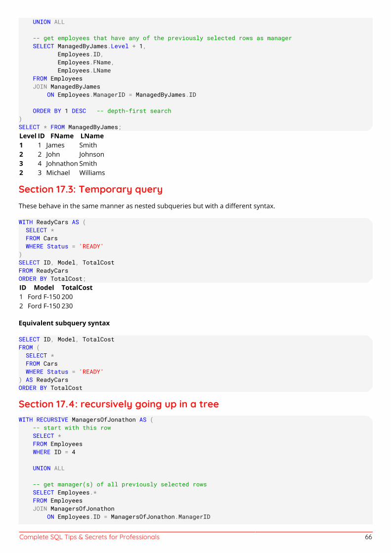
Complete SQL Tips & Secrets for Professionals 66

UNION ALL

-- get employees that have any of the previously selected rows as manager SELECT ManagedByJames.Level + 1, Employees.ID, Employees.FName, Employees.LName FROM Employees JOIN ManagedByJames ON Employees.ManagerID = ManagedByJames.ID

ORDER BY 1 DESC -- depth-first search)SELECT * FROM ManagedByJames;Level ID FName LName1 1 James Smith2 2 John Johnson3 4 Johnathon Smith2 3 Michael Williams

Section 17.3: Temporary queryThese behave in the same manner as nested subqueries but with a different syntax.

WITH ReadyCars AS ( SELECT * FROM Cars WHERE Status = 'READY')SELECT ID, Model, TotalCostFROM ReadyCarsORDER BY TotalCost;ID Model TotalCost1 Ford F-150 2002 Ford F-150 230

Equivalent subquery syntax

SELECT ID, Model, TotalCostFROM ( SELECT * FROM Cars WHERE Status = 'READY') AS ReadyCarsORDER BY TotalCost

Section 17.4: recursively going up in a treeWITH RECURSIVE ManagersOfJonathon AS ( -- start with this row SELECT * FROM Employees WHERE ID = 4

UNION ALL

-- get manager(s) of all previously selected rows SELECT Employees.* FROM Employees JOIN ManagersOfJonathon ON Employees.ID = ManagersOfJonathon.ManagerID

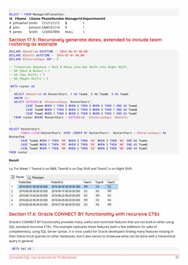
Complete SQL Tips & Secrets for Professionals 67

)SELECT * FROM ManagersOfJonathon;Id FName LName PhoneNumber ManagerId DepartmentId4 Johnathon Smith 1212121212 2 12 John Johnson 2468101214 1 11 James Smith 1234567890 NULL 1

Section 17.5: Recursively generate dates, extended to include teamrostering as exampleDECLARE @DateFrom DATETIME = '2016-06-01 06:00'DECLARE @DateTo DATETIME = '2016-07-01 06:00'DECLARE @IntervalDays INT = 7

-- Transition Sequence = Rest & Relax into Day Shift into Night Shift-- RR (Rest & Relax) = 1-- DS (Day Shift) = 2-- NS (Night Shift) = 3

;WITH roster AS( SELECT @DateFrom AS RosterStart, 1 AS TeamA, 2 AS TeamB, 3 AS TeamC UNION ALL SELECT DATEADD(d, @IntervalDays, RosterStart), CASE TeamA WHEN 1 THEN 2 WHEN 2 THEN 3 WHEN 3 THEN 1 END AS TeamA, CASE TeamB WHEN 1 THEN 2 WHEN 2 THEN 3 WHEN 3 THEN 1 END AS TeamB, CASE TeamC WHEN 1 THEN 2 WHEN 2 THEN 3 WHEN 3 THEN 1 END AS TeamC FROM roster WHERE RosterStart < DATEADD(d, -@IntervalDays, @DateTo))

SELECT RosterStart, ISNULL(LEAD(RosterStart) OVER (ORDER BY RosterStart), RosterStart + @IntervalDays) ASRosterEnd, CASE TeamA WHEN 1 THEN 'RR' WHEN 2 THEN 'DS' WHEN 3 THEN 'NS' END AS TeamA, CASE TeamB WHEN 1 THEN 'RR' WHEN 2 THEN 'DS' WHEN 3 THEN 'NS' END AS TeamB, CASE TeamC WHEN 1 THEN 'RR' WHEN 2 THEN 'DS' WHEN 3 THEN 'NS' END AS TeamCFROM roster

Result

I.e. For Week 1 TeamA is on R&R, TeamB is on Day Shift and TeamC is on Night Shift.

Section 17.6: Oracle CONNECT BY functionality with recursive CTEsOracle's CONNECT BY functionality provides many useful and nontrivial features that are not built-in when usingSQL standard recursive CTEs. This example replicates these features (with a few additions for sake ofcompleteness), using SQL Server syntax. It is most useful for Oracle developers finding many features missing intheir hierarchical queries on other databases, but it also serves to showcase what can be done with a hierarchicalquery in general.

WITH tbl AS (

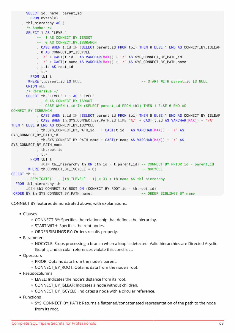
Complete SQL Tips & Secrets for Professionals 68

SELECT id, name, parent_id FROM mytable) , tbl_hierarchy AS ( /* Anchor */ SELECT 1 AS "LEVEL" --, 1 AS CONNECT_BY_ISROOT --, 0 AS CONNECT_BY_ISBRANCH , CASE WHEN t.id IN (SELECT parent_id FROM tbl) THEN 0 ELSE 1 END AS CONNECT_BY_ISLEAF , 0 AS CONNECT_BY_ISCYCLE , '/' + CAST(t.id AS VARCHAR(MAX)) + '/' AS SYS_CONNECT_BY_PATH_id , '/' + CAST(t.name AS VARCHAR(MAX)) + '/' AS SYS_CONNECT_BY_PATH_name , t.id AS root_id , t.* FROM tbl t WHERE t.parent_id IS NULL -- START WITH parent_id IS NULL UNION ALL /* Recursive */ SELECT th."LEVEL" + 1 AS "LEVEL" --, 0 AS CONNECT_BY_ISROOT --, CASE WHEN t.id IN (SELECT parent_id FROM tbl) THEN 1 ELSE 0 END ASCONNECT_BY_ISBRANCH , CASE WHEN t.id IN (SELECT parent_id FROM tbl) THEN 0 ELSE 1 END AS CONNECT_BY_ISLEAF , CASE WHEN th.SYS_CONNECT_BY_PATH_id LIKE '%/' + CAST(t.id AS VARCHAR(MAX)) + '/%'THEN 1 ELSE 0 END AS CONNECT_BY_ISCYCLE , th.SYS_CONNECT_BY_PATH_id + CAST(t.id AS VARCHAR(MAX)) + '/' ASSYS_CONNECT_BY_PATH_id , th.SYS_CONNECT_BY_PATH_name + CAST(t.name AS VARCHAR(MAX)) + '/' ASSYS_CONNECT_BY_PATH_name , th.root_id , t.* FROM tbl t JOIN tbl_hierarchy th ON (th.id = t.parent_id) -- CONNECT BY PRIOR id = parent_id WHERE th.CONNECT_BY_ISCYCLE = 0) -- NOCYCLESELECT th.* --, REPLICATE(' ', (th."LEVEL" - 1) * 3) + th.name AS tbl_hierarchy FROM tbl_hierarchy th JOIN tbl CONNECT_BY_ROOT ON (CONNECT_BY_ROOT.id = th.root_id) ORDER BY th.SYS_CONNECT_BY_PATH_name; -- ORDER SIBLINGS BY name

CONNECT BY features demonstrated above, with explanations:

ClausesCONNECT BY: Specifies the relationship that defines the hierarchy.START WITH: Specifies the root nodes.ORDER SIBLINGS BY: Orders results properly.

ParametersNOCYCLE: Stops processing a branch when a loop is detected. Valid hierarchies are Directed AcyclicGraphs, and circular references violate this construct.

OperatorsPRIOR: Obtains data from the node's parent.CONNECT_BY_ROOT: Obtains data from the node's root.

PseudocolumnsLEVEL: Indicates the node's distance from its root.CONNECT_BY_ISLEAF: Indicates a node without children.CONNECT_BY_ISCYCLE: Indicates a node with a circular reference.

FunctionsSYS_CONNECT_BY_PATH: Returns a flattened/concatenated representation of the path to the nodefrom its root.

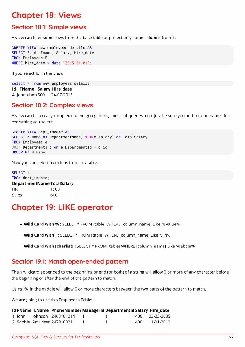
Complete SQL Tips & Secrets for Professionals 69

Chapter 18: ViewsSection 18.1: Simple viewsA view can filter some rows from the base table or project only some columns from it:

CREATE VIEW new_employees_details ASSELECT E.id, Fname, Salary, Hire_dateFROM Employees EWHERE hire_date > date '2015-01-01';

If you select form the view:

select * from new_employees_detailsId FName Salary Hire_date4 Johnathon 500 24-07-2016

Section 18.2: Complex viewsA view can be a really complex query(aggregations, joins, subqueries, etc). Just be sure you add column names foreverything you select:

Create VIEW dept_income ASSELECT d.Name as DepartmentName, sum(e.salary) as TotalSalaryFROM Employees eJOIN Departments d on e.DepartmentId = d.idGROUP BY d.Name;

Now you can select from it as from any table:

SELECT *FROM dept_income;DepartmentName TotalSalaryHR 1900Sales 600

Chapter 19: LIKE operator

Wild Card with % : SELECT * FROM [table] WHERE [column_name] Like '%Value%'

Wild Card with _ : SELECT * FROM [table] WHERE [column_name] Like 'V_n%'

Wild Card with [charlist] : SELECT * FROM [table] WHERE [column_name] Like 'V[abc]n%'

Section 19.1: Match open-ended patternThe % wildcard appended to the beginning or end (or both) of a string will allow 0 or more of any character beforethe beginning or after the end of the pattern to match.

Using '%' in the middle will allow 0 or more characters between the two parts of the pattern to match.

We are going to use this Employees Table:

Id FName LName PhoneNumber ManagerId DepartmentId Salary Hire_date1 John Johnson 2468101214 1 1 400 23-03-20052 Sophie Amudsen 2479100211 1 1 400 11-01-2010

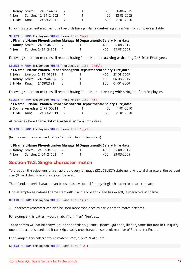
Complete SQL Tips & Secrets for Professionals 70

3 Ronny Smith 2462544026 2 1 600 06-08-20154 Jon Sanchez 2454124602 1 1 400 23-03-20055 Hilde Knag 2468021911 2 1 800 01-01-2000

Following statement matches for all records having FName containing string 'on' from Employees Table.

SELECT * FROM Employees WHERE FName LIKE '%on%';Id FName LName PhoneNumber ManagerId DepartmentId Salary Hire_date3 Ronny Smith 2462544026 2 1 600 06-08-20154 Jon Sanchez 2454124602 1 1 400 23-03-2005

Following statement matches all records having PhoneNumber starting with string '246' from Employees.

SELECT * FROM Employees WHERE PhoneNumber LIKE '246%';Id FName LName PhoneNumber ManagerId DepartmentId Salary Hire_date1 John Johnson 2468101214 1 1 400 23-03-20053 Ronny Smith 2462544026 2 1 600 06-08-20155 Hilde Knag 2468021911 2 1 800 01-01-2000

Following statement matches all records having PhoneNumber ending with string '11' from Employees.

SELECT * FROM Employees WHERE PhoneNumber LIKE '%11'Id FName LName PhoneNumber ManagerId DepartmentId Salary Hire_date2 Sophie Amudsen 2479100211 1 1 400 11-01-20105 Hilde Knag 2468021911 2 1 800 01-01-2000

All records where Fname 3rd character is 'n' from Employees.

SELECT * FROM Employees WHERE FName LIKE '__n%';

(two underscores are used before 'n' to skip first 2 characters)

Id FName LName PhoneNumber ManagerId DepartmentId Salary Hire_date3 Ronny Smith 2462544026 2 1 600 06-08-20154 Jon Sanchez 2454124602 1 1 400 23-03-2005

Section 19.2: Single character matchTo broaden the selections of a structured query language (SQL-SELECT) statement, wildcard characters, the percentsign (%) and the underscore (_), can be used.

The _ (underscore) character can be used as a wildcard for any single character in a pattern match.

Find all employees whose Fname start with 'j' and end with 'n' and has exactly 3 characters in Fname.

SELECT * FROM Employees WHERE FName LIKE 'j_n'

_ (underscore) character can also be used more than once as a wild card to match patterns.

For example, this pattern would match "jon", "jan", "jen", etc.

These names will not be shown "jn","john","jordan", "justin", "jason", "julian", "jillian", "joann" because in our queryone underscore is used and it can skip exactly one character, so result must be of 3 character Fname.

For example, this pattern would match "LaSt", "LoSt", "HaLt", etc.

SELECT * FROM Employees WHERE FName LIKE '_A_T'

Complete SQL Tips & Secrets for Professionals 71

Section 19.3: ESCAPE statement in the LIKE-queryIf you implement a text-search as LIKE-query, you usually do it like this:

SELECT *FROM T_WhateverWHERE SomeField LIKE CONCAT('%', @in_SearchText, '%')

However, (apart from the fact that you shouldn't necessarely use LIKE when you can use fulltext-search) thiscreates a problem when somebody inputs text like "50%" or "a_b".

So (instead of switching to fulltext-search), you can solve that problem using the LIKE-escape statement:

SELECT *FROM T_WhateverWHERE SomeField LIKE CONCAT('%', @in_SearchText, '%') ESCAPE '\'

That means \ will now be treated as ESCAPE character. This means, you can now just prepend \ to every characterin the string you search, and the results will start to be correct, even when the user enters a special character like %or _.

e.g.

string stringToSearch = "abc_def 50%";string newString = "";foreach(char c in stringToSearch) newString += @"\" + c; sqlCmd.Parameters.Add("@in_SearchText", newString);// instead of sqlCmd.Parameters.Add("@in_SearchText", stringToSearch);

Note: The above algorithm is for demonstration purposes only. It will not work in cases where 1 grapheme consistsout of several characters (utf-8). e.g. string stringToSearch = "Les Mise\u0301rables"; You'll need to do thisfor each grapheme, not for each character. You should not use the above algorithm if you're dealing withAsian/East-Asian/South-Asian languages. Or rather, if you want correct code to begin with, you should just do thatfor each graphemeCluster.

See also ReverseString, a C# interview-question

Section 19.4: Search for a range of charactersFollowing statement matches all records having FName that starts with a letter from A to F from Employees Table.

SELECT * FROM Employees WHERE FName LIKE '[A-F]%'

Section 19.5: Match by range or setMatch any single character within the specified range (e.g.: [a-f]) or set (e.g.: [abcdef]).

This range pattern would match "gary" but not "mary":

SELECT * FROM Employees WHERE FName LIKE '[a-g]ary'

This set pattern would match "mary" but not "gary":

SELECT * FROM Employees WHERE Fname LIKE '[lmnop]ary'

The range or set can also be negated by appending the ^ caret before the range or set:

Complete SQL Tips & Secrets for Professionals 72

This range pattern would not match "gary" but will match "mary":

SELECT * FROM Employees WHERE FName LIKE '[^a-g]ary'

This set pattern would not match "mary" but will match"gary":

SELECT * FROM Employees WHERE Fname LIKE '[^lmnop]ary'

Section 19.6: Wildcard characterswildcard characters are used with the SQL LIKE operator. SQL wildcards are used to search for data within a table.

Wildcards in SQL are:%, _, [charlist], [^charlist]

% - A substitute for zero or more characters

Eg: //selects all customers with a City starting with "Lo" SELECT * FROM Customers WHERE City LIKE 'Lo%';

//selects all customers with a City containing the pattern "es" SELECT * FROM Customers WHERE City LIKE '%es%';

_ - A substitute for a single character

Eg://selects all customers with a City starting with any character, followed by "erlin"SELECT * FROM CustomersWHERE City LIKE '_erlin';

[charlist] - Sets and ranges of characters to match

Eg://selects all customers with a City starting with "a", "d", or "l"SELECT * FROM CustomersWHERE City LIKE '[adl]%';

//selects all customers with a City starting with "a", "d", or "l"SELECT * FROM CustomersWHERE City LIKE '[a-c]%';

[^charlist] - Matches only a character NOT specified within the brackets

Eg://selects all customers with a City starting with a character that is not "a", "p", or "l"SELECT * FROM CustomersWHERE City LIKE '[^apl]%';

or

SELECT * FROM CustomersWHERE City NOT LIKE '[apl]%' and city like '_%';

Chapter 20: Functions (Aggregate)Function([DISTINCT] expression) -DISTINCT is an optional parameterAVG ( [ ALL | DISTINCT ] expression )COUNT( { [ALL | DISTINCT ] expression ] | * } )GROUPING(<column_expression>)MAX ( [ ALL | DISTINCT ] expression )MIN ( [ ALL | DISTINCT ] expression )

Complete SQL Tips & Secrets for Professionals 73

SUM ( [ ALL | DISTINCT ] expression )VAR ( [ ALL | DISTINCT ] expression )OVER ( [ partition_by_clause ] order_by_clause )VARP ( [ ALL | DISTINCT ] expression )OVER ( [ partition_by_clause ] order_by_clauseSTDEV ( [ ALL | DISTINCT ] expression )OVER ( [ partition_by_clause ] order_by_clause )STDEVP ( [ ALL | DISTINCT ] expression )OVER ( [ partition_by_clause ] order_by_clause )

Section 20.1: Conditional aggregationPayments Table

Customer Payment_type AmountPeter Credit 100Peter Credit 300John Credit 1000John Debit 500select customer, sum(case when payment_type = 'credit' then amount else 0 end) as credit, sum(case when payment_type = 'debit' then amount else 0 end) as debitfrom paymentsgroup by customer

Result:

Customer Credit DebitPeter 400 0John 1000 500select customer, sum(case when payment_type = 'credit' then 1 else 0 end) as credit_transaction_count, sum(case when payment_type = 'debit' then 1 else 0 end) as debit_transaction_countfrom paymentsgroup by customer

Result:

Customer credit_transaction_count debit_transaction_countPeter 2 0John 1 1

Section 20.2: List ConcatenationPartial credit to this SO answer.

List Concatenation aggregates a column or expression by combining the values into a single string for each group. Astring to delimit each value (either blank or a comma when omitted) and the order of the values in the result can bespecified. While it is not part of the SQL standard, every major relational database vendor supports it in their ownway.

MySQLSELECT ColumnA , GROUP_CONCAT(ColumnB ORDER BY ColumnB SEPARATOR ',') AS ColumnBs FROM TableName GROUP BY ColumnA ORDER BY ColumnA;

Complete SQL Tips & Secrets for Professionals 74

Oracle & DB2SELECT ColumnA , LISTAGG(ColumnB, ',') WITHIN GROUP (ORDER BY ColumnB) AS ColumnBs FROM TableName GROUP BY ColumnA ORDER BY ColumnA;PostgreSQLSELECT ColumnA , STRING_AGG(ColumnB, ',' ORDER BY ColumnB) AS ColumnBs FROM TableName GROUP BY ColumnA ORDER BY ColumnA;SQL ServerSQL Server 2016 and earlier

(CTE included to encourage the DRY principle)

WITH CTE_TableName AS ( SELECT ColumnA, ColumnB FROM TableName)SELECT t0.ColumnA , STUFF(( SELECT ',' + t1.ColumnB FROM CTE_TableName t1 WHERE t1.ColumnA = t0.ColumnA ORDER BY t1.ColumnB FOR XML PATH('')), 1, 1, '') AS ColumnBs FROM CTE_TableName t0 GROUP BY t0.ColumnA ORDER BY ColumnA;SQL Server 2017 and SQL AzureSELECT ColumnA , STRING_AGG(ColumnB, ',') WITHIN GROUP (ORDER BY ColumnB) AS ColumnBs FROM TableName GROUP BY ColumnA ORDER BY ColumnA;SQLite

without ordering:

SELECT ColumnA , GROUP_CONCAT(ColumnB, ',') AS ColumnBs FROM TableName GROUP BY ColumnA ORDER BY ColumnA;

ordering requires a subquery or CTE:

WITH CTE_TableName AS ( SELECT ColumnA, ColumnB FROM TableName ORDER BY ColumnA, ColumnB)SELECT ColumnA , GROUP_CONCAT(ColumnB, ',') AS ColumnBs FROM CTE_TableName GROUP BY ColumnA ORDER BY ColumnA;

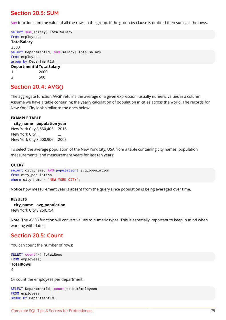
Complete SQL Tips & Secrets for Professionals 75

Section 20.3: SUMSum function sum the value of all the rows in the group. If the group by clause is omitted then sums all the rows.

select sum(salary) TotalSalaryfrom employees;TotalSalary2500select DepartmentId, sum(salary) TotalSalaryfrom employeesgroup by DepartmentId;DepartmentId TotalSalary1 20002 500

Section 20.4: AVG()The aggregate function AVG() returns the average of a given expression, usually numeric values in a column.Assume we have a table containing the yearly calculation of population in cities across the world. The records forNew York City look similar to the ones below:

EXAMPLE TABLEcity_name population year

New York City 8,550,405 2015New York City ... ...New York City 8,000,906 2005

To select the average population of the New York City, USA from a table containing city names, populationmeasurements, and measurement years for last ten years:

QUERYselect city_name, AVG(population) avg_populationfrom city_populationwhere city_name = 'NEW YORK CITY';

Notice how measurement year is absent from the query since population is being averaged over time.

RESULTScity_name avg_population

New York City 8,250,754

Note: The AVG() function will convert values to numeric types. This is especially important to keep in mind whenworking with dates.

Section 20.5: CountYou can count the number of rows:

SELECT count(*) TotalRowsFROM employees;TotalRows4

Or count the employees per department:

SELECT DepartmentId, count(*) NumEmployeesFROM employeesGROUP BY DepartmentId;

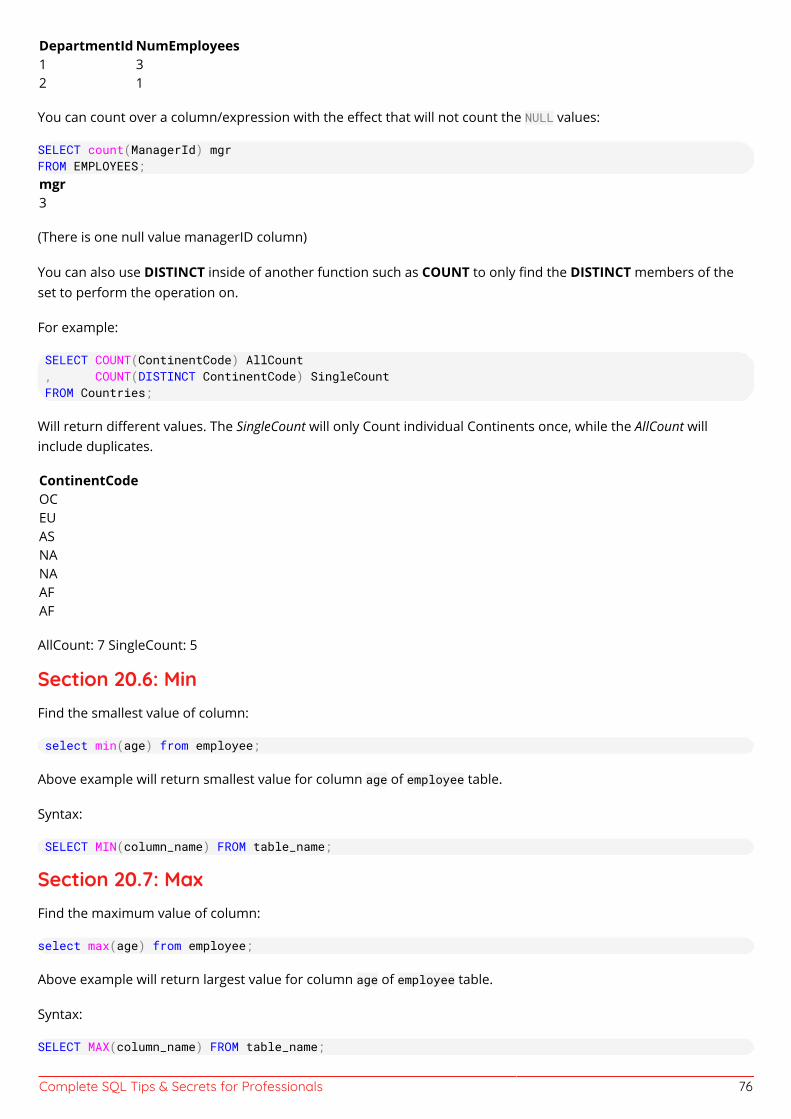
Complete SQL Tips & Secrets for Professionals 76

DepartmentId NumEmployees1 32 1

You can count over a column/expression with the effect that will not count the NULL values:

SELECT count(ManagerId) mgrFROM EMPLOYEES;mgr3

(There is one null value managerID column)

You can also use DISTINCT inside of another function such as COUNT to only find the DISTINCT members of theset to perform the operation on.

For example:

SELECT COUNT(ContinentCode) AllCount , COUNT(DISTINCT ContinentCode) SingleCount FROM Countries;

Will return different values. The SingleCount will only Count individual Continents once, while the AllCount willinclude duplicates.

ContinentCodeOCEUASNANAAFAF

AllCount: 7 SingleCount: 5

Section 20.6: MinFind the smallest value of column:

select min(age) from employee;

Above example will return smallest value for column age of employee table.

Syntax:

SELECT MIN(column_name) FROM table_name;

Section 20.7: MaxFind the maximum value of column:

select max(age) from employee;

Above example will return largest value for column age of employee table.

Syntax:

SELECT MAX(column_name) FROM table_name;

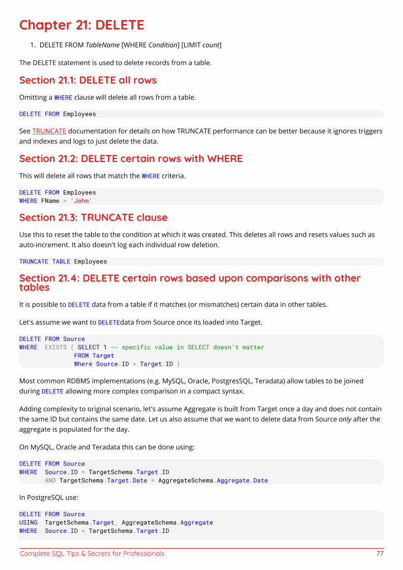
Complete SQL Tips & Secrets for Professionals 77

Chapter 21: DELETEDELETE FROM TableName [WHERE Condition] [LIMIT count]1.

The DELETE statement is used to delete records from a table.

Section 21.1: DELETE all rowsOmitting a WHERE clause will delete all rows from a table.

DELETE FROM Employees

See TRUNCATE documentation for details on how TRUNCATE performance can be better because it ignores triggersand indexes and logs to just delete the data.

Section 21.2: DELETE certain rows with WHEREThis will delete all rows that match the WHERE criteria.

DELETE FROM EmployeesWHERE FName = 'John'

Section 21.3: TRUNCATE clauseUse this to reset the table to the condition at which it was created. This deletes all rows and resets values such asauto-increment. It also doesn't log each individual row deletion.

TRUNCATE TABLE Employees

Section 21.4: DELETE certain rows based upon comparisons with othertablesIt is possible to DELETE data from a table if it matches (or mismatches) certain data in other tables.

Let's assume we want to DELETEdata from Source once its loaded into Target.

DELETE FROM SourceWHERE EXISTS ( SELECT 1 -- specific value in SELECT doesn't matter FROM Target Where Source.ID = Target.ID )

Most common RDBMS implementations (e.g. MySQL, Oracle, PostgresSQL, Teradata) allow tables to be joinedduring DELETE allowing more complex comparison in a compact syntax.

Adding complexity to original scenario, let's assume Aggregate is built from Target once a day and does not containthe same ID but contains the same date. Let us also assume that we want to delete data from Source only after theaggregate is populated for the day.

On MySQL, Oracle and Teradata this can be done using:

DELETE FROM SourceWHERE Source.ID = TargetSchema.Target.ID AND TargetSchema.Target.Date = AggregateSchema.Aggregate.Date

In PostgreSQL use:

DELETE FROM SourceUSING TargetSchema.Target, AggregateSchema.AggregateWHERE Source.ID = TargetSchema.Target.ID

Complete SQL Tips & Secrets for Professionals 78

AND TargetSchema.Target.DataDate = AggregateSchema.Aggregate.AggDate

This essentially results in INNER JOINs between Source, Target and Aggregate. The deletion is performed on Sourcewhen the same IDs exist in Target AND date present in Target for those IDs also exists in Aggregate.

Same query may also be written (on MySQL, Oracle, Teradata) as:

DELETE SourceFROM Source, TargetSchema.Target, AggregateSchema.AggregateWHERE Source.ID = TargetSchema.Target.ID AND TargetSchema.Target.DataDate = AggregateSchema.Aggregate.AggDate

Explicit joins may be mentioned in Delete statements on some RDBMS implementations (e.g. Oracle, MySQL) butnot supported on all platforms (e.g. Teradata does not support them)

Comparisons can be designed to check mismatch scenarios instead of matching ones with all syntax styles (observeNOT EXISTS below)

DELETE FROM SourceWHERE NOT EXISTS ( SELECT 1 -- specific value in SELECT doesn't matter FROM Target Where Source.ID = Target.ID )

Chapter 22: String FunctionsCONCAT ( string_value1, string_value2 [, string_valueN ] )LTRIM ( character_expression )RTRIM ( character_expression )SUBSTRING ( expression ,start , length )ASCII ( character_expression )REPLICATE ( string_expression ,integer_expression )REVERSE ( string_expression )UPPER ( character_expression )TRIM ( [ characters FROM ] string )STRING_SPLIT ( string , separator )STUFF ( character_expression , start , length , replaceWith_expression )REPLACE ( string_expression , string_pattern , string_replacement )

String functions perform operations on string values and return either numeric or string values.

Using string functions, you can, for example, combine data, extract a substring, compare strings, or convert a stringto all uppercase or lowercase characters.

Section 22.1: ConcatenateIn (standard ANSI/ISO) SQL, the operator for string concatenation is ||. This syntax is supported by all majordatabases except SQL Server:

SELECT 'Hello' || 'World' || '!'; --returns HelloWorld!

Many databases support a CONCAT function to join strings:

SELECT CONCAT('Hello', 'World'); --returns 'HelloWorld'

Some databases support using CONCAT to join more than two strings (Oracle does not):

SELECT CONCAT('Hello', 'World', '!'); --returns 'HelloWorld!'

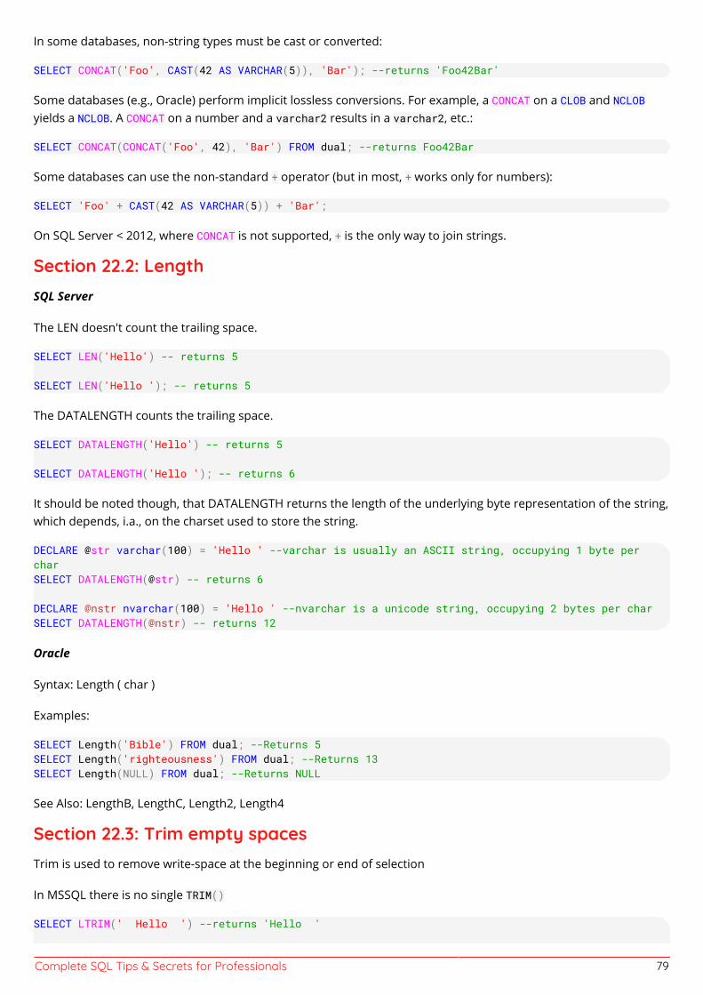
Complete SQL Tips & Secrets for Professionals 79

In some databases, non-string types must be cast or converted:

SELECT CONCAT('Foo', CAST(42 AS VARCHAR(5)), 'Bar'); --returns 'Foo42Bar'

Some databases (e.g., Oracle) perform implicit lossless conversions. For example, a CONCAT on a CLOB and NCLOByields a NCLOB. A CONCAT on a number and a varchar2 results in a varchar2, etc.:

SELECT CONCAT(CONCAT('Foo', 42), 'Bar') FROM dual; --returns Foo42Bar

Some databases can use the non-standard + operator (but in most, + works only for numbers):

SELECT 'Foo' + CAST(42 AS VARCHAR(5)) + 'Bar';

On SQL Server < 2012, where CONCAT is not supported, + is the only way to join strings.

Section 22.2: LengthSQL Server

The LEN doesn't count the trailing space.

SELECT LEN('Hello') -- returns 5

SELECT LEN('Hello '); -- returns 5

The DATALENGTH counts the trailing space.

SELECT DATALENGTH('Hello') -- returns 5

SELECT DATALENGTH('Hello '); -- returns 6

It should be noted though, that DATALENGTH returns the length of the underlying byte representation of the string,which depends, i.a., on the charset used to store the string.

DECLARE @str varchar(100) = 'Hello ' --varchar is usually an ASCII string, occupying 1 byte percharSELECT DATALENGTH(@str) -- returns 6

DECLARE @nstr nvarchar(100) = 'Hello ' --nvarchar is a unicode string, occupying 2 bytes per charSELECT DATALENGTH(@nstr) -- returns 12

Oracle

Syntax: Length ( char )

Examples:

SELECT Length('Bible') FROM dual; --Returns 5SELECT Length('righteousness') FROM dual; --Returns 13SELECT Length(NULL) FROM dual; --Returns NULL

See Also: LengthB, LengthC, Length2, Length4

Section 22.3: Trim empty spacesTrim is used to remove write-space at the beginning or end of selection

In MSSQL there is no single TRIM()

SELECT LTRIM(' Hello ') --returns 'Hello '

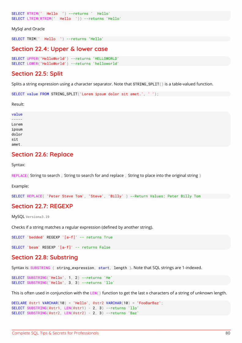
Complete SQL Tips & Secrets for Professionals 80

SELECT RTRIM(' Hello ') --returns ' Hello'SELECT LTRIM(RTRIM(' Hello ')) --returns 'Hello'

MySql and Oracle

SELECT TRIM(' Hello ') --returns 'Hello'

Section 22.4: Upper & lower caseSELECT UPPER('HelloWorld') --returns 'HELLOWORLD'SELECT LOWER('HelloWorld') --returns 'helloworld'

Section 22.5: SplitSplits a string expression using a character separator. Note that STRING_SPLIT() is a table-valued function.

SELECT value FROM STRING_SPLIT('Lorem ipsum dolor sit amet.', ' ');

Result:

value-----Loremipsumdolorsitamet.

Section 22.6: ReplaceSyntax:

REPLACE( String to search , String to search for and replace , String to place into the original string )

Example:

SELECT REPLACE( 'Peter Steve Tom', 'Steve', 'Billy' ) --Return Values: Peter Billy Tom

Section 22.7: REGEXPMySQL Version≥3.19

Checks if a string matches a regular expression (defined by another string).

SELECT 'bedded' REGEXP '[a-f]' -- returns True

SELECT 'beam' REGEXP '[a-f]' -- returns False

Section 22.8: SubstringSyntax is: SUBSTRING ( string_expression, start, length ). Note that SQL strings are 1-indexed.

SELECT SUBSTRING('Hello', 1, 2) --returns 'He'SELECT SUBSTRING('Hello', 3, 3) --returns 'llo'

This is often used in conjunction with the LEN() function to get the last n characters of a string of unknown length.

DECLARE @str1 VARCHAR(10) = 'Hello', @str2 VARCHAR(10) = 'FooBarBaz';SELECT SUBSTRING(@str1, LEN(@str1) - 2, 3) --returns 'llo'SELECT SUBSTRING(@str2, LEN(@str2) - 2, 3) --returns 'Baz'

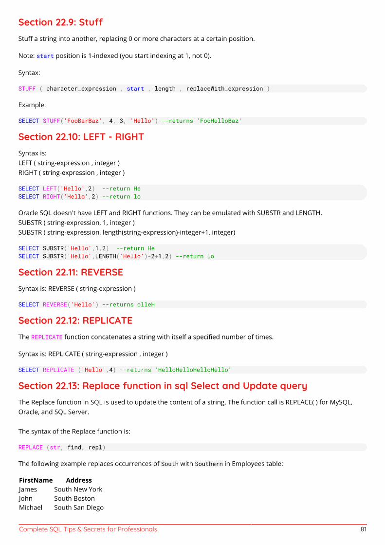
Complete SQL Tips & Secrets for Professionals 81

Section 22.9: StuStuff a string into another, replacing 0 or more characters at a certain position.

Note: start position is 1-indexed (you start indexing at 1, not 0).

Syntax:

STUFF ( character_expression , start , length , replaceWith_expression )

Example:

SELECT STUFF('FooBarBaz', 4, 3, 'Hello') --returns 'FooHelloBaz'

Section 22.10: LEFT - RIGHTSyntax is:LEFT ( string-expression , integer )RIGHT ( string-expression , integer )

SELECT LEFT('Hello',2) --return He SELECT RIGHT('Hello',2) --return lo

Oracle SQL doesn't have LEFT and RIGHT functions. They can be emulated with SUBSTR and LENGTH.SUBSTR ( string-expression, 1, integer )SUBSTR ( string-expression, length(string-expression)-integer+1, integer)

SELECT SUBSTR('Hello',1,2) --return He SELECT SUBSTR('Hello',LENGTH('Hello')-2+1,2) --return lo

Section 22.11: REVERSESyntax is: REVERSE ( string-expression )

SELECT REVERSE('Hello') --returns olleH

Section 22.12: REPLICATEThe REPLICATE function concatenates a string with itself a specified number of times.

Syntax is: REPLICATE ( string-expression , integer )

SELECT REPLICATE ('Hello',4) --returns 'HelloHelloHelloHello'

Section 22.13: Replace function in sql Select and Update queryThe Replace function in SQL is used to update the content of a string. The function call is REPLACE( ) for MySQL,Oracle, and SQL Server.

The syntax of the Replace function is:

REPLACE (str, find, repl)

The following example replaces occurrences of South with Southern in Employees table:

FirstName AddressJames South New YorkJohn South BostonMichael South San Diego

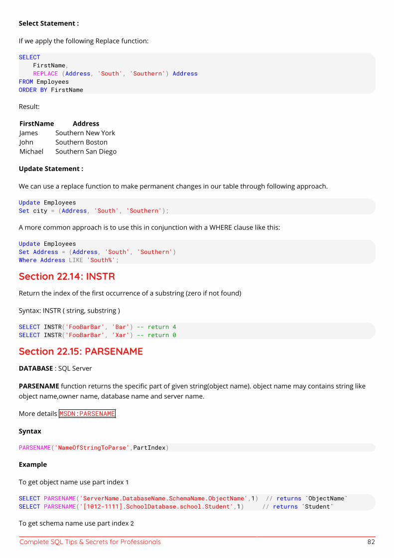
Complete SQL Tips & Secrets for Professionals 82

Select Statement :

If we apply the following Replace function:

SELECT FirstName, REPLACE (Address, 'South', 'Southern') AddressFROM EmployeesORDER BY FirstName

Result:

FirstName AddressJames Southern New YorkJohn Southern BostonMichael Southern San Diego

Update Statement :

We can use a replace function to make permanent changes in our table through following approach.

Update EmployeesSet city = (Address, 'South', 'Southern');

A more common approach is to use this in conjunction with a WHERE clause like this:

Update EmployeesSet Address = (Address, 'South', 'Southern')Where Address LIKE 'South%';

Section 22.14: INSTRReturn the index of the first occurrence of a substring (zero if not found)

Syntax: INSTR ( string, substring )

SELECT INSTR('FooBarBar', 'Bar') -- return 4SELECT INSTR('FooBarBar', 'Xar') -- return 0

Section 22.15: PARSENAMEDATABASE : SQL Server

PARSENAME function returns the specific part of given string(object name). object name may contains string likeobject name,owner name, database name and server name.

More details MSDN:PARSENAME

Syntax

PARSENAME('NameOfStringToParse',PartIndex)

Example

To get object name use part index 1

SELECT PARSENAME('ServerName.DatabaseName.SchemaName.ObjectName',1) // returns `ObjectName`SELECT PARSENAME('[1012-1111].SchoolDatabase.school.Student',1) // returns `Student`

To get schema name use part index 2

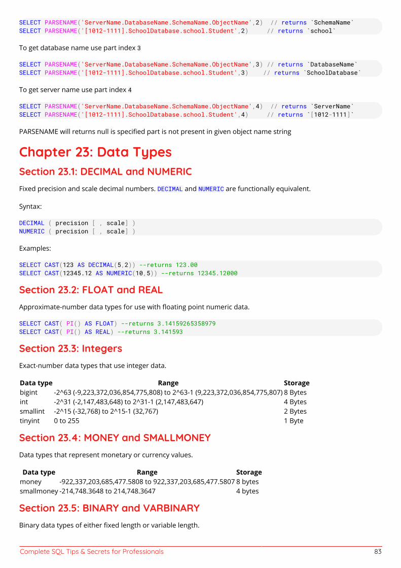
Complete SQL Tips & Secrets for Professionals 83

SELECT PARSENAME('ServerName.DatabaseName.SchemaName.ObjectName',2) // returns `SchemaName`SELECT PARSENAME('[1012-1111].SchoolDatabase.school.Student',2) // returns `school`

To get database name use part index 3

SELECT PARSENAME('ServerName.DatabaseName.SchemaName.ObjectName',3) // returns `DatabaseName`SELECT PARSENAME('[1012-1111].SchoolDatabase.school.Student',3) // returns `SchoolDatabase`

To get server name use part index 4

SELECT PARSENAME('ServerName.DatabaseName.SchemaName.ObjectName',4) // returns `ServerName`SELECT PARSENAME('[1012-1111].SchoolDatabase.school.Student',4) // returns `[1012-1111]`

PARSENAME will returns null is specified part is not present in given object name string

Chapter 23: Data TypesSection 23.1: DECIMAL and NUMERICFixed precision and scale decimal numbers. DECIMAL and NUMERIC are functionally equivalent.

Syntax:

DECIMAL ( precision [ , scale] )NUMERIC ( precision [ , scale] )

Examples:

SELECT CAST(123 AS DECIMAL(5,2)) --returns 123.00SELECT CAST(12345.12 AS NUMERIC(10,5)) --returns 12345.12000

Section 23.2: FLOAT and REALApproximate-number data types for use with floating point numeric data.

SELECT CAST( PI() AS FLOAT) --returns 3.14159265358979SELECT CAST( PI() AS REAL) --returns 3.141593

Section 23.3: IntegersExact-number data types that use integer data.

Data type Range Storagebigint -2^63 (-9,223,372,036,854,775,808) to 2^63-1 (9,223,372,036,854,775,807) 8 Bytesint -2^31 (-2,147,483,648) to 2^31-1 (2,147,483,647) 4 Bytessmallint -2^15 (-32,768) to 2^15-1 (32,767) 2 Bytestinyint 0 to 255 1 Byte

Section 23.4: MONEY and SMALLMONEYData types that represent monetary or currency values.

Data type Range Storagemoney -922,337,203,685,477.5808 to 922,337,203,685,477.5807 8 bytessmallmoney -214,748.3648 to 214,748.3647 4 bytes

Section 23.5: BINARY and VARBINARYBinary data types of either fixed length or variable length.

Complete SQL Tips & Secrets for Professionals 84

Syntax:

BINARY [ ( n_bytes ) ]VARBINARY [ ( n_bytes | max ) ]

n_bytes can be any number from 1 to 8000 bytes. max indicates that the maximum storage space is 2^31-1.

Examples:

SELECT CAST(12345 AS BINARY(10)) -- 0x00000000000000003039SELECT CAST(12345 AS VARBINARY(10)) -- 0x00003039

Section 23.6: CHAR and VARCHARString data types of either fixed length or variable length.

Syntax:

CHAR [ ( n_chars ) ]VARCHAR [ ( n_chars ) ]

Examples:

SELECT CAST('ABC' AS CHAR(10)) -- 'ABC ' (padded with spaces on the right)SELECT CAST('ABC' AS VARCHAR(10)) -- 'ABC' (no padding due to variable character)SELECT CAST('ABCDEFGHIJKLMNOPQRSTUVWXYZ' AS CHAR(10)) -- 'ABCDEFGHIJ' (truncated to 10 characters)

Section 23.7: NCHAR and NVARCHARUNICODE string data types of either fixed length or variable length.

Syntax:

NCHAR [ ( n_chars ) ]NVARCHAR [ ( n_chars | MAX ) ]

Use MAX for very long strings that may exceed 8000 characters.

Section 23.8: UNIQUEIDENTIFIERA 16-byte GUID / UUID.

DECLARE @GUID UNIQUEIDENTIFIER = NEWID();SELECT @GUID -- 'E28B3BD9-9174-41A9-8508-899A78A33540'DECLARE @bad_GUID_string VARCHAR(100) = 'E28B3BD9-9174-41A9-8508-899A78A33540_foobarbaz'SELECT @bad_GUID_string, -- 'E28B3BD9-9174-41A9-8508-899A78A33540_foobarbaz' CONVERT(UNIQUEIDENTIFIER, @bad_GUID_string) -- 'E28B3BD9-9174-41A9-8508-899A78A33540'

Chapter 24: AND & OR Operators

SELECT * FROM table WHERE (condition1) AND (condition2);1.

SELECT * FROM table WHERE (condition1) OR (condition2);2.

Complete SQL Tips & Secrets for Professionals 85

Section 24.1: AND OR ExampleHave a table

Name Age CityBob 10 ParisMat 20 BerlinMary 24 Pragueselect Name from table where Age>10 AND City='Prague'

Gives

NameMaryselect Name from table where Age=10 OR City='Prague'

Gives

NameBobMary

Chapter 25: TriggersSection 25.1: CREATE TRIGGERThis example creates a trigger that inserts a record to a second table (MyAudit) after a record is inserted into thetable the trigger is defined on (MyTable). Here the "inserted" table is a special table used by Microsoft SQL Server tostore affected rows during INSERT and UPDATE statements; there is also a special "deleted" table that performs thesame function for DELETE statements.

CREATE TRIGGER MyTrigger ON MyTable AFTER INSERT

AS

BEGIN -- insert audit record to MyAudit table INSERT INTO MyAudit(MyTableId, User) (SELECT MyTableId, CURRENT_USER FROM inserted)END

Section 25.2: Use Trigger to manage a "Recycle Bin" for deleted itemsCREATE TRIGGER BooksDeleteTrigger ON MyBooksDB.Books AFTER DELETEAS INSERT INTO BooksRecycleBin SELECT * FROM deleted;GO

Chapter 26: TRUNCATETRUNCATE TABLE table_name;

Complete SQL Tips & Secrets for Professionals 86

The TRUNCATE statement deletes all data from a table. This is similar to DELETE with no filter, but, depending onthe database software, has certain restrictions and optimizations.

Section 26.1: Removing all rows from the Employee tableTRUNCATE TABLE Employee;

Using truncate table is often better then using DELETE TABLE as it ignores all the indexes and triggers and justremoves everything.

Delete table is a row based operation this means that each row is deleted. Truncate table is a data page operationthe entire data page is reallocated. If you have a table with a million rows it will be much faster to truncate the tablethan it would be to use a delete table statement.

Though we can delete specific Rows with DELETE, we cannot TRUNCATE specific rows, we can only TRUNCATE allthe records at once. Deleting All rows and then inserting a new record will continue to add the Auto incrementedPrimary key value from the previously inserted value, where as in Truncate, the Auto Incremental primary key valuewill also get reset and starts from 1.

Note that when truncating table, no foreign keys must be present, otherwise you will get an error.

Chapter 27: MERGEMERGE (often also called UPSERT for "update or insert") allows to insert new rows or, if a row already exists, toupdate the existing row. The point is to perform the whole set of operations atomically (to guarantee that the dataremain consistent), and to prevent communication overhead for multiple SQL statements in a client/server system.

Section 27.1: MERGE to make Target match SourceMERGE INTO targetTable t USING sourceTable s ON t.PKID = s.PKID WHEN MATCHED AND NOT EXISTS ( SELECT s.ColumnA, s.ColumnB, s.ColumnC INTERSECT SELECT t.ColumnA, t.ColumnB, s.ColumnC ) THEN UPDATE SET t.ColumnA = s.ColumnA ,t.ColumnB = s.ColumnB ,t.ColumnC = s.ColumnC WHEN NOT MATCHED BY TARGET THEN INSERT (PKID, ColumnA, ColumnB, ColumnC) VALUES (s.PKID, s.ColumnA, s.ColumnB, s.ColumnC) WHEN NOT MATCHED BY SOURCE THEN DELETE ;

Note: The AND NOT EXISTS portion prevents updating records that haven't changed. Using the INTERSECT constructallows nullable columns to be compared without special handling.

Section 27.2: MySQL: counting users by nameSuppose we want to know how many users have the same name. Let us create table users as follows:

create table users( id int primary key auto_increment, name varchar(8),

Complete SQL Tips & Secrets for Professionals 87

count int, unique key name(name));

Now, we just discovered a new user named Joe and would like to take him into account. To achieve that, we need todetermine whether there is an existing row with his name, and if so, update it to increment count; on the otherhand, if there is no existing row, we should create it.

MySQL uses the following syntax : insert … on duplicate key update …. In this case:

insert into users(name, count) values ('Joe', 1) on duplicate key update count=count+1;

Section 27.3: PostgreSQL: counting users by nameSuppose we want to know how many users have the same name. Let us create table users as follows:

create table users( id serial, name varchar(8) unique, count int);

Now, we just discovered a new user named Joe and would like to take him into account. To achieve that, we need todetermine whether there is an existing row with his name, and if so, update it to increment count; on the otherhand, if there is no existing row, we should create it.

PostgreSQL uses the following syntax : insert … on conflict … do update …. In this case:

insert into users(name, count) values('Joe', 1) on conflict (name) do update set count = users.count + 1;

Chapter 28: Foreign KeysSection 28.1: Foreign Keys explainedForeign Keys constraints ensure data integrity, by enforcing that values in one table must match values in anothertable.

An example of where a foreign key is required is: In a university, a course must belong to a department. Code forthe this scenario is:

CREATE TABLE Department ( Dept_Code CHAR (5) PRIMARY KEY, Dept_Name VARCHAR (20) UNIQUE);

Insert values with the following statement:

INSERT INTO Department VALUES ('CS205', 'Computer Science');

The following table will contain the information of the subjects offered by the Computer science branch:

CREATE TABLE Programming_Courses ( Dept_Code CHAR(5), Prg_Code CHAR(9) PRIMARY KEY, Prg_Name VARCHAR (50) UNIQUE,

Complete SQL Tips & Secrets for Professionals 88

FOREIGN KEY (Dept_Code) References Department(Dept_Code));

(The data type of the Foreign Key must match the datatype of the referenced key.)

The Foreign Key constraint on the column Dept_Code allows values only if they already exist in the referenced table,Department. This means that if you try to insert the following values:

INSERT INTO Programming_Courses Values ('CS300', 'FDB-DB001', 'Database Systems');

the database will raise a Foreign Key violation error, because CS300 does not exist in the Department table. Butwhen you try a key value that exists:

INSERT INTO Programming_Courses VALUES ('CS205', 'FDB-DB001', 'Database Systems');INSERT INTO Programming_Courses VALUES ('CS205', 'DB2-DB002', 'Database Systems II');

then the database allows these values.

A few tips for using Foreign Keys

A Foreign Key must reference a UNIQUE (or PRIMARY) key in the parent table.Entering a NULL value in a Foreign Key column does not raise an error.Foreign Key constraints can reference tables within the same database.Foreign Key constraints can refer to another column in the same table (self-reference).

Section 28.2: Creating a table with a foreign keyIn this example we have an existing table, SuperHeros.

This table contains a primary key ID.

We will add a new table in order to store the powers of each super hero:

CREATE TABLE HeroPowers( ID int NOT NULL PRIMARY KEY, Name nvarchar(MAX) NOT NULL, HeroId int REFERENCES SuperHeros(ID))

The column HeroId is a foreign key to the table SuperHeros.

Chapter 29: Finding Duplicates on a Column Subset withDetailSection 29.1: Students with same name and date of birthWITH CTE (StudentId, Fname, LName, DOB, RowCnt)as (SELECT StudentId, FirstName, LastName, DateOfBirth as DOB, SUM(1) OVER (Partition By FirstName,LastName, DateOfBirth) as RowCntFROM tblStudent)SELECT * from CTE where RowCnt > 1ORDER BY DOB, LName

This example uses a Common Table Expression and a Window Function to show all duplicate rows (on a subset ofcolumns) side by side.

Complete SQL Tips & Secrets for Professionals 89

Chapter 30: SequenceSection 30.1: Create Sequence CREATE SEQUENCE orders_seq START WITH 1000 INCREMENT BY 1;

Creates a sequence with a starting value of 1000 which is incremented by 1.

Section 30.2: Using Sequencesa reference to seq_name.NEXTVAL is used to get the next value in a sequence. A single statement can only generatea single sequence value. If there are multiple references to NEXTVAL in a statement, they use will use the samegenerated number.

NEXTVAL can be used for INSERTS

INSERT INTO Orders (Order_UID, Customer) VALUES (orders_seq.NEXTVAL, 1032);

It can be used for UPDATES

UPDATE OrdersSET Order_UID = orders_seq.NEXTVALWHERE Customer = 581;

It can also be used for SELECTS

SELECT Order_seq.NEXTVAL FROM dual;

Chapter 31: CommentsSection 31.1: Single-line commentsSingle line comments are preceded by --, and go until the end of the line:

SELECT *FROM Employees -- this is a commentWHERE FName = 'John'

Section 31.2: Multi-line commentsMulti-line code comments are wrapped in /* ... */:

/* This query returns all employees */SELECT *FROM Employees

It is also possible to insert such a comment into the middle of a line:

SELECT /* all columns: */ *FROM Employees

Chapter 32: Subqueries

Complete SQL Tips & Secrets for Professionals 90

Section 32.1: Subquery in FROM clauseA subquery in a FROM clause acts similarly to a temporary table that is generated during the execution of a queryand lost afterwards.

SELECT Managers.Id, Employees.SalaryFROM ( SELECT Id FROM Employees WHERE ManagerId IS NULL) AS ManagersJOIN Employees ON Managers.Id = Employees.Id

Section 32.2: Subquery in SELECT clauseSELECT Id, FName, LName, (SELECT COUNT(*) FROM Cars WHERE Cars.CustomerId = Customers.Id) AS NumberOfCarsFROM Customers

Section 32.3: Subquery in WHERE clauseUse a subquery to filter the result set. For example this will return all employees with a salary equal to the highestpaid employee.

SELECT *FROM EmployeesWHERE Salary = (SELECT MAX(Salary) FROM Employees)

Section 32.4: Correlated SubqueriesCorrelated (also known as Synchronized or Coordinated) Subqueries are nested queries that make references tothe current row of their outer query:

SELECT EmployeeId FROM Employee AS eOuter WHERE Salary > ( SELECT AVG(Salary) FROM Employee eInner WHERE eInner.DepartmentId = eOuter.DepartmentId )

Subquery SELECT AVG(Salary) ... is correlated because it refers to Employee row eOuter from its outer query.

Section 32.5: Filter query results using query on dierent tableThis query selects all employees not on the Supervisors table.

SELECT *FROM EmployeesWHERE EmployeeID not in (SELECT EmployeeID FROM Supervisors)

The same results can be achieved using a LEFT JOIN.

SELECT *FROM Employees AS eLEFT JOIN Supervisors AS s ON s.EmployeeID=e.EmployeeIDWHERE s.EmployeeID is NULL

Complete SQL Tips & Secrets for Professionals 91

Section 32.6: Subqueries in FROM clauseYou can use subqueries to define a temporary table and use it in the FROM clause of an "outer" query.

SELECT * FROM (SELECT city, temp_hi - temp_lo AS temp_var FROM weather) AS wWHERE temp_var > 20;

The above finds cities from the weather table whose daily temperature variation is greater than 20. The result is:

city temp_varST LOUIS 21LOS ANGELES 31LOS ANGELES 23LOS ANGELES 31LOS ANGELES 27LOS ANGELES 28LOS ANGELES 28LOS ANGELES 32

.

Section 32.7: Subqueries in WHERE clauseThe following example finds cities (from the cities example) whose population is below the average temperature(obtained via a sub-qquery):

SELECT name, pop2000 FROM citiesWHERE pop2000 < (SELECT avg(pop2000) FROM cities);

Here: the subquery (SELECT avg(pop2000) FROM cities) is used to specify conditions in the WHERE clause. The resultis:

name pop2000San Francisco 776733ST LOUIS 348189Kansas City 146866

Chapter 33: Execution blocksSection 33.1: Using BEGIN ... ENDBEGIN UPDATE Employees SET PhoneNumber = '5551234567' WHERE Id = 1; UPDATE Employees SET Salary = 650 WHERE Id = 3;END

Chapter 34: Stored ProceduresSection 34.1: Create and call a stored procedureStored procedures can be created through a database management GUI (SQL Server example), or through a SQLstatement as follows:

-- Define a name and parametersCREATE PROCEDURE Northwind.getEmployee @LastName nvarchar(50), @FirstName nvarchar(50) AS

Complete SQL Tips & Secrets for Professionals 92

-- Define the query to be runSELECT FirstName, LastName, Department FROM Northwind.vEmployeeDepartmentWHERE FirstName = @FirstName AND LastName = @LastName AND EndDate IS NULL;

Calling the procedure:

EXECUTE Northwind.getEmployee N'Ackerman', N'Pilar';

-- Or EXEC Northwind.getEmployee @LastName = N'Ackerman', @FirstName = N'Pilar'; GO

-- Or EXECUTE Northwind.getEmployee @FirstName = N'Pilar', @LastName = N'Ackerman'; GO

Chapter 35: DROP TableSection 35.1: Check for existence before droppingMySQL Version≥3.19DROP TABLE IF EXISTS MyTable;PostgreSQL Version≥8.xDROP TABLE IF EXISTS MyTable;SQL Server Version≥2005If Exists(Select * From Information_Schema.Tables Where Table_Schema = 'dbo' And Table_Name = 'MyTable') Drop Table dbo.MyTableSQLite Version≥3.0DROP TABLE IF EXISTS MyTable;

Section 35.2: Simple dropDrop Table MyTable;

Chapter 36: Row numberROW_NUMBER ( )OVER ( [ PARTITION BY value_expression , ... [ n ] ] order_by_clause )

Section 36.1: Delete All But Last Record (1 to Many Table)WITH cte AS ( SELECT ProjectID, ROW_NUMBER() OVER (PARTITION BY ProjectID ORDER BY InsertDate DESC) AS rn FROM ProjectNotes)DELETE FROM cte WHERE rn > 1;

Section 36.2: Row numbers without partitionsInclude a row number according to the order specified.

SELECT ROW_NUMBER() OVER(ORDER BY Fname ASC) AS RowNumber, Fname, LName

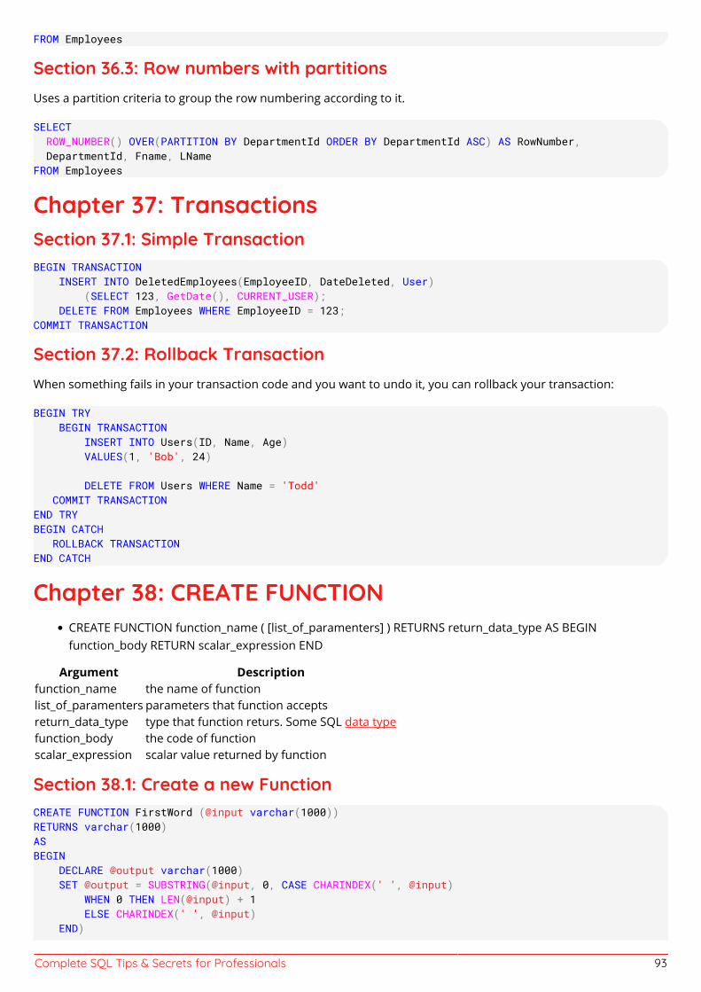
Complete SQL Tips & Secrets for Professionals 93

FROM Employees

Section 36.3: Row numbers with partitionsUses a partition criteria to group the row numbering according to it.

SELECT ROW_NUMBER() OVER(PARTITION BY DepartmentId ORDER BY DepartmentId ASC) AS RowNumber, DepartmentId, Fname, LNameFROM Employees

Chapter 37: TransactionsSection 37.1: Simple TransactionBEGIN TRANSACTION INSERT INTO DeletedEmployees(EmployeeID, DateDeleted, User) (SELECT 123, GetDate(), CURRENT_USER); DELETE FROM Employees WHERE EmployeeID = 123;COMMIT TRANSACTION

Section 37.2: Rollback TransactionWhen something fails in your transaction code and you want to undo it, you can rollback your transaction:

BEGIN TRY BEGIN TRANSACTION INSERT INTO Users(ID, Name, Age) VALUES(1, 'Bob', 24) DELETE FROM Users WHERE Name = 'Todd' COMMIT TRANSACTIONEND TRYBEGIN CATCH ROLLBACK TRANSACTIONEND CATCH

Chapter 38: CREATE FUNCTIONCREATE FUNCTION function_name ( [list_of_paramenters] ) RETURNS return_data_type AS BEGINfunction_body RETURN scalar_expression END

Argument Descriptionfunction_name the name of functionlist_of_paramenters parameters that function acceptsreturn_data_type type that function returs. Some SQL data typefunction_body the code of functionscalar_expression scalar value returned by function

Section 38.1: Create a new FunctionCREATE FUNCTION FirstWord (@input varchar(1000))RETURNS varchar(1000)ASBEGIN DECLARE @output varchar(1000) SET @output = SUBSTRING(@input, 0, CASE CHARINDEX(' ', @input) WHEN 0 THEN LEN(@input) + 1 ELSE CHARINDEX(' ', @input) END)

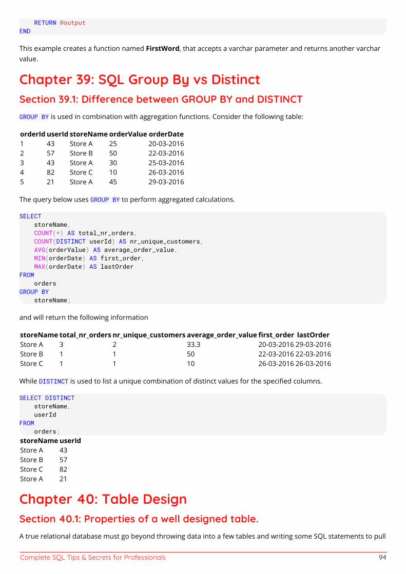
Complete SQL Tips & Secrets for Professionals 94

RETURN @outputEND

This example creates a function named FirstWord, that accepts a varchar parameter and returns another varcharvalue.

Chapter 39: SQL Group By vs DistinctSection 39.1: Dierence between GROUP BY and DISTINCTGROUP BY is used in combination with aggregation functions. Consider the following table:

orderId userId storeName orderValue orderDate1 43 Store A 25 20-03-20162 57 Store B 50 22-03-20163 43 Store A 30 25-03-20164 82 Store C 10 26-03-20165 21 Store A 45 29-03-2016

The query below uses GROUP BY to perform aggregated calculations.

SELECT storeName, COUNT(*) AS total_nr_orders, COUNT(DISTINCT userId) AS nr_unique_customers, AVG(orderValue) AS average_order_value, MIN(orderDate) AS first_order, MAX(orderDate) AS lastOrderFROM ordersGROUP BY storeName;

and will return the following information

storeName total_nr_orders nr_unique_customers average_order_value first_order lastOrderStore A 3 2 33.3 20-03-2016 29-03-2016Store B 1 1 50 22-03-2016 22-03-2016Store C 1 1 10 26-03-2016 26-03-2016

While DISTINCT is used to list a unique combination of distinct values for the specified columns.

SELECT DISTINCT storeName, userIdFROM orders;storeName userIdStore A 43Store B 57Store C 82Store A 21

Chapter 40: Table DesignSection 40.1: Properties of a well designed table.A true relational database must go beyond throwing data into a few tables and writing some SQL statements to pull

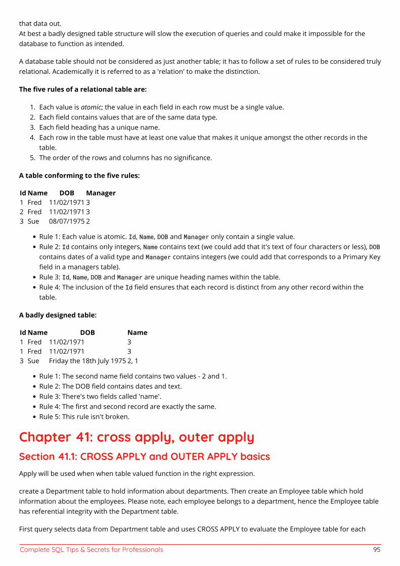
Complete SQL Tips & Secrets for Professionals 95

that data out.At best a badly designed table structure will slow the execution of queries and could make it impossible for thedatabase to function as intended.

A database table should not be considered as just another table; it has to follow a set of rules to be considered trulyrelational. Academically it is referred to as a 'relation' to make the distinction.

The five rules of a relational table are:

Each value is atomic; the value in each field in each row must be a single value.1.Each field contains values that are of the same data type.2.Each field heading has a unique name.3.Each row in the table must have at least one value that makes it unique amongst the other records in the4.table.The order of the rows and columns has no significance.5.

A table conforming to the five rules:

Id Name DOB Manager1 Fred 11/02/1971 32 Fred 11/02/1971 33 Sue 08/07/1975 2

Rule 1: Each value is atomic. Id, Name, DOB and Manager only contain a single value.Rule 2: Id contains only integers, Name contains text (we could add that it's text of four characters or less), DOBcontains dates of a valid type and Manager contains integers (we could add that corresponds to a Primary Keyfield in a managers table).Rule 3: Id, Name, DOB and Manager are unique heading names within the table.Rule 4: The inclusion of the Id field ensures that each record is distinct from any other record within thetable.

A badly designed table:

Id Name DOB Name1 Fred 11/02/1971 31 Fred 11/02/1971 33 Sue Friday the 18th July 1975 2, 1

Rule 1: The second name field contains two values - 2 and 1.Rule 2: The DOB field contains dates and text.Rule 3: There's two fields called 'name'.Rule 4: The first and second record are exactly the same.Rule 5: This rule isn't broken.

Chapter 41: cross apply, outer applySection 41.1: CROSS APPLY and OUTER APPLY basicsApply will be used when when table valued function in the right expression.

create a Department table to hold information about departments. Then create an Employee table which holdinformation about the employees. Please note, each employee belongs to a department, hence the Employee tablehas referential integrity with the Department table.

First query selects data from Department table and uses CROSS APPLY to evaluate the Employee table for each

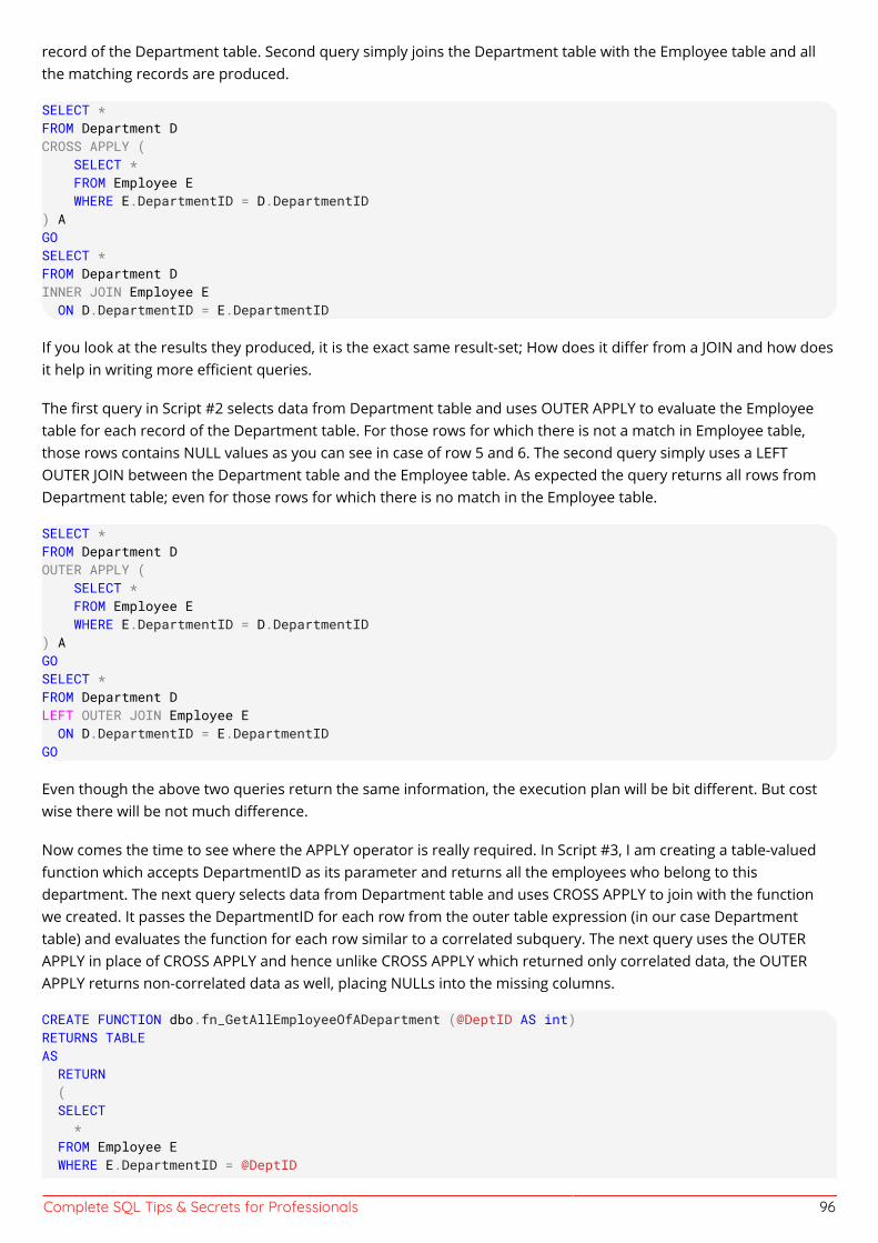
Complete SQL Tips & Secrets for Professionals 96

record of the Department table. Second query simply joins the Department table with the Employee table and allthe matching records are produced.

SELECT *FROM Department DCROSS APPLY ( SELECT * FROM Employee E WHERE E.DepartmentID = D.DepartmentID) AGOSELECT *FROM Department DINNER JOIN Employee E ON D.DepartmentID = E.DepartmentID

If you look at the results they produced, it is the exact same result-set; How does it differ from a JOIN and how doesit help in writing more efficient queries.

The first query in Script #2 selects data from Department table and uses OUTER APPLY to evaluate the Employeetable for each record of the Department table. For those rows for which there is not a match in Employee table,those rows contains NULL values as you can see in case of row 5 and 6. The second query simply uses a LEFTOUTER JOIN between the Department table and the Employee table. As expected the query returns all rows fromDepartment table; even for those rows for which there is no match in the Employee table.

SELECT *FROM Department DOUTER APPLY ( SELECT * FROM Employee E WHERE E.DepartmentID = D.DepartmentID) AGOSELECT *FROM Department DLEFT OUTER JOIN Employee E ON D.DepartmentID = E.DepartmentIDGO

Even though the above two queries return the same information, the execution plan will be bit different. But costwise there will be not much difference.

Now comes the time to see where the APPLY operator is really required. In Script #3, I am creating a table-valuedfunction which accepts DepartmentID as its parameter and returns all the employees who belong to thisdepartment. The next query selects data from Department table and uses CROSS APPLY to join with the functionwe created. It passes the DepartmentID for each row from the outer table expression (in our case Departmenttable) and evaluates the function for each row similar to a correlated subquery. The next query uses the OUTERAPPLY in place of CROSS APPLY and hence unlike CROSS APPLY which returned only correlated data, the OUTERAPPLY returns non-correlated data as well, placing NULLs into the missing columns.

CREATE FUNCTION dbo.fn_GetAllEmployeeOfADepartment (@DeptID AS int)RETURNS TABLEAS RETURN ( SELECT * FROM Employee E WHERE E.DepartmentID = @DeptID

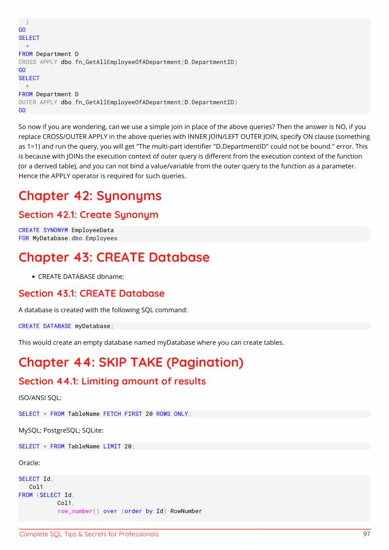
Complete SQL Tips & Secrets for Professionals 97

)GOSELECT *FROM Department DCROSS APPLY dbo.fn_GetAllEmployeeOfADepartment(D.DepartmentID)GOSELECT *FROM Department DOUTER APPLY dbo.fn_GetAllEmployeeOfADepartment(D.DepartmentID)GO

So now if you are wondering, can we use a simple join in place of the above queries? Then the answer is NO, if youreplace CROSS/OUTER APPLY in the above queries with INNER JOIN/LEFT OUTER JOIN, specify ON clause (somethingas 1=1) and run the query, you will get "The multi-part identifier "D.DepartmentID" could not be bound." error. Thisis because with JOINs the execution context of outer query is different from the execution context of the function(or a derived table), and you can not bind a value/variable from the outer query to the function as a parameter.Hence the APPLY operator is required for such queries.

Chapter 42: SynonymsSection 42.1: Create SynonymCREATE SYNONYM EmployeeDataFOR MyDatabase.dbo.Employees

Chapter 43: CREATE DatabaseCREATE DATABASE dbname;

Section 43.1: CREATE DatabaseA database is created with the following SQL command:

CREATE DATABASE myDatabase;

This would create an empty database named myDatabase where you can create tables.

Chapter 44: SKIP TAKE (Pagination)Section 44.1: Limiting amount of resultsISO/ANSI SQL:

SELECT * FROM TableName FETCH FIRST 20 ROWS ONLY;

MySQL; PostgreSQL; SQLite:

SELECT * FROM TableName LIMIT 20;

Oracle:

SELECT Id, Col1FROM (SELECT Id, Col1, row_number() over (order by Id) RowNumber

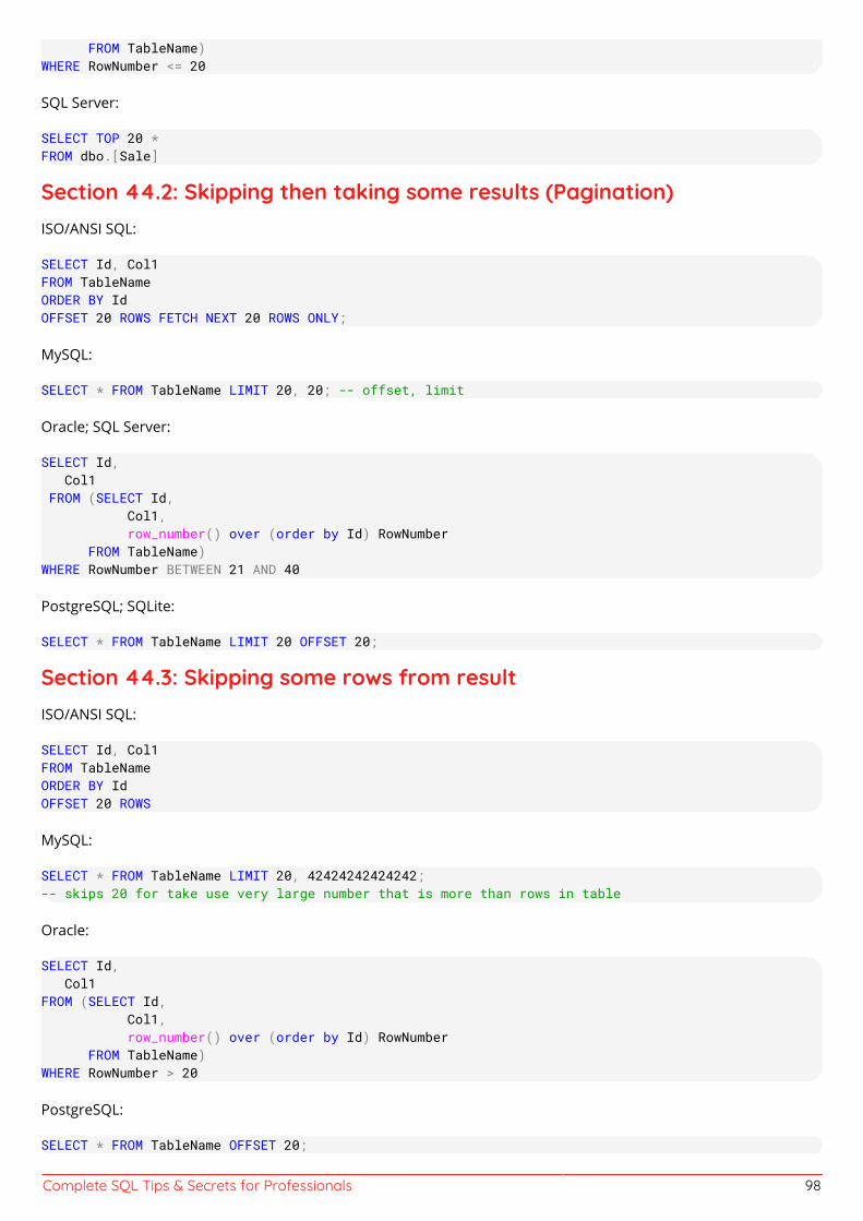
Complete SQL Tips & Secrets for Professionals 98

FROM TableName)WHERE RowNumber <= 20

SQL Server:

SELECT TOP 20 *FROM dbo.[Sale]

Section 44.2: Skipping then taking some results (Pagination)ISO/ANSI SQL:

SELECT Id, Col1FROM TableNameORDER BY IdOFFSET 20 ROWS FETCH NEXT 20 ROWS ONLY;

MySQL:

SELECT * FROM TableName LIMIT 20, 20; -- offset, limit

Oracle; SQL Server:

SELECT Id, Col1 FROM (SELECT Id, Col1, row_number() over (order by Id) RowNumber FROM TableName)WHERE RowNumber BETWEEN 21 AND 40

PostgreSQL; SQLite:

SELECT * FROM TableName LIMIT 20 OFFSET 20;

Section 44.3: Skipping some rows from resultISO/ANSI SQL:

SELECT Id, Col1FROM TableNameORDER BY IdOFFSET 20 ROWS

MySQL:

SELECT * FROM TableName LIMIT 20, 42424242424242;-- skips 20 for take use very large number that is more than rows in table

Oracle:

SELECT Id, Col1FROM (SELECT Id, Col1, row_number() over (order by Id) RowNumber FROM TableName)WHERE RowNumber > 20

PostgreSQL:

SELECT * FROM TableName OFFSET 20;

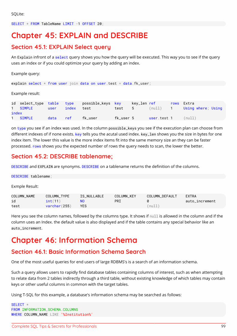
Complete SQL Tips & Secrets for Professionals 99

SQLite:

SELECT * FROM TableName LIMIT -1 OFFSET 20;

Chapter 45: EXPLAIN and DESCRIBESection 45.1: EXPLAIN Select queryAn Explain infront of a select query shows you how the query will be executed. This way you to see if the queryuses an index or if you could optimize your query by adding an index.

Example query:

explain select * from user join data on user.test = data.fk_user;

Example result:

id select_type table type possible_keys key key_len ref rows Extra1 SIMPLE user index test test 5 (null) 1 Using where; Usingindex1 SIMPLE data ref fk_user fk_user 5 user.test 1 (null)

on type you see if an index was used. In the column possible_keys you see if the execution plan can choose fromdifferent indexes of if none exists. key tells you the acutal used index. key_len shows you the size in bytes for oneindex item. The lower this value is the more index items fit into the same memory size an they can be fasterprocessed. rows shows you the expected number of rows the query needs to scan, the lower the better.

Section 45.2: DESCRIBE tablename;DESCRIBE and EXPLAIN are synonyms. DESCRIBE on a tablename returns the definition of the columns.

DESCRIBE tablename;

Exmple Result:

COLUMN_NAME COLUMN_TYPE IS_NULLABLE COLUMN_KEY COLUMN_DEFAULT EXTRAid int(11) NO PRI 0 auto_incrementtest varchar(255) YES (null)

Here you see the column names, followed by the columns type. It shows if null is allowed in the column and if thecolumn uses an Index. the default value is also displayed and if the table contains any special behavior like anauto_increment.

Chapter 46: Information SchemaSection 46.1: Basic Information Schema SearchOne of the most useful queries for end users of large RDBMS's is a search of an information schema.

Such a query allows users to rapidly find database tables containing columns of interest, such as when attemptingto relate data from 2 tables indirectly through a third table, without existing knowledge of which tables may containkeys or other useful columns in common with the target tables.

Using T-SQL for this example, a database's information schema may be searched as follows:

SELECT *FROM INFORMATION_SCHEMA.COLUMNSWHERE COLUMN_NAME LIKE '%Institution%'

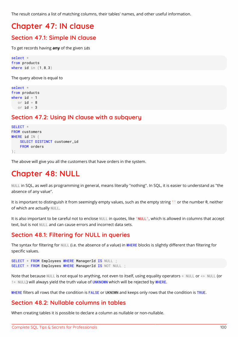
Complete SQL Tips & Secrets for Professionals 100

The result contains a list of matching columns, their tables' names, and other useful information.

Chapter 47: IN clauseSection 47.1: Simple IN clauseTo get records having any of the given ids

select *from productswhere id in (1,8,3)

The query above is equal to

select *from productswhere id = 1 or id = 8 or id = 3

Section 47.2: Using IN clause with a subquerySELECT *FROM customersWHERE id IN ( SELECT DISTINCT customer_id FROM orders);

The above will give you all the customers that have orders in the system.

Chapter 48: NULLNULL in SQL, as well as programming in general, means literally "nothing". In SQL, it is easier to understand as "theabsence of any value".

It is important to distinguish it from seemingly empty values, such as the empty string '' or the number 0, neitherof which are actually NULL.

It is also important to be careful not to enclose NULL in quotes, like 'NULL', which is allowed in columns that accepttext, but is not NULL and can cause errors and incorrect data sets.

Section 48.1: Filtering for NULL in queriesThe syntax for filtering for NULL (i.e. the absence of a value) in WHERE blocks is slightly different than filtering forspecific values.

SELECT * FROM Employees WHERE ManagerId IS NULL ;SELECT * FROM Employees WHERE ManagerId IS NOT NULL ;

Note that because NULL is not equal to anything, not even to itself, using equality operators = NULL or <> NULL (or!= NULL) will always yield the truth value of UNKNOWN which will be rejected by WHERE.

WHERE filters all rows that the condition is FALSE or UKNOWN and keeps only rows that the condition is TRUE.

Section 48.2: Nullable columns in tablesWhen creating tables it is possible to declare a column as nullable or non-nullable.

Complete SQL Tips & Secrets for Professionals 101

CREATE TABLE MyTable( MyCol1 INT NOT NULL, -- non-nullable MyCol2 INT NULL -- nullable) ;

By default every column (except those in primary key constraint) is nullable unless we explicitly set NOT NULLconstraint.

Attempting to assign NULL to a non-nullable column will result in an error.

INSERT INTO MyTable (MyCol1, MyCol2) VALUES (1, NULL) ; -- works fine

INSERT INTO MyTable (MyCol1, MyCol2) VALUES (NULL, 2) ; -- cannot insert -- the value NULL into column 'MyCol1', table 'MyTable'; -- column does not allow nulls. INSERT fails.

Section 48.3: Updating fields to NULLSetting a field to NULL works exactly like with any other value:

UPDATE EmployeesSET ManagerId = NULLWHERE Id = 4

Section 48.4: Inserting rows with NULL fieldsFor example inserting an employee with no phone number and no manager into the Employees example table:

INSERT INTO Employees (Id, FName, LName, PhoneNumber, ManagerId, DepartmentId, Salary, HireDate)VALUES (5, 'Jane', 'Doe', NULL, NULL, 2, 800, '2016-07-22') ;

Chapter 49: SQL InjectionSQL injection is an attempt to access a website's database tables by injecting SQL into a form field. If a web serverdoes not protect against SQL injection attacks, a hacker can trick the database into running the additional SQL code.By executing their own SQL code, hackers can upgrade their account access, view someone else's privateinformation, or make any other modifications to the database.

Section 49.1: SQL injection sampleAssuming the call to your web application's login handler looks like this:

https://somepage.com/ajax/login.ashx?username=admin&password=123

Now in login.ashx, you read these values:

strUserName = getHttpsRequestParameterString("username");strPassword = getHttpsRequestParameterString("password");

and query your database to determine whether a user with that password exists.

So you construct an SQL query string:

txtSQL = "SELECT * FROM Users WHERE username = '" + strUserName + "' AND password = '"+ strPassword+"'";

Complete SQL Tips & Secrets for Professionals 102

This will work if the username and password do not contain a quote.

However, if one of the parameters does contain a quote, the SQL that gets sent to the database will look like this:

-- strUserName = "d'Alambert";txtSQL = "SELECT * FROM Users WHERE username = 'd'Alambert' AND password = '123'";

This will result in a syntax error, because the quote after the d in d'Alambert ends the SQL string.

You could correct this by escaping quotes in username and password, e.g.:

strUserName = strUserName.Replace("'", "''");strPassword = strPassword.Replace("'", "''");

However, it's more appropriate to use parameters:

cmd.CommandText = "SELECT * FROM Users WHERE username = @username AND password = @password";

cmd.Parameters.Add("@username", strUserName);cmd.Parameters.Add("@password", strPassword);

If you do not use parameters, and forget to replace quote in even one of the values, then a malicious user (akahacker) can use this to execute SQL commands on your database.

For example, if an attacker is evil, he/she will set the password to

lol'; DROP DATABASE master; --

and then the SQL will look like this:

"SELECT * FROM Users WHERE username = 'somebody' AND password = 'lol'; DROP DATABASE master; --'";

Unfortunately for you, this is valid SQL, and the DB will execute this!

This type of exploit is called an SQL injection.

There are many other things a malicious user could do, such as stealing every user's email address, steal everyone'spassword, steal credit card numbers, steal any amount of data in your database, etc.

This is why you always need to escape your strings.And the fact that you'll invariably forget to do so sooner or later is exactly why you should use parameters. Becauseif you use parameters, then your programming language framework will do any necessary escaping for you.

Section 49.2: simple injection sampleIf the SQL statement is constructed like this:

SQL = "SELECT * FROM Users WHERE username = '" + user + "' AND password ='" + pw + "'";db.execute(SQL);

Then a hacker could retrieve your data by giving a password like pw' or '1'='1; the resulting SQL statement willbe:

SELECT * FROM Users WHERE username = 'somebody' AND password ='pw' or '1'='1'

This one will pass the password check for all rows in the Users table because '1'='1' is always true.

To prevent this, use SQL parameters:

SQL = "SELECT * FROM Users WHERE username = ? AND password = ?";

Complete SQL Tips & Secrets for Professionals 103

db.execute(SQL, [user, pw]);

Chapter 50: Cascading DeleteSection 50.1: ON DELETE CASCADEAssume you have a application that administers rooms.Assume further that your application operates on a per client basis (tenant).You have several clients.So your database will contain one table for clients, and one for rooms.

Now, every client has N rooms.

This should mean that you have a foreign key on your room table, referencing the client table.

ALTER TABLE dbo.T_Room WITH CHECK ADD CONSTRAINT FK_T_Room_T_Client FOREIGN KEY(RM_CLI_ID)REFERENCES dbo.T_Client (CLI_ID)GO

Assuming a client moves on to some other software, you'll have to delete his data in your software. But if you do

DELETE FROM T_Client WHERE CLI_ID = x

Then you'll get a foreign key violation, because you can't delete the client when he still has rooms.

Now you'd have write code in your application that deletes the client's rooms before it deletes the client. Assumefurther that in the future, many more foreign key dependencies will be added in your database, because yourapplication's functionality expands. Horrible. For every modification in your database, you'll have to adapt yourapplication's code in N places. Possibly you'll have to adapt code in other applications as well (e.g. interfaces toother systems).

There is a better solution than doing it in your code.You can just add ON DELETE CASCADE to your foreign key.

ALTER TABLE dbo.T_Room -- WITH CHECK -- SQL-Server can specify WITH CHECK/WITH NOCHECKADD CONSTRAINT FK_T_Room_T_Client FOREIGN KEY(RM_CLI_ID)REFERENCES dbo.T_Client (CLI_ID)ON DELETE CASCADE

Now you can say

DELETE FROM T_Client WHERE CLI_ID = x

and the rooms are automagically deleted when the client is deleted.Problem solved - with no application code changes.

One word of caution: In Microsoft SQL-Server, this won't work if you have a table that references itselfs. So if you tryto define a delete cascade on a recursive tree structure, like this:

IF NOT EXISTS (SELECT * FROM sys.foreign_keys WHERE object_id =OBJECT_ID(N'[dbo].[FK_T_FMS_Navigation_T_FMS_Navigation]') AND parent_object_id =OBJECT_ID(N'[dbo].[T_FMS_Navigation]'))ALTER TABLE [dbo].[T_FMS_Navigation] WITH CHECK ADD CONSTRAINT[FK_T_FMS_Navigation_T_FMS_Navigation] FOREIGN KEY([NA_NA_UID])REFERENCES [dbo].[T_FMS_Navigation] ([NA_UID])ON DELETE CASCADEGO

Complete SQL Tips & Secrets for Professionals 104

IF EXISTS (SELECT * FROM sys.foreign_keys WHERE object_id =OBJECT_ID(N'[dbo].[FK_T_FMS_Navigation_T_FMS_Navigation]') AND parent_object_id =OBJECT_ID(N'[dbo].[T_FMS_Navigation]'))ALTER TABLE [dbo].[T_FMS_Navigation] CHECK CONSTRAINT [FK_T_FMS_Navigation_T_FMS_Navigation]GO

it won't work, because Microsoft-SQL-server doesn't allow you to set a foreign key with ON DELETE CASCADE on arecursive tree structure. One reason for this is, that the tree is possibly cyclic, and that would possibly lead to adeadlock.

PostgreSQL on the other hand can do this;the requirement is that the tree is non-cyclic.If the tree is cyclic, you'll get a runtime error.In that case, you'll just have to implement the delete function yourselfs.

A word of caution:This means you can't simply delete and re-insert the client table anymore, because if you do this, it will delete allentries in "T_Room"... (no non-delta updates anymore)

Chapter 51: Order of ExecutionSection 51.1: Logical Order of Query Processing in SQL/*(8)*/ SELECT /*9*/ DISTINCT /*11*/ TOP /*(1)*/ FROM/*(3)*/ JOIN/*(2)*/ ON/*(4)*/ WHERE/*(5)*/ GROUP BY/*(6)*/ WITH {CUBE | ROLLUP}/*(7)*/ HAVING/*(10)*/ ORDER BY/*(11)*/ LIMIT

The order in which a query is processed and description of each section.

VT stands for 'Virtual Table' and shows how various data is produced as the query is processed

FROM: A Cartesian product (cross join) is performed between the first two tables in the FROM clause, and as1.a result, virtual table VT1 is generated.

ON: The ON filter is applied to VT1. Only rows for which the is TRUE are inserted to VT2.2.

OUTER (join): If an OUTER JOIN is specified (as opposed to a CROSS JOIN or an INNER JOIN), rows from the3.preserved table or tables for which a match was not found are added to the rows from VT2 as outer rows,generating VT3. If more than two tables appear in the FROM clause, steps 1 through 3 are applied repeatedlybetween the result of the last join and the next table in the FROM clause until all tables are processed.

WHERE: The WHERE filter is applied to VT3. Only rows for which the is TRUE are inserted to VT4.4.

GROUP BY: The rows from VT4 are arranged in groups based on the column list specified in the GROUP BY5.clause. VT5 is generated.

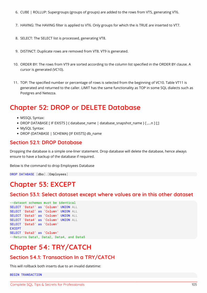
Complete SQL Tips & Secrets for Professionals 105

CUBE | ROLLUP: Supergroups (groups of groups) are added to the rows from VT5, generating VT6.6.

HAVING: The HAVING filter is applied to VT6. Only groups for which the is TRUE are inserted to VT7.7.

SELECT: The SELECT list is processed, generating VT8.8.

DISTINCT: Duplicate rows are removed from VT8. VT9 is generated.9.

ORDER BY: The rows from VT9 are sorted according to the column list specified in the ORDER BY clause. A10.cursor is generated (VC10).

TOP: The specified number or percentage of rows is selected from the beginning of VC10. Table VT11 is11.generated and returned to the caller. LIMIT has the same functionality as TOP in some SQL dialects such asPostgres and Netezza.

Chapter 52: DROP or DELETE DatabaseMSSQL Syntax:DROP DATABASE [ IF EXISTS ] { database_name | database_snapshot_name } [ ,...n ] [;]MySQL Syntax:DROP {DATABASE | SCHEMA} [IF EXISTS] db_name

Section 52.1: DROP DatabaseDropping the database is a simple one-liner statement. Drop database will delete the database, hence alwaysensure to have a backup of the database if required.

Below is the command to drop Employees Database

DROP DATABASE [dbo].[Employees]

Chapter 53: EXCEPTSection 53.1: Select dataset except where values are in this other dataset--dataset schemas must be identicalSELECT 'Data1' as 'Column' UNION ALLSELECT 'Data2' as 'Column' UNION ALLSELECT 'Data3' as 'Column' UNION ALLSELECT 'Data4' as 'Column' UNION ALLSELECT 'Data5' as 'Column'EXCEPTSELECT 'Data3' as 'Column'--Returns Data1, Data2, Data4, and Data5

Chapter 54: TRY/CATCHSection 54.1: Transaction In a TRY/CATCHThis will rollback both inserts due to an invalid datetime:

BEGIN TRANSACTION

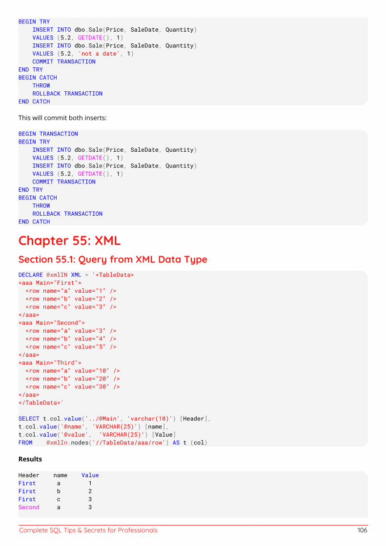
Complete SQL Tips & Secrets for Professionals 106

BEGIN TRY INSERT INTO dbo.Sale(Price, SaleDate, Quantity) VALUES (5.2, GETDATE(), 1) INSERT INTO dbo.Sale(Price, SaleDate, Quantity) VALUES (5.2, 'not a date', 1) COMMIT TRANSACTIONEND TRYBEGIN CATCH THROW ROLLBACK TRANSACTIONEND CATCH

This will commit both inserts:

BEGIN TRANSACTIONBEGIN TRY INSERT INTO dbo.Sale(Price, SaleDate, Quantity) VALUES (5.2, GETDATE(), 1) INSERT INTO dbo.Sale(Price, SaleDate, Quantity) VALUES (5.2, GETDATE(), 1) COMMIT TRANSACTIONEND TRYBEGIN CATCH THROW ROLLBACK TRANSACTIONEND CATCH

Chapter 55: XMLSection 55.1: Query from XML Data TypeDECLARE @xmlIN XML = '<TableData><aaa Main="First"> <row name="a" value="1" /> <row name="b" value="2" /> <row name="c" value="3" /></aaa><aaa Main="Second"> <row name="a" value="3" /> <row name="b" value="4" /> <row name="c" value="5" /></aaa><aaa Main="Third"> <row name="a" value="10" /> <row name="b" value="20" /> <row name="c" value="30" /></aaa></TableData>'

SELECT t.col.value('../@Main', 'varchar(10)') [Header],t.col.value('@name', 'VARCHAR(25)') [name], t.col.value('@value', 'VARCHAR(25)') [Value]FROM @xmlIn.nodes('//TableData/aaa/row') AS t (col)

Results

Header name ValueFirst a 1First b 2First c 3Second a 3

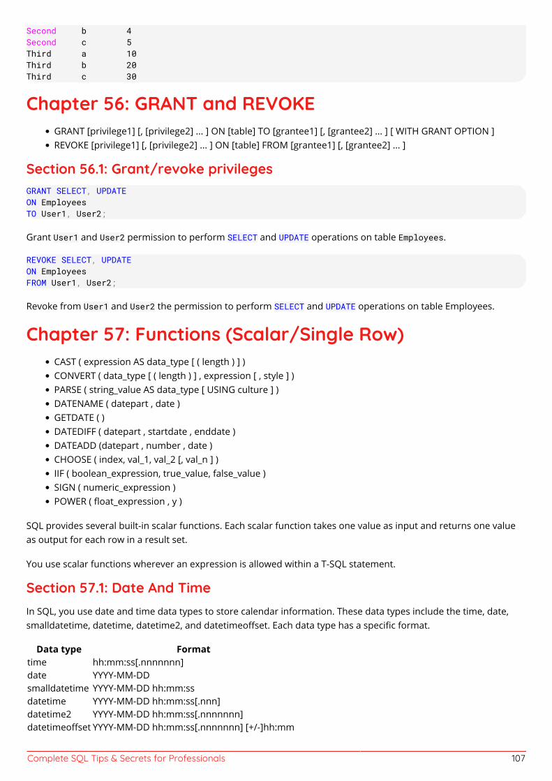
Complete SQL Tips & Secrets for Professionals 107

Second b 4Second c 5Third a 10Third b 20Third c 30

Chapter 56: GRANT and REVOKEGRANT [privilege1] [, [privilege2] ... ] ON [table] TO [grantee1] [, [grantee2] ... ] [ WITH GRANT OPTION ]REVOKE [privilege1] [, [privilege2] ... ] ON [table] FROM [grantee1] [, [grantee2] ... ]

Section 56.1: Grant/revoke privilegesGRANT SELECT, UPDATEON EmployeesTO User1, User2;

Grant User1 and User2 permission to perform SELECT and UPDATE operations on table Employees.

REVOKE SELECT, UPDATEON EmployeesFROM User1, User2;

Revoke from User1 and User2 the permission to perform SELECT and UPDATE operations on table Employees.

Chapter 57: Functions (Scalar/Single Row)CAST ( expression AS data_type [ ( length ) ] )CONVERT ( data_type [ ( length ) ] , expression [ , style ] )PARSE ( string_value AS data_type [ USING culture ] )DATENAME ( datepart , date )GETDATE ( )DATEDIFF ( datepart , startdate , enddate )DATEADD (datepart , number , date )CHOOSE ( index, val_1, val_2 [, val_n ] )IIF ( boolean_expression, true_value, false_value )SIGN ( numeric_expression )POWER ( float_expression , y )

SQL provides several built-in scalar functions. Each scalar function takes one value as input and returns one valueas output for each row in a result set.

You use scalar functions wherever an expression is allowed within a T-SQL statement.

Section 57.1: Date And TimeIn SQL, you use date and time data types to store calendar information. These data types include the time, date,smalldatetime, datetime, datetime2, and datetimeoffset. Each data type has a specific format.

Data type Formattime hh:mm:ss[.nnnnnnn]date YYYY-MM-DDsmalldatetime YYYY-MM-DD hh:mm:ssdatetime YYYY-MM-DD hh:mm:ss[.nnn]datetime2 YYYY-MM-DD hh:mm:ss[.nnnnnnn]datetimeoffset YYYY-MM-DD hh:mm:ss[.nnnnnnn] [+/-]hh:mm

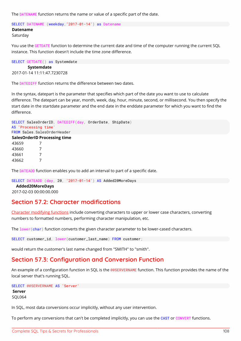
Complete SQL Tips & Secrets for Professionals 108

The DATENAME function returns the name or value of a specific part of the date.

SELECT DATENAME (weekday,'2017-01-14') as DatenameDatenameSaturday

You use the GETDATE function to determine the current date and time of the computer running the current SQLinstance. This function doesn't include the time zone difference.

SELECT GETDATE() as SystemdateSystemdate

2017-01-14 11:11:47.7230728

The DATEDIFF function returns the difference between two dates.

In the syntax, datepart is the parameter that specifies which part of the date you want to use to calculatedifference. The datepart can be year, month, week, day, hour, minute, second, or millisecond. You then specify thestart date in the startdate parameter and the end date in the enddate parameter for which you want to find thedifference.

SELECT SalesOrderID, DATEDIFF(day, OrderDate, ShipDate)AS 'Processing time'FROM Sales.SalesOrderHeaderSalesOrderID Processing time43659 743660 743661 743662 7

The DATEADD function enables you to add an interval to part of a specific date.

SELECT DATEADD (day, 20, '2017-01-14') AS Added20MoreDaysAdded20MoreDays

2017-02-03 00:00:00.000

Section 57.2: Character modificationsCharacter modifying functions include converting characters to upper or lower case characters, convertingnumbers to formatted numbers, performing character manipulation, etc.

The lower(char) function converts the given character parameter to be lower-cased characters.

SELECT customer_id, lower(customer_last_name) FROM customer;

would return the customer's last name changed from "SMITH" to "smith".

Section 57.3: Configuration and Conversion FunctionAn example of a configuration function in SQL is the @@SERVERNAME function. This function provides the name of thelocal server that's running SQL.

SELECT @@SERVERNAME AS 'Server'ServerSQL064

In SQL, most data conversions occur implicitly, without any user intervention.

To perform any conversions that can't be completed implicitly, you can use the CAST or CONVERT functions.

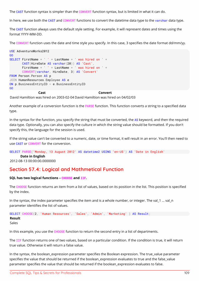
Complete SQL Tips & Secrets for Professionals 109

The CAST function syntax is simpler than the CONVERT function syntax, but is limited in what it can do.

In here, we use both the CAST and CONVERT functions to convert the datetime data type to the varchar data type.

The CAST function always uses the default style setting. For example, it will represent dates and times using theformat YYYY-MM-DD.

The CONVERT function uses the date and time style you specify. In this case, 3 specifies the date format dd/mm/yy.

USE AdventureWorks2012GOSELECT FirstName + ' ' + LastName + ' was hired on ' + CAST(HireDate AS varchar(20)) AS 'Cast', FirstName + ' ' + LastName + ' was hired on ' + CONVERT(varchar, HireDate, 3) AS 'Convert'FROM Person.Person AS pJOIN HumanResources.Employee AS eON p.BusinessEntityID = e.BusinessEntityIDGO

Cast ConvertDavid Hamiltion was hired on 2003-02-04 David Hamiltion was hired on 04/02/03

Another example of a conversion function is the PARSE function. This function converts a string to a specified datatype.

In the syntax for the function, you specify the string that must be converted, the AS keyword, and then the requireddata type. Optionally, you can also specify the culture in which the string value should be formatted. If you don'tspecify this, the language for the session is used.

If the string value can't be converted to a numeric, date, or time format, it will result in an error. You'll then need touse CAST or CONVERT for the conversion.

SELECT PARSE('Monday, 13 August 2012' AS datetime2 USING 'en-US') AS 'Date in English'Date in English

2012-08-13 00:00:00.0000000

Section 57.4: Logical and Mathmetical FunctionSQL has two logical functions – CHOOSE and IIF.

The CHOOSE function returns an item from a list of values, based on its position in the list. This position is specifiedby the index.

In the syntax, the index parameter specifies the item and is a whole number, or integer. The val_1 … val_nparameter identifies the list of values.

SELECT CHOOSE(2, 'Human Resources', 'Sales', 'Admin', 'Marketing' ) AS Result;ResultSales

In this example, you use the CHOOSE function to return the second entry in a list of departments.

The IIF function returns one of two values, based on a particular condition. If the condition is true, it will returntrue value. Otherwise it will return a false value.

In the syntax, the boolean_expression parameter specifies the Boolean expression. The true_value parameterspecifies the value that should be returned if the boolean_expression evaluates to true and the false_valueparameter specifies the value that should be returned if the boolean_expression evaluates to false.

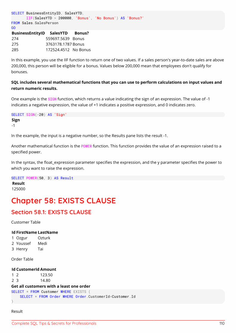
Complete SQL Tips & Secrets for Professionals 110

SELECT BusinessEntityID, SalesYTD, IIF(SalesYTD > 200000, 'Bonus', 'No Bonus') AS 'Bonus?'FROM Sales.SalesPersonGOBusinessEntityID SalesYTD Bonus?274 559697.5639 Bonus275 3763178.1787 Bonus285 172524.4512 No Bonus

In this example, you use the IIF function to return one of two values. If a sales person's year-to-date sales are above200,000, this person will be eligible for a bonus. Values below 200,000 mean that employees don't qualify forbonuses.

SQL includes several mathematical functions that you can use to perform calculations on input values andreturn numeric results.

One example is the SIGN function, which returns a value indicating the sign of an expression. The value of -1indicates a negative expression, the value of +1 indicates a positive expression, and 0 indicates zero.

SELECT SIGN(-20) AS 'Sign'Sign-1

In the example, the input is a negative number, so the Results pane lists the result -1.

Another mathematical function is the POWER function. This function provides the value of an expression raised to aspecified power.

In the syntax, the float_expression parameter specifies the expression, and the y parameter specifies the power towhich you want to raise the expression.

SELECT POWER(50, 3) AS ResultResult125000

Chapter 58: EXISTS CLAUSESection 58.1: EXISTS CLAUSECustomer Table

Id FirstName LastName1 Ozgur Ozturk2 Youssef Medi3 Henry Tai

Order Table

Id CustomerId Amount1 2 123.502 3 14.80Get all customers with a least one orderSELECT * FROM Customer WHERE EXISTS ( SELECT * FROM Order WHERE Order.CustomerId=Customer.Id)

Result

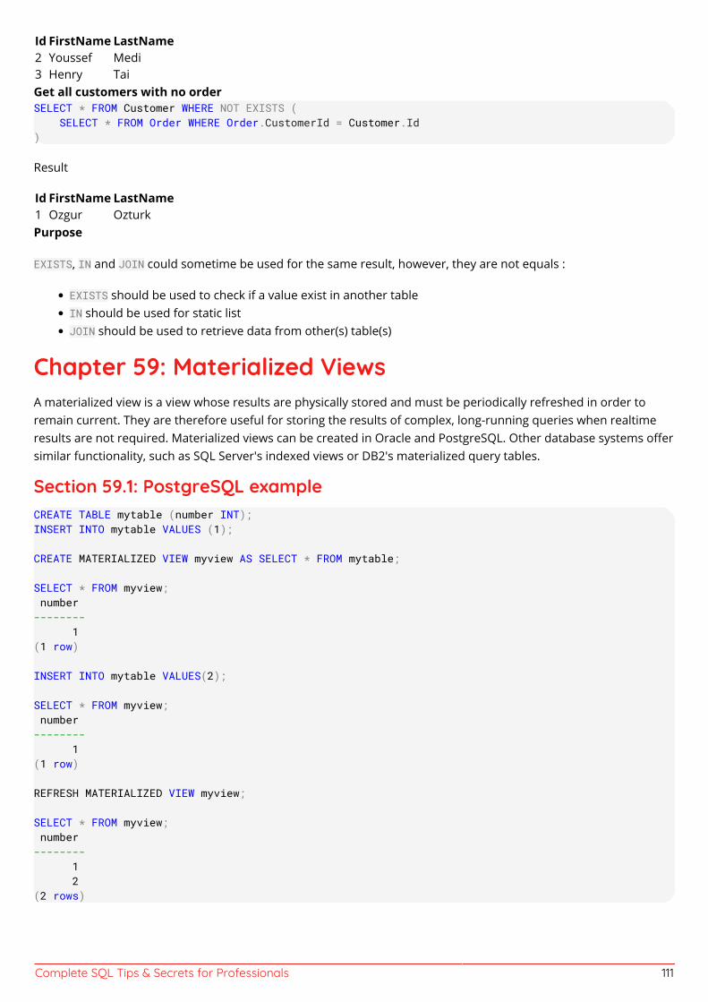
Complete SQL Tips & Secrets for Professionals 111

Id FirstName LastName2 Youssef Medi3 Henry TaiGet all customers with no orderSELECT * FROM Customer WHERE NOT EXISTS ( SELECT * FROM Order WHERE Order.CustomerId = Customer.Id)

Result

Id FirstName LastName1 Ozgur OzturkPurpose

EXISTS, IN and JOIN could sometime be used for the same result, however, they are not equals :

EXISTS should be used to check if a value exist in another tableIN should be used for static listJOIN should be used to retrieve data from other(s) table(s)

Chapter 59: Materialized ViewsA materialized view is a view whose results are physically stored and must be periodically refreshed in order toremain current. They are therefore useful for storing the results of complex, long-running queries when realtimeresults are not required. Materialized views can be created in Oracle and PostgreSQL. Other database systems offersimilar functionality, such as SQL Server's indexed views or DB2's materialized query tables.

Section 59.1: PostgreSQL exampleCREATE TABLE mytable (number INT);INSERT INTO mytable VALUES (1);

CREATE MATERIALIZED VIEW myview AS SELECT * FROM mytable;

SELECT * FROM myview; number-------- 1(1 row)

INSERT INTO mytable VALUES(2);

SELECT * FROM myview; number-------- 1(1 row)

REFRESH MATERIALIZED VIEW myview;

SELECT * FROM myview; number-------- 1 2(2 rows)

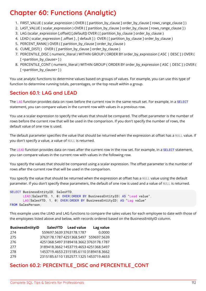
Complete SQL Tips & Secrets for Professionals 112

Chapter 60: Functions (Analytic)FIRST_VALUE ( scalar_expression ) OVER ( [ partition_by_clause ] order_by_clause [ rows_range_clause ] )1.LAST_VALUE ( scalar_expression ) OVER ( [ partition_by_clause ] order_by_clause [ rows_range_clause ] )2.LAG (scalar_expression [,offset] [,default]) OVER ( [ partition_by_clause ] order_by_clause )3.LEAD ( scalar_expression [ ,offset ] , [ default ] ) OVER ( [ partition_by_clause ] order_by_clause )4.PERCENT_RANK( ) OVER ( [ partition_by_clause ] order_by_clause )5.CUME_DIST( ) OVER ( [ partition_by_clause ] order_by_clause )6.PERCENTILE_DISC ( numeric_literal ) WITHIN GROUP ( ORDER BY order_by_expression [ ASC | DESC ] ) OVER (7.[ <partition_by_clause> ] )PERCENTILE_CONT ( numeric_literal ) WITHIN GROUP ( ORDER BY order_by_expression [ ASC | DESC ] ) OVER (8.[ <partition_by_clause> ] )

You use analytic functions to determine values based on groups of values. For example, you can use this type offunction to determine running totals, percentages, or the top result within a group.

Section 60.1: LAG and LEADThe LAG function provides data on rows before the current row in the same result set. For example, in a SELECTstatement, you can compare values in the current row with values in a previous row.

You use a scalar expression to specify the values that should be compared. The offset parameter is the number ofrows before the current row that will be used in the comparison. If you don't specify the number of rows, thedefault value of one row is used.

The default parameter specifies the value that should be returned when the expression at offset has a NULL value. Ifyou don't specify a value, a value of NULL is returned.

The LEAD function provides data on rows after the current row in the row set. For example, in a SELECT statement,you can compare values in the current row with values in the following row.

You specify the values that should be compared using a scalar expression. The offset parameter is the number ofrows after the current row that will be used in the comparison.

You specify the value that should be returned when the expression at offset has a NULL value using the defaultparameter. If you don't specify these parameters, the default of one row is used and a value of NULL is returned.

SELECT BusinessEntityID, SalesYTD, LEAD(SalesYTD, 1, 0) OVER(ORDER BY BusinessEntityID) AS "Lead value", LAG(SalesYTD, 1, 0) OVER(ORDER BY BusinessEntityID) AS "Lag value"FROM SalesPerson;

This example uses the LEAD and LAG functions to compare the sales values for each employee to date with those ofthe employees listed above and below, with records ordered based on the BusinessEntityID column.

BusinessEntityID SalesYTD Lead value Lag value274 559697.5639 3763178.1787 0.0000275 3763178.1787 4251368.5497 559697.5639276 4251368.5497 3189418.3662 3763178.1787277 3189418.3662 1453719.4653 4251368.5497278 1453719.4653 2315185.6110 3189418.3662279 2315185.6110 1352577.1325 1453719.4653

Section 60.2: PERCENTILE_DISC and PERCENTILE_CONT

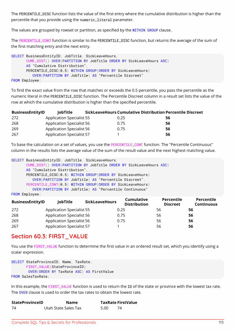
Complete SQL Tips & Secrets for Professionals 113

The PERCENTILE_DISC function lists the value of the first entry where the cumulative distribution is higher than thepercentile that you provide using the numeric_literal parameter.

The values are grouped by rowset or partition, as specified by the WITHIN GROUP clause.

The PERCENTILE_CONT function is similar to the PERCENTILE_DISC function, but returns the average of the sum ofthe first matching entry and the next entry.

SELECT BusinessEntityID, JobTitle, SickLeaveHours, CUME_DIST() OVER(PARTITION BY JobTitle ORDER BY SickLeaveHours ASC) AS "Cumulative Distribution", PERCENTILE_DISC(0.5) WITHIN GROUP(ORDER BY SickLeaveHours) OVER(PARTITION BY JobTitle) AS "Percentile Discreet"FROM Employee;

To find the exact value from the row that matches or exceeds the 0.5 percentile, you pass the percentile as thenumeric literal in the PERCENTILE_DISC function. The Percentile Discreet column in a result set lists the value of therow at which the cumulative distribution is higher than the specified percentile.

BusinessEntityID JobTitle SickLeaveHours Cumulative Distribution Percentile Discreet272 Application Specialist 55 0.25 56268 Application Specialist 56 0.75 56269 Application Specialist 56 0.75 56267 Application Specialist 57 1 56

To base the calculation on a set of values, you use the PERCENTILE_CONT function. The "Percentile Continuous"column in the results lists the average value of the sum of the result value and the next highest matching value.

SELECT BusinessEntityID, JobTitle, SickLeaveHours, CUME_DIST() OVER(PARTITION BY JobTitle ORDER BY SickLeaveHours ASC) AS "Cumulative Distribution", PERCENTILE_DISC(0.5) WITHIN GROUP(ORDER BY SickLeaveHours) OVER(PARTITION BY JobTitle) AS "Percentile Discreet", PERCENTILE_CONT(0.5) WITHIN GROUP(ORDER BY SickLeaveHours) OVER(PARTITION BY JobTitle) AS "Percentile Continuous"FROM Employee;

BusinessEntityID JobTitle SickLeaveHours CumulativeDistribution

PercentileDiscreet

PercentileContinuous

272 Application Specialist 55 0.25 56 56268 Application Specialist 56 0.75 56 56269 Application Specialist 56 0.75 56 56267 Application Specialist 57 1 56 56

Section 60.3: FIRST_VALUEYou use the FIRST_VALUE function to determine the first value in an ordered result set, which you identify using ascalar expression.

SELECT StateProvinceID, Name, TaxRate, FIRST_VALUE(StateProvinceID) OVER(ORDER BY TaxRate ASC) AS FirstValueFROM SalesTaxRate;

In this example, the FIRST_VALUE function is used to return the ID of the state or province with the lowest tax rate.The OVER clause is used to order the tax rates to obtain the lowest rate.

StateProvinceID Name TaxRate FirstValue74 Utah State Sales Tax 5.00 74

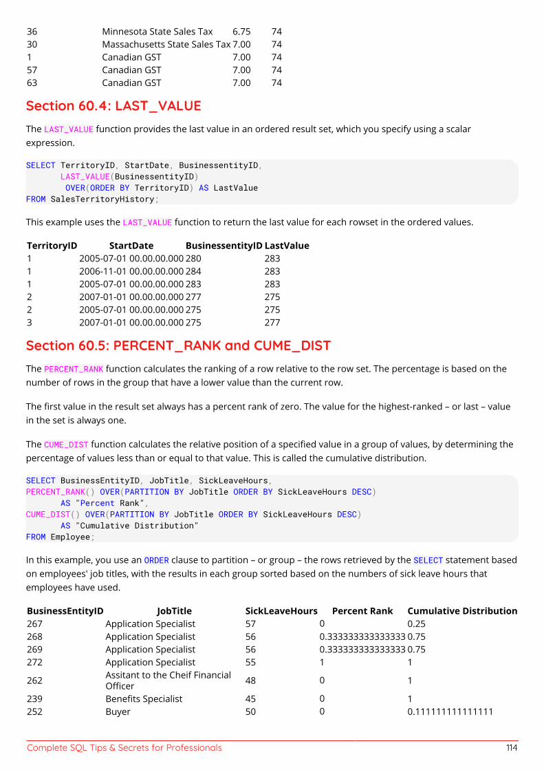
Complete SQL Tips & Secrets for Professionals 114

36 Minnesota State Sales Tax 6.75 7430 Massachusetts State Sales Tax 7.00 741 Canadian GST 7.00 7457 Canadian GST 7.00 7463 Canadian GST 7.00 74

Section 60.4: LAST_VALUEThe LAST_VALUE function provides the last value in an ordered result set, which you specify using a scalarexpression.

SELECT TerritoryID, StartDate, BusinessentityID, LAST_VALUE(BusinessentityID) OVER(ORDER BY TerritoryID) AS LastValueFROM SalesTerritoryHistory;

This example uses the LAST_VALUE function to return the last value for each rowset in the ordered values.

TerritoryID StartDate BusinessentityID LastValue1 2005-07-01 00.00.00.000 280 2831 2006-11-01 00.00.00.000 284 2831 2005-07-01 00.00.00.000 283 2832 2007-01-01 00.00.00.000 277 2752 2005-07-01 00.00.00.000 275 2753 2007-01-01 00.00.00.000 275 277

Section 60.5: PERCENT_RANK and CUME_DISTThe PERCENT_RANK function calculates the ranking of a row relative to the row set. The percentage is based on thenumber of rows in the group that have a lower value than the current row.

The first value in the result set always has a percent rank of zero. The value for the highest-ranked – or last – valuein the set is always one.

The CUME_DIST function calculates the relative position of a specified value in a group of values, by determining thepercentage of values less than or equal to that value. This is called the cumulative distribution.

SELECT BusinessEntityID, JobTitle, SickLeaveHours,PERCENT_RANK() OVER(PARTITION BY JobTitle ORDER BY SickLeaveHours DESC) AS "Percent Rank",CUME_DIST() OVER(PARTITION BY JobTitle ORDER BY SickLeaveHours DESC) AS "Cumulative Distribution"FROM Employee;

In this example, you use an ORDER clause to partition – or group – the rows retrieved by the SELECT statement basedon employees' job titles, with the results in each group sorted based on the numbers of sick leave hours thatemployees have used.

BusinessEntityID JobTitle SickLeaveHours Percent Rank Cumulative Distribution267 Application Specialist 57 0 0.25268 Application Specialist 56 0.333333333333333 0.75269 Application Specialist 56 0.333333333333333 0.75272 Application Specialist 55 1 1

262 Assitant to the Cheif FinancialOfficer 48 0 1

239 Benefits Specialist 45 0 1252 Buyer 50 0 0.111111111111111

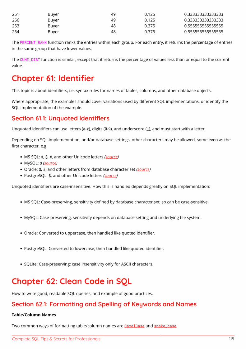
Complete SQL Tips & Secrets for Professionals 115

251 Buyer 49 0.125 0.333333333333333256 Buyer 49 0.125 0.333333333333333253 Buyer 48 0.375 0.555555555555555254 Buyer 48 0.375 0.555555555555555

The PERCENT_RANK function ranks the entries within each group. For each entry, it returns the percentage of entriesin the same group that have lower values.

The CUME_DIST function is similar, except that it returns the percentage of values less than or equal to the currentvalue.

Chapter 61: IdentifierThis topic is about identifiers, i.e. syntax rules for names of tables, columns, and other database objects.

Where appropriate, the examples should cover variations used by different SQL implementations, or identify theSQL implementation of the example.

Section 61.1: Unquoted identifiersUnquoted identifiers can use letters (a-z), digits (0-9), and underscore (_), and must start with a letter.

Depending on SQL implementation, and/or database settings, other characters may be allowed, some even as thefirst character, e.g.

MS SQL: @, $, #, and other Unicode letters (source)MySQL: $ (source)Oracle: $, #, and other letters from database character set (source)PostgreSQL: $, and other Unicode letters (source)

Unquoted identifiers are case-insensitive. How this is handled depends greatly on SQL implementation:

MS SQL: Case-preserving, sensitivity defined by database character set, so can be case-sensitive.

MySQL: Case-preserving, sensitivity depends on database setting and underlying file system.

Oracle: Converted to uppercase, then handled like quoted identifier.

PostgreSQL: Converted to lowercase, then handled like quoted identifier.

SQLite: Case-preserving; case insensitivity only for ASCII characters.

Chapter 62: Clean Code in SQLHow to write good, readable SQL queries, and example of good practices.

Section 62.1: Formatting and Spelling of Keywords and NamesTable/Column Names

Two common ways of formatting table/column names are CamelCase and snake_case:

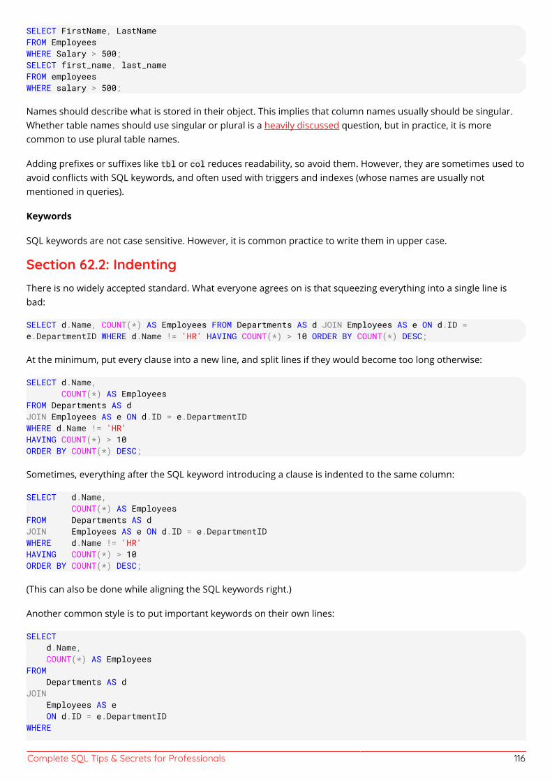
Complete SQL Tips & Secrets for Professionals 116

SELECT FirstName, LastNameFROM EmployeesWHERE Salary > 500;SELECT first_name, last_nameFROM employeesWHERE salary > 500;

Names should describe what is stored in their object. This implies that column names usually should be singular.Whether table names should use singular or plural is a heavily discussed question, but in practice, it is morecommon to use plural table names.

Adding prefixes or suffixes like tbl or col reduces readability, so avoid them. However, they are sometimes used toavoid conflicts with SQL keywords, and often used with triggers and indexes (whose names are usually notmentioned in queries).

Keywords

SQL keywords are not case sensitive. However, it is common practice to write them in upper case.

Section 62.2: IndentingThere is no widely accepted standard. What everyone agrees on is that squeezing everything into a single line isbad:

SELECT d.Name, COUNT(*) AS Employees FROM Departments AS d JOIN Employees AS e ON d.ID =e.DepartmentID WHERE d.Name != 'HR' HAVING COUNT(*) > 10 ORDER BY COUNT(*) DESC;

At the minimum, put every clause into a new line, and split lines if they would become too long otherwise:

SELECT d.Name, COUNT(*) AS EmployeesFROM Departments AS dJOIN Employees AS e ON d.ID = e.DepartmentIDWHERE d.Name != 'HR'HAVING COUNT(*) > 10ORDER BY COUNT(*) DESC;

Sometimes, everything after the SQL keyword introducing a clause is indented to the same column:

SELECT d.Name, COUNT(*) AS EmployeesFROM Departments AS dJOIN Employees AS e ON d.ID = e.DepartmentIDWHERE d.Name != 'HR'HAVING COUNT(*) > 10ORDER BY COUNT(*) DESC;

(This can also be done while aligning the SQL keywords right.)

Another common style is to put important keywords on their own lines:

SELECT d.Name, COUNT(*) AS EmployeesFROM Departments AS dJOIN Employees AS e ON d.ID = e.DepartmentIDWHERE

Complete SQL Tips & Secrets for Professionals 117

d.Name != 'HR'HAVING COUNT(*) > 10ORDER BY COUNT(*) DESC;

Vertically aligning multiple similar expressions improves readability:

SELECT Model, EmployeeIDFROM CarsWHERE CustomerID = 42 AND Status = 'READY';

Using multiple lines makes it harder to embed SQL commands into other programming languages. However, manylanguages have a mechanism for multi-line strings, e.g., @"..." in C#, """...""" in Python, or R"(...)" in C++.

Section 62.3: SELECT *SELECT * returns all columns in the same order as they are defined in the table.

When using SELECT *, the data returned by a query can change whenever the table definition changes. Thisincreases the risk that different versions of your application or your database are incompatible with each other.

Furthermore, reading more columns than necessary can increase the amount of disk and network I/O.

So you should always explicitly specify the column(s) you actually want to retrieve:

--SELECT * don't SELECT ID, FName, LName, PhoneNumber -- do FROM Emplopees;

(When doing interactive queries, these considerations do not apply.)

However, SELECT * does not hurt in the subquery of an EXISTS operator, because EXISTS ignores the actual dataanyway (it checks only if at least one row has been found). For the same reason, it is not meaningful to list anyspecific column(s) for EXISTS, so SELECT * actually makes more sense:

-- list departments where nobody was hired recentlySELECT ID, NameFROM DepartmentsWHERE NOT EXISTS (SELECT * FROM Employees WHERE DepartmentID = Departments.ID AND HireDate >= '2015-01-01');

Section 62.4: JoinsExplicit joins should always be used; implicit joins have several problems:

The join condition is somewhere in the WHERE clause, mixed up with any other filter conditions. This makesit harder to see which tables are joined, and how.

Due to the above, there is a higher risk of mistakes, and it is more likely that they are found later.

In standard SQL, explicit joins are the only way to use outer joins:

Complete SQL Tips & Secrets for Professionals 118

SELECT d.Name, e.Fname || e.LName AS EmpNameFROM Departments AS dLEFT JOIN Employees AS e ON d.ID = e.DepartmentID;

Explicit joins allow using the USING clause:

SELECT RecipeID, Recipes.Name, COUNT(*) AS NumberOfIngredientsFROM RecipesLEFT JOIN Ingredients USING (RecipeID);

(This requires that both tables use the same column name.USING automatically removes the duplicate column from the result, e.g., the join in this query returns asingle RecipeID column.)

Complete SQL Tips & Secrets for Professionals 119

CreditsThank you greatly to all the people from Stack Overflow Documentation who helped provide this content,

more changes can be sent to web@petercv.com for new content to be published or updated

Özgür Öztürk Chapters 13 and 583N1GM4 Chapter 14a1ex07 Chapter 6Abe Miessler Chapter 14Abhilash R Vankayala Chapters 2, 4, 19, 26, 27 and 52aholmes Chapter 2Aidan Chapters 7 and 9alex9311 Chapter 7Almir Vuk Chapters 6 and 7Alok Singh Chapter 2Ameya Deshpande Chapter 11Amir Pourmand Chapter 37Amnon Chapter 2Andrea Chapter 8Andrea Montanari Chapter 12Andreas Chapter 61Andy G Chapter 3apomene Chapter 2Ares Chapter 7Arkh Chapter 16Arpit Solanki Chapter 2Arthur D Chapter 22Arulkumar Chapters 15 and 22ashja99 Chapters 19 and 20Athafoud Chapter 8A_Arnold Chapter 3Bart Schuijt Chapter 19Batsu Chapter 22bhs Chapter 16bignose Chapter 4blackbishop Chapter 9Blag Chapter 58Bostjan Chapters 4, 14 and 15Branko Dimitrijevic Chapter 3Brent Oliver Chapter 2brichins Chapter 34carlosb Chapters 6 and 39Chris Chapter 2Christian Chapter 4Christian Sagmüller Chapter 2Christos Chapter 2CL. Chapters 1, 2, 3, 5, 6, 7, 10, 12, 13, 17, 20, 22, 31, 35, 44, 49, 61 and Chapter 63Cristian Abelleira Chapter 26DaImTo Chapter 26Daniel Chapter 17Daniel Langemann Chapters 3 and 8dariru Chapter 2Dariusz Chapters 5 and 10Darrel Lee Chapter 29

Complete SQL Tips & Secrets for Professionals 120

Darren Bartrup Chapters 3 and 40Daryl Chapters 2, 25, 37 and 42dasblinkenlight Chapter 32David Manheim Chapter 6David Pine Chapter 2David Spillett Chapter 2day_dreamer Chapter 2dd4711 Chapter 17dmfay Chapter 59Durgpal Singh Chapter 2Dylan Vander Berg Chapters 7 and 21Emil Rowland Chapter 43Eric VB Chapter 2Florin Ghita Chapters 3, 4, 9, 18 and 20FlyingPiMonster Chapters 2, 4, 5, 6 and 12forsvarir Chapters 3 and 4Franck Dernoncourt Chapters 2, 3 and 22Frank Chapter 14fuzzy_logic Chapter 17Gallus Chapter 51geeksal Chapter 1Gidil Chapter 16Golden Gate Chapter 22guiguiblitz Chapter 24H. Pauwelyn Chapter 7Hack Chapter 46Harish Gyanani Chapter 19Harjot Chapter 28hatchet Chapter 22hellyale Chapter 19HK1 Chapter 3HLGEM Chapter 3HoangHieu Chapter 2Horaciux Chapter 6Hynek Bernard Chapter 26Ian Kenney Chapter 20iliketocode Chapter 2Imran Ali Khan Chapters 2, 20 and 22Inca Chapter 2IncrediApp Chapter 25Jared Hooper Chapter 2Jason W Chapter 8JavaHopper Chapter 4Jaydip Jadhav Chapter 22Jaydles Chapters 2, 10, 13 and 14Jenism Chapter 6Jerry Jeremiah Chapter 16Jim Chapter 8Joe Taras Chapter 8Joel Chapters 21 and 35John Odom Chapters 2, 3, 37, 38 and 52John Slegers Chapters 2 and 3John Smith Chapter 30JohnLBevan Chapter 1Jojodmo Chapter 7

Complete SQL Tips & Secrets for Professionals 121

Jon Chan Chapter 15Jon Ericson Chapters 1 and 15JonH Chapter 2juergen d Chapters 15, 20 and 47Karthikeyan Chapter 41Kewin Björk Nielsen Chapters 22 and 57KIRAN KUMAR MATAM Chapter 7KjetilNordin Chapter 12Knickerless Chapter 49Lankymart Chapter 2LCIII Chapter 53Leigh Riffel Chapter 22Lexi Chapter 9Lohitha Palagiri Chapter 19Magisch Chapter 4Mark Iannucci Chapters 2 and 3Mark Perera Chapters 2 and 19Mark Stewart Chapter 57Matas Vaitkevicius Chapters 2, 5, 7, 15, 22 and 44Mateusz Piotrowski Chapter 22Matt Chapters 2, 4 and 10Matt S Chapter 2Mattew Whitt Chapter 2mauris Chapter 6Mihai Chapters 2 and 8mithra chintha Chapters 9 and 13MotKohn Chapter 10Mr. Developer Chapter 19Mureinik Chapters 3, 10 and 16mustaccio Chapters 2 and 16Mzzzzzz Chapter 4Nathan Chapter 20nazark Chapter 13Neria Nachum Chapter 22Nunie123 Chapter 32Oded Chapter 2Ojen Chapters 2 and 19omini data Chapters 20 and 60onedaywhen Chapter 2Ozair Kafray Chapter 9Parado Chapters 6 and 13Paul Bambury Chapter 26Paulo Freitas Chapter 6Peter K Chapters 17 and 20Phrancis Chapters 1, 3, 5, 13, 15, 17, 19, 21, 22, 23, 31, 32, 33, 36 and 48Prateek Chapters 1, 2 and 7Preuk Chapter 2Racil Hilan Chapter 2raholling Chapter 3rajarshig Chapter 11RamenChef Chapter 22Reboot Chapter 20Redithion Chapter 19Ricardo Pontual Chapter 38Robert Columbia Chapters 2 and 22

Complete SQL Tips & Secrets for Professionals 122

Ryan Chapter 6Ryan Rockey Chapter 51Saroj Sasmal Chapters 2 and 48Shiva Chapter 4Sibeesh Venu Chapter 17Simon Foster Chapter 9Simone Chapter 14Simulant Chapter 45SommerEngineering Chapter 2SQLFox Chapter 27sqluser Chapter 2StanislovasKalašnikovas Chapter 10

Stefan Steiger Chapters 3, 19, 49 and 50Steven Chapter 55Stivan Chapter Chapter 63Stu Chapter 35Timothy Chapter 2tinlyx Chapter 32Tot Zam Chapters 3, 4, 5, 11, 15 and 20Uberzen1 Chapter 54Umesh Chapter 21user1221533 Chapter 36user1336087 Chapter 2user2314737 Chapter 56Vikrant Chapter 19vmaroli Chapters 5, 19 and 22walid Chapters 47 and 48WesleyJohnson Chapter 4William Ledbetter Chapter 20wintersolider Chapter 2Wolfgang Chapter 13xenodevil Chapters 3 and 21xQbert Chapter 2Yehuda Shapira Chapter 28yper Chapters 1 and 48Yury Fedorov Chapter 2Zaga Chapter 47Zahiro Mor Chapters 2 and 14zedfoxus Chapter 2Zoyd Chapter 27zplizzi Chapter 11ɐlǝx Chapters 10 and 22Алексей Неудачин Chapter 20Рахул Маквана Chapter 3

You may also like