Compensating Wage Compensating Wage DifferentialsDifferentials

The model of competitive labor markets The model of competitive labor markets implies that as long as workers or firms can implies that as long as workers or firms can freely enter and exit the marketplace, there freely enter and exit the marketplace, there will be a single wage in the economy will be a single wage in the economy if all if all jobs are alike and all workers are alikejobs are alike and all workers are alike. .

All jobs are not the same. Adam Smith in 1776 All jobs are not the same. Adam Smith in 1776 argued that compensating wage differentials arise to argued that compensating wage differentials arise to compensate workers for the nonwage characteristics compensate workers for the nonwage characteristics of jobs. It is not the wage that is equated across jobs of jobs. It is not the wage that is equated across jobs in a competitive market, but the “whole of the in a competitive market, but the “whole of the advantages and disadvantages” of the job.advantages and disadvantages” of the job.

Workers differ in their preferences for job Workers differ in their preferences for job characteristics and firms differ in the working characteristics and firms differ in the working conditions that they offer. The theory of conditions that they offer. The theory of compensating differentials tells a story of how compensating differentials tells a story of how workers and firms “match and mate” in the labor workers and firms “match and mate” in the labor market.market.

各行業受雇員工每人每月平均薪資

資料來源 :行政院主計處

1. Workers’ and Firms’ Choice with Risky Jobs1. Workers’ and Firms’ Choice with Risky Jobs

E.g. Employer X: NT.$100 per hour, clean, safe work conditionsE.g. Employer X: NT.$100 per hour, clean, safe work conditions Employer Y: NT.$100 per hour, dirty, noisy factoryEmployer Y: NT.$100 per hour, dirty, noisy factory→ → Most workers would undoubtedly choose employer X.Most workers would undoubtedly choose employer X. If employer Y decides not to alter working conditions, it must If employer Y decides not to alter working conditions, it must

pay wage above NT.$100 to be competitive in the labor market.pay wage above NT.$100 to be competitive in the labor market.→ → The extra wage it must pay to attract workers is called a The extra wage it must pay to attract workers is called a

compensating wage differentialcompensating wage differential because the higher wage is because the higher wage is paid to compensate workers for the undesirable working paid to compensate workers for the undesirable working conditions.conditions.

After the wage rise of firm Y, if both firms could obtain the After the wage rise of firm Y, if both firms could obtain the quantity and quality of works they wanted, the wage differential quantity and quality of works they wanted, the wage differential would be an equilibrium differential, in the sense that there be would be an equilibrium differential, in the sense that there be no forces causing the differential to change.no forces causing the differential to change.

* The compensating wage differential ser* The compensating wage differential serves two purposes:ves two purposes:

1.1. It serves a social need by giving people an incentive It serves a social need by giving people an incentive to voluntarily do dirty, dangerous, or unpleasant to voluntarily do dirty, dangerous, or unpleasant work or a financial penalty on employers offering work or a financial penalty on employers offering unfavorable working conditions.unfavorable working conditions.

2.2. At an individual level, it serves as a reward to At an individual level, it serves as a reward to workers who accept unpleasant jobs by paying them workers who accept unpleasant jobs by paying them more than comparable workers in more pleasant more than comparable workers in more pleasant jobs. Those who opt for more pleasant conditions jobs. Those who opt for more pleasant conditions have to buy them by accepting lower pay.have to buy them by accepting lower pay.

→ → Compensating wage differentials provide the key to tCompensating wage differentials provide the key to the valuation of the nonpecuniary aspects of employmhe valuation of the nonpecuniary aspects of employment.ent.

Note: Note:

The predicted outcome of the compensating wage diffThe predicted outcome of the compensating wage differential theory of job choice is not that employees woerential theory of job choice is not that employees working under “bad” conditions receive more than those rking under “bad” conditions receive more than those working in “good” conditions. The prediction is that, working in “good” conditions. The prediction is that, holding worker characteristics constant, employees in holding worker characteristics constant, employees in bad jobs receive higher wages than those working unbad jobs receive higher wages than those working under more pleasant conditions.der more pleasant conditions.

* The compensating wage differential the* The compensating wage differential theory is based on three assumptions:ory is based on three assumptions:

1.1. Utility MaximizationUtility Maximization Workers seek to maximize their utility, not their incWorkers seek to maximize their utility, not their inc

ome. Compensating wage differentials will only ariome. Compensating wage differentials will only arise if some people do not choose the highest-paying se if some people do not choose the highest-paying job offered, preferring instead a lower-paying but mjob offered, preferring instead a lower-paying but more pleasant job. ore pleasant job.

→ → Wages do not equalize in this case. The net advantagWages do not equalize in this case. The net advantage – the overall utility from the pay and the psychic ae – the overall utility from the pay and the psychic aspects of the job – tend to equalize for the marginal spects of the job – tend to equalize for the marginal workers. workers.

2.2. Worker Information Worker Information Workers are aware of the job characteristics of Workers are aware of the job characteristics of potential importance to them.potential importance to them.→ → Company offering a “bad” job with no compensating Company offering a “bad” job with no compensating

wage differential would have trouble recruiting or wage differential would have trouble recruiting or retaining workers, trouble that would eventually retaining workers, trouble that would eventually force it to raise its wage.force it to raise its wage.

Note: Our predictions about compensating wage Note: Our predictions about compensating wage differentials hold only for job characteristics that differentials hold only for job characteristics that workers know about.workers know about.

3.3. Workers Mobility Workers Mobility Workers have a range of job offers from which to Workers have a range of job offers from which to

choose. It is the act of choosing safe jobs over choose. It is the act of choosing safe jobs over dangerous ones that forces employers offering dangerous ones that forces employers offering dangerous work to raise wages.dangerous work to raise wages.

2. The Hedonic Wage Function2. The Hedonic Wage Function

A wage theory based on the assumption of A wage theory based on the assumption of philosophical hedonism that workers strive to philosophical hedonism that workers strive to maximize utility.maximize utility.

To simplify our discussion, we shall analyze just one To simplify our discussion, we shall analyze just one dimension –risk of injury on the job – and assume dimension –risk of injury on the job – and assume that the compensating wage differentials for every that the compensating wage differentials for every other dimension have already been established.other dimension have already been established.

→ → To obtain a complete understanding of the job To obtain a complete understanding of the job selection process and the outcomes of that process, it selection process and the outcomes of that process, it is necessary to consider both the employer and is necessary to consider both the employer and employee sides of the market.employee sides of the market.

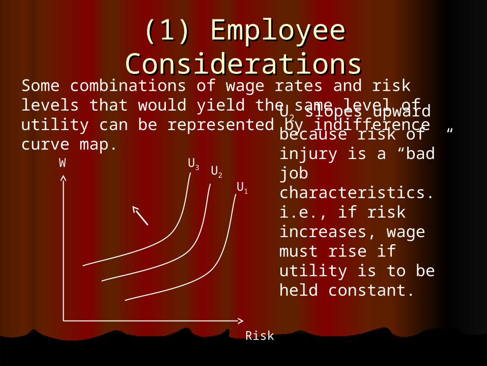
(1) Employee Considerations(1) Employee ConsiderationsSome combinations of wage rates and risk levels that would yield the same level of utility can be represented by indifference curve map.

W

Risk

U1

U2

U3U2 slopes upward because

risk of injury is a “bad” jobcharacteristics. i.e., if riskincreases, wage must rise ifutility is to be held constant.

W

Risk

Highly Averse to Risk

Moderately Averse to Risk

UL

UH

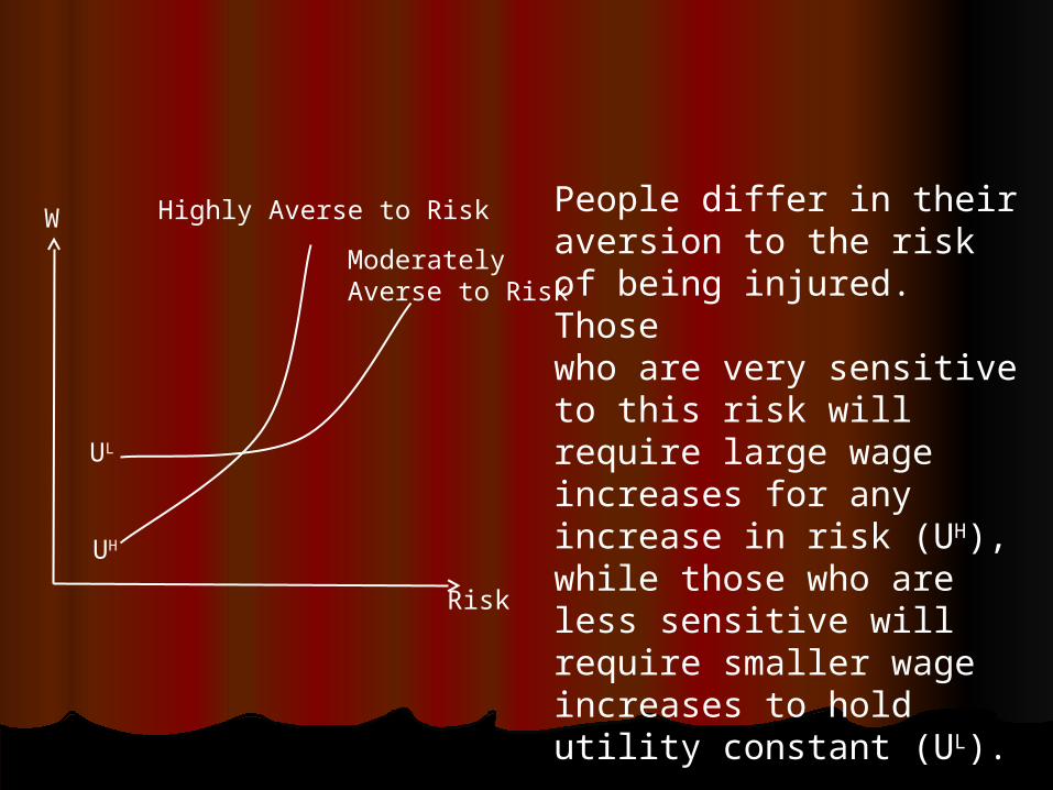
People differ in their aversion to the risk of being injured. Thosewho are very sensitive to this risk will require large wage increases for any increase in risk (UH), while those who are less sensitive will require smaller wage increases to hold utility constant (UL).

(2) Employer Considerations(2) Employer Considerations

Assumptions:Assumptions:a.a. It is presumably costly to reduce the risk of It is presumably costly to reduce the risk of

injury facing employees.injury facing employees.b.b. Perfect competition → Firms operate at zero Perfect competition → Firms operate at zero

profits.profits.c.c. All other job characteristics are presumably All other job characteristics are presumably

given or already determined. given or already determined. → → If a firm undertakes a program to reduce the If a firm undertakes a program to reduce the

risk of injury, it must reduce wages to remain risk of injury, it must reduce wages to remain competitive.competitive.

Forces on the employer side of the market tent Forces on the employer side of the market tent to cause low risk to be associated with low wato cause low risk to be associated with low wages and high risk to be associated with high wages and high risk to be associated with high wages, holding other things constant.ges, holding other things constant.

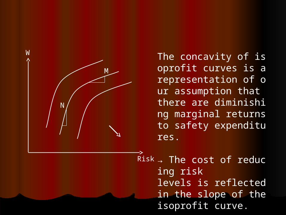
→→The employer trade-offs between wages and leThe employer trade-offs between wages and levels of injury risk can be graphed through the vels of injury risk can be graphed through the use of isoprofit curves , which show the variouuse of isoprofit curves , which show the various combinations of risk and wage level that yiels combinations of risk and wage level that yield a given level of profits.d a given level of profits.

W

Risk

M

N

The concavity of isoprofit curves is a representation of our assumption that there are diminishing marginal returns to safety expenditures.

→ The cost of reducing risklevels is reflected in the slope of the isoprofit curve.

W

Risk

X

Y

X’Y’

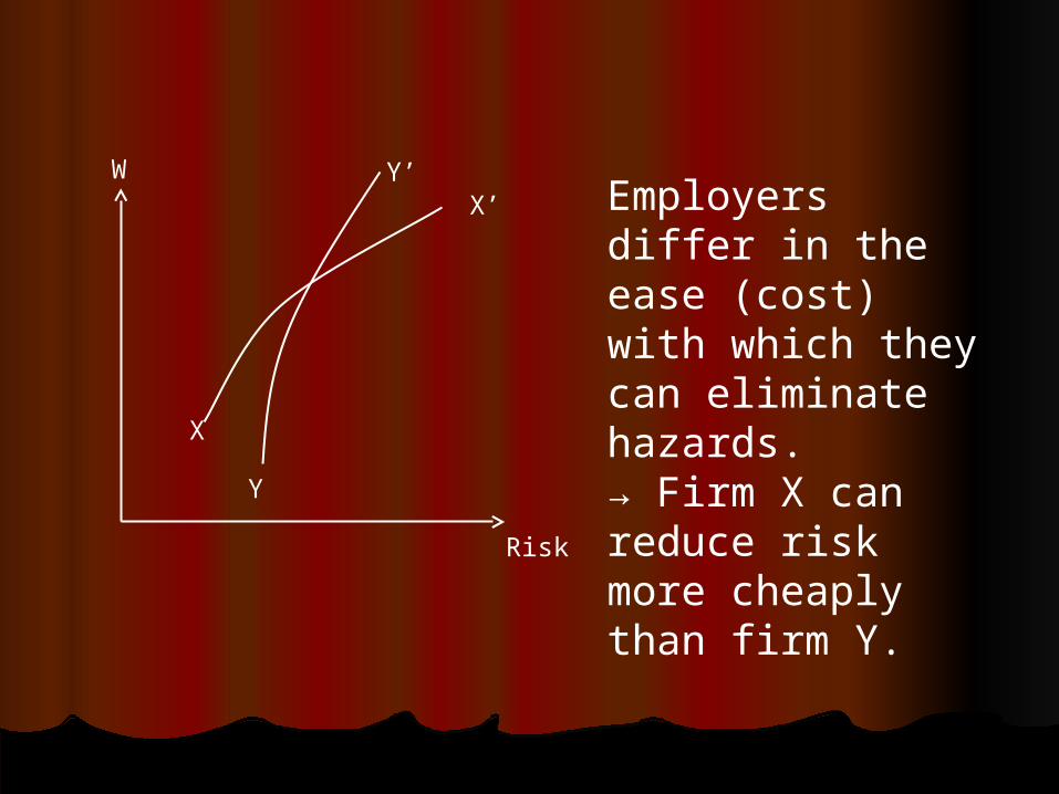
Employers differ in the ease (cost) with which they can eliminatehazards.→ Firm X can reduce risk more cheaply than firm Y.

(3) The Matching of Employer and Employees(3) The Matching of Employer and Employees

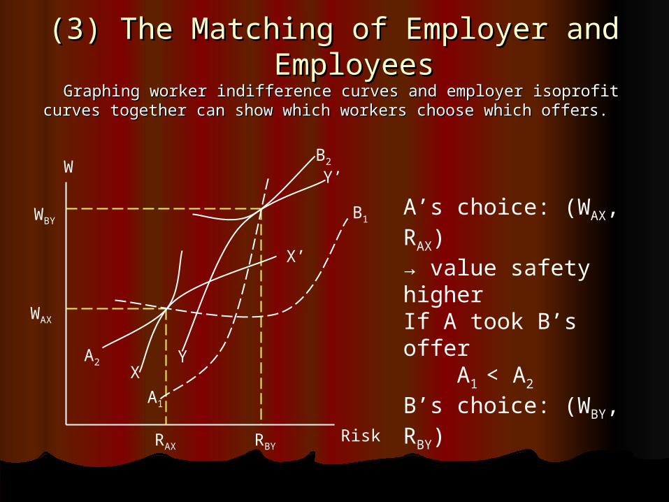
Graphing worker indifference curves and employer isoprofit curGraphing worker indifference curves and employer isoprofit curves together can show which workers choose which offers.ves together can show which workers choose which offers.

A’s choice: (WAX, RAX) → value safety higherIf A took B’s offer A1 < A2

B’s choice: (WBY, RBY)

W

Risk

WBY

WAX

RAX RBY

A1

B1

A2

B2

X

X’

Y

Y’

Since X can produce safety more cheaply than Y, X Since X can produce safety more cheaply than Y, X will be a low-risk producer who attracts employees, will be a low-risk producer who attracts employees, like A, who value safety highly. Y attracts people like like A, who value safety highly. Y attracts people like B, who have a relatively strong preference for money B, who have a relatively strong preference for money wages and a relatively weak preference for safety.wages and a relatively weak preference for safety.

Note: The only offers of jobs to workers with a Note: The only offers of jobs to workers with a chance of being accepted lie along XR’Y’.chance of being accepted lie along XR’Y’.

→ → The curve XR’Y’ can be called an “offer curve”, The curve XR’Y’ can be called an “offer curve”, because only along XR’Y’ will offers employers can because only along XR’Y’ will offers employers can afford to make be potentially acceptable to afford to make be potentially acceptable to employees.employees.

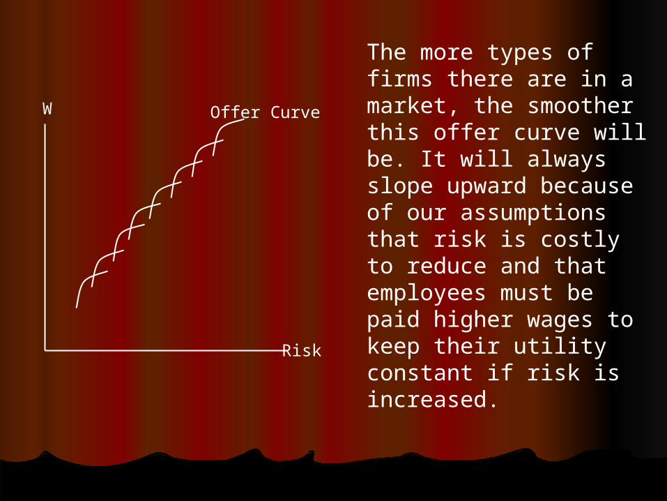
The more types of firms there are in a market, the smoother this offer curve will be. It will always slope upward because of our assumptions that risk is costly to reduce and that employees must be paid higher wages to keep their utility constant if risk is increased.

W

Risk

Offer Curve

* Major Insights:* Major Insights:

1.1. Wages rise with risk, other things equal. Wages rise with risk, other things equal. → There will be compensating wage differenti→ There will be compensating wage differentials for job characteristics that are viewed as unals for job characteristics that are viewed as undesirable by workers. desirable by workers.

2.2. Workers with strong preferences for safety wilWorkers with strong preferences for safety will tend to take jobs in firms where safety can be l tend to take jobs in firms where safety can be generated most cheaply. generated most cheaply. → Firms and workers offer and accept jobs in → Firms and workers offer and accept jobs in a fashion that makes the most of their strengths a fashion that makes the most of their strengths and preferences. and preferences.

3. Policy Application: How Much is a Life Worth?3. Policy Application: How Much is a Life Worth?

1.1. Empirical EvidencesEmpirical Evidences Many studies estimate the hedonic function relating wages Many studies estimate the hedonic function relating wages and the probability of injury on the job. This literatureand the probability of injury on the job. This literature typically estimates regressions of the form:typically estimates regressions of the form: wwii = = γργρi i + other variables+ other variables Where Where wwii gives the wage of worker gives the wage of worker ii and and ρρii.. gives the gives the probability of injury on the worker’s job. The coefficiprobability of injury on the worker’s job. The coeffici

ententγγgives the wage change associated with a one-unit gives the wage change associated with a one-unit increase in the probability of injury.increase in the probability of injury.

Many empirical studies report a positive relationshipMany empirical studies report a positive relationship between wages and hazardous or unsafe work conditions,between wages and hazardous or unsafe work conditions, regardless of how the hazard or the unsafe nature of the regardless of how the hazard or the unsafe nature of the work environment is defined. work environment is defined.

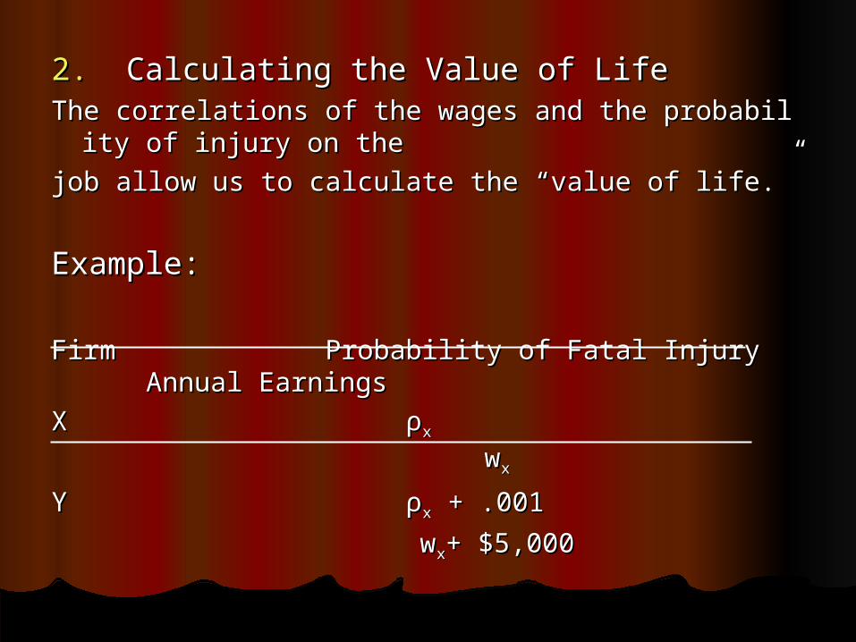
2.2. Calculating the Value of Life Calculating the Value of Life The correlations of the wages and the probability of injury on the The correlations of the wages and the probability of injury on the

job allow us to calculate the “value of life.” job allow us to calculate the “value of life.”

Example: Example:

Firm Probability of Fatal Injury Annual EarningsFirm Probability of Fatal Injury Annual Earnings

X ρX ρxx w wxx

Y ρY ρxx + .001 w + .001 wxx+ $5,000+ $5,000

The data suggests that each of the workers in firm Y The data suggests that each of the workers in firm Y is willing to give up $5,000 per year to reduce the is willing to give up $5,000 per year to reduce the probability of fatal injury in their job by 0.001 units. probability of fatal injury in their job by 0.001 units. Put differently, the 1,000 workers employed in firm Y Put differently, the 1,000 workers employed in firm Y are willing to give up $5 million (or $5,000x 1,000 are willing to give up $5 million (or $5,000x 1,000 workers) to save the life of the one worker who will workers) to save the life of the one worker who will almost surely die in any given year. The workers in almost surely die in any given year. The workers in firm Y, therefore, value a life at $5 million. firm Y, therefore, value a life at $5 million.

This calculation instead gives the amount that This calculation instead gives the amount that workers are jointly willing to pay to reduce the workers are jointly willing to pay to reduce the likelihood that one of them will suffer a fatal injury in likelihood that one of them will suffer a fatal injury in any given year. It is the any given year. It is the statistical value of a lifestatistical value of a life..