comparison of empirical decline curve analysis for
TRANSCRIPT
COMPARISON OF EMPIRICAL DECLINE CURVE ANALYSIS FOR SHALE
WELLS
A Thesis
by
MOHAMMED SAMI A KANFAR
Submitted to the Office of Graduate Studies of Texas A&M University
in partial fulfillment of the requirements for the degree of
MASTER OF SCIENCE
Chair of Committee, Robert A. Wattenbarger Committee Members, David S. Schechter Yuefeng Sun Head of Department, A. Daniel Hill
August 2013
Major Subject: Petroleum Engineering
Copyright 2013 Mohammed Sami A Kanfar
ii
ABSTRACT
This study compares four recently developed decline curve methods and the
traditional Arps or Fetkovich approach. The four methods which are empirically
formulated for shale and tight gas wells are:
1. Power Law Exponential Decline (PLE).
2. Stretched Exponential Decline (SEPD).
3. Duong Method.
4. Logistic Growth Model (LGM).
Each method has different tuning parameters and equation forms. The main objective of
this work is to determine the best method(s) in terms of Estimated Ultimate Recovery
(EUR) accuracy, goodness of fit, and ease of matching. In addition, these methods are
compared against each other at different production times in order to understand the
effect of production time on forecasts. As a part of validation process, all methods are
benchmarked against simulation.
This study compares the decline methods to four simulation cases which
represent the common shale declines observed in the field. Shale wells, which are
completed with horizontal wells and multiple traverse highly-conductive hydraulic
fractures, exhibit long transient linear flow. Based on certain models, linear flow is
preceded by bilinear flow if natural fractures are present. In addition to this, linear flow
is succeeded by Boundary Dominated Flow (BDF) decline when pressure wave reaches
iii
boundary. This means four declines are possible, hence four simulation cases are
required for comparison.
To facilitate automatic data fitting, a non-linear regression program was
developed using excel VBA. The program optimizes the Least-Square (LS) objective
function to find the best fit. The used optimization algorithm is the Levenberg-
Marquardt Algorithm (LMA) and it is used because of its robustness and ease of use.
This work shows that all methods forecast different EURs and some fit certain
simulation cases better than others. In addition, no method can forecast EUR accurately
without reaching BDF. Using this work, engineers can choose the best method to
forecast EUR after identifying the simulation case that is most analogous to their field
wells. The VBA program and the matching procedure presented here can help engineers
automate these methods into their forecasting sheets.

iv
ACKNOWLEDGEMENTS
I would like to express my sincere gratitude to my research advisor and
committee chair, Dr. Robert A. Wattenbarger for his valued guidance and inspiration. It
has been an honor and a pleasure working with him during the past two years. In
addition, I would like to thank Dr. David S. Schechter and Dr. Yuefeng Sun, for serving
on my advisory committee. Their constructive feedback helped to greatly improve this
work.
I also would like to extend my gratitude to Saudi Aramco for sponsoring me and
giving me the opportunity to pursue my advanced degree. Thanks also go to my friends
and colleagues and the department faculty and staff for making my time at Texas A&M
University a great experience.
Finally, I would like to thank my mother and father for their encouragement and
support.
v
NOMENCLATURE
Duong or LGM constant.
Area perpendicular to flow, sq-ft
Derivative of loss-ratio (Arps’ decline exponent), dimensionless
Total compressibility, psi-1
Loss-ratio (Arps’ decline constant), Days-1
Initial loss-ratio, Days-1
Loss-ratio at ( ), Days-1
Loss-ratio at ( ), Days-1
Cumulative gas production. Mscf
Permeability, md
Carrying capacity of LGM method.
Hydraulic fracture spacing, ft
Time exponent (hyperbolic exponent).
Pressure, psi
Flow rate, STB/Day or Mscf/Day
Flow rate at ( ), STB/Day or Mscf/Day
Flow rate at ( ), STB/Day or Mscf/Day
Flow rate at ( ), STB/Day or Mscf/Day
Critical flow rate
Cumulative production, Mscf or STB
vi
First calculated cumulative
Coefficient of determination, fraction
Error of sum of squares
Residual of sum of squares
Time, Days
First day of production (usually 1), Days
Time of end of square-root or time of end of linear flow
Last input time, Days
( ) Duong’s time function based on Eqn. 2.12
Characteristic time parameter for SEPD model, Days
Temperature, Rankin
Critical velocity
Weighting factor at time=i.
Mean of data
Data at row i
Gas deviation factor, dimensionless
vii
Abbreviations
BDF Boundary dominated flow
EUR Estimated ultimate recovery, Bscf or MMSTB
LGM Logistic growth model
LMA Levenberg-Marquardt Algorithm
PLE Power law exponential decline
SEPD Stretched exponential decline
SRV Simulated reservoir volume
Greek Symbols
Porosity, fraction
Viscoity, cp
viii
TABLE OF CONTENTS
Page
ABSTRACT .......................................................................................................................ii
ACKNOWLEDGEMENTS .............................................................................................. iv
NOMENCLATURE ........................................................................................................... v
TABLE OF CONTENTS ............................................................................................... viii
LIST OF FIGURES ............................................................................................................ x
LIST OF TABLES .......................................................................................................... xiv
CHAPTER I INTRODUCTION ....................................................................................... 1
1.1 Objective .................................................................................................................. 4 1.2 Thesis Organization.................................................................................................. 5
CHAPTER II LITERATURE REVIEW ............................................................................ 6
2.1 Traditional Decline Curve Methods ......................................................................... 7
2.2 Shale Wells Decline Curve Methods ..................................................................... 10 2.2.1 Power Law Exponential Decline (PLE) .......................................................... 10 2.2.2 Stretched Exponential Decline (SEPD) ........................................................... 11 2.2.3 Duong’s Method .............................................................................................. 12 2.2.4 Logistic Growth Model (LGM) ....................................................................... 16
CHAPTER III INVESTIGATION OF METHODS ........................................................ 17
3.1 Arps’ Unbounded Reserves Problem and Improvements ...................................... 17
3.1.1 Composite Arps’ Method ................................................................................ 19 3.2 PLE Iteration Blow-up ........................................................................................... 20 3.3 SEPD Equation Form and Iteration Time Problem ................................................ 23
3.3.1 The SEPD Method and Long Iteration Convergence Time ............................ 24
3.4 Doung’s Method Precautions ................................................................................. 26
3.4.1 Duong’s Error and Improvements ............................................................ 26 3.4.2 Error in Linear or Bilinear Flow ...................................................................... 26
3.4.3 Material-balance Time Error Results in Recovery Underestimation .............. 27
ix
CHAPTER IV MATCHING AND CALCULATION PROCEDURE ............................ 31
4.1 Liquid Loading Filter ............................................................................................. 31 4.2 Matching Data to Model ........................................................................................ 32 4.3 EUR Calculations ................................................................................................... 33
CHAPTER V COMPARISON WITH SIMULATION ................................................... 35
5.1 Model Description .................................................................................................. 35 5.2 Simulation and Model Simplifications ................................................................... 37 5.3 Matching Methods to Simulation: A Decline Fit Comparison .............................. 41
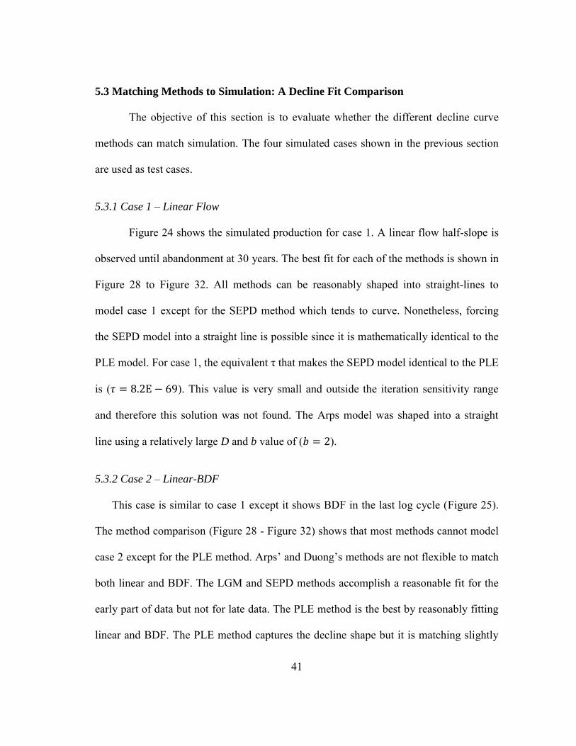
5.3.1 Case 1 – Linear Flow ....................................................................................... 41
5.3.2 Case 2 – Linear-BDF ....................................................................................... 41 5.3.3 Case 3 – Bilinear-Linear Flow ........................................................................ 42 5.3.4 Case 4 – Bilinear-Linear-BDF ........................................................................ 42
5.4 Effect of Production Time on Forecast .................................................................. 48 5.4.1 Case 1 – Linear Flow ....................................................................................... 48 5.4.2 Case 2 – Linear-BDF ....................................................................................... 48 5.4.3 Case 3 – Bilinear-Linear Flow ........................................................................ 49 5.4.4 Case 4 – Bilinear-Linear-BDF ........................................................................ 49
CHAPTER VI FIELD EXAMPLES ................................................................................ 62
6.1 Barnett Shale Gas - Well B-314. ............................................................................ 62 6.2 Bakken Shale Oil - Well BK-86. ............................................................................ 64
6.3 Eagleford Shale Gas - Well EF-3. .......................................................................... 65 6.4 Fayetteville Shale Gas - Well FF-3. ....................................................................... 66
CHAPTER VII DISCUSSION AND CONCLUSIONS .................................................. 67
REFERENCES ................................................................................................................. 69
APPENDIX A PLE DERIVATION ................................................................................ 71
APPENDIX B DOUNG’S METHOD DERIVATION .................................................... 73
APPENDIX C TIME AND MATERIAL-BALANCE TIME RELATION .................... 75
APPENDIX D LEVENBERG-MARQUARDT ALGORITHM (LMA) ......................... 76
x
LIST OF FIGURES
Page
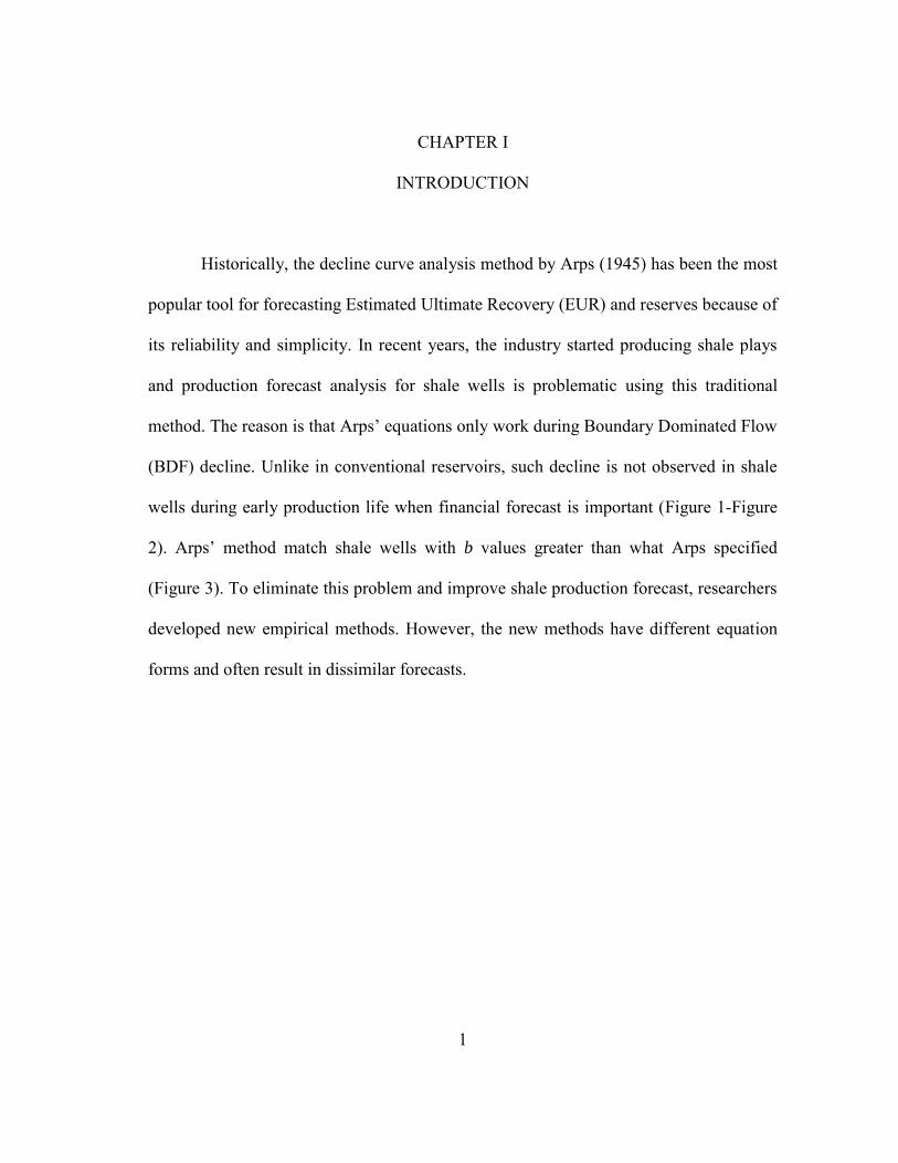
Figure 1. A conceptual vertical well in a conventional oil reservoir was simulated and production is shown by the green curve. Transient flow is relatively short and BDF is reached quickly. Arps exponential decline (marked in red) results in an excellent fit even at an early production time of 3 days. ........ 2
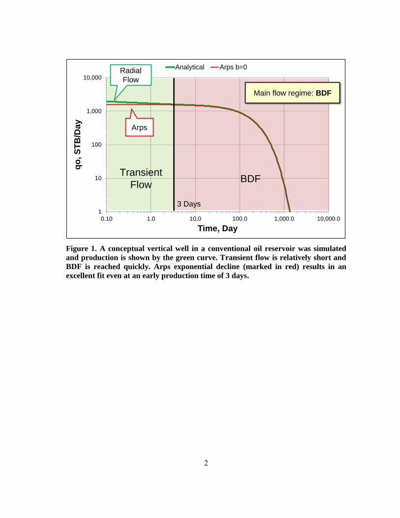
Figure 2. A conceptual horizontal shale-well with multiple traverse hydraulic fractures was simulated and production is shown by the green curve. Arps’ method (marked in red) can only fit BDF decline which does not occur until after 700 days of production. ............................................................ 3
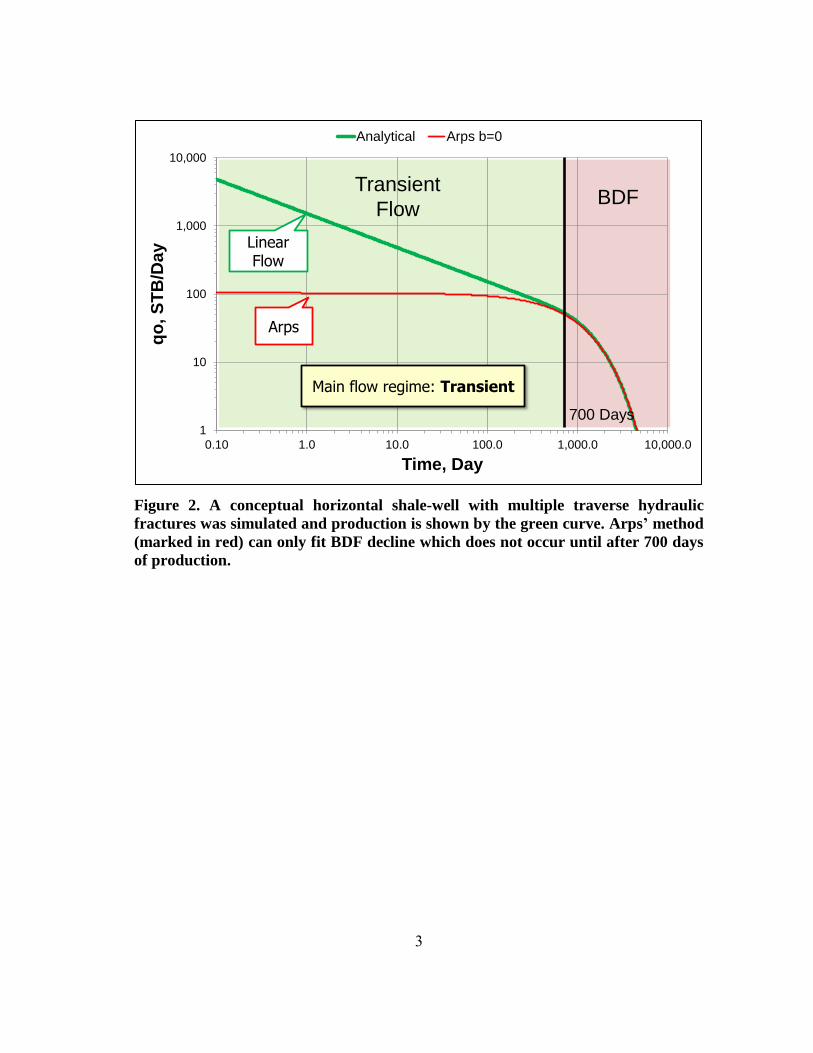
Figure 3. Arps' method matches a Fayetteville shale well with a b value greater than 1. ......................................................................................................................... 4
Figure 4. Arps' three types of decline and their formulas on a semi-log plot after Arps (1945). ........................................................................................................ 7
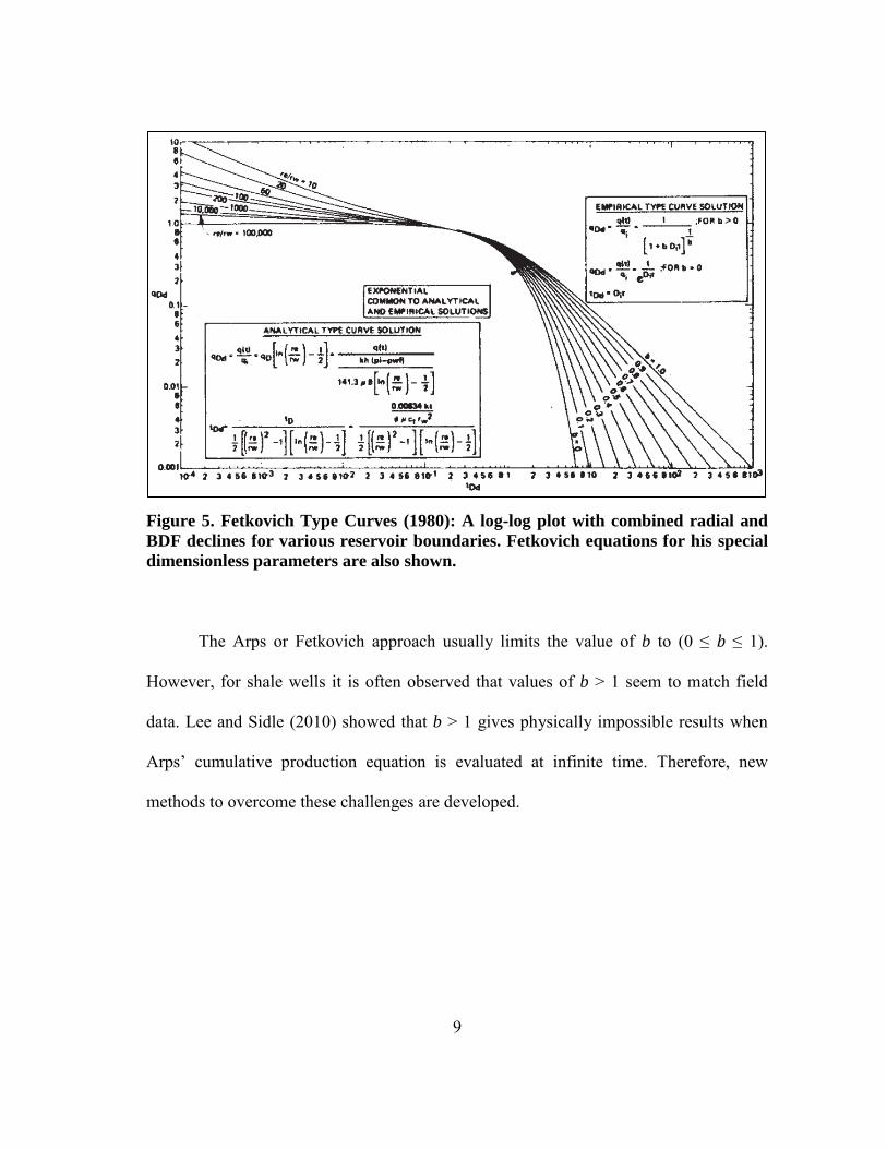
Figure 5. Fetkovich Type Curves (1980): A log-log plot with combined radial and BDF declines for various reservoir boundaries. Fetkovich equations for his special dimensionless parameters are also shown. ........................................ 9
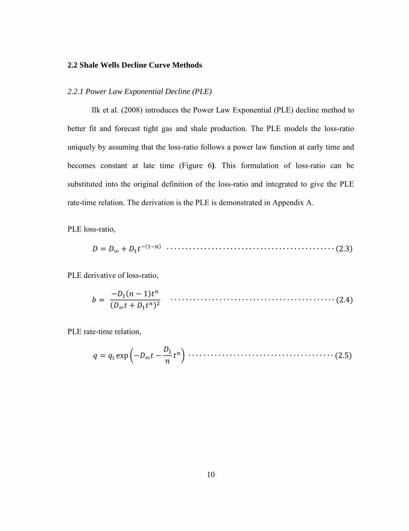
Figure 6. PLE schematic after Ilk et al. (2008). Loss-ratio is modeled uniquely by assuming it follows a power law function at early times and becomes constant at late time. ......................................................................................... 11
Figure 7. Duong's Type Curves (2011). Curves with different m values are shown. The variable a and m are related by a correlation defined by Duong. .............. 14
Figure 8. A correlation between a and m for various gas plays (Duong 2011)................ 15
Figure 9. Modified Fetkovich type curve which includes transient linear (b=2) and bilinear flow (b=4). ........................................................................................... 18
Figure 10. A simulated shale gas well fitted using the composite Arps method. Arps’ equation with is used until the start of BDF ( ) while is used afterwards. ........................................................................... 20
Figure 11. The first matching plot for the PLE method. In this plot, the parameters , and are found through iteration. ..................................................... 21
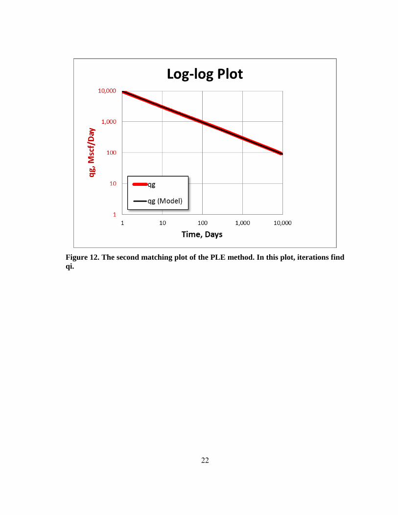
Figure 12. The second matching plot of the PLE method. In this plot, iterations find qi. ...................................................................................................................... 22
xi
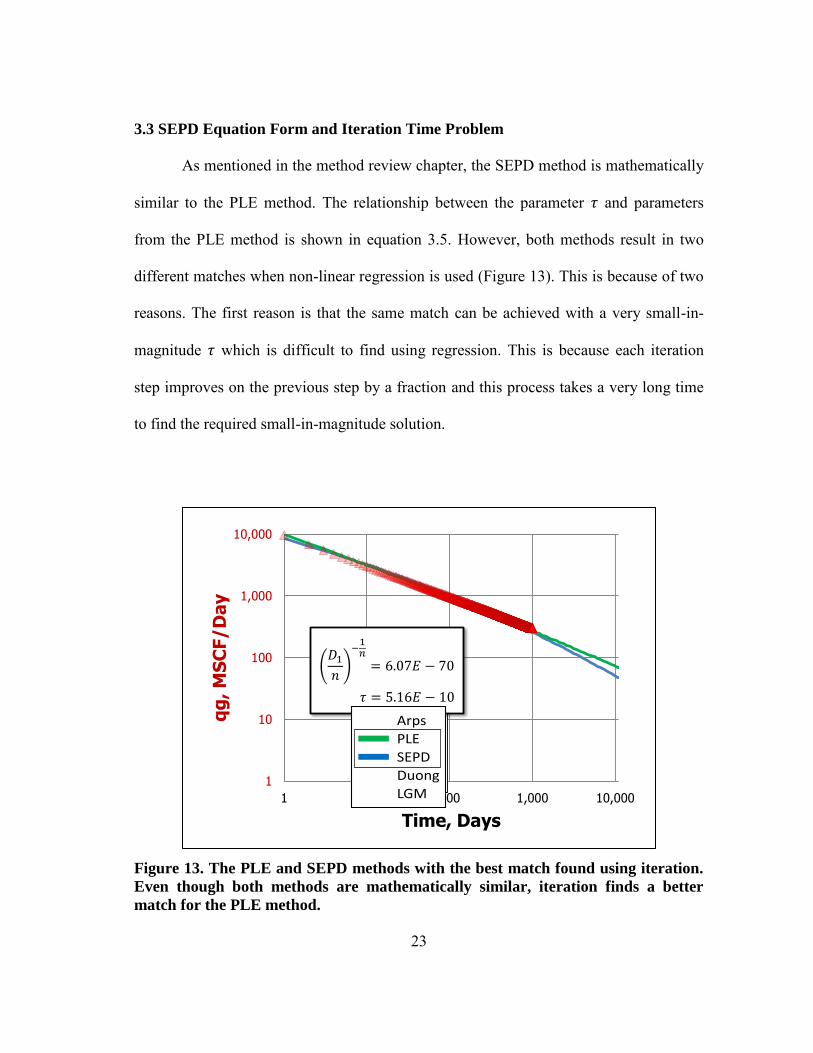
Figure 13. The PLE and SEPD methods with the best match found using iteration. Even though both methods are mathematically similar, iteration finds a better match for the PLE method. ..................................................................... 23
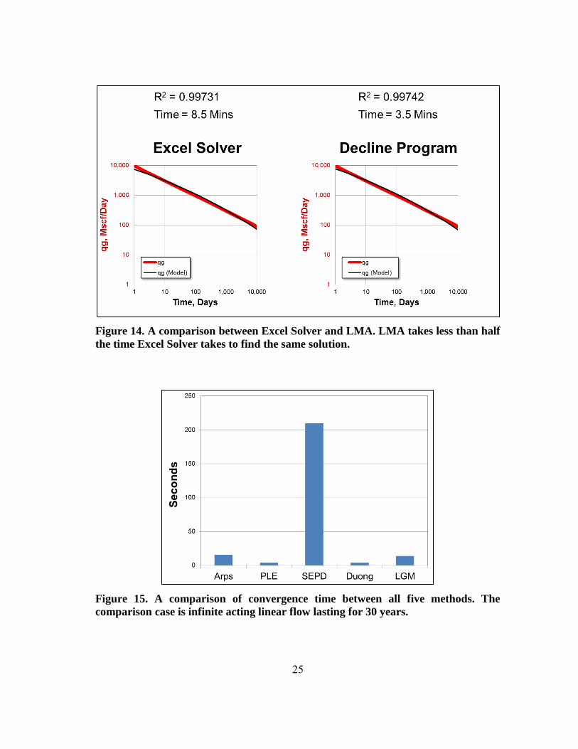
Figure 14. A comparison between Excel Solver and LMA. LMA takes less than half the time Excel Solver takes to find the same solution. .............................. 25
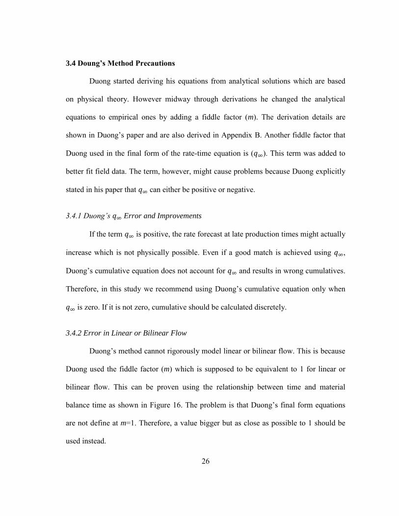
Figure 15. A comparison of convergence time between all five methods. The comparison case is infinite acting linear flow lasting for 30 years. .................. 25
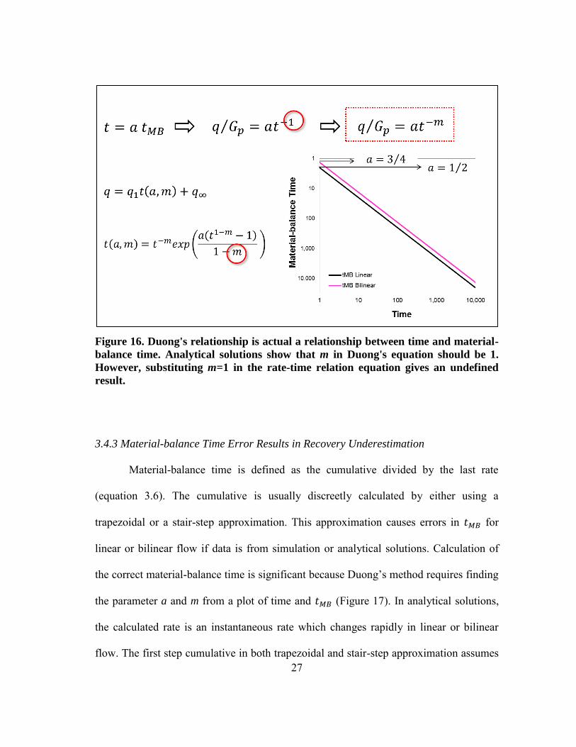
Figure 16. Duong's relationship is actual a relationship between time and material-balance time. Analytical solutions show that m in Duong's equation should be 1. However, substituting m=1 in the rate-time relation equation gives an undefined result. ................................................................................. 27
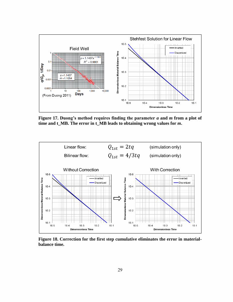
Figure 17. Duong’s method requires finding the parameter a and m from a plot of time and t_MB. The error in t_MB leads to obtaining wrong values for m. .... 29
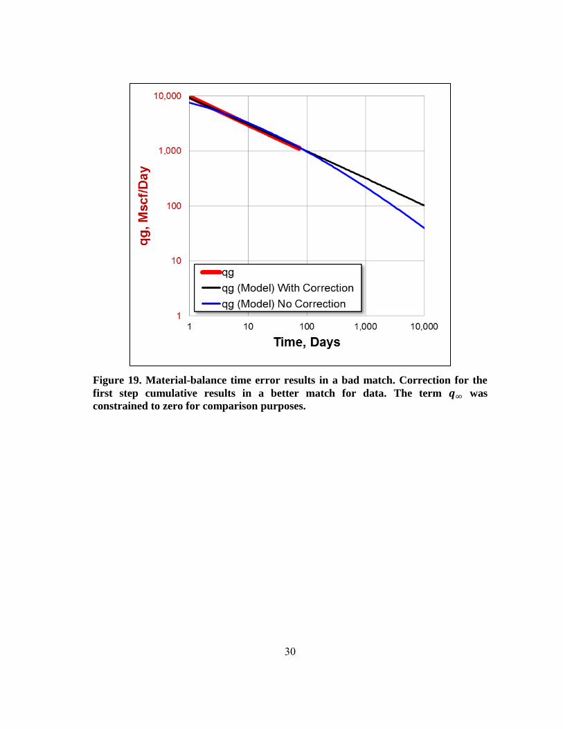
Figure 18. Correction for the first step cumulative eliminates the error in material-balance time. ..................................................................................................... 29
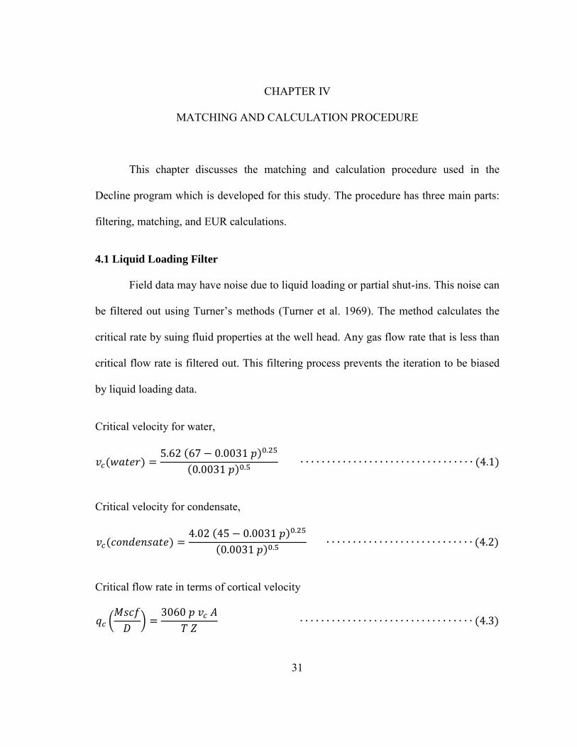
Figure 19. Material-balance time error results in a bad match. Correction for the first step cumulative results in a better match for data. The term was constrained to zero for comparison purposes. .................................................. 30
Figure 20. Illustration of procedure to calculate EUR. .................................................... 34
Figure 21. Schematic of the Homogenous Model and Naturally Fractured Model. Both models have parallel hydraulic fractures and assume a constant reservoir volume. The naturally fracture models has also parallel naturally fractures that are perpendicular to hydraulic fractures (Tivayanonda et al. 2012). ................................................................................................................ 36
Figure 22. Different ways to visualize fractures in shale wells. ...................................... 36
Figure 23. Detailed schematics showing the homogenous and naturally fractured model as well as the simulated segments. ........................................................ 38
Figure 24. Case 1: infinite acting linear flow until abandonment. ................................... 39
Figure 25. Case 2: linear flow following by boundary dominated flow at around 1000 days. ......................................................................................................... 39
Figure 26. Case 3: Bilinear flow followed by linear flow which lasts until abandonment. .................................................................................................... 40
xii
Figure 27. Case 4: The case has all three flow regimes. Bilinear then linear then BDF................................................................................................................... 40
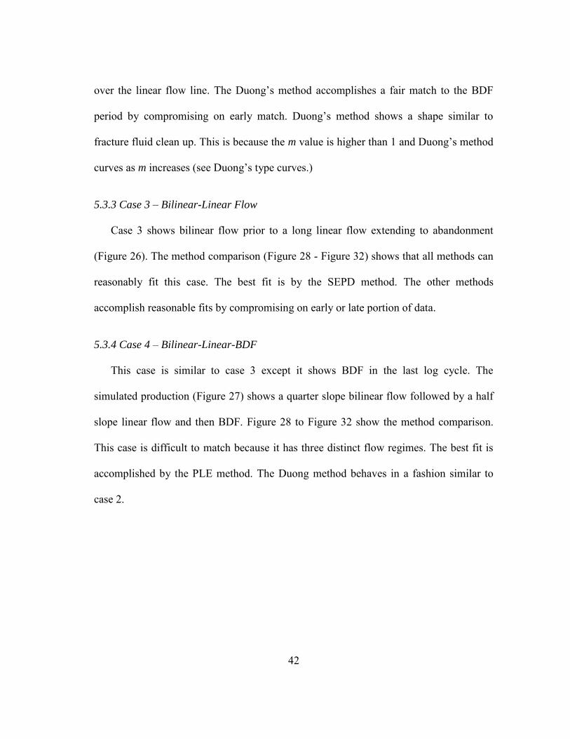
Figure 28. The final iteration match for the Arps Method. Arps Fit Case 1 Perfectly. Arps' method does not fit the other cases accurately because it cannot model multiple flow regimes. ........................................................................... 43
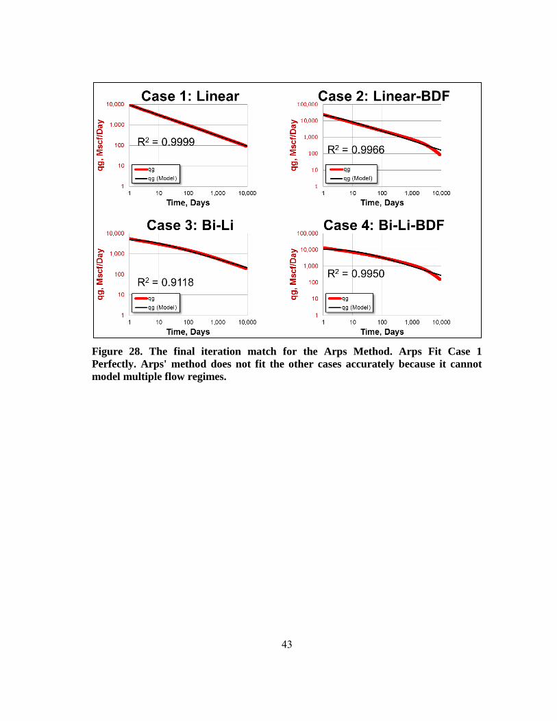
Figure 29. The final iteration match for the PLE method. The PLE method fits Case 1 perfectly and fairly fits Case 2 and 4. Case 3, however, is fitted by coincidence here and might not fit other scenarios similar to case 3 as accurately. ......................................................................................................... 44
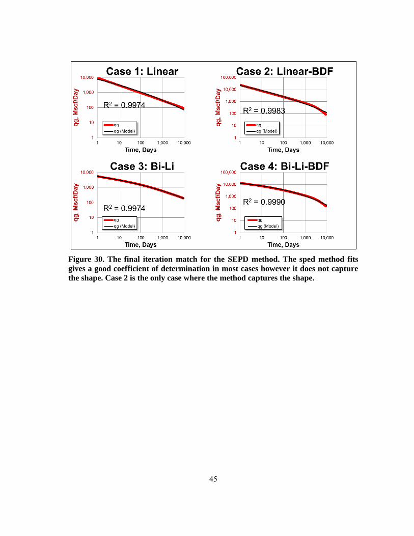
Figure 30. The final iteration match for the SEPD method. The sped method fits gives a good coefficient of determination in most cases however it does not capture the shape. Case 2 is the only case where the method captures the shape. .......................................................................................................... 45
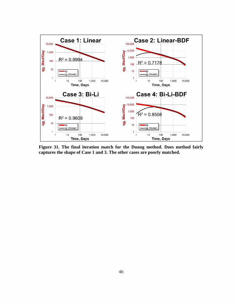
Figure 31. The final iteration match for the Duong method. Does method fairly captures the shape of Case 1 and 3. The other cases are poorly matched. ....... 46
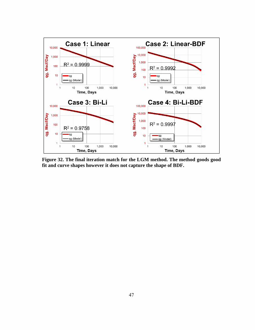
Figure 32. The final iteration match for the LGM method. The method goods good fit and curve shapes however it does not capture the shape of BDF. ............... 47
Figure 33. Case 1 forecast comparison with 100 days of production data. ...................... 50
Figure 34. Case 1 forecast comparison with 1000 days of production data. .................... 51
Figure 35. Case 1 forecast comparison with 9000 days for production data. .................. 52
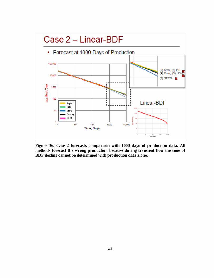
Figure 36. Case 2 forecasts comparison with 1000 days of production data. All methods forecast the wrong production because during transient flow the time of BDF decline cannot be determined with production data alone. ......... 53
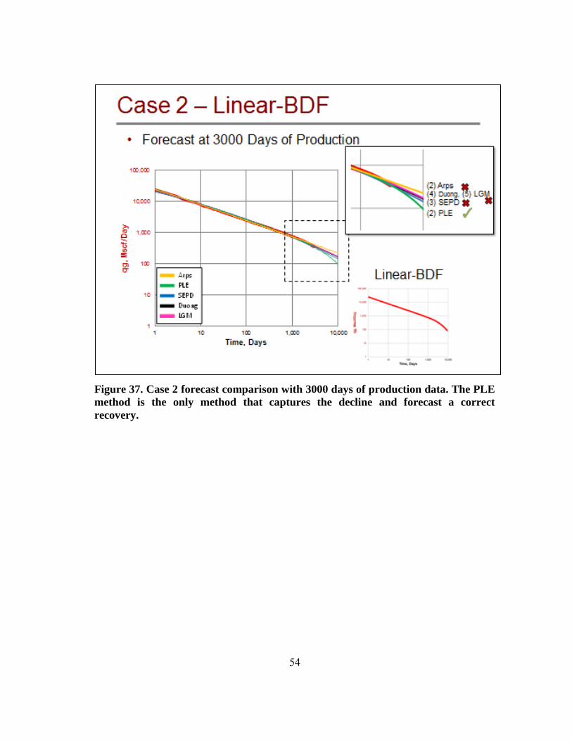
Figure 37. Case 2 forecast comparison with 3000 days of production data. The PLE method is the only method that captures the decline and forecast a correct recovery. ........................................................................................................... 54
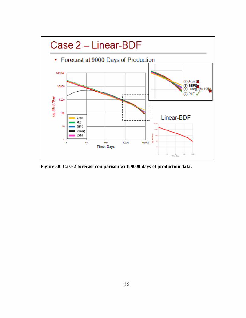
Figure 38. Case 2 forecast comparison with 9000 days of production data. .................... 55
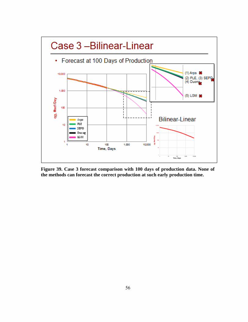
Figure 39. Case 3 forecast comparison with 100 days of production data. None of the methods can forecast the correct production at such early production time. .................................................................................................................. 56
xiii
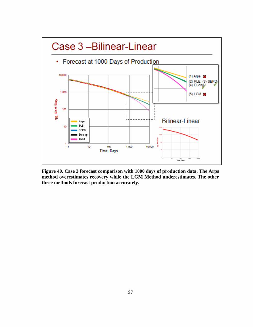
Figure 40. Case 3 forecast comparison with 1000 days of production data. The Arps method overestimates recovery while the LGM Method underestimates. The other three methods forecast production accurately. ................................. 57
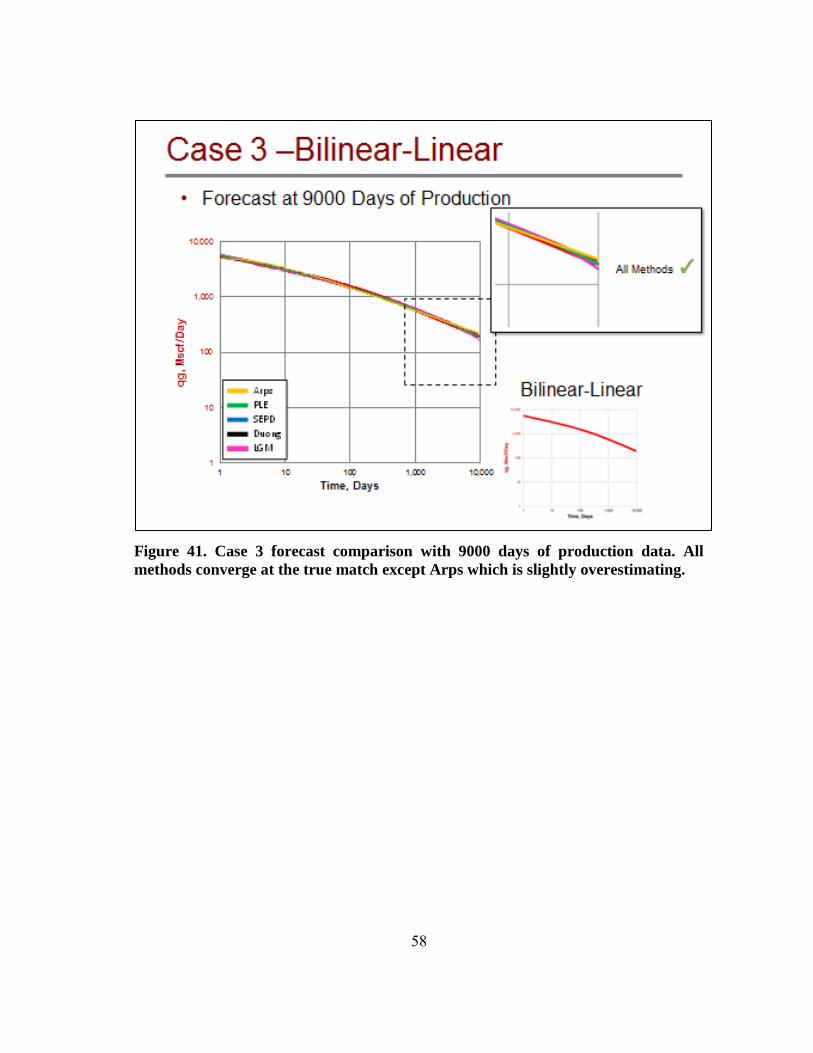
Figure 41. Case 3 forecast comparison with 9000 days of production data. All methods converge at the true match except Arps which is slightly overestimating. .................................................................................................. 58
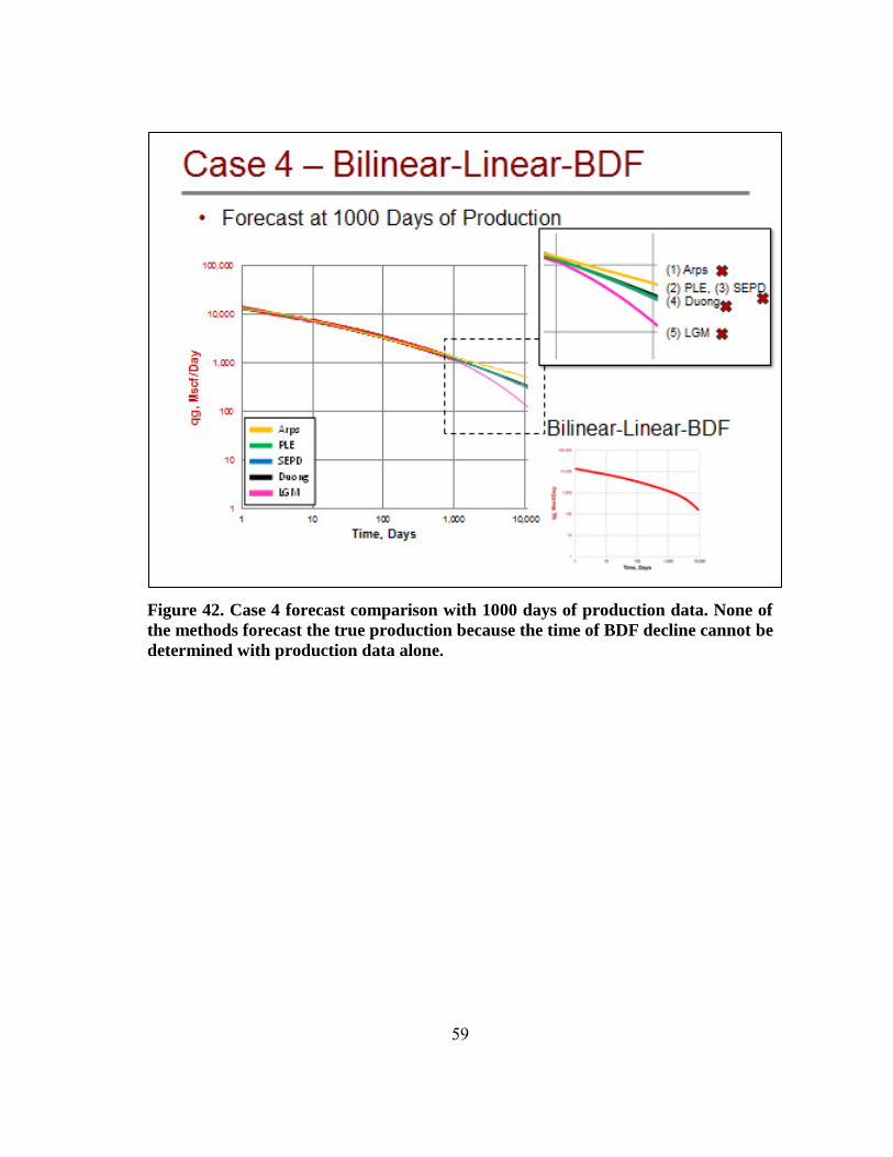
Figure 42. Case 4 forecast comparison with 1000 days of production data. None of the methods forecast the true production because the time of BDF decline cannot be determined with production data alone. ........................................... 59
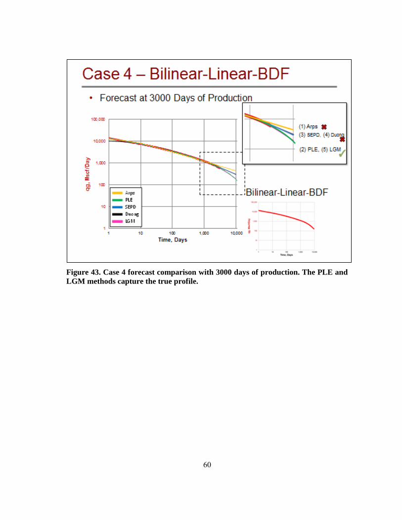
Figure 43. Case 4 forecast comparison with 3000 days of production. The PLE and LGM methods capture the true profile. ............................................................ 60
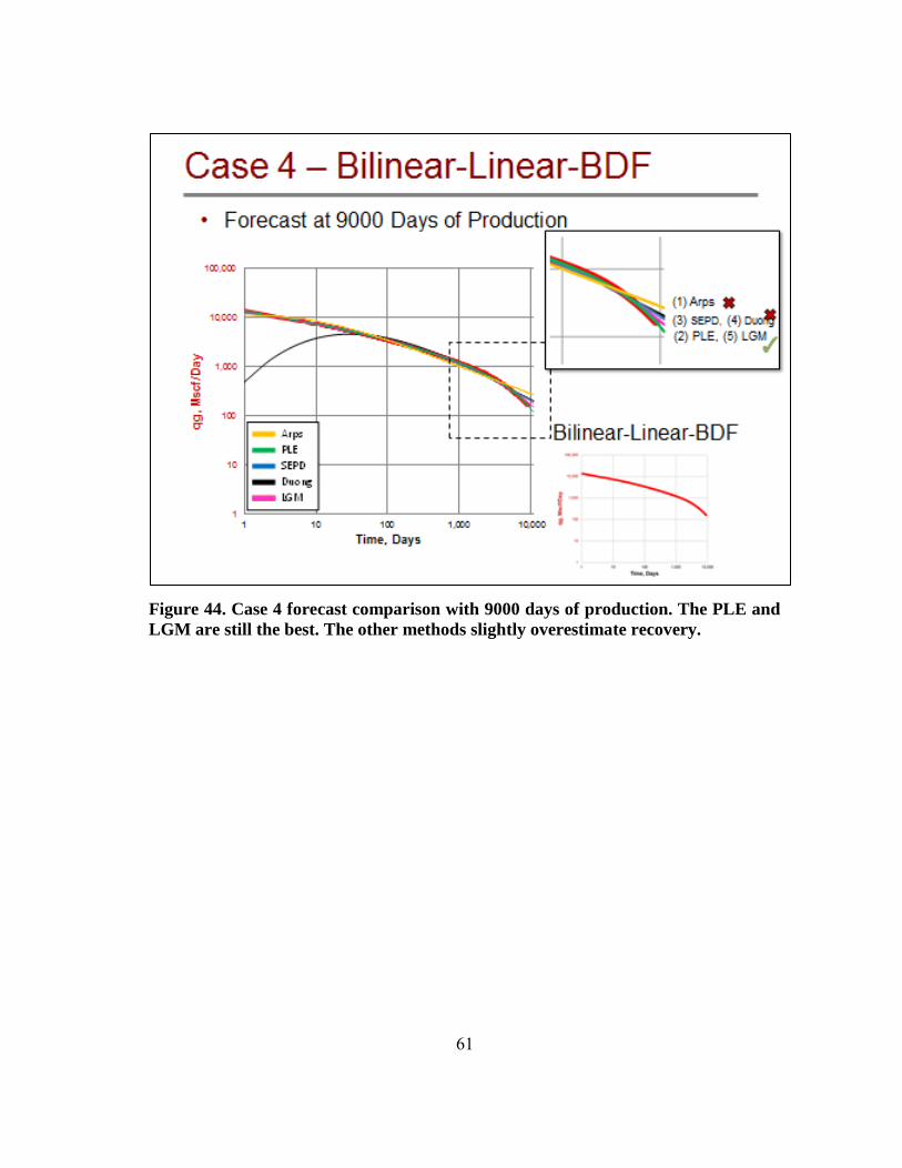
Figure 44. Case 4 forecast comparison with 9000 days of production. The PLE and LGM are still the best. The other methods slightly overestimate recovery. ..... 61
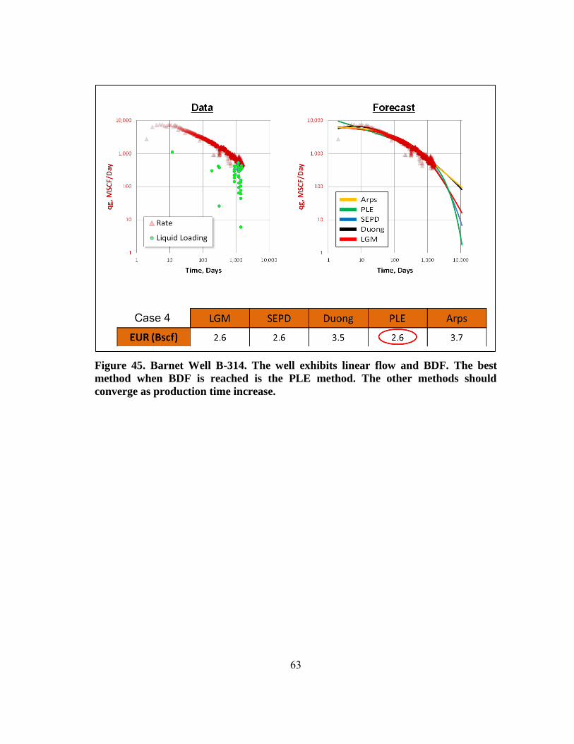
Figure 45. Barnet Well B-314. The well exhibits linear flow and BDF. The best method when BDF is reached is the PLE method. The other methods should converge as production time increase. .................................................. 63
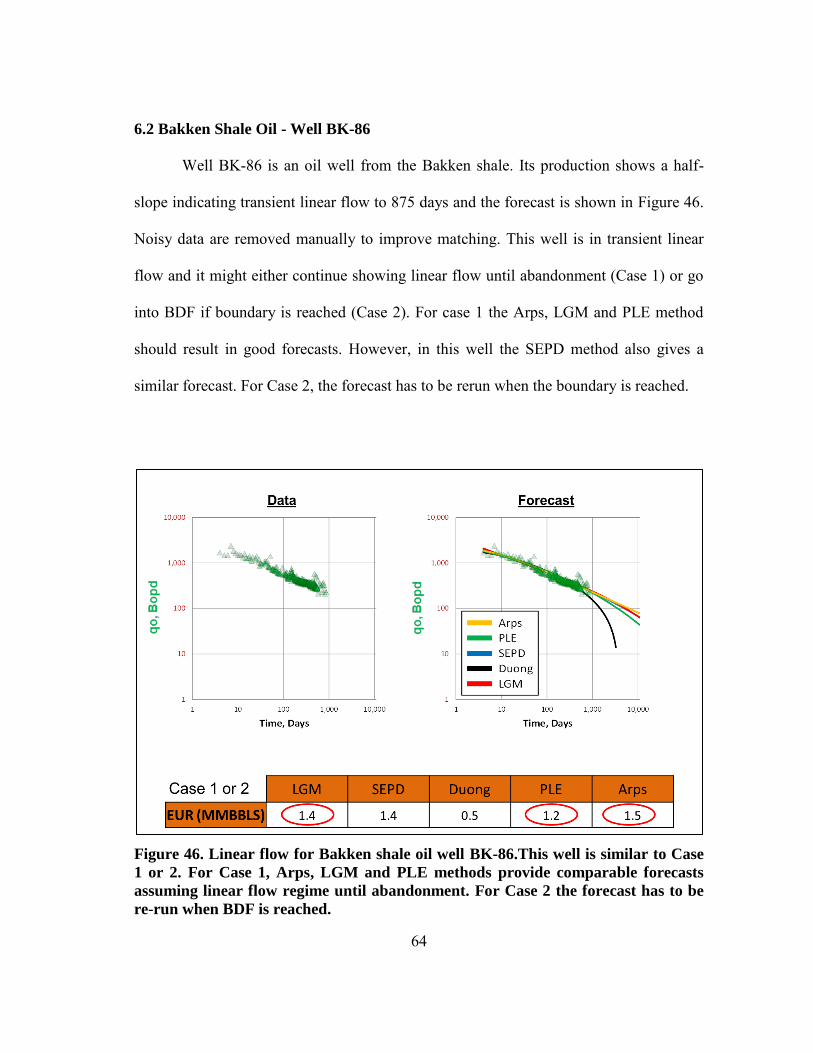
Figure 46. Linear flow for Bakken shale oil well BK-86.This well is similar to Case 1 or 2. For Case 1, Arps, LGM and PLE methods provide comparable forecasts assuming linear flow regime until abandonment. For Case 2 the forecast has to be re-run when BDF is reached. ............................................... 64
Figure 47. Eagleford well 204. This well is similar to case 3 or 4. For Case 3 the true forecast should be bracketed between Arps and the LGM method. Fore Case 4 the forecast has to be re-run when BDF is reached. ..................... 65
Figure 48. Fayetteville Well FF-3. The well is not similar to any of the run cases. The best method cannot be determined. ........................................................... 66

xiv
LIST OF TABLES
Page
Table 1 – Arps equations for rate and cumulative (1945). ................................................. 8
1
CHAPTER I
INTRODUCTION
Historically, the decline curve analysis method by Arps (1945) has been the most
popular tool for forecasting Estimated Ultimate Recovery (EUR) and reserves because of
its reliability and simplicity. In recent years, the industry started producing shale plays
and production forecast analysis for shale wells is problematic using this traditional
method. The reason is that Arps’ equations only work during Boundary Dominated Flow
(BDF) decline. Unlike in conventional reservoirs, such decline is not observed in shale
wells during early production life when financial forecast is important (Figure 1-Figure
2). Arps’ method match shale wells with b values greater than what Arps specified
(Figure 3). To eliminate this problem and improve shale production forecast, researchers
developed new empirical methods. However, the new methods have different equation
forms and often result in dissimilar forecasts.
2
Figure 1. A conceptual vertical well in a conventional oil reservoir was simulated
and production is shown by the green curve. Transient flow is relatively short and
BDF is reached quickly. Arps exponential decline (marked in red) results in an
excellent fit even at an early production time of 3 days.
1
10
100
1,000
10,000
0.10 1.0 10.0 100.0 1,000.0 10,000.0
qo
, S
TB
/Day
Time, Day
Analytical Arps b=0
Transient
FlowBDF
3 Days
Arps
Radial
Flow
Main flow regime: BDF
3
Figure 2. A conceptual horizontal shale-well with multiple traverse hydraulic
fractures was simulated and production is shown by the green curve. Arps’ method
(marked in red) can only fit BDF decline which does not occur until after 700 days
of production.
1
10
100
1,000
10,000
0.10 1.0 10.0 100.0 1,000.0 10,000.0
qo
, S
TB
/Day
Time, Day
Analytical Arps b=0
700 Days
Arps
Linear Flow
Transient
FlowBDF
Main flow regime: Transient
4
Figure 3. Arps' method matches a Fayetteville shale well with a b value greater
than 1.
1.1 Objective
The main purpose of this work is to identify the most accurate method(s) by
comparing it/them to analytical and conceptual simulation models. Analytical and
simulation models are used for benchmarking because they are applied, validated, and
well established in literature (Ahmadi et al. 2010; Bello and Wattenbarger 2008; Bello
and Wattenbarger 2010; Samandarli et al. 2011). Other objectives of this work include
identifying of strengths and weaknesses of each empirical method and establishing a
workflow to automatically match methods to data using non-linear regression. The
methods are compared in terms of:
5
1. Ultimate recovery accuracy
2. Goodness of fit
3. Ease of matching
1.2 Thesis Organization
This thesis is divided into seven chapters. The organization of these chapters is as
follows:
Chapter I is an introduction to the subject of this research, its motivations and
objectives.
Chapter II is a literature review including history of empirical decline curve
analysis and the traditional decline curve methods of Arps and Fetkovich. The chapter
also reviews recent empirical decline methods that are developed specifically for tight
gas and shale wells.
Chapter III investigates the advantages and shortcomings of the new methods. It
also shows problems that engineers might encounter while applying the methods as well
as procedures to mitigate such problems.
Chapter IV describes the proposed procedure for matching and forecasting.
Chapter V compares the new decline methods and the traditional methods against
conceptual simulation models. The methods which best fit simulation cases and predict
their EUR are determined.
Chapter VI shows field examples and applications of the proposed methodology.
Chapter VII presents discussion and conclusions.
6
CHAPTER II
LITERATURE REVIEW
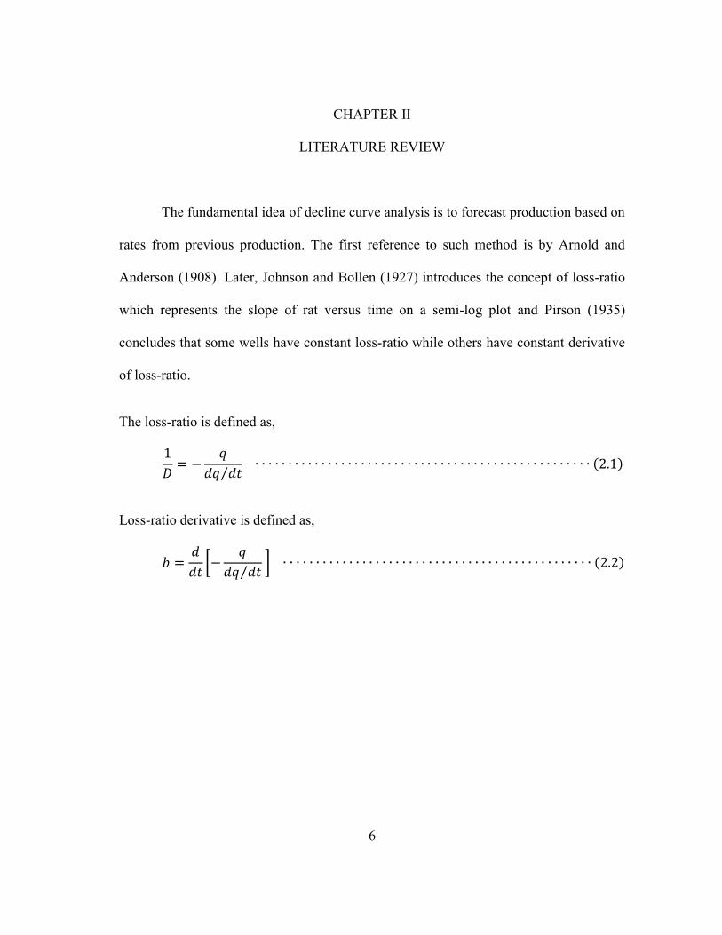
The fundamental idea of decline curve analysis is to forecast production based on
rates from previous production. The first reference to such method is by Arnold and
Anderson (1908). Later, Johnson and Bollen (1927) introduces the concept of loss-ratio
which represents the slope of rat versus time on a semi-log plot and Pirson (1935)
concludes that some wells have constant loss-ratio while others have constant derivative
of loss-ratio.
The loss-ratio is defined as,
⁄ ( )
Loss-ratio derivative is defined as,
[
⁄ ] ( )
7
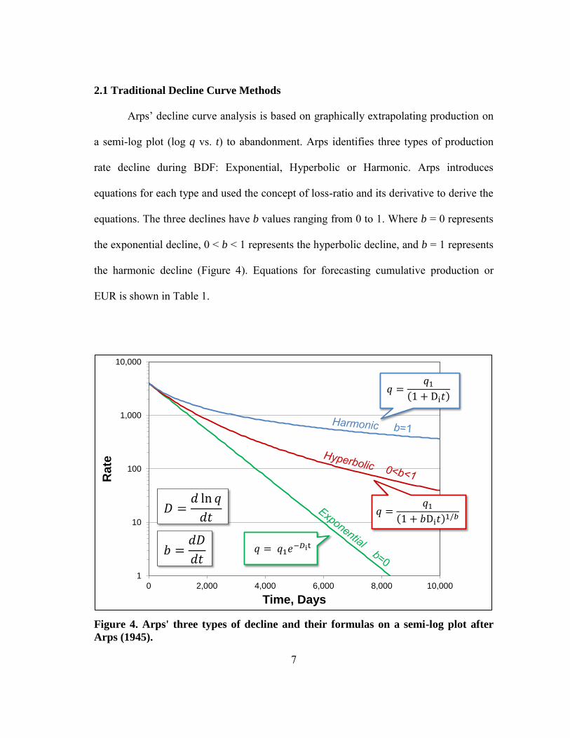
2.1 Traditional Decline Curve Methods
Arps’ decline curve analysis is based on graphically extrapolating production on
a semi-log plot (log q vs. t) to abandonment. Arps identifies three types of production
rate decline during BDF: Exponential, Hyperbolic or Harmonic. Arps introduces
equations for each type and used the concept of loss-ratio and its derivative to derive the
equations. The three declines have b values ranging from 0 to 1. Where b = 0 represents
the exponential decline, 0 < b < 1 represents the hyperbolic decline, and b = 1 represents
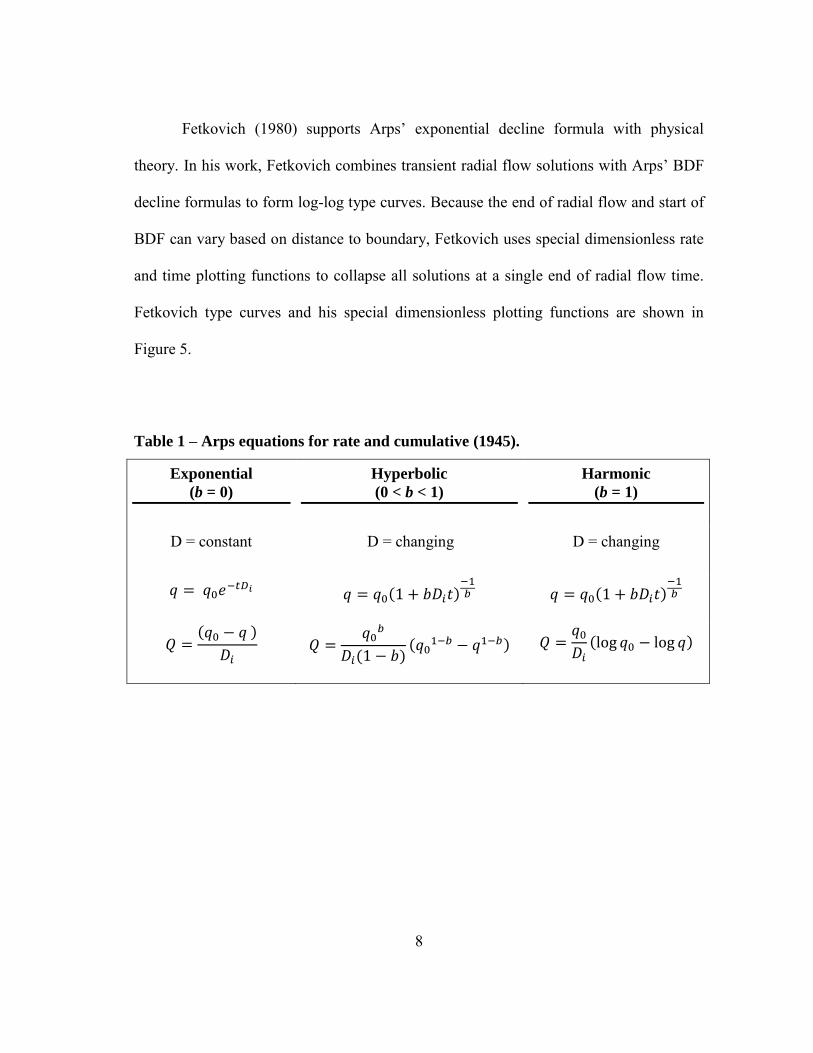
the harmonic decline (Figure 4). Equations for forecasting cumulative production or
EUR is shown in Table 1.
Figure 4. Arps' three types of decline and their formulas on a semi-log plot after
Arps (1945).
1
10
100
1,000
10,000
0 2,000 4,000 6,000 8,000 10,000
Ra
te
Time, Days
8
Fetkovich (1980) supports Arps’ exponential decline formula with physical
theory. In his work, Fetkovich combines transient radial flow solutions with Arps’ BDF
decline formulas to form log-log type curves. Because the end of radial flow and start of
BDF can vary based on distance to boundary, Fetkovich uses special dimensionless rate
and time plotting functions to collapse all solutions at a single end of radial flow time.
Fetkovich type curves and his special dimensionless plotting functions are shown in
Figure 5.
Table 1 – Arps equations for rate and cumulative (1945).
Exponential
(b = 0)
Hyperbolic
(0 < b < 1)
Harmonic
(b = 1)
D = constant D = changing D = changing
( )
( )
( )
( )(
) ( )
9
Figure 5. Fetkovich Type Curves (1980): A log-log plot with combined radial and
BDF declines for various reservoir boundaries. Fetkovich equations for his special
dimensionless parameters are also shown.
The Arps or Fetkovich approach usually limits the value of b to (0 ≤ ≤ 1).
However, for shale wells it is often observed that values of b > 1 seem to match field
data. Lee and Sidle (2010) showed that b > 1 gives physically impossible results when
Arps’ cumulative production equation is evaluated at infinite time. Therefore, new
methods to overcome these challenges are developed.
10
2.2 Shale Wells Decline Curve Methods
2.2.1 Power Law Exponential Decline (PLE)
Ilk et al. (2008) introduces the Power Law Exponential (PLE) decline method to
better fit and forecast tight gas and shale production. The PLE models the loss-ratio
uniquely by assuming that the loss-ratio follows a power law function at early time and
becomes constant at late time (Figure 6). This formulation of loss-ratio can be
substituted into the original definition of the loss-ratio and integrated to give the PLE
rate-time relation. The derivation is the PLE is demonstrated in Appendix A.
PLE loss-ratio,
( ) ( )
PLE derivative of loss-ratio,
( )
( ) ( )
PLE rate-time relation,
( ) ( )
11
Figure 6. PLE schematic after Ilk et al. (2008). Loss-ratio is modeled uniquely by
assuming it follows a power law function at early times and becomes constant at
late time.
2.2.2 Stretched Exponential Decline (SEPD)
Valko (2009) independently proposes the Stretched Exponential Decline (SEPD)
which is similar to the PLE method. Valko uses this method to evaluate the effect of
stimulation (re-stimulation) treatment in Barnett shale by analyzing monthly production
from public databases. Later, Valko and Lee (2010) use this method for forecasting.
12
SEPD rate-time relation,
[ (
)
] ( )
SEPD cumulative-time relation,
{ [
] [
(
)
]} ( )
The SEPD equation differs from the PLE model in not considering the behavior
at late times (the term). In the SEPD method, is always considered to be zero and
is equivalent to ( ⁄ ) ⁄ . One advantage of SEPD over PLE is the provided
cumulative-time relation. This relation adds the option of fitting data to cumulative
production, which is smoother and easier to regress on than the usually scattered
production rate trends. In the cumulative equation, the first term inside the brackets is
the complete gamma function and the second term is the incomplete gamma function.
2.2.3 Duong’s Method
Duong’s method (2011) is developed on the basis that production rate and time
have a power law relation or form a straight line when plotted on a log-log scale.
Integrating this relation with respect to time from (0 to t) gives a relationship between
time and material balance time (equation 3.8).
Duong’s time/material-balance-time relation,
( )
13
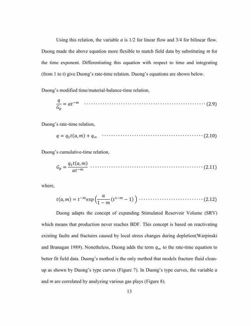
Using this relation, the variable a is 1/2 for linear flow and 3/4 for bilinear flow.
Duong made the above equation more flexible to match field data by substituting m for
the time exponent. Differentiating this equation with respect to time and integrating
(from 1 to t) give Duong’s rate-time relation. Duong’s equations are shown below.
Duong’s modified time/material-balance-time relation,
( )
Duong’s rate-time relation,
( ) ( )
Duong’s cumulative-time relation,
( )
( )
where,
( ) (
( ) ) ( )
Duong adapts the concept of expanding Stimulated Reservoir Volume (SRV)
which means that production never reaches BDF. This concept is based on reactivating
existing faults and fractures caused by local stress changes during depletion(Warpinski
and Branagan 1989). Nonetheless, Duong adds the term to the rate-time equation to
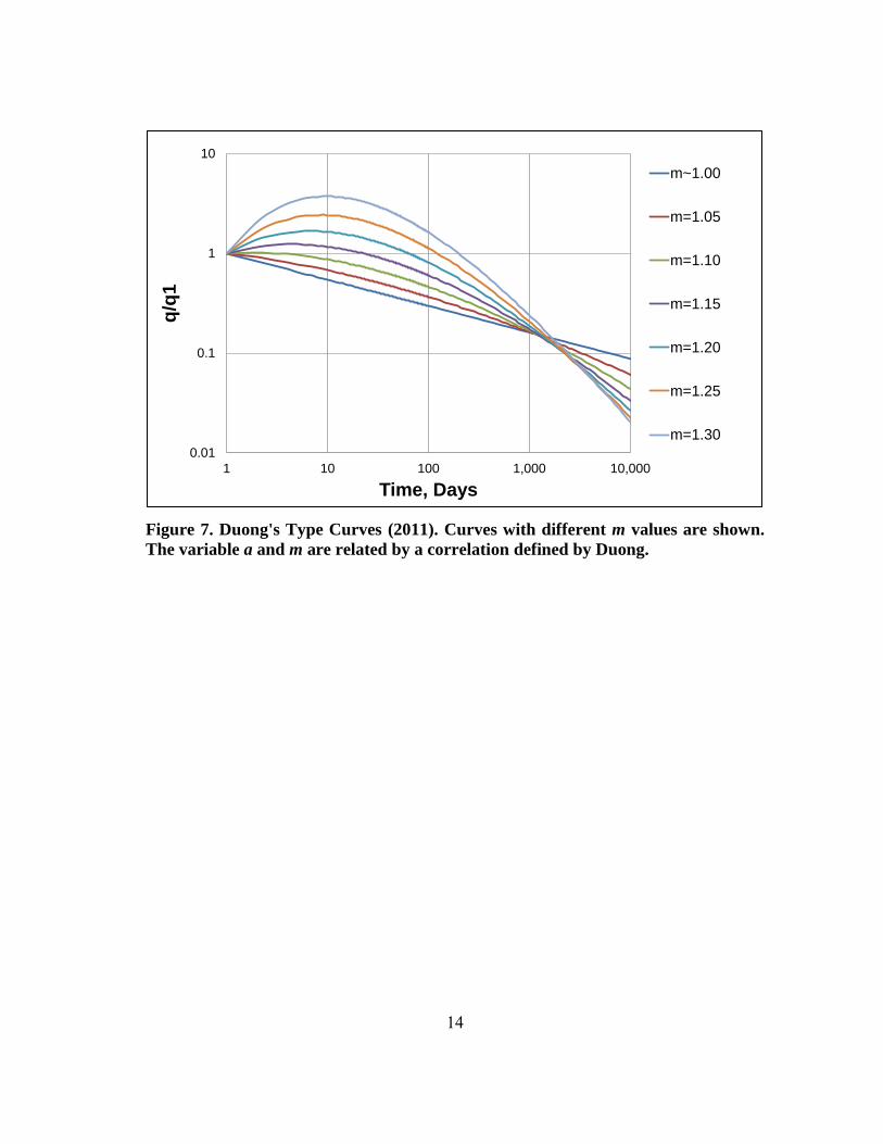
better fit field data. Duong’s method is the only method that models fracture fluid clean-
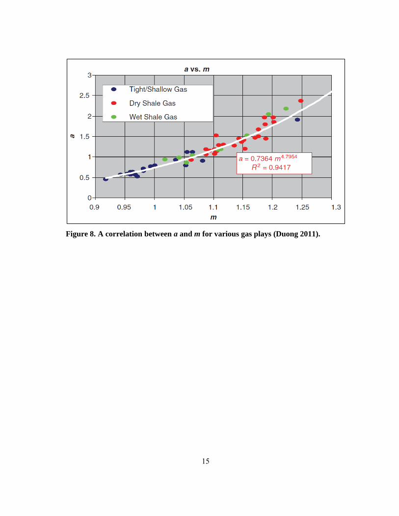
up as shown by Duong’s type curves (Figure 7). In Duong’s type curves, the variable a
and m are correlated by analyzing various gas plays (Figure 8).
14
Figure 7. Duong's Type Curves (2011). Curves with different m values are shown.
The variable a and m are related by a correlation defined by Duong.
0.01
0.1
1
10
1 10 100 1,000 10,000
q/q
1
Time, Days
m~1.00
m=1.05
m=1.10
m=1.15
m=1.20
m=1.25
m=1.30
15
Figure 8. A correlation between a and m for various gas plays (Duong 2011).
16
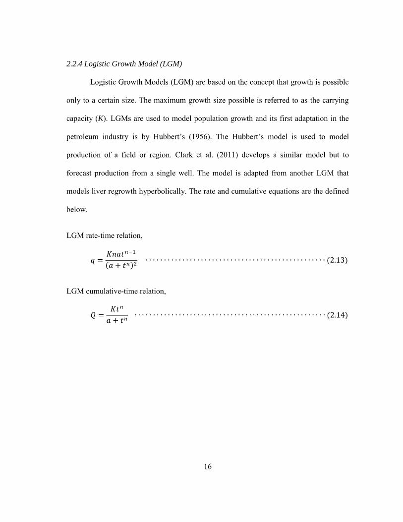
2.2.4 Logistic Growth Model (LGM)
Logistic Growth Models (LGM) are based on the concept that growth is possible
only to a certain size. The maximum growth size possible is referred to as the carrying
capacity (K). LGMs are used to model population growth and its first adaptation in the
petroleum industry is by Hubbert’s (1956). The Hubbert’s model is used to model
production of a field or region. Clark et al. (2011) develops a similar model but to
forecast production from a single well. The model is adapted from another LGM that
models liver regrowth hyperbolically. The rate and cumulative equations are the defined
below.
LGM rate-time relation,
( ) ( )
LGM cumulative-time relation,
( )
17
CHAPTER III
INVESTIGATION OF METHODS
The previous chapter provided an overview of both traditional and new empirical
decline methods. This chapter shows the drawback and advantages of each method and
provides simple solutions to mitigate difficulties which might be encountered while
applying the methods.
3.1 Arps’ Unbounded Reserves Problem and Improvements
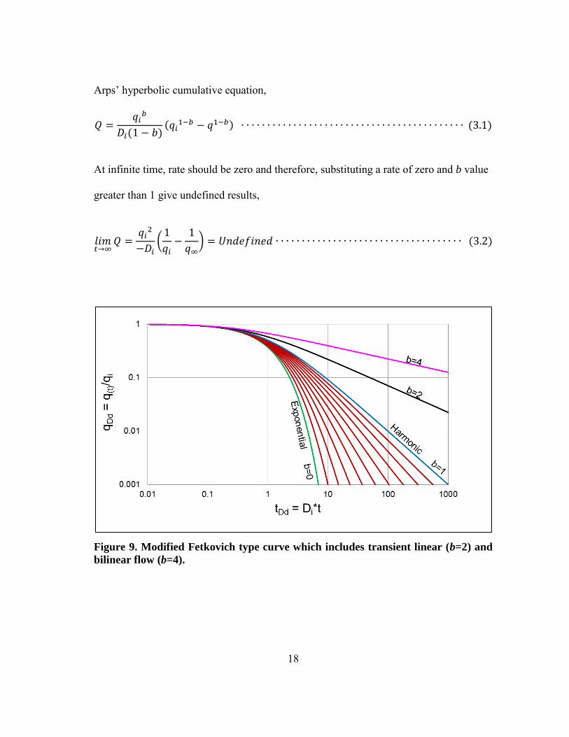
Arps’ equations are designed for BDF decline and the reason shale wells have b
values greater than 1 is the fact that shale wells are generally in transient flow. Shale has
low permeability and is usually produced from hydraulically fracture wells. This results
in a long transient linear or bilinear flow which can be fitted using Arps’ hyperbolic
equation and b values of 2 or 4 respectively (Figure 9). However, these values are
outside the range that Arps’ specified ( ) and result in two problems. The first
problem is that extrapolation on transient flow overestimates reserves. The second
problem is that the hyperbolic equation with b values greater than one never goes to zero
and therefore reserves is unbounded. Lee and Sidle (2010) demonstrated the second
problem with the following:
18
Arps’ hyperbolic cumulative equation,
( )(
) ( )
At infinite time, rate should be zero and therefore, substituting a rate of zero and b value
greater than 1 give undefined results,
(
) ( )
Figure 9. Modified Fetkovich type curve which includes transient linear (b=2) and
bilinear flow (b=4).
19
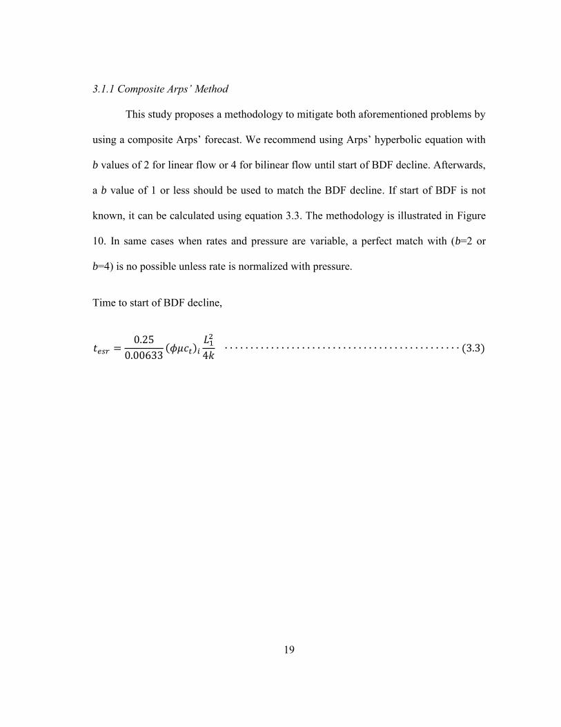
3.1.1 Composite Arps’ Method
This study proposes a methodology to mitigate both aforementioned problems by
using a composite Arps’ forecast. We recommend using Arps’ hyperbolic equation with
b values of 2 for linear flow or 4 for bilinear flow until start of BDF decline. Afterwards,
a b value of 1 or less should be used to match the BDF decline. If start of BDF is not
known, it can be calculated using equation 3.3. The methodology is illustrated in Figure
10. In same cases when rates and pressure are variable, a perfect match with (b=2 or
b=4) is no possible unless rate is normalized with pressure.
Time to start of BDF decline,
( )
( )
20
Figure 10. A simulated shale gas well fitted using the composite Arps method. Arps’
equation with is used until the start of BDF ( ) while is used
afterwards.
3.2 PLE Iteration Blow-up
The PLE method requires fitting on two different plots. The first plot is a log-log
plot of loss-ratio versus time (Figure 11). The parameters , , and are obtained
from this plot. The parameter n is the slope, the parameter is the intercept, and the
parameter is the value of loss-ratio at infinite time. The second plot is either a semi-
log or log-log plot of rate verses time and it is used to find the parameter (Figure 12).
We fitted various cases using the PLE model using non-linear regression. In many cases,
the best match for is very large and exceeds the range that excel can handle. The
reason is very large is that parameter n is small. This can be illustrated by rearranging
the rate-time relation (equation 2.5) to equation 3.4. If parameter n is small, the solution
becomes too large because of the exponential function. The range for positive values
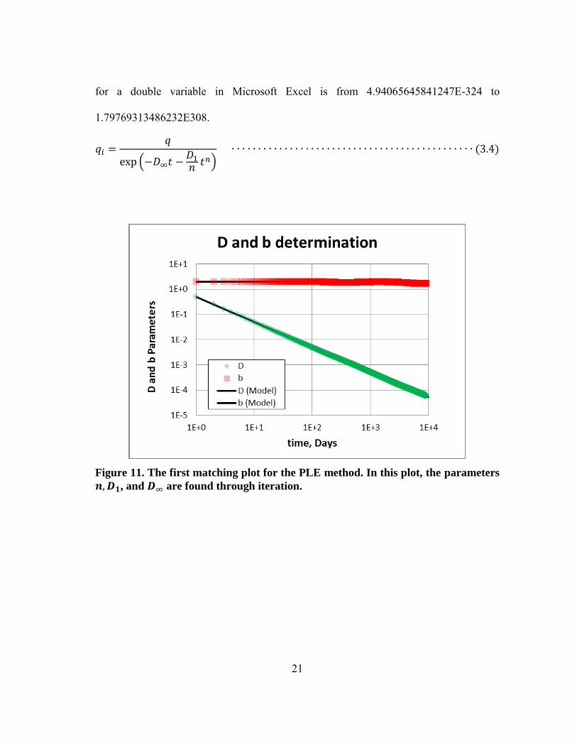
21
for a double variable in Microsoft Excel is from 4.94065645841247E-324 to
1.79769313486232E308.
(
) ( )
Figure 11. The first matching plot for the PLE method. In this plot, the parameters
, and are found through iteration.
22
Figure 12. The second matching plot of the PLE method. In this plot, iterations find
qi.
23
3.3 SEPD Equation Form and Iteration Time Problem
As mentioned in the method review chapter, the SEPD method is mathematically
similar to the PLE method. The relationship between the parameter and parameters
from the PLE method is shown in equation 3.5. However, both methods result in two
different matches when non-linear regression is used (Figure 13). This is because of two
reasons. The first reason is that the same match can be achieved with a very small-in-
magnitude which is difficult to find using regression. This is because each iteration
step improves on the previous step by a fraction and this process takes a very long time
to find the required small-in-magnitude solution.
Figure 13. The PLE and SEPD methods with the best match found using iteration.
Even though both methods are mathematically similar, iteration finds a better
match for the PLE method.
1
10
100
1,000
10,000
1 10 100 1,000 10,000
qg
, M
SC
F/D
ay
Time, Days
LGM
SEPD
Duong
PLE
Arps
LGM
SEPD
Duong
PLE
Arps
24
The second reason is that the PLE method finds most parameters by fitting a
straight-line in loss-ratio plot. Fitting a straight line is faster than fitting the complicated
power-law equation of the SEPD method.
(
)
( )
3.3.1 The SEPD Method and Long Iteration Convergence Time
To overcome the long iteration problem we use the Levenberg-Marquardt
Algorithm (LMA) which is faster than Excel Solver. Figure 14 shows a comparison
between Excel Solver and LMA. Both methods find similar solutions however the LMA
method takes less than half the time Solver takes. The SEPD method is the slowest
method to converge compared to the other four methods. A comparison of the
convergence time is shown in Figure 15.
25
Figure 14. A comparison between Excel Solver and LMA. LMA takes less than half
the time Excel Solver takes to find the same solution.
Figure 15. A comparison of convergence time between all five methods. The
comparison case is infinite acting linear flow lasting for 30 years.
26
3.4 Doung’s Method Precautions
Duong started deriving his equations from analytical solutions which are based
on physical theory. However midway through derivations he changed the analytical
equations to empirical ones by adding a fiddle factor (m). The derivation details are
shown in Duong’s paper and are also derived in Appendix B. Another fiddle factor that
Duong used in the final form of the rate-time equation is ( ). This term was added to
better fit field data. The term, however, might cause problems because Duong explicitly
stated in his paper that can either be positive or negative.
3.4.1 Duong’s Error and Improvements
If the term is positive, the rate forecast at late production times might actually
increase which is not physically possible. Even if a good match is achieved using ,
Duong’s cumulative equation does not account for and results in wrong cumulatives.
Therefore, in this study we recommend using Duong’s cumulative equation only when
is zero. If it is not zero, cumulative should be calculated discretely.
3.4.2 Error in Linear or Bilinear Flow
Duong’s method cannot rigorously model linear or bilinear flow. This is because
Duong used the fiddle factor (m) which is supposed to be equivalent to 1 for linear or
bilinear flow. This can be proven using the relationship between time and material
balance time as shown in Figure 16. The problem is that Duong’s final form equations
are not define at m=1. Therefore, a value bigger but as close as possible to 1 should be
used instead.
27
Figure 16. Duong's relationship is actual a relationship between time and material-
balance time. Analytical solutions show that m in Duong's equation should be 1.
However, substituting m=1 in the rate-time relation equation gives an undefined
result.
3.4.3 Material-balance Time Error Results in Recovery Underestimation
Material-balance time is defined as the cumulative divided by the last rate
(equation 3.6). The cumulative is usually discreetly calculated by either using a
trapezoidal or a stair-step approximation. This approximation causes errors in for
linear or bilinear flow if data is from simulation or analytical solutions. Calculation of
the correct material-balance time is significant because Duong’s method requires finding
the parameter a and m from a plot of time and (Figure 17). In analytical solutions,
the calculated rate is an instantaneous rate which changes rapidly in linear or bilinear
flow. The first step cumulative in both trapezoidal and stair-step approximation assumes
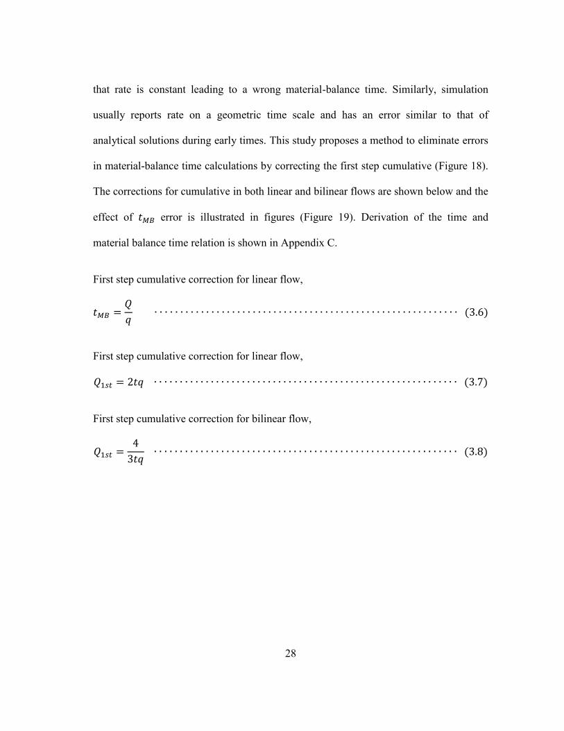
28
that rate is constant leading to a wrong material-balance time. Similarly, simulation
usually reports rate on a geometric time scale and has an error similar to that of
analytical solutions during early times. This study proposes a method to eliminate errors
in material-balance time calculations by correcting the first step cumulative (Figure 18).
The corrections for cumulative in both linear and bilinear flows are shown below and the
effect of error is illustrated in figures (Figure 19). Derivation of the time and
material balance time relation is shown in Appendix C.
First step cumulative correction for linear flow,
( )
First step cumulative correction for linear flow,
( )
First step cumulative correction for bilinear flow,
( )
29
Figure 17. Duong’s method requires finding the parameter a and m from a plot of
time and t_MB. The error in t_MB leads to obtaining wrong values for m.
Figure 18. Correction for the first step cumulative eliminates the error in material-
balance time.
30
Figure 19. Material-balance time error results in a bad match. Correction for the
first step cumulative results in a better match for data. The term was
constrained to zero for comparison purposes.
31
CHAPTER IV
MATCHING AND CALCULATION PROCEDURE
This chapter discusses the matching and calculation procedure used in the
Decline program which is developed for this study. The procedure has three main parts:
filtering, matching, and EUR calculations.
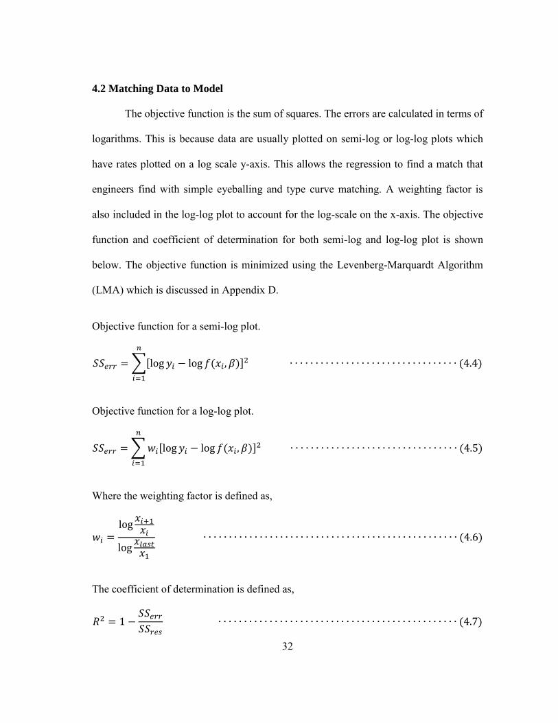
4.1 Liquid Loading Filter
Field data may have noise due to liquid loading or partial shut-ins. This noise can
be filtered out using Turner’s methods (Turner et al. 1969). The method calculates the
critical rate by suing fluid properties at the well head. Any gas flow rate that is less than
critical flow rate is filtered out. This filtering process prevents the iteration to be biased
by liquid loading data.
Critical velocity for water,
( ) ( )
( ) ( )
Critical velocity for condensate,
( ) ( )
( ) ( )
Critical flow rate in terms of cortical velocity
(
)
( )
32
4.2 Matching Data to Model
The objective function is the sum of squares. The errors are calculated in terms of
logarithms. This is because data are usually plotted on semi-log or log-log plots which
have rates plotted on a log scale y-axis. This allows the regression to find a match that
engineers find with simple eyeballing and type curve matching. A weighting factor is
also included in the log-log plot to account for the log-scale on the x-axis. The objective
function and coefficient of determination for both semi-log and log-log plot is shown
below. The objective function is minimized using the Levenberg-Marquardt Algorithm
(LMA) which is discussed in Appendix D.
Objective function for a semi-log plot.
∑[ ( )]
( )
Objective function for a log-log plot.
∑ [ ( )]
( )
Where the weighting factor is defined as,
( )
The coefficient of determination is defined as,
( )
33
Where the residual for a semi-log plot is defined as,
∑[ ]
( )
And the residual for a log-log plot is defined as,
∑ [ ]
( )
The mean of data is for a semi-log plot is,
∑
( )
The mean of data is for a log-log plot is,
∑
( )
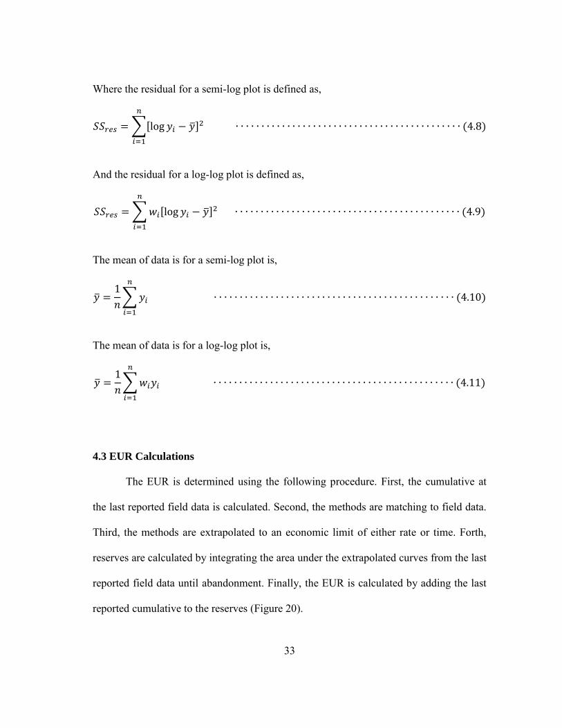
4.3 EUR Calculations
The EUR is determined using the following procedure. First, the cumulative at
the last reported field data is calculated. Second, the methods are matching to field data.
Third, the methods are extrapolated to an economic limit of either rate or time. Forth,
reserves are calculated by integrating the area under the extrapolated curves from the last
reported field data until abandonment. Finally, the EUR is calculated by adding the last
reported cumulative to the reserves (Figure 20).
34
Figure 20. Illustration of procedure to calculate EUR.
35
CHAPTER V
COMPARISON WITH SIMULATION
5.1 Model Description
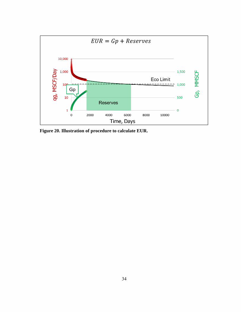
Shale wells with multiple traverse hydraulic fractures can be described with two
main models: a homogenous model and a naturally fractured model (Figure 21). The
former model assumes that fluid flows directly from matrix to hydraulic fractures. The
latter model assumes that fluid flows from matrix to hydraulic fractures through natural
fractures. Both models have parallel hydraulic fractures and drain a constant stimulated
reservoir volume (SRV). In addition to this, natural fractures in the second model are
parallel to wells (Ahmadi et al. 2010; Tivayanonda et al. 2012).
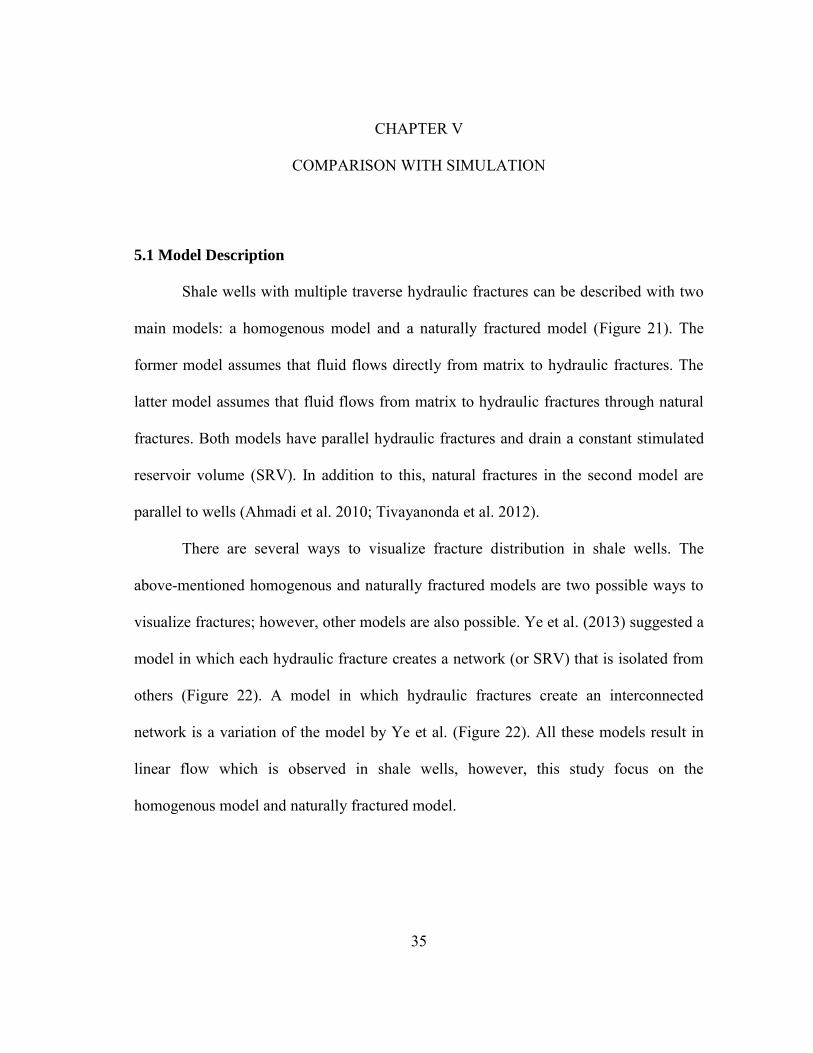
There are several ways to visualize fracture distribution in shale wells. The
above-mentioned homogenous and naturally fractured models are two possible ways to
visualize fractures; however, other models are also possible. Ye et al. (2013) suggested a
model in which each hydraulic fracture creates a network (or SRV) that is isolated from
others (Figure 22). A model in which hydraulic fractures create an interconnected
network is a variation of the model by Ye et al. (Figure 22). All these models result in
linear flow which is observed in shale wells, however, this study focus on the
homogenous model and naturally fractured model.
36
Figure 21. Schematic of the Homogenous Model and Naturally Fractured Model.
Both models have parallel hydraulic fractures and assume a constant reservoir
volume. The naturally fracture models has also parallel naturally fractures that are
perpendicular to hydraulic fractures (Tivayanonda et al. 2012).
Figure 22. Different ways to visualize fractures in shale wells.
37
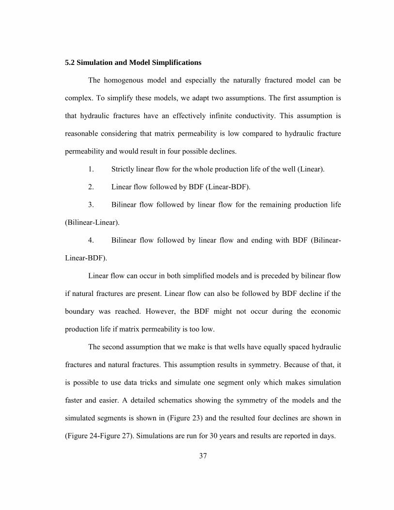
5.2 Simulation and Model Simplifications
The homogenous model and especially the naturally fractured model can be
complex. To simplify these models, we adapt two assumptions. The first assumption is
that hydraulic fractures have an effectively infinite conductivity. This assumption is
reasonable considering that matrix permeability is low compared to hydraulic fracture
permeability and would result in four possible declines.
1. Strictly linear flow for the whole production life of the well (Linear).
2. Linear flow followed by BDF (Linear-BDF).
3. Bilinear flow followed by linear flow for the remaining production life
(Bilinear-Linear).
4. Bilinear flow followed by linear flow and ending with BDF (Bilinear-
Linear-BDF).
Linear flow can occur in both simplified models and is preceded by bilinear flow
if natural fractures are present. Linear flow can also be followed by BDF decline if the
boundary was reached. However, the BDF might not occur during the economic
production life if matrix permeability is too low.
The second assumption that we make is that wells have equally spaced hydraulic
fractures and natural fractures. This assumption results in symmetry. Because of that, it
is possible to use data tricks and simulate one segment only which makes simulation
faster and easier. A detailed schematics showing the symmetry of the models and the
simulated segments is shown in (Figure 23) and the resulted four declines are shown in
(Figure 24-Figure 27). Simulations are run for 30 years and results are reported in days.
38
Figure 23. Detailed schematics showing the homogenous and naturally fractured
model as well as the simulated segments.
39
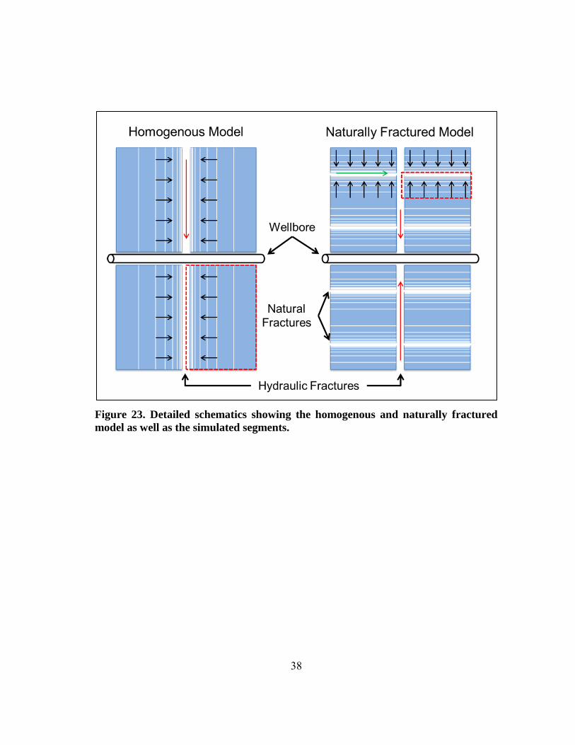
Figure 24. Case 1: infinite acting linear flow until abandonment.
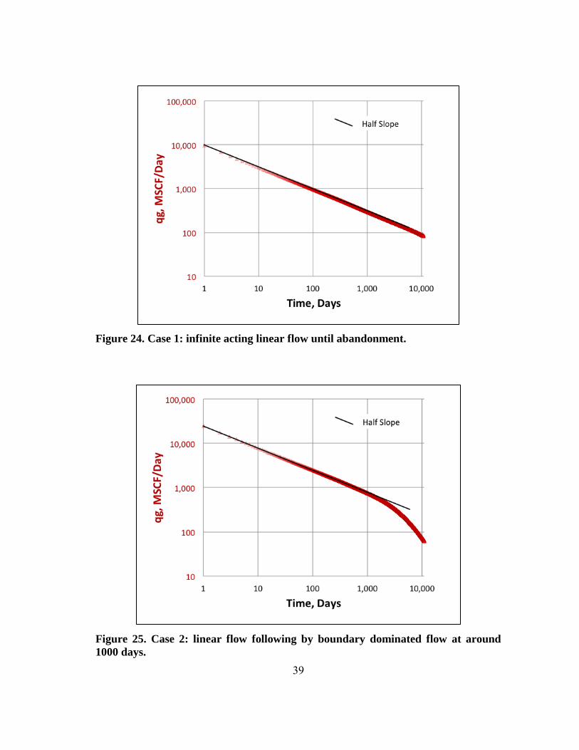
Figure 25. Case 2: linear flow following by boundary dominated flow at around
1000 days.
40
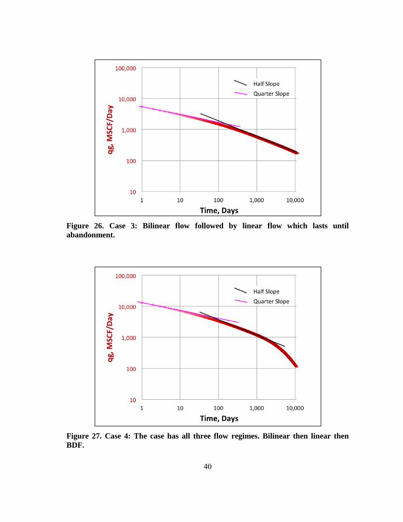
Figure 26. Case 3: Bilinear flow followed by linear flow which lasts until
abandonment.
Figure 27. Case 4: The case has all three flow regimes. Bilinear then linear then
BDF.
41
5.3 Matching Methods to Simulation: A Decline Fit Comparison
The objective of this section is to evaluate whether the different decline curve
methods can match simulation. The four simulated cases shown in the previous section
are used as test cases.
5.3.1 Case 1 – Linear Flow
Figure 24 shows the simulated production for case 1. A linear flow half-slope is
observed until abandonment at 30 years. The best fit for each of the methods is shown in
Figure 28 to Figure 32. All methods can be reasonably shaped into straight-lines to
model case 1 except for the SEPD method which tends to curve. Nonetheless, forcing
the SEPD model into a straight line is possible since it is mathematically identical to the
PLE model. For case 1, the equivalent τ that makes the SEPD model identical to the PLE
is ( ). This value is very small and outside the iteration sensitivity range
and therefore this solution was not found. The Arps model was shaped into a straight
line using a relatively large D and b value of ( ).
5.3.2 Case 2 – Linear-BDF
This case is similar to case 1 except it shows BDF in the last log cycle (Figure 25).
The method comparison (Figure 28 - Figure 32) shows that most methods cannot model
case 2 except for the PLE method. Arps’ and Duong’s methods are not flexible to match
both linear and BDF. The LGM and SEPD methods accomplish a reasonable fit for the
early part of data but not for late data. The PLE method is the best by reasonably fitting
linear and BDF. The PLE method captures the decline shape but it is matching slightly
42
over the linear flow line. The Duong’s method accomplishes a fair match to the BDF
period by compromising on early match. Duong’s method shows a shape similar to
fracture fluid clean up. This is because the m value is higher than 1 and Duong’s method
curves as m increases (see Duong’s type curves.)
5.3.3 Case 3 – Bilinear-Linear Flow
Case 3 shows bilinear flow prior to a long linear flow extending to abandonment
(Figure 26). The method comparison (Figure 28 - Figure 32) shows that all methods can
reasonably fit this case. The best fit is by the SEPD method. The other methods
accomplish reasonable fits by compromising on early or late portion of data.
5.3.4 Case 4 – Bilinear-Linear-BDF
This case is similar to case 3 except it shows BDF in the last log cycle. The
simulated production (Figure 27) shows a quarter slope bilinear flow followed by a half
slope linear flow and then BDF. Figure 28 to Figure 32 show the method comparison.
This case is difficult to match because it has three distinct flow regimes. The best fit is
accomplished by the PLE method. The Duong method behaves in a fashion similar to
case 2.
43
Figure 28. The final iteration match for the Arps Method. Arps Fit Case 1
Perfectly. Arps' method does not fit the other cases accurately because it cannot
model multiple flow regimes.
44
Figure 29. The final iteration match for the PLE method. The PLE method fits
Case 1 perfectly and fairly fits Case 2 and 4. Case 3, however, is fitted by
coincidence here and might not fit other scenarios similar to case 3 as accurately.
45
Figure 30. The final iteration match for the SEPD method. The sped method fits
gives a good coefficient of determination in most cases however it does not capture
the shape. Case 2 is the only case where the method captures the shape.
46
Figure 31. The final iteration match for the Duong method. Does method fairly
captures the shape of Case 1 and 3. The other cases are poorly matched.
47
Figure 32. The final iteration match for the LGM method. The method goods good
fit and curve shapes however it does not capture the shape of BDF.
48
5.4 Effect of Production Time on Forecast
The objective of this section is to evaluate the effect of production time on the methods.
Data from the four simulated declines are cut at different production times and
forecasted using all methods.
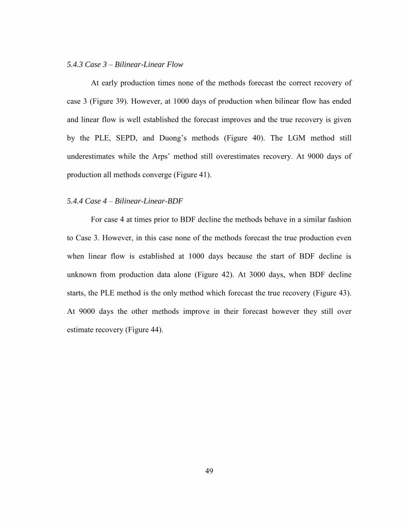
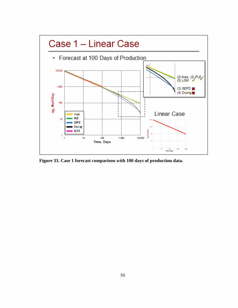
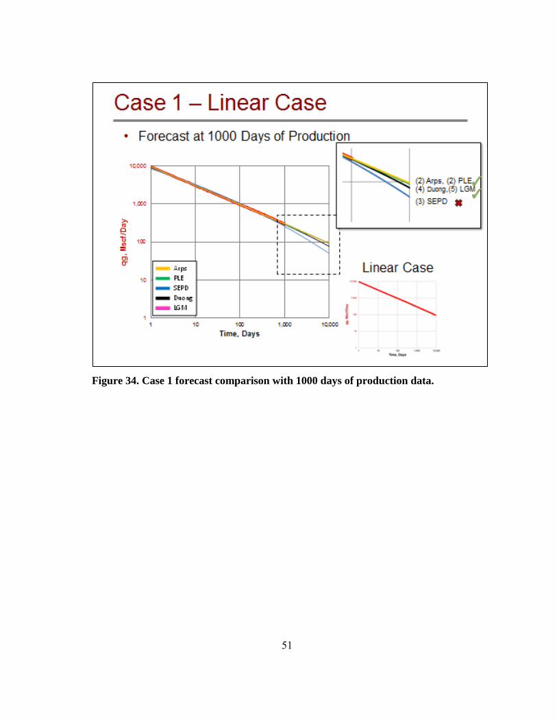
5.4.1 Case 1 – Linear Flow
In this case at only 100 days of production (Figure 33), Arps’ LGM and PLE
method extrapolate linearly and forecast the correct recovery. The SEPD and Duong’s
methods curve down and forecast the wrong recovery. As production time increases the
methods gradually improve until they converge at 9000 days of production (Figure 34-
Figure 35). The curving in Duong’s method is due to . If the term is constrained to
zero, a straight-line forecast is obtained.
5.4.2 Case 2 – Linear-BDF
For case 2 at times prior to BDF decline the methods behave in a similar fashion
to Case 1 (Figure 36). However, in this case none of the methods forecast the correct
production because the start of BDF decline is unknown from production data alone. At
3000 days, when BDF decline starts, the PLE method is the only method which forecast
the correct recovery (Figure 37). At 9000 days the other methods improve in their
forecast however they still over estimate recovery (Figure 38).
49
5.4.3 Case 3 – Bilinear-Linear Flow
At early production times none of the methods forecast the correct recovery of
case 3 (Figure 39). However, at 1000 days of production when bilinear flow has ended
and linear flow is well established the forecast improves and the true recovery is given
by the PLE, SEPD, and Duong’s methods (Figure 40). The LGM method still
underestimates while the Arps’ method still overestimates recovery. At 9000 days of
production all methods converge (Figure 41).
5.4.4 Case 4 – Bilinear-Linear-BDF
For case 4 at times prior to BDF decline the methods behave in a similar fashion
to Case 3. However, in this case none of the methods forecast the true production even
when linear flow is established at 1000 days because the start of BDF decline is
unknown from production data alone (Figure 42). At 3000 days, when BDF decline
starts, the PLE method is the only method which forecast the true recovery (Figure 43).
At 9000 days the other methods improve in their forecast however they still over
estimate recovery (Figure 44).
50
Figure 33. Case 1 forecast comparison with 100 days of production data.
51
Figure 34. Case 1 forecast comparison with 1000 days of production data.
52
Figure 35. Case 1 forecast comparison with 9000 days for production data.
53
Figure 36. Case 2 forecasts comparison with 1000 days of production data. All
methods forecast the wrong production because during transient flow the time of
BDF decline cannot be determined with production data alone.
54
Figure 37. Case 2 forecast comparison with 3000 days of production data. The PLE
method is the only method that captures the decline and forecast a correct
recovery.
55
Figure 38. Case 2 forecast comparison with 9000 days of production data.
56
Figure 39. Case 3 forecast comparison with 100 days of production data. None of
the methods can forecast the correct production at such early production time.
57
Figure 40. Case 3 forecast comparison with 1000 days of production data. The Arps
method overestimates recovery while the LGM Method underestimates. The other
three methods forecast production accurately.
58
Figure 41. Case 3 forecast comparison with 9000 days of production data. All
methods converge at the true match except Arps which is slightly overestimating.
59
Figure 42. Case 4 forecast comparison with 1000 days of production data. None of
the methods forecast the true production because the time of BDF decline cannot be
determined with production data alone.
60
Figure 43. Case 4 forecast comparison with 3000 days of production. The PLE and
LGM methods capture the true profile.
61
Figure 44. Case 4 forecast comparison with 9000 days of production. The PLE and
LGM are still the best. The other methods slightly overestimate recovery.
62
CHAPTER VI
FIELD EXAMPLES
The different decline methods were applied to 4 wells from different fields.
These fields are the Barnett, Bakken, Eagleford, and Fayetteville fields.
6.1 Barnett Shale Gas - Well B-314
Well B-314 is a shale gas well from the Barnett shale. The well shows linear
flow half-slope followed by a deviation that can be considered as BDF (Figure 45). At
long production times some rates fall short from the linear flow half-slope trend. These
lower rates are cause by either liquid loading or partial shut-ins. These rates are filtered
out using turner’s method.
The forecast and EUR is shown in Figure 45. This case is similar to Case 4 and
the PLE should be the most accurate method while the other methods should improve
with production time. The LGM and SEPD methods give forecasts similar to the PLE.
The Duong method is overestimating because production time of BDF decline is not
sufficient.
63
Figure 45. Barnet Well B-314. The well exhibits linear flow and BDF. The best
method when BDF is reached is the PLE method. The other methods should
converge as production time increase.
64
6.2 Bakken Shale Oil - Well BK-86
Well BK-86 is an oil well from the Bakken shale. Its production shows a half-
slope indicating transient linear flow to 875 days and the forecast is shown in Figure 46.
Noisy data are removed manually to improve matching. This well is in transient linear
flow and it might either continue showing linear flow until abandonment (Case 1) or go
into BDF if boundary is reached (Case 2). For case 1 the Arps, LGM and PLE method
should result in good forecasts. However, in this well the SEPD method also gives a
similar forecast. For Case 2, the forecast has to be rerun when the boundary is reached.
Figure 46. Linear flow for Bakken shale oil well BK-86.This well is similar to Case
1 or 2. For Case 1, Arps, LGM and PLE methods provide comparable forecasts
assuming linear flow regime until abandonment. For Case 2 the forecast has to be
re-run when BDF is reached.
65
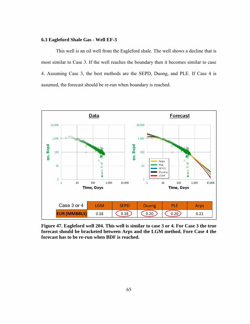
6.3 Eagleford Shale Gas - Well EF-3
This well is an oil well from the Eagleford shale. The well shows a decline that is
most similar to Case 3. If the well reaches the boundary then it becomes similar to case
4. Assuming Case 3, the best methods are the SEPD, Duong, and PLE. If Case 4 is
assumed, the forecast should be re-run when boundary is reached.
Figure 47. Eagleford well 204. This well is similar to case 3 or 4. For Case 3 the true
forecast should be bracketed between Arps and the LGM method. Fore Case 4 the
forecast has to be re-run when BDF is reached.
66
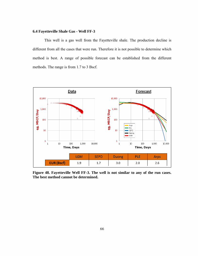
6.4 Fayetteville Shale Gas - Well FF-3
This well is a gas well from the Fayetteville shale. The production decline is
different from all the cases that were run. Therefore it is not possible to determine which
method is best. A range of possible forecast can be established from the different
methods. The range is from 1.7 to 3 Bscf.
Figure 48. Fayetteville Well FF-3. The well is not similar to any of the run cases.
The best method cannot be determined.
67
CHAPTER VII
DISCUSSION AND CONCLUSIONS
The decline methods shown here have different models and equation forms, thus
often provide different forecasts. Arp’s hyperbolic equation can be shaped into a straight
line to fit either bilinear or linear flow with b values of 2 and 4 respectively. However, it
cannot model multiple flow regimes. The PLE is the only method that models transient
and BDF decline. The SEPD model is difficult to shape into a straight-line because of its
equation formulation. Duong’s is the only method that models clean-up while the LGM
is the easiest method to use. If BDF is expected, the EUR cannot be accurately
established until BDF is observed. Four cases that represent the typical flow regimes of
shale wells were simulated to evaluate which method(s) is/are best for each case:
Linear: if a well is expected to show linear flow to abandonment, the
most accurate EUR is determined using Arps, PLE, or LGM. The Duong
method can also be used if is constrained to 0.
Bilinear-Linear: if a well is expected to show linear flow to abandonment
but was preceded by bilinear flow, the most accurate EUR is determined
by the PLE, SEPD, or Duong methods.
Linear-BDF or Bilinear-Linear-BDF: if the well is expected to show BDF
prior to abandonment, a reliable forecast cannot be established. The BDF
must be observed to reliably estimate ultimate recovery. The method that
best models both transient and BDF of shale wells is the PLE method.
68
In addition, the methods equation forms are investigated and improvements were
suggested.
Arps cannot fit multiple flow regimes and therefore a composite Arps’
method with two different b values is suggested.
The iteration of the PLE method might blow-up because the parameter
can be too large for Excel to handle. A constraint to prevent this is
introduced.
The SEPD method takes a very long time for iteration. The use of LMA
reduces the time greatly.
Duong’s method cannot rigorously model linear or bilinear flow.
Programmers who develop a decline program might encounter an error
while validating Duong’s method against linear or bilinear flow models.
A correction for this error is introduced.
69
REFERENCES
Ahmadi, H.A.A., Almarzooq, A.M., and Wattenbarger, R.A. 2010. Application of Linear Flow Analysis to Shale Gas Wells - Field Cases. Paper presented at the SPE Unconventional Gas Conference, Pittsburgh, Pennsylvania, USA. Society of Petroleum Engineers SPE-130370-MS. DOI: 10.2118/130370-ms.
Arnold, R., Anderson, R. 1908. Preliminary Report on Coalinga Oil District. U.S. Geol. Survey Bull. 357 (1908) 79.
Arps, J.J. 1945. Analysis of Decline Curves Original edition. ISBN 0096-4778.
Bello, R.O. and Wattenbarger, R.A. 2008. Rate Transient Analysis in Naturally Fractured Shale Gas Reservoirs. Paper presented at the CIPC/SPE Gas Technology Symposium 2008 Joint Conference, Calgary, Alberta, Canada. Society of Petroleum Engineers SPE-114591-MS. DOI: 10.2118/114591-ms.
Bello, R.O. and Wattenbarger, R.A. 2010. Modelling and Analysis of Shale Gas Production with a Skin Effect. Journal of Canadian Petroleum Technology 49 (12): pp. 37-48. DOI: 10.2118/143229-pa
Clark, A.J., Lake, L.W., and Patzek, T.W. 2011. Production Forecasting with Logistic Growth Models. Paper presented at the SPE Annual Technical Conference and Exhibition, Denver, Colorado, USA. Society of Petroleum Engineers SPE-144790-MS. DOI: 10.2118/144790-ms.
Duong, A.N. 2011. Rate-Decline Analysis for Fracture-Dominated Shale Reservoirs. SPE Reservoir Evaluation & Engineering 14 (3): pp. 377-387. DOI: 10.2118/137748-pa
Fetkovich, M.J. 1980. Decline Curve Analysis Using Type Curves. Journal of Petroleum
Technology 32 (6): 1065-1077. DOI: 10.2118/4629-pa
Hubbert, M.K. 1956. Nuclear Energy and the Fossil Fuel. American Petroleum Institute API-56-007.
Ilk, D., Rushing, J.A., Perego, A.D. et al. 2008. Exponential Vs. Hyperbolic Decline in Tight Gas Sands — Understanding the Origin and Implications for Reserve Estimates Using Arps' Decline Curves. Paper presented at the SPE Annual Technical Conference and Exhibition, Denver, Colorado, USA. Society of Petroleum Engineers SPE-116731-MS. DOI: 10.2118/116731-ms.
70
Johnson, R.H. and Bollens, A.L. 1927. The Loss Ratio Method of Extrapolating Oil Well
Decline Curves Original edition. ISBN 0096-4778.
Lee, W.J. and Sidle, R. 2010. Gas-Reserves Estimation in Resource Plays. SPE
Economics & Management 2 (2): pp. 86-91. DOI: 10.2118/130102-pa
Pirson S.J. 1935. Production Decline Curve of Oil Well My Be Extrapolated by Loss-Ratio. Oil and Gas Jnl. (Nov. 14, 1935).
Samandarli, O., Ahmadi, H.A.A., and Wattenbarger, R.A. 2011. A Semi-Analytic Method for History Matching Fractured Shale Gas Reservoirs. Paper presented at the SPE Western North American Region Meeting, Anchorage, Alaska, USA. Society of Petroleum Engineers SPE-144583-MS. DOI: 10.2118/144583-ms.
Tivayanonda, V., Apiwathanasorn, S., Economides, C. et al. 2012. Alternative Interpretations of Shale Gas/Oil Rate Behavior Using a Triple Porosity Model. Paper presented at the SPE Annual Technical Conference and Exhibition, San Antonio, Texas, USA. Society of Petroleum Engineers SPE-159703-MS. DOI: 10.2118/159703-ms.
Turner, R.G., Hubbard, M.G., and Dukler, A.E. 1969. Analysis and Prediction of
Minimum Flow Rate for the Continuous Removal of Liquids from Gas Wells Original edition. ISBN.
Valko, P.P. 2009. Assigning Value to Stimulation in the Barnett Shale: A Simultaneous Analysis of 7000 Plus Production Histories and Well Completion Records. Paper presented at the SPE Hydraulic Fracturing Technology Conference, The Woodlands, Texas. Society of Petroleum Engineers SPE-119369-MS. DOI: 10.2118/119369-ms.
Valko, P.P. and Lee, W.J. 2010. A Better Way to Forecast Production from Unconventional Gas Wells. Paper presented at the SPE Annual Technical Conference and Exhibition, Florence, Italy. Society of Petroleum Engineers SPE-134231-MS. DOI: 10.2118/134231-ms.
Warpinski, N.R. and Branagan, P.T. 1989. Altered-Stress Fracturing. Journal of
Petroleum Technology 41 (9): 990-997. DOI: 10.2118/17533-pa
Ye, P., Chu, L., Harmawan, I. et al. 2013. Beyond Linear Analysis in an Unconventional Oil Reservoir. Paper presented at the SPE Unconventional Resources Conference, The Woodlands, TX, USA. Society of Petroleum Engineers SPE-164543-MS. DOI: 10.2118/164543-ms.
71
APPENDIX A
PLE DERIVATION
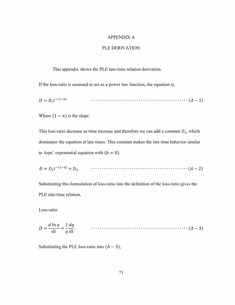
This appendix shows the PLE rate-time relation derivation.
If the loss-ratio is assumed to act as a power law function, the equation is,
( ) ( )
Where ( ) is the slope.
This loss-ratio decrease as time increase and therefore we can add a constant which
dominates the equation at late times. This constant makes the late time behavior similar
to Arps’ exponential equation with ( ).
( ) ( )
Substituting this formulation of loss-ratio into the definition of the loss-ratio gives the
PLE rate-time relation,
Loss-ratio
( )
Substituting the PLE loss-ratio into ( ),
72
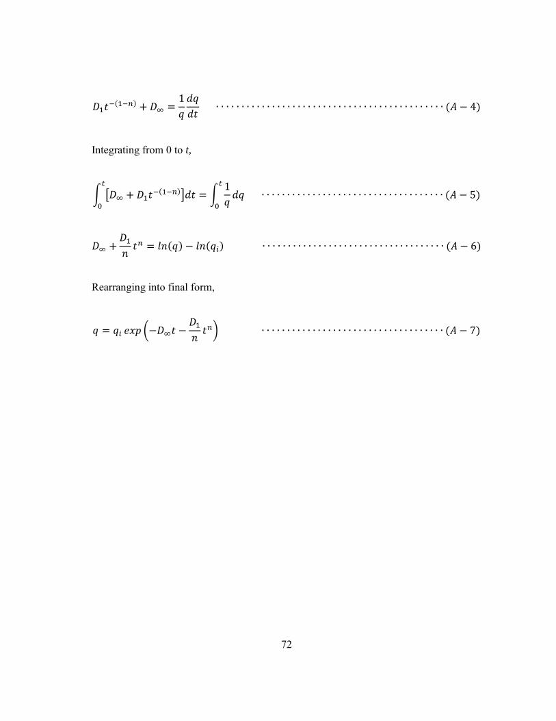
( )
( )
Integrating from 0 to t,
∫ [ ( )]
∫
( )
( ) ( ) ( )
Rearranging into final form,
( ) ( )
73
APPENDIX B
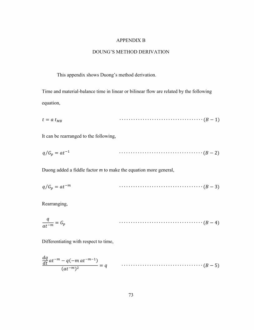
DOUNG’S METHOD DERIVATION
This appendix shows Duong’s method derivation.
Time and material-balance time in linear or bilinear flow are related by the following
equation,
( )
It can be rearranged to the following,
⁄ ( )
Duong added a fiddle factor m to make the equation more general,
⁄ ( )
Rearranging,
( )
Differentiating with respect to time,
( )
( ) ( )
74
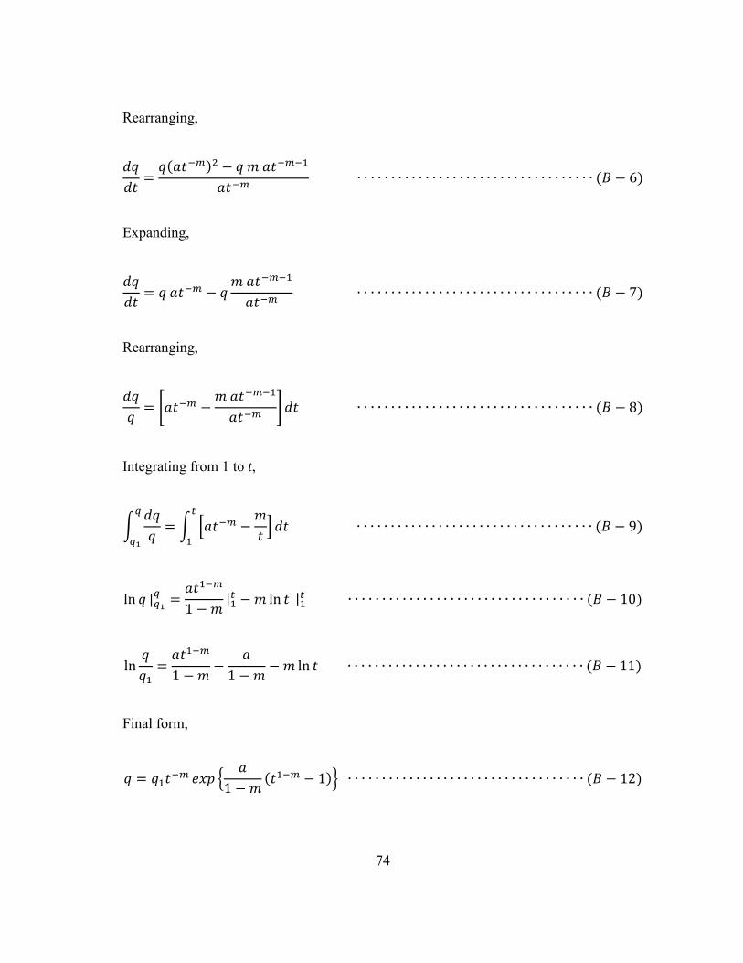
Rearranging,
( )
( )
Expanding,
( )
Rearranging,
[
] ( )
Integrating from 1 to t,
∫
∫ [
]
( )
( )
( )
Final form,
{
( )} ( )
75
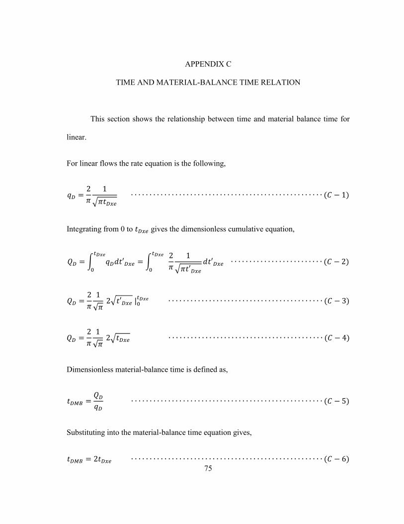
APPENDIX C
TIME AND MATERIAL-BALANCE TIME RELATION
This section shows the relationship between time and material balance time for
linear.
For linear flows the rate equation is the following,
√ ( )
Integrating from 0 to gives the dimensionless cumulative equation,
∫
∫
√
( )
√ √
( )
√ √ ( )
Dimensionless material-balance time is defined as,
( )
Substituting into the material-balance time equation gives,
( )
76
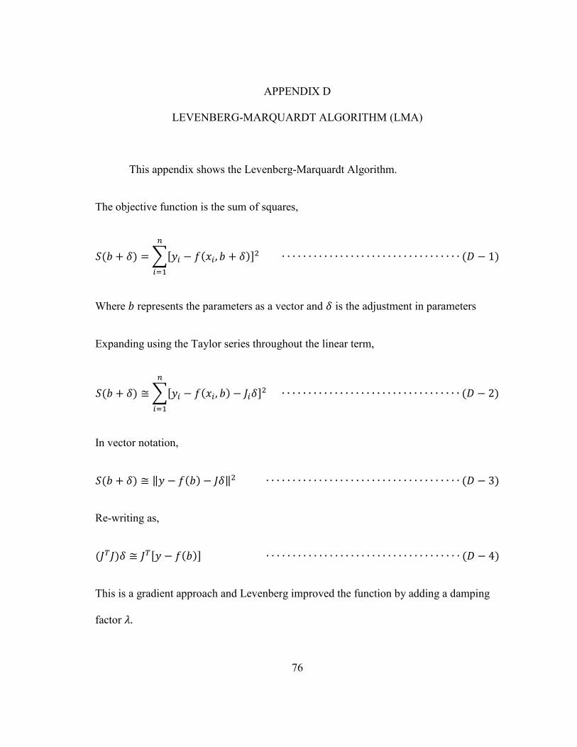
APPENDIX D
LEVENBERG-MARQUARDT ALGORITHM (LMA)
This appendix shows the Levenberg-Marquardt Algorithm.
The objective function is the sum of squares,
( ) ∑[ ( )]
( )
Where represents the parameters as a vector and is the adjustment in parameters
Expanding using the Taylor series throughout the linear term,
( ) ∑[ ( ) ]
( )
In vector notation,
( ) ‖ ( ) ‖ ( )
Re-writing as,
( ) [ ( )] ( )
This is a gradient approach and Levenberg improved the function by adding a damping
factor .
77
The Levenberg-Marquardt Algorithm (LMA),
( ) [ ( )] ( )
Where I is the identity matrix.
Each iteration step, the damping factor is adjusted. If improvement in the sum of
least-squares is slow, the damping factor is increased. This brings the solution faster
towards the gradient descent direction. On the other hand if the increased damping
parameter results in a worse sum of least-squares, the damping value from the previous
step is used.