1

Comparing Feed-In Tariffs and

Renewable Obligation Certificates -

The Case of Repowering Wind Farms

By Tim Mennel1, Teresa Romano2, Sara Scatasta3

June, 28 2013

Abstract

This paper compares support mechanisms for renewable energy with respect to their ex-ante effectiveness in promoting the adoption of innovative technologies. We analyse two stylized policy instruments in the context of the example of wind repowering: renewable quotas and feed-in tariffs. Quota systems, such as the British Renewable Obligation Certificates (ROCs), are based on mandatory renewable quotas. Feed-in tariffs (FITs), such as the German EEG tariffs, guarantee a certain, fixed price for ’green’ electricity over the economic lifetime of the investment. This paper focuses on one aspect of the difference between the two instruments: the allocation of uncertainty. While under ROCs both electricity price and capital cost risks are borne by the owner of the wind farm, under FITs only capital cost risks remain with the owner. The model is calibrated on data for German wind power plants. Our general result is that the owner is more likely to adopt a new technology under price certainty as provided by FITs. Another finding is that electricity price and capital cost volatility have different impacts on the propensity to invest under ROCs. While, even a small positive variation in electricity price volatility increases the propensity to invest, an increase in capital cost volatility does not affect the likelihood to repower wind farms. The last result also applies under FITs.

1Dr. Tim Mennel (previously ZEW), DNV KEMA Energy & Sustainability, Kurt-Schumacher-Str. 8, D-53113 Bonn, Germany. This Discussion Paper does not necessarily present the views of DNV KEMA or one of its clients, but sole the authors. 2Teresa Romano, PhD student, Politecnico di Milano, Piazza L. Da Vinci, 32 – 20133 Milano, Italy. 3Dr. Sara Scatasta (previously ZEW), Bosch Energy and Building Solutions GmbH, Mittlere Pfad 4, D-70499 Stuttgart-Weilimdorf, Germany. This Discussion Paper does not necessarily present the views of Bosch Energy and Building Solutions GmbH or one of its clients, but sole the authors.

2

1. Introduction

The promotion of renewable energy is high on the energy policy agenda in Europe and worldwide. It is

widely seen as one of the key factors in mitigating climate change. In one of the climate policy scenarios

developed by the International Energy Agency (IEA), renewable energy carriers take a major share of

carbon emission abatement efforts, in particular in electricity generation where the IEA scenarios show a

contribution of more than 60% of worldwide generation by 2050 (IEA, 2012). In the policy arena, EU

leaders have included a renewable target in their 2020 climate policy targets: renewable energy sources

(RES) shall contribute 20% to primary energy consumption by that date. The EU Renewable Energy

Roadmap of 2007 states:

“In the complex picture of energy policy, the renewable energy sector is the one energy sector which

stands out in terms of ability to reduce greenhouse gas emissions and pollution, exploit local and

decentralised energy sources, and stimulate world-class high-tech industries. The EU has compelling

reasons for setting up an enabling framework to promote renewables. They are largely indigenous, they

do not rely on uncertain projections on the future availability of fuels, and their predominantly

decentralised nature makes our societies less vulnerable. It is thus undisputed that renewable energies

constitute a key element of a sustainable future.”

While there is widespread consensus over the general policy aim of promoting renewable energy,

opinions diverge over suitable renewable sources, policy instruments and time frames for achieving

renewable energy targets. After long negotiations over a harmonization of RES support schemes across

the EU failed, in its Renewable Directive 2009/28/EU the EU introduced mandatory national targets

consistent with the overall 20% renewable share, explaining in article 14 that “the main purpose of

mandatory national targets is to provide certainty for investors and to encourage continuous development

of technologies which generate energy from all types of renewable sources. Deferring a decision about

whether a target is mandatory until a future event takes place is thus not appropriate.”

3

As stated in the directive, the overall purpose of RES support policy is thus not only to substitute fossil

fuels to avoid emissions but also to promote innovation in the RES sector, so as to reduce energy supply

cost in the long term and making RES efficient alternatives to conventional sources of energy. The

Directive also states that certainty for investors is necessary to achieve this aim. In this Discussion Paper

we want to analyze this assertion in the framework of a model for repowering wind farms. The question is

to what extent uncertainty will impede or spur the investment into new technology when the owner of a

wind park considers renewing the technology in use.

The answer to this question has some policy relevance, for indeed policy instruments applied for RES

support differ in the allocation of risk and uncertainty among governments, investors and operators. The

policy instruments in use fall into two categories: quotas and feed-in tariffs. Quota systems have been in

use in many of the US states for more than three decades (in US regulation they are called renewable

portfolio standards). In Europe, they are applied, for instance, in the UK. Under such a system eligible

renewable energy plants receive so called Renewables Obligation Certificates (ROCs) corresponding to

the amount of electricity they produce4. Electricity supply companies are obliged to purchase ROCs from

the producers up to a specified quota of their electricity sales set by the government. If it fails to reach the

quota, the electricity company has to make buy-out payments. Other European countries that have

adopted a quota system include Belgium, Italy (for wind and bioenergy), and Sweden. Germany, instead,

has opted for the introduction of feed-in tariffs (FITs) for renewable energy. Under this system, the

electricity generated from renewable energy is sold to power supply companies at a fixed minimum price.

Feed-in tariffs often decline over time to take account of technological progress (“tariff degression”)5.

The costs for this fixed-price regime for renewable electricity are covered by an additional per KWh

4Since 2009 ROCs have been complemented by feed-in-tariffs in the UK. 5In Germany, for example, the price for wind energy is set at 9.1 c/KWh in the first five years of operation and at 6.19 c/KWh for further 15 years; with the tariffs falling by nominal 1.5% for each year the investment occurs after 2002.

4

charge on all consumers The German renewable support scheme is seen to be largely effective6. Feed-in

tariffs are today most common in the EU and have been used for many years in Spain, Austria, Denmark

and Portugal.

In our study we want to investigate the ex-ante relative effectiveness of quotas and feed-in tariffs in

promoting the use of renewable energy with a view on the adoption of new technologies. The focus is on

one aspect of the differences between the two instruments: the allocation of uncertainty. One major

difference between quotas and feed-in tariffs is the fact that the minimum price granted under feed-in

tariffs cuts the downside risk for investors by fixing the electricity price. In order to take into account the

different price uncertainties under the two policies, our analysis uses the option value of investment into a

renewable plant. Real option models, originally developed in the finance literature, are able to describe

optimal investment strategies in the presence of irreversibility and uncertainty. By modelling both the

price dynamics for fossil fuels as well as the (stochastic) technological progress in the renewable energy

sector we ask which policy instrument is most likely to speed up market maturity, looking at the example

of repowering wind parks.

Some previous literature has compared feed-in tariffs and quota systems in renewable support from

different viewpoints and with different methodology. Popp et al. (2011) do not find evidence that

differences in types of policies to meet Kyoto’s goals significantly affect the level of investment. But this

represents a minority view, as the recent literature seems to agree on the superiority of feed-in tariffs,

considered as a “more balanced option” (Hiroux and Saguan, 2010), ensuring both effectiveness and

economic efficiency (Resch et al., 2007). Also, they seem to be preferred by investors, especially in

Europe (Bürer and Wüstenhagen, 2009), and more able to meet multiple objectives (Lipp, 2007).

However, as Dinica (2006) points out in a more investor-oriented perspective, the result in terms of

diffusion strongly depends on the policy design. Highlighting the fact that the effects of a policy vary

6The share of renewables in electricity consumption was raised from 3% in 1990 to 23% in 2012.

5

with the technology, Johnstone et al. (2010) find that ROCs are still important for the diffusion of wind

power while, in the context of the German feed-in-tariff law (EEG), Mennel (2012) argues that the cost of

RES support in Germany is excessive, and that there is lack of empirical evidence of the EEG

effectiveness with respect to technological improvements.

By comparing UK and German policies (with the due adjustments) through descriptive statistics, both

Mitchell et al. (2006) and Butler and Neuhoff7(2008) argue that feed-in tariffs encourage the deployment

of wind turbines more effectively and at a lower cost to society. We check whether the findings of the two

authors are confirmed in our formalized context. Also, by explicitly considering the role of uncertainty

and irreversibility, we add it to the list of possible reasons that, according to Kildegaard (2008), can

explain the failure in terms of dynamic efficiency of a quota system such as ROCs. In particular, he shows

that such a failure may be due to the presence of low-fixed cost technology competing against high fixed-

cost technologies in the certificates market, and also in the case where only the latter technology exists, in

absence of long-term contracts the investors face an asymmetric risk of over-investment. Another aspect

that would be interesting to investigate is the effect on renewable energy deployment of technology-

specific regulation compared to policies that are neutral in this respect. The arguments in favour of feed-

in tariffs could be undermined if we allow for technology specific premiums. For example, Böhringer et

al. (2007), through a stylized partial equilibrium model of the electricity market calibrated to empirical

data for 23 EU countries, suggest that differentiated feed-in tariff schemes may lead to excess cost

compared to technology-neutral policies (both price-based and quantity-based). However, as our model

considers only one technology, this topic goes beyond our analysis’ aim. In our setting, we find that the

argument of investment certainty is largely confirmed: investors, under electricity price certainty in

repowering as provided by feed-in tariffs, are more prone to invest in new technologies than under

electricity price uncertainty, as provided by a quota system. Potential lock-in effects where the owner

7 Apart from the statistical review, the authors present interviews with renewable plant developers.

6

prefers to stay with the once adopted technology when revenues are guaranteed are not visible.

Surprisingly, though, larger volatilities, do not lower the propensity to invest in the more uncertain system:

in this case ROCs are slightly more likely to incentivize the adoption of a newer technology. In contrast,

the volatility of capital costs has little effect on the propensity to invest under either policy instrument.

This paper is structured as follows: Section 2 discusses the economic background of support for

renewable energy and put it into context. While providing useful theoretical references it is not essential

for the understanding of rest of the paper, and can be skipped by a reader interested primarily in our

model and results. Section 3 introduces the model and formalizes the notion of the two policy regimes.

The calibration is presented in section 4. Section 5 introduces the results and the sensitivity analysis of

our numerical exercise, Section 6 concludes.

2. Theoretical Background

In the public support for renewable energy is often motivated by environmental concerns. Solar cells, for

example, do neither emit CO2 nor SOx such as an electricity plant fired by coal. In economic theory,

damages caused by polluting emissions (pollutants) are classified as externalities. The concept was

introduced by Pigou (1932) and further developed in the 60ies and 70ies (compare the seminal

monograph by Baumol and Oates 1974), and refers to a situation in which one party’s utility or

production function depends on (real) variables that are chosen by another party without regard of the

impact of that choice on the first party. Following the classical argument by Coase (1960), the

introduction of property rights for a clean environment and subsequent trading of pollution rights will

induce an efficient use of pollutants. When such property rights do not exist, government intervention is

required, for example through taxes, subsidies, or tradable emission permits. A number of economists

have criticized the justification of renewable support on grounds of external effects by (greenhouse gas)

emissions: they quote Tinbergen's rule (Tinbergen 1952) that states that each externality can be

internalized by one instrument – in the case of emissions a Pigouvian tax or an Emission Trading Scheme

7

(see e.g. Böhringer et al. 2009). Indeed, authors arguing in favor of a policy mix including renewable

support usually refer to multiple externalities (e.g. Bennear and Stavins 2007).

A second argument put forward in favor of government intervention to promote renewable energy relates

to concerns about sustainable development. The use of renewable resources enables society to economise

precious exhaustible raw material. Economic theory is less supportive of government intervention

following this argument. In 1931, Hotelling argued that competitive markets for exhaustible goods

guarantee an efficient dynamic allocation: the increasing scarcity of these resources should be reflected in

increasing prices, leading to an optimal depletion path. However, empirical evidence does not support the

predictions of this theory (compare, e.g. Halvorsen and Smith (1991)). Solow (1974) and Hartwick (1978)

challenge Hotelling’s view. They argue that in a framework with finitely-lived, overlapping generations

markets do not guarantee efficient intergenerational allocation of exhaustible goods. Present generations

tend to over-consume the exhaustible good. According to Hartwick (1978), for reasons of

intergenerational fairness, an (altruistic) government should invest into durable capital for later

generations. The debate continues. Recent contributions include Agnani et al. (2005), Just et al. (2005)

and also Gaudet (2007), who points out how the failure of the Hotelling rule can be linked to extraction

costs, market structure, durability of the resource and uncertainty. In the case of renewable energy,

investments into renewable plants could be seen as capital "replacing" fossil fuels. However, to justify

public support for this investment we have to take its innovative character into account.

So indeed the third argument raised in favor of government intervention for renewable energy is focused

on its contribution to innovation (e.g. Lehmann, Gawel 2013): an early adoption of renewable energy in

the energy supply chain speeds up technological development, leading to an earlier market maturity. The

cautious version of the argument favours subsidies to research and development in renewable energy

technology: classical economic theory is not in line with this view of the government’s role in innovation

activities. According to the traditional view, it is the scarcity of input factors rather than a government

subsidy that drive invention and innovation efficiently. “A change in the relative prices of the factors of

8

production is itself a spur to invention, and to invention of a particular kind - directed to economizing the

use of a factor which has become relatively expensive” (Hicks, 1932). The empirical evidence for this

“induced innovation hypothesis” in the energy sector is somewhat inconclusive: Newell et al. (1999) find

the larger part of innovations to be autonomous, while Popp (2002) establishes a positive effect of energy

prices on energy technology innovation. However, there is a widespread consensus among policy makers

and economists today that the government has a role in research and development. These can take the

form of a R&D subsidy, or direct subsidies to an innovative industry under the “Learning by Doing”

paradigm (Arrow, 1962, Young, 1993). Economists have widely accepted the argument put forward by

Griliches (1979): innovation is risky and not fully appropriable, i.e. knowledge, which has been acquired

at some cost, will spill-over from the innovative company to its competitors at a certain rate. These spill-

over effects do not suppress innovation, but lead to inefficient under-investment. Subsidies to research

and development can thus enhance welfare. Empirical evidence for spill-over effects is given by Griliches

(1979, 1992). It is worth to recall that there are other factors influencing eco-innovation. Kesidou and

Demirel (2012), for example, in a cross-sectional analysis of 1566 UK firms, find that the decision to

innovate is driven by demand-side mechanisms (e.g. customers and societal requirements). Regulations

and supply-side factors (e.g. cost savings, organizational capabilities, etc.) will then affect the level of

investments.

In a framework close to the evolutionary approach to innovation, another hypothesis about innovation in

environmental technologies turns out to be controversial: Porter and van der Linde (1995) propose that, in

a world with highly incomplete information, organizational inertia and controls problems, environmental

regulation fosters innovation in a way that leads to economic growth in the long-run. According to the

authors, regulation sends signals to the companies about the existence of inefficiencies and potential

technological improvements. It can also solve some information problem and reduce uncertainty, risk and

inertia. The win-win argument has become popular in the public policy debate, however, it lacks a sound

9

theoretical foundation. Also, empirical studies have not found evidence in support of it (see Jaffe and

Palmer (1997)).

To summarize the discussion of government intervention to foster renewable energy, we can broadly say

that there are more widely accepted favorable arguments – environmental externalities and innovation

spill-over - and two controversial arguments – economizing exhaustible resources and inducing economic

growth (see Jaffe et al., 2005). As for the choice of the policy instrument to be adopted, there is wide

agreement in the economic literature about that market-based instruments (taxes, subsidies, permits and

certificates) are more efficient than command-and-control instruments (quotas, product and process

standards) in achieving a given level of environmental protection. Market-based instruments, furthermore,

provide dynamic incentives for an efficient green technological development (see Coase, 1960; Dales,

1968; Montgomery, 1972 and Weitzman, 1974). Moreover, in the vintage capital theory, from the early

contributions by Johansen (1959) and Solow (1960) to the more recent work by Gilchrist and Williams

(2000, 2001), and Laitner and Stolyarov (2002), new technologies, especially those subsidized by the

government, should instantly dominate existing ones. Yet two empirical facts seem to be in contrast with

these theoretical findings. First, policy makers seem to rely heavily on command-and-control instruments

when it comes to environmental protection rather than market-based instruments or a combination of the

two. Examples are fuel standards in cars or the discussion on an “energy passport” for buildings in

Germany. Second, the observed slow speed of diffusion of new technologies that we mentioned earlier.

Given their importance in the study of innovation and diffusion of technologies, our model explicitly

accounts for the existence of uncertainty and irreversibility in investments. In our work we will build on

this latter hypothesis and on the work by Pizer (1997), who shows that ignoring uncertainty in policy

decisions concerning stringency and instrument choice leads to inefficient policy recommendations, and

of Dixit and Pindyck (1994), who model the decision to invest in a plant or a particular technology as a

real option. A real option is defined as the right, but not the obligation, to take an action. It differs from a

financial option in that the action concerns a tangible or “real” asset instead of a financial security. Real

10

option theory draws its foundations from financial option pricing theory as developed by Merton (1971,

1973, 1976, 1977 and 1990) and Myers (1977, 1984, and 1992), and has been applied to study liberalized

electricity markets by a number of authors (e.g. Botterud, Ilic and Wangensteen (2005), Botterud and

Korpås (2007), Madlener et al. 2005). The authors look at how uncertainty influences the optimal timing

of investments in new power generation capacity. They use a discrete time approach, as we do in this

paper. We present a stylised model analysing the effect that the two support policies, feed-in tariffs and

renewable obligation certificates, have on the uncertainty faced by investors in renewable energy plants.

In particular, we are interested to understand the effect the two instruments have on the diffusion of new

technology. In our empirical application we will focus on the case of wind energy power plants. A

detailed description of the model can be found in the section that follows.

11

3. Model

Motivation

In this section, we present our modeling framework. As explained in the introduction, the overall aim is to

analyze the effect of the allocation of uncertainty on investment into a renewable energy plant under

different RES policies. We want to investigate whether the allocation of uncertainty with the

owner/investor of a wind park impedes or spurs his likeliness to adopt newly available technologies and

to improve the performance of his wind plant. The underlying question is which policy regime is better

suited to promote market maturity of renewable energy plants. Two important assumptions apply: first,

uncertainty resolves over time, i.e. the plant owner can predict future from past price developments to

some degree. Second, investments are irreversible, as is plausible in the case of power plants that involve

a lot of construction work in their setup.

To capture this economic setup we formulate a discrete dynamic programming problem with infinite time

horizon8. There are four state variables, which are introduced below, and one (discrete) control variable

depicting the investment decision. The model is set up to capture the decision of a single investor to

renew his renewable energy plant under uncertainty about the electricity price and the cost of capital. We

will then study the propensity to adopt new technologies under two stylized policy regimes: feed-in tariffs

(FITs) and renewable obligation certificates (ROCs). They are distinguished by the way they influence

the price of electricity. Whereas the owner of a renewable plant faces a certain and foreseeable price path

for his sales of electricity under FITs, the price is volatile under ROCs: as they implement tradable

renewable quotas for green electricity, their price depends on (volatile) electricity demand, investment

paths in conventional and in renewable capacities beyond immediate observation of a single investor. In

our model, we do not make those uncertainties explicit, but assume that prices for green electricity are

8Formally, this is a real option modelling framework.

12

volatile under ROCs and deterministic under FITs. This notion of the policies will be formalized below.

A second source of uncertainty in our model concerns the cost of capital. When deciding to invest into a

new power plant, the owner has to take into consideration uncertainty about future revenues as well as

opportunity costs (or benefits) that arise from reductions (or increases) in the cost of capital.

State Variables

As stated before, in our model price uncertainty is not erratic, i.e. both electricity price and capital cost

can be predicted within a certain band. Thus waiting can gain value over time, when uncertainty resolves.

To this end, we model the two price uncertainties as Markov processes: �� is the current electricity price

and a Markov state variable9

��′ = �� + ���� + ��, (1)

where ��is an i.i.d. stochastic shock variable with mean zero.

�� is the current cost of capital and also a Markov state variable

��′ = �� + ���� + ��, (2)

with �� being an i.i.d. stochastic shock variable with mean zero, too.

9 Here and in the sequel, we denote the forward time shift by a dash.

13

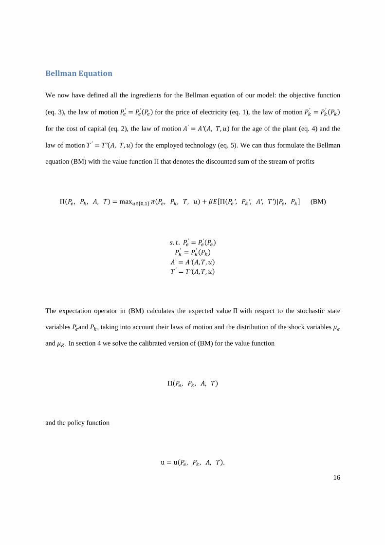
Since we intend to model the influence of technological progress on the investment decision, we

introduce both the age A of the plant and the state of employed technology10T as two deterministic state

variables. As we assume a finite lifetime m of the plant, the value m−A indicates the remaining time of

operation. We set A = 0 and T = 0 when the lifetime is expired and the plant is out of operation; other

than that age increases by 1 each period. The state of employed technology T translates into the technical

efficiency of the plant with a function �� such that �� gives the electricity produced, where by

we denote the primary energy input, e.g. wind or water flow. The function �� is increasing, � > 0,

reflecting technological progress, which in our model is assumed to be deterministic. We assume Q to be

fixed for simplicity’s sake, a possible extension would allow for Q being stochastic. This setup yields the

following current profit function of the investor

� = �� − ���� ,

where c denotes unit operational costs. We thus assume that the plant operates under a constant return to

scale technology. This assumption can, however, be modified easily.

Control Variable

We now introduce the investment decision. The owner of a plant has to decide whether or not to adopt a

new technology, incurring the cost of the new investment and renouncing profits with his current

technology (note that the latter are limited to the remaining lifetime of the plant). His choice is captured

by the discrete control variable u

10 By the term “employed technology” we refer to the technology installed as distinguished from available technology.

14

� = � 1 ∶ �����0 ∶ ��� − ������

The control variable enters both into the objective function and the laws of motion of the deterministic

state variables age A and technology T.

Objective Function

The objective function is the current profit minus the cost of an investment if it occurs. It thus mimics the

one period balance sheet of the investor:

��� , �� , �, �� = �� − ���� − ��� (3)

Here T stands for the current state of technology. Any investment comes into effect with a time lag of one

period, which is modeled by the effect of the choice � = 1 on T. The effect is captured by the laws of

motion for A and T.

The law of motion for A is straightforward:

!′ = " 1 : � = 10 : � = 0, ! = 0! + 1 $��$ : � = 0, ! ≠ 0� (4)

Any decision to invest sets the age of the plant to 1 - this explains the first case. Recall that ! = 0 refers

to the case where there is no plant. This state is left unchanged if there is no new investment and thus

� = 0 - this explains the second case. If there is a plant and the owner decides against reinvestment, it

grows older by 1 until the maximal age m is reached - this explains the third case.

15

The law of motion for T requires some more explanation. We look at the formula.

� ′ = & � : � = 01 : � = 1, � = 0$� + ! :: � = 1, � + ! ≥ $� = 1, � + ! < $� (5)

The first case is simple - whenever the control variable is chosen to be � = 0, no investment occurs and

the state of technology is left unchanged. An investment in the case of no technology results in the setting

of technology to state 1. The third and the fourth line show the rule of technological augmentation in case

of adoption of new technology explained below. Before, we have to discuss one limitation: a general

problem of the dynamic programming approach is that in principle, technology T should advance

indefinitely - which would make the model intractable. The implementation requires boundaries for each

state variable. Consequently, in the case of the plant being put down (� = 0), we limit the technological

progress to the maximal age m, which explains the boundary in the third and fourth case in the law of

motion for the state of technology.

The rule for augmentation implicit in the third and fourth case can be explained as follows: technology

advances each period, independently of the investment decision of the owner. The number of periods that

passed since the last innovation is expressed by the age of the plant A. Thus, if the owner of a plant in

technological state T and age A decides to renew his plant, the available state of technology is � + !.

Note that one implicit assumption we make in the model is that only current technology is available at one

cost level ��.

16

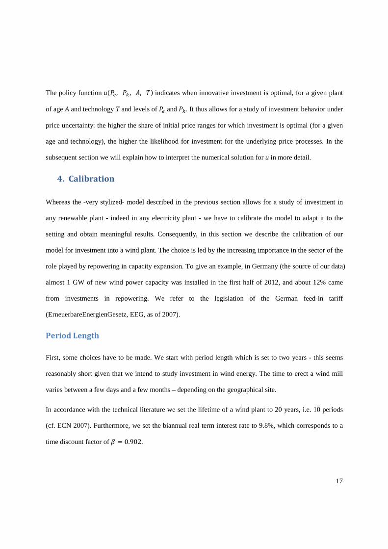
Bellman Equation

We now have defined all the ingredients for the Bellman equation of our model: the objective function

(eq. 3), the law of motion ��′ = ��′��� for the price of electricity (eq. 1), the law of motion ��′ = ��′ ���

for the cost of capital (eq. 2), the law of motion !′ = !′!, �, �� for the age of the plant (eq. 4) and the

law of motion � ′ = �′!, �, �� for the employed technology (eq. 5). We can thus formulate the Bellman

equation (BM) with the value function Π that denotes the discounted sum of the stream of profits

Π�� ,��,!,�� = max,∈./,01 ��� ,�� ,�,�� + �23Π��′,��′,!′,�′�|�� ,��5 (BM)

6. �.��′ = ��′�����′ = ��′ ���!′ = !′!, �, ��� ′ = �′!, �, ��

The expectation operator in (BM) calculates the expected value Π with respect to the stochastic state

variables ��and ��, taking into account their laws of motion and the distribution of the shock variables ��

and �9. In section 4 we solve the calibrated version of (BM) for the value function

�� ,��,!,��

and the policy function

u = u�� ,�� ,!,��.

17

The policy function u�� ,�� ,!,�� indicates when innovative investment is optimal, for a given plant

of age A and technology T and levels of �� and ��. It thus allows for a study of investment behavior under

price uncertainty: the higher the share of initial price ranges for which investment is optimal (for a given

age and technology), the higher the likelihood for investment for the underlying price processes. In the

subsequent section we will explain how to interpret the numerical solution for u in more detail.

4. Calibration

Whereas the -very stylized- model described in the previous section allows for a study of investment in

any renewable plant - indeed in any electricity plant - we have to calibrate the model to adapt it to the

setting and obtain meaningful results. Consequently, in this section we describe the calibration of our

model for investment into a wind plant. The choice is led by the increasing importance in the sector of the

role played by repowering in capacity expansion. To give an example, in Germany (the source of our data)

almost 1 GW of new wind power capacity was installed in the first half of 2012, and about 12% came

from investments in repowering. We refer to the legislation of the German feed-in tariff

(ErneuerbareEnergienGesetz, EEG, as of 2007).

Period Length

First, some choices have to be made. We start with period length which is set to two years - this seems

reasonably short given that we intend to study investment in wind energy. The time to erect a wind mill

varies between a few days and a few months – depending on the geographical site.

In accordance with the technical literature we set the lifetime of a wind plant to 20 years, i.e. 10 periods

(cf. ECN 2007). Furthermore, we set the biannual real term interest rate to 9.8%, which corresponds to a

time discount factor of � = 0.902.

18

Technology

As for technological progress, we calibrate it as growth in size. That is, wind energy plants become more

productive as they become bigger, which corresponds exactly to the idea of repowering we want to model.

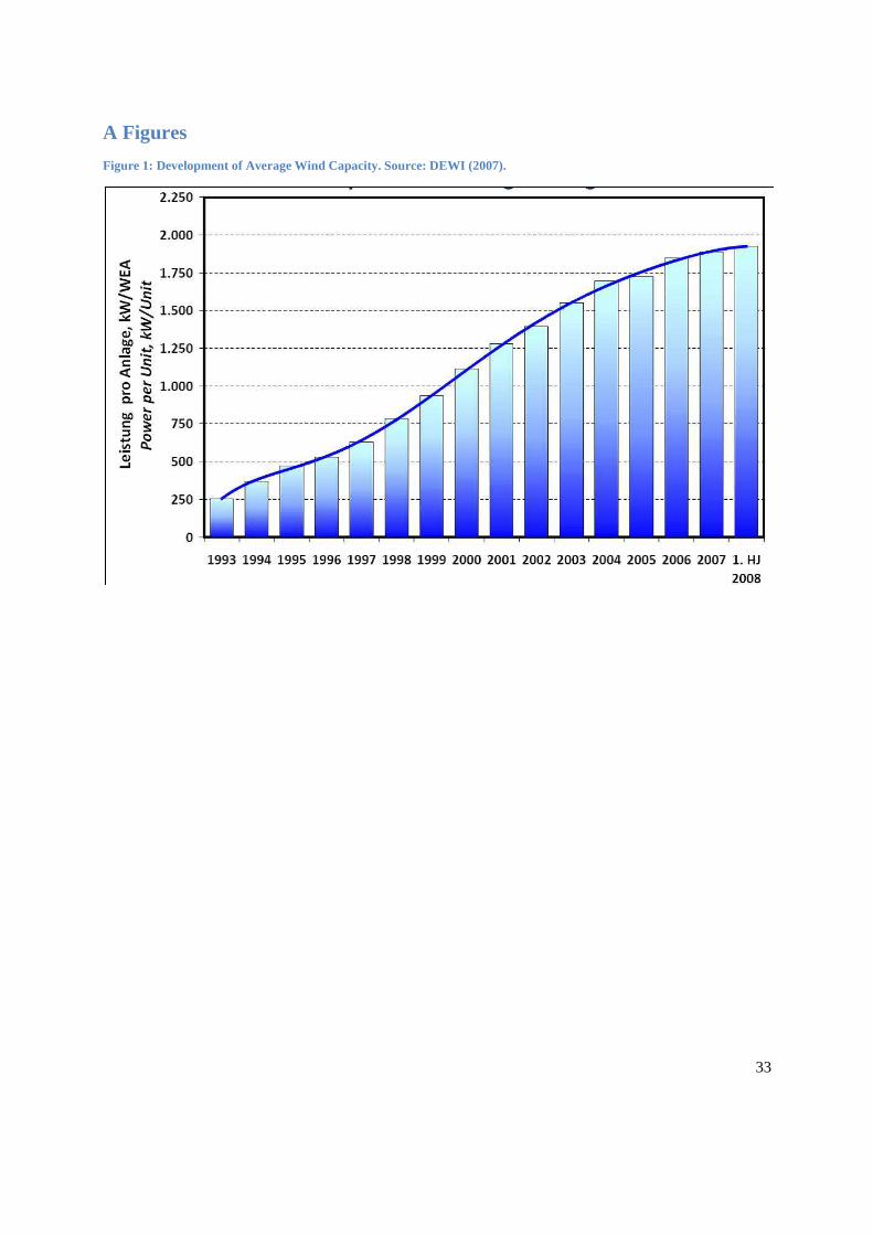
Moreover, this choice is motivated by the technological development of the last decade, as depicted in

Figure 1. The data provided by DEWI (2007) show an increase in average capacity between 1.02% and

1.49% for the years from 1993 to 2007. The average growth rate for that period is = = 1.16% per year.

To capture the development correctly (as explained above), we modify the original profit function and use

the following instead:

��� ,�� ,!,�� = �� − ���� − ���′��

where we specify technological growth by

�� = 1 + =�@

The new formulation of the profit function takes into account that replacing a small by a large wind plant

requires a higher investment: �� is the unit cost for wind power capacity, the growth in capacity is

reflected in the cost of the new plant ����. The second modification of the profit function is due to the

fact that operating a wind plant entails fixed rather than operational costs: the bulk of costs is in

operations and maintenance (O&M) which has to be paid for independently of the actual output that is

largely determined by the weather. O&M costs roughly increase proportionally with the size of capacity -

and so they enter with c into the profit function. The value of c is taken from the study by ECN (2007)

and corresponds to 18 euros. Given our choice of profit function, Q is calibrated as the biannual average

19

output of electricity for a unit of installed capacity. To obtain the figure, we have evaluated tables of

electricity output of wind plants published by the German Association of Wind Energy (BWE 2008). The

average output for the years 1990 to 2007 is = 160.38 MWh for one Megawatt of installed capacity.

Price Processes

The publication BWE (2008) is also used to calibrate the process �� for capital cost. The collection of

annually published reports from 1990 to 2007contains advertisements of wind plants, specifying capacity

and price. From this information we calculate a time series of average prices of capacity11. The time series

is then used to calibrate the Markov price process for capital

��′ = �� + ���� + ��

Assuming �� to be normally distributed we obtain �� = 0.8937, �� = 0.8144 and variance E� = 0.04

for the process (2) for ��.

The case of the electricity price is more intricate, since we are going to study support programs for

renewables. The decisive difference between FITs and ROCs regulation is the allocation of risk: Under

FIT, the owner of a renewable plant only bears the climatic risk associated with his particular technology

(wind intensity in our case), which we do not model explicitly, but no price risk.

In contrast, under ROCs the owner bears both the price risk of the electricity price and the renewable

obligation certificate, leading to a particularly volatile price process. Moreover, as discussed in the

literature review, ROCs are normally augmented with a price cap to avoid extreme price spikes in times

of high demand for electricity and short supply of renewable energy (in Britain, this price cap was

11 Only wind plants with a capacity of more than 0.5 MW were taken into account.

20

relatively low and usually binding). Both the construction of ROCs regulation and the physical potential

for electricity generation from renewable energy influence the likely price path for electricity faced by the

owner of a renewable plant. As the concept has not been implemented in Germany, we can only calculate

a stylized example for an ROCs price process. Our main goal is to understand the reaction of the investor

to the price volatility he faces under ROCs in comparison to FITs.

For FITs, we implement the price scheme for wind energy from the German renewable-energy-feed-in-

law (EEG) of 2007. As a comparison we implement a price process that has the same mean but higher

volatility as the electricity price process actually to be found in Germany. To obtain this volatility, we

estimate a time series of household electricity prices from OECD data. This estimation yields the

coefficients �� = -0.1446, �� =0.9188 and variance E� = 0.0279 for the econometric specification of

equation (1)

��′ = �� + ���� + ��.

The details of the policy analysis are discussed in the following section.

Boundaries

Finally we set bounds on the state variables. As mentioned in the section ''Model'', all state variables have

to be bounded from above and below to allow for the numerical implementation. We have already

justified our choice for the maximal age m of a plant. For the technology parameter, we allow a maximum

of five steps - or ten years growth of average capacity. While putting a somewhat arbitrary cap on a

possibly much larger increase in scale, the range chosen for T certainly allows for a study of the

implication of renewable support policy. As for the price process, we have chosen the following ranges:

Between 0% and 200% of the long-term average cost of capital �� and between 30% and 170% for the

21

average price of electricity �� . As the time series we have calculated show, these ranges chosen

encompass the variation of data in our sample period.

5. Results

In this section, we present the results of our simulation exercise. Our model has been implemented in

MATLAB. The price processes have been discretized - including the shock variables – and the price grids

have a length of 20. The Bellman equation (BM) has been solved by value function iteration. For our first

analysis, we use an electricity price process with the mean equal to the tariff in the German renewable law

(EEG) and the variance the one of the electricity prices. As a numerical output, we obtain the value

function �� , �� , !, �� and the policy function ��� , �� , !, ��. These take the form of a 20x20x10x5 array -

a rather large number of points. Fortunately, the function that is of most interest to us, the control

variable�. , . , . , . �, only takes binary values.

Central Outcomes

To understand the numerical outcome of our exercise, we need a concept for the definition of diagrams

and indicators, as in the first place the value and the policy function are difficult to handle (given the four

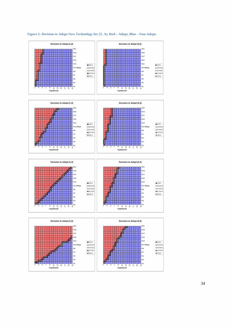
input variables). Plotting the price of electricity �� against ��, Figure 2 shows the areas for which the

owner of a wind plant decides to invest (red) or not to invest (blue), given a certain age A of a plant and a

state of technology T. A given price of electricity and capital cost means that the investor can form his

expectation of the further development of that price, given the underlying Markov process.

A glance at the diagrams gives a first impression of the outcome: we see that in all diagrams the likeliness

to invest (i.e. to adopt a new technology – in our context: to repower the wind farm) increases with the

price of electricity and decreases with capital costs. This is a plausible result: higher electricity prices lead

to higher future revenues, lower capital prices to lower investment costs. A comparison of diagrams

shows that the likeliness to invest increases with the age of the plant and decreases with the advance of

technology. This is plausible, too: an older plant is closer to the end of its lifetime, so the opportunity

22

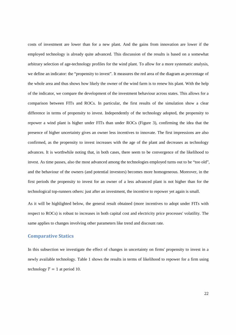
costs of investment are lower than for a new plant. And the gains from innovation are lower if the

employed technology is already quite advanced. This discussion of the results is based on a somewhat

arbitrary selection of age-technology profiles for the wind plant. To allow for a more systematic analysis,

we define an indicator: the “propensity to invest”. It measures the red area of the diagram as percentage of

the whole area and thus shows how likely the owner of the wind farm is to renew his plant. With the help

of the indicator, we compare the development of the investment behaviour across states. This allows for a

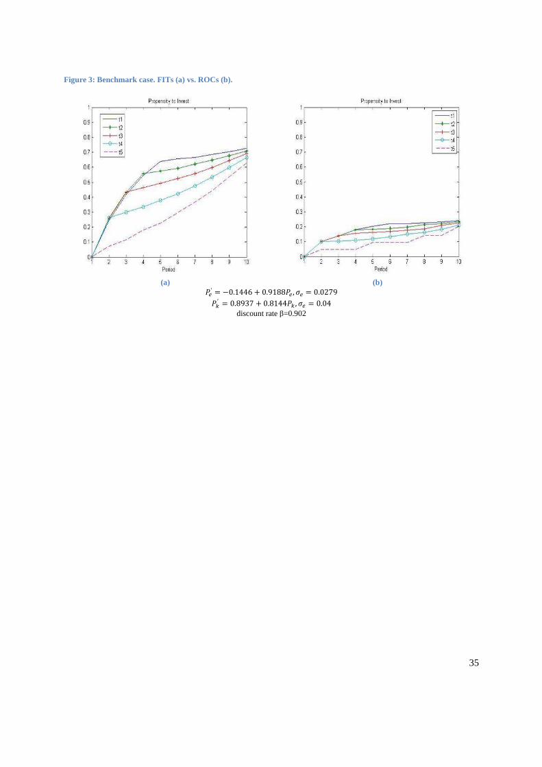
comparison between FITs and ROCs. In particular, the first results of the simulation show a clear

difference in terms of propensity to invest. Independently of the technology adopted, the propensity to

repower a wind plant is higher under FITs than under ROCs (Figure 3), confirming the idea that the

presence of higher uncertainty gives an owner less incentives to innovate. The first impressions are also

confirmed, as the propensity to invest increases with the age of the plant and decreases as technology

advances. It is worthwhile noting that, in both cases, there seem to be convergence of the likelihood to

invest. As time passes, also the most advanced among the technologies employed turns out to be “too old”,

and the behaviour of the owners (and potential investors) becomes more homogeneous. Moreover, in the

first periods the propensity to invest for an owner of a less advanced plant is not higher than for the

technological top-runners others: just after an investment, the incentive to repower yet again is small.

As it will be highlighted below, the general result obtained (more incentives to adopt under FITs with

respect to ROCs) is robust to increases in both capital cost and electricity price processes' volatility. The

same applies to changes involving other parameters like trend and discount rate.

Comparative Statics

In this subsection we investigate the effect of changes in uncertainty on firms' propensity to invest in a

newly available technology. Table 1 shows the results in terms of likelihood to repower for a firm using

technology � = 1 at period 10.

23

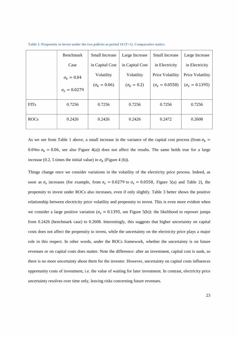
Table 1: Propensity to invest under the two policies at period 10 (T=1). Comparative statics.

Benchmark

Case

E� = 0.04

E� = 0.0279

Small Increase

in Capital Cost

Volatility

(E� = 0.06)

Large Increase

in Capital Cost

Volatility

(E� = 0.2)

Small Increase

in Electricity

Price Volatility

(E� = 0.0558)

Large Increase

in Electricity

Price Volatility

(E� = 0.1395)

FITs 0.7256 0.7256 0.7256 0.7256 0.7256

ROCs 0.2426 0.2426 0.2426 0.2472 0.2608

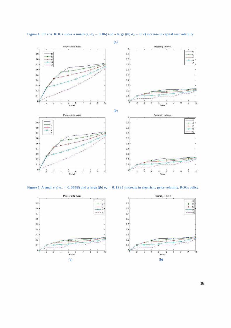
As we see from Table 1 above, a small increase in the variance of the capital cost process (from E� =0.04to E� = 0.06, see also Figure 4(a)) does not affect the results. The same holds true for a large

increase (0.2, 5 times the initial value) in E� (Figure 4 (b)).

Things change once we consider variations in the volatility of the electricity price process. Indeed, as

soon as E� increases (for example, from E� = 0.0279 to E� = 0.0558, Figure 5(a) and Table 2), the

propensity to invest under ROCs also increases, even if only slightly. Table 3 better shows the positive

relationship between electricity price volatility and propensity to invest. This is even more evident when

we consider a large positive variation (E� = 0.1395, see Figure 5(b)): the likelihood to repower jumps

from 0.2426 (benchmark case) to 0.2608. Interestingly, this suggests that higher uncertainty on capital

costs does not affect the propensity to invest, while the uncertainty on the electricity price plays a major

role in this respect. In other words, under the ROCs framework, whether the uncertainty is on future

revenues or on capital costs does matter. Note the difference: after an investment, capital cost is sunk, so

there is no more uncertainty about them for the investor. However, uncertainty on capital costs influences

opportunity costs of investment, i.e. the value of waiting for later investment. In contrast, electricity price

uncertainty resolves over time only, leaving risks concerning future revenues.

24

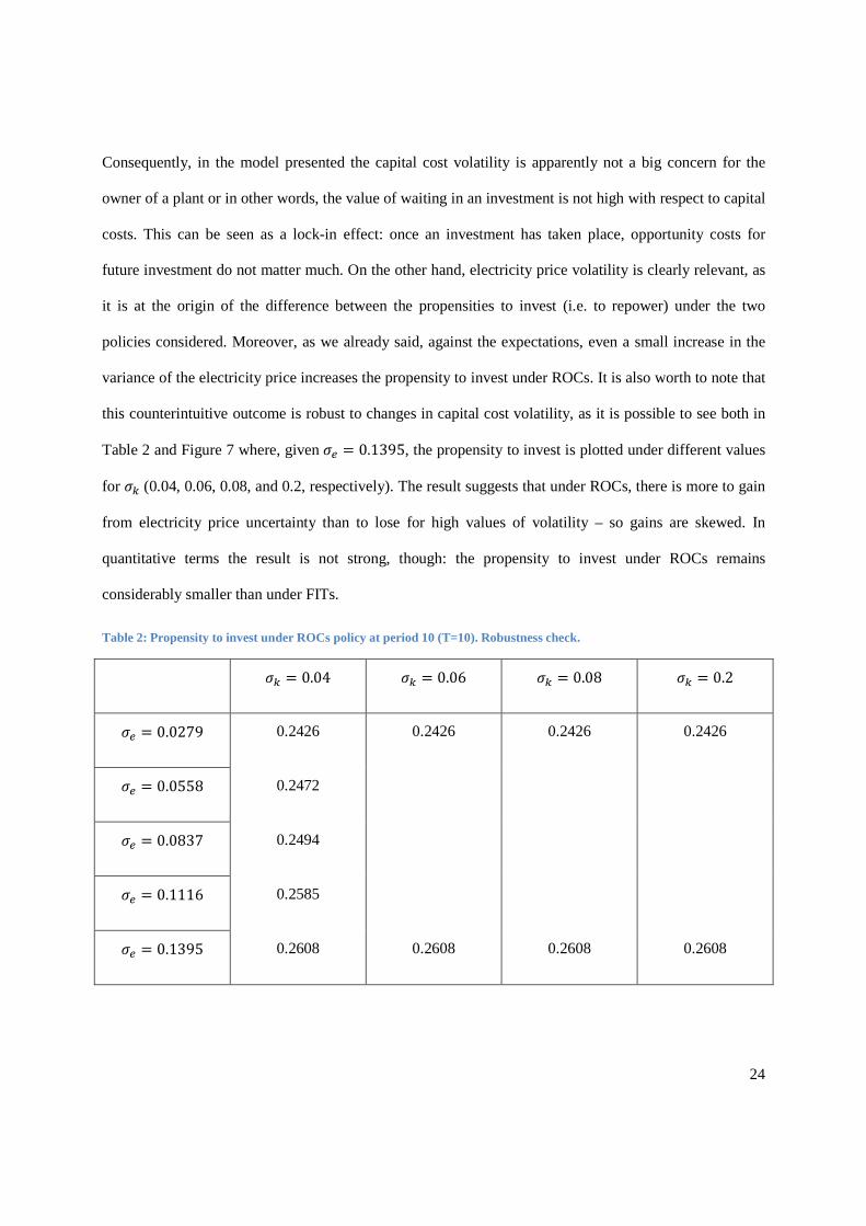
Consequently, in the model presented the capital cost volatility is apparently not a big concern for the

owner of a plant or in other words, the value of waiting in an investment is not high with respect to capital

costs. This can be seen as a lock-in effect: once an investment has taken place, opportunity costs for

future investment do not matter much. On the other hand, electricity price volatility is clearly relevant, as

it is at the origin of the difference between the propensities to invest (i.e. to repower) under the two

policies considered. Moreover, as we already said, against the expectations, even a small increase in the

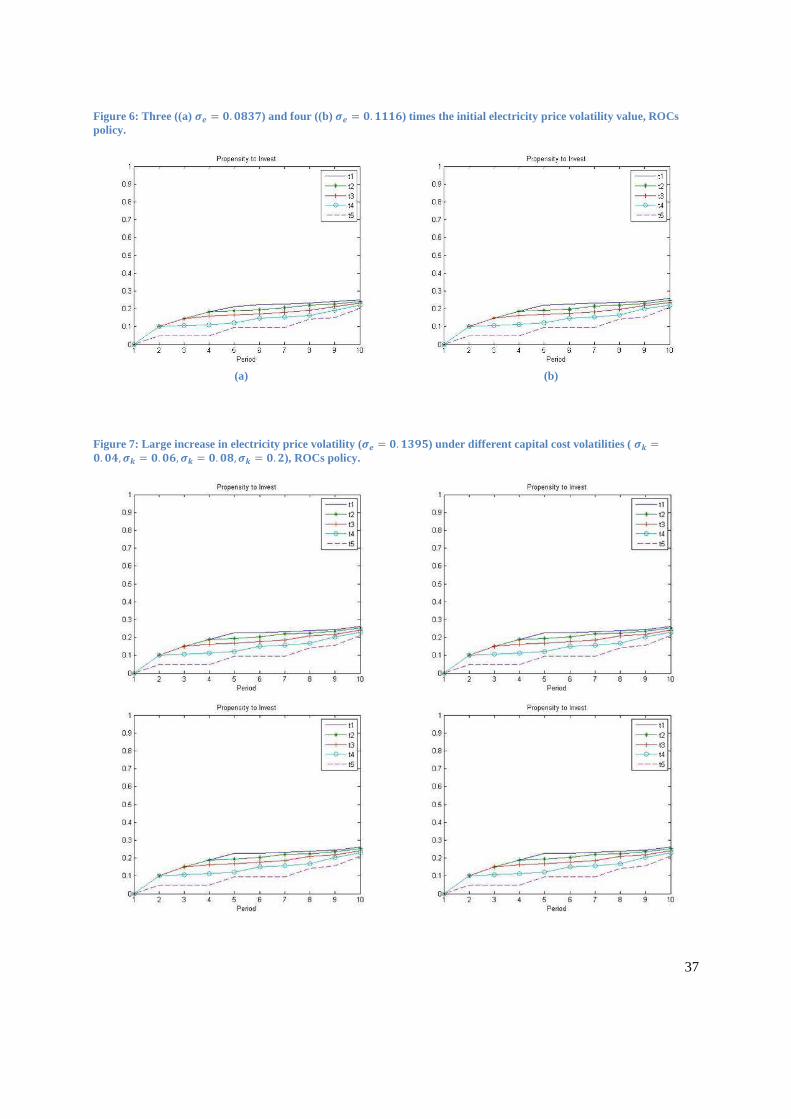
variance of the electricity price increases the propensity to invest under ROCs. It is also worth to note that

this counterintuitive outcome is robust to changes in capital cost volatility, as it is possible to see both in

Table 2 and Figure 7 where, given E� = 0.1395, the propensity to invest is plotted under different values

for E� (0.04, 0.06, 0.08, and 0.2, respectively). The result suggests that under ROCs, there is more to gain

from electricity price uncertainty than to lose for high values of volatility – so gains are skewed. In

quantitative terms the result is not strong, though: the propensity to invest under ROCs remains

considerably smaller than under FITs.

Table 2: Propensity to invest under ROCs policy at period 10 (T=10). Robustness check.

E� = 0.04 E� = 0.06 E� = 0.08 E� = 0.2

E� = 0.0279 0.2426 0.2426 0.2426 0.2426

E� = 0.0558 0.2472

E� = 0.0837 0.2494

E� = 0.1116 0.2585

E� = 0.1395 0.2608 0.2608 0.2608 0.2608

25

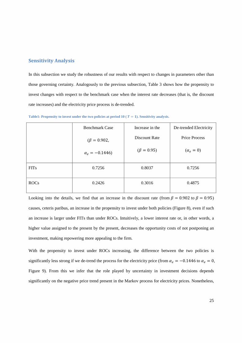
Sensitivity Analysis

In this subsection we study the robustness of our results with respect to changes in parameters other than

those governing certainty. Analogously to the previous subsection, Table 3 shows how the propensity to

invest changes with respect to the benchmark case when the interest rate decreases (that is, the discount

rate increases) and the electricity price process is de-trended.

Table1: Propensity to invest under the two policies at period 10 ( G = H). Sensitivity analysis.

Benchmark Case

(� = 0.902,

�� = −0.1446)

Increase in the

Discount Rate

(� = 0.95)

De-trended Electricity

Price Process

(�� = 0)

FITs 0.7256 0.8037 0.7256

ROCs 0.2426 0.3016 0.4875

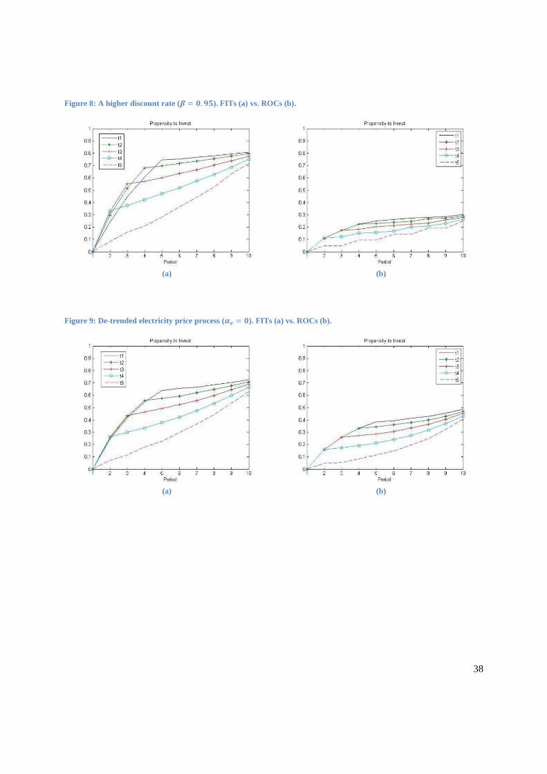
Looking into the details, we find that an increase in the discount rate (from � = 0.902 to � = 0.95)

causes, ceteris paribus, an increase in the propensity to invest under both policies (Figure 8), even if such

an increase is larger under FITs than under ROCs. Intuitively, a lower interest rate or, in other words, a

higher value assigned to the present by the present, decreases the opportunity costs of not postponing an

investment, making repowering more appealing to the firm.

With the propensity to invest under ROCs increasing, the difference between the two policies is

significantly less strong if we de-trend the process for the electricity price (from �� = −0.1446 to �� = 0,

Figure 9). From this we infer that the role played by uncertainty in investment decisions depends

significantly on the negative price trend present in the Markov process for electricity prices. Nonetheless,

26

in qualitative terms, the initial result, namely the superiority of FITs with respect to ROCs in terms of

incentivising repowering, is confirmed.

6. Conclusions

As governments seek to mitigate climate change, they widely regard renewable energy as key for a low-

carbon future. Therefore different countries have introduced a variety of different support schemes for

renewable energy to increase its share in overall energy supply, in particular in the electricity sector.

While efficiency and effectiveness of different support policy instruments have been studied widely in the

literature, their effect on innovation and diffusion has been largely ignored. This is odd, as induced

innovation is one of the main justifications for government intervention in favour of renewable energy.

Also, the adoption of new, innovative technologies is an empirical fact in countries with renewable

support schemes. For instance, investments in repowering have become more and more important in the

wind energy sector. In several federal states of Germany, for example, in the first half of 2012 a

significant share of new installations was represented by repowering, i.e. the replacement of old by new

wind mills. Moreover, the revised law for renewable support (EEG) gives repowering a bigger role.

Generally the unit cost of capital for wind power installations has been falling over the past decades,

highlighting technological progress in this area (cf. Ahlhaus and Mennel, 2011). It is generally assumed

that this process reflects technical change induced by government regulation – however we think it is

crucial to understand how regulation and specific instruments influence the process of innovation and

diffusion in the renewable energy sector.

In this Discussion Paper we have studied the investment behaviour of a wind park owner under

uncertainty. The underlying research question was how the allocation of uncertainty under different

renewable support schemes affects the likelihood to repower a wind plant; more precisely we have

compared feed-in tariffs that fix a price over time with renewable obligation certificates (‘green

certificates’) whose price can float over time. In line with our central focus in our model we have

neglected other differences in the two support schemes, such as technology specific vs. neutral support.

27

The main result confirms the general intuition: under a calibration that captures the volatility of German

wholesale electricity prices, the owner is more likely to adopt a new technology under price certainty as

provided by feed-in tariffs. In contrast under uncertainty, as provided by ROCs, he is less likely to adopt

an innovation. However, counter-intuitively, as soon as electricity price volatility increases, the difference

in terms of propensity to invest between the two policies is softened: the possibility of greater future

profits with a new technology encourages the wind park owner to adopt it more often (that is even at

relatively low electricity prices and high costs for capital, i.e. investment cost) under ROCs. As for

potential investors’ reaction to capital cost volatility, we see little differences when it increases: it does

not matter too much under either policy. In quantitative terms, the difference between the two policies is

limited once we de-trend the electricity price process, but still clearly visible – an indication that in

qualitative terms, our results are robust even when the negative trend in electricity prices matters.

Moreover, the likelihood to invest strongly depends on the time discount rate.

More generally, it is confirmed that uncertainty generated by the policy design creates differences in

terms of propensity to invest. However, this is not the case when uncertainty is independent of the policy

(the one on capital costs in our case). In this latter respect our results approach Popp et al. (2011) that

argue from their empirical studies that uncertainty does not matter too much for investment decisions in

renewable energy. The argument for ensuring certainty of the environment, explicitly named in the EU

Renewable Energy Directive, for investment in RES seems to be overdone if fostering innovation is the

main policy driver. Our analysis, however, leaves a number of related questions to future research: e.g.

the model could be extended to incorporate uncertainty on the policy itself: under FITs, for example, there

might be uncertainty on future tariffs that could lead owners to anticipate the investment. Also, the study

of uncertainty should be combined with empirical research on the effect of renewable support on

innovation activities in the sector. The insights will be useful to achieve wider climate policy goals.

28

29

References

Agnani, B. and M. J. Gutierrez and A. Iza (2005), "Growth in overlapping generation economies with non-renewable resources",Journal of Environmental Economics and Management 50 (2), pp. 387-407. Ahlhaus, P. and T. Mennel (2011), "Vom Atom- ins Erneuerbaren-Zeitalter - der Beitrag der Windenergie", emw 4/11, pp. 62-67. Arrow, K. (1962), “The Economic Implications of Learning by Doing”, Review of Economic Studies (29), pp. 155-173. Bennear, S. and R. Stavins (2007), "Second-Best Theory and the Use of Multiple Policy Instruments", Environmental and Resource Economics (37) pp. 111-129 Böhringer, C. and T. Hoffmann and T. F. Rutherford (2007), ”Alternative Strategies for Promoting Renewable Energy in EU Electricity Markets”, Applied Economics Quarterly 58 Supplement, pp. 9-26. Böhringer, C., T. F. Rutherford and R. Tol (2009), "The Large Welfare Cost of Second Best EU Climate Policies", published on www.voxeu.org Botterud, A. and M. D. Ilic and I. Wangensteen (2005), “Optimal Investments in Power Generation under Centralized and Decentralized Decision Making”, IEEE Transactions on Power Systems 20 (1), pp. 254-263. Botterud, A. and M. Korpås (2007), “A Stochastic Dynamic Model for Optimal Timing of Investments in New Generation Capacity in Restructured Power Systems”, International Journal of Electrical Power and Energy Systems 29 (2), pp.163-174. Bürer, M. J. and R. Wüstenhagen (2009), “Which renewable energy policy is a venture capitalist’s best friend?Empirical evidence from a survey of international cleantech investors”, Energy Policy 37, pp. 4997-5006. Butler, L. and K. Neuhoff (2008), ”Comparison of feed-in tariff, quota and auction mechanisms to support wind power development”, Renewable Energy 33 (8), pp. 1854-1867. Coase, R. H. (1960), “The Problem of Social Cost”, Journal of Law and Economics 3 (1), pp. 1-44. Dales, J.H. (1968), “Land, water, and ownership”, The Canadian Journal of Economics 1 (4), pp. 791-804. Dinica, V. (2006), “Support systems for the diffusion of renewable energy technologies - an investor perspective”, Energy Policy 34, pp. 461-480. Dixit, A. K. and R. S. Pindyck (1994), “Investment under Uncertainty”, Princeton University Press, NJ. Gaudet, G. (2007), “Natural Resource Economics under the Rule of Hotelling”, Canadian Journal of Economics 40 (4), pp. 1033-1059. Gilchrist, S. and J. C. Williams (2000), “Putty-Clay and Investment: A Business Cycle Analysis", Journal of Political Economy 108 (5), pp. 928-960.

30

Gilchrist, S. and J. C. Williams (2001), “Transition dynamics in vintage capital models: explaining the postwar catch-up of Germany and Japan", Working Papers 01-1, Federal Reserve Bank of Boston. Griliches, Z. (1979), “Issues in Assessing the Contribution of Research and Development to Productivity Growth", Bell Journal of Economics 10 (1), pp. 92-116. Griliches, Z. (1992), “The Search for R&D Spillovers", Scandinavian Journal of Economics 94 (0), Supplement, pp. S29-47. Halvorsen, R. and T.R. Smith (1991), “A test of the theory of exhaustible resources”, Quarterly Journal of Economics 106, pp. 123-140. Hartwick, J. M. (1978), “Exploitation of Many Deposits of an Exhaustible Resource”, Econometrica 46 (1), pp. 201-218. Hicks, J. R. (1932, 2nd ed., 1963), “The Theory of Wages”, London: Macmillan. Hiroux, C. and M. Saguan (2010), “Large-scale wind power in European electricity markets: Time for revisiting support schemes and market designs?”, Energy Policy 38, pp. 3135-3145. Hotelling, H. (1931), “The Economics of Exhaustible Resources”, Journal of Political Economy 39, pp. 137-175. Jaffe, A. B., R. G. Newell and R. N. Stavins (2005), “A Tale of Two Market Failures: Technology and Environmental Policy”, Ecological Economics 54, pp. 164-174. Jaffe, A. B. and K. Palmer (1997), “Environmental Regulation and Innovation: A Panel Data Study", The Review of Economics and Statistics 79 (4), pp. 610-619. Johansen, L. (1959), “Substitution versus fixed coefficients in the theory of economic growth: A synthesis”, Econometrica 27 (2), pp. 157-176. Johnstone, N., and I. Hascic and D. Popp (2010), “Renewable energy policies and technological innovation: evidence based on patent counts”, Environmental and Resource Economics 45 (1), pp. 133-155. Just, R. E. and L. Olson and S. Netanyahu (2005), “Resource Depletion, Technological Uncertainty and Adoption of Improved Technology: The Case of Desalination”, Resource and Energy Economics 27 (2) pp. 92-108. Kesidou, E. and P. Demirel (2012), “On the drivers of eco-innovations: Empirical evidence from the UK”, Research Policy 41, pp. 862-870. Kildegaard, A. (2008), ”Green certificate markets, the risk of overinvestment and the role of long-term contracts”, Energy Policy 36, pp. 3413-3421. Laitner, J. and D. Stolyarov (2003), “Technological Change and the Stock Market", American Economic Review 93 (4), pp. 1240-1267.

31

Lehmann, P. and E. Gawel (2013), “Why Should Support Schemes for Renewable Electricity Complement the EU Emissions Trading Scheme?”, Energy Policy 52, pp. 597-607. Lipp, J. (2007), “Lessons for effective renewable electricity policy from Denmark, Germany and the United Kingdom”, Energy Policy 35, pp. 5481-5495. Madlener, R. and G. Kumbaroglu and V. S. Ediger (2005), “Modeling technology adoption as an irreversible investment under uncertainty: the case of the Turkish electricity supply industry”, Energy Economics 27, pp. 139-163. Mennel, T. (2012), "Das Erneuerbare-Energie-Gesetz - Erfolgsgeschichte oder Kostenfalle?", Wirtschaftsdienst S 2012, pp. 17-22. Merton, R. C. (1971), “Optimum consumption and portfolio rules in a continuous-time model", Journal of Economic Theory 3 (4), pp. 373-413. Mitchell, C. and Bauknecht, D. and P. M. Connor (2006), ”Effectiveness through risk reduction: a comparison of the renewable obligation in England and Wales and the feed-in-tariff system in Germany”, Energy Policy 34, pp. 297-305. Montgomery, W. D. (1972), “Markets in Licenses and Efficient Pollution Control Programs”, Journal of Economic Theory (5), pp. 395-418. Newell, R., A. Jaffe and R. Stavins (1999), “The Induced Innovation Hypothesis and Energy-Saving Technological Change”, Quarterly Journal of Economics (114), pp. 941-975. Pigou, A. C. (1932), “The Economics of Welfare”, London: Macmillan and Co. Popp, D. (2002), “Induced Innovation and Energy Prices”, American Economic Review (92), pp. 160-180. Popp, D. and I. Hascic and N. Medhi (2011), “Technology and the diffusion of renewable energy”, Energy Economics 33, pp. 648-662. Porter, M.E. and C. Van Der Linde (1995), “Toward a new conception of the environment-competitiveness relationship”, Journal of Economic Perspective 9, pp. 97-118. Pizer, W. (1997), “Optimal Choice of Policy Instrument and Stringency under Uncertainty: The Case of Climate Change”, Discussion Paper dp 97-17, Resources For The Future. Resch, G. and M. Ragwitz and A. Held and T. Faber and R. Haas (2007), “Feed-in tariffs and quotas for renewable energy in Europe”, CESifo DICE Report 4/2007, pp. 26-32. Solow, R. (1960), “Investment and Technical Progress”, in Arrow, K. and S. Karlin, Suppes, P. (Eds.), “Mathematical Methods in the Social Sciences”, Stanford: Stanford Univ. Press, pp. 89-104. Tinbergen, J. (1952), "On the Theory of Economic Policy" North Holland, Amsterdam. Weitzman, M.L. (1974), “Prices vs. Quantities”, The Review of Economic Studies 41 (4), pp. 477-491.

32

33

A Figures

Figure 1: Development of Average Wind Capacity. Source: DEWI (2007).

34

Figure 2: Decision to Adopt New Technology for (T, A). Red – Adopt, Blue – Non-Adopt.

1 3 5 7 9 11 13 15 17 19 21

R1

R3

R5

R7

R9

R11

R13

R15

R17

R19

R21

Capitalcost

Price

Decision to Adopt (1,2)

0,8-1

0,6-0,8

0,4-0,6

0,2-0,4

0-0,2

1 3 5 7 9 11 13 15 17 19 21

R1

R3

R5

R7

R9

R11

R13

R15

R17

R19

R21

Capitalcost

Price

Decision to Adopt (3,2)

0,8-1

0,6-0,8

0,4-0,6

0,2-0,4

0-0,2

1 3 5 7 9 11 13 15 17 19 21

R1

R3

R5

R7

R9

R11

R13

R15

R17

R19

R21

Capitalcost

Price

Decision to Adopt (1,3)

0,8-1

0,6-0,8

0,4-0,6

0,2-0,4

0-0,2

1 3 5 7 9 11 13 15 17 19 21

R1

R3

R5

R7

R9

R11

R13

R15

R17

R19

R21

Capitalcost

Price

Decision to Adopt (3,3)

0,8-1

0,6-0,8

0,4-0,6

0,2-0,4

0-0,2

1 3 5 7 9 11 13 15 17 19 21

R1

R3

R5

R7

R9

R11

R13

R15

R17

R19

R21

Capitalcost

Price

Decision to Adopt (1,4)

0,8-1

0,6-0,8

0,4-0,6

0,2-0,4

0-0,2

1 3 5 7 9 11 13 15 17 19 21

R1

R3

R5

R7

R9

R11

R13

R15

R17

R19

R21

Capitalcost

Price

Decision to Adopt (3,4)

0,8-1

0,6-0,8

0,4-0,6

0,2-0,4

0-0,2

1 3 5 7 9 11 13 15 17 19 21

R1

R3

R5

R7

R9

R11

R13

R15

R17

R19

R21

Capitalcost

Price

Decision to Adopt (1,5)

0,8-1

0,6-0,8

0,4-0,6

0,2-0,4

0-0,2

1 3 5 7 9 11 13 15 17 19 21

R1

R3

R5

R7

R9

R11

R13

R15

R17

R19

R21

Capitalcost

Price

Decision to Adopt (3,5)

0,8-1

0,6-0,8

0,4-0,6

0,2-0,4

0-0,2

35

Figure 3: Benchmark case. FITs (a) vs. ROCs (b).

(a) (b) ��′ = −0.1446 + 0.9188�� , E� = 0.0279��′ = 0.8937 + 0.8144�� , E� = 0.04

discount rate β=0.902

36

Figure 4: FITs vs. ROCs under a small ((a) IJ = K. KL) and a large ((b) IJ = K. M) increase in capital cost volatility.

(a)

(b)

Figure 5: A small ((a) IN = K. KOOP) and a large ((b) IN = K. HQRO) increase in electricity price volatility, ROCs policy.

(a) (b)

37

Figure 6: Three ((a) IN = K. KPQS) and four ((b) IN = K. HHHL) times the initial electricity price volatility value, ROCs policy.

(a) (b)

Figure 7: Large increase in electricity price volatility ( IN = K. HQRO) under different capital cost volatilities ( IJ =K. KT, IJ = K. KL, IJ = K. KP, IJ = K. M), ROCs policy.

38

Figure 8: A higher discount rate (U = K. RO). FITs (a) vs. ROCs (b).

(a) (b)

Figure 9: De-trended electricity price process (VN = K). FITs (a) vs. ROCs (b).

(a) (b)