Comparative Advantage and Optimal Trade Taxes∗

Arnaud Costinot

MIT

Dave Donaldson

MIT

Jonathan Vogel

Columbia

Iván Werning

MIT

September 2013

Abstract

Intuitively, a country should have more room to manipulate world prices in sectors

in which it has a comparative advantage. In this paper we formalize this intuition in

the context of a canonical Ricardian model of international trade. We then study the

quantitative importance of such considerations for the design of unilaterally optimal

trade taxes in two sectors: agriculture and manufacturing.

∗We thank Rodrigo Rodrigues Adao for superb research assistance. Costinot and Donaldson thank theNational Science Foundation (under Grant SES-1227635) for research support. Vogel thanks the PrincetonInternational Economics Section for their support.

1 Introduction

Two of the most central questions in international economics are “Why do nations trade?”and “How should a nation conduct its trade policy?” Since David Ricardo’s pioneeringwork, the theory of comparative advantage is one of the most influential answers to theformer question. Yet after almost two hundred years, it has had virtually no impact onanswers to the latter question. In this paper we go back to Ricardo’s model, a frameworkthat has become a new workhorse model for theoretical and quantitative work in the field,and explore the relationship between comparative advantage and optimal trade taxes.

Our main result can be stated as follows. Optimal trade taxes should be uniformacross imported goods and weakly monotone with respect to comparative advantageacross exported goods. Examples of optimal trade taxes include (i) a zero import tariffaccompanied by export taxes that are weakly increasing with comparative advantage or(ii) a uniform, positive import tariff accompanied by export subsidies that are weaklydecreasing with comparative advantage. While the latter pattern accords well with theobservation that countries tend to protect their least competitive sectors in practice, largersubsidies do not stem from a greater desire to expand production in less competitive sec-tors. Rather they reflect tighter constraints on the ability to exploit monopoly power bycontracting exports. Put simply, countries have more room to manipulate world prices intheir comparative-advantage sectors.

Our starting point is a canonical Ricardian model of international trade with a contin-uum of goods and Constant Elasticity of Substitution (CES) utility, as in Dornbusch et al.(1977), Wilson (1980), Eaton and Kortum (2002), and Alvarez and Lucas (2007). We con-sider a world economy with two countries, Home and Foreign. Labor productivity canvary arbitrarily across sectors in both countries. Home sets trade taxes in order to max-imize domestic welfare, whereas Foreign is passive. In the interest of clarity we assumeno other trade costs in our baseline model. Iceberg trade costs are incorporated later asan extension.

In order to characterize the structure of optimal trade taxes, we use the primal ap-proach and consider first a fictitious planning problem in which the domestic governmentdirectly controls consumption and output decisions. Using Lagrange multiplier methods,we then show how to transform this infinite dimensional problem with constraints intoa series of simple unconstrained, low-dimensional problems. This allows us to derivesharp predictions about the structure of the optimal allocation. Finally, we demonstratehow that allocation can be implemented through trade taxes and relate optimal tradetaxes to comparative advantage.

1

After demonstrating the robustness of our main insights to the introduction of gen-eral preferences and trade costs, we apply our theoretical results to study the design ofoptimal trade policy in two sectors: agriculture and manufacturing. In our numericalexamples, we find gains from trade under optimal trade taxes that are 24% larger thanthose obtained under laissez-faire for the agricultural case and 32% larger for the man-ufacturing case. Interestingly, a significant fraction of these gains arises from the use oftrade taxes that are monotone in comparative advantage. Under an optimal uniform tar-iff, gains from trade for the agriculture and manufacturing cases would only be 16% and9% larger, respectively, than those obtained under laissez-faire.

Our paper makes two distinct contributions to the existing literature. The first one isto study the relationship between comparative advantage and optimal trade taxes. In hissurvey of the literature, Dixit (1985) sets up the general problem of optimal taxes in anopen economy as a fictitious planning problem and derives the associated first-order con-ditions. As Bond (1990) demonstrates, such conditions impose very weak restrictions onthe structure of optimal trade taxes. Hence, optimal tariff arguments are typically cast insimple economies featuring only two goods or quasi-linear preferences. In such environ-ments, characterizing optimal trade taxes reduces to solving the problem of a single-goodmonopolist/monopsonist and leads to the prediction that the optimal tariff should beequal to the inverse of the (own-price) elasticity of the foreign export supply curve.1

In a canonical Ricardian model, countries buy and sell many goods whose prices de-pend on the entire vector of net imports through their effects on wages. Thus the (own-price) elasticity of the foreign export supply curve no longer provides a sufficient statisticfor optimal trade taxes. Nevertheless our analysis shows that for any wage level, optimaltrade taxes must satisfy simple and intuitive properties. What matters for one of our mainresults is not the entire schedule of own-price and cross-price elasticities faced by a coun-try acting as a monopolist, which determines the optimal level of wages in a non-trivialmanner, but the cross-sectional variation in own-price elasticities across sectors holdingwages fixed, which is tightly connected to a country’s comparative advantage.

The paper most closely related to ours is Itoh and Kiyono (1987). They show that in aRicardian model with Cobb-Douglas preferences, export subsidies that are concentratedon “marginal” goods may be welfare-enhancing. This resonates well with our findingthat, at the optimum, export subsidies should be weakly decreasing with comparativeadvantage, so that “marginal” goods should indeed be subsidized more. Our analysis,

1This idea has a long history in the international trade literature, going back to Torrens (1844) and Mill(1844). This rich history is echoed by recent theoretical and empirical work emphasizing the role of terms-of-trade manipulation in the analysis of optimal tariffs and its implication for the WTO; see Bagwell andStaiger (1990), Bagwell and Staiger (2011) and Broda et al. (2008).

2

however, goes beyond the results of Itoh and Kiyono (1987) by considering a Ricardianenvironment with general CES utility and, more importantly, by solving for optimal tradetaxes rather than providing examples of welfare-enhancing policies.2 Beyond general-ity, our results also shed light on the simple economics behind optimal trade taxes in acanonical Ricardian model: taxes should be monotone in comparative advantage becausecountries have more room to manipulate prices in their comparative-advantage sectors.

The second contribution of our paper is technical. The problem of finding optimaltrade taxes in a canonical Ricardian model is infinite-dimensional (since there is a contin-uum of goods), non-concave (since indirect utility functions are quasi-convex in prices),and non-smooth (since the world production possibility frontier has kinks). To makeprogress on this question, we follow a three-step approach. First, we use the primal ap-proach to go from taxes to quantities. Second, we identify concave subproblems for whichgeneral Lagrangian necessity and sufficiency theorems problems apply. Third, we use theadditive separability of preferences to break down the maximization of a potentially infi-nite dimensional Lagrangian into multiple low-dimensional maximization problems thatcan be solved by simple calculus. The same approach could be used to study optimaltrade taxes in economies with alternative market structures, as in Bernard et al. (2003)and Melitz (2003), or multiple factors of production, as in Dornbusch et al. (1980).

Our approach is broadly related to recent work by Amador et al. (2006) and Amadorand Bagwell (2013) who have used general Lagrange multiplier methods to study optimaldelegation problems, including the design of optimal trade agreements, and to Costinotet al. (2013) who have used these methods together with the time-separable structure ofpreferences typically used in macro applications to study optimal capital controls. Webriefly come back to the specific differences between these various approaches in Section3. For now, we note that like in Costinot et al. (2013), our approach heavily relies on theobservation, first made by Everett (1963), that Lagrange multiplier methods are partic-ularly well suited for studying “cell-problems,” i.e., additively separable maximizationproblems with constraints. Given the importance of additively separable utility in thefield of international trade, we believe that these methods could prove useful beyond thequestion of how comparative advantage shapes optimal trade taxes. We hope that ourpaper will help make such methods part of the standard toolbox of trade economists.

The rest of our paper is organized as follows. Section 2 describes our baseline Ricar-dian model. Section 3 sets up and solves the domestic government’s planning problem inthis environment. Section 4 shows how to decentralize the solution of the planning prob-

2Opp (2009) also studies optimal trade taxes in a two-country Ricardian model with CES utility, but hisanalysis focuses on optimal tariffs that are uniform across goods.

3

lem through trade taxes and derive our main theoretical results. Section 5 establishes therobustness of our main insights to departures from CES utility and the introduction oftrade costs. Section 6 applies our theoretical results to the design of optimal trade taxesin the agricultural and manufacturing sectors. Section 7 offers some concluding remarks.

2 Basic Environment

2.1 A Ricardian Economy

Consider a world economy with two countries, Home and Foreign, one factor of produc-tion, labor, and a continuum of goods indexed by i.3 Preferences at home are representedby the Constant Elasticity of Substitution (CES) utility,

U ≡ ´i ui(ci)di,

where ui(ci) ≡ βi

(c

1−1/σ

i − 1)/

(1− 1/σ) denotes utility per good; σ ≥ 1 denotes theelasticity of substitution between goods; and (βi) are exogenous preference parameterssuch that

´i βidi = 1. Preferences abroad have a similar form with asterisks denoting

foreign variables. Production is subject to constant returns to scale in all sectors. ai anda∗i denote the constant unit labor requirements at home and abroad, respectively. Laboris perfectly mobile across sectors and immobile across countries. L and L∗ denote theinelastic labor supply at home and abroad, respectively.

2.2 Trade Equilibrium

We are interested in situations in which the domestic government imposes ad-valoremtrade taxes, t ≡ (ti), that are rebated to domestic consumers in a lump-sum fashion,whereas the foreign government does not have any tax policy in place. ti ≥ 0 correspondsto an import tariff if good i is imported or an export subsidy if it is exported. Conversely,ti ≤ 0 corresponds to an import subsidy or an export tax. Here, we characterize thetrade equilibrium for arbitrary taxes. Next, we will describe the domestic government’sproblem, of which optimal taxes are a solution.

In a trade equilibrium, consumers in both countries maximize their utility subject to

3All subsequent results generalize trivially to economies with a countable number of goods. Wheneverthe integral sign “

´” appears, one should simply think of a Lebesgue integral. If the set of goods is finite or

countable, “´

” is equivalent to “∑.”

4

their budget constraints. The associated necessary and sufficient conditions are given by

u′i (ci) = θpi (1 + ti) , (1)´i pi (1 + ti) di (θpi (1 + ti)) di = wL + T, (2)

u∗′i (c∗i ) = pi, (3)´i pid∗i (pi) di = w∗L∗, (4)

where w and w∗ are the domestic and foreign wages; p ≡ (pi) is the schedule of worldprices; di (·) ≡ u′−1

i (·) and d∗i (·) ≡ u∗′−1i (·) are the “Frisch” demand functions for good

i in the two countries; T is Home’s total tax revenues; and θ is the Lagrange multiplierassociated with the domestic budget constraint. Note that we have normalized prices sothat the Lagrange multiplier associated with the foreign budget constraint is equal to one.We maintain this normalization throughout our analysis.

Profit maximization by firms in both countries implies

pi (1 + ti) ≤ wai, with equality if qi > 0, (5)

pi ≤ w∗a∗i , with equality if q∗i > 0, (6)

where qi and q∗i denote the output of good i at home and abroad, respectively. Finally,good and foreign labor market clearing requires

ci + c∗i = qi + q∗i , (7)´i a∗i q∗i di = L∗. (8)

Given a schedule of taxes t ≡ (ti), a trade equilibrium corresponds to wages, w andw∗, a schedule of world prices, p ≡ (pi), a pair of consumption schedules, c ≡ (ci) andc∗ ≡

(c∗i), and a pair of output schedules, q ≡ (qi) and q∗ ≡

(q∗i), such that equations

(1)-(8) hold. By Walras’ Law, if the previous conditions hold, then labor market clearingat home holds as well.

2.3 The Domestic Government’s Problem

We assume that Home is a strategic country that sets ad-valorem trade taxes t ≡ (ti)

in order to maximize domestic welfare, whereas Foreign is passive. Formally, the do-mestic government’s problem is to choose t in order to maximize the utility of its rep-resentative consumer, U, subject to (i) utility maximization and profit maximization bydomestic consumers and firms at (distorted) local prices pi (1 + ti), conditions (1), (2), and

5

(5); (ii) utility maximization and profit maximization by foreign consumers and firms at(undistorted) world prices pi, conditions (3), (4), and (6); and (iii) good and labor marketclearing, conditions (7) and (8). This leads to the following definition.

Definition 1. The domestic government’s problem is maxt U subject to (1)-(8).

The goal of the next two sections is to characterize how unilaterally optimal tradetaxes, i.e., taxes that solve the domestic government’s problem, vary with Home’s com-parative advantage, as measured by the relative unit labor requirements a∗i /ai. To doso we follow the public finance literature and use the primal approach. Namely, wewill first approach the optimal policy problem of the domestic government in terms ofa planning problem in which domestic consumption and domestic output can be chosendirectly (Section 3). We will then establish that the optimal allocation can be implementedthrough trade taxes and characterize the structure of these taxes (Section 4).

3 Optimal Allocation

3.1 Home’s Planning Problem

Throughout this section we focus on a fictitious environment in which the domestic gov-ernment directly controls domestic consumption, c, and domestic output, q. In this fullycontrolled economy, the domestic government’s problem can be rearranged as a planningproblem ignoring the three equilibrium conditions associated with utility maximizationand profit maximization by domestic consumers and firms. We refer to this new maxi-mization problem as Home’s planning problem.

Definition 2. Home’s planning problem is maxc,c∗,q≥0,q∗≥0,p≥0 U subject to (3), (4), (6), (7), (8),and the resource constraint,

´i aiqidi ≤ L.

In order to facilitate our discussion of optimal trade taxes, we focus on the scheduleof net imports m ≡ c − q and the foreign wage w∗ as the two key control variables ofthe domestic government. In the proof of the next lemma, we establish that if foreignconsumers maximize their utility, foreign firms maximize their profits, and markets clear,then the equilibrium world prices and foreign output are equal to

pi (mi, w∗) ≡ min{

u∗′i (−mi) , w∗a∗i}

, (9)

q∗i (mi, w∗) ≡ max {mi + d∗i (w∗a∗i ), 0} , (10)

where we slightly abuse notation and adopt the convention u∗′i (−mi) = ∞ if mi ≥ 0.

6

Using the previous observation, the set of solutions to Home’s planning problem can becharacterized as follows.

Lemma 1. If(c0, c0∗, q0, q0∗, p0) solves Home’s planning problem, then there exists w0∗ ≥ 0

such that(m0 = c0 − q0, q0, w0∗) solves

maxm,q≥0,w∗≥0

´i ui(qi + mi)di (P)

subject to:

´i aiqidi ≤ L, (11)´

i a∗i q∗i (mi, w∗) di ≤ L∗, (12)´i pi(mi, w∗)midi ≤ 0. (13)

Conversely, if(m0, q0, w0∗) solves (P), then there exists a solution

(c0, c0∗, q0, q0∗, p0) to Home’s

planning problem such that c0 − q0 = m0.

The formal proof of Lemma 1 as well as all subsequent proofs can be found in the Ap-pendix. The first and second constraints, equations (11) and (12), correspond to resourceconstraints in Home and Foreign. The third constraint, equation (13), corresponds toHome’s (or Foreign’s) trade balance condition. It characterizes the set of feasible net im-ports. If Home were a small open economy, then it would take pi(mi, w∗) as exogenouslygiven and the solution to (P) would coincide with the free trade equilibrium. Here, incontrast, Home internalizes the fact that net import decisions affect world prices, both di-rectly through their effects on the marginal utility of the foreign consumer and indirectlythrough their effects on the foreign wage.

Two technical aspects of Home’s planning problem are worth mentioning at this point.First, in spite of the fact that Foreign’s budget constraint and labor market clearing con-dition, equations (4) and (8), must bind in equilibrium, the solution to Home’s planningproblem can be obtained as the solution to a relaxed planning problem (P) that only fea-tures inequality constraints. This will allow us to invoke Lagrangian (necessity) theoremsin Section 3.2. Second, for all values of w∗ that are feasible in the sense that the set ofimport and output levels m, q ≥ 0 that satisfy (11)-(13) is non-empty, Home’s planningproblem can be decomposed into: (i) an inner problem:

V(w∗) ≡ maxm,q≥0

´i ui(qi + mi)di (Pw∗)

7

subject to (11)-(13), that takes the foreign wage w∗ as given; and (ii) an outer problem:

maxw∗≥0

V(w∗),

that maximizes the value function V(w∗) associated with (Pw∗) over all possible values ofthe foreign wage. It is the particular structure of the inner problem (Pw∗) that will allowus to characterize the main qualitative properties of the optimal allocation.

Compared to the general problem studied in Dixit (1985), the Ricardian nature of theeconomy and the assumption of additively separable utility imposes additional structureon the world price schedule, as captured in equation (9). Conditional on the foreign wagew∗, the world price of each good only depends on its own net imports, as in a two-goodgeneral equilibrium model or in a partial equilibrium model. Whenever Foreign producesa good, world prices must equal foreign labor costs, regardless of how much Home sellsto or buys from world markets. Whenever Foreign does not produce a good, world pricesmust equal the marginal utility of the foreign consumer, which then depends on the levelof domestic (net) imports of that particular good.

In the next two subsections, we will take the foreign wage w∗ as given and character-ize the main qualitative properties of the solutions to the inner problem (Pw∗). Since suchproperties will hold for all feasible values of the foreign wage, they will hold for the opti-mal one, w0∗ ∈ arg maxw∗≥0 V(w∗), and so by Lemma 1, they will apply to any solution toHome’s planning problem. Of course, for the purposes of obtaining quantitative resultswe also need to solve for the optimal foreign wage, w0∗, which we will do in Section 6.

Two observations will facilitate our analysis of the inner problem (Pw∗). First, as wewill formally demonstrate, (Pw∗) is concave, which implies that its solutions can be com-puted using Lagrange multiplier methods.4 Second, both the objective function and theconstraints in (Pw∗) are additively separable in (mi, qi). In the words of Everett (1963),(Pw∗) is a “cell-problem.” Using Lagrange multiplier methods, we will therefore be ableto transform an infinite dimensional problem with constraints into a series of simple un-constrained, low-dimensional problems.

4At a technical level, this is a key difference between our approach and the approaches used in Amadoret al. (2006), Amador and Bagwell (2013), and Costinot et al. (2013). Amador et al. (2006) and Costinot et al.(2013) both analyze optimization problems that are assumed to be concave, whereas Amador and Bagwell(2013) construct Lagrange multipliers such that Lagrangians are concave. Section 5 further illustrates theusefulness of being able to identify concave subproblems by showing how our results can be extended toenvironments with weakly separable preferences in a straightforward manner.

8

3.2 Lagrangian Formulation

The Lagrangian associated with (Pw∗) is given by

L (m, q, λ, λ∗, µ; w∗) ≡´

i ui (qi + mi) di−λ´

i aiqidi−λ∗´

i a∗i q∗i (mi, w∗) di−µ´

i pi(mi, w∗)midi,

where λ ≥ 0, λ∗ ≥ 0, and µ ≥ 0 are the Lagrange multipliers associated with constraints(11)-(13). As alluded to above, the crucial property of L is that it is additively separable in(mi, qi). This implies that in order to maximize Lwith respect to (m, q), one simply needsto maximize the good-specific Lagrangian,

Li (mi, qi, λ, λ∗, µ; w∗) ≡ ui (qi + mi)− λaiqi − λ∗a∗i q∗i (mi, w∗)− µpi(mi, w∗)mi,

with respect to (mi, qi) for almost all i. In short, cell problems can be solved cell-by-cell,or in the present context, good-by-good.

Building on the previous observation, the concavity of (Pw∗), and Lagrangian necessityand sufficiency theorems—Theorem 1, p. 217 and Theorem 1, p. 220 in Luenberger (1969),respectively—we obtain the following characterization of the set of solutions to (Pw∗).

Lemma 2. For any feasible w∗,(m0, q0) solves (Pw∗) if and only if there exist Lagrange multipliers

(λ, λ∗, µ) such that for almost all i,(m0

i , q0i)

solves

maxmi,qi≥0

Li (mi, qi, λ, λ∗, µ; w∗) (Pi)

and the three following conditions hold:

λ ≥ 0,´

i aiq0i di ≤ L, with complementary slackness, (14)

λ∗ ≥ 0,´

i a∗i q∗i(m0

i , w∗)

di ≤ L∗, with complementary slackness, (15)

µ ≥ 0,´

i pi(mi, w∗)m0i di ≤ 0, with complementary slackness. (16)

Let us take stock. We started with Home’s planning problem, which is an infinite di-mensional problem in consumption and output in both countries as well as world prices.We then transformed it into a new planning problem (P) that only involves the scheduleof domestic net imports, m, domestic output, q, and the foreign wage, w∗, but remainsinfinitely dimensional (Lemma 1). Finally, in this subsection we have taken advantageof the concavity and the additive separability of the inner problem (Pw∗) in (mi, qi) to gofrom one high-dimensional problem with constraints to many two-dimensional, uncon-strained maximization problems (Pi) using Lagrange multiplier methods.

9

The goal of the next subsection is to solve these two-dimensional problems in (mi, qi)

taking both the foreign wage, w∗, and the Lagrange multipliers, (λ, λ∗, µ), as given. Thisis all we will need to characterize qualitatively how comparative advantage affects thesolution of Home’s planning problem and, as discussed in Section 4, the structure ofoptimal trade taxes. Once again, a full quantitative computation of optimal trade taxeswill depend on the equilibrium values of (λ, λ∗, µ), found by using conditions (14)-(16),and the value of w∗ that maximizes V(w∗), calculations that we defer until Section 6.

3.3 Optimal Output and Net Imports

Our objective here is to find the solution(m0

i , q0i)

of

maxmi,qi≥0

Li (mi, qi, λ, λ∗, µ; w∗) ≡ ui (qi + mi)− λaiqi − λ∗a∗i q∗i (mi, w∗)− µpi(mi, w∗)mi,

deferring a discussion of the intuition underlying our results until we re-introduce tradetaxes in Section 4. We proceed in two steps. First, we solve for the output level q0

i (mi)

that maximizes Li (mi, qi, λ, λ∗, µ; w∗), taking mi as given. Second, we solve for the netimport level m0

i that maximizes Li(mi, q0

i (mi) , λ, λ∗, µ; w∗). The optimal output level is

then simply given by q0i = q0

i(m0

i).

Since Li (mi, qi, λ, λ∗, µ; w∗) is strictly concave and differentiable in qi, the optimal out-put level, q0

i (mi), is given by the necessary and sufficient first-order condition,

u′i(

q0i (mi) + mi

)≤ λai, with equality if q0

i (mi) > 0.

The previous condition can be rearranged in a more compact form as

q0i (mi) = max {di (λai)−mi, 0} . (17)

Let us now turn to our second Lagrangian problem, finding the value of mi that maxi-mizesLi

(mi, q0

i (mi) , λ, λ∗, µ; w∗). By using the same arguments as in the proof of Lemma

2, one can check that the previous Lagrangian is concave in mi. However, it has two kinks.The first one occurs at mi = MI

i ≡ −d∗i (w∗a∗i ) < 0, when Foreign starts producing good i.

The second one occurs at mi = MI Ii ≡ di (λai) > 0, when Home stops producing good i.

Accordingly, we cannot search for maxima of Li(mi, q0

i (mi) , λ, λ∗, µ; w∗)

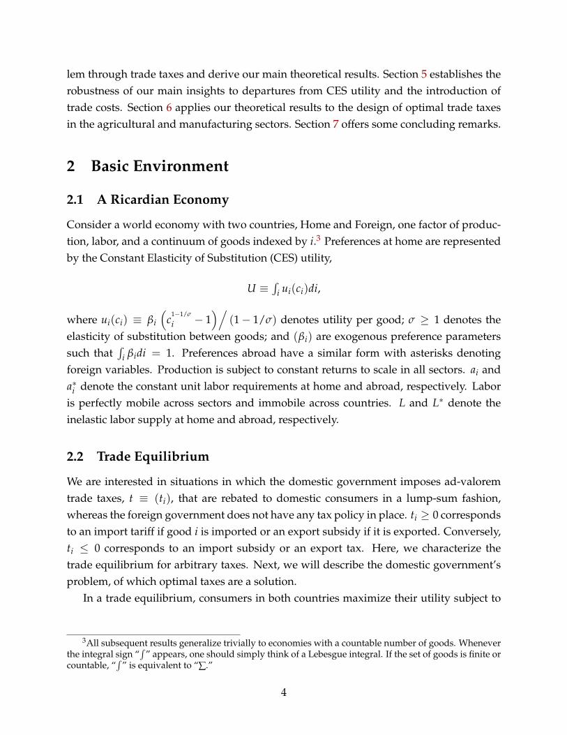
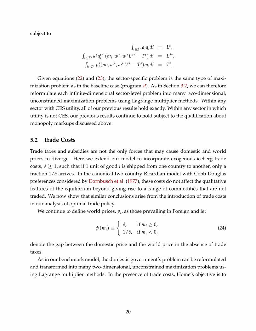
by looking forstationary points. But, as we now demonstrate, this technicality is of little consequence forour approach, the end goal of which is the maximization of the Lagrangian with respectto mi, not the location of its stationary points.

10

mi

Li

mIi MI

i 0 MI Ii

(a) ai/a∗i < AI .

mi

Li

MIi 0 MI I

i

(b) ai/a∗i ∈ [AI , AI I).

mi

Li

MIi 0 MI I

i

(c) ai/a∗i = AI I .

mi

Li

MIi 0 MI I

i mI I Ii

(d) ai/a∗i > AI I .

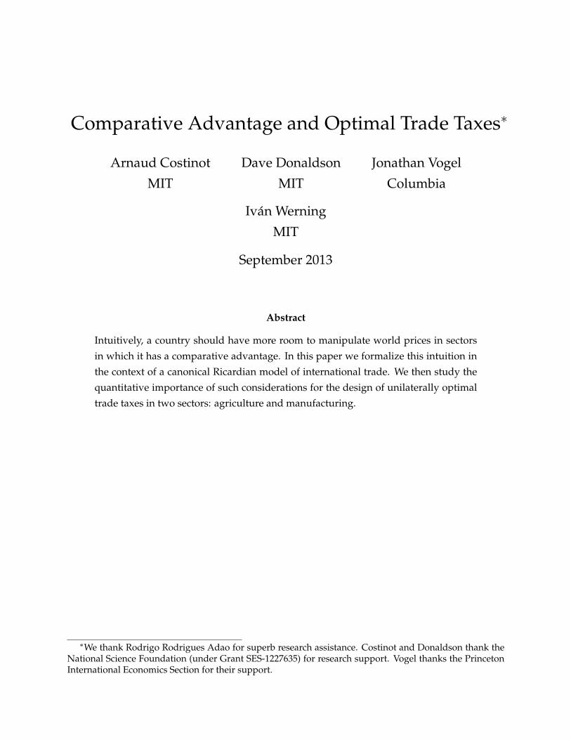
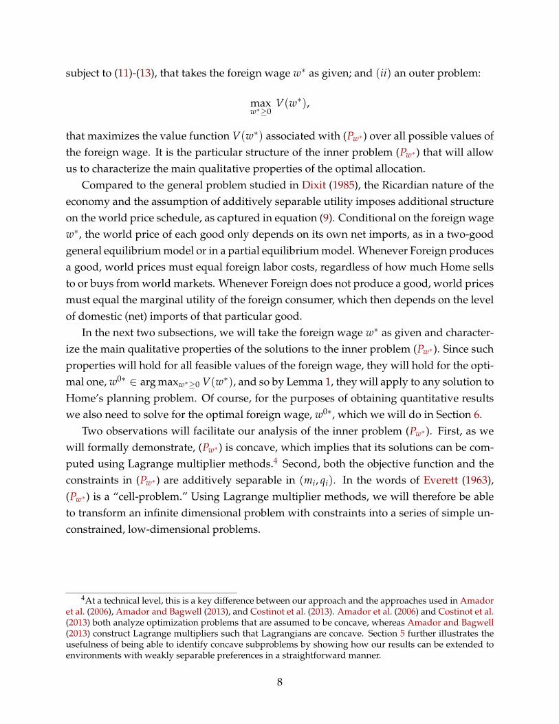
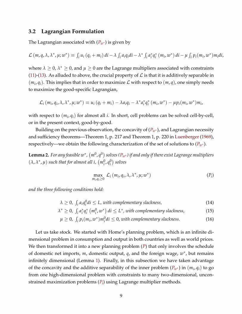
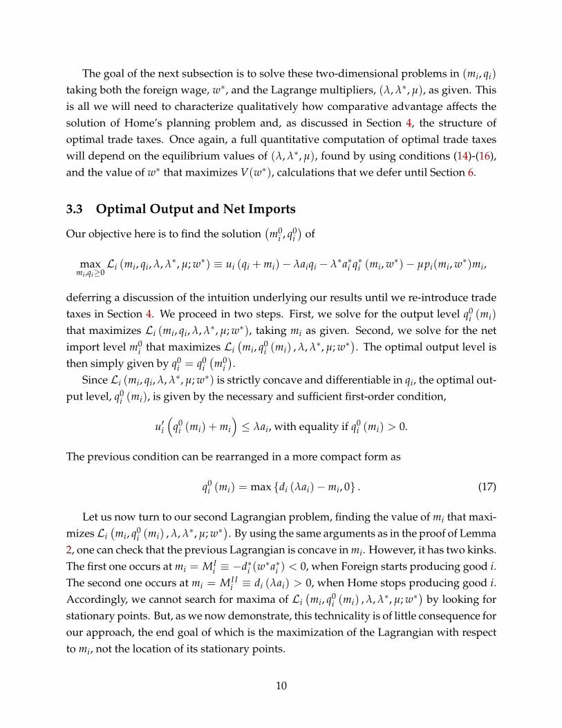
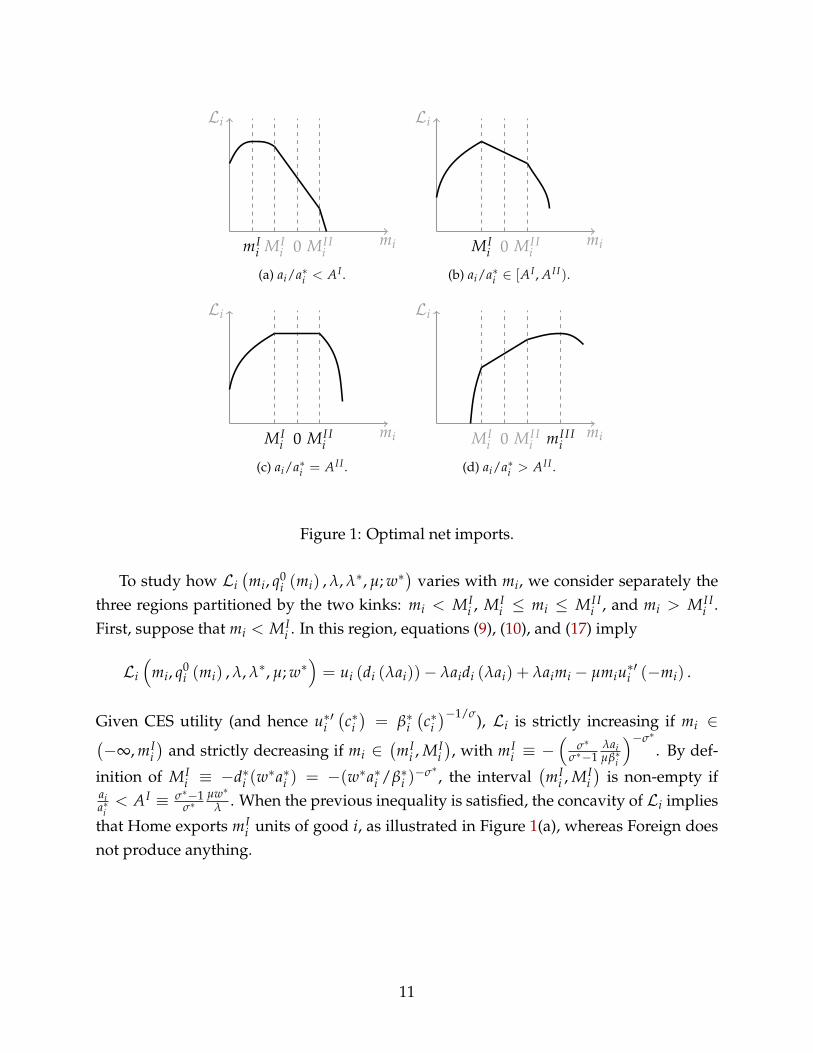
Figure 1: Optimal net imports.

fdsfdasfdasfdsafdsafdsafdsfdsafdsfdsfdsfdsfdsfdsfdsffdsfdsf

1

Figure 1: Optimal net imports.

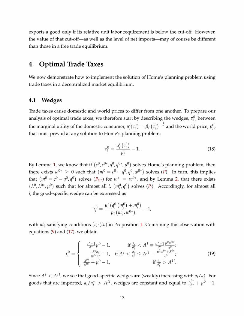
To study how Li(mi, q0

i (mi) , λ, λ∗, µ; w∗)

varies with mi, we consider separately thethree regions partitioned by the two kinks: mi < MI

i , MIi ≤ mi ≤ MI I

i , and mi > MI Ii .

First, suppose that mi < MIi . In this region, equations (9), (10), and (17) imply

Li

(mi, q0

i (mi) , λ, λ∗, µ; w∗)= ui (di (λai))− λaidi (λai) + λaimi − µmiu∗′i (−mi) .

Given CES utility (and hence u∗′i(c∗i)= β∗i

(c∗i)−1/σ), Li is strictly increasing if mi ∈(

−∞, mIi)

and strictly decreasing if mi ∈(mI

i , MIi), with mI

i ≡ −(

σ∗σ∗−1

λaiµβ∗i

)−σ∗. By def-

inition of MIi ≡ −d∗i (w

∗a∗i ) = −(w∗a∗i /β∗i )−σ∗ , the interval

(mI

i , MIi)

is non-empty ifaia∗i

< AI ≡ σ∗−1σ∗

µw∗λ . When the previous inequality is satisfied, the concavity of Li implies

that Home exports mIi units of good i, as illustrated in Figure 1(a), whereas Foreign does

not produce anything.

11

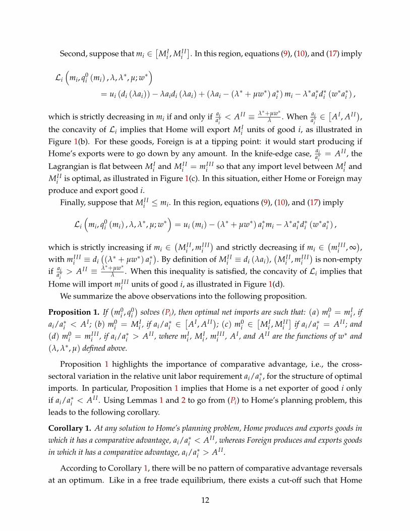
Second, suppose that mi ∈[MI

i , MI Ii]. In this region, equations (9), (10), and (17) imply

Li

(mi, q0

i (mi) , λ, λ∗, µ; w∗)

= ui (di (λai))− λaidi (λai) + (λai − (λ∗ + µw∗) a∗i )mi − λ∗a∗i d∗i (w∗a∗i ) ,

which is strictly decreasing in mi if and only if aia∗i

< AI I ≡ λ∗+µw∗λ . When ai

a∗i∈[AI , AI I),

the concavity of Li implies that Home will export MIi units of good i, as illustrated in

Figure 1(b). For these goods, Foreign is at a tipping point: it would start producing ifHome’s exports were to go down by any amount. In the knife-edge case, ai

a∗i= AI I , the

Lagrangian is flat between MIi and MI I

i = mI I Ii so that any import level between MI

i andMI I

i is optimal, as illustrated in Figure 1(c). In this situation, either Home or Foreign mayproduce and export good i.

Finally, suppose that MI Ii ≤ mi. In this region, equations (9), (10), and (17) imply

Li

(mi, q0

i (mi) , λ, λ∗, µ; w∗)= ui (mi)− (λ∗ + µw∗) a∗i mi − λ∗a∗i d∗i (w

∗a∗i ) ,

which is strictly increasing if mi ∈(

MI Ii , mI I I

i)

and strictly decreasing if mi ∈(mI I I

i , ∞),

with mI I Ii ≡ di

((λ∗ + µw∗) a∗i

). By definition of MI I

i ≡ di (λai),(

MI Ii , mI I I

i)

is non-emptyif ai

a∗i> AI I ≡ λ∗+µw∗

λ . When this inequality is satisfied, the concavity of Li implies that

Home will import mI I Ii units of good i, as illustrated in Figure 1(d).

We summarize the above observations into the following proposition.

Proposition 1. If(m0

i , q0i)

solves (Pi), then optimal net imports are such that: (a) m0i = mI

i , ifai/a∗i < AI ; (b) m0

i = MIi , if ai/a∗i ∈

[AI , AI I); (c) m0

i ∈[MI

i , MI Ii]

if ai/a∗i = AI I ; and(d) m0

i = mI I Ii , if ai/a∗i > AI I , where mI

i , MIi , mI I I

i , AI , and AI I are the functions of w∗ and(λ, λ∗, µ) defined above.

Proposition 1 highlights the importance of comparative advantage, i.e., the cross-sectoral variation in the relative unit labor requirement ai/a∗i , for the structure of optimalimports. In particular, Proposition 1 implies that Home is a net exporter of good i onlyif ai/a∗i < AI I . Using Lemmas 1 and 2 to go from (Pi) to Home’s planning problem, thisleads to the following corollary.

Corollary 1. At any solution to Home’s planning problem, Home produces and exports goods inwhich it has a comparative advantage, ai/a∗i < AI I , whereas Foreign produces and exports goodsin which it has a comparative advantage, ai/a∗i > AI I .

According to Corollary 1, there will be no pattern of comparative advantage reversalsat an optimum. Like in a free trade equilibrium, there exists a cut-off such that Home

12

exports a good only if its relative unit labor requirement is below the cut-off. However,the value of that cut-off—as well as the level of net imports—may of course be differentthan those in a free trade equilibrium.

4 Optimal Trade Taxes

We now demonstrate how to implement the solution of Home’s planning problem usingtrade taxes in a decentralized market equilibrium.

4.1 Wedges

Trade taxes cause domestic and world prices to differ from one another. To prepare ouranalysis of optimal trade taxes, we therefore start by describing the wedges, τ0

i , between

the marginal utility of the domestic consumer, u′i(c0i ) = βi

(c0

i)− 1

σ and the world price, p0i ,

that must prevail at any solution to Home’s planning problem:

τ0i ≡

u′i(c0

i)

p0i− 1. (18)

By Lemma 1, we know that if(c0, c0∗, q0, q0∗, p0) solves Home’s planning problem, then

there exists w0∗ ≥ 0 such that(m0 = c0 − q0, q0, w0∗) solves (P). In turn, this implies

that(m0 = c0 − q0, q0) solves (Pw∗) for w∗ = w0∗, and by Lemma 2, that there exists(

λ0, λ0∗, µ0) such that for almost all i,(m0

i , q0i)

solves (Pi). Accordingly, for almost alli, the good-specific wedge can be expressed as

τ0i =

u′i(q0

i(m0

i)+ m0

i)

pi(m0

i , w0∗) − 1,

with m0i satisfying conditions (i)-(iv) in Proposition 1. Combining this observation with

equations (9) and (17), we obtain

τ0i =

σ∗−1

σ∗ µ0 − 1, if aia∗i

< AI ≡ σ∗−1σ∗

µ0w0∗

λ0 ;λ0ai

w0∗a∗i− 1, if AI < ai

a∗i≤ AI I ≡ µ0w0∗+λ0∗

λ0 ;λ0∗w0∗ + µ0 − 1, if ai

a∗i> AI I .

(19)

Since AI < AI I , we see that good-specific wedges are (weakly) increasing with ai/a∗i . Forgoods that are imported, ai/a∗i > AI I , wedges are constant and equal to λ0∗

w0∗ + µ0 − 1.

13

For goods that are exported, ai/a∗i < AI I , the magnitude of the wedge depends on thestrength of Home’s comparative advantage: it increases linearly with ai/a∗i for goods suchthat ai/a∗i ∈ (AI , AI I) and attains its minimum value for goods such that ai/a∗i < AI .

4.2 Comparative Advantage and Trade Taxes

To conclude our baseline theoretical analysis, we now demonstrate that any solutionto Home’s planning problem can be implemented by constructing a schedule of taxest0 = τ0. To do so, we only need to check that the sufficient conditions for utility maxi-mization and profit maximization by domestic consumers and firms at (distorted) localprices p0

i(1 + t0

i)

are satisfied at the solution to Home’s planning problem if t0i = τ0

i .Consider first the domestic consumer’s problem. By equation (18), we know that

u′i(

c0i

)= p0

i

(1 + t0

i

).

Thus for any pair of goods, i1 and i2, we have

u′i1

(c0

i1

)u′i2

(c0

i2

) =1 + t0

i11 + t0

i2

p0i1

p0i2

.

Hence, the domestic consumer’s marginal rates of substitution are equal to domestic rel-ative prices. At a solution to Home’s planning problem we also know from Lemma 1 that´

i m0i p0

i di = 0. Thus the domestic consumer’s budget constraint must hold as well, whichimplies that the sufficient conditions for utility maximization are satisfied.

Let us now turn to the domestic firm’s problem. At a solution to Home’s planningproblem, we have already argued in Section 3.3 that for almost all i,

u′i(

q0i + m0

i

)≤ λ0ai, with equality if q0

i > 0.

Since u′i(q0

i + m0i)= u′i

(c0

i)= p0

i(1 + t0

i), the sufficient condition for profit maximiza-

tion is satisfied, with the domestic wage in the trade equilibrium given by the Lagrangemultiplier on the labor resource constraint, λ0.

At this point, we have established that any solution to Home’s planning problem canbe implemented by constructing a schedule of taxes t0 = τ0. Furthermore, by the anal-ysis of Section 4.1, such a schedule of taxes must satisfy equation (19). Conversely, if t0

is a solution to the domestic’s government problem, then the allocation and prices in thetrade equilibrium associated with taxes t0,

(c0, c0∗, q0, q0∗, p0), must solve Home’s plan-

14

ning problem and, by utility maximization, satisfy

t0i =

u′i(c0

i)

θp0i− 1,

with θ the Lagrange multiplier on the domestic consumer’s budget constraint. By theexact same logic as in Section 4.1, such a schedule of taxes must then be such that

t0i ≡

σ∗−1

σ∗µ0

θ − 1, if aia∗i

< AI ≡ σ∗−1σ∗

µ0w0∗

λ0 ;λ0ai

w0∗a∗i θ− 1, if AI < ai

a∗i≤ AI I ≡ µ0w0∗+λ0∗

λ0 ;λ0∗+µ0w0∗

θw0∗ − 1, if aia∗i

> AI I .

(20)

This leads to the following characterization of optimal trade taxes.

Proposition 2. At any solution t0 of the domestic government’s problem: (a) t0i = (1 + t̄) (AI/AI I)−

1, if ai/a∗i < AI ; (b) t0i = (1 + t̄)

((ai/a∗i

)/AI I)− 1, if ai/a∗i ∈

[AI , AI I]; and (c) t0

i = t̄, ifai/a∗i > AI I , with t̄ > −1 and AI < AI I .

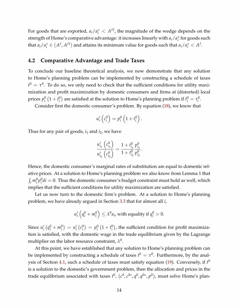
Proposition 2 states that optimal trade taxes vary with comparative advantage aswedges do. Trade taxes are at their lowest values, (1 + t̄) (AI/AI I) − 1, for goods inwhich Home’s comparative advantage is the strongest, ai/a∗i < AI ; they are linearlyincreasing with ai/a∗i for goods in which Home’s comparative advantage is in some in-termediate range, ai/a∗i ∈

[AI , AI I]; and they are at their highest value, t̄, for goods in

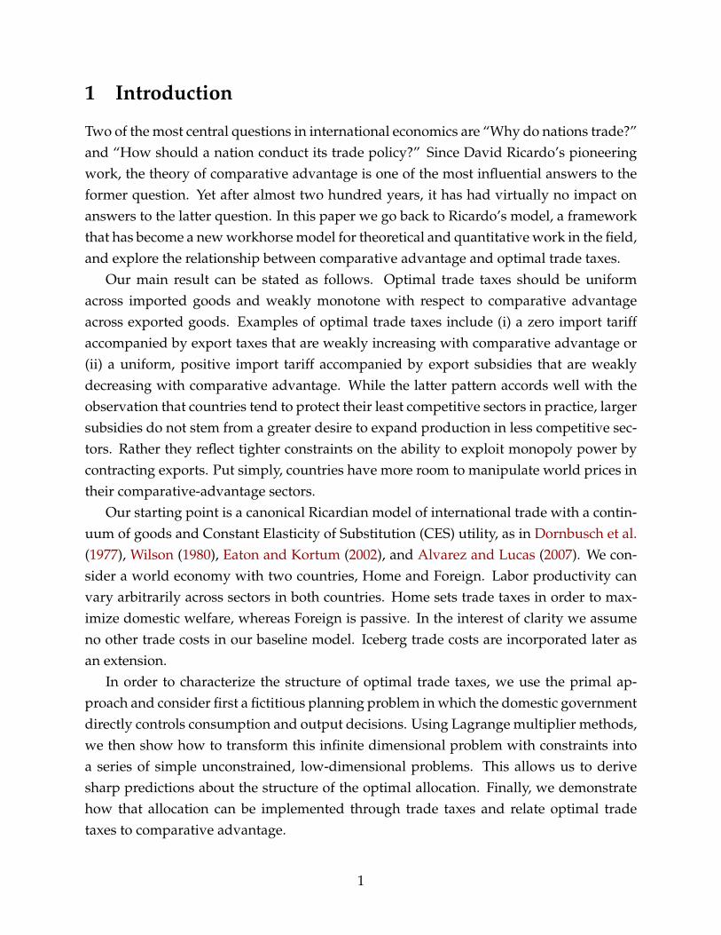
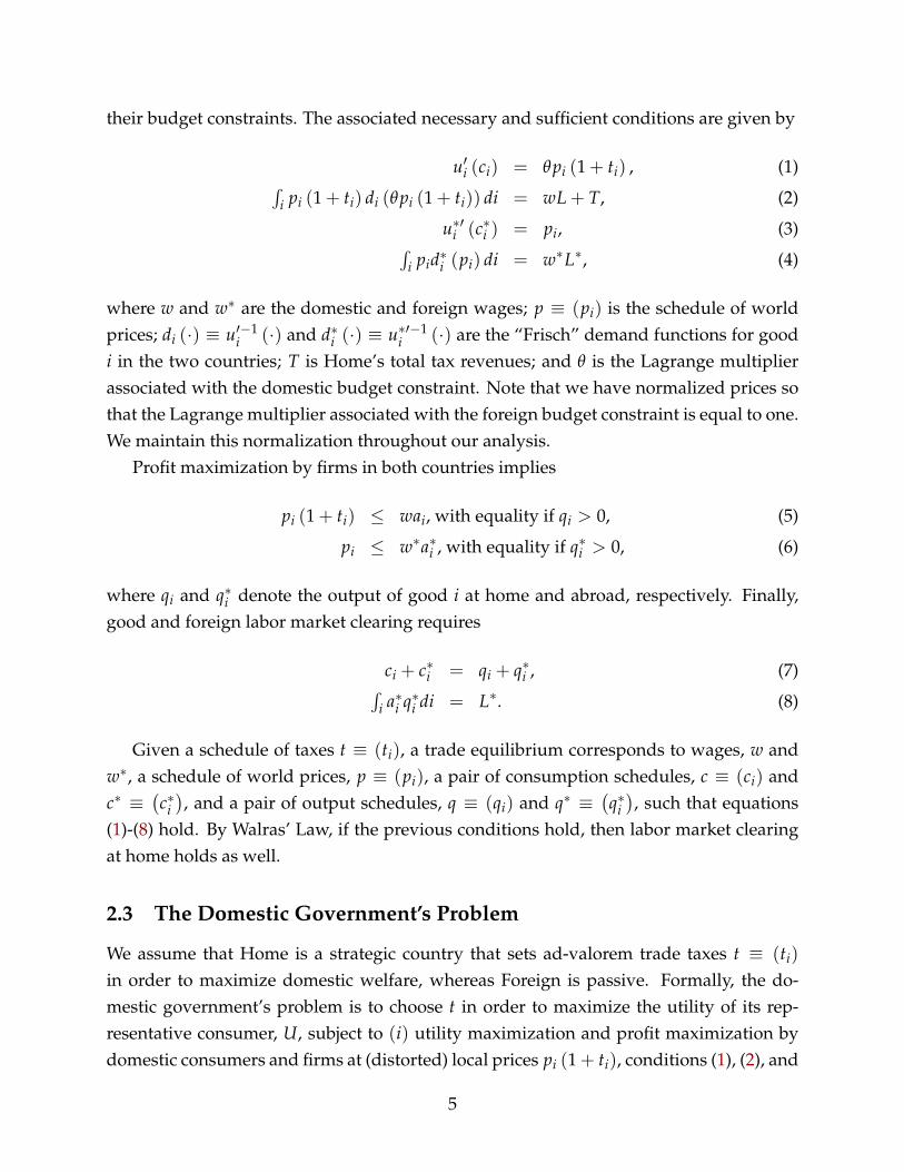
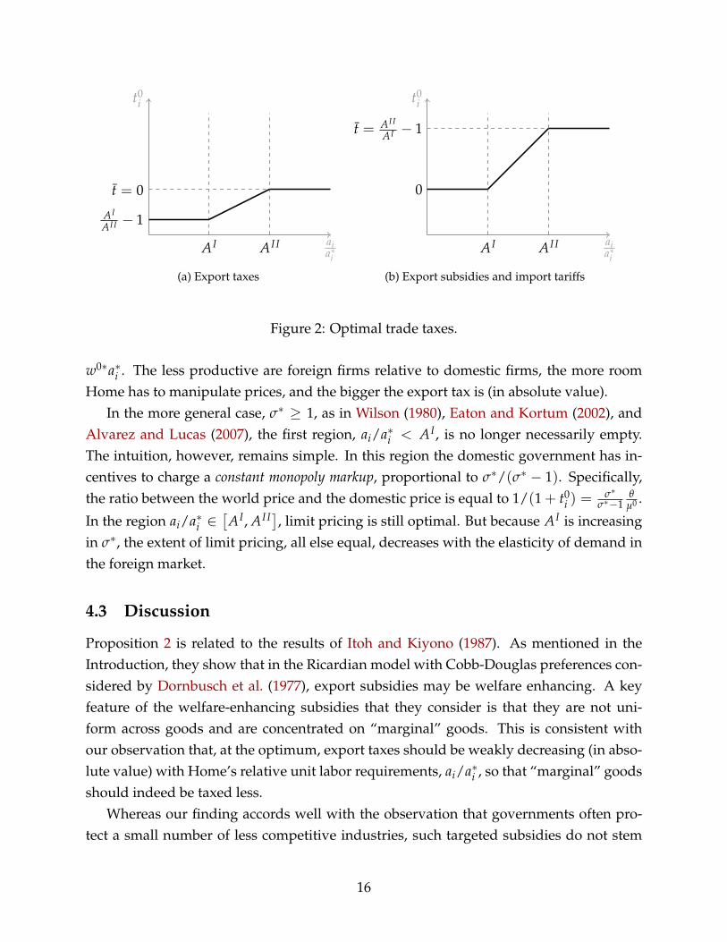
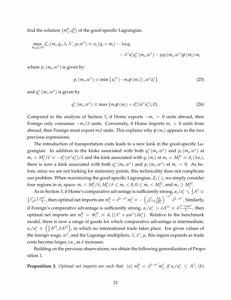
which Home’s comparative advantage is the weakest, ai/a∗i > AI I . Of course, the overalllevel of taxes is indeterminate, as captured by t̄ > −1 in the previous proposition, sinceonly relative prices and hence relative taxes matter for domestic consumers and firms.Figure 2 illustrates two polar cases. On Panel (a), there are no import tariffs, t̄ = 0, andall exported goods are subject to an export tax that rises with comparative advantage. OnPanel (b), in contrast, all imported goods are subject to a tariff t̄ = AI I

AI − 1 ≥ 0, whereasexported goods receive a subsidy that falls with comparative advantage. For expositionalpurposes, we focus in the rest of our discussion on the solution with zero import tariffs,t̄ = 0.

To gain intuition about the economic forces that shape optimal trade taxes, considerfirst the case in which foreign preferences are Cobb-Douglas, σ∗ = 1, as in Dornbusch etal. (1977). In this case, AI = 0 so that the first region, ai/a∗i < AI , is empty. In the secondregion, ai/a∗i ∈

[AI , AI I], there is limit pricing: Home exports the goods and sets export

taxes t0i < t̄ = 0 such that foreign firms are exactly indifferent between producing and

not producing those goods, i.e., such that the world price satisfies p0i = λ0ai/θ(1 + t0

i ) =

15

aia∗i

t0i

AI AI I

t̄ = 0

AI

AI I − 1

(a) Export taxes

aia∗i

t0i

AI AI I

0

t̄ = AI I

AI − 1

(b) Export subsidies and import tariffs

Figure 1: Optimal trade policy

fdsfdasfdasfdsafdsafdsafdsfdsafdsfdsfdsfdsfdsfdsfdsffdsfdsfdsfdsfdsfdsffds

1

Figure 2: Optimal trade taxes.

w0∗a∗i . The less productive are foreign firms relative to domestic firms, the more roomHome has to manipulate prices, and the bigger the export tax is (in absolute value).

In the more general case, σ∗ ≥ 1, as in Wilson (1980), Eaton and Kortum (2002), andAlvarez and Lucas (2007), the first region, ai/a∗i < AI , is no longer necessarily empty.The intuition, however, remains simple. In this region the domestic government has in-centives to charge a constant monopoly markup, proportional to σ∗/(σ∗ − 1). Specifically,the ratio between the world price and the domestic price is equal to 1/(1 + t0

i ) =σ∗

σ∗−1θ

µ0 .

In the region ai/a∗i ∈[AI , AI I], limit pricing is still optimal. But because AI is increasing

in σ∗, the extent of limit pricing, all else equal, decreases with the elasticity of demand inthe foreign market.

4.3 Discussion

Proposition 2 is related to the results of Itoh and Kiyono (1987). As mentioned in theIntroduction, they show that in the Ricardian model with Cobb-Douglas preferences con-sidered by Dornbusch et al. (1977), export subsidies may be welfare enhancing. A keyfeature of the welfare-enhancing subsidies that they consider is that they are not uni-form across goods and are concentrated on “marginal” goods. This is consistent withour observation that, at the optimum, export taxes should be weakly decreasing (in abso-lute value) with Home’s relative unit labor requirements, ai/a∗i , so that “marginal” goodsshould indeed be taxed less.

Whereas our finding accords well with the observation that governments often pro-tect a small number of less competitive industries, such targeted subsidies do not stem

16

from a greater desire to expand production in less competitive sectors. On the contrary,they reflect tighter constraints on the ability to exploit monopoly power by contractingexports. According to Proposition 2, Home can only charge constant monopoly markupsfor exported goods in which its comparative advantage is the strongest. For other ex-ported goods, the threat of entry of foreign firms lead markups to go down with Home’scomparative advantage.

An interesting issue is whether the structure of optimal trade taxes crucially relies onthe assumption that domestic firms are perfectly competitive. Since Home’s governmentbehaves like a domestic monopolist competing à la Bertrand against foreign firms, onemay conjecture that if each good were produced by only one domestic firm, then Homewould no longer have to use trade taxes to manipulate prices: domestic firms wouldalready manipulate prices under laissez-faire. This conjecture, however, is incorrect fortwo reasons. The first one is that although the government behaves like a monopolist,the domestic government’s problem involves non-trivial general equilibrium considera-tions, as reflected in the values of (w0∗, λ0, λ0∗, µ0). Even when Home charges a constantmonopoly markup, the optimal level of the markup differs from what an individual firmwould choose, i.e., σ∗/ (σ∗ − 1). The second reason is that to manipulate prices, Home’sgovernment needs to affect the behaviors of both firms and consumers: net imports de-pend both on supply and demand. If each good were produced by only one domesticfirm, Home’s government would still need to impose good-varying consumption taxesthat mimic the trade taxes described above (plus output subsidies that reflect generalequilibrium considerations). Intuitively, if each good were produced by only one domes-tic firm, consumers would face monopoly markups in each country, whereas optimalityrequires a wedge between consumer prices at home and abroad, as we show above.

5 Robustness

In this section we incorporate general preferences and trade costs into the Ricardianmodel presented in Section 2. Our goal is twofold. First, we want to demonstrate thatLagrange multiplier methods, and in particular our strategy of identifying concave cell-problems, remain well suited to analyzing optimal trade policy in this more general en-vironment. Second, we want to show that the central predictions derived in Section 4 donot crucially hinge on the assumption of CES utility or the absence of trade costs. To saveon space, we focus on sketching alternative environments and summarizing their mainimplications.

17

5.1 Preferences

While the assumption of CES utility is standard in the Ricardian literature—from Dorn-busch et al. (1977) to Eaton and Kortum (2002)—it implies strong restrictions on thedemand-side of the economy: own-price elasticities and elasticities of substitution areboth constant and pinned down by a single parameter, σ. In practice, price elasticitiesmay vary with quantities consumed and patterns of substitutions may vary across goods.For instance, one would expect two varieties of cars to be closer substitutes than, say, carsand bikes.

Here we relax the assumptions of Section 2 by assuming that: (i) Home’s preferencesare weakly separable over a discrete number of sectors, s ∈ S ≡ {1, ..., S}; and that:(ii) subutility within each sector, Us, is additively separable, though not necessarily CES.Specifically, we assume that Home’s preferences can be represented by the following util-ity function,

U = F(

U1(

c1)

, ...., US(

cS))

,

where F is a strictly increasing function; cs ≡ (ci)i∈I s denotes the consumption of goodsin sector s, with I s the set of goods that belongs to that sector; and the subutility Us issuch that

Us (cs) =´

i∈I s usi (ci)di.

Foreign’s preferences are similar, and asterisks denote foreign variables. Section 2 cor-responds to the special case in which there is only one-sector, S = 1, and Us is CES,us

i (ci) ≡ βsi

(c

1−1/σs

i − 1)/

(1− 1/σs).5

For expositional purposes, let us start by considering an intermediate scenario inwhich utility is not CES, but we maintain the assumption that there is only one sector,S = 1. It should be clear that the CES assumption is not crucial for the results derived inSections 2.2-3.2. In contrast, CES plays a key role in determining the optimal level of net

imports, mIi = −

(σ∗

σ∗−1λaiµβ∗i

)−σ∗, in Section 3.3 and, in turn, in establishing that trade taxes

are at their lowest values, (1 + t̄) (AI/AI I)− 1, for goods in which Home’s comparativeadvantage is the strongest in Section 4.2. Absent CES utility, trade taxes would still be attheir highest value, t̄, for goods in which Home’s comparative advantage is the weakestand linearly increasing with ai/a∗i for goods in which Home’s comparative advantage isin some intermediate range. But for goods in which Home’s comparative advantage is thestrongest, the optimal trade tax would now vary with the elasticity of demand, reflecting

5The analysis in this section trivially extends to the case in which only a subset of sectors have additivelyseparable utility. For this subset of sectors, and this subset only, our predictions would remain unchanged.

18

the incentives to charge different monopoly markups.Now let us turn to the general case with multiple sectors, S ≥ 1. With weakly separa-

ble preferences abroad, one can check that foreign consumption in each sector must be asolution to

maxcs∗ Us∗ (cs∗)

subject to ´i∈I s ps

i cs∗i di = Es∗, (21)

where Es∗ is total expenditure on sector s goods. Accordingly, by the same argument asin Section 3.1, we can write the world price and foreign output for all s ∈ S and i ∈ I s as

psi (mi, w∗, Es∗) ≡ min

{us∗′

i (−mi) θs∗ (Es∗) , w∗a∗i}

, (22)

andqs∗

i (mi, w∗, Es∗) ≡ max {mi + ds∗i (w∗a∗i /θs∗ (Es∗)), 0} , (23)

where θs∗ (Es∗) is the Lagrange multiplier associated with (21) for a given value of Es∗.As we show in our online Addendum, Home’s planning problem can still be decom-

posed into an outer problem and multiple inner problems, one for each sector. At theouter level, the government now chooses the foreign wage, w∗, together with the sectorallabor allocations in Home and Foreign, Ls and Ls∗, the sectoral trade deficits, Ts, subjectto aggregate factor market clearing and trade balance. At the inner level, the governmenttreats Ls, Ls∗, Ts, and w∗ as constraints and maximizes sector-level utility sector-by-sector.More precisely, , Home’s planning problem can be expressed as

max{Ls,Ls∗,Ts}s∈S ,w∗≥0

F(

V1(

L1, L1∗, T1, w∗)

, ..., VS(

LS, LS∗, TS, w∗))

subject to

∑s∈S Ls = L,

∑s∈S Ls∗ = L∗,

∑s∈S Ts = 0,

where the sector-specific value function satisfies

Vs (Ls, Ls∗, Ts, w∗) ≡ maxms,qs≥0

´i∈I s us

i (mi + qi)di

19

subject to

´i∈I s aiqidi = Ls,´

i∈I s a∗i qs∗i (mi, w∗, w∗Ls∗ − Ts) di = Ls∗,´

i∈I s psi (mi, w∗, w∗Ls∗ − Ts)midi = Ts.

Given equations (22) and (23), the sector-specific problem is the same type of maxi-mization problem as in the baseline case (program P). As in Section 3.2, we can thereforereformulate each infinite-dimensional sector-level problem into many two-dimensional,unconstrained maximization problems using Lagrange multiplier methods. Within anysector with CES utility, all of our previous results hold exactly. Within any sector in whichutility is not CES, our previous results continue to hold subject to the qualification aboutmonopoly markups discussed above.

5.2 Trade Costs

Trade taxes and subsidies are not the only forces that may cause domestic and worldprices to diverge. Here we extend our model to incorporate exogenous iceberg tradecosts, δ ≥ 1, such that if 1 unit of good i is shipped from one country to another, only afraction 1/δ arrives. In the canonical two-country Ricardian model with Cobb-Douglaspreferences considered by Dornbusch et al. (1977), these costs do not affect the qualitativefeatures of the equilibrium beyond giving rise to a range of commodities that are nottraded. We now show that similar conclusions arise from the introduction of trade costsin our analysis of optimal trade policy.

We continue to define world prices, pi, as those prevailing in Foreign and let

φ (mi) ≡{

δ, if mi ≥ 0,1/δ, if mi < 0,

(24)

denote the gap between the domestic price and the world price in the absence of tradetaxes.

As in our benchmark model, the domestic government’s problem can be reformulatedand transformed into many two-dimensional, unconstrained maximization problems us-ing Lagrange multiplier methods. In the presence of trade costs, Home’s objective is to

20

find the solution(m0

i , q0i)

of the good-specific Lagrangian,

maxmi,qi≥0

Li (mi, qi, λ, λ∗, µ; w∗) ≡ ui (qi + mi)− λaiqi

− λ∗a∗i q∗i (mi, w∗)− µpi(mi, w∗)φ (mi)mi

where pi (mi, w∗) is given by

pi (mi, w∗) ≡ min{

u∗′i (−miφ (mi)) , w∗a∗i}

(25)

and q∗i (mi, w∗) is given by

q∗i (mi, w∗) ≡ max {miφ (mi) + d∗i (w∗a∗i ), 0} . (26)

Compared to the analysis of Section 3, if Home exports −mi > 0 units abroad, thenForeign only consumes −mi/δ units. Conversely, if Home imports mi > 0 units fromabroad, then Foreign must export miδ units. This explains why φ (mi) appears in the twoprevious expressions.

The introduction of transportation costs leads to a new kink in the good-specific La-grangian. In addition to the kinks associated with both q∗i (mi, w∗) and pi (mi, w∗) atmi = MI

i /δ ≡ −d∗i (w∗a∗i )/δ and the kink associated with qi (mi) at mi = MI I

i ≡ di (λai),there is now a kink associated with both q∗i (mi, w∗) and pi (mi, w∗) at mi = 0. As be-fore, since we are not looking for stationary points, this technicality does not complicateour problem. When maximizing the good-specific Lagrangian, Li (·), we simply considerfour regions in mi space: mi < MI

i /δ, MIi /δ ≤ mi < 0, 0 ≤ mi < MI I

i , and mi ≥ MI Ii .

As in Section 3, if Home’s comparative advantage is sufficiently strong, ai/a∗i ≤ 1δ AI ≡

1δ

σ∗−1σ∗

µw∗λ , then optimal net imports are m0

i = δ1−σ∗mIi ≡ −

(σ∗

σ∗−1λaiµβ∗i

)−σ∗δ1−σ∗ . Similarly,

if Foreign’s comparative advantage is sufficiently strong, ai/a∗i > δAI I ≡ δλ∗+µw∗

λ , thenoptimal net imports are m0

i = m̃I Ii ≡ di

((λ∗ + µw∗) δa∗i

). Relative to the benchmark

model, there is now a range of goods for which comparative advantage is intermediate,ai/a∗i ∈

(1δ AI I , δAI I

), in which no international trade takes place. For given values of

the foreign wage, w∗, and the Lagrange multipliers, λ, λ∗, µ, this region expands as tradecosts become larger, i.e., as δ increases.

Building on the previous observations, we obtain the following generalization of Propo-sition 1.

Proposition 3. Optimal net imports are such that: (a) m0i = δ1−σ∗mI

i , if ai/a∗i ≤ AI ; (b)

21

m0i = 1

δ MIi , if ai/a∗i ∈

(AI , 1

δ AI I)

; (c) m0i ∈

[1δ MI

i , 0]

if ai/a∗i = 1δ AI I ; (d) m0

i = 0, if

ai/a∗i ∈(

1δ AI I , δAI I

); (e) m0

i ∈(0, m̃I I

i)

if ai/a∗i = δAI I ; and ( f ) m0i = m̃I I

i , if ai/a∗i > δAI I .

Using Proposition 3, it is straightforward to show, as in Section 4.1, that good-specificwedges are (weakly) increasing with Home’s comparative advantage. Similarly, as in Sec-tion 4.2, we can show that any solution to Home’s planning problem can be implementedby constructing a schedule of taxes, and that the optimal trade taxes vary with compara-tive advantage as wedges do. In summary, our main theoretical results are also robust tothe introduction of exogenous iceberg trade costs.

6 Applications

To conclude, we apply our theoretical results to two sectors: agriculture and manufactur-ing. Our goal is to take a first look at the quantitative importance for welfare of optimaltrade taxes, both in an absolute sense and relative to simpler uniform trade taxes.

In both applications, we compute optimal trade taxes as follows. First, we use Propo-sition 1 to solve for optimal imports and output given arbitrary values of the Lagrangemultipliers, (λ, λ∗, µ), and the foreign wage, w∗. Second, we use conditions (14)-(16) inLemma 2 to solve for the Lagrange multipliers. Finally, we find the value of the foreignwage that maximizes the value function V(w∗) associated with the inner problem. Giventhe optimal foreign wage, w0∗, and the associated Lagrange multipliers,

(λ0, λ0∗, µ0), we

finally compute optimal trade taxes using Proposition 2.

6.1 Agriculture

In many ways, agriculture provides the perfect environment in which to explore the quan-titative importance of our results. From a theoretical perspective, market structure is asclose as possible to the neoclassical ideal. From a measurement perspective, the scien-tific knowledge of agronomists provides a unique window into the structure of compar-ative advantage, as discussed in Costinot and Donaldson (2011). Finally, from a policyperspective, agricultural trade taxes are pervasive and one of the most salient and con-tentious global economic issues, as illustrated by the World Trade Organization’s current,long-stalled Doha round.

Calibration. We start from the Ricardian economy presented in Section 2.1 and assumethat each good corresponds to one of 39 crops for which we have detailed productivitydata, as we discuss below. All crops enter utility symmetrically in all countries, βi =

22

β∗i = 1. Home is the United States and Foreign is an aggregate of the rest of the world(henceforth R.O.W.). The single factor of production is equipped land . We also explorehow our results change in the presence of exogenous iceberg trade costs, as in Section 5.2.

The parameters necessary to apply our theoretical results are: (i) the unit factor re-quirement for each crop in each country, ai and a∗i ; (ii) the elasticity of substitution, σ;(iii) the relative size of the two countries, L∗/L; and (iv) trade costs, δ, when relevant. Forsetting each crop’s unit factor requirements, we use data from the Global Agro-EcologicalZones (GAEZ) project from the Food and Agriculture Organization (FAO); see Costinotand Donaldson (2011). Feeding data on local conditions—e.g., soil, topography, eleva-tion and climatic conditions—into an agronomic model, scientists from the GAEZ projecthave computed the yield that parcels of land around the world could obtain if they wereto grow each of the 39 crops we consider in 2009.6 We set ai and a∗i equal to the aver-age hectare per ton of output across all parcels of land in the United States and R.O.W.,respectively; see Table 1 in our online Addendum.

The other parameters are chosen as follows. We set σ = 8.1 in line with the estimatesof Costinot et al. (2012) using trade and price data for 10 major crops in 2009 from theFAOSTAT program at the FAO. We set L = 1 and L∗ = 13 to match the relative acreagedevoted to the 39 crops considered, as reported in the FAOSTAT data in 2009. Finally,in the extension with trade costs, we set δ = 1.32 so that Home’s import share in theequilibrium without trade policy matches the U.S. agriculture import share—that is, thetotal value of U.S. imports over the 39 crops considered divided by the total value of U.S.expenditure over those same crops—in the FAOSTAT data in 2009, 11.1%.

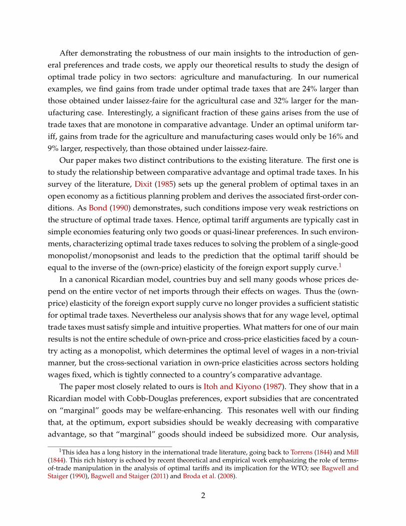
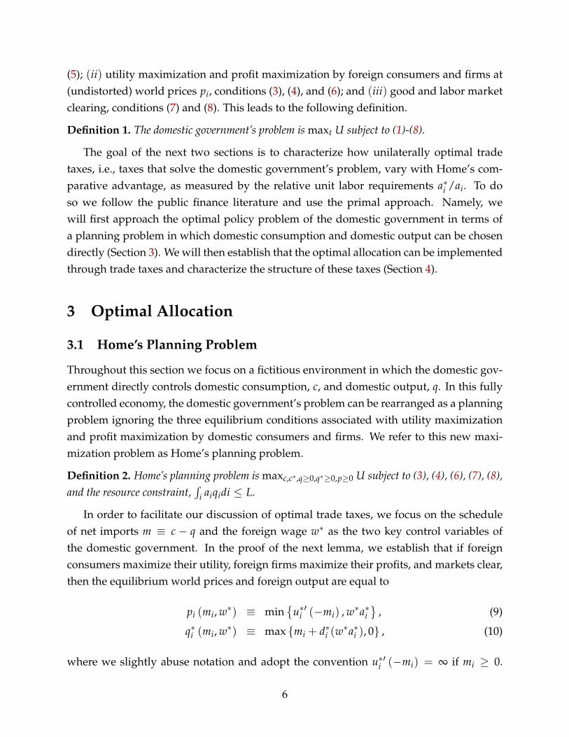
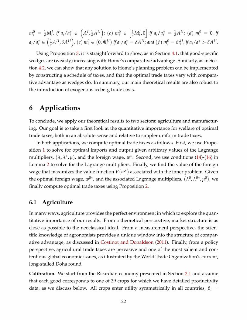
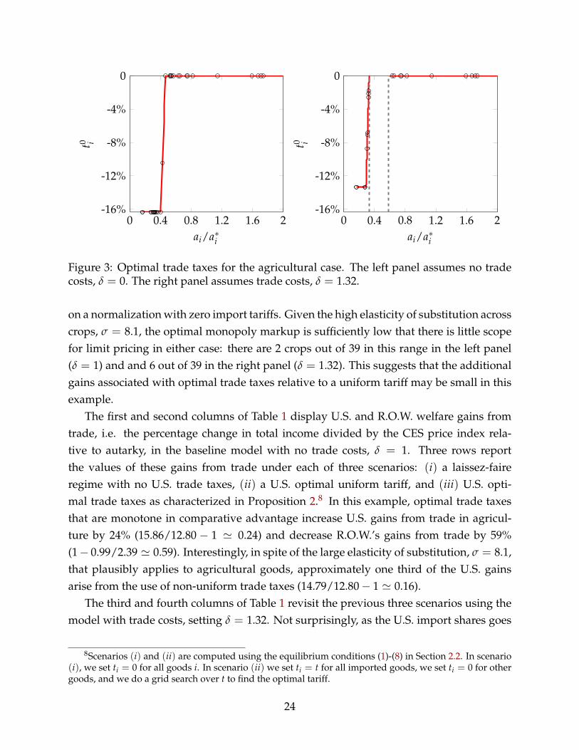
Results. The left and right panels of Figure 3 report optimal trade taxes on all tradedcrops i as a function of comparative advantage, ai/a∗i , in the calibrated examples withouttrade costs, δ = 1, and with trade costs, δ = 1.32, respectively.7 The region betweenthe two vertical lines in the right panel corresponds to goods that are not traded at thesolution of Home’s planning problem.

As discussed in Section 4.2, the overall level of taxes is indeterminate. Here we focus

6The GAEZ project constructs output per hectare predictions under different assumptions on a farmer’suse of complementary inputs (e.g. irrigation, fertilizers, and machinery). We use the measure that is con-structed under the assumption that irrigation and a “moderate” level of other inputs (fertilizers, machinery,etc.) are available to farmers.

7We compute optimal trade taxes, throughout this and the next subsection, by performing a grid searchover the foreign wage w∗ so as to maximize V(w∗). Since Foreign cannot be worse off under trade thanunder autarky—whatever world prices may be, there are gains from trade—and cannot be better off thanunder free trade—since free trade is a Pareto optimum, Home would have to be worse off—we restrictour grid search to values of the foreign wage between those that would prevail in the autarky and freetrade equilibria. Recall that we have normalized prices so that the Lagrange multiplier associated with theforeign budget constraint is equal to one. Thus w∗ is the real wage abroad.

23

0 0.4 0.8 1.2 1.6 2-16%

-12%

-8%

-4%

0

ai/a∗i

t0 i

0 0.4 0.8 1.2 1.6 2-16%

-12%

-8%

-4%

0

ai/a∗i

t0 i

Figure 3: Optimal trade taxes for the agricultural case. The left panel assumes no tradecosts, δ = 0. The right panel assumes trade costs, δ = 1.32.

on a normalization with zero import tariffs. Given the high elasticity of substitution acrosscrops, σ = 8.1, the optimal monopoly markup is sufficiently low that there is little scopefor limit pricing in either case: there are 2 crops out of 39 in this range in the left panel(δ = 1) and and 6 out of 39 in the right panel (δ = 1.32). This suggests that the additionalgains associated with optimal trade taxes relative to a uniform tariff may be small in thisexample.

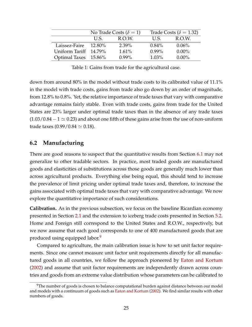
The first and second columns of Table 1 display U.S. and R.O.W. welfare gains fromtrade, i.e. the percentage change in total income divided by the CES price index rela-tive to autarky, in the baseline model with no trade costs, δ = 1. Three rows reportthe values of these gains from trade under each of three scenarios: (i) a laissez-faireregime with no U.S. trade taxes, (ii) a U.S. optimal uniform tariff, and (iii) U.S. opti-mal trade taxes as characterized in Proposition 2.8 In this example, optimal trade taxesthat are monotone in comparative advantage increase U.S. gains from trade in agricul-ture by 24% (15.86/12.80 − 1 ' 0.24) and decrease R.O.W.’s gains from trade by 59%(1− 0.99/2.39 ' 0.59). Interestingly, in spite of the large elasticity of substitution, σ = 8.1,that plausibly applies to agricultural goods, approximately one third of the U.S. gainsarise from the use of non-uniform trade taxes (14.79/12.80− 1 ' 0.16).

The third and fourth columns of Table 1 revisit the previous three scenarios using themodel with trade costs, setting δ = 1.32. Not surprisingly, as the U.S. import shares goes

8Scenarios (i) and (ii) are computed using the equilibrium conditions (1)-(8) in Section 2.2. In scenario(i), we set ti = 0 for all goods i. In scenario (ii) we set ti = t for all imported goods, we set ti = 0 for othergoods, and we do a grid search over t to find the optimal tariff.

24

No Trade Costs (δ = 1) Trade Costs (δ = 1.32)U.S. R.O.W. U.S. R.O.W.

Laissez-Faire 12.80% 2.39% 0.84% 0.06%Uniform Tariff 14.79% 1.61% 0.99% 0.00%Optimal Taxes 15.86% 0.99% 1.03% 0.00%

Table 1: Gains from trade for the agricultural case.

down from around 80% in the model without trade costs to its calibrated value of 11.1%in the model with trade costs, gains from trade also go down by an order of magnitude,from 12.8% to 0.8%. Yet, the relative importance of trade taxes that vary with comparativeadvantage remains fairly stable. Even with trade costs, gains from trade for the UnitedStates are 23% larger under optimal trade taxes than in the absence of any trade taxes(1.03/0.84− 1 ' 0.23) and about one fifth of these gains arise from the use of non-uniformtrade taxes (0.99/0.84 ' 0.18).

6.2 Manufacturing

There are good reasons to suspect that the quantitative results from Section 6.1 may notgeneralize to other tradable sectors. In practice, most traded goods are manufacturedgoods and elasticities of substitutions across those goods are generally much lower thanacross agricultural products. Everything else being equal, this should tend to increasethe prevalence of limit pricing under optimal trade taxes and, therefore, to increase thegains associated with optimal trade taxes that vary with comparative advantage. We nowexplore the quantitative importance of such considerations.

Calibration. As in the previous subsection, we focus on the baseline Ricardian economypresented in Section 2.1 and the extension to iceberg trade costs presented in Section 5.2.Home and Foreign still correspond to the United States and R.O.W., respectively, butwe now assume that each good corresponds to one of 400 manufactured goods that areproduced using equipped labor.9

Compared to agriculture, the main calibration issue is how to set unit factor require-ments. Since one cannot measure unit factor unit requirements directly for all manufac-tured goods in all countries, we follow the approach pioneered by Eaton and Kortum(2002) and assume that unit factor requirements are independently drawn across coun-tries and goods from an extreme value distribution whose parameters can be calibrated to

9The number of goods is chosen to balance computational burden against distance between our modeland models with a continuum of goods such as Eaton and Kortum (2002). We find similar results with othernumbers of goods.

25

match a few key moments in the macro data. In a two-country setting, Dekle et al. (2007)have shown that this approach is equivalent to assuming

ai =

(iT

) 1θ

and a∗i =

(1− iT∗

) 1θ

,

with θ the shape parameter of the extreme value distribution, that is assumed to be com-mon across countries, and T and T∗ the scale parameters, that are allowed to vary acrosscountries. We let the good index i be equally spaced between 1/10, 000 and 1− 1/10, 000for the 400 goods in the economy.

Given the previous functional form assumptions, we choose parameters as follows.We set σ = 2.6 to match the median estimate of the elasticity of substitution across 5-digit SITC sectors in Broda and Weinstein (2006). We set L = 1 and L∗ = 19.5 to matchpopulation in the U.S. relative to R.O.W., as reported by the World Bank in 2009. Since theshape parameter θ determines the elasticity of trade flows with respect trade costs, we setθ = 5, which is a typical estimate in the literature; see e.g. Anderson and Van Wincoop(2004) and Head and Mayer (2013). Given the previous parameters, we then set T =

5, 194.6 and T∗ = 1 so that Home’s share of world GDP matches the U.S. share, 26%, asreported by the World Bank in 2009. Finally, in the extension with trade costs, we nowset δ = 1.44 so that Home’s import share in the equilibrium without trade policy matchesthe U.S. manufacturing import share—i.e. , total value of U.S. manufacturing importsdivided by total value of U.S. expenditure in manufacturing—as reported in the OECDSTructural ANalysis (STAN) database in 2009, 24.7%.

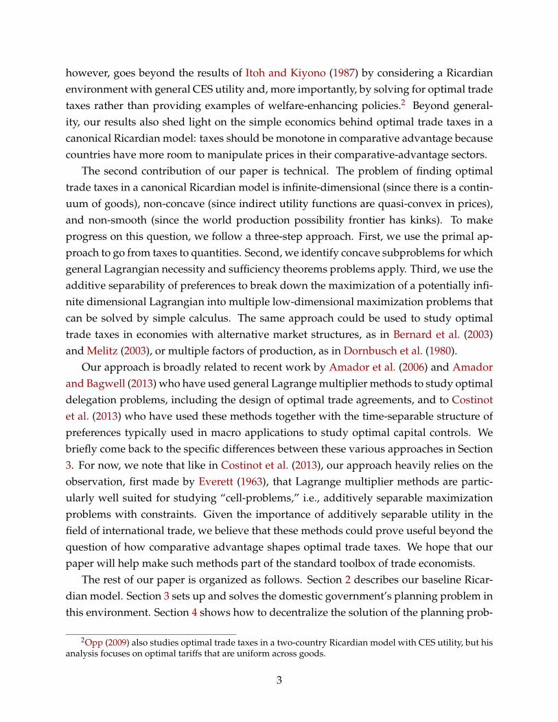
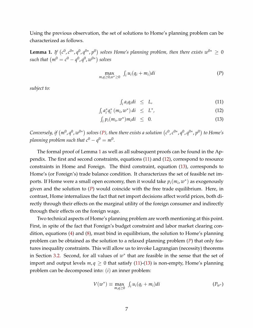
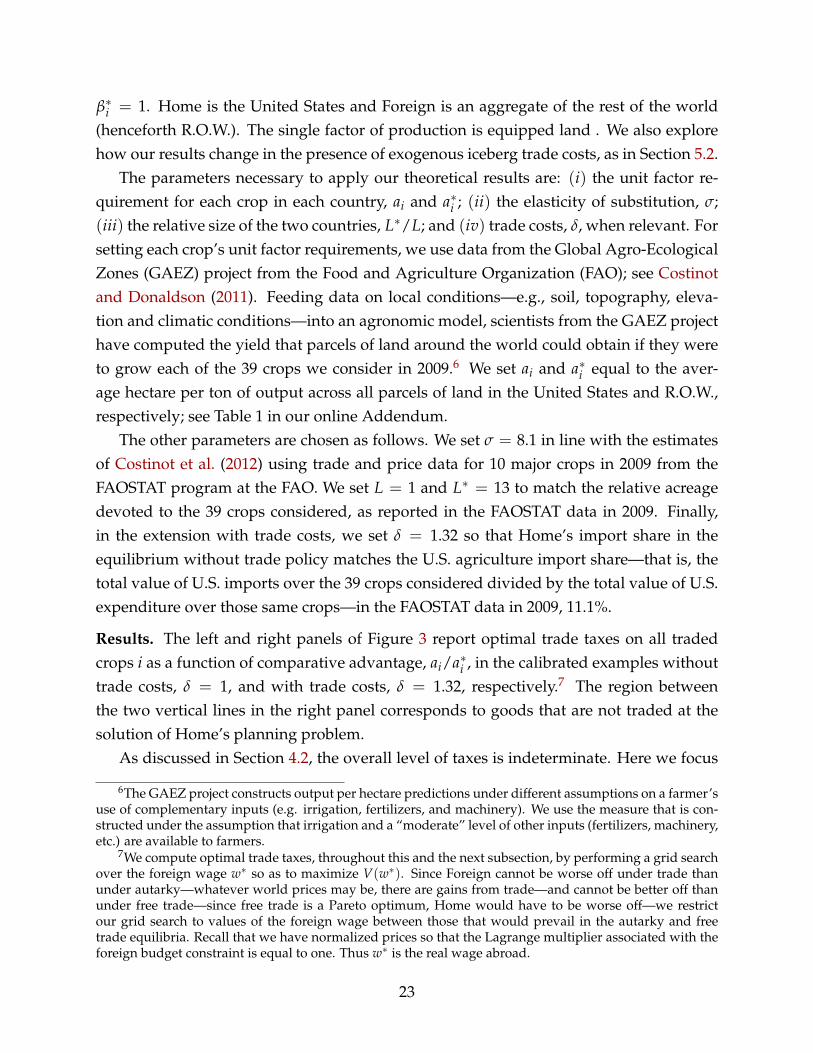
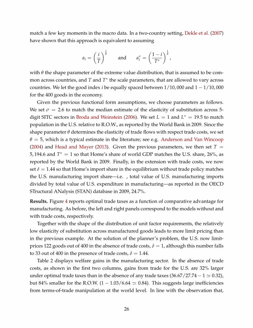
Results. Figure 4 reports optimal trade taxes as a function of comparative advantage formanufacturing. As before, the left and right panels correspond to the models without andwith trade costs, respectively.

Together with the shape of the distribution of unit factor requirements, the relativelylow elasticity of substitution across manufactured goods leads to more limit pricing thanin the previous example. At the solution of the planner’s problem, the U.S. now limit-prices 122 goods out of 400 in the absence of trade costs, δ = 1, although this number fallsto 33 out of 400 in the presence of trade costs, δ = 1.44.

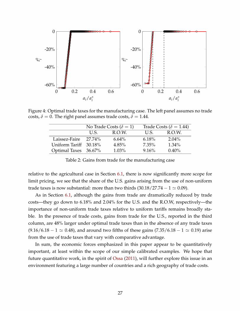
Table 2 displays welfare gains in the manufacturing sector. In the absence of tradecosts, as shown in the first two columns, gains from trade for the U.S. are 32% largerunder optimal trade taxes than in the absence of any trade taxes (36.67/27.74− 1 ' 0.32),but 84% smaller for the R.O.W. (1− 1.03/6.64 ' 0.84). This suggests large inefficienciesfrom terms-of-trade manipulation at the world level. In line with the observation that,

26

0 0.2 0.4 0.6-60%

-40%

-20%

0

ai/a∗i

t0 i

0 0.2 0.4 0.6-60%

-40%

-20%

0

ai/a∗i

t0 i

Figure 4: Optimal trade taxes for the manufacturing case. The left panel assumes no tradecosts, δ = 0. The right panel assumes trade costs, δ = 1.44.

No Trade Costs (δ = 1) Trade Costs (δ = 1.44)U.S. R.O.W. U.S. R.O.W.

Laissez-Faire 27.74% 6.64% 6.18% 2.04%Uniform Tariff 30.18% 4.85% 7.35% 1.34%Optimal Taxes 36.67% 1.03% 9.16% 0.40%

Table 2: Gains from trade for the manufacturing case

relative to the agricultural case in Section 6.1, there is now significantly more scope forlimit pricing, we see that the share of the U.S. gains arising from the use of non-uniformtrade taxes is now substantial: more than two thirds (30.18/27.74− 1 ' 0.09).

As in Section 6.1, although the gains from trade are dramatically reduced by tradecosts—they go down to 6.18% and 2.04% for the U.S. and the R.O.W, respectively—theimportance of non-uniform trade taxes relative to uniform tariffs remains broadly sta-ble. In the presence of trade costs, gains from trade for the U.S., reported in the thirdcolumn, are 48% larger under optimal trade taxes than in the absence of any trade taxes(9.16/6.18− 1 ' 0.48), and around two fifths of these gains (7.35/6.18− 1 ' 0.19) arisefrom the use of trade taxes that vary with comparative advantage.

In sum, the economic forces emphasized in this paper appear to be quantitativelyimportant, at least within the scope of our simple calibrated examples. We hope thatfuture quantitative work, in the spirit of Ossa (2011), will further explore this issue in anenvironment featuring a large number of countries and a rich geography of trade costs.

27

7 Concluding Remarks

Comparative advantage is at the core of neoclassical trade theory. In this paper we havetaken a first stab at exploring how comparative advantage across nations affects the de-sign of optimal trade taxes. In the context of a canonical Ricardian model of internationaltrade we have shown that optimal trade taxes should be uniform across imported goodsand weakly monotone with respect to comparative advantage across exported goods.Specifically, export goods featuring weaker comparative advantage should be taxed less(or subsidized more) relative to those featuring stronger comparative advantage. Our re-sults formalize the intuition that countries should have more room to manipulate worldprices in their comparative-advantage sectors.

Characterizing optimal trade taxes in a Ricardian model is technically non-trivial. Asmentioned in the Introduction, the maximization problem of the country manipulatingits terms-of-trade is potentially infinite-dimensional, non-concave, and non-smooth. Asecond contribution of our paper is to show how to use Lagrange multiplier methods tosolve such problems. Our basic strategy can be sketched as follows: (i) use the primal ap-proach to go from taxes to quantities; (ii) identify concave subproblems for which generalLagrangian necessity and sufficiency theorems problems apply; and (iii) use the additiveseparability of preferences to break down the Lagrangian into multiple low-dimensionalmaximization problems that can be solved by simple calculus. Although we have focusedon optimal trade taxes in a Ricardian model, our approach is well suited to other addi-tively separable problems. For instance, one could use these tools to compute fully opti-mal policy in the Melitz (2003) model, extending the results of Demidova and Rodríguez-Clare (2009) and Felbermayr et al. (2011).

Finally, we have studied the quantitative implications of our theoretical results for thedesign of unilaterally optimal trade taxes in agricultural and manufacturing sectors. Inour applications, we have found that trade taxes that vary with comparative advantageacross goods lead to substantially larger welfare gains than optimal uniform trade taxes.In spite of the similarities between welfare gains from trade across models featuring dif-ferent margins of adjustment—see e.g. Atkeson and Burstein (2010) and Arkolakis et al.(2012)—this result suggests that the design of and the gains associated with optimal tradepolicy may crucially depend on the extent of heterogeneity at the micro level.

28

References

Alvarez, Fernando and Robert E. Lucas, “General Equilibrium Analysis of the Eaton-Kortum Model of International Trade,” Journal of Monetary Economics, 2007, 54 (6), 1726–1768.

Amador, Manuel and Kyle Bagwell, “The Theory of Optimal Delegation with an Appli-cation to Tariff Caps,” Econometrica, 2013, 81 (4), 1541–600.

, Ivan Werning, and George-Marios Angeletos, “Commitment versus Flexibility,”Econometrica, 2006, 74 (2), 365–396.

Anderson, James E. and Eric Van Wincoop, “Trade Costs,” Journal of Economic Literature,2004, 42 (3), 691–751.

Arkolakis, Costas, Arnaud Costinot, and Andres Rodríguez-Clare, “New Trade Models,Same Old Gains?,” American Economic Review, 2012, 102 (1), 94–130.

Atkeson, Andrew and Ariel Burstein, “Innovation, Firm Dynamics, and InternationalTrade,” Journal of Political Economy, 2010, 118 (3), 433–489.

Bagwell, Kyle and Robert W Staiger, “A Theory of Managed Trade,” American EconomicReview, September 1990, 80 (4), 779–95.

and Robert W. Staiger, “What Do Trade Negotiators Negotiate About? EmpiricalEvidence from the World Trade Organization,” American Economic Review, 2011, 101(4), 1238–73.

Bernard, Andew B., Jonathan Eaton, J. Bradford Jensen, and Samuel Kortum, “Plantsand Productivity in International Trade,” American Economic Review, 2003, 93 (4), 1268–1290.

Bond, Eric W, “The Optimal Tariff Structure in Higher Dimensions,” International Eco-nomic Review, February 1990, 31 (1), 103–16.

Broda, Christian, Nuno Limao, and David E. Weinstein, “Optimal Tariffs and MarketPower: The Evidence,” American Economic Review, December 2008, 98 (5), 2032–65.

Broda, Cristian and David Weinstein, “Globalization and the Gains from Variety,” Quar-terly Journal of Economics, 2006, 121 (2), 541–585.

29

Costinot, Arnaud and Dave Donaldson, “How Large Are the Gains from Economic In-tegration? Theory and Evidence from U.S. Agriculture, 1880-2002,” mimeo MIT, 2011.

, , and Cory Smith, “Evolving Comparative Advantage and the Impact of ClimateChange in Agricultural Markets: Evidence from a 9 Million-Field Partition of theEarth,” mimeo MIT, 2012.

, Guido Lorenzoni, and Ivan Werning, “A Theory of Capital Controls as DynamicTerms-of-Trade Manipulation,” mimeo MIT, 2013.

Dekle, Robert, Jonathan Eaton, and Samuel Kortum, “Unbalanced Trade,” NBER work-ing paper 13035, 2007.

Demidova, Svetlana and Andres Rodríguez-Clare, “Trade policy under firm-level het-erogeneity in a small economy,” Journal of International Economics, 2009, 78 (1), 100–112.

Dixit, Avinash, “Tax policy in open economies,” in A. J. Auerbach and M. Feldstein,eds., Handbook of Public Economics, Vol. 1 of Handbook of Public Economics, Elsevier, 1985,chapter 6, pp. 313–374.

Dornbusch, Rudiger S., Stanley Fischer, and Paul A. Samuelson, “Comparative Ad-vantage, Trade, and Payments in a Ricardian Model with a Continuum of Goods,” TheAmerican Economic Review, 1977, 67 (5), 823–839.

Dornbusch, Rudiger, Stanley Fischer, and Paul Samuelson, “Heckscher-Ohlin TradeTheory with a Continuum of Goods,” Quarterly Journal of Economics, 1980, 95 (2), 203–224.

Eaton, Jonathan and Samuel Kortum, “Technology, Geography and Trade,” Econometrica,2002, 70 (5), 1741–1779.

Everett, Hugh, “Generalized Lagrange Multiplier Methods for Solving Problems of Opti-mal Allocation of Resources,” Operations Research, 1963, 11 (3), 399–417.

Felbermayr, Gabriel J., Benjamin Jung, and Mario Larch, “Optimal Tariffs, Retaliationand the Welfare Loss from Tariff Wars in the Melitz Model,” CESifo Working Paper Series,2011.

Head, Keith and Thierry Mayer, Gravity Equations: Toolkit, Cookbook, Workhorse, Vol. 4 ofHandbook of International Economics, Elsevier, 2013.

30

Itoh, Motoshige and Kazuharu Kiyono, “Welfare-Enhancing Export Subsidies,” Journalof Political Economy, February 1987, 95 (1), 115–37.

Luenberger, David G., Optimization by Vector Space Methods, John Wiley and Sons, Inc,1969.

Melitz, Marc J., “The Impact of Trade on Intra-Industry Reallocations and AggregateIndustry Productivity,” Econometrica, 2003, 71 (6), 1695–1725.

Mill, J.S, Essays on Some Unsettled Questions of Political Economy, London: Parker, 1844.

Opp, Marcus M., “Tariff Wars in the Ricardian Model with a Continuum of Goods,” Jour-nal of Intermational Economics, 2009, 80, 212–225.

Ossa, Ralph, “Trade Wars and Trade Talks with Data,” NBER Working Paper, 2011.

Torrens, R., The Budget: On Commercial Policy and Colonial Policy, London: Smith, Elder,1844.

Wilson, Charles A., “On the General Structure of Ricardian Models with a Continuumof Goods: Applications to Growth, Tariff Theory, and Technical Change,” Econometrica,1980, 48 (7), 1675–1702.

31

A Proofs

A.1 Lemma 1

In order to establish Lemma 1, we will make use of the following lemma that characterizes Home’s

planning problem as an optimization problem with both equality and inequality constraints. We

will then demonstrate that the solution to this optimization problem coincides with the solution

to the relaxed problem with only inequality constraints.

Lemma 0. If(c0, c0∗, q0, q0∗, p0) solves Home’s planning problem, then there exists w0∗ ≥ 0 such that(

m0 = c0 − q0, q0, w0∗) solvesmax

m,q≥0,w∗≥0

´i ui(qi + mi)di (P′)

subject to:

´i aiqidi ≤ L, (27)´

i a∗i q∗i (mi, w∗) di = L∗, (28)´i pi(mi, w∗)midi = 0. (29)

Conversely, if(m0, q0, w0∗) solves (P), then there exists a solution

(c0, c0∗, q0, q0∗, p0) of Home’s planning

problem such that c0 − q0 = m0.

Proof. (⇒) Suppose that(c0, c0∗, q0, q0∗, p0) solves Home’s planning problem. By Definition 1,(

c0, c0∗, q0, q0∗, p0) solves

maxc,c∗,q≥0,q∗≥0,p

´ui (ci) di

subject to (3), (4), (6), (7), (8), and the resource constraint,´

i aiqidi ≤ L. Introducing m ≡ c − qto substitute for c and using (3) and (7) to substitute for c∗ and q∗,

(m0 = c0 − q0, q0, p0) therefore

solves

maxm,q≥0,p≥0

´ui (qi + mi) di (P′′)

subject to:

´i pid∗i (pi)di = w∗L∗, (30)

pi ≤ w∗a∗i , d∗i (pi) + mi ≥ 0, with complementary slackness, (31)´i a∗i (d

∗i (pi) + mi) di = L∗, (32)´

i aiqidi ≤ L. (33)

Note that (m, p) satisfy constraints (31) if and only if

pi = min{

u∗′i (−mi) , w∗a∗i}

. (34)

32

Note also that if equation (34) holds, then

d∗i (pi) + mi = max {mi + d∗i (w∗a∗i ), 0} . (35)

Using equations (9), (10), (34), and (35) to substitute for pi and d∗i (w∗pi) + mi, we obtain that if(

m0 = c0 − q0, q0, p0) solves (P′′), then there must exist w0∗ ≥ 0 such that(m0 = c0 − q0, q0, w0∗)

solves

maxm,q≥0,w∗≥0

´ui (qi + mi) di

subject to:

´i pi (mi, w∗) d∗i (pi)di = w∗L∗, (36)´

i a∗i q∗i (mi, w∗)di = L∗, (37)´i aiqidi ≤ L. (38)

By construction, q∗i (mi, w∗) = 0 if pi (mi, w∗) 6= w∗a∗i . Thus constraint (37) is equivalent to´i pi (mi, w∗) q∗i (mi, w∗)di = w∗L∗. Together with constraint (36), the previous constraint implies

constraint (29). Hence constraints (36)-(38) are equivalent to constraints (27)-(29). This implies

that if(c0, c0∗, q0, q0∗, p0) solves Home’s planning problem, then there exists w0∗ ≥ 0 such that(

m0 = c0 − q0, q0, w0∗) solves (P′).(⇐) Suppose that

(m0, q0, w0∗) solves (P′). To construct a solution

(c0, c0∗, q0, q0∗, p0) of Home’s

planning problem such that c0− q0 = m0, one can proceed as follows. Given m0 and w0∗, construct

the schedule of equilibrium prices p0 using equations (9), the schedule of foreign consumption

c0∗ using equation (3), and the schedule of foreign output using equation (10). Since(m0, w0∗)

satisfy constraints (28) and (29), the foreign budget constraint (4) and the foreign labor market

clearing condition (8) hold. Since p0i and q0∗

i have been constructed using (9) and (3), we have

p0i ≤ w∗a∗i , with equality if q0∗

i > 0 so that condition (6) is satisfied. We also have q0∗i = m0

i +

d∗i (p0i ) so that the good market clearing condition (7) is satisfied as well. To conclude, set q0 =

arg maxq≥0{´

i ui(qi + m0

i

)di| ´i aiqidi ≤ L

}and c0 = q0 +m0.

(c0, c0∗, q0, q0∗, p0)maximizes U and

satisfies all the constraints of Home’s planning problem. So it is a solution to Home’s planning

problem such that c0 − q0 = m0.

We are now ready to establish Lemma 1.

Proof. [Proof of Lemma 1] Let us show that(m0, q0, w0∗) solves (P′) if and only if

(m0, q0, w0∗)

solves the relaxed problem (P).

(⇒) We proceed by contradiction. Suppose that(m0, q0, w0∗) solves (P′), but does not solve

(P). If(m0, q0, w0∗) is not a solution to (P), then there must exist a solution

(m1, q1, w1∗) of (P)

such that at least one of the two constraints (12) and (13) is slack. There are three possible cases.

First, constraints (12) and (13) may be simultaneously slack. In this case, starting from m1, one

33

could strictly increase imports for a positive measure of goods by a small amount, while still

satisfying (11)-(13). This would strictly increase utility and contradict the fact that(m1, q1, w1∗)

solves (P). Second, constraint (12) may be slack, whereas constraint (13) is binding. In this case,

starting from m1 and w∗1, one could strictly increase imports for a positive measure of goods and

decrease the foreign wage by a small amount such that (13) still binds. Since (11) is independent

of m and w∗ and (12) is slack to start with, (11)-(13) would still be satisfied. Since domestic utility

is independent of w∗, this would again increase utility and contradict the fact that(m1, q1, w1∗)

solves (P). Third, constraint (13) may be slack, whereas constraint (12) is binding. In this case,

starting from m1 and w∗1, one could strictly increase imports for a positive measure of goods and

increase the foreign wage by a small amount such that (12) still binds. For the exact same reasons

as in the previous case, this would again contradict the fact that(m1, q1, w1∗) solves (P).

(⇐) Suppose that(m0, q0, w0∗) solves (P). From the first part of our proof we know that at any

solution to (P), (12) and (13) must be binding. Thus(m0, q0, w0∗) solves (P′).

At this point, we have shown that the solutions to (P) and (P′) coincide. Combining this

observation with Lemma 0, we obtain Lemma 1.

A.2 Lemma 2

Proof. [Proof of Lemma 2] (⇒) Suppose that(m0, q0) solves (Pw∗). Let us first demonstrate that

(Pw∗) is a concave maximization problem. Consider fi(mi) ≡ pi(mi, w0∗)mi. By equation (9), we

know that

fi(mi) =

{miw∗a∗i , if mi > −d∗i (w

∗a∗i ),miu∗′i (−mi), if mi ≤ −d∗i (w

∗a∗i )..

For mi > −d∗i (w∗a∗i ), we have f ′i (mi) = w∗a∗i . For mi < −d∗i (w

∗a∗i ), σ∗ ≥ 1 implies f ′i (mi) =(1− 1

σ∗)

β∗i (−mi)− 1

σ∗ > 0 and f ′′i (mi) =1

σ∗(1− 1

σ∗)

β∗i (−mi)− 1

σ∗−1 > 0. Since

limmi→+−d∗i (w

∗a∗i )f ′ (mi) = w∗a∗i > lim

mi→−−d∗i (w∗a∗i )

(1− 1

σ∗

)w∗a∗i ,

fi is strictly convex and increasing for all i.Now consider gi(mi) ≡ a∗i q∗i

(mi, w0∗). By equation (10), we know that

gi(mi) =

{mia∗i + a∗i d∗i (w

∗a∗i ), if mi > −d∗i (w∗a∗i ),

0, if mi ≤ −d∗i (w∗a∗i ).

For mi > −d∗i (w∗a∗i ), we have g′i (mi) = a∗i . For mi < −d∗i (w

∗a∗i ), g′ (mi) = 0. Thus gi is strictly

convex and increasing for all i.Since ui is strictly concave in (mi, qi), aiqi is linear in qi, and fi and gi are convex in mi, the

objective function is a concave functional, whereas the constraints are of the form G(m, q) ≤ 0,

with G a convex functional. Accordingly, Theorem 1, p. 217 in Luenberger (1969) implies the

34

existence of (λ, λ∗, µ) ≥ 0 such that(m0, q0) solves

maxm,q≥0

L (m, q, λ, λ∗, µ; w∗) ≡´

i ui (qi + mi) di− λ´

i aiqidi

− λ∗´

i a∗i q∗i (mi, w∗) di− µ´

i pi(mi, w∗)midi.

and the three following conditions hold:

λ(

L− ´i aiq0i di)

= 0,

λ∗(

L∗ − ´i a∗i q∗i(m0

i , w∗)

di)

= 0,

µ(´

i pi(m0i , w∗)m0

i di)

= 0.

Since(m0, q0) satisfy constraints (11)-(13), conditions (14)-(16) must hold. To conclude, note that

if(m0, q0) solves maxm,q≥0 L (m, q, λ, λ∗, µ; w∗), then for almost all i,

(m0

i , q0i

)must solve

maxmi ,qi≥0

Li (mi, qi, λ, λ∗, µ; w∗) ≡ ui (qi + mi)− λaiqi

− λ∗a∗i q∗i (mi, w∗)− µpi(mi, w∗)mi.

(⇐) Now suppose that(m0

i , q0i

)solves (Pi) for almost all i with λ, λ∗, µ such that conditions

(14)-(16) hold. This implies

(m0, q0) ∈ arg max

m,q≥0L (m, q, λ, λ∗, µ; w∗) .

Suppose first that all Lagrange multipliers are strictly positive: λ > 0, λ∗ > 0, µ > 0, then

conditions (14)-(16) imply

´i aiq0

i di = L,´i a∗i q∗i

(m0

i , w∗)

di = L∗,´i pi(m0

i , w∗)m0i di = 0.

Thus Theorem 1, p. 220 in Luenberger (1969) immediately implies that(m0, q0) is a solution to

(Pw∗). Now suppose that at least one Lagrange multiplier is equal to zero. For expositional pur-

poses suppose that λ = 0, whereas λ∗ > 0 and µ > 0. In this case, we have

(m0, q0) ∈ arg max

m,q≥0L (m, q, 0, λ∗, µ; w∗)

35

and

´i a∗i q∗i

(m0

i , w∗)

di = L∗,´i pi(m0

i , w∗)m0i di = 0.

Thus Theorem 1, p. 220 in Luenberger (1969) now implies that(m0, q0) is a solution to

maxm,q≥0

´i ui (qi + mi) di

subject to:

´i a∗i q∗i (mi, w∗) di ≤ L∗,´i mi pi(mi, w∗)di ≤ 0.

Since´

i aiq0i di ≤ L by condition (14),

(m0, q0) is therefore also a solution to (Pw∗). The other cases

can be dealt with in a similar manner.

36