compact objects for everyone: i. white dwarf starsmoloney/ph425/ejp... · in dealing with white...

INSTITUTE OF PHYSICS PUBLISHING EUROPEAN JOURNAL OF PHYSICS

Eur. J. Phys. 26 (2005) 695–709 doi:10.1088/0143-0807/26/5/003

Compact objects for everyone: I. Whitedwarf stars

C B Jackson, J Taruna, S L Pouliot, B W Ellison, D D Leeand J Piekarewicz

Department of Physics, Florida State University, Tallahassee, FL 32306, USA

Received 13 January 2005, in final form 7 April 2005Published 10 June 2005Online at stacks.iop.org/EJP/26/695

AbstractBased upon previous discussions on the structure of compact stars gearedtowards undergraduate physics students, a real experiment involving two upper-level undergraduate physics students, a beginning physics graduate and twoadvanced graduate students was conducted. A recent addition to the physicscurriculum at Florida State University, The Physics of Stars, sparked quite afew students’ interests in the subject matter involving stellar structure. This,coupled with Stars and statistical physics by Balian and Blaizot (1999 Am.J. Phys. 67 1189) and Neutron stars for undergraduates by Silbar and Reddy(2004 Am. J. Phys. 72 892), is the cornerstone of this small research groupwho tackled solving the structure equations for compact objects in the summerof 2004. Through the use of a simple finite-difference algorithm coupled toMicrosoft Excel and Maple, solutions to the equations for stellar structure arepresented in the Newtonian regime appropriate to the physics of white dwarfstars.

(Some figures in this article are in colour only in the electronic version)

1. Overview of the project

It is the central tenet of the present ‘experiment’ that advances in both algorithms and computerarchitecture bring the once-challenging problem of the structure of compact objects withinthe reach of beginning undergraduate students—and even high-school students. After abrief historical review in section 2, a synopsis of stellar evolution is presented in section 3that culminates with a detailed description of the physics of collapsed stars. Followingthis background information, the equations of hydrostatic equilibrium for Newtonian stars arederived in section 4. In particular, the need for an equation of state and the enormous advantageof scaling the equations are emphasized. The section concludes with the presentation of mass-versus-radius relationships for white dwarf stars obtained using both Excel and Maple. Thespecial role played by special relativity for the existence of a limiting mass, the Chandrasekhar

0143-0807/05/050695+15$30.00 c© 2005 IOP Publishing Ltd Printed in the UK 695

http://dx.doi.org/10.1088/0143-0807/26/5/003

http://stacks.iop.org/ej/26/695

696 C B Jackson et al

limit, is strongly emphasized. Finally, a summary and some concluding remarks are offeredin section 6.

2. Historical perspective

The story of collapsed stars starts in earnest with Subrahmanyan Chandrasekhar in the early1930s. As a young man of 20, he was embarking from his native India to CambridgeUniversity to start life as a graduate student under Fowler’s supervision. By 1926 Fowlerhad already explained the structure of white dwarf stars by using the electron degeneratepressure only a few months after the formulation of the Fermi–Dirac statistics [3]. However,Chandrasekhar noted a critical ingredient missing from Fowler’s analysis: special relativity[4]. Chandrasekhar discovered that as the density of the star increases and the momentumof the electrons p becomes comparable with and later exceeds mc, where m is the restmass and c the speed of light, then their ability to support the star against gravity weakens.Chandrasekhar concluded that stars with masses above MCh ≡ 1.44M� (M� a solar mass)cannot cool down but will continue to contract and heat up. This limiting mass MCh is fittinglyknown as the Chandrasekhar mass. However, it was not all smooth sailing for Chandrasekhar.One pre-eminent figure in the field, Sir Arthur Eddington, opposed Chandrasekhar publiclyand privately with great vigour, even claiming—by arguments found generally difficult tofollow—that the non-relativistic pressure–density relation should be used at all densities.

Why would not Chandrasekhar silence his critics by revealing the ultimate fate of aheavy (M >MCh) star? After all, we now know that such a star will collapse into a neutronstar or, if too heavy, into a black hole. Unfortunately for Chandrasekhar, at the time of hisground-breaking discovery it was impossible for him (or for anyone else for that matter) tohave predicted the existence of neutron stars. It was one year later in 1932 that Chadwickproved the existence of the neutron [5]. From that point on things developed very quickly,culminating with the 1933 proposal by Baade and Zwicky that supernovae are created by thecollapse of a ‘normal’ star to form a neutron star [6]. Chandrasekhar was thus vindicatedand awarded the Nobel Prize in Physics in 1983 for his lifetime contributions to the physicalprocesses of importance to the structure and evolution of the stars.

The process of discovery of these two classes of compact objects (white dwarf andneutron stars) is radically different. In the case of white dwarf stars, observation predatedFowler’s theoretical explanation by more than 10 years. Indeed, in 1915 at the Mount WilsonObservatory in California, a group of astronomers headed by Walter Sydney Adams discoveredthat Sirius B—the companion of the brightest star in the night sky—was a white dwarf star, thefirst to be discovered. On the other hand, it took more than 30 years since the bold predictionby Baade and Zwicky [6] to discover neutron stars. As is often the case in science, thisdiscovery marks one of the greatest examples of serendipity. Antony Hewish and his team atthe Cavendish Laboratory built a radio telescope to study some of the most energetic quasi-stellar objects in the universe (quasars). Among the members of the team was a young researchstudent by the name of Jocelyn Bell [7]. Shortly after the telescope started gathering data in1967, Bell observed a signal of seemingly unknown origin (a ‘scruff’). Particularly puzzlingwas that the signal showed at a remarkably precise pulse rate of 1.33 s [8]. So unexpectedwas the signal, that after a month of futile attempts at understanding it, it was dubbed the‘Little Green Men’. However, by the beginning of 1968, Hewish, Bell and collaborators hadfound three additional pulsating sources of radio waves, or pulsars [9]. The final explanation ofthese enigmatic sources was due to Gold shortly after Hewish and Bell published their findings[10, 11]. Gold suggested that the radio signals were due to rapidly rotating neutron stars that,rather than emitting pulses of radiation, could emit a steady radio signal that it swept around in

Compact objects for everyone: I. White dwarf stars 697

circles. When the pulsar ‘lighthouse’ was pointing in the direction of the telescope, the signalwould indeed show up as the short ‘pulses’ that Bell had discovered. It is not our intentionto present here a comprehensive review of either the history or the fascinating phenomenabehind pulsars. For a recent account see [12].

3. Stellar evolution—a synopsis

Stellar objects are dynamical systems involving a symbiotic relationship between matterand radiation creating enough pressure to oppose gravitational contraction. Thermonuclearfusion, the thermally-induced combining of nuclei as they tunnel through the Coulomb barrier,is initially responsible for supporting stars against gravitational contraction. The ultimate fateof the star depends upon its remaining mass once thermonuclear fusion can no longer providethe pressure required to counteract gravity.

Thermonuclear fusion drives stars through many stages of combustion; the hot centre ofthe star allows hydrogen to fuse into helium. Once the core has burned all available hydrogen,it will contract until another source of support becomes available. As the core contracts andheats, transforming gravitational energy into kinetic (or thermal) energy, the burning of thehelium ashes begins. For stars to burn heavier elements, higher temperatures are necessary toovercome the increasing Coulomb repulsion and allow fusion through quantum-mechanicaltunnelling. Thermonuclear burning continues until the formation of an iron core. Once iron—the most stable of nuclei—is reached, fusion becomes an endothermic process. However,combustion to iron is only possible for the most massive of stars. When thermonuclearfusion can no longer support the star against gravitational collapse, either because they are notmassive enough (such as our Sun) or because they have developed an iron core, the star diesand a compact object is ultimately formed. The three final possible stages a star can take is awhite dwarf, a neutron star or a black hole. In this our first contribution—one that should beaccessible to motivated high-school students—we focus exclusively on the physics of whitedwarf stars. The fascinating topic of neutron stars requires the use of general relativity and istherefore reserved for a more advanced forthcoming publication.

Our Sun will die as a white dwarf star once all of the hydrogen and helium in the corehas been burned. Towards the final stages of burning, the star will expand and expel mostof the outer matter to create a planetary nebula. At the beginning, the non-degenerate corecontracts and heats up through conversion of gravitational energy into thermal kinetic energy.However, at some point the Fermi pressure of the degenerate electrons begins to dominate,the contraction is slowed up, and the core becomes a compact object known as a white dwarf,cooling steadily towards the ultimate cold, dark, static black dwarf state. On the other hand,neutron stars result from one of the most cataclysmic events in the universe, the death of astar with a mass much greater than that of our Sun. Electrons in these stars behave ultra-relativistically and, as pointed out by Chandrasekhar, in hydrostatic equilibrium as a coldbody becomes impossible to achieve when M > MCh. However, during the collapse of thecore, a supernovae shock develops ejecting most of the mass of the star into the interstellarspace and leaving behind an extremely dense core—the neutron star. As the star collapses, itbecomes energetically favourable for electrons to be captured by protons, making neutrons andneutrinos. The neutrinos carry away 99% of the gravitational binding energy of the compactobject, leaving neutrons behind to support the star against further collapse. The pressureprovided by the degenerate neutrons, like degenerate electron pressure for white dwarf stars,has a limit on the mass it can bear. Beyond this limiting mass, no source of pressure exists thatcan prevent gravitational contraction. If such is the case, then the star will continue to collapse


into an object of zero radius: a black hole. There is a large number of excellent textbooks onthe birth, life and death of stars. The following are some references used in this work [13–18].

3.1. The physics of collapsed stars

It is a remarkable fact that quantum mechanics and special relativity—both theories perceivedas of the very small—play such a crucial role in the dynamics of stars, the former in preventinglow-mass stars from collapsing into black holes, while the latter in driving the collapse ofmassive stars. In this research experiment we limit ourselves to the study of white dwarf (orNewtonian) stars. Further, we assume that white dwarf stars are ‘cold’, spherically symmetric,non-rotating objects in hydrostatic equilibrium.

In dealing with white dwarf stars, the system may be approximated as a plasma containingpositively charged nuclei and electrons, with the nuclei providing (almost) all the mass andnone of the pressure and the electrons providing all the pressure and none of the mass. Thisstate of matter corresponds to a gas that is electrically neutral on a global scale, but locallycomposed of positively charged ions (nuclei) and the negatively charged electrons. Note thateven in a zero-temperature, black dwarf state, the matter is effectively ionized. For a free atom,the Heisenberg uncertainty relation ensures that in the state of minimum total energy—kineticplus electric potential energy—the electrons occupy a finite volume of dimension given by theFermi–Thomas distance, the analogue for more massive atoms of the Bohr radius for hydrogen.The density of a collapsed star is so high that the mean distance between nuclei is less thanthe Fermi–Thomas distance: the matter is ‘pressure-ionized’, with the electrons forming aneffectively free gas. However, all identical fermions (such as electrons, protons and neutrons)obey Fermi–Dirac statistics in that the occupation of states is governed by the Pauli exclusionprinciple—no two fermions can exist in the same quantum state. For a zero-temperature Fermigas, all available electron states below the Fermi energy are filled, while the rest are empty.The Fermi energy is determined solely by the electron number density and rest mass. For acompact object such as a white dwarf star, the number density is very high and so is the Fermienergy. Typical electron Fermi energies are of the order of 1 MeV which correspond to aFermi temperature of TF � 1010 K. As the temperature of the system is increased (say fromT = 0 to T = 106 K or more, as estimated for white dwarf interiors), electrons try to jump toa state higher in energy by an amount of the order of kBT but fail, as most of these transitionsare Pauli blocked. Only those high-energy electrons that are within kBT � 100 eV from theFermi surface can make the transition, but those represent a tiny fraction (T /TF � 10−4) ofthe electrons in the star. Hence, for the purpose of computing the pressure of the system,it is extremely accurate—to 1 part in 104—to describe the electrons as a Fermi gas at zerotemperature.

4. Newtonian stars

Let us start by addressing Newtonian stars. For these stars we assume that corrections due toEinstein’s greatest triumph—the theory of general relativity—may safely be ignored. Whitedwarf stars, with escape velocities of only 3% of the speed of light, fall into this category. Notso neutron stars—typical escape velocities of half the speed of light cause extreme sensitivityto these corrections.

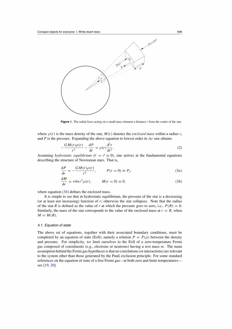
We start by considering the radial force acting on a small mass element (�m = ρ(r)�V )

located at a distance r from the centre of the star (see figure 1):

Fr = −GM(r)�m

r2− P(r + �r)�A + P(r)�A = �m

d2r

dt2, (1)


r∆

∆Α

r

∆P(r+

r)

P(r)F

Figure 1. The radial force acting on a small mass element a distance r from the centre of the star.

where ρ(r) is the mass density of the star, M(r) denotes the enclosed mass within a radius r,and P is the pressure. Expanding the above equation to lowest order in �r one obtains

−GM(r)ρ(r)

r2− dP

dr= ρ(r)

d2r

dt2. (2)

Assuming hydrostatic equilibrium (r = r ≡ 0), one arrives at the fundamental equationsdescribing the structure of Newtonian stars. That is,

dP

dr= −GM(r)ρ(r)

r2, P (r = 0) ≡ Pc; (3a)

dM

dr= +4πr2ρ(r), M(r = 0) ≡ 0, (3b)

where equation (3b) defines the enclosed mass.It is simple to see that in hydrostatic equilibrium, the pressure of the star is a decreasing

(or at least not increasing) function of r; otherwise the star collapses. Note that the radiusof the star R is defined as the value of r at which the pressure goes to zero, i.e., P(R) = 0.Similarly, the mass of the star corresponds to the value of the enclosed mass at r = R, whenM = M(R).

4.1. Equation of state

The above set of equations, together with their associated boundary conditions, must becompleted by an equation of state (EoS), namely a relation P = P(ρ) between the densityand pressure. For simplicity, we limit ourselves to the EoS of a zero-temperature Fermigas composed of constituents (e.g., electrons or neutrons) having a rest mass m. The mainassumption behind the Fermi gas hypothesis is that no correlations (or interactions) are relevantto the system other than those generated by the Pauli exclusion principle. For some standardreferences on the equation of state of a free Fermi gas—at both zero and finite temperatures—see [19, 20].


To start, the Fermi wavenumber kF is defined; kF represents the momentum of the fastestmoving fermion and is solely determined by the number density (n ≡ N/V ) of the system,where N is the total number of particles in our system, and V is the enclosed volume.

That is,

N = 2∑

k

�(kF − |k|) = 2∫

V

(2π)3d3k�(kF − |k|) = V

k3F

3π2, (4)

or equivalently

kF = (3π2n)1/3. (5)

In equation (4), �(x) represents the Heaviside (or step) function. Having defined the Fermiwavenumber kF, the energy density of the system is obtained from a configuration in which allsingle-particle momentum states are progressively filled in accordance with the Pauli exclusionprinciple. For a degenerate (spin-1/2) Fermi gas at zero temperature, exactly two fermionsoccupy each single-particle state below the Fermi momentum pF = hkF; all remaining statesabove the Fermi momentum are empty. In this manner we obtain the following expression forthe energy density:

E ≡ E/V = 2∫

d3k

(2π)3�(kF − |k|)ε(k), (6)

where ε(k) is the single-particle energy of a fermion with momentum k. In what follows, themost general free-particle dispersion (energy versus momentum) relation is assumed, namely,one consistent with the postulates of special relativity. That is,

ε(k) =√

(hkc)2 + (mc2)2 = mc2√

1 + x2,

(with x ≡ hkc

mc2

). (7)

In spite of its slightly intimidating form, the integral in equation (6) may be performed inclosed form. We obtain

E = E0E(xF), (8)

where E0 is a dimensionful constant that may be written using dimensional analysis

E0 ≡ (mc2)4

(hc)3, (9)

and E(xF) is a dimensionless function of the single variable xF = hkFc/mc2 given by

E(xF) ≡ 1

π2

∫ xF

0x2

√1 + x2 dx = 1

8π2

[xF

(1 + 2x2

F

) √1 + x2

F − ln

(xF +

√1 + x2

F

)]. (10)

The pressure of the system may now directly be obtained from the energy density by usingthe following thermodynamic relation—which is only valid at zero temperature:

P = −(

∂E

∂V

)N,T ≡0

= −(

∂(V E)

∂V

)N,T ≡0

≡ P0P . (11)

In analogy to the energy density, dimensionful and dimensionless quantities for the pressurehave been defined:

P0 = E0 = (mc2)4

(hc)3, (12a)

P(xF) ≡[xF

3E ′

(xF) − E(xF)]. (12b)


It may be surprising to find that a gas of particles at zero-temperature may still generate anonzero pressure. It is quantum statistics, in the form of the Pauli exclusion principle—nottemperature—that is responsible for generating the pressure. It is nevertheless surprising thatquantum pressure, a purely microscopic phenomenon, should be ultimately responsible forsupporting compact stars against gravitational collapse.

With an expression for the pressure in hand, we are finally in a position to compute itsderivative with respect to xF (a quantity that we label as η). As we shall see in the next section,η—a function closely related to the zero-temperature incompressibility—is the only propertyof the EoS that Newtonian stars are sensitive to [20]. We obtain

η ≡ dP

dxF= P0

[xF

3E ′′

(xF) − 2

3E ′

(xF)

]= P0

3π2

x4F√

1 + x2F

. (13)

The above expression has a surprisingly simple form that depends on the energy density onlythrough its derivatives. Alternatively, one could have bypassed the above derivation in favourof the following general relation valid for a zero-temperature Fermi gas:

dP

dxF= n

dεF

dxF. (14)

In view of equation (14), the attentive reader may be asking why we go through the troubleof computing the energy density and the corresponding pressure if all that is required is thedependence of the Fermi energy on xF. The answer is general relativity. While Newtonianstars depend exclusively on η, the structure of relativistic stars (such as neutron stars) arehighly sensitive to corrections from general relativity. These corrections depend on both theenergy density and the pressure and will be treated in detail in a future publication.

4.2. Toy model of white dwarf stars

Before attempting a numerical solution to the equations of hydrostatic equilibrium, we consideras a warm-up exercise a toy model of a white dwarf star [21]. Assume a white dwarf star witha uniform, spherically symmetric mass distribution of the form

ρ(r) ={ρ0 = 3M/4πR3, if r � R;0, if r > R,

(15)

where M and R are the mass and radius of the star, respectively. For such a sphericallysymmetric star, the gravitational energy released during the process of ‘building’ the star isgiven by

EG = −4πG

∫ R

0M(r)ρ(r)r dr, (16a)

M(r) =∫ r

04πr ′2ρ(r ′) dr ′. (16b)

For a uniform density star as assumed in equation (15), it is straightforward to perform theabove two integrals. Thus, the gravitational energy released in ‘building’ such a star isgiven by

EG(M,R) = −3

5

GM2

R. (17)

From equation (17), we conclude that without a source of gravitational support, a star witha fixed mass M will minimize its energy by collapsing into an object of zero radius, namely,


into a black hole. We know, however, that white dwarf stars are supported by the quantum-mechanical pressure from its degenerate electrons, which (at temperatures of about 106 K) arefully ionized in the star (recall that 1eV � 104 K). In what follows, we assume that electronsprovide all the pressure support of the star but none of its mass, while nuclei (e.g., 4He,12C, . . .) provide all the mass but none of the pressure. The electronic contribution to the massof the star is inconsequential, as the ratio of electron to nucleon mass is approximately equalto 1:2000.

The energy of a degenerate electron gas was computed in the previous section. Usingequations (5) and (8) we obtain

EF(M,R) = 3π2Nmec2 E(xF)

x3F

, (18)

where me is the rest mass of the electron. Naturally, the above expression depends on the massand the radius of the star, although this dependence is implicit in xF. While the toy problem athand is instructive of the simple, yet subtle, physics that is displayed in compact stars, it alsoserves as a useful framework to illustrate how to scale the equations.

4.2.1. Scaling the equations. One of the great challenges in astrophysics, and the physicsof compact stars is certainly no exception, is the enormous range of scales that one mustsimultaneously address. For example, in the case of white dwarf stars it is the pressuregenerated by the degenerate electrons (constituents with a mass of me = 9.110×10−31 kg)that must support stars with masses comparable to that of the Sun (M� = 1.989×1030 kg).This represents a disparity in masses of 60 orders of magnitude! Without properly scaling theequations, there is no hope of dealing with this problem with a computer.

We start by defining fF ≡ EF/Nmec2 from equation (18), a quantity that is both

dimensionless and intensive (i.e., independent of the size of the system). That is,

fF(xF) = 3π2 E(xF)

x3F

, (19)

where a closed-form expression for E(xF) has been displayed in equation (10). Note that thescaled Fermi momentum xF quantifies the importance of relativistic effects. At low density(xF � 1), the corrections from special relativity are negligible and electrons behave as anon-relativistic Fermi gas. In the opposite high-density limit (xF � 1) the system becomesultra-relativistic and the ‘small’ (relative to the Fermi momentum) electron mass may beneglected. We shall see that in the case of white dwarf stars, the most interesting physicsoccurs in the xF ∼1 regime.

The dynamics of the star consists of a tug-of-war between gravity that favours the collapseof the star and electron-degeneracy pressure that opposes the collapse. To efficiently comparethese two contributions, the contribution from gravity to the energy must be scaled accordingly.Thus, in analogy to equation (19), we form the corresponding dimensionless and intensivequantity for the gravitational energy (fG ≡EG/Nmec

2):

fG(M,R) = −3

5

(GM

Rc2

) (M

Nme

)= −3

5

(GM

Rc2

)(mn

Yeme

), (20)

where we have assumed that the mass of the star, M = Amn, may be written exclusively interms of its baryon number A and the nucleon mass mn (the small difference between protonand neutron masses is neglected). This is an accurate approximation as both nuclear andgravitational binding energies per nucleon are small relative to the nucleon mass. Further,Ye ≡Z/A represents the electron-per-baryon fraction of the star (e.g., Ye = 1/2 for 4He and12C, and Ye = 26/56 in the case of 56Fe).


The final step in the scaling procedure is to introduce dimensionful mass M0 and radiusR0, quantities that, when chosen wisely, will embody the natural mass and length scales in theproblem. To this effect we define

M ≡M/M0 and R≡R/R0. (21)

In terms of these natural mass and length scales, the gravitational contribution to the energyof the system takes the following form:

fG(M,R) = −[

3

5

(GM0

R0c2

) (mn

Yeme

)]M

R. (22)

While the dependence of the above equation on M and R is already explicit, the Fermi gascontribution to the energy depends implicitly on them through xF. To expose explicitly thedependence of fF on M and R we perform the following manipulation aided by relationsderived in section 4.1.

x3F =

(hkFc

mec2

)3

=[(

9π

4Ye

) (M0

mn

)(hc/mec

2

R0

)3]

M

R3 . (23)

We have already referred earlier to M0 and R0 as the natural mass and length scales inthe problem, but their values have yet to be determined. Thus, they are still at our disposal.Their values will be fixed by adopting the following choice: let the ‘complicated’ expressionsenclosed between square brackets in equations (22) and (23) be set equal to one. That is,[

3

5

(GM0

R0c2

) (mn

Yeme

)]=

[(9π

4Ye

) (M0

mn

) (hc/mec

2

R0

)3]

= 1. (24)

This choice implies the following values for white dwarf stars with an electron-to-baryon ratioequal to Ye = 1/2:

M0 = 5

6

√15πα

−3/2G mnY

2e = 10.599M�Y 2

e −→Ye=1/2

= 2.650M�, (25a)

R0 =√

15π

2α

−1/2G

(hc

mec2

)Ye = 17 250 km Ye −→

Ye=1/2= 8623 km. (25b)

Here the minute dimensionless strength of the gravitational coupling between two nucleonshas been introduced as

αG = Gm2n

hc= 5.906 × 10−39. (26)

The aim of this toy-model exercise is to find the minimum value of the total (gravitationalplus Fermi gas) energy of the star as a function of its radius for a fixed value of its mass. Beforedoing so, however, a few comments are in order. First, from merely scaling the equations andwith no recourse to any dynamical calculation we have established that white dwarf stars havemasses comparable to that of our Sun but typical radii of only 10 000 km (recall that the radiusof the Sun is R� ≈ 700 000 km). Further, we observe that while R0 scales with the inverseelectron mass, the mass scale M0 is independent of it. This suggests that neutron stars, wherethe neutrons provide all the pressure and all the mass, will also have masses comparable tothat of the Sun but typical radii of only about 10 km.

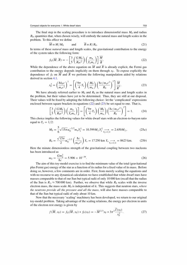
Now that the necessary ‘scaling’ machinery has been developed, we return to our originaltoy-model problem. Taking advantage of the scaling relations, the energy per electron in unitsof the electron rest energy is given by

f (M, xF) = fG(M, xF) + fF(xF) = −M 2/3xF + 3π2 E(xF)

x3F

. (27)


0

0.2

0.4

0.6

0.8

1

1.2

0.2 0.4 0.6 0.8 1 1.2 1.4 1.6 1.8 2xF

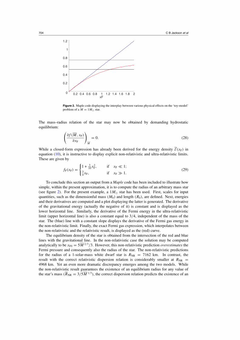
Figure 2. Maple code displaying the interplay between various physical effects on the ‘toy-model’problem of a M = 1M� star.

The mass–radius relation of the star may now be obtained by demanding hydrostaticequilibrium: (

∂f (M, xF)

∂xF

)M

= 0. (28)

While a closed-form expression has already been derived for the energy density E(xF) inequation (10), it is instructive to display explicit non-relativistic and ultra-relativistic limits.These are given by

fF(xF) ={

1 + 310x2

F, if xF � 1;34xF, if xF � 1.

(29)

To conclude this section an output from a Maple code has been included to illustrate howsimple, within the present approximation, it is to compute the radius of an arbitrary mass star(see figure 2). For the present example, a 1M� star has been used. First, scales for inputquantities, such as the dimensionful mass (M0) and length (R0), are defined. Next, energiesand their derivatives are computed and a plot displaying the latter is generated. The derivativeof the gravitational energy (actually the negative of it) is constant and is displayed as thelower horizontal line. Similarly, the derivative of the Fermi energy in the ultra-relativisticlimit (upper horizontal line) is also a constant equal to 3/4, independent of the mass of thestar. The (blue) line with a constant slope displays the derivative of the Fermi gas energy inthe non-relativistic limit. Finally, the exact Fermi gas expression, which interpolates betweenthe non-relativistic and the relativistic result, is displayed as the (red) curve.

The equilibrium density of the star is obtained from the intersection of the red and bluelines with the gravitational line. In the non-relativistic case the solution may be computedanalytically to be xF0 = 5M 2/3/3. However, this non-relativistic prediction overestimates theFermi pressure and consequently also the radius of the star. The non-relativistic predictionsfor the radius of a 1-solar-mass white dwarf star is RNR = 7162 km. In contrast, theresult with the correct relativistic dispersion relation is considerably smaller at RNR =4968 km. Yet an even more dramatic discrepancy emerges among the two models. Whilethe non-relativistic result guarantees the existence of an equilibrium radius for any value ofthe star’s mass (RNR = 3/5M 1/3), the correct dispersion relation predicts the existence of an


upper limit beyond which the pressure from the degenerate electrons can no longer supportthe star against gravitational collapse. This upper mass limit, known as the Chandrasekharmass, is predicted in the simple toy model to be equal to

MCh = (3/4)3/2M0 = 1.72M�. (30)

As will be shown later, accurate numerical results yield (for Ye = 1/2) a Chandrasekhar massof MCh = 1.44M�. Thus, not only does the toy model predict the existence of a maximummass star, but it does so with an 80% accuracy.

4.3. Numerical analysis

We now return to the exact (numerical) treatment of white dwarf stars. While the toy-modelproblem developed earlier provides a particularly simple framework to understand the interplaybetween gravity, quantum mechanics and special relativity, a quantitative description of thesystems demands the numerical solution of the hydrostatic equations (equation (3)). Forthe present treatment, however, we continue to assume that the equation of state is that of asimple degenerate Fermi gas. In this case the equation of state is known analytically and it isconvenient to incorporate it directly into the differential equation. In this way equation (3a)becomes

dxF

dr= −GM(r)ρ(r)

r2η, (31)

where the equation of state enters only through a quantity directly related to the zero-temperature incompressibility [20]. This quantity, η = dP/dxF, was defined and evaluated inequation (13). Moreover, the density of the system ρ(r) is easily expressed in terms of xF. Itis given by

ρ =(

mec2

hc

)3mn

3π2Yex3

F. (32)

At this point all necessary relations have been derived and the equations of hydrostaticequilibrium, first displayed in equation (3) but with an equation of state still missing, may nowbe written in the following form:

dxF

dr= −

[(GM0

R0c2

) (mn

Yeme

)]M

r2

√1 + x2

F

xF, xF(r = 0) ≡ xFc; (33a)

dM

dr= +

[(3π

4Ye

)(M0

mn

) (hc/mec

2

R0

)3]−1

r2x3F, M(r = 0) ≡ 0. (33b)

Here the dimensionless distance r and the central (scaled) Fermi momentum xFc have beenintroduced. The structure of the above set of differential equations indicates that our goal ofturning equation (3) into a well-posed problem, by directly incorporating the equation of stateinto the differential equations, has been accomplished. But we have done better. By definingthe natural mass and length scales of the system (M0 and R0) according to equation (24), thetwo long expressions in brackets in the above equations reduce to the simple numerical valuesof 5/3 and 1/3, respectively. Finally, then, the equations of hydrostatic equilibrium describingthe structure of white dwarf stars are given by the following expressions:

dxF

dr= f (r; xF,M), xF(r = 0) ≡ xFc; (34a)


dM

dr= g(r; xF,M), M(r = 0) ≡ 0, (34b)

where the two functions on the right-hand side of the equations (f and g) are given by

f (r; xF,M) ≡ −5

3

M

r2

√1 + x2

F

xFand g(r; xF,M) ≡ +3r2x3

F. (35)

This coupled set of first-order differential equations may now be solved using standardnumerical techniques, such as the Runge–Kutta algorithm [21]. However, for those students notyet comfortable with writing their own source codes, the use of an ‘off-the-shelf’ spreadsheet(here Microsoft Excel has been used), together with a crude low-order approximation forthe derivatives, has been shown to be adequate. As in the toy-model problem, solutionswill be presented using the full relativistic dispersion relation as well as the non-relativisticapproximation, where in the latter case the square-root term appearing in the functionf (r; xF,M) is set to one.

5. Numerical techniques for everyone

In this section we present numerical solutions for the structure of Newtonian (white dwarf)stars by employing a variety of numerical techniques and programming tools.

5.1. White dwarf stars with Excel

This section should be ideal for those students with a basic knowledge of calculus and withno programming skills. High school students that have learned the concept of derivatives intheir introductory calculus class should be able to complete this part of the project with noproblem. Indeed, one could use the definition of the derivative of a function F(x)

F ′(x) = limh→0

F(x + h) − F(x)

h, (36)

to approximate the value of the function at a neighbouring point x + h. That is,

F(x + h) = F(x) + hF ′(x) + O(h2). (37)

The term O(h2) indicates that the error that one makes in computing the value of the functionat the neighbouring point scales as the square of h. Thus, for this low-order approximationof the derivative, we selected a very small value of h in order to ensure numerical accuracy.Other higher order algorithms, such as the venerated Runge–Kutta method, contain errors thatscale as O(h4). These algorithms can attain the same degree of numerical accuracy as the onepresented here with a dramatic reduction in computational time.

So how do we turn equation (37) to our advantage? By simply looking at the structure ofthe (scaled) equations of hydrostatic equilibrium equation (34) we can readily write

xF(r + �r) = xF(r) + �rf (r; xF,M), (38a)

M(r + �r) = M(r) + �rg(r; xF,M). (38b)

The resulting difference equations are recursion relations that enables one to ‘leapfrog’ frompoint to point in a grid for which the various points are separated by a fixed distance �r .Recursion relations such as this one are particularly well suited to being solved with aspreadsheet. Figure 3 shows the results produced using Excel (lines).


0 0.2 0.4 0.6 0.8 1 1.2 1.4 1.6 1.8 2Mass (M

sun)

0

0.5

1

1.5

2

2.5

3

R (

104 k

m)

NR (Ye=1/2)SR (Ye=1/2)SR (Ye=26/56)

Chandrasekhar Mass

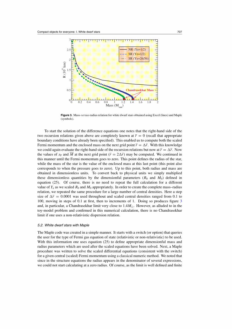
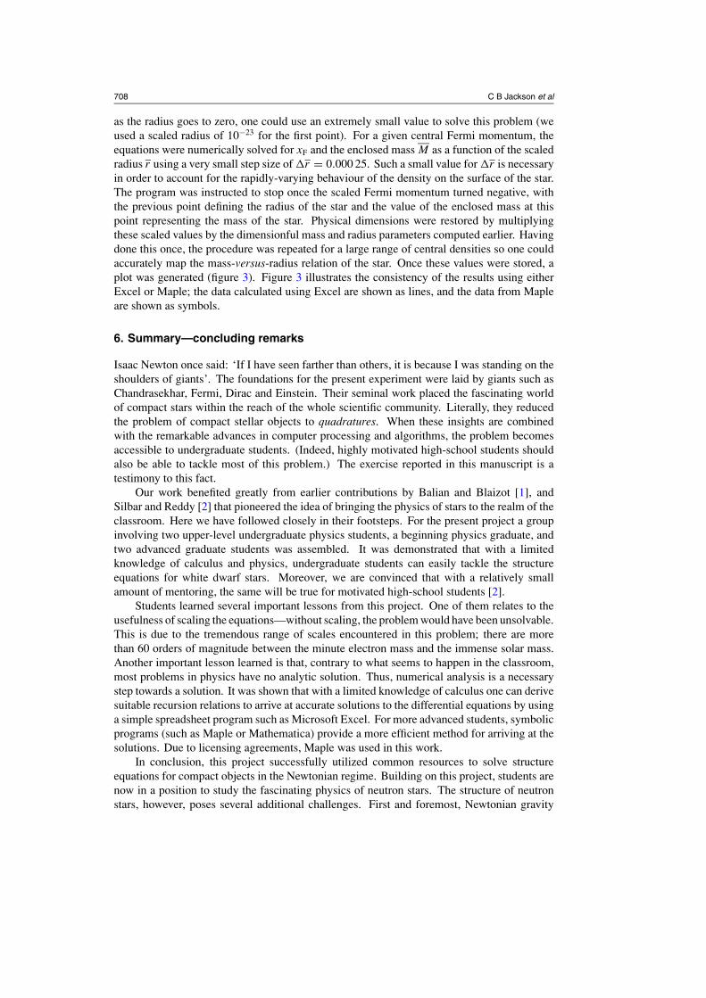
Figure 3. Mass-versus-radius relation for white dwarf stars obtained using Excel (lines) and Maple(symbols).

To start the solution of the difference equations one notes that the right-hand side of thetwo recursion relations given above are completely known at r = 0 (recall that appropriateboundary conditions have already been specified). This enabled us to compute both the scaledFermi momentum and the enclosed mass on the next grid point r = �r . With this knowledgewe could again evaluate the right-hand side of the recursion relations but now at r = �r . Nowthe values of xF and M at the next grid point (r = 2�r) may be computed. We continued inthis manner until the Fermi momentum goes to zero. This point defines the radius of the star,while the mass of the star is the value of the enclosed mass at this last point (this point alsocorresponds to when the pressure goes to zero). Up to this point, both radius and mass areobtained in dimensionless units. To convert back to physical units we simply multipliedthese dimensionless quantities by the dimensionful parameters (R0 and M0) defined inequation (25). Of course, there is no need to repeat the full calculation for a differentvalue of Ye as we scaled R0 and M0 appropriately. In order to create the complete mass–radiusrelation, we repeated the same procedure for a large number of central densities. Here a stepsize of �r = 0.0001 was used throughout and scaled central densities ranged from 0.1 to100, moving in steps of 0.1 at first, then to increments of 1. Doing so produces figure 3and, in particular, a Chandrasekhar limit very close to 1.4M�. However, as alluded to in thetoy-model problem and confirmed in this numerical calculation, there is no Chandrasekharlimit if one uses a non-relativistic dispersion relation.

5.2. White dwarf stars with Maple

The Maple code was created in a simple manner. It starts with a switch (or option) that queriesthe user for the type of Fermi gas equation of state (relativistic or non-relativistic) to be used.With this information one uses equation (25) to define appropriate dimensionful mass andradius parameters which are used after the scaled equations have been solved. Next, a Mapleprocedure was written to solve the scaled differential equations (consistent with the switch)for a given central (scaled) Fermi momentum using a classical numeric method. We noted thatsince in the structure equations the radius appears in the denominator of several expressions,we could not start calculating at a zero radius. Of course, as the limit is well defined and finite


as the radius goes to zero, one could use an extremely small value to solve this problem (weused a scaled radius of 10−23 for the first point). For a given central Fermi momentum, theequations were numerically solved for xF and the enclosed mass M as a function of the scaledradius r using a very small step size of �r = 0.000 25. Such a small value for �r is necessaryin order to account for the rapidly-varying behaviour of the density on the surface of the star.The program was instructed to stop once the scaled Fermi momentum turned negative, withthe previous point defining the radius of the star and the value of the enclosed mass at thispoint representing the mass of the star. Physical dimensions were restored by multiplyingthese scaled values by the dimensionful mass and radius parameters computed earlier. Havingdone this once, the procedure was repeated for a large range of central densities so one couldaccurately map the mass-versus-radius relation of the star. Once these values were stored, aplot was generated (figure 3). Figure 3 illustrates the consistency of the results using eitherExcel or Maple; the data calculated using Excel are shown as lines, and the data from Mapleare shown as symbols.

6. Summary—concluding remarks

Isaac Newton once said: ‘If I have seen farther than others, it is because I was standing on theshoulders of giants’. The foundations for the present experiment were laid by giants such asChandrasekhar, Fermi, Dirac and Einstein. Their seminal work placed the fascinating worldof compact stars within the reach of the whole scientific community. Literally, they reducedthe problem of compact stellar objects to quadratures. When these insights are combinedwith the remarkable advances in computer processing and algorithms, the problem becomesaccessible to undergraduate students. (Indeed, highly motivated high-school students shouldalso be able to tackle most of this problem.) The exercise reported in this manuscript is atestimony to this fact.

Our work benefited greatly from earlier contributions by Balian and Blaizot [1], andSilbar and Reddy [2] that pioneered the idea of bringing the physics of stars to the realm of theclassroom. Here we have followed closely in their footsteps. For the present project a groupinvolving two upper-level undergraduate physics students, a beginning physics graduate, andtwo advanced graduate students was assembled. It was demonstrated that with a limitedknowledge of calculus and physics, undergraduate students can easily tackle the structureequations for white dwarf stars. Moreover, we are convinced that with a relatively smallamount of mentoring, the same will be true for motivated high-school students [2].

Students learned several important lessons from this project. One of them relates to theusefulness of scaling the equations—without scaling, the problem would have been unsolvable.This is due to the tremendous range of scales encountered in this problem; there are morethan 60 orders of magnitude between the minute electron mass and the immense solar mass.Another important lesson learned is that, contrary to what seems to happen in the classroom,most problems in physics have no analytic solution. Thus, numerical analysis is a necessarystep towards a solution. It was shown that with a limited knowledge of calculus one can derivesuitable recursion relations to arrive at accurate solutions to the differential equations by usinga simple spreadsheet program such as Microsoft Excel. For more advanced students, symbolicprograms (such as Maple or Mathematica) provide a more efficient method for arriving at thesolutions. Due to licensing agreements, Maple was used in this work.

In conclusion, this project successfully utilized common resources to solve structureequations for compact objects in the Newtonian regime. Building on this project, students arenow in a position to study the fascinating physics of neutron stars. The structure of neutronstars, however, poses several additional challenges. First and foremost, Newtonian gravity


must be replaced by general relativity. This implies that the structure equations must bereplaced by the Tolman–Oppenheimer–Volkoff equations [13, 17, 18]. Second, at the higherdensities encountered in the interior of neutron stars, the equation of state receives importantcorrections from the interactions among the neutrons. That is, Pauli correlations are no longersufficient to describe the equation of state and some realistic equations of state should be used[2, 22]. This topic of intense research activity is of relevance to the physics of neutron starsand to the structure of those exotic compact objects known as hybrid and quark stars.

Acknowledgments

One of us (JP) is extremely grateful to the faculty and students of the Departament d’Estructurai Constituents de la Materia at the Universitat de Barcelona, especially to Professors Centellesand Vinas, for their hospitality during the time that this project/lectures were developed. Inaddition, CBJ would like to thank Ray Kallaher for their useful discussions. Finally, we are allappreciative of Dr Blessing for her help on the entirety of this work. This work was supportedin part by the US Department of Energy under contract no DE-FG05-92ER40750.

References

[1] Balian R and Blaizot J-P 1999 Am. J. Phys 67 1189[2] Silbar R R and Reddy S 2004 Am. J. Phys. 72 892 (Preprint nucl-th/0309041)[3] Fowler R H 1926 Mon. Not. R. Astron. Soc. 87 114[4] Chandrasekhar S 1984 Rev. Mod. Phys. 56 137[5] Chadwick J 1932 Proc. R. Soc. A 136 692[6] Baade W and Zwicky F 1934 Phys. Rev. 46 76[7] Burnell S J B 2004 Science 304 489[8] Hewish A, Bell S J, Pilkington J D H, Scott P F and Collins R A 1968 Nature 217 709[9] Pilkington J D H, Hewish A, Bell S J and Cole T W 1968 Nature 218 126

[10] Gold T 1968 Nature 218 731[11] Gold T 1969 Nature 221 25[12] 2004 Science 304 (23 April 2004, Special Issue: Pulsars)[13] Weinberg S 1972 Gravitation and Cosmology (New York: Wiley)[14] Misner C W, Thorne K and Wheeler J 1973 Gravitation (New York: Freeman)[15] Shapiro S L and Teukolsky S A 1983 Black Holes, White Dwarfs, and Neutron Stars: The Physics of Compact

Objects (New York: Wiley)[16] Thorne K S 1994 Black Holes and Time Warps: Einstein’s Outrageous Legacy 2nd edn (New York:

W W Norton)[17] Glendenning N K 2000 Compact Stars 2nd edn (New York: Springer)[18] Phillips A C 2002 The Physics of Stars 2nd edn (New York: Wiley)[19] Huang K 1987 Statistical Mechanics 2nd edn (New York: Wiley)[20] Pathria R K 1996 Statistical Mechanics 2nd edn (Oxford: Butterworth-Heinemann)[21] Koonin S E and Meredith D C 1990 Computational Physics (Reading, MA: Addison-Wesley)[22] Lattimer J M and Prakash M 2001 Astrophys. J. 550 426 (Preprint astro-ph/0002232)

compact objects for everyone: i. white dwarf starsmoloney/ph425/ejp... · in dealing with white...

Documents