communications in commun. math. phys. 76, 211554 (1980 ...knill/history/lanford/papers/... ·...
TRANSCRIPT
Commun. Math. Phys. 76, 211554 (1980) Communications in
Physics © by Springer-Verlag 1980
Universal Properties of Maps on an Interval
P. Collet 1, J.-P. Eckmann z, and O. E. Lanford III 3
1 Harvard University, Cambridge, MA 02138, USA 2 D6partement de Physique Th6orique, Universit6 de Gen+ve, CH-1211 Gen6ve 4, Switzerland 3 University of California, Berkeley, CA 94720, USA
Abstract. We consider iterates of maps of an interval to itself and their stable periodic orbits. When these maps depend on a parameter, one can observe period doubling bifurcations as the parameter is varied. We investigate rigorously those aspects of these bifurcations which are universal, i.e. inde- pendent of the choice of a particular one-parameter family. We point out that this universality extends to many other situations such as certain chaotic regimes. We describe the ergodic properties of the maps for which the parameter value equals the limit of the bifurcation points.
1. Introduction
Continuous mappings of intervals into themselves display some remarkable properties when regarded as discrete dynamical systems. (For a survey, see May [9] or Collet and Eckmann [14].) One much-studied example is the one-parameter
family x ~ 1 - # x 2 (1.1)
which maps [-- 1, 1] into itself for 0 __< #=2 . In this and similar examples, what is interesting is not so much the behavior of any particular mapping; rather, it is the way this behavior changes with #.
The example (1.1), and the more general one-parameter families # ~ P u we will study, have a simplifying qualitative feature: Each tp, has a unique (differentiable) maximum - at x = 0 in the example - below which it is increasing and above which it is decreasing. We will consider mappings p which satisfy
P1) ~ is a continuously differentiable mapping of [ - 1, 1] into itself. P2) ~p(0)--1; ~ is strictly increasing on [ - 1 , 0 ] and strictly decreasing on
[0, 1]. P3) ~ ( - x ) = ~p(x). The space of all such mappings will be denoted by N. (The condition that the
maximum of ~p occurs at zero and that ~ sends zero to one can frequently be arranged, if necessary, by making an affine change of variables.) We have included
0010-3 616/80/0076/0211/$08.80
212 P. Collet, J.-P. Eckmann, and O. E. Lanford III
condition P3) mostly for convenience; it simplifies matters and is satisfied by the ~p's we are able to analyze in detail.
One important property of such a transformation is having - or not having - an attracting periodic orbit. (Existence of periodic orbits which are not attracting is much less important, directly at least, in accounting for the behavior of typical orbits.) The fact that [ - 1, 1] is ordered and connected gives rise to powerful and general methods for proving the existence of periodic orbits - see, for example, Stefan [13] - but these methods do not help very much with the existence of attracting periodic orbits. Note, however, that if 0 is periodic for ~pe ~ , then, since tp'(0)--0, its orbit is necessarily attracting. We will say that ~p is superstable of period p if 0 is periodic of (minimal) period p for tp. If tpo is superstable of period p, then any ~ p ~ which is near enough to ~Po in the C 1 topology will also have an attracting periodic orbit of period p. Thus for example if
is a one-parameter family of elements of N with ~u0 superstable of period p, there is an open interval about #o in the parameter space such that each corresponding ~pg has an attracting periodic orbit of period p.
The existence of superstable ~p's can sometimes be proved by simple topologi- cal arguments. For example, with our normalization, tp is superstable of period 2 if and onlj~ if ~p(1)=0. If we now consider a continuous one-parameter family ~Pu defined on some interval of #'s, and if ~p~(1) is sometimes positive and sometimes negative, then there must be at least one # for which ~p~ is superstable of period 2. We give in Sect. 3 an elaboration of this simple argument which shows that, if qJ,(1) is near 1 for p near the left end of the parameter interval and near - 1 near the right end, there exists a sequence
#1 <#2 </x3 < ...
such that ~,~ is superstable of period 2 J. (See Guckenheimer [4] for an alternative approach to the existence of the/xfs.) It is clear that, if we allow arbitrary (non- monotone) reparametrizations, we cannot hope to prove the existence of unique #i's. Moreover, similar topological considerations guarantee that such a param- etrized family has, for each large j, many values of/x where lp~ is superstable of period 2 J. Nevertheless, in examples like
x - ~ l - # x 2
the first superstable values of # appear to occur with periods
2,4,8,16,.. .
in that order. We will denote the corresponding values of p by #j and !im #j by j - * o:~
By investigating numerically a number of one-parameter families, Feigenbaum [3] discovered a striking universality property: For large j, # ~ - #j is asymptotic to
const x c$-J,

U n i v e r s a l P r o p e r t i e s o f M a p s o n a n In t e rva l 213
where 3=4.66920... is apparently the same whatever one-parameter family is considered. (Note that, encouragingly, this property of the ~Lj's is not changed by making a differentiable change of parameter with derivative which does not vanish at #oo-)
Having discovered the universality of 6 experimentally, Feigenbaum went on to propose an explanation for it which was inspired by the renormalization group approach to critical phenomena in statistical mechanics. The principal result of this paper is to show that Feigenbaum's explanation is correct, at least in a certain limiting regime to be explained below. We will next sketch our version of Feigenbaum's theory, ignoring numerous technical details which will need to be made precise later.
Consider a mapping ~ ~ and define
Assume
a=a(~p)=-~(1 ) ; b=bOp)=tp(a).
and assume also that
0 < a < b ( < l )
l p (b ) = ~ , 2 ( a ) < a .
then maps
[ -a ,a] onto [b,1] and [b,1] onto [ - a, ~p(b)] C [ - a, a] ,
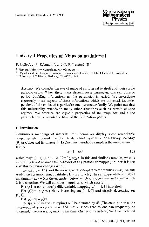
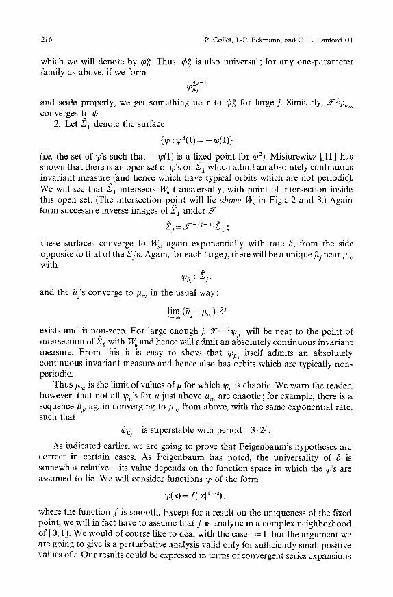
i.e. it exchanges the two non-intersecting intervals [ - a , a] and [b, 1]. Hence tp o~ maps [ - a , a] into itself, and -~po~ is again unimodal on [ - a, a] (see Fig. 1). If we
reverse orientation and scale up by a factor of-i, i.e. if we make the linear change of a variables
Xol d ~ - - aXne w
then h0 ou2 on [ - a , a] is transformed to
1 - - ~ o ~ J ( - a x ) =- (J~)(x)
a
on [ - 1, 1]. It is easy to verify that, with our hypotheses, Y ~ again has properties P1)-P3) [-but the condition a(Y~o)> 0 or a ( J p ) < b(~--~) may fail]. We will refer to the transformation 3- as the doublin 9 transformation. The doubling transformation is essentially just composition of ~0 with itself, but combined with restriction of tpo~p to a subdomain of the original domain and then a scaling (and reversal of orientation) chosen to preserve the "normalization" ~(0)= 1. This combined operation, in contrast with composition alone, does not give rise to a more complicated-looking transformation. The utility of J - in studying superstable ~p's lies largely in the remark that, provided ~ satisfies the conditions given above for Y--~p to be defined, 1/) is superstable of period p if and only if 3--~, is superstable of period p/2 (and, in particular, p must be even).
214 P. Collet, J.-P. Eckmann, and O. E. Lanford III
Fig. 1
(Vx(x) =I -1.4 x 2 )
/
\ /
¢
q,
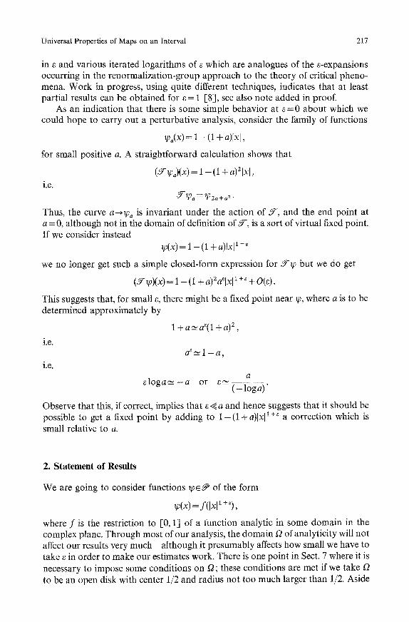
We now, following Feigenbaum, propose some geometrical hypotheses about how ~- acts in the space N of transformations and show how these hypotheses account for the universality of 6. The picture is as follows :
a) 3- has a fixed point 4~. b) The derivative of 3- at the fixed point ~ has a simple eigenvalue which is
larger than one (and which will turn out to be 6); the remainder of its spectrum is contained in the open unit disk. Y- thus has a one-dimensional unstable manifold W, and a codimension-one stable manifold W~ at qS.
c) The unstable manifold W, intersects transversally the codimension-one
surface 221, Z I = {~p : tp(1)=0}.
(Note that Z a is exactly the set of ~p's which are superstable of period 2.) See Fig. 2.
Universa l Proper t ies of M a p s on an In te rva l 215
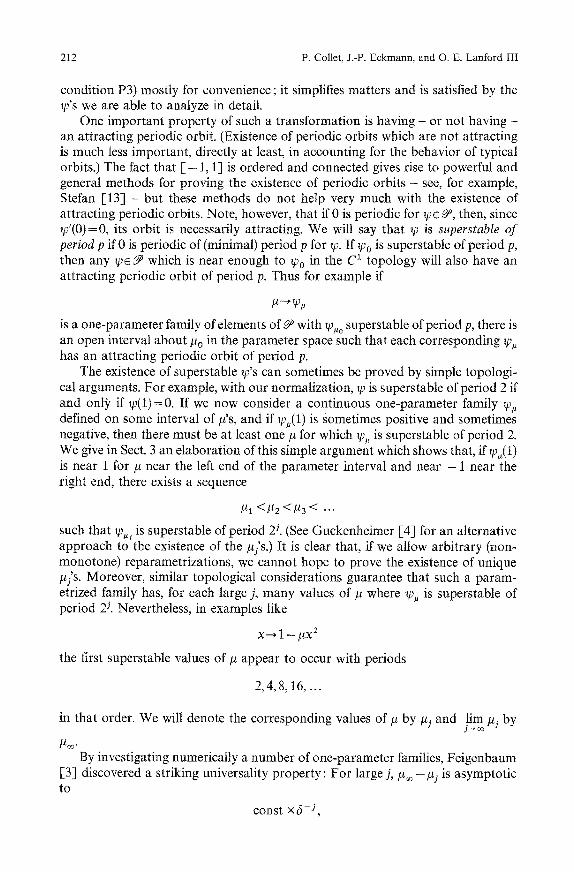
Using this picture, we can account for the universality of 6 as follows: Form successive inverse images Z2, Z3 . . . . of £'1 under 9"- :
~ j = 3 - - ( J - I)X~ .
Note that if ~ e Z j then ~-(J- ~)tpeX~, so ~--J ~tp is superstable of period 2, so ~ is superstable of period 2 J. The successive Z/s come closer and closer to W~; in fact, a straightforward argument (which we will give in detail later) shows that the separation between 27j and W~ decreases exponentially like & - j for large j, where is the large eigenvalue of the derivative of ~- at q~.
Fig. 2
j W u
.---- \ " - " - ~ 1
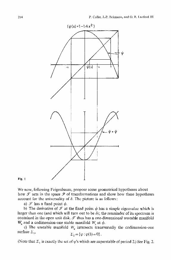
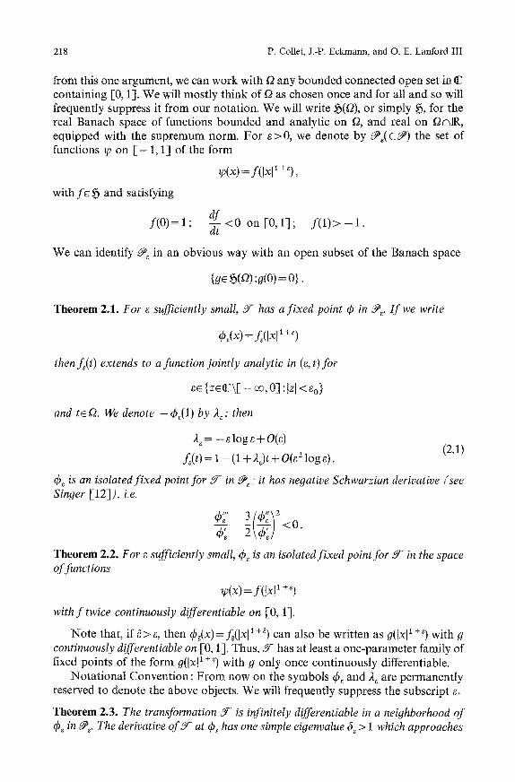
Now consider a one-parameter family # ~ 0 ~ of transformations and regard it as a curve in N. Suppose this curve crosses the stable manifold HIs at/~ = #~ with non-zero transverse velocity. It is then clear that, at least for targej, there will be a unique #j near #~ such that ~p, ~Zj (which implies that tpu~ is superstable of period 2 j) and that
lira 6J(#~ - #j) j--* oo
exists and is non-zero (see Fig. 3).
Fig. 3 ............... l.~..Wu "-~_~I Thus, Feigenbaum's hypotheses not only account for the universal rate at
which #i approaches #~ ; they also provide in principle an independent pre- scription for computing 6. They have other consequences as well; we will mention here just two of them:
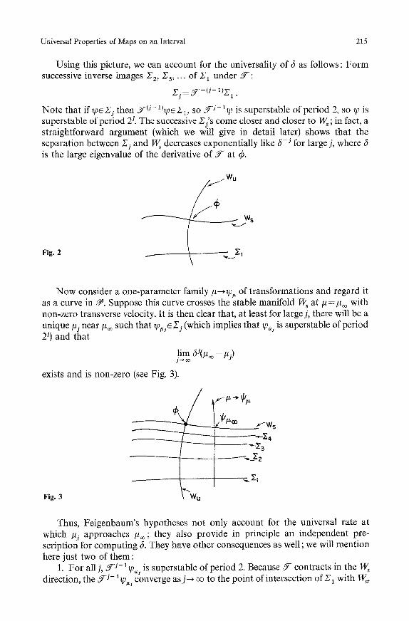
1. For all j, 3 -j- l~pu j is superstable of period 2. Because 0Y-- contracts in the W~ direction, the Y-J- l~p.i converge a s j ~ oe to the point of intersection of Zl with W~,
216 P. Collet, J.-P. Eckmann, and O. E. Lanford III
which we will denote by ~b~. Thus, q~ is also universal; for any one-parameter family as above, if we form
and scale properly, we get something near to 4~ for large j. Similarly, YJ~Pu~ converges to 0-
2. Let 21 denote the surface
{~p : tpa(1) = - ~(1)}
(i.e. the set of ~p's such that -~p(1) is a fixed point for @). Misiurewicz [11] has shown that there is an open set of ~'s on 2 , which admit an absolutely continuous invariant measure (and hence which have typical orbits which are not periodic). We will see that 21 intersects W~ transversally, with point of intersection inside this open set. (The intersection point will lie above W~ in Figs. 2 and 3.) Again form successive inverse images of X1 under J
2j = ~--(J- 1)21 ;
these surfaces converge to W~, again exponentially with rate ~, from the side opposite to that of the Zj's. Again, for each large j, there will be a unique ~j near #~ with
tp;ty Z j,
and the/ t fs converge to #~ in the usual way:
li2n ~ (~ j - #~). 5~
exists and is non-zero. For large enough j, J J-1F~j will be near to the point of intersection of,~l with W~ and hence will admit an absolutely continuous invariant measure. From this it is easy to show that F~j itself admits an absolutely continuous invariant measure and hence also has orbits which are typically non- periodic.
Thus #o~ is the limit of values of p for which ~u is chaotic. We warn the reader, however, that not all ~ ' s for # just above #o0 are chaotic; for example, there is a sequence fii, again converging to #~ from above, with the same exponential rate, such that
~ j is superstable with period 3.2 j.
As indicated earlier, we are going to prove that Feigenbaum's hypotheses are correct in certain cases. As Feigenbaum has noted, the universality of b is somewhat relative - its value depends on the function space in which the ~'s are assumed to lie. We will consider ffmctions ~ of the form
~(x) = f(]x] 1 + ~).
where the function f is smooth. Except for a result on the uniqueness of the fixed point, we will in fact have to assume that f is analytic in a complex neighborhood of [0, 1]. We would of course like to deal with the case e = 1, but the argument we are going to give is a perturbative analysis valid only for sufficiently small positive values of e. Our results could be expressed in terms of convergent series expansions
Universal Propert ies of Maps on an Interval 217
in e and various iterated logarithms of e which are analogues of the e-expansions occurring in the renormalization-group approach to the theory of critical pheno- mena. Work in progress, using quite different techniques, indicates that at least partial results can be obtained for e = 1 [8], see also note added in proof.
As an indication that there is some simple behavior at e = 0 about which we could hope to carry out a perturbative analysis, consider the family of functions
~)a(X) = 1 - - (1 -[- a ) l x l ,
for small positive a. A straightforward calculation shows that
(JW,)(x) = 1 - ( 1 + a)elxl,
i.e.
Thus, the curve a ~ P a is invariant under the action of J- , and the end point at a = 0, although not in the domain of definition of.Y, is a sort of virtual fixed point. If we consider instead
~o(x)-- 1 - ( 1 + a)lxl 1+~
we no longer get such a simple closed-form expression for 3"-~ but we do get
(J~v)(x) = 1 - (1 + a)2aqxl ~ +~ + O(e).
This suggests that, for small e, there might be a fixed point near he,, where a is to be determined approximately by
1 + a ~- a~(1 +a) 2 ,
i,e.
i.e.
a~_ l - a ,
a e l o g a ~ _ - a or s-~(_--i-oga- ~ .
Observe that this, if correct, implies that e ~ a and hence suggests that it should be possible to get a fixed point by adding to 1 - ( 1 + a)lxl 1 +~ a correction which is small relative to a.
2. Statement of Results
We are going to consider functions tp~N of the form
~v(x) -- f(lxl I + ~),
where f is the restriction to [0, 1] of a function analytic in some domain in the complex plane. Through most of our analysis, the domain f2 of analyticity will not affect our results very much although it presumably affects how small we have to take e in order to make our estimates work. There is one point in Sect. 7 where it is necessary to impose some conditions on f2 ; these conditions are met if we take O to be an open disk with center 1/2 and radius not too much larger than 1/2. Aside
218 P. Collet, J.-P. Eckmann, and O. E. Lanford III
from this one argument, we can work with 1"2 any bounded connected open set in t17 containing [0,1]. We will mostly think of O as chosen once and for all and so will frequently suppress it from our notation. We will write ~(~2), or simply ~, for the real Banach space of functions bounded and analytic on Q, and real on (2~IR, equipped with the supremum norm. For e > 0, we denote by ~ ( C N ) the set of functions tp on [ - 1 , 1] of the form
with f e ~ and satisfying
f(O) = 1;
~(x) = f(Ixl* +~),
df -d-~<0 on [-0,1]; f ( 1 ) > - l .
We can identify N~ in an obvious way with an open subset of the Banach space
{geS(~) :o(0) = o}.
Theorem 2.1. For e sufficiently small, 3- has a fixed point 0 in ~ . I f we write
¢ . ( x ) = L(IxP + ~)
then f~(t) extends to a function jointly analytic in (e, t)for
ee { z e ¢ \ [ - o0, 0] :lzl < Co}
and te£2. We denote -q~(1) by 2~; then
2~ = - e log e + O(Q (2.1)
£ ( t ) = 1 - (1 + 2~)t + O(e 2 log e).
~ is an isolated f ixed point for 3- in ~ , ; it has negative Schwarzian derivative (see Singer [12]), i.e.
<, 3(<)2 ~b; 2 \q~;/ < 0 .
Theorem 2.2. For e sufficiently small, (a ~ is an isolated fixed point for Y- in the space o f functions
tp(x) = f ( t x l I + ~)
with f twice continuously differentiable on [0, 11.
Note that, if ~>e, then ~b&)=L(lxl 1 +~) can also be written as 0(Ixl x +9 with g continuously differentiable on [0, 1]. Thus, Y has at least a one-parameter family of fixed points of the form g(lxl 1 +~) with g only once continuously differentiable.
Notational Convention : From now on the symbols q~ and 2~ are permanently reserved to denote the above objects. We will frequently suppress the subscript e.
Theorem 2.3. The transformation J- is infinitely differentiabIe in a neighborhood of (o ~ in ~ . The derivative o f f at ~)~ has one simple eigenvalue 6~ > 1 which approaches

Universal Properties of Maps on an Interval 219
2 as e approaches zero. The diameter of the smallest disk centered at zero containing the rest of its spectrum goes to zero with e.
Theorem 2.4. J- has a smooth stable manifold, W~, of codimension one and a smooth unstable manifold, W,, of dimension one, at ~ . For each ae [ - 1, 1] there is a unique point O* on W, with
¢~*0) = - a .
W. crosses the surfaces Z 1 and $1 (defined in Sect. 1) transversally. Each (9" has negative Schwarzian derivative.
Theorem 2.5. Let l ~ p u be a continuously differentiable parametrized curve in ~ which crosses the stable manifold W~ with non-zero transverse velocity at # = l ~ . There exist sequences l~j and [zj converging to #~ from opposite sides such that
lim 6J(#~o - #i) and lira 6i(/z~ - ~i) j ~ j-,oo
are both finite and non-zero, and such that ~ is superstable of period 2 j and ~p~,j admits an absolutely continuous invariant measure for each sufficiently large j.
Moreover, the ratio of lim 6J(lz® -I~j) to lim 6J(#o~-[tj) is also universal, i.e. does
not depend on the particular parametrized family under consideration.
Remark. One instance of such a parametrized family is
~ . ( x ) = ~(~- x)
for a fixed function tp sufficiently near to (9=. We can then in particular take
~)~(x) = 1 - /~ lxl ~ +~
[Actually, the first statement is not quite true. For i f / z> 1, then x ~ p ( # . x ) need not be in N~(f2), but it is in N,(#-t l +~)£2).]
Theorem 2.6. I f ~pE W~, then ~p has an invariant Cantor set d. 1) There is a decreasing chain of closed subsets of [ - 1, 13
j(o) ~ j(~) 3 j(2) 3 . . .
each of which contains O, and each of which is mapped onto itself by ~p. 2) Each j(i) is a disjoint union of 2 ~ closed intervals, jti+ l) is constructed by
deleting an open subinterval from the middle of each of the intervals making up j(i). 3) ~ maps each of the intervals making up j(i) onto another one; the induced
action on the set of intervals is a cyclic permutation of order 2 i.
We let J denote ~ J(i). ~p maps J onto itself in a one-one fashion. Every orbit in J i
is dense in J. If, besides being on W~, ~ has negative Schwarzian derivative-for which it suffices that it be near (9~ - then we have:
4) For each k= 1, 2 . . . . ~, has exactly one periodic orbit of period 2 k - t. This periodic orbit is repelling and does not belong to j(k) ; ~p has no periodic orbits other than these.
220 P. CoUet, J.-P. Eckmann, and O. E. Lanford III
5) Every orbit of ~p either a) lands after a finite number of steps exactly on one of the periodic orbits
enumerated in 4) or o r
b) converges to the Cantor set J in the sense that, for each k, it is eventually contained in j(k).
There are only countably many orbits of type a).
Theorem 2.7. Again assume that ~p~ W~, and let j(o, j be as in Theorem 2.6. Let v denote the probability measure with support J which for each i assigns equal weight to each of the 2 i intervals making up j(1).
1) v is invariant under the action o f f ; it is the only invariant probability measure on J.
2) The abstract dynamical system (v, ~p) is ergodic but not weak mixing. 3) I f x is any point of [ - 1 , 1] whose orbit converges to J, and if f is any
continuous function on [ - 1, 1], then
N - 1
?¢ ~zv n : 0
In particular, if ~ is close enough to ~b~ so that Theorem 2.6 holds, then this equality holds for all but countably many x's. Similar results were obtained by Misiurewicz [10]. The analysis leading to the Cantor set also gives an attractive picture of how the bifurcation at #~ looks. This is described in detail at the end of Sect. 8.
The proofs will be organized as follows: In Sect. 3 we develop the elementary theory of the doubling transformation Y,
and prove for a fairly general class of one-parameter families {~v,} in :@ the existence of an increasing sequence #j of parameter values such that ~v,j is superstable of period 2 j.
Section 4 gives the proofs of Theorem 2.1 - except for the estimate (2.1) on the precise form of the fixed point, which is deferred to Sect. 7 - and Theorem 2.3. Theorem 2.2 is proved in Sect. 5.
Section 5 gives the precise definitions of global stable and unstable manifolds that we use and proves a general theorem, sketched in the introduction, permitting us to deduce Theorem 2.5 immediately from Theorem 2.4. Theorem 2.4 is proved in Sect. 7, and Theorems 2.6 and 2.7 in Sect. 8.
3. The Doubling Transformation
In this section we develop the elementary theory of the doubling transformation Y. Let ~ e ~ , and define
a = a ( ~ ) = - tp(1).
If a > 0 we also define
b = bOp) = ~p( a) .

Universal Properties of Maps on an Interval 221
The domain of J ' , N(J-), is the set of all WeN such that:
1) a > 0
2) b > a
3) ~P0P(a)) ~ a,
and for tpe@(Y-) we define
1 ( y - ~ ) ( x ) = - a ~ o~; (ax ) .
Remark. Although ~(Y-) is defined by three conditions, the boundary of ~ ( J ) consists in fact of two surfaces:
a = 0 p(~(a))=a.
This comes about because, in moving from ~(Y) to a region where 2) fails we must pass through a point where b=a, i.e. ~p(a)=a, and this implies ~p(~(a))=a. Normally, we would expect conditions 2) and 3) to fail simultaneously, but it is easy to find situations in which 3) fails and 2) does not.
Proposition 3.1. Let ~p~ ~ satisfy aOp)= O, and let (tp,) be a sequence in ~ converging to ~p in the C 1 topology and with a(~n)>O for all n. Then
1) ~p,eN(Y-)for sufficiently large n. 2) (J'~p,)(1)-+l as n~oo. In other words: Every point on the surface {a0P) =0} is part of the boundary of
@(~-), and Y- sends ~p's near this surface to functions near the constant function 1.
Proof It is easy to see that, if to2(a)< 0, then ~ N ( Y ) . We will show:
tp.Z(a.)- ( - a.) ~ 0 (a. = a(~.)) a n
which implies both 1) [since it implies tpZ(a.)<0 eventually] and 2) [since 3-~p.(1 ) = - ~Z.(a.)/a.].
In view of the facts that
a.--*0;
we get
On the other hand,
SO
~p.~p in C1;
~.(a.)- ~.(0) an
~'(0)=0,
,0.
W,(x)[ _-< M uniformly in x, n
~.Z(a . )~(-a . ) = ~.(~.(a.))a~tp.(~p.(0)) " < M N. (a . )~ . (O)- - , .0
as claimed.
222 P. Collet, J.-P. Eckmann, and O. E. Lanford III
It is on the other hand clear that if tp satisfies ~poq)(a)=a and if ~,e@(c-); ~p~tp, then
1 o c - ~ , ( 1 ) = - ~ w ° ~ , ( a . ) - - , - t .
Consider now a mapping #--.W, from an interval (#o, ~to) into N, i.e., a one- parameter family of elements of N. We assume the mapping to be continuous in the C 1 topology. We will say that such a one-parameter family is full if
tpu(1)--*l as #'-*go
and
~&(1)-->-i as #--'no
(e.g. lpu(x) = 1 - # x 2 ; #o =0 ; n0 =2). We have already remarked that for any such one-parameter family there must
be at least one # such that ~pu(1)=0, i.e. such that ~p, is superstable. There may be many such #'s; in any case, we denote by #1 the largest such. Proposition 1 shows that, for # slightly larger than #,, ~vueN(c- ). We will denote by ~, the smallest # > # 1 such that ~ ,q~(c- ) . [Since b0pu)=~p~(1)~-i as # ~ 0 , whereas aOPu) = -~,(1)--* 1, condition 2) in the definition of ~(C-) must fail before p reaches no.] By our earlier remarks, ~p~(a~)= a~.
Proposition 3.2. I f #~Ip , is a full one-parameter family, then
# ~ c - t p , , #1 < # < ~ 1
is also a fidl one-parameter family.
Proof. By Proposition 1, c-tpu(1)~l as #+#1, and by the remark following Proposition 1,
By induction, then, there exist two sequences
~0</~1 < # 2 < . - -<~2 </~1<~0
such that, for & < # < ~j, ~v,~ N(C-J) and
#-"+ ~¢--Jll) # , ].,lj <~ # < f.lj
is a full one-parameter family. In particular these sequences are constructed in such a way that
C -s- b&j(1)=0
i.e. c-s-~P,s is superstable of period 2, i.e. ~P,s is superstable of period 2 j.
4. Existence and Elementary Properties of the Fixed Point
If ~ p ~ is in ~(C-) as defined in Sect. 3, and if tp(x)=f(lx[ 1 +"), then
(C-W)(x) = f(lxl 1 +") xe [ - 1, 1],

Universal Properties of Maps on an Interval 223
where
F(t) = -- 1 f ( l ( f (al + ~t))[ 1 + ~) ; a = -- f(1) > 0.
The conditions for the definition of J~p imply that
f(al+~t)>O for 0_< t< l
and we can therefore drop the absolute value sign. If we define @~ to be the set of such functions ~p satisfying in addition
a l + ~ C f 2 ; f(al+~g2)n(-- o% 0) =0 ;
[f(aa +~f2)] 1 +~ C ~
then, if ~ps @~, ~--V' is again in ~ . We are going to prove that J - has a fixed point in N~ for each sufficiently small positive s.
It is convenient to introduce a new variable c( related to e by
-(z
1 + log (c~)"
Note that for each small positive e there corresponds exactly one small positive and vice versa. Any ~ p ~ can be written uniquely as
~(x) = f(lx[ 1 + 9 ; f ( t ) = 1 - t + o:t(g(t) - 1),
with ge ~(f2). Working with g rather than ~p is simply a (linear) change of variables in function space. If ~ N~, we will write the g corresponding to J-~p as T~g. The domain of C- is bounded on one side by the surface
~(i)=0
which corresponds to
g(1) = 1.
We are going to show that, for small ~, ~ is defined and well behaved on the open unit ball in .~ and has a fixed point near zero.
To formulate our results concisely, we need some special terminology. If ~r is a normed space and Q a positive number, we write ~ r for the open ball in ~r with center 0 and radius Q. A mapping defined on/g'l will be said to be nearly bounded if it is bounded on each . ~ with ~ < 1. Similarly, functions will be said to converge nearly uniformly if they converge uniformly on each ~ with ~ < 1.
Proposition 4.1. For s > 0 sufficiently small, T~ is defined on ~1(g2). The mapping
(e, g)-* ~(g)
is jointly infinitely differentiabte. For f ixed ~, derivatives o f all orders of T~ with respect to g are nearly bounded on ~ l . We can decompose T~ as
T~(g) = Tog + r~(g),

224 P. Collet, J.-P. Eckmann, and O. E. Lanford III
where T o is a rank-one linear operator with range the constant functions:
(Tog)(t) = g(0) + g(1) + g'(1)
and r~ and its g-derivatives of all orders converge almost uniform.ly to zero with ~.
We emphasize that: Although 7~ is highly non-linear, its zeroth order part T o is not only linear but very simple - dividing it by two gives a projection onto the constant functions. Its simplicity makes possible a detailed analysis of the behavior of T~ for small e.
Before proving the proposition we note its principal corollary.
Corollary 4.2. 1. For each sufficiently small ~ > 0, there is exactly one solution g~O) for the fixed point problem
a = T~(g)
in ~1/2. (Here, ½ may be replaced by any number less than one.)
__~ g~O)
is infinitely differentiable and g~O) approaches zero with ~. 2. D T~(g~ °)) varies continuously with ~ and approaches T O in operator norm as
approaches zero. 3. Let 0 < Q < 1. For sufficiently small ~, the only part of the spectrum of
DT~(g~ °)) at a distance greater than Q from 0 is a simple positive eigenvalue 6~ which approaches two as e approaches zero. The corresponding eigenspace converges to the space of constant functions.
To prove 1., we write the fixed point problem as
g = Tog + r~(g)
or equivalently as
( I - To)g = r~(g) .
Since To 2 =2To, we have ( I - T o ) 2 = I and so the above equation is equivalent to
g = ( I - 7o)r~(g).
Since r~ and Dr~ converge to zero nearly uniformly with e,
g-~ (I - To)r~(g)
is a contraction on ~1/2 for e sufficiently small. The existence and uniqueness of g~O) follows from the contraction mapping principle. The smoothness of the de- pendence of g~o) on e follows from the implicit function theorem in Banach space. (See, for example, Dieudonn6 [2].) That ~(o) approaches 0 with e follows ~e immediately from the nearly-uniform convergence of r~ to zero.
Part 2 follows from the joint continuity of DT~(g) in g, e and the continuity of g~O) in ~. Part 3 follows from 2 by standard perturbation theory (Kato [7]) and the fact that the spectrum of T O reduces to {0, 2} with 2 a simple eigenvalue whose associated eigenspace is the constant functions.
The proof of the proposition is a relatively straightforward computation supported by some general theorems. We will give the computation first; then
Universal Properties of Maps on an Interval 225
sketch the justification that the remainder terms do indeed have the properties claimed.
We first do a computa t ion whose result we will need to use again later. We have already seen that if
~ ( x ) = f ( l x l l + ~ ) ; a = --~p(1)
then the t ransformat ion tp~J-~p translates to
f - ~ - -~ f ( ( f ( a 1 ~ ~t))l +~).
We will next write f ( t ) = 1, - th(t)
and determine how h transforms. We will need the following nota t ion : If t o ~ ~2, we define a bounded linear opera tor Ato on 9((2) by
(Ato f ) ( t ) = f ( t ) - f ( t o ) t #: t o r - - t o
= i f ( t o ) t = t o .
N o w define rh, r/2 by
f ( a l + " t ) = l - a t r l l [so r l l=a~h(a l+~ t ) ]
( 1 - at t l l ) 1 +~" = 1 - atrl2.
We now claim: Under the action of J- , h transforms as
h~t /2 x {h(1 - atrl2) + ( A lh) (t - a t q z ) } .
To verify this, write
f ( ( f ( a 1 +~t)) 1 +~)= 1 - ( 1 - atrl2)h(1 - a t t l 2 )
= 1 - h(1 - attt2) + atrlzh(1 - at~12).
N o w use the following expression for the first h ( 1 - atrl2),
h(1 - atrl2) = h(1) - atrt2(A l h)(1 - atrt2)
and recall that a = - f ( 1 ) = h ( 1 ) - 1 , to get
- a + atrl2 {(A lh)(1 - atrt2 ) + h(1 - atr/2)}.
Thus
1 - - f ( ( f ( a 1 + ~t)) 1 + ~) = 1 - tr/2 {(A 1 h) (1 - attl2 ) + h(1 - atr/2) }
a
from which the formula (4.1) for the action of ,Y- on h can be read off. We must next insert the expression
h(O = 1 - ~(g(t) - 1)
(4,1)

226 P. Collet, J.-P. Eckmann, and O. E. Lanford III
and extract the principal terms for small e. In so doing, we generate a large number of remainder terms, and it is convenient to have a systematic nota t ion for the spaces in which the remainder terms lie. Let 9~ denote the space of all mappings
r : (e, g)-~ r(e, g)
defined on a set of the form (0, Co) x.~1((2 ) with values in .~(f2). Here eo is a strictly positive number which may vary with r. These mappings are required to be jointly infinitely differentiable in e, g, and derivatives of all orders with respect to g are required to be nearly bounded in .~1((2) for each ~ and to converge to zero nearly uniformly with e. We will use ~ to denote the analogous space of functions which, together with their g derivatives, will merely be required to remain bounded as approaches zero and No, ~ o to denote the analogous spaces of functions taking values in IR rather than 9- Recall, also, that e and ~ are related by
e - (1 + log~) '
whenever c~ appears in one of our formulas it is to be regarded as a function of e. Since a = h (1 ) - 1 and we are writing h( t )= 1 - ~ ( g ( t ) - 1 ) we have
a=~(1-g0))
and hence
[ - ~ logct~ N o w ~ = exp [~ loges] = exp ,~ i ~ ) = exp [ - ~ - ~].
/
Thus
a ~ = e - ~ + e b l ; b l E ~ o .
Also,
Thus
g(a i + ~t) = g(O) + a 1 + ~t(A og)(a 1 + ~t) = g(O) + ~b2, b 2 ~ 26.
r/1 = a~(1 + e(1 - g ( a 1 + ~t)))
= (e- ~ + ebl)(1 + c~ - ~g(O) - ~2bz)
= 1 - c~g(O) +ctr 1 , r l e N .
[We have used the fact that e/e goes to zero with ~ to replace eb t by e(e/cOb 1 with e/c~b l ~ 9~o. ] N o w
1 - att?z = (1 - atr/1) l+~ ,
so
so t / 2 = t / l + e ~ b 3, b 3 ~ ,
~/2 = 1 -- ~z9(0) + o~r2, r 2 E ~ .

Universal Properties of Maps on an Interval
Also
h(1 - atqz) + (A lh)(1 - atrl2 ) = 1 + 0~ - - eg(1 -- ate12)-- a(A 19)(1 - - atrt2) =l+e(1-g(1)-g'(1)+r3), r3~9l.
Thus
r/z {h(1 - atrh) + (A 1h)(1 - art/2) } = (1 - c~g(O) + er2)(1 + e(1 - g(1) - g'(1) + ra) )
and hence by inspection
=l-e(g(O)+g(1)+g'(1)--l+r¢), r4sN
Tg = g(0) + g(1) + g'(1) + r 4 ,
as desired.
227
and that
)~, = - e logs + O(e)
q~(x) = 1 - ( t +)~01xP +" + 0 ( - ~ ~ logs).
We turn now to the problem of justifying the above computations, i.e. of showing that the remainder terms do indeed have the asserted properties. The verifications are tedious and we will not do all of them, but we will work through one in full detail. We wrote, in the course of the computation,
al+~t(Aog)(at+~t)=~b2 with b2~23. (4.2)
We now want to prove this. The proof is based on a number of principles which we list here:
a) The mapping (~, g)--+g is in 23. b) For any go~5, the constant mapping (e,g)--,g o is in 23. c) If bo~23 o, the mapping (s,g)-+(the constant function with value bo(s,g))
is in 23. d) Let 2}1,..., 2}, be open sets in ~ and let
~ : 2 } 1 x .. . x ~ 8 . - + 5
More detailed computations to be done in Sect. 7 show that in fact
Remark. These computations show that ~ admits a fixed point q S ~ with
~(x) = 1 - (1 +,(8))lxl 1 +~ + correction,
where the correction vanishes more rapidly than ~ as e goes to zero. They also show that there is no other fixed point in a ball about ~b~ whose radius is bounded below by conste(s). If we write
2~= - ~(1) ,
then
2 ,=e (e )+0 (e ) , or 2,=-eloge+o(eloge).
228 P. Collet, J.-P. Eckmann, and O. E. Lanford III
be bounded, infinitely differentiable, and have bounded derivatives. Further, let bl . . . . ,b,e~3, with the range of b~ contained in ~B~ for each e. Then
@, g ) ~ q)(b l (~, g), .. . , b,(e, g))
is in ~. e) (Corollary of d.) If b 1, b2e~, then
(~, g )~b l ( e , g)" b2(,% g)
(pointwise product of analytic functions) is in ~8. Similarly, if b 1, b 2 a r e in ~o, so is their product.
f) If t21, f22 are bounded open sets in 117, we write 5(t21, f22) for the set of all geS(f/1) with g(f21)Ct? 2. [-Hence, if f22 is the open unit disk, 5(f/,f22)=51(O). ]
' t~' 5(f/1, f22) is an open subset of 5(t21). Now let f22C /COg. Then composition (gl,g2)~g2°gl is a C ~ function with bounded derivatives from 5(f21, f2~) xS(f22, ~3) into 5(f/1, f23).
We omit the proofs of these statements. Note that a)-e) remain true if we replace 5 by C 2, but that t) depends upon the properties of analytic functions, and fails in C a .
We are now ready to verify 2). 1. The mappings
(g, g)-~ 1 - g(1), (1 - g(1)) ~ , a, e -~ , e -s:
are all in $0. This is readily proved by direct verification. Note that the g-derivatives of ( 1 - g(1)) ~ have singularities as g(1)--> 1; it is for this reason (only) that we have to work with functions with derivatives which are nearly bounded - rather than bounded - on the unit ball of 9-
We will from now on write, as a shorthand, statements like (1-g(1))~e$o rather than the more logical
((e, g)~(1 - g(1)y)s $o .
2. a=:¢(1 -g(1))~B0 ; a~=e-~e-~(1 -g(1))~e!B0 ; a 1 +~e~3 o. [Use le).] 3. a 1 + ~t~ ~. [Use 2b), c), and e).] If e o is small enough there exists a domain ~1
with ~ Cf /such that a~+~tef21 for all e<eo, ge51, tar2. 4. A o g e ~ . [Use a), d).] 5. Aog(at+~t)e~. [Use 3., 4., f), d).]
6. l -al+"Aog(al+~t)=(1-g(1))a~Aog(al+~t)ef& [Use 1., 2., 5., c), e).]
This completes the proof of (4.1). The arguments given so far show that the fixed point g~O) varies smoothly with
e. We next show that g~°)(t) is jointly analytic in e, t. The logarithm appearing in the relation between 2~ = -0~(1) and e shows that there must be a singularity at e = 0, and we want to clarify the structure of that singularity. For this purpose it turns out to be useful to consider a somewhat contrived generalized fixed point problem in which the relation between e and c¢ is partly relaxed. Recall that ~9- takes the form
f ~ - }. f ( ( f ( a 1 + ~r))l + ~) a

Universa l Proper t ies of M a p s on an Interval 229
with a = - f ( 1 ) = a ( 1 - g ( 1 ) ) . We modify this transformation as follows: In the innermost argument we replace a ~ by e-~-~(1- g(1)) ~. We then replace e wherever it appears by #. ~ and we regard #, a as independent parameters. This gives a two- parameter family of transformations whose action we can again express in terms of g related to f as above. Expressed in terms of g, we will denote the transformations by
g--* T~.,(g).
Our original transformations T~ are recovered through
T~(c0 ~--~ T , 1 1 + Iogc~
The advantage of considering c~, # as independent variables is that T~,, turns out to be, heuristically, jointly analytic in e, # at (0, 0) ; the non-analyticity appears only in the relation between # and c~.
We now, temporarily, drop the requirement of reality for real values of the argument in the definition of the space 9, and we consider the transformations T~., for arbitrary small complex values of e, #. Exactly the same computations as were done in the proof of Proposition 4.1 go through, and we obtain
T~,.(g)=Tog+G,u(g),
where G., and its derivatives of all orders with respect to g converge nearly uniformly to zero as e, # both go to zero. Hence, as before, the fixed point problem
g = T~..(O)
can be rewritten as
g = (I - To)G, ~(g)
and the right hand side is contractive on 91/2 for sufficiently small [a[, [#[, Thus, there exist c%, go >0 such that for all ~, # with I~l < So, 1#1 <go, T~,~ has a unique
~(o) in fixed point g~,. -~t/2. Moreover, the computations which show that r~,. is small for small a, # also show that ifa, #--*g~.. is a mapping from {(~, #) :N < So, 1#t < go} into 91/2 such that g~..(t) is jointly analytic in c~, #, t then r~. ~(g~..)(t) is again jointly analytic, and so the same is true for
(I - T0)G,.(g~, ~)(t).
From this it is easy to show - using the contraction mapping principle in an appropriate space of jointly analytic functions that Ao)(t ~ is jointly analytic in - - ~ 4 ~ , ~ y
c~, #, t. Since the parameter e was introduced artificially, it is desirable to express
directly the dependence of g(O) on e. To do this we need the following lemma.
Lemma 4.3. There exists a function r(zl, z2), analytic on a neighborhood of zero in 112 2 and with r(O, O) = 1 such that for small positive e
1 l ° g ( - l°gOl ]

230 P. Collet, J.-P. Eckmarm, and O. E, Lanford III
is the unique small posit ive solution o f the equation
- (4.3) 1 + loge"
Proo f . Write c~= -e - loge . r and insert in (4.3). The result is
1 log(- loge) logr 1 + ~ g e + loge + loge = r.
For fixed e in (0, 1) this equation has a unique solution r; for e small, the solution is near 1. On the other hand, by the implicit function theorem, there is a uniquely determined function r(zl, 22) defined and analytic on a neighborhood of zero in C 2 and satisfying
l + z l + z 2 + z 1 l og r= r ;
and r(0, 0)= 1. This is thus our desired function r. We can express the conclusion of the lemma more concisely by saying simply
that a/eloge is an analytic function of 1/loga and log(-loge)/loge. It follows immediately that e/a is also an analytic function of 1/loge and log(-loge)/loge. Thus we get:
1 log(-log~) and t. In Proposition 4.4. ~(°)(t), . is an analyt ic func t ion o f e loge, loge '----loge
particular, 9~°)(t) is jo in t ly analyt ic and bounded in ~, t f o r e in a small disk about zero in 112 and o f f the negat ive real axis and t in f2.
5. Existence and Uniqueness in C z
Write
f ( t ) = 1 -- (1 + 2)t + )~2f(t). (5.1)
We are looking for (e, E) such that
2f(t) + f ( f ( ,~ ) +*t)* + ~) = 0. (5.2)
We study the equation to be satisfied by the second derivative of f . If (5.2) holds, then
i f ( t ) = - ) ? f ' ( f ( 2 ~ + ~t) ~ +") f ( ; ? + ~t)~(1 + e f t ' ( )? + st), (5.3)
and
i f ( t ) = - )ol + 2~{f , ( f ( .~) +,t)l +~)fOol + ~t)2,(1 + ~)2f,() 1 +~t)2
+ f ' ( f ( 2 1 + ~t) 1 + ~)f(21 + ~t)~(1 + e)f"(21 +~t)
+ f , ( f ( 2 1 + ~t)l + ~)f(21 + ~t)~- 1(1 + e)ef,(21 + ~t)2}. (5.4)
Setting t = 1 in (5.3) we get
1 + 2 - ) ~ 2 f ' ( 1 ) = )f{(1 q- 5~) - - 2z~ ' ( f0 o* + ~)1 + ~)}
• { 1 - ( 1 + ~)21 +, + ;?E(,~I + ~)},(1 + e)
• {1 + ~ t - 22~(2 * +~)}, (5.5)

Universal Properties of Maps on an Interval 231
o r
i.e.
0 =)~ + e + e log2 + 22filo(~, e, 2),
We also rewrite (5.4):
(5.6)
f" = 2Kz(f, e)(" + Ma(?, e), (5.8)
where for ~eC°[0 ,1 ] , and f defined as in (5.1),
(Ka((, e)~)(t) = - 2a~{~(f(21 + ~t) ~ + ~)f(2 i + ~t)2~(1 + ~)2f'(2~ + h)
+A O) + h)f '(f()J + ~t) i +")f(2 i + h)~(1 + e)}, (5.9)
and
and
Mi(t ~, e)(t) = 2~ ~ , o i +~ ~ +h)~- -,~ ~ f ( f ( , t t) +~)f(21 i(l+8)f'(,~t+~t)2. (5.10)
Finally, we define Y by
t I.
(£a~)(t) = ~ ( t - z)~(z)dv- t ~ (1 - ~)~(~)d'c. (5.11) 0 0
Instead of solving (5.2) directly, we rather discuss first the set of equations (for fixed, small 2 > O)
=N~(E,e), (5.12a)
f = 5 f ( I - 2Ka((, e))- 1M z(f, e). (5.12b)
We claim that the solutions (e,() of (5.12a, b) solve actually (5.2).
[Proof. (5.12a) implies (5.6) and (5.5), and hence (5.3) at t = 1. Equat ion (5.12b) implies (5.4). Integrating, we find that (5.3) must hold up to an additive constant, but this constant is zero since we have already seen that (5.3) holds at t = 1. Integrating again, we find that (5.12) holds up to an additive constant, which however must be zero, since, by (5.12b) and the definition of ~ , E(0)=((1)= 1.]
We now discuss the existence and uniqueness of solutions of (5.12). [This also implies uniqueness of the solution of (5.2) since every solution of (5.2) solves (5.12).] The appropriate function space is
e = {(~,~), ~ec2[o, 1], ~(o)=~(1)=o, ~e¢}
equipped with the norm
log). + 1 Ii(f,e)rle= sup V"(x)t-tel , (2 is small).
x~lO, 1] 22
2 + 22Nl(Y, e, 2 ) - Na(#, e) (5.7) 1 + log,~
232 P. Collet, J.-P. Eckmann, and O. E. Lanford III
Let e 1 be the unit ball in ~. ~ is a Banach space. In fact [ = ~q(['), and I(~q~d)'(t)[ + / (~) ( t ) r_-<cons t sup [A(t)[. (All spaces C °, C a are on [0, 1].)
te[O, 11 We claim tha t for sufficiently small 2 > O, a) N z is a contract ion 1 f rom ~a to ~;. b) M~ is a contract ion f rom @t to C a. c) Fo r (d, O e ~ 1, K~.(d,e) is a bounded linear m a p f rom C o to C O and f rom C 1
to C 1.
d) Fo r X 1 , X 2 e ~ l ,
t K ~ (Xa)d - g).(X2)d[co <--__ const I[X 1 - X 2 Itelfilc, -
e) ~ is bounded linear f rom C o to C a, and ( ~ d ) ( 0 ) = ( ~ d ) ( 1 ) = 0 . Note that f rom c), d) above it follows that
t(1 - 2K;,(X a))- ~d - (1 - ,~.K~(X2) )- ~dlco = 2l(1 - 2Kx(Xl))- I (K;~(X1) - Kx(X2))(1 - 2Kx(X2))- ld[co = 2 const [IX a - X 2 [[ eIdtc~,
and hence we see that (5.12) has a unique solution. It remains to verify the claims a)-e). This is tedious but straightforward. Each t ime we have to est imate
we use the formula
t~(u)-~(v)l _-< t 4 c l l U - v l . (5.t3)
This is responsible for the fact that the contract ions in b) and d) lose a derivative. We only commen t on the otherwise trivial verifications: a): Obvious f rom (5.5), (5.6), (5.7). b): Obvious f rom (5.10). [No te that f (21+~t)>½ for small 2 > 0 . ] c): Obvious f rom (5.9) since no derivatives of d occur. d): Obvious f rom (5.9) using (5.13). e): By construct ion, ( ~ , ) ( 0 ) = ( Y A ) ( 1 ) = 0 , cf. (5.11). On the other hand, a
direct compu ta t ion shows
f~e~lco_-< 14co ; I(~,~)'lco <= I~[co ; I(~e~)"[c,0=< I~lco.
This proves existence and uniqueness in C 2 and hence T h e o r e m 2.2. The same p roo f works on any interval [0, A] provided 2 > 0 is sufficiently small, and A > 1.
6. Stable and Unstable Manitolds
In this section, we present a general a rgument deriving some analytic con- sequences f rom a geometr ic situation. The geometr ic s i tuat ion is as follows:
We consider a twice cont inuously differentiable mapp ing J - defined on an open set ~ in a Banach space .~ and taking values in .~. We do not assume that J
1 By contraction we mean a bounded, contractive map

Universal Properties of Maps on an Interval 233
maps ~ into itself, but we do assume that it has a fixed point qS. We further assume that DJ-(qS), the derivative of J - at 4~ (which is a bounded linear operator on ~5) has spectrum which, except for a single simple eigenvalue 6 > 1, is entirely contained in the open unit circle. It then follows from invariant manifold theory that Y admits a stable manifold W~ of codimension one and an unstable manifold W u of dimension one. We will define these submanifolds precisely later; for present purposes, it is good enough to think of W s as an invariant surface and W, an invariant curve (the two of them crossing at the fixed point 4~) with Y acting in a purely contractive way on ~1/; and in a purely expansive way on W~.
We also give ourselves two further objects: A submanifold I/1 of ~ of codimension one which intersects W~, transversatly
at some point ~b*+ ~b. A continuously differentiable parameterized curve # ~ p u in ~ which crosses
the stable manifold W~ at # = ~ with non-zero transverse velocity. Although the notation in this section will be chosen to suggest the application
of the results obtained here to the main topic of the paper, the reader should note that these results depend only on a few explicit assumptions about the objects under consideration. Symbols like Y, qS, W,, etc. are used in a more general sense here than in the remainder of the paper. Moreover,/ /1 will be later on identified with 2; 1 (see Fig. 3).
From this set-up we want to conclude: a) There exists a sequence/~. (perhaps defined only for large n), converging to
#~, with ~J"-ltpu ~ir/p and such that lim 6"(# , -#~) exists and is non-zero.
b) The sequence ~--"-l~pu n converges to 4)*. The significance of these conclusions has been discussed in the introduction.
(We would like to be able to make the more precise assertion that #, is the unique value of # n e a r / ~ such that 3-"-l~pu~//1. Whether this is true or not depends on relatively inaccessible global properties of 3-; but we can say, informally, tha t /4 is the unique such # for w h i c h ~-lDg, f2~)[~ . . . . . ~'-n--21D u all lie between I4~ and H1. )
The first step in our analysis will be to define precisely what we mean by stable and unstable manifolds. This is not entirely routine since, in the application we have in mind, the transformation ,Y- is not invertible; in fact, it is not even locally one-one near qS.
If 2} is a sufficiently small open ball in .~ with center ~b then
{~pe~3:~--Jtpe~ for j=1 ,2 ,3 , . . .}
may be shown to be a smooth connected submanifold of ~ of codimension one. We will call this set a local stable manifold for ~ at ~b and denote it by W~ ~°). It passes through ~b and is tangent there to the stable eigenspace for DJ-(~b), i.e. the spectral subspace for the part of the spectrum which is inside the unit disk. The set 14~ °) is mapped into itself by ~--, and the sequence of sets Y-JW~ ~°) shrinks to {~b}, i.e. is eventually contained in any neighborhood of ~b. The proofs of these facts, as well as those to be cited in the next paragraph on local unstable manifolds, can be found in the monograph of Hirsch et al. [6].
If we define (again for ~ a small open ball with center q~)
~0 = ~ ; ~j+~ = ( Y - ~ ) c ~ ,

234 P. Collet, J.-P. Eckmann, and O. E. Lanford III
then (~ ~3j is a smooth connected one-dimensional submanifold of 2~, passing J
through ~b and tangent there to the eigenspace of DJ(~b) corresponding to the large eigenvalue 3. We call this set a local unstable manifold for J - at q~ and denote it by W~ °).
We have:
and, for any ~pe W, (°) and a n y j = l , 2 , 3 . . . . , there is a unique ~oje W~, °) such that
~ - ' J p j = 1]) ;
moreover, the sequence (~0j) converges to 4. The gtobalization of the stable and unstable manifolds is complicated by the
non-invertibility of J-. We will simply define what we mean by a stable or unstable manifold without investigating the existence of a unique largest one. Thus we define:
A stable maniJbtd for 3" is a smooth codimension-one submanifold W~ of the domain of 3- such that:
a) J ~ c ~ . b) If ~pe~;, then lim JJ~p=qk (Note that this implies that ~--J~oE 14~ °) for
j ~ m
sufficiently large j.) c) (Transversality.) For any ~p in W~, the range of DY(~c,) is not contained in the
tangent space to W~ at ~--~p. An unstable manifold for Y- is a smooth one-dimensional submanifold W u of
(not necessarily contained in the domain of J-) such that a) 3- (W.c~(9-) )~ %. / b) If ~pe W~, there is a sequence ~pj converging to 4) such that ~o = J%pj. {This
\ implies that 14] C ~) J q 4 ~ ° ) . . =
c) For any ~ e Wuc~(J-), the tangential derivative of J - along I4/~ at ~p does not vanish.
Since l ~ °) and V~, °) are, respectively, stable and unstable manifolds, stable and unstable manifolds do exist.
We now need some special terminology. Let //~, j = 1 , 2 , 3 . . . . and W be submanifolds of ~ of codimension one. We will say that the sequence Hj converges to WexponentialIy with rate ~ (3 a real number larger than one) if, for each tpe W there is a diffeomorphism from £r x ( - 1, 1), Y'a the open unit ball in some Banach space £r, onto a neighborhood ~ o f ~ (i.e. a set of local coordinates at ~) such that
1. ~p is the image of (0, 0). 2. Wn~3 is the image of~r 1 x{0}. 3. For each sufficiently large j , / / f ~ is the image of the graph of a mapping
i~j : f l - + ( -- 1, 1), where
4. fiJlIj converges in the C 1 topology on ~ , to a nowhere vanishing limit. Intuitively, this means that the separation between Hj and Wvaries asymptoti-
cally (for large j) like 6 - j multiplied by a differentiable function of position on W. The following proposition is nearly obvious:
Universal Properties of Maps on an Interval 235
Proposition 6.1. Let IIj converge exponentially to Wwith rate 6, and let # - ~ u be a continuously differentiable parametrized curve in .~ crossing W with non-zero transverse velocity at #=#~ . There is then a sequence # j ~ p ~ (defined for sufficiently large j) such that ~p,y I1j ; the quantity 8J(#~ - # ) converges as j ~ oo to a finite non-zero limit.
Returning to the principal objective of this section, we see that the proof of a) p. 233 now reduced to constructing appropriately localized preimages Hj of HI under y j-1 and showing that they converge exponentially to V¢~ with rate b. The following theorem asserts that this is possible; it also asserts that b) holds.
Theorem 6.2. Let J ' , 4, B~ W~, 8, H 1, and 4" be as above. Then there exists a sequence (17;) of codimension-one submanifolds of fj, converging exponentially to W~ with rate 8, such that
9--J-IHjCHI.
Moreover, if ~p~ W~ and if ffl3 is a sufficiently small neighborhood of p in 9, then
J-J-I(Iljc~flB)~{qS*} as j ~ .
The first step in proving this theorem is to reduce it to a statement which is local at ~b. More precisely, we claim that the theorem as stated is true if we can find an open neighborhood ~ of q5 such that it is true for W~ and W~ replaced by Wsn~ and W~n~ respectively, with the added assumption that H~ C~B. Proof of this ciaim is straight-forward, using (notably) the transversality conditions in the definition of stable and unstable manifolds. We will sketch one part of the argument, showing that there is no loss of generality in assuming that/7~ C ~3.
As before, we let q~* denote the (first) point where 14] intersects H r Since q~*~ W,, there is an integer k and a point 4~*e W,n~B such that ~--k-15~, =q~,. By our definition of W,, the tangential derivative of y-k- 1 along W, at ~b~ does not vanish. From this (and the implicit function theorem) it follows that, for 11' a sufficiently small open ball about ~b*,
H' 1 = {~,~ ~I' :y-k- ~ H x }
is a smooth codimension-one submanifold of ~ intersecting W, transversally at ~b*. The localized version of the theorem implies the existence of a sequence of surfaces H~. converging exponentially to V ¢ ~ with rate 8 and with
We can thus take
s-;- nl.
H j + i = H I j + 1 "
This establishes localizability in the expanding direction. A similarly straightfor- ward argument, which we omit, establishes localizability in the contracting direction.
Thus, we have only to prove the localized version of the theorem. We do this by choosing special coordinates in which Y and H t take particularly simple forms. The result we need is the following:
236 P. Collet, J.-P. Eckmann, and O. E. Lanford III
If ~b* is close enough to q), then there exists a C 1 diffoemorphism from a set of the form £r 1 x [ - 1 , 1], 5f 1 the unit ball in some Banach space, onto a neigh- borhood 2~ of q5 such that
q) is the image of (0, 0), Vf=c~3 is the image of £r 1 x {0}, Wuc~B is the image of {0} x ( - 1 , 1), / / l n ~ is the image of ~1 x{1}. If we regard x~£r 1, y~ [ - 1, 1] as coordinates for their image in 2~, then in these
coordinates 9-- takes the form
y :(x, y)-->(M(x, y), ,~y), where
[IM(xl, Y ) - M(x2, Y)[I ~c~[Ixl - x2 N,
with e < 1, and M(0, y) = 0. In terms of these coordinates we can take simply
Hj= image of X 1 x{6 -(;-1)}
and this sequence of surfaces converges exponentially to I /V j~ with rate 6. Moreover, in view of the contractivity of M(x, y) in x, the diameter of J J- 1H~ goes to zero as j--> oo. Since this set always contains q)*, we have
YJ-IHj-~{~b*} as j ~ o o .
The proof of the theorem is thus reduced to proving the existence of the indicated "normal coordinates" for J - and/ /1 . We will concentrate on showing the existence of coordinates in which 9" has the desired form, since this result may be of interest in other contexts; we will then at the end sketch how the argument can be modified to bring I/1 into normal form as well. The proof of the following theorem is based on an analogous but more complicated result proved in Collet and Eckmann [1].
Theorem 6.3. Let Y be a twice continuously differentiable mapping from an open set ~3 in a Banach space into the Banach space. Let (o be a fixed point for J-. Assume that DJ-(~) has a single simple eigenvalue 6 > 1 and that the rest of its spectrum is in the interior of the unit disk. Then there exists a C I diffeomorphism of .~r 1 x ( - 1 , 1 ) (~'1 denoting the open unit ball in some Banach space) onto a neighborhood fg of d? - i.e. a set of local coordinates at & - such that
(0, O) represents 4, 5~ 1 x {0} represents W s c ~ , {0} x ( - 1, 1) represents W S ~ , J- takes the form (x, y)~(M(x, y), 6y),
where M(0,y)=0; [ID=M(x,y)I[<e<I for (x,y)sY[a x ( - 1 , 1 ) .
We emphasize 1. tn these coordinates the action of 3" in the y direction has been made
exactly linear.
Universal Properties of Maps on an Interval 237
2. We do not require - and it is generally not possible - that Y be linearized smoothly in the x direction as well.
The first step in the proof is to introduce coordinates which are approximately right. We do this in a sequence of steps:
- Make a translation to put 4) at the origin. - Write the Banach space as the direct sum of the one-dimensional eigenspace
corresponding to the eigenvalue 6 (y direction) and the complementary spectral subspace (x direction).
- Carry out an x-dependent translation in the y direction to bring the stable manifold to the surface {y = 0}.
- Carry out a y-dependent translation in the x direction to bring the unstable manifold to the line segment x =0.
- Reparametrize the y coordinate in such a way that the action of 3- on the unstable manifold becomes exactly multiplication by b. The possibility of doing this follows from a trivial case of the Sternberg Linearization Theorem. (See, for example, Hartmann [5].)
Thus we can assume that: 1. The domain of J is Y'I x ( - 1, 1) and Y ( x , y ) = ( M ( x , y ) , @ + N ( x , y ) ) where
M, N are continuously differentiable and M(0, y) = 0; N(x, O) = 0; N(O, y) = 0. In the course of the argument, we will need to assume that the nonlinear terms
in Y are small. This can be accomplished by magnification, i.e. by replacing (x, y) with new coordinates x' = 2x, y' = 2y with 2 large (and restricting the domain to the set IIx'll < 1, lyq_<_l). This transformation leaves the linear terms unchanged but shrinks the nonlinear terms by a factor of at least 1/2. In this way (and possibly also renorming the space Y') we can arrange that, for some fi > 0,
2. IiD,~M(x, y)[[ <c~ < 1 for Ilxll < 1 , t y l < l .
1 <f i< 6 y + N ( x , y ) Y
It will also be convenient to assume that J-(x, y) is defined and well behaved for all y. To extend it, we choose a smooth cut-off function ~(y),
0=<0(y)= 1,
with
O(Y) = 1
Q(y) =0
and modify ~- to the mapping
1
for ly[< ~-
for tYl->-I
(x, y)--, (O(y)M(x, y), 6y + O(y)N(x, y)), [Yl < 1
-~(0, ay), lyl _>- 1.
The modified Y- agrees with the original Y- on all (x,y) with J ( x , y)eY" 1 x [ - 1,1] ; it maps f l x IR into itself and satisfies the inequalities (2.) for all y. We will work, from now on, with this modified 3--.
238 P. Collet, J.-P. Eckmalan, and O. E. Lanford III
To prove the theorem, it suffices to find a continuously differentiable function z such that
zoJ-=6.z , z(O,y)=y.
The inverse function theorem then assures us that (x, z) is a set of local coordinates at (0, 0) and Y- evidently has the desired form in these coordinates, To construct z, we let y.(x, y) denote the y coordinate of :-"(x, y), and we put
Zn(X, y) = ~-"y . (x , y).
It is immediate that z.(x, y) is continuously differentiabte and that z.(O, y )= O. Also,
ZnO~-:O'Zn+ i
so if
exists, we have immediately
lim z. - z n ~ o o
zo~:6.z
as desired, Evidently, z,(x, O) = O, so the limit exists in this case. On the other hand, if y 4= O, then, since
ly.I >/3ntYl,
lY.l is eventually larger than one. But because of the way J - is cut off, y. + t = 6y. if l y J > l , and so z.+l(x,y)=z.(x,y ). Hence, for all x,y
z(x, y) = lim z.(x, y) . ~ clo
exists, and the only problem is to prove that it is continuously differentiable. Note, incidentally, that if y + 0 and n is sufficiently large, z=z . on a neighborhood of (x, y) and so z is continuously differentiable on that neighborhood; the only place where differentiability could fail is for y=0 .
We will write
z.(x, y) = y + r.(x, y);
then a simple computation using
1 z.+ i = ~ z . o Y
and the expression (1.) for 0Y- gives:
1 1 r.+ i(x,y)= ~N(x,y)+ -~r.o~--(x,y).
Defining a linear operator L by
Ls(x, y) = 1 so 5"(x, y)
Universal Properties of Maps on an Interval 239
we see that 1 n
= ~=o L~N' rn+l ~j=
so, if we can find a normed space containing N on which L is a contraction, we can write
lOO ~=o LJN. z--y= ~j=
We will use the norm
max fsu is(x, Y)I tDys(x, Y)I } {llslll= ~x,P H--~ -'sups,, --IIx/I ,sup~.r tJDxs(x'Y)tJ
on the space of those continuously differentiable functions vanishing for x = 0 for which the norm is finite. (It is to guarantee that N belongs to this space that we have to assume that 3- is twice continuously differentiable. We could make do with less, but simple continuous differentiability does not seem to be enough.)
The proof that L is a contraction in this norm is straightforward; we will describe explicitly only the most sensitive of the estimates,
1 Dy(Ls) (x, y) = ~ (Dxs) (M(x, y), 6y + N(x, y)). DrM(x, y)
+ ~ (Ors) (M(x, y), 6y + N(x, y)) (6 + OrS(x, y)),
1 ID~s(M(x, Y), 6y + N(x, y))DyM(x, y) t < 1 II Is lit sup 11DxDyM( x, Y)tl. 6 Ilxll x,y
Now DxDrM(x, y) comes from the nonlinear terms in ~-- which can be made small by magnification, so we can estimate this expression by an arbitrarily small multiple of Ittsltl. From
it follows that
and thus
M(O,y)=O; IIDxM(x,y)[ I <=c~
[IM(x, y)ll ~c~. I[xl[
~ Drs(M(x,y),@+ N(x,y))(6+DyN(x,y)) _<~][[s]][(l+ 1 [[DyN(x,y)[]) ~sup Ilxll x,~
Again, the last term can be made arbitrarily small by magnification. The final result is, then, that we have an estimate
sup ~ !D'Ls(x' y)[ ~ < IlJs Ill x (~ + something small). x , , [ llxll J =
The other two terms are estimated similarly.

240 P. Collet, J.-P. Eckmann, and O. E, Lanford III
Hence, L is a contraction so the series
1 oo LJN
j=O
converges in this normed space; the sum is z - y so z is continuously differentiable.
Remark. Similar estimates show that if c~. 6~- 1 < 1 then z is C r (assuming that J - is 0+1).
On the other hand, no matter how smooth J" is, it is usually not possible to 1 1 1
find a C r solution to z o Y = 6 .z, z(O,y)=y if one o f ~ , ~ ..... 6~-2 can be written as
a product of points of the spectrum of DxM(O, 0). Finally, we have to show how to modify the above argument to bring a
codimension=one surface crossing the unstable manifold transversally away from the fixed point simultaneously into the desired normal form, a flat horizontal surface. We start as before, choosing coordinates in a neighborhood of q~ in which Y takes the form (1.) and (2.) holds. Le t / I1 intersect the unstable manifold inside this coordinate neighborhood; then a part of / I1 near the intersection point can be represented in our coordinate system as the graph of a function x-~/11(x)s ( - 1,1) with/I1 defined in a neighborhood of 0. By magnifying in the x dimension we can assume that 1) 1 is defined and non-zero on all of ~1.
Now define a new y coordinate by
Yold Ynew ~ ^ //~(x)"
In terms of the new coordinates, (1.) still holds; if (2.) doesn't then it can be made to hold by a further magnification in the x direction. We have thus arranged so that (1.) and (2.) hold, and, in addit ion,/ /1 corresponds to the surface {y= 1}. We then proceed to cut off and extend N, M as indicated. Note that, because of the way we have done the cutting off, the inverse image under • of any set in 2F 1 × [ - 1, 1] is exactly the same as it was before the modification of Y but, on the Other hand,
J-"(x, 1) = (0, ,~").
From this last equation, it follows that
z(x, 1)= 1
i.e. that F/1 corresponds to the surface {z= 1}. It still has to be shown that z is continuously differentiable. To prove that, one
needs to know that
sup qlDxD,M(x, y)ll , sup ]lDyg(x, y)lt , sup tlOxN(x, y)l I x , y x , y X , y
are all small. This would normally be arranged by magnifying sufficiently before cutting off in the y direction. We note, however, that the magnification can just as well be done after cutting off, and that this does not spoil the flatness of H 1 in the z coordinate.
Universal Properties of Maps on an Interval 241
7 . T h e G l o b a l U n s t a b l e M a n i f o l d
The preceding section shows that the universali ty of the rate of period doubl ing can be unders tood if the unstable manifold for the fixed point ~b~ crosses the surface Z l = { ~ p : t p ( t ) = 0 } transversally. In this section, we est imate the global s tructure of the unstable manifold. In essence, we show that it remains close to the line segment {~(x) = 1 - (1 + a)lxl 1 +~ : - 1 < a < 1} th roughou t the full length of this segment, provided tha t e is small enough.
We need yet ano ther realization of the act ion of 3"- in convenient coordinates. Recall that we showed that if we write
~p(x) = f(lxl 1 + ~); f ( t ) = 1 - th( t ) ;
then in terms of h, Y takes the form
h ~t /2 {h(1 - atq2 ) + A lh(1 - atq2)}, (7.1)
where the nota t ion is as in Sect. 4. Deviat ing f rom the nota t ion of that section, we will write
h(t) = 1 + a + ( t - 1)9(t ) (7.2)
and determine the form of Y- expressed in terms of the coordinates a ( s ( - 1, 1)) and g(e~) . Note that
l + a = h ( 1 )
g(t) = (A lh) (t)
so it is easy, in principle, to read off this form f rom (7.1). We will need, however, to look with some care at the expression for t/2. Recall
rl 1 = a~h( a t + ~t)
(1 - att/i) 1 +~ = 1 - a t t l z .
A stra ightforward computa t ion shows that
(1 - z) 1 +~ = 1 - z(1 + es(z, e)),
where s(z, e) (which can easily be writ ten explicitly) is analytic for all e and all z¢[1, co). Hence
r/2 =t/ l (1 + ~ s ( - a t r l p ~ ) ) .
Also,
h( 1 - atrl 2) + A 1 h( 1 - atl/2) = 1 + a - atrt ag(1 - atrt z) + g( 1 - a t r I a)
= 1 + a + (1 - atrl2)g(1 - atrl2).
Thus the t ransformed h becomes
a~(1 + a + (a 1 +st - 1)g(a 1 + st)) (1 + es( - attl a, ~)) (1 + a + (1 - at~12)g(1 - at~ 2)).
(7.3)
We will write A(c, a, g) and G(e, a, g) for the a, g componen t s of the representat ion of (7.3) in the form (7.2). Thus, to get A(e, a, g) we have simply to insert t = 1 in (7.3)

242 P. Collet, J.-P. Eckmann, and O. E. Lanford III
and then subtract 1. Doing this, and grouping terms in a straightforward way, we find
A = a~(1 +a) 2 - 1 + A 1 +cA2,
where A 1 = 0 for g = 0 and where A1 ,A 2 are both "regular". The meaning of "regular" has to be specified with a bit of care. The formulas are full of factors o fa ~ whose a-derivatives become infinite as a approaches zero. The idea is that these are the only singularities for small e, a, g. One way to formulate this is indicated in the following proposition.
Proposition 7.1. We can write
A = a*(1 + a ) 2 - - 1 + A l ( ~ ; , a, a ~, g) + 8A2(,~ , a, a ~, g) (7.4)
G = aGi(e, a, a ~, g) + aeG2(e, a, a ~ , g)
(A a and A 2 take values in IR; G 1 and G 2 in ~(~2)) where A1,A2, G1, G 2 are all infinitely differentiable with bounded derivatives on
(0, %) x(0, ao) x(0,1) x { g e 5 : tlgl[ <go}
(Jbr sufficiently small eo, ao, go) and where A 1 and G i vanish identically for g=0 .
We have already indicated the proof for A. To get the formula for G, apply A 1 to (7.3) using the "product rule"
d l g l g 2 = g i A i g z +g2(1)Algl ;
group the contributions from differencing in the first and third factors to form a. G 1 and the contribution from the second factor to form a. e- G z. To extract the indicated explicit factors of a, make repeated use of the "chain rule"
(~o(g 1 °g2)) (z) = (~g2(~o)g~) (a2(z))A~og~(z)
and observe that every t in (7.3) is accompanied by a multiplicative factor of a.
Corollary 7.2. There exist constants B~, B 2 such that
[]G{1 <=a'B 1 ]{glt +aeB2 ( 0 < a < a o , 0 < e < % , llgt] <go). (7.5)
In particular, at the fixed point, a = 2~ and we write g~O) for the corresponding g. Then
r[ g~O)if < 2~B1 f[ g~o)iT + 2"eB2
from which it follows at once that
(o) ~2~B2 g~ ] [ < - - -O(e2 3
(1 - 2~B~)
for small e. Since 2~ = O ( - e log0 for small e, this estimate gives exactly the estimate
~(x) = 1 - (1 + 2~)]xl x +~ + 0 ( - ~2 log0
announced in Sect. 2.
Universal Properties of Maps on an Interval 243
Corollary 7.3. I f
and if
then
a(B 1 -I- B 2 ) = t ,
IIg[l<~,
ItGII=<~.
In other words, Y- can push a point out of the cylinder { ( a , g ) : 0 < a < a l , []g[[ =<e}, [with a 1 the smaller of a o, 1/(B 1 + B2)], only through the ends.
We have noted already that singularities appear when we differentiate a ~ for a near zero. However, since
d __a~= _a t da a
the singularities are not much in evidence in the first derivative for a->_ e. Since the fixed point occurs at 2~>e, we don't have to worry about the singularities when looking at first derivatives near and beyond the fixed point. Thus:
Corollary 7.4. There exist constants B 3, B 4, B 5 such that
d G ( a , g , ) _-<B31[g, fl + B4E+ B5a dg da I
for any differentiable mapping a - ,g , provided
e < a < a o ; Il g~ [I --< go .
Proof. The B 3 term comes from the explicit aa ~ dependence in aG 1 ; the B 4 term from the explicit aa ~ dependence in aG 2 ; the B 5 term from the g dependence of the s l im .
Corollary 7.5. Consider a curve given as the graph of a .function a-*g,, defined in a subinterval of (~, ao). Assume
dA(a, g,) _> 1. (7.6) da -
Then the image of this curve under the action of Y is again representable as the graph of a fimction
and
I aa~A(e'a'g) =<B3]lgal [ +B4e+Bsa ~a " (7.7)
We can apply this corollary in particular to a (possibly very small) local unstable manifold. Such a manifold can be represented as the graph of a mapping defined

244 P. Collet, J.-P. Eckmann, and O. E. Lanford III
on a small interval I about 2~; condit ion (7.6) is satisfied and we can assume
N = sup []ga[[ ~ e .
Pu t
= sup dg . M a e I bg(A.
Since the local unstable manifold is mapped onto itself by 9--, we get
M < B3N + B4e + 2B52~M
or, for small e,
M < 2B48.
Consider now a manifold specified by
b-*g b
defined on a subinterval of (e, a), and satisfying
[Ig°ll<~; Tadg~ <=2(BN+B4)e. (7.8)
F r o m (7.4) it is easy to check that there exists a constant B 6 such that, under these hypotheses,
dA(a,,aa) > 2 - B6e da
(and so ____ 1 for small e); then from (7.7) the image curve satisfies
d~ ~ (B 3 + B4)e + Bsa2(B s + B4)~
so if
we get again
a<ao ; a(B1 + B e ) < 1 ; 2aB5 < 1
d~a ~2(B3 +B4)~.
Summarizing and simplifying the notation, we get:
Proposition 7.6. There exist constants ~1 > 0; a 1 > 0, B 7 such that, if 0 < e < e 1, and if we have a curve in ~ specified by
a-+ g a
defined on a subinterval o f (e, al) and satisfying
tlgatl <=e ; , dg~ < BTe (7.9)
Universal Properties of Maps on an Interval 245
then d da A(e, a, 9a) ~ t.5, (7.10)
so the image curve also admits a representation as
a---~ Oa
and the bounds (7.9) hold with 9 replaced by (~. A sujficiently small local unstable manfold satisfies these hypotheses.
Now let e<e 1, a small local unstable manifold, and apply Y to it repeatedly, throwing away at each step the part of the image curve with a outside of (e, a 1). In view of (7.10), we obtain after a finite number of iterations a curve a~9* defined on all of (e, al) contained in the unstable manifold and satisfying the inequalities (7.9).
It remains to show that the unstable manifold in the form a ~ 9 * can be extended to all a e ( - 1 , 1). We will consider only the problem of extending it to values of a > a 1 ; the extension to a e ( - t, e) is similar but easier.
If we write
f*(t) = 1 - t(1 + a + ( t - 1)9"), q~*(x) = f*(tx[ 1 + ~),
it will suffice, by the general theory of Sect. 3, to show that 9* can be extended to a value of a such that
qS*(a) = a
(i.e. such that (qSa*)4(0) is the fixed point of qS* in [0, 1]); then one more iteration of 3- gives values of a running all the way to 1. By continuity, it will suffice to extend it to a value of a such that
qS*(a) < a. (7.11)
As above, we will write qS* in the form
¢*(x)=L*(Ixll +9 ; f * ( t ) = l - t [ l + a + ( t - 1 ) g ( t ) ] .
Ignoring 9 and terms of order e, we get
0*(a) ~ 1 - a (1 + a ) ;
from this it is easy to see that (7.11) will hold provided a ( 2 + a ) > 1, i.e. a > 1 / 2 - 1 and provided [[g[I and e are small enough.
Next we will argue that we can take a o > V 2 - 1 in Proposition 7.t. To do this we need, for the first time, to be careful about our choice of the domain f2. Examination of the proof of Proposition 7.1 shows that the only limitations on % ao, and 90 are that
1) al +~(-Q
2) f(a~*~(an(- oo,0]--0
3) If(a1 +~O)]1 +~ el2
246 P. Collet, J.-P. Eckmann, and O. E. Lanford III
for 0 < a < ao; 0 < e < Co; lf glt < go. If these three conditions are satisfied with g = 0 and e = 0, it follows by continuity (and compactness) that they will be satisfied for all sufficiently small e and g. Thus, a o is limited by:
1') a~C(2
2') ( l - a ( 1 + a ) ~ ) C ~ \ ( - go,0]
for 0 < a < a o. It is easy to check that these conditions hold, for example, for
a o = 1/2 > V 2 - 1 and for £2 the open disk with radius 3/4 and center 1/2. We can thus assume that estimates (7.5), (7.7), and (7.10) hold for e < a < 1/2,
and that the unstable manifold has been extended to a curve of the form a-4g* satisfying (7.9) and defined on (~, al) where a 1 may be taken to be independent of e. Because of (7.10), a number of iterations of J - which is bounded uniformly in e for small e suffices to extend the unstable manifold to a curve of the above form defined on (e, 1/2). The bounds (7.9) are no longer necessarily propagated by application of ~--, but each such application worsens them by only a finite amount [because of (7.5), (7.7)]. In this way (and also extending similarly in the direction a-+0) we get:
Proposition 7.7. Let ~2 be the open disk o f radius 3/4 and center 1/2. There exist constants Bs, B9, and e o > O, such that for 0 < e < %, the unstable maniJold for 3 - in ~ contains a curve
a ~ ~b* : q~*(x)= 1 - ( 1 + a)[xl 1 + ~-Ix[ I + ~(1 - [x l 1 + ~)g*([x] I + 8)
defined on as [0, ~] and satisfying :
Hg*]] <=B8e " dg* <=B9e ; (b*(fi)=a da
dA J * l Moreover if A(a) = - ( 4 , ) ( ), then daa > 1.5 on [0, gt].
Remarks. The estimates developed in this section show that any ~ near qS~ and not on the stable manifold will be driven out of ~ (Y) by a finite number of iterations of Y. This justifies the restriction in Sect. 6 to a non-recurrent fixed point. It also permits us to clarify the uniqueness of the /~js. Consider the cylinder in ~ corresponding to
0 < a < l ; Ilg[[ < g l .
For fixed small e, and sufficiently small gl, the stable manifold cuts across this cylinder and thus divides it into two parts. We will refer to the part on the side of a = 0 as "above" the unstable manifold and the other part as "below" it (see Fig. 4). The surfaces Z i further divide the part of the cylinder above the stable manifold into slabs. If ~ lies between Z~ and Zi+ 1, then ~ = 3"-J~, is defined and (~j)(1)> 0. Thus, ~pj maps all of [ - 1, 1] into the interval [~pj(1), 1], which does not contain 0, and hence ~p~(0) # 0 for p = 1, 2, . . . . But ~j differs from ~p2, only by a scale factor, so pv2J(0) # 0 for all p. This implies that ~v(0) 4= 0, so ~p is not superstable. Thus : The

Universal Properties of Maps on an Interval 247
only superstable ,¢'s lying in the part of the cylinder above W~ are those on the surfaces J@ j = 1, 2 . . . . . If ~pu is a parametrized curve crossing W~ from above when /~=#~o, at a point inside the cylinder, with non-zero vertical velocity, then for sufficiently large j, the/~j are uniquely determined by the conditions
~o,j is superstable of period 2 i; #j < #~ , #~ - #~ is small.
On the other hand, it is not hard to see that, for large j, there are very many values of #, larger than but near to #~, where ~p, is superstable with period 2 ~.
Wu
~! =, I # WS ¢
Fig. 4
In another direction : It is easy to verify (using the implicit function theorem) that, for small e, 9 there is a uniquely determined a = ~(9) such that ~p correspond- ing to (a, g) is superstabte of period 3. Moreover g~a(9) is smooth and defines a codimension-one surface crossing W, transversally. Call this surface 21, and apply the theory of the preceding section to show that ots successive inverse images
I , ,
Fig. 5 l ~,,_Wu
22, 23, ... (under J-) converge to W~ exponentially with rate 6. If/~--,lpu is a parametrized curve as before, there exists a sequence/~:, converging down to p~, such that ~ j e 2j, i e ~p~j is superstable of period 3.2 j - I. Moreover, just as before
converges to a finite non-zero limit. A warning, however: There is another sequence, say #~, with h0~j superstable of period 3-2 ~- 1 and/~j_ 2 >/2j >/2j_ 1- In

248 P. Collet, J.-P. Eckmann, and O. E. Lanford III
fact, there are infinitely many more distinct, interleaved, sequences of periods 3.2 J- 1
Similarly, the equation
~p(a) = a [i.e. @(0) = ~04(0)]
defines a surface, say X1, of codimension onecrossing W~ transversally. A general result of Misiurewicz implies that any p~I;1 sufficiently near to the unstable manifold admits an absolutely continuous invariant measure. It is easy to see, however, that if ~-~p admits an absoiutely continuous invariant measure, then so does ~p, so, applying the machinery described above, we see that, for each ~ p , as above, there is a sequence ~j converging to #oo such that each ~ admits an absolutely continuous invariant measure and such that
approaches a finite non-zero limit. Many other such examples could be con- sidered, e.g., take for the initial surface the set of ~c,'s such that ~'(xo) = - 1, where x o denotes the unique fixed point of~p in [0, 1]. The #j's in this case will correspond to bifurcation points, where the orbit of period 2 j - t becomes unstable and the orbit of period 2 j appears.
8. Attracting Cantor Sets
Let ~v6~(~-). As in Sect. 1, we write
a = - ~ ( t ) ; b = ~2(a) ;
and we will also write
c = ~p(b),
and we will assume c > 0. [This would follow automatically if tp~ ~ ( j 2 ) . ] Since maps [ - 1 , 1] into I - a , 1], we may as well restrict its definition to the interval I - a , 1]. We have seen that ~p maps [ - a , a] onto [b, 1] and it evidently maps [b, 1] in a one-to-one fashion onto I - a , c]. Thus, the set
[ - a , c ] u [ b , 1]
is mapped onto itself by tp. Note that this invariant set is constructed out of the original interval [ - a, 1] by deleting an open subinterval (c, b) in the middle, i.e. as in the first step of constructing a Cantor set. Note also that [ - a , c] is mapped onto itself by ~p o~p and that 3 -~ is obtained from the restriction of ~p o~p to [ - a, c] by a linear change of variable x ~ - a x . Observe, finally, also that if K C [ - a , c] is mapped onto itself by ~otp, then
J = KuO#- 1Kn[b, 1])
is mapped onto itself by J-~p.
If J-~p is also in ~3(~-2), we can apply the same operation to ~-~p and thus obtain an invariant set for ~p by deleting an open subinterval from the middle of each of [ - a , c ] and [b, 1]. Continuing, if ~p~ VV~ and hence ~e ~)(¢-J) for all j, we

Universal Properties of Maps on an Interval 249
can repeat this operation infinitely often and so obtain an invariant Cantor set for ~p. In this section, we will analyze the construction of this Cantor set in more detail. In particular, we determine the action of tp on the Cantor set, show that orbits of tp which converge to the Cantor set have simple statistical properties, and show that if ~0 is near enough to the fixed point all but countably many orbits do indeed converge to the Cantor set.
We deal first with some combinatorial aspects of the construction of the Cantor set. For p as above we write
J(11) = [b, 1] ; J(21)=[-a,c]; J(1)=J(1)uJ(1).
Observe that ~p maps j~l) onto j~l) and J(2 *) back onto j(1); also that the end-points of j~l) are ~(0) and @(0) while those of J(21) are ~p2(0) and ~04(0). The following proposition is proved in a straightforward way by induction, using the remarks already made.
Proposition 8.1. Let ~p~(3"-') and assume (Jn~p)(1)<0. There then exists a decreasing sequence of closed sets
j(1) ~ j(2) 3 j(3) 3 ... 3 J(") with the following properties:
1. Each j(o is mapped onto itself by ~p. 2. Each j~o is a union of 2 ~ disjoint closed intervals which we can label j(o, ... , o 2,~(~
in such a way that p maps j}o onto j}i~+ 1, where addition is understood modulo 2 i. The interval J(~ contains O.
3. J(~+ 1) is constructed by removing an open subinterval from the middle of each of the intervals j}i). The resulting two intervals are labelled j}i+ 1) and j}i+}). The interval to be removed and the labelling are determined as follows: FV restricted to J(~2, differs from ~pi=Ji~p only by a scale factor. Remove from 0 2,r(il the interval corresponding, under this scaling, to (c(t&),b(~i)). Call the remaining subinterval
j(~+l) and the other J(~+~). (Note that tp 2. interchanges these which contains zero 2~+ intervals.) Then put j}i+ 1~ --~Jrt(i+L"2,+, j, j = 1, 2, . 1 t l .., 2i+ 1 _ 1.
4. The end points of j}i) are ty(O) and ~0J+v(0).
Corollary 8.2. I f tpe W~ (so tpe ~ ( J TM) for all n) then ~p admits an invariant Cantor set J= ~. j(i). This Cantor set is homeomorphic to {0, 1} N, with a correspondence
such that x , ~ i p i 2 . . . . )eJ~ ) if and only if j = i 1 +2i2+22i3+ ... +2J - tij.
In this representation ~Plj takes the following form
:(1, 1, 1 . . . . )~(0, 0, 0 . . . . )
~p :(1, 1 . . . . . 1,0, i,+ p . . . ) ~ 0 , 0 , 0 . . . . . 0,1,i,+ 1 . . . . ).
The orbit of each element of J is dense in J ; ~p is invertible on J. Heuristically, we can think of the sequence (i~,i 2 . . . . ) as the binary representation of a (usually infinite) integer
k = ~ ie2 ~- 1 ~=1
In terms of k, the action of t; is simply k ~ k + 1.
250 P. Collet, J.-P. Eckmann, and O. E. Lanford III
Next we continue to assume that tpe N~ and we look at the ergodic theory of the action of V; on J. Let v be the unique probability measure on J defined by
v(J} i)) = 2-i for all i, j
(i.e. v assigns equal weight to each of the intervals making up J%) Since
- 1 ( i ) ( i ) ( i ) tp (Js )c~J = J j - 1 ,
the uniqueness of v implies that it is invariant under the action of ~0; on the other hand, this same equation shows that any ~#-invariant probability measure assigning measure zero to the complement of J must assign equal measure to each j}i} (i fixed but arbitrary, j = 0 , 1, 2 . . . . ,2 i - t) and hence must coincide with v.
Proposition 8.3. v is the only q~-invariant probability measure on J. I f xE [ - 1, 1] has the property that lp"(x) approaches J as n---, oo and if f is any continuous function on [ - - 1, 1] then
lim 1 N- 1 N-,~ N Z foq~"(x)=~ fdv .
n=O
The abstract dynamical system (v, ~) is ergodic but not weak mixing.
Proof. The first statement has already been proved. To prove the second, suppose it is not true. By standard compactness arguments, there then exists a sequence Nj going to oo with j such that
f = lim 1 u~-i J-'® ~ ,=oZ f og,"(x)
exists for all continuous functions f on [ - 1, 1] but such that f # j ' f d v for some f . But f - , f is a positive linear functional on the space of continuous functions, taking the value 1 on the constant function 1, and vanishing if f = 0 on J [since ~"(x)-~J by assumption]. Thus, there is a probability measure g on J such that
Y=ffd . A standard argument shows that ~ = f , so V is w-invariant, so V = v, contradict- ing the fact that f ~ S f d v for some f .
The ergodicity of (v,•) follows at once from the fact that v is the unique ~-invariant probability measure on J. On the other hand, the set
J c ~ J (o 1)
is invariant under ~p2 and has measure 1/2, so ~)2 is not ergodic, so ~p is not weak mixing. One can also show that the spectrum is discrete.
We next show that, if ~ is sufficiently near to the fixed point (and on ~19, then all but countably many orbits of ~p converge to J. In general, if ~eo~, it has a unique fixed point in [0, 1], which we will denote by x o.
Lemma 8.4. For 8 sufficiently small and ~p sufficiently close to the f ixed point ~ (but tp not necessarily on W,), the orbit of every x +- -t-x o is eventually in j(1).
Proof. Note first that, since tp(Xo)= x o and ~ ( - x o ) = ~P(xo)=Xo, the orbits of x o and - x o are extremely simple. Note also that, for any x~ [ - 1, 1], ~0"(x)~ I - a , 1]
Universal Properties of Maps on an Interval 251
for all n > 1 and that
[ - a, I ] = J(1)w {Xo} u(c, Xo)W(x o, b).
Now ~p maps (x0, b) onto (c, Xo) and (c, Xo) onto an interval containing (x0, b). Any orbit must therefore either
land on x 0 after no more than one step or
land in j(1) after no more than two steps (and remain there, by invariance)
o r
land in (c, xo) after no more than two steps.
(These are not mutual ly exclusive.) We have to show that, in the third case, ~n(x) is eventually in j(1). Now ~po~p
leaves x o fixed and maps (c, xo) onto a larger interval contained in ( - % , Xo). The idea is that ~p o~p pushes points further and further from x o and we want to show that every orbit for ~po~p starting in (c, Xo) eventually reaches [ - % , c]. If it reaches [c, a], then one more iteration of ~p o~p will put it in [ - a, c], so what have to show is that it is impossible that
(tpotp)"(x)~(a, Xo) for all n.
Since tpo~(Xo)=Xo, it will suffice to prove
(~po~p)'(x)>l on [a, Xo].
The p roof of this last s tatement is straightforward, using the fact that since
~b(x) = 1 - (1 + 2~)[x[ i +~ + 0(2~)
we can, by making ~p sufficiently close to 4), arrange that (for example)
W'(x)_<_-(1÷32).~)(1-t-e)lxt ~ on [0,1]
and also that a > 2J2 ; x o _>_ 1/3.
We will now iterate this ar rangement to prove:
Proposition 8.4. I f tps W~ is near enough to O, then 1) h0 has exactly one periodic orbit of each period 1, 2, 4, 8 . . . . . and no periodic
orbits of other periods. All these periodic orbits are repelling. 2) Every orbit of lp which does not eventually fall exactly on one of the repelling
periodic orbits converges to the invariant Cantor set J.
Proof. The preceding lemma tells us that x o is a repelling fixed point for ~p and that every orbit which does not eventually fall exactly on x o is eventually in j(1) j(i) consists of the two pieces J(o l) and j(1) which are exchanged by W, so to analyze orbits which are eventually in j(1) it suffices to analyze orbits of W o~p in J(o 1), i.e., of ~p in [ - 1, 1]. Since ~, is again in I~] and near qS, we can apply Lemma 3 to it. Thus, ~po~p has a repelling fixed point in J(o 1), which corresponds to a repelling orbit of period 2 for ~, and every orbit for N o~0 in J(o l) which does not eventually land on
252 P. Collet, J.-P. E c k m a n n , and O. E. Lan fo rd I I I
the fixed point is eventually in 1(2), ,1(2) Expressed in terms of,#, every orbit which o 0 ,--'o 2 •
does not land eventually on either the fixed point x o or the orbit of period 2 just described is eventually in j(2).
Continuing in this way we find, for each n, a repelling periodic orbit of period 2"-1 and show that every orbit which does not fall exactly on one of the constructed orbits of periods 1, 2, 4, ..., 2"- 1 is eventually in J(").
This proves everything in the proposition except for the non-existence of periodic orbits other than the ones enumerated. From 2) any such orbit, if one exists, must be in J. But for any n, J can be broken into 2 ~ disjoint pieces
JnJ~ n) , j = O, 1, 2 . . . . . 2" - 1,
which are permuted cyclically by ~p. It follows that periodic orbits in J would have to have a period which is divisible by 2" for all n. This is impossible, so there are no further periodic orbits.
Remarks. 1. We note that 2~ appears as an asymptotic scaling parameter for the Cantor set J. Specifically, J(on)C3J and J(0 "+ 1)~a asymptotically differ by a scale factor of 2,. This means the following: If we write
A, = a(~) ... a(J-tp) ... a(~-"- l~p)
then
J(on) ~ J = a,J(~-n~).
As n ~ oo, .Y-'~#~b, so, in a sense which is easy to make precise, J(Ynt!))-~J(~ ). Thus,
A;a(J(o')nJ ) and A,7+ll(J(on+ l)~J)
look essentially the same for large n. In other words, J~+ 1)c~J looks almost th.e same as J(On)C~J multiplied by a scale factor of A,+a/A,=a(J '" lp ). Again, since 3 "~p~¢ , this scale factor converges to a(¢)=2~. Observe, however, that this scaling is different for other pieces of the Cantor set, For example, successive terms in the decreasing sequence JnJ(ll) D J~J(2)D J~J(13) D ... differ asymptotically by a numerical factor of 2~ +~ rather than 2~, and the same is true for any of the sequences J~J~) for fixed, non-zero j.
2. It is easy to see that, for ~p near ~b, J(0 2) is longer than J]Z). More generally for any "(") n, a 0 is the longest of the 2" intervals making up J(") and J]") is the shortest. The length of J(o n) is A,(1 +a(J"q))) which behaves asymptotically like const x 2~. The conclusion that the longest interval in J(0 ") has length bounded by const x 2~ holds even for all ~ on W~ since Y"~p still converges to 4-
3. Proposition 4 remains true even for ~p not near q5 provided that ~p is near the unstable manifold W,, that ~pe~(~--), and that 3-~p(1) __< 0. This leads to the following picture of the "bifurcation" which occurs on the stable manifold :
If ~pe ~(~-"), and if (Y"~p)(1)<0, then ~p admits a finite decreasing chain
J(~) 3 J (z) 3 ... DJ (")
of invariant sets ; J(") is a sort of approximate Cantor set ; it is a union of 2" disjoint closed intervals permuted cyclically by ~p. If in addition ~p is not too far from qS, then the space between successive pairs of these intervals contains exactly one
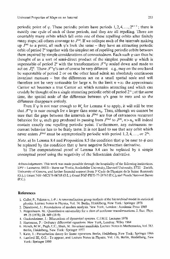
Universal Properties of Maps on an Interval 253
periodic point of ~p. These periodic points have periods 1, 2, 4 . . . . , 2 " -1 ; there is exactly one cycle of each of these periods, and they are all repelling. There are countably many orbits which fall onto one of these repelling orbits after finitely many steps ; all others converge to J("). I f we collapse each of the intervals making up J(") to a point, all such tp's look the same - they have an at tracting periodic orbit of period 2" together with the simplest set of repelling periodic orbits between them required by simple considerations of connectedness. Each such ~ can thus be thought of as a sort of semi-direct p roduc t of the simplest possible q~ which is superstable of period 2" with the t ransformat ion ~--"~ scaled down and made to act on J~0 "). These Y"W's can of course be very different e.g., may on the one hand be superstable of period 2 or on the other hand admit an absolutely cont inuous invariant measure - but the differences act on a small spatial scale and will therefore not be very noticeable for large n. In the limit n--, oe the approximate Can to r set becomes a true Cantor set which remains at tracting and which can crudely be thought of as a single at tract ing periodic orbit of period 2 ~ ; at the same time, the spatial scale of the difference between ~/J's goes to zero and so the difference disappears entirely.
Even if tp is not near enough to W u for L e m m a 4 to apply, it will still be true that F ' h p is near enough for n larger than some n o. Thus, a l though we cannot be sure that the gaps between the intervals in j(,o) are free of extraneous recurrent behavior for ~p, each gap produced in passing from j(,o) to J("), n > n o will indeed contain exactly one repelling periodic point. Fur thermore, any extraneous re- current behavior has to be fairly tame. It is not hard to see that any orbit which never enters j(,o) must be asymptotically periodic with period 1, 2, 4 . . . . . or 2 "°.
Note. a) In L e m m a 8.4 and Proposi t ion 8.5 the condit ion that p be near to q5 can be replaced by the condit ion that ~p have negative Schwarzian derivative.
b) The computa t ional p roof of Lemma 8.4 can be replaced by a simple conceptual p roof using the negativity of the Schwarzian derivative.
Acknowledgements. This work was made possible through the hospitality of the following institutions. EPF - Lausanne, IHES - Bures sur Yvette, RockefeIler University, Harvard University, ETH - Zurich, University of Geneva, and further financial support from 3 e Cycle de Physique de la Suisse Romande (Oi.), Grant NSF-MCS 78-06718 (O.L.), Grant NSF-PHY-77-18762 (P.C.), and Fonds National Suisse Oo.c.).
References
1. Collet, P., Eckmann, J.-P.: A renormalization group analysis of the hierarchical model in statistical physics. Lecture Notes in Physics, Vol. 74. Berlin, Heidelberg, New York : Springer 1978
2. Dieudonn~, J. : Foundations of modern analysis. New York, London : Academic Press 1969 3. Feigenbaum, M.: Quantitative universality for a class of nonlinear transtbrmations. J. Stat. Phys.
19, 25 (1978); 21, 669 (1979) 4. Guckenheimer, J. : Bifurcations of dynamical systems. C.I.M.E. Lectures 1978 5. Hartmann, P. : Ordinary differential equations. New York, London: Wiley 1964 6. Hirsch, M.W., Pugh, C.C., Shub, M.: Invariant manifolds. Lecture Notes in Mathematics, Vol. 583.
Berlin, Heidelberg, New York: Springer 1977 7. Kato, T. : Perturbation theory for linear operators. Berlin, Heidelberg, New York : Springer 1966 8. Lanford III, O.E. : To appear, and Lecture Notes in Physics, Vol. 116, Berlin, Heidelberg, New
York: Springer 1980
254 P. Cotlet, J.-P. Eckmann, and O. E. Lanford III
9. May, R.M. : Simple mathematical models with very complicated dynamics. Nature 261, 259 467 (1976)
10. Misiurewicz, M. : Structure of mappings of the interval with zero entropy. Preprint I.H.E.S. (t978) 11. Misiurewicz, M. : Absolutely continuous measures for certain maps on an interval. Preprint
I.H.E.S./M/79/293 (1979) 12. Singer, D.: Stable orbits and bifurcations of maps of the interval. S.I.A.M.J. Appl. Math. 35,
260-267 (t978) 13. Stefan, P.: A theorem of Sharkovskii on the existence of periodic orbits of continuous en-
domorphisms of the real line. Commun. Math. Phys. 54, 237-248 (1977) 14. Cotlet, P., Eckmann, J.-P.: Iterated maps on the interval as dynamical systems. Progress in Physics.
Birkh~iuser Boston t980 (to appear)
Communicated by D. Ruelle
Received February 28, 1980
Note added in proof. An alternate proof of existence of a fixed point for e = 1 has been provided by M. Campanino, H. Epstein, D. Ruetle, (to appear). For the extension of the results to multidimensional dissipative maps, see P. Collet, J.-P. Eckmann, H. Koch, J. Stat. Phys. (to appear)