communication complexity - department of computer...

Communication Complexity

Alexander A. Razborov

Abstract. When I was asked to write a contribution for this book aboutsomething related to my research, I immediately thought of CommunicationComplexity. This relatively simple but extremely beautiful and importantsub-area of Complexity Theory studies the amount of communication neededfor several distributed parties to learn something new. We will review thebasic communication model and some of the classical results known for it,sometimes even with proofs. Then we will consider a variant in which theplayers are allowed to flip fair unbiased coins. We will finish with a brief reviewof more sophisticated models in which our current state of knowledge is lessthan satisfactory. All our definitions, statements and proofs are completelyelementary, and yet we will state several open problems that have evadedstrong researchers for decades.

1 Introduction

As the reader can guess from the name, Communication Complexity studiesways to arrange communication between several parties so that at the end ofthe day they learn what they are supposed to learn, and to do this in the mostefficient, or least complex way. This theory constitutes a small but, as we willsee below, very beautiful and important part of Complexity Theory which,in turn, is situated right at the intersection of Mathematics and TheoreticalComputer Science. For this reason I would like to begin with a few wordsabout Complexity Theory in general and what kind of problems researchers

Alexander A. RazborovDepartment of Computer Science, The University of Chicago, 1100 East 58th Street,Chicago, IL 60637, USA; and Steklov Mathematical Institute, Moscow, Russia,117 966. e-mail: [email protected]

1

2 Alexander A. Razborov

are studying there. The reader favoring concrete mathematical content overphilosophy should feel free to skip the introduction and go directly to Sec-tion 2.

Complexity Theory is interested in problems that in most cases canroughly be described as follows. Assume that we have a task T that wewant to accomplish. In most cases this involves one or more computers doingsomething, but it is not absolutely necessary. There can be many differentways to achieve our goal, and we denote the whole set of possibilities byPT . Depending on the context, elements of PT can be called algorithms or,as in our article, protocols. In most cases of interest it is trivial that thereis at least one algorithm/protocol to solve T , that is the set PT is non-empty.

While all P ∈ PT solve our original task T , not all solutions are bornequal. Some of them may be better than others because they are shorter,consume less resources, are simpler, or for any other reason. The main idea ofmathematical complexity theory is to try to capture our intuitive preferencesby a positive real-valued function µ(P ) (P ∈ PT ) called complexity measurewith the idea that the smaller µ(P ) is, the better is our solution P . Ideally,we would like to find the best solution P ∈ PT , that is the one minimizing thefunction µ(P ). This is usually very hard to do, so in most cases researcherstry to approach this ideal from two opposite sides as follows:

• try to find “reasonably good” solutions P ∈ PT for which µ(P ) may per-haps not be minimal, but still is “small enough”. Results of this sort arecalled “upper bounds” as what we are trying to do mathematically is toprove upper bounds on the quantity

minP∈PT

µ(P )

that (not surprisingly!) is called the complexity of the task T .• Lower bound problems: for some a ∈ R we try to show that µ(P ) ≥ a for

any P , that is that there is no solution in PT better than a. The classPT is usually very rich and solutions P ∈ PT can be based upon verydifferent and often unexpected ideas. We have to take care of all of themwith a uniform argument. This is why lower bound problems are amongstthe most difficult in modern mathematics, and the overwhelming majorityof them is still wide open.

All right, it is a good time for some examples. A great deal of mathe-matical olympiad problems are actually of complexity flavor even if it is notimmediately clear from their statements.

Communication Complexity 3

You have 7 (or 2010, n, . . . ) coins, of which 3 (at most 100, anunknown number, . . . ) are counterfeit and are heavier (are lighter,weigh one ounce more, . . . ) than the others. You also have a scalethat can weigh (compare, . . . ) as many coins as you like (compareat most 10 coins, . . . ). How many weighings do you need to identifyall (one counterfeit, . . . ) coin(s)?

These are typical complexity problems, and they are very much related towhat is called sorting networks and algorithms in the literature. The task Tis to identify counterfeit coins, and PT consists of all sequences of weighingsthat allow us to accomplish it. The complexity measure µ(P ) is just thelength of P (that is, the number of weighings used).

You have a number (polynomial, expression, . . . ), how many addi-tions/ multiplications do you need to build it from certain primitiveexpressions?

Not only is this a complexity problem, but also a paradigmatic one. Can youdescribe T,PT and µ in this case? And, by the way, if you think that the“school” method of multiplying integers is optimal in terms of the number ofdigit operations used, then this is incorrect. It was repeatedly improved in thework of Karatsuba [13], Toom and Cook (1966), Schonhage and Strassen [26]and Furer [11], and it is still open whether Furer’s algorithm is the optimalone. It should be noted, however, that these advanced algorithms becomemore efficient than the “school” algorithm only for rather large numbers(typically at least several thousand digits long).

If you have heard of the famous P vs. NP question (otherwise I recom-mend to check out e.g. http://www.claymath.org/millennium/P_vs_NP),it is another complexity problem. Here T is the task of solving a fixed NP-complete problem, e.g. SATISFIABILITY, and PT is the class of all deter-ministic algorithms fulfilling this task.

In this article we will discuss complexity problems involving communi-cation. The model is very clean and easy to explain, but quite soon wewill plunge into extremely interesting questions that have been open fordecades. . . And, even if we will not have time to discuss it here at length,the ideas and methods of communication complexity penetrate today virtu-ally all other branches of complexity theory.

Almost all material contained in our article (and a lot more) can be foundin the classical book [17]. The recent textbook [3] on Computational Com-plexity has Chapter 13 devoted entirely to Communication Complexity, andyou can find its applications in many other places all over the book.

Since the text involves quite a bit of notation, some of it is collectedtogether at the end of the article, along with a brief description.


2 The Basic Model

The basic (deterministic) model was introduced in the seminal paper by Yao[27]. We have two players traditionally (cf. the remark below) called Alice andBob, we have finite sets X,Y and we have a function f : X × Y −→ 0, 1.The task Tf facing Alice and Bob is to evaluate f(x, y) for a given input(x, y). The complication that makes things interesting is that Alice holds thefirst part x ∈ X of their shared input, while Bob holds another part y ∈ Y .They do have a two-sided communication channel, but it is something like atransatlantic phone line or a beam communicator with a spacecraft orbitingMars. Communication is expensive, and Alice and Bob are trying to minimizethe number of bits exchanged while computing f(x, y).

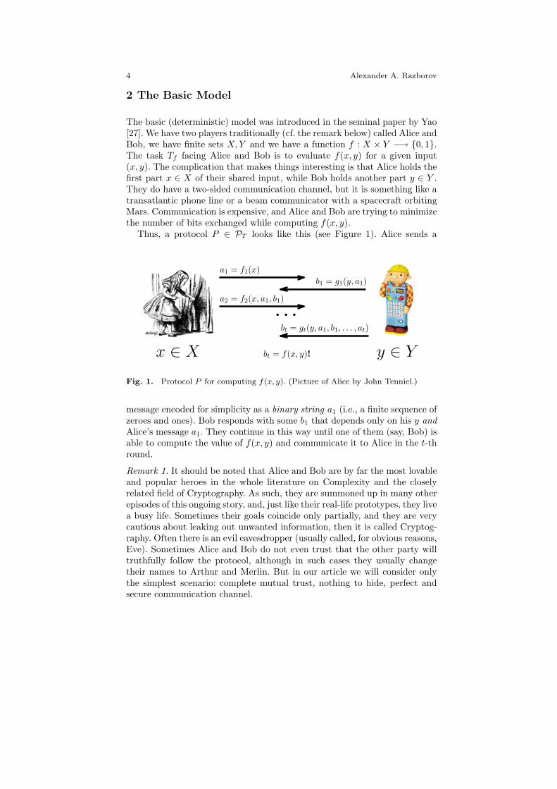
Thus, a protocol P ∈ PT looks like this (see Figure 1). Alice sends a

All material contained in our article (and much more) can be found in theclassical monograph [1]. The recent textbook on Computational Complexity[2] has the whole Chapter 13 devoted entirely to Communication Complexity,and you can find its applications in many other paces all over the book.

After this introduction, let us do something slightly more technical. Thebasic (deterministic) model was introduced in the seminal paper by Yao [3].We have two players traditionally called Alice and Bob, we have finite setsX,Y and we have a function f : X !Y "# 0, 1. The task Tf facing Aliceand Bob is to evaluate f on a given input (x, y): f(x, y) =? The complicationthat makes things interesting is that Alice holds the first part x $ X of theirshared input, while Bob holds another part y $ Y . They do have a two-sidedcommunication channel, but it is something like a transatlantic phone lineor beam communicators with a spacecraft orbiting Mars. Communicationis expensive, and Alice and Bob are trying to minimize the number of bitsexchanged while computing f(x, y).

Thus, a protocol P $ PT looks like this (see Figure 1). Alice sends a

a1 = f1(x)

x $ X y $ Y

b1 = g1(y, a1)

a2 = f2(x, a1, b1)

. . .bt = gt(y, a1, b1, . . . , at)

bt = f(x, y)!

Figure 1: Protocol P for computing f(x, y)

message encoded for simplicity as a binary string a1 $ 0, 1!. Bob respondswith some b1 that depends only on his y and Alice’s message a1. Theycontinue in this way until one of them (say, Bob) is able to compute thevalue of f(x, y) and communicate it to Alice in the tth round.

In this definition we deliberately left a few things imprecise. For example,is the length of Alice’s message a1 fixed or is it allowed to depend on x?Likewise, can the number of rounds t depend on x and y and, if so, howcan Alice know that Bob’s message bt is actually the last one and alreadygives the final answer? It turns out, however, that all these details are veryinessential, and the reader can fill them any way he likes – this will change

3

Fig. 1. Protocol P for computing f(x, y). (Picture of Alice by John Tenniel.)

message encoded for simplicity as a binary string a1 (i.e., a finite sequence ofzeroes and ones). Bob responds with some b1 that depends only on his y andAlice’s message a1. They continue in this way until one of them (say, Bob) isable to compute the value of f(x, y) and communicate it to Alice in the t-thround.

Remark 1. It should be noted that Alice and Bob are by far the most lovableand popular heroes in the whole literature on Complexity and the closelyrelated field of Cryptography. As such, they are summoned up in many otherepisodes of this ongoing story, and, just like their real-life prototypes, they livea busy life. Sometimes their goals coincide only partially, and they are verycautious about leaking out unwanted information, then it is called Cryptog-raphy. Often there is an evil eavesdropper (usually called, for obvious reasons,Eve). Sometimes Alice and Bob do not even trust that the other party willtruthfully follow the protocol, although in such cases they usually changetheir names to Arthur and Merlin. But in our article we will consider onlythe simplest scenario: complete mutual trust, nothing to hide, perfect andsecure communication channel.


In this definition we deliberately left a few things imprecise. For example,is the length of Alice’s message a1 fixed or is it allowed to depend on x?Likewise, can the number of rounds t depend on x and y and, if so, howcan Alice know that Bob’s message bt is actually the last one and alreadygives the final answer? It turns out, however, that all these details are veryinessential, and the reader can fill them any way he or she likes — this willchange the complexity only by a small additive factor.

How to measure the complexity µ(P ) of this protocol P? There are severalways of doing this, all of them reasonable. In this article we will focus only onthe most important and popular model called worst-case complexity. For anygiven input (x, y) ∈ X×Y we define the cost of the protocol P on this inputas the total number of bits1 |a1|+ |b1|+ . . .+ |bt| exchanged on this input (cf.Figure 1). And then we define the complexity (that, for historical reasons, isalso called cost in this case) cost(P ) of the protocol P as the maximal cost ofP over all inputs (x, y) ∈ X×Y . Finally, the communication complexity C(f)of (computing) the function f : X × Y −→ 0, 1 is defined as the minimumminP∈Pf cost(P ) taken over all legitimate protocols P , i.e., those protocolsthat correctly output the value f(x, y) for all possible inputs. We would liketo be able to compute C(f) for “interesting” functions f , or at least get goodestimates for it.

The first obvious remark is that

C(f) ≤ dlog2 |X|e+ 1 (1)

for any problem2 f . The protocol of this cost is very simple: Alice encodes herinput x as a binary string of length dlog2 |X|e using any injective encodingf1 : X −→ 0, 1dlog2 |X|e and sends a1 = f1(x) to Bob. Then Bob decodesthe message (we assume that the encoding scheme f1 is known to both partiesin advance!) and sends the answer f(f−1

1 (a1), y) back to Alice.Surprisingly, there are only very few interesting functions f for which we

can do significantly better than (1) in the basic model. One example that issort of trivial is this. Assume that X and Y consist of integers not exceedingsome fixed N : X = Y = 1, 2, . . . , N. Alice and Bob want to computethe 0, 1-valued function fN (x, y) that outputs 1 if and only if x + y isdivisible by 2010. A much more economical way to solve this problem wouldbe for Alice to send to Bob not her whole input x, but only its remainderx mod 2010. Clearly, this still will be sufficient for Bob to compute x + ymod 2010 (and hence also fN (x, y)), and the cost of this protocol is onlydlog2 2010e+ 1 (= 12). Thus,

C(fN ) ≤ dlog2 2010e+ 1 . (2)

1 |a| is the length of the binary word a.2 Note that complexity theorists often identify functions f with computational prob-lems they naturally represent. For example, the equality function EQN defined belowis also viewed as the problem of checking if two given strings are equal.


Now, complexity theorists are lazy people, and not very good at elementaryarithmetic. What is really remarkable about the right-hand side of (2) is thatit represents some absolute constant that magically does not depend on theinput size at all! Thus, instead of calculating this expression, we prefer tostress this fact using the mathematical big-O notation and write (2) in thesimpler, even if weaker, form

C(fN ) ≤ O(1) .

This means that there exists a positive universal constant K > 0 that anyoneinterested can (usually) extract from the proof such that for all N we haveC(fN ) ≤ K ·1 = K. Likewise, C(fN ) ≤ O(log2 N) would mean that C(fN ) ≤K log2 N etc. We will extensively use this standard3 notation in our article.

Let us now consider a simpler problem that looks as fundamental as itcan only be. We assume that X = Y are equal sets of cardinality N . Thereader may assume that this set is again 1, 2, . . . , N, but now this is notimportant. The equality function EQN is defined by letting EQN (x, y) = 1if and only if x = y. In other words, Alice and Bob want to check if theirfiles, databases etc. are equal, which is clearly an extremely important taskin many applications.

We can of course apply the trivial bound (1), that is, Alice can simplytransmit her whole input x to Bob. But can we save even a little bit overthis trivial protocol? At this point I would like to strongly recommend youto put this book aside for a while and try out a few ideas toward this goal.That would really help to better appreciate what will follow.

3 We should warn the reader that in most texts this notation is used with the equal-ity, rather than inequality, sign, i.e., C(fN ) = O(log2 N) in the previous example.However, we see numerous issues with this usage and in particular it becomes ratherawkward and uninformative in complicated cases.


3 Lower Bounds

Did you have any luck? Well, you do not have to be distressed by the resultsince it turns out that the bound (1) actually can not be improved, that is anyprotocol for EQN must have cost at least log2 N . This was proven in the sameseminal paper by Yao [27], and many ideas from that paper determined thedevelopment of Complexity Theory for several decades to follow. Let us seehow the proof goes, the argument is not very difficult but it is very instructive.

We are given a protocol P of the form shown on Figure 1, and we knowthat upon executing this protocol Bob knows EQN (x, y). We should somehowconclude that cost(P ) ≥ log2 N .

One very common mistake often made by new players in the lower boundsgame is that they begin telling P what it “ought to do”, that is, consciously orunconsciously, begin making assumptions about the best protocol P based onthe good common sense. In our situation a typical argument would start offby something like “let i be the first bit in the binary representation of x and ythat the protocol P compares”. “Arguments” like this are dead wrong since itis not clear at all that the best protocol should proceed in this way, or, to thatend, in any other way we would consider “intelligent”. Complexity Theoryis full of ingenious algorithms and protocols that do something strange andapparently irrelevant almost all the way down, and only at the end of theday they conjure the required answer like a rabbit from the hat — we will seeone good example below. The beauty and the curse of Complexity Theoryis that we should take care of all protocols with seemingly irrational (in ouropinion) behavior all the same, and in our particular case we may not assumeanything about the protocol P besides what is explicitly shown on Figure 1.

Equipped with this word of warning, let us follow Yao and see what usefulinformation we still can retrieve from Figure 1 alone. Note that although weare currently interested in the case f = EQN , Yao’s argument is more generaland can be applied to any function f . Thus, for the time being we assumethat f is an arbitrary function whose communication complexity we want toestimate; we will return to EQN in Corollary 2.

The first thing to do is to introduce an extremely useful concept of a his-tory or a transcript: this is the whole sequence (a1, b1, . . . , at, bt) of messagesexchanged by Alice and Bob during the execution of the protocol on someparticular input. This notion is very broad and general and is successfullyapplied in many different situations, not only in communication complexity.

Next, we can observe that there are at most 2cost(P ) different histories asthere are only that many different strings4 of length cost(P ). Given any fixedhistory h, we can form the set Rh of all those inputs (x, y) that lead to thishistory. Let us see what we can say about these sets.

4 Depending on finer details of the model, histories may have different length, theplacement of commas can be also important etc. that might result in a slight increaseof this number. But remember that we are lazy and prefer to ignore small additive,or even multiplicative factors.


First of all, every input (x, y) leads to one and only one history. This meansthat the collection Rh forms a partition or disjoint covering of the set ofall inputs X × Y :

X × Y =[

h∈HRh , (3)

where H is the set of all possible histories. The notationS

stands for disjointunion and simultaneously means two different things: that X×Y =

Sh∈H Rh,

and that Rh ∩Rh0 = ∅ for any two different histories h 6= h0 ∈ H.Now, every history h includes the value of the function f(x, y) as Bob’s

last message bt. That is, any Rh is an f-monochromatic set, which meansthat either f(x, y) = 0 for all (x, y) ∈ Rh or f(x, y) = 1 for all such (x, y).

Finally, and this is very crucial, every Rh is a combinatorial rectangle(or simply a rectangle), that is it has the form Rh = Xh × Yh for someXh ⊆ X, Yh ⊆ Y . In order to understand why, we should simply expand thesentence “(x, y) leads to the history (a1, b1, . . . , at, bt)”. Looking again at Fig-ure 1, we see that this is equivalent to the set of “constraints” on (x, y) shownthere: f1(x) = a1, g1(y, a1) = b1, f2(x, a1, b1) = a2, . . . , gt(y, a1, . . . , at) = bt.Let us observe that odd-numbered constraints in this chain depend only onx (remember that h is fixed!); let us denote by Xh the set of those x ∈ Xthat satisfy all these constraints. Likewise, let Yh be the set of all y ∈ Ysatisfying even-numbered constraints. Then it is easy to see that we preciselyhave Rh = Xh × Yh!

Let us summarize a little bit. For any protocol P solving our problemf : X × Y −→ 0, 1, we have been able to chop X × Y into at most 2cost(P )

pieces so that each such piece is an f -monochromatic combinatorial rectangle.Re-phrasing it a little bit differently, let us denote by χ(f) (yes, complexitytheorists love to introduce complexity measures!) the minimal number of f -monochromatic rectangles into which we can partition X × Y . We thus haveproved, up to a small multiplicative constant that may depend on finer detailsof the model:

Theorem 1 (Yao). C(f) ≥ log2 χ(f). ut

Let us return to our particular case f = EQN . All f -monochromatic com-binatorial rectangles can be classified into 0-rectangles (i.e., those on whichf is identically 0) and 1-rectangles. The function EQN has many large 0-rectangles. (Can you find one?) But all its 1-rectangles are very primitive,namely every such rectangle consists of just one point (x, x). Therefore, in or-der to cover even the “diagonal” points (x, x) | x ∈ X , one needs N different1-rectangles, which proves χ(EQN ) ≥ N . Combining this with Theorem 1,we get the result we were looking for:

Corollary 2. C(EQN ) ≥ log2 N . ut

Exercise 1. The function LEN (less-or-equal) is defined on 1, 2, . . . , N ×1, 2, . . . , N as

LEN (x, y) = 1 iff x ≤ y .


Prove that C(LEN ) ≥ log2 N .

Exercise 2 (difficult). The function DISJn is defined on 0, 1n × 0, 1n

asDISJn(x, y) = 1 iff ∀i ≤ n : xi = 0 ∨ yi = 0 ,

that is, the sets of positions where the strings x and y have a 1 are disjoint.Prove that C(DISJn) ≥ Ω(n).

(Here Ω is yet another notation that complexity theorists love. It is dual to“big-O” and means that there exists a constant ε > 0 that we do not wantto compute such that C(DISJn) ≥ εn for all n.)

Hint. How many points (x, y) with DISJn(x, y) = 1 do we have? And whatis the maximal size of a 1-rectangle?

4 Are These Bounds Tight?

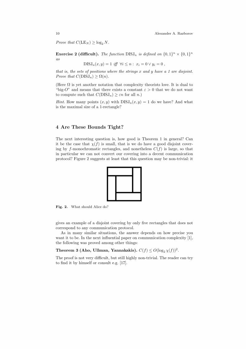
The next interesting question is, how good is Theorem 1 in general? Canit be the case that χ(f) is small, that is we do have a good disjoint cover-ing by f -monochromatic rectangles, and nonetheless C(f) is large, so thatin particular we can not convert our covering into a decent communicationprotocol? Figure 2 suggests at least that this question may be non-trivial: it

4

Fig. 2. What should Alice do?

gives an example of a disjoint covering by only five rectangles that does notcorrespond to any communication protocol.

As in many similar situations, the answer depends on how precise youwant it to be. In the next influential paper on communication complexity [1],the following was proved among other things:

Theorem 3 (Aho, Ullman, Yannakakis). C(f) ≤ O(log2 χ(f))2.

The proof is not very difficult, but still highly non-trivial. The reader can tryto find it by himself or consult e.g. [17].


Can we remove the square in Theorem 3? For almost thirty years that haveelapsed since the paper [1], many people have tried to resolve the questionone or the other way. But it has resisted all efforts so far. . .

Open Problem 1. Is it true that C(f) ≤ O(log2 χ(f))?

Besides Theorem 3, the paper [1] contains many other great things per-taining to the so-called non-deterministic communication complexity. In thismodel, Alice and Bob are also given access to a shared string z not deter-mined by the protocol (whence comes the name) but rather given to themby a third all-powerful party trying to convince them that f(x, y) = 1. Werequire that a convincing string z exists if and only if f(x, y) is indeed equalto 1, and we note that in this definition we give up on the symmetry of an-swers 0 and 1. Due to lack of space we discuss this important concept onlyvery briefly, and complexity measures we mention during the discussion willhardly be used in the rest of the article.

Define t(f) in the same way as χ(f), only now we allow the monochromaticrectangles in our cover to overlap with each other. Clearly, t(f) ≤ χ(f), butit turns out that the bound of Theorem 3 still holds: C(f) ≤ O(log2 t(f))2.On the other hand, there are examples for which C(f) is of order (log2 t(f))2.This means that the (negative) solution to the analogue of Problem 1 for notnecessarily disjoint coverings is known.

Let χ0(f) and χ1(f) be defined similarly to χ(f), except now we are in-terested in a disjoint rectangular covering of only those inputs that yieldvalue 0 (respectively, value 1); note that χ(f) = χ0(f) + χ1(f). Thenstill C(f) ≤ O(log2 χ1(f))2 and (by symmetry) C(f) ≤ O(log2 χ0(f))2.By analogy, we can also define the quantities t0(f) and t1(f) (the non-deterministic communication complexity we mentioned above turns out tobe equal to log2 t1(f)). We cannot get any reasonable (say, better than expo-nential) bound on C(f) in terms of log2 t1(f) or log2 t0(f) only: for example,t0(EQN ) ≤ O(log2 N) (why?) while, as we already know, C(EQN ) ≥ log2 N .In conclusion, there is no good bound on the deterministic communicationcomplexity in terms of the non-deterministic one, but such a bound becomespossible if we know that the non-deterministic communication complexity ofthe negated function is also small.

The next landmark paper we want to discuss is the paper [19] that intro-duced to the area algebraic methods. So far all our methods for estimatingχ(f) from below (Corollary 2 and Exercises 1 and 2) were based on the sameunsophisticated idea: select “many” inputs D ⊆ X × Y such that every f -monochromatic rectangle R may cover only “a few” of them, and then applythe pigeonhole principle. This method does not use anyhow that the covering(3) is disjoint or, in other words, it can be equally well applied to boundingfrom below t(f) as well as χ(f). Is it good or bad? The answer depends. It isalways nice, of course, to be able to prove more results, like lower bounds onthe non-deterministic communication complexity log2 t1(f), with the same


shot. But sometimes it turns out that the quantity analogous to t(f) is al-ways small and, thus, if we still want to bound χ(f) from below, we mustuse methods that “feel” the difference between these two concepts. The ranklower bound of Mehlhorn and Schmidt [19] was the first of such methods.

We will need the most basic concepts from linear algebra like a matrix Mor its rank rk(M), as well as their simplest properties. If the reader is not yetfamiliar with them, then this is a perfect opportunity to grab any textbookin basic linear algebra and read a couple of chapters from it. You will haveto learn this eventually anyway, but now you will also immediately see quitean unexpected and interesting application of these abstract things.

Given any function f : X × Y −→ 0, 1, we can arrange its values in theform of the communication matrix Mf . Rows of this matrix are enumeratedby elements of X, its columns are enumerated by elements of Y (the order isunimportant in both cases), and in the intersection of the x-th row and they-th column we write f(x, y). The following result relates two quite differentworlds, those of combinatorics and linear algebra.

Theorem 4. χ(f) ≥ rk(Mf ).

Proof. The proof is remarkably simple. Let R1, . . . , Rχ be disjoint 1-rectanglescovering all (x, y) with f(x, y) = 1 so that χ ≤ χ(f). Let fi : X×Y −→ 0, 1be the characteristic function of the rectangle Ri, i.e., fi(x, y) = 1 if andonly if (x, y) ∈ Ri, and let Mi = Mfi be its communication matrix. Thenrk(Mi) = 1 (why?) and Mf =

Pχi=1 Mi. Therefore, rk(Mf ) ≤

Pχi=1 rk(Mi) ≤

χ ≤ χ(f). ut

In order to fully appreciate how useful Theorem 4 is, let us note thatMEQN

is the identity matrix (we tacitly assume that if X = Y then theorders on rows and columns are consistent) and, therefore, rk(MEQN

) = N .This immediately gives Corollary 2. MLEN is the upper triangular matrix,and therefore we also have rk(MLEN ) = N . Exercise 1 follows. It does requirea little bit of thinking to see that the communication matrix MDISJn is non-singular, that is rk(MDISJn) = 2n. But once it is done, we immediately obtainC(DISJn) ≥ n which is essentially tight by (1) and also stronger than whatwe could do with combinatorial methods in Exercise 2 (the Ω is gone).

How tight is the bound of Theorem 4? It had been conjectured for a whilethat perhaps χ(f) ≤ (rk(Mf ))O(1) or maybe even χ(f) ≤ O(rk(Mf )). In thisform the conjecture was disproved in the series of papers [2, 23, 21]. But itis still possible and plausible that, say,

χ(f) ≤ 2O(log2 rk(Mf ))2 ;

note that in combination with Theorem 3 that would still give a highly non-trivial inequality C(f) ≤ O(log2 rk(Mf ))4.

Despite decades of research, we still do not know the answer, and weactually do not have a very good clue how to even approach this problemthat has become notoriously known as the Log-Rank Conjecture:


Open Problem 2 (Log-Rank Conjecture). Is it true that

χ(f) ≤ 2(log2 rk(Mf ))O(1)?

Equivalently (by Theorems 1, 3), is it true that C(f) ≤ (log2 rk(Mf ))O(1)?

5 Probabilistic Models

This is all we wanted to say about the basic model of communication com-plexity. Even more fascinating and difficult problems arise when we introducesome variations. The most important of them, and the only one that we treatin sufficient detail in the rest of this article, is the model of probabilistic com-munication complexity.

Assume that Alice and Bob are now slightly less ambitious and agree totolerate some small probability of error when computing the value of f(x, y) ∈0, 1. Both of them are equipped with a fair unbiased coin (scientificallyknown as generator of random bits) that they can toss during the executionof the protocol, and adjust the messages they send to each other according tothe result. Everything else is the same (that is, as on Figure 1) but we have tospecify what it means that the protocol P correctly computes the function f .

Fix an input (x, y) and assume that Alice and Bob together flip their coinsr times during the execution, which gives 2r possible outcomes of these cointosses. Some of them are good in the sense that Bob outputs the correct valuef(x, y), but some are bad and he errs. Let Good(x, y) be the set of all goodoutcomes, then the quantity

pxy =|Good(x, y)|

2r(4)

is for obvious reasons called the probability of success on the input (x, y).What do we want from it? There is a very simple protocol of cost 1 that

achieves pxy = 1/2: Bob simply tosses his coin and claims that its outcomeis f(x, y). Thus, we definitely want to demand that

pxy > 1/2 . (5)

But how well should the probability of success be separated from 1/2?It turns out that there are essentially only three different possibilities

(remember that we are lazy and do not care much about exact values ofour constants). In the most popular and important version we require thatpxy ≥ 2/3 for any input (x, y). The minimal cost of a probabilistic protocolthat meets this requirement is called bounded-error probabilistic communica-tion complexity of the function f and denoted by R(f). If for any input pair(x, y) we only require (5) then the model is called unbounded-error, and the


corresponding complexity measure is denoted by U(f). In the third model(that is less known and will not be considered in our article), we still require(5), but now Alice and Bob are also charged for coin tosses. This e.g. impliesthat in any protocol of cost O(log2 n), (5) automatically implies the betterbound px,y ≥ 1

2 + 1p(n) for some polynomial p(n).

Why, in the definition of R(f), did we request that pxy ≥ 2/3, not pxy ≥0.9999? By using quite a general technique called amplification, it can beshown not to be very important. Namely, assume that Alice and Bob have attheir disposal a protocol of cost R(f) that achieves pxy ≥ 2/3, they repeat itindependently 1000 times and output at the end the most frequent answer.Then the error probability of this repeated protocol of cost only 1000R(f)will not exceed 10−10. . . (In order to prove this statement, some knowledgeof elementary probability theory, like Chernoff bounds, is needed.)

Are coins really helpful for anything, that is are there any interesting prob-lems that can be more efficiently solved using randomization than withoutit? An ultimate answer to this question is provided by the following beautifulconstruction, usually attributed to Rabin and Yao, that has to be comparedwith Corollary 2.

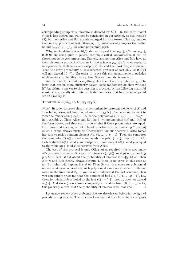
Theorem 5. R(EQN ) ≤ O(log2 log2 N).

Proof. In order to prove this, it is convenient to represent elements of X andY as binary strings of length n, where n = dlog2 Ne. Furthermore, we want toview the binary string x1x2 . . . xn as the polynomial x1 + x2ξ + . . . + xnξn−1

in a variable ξ. Thus, Alice and Bob hold two polynomials g(ξ) and h(ξ) ofthe form above, and they want to determine if these polynomials are equal.For doing that they agree beforehand on a fixed prime number p ∈ [3n, 6n](such a prime always exists by Chebyshev’s famous theorem). Alice tossesher coin to pick a random element ξ ∈ 0, 1, . . . , p− 1. Then she computesthe remainder (!) g(ξ) mod p and sends the pair (ξ, g(ξ) mod p) to Bob.Bob evaluates h(ξ) mod p and outputs 1 if and only if h(ξ) mod p is equalto the value g(ξ) mod p he received from Alice.

The cost of this protocol is only O(log2 n) as required: this is how manybits you need to transmit a pair of integers (ξ, g(ξ) mod p) not exceedingp ≤ O(n) each. What about the probability of success? If EQ(g, h) = 1 theng = h and Bob clearly always outputs 1, there is no error in this case atall. But what will happen if g 6= h? Then (h − g) is a non-zero polynomialof degree at most n. And any such polynomial can have at most n differentroots in the finite field Fp. If you do not understand the last sentence, thenyou can simply trust me that the number of bad ξ ∈ 0, 1, . . . , p − 1, i.e.,those for which Bob is fooled by the fact g(ξ) = h(ξ) mod p, does not exceedn ≤ p

3 . And since ξ was chosen completely at random from 0, 1, . . . , p− 1,this precisely means that the probability of success is at least 2/3. ut

Let us now review other problems that we already saw before in the light ofprobabilistic protocols. The function less-or-equal from Exercise 1 also gives


in to such protocols: R(LEN ) ≤ O(log2 log2 N), although the proof is waymore complicated than for equality [17, Exercise 3.18]. On the other hand,randomization does not help much for computing the disjointness function[4, 12, 24]:

Theorem 6. R(DISJn) ≥ Ω(n).

The proof is too complicated to discuss here. It becomes slightly easier foranother important function, inner product mod 2, that we now describe.

Given x, y ∈ 0, 1n, we consider, like in the case of disjointness, the set ofall indices i for which xi = 1 and yi = 1. Then IPn(x, y) = 1 if the cardinalityof this set is odd, and IPn(x, y) = 0 if it is even. Chor and Goldreich [9] provedthe following:

Theorem 7. R(IPn) ≥ Ω(n).

The full proof is still too difficult to be included here, but we would like tohighlight its main idea.

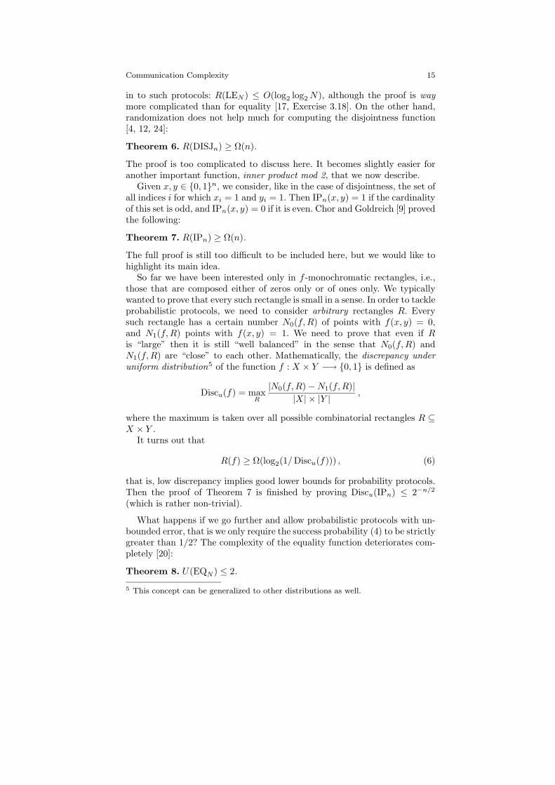
So far we have been interested only in f -monochromatic rectangles, i.e.,those that are composed either of zeros only or of ones only. We typicallywanted to prove that every such rectangle is small in a sense. In order to tackleprobabilistic protocols, we need to consider arbitrary rectangles R. Everysuch rectangle has a certain number N0(f,R) of points with f(x, y) = 0,and N1(f,R) points with f(x, y) = 1. We need to prove that even if Ris “large” then it is still “well balanced” in the sense that N0(f,R) andN1(f,R) are “close” to each other. Mathematically, the discrepancy underuniform distribution5 of the function f : X × Y −→ 0, 1 is defined as

Discu(f) = maxR

|N0(f,R)−N1(f,R)||X|× |Y | ,

where the maximum is taken over all possible combinatorial rectangles R ⊆X × Y .

It turns out that

R(f) ≥ Ω(log2(1/Discu(f))) , (6)

that is, low discrepancy implies good lower bounds for probability protocols.Then the proof of Theorem 7 is finished by proving Discu(IPn) ≤ 2−n/2

(which is rather non-trivial).

What happens if we go further and allow probabilistic protocols with un-bounded error, that is we only require the success probability (4) to be strictlygreater than 1/2? The complexity of the equality function deteriorates com-pletely [20]:

Theorem 8. U(EQN ) ≤ 2.

5 This concept can be generalized to other distributions as well.


The disjointness function also becomes easy, and this is a good exercise:

Exercise 3. Prove that U(DISJn) ≤ O(log2 n).

The inner product, however, still holds the fort:

Theorem 9. U(IPn) ≥ Ω(n).

This result by Forster [10] is extremely beautiful and ingenious, and it is oneof my favorites in the whole Complexity Theory.

6 Other Variations

We conclude with briefly mentioning a few modern directions in communica-tion complexity where current research is particularly active.

6.1 Quantum Communication Complexity

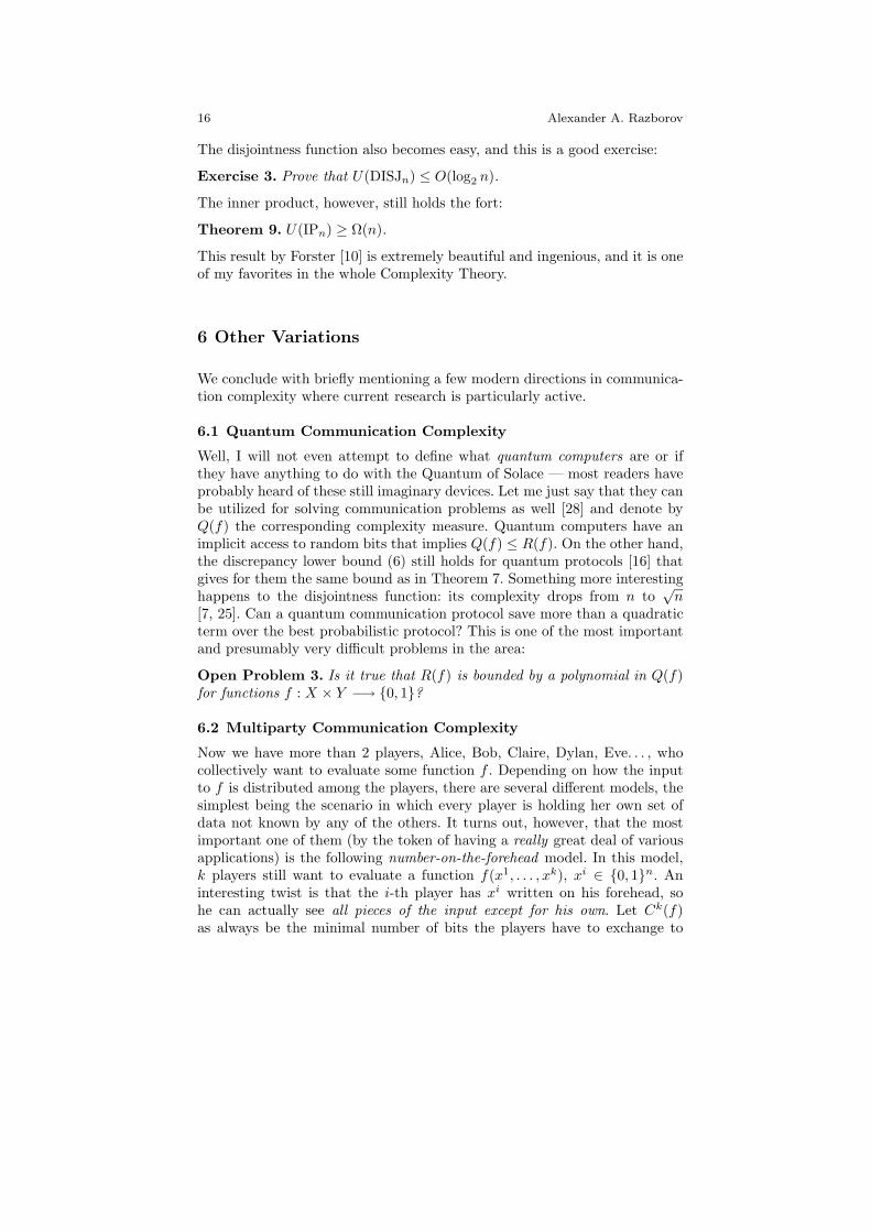
Well, I will not even attempt to define what quantum computers are or ifthey have anything to do with the Quantum of Solace — most readers haveprobably heard of these still imaginary devices. Let me just say that they canbe utilized for solving communication problems as well [28] and denote byQ(f) the corresponding complexity measure. Quantum computers have animplicit access to random bits that implies Q(f) ≤ R(f). On the other hand,the discrepancy lower bound (6) still holds for quantum protocols [16] thatgives for them the same bound as in Theorem 7. Something more interestinghappens to the disjointness function: its complexity drops from n to

√n

[7, 25]. Can a quantum communication protocol save more than a quadraticterm over the best probabilistic protocol? This is one of the most importantand presumably very difficult problems in the area:

Open Problem 3. Is it true that R(f) is bounded by a polynomial in Q(f)for functions f : X × Y −→ 0, 1?

6.2 Multiparty Communication Complexity

Now we have more than 2 players, Alice, Bob, Claire, Dylan, Eve. . . , whocollectively want to evaluate some function f . Depending on how the inputto f is distributed among the players, there are several different models, thesimplest being the scenario in which every player is holding her own set ofdata not known by any of the others. It turns out, however, that the mostimportant one of them (by the token of having a really great deal of variousapplications) is the following number-on-the-forehead model. In this model,k players still want to evaluate a function f(x1, . . . , xk), xi ∈ 0, 1n. Aninteresting twist is that the i-th player has xi written on his forehead, sohe can actually see all pieces of the input except for his own. Let Ck(f)as always be the minimal number of bits the players have to exchange to


correctly compute f(x1, . . . , xk); for simplicity we assume that every messageis broadcasted to all other players at once.

Our basic functions DISJn and IPn have “unique” natural generalizationsDISJk

n and IPkn in this model. (Can you fill in the details?) The classical paper

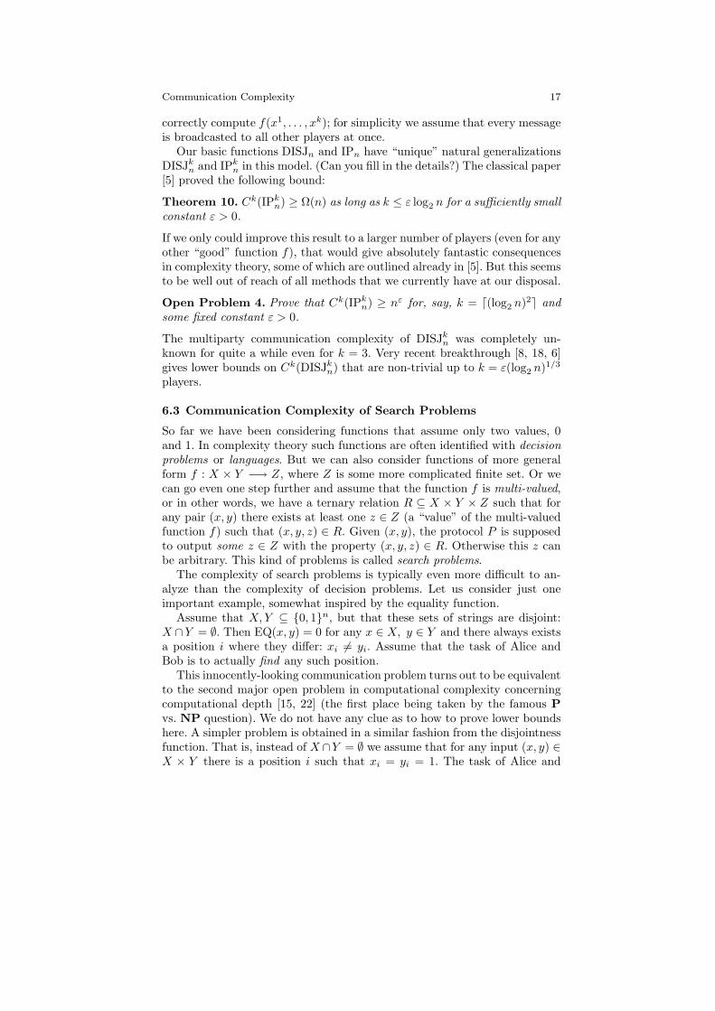
[5] proved the following bound:

Theorem 10. Ck(IPkn) ≥ Ω(n) as long as k ≤ ε log2 n for a sufficiently small

constant ε > 0.

If we only could improve this result to a larger number of players (even for anyother “good” function f), that would give absolutely fantastic consequencesin complexity theory, some of which are outlined already in [5]. But this seemsto be well out of reach of all methods that we currently have at our disposal.

Open Problem 4. Prove that Ck(IPkn) ≥ nε for, say, k = d(log2 n)2e and

some fixed constant ε > 0.

The multiparty communication complexity of DISJkn was completely un-

known for quite a while even for k = 3. Very recent breakthrough [8, 18, 6]gives lower bounds on Ck(DISJk

n) that are non-trivial up to k = ε(log2 n)1/3

players.

6.3 Communication Complexity of Search Problems

So far we have been considering functions that assume only two values, 0and 1. In complexity theory such functions are often identified with decisionproblems or languages. But we can also consider functions of more generalform f : X × Y −→ Z, where Z is some more complicated finite set. Or wecan go even one step further and assume that the function f is multi-valued,or in other words, we have a ternary relation R ⊆ X × Y × Z such that forany pair (x, y) there exists at least one z ∈ Z (a “value” of the multi-valuedfunction f) such that (x, y, z) ∈ R. Given (x, y), the protocol P is supposedto output some z ∈ Z with the property (x, y, z) ∈ R. Otherwise this z canbe arbitrary. This kind of problems is called search problems.

The complexity of search problems is typically even more difficult to an-alyze than the complexity of decision problems. Let us consider just oneimportant example, somewhat inspired by the equality function.

Assume that X,Y ⊆ 0, 1n, but that these sets of strings are disjoint:X ∩Y = ∅. Then EQ(x, y) = 0 for any x ∈ X, y ∈ Y and there always existsa position i where they differ: xi 6= yi. Assume that the task of Alice andBob is to actually find any such position.

This innocently-looking communication problem turns out to be equivalentto the second major open problem in computational complexity concerningcomputational depth [15, 22] (the first place being taken by the famous Pvs. NP question). We do not have any clue as to how to prove lower boundshere. A simpler problem is obtained in a similar fashion from the disjointnessfunction. That is, instead of X ∩Y = ∅ we assume that for any input (x, y) ∈X × Y there is a position i such that xi = yi = 1. The task of Alice and


Bob is once again to exhibit any such i. Lower bounds for this problem wereindeed proved in [15, 22, 14], and they lead to very interesting consequencesabout the monotone circuit depth of Boolean functions.

7 Conclusion

In this article we tried to give some impression of how soon simple, elementaryand innocent questions turn into open problems that have been challenging usfor decades. There are even more such challenges in the field of computationalcomplexity, and we are in the need of young and creative minds to answerthese challenges. If this article has encouraged at least some of the readersto look more closely into this fascinating subject, the author considers itspurpose fulfilled in its entirety.

List of Notation

Since this text uses quite a bit of notation, some of the most importantnotations are collected here together with a brief description, as well as thepage of first appearance.

Complexity Measures

cost(P ) cost of protocol P — maximal number of bits to transmit in order tocalculate the value of a function on any input (x, y) using protocolP 5

C(f) (worst-case) communication complexity of function f — minimalcost of any protocol computing f 5

χ(f) partition number of function f — minimal number of pairwise dis-joint f -monochromatic rectangles covering domain of f 9

t(f) cover number of function f — minimal number of f -monochromaticrectangles covering domain of f 11

χ0(f) minimal number of pairwise disjoint f -monochromatic rectanglescovering f−1(0) 11

χ1(f) minimal number of pairwise disjoint f -monochromatic rectanglescovering f−1(1) 11

t0(f) minimal number of f -monochromatic rectangles covering f−1(0)11

t1(f) minimal number of f -monochromatic rectangles covering f−1(1)(log2 t1(f) is called non-deterministic communication complexity off) 11


R(f) bounded-error probabilistic communication complexity of functionf — minimal cost of randomized protocol that assures that for anyinput the output will be correct with probability at least 2

3 13U(f) unbounded-error probabilistic communication complexity of func-

tion f — minimal cost of randomized protocol that assures thatfor any input the output will be correct with probability greaterthan 1

2 14Discu(f) discrepancy (under uniform distribution) of function f — maxi-

mal difference of how often values 0 and 1 occur on any rectangle(divided by |X × Y |, where X × Y is the domain of f) 15

Q(f) quantum communication complexity of function f — minimal costof quantum computer protocol evaluating f 16

Ck(f) multi-party communication complexity of function f — minimalnumber of bits that k players have to transmit in order to correctlycompute the value of f (in number-on-the-forehead model) 17

Binary Functions

EQN equality function — maps 1, 2, . . . , N × 1, 2, . . . , N to 0, 1with EQN (x, y) = 1 iff x = y 6

LEN less-or-equal function — maps 1, 2, . . . , N×1, 2, . . . , N to 0, 1with LEN (x, y) = 1 iff x ≤ y 9

DISJn disjointness function (“NAND”) — maps 0, 1n×0, 1n to 0, 1with DISJn(x, y) = 1 iff for all i ≤ n we have xi = 0 or yi = 0 10

IPn inner product mod 2 — maps 0, 1n × 0, 1n to 0, 1 withIPn(x, y) = 1 iff xi = yi = 1 for an odd number of indices i 15

DISJkn generalized disjointness function — maps (0, 1n)k to 0, 1 with

DISJkn(x1, . . . , xk) = 1 iff for all i ≤ n there exists ν ∈ 1, . . . , k

with xνi = 0 17

IPkn generalized inner product mod 2 — maps (0, 1n)k to 0, 1 with

IPkn(x1, . . . , xk) = 1 iff the number of indices i ≤ n for which x1

i =x2

i = . . . = xki = 1 is odd 17

Growth of Functions6 and Other

O(f(n)) g(n) ≤ O(f(n)) iff there is C > 0 with g(n) ≤ Cf(n) for all n 6Ω(f(n)) g(n) ≥ Ω(f(n)) iff there is ε > 0 with g(n) ≥ εf(n) for all n 10

dxe the smallest integer n ≥ x, for x ∈ R 5

6 The more traditional notation is g(n) = O(f(n)) and g(n) = Ω(f(n)); see alsofootnote 3.


References

[1] Alfred V. Aho, Jeffrey D. Ullman, and Mihalis Yannakakis, On notions of infor-mation transfer in VLSI circuits. In: Proceedings of the 15th ACM symposiumon the theory of computing, ACM Press, New York, 1983, 133–139.

[2] Noga Alon and Paul Seymour, A counterexample to the rank-coloring conjecture.Journal of Graph Theory 13 (1989), 523–525.

[3] Sanjeev Arora and Boaz Barak, Computational complexity: a modern approach.Cambridge University Press, Cambridge, 2009.

[4] Laszlo Babai, Peter Frankl, and Janos Simon, Complexity classes in commu-nication complexity theory. In: Proceedings of the 27th IEEE symposium onfoundations of computer science, IEEE Computer Society, Los Alamitos, 1986,337–347.

[5] Laszlo Babai, Noam Nisan, and Mario Szegedy, Multiparty protocols, pseudo-random generators for logspace, and time-space trade-offs. Journal of Computerand System Sciences 45 (1992), 204–232.

[6] Paul Beame and Dang-Trinh Huynh-Ngoc, Multiparty communication complex-ity and threshold circuit size of AC0. Technical Report TR08-082, ElectronicColloquium on Computational Complexity, 2008.

[7] Harry Buhrman, Richard Cleve, and Avi Wigderson, Quantum vs. classical com-munication and computation. In: Proceedings of the 30th ACM symposium onthe theory of computing, ACM Press, New York, 1998, 63–86; preliminary versionavailable at http://arxiv.org/abs/quant-ph/9802040 .

[8] Arkadev Chattopadhyay and Anil Ada, Multiparty communication complexityof disjointness. Technical Report TR08-002, Electronic Colloquium on Compu-tational Complexity, 2008.

[9] Benny Chor and Oded Goldreich, Unbiased bits from sources of weak randomnessand probabilistic communication complexity. SIAM Journal on Computing 17 2(1988), 230–261.

[10] Jurgen Forster, A linear lower bound on the unbounded error probabilistic com-munication complexity. Journal of Computer and System Sciences 65 4 (2002),612–625.

[11] Martin Furer, Faster integer multiplication. SIAM Journal on Computing 39 3(2009), 979–1005.

[12] Bala Kalyanasundaram and Georg Schnitger, The probabilistic communicationcomplexity of set intersection. SIAM Journal on Discrete Mathematics 5 4(1992), 545–557.

[13] Anatolii A. Karatsuba and Yuri P. Ofman, Multiplication of many-digital num-bers by automatic computers. Proceedings of the USSR Academy of Sciences145 (1962), 293–294.

[14] Mauricio Karchmer, Ran Raz, and Avi Wigderson, Super-logarithmic depthlower bounds via direct sum in communication complexity. Computational Com-plexity 5 (1995), 191–204.

[15] Mauricio Karchmer and Avi Wigderson, Monotone circuits for connectivityrequire super-logarithmic depth. SIAM Journal on Discrete Mathematics 3 2(1990), 255–265.

[16] Ilan Kremer, Quantum communication. Master’s thesis, Hebrew University,Jerusalem, 1995.

[17] Eyal Kushilevitz and Noam Nisan, Communication complexity. Cambridge Uni-versity Press, Cambridge, 1997.

[18] Troy Lee and Adi Shraibman, Disjointness is hard in the multiparty number-on-the-forehead model. Computational Complexity 18 2 (2009), 309–336.

[19] Kurt Mehlhorn and Erik M. Schmidt, Las Vegas is better than determinism inVLSI and distributive computing. In: Proceedings of the 14th ACM symposiumon the theory of computing, ACM Press, New York, 1982, 330–337.


[20] Ramamohan Paturi and Janos Simon, Probabilistic communication complexity.Journal of Computer and System Sciences 33 1 (1986), 106–123.

[21] Ran Raz and Boris Spieker, On the “log-rank”-conjecture in communicationcomplexity. Combinatorica 15 4 (1995), 567–588.

[22] Alexander Razborov, Applications of matrix methods to the theory of lowerbounds in computational complexity. Combinatorica 10 1 (1990), 81–93.

[23] Alexander Razborov, The gap between the chromatic number of a graph and therank of its adjacency matrix is superlinear. Discrete Mathematics 108 (1992),393–396.

[24] Alexander Razborov, On the distributional complexity of disjointness. Theoret-ical Computer Science 106 (1992), 385–390.

[25] Alexander Razborov, Quantum communication complexity of symmetric predi-cates. Izvestiya: Mathematics 67 1 (2003), 145–159.

[26] Arnold Schonhage and Volker Strassen, Schnelle Multiplikation großer Zahlen.Computing 7 (1971), 281–292.

[27] Andrew Yao, Some complexity questions related to distributive computing. In:Proceedings of the 11th ACM symposium on the theory of computing, ACMPress, New York, 1979, 209–213.

[28] Andrew Yao, Quantum circuit complexity. In: Proceedings of the 34th IEEEsymposium on foundations of computer science, IEEE Computer Society, LosAlamitos, 1993, 352–361.

communication complexity - department of computer...

Documents