combined electromagnetic and magnetometer data acquisition ... · combined electromagnetic and...

Combined Electromagnetic and Magnetometer Data Acquisition and Processing

Project UX-0208

Final Report 12/27/2002

V4.0 [updated 10/27/2004] Rob Siegel

GEO-CENTERS, Inc.

Report Documentation Page Form ApprovedOMB No. 0704-0188

Public reporting burden for the collection of information is estimated to average 1 hour per response, including the time for reviewing instructions, searching existing data sources, gathering andmaintaining the data needed, and completing and reviewing the collection of information. Send comments regarding this burden estimate or any other aspect of this collection of information,including suggestions for reducing this burden, to Washington Headquarters Services, Directorate for Information Operations and Reports, 1215 Jefferson Davis Highway, Suite 1204, ArlingtonVA 22202-4302. Respondents should be aware that notwithstanding any other provision of law, no person shall be subject to a penalty for failing to comply with a collection of information if itdoes not display a currently valid OMB control number.

1. REPORT DATE 27 OCT 2004 2. REPORT TYPE

3. DATES COVERED 00-00-2004 to 00-00-2004

4. TITLE AND SUBTITLE Combined Electromagnetic and Magnetometer Data Acquisition and Processing

5a. CONTRACT NUMBER

5b. GRANT NUMBER

5c. PROGRAM ELEMENT NUMBER

6. AUTHOR(S) 5d. PROJECT NUMBER

5e. TASK NUMBER

5f. WORK UNIT NUMBER

7. PERFORMING ORGANIZATION NAME(S) AND ADDRESS(ES) GEO-CENTERS, Inc,7 Wells Avenue,Newton,MA,02459

8. PERFORMING ORGANIZATIONREPORT NUMBER

9. SPONSORING/MONITORING AGENCY NAME(S) AND ADDRESS(ES) 10. SPONSOR/MONITOR’S ACRONYM(S)

11. SPONSOR/MONITOR’S REPORT NUMBER(S)

12. DISTRIBUTION/AVAILABILITY STATEMENT Approved for public release; distribution unlimited

13. SUPPLEMENTARY NOTES

14. ABSTRACT Under this project, GEO-CENTERS, Inc and the US Army Corps of Engineers developed anddemonstrated a proof-of-concept synchronized data acquisition and processing system (referred to as?Simultaneous Multisensor STOLS?) that allows simultaneous deployment of industrystandard GeonicsEM61 pulsed induction sensors and Geometrics 822A total field magnetometers on a singlevehicular-towed platform. New sampling electronics were designed and developed that interleave themagnetometer and the EM61 data, sampling the magnetometers only after the EM61 pulse has diminished,thereby eliminating the EM61- induced noise on the magnetometers that plagues these sensors whenconventionally codeployed. This allows, for the first time, magnetometers and EM61 coils to be co-locatedon a single towed platform. Both magnetometer and EM61 data are geodetically located using positioninginformation from a single GPS navigation system, creating spatially co-registered data sets.GEO-CENTERS’ existing vehicular towed array (the Surface Towed Ordnance Location System, orSTOLS) was employed as a development system; the vehicle, sensors centimeter-level GPS navigationsystem, sensors, and data processing capabilities were all reused. A new non-metallic proof-of-concepttowed sensor platform was developed to host the magnetometers and EM61 sensors in a very low-noiseenvironment. Constructed almost entirely from fiberglass, the platform has had the metallic mass reducedby over 99% as compared to the previous aluminum platform. Existing data processing software wasmodified to allow simultaneous viewing and analysis of magnetometer and EM61 data so that panning,zooming or drawing an area of interest in one view of data does the same in the other view. Corrected dataare written out in a Geosoft Montaj-compatible format. Although the scope of the project did not extend todevelopment of new discrimination algorithms, the spatially co-registered data (and the software thatsimultaneously analyzes it, if desired) can be made available to algorithm developers. The system wasdemonstrated at the Standardized UXO Technology Demonstration Test Site at Aberdeen ProvingGrounds, MD, where it completed the 13-acre Open Site in roughly a day and a half, successfully acquiringhigh-quality co-located magnetometer and EM61 data in a single survey. [Author?s note: Since projectcompletion, the Simultaneous Multisensor STOLS has been incrementally improved through a CRADAwith CEHNC, and employed outside this ESTCPfunded project at two large commercial surveys: The Jeep/ Demo range at The Former Lowry Bombing and Gunnery Range, and the Former Portland Army AirBase. In both cases, the system functioned nearly flawlessly, simultaneously collecting nearly 100 acres of high-quality

15. SUBJECT TERMS

16. SECURITY CLASSIFICATION OF: 17. LIMITATION OF ABSTRACT Same as

Report (SAR)

18. NUMBEROF PAGES

100

19a. NAME OFRESPONSIBLE PERSON

a. REPORT unclassified

b. ABSTRACT unclassified

c. THIS PAGE unclassified

Standard Form 298 (Rev. 8-98) Prescribed by ANSI Std Z39-18

2

Table of Contents 1 Introduction........................................................................................................................................................... 11

1.1 Background................................................................................................................................................... 11 1.2 Objectives of the Demonstration .................................................................................................................. 12 1.3 Regulatory Drivers........................................................................................................................................ 12 1.4 Stakeholder/End-User Issues ........................................................................................................................ 12

2 Technology Description........................................................................................................................................ 13 2.1 Technology Development and Application.................................................................................................. 13

2.1.1 Chronological Summary of Development of Technology ................................................................... 13 2.1.2 Theory of Operation ............................................................................................................................. 16 2.1.3 System Components ............................................................................................................................. 20

2.2 Previous Testing of the Technology ............................................................................................................. 27 2.2.1 CEHNC-Funded Feasibility Testing .................................................................................................... 27 2.2.2 Benchtop Testing .................................................................................................................................. 29 2.2.3 Parking Lot Testing .............................................................................................................................. 29 2.2.4 Discovery of 15 Hz Noise on the Magnetometers from 60 Hz Power Lines ....................................... 32 2.2.5 McKinley Test Range, Redstone Arsenal Demonstration.................................................................... 33 2.2.6 Time-Series Comparison of Magnetometer Data With EM61 On and Off ......................................... 39 2.2.7 Quantification of 15 Hz Noise on Magnetometers at McKinley Test Range....................................... 41

2.3 Factors Affecting Cost and Performance...................................................................................................... 45 2.4 Advantages and Limitations of the Technology........................................................................................... 46

3 Demonstration Design .......................................................................................................................................... 48 3.1 Performance Objectives................................................................................................................................ 48 3.2 Selecting Test Site(s) .................................................................................................................................... 48 3.3 Test Site History/Characteristics .................................................................................................................. 48 3.4 Present Operations ........................................................................................................................................ 48 3.5 Pre-Demonstration Testing and Analysis ..................................................................................................... 48 3.6 Testing and Evaluation Plan ......................................................................................................................... 49

3.6.1 Demonstration Set-Up and Start-Up..................................................................................................... 49 3.6.2 Period of Operation............................................................................................................................... 49 3.6.3 Area Characterized or Remediated....................................................................................................... 50 3.6.4 Residuals Handling............................................................................................................................... 50 3.6.5 Operating Parameters for the Technology............................................................................................ 50 3.6.6 Experimental Design ............................................................................................................................ 51 3.6.7 Sampling Plan ....................................................................................................................................... 59 3.6.8 Demobilization...................................................................................................................................... 61

4 Performance Assessment ...................................................................................................................................... 62 4.1 Performance Criteria..................................................................................................................................... 62 4.2 Performance Confirmation Methods ............................................................................................................ 63 4.3 Data Analysis, Interpretation and Evaluation............................................................................................... 64

4.3.1 Signal-To-Noise Analysis..................................................................................................................... 64 4.3.2 Calibration Test Grid Data.................................................................................................................... 68 4.3.3 Blind Test Grid Data............................................................................................................................. 72 4.3.4 Blind Test Grid Scored Results ............................................................................................................ 75 4.3.5 Open Site Data ...................................................................................................................................... 76 4.3.6 Open Site Scored Results...................................................................................................................... 79

5 Cost Assessment ................................................................................................................................................... 81 5.1 Cost Reporting .............................................................................................................................................. 81 5.2 Cost Analysis ................................................................................................................................................ 81

5.2.1 Cost Comparison .................................................................................................................................. 81 5.2.2 Cost Basis ............................................................................................................................................. 81 5.2.3 Cost Drivers .......................................................................................................................................... 81 5.2.4 Life Cycle Costs ................................................................................................................................... 81 5.2.5 Actual Survey Costs ............................................................................................................................. 82

6 Implementation Issues .......................................................................................................................................... 83

3

6.1 Environmental Checklist .............................................................................................................................. 83 6.2 Other Regulatory Issues................................................................................................................................ 83 6.3 End-User Issues ............................................................................................................................................ 83

7 Ongoing Improvements and Commercial Use of the System .............................................................................. 85 7.1 Improve EM61 Reliability ............................................................................................................................ 85 7.2 Improve Data Acquisition Reliability........................................................................................................... 85 7.3 Modify Platform to Include a Suspension .................................................................................................... 86 7.4 Survey of Jeep / Demo Range at The Former Lowry Bombing and Gunnery Range, Aurora, CO............. 88 7.5 Stiffening of Platform Trailing Arms ........................................................................................................... 90 7.6 Modify System for Five 1 by ½ Meter Coils................................................................................................ 91 7.7 Survey of The Former Portland Army Air Base........................................................................................... 95 7.8 Further Work................................................................................................................................................. 97

8 References............................................................................................................................................................. 99 9 Points of Contact................................................................................................................................................. 100

4

List of Figures and Tables Figure 1: The Prototype STOLS developed by GEO-CENTERS for NAVEODTECHCEN and NRL in 1988......... 13 Figure 2: Image of 60 Acre Undex Impact Area Survey at Aberdeen Proving Grounds in 1989 with Prototype

STOLS. The survey represented one of the first wide-area applications of a position-integrated towed magnetometer array. ............................................................................................................................................. 14

Figure 3: GEO-CENTERS' commercial STOLS as first deployed in 1993................................................................. 14 Figure 4: The MTADS vehicle and towed magnetometer platform developed by GEO-CENTERS for NRL in 1995.

............................................................................................................................................................................... 15 Figure 5: STOLS with front-mounted EM61 coils as deployed at JPG3. .................................................................... 15 Figure 6: ½ acre magnetometer (left) and EM61(right) images from JPG3, showing that the two sensors detect

different things. Images are at +- 50 gamma (magnetometer) and +- 50 millivolts (EM61). Survey tracks are not identical because the magnetometer array was towed and the EM61 array was front-mounted, separated by 32 feet and two pivot points....................................................................................................................................... 16

Figure 7: Noise induced on magnetometers by asynchronous EM61 transmission pulse as a function of sensor-to-sensor separation................................................................................................................................................... 17

Figure 8: Timing Diagram of Asynchronous EM61 and Magnetometer Data Acquisition. Note that magnetometer sampling is occurring during EM61 transmission, resulting in noise. ................................................................. 18

Figure 9: Timing Diagram of Synchronous EM61 and Magnetometer Data Acquisition. Note that magnetometer sampling only occurs when EM61 transmission pulse has died down. ............................................................... 18

Table 1: Magnetometer Precision of Original STOLS................................................................................................. 19 Table 2: Magnetometer Precision of Multisensor STOLS ........................................................................................... 19 Table 3: Original and Multi-sensor Synchronization Parameters ................................................................................ 20 Figure 10: The STOLS low magnetic self-signature tow vehicle. ............................................................................... 21 Figure 11: Non-conductive towed platform with front-mounted magnetometer boom and rear-mounted EM61 array.

............................................................................................................................................................................... 22 Figure 12: Close-up of EM61 array showing swing-back mounting. .......................................................................... 22 Figure 13: Five total field magnetometers spaced ½ meter apart mounted on swing-back boom............................... 23 Figure 14: Wheel assembly. The aluminum hub and stainless axle are the only metallic components on the platform.

............................................................................................................................................................................... 24 Figure 15: The newly-designed magnetometer period counter (MPC) board.............................................................. 25 Figure 16: The gray box on the front of the platform houses the MPC board, single board computer, and related

electronics. ............................................................................................................................................................ 25 Figure 17: Platform-induced noise on EM61 as a function of separation .................................................................... 28 Figure 18: Magnetometer data acquired during integration and testing (magnetometers only, EM61 electronics

switch off). Image scale +- 100 gamma................................................................................................................ 29 Figure 19: Magnetometer data acquired during integration and testing (magnetometers while EM61 electronics are

running). Image scale +- 100 gamma. .................................................................................................................. 30 Figure 20: EM61 data acquired during integration and testing (EM61 data while magnetometers are running). Image

scale +- 100 gamma. ............................................................................................................................................. 31 Figure 21: EM61 data verifying that there is no effect from the metal hubs and axles with the EM61 coils moved

forward. Data on the left are without left rear wheel spinning; data on the right are with left rear wheel spinning. Left lower EM61 coil (blue graph) is closest to spinning wheel. ......................................................... 32

Figure 22: Magnetometer Images from 6-Line QA Test. Scale is +- 25 gamma. Presence of peak anomaly beneath actual object location (red cross hair) indicates correct sensor/positioning synchronization. ............................. 34

Figure 23: EM61 (lower coil) Images from 6-Line QA Test. Scale is +- 25 gamma. Presence of peak anomaly beneath actual object location (red cross hair) indicates correct sensor/positioning synchronization................. 35

Figure 24: Multisensor system on the test grid at McKinley Test Range, Redstone Arsenal. The DGPS base station on corner "E" is shown in background. ................................................................................................................ 37

Figure 25: Magnetometer data over grid while EM61 electronics were switched off. Image scale +- 25 gamma...... 37 Figure 26: Magnetometer data over grid while EM61 electronics were switched on. Image scale +- 25 gamma. ..... 38 Figure 27: EM61 data over grid while magnetometers were also running. Image scale +- 25 millivolts. .................. 38 Figure 28: Magnetometer Data with EM61s Turned Off ............................................................................................. 40 Figure 29: Magnetometer Data with EM61s Turned On.............................................................................................. 40 Figure 30: Magnetometer Data with EM61s Turned On, Smoothed with an 11 Point Window ................................. 41

5

Figure 31: Representative 10 Gamma Peak-To-Peak Noise on Four of the Five Magnetometers Seen at Test Grid, McKinley Test Range. .......................................................................................................................................... 42

Figure 32: 15 Hz noise on three of the five magnetometers, McKinley Test Range, acquired with system directly beneath a power line. Noise level is approximately 25 gamma peak-to-peak. .................................................... 43

Figure 33: 15 Hz noise on all five magnetometers, McKinley Test Range, acquired with system roughly 100 yards from a power line. Noise level is approximately 12 gamma peak-to-peak. ......................................................... 44

Figure 34: 15 Hz noise on all five magnetometers, McKinley Test Range, acquired with system roughly 1000 yards from a power line. Noise level is approximately 5 gamma peak-to-peak. ........................................................... 45

Figure 35: Traverses from the simultaneous multisensor STOLS over the Open Site. Survey lines oriented along the longest axis of the site were used to survey the site in the most efficient manner............................................... 52

Figure 36: Data Processing and Analysis Flow............................................................................................................ 54 Table 4: Confirmatory Methods Used .......................................................................................................................... 64 Figure 37: The magnetometer response from the first traverse at McKinley Test Range without the EM61s running

............................................................................................................................................................................... 65 Figure 38: Noise levels in the first three seconds of magnetometer data from the first traverse at McKinley Test

Range without the EM61 running......................................................................................................................... 66 Figure 39: The magnetometer response from the first traverse at McKinley Test Range with the EM61s running ... 67 Figure 40: Noise levels in the first three seconds of magnetometer data from the first traverse at McKinley Test

Range with the EM61 running.............................................................................................................................. 68 Table 5: Comparison of signal-to-noise levels in mag-only mode and concurrent mag/EM mode............................. 68 Figure 41: Magnetometer data from the calibration test grid acquired with the EM61s switched off. Image scale +-

25 gamma.............................................................................................................................................................. 69 Figure 42: Magnetometer data from the calibration test grid acquired while the EM61s were simultaneously

acquiring data. Image scale +- 25 gamma. ........................................................................................................... 70 Figure 43: EM61 data from the calibration test grid acquired while the magnetometers were simultaneously

acquiring data. Image scale +- 25 millivolts......................................................................................................... 71 Figure 44: Magnetometer data from a section of the Blind Test Grid. Image scale +- 25 gamma.............................. 72 Figure 45: EM61 data from a section of the Blind Test Grid. Image scale +- 25 gamma. .......................................... 73 Figure 46: Blowup of representative area in magnetometer data. Image scale +- 25 gamma. It is difficult to discern

the exact number of objects in the area of interest because the magnetic anomalies are superposing. Cross-hairs indicate maximum and minimum within area of interest, not object location. .................................................... 74

Figure 47: The same area of interest in the EM61 data. Image scale +- 25 millivolts. The individual anomalies are much clear in the EM61 data than in the magnetometer data. Cross-hairs indicate maximum and minimum values within area of interest, not object location. ............................................................................................... 75

Table 7: Summary of Blind Grid Results ..................................................................................................................... 76 Figure 48: Magnetometer data from a section of the Open Site. Image scale +- 25 gamma. ...................................... 77 Figure 49: EM61 data from a section of the Open Site. Image scale +- 25 millivolts. ................................................ 77 Figure 50: Compound object in magnetometer data from the Open Site. Image scale +- 25 gamma. No anomaly is

visible within the yellow area of interest. Compare this to Figure 51.................................................................. 78 Figure 51: The same area in the EM61 data. Image scale +- 25 gamma. Note how the individual anomalies are

resolvable, and how the yellow area of interest contains an anomaly that is not visible in the magnetometer data. ....................................................................................................................................................................... 79

Table 8: Summary of Open Site Results....................................................................................................................... 79 Table 9: Actual Survey Costs at FLBGR ..................................................................................................................... 82 Figure 52: Ruggedized Panasonic Toughbook Mounted in STOLS Vehicle............................................................... 86 Figure 53: Non-metallic platform from rear showing addition of springs to trailing arms.......................................... 87 Figure 54: Close-up of starboard trailing arm showing springs and perches. .............................................................. 87 Figure 55: 15 Acres of concurrently collected magnetometer data from the pit at the Jeep / Demo Range (+- 150

gamma). High object densit y results in complex magnetometer data................................................................. 89 Figure 56: 15 acres of concurrently collected EM61 data from the pit at the Jeep / Demo Range (+- 50 mV). For this

section, the sharper response of the EM61 helps to separate signals from closely-spaced objects. .................... 89 Figure 57: STOLS inside the demolition pit at Lowry. ................................................................................................ 90 Figure 58: Platform trailing arm in the configuration used at Portland Airport with suspension, upper and lower box

stiffeners, and wheel moved outboard on the axle for added stability. ................................................................ 91 Figure 59: Planned configuration of platform with cage to accommodate five 1 by 1/2 meter coils .......................... 92 Figure 60: Five 1 by 1/2 meter EM61 coils mounted on the fiberglass platform at Portland International Airport.... 93

6

Figure 61: Five sets of EM61 Mk1 electronics and cabling......................................................................................... 94 Figure 62: Isolated deep-discharge battery utilized to power the EM electronics. A second battery has since been

added to allow the EM61s to run all day without requiring that the batteries be recharged. ............................... 94 Figure 63: 85 Acres of Concurrent Magnetometer Data from The Former Portland Army Air Base ......................... 96 Figure 64: 85 Acres of Concurrent EM61 Data from The Former Portland Army Air Base ...................................... 96 Figure 65: EM61 Mk2 Electronics Integrated into STOLS Buggy.............................................................................. 97 Figure 66: STOLS as Currently Configured................................................................................................................. 98

7

List of Acronyms APG: Aberdeen Proving Grounds, Maryland ATC: US Army Aberdeen Test Center CEHNC: US Army Corps of Engineers Engineering and Support Center CERCLA: Comprehensive Environmental Response Compensation and Liability Act COTS: Commercial Off The Shelf CRADA: Cooperative Research and Development Agreement DAS: Data Analysis System (MTADS) EM: Electromagnetic EMI: Electromagnetic Induction ERDC: US Army Corps of Engineers Engineering Research and Development

Center FLBGR: Former Lowry Bombing and Gunnery Range GPS: Global Positioning System HTRW: Hazardous Toxic and Radioactive Waste JPG: Jefferson Proving Grounds, Indiana MPC: Magnetometer Period Counter MTADS: Multisensor Towed Anomaly Detection System NAVEODTECHCEN:Naval Explosive Ordnance Technology Center NRL: Naval Research Lab PCMCIA: Personal Computer Memory Card International Association PPS: Pulse Per Second SBC: Single Board Computer STOLS: Surface Towed Ordnance Location System UBC: University of British Columbia USAEC: US Army Environmental Center USB: Universal Standard Bus UXO: Unexploded Ordnance

8

Acknowledgements The author would like to thank ESTCP for providing funding for this project, Roger Young of the US Army Corps of Engineers Huntsville for partnering on this project through a CRADA, Robert Selfridge from the US Army Corps of Engineers Huntsville for his advice on data quality and loan of spare equipment, Amy Walker from the US Army Corps of Engineers Huntsville for her attention to detail during the viewing of data and editing of this report, Al Crandall from USA Environmental for providing field support at the Standardized UXO Technology Demonstration Test Site, and George Robitaille of USAEC and Larry Overbay from ATC for use of the Aberdeen test site and the time spent scoring multisensor data that did not fit into their original scoring paradigm.

9

Abstract Under this project, GEO-CENTERS, Inc and the US Army Corps of Engineers developed and demonstrated a proof-of-concept synchronized data acquisition and processing system (referred to as “Simultaneous Multisensor STOLS”) that allows simultaneous deployment of industry-standard Geonics EM61 pulsed induction sensors and Geometrics 822A total field magnetometers on a single vehicular-towed platform. New sampling electronics were designed and developed that interleave the magnetometer and the EM61 data, sampling the magnetometers only after the EM61 pulse has diminished, thereby eliminating the EM61-induced noise on the magnetometers that plagues these sensors when conventionally co-deployed. This allows, for the first time, magnetometers and EM61 coils to be co-located on a single towed platform. Both magnetometer and EM61 data are geodetically located using positioning information from a single GPS navigation system, creating spatially co-registered data sets. GEO-CENTERS' existing vehicular towed array (the Surface Towed Ordnance Location System, or STOLS) was employed as a development system; the vehicle, sensors, centimeter-level GPS navigation system, sensors, and data processing capabilities were all reused. A new non-metallic proof-of-concept towed sensor platform was developed to host the magnetometers and EM61 sensors in a very low-noise environment. Constructed almost entirely from fiberglass, the platform has had the metallic mass reduced by over 99% as compared to the previous aluminum platform. Existing data processing software was modified to allow simultaneous viewing and analysis of magnetometer and EM61 data so that panning, zooming, or drawing an area of interest in one view of data does the same in the other view. Corrected data are written out in a Geosoft Montaj-compatible format. Although the scope of the project did not extend to development of new discrimination algorithms, the spatially co-registered data (and the software that simultaneously analyzes it, if desired) can be made available to algorithm developers. The system was demonstrated at the Standardized UXO Technology Demonstration Test Site at Aberdeen Proving Grounds, MD, where it completed the 13-acre Open Site in roughly a day and a half, successfully acquiring high-quality co-located magnetometer and EM61 data in a single survey. [Author’s note: Since project completion, the Simultaneous Multisensor STOLS has been incrementally improved through a CRADA with CEHNC, and employed outside this ESTCP-funded project at two large commercial surveys: The Jeep / Demo range at The Former Lowry Bombing and Gunnery Range, and the Former Portland Army Air Base. In both cases, the system functioned nearly flawlessly, simultaneously collecting nearly 100 acres of high-quality total field magnetometer and EM61 data.] The performance objectives were: constructing a system that generated high-quality co-registered magnetometer and EM61 data through interleaving; and demonstrating that the system could function well enough in real-world conditions to acquire both data streams, effectively yielding two surveys (mag and EM61) for the price of one. Comparing the magnetometer data acquired while the EM61 system was switched off with the magnetometer data acquired while the EM61 system was running and verifying that the data quality is similar, and examining the data from the EM61 system, shows that the first performance objective was met. The successful

10

demonstration at the Standardized UXO Technology Demonstration Test Site (acquiring 13 acres of high-quality interleaved mag and EM61 data in a day and a half) shows that the second objective was met. Performance should be evaluated as compared to other vehicular towed arrays such as the previous single-sensor (magnetometer only) version of STOLS. GEO-CENTERS typically quoted STOLS survey rates as between 8 and 30 acres per day, depending on terrain. The coverage rate demonstrated in this project was at the low end of that range due to the ruggedness of the APG Standardized UXO Technology Demonstration Test Site (craters on the site swallowed wheels of the survey vehicle on several occasions) as well as the prototype nature of the low-noise survey platform, which was driven very carefully since it was made of fiberglass and had no suspension. Due to the rugged nature of the site, it is doubtful, however, that the system would have been driven appreciably faster had it been equipped with its original mag-only platform. Thus the “two data streams from one survey” metric was satisfied. GEO-CENTERS has received a paper copy of the results of the Blind Test Grid at APG. These results are presented in this document. The conclusions of this project are: • The synchronous interleaved magnetometer and EM61 electronics function correctly. • The system collects high-quality, low-noise magnetometer data while the EM61 array is

running. The magnetometer data collected while the EM61 array is running looks like the magnetometer data collected alone (while the EM61 array is not running).

• By using the technology and acquiring magnetometer and EM61 data simultaneously, objects

not discernible in one data set may be readily discernable in the other data set. This is particularly true with data from high-density areas. In the magnetometer data, the fields from closely-spaced objects often superpose, making it difficult to delineate individual objects, whereas in the EM61 data, individual objects can often be clearly resolved.

• The efficiency of the system is very high. Using a crew of only two people, multisensor data

were collected over the Calibration Grid and the Blind Test Grid in roughly ½ hour each, and over the 13 acre Open Site in less than a day and a half. Most of the Open Site was, in fact, covered in a single day by a single operator.

• The data from the system could be used by algorithm developers (including us) to investigate

discrimination techniques. • The system could easily be made more hospitable to real-world fielding by adding a

suspension to the non-metallic towed platform, replacing the three ½ x ½ meter coils with five 1 x ½ meter coils, updating the EM61 electronics and cabling, and replacing the COTS notebook computer used for data acquisition with a hardened PC. [author’s note: These and other modifications have since been accomplished through the CRADA with CEHNC.]

11

1 Introduction 1.1 Background In UXO detection demonstrations at Jefferson Proving Ground (JPG) and other places, active electromagnetic induction (EM) technology and magnetometry have consistently demonstrated the best UXO detection capabilities. Clearly, UXO site characterization is normally best accomplished using both EM and magnetometry, as each technology brings a complimentary detection and discrimination capability; magnetometers typically perform better for large, deep ferrous objects, and EM sensors such as the Geonics EM61 typically perform better for small, shallow objects of all metals. However, simultaneous deployment of these two technologies on a single platform is difficult due to the active nature of electromagnetic induction technology, which generates noise that is picked up by magnetometers operated at close proximity. As economics often restrict site characterization technology to only one survey, this constraint leads most often to the down-selection and use of only one technology, based on local prove-out results. Occasionally, sequential surveys with different sensors are employed, but with attendant higher survey costs and added safety/risk exposures. Thus, for reasons of performance, economy, and safety, a single-platform magnetometer and EM61 solution would be widely used, if it existed. Under this project, GEO-CENTERS and the US Army Corps of Engineers developed and demonstrated a proof-of-concept synchronized data acquisition and processing system that allows simultaneous deployment of both EM61 and magnetometer sensors on a single vehicular-towed platform. New sampling electronics were designed and developed that interleave the magnetometer and the EM61 data, sampling the magnetometers only after the EM61 pulse has diminished, thereby eliminating EM61-induced noise on the magnetometers. This allows, for the first time, magnetometers and EM61 coils to be co-located on a single towed platform. Both magnetometer and EM61 data are geodetically located using positioning information from a single GPS navigation system, creating spatially co-registered data sets. GEO-CENTERS' existing vehicular towed array was employed as a development system; the vehicle, magnetometers, centimeter-level GPS navigation system, and data processing capabilities were all reused. A new non-metallic proof-of-concept towed sensor platform was developed to host the magnetometers and EM61 sensors in a very low-noise environment. Constructed almost entirely from fiberglass, the platform has had the metallic mass reduced by over 99% as compared to the previous aluminum platform. Existing data processing software was modified to allow simultaneous viewing and analysis of magnetometer and EM data so that panning, zooming, or drawing an area of interest in one view of data does the same in the other view. In addition, corrected data are written out in a Geosoft Montaj-compatible format. Although the scope of the project did not extend to development of new discrimination algorithms, the spatially co-registered data (and the software that simultaneously analyzes it, if desired) can be made available to algorithm developers. The system was been proved-out at the McKinley Test Range at Redstone Arsenal, Huntsville and at the Standardized UXO Technology Demonstration Test Site at Aberdeen Proving Grounds, MD, where it completed the 13-acre Open Site in roughly a day and a half with an overall combined Pd of 60% (see the Cost and Performance Report for more information).

12

1.2 Objectives of the Demonstration The demonstration objective was validation of the synchronous interleaved magnetometer and EM61 technology in a real-world environment. This included simultaneously acquiring magnetometer and EM61 data in a single survey pass, verifying that the magnetometer and EM61 data were of high quality, and demonstrating that a high detection rate could be achieved by combining the data sets. Note that discrimination was not an objective, as it was not part of the funded scope of the project. The demonstration environment was the Standardized UXO Technology Demonstration Test Site at APG – a vehicularly navigable though extremely rugged 13-acre former impact area containing both existing and emplaced ordnance items. The system was deployed at APG the week of October 10th, 2002 and surveyed the calibration test grid, Blind Test Grid, and Open Site. Data over the 13-acre Open Site was acquired in roughly a day and a half. In January 2004, ATC released the scores in the printed report “Standardized UXO Technology Demonstration Site Blind Grid Scoring Record No. 40.” In August 2004, ATC released “Standardized UXO Technology Demonstration Site Open Field Scoring Record No. 187.” The APG demonstration proved that the system acquires high-quality magnetometer and EM61 data can be acquired in a single survey pass, roughly halving the time to acquire magnetometer and EM61 data in separate survey passes. 1.3 Regulatory Drivers Many OE projects are performed as CERCLA response actions. As such, a variety of local, State, and Federal regulators participate in the development of project performance standards. Although there currently are no numerical standards for detection rates, false alarm rates, etc., DoD and regulators continue to press for technology improvements. The multi-sensor system represents such a step. Note that the two sensors used – total field cesium vapor magnetometers and Geonics EM61 pulsed induction coils and electronics – are widely used within the industry and well-accepted by the geophysical and regulatory community. 1.4 Stakeholder/End-User Issues A successful multi-sensor towed array system represents a new tool in the OE detection toolbox. Its use would be determined on a project-by-project basis. Such a determination would be made by considering project objectives such as the type of munitions present and the desired depth of detection, the physical nature of the site including size, vegetation and terrain, cost, and availability. However, this system is expected to be very competitive from both a data quality perspective and cost perspective for large, relatively Open Sites, and there are no known Stakeholder of End/User Issues that would limit its use.

13

2 Technology Description 2.1 Technology Development and Application The simultaneous magnetometer and EM61 towed array developed on this project substantially leveraged GEO-CENTERS’ existing Surface Towed Ordnance Location System (STOLS) GPS-integrated towed magnetometer array as a development platform, and augmented it with newly designed interleaving hardware, a new non-metallic towed platform, and existing EM61 electronics and coils. A brief description of STOLS is included below for historical context. 2.1.1 Chronological Summary of Development of Technology As a contractor to NRL and NAVEODTECHCEN in the 1980s, GEO-CENTERS developed a proof-of-concept prototype version of STOLS (figure 1) that utilized seven total field cesium vapor magnetometers, a small skid-steered tow vehicle, an aluminum towed platform with no suspension, a microwave navigation system, custom data processing software, and a non-linear least squares curve fit to a model of a point dipole with adjustable angular parameters. NRL was the COTR for this work. The system was among the first to perform what is now known as “digital geophysical mapping,” successfully performing environmental characterization on sites at Aberdeen Proving Grounds (figure 2), Sandia National Laboratory, and others. The project was technically successful but the proof-of-concept system was not robust and required frequent repairs. It was delivered to NAVEODTECHCEN in 1991. GEO-CENTERS continued development of the data processing software, porting it to a standard Unix platform, and providing it free of charge to NRL as the starting point for their MTADS “DAS” software.

Figure 1: The Prototype STOLS developed by GEO-CENTERS for NAVEODTECHCEN and NRL in 1988.

14

Figure 2: Image of 60 Acre Undex Impact Area Survey at Aberdeen Proving Grounds in 1989 with Prototype

STOLS. The survey represented one of the first wide-area applications of a position-integrated towed magnetometer array.

In 1993, leveraging the lessons learned from developing the prototype STOLS, GEO-CENTERS spent nearly $4 million of internal R&D dollars to develop the second-generation commercial STOLS (figure 3). With a rugged low magnetic self-signature tow vehicle and towed aluminum platform with suspension, GPS positioning, an in-house-designed magnetometer period counter (MPC) board, and upgraded hardware and software, the commercial STOLS towed magnetometer array successfully surveyed over a hundred government and commercial UXO and HTRW sites over the next seven years.

Figure 3: GEO-CENTERS' commercial STOLS as first deployed in 1993.

During this period, GEO-CENTERS remained a contractor to NRL, and developed the vehicle and towed sensor platforms for MTADS (figure 4). The MTADS towed magnetometer platform was virtually identical to GEO-CENTERS’ with the addition of extra sensor mounts to allow the magnetometers to be spaced ¼ meter apart. The MTADS vehicle was improved over STOLS vehicle; the passenger cabin was better protected from the elements. The towed EM61 platform was a new design specifically for MTADS; STOLS had no towed EM61 capability at that time.

15

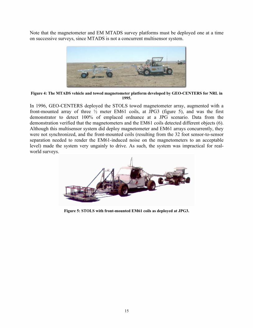
Note that the magnetometer and EM MTADS survey platforms must be deployed one at a time on successive surveys, since MTADS is not a concurrent multisensor system.

Figure 4: The MTADS vehicle and towed magnetometer platform developed by GEO-CENTERS for NRL in

1995.

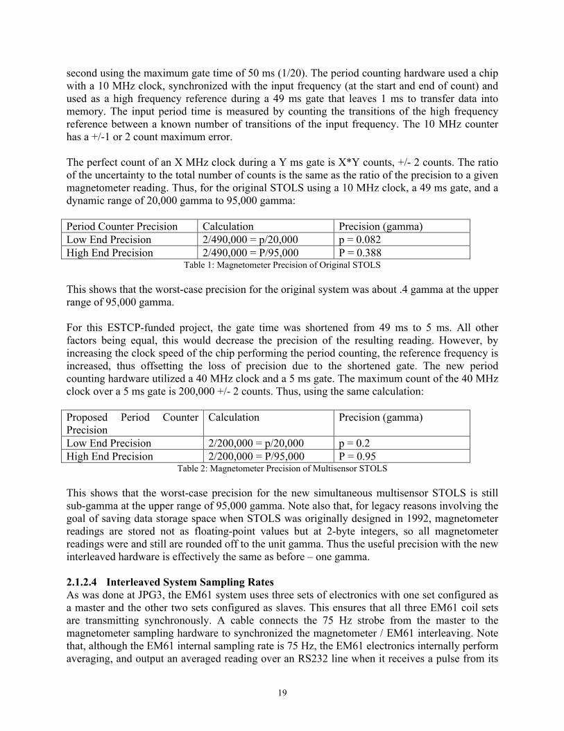
In 1996, GEO-CENTERS deployed the STOLS towed magnetometer array, augmented with a front-mounted array of three ½ meter EM61 coils, at JPG3 (figure 5), and was the first demonstrator to detect 100% of emplaced ordnance at a JPG scenario. Data from the demonstration verified that the magnetometers and the EM61 coils detected different objects (6). Although this multisensor system did deploy magnetometer and EM61 arrays concurrently, they were not synchronized, and the front-mounted coils (resulting from the 32 foot sensor-to-sensor separation needed to render the EM61-induced noise on the magnetometers to an acceptable level) made the system very ungainly to drive. As such, the system was impractical for real-world surveys.

Figure 5: STOLS with front-mounted EM61 coils as deployed at JPG3.

16

Figure 6: ½ acre magnetometer (left) and EM61(right) images from JPG3, showing that the two sensors detect different things. Images are at +- 50 gamma (magnetometer) and +- 50 millivolts (EM61). Survey

tracks are not identical because the magnetometer array was towed and the EM61 array was front-mounted, separated by 32 feet and two pivot points.

The above context is included because this ESTCP project for concurrent synchronous multisensor data acquisition was possible, under the funding constraints, due to the availability of STOLS as a development platform. STOLS was “reversibly cannibalized,” donating its low magnetic signature vehicle, total field magnetometers, GPS, EM61 electronics and ½ by ½ meter coils, wiring harnesses, and data processing infrastructure. Along with the basic use of STOLS came many tricks and lessons learned in the development of a low-noise vehicular system. For example, the alternator on the tow vehicle’s engine has had its windings removed, as they proved to be a source of electromagnetic noise, and the tires on the towed platform, which have no metal beads, were reused for the project. Further, the fact that GEO-CENTERS had previously designed its own magnetometer period counter (MPC) board, rather than using the existing COTS interface for the Geometrics 822 magnetometers, was absolutely central to the success of the project. The design of the existing interface needed to be modified to perform the synchronous interleaving of magnetometer data; this was far easier than designing an entirely new period counter board from scratch. 2.1.2 Theory of Operation The physics of magnetometry and pulsed electromagnetics, and the use of those sensors in a GPS-integrated towed array configuration as applied to detection of subsurface UXO, are well-understood and will not be repeated here. The new development in this project centered around simultaneously using magnetometry and EM61 on a single towed platform. 2.1.2.1 Interference Between EM61 and Magnetometers Historically, simultaneous deployment of magnetometers and pulsed EM such as the Geonics EM61 on a common platform has not been possible due to the fact that the EM transmission pulse is asynchronous with the magnetometer sampling, and thus is picked up by the magnetometers as noise. Figure 7 shows the EM61-engendered noise on the magnetometers as a function of sensor-to-sensor separation. This was measured using STOLS’ magnetometer data

17

acquisition system, and placing an array of three EM61 ½ meter coils at distances behind the magnetometers. Note that even at 10 feet – a practical separation distance for sensor co-location on a common towed platform – the EM61-induced noise is over 100 gamma.

0

100

200

300

400

500

600

700

0 10 20 30 40 50Sensor-to-Sensor Separation, Feet

Sign

al, G

amm

a

Figure 7: Noise induced on magnetometers by asynchronous EM61 transmission pulse as a function of

sensor-to-sensor separation The asynchronous sampling of the original STOLS MPC board that was used to generate the data shown in figure 7 is depicted in figure 8. Note that, at STOLS’ original 20 Hz sampling rate, there were an indeterminate number of 75 Hz transmit pulses (e.g., 3 or 4 pulses) from the EM61 system. These pulses were affecting the magnetometers while the magnetometers were being sampled, resulting in the noise levels shown in the graph in figure 7. Note also that the design of the original period counter board had the acquisition of magnetometer data triggered by the GPS’ 1 PPS, always resulting in correctly synchronized GPS/magnetometer data with no need to correct for latency post-hoc. 2.1.2.2 Interleaving Magnetometer and EM61 Data Acquisition In contrast, the newly-developed MPC board is designed to interleave the magnetometer and EM61 data acquisition cycles as follows. The 1 PPS strobe from the GPS and the 75 Hz EM61 transmission pulse are both input to the period counter board. The MPC circuitry looks for the 1 PPS from the GPS, then looks for the rising edge of the next EM61 transmission pulse. The system timing then uses a programmable waiting period and a sampling period. The 75 Hz EM61 transmission pulse comes in every 13.3 ms. The board waits 8 ms, at which point the EM61 transmission pulse has died off. This has been verified by direct measurement. The MPC board then samples the magnetometers for 5 ms, during the period in which the EM61s are not transmitting. In this way, the magnetometers are only sampled when the EM61s are quiet. The timing diagram for this interleaved synchronous data acquisition is shown in figure 9. Note that in this new design, acquisition of magnetometer data is triggered by the receipt of a 75 Hz strobe from the EM61 electronics after the GPS’ 1 PPS. Like the original MPC board, this results in correctly synchronized GPS/magnetometer data with no latency.

18

Figure 8: Timing Diagram of Asynchronous EM61 and Magnetometer Data Acquisition. Note that

magnetometer sampling is occurring during EM61 transmission, resulting in noise.

Figure 9: Timing Diagram of Synchronous EM61 and Magnetometer Data Acquisition. Note that

magnetometer sampling only occurs when EM61 transmission pulse has died down.

2.1.2.3 Precision of Magnetometer Readings for a 5 Ms Interleaved Sampling Window STOLS uses a custom-designed period counter to measure the output frequency for the Geometrics model 822A total field magnetometers. This technique for frequency counting measures the time interval between input transitions (zero crossings). While it is possible to measure the period using a single cycle of the signal, the longer the measurement “window” or gate, the greater the measurement accuracy. The original design made 20 measurements per

19

second using the maximum gate time of 50 ms (1/20). The period counting hardware used a chip with a 10 MHz clock, synchronized with the input frequency (at the start and end of count) and used as a high frequency reference during a 49 ms gate that leaves 1 ms to transfer data into memory. The input period time is measured by counting the transitions of the high frequency reference between a known number of transitions of the input frequency. The 10 MHz counter has a +/-1 or 2 count maximum error. The perfect count of an X MHz clock during a Y ms gate is X*Y counts, +/- 2 counts. The ratio of the uncertainty to the total number of counts is the same as the ratio of the precision to a given magnetometer reading. Thus, for the original STOLS using a 10 MHz clock, a 49 ms gate, and a dynamic range of 20,000 gamma to 95,000 gamma: Period Counter Precision Calculation Precision (gamma) Low End Precision 2/490,000 = p/20,000 p = 0.082 High End Precision 2/490,000 = P/95,000 P = 0.388

Table 1: Magnetometer Precision of Original STOLS This shows that the worst-case precision for the original system was about .4 gamma at the upper range of 95,000 gamma. For this ESTCP-funded project, the gate time was shortened from 49 ms to 5 ms. All other factors being equal, this would decrease the precision of the resulting reading. However, by increasing the clock speed of the chip performing the period counting, the reference frequency is increased, thus offsetting the loss of precision due to the shortened gate. The new period counting hardware utilized a 40 MHz clock and a 5 ms gate. The maximum count of the 40 MHz clock over a 5 ms gate is 200,000 +/- 2 counts. Thus, using the same calculation: Proposed Period Counter Precision

Calculation Precision (gamma)

Low End Precision 2/200,000 = p/20,000 p = 0.2 High End Precision 2/200,000 = P/95,000 P = 0.95

Table 2: Magnetometer Precision of Multisensor STOLS This shows that the worst-case precision for the new simultaneous multisensor STOLS is still sub-gamma at the upper range of 95,000 gamma. Note also that, for legacy reasons involving the goal of saving data storage space when STOLS was originally designed in 1992, magnetometer readings are stored not as floating-point values but at 2-byte integers, so all magnetometer readings were and still are rounded off to the unit gamma. Thus the useful precision with the new interleaved hardware is effectively the same as before – one gamma. 2.1.2.4 Interleaved System Sampling Rates As was done at JPG3, the EM61 system uses three sets of electronics with one set configured as a master and the other two sets configured as slaves. This ensures that all three EM61 coil sets are transmitting synchronously. A cable connects the 75 Hz strobe from the master to the magnetometer sampling hardware to synchronized the magnetometer / EM61 interleaving. Note that, although the EM61 internal sampling rate is 75 Hz, the EM61 electronics internally perform averaging, and output an averaged reading over an RS232 line when it receives a pulse from its

20

wheel encoder. As was done at JPG3, this wheel encoder has been replaced with a circuit that divides down the 1 PPS pulse from the GPS into a 10 Hz pulse train. As such, the output rate of the EM61 data to the data acquisition computer is not the 75 Hz sampling rate, but 10 Hz. The magnetometer data output rate, however, is the same as its sampling rate of 75 Hz. The table below summarizes the operating parameters of the original and the simultaneous multisensor STOLS.

ORIGINAL MULTISENSOR RELATIONSHIP BETWEEN EM61 AND MAGNETOMETER

Asynchronous Synchronous

EM61 SAMPLING RATE

75 Hz 75 Hz

EM61 OUTPUT RATE 10 Hz 10 Hz MAGNETOMETER SAMPLING RATE

20 Hz 75 Hz

MAGNETOMETER SAMPLING LENGTH

50 ms 5 ms

MAGNETOMETER OUTPUT RATE

20 Hz 75 Hz

MAGNETOMETER SAMPLING PRECISION (WORST CASE)

.39 gamma .95 gamma

GPS 1 PPS 1 PPS Triggers Magnetometer Data Acquisition

System waits for 1 PPS, then for next EM61 transmit pulse

Table 3: Original and Multi-sensor Synchronization Parameters 2.1.3 System Components The interleaved multisensor system consists of four main subsystems: The tow vehicle; the non-metallic towed platform, including the sensors; the interleaved data acquisition hardware, and the data processing software. 2.1.3.1 Low Magnetic Self-Signature Tow Vehicle The tow vehicle was specified by GEO-CENTERS and design and built to specification by Chenowth Racing in San Diego, CA in 1993 (figure 10). Chenowth also developed the MTADS tow vehicle in 1995. The vehicle utilizes a tubular aluminum frame and an air-cooled Volkswagen engine with a magnesium alloy block. Although certain engine components such as the crankshaft and camshafts are steel, the use of ferromagnetic materials on the vehicle have been kept to an absolute minimum to reduce the magnetic self-signature. Modifications for this project included removing the obsolete data acquisition computer from the back deck (black box

21

in photo), mounting the EM61 electronics in its place, and mounting a COTS notebook computer within the field of view of the driver.

Figure 10: The STOLS low magnetic self-signature tow vehicle.

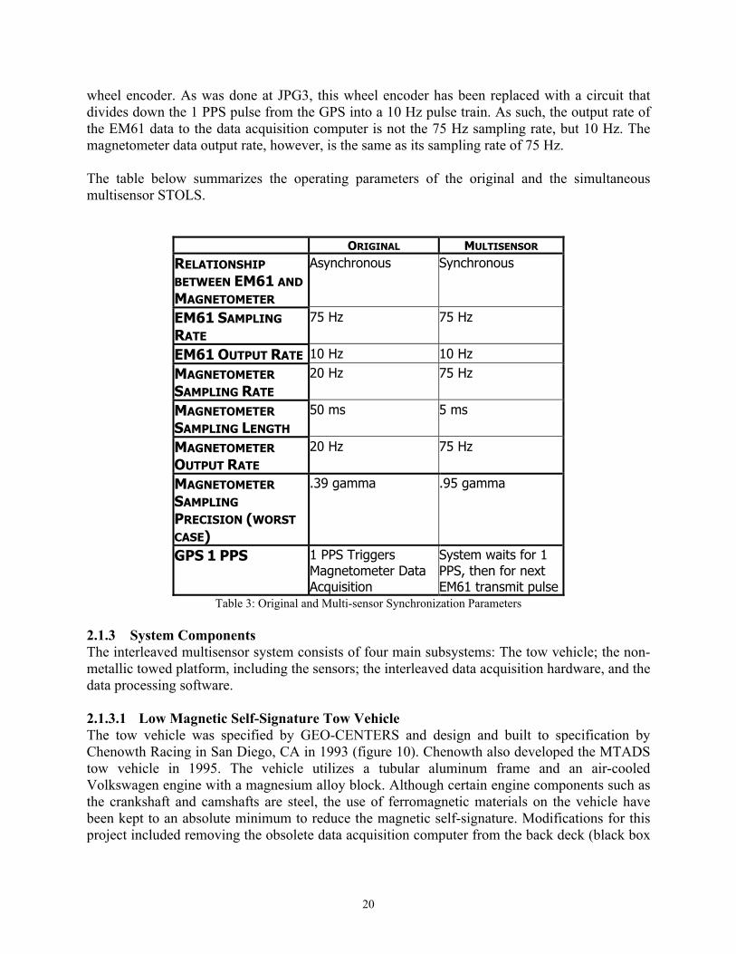
2.1.3.2 Non-Conductive Towed Platform and Sensors The original STOLS towed magnetometer platform was made out of aluminum and used a suspension designed from non-ferrous components. While it was well-designed for a magnetometer-specific application, the aluminum platform was clearly not hospitable for deployment of both magnetometers and EM61 sensors in a low-noise environment. As such, a new non-conductive, non-metallic towed platform was designed and built for this project. Constructed primarily out of fiberglass with marine plywood reinforcements at key locations, the platform reduces the metallic mass by over 99% by weight as compared to the previous STOLS aluminum platform. Figure 11 shows the platform equipped with the front-mounted boom of five total field magnetometers and the rear-mounted array of three ½ meter EM61 coils. In this picture, the EM61 coils are in their most rearward configuration. The coils were eventually moved ½ meter forward, directly against the fiberglass superstructure of the frame, to reduce the cantilevered moment on the platform.

22

Figure 11: Non-conductive towed platform with front-mounted magnetometer boom and rear-mounted

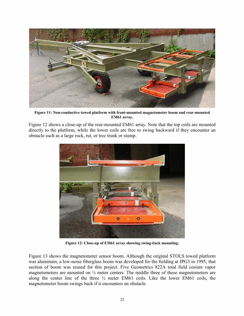
EM61 array. Figure 12 shows a close-up of the rear-mounted EM61 array. Note that the top coils are mounted directly to the platform, while the lower coils are free to swing backward if they encounter an obstacle such as a large rock, rut, or tree trunk or stump.

Figure 12: Close-up of EM61 array showing swing-back mounting.

Figure 13 shows the magnetometer sensor boom. Although the original STOLS towed platform was aluminum, a low-noise fiberglass boom was developed for the fielding at JPG3 in 1995; that section of boom was reused for this project. Five Geometrics 822A total field cesium vapor magnetometers are mounted on ½ meter centers. The middle three of these magnetometers are along the center line of the three ½ meter EM61 coils. Like the lower EM61 coils, the magnetometer boom swings back if it encounters an obstacle.

23

Figure 13: Five total field magnetometers spaced ½ meter apart mounted on swing-back boom.

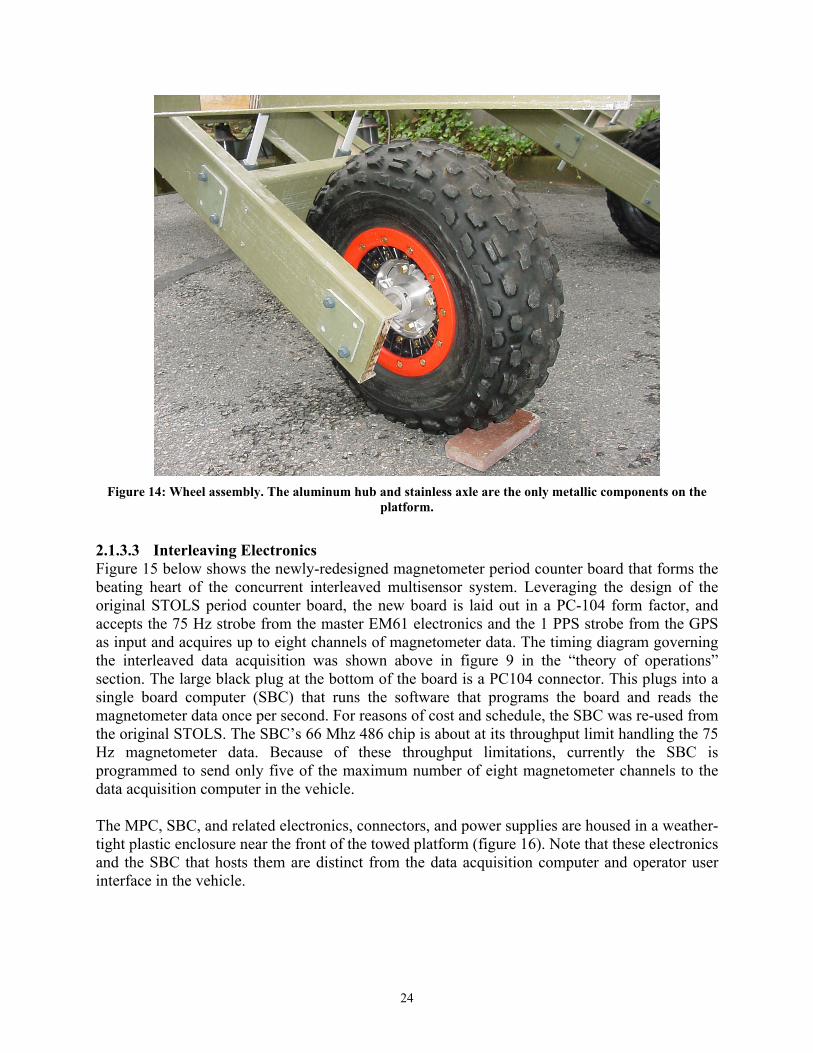
Figure 14 shows a close-up of the wheel assembly on the platform. The wheel itself is composite. The hub is aluminum, and the axle is stainless steel. Other than a handful of brass bolts, these are the only metallic components on the towed platform. The tires were reused from the original STOLS platform, and have had the ferromagnetic metal beads, which are a major source of noise to the magnetometers, removed.

24

Figure 14: Wheel assembly. The aluminum hub and stainless axle are the only metallic components on the

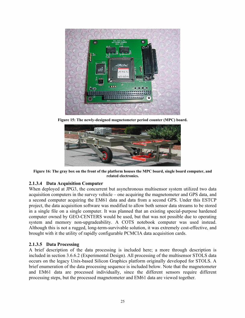
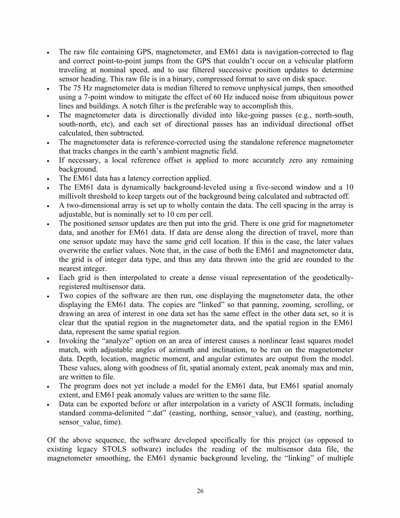
platform. 2.1.3.3 Interleaving Electronics Figure 15 below shows the newly-redesigned magnetometer period counter board that forms the beating heart of the concurrent interleaved multisensor system. Leveraging the design of the original STOLS period counter board, the new board is laid out in a PC-104 form factor, and accepts the 75 Hz strobe from the master EM61 electronics and the 1 PPS strobe from the GPS as input and acquires up to eight channels of magnetometer data. The timing diagram governing the interleaved data acquisition was shown above in figure 9 in the “theory of operations” section. The large black plug at the bottom of the board is a PC104 connector. This plugs into a single board computer (SBC) that runs the software that programs the board and reads the magnetometer data once per second. For reasons of cost and schedule, the SBC was re-used from the original STOLS. The SBC’s 66 Mhz 486 chip is about at its throughput limit handling the 75 Hz magnetometer data. Because of these throughput limitations, currently the SBC is programmed to send only five of the maximum number of eight magnetometer channels to the data acquisition computer in the vehicle. The MPC, SBC, and related electronics, connectors, and power supplies are housed in a weather-tight plastic enclosure near the front of the towed platform (figure 16). Note that these electronics and the SBC that hosts them are distinct from the data acquisition computer and operator user interface in the vehicle.

25

Figure 15: The newly-designed magnetometer period counter (MPC) board.

Figure 16: The gray box on the front of the platform houses the MPC board, single board computer, and

related electronics. 2.1.3.4 Data Acquisition Computer When deployed at JPG3, the concurrent but asynchronous multisensor system utilized two data acquisition computers in the survey vehicle – one acquiring the magnetometer and GPS data, and a second computer acquiring the EM61 data and data from a second GPS. Under this ESTCP project, the data acquisition software was modified to allow both sensor data streams to be stored in a single file on a single computer. It was planned that an existing special-purpose hardened computer owned by GEO-CENTERS would be used, but that was not possible due to operating system and memory non-upgradeability. A COTS notebook computer was used instead. Although this is not a rugged, long-term-survivable solution, it was extremely cost-effective, and brought with it the utility of rapidly configurable PCMCIA data acquisition cards. 2.1.3.5 Data Processing A brief description of the data processing is included here; a more through description is included in section 3.6.6.2 (Experimental Design). All processing of the multisensor STOLS data occurs on the legacy Unix-based Silicon Graphics platform originally developed for STOLS. A brief enumeration of the data processing sequence is included below. Note that the magnetometer and EM61 data are processed individually, since the different sensors require different processing steps, but the processed magnetometer and EM61 data are viewed together.

26

• The raw file containing GPS, magnetometer, and EM61 data is navigation-corrected to flag and correct point-to-point jumps from the GPS that couldn’t occur on a vehicular platform traveling at nominal speed, and to use filtered successive position updates to determine sensor heading. This raw file is in a binary, compressed format to save on disk space.

• The 75 Hz magnetometer data is median filtered to remove unphysical jumps, then smoothed using a 7-point window to mitigate the effect of 60 Hz induced noise from ubiquitous power lines and buildings. A notch filter is the preferable way to accomplish this.

• The magnetometer data is directionally divided into like-going passes (e.g., north-south, south-north, etc), and each set of directional passes has an individual directional offset calculated, then subtracted.

• The magnetometer data is reference-corrected using the standalone reference magnetometer that tracks changes in the earth’s ambient magnetic field.

• If necessary, a local reference offset is applied to more accurately zero any remaining background.

• The EM61 data has a latency correction applied. • The EM61 data is dynamically background-leveled using a five-second window and a 10

millivolt threshold to keep targets out of the background being calculated and subtracted off. • A two-dimensional array is set up to wholly contain the data. The cell spacing in the array is

adjustable, but is nominally set to 10 cm per cell. • The positioned sensor updates are then put into the grid. There is one grid for magnetometer

data, and another for EM61 data. If data are dense along the direction of travel, more than one sensor update may have the same grid cell location. If this is the case, the later values overwrite the earlier values. Note that, in the case of both the EM61 and magnetometer data, the grid is of integer data type, and thus any data thrown into the grid are rounded to the nearest integer.

• Each grid is then interpolated to create a dense visual representation of the geodetically-registered multisensor data.

• Two copies of the software are then run, one displaying the magnetometer data, the other displaying the EM61 data. The copies are "linked” so that panning, zooming, scrolling, or drawing an area of interest in one data set has the same effect in the other data set, so it is clear that the spatial region in the magnetometer data, and the spatial region in the EM61 data, represent the same spatial region.

• Invoking the “analyze” option on an area of interest causes a nonlinear least squares model match, with adjustable angles of azimuth and inclination, to be run on the magnetometer data. Depth, location, magnetic moment, and angular estimates are output from the model. These values, along with goodness of fit, spatial anomaly extent, peak anomaly max and min, are written to file.

• The program does not yet include a model for the EM61 data, but EM61 spatial anomaly extent, and EM61 peak anomaly values are written to the same file.

• Data can be exported before or after interpolation in a variety of ASCII formats, including standard comma-delimited “.dat” (easting, northing, sensor_value), and (easting, northing, sensor_value, time).

Of the above sequence, the software developed specifically for this project (as opposed to existing legacy STOLS software) includes the reading of the multisensor data file, the magnetometer smoothing, the EM61 dynamic background leveling, the “linking” of multiple

27

copies of the program for simultaneous viewing of multisensor data grids, and the augmentation of the target file format to include both magnetometer and EM61 feature values. 2.2 Previous Testing of the Technology Towed GPS-integrated magnetometer array technology has been proved-out by both MTADS and GEO-CENTERS’ STOLS, and is well-documented in published reports from the multi-year exercises at Jefferson Proving Grounds. Prior to this ESTCP-funded project, no concurrent interleaved magnetometer / EM61 technology existed. 2.2.1 CEHNC-Funded Feasibility Testing In June 2001, in anticipation of this ESTCP project being funded, CEHNC funded GEO-CENTERS $20k under GSA contract number GS-35F-5176H to begin verifying the feasibility of the interleaved magnetometer/EM61 concept. The areas examined were: • Magnetometer Saturation as a Function of EM61 Distance • Magnetometer Noise Due to EM61 Coil Motion • Aluminum Towed platform Effects on EM61 Data • Magnetometer Recovery Time The four sections below are excerpted from “Final Report: Combined Electromagnetic and Magnetometer Data Acquisition and Processing” submitted to Mr. Roger Young at CEHNC in December 2001. 2.2.1.1 Magnetometer Saturation as a Function of EM61 Distance If the EM61 array is too close to the magnetometers, it will drive the magnetometers into saturation, and the magnetometer recovery time might be longer than could be accommodated with interleaved sampling. It was discovered that magnetometer saturation occurred with the EM61 array at a separation distance of approximately 3 feet. Decreasing effects on the magnetometer signal amplitude were observed at separation distances of 4 to 5 feet, with normal magnetometer signal amplitude recovered within 8 ms of each EM61 transmit pulse. This result showed that it was possible to have the EM61 array cantilevered off the back of the existing STOLS towed platform, roughly 8.5 feet behind the magnetometers, and not have magnetometer saturation from the EM61 signal jeopardize the synchronization. 2.2.1.2 Magnetometer Noise Due to EM61 Coil Motion EM61 coil motion noise tests were performed because the motion of any kind of conductive metal, particularly closed loops of metal, in the earth’s ambient magnetic field produces eddy currents which can be picked up by magnetometers. Thus, even with the coils turned off, it is possible that motion of the coils, if they are sufficiently close to the magnetometers, could create signals which register on the magnetometers as noise. The tests, however, showed that even gross and exaggerated EM61 coil motion within 2.5 feet of a magnetometer, regardless of orientation or sensor height, showed no adverse affects on the magnetometer output. 2.2.1.3 Aluminum Towed Platform Effects on the EM61 Array Because STOLS was originally designed as a magnetometer-only system, the towed platform was constructed mostly from aluminum. Obviously this creates a significant signal on platform-mounted EM61 coils; aluminum would not be the material of choice if one were constructing a

28

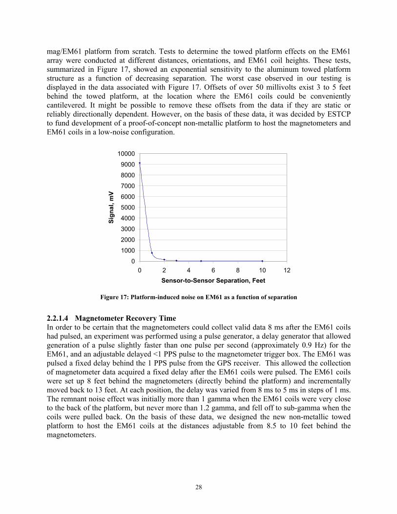
mag/EM61 platform from scratch. Tests to determine the towed platform effects on the EM61 array were conducted at different distances, orientations, and EM61 coil heights. These tests, summarized in Figure 17, showed an exponential sensitivity to the aluminum towed platform structure as a function of decreasing separation. The worst case observed in our testing is displayed in the data associated with Figure 17. Offsets of over 50 millivolts exist 3 to 5 feet behind the towed platform, at the location where the EM61 coils could be conveniently cantilevered. It might be possible to remove these offsets from the data if they are static or reliably directionally dependent. However, on the basis of these data, it was decided by ESTCP to fund development of a proof-of-concept non-metallic platform to host the magnetometers and EM61 coils in a low-noise configuration.

0

1000

2000

3000

4000

5000

6000

7000

8000

9000

10000

0 2 4 6 8 10 12Sensor-to-Sensor Separation, Feet

Sign

al, m

V

Figure 17: Platform-induced noise on EM61 as a function of separation

2.2.1.4 Magnetometer Recovery Time In order to be certain that the magnetometers could collect valid data 8 ms after the EM61 coils had pulsed, an experiment was performed using a pulse generator, a delay generator that allowed generation of a pulse slightly faster than one pulse per second (approximately 0.9 Hz) for the EM61, and an adjustable delayed <1 PPS pulse to the magnetometer trigger box. The EM61 was pulsed a fixed delay behind the 1 PPS pulse from the GPS receiver. This allowed the collection of magnetometer data acquired a fixed delay after the EM61 coils were pulsed. The EM61 coils were set up 8 feet behind the magnetometers (directly behind the platform) and incrementally moved back to 13 feet. At each position, the delay was varied from 8 ms to 5 ms in steps of 1 ms. The remnant noise effect was initially more than 1 gamma when the EM61 coils were very close to the back of the platform, but never more than 1.2 gamma, and fell off to sub-gamma when the coils were pulled back. On the basis of these data, we designed the new non-metallic towed platform to host the EM61 coils at the distances adjustable from 8.5 to 10 feet behind the magnetometers.

29

2.2.2 Benchtop Testing Testing of the technology in the ESTCP-funded project first occurred on the benchtop. The new MPC board was designed, delivered, tested, and debugged. Firmware went through several revisions to ensure robust operation for drift of the 75 Hz EM61 transmit trigger and the 1 PPS GPS trigger. Hardware and software were tested on the benchtop using signal generators under worse-than-anticipated drift conditions. 2.2.3 Parking Lot Testing Final integration and testing was performed at GEO-CENTERS in Newton, MA. Al Crandall, who formerly worked for GEO-CENTERS and is now with USA Environmental, traveled to GEO-CENTERS to assist in the integration and testing exercise. A 75mm, 81mm, a Russian mortar, a 155mm, and a 12" metal antitank mine were emplaced in the parking lot behind the building and used as sample targets. The DGPS base station receiver was set up and the magnetometer/EM61 system was run over these items. The parking lot behind the building is ringed by trees, so RTK-quality GPS is far from assured. Further, the area is fairly magnetically cluttered by subsurface utilities. The object locations were stored using the DGPS to obtain ground truth. The system then acquired magnetometer only data, then acquired simultaneous magnetometer and EM61 data. The first image, figure 18, shows the baseline data set, acquired with the magnetometers only (EM61 switched off). The double signal of the 155 is due to bad GPS in the area resulting in the target location being mis-positioned on the incoming versus the outgoing traverse. Note that there is no obvious directionally-dependent magnetic offset from the STOLS tow vehicle, which is especially encouraging considering that the magnetometers are nearly two feet closer to the vehicle than they were with the old towed platform.

Figure 18: Magnetometer data acquired during integration and testing (magnetometers only, EM61

electronics switch off). Image scale +- 100 gamma.

30

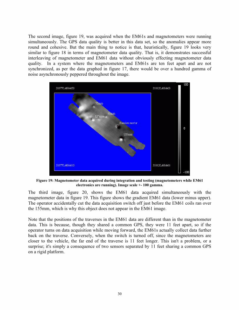
The second image, figure 19, was acquired when the EM61s and magnetometers were running simultaneously. The GPS data quality is better in this data set, so the anomalies appear more round and cohesive. But the main thing to notice is that, heuristically, figure 19 looks very similar to figure 18 in terms of magnetometer data quality. That is, it demonstrates successful interleaving of magnetometer and EM61 data without obviously effecting magnetometer data quality. In a system where the magnetometers and EM61s are ten feet apart and are not synchronized, as per the data graphed in figure 17, there would be over a hundred gamma of noise asynchronously peppered throughout the image.

Figure 19: Magnetometer data acquired during integration and testing (magnetometers while EM61

electronics are running). Image scale +- 100 gamma.

The third image, figure 20, shows the EM61 data acquired simultaneously with the magnetometer data in figure 19. This figure shows the gradient EM61 data (lower minus upper). The operator accidentally cut the data acquisition switch off just before the EM61 coils ran over the 155mm, which is why this object does not appear in the EM61 image. Note that the positions of the traverses in the EM61 data are different than in the magnetometer data. This is because, though they shared a common GPS, they were 11 feet apart, so if the operator turns on data acquisition while moving forward, the EM61s actually collect data further back on the traverse. Conversely, when the switch is turned off, since the magnetometers are closer to the vehicle, the far end of the traverse is 11 feet longer. This isn't a problem, or a surprise; it's simply a consequence of two sensors separated by 11 feet sharing a common GPS on a rigid platform.

31

Figure 20: EM61 data acquired during integration and testing (EM61 data while magnetometers are

running). Image scale +- 100 gamma.

The data above were acquired with the EM61 array at the rearmost location on the platform. Since the array location is adjustable, and since no interference between the magnetometers and the EM61 array was noticed in the rear-mounted location, it was decided to move the EM61 array forward by ½ meter (the coil size). Data was then acquired to test whether, in this new location, the EM61 coils detected any noise from their proximity to the aluminum hub and steel axle on the towed platform that could not be removed through background leveling. A static test was conducted. The left rear wheel of the platform was jacked up and data was acquired for roughly 10 seconds. The system was then paused, the left rear wheel was spun, and data were acquired for 10 more seconds. These data are shown in figure 21 below. The data on the left side of the graph are without the left wheel spinning; data on the right side are with the left wheel spinning. All six EM61 channels (1-port bottom, 2-port upper, 3-middle bottom, 4-middle upper, 5-starboard lower and 6-starboard upper) are shown. The bottom port coil (the one closest to the wheel being spun) is depicted as “series 1” in blue. Effects of a spinning wheel on the EM61 would be expected to show up as a periodic variation over time (along the graph’s abscissa), and if an effect were present, it would be expected to show up strongest in the bottom port coil (blue graph). No such effect is seen; the slight differences between the plots with the wheel spinning and without can be attributed to the nominal EM61 noise level. On the basis of these data, it was decided that the EM61 coils could be left in this forward-mounted location. This had the added benefit of reducing the cantilevered load on the back of the platform caused by the weight of the coils.

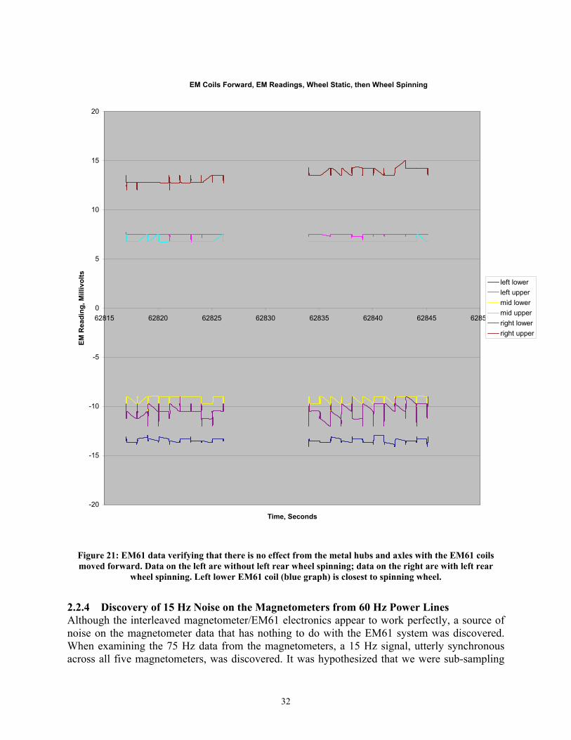
32

EM Coils Forward, EM Readings, Wheel Static, then Wheel Spinning

-20

-15

-10

-5

0

5

10

15

20

62815 62820 62825 62830 62835 62840 62845 62850

Time, Seconds

EM R

eadi

ng, M

illiv

olts

left lowerleft uppermid lowermid upperright lowerright upper

Figure 21: EM61 data verifying that there is no effect from the metal hubs and axles with the EM61 coils moved forward. Data on the left are without left rear wheel spinning; data on the right are with left rear

wheel spinning. Left lower EM61 coil (blue graph) is closest to spinning wheel.

2.2.4 Discovery of 15 Hz Noise on the Magnetometers from 60 Hz Power Lines Although the interleaved magnetometer/EM61 electronics appear to work perfectly, a source of noise on the magnetometer data that has nothing to do with the EM61 system was discovered. When examining the 75 Hz data from the magnetometers, a 15 Hz signal, utterly synchronous across all five magnetometers, was discovered. It was hypothesized that we were sub-sampling

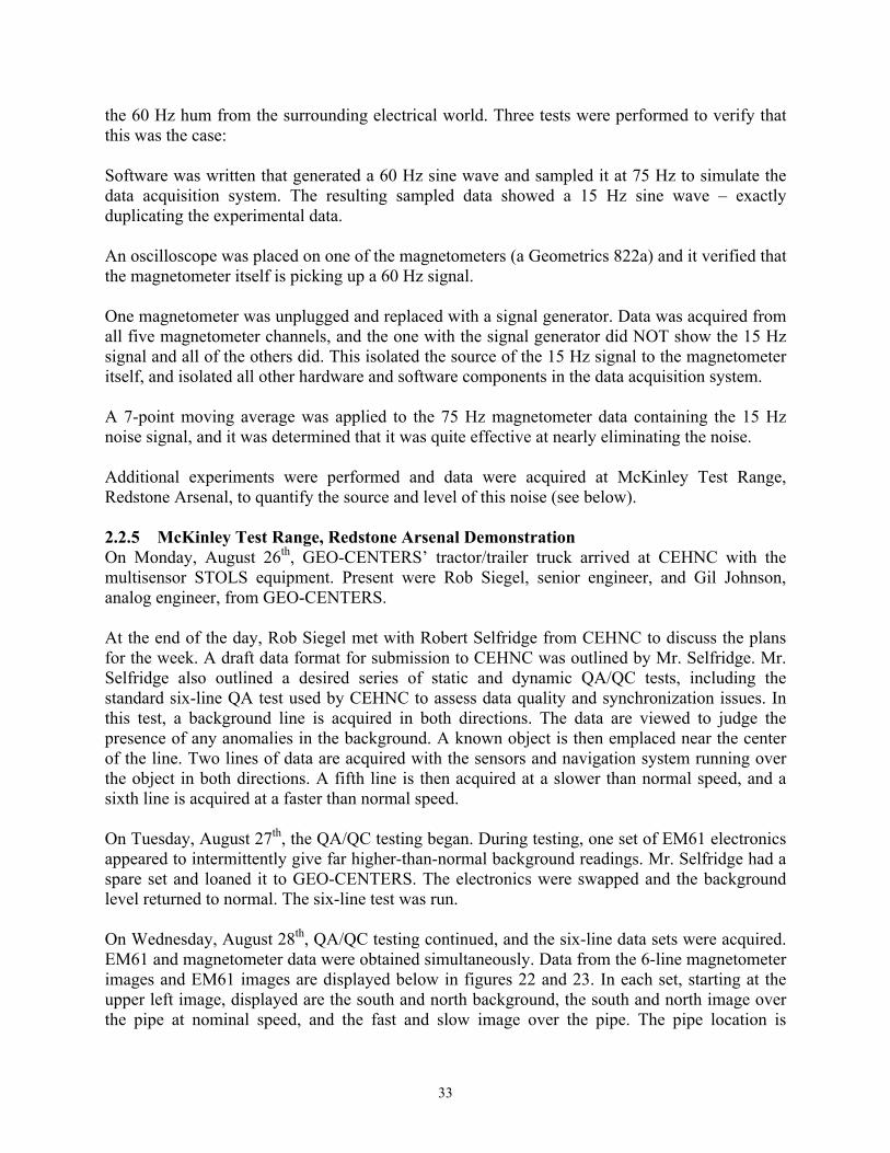
33

the 60 Hz hum from the surrounding electrical world. Three tests were performed to verify that this was the case: Software was written that generated a 60 Hz sine wave and sampled it at 75 Hz to simulate the data acquisition system. The resulting sampled data showed a 15 Hz sine wave – exactly duplicating the experimental data. An oscilloscope was placed on one of the magnetometers (a Geometrics 822a) and it verified that the magnetometer itself is picking up a 60 Hz signal. One magnetometer was unplugged and replaced with a signal generator. Data was acquired from all five magnetometer channels, and the one with the signal generator did NOT show the 15 Hz signal and all of the others did. This isolated the source of the 15 Hz signal to the magnetometer itself, and isolated all other hardware and software components in the data acquisition system. A 7-point moving average was applied to the 75 Hz magnetometer data containing the 15 Hz noise signal, and it was determined that it was quite effective at nearly eliminating the noise. Additional experiments were performed and data were acquired at McKinley Test Range, Redstone Arsenal, to quantify the source and level of this noise (see below). 2.2.5 McKinley Test Range, Redstone Arsenal Demonstration On Monday, August 26th, GEO-CENTERS’ tractor/trailer truck arrived at CEHNC with the multisensor STOLS equipment. Present were Rob Siegel, senior engineer, and Gil Johnson, analog engineer, from GEO-CENTERS. At the end of the day, Rob Siegel met with Robert Selfridge from CEHNC to discuss the plans for the week. A draft data format for submission to CEHNC was outlined by Mr. Selfridge. Mr. Selfridge also outlined a desired series of static and dynamic QA/QC tests, including the standard six-line QA test used by CEHNC to assess data quality and synchronization issues. In this test, a background line is acquired in both directions. The data are viewed to judge the presence of any anomalies in the background. A known object is then emplaced near the center of the line. Two lines of data are acquired with the sensors and navigation system running over the object in both directions. A fifth line is then acquired at a slower than normal speed, and a sixth line is acquired at a faster than normal speed. On Tuesday, August 27th, the QA/QC testing began. During testing, one set of EM61 electronics appeared to intermittently give far higher-than-normal background readings. Mr. Selfridge had a spare set and loaned it to GEO-CENTERS. The electronics were swapped and the background level returned to normal. The six-line test was run. On Wednesday, August 28th, QA/QC testing continued, and the six-line data sets were acquired. EM61 and magnetometer data were obtained simultaneously. Data from the 6-line magnetometer images and EM61 images are displayed below in figures 22 and 23. In each set, starting at the upper left image, displayed are the south and north background, the south and north image over the pipe at nominal speed, and the fast and slow image over the pipe. The pipe location is

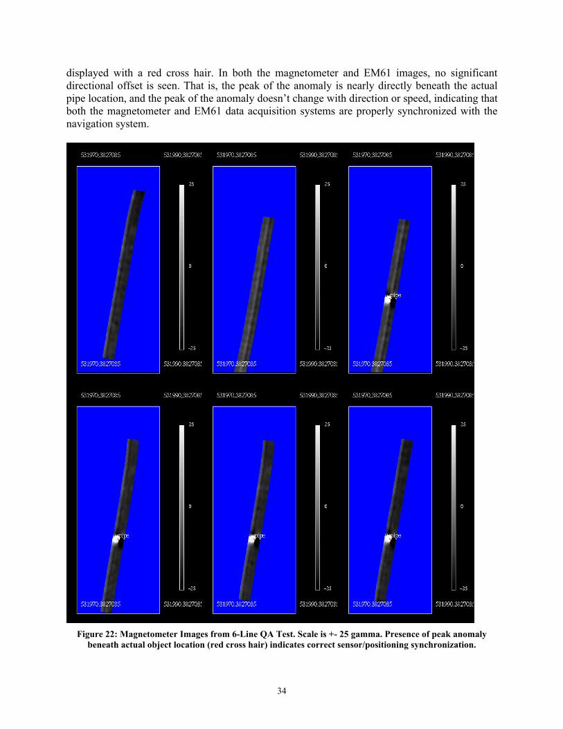
34

displayed with a red cross hair. In both the magnetometer and EM61 images, no significant directional offset is seen. That is, the peak of the anomaly is nearly directly beneath the actual pipe location, and the peak of the anomaly doesn’t change with direction or speed, indicating that both the magnetometer and EM61 data acquisition systems are properly synchronized with the navigation system.

Figure 22: Magnetometer Images from 6-Line QA Test. Scale is +- 25 gamma. Presence of peak anomaly

beneath actual object location (red cross hair) indicates correct sensor/positioning synchronization.

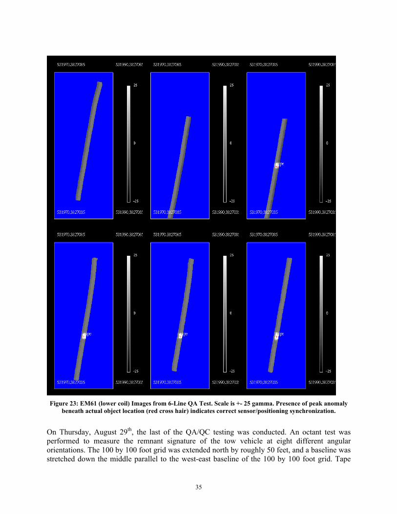
35

Figure 23: EM61 (lower coil) Images from 6-Line QA Test. Scale is +- 25 gamma. Presence of peak anomaly

beneath actual object location (red cross hair) indicates correct sensor/positioning synchronization.

On Thursday, August 29th, the last of the QA/QC testing was conducted. An octant test was performed to measure the remnant signature of the tow vehicle at eight different angular orientations. The 100 by 100 foot grid was extended north by roughly 50 feet, and a baseline was stretched down the middle parallel to the west-east baseline of the 100 by 100 foot grid. Tape

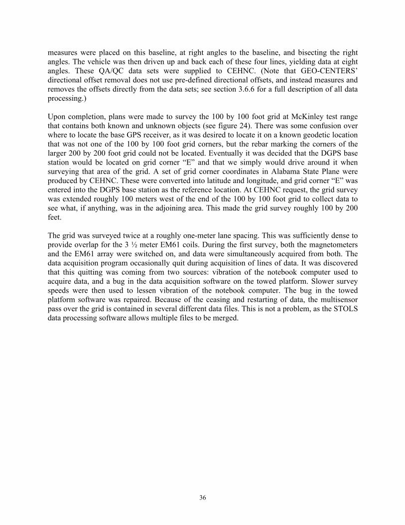
36

measures were placed on this baseline, at right angles to the baseline, and bisecting the right angles. The vehicle was then driven up and back each of these four lines, yielding data at eight angles. These QA/QC data sets were supplied to CEHNC. (Note that GEO-CENTERS’ directional offset removal does not use pre-defined directional offsets, and instead measures and removes the offsets directly from the data sets; see section 3.6.6 for a full description of all data processing.) Upon completion, plans were made to survey the 100 by 100 foot grid at McKinley test range that contains both known and unknown objects (see figure 24). There was some confusion over where to locate the base GPS receiver, as it was desired to locate it on a known geodetic location that was not one of the 100 by 100 foot grid corners, but the rebar marking the corners of the larger 200 by 200 foot grid could not be located. Eventually it was decided that the DGPS base station would be located on grid corner “E” and that we simply would drive around it when surveying that area of the grid. A set of grid corner coordinates in Alabama State Plane were produced by CEHNC. These were converted into latitude and longitude, and grid corner “E” was entered into the DGPS base station as the reference location. At CEHNC request, the grid survey was extended roughly 100 meters west of the end of the 100 by 100 foot grid to collect data to see what, if anything, was in the adjoining area. This made the grid survey roughly 100 by 200 feet. The grid was surveyed twice at a roughly one-meter lane spacing. This was sufficiently dense to provide overlap for the 3 ½ meter EM61 coils. During the first survey, both the magnetometers and the EM61 array were switched on, and data were simultaneously acquired from both. The data acquisition program occasionally quit during acquisition of lines of data. It was discovered that this quitting was coming from two sources: vibration of the notebook computer used to acquire data, and a bug in the data acquisition software on the towed platform. Slower survey speeds were then used to lessen vibration of the notebook computer. The bug in the towed platform software was repaired. Because of the ceasing and restarting of data, the multisensor pass over the grid is contained in several different data files. This is not a problem, as the STOLS data processing software allows multiple files to be merged.

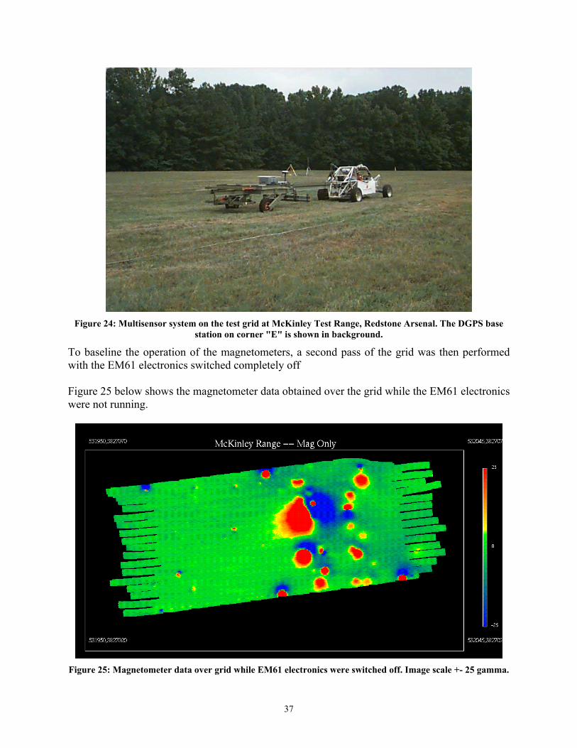
37

Figure 24: Multisensor system on the test grid at McKinley Test Range, Redstone Arsenal. The DGPS base

station on corner "E" is shown in background.

To baseline the operation of the magnetometers, a second pass of the grid was then performed with the EM61 electronics switched completely off Figure 25 below shows the magnetometer data obtained over the grid while the EM61 electronics were not running.

Figure 25: Magnetometer data over grid while EM61 electronics were switched off. Image scale +- 25 gamma.

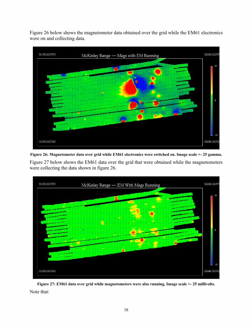
38

Figure 26 below shows the magnetometer data obtained over the grid while the EM61 electronics were on and collecting data.

Figure 26: Magnetometer data over grid while EM61 electronics were switched on. Image scale +- 25 gamma.

Figure 27 below shows the EM61 data over the grid that were obtained while the magnetometers were collecting the data shown in figure 26.

Figure 27: EM61 data over grid while magnetometers were also running. Image scale +- 25 millivolts.

Note that:

39

• The magnetometer data in figure 25 (while the EM61 electronics were not running) look very

similar to the magnetometer data in figure 26 (while the EM61 electronics were running). • The gaps in figures 26 and 27 were caused by operator error; the system operator (Rob

Siegel) did not notice that the data acquisition system program had sensed errors and had shut down data acquisition during these lines. During other lines, the operator noticed the errors and redid the lines on which they occurred.

• The vehicle’s traverses in images 24 and 25 are nearly identical. They are not, however, exactly the same, because the GPS antenna is directly over the center magnetometer, and the EM61 array is nearly 8 feet behind the magnetometers.

The evening of Wednesday, August 28th, Mr. Selfridge observed Rob Siegel process the single-sensor and multi-sensor data from the test grid. Navigation data was corrected, heading was calculated, and background leveling was performed. For the EM61 data, background leveling was performed individually for each file. For the magnetometer data, background leveling was performed individually for east, and west data sets. 2.2.6 Time-Series Comparison of Magnetometer Data With EM61 On and Off The visual comparison of the data images in figures 26 and 27 is heuristic. That is, the image of the magnetometer data with the EM61 turned on “looks like” the image of the magnetometer data with the EM61 turned off. To provide a more rigorous comparison, three plots of time-series magnetometer data over an anomaly are shown below. In all three, “series 1” is the leftmost magnetometer, and “series 5” is the rightmost magnetometer. The anomaly is due to a piece of rebar marking the southwest corner of the grid (the anomaly in the middle of the southern-most traverse shown in figures 26 and 27). Figure 28 shows the time-series plots from the five magnetometers with the EM61s switched completely off. Figure 29 shows the plots over the same object but when the EM61s were concurrently pulsing and the system was collecting EM data. From these time-series plots, we can see that there is no discernable difference in the shape, amplitude, or character of the magnetometer data whether or not the EM61s are pulsing. This provides the best validation that the interleaving hardware is functioning as designed; if it were not, hundreds of gamma of random noise would be visible in the data. However, what is clearly visible in the data is a 15 Hz ring, utterly coherent across all five magnetometers. The shape, period, and amplitude of the ring is identical whether or not the EM61s are pulsing. Figure 30 shows the result of applying a simple 11-point smooth to the data, which knocks out most of the ring. As is explained below, the ring is due to the 60 Hz hum from nearby power lines. Both the vehicular and the airborne MTADS experience this same problem, and remove this ring with a notch filter.

40

McKinley Test Range, Mag Data, EM61 Turned Off, Unsmoothed

51600

51800

52000

52200

52400

52600

52800

53000

53200

58220 58220.5 58221 58221.5 58222 58222.5 58223 58223.5 58224 58224.5 58225

Time, Seconds

Gam

ma

Series1

Series2

Series3

Series4

Series5

Figure 28: Magnetometer Data with EM61s Turned Off

McKinley Test Range, Mag Data, EM61 Turned On, Unsmoothed

51600

51800

52000

52200

52400

52600

52800

53000

53200

70558.5 70559 70559.5 70560 70560.5 70561 70561.5 70562 70562.5 70563 70563.5

Time, Seconds

Gam

ma

Series1

Series2

Series3

Series4

Series5

Figure 29: Magnetometer Data with EM61s Turned On

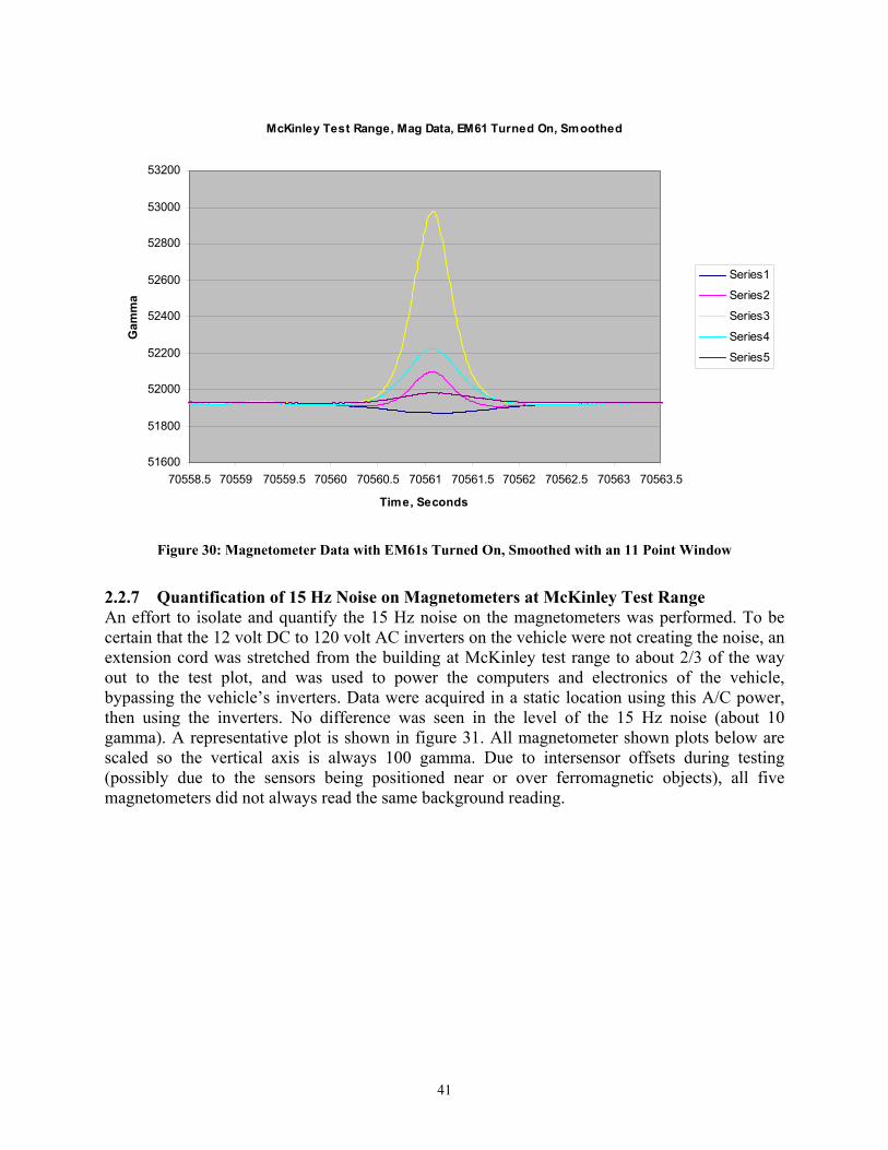
41

McKinley Test Range, Mag Data, EM61 Turned On, Smoothed

51600

51800

52000

52200

52400

52600

52800

53000

53200

70558.5 70559 70559.5 70560 70560.5 70561 70561.5 70562 70562.5 70563 70563.5

Time, Seconds

Gam

ma

Series1

Series2

Series3

Series4

Series5

Figure 30: Magnetometer Data with EM61s Turned On, Smoothed with an 11 Point Window

2.2.7 Quantification of 15 Hz Noise on Magnetometers at McKinley Test Range An effort to isolate and quantify the 15 Hz noise on the magnetometers was performed. To be certain that the 12 volt DC to 120 volt AC inverters on the vehicle were not creating the noise, an extension cord was stretched from the building at McKinley test range to about 2/3 of the way out to the test plot, and was used to power the computers and electronics of the vehicle, bypassing the vehicle’s inverters. Data were acquired in a static location using this A/C power, then using the inverters. No difference was seen in the level of the 15 Hz noise (about 10 gamma). A representative plot is shown in figure 31. All magnetometer shown plots below are scaled so the vertical axis is always 100 gamma. Due to intersensor offsets during testing (possibly due to the sensors being positioned near or over ferromagnetic objects), all five magnetometers did not always read the same background reading.

42

Representative 15 Hz Noise on Magnetometers, McKinley Test Range

51800

51810

51820

51830

51840

51850

51860

51870

51880

51890

51900

63225 63225.1 63225.2 63225.3 63225.4 63225.5 63225.6 63225.7 63225.8 63225.9 63226

Time, Seconds

Mag

Val

ue, G

amm

a

Mag 1Mag 2Mag 3Mag 4

Figure 31: Representative 10 Gamma Peak-To-Peak Noise on Four of the Five Magnetometers Seen at Test

Grid, McKinley Test Range.

The vehicle was then driven to three locations: directly beneath an overhead power line, out to the test plot (further from an overhead power line), and as far downrange as it was practical to drive (even further from an overhead power line). The plots below demonstrate that the peak-to-peak of the 15 Hz noise signal went from 25 gamma to 12 gamma to 5 gamma, showing that the signal falls off with increasing distance from the power lines, and strongly implying that the signal is, in fact, due to the power lines. The graphs of these data are shown in figures 31, 32, and 33 below.

43

15 Hz Noise on Magnetometers, McKinley Test Range, Directly Beneath Power Line

51900

51910

51920

51930

51940

51950

51960

51970

51980

51990

52000

67390 67390.1 67390.2 67390.3 67390.4 67390.5 67390.6 67390.7 67390.8 67390.9 67391

Time, Seconds

Mag

Val

ue, G

amm

a

Mag 3Mag 4Mag 5

Figure 32: 15 Hz noise on three of the five magnetometers, McKinley Test Range, acquired with system

directly beneath a power line. Noise level is approximately 25 gamma peak-to-peak.

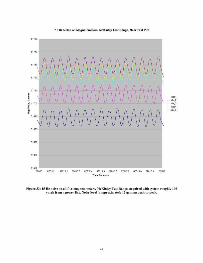
44

15 Hz Noise on Magnetometers, McKinley Test Range, Near Test Plot

51650

51660

51670

51680

51690

51700

51710

51720

51730

51740

51750

67815 67815.1 67815.2 67815.3 67815.4 67815.5 67815.6 67815.7 67815.8 67815.9 67816

Time, Seconds

Mag

Val

ue, G

amm

a

Mag1Mag2Mag3Mag4Mag5

Figure 33: 15 Hz noise on all five magnetometers, McKinley Test Range, acquired with system roughly 100

yards from a power line. Noise level is approximately 12 gamma peak-to-peak.

45

15 Hz Noise on Magnetometers, McKinley Test Range, Downrange

51900

51910

51920

51930

51940

51950

51960

51970

51980

51990

52000

68170 68170.1 68170.2 68170.3 68170.4 68170.5 68170.6 68170.7 68170.8 68170.9 68171

Time, Seconds

Mag

Val

ue, G

amm

a

Mag1Mag2Mag3Mag4Mag5

Figure 34: 15 Hz noise on all five magnetometers, McKinley Test Range, acquired with system roughly 1000

yards from a power line. Noise level is approximately 5 gamma peak-to-peak.

The question of 60 Hz-induced hum on high-update magnetometers was discussed with Dr. J.R. McDonald, formerly of NRL, now with AETC. Dr. McDonald verified that both the 50 Hz vehicular MTADS and the 100 Hz airborne MTADS pick up the 60 Hz hum from power lines, and that MTADS removes the effect using a notch filter. We are currently using a 7-point smooth to remove the effect. 2.3 Factors Affecting Cost and Performance Factors affecting cost include: Terrain: The economics of surveys bid at a fixed acreage rate per day depends on coverage rate. Smooth, grassy areas that have already been run over by heavy equipment are far more vehicularly navigable than rocky or stumpy areas, and lower coverage rates engender higher survey cost. This is particularly true due to the proof-of-concept nature of the fiberglass towed platform, which has no suspension and thus must be treated gently.

46

Physical Size of System: Because the system is a vehicular-towed array, it requires a tractor / trailer to transport it, which is inherently more costly than using man-portable systems than can be cheaply shipped. As part of the in-house development of STOLS, GEO-CENTERS owns a tractor / trailer, but no longer employs a truck driver. As such, driving services must be contracted. Required Expertise: The system is a proof-of-concept prototype, and at least initially, should be accompanied by Mr. Rob Siegel when deployed. Swath Width: The system uses five magnetometers on ½ meter spacing, but only three ½ meter EM61 coils on ½ meter spacing, so the effective multisensor swath width is only 1.5 meters. This is because all sensors were COTS from GEO-CENTERS’ existing STOLS equipment (no sensors were purchased under the program’s budget). Widening the EM61 swath width to match the 5-magnetometer swath width (2.5 meters) would increase area coverage rates and thus further reduce survey costs. Factors affecting performance include: Nature and Age of EM61 Equipment: The EM61 coils, electronics, and cabling used on this project were purchased by GEO-CENTERS for use at JPG3 in 1995. The coils are ½ by ½ meter. This configuration was originally specified by GEO-CENTERS in 1995 to aid in the detection of small, shallow targets for the JPG3 exercise, but it is a non-standard size; conventional 1 x 1 meter, or 1 x ½ meter coils would probably be better at detecting objects deeper. The use of 1 by ½ meter coils, in particular, is appealing, as it could be done with virtually no modification to the existing towed platform. The EM61 electronics are of the Mark 1 variety (single time gate). Newer multi-time gate electronics could be integrated, although the level of effort is uncertain. The age of the EM61 system in general has been somewhat problematic, as intermittent noise and cabling problems have cropped up during demonstrations [note that, as of 8/2004, the EM61 system has been updated to include five new Mk2 receivers and five 1 x ½ meter coils]. Terrain: In addition to reducing the coverage rate, uneven terrain affects data quality of both the magnetometer and EM61 data. The platform is not instrumented with inclinometers and other additional sensors to mitigate these effects, so the result can be that data are miss-positioned and the resulting target locations, depth, and size estimates can suffer. Geology: The effects of magnetic geology on magnetometers and EM61s are well-documented, and are not contravened by the fact that the system operates both sensors concurrently. However, by having both sensors deployed concurrently, there should be a better chance of developing algorithms to reject geological clutter. GPS Coverage: Centimeter-level GPS depends on adequate satellite geometry. Miss-positioned sensor data affects the accuracy of results. 2.4 Advantages and Limitations of the Technology The overriding advantage of the technology is the ability to concurrently collect both magnetometer and EM61 data in a single survey pass. MTADS, in both its NRL and Blackhawk-

47

fielded configurations, has a separate towed magnetometer and towed EM61 platform, and thus would require two separate surveys to acquire both data sets. Further, the data from the simultaneous multisensor STOLS, because they are acquired on a common rigid sensor platform, are spatially co-registered, whereas data acquired in separate survey passes may not traverse the same objects in the same way. This may limit the efficacy of the data for discrimination algorithms. The main limitations of the technology as compared to MTADS come from the fact that STOLS preceded MTADS by several years, and MTADS has had the benefit of consistent funding, technology insertion, and scientific scrutiny. Specifically, the cross-track magnetometer spacing in MTADS is tighter than STOLS (1/4 meter versus ½ meter). The EM61 electronics in MTADS have had the transmit moment increased, and the coils are larger than those used in STOLS (1 meter versus ½ meter). The MTADS sensor platforms are instrumented to measure pitch and roll, and their data processing software uses these data to more accurately position sensor updates. MTADS has both a magnetic data model and inversion and an EM61 data model and inversion; STOLS has only a magnetic data model and inversion. However, note that these are limitations on the specific implementation of the technology as manifested in the current Simultaneous Multisensor STOLS. The core technology – interleaving acquisition of magnetometer data between EM61 pulses -- does not have these limitations. The main limitation of the core interleaving technology is that it applies only to pulsed induction EM systems, and is not applicable to frequency-domain EM systems.

48

3 Demonstration Design 3.1 Performance Objectives The performance objectives listed in the Work Plan were: • To demonstrate the new multisensor STOLS’ ability to acquire combined EM61 and

magnetometer data in a single survey under controlled, but more realistic field conditions • To demonstrate the success of the project in terms of: • Faster multisensor survey time • Cheaper multisensor survey costs • Better (high-quality) synchronous, co-located magnetometer and EM61 data which can be

used for enhanced detection and discrimination algorithm development • To identify design areas that would need to be improved in order to robustly survive the

rigors of sustained field work 3.2 Selecting Test Site(s) Criteria for selecting a test site were the following:

1. Terrain hospitable to a vehicular towed array. 2. Clear view of the sky hospitable to GPS. 3. Accessible to all project participants within project budget (original plan called for Mass.

Military Reservation, which is very close to GEO-CENTERS, but it was not available). 4. A combination of a calibration area with known emplaced objects, and a blind test area.

The selected test site was the Standardized UXO Technology Demonstration Test Site at Aberdeen Proving Grounds in Aberdeen MD, which became available as the system was undergoing integration and testing. 3.3 Test Site History/Characteristics The Standardized UXO Technology Demonstration Test Site at Aberdeen Proving Grounds is operated and maintained by USAEC with support from ATC, ERDC, and ESTCP. The Open Field Site is generally flat with a low area that is wet during a portion of the year, a power line area, and a section of gravel road, all of which provided technical challenges for the vehicularly towed Multisensor STOLS. The site contains a Calibration Test Grid, a Blind Test Grid, and a mine lane, which were traversed along with the Open Site. The site also contains a wooded area and a mogul area which were not surveyed. 3.4 Present Operations The site is used for testing and evaluation of unexploded ordnance detection technology. 3.5 Pre-Demonstration Testing and Analysis

49

The McKinley Range, Redstone Arsenal Demonstration was performed as a pre-demonstration test of the Simultaneous Multisensor STOLS (see section 2.2.5 above). . 3.6 Testing and Evaluation Plan 3.6.1 Demonstration Set-Up and Start-Up On Monday, October 7th, GEO-CENTERS’ tractor/trailer truck arrived at the Standardized UXO Technology Demonstration Site at Aberdeen Proving Grounds, MD, with the multisensor STOLS equipment. Present were Rob Siegel, senior engineer, and Al Crandall, geophysicist from USA Environmental. GEO-CENTERS regular truck driver, Richard Kimball, was not present due to health problems, and a temporary truck driver was used. This is mentioned because Mr. Kimball, in addition to driving the truck, generally assists in general survey operations such as flagging survey lines to help the crew to efficiently cover the site. Without Mr. Kimball, all survey operations were conducted by the two-person crew of Rob Siegel and Al Crandall. The multisensor STOLS was inspected, unpacked, assembled, and operated statically to verify that it was not damaged in transit. The GPS base station was set up on the corner farthest from the tree line (the southern-most corner), and the magnetometer reference station was set up in a magnetically clean area. The tractor/trailer that transports STOLS is equipped with two diesel generators to provide on-board electricity generation for on-site data processing and recharging of the batteries that power the tow vehicle’s electrical systems, the GPS base station, and the reference magnetometer, but because a heated on-site trailer was provided by ATC, data processing equipment was set up in the on-site trailer, and battery charging activity was centralized there as well. The system was then run over the Calibration Grid with both the magnetometers and EM61 sensors operating simultaneously. The survey was completed in approximately 32 minutes. Magnetometer and EM61 data were immediately processed and imaged on-site to judge data quality (see the figures in section 4.3.1 below). The magnetometer data were of very high quality. The data from the EM61 system contained fixed offsets that generally did not change over the course of the survey, and thus were able to be background-leveled using standard STOLS processing techniques. 3.6.2 Period of Operation Monday, 10/7/2002 Mobilize to the site and survey Calibration Test Grid with both

magnetometers and EM61s operating simultaneously. QA/QC data.

Tuesday, 10/8/2002 Resurvey Calibration Test Grid with only magnetometers

operating. Survey Blind Test Grid with both magnetometers and EM61s operating simultaneously. QA/QC data.

Wednesday, 10/9/2002 Resurvey Blind Test Grid with both magnetometers and EM61s

operating simultaneously. Begin surveying Open site with both

50

magnetometers and EM61s operating simultaneously. QA/QC data.

Thursday, 10/10/2002 Complete surveying Open site with both magnetometers and

EM61s operating simultaneously. QA/QC data. Friday, 10/11/2002 Final QA/QC. Pack and demobilize. 3.6.3 Area Characterized or Remediated The Open Site, which contains the Mine Grid, the Calibration Test Grid, and Blind Test Grid, was approximately 13 acres. 3.6.4 Residuals Handling None. 3.6.5 Operating Parameters for the Technology Strictly speaking, no operating parameters are required. Setup of the GPS base station, the diurnal variation station (“reference magnetometer”), and the multisensor towed array is by checklist, requiring little or no operator judgment. The total field magnetometers do not require calibration, only a period of warm-up. The EM61 electronics employed do not have a zeroing knob; any background-leveling is carried out in software at the data correction stage. The vehicle driver, in this case Mr. Crandall, planned the survey traverses to maximize area coverage and minimize time spent turning the vehicle around, while being mindful of location of the tree line and any cultural obstacles. The survey crew typically consists of two people – a vehicle operator and a data analyst. Although equipment setup and vehicle operation may be performed by a single person, it is typically performed by two people, with the data analyst setting up the GPS, and the vehicle operator setting up the diurnal variation station and the vehicle systems. Although the vehicle computer has track guidance software that allows an operator to follow pre-planned survey traverses, this is rarely used, and instead the vehicle operator follows his visible survey tracks along the ground. Flags are employed to help the operator see the end of the last survey track to aid in positioning of the next survey track. This method was effectively used to traverse the Open Site. In fact, Mr. Siegel had to leave for a day to attend an ESTCP interim program review, and Mr. Crandall surveyed large sections of the Open Site himself (Rick Fling, from ATC, was on-site at all times). The data analyst typically QA/QCs data at lunchtime and again at the end of the day, and corrects and processes data in the evening. Sometimes the data analyst is stationed off-site and data are sent to him via modem.

51

Although a two-person crew was sufficient for the Open Site, additional crew members are sometimes required for UXO or site safety reasons, or if vehicle traverses are not plainly visible and “flaggers” are needed. 3.6.6 Experimental Design 3.6.6.1 Parameters That Were Varied Because towed GPS-integrated magnetometry and EM61 surveys in general and STOLS in particular have been validated at many test sites, and because STOLS with front-mounted EM61s (simultaneous, non-interleaved) had been validated at JPG3, the experimental design centered around: 1) verifying that the quality of the magnetometer data were not compromised by the

simultaneous acquisition of the EM61 data, and 2) verifying that the quality of the EM61 data were nominal. As such, the main parameter that was varied was: collecting magnetometer data over the Calibration Test Grid while the EM61s were switched off versus collecting magnetometer data while the EM61s were switched on. 3.6.6.2 How the UXO Screening Effort Was Undertaken The Open Site was vehicularly traversed in the manner in which STOLS and other towed arrays have historically been used for real-world surveys – not by laying out grids, but instead by running parallel lines along the longest axis of the survey area to cover the survey area as completely as possible in the most time-efficient manner possible. A 1.5 meter lane spacing was used. This effectively put the innermost sensor ½ meter from the outermost sensor on the previous pass, emulating the ½ meter sensor spacing on the platform. Lane spacing was estimated by driving the vehicle in a pattern that overlapped the inner tire with the outer tire track on the previous pass. Vehicle traverses over the Open Site are displayed in figure 35. Data collected in different files are displayed in different colors. These traverse data, along with interpolated image data, were used to judge that the data coverage were sufficient; only two small slivers of unsurveyed area are apparent.

52

Figure 35: Traverses from the simultaneous multisensor STOLS over the Open Site. Survey lines oriented

along the longest axis of the site were used to survey the site in the most efficient manner. 3.6.6.3 Data Reduction: Correction, Processing, and Analysis

3.6.6.3.1 Overview The data are: • Navigation-corrected • Background-leveled In addition, magnetometer data are: • Median-filtered to remove spurious values • Smoothed to remove 60 Hz-induced noise subsampled with the 75 Hz sampling rate • Reference-corrected • Directionally divided to optimize background leveling And EM61 data are: • Navigation offset-corrected • Dynamically background leveled

53

For analysis: • Magnetometer and EM61 data are viewed simultaneously • The operator manually selects an area of interest in one data set, and it is automatically

drawn in the other • For the magnetometer data, A non-linear least squares curve fit is performed to a model of a

point dipole • For the EM61 data, there is currently no model employed; the location of the peak value is

used • Dipole parameters, peak values, anomaly spatial extent, and other parameters are written to a

target file • The operator manually specifies a trinary confidence field (low, medium, or high) The overall data flow is depicted in figure 36 below.

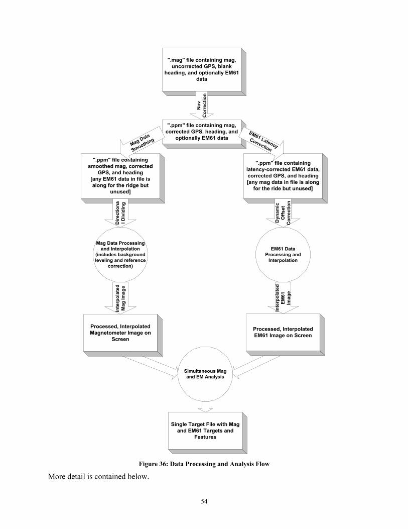
54

Mag Data Processingand Interpolation

(includes backgroundleveling and reference

correction)

".mag" file containing mag,uncorrected GPS, blank

heading, and optionally EM61data

Nav

Cor

rect

ion

".ppm" file containing mag,corrected GPS, heading, and

optionally EM61 data

".ppm" file containingsmoothed mag, corrected

GPS, and heading[any EM61 data in file isalong for the ridge but

unused]

Mag Data

Smoothing

Dire

ctio

nal D

ivid

ing

Inte

rpol

ated

Mag

Imag

e

Processed, InterpolatedMagnetometer Image on

Screen

".ppm" file containinglatency-corrected EM61 data,corrected GPS, and heading[any mag data in file is along

for the ride but unused]

EM61 LatencyCorrection

EM61 DataProcessing and

Interpolation

Dyn

amic

Offs

etC

orre

ctio

n

Inte

rpol

ated

EM61

Imag

e

Processed, InterpolatedEM61 Image on Screen

Simultaneous Magand EM Analysis

Single Target File with Magand EM61 Targets and

Features

Figure 36: Data Processing and Analysis Flow

More detail is contained below.

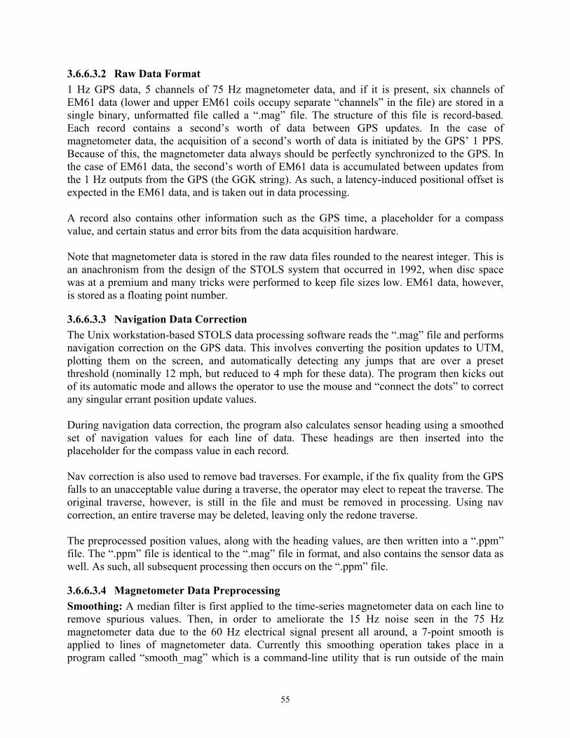
55

3.6.6.3.2 Raw Data Format 1 Hz GPS data, 5 channels of 75 Hz magnetometer data, and if it is present, six channels of EM61 data (lower and upper EM61 coils occupy separate “channels” in the file) are stored in a single binary, unformatted file called a “.mag” file. The structure of this file is record-based. Each record contains a second’s worth of data between GPS updates. In the case of magnetometer data, the acquisition of a second’s worth of data is initiated by the GPS’ 1 PPS. Because of this, the magnetometer data always should be perfectly synchronized to the GPS. In the case of EM61 data, the second’s worth of EM61 data is accumulated between updates from the 1 Hz outputs from the GPS (the GGK string). As such, a latency-induced positional offset is expected in the EM61 data, and is taken out in data processing. A record also contains other information such as the GPS time, a placeholder for a compass value, and certain status and error bits from the data acquisition hardware. Note that magnetometer data is stored in the raw data files rounded to the nearest integer. This is an anachronism from the design of the STOLS system that occurred in 1992, when disc space was at a premium and many tricks were performed to keep file sizes low. EM61 data, however, is stored as a floating point number.

3.6.6.3.3 Navigation Data Correction The Unix workstation-based STOLS data processing software reads the “.mag” file and performs navigation correction on the GPS data. This involves converting the position updates to UTM, plotting them on the screen, and automatically detecting any jumps that are over a preset threshold (nominally 12 mph, but reduced to 4 mph for these data). The program then kicks out of its automatic mode and allows the operator to use the mouse and “connect the dots” to correct any singular errant position update values. During navigation data correction, the program also calculates sensor heading using a smoothed set of navigation values for each line of data. These headings are then inserted into the placeholder for the compass value in each record. Nav correction is also used to remove bad traverses. For example, if the fix quality from the GPS falls to an unacceptable value during a traverse, the operator may elect to repeat the traverse. The original traverse, however, is still in the file and must be removed in processing. Using nav correction, an entire traverse may be deleted, leaving only the redone traverse. The preprocessed position values, along with the heading values, are then written into a “.ppm” file. The “.ppm” file is identical to the “.mag” file in format, and also contains the sensor data as well. As such, all subsequent processing then occurs on the “.ppm” file.

3.6.6.3.4 Magnetometer Data Preprocessing Smoothing: A median filter is first applied to the time-series magnetometer data on each line to remove spurious values. Then, in order to ameliorate the 15 Hz noise seen in the 75 Hz magnetometer data due to the 60 Hz electrical signal present all around, a 7-point smooth is applied to lines of magnetometer data. Currently this smoothing operation takes place in a program called “smooth_mag” which is a command-line utility that is run outside of the main

56

STOLS data processing program. Note that the GPS, compass, and if present, EM61 data are unchanged. Directional Dividing: In order to create low-noise images that are as free of streaks as possible, the traverses in a data file may be divided up into north-going, south-going, west-going, and east-going subsets. This is automatically performed by a command-line program called “bidir” (bi-directional) which uses a set of acceptance angles around a basic direction. This technique is nearly always sufficient to break up a file containing traverses of multiple directions into a set of up to four files (north-south, south-north, west-east, and east-west) each containing traverses in nominally a single direction. Each set of traverses in a single direction can then be background-leveled separately (described below). If the background value at each sensor could be known in advance for a sufficient number of orientations to accurately look up and subtract it off, directional dividing would not be necessary. However, this sort of measurement is not always practical, and alterations in vehicle, platform, and system configuration may change these values, necessitating that the measurement be redone. For these reasons, directional dividing has proven to be a fairly simple and extremely effective way of achieving the desired result of background leveling. There is no need to perform directional dividing on EM61 data, since the background levels do not change with system orientation. Note that, although raw magnetometer data are stored as integers, magnetometer data are processed as floating point numbers, and operations such as background leveling create sub-gamma values. Reference Offset: If the entire image is too light or too dark, indicating that the reference magnetometer was set up over or near metal, or over an area with geology that differs substantially from the survey area, an area of interest may be drawn in a region of the data containing no apparent magnetic anomalies. The sensor values in that area of interest are then averaged, and this average value is then subtracted from each sensor value the next time the data are processed.

3.6.6.3.5 EM61 Data Preprocessing Latency Correction: The EM61 data can have a time-offset dialed in to remove a positional shift due to the latency of the EM61 and the GPS data. This is performed by a program called “fixemoff” that is run on the command line outside of the main data processing program. The result is a “.ppm” file containing all of the original data – including GPS and magnetometer – but with the EM61 data shifted by a fixed number of 10 Hz readings. A shift of two 10 Hz readings was empirically determined to be the best shift for these data. Dynamic Background Leveling: Typically, EM61 data have different bias files for each data file acquired. However, EM61 data from the Standardized UXO Technology Demonstration Site had an unusual time-varying offset, and a new tool was developed to perform dynamic background leveling by using a window to maintain a running average for each coil, and a

57

threshold to keep EM61 anomalies out of the background calculation. The background values were then subtracted from the values in the center of the window, resulting in nearly offset-free EM61 data. The program “levelem” was used to dynamically calculate and subtract a background value for each sensor in each file. A window of 50 points (5 seconds) and a threshold of 5 millivolts above background were empirically determined to almost completely remove any dynamic offset in these data.

3.6.6.3.6 Data Processing Sequence Whether processing magnetometer or EM61 data, the workstation-based data processing software performs the following steps: 1. It reads a second’s worth of data in an input “.ppm” file to get the sensor data, the location of

the GPS antenna, and the heading. This file contains corrected navigation data and heading. When processing magnetometer data, this file contains median-filtered smoothed data. When processing EM61 data, this file contains latency-corrected background-leveled data.

2. It reads the next second’s worth of data. 3. It throws out any data that exceed the sensor’s operating range, or that have certain status and

error flags set by the hardware. 4. It looks at the changes between sensor updates and throws out values that are changing by an

unphysically possible amount (e.g., tens of thousands of gamma in 1/75th of a second). 5. Knowing the GPS location and heading at the start and the end of the second, and knowing

the number of sensors, the spacing between sensors, the sensor update rate, and the distance from the GPS antenna to the center of the sensor array, it calculates the UTM X and Y location of each sensor value. For magnetometer data, this is 5 channels of data updating at 75 Hz. For EM61 data, this is six channels of data updating at 10 Hz.

6. In the case of magnetometer data, it finds the time-correlated reference value in the diurnal data file (or uses a static reference value if no reference file is available) and subtracts it off from the sensor data.

7. If a “bias file” is specified, a sensor-specific bias value is used to background-level the sensor data.

8. If a “reference offset” is specified, a data set-wide reference offset value is used to background level the entire data set.

9. If a file-specific reference offset is specified, a reference offset value specific to an individual data file is used to level minor background differences between data files if the reference magnetometer was moved.

10. A two-dimensional array is set up to wholly contain the data. The cell spacing in the array is adjustable, but is nominally set to 10 cm per cell. The positioned sensor updates are then put into the grid. If data are dense along the direction of travel, more than one sensor update may have the same grid cell location. If this is the case, the later values overwrite the earlier values. Note that, in both the case of EM61 and magnetometer data, the grid is of integer data type, and thus any data thrown into the grid are rounded to the nearest integer.

11. It repeats this process for each second’s worth of data in the “.ppm” file. 12. It repeats this process for any number of “.ppm” files specified which collectively comprise

data from a survey site.

3.6.6.3.7 Interpolation for Visualization

58

After data have been thrown into the grid with the appropriate corrections applied, the grid is interpolated using a simple nearest neighbor inverse distance squared algorithm. At each point in the 10 cm grid, a window is drawn, moving out three points in each direction. Since the sensor spacing is 5 cm (5 grid points for axially-aligned data), this window has the effect of “filling in” the spacing between the sensors. At least three original data points must be present within the window for a new point to be interpolated. This prevents the program from interpolating off into nothingness on the basis of sparse data. The interpolated data provide a pleasing visual image that aids data interpretation. The model-match to a point dipole that is used for analysis, however, works on the uninterpolated data.

3.6.6.3.8 Data Analysis Historically, all data analysis in STOLS has been performed using two-dimensional image data; no one-dimensional analysis is performed on time-series magnetometer or EM61 data. The data from the Standardized UXO Test Site was analyzed in this same way – as image-based data. A 25-meter quadrant’s worth of data was displayed and analyzed at a time, with magnetometer and EM61 images viewed simultaneously. The operator used his eyeball to pick out anomalies from the data, and used the mouse to draw an area of interest around each chosen anomaly. This area of interest could be drawn over either the magnetometer image or the EM61 image, and would automatically appear over the other image. For the magnetometer data, a non-linear least squares three-dimensional curve fit to a model of a point dipole was performed. GEO-CENTERS software does not currently include an EM model, however, so for EM61 data, the peak anomaly value and its location were logged. Although a nominal 2-5 gamma threshold was used for the magnetometer data, the effects of varying geologic background level and geologic noise make it such that a simple fixed threshold could not be applied without engendering an unnecessarily high false alarm rate. Instead of fixed thresholding, the operator used his judgment, along with a sliding colorization tool, to pick out magnetic dipole-like anomalies and EM61 anomalies. Priority was given to anomalies that were round and had good, clear, adjacent positive and negative lobes. In this way, the operator attempted to screen out the magnetic “ripples” along the survey site that were most likely due to local geology. Similarly, when viewing the EM61 data, although a 2-5 millivolt threshold was nominally applied, anomalies that were strong and had a round shape were given priority over those that were weak, or were unnaturally elongated along the direction of travel, or that appeared on only one of the three EM61 coils. While hand-picking each anomaly, the operator hand-entered one of three heuristic classes of target confidence: • High-confidence targets were those with anomalies that were strong and round. These high-

confidence targets usually appeared in both the magnetometer and EM61 images, but the operator could still flag a target as high confidence if it only appeared in one image (magnetometer or EM61), as long as it had a textbook strong, clear, round, completely unambiguous signature.

• Medium-confidence targets were those with anomalies that were clear but appeared in only

one of the two images (magnetometer or EM61), or targets that appeared in both the magnetometer and EM61 images with weaker, less defined, less round anomalies.

59

• Low-confidence targets were those with small, weak, ill-defined anomalies that the operator thought most likely to be due to debris, clutter, geology or noise (though anomalies specifically thought by the operator to be geology or noise were not picked at all). In most cases, a low-confidence target appeared on the magnetometer or the EM61 image but not both, and the anomaly was of such small spatial extent that it was caused by a single sensor (e.g., one magnetometer or one EM61 coil).

Response Stage Column: In formatting the target list to comply with the data submission requirements, there is a column required for “response stage” intended to contain the signal strength of each chosen anomaly. The multisensor STOLS generates both magnetometer and EM61 data, so there would normally be two such columns. In order to concatenate the two anomalies from the multisensor target picks into a single response value, the peak magnetometer value and the peak EM61 value were added together and divided by the goodness of fit (chi squared) from the magnetometer’s dipole model match. This is not intended to provide discrimination capability; it is merely a way of generating a single anomaly value from two peak sensor values. Discrimination Stage Ranking Column: The ranking was determined as follows. Individually, within the classes of high-confidence, medium-confidence, and low-confidence targets that were heuristically assigned by the operator and hand-entered, the data were sorted by response stage, which, as described above, is calculated as (peak_mag + peak_EM61)/chi_squared. A column was then added that contained the row number of these targets once they were sorted by hand-assigned confidence, then by response. As with the response, this is not intended to provide discrimination capability; it is merely a way to rank the targets. Classification Column: Because we do not claim to be able to discriminate, this column was set to “O,” indicating ordnance. Type Column: Because we do not claim to be able to discriminate, this column was left blank. Depth Column: For targets whose depth was estimated by the curve fit to the magnetometer dipole model, the depth is listed. For targets for which the curve fit to the magnetometer dipole model did not converge to reasonable results (such as the target being above the ground our outside the original area of interest), and for targets for which there was EM61 signature but no magnetic signature, the flag “-999” is used to indicate that there is no depth information. Angular Columns: The angle of incidence and angle of orientation are output from the curve fit to the magnetic dipole model. 3.6.7 Sampling Plan 3.6.7.1 Overview As described in section 3.6.6.2, the Open Site was vehicularly traversed in the manner in which STOLS and other towed arrays have historically been used for real-world surveys – not by laying out grids, but instead by running parallel lines along the longest axis of the survey area to cover the survey area as completely as possible in the most time-efficient manner possible. A 1.5 meter

60

lane spacing was used. This effectively put the innermost sensor ½ meter from the outermost sensor on the previous pass, emulating the ½ meter sensor spacing on the platform. Lane spacing was estimated by driving the vehicle in a pattern that overlapped the inner tire with the outer tire track on the previous pass. Vehicle traverses over the Open Site are displayed in figure 36. Data collected in different files are displayed in different colors. These traverse data, along with interpolated image data, were used to judge that the data coverage were sufficient; only two small slivers of unsurveyed area are apparent. 3.6.7.2 Sample Analysis The data were viewed for QA screening on-site twice per day in the trailer at the test site. Data correction and preprocessing occurred during the evening. Final data processing occurred off-site back at GEO-CENTERS. All target detection and analysis occurred at GEO-CENTERS. A detailed description of the data processing is contained above in section 3.6.6.6. 3.6.7.3 Experimental Controls Background magnetometer data was acquired using a proton precession magnetometer updating at a 15-second interval. Time-stamped background magnetometer values were time-correlated with vehicular magnetometer values and subtracted off during data processing. 3.6.7.4 Data Quality Parameters The most important data quality parameter is the GPS Fix Quality. The system utilizes a Trimble differential GPS with Real Time Kinematic (RTK) capability, and the data acquisition software on the vehicle computer monitors the fix quality that is output every second along with the GPS location and time. A fix quality of 3 indicates a fixed-integer RTK centimeter-level solution, and is essential for accurate geodetic positioning of the data. If the fix quality is other than 3 (for example, a fix quality 4 indicates an RTK float solution, a fix quality of 2 indicates a standard differential GPS solution, a fix quality of 1 indicates an autonomous, non-differential solution, and a fix quality of 0 indicates no solution due to an insufficient number of satellites in view), the computer screen on the vehicle computer turns bright red, indicating that the operator should stop the survey until the GPS fix quality returned to RTK fix quality 3. Momentary losses in fix quality 3 occurred while collecting data along the tree line (along the northwest corner of the Open Site) when clear view of the sky was obscured by the trees. Longer losses in fix quality 3 data occurred during periods of poor satellite geometry. These were verified by using Trimble-supplied GPS planning software (“QuickPlan”). At the onset of poor fix quality data, data collection immediately ceased, and we simply waited out the poor fix quality window. The number of drop-outs in the magnetometer data is used to judge magnetometer data quality. When the magnetometer data are processed and interpolated, spuriously low values that are still within the valid dynamic range of the magnetometers appear as small black squares in the data. Isolated occurrences pose no problem, and a median filter is used to remove them from the data, but large numbers of drop-outs can indicate a failing magnetometer. A surprise data quality parameter was the degree of drift of the EM61 background. As was discussed in the section on data processing, the background level in the EM61 signal seemed to drift in a manner that had not been previously seen. Survey operations on the Open Site did not

61

commence until we were confident that the drift was addressable through algorithmic means; a dynamic background-leveling algorithm was used to remove the drift. 3.6.7.5 Data Quality Indicators The best data quality indicator is the processed and imaged data. After data correction, streak-free images containing round anomalies indicates high-quality data for both the magnetometers and the EM61s. 3.6.7.6 Calibration Procedures, Quality Control Checks, and Corrective Action No sensor-based calibration is used per se (no standard metallic source is put beneath the magnetometer or EM61 sensor and used to calibrate the output to a preset level). Quality control checks are described above (watching the GPS fix quality and the sensor values themselves during surveying; processing the magnetometer and EM61 data and visually screening the interpolated image for magnetometer drop-outs and EM61 drift). Corrective action is described in the data processing description in section 3.6.6.2 (correcting isolated jumps in the navigation data, removal of magnetometer drop-outs through median filtering, and removal of EM61 drift through dynamic background leveling). 3.6.8 Demobilization The GPS base station and reference magnetometer stations are taken down and stored in the tractor-trailer. The non-metallic tow platform is disconnected from the survey vehicle and the wiring harness is rolled up. The survey vehicle is driven into the tractor-trailer. The platform is rolled in behind the vehicle; the long tow bar, still connected to the platform to minimize set-up and tear-down time, rests on top of the survey vehicle. The vehicle and platform are strapped down.

62

4 Performance Assessment It should be noted that Project UX-0208 was not a discrimination project; it was a hardware and platform development project to develop and demonstrate a system that can generate high-quality, spatially co-registered magnetometer and EM61 data in a single survey without the magnetometer data being compromised by noise engendered by the EM61s. While these data can be given to algorithm developers to perform discrimination work, the scope of this project did not include algorithm development for discrimination. It should also be noted that the original work plan called for demonstration of the system at the nearby Massachusetts Military Reservation (local to GEO-CENTERS), whereas the system was actually demonstrated at the Standardized UXO Technology Demonstration Site at APG. GEO-CENTERS was pleased to be one of the first demonstrators on this excellent site, but the target submission and reporting format for this site has discrimination-specific required entries (for example, ranking the targets in order of decreasing probability that the targets are UXO). We did our best to comply with these reporting requirements, but we do not claim to have a technical approach to discrimination. The performance objectives listed in the work plan were: • To demonstrate the new multisensor STOLS’ ability to acquire combined EM61 and

magnetometer data in a single survey under controlled, but more realistic field conditions • To demonstrate the success of the project in terms of:

• Faster multisensor survey time • Cheaper multisensor survey costs • Better (high-quality) synchronous, co-located magnetometer and EM61 data which can

be used for enhanced detection and discrimination algorithm development • To identify design areas that would need to be improved in order to robustly survive the

rigors of sustained field work 4.1 Performance Criteria The performance criteria were as follows: Performance Criteria Description Primary or Secondary Functionality of sensor interleaving

Demonstration that the hardware designed to acquire magnetometer data between pulses from the EM61 system is functional

Primary

Data Quality Demonstration that the magnetometer data acquired through interleaving is high-quality

Primary

Efficiency Demonstration that the simultaneous acquisition of magnetometer and EM61 data is more efficient than surveying the same area twice in separate surveys.

Primary

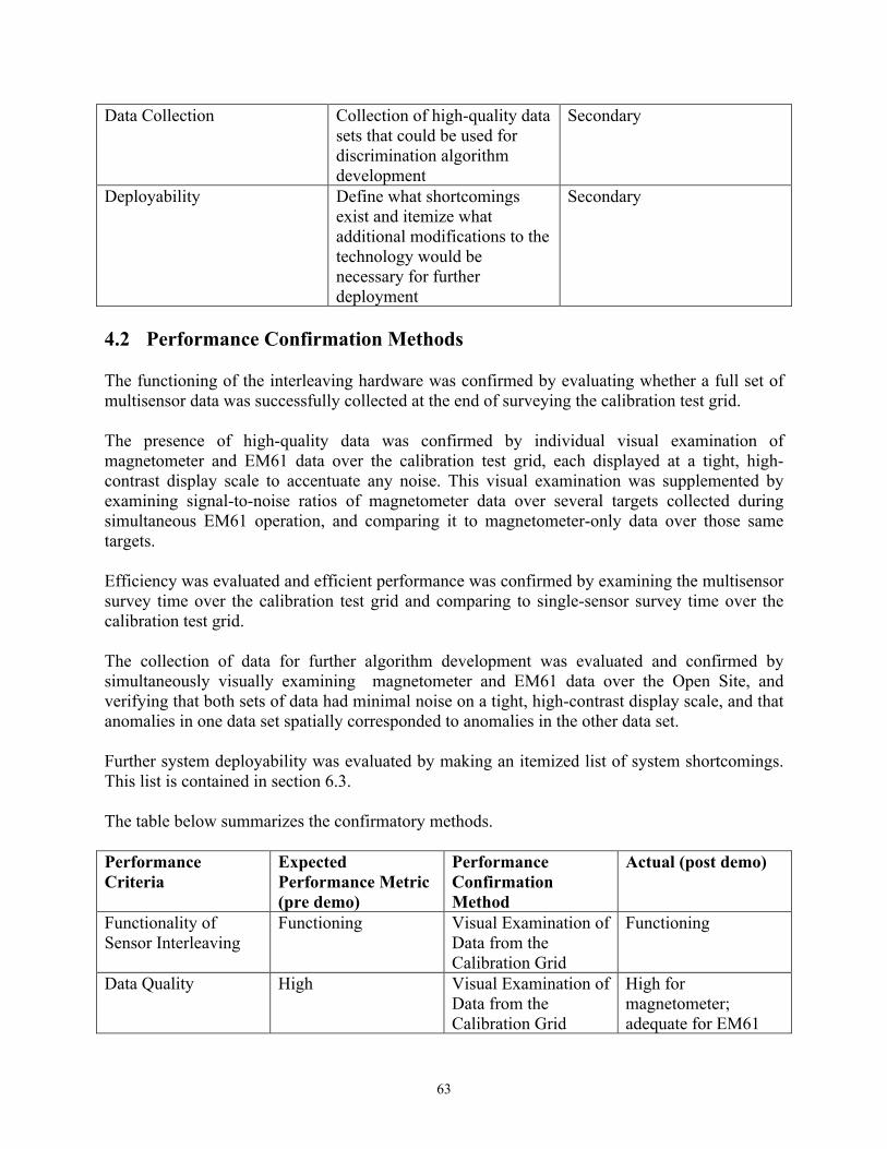
63

Data Collection Collection of high-quality data sets that could be used for discrimination algorithm development

Secondary

Deployability Define what shortcomings exist and itemize what additional modifications to the technology would be necessary for further deployment

Secondary

4.2 Performance Confirmation Methods The functioning of the interleaving hardware was confirmed by evaluating whether a full set of multisensor data was successfully collected at the end of surveying the calibration test grid. The presence of high-quality data was confirmed by individual visual examination of magnetometer and EM61 data over the calibration test grid, each displayed at a tight, high-contrast display scale to accentuate any noise. This visual examination was supplemented by examining signal-to-noise ratios of magnetometer data over several targets collected during simultaneous EM61 operation, and comparing it to magnetometer-only data over those same targets. Efficiency was evaluated and efficient performance was confirmed by examining the multisensor survey time over the calibration test grid and comparing to single-sensor survey time over the calibration test grid. The collection of data for further algorithm development was evaluated and confirmed by simultaneously visually examining magnetometer and EM61 data over the Open Site, and verifying that both sets of data had minimal noise on a tight, high-contrast display scale, and that anomalies in one data set spatially corresponded to anomalies in the other data set. Further system deployability was evaluated by making an itemized list of system shortcomings. This list is contained in section 6.3. The table below summarizes the confirmatory methods. Performance Criteria

Expected Performance Metric (pre demo)

Performance Confirmation Method

Actual (post demo)

Functionality of Sensor Interleaving

Functioning Visual Examination of Data from the Calibration Grid

Functioning

Data Quality High Visual Examination of Data from the Calibration Grid

High for magnetometer; adequate for EM61

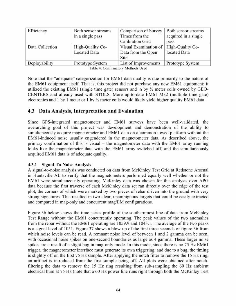
64

Efficiency Both sensor streams in a single pass

Comparison of Survey Times from the Calibration Grid

Both sensor streams acquired in a single pass

Data Collection High-Quality Co-Located Data

Visual Examination of Data from the Open Site

High-Quality Co-located Data

Deployability Prototype System List of Improvements Prototype System Table 4: Confirmatory Methods Used

Note that the “adequate” categorization for EM61 data quality is due primarily to the nature of the EM61 equipment itself. That is, this project did not purchase any new EM61 equipment; it utilized the existing EM61 (single time gate) sensors and ½ by ½ meter coils owned by GEO-CENTERS and already used with STOLS. More up-to-date EM61 Mk2 (multiple time gate) electronics and 1 by 1 meter or 1 by ½ meter coils would likely yield higher quality EM61 data. 4.3 Data Analysis, Interpretation and Evaluation Since GPS-integrated magnetometer and EM61 surveys have been well-validated, the overarching goal of this project was development and demonstration of the ability to simultaneously acquire magnetometer and EM61 data on a common towed platform without the EM61-induced noise usually engendered in the magnetometer data. As described above, the primary confirmation of this is visual – the magnetometer data with the EM61 array running looks like the magnetometer data with the EM61 array switched off, and the simultaneously acquired EM61 data is of adequate quality. 4.3.1 Signal-To-Noise Analysis A signal-to-noise analysis was conducted on data from McKinley Test Grid at Redstone Arsenal in Huntsville AL to verify that the magnetometers performed equally well whether or not the EM61 were simultaneously operating. McKinley data was chosen for this analysis over APG data because the first traverse of each McKinley data set ran directly over the edge of the test plot, the corners of which were marked by two pieces of rebar driven into the ground with very strong signatures. This resulted in two clear, unambiguous targets that could be easily extracted and compared in mag-only and concurrent mag/EM configurations. Figure 36 below shows the time-series profile of the southernmost line of data from McKinley Test Range without the EM61 concurrently operating. The peak values of the two anomalies from the rebar without the EM61 operating are 1059.9 and 1043.1. The average of the two peaks is a signal level of 1051. Figure 37 shows a blow-up of the first three seconds of figure 36 from which noise levels can be read. A remnant noise level of between 1 and 2 gamma can be seen, with occasional noise spikes on one-second boundaries as large as 4 gamma. These larger noise spikes are a result of a slight bug in mag-only mode. In this mode, since there is no 75 Hz EM61 trigger, the magnetometer interface must generate its own triggering, and due to a bug, the timing is slightly off on the first 75 Hz sample. After applying the notch filter to remove the 15 Hz ring, an artifact is introduced from the first sample being off. All plots were obtained after notch-filtering the data to remove the 15 Hz ring resulting from sub-sampling the 60 Hz ambient electrical hum at 75 Hz (note that a 60 Hz power line runs right through both the McKinley Test

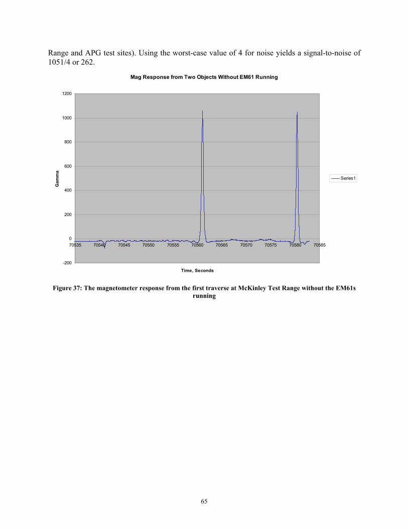
65

Range and APG test sites). Using the worst-case value of 4 for noise yields a signal-to-noise of 1051/4 or 262.

Mag Response from Two Objects Without EM61 Running

-200

0

200

400

600

800

1000

1200

70535 70540 70545 70550 70555 70560 70565 70570 70575 70580 70585

Time, Seconds

Gam

ma

Series1

Figure 37: The magnetometer response from the first traverse at McKinley Test Range without the EM61s

running

66

Noise Without EM61 Running

-30

-28

-26

-24

-22

-20

-18

-16

-14

-12

-1070535 70535.5 70536 70536.5 70537 70537.5 70538

Time, Seconds

Gam

ma

Series1

Figure 38: Noise levels in the first three seconds of magnetometer data from the first traverse at McKinley

Test Range without the EM61 running

Figure 39 below shows the profile over the two rebar objects acquired while the EM61 was simultaneously operating. The two peak values are 1063.7 and 1025.3, yielding an average value of 1044. We see that this signal level is within about 1% of the value 1051 obtained in the mag-only mode. Figure 40 shows a blow-up of the first three seconds of data, from which a noise level of between 1 and 2 gamma can be read. As with the mag-only plot above, this noise is the remnant of filtering the 15 Hz ring due to a nearby 60 power line being sampled at 75 Hz. This yields a signal-to-noise of 1044/2, or 522. However, the noise is actually less than in mag-only mode; the larger 4 gamma noise signal, visible every second in the magnetometer-only data, is not present in the concurrent mag/EM data. This is because the 4 gamma noise signal the mag-only triggering mode is an artifact of a sampling bug. Without this bug repaired, near power lines, there is somewhat more noise, thus somewhat lower signal-to-noise, in the mag-only mode. If this bug were repaired, the two signal-to-noise levels would be nearly identical. These results are summarized in table 5 below.

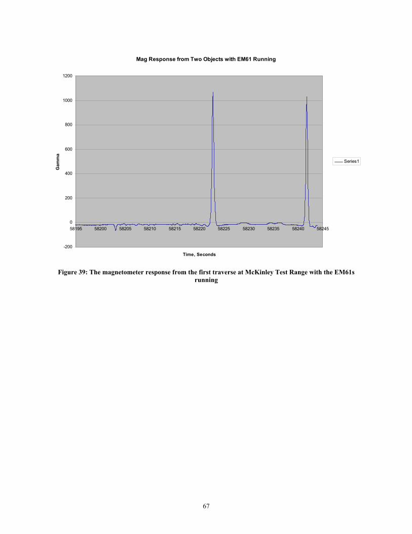
67

Mag Response from Two Objects with EM61 Running

-200

0

200

400

600

800

1000

1200

58195 58200 58205 58210 58215 58220 58225 58230 58235 58240 58245

Time, Seconds

Gam

ma

Series1

Figure 39: The magnetometer response from the first traverse at McKinley Test Range with the EM61s

running

68

Mag Response from Two Objects with EM61 Running

-30

-28

-26

-24

-22

-20

-18

-16

-14

-12

-1058195 58195.5 58196 58196.5 58197 58197.5 58198

Time, Seconds

Gam

ma

Series1

Figure 40: Noise levels in the first three seconds of magnetometer data from the first traverse at McKinley

Test Range with the EM61 running

Mode Signal-To-Noise Magnetometer Only (with sampling error)

262

Magnetometer Only (if sampling error were fixed)

514

Concurrent Magnetometer and EM61 522 Table 5: Comparison of signal-to-noise levels in mag-only mode and concurrent mag/EM mode

4.3.2 Calibration Test Grid Data The visual confirmation of magnetometer data quality is displayed in figure 41. This shows magnetometer data acquired over the Calibration Test Grid while the EM61s were switched off. Figure 42 shows magnetometer data over the same area acquired while the EM61s were synchronously collecting data. Both images are displayed to a very tight +-25 gamma scale to highlight magnetic anomalies as well as any noise. Heuristically comparing these two images, they are extremely similar; the image of magnetometer data obtained while the EM61s were running does not visually contain noise that is not also present in the image of the magnetometer data obtained while the EM61s were switched off. This provides visual confirmation that the acquisition of magnetometer data between EM61 transmit pulses is not adversely affecting magnetometer data quality. (For a time-series representation of this confirmation, see section 2.2.6 These data were converted to an ASCII data format and submitted to ESTCP and CEHNC.

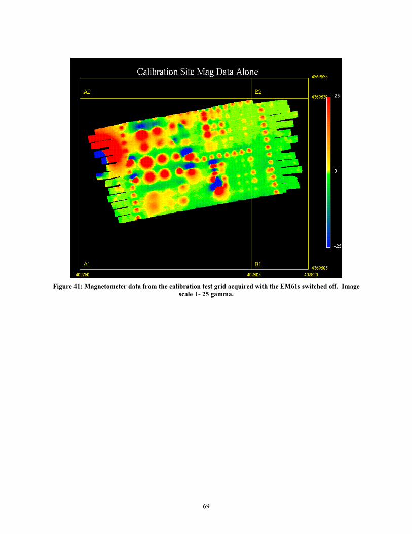
69

Figure 41: Magnetometer data from the calibration test grid acquired with the EM61s switched off. Image

scale +- 25 gamma.

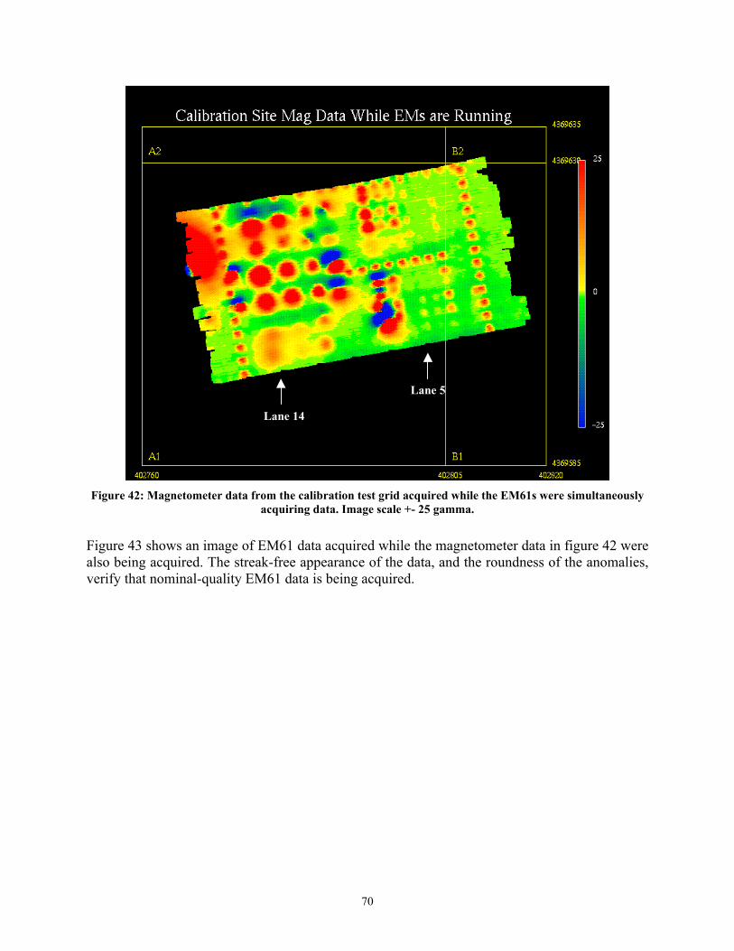
70

Lane 14

Lane 5

Figure 42: Magnetometer data from the calibration test grid acquired while the EM61s were simultaneously

acquiring data. Image scale +- 25 gamma.

Figure 43 shows an image of EM61 data acquired while the magnetometer data in figure 42 were also being acquired. The streak-free appearance of the data, and the roundness of the anomalies, verify that nominal-quality EM61 data is being acquired.

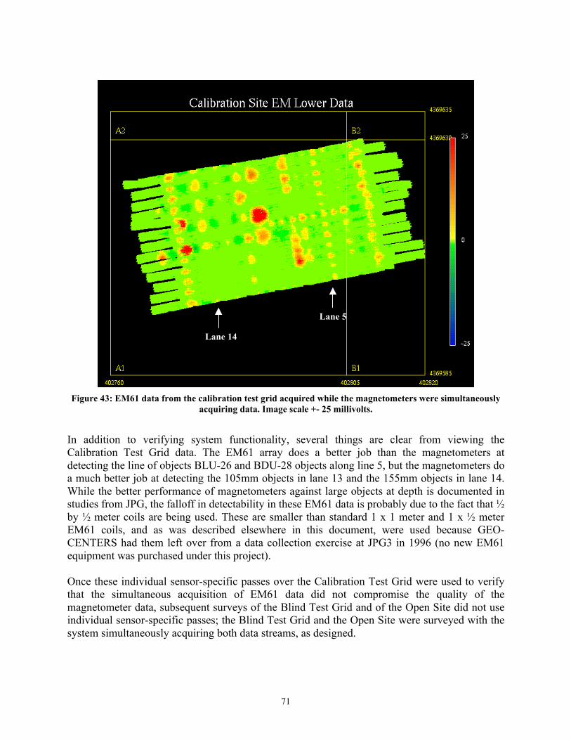
71

Lane 5

Lane 14

Figure 43: EM61 data from the calibration test grid acquired while the magnetometers were simultaneously

acquiring data. Image scale +- 25 millivolts.

In addition to verifying system functionality, several things are clear from viewing the Calibration Test Grid data. The EM61 array does a better job than the magnetometers at detecting the line of objects BLU-26 and BDU-28 objects along line 5, but the magnetometers do a much better job at detecting the 105mm objects in lane 13 and the 155mm objects in lane 14. While the better performance of magnetometers against large objects at depth is documented in studies from JPG, the falloff in detectability in these EM61 data is probably due to the fact that ½ by ½ meter coils are being used. These are smaller than standard 1 x 1 meter and 1 x ½ meter EM61 coils, and as was described elsewhere in this document, were used because GEO-CENTERS had them left over from a data collection exercise at JPG3 in 1996 (no new EM61 equipment was purchased under this project). Once these individual sensor-specific passes over the Calibration Test Grid were used to verify that the simultaneous acquisition of EM61 data did not compromise the quality of the magnetometer data, subsequent surveys of the Blind Test Grid and of the Open Site did not use individual sensor-specific passes; the Blind Test Grid and the Open Site were surveyed with the system simultaneously acquiring both data streams, as designed.

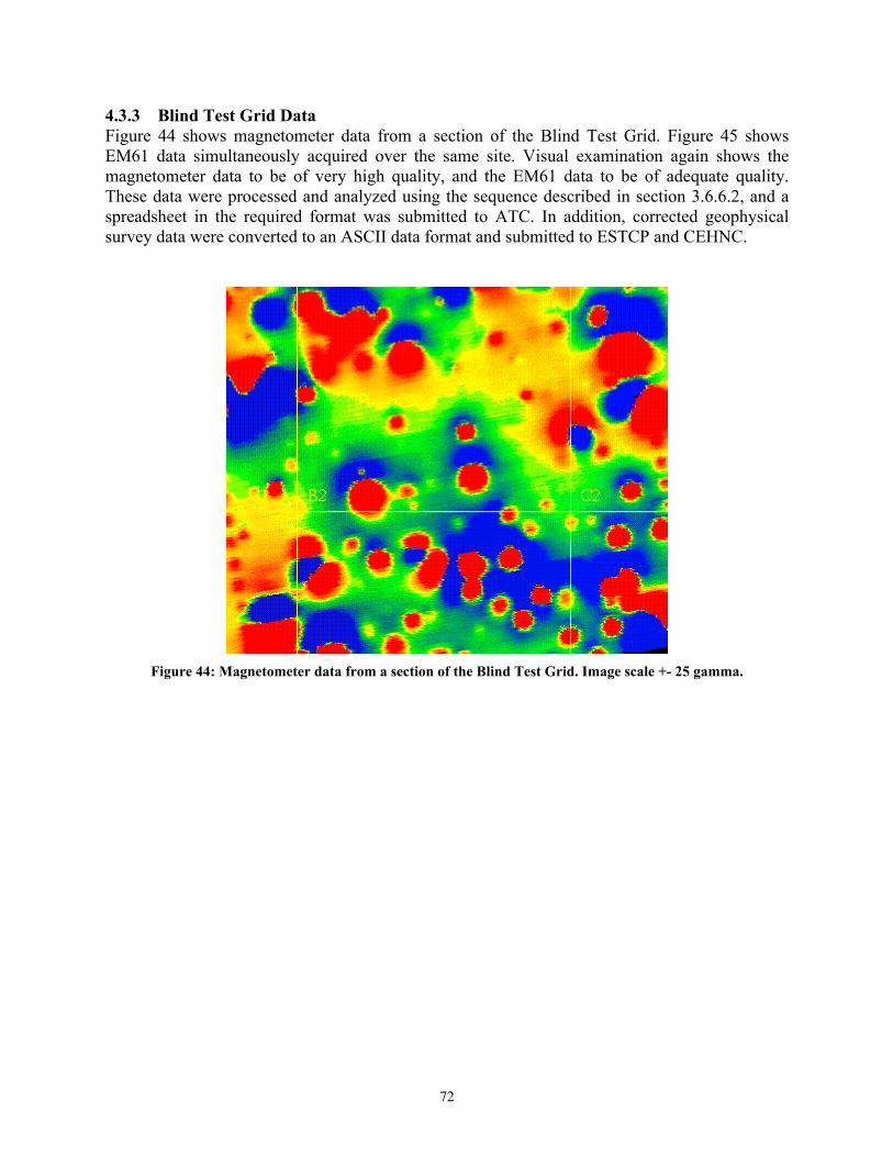
72

4.3.3 Blind Test Grid Data Figure 44 shows magnetometer data from a section of the Blind Test Grid. Figure 45 shows EM61 data simultaneously acquired over the same site. Visual examination again shows the magnetometer data to be of very high quality, and the EM61 data to be of adequate quality. These data were processed and analyzed using the sequence described in section 3.6.6.2, and a spreadsheet in the required format was submitted to ATC. In addition, corrected geophysical survey data were converted to an ASCII data format and submitted to ESTCP and CEHNC.

Figure 44: Magnetometer data from a section of the Blind Test Grid. Image scale +- 25 gamma.

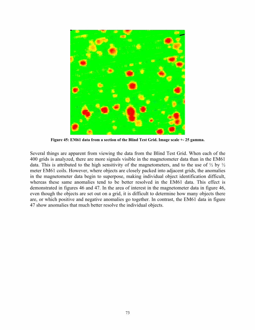
73

Figure 45: EM61 data from a section of the Blind Test Grid. Image scale +- 25 gamma.

Several things are apparent from viewing the data from the Blind Test Grid. When each of the 400 grids is analyzed, there are more signals visible in the magnetometer data than in the EM61 data. This is attributed to the high sensitivity of the magnetometers, and to the use of ½ by ½ meter EM61 coils. However, where objects are closely packed into adjacent grids, the anomalies in the magnetometer data begin to superpose, making individual object identification difficult, whereas these same anomalies tend to be better resolved in the EM61 data. This effect is demonstrated in figures 46 and 47. In the area of interest in the magnetometer data in figure 46, even though the objects are set out on a grid, it is difficult to determine how many objects there are, or which positive and negative anomalies go together. In contrast, the EM61 data in figure 47 show anomalies that much better resolve the individual objects.

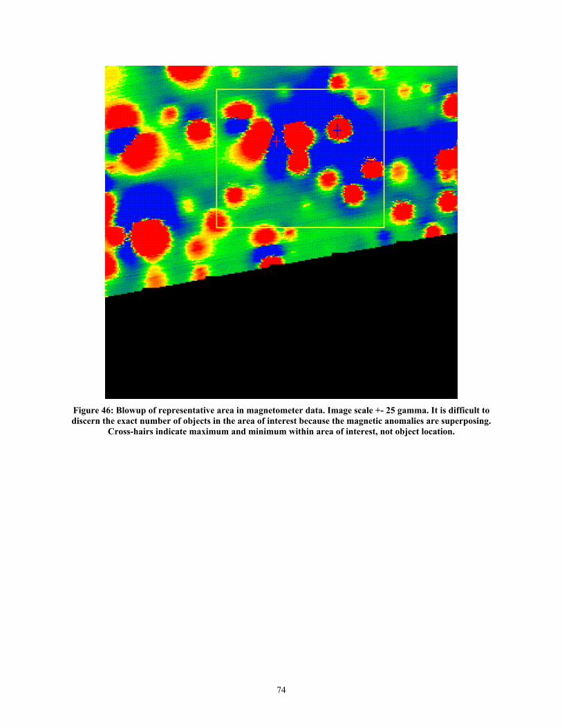
74

Figure 46: Blowup of representative area in magnetometer data. Image scale +- 25 gamma. It is difficult to discern the exact number of objects in the area of interest because the magnetic anomalies are superposing.

Cross-hairs indicate maximum and minimum within area of interest, not object location.

75

Figure 47: The same area of interest in the EM61 data. Image scale +- 25 millivolts. The individual anomalies

are much clear in the EM61 data than in the magnetometer data. Cross-hairs indicate maximum and minimum values within area of interest, not object location.

Another observation in viewing the Blind Test Grid data is that, like data from the Calibration Test Grid, the magnetometer data are of extremely high quality, whereas the anomalies in the EM61 data sometimes have a slightly elongated appearance, indicating that perhaps the synchronization between the GPS and the EM61 electronics is not remaining precisely constant. 4.3.4 Blind Test Grid Scored Results On January 22nd, 2004, GEO-CENTERS received from ATC a paper copy of the report “Standardized UXO Technology Demonstration Site Blind Grid Scoring Record No. 40.” The summary table from the Report is listed below.

76

By Size By Depth, m

Metric Overall Standard Non-Standard Small Medium Large < 0.3 0.3 to <1 >= 1 EM RESPONSE STAGE

Pd 0.80 0.80 0.75 0.80 0.75 0.80 0.90 0.70 0.50 Pd Low 90% Conf 0.71 0.72 0.62 0.71 0.61 0.55 0.82 0.58 0.27 Pfp 0.85 - - - - - 0.85 0.90 1.00 Pfp Low 90% Conf 0.80 - - - - - 0.74 0.79 0.63 Pba 0.50 - - - - - - - -

MAG RESPONSE STAGE Pd 0.85 0.90 0.70 0.75 0.85 1.00 0.80 0.85 0.90 Pd Low 90% Conf 0.77 0.84 0.59 0.66 0.76 0.79 0.71 0.72 0.66 Pfp 0.90 - - - - - 0.90 0.90 1.00 Pfp Low 90% Conf 0.85 - - - - - 0.81 0.82 0.63 Pba 0.70 - - - - - - - -

COMBINED MAG/EM RESPONSE STAGE Pd 0.65 0.75 0.45 0.50 0.70 0.90 0.65 0.70 0.20 Pd Low 90% Conf - - - - - - - - - Pfp 0.75 - - - - - 0.70 0.75 1.00 Pfp Low 90% Conf - - - - - - - - - Pba 0.10 - - - - - - - -

Table 7: Summary of Blind Grid Results From here, we see that the magnetometers performed best on large, deep objects, and the EM61s performed best for more shallow objects. Because the combined results show a lower probability of detection than the individual mag or EM results, it is unclear how the combined results were calculated, and GEO-CENTERS defers questions on them to ATC. 4.3.5 Open Site Data Figure 48 shows magnetometer data from a section of the 13-acre Open Site. Figure 49 shows EM61 data acquired simultaneously with the EM61 array. Again, visual examination again shows the magnetometer data to be of very high quality, and the EM61 data to be of adequate quality. The data were processed and analyzed using the sequence described in section 3.6.6.2, and a spreadsheet with 2166 entries in the required format was submitted to ATC. In addition, corrected geophysical survey data were converted to an ASCII data format and submitted to ESTCP and CEHNC.

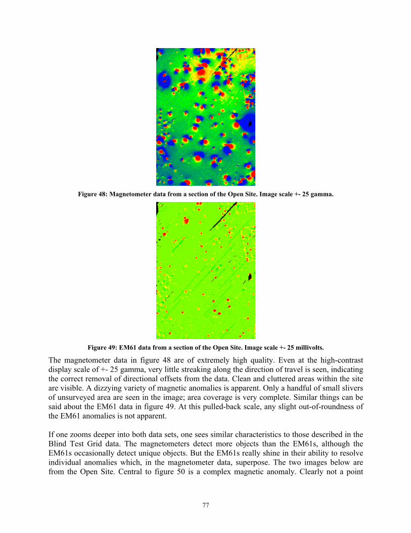
77

Figure 48: Magnetometer data from a section of the Open Site. Image scale +- 25 gamma.

Figure 49: EM61 data from a section of the Open Site. Image scale +- 25 millivolts.

The magnetometer data in figure 48 are of extremely high quality. Even at the high-contrast display scale of +- 25 gamma, very little streaking along the direction of travel is seen, indicating the correct removal of directional offsets from the data. Clean and cluttered areas within the site are visible. A dizzying variety of magnetic anomalies is apparent. Only a handful of small slivers of unsurveyed area are seen in the image; area coverage is very complete. Similar things can be said about the EM61 data in figure 49. At this pulled-back scale, any slight out-of-roundness of the EM61 anomalies is not apparent. If one zooms deeper into both data sets, one sees similar characteristics to those described in the Blind Test Grid data. The magnetometers detect more objects than the EM61s, although the EM61s occasionally detect unique objects. But the EM61s really shine in their ability to resolve individual anomalies which, in the magnetometer data, superpose. The two images below are from the Open Site. Central to figure 50 is a complex magnetic anomaly. Clearly not a point

78

dipole, it is unclear from the magnetometer image what assortment of individual and/or extended objects produce this anomaly. Further, a yellow area of interest in the magnetometer data shows no discernable anomaly in an area where the EM61 data (below) show an anomaly.

Figure 50: Compound object in magnetometer data from the Open Site. Image scale +- 25 gamma. No

anomaly is visible within the yellow area of interest. Compare this to Figure 51.

In contrast, figure 51 shows the same area in the EM61 data. Although the image contains fewer total anomalies than the magnetometer data, the size and shapes of the individual anomalies in the compound object are much more clearly delineated than they were in the magnetometer data. Further, the yellow area of interest clearly shows a visibly apparent anomaly in an area where no such anomaly is visible in the magnetometer data. This image visually depicts the advantages of utilizing simultaneous magnetometry and EM61.

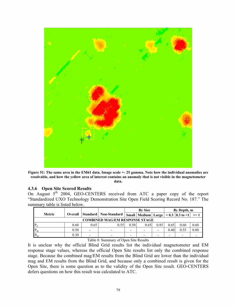
79

Figure 51: The same area in the EM61 data. Image scale +- 25 gamma. Note how the individual anomalies are

resolvable, and how the yellow area of interest contains an anomaly that is not visible in the magnetometer data.

4.3.6 Open Site Scored Results On August 5th 2004, GEO-CENTERS received from ATC a paper copy of the report “Standardized UXO Technology Demonstration Site Open Field Scoring Record No. 187.” The summary table is listed below.

By Size By Depth, m Metric Overall Standard Non-Standard Small Medium Large < 0.3 0.3 to <1 >= 1

COMBINED MAG/EM RESPONSE STAGE Pd 0.60 0.65 0.55 0.50 0.65 0.85 0.65 0.60 0.60 Pfp 0.50 - - - - - 0.40 0.55 0.80 Pba 0.30 - - - - - - - -

Table 8: Summary of Open Site Results It is unclear why the official Blind Grid results list the individual magnetometer and EM response stage values, whereas the official Open Site results list only the combined response stage. Because the combined mag/EM results from the Blind Grid are lower than the individual mag and EM results from the Blind Grid, and because only a combined result is given for the Open Site, there is some question as to the validity of the Open Site result. GEO-CENTERS defers questions on how this result was calculated to ATC.

80

Note that, since the APG fielding in 2002, the system has been improved in many ways, including the addition of an array of five EM61 Mk2 (multiple time gate) sensors, and that the improved system was retested at APG in August 2004 and at Yuma Proving Grounds in October 2004, with the data submitted to Dr. Stephen Billings and Dr. Leonard Pasion for discrimination processing.

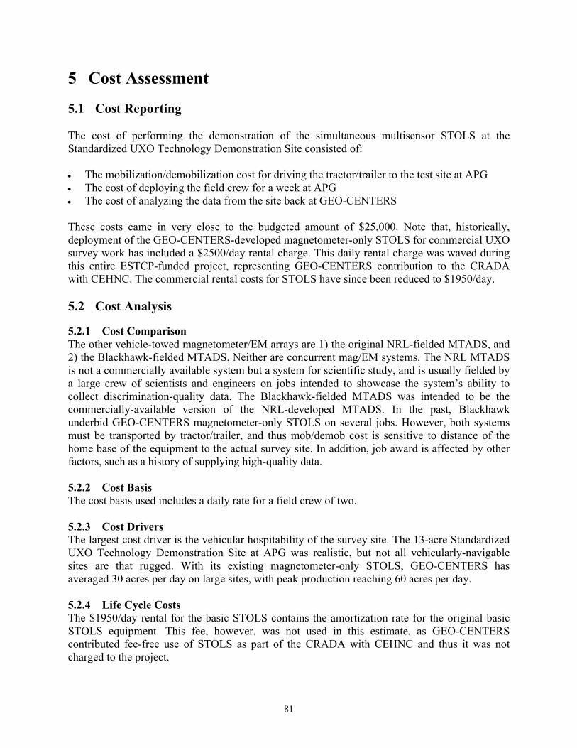
81

5 Cost Assessment 5.1 Cost Reporting The cost of performing the demonstration of the simultaneous multisensor STOLS at the Standardized UXO Technology Demonstration Site consisted of: • The mobilization/demobilization cost for driving the tractor/trailer to the test site at APG • The cost of deploying the field crew for a week at APG • The cost of analyzing the data from the site back at GEO-CENTERS These costs came in very close to the budgeted amount of $25,000. Note that, historically, deployment of the GEO-CENTERS-developed magnetometer-only STOLS for commercial UXO survey work has included a $2500/day rental charge. This daily rental charge was waved during this entire ESTCP-funded project, representing GEO-CENTERS contribution to the CRADA with CEHNC. The commercial rental costs for STOLS have since been reduced to $1950/day. 5.2 Cost Analysis 5.2.1 Cost Comparison The other vehicle-towed magnetometer/EM arrays are 1) the original NRL-fielded MTADS, and 2) the Blackhawk-fielded MTADS. Neither are concurrent mag/EM systems. The NRL MTADS is not a commercially available system but a system for scientific study, and is usually fielded by a large crew of scientists and engineers on jobs intended to showcase the system’s ability to collect discrimination-quality data. The Blackhawk-fielded MTADS was intended to be the commercially-available version of the NRL-developed MTADS. In the past, Blackhawk underbid GEO-CENTERS magnetometer-only STOLS on several jobs. However, both systems must be transported by tractor/trailer, and thus mob/demob cost is sensitive to distance of the home base of the equipment to the actual survey site. In addition, job award is affected by other factors, such as a history of supplying high-quality data. 5.2.2 Cost Basis The cost basis used includes a daily rate for a field crew of two. 5.2.3 Cost Drivers The largest cost driver is the vehicular hospitability of the survey site. The 13-acre Standardized UXO Technology Demonstration Site at APG was realistic, but not all vehicularly-navigable sites are that rugged. With its existing magnetometer-only STOLS, GEO-CENTERS has averaged 30 acres per day on large sites, with peak production reaching 60 acres per day. 5.2.4 Life Cycle Costs The $1950/day rental for the basic STOLS contains the amortization rate for the original basic STOLS equipment. This fee, however, was not used in this estimate, as GEO-CENTERS contributed fee-free use of STOLS as part of the CRADA with CEHNC and thus it was not charged to the project.

82

5.2.5 Actual Survey Costs Because, the Simultaneous Multisensor STOLS has been used at several large survey sites since the close of this ESTCP-funded project, actual survey costs can be stated. Note that mob/demob, work plan, site safety and health plan, and other tasks typically itemized on a Statement of Work are excluded because they are highly site-specific. Also note that, even for the daily rate, different surveys have different requirements and different levels of risk that can affect the quoted daily rate. Folded into the daily rate for Lowry was a 2-man crew of expert operators, the $1950/day rental charge for the Simultaneous Multisensor STOLS, as well as other factors and assumptions. The 110 acre survey of the Jeep / Demo Range at The Former Lowry Bombing and Gunnery Range (FLBGR) is used as an example:

Labor $39,983.38ODCs $14,583.91Rental $23,400.00Total $77,967.29

Table 9: Actual Survey Costs at FLBGR Dividing the total cost by 110 acres yields a cost per acre of $708.

83

6 Implementation Issues 6.1 Environmental Checklist Other than the emissions created by the tow vehicle’s gasoline-powered internal combustion engine, no residuals or pollutants are produced by the system. 6.2 Other Regulatory Issues Any applicable regulatory issues involve detection and discrimination systems of all kinds (i.e., how clean is clean, etc) and are not specific to this project or technology. 6.3 End-User Issues The envisioned end-user is the Army Corps of Engineers Huntsville (CEHNC) and the contractors that they employ for UXO site assessment and cleanup. As CEHNC was a partner on this project, there are no inherent impediments toward adoption of the technology. The applicability of the technology is largely a function of the vehicular navigability and GPS coverage on a particular site; these are factors that apply to any towed vehicular sensor array, not just Simultaneous Multisensor STOLS. The equipment developed under this project augmented STOLS (already a proven, robust magnetometer-based GPS-integrated vehicular-towed array) with a simultaneous EM61 capability in such a way that the magnetometers and EM61 data acquisition are interleaved and thus do not interfere with each other. When discussing procurement issues, a distinction must be made between portions of the system that are new (such as the interleaving electronics) and portions that were previously resident in STOLS. The new interleaving hardware – the beating heart of the project – is well-designed and appears to function robustly. An initial small production run of three boards was performed. One board is in the STOLS system, one is in a benchtop development system, and the third is a spare. The Trimble RTK-equipped GPS, the Geometrics 822A magnetometers, and the EM61 Mark 1 (single time gate) electronics are COTS. The non-metallic non-conductive towed array was designed to fit into the budget of this project, and as such was explicitly designed to be a proof-of-concept platform. It was fabricated at GEO-CENTERS. Fabrication could be farmed out, but at a bare minimum, a suspension should be incorporated (ideally an entirely new platform design should be investigated). The existing low magnetic self-signature STOLS tow vehicle was specified by GEO-CENTERS and built to specification by Chenowth Racing in San Diego, CA, who also builds the MTADS tow vehicle. The data processing software utilized for the project is GEO-CENTERS’ legacy Unix workstation-based software. Although the software represents 15 years of development and possesses great capability to correct, process, view, and analyze the simultaneous multisensor data, Geosoft Montaj has emerged as the chosen standard for UXO-related data processing, and its use should be included into the project. Whether GEO-CENTERS’ software should be used to

84

pre-process and correct the data before importing it into Montaj, or should be jettisoned completely, is unclear at this time. Recommended upgrades to the system include: New EM61 electronics (possibly multi-time-gate); changing from three ½ x ½ meter EM61 coils to five ½ x 1 meter coils; installing a suspension on the towed platform, and upgrading the data acquisition computer from a notebook PC to something more environmentally sealed. The simultaneous spatially co-located multisensor data stream should be mined for discrimination capability. GEO-CENTERS’ partner in this project, the Army Corps of Engineers Huntsville (CEHNC), plans to use the system at an applicable site in 2003. GEO-CENTERS plans to support this effort, and to attend conferences and other appropriate events to increase the visibility of the technology. GEO-CENTERS would be pleased to interact with any organization interested in using the Simultaneous Multisensor STOLS system, or in licensing the underlying interleaving technology.

7 Ongoing Improvements and Commercial Use of the System

In the 15 months since the demonstration at APG, GEO-CENTERS and CEHNC have made continued improvements to the system, and deployed the modified system for a 100-acre survey of The Jeep / Demo Range at The Former Lowry Bombing and Gunnery Range in Aurora, CO, and an 82-acre survey at The Former Portland Army Air Base. Although these efforts are outside the ESTCP-funded project, they are described below because they represent a major success at technology transfer. 7.1 Improve EM61 Reliability The goal of this task was to address some of the reliability issues surrounding the EM61 data acquisition system. Two of the five existing sets of EM61 Mk1 electronics were returned to Geonics for testing. Problems were found with both sets of electronics. They were repaired, tested, and returned to GEO-CENTERS. Both sets were installed into multisensor STOLS and field-tested in the parking lot. Cables and connectors were shaken while system output was examined. Data was collected and processed. The data appeared to be largely free of the abrupt drift and level-shifting previously seen. It was assumed that this task was complete. However, the survey at Lowry showed that the drift and level-shifting were still with the system. Conversations with Geonics revealed that Geonics recommends that we do not power the electronics off an inverter and power supply, as we have been, and instead use a single isolated large deep-discharge 12V battery. This was done by GEO-CENTERS prior to the Portland survey. Also prior to the Portland survey, another set of EM electronics was returned to Geonics for calibration and testing. The EM data from Portland (collected with five 1 by ½ meter coils, see below) are by far the highest quality data that have ever been collected with STOLS, and are free of the abrupt drift and level-shifting that was apparent at Lowry. We feel that, at this point, we are probably collecting as high-quality EM61 Mk1 data as is the industry-standard. 7.2 Improve Data Acquisition Reliability The ESTCP-funded project utilized a fragile, office-quality notebook computer and PCMCIA cards for serial data acquisition. New computers that are hardened to military specifications are quite expensive. It was felt that a cost-effective method of making the system more robust was to purchase a used ruggedized notebook computer. GEO-CENTERS purchased for STOLS a two-year-old factory refurbished Panasonic Toughbook with an 800 Mhz processor and a color sunlight-readable touchscreen (figure 52), and this computer was used for the Portland International Airport survey. The computer worked well, suffering no heat, cold, or weather-related failures. However, two issues needed to be addressed. Firstly, when the vehicle was moving, the computer appeared to drop GPS data (to not write it to disk every second). It is assumed that, because this never happened during parking lot testing at GEO-CENTERS, never happened during the three minutes of daily static QA testing at Portland,

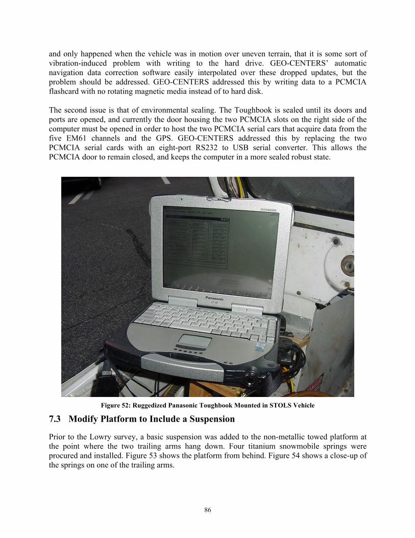
86

and only happened when the vehicle was in motion over uneven terrain, that it is some sort of vibration-induced problem with writing to the hard drive. GEO-CENTERS’ automatic navigation data correction software easily interpolated over these dropped updates, but the problem should be addressed. GEO-CENTERS addressed this by writing data to a PCMCIA flashcard with no rotating magnetic media instead of to hard disk. The second issue is that of environmental sealing. The Toughbook is sealed until its doors and ports are opened, and currently the door housing the two PCMCIA slots on the right side of the computer must be opened in order to host the two PCMCIA serial cars that acquire data from the five EM61 channels and the GPS. GEO-CENTERS addressed this by replacing the two PCMCIA serial cards with an eight-port RS232 to USB serial converter. This allows the PCMCIA door to remain closed, and keeps the computer in a more sealed robust state.

Figure 52: Ruggedized Panasonic Toughbook Mounted in STOLS Vehicle

7.3 Modify Platform to Include a Suspension Prior to the Lowry survey, a basic suspension was added to the non-metallic towed platform at the point where the two trailing arms hang down. Four titanium snowmobile springs were procured and installed. Figure 53 shows the platform from behind. Figure 54 shows a close-up of the springs on one of the trailing arms.

87

Figure 53: Non-metallic platform from rear showing addition of springs to trailing arms

Figure 54: Close-up of starboard trailing arm showing springs and perches.

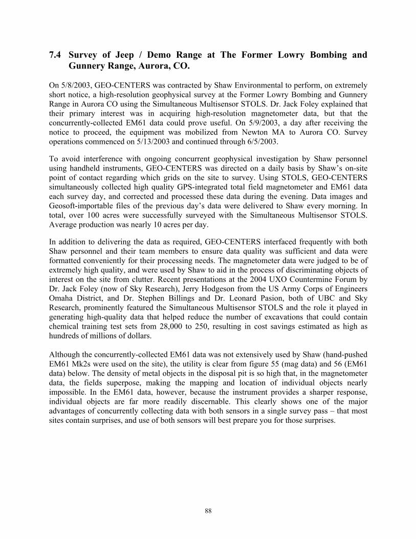
88

7.4 Survey of Jeep / Demo Range at The Former Lowry Bombing and Gunnery Range, Aurora, CO.

On 5/8/2003, GEO-CENTERS was contracted by Shaw Environmental to perform, on extremely short notice, a high-resolution geophysical survey at the Former Lowry Bombing and Gunnery Range in Aurora CO using the Simultaneous Multisensor STOLS. Dr. Jack Foley explained that their primary interest was in acquiring high-resolution magnetometer data, but that the concurrently-collected EM61 data could prove useful. On 5/9/2003, a day after receiving the notice to proceed, the equipment was mobilized from Newton MA to Aurora CO. Survey operations commenced on 5/13/2003 and continued through 6/5/2003. To avoid interference with ongoing concurrent geophysical investigation by Shaw personnel using handheld instruments, GEO-CENTERS was directed on a daily basis by Shaw’s on-site point of contact regarding which grids on the site to survey. Using STOLS, GEO-CENTERS simultaneously collected high quality GPS-integrated total field magnetometer and EM61 data each survey day, and corrected and processed these data during the evening. Data images and Geosoft-importable files of the previous day’s data were delivered to Shaw every morning. In total, over 100 acres were successfully surveyed with the Simultaneous Multisensor STOLS. Average production was nearly 10 acres per day. In addition to delivering the data as required, GEO-CENTERS interfaced frequently with both Shaw personnel and their team members to ensure data quality was sufficient and data were formatted conveniently for their processing needs. The magnetometer data were judged to be of extremely high quality, and were used by Shaw to aid in the process of discriminating objects of interest on the site from clutter. Recent presentations at the 2004 UXO Countermine Forum by Dr. Jack Foley (now of Sky Research), Jerry Hodgeson from the US Army Corps of Engineers Omaha District, and Dr. Stephen Billings and Dr. Leonard Pasion, both of UBC and Sky Research, prominently featured the Simultaneous Multisensor STOLS and the role it played in generating high-quality data that helped reduce the number of excavations that could contain chemical training test sets from 28,000 to 250, resulting in cost savings estimated as high as hundreds of millions of dollars. Although the concurrently-collected EM61 data was not extensively used by Shaw (hand-pushed EM61 Mk2s were used on the site), the utility is clear from figure 55 (mag data) and 56 (EM61 data) below. The density of metal objects in the disposal pit is so high that, in the magnetometer data, the fields superpose, making the mapping and location of individual objects nearly impossible. In the EM61 data, however, because the instrument provides a sharper response, individual objects are far more readily discernable. This clearly shows one of the major advantages of concurrently collecting data with both sensors in a single survey pass – that most sites contain surprises, and use of both sensors will best prepare you for those surprises.

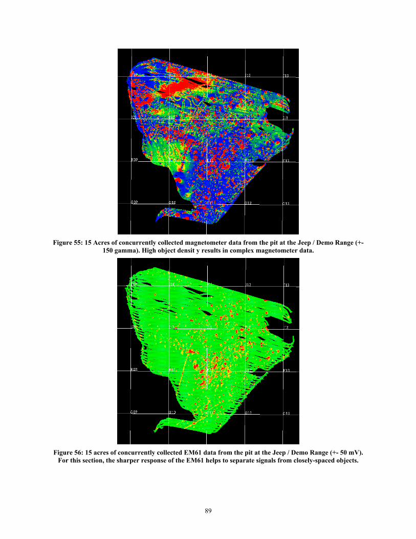
89

Figure 55: 15 Acres of concurrently collected magnetometer data from the pit at the Jeep / Demo Range (+-

150 gamma). High object densit y results in complex magnetometer data.

Figure 56: 15 acres of concurrently collected EM61 data from the pit at the Jeep / Demo Range (+- 50 mV).

For this section, the sharper response of the EM61 helps to separate signals from closely-spaced objects.

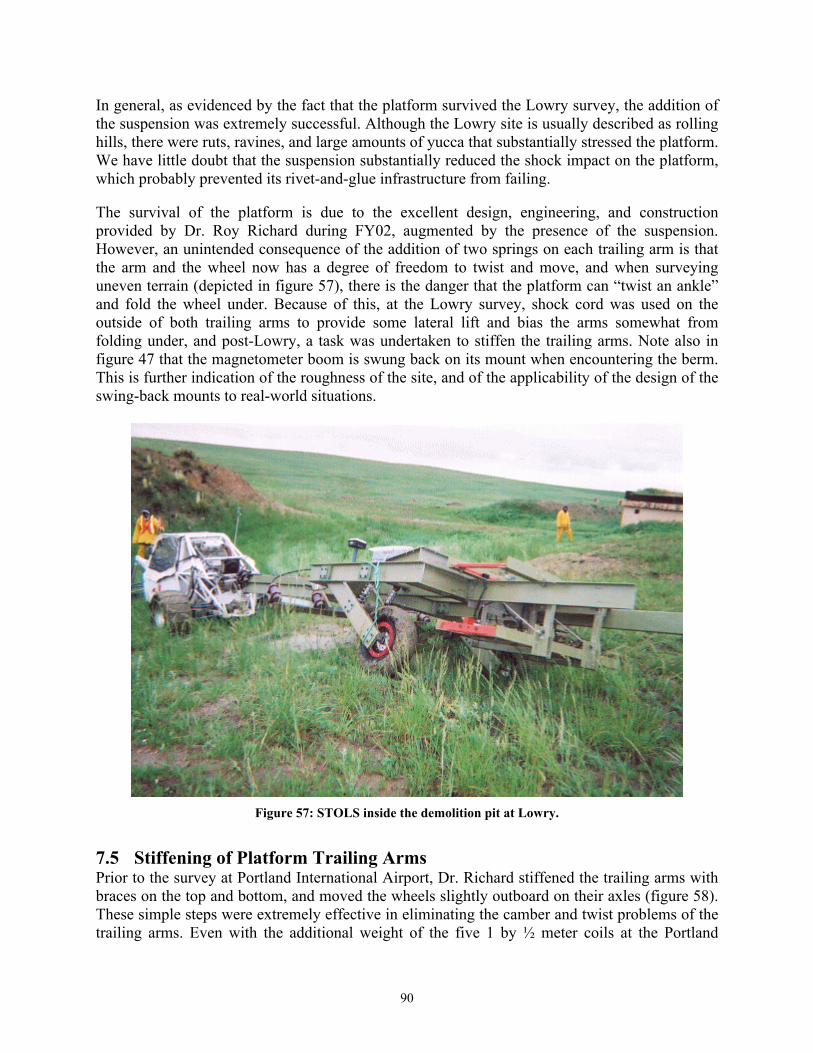
90

In general, as evidenced by the fact that the platform survived the Lowry survey, the addition of the suspension was extremely successful. Although the Lowry site is usually described as rolling hills, there were ruts, ravines, and large amounts of yucca that substantially stressed the platform. We have little doubt that the suspension substantially reduced the shock impact on the platform, which probably prevented its rivet-and-glue infrastructure from failing.

The survival of the platform is due to the excellent design, engineering, and construction provided by Dr. Roy Richard during FY02, augmented by the presence of the suspension. However, an unintended consequence of the addition of two springs on each trailing arm is that the arm and the wheel now has a degree of freedom to twist and move, and when surveying uneven terrain (depicted in figure 57), there is the danger that the platform can “twist an ankle” and fold the wheel under. Because of this, at the Lowry survey, shock cord was used on the outside of both trailing arms to provide some lateral lift and bias the arms somewhat from folding under, and post-Lowry, a task was undertaken to stiffen the trailing arms. Note also in figure 47 that the magnetometer boom is swung back on its mount when encountering the berm. This is further indication of the roughness of the site, and of the applicability of the design of the swing-back mounts to real-world situations.

Figure 57: STOLS inside the demolition pit at Lowry.

7.5 Stiffening of Platform Trailing Arms Prior to the survey at Portland International Airport, Dr. Richard stiffened the trailing arms with braces on the top and bottom, and moved the wheels slightly outboard on their axles (figure 58). These simple steps were extremely effective in eliminating the camber and twist problems of the trailing arms. Even with the additional weight of the five 1 by ½ meter coils at the Portland

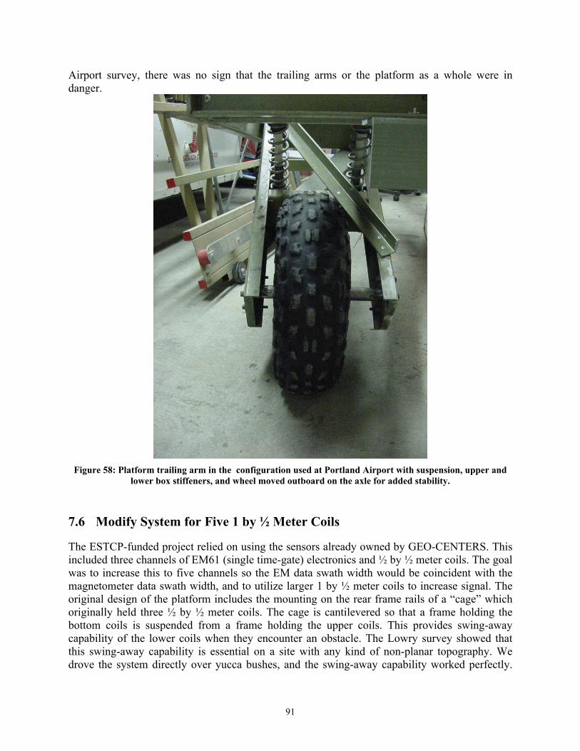
91

Airport survey, there was no sign that the trailing arms or the platform as a whole were in danger.

Figure 58: Platform trailing arm in the configuration used at Portland Airport with suspension, upper and

lower box stiffeners, and wheel moved outboard on the axle for added stability.

7.6 Modify System for Five 1 by ½ Meter Coils The ESTCP-funded project relied on using the sensors already owned by GEO-CENTERS. This included three channels of EM61 (single time-gate) electronics and ½ by ½ meter coils. The goal was to increase this to five channels so the EM data swath width would be coincident with the magnetometer data swath width, and to utilize larger 1 by ½ meter coils to increase signal. The original design of the platform includes the mounting on the rear frame rails of a “cage” which originally held three ½ by ½ meter coils. The cage is cantilevered so that a frame holding the bottom coils is suspended from a frame holding the upper coils. This provides swing-away capability of the lower coils when they encounter an obstacle. The Lowry survey showed that this swing-away capability is essential on a site with any kind of non-planar topography. We drove the system directly over yucca bushes, and the swing-away capability worked perfectly.

92

Problems eventually occurred because, when the lower coils swing back, the motion is undamped, and the coils hit with such force that the connectors coupling them to the cables began breaking. At Lowry, this was mitigated by, eventually, driving around rather than over large yucca. But the basic design of the cage is sound and is in keeping with the fast, light, and relatively inexpensive construction techniques of the proof-of-concept fiberglass platform. Incorporating five 1 by ½ meter coils (allowing the EM swath width to match the magnetometer swath width while yielding greater power into the ground than the ½ by ½ meter coils) necessitates construction of a similar cage, but wider and longer. The drawing of the platform with the larger cage is depicted in figure 59.

Figure 59: Planned configuration of platform with cage to accommodate five 1 by 1/2 meter coils

Design and construction were completed prior to the Portland survey. Two 1 by ½ meter EM61 coils were rented to test-fit them to the modified platform. Due to the presence of handle mounting brackets on both sides of some (but not all) of the rented coils, the coils could not be directly abutted and thus mounting holes were drilled to set the intersensor spacing at several centimeters more than ½ meter. An unintended consequence of the new configuration is that the width of five coils makes the platform’s width too large to fit in the STOLS trailer for transport or overnight storage. Thus, prior to the Portland deployment, the cage was removed from the back of the platform and slid beneath the platform in the STOLS trailer. Upon arriving at Portland Airport, the five rented EM61 coils were uncrated and the entire EM61 array was reassembled (figure 60). While Dr. Richard was concerned that the roughly 2.5 times the added weight from the larger number of larger coils were likely to make this new iteration of the platform far more of a demonstration-only entity, the platform behaved extremely well at the Portland survey, and did not give us pause to think that it was grossly overloaded (though the springs are certainly being

93

used). Granted, the topography of the Portland survey area was gentle, but in contrast to the Lowry survey, where there were obvious lessons learned that translated into immediately required platform improvements, there are no show-stopper incremental improvements required to the platform at this time in order to conduct another survey.

Figure 60: Five 1 by 1/2 meter EM61 coils mounted on the fiberglass platform at Portland International

Airport.

In addition to the three sets of EM61 Mk1 electronics and cabling originally used under ESTCP project UX-0208, GEO-CENTERS owns two other sets of EM61 Mk1 electronics and cabling. These additional two sets were mounted in the STOLS vehicle and additional cabling was added (figure 61). As part of the wiring of the additional electronics, the 12 volt power supply originally used to power the EM61 electronics from the 120v inverter was jettisoned, and a marine quality deep-discharge battery was added (figure 62). This battery is completely separate from the other five deep-discharge batteries used to power the STOLS vehicle, computers, magnetometers, and electronics. A second EM-specific battery has since been added to allow the EM61s to be run all day without requiring the batteries to be recharged.

94

Figure 61: Five sets of EM61 Mk1 electronics and cabling

Figure 62: Isolated deep-discharge battery utilized to power the EM electronics. A second battery has since

been added to allow the EM61s to run all day without requiring that the batteries be recharged.

95

Additional serial ports were added to the data acquisition computer to host the five EM61 channels. Each of the computer’s two PCMCIA slots now holds a four-port serial PCMCIA card. As noted above, PCMCIA cards are convenient but not necessarily optimum for a rugged configuration, as opening the PCMCIA door exposes the computer’s internal components to weather. GEO-CENTERS has since converted to using an eight-port USB to serial converter. The data acquisition, data storage, and data processing software all needed to be modified to acquire, store, and process the additional channels of EM61 data. Prior to the mobilization for the Portland Airport survey, the system, with its new data acquisition computer, recalibrated EM61 electronics, additional EM61 channels, modified platform with suspension and stiffened trailing arms, and wider EM61 array, was tested at GEO-CENTERS. 7.7 Survey of The Former Portland Army Air Base An anecdotal report of a trench at The Former Portland Army Air Base (now Portland International Airport) filled with a million rounds of small munitions resulted in CEHNC contacting GEO-CENTERS. Interest was expressed in the Simultaneous Multisensor STOLS system because of the increased detection probability inherent in the simultaneous use of multiple sensors. Specifically, since the trench was anecdotal in nature, the exact nature of its was uncertain, and it was thought that a system that utilized both total field magnetometers and pulsed induction sensors would provide the greatest chance of detecting and locating the trench, if it existed. Also, since the site was on an active airfield, there was concern over the degree to which potential noise sources might interfere with detection and mask candidate signals. The concurrent use of multiple complimentary sensors also offered the possible additional benefit of detection if one sensor was susceptible to unavoidable site noise. GEO-CENTERS surveyed the 85-acre site with the Simultaneous Multisensor STOLS with an average production rate of nearly 15 acres per day. The system functioned flawlessly, collecting very high quality magnetometer and EM61 data (figures 63 and 64). As with the data from Lowry, there were clear advantages to using both sensors. On the airfield itself, strong fields from high-voltage equipment rendered the EM61 data noisy, whereas the magnetometers continued to function. Conversely, one section of the site had a high concentration of anomalies that showed up weakly in the magnetometer data but rang out very clearly in the EM61 data, possibly indicating a collection of non-ferrous objects intermixed with ferrous ones, or a collection objects with both ferrous and non-ferrous components. Although no signature that correlated with the description of the anecdotal trench was found, the use of both sensors helped to “prove the negative.”

96

Figure 63: 85 Acres of Concurrent Magnetometer Data from The Former Portland Army Air Base

Figure 64: 85 Acres of Concurrent EM61 Data from The Former Portland Army Air Base

97

7.8 Further Work Through the CRADA with CEHNC, modern EM61 Mk2 (multiple time gate) electronics (figure 65) have been interfaced to the system. Together with the prior integration of larger 1 by ½ meter coils, this brings the EM61 capability of the system to modern standards, and generates EM61 data of a quality commensurate with the magnetometer data and far more useful for discrimination algorithms than the single time-gate data collected previously. New EM61 Mk2 hardware and 1 by ½ meter coils were purchased for the system with funding from the Army Environmental Quality Technology (EQT) program for further testing of the improved system at the Standardized UXO Demonstration Test Sites at Aberdeen Proving Grounds and Yuma Proving Grounds. The system as currently configured is shown in figure 66.

Figure 65: EM61 Mk2 Electronics Integrated into STOLS Buggy

98

Figure 66: STOLS as Currently Configured

Through the CRADA with CEHNC, tighter integration with researchers at UBC and Sky Research (Drs. Stephen Billings and Leonard Pasion) is being pursued so that their discrimination algorithms can be applied on data collected by the system in upcoming surveys.

8 References 1991. Remote Detection of Unexploded Ordnance, Surface Towed Ordnance Locator System. Technical Report TR-302, Naval Explosive Ordnance Disposal Center, Indian Head, MD, 20640-5070, 1991 1999. ESTCP Cost and Performance Report UX-9526) Multisensor Towed Array Detection System (MTADS), Naval Research Laboratory, 1999. 1997. UXO Technology Demonstration at Jefferson Proving Ground, Phase III. US Army Environmental Center, April 1997 Siegel, Robert. 2002. Work Plan for Test, Evaluation, and Demonstration of the Combined Electromagnetic and Magnetometer Data Acquisition and Processing System, GEO-CENTERS, July 2002 2004. Proceedings of the 2004 UXO Countermine Forum, March 2004.

100

9 Points of Contact

POINT OF CONTACT

Name

Organization Name

Address

Phone/Fax/email Role in Project

Roger Young US Army Corps of Engineers, Huntsville 4820 University Square Huntsville, AL 35816-1822

256-895-1629 256-895-1737 [email protected]

Principle Investigator

Rob Siegel GEO-CENTERS, Inc 7 Wells Ave Newton, MA 02465

617-964-7070 x262 617-527-7592 [email protected]

Principle Technology Developer

Alan Crandall USA Environmental 5802 Benjamin Center Drive, Suite 101 Tampa, FL 33634

813-884-5722 x106 813-884-1876 [email protected]

Field Support

combined electromagnetic and magnetometer data acquisition ... · combined electromagnetic and...

Documents