column generation based tactical planning method for ...fvanderb/papers/presivrp.pdf · adding...

Column Generation based Tactical PlanningMethod

for Inventory RoutingSophie Michel (Universite du Havre & INRIA),

Francois Vanderbeck (Universite Bordeaux 1 & INRIA)

Column Generation Solution for Inventory Routing – p.1/26

Vehicle routing


Inventory Routing


Inventory Routing

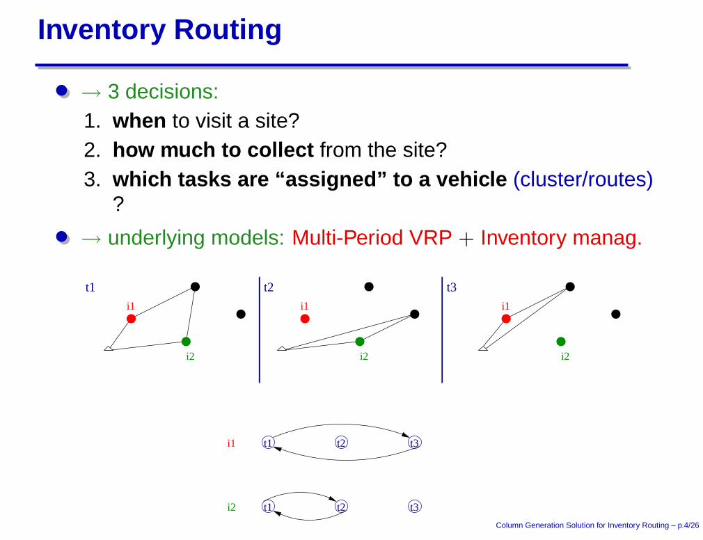
→ 3 decisions:1. when to visit a site?2. how much to collect from the site?3. which tasks are “assigned” to a vehicle (cluster/routes)

?

→ underlying models: Multi-Period VRP + Inventory manag.

i1

i2

t3t2t1

i1

i2

i1

i2

i1

i2

t1 t2 t3

t3t2t1


Literature

many variants: # of products - Time horizon - det./stoch demands -stock manag. policy - routing vs clustering

various applications: ammonia shipping, petrol stations,supermarkets

low size of instances: 15 customers, or 1 period, or 2 customers pervehicles

Non exact solution approaches:

restrictive assumptions: “fixed partition policy” (sets ofcustomers that are serviced together)

(Bramel and Simchi-Levi 1995)

hierarchical approach: planning first, routing second(Campbell and Savelsbergh 2004)

Mostly heuristics . Some studies use branch-and-price .Column Generation Solution for Inventory Routing – p.5/26

Collecting recycle waste from deposit points

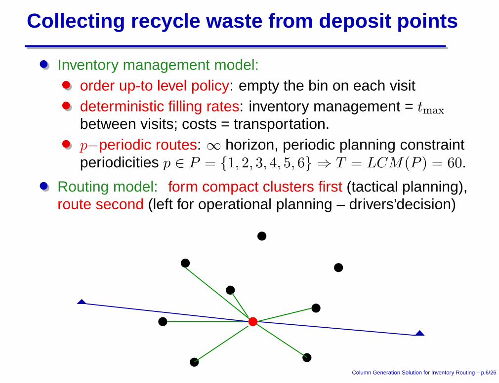
Inventory management model:order up-to level policy: empty the bin on each visitdeterministic filling rates: inventory management = tmax

between visits; costs = transportation.p−periodic routes: ∞ horizon, periodic planning constraintperiodicities p ∈ P = {1, 2, 3, 4, 5, 6} ⇒ T = LCM(P ) = 60.

Routing model: form compact clusters first (tactical planning),route second (left for operational planning – drivers’decision)


Challenges

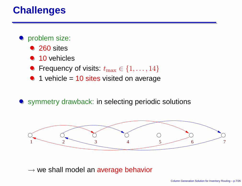
problem size:260 sites10 vehiclesFrequency of visits: tmax ∈ {1, . . . , 14}

1 vehicle = 10 sites visited on average

symmetry drawback: in selecting periodic solutions

1 2 3 4 5 6 7

→ we shall model an average behaviorColumn Generation Solution for Inventory Routing – p.7/26

Saving vehicles compared to Bin-Packing sol

filling rates = (51, 50, 34, 33, 18), W = 100 ⇒ V (bpp) = 3

34

51

33

34

33

t1

t251

50

50

1818

Vehicle 1 Vehicle 2Column Generation Solution for Inventory Routing – p.8/26

Solution approach & results

Truncated branch-and-price-and-cut

Column generation based primal heuristics

state space relaxation

av # of customer # of av travelvisits per week vehicles av distance

our sol 98 9 711 kmindust. solution 59 10 782 km

+ regional partition of routes


Outline

1. Clustering Model

2. “Compact” Formulation

3. Decomposition into Vehicle Tasks

4. DW reformulationsDiscrete timeAggregate time

5. Dual boundsUse the aggregate formulationAdding cutsDoing partial branching

6. Primal Bounds: heuristicsUse of the Discrete formulationCol Gen based heuristics: Restricted Master, Greedy,Rounding, Local Search


Surrogate transportation costs

19

149

1516

91 1

000

25

39

412

512

617

75

81

927

1036

1130

129

1319

149

1516

19

25

39

412

512

617

75

81

927

1036

1130

129

1319

149

1516

925

39

412

512

617

75

81

927

1036

1130

129

13

cik = di,k + min{d0,i − d0,k, di,n+1 − dk,n+1}


Surrogate transportation costs

19

149

1516

91 1

000

25

39

412

512

617

75

81

927

1036

1130

129

1319

149

1516

19

25

39

412

512

617

75

81

927

1036

1130

129

1319

149

1516

925

39

412

512

617

75

81

927

1036

1130

129

13

cik = di,k + min{d0,i − d0,k, di,n+1 − dk,n+1}

costs routing cluster facility loc

routing sol 190.9 214.1 184.5cluster sol 196.8 200.4 147.0facility loc sol 198.8 208.7 135.5


Compact Formulation

xiℓvps = 1 if cust. i is collected ℓ periods worth of stock by vehicle v,every p periods, starting in s;yvps = 1 if vehicle v ... zikvps = 1 if cust. i is in a cluster of seed k ...

min Vmax + α∑

v,p,s

1

p(∑

k

fkzkkvps +∑

i,k:i 6=k

cikzikvps) (1)

∑

ℓ,v,p,s

θℓpst xiℓvps = 1 ∀i ∈ N ′, t = 1, . . . , T (2)

∑

k∈N ′

zikvps =∑

ℓ

xiℓvps ∀i ∈ N ′, v, p, s (3)

zikvps ≤ zkkvps ∀i ∈ N ′, k ∈ N ′, v, p, s (4)∑

i∈N ′,ℓ

ℓ ri xiℓvps ≤ Wyvps ∀v, p, s (5)

∑

v,p,s

δpst yvps ≤ Vmax ∀t = 1, . . . , T (6)


Decomposition into Vehicle Tasks

A Complete planning can be decomposed in periodic vehicle tasks:

t3t2t1

i1

i2

i1

i2

i1

i2

i3 i3 i3

i4 i4i4

3 vehicle tasks of periodicity 3 → 1 vehicle needed

A periodic vehicle task q is defined by:

its pickup pattern xq: xqil = 1 if l period worth of stock is pickup

from cust i.

its cluster cost cq

its first occurrence (starting time) sq

its periodicity pq


Column Generation Formulation

Each column defines a periodic vehicle task: {(cq, sq, pq, xq)}q∈Q

t3t2t1

i1

i2

i1

i2

i1

i2

i3 i3 i3

i4 i4i4

The master models inventory planning

[DM ] ≡ min Vmax + α∑

q∈Q

cq

pqλq (7)

∑

q

θqitλq ≥ 1 ∀i ∈ N ′, t = 1, . . . , T (8)

∑

q

δqt λq ≤ Vmax ∀t = 1, . . . , T (9)

λq ∈ {0, 1} ∀ q ∈ Q (10)

≥ ∈ (11)


Pricing Subproblem

For each starting time s periodicity p cluster center k, solve amultiple choice knapsack problem:

max∑

i,ℓ

giℓxiℓ (12)

∑

ℓ

xkℓ = 1 (13)

∑

ℓ

xiℓ ≤ 1 ∀ i 6= k (14)

∑

i,ℓ

ℓ ri xiℓ ≤ W (15)

xiℓ ∈ {0, 1} ∀ i, ℓ. (16)


State Space Relaxation

Aggregate columns that differ only by their starting dates:

{(cq, sq, pq, xq)}q∈Q → {(cr, pr, xr)}r∈R.

Summing over t, leads to a master modeling an average behavior:

ZA = min Vaver + α∑

r∈R

cr

prλr (17)

∑

r∈R,ℓ

ℓ

prxr

iℓ λr ≥ 1 ∀ i ∈ N ′ (18)

∑

r∈R

1

prλr ≤ Vaver (19)

λr ∈ IN ∀ r ∈ R (20)

V ≥ Vaver ∈ IN, (21)


Discrete versus Aggregate Time Formulation

LP equivalence:

λr =∑

q∈Q(r)

λq , (22)

λq =1

prλr, q ∈ Q(r) (23)

No IP equivalence

6= LP computing time

discrete form. aggregate form.

Instance Col Time Col Time

IND8 71 1.75s 20 0.25sIND27 - >1h 123 5.00sRAND100 - >1h 701 3.52s


Discrete 6= Aggregate Time IP Formulation

3

0

1 p=2

0

31

2p=3

2

aggreg. sol. λr discrete sol. λq t1 t2 t3 t4 t5 t6

λA = 1λA1

= 12 sA1

= 1 X X X

λA2= 1

2 sA2= 2 X X X

λB = 1

λB1= 1

3 sB1= 1 X X X X

λB2= 1

3 sB2= 2 X X X X

λB3= 1

3 sB3= 3 X X X X

Task A: 0 − 1(2) − 3 with pA = 2,

Task B: 0 − 2(3) − 3 with pB = 3,

Vaver = 1 ≥ 12 + 1

3 while Vmax = 2


Discrete 6= Aggregate Time IP Formulation

task A: 0 − · · · − 1(3) − · · · − n + 1 with pA = 6, and

task B: 0 − · · · − 1(2) − · · · − n + 1 with pB = 4.

t1 t2 t3 t4 t5 t6 t7 t8 t9 t10 t11 t12

θA1t X X X X

θB1t X X X

customer pick-up date conflict


Solving the Aggregate Master

Include artificial columns; their cost defines an UB on dual var.

Use a dual heuristic to “warm start” the col. gen. procedure.

Solve multiple choice knapsacks using Dynamic Prog.(Pisinger, 95).

Partial Pricing: consider

periodicities in decreasing order,most attractive seed first.

Re-optimisation ofseed location,periodicity: p = maxi{ℓ : xiℓ = 1}


Adding Cutting Planes

In Mast LP sol: a pattern that covers 56 of customer i’s demand

whose tmax = 5, can be selected 1.2 time.

aggreg. sol. λr t1 t2 t3 t4 t5 t6

λr = 1.2 X X X X

To cut this LP solution is:

∑

r,ℓ: ℓ=pr

xriℓ λr +

1

2

∑

r,ℓ: ℓ 6=pr

xriℓ λr ≥ 1,

small improvement: 2% gap

large increase in computing time: 70% of the time in re-opt.

modifications to the structure of master LP solution: bad forprimal heuristic


Branching on Vaver

Vaver >= vN0

N2N1

Vaver <= v−1

v is a lower bound on number of vehicles if N1 infeasible

Improvement in dual bound in N2: sinceZA = min Vaver + α

∑r∈R

cr

prλr

Cutting Planes + Partial Branching

gapsgap-root gap-cut gap-br gap-br-cut

23.05 21.80 10.63 9.67

% timePP RM CP Sep N0 N1 N2

10.84 8.14 73.49 4.14 5.87 16.17 77.91Column Generation Solution for Inventory Routing – p.23/26

Primal Heuristics

Rounding:Round aggregate master solution to construct discrete mastersolution

Round-up mast col and select starting date : greedyselection, argminrs{(δrs + α cr

pr)/(

∑i,ℓ ℓxiℓ)}

Solve the residual master: pricing requires enumeratingover starting datesDiversify the search: limited backtracking at the root node

Local Search: starting from a master IP solRemove “worst” col : low load columns + complementary:

favour custo. exchange: i.e. close-by clusters;favour vehicle saving: i.e. same (s, p).

Solve the residual master using the Rounding heur.


Computational results

260 customers, 60 periods, 10 vehiclesDual Bounds:

Algorithm bound time

AM LP + br + cut 838.17 5h21m

Primal Bounds:

Algorithm gap (in %) Vmax time

RH + Branch, P = {1, 2, 3, 4, 5, 6} 9.25 9 4h29mRH + LS, P = {1, 2, 3, 4, 5, 6} 8.92 9 3h40m

RH + Branch, P = {1, 2, 3} + post-opt 6.67 9 1h49mRH + LS, P = {1, 2, 3} + post-optim 6.23 9 2h53m


Summary: Planning for Inventory Routing

Column generation + surrogate relaxation to avoid symmetries

Rounding heuristic implicitly carried in discrete time formulation

Solutions with quality warranty: LB6%↔ SOL

10%↔ INDUST


column generation based tactical planning method for ...fvanderb/papers/presivrp.pdf · adding...

Documents