Colored Stochastic Shadow Maps

Morgan McGuireNVIDIA and Williams College

Eric EndertonNVIDIA

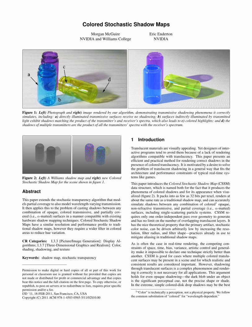
Figure 1: Left) Photograph and right) image rendered by our algorithm, demonstrating transmissive shadowing phenomena it correctlysimulates, including: a) directly illuminated transmissive surfaces receive no shadowing; b) surfaces indirectly illuminated by transmittedlight exhibit shadows matching the product of the transmitter’s and receiver’s spectra, which also leads to c) colored highlights; and d) theshadows of multiple transmitters are the product of all the transmitters’ spectra with the receiver’s spectrum.

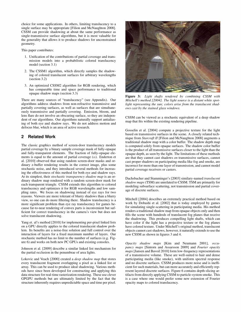
Figure 2: Left) A Williams shadow map and right) new ColoredStochastic Shadow Map for the scene shown in figure 1.

Abstract

This paper extends the stochastic transparency algorithm that mod-els partial coverage to also model wavelength-varying transmission.It then applies this to the problem of casting shadows between anycombination of opaque, colored transmissive, and partially cov-ered (i.e., α-matted) surfaces in a manner compatible with existinghardware shadow mapping techniques. Colored Stochastic ShadowMaps have a similar resolution and performance profile to tradi-tional shadow maps, however they require a wider filter in coloredareas to reduce hue variation.

CR Categories: I.3.3 [Picture/Image Generation]: Display Al-gorithms; I.3.7 [Three-Dimensional Graphics and Realism]: Color,shading, shadowing, and texture

Keywords: shadow map, stochastic transparency

Permission to make digital or hard copies of all or part of this work forpersonal or classroom use is granted without fee provided that copies arenot made or distributed for profit or commercial advantage and that copiesbear this notice and the full citation on the first page. To copy otherwise, orrepublish, to post on servers or to redistribute to lists, requires prior specificpermission and/or a fee.I3D ‘11, 18-FEB-2011, San Francisco, CA, USACopyright (C) 2011 ACM 978-1-4503-0565-5/11/02$10.00

1 Introduction

Translucent materials are visually appealing. Yet designers of inter-active programs tend to avoid them because of a lack of renderingalgorithms compatible with translucency. This paper presents anefficient and practical method for rendering correct shadows in thepresence of colored translucency. It is motivated by a desire to solvethe problem of translucent shadowing in a general way that fits thearchitecture and performance constraints of typical real-time sys-tems like games.

This paper introduces the Colored Stochastic Shadow Map (CSSM)data structure, which is named both for the fact that it produces thephenomena of colored shadows and for its appearance when visu-alized (figure 2). It packs into as few as 32 bits per texel, renders atabout the same rate as a traditional shadow map, and can accuratelysimulate shadows between any combination of colored1 opaque,non-refractive transmissive, and partial coverage (i.e., α-matted)surfaces, including single-scattering particle systems. CSSM re-quires only one order-independent pass over geometry to generateand has no limit on the number of overlapping translucent layers. Ithas the nice theoretical property that the primary artifact, stochasticcolor noise, can be driven arbitrarily low by increasing the reso-lution, filter radius, and filter shape—practices already in use tomitigate aliasing in traditional shadow maps.

As is often the case in real-time rendering, the competing con-straints of space, time, bias, variance, artistic control and general-ity make it impossible to declare one technique strictly better thananother. CSSM is good for cases where multiple colored translu-cent surfaces may be present in a scene and for which realistic andconsistent results are considered important. However, shadowingthrough translucent surfaces is a complex phenomenon and render-ing it correctly is not necessary for all applications. This argumentholds for even opaque shadowing—the dark blob under an objectis the significant perceptual cue, not the precise shape or shade.In the extreme, simple colored-disk drop shadows may be the best

1“Color” is technically a perception, not a physical property. We followthe common substitution of “colored” for “wavelength-dependent.”

choice for some applications. In others, limiting translucency to asingle surface may be appropriate [Filion and McNaughton 2008].CSSM can provide shadowing at about the same performance assingle-transmissive surface algorithms, but it is most valuable forthe generality that allows it to produce shadows for unconstrainedgeometry.

This paper contributes:

1. Unification of the contributions of partial coverage and trans-mission models into a probabilistic colored translucencymodel (section 3.1)

2. The CSSM1 algorithm, which directly samples the shadow-ing of colored translucent surfaces for arbitrary wavelengths(section 3.2)

3. An optimized CSSM2 algorithm for RGB rendering, whichhas comparable time and space performance to traditionalopaque shadow maps (section 3.3)

There are many sources of “translucency” (see Appendix). Ouralgorithms address shadows from non-refractive transmissive andpartially covering surfaces, as well as surfaces that are simultane-ously transmissive and partially covering. Emission, bloom, andlens flare do not involve an obscuring surface, so they are indepen-dent of our algorithms. Our algorithms naturally support antialias-ing of both eye and shadow rays. We do not address motion anddefocus blur, which is an area of active research.

2 Related Work

The classic graphics method of screen-door translucency modelspartial coverage by a binary sample coverage mask of fully-opaqueand fully-transparent elements. The fraction of fully-opaque ele-ments is equal to the amount of partial coverage (α). Enderton etal. [2010] observed that using random screen-door masks and or-dinary z-buffer rendering results in the correct image, plus somestochastic noise, and they introduced several methods for increas-ing the effectiveness of this method for both eye and shadow rays.At its simplest, their stochastic transparency shadow map is an or-dinary shadow map rendered with a random screen-door mask foreach transparent triangle. CSSM extends this algorithm to coloredtranslucency and optimizes it for RGB wavelengths and low sam-pling rates. We focus on shadowing instead of eye rays for tworeasons. Viewers are more tolerant of blurry shadows than a blurryview, so one can do more filtering there. Shadow translucency is amore significant problem than eye ray translucency for games be-cause far-to-near rendering of convex parts is inconvenient but suf-ficient for correct translucency in the camera’s view but does notsolve translucent shadowing.

Yang et. al’s method [2010] for implementing per-pixel linked listson a GPU directly applies to the colored translucent shadow prob-lem. Its benefits are a noise-free solution and full control over theinteraction of layers for a fixed maximum number of layers. Ourstochastic method has no limit to the number of surfaces (e.g. Fig-ure 6) and works on both new PC GPUs and existing consoles.

Johnson et al. [2009] describe a similar linked list mechanism forthe partial occlusion in the penumbrae of area lights.

Lokovic and Veach [2000] created a deep shadow map that storesevery translucent fragment overlapping a pixel as a linked list orarray. This can be used to produce ideal shadowing. Various meth-ods have since been developed for constructing and applying thisdata structure for real-time rasterization rendering. These use cleverGPGPU methods but are ultimately limited by the fact that thestructure inherently requires unpredictable space and time per pixel.

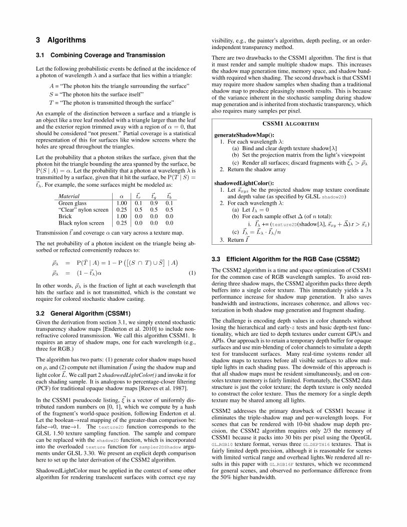
Figure 3: Light shafts rendered by combining CSSM withMitchell’s method [2004]. The light source is a distant white spot-light representing the sun; colors arise from the translucent shad-ows cast by the stained glass windows.

CSSM can be viewed as a stochastic equivalent of a deep shadowmap that fits within the existing rendering pipeline.

Gosselin et al. [2004] compute a projective texture for the lightbased on transmissive surfaces in the scene. A closely related tech-nique from Starcraft II [Filion and McNaughton 2008] augments atraditional shadow map with a color buffer. The shadow depth mapis computed solely from opaque surfaces. The shadow color bufferis the product of all transmissive surfaces closer to the light than theopaque depth, as seen by the light. The limitations of these methodsare that they cannot cast shadows on transmissive surfaces, cannotcast proper shadows on participating media like fog and smoke, areincorrect for more than one layer of transmission, and cannot modelpartial coverage receivers or casters.

Dachsbacher and Stamminger’s [2003] similary-named translucentshadow maps (TSM) are unrelated to CSSM. TSM are primarily formodeling subsurface scattering, not transmission and partial cover-age of discrete surfaces.

Mitchell [2004] describes an extremely practical method based onwork by Dobashi et al. [2002] that is today employed by gamesfor simulating single-scattering in participating media. His methodrenders a traditional shadow map from opaque objects only and thenfills the scene with hundreds of translucent fog planes that receivethe shadowing. This produces compelling light shafts, which canhave color if the light has a projective texture or the fog planeshave colored texture. Under Mitchell’s original method, translucentobjects cannot cast shadows, however, it naturally extends to use thenew CSSM as shown in figures 3 and 4.

Opacity shadow maps [Kim and Neumann 2001], occu-pancy maps [Sintorn and Assarsson 2009] and Fourier opacitymaps [Jansen and Bavoil 2010] form low-frequency representationsof a transmissive volume. These are well-suited to hair and denseparticipating media (like smoke), with uniform spectral responseand no discrete surfaces. CSSM produces more noise and is ineffi-cient for such materials, but can more accurately and efficiently rep-resent layered discrete surfaces. Figure 6 contains depth-slicing ar-tifacts from directly applying CSSM to particle-system smoke. Thisis a case where one would prefer some new extension of Fourieropacity maps to colored translucency.

3 Algorithms

3.1 Combining Coverage and Transmission

Let the following probabilistic events be defined at the incidence ofa photon of wavelength λ and a surface that lies within a triangle:

A = “The photon hits the triangle surrounding the surface”S = “The photon hits the surface itself”T = “The photon is transmitted through the surface”

An example of the distinction between a surface and a triangle isan object like a tree leaf modeled with a triangle larger than the leafand the exterior region trimmed away with a region of α = 0, thatshould be considered “not present.” Partial coverage is a statisticalrepresentation of this for surfaces like window screens where theholes are spread throughout the triangles.

Let the probability that a photon strikes the surface, given that thephoton hit the triangle bounding the area spanned by the surface, beP(S | A) = α. Let the probability that a photon at wavelength λ istransmitted by a surface, given that it hit the surface, be P(T | S) =~tλ. For example, the some surfaces might be modeled as:

Material α ~tr ~tg ~tbGreen glass 1.00 0.1 0.9 0.1“Clear” nylon screen 0.25 0.5 0.5 0.5Brick 1.00 0.0 0.0 0.0Black nylon screen 0.25 0.0 0.0 0.0

Transmission ~t and coverage α can vary across a texture map.

The net probability of a photon incident on the triangle being ab-sorbed or reflected conveniently reduces to:

~ρλ = P(T | A) = 1− P([

(S ∩ T ) ∪ S]| A

)~ρλ = (1− ~tλ)α (1)

In other words, ~ρλ is the fraction of light at each wavelength thathits the surface and is not transmitted, which is the constant werequire for colored stochastic shadow casting.

3.2 General Algorithm (CSSM1)Given the derivation from section 3.1, we simply extend stochastictransparency shadow maps [Enderton et al. 2010] to include non-refractive colored transmission. We call this algorithm CSSM1. Itrequires an array of shadow maps, one for each wavelength (e.g.,three for RGB.)

The algorithm has two parts: (1) generate color shadow maps basedon ρ, and (2) compute net illumination ~I using the shadow map andlight color ~L. We call part 2 shadowedLightColor() and invoke it foreach shading sample. It is analogous to percentage-closer filtering(PCF) for traditional opaque shadow maps [Reeves et al. 1987].

In the CSSM1 pseudocode listing, ~ξ is a vector of uniformly dis-tributed random numbers on [0, 1], which we compute by a hashof the fragment’s world-space position, following Enderton et al.Let the boolean→real mapping of the greater-than comparison be:false→0, true→1. The texture2D function corresponds to theGLSL 1.50 texture sampling function. The sample and comparecan be replaced with the shadow2D function, which is incorporatedinto the overloaded texture function for sampler2DShadow argu-ments under GLSL 3.30. We present an explicit depth comparisonhere to set up the later derivation of the CSSM2 algorithm.

ShadowedLightColor must be applied in the context of some otheralgorithm for rendering translucent surfaces with correct eye ray

visibility, e.g., the painter’s algorithm, depth peeling, or an order-independent transparency method.

There are two drawbacks to the CSSM1 algorithm. The first is thatit must render and sample multiple shadow maps. This increasesthe shadow map generation time, memory space, and shadow band-width required when shading. The second drawback is that CSSM1may require more shadow samples when shading than a traditionalshadow map to produce pleasingly smooth results. This is becauseof the variance inherent in the stochastic sampling during shadowmap generation and is inherited from stochastic transparency, whichalso requires many samples per pixel.

CSSM1 ALGORITHM

generateShadowMap():1. For each wavelength λ:

(a) Bind and clear depth texture shadow[λ](b) Set the projection matrix from the light’s viewpoint(c) Render all surfaces; discard fragments with ~ξλ > ~ρλ

2. Return the shadow array

shadowedLightColor():1. Let ~sxyz be the projected shadow map texture coordinate

and depth value (as specified by GLSL shadow2D)2. For each wavelength λ:

(a) Let Iλ = 0(b) For each sample offset ∆ (of n total):

i. ~Iλ += (texture2D(shadow[λ], ~sxy + ~∆).r > ~sz)(c) ~Iλ = ~Lλ · ~Iλ/n

3. Return ~I

3.3 Efficient Algorithm for the RGB Case (CSSM2)

The CSSM2 algorithm is a time and space optimization of CSSM1for the common case of RGB wavelength samples. To avoid ren-dering three shadow maps, the CSSM2 algorithm packs three depthbuffers into a single color texture. This immediately yields a 3xperformance increase for shadow map generation. It also savesbandwidth and instructions, increases coherence, and allows vec-torization in both shadow map generation and fragment shading.

The challenge is encoding depth values in color channels withoutlosing the hierarchical and early-z tests and basic depth-test func-tionality, which are tied to depth textures under current GPUs andAPIs. Our approach is to retain a temporary depth buffer for opaquesurfaces and use min-blending of color channels to simulate a depthtest for translucent surfaces. Many real-time systems render allshadow maps to textures before all visible surfaces to allow mul-tiple lights in each shading pass. The downside of this approach isthat all shadow maps must be resident simultaneously, and on con-soles texture memory is fairly limited. Fortunately, the CSSM2 datastructure is just the color texture; the depth texture is only neededto construct the color texture. Thus the memory for a single depthtexture may be shared among all lights.

CSSM2 addresses the primary drawback of CSSM1 because iteliminates the triple-shadow map and per-wavelength loops. Forscenes that can be rendered with 10-bit shadow map depth pre-cision, the CSSM2 algorithm requires only 2/3 the memory ofCSSM1 because it packs into 30 bits per pixel using the OpenGLGL RGB10 texture format, versus three GL DEPTH16 textures. That isfairly limited depth precision, although it is reasonable for sceneswith limited vertical range and overhead lights.We rendered all re-sults in this paper with GL RGB16F textures, which we recommendfor general scenes, and observed no performance difference fromthe 50% higher bandwidth.

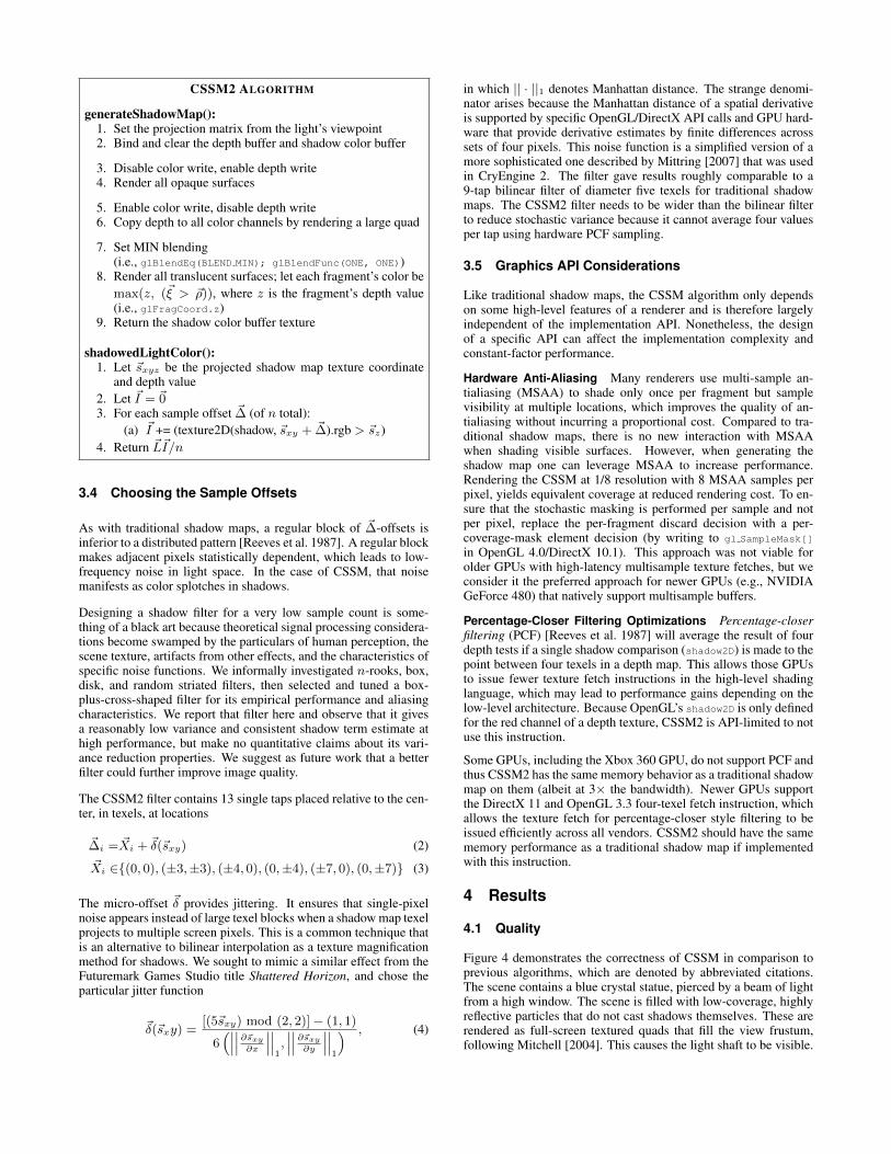
CSSM2 ALGORITHM

generateShadowMap():1. Set the projection matrix from the light’s viewpoint2. Bind and clear the depth buffer and shadow color buffer

3. Disable color write, enable depth write4. Render all opaque surfaces

5. Enable color write, disable depth write6. Copy depth to all color channels by rendering a large quad

7. Set MIN blending(i.e., glBlendEq(BLEND MIN); glBlendFunc(ONE, ONE))

8. Render all translucent surfaces; let each fragment’s color bemax(z, (~ξ > ~ρ)), where z is the fragment’s depth value(i.e., glFragCoord.z)

9. Return the shadow color buffer texture

shadowedLightColor():1. Let ~sxyz be the projected shadow map texture coordinate

and depth value2. Let ~I = ~03. For each sample offset ~∆ (of n total):

(a) ~I += (texture2D(shadow, ~sxy + ~∆).rgb > ~sz)4. Return ~L~I/n

3.4 Choosing the Sample Offsets

As with traditional shadow maps, a regular block of ~∆-offsets isinferior to a distributed pattern [Reeves et al. 1987]. A regular blockmakes adjacent pixels statistically dependent, which leads to low-frequency noise in light space. In the case of CSSM, that noisemanifests as color splotches in shadows.

Designing a shadow filter for a very low sample count is some-thing of a black art because theoretical signal processing considera-tions become swamped by the particulars of human perception, thescene texture, artifacts from other effects, and the characteristics ofspecific noise functions. We informally investigated n-rooks, box,disk, and random striated filters, then selected and tuned a box-plus-cross-shaped filter for its empirical performance and aliasingcharacteristics. We report that filter here and observe that it givesa reasonably low variance and consistent shadow term estimate athigh performance, but make no quantitative claims about its vari-ance reduction properties. We suggest as future work that a betterfilter could further improve image quality.

The CSSM2 filter contains 13 single taps placed relative to the cen-ter, in texels, at locations

~∆i = ~Xi + ~δ(~sxy) (2)~Xi ∈{(0, 0), (±3,±3), (±4, 0), (0,±4), (±7, 0), (0,±7)} (3)

The micro-offset ~δ provides jittering. It ensures that single-pixelnoise appears instead of large texel blocks when a shadow map texelprojects to multiple screen pixels. This is a common technique thatis an alternative to bilinear interpolation as a texture magnificationmethod for shadows. We sought to mimic a similar effect from theFuturemark Games Studio title Shattered Horizon, and chose theparticular jitter function

~δ(~sxy) =[(5~sxy) mod (2, 2)]− (1, 1)

6(∣∣∣∣∣∣ ∂~sxy

∂x

∣∣∣∣∣∣1,∣∣∣∣∣∣ ∂~sxy

∂y

∣∣∣∣∣∣1

) , (4)

in which || · ||1 denotes Manhattan distance. The strange denomi-nator arises because the Manhattan distance of a spatial derivativeis supported by specific OpenGL/DirectX API calls and GPU hard-ware that provide derivative estimates by finite differences acrosssets of four pixels. This noise function is a simplified version of amore sophisticated one described by Mittring [2007] that was usedin CryEngine 2. The filter gave results roughly comparable to a9-tap bilinear filter of diameter five texels for traditional shadowmaps. The CSSM2 filter needs to be wider than the bilinear filterto reduce stochastic variance because it cannot average four valuesper tap using hardware PCF sampling.

3.5 Graphics API Considerations

Like traditional shadow maps, the CSSM algorithm only dependson some high-level features of a renderer and is therefore largelyindependent of the implementation API. Nonetheless, the designof a specific API can affect the implementation complexity andconstant-factor performance.

Hardware Anti-Aliasing Many renderers use multi-sample an-tialiasing (MSAA) to shade only once per fragment but samplevisibility at multiple locations, which improves the quality of an-tialiasing without incurring a proportional cost. Compared to tra-ditional shadow maps, there is no new interaction with MSAAwhen shading visible surfaces. However, when generating theshadow map one can leverage MSAA to increase performance.Rendering the CSSM at 1/8 resolution with 8 MSAA samples perpixel, yields equivalent coverage at reduced rendering cost. To en-sure that the stochastic masking is performed per sample and notper pixel, replace the per-fragment discard decision with a per-coverage-mask element decision (by writing to gl SampleMask[]

in OpenGL 4.0/DirectX 10.1). This approach was not viable forolder GPUs with high-latency multisample texture fetches, but weconsider it the preferred approach for newer GPUs (e.g., NVIDIAGeForce 480) that natively support multisample buffers.

Percentage-Closer Filtering Optimizations Percentage-closerfiltering (PCF) [Reeves et al. 1987] will average the result of fourdepth tests if a single shadow comparison (shadow2D) is made to thepoint between four texels in a depth map. This allows those GPUsto issue fewer texture fetch instructions in the high-level shadinglanguage, which may lead to performance gains depending on thelow-level architecture. Because OpenGL’s shadow2D is only definedfor the red channel of a depth texture, CSSM2 is API-limited to notuse this instruction.

Some GPUs, including the Xbox 360 GPU, do not support PCF andthus CSSM2 has the same memory behavior as a traditional shadowmap on them (albeit at 3× the bandwidth). Newer GPUs supportthe DirectX 11 and OpenGL 3.3 four-texel fetch instruction, whichallows the texture fetch for percentage-closer style filtering to beissued efficiently across all vendors. CSSM2 should have the samememory performance as a traditional shadow map if implementedwith this instruction.

4 Results

4.1 Quality

Figure 4 demonstrates the correctness of CSSM in comparison toprevious algorithms, which are denoted by abbreviated citations.The scene contains a blue crystal statue, pierced by a beam of lightfrom a high window. The scene is filled with low-coverage, highlyreflective particles that do not cast shadows themselves. These arerendered as full-screen textured quads that fill the view frustum,following Mitchell [2004]. This causes the light shaft to be visible.

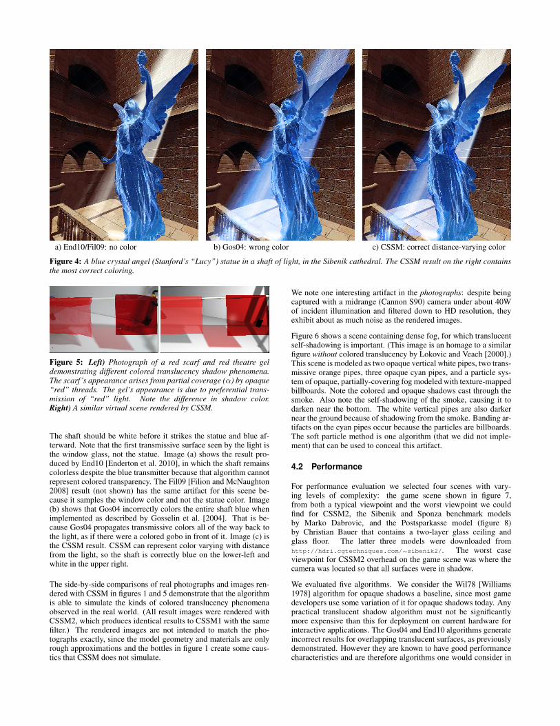
a) End10/Fil09: no color b) Gos04: wrong color c) CSSM: correct distance-varying color

Figure 4: A blue crystal angel (Stanford’s “Lucy”) statue in a shaft of light, in the Sibenik cathedral. The CSSM result on the right containsthe most correct coloring.

Figure 5: Left) Photograph of a red scarf and red theatre geldemonstrating different colored translucency shadow phenomena.The scarf’s appearance arises from partial coverage (α) by opaque“red” threads. The gel’s appearance is due to preferential trans-mission of “red” light. Note the difference in shadow color.Right) A similar virtual scene rendered by CSSM.

The shaft should be white before it strikes the statue and blue af-terward. Note that the first transmissive surface seen by the light isthe window glass, not the statue. Image (a) shows the result pro-duced by End10 [Enderton et al. 2010], in which the shaft remainscolorless despite the blue transmitter because that algorithm cannotrepresent colored transparency. The Fil09 [Filion and McNaughton2008] result (not shown) has the same artifact for this scene be-cause it samples the window color and not the statue color. Image(b) shows that Gos04 incorrectly colors the entire shaft blue whenimplemented as described by Gosselin et al. [2004]. That is be-cause Gos04 propagates transmissive colors all of the way back tothe light, as if there were a colored gobo in front of it. Image (c) isthe CSSM result. CSSM can represent color varying with distancefrom the light, so the shaft is correctly blue on the lower-left andwhite in the upper right.

The side-by-side comparisons of real photographs and images ren-dered with CSSM in figures 1 and 5 demonstrate that the algorithmis able to simulate the kinds of colored translucency phenomenaobserved in the real world. (All result images were rendered withCSSM2, which produces identical results to CSSM1 with the samefilter.) The rendered images are not intended to match the pho-tographs exactly, since the model geometry and materials are onlyrough approximations and the bottles in figure 1 create some caus-tics that CSSM does not simulate.

We note one interesting artifact in the photographs: despite beingcaptured with a midrange (Cannon S90) camera under about 40Wof incident illumination and filtered down to HD resolution, theyexhibit about as much noise as the rendered images.

Figure 6 shows a scene containing dense fog, for which translucentself-shadowing is important. (This image is an homage to a similarfigure without colored translucency by Lokovic and Veach [2000].)This scene is modeled as two opaque vertical white pipes, two trans-missive orange pipes, three opaque cyan pipes, and a particle sys-tem of opaque, partially-covering fog modeled with texture-mappedbillboards. Note the colored and opaque shadows cast through thesmoke. Also note the self-shadowing of the smoke, causing it todarken near the bottom. The white vertical pipes are also darkernear the ground because of shadowing from the smoke. Banding ar-tifacts on the cyan pipes occur because the particles are billboards.The soft particle method is one algorithm (that we did not imple-ment) that can be used to conceal this artifact.

4.2 Performance

For performance evaluation we selected four scenes with vary-ing levels of complexity: the game scene shown in figure 7,from both a typical viewpoint and the worst viewpoint we couldfind for CSSM2, the Sibenik and Sponza benchmark modelsby Marko Dabrovic, and the Postsparkasse model (figure 8)by Christian Bauer that contains a two-layer glass ceiling andglass floor. The latter three models were downloaded fromhttp://hdri.cgtechniques.com/∼sibenik2/. The worst caseviewpoint for CSSM2 overhead on the game scene was where thecamera was located so that all surfaces were in shadow.

We evaluated five algorithms. We consider the Wil78 [Williams1978] algorithm for opaque shadows a baseline, since most gamedevelopers use some variation of it for opaque shadows today. Anypractical translucent shadow algorithm must not be significantlymore expensive than this for deployment on current hardware forinteractive applications. The Gos04 and End10 algorithms generateincorrect results for overlapping translucent surfaces, as previouslydemonstrated. However they are known to have good performancecharacteristics and are therefore algorithms one would consider in

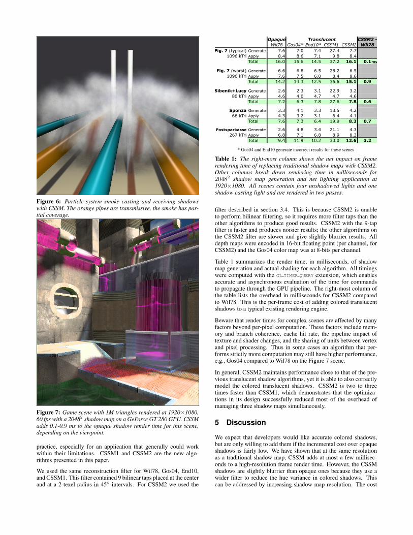
Figure 6: Particle-system smoke casting and receiving shadowswith CSSM. The orange pipes are transmissive, the smoke has par-tial coverage.

Figure 7: Game scene with 1M triangles rendered at 1920×1080,60 fps with a 20482 shadow map on a GeForce GT 280 GPU. CSSMadds 0.1-0.9 ms to the opaque shadow render time for this scene,depending on the viewpoint.

practice, especially for an application that generally could workwithin their limitations. CSSM1 and CSSM2 are the new algo-rithms presented in this paper.

We used the same reconstruction filter for Wil78, Gos04, End10,and CSSM1. This filter contained 9 bilinear taps placed at the centerand at a 2-texel radius in 45◦ intervals. For CSSM2 we used the

Opaque CSSM2 -Wil78 Gos04* End10* CSSM1 CSSM2 Wil78

Fig. 7 (typical) Generate 7.6 7.0 7.4 27.4 7.71096 kTri Apply 8.4 8.6 7.1 9.8 8.4

Total 16.0 15.6 14.5 37.2 16.1 0.1

Fig. 7 (worst) Generate 6.6 6.8 6.5 28.2 6.51096 kTri Apply 7.6 7.5 6.0 8.4 8.6

Total 14.2 14.3 12.5 36.6 15.1 0.9

Sibenik+Lucy Generate 2.6 2.3 3.1 22.9 3.280 kTri Apply 4.6 4.0 4.7 4.7 4.6

Total 7.2 6.3 7.8 27.6 7.8 0.6

Sponza Generate 3.3 4.1 3.3 13.5 4.266 kTri Apply 4.3 3.2 3.1 6.4 4.1

Total 7.6 7.3 6.4 19.9 8.3 0.7

Postsparkasse Generate 2.6 4.8 3.4 21.1 4.3267 kTri Apply 6.8 7.1 6.8 8.9 8.3

Total 9.4 11.9 10.2 30.0 12.6 3.2

Translucent

ms  

* Gos04 and End10 generate incorrect results for these scenes

Table 1: The right-most column shows the net impact on framerendering time of replacing traditional shadow maps with CSSM2.Other columns break down rendering time in milliseconds for20482 shadow map generation and net lighting application at1920×1080. All scenes contain four unshadowed lights and oneshadow casting light and are rendered in two passes.

filter described in section 3.4. This is because CSSM2 is unableto perform bilinear filtering, so it requires more filter taps than theother algorithms to produce good results. CSSM2 with the 9-tapfilter is faster and produces noisier results; the other algorithms onthe CSSM2 filter are slower and give slightly blurrier results. Alldepth maps were encoded in 16-bit floating point (per channel, forCSSM2) and the Gos04 color map was at 8-bits per channel.

Table 1 summarizes the render time, in milliseconds, of shadowmap generation and actual shading for each algorithm. All timingswere computed with the GL TIMER QUERY extension, which enablesaccurate and asynchronous evaluation of the time for commandsto propagate through the GPU pipeline. The right-most column ofthe table lists the overhead in milliseconds for CSSM2 comparedto Wil78. This is the per-frame cost of adding colored translucentshadows to a typical existing rendering engine.

Beware that render times for complex scenes are affected by manyfactors beyond per-pixel computation. These factors include mem-ory and branch coherence, cache hit rate, the pipeline impact oftexture and shader changes, and the sharing of units between vertexand pixel processing. Thus in some cases an algorithm that per-forms strictly more computation may still have higher performance,e.g., Gos04 compared to Wil78 on the Figure 7 scene.

In general, CSSM2 maintains performance close to that of the pre-vious translucent shadow algorithms, yet it is able to also correctlymodel the colored translucent shadows. CSSM2 is two to threetimes faster than CSSM1, which demonstrates that the optimiza-tions in its design successfully reduced most of the overhead ofmanaging three shadow maps simultaneously.

5 Discussion

We expect that developers would like accurate colored shadows,but are only willing to add them if the incremental cost over opaqueshadows is fairly low. We have shown that at the same resolutionas a traditional shadow map, CSSM adds at most a few millisec-onds to a high-resolution frame render time. However, the CSSMshadows are slightly blurrier than opaque ones because they use awider filter to reduce the hue variance in colored shadows. Thiscan be addressed by increasing shadow map resolution. The cost

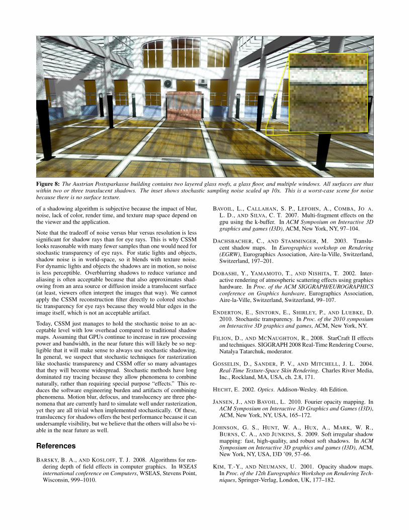
Figure 8: The Austrian Postsparkasse building contains two layered glass roofs, a glass floor, and multiple windows. All surfaces are thuswithin two or three translucent shadows. The inset shows stochastic sampling noise scaled up 10x. This is a worst-case scene for noisebecause there is no surface texture.

of a shadowing algorithm is subjective because the impact of blur,noise, lack of color, render time, and texture map space depend onthe viewer and the application.

Note that the tradeoff of noise versus blur versus resolution is lesssignificant for shadow rays than for eye rays. This is why CSSMlooks reasonable with many fewer samples than one would need forstochastic transparency of eye rays. For static lights and objects,shadow noise is in world-space, so it blends with texture noise.For dynamic lights and objects the shadows are in motion, so noiseis less perceptible. Overblurring shadows to reduce variance andaliasing is often acceptable because that also approximates shad-owing from an area source or diffusion inside a translucent surface(at least, viewers often interpret the images that way). We cannotapply the CSSM reconstruction filter directly to colored stochas-tic transparency for eye rays because they would blur edges in theimage itself, which is not an acceptable artifact.

Today, CSSM just manages to hold the stochastic noise to an ac-ceptable level with low overhead compared to traditional shadowmaps. Assuming that GPUs continue to increase in raw processingpower and bandwidth, in the near future this will likely be so neg-ligible that it will make sense to always use stochastic shadowing.In general, we suspect that stochastic techniques for rasterizationlike stochastic transparency and CSSM offer so many advantagesthat they will become widespread. Stochastic methods have longdominated ray tracing because they allow phenomena to combinenaturally, rather than requiring special purpose “effects.” This re-duces the software engineering burden and artifacts of combiningphenomena. Motion blur, defocus, and translucency are three phe-nomena that are currently hard to simulate well under rasterization,yet they are all trivial when implemented stochastically. Of these,translucency for shadows offers the best performance because it canundersample visibility, but we believe that the others will also be vi-able in the near future as well.

References

BARSKY, B. A., AND KOSLOFF, T. J. 2008. Algorithms for ren-dering depth of field effects in computer graphics. In WSEASinternational conference on Computers, WSEAS, Stevens Point,Wisconsin, 999–1010.

BAVOIL, L., CALLAHAN, S. P., LEFOHN, A., COMBA, JO A.L. D., AND SILVA, C. T. 2007. Multi-fragment effects on thegpu using the k-buffer. In ACM Symposium on Interactive 3Dgraphics and games (I3D), ACM, New York, NY, 97–104.

DACHSBACHER, C., AND STAMMINGER, M. 2003. Translu-cent shadow maps. In Eurographics workshop on Rendering(EGRW), Eurographics Association, Aire-la-Ville, Switzerland,Switzerland, 197–201.

DOBASHI, Y., YAMAMOTO, T., AND NISHITA, T. 2002. Inter-active rendering of atmospheric scattering effects using graphicshardware. In Proc. of the ACM SIGGRAPH/EUROGRAPHICSconference on Graphics hardware, Eurographics Association,Aire-la-Ville, Switzerland, Switzerland, 99–107.

ENDERTON, E., SINTORN, E., SHIRLEY, P., AND LUEBKE, D.2010. Stochastic transparency. In Proc. of the 2010 symposiumon Interactive 3D graphics and games, ACM, New York, NY.

FILION, D., AND MCNAUGHTON, R., 2008. StarCraft II effectsand techniques. SIGGRAPH 2008 Real-Time Rendering Course,Natalya Tatarchuk, moderator.

GOSSELIN, D., SANDER, P. V., AND MITCHELL, J. L. 2004.Real-Time Texture-Space Skin Rendering. Charles River Media,Inc., Rockland, MA, USA, ch. 2.8, 171.

HECHT, E. 2002. Optics. Addison-Wesley. 4th Edition.

JANSEN, J., AND BAVOIL, L. 2010. Fourier opacity mapping. InACM Symposium on Interactive 3D Graphics and Games (I3D),ACM, New York, NY, USA, 165–172.

JOHNSON, G. S., HUNT, W. A., HUX, A., MARK, W. R.,BURNS, C. A., AND JUNKINS, S. 2009. Soft irregular shadowmapping: fast, high-quality, and robust soft shadows. In ACMSymposium on Interactive 3D graphics and games (I3D), ACM,New York, NY, USA, I3D ’09, 57–66.

KIM, T.-Y., AND NEUMANN, U. 2001. Opacity shadow maps.In Proc. of the 12th Eurographics Workshop on Rendering Tech-niques, Springer-Verlag, London, UK, 177–182.

LOKOVIC, T., AND VEACH, E. 2000. Deep shadow maps. InProc. of SIGGRAPH 2000, ACM Press/Addison-Wesley Pub-lishing Co., New York, NY, USA, 385–392.

MITCHELL, J. L. 2004. Light Shaft Rendering. Charles RiverMedia, ch. 8.1, 573–588. in ShaderX3: Advanced Renderingwith DirectX and OpenGL, W. Engel, ed.

MITTRING, M. 2007. Finding next gen: Cryengine 2. In SIG-GRAPH ’07: ACM SIGGRAPH 2007 courses, ACM, New York,NY, USA, 97–121.

PORTER, T., AND DUFF, T. 1984. Compositing digital images. InSIGGRAPH 1984, 253–259.

REEVES, W. T., SALESIN, D. H., AND COOK, R. L. 1987. Ren-dering antialiased shadows with depth maps. In Proc. of SIG-GRAPH 1987, ACM, New York, NY, USA, 283–291.

SINTORN, E., AND ASSARSSON, U. 2009. Hair self shadowingand transparency depth ordering using occupancy maps. In Proc.of SI3D 2009, 67–74.

SUNG, K., PEARCE, A., AND WANG, C. 2002. Spatial-temporalantialiasing. IEEE Transactions on Visualization and ComputerGraphics 8, 2, 144–153.

WILLIAMS, L. 1978. Casting curved shadows on curved surfaces.In SIGGRAPH 1978, ACM, New York, NY, USA, 270–274.

WYMAN, C. 2005. Interactive image-space refraction of nearbygeometry. In GRAPHITE, ACM, New York, NY, 205–211.

YANG, J. C., HENSLEY, J., GRUN, H., AND THIBIEROZ, N.2010. Real-time concurrent linked list construction on the gpu.Comput. Graph. Forum 29, 4, 1297–1304.

Appendix: Translucency PhenomenaMultiple distinct light transport phenomena can produce the com-mon perceptual phenomenon of “translucency.” All result in mul-tiple objects along a ray contributing to the radiant flux througha pixel. Real-time approximations of these phenomena are oftenbuilt on raster blending modes, which are selected by glBlendFunc

and glBlendEq in the OpenGL API. That commonality leads to afrequent source of error, in that many renderers conflate phenom-ena with different underlying causes and attempt to use one blend-ing mode to simulate all of them. That source of error has in turnmade it challenging to implement correct translucency and translu-cent shadowing in such renderers.

The following paragraphs describe five distinct phenomena and ef-ficient methods for coarsely approximating them along eye rays inOpenGL. This clarifies the scope and terminology of the paper,which is concerned with applying these ideas to the related prob-lem of approximating translucent phenomena along shadow rays.

Transmission (e.g., by glass) occurs when light is modulated bythe transmission spectrum of a material that it intersects. For ex-ample, this causes the back of a white label on a green wine bottleto appear green when viewed through the bottle. For a transmis-sive object with uniform material properties, the fraction of lightat wavelength λ transmitted through distance d of material is givenby exp(−4πdκλ/λ), where extinction coefficient κλ is the imag-inary part of its complex index of refraction [Hecht 2002, 128].The transmission is non-refractive if the exitant ray has the samedirection as the incident ray, which occurs when the real part, η,of the index of refraction is the same for both the intersected andsurrounding media.

One method for approximating non-refractive transmission understrict depth ordering is as follows. Render surfaces from farthest

to nearest. At each, first modulate the previously sampled radianceat each pixel (e.g., using glBlendFunc(GL ZERO, GL SRC COLOR)) bythe transmission spectrum of the surface, which is zero for opaquesurfaces. Second, add radiance reflected and emitted at the surface(glBlendFunc(GL ONE, GL ONE)).

A thin surface has fixed thickness d (at normal incidence), so itis common practice to precompute the net transmission throughthat thickness at several wavelengths, which we call ~t, e.g., withnamed components ~t = (~tr,~tg,~tb). This is the “source color”for the OpenGL command. For thick transmitters, more sophis-ticated methods have been developed for efficiently sampling thebackground color from an offset location to approximate refrac-tion (e.g., [Wyman 2005]), and for computing the varying transmis-sion levels (e.g., [Bavoil et al. 2007]). Note that in the real world,physics constrains all transmissive surfaces to also be specularly re-flective to some extent. Transmission always falls off with the angleof incidence according to the Fresnel equations.

Partial coverage (e.g., by a window screen) occurs when a sub-set of the rays within one pixel’s bundle of samples are occludedby a perforated foreground surface or particle set. The fraction ofrays that are occluded is denoted by α. Note that at the highestresolution of a model (i.e., level 0 MIP-map) α is ideally either1 or 0 at every sample. Fractional α arises from taking multiplebinary samples per pixel. This is the case for higher MIP levels,GL ALPHA TO COVERAGE, and GL POLYGON SMOOTH rendering.

The observed spectrum of multiple uncorrelated partial coveragelayers is given by repeated application of Porter and Duff’s [1984]linear over operator: αF + (1 − α)B. In this equation, F andB are the radiance that would be transported to the viewer from aforeground layer and a background layer in isolation. One methodfor approximating partial coverage is rendering objects from far-thest to nearest with linear radiance interpolation (e.g., usingglBlendFunc(GL SRC ALPHA, GL ONE MINUS SRC ALPHA)). Note thata surface can be both transmissive and partially covering. In thatcase, the observed foreground spectrum contains a term that is amodulated version of the background spectrum.

Emission by a translucent surface occurs when a partial ortransmissive surface or medium also emits light. Phosphorescentalgae clouds, neon bulbs, and flame are real-world cases. Sciencefiction force fields and fantasy magical effects are imaginary ones.One method for simulating this is simple accumulation of radianceat a pixel (e.g., by glBlendFunc(GL ONE, GL ONE).)

Bloom and lens flare occur when dispersion and internal reflec-tions within a lens objective cause bright scene points to affect pix-els other than those dictated by pinhole projection. Direct simula-tion of a compound lens as in-scene surfaces tends to be inefficient,so these effects are commonly approximated by post-processingwith additive blending (e.g., glBlendFunc(GL ONE, GL ONE).)

Motion blur, defocus blur, and antialiasing are cases wheresamples over multiple dimensions allow multiple scene points tocontribute to a sample and therefore can create translucency. Be-cause net radiant flux is the sum over the contribution of each ray, itis mathematically equivalent to the weighted sum provided by par-tial coverage. These phenomena can therefore be accurately mod-eled by extending partial coverage by α′ = α ∗ w, where weightw is an estimate of the product of the fractional of exposure time,projected solid angle, and projected area that the surface covers rel-ative for a pixel, and α is the original partial coverage of the surface.This is an area of significant current research and product develop-ment. See Sung et al. [2002] and Barskey and Kosloff [2008] forsurveys of various blurring approximations for eye rays, most ofwhich cannot be directly applied to the shadowing.