clustered compressive sensingbased
TRANSCRIPT
David C. Wyld et al. (Eds) : ITCS, CST, JSE, SIP, ARIA, DMS - 2015
pp. 185–197, 2015. © CS & IT-CSCP 2015 DOI : 10.5121/csit.2015.50118
CLUSTERED COMPRESSIVE SENSING-
BASED IMAGE DENOISING USING
BAYESIAN FRAMEWORK
Solomon A. Tesfamicael * †
Faraz Barzideh ‡
*
Sør-Trondlag University College (HiST), Trondheim, Norway †Norwegian University of Science and Technology (NTNU),
Trondheim, Norway [email protected]/[email protected]
‡ Department of Electrical Engineering and Computer Science,
University of Stavanger (UiS), Stavanger, Norway [email protected]
ABSTRACT
This paper provides a compressive sensing (CS) method of denoising images using Bayesian
framework. Some images, for example like magnetic resonance images (MRI) are usually very
weak due to the presence of noise and due to the weak nature of the signal itself. So denoising
boosts the true signal strength. Under Bayesian framework, we have used two different priors:
sparsity and clusterdness in an image data as prior information to remove noise. Therefore, it is
named as clustered compressive sensing based denoising (CCSD). After developing the
Bayesian framework, we applied our method on synthetic data, Shepp-logan phantom and
sequences of fMRI images. The results show that applying the CCSD give better results than
using only the conventional compressive sensing (CS) methods in terms of Peak Signal to Noise
Ratio (PSNR) and Mean Square Error (MSE). In addition, we showed that this algorithm could
have some advantages over the state-of-the-art methods like Block-Matching and 3D
Filtering (BM3D).
KEYWORDS
Denoising, Bayesian framework, Sparse prior, Clustered prior, posterior, Compressive sensing,
LASSO, Clustered Compressive Sensing
1. INTRODUCTION
Image denoising is an integral part of image processing. There are different sources of noise for
images and different noise models are assumed to remove or reduce noise (to denoise),
accordingly. Mostly image noises are modelled by additive white Gaussian distribution while
others like ultrasound and MRI images can be modelled by speckle and Rican distribution
respectively [1]. In the past decades, removing the noises has been given ample attention and
there are several ways to de-noise an image. A good image denoising technique removes the
noise to a desirable level while keeping the edges. Traditionally, this has been done using spatial
filtering and transform domain filtering. The former uses median filter, Weiner filter and so on
while the later uses Fast Fourier Transform (FFT) and Wavelet Transform (WT) to transform the
186 Computer Science & Information Technology (CS & IT)
image data to frequency or time-frequency domain, respectively. The later transform method have
been used intensively due to the fact that the Wavelet transform based methods surpasses the
others in the sense of mean square error (MSE) or pick signal to noise ratio (PSNR) and other
performance metrics [1], [2], [3].
Recently, another way of image denoising has been used after a new way of signal processing
method called compressive sensing (CS) was revived by authors like Donoho, Candés, Romberg
and Tao [4]- [7]. CS is a method to capture information at lower rate than the Nyquist- Shannon
sampling rate when signals are sparse or sparse in some domain. It has already been applied in
medical imaging. In [8] the authors have used the sparsity of magnetic resonance imaging (MRI)
signals and showed that this can be exploited to significantly reduce scan time, or alternatively,
improve the resolution of MR imagery and in [9] it is applied for Biological Microscopy image
denoising to reduce exposure time along with photo- toxicity and photo-bleaching. Since CS-
based denoising is done using reduced amount of data or measurement. Actually, it can remove
noise better than the state-of the art methods while using few measurements and preserving the
perceptual quality [10]. This paper builds up on the CS based denoising and incorporates it with
the clustredness of some image data. This is done using a statistical method called Bayesian
framework.
There are two schools of thoughts called the classical (also called the frequentist) and the
Bayesian in the statistical world. Their basic difference arises from the basic definition of
probability. Frequentists define P(x) as a long-run relative frequency with which x occurs in
identical repeats of an experiment. Where as Bayesian defines P(x|y) as a real number measure of
the probability of a proposition x, given the truth of the information represented by proposition y.
So under Bayesian theory, probability is considered as an extension of logic. Probabilities
represent the investigators degree of belief- hence it is subjective. That belief or prior information
is an integral part of the inference done by the Bayesian [11] - [20]. For its flexibility and
robustness this paper focuses on Bayesian approach. Specifically the prior information’s like
sparsity and clusterdness (or structures on the patterns of sparsity) of an image as two different
priors are used and the noise is removed by using reconstructing algorithms.
Our contribution in this work is to use the Bayesian framework and incorporate two different
priors in order to remove the noise in an image data and in addition we compare different
algorithms. Therefore, this paper is organized as follows. In section II we discuss the problem of
denosing using the CS theory under the Bayesian framework, that is using two priors on the data,
the sparse and clustered priors, and define the denosing problem in this context. In section III we
provide how we implemented the analysis. Section IV shows our results using synthetic and MRI
data, and section V presents conclusion and future work.
2. COMPRESSED SENSING BASED DENOISING
In Wavelet based transform denosing the image data is transformed to time-frequency domain
using Wavelet. Only the largest coefficients are kept and the rest are thrown away using
thresholding. Then by applying the inverse Wavelet transform the image is denoised [21],
however, in this paper we used CS recovery as denosing.
Considering an image which is sparse or sparse in some domain, which has sparse representation
in some domain or most of the energy of the image is compressed in few coefficients, say � ϵ ℝ�
with non zero elements k, corrupted by noise n ϵ ℝ�. It is possible to use different models of
noise distribution. By using a measurement matrix A ϵ ℝ�×�, we get a noisy and under sampled
measurements ϵ ℝ�. Further we assume that w = An ϵ ℝ� is i.i.d. Gaussian random variables
with zero mean and covariance matrix σ�I, due to the central limit theorem. This assumption can
Computer Science & Information Technology (CS & IT) 187
be improved further. However, in this work we approximate it by Gaussian distribution for �.
The linear model that relates these variables is given by
= �� � � 2.1
Here � ≫ � and � ≫ �, where � is the number of nonzero entries in �. Applying CS
reconstructions using different algorithms we recover the estimate of the original signal �, say ��.
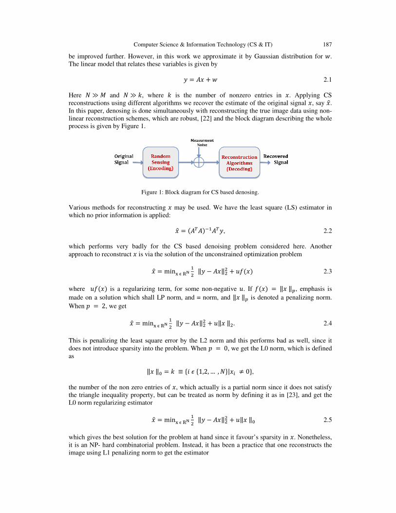
In this paper, denosing is done simultaneously with reconstructing the true image data using non-
linear reconstruction schemes, which are robust, [22] and the block diagram describing the whole
process is given by Figure 1.
Figure 1: Block diagram for CS based denosing.
Various methods for reconstructing � may be used. We have the least square (LS) estimator in
which no prior information is applied:
�� = ���������, 2.2
which performs very badly for the CS based denoising problem considered here. Another
approach to reconstruct � is via the solution of the unconstrained optimization problem
�� = min� ℝ!��
‖ # ��‖�� � $%��� 2.3
where $%��� is a regularizing term, for some non-negative $. If %��� = ‖� ‖&, emphasis is
made on a solution which shall LP norm, and = norm, and ‖� ‖& is denoted a penalizing norm.
When ' = 2, we get
�� = min� ℝ!��
‖ # ��‖�� � $‖� ‖�. 2.4
This is penalizing the least square error by the L2 norm and this performs bad as well, since it
does not introduce sparsity into the problem. When ' = 0, we get the L0 norm, which is defined
as
‖� ‖+ = � ≡ -. / -1,2, … , �3|�5 6 03,
the number of the non zero entries of �, which actually is a partial norm since it does not satisfy
the triangle inequality property, but can be treated as norm by defining it as in [23], and get the
L0 norm regularizing estimator
�� = min� ℝ!��
‖ # ��‖�� � $‖� ‖+ 2.5
which gives the best solution for the problem at hand since it favour’s sparsity in �. Nonetheless,
it is an NP- hard combinatorial problem. Instead, it has been a practice that one reconstructs the
image using L1 penalizing norm to get the estimator
188 Computer Science & Information Technology (CS & IT)
�� = min� ℝ!��
‖ # ��‖�� � $‖� ‖� 2.6
which is a convex approximation to the L0 penalizing solution II.5. These estimators, 2.4 - 2.6,
can equivalently be presented as solutions to constrained optimization problem [4] - [7], and in
the CS literature there are many different types of algorithms to implement them. A very popular
one is the L1 penalized L2 minimization called LASSO (Least Absolute Shrinkage and Selection
Operator), which we later will present it in Bayesian framework. So first we present what a
Bayesian approach is and come back to the problem at hand.
2.1. Bayesian framework
Under Bayesian inference consider two random variables � and with probability density
function (pdf) '��� and '��, respectively. Using Bayes’ theorem it is possible to show that the
posterior distribution, '��|�, is proportional to the product of the likelihood function, '�|��, and the prior distribution, '���,
'��|� ∝ '�|��'��� 2.7
Equation (2.7) is called Updating Rule in which the data allows us to update our prior views
about �. And as a result we get the posterior which combines both the data and non-data
information of � [11], [12], [20].
Further, the Maximum a posterior (MAP), ��89, is given by
��89 = arg max> '�|��'���
To proceed further, we assume two prior distributions on �.
2.2. Sparse Prior
The reconstruction of � resulting from the estimator (2.3) for the sparse problem we consider in
this paper given by, (2.4) - (2.5), can be presented as a maximum a posteriori (MAP) estimator
under the Bayesian framework as in [23]. We show this by defining a prior probability
distribution for � on the form
'��� = ?@AB�C�
D ?@AB�C�E>C F ℝG 2.8
where the regulirizing function % ∶ I → K is some scalarvalued, non negative function with
I ⊆ ℝ which can be expanded to a vector argument by
%��� = ∑ %��5�N5O� 2.9
such that for sufficiently large $, D P�QR�>�S�> T ℝG is finite. Further, let the assumed variance of
the noise be given by
U� = V$
where V is system parameter which can be taken as V = U�$. Note that the prior, (2.8), is
defined in such a way that it can incorporate the different estimators considered above by
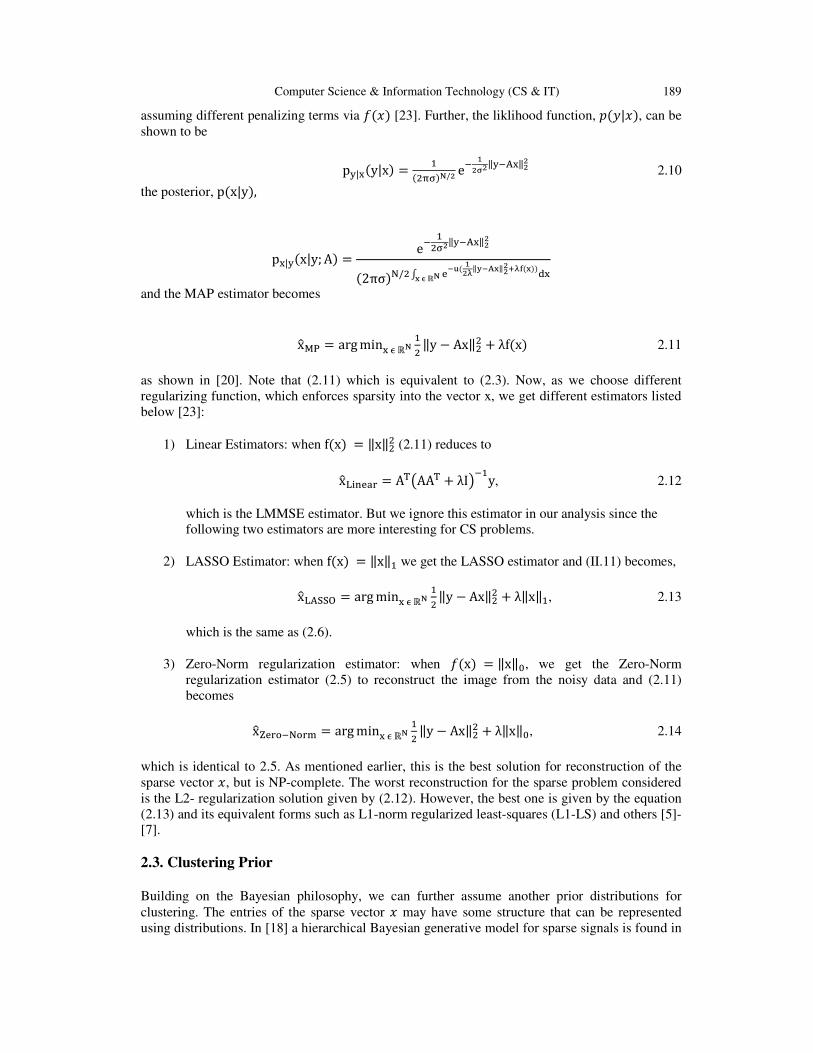
Computer Science & Information Technology (CS & IT) 189
assuming different penalizing terms via %��� [23]. Further, the liklihood function, '�|��, can be
shown to be
pX|��y|x� = ���Z[�!/] e� _
]`]‖X�a�‖]] 2.10
the posterior, p�x|y�,
p�|X�x|y; A� =e� �
�[]‖X�a�‖]]
�2πσ��/� D d@e� _]f‖g@hi‖]
]jfk�i��l�i m ℝ!
and the MAP estimator becomes
x��n = arg min� ℝ!��
‖y # Ax‖�� � λf�x� 2.11
as shown in [20]. Note that (2.11) which is equivalent to (2.3). Now, as we choose different
regularizing function, which enforces sparsity into the vector x, we get different estimators listed
below [23]:
1) Linear Estimators: when f�x� = ‖x‖�� (2.11) reduces to
x�qrsdtu = AvwAAv � λIx��
y, 2.12
which is the LMMSE estimator. But we ignore this estimator in our analysis since the
following two estimators are more interesting for CS problems.
2) LASSO Estimator: when f�x� = ‖x‖� we get the LASSO estimator and (II.11) becomes,
x�qayyz = arg min� ℝ!��
‖y # Ax‖�� � λ‖x‖�, 2.13
which is the same as (2.6).
3) Zero-Norm regularization estimator: when %�x� = ‖x‖+, we get the Zero-Norm
regularization estimator (2.5) to reconstruct the image from the noisy data and (2.11)
becomes
x�{du|��|u} = arg min� ℝ!��
‖y # Ax‖�� � λ‖x‖+, 2.14
which is identical to 2.5. As mentioned earlier, this is the best solution for reconstruction of the
sparse vector �, but is NP-complete. The worst reconstruction for the sparse problem considered
is the L2- regularization solution given by (2.12). However, the best one is given by the equation
(2.13) and its equivalent forms such as L1-norm regularized least-squares (L1-LS) and others [5]-
[7].
2.3. Clustering Prior
Building on the Bayesian philosophy, we can further assume another prior distributions for
clustering. The entries of the sparse vector � may have some structure that can be represented
using distributions. In [18] a hierarchical Bayesian generative model for sparse signals is found in
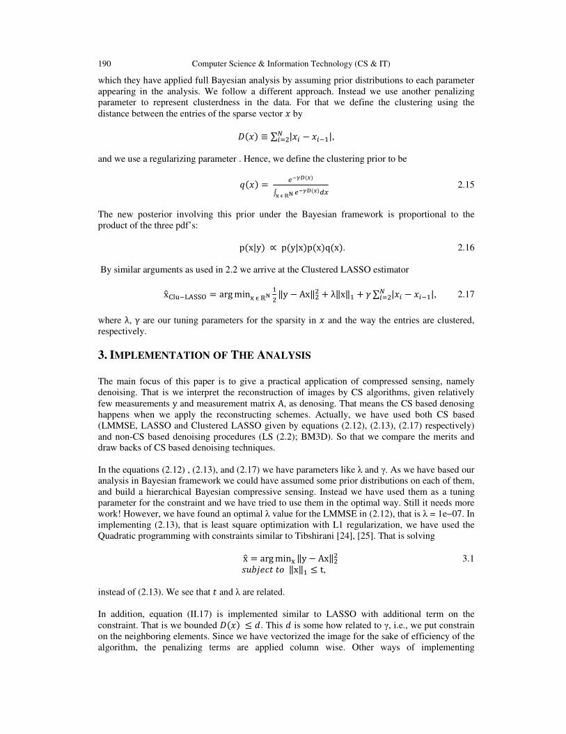
190 Computer Science & Information Technology (CS & IT)
which they have applied full Bayesian analysis by assuming prior distributions to each parameter
appearing in the analysis. We follow a different approach. Instead we use another penalizing
parameter to represent clusterdness in the data. For that we define the clustering using the
distance between the entries of the sparse vector � by
~��� ≡ ∑ |�5 # �5��|N5O� ,
and we use a regularizing parameter . Hence, we define the clustering prior to be
���� = ?@���C�
D ?@���C�E>i m ℝ! 2.15
The new posterior involving this prior under the Bayesian framework is proportional to the
product of the three pdf’s:
p�x|y) ∝ p(y|x)p(x)q(x). 2.16
By similar arguments as used in 2.2 we arrive at the Clustered LASSO estimator
x�����qayyz = arg min� ℝ!�
�‖y − Ax‖�
� + λ‖x‖� + � ∑ |�5 − �5��|N5O� , 2.17
where λ, γ are our tuning parameters for the sparsity in � and the way the entries are clustered,
respectively.
3. IMPLEMENTATION OF THE ANALYSIS
The main focus of this paper is to give a practical application of compressed sensing, namely
denoising. That is we interpret the reconstruction of images by CS algorithms, given relatively
few measurements y and measurement matrix A, as denosing. That means the CS based denosing
happens when we apply the reconstructing schemes. Actually, we have used both CS based
(LMMSE, LASSO and Clustered LASSO given by equations (2.12), (2.13), (2.17) respectively)
and non-CS based denoising procedures (LS (2.2); BM3D). So that we compare the merits and
draw backs of CS based denoising techniques.
In the equations (2.12) , (2.13), and (2.17) we have parameters like λ and γ. As we have based our
analysis in Bayesian framework we could have assumed some prior distributions on each of them,
and build a hierarchical Bayesian compressive sensing. Instead we have used them as a tuning
parameter for the constraint and we have tried to use them in the optimal way. Still it needs more
work! However, we have found an optimal λ value for the LMMSE in (2.12), that is λ = 1e−07. In
implementing (2.13), that is least square optimization with L1 regularization, we have used the
Quadratic programming with constraints similar to Tibshirani [24], [25]. That is solving
x� = arg min� ‖y − Ax‖�� 3.1
�$��P�� �� ‖x‖� ≤ t,
instead of (2.13). We see that � and λ are related.
In addition, equation (II.17) is implemented similar to LASSO with additional term on the
constraint. That is we bounded ~(�) ≤ S. This S is some how related to γ, i.e., we put constrain
on the neighboring elements. Since we have vectorized the image for the sake of efficiency of the
algorithm, the penalizing terms are applied column wise. Other ways of implementing
Computer Science & Information Technology (CS & IT) 191
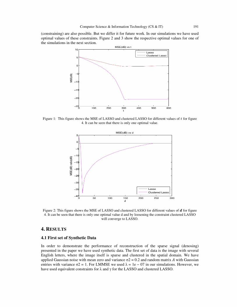
(constraining) are also possible. But we differ it for future work. In our simulations we have used
optimal values of these constraints. Figure 2 and 3 show the respective optimal values for one of
the simulations in the next section.
Figure 1: This figure shows the MSE of LASSO and clustered LASSO for different values of � for figure
4. It can be seen that there is only one optimal value.
Figure 2: This figure shows the MSE of LASSO and clustered LASSO for different values of � for figure
4. It can be seen that there is only one optimal value d and by loosening the constraint clustered LASSO
will converge to LASSO.
4. RESULTS
4.1 First set of Synthetic Data
In order to demonstrate the performance of reconstruction of the sparse signal (denosing)
presented in the paper we have used synthetic data. The first set of data is the image with several
English letters, where the image itself is sparse and clustered in the spatial domain. We have
applied Gaussian noise with mean zero and variance σ2 = 0.2 and random matrix � with Gaussian
entries with variance σ2 = 1. For LMMSE we used λ = 1e − 07 in our simulations. However, we
have used equivalent constraints for λ and γ for the LASSO and clustered LASSO.
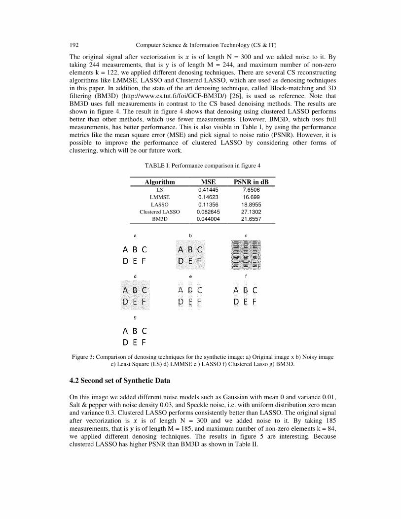
192 Computer Science & Information Technology (CS & IT)
The original signal after vectorization is � is of length N = 300 and we added noise to it. By
taking 244 measurements, that is y is of length M = 244, and maximum number of non-zero
elements k = 122, we applied different denosing techniques. There are several CS reconstructing
algorithms like LMMSE, LASSO and Clustered LASSO, which are used as denosing techniques
in this paper. In addition, the state of the art denosing technique, called Block-matching and 3D
filtering (BM3D) (http://www.cs.tut.fi/foi/GCF-BM3D/) [26], is used as reference. Note that
BM3D uses full measurements in contrast to the CS based denoising methods. The results are
shown in figure 4. The result in figure 4 shows that denosing using clustered LASSO performs
better than other methods, which use fewer measurements. However, BM3D, which uses full
measurements, has better performance. This is also visible in Table I, by using the performance
metrics like the mean square error (MSE) and pick signal to noise ratio (PSNR). However, it is
possible to improve the performance of clustered LASSO by considering other forms of
clustering, which will be our future work.
TABLE I: Performance comparison in figure 4
Algorithm MSE PSNR in dB LS 0.41445 7.6506
LMMSE 0.14623 16.699
LASSO 0.11356 18.8955
Clustered LASSO 0.082645 27.1302
BM3D 0.044004 21.6557
Figure 3: Comparison of denosing techniques for the synthetic image: a) Original image x b) Noisy image
c) Least Square (LS) d) LMMSE e ) LASSO f) Clustered Lasso g) BM3D.
4.2 Second set of Synthetic Data
On this image we added different noise models such as Gaussian with mean 0 and variance 0.01,
Salt & pepper with noise density 0.03, and Speckle noise, i.e. with uniform distribution zero mean
and variance 0.3. Clustered LASSO performs consistently better than LASSO. The original signal
after vectorization is � is of length N = 300 and we added noise to it. By taking 185
measurements, that is is of length M = 185, and maximum number of non-zero elements k = 84,
we applied different denosing techniques. The results in figure 5 are interesting. Because
clustered LASSO has higher PSNR than BM3D as shown in Table II.
Computer Science & Information Technology (CS & IT) 193
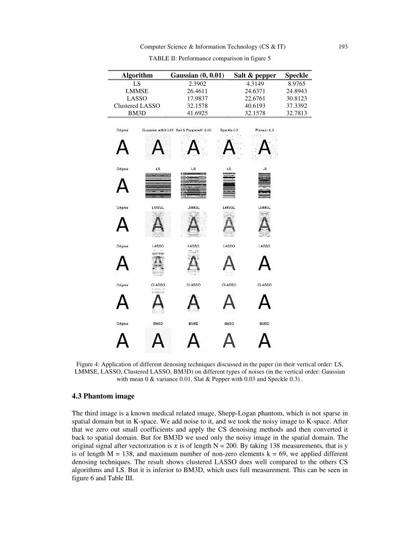
TABLE II: Performance comparison in figure 5
Algorithm Gaussian (0, 0.01) Salt & pepper Speckle
LS 2.3902 4.3149 8.9765
LMMSE 26.4611 24.6371 24.8943
LASSO 17.9837 22.6761 30.8123
Clustered LASSO 32.1578 40.6193 37.3392
BM3D 41.6925 32.1578 32.7813
Figure 4: Application of different denosing techniques discussed in the paper (in their vertical order: LS,
LMMSE, LASSO, Clustered LASSO, BM3D) on different types of noises (in the vertical order: Gaussian
with mean 0 & variance 0.01, Slat & Pepper with 0.03 and Speckle 0.3) .
4.3 Phantom image
The third image is a known medical related image, Shepp-Logan phantom, which is not sparse in
spatial domain but in K-space. We add noise to it, and we took the noisy image to K-space. After
that we zero out small coefficients and apply the CS denoising methods and then converted it
back to spatial domain. But for BM3D we used only the noisy image in the spatial domain. The
original signal after vectorization is � is of length N = 200. By taking 138 measurements, that is y
is of length M = 138, and maximum number of non-zero elements k = 69, we applied different
denosing techniques. The result shows clustered LASSO does well compared to the others CS
algorithms and LS. But it is inferior to BM3D, which uses full measurement. This can be seen in
figure 6 and Table III.
194 Computer Science & Information Technology (CS & IT)
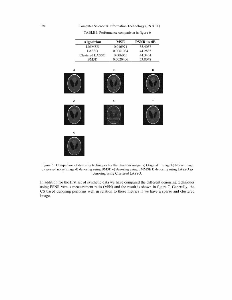
TABLE I: Performance comparison in figure 6
Algorithm MSE PSNR in dB
LMMSE 0.016971 35.4057
LASSO 0.0061034 44.2885
Clustered LASSO 0.006065 44.3434
BM3D 0.0020406 53.8048
Figure 5: Comparison of denosing techniques for the phantom image: a) Original image b) Noisy image
c) sparsed noisy image d) denosing using BM3D e) denosing using LMMSE f) denosing using LASSO g)
denosing using Clustered LASSO.
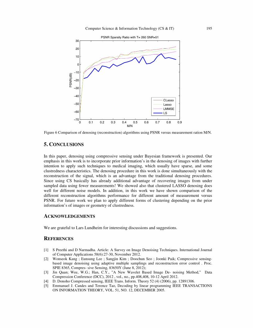
In addition for the first set of synthetic data we have compared the different denoising techniques
using PSNR versus measurement ratio (M/N) and the result is shown in figure 7. Generally, the
CS based denosing performs well in relation to these metrics if we have a sparse and clustered
image.
Computer Science & Information Technology (CS & IT) 195
Figure 6 Comparison of denosing (reconstruction) algorithms using PSNR versus measurement ration M/N.
5. CONCLUSIONS
In this paper, denosing using compressive sensing under Bayesian framework is presented. Our
emphasis in this work is to incorporate prior information’s in the denosing of images with further
intention to apply such techniques to medical imaging, which usually have sparse, and some
clustredness characteristics. The denosing procedure in this work is done simultaneously with the
reconstruction of the signal, which is an advantage from the traditional denosing procedures.
Since using CS basically has already additional advantage of recovering images from under
sampled data using fewer measurements! We showed also that clustered LASSO denosing does
well for different noise models. In addition, in this work we have shown comparison of the
different reconstruction algorithms performance for different amount of measurement versus
PSNR. For future work we plan to apply different forms of clustering depending on the prior
information’s of images or geometry of clustredness.
ACKNOWLEDGEMENTS
We are grateful to Lars Lundheim for interesting discussions and suggestions.
REFERENCES
[1] S Preethi and D Narmadha. Article: A Survey on Image Denoising Techniques. International Journal
of Computer Applications 58(6):27-30, November 2012.
[2] Wonseok Kang ; Eunsung Lee ; Sangjin Kim ; Doochun Seo ; Joonki Paik; Compressive sensing-
based image denoising using adaptive multiple samplings and reconstruction error control . Proc.
SPIE 8365, Compres- sive Sensing, 83650Y (June 8, 2012);
[3] Jin Quan; Wee, W.G.; Han, C.Y., ”A New Wavelet Based Image De- noising Method,” Data
Compression Conference (DCC), 2012 , vol., no., pp.408,408, 10-12 April 2012.
[4] D. Donoho Compressed sensing, IEEE Trans. Inform. Theory 52 (4) (2006), pp. 12891306.
[5] Emmanuel J. Candes and Terence Tao, Decoding by linear programming IEEE TRANSACTIONS
ON INFORMATION THEORY, VOL. 51, NO. 12, DECEMBER 2005.
196 Computer Science & Information Technology (CS & IT)
[6] E. Cand‘es, J. Romberg, and T. Tao, Robust uncertainty principles: Ex- act signal reconstruction from
highly incomplete frequency information, IEEE Trans. Inform. Theory, vol. 52, no. 2, pp. 489509,
Feb. 2006.
[7] E. J. Cande‘s and T. Tao, Near-optimal signal recovery from random projections: Universal encoding
strategies?, IEEE Trans. Inf. Theory, vol. 52, pp. 54065425, Dec. 2006.
[8] Michael Lustig and David Donoho and John M. Pauly, Sparse MRI: The Application of Compressed
Sensing for Rapid MR Imaging SPARS’09 Signal Processing with Adaptive Sparse Structured
Representations inria- 00369642, version 1 (2009).
[9] Marcio M. Marim, Elsa D. Angelini, Jean-Christophe Olivo-Marin, A Compressed Sensing Approach
for Biological Microscopy Image Denoising IEEE Transactions 2007.
[10] Wonseok Kang; Eunsung Lee;Eunjung Chea; Katsaggelos, A.K.; Joonki Paik, Compressive sensing-
based image denoising using adaptive multiple sampling and optimal error tolerance Acoustics,
Speech and Signal Processing (ICASSP), 2013 IEEE International Conference on , vol., no.,
pp.2503,2507, 26-31 May 2013.
[11] E.T. Jaynes, Probability Theory, The Logic of Science, Cambridge University Press., ISBN:. 2003.
[12] David J.C. Mackay Information Theory, Inference, and Learning Algorithms, Cambridge University
Press., ISBN: 978-0-521-64298-9, 2003.
[13] Anthony O’Hagen and Jonathan Forster, Kendall’s Advanced Theory of statistics, volume 2B,,
Bayesian Inference, Arnold, a member of the Hodder Headline Group ,ISBN: 0 340 807520, 2004.
[14] James O. Berger Bayesian and Conditional Frequentist Hypothesis Testing and Model Selection, VIII
C:L:A:P:E:M: La Havana, Cuba, November 2001.
[15] Bradley Efron, Modern Science and the Bayesian-Frequentist Controversy; 2005-19B/233, January,
2005.
[16] Michiel Botje R.A.Fisher on Bayes and Bayes’ Theorem ,Bayesian Analysis ,2008.
[17] Elias Moreno and F. Javier Giron, On the Frequentist and Bayesian approaches to hypothesis testing .
January-June 2006,3-28.
[18] Lei Yu, Hong Sun, Jean Pierre Barbot, Gang Zheng, Bayesian Compressive Sensing for clustered
sparse signals IEEE International Conference on Acoustics, Speech and Signal Processing (ICASSP),
2011.
[19] K.J. Friston, W. Penny, C. Phillips, S. Kiebel, G. Hinton, J. Ashburner, Classical and Bayesian
Inference in Neuroimaging: Theory Neuro Image, Volume 16, Issue 2, Pages 465 483 June 2002.
[20] Solomon A. Tesfamicael and Faraz Barzideh, Clustered Compressed Sensing in fMRI Data Analysis
Using a Bayesian Framework, International Journal of Information and Electronics Engineering vol.
4, no. 2, pp. 74-80, 2014.
[21] Dharmpal D. Doye and Sachin D Ruikarh, Wavelet Based Image Denoising Technique, International
Journal of Advanced Computer Science and Applications IJACSA (2011).
[22] Amin Tavakoli and Ali Pourmohammad, Image Denoising Based on Compressed Sensing,
International Journal of Computer Theory and Engineering vol. 4, no. 2, pp. 266-269, 2012.
[23] S. Rangan, A. K. Fletcher, and V. K. Goyal, Asymptotic analysis of MAP estimation via the replica
method and applications to compressed sensing, arXiv:0906.3234v1, 2009.
[24] Mark Schmidt, Least Squares Optimization with L1-Norm Regularization 2005.
[25] Robert Tibshirani, Regression shrinkage and selection via the lasso, In Journal of the Royal Statistical
Society, Series B, volume 58, pages 267288, 1994.
[26] Dabov, K.; Foi, A.; Katkovnik, V.; Egiazarian, K., Image Denoising by Sparse 3-D Transform
Domain Collaborative Filtering Image Processing, IEEE Transactions on , vol.16, no.8, pp.2080,2095,
Aug. 2007.
Computer Science & Information Technology (CS & IT) 197
AUTHORS
Solomon A. Tesfamicael was born in Gonder, Ethiopia in 1973. He received his
Bachelor degree in Mathematics from Bahirdar university, Bahirdar, Ethiopia in 2000
and Master degree in Coding theory from the Norwegian University of Science and
Technology (NTNU) in Trondheim, Norway in 2004. He began his PhD studies in
signal processing sept, 2009 at the department of Electronics and Telecomunications at
NTNU. He is currently working as LECTURER at the Sør-Trondlag university collge
(HiST), in Trondheim, Norway. He has worked as mathematics teacher for secondary schools and as
assistant LECTURER at the Engineering faculity in Bahirdar university in Ethiopia. In addition, he has a
pedagogical studies both in Ethiopia and in Norway. He has authored and co-authtored papers related to
compressed sensing (CS) and multiple input and multiple out put (MIMO) systems. His research interest
are signal processing, Compresses sensing, multiuser communication (MIMO, CDMA), statistical
mechanical methods like replica method, functional magnetic resonance imaging (fMRI) and
mathematical education.
Faraz Barzideh was born in Tehran, Iran in 1987. He received his bachelor degree from
Zanjan University, Zanjan, Iran, in the field of Electronic Engineering in 2011 and
finished his master degree in the field of Medical Signal Processing and Imaging from
Norwegian University of Science and Technology (NTNU) in 2013 and started his PhD
study in University of Stavanger (UiS) in 2014. His research interests are medical signal
and image processing especially in MRI and also compressive sensing and dictionary
learning.