DI

SC

US

SI

ON

P

AP

ER

S

ER

IE

S

Forschungsinstitut zur Zukunft der ArbeitInstitute for the Study of Labor

Climate Variability and International Migration: The Importance of the Agricultural Linkage

IZA DP No. 8183

May 2014

Ruohong CaiShuaizhang FengMariola PytlikováMichael Oppenheimer

Climate Variability and International Migration: The Importance of the

Agricultural Linkage

Ruohong Cai Princeton University

Shuaizhang Feng

Shanghai University of Finance and Economics, Chinese University of Hong Kong and IZA

Mariola Pytliková

VSB-Technical University Ostrava and KORA-The Danish Institute of Local Governmental Research

Michael Oppenheimer

Princeton University

Discussion Paper No. 8183 May 2014

IZA

P.O. Box 7240 53072 Bonn

Germany

Phone: +49-228-3894-0 Fax: +49-228-3894-180

E-mail: iza@iza.org

Any opinions expressed here are those of the author(s) and not those of IZA. Research published in this series may include views on policy, but the institute itself takes no institutional policy positions. The IZA research network is committed to the IZA Guiding Principles of Research Integrity. The Institute for the Study of Labor (IZA) in Bonn is a local and virtual international research center and a place of communication between science, politics and business. IZA is an independent nonprofit organization supported by Deutsche Post Foundation. The center is associated with the University of Bonn and offers a stimulating research environment through its international network, workshops and conferences, data service, project support, research visits and doctoral program. IZA engages in (i) original and internationally competitive research in all fields of labor economics, (ii) development of policy concepts, and (iii) dissemination of research results and concepts to the interested public. IZA Discussion Papers often represent preliminary work and are circulated to encourage discussion. Citation of such a paper should account for its provisional character. A revised version may be available directly from the author.

IZA Discussion Paper No. 8183 May 2014

ABSTRACT

Climate Variability and International Migration: The Importance of the Agricultural Linkage1

While there is considerable interest in understanding the climate-migration relationship, particularly in the context of concerns about global climatic change, little is known about underlying mechanisms. We analyze a unique and extensive set of panel data characterizing annual bilateral international migration flows from 163 origin countries to 42 OECD destination countries covering the last three decades. We find a positive and statistically significant relationship between temperature and international outmigration only in the most agriculture-dependent countries, consistent with the widely-documented adverse impact of temperature on agricultural productivity. In addition, migration flows to current major destinations are especially temperature-sensitive. Policies to address issues related to climate-induced international migration would be more effective if focused on the agriculture-dependent countries and especially people in those countries whose livelihoods depend on agriculture. JEL Classification: Q54, J10 Keywords: international migration, climate variability, agricultural productivity Corresponding author: Ruohong Cai 411A Robertson Hall Princeton University Princeton, NJ 08544 USA E-mail: ruohongc@princeton.edu

1 We thank conference participants at the Heartland Environmental & Resource Economics Workshop at the University of Illinois at Urbana-Champaign, SOLE conference 2014 and the 5th NORFACE Migration Conference for comments. We thank colleagues in Princeton University for helpful discussions and comments. Cai and Oppenheimer gratefully acknowledge support from the High Meadows Foundation. Feng’s research is supported by Program for New Century Excellent Talents in University (NCET-12-0903) of the Ministry of Education of China. Pytliková’s research is supported by the NORFACE Migration Program and by the Operational Programme “Education for Competitiveness” – Project No. CZ.1.07/2.3.00/20.0296.

3 Introduction

Climate change has become an increasing global concern as its current and future impacts

are understood in greater detail (IPCC, 2007). One widely cited response to such impacts is the

potential for large-scale displacement of segments of human population (Myers, 2002; Stern,

2007; Warner et al., 2009; Marchiori et al., 2012). Among all climate-induced migrants, those

crossing the political borders would be a matter of particular concern as both receiving and

sending countries are affected. Identification of the mechanisms underlying the climate-

migration relationship would be useful to national governments and international agencies

devising policies to manage migration flows.

Despite growing interest from policymakers and the general public, the quantitative

literature on weather- and climate- induced migration is still in its infancy.2 The empirical results

so far are mixed – while many studies support a significant relationship between migration and

climatic factors such as natural disasters, temperature, and precipitation (Reuveny and Moore,

2009; Feng et al., 2010; Marchiori et al., 2012; Gray and Muller, 2012; Feng and Oppenheimer,

2012), some researchers find that climate is an inconsequential factor compared to other drivers

of migration (Mortreux and Barnett, 2009; Naudé, 2010). The apparent inconsistencies among

the outcomes of various studies arise partly because such studies are mostly context-specific –

they differ in the geographic regions covered and the time frames of study. The effects of climate

on human migration are likely to be heterogeneous across time and space, as climate may

2 While we acknowledge the difference between climate and weather, the terms “climate” and

“weather” will be used interchangeably in this paper. Our analysis is performed with annual

temperature and precipitation for the period of 1980-2010.

4 interact with region-specific factors, such as other environmental and socio-economic conditions,

cultural and lifestyle characteristics, and social networks (Black et al., 2011).

To move this literature forward and gain a more complete picture of the climate-

migration relationship, one can either continue to accumulate such context-specific evidence or

conduct the analysis at a more aggregate level and focus on the most important linkage(s). This

paper takes the second approach, and considers agriculture to be a possible intermediate link

between climate and (international) migration. We do so for the following reasons. First, a large

body of literature has already established a significant sensitivity of crop yields to climatic

changes, especially temperature increases (Lobell et al., 2008; Schlenker and Roberts, 2009;

Lobell et al., 2011). Second, agriculture is an important economic sector in many countries,

especially in the developing world, where a large proportion of the population still directly

depends on agriculture for a living. Thus it is a plausible hypothesis that agriculture plays an

important role in the climate-migration relationship.

In this paper, we use a comprehensive bilateral annual migration dataset covering 163

origin countries and 42 OECD destination countries over the period of 1980-2010 to study the

climate-migration relationship empirically. We first estimate a reduced-form model that links

origin country weather variations to its international outmigration, while controlling for an

important migration determinant – income (approximated by GDP per capita) – as well as

unobserved time-invariant country-pair factors and country-specific time trends. To investigate

the role of agriculture, interaction terms between weather and agricultural dependence are

included in the model.3 We find that the effect of temperature on outmigration is positive and

3 Agricultural dependence is a dummy variable, where the top 25% agriculture-dependent

countries are assigned with 1, and the remaining countries are assigned with 0. Agriculture-

5 statistically significant only in agriculture-dependent countries. Because most agriculture-

dependent countries are also relatively poor, we use the instrumental variables approach to

provide more direct evidence on the agricultural linkage to rule out the alternative hypothesis

that the sensitivity of outmigration to climate is due to a country’s being poor per se. We

estimate the yield-migration relationship, using temperature and precipitation as instruments for

cereal yields. We find that outmigration is highly responsive to climate-induced yield shocks, but

only in agricultural countries. Our results thus suggest that, globally, agriculture is an important

intermediate link between climate and international migration. It should be noted that the relation

between the sensitivity of past migration to climate/weather variability and future migration due

to long term climate change is uncertain. Here we focus on the former which provides insights

on current motivations for migration while potentially informing projections of the latter.

The rest of the paper proceeds as follows. The next section reviews the emerging

literature on climate-induced migration. Then we present a theoretical model of international

migration that incorporates climate formally, followed by our empirical strategy. Following that

are our empirical results. Then the final section concludes.

Literature Review

There is a large literature on the determinants of human migration that encompasses

several disciplines. Income maximization is usually considered to be one of the most important

migration determinants (Roy, 1951; Borjas, 1989; Clark et al., 2007; Mayda, 2010). Simply put,

a potential migrant is assumed to compare the income differences between origin and several

dependent countries (or agricultural countries, used interchangeably in our paper) are defined as

those with relatively high share of agriculture value added in GDP.

6 destinations and the cost of migration, and select a destination which maximizes income. The

income maximization framework can be extended to utility maximization in order to incorporate

non-pecuniary determinants of migration (Borjas, 1989), such as cultural and linguistic distance,

political pressures, conflicts and wars, networks of family and friends, educational and social

benefits, immigration policies, and amenities (Massey et al., 1993; Borjas, 1999; Clark et al.,

2007; Pedesen et al., 2008; Ortega and Peri, 2009; Mayda, 2010; Adsera and Pytlikova, 2012).

During recent decades, the migration literature has paid more and more attention to

climatic and environmental factors, such as sea level rise, environmental degradation, weather-

related crop failures, and extreme weather events (Hugo, 1996; Myers, 2002; Warner et al., 2009;

Piguet et al., 2011; Foresight, 2011; Gray and Mueller, 2012). Many studies found a significant

influence of climate on human migration. Using unbalanced panel data, Barrios et al. (2006)

found that rainfall affects rural-to-urban migration in sub-Saharan Africa. Feng et al. (2010) and

Feng and Oppenheimer (2012) used a Mexican state-level panel data of migration flows, and

found a significant semi-elasticity of migration from Mexico to the United States with respect to

climate-driven changes in crop yields. Gray and Mueller (2012) showed that crop failures driven

by rainfall deficits have a strong effect on mobility in Bangladesh, while flooding has a modest

effect. Using a country-level panel data of sub-Saharan Africa, Marchiori et al. (2012) found that

weather anomalies increase internal and international migration through both amenity and

economic geography channels. Mueller et al. (2014) found that flooding has modest impact on

migration, while heat stress increases the long-term migration in Pakistan.

In contrast, some other studies have not found a significant role for climate. Based on a

survey conducted in Tuvalu, Mortreux and Barnett (2009) showed that the vast majority of

potential migrants do not consider climate change as a possible reason for leaving the country.

7 Naudé (2010) also reported that natural disasters do not have significant effects on international

migration across sub-Saharan African countries. However, these studies did not consider

possible indirect impact of climate through income differences and other channels. For example,

in the survey data used by Mortreux and Barnett (2009), migrants might not be aware of the

possibility that climate change implicitly contributes to socio-economic shocks which directly

affect migration, and thus do not cite climate change as a reason to leave. When discussing the

insignificant effects of natural disasters on migration, Naudé (2010) also acknowledged that

natural disasters may affect conflict and job opportunities and, as such, have an indirect impact

on migration.

Due to data limitations, previous studies on the determinants of migration usually relied

on analyses of migrants moving from one origin to one destination (Massey and Espinosa, 1997;

Feng et al., 2010) or multiple destinations (Hanson and McIntosh, 2010), or from multiple

origins to one destination (Clark et al., 2007; Vogler and Rotte, 2000). More recently,

researchers have begun to rely on multi-country bilateral migration data, which not only

increases the sample size but also allows controls for country-pair specific factors through the

fixed effects model and facilitates drawing more general conclusions (Pedersen et al., 2008;

Ortega and Peri, 2009; Mayda, 2010; Adsera and Pytlikova, 2012). Nevertheless, its application

in the climate-migration studies remains limited. Reuveny and Moore (2009) used a cross-

sectional data of bilateral international migration flows to 15 OECD destination countries in the

late 1980s and 1990s to investigate the effects of environmental degradation, e.g., weather-

related natural disasters. Beine and Parsons (2012) used a panel of bilateral migration for the

period of 1960-2000 to study the impact of climatic change. Their dataset has only five panels of

foreign population stock data based on the last five completed censuses. Thus their migration

8 flow data are approximated by the change in migration stocks between census years. We use a

more comprehensive bilateral annual migration dataset covering 42 OECD destination countries

and 163 origin countries over the period of 1980-2010 to study the climate-migration

relationship.

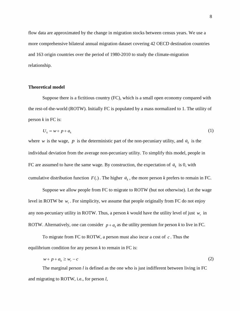
Theoretical model

Suppose there is a fictitious country (FC), which is a small open economy compared with

the rest-of-the-world (ROTW). Initially FC is populated by a mass normalized to 1. The utility of

person k in FC is:

k kU w p a= + + (1)

where w is the wage, p is the deterministic part of the non-pecuniary utility, and ka is the

individual deviation from the average non-pecuniary utility. To simplify this model, people in

FC are assumed to have the same wage. By construction, the expectation of ka is 0, with

cumulative distribution function (.)F . The higher ka , the more person k prefers to remain in FC.

Suppose we allow people from FC to migrate to ROTW (but not otherwise). Let the wage

level in ROTW be rw . For simplicity, we assume that people originally from FC do not enjoy

any non-pecuniary utility in ROTW. Thus, a person k would have the utility level of just rw in

ROTW. Alternatively, one can consider kp a+ as the utility premium for person k to live in FC.

To migrate from FC to ROTW, a person must also incur a cost of c . Thus the

equilibrium condition for any person k to remain in FC is:

k rw p a w c+ + ≥ − (2)

The marginal person l is defined as the one who is just indifferent between living in FC

and migrating to ROTW, i.e., for person l,

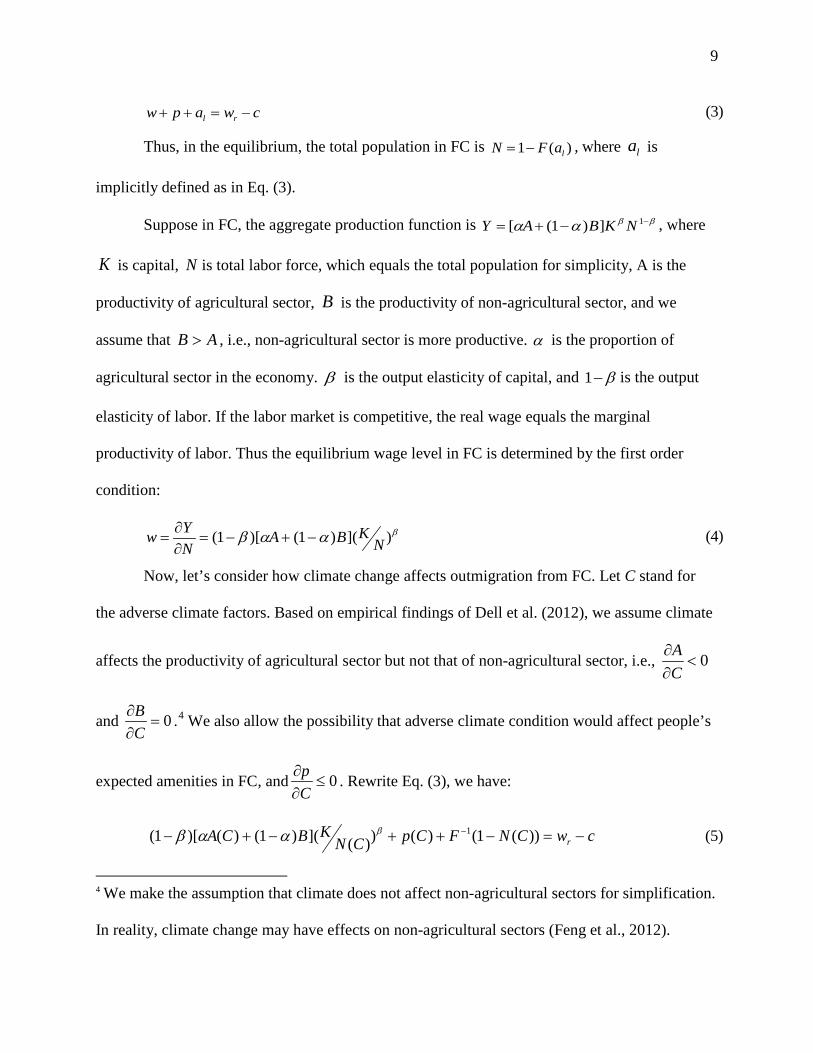
9

l rw p a w c+ + = − (3)

Thus, in the equilibrium, the total population in FC is 1 ( )lN F a= − , where la is

implicitly defined as in Eq. (3).

Suppose in FC, the aggregate production function is ββαα −−+= 1])1([ NKBAY , where

K is capital, N is total labor force, which equals the total population for simplicity, A is the

productivity of agricultural sector, B is the productivity of non-agricultural sector, and we

assume that AB > , i.e., non-agricultural sector is more productive. α is the proportion of

agricultural sector in the economy. β is the output elasticity of capital, and β−1 is the output

elasticity of labor. If the labor market is competitive, the real wage equals the marginal

productivity of labor. Thus the equilibrium wage level in FC is determined by the first order

condition:

βααβ )]()1()[1( NKBA

NYw −+−=∂∂

= (4)

Now, let’s consider how climate change affects outmigration from FC. Let C stand for

the adverse climate factors. Based on empirical findings of Dell et al. (2012), we assume climate

affects the productivity of agricultural sector but not that of non-agricultural sector, i.e., 0<∂∂CA

and 0=∂∂CB .4 We also allow the possibility that adverse climate condition would affect people’s

expected amenities in FC, and 0≤∂∂Cp . Rewrite Eq. (3), we have:

cwCNFCpCNKBCA r −=−++−+− − ))(1()())(]()1()()[1( 1βααβ (5)

4 We make the assumption that climate does not affect non-agricultural sectors for simplification.

In reality, climate change may have effects on non-agricultural sectors (Feng et al., 2012).

10

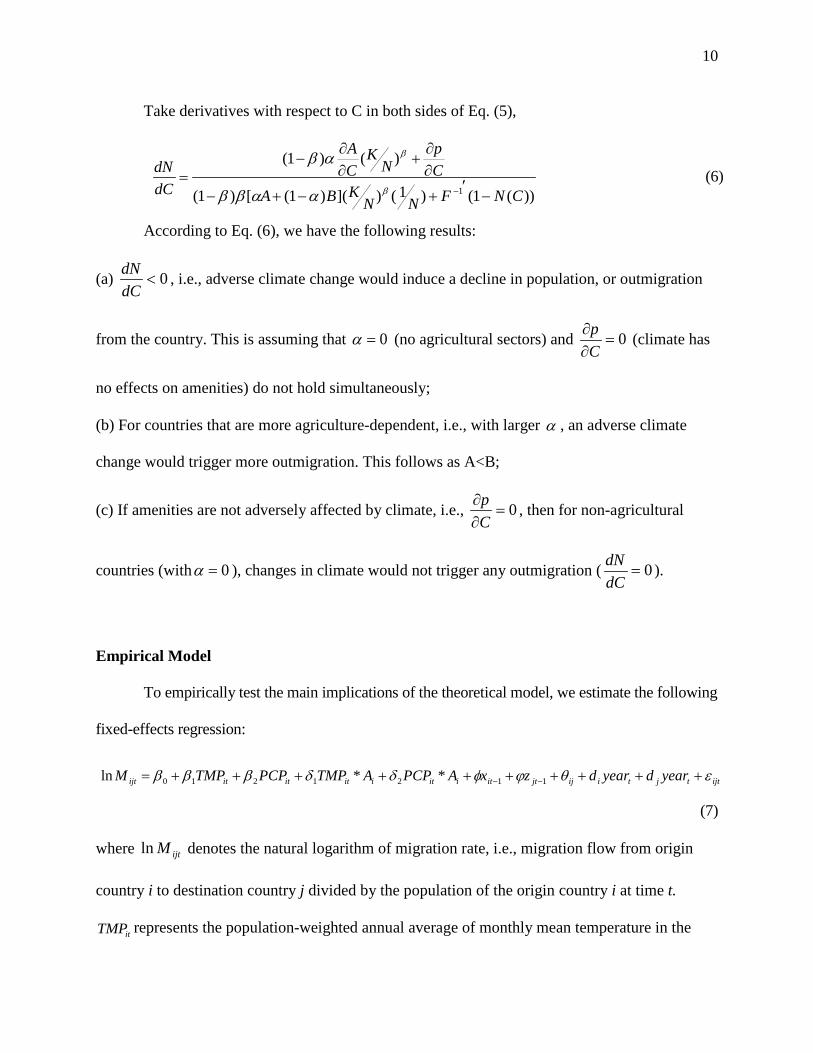
Take derivatives with respect to C in both sides of Eq. (5),

))(1()1()]()1([)1(

)()1(

1 CNFNNKBA

Cp

NK

CA

dCdN

−′

+−+−

∂∂

+∂∂

−=

−β

β

ααββ

αβ (6)

According to Eq. (6), we have the following results:

(a) 0<dCdN , i.e., adverse climate change would induce a decline in population, or outmigration

from the country. This is assuming that 0=α (no agricultural sectors) and 0=∂∂Cp (climate has

no effects on amenities) do not hold simultaneously;

(b) For countries that are more agriculture-dependent, i.e., with larger α , an adverse climate

change would trigger more outmigration. This follows as A<B;

(c) If amenities are not adversely affected by climate, i.e., 0=∂∂Cp , then for non-agricultural

countries (with 0=α ), changes in climate would not trigger any outmigration ( 0=dCdN ).

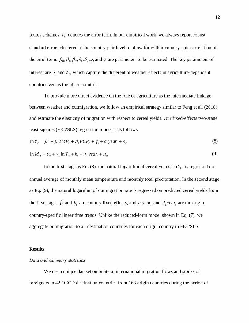
Empirical Model

To empirically test the main implications of the theoretical model, we estimate the following

fixed-effects regression:

(7)

where ijtMln denotes the natural logarithm of migration rate, i.e., migration flow from origin

country i to destination country j divided by the population of the origin country i at time t.

itTMP represents the population-weighted annual average of monthly mean temperature in the

ijttjtiijjtitiitiitititijt yeardyeardzxAPCPATMPPCPTMPM εθϕφδδβββ ++++++++++= −− 1121210 **ln

11 origin country i in degree Celsius.5 itPCP represents the population-weighted annual average of

monthly total precipitation in the origin country i in millimeters.6 iA is a dummy variable that

equals 1 if the origin country i is defined as agriculture-dependent, 0 otherwise. 1−itx and 1−jtz are

other control variables specific to origin country i and destination country j, respectively, such as

the natural logarithm of GDP per capita, which are commonly accepted as the main determinant

of migration. The lagged value of GDP per capita is employed to address possible reverse

causality that migration flow affects destination countries’ income (Mayda, 2010). ijθ denotes

country-pair fixed effects, which capture time-invariant unobserved characteristics between two

specific countries, such as distance, historical and cultural ties, linguistic distance, and many

more. Using country-pair fixed effects, we only explore the variations over time within each

country pair. ti yeard and tj yeard denote origin and destination country-specific linear time

trend, which control for factors evolving over time within specific countries, such as

urbanization, employment possibilities, welfare schemes, migrant networks or immigration

5 We use annual average temperature and precipitation data, since we focus on international

migration and Piguet et al. (2011) summarized that “rapid onset phenomena lead

overwhelmingly to short-term internal displacements rather than long-term or long-distance

migration”. It should be noted that rapid onset extreme events may affect the annual average

weather data. For instance, a heat wave increases the average temperature, and flooding increases

the total precipitation of a particular year.

6 In studies of climate impact on agriculture, growing season weather variables are usually used.

However, for cereal yields (including corn, rice, wheat, and many more) from all the countries,

growing seasons are rather diverse, so annual weather variables are a better choice.

12 policy schemes. ijtε denotes the error term. In our empirical work, we always report robust

standard errors clustered at the country-pair level to allow for within-country-pair correlation of

the error term. ,,,,,, 21210 φδδβββ and ϕ are parameters to be estimated. The key parameters of

interest are 1δ and 2δ , which capture the differential weather effects in agriculture-dependent

countries versus the other countries.

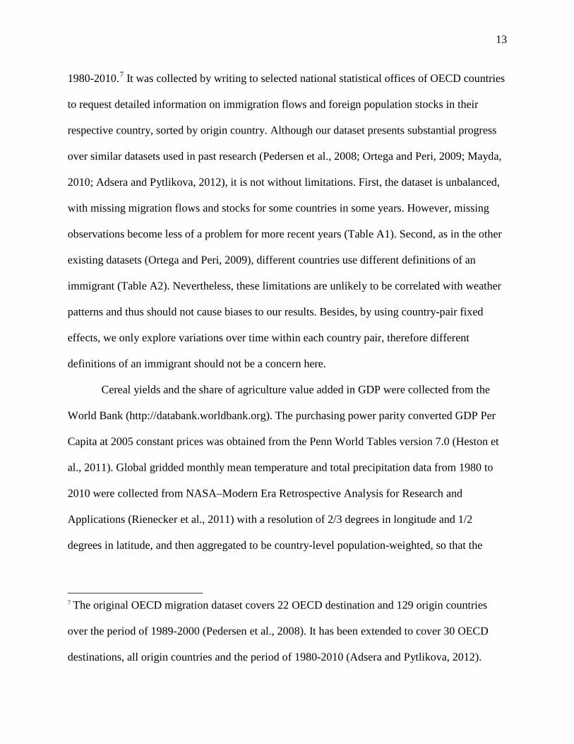
To provide more direct evidence on the role of agriculture as the intermediate linkage

between weather and outmigration, we follow an empirical strategy similar to Feng et al. (2010)

and estimate the elasticity of migration with respect to cereal yields. Our fixed-effects two-stage

least-squares (FE-2SLS) regression model is as follows:

ittiiititit yearcfPCPTMPY εβββ +++++= 110ln (8)

ittiiitit yeardhYM µγγ ++++= lnln 10 (9)

In the first stage as Eq. (8), the natural logarithm of cereal yields, itYln , is regressed on

annual average of monthly mean temperature and monthly total precipitation. In the second stage

as Eq. (9), the natural logarithm of outmigration rate is regressed on predicted cereal yields from

the first stage. if and ih are country fixed effects, and ti yearc and ti yeard are the origin

country-specific linear time trends. Unlike the reduced-form model shown in Eq. (7), we

aggregate outmigration to all destination countries for each origin country in FE-2SLS.

Results

Data and summary statistics

We use a unique dataset on bilateral international migration flows and stocks of

foreigners in 42 OECD destination countries from 163 origin countries during the period of

13 1980-2010.7 It was collected by writing to selected national statistical offices of OECD countries

to request detailed information on immigration flows and foreign population stocks in their

respective country, sorted by origin country. Although our dataset presents substantial progress

over similar datasets used in past research (Pedersen et al., 2008; Ortega and Peri, 2009; Mayda,

2010; Adsera and Pytlikova, 2012), it is not without limitations. First, the dataset is unbalanced,

with missing migration flows and stocks for some countries in some years. However, missing

observations become less of a problem for more recent years (Table A1). Second, as in the other

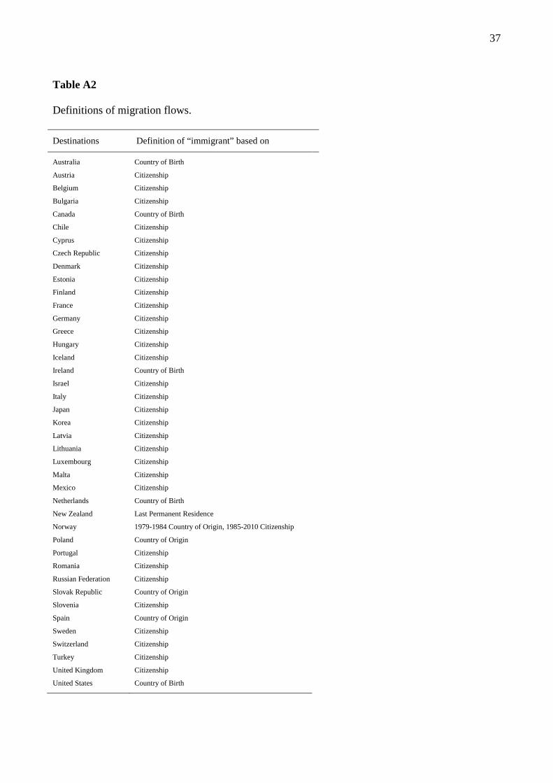
existing datasets (Ortega and Peri, 2009), different countries use different definitions of an

immigrant (Table A2). Nevertheless, these limitations are unlikely to be correlated with weather

patterns and thus should not cause biases to our results. Besides, by using country-pair fixed

effects, we only explore variations over time within each country pair, therefore different

definitions of an immigrant should not be a concern here.

Cereal yields and the share of agriculture value added in GDP were collected from the

World Bank (http://databank.worldbank.org). The purchasing power parity converted GDP Per

Capita at 2005 constant prices was obtained from the Penn World Tables version 7.0 (Heston et

al., 2011). Global gridded monthly mean temperature and total precipitation data from 1980 to

2010 were collected from NASA–Modern Era Retrospective Analysis for Research and

Applications (Rienecker et al., 2011) with a resolution of 2/3 degrees in longitude and 1/2

degrees in latitude, and then aggregated to be country-level population-weighted, so that the

7 The original OECD migration dataset covers 22 OECD destination and 129 origin countries

over the period of 1989-2000 (Pedersen et al., 2008). It has been extended to cover 30 OECD

destinations, all origin countries and the period of 1980-2010 (Adsera and Pytlikova, 2012).

14 weather conditions for populated regions within a country are given more weights. Data are

available upon request.

Our bilateral migration data covers 163 origin countries, and 42 of them are also

destination countries, with a total of 95,712 observations during the period of 1980-2010. On

average, for an origin country, about 1,077 people migrate to another specific country during a

specific year. During the period of 1980-2010, there were in total about 108 million people

migrating to another country; among them, about 85 million (50 million) people migrated

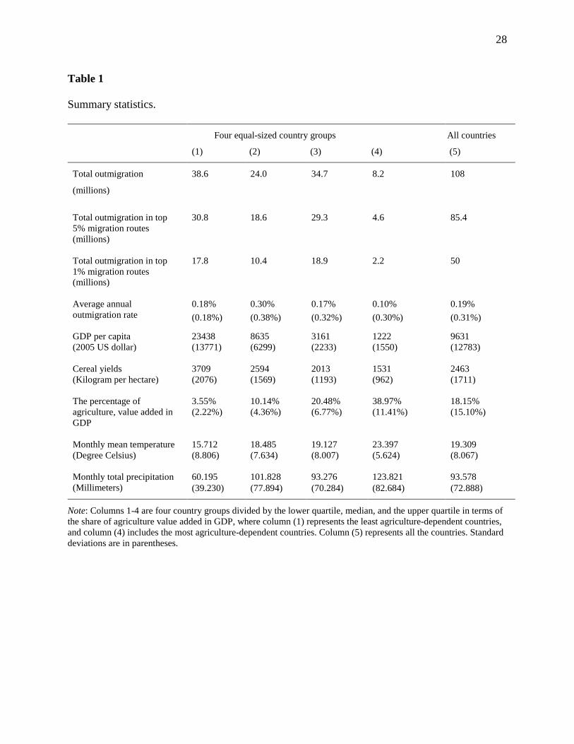
through the top 5% (1%) country pairs with large migration flows. Table 1 presents detailed

information about our data. We observe that non-agricultural countries have higher outmigration

rates. This may be due to the fact that most of agricultural countries are also poor, which usually

have limited out-migration flows due to poverty constraints (Pedersen et al., 2008; Hatton and

Williamson, 2002 and 2011). GDP per capita and cereal yields are lower for agricultural

countries. Agricultural countries tend to have higher temperatures as they are more likely to be

located in lower latitude regions than non-agricultural countries. Agricultural countries also tend

to have higher precipitation.

The Reduced-form Regression Results

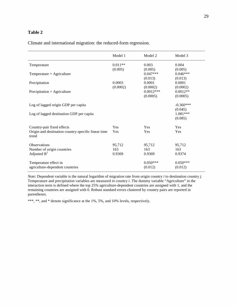
In Model 1 of Table 2, we regress the natural logarithm of migration rate (migration flow

from one origin country to one destination country divided by the origin country population) on

contemporaneous temperature and precipitation of origin countries. In Model 2 of Table 2, the

interaction terms between weather and agricultural dependence are included to test if the weather

effect is different between the top 25% agriculture-dependent countries and the remaining

countries. In Model 3 of Table 2, our preferred specification as Eq. (7), we further include the

15 natural logarithm of lagged GDP per capita for both origin and destination countries. All three

models contain a set of country-pair fixed effects and the origin and destination country specific

linear time trends. A positive and significant coefficient estimate for the interaction term

suggests that the temperature effects are significantly different between agricultural and non-

agricultural countries – and more likely to induce significant outmigration from agricultural

countries. Specifically, based on Model 3 of Table 2, each 1°C increase in temperature implies a

5% increase in the outmigration from the top 25% agricultural countries (significant at the 1%

level), as compared to only 0.4% increase (statistically insignificant) in outmigration from the

remaining countries. This is in line with Marchiori et al. (2012) who also found that weather in

agricultural countries induces outmigration. As shown in Models 2 and 3 of Table 2, our results

hold whether we control for GDP per capita or not.

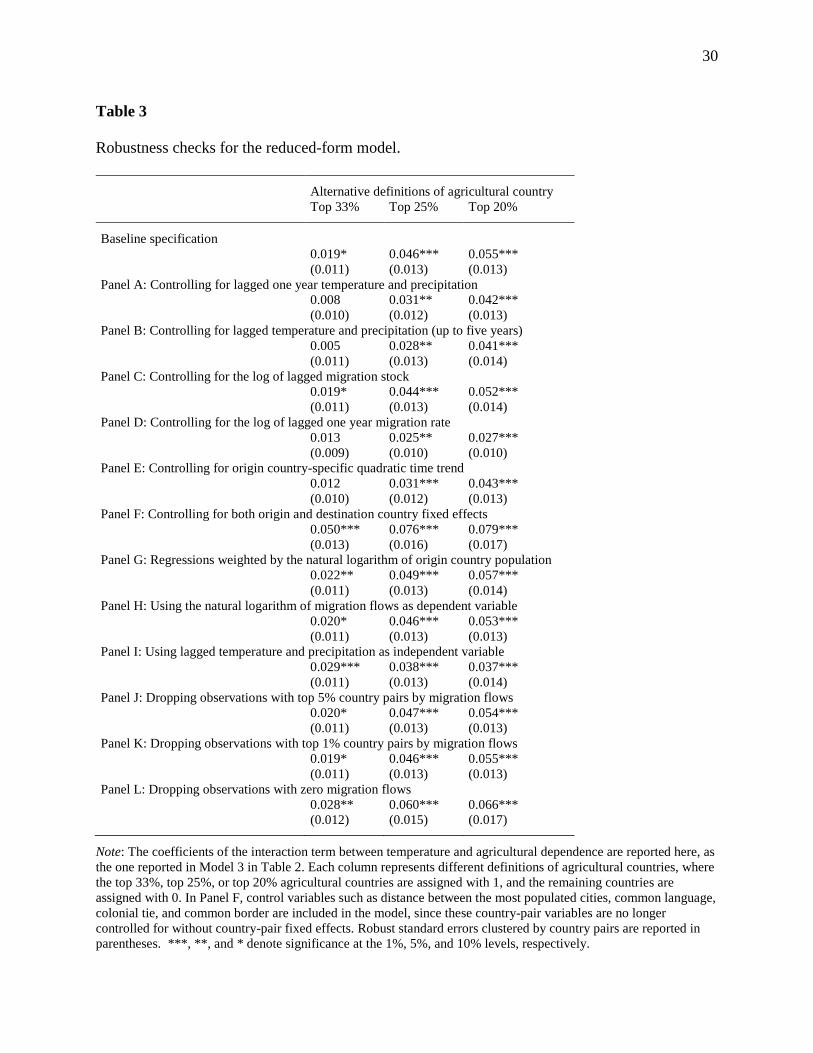
In Table 3, we present a number of robustness checks for the coefficient of the interaction

term between temperature and agricultural dependence. Our main results are qualitatively the

same whether we use different control variables (Panels A-F), different regression techniques

(Panel G), different dependent and independent variables (Panels H and I), or slightly different

samples (Panels J-L). When conducting robustness checks, we also allow different thresholds for

the definition of agricultural countries – the top one-third (33%), top one-fourth (25%), and top

one-fifth (20%) countries with higher share of agriculture value added in GDP, as shown in

different columns in Table 3. In general, the differential temperature effects for agricultural

countries become larger in magnitude and more statistically significant when a higher threshold

is set to identify agricultural countries. The results are thus consistent with the idea that more

agriculture-dependent countries are more likely to experience outmigration when temperature

rises, as shown in the theoretical model.

16

The contemporaneous temperature effects become slightly weaker but still significant

when the lagged terms up to five years are also included in the model (Panels A and B). This

implies that temperature may have some lagged effects on outmigration as it may take time to

stimulate some of international migration flow. Migration flows may be largely determined by

the existing co-ethnic networks, i.e. networks of family members, friends and people of the same

origin that have already lived in a host country (Munshi, 2003; Pedersen et al., 2008). In Panel C,

we use migration stock (foreign population from country i residing in country j) as a proxy for

migrant networks and find that our results still hold. We also use the lagged dependent variable –

the natural logarithm of lagged migration rate as one of the independent variables (Panel D),

since the migration rate may be serially correlated. Again, we obtained a similar estimate as our

baseline specification. This specification in Panel D could be viewed as an alternative way to

control for migrant networks as Panel C.

In Panel E, the temperature effects are still positive and significant when we include an

origin country-specific quadratic time trend, which controls for some nonlinear determinants of

migration trending over time for each origin country. We used the country-pair fixed effects in

the baseline specification, while two separate country fixed effects – one for origin and the other

for destination countries – were chosen as baseline specifications in some other studies (Ortega

and Peri, 2009; Mayda, 2010). In Panel F, we control for the separate country fixed effects and

other variables such as distance between the most populated cities, common language, colonial

tie, and common border which were not included in the model with country-pair fixed effects

since they were absorbed by country-pair fixed effects (Ortega and Peri, 2009). With this

alternative fixed effects specification, the temperature effects are still positive and significant for

all definitions of agriculture-dependent countries.

17

In panel G, we run a weighted least squares regression using the natural logarithm of

origin country’s total population as weights, which does not change our baseline results. We

further use the natural logarithm of migration flow (Panel H), instead of the natural logarithm of

migration rate, as dependent variable. The results are very similar to the baseline specification.

Instead of estimating the contemporaneous temperature effects, we estimate the effects of the

lagged temperature in Panel I, and find the lagged response of migration flow to temperature

variability, which is consistent with our expectation based on Panels A and B.

We also study if the results are driven by specific countries or country pairs. During the

past three decades, 85 million (50 million) out of 108 million migrants are in the top 5% (1%)

migration routes (from one country to another) by the size of migration flow. Now we remove

the data from the top 5% (1%) migration routes in Panel J (Panel K) and find that the

temperature effects are still positive and statistically significant across all three definitions of

agriculture dependence. In addition, about 11% of all the country pairs do not have any

migration flows. In Panel L, we drop those zero migration flows from the sample. The

coefficient estimates for the interaction term remain positive and statistically significant.

Both temperature and precipitation variables are included in the baseline specification,

due to their frequent use in the literature. We do not interpret the precipitation coefficients here,

since statistical methods appear more reliable for temperature variables (Lobell and Burke,

2010); this may be explained by the fact that precipitation has higher spatial variability and thus

is less well captured than temperature by the relatively coarse climate data (Burke et al., 2009),

e.g., country-level in our study. However, it is still necessary to control for precipitation in our

model since it is a possible confounding factor, which may be correlated with both temperature

(independent variable) and migration (dependent variable).

18

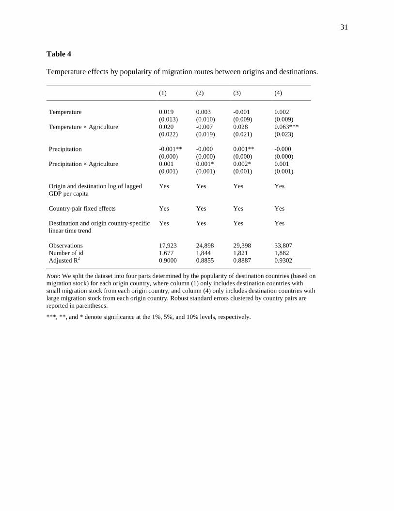
We further study the role of different destination countries in climate-induced migration.

In Table 4, we split our dataset into four parts determined by the popularity of destination

countries (based on migration stock) for each origin country. In other words, each of these four

sub-datasets includes all 163 origin countries, but only a quarter of destination countries. We find

that our main results – positive temperature effects on outmigration from agricultural countries –

are only detected in the migration routes to their top 25% migration destination countries (Table

4, column 4). The results imply that temperature tends to intensify migration mostly in the

already established migration routes, while it has insignificant effect on migration to the

countries which are previously not major destinations. This finding is in line with previous

hypotheses that climate change will affect existing migration routes (McLeman and Hunter, 2010;

World Bank, 2010).

Two-stage least squares regression results

The finding of a positive and statistically significant relationship between temperature

and outmigration only for agricultural countries is quite revealing, but does not yet provide a

definite answer on whether agriculture plays an important intermediate role, as many agricultural

countries are also very poor. To rule out a poor-country effect, one needs to provide more direct

evidence on the role of agriculture.

In this subsection, we estimate the relationship between cereal yields (an indicator of

agricultural productivity) and international outmigration. To deal with the biases caused by

omitted variables, we use temperature and precipitation to instrument for cereal yields and use

FE-2SLS to estimate the Eq. (8) and (9). To the extent that weather factors are exogenous, the

19 FE-2SLS is consistent; see Feng et al. (2010) and Feng and Oppenheimer (2012) for more

discussion of this point.

Tables 5 contains the second stage results of the instrumental variables approach for four

country groups categorized based on the agricultural dependence. Cereal yields are found to be

negatively associated with outmigration only in the top 25% agricultural countries (Table 5,

column 4), suggesting that cereal yields appear to be an important factor for migration from such

countries, consistent with earlier studies (Feng et al., 2010; Feng and Oppenheimer, 2012). In

particular, the estimated elasticity of outmigration rate with respect to cereal yields in the top

25% agricultural countries is about -2.4. To put the number in perspective, for a country with

0.1% outmigration rate, a 10% reduction in cereal yields would raise the outmigration rate by

around 24%, or to 0.124%. Table 5 shows that the FE-2SLS estimates are substantially different

from the OLS estimates and more negative, which implies that the unobserved omitted variables

jointly determining cereal yields and migration would bias the OLS estimates towards zero.

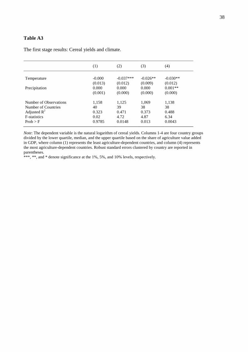
A concern for the instrumental variables approach is the weak instrument. In Table A3,

although F-statistics of the instruments in the first stage are all significant at the 5% level, all of

them are less than 10, a value usually used as a rule of thumb to detect weak instruments (Staiger

and Stock, 1997). However, this rule of thumb is only for regular standard errors while we report

robust standard errors clustered at the country level in this study. On the other hand, the slightly

low F-statistics reported here might be due to imprecise measurements of weather and yields.

Country-level data are relatively coarse for both weather and cereal yields; thus the correlation

between them is expected to be less significant than is the case when finer subnational data are

used. The slightly low F-statistics could also be due to the possible nonlinear relationship

between temperature and yields (Schlenker and Roberts, 2009). Furthermore, cereal includes

20 multiple crops such as corn, rice, wheat, and many more, which have different growing seasons,

and also different sensitivities to weather variations. Additional noise is thus introduced when

pooling them together, as we do in this paper.

Another concern is whether or not our exclusion restriction is valid. If weather affects

migration through channels other than cereal yields, the FE-2SLS estimates would be biased. For

instance, if people have a direct preference to live in less hot areas, our FE-2SLS estimates

would be biased upward in absolute value. If this is the case, we would expect a negative and

significant coefficient even for non-agricultural countries, i.e., non-agricultural countries serve as

a control group in our empirical methodology. However, this is not the case. As shown in Table

5, for less agriculture-dependent countries (columns 1-3), we cannot reject the null of zero

coefficients. This is also consistent with our findings reported in Table 2, which shows no

reduced-form relationship between temperature and outmigration for non-agricultural countries.

In Table 6, we conduct several robustness checks for the coefficient of cereal yields in the

second stage of instrumental variables approach. In this table, we only report the coefficient for

agricultural countries as we reported in column (4) in Table 5. In addition to the FE-2SLS results,

we also perform the fixed-effects limited-information maximum-likelihood (FE-LIML)

estimations. The results are quite robust to various model specifications. First, to alleviate

concerns regarding weak instruments, we use either only temperature or only precipitation as the

instrument, as it is well known in the econometrics literature that the use of fewer instruments

reduces the possible weak instrument bias (Angrist and Pischke, 2009). The results are shown in

Panels A and B in Table 6. When temperature is used as the only instrument, the estimate is quite

similar to the baseline specification. When precipitation is used as the only instrument, the

21 coefficient is slightly smaller (still significant at the 10% level), as the average precipitation data

at the country level may not be reliable.

In Panel C, we use the lagged (one-year) weather variables and cereal yields in the

regression. In Panel D, we include GDP per capita as an additional control variable, as income is

frequently used as a main explanatory variable in studies of international migration. In Panel E,

we try an alternative definition of migration, using the natural logarithm of migration flows

rather than the natural logarithm of migration rate as the dependent variable. In all these cases,

the coefficient estimates remain negative and statistically significant.

Lastly, instead of using only the top 25% agricultural countries as in the baseline

specification, we use the top 33% and top 20% agricultural countries in Panels F and G in Table

6, respectively. The estimated coefficients are very close to the baseline results, suggesting that

the threshold for agricultural dependence that we use is not the key.

Conclusions

In this study, we have employed an empirical approach to quantify the effects of weather

variations on global bilateral international migration flows. The results show that temperature

has positive and statistically significant effect on outmigration, but only from agriculture-

dependent countries. Therefore, among the intermediate links between weather and international

migration, agriculture appears to be an important factor. Our results are robust to alternative

model specifications.

While our results suggest that significant climate-induced international outmigration only

happens in agriculture-dependent countries, the consequences may be substantial – we further

find that climate-induced migration specifically enlarges the flow in already established

22 migration routes, potentially presenting challenges to major migrant-receiving countries, mostly

industrialized. Studies such as this one could provide a basis for advanced consideration of

policies to address the consequences (both positive and negative) of potential increases in

migration due to climate change. Our results provide some guidance to those developing policies

to anticipate and manage these flows by focusing attention on agricultural countries and

especially people in those countries whose livelihoods depend on agriculture. Agricultural

adaptation, which builds resilience and enhances farmers’ earnings capacities, may reduce

incentives to migrate. Diversifying livelihoods for those who now depend on agriculture, such as

by encouraging off-farm work, urbanization or structural upgrading, also has the potential to

reduce migration.

Most previous studies are region-specific, thus generating mixed results when taken

together and less likely to identify a universal underlying mechanism for the climate-induced

international migration. Based on a comprehensive international migration dataset, this study

provides robust empirical evidence that agriculture is an important factor influencing climate-

induced international migration for the past three decades. Future research should further test our

results as additional migration and climate/weather data becomes available. While we perform

the analysis using the reduced-form model and instrumental variables approach, alternative

methods and tools should also be used to study these relationships where appropriate.

23 References

Adsera, A., Pytlikova, M., 2012. The role of language in shaping international migration. IZA

Discussion Paper No. 6333.

Angrist, J.D., Pischke, J.-S., 2009. Mostly Harmless Econometrics: An Empiricist’s Companion.

Princeton University Press, Princeton, NJ.

Barrios, S., Bertinelli, L., Strobl, E., 2006. Climatic change and rural–urban migration: the case

of Sub-Saharan Africa. Journal of Urban Economics 60 (3), 357–371.

Beine, M., Parsons, C., 2012. Climatic factors as determinants of International Migration. CES-

IFO Working paper No. 3747.

Black, R., Kniveton, D., Schmidt-Verkerk, K., 2011. Migration and climate change: Towards an

integrated assessment of sensitivity. Environment and Planning A 43 (2), 431–450.

Borjas, G.J., 1989. Economic theory and international migration. Internetional Migration Review

23 (3), 457–485.

Borjas, G.J., 1999. The economic analysis of immigration. In: Ashenfelter, O., Card, D. (Eds.),

Handbook of Labor Economics, Elsevier, Amsterdam, pp. 1697–1760.

Burke, M.B., Miguel, E., Satyanath, S., Dykema, J.A., Lobell, D.B., 2009. Warming increases

the risk of civil war in Africa. Proceedings of the National Academy of Sciences 106 (49),

20670–20674.

Clark, X., Hatton, T.J., Williamson, J.G., 2007. Explaining US immigration, 1971–1998. Review

of Economics and Statistics 89 (2), 359–373.

Feng, S., Krueger, A.B., Oppenheimer, M., 2010. Linkages among climate change, crop yields

and Mexico-US cross-border migration. Proceedings of the National Academy of

Sciences 107 (32), 14257–14262.

24 Feng, S., Oppenheimer, M., 2012. Applying statistical models to the climate–migration

relationship. Proceedings of the National Academy of Sciences 109 (43), E2915.

Feng, S., Oppenheimer, M., Schlenker, W., 2012. Climate change, crop Yields and internal

migration in the United States. NBER Working Paper No. 17734.

Foresight, 2011. Migration and global environmental change: Future challenges and

opportunities. Final project report. The Government Office for Science, London.

Gray, C.L., Mueller, V., 2012. Natural disasters and population mobility in

Bangladesh. Proceedings of the National Academy of Sciences 109 (16), 6000–6005.

Hanson, G.H., McIntosh, C., 2010. The great Mexican emigration. The Review of Economics

and Statistics 92 (4), 798–810.

Hatton, T.J., Williamson, J.G., 2002. What fundamentals drive world migration? NBER Working

Paper No. 9159.

Hatton, T.J., Williamson, J.G., 2011. Are third world emigration forces abating? World

Development 39 (1), 20–32.

Heston, A., Summers, R., Aten, B., 2011. Penn World Table Version 7.0. Center for

International Comparisons of Production, Income and Prices. University of Pennsylvania.

Hugo, G., 1996. Environmental concerns and international migration. International Migration

Review, Special Issue: Ethics, Migration, and Global Stewardship 30 (1), 105–131.

IPCC, 2007. Climate Change 2007: Synthesis Report. In: By the Core Writing Team, Pachauri,

R.K., Reisinger, A. (Eds.), Contribution of Working Groups I, II and III to the Fourth

Assessment. Intergovernmental Panel on Climate Change, Geneva, Switzerland.

25 Lobell, D.B., Burke, M.B.,Tebaldi, C.,Mastrandrea, M.D., Falcon,W.P., Naylor, R.L., 2008.

Prioritizing climate change adaptation needs for food security in 2030. Science 319

(5863), 607–610.

Lobell, D.B., Burke, M.B., 2010. On the use of statistical models to predict crop yield responses

to climate change. Agricultural and Forest Meteorology 150 (11), 1443–1452.

Lobell, D.B., Schlenker, W., Costa-Roberts, J., 2011. Climate trends and global crop production

since 1980. Science 333 (6042), 616–620.

Marchiori, L., Maystadt, J.F., Schumacher, I., 2012. The impact of weather anomalies on

migration in Sub-Saharan Africa. Journal of Environmental Economics and

Management 63 (3), 355–374.

Massey, D.S., Arango, J., Hugo, G., Kouaouci, A., Pellegrino, A., Taylor, J.E., 1993. Theories of

international migration: A review and appraisal. Population and Development Review 19

(3), 431–466.

Massey, D.S., Espinosa, K.E., 1997. What’s driving Mexico - U.S. migration? A theoretical,

empirical, and policy analysis. American Journal of Sociology 102 (4), 939–999.

Mayda, A.M., 2010. International migration: A panel data analysis of the determinants of

bilateral flows. Journal of Population Economics 23 (4), 1249–1274.

McLeman, R.A., Hunter, L.M., 2010. Migration in the context of vulnerability and adaptation to

climate change: insights from analogues. Wiley Interdisciplinary Reviews: Climate

Change 1 (3), 450–461.

Mortreux, C., Barnett, J., 2009. Climate change, migration and adaptation in Funafuti, Tuvalu.

Global Environmental Change 19 (1), 105–112.

26 Mueller, V., Gray, C., Kosec, K., 2014. Heat stress increases long-term human migration in rural

Pakistan. Nature Climate Change (http://dx.doi.org/10.1038/nclimate2103).

Munshi, K., 2003. Networks in the modern economy: Mexican migrants in the US labor market.

Quarterly Journal of Economics 118 (2), 549–599.

Myers, N., 2002. Environmental refugees: A growing phenomenon of the 21st

Century. Philosophical Transactions of the Royal Society of London, Series B: Biological

Sciences 357 (1420), 609–613.

Naudé, W., 2010. The determinants of migration from Sub-Saharan African countries. Journal of

African Economies 19 (3), 330–356.

Ortega, F., Peri, G., 2009. The causes and effects of international migrations: Evidence from

OECD Countries 1980-2005. NBER Working Paper No. 14833.

Pedersen, P.J., Pytlikova, M., Smith, N., 2008. Selection and network effects – Migration flows

into OECD countries, 1990-2000. European Economic Review 52 (7), 1160–1186.

Piguet, E., Pécoud, A., De Guchteneire, P., 2011. Migration and climate change: An

overview. Refugee Survey Quarterly 30 (3), 1–23.

Reuveny, R., Moore, W.H., 2009. Does environmental degradation influence migration?

Emigration to developed countries in the late 1980s and 1990s. Social Science Quarterly

90 (3), 461–479.

Rienecker, M.M., Suarez, M.J., Gelaro, Todling, R., Bacmeister, J., Liu, E., Bosilovich, M.G.,

Schubert, S.D., Takacs, L., Kim, G.-K., 2011. MERRA: NASA's Modern-Era

Retrospective Analysis for Research and Applications. Journal of Climate 24 (14), 3624–

3648.

27 Roy, A.D., 1951. Some thoughts on the distribution of earnings. Oxford Economic Papers 3 (2),

135–146.

Schlenker, W., Roberts, M.J., 2009. Nonlinear temperature effects indicate severe damages to

US crop yields under climate change. Proceedings of the National Academy of

Sciences 106 (37), 15594–15598.

Staiger, D., Stock, J.H., 1997. Instrumental variables regression with weak instruments.

Econometrica 65 (3), 557–586.

Stern, N., 2007. The Economics of Climate Change: The Stern Review. Cambridge University

Press, Cambridge.

Vogler, M., Rotte, R., 2000. The effects of development on migration: Theoretical issues and

new empirical evidence. Journal of Population Economics 13 (3), 485–508.

Warner, K., Erhart, C., de Sherbinin, A., Adamo, S.B., Onn, T.C., 2009. In search of shelter:

Mapping the effects of climate change on human migration and displacement. A policy

paper prepared for the 2009 Climate Negotiations. Bonn, Germany: United Nations

University, CARE, and CIESIN-Columbia University and in close collaboration with the

European Commission "Environmental Change and Forced Migration Scenarios Project",

the UNHCR, and the World Bank.

World Bank, 2010. World Development Report 2010: Development and Climate Change, World

Bank, Washington, DC.

28 Table 1

Summary statistics.

Four equal-sized country groups All countries

(1) (2) (3) (4) (5)

Total outmigration

(millions)

38.6 24.0 34.7 8.2 108

Total outmigration in top 5% migration routes (millions)

30.8 18.6 29.3 4.6 85.4

Total outmigration in top 1% migration routes (millions)

17.8 10.4 18.9 2.2 50

Average annual outmigration rate

0.18% 0.30% 0.17% 0.10% 0.19% (0.18%) (0.38%) (0.32%) (0.30%) (0.31%)

GDP per capita (2005 US dollar)

23438 8635 3161 1222 9631 (13771) (6299) (2233) (1550)

(12783)

Cereal yields (Kilogram per hectare)

3709 2594 2013 1531 2463 (2076) (1569) (1193) (962)

(1711)

The percentage of agriculture, value added in GDP

3.55% 10.14% 20.48% 38.97% 18.15% (2.22%) (4.36%) (6.77%) (11.41%) (15.10%)

Monthly mean temperature (Degree Celsius)

15.712 18.485 19.127 23.397 19.309 (8.806) (7.634) (8.007) (5.624) (8.067)

Monthly total precipitation (Millimeters)

60.195 101.828 93.276 123.821 93.578 (39.230) (77.894) (70.284) (82.684) (72.888)

Note: Columns 1-4 are four country groups divided by the lower quartile, median, and the upper quartile in terms of the share of agriculture value added in GDP, where column (1) represents the least agriculture-dependent countries, and column (4) includes the most agriculture-dependent countries. Column (5) represents all the countries. Standard deviations are in parentheses.

29 Table 2

Climate and international migration: the reduced-form regression.

Model 1 Model 2 Model 3

Temperature 0.011** 0.003 0.004 (0.005) (0.005) (0.005) Temperature × Agriculture 0.047*** 0.046*** (0.013) (0.013) Precipitation 0.0003 0.0001 0.0001 (0.0002) (0.0002) (0.0002) Precipitation × Agriculture 0.0012*** 0.0012** (0.0005) (0.0005) Log of lagged origin GDP per capita -0.360*** (0.045) Log of lagged destination GDP per capita 1.081*** (0.085) Country-pair fixed effects Yes Yes Yes Origin and destination country-specific linear time trend

Yes Yes Yes

Observations 95,712 95,712 95,712 Number of origin countries 163 163 163 Adjusted R2 0.9369 0.9369 0.9374 Temperature effect in 0.050*** 0.050*** agriculture-dependent countries (0.012) (0.012)

Note: Dependent variable is the natural logarithm of migration rate from origin country i to destination country j. Temperature and precipitation variables are measured in country i. The dummy variable “Agriculture” in the interaction term is defined where the top 25% agriculture-dependent countries are assigned with 1, and the remaining countries are assigned with 0. Robust standard errors clustered by country pairs are reported in parentheses.

***, **, and * denote significance at the 1%, 5%, and 10% levels, respectively.

30 Table 3

Robustness checks for the reduced-form model.

Alternative definitions of agricultural country Top 33% Top 25% Top 20%

Baseline specification 0.019* 0.046*** 0.055*** (0.011) (0.013) (0.013) Panel A: Controlling for lagged one year temperature and precipitation 0.008 0.031** 0.042*** (0.010) (0.012) (0.013) Panel B: Controlling for lagged temperature and precipitation (up to five years) 0.005 0.028** 0.041*** (0.011) (0.013) (0.014) Panel C: Controlling for the log of lagged migration stock 0.019* 0.044*** 0.052*** (0.011) (0.013) (0.014) Panel D: Controlling for the log of lagged one year migration rate 0.013 0.025** 0.027*** (0.009) (0.010) (0.010) Panel E: Controlling for origin country-specific quadratic time trend 0.012 0.031*** 0.043*** (0.010) (0.012) (0.013) Panel F: Controlling for both origin and destination country fixed effects 0.050*** 0.076*** 0.079*** (0.013) (0.016) (0.017) Panel G: Regressions weighted by the natural logarithm of origin country population 0.022** 0.049*** 0.057*** (0.011) (0.013) (0.014) Panel H: Using the natural logarithm of migration flows as dependent variable 0.020* 0.046*** 0.053*** (0.011) (0.013) (0.013) Panel I: Using lagged temperature and precipitation as independent variable 0.029*** 0.038*** 0.037*** (0.011) (0.013) (0.014) Panel J: Dropping observations with top 5% country pairs by migration flows 0.020* 0.047*** 0.054*** (0.011) (0.013) (0.013) Panel K: Dropping observations with top 1% country pairs by migration flows 0.019* 0.046*** 0.055*** (0.011) (0.013) (0.013) Panel L: Dropping observations with zero migration flows 0.028** 0.060*** 0.066*** (0.012) (0.015) (0.017)

Note: The coefficients of the interaction term between temperature and agricultural dependence are reported here, as the one reported in Model 3 in Table 2. Each column represents different definitions of agricultural countries, where the top 33%, top 25%, or top 20% agricultural countries are assigned with 1, and the remaining countries are assigned with 0. In Panel F, control variables such as distance between the most populated cities, common language, colonial tie, and common border are included in the model, since these country-pair variables are no longer controlled for without country-pair fixed effects. Robust standard errors clustered by country pairs are reported in parentheses. ***, **, and * denote significance at the 1%, 5%, and 10% levels, respectively.

31 Table 4

Temperature effects by popularity of migration routes between origins and destinations.

(1) (2) (3) (4)

Temperature 0.019 0.003 -0.001 0.002 (0.013) (0.010) (0.009) (0.009) Temperature × Agriculture 0.020 -0.007 0.028 0.063*** (0.022) (0.019) (0.021) (0.023) Precipitation -0.001** -0.000 0.001** -0.000 (0.000) (0.000) (0.000) (0.000) Precipitation × Agriculture 0.001 0.001* 0.002* 0.001 (0.001) (0.001) (0.001) (0.001) Origin and destination log of lagged GDP per capita

Yes Yes Yes Yes

Country-pair fixed effects Yes Yes Yes Yes Destination and origin country-specific linear time trend

Yes Yes Yes Yes

Observations 17,923 24,898 29,398 33,807 Number of id 1,677 1,844 1,821 1,882 Adjusted R2 0.9000 0.8855 0.8887 0.9302

Note: We split the dataset into four parts determined by the popularity of destination countries (based on migration stock) for each origin country, where column (1) only includes destination countries with small migration stock from each origin country, and column (4) only includes destination countries with large migration stock from each origin country. Robust standard errors clustered by country pairs are reported in parentheses.

***, **, and * denote significance at the 1%, 5%, and 10% levels, respectively.

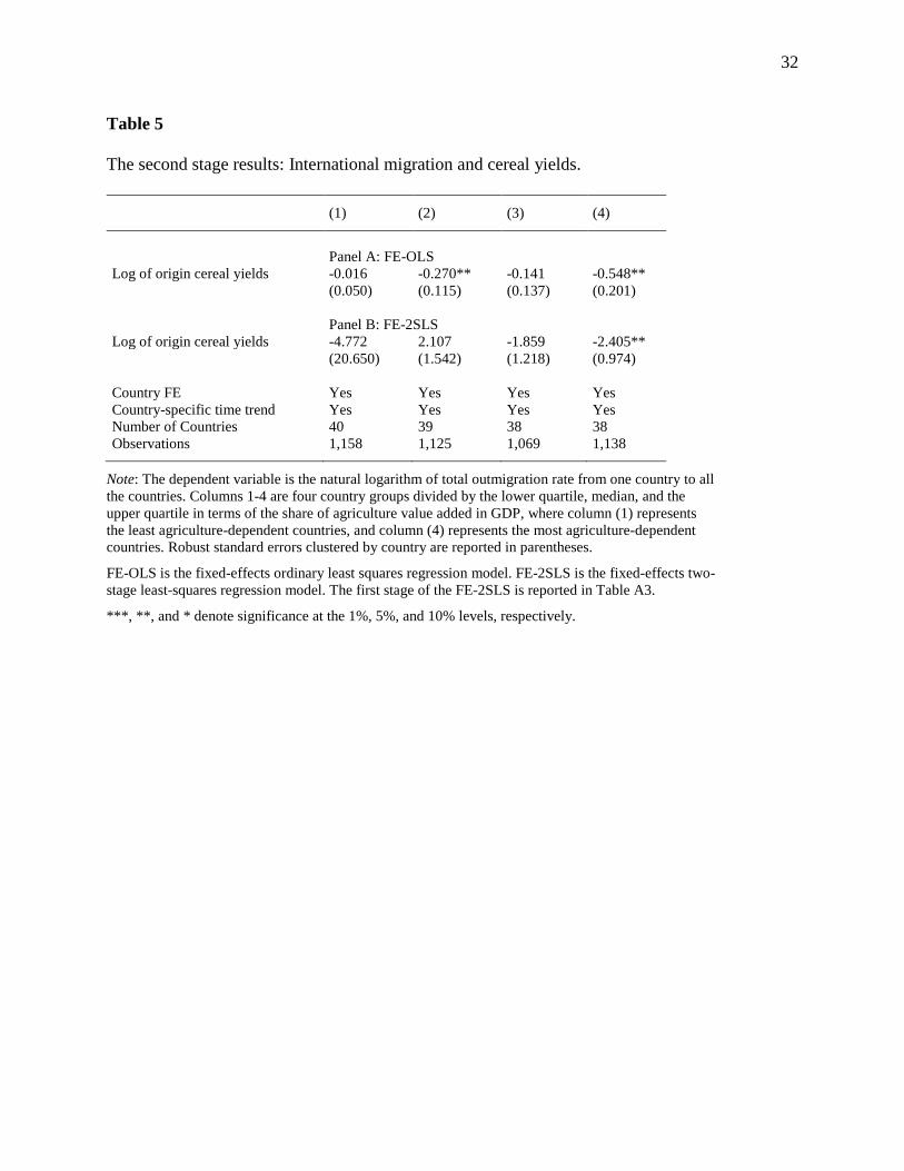
32 Table 5

The second stage results: International migration and cereal yields.

(1) (2) (3) (4)

Panel A: FE-OLS Log of origin cereal yields -0.016 -0.270** -0.141 -0.548** (0.050) (0.115) (0.137) (0.201)

Panel B: FE-2SLS Log of origin cereal yields -4.772 2.107 -1.859 -2.405** (20.650) (1.542) (1.218) (0.974)

Country FE Yes Yes Yes Yes Country-specific time trend Yes Yes Yes Yes Number of Countries 40 39 38 38 Observations 1,158 1,125 1,069 1,138

Note: The dependent variable is the natural logarithm of total outmigration rate from one country to all the countries. Columns 1-4 are four country groups divided by the lower quartile, median, and the upper quartile in terms of the share of agriculture value added in GDP, where column (1) represents the least agriculture-dependent countries, and column (4) represents the most agriculture-dependent countries. Robust standard errors clustered by country are reported in parentheses.

FE-OLS is the fixed-effects ordinary least squares regression model. FE-2SLS is the fixed-effects two-stage least-squares regression model. The first stage of the FE-2SLS is reported in Table A3.

***, **, and * denote significance at the 1%, 5%, and 10% levels, respectively.

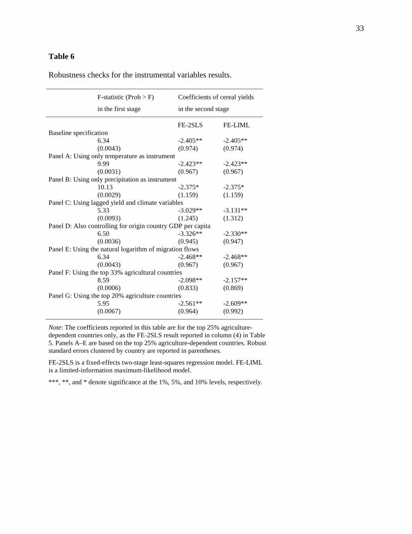
33 Table 6

Robustness checks for the instrumental variables results.

F-statistic (Prob > F)

in the first stage

Coefficients of cereal yields

in the second stage

FE-2SLS FE-LIML Baseline specification

6.34 -2.405** -2.405** (0.0043) (0.974) (0.974)

Panel A: Using only temperature as instrument 9.99 -2.423** -2.423** (0.0031) (0.967) (0.967)

Panel B: Using only precipitation as instrument 10.13 -2.375* -2.375* (0.0029) (1.159) (1.159)

Panel C: Using lagged yield and climate variables 5.33 -3.029** -3.131** (0.0093) (1.245) (1.312)

Panel D: Also controlling for origin country GDP per capita 6.50 -3.326** -2.330** (0.0036) (0.945) (0.947)

Panel E: Using the natural logarithm of migration flows 6.34 -2.468** -2.468** (0.0043) (0.967) (0.967)

Panel F: Using the top 33% agricultural countries 8.59 -2.098** -2.157** (0.0006) (0.833) (0.869)

Panel G: Using the top 20% agriculture countries 5.95 -2.561** -2.609** (0.0067) (0.964) (0.992)

Note: The coefficients reported in this table are for the top 25% agriculture-dependent countries only, as the FE-2SLS result reported in column (4) in Table 5. Panels A–E are based on the top 25% agriculture-dependent countries. Robust standard errors clustered by country are reported in parentheses.

FE-2SLS is a fixed-effects two-stage least-squares regression model. FE-LIML is a limited-information maximum-likelihood model.

***, **, and * denote significance at the 1%, 5%, and 10% levels, respectively.

34 Appendix A

See Tables A1, A2, and A3.

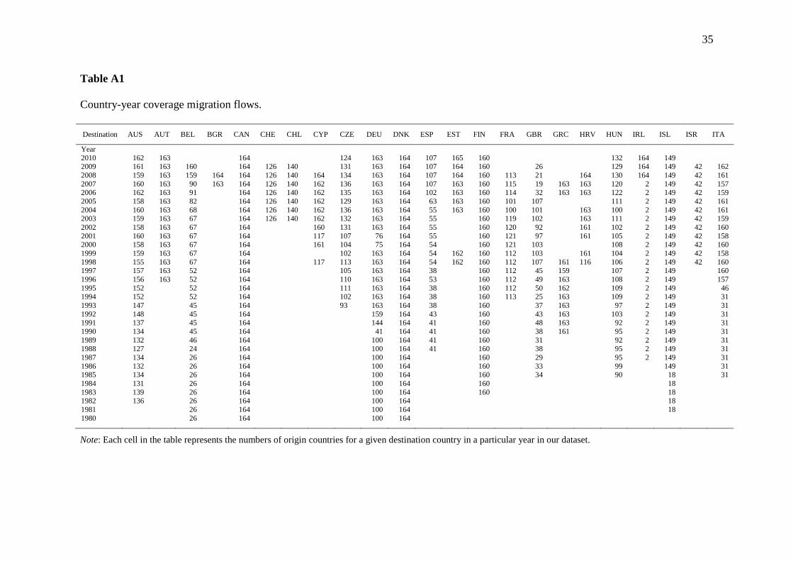
35 Table A1

Country-year coverage migration flows.

Destination AUS AUT BEL BGR CAN CHE CHL CYP CZE DEU DNK ESP EST FIN FRA GBR GRC HRV HUN IRL ISL ISR ITA

Year 2010 162 163 164 124 163 164 107 165 160 132 164 149 2009 161 163 160 164 126 140 131 163 164 107 164 160 26 129 164 149 42 162 2008 159 163 159 164 164 126 140 164 134 163 164 107 164 160 113 21 164 130 164 149 42 161 2007 160 163 90 163 164 126 140 162 136 163 164 107 163 160 115 19 163 163 120 2 149 42 157 2006 162 163 91 164 126 140 162 135 163 164 102 163 160 114 32 163 163 122 2 149 42 159 2005 158 163 82 164 126 140 162 129 163 164 63 163 160 101 107 111 2 149 42 161 2004 160 163 68 164 126 140 162 136 163 164 55 163 160 100 101 163 100 2 149 42 161 2003 159 163 67 164 126 140 162 132 163 164 55 160 119 102 163 111 2 149 42 159 2002 158 163 67 164 160 131 163 164 55 160 120 92 161 102 2 149 42 160 2001 160 163 67 164 117 107 76 164 55 160 121 97 161 105 2 149 42 158 2000 158 163 67 164 161 104 75 164 54 160 121 103 108 2 149 42 160 1999 159 163 67 164 102 163 164 54 162 160 112 103 161 104 2 149 42 158 1998 155 163 67 164 117 113 163 164 54 162 160 112 107 161 116 106 2 149 42 160 1997 157 163 52 164 105 163 164 38 160 112 45 159 107 2 149 160 1996 156 163 52 164 110 163 164 53 160 112 49 163 108 2 149 157 1995 152 52 164 111 163 164 38 160 112 50 162 109 2 149 46 1994 152 52 164 102 163 164 38 160 113 25 163 109 2 149 31 1993 147 45 164 93 163 164 38 160 37 163 97 2 149 31 1992 148 45 164 159 164 43 160 43 163 103 2 149 31 1991 137 45 164 144 164 41 160 48 163 92 2 149 31 1990 134 45 164 41 164 41 160 38 161 95 2 149 31 1989 132 46 164 100 164 41 160 31 92 2 149 31 1988 127 24 164 100 164 41 160 38 95 2 149 31 1987 134 26 164 100 164 160 29 95 2 149 31 1986 132 26 164 100 164 160 33 99 149 31 1985 134 26 164 100 164 160 34 90 18 31 1984 131 26 164 100 164 160 18 1983 139 26 164 100 164 160 18 1982 136 26 164 100 164 18 1981 26 164 100 164 18 1980 26 164 100 164

Note: Each cell in the table represents the numbers of origin countries for a given destination country in a particular year in our dataset.

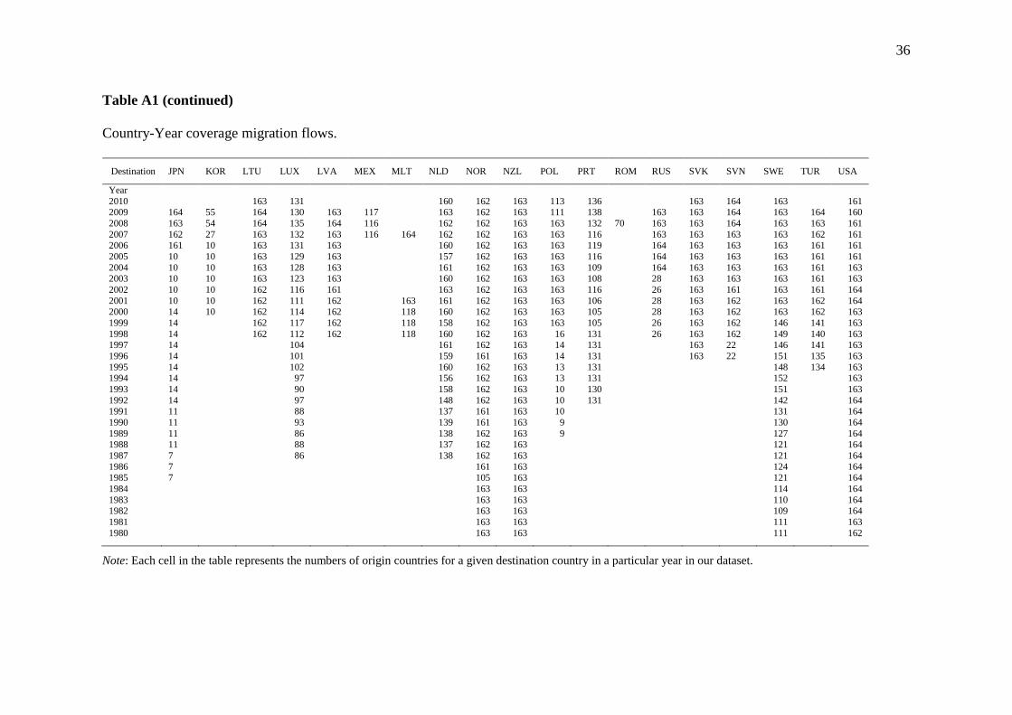
36 Table A1 (continued)

Country-Year coverage migration flows.

Destination JPN KOR LTU LUX LVA MEX MLT NLD NOR NZL POL PRT ROM RUS SVK SVN SWE TUR USA

Year 2010 163 131 160 162 163 113 136 163 164 163 161 2009 164 55 164 130 163 117 163 162 163 111 138 163 163 164 163 164 160 2008 163 54 164 135 164 116 162 162 163 163 132 70 163 163 164 163 163 161 2007 162 27 163 132 163 116 164 162 162 163 163 116 163 163 163 163 162 161 2006 161 10 163 131 163 160 162 163 163 119 164 163 163 163 161 161 2005 10 10 163 129 163 157 162 163 163 116 164 163 163 163 161 161 2004 10 10 163 128 163 161 162 163 163 109 164 163 163 163 161 163 2003 10 10 163 123 163 160 162 163 163 108 28 163 163 163 161 163 2002 10 10 162 116 161 163 162 163 163 116 26 163 161 163 161 164 2001 10 10 162 111 162 163 161 162 163 163 106 28 163 162 163 162 164 2000 14 10 162 114 162 118 160 162 163 163 105 28 163 162 163 162 163 1999 14 162 117 162 118 158 162 163 163 105 26 163 162 146 141 163 1998 14 162 112 162 118 160 162 163 16 131 26 163 162 149 140 163 1997 14 104 161 162 163 14 131 163 22 146 141 163 1996 14 101 159 161 163 14 131 163 22 151 135 163 1995 14 102 160 162 163 13 131 148 134 163 1994 14 97 156 162 163 13 131 152 163 1993 14 90 158 162 163 10 130 151 163 1992 14 97 148 162 163 10 131 142 164 1991 11 88 137 161 163 10 131 164 1990 11 93 139 161 163 9 130 164 1989 11 86 138 162 163 9 127 164 1988 11 88 137 162 163 121 164 1987 7 86 138 162 163 121 164 1986 7 161 163 124 164 1985 7 105 163 121 164 1984 163 163 114 164 1983 163 163 110 164 1982 163 163 109 164 1981 163 163 111 163 1980 163 163 111 162

Note: Each cell in the table represents the numbers of origin countries for a given destination country in a particular year in our dataset.

37

Table A2

Definitions of migration flows.

Destinations Definition of “immigrant” based on

Australia Country of Birth

Austria Citizenship

Belgium Citizenship

Bulgaria Citizenship

Canada Country of Birth

Chile Citizenship

Cyprus Citizenship

Czech Republic Citizenship

Denmark Citizenship

Estonia Citizenship

Finland Citizenship

France Citizenship

Germany Citizenship

Greece Citizenship

Hungary Citizenship

Iceland Citizenship

Ireland Country of Birth

Israel Citizenship

Italy Citizenship

Japan Citizenship

Korea Citizenship

Latvia Citizenship

Lithuania Citizenship

Luxembourg Citizenship

Malta Citizenship

Mexico Citizenship

Netherlands Country of Birth

New Zealand Last Permanent Residence

Norway 1979-1984 Country of Origin, 1985-2010 Citizenship

Poland Country of Origin

Portugal Citizenship

Romania Citizenship

Russian Federation Citizenship

Slovak Republic Country of Origin

Slovenia Citizenship

Spain Country of Origin

Sweden Citizenship

Switzerland Citizenship

Turkey Citizenship

United Kingdom Citizenship

United States Country of Birth

38

Table A3

The first stage results: Cereal yields and climate.

Note: The dependent variable is the natural logarithm of cereal yields. Columns 1-4 are four country groups divided by the lower quartile, median, and the upper quartile based on the share of agriculture value added in GDP, where column (1) represents the least agriculture-dependent countries, and column (4) represents the most agriculture-dependent countries. Robust standard errors clustered by country are reported in parentheses. ***, **, and * denote significance at the 1%, 5%, and 10% levels, respectively.

(1) (2) (3) (4)

Temperature -0.000 -0.037*** -0.026** -0.030** (0.013) (0.012) (0.009) (0.012) Precipitation 0.000 0.000 0.000 0.001** (0.001) (0.000) (0.000) (0.000) Number of Observations 1,158 1,125 1,069 1,138 Number of Countries 40 39 38 38 Adjusted R2 0.323 0.471 0.373 0.488 F-statistics 0.02 4.72 4.87 6.34 Prob > F 0.9785 0.0148 0.013 0.0043