climate change and drought effects on rural income ... · climate-change-induced impacts on society...

Nat. Hazards Earth Syst. Sci., 16, 1369–1385, 2016www.nat-hazards-earth-syst-sci.net/16/1369/2016/doi:10.5194/nhess-16-1369-2016© Author(s) 2016. CC Attribution 3.0 License.

Climate change and drought effects on rural income distributionin the Mediterranean: a case study for SpainSonia Quiroga and Cristina SuárezDepartment of Economics, Universidad de Alcalá, Alcalá de Henares, Spain

Correspondence to: Sonia Quiroga ([email protected])

Received: 1 February 2015 – Published in Nat. Hazards Earth Syst. Sci. Discuss.: 23 July 2015Revised: 6 April 2016 – Accepted: 30 April 2016 – Published: 15 June 2016

Abstract. This paper examines the effects of climate changeand drought on agricultural incomes in Spanish rural areas.Present research has focused on the effects of these extremeclimatological events through response functions, consider-ing effects on crop productivity and average incomes. Amongthe impacts of droughts, we focused on potential effects onincome distribution. The study of the effects on abnormallydry periods is therefore needed in order to perform an anal-ysis of diverse social aspects in the long term. We estimatecrop production functions for a range of Mediterranean cropsin Spain and we use a measure of the decomposition of in-equality to estimate the impact of climate change and droughton yield disparities. Certain adaptation measures may requirea better understanding of risks by the public to achieve gen-eral acceptance. We provide empirical estimations for themarginal effects of the two impacts considered: farms’ av-erage income and income distribution. Our estimates con-sider crop production response to both biophysical and socio-economic aspects to analyse long-term implications on com-petitiveness and disparities. As for the results, we find dispar-ities in the adaptation priorities depending on the crop and theregion analysed.

1 Introduction

Climate-change-induced impacts on society have capturedan important part of the attention of environmental researchin the last decades, usually estimated in a two-step pro-cess, where in a first phase physical units are calculated(changes in crop yield, life expectancy, sea level rise, num-ber of species, etc.), while in a second step macroeconomicmodels are employed in order to translate the first result into

monetary units (Ciscar et al., 2011; Watkins et al., 2005).Market equilibrium approaches are avoided here. We con-sider the economic revenues of the farms directly to estimatethe impact of drought on income inequality. We then make aprojection in terms of these econometric results without anyadditional assumption about market behaviour. In general,individuals and firms are modelled as representative agentswithin, respectively, one region and one market sector. Thisimplies assuming the same socio-economic types of prefer-ences across the world and across economies (Michetti andZampieri, 2014). As an alternative we consider market issuesdirectly through incomes at farm level which may reveal an-other part of the picture. This is also interesting in order tounderstand the expected impacts over producers.

Even if income inequality has been revealed as one ofthe most important drivers for significant changes in thesocio-political framework in the European Union (EU) af-ter the 2008 economic crisis and with equitable growth nowat the forefront of economic debate (Piketty, 2013), not somuch attention has been placed on the distributional effectsof climate change extreme events and hazards on economicoutputs. Economic evaluation efforts have been focused onrisks at the average level, but it is becoming clear that adap-tation policy needs to face climate-driven income inequal-ity (Quiroga et al., 2015). There are important referencesin literature pointing towards an increase in food inequal-ity induced by climate change (Wheeler and von Braun,2013; Pindyck, 2013; Marino and Ribot, 2012) based onnon-monetary units like yields or ingested calories. To datethere has been little empirical research on how and whereclimate change interventions are shaping income inequality.This is indeed important in the agricultural sector due to itsintrinsical link to rural development. It is also relevant in

Published by Copernicus Publications on behalf of the European Geosciences Union.

1370 S. Quiroga and C. Suárez: Climate change effects on rural income distribution

terms of EU Common Agricultural Policy (CAP, 2nd Pil-lar) and it is closely related to ecosystem conservation atthe same time – through decoupling subsidies and develop-ing agro-environmental programmes, which also affect for-est area, that has significantly increased in Spain in the lastdecade as a result of land abandonment, with implicationsfor conservation policies, forest landscape connectivity, etc.(Martín-Martín et al., 2013). Crop yield changes, as a re-sponse to climate change projections, have been estimated inmany relevant studies dealing with climate change impacts(Rosenzweig et al., 2004; González-Zeas et al., 2014; Lo-bell et al., 2014), and the Mediterranean region in particularhas been identified as a major hotspot due to the expectedincrease in drought risk (Garrote et al., 2007). As for theSpanish case, climate change will probably increase waterconflicts among sectors, as well as an improvement in theefficiency of water use, which will be essential to maintainenvironmental flows and therefore ecosystem sustainability.In this context we have analysed the response of rain-fedcrops to climate conditions including extreme events suchas drought. Here we have selected crops best representingMediterranean crop systems. Cereals, grapes, and olives arethe three basic products of Mediterranean agriculture, theones representing a higher proportion of harvested area, butalso with an important cultural heritage in the region. Table 1shows the percentage of total agricultural rain-fed area ded-icated to the selected crops. We can see that they accountfor more than 50 % of the rain-fed crop systems. Althoughagriculture does not represent a high proportion of gross do-mestic product (GDP) in Spain (less than 3 %), more than3000 farms highly depend on these crops as their main ac-tivity. Due to the significant agricultural land abandonmentin Spain (Beilin et al., 2014) the economic effects on thesethree crops are also important for the wider analysis of ruraldevelopment.

Our main goal of the paper is to study drought-inducedchanges in the distribution of incomes that are based on agri-cultural output. We estimate crop production functions tosimulate factor productivity in order to then calculate the re-sponse of income distribution to climate change. Particularattention is directed towards the economic outputs of crops.The value of production (in monetary units) is what we con-sider a change in income. The database we analyse providesresults on the monetary value of production, which is usedto check the factors’ productivity, which is general practicewhen the focus is on the monetary units instead of physi-cal units. This choice is important here since results allow usto analyse the change in the monetary units as a response tochanges in the determinants (both observable and not observ-able).

Production is usually affected by unobserved factors. Theway in which these influences can be separated from the ef-fects of more tangible and traditional inputs – such as land,labour, or capital – is at the heart of a new debate. Differ-ent approaches to the appropriate identification strategies for

Table 1. Cultivation of cereals, grapes, and olives in Spain.

Area in Percentage Number ofSpain of total farms in

(106 ha) agricultural the studyrain-fed area

Total agriculturalrain-fed area 13.7 – –Cereals 5.0 37 2250Grapes 1.9 14 503Olives 0.7 5 401Total of all three crops 7.7 56 3154

Source: MAGRAMA (2015) and own elaboration.

addressing endogeneity and collinearity problems have ap-peared over the last years. The aim is to avoid simultane-ity and selection biases that are common in most produc-tion function estimates (Petrick and Kloss, 2013; Yasar etal., 2008). We estimate the production function using the ap-proach provided by Olley and Pakes (1996), which allowscontrol of both traditional inputs and state variables – suchas climate – to be combined and different kinds of biasesto be avoided, such as those resulting from the exit of inef-ficient farms. This model allows the effect of unobservableinputs such as soil quality, human capital of the labour force,farmer’s effort, etc, to be accounted for.

Our study is centred on Spanish farms located in theMediterranean agroclimatic region. The present situationdoes not allow for much optimism. Explicit restrictions onwater availability have been introduced in most of the Span-ish river basins and there are big socio-economic conflicts,especially in the agricultural sector. Extraordinarily bad gov-ernance practices related to water and irrigators have beenreported, especially in relation to water rights in Spain. Inthe Tagus river basin, especially in the case of Western Man-cha, the lack of clear definition of water rights currently cre-ates critical conflicts with estimated thousands of illegal ab-stractors. To achieve more effective water governance in thearea, it is necessary to create an enabling environment, whichfacilitates efficient private and public sector initiatives andstakeholder involvement in articulating needs (De Stefano etal., 2013; Rogers et al., 2006).

This paper is organized as follows: Sect. 2 focuses on thesteps within the methodology, models, and data. Section 2.1details the climate change scenarios considered for the sim-ulations; Sect. 2.2 presents the econometric model for theOlley and Pakes crop production estimation, Mediterraneancrops, and Gini index decomposition. Section 2.3 explainsthe Gini index for measuring income distribution and the de-composition for calculating the marginal effects of drought.Sections 3.1 to 3.3 present the results for the production func-tions, the simulations of marginal effects of drought for thedifferent scenarios, and the calculations for the changes infarms’ income distribution.

Nat. Hazards Earth Syst. Sci., 16, 1369–1385, 2016 www.nat-hazards-earth-syst-sci.net/16/1369/2016/

S. Quiroga and C. Suárez: Climate change effects on rural income distribution 1371

36

1 2 Figure 1 Steps of methodology 3 4

5

Step 1Characterization of productivity drivers

Nature state patterns•Climatic spatial information

•River basin locations•Drought characterization

(SPI )

Management input factors

•Labour, materials (fertilizers, energy)•Land, capital, investment

Step 2 Characterization of crop productivity• Olley and Pakes production functions•Climate risk semi-elasticities estimates

Step 4 Climate change scenarios• A1B, E1 (CO2 representative concentration pathways)

Step 5 Projections of crop production and income distribution

• Simulations of crop production and Lorenz curves (GINI index) for the selected scenarios

Step 3Income distribution decomposition

Characterization of inequalities• GINI index decomposition

•Marginal effects of drivers (climate change, drought)

Production functions of income response

Selection of climate change scenarios

Climate-induced effects onrural income inequalities

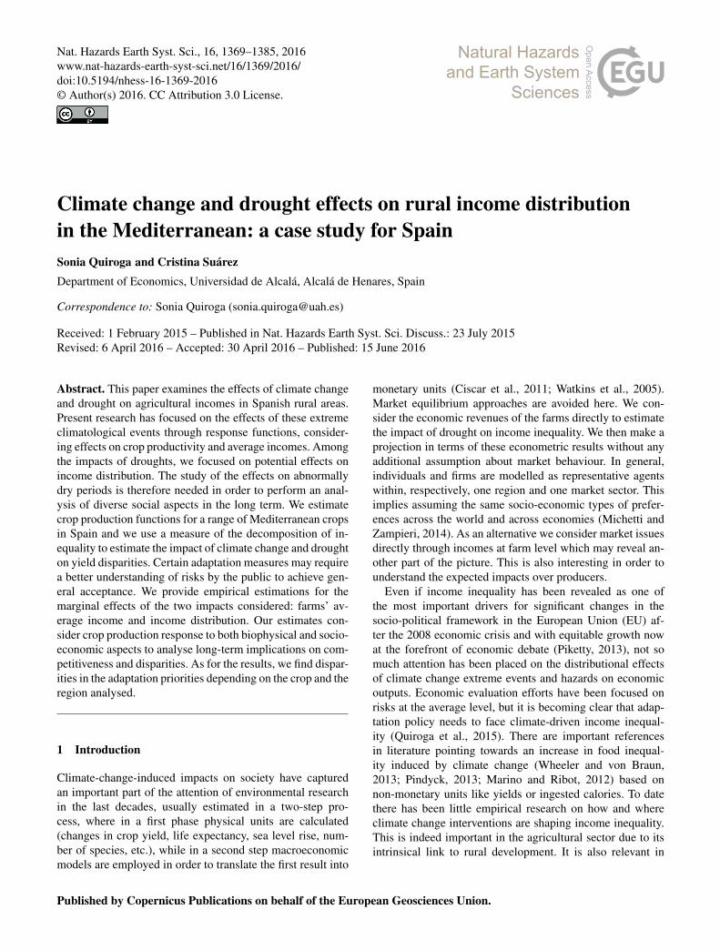
Figure 1. Steps of methodology.

2 Methods

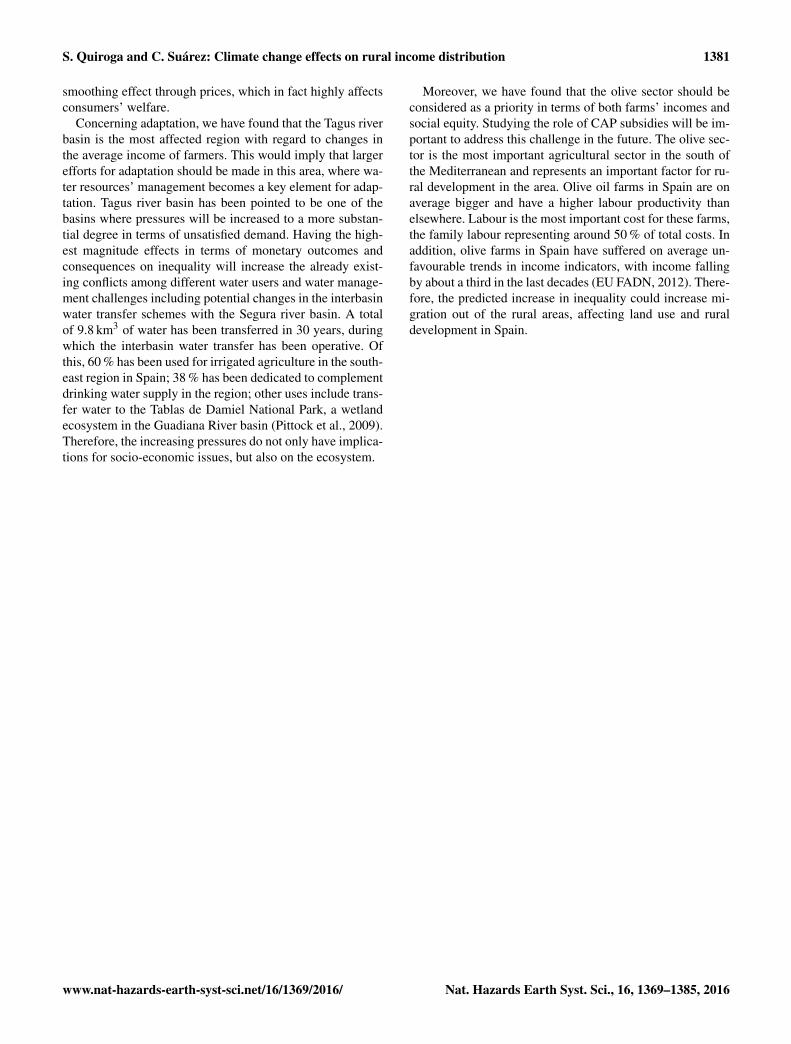
This paper provides an assessment of income distribution asa response to a climate-change-induced increase in droughtsin the Mediterranean. Our analysis integrates two essentialcomponents of the economic perspective of adaptation pol-icy: productivity and equity. We first analyse the drivers forthe agricultural systems’ production through a semiparamet-ric method using 1990–2013 data for production in monetaryterms at the farm level in different river basins in Spain. Wehave integrated biophysical and socio-economic databases tocharacterize the nature state variables and management fac-tors. Second, we explore the distributional aspects computingthe marginal effect of changes on seasonal rainfall distribu-tion, using a decomposition of the standard Gini coefficientto then simulate production and income distribution accord-ing to these climate scenarios. Figure 1 summarizes the stepson the methodology.

2.1 Agricultural production function simultaneousestimates: observed inputs and unobservedproductivity shocks

We first need to define and estimate a production function.The Olley and Pakes (1996) approach assumes that incum-bent farms decide at the beginning of each period whetherto continue to participate in farming activity depending ontheir productivity level, which in turn depends on their pro-duction factors (it corrects the selection bias). To this end,investment (ii t ) is considered as a proxy for the unobservedproductivity shocks. Additionally, this method corrects thesimultaneity bias arising from the fact that farms choose their

level of input once they know their level of productivity. Mostof the studies in the literature using Olley–Pakes methodol-ogy assume a Cobb–Douglas production function (see Rizovet al., 2013 and Kazukauskas et al., 2010, as recent exam-ples focused on EU farm data). Since this is the functionalform more commonly accepted, we assumed it for our study.The robustness of this method has been proved previouslyin Petrick and Kloss (2013). Simultaneity exists between thechoice of inputs and productivity since productive farms aremore likely to make capital investments to increase the futurevalue of the farm. Therefore, the farm’s decision to invest infurther capital implies that future productivity is increasingin the current productivity shock, so farms that experience alarge positive productivity shock in period t will invest morein period t + 1. The Olley and Pakes (1996) semiparametricmethod accounts for these issues.

There is also a selection bias caused by the fact that farmsonly stay in business if the liquidation value is smaller thanthe anticipated future value of profits. Controlling for this se-lection bias requires a second step to estimate survival prob-abilities. In our implementation, we estimate the probabilityof survival by fitting a Probit model. Details on the produc-tion function are reported in Appendix A. In order to anal-yse the effects of climate we can examine these coefficientsthat represent climate elasticity (or semi-elasticity to be moreprecise), that can be defined as the percentage change in thefunction’s output as a result of a one-unit change in the levelof a climate variable. For example, the average temperaturecoefficient indicates the percentage change in monetary out-come for the farms due to an increase in 1 ◦C in the averagetemperature.

www.nat-hazards-earth-syst-sci.net/16/1369/2016/ Nat. Hazards Earth Syst. Sci., 16, 1369–1385, 2016


Marginal product – the change in output resulting fromemploying one more unit of a particular input, assumingother variables are kept constant (Brewer, 2010) – has beencalculated for when the drought effect is analysed.

2.2 Measuring rural income distribution:a decomposition of the Gini index with regard tosocial equity

To characterize the inequality level generated by agriculturaloutput, we use the Gini coefficient decomposition proposedby Pyatt et al. (1980) and Shorrocks (1982), and extended byLópez-Feldman et al. (2007), which includes the marginaleffects of different sources on overall yield inequality, focus-ing on the impact of water-related variables. The Gini coef-ficient is probably the most common inequality measure be-cause of its simplicity and its desirable properties. In a gen-eral context, it fulfils the properties of mean independence,population size independence, symmetry, and Pigou–Daltontransfer sensitivity (Haughton and Khandker, 2009). How-ever, this tool presents two main shortcomings: (i) difficultdecomposability as entropy measures, and (ii) difficult sta-tistical testability for the significance of changes in the in-dex over time. Haughton and Khandker (2009) suggestedthat the latter is not a real problem because confidence in-tervals can usually be produced by means of bootstrap tech-niques. Taking these considerations into account, we use thisapproach. This concentration ratio is widely used in manyfields of economics as well as in ecology and agronomics,but there are fewer applications in agricultural and environ-mental economics together (Quiroga et al., 2014; Sadras andBongiovanni, 2004; Seekell et al., 2011). In a general con-text, it ranges from zero (equal distribution) to one (perfectinequality).

The decomposition of the overall Gini into specific sourcefactor effects was derived from Lerman and Yitzhaki (1985).It is a good measure to help to understand the determinantsof inequality, and allows the effect of small changes in a spe-cific source of yield (or, in this case, income) on inequalityto be estimated, while the other sources’ constant is main-tained. In this paper, we include drought as a source factor. Ifwe consider the relationship between drought and crop yield,the interpretation of Gini decomposition will be the follow-ing: (i) if drought as a source represents a large share of totalcrop yield, it could probably have a large impact on inequal-ity; (ii) if crop yield is equally distributed, it cannot affectinequality, even if its magnitude is large; and (iii) if this cropyield source is large and unequally distributed, it could eitherincrease or decrease inequality, depending on which farmers,at which points in the crop yield distribution, earn it.

Here we use the Lorenz curves as the most common Giniindex representation to analyse how rural inequality respondsto climate-change-induced drought. The Lorenz curves rep-resent the cumulative distribution function of income distri-bution. Since a perfectly equal income distribution would be

one in which every farmer has the same income, this could berepresented by the line y = x, also called the “perfect equal-ity” or “equi-distribution” line. In this hypothetical case,N%of rural population would always have N% of the rural in-come. The Gini index corresponds to the area between theLorenz curve and the equi-distribution line.

A detailed description of Gini decomposition can be foundin Appendix B.

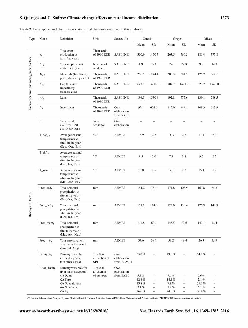
2.3 Data

Since our model considers the interrelation among manage-ment factors and climate state variables, it was necessary tocombine several socio-economic and biophysical databasesfor the analysis. Table 2 shows detailed information aboutthe variables we used, the units and source of the data, andmain descriptive statistics. We have used the SABI database(Iberian Balance sheet Analysis System), which provides in-formation about farm production in monetary terms, man-agement factors (land, labour, and capital), and spatial farmlocation. The SABI database is produced jointly by Bureauvan Dijk and Informa and comes from the financial infor-mation that farms must present to the Companies Registra-tion Office. It is an annual survey which looks at a panel ofrepresentative Spanish agricultural farms and contains bal-ance sheet data, cash flow, and other data. Our database is anunbalanced panel observed over the period 1990–2013. Themost difficult issue with an unbalanced panel is precisely de-termining the origin of the lack of balance: (1) if the reasona farm leaves the sample is not correlated with the idiosyn-cratic error (those unobserved factors that change over timeand affect profits), then the unbalanced panel causes no prob-lems. (2) If the reason a farm leaves the sample is correlatedwith the idiosyncratic error, then the resulting sample cancause biased estimators. One advantage of the mechanics ofOlley and Pakes (1996) (as it is explained in the Appendix A)is that it takes into account the selection bias resulting fromthe exit of inefficient farms.

SABI also provides information about the major digitNACE codes (National Classification of Economic Activi-ties) to which the farms belong. The data are at the farm leveland they are provided for different sectors. Here we haveanalysed the farms from 1990 to 2013 in the most importantsectors regarding Mediterranean representative crops: the ce-real sector (NACE code A1.1.1), the grape sector (NACEcode A1.2.1), and the olive sector (NACE code A1.2.6). Oursample includes all the farms providing information for theselected sectors.

The SABI database provides the data in real currency (cur-rent EUR), so to consider real increase in purchase capacityand discount the effect of market price increases, we havedeflated the current monetary variables into real values with1990 as the base year, using national account data for Spain(INE, Spanish National Statistics Bureau). Climatic infor-mation for the period 1990–2013 has been collected from



Table 2. Description and descriptive statistics of the variables used in the analysis.

Type Name Definition Unit Source (∗) Cereals Grapes Olives

Mean SD Mean SD Mean SD

Soci

o-ec

onom

ican

dm

anag

emen

tfac

tors

Total crop ThousandsYi t production at of 1990 EUR SABI, INE 330.9 1470.7 263.5 766.2 181.4 375.8

farm i in year t

Li t Total employment Number of SABI, INE 8.9 29.8 7.6 29.8 9.8 14.3at farm i in year t workers

Mi t Materials (fertilizers, Thousands SABI, INE 276.5 1274.4 200.3 684.3 125.7 362.1pesticides,energy, etc.) of 1990 EUR

Ki t Capital assets Thousands SABI, INE 647.1 1480.6 707.7 1471.9 821.2 1740.0(machinery, of 1990 EURtractors, etc.)

Ai t Land Thousands SABI, INE 196.3 1530.4 192.8 777.6 139.1 788.5of 1990 EUR

Ii t Investment Thousands Own 93.1 608.6 115.0 444.1 108.3 617.9of 1990 EUR elaboration

from SABI

t Time trend: Year Own – – – – – –t = 1 for 1991, sequence elaborationt = 23 for 2013

Bio

phys

ical

fact

ors

T_soni t Average seasonal ◦C AEMET 16.9 2.7 16.3 2.6 17.9 2.0temperature atsite i in the year t(Sept, Oct, Nov)

T_djfi t Average seasonaltemperature at ◦C AEMET 8.5 3.0 7.9 2.8 9.5 2.3site i in the year t(Dec, Jan, Feb)

T_mami t Average seasonal ◦C AEMET 15.0 2.5 14.1 2.3 15.8 1.9temperature atsite i in the year t(Mar, Apr, May)

Prec_soni t Total seasonal mm AEMET 154.2 78.4 171.8 103.9 167.8 85.3precipitation atsite in the year t(Sep, Oct, Nov)

Prec_defi t Total seasonal mm AEMET 139.2 124.8 129.0 118.4 175.9 149.3precipitation atsite i in the year t(Dec, Jan, Feb)

Prec_mami t Total seasonal mm AEMET 131.8 60.3 143.5 79.6 147.1 72.4precipitation atsite in the year t(Mar, Apr, May)

Prec_jjai t Total precipitation mm AEMET 37.6 39.8 56.2 49.4 26.3 35.9at a site in the year t(Jun, Jul, Aug)

Droughti t Dummy variable 1 or 0 as Own 55.0 % – 49.0 % – 54.1 % –(1 for dry years, a function of elaboration0 in other cases) SPI from AEMET

River_basini Dummy variables for 1 or 0 as Ownriver basin selection: a function elaboration(1) Duero of the area from SABI 5.8 % – 7.1 % – 0.6 % –(2) Ebro 12.8 % – 14.1 % – 2.1 % –(3) Guadalquivir 23.8 % – 7.9 % – 55.1 % –(4) Guadiana 5.1 % – 1.6 % – 3.1 % –(5) Tajo 26.6 % – 24.6 % – 16.8 % –

(∗) Iberian Balance sheet Analysis System (SABI); Spanish National Statistics Bureau (INE), State Meteorological Agency in Spain (AEMET). SD denotes standard deviation.



AEMET (State Meteorological Agency in Spain). Table 2presents the descriptive analysis of the variables used.

The current work uses each firm’s sales volume and it isconverted into real terms. With regard to the inputs, labouris measured as the number of workers. In this type of study,the standard practice is to define labour in terms of hoursworked but this information is not available. Capital quantityis defined as the market value of capital assets (machinery,tractors, etc.) owned by the farms, in constant prices. Land isdefined as the real value in monetary terms for the plantingarea for every farm, so this is not constant during the consid-ered period. Every year farms declare the value of their prop-erties (which can be sold or bought). This value, expressedin real terms to avoid inflation effects, is what we consider asland input. Although we do not have information about realland use, which does not only depend on the variation of theamount and value of planting area but also on the competitionbetween the use of a portion of land amongst different scopes(abandonment, urban, afforestation, food production, energyproduction etc.), which constitutes a limitation, we can cap-ture the evolution of agricultural land value. Material is de-fined as intermediate spending carried out in the productionprocess (fertilizers, pesticides, energy, etc.). The farm invest-ment is calculated according to the proposal by Lewellen andBadrinath (1997) as follows:

ii t = nfi t − nfi t−1+ bdi t ,

where nf is net fixed assets and bd is book depreciation ex-penses. Theoretically, the model mentioned in the last sec-tion requires investment to be strictly positive to invert the in-vestment function. In their empirical implementation, Olleyand Pakes (1996) drop all observations with zero investment.Other authors have noted that in practice, zero investmentis often observed and that the methodology seems to workeven when the theory is violated (see, for example, Pavcnik,2002). Therefore, our approach will be to retain all the ob-servations with zero investment but also introduce dummyvariables (dummy variables for zero investment interactingwith state inputs) to account for these observations, as inBlalock and Gertler (2004) and Breunig and Wong (2008).As a robusticity check, we estimated the model droppingall of the observations with zero investment and the result-ing coefficient estimates, similar to those reported below.We add t , which is a variable included here to measure theHicks-neutral technical change that is common among firmsin the same sector and autonomous region. A Hicks-neutraltechnical change is a change in the production function ofa farm that satisfies certain economic neutrality conditions.A change is considered to be Hicks-neutral if the changedoes not affect the balance of labour and capital in the prod-ucts’ production function. Factor-neutral (also called Hicks-neutral) technological change is assumed, either explicitly orimplicitly, in most of the standard techniques for measuringproductivity, ranging from the classic growth decompositions

of Solow (1957) and Hall (1988) to the recent structural es-timators for production functions (Olley and Pakes, 1996;Levinsohn and Petrin, 2003; Ackerberg et al., 2006).

In our paper, we measure Hicks-neutral technologicalprogress with the time trend in production function. As-suming neutral technical change implies that the coefficientsof the interactions between the yearly trend and the inputvariables are zero. We also tried to estimate a non-neutraltechnical progress, but the resulting coefficients were notsignificant, so the Hicks-neutral technological progress wasdeemed appropriate.

Drought characterization is always a difficult task, giventhe spatial and temporal properties of drought and no singleaccepted definition (Tsakiris et al., 2007). In the most generalsense, drought originates from a deficiency of precipitationover an extended period of time – usually a season or more– resulting in a water shortage for some activity group or en-vironmental sector (NDMC, 2015). Operational definitionshelp define the onset, severity, and end of droughts. No singleoperational definition of drought works in all circumstances,and this is a big part of why policymakers, resource plan-ners, and others have more trouble recognizing and planningfor drought than they do for other natural disasters (NDMC,2015). To characterize drought in this study, we take the com-monly used Standardized Precipitation Index (SPI, McKeeet al., 1993). Broadly considered, this index is based on theprobability of precipitation for any timescale. It is calculatedas the difference in accumulated precipitation between a se-lected aggregation period and the average precipitation forthat same period. We have introduced the SPI in a dummyform since we are also interested in the direct effect of tem-perature and precipitation and we wanted to avoid collinear-ity problems with the SPI since it is constructed from precip-itation data. This approach has been used before in some pre-vious analysis in Spain (Iglesias and Quiroga, 2007; Quirogaand Iglesias, 2009; Iglesias et al., 2010; Garrote et al., 2007).We have used SPI to characterize drought since it is widelyused and more comparable across regions with different cli-mates than other more complex indexes such as the PalmerDrought Severity Index (PDSI). SPI does not consider tem-perature, which is responsible for affecting evapotranspira-tion, but we have considered temperature effects among theexplanatory variables of the model. However, other limita-tions include SPI not considering the intensity of precipita-tion and its potential impacts on runoff, streamflow, and wa-ter availability within the system of interest (Keyantash andNational Center for Atmospheric Research Staff, 2015).

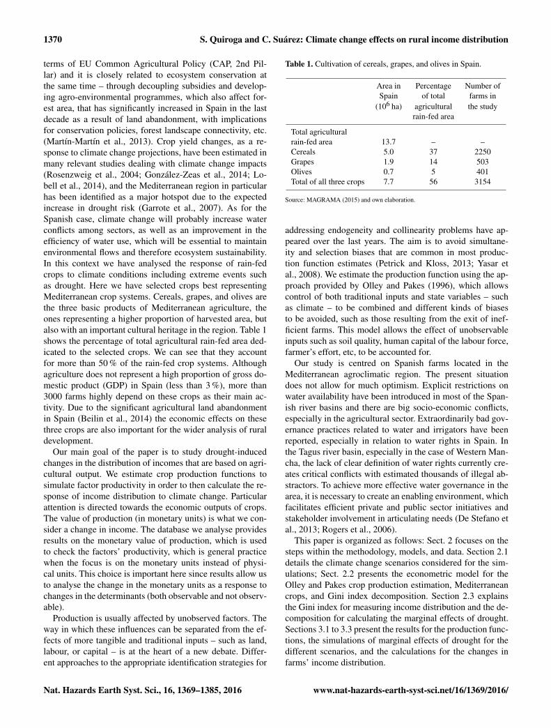
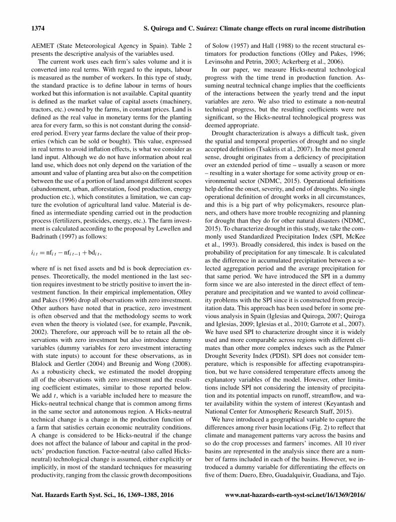
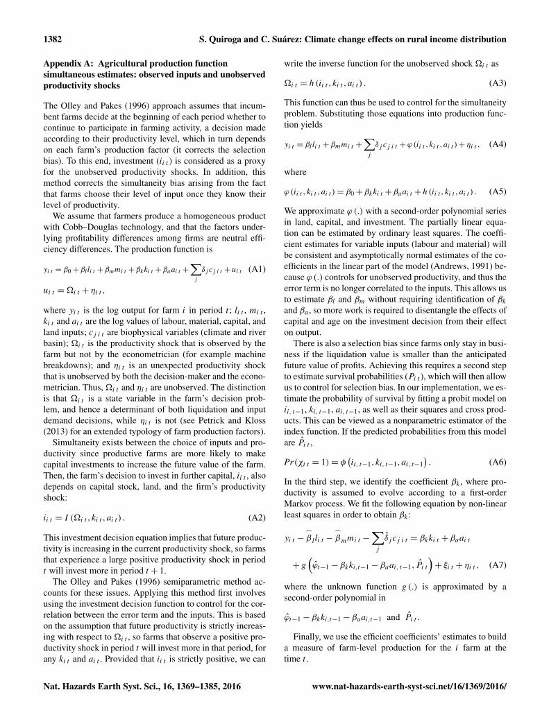
We have introduced a geographical variable to capture thedifferences among river basin locations (Fig. 2) to reflect thatclimate and management patterns vary across the basins andso do the crop processes and farmers’ incomes. All 10 riverbasins are represented in the analysis since there are a num-ber of farms included in each of the basins. However, we in-troduced a dummy variable for differentiating the effects onfive of them: Duero, Ebro, Guadalquivir, Guadiana, and Tajo.



Figure 2. Spanish river basins.

This allows us to compare differential marginal effects forthese important basins. For example, if we have a significantand positive effect on the variable capturing the Duero riverbasin effect, this indicates that for this basin the effects arehigher than the average effects. For the river basins not repre-sented we just have the average value as reference. Introduc-ing dummy variables allocates differential marginal effectswith respect to the representative average value. We considerthe most important river basins to allocate these differences.

2.4 Climate change scenarios and drought in theMediterranean

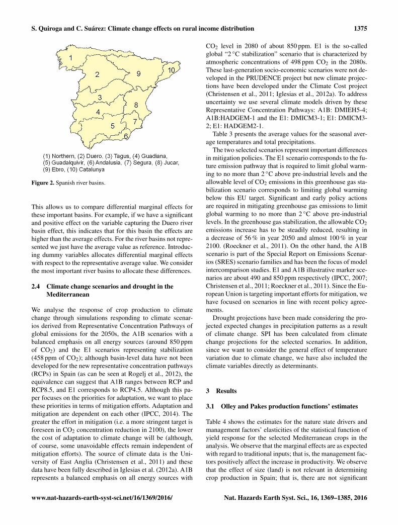
We analyse the response of crop production to climatechange through simulations responding to climate scenar-ios derived from Representative Concentration Pathways ofglobal emissions for the 2050s, the A1B scenarios with abalanced emphasis on all energy sources (around 850 ppmof CO2) and the E1 scenarios representing stabilization(458 ppm of CO2); although basin-level data have not beendeveloped for the new representative concentration pathways(RCPs) in Spain (as can be seen at Rogelj et al., 2012), theequivalence can suggest that A1B ranges between RCP andRCP8.5, and E1 corresponds to RCP4.5. Although this pa-per focuses on the priorities for adaptation, we want to placethese priorities in terms of mitigation efforts. Adaptation andmitigation are dependent on each other (IPCC, 2014). Thegreater the effort in mitigation (i.e. a more stringent target isforeseen in CO2 concentration reduction in 2100), the lowerthe cost of adaptation to climate change will be (although,of course, some unavoidable effects remain independent ofmitigation efforts). The source of climate data is the Uni-versity of East Anglia (Christensen et al., 2011) and thesedata have been fully described in Iglesias et al. (2012a). A1Brepresents a balanced emphasis on all energy sources with

CO2 level in 2080 of about 850 ppm. E1 is the so-calledglobal “2 ◦C stabilization” scenario that is characterized byatmospheric concentrations of 498 ppm CO2 in the 2080s.These last-generation socio-economic scenarios were not de-veloped in the PRUDENCE project but new climate projec-tions have been developed under the Climate Cost project(Christensen et al., 2011; Iglesias et al., 2012a). To addressuncertainty we use several climate models driven by theseRepresentative Concentration Pathways: A1B: DMIEH5-4;A1B:HADGEM-1 and the E1: DMICM3-1; E1: DMICM3-2; E1: HADGEM2-1.

Table 3 presents the average values for the seasonal aver-age temperatures and total precipitations.

The two selected scenarios represent important differencesin mitigation policies. The E1 scenario corresponds to the fu-ture emission pathway that is required to limit global warm-ing to no more than 2 ◦C above pre-industrial levels and theallowable level of CO2 emissions in this greenhouse gas sta-bilization scenario corresponds to limiting global warmingbelow this EU target. Significant and early policy actionsare required in mitigating greenhouse gas emissions to limitglobal warming to no more than 2 ◦C above pre-industriallevels. In the greenhouse gas stabilization, the allowable CO2emissions increase has to be steadily reduced, resulting ina decrease of 56 % in year 2050 and almost 100 % in year2100. (Roeckner et al., 2011). On the other hand, the A1Bscenario is part of the Special Report on Emissions Scenar-ios (SRES) scenario families and has been the focus of modelintercomparison studies. E1 and A1B illustrative marker sce-narios are about 490 and 850 ppm respectively (IPCC, 2007;Christensen et al., 2011; Roeckner et al., 2011). Since the Eu-ropean Union is targeting important efforts for mitigation, wehave focused on scenarios in line with recent policy agree-ments.

Drought projections have been made considering the pro-jected expected changes in precipitation patterns as a resultof climate change. SPI has been calculated from climatechange projections for the selected scenarios. In addition,since we want to consider the general effect of temperaturevariation due to climate change, we have also included theclimate variables directly as determinants.

3 Results

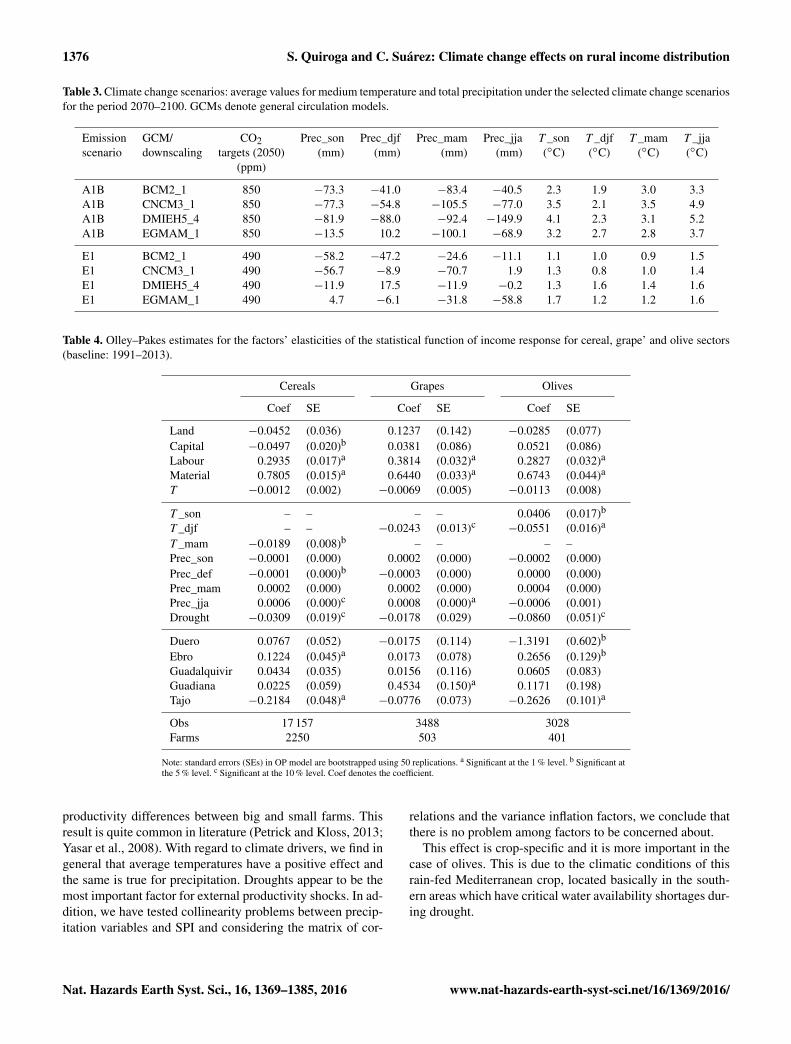
3.1 Olley and Pakes production functions’ estimates

Table 4 shows the estimates for the nature state drivers andmanagement factors’ elasticities of the statistical function ofyield response for the selected Mediterranean crops in theanalysis. We observe that the marginal effects are as expectedwith regard to traditional inputs; that is, the management fac-tors positively affect the increase in productivity. We observethat the effect of size (land) is not relevant in determiningcrop production in Spain; that is, there are not significant



Table 3. Climate change scenarios: average values for medium temperature and total precipitation under the selected climate change scenariosfor the period 2070–2100. GCMs denote general circulation models.

Emission GCM/ CO2 Prec_son Prec_djf Prec_mam Prec_jja T _son T _djf T _mam T _jjascenario downscaling targets (2050) (mm) (mm) (mm) (mm) (◦C) (◦C) (◦C) (◦C)

(ppm)

A1B BCM2_1 850 −73.3 −41.0 −83.4 −40.5 2.3 1.9 3.0 3.3A1B CNCM3_1 850 −77.3 −54.8 −105.5 −77.0 3.5 2.1 3.5 4.9A1B DMIEH5_4 850 −81.9 −88.0 −92.4 −149.9 4.1 2.3 3.1 5.2A1B EGMAM_1 850 −13.5 10.2 −100.1 −68.9 3.2 2.7 2.8 3.7

E1 BCM2_1 490 −58.2 −47.2 −24.6 −11.1 1.1 1.0 0.9 1.5E1 CNCM3_1 490 −56.7 −8.9 −70.7 1.9 1.3 0.8 1.0 1.4E1 DMIEH5_4 490 −11.9 17.5 −11.9 −0.2 1.3 1.6 1.4 1.6E1 EGMAM_1 490 4.7 −6.1 −31.8 −58.8 1.7 1.2 1.2 1.6

Table 4. Olley–Pakes estimates for the factors’ elasticities of the statistical function of income response for cereal, grape’ and olive sectors(baseline: 1991–2013).

Cereals Grapes Olives

Coef SE Coef SE Coef SE

Land −0.0452 (0.036) 0.1237 (0.142) −0.0285 (0.077)Capital −0.0497 (0.020)b 0.0381 (0.086) 0.0521 (0.086)Labour 0.2935 (0.017)a 0.3814 (0.032)a 0.2827 (0.032)a

Material 0.7805 (0.015)a 0.6440 (0.033)a 0.6743 (0.044)a

T −0.0012 (0.002) −0.0069 (0.005) −0.0113 (0.008)

T _son – – – – 0.0406 (0.017)b

T _djf – – −0.0243 (0.013)c−0.0551 (0.016)a

T _mam −0.0189 (0.008)b – – – –Prec_son −0.0001 (0.000) 0.0002 (0.000) −0.0002 (0.000)Prec_def −0.0001 (0.000)b

−0.0003 (0.000) 0.0000 (0.000)Prec_mam 0.0002 (0.000) 0.0002 (0.000) 0.0004 (0.000)Prec_jja 0.0006 (0.000)c 0.0008 (0.000)a

−0.0006 (0.001)Drought −0.0309 (0.019)c

−0.0178 (0.029) −0.0860 (0.051)c

Duero 0.0767 (0.052) −0.0175 (0.114) −1.3191 (0.602)b

Ebro 0.1224 (0.045)a 0.0173 (0.078) 0.2656 (0.129)b

Guadalquivir 0.0434 (0.035) 0.0156 (0.116) 0.0605 (0.083)Guadiana 0.0225 (0.059) 0.4534 (0.150)a 0.1171 (0.198)Tajo −0.2184 (0.048)a

−0.0776 (0.073) −0.2626 (0.101)a

Obs 17 157 3488 3028Farms 2250 503 401

Note: standard errors (SEs) in OP model are bootstrapped using 50 replications. a Significant at the 1 % level. b Significant atthe 5 % level. c Significant at the 10 % level. Coef denotes the coefficient.

productivity differences between big and small farms. Thisresult is quite common in literature (Petrick and Kloss, 2013;Yasar et al., 2008). With regard to climate drivers, we find ingeneral that average temperatures have a positive effect andthe same is true for precipitation. Droughts appear to be themost important factor for external productivity shocks. In ad-dition, we have tested collinearity problems between precip-itation variables and SPI and considering the matrix of cor-

relations and the variance inflation factors, we conclude thatthere is no problem among factors to be concerned about.

This effect is crop-specific and it is more important in thecase of olives. This is due to the climatic conditions of thisrain-fed Mediterranean crop, located basically in the south-ern areas which have critical water availability shortages dur-ing drought.



Table 5. Gini decomposition for drought by crop and river basin.

Crop River basin G Sk=Drought Gk=Drought Rk=Drought % Change [95 % conf. interval]

Duero 0.561 0.003 0.413 −0.051 −0.32 [−0.35 −0.28]Ebro 0.704 0.002 0.424 −0.022 −0.21 [−0.23 −0.18]

Cereals Guadalquivir 0.729 0.002 0.398 −0.039 −0.17 [−0.19 −0.16]Guadiana 0.664 0.002 0.412 −0.009 −0.18 [−0.21 −0.16]Tajo 0.714 0.003 0.466 −0.056 −0.27 [−0.32 −0.21]

Duero 0.651 0.002 0.399 −0.054 −0.23 [−0.29 −0.19]Ebro 0.642 0.002 0.408 −0.028 −0.23 [−0.27 −0.18]

Grapes Guadalquivir 0.769 0.001 0.444 0.025 −0.10 [−0.17 −0.08]Guadiana 0.3642 0.004 0.395 0.303 −0.27 [−0.44 −0.15]Tajo 0.644 0.003 0.522 0.045 −0.28 [−0.34 −0.23]

Duero 0.694 0.008 0.500 −0.167 −0.91 [−0.79 −0.32]Ebro 0.720 0.002 0.539 0.077 −0.18 [−0.32 −0.09]

Olives Guadalquivir 0.609 0.003 0.426 −0.009 −0.35 [−0.39 −0.31]Guadiana 0.550 0.004 0.403 −0.011 −0.46 [−0.64 −0.23]Tajo 0.485 0.005 0.412 −0.029 −0.50 [−0.61 −0.42]

3.2 Simulations of drought-driven production changes

Table 5 shows the Gini coefficient for the total income, andthe marginal effects of the increase of drought on the farms’income distribution for the main river basins in Spain. Weobserve that the most unequal distribution of incomes is pre-sented in the Duero river basin for cereals, in the Guadianafor grapes, and in the Tagus river basin for olives. We findthat the increase in drought occurrence will reduce the Giniindex in all the cases studied, meaning it will increase the in-equality for the rural incomes. Although the effects are notlarge, they are mostly significant.

The estimation of the percentage change of this rural in-equality allows us to explain the changes in the Gini indexas a response to changes in the precipitation patterns due toclimate change.

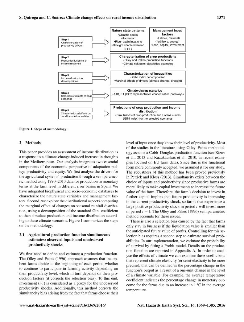
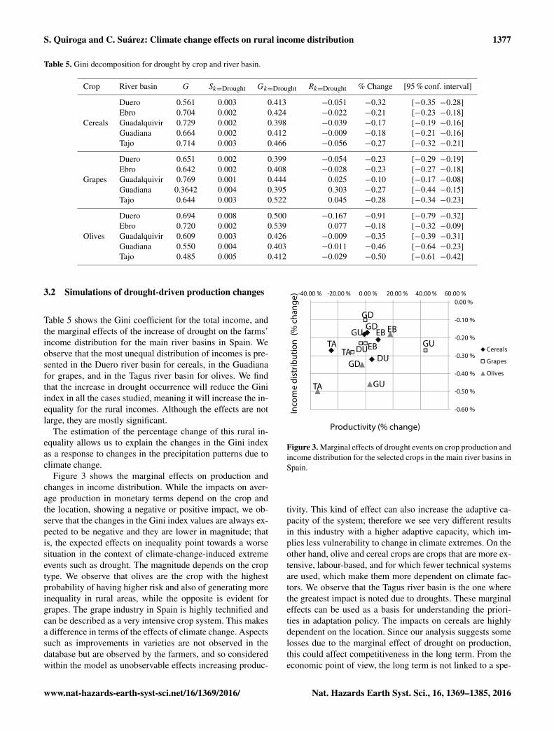
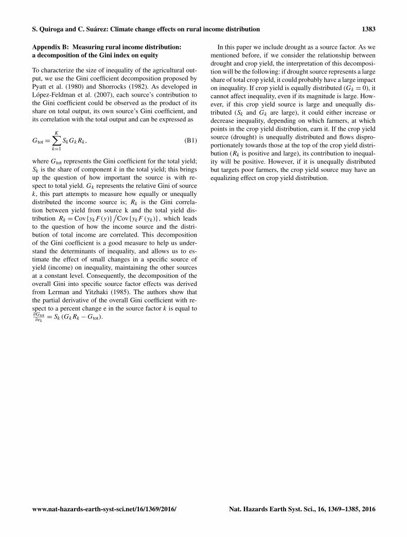
Figure 3 shows the marginal effects on production andchanges in income distribution. While the impacts on aver-age production in monetary terms depend on the crop andthe location, showing a negative or positive impact, we ob-serve that the changes in the Gini index values are always ex-pected to be negative and they are lower in magnitude; thatis, the expected effects on inequality point towards a worsesituation in the context of climate-change-induced extremeevents such as drought. The magnitude depends on the croptype. We observe that olives are the crop with the highestprobability of having higher risk and also of generating moreinequality in rural areas, while the opposite is evident forgrapes. The grape industry in Spain is highly technified andcan be described as a very intensive crop system. This makesa difference in terms of the effects of climate change. Aspectssuch as improvements in varieties are not observed in thedatabase but are observed by the farmers, and so consideredwithin the model as unobservable effects increasing produc-

38

1

Figure 3.Marginal e�ects of drought events on crop production and income distribution for 2 the selected crops in the main river basins in Spain. 3

4

5

-0.60 %

-0.50 %

-0.40 %

-0.30 %

-0.20 %

-0.10 %

0.00 %-40.00 % -20.00 % 0.00 % 20.00 % 40.00 % 60.00 %

Cereals

Grapes

Olives

Productivity (% change)

Inco

me

dist

ribut

ion

(% c

hang

e)

DU

EBGD

GUTA

TAGUEBDU

GD

EB

GU

GD

TA

Figure 3. Marginal effects of drought events on crop production andincome distribution for the selected crops in the main river basins inSpain.

tivity. This kind of effect can also increase the adaptive ca-pacity of the system; therefore we see very different resultsin this industry with a higher adaptive capacity, which im-plies less vulnerability to change in climate extremes. On theother hand, olive and cereal crops are crops that are more ex-tensive, labour-based, and for which fewer technical systemsare used, which make them more dependent on climate fac-tors. We observe that the Tagus river basin is the one wherethe greatest impact is noted due to droughts. These marginaleffects can be used as a basis for understanding the priori-ties in adaptation policy. The impacts on cereals are highlydependent on the location. Since our analysis suggests somelosses due to the marginal effect of drought on production,this could affect competitiveness in the long term. From theeconomic point of view, the long term is not linked to a spe-



39

1 (1) Baseline, (2-5) Climate change scenarios. 2 Figure 4. Lorenz curves (Gini index) for the selected crops under the baseline (1990-2013) 3 and climate change scenarios (A1B, E1). 4 5 6 7

020

4060

80Ge

n. Lo

renz p

hatce

r1 (by

ind)

0 .2 .4 .6 .8 1Cumulative population proportionind==1 ind==2ind==3 ind==4ind==5

010

2030

4050

Gen.

Lorenz

phatg

r (by in

d)


020

4060

Gen.

Loren

z pha

tol (by

ind)


020

4060

80Ge

n. Lore

nz ph

atcer

(by ind

)


010

2030

4050

Gen. L

orenz

phatg

r1 (by

ind)


020

4060

Gen.

Lorenz

phato

l1 (by

ind)


Cereals

Grapes

Olives

Cereals (A1B)

Grapes (A1B)

Olives (A1B)

Cereals (E1)

Grapes (E1)

Olives (E1)

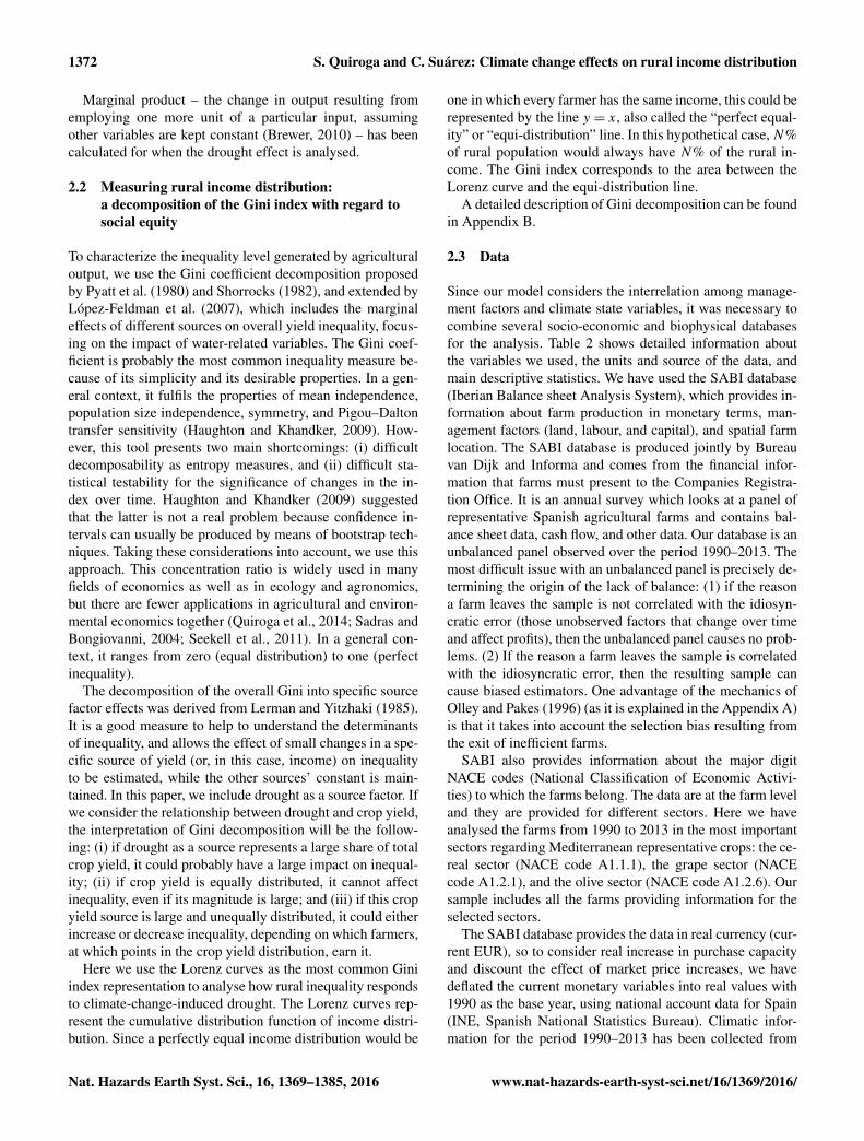
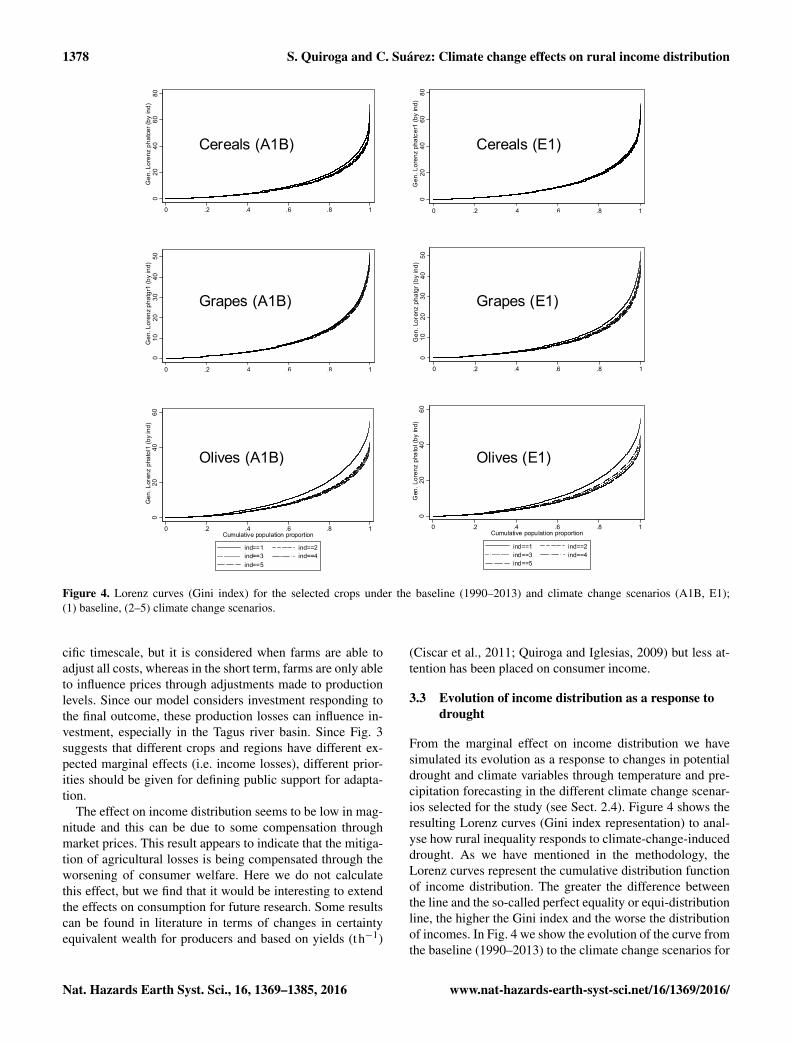
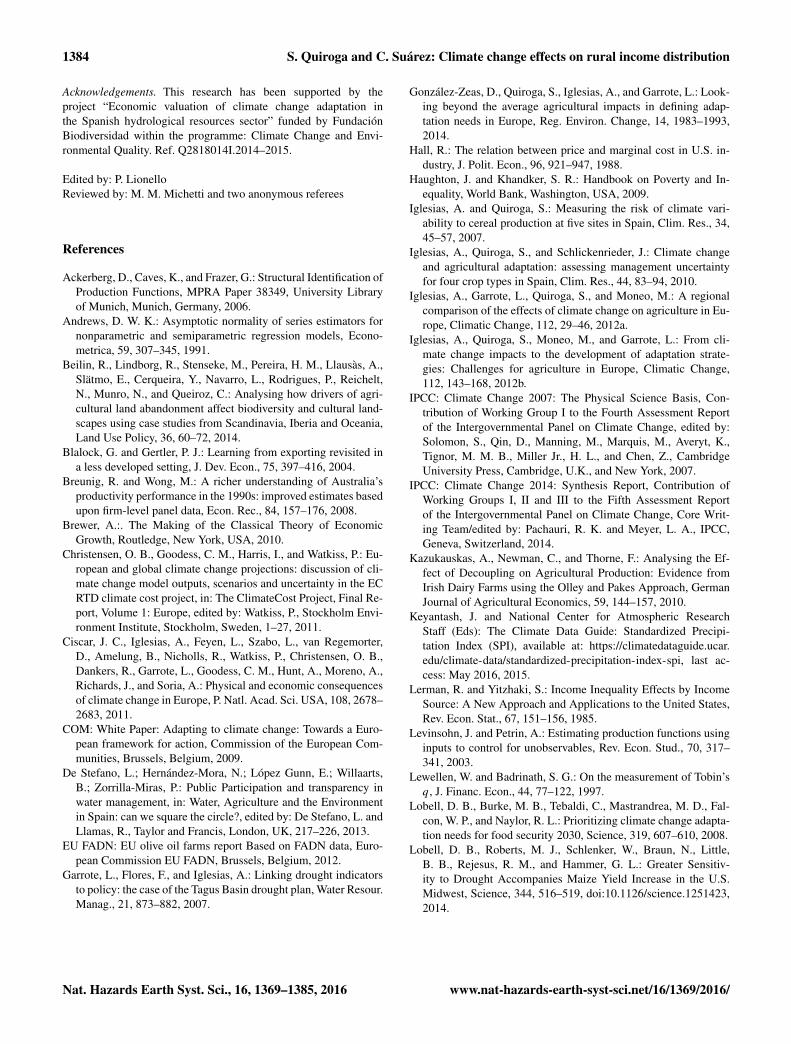
Figure 4. Lorenz curves (Gini index) for the selected crops under the baseline (1990–2013) and climate change scenarios (A1B, E1);(1) baseline, (2–5) climate change scenarios.

cific timescale, but it is considered when farms are able toadjust all costs, whereas in the short term, farms are only ableto influence prices through adjustments made to productionlevels. Since our model considers investment responding tothe final outcome, these production losses can influence in-vestment, especially in the Tagus river basin. Since Fig. 3suggests that different crops and regions have different ex-pected marginal effects (i.e. income losses), different prior-ities should be given for defining public support for adapta-tion.

The effect on income distribution seems to be low in mag-nitude and this can be due to some compensation throughmarket prices. This result appears to indicate that the mitiga-tion of agricultural losses is being compensated through theworsening of consumer welfare. Here we do not calculatethis effect, but we find that it would be interesting to extendthe effects on consumption for future research. Some resultscan be found in literature in terms of changes in certaintyequivalent wealth for producers and based on yields (t h−1)

(Ciscar et al., 2011; Quiroga and Iglesias, 2009) but less at-tention has been placed on consumer income.

3.3 Evolution of income distribution as a response todrought

From the marginal effect on income distribution we havesimulated its evolution as a response to changes in potentialdrought and climate variables through temperature and pre-cipitation forecasting in the different climate change scenar-ios selected for the study (see Sect. 2.4). Figure 4 shows theresulting Lorenz curves (Gini index representation) to anal-yse how rural inequality responds to climate-change-induceddrought. As we have mentioned in the methodology, theLorenz curves represent the cumulative distribution functionof income distribution. The greater the difference betweenthe line and the so-called perfect equality or equi-distributionline, the higher the Gini index and the worse the distributionof incomes. In Fig. 4 we show the evolution of the curve fromthe baseline (1990–2013) to the climate change scenarios for



2080 (A1B and E1 concentration pathways simulated by fourdifferent climate models and downscaling).

These curves show for the bottom percentage of farmers(x axis), what percentage of the total agricultural income(y axis) they have, and what percentage can be considereda measure of inequality. We observe that the effects are nothuge in terms of income distribution, but they are negativefor all the crops and for the different scenarios, so climate-change-induced drought increase will definitely worsen ruralinequality. In addition, we observe that the sector in whichthe income inequality will rise is the olive sector, followed bythe cereals sector. In the case of grape production, the sim-ulated effect on inequality is not significant. Since droughtevents will be suffered by all the farmers independently oftheir income level, our results suggest that at least in rain-fed crops, investment, which is mostly made by farmers withhigher incomes, would not be enough to compensate the ex-pected losses, because in other cases we will expect a verycritical effect on income distribution as a consequence ofdrought. Although the EU White paper for adaptation (COM,2009) indicates that there is great room for adaptation in theagricultural sector, these results suggest that in the case ofdrought, the adaptation measures should prioritize water re-source management. A limitation of this study is the fact thatwe do not analyse the effects on irrigated crops. The chal-lenge for this kind of analysis is that data on spatial resolu-tion for water availability have to be linked to informationat the farm level. In a further step, remote sensing methodscould help to better characterize information on water use.

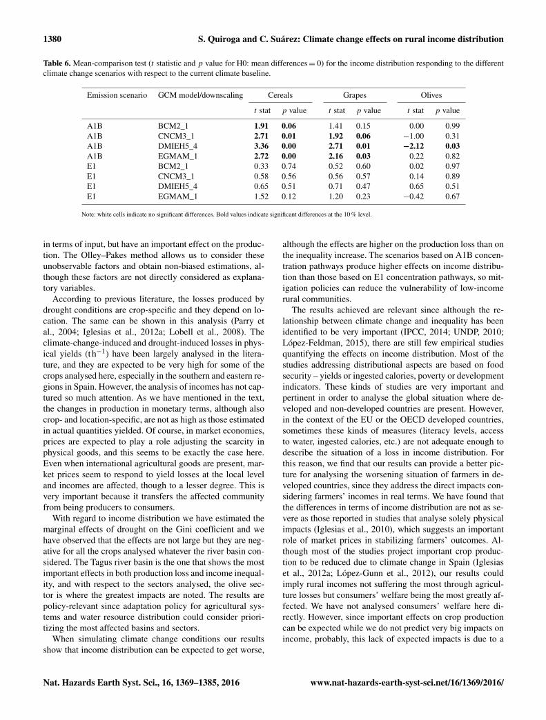
We observe in Fig. 4 that the projected scenarios are verysimilar for the different models considered; that is, the re-sults we obtain for income distribution changes are very ro-bust in terms of the different models considered. Slightlylarger differences appear among the different mitigation tar-gets (A1B and E1). In Table 6 we have analysed these dif-ferences, considering the quantification of uncertainty in ourmodel as well. We have computed the mean-comparison testfor the projected income distribution response to climate sce-narios in relation to the current climate baseline. We showthe t statistic and p value for the null hypothesis of hav-ing no significant differences among the scenarios with re-spect to the baseline. A p value over 10 % means that theresults show no statistical significant differences in inequal-ity, while the opposite applies when the p value is less than10 %. We observe that only some of the scenarios consider-ing A1B concentration pathways produce significant effectson income distribution. Although the olive crop shows a big-ger effect at a glance, we can see that considering the uncer-tainty of the model, these impacts are not significant (this isdue to a bigger standard error in the model of this crop). Thescenarios for the A1B concentration pathways have a biggereffect on income distribution than those for the E1 concen-tration pathways, both in magnitude and confidence level; somitigation policies can help to reduce the effects of climatechange on social equity.

Here we do not explicitly analyse rural communities, butincome distribution at the farm level. However, we think thata worsening in the distribution of farms’ incomes will affectsocial issues in these rural communities. We observe that themost important effects are expected on the olive crop in thesouthern areas in Spain. The increase in income inequalityin these rural communities can be very important in termsof social conflicts since this region is mostly based on agri-cultural outcomes with very low development of industry.This problem we find in Spain could be the same in otherMediterranean countries where southern areas are also verymuch driven by the olive crop sector. Another limitation inthis study is that we do not explicitly consider the role ofCAP subsidies which are in fact very important, particularlyin this area. Further analysis could include separated incomesfrom market and from CAP subsidies to explicitly examinethe agricultural policy effects. However, since farm incomeand its distribution seem to be affected by climate changeand drought challenges, the role of CAP seems to be revisedin order to help competitiveness and income redistributionfunctions.

Here we consider the contribution of the studied crops tofarmers’ production and the effect of these losses on incomedistribution. However, we do not analyse cross-compensationor adaptation measures explicitly (i.e. crop rotation, changein varieties, part-time non-agricultural incomes, etc). Farm-ers of course can make several important decisions to adaptto the expected losses and it would be interesting in furtheranalyses to take these compensation effects on income dis-parities into account. Therefore, adaptation measures shouldbe designed considering both economic and social aspects.

4 Discussion and conclusions

This paper focuses on the effects of droughts and climatechange on agricultural production and rural income dis-tribution. We have estimated the drivers for production inmonetary units and we find that traditional inputs such aslabour, capital, and intermediate consumptions (energy, fer-tilizers, pesticides, etc.) positively affect production as ex-pected. However, there are also nature state variables, suchas drought, temperature increase, or precipitation decreases,which are not controlled by the farmers, but can produce im-portant productivity shocks. We have estimated the elasticityfor these shocks and we have especially focused on droughteffects on productivity losses.

The relatively complex methodology used allows us to fo-cus on the economic aspects of climate change and droughtimpacts on agriculture. We estimate directly in monetaryunits. For this purpose, we used economic information aboutmarketable outputs and inputs (such as cost of labour, cap-ital, intermediate consumptions – energy, fertilizers, etc.) inmonetary terms. However, there are other factors such as soilquality or farmer’s effort that are not causing a marginal cost



Table 6. Mean-comparison test (t statistic and p value for H0: mean differences= 0) for the income distribution responding to the differentclimate change scenarios with respect to the current climate baseline.

Emission scenario GCM model/downscaling Cereals Grapes Olives

t stat p value t stat p value t stat p value

A1B BCM2_1 1.91 0.06 1.41 0.15 0.00 0.99A1B CNCM3_1 2.71 0.01 1.92 0.06 −1.00 0.31A1B DMIEH5_4 3.36 0.00 2.71 0.01 −2.12 0.03A1B EGMAM_1 2.72 0.00 2.16 0.03 0.22 0.82E1 BCM2_1 0.33 0.74 0.52 0.60 0.02 0.97E1 CNCM3_1 0.58 0.56 0.56 0.57 0.14 0.89E1 DMIEH5_4 0.65 0.51 0.71 0.47 0.65 0.51E1 EGMAM_1 1.52 0.12 1.20 0.23 −0.42 0.67

Note: white cells indicate no significant differences. Bold values indicate significant differences at the 10 % level.

in terms of input, but have an important effect on the produc-tion. The Olley–Pakes method allows us to consider theseunobservable factors and obtain non-biased estimations, al-though these factors are not directly considered as explana-tory variables.

According to previous literature, the losses produced bydrought conditions are crop-specific and they depend on lo-cation. The same can be shown in this analysis (Parry etal., 2004; Iglesias et al., 2012a; Lobell et al., 2008). Theclimate-change-induced and drought-induced losses in phys-ical yields (t h−1) have been largely analysed in the litera-ture, and they are expected to be very high for some of thecrops analysed here, especially in the southern and eastern re-gions in Spain. However, the analysis of incomes has not cap-tured so much attention. As we have mentioned in the text,the changes in production in monetary terms, although alsocrop- and location-specific, are not as high as those estimatedin actual quantities yielded. Of course, in market economies,prices are expected to play a role adjusting the scarcity inphysical goods, and this seems to be exactly the case here.Even when international agricultural goods are present, mar-ket prices seem to respond to yield losses at the local leveland incomes are affected, though to a lesser degree. This isvery important because it transfers the affected communityfrom being producers to consumers.

With regard to income distribution we have estimated themarginal effects of drought on the Gini coefficient and wehave observed that the effects are not large but they are neg-ative for all the crops analysed whatever the river basin con-sidered. The Tagus river basin is the one that shows the mostimportant effects in both production loss and income inequal-ity, and with respect to the sectors analysed, the olive sec-tor is where the greatest impacts are noted. The results arepolicy-relevant since adaptation policy for agricultural sys-tems and water resource distribution could consider priori-tizing the most affected basins and sectors.

When simulating climate change conditions our resultsshow that income distribution can be expected to get worse,

although the effects are higher on the production loss than onthe inequality increase. The scenarios based on A1B concen-tration pathways produce higher effects on income distribu-tion than those based on E1 concentration pathways, so mit-igation policies can reduce the vulnerability of low-incomerural communities.

The results achieved are relevant since although the re-lationship between climate change and inequality has beenidentified to be very important (IPCC, 2014; UNDP, 2010;López-Feldman, 2015), there are still few empirical studiesquantifying the effects on income distribution. Most of thestudies addressing distributional aspects are based on foodsecurity – yields or ingested calories, poverty or developmentindicators. These kinds of studies are very important andpertinent in order to analyse the global situation where de-veloped and non-developed countries are present. However,in the context of the EU or the OECD developed countries,sometimes these kinds of measures (literacy levels, accessto water, ingested calories, etc.) are not adequate enough todescribe the situation of a loss in income distribution. Forthis reason, we find that our results can provide a better pic-ture for analysing the worsening situation of farmers in de-veloped countries, since they address the direct impacts con-sidering farmers’ incomes in real terms. We have found thatthe differences in terms of income distribution are not as se-vere as those reported in studies that analyse solely physicalimpacts (Iglesias et al., 2010), which suggests an importantrole of market prices in stabilizing farmers’ outcomes. Al-though most of the studies project important crop produc-tion to be reduced due to climate change in Spain (Iglesiaset al., 2012a; López-Gunn et al., 2012), our results couldimply rural incomes not suffering the most through agricul-ture losses but consumers’ welfare being the most greatly af-fected. We have not analysed consumers’ welfare here di-rectly. However, since important effects on crop productioncan be expected while we do not predict very big impacts onincome, probably, this lack of expected impacts is due to a



smoothing effect through prices, which in fact highly affectsconsumers’ welfare.

Concerning adaptation, we have found that the Tagus riverbasin is the most affected region with regard to changes inthe average income of farmers. This would imply that largerefforts for adaptation should be made in this area, where wa-ter resources’ management becomes a key element for adap-tation. Tagus river basin has been pointed to be one of thebasins where pressures will be increased to a more substan-tial degree in terms of unsatisfied demand. Having the high-est magnitude effects in terms of monetary outcomes andconsequences on inequality will increase the already exist-ing conflicts among different water users and water manage-ment challenges including potential changes in the interbasinwater transfer schemes with the Segura river basin. A totalof 9.8 km3 of water has been transferred in 30 years, duringwhich the interbasin water transfer has been operative. Ofthis, 60 % has been used for irrigated agriculture in the south-east region in Spain; 38 % has been dedicated to complementdrinking water supply in the region; other uses include trans-fer water to the Tablas de Damiel National Park, a wetlandecosystem in the Guadiana River basin (Pittock et al., 2009).Therefore, the increasing pressures do not only have implica-tions for socio-economic issues, but also on the ecosystem.

Moreover, we have found that the olive sector should beconsidered as a priority in terms of both farms’ incomes andsocial equity. Studying the role of CAP subsidies will be im-portant to address this challenge in the future. The olive sec-tor is the most important agricultural sector in the south ofthe Mediterranean and represents an important factor for ru-ral development in the area. Olive oil farms in Spain are onaverage bigger and have a higher labour productivity thanelsewhere. Labour is the most important cost for these farms,the family labour representing around 50 % of total costs. Inaddition, olive farms in Spain have suffered on average un-favourable trends in income indicators, with income fallingby about a third in the last decades (EU FADN, 2012). There-fore, the predicted increase in inequality could increase mi-gration out of the rural areas, affecting land use and ruraldevelopment in Spain.



Appendix A: Agricultural production functionsimultaneous estimates: observed inputs and unobservedproductivity shocks

The Olley and Pakes (1996) approach assumes that incum-bent farms decide at the beginning of each period whether tocontinue to participate in farming activity, a decision madeaccording to their productivity level, which in turn dependson each farm’s production factor (it corrects the selectionbias). To this end, investment (ii t ) is considered as a proxyfor the unobserved productivity shocks. In addition, thismethod corrects the simultaneity bias arising from the factthat farms choose their level of input once they know theirlevel of productivity.

We assume that farmers produce a homogeneous productwith Cobb–Douglas technology, and that the factors under-lying profitability differences among firms are neutral effi-ciency differences. The production function is

yi t = β0+βl li t +βmmi t +βkki t +βaai t +∑j

δj cj i t + ui t (A1)

ui t =�i t + ηi t ,

where yi t is the log output for farm i in period t ; li t , mi t ,ki t and ai t are the log values of labour, material, capital, andland inputs; cj i t are biophysical variables (climate and riverbasin); �i t is the productivity shock that is observed by thefarm but not by the econometrician (for example machinebreakdowns); and ηi t is an unexpected productivity shockthat is unobserved by both the decision-maker and the econo-metrician. Thus,�i t and ηi t are unobserved. The distinctionis that �i t is a state variable in the farm’s decision prob-lem, and hence a determinant of both liquidation and inputdemand decisions, while ηi t is not (see Petrick and Kloss(2013) for an extended typology of farm production factors).

Simultaneity exists between the choice of inputs and pro-ductivity since productive farms are more likely to makecapital investments to increase the future value of the farm.Then, the farm’s decision to invest in further capital, ii t , alsodepends on capital stock, land, and the firm’s productivityshock:

ii t = I (�i t ,ki t ,ai t ) . (A2)

This investment decision equation implies that future produc-tivity is increasing in the current productivity shock, so farmsthat experience a large positive productivity shock in periodt will invest more in period t + 1.

The Olley and Pakes (1996) semiparametric method ac-counts for these issues. Applying this method first involvesusing the investment decision function to control for the cor-relation between the error term and the inputs. This is basedon the assumption that future productivity is strictly increas-ing with respect to �i t , so farms that observe a positive pro-ductivity shock in period t will invest more in that period, forany ki t and ai t . Provided that ii t is strictly positive, we can

write the inverse function for the unobserved shock �i t as

�i t = h(ii t ,ki t ,ai t ) . (A3)

This function can thus be used to control for the simultaneityproblem. Substituting those equations into production func-tion yields

yi t = βl li t +βmmi t +∑j

δj cj i t +ϕ (ii t ,ki t ,ai t )+ ηi t , (A4)

where

ϕ (ii t ,ki t ,ai t )= β0+βkki t +βaai t +h(ii t ,ki t ,ai t ) . (A5)

We approximate ϕ (.) with a second-order polynomial seriesin land, capital, and investment. The partially linear equa-tion can be estimated by ordinary least squares. The coeffi-cient estimates for variable inputs (labour and material) willbe consistent and asymptotically normal estimates of the co-efficients in the linear part of the model (Andrews, 1991) be-cause ϕ (.) controls for unobserved productivity, and thus theerror term is no longer correlated to the inputs. This allows usto estimate βl and βm without requiring identification of βkand βa , so more work is required to disentangle the effects ofcapital and age on the investment decision from their effecton output.

There is also a selection bias since farms only stay in busi-ness if the liquidation value is smaller than the anticipatedfuture value of profits. Achieving this requires a second stepto estimate survival probabilities (Pi t ), which will then allowus to control for selection bias. In our implementation, we es-timate the probability of survival by fitting a probit model onii, t−1, ki, t−1, ai, t−1, as well as their squares and cross prod-ucts. This can be viewed as a nonparametric estimator of theindex function. If the predicted probabilities from this modelare P̂i t ,

Pr(χi t = 1)= φ(ii, t−1,ki, t−1,ai, t−1

). (A6)

In the third step, we identify the coefficient βk , where pro-ductivity is assumed to evolve according to a first-orderMarkov process. We fit the following equation by non-linearleast squares in order to obtain βk:

yi t −_

β l li t −_

βmmi t −∑j

δ̂j cj i t = βkki t +βaai t

+ g(ϕ̂t−1−βkki,t−1−βaai, t−1, P̂i t

)+ ξi t + ηi t , (A7)

where the unknown function g (.) is approximated by asecond-order polynomial in

ϕ̂t−1−βkki,t−1−βaai,t−1 and P̂i t .

Finally, we use the efficient coefficients’ estimates to builda measure of farm-level production for the i farm at thetime t .



Appendix B: Measuring rural income distribution:a decomposition of the Gini index on equity

To characterize the size of inequality of the agricultural out-put, we use the Gini coefficient decomposition proposed byPyatt et al. (1980) and Shorrocks (1982). As developed inLópez-Feldman et al. (2007), each source’s contribution tothe Gini coefficient could be observed as the product of itsshare on total output, its own source’s Gini coefficient, andits correlation with the total output and can be expressed as

Gtot =

K∑k=1

SkGkRk, (B1)

where Gtot represents the Gini coefficient for the total yield;Sk is the share of component k in the total yield; this bringsup the question of how important the source is with re-spect to total yield. Gk represents the relative Gini of sourcek, this part attempts to measure how equally or unequallydistributed the income source is; Rk is the Gini correla-tion between yield from source k and the total yield dis-tribution Rk = Cov {ykF(y)}

/Cov {ykF (yk)} , which leads

to the question of how the income source and the distri-bution of total income are correlated. This decompositionof the Gini coefficient is a good measure to help us under-stand the determinants of inequality, and allows us to es-timate the effect of small changes in a specific source ofyield (income) on inequality, maintaining the other sourcesat a constant level. Consequently, the decomposition of theoverall Gini into specific source factor effects was derivedfrom Lerman and Yitzhaki (1985). The authors show thatthe partial derivative of the overall Gini coefficient with re-spect to a percent change e in the source factor k is equal to∂Gtot∂ek= Sk (GkRk −Gtot).

In this paper we include drought as a source factor. As wementioned before, if we consider the relationship betweendrought and crop yield, the interpretation of this decomposi-tion will be the following: if drought source represents a largeshare of total crop yield, it could probably have a large impacton inequality. If crop yield is equally distributed (Gk = 0), itcannot affect inequality, even if its magnitude is large. How-ever, if this crop yield source is large and unequally dis-tributed (Sk and Gk are large), it could either increase ordecrease inequality, depending on which farmers, at whichpoints in the crop yield distribution, earn it. If the crop yieldsource (drought) is unequally distributed and flows dispro-portionately towards those at the top of the crop yield distri-bution (Rk is positive and large), its contribution to inequal-ity will be positive. However, if it is unequally distributedbut targets poor farmers, the crop yield source may have anequalizing effect on crop yield distribution.



Acknowledgements. This research has been supported by theproject “Economic valuation of climate change adaptation inthe Spanish hydrological resources sector” funded by FundaciónBiodiversidad within the programme: Climate Change and Envi-ronmental Quality. Ref. Q2818014I.2014–2015.

Edited by: P. LionelloReviewed by: M. M. Michetti and two anonymous referees

References

Ackerberg, D., Caves, K., and Frazer, G.: Structural Identification ofProduction Functions, MPRA Paper 38349, University Libraryof Munich, Munich, Germany, 2006.

Andrews, D. W. K.: Asymptotic normality of series estimators fornonparametric and semiparametric regression models, Econo-metrica, 59, 307–345, 1991.

Beilin, R., Lindborg, R., Stenseke, M., Pereira, H. M., Llausàs, A.,Slätmo, E., Cerqueira, Y., Navarro, L., Rodrigues, P., Reichelt,N., Munro, N., and Queiroz, C.: Analysing how drivers of agri-cultural land abandonment affect biodiversity and cultural land-scapes using case studies from Scandinavia, Iberia and Oceania,Land Use Policy, 36, 60–72, 2014.

Blalock, G. and Gertler, P. J.: Learning from exporting revisited ina less developed setting, J. Dev. Econ., 75, 397–416, 2004.

Breunig, R. and Wong, M.: A richer understanding of Australia’sproductivity performance in the 1990s: improved estimates basedupon firm-level panel data, Econ. Rec., 84, 157–176, 2008.

Brewer, A.:. The Making of the Classical Theory of EconomicGrowth, Routledge, New York, USA, 2010.

Christensen, O. B., Goodess, C. M., Harris, I., and Watkiss, P.: Eu-ropean and global climate change projections: discussion of cli-mate change model outputs, scenarios and uncertainty in the ECRTD climate cost project, in: The ClimateCost Project, Final Re-port, Volume 1: Europe, edited by: Watkiss, P., Stockholm Envi-ronment Institute, Stockholm, Sweden, 1–27, 2011.

Ciscar, J. C., Iglesias, A., Feyen, L., Szabo, L., van Regemorter,D., Amelung, B., Nicholls, R., Watkiss, P., Christensen, O. B.,Dankers, R., Garrote, L., Goodess, C. M., Hunt, A., Moreno, A.,Richards, J., and Soria, A.: Physical and economic consequencesof climate change in Europe, P. Natl. Acad. Sci. USA, 108, 2678–2683, 2011.

COM: White Paper: Adapting to climate change: Towards a Euro-pean framework for action, Commission of the European Com-munities, Brussels, Belgium, 2009.

De Stefano, L.; Hernández-Mora, N.; López Gunn, E.; Willaarts,B.; Zorrilla-Miras, P.: Public Participation and transparency inwater management, in: Water, Agriculture and the Environmentin Spain: can we square the circle?, edited by: De Stefano, L. andLlamas, R., Taylor and Francis, London, UK, 217–226, 2013.

EU FADN: EU olive oil farms report Based on FADN data, Euro-pean Commission EU FADN, Brussels, Belgium, 2012.

Garrote, L., Flores, F., and Iglesias, A.: Linking drought indicatorsto policy: the case of the Tagus Basin drought plan, Water Resour.Manag., 21, 873–882, 2007.

González-Zeas, D., Quiroga, S., Iglesias, A., and Garrote, L.: Look-ing beyond the average agricultural impacts in defining adap-tation needs in Europe, Reg. Environ. Change, 14, 1983–1993,2014.

Hall, R.: The relation between price and marginal cost in U.S. in-dustry, J. Polit. Econ., 96, 921–947, 1988.

Haughton, J. and Khandker, S. R.: Handbook on Poverty and In-equality, World Bank, Washington, USA, 2009.

Iglesias, A. and Quiroga, S.: Measuring the risk of climate vari-ability to cereal production at five sites in Spain, Clim. Res., 34,45–57, 2007.

Iglesias, A., Quiroga, S., and Schlickenrieder, J.: Climate changeand agricultural adaptation: assessing management uncertaintyfor four crop types in Spain, Clim. Res., 44, 83–94, 2010.

Iglesias, A., Garrote, L., Quiroga, S., and Moneo, M.: A regionalcomparison of the effects of climate change on agriculture in Eu-rope, Climatic Change, 112, 29–46, 2012a.

Iglesias, A., Quiroga, S., Moneo, M., and Garrote, L.: From cli-mate change impacts to the development of adaptation strate-gies: Challenges for agriculture in Europe, Climatic Change,112, 143–168, 2012b.

IPCC: Climate Change 2007: The Physical Science Basis, Con-tribution of Working Group I to the Fourth Assessment Reportof the Intergovernmental Panel on Climate Change, edited by:Solomon, S., Qin, D., Manning, M., Marquis, M., Averyt, K.,Tignor, M. M. B., Miller Jr., H. L., and Chen, Z., CambridgeUniversity Press, Cambridge, U.K., and New York, 2007.

IPCC: Climate Change 2014: Synthesis Report, Contribution ofWorking Groups I, II and III to the Fifth Assessment Reportof the Intergovernmental Panel on Climate Change, Core Writ-ing Team/edited by: Pachauri, R. K. and Meyer, L. A., IPCC,Geneva, Switzerland, 2014.

Kazukauskas, A., Newman, C., and Thorne, F.: Analysing the Ef-fect of Decoupling on Agricultural Production: Evidence fromIrish Dairy Farms using the Olley and Pakes Approach, GermanJournal of Agricultural Economics, 59, 144–157, 2010.

Keyantash, J. and National Center for Atmospheric ResearchStaff (Eds): The Climate Data Guide: Standardized Precipi-tation Index (SPI), available at: https://climatedataguide.ucar.edu/climate-data/standardized-precipitation-index-spi, last ac-cess: May 2016, 2015.

Lerman, R. and Yitzhaki, S.: Income Inequality Effects by IncomeSource: A New Approach and Applications to the United States,Rev. Econ. Stat., 67, 151–156, 1985.

Levinsohn, J. and Petrin, A.: Estimating production functions usinginputs to control for unobservables, Rev. Econ. Stud., 70, 317–341, 2003.

Lewellen, W. and Badrinath, S. G.: On the measurement of Tobin’sq, J. Financ. Econ., 44, 77–122, 1997.

Lobell, D. B., Burke, M. B., Tebaldi, C., Mastrandrea, M. D., Fal-con, W. P., and Naylor, R. L.: Prioritizing climate change adapta-tion needs for food security 2030, Science, 319, 607–610, 2008.

Lobell, D. B., Roberts, M. J., Schlenker, W., Braun, N., Little,B. B., Rejesus, R. M., and Hammer, G. L.: Greater Sensitiv-ity to Drought Accompanies Maize Yield Increase in the U.S.Midwest, Science, 344, 516–519, doi:10.1126/science.1251423,2014.


https://climatedataguide.ucar.edu/climate-data/standardized-precipitation-index-spi

https://climatedataguide.ucar.edu/climate-data/standardized-precipitation-index-spi

http://dx.doi.org/10.1126/science.1251423


López-Feldman, A.: Cambio climático, distribución del ingreso y lapobreza: El caso de México, CEPAL, Documentos de ProyectosNo. 555, 2015.

López-Feldman, A., Mora, J., and Taylor, J. E.: Does natural re-source extraction mitigate poverty and inequality? Evidencefrom rural Mexico and a Lacandona Rainforest Community, En-viron. Dev. Econ., 12, 251–269, 2007.

Lopez-Gunn, E., Zorrilla, P., Prieto, F., and Llamas, M. R.: Lost intranslation? Water efficiency in Spanish agriculture, Agr. WaterManage., 108, 83–95, 2012.

MAGRAMA: Anuario de Estadística, Avance 2014, MAGRAMA,Madrid, available at: http://www.magrama.gob.es/estadistica/pags/anuario/2014-Avance/AE_2014_Avance, last access: May2016, 2015.

Marino, E. and Ribot, J.: Special Issue Introduction: Adding insultto injury: Climate change and the inequities of climate interven-tion Global Environ. Chang., 22, 323–328, 2012.

Martín-Martín, C., Bunce, R., Saura, S., and Elena-Rosselló, R.:Changes and interactions between forest landscape connectivityand burnt area in Spain, Ecol. Indic., 33, 129–138, 2013.

McKee, T. B., Doesken, N. J., and Kleist, J.: The relationship ofdrought frequency and duration to time scales, in: Proceedingsof the 8th Conference on Applied Climatology, 17–22 January1993, Anaheim, CA, USA, 1993.

Michetti, M. and Zampieri, M.: Climate–Human–Land Interactions:A Review of Major Modelling Approaches, Land, 3, 793–833,2014.

NDMC: What is drought?, The National Drought Mitigation Center,Lincoln, Nebraska, USA, 2015.

Olley, S. and Pakes, A.: The dynamics of productivity inthe telecommunications equipment industry, Econometrica, 64,1263–1297, 1996.

Parry, M. A., Rosenzweig, C., Iglesias, A., Livermore, M., and Fis-cher, G.: Effects of climate change on global food production un-der SRES emissions and socio-economic scenarios, Global Env-iron. Chang., 14, 53–67, 2004.

Pavcnik, N.: Trade liberalization, exit, and productivity improve-ment: Evidence from chilean plants, Rev. Econ. Stud., 69, 245–276, 2002.

Petrick, M. and Kloss, M.: Synthesis Report on the Impact of Cap-ital Use, Factor Markets Working Papers 169, Centre for Euro-pean Policy Studies, Brussels, Belgium, 2013.

Piketty, T.: Capital in the 21st Century.Éditions du Seuil, HarvardUniversity Press, Cambridge, Massachusetts, London, England,2013.

Pindyck, R.: Climate Change Policy: What Do the Models Tell Us?,J. Econ. Lit., 51, 860–872, 2013.

Pittock, J., Meng, J., Geiger, J. M., and Chapagain, A. K.: Inter-basin water transfers and water scarcity in a changing world – asolution or a pipedream? WWF Germany, 2009.

Pyatt, G., Chen, C., and Fei, J.: The distribution of income by factorcomponents, The Quarterly Journal of Economics, 95, 451–74,1980.

Quiroga, S. and Iglesias, A.: A comparison of the climate risks ofcereal, citrus, grapevine and olive production in Spain, Agr. Syst.,101, 91–100, 2009.

Quiroga, S., Suárez, C., and Fernández-Haddad, Z.: Do water rightsaffect technical efficiency and social disparities of crop produc-tion in the Mediterranean?, Water, 6, 3300–3319, 2014.

Quiroga, S., Suárez, C., and Solís, J. D.: Exploring coffee farmers’awareness about climate change and water needs: smallholders’perceptions of adaptive capacity, Environ, Sci. Policy, 45, 53–66,2015.

Rizov, M., Pokrivcak, J., and Ciaian, P.: CAP subsidies and pro-ductivity of the EU farms, Journal Agricultural Econmics, 64,537–557, 2013.

Roeckner, E., Giorgetta, M. A., Crüger, T., Esch, M., and Pongratz,J.: Historical and future anthropogenic emission pathways de-rived from coupled climate-carbon cycle simulations, ClimaticChange, 105, 91–108, 2011.

Rogelj, J., Meinshausen, M., and Knutti, R.: Global warming un-der old and new scenarios using IPCC climate sensitivity rangeestimates, Nature Climate Change, 2, 248–253, 2012.

Rogers, P. P., Llamas, R., Martínez-Cortina, L.: Water Crisis: Mythor Reality?, Taylor & Francis plc., London, UK, 2006.

Rosenzweig, C., Strzepek, K., Major, D., Iglesias, A., Yates, D.,Holt, A., and Hillel, D.: Water availability for agriculture un-der climate change: five international studies, Global Environ.Chang., 14, 345–360, 2004.

Sadras, V. O. and Bongiovanni, R.: Use of Lorenz curves and Ginicoefficients to assess yield inequality within paddocks, FieldCrop. Res., 90, 303–310, 2004.

Seekell, D. A., D’Odorico, P., and Pace, M. L.: Virtual water trans-fers unlikely to redress inequality in global water use, Environ.Res. Lett., 6, 1–6, 2011.

Shorrocks, A. F.: Inequality decomposition by factor components,Econometrica, 50, 193–212, 1982.

Solow, R.: Technical change and the aggregate production function,Rev. Econ. Stat., 39, 312–320, 1957.

Tsakiris, G., Loukas, A., Pangalou, D., Vangelis, H., Tigkas,D., Rossi, G., and Cancelliere, A.: Drought characterization,in: Drought Management Guidelines Technical Annex, Op-tions Méditerranéennes Series B, No. 58, edited by: Igle-sias, A., Moneo, M., and Lopez-Francos, A., Publisher CI-HEAM/EC MEDA Water, Centro Internacional de Altos Estu-dios Agronómicos Mediterráneos/Euro-Mediterranean RegionalProgramme for Local Water Management, Zaragoza, Spain, 85–102, 2007.

UNDP: Mapping Climate Change Vulnerability and Impact Scenar-ios, United Nations Development Programme, New York, USA,2010.

Watkins, P., Holland, M., King, K., and Hunt, A.: Damages toland, in: Green Accounting in Europe, Volume 2: A ComparativeStudy, edited by: Markandya, A. and Tamborra, M., FondazioneEni Enrico Mattei Series on Economics and the Environment, El-gar, Cheltenham, UK and Northampton, Mass., 381–410, 2005.

Wheeler, T. and von Braun, J.: Climate change impacts on globalfood security, Science, 341, 508–513, 2013.

Yasar, M., Raciborski, R., and Poi, B.: Production function estima-tion in Stata using the Olley and Pakes method, Stata J., 8, 221–231, 2008.


http://www.magrama.gob.es/estadistica/pags/anuario/2014-Avance/AE_2014_Avance

http://www.magrama.gob.es/estadistica/pags/anuario/2014-Avance/AE_2014_Avance

climate change and drought effects on rural income ... · climate-change-induced impacts on society...

Documents