classroom tips and techniques: applying the epsilon-delta ... classroom tips and techniques:...
TRANSCRIPT
Classroom Tips and Techniques: Applying the Epsilon-Delta Definition of a Limit
Robert J. Lopez
Emeritus Professor of Mathematics and Maple Fellow
Maplesoft
Introduction
My experience in teaching calculus at two universities and an undergraduate engineering school
was that students struggled to apply the epsilon-delta definition of a limit. This is understandable,
given the history of the concept's development. Much of the objection to Newton's introduction
of the derivative stemmed from complaints about the limiting process involved. Many of his
contemporaries, steeped in a geometric mode of thought, had trouble with the notion of a ratio of
vanishingly small quantities. In fact, it took nearly two centuries for the present definition of the
limit to evolve, and before this could happen, a theory of the real number system had to be
articulated.
I can remember the examples that were used even in my real analysis classes in grad school,
examples where the tricks for manipulating the requisite inequalities all but obscured the
underlying concept. Each different function to which the definition is applied evokes a new
amalgamation of manipulations specific to the function. There seems to be no unifying principle
that can be used for a range of examples, from which a student can extract the essence of what is
really a pretty deep concept.
The following four examples demonstrate a unified approach to finding as a function of .
Implemented in Maple, the necessary calculations are a straight-forward demonstration of how,
given an , one can find a for which .
Definition 1
The epsilon-delta definition of a limit is generally captured by a statement such as the following.
Definition 1
The limit of as approaches is the number , that is
if and only if for every there exists a number with the property that if
(and is in the domain of f), then
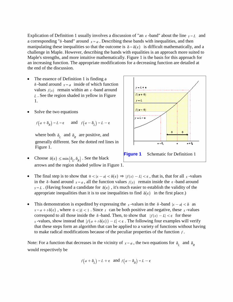
Explication of Definition 1 usually involves a discussion of "an -band" about the line and
a corresponding " -band" around . Describing these bands with inequalities, and then
manipulating these inequalities so that the outcome is is difficult mathematically, and a
challenge in Maple. However, describing the bands with equalities is an approach more suited to
Maple's strengths, and more intuitive mathematically. Figure 1 is the basis for this approach for
an increasing function. The appropriate modifications for a decreasing function are detailed at
the end of the discussion.
The essence of Definition 1 is finding a
-band around inside of which function
values remain within an -band around
. See the region shaded in yellow in Figure
1.
Solve the two equations
and
where both and are positive, and
generally different. See the dotted red lines in
Figure 1.
Choose . See the black
arrows and the region shaded yellow in Figure 1.
The final step is to show that ⇒ , that is, that for all -values
in the -band around , all the function values remain inside the -band around
. (Having found a candidate for , it's much easier to establish the validity of the
appropriate inequalities than it is to use inequalities to find in the first place.)
This demonstration is expedited by expressing the -values in the -band as
, where . Since can be both positive and negative, these -values
correspond to all those inside the -band. Then, to show that for these
-values, show instead that . The following four examples will verify
that these steps form an algorithm that can be applied to a variety of functions without having
to make radical modifications because of the peculiar properties of the function .
Note: For a function that decreases in the vicinity of , the two equations for and
would respectively be
and
Figure 1 Schematic for Definition 1
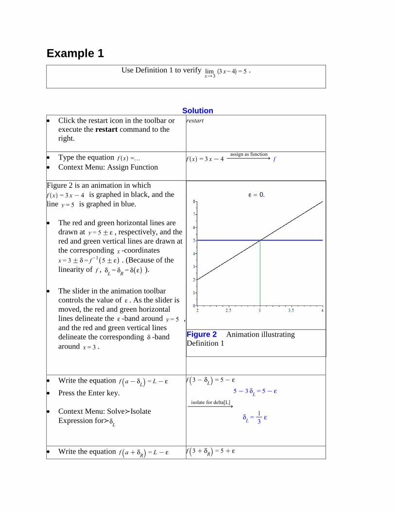
Example 1
Use Definition 1 to verify .
Solution
Click the restart icon in the toolbar or
execute the restart command to the
right.
Type the equation
Context Menu: Assign Function
Figure 2 is an animation in which
is graphed in black, and the
line is graphed in blue.
The red and green horizontal lines are
drawn at , respectively, and the
red and green vertical lines are drawn at
the corresponding -coordinates
. (Because of the
linearity of , ).
The slider in the animation toolbar
controls the value of . As the slider is
moved, the red and green horizontal
lines delineate the -band around ,
and the red and green vertical lines
delineate the corresponding -band
around .
Figure 2 Animation illustrating
Definition 1
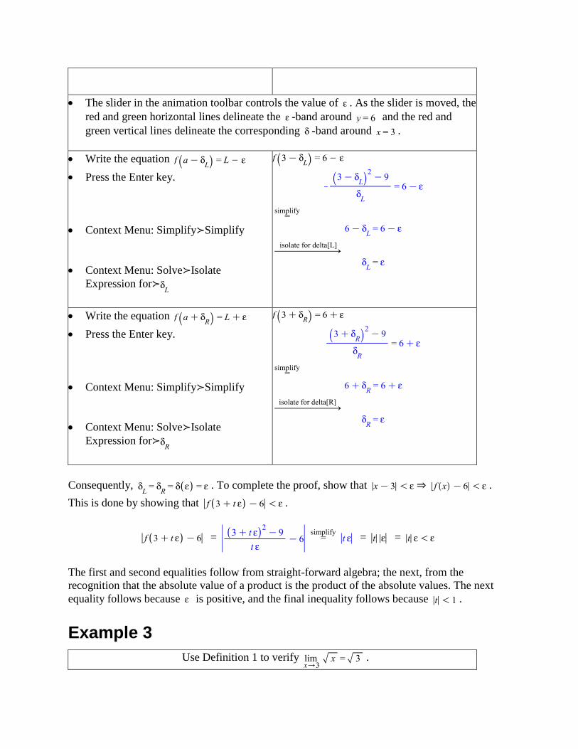
Write the equation
Press the Enter key.
Context Menu: Solve≻Isolate
Expression for≻
Write the equation
Press the Enter key.
Context Menu: Solve≻Isolate
Expression for≻
Consequently, . To complete the proof, show that ⇒
. This is done by showing that .
= =
The first equality follows from straight-forward algebra, and the second from the recognition that
the absolute value of a product is the product of the absolute values. The next equality follows
because is positive, and the final inequality follows because .
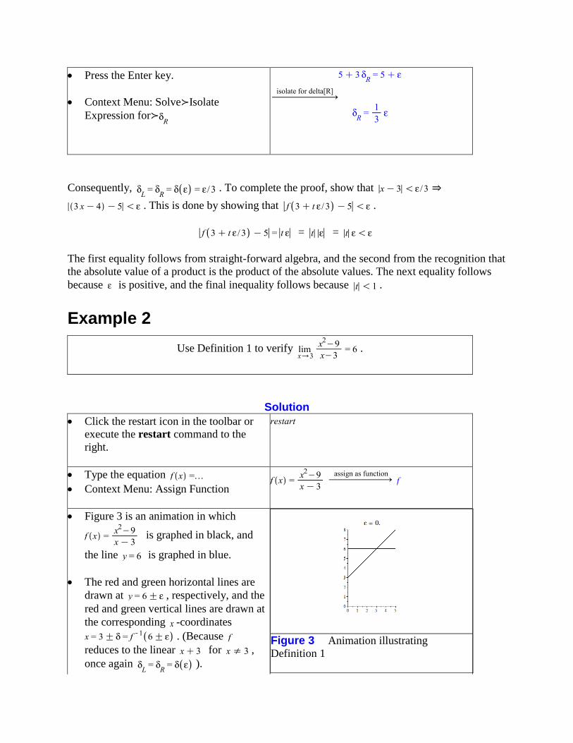
Example 2
Use Definition 1 to verify .
Solution
Click the restart icon in the toolbar or
execute the restart command to the
right.
Type the equation
Context Menu: Assign Function
Figure 3 is an animation in which
is graphed in black, and
the line is graphed in blue.
The red and green horizontal lines are
drawn at , respectively, and the
red and green vertical lines are drawn at
the corresponding -coordinates
. (Because
reduces to the linear for ,
once again ).
Figure 3 Animation illustrating
Definition 1
The slider in the animation toolbar controls the value of . As the slider is moved, the
red and green horizontal lines delineate the -band around and the red and
green vertical lines delineate the corresponding -band around .
Write the equation
Press the Enter key.
Context Menu: Simplify≻Simplify
Context Menu: Solve≻Isolate
Expression for≻
Write the equation
Press the Enter key.
Context Menu: Simplify≻Simplify
Context Menu: Solve≻Isolate
Expression for≻
Consequently, . To complete the proof, show that ⇒ .
This is done by showing that .
= = =
The first and second equalities follow from straight-forward algebra; the next, from the
recognition that the absolute value of a product is the product of the absolute values. The next
equality follows because is positive, and the final inequality follows because .
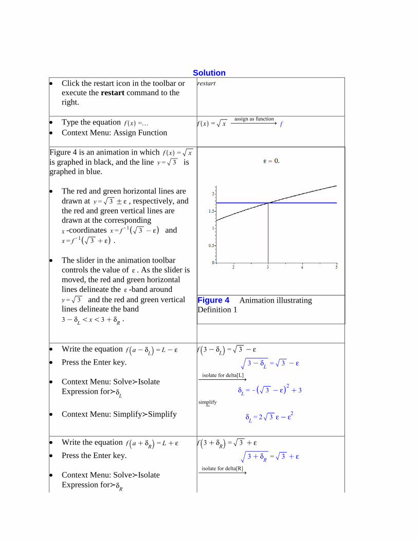
Example 3
Use Definition 1 to verify .
Solution
Click the restart icon in the toolbar or
execute the restart command to the
right.
Type the equation
Context Menu: Assign Function
Figure 4 is an animation in which
is graphed in black, and the line is
graphed in blue.
The red and green horizontal lines are
drawn at , respectively, and
the red and green vertical lines are
drawn at the corresponding
-coordinates and
.
The slider in the animation toolbar
controls the value of . As the slider is
moved, the red and green horizontal
lines delineate the -band around
and the red and green vertical
lines delineate the band
.
Figure 4 Animation illustrating
Definition 1
Write the equation
Press the Enter key.
Context Menu: Solve≻Isolate
Expression for≻
Context Menu: Simplify≻Simplify
Write the equation
Press the Enter key.
Context Menu: Solve≻Isolate
Expression for≻
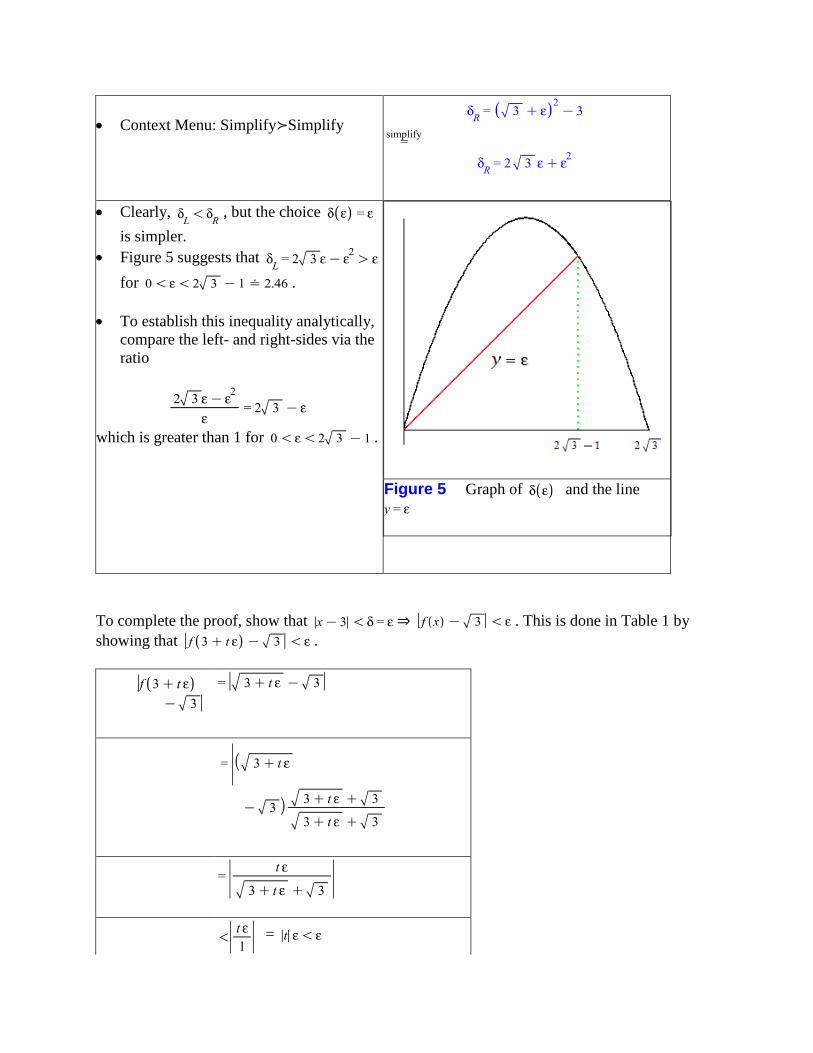
Context Menu: Simplify≻Simplify
Clearly, , but the choice
is simpler.
Figure 5 suggests that
for .
To establish this inequality analytically,
compare the left- and right-sides via the
ratio
which is greater than 1 for .
Figure 5 Graph of and the line
To complete the proof, show that ⇒ . This is done in Table 1 by
showing that .
=
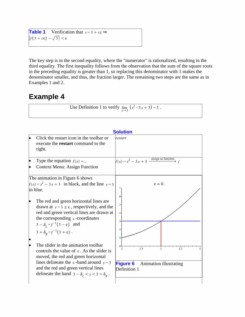
Table 1 Verification that ⇒
The key step is in the second equality, where the "numerator" is rationalized, resulting in the
third equality. The first inequality follows from the observation that the sum of the square roots
in the preceding equality is greater than 1, so replacing this denominator with 1 makes the
denominator smaller, and thus, the fraction larger. The remaining two steps are the same as in
Examples 1 and 2.
Example 4
Use Definition 1 to verify .
Solution
Click the restart icon in the toolbar or
execute the restart command to the
right.
Type the equation
Context Menu: Assign Function
The animation in Figure 6 shows
in black, and the line
in blue.
The red and green horizontal lines are
drawn at , respectively, and the
red and green vertical lines are drawn at
the corresponding -coordinates
and
.
The slider in the animation toolbar
controls the value of . As the slider is
moved, the red and green horizontal
lines delineate the -band around
and the red and green vertical lines
delineate the band .
Figure 6 Animation illustrating
Definition 1
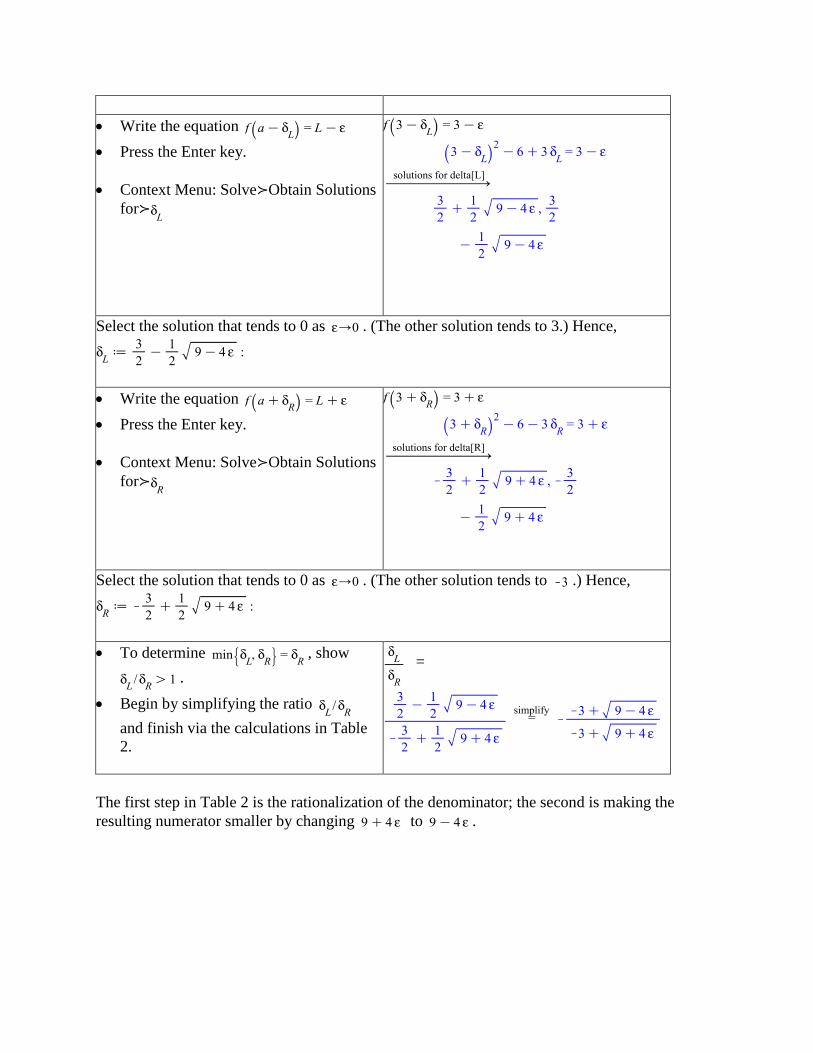
Write the equation
Press the Enter key.
Context Menu: Solve≻Obtain Solutions
for≻
Select the solution that tends to 0 as . (The other solution tends to 3.) Hence,
Write the equation
Press the Enter key.
Context Menu: Solve≻Obtain Solutions
for≻
Select the solution that tends to 0 as . (The other solution tends to .) Hence,
To determine , show
.
Begin by simplifying the ratio
and finish via the calculations in Table
2.
=
The first step in Table 2 is the rationalization of the denominator; the second is making the
resulting numerator smaller by changing to .
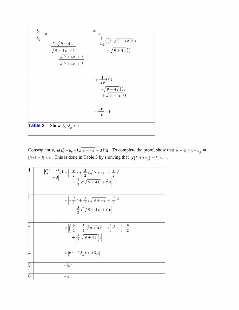
=
=
Table 2 Show
Consequently, . To complete the proof, show that ⇒
. This is done in Table 3 by showing that .
1
2
3
4
5
6
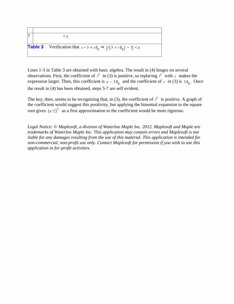
7
Table 3 Verification that ⇒
Lines 1-3 in Table 3 are obtained with basic algebra. The result in (4) hinges on several
observations. First, the coefficient of in (3) is positive, so replacing with makes the
expression larger. Then, this coefficient is and the coefficient of in (3) is . Once
the result in (4) has been obtained, steps 5-7 are self evident.
The key, then, seems to be recognizing that, in (3), the coefficient of is positive. A graph of
the coefficient would suggest this positivity, but applying the binomial expansion to the square
root gives as a first approximation to the coefficient would be more rigorous.
Legal Notice: © Maplesoft, a division of Waterloo Maple Inc. 2012. Maplesoft and Maple are
trademarks of Waterloo Maple Inc. This application may contain errors and Maplesoft is not
liable for any damages resulting from the use of this material. This application is intended for
non-commercial, non-profit use only. Contact Maplesoft for permission if you wish to use this
application in for-profit activities.