classification of asteroid spectra using a neural network · classification of asteroid spectra...

JOURNAL OF GEOPHYSICAL RESEARCH, VOL. 99, NO. E5, PAGES 10,847-10,865, MAY 25, 1994

Classification of asteroid spectra using a neural network

E. S. Howell, E. Mer6nyi, and L. A. Lebofsky

Lunar and Planetary Laboratory, University of Arizona, Tucson

Abstract. The 52-color asteroid survey (Bell et al., 1988) together with the 8-color asteroid survey (Zellner et al., 1985) provide a data set of asteroid spectra spanning 0.3-2.5 pm. An artificial neural network clusters these asteroid spectra based on their similarity to each other. We have also trained the neural network with a categorization learning output layer in a supervised mode to associate the established clusters with taxonomic classes. Results of our classification agree with Tholen's classification based on the 8-color data alone. When extending the spectral range using the 52-color survey data, we find that some modification of the Tholen classes is indicated to produce a cleaner, self-consistent set of taxonomic classes. After supervised training using our modified classes, the network correctly classifies both the training examples, and additional spectra into the correct class with an average of 90% accuracy. Our classification supports the separation of the K class from the S class, as suggested by Bell et al. (1987), based on the near-infrared spectrum. We define two end-member subclasses which seem to have compositional significance within the S class: the So class, which is olivine-rich and red, and the Sp class, which is pyroxene-rich and less red. The remaining S-class asteroids have intermediate compositions of both olivine and pyroxene and moderately red continua. The network clustering suggests some additional structure within the E-, M-, and P-class asteroids, even in the absence of albedo information, which is the only discriminant between these in the Tholen classification. New relationships are seen between the C class and related G, B, and F classes. However, in both cases, the number of spectra is too small to interpret or determine the significance of these separations.

Introduction

The first step to understanding the relationships within a group of diverse objects is to classify them according to their physical characteristics. Many re- searchers have classified asteroids based on various cri-

teria. Tholen and Barucci [1989] have recently presented a comprehensive review of the various taxonomies that have been put forth. These taxonomies are all based on similarities in the reflectance spectra and in some cases the albedos of the objects. The spectrum is related to the surface composition, so any taxonomy based on these data is at least in some way related to the surface composition of the asteroid. However, many asteroid spectra do not have unique compositional interpretations.

What is striking about the many different systems of classification is not so much the differences, but the similarities. The same general groupings appear regard- less of the parameterization chosen. These similarities

Copyright 1994 by the American Geophysical Union.

Paper number 93JE03575. 0148- 0227 / 94 / 93J E-03575505.00

indicate that these are real divisions among the objects manifested in different ways, not artifacts of the parameterization. However, it is important to remember that in different wavelength ranges, spectral differences may result from a single compositional element, and possibly only a minor constituent of the asteroid.

While a taxonomic system is a useful first step in understanding the overall structure of the asteroid belt, it necessarily does not include all the information we have available. In the formal classification, we must limit ourselves to the data that are available for all of the

objects considered. Thus, interpretation of this or any asteroid taxonomy should also consider any additional pieces of information that were not included in deriving the taxonomy itself.

Compositional structure seen in the asteroid belt re- flects not only compositional gradients in the the solar nebula, but also subsequent processing over the age of the solar system. While it is clear that most of these objects are closer to their pristine state than the larger planets, they may still be sufficiently altered to make determination of solar nebula conditions difficult. How-

ever, learning about the alteration mechanisms may be equally valuable. A great success of Tholen's asteroid taxonomy is the clear indication of differences in

10,847

10,848 HOWELL ET AL.: CLASSIFICATION OF ASTEROID SPECTRA

the distribution of different asteroid classes with helio-

centtic distance. However, subsequent work by Jones et al. [1990] shows that significant effects of later heat- ing events are also present and also have a strong dependence on heliocentric distance. Bell et al. [1989] discuss additional asteroid alteration processes which may also have a spatial dependence. In some cases it may not be possible to distinguish between formation processes and those attributable to later events.

In this paper we describe the application of an artificial neural network (ANN) for the classification of asteroid spectra, and present an augmented asteroid taxonomy using that technique. First, previous taxonomic systems are briefly reviewed and the Tholen taxonomy is described, since our system extends his system by using additional spectral information. We briefly describe the data that were used for our classification

of the asteroids. To compare the neural network technique to the minimum tree classification method that Tholen used, we use the same 8-color data that Tholen used for his analysis. Then we apply the neural network technique to the combined 8-color and 52-color data acquired by Bell et al. [1988], to take advantage of the larg•.r spectral range. The results and interpretation of the asteroid groupings are presented, followed by some notes on unusual objects and cases where our ANN classification differs from that of Tholen.

Previous Taxonomies

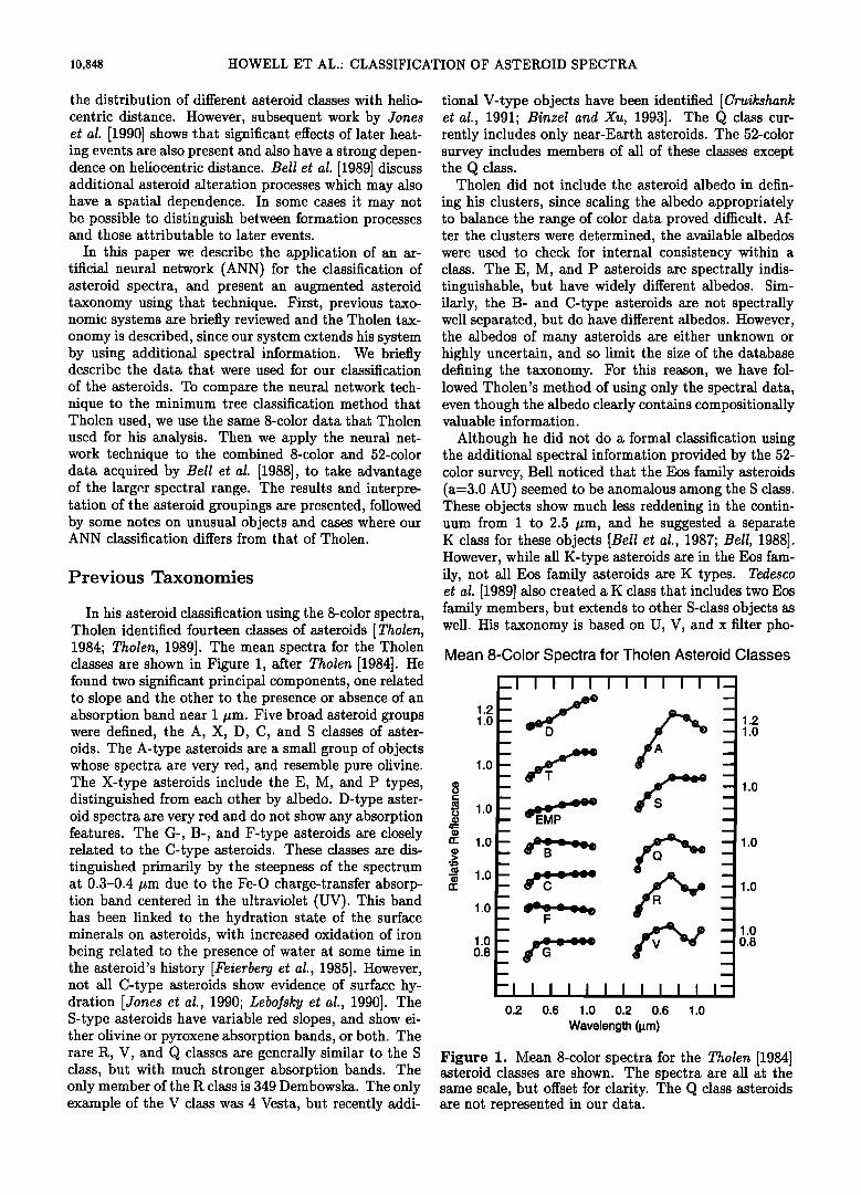
In his asteroid classification using the 8-color spectra, Tholen identified fourteen classes of asteroids [Tholen, 1984; Tholen, 1989]. The mean spectra for the Tholen classes are shown in Figure 1, after Tholen [1984]. He found two significant principal components, one related to slope and the other to the presence or absence of an absorption band near 1/•m. Five broad asteroid groups were defined, the A, X, D, C, and S classes of asteroids. The A-type asteroids are a small group of objects whose spectra are very red, and resemble pure olivine. The X-type asteroids include the E, M, and P types, distinguished from each other by albedo. D-type asteroid spectra are very red and do not show any absorption features. The G-, B-, and F-type asteroids are closely related to the C-type asteroids. These classes are distinguished primarily by the steepness of the spectrum at 0.3-0.4/•m due to the Fe-O charge-transfer absorption band centered in the ultraviolet (UV). This band has been linked to the hydration state of the surface minerals on asteroids, with increased oxidation of iron being related to the presence of water at some time in the asteroid's history [Feierberg et al., 1985]. However, not all C-type asteroids show evidence of surface hydration [Jones et al., 1990; Lebofsky et al., 1990]. The S-type asteroids have variable red slopes, and show either olivine or pyroxene absorption bands, or both. The rare R, V, and Q classes are generally similar to the S class, but with much stronger absorption bands. The only member of the R class is 349 Dembowska. The only example of the V class was 4 Vesta, but recently addi-

tional V-type objects have been identified [Cruikshank et al., 1991; Binzel and Xu, 1993]. The Q class currently includes only near-Earth asteroids. The 52-color survey includes members of all of these classes except the Q class.

Tholen did not include the asteroid albedo in defin-

ing his clusters, since scaling the albedo appropriately to balance the range of color data proved difficult. Af- ter the clusters were determined, the available albedos were used to check for internal consistency within a class. The E, M, and P asteroids are spectrally indistinguishable, but have widely different albedos. Sim- ilarly, the B- and C-type asteroids are not spectrally well separated, but do have different albedos. However, the albedos of many asteroids are either unknown or highly uncertain, and so limit the size of the database defining the taxonomy. For this reason, we have followed Tholen's method of using only the spectral data, even though the albedo clearly contains compositionally valuable information.

Although he did not do a formal classification using the additional spectral information provided by the 52- color survey, Bell noticed that the Eos family asteroids (a-3.0 AU) seemed to be anomalous among the S class. These objects show much less reddening in the continuum from 1 to 2.5 /•m, and he suggested a separate K class for these objects [Bell et al., 1987; Bell, 1988]. However, while all K-type asteroids are in the Eos family, not all Eos family asteroids are K types. Tedesco et al. [1989] also created a K class that includes two Eos family members, but extends to other S-class objects as well. His taxonomy is based on U, V, and x filter pho-

Mean 8-Color Spectra for Tholen Asteroid Classes

_1 I I I I I I I I I I I--

1.0

• • 1.0 • 1.0 EM• m 1.0- • - 1.0

• 1.0 •: ::• 1.0 1.0

1.0 0.8

0.2 0.6 1.0 0.2 0.6 1.0

Wavelength (!zm)

1.0 0.8

Figure 1. Mean 8-color spectra for the T,5olen [1984] asteroid classes are shown. The spectra are all at the same scale, but offset for clarity. The Q class asteroids are not represented in our data.

HOWELL ET AL.: CLASSIFICATION OF ASTEROID SPECTRA 10,849

tometry (with central wavelengths of 0.365, 0.550, and 0.701 /•m, respectively) and the IRAS albedo, and did not include any near-infrared data. In fact, the K class as defined by Bell is a subset of the Tedesco et al. K class, in spite of the differences in the defining spectral parameters.

Burbine [1991] performed a principal components transformation using the 52-color survey data combined with the 8-color data. He found five significant principal components. The first is correlated with the overall slope of the spectrum. The second is correlated with the depth of the 1-/•m absorption band, consistent with the first two principal components in the 8-color analysis [Tholen, 1984]. The third is correlated with the depths of both the 1- and 2-/•m absorption bands for most objects, separating olivine-rich objects from pyroxene-rich objects. The fourth and fifth do not have a clear interpretation, but each contain only 2.2% of the total variance. He found that the Tholen groups remained distinct, and did not change or augment that taxonomy. However, it is important to note that Burbine did not do an independent classification, but only tried the Tholen groupings and found them adequate. He used only 66 of the highest quality spectra for his principal component analysis, and did not have all taxonomic classes represented.

The majority of the 52-color survey asteroids are S class. There is considerable diversity in the spectral appearance of these objects, especially between 0.8 and 2.5/•m. However, in the visual range there is also great diversity, and many workers have suggested that subdivisions among the S-type asteroids may be appropriate. Chapman [1987] suggested a division into several groups based on the U-B and B-V colors. These were not selected as natural divisions among the objects, but as convenient, unambiguous divisions of the group into seven subgroups. Gaffey et al. [1993] parameterized the spectra using the pyroxene band positions and depths to measure pyroxene composition and olivine/pyroxene ratio. These measures were correlated with meteorite

compositions in an attempt to determine which asteroids might be likely parent bodies of ordinary chondrites. Barucci et al. [1987] combined the 8-color photometry and IRAS albedos and classified 438 asteroids using G-mode analysis. They obtain four subclasses of Tholen's S-type asteroids, though the majority of the objects are of the first or SO class. We compare our division of the S-type asteroids with these other groupings in a later section.

The Data

The data upon which most asteroid classification systems have been based are reflectance spectra. The two surveys which we have used, the 8-color survey and the 52-color survey, have been described in detail by Zell- her et al. [1985] and Bell et al. [1988], respectively. We will briefly summarize these data here, and describe the modifications that were made before entering these data into the neural network.

The taxonomy developed by Tholen is based on the 8-color asteroid survey, which remains unchallenged as the most complete sampling of the asteroid belt to date. The 8-color spectrophotometry spanned 0.3-1.1 •um for most of the 589 asteroids surveyed. A large range of heliocentric distances was sampled, including groups such as the Hildas (3.9 AU) and the Trojans (5.2 AU). The data are given as magnitudes relative to the Sun, represented by a mean of four solar analog stars. The spectra are normalized to 0.0 magnitude at 0.55 •um. Typical errors are 1-3%, larger in a few cases. Tholen used 405 of the 589 objects, representing the highest quality spectra for his cluster analysis. We omitted 50 of the 589 asteroids which had only five of the eight colors measured, but did not exclude any on the basis of large errors. Since the formation of the cluster structure determined by the neural network is less sensitive to noise in the data than many classical methods, these two classifications are comparable.

Bell et al. [1988] carried out a smaller-scale asteroid survey covering 0.8-2.5 /•m for 117 asteroids chosen to represent all of the established Tholen classes. A circularly variable filter with 3.5%-5.2% spectral resolution was used to obtain 52-color spectrophotometry. They found that the S-type asteroids showed considerable variability in the pyroxene and olivine absorption bands in the near infrared, and changed their observing strategy to include more of these objects; thus 59 of the 117 objects are members of Tholen's S class.

We extended the 52-color data to 0.34/•m by adding Tholen's 8-color photomerry, matching the spectra in the region of overlap. Bell et al. reported relative reflectance values, so for consistency, we converted the Tholen magnitude values to relative reflectance, scaled to 1.0 at 0.55 •um. These quantities are related by

M - -2.5 log10(F )

where M is magnitude and F is flux, or in this case where it has been divided by the solar analog flux value, relative reflectance.

The 52-color spectra were taken in two sections with different spectral sampling. For convenience, we resam- pied these data at a uniform spacing throughout the spectral range. Seventeen asteroids did not have 8-color photomerry available, but 12 of those had UBV photometry reported [Tedesco, 1989], and Tholen classifications [Tholen, 1989]. Using solar colors from Hardorp [1980], we converted these data to reflectance, and used a cubic spline to produce 0.34- to 0.8-/•m data consistent with the other objects for which 8-color photometry was available. The interpolations were checked care- fully to guard against artifacts produced by the cubic spline. We used 65 points from 0.34 to 2.57 •um, spaced at 0.035 •um, as the input data to the neural network. Hence we will refer to these modified spectra as the 65- color spectra. Gaps due to telluric water absorption at 1.4 and 1.9 •um are also closed in this manner. Since the spline sampling is comparable to the original spectral resolution of the data in most of the range, the noise variability is reproduced by the spline with only

lO,85o HOWELL ET AL.: CLASSIFICATION OF ASTEROID SPECTRA

minimal smoothing. The errors are not explicitly used by the neural network. A classification using only the 52-color data in its original form showed little difference from the version based on resampled data, giving confidence that this treatment did not affect the results.

During the 52-color survey, several asteroids were observed on two or more different nights. These spectra were examined individually, and in those cases where the spectra were nearly identical, they were averaged to improve the signal-to-noise ratio. When the spectra were sufficiently different, they were not averaged, and two versions were retained. We define significantly different as point to point differences of more than two sigma for three or more adjacent points. Two spectra of 367 Amicitia showed significant variation, but since no visible data were available for this object, it was not included in either classification. There were four separate spectra of 43 Ariadne with two distinct shapes. Each pair was averaged, but the two differently shaped spectra were retained. Altogether, 20 objects were observed on two or more nights, and six of those showed spectral variation. These differences may be due to surface inhomogeneity, but could also be due to lightcurve variations during the time necessary to obtain the spectrum. Other sources of observational or instrumental

errors are also possible, though we feel they are less likely. Additional observations of these asteroids would be especially valuable to resolve this issue.

Artificial Neural Networks

The human eye and brain are extremely efficient at pattern recognition compared to traditional image processing algorithms. Ideally, to classify groups of spectra into generalized groups, we would like to look at and evaluate each example. However, as databases get large, this is not a practical technique, nor are we able to be unbiased in our view of the data. We tend to see

the features we can interpret as dominating the spectrum, and to ignore those features which we cannot interpret. Over the last decade, ANNs have been shown to excel in the field of pattern recognition and classification [Mer•nyi et al., 1993a; Mer•nyi et al., 1993b; Huang and Lippman, 1987]. They are able to handle large data sets easily and quickly. A very good review on ANNs is given by Pao [1989].

ANNs are massively parallel, finely distributed computing architectures that mimic the information processing of the nervous system in a simplified way. They consist of a large number of artificial neurons, or processing elements (PEs) as shown in Figure 2. These simple PEs are (usually) identical, and are densely wired into a net-like structure with weighted connections. This net structure is typically organized into one input, one output, and one or more hidden layers. An example for an ANN architecture is illustrated in Figure 3. PEs in one layer can be connected to any PE in other layers. For the networks in this study, all PEs in a given layer are connected to all PEs in the subsequent layer. At any time step, each PE in each

Xo I = Y'i Wji Xi summation x. 1 • yj= f(I) transfer

o

Weiglts Y'

Xr/ element

Figure 2. The structure of a processing element, the building block of neural networks, is shown. Each processing element computes the weighted sum of its in- puts. The weights, Wi, are adjusted during the learning process. The output of the processing element is a function, called the transfer function, of this sum. In general, the transfer function is a nonlinear function. Reproduced with permission from NeuralWare, Inc. [1991].

layer receives signals from its input connections. For example, at the ;_spur layer, each PE will receive the weighted sum of all the spectral channels of a given spectrum. This weighted sum is transformed by the so- called transfer function, which is generally a nonlinear function (e.g., sigmoid, hyperbolic tangent, or similar function). The result is sent to the PE's output connections, which in turn will be input to the PEs in the next layer. The data are driven through the network in this fashion and finally an output vector is presented at the top layer. For example, this vector can represent the labels of different classes, encoded in the form of

Output t t t buffer Hidden ( Ioyer

Inpuf

buffer Figure 3. A sample artificial neural network interconnection pattern is shown. The circles represent processing elements (PEs). Data flow from bottom to top. In this example, each element of the hidden layer receives input from each data channel in the input buffer. Similarly, each element of the output buffer receives input from all elements of the hidden layer. The dense interconnectivity gives the network its computational flexibility. The interconnection pattern between PEs is one of the main characteristics of a particular neural network paradigm. Reproduced with permission from NeuralWare, Inc. [1991].


binary vectors (class A = 1, 0, ..., 0; class B = 0, 1, ..., 0, etc.).

In supervised training, ANNs learn to derive the characteristics of a group of spectra (a class) from a subset of that group for which the class memberships (the class labels) are known. The collection of such subsets for all classes is the training set, and the spectra in this set are called the training spectra. These patterns are presented many times to the network along with their known class labels. For a given pattern, the network compares its own actual output with the known class label (this latter is the "desired output" in neural net terminology). Based on the difference between the actual and desired output, the weights throughout the entire network are then adjusted so that next time the actual output more closely approximates the desired output (the correct class label) for this pattern. The adjustment procedure is prescribed by the so-called learning rule. If the training samples are consistent, the training will converge after some number of iterations, i.e., the weights will no longer change significantly. At this point, the network is trained, which means that it will give the correct label for the training patterns, and it can make predictions for patterns that were not included in the training set. An inconsistent set of training samples can prevent convergence of the training. In some cases, the network may be able to learn inconsistent labels, but then it will not be able to make good predictions for unknown patterns based on that knowl- edge.

ANNs are proven to be more robust and less sensitive to noise than most conventional methods. Their

capability to learn relationships from samples of under- represented or unevenly represented classes, and learn complicated (e.g., nonlinear, embedded) class boundaries is superior to most standard techniques [Huang and Lippman, 1987]. The massively parallel and distributed architecture offers dramatically increased computing speed, often with significantly reduced memory requirements compared to conventional sequential com- puters. The numerous ANN paradigms developed for various problems differ mainly in the connection pattern among the PEs, the transfer function and the learning rule.

Our Classification Method

The ANN paradigm employed here is a hybrid network. Its hidden layer is a two-dimensional self- organizing map (SOM) developed by Kohonen [1988], which is coupled with a categorization learning output layer. These two layers have different learning rules. The mathematical formulae for self-organization as well as for the Widrow-Hoff learning rule of the output layer can be found in the work by, e.g., Pao [1989]. The particular software implementation that we used is from NeuralWare, Inc. [1991]. The layout is shown in Fig- ure 4. This ANN performs classification in two phases. First, in unsupervised mode, it forms a topologically or- dered map of the input patterns in the two-dimensional

(2-D) hidden layer (the Kohonen layer), based on their similarity to each other. Each PE becomes a representative of several input patterns: very similar patterns will be mapped onto the same PE or PEs that are close to each other in terms of their input connection weights. The similarity measure in this case is the Euclidean distance, but could be different if so dictated by the characteristics of the data. The minimum tree algorithm used by Tholen also uses the Euclidean distance as the similarity measure. This topological map, together with the Euclidean distances between the PEs in terms of their weights, yield information about the cluster structure of the data as explained below. No a priori assumption on the number, size, or center of the clusters is used. The output layer is not learning during the unsupervised phase. After the unsupervised training has converged (no more significant changes occur in the weights), we switch to the supervised phase and train the output layer to associate the previously clustered patterns into the classes that are thought to be meaningful. As we mentioned above, the network will have difficulty if we try to teach class labels that are in contradiction with the cluster structure it has

formed. Decisions about meaningful classes are based on initial assumptions about taxonomic classes, and in some cases additional data, such as albedo and a pos- teriori interpretations of clusters that the network may suggest (as was the case with the subclasses of the S asteroids).

The 2-D Kohonen layer maps the n-dimensional data space nonlinearly onto a 2-D lattice, with the preser- vation of the topology, i.e., the similarity relationship among input patterns. Unlike principal component plots, which only present 2-D or three-dimensional (3-D) projections of the data, the Kohonen map fully represents the n-D data space in 2-D, in terms of the ordering of the patterns based on similarity. The information about possible cluster separations lies in the PE weights. After appropriate analysis, separations can be defined and overlain on this 2-D topological map in the form of fences, the height of which represents the degree of separation between PEs. Ultsch and Simeon [1990] describe a successful approach to the analysis of the Ko- honen map and representation of cluster separations by these fences. We used their technique with some mi- nor modification. For example, in Figure 5a, the fences derived from the PE weights are superimposed on the Kohonen map, a wider line indicating a stronger separation, or higher fence. Further development of this method is in progress and a more detailed discussion will be given in a subsequent paper (E. Mer•nyi et al., manuscript in preparation, 1994). The fences determined at this stage should be considered preliminary. Naturally, these class boundaries are not rigid and can change if more objects are used in the network clustering. An advantage of this ANN paradigm is that training time is modest, so the classification can be easily revised as more spectra are obtained. Once trained, the network identifies unknown patterns very quickly and easily.

1o,852 HOWELL ET AL.: CLASSIFICATION OF ASTEROID SPECTRA

SOM u/C trained on 65 p. data• s65o15• 20+10K 6/7/91

Figure 4. The layout of the Kohonen self-organizing map, coupled with a categorization learning output layer is shown. The bottom layer is the input data. The center square is the 2-D hidden layer, or Kohonen map. The output layer is shown at the top. Each processing element (PE) in the input (bottom) layer is connected to all PEs in the 2-D Kohonen layer. All PEs in the Kohonen layer are connected to each of the output PEs. For illustration, the input connections to one Kohonen PE and the connections of two Kohonen PEs to the output (top) layer are drawn here. Reproduced with permission from screen graphics, (• NeuralWare, Inc.

In the application of this ANN paradigm to asteroid classification, we assumed the Tholen [1989] classes were a good first estimate of the class membership of most asteroids. The network is initially trained using all of the spectra with their Tholen class labels. Later, subsets of the available data are used, with some examples set aside as "unknowns" to check the network's abil-

ity to generalize from the examples it has seen. These jackknifing tests are described in more detail in a later section. We turned to the examination of the Kohonen

map when the network had difficulty learning the membership of certain objects. It is important to emphasize that the cluster structure is defined by the data in the unsupervised training phase and is not changed in the supervised phase. The network only learns to assign class labels to previously defined areas of the cluster structure during training. If the labels it is taught are too sparse or contradictory, it will not learn to identify the class, and/or it will misclassify patterns which were not included in the training set.

Results and Discussion The 8-Color Classification

We used the neural network to classify asteroids first using.the 8-color spectra alone, and then combining the

8-color and 52-color surveys into a 65-color resampled spectrum. We first make a direct comparison of our classification and Tholen's. The two are based on the

same data, although we used a larger subset of the 8- color data for our classification, including some lower signal-to-noise spectra. Even though the two classification techniques are very different, the similarity measures are the same. Although the cluster structure is determined differently, we obtain very similar results, giving us confidence in the technique. We then apply the neural network technique to the additional spectral information in the 65-color spectra. We discuss the classification results, and present suggestions for modifications to the Tholen taxonomic system.

The Kohonen SOM in Figure 5a shows the cluster structure determined from the neural network, using only the 8-color data. For comparison, Figure 5b shows Tholen's principal component analysis (PCA) with the clusters determined using the minimum tree algorithm. The heavy lines on the SOM indicate the degree of separation, or fence height between the PEs, heavier lines representing higher fences. Although most of the asteroids in our 8-color classification agree with their Tholen class labels, there are some that do not, even though the two techniques used the same data and the same

HOWELL ET AL.' CLASSIFICATION OF ASTEROID SPECTRA 10,853

15

14

13

12

11

10

8

7

6

4

2

a b c d e f g h i j k 1 rn n o

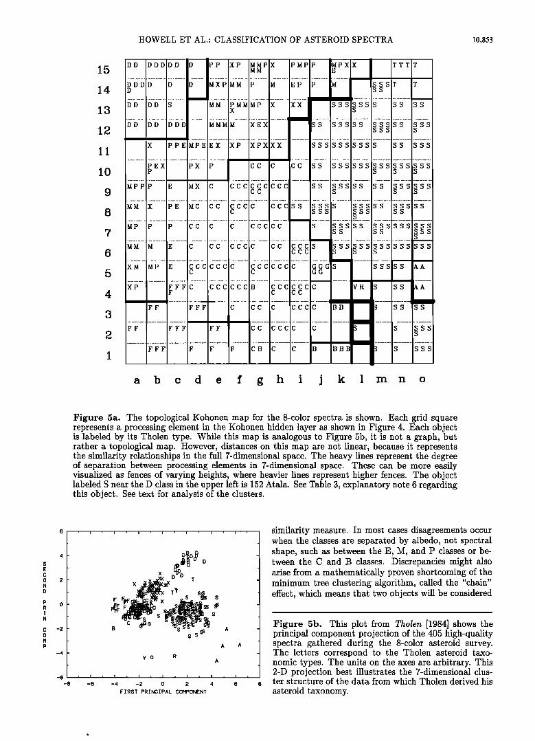
Figure 5a. The topological Kohonen map for the 8-color spectra is shown. Each grid square represents a processing element in the Kohonen hidden layer as shown in Figure 4. Each object is labeled by its Tholen type. While this map is analogous to Figure 5b, it is not a graph, but rather a topological map. However, distances on this map are not linear, because it represents the similarity relationships in the full 7-dimensional space. The heavy lines represent the degree of separation between processing elements in 7-dimensional space. These can be more easily visualized as fences of varying heights, where heavier lines represent higher fences. The object labeled S near the D class in the upper left is 152 Atala. See Table 3, explanatory note 6 regarding this object. See text for analysis of the clusters.

-2

-4

$ $

v o R

• • t • I • I ,, I

-4 -2 0 2 4

FIRST PRINCIPAL COMPONENT

I

similarity measure. In most cases disagreements occur when the classes are separated by albedo, not spectral shape, such as between the E, M, and P classes or between the C and B classes. Discrepancies might also arise from a mathematically proven shortcoming of the minimum tree clustering algorithm, called the "chain" effect, which means that two objects will be considered

Figure 5b. This plot from Tholen [1984] shows the principal component projection of the 405 high-quality spectra gathered during the 8-color asteroid survey. The letters correspond to the Tholen asteroid taxonomic types. The units on the axes are arbitrary. This 2-D projection best illustrates the 7-dimensional cluster structure of the data from which Tholen derived his

asteroid taxonomy.


close if a short chain exists between them. The defini-

tion of a short chain is the length of the longest link in the chain that leads from one object to the other, through any number of objects. Therefore, two objects that are connected by a large •number of short links, may be put in the same cluster even if they are far apart. A complete and rigorous discussion of this can be found in the work by Fu [1976]. Tholen used the distance of an object from identified cluster centers as well as the chain length between up to three objects in the minimum tree to reduce this problem.

In general, the relationships of the groups to each other in both the Tholen PCA and the Kohonen SOM

(Figures 5a and 5b) are the same. For ease in refer- ring to the SOM, the grid of PEs are labeled on the axes. These should not be interpreted as representing variables, but rather as analogous to cartographic grid labels. The olivine-rich A-type asteroids are a very distinct group in both systems. The C-type asteroids are a diverse group in both systems. The G-type asteroids are a well-defined subgroup in the SOM at j5, as well as in the PCA. The F-type asteroids are also separated from the C-type objects, but less tightly clustered. In the SOM there are some divisions between the F-type asteroids. The B-type asteroids are only partly separated from the C-type asteroids in spectral appearance (note objects at g4 and gl), but are higher in albedo. The D-type asteroids in the upper left corner are well separated in both systems. In the SOM, there is an additional separation of two main belt D-type asteroids in PEs dl4 and d15. The T-type asteroids seem transi- tional between the D- and S-type objects in the PCA. In the SOM, they are more closely related to the S types, and are not strongly separated. Asteroid 570 Kythera at n14, is weakly separated from the other T-type objects. The S-type asteroids are also a very diverse group in both systems, although not divided by large distances as are the F types. There are some fences separating S objects such as at PEs k5 and 12. Asteroid ll5 Thyra, at k5, is also unusual in the 65-color classification. The iso- lated object at 12 is the near-Earth asteroid 1627 Ivar. The group of S objects near the A asteroids includes many of the objects designated So in the 52-color classification. The X-type asteroids, that is, the E, M, and P types, seem to show more diversity in the SOM than in the PCA. These objects are well separated from the S-type and D-type asteroids, but are not well separated from the C-type asteroids. The distinction between C- type and P-type asteroids is somewhat arbitrary, since it is based on the span of colors among the M-type objects. The SOM shows some indication that there is a division among X-type objects, one group in the upper right, and another in the lower left. This possibility will be considered in a later section.

The 65-Color Classification

When we add more spectral information, we expect that the cluster structure might be different. How- ever, as Burbine found when performing a PCA on the combined 8-color and 52-color survey data, the Tholen

classes still seem to do a reasonable job. Plate 1 shows the SOM for the 65-color spectra, again with lines indicating the fence heights, and grid labels for ease of discussion. For clarification, the different classes are color coded. For any PE, there are fences both diagonally and horizontally between adjoining PEs, the heights of which are not necessarily related. For example, the So asteroid 354 Eleonora, at 113, is well separated from the PEs in all directions except diagonally to the lower left to k12 and j12. It is not strongly separated from the other So objects. The groupings are similar to the 8- color clusters with the additional spectral information being clearly most diagnostic for the S-type asteroids since the olivine and pyroxene bands are providing new compositional information. The diversity in the C-type asteroids and related G, B, and F types has decreased, while the diversity of the S types has increased when going from 8-color to 65-color spectra. This change is certainly due in part to the small number of samples of these asteroid types. The E-, M-, and P-type objects still show some groupings among themselves, but it is not clearly related to the patterns seen in the 8-color classification. Especially in the bottom right part of the map, the Cv objects are not well separated from the P-type objects, the multiple labels indicating con- tributions from both class types.

The S class. From examination of the 65-color

SOM (Plate 1), some internal groupings were appar- ent among the S-class asteroids. The same groupings were present when the neural network was trained on the S-type asteroids alone. We introduce two subgroups among the S-type asteroids. The So type, which are olivine-rich and reddest, and the Sp type, which are olivine-poor and least red. The remaining S types are intermediate in olivine content and continuum slope. In the SOM for the 65-color asteroids, the olivine-rich A-type asteroids are more similar to the So-type asteroids than to any other type, although a high fence surrounds the A class. This association confirms that

spectral similarity is correlated with composition in this case. It is important to note that these subdivisions do not necessarily represent natural divisions among the former S-class asteroids. That is, a continuum of compositions exists from So to S and from S to Sp. In our experiments, no misclassification ever occurred between So and Sp. With the division we report, no misclassification occurred between So and S or S and Sp. How- ever, moving these boundaries either toward or away from the extrema in the continuum slope-olivine space might produce equally clean subgroups. There are low fences separating some Sp objects, especially near h-j, 2-6. Given the small number of spectra, any groupings which appear well separated could instead be an artifact of this particular set of examples. The important point is the So and Sp subclasses define the ends of a broad continuum of the former S-class asteroids for future studies of compositionally different objects which may lead to finer divisions with clearer evolutionary interpretations.

HOWELL ET AL.- CLASSIFICATION OF ASTEROID SPECTRA 10,855

15

14

13

12

11

10

9

8

7

6

5

4

3

2

TSo

D

i

T T M T M

T M ' i P

, ,

' o

!P iCx i [ !cx icx i i ...... '

i ' i

a b c d e f g h i j k 1 rn n o

Plate 1. The topological map formed in the Kohonen layer, as in Figure 5a, for our 65-color (8-color combined with 52-color) asteroid spectra is shown. Objects are labeled with our modified types, and color coded for clarity. Distances on the map are nonlinear, even more so than in Figure 5a, due to the higher dimensionality of the data. The degree of separation in the 65-color space is denoted by lines or fences, where heavier lines represent higher fences. Analysis of the clusters is discussed extensively in the text.

The ordering of the S-type asteroids on the 65-color SOM indicates a trend in spectral shape, but is not useful in itself if we cannot interpret it. Visual inspection of the spectra indicates that the spectral slope was obviously a major factor in the grouping among the S-class asteroids. Figure 6a shows the V-J versus J-K colors for these S-type asteroids, where the effective wavelengths are 0.55, 1.25, and 2.2/•m for V, J, and K filters, respectively. The redness of the spectrum was clearly a factor in determining the cluster structure, but did not explain everything. Figure 6a indicates that the V-K color is diagnostic for these asteroids. Previously, Chapman suggested subdividing the S asteroids on the basis of U-B and B-V colors. (Central wavelengths for U and B filters are 0.365 and 0.44 ium, respectively.) However, there is no correlation between the UBV and

VJK colors for the S asteroids, so our groupings are not the same as Chapman's groups.

Barucci et al. [1987] subdivided the S-class asteroids based on spectral shape differences in the 8-color spectra. They designate their classes S0-S3, with most of the objects falling in the primary or SO class. This group includes the K-class objects. Three of our So objects are classed as S2 in the Barucci system. These objects have a steeper slope in the UV region than the main SO group, but are otherwise indistinguishable. Asteroid 115 Thyra, at 17, is the only example of the S1 group in the 65-color data. We classify this object as Sp, but it has an unusual blue spectral slope between 1.5 and 2.5 ium. Barucci's S1 asteroids are characterized by the lowest overall spectral slope, but the slope from 0.3 to 1.1 /•m may not be a good general predictor of slope

10,856 HOWELL ET AL.' CLASSIFICATION OF ASTEROID SPECTRA

1.6

1.5

S A•teroids -

-

.3 .4 .5 .6 .7 J-K

0 .5 1 1.5 2 2.5

Band II/Band I Area

1.1 S Asteroids [ - • ea 1.os ß • oO _

: i 1 a a -.:

o ,so ao ac• as

b osp .5 1 1.5 2 2.5

Band II/Band I Area

Quality IS Asteroids I -

0 0 0 - _ eSo -

1.6 osp

0 .5 1 1.5 2 2.5

2.2/'"'1"' F Higliest •ee ß

• • o •1.8 • oo o

Band II/Band I Area

Figure 6. (a) A color-color plot for the asteroids designated S-type by Tholen is shown [after Hartmann et al., 1982]. The broadband colors V-J and J-K, expressed in magnitudes, characterize the overall slope of the spectrum from the visible to the near infrared. The 1-or error bars are shown. The combined color, V-K, characterizes the differences between these three groups well. (b) After Gaffey et al. [1993], this figure illustrates a parameterization of the pyroxene and olivine absorption bands shown to be characteristic of the olivine fraction of the matic component (pyroxene plus olivine). Pyroxene has absorption bands near I /zm and 2 /zm, while olivine has a single absorption centered near 1.2/•m. The horizontal axis shows the 2-/•m to 1-/•m pyroxene band area ratio. The vertical axis shows the band center of the 1-/•m absorption band, due to pyroxene, olivine or a combination. The So and Sp groups are moderately well separated in this space, but the S group overlaps both. The error bar shown is the 1-or error in the vertical direction, but shows the median error in the horizontal direction. See text for discussion of the error determination. (c) Combining the color data in Figure 6a with the band area ratio from Figure 6b, the groups So, S, and Sp are well separated. This parameterization corresponds to the clusters determined by the neural network on the basis of spectral similarity. The So and S groups are separated primarily in spectral slope, while the S and Sp groups are better separated by band area ratio. The reflectance spectrum is related to the matic composition as well as the continuum slope, which may or may not be due to compositional differences. The error bar shown is the median error in the horizontal direction, and the 1-or error in the vertical direction. Three pairs of connected points are observations of the same object taken on different nights, which showed significant spectral differences. (d) Same as Figure 6c, but only those points with errors less than 1.5 times the median error are included. The connected pairs of points have been omitted, since they indicate asteroids which have large spectral variability. The horizontal error bar indicated is the new median error of the points included.

between 1 and 2.5/•m. We did not have any examples of objects classified by Barucci as S3.

To test the hypothesis that the ordering of the S- type asteroids was related to compositional differences, we followed the method of Gaffey et al. [1993]. They parameterize the 1- and 2-/•m absorption bands in a

way that is sensitive to the olivine/pyroxene ratio and pyroxene composition in laboratory samples and meteorites. Using the asteroid spectra, we calculated the 1-/zm band center wavelength, and 2-/zm band to band area ratio for these asteroids. The continuum was

estimated by generating a convex hull over the 0.7- to

HOWELL ET AL.- CLASSIFICATION OF ASTEROID SPECTRA 10,857

2.5-/•m region of the 65-color spectrum. The band area was then calculated numerically using the 65-color data values, without additional smoothing. Compared to the methods employed by Gaffey et al., these calculations are somewhat crude, but fall within the calculated errors of his values for the same asteroids. Figure 6b shows this compositional space for the So, S, and Sp asteroids excluding those for which the calculated errors were larger than the sizes of the different regions that Gaffey et al. outlined. The error bar on Figure 6b in the band area ratio is a median error. This error is

determined from the observational error for each point, and the estimated error from the continuum determi-

nation, but does not include a contribution from any wavelength uncertainty. The error in the continuum fit is based on formal propagation of the error in the line fit from two points, each of which is a mean of five adjacent data points. However, determining the continuum is difficult and based on subjective judgment, especially where the spectral coverage is limited. Because the continuum is often not easily determined for observational data, band areas may have very large uncertainties due to both noise and limited spectral coverage. The So and Sp groups are slightly separated in this space, but there is a complete overlap of the S group with both So and Sp groups. Figure 6c indicates that a combination of the band area ratio and the spectral slope matches the groupings formed by the neural network. The olivine- rich asteroids also tend to be the ones with very red continuum slope, and the olivine-poor objects tend to have less reddish slopes, but there is enough overlap that both parameters are necessary to explain the cluster structure. The V-K color is a good predictor of the group membership except for the transition region from S to Sp. In this region, the primary distinction is the band area ratio, which is a better indicator of pyroxene content. Since the olivine spectrum is very steep from 0.55 to 2 /•m, the color alone is a sensitive measure of the olivine contribution to the spectrum for these asteroids. The color can also be determined ob-

servationally with much greater accuracy and for much fainter asteroids than the band area ratio.

Bearing in mind that the errors are large in calcu- lating band area ratio, we eliminated the points for which the errors are especially large, that is, greater than 1.5 times the median error. For clarity, we also re- moved those points corresponding to spectra for which there seem to be large spectral variations between observations made on different nights (connected pairs of points in Figure 6c). These asteroids may be unusual in that they are especially inhomogeneous or perhaps lightcurve or other systematic errors affect the spectra. The remaining points are shown in Figure 6d, and the new median error bar is illustrated in the upper right. Note that the y-axis error bar is the calculated 1-rr error. Figure 6d shows the relationships between these three groups more clearly. The Sp asteroid 115 Thyra, ap- pearing in the lower left, has a blue-sloping continuum from 1.5 to 2.5/•m, which may indicate that the band area ratio is underestimated. Harris and Young [1983]

report observed lightcurve variability for 115 Thyra of up to 20%, which might have affected the continuum slope. However, the raw data show no indication of lightcurve variations over the time of these observations (J. F. Bell, personal communication, 1992).

Applying the parameterization described above, Gal- ley et al. [1993] outline seven regions based on compositionally distinct meteorite samples. Figure 7a shows the separation of these groups; however, we have combined groups I and II, as well as VI and VII due to the small number of objects. We tried training the network to learn the Gaffey et al. groups, but did not achieve a high learning rate. Figure 7b shows that, upon com-

1.1

.9

8.8

8

1.6

0 .5 1 1.5 2 2.5

Band II/Band I Area

- ß S Asteroids - _eo i -

m

m

....m

Figure 7. (a) As in Figure 6b, the Gaffey et al. [1993] groupings of S-class asteroids are based on the chemi- cal composition of meteorites and laboratory samples. For clarity, we have combined their groups I and II, and groups VI and VII due to the small number of objects. Asteroids for which our calculated errors are larger than the region occupied by its group have been omitted. (b) The groups defined by Gaffey et al., as in Figure 7a, but with the same axes as Figure 6c are shown. These compositional groups do not separate well using this parameterization, although the So asteroids include most of the Gaffey et al. groups I and II, and the Sp asteroids include the Gaffey et al. groups V, VI, and VII.

10,858 HOWELL ET AL.- CLASSIFICATION OF ASTEROID SPECTRA

bining the band area ratio with the spectral slope, the Gaffey et al. groups no longer separate well.

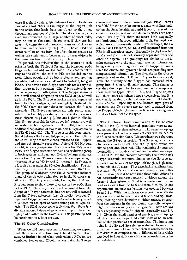
C. R. Chapman (personal communication, 1992) used an admittedly subjective evaluation of the pyroxene and olivine absorption band strength in his asteroid classification. Figure 8 shows that the So and Sp asteroids are more likely to have strong olivine and pyroxene designations, respectively, than S or K asteroids. For those objects with Chapman's "p" designation, one can rule out So as a probable class. Likewise, for those objects designated by Chapman as "o", Sp is an unlikely class. However, asteroids remaining in the S subclass occur with and without these designations. It is encouraging that the neural network results agree with those obtained by careful inspection of individual spectra. In cases where the data involved are simply too extensive for manual treatment, ANNs are a good alternative. Near-infrared spectra of these objects would determine their subclass membership.

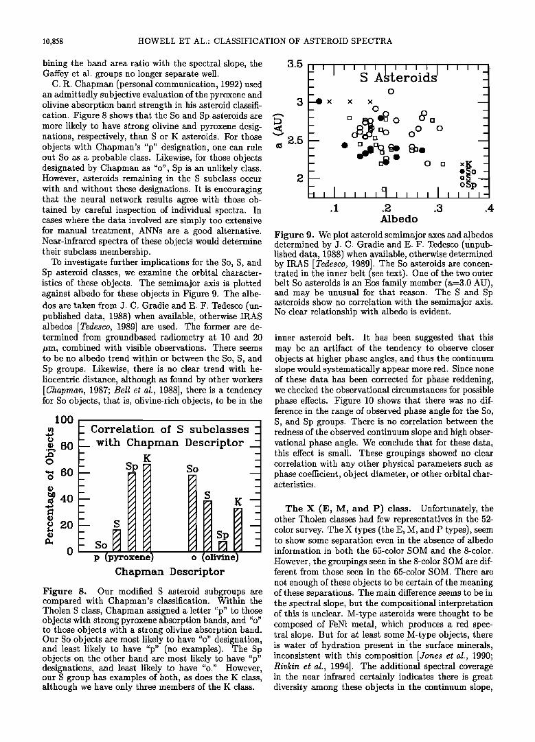
To investigate further implications for the So, S, and Sp asteroid classes, we examine the orbital characteristics of these objects. The semimajor axis is plotted against albedo for these objects in Figure 9. The albedos are taken from J. C. Gradie and E. F. Tedesco (unpublished data, 1988) when available, otherwise IRAS albedos [Tedesco, 1989] are used. The former are determined from groundbased radiometry at 10 and 20 pm, combined with visible observations. There seems to be no albedo trend within or between the So, S, and Sp groups. Likewise, there is no clear trend with heliocentric distance, although as found by other workers [Chapman, 1987; Bell et al., 1988], there is a tendency for So objects, that is, olivine-rich objects, to be in the

100

80

60

• 40

o 20

- Correlation of S subclasses

- with Chapman Descriptor - K -- Sp

-- S

p (pyroxene

_-

So

_-

S K --_

Sp _- M -

) o (olivine)

Chapman Descrip[or

Figure 8. Our modified S asteroid subgroups are compared with Chapman's classification. Within the Tholen S class, Chapman assigned a letter "p" to those objects with strong pyroxene absorption bands, and "o" to those objects with a strong olivine absorption band. Our So objects are most likely to have "o" designation, and least likely to have "p" (no examples). The Sp objects on the other hand are most likely to have "p" designations, and least likely to have "o." However, our S group has examples of both, as does the K class, although we have only three members of the K class.

3.5

2.5

- S teroids - _ 0 --•x x x •

- 0 0 -

: - _ ø ̧ o -

- - - - O xK [] --

-- •o

.1

oSp _

.2 .3 .4 Albedo

Figure 9. We plot asteroid semimajor axes and albedos determined by J. C. Gradie and E. F. Tedesco (unpublished data, 1988) when available, otherwise determined by IRAS [Tedesco, 1989]. The So asteroids are concen- trated in the inner belt (see text). One of the two outer belt So asteroids is an Eos family member (a=3.0 and may be unusual for that reason. The S and Sp asteroids show no correlation with the semimajor axis. No clear relationship with albedo is evident.

inner asteroid belt. It has been suggested that this may be an artifact of the tendency to observe closer objects at higher phase angles, and thus the continuum slope would systematically appear more red. Since none of these data has been corrected for phase reddening, we checked the observational circumstances for possible phase effects. Figure 10 shows that there was no difference in the range of observed phase angle for the So, S, and Sp groups. There is no correlation between the redness of the observed continuum slope and high observational phase angle. We conclude that for these data, this effect is small. These groupings showed no clear correlation with any other physical parameters such as phase coef[icient, object diameter, or other orbital characteristics.

The X (E, M, and P) class. Unfortunately, the other Tholen classes had few representatives in the 52- color survey. The X types (the E, M, and P types), seem to show some separation even in the absence of albedo information in both the 65-color SOM and the 8-color.

However, the groupings seen in the 8-color SOM are different from those seen in the 65-color SOM. There are

not enough of these objects to be certain of the meaning of these separations. The main difference seems to be in the spectral slope, but the compositional interpretation of this is unclear. M-type asteroids were thought to be composed of FeNi metal, which produces a red spectral slope. But for at least some M-type objects, there is water of hydration present in'the surface minerals, inconsistent with this composition [Jones et al., 1990; Rivkin et al., 1994]. The additional spectral coverage in the near infrared certainly indicates there is great diversity among these objects in the continuum slope,

HOWELL ET AL.' CLASSIFICATION OF ASTEROID SPECTRA 10,859

5O

ß 40

3O

S Asteroids

ß So -

1.6 1.8 2 2.2 V-K

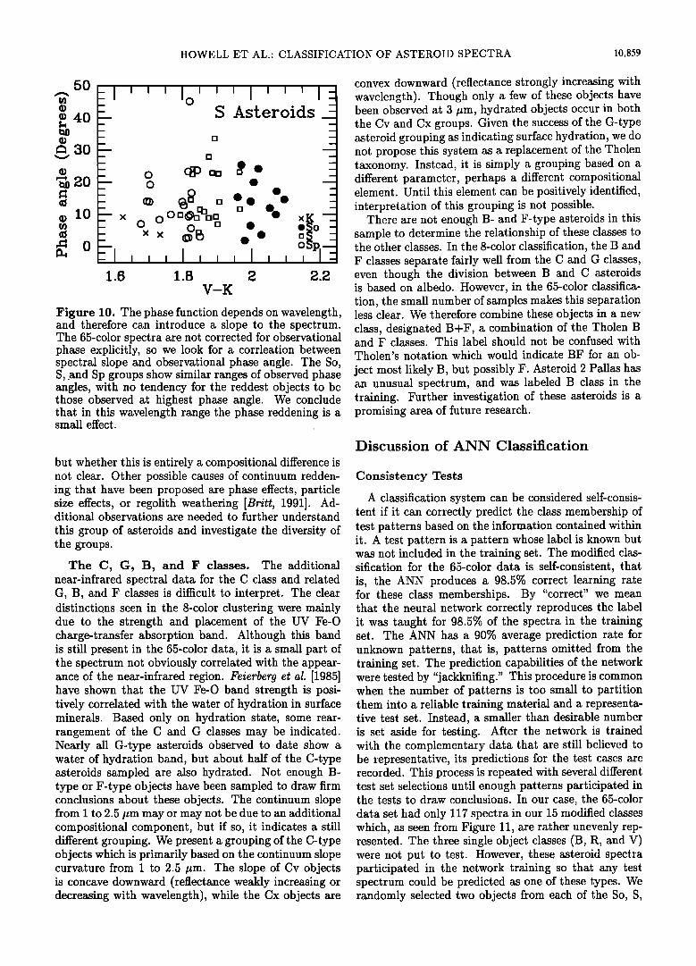
Figure 10. The phase function depends on wavelength, and therefore can introduce a slope to the spectrum. The 65-color spectra are not corrected for observational phase explicitly, so we look for a corrleation between spectral slope and observational phase angle. The So, S, .and Sp groups show similar ranges of observed phase angles, with no tendency for the reddest objects to be those observed at highest phase angle. We conclude that in this wavelength range the phase reddening is a small effect.

but whether this is entirely a compositional difference is not clear. Other possible causes of continuum reddening that have been proposed are phase effects, particle size effects, or regolith weathering [Britt, 1991]. Ad- ditional observations are needed to further understand

this group of asteroids and investigate the diversity of the groups.

The C, G, B, and F classes. The additional near-infrared spectral data for the C class and related G, B, and F classes is difficult to interpret. The clear distinctions seen in the 8-color clustering were mainly due to the strength and placement of the UV Fe-O charge-transfer absorption band. Although this band is still present in the 65-color data, it is a small part of the spectrum not obviously correlated with the appearance of the near-infrared region. Feierberg et al. [1985] have shown that the UV Fe-O band strength is positively correlated with the water of hydration in surface minerals. Based only on hydration state, some rear- rangement of the C and G classes may be indicated. Nearly all G-type asteroids observed to date show a water of hydration band, but about half of the C-type asteroids sampled are also hydrated. Not enough B- type or F-type objects have been sampled to draw firm conclusions about these objects. The continuum slope from 1 to 2.5 •m may or may not be due to an additional compositional component, but if so, it indicates a still different grouping. We present a grouping of the C-type objects which is primarily based on the continuum slope curvature from 1 to 2.5 •um. The slope of Cv objects is concave downward (reflectance weakly increasing or decreasing with wavelength), while the Cx objects are

convex downward (reflectance strongly increasing with wavelength). Though only a few of these objects have been observed at 3 •m, hydrated objects occur in both the Cv and Cx groups. Given the success of the G-type asteroid grouping as indicating surface hydration, we do not propose this system as a replacement of the Tholen taxonomy. Instead, it is simply a grouping based on a different parameter, perhaps a different compositional element. Until this element can be positively identified, interpretation of this grouping is not possible.

There are not enough B- and F-type asteroids in this sample to determine the relationship of these classes to the other classes. In the 8-color classification, the B and F classes separate fairly well from the C and G classes, even though the division between B and C asteroids is based on albedo. However, in the 65-color classification, the small number of samples makes this separation less clear. We therefore combine these objects in a new class, designated B+F, a combination of the Tholen B and F classes. This label should not be confused with Tholen's notation which would indicate BF for an ob-

ject most likely B, but possibly F. Asteroid 2 Pallas has an unusual spectrum, and was labeled B class in the training. Further investigation of these asteroids is a promising area of future research.

Discussion of ANN Classification

Consistency Tests

A classification system can be considered self-consistent if it can correctly predict the class membership of test patterns based on the information contained within it. A test pattern is a pattern whose label is known but was not included in the training set. The modified classification for the 65-color data is self-consistent, that is, the ANN produces a 98.5% correct learning rate for these class memberships. By "correct" we mean that the neural network correctly reproduces the label it was taught for 98.5% of the spectra in the training set. The ANN has a 90% average prediction rate for unknown patterns, that is, patterns omitted from the training set. The prediction capabilities of the network were tested by "jackknifing." This procedure is common when the number of patterns is too small to partition them into a reliable training material and a representative test set. Instead, a smaller than desirable number is set aside for testing. After the network is trained with the complementary data that are still believed to be representative, its predictions for the test cases are recorded. This process is repeated with several different test set selections until enough patterns participated in the tests to draw conclusions. In our case, the 65-color data set had only 117 spectra in our 15 modified classes which, as seen from Figure 11, are rather unevenly represented. The three single object classes (B, R, and V) were not put to test. However, these asteroid spectra participated in the network training so that any test spectrum could be predicted as one of these types. We randomly selected two objects from each of the So, S,

10,860 HOWELL ET AL.' CLASSIFICATION OF ASTEROID SPECTRA

65-Color Asteroid Spectra

Grouped by ANN Classes Grouped by Tholen Classes

A ..,v' / / / /

BCv

B+F

Cv

Cx 241 324 lg 130 44 84 317 422 somaam, b•mbers, olek•r ....... berohn,

D 130

K •ll cloe•, beren•k, o• ½1oelll

M

P

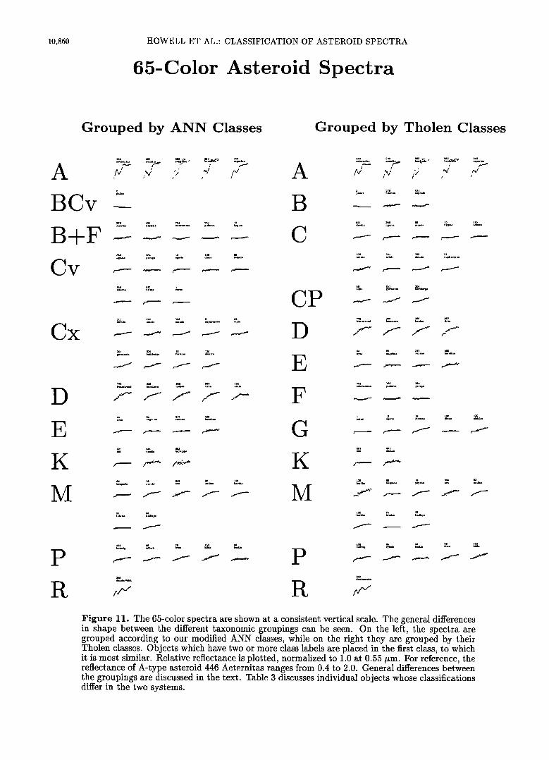
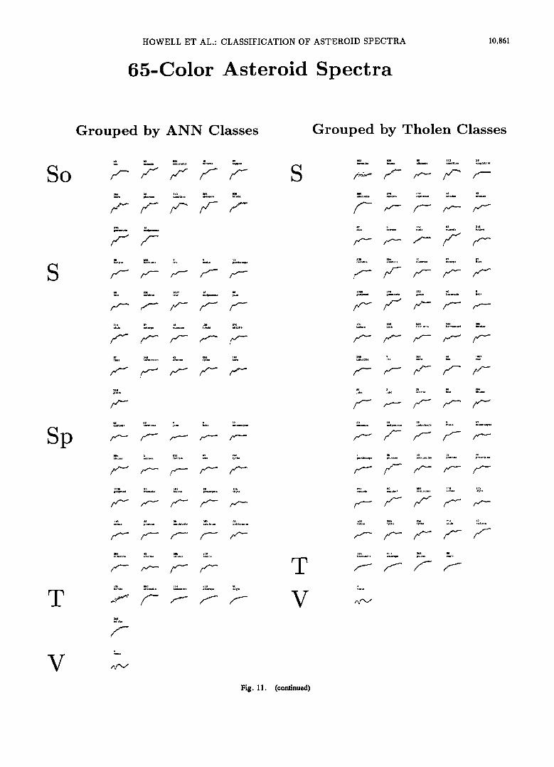
Figure 11. The 65-color spectra are shown at a consistent vertical scale. The general differences in shape between the different taxonomic groupings can be seen. On the left, the spectra are grouped according to our modified ANN classes, while on the right they are grouped by their Tholen classes. Objects which have two or more class labels are placed in the first class, to which it is most similar. Relative reflectance is plotted, normalized to 1.0 at 0.55/•m. For reference, the reflectance of A-type asteroid 446 Aeternitas ranges from 0.4 to 2.0. General differences between the groupings are discussed in the text. Table 3 discusses individual objects whose classifications differ in the two systems.

HOWELL ET AL- CLASSIFICATION OF ASTEROID SPECTRA 10,861

65-Color Asteroid Spectra

Grouped by ANN Classes Grouped by Tholen Classes

So

s

• is 32 20 as? 33

tndustrl. t•m&tnr

T 3oe

s oeo 2?0 ae? 42 42

103 •,32 348 386

380 ? 364 i4s•, 1827 mdustrl, ,.M'&

v 4

Fig. 11. (continued)


and Sp classes and one object from each of the other classes, thus having 16 test cases and 101 training samples in one jackknife. We repeated this six times, with different random selections. Altogether, 68 spectra participated in at least one test set. Among the So, S, and Sp classes, 26 were tested. Misclassifications among E, M, and P types were not counted, although we kept these separate class designations. The results are sum- marized in Table 1. Trained with our modified class la-

bels, the network achieves a 98% learning success rate. The network has a 90% average prediction rate for patterns omitted in the jackknifing tests. For comparison, we ran the same experiment with exactly the same test set selections, for the original Tholen class designations. As shown in Table 1, the learning and prediction success rates were 97.3% and 71%, respectively. Because of the small number of patterns, the resolution of the prediction rate is 6% (i.e., if one, two or three patterns are misclassified, the prediction rate is 94%, 88% and 82%, respectively). The resolution of the training success rate is 1%. Our results indicate that we achieved a

cleaner class structure for the 65-color spectra than the initially assumed class memberships. The network is utilizing the additional spectral information effectively.

The Spectra

Our modified classes for the asteroids with 65-color

spectra are listed in Table 2. Figure 11 shows the 65- color spectra grouped according to the ANN classification on the left. For comparison, the spectra are grouped by Tholen's classification on the right. The objects Bell et al. [1988] designated as K, are separated from Tholen's S class, and 422 Berolina is classed as EM, rather than its original DX Tholen class, since it has a high albedo (J. C. Gradie and E. F. Tedesco, unpublished data, 1988). Table 3 lists those objects for which our class determination differs from the Tholen

class either in the 8-color classification, the 65-color classification, or both. Special cases or unusual objects are also listed with explanatory notes. For those objects that did not show a clear class a•nity, Tholen listed other possibilities in order of preference. For example, CP is most likely C, but possibly P. Our 8-color classification showed all of the CP objects in the 65-

color data are more closely related to other C-class asteroids than to the P class, so we list them as C class. The network determines weighted multiple class asso- cie•tions. For those objects that showed at least 30% contribution by at least one other class in at least two of the six jackknife tests, we list the additional class designation. In some cases, the albedo narrows the class membership possibilities (see Table 2 notes). We define the B+F class as a combination of Tholen's B and F classes, with the exception of 2 Pallas, which was trained as B. The remaining B and F asteroids are not distinguishable in our 65-color classification due to the small number of samples. In the jackknife testing, 2 Pallas showed a similarity to the Cv class, so its ANN classification is BCv. The spectrum of 1 Ceres is also unusual, and it showed similarity to 2 Pallas, giving it a CvB class. However, the two objects are different from each other.

Among 20 objects observed on two or more separate occasions, six showed significant spectral variation as described earlier. One of these objects, 367 Amicitia, was not included due to lack of visual observations. Two

spectra of 43 Ariadne, 863 Benkoela, 18 Melpomene, 258 Tyche, and 135 Hertha were analyzed separately. Although noisy, both versions of 863 Benkoela classified as A. One spectrum of 43 Ariadne classified as Sp while the other classified as S, but very near the bound- ary between S and Sp. One spectrum of 18 Melpomene classified as SoT, the other as S. One 258 Tyche spectrum classified as Sp, the other as SSp. In the case of 135 Hertha, one of the spectra classified as M, but the other classified as T, although it is somewhat noisy. If these variations are due to compositional variation on the asteroid, then the implication is that asteroid inho- mogeneities occur at a level that is easily detectable at near-infrared wavelengths. However, these variations may also result from systematic errors. Rotationally resolved spectra of these objects are needed to settle this important issue, since the fundamental meaning of a taxonomic class is quite different if objects routinely show different classes on different faces.

Summary and Conclusions

We classified combined 8- and 52-color asteroid re-

flectance spectra with a Kohonen-type artificial neural

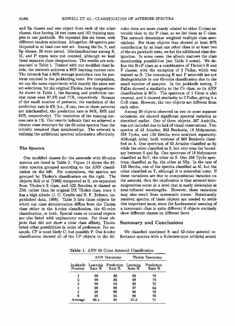
Table 1. ANN 65-Color Asteroid Classification

ANN Taxonomy Tholen Taxonomy

Jackknife Learnipg Prediction Learnipg Prediction Number Rate % Rate % Rate % Rate %

1 98 88 99 76

2 99 88 98 76 3 99 94 96 70 4 99 88 97 64 5 98 88 96 70 6 98 94 98 70

Average 98.5 90 97.3 71


Table 2. ANN Asteroid Classification

Number Asteroid Class Number Asteroid Class Number Asteroid Class

1 Ceres CvB 67 Asia Sp 336 Lacadiera D 2 Pallas BCv 68 Leto S 346 Hermentaria S 3 Juno Sp 69 Hesperia M 349 Dembowska R 4 Vesta V 76 Freia P 352 Gisela SSp 5 Astraea Sp 80 Sappho So 354 Eleonora So 6 Hebe Sp 82 Alkmene Sp 356 Liguria Cv 7 Iris S 86 Semele CvP 364 Isara So 9 Metis S 89 Julia S 368 Haidea D

10 Hygiea B+F 92 Undina M 376 Geometria So 11 Parthenope S 96 Aegle T 379 Huenna B+F 12 Victoria So 101 Helena Sp 385 Ilmatar Sp 13 Egeria Cv 103 Hera SSp 387 Aquitania Sp 15 Eunomia S 106 Dione Cv 389 Industria Sp 16 Psyche M 113 Amalthea So 422 Berolina EM 18 Melpomene S,SoT 114 Kassandra T 431 Nephele B+F 19 Fortuna Cx 115 Thyra Sp 446 Aeternitas A 20 Massalia Sp 116 Sirona Sp 476 Hedwig P 21 Lutetia • M 130 Elektra Cx 511 Davida Cx 22 Kalliope M 135 Hertha M,T 521 Brixia CvP 25 Phocaea So 138 Tolosa S 532 Herculina S 26 Proserpina Sp 145 Adeona CvP 554 Peraga Cv 27 Euterpe S 152 Atala D(S) 584 Semiramis So 29 Amphitrite Sp 153 Hilda P 639 Latona So 31 Euphrosyne Cx 218 Bianca SpS 653 Berenike K 32 Pomona Sp 221 Eos I K 661 Cloelia K 33 Polyhymnia Sp 233 Asterope T 674 Rachele Sp 37 Fides S 235 Carolina S 702 Alauda Cx 39 Laetitia S 241 Germania Cx 704 Interamnia B+F 40 Harmonia Sp 246 Asporina A 714 Ulula S 42 Isis So 258 Tyche Sp,SSp 762 Pulcova B+F 43 Ariadne Sp,S 264 Libussa Sp 772 Tanete Cx 44 Nysa E 267 Tirza D 773 Irmintraud D 46 Hestia P 270 Anahita S 849 Ara M 57 Mnemosyne Sp 289 Nenetta A 863 Benkoela A 59 Elpis Cx 308 Polyxo TSo 980 Anacostia T 63 Ausonia So 317 Roxane* E 1036 Ganymed Sp 64 Angelina E 324 Bamberga Cx 1627 Ivar S 65 Cybele P

Classification determined by the neural network using the 65-color spectra are presented. In cases where two or more classes contributed at least 30% in at least one third of the jackknife tests, multiple class labels are shown. In most cases, one class was clearly dominant. Labels are listed in decreasing order of contribution. In cases where two different spectra for the same object classified differently, the classes are separated by a comma. See Table 3 note 6 for a description of observational problems with 152 Atala.

•Asteroid 21 Lutetia classified as MCv; however, its albedo excludes the Cv class. I Asteroid 221 Eos classified as KCvP; however, its albedo excludes both Cv and P classes. *Asteroid 317 Roxane classified as ECv; however, its albedo excludes the Cv class.

network. Although the method is very different from that used by Tholen to determine his now widely used taxonomic system, our results are generally consistent with Tholen's taxonomy when based on a similar data set. We extend the spectral range of the data to include the near infrared, and introduce our classification, aug- menting the Tholen taxonomy: some classes are rear- ranged, and certain objects are assigned class labels different from Tholen's. Two compositionally meaningful subclasses are defined within the S asteroids. We define

So as olivine-rich, red asteroids, and Sp as olivine-poor, less red objects. This classification is self-consistent to a high degree, i.e., the neural network trained with our modified class labels produces 98% learning success, and a 90% average prediction rate for unseen patterns.

We find some evidence to suggest the C class and related G, B, and F classes show different clusterings with the extended spectral coverage. One such rearrange- ment is presented, although the compositional interpretation is not clear. The number of samples of these objects is small, and more observations are required to clarify these groupings. Similarly, the X asteroids, that is, the E, M, and P classes, exhibit clusters within the group that are not related to albedo, but the number of objects is currently too small to interpret the meaning of these groups.

The neural network approach used here is powerful in clustering and classifying high-dimensional spectral data. Since artificial neural networks are well suited to combine data of disparate natures, we may be able to


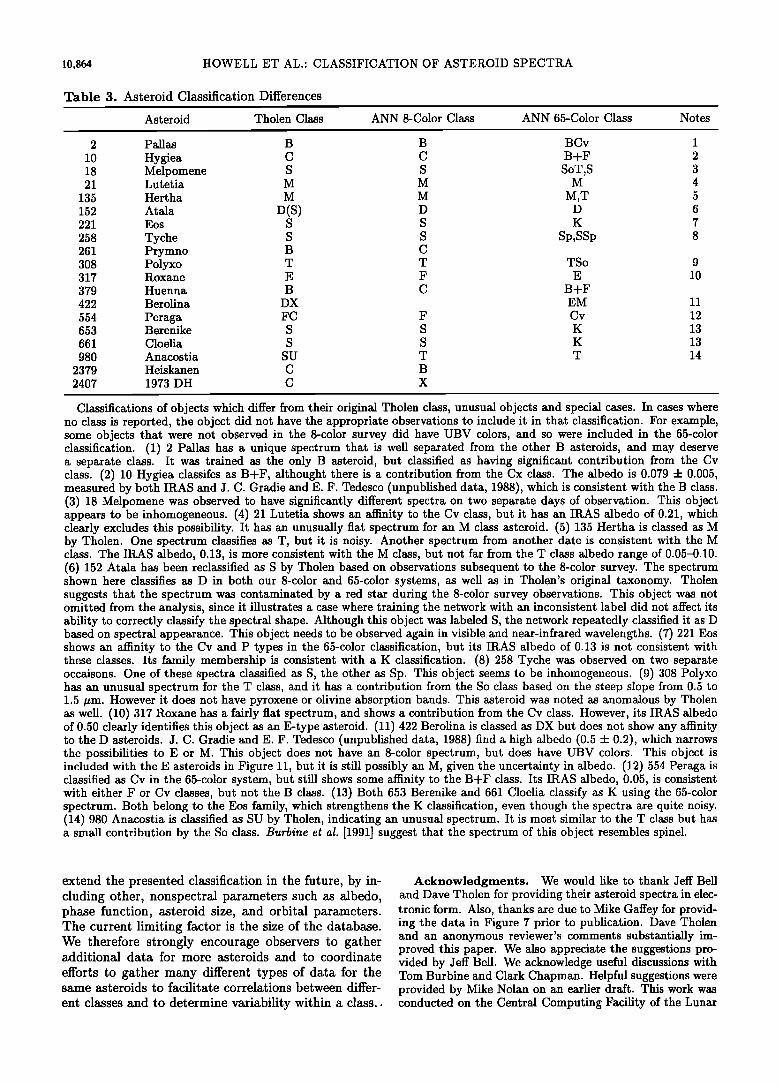
Table 3. Asteroid Classification Differences

Asteroid Tholen Class ANN 8-Color Class ANN 65-Color Class Notes

2 Pallas B B BCv 1 10 Hygiea C C B+F 2 18 Melpomene S S SoT,S 3 21 Lutetia M M M 4

135 Hertha M M M,T 5 152 Atala D(S) D D 6 221 Eos S S K 7 258 Tyche S S Sp,SSp 8 261 Prymno B C 308 Polyxo T T TSo 9 317 Roxane E F E 10 379 Huenna B C B+F 422 Berolina DX EM 11 554 Peraga FC F Cv 12 653 Berenike S S K 13 661 Cloelia S S K 13 980 Anacostia SU T T 14

2379 Heiskanen C B 2407 1973 DH C X

Classifications of objects which differ from their original Tholen class, unusual objects and special cases. In cases where no class is reported, the object did not have the appropriate observations to include it in that classification. For example, some objects that were not observed in the 8-color survey did have UBV colors, and so were included in the 65-color classification. (1) 2 Pallas has a unique spectrum that is well separated from the other B asteroids, and may deserve a separate class. It was trained as the only B asteroid, but classified as having significant contribution from the Cv class. (2) 10 Hygiea classifes as B+F, althought there is a contribution from the Cx class. The albedo is 0.079 :k 0.005, measured by both IRAS and J. C. Gradie and E. F. Tedesco (unpublished data, 1988), which is consistent with the B class. (3) 18 Melpomene was observed to have significantly different spectra on two separate days of observation. This object appears to be inhomogeneous. (4) 21 Lutetia shows an affinity to the Cv class, but it has an IRAS albedo of 0.21, which clearly excludes this possibility. It has an unusually fiat spectrum for an M class asteroid. (5) 135 Hertha is classed as M by Tholen. One spectrum classifies as T, but it is noisy. Another spectrum from another date is consistent with the M class. The IRAS albedo, 0.13, is more consistent with the M class, but not far from the T class albedo range of 0.05-0.10. (6) 152 Atala has been reclassified as S by Tholen based on observations subsequent to the 8-color survey. The spectrum shown here classifies as D in both our 8-color and 65-color systems, as well as in Tholen's original taxonomy. Tholen suggests that the spectrum was contaminated by a red star during the 8-color survey observations. This object was not omitted from the analysis, since it illustrates a case where training the network with an inconsistent label did not affect its ability to correctly classify the spectral shape. Although this object was labeled S, the network repeatedly classified it as D based on spectral appearance. This object needs to be observed again in visible and near-infrared wavelengths. (7) 221 Eos shows an affinity to the Cv and P types in the 65-color classification, but its IRAS albedo of 0.13 is not consistent with these classes. Its family membership is consistent with a K classification. (8) 258 Tyche was observed on two separate occaisons. One of these spectra classified as S, the other as Sp. This object seems to be inhomogeneous. (9) 308 Polyxo has an unusual spectrum for the T class, and it has a contribution from the So class based on the steep slope from 0.5 to 1.5 pm. However it does not have pyroxene or olivine absorption bands. This asteroid was noted as anomalous by Tholen as well. (10) 317 Roxane has a fairly fiat spectrum, and shows a contribution from the Cv class. However, its IRAS albedo of 0.50 clearly identifies this object as an E-type asteroid. (11) 422 Berolina is classed as DX but does not show any affinity to the D asteroids. J. C. Gradie and E. F. Tedesco (unpublished data, 1988) find a high albedo (0.5 :k 0.2), which narrows the possibilities to E or M. This object does not have an 8-color spectrum, but does have UBV colors. This object is included with the E asteroids in Figure 11, but it is still possibly an M, given the uncertainty in albedo. (12) 554 Peraga is classified as Cv in the 65-color system, but still shows some affinity to the B+F class. Its IRAS albedo, 0.05, is consistent with either F or Cv classes, but not the B class. (13) Both 653 Berenike and 661 Cloelia classify as K using the 65-color spectrum. Both belong to the Eos family, which strengthens the K classification, even though the spectra are quite noisy. (14) 980 Anacostia is classified as SU by Tholen, indicating an unusual spectrum. It is most similar to the T class but has a small contribution by the So class. Burbine et al. [1991] suggest that the spectrum of this object resembles spinel.

extend the presented classification in the future, by including other, nonspectral parameters such as albedo, phase function, asteroid size, and orbital parameters. The current limiting factor is the size of the database. We therefore strongly encourage observers to gather additional data for more asteroids and to coordinate

efforts to gather many different types of data for the same asteroids to facilitate correlations between differ-

ent classes and to determine variability within a class..

Acknowledgments. We would like to thank Jeff Bell and Dave Tholen for providing their asteroid spectra in elec- tronic form. Also, thanks are due to Mike Gaffey for providing the data in Figure 7 prior to publication. Dave Tholen and an anonymous reviewer's comments substantially im- proved this paper. We also appreciate the suggestions provided by Jeff Bell. We acknowledge useful discussions with Tom Burbine and Clark Chapman. Helpful suggestions were provided by Mike Nolan on an earlier draft. This work was conducted on the Central Computing Facility of the Lunar


and Planetary Laboratory. For artificial neural network sim- ulation, we used the NeuralWorks Professional II Package, by (•) NeuralWare, Inc., provided by the Planetary Image Research Laboratory. This work has been partially sup- ported by grants NAGW-1975 and NAGW-1146.

References

Barucci, M. A., M. T. Capria, A. Coradini, and M. Fulchi- gnoni, Classification of asteroids using G-mode analysis, Icarus, 7œ, 304-324, 1987.

Bell, J. F., A probable asteroidal parent body for the CV or CO chondrites, Bull. Am. Astron. Soc., 19, 841, 1987.

Bell, J. F., A probable asteroidal parent body for the CV or CO chondrites, Meteoritics, œ$, 256-257, 1988.

Bell, J. F., B. R. Hawke, and P. D. Owensby, Carbonaceous chondrites from S-type asteroids?, Bull. Am. Astron. Soc., 19, 841, 1987.

Bell, J. F., P. D. Owensby, B. R. Hawke and M. J. Gaffey, The 52-color asteroid survey: Final results and interpretation, (abstract), Lunar Planet. Sci. Uonf., XIX, 57, 1988.

Bell, J. F., D. R. Davis, W. K. Hartmann, and M. J. Gaffey, Asteroids: The big picture, in Asteroids H, edited by R. P. Binzel et al., pp. 921-945, University of Arizona Press, Tucson, 1989.

Binzel, R. P., and S. Xu, Chips off of asteroid 4 Vesta: Ev- idence for the parent body of basaltic achondrite meteorites, Science, 260, 186-191, 1993.

Britt, D. T., "Space Weathering": Are regolith processes an important factor in the S-type controversy?, Meteoritics, 26, 324, 1991.

Burbine, T. H., Principal component analysis of asteroid and meteorite spectra from 0.3 to 2.5/•m, Master's thesis, University of Pittsburgh, Pittsburgh, Pa, 1991.

Burbine, T. H., M. J. Gaffey, and J. F. Bell, S-asteroids 387 Aquitania and 980 Anancostia: Possible fragments of the breakup of a spinel-bearing parent body with CO3/CV3 affinities, Meteoritics, 27, 424-434, 1991.

Chapman, C. R., The asteroid belt: Compositional structure and size distributions, Bull. Am. Astron. Soc., 19, 839, 1987.

Chapman, C. R., D. Morrison, and B. Zellner, Surface prop- erties of asteroids: A synthesis of polarimetry, radiometry, and spectrophotometry, Icarus, 25, 104-130, 1975.

Cruikshank, D. P., D. J. Tholen, W. K. Hartmann, J. F. Bell and R. H. Brown, Three basaltic earth-approaching asteroids and the source of the basaltic meteorites, Icarus, 89, 1, 1991.

Feierberg, M. A., L. A. Lebofsky, and D. J. Tholen, The nature of C-class asteroids from 3-/•m spectrophotometry, Icarus, 63, 183-191, 1985.

Fu, K. S. (Ed.), Digital Pattern Recognition, Springer- Verlag, New York, 1976.

Gaffey, M. J., J. F. Bell, R. H. Brown, T. Burbine, J. L. Piatek, K. L. Reed, and D. A. Chakey, Mineralogical variations within the S-type asteroid class, Icarus, 106, 573- 602, 1993.

Hardorp, J., The sun among the stars, Astron. Astrophys., 91, 221, 1980.

Harris, A. W., and J. W. Young, Asteroid rotation, Icarus, 54{, 59-109, 1983.

Hartmann, W. K., D. P. Cruikshank, and J. Degewij, Re-

mote comets and related bodies: VJHK colorimetry and surface materials, Icarus, 52, 377-408, 1982.

Huang, W., and R. Lippman, Comparisons between neural network and conventional classifiers, in Institute of Elec- trical and Electronics Engineers, New York, First Inter- national Conference on Neural Networks, San Diego, vol. IV, pp. 485-494, 1987.

Jones, T. D., L. A. Lebofsky, J. S. Lewis, and M. S. Marley, The composition and origin of the C, P, and D asteroids: Water as a tracer of thermal evolution in the outer belt, Icarus, 88, 172-192, 1990.

Kohonen, T., Self-Organization and Associative Memory, Springer-Verlag, New 'fork, 1988.

Lebofsky, L. A., T. D. Jones, P. D. Owensby, M. A. Feier- berg, and G.J. Consolmagno, The nature of low albedo asteroids from 3-tzm spectrophotometry, Icarus, 83, 12- 26, 1990.

Mer•nyi, E., K. Edgett, and R. B. Singer, Deucalionis Regio, Mars: Evidence for a new type of immobile weathered soil unit, Icarus, submitted, 1993a.

Merdnyi, E., R. B. Singer, and W. H. Farrand, Classifica- tion of the LCVF AVIRIS test site with a Kohonen artifi-

cial neural network. in Proceedings of the Fourth Airborne Geoscience Workshop, Washington, D.C., Oct. 25-29, pp. 117-120, 1993b.

NeuralWare, Inc., Neural computing, in NeuralWorks Pro- fessional H Manual, Pittsburgh, Pa., 1991.

Pao, Y.-H., Adaptive Pattern Recognition and Neural Net- works, Addison-Wesley, Reading, Mass., 1989.

Rivkin, A. S., D. T. Britt, E. S. Howell, and L. A. Lebofsky, Hydrated E-class and M-class asteroids, (abstract), Lunar Pla,et. Sci. Conf., XXV, 1135, 1994.

Tedesco, E. F., J. G. Williams, D. L. Matson, G.J. Veeder, J. C. Gradie, and L. A. Lebofsky, A three-parameter asteroid taxonomy, Astron. J., 97, 580-606, 1989.

Tedesco, E. F., UBV colors, and IRAS albedos and di- ameters, in Asteroids II, edited by R. P. Binzel et al., pp. 1090-1138, University of Arizona Press, Tucson, 1989.

Tholen, D. J., Asteroid taxonomy from cluster analysis of photometry. Ph.D. dissertation, University of Arizona, Tucson, 1984.

Tholen, D. J., Asteroid taxonomic classification, in Aster- oids H, edited by R. P. Binzel et al., pp. 1139-1150, Uni- versity of Arizona Press, Tucson, 1989.

Tholen, D. J., and M. A. Barucci, Asteroid taxonomy, in Asteroids II, edited by R. P. Binzel et al., pp. 298-315, University of Arizona Press, Tucson, 1989.

Ultsch, A., and H. P. Simeon, Kohonen's self organizing fea- ture map for exploratory data analysis, in International Neural Netowrk Conference 90 Paris, Kluwer Academic, Dordrecht, pp. 305-308, 1990.

Zellner, B., D. J. Tholen, and E. F. Tedesco, The eight-color asteroid survey: Results for 589 minor planets, Icarus, 61, 355-416, 1985.

E. S. Howell, L. A. Lebofsky and E. Merdnyi Lunar and Planetary Laboratory, University of Arizona, Tuc- son, AZ 85721 (e-maih [email protected]; lebof- [email protected]; [email protected])

(Received July 22, 1992; revised December 10, 1993; accepted December 17, 1993.)

classification of asteroid spectra using a neural network · classification of asteroid spectra...

Documents