civilizations as dynamic networks
DESCRIPTION
prezentation for Civilizations as Dynamic NetworksTRANSCRIPT
Civilizations as dynamic networks
Cities, hinterlands, populations, industries,
trade and conflict
Douglas R. White
© 2005 All rights reserved
50 slides - also viewable on drw conference paper website version 1.3 of 11/12/2005
European Conference on Complex Systems Paris, 14-18 November 2005

2
acknowledgements
Thanks to the International Program of the Santa Fe Institute for support of the work on urban scaling with Nataša Kejžar and Constantino Tsallis, and thanks to the ISCOM project (Information Society as a Complex System) principal investigators David Lane, Geoff West, Sander van der Leeuw and Denise Pumain for ISCOM support of collaboration with Peter Spufford at Cambridge, and for research assistance support from Joseph Wehbe. Also thanks to David Krakauer and Luis Bettencourt at SFI in suggesting how our multilayered models of rise and fall of city networks could be guided by sufficient statistics modeling principles and to Lane and van der Leeuw for suggestions on the slides. This study is complemented by others within the ISCOM project concerned with urban scaling and innovation and draws several slides from those projects.
Thanks to Peter Spufford for his generous support in providing systematic empirical data on intercity networks and industries in the medieval period to complement the data in his book, Dean Anuska Ferligoj, School of Social Sciences, University of Ljubljana, for five weeks of support for work carried out with Kejžar in Ljubljana in summer, 2005, Céline Rozenblat (ISCOM project) for providing the historical urban size data, and Camille Roth (Polytechnic, Paris) for collaborations on representing evolutions of multiple industries across city netwks.
A jointly authored on this project is in draft with Spufford and possibly others.
3
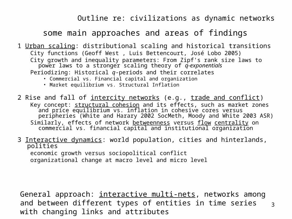
some main approaches and areas of findings
1 Urban scaling: distributional scaling and historical transitionsCity functions (Geoff West , Luis Bettencourt, José Lobo 2005)City growth and inequality parameters: From Zipf's rank size laws to power laws to a
stronger scaling theory of q-exponentialsPeriodizing: Historical q-periods and their correlates
• Commercial vs. Financial capital and organization• Market equilibrium vs. Structural Inflation
2 Rise and fall of intercity networks (e.g., trade and conflict)Key concept: structural cohesion and its effects, such as market zones and price
equilibrium vs. inflation in cohesive cores versus peripheries (White and Harary 2002 SocMeth, Moody and White 2003 ASR)
Similarly, effects of network betweenness versus flow centrality on commercial vs. financial capital and institutional organization
3 Interactive dynamics: world population, cities and hinterlands, polities economic growth versus sociopolitical conflictorganizational change at macro level and micro level.
Outline re: civilizations as dynamic networks
General approach: interactive multi-nets, networks among and between different types of entities in time series with changing links and attributes
4
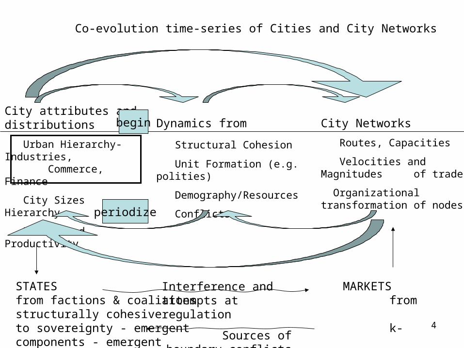
City Networks
Routes, Capacities
Velocities and Magnitudes of trade
Organizational transformationof nodes
STATES MARKETSfrom factions & coalitions from structurally cohesiveto sovereignty - emergent k-components - emergent Spatiopolitical units Network units (overlap)
City attributes and distributions
Urban Hierarchy-Industries, _______Commerce, Finance
City Sizes Hierarchy
Hinterland Productivity
Dynamics from
Structural Cohesion
Unit Formation (e.g. polities)
Demography/Resources
Conflicts
Co-evolution time-series of Cities and City Networks
Interference and attempts at regulation
Sources of boundary conflicts
begin
periodize
5
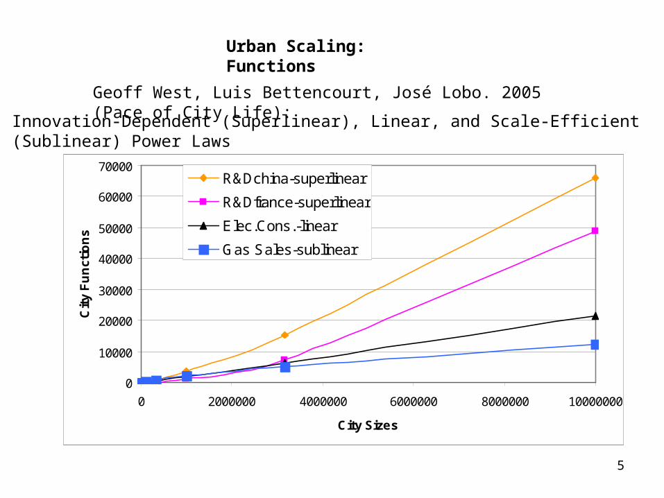
Geoff West, Luis Bettencourt, José Lobo. 2005 (Pace of City Life):
Innovation-Dependent (Superlinear), Linear, and Scale-Efficient (Sublinear) Power Laws
0
10000
20000
30000
40000
50000
60000
70000
0 2000000 4000000 6000000 8000000 10000000
City Sizes
Cit
y F
un
ctio
ns
R&Dchina-superlinear
R&Dfrance-superlinear
Elec.Cons.-linear
Gas Sales-sublinear
Urban Scaling: Functions

6
Superlinear ~ 1.67
Linear ~ 1
Sublinear ~ .85
ISCOM working paper
7
1
10
100
1000
10000
100000 1000000 10000000
(White, Kejžar, Tsallis, and Rozenblat © 2005 working paper)
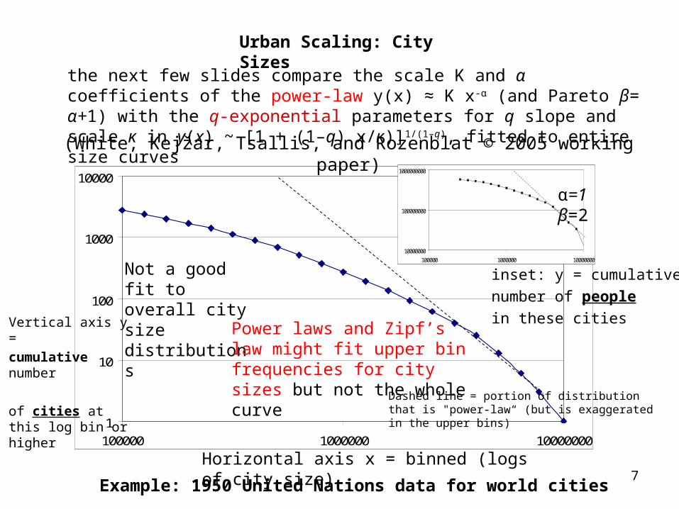
the next few slides compare the scale K and α coefficients of the power-law y(x) ≈ K x-α (and Pareto β= α+1) with the q-exponential parameters for q slope and scale κ in y(x) ~ [1 + (1–q) x/κ)]1/(1–q), fitted to entire size curves
Not a good fit to overall city size distributions
Power laws and Zipf’s law might fit upper bin frequencies for city sizes but not the whole curve
inset: y = cumulative
number of people
in these cities
Dashed line = portion of distribution that is "power-law“ (but is exaggerated in the upper bins)
Horizontal axis x = binned (logs of city size)
Vertical axis y =
cumulative number
of cities at this log bin or higher
10000000
100000000
1000000000
100000 1000000 10000000
Urban Scaling: City Sizes
α=1β=2
Example: 1950 United Nations data for world cities
8
% Urban in Europe
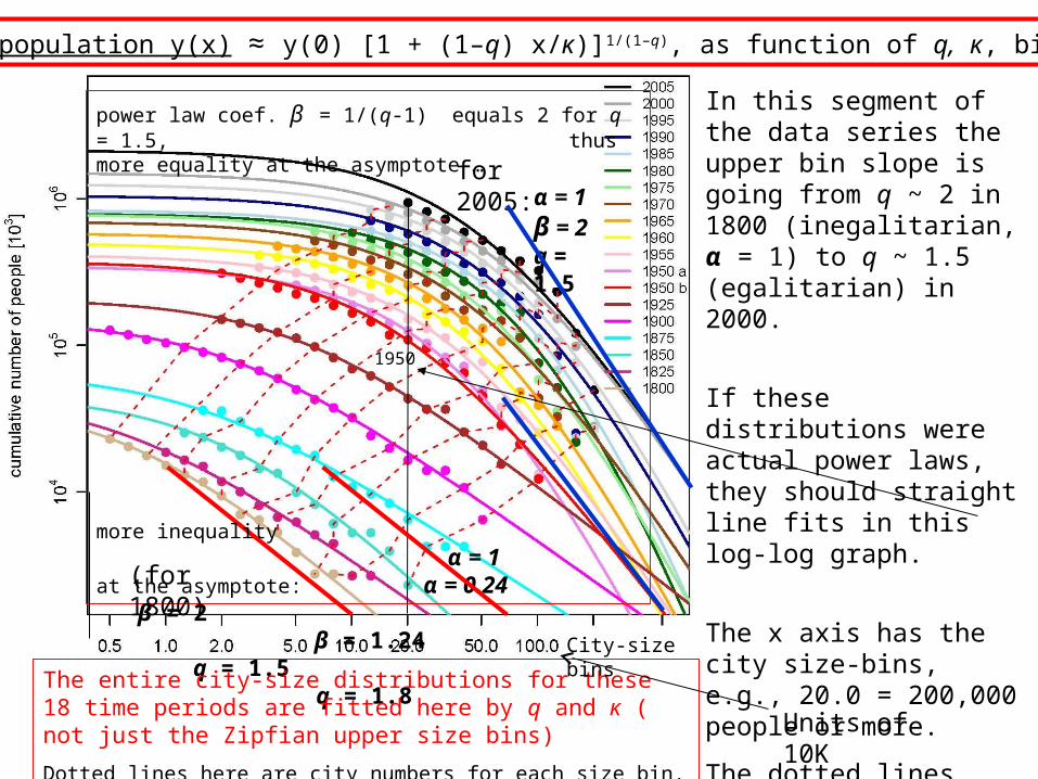
fitted q-exponential distributions, q, κ.
power law coef. β = 1/(q-1) equals 2 for q = 1.5, thus more equality at the asymptote …
more inequality α = 1at the asymptote: α = 0.24 β = 2
β = 1.24 q = 1.5 q = 1.8
In this segment of the data series the upper bin slope is going from q ~ 2 in 1800 (inegalitarian, α = 1) to q ~ 1.5 (egalitarian) in 2000.
If these distributions were actual power laws, they should straight line fits in this log-log graph.
The x axis has the city size-bins, e.g., 20.0 = 200,000 people or more.
The dotted lines show number of cities in multiples of two: 2,4,8,16,32,etc.
The entire city-size distributions for these 18 time periods are fitted here by q and κ ( not just the Zipfian upper size bins)
Dotted lines here are city numbers for each size bin.
(for 1800)
for 2005:
City-size bins
1950
Units of 10K
Q-exponential scaling ~ .99+ fit to 18 post-1800 and 22 pre-1800 distributionsAt time t, population y(x) ≈ y(0) [1 + (1–q) x/κ)]1/(1–q), as function of q, κ, binned size x
α = 1 β = 2 q = 1.5
9
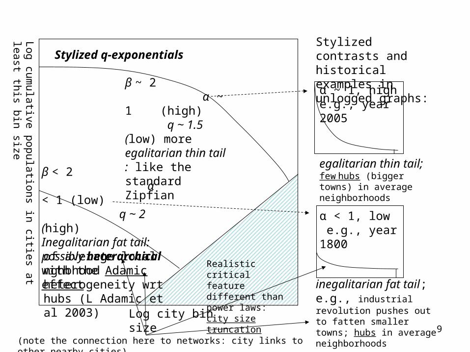
Stylized contrasts and historical examples in unlogged graphs:
β ~ 2 α ~ 1 (high) q ~ 1.5 (low) more egalitarian thin tail : like the standard Zipfian
β < 2 α < 1 (low) q ~ 2 (high) Inegalitarian fat tail: possibly heterarchical with the Adamic effect
Log city bin size
Realistic critical feature different than power laws: city size truncation
inegalitarian fat tail; e.g., industrial revolution pushes out to fatten smaller towns; hubs in average neighborhoods
of average local nghbhood heterogeneity wrt hubs (L Adamic et al 2003)
Log cumulative populations in cities at least this bin size
egalitarian thin tail; few hubs (bigger towns) in average neighborhoods
α ~ 1, high e.g., year 2005
α < 1, low e.g., year 1800
Stylized q-exponentials
(note the connection here to networks: city links to other nearby cities)
10
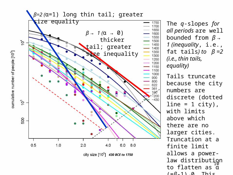
β=2 (α=1) long thin tail; greater size equality
The q-slopes for all periods are well bounded from β → 1 (inequality, i.e., fat tails) to β =2 (i.e., thin tails, equality)
Tails truncate because the city numbers are discrete (dotted line = 1 city), with limits above which there are no larger cities. Truncation at a finite limit allows a power- law distribution to flatten as α (=β-1)→0. This is more realistic than a scale-free model.
β → 1 (α → 0) thicker tail; greater size inequality
430 BCE to 1750
11
Kappa detrended
y = 12298x-1.5684
R2 = 0.8263
y = 0.000052x + 1.700698
R2 = 0.016064
0.01
0.10
1.00
10.00
100.00
0 5 10 15 20 25Hundreds
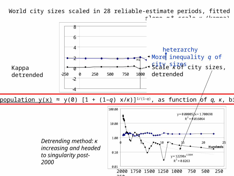
World city sizes scaled in 28 reliable-estimate periods, fitted slope q & scale κ (kappa)
2000 1750 1500 1250 1000 750 500 250 0 -250
-4
-2
0
2
4
6
8
-250 0 250 500 750 1000 1250 1500 1750 2000
q (NLS)
κ detrended
HiHi HiLoLo Lo
More inequality q of city sizes
Scale κ of city sizes, detrended
At time t, population y(x) ≈ y(0) [1 + (1–q) x/κ)]1/(1–q), as function of q, κ, binned size x
heterarchy
Detrending method: κ increasing and headed to singularity post-2000
12
y = 12298x-1.5684
R2 = 0.8263
y = 0.000052x + 1.700698
R2 = 0.016064
0.01
0.10
1.00
10.00
100.00
0 5 10 15 20 25Hundreds
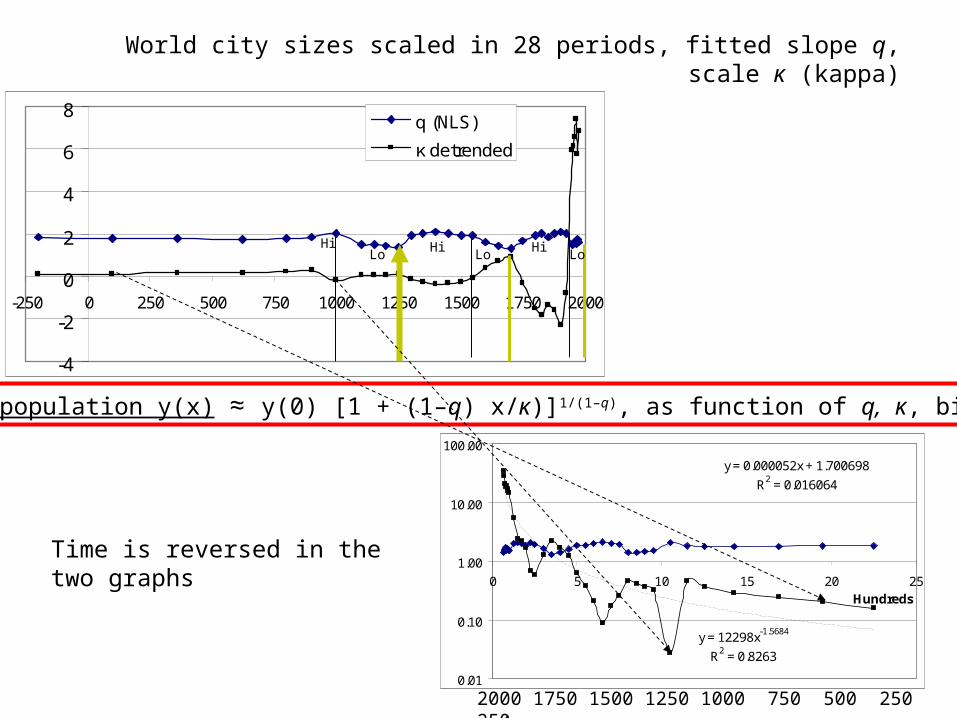
World city sizes scaled in 28 periods, fitted slope q, scale κ (kappa)
2000 1750 1500 1250 1000 750 500 250 0 -250
-4
-2
0
2
4
6
8
-250 0 250 500 750 1000 1250 1500 1750 2000
q (NLS)
κ detrended
HiHi HiLoLo Lo
At time t, population y(x) ≈ y(0) [1 + (1–q) x/κ)]1/(1–q), as function of q, κ, binned size x
Time is reversed in the two graphs
13
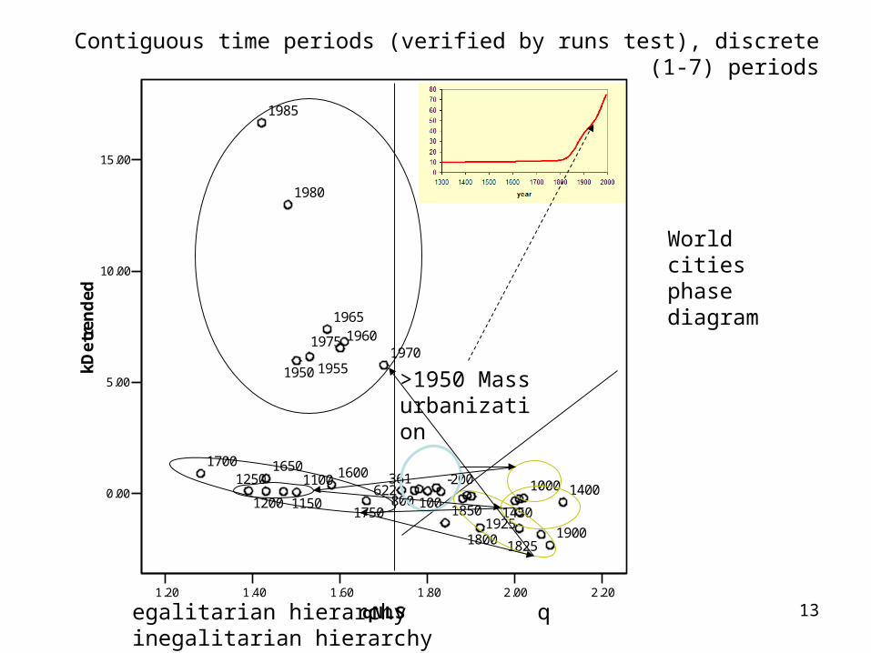
Contiguous time periods (verified by runs test), discrete (1-7) periods
1.20 1.40 1.60 1.80 2.00 2.20
qNLS
0.00
5.00
10.00
15.00
kDet
ren
ded
-200
100
361622
80010001100
11501200
12501400
1450
160016501700
1750
1800 1825
1850
19001925
1950 1955
19601965
19701975
1980
1985
egalitarian hierarchy q inegalitarian hierarchy
>1950 Mass urbanization
World cities phase diagram
14
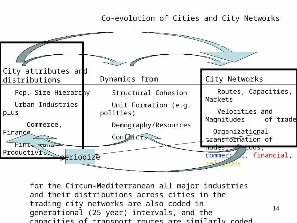
City attributes and distributions
Pop. Size Hierarchy
Urban Industries plus
Commerce, Finance
Hinterland Productivity
City Networks
Routes, Capacities, Markets
Velocities and Magnitudes of trade
Organizational transformationof nodes, periods;
commercial, financial, religious
Dynamics from
Structural Cohesion
Unit Formation (e.g. polities)
Demography/Resources
Conflicts
Co-evolution of Cities and City Networks
for the Circum-Mediterranean all major industries and their distributions across cities in the trading city networks are also coded in generational (25 year) intervals, and the capacities of transport routes are similarly coded in 25 year intervals. All-Eurasia coding incomplete.
periodize
15
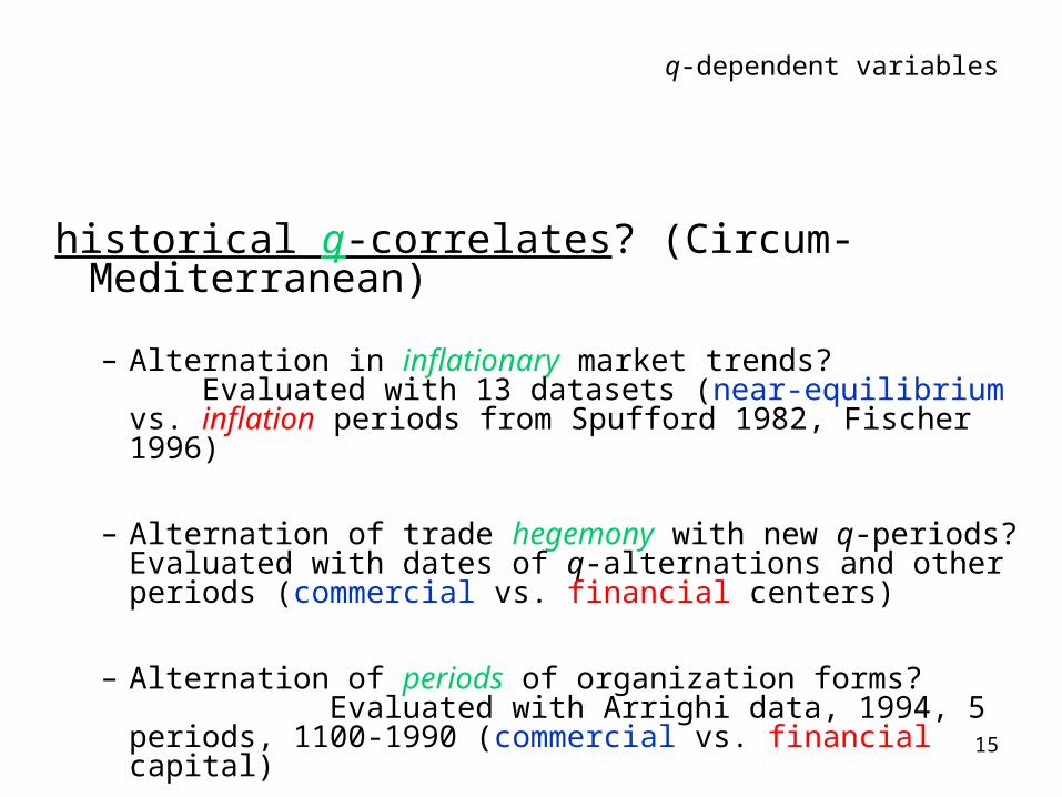
q-dependent variables
historical q-correlates? (Circum-Mediterranean)
– Alternation in inflationary market trends? Evaluated with 13 datasets (near-equilibrium vs. inflation periods from Spufford 1982, Fischer 1996)
– Alternation of trade hegemony with new q-periods? Evaluated with dates of q-alternations and other periods (commercial vs. financial centers)
– Alternation of periods of organization forms? Evaluated with Arrighi data, 1994, 5 periods, 1100-1990 (commercial vs. financial capital)
16
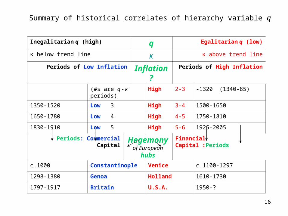
Summary of historical correlates of hierarchy variable q
Inegalitarian q (high) q Egalitarian q (low)
κ below trend line κ κ above trend line
Periods of Low Inflation Inflation? Periods of High Inflation
(#s are q - κ periods) High 2-3 -1320 (1340-85)
1350-1520 Low 3 High 3-4 1500-1650
1650-1780 Low 4 High 4-5 1750-1810
1830-1910 Low 5 High 5-6 1925-2005
Periods: Commercial Capital
Hegemony of European
hubs
Financial Capital :Periods
c.1000 Constantinople Venice c.1100-1297
1298-1380 Genoa Holland 1610-1730
1797-1917 Britain U.S.A. 1950-?
17
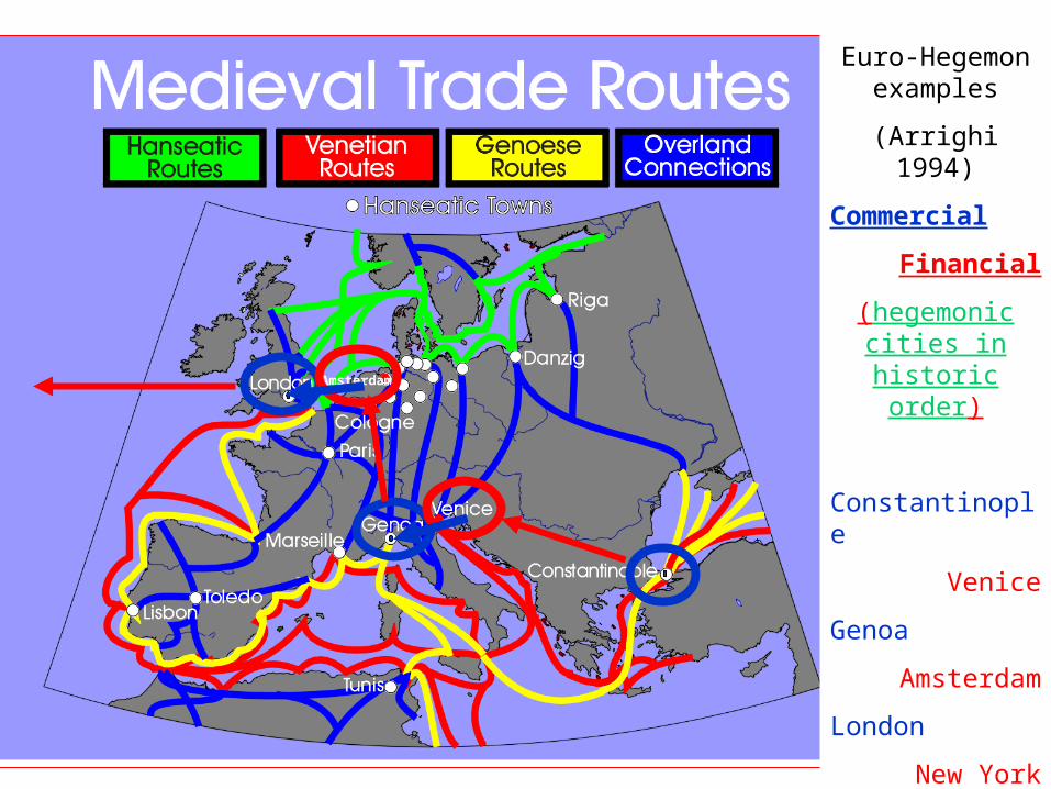
Euro-Hegemon examples
(Arrighi 1994)
Commercial
Financial
(hegemonic cities in historic order)
Constantinople
Venice
Genoa
Amsterdam
London
New York
Amsterdam
18
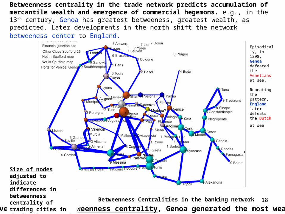
Given its 13th C betweenness centrality, Genoa generated the most wealth
Betweenness centrality in the trade network predicts accumulation of mercantile wealth and emergence of commercial hegemons. e.g., in the 13th century, Genoa has greatest betweeness, greatest wealth, as predicted. Later developments in the north shift the network betweeness center to England.
Size of nodes adjusted to indicate differences in betweenness centrality of trading cities in the banking network
Betweenness Centralities in the banking network
Episodically, in 1298, Genoa defeated the Venetians at sea.
Repeating the pattern, England later defeats the
Dutch at sea
19
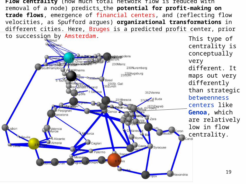
Flow centrality (how much total network flow is reduced with removal of a node) predicts the potential for profit-making on trade flows, emergence of financial centers, and (reflecting flow velocities, as Spufford argues) organizational transformations in different cities. Here, Bruges is a predicted profit center, prior to succession by Amsterdam.
This type of centrality is conceptually very different. It maps out very differently than strategic betweenness centers like Genoa, which are relatively low in flow centrality.
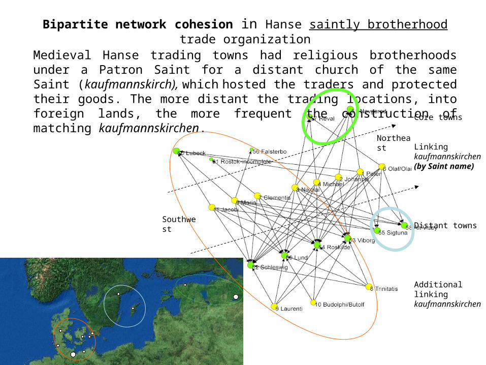
Core towns
Linking kaufmannskirchen (by Saint name)
Distant towns
Additional linking kaufmannskirchen
Medieval Hanse trading towns had religious brotherhoods under a Patron Saint for a distant church of the same Saint (kaufmannskirch), which hosted the traders and protected their goods. The more distant the trading locations, into foreign lands, the more frequent the construction of matching kaufmannskirchen.
Northeast
Southwest
Bipartite network cohesion in Hanse saintly brotherhood trade organization
21
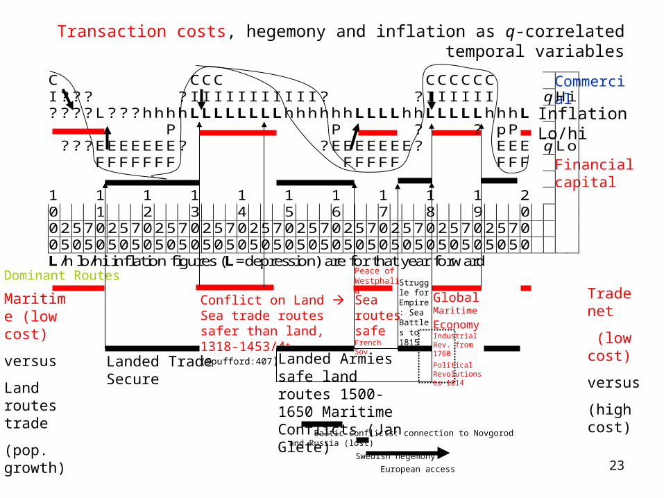
C C C C C C C C C C I ? ? ? ? I I I I I I I I I I I ? ? I I I I I I q H i ? ? ? ? L ? ? ? h h h h L L L L L L L L h h h h h h L L L L h h L L L L L h h h L P P ? ? p P ? ? ? E E E E E E E ? ? E E E E E E E ? E E E q L o F F F F F F F F F F F F F F F 1 1 1 1 1 1 1 1 1 1 2 0 1 2 3 4 5 6 7 8 9 0 0 2 5 7 0 2 5 7 0 2 5 7 0 2 5 7 0 2 5 7 0 2 5 7 0 2 5 7 0 2 5 7 0 2 5 7 0 2 5 7 0 0 5 0 5 0 5 0 5 0 5 0 5 0 5 0 5 0 5 0 5 0 5 0 5 0 5 0 5 0 5 0 5 0 5 0 5 0 5 0 5 0 L/h lo/hi inflation figures (L=depression) are for that year forward
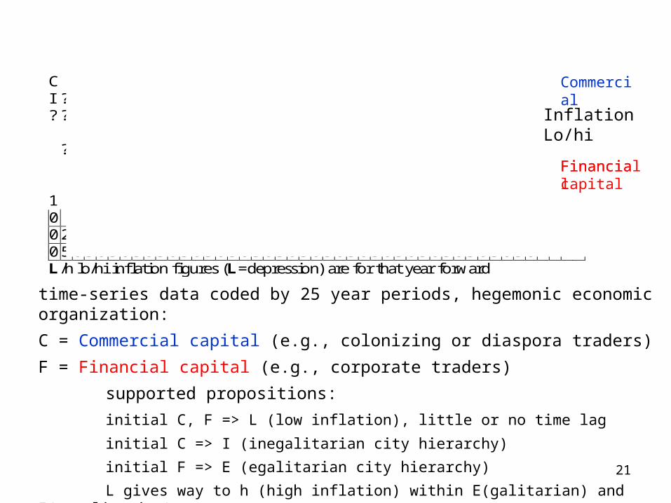
time-series data coded by 25 year periods, hegemonic economic organization:
C = Commercial capital (e.g., colonizing or diaspora traders)
F = Financial capital (e.g., corporate traders)
supported propositions:
initial C, F => L (low inflation), little or no time lag
initial C => I (inegalitarian city hierarchy)
initial F => E (egalitarian city hierarchy)
L gives way to h (high inflation) within E(galitarian) and I(negalitarian)
Inflation Lo/hi
Financial
Commercial
Financial capital
22
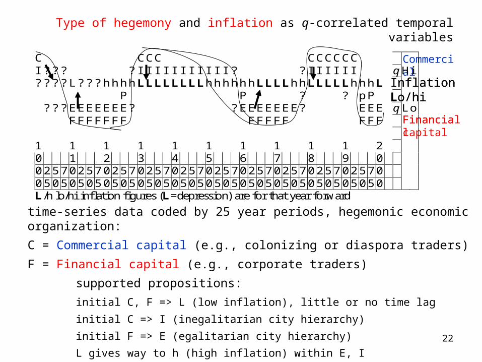
time-series data coded by 25 year periods, hegemonic economic organization:
C = Commercial capital (e.g., colonizing or diaspora traders)
F = Financial capital (e.g., corporate traders)
supported propositions:
initial C, F => L (low inflation), little or no time lag
initial C => I (inegalitarian city hierarchy)
initial F => E (egalitarian city hierarchy)
L gives way to h (high inflation) within E, I
Type of hegemony and inflation as q-correlated temporal variables
Inflation Lo/hiInflation Lo/hi
Financial
Commercial
Financial capital
C C C C C C C C C C I ? ? ? ? I I I I I I I I I I I ? ? I I I I I I q H i ? ? ? ? L ? ? ? h h h h L L L L L L L L h h h h h h L L L L h h L L L L L h h h L P P ? ? p P ? ? ? E E E E E E E ? ? E E E E E E E ? E E E q L o F F F F F F F F F F F F F F F 1 1 1 1 1 1 1 1 1 1 2 0 1 2 3 4 5 6 7 8 9 0 0 2 5 7 0 2 5 7 0 2 5 7 0 2 5 7 0 2 5 7 0 2 5 7 0 2 5 7 0 2 5 7 0 2 5 7 0 2 5 7 0 0 5 0 5 0 5 0 5 0 5 0 5 0 5 0 5 0 5 0 5 0 5 0 5 0 5 0 5 0 5 0 5 0 5 0 5 0 5 0 5 0 L/h lo/hi inflation figures (L=depression) are for that year forward
23
Transaction costs, hegemony and inflation as q-correlated temporal variables
Conflict on Land Sea trade routes safer than land, 1318-1453/4+ (Spufford:407)
Inflation Lo/hi
Landed Armies safe land routes 1500-1650 Maritime Conflicts (Jan Glete)
Landed Trade Secure
Dominant Routes
Sea routes safe French Sov.
Peace of Westphalia
Baltic conflicts: connection to Novgorod and Russia (lost)
Swedish hegemony
European access
Struggle for Empire: Sea Battles to 1815
Global Maritime
Economy Industrial Rev. from 1760
Political Revolutions to 1814
Trade net
(low cost)
versus
(high cost)
Maritime (low cost)
versus
Land routes trade
(pop. growth)
Financial capital
CommercialC C C C C C C C C C I ? ? ? ? I I I I I I I I I I I ? ? I I I I I I q H i ? ? ? ? L ? ? ? h h h h L L L L L L L L h h h h h h L L L L h h L L L L L h h h L P P ? ? p P ? ? ? E E E E E E E ? ? E E E E E E E ? E E E q L o F F F F F F F F F F F F F F F 1 1 1 1 1 1 1 1 1 1 2 0 1 2 3 4 5 6 7 8 9 0 0 2 5 7 0 2 5 7 0 2 5 7 0 2 5 7 0 2 5 7 0 2 5 7 0 2 5 7 0 2 5 7 0 2 5 7 0 2 5 7 0 0 5 0 5 0 5 0 5 0 5 0 5 0 5 0 5 0 5 0 5 0 5 0 5 0 5 0 5 0 5 0 5 0 5 0 5 0 5 0 5 0 L/h lo/hi inflation figures (L=depression) are for that year forward
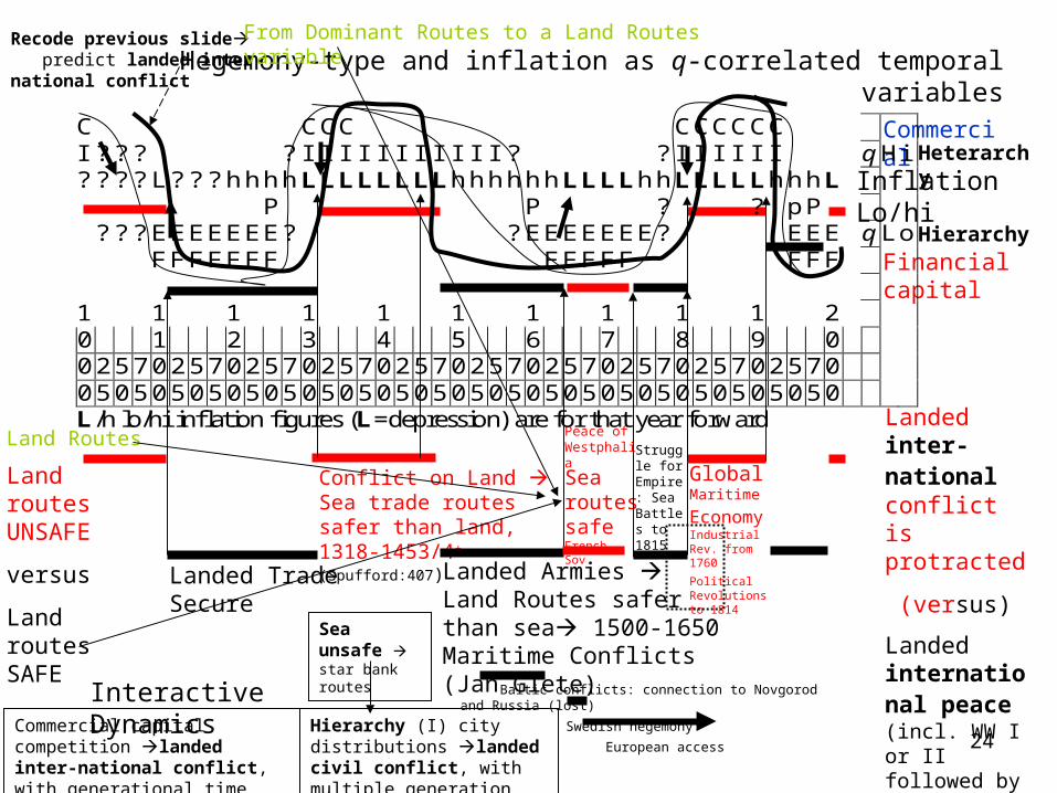
24Hierarchy (I) city distributions landed civil conflict, with multiple generation time lag
Recode previous slide predict landed inter-national conflict
Hegemony-type and inflation as q-correlated temporal variables
Conflict on Land Sea trade routes safer than land, 1318-1453/4+ (Spufford:407)
Inflation Lo/hi
Landed Armies Land Routes safer than sea 1500-1650 Maritime Conflicts (Jan Glete)
Landed Trade Secure
Sea routes safe French Sov.
Peace of Westphalia
Baltic conflicts: connection to Novgorod and Russia (lost)
Swedish hegemony
European access
Struggle for Empire: Sea Battles to 1815
Global Maritime
Economy Industrial Rev. from 1760
Political Revolutions to 1814
Landed inter-national conflict is protracted
(versus)
Landed international peace (incl. WW I or II followed by peace)
Land routes UNSAFE
versus
Land routes SAFE
Financial capital
Commercial
Commercial capital competition landed inter-national conflict, with generational time lag
Interactive Dynamics
Hierarchy
Heterarchy
Land Routes
From Dominant Routes to a Land Routes variable
Sea unsafe star bank routes
C C C C C C C C C C I ? ? ? ? I I I I I I I I I I I ? ? I I I I I I q H i ? ? ? ? L ? ? ? h h h h L L L L L L L L h h h h h h L L L L h h L L L L L h h h L P P ? ? p P ? ? ? E E E E E E E ? ? E E E E E E E ? E E E q L o F F F F F F F F F F F F F F F 1 1 1 1 1 1 1 1 1 1 2 0 1 2 3 4 5 6 7 8 9 0 0 2 5 7 0 2 5 7 0 2 5 7 0 2 5 7 0 2 5 7 0 2 5 7 0 2 5 7 0 2 5 7 0 2 5 7 0 2 5 7 0 0 5 0 5 0 5 0 5 0 5 0 5 0 5 0 5 0 5 0 5 0 5 0 5 0 5 0 5 0 5 0 5 0 5 0 5 0 5 0 5 0 L/h lo/hi inflation figures (L=depression) are for that year forward
25
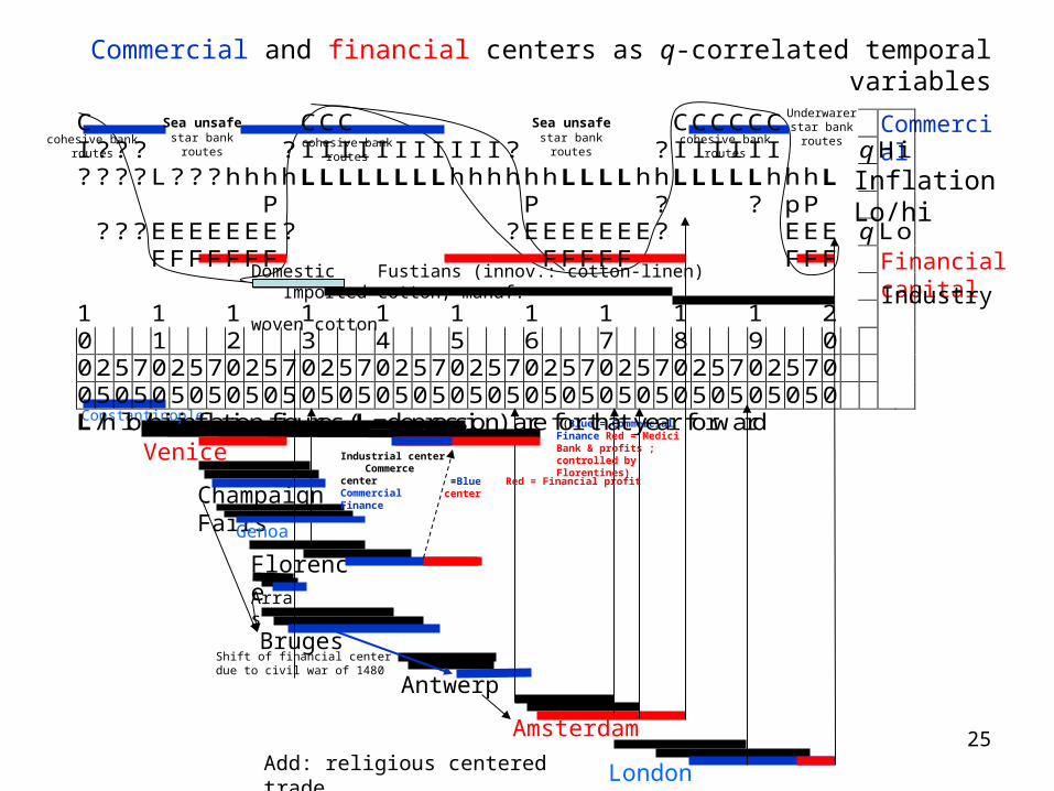
Commercial and financial centers as q-correlated temporal variables
Inflation Lo/hi
Florence
Venice
Arras
Bruges
Antwerp
Amsterdam
London
Champaign Fairs
Constantinople
Genoa
Shift of financial center due to civil war of 1480
Industrial center Commerce center Commercial Finance =Blue Red = Financial profit center
(Blue = Commercial Finance Red = Medici Bank & profits ; controlled by Florentines)
Domestic Fustians (innov.: cotton-linen) Imported cotton, manuf.
woven cotton
Commercial
Financial capital
Industry
Add: religious centered trade
Sea unsafe star bank routes
Sea unsafe star bank routes
Underwarer star bank
routescohesive bank routescohesive bank routes cohesive bank routesC C C C C C C C C C I ? ? ? ? I I I I I I I I I I I ? ? I I I I I I q H i ? ? ? ? L ? ? ? h h h h L L L L L L L L h h h h h h L L L L h h L L L L L h h h L P P ? ? p P ? ? ? E E E E E E E ? ? E E E E E E E ? E E E q L o F F F F F F F F F F F F F F F 1 1 1 1 1 1 1 1 1 1 2 0 1 2 3 4 5 6 7 8 9 0 0 2 5 7 0 2 5 7 0 2 5 7 0 2 5 7 0 2 5 7 0 2 5 7 0 2 5 7 0 2 5 7 0 2 5 7 0 2 5 7 0 0 5 0 5 0 5 0 5 0 5 0 5 0 5 0 5 0 5 0 5 0 5 0 5 0 5 0 5 0 5 0 5 0 5 0 5 0 5 0 5 0 L/h lo/hi inflation figures (L=depression) are for that year forward
26
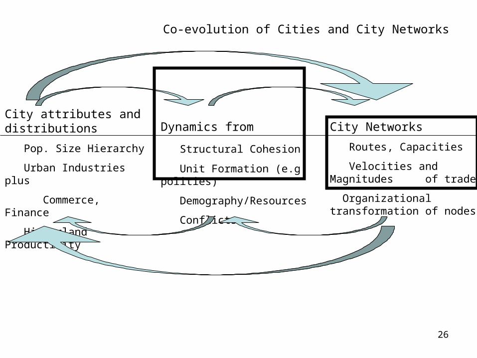
City attributes and distributions
Pop. Size Hierarchy
Urban Industries plus
Commerce, Finance
Hinterland Productivity
City Networks
Routes, Capacities
Velocities and Magnitudes of trade
Organizational transformationof nodes
Dynamics from
Structural Cohesion
Unit Formation (e.g. polities)
Demography/Resources
Conflicts
Co-evolution of Cities and City Networks
28
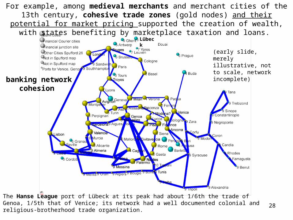
For example, among medieval merchants and merchant cities of the 13th century, cohesive trade zones (gold nodes) and their potential for market pricing supported the
creation of wealth, with states benefiting by marketplace taxation and loans.
The Hanse League port of Lübeck at its peak had about 1/6th the trade of Genoa, 1/5th that of Venice; its network had a well documented colonial and religious-brotherhood trade organization.
(early slide, merely illustrative, not to scale, network incomplete)
Lübeck
banking networkcohesion
29
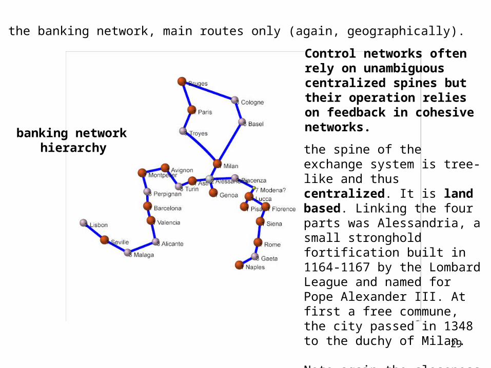
the banking network, main routes only (again, geographically).
the spine of the exchange system is tree-like and thus centralized. It is land based. Linking the four parts was Alessandria, a small stronghold fortification built in 1164-1167 by the Lombard League and named for Pope Alexander III. At first a free commune, the city passed in 1348 to the duchy of Milan.
Note again the closeness of Genoa to the center, and the exclusion of Venice.
Control networks often rely on unambiguous centralized spines but their operation relies on feedback in cohesive networks.
banking networkhierarchy
30In Northern Europe the main Hanse League port of Lubeck had about 1/6th the trade of Genoa, 1/5th that of Venice.
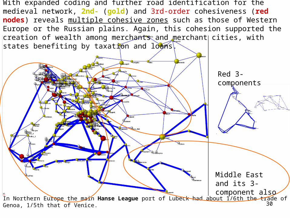
Red 3-components
Middle East and its 3-component also
With expanded coding and further road identification for the medieval network, 2nd- (gold) and 3rd-order cohesiveness (red nodes) reveals multiple cohesive zones such as those of Western Europe or the Russian plains. Again, this cohesion supported the creation of wealth among merchants and merchant cities, with states benefiting by taxation and loans.
31
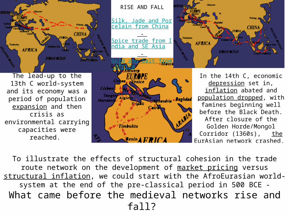
RISE AND FALL
Silk, Jade and Porcelain from China
- Spice trade from India and SE Asia
- Gold and Salt from Africa
The lead-up to the 13th C world-system and its economy
was a period of population expansion and then crisis as
environmental carrying capacities were reached.
In the 14th C, economic depression set in, inflation abated and
population dropped, with famines beginning well before the Black
Death. After closure of the Golden Horde/Mongol Corridor (1360s), the EurAsian network crashed.
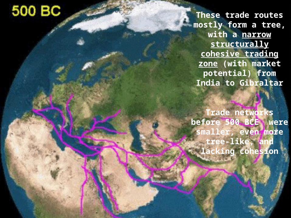
To illustrate the effects of structural cohesion in the trade route network on the development of market pricing versus structural inflation, we could start with the AfroEurasian world-system at the end of the pre-classical period in 500 BCE -
What came before the medieval networks rise and fall?
32
These trade routes mostly form a tree, with
a narrow structurally cohesive trading zone (with market potential) from India to Gibraltar
Trade networks before 500 BCE were smaller, even more tree-like, and
lacking cohesion

33
(figures courtesy of Andrew Sherratt, ArchAtlas)
Cohesive extension of trade routes leads to a host of other developments…

34
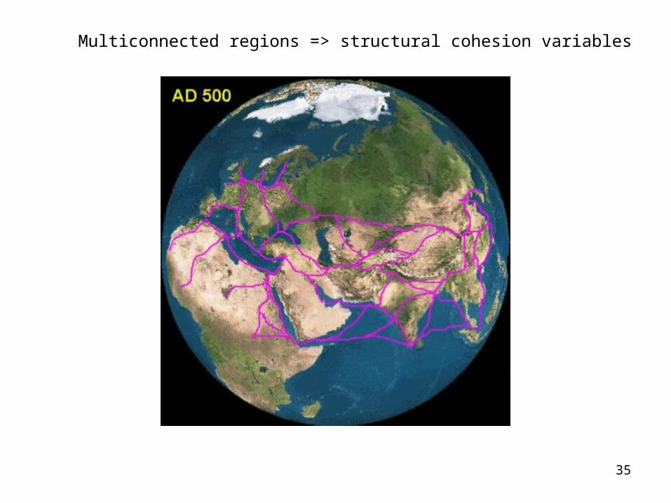
Multiconnected regions => structural cohesion variables
During classical antiquity trade routes become
much more structurally
cohesive from China to France
35
Multiconnected regions => structural cohesion variables
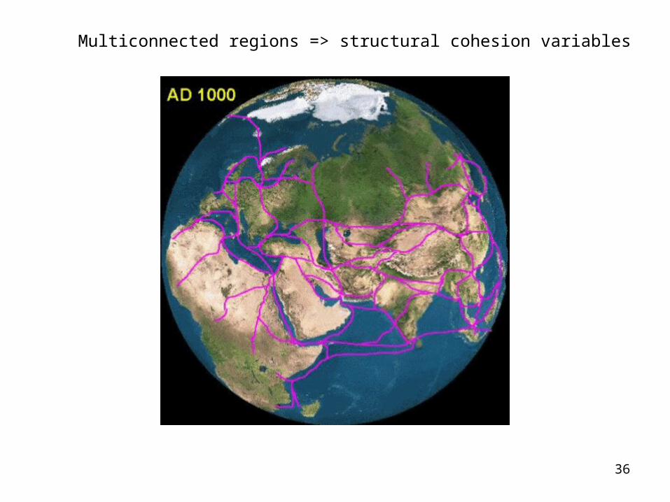
36
Multiconnected regions => structural cohesion variables
37
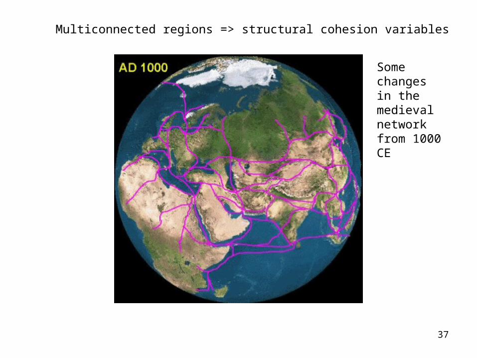
Some changes in the medieval network from 1000 CE
Multiconnected regions => structural cohesion variables
38
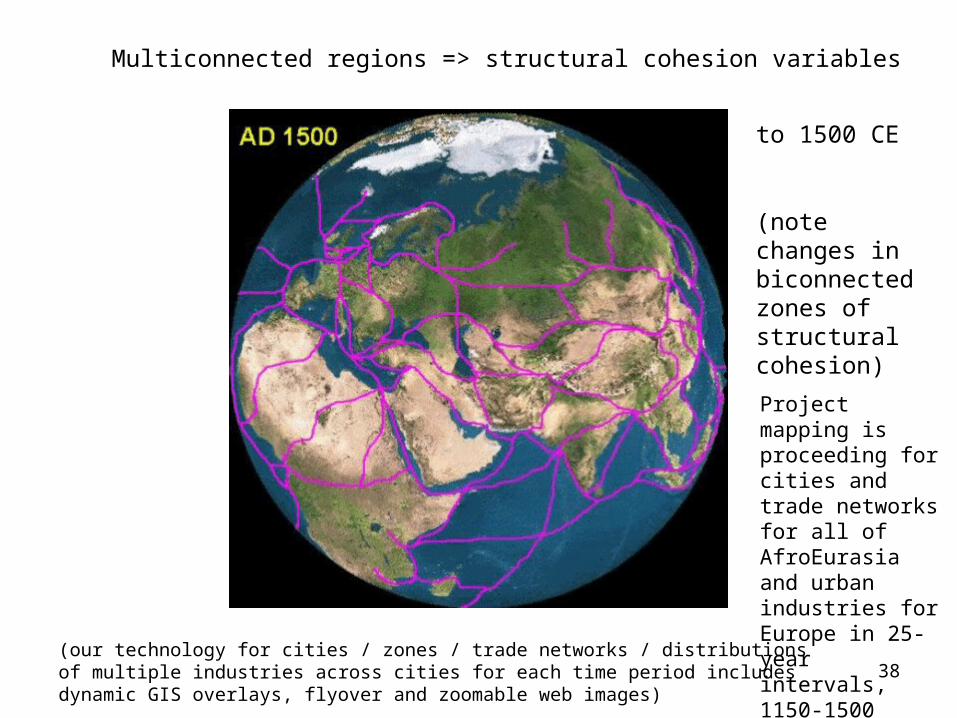
to 1500 CE
(note changes in biconnected zones of structural cohesion)
Project mapping is proceeding for cities and trade networks for all of AfroEurasia and urban industries for Europe in 25-year intervals, 1150-1500
(our technology for cities / zones / trade networks / distributions of multiple industries across cities for each time period includes dynamic GIS overlays, flyover and zoomable web images)
Multiconnected regions => structural cohesion variables
39
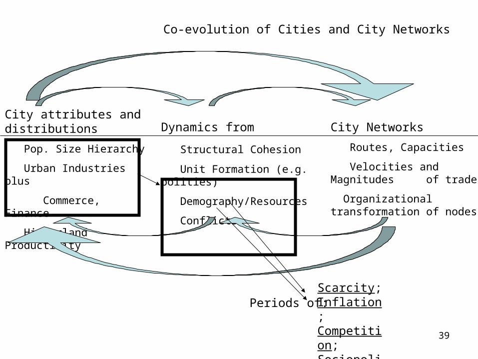
City attributes and distributions
Pop. Size Hierarchy
Urban Industries plus
Commerce, Finance
Hinterland Productivity
City Networks
Routes, Capacities
Velocities and Magnitudes of trade
Organizational transformationof nodes
Dynamics from
Structural Cohesion
Unit Formation (e.g. polities)
Demography/Resources
Conflicts
Co-evolution of Cities and City Networks
Scarcity; Inflation; Competition; Sociopolitical violence;
Periods of:

40
• Peter Spufford - in Power & Profit (2002)– shows how rises in the velocity of trade in intercity networks
causes transformations in organizations.• Peter Turchin - in Structure & Dynamics (2005)
– demonstrates dynamic interactions between governance, conflicts, unraveling, on the one hand, and population oscillations on the other (structural demographic theory)
Data sources and dynamic interaction analyses
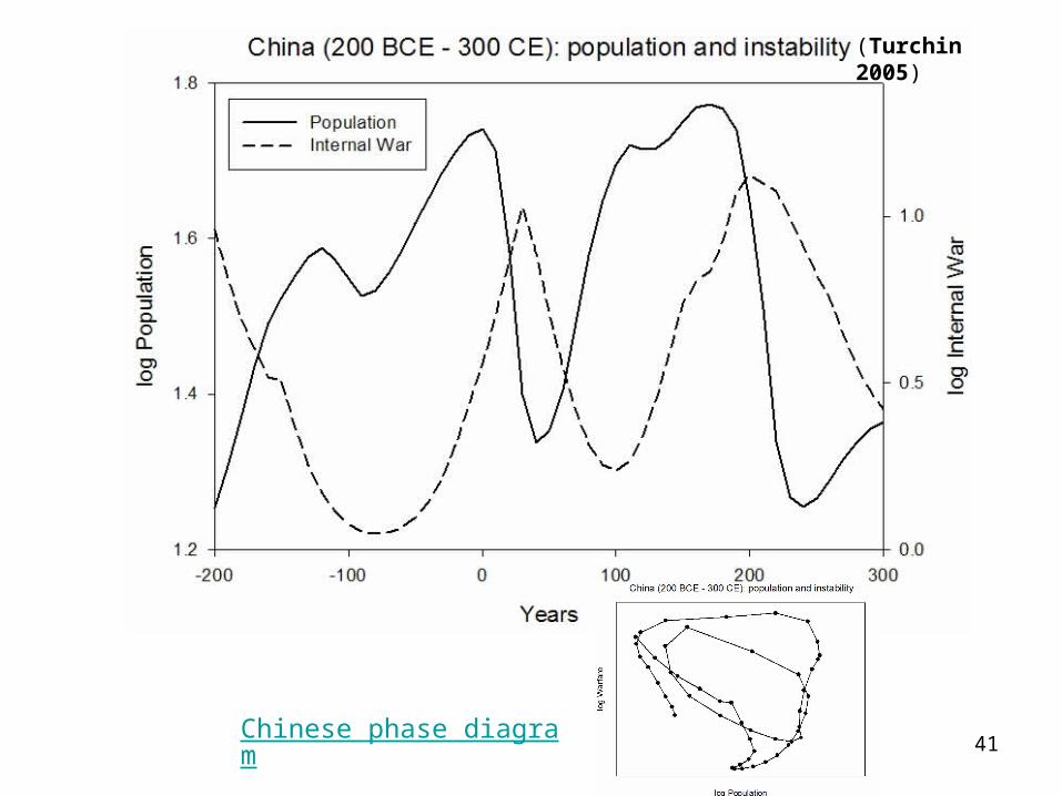
41Chinese phase diagram
(Turchin 2005)
42
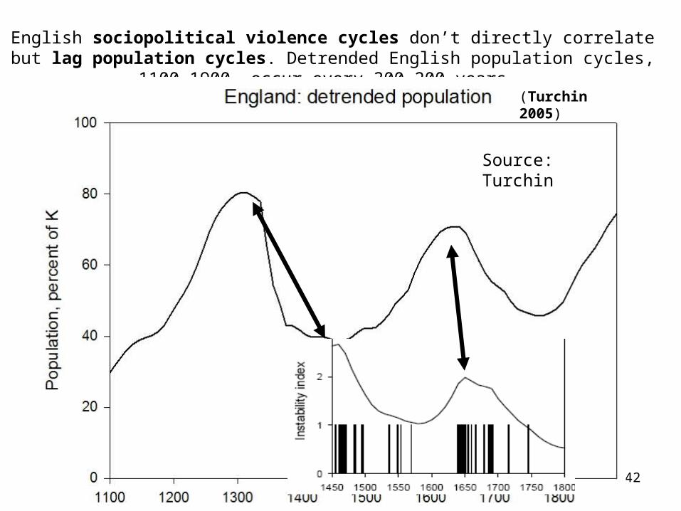
English sociopolitical violence cycles don’t directly correlate but lag population cycles. Detrended English population cycles, 1100-1900, occur every 300-200 years.
Source: Turchin
(Turchin 2005)
43
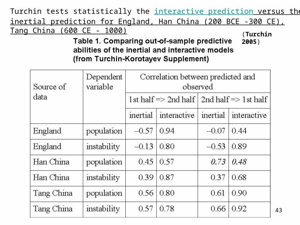
Turchin tests statistically the interactive prediction versus the inertial prediction for England, Han China (200 BCE -300 CE), Tang China (600 CE - 1000)
(Turchin 2005)
44
0
10000
20000
30000
40000
50000
60000
70000
0 2000000 4000000 6000000 8000000 10000000
City Sizes
Cit
y F
un
ctio
ns
R&Dchina-superlinear
R&Dfrance-superlinear
Elec.Cons.-linear
Gas Sales-sublinear
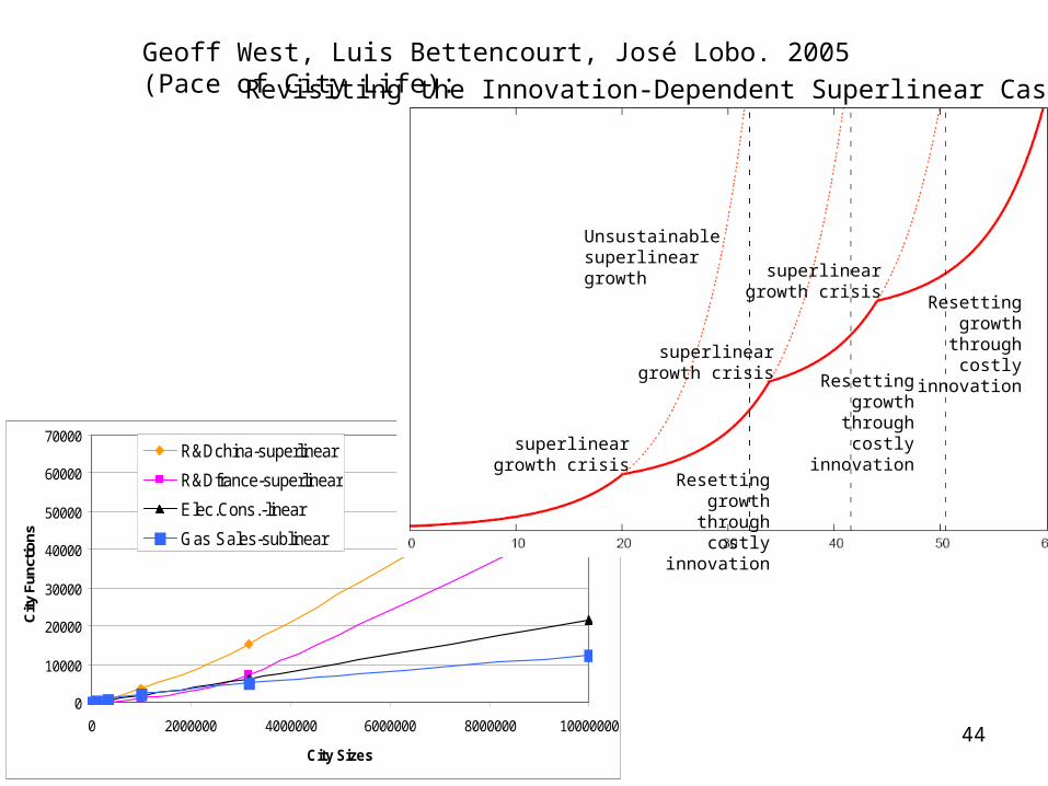
Geoff West, Luis Bettencourt, José Lobo. 2005 (Pace of City Life):
Revisiting the Innovation-Dependent Superlinear Case
Unsustainable superlinear growth
superlinear growth crisis
superlinear growth crisis
superlinear growth crisis
Resetting growth through costly
innovation
Resetting growth through costly
innovation
Resetting growth through costly
innovation
45
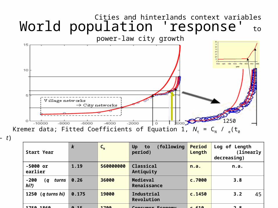
World population 'response' to power-law city growth
Cities and hinterlands context variables
Kremer data; Fitted Coefficients of Equation 1, Nt = CN /
e(t0 – t)
Start Yeark CN Up to (following period) Period
Length Log of Length . (linearly decreasing)
-5000 or earlier 1.19 560000000 Classical Antiquity n.a. n.a.
-200 (q turns hi?) 0.26 36000 Medieval Renaissance c.7000 3.8
1250 (q turns hi) 0.175 19000 Industrial Revolution c.1450 3.2
1750-1860 (ditto) 0.15 1700 Consumer Economy c.610 2.8
Post-1962 (ditto) ? c.100? 2.0
1250
46
q-dependent variables
– power-law population growth is unsustainable, generates decreasing lengths of oscillations, also general inflection points (e.g., flattening, crisis)
– World population growth rate is slower with q-flat city growth, but also tends to diminish at the end of each type of q-period. Possibly a failure of innovation rate because leading cities depend on innovation.
47
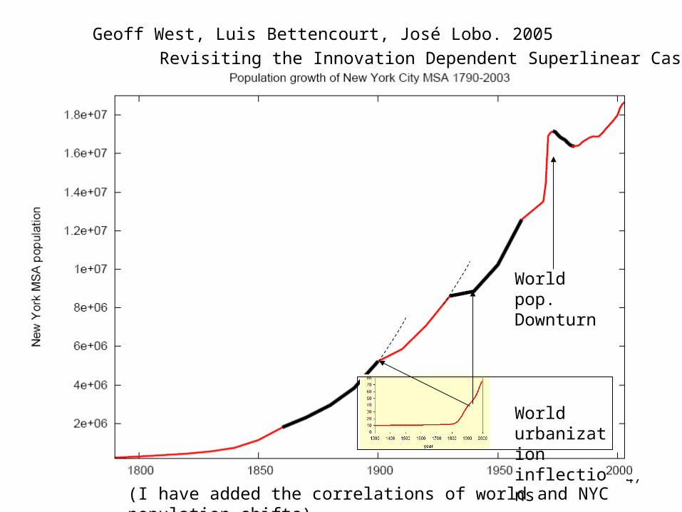
Geoff West, Luis Bettencourt, José Lobo. 2005 (Pace of City Life):
Revisiting the Innovation Dependent Superlinear Case
World pop. Downturn
World urbanization inflections
(I have added the correlations of world and NYC population shifts)
48
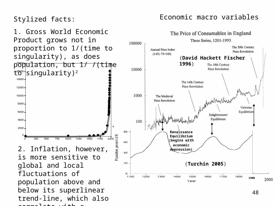
Economic macro variables
1900
Renaissance Equilibrium (begins with
economic depression)
Stylized facts:
1. Gross World Economic Product grows not in proportion to 1/(time to singularity), as does population, but 1/ /(time to singularity)2
2. Inflation, however, is more sensitive to global and local fluctuations of population above and below its superlinear trend-line, which also correlate with q-periods.
(David Hackett Fischer 1996)
(Turchin 2005)
49
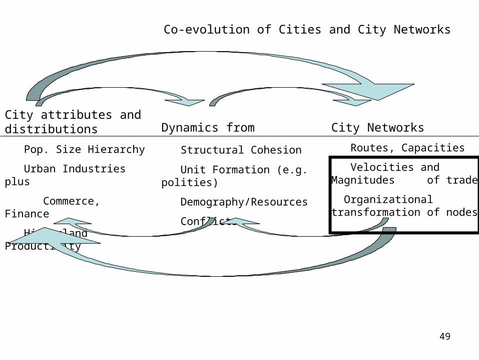
City attributes and distributions
Pop. Size Hierarchy
Urban Industries plus
Commerce, Finance
Hinterland Productivity
City Networks
Routes, Capacities
Velocities and Magnitudes of trade
Organizational transformationof nodes
Dynamics from
Structural Cohesion
Unit Formation (e.g. polities)
Demography/Resources
Conflicts
Co-evolution of Cities and City Networks
50
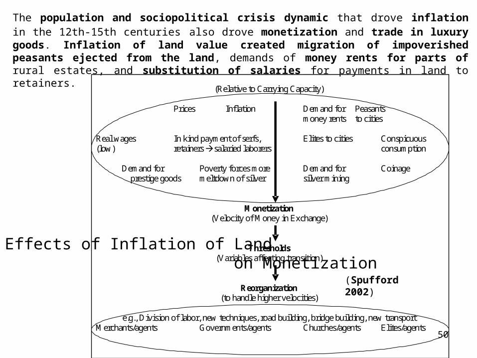
Effects of Inflation of Land on Monetization
(Relative to Carrying Capacity) Prices Inflation Demand for Peasants money rents to cities Real wages In kind payment of serfs, Elites to cities Conspicuous (low) retainers salaried laborers consumption Demand for Poverty forces more Demand for Coinage prestige goods meltdown of silver silver mining
Monetization (Velocity of Money in Exchange)
Thresholds (Variables affecting transition)
Reorganization (to handle higher velocities)
e.g., Division of labor, new techniques, road building, bridge building, new transport
Merchants/agents Governments/agents Churches/agents Elites/agents
GET TURCHIN VARIABLES
The population and sociopolitical crisis dynamic that drove inflation in the 12th-15th centuries also drove monetization and trade in luxury goods. Inflation of land value created migration of impoverished peasants ejected from the land, demands of money rents for parts of rural estates, and substitution of salaries for payments in land to retainers.
(Spufford 2002)
51
– Adamic, Lada, et al. 2003. Local search in unstructured networks. In, Bornholdt and Schuster, eds., Handbook of Graphs and Networks. Wiley-VCH.
– Arrighi, Giovanni. 1994. The Long Twentieth Century. London: Verso.
– Fischer, David Hackett. 1996. The Great Wave: Price Revolutions and the Rhythm of History. Oxford University Press
– Sherratt, Andrew. (visited) 2005. ArchAtlas. http://www.arch.ox.ac.uk/ArchAtlas/
– Spufford, Peter. 2002. Power and Profit: The Merchant in Medieval Europe. Cambridge U Press.
– Tsallis, Constantino. 1988. Possible generalization of Boltzmann-Gibbs statistics, J.Stat.Phys. 52, 479.
– Turchin, Peter. 2005. Dynamical Feedbacks between Population Growth and Sociopolitical Instability in Agrarian States. Structure and Dynamics 1(1):Art2. http://repositories.cdlib.org/imbs/socdyn/sdeas/
– West, Geoff, Luis Bettencourt, José Lobo. 2005. The Pace of City Life: Growth, Innovation and Scale. Ms. Santa Fe Institute, Project ISCOM.
– Douglas R. White, Natasa Kejzar, Constantino Tsallis, Doyne Farmer, and Scott White. 2005. A generative model for feedback networks. Physica A forthcoming. http://arxiv.org/abs/cond-mat/0508028
– White, Douglas R., Natasa Keyzar, Constantino Tsallis and Celine Rozenblat. 2005. Ms. Generative Historical Model of City Size Hierarchies: 430 BCE – 2005. Ms. Santa Fe Institute.
– White, Douglas R., and Peter Spufford. (Book Ms.) 2005. Medieval to Modern: Civilizations as Dynamic Networks. Cambridge: Cambridge University Press.
References
52
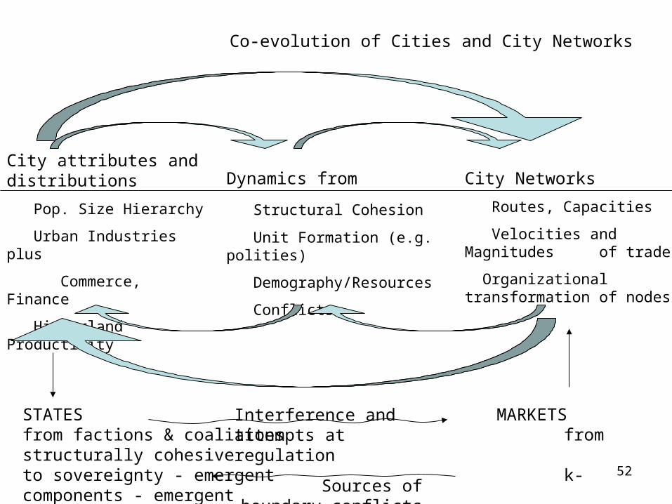
City Networks
Routes, Capacities
Velocities and Magnitudes of trade
Organizational transformationof nodes
STATES MARKETSfrom factions & coalitions from structurally cohesiveto sovereignty - emergent k-components - emergent Spatiopolitical units Network units (overlap)
City attributes and distributions
Pop. Size Hierarchy
Urban Industries plus
Commerce, Finance
Hinterland Productivity
Dynamics from
Structural Cohesion
Unit Formation (e.g. polities)
Demography/Resources
Conflicts
Co-evolution of Cities and City Networks
Interference and attempts at regulation
Sources of boundary conflicts

53

54
0
5000
10000
15000
20000
25000
30000
35000
40000
0 1000 2000 3000 4000 5000 6000 7000 8000 9000 10000
-100000
-50000
0
50000
100000
150000
200000
250000
300000
350000
0 1000 2000 3000 4000 5000 6000 7000 8000 9000 10000
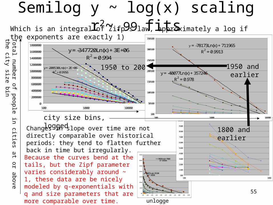
Semilog y ~ log(x): poor fit
Cumulative population is used because by taking only the populations in each size bin in different growth periods differential city growth generates the
dogs-eaten-by-snake phenomena:
Actual 1965 data on distribution at one time smoothed cumulative distributions
A cumulative distribution has with more population in the lower bins requires curve fitting such as y ~ log (x) with lower bins weighted proportional to population. The upper bins show bias toward longer tails compared to semi-log but less than a power-law tendency, as in these data.
y = 3E+06x-0.4432
R2 = 0.9714
0
50000
100000
150000
200000
250000
300000
350000
0 1000 2000 3000 4000 5000 6000 7000 8000 9000 10000
Power-law: poor fit
Time1 Time2 Time3 Time4 Time5
“innovative bulges” in city
sizes move thru time
Fitting here uses bins with largest numbers
55
y = -40077Ln(x) + 357246R2 = 0.978
y = -78173Ln(x) + 711965R2 = 0.9913
100
50100
100100
150100
200100
250100
300100
350100
100 1100 2100 3100 4100 5100 6100 7100 8100 9100 10100
unlogged
Semilog y ~ log(x) scaling r2~.99 fits
y = -208530Ln(x) + 2E+06
R2 = 0.9956
y = -347720Ln(x) + 3E+06
R2 = 0.994
0
200000
400000
600000
800000
1000000
1200000
1400000
1600000
1800000
100 1000 10000 100000
1950 to 2005
100
1100
2100
3100
4100
5100
6100
7100
8100
9100
10100
100 1000
1800 and earlier
Because the curves bend at the tails, but the Zipf parameter varies considerably around ~ 1, these data are be nicely modeled by q-exponentials with q and size parameters that are more comparable over time.
y = -40077Ln(x) + 357246
R2 = 0.978
y = -78173Ln(x) + 711965
R2 = 0.9913
100
50100
100100
150100
200100
250100
300100
350100
100 1000 10000
1950 and earlier
To
tal n
um
be
r of p
eo
ple
in citie
s at o
r ab
ove
the
city size b
in
city size bins, logged
Which is an integral of Zifp's law, approximately a log if the exponents are exactly 1)
Changes in slope over time are not directly comparable over historical periods: they tend to flatten further back in time but irregularly.
56
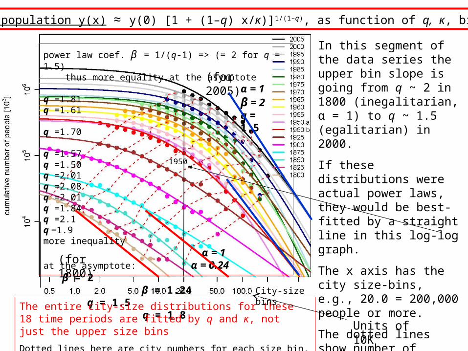
% Urban in Europe
fitted q-exponential distributions, q, κ.
power law coef. β = 1/(q-1) => (= 2 for q = 1.5) thus more equality at the asymptote
q =1.81 q =1.61
q =1.70
q =1.57 q =1.50q =2.01q =2.08q =2.01q =1.84 q =2.1 q =1.9 more inequality α = 1at the asymptote: α = 0.24 β = 2
β = 1.24 q = 1.5 q = 1.8
In this segment of the data series the upper bin slope is going from q ~ 2 in 1800 (inegalitarian, α = 1) to q ~ 1.5 (egalitarian) in 2000.
If these distributions were actual power laws, they would be best-fitted by a straight line in this log-log graph.
The x axis has the city size-bins, e.g., 20.0 = 200,000 people or more.
The dotted lines show number of cities in multiples of two: 4, 8,16,32,etc.
The entire city-size distributions for these 18 time periods are fitted by q and κ, not just the upper size bins
Dotted lines here are city numbers for each size bin.
(for 1800)
(for 2005)
City-size bins
1950
Units of 10K
Q-exponential scaling ~ .99+ fitAt time t, population y(x) ≈ y(0) [1 + (1–q) x/κ)]1/(1–q), as function of q, κ, binned size x
α = 1 β = 2 q = 1.5