Northumbria Research Link

Citation: Popoola, Wasiu Oyewole (2009) Subcarrier intensity modulated free-space optical communication systems. Doctoral thesis, Northumbria University.

This version was downloaded from Northumbria Research Link: http://nrl.northumbria.ac.uk/1939/

Northumbria University has developed Northumbria Research Link (NRL) to enable users to access the University’s research output. Copyright © and moral rights for items on NRL are retained by the individual author(s) and/or other copyright owners. Single copies of full items can be reproduced, displayed or performed, and given to third parties in any format or medium for personal research or study, educational, or not-for-profit purposes without prior permission or charge, provided the authors, title and full bibliographic details are given, as well as a hyperlink and/or URL to the original metadata page. The content must not be changed in any way. Full items must not be sold commercially in any format or medium without formal permission of the copyright holder. The full policy is available online: http://nrl.northumbria.ac.uk/pol i cies.html

SUBCARRIER INTENSITY

MODULATED FREE-SPACE

OPTICAL COMMUNICATION

SYSTEMS

WASIU OYEWOLE POPOOLA

A thesis submitted in partial fulfilment

of the requirements of the

University of Northumbria at Newcastle

for the degree of

Doctor of Philosophy

Research undertaken in the

School of Computing, Engineering and Information

Sciences

September 2009

ii

Abstract

This thesis investigates and analyses the performance of terrestrial free-space optical

communication (FSO) system based on the phase shift keying pre-modulated subcarrier

intensity modulation (SIM). The results are theoretically and experimentally compared

with the classical On-Off keying (OOK) modulated FSO system in the presence of

atmospheric turbulence. The performance analysis is based on the bit error rate (BER)

and outage probability metrics. Optical signal traversing the atmospheric channel

suffers attenuation due to scattering and absorption of the signal by aerosols, fog,

atmospheric gases and precipitation. In the event of thick fog, the atmospheric

attenuation coefficient exceeds 100 dB/km, this potentially limits the achievable FSO

link length to less than 1 kilometre. But even in clear atmospheric conditions when

signal absorption and scattering are less severe with a combined attenuation coefficient

of less than 1 dB/km, the atmospheric turbulence significantly impairs the achievable

error rate, the outage probability and the available link margin of a terrestrial FSO

communication system.

The effect of atmospheric turbulence on the symbol detection of an OOK based

terrestrial FSO system is presented analytically and experimentally verified. It was

found that atmospheric turbulence induced channel fading will require the OOK

threshold detector to have the knowledge of the channel fading strength and noise levels

if the detection error is to be reduced to its barest minimum. This poses a serious design

difficulty that can be circumvented by employing phase shift keying (PSK) pre-

modulated SIM. The results of the analysis and experiments showed that for a binary

PSK-SIM based FSO system, the symbol detection threshold level does not require the

knowledge of the channel fading strength or noise level. As such, the threshold level is

fixed at the zero mark in the presence or absence of atmospheric turbulence. Also for

the full and seamless integration of FSO into the access network, a study of SIM-FSO

performance becomes compelling because existing networks already contain subcarrier-

like signals such as radio over fibre and cable television signals. The use of multiple

subcarrier signals as a means of increasing the throughput/capacity is also investigated

and the effect of optical source nonlinearity is found to result in intermodulation

distortion. The intermodulation distortion can impose a BER floor of up to 10-4

on the

system error performance.

In addition, spatial diversity and subcarrier delay diversity techniques are studied as

means of ameliorating the effect of atmospheric turbulence on the error and outage

performance of SIM-FSO systems. The three spatial diversity linear combining

techniques analysed are maximum ratio combining, equal gain combining and selection

combining. The system performance based on each of these combining techniques is

presented and compared under different strengths of atmospheric turbulence. The results

predicted that achieving a 4 km SIM-FSO link length with no diversity technique will

require about 12 dB of power more than using a 4 × 4 transmitter/receiver array system

with the same data rate in a weak turbulent atmospheric channel. On the other hand,

retransmitting the delayed copy of the data once on a different subcarrier frequency was

found to result in a gain of up to 4.5 dB in weak atmospheric turbulence channel.

iii

Contents

Abstract ii

List of Figures viii

List of Tables xiv

Glossary of Abbreviations xv

Glossary of Symbol xviii

Dedication xxiv

Acknowledgements xxv

Declaration xxvi

Chapter One

Introduction 1

1.1 Background 1

1.2 Research Motivation and Justification 5

1.3 Research Objectives 11

1.4 Thesis Organisation 13

1.5 Original Contributions 15

1.6 List of Publications and Awards 18

Chapter Two

Fundamentals of FSO 21

2.1 Introduction 21

2.2 Overview of FSO Technology 22

2.3 Features of FSO 23

2.3.1 Areas of application 26

2.4 FSO Block Diagram 27

iv

2.4.1 The transmitter 28

2.4.2 The atmospheric channel 30

2.4.3 The receiver 33

2.5 Eye Safety and Standards 36

2.5.1 Maximum Permissible Exposures (MPE) 40

2.6 Summary 41

Chapter Three

Optical Detection Theory 42

3.1 Introduction 42

3.2 Photodetectors 43

3.2.1 PIN photodetector 44

3.2.2 APD photodetector 46

3.3 Photodetection Techniques 47

3.3.1 Direct detection 47

3.3.2 Coherent detection 48

3.4 Photodetection Noise 51

3.4.1 Photon fluctuation noise 52

3.4.2 Dark current and excess noise 52

3.4.3 Background radiation 54

3.4.4 Thermal noise 55

3.5 Optical Detection Statistics 55

3.6 Summary 58

Chapter Four

The Atmospheric Turbulence Models 59

4.1 Introduction 59

4.2 Turbulent Atmospheric Channel 60

4.3 Log-normal Turbulence Model 64

4.3.1 Spatial coherence in weak turbulence 70

v

4.3.2 Limit of log-normal turbulence model 73

4.4 The Gamma-Gamma Turbulence Model 73

4.5 The Negative Exponential Turbulence Model 78

4.6 Summary 80

Chapter Five

FSO Modulation Techniques 81

5.1 Introduction 81

5.2 On-Off Keying 83

5.2.1 OOK in a Poisson atmospheric optical channel 84

5.2.2 OOK in a Gaussian atmospheric optical channel 87

5.3 Pulse Position Modulation 93

5.4 Subcarrier Intensity Modulation 97

5.4.1 SIM generation and detection 99

5.5 Summary 104

Chapter Six

Subcarrier Intensity Modulated FSO in Atmospheric Turbulence Channels 105

6.1 Introduction 105

6.2 SIM-FSO Performance in Log-normal Atmospheric Channels 106

6.2.1 Bit error probability analysis of SIM-FSO 109

6.2.2 Outage probability in log-normal atmospheric channels 121

6.3 SIM-FSO Performance in Gamma-Gamma and Negative Exponential

Atmospheric Channels 123

6.3.1 Outage probability in negative exponential model atmospheric

channels 127

6.4 Atmospheric Turbulence Induced Penalty 129

6.5 Intermodulation Distortion Due to Laser Non-linearity 132

6.6 Summary 144

Chapter Seven

SIM-FSO with Spatial and Temporal Diversity Techniques 145

vi

7.1 Introduction 145

7.2 Receiver Diversity in Log-normal Atmospheric Channels 148

7.2.1 Maximum ratio combining (MRC) 150

7.2.2 Equal gain combining (EGC) 153

7.2.3 Selection combining (SelC) 155

7.2.4 Effect of received signal correlation on error performance 157

7.2.5 Outage probability with receiver diversity in a log-normal

atmospheric channel 159

7.3 Transmitter Diversity in a Log-normal Atmospheric Channel 160

7.4 Transmitter-Receiver Diversity in a Log-normal Atmospheric Channel 162

7.5 Results and Discussions of SIM-FSO with Spatial Diversity in a

Log-normal Atmospheric Channel 163

7.6 SIM-FSO with Receiver Diversity in Gamma-gamma and Negative

Exponential Atmospheric Channels 170

7.6.1 BER and outage probability of BPSK-SIM with spatial diversity 171

7.6.2 BER and outage probability of DPSK-SIM in negative exponential

channels 177

7.7 SIM-FSO with Subcarrier Time Delay Diversity 184

7.7.1 Error performance with the subcarrier TDD 187

7.7.2 Performance of multiple-SIM with TDD and intermodulation

distortion 189

7.7.3 Subcarrier TDD results and discussions 191

7.8 Summary 195

Chapter Eight

Link Budget Analysis 197

8.1 Introduction 197

8.2 Power Loss 198

8.2.1 Atmospheric channel loss 198

8.2.2 Beam divergence 205

vii

8.2.3 Optical and window loss 209

8.2.4 Pointing loss 210

8.3 The Link Budget 210

8.4 Summary 214

Chapter Nine

Experimental Demonstration of Scintillation Effect 215

9.1 Introduction 215

9.2 Experimental Set-up 216

9.2.1 The transmitter 217

9.2.2 Turbulence simulation chamber 219

9.2.3 The receiver 220

9.3 Characterisation of Simulated Turbulence 225

9.4 Experimental Results 228

9.4.1 Scintillation effect on OOK signalling 228

9.4.2 Scintillation effect on BPSK-SIM modulation 233

9.5 Summary 239

Chapter Ten

Conclusions and Future work 240

10.1 Conclusions 240

10.2 Recommendations for Future Work 247

Appendix A: Zeros and weights of Gauss Hermite integration 250

Appendix B: Mean and variance of the sum of log-normal distribution 251

Appendix C: Probability density function of for log-normal

distributed variables 253

Appendix D: Probability density function of for negative exponential

distributed variables 255

References 257

viii

List of Figures

Fig.1.1 Summary of thesis contributions.

Fig. 2.1 Conventional FSO system block diagram.

Fig. 2.2 Modulated retro-reflector based FSO system block diagram.

Fig. 2.3 Block diagram of a terrestrial FSO link.

Fig. 2.4 Response/absorption of the human eye at various wavelengths.

Fig. 3.1 PIN photodetector schematic diagram.

Fig. 3.2 Responsivity and quantum efficiency as a function of wavelength for

PIN photodetectors.

Fig. 3.3 Block diagram of a direct detection optical receiver.

Fig. 3.4 Block diagram of a coherent detection optical receiver.

Fig. 4.1 Atmospheric channel with turbulent eddies.

Fig. 4.2 Log-normal probability density function with E[I] = 1 for a range of

log irradiance variance .

Fig. 4.3 Plane wave transverse coherence length for λ = 850nm and a range of

Cn2.

Fig. 4.4 Plane wave transverse coherence length for λ = 1550nm and a range of

Cn2.

Fig. 4.5 Gamma-gamma probability density function for three different

turbulence regimes, namely weak, moderate and strong.

Fig. 4.6 S.I. against log intensity variance for Cn2 = 10

-15 m

-2/3 and λ = 850nm.

Fig. 4.7 Values of α and β under different turbulence regimes: weak, moderate

to strong and saturation.

Fig. 4.8 Negative exponential probability density function for different values

of I0.

Fig. 5.1 Modulation tree.

Fig. 5.2 BER against the average photoelectron count per bit for OOK-FSO in a

Poisson atmospheric turbulence channel for .

Fig. 5.3 The likelihood ratio against the received signal for different turbulence

levels and noise variance of 10-2

.

Fig. 5.4 OOK threshold level against the log intensity standard deviation for

various noise levels.

ix

Fig. 5.5 BER of OOK based FSO in atmospheric turbulence with σl2 = 0.2

considering fixed and adaptive threshold levels.

Fig. 5.6 BER of OOK-FSO with fixed and adaptive threshold at various levels

of scintillation, and I0 = 1.

Fig. 5.7 Time waveforms for 4-bit OOK and 16-PPM.

Fig. 5.8 Binary PPM BER as a function of scintillation index for KBg = 10;

Te = 300 K, = 0.028, Rb = 155 Mbps and = 150.

Fig. 5.9 Block diagram of SIM-FSO: (a) transmitter, and (b) receiver.

Fig. 5.10 Output characteristic of an optical source driven by a subcarrier signal

showing optical modulation index.

Fig. 6.1 QPSK constellation of the input subcarrier signal without noise and

channel fading.

Fig. 6.2 Received constellation of QPSK pre-modulated SIM-FSO with noise

and channel fading for SNR = 2 dB and .

Fig. 6.3 Received constellation of QPSK pre-modulated SIM-FSO with noise

and channel fading for SNR = 2 dB and .

Fig. 6.4 BER against the normalised SNR using numerical and 20th

order Gauss-

Hermite integration methods in weak atmospheric turbulence for

.

Fig. 6.5 The BER against the average received irradiance in weak turbulence

under different noise limiting conditions for Rb = 155 Mpbs and

σl2 = 0.3.

Fig. 6.6 Block diagram of an FSO link employing DPSK modulated SIM; (a)

transmitter and (b) receiver.

Fig. 6.7 BER against the received irradiance for SIM-FSO with different

subcarrier modulation techniques in weak atmospheric turbulence for

σl2 = 0.3, and link range = 1 km.

Fig. 6.8 BER against the normalised SNR for multiple subcarriers FSO system

in weak atmospheric turbulence for and σl2 = 0.3.

Fig. 6.9 SNR required to attain a BER of 10-6

against the number of subcarriers

for BPSK modulated SIM-FSO system with .

Fig. 6.10 Outage probability against the power margin for a log-normal turbulent

atmospheric channel for .

x

Fig. 6.11 BER performance against the normalised electrical SNR across all of

turbulence regimes based on gamma-gamma and negative exponential

modes.

Fig. 6.12 Error performance of BPSK SIM and OOK with fixed and adaptive

threshold based FSO in weak turbulence regime modeled using gamma-

gamma distribution.

Fig. 6.13 The outage probability against the power margin in saturation and weak

turbulence regimes for .

Fig. 6.14 Error rate performance against normalised SNR for BPSK-SIM based

FSO in weak atmospheric turbulence channel for

.

Fig. 6.15 Turbulence induced SNR penalty as function of log irradiance variance

for BPSK-SIM based FSO for BER = [10-3

, 10-6

, 10-9

].

Fig. 6.16 BER of BPSK-SIM against the turbulence strength in weak atmospheric

turbulence for normalised SNR (dB) = [5, 20, 25, 30].

Fig. 6.17 POut of BPSK-SIM against the turbulence strength in weak atmospheric

turbulence for m (dBm) = [30, 35, 38, 40].

Fig. 6.18 In-band intermodulation products against number of subcarriers for

k = = 1.

Fig. 6.19 Modulation index against the irradiance in the absence of atmospheric

turbulence for N = [10, 15, 25].

Fig. 6.20 CINRave (dB) against the modulation depth in atmospheric turbulence

for σ2

= 10-2

, σl2 = 0.25, a3 = 0.3, = k = 1 and N = 12.

Fig. 6.21 Unconditional BER against the modulation depth in atmospheric

turbulence for σ2

= 10-2

, σl2 = 0.25, a3 = 0.3, = k = 1 and N = 12.

Fig. 6.22 Optimum modulation index based on minimum BER and maximum

CINRave against I0 for N = 12, a3 = 0.3, = k = 1, σ2

= 10-3

and

σl2 = 0.1.

Fig. 6.23 BER of multiple SIM-FSO against I0 in atmospheric turbulence for N =

12, a3 = 0.3, = k = 1, σ2

= 10-3

and σl2 = 0.1 using optimum and

suboptimum modulation index.

Fig. 7.1 Block diagram of a spatial diversity receiver with detectors.

Fig. 7.2 Correlation coefficient for a weak turbulent field as a function of

transverse separation.

xi

Fig. 7.3 The exact outage probability and its upper bound against the power

margin with EGC spatial diversity in weak turbulent atmospheric

channel for and .

Fig. 7.4 BPSK-SIM link margin with EGC and SelC against number of

photodetectors for various turbulence levels and a BER of 10-6

.

Fig. 7.5 DPSK-SIM with SelC spatial diversity link margin against turbulence

strength for .

Fig. 7.6 BPSK-SIM diversity link margin with EGC and MRC against number

of photodetectors for various turbulence levels and a BER of 10-6

.

Fig. 7.7 EGC diversity gain in log-normal atmospheric channel against the

number of photodetectors at POut of 10-6

and .

Fig. 7.8 Error performance of BPSK-SIM at different values of correlation

coefficient for and .

Fig. 7.9 Error performance of BPSK-SIM with MIMO configuration in

turbulent atmospheric channel for

.

Fig. 7.10 BPSK-SIM error rate against the normalised SNR in gamma-gamma

and negative exponential channels for two photodetectors.

Fig. 7.11 The outage probability as a function of power margin mEGC (dBm) for

in negative exponential channel.

Fig. 7.12 Diversity gain against number of independent photodetectors at BER

and POut of 10-6

in negative exponential atmospheric channel.

Fig. 7.13 The pdf, for , and I0 = 1 in a negative

exponential channel.

Fig. 7.14 Error rate of DPSK-SIM against the average received irradiance with

spatial diversity in negative exponential channel for

.

Fig. 7.15 Outage probability against the average irradiance with SelC spatial

diversity in negative exponential channel for I* = 0 dBm and

Fig. 7.16 Predicted SelC diversity gain per photodetector against Pout in

saturation regime for .

Fig. 7.17 Predicted SelC diversity gain (dB) per photodetector for

POut = [10-6

, 10-3

, 10-2

] in saturation regime.

xii

Fig. 7.18 Proposed subcarrier TDD block diagram: (a) transmitter, and (b)

receiver.

Fig. 7.19 Performance of 12-subcarrier FSO link with and without TDD (a)

average CINR and BER as a function of modulation index at 14 dB

SNR, and (b) optimum BER against I0 for σl2

= 0.3, a3 = 0.3, and

= k = 1.

Fig. 7.20 Error performance of BPSK-SIM against I0 at 155 Mbps

and with no fading and with/without TDD.

Fig. 7.21 Average irradiance and 1-TDD gain for different turbulence strength,

Mbps and N = 1.

Fig. 7.22 Error performance against the normalised SNR for N = 12,

, and (a) with 1-TDD, and (b) with no

TDD.

Fig. 8.1 Atmospheric absorption transmittance over a sea level 1820 m

horizontal path.

Fig. 8.2 Measured attenuation coefficient as a function of visibility range at

λ = 830 nm in early 2008, Prague, Czech Republic.

Fig. 8.3 Beam divergence.

Fig. 8.4 Typical beam expander.

Fig. 8.5 Link length against the available link margin for OOK-FSO in a

channel with visibility values 5, 30 and 50 km.

Fig. 8.6 Link length against the available link margin for SIM-FSO considering

1-TDD, 4×4-MIMO configuration and no diversity in clear turbulent

atmospheric channel.

Fig. 9.1 An FSO experimental system block diagram to evaluate the turbulence

effect.

Fig. 9.2 Schematic diagram of the BPSK subcarrier modulator.

Fig. 9.3 Impedance matching network.

Fig. 9.4 Schematic diagram of the turbulence simulation chamber.

Fig. 9.5 LT6202 trans-impedance amplifier schematic diagram.

Fig. 9.6 10th

order low-pass filter with root raised cosine response.

Fig. 9.7 OOK modulated laser input and received signal waveforms without

turbulence, input signal 100 mV p-p, 40 kHz.

Fig. 9.8 BPSK subcarrier modulated laser: (a) input and received signal

waveforms before demodulation in the absence of turbulence (b)

xiii

received signals after demodulation. Carrier signal input: 150 mV p-p,

1MHz, modulating signal: 100 mVp-p, 40 kHz.

Fig. 9.9 Turbulence simulation set-up picture.

Fig. 9.10 Received mean signal distribution in the absence of turbulence

Fig. 9.11 Received mean signal distribution with simulated turbulence and

photodetection noise.

Fig. 9.12 OOK modulated laser received signal waveform and its distribution for

50 mV p-p input signal: (a) without turbulence, and (b) with turbulence.

Fig. 9.13 OOK modulated laser received signal waveform and its distribution for

100 mV p-p input signal: (a) without turbulence and (b) with

turbulence.

Fig. 9.14 OOK modulated laser received signal waveform and its distribution for

200 mV p-p input signal: (a) without turbulence, and (b) with

turbulence.

Fig. 9.15 Received signal waveform for BPSK-SIM modulated laser and its

distribution for 50 mV p-p modulating signal: (a) without turbulence,

and (b) with turbulence.

Fig. 9.16 BPSK-SIM modulated laser received signal waveform and its

distribution for 100 mV p-p modulating signal: (a) without turbulence,

and (b) with turbulence.

Fig. 9.17 Received signal waveform for BPSK-SIM modulated laser and its

distribution for 200 mV p-p modulating signal: (a) without turbulence,

and (b) with turbulence.

xiv

List of Tables

Table 2.1 Optical sources.

Table 2.2 The gas constituents of the atmosphere.

Table 2.3 FSO Photodetectors.

Table 2.4 Classification of lasers according to the IEC 60825-1 standard.

Table 2.5 Accessible emission limits for two wavelengths, 850 and 1550 nm.

Table 2.6 Example of MPE values (W/m2) of the eye (cornea) at 850 nm and

1550 nm wavelengths.

Table 3.1 Operating wavelength ranges for different photodetector materials.

Table 3.2 Dark current values for different materials.

Table 3.3 Statistical parameters of Poisson random distribution.

Table 5.1 Comparison of FSO modulation techniques.

Table 6.1 Values of K1 and K0 for different noise limiting conditions.

Table 6.2 Simulation parameters.

Table 6.3 Fading strength parameters for gamma-gamma turbulence model.

Table 6.4 Third order intermodulation products.

Table 6.5 Number of in-band intermodulation products for N = 12.

Table 7.1 Diversity gain at a BER of 10-6

in gamma-gamma and negative

exponential channels.

Table 7.2 Numerical simulation parameters.

Table 7.3 Gain per photodetector at a BER of 10-6

.

Table 7.4 Fading penalty and TDD gain at BER = 10-9

, , .

Table 8.1 Typical atmospheric scattering particles with their radii and scattering

process at λ = 850 nm.

Table 8.2 International visibility range and attenuation coefficient in the visible

waveband for various weather conditions.

Table 8.3 Typical link budget parameters.

Table 8.4 Required irradiance to achieve a BER of 10-9

based on BPSK-SIM,

Rb = 155 Mbps and .

Table 9.1 Parameters for the OOK and BPSK subcarrier modulation experiment.

Table 9.2 Turbulence simulation chamber temperature at four different positions.

Table 9.3 Challenges in optical wireless communications.

xv

Glossary of Abbreviations

3G Third generation

4G Fourth generation

ADSL Asynchronous digital subscriber loop

AEL Accessible emission limits

AM Amplitude modulation

ANSI American national standards institute

APD Avalanche photodetector

AWGN Additive white Gaussian noise

BER Bit error rate

BPF Band pass filter

bps Bits per second

BPSK Binary phase shift keying

CDMA Code division multiple access

CDRH Centre for devices and radiological health

CENELEC European committee for electrotechnical standardization

CNIR Carrier-to-noise-and-interference ratio

CNIRave Average carrier-to-noise-and-interference ratio

CW Continuous wave

DC Direct current

DPIM Digital pulse interval modulation

DPSK Differential phase shift keying

DSL Digital subscriber loop

EGC Equal gain combining

FCC Federal communications commission

FEC Forward error control

FM Frequency modulation

FOV Field of view

FSO Free-space optics

FTTH Fibre to the home

GaAs Gallium arsenide

xvi

Ge Germanium

H-V Hufnagel-Valley model of index of refraction structure parameter

IEC International electrotechnical commission

IMD Inter-modulation distortion

IMD2 Second order inter-modulation distortion

IMD3 Third order inter-modulation distortion

IMP Inter-modulation product

InP Indium phosphide

ISI Inter symbol interference

LED Light emitting diode

LIA Laser Institute of America

LMDS Local multipoint distribution service

LOS Line of sight

M-ASK M-level amplitude shift keying

M-FSK M-level frequency shift keying

MIMO Multi-input multi-output

MLCD Mars laser communication demonstration

MPE Maximum permissible exposure

M-PSK M-level phase shift keying

MRC Maximum ratio combining

MRR Modulated retro-reflector

NRZ Non-return-to-zero

OBPF Optical band pass filter

Ofcom Office of communications

OOK On-off keying

PAM Pulse amplitude modulation

PAT Pointing, acquisition and tracking

pdf Probability density function

PFM Pulse frequency modulation

PIN p-type-intrinsic-n-type photodetector

POut Outage probability

PPM Pulse position modulation

PSD Power spectral density

PWM Pulse width modulation

xvii

QAM Quadrature amplitude modulation

QPSK Quadrature phase shift keying

RF Radio frequency

RoFSO Radio over free-space optics

RT Receiver telescope

RZ Return to zero

S.I. Scintillation index

SelC Selection combining

SILEX Semiconductor-laser inter-satellite link experiment

SIM Subcarrier intensity modulation

SNR Signal to noise ratio

TDD Time delay diversity

TIA Trans-impedance amplifier

TT Transmitter telescope

UWB Ultra wide band

WDM Wavelength division multiplexing

xviii

Glossary of Symbols

Photodetector responsivity

Cross-sectional area of scattering

Linear combining gain factor

Degree of laser nonlinearity coefficient

Signal constellation symbol amplitude for N subcarriers

Weight factors of the nth

order Hermite polynomial

Zeros of the nth

order Hermite polynomial

Mean square current gain of an APD

Mean photodetector dark current

Wavelength dependent aerosol absorption coefficient

Wavelength dependent molecular absorption coefficient

Wavelength dependent aerosol scattering coefficient

Wavelength dependent molecular scattering coefficient

Average electrical SNR

Total attenuation coefficient in m-1

as function of wavelength

Spatial coherence as a function of spatial distance

Optical local oscillator field phase

Diffraction limited beam divergence angle in radians

Incoming optical carrier field phase

Optical source divergence angle in milliradians

Mean of sum of log-normal variables

Optimum optical modulation index

Suboptimum optical modulation index

Spatial coherence distance of a field traversing a turbulent channel

Total noise variance

Third order inter-modulation distortion variance

Background radiation noise variance

Dark current noise variance

Irradiance fluctuation variance

xix

Normalised irradiance fluctuation variance

Quantum noise variance

Shot noise variance

Thermal noise variance

Variance of

Log irradiance variance

Log field amplitude fluctuation variance

Variance of sum of log-normal variables

Temporal coherence time of a turbulent channel

Field phase as a function of position without atmospheric turbulence

Refractive index fluctuation power spectral density as a function of K

Local oscillator field angular frequency in radian per second

Radiating solid angle of an optical source

Carrier field angular frequency in radian per second

Incoming optical carrier angular frequency in radians

Field amplitude as a function of position without atmospheric turbulence

Receiver aperture area without spatial diversity

Local oscillator field amplitude

Transmitter aperture area

Carrier field amplitude

Photodetector area

Optical source area

Electric field

Local oscillator field as a function of time

Carrier field as a function of time

Receiver effective antenna gain

Transmitter effective antenna gain

Average photon count due to the background radiation

Number of particles per unit volume along the propagation path

Fresnel zone

Optical source diameter

Effective focal length

Average APD gain

xx

Mean generated electric current over a given period of time

Laser bias current

Subcarrier signal coherent demodulator output as a function of time

Photodetector dark current

Instantaneous generated current during optical coherent detection

Received signal threshold level

Mean of

Mean received photoelectron count

Mean value of variable x

Particle size parameter

Atmospheric channel refractive index in the absence of turbulence

Extinction ratio

Subcarrier frequency separation

B Bandwidth in Hz

b0 DC bias level

c Speed of light in vacuum

Cn2 Index of refraction structure parameter

d Photodetector diameter

D Receiver telescope aperture

dim Image diameter

E[.] Expectation

Eg Energy band gap in (eV)

F Photodetector excess noise

f Frequency in Hz

F# f-number

g Photodetector gain/multiplication factor

g(t) Pulse shaping function

h Planck‟s constant

I Received irradiance at the receiver plane.

i(t) Instantaneous current generated by a photodetector

I0 Mean received irradiance without atmospheric turbulence

Isky Background irradiance from the sky

Isun Background irradiance from the Sun

iTh Laser source threshold level

xxi

K Spatial wave number

k Wavenumber

Kn(.) Modified Bessel function of the 2nd

kind of order n

Ks Average photoelectron count per unit pulse position modulation time slot

L Link range

Free space path loss

l0 Inner scale of turbulence

L0 Outer scale of turbulence

LGeom Geometric loss

LM Link margin

Lop Optical/window loss

LP Pointing loss

m Power margin needed to achieve a given outage probability in dB

M Number of signal levels or symbols

Number of optical sources in a multiple source system

m(t) Subcarrier signal

n Number of photo-electron count

N Number of subcarriers

N(λ) Spectral irradiance of the sky

nb Photoelectron count due to background radiation of power PBg

nth Threshold photo-electron count

P Atmospheric pressure

p(.) Probability density function

P(t) Instantaneous received optical power

P0 Received average optical power in the absence of scintillation

PBg Background radiation power

Pe Unconditional bit error rate

Pe* Threshold or reference bit error rate

Pec Bit error rate conditioned on the received optical power/irradiance

PR Received optical power over a period of time

PT Transmitted peak optical power over a period of time

q Electronic charge

Q-function

r Position vector

xxii

Rb Data symbol rate

RL Equivalent load resistance

T Pulse duration/symbol duration

t Instantaneous time

Te Temperature in Kelvin

Ts Pulse position modulation slot duration

V Visibility

v(r) Local wind velocity as function of position, r

W(λ) Spectral radiant emittance of the sun

Z Sum of received irradiance in a system with receiver diversity

α Effective number of atmospheric turbulence large scale eddies

β Effective number of atmospheric turbulence small scale eddies

Γ(.) Gamma function

γ(a, x) Incomplete gamma function with variables a and x

Electrical SNR as a function of received irradiance

γ* Threshold or reference signal to noise ratio

Δλ Optical band pass filter bandwidth

APD ionisation factor

η Quantum efficiency of a photodetector

Boltzmann‟s constant

λ Radiation wavelength

Likelihood function

λc Cut-off wavelength in micrometres (µm)

Optical modulation index

Temporal diversity delay time

Field phase as a function of position in atmospheric turbulence channel

Natural logarithm of the propagating field

Ω Photodetector field of view angle in radians

Field amplitude as a function of position in a turbulent channel

Noise factor of an APD

nth

order Hermite polynomial

Number of time delay diversity paths per subcarrier channel

Time varying additive white noise

Number of photodetectors in a multi-detector system

xxiii

Gaussian distributed phase fluctuation

Gaussian distributed log-amplitude fluctuation

Altitude in metres

Atmospheric channel refractive index

Atmospheric scattering particle radius

Photodetector separation in a multi-detector system

Photodetector quantum efficiency

Boltzmann‟s constant

Transmittance of the atmosphere at wavelength, and distance, L

Subcarrier signal phase

xxiv

Dedication

To the memory of my darling mum Mrs Falilat Adetoro Popoola.

xxv

Acknowledgements

The work presented in this thesis was carried out in the Optical Communications

Research Group within the School of Computing, Engineering and Information

Sciences at Northumbria University, Newcastle upon Tyne. The work was part funded

by Northumbria University and through the Overseas Research Students Award

organised by the UK Government, both which are gratefully acknowledged.

I would like to thank my director of studies, Professor Z. Ghassemlooy, for his advice,

guidance, support and constant enthusiasm throughout this work. I would also like to

thank him for proof reading this thesis, and for giving me the opportunity to undertake

my studies within his research group in the first place.

Sincere thanks also go to Mr. Joseph Allen and Dr. Erich Leitgeb of Graz University of

Technology, who are my first and second supervisors in that order, for providing

invaluable help and advice throughout this work. A word of thanks must also go to Dr.

G. Brooks and the entire academic and technical members of Northumbria

Communication Research Laboratory for helping me out from time to time.

I would also like to thank my colleagues in the Optical Communications Research

Group, both past and present, for sharing a few laughs with me and generally making

my time in Newcastle a very enjoyable experience.

I specially thank my family, especially my wife - Aisha, for their constant support,

patience, understanding and encouragement throughout the duration of this work.

Finally, I would like to acknowledge the unique joy I enjoy from my little angel –

Widad – right from the very moment she arrived in the family some eight months ago.

xxvi

Declaration

I declare that the work contained in this thesis is entirely mine and that no portion of it

has been submitted in support of an application for another degree or qualification in

this, or any other university, or institute of learning, or industrial organisation.

Popoola, Wasiu Oyewole

September 2009

Chapter One

Introduction

1.1 Background

Free-space optical communication (FSO) or better still, laser communication is an age

long technology that entails the transmission of information laden optical radiation

through the atmosphere from one point to the other. Around 800 BC, ancients Greeks

and Romans used fire beacons for signalling and by 150 BC the American Indians were

using smoke signals for the same purpose of signalling. Other optical signalling

techniques such as the semaphore were used the French sea navigators in the 1790s; but

what can be termed the first optical communication in an unguided channel was the

2

Photophone experiment by Alexander Graham Bell in 1880 [1, 2]. In his experiment,

Bell modulated the Sun radiation with voice signal and transmitted it over a distance of

about 200 metres. The receiver was made of a parabolic mirror with a selenium cell at

its focal point. However, the experiment did not go very well because of the crudity of

the devices used and the intermittent nature of the sun radiation.

The fortune of FSO changed in the 1960s with the discovery of optical sources, most

importantly, the laser. A flurry of FSO demonstrations was recorded in the early 1960s

into 1970s. Some of these included the: spectacular transmission of television signal

over a 30 mile (48 km) distance using a GaAs light emitting diode by researchers

working in the MIT Lincolns Laboratory in 1962 [3]; a record 118 miles (190 km)

transmission of voice modulated He-Ne laser between Panamint Ridge and San Gabriel

Mountain, USA in May 1963 [3]; and the first TV-over-laser demonstration in March

1963 by a group of researchers working in the North American Aviation [3]. The first

laser link to handle commercial traffic was built in Japan by the Nippon Electric

Company (NEC) around 1970. The link was a full duplex 0.6328 µm He-Ne laser FSO

between Yokohama and Tamagawa, a distance of 14 km [3].

From this time on, FSO has continued to be researched and used chiefly by the military

for covert communications. FSO has also been heavily researched for deep space

applications by NASA and ESA with programmes such as the then Mars Laser

Communication Demonstration (MLCD) and the Semiconductor-laser Inter-satellite

Link Experiment (SILEX) respectively [4, 5]. Although, deep space FSO lies outside

the scope of our discussion here, it is worth mentioning that over the past decade, near

Earth FSO were successfully demonstrated in space between satellites at data rates of up

to 10 Gbps [6]. In spite of early knowledge of the necessary techniques to build an

3

operational laser communication system, the usefulness and practicality of a laser

communication system was until recently questionable for many reasons [3]. First,

existing communications systems were adequate to handle the demands of the time.

Second, considerable research and development were required to improve the reliability

of components to assure reliable system operation. Third, a system in the atmosphere

would always be subject to interruption in the presence of heavy fog. Fourth, use of the

system in space where atmospheric effects could be neglected required accurate

pointing and tracking optical systems which were not then available. In view of these

problems, it is not surprising that until now, FSO had to endure a slow penetration into

the access network.

With the rapid development and maturity of optoelectronic devices, FSO has now

witnessed a re-birth. Also, the increasing demand for more bandwidth in the face of new

and emerging applications implies that the old practice of relying on just one access

technology to connect with the end users has to give way. These forces coupled with the

recorded success of FSO in military applications have rejuvenated interest in its civil

applications within the access network. Several successful field trials have been

recorded in the last few years in various parts of the world which have further

encouraged investments in the field [7-14]. This has now culminated into the increased

commercialisation and the deployment of FSO in today‟s communication

infrastructures.

FSO has now emerged as a commercially viable complementary technology to radio

frequency (RF) and millimetre wave wireless systems for reliable and rapid deployment

of data, voice and video within the access networks. RF and millimetre wave based

wireless networks can offer data rates from tens of Mbps (point-to-multipoint) up to

4

several hundred Mbps (point-to-point) [15]. However, there is a limitation to their

market penetration due to spectrum congestion, licensing issues and interference from

unlicensed bands. The future emerging license-free bands are promising [16], but still

have certain bandwidth and range limitations compared to the FSO. The short-range

FSO links are used as an alternative to the RF links for the last or first mile to provide

broadband access network to homes and offices as well as a high bandwidth bridge

between the local and wide area networks [17]. Full duplex FSO systems running at

1.25 Gbps between two static nodes are now common sights in today‟s market just like

FSO systems that operate reliably in all weather conditions over a range of up to 3.5

km. In 2008, the first 10 Gbps FSO system was introduced to the market, making it the

highest-speed commercially available wireless technology [18]. Efforts are continuing

to further increase the capacity via integrated FSO/fibre communication systems and

wavelength division multiplexed (WDM) FSO systems which are currently at

experimental stages [19].

The earlier scepticism about FSO‟s efficacy, its dwindling acceptability by service

providers and slow market penetration that bedevilled it in the 1980s are now rapidly

fading away judging by the number of service providers, organisations, government and

private establishments that now incorporate FSO into their network infrastructure [7,

20]. Terrestrial FSO has now proven to be a viable complementary technology in

addressing the contemporary communication challenges, most especially the

bandwidth/high data rate requirements of end users at an affordable cost. The fact that

FSO is transparent to traffic type and data protocol makes its integration into the

existing access network far more rapid. Nonetheless, the atmospheric channel effects

such as thick fog, smoke and turbulence as well as the attainment of 99.999%

availability still pose the greatest challenges to long range terrestrial FSO.

5

1.2 Research Motivation and Justification

The ever increasing bandwidth requirement of present and emerging communication

systems is the driving force behind research in optical communications (both fibre

optics and optical wireless). Optical communication guarantees abundant bandwidth,

which translates into high data rate capabilities. The huge bandwidth available on the

fibre ring networks that form the backbone of modern communication technology is still

not available to end users within the access network. This is mainly due to the

bandwidth limitations of the copper wire based technologies that, in most places,

connect the end users to the backbone. This places a restrictive limit on the data

rate/download rate available to end users. This problem is termed „access network

bottleneck‟ and a number of approaches, including fibre to the home (FTTH), Digital

subscriber loop (DSL) or cable modems, power-line communication, local multipoint

distribution service (LMDS), ultra-wide band technologies (UWB) and terrestrial free

space optics (FSO), have been proposed to tackle this bottleneck.

The FTTH technology would be an ideal solution to the access network bottleneck, and

it continues to be deployed with Japan and South Korea being the world leaders in terms

of FTTH deployment and penetration rates [21]. FTTH technology can conveniently

deliver up top 10 Gbps to the end users and with the implementations of schemes such

as dense wavelength division multiplexing, higher data rates of up to 10 Tbps are

feasible [15, 22, 23]. The most prominent obstacle inhibiting a wider deployment of

FTTH is its prohibitive cost of implementation. Also, the fact that both DSL and power-

line communication systems are copper-based make them less attractive [20]. The

LMDS is a fixed broadband, line of sight, wireless radio access system using a range of

frequencies around 27.5 - 31.3 GHz and 40.5 - 42.5 GHz in the US and Europe,

6

respectively [24]. It has bandwidth capabilities of several hundreds of Mbps, but the

fact that its carrier frequencies are within the licensed bands makes it less attractive

[15], it also surfers severe signal attenuation and outage during rainfall [24].

The UWB is another wireless radio solution whose spectrum is unlicensed just like the

FSO technology; the Federal Communications Commission in 2002 approved it for

unlicensed operation in the 3.1-10.6 GHz band [16]. UWB can potentially deliver

several Mbps data rate over a short range. The technology is appealing but just as

copper wire based solutions, its potential data rate is a far cry from the several Gbps

available in the backbone. Moreover, being a wideband technology, there are serious

concerns regarding the interference of UWB signals with other systems/gadgets

operating within the same frequency spectrum [25].

Terrestrial FSO is now receiving an increasing interest as a very promising

complementary technology in this regard. The capacity of FSO is comparable with that

of optical fibre and at a fraction of FTTH deployment cost; it requires less time to

deploy, is re-deployable (no sunk cost), and is requires no digging of trenches and rights

of way [26, 27]. FSO is transparent to traffic type and protocol, making its integration

into the access network almost hitch free. To further enhance its seamless integration,

an understanding of the capabilities, limitations and performance analysis of an optical

wireless system that is based on some of the existing access network traffic types,

modulation techniques, is therefore highly desirable.

The greatest challenges facing FSO result from the atmospheric channel, resulting in

signal scattering, absorption and fluctuation [28-33]. The presence of aerosols (fog,

smoke and other suspended particles) and gases in the atmosphere cause attenuation of

7

the traversing optical signal. Thick fog presents the highest attenuation, and in

experimental results for: Prague, Graz, Italy, United Kingdom, America and other parts

of the World, atmospheric attenuation of over 100 dB have been recorded [9, 15, 34-

37]. Fog distribution, its different types and characterisation are well reported in

literature [36, 38-40]; during thick fog, the atmospheric attenuation is independent of

wavelength [15, 31, 34].

Atmospheric attenuation, due to fog, places an additional requirement on the design of

an FSO system in that, more optical power will have to be transmitted to cater for the

loss without exceeding the safety limits stipulated by regulatory bodies or the link range

be shortened [15]. In the study reported in [15, 34], the authors argued that it is

impossible to achieve a reliable FSO link of over 500 metres in the presence of thick

fog without exceeding the regulatory limits on the amount of optical power that can be

transmitted through the atmosphere. Since the occurrence of thick fog is localised, short

lived and not experienced in all locations, FSO links longer than 1 km are viable. In

regions prune to thick fog, an RF back-up link can be incorporated to have an FSO-RF

hybrid system which is capable of delivering 99.999% availability in all weather

conditions as reported in [34, 41]. The use of this hybrid system however means that a

reduced data rate will be in operation whenever the RF back-up link is in action [15].

Some of the challenges of the hybrid system include loss of data during switch over

from FSO to RF or vice versa and/or loss of real time operation due to temporary

storage of data when switching. Preventing data loss during switching will require the

use of buffers. In addition, the change over switch is expected to be fast and quite clever

to avoid any false trigger.

8

Apart from attenuation, another important channel effect is the atmospheric scintillation.

It is caused by atmospheric turbulence, which is a direct product of atmospheric

temperature inhomogeneity [28-30, 40, 42]. The scintillation effect results in signal

fading, due to constructive and destructive interference of the optical beam traversing

the atmosphere. For FSO links spanning 500 meters or less, typical scintillation fade

margins are 2 to 5 dB, which is less than the margins for atmospheric attenuation [43],

making scintillation insignificant for short range FSO systems. However, in clear air

when the atmospheric channel attenuation is less than 1 dB/km and most especially

when the link range is in excess of 1 km, scintillation impairs the FSO link availability,

attainable error performance and the available link margin significantly [29, 31, 42, 44].

The most commonly reported model for describing the atmospheric turbulence induced

scintillation is the log-normal model [30, 45-47]. This model is valid only in weak

atmospheric turbulence and as the strength of turbulence increases, multiple scattering

effects, not accounted for by the log-normal model, must be taken into account. Beyond

the weak turbulence regime, the log-normal model exhibit large deviations compared to

experimental data [28-30] and its probability density function (pdf) also underestimates

the signal distribution behaviour in the tails as compared with measurements results [9].

Since bit error and fade probabilities are primarily based on the tails of the pdf,

underestimating this region will significantly affect the accuracy of any error

performance analysis carried out with it [45]. For longer range FSO systems (> 1km),

the atmospheric turbulence strength increases from weak to strong and ultimately to

saturation regime as the link range increases. The gamma-gamma and negative

exponential models [30, 48-50], which will be discussed in details in Chapter Four, are

other models for describing the signal fluctuation under a wide range of atmospheric

turbulence conditions.

9

In evaluating the performance of FSO systems in turbulent atmospheric channels,

researchers [48, 51, 52] have analysed the bit error probabilities, based on on-off keying

(OOK) modulated FSO systems, across all turbulence regimes. Also, an alternative

modulation technique - the pulse position modulation (PPM) technique - which has a

superior power efficiency compared to OOK has also been studied in atmospheric

turbulence channels [53-56]. The low peak-to-average power requirement of the PPM

makes it a prime candidate in deep space laser communications, where it is being used

predominantly [4, 6]. PPM however suffers from poor bandwidth efficiency due to its

short duration pulses, stringent slot and symbol synchronisation requirements and as

such, is not used in commercial terrestrial FSO systems at the moment.

Typical scintillation fades last between 1 µs and 100 µs, and when the link is operated

at multi-gigabits per second data rate, the loss of potentially up to 109 consecutive bits

may occur, thus causing devastating effect on the throughput of the network due to

interactions with the upper layer protocols [44]. Therefore, the turbulence induced

fading duration and strength has to be mitigated. To achieve this goal, the use of

forward error control mechanisms with OOK-FSO have been reported in [48, 51, 57-

60]. Invoking error control coding introduces huge processing delays and efficiency

degradation in view of the number of redundant bits that will be required [61, 62]. To

this end, the use of receiver array with OOK-FSO has been proposed and analysed in

[61, 63-65] while [66] reported on the error performance analysis of PPM-FSO with

photo-counting array receivers used to lessen the atmospheric turbulence induced

channel fading. In the work reported in [67], semiconductor amplifiers operated in

saturation mode have been proposed to reduce the channel fading. The study of adaptive

optics to correct the wavefront deformation caused by atmospheric turbulence has also

10

been investigated in [68], but this technique is very expensive and complex to

implement on terrestrial FSO systems.

The OOK modulation technique is very simple to implement and is therefore the

modulation technique of choice in all commercially available terrestrial FSO systems at

the moment [20, 29, 31, 34, 40]. In the standard OOK-FSO, the threshold level/point in

the decision circuitry used to distinguish between bits zero and one is always fixed

midway between the expected levels of data bits one and zero [69]. This works fine and

gives the optimum error performance in non-fading channels. In the presence of

turbulence induced channel fading, the received signal level fluctuates, this means that

the threshold detector has to track this fluctuation in order to determine the optimum

decision point [70]. This poses a great design challenge, as the channel noise and fading

will have to be continually tracked for the OOK-FSO to perform optimally. Ignoring the

signal fluctuation and operating the OOK-FSO system with a fixed threshold level

however will result in increased detection error as reported in [71].

In order to address the symbol detection challenges of OOK-FSO in atmospheric

turbulence induced channels and the poor bandwidth efficiency of PPM; this research

will be investigating the phase shift keying pre-modulated subcarrier intensity

modulation (SIM) as an alternative modulation technique. Moreover for the full and

seamless integration of FSO into existing networks, some of which already contain

subcarrier/multicarrier signals, such as, cable television signals, multi carrier and radio

over fibre signals, the understanding and error performance analysis of subcarrier

modulated FSO becomes imperative. In this thesis, the error and outage performance of

SIM-FSO will be broadly investigated in the following atmospheric turbulence regimes,

weak, moderate, strong and saturation. In order to ameliorate the fading effect of

11

turbulent atmospheric channels on SIM-FSO systems and avoid the huge processing

delays associated with forward error control, the cost and complexity of adaptive optics,

this research will be considering spatial and temporal diversity techniques. The

following research objectives have been formulated in order to achieve these goals.

1.3 Research Objectives

This research work is aimed at investigating the performance of a subcarrier intensity

modulated FSO system with the view to understanding its benefits and limitations. The

research is also aimed at comparing the error performance of SIM-FSO with that of

OOK-FSO. The results of the analysis will be useful in determining the power required

to achieve a desired level of performance and consequently, the achievable link margin

and possible link range. To achieve this, a number of research objectives have been

outlined as follows:

Review the fundamental properties of terrestrial FSO and understand the

characteristics properties of the atmospheric channel and the challenges imposed

on the system performance.

Review the models for describing the channel fading induced by a turbulent

atmosphere. To understand the limits and range of validity of each of the

models.

Review the performance of terrestrial FSO based on OOK and PPM in a

turbulent atmospheric channel.

12

Investigate the performance of SIM free-space optical communication systems

in terms of the bit error rate and outage probability in all atmospheric turbulence

conditions – weak, moderate, strong and saturation turbulence regimes – based

on the following atmospheric turbulence models:

o Log-normal

o Gamma-gamma

o Negative exponential

Investigate the spatial diversity as a technique for ameliorating the fading effect

of atmospheric turbulence on the performance of terrestrial SIM-FSO systems.

Investigate the temporal diversity as an alternative or complementary technique

for ameliorating the effect of atmospheric turbulence on the performance of

SIM-FSO systems.

Investigate the effect of optical source (transmitter) inherent non-linearity on the

system error performance.

To develop an experimental test-bed to validate the atmospheric turbulence

fading effect on an FSO system. Verify experimentally the turbulence induced

fading effect on the threshold level of OOK-FSO and compare with SIM-FSO.

13

1.4 Thesis Organisation

This thesis is arranged into ten chapters, following the introduction chapter, Chapter

Two examines the basic fundamentals of FSO. In the chapter, an overview of the FSO

technology is presented with its distinguishing features. The three main building blocks

of FSO are also introduced in this chapter and the functions of each block highlighted.

The chapter mentions areas where terrestrial FSO currently finds application and

atmospheric channel effects are introduced in the remainder of the chapter. The methods

and process of recovering information from an incoming optical radiation is discussed

in Chapter Three. The chapter discusses photodetectors used for converting optical

radiation to an electrical signal and the properties of the two classes of photodetectors.

A review of both direct and coherent optical detection theory as well as various sources

of noise encountered in terrestrial FSO is presented. The chapter is concluded with a

review of optical detection statistics, this provides the required background for the

analysis presented in later chapters.

In Chapter Four, a review of atmospheric turbulence is presented and its effect on

optical radiation traversing the atmosphere highlighted. Three different statistical

distributions for modelling the irradiance fluctuation of optical radiation travelling

through a turbulent atmosphere are discussed. The discussion of these models is vital as

they will be used in later chapters to model the statistical behaviour of the received

signal in a short, long and very long range FSO link. Also in this chapter, the spatial

coherence of a field travelling through a turbulent channel is discussed; this will be later

used in determining the spacing of detectors in a receiver array of Chapter Seven.

14

The error performance of a terrestrial FSO system based on OOK and PPM signalling

techniques is the subject of discussion in Chapter Five. The error performance of PPM

modulated FSO is reviewed and its pros and cons highlighted and same is done for

OOK-FSO. This chapter highlights the performance limitation of OOK-FSO operating

in turbulent atmospheric channel and proposes SIM as an alternative modulation

technique. Chapter Six presents the performance of an SIM-FSO link, based on the bit

error and the probability of outage performance metrics. The turbulent atmospheric

channel is described by the models reviewed in Chapter Four and closed form

expressions are derived for the system performance under different turbulence strength

and noise conditions. The chapter is concluded by investigating intermodulation

distortion due to non linearity of the optical source and its implication on the

modulation index and system performance.

The use of two methods, namely, spatial and temporal diversity techniques, to mitigate

the power penalty induced by the channel fading is investigated in Chapter Seven. The

chapter discusses and contains the process of deriving both the error rate and outage

probabilities of a SIM-FSO employing spatial diversity. Three different ways of linearly

combining the signals from the multiple photodetectors are investigated and the error

rate equations derived for each one of them. The chapter goes on to consider the impact

of signal correlation on the predicted gain of using multiple photodetectors. Other

spatial diversity configurations, such as multiple sources with or without multiple

photodetectors, are also analysed in this chapter with the view to obtaining the optimum

number of sources/photodetectors.

In Chapter Eight, the different types of loss mechanisms encountered in the design of an

FSO system, including but not limited to the channel absorption and scattering, are

15

examined and the link budget expression derived. Based on the results of previous

chapters, an estimate of achievable link ranges and margins are also presented in this

chapter. Chapter Nine gives a detailed description of the experiment used to

demonstrate the effect of atmospheric turbulence on the threshold level of an OOK-FSO

system along with its SIM-FSO counterpart. In the experiment, optical beam is passed

through a „turbulence chamber‟ to create the turbulence induced scintillation effect.

Finally in Chapter Ten, keys findings of this research are summarised, concluding

comments made and recommendations for future are outlined.

1.5 Original Contributions

During the course of this research, the author has:

1. Investigated the performance limit imposed on a terrestrial FSO system based on

the OOK signalling technique. Expression for the error performance of OOK-

SIM has been derived in turbulence induced fading channel and the difficulty of

estimating the optimum threshold level highlighted, as detailed in Chapter Five.

2. Derived closed form expressions for the bit error rate and the outage

probabilities of phase shift keying pre-modulated SIM-FSO in turbulent

atmosphere, covering weak, moderate, strong and saturation atmospheric

turbulence regimes. Compared the error performance of SIM-FSO with its

OOK-FSO counterpart operating under the same channel conditions.

Investigated in Chapter Six, the use of multiple subcarrier systems to increase

the capacity/throughput and its accompanying penalty.

16

3. Investigated the atmospheric turbulence induced power penalty, impact of

optical source inherent non linearity on the error performance of SIM-FSO and

analytical method of determining optimum modulation index in the presence of

intermodulation distortion, these are all detailed in Chapter Six.

4. Derived closed form expressions for the error performance of SIM-FSO with

linearly combined multiple sources and/or receivers in Chapter Seven.

Considered and investigated the impact of signal correlation on the error

performance and compared three different ways of combining the signals

received by an array of detectors.

5. Introduced subcarrier time delay diversity as a channel fading mitigating

technique in Chapter Seven and investigated its performance with and without

intermodulation distortion.

6. Experimentally verified the difficulty imposed on the determination of the

threshold level of an OOK modulated FSO operating in turbulent atmosphere

and compared that with a binary phase shift keying pre-modulated SIM-FSO as

detailed in Chapter Nine.

These contributions are summarised in Fig.1.1 and have led to the following

publications and awards:

Fig.1.1: Summary of thesis contributions

Terrestrial FSO

Fog, Aerosols, Smog Atmospheric turbulence Eye and skin safety

Power lossSignal fading

(scintillation)

Coherence

degradation

Beam

spreadingImage dancing

Limited average transmitted

optical power

Short range in

thick fog (< 500m) Hybrid RF/FSO

Diversity

techniques

Robust modulation

technique

Forward error

control

Adaptive

optics

Power efficient

modulation

LED/Class 1

or 1M laser

1550 nm

wavelength

Link budget

analysis

PSK-SIMTemporal

diversity

Spatial

diversity

SIM with receiver

diversity

SIM with transmitter

diversity

Subcarrier time

delay diversity

Experimental

verification

On-Off keying

Ch

allen

ges

Effects

Mitig

atio

n

Tech

niq

ues

Th

esis

Co

ntrib

utio

ns

18

1.6 List of Publications and Awards

Book Chapter

1. Terrestrial Free-Space Optical Communications in “Mobile and Wireless

Communications: Key Technologies and Future Applications" ISBN 978-3-902613-

47-9” (In print).

Refereed Journal Papers

2. W. Popoola, Z. Ghassemlooy, C. G. Lee, and A. C. Boucouvalas,: “Scintillation

Effect on Intensity Modulated Laser Communication Systems - A Laboratory

Demonstration”, Elsevier‟s Optics and Laser Technology Journal (In print)

3. W. O. Popoola, Z. Ghassemlooy,: “BER and Outage Probability of DPSK Subcarrier

Intensity Modulated Free Space Optics in Fully Developed Speckle” Journal of

Communications (In print).

4. W. O. Popoola, and Z. Ghassemlooy,: “BPSK Subcarrier Modulated Free-Space

Optical Communications in Atmospheric Turbulence” IEEE-Journal of Lightwave

Technology, Vol. 27. No 8, pp. 967-973, April 15 2009.

5. W. O. Popoola, Z. Ghassemlooy, and V. Ahmadi,: “Performance of sub-carrier

modulated Free-Space optical communication link in negative exponential

atmospheric turbulence environment,” International Journal of Autonomous and

Adaptive Communications Systems, Vol. 1, No. 3, pp.342–355, 2008.

6. *W. O. Popoola, Z Ghassemlooy, J I H Allen, E Leitgeb, S Gao: “ Free-Space

Optical Communication employing Subcarrier Modulation and Spatial Diversity in

Atmospheric Turbulence Channel” IET Optoelectronics, Vol. 2, Issue 1, pp.16 – 23,

Feb. 2008.

7. Ghassemlooy, Z., Popoola, W. O., and Aldibbiat, N. M.: “Equalised Dual Header

Pulse Interval modulation for diffuse optical wireless communication system”,

Mediterranean J. of Electronics and Communications, Vol. 2, No. 1, pp. 56-61, 2006.

*According to IET, this paper ranked No. 2 in terms of the number of full text

downloads within IEEE Xplore in 2008, from the hundreds of papers published by IET

Optoelectronics since 1980.

19

Conference Papers

8. Ijaz, M., Wu, S., Fan, Z., Popoola, W. O., and Ghassemlooy, Z.: “Study of the

atmospheric turbulence in free space optical communications,” 10th Annual

Postgraduate Symposium On the Convergence of Telecommunications, Networking

and Broadcasting, Liverpool, UK, pp. 88-91, 22-23 June 2009.

9. Z. Ghassemlooy, W. O. Popoola, V. Ahmadi, and E Leitgeb: “MIMO Free-Space

Optical Communication Employing Subcarrier Intensity Modulation in Atmospheric

Turbulence Channels” Invited paper. The First International ICST Conference on

Communications Infrastructure, Systems and Applications in Europe

(EuropeComm), London, UK, 11-13 August 2009.

10. W. Popoola, Z. Ghassemlooy, M. S. Awan, and E. Leitgeb: “Atmospheric Channel

Effects on Terrestrial Free Space Optical Communication Links” Invited paper. 3rd

International Conference on Computers and Artificial Intelligence (ECAI 2009), 3-5,

Piteşti, Romania, July, 2009.

11. W. O. Popoola, Z. Ghassemlooy and E. Leitgeb “BER Performance of DPSK

Subcarrier Modulated Free Space Optics in fully Developed Speckle”, IEEE -

CSNDSP, Graz, Austria, pp. 273-277, 23-25 July 2008.

12. Z. Ghassemlooy, W.O. Popoola, S. Rajbhandari, M. Amiri, S. Hashemi,: “A

synopsis of modulation techniques for wireless infrared communication”, Invited

paper. IEEE - International Conference on Transparent Optical Networks,

Mediterranean Winter (ICTON-MW), Sousse, Tunisia, pp. 1-6. 6-8 Dec. 2007.

13. W.O. Popoola and Z. Ghassemlooy.: “Free-Space optical communication in

atmospheric turbulence using DPSK subcarrier modulation”, Ninth International

Symposium on Communication Theory and Applications, ISCTA'07, Ambleside,

Lake District, UK, 16-20 July 2007.

14. Z. Ghassemlooy, W.O. Popoola, and E. Leitgeb. “Free-Space optical

communication using subcarrier modulation in Gamma-Gamma atmospheric

turbulence” Invited paper. IEEE - 9th International Conference on Transparent

Optical Networks, Rome, Italy, 1-5 July 2007.

15. W. O. Popoola, Z. Ghassemlooy and J. I. H. Allen. “Performance of subcarrier

modulated Free-Space optical communications”, 8th Annual Post Graduate

Symposium on the Convergence of Telecommunications, Networking and

Broadcasting (PGNET), Liverpool, UK, 28-29 June 2007.

16. S. Rajbhandari, Z. Ghassemlooy, N. M. Aldibbiat, M. Amiri, and W. O. Popoola.:

“Convolutional coded DPIM for indoor non-diffuse optical wireless link”, 7th

20

IASTED International Conferences on Wireless and Optical Communications

(WOC 2007), Montreal, Canada, pp. 286-290, May-Jun. 2007.

17. Popoola, W. O., Ghassemlooy, Z., and Amiri, M.: "Coded-DPIM for non-diffuse

indoor optical wireless communications", PG Net 2006, ISBN: 1-9025-6013-9,

Liverpool, UK, pp. 209-212, 26-27 June 2006.

18. W. O. Popoola, Z Ghassemlooy, and N. M. Aldibbiat,: "DH-PIM employing LMSE

equalisation for indoor infrared diffuse systems", 14th

ICEE, Tehran, Iran, 2006.

19. W. O. Popoola, Z. Ghassemlooy and N. M. Aldibbiat: "Performance of DH-PIM

employing equalisation for diffused infrared communications", LCS 2005, London,

pp. 207-210, Sept. 2005.

Posters

20. Popoola, W. O., and Ghassemlooy, Z.: “Free space optical communication”, UK

GRAD Programme Yorkshire & North East Hub, Poster Competition & Network

Event, Leeds, Poster No. 52, 9 May 2007.

21. Burton, A, Ghassemlooy, Z, Popoola, W.O., Simulation software for the evaluation

of free space optical communications links, 19th International Scientific

Conference, Mittweida, Germany, July 2008.

Research Related Awards

2009: 2nd most downloaded paper in terms of the number of full text

downloads within IEEE Xplore in 2008, from the hundreds of papers published

by IET Optoelectronics since 1980.

2008: C. R. Barber Conference Grant awarded by the Institute of Physics (IoP)

to attend CSNDSP international conference in Graz, Austria.

2008 – 2009: Best performing PhD student for two consecutive academic

sessions, 2007/2008 and 2008/2009.

2006 – 2009: Northumbria University PhD Studentship.

2006 – 2009: Overseas Research Student Award (ORSA) by the UK

Government.

Chapter Two

Fundamentals of FSO

2.1 Introduction

An overview of the FSO technology is presented in this chapter alongside its salient

features that make it a viable complementary access network technology. The

fundamental challenges facing FSO are also introduced and areas where FSO presently

find application are highlighted. The chapter looks into the optoelectronic devices used

in FSO and concludes with a discussion on eye/skin safety from optical radiation.

22

2.2 Overview of FSO Technology

In basic terms, FSO involves the transfer of data/information between two points using

optical radiation as the carrier signal through unguided channels. The data to be

transported could be modulated on the intensity, phase or frequency of the optical

carrier. An FSO link is essentially based on line-of sight (LOS), thus to ensure a

successful exchange of information requires that both the transmitter and the receiver

directly „see‟ one another without any obstruction in their path. The unguided channels

could be any, or a combination, of space, sea-water, or atmosphere. The emphasis in

this work is however on terrestrial FSO and, as such, the channel of interest is the

atmosphere.

An FSO communication system can be implemented in two variants. The conventional

FSO, shown in Fig. 2.1, is for point-to-point communication with two similar

transceivers, one at each end of the link. This configuration allows for a full-duplex

communication, in which information can be exchanged simultaneously between the

two link heads in both directions. The second variant uses a modulated retro-reflector

(MRR). Laser communication links with MRRs are composed of two different

terminals and hence are asymmetric links. On one end of the link there is the MRR,

while the other hosts the interrogator as shown in Fig. 2.2. The interrogator projects a

continuous wave (CW) laser beam out to the retro-reflector. The modulated retro-

reflector then modulates the CW beam with the input data stream. The beam is then

retro-reflected back to the interrogator. The interrogator receiver collects the return

beam and recovers the data stream from it. The system just described permits only

simplex communication. A two-way communication can also be achieved with the

MRR by adding a photodetector to the MRR terminal and the interrogator beam is then

23

shared in a half-duplex manner. Unless otherwise stated however, the conventional FSO

link is assumed throughout this work.

Data

stream 2

Data

stream 1Data

stream 1

Data

stream 2

Transceiver 1 Transceiver 2

Fig. 2.1: Conventional FSO system block diagram

Data

stream

Data

stream

Transmitted laser beam

Modulated return beam

Interrogator Modulating

retro-reflector

Fig. 2.2: Modulated retro-reflector based FSO system block diagram

The basic features, areas of application and the description of each fundamental block of

an FSO system are further discussed in the following sections.

2.3 Features of FSO

Given below are the basic features of FSO technology:

Huge modulation bandwidth – In any communication system, the amount of data

transported is directly related to the bandwidth of the modulated carrier. The allowable

data bandwidth can be up to 20 % of the carrier frequency. Using an optical carrier

whose frequency ranges from 1012

– 1016

Hz could thus permit up to 2000 THz data

24

bandwidth. Optical communication therefore guarantees an increased information

capacity compared to radio frequency based communication systems. This is simply

because on the electromagnetic spectrum, the optical carrier frequency, which includes

infrared, visible and ultra violet frequencies, is far greater than the radio frequency. The

usable frequency bandwidth in RF range is comparatively lower by a factor of 105.

Narrow beam size – The optical radiation is known for its extremely narrow beam, a

typical laser beam has a diffraction limited divergence of between 0.01 – 0.1 mrad [1].

This implies that the transmitted power is only concentrated within a very narrow area,

thus providing an FSO link with adequate spatial isolation from its potential interferers.

The tight spatial confinement also allows for the laser beams to operate nearly

independently, providing virtually unlimited degrees of frequency reuse in many

environments and makes data interception by unintended users difficult. Conversely, the

narrowness of the beam implies a tighter alignment requirement.

Unlicensed spectrum – Due to the congestion of the RF spectrum, interference from

adjacent carriers is a major problem facing wireless RF communication. To minimise

this interference, regulatory authorities, such as the Federal Communication

Commission (FCC) in US and Office of Communication (Ofcom) in the UK, put

stringent regulations in place. To be allocated a slice of the RF spectrum therefore

requires a huge fee and several months of bureaucracy. At present, the optical

frequencies are free from all of this. The absence of a license fee and its bureaucratic

time delay implies that the return on investments in FSO technology begins to trickle in

far more quickly since the initial set-up cost is lower and the deployment time shorter.

25

Cheap – The cost of deploying FSO is lower than that of an RF with a comparable data

rate. FSO can deliver the same bandwidth as optical fibre but without the extra cost of

right of way and trenching. Based on a recent findings by „fSONA‟, an FSO company

based in Canada, the cost per Mbps per month based on FSO is about half that of RF

based systems [72].

Quick to deploy and redeploy – The time it takes for an FSO link to become fully

operational, starting from installation down to link alignment, could be as low as four

hours. The key requirement is the establishment of an unimpeded line of sight between

the transmitter and the receiver. It can also be taken down and redeployed to another

location quite easily.

Weather dependent – The performance of terrestrial FSO is tied to the atmospheric

conditions. The „unfixed‟ properties of the FSO channel undoubtedly pose the greatest

challenge. However this is not peculiar to FSO, as RF and satellite communication links

also experience link outages during heavy rainfall and in stormy weather.

In addition to the above points, other secondary features of FSO include:

It leverages on existing fibre optics communications optoelectronics

It is free from, and does not cause, electromagnetic interference

Unlike wired systems, FSO is a non-fixed recoverable asset

The optical radiation power must be within the stipulated safety limits

It has light weight and is very compact

It consumes low power

It requires line of sight and strict alignment as a result of its beam narrowness.

26

2.3.1 Areas of application

The characteristic features of FSO discussed above make it very attractive for various

applications within the access and the metro networks. It can conveniently complement

other technologies, such as wired and wireless radio frequency communications, fibre-

to-the-X technologies and hybrid fibre coaxial among others, in making the huge

bandwidth that resides in an optical fibre backbone available to the end users. The point

that most end users are within a short distance from the backbone – one mile or less –

makes FSO very attractive as a data bridge between the backbone and the end-users.

Among other emerging areas of application, terrestrial FSO has been found suitable for

use in the following areas:

Last mile access – FSO is used to bridge the bandwidth gap (last mile bottleneck) that

exists between the end-users and the fibre optic backbone. Links ranging from 50 m up

to a few km are readily available in the market with data rates covering 1 Mbps to 10

Gbps [18, 20].

Optical fibre back up link – Used to provide back-up against loss of data or

communication breakdown in the event of damage or unavailability of the main optical

fibre link [20].

Cellular communication back-haul – Can be used to back-haul traffic between base

stations and switching centres in the 3rd

/4th

generation (3G/4G) networks, as well as

transporting IS-95 code division multiple access (CDMA) signals from macro and

micro-cell sites to the base stations [20].

27

Disaster recovery/Temporary links – The technology finds application where a

temporary link is needed, be it for a conference or ad-hoc connectivity in the event of a

collapse of an existing communication network [73].

Multi-campus communication network – FSO has found applications in

interconnecting campus networks and providing back-up links at Fast-Ethernet or

Gigabit-Ethernet speeds [73].

Difficult terrains – FSO is an attractive data bridge in such instances as across a river, a

very busy street, rail tracks or where right of way is not available or too expensive to

pursue.

High definition television – In view of the huge bandwidth requirement of high

definition cameras and television signals, FSO is increasingly being used in the

broadcast industry to transport live signals from high definition cameras in remote

locations to a central office [18].

2.4 FSO Block Diagram

The block diagram of a typical terrestrial FSO link is shown in Fig. 2.3. Like any other

communication technology, an FSO system essentially comprises the following three

parts: transmitter, channel and receiver. Further discussion of each of these blocks is

presented in the following sections.

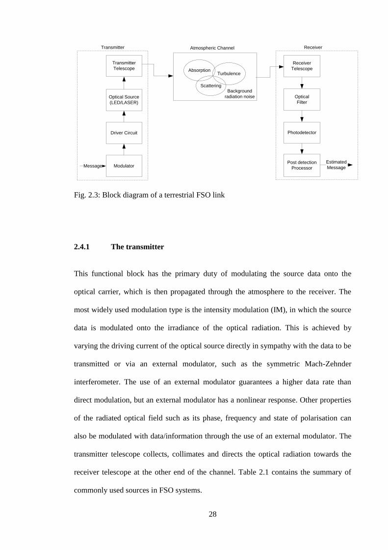
28

Absorption

Scattering

Turbulence

Modulator

Optical Source

(LED/LASER)

Driver Circuit

Transmitter

Telescope

Message

Optical

Filter

Post detection

Processor

Photodetector

Receiver

Telescope

Estimated

Message

Transmitter ReceiverAtmospheric Channel

Background

radiation noise

Fig. 2.3: Block diagram of a terrestrial FSO link

2.4.1 The transmitter

This functional block has the primary duty of modulating the source data onto the

optical carrier, which is then propagated through the atmosphere to the receiver. The

most widely used modulation type is the intensity modulation (IM), in which the source

data is modulated onto the irradiance of the optical radiation. This is achieved by

varying the driving current of the optical source directly in sympathy with the data to be

transmitted or via an external modulator, such as the symmetric Mach-Zehnder

interferometer. The use of an external modulator guarantees a higher data rate than

direct modulation, but an external modulator has a nonlinear response. Other properties

of the radiated optical field such as its phase, frequency and state of polarisation can

also be modulated with data/information through the use of an external modulator. The

transmitter telescope collects, collimates and directs the optical radiation towards the

receiver telescope at the other end of the channel. Table 2.1 contains the summary of

commonly used sources in FSO systems.

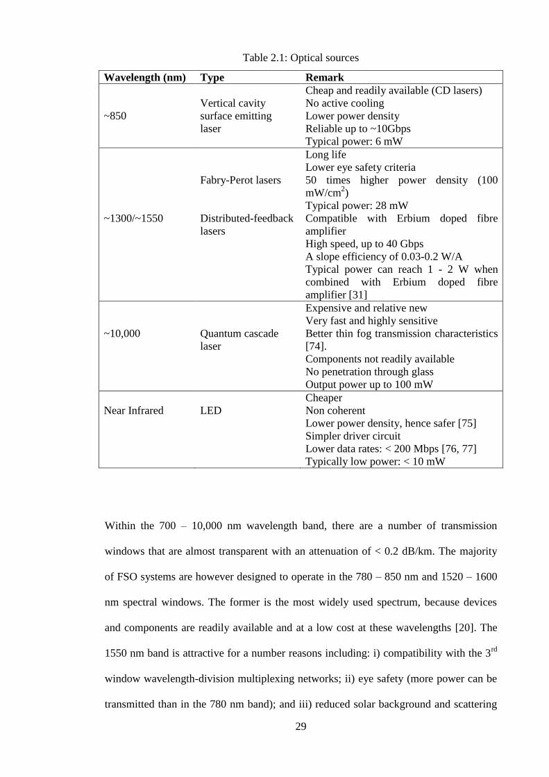
29

Table 2.1: Optical sources

Wavelength (nm) Type Remark

~850

Vertical cavity

surface emitting

laser

Cheap and readily available (CD lasers)

No active cooling

Lower power density

Reliable up to ~10Gbps

Typical power: 6 mW

~1300/~1550

Fabry-Perot lasers

Distributed-feedback

lasers

Long life

Lower eye safety criteria

50 times higher power density (100

mW/cm2)

Typical power: 28 mW

Compatible with Erbium doped fibre

amplifier

High speed, up to 40 Gbps

A slope efficiency of 0.03-0.2 W/A

Typical power can reach 1 - 2 W when

combined with Erbium doped fibre

amplifier [31]

~10,000

Quantum cascade

laser

Expensive and relative new

Very fast and highly sensitive

Better thin fog transmission characteristics

[74].

Components not readily available

No penetration through glass

Output power up to 100 mW

Near Infrared

LED

Cheaper

Non coherent

Lower power density, hence safer [75]

Simpler driver circuit

Lower data rates: < 200 Mbps [76, 77]

Typically low power: < 10 mW

Within the 700 – 10,000 nm wavelength band, there are a number of transmission

windows that are almost transparent with an attenuation of < 0.2 dB/km. The majority

of FSO systems are however designed to operate in the 780 – 850 nm and 1520 – 1600

nm spectral windows. The former is the most widely used spectrum, because devices

and components are readily available and at a low cost at these wavelengths [20]. The

1550 nm band is attractive for a number reasons including: i) compatibility with the 3rd

window wavelength-division multiplexing networks; ii) eye safety (more power can be

transmitted than in the 780 nm band); and iii) reduced solar background and scattering

30

in light haze/fog. Consequently at 1550 nm significantly more power can be transmitted

to overcome attenuation by fog [78]. However, the drawbacks of the 1550 nm band are

slightly reduced detector sensitivity, higher component cost and stricter alignment

requirements.

2.4.2 The atmospheric channel

An optical communications channel differs from the conventional Gaussian-noise

channel in that the signal x(t) represents power rather than amplitude. This leads to two

constraints on the transmitted signal: i) x(t) must be non-negative; and ii) the average

value of x(t) must not exceed a specified maximum power Pmax, that is

. In contrast to the conventional channels, where the signal-to-

noise ratio (SNR) is proportional to the power, in optical systems the received electrical

power and the variance of the shot noise are proportional to Ad2 and Ad, respectively,

where Ad is the receiver detector area. Thus, for a shot noise limited optical system, the

SNR is proportional to Ad. This implies that for a given transmitted power, a higher

SNR can be attained by using a large area detector. However, as Ad increases so does its

capacitance, which has a limiting effect on the receiver bandwidth.

The atmospheric channel consists of gases, listed in Table 2.2, and aerosols – tiny

particles suspended in the atmosphere. Also present in the atmosphere are rain, haze,

fog and other forms of precipitation. The amount of precipitation present in the

atmosphere depends on the location (longitude and latitude) and the season. The highest

concentration of particles is obviously near the Earth surface within the troposphere and

this decreases with increasing altitude up through to the ionosphere [79]. With the size

distribution of the atmospheric constituents ranging from sub-micrometres to

31

centimetres, an optical field that traverses the atmosphere is scattered and/or absorbed

resulting in power loss.

Table 2.2: The gas constituents of the atmosphere [80].

Constituent Volume Ratio (%) Parts Per Million (ppm)

Nitrogen (N2) 78.09

Oxygen (O2) 20.95

Argon (Ar) 0.93

Carbon dioxide (CO2) 0.03

Water vapour (H2O) 40 – 40,000

Neon (Ne) 20

Helium (He) 5.2

Methane (CH4) 1.5

Krypton (Kr) 1.1

Hydrogen (H2) 1

Nitrous oxide (N2O) 0.6

Carbon monoxide (CO) 0.2

Ozone (O3) 0.05

Xenon (Xe) 0.09

For an optical radiation traversing the atmosphere, some of the photons are extinguished

(absorbed) by the molecular constituents (water vapour, CO2, fog, ozone etc) and their

energy converted into heat, while others experience no loss of energy but their initial

directions of propagation are changed (scattering). The beam also spreads out while

traversing the channel causing the size of the received beam to be greater than the

receiver aperture. The Beer - Lambert law describes the transmittance of an optical field

through the atmosphere as [20]:

(2.1)

where and represent the total attenuation/extinction coefficient (m-1

) and

the transmittance of the atmosphere at wavelength λ, respectively. is the transmitted

32

optical power and the received optical power after distance, L. This process of

optical transmission power loss will be further discussed in Chapter Eight.

Another feature of interest is the atmospheric turbulence. When radiation strikes the

Earth from the Sun, some of the radiation is absorbed by the Earth‟s surface thereby

heating up its (Earth‟s) surface air mass. The resulting mass of warm and lighter air then

rises up to mix turbulently with the surrounding cooler air mass. This culminates in

small (in the range of 0.01 to 0.1 degrees) but spatially and temporally fluctuating

atmospheric temperature [1]. The temperature inhomogeneity of the atmosphere causes

corresponding changes in the index of refraction of the atmosphere, resulting in eddies,

cells or air packets having varying sizes from ~0.1 cm to ~10 m. These air packets act

like refractive prisms of varying indices of refraction. The propagating optical radiation

is therefore fully or partially deviated depending on the relative size of the beam and the

degree of temperature inhomogeneity along its path. Consequently the optical radiation

traversing the turbulent atmosphere experiences random variation/fading in its

irradiance (scintillation) and phase. Familiar effects of turbulence are the twinkling of

stars caused by random fluctuations of stars‟ irradiance, and the shimmer of the horizon

on a hot day caused by random changes in the optical phase of the light beam resulting

in reduced image resolution [1]. Atmospheric turbulence depends on i) atmospheric

pressure/altitude, ii) wind speed, and iii) variation of index of refraction due to

temperature inhomogeneity. Known effects of atmospheric turbulence include [32]:

a) Beam steering – Angular deviation of the beam from its original LOS causing

the beam to miss the receiver.

b) Image dancing – The received beam focus moves in the image plane due to

variations in the beam‟s angle of arrival.

33

c) Beam spreading – Increased beam divergence due to scattering. This leads to a

reduction in received power density.

d) Beam scintillation – Variations in the spatial power density at the receiver plane

caused by small scale destructive interference within the optical beam.

e) Spatial coherence degradation – Turbulence also induces losses in phase

coherence across the beam phase fronts. This is particularly deleterious for

photomixing (e.g. in coherent receiver) [45].

f) Polarisation fluctuation – This results from changes in the state of polarisation

of the received optical field after passing through a turbulent medium. However

for a horizontally travelling optical radiation, the amount of polarisation

fluctuation is negligible [30].

The modelling of the fluctuation of an optical radiation traversing a turbulent

atmosphere will be examined in Chapter Four, with the view to understanding the

statistical behaviour of the signal received at the receiver plane.

2.4.3 The receiver

This essentially helps recover the transmitted data from the incident optical field. The

receiver is composed of the following:

a) Receiver telescope – collects and focuses the incoming optical radiation onto the

photodetector. It should be noted that a large receiver telescope aperture is desirable as

it collects multiple uncorrelated radiations and focuses their average on the

photodetector. This is referred to as aperture averaging but a wide aperture also means

more background radiation/noise.

34

b) Optical bandpass filter – to reduce the amount of background radiation.

c) Photodetector – p-i-n diode (PIN) or avalanche photodiode (APD) that converts

the incident optical field into an electrical signal. The commonly used photodetectors in

contemporary laser communication systems are summarised in Table 2.3. Germanium

only detectors are generally not used in FSO because of their high dark current [31].

d) Post-detection processor/decision circuit – this is where the required

amplification, filtering and signal processing necessary to guarantee a high fidelity data

recovery are carried out.

Due to detector capacitance effect, higher speed detectors are inherently smaller in size

(70 µm and 30 µm for 2.5 Gbps and 10 Gbps, respectively) with a limited field-of-view

(FOV) that requires accurate alignment. The FOV of the receiver is the ratio of the

detector size to the focal length [81]: , where d is the detector

diameter, is the effective focal length, and D is the receiver aperture. The quantity F#

is the f-number. For a 75 µm size detector, with F# = 1 and D = 150 mm telescope, the

FOV = ~0.5 mrad.

Table 2.3: FSO Photodetectors

Material/Structure Wavelength (nm) Responsivity Typical Sensitivity Gain

Silicon PIN 300 – 1100 0.5 -34dBm@155Mbps 1

Silicon PIN, with

transimpedance

amplifier

300 – 1100 0.5 -26dBm@1.25 Gbps 1

InGaAs PIN 1000 – 1700 0.9 -46dBm@155Mbps 1

Silicon APD 400 – 1000 77 -52dBm@155Mbps 150

InGaAs APD 1000 – 1700 9 -33dBm @ 1.25

Gbps

10

Quantum–well and

quatum-dot

detectors

~10,000

35

The receiver detection process can be classified into:

Direct detection receiver – This type of receiver detects the instantaneous intensity or

power of the optical radiation impinging on the photodetector. Hence the output of the

photodetector is proportional to the power of the incident field. Its implementation is

very simple and most suitable for intensity modulated optical systems [32, 79].

Coherent detection receiver – The coherent receiver works on the photo-mixing

phenomenon. The incoming optical field is mixed with another locally generated optical

field on the surface of the photodetector. The coherent receiver can be further divided

into homodyne and heterodyne receivers. In homodyne receivers the

frequency/wavelength of the local (optical) oscillator is exactly the same as that of the

incoming radiation [32], while in heterodyne detection the incoming radiation and the

local oscillator frequencies are different [82]. In contrast to RF coherent detection, the

output of the local oscillator in an optical coherent detection is not required to have the

same phase as the incoming radiation. The principal advantages of a coherent receiver

are: relative ease of amplification at an intermediate frequency and the fact that the

signal-to-noise ratio can be significantly improved by simply raising the local oscillator

power.

These receiver structures and the detection process are discussed in more details in the

next chapter.

36

2.5 Eye Safety and Standards

In the design of optical communication systems, efforts must be made to ensure that the

optical radiation is safe and does not cause any damage to the people that might come in

contact with it. The optical beams can cause injury to both the skin and eye, but the

damage to the eye is far more significant because of the eye‟s ability to focus and

concentrate optical energy. The eye can focus light covering the wavelengths around 0.4

– 1.4 µm on to the retina, other wavelengths tend to be absorbed by the front part of the

eye (the cornea) before the energy is focused. Fig. 2.4 shows the absorption of the eye at

different wavelengths.

Photopic eye response

Total absorption

near IR wavelengths

Fig. 2.4: Response/absorption of the human eye at various wavelengths [31].

There are a number of international standard bodies which provide guidelines on safety

of optical beams, notable among these are [31]:

Center for Devices and Radiological Health (CDRH) - An agency within the United

States (U.S.) Food and Drug Administration (FDA). It establishes regulatory standards

for lasers and laser equipment that are enforceable by law (21 CFR 1040).

37

International Electrotechnical Commission (IEC) - Publishes international standards

related to all electrical equipment, including lasers and laser equipment (IEC60825-1).

These standards are not automatically enforceable by law, and the decision to adopt and

enforce IEC standards is at the discretion of individual countries.

American National Standards Institute (ANSI) - Publishes standards for laser use

(ANSI Z136.1). ANSI standards are not enforceable by law but do form the basis for the

U.S. Occupational Safety and Health Administration (OSHA) legal standards, as well as

comparable legal standards that have been adopted by various state regulatory agencies.

European Committee for Electrotechnical Standardization (CENELEC) - An

organisation that establishes electrotechnical standards based on recommendations made

by 19 European member nations. CENELEC standards are not directly enforceable by

law but, as with IEC standards, are often integrated into the legal requirements

developed by individual countries.

Laser Institute of America (LIA). LIA is an organization that promotes the safe use of

lasers, provides laser safety information, and sponsors laser conferences, symposia,

publications, and training courses.

Each of these organisation have developed ways of classifying lasers, the specific

criteria vary slightly from one body to the other but the IEC classifications will be

considered in this section. Lasers are generally divided into four groups, Class 1 to

Class 4, with Class 1 being the least powerful and Class 4 being the most powerful.

Each class is defined by the accessible emission limits (AEL) metric, this depends on

the wavelength of the optical source, the geometry of the emitter and the intensity of the

source [83].

38

Table 2.4 presents, the main characteristics and requirements for the classification

system as specified by the revised IEC 60825-1 standard [78, 84]. In addition, classes 2

and higher must have the triangular warning label and other labels are required in

specific cases indicating laser emission, laser apertures, skin hazards, and invisible

wavelengths.

Table 2.4: Classification of lasers according to the IEC 60825-1 standard

Category Description

Class 1

Low power device emitting radiation at a wavelength in the band

302.5−4000 nm. Device intrinsically without danger from its

technical design under all reasonably foreseeable usage conditions,

including vision using optical instruments (binoculars, microscope,

monocular)

Class 1M

Same as Class 1 but there is possibility of danger when viewed with

optical instruments such as binoculars, telescope, etc. Class 1M

lasers produce large-diameter beams, or beams that are divergent.

Class 2

Low power device emitting visible radiation (in the band 400−700

nm). Eye protection is normally ensured by the defence reflexes

including the palpebral reflex (closing of the eyelid). The palpebral

reflex provides effective protection under all reasonably foreseeable

usage conditions, including vision using optical instruments

(binoculars, microscope, monocular).

Class 2M

Low power device emitting visible radiation (in the band 400−700

nm). Eye protection is normally ensured by the defence reflexes

including the palpebral reflex (closing of the eyelid). The palpebral

reflex provides an effective protection under all reasonably

foreseeable usage conditions, with the exception of vision using

optical instruments

(binoculars, microscope, monocular).

Class 3R

Average power device emitting a radiation in the band 302.5−4000

nm. Direct vision is potentially dangerous

Class 3B

Average power device emitting a radiation in the band 302.5−4000

nm. Direct vision of the beam is always dangerous. Medical checks

and specific training required before installation or maintenance is

carried out.

Class 4

High power device There is always danger to the eye and for the

skin, fire risk exists. Must be equipped with a key switch and a

safety interlock. Medical checks and specific training required

before installation or maintenance is carried out.

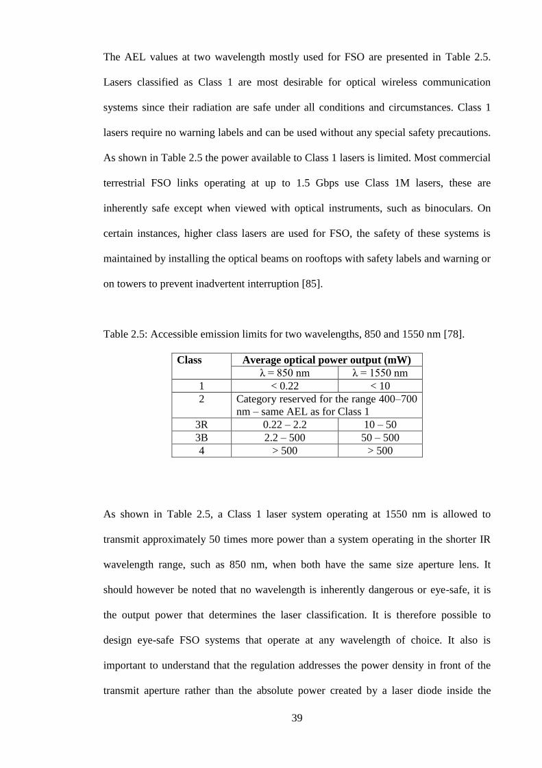
39

The AEL values at two wavelength mostly used for FSO are presented in Table 2.5.

Lasers classified as Class 1 are most desirable for optical wireless communication

systems since their radiation are safe under all conditions and circumstances. Class 1

lasers require no warning labels and can be used without any special safety precautions.

As shown in Table 2.5 the power available to Class 1 lasers is limited. Most commercial

terrestrial FSO links operating at up to 1.5 Gbps use Class 1M lasers, these are

inherently safe except when viewed with optical instruments, such as binoculars. On

certain instances, higher class lasers are used for FSO, the safety of these systems is

maintained by installing the optical beams on rooftops with safety labels and warning or

on towers to prevent inadvertent interruption [85].

Table 2.5: Accessible emission limits for two wavelengths, 850 and 1550 nm [78].

Class Average optical power output (mW)

λ = 850 nm λ = 1550 nm

1 < 0.22 < 10

2 Category reserved for the range 400–700

nm – same AEL as for Class 1

3R 0.22 – 2.2 10 – 50

3B 2.2 – 500 50 – 500

4 > 500 > 500

As shown in Table 2.5, a Class 1 laser system operating at 1550 nm is allowed to

transmit approximately 50 times more power than a system operating in the shorter IR

wavelength range, such as 850 nm, when both have the same size aperture lens. It

should however be noted that no wavelength is inherently dangerous or eye-safe, it is

the output power that determines the laser classification. It is therefore possible to

design eye-safe FSO systems that operate at any wavelength of choice. It also is

important to understand that the regulation addresses the power density in front of the

transmit aperture rather than the absolute power created by a laser diode inside the

40

equipment. For example, the laser diode inside the FSO equipment can actually be Class

3B even though the system itself is considered to be a Class 1 or 1M laser product if the

light is launched from a large-diameter lens that spreads out the radiation over a large

area before it enters the space in front of the aperture [31]. In order to maintain the Class

1 or 1M safety classifications, it is possible to use higher power laser with increased

lens aperture or to use multiple large transmission apertures [31].

2.5.1 Maximum Permissible Exposures (MPE)

To provide a better protection to the eye or skin of anybody that might come in contact

with the radiation of laser equipments, the maximum permissible exposure limits have

been stipulated by standard organisations. It is the highest radiation power or energy,

measured in W/cm2 or J/cm

2 that is considered safe with a negligible probability of

causing damage. The MPE is measured at the cornea of the human eye or at the skin, for

a given wavelength and exposure time. It is usually about 10 % of the dose that has a 50

% chance of creating damage under worst-case conditions [86]. In Table 2.6, the MPE

values for the eye at two commonly used wavelengths for FSO are presented; the values

for the skin are much lower since the skin is usually less sensitive to laser radiation.

Table 2.6: Example of MPE values (W/m2) of the eye (cornea) at 850 nm and 1550 nm

wavelengths [78].

Exposure

duration (s)

1 2 4 10 100 1000 10000

MPE (W/m2)

at 850 nm

36 30 25 20 11 6.5 3.6

MPE (W/m2)

at 1550 nm

5600 3300 1900 1000 1000 1000 1000

41

As shown in Table 2.6, the MPE is higher for brief exposure durations than for high

exposures times. The MPE for the eye is much higher at 1550 nm than at 850 nm, this is

related to the laser radiation absorption at the level of the various eye components. This

difference in MPE values can be explained by the fact that at 850 nm approximately

50% of the signal can reach the retina whereas at 1550 nm the signal is almost

completely absorbed by the cornea and aqueous humour [78].

2.6 Summary

A review of the FSO technology has been carried out in this chapter. Key features that

make FSO suitable for use within the access network have been highlighted while the

challenges posed by the atmospheric channel to an optical beam travelling though it

have also been introduced. Areas where FSO systems have been found suitable to

provide a data bridge have equally been mentioned and the issue of laser safety and

classification has also been discussed.

Chapter Three

Optical Detection Theory

3.1 Introduction

This chapter discusses the process of converting optical radiation into an electrical

signal used in the decision-making and other signal processing that takes place in an

optical communication receiver. The primary aim of optical detection in communication

engineering is to recover the information embedded on the intensity, phase or frequency

of the incoming optical radiation. The different types of transducers used in this process

and the commonly used optical detection processes (direct and coherent detection) are

also explained in this chapter. In addition, the various sources of noise in an FSO

43

system are discussed with a view to understanding the limit they imposed on the system

performance. The chapter is concluded with a discussion on the Poisson optical

detection statistics and its Gaussian approximation.

3.2 Photodetectors

The photodetector is a square law optoelectronic transducer that generates an electrical

signal which is proportional to the square of the instantaneous optical field impinging

on its surface. Thus, the signal generated by a photodetector is always proportional to

the instantaneous (received) optical power. Since the optical signal is generally weak,

having travelled through the communication channel, the photodetector must therefore

meet stringent performance requirements such as high sensitivity within its operational

range of wavelengths, low noise level and adequate bandwidth to accommodate the

desired data rate. The effect of temperature fluctuations on the response of the

photodetector is required to be minimal and the device must equally have a long

operating life.

The ratio of the number of electron-hole pairs generated by a photodetector to the

incident photons in a given time is termed the quantum efficiency and has the symbol η.

This is often used as a metric to characterise a photodetector. Consider an incoming

optical radiation with an average power PR impinging on a photodetector over a period

T, then the electric current (quantity of charge per unit time) generated by the detector is

given by [87]:

(3.1)

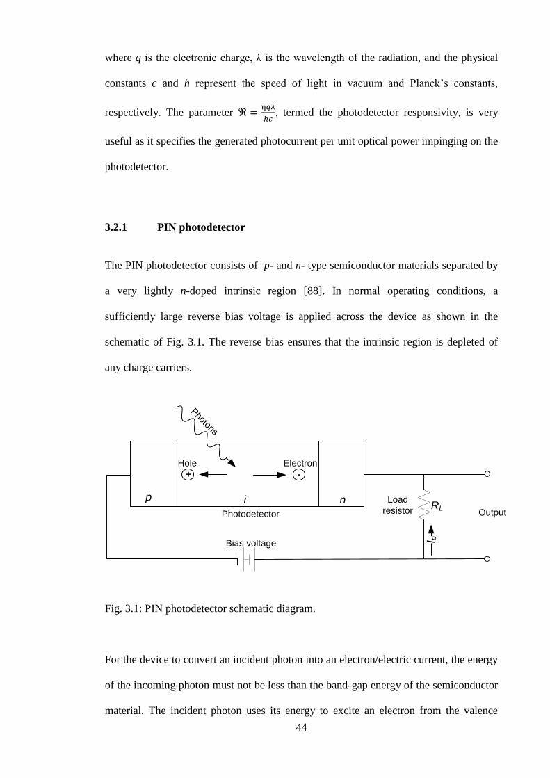
44

where q is the electronic charge, λ is the wavelength of the radiation, and the physical

constants c and h represent the speed of light in vacuum and Planck‟s constants,

respectively. The parameter , termed the photodetector responsivity, is very

useful as it specifies the generated photocurrent per unit optical power impinging on the

photodetector.

3.2.1 PIN photodetector

The PIN photodetector consists of p- and n- type semiconductor materials separated by

a very lightly n-doped intrinsic region [88]. In normal operating conditions, a

sufficiently large reverse bias voltage is applied across the device as shown in the

schematic of Fig. 3.1. The reverse bias ensures that the intrinsic region is depleted of

any charge carriers.

p ni

Bias voltage

Output

Load

resistorRL

Photodetector

+ -

Hole Electron

I p

Photons

Fig. 3.1: PIN photodetector schematic diagram.

For the device to convert an incident photon into an electron/electric current, the energy

of the incoming photon must not be less than the band-gap energy of the semiconductor

material. The incident photon uses its energy to excite an electron from the valence

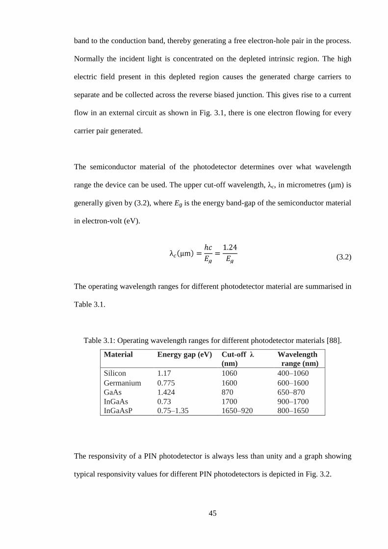
45

band to the conduction band, thereby generating a free electron-hole pair in the process.

Normally the incident light is concentrated on the depleted intrinsic region. The high

electric field present in this depleted region causes the generated charge carriers to

separate and be collected across the reverse biased junction. This gives rise to a current

flow in an external circuit as shown in Fig. 3.1, there is one electron flowing for every

carrier pair generated.

The semiconductor material of the photodetector determines over what wavelength

range the device can be used. The upper cut-off wavelength, λc, in micrometres (µm) is

generally given by (3.2), where Eg is the energy band-gap of the semiconductor material

in electron-volt (eV).

(3.2)

The operating wavelength ranges for different photodetector material are summarised in

Table 3.1.

Table 3.1: Operating wavelength ranges for different photodetector materials [88].

Material Energy gap (eV) Cut-off λ

(nm)

Wavelength

range (nm)

Silicon 1.17 1060 400–1060

Germanium 0.775 1600 600–1600

GaAs 1.424 870 650–870

InGaAs 0.73 1700 900–1700

InGaAsP 0.75–1.35 1650–920 800–1650

The responsivity of a PIN photodetector is always less than unity and a graph showing

typical responsivity values for different PIN photodetectors is depicted in Fig. 3.2.

46

Fig. 3.2: Responsivity and quantum efficiency as a function of wavelength for PIN

photodetectors. Reproduced from [88].

3.2.2 APD photodetector

The avalanche photodiode (APD) is different from the PIN photodetector in that it

provides an inherent current gain through the process called repeated electron

ionisation. This culminates in increased sensitivity since the photocurrent is now

multiplied before encountering the thermal noise associated with the receiver circuit.

Hence the expression for the responsivity of an APD includes a multiplication (or gain)

factor g. Typical gain values lie in the range 50 to 300 [79], thus the responsivity value

of an APD can be greater than unity. The APD offers a higher sensitivity than the PIN

detector but the statistical nature of the ionisation/avalanche process means that there is

always a multiplication noise associated with the APD. The avalanche process is also

47

very temperature-sensitive. These factors are very important and must always be taken

into account whenever an APD is used in an optical communication system.

3.3 Photodetection Techniques

Photodetection is the process of converting information-bearing optical radiation into its

equivalent electrical signal with the aim of recovering the transmitted information. At

the transmitter, the information can be encoded on the frequency, phase or the intensity

of the radiation from an optical source. This encoded radiation is then transmitted to

the receiver via the free-space channel or the optical fibre. The receiver front-end

devices (telescope and optical filter) focus the filtered radiation onto the photodetecting

surface in the focal plane. Depending on whether a local oscillator is used during the

detection process or not, the following photodetection techniques are possible.

3.3.1 Direct detection

Here, a local oscillator is not used in the detection process and for this type of receiver

to recover the encoded information, it is essential that the transmitted information be

associated with the intensity variation of the transmitted field [79]. Hence this type of

detection is also called envelope detection. For an instantaneous incident power P(t), the

instantaneous photodetector current i(t) is given by:

(3.3)

where g is the photodetector gain factor whose value is unity for a PIN photodetector.

The block diagram of the direct detection receiver is illustrated in Fig. 3.3.

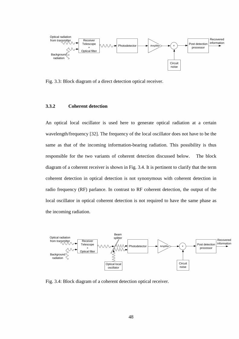
48

Receiver

Telescope

+

Optical filter

PhotodetectorPost detection

processorAmplifier +

Circuit

noise

Optical radiation

from transmitter

Background

radiation

Recovered

information

Fig. 3.3: Block diagram of a direct detection optical receiver.

3.3.2 Coherent detection

An optical local oscillator is used here to generate optical radiation at a certain

wavelength/frequency [32]. The frequency of the local oscillator does not have to be the

same as that of the incoming information-bearing radiation. This possibility is thus

responsible for the two variants of coherent detection discussed below. The block

diagram of a coherent receiver is shown in Fig. 3.4. It is pertinent to clarify that the term

coherent detection in optical detection is not synonymous with coherent detection in

radio frequency (RF) parlance. In contrast to RF coherent detection, the output of the

local oscillator in optical coherent detection is not required to have the same phase as

the incoming radiation.

Receiver

Telescope

+

Optical filter

PhotodetectorPost detection

processorAmplifier +

Optical local

oscillator

Circuit

noise

Beam

splitterOptical radiation

from transmitter

Background

radiation

Recovered

information

Fig. 3.4: Block diagram of a coherent detection optical receiver.

49

3.3.2.1 Heterodyne detection

In a heterodyne detection optical receiver, the incoming radiation (carrier) is combined

with a reference wave from a local laser on the photodetector surface as shown in Fig.

3.4. This optical mixing process produces another wave at an intermediate frequency

(IF) which is the difference between the incoming laser carrier and the reference signal

frequencies [32]. This IF signal passes through a band-pass filter to an electrical second

detector (the post detection processor in Fig. 3.4) for the final demodulation. Assuming

that the electric fields of the carrier of frequency , and that of the reference (local)

radiation of frequency are respectively given by:

(3.4a)

(3.4b)

where and are the amplitude and phase of the carrier field respectively while the

local oscillator amplitude and phase are and in that order. When the instantaneous

field amplitudes, Ec(t) and EL(t) combine on the photodetector surface, they produce an

instantaneous signal whose intensity is given by:

(3.5)

The time average of C(t) multiplied by the responsivity gives the resultant instantaneous

carrier and local oscillator current, ip(t), at the photodetector output.

Hence:

(3.6)

50

The first two terms are time invariant, the 3rd

term is very slowly varying with respect to

the short time over which the average is taken, while the 4th

term is out of the IF band

[32]. Equation 3.6 is now reduced to:

(3.7)

Therefore the IF filter, which is an integral part of the post detection processor of Fig.

3.4, only allows the 3rd

term to go through while the others are suppressed resulting in

the following expression for the instantaneous current:

(3.8)

The above result makes it possible to recover any information impressed on the carrier

field amplitude, frequency or even phase. The following points can therefore be

deduced from this, that heterodyne detection offers:

1) A relatively easy means of amplifying the photocurrent by simply increasing the

local oscillator power.

2) Improved signal-to-noise ratio. This is achieved by increasing the local oscillator

power so much that its inherent shot noise dwarfs the thermal and the shot noise

from other sources.

However the frequency of an optical source is known to drift over time. Therefore the

IF frequency needs to be continually monitored at the input of the electrical detector and

the local oscillator frequency varied accordingly to keep the IF centre frequency

constant. Also the optical source, particularly a laser, does suffer from phase noise

which means that θc and θL in (3.8) are not absolutely fixed, they fluctuate. These factors

contribute to the challenges of implementing a coherent optical communication system.

51

3.3.2.2 Homodyne detection

This is similar to the heterodyne detection process discussed above except that the local

oscillator has the same frequency as the incoming optical radiation/carrier [32]. The

resultant photocurrent thus contains the information signal at the baseband. Following

the same step as in heterodyne detection, the instantaneous photocurrent is obtained

thus:

(3.9)

The 3rd

term is time invariant and the 4th

term is suppressible via filtering to obtain:

(3.10)

By increasing the locally generated radiation power such that AcAL >> 0.5Ac [32],

expression (3.10) reduces to:

(3.11)

3.4 Photodetection Noise

The types of noise encountered in optical communications can be broadly stratified into

shot noise and thermal noise. The various sources of noise in optical communications

are discussed below. For FSO systems, the noise from the background radiation can be

significant, while in fibre optics communication the background radiation noise is

negligible.

52

3.4.1 Photon fluctuation noise

For an ideal photodetector, the only significant noise that affects its performance is that

associated with the quantum nature of light itself, the by-product of which is that the

number of photons emitted by a coherent optical source in a given time is never

constant. Although for a constant power optical source the mean number of photons

generated per second is constant, the actual number of photons per second follows the

Poisson distribution. This results in photon fluctuation or quantum noise.

The quantum fluctuation is also important because it is dominates over the thermal

fluctuations within the photodetector, since hf > κTe where h and f are the Planck‟s

constant and radiation frequency respectively while κ and Te represent the Boltzmann‟s

constant and temperature. The quantum noise is a shot noise with variance:

(3.12)

where the bandwidth of the electrical filter that follows the photodetector is represented

by B Hz.

3.4.2 Dark current and excess noise

The dark current is the photocurrent generated when no photon is impinging on the

photodetector. It is produced by the transition of electrons from the valence to the

conduction band due to causes other than photon-induced excitation; its magnitude is

closely related to the energy band-gap of the photodetector material(s). Large band-gap

materials, such as Silicon (Si), Indium phosphide (InP) and Gallium arsenide (GaAs)

show very low values of mean dark current, , while for Germanium (Ge), the value

could be significant when they are operated at room temperature [82]. The dark current

53

consists of diffusion, tunnel, leakage currents and generation-recombination taking

place in the space-charge region and is proportional to the volume of the depletion

region [82].

Photodetectors that employ internal avalanche gain mechanism to boost the signal

above the thermal noise of amplifier stages on the receiver exhibit what is referred to as

excess noise [45]. According to [45], the excess noise in an APD is due to the

multiplication process in the high-field region of the detector where each primary

electron hole can generate an additional electron through impact ionisation of bound

electrons. These additional carriers can then create still additional carriers in a cascading

process.

If all primary carriers were to be multiplied equally in an APD, the mean-square current

gain would be equal to the mean gain, , and the excess noise, defined as

would be equal to 1. This is the case for PIN photodetectors [45]. However, due

to the statistical nature of the avalanche process, F is always greater than 1 in an APD

and other avalanche devices. Typical dark current values for some photodetector

materials are shown in Table 3.2.

Table 3.2: Dark current values for different materials [77].

Photodetector

material Dark current (nA)

PIN APD

Silicon 1 – 10 0.1 – 1

Germanium 50 – 500 50 – 500

InGaAs 0.5 – 2.0 10 – 50 @ g =10

The dark current carries no useful information and thereby constitutes a shot noise

whose variance is given by the following:

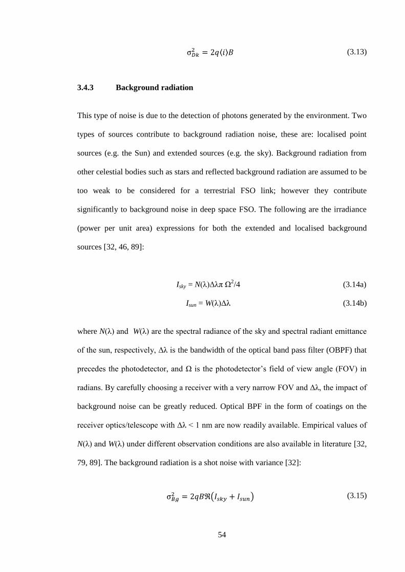
54

(3.13)

3.4.3 Background radiation

This type of noise is due to the detection of photons generated by the environment. Two

types of sources contribute to background radiation noise, these are: localised point

sources (e.g. the Sun) and extended sources (e.g. the sky). Background radiation from

other celestial bodies such as stars and reflected background radiation are assumed to be

too weak to be considered for a terrestrial FSO link; however they contribute

significantly to background noise in deep space FSO. The following are the irradiance

(power per unit area) expressions for both the extended and localised background

sources [32, 46, 89]:

Isky = N(λ)Δλπ Ω2/4

Isun = W(λ)Δλ

(3.14a)

(3.14b)

where N(λ) and W(λ) are the spectral radiance of the sky and spectral radiant emittance

of the sun, respectively, Δλ is the bandwidth of the optical band pass filter (OBPF) that

precedes the photodetector, and Ω is the photodetector‟s field of view angle (FOV) in

radians. By carefully choosing a receiver with a very narrow FOV and Δλ, the impact of

background noise can be greatly reduced. Optical BPF in the form of coatings on the

receiver optics/telescope with Δλ < 1 nm are now readily available. Empirical values of

N(λ) and W(λ) under different observation conditions are also available in literature [32,

79, 89]. The background radiation is a shot noise with variance [32]:

(3.15)

55

Combining these noise processes together results in the total shot noise whose variance,

, is the sum of the individual noise variances. This is however dominated by the

background radiation as the other two are usually smaller.

3.4.4 Thermal noise

This is the noise caused by the thermal fluctuation of electrons in any receiver circuit of

equivalent resistance RL, and temperature Te. The thermal noise is regarded as a „white‟

noise. This is because the power spectral density (PSD) is independent of frequency.

Moreover, the thermal noise obeys the Gaussian distribution with mean zero and has a

variance defined by [77]:

(3.16)

where is the Boltzmann‟s constant.

3.5 Optical Detection Statistics

According to the semi-classical approach, which treats an optical radiation as a wave

and prescribes a probabilistic relation to account for its interaction with the atomic

structure of the detector surface [79], the probability of a detector with an aperture area

AD, emitting n number of electrons from impinging photons during a period T obeys the

Poisson distribution given as:

(3.17)

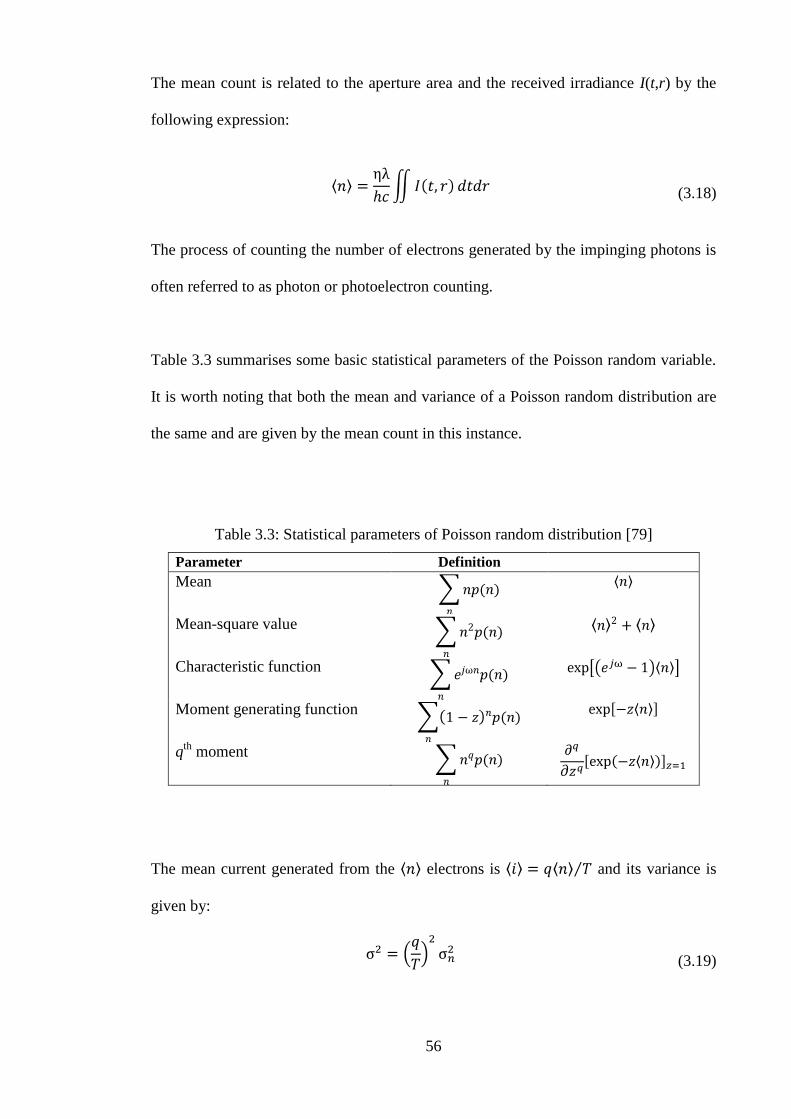
56

The mean count is related to the aperture area and the received irradiance I(t,r) by the

following expression:

(3.18)

The process of counting the number of electrons generated by the impinging photons is

often referred to as photon or photoelectron counting.

Table 3.3 summarises some basic statistical parameters of the Poisson random variable.

It is worth noting that both the mean and variance of a Poisson random distribution are

the same and are given by the mean count in this instance.

Table 3.3: Statistical parameters of Poisson random distribution [79]

Parameter Definition

Mean

Mean-square value

Characteristic function

Moment generating function

qth

moment

The mean current generated from the electrons is and its variance is

given by:

(3.19)

57

Since for a Poisson distribution the mean and variance are equal, and by choosing the

electrical bandwidth of the post detection filter as 1/2T (which is the Nyquist minimum

bandwidth requirement), the expression (3.19) becomes:

(3.20)

This is the general expression for the variance of any shot noise process associated with

photodetection. It should be mentioned that the photon counts from the desired

incoming optical radiation, background radiation and that due to dark current are

independent Poisson random variables. Hence, the pdf of the photoelectron emission

due to all of these processes occurring together is also a Poisson distribution whose

mean is the sum of the means of the individual processes.

With large signal photoelectron counts the generated signal current probability

distribution can be approximated to be Gaussian [32]. That is:

(3.21)

By taking the AWGN into account, this expression is modified to become:

(3.22)

These expressions (3.17), (3.21) and (3.22) are only valid for a non-varying received

optical field. However, if the incoming field is randomly varying, then the received

irradiance and also vary accordingly. Assuming the randomly varying field has a pdf

given by p( ), it follows therefore that the generated photocurrent is now doubly

58

stochastic and its pdf given by (3.23) is obtained by averaging (3.22) over the statistics

of the varying field.

(3.23)

In free-space optical communications, atmospheric turbulence is the principal source of

random fluctuations in the received optical radiation irradiance. This source of

fluctuation is therefore the subject of discussion in the next chapter.

3.6 Summary

This chapter has discussed the process of optical detection by first reviewing the

transducers used for converting optical radiation to their equivalent electrical signals.

When using direct detection, it is essential that the transmitted information is associated

with the intensity variation of the optical beam. While in coherent detection, the

information can be encoded on the phase, field amplitude or frequency of the optical

radiation. The different types of noise encountered in optical detection have also been

reviewed and the statistics of the optical detection process discussed.

Chapter Four

The Atmospheric Turbulence Models

4.1 Introduction

Solar radiation absorbed by the Earth‟s surface causes air around the earth surface to be

warmer than that at higher altitude. This layer of warmer air becomes less dense and

rises to mix turbulently with the surrounding cooler air causing the air temperature to

fluctuate randomly [32]. Inhomogeneities caused by turbulence can be viewed as

discrete cells, or eddies of different temperature, acting like refractive prisms of

different sizes and indices of refraction. The interaction between the laser beam and the

turbulent medium results in random phase and amplitude variations (scintillation) of the

60

information-bearing optical beam which ultimately results in performance degradation

of FSO links. Of all the effects of atmospheric turbulence introduced in Chapter Two,

only the modelling of the atmospheric turbulence induced fluctuation of the received

optical power (or irradiance) will be discussed in this chapter, since in the intensity

modulated, direct detection FSO system under consideration, it is only the received

power/irradiance that matters. Atmospheric turbulence is usually categorised in regimes

depending on the magnitude of index of refraction variation and inhomogeneities. These

regimes are a function of the distance travelled by the optical radiation through the

atmosphere and are classified as weak, moderate, strong and saturation.

In this chapter, models describing the probability density function (pdf) statistics of the

irradiance fluctuation will be described. Unfortunately, due to the extreme complexity

involved in mathematically modelling of atmospheric turbulence, a universal model

valid for all the turbulence regimes does not currently exist. As such, this chapter will

review three most reported models for irradiance fluctuation in a turbulent channel.

These are log-normal, gamma-gamma and negative exponential models. Their

respective ranges of validity, as reported in literature [30, 45, 47, 49, 50], are in the

weak, weak-to-strong and saturate regimes.

4.2 Turbulent Atmospheric Channel

Atmospheric turbulence results in random fluctuation of the atmospheric refractive

index, n along the path of the optical field/radiation traversing the atmosphere. This

refractive index fluctuation is the direct end product of random variations in

atmospheric temperature from point to point [32]. These random temperature changes

are a function of the atmospheric pressure, altitude and wind speed. The smallest and

61

the largest of the turbulence eddies are termed the inner scale, l0, and the outer scale, L0,

of turbulence respectively. l0 is typically on the order of a few millimetres while L0 is

typically on the order of several metres [29, 49]. These weak lens-like eddies shown

graphically in Fig. 4.1 result in a randomised interference effect between different

regions of the propagating beam causing the wavefront to be distorted in the process.

Atmospheric channel

L0

Velocity

Input wave Output wave

l0

Fig. 4.1: Atmospheric channel with turbulent eddies

In an attempt to model the turbulent atmospheric channel, the widely accepted „Taylor

hypothesis‟ [30], which says that the turbulent eddies are fixed or frozen and can only

move in their frozen form with the transverse component of the mean local wind will be

followed. This hypothesis means that the temporal variations in the beam pattern or its

statistical properties are caused by the component of the local wind that is perpendicular

to the beam direction of propagation. In addition, the temporal coherence time, o, of

atmospheric turbulence is reported to be in the order of milliseconds [45]. This value is

very large compared to the duration of a typical data symbol, thus the turbulent

62

atmospheric channel can be described as a „slow fading channel‟ since it is static over

the duration of a data symbol.

The relationship between the temperature of the atmosphere and its refractive index is

given by (4.1) [90] while for most engineering applications, the rate of change of the

refractive with respect to channel temperature is represented by equation (4.2) [30].

(4.1)

(4.2)

where P is the atmospheric pressure in millibars, Te is the temperature in Kelvin and

the wavelength in microns. Near sea level, K-1

[30]. The

contribution of humidity to the refractive index fluctuation is not accounted for in (4.1)

because this is negligible at optical wavelengths [45].

The position and time dependent index of refraction denoted by can be

expressed as the sum of its free-space (no turbulence) value, , and a turbulence

induced random fluctuation component . Thus:

(4.3)

In accordance with the Taylor's 'frozen-flow' hypothesis, which implies that the

temporal variations of the index of refraction of the channel are mainly due to the

transverse component of the atmospheric wind, the randomly fluctuating part of

equation (4.3) can then be written as:

63

(4.4)

where v(r) is the local wind velocity perpendicular to the field direction of travel. In

atmospheric turbulence, an important parameter for characterising the amount refractive

index fluctuation is the index of refraction structure parameter, Cn2, introduced by

Kolmogorov [91]. The value of Cn2

varies with altitude and a commonly used model to

describe it is the Hufnagel-Valley (H-V) model given below as [49]:

(4.5)

where  is taken as the nominal value of Cn2(0) at the ground in m

-2/3 and is the

altitude in metres. The value of the index of refraction structure parameter varies with

altitude, but for a horizontally propagating field it is usually assumed constant.

typically ranges from 10-12

m-2/3

for strong turbulence to 10-17

m-2/3

for weak turbulence

with a typical average value being 10-15

m-2/3

[47].

A similar parameter for temperature variations is the temperature structure parameter

and it is related to Cn2

by (4.6) [30].

(4.6)

In the spectral domain, the power spectral density of the refractive index fluctuation is

related to Cn2 by the following expression [91, 92]:

(4.7)

64

where is the spatial wave number. For a wider range of K however, this expression

has been modified by Tatarski and von Karman and reported in the following references

[47, 93, 94].

By their very nature, turbulent media are extremely difficult to describe mathematically,

the difficulty, according to [45], is primarily due to the presence of non-linear mixing of

observable quantities which is fundamental to the process. In order to derive

expressions for the statistical properties, namely the pdf and variance, of an optical

beam travelling through the turbulent atmosphere; the following simplifying but valid

assumptions will be used to reduce the mathematics to a manageable level [45]:

1) The atmosphere is a non-dissipative channel for the propagating wave. This

assumption can be explained thus, in the event of absorption of the propagating

wave or radiation by the atmosphere, the heat so generated is insignificant

compared to diurnal contributions.

2) The process of scattering by the turbulent eddies does not result in loss of energy

from the beam. Hence the mean energy in the presence of turbulence is assumed

equal to the mean energy in the absence of turbulence. This assumption is valid

for plane and spherical waves. The plane wave, is generally applicable to laser

beams propagating over a long distance [45, 79].

4.3 Log-normal Turbulence Model

In describing the pdf of the irradiance fluctuation in a turbulent atmosphere, the beam is

first represented by its constituent electric field . By employing Maxwell‟s electro-

magnetic equations for the case of a spatially variant dielectric like the atmosphere, the

65

following expression is derived [45]:

(4.8)

where the wave number , and the vector gradient operator

with i, j, and k being the unit vectors along the x, y and z axes

respectively. The last term on the left hand side of (4.8) represents the turbulence

induced depolarisation of the wave. In weak atmospheric turbulence, which is

characterised by single scattering event, the wave depolarisation is negligible [30, 95,

96]. In fact, it has been shown both theoretically [97] and experimentally [98] that the

depolarisation is insignificant even for strong turbulence conditions. Equation (4.8) then

reduces to:

(4.9)

The position vector will henceforth be denoted by r and represented by for

convenience.

In solving this last equation, Tatarski [93] in his approach introduced a Gaussian

complex variable defined as the natural logarithm of the propagating field ,

and termed it the Rytov transformation. That is:

The Rytov approach is also based on a fundamental assumption that the turbulence is

weak and that it is characterised by single scattering process. By invoking the Rytov

transformation (4.10), and equating the mean refractive index of the channel, , to

(4.10)

66

unity, equation (4.9) transforms to the following Riccati equation whose solution

already exists:

(4.11)

The next stage involves breaking down to its free-space form, , and its

turbulence induced departure from it represented by . This is done via the smooth

perturbing method [45], which in effect implies that .

Combining this with the Rytov change of variable (4.10), results in the following:

(4.12)

(4.13)

Where the electric field and its free-space (without turbulence) form, , are by

definition given as:

(4.14a)

(4.14b)

where and represent the amplitude and phase of the actual field with

atmospheric turbulence, respectively while and represent the amplitude

and phase of the field without atmospheric turbulence, respectively. These

transformations can then be used to arrive at the solution of (4.11) which describes the

behaviour of a field in weak atmospheric turbulence. In finding the irradiance

fluctuation statistical distribution, first combine equations (4.13) and (4.14) to arrive at

the turbulence induced field amplitude fluctuation given below as:

67

(4.15)

Since is Gaussian, it follows therefore that, is the Gaussian distributed log-

amplitude fluctuation, and similarly is the Gaussian distributed phase fluctuation of

the field. By concentrating only on the field amplitude however, the pdf of is thus

[45, 47]:

(4.16)

where E[ ] denotes the expectation of and is the log-amplitude variance,

commonly referred to as the Rytov parameter. According to [30], the which

characterises the extent of field amplitude fluctuation in atmospheric turbulence is

related to the index of refraction structure parameter, the horizontal distance, L,

travelled by the optical field/radiation by the following equations:

for a plane wave

(4.17a)

and

for a spherical wave

(4.17b)

For a field propagating horizontally through the turbulent medium, as is the case in most

terrestrial applications, the refractive index structure parameter, , is constant, and the

log irradiance variance for a plane wave becomes:

68

(4.18)

The field irradiance (intensity) in the turbulent medium is while the

intensity in free-space (no turbulence) is given by , the log-intensity is

then given by:

(4.19)

Hence,

(4.20)

To obtain the irradiance pdf, invoke the transformation of variable, ,

to arrive at the log-normal distribution function given by (4.21) .

(4.21)

In the region of weak fluctuations, the statistics of the irradiance fluctuations have been

experimentally found to obey the log-normal distribution. From (4.19) the log-intensity

variance and the mean log intensity, . Based on the second

assumption of Section 4.2, it follows that since there is no

energy loss during the turbulence induced scattering process and as such . The

expectation, E[l] is obtained by invoking the standard relation (4.22) which is valid for

any real-valued Gaussian random variable [47]. An expression for E[l] is then obtained

as illustrated in the following steps:

69

(4.22)

(4.23)

Hence,

(4.24)

The log-normal pdf is plotted in Fig. 4.2 for different values of log irradiance variance,

. As the value of increases, the distribution becomes more skewed with longer tails

in the infinity direction. This denotes the extent of fluctuation of the irradiance as the

channel inhomogeneity increases.

0 0.5 1 1.5 2 2.5 30

0.2

0.4

0.6

0.8

1

1.2

1.4

Normalised irradiance, I /E[I]

p(I

)

2l = 0.1

2l = 0.2

2l = 0.5

2l = 0.8

Fig. 4.2: Log-normal probability density function with E[I] = 1 for a range of log

irradiance variance .

70

After obtaining the pdf of the irradiance fluctuation, it is also paramount to derive an

expression for the variance of the irradiance fluctuation, , which characterises the

strength of irradiance fluctuation. This is carried out in the following steps:

(4.25)

By applying (4.22) to (4.25) and substituting for E[l], the intensity variance is obtained

as:

(4.26)

The normalised variance of intensity, often referred to as the scintillation index (S.I.) is

thus:

(4.27)

4.3.1 Spatial coherence in weak turbulence

When a coherent optical radiation propagates through a turbulent medium like the

atmosphere, it experiences a decrease in its spatial coherence. The extent of this

coherence degradation is, of course, a function of the atmospheric turbulence strength

and the propagation distance. In effect, the turbulent channel breaks the coherent

radiation up into various fragments whose diameters represent the reduced spatial

coherence distance. Following from the Rytov approach used in modelling weak

atmospheric turbulence, the spatial coherence of a field travelling through the

atmosphere can be derived as [30]:

(4.28)

where is the transverse coherence length of the field, this is the transverse distance at

71

which the coherence of the field is reduced to . Equations 4.29(a-b) give the

expressions for the transverse coherence distance, for plane and spherical waves

respectively [30].

(4.29a)

(4.29b)

The coherence distance is particularly useful in determining the size of the receiver

aperture needed to collect the bulk of the propagating field through the process called

aperture averaging, and also to determine the separation distance of detectors in a

multiple receiver system. In order for the detectors in the array to receive uncorrelated

signals, they must be spaced at a minimum distance apart. Figures 4.3 and 4.4

illustrate the coherence length for a horizontal link at two commonly used FSO

wavelengths, λ = 850nm and 1550nm, for typical values of Cn2. The spatial coherence

length is generally longer at longer wavelengths and decreases as both the propagation

distance and the atmospheric turbulence increase.

72

10-1

100

101

102

10-5

10-4

10-3

10-2

10-1

100

101

Propagation distance, (km)

Spatial cohere

nce d

ista

nce (

m)

10-17 m-2/3

10-15 m-2/3

10-14 m-2/3

10-13 m-2/3

10-12 m-2/3

Cn2

Fig. 4.3: Plane wave transverse coherence length for λ = 850nm and a range of Cn

2.

10-1

100

101

102

10-4

10-3

10-2

10-1

100

101

Propagation distance, (km)

Spatial cohere

nce d

ista

nce (

m)

10-17 m-2/3

10-15 m-2/3

10-14 m-2/3

10-13 m-2/3

10-12 m-2/3

Cn2

Fig. 4.4: Plane wave transverse coherence length for λ = 1550nm and a range of Cn

2.

73

4.3.2 Limit of log-normal turbulence model

Thus far, the Rytov approximation has been used to describe atmospheric turbulence

and the log-normal turbulence model has been derived. The Rytov approximation

predicts that the Rytov parameter increases without limit with the index of refraction

structure parameter and/or the path length. However, based on experimental results as

reported in [45], this prediction holds only in the weak turbulence regime when

. As the turbulence strength increases beyond the weak regime, due to a

combination of increased path length and/or increased , the turbulent eddies result in

multiple scatterings that are not accounted for by Rytov in his approximation [30, 49].

Based on experiments reported in [30, 45] , the scintillation index, S.I., increases

linearly with the Rytov parameter within the weak regime and continues to increase to a

maximum value greater than unity. The regime in which S.I. attains its maximum value

characterises the highest strength of inhomogeneity or random focusing. The S.I. then

starts to decrease due self interference as a result of multiple scattering and approaches

unity as the Rytov parameter increases [45]. This observation is in contrast to the

prediction of the Rytov approximation beyond the weak atmospheric regime. In the next

section, two other irradiance fluctuation models that account for the multiple scatterings

will be reviewed and their pdfs will be presented.

4.4 The Gamma-Gamma Turbulence Model

This model proposed by Andrews et al. [49] is based on the modulation process where

the fluctuation of light radiation traversing a turbulent atmosphere is assumed to consist

of small scale (scattering) and large scale (refraction) effects. The former includes

contributions due to eddies/cells smaller than the Fresnel zone, or the

74

coherence radius, , whichever is smaller. Large scale fluctuations on the other hand

are generated by turbulent eddies larger than that of the first Fresnel zone or the

scattering disk , whichever is larger. The small scale eddies are assumed to be

modulated by the large scale eddies. Consequently, the normalised received irradiance I

is defined as the product of two statistically independent random processes Ix and Iy:

(4.30)

Ix and Iy arise from the large scale and small scale turbulent eddies respectively and are

both proposed to obey the gamma distribution by Andrews et al [49, 50, 57]. Their pdfs

are thus given by:

(4.31a)

(4.31b)

By fixing and using the change of variable, , the conditional pdf given by

(4.32) is obtained in which is the (conditional) mean value of I.

(4.32)

To obtain the unconditional irradiance distribution, the conditional probability,

is averaged over the statistical distribution of given by 4.31(a) to obtain the following

gamma-gamma irradiance distribution function.

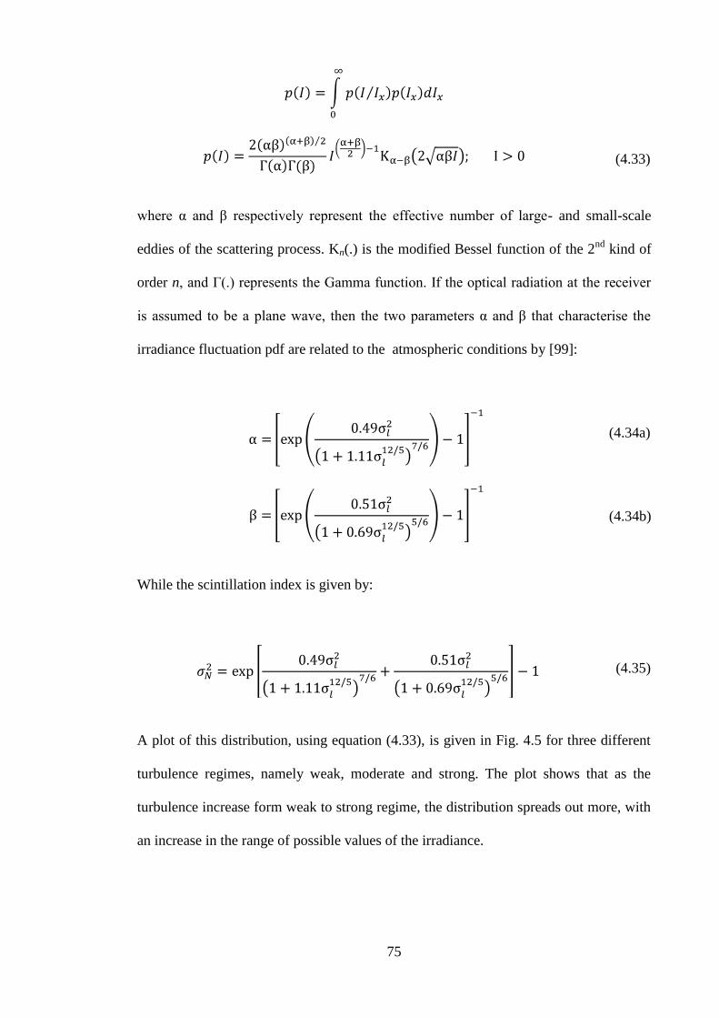
75

(4.33)

where α and β respectively represent the effective number of large- and small-scale

eddies of the scattering process. Kn(.) is the modified Bessel function of the 2nd

kind of

order n, and Γ(.) represents the Gamma function. If the optical radiation at the receiver

is assumed to be a plane wave, then the two parameters α and β that characterise the

irradiance fluctuation pdf are related to the atmospheric conditions by [99]:

(4.34a)

(4.34b)

While the scintillation index is given by:

(4.35)

A plot of this distribution, using equation (4.33), is given in Fig. 4.5 for three different

turbulence regimes, namely weak, moderate and strong. The plot shows that as the

turbulence increase form weak to strong regime, the distribution spreads out more, with

an increase in the range of possible values of the irradiance.

76

0.5 1 1.5 2 2.5 3 3.5 4

0

0.2

0.4

0.6

0.8

1

Irradiance, I

Gam

ma g

am

ma p

df:

p

(I)

Weak: = 11.6, = 10.1, l2 = 0.2

Moderate: = 4, = 1.9, l2 = 1.6

Strong: = 4.2, = 1.4, l2 = 3.5

Turbulence strength

Fig. 4.5: Gamma-gamma probability density function for three different turbulence

regimes, namely weak, moderate and strong.

The gamma-gamma turbulence model given by (4.33) is valid for all turbulence

scenarios from weak to strong and the values of α and β at any given regime can be

obtained from (4.34). Figure 4.6 shows the variation of S.I. as a function of the Rytov

parameter based on (4.35), this graph shows that as the Rytov parameter increases, the

S.I. approaches a maximum value greater than one, and then approaches unity as the

turbulence induced fading approaches the saturation regime. The values of α and β

under different turbulence regimes are depicted in Fig. 4.7.

77

0 10 20 30 40 50 60 700

0.2

0.4

0.6

0.8

1

1.2

Rytov parameter (Log intensity variance)

Scin

tilla

tion I

ndex

Fig. 4.6: S.I. against log intensity variance for Cn

2 = 10

-15 m

-2/3 and λ = 850nm.

In the very weak turbulence regime, and as shown in Fig. 4.7, this means

that the effective numbers of small and large scale eddies are very large. But, as the

irradiance fluctuations increase (beyond ) and the focusing regime is

approached, where and then decrease substantially as illustrated in Fig. 4.7. Beyond

the focussing (moderate to strong) regime and approaching the saturation regime,

. The implication of this according to [57], is that the effective number of small scale

cells/eddies ultimately reduces to a value determined by the transverse spatial coherence

radius of the optical wave. On the other hand, the effective number of discrete refractive

scatterers, , increases again with increasing turbulence and eventually becomes

unbounded in the saturation regime as shown in Fig. 4.7. Under these conditions, the

gamma-gamma distribution approaches the negative exponential distribution of Section

4.5.

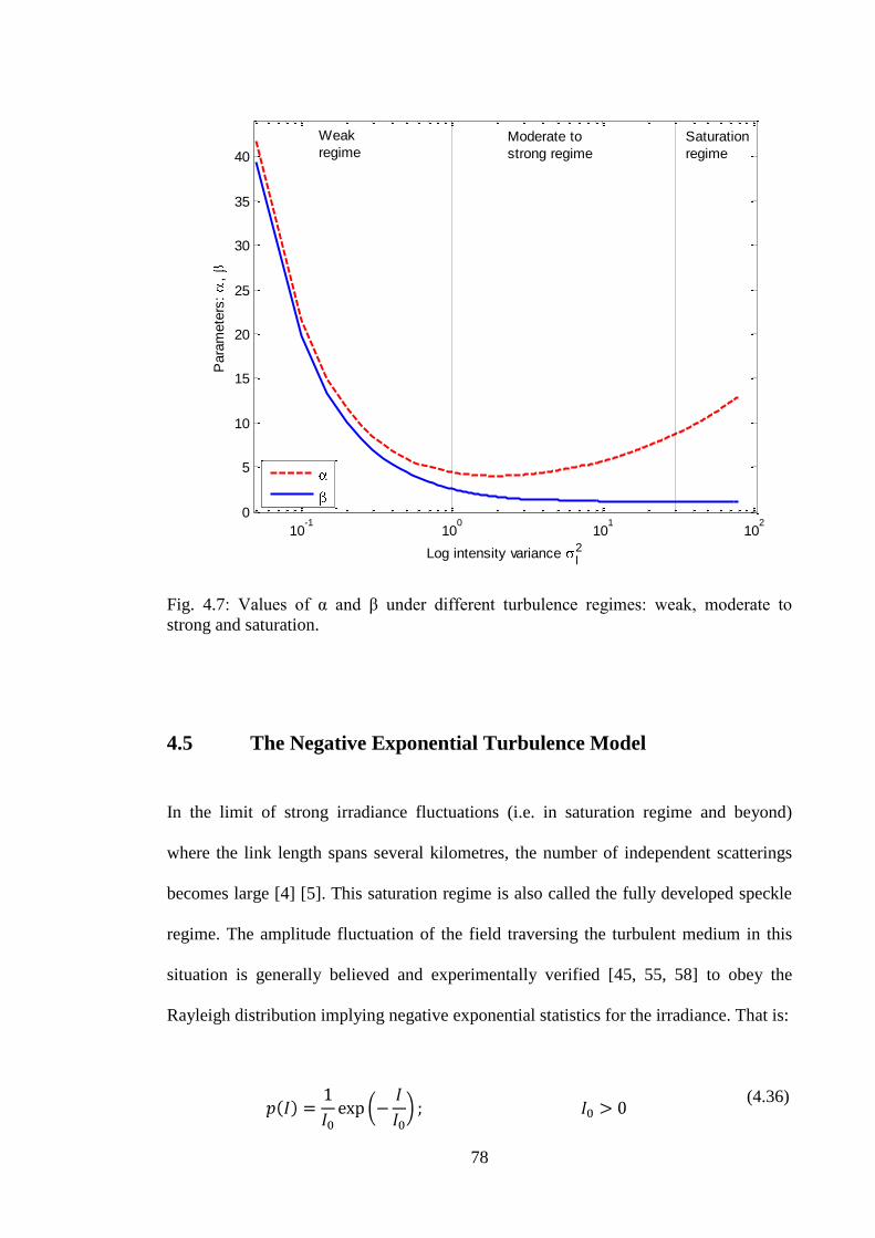
78

10-1

100

101

102

0

5

10

15

20

25

30

35

40

Log intensity variance l2

Para

mete

rs:

,

Weak

regimeModerate to

strong regime

Saturation

regime

Fig. 4.7: Values of α and β under different turbulence regimes: weak, moderate to

strong and saturation.

4.5 The Negative Exponential Turbulence Model

In the limit of strong irradiance fluctuations (i.e. in saturation regime and beyond)

where the link length spans several kilometres, the number of independent scatterings

becomes large [4] [5]. This saturation regime is also called the fully developed speckle

regime. The amplitude fluctuation of the field traversing the turbulent medium in this

situation is generally believed and experimentally verified [45, 55, 58] to obey the

Rayleigh distribution implying negative exponential statistics for the irradiance. That is:

(4.36)

79

where E[I] = I0 is the mean received irradiance. During the saturation regime, the value

of the scintillation index, S.I. . It is noteworthy that other turbulence models such as

the log-normal-Rician [100] and the I–K [101] distributions, which are both valid from

weak to strong turbulence regime; the K-model [102, 103], which is only valid for the

strong regime, and the gamma–gamma turbulence models all reduce to the negative

exponential in the limit of strong turbulence. The negative exponential pdf is shown in

Fig. 4.8.

0 0.5 1 1.5 2 2.5 3 3.5 4 4.5 50

0.2

0.4

0.6

0.8

1

1.2

1.4

1.6

1.8

2

Irradiance, I

Negative e

xponential pdf:

p(I

)

I0 = 0.5

I0 = 1

I0 = 2

Fig. 4.8: Negative exponential probability density function for different values of I0

80

4.6 Summary

In this chapter, different atmospheric turbulence models have been introduced covering

short to very long range FSO links. The log-normal is mathematically tractable but only

valid in the weak regime. Beyond the weak regime, where multiple scattering needs to

be accounted for, the gamma-gamma model is more suitable but lack the mathematical

convenience of the log-normal distribution. This model has a validity that covers both

the weak and strong turbulence regimes while in the saturation regime, which is

otherwise called the fully developed speckle regime, the appropriate model is the

negative exponential distribution. These models will then be used in the subsequent

chapters to characterise the statistical behaviour of the received signal and in deriving

expressions for the error performance of short to very long FSO links.

Chapter Five

FSO Modulation Techniques

5.1 Introduction

This chapter introduces the modulation techniques used in FSO and their performance

in the presence of channel impairments such as noise and channel fading induced by

atmospheric turbulence. There are many different types of modulation schemes which

are suitable for optical wireless communication systems, as shown the modulation tree

of Fig. 5.1. The emphasis in this chapter will be on the following digital modulations

techniques: OOK, pulse position modulation (PPM) and phase shift keying pre-

modulated subcarrier intensity modulation. Since the average emitted optical power is

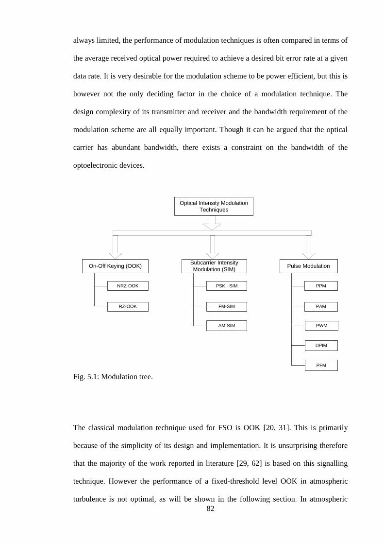
82

always limited, the performance of modulation techniques is often compared in terms of

the average received optical power required to achieve a desired bit error rate at a given

data rate. It is very desirable for the modulation scheme to be power efficient, but this is

however not the only deciding factor in the choice of a modulation technique. The

design complexity of its transmitter and receiver and the bandwidth requirement of the

modulation scheme are all equally important. Though it can be argued that the optical

carrier has abundant bandwidth, there exists a constraint on the bandwidth of the

optoelectronic devices.

Optical Intensity Modulation

Techniques

On-Off Keying (OOK)

NRZ-OOK

RZ-OOK

Pulse Modulation

PPM

PAM

DPIM

PFM

PWM

Subcarrier Intensity

Modulation (SIM)

PSK - SIM

AM-SIM

FM-SIM

Fig. 5.1: Modulation tree.

The classical modulation technique used for FSO is OOK [20, 31]. This is primarily

because of the simplicity of its design and implementation. It is unsurprising therefore

that the majority of the work reported in literature [29, 62] is based on this signalling

technique. However the performance of a fixed-threshold level OOK in atmospheric

turbulence is not optimal, as will be shown in the following section. In atmospheric

83

turbulence an optimal performing OOK requires the threshold level to vary in sympathy

with the prevailing irradiance fluctuation and noise, that is, to be adaptive. The PPM

requires no adaptive threshold and is predominantly used for deep space free space

optical communication links because of its enhanced power efficiency compared to the

OOK signalling [6, 53-55, 61, 104]. The PPM modulation technique, however, requires

a complex transceiver design due to tight synchronisation requirements and a higher

bandwidth than the OOK.

The performance analysis of these modulation schemes and that of the SIM will be

further discussed in both this chapter and the next. The SIM also requires no adaptive

threshold and does not require as much bandwidth as PPM, but suffers from a high peak

to average power ratio, which translates into poor power efficiency. Choosing a

modulation scheme for a particular application therefore entails trade-offs among these

listed factors.

5.2 On-Off Keying

OOK is the dominant modulation scheme employed in commercial terrestrial wireless

optical communications systems. This is primarily due to its simplicity and resilience to

the innate nonlinearities of the laser and the external modulator. OOK can use either

non-return-to-zero (NRZ) or return-to-zero (RZ) pulse formats. In NRZ-OOK, an

optical pulse of peak power αePT represents a digital symbol „0‟ while the transmission

of an optical pulse of peak power PT represents a digital symbol „1‟. The optical source

extinction ratio, αe, has the range 0 ≤ αe < 1. The finite duration of the optical pulse is

the same as the symbol duration T. With OOK-RZ, the pulse duration is lower than the

bit duration, giving an improvement in power efficiency over NRZ-OOK at the expense

84

of an increased bandwidth requirement. In all the analyses that follow, the extinction

ratio, αe , is equal to zero and NRZ-OOK, which is the scheme deployed in present

commercial FSO systems, is assumed unless otherwise stated.

5.2.1 OOK in a Poisson atmospheric optical channel

If the received average power is given by , where represents to

overall channel attenuation, then the average received photoelectron count is given by

[88]:

(5.1)

where h and c are Planck‟s constant and the speed of light in vacuum respectively, η is

the quantum efficiency of the photodetector and T is the optical pulse duration.

However the instantaneous count n, unlike the average count, is not constant. As

mentioned in Chapter Three, it varies with time due to the following reasons:

i) The quantum nature of the light/photodetection process, which suggests that

the instantaneous number of counts n follows the discrete Poisson

distribution with an associated quantum noise of variance , (the mean and

variance of a Poisson distribution are the same).

ii) The received signal field varies randomly due to the effect of scintillation.

This implies that the number of counts is now doubly stochastic and based on the log

normal turbulence model of Section 4.2, the probability of n counts is derived as [105]:

85

(5.2)

where P0 is the received average power in the absence of atmospheric turbulence and σl2

is the strength of power fluctuation indicator. When an optical pulse is transmitted (that

is bit „1‟ sent), a decision error occurs when the number of counts, n, is less than a pre-

determined threshold count, nth. Thus, the probability of detecting bit „0‟ when bit‟1‟ is

transmitted is given by [105]:

(5.3)

where PBg is the power of the background radiation that falls within the receiver‟s field

of view and nb = ηλTPBg/hc.

Similarly, the probability of detecting bit „1‟ when bit „0‟ is transmitted is derived as

[105]:

(5.4)

It should be noted from (5.4) that atmospheric turbulence has no impact when no optical

power is transmitted. If the bits „1‟and „0‟ are assumed to be equally likely to be

transmitted, then the system theoretical bit error rate, Pe becomes:

86

(5.5)

For an optimal performance, nth is the value of n that satisfies expression (5.6) obtained

by invoking the maximum likelihood symbol-by-symbol detection condition.

(5.6)

The impact of scintillation on the achievable bit error rate (BER) of the system is shown

in Fig. 5.2, the figure is obtained by combining equations (5.3), (5.4) and (5.5), while

the values of nth used is obtained from the solution of equation (5.6).

10 20 30 40 50 60

10-5

10-4

10-3

10-2

10-1

Average Photoelectron Count , n0

BE

R

l2 = 0

l2 = 0.1

l2 = 0.2

l2 = 0.5

nb = 5

Fig. 5.2: BER against the average photoelectron count per bit for OOK-FSO in a

Poisson atmospheric turbulence channel for. .

87

In the figure, the BER is plotted against the average count n0 = ηλTP0/hc. The penalty

incurred due to scintillation is quite evident from the plot. For examples, with respect to

no scintillation condition, over 20 additional photoelectron counts per bit are needed to

maintain the same BER of 10-4

in a channel characterised by σl2 > 0.1. Consequently,

when designing a terrestrial laser communication link, an adequate margin, based on the

results shown in Fig. 5.2, should be provided to cater for the scintillation effect.

The figure also shows that increasing the average count can help ameliorate the effect of

turbulence and result in improved BER in very weak turbulence, but as the strength of

turbulence increases, increased average photoelectron count has a less significant

impact. For example at σl2 = 0.1 and n0 = 10, the BER was about 10

-1 but this decreases

to less than 10-3

when n0 is increased to 40. In comparison, when σl2 = 0.5, the BER is

higher than 10-1

for n0 = 10 and remains higher than 10-2

with n0 increased to 40. Note

that in the absence of turbulence, and that the result presented in Fig. 5.2

should be viewed as the theoretical performance lower bound since the photo-

multiplication process has been assumed ideal.

5.2.2 OOK in a Gaussian atmospheric optical channel

With large signal photoelectron counts, and by taking the detection thermal noise into

account, the generated signal current probability distribution can be approximated as the

tractable Gaussian distribution. Without any loss of generality, the receiver area may be

normalised to unity such that the optical power may be represented by the optical

intensity, I. If represents the responsivity of the PIN photodetector, the received

signal in an OOK system is therefore given by:

88

(5.7)

where is the additive white Gaussian noise, is the pulse

shaping function and dj = [-1, 0]. At the receiver, the received signal is fed into a

threshold detector which compares the received signal with a pre-determined threshold

level. A digital symbol „1‟ is assumed to have been received if the received signal is

above the threshold level and „0‟ otherwise.

The probability of error is therefore given as:

(5.8)

where is the threshold signal level and the marginal probabilities are defined as:

(5.9a)

(5.9b)

For equiprobable symbols, , hence the optimum threshold point is

at and the conditional probability of error reduces to:

(5.10)

where . In the presence of atmospheric turbulence, the threshold

level is no longer fixed midway between the signal levels representing symbols „1‟ and

„0‟. The marginal probability is then modified by averaging the conditional pdf

89

of i(t) over the scintillation statistics. Note that scintillation does not occur when no

pulse is transmitted.

(5.11)

Assuming equiprobable symbol transmission and invoking the maximum a posteriori

symbol-by-symbol detection, the likelihood function , becomes [106]:

(5.12)

Fig. 5.3 below shows the plot of log (Λ) against the average photocurrent i, at various

levels of scintillation and noise variance of 10-2

. The threshold level, as would be

expected, is at the point where Λ = 1 (i.e. when log (Λ) = 0).

0 0.1 0.2 0.3 0.4 0.5 0.6 0.7 0.8 0.9-25

-20

-15

-10

-5

0

5

10

15

20

Log lik

elih

ood r

atio

Received average photocurrent (A)

l2 = 0.252

l2 = 0.12

l2 = 0.022

l2 = 0.52

l2 = 0.82

Threshold line

2 = 10-2

E[I] = Io = 1

Fig. 5.3: The likelihood ratio against the received signal for different turbulence levels

and noise variance of 10-2

.

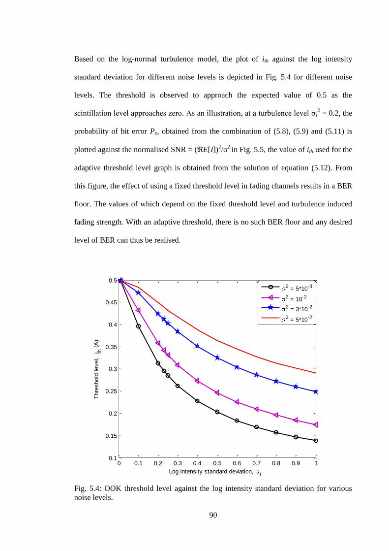
90

Based on the log-normal turbulence model, the plot of ith against the log intensity

standard deviation for different noise levels is depicted in Fig. 5.4 for different noise

levels. The threshold is observed to approach the expected value of 0.5 as the

scintillation level approaches zero. As an illustration, at a turbulence level σl2 = 0.2, the

probability of bit error Pe, obtained from the combination of (5.8), (5.9) and (5.11) is

plotted against the normalised SNR = ( E[I])2/σ

2 in Fig. 5.5, the value of ith used for the

adaptive threshold level graph is obtained from the solution of equation (5.12). From

this figure, the effect of using a fixed threshold level in fading channels results in a BER

floor. The values of which depend on the fixed threshold level and turbulence induced

fading strength. With an adaptive threshold, there is no such BER floor and any desired

level of BER can thus be realised.

0 0.1 0.2 0.3 0.4 0.5 0.6 0.7 0.8 0.9 10.1

0.15

0.2

0.25

0.3

0.35

0.4

0.45

0.5

Log intensity standard deviation, l

Thre

shold

level,

i th (

A)

2 = 5*10-3

2 = 10-2

2 = 3*10-2

2 = 5*10-2

Fig. 5.4: OOK threshold level against the log intensity standard deviation for various

noise levels.

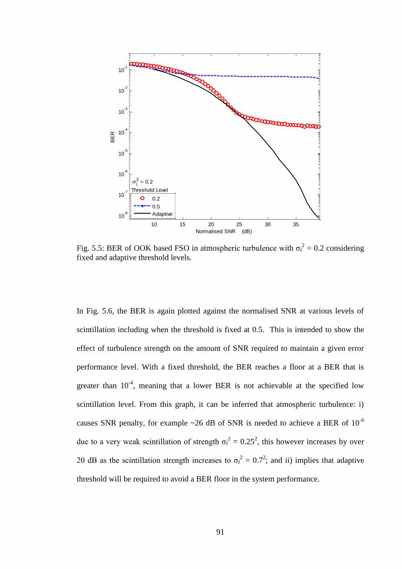
91

10 15 20 25 30 35

10-8

10-7

10-6

10-5

10-4

10-3

10-2

10-1

Normalised SNR (dB)

BE

R

0.2

0.5

Adaptive

l2 = 0.2

Threshold Level

Fig. 5.5: BER of OOK based FSO in atmospheric turbulence with σl

2 = 0.2 considering

fixed and adaptive threshold levels.

In Fig. 5.6, the BER is again plotted against the normalised SNR at various levels of

scintillation including when the threshold is fixed at 0.5. This is intended to show the

effect of turbulence strength on the amount of SNR required to maintain a given error

performance level. With a fixed threshold, the BER reaches a floor at a BER that is

greater than 10-4

, meaning that a lower BER is not achievable at the specified low

scintillation level. From this graph, it can be inferred that atmospheric turbulence: i)

causes SNR penalty, for example ~26 dB of SNR is needed to achieve a BER of 10-6

due to a very weak scintillation of strength σl2 = 0.25

2, this however increases by over

20 dB as the scintillation strength increases to σl2 = 0.7

2; and ii) implies that adaptive

threshold will be required to avoid a BER floor in the system performance.

92

5 10 15 20 25 30 35 40

10-6

10-5

10-4

10-3

10-2

10-1

Normalised SNR (dB)

BE

R

l2 = 0.252

l2 = 0.52

l2 = 0.72

l2 = 0.252

Fixed threshold

Adaptive threshold

E[I] = I0 = 1

Fig. 5.6: BER of OOK-FSO with fixed and adaptive threshold at various levels of

scintillation, and I0 = 1.

The above results illustrate that for the OOK modulated FSO system to perform at its

best, the receiver will require knowledge of both the fading strength and the noise level.

This can be resolved by integrating into the system an intensity estimation network

which can predict the scintillation level based on past events. The implementation of

this is not trivial, and as such, commercial FSO designers tend to adopt the fixed

threshold approach and include a sufficiently large link margin in the link budget to

cater for turbulence induced fading [20].

93

5.3 Pulse Position Modulation

This is an orthogonal modulation technique and a member of the pulse modulation

family (see Fig. 5.1). The PPM modulation technique improves on the power efficiency

of OOK but at the expense of an increased bandwidth requirement and greater

complexity. In PPM, each block of log2M data bits is mapped to one of M possible

symbols. Generally the notation M-PPM is used to indicate the order. Each symbol

consists of a pulse of constant power, PT, occupying one slot, along with M-1 empty

slots. The position of the pulse corresponds to the decimal value of the log2M data bits.

Hence, the information is encoded by the position of the pulse within the symbol. The

slot duration, Ts, is related to the bit duration by the following expression:

(5.13)

The transmitted waveforms for 16-PPM and OOK are shown in Fig. 5.7.

M

Fig. 5.7: Time waveforms for 4-bit OOK and 16-PPM

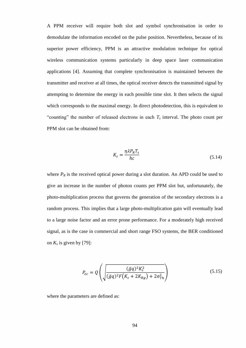
94

A PPM receiver will require both slot and symbol synchronisation in order to

demodulate the information encoded on the pulse position. Nevertheless, because of its

superior power efficiency, PPM is an attractive modulation technique for optical

wireless communication systems particularly in deep space laser communication

applications [4]. Assuming that complete synchronisation is maintained between the

transmitter and receiver at all times, the optical receiver detects the transmitted signal by

attempting to determine the energy in each possible time slot. It then selects the signal

which corresponds to the maximal energy. In direct photodetection, this is equivalent to

“counting” the number of released electrons in each Ts interval. The photo count per

PPM slot can be obtained from:

(5.14)

where PR is the received optical power during a slot duration. An APD could be used to

give an increase in the number of photon counts per PPM slot but, unfortunately, the

photo-multiplication process that governs the generation of the secondary electrons is a

random process. This implies that a large photo-multiplication gain will eventually lead

to a large noise factor and an error prone performance. For a moderately high received

signal, as is the case in commercial and short range FSO systems, the BER conditioned

on Ks is given by [79]:

(5.15)

where the parameters are defined as:

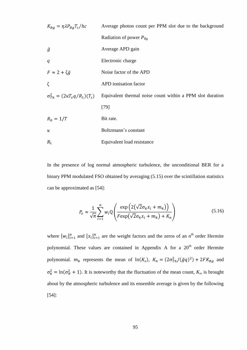
95

Average photon count per PPM slot due to the background

Radiation of power PBg

Average APD gain

q Electronic charge

Noise factor of the APD

APD ionisation factor

Equivalent thermal noise count within a PPM slot duration

[79]

Bit rate.

Boltzmann‟s constant

RL Equivalent load resistance

In the presence of log normal atmospheric turbulence, the unconditional BER for a

binary PPM modulated FSO obtained by averaging (5.15) over the scintillation statistics

can be approximated as [54]:

(5.16)

where and are the weight factors and the zeros of an nth

order Hermite

polynomial. These values are contained in Appendix A for a 20th

order Hermite

polynomial. represents the mean of , and

. It is noteworthy that the fluctuation of the mean count, Ks, is brought

about by the atmospheric turbulence and its ensemble average is given by the following

[54]:

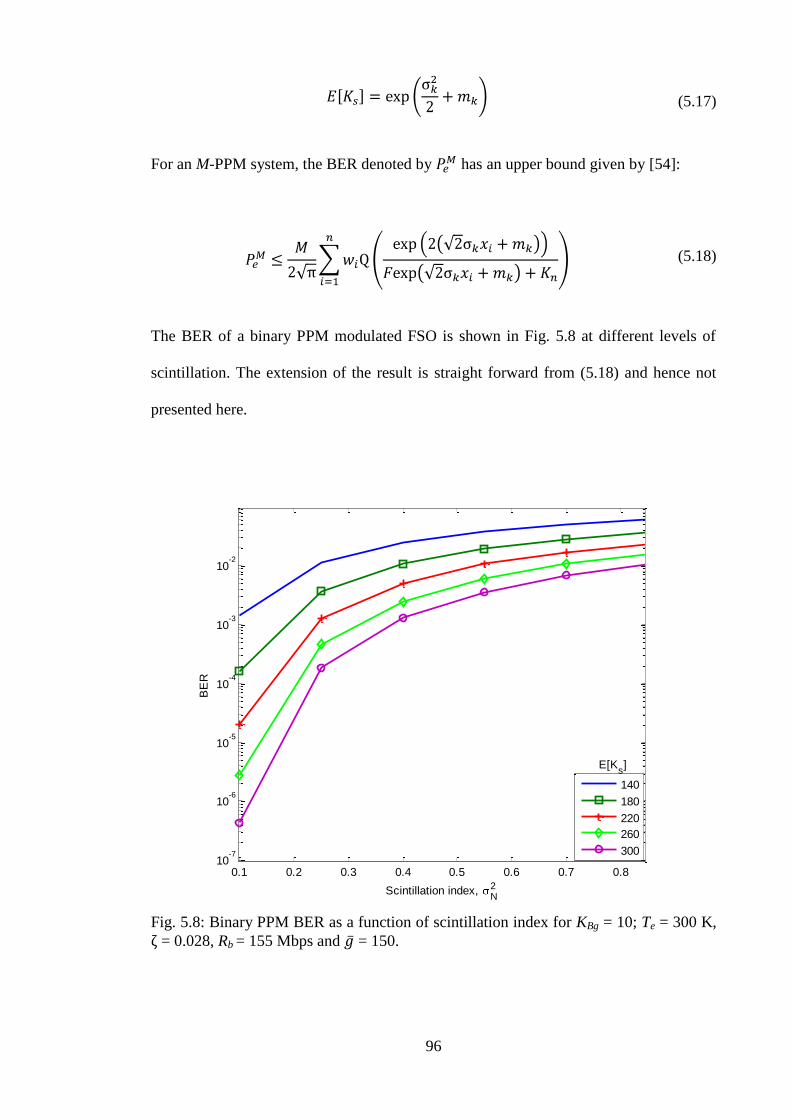
96

(5.17)

For an M-PPM system, the BER denoted by has an upper bound given by [54]:

(5.18)

The BER of a binary PPM modulated FSO is shown in Fig. 5.8 at different levels of

scintillation. The extension of the result is straight forward from (5.18) and hence not

presented here.

0.1 0.2 0.3 0.4 0.5 0.6 0.7 0.810

-7

10-6

10-5

10-4

10-3

10-2

Scintillation index, N2

BE

R

140

180

220

260

300

E[Ks]

Fig. 5.8: Binary PPM BER as a function of scintillation index for KBg = 10; Te = 300 K,

= 0.028, Rb = 155 Mbps and = 150.

97

As expected, an increase in the atmospheric scintillation results in an increase in the

required signal level to achieve a given BER. Increasing the signal strength can be used

to minimise the scintillation effect at a low scintillation index, but as turbulence strength

increases, it is observed that the BERs all tend towards a high BER asymptotic value.

5.4 Subcarrier Intensity Modulation

Subcarrier intensity modulation is a technique borrowed from the very successful

multiple carrier radio frequency (RF) communications already deployed in applications

such as digital television, local area networks (LANs), asymmetric digital subscriber

line (ADSL), 4G communication systems and optical fibre communications [107, 108].

In optical fibre communication networks for example, the subcarrier modulation

techniques have been commercially adopted in transmitting cable television signals and

have also been used in conjunction with wavelength division multiplexing [109]. For

the seamless integration of FSO systems into present and future networks, which

already harbour subcarrier modulated (or multiple carrier) signals, the study of

subcarrier modulated FSO is thus imperative. Other reasons for studying the subcarrier

intensity modulated FSO systems include:

a) It benefits from already developed and evolved RF communication components

such as stable oscillators and narrow filters [110].

b) It avoids the need for an adaptive threshold required by optimum performing

OOK modulated FSO [99].

c) It can be used to increase capacity by accommodating data from different users

on different subcarriers.

98

d) It has comparatively lower bandwidth requirement than the PPM.

There are however some challenges in the implementation of SIM, these are:

a) Relatively high average transmitted power due to:

(i) the optical source being ON during the transmission of both binary digits

„1‟ and „0‟, unlike in OOK where the source is ON during the

transmission of bit „1‟ only.

(ii) the multiple subcarrier composite electrical signal being the sum of the

modulated sinusoids (i.e. dealing with both negative and positive values)

requires a DC bias. This is to ensure that this composite electrical signal,

that will eventually modulate the laser irradiance, is never negative.

Increasing the number of subcarriers leads to increased average

transmitted power, because the minimum value of the composite

electrical signal decreases (becomes more negative) and the required DC

bias therefore increases [111]. This factor results in poor power

efficiency and places a bound on the number of subcarriers that can be

accommodated when using multiple SIM.

b) The possibility of signal distortions due to: inherent laser non-linearity and

signal clipping due to over-modulation.

c) Stringent synchronization requirements at the receiver side.

99

It is therefore worthwhile to mention that multiple-SIM is only recommended when the

quest for higher capacity/users outweighs the highlighted challenges or where FSO is to

be integrated into existing networks that already contain multiple RF carriers. Several

methods have been researched and documented [111-113] to improve the poor power

efficiency of SIM but not be considered in this thesis.

5.4.1 SIM generation and detection

In optical SIM links an RF subcarrier signal, m(t), pre-modulated with the source data,

d(t), is used to modulate the intensity, PT, of the optical source - a continuous wave laser

diode. Figure 5.9 illustrates the system block diagram of a SIM-FSO with N subcarriers.

The serial-to-parallel converter distributes the incoming data across the N-subcarriers.

Each subcarrier carries a reduced symbol rate but the aggregate must be equal to the

symbol rate of d(t).

Another obvious possibility, not shown in the figure, is to have different users

occupying the N different subcarriers. Prior to modulating the laser irradiance, the

source data d(t) are modulated onto the RF subcarriers. For the M-PSK subcarrier

modulation shown in Fig. 5.9, the encoder maps each subcarrier symbol onto the

symbol amplitude that corresponds to the constellation in use. Since the

subcarrier signal, m(t), is sinusoidal, having both positive and negative values, a DC

level b0 is added to m(t) before it is used to directly drive the laser diode – to avoid any

signal clipping.

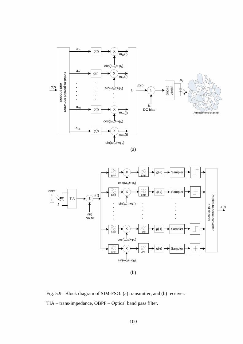
100

g(t) X

cos(ωc1t+φ1)

sin(ωc1t+φ1)

a1c

cos(ωcNt+φN)

sin(ωcNt+φN)

aNc

aNs

.

.

.

.

.

.

.

.

.

.

.

.

.

Σ Σ

bo

DC bias

Driv

er

circ

uit

d(t)

g(t) Xa1s

g(t) X

g(t) X

Se

rial-to

-pa

ralle

l co

nve

rter

an

d e

nco

de

r

m(t)

m1c(t)

m1s(t)

mNc(t)

mNs(t)

Atmospheric channel

PT

(a)

TIA

SamplerLPF

cos(ωc1t+φ1)

BPF

Σ

n(t)

Noise

g(-t)X

OBPF Pa

ralle

l-to-s

eria

l co

nve

rter

an

d d

eco

de

r

SamplerLPF

sin(ωc1t+φ1)

BPF

g(-t)X

SamplerLPF

cos(ωcNt+φN)

BPF

g(-t)X

SamplerLPF

sin(ωcNt+φN)

BPF

g(-t)X

.

.

.

.

.

.

.

.

.

.

.

.

.

.

.

)(ˆ tdI

i(t)

(b)

Fig. 5.9: Block diagram of SIM-FSO: (a) transmitter, and (b) receiver.

TIA – trans-impedance, OBPF – Optical band pass filter.

101

The following gives the general expression for m(t) in the N-SIM-FSO system:

(5.19)

During a symbol duration, each RF subcarrier signal is generally represented by:

(5.20)

where g(t) is the pulse shaping function, and the subcarrier angular frequency and phase

are represented by . It follows that each subcarrier can be modulated by any

standard RF digital/analogue modulation technique, such as QAM, M-PSK, M-FSK and

M-ASK. Using direct detection at the receiver, the incoming optical radiation, PR, is

converted into an electrical signal, i(t). This is followed by a standard RF demodulator

to recover the transmitted symbol as shown in Fig. 5.9(b). By normalising the receiver

area to unity and representing the received power by irradiance, I, the received signal

can be modelled as:

(5.21)

where the optical modulation index , as shown in Fig. 5.10.

102

0

iTh

Imax

iB

m(t)

Ipeak

I

Irradiance

Drive current

ξ = |m(t)| / iB - iTh

Fig. 5.10: Output characteristic of an optical source driven by a subcarrier signal

showing optical modulation index.

The electrical band pass filter (BPF) with a minimum bandwidth of 2Rb performs the

following functions: selection of the individual subcarrier for demodulation; reduction

of the noise power; and suppression of any slow varying component present in the

received signal. For a subcarrier at ωci the received signal is:

(5.22)

where

(5.23a)

(5.23b)

103

nI(t) and nQ(t) are the independent additive white Gaussian noise (AWGN) with a zero

mean and a variance σ2. The quadrature components Icomp and Qcomp are down converted

by the reference signals cosωct and sinωct respectively, and applied to the standard

receiver architecture. The electrical low pass filters, which are part of the standard RF

receiver, remove any out of band (unwanted) signals from the down converted signal

and then pass it onto the decision circuit. In the case of phase shift keying modulated

subcarrier, the decision circuit estimates the phase of the received signal and decides

which symbol has been received. By adopting the approach in [114], the conditional

BER expressions can be deduced. This error performance analysis is the subject of the

next chapter. Table 5.1 presents a comparison of the three modulation techniques

discussed in this chapter.

Table 5.1: Comparison of FSO modulation techniques

On-Off Keying

Pulse Position

Modulation

Subcarrier Intensity

Modulation

Simple to implement Power efficient Power inefficient

Synchronisation not

required

Synchronisation

required

Higher throughput

Adaptive threshold

required in fading

channels

Adaptive threshold

not required in

fading channels

Adaptive threshold not

required in fading channels

Component

nonlinearity not an

issue

Component

nonlinearity not an

issue

Component nonlinearity

an issue with multiple

subcarrier

Suboptimal with fixed

threshold

High bandwidth

requirement

Benefits from advances in

digital signal processing

and matured RF

components

104

5.5 Summary

The modulation techniques for FSO have been discussed. The error performance of both

OOK and PPM techniques have been analysed in the presence of noise and atmospheric

turbulence, and the effect of turbulence on the BER highlighted. For instance, an OOK-

FSO system will require ~26 dB of SNR is needed to achieve a BER of 10-6

due to a

very weak scintillation of strength σl2 = 0.25

2, this however increases by over 20 dB as

the scintillation strength increases to σl2 = 0.7

2. It has also been shown that, in very

weak turbulence situations, increased signal strength could be used to combat the

channel fading. This approach however does not work beyond the very weak regime

and alternative techniques, to be discussed in Chapter Seven, will have to be explored.

The choice of modulation technique involves a balance between simplicity, power

efficiency and bandwidth efficiency. In view of the BER floor experienced in OOK, the

poor bandwidth efficiency of PPM and the requisite slot and symbol synchronisation

requirements, the focus in this work will be on SIM. However, this does suffer from

poor power efficiency due to its high peak to average power ratio. In the next chapter,

the performance of SIM-FSO in all turbulence regimes is presented.

Chapter Six

Subcarrier Intensity Modulated FSO

in Atmospheric Turbulence Channels

6.1 Introduction

In this chapter, the error performance analysis of both single and multiple subcarriers

based FSO systems in a turbulent atmospheric channel will be discussed. The chapter

will also examine the intermodulation distortion caused by the optical source and ways

of choosing the optical modulation in order to optimise the system error performance.

The performance analysis in this chapter will be based on the direct detection with a

PIN photo-detector. Since the FSO link is a line-of-sight (LOS) system with no

106

multipath, the inter-symbol interference (ISI) will therefore not be considered. Also the

number of photons received is sufficient to justify the use of Gaussian statistics

approximation for the detection process. The log normal, gamma-gamma and the

negative exponential turbulence models discussed in Chapter Four will be used to

describe received irradiance fluctuation for the short, medium to long and the very long

span FSO systems, respectively.

Performance metrics are used to characterise, model and predict the behaviour of a

system under different channel conditions. In addition to the generic bit-error-rate

(BER) metric which models the fraction of bits received incorrectly in a digital

communication system, the outage probability due to turbulence induced signal fading

will also be considered. The outage probability is a measure of the probability that the

instantaneous BER is greater that a pre-determined threshold level. This metric

adequately describes the system performance including short duration deep fades, which

the generic average BER might not capture.

6.2 SIM-FSO Performance in Log-normal Atmospheric

Channels

Prior to the analytical estimation of the effect of scintillation on the system

performance, the effect of turbulence and noise on a subcarrier signal constellation will

first be presented. The simulation will be based on the block diagram of Fig. 5.9, with a

QPSK modulated single subcarrier. The constellation at the input of the transmitter is

shown in Fig. 6.1. The signal is then transmitted through the atmospheric channel with

turbulence induced fading and noise. For this illustration, the electrical

is fixed, for instance, at 2 dB. The received constellation under a very

low fading of is shown in Fig. 6.2 while the effect of turbulence induced

107

fading is made evident by displaying in Fig. 6.3 the received constellation with a much

higher fading with .

-0.6 -0.4 -0.2 0 0.2 0.4 0.6

-0.6

-0.4

-0.2

0

0.2

0.4

0.6

Quadra

ture

In-Phase

Fig. 6.1: QPSK constellation of the input subcarrier signal without noise and channel

fading

-1 -0.8 -0.6 -0.4 -0.2 0 0.2 0.4 0.6 0.8 1

-1

-0.8

-0.6

-0.4

-0.2

0

0.2

0.4

0.6

0.8

1

Quadra

ture

In-Phase

Fig. 6. 2: Received constellation of QPSK pre-modulated SIM-FSO with noise and

channel fading for SNR = 2 dB and

108

-1 -0.8 -0.6 -0.4 -0.2 0 0.2 0.4 0.6 0.8 1

-1

-0.8

-0.6

-0.4

-0.2

0

0.2

0.4

0.6

0.8

1

Quadra

ture

In-Phase

Fig. 6.3: Received constellation of QPSK pre-modulated SIM-FSO with noise and

channel fading for SNR = 2 dB and

With a very low turbulence induced fading strength , the constellations

form clusters that are clearly confined within their respective quadrants and the chance

of erroneous demodulation is very low but as the turbulence level increases to ,

the confinement is lost and the constellation points become more staggered and move

toward the centre of the plot. This apparently increases the chance of demodulation

error during the symbol detection process. To quantify this observation, the bit error and

the outage probabilities of SIM-FSO in atmospheric turbulence will now be presented.

109

6.2.1 Bit error probability analysis of SIM-FSO

In this section the BER analysis is presented in a clear but turbulent atmospheric

channel, the turbulence induced irradiance fluctuation considered in this section is based

on the log normal model of Section 4.2. A single BPSK pre-modulated subcarrier will

first be considered and this will be followed by the M-PSK and then the DPSK

modulated subcarrier.

6.2.1.1 BPSK modulated subcarrier

The result of this section will be for a single BPSK pre-modulated subcarrier

, over a symbol duration, where represents the data

symbols „0‟ and „1‟. By employing a coherent demodulation at the subcarrier level, the

symbol-by-symbol detection is carried out by multiplying the received signal, given by

equation 5.23(a), by a locally generated RF signal of the same frequency ωc, and phase

as follows. Without any loss of generality, the subcarrier phase is equated to zero, that

is . The coherent demodulator output, is then given by:

(6.1)

Passing through a low pass filter with a bandwidth of 1/T suppresses the

term without distorting the information bearing signal. This also reduces the

noise variance at the output of the coherent demodulator filter to half its value at the

input of the demodulator. Equation (6.1) therefore reduces to:

(6.2)

110

where the additive noise . Assuming an equiprobable data

transmission such that p(0) = p(1) = ½, the probability of error conditioned on the

received irradiance becomes:

(6.3)

The marginal probabilities are given by:

(6.4a)

(6.4b)

Where and for and zero elsewhere. Here both binary

symbols '1' and '0' are affected by the irradiance fluctuation since the optical source is

on during the transmission of both data symbols '1' and '0'. This is in contrast to the

OOK signalling technique where irradiance fluctuation only affects the data symbol '1'.

Based on the antipodal nature of (6.2), the decision threshold level can hence be fixed at

the zero mark. This zero level threshold is irradiance independent and hence not

affected by the irradiance fluctuation caused by the atmospheric turbulence. From the

foregoing and the apparent symmetry of (6.4), the BER conditioned on the received

irradiance can now be written as:

(6.5)

111

At the input of the subcarrier coherent demodulator, the electrical SNR per bit is given

by:

(6.6)

where , from which . Equation (6.6) can now be

expressed in terms of the SNR at the demodulator input as:

(6.7)

The unconditional probability , is obtained by averaging (6.7) over the log normal

irradiance fluctuation statistics to obtain the following:

(6.8a)

(6.8b)

A closed form solution of equation 6.8(b) does not exist and using the numerical

integration could result in truncating its upper limit. Also, the presence of the argument

of the Q-function at the lower limit of the Q-function integral always poses analytical

problems [115]. By combining an alternative representation of the Q-function given by

(6.9) with the Gauss-Hermite quadrature integration approximation of (6.10), the

analytical difficulty involved solving (6.8) can be circumvented.

for y > 0

(6.9)

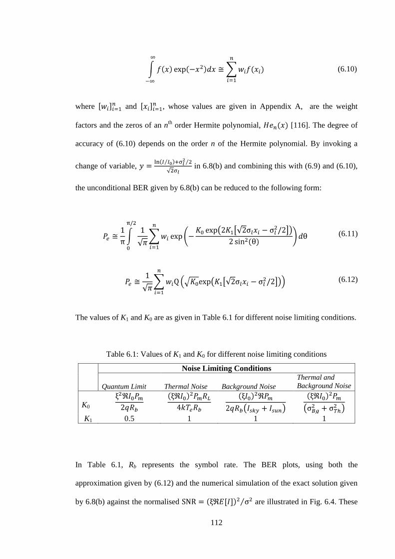
112

(6.10)

where and , whose values are given in Appendix A, are the weight

factors and the zeros of an nth

order Hermite polynomial, [116]. The degree of

accuracy of (6.10) depends on the order n of the Hermite polynomial. By invoking a

change of variable, in 6.8(b) and combining this with (6.9) and (6.10),

the unconditional BER given by 6.8(b) can be reduced to the following form:

(6.11)

(6.12)

The values of K1 and K0 are as given in Table 6.1 for different noise limiting conditions.

Table 6.1: Values of K1 and K0 for different noise limiting conditions

Noise Limiting Conditions

Quantum Limit

Thermal Noise

Background Noise

Thermal and

Background Noise

K0

K1 0.5 1 1 1

In Table 6.1, Rb represents the symbol rate. The BER plots, using both the

approximation given by (6.12) and the numerical simulation of the exact solution given

by 6.8(b) against the normalised are illustrated in Fig. 6.4. These

113

results hint that using the 20th

order Gauss Hermite approximation gives an accurate

representation of the exact BER. The Gauss Hermite integration solution of the BER is

however preferred for its simplicity and compactness.

10 11 12 13 14 15 16 17 18 19 20

10-9

10-8

10-7

10-6

10-5

10-4

10-3

10-2

Normalised SNR (dB)

BE

R

Numerical

Gauss-Hermite

l2 = 0.12

Fig. 6.4: BER against the normalised SNR using numerical and 20

th order Gauss-

Hermite integration methods in weak atmospheric turbulence for .

In order to keep the optical source (laser) within its linear dynamic range and avoid

signal clipping distortion, the condition must always hold. For a given

value of , this places an upper bound on the amplitude of each subcarrier. The BER

given by (6.12) is plotted against the normalised SNR for different noise limiting

conditions in Fig. 6.5, based on the simulation parameters given in Table 6.2. The figure

illustrates clearly that for an FSO link with a suitable optical BPF and a narrow FOV

detector, the system performance is limited by thermal noise. Moreover, under this

thermal noise limited condition, the SIM-FSO still requires about additional 30 dB of

SNR compared with the theoretical quantum limit.

114

-60 -55 -50 -45 -40 -35 -30 -25 -20 -15

10-14

10-12

10-10

10-8

10-6

10-4

10-2

Average received irradiance, I0 (dBm)

BE

R

Thermal noise

Background noise

Thermal+Background

Quantum

l2 = 0.3

Fig. 6.5: The BER against the average received irradiance in weak turbulence under

different noise limiting conditions for Rb = 155 Mpbs and σl2

= 0.3.

Table 6.2: Simulation parameters

Parameter Value

Symbol rate Rb 155 Mbps

Spectral radiance of the sky N(λ) 10-3

W/cm2µmSr

Spectral radiant emittance of the sun W(λ) 0.055 W/cm2µm

Optical band-pass filter bandwidth Δλ @ λ = 850 nm 1 nm

PIN photodetector field of view (FOV) 0.6 rad

Radiation wavelength λ 850 nm

Number of subcarriers N 1

Link range L 1 km

Index of refraction structure parameter Cn2 0.75×10

-14 m

-2/3

Load resistance RL 50 Ω

PIN photodetector responsivity 1

Operating temperature Te 300 K

Optical modulation index 1

115

6.2.1.2 M-ary PSK modulated subcarrier

Here the data symbols which comprise of binary digits are mapped onto one of

the M available phases on each subcarrier signal, m(t). Based on the subcarrier coherent

demodulation and by following the analytical approach given in [114], the following

conditional BER expressions are obtained:

for M-PSK, M ≥ 4

(6.13a)

for M-QAM, log2M even

(6.13b)

The unconditional BER, Pe, is thus obtained in a similar fashion, by averaging the

conditional bit error rate over the atmospheric turbulence statistics. The resulting BER

expression (6.14) for M-PSK has no closed form solution and can only be evaluated

numerically.

(6.14)

Whenever a subcarrier coherent detection is used, there is always an ambiguity

associated with the estimation of the absolute phase of the subcarrier signal [114]. This

poses an implementation challenge for the subcarrier coherent demodulation based

systems, this can however be solved by considering a differential phase shift keying

(DPSK) based SIM-FSO system as discussed below.

116

6.2.1.3 DPSK modulated subcarrier

This modulation scheme is the most suitable when the absolute phase estimation needed

for the subcarrier coherent demodulation is not feasible or too complex to realise. The

DPSK pre-modulated SIM-FSO is demodulated by comparing the phase of the received

signal in any signalling interval with the phase of the signal received in the preceding

signalling interval [114], as shown in Fig. 6.6 for a single subcarrier FSO system.

Accurate demodulation of the present data symbol thus depends on whether the

preceding symbol has been correctly demodulated or not. The demodulation of DPSK

based SIM-FSO is feasible during atmospheric turbulence because the turbulence

coherence time, which is in the order of milliseconds, is far greater than the typical

duration of two consecutive data symbols. This implies that the channel properties are

fixed during a minimum of two symbol durations – a pre-requisite for non-coherent

demodulation of DPSK subcarrier signal.

g(t) +Laser

driver

DC bias

b0

Input

data XOR

)(td

m(t)TT Atmospheric

channel

Carrier

cosωct

×

Delay

(T)

(a)

x g(-t) Symbol rate

Sampler

Delay ( T)Phase

comparator

cosωct

Output data

Photo-

detector/

TIA

i

RTLPFBPF

)(ˆ td

Atmospheric

channel

DPSK demodulator

yk

yk-1

y(t)

(b)

Fig. 6.6: Block diagram of an FSO link employing DPSK modulated SIM; (a)

transmitter and (b) receiver.

TIP-trans-impedance amplifier; TT-Transmitter telescope; RT-Receiver telescope.

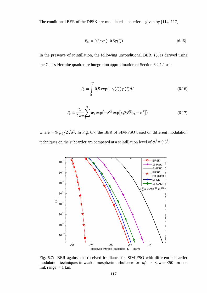
117

The conditional BER of the DPSK pre-modulated subcarrier is given by [114, 117]:

(6.15)

In the presence of scintillation, the following unconditional BER, Pe, is derived using

the Gauss-Hermite quadrature integration approximation of Section 6.2.1.1 as:

(6.16)

(6.17)

where . In Fig. 6.7, the BER of SIM-FSO based on different modulation

techniques on the subcarrier are compared at a scintillation level of σl2 = 0.5

2.

-30 -25 -20 -15 -10

10-10

10-9

10-8

10-7

10-6

10-5

10-4

10-3

Received average irradiance, I0 (dBm)

BE

R

BPSK

16-PSK

64-PSK

BPSK

No fading

DPSK

16-QAM

Cn2 = 75*10-16 m-2/3

Fig. 6.7: BER against the received irradiance for SIM-FSO with different subcarrier

modulation techniques in weak atmospheric turbulence for σl2 = 0.3, and

link range = 1 km.

118

The performance in a turbulence free channel is included in the figure for the estimation

of turbulence induced fading penalty. The figure shows clearly the performance

superiority of BPSK modulated SIM in terms of the amount of SNR required to achieve

a given BER. Due to atmospheric turbulence induced channel fading, a BPSK pre-

modulated SIM-FSO system will incur a power penalty of ~5 dB at a BER of 10-6

, the

penalty rises to ~10 dB when the error performance level is raised to a BER of 10-9

.

This penalty is higher for other modulation techniques as shown in the figure. The M-

PSK (with ) modulated subcarrier is known to be more bandwidth efficient [114],

while the DPSK is advantageous in that it does not require absolute phase estimation

but both are not as power efficient as the BPSK-SIM. The choice of modulation

technique at the subcarrier level therefore depends on the application at hand and

requires a compromise between simplicity, power and bandwidth efficiencies.

6.2.1.4 Multiple SIM performance analysis

The use of multiple subcarriers is a viable way of increasing system

throughput/capacity. To archive this, different data/users are pre-modulated on different

subcarrier frequencies. These are then aggregated and the resulting composite signal

used to modulate the intensity of the optical source. For a subcarrier system with N

subcarrier signals operating at different frequencies, the inherent non-linearity of the

optical source will result in the transfer of energy among the subcarrier frequencies (i.e.

the inter-modulation distortion (IMD)). The IMD potentially results in a reduced SNR

as it contributes to the amount of unwanted signals within the frequency band of

interest. The detailed discussion of the IMD due to optical source non-linearity will be

covered in Section 6.5. In the mean time, the multiple subcarriers system will be

examined by assuming an ideal optical source with no reference to the IMD and the

clipping distortion.

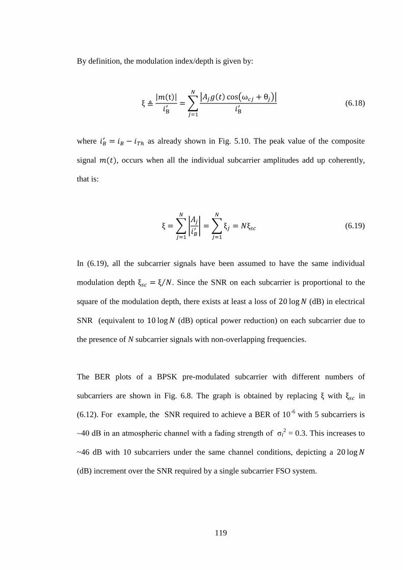
119

By definition, the modulation index/depth is given by:

(6.18)

where as already shown in Fig. 5.10. The peak value of the composite

signal , occurs when all the individual subcarrier amplitudes add up coherently,

that is:

(6.19)

In (6.19), all the subcarrier signals have been assumed to have the same individual

modulation depth . Since the SNR on each subcarrier is proportional to the

square of the modulation depth, there exists at least a loss of (dB) in electrical

SNR (equivalent to (dB) optical power reduction) on each subcarrier due to

the presence of N subcarrier signals with non-overlapping frequencies.

The BER plots of a BPSK pre-modulated subcarrier with different numbers of

subcarriers are shown in Fig. 6.8. The graph is obtained by replacing with in

(6.12). For example, the SNR required to achieve a BER of 10-6

with 5 subcarriers is

~40 dB in an atmospheric channel with a fading strength of σl2 = 0.3. This increases to

~46 dB with 10 subcarriers under the same channel conditions, depicting a

(dB) increment over the SNR required by a single subcarrier FSO system.

120

5 10 15 20 25 30 35 40 45 50

10-8

10-7

10-6

10-5

10-4

10-3

10-2

10-1

Normalised SNR (dB)

BE

R

1

2

5

10

Number of

subcarriers

Fig. 6.8: BER against the normalised SNR for multiple subcarriers FSO system in weak

atmospheric turbulence for and σl2 = 0.3.

In Fig. 6.9, these SNR values required to attain a BER of 10-6

are plotted against the

number of subcarriers for turbulent atmospheric channels of different fading strengths.

This shows explicitly that for a given BER value, the SNR values increase with an

increase in both number of subcarriers and the fading strength. Based on the foregoing

therefore, the multiple SIM-FSO is only recommended whenever the quest for increased

throughput/capacity outweighs its accompanying power penalty.

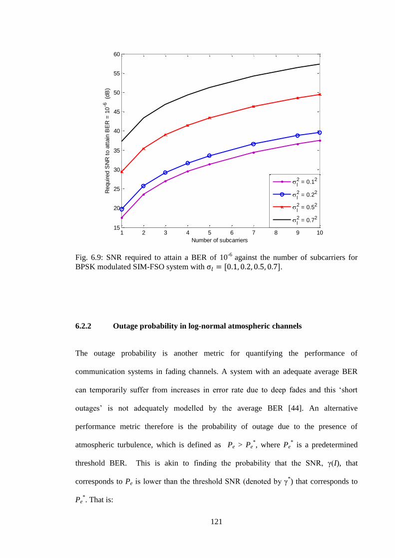
121

1 2 3 4 5 6 7 8 9 1015

20

25

30

35

40

45

50

55

60

Number of subcarriers

Required S

NR

to a

ttain

BE

R =

10

-6

(dB

)

l2 = 0.12

l2 = 0.22

l2 = 0.52

l2 = 0.72

Fig. 6.9: SNR required to attain a BER of 10

-6 against the number of subcarriers for

BPSK modulated SIM-FSO system with .

6.2.2 Outage probability in log-normal atmospheric channels

The outage probability is another metric for quantifying the performance of

communication systems in fading channels. A system with an adequate average BER

can temporarily suffer from increases in error rate due to deep fades and this „short

outages‟ is not adequately modelled by the average BER [44]. An alternative

performance metric therefore is the probability of outage due to the presence of

atmospheric turbulence, which is defined as Pe > Pe*, where Pe

* is a predetermined

threshold BER. This is akin to finding the probability that the SNR, γ(I), that

corresponds to Pe is lower than the threshold SNR (denoted by γ*) that corresponds to

Pe*. That is:

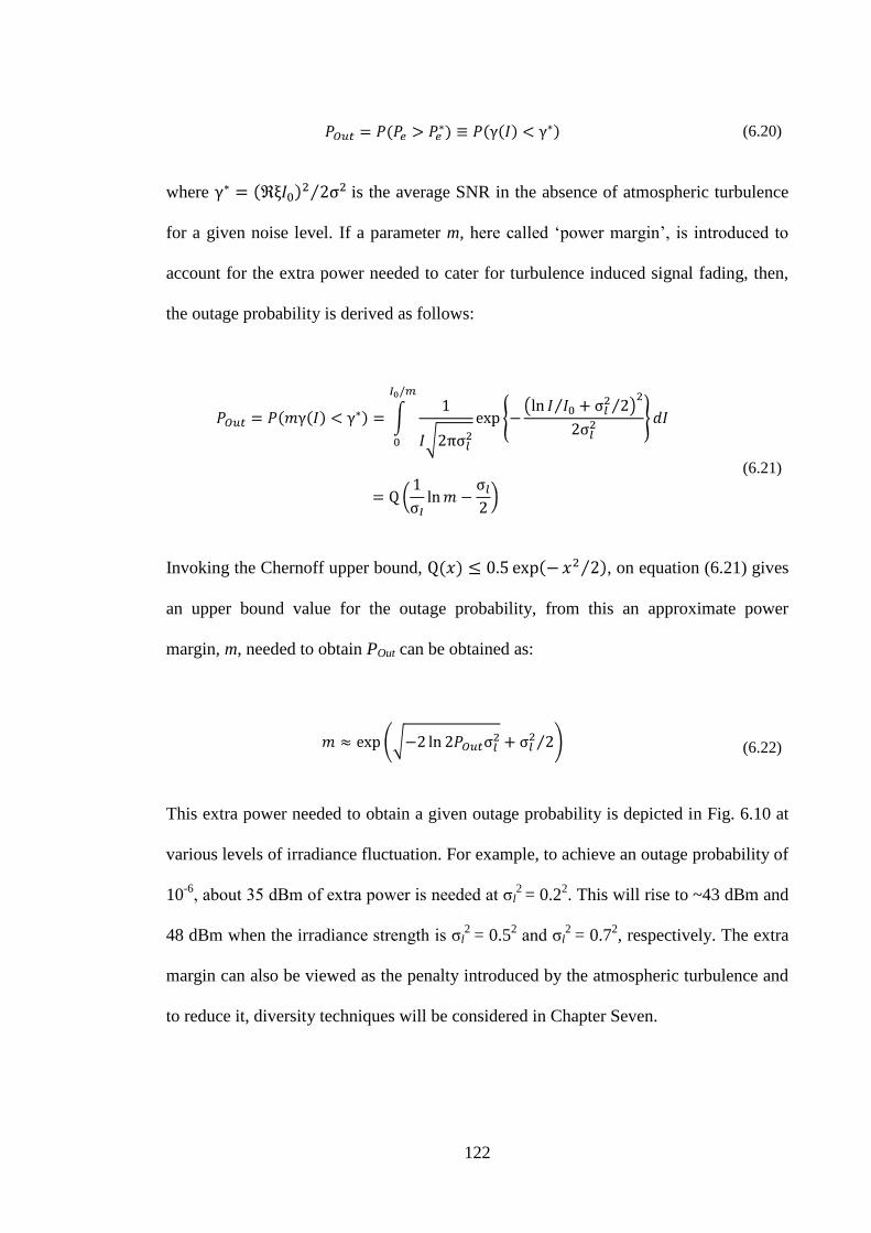
122

(6.20)

where is the average SNR in the absence of atmospheric turbulence

for a given noise level. If a parameter m, here called „power margin‟, is introduced to

account for the extra power needed to cater for turbulence induced signal fading, then,

the outage probability is derived as follows:

(6.21)

Invoking the Chernoff upper bound, , on equation (6.21) gives

an upper bound value for the outage probability, from this an approximate power

margin, m, needed to obtain POut can be obtained as:

(6.22)

This extra power needed to obtain a given outage probability is depicted in Fig. 6.10 at

various levels of irradiance fluctuation. For example, to achieve an outage probability of

10-6

, about 35 dBm of extra power is needed at σl2

= 0.22. This will rise to ~43 dBm and

48 dBm when the irradiance strength is σl2

= 0.52 and σl

2 = 0.7

2, respectively. The extra

margin can also be viewed as the penalty introduced by the atmospheric turbulence and

to reduce it, diversity techniques will be considered in Chapter Seven.

123

35 40 45 50 55 6010

-10

10-8

10-6

10-4

10-2

Power Margin (dBm)

Outa

ge P

robabili

ty,

PO

ut

l2 = 0.1

l2 = 0.3

l2 = 0.5

l2 = 1

Fig. 6.10: Outage probability against the power margin for a log-normal turbulent

atmospheric channel for .

6.3 SIM-FSO Performance in Gamma-Gamma and Negative

Exponential Atmospheric Channels

To obtain the unconditional BER in a gamma-gamma turbulent atmospheric channel,

the irradiance fluctuation statistics in the previous section is replaced appropriately by

the gamma-gamma pdf. For a BPSK pre-modulated subcarrier, the unconditional BER

now becomes:

6.23)

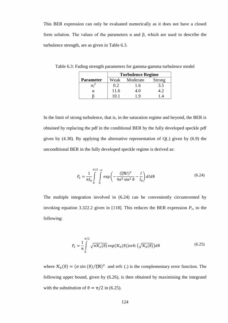
124

This BER expression can only be evaluated numerically as it does not have a closed

form solution. The values of the parameters α and β, which are used to describe the

turbulence strength, are as given in Table 6.3.

Table 6.3: Fading strength parameters for gamma-gamma turbulence model

Parameter

Turbulence Regime

Weak Moderate Strong

σl2 0.2 1.6 3.5

α 11.6 4.0 4.2

β 10.1 1.9 1.4

In the limit of strong turbulence, that is, in the saturation regime and beyond, the BER is

obtained by replacing the pdf in the conditional BER by the fully developed speckle pdf

given by (4.38). By applying the alternative representation of Q(.) given by (6.9) the

unconditional BER in the fully developed speckle regime is derived as:

(6.24)

The multiple integration involved in (6.24) can be conveniently circumvented by

invoking equation 3.322.2 given in [118]. This reduces the BER expression Pe, to the

following:

(6.25)

where and erfc (.) is the complementary error function. The

following upper bound, given by (6.26), is then obtained by maximising the integrand

with the substitution of in (6.25).

125

(6.26)

where . From these BER expressions, the error performance of the

system can be predicted for any given value of SNR and turbulence strength (or link

range). The numerical simulations of the BER expressions (6.23), (6.25) and the upper

bound (6.26) are shown in Fig. 6.11, where the Pe is plotted against the normalised SNR

under different turbulence regimes.

20 40 60 80 100 120

10-6

10-5

10-4

10-3

10-2

Electrical SNR (dB)

BE

R

Weak

Moderate

Strong

Saturation (Exact)

Saturation

(Upper bound)

Turbulence regime

Fig. 6.11: BER performance against the normalised electrical SNR across all of

turbulence regimes based on gamma-gamma and negative exponential modes.

126

For instance, to achieve a BER of 10-6

in a weak atmospheric turbulence, the required

SNR is ~29 dB and this rises to ~65 dB and ~67 dB, respectively for moderate and

intermediate regimes. While in the saturation regime, a staggering ~115 dB (the upper

bound value is 4 dB higher) is required to achieve the same level of error performance

(i.e. BER of 10-6

). Achieving a BER lower than 10-6

in the saturation regime requires a

phenomenal increase in SNR as seen in Fig. 6.11. It is noteworthy that the normalised

SNR is in the electrical domain and it is based on the average received irradiance, E[I].

Also the „kinks‟ observed in the curves for strong and moderate turbulence are due to

the numerical integration process.

On order to compare the error performance BPSK-SIM with an OOK modulated FSO

system of the same average transmitted optical power, the unconditional BER of the

OOK-FSO is modified to become:

(6.27)

In Fig. 6.12, the BER performances of the OOK system employing adaptive (optimum)

and fixed threshold values of 0.05 and 0.8 are shown alongside that of BPSK-SIM in a

weak turbulent atmospheric fading. Although the optimum OOK is marginally superior

to BPSK-SIM under the stated conditions, as it requires 1.6 dB electrical SNR less at a

BER of 10-6

, it does require an accurate knowledge of both the additive noise and fading

levels to achieve this performance. With the threshold fixed at say 0.05, the OOK

requires about 7 dB electrical SNR more than BPSK-SIM at a BER of 10-6

. Also, the

BER performance of OOK with a fixed threshold level exhibits a BER floor as shown in

Fig. 2(b) for ith = 0.8 and in the previous work by [8]. The SIM is therefore

recommended in atmospheric turbulence channels as against the fixed threshold OOK

currently used in commercial terrestrial FSO systems.

127

5 10 15 20 25 30 35

10-6

10-5

10-4

10-3

10-2

10-1

Normalised SNR (dB)

BE

R

OOK (ith

= 0.8)

OOK (ith

= 0.05)

BPSK-SIM

OOK (Optimum)

Weak turbulence regime

Fig. 6.12: Error performance of BPSK SIM and OOK with fixed and adaptive threshold

based FSO in weak turbulence regime modeled using gamma-gamma distribution.

6.3.1 Outage probability in negative exponential model atmospheric channels

By following the approach of Section 6.2.2, the outage probability in the fully

developed speckle is obtained as follows:

6.28)

From (6.28) the power margin m, needed to achieve a given POut saturation regime is as

given by (6.29). This is plotted in Fig. 6.13, alongside equation (6.22) with ,

which represents the outage probability in weak atmospheric turbulence. A comparison

128

of the results in this figure reveals that, the power margin required to achieve a POut of

10-6

in the fully developed speckle regime is about 40 dB higher than that required in

the weak turbulence regime with , and this will increase as the required outage

probability level is reduced to below 10-6

.

(6.29)

40 50 60 70 80 90 100 110 120 13010

-10

10-8

10-6

10-4

10-2

Power Margin (dBm)

Outa

ge P

robabili

ty,

PO

ut

l2 = 0.5

Saturation

regime

Fading strength

Fig. 6.13: The outage probability against the power margin in saturation and weak

turbulence regimes for .

The prohibitive power required in the saturation regime suggests that the establishment

of a reliable communication link in this regime is impossible unless the fading effect

due to turbulence is mitigated or compensated for.

129

6.4 Atmospheric Turbulence Induced Penalty

In this section, the additional power required, due to the presence of turbulence induced

channel fading, to achieve a given level of performance will be examined. Without any

loss of generality, the result here will be based on the log normal turbulence model, and

the BPSK modulated subcarrier. This can however be extended to other turbulence

models and modulation schemes in a straight forward manner. In Fig. 6.14, the BER is

plotted as a function of normalised for different levels of atmospheric turbulence. As an

example, to achieve a BER of 10-6

in a channel characterised by a SNR of

about 24 dB will be required. This increases to ~37 dB as the fading strength increases

to .

15 20 25 30 35 40 45

10-12

10-10

10-8

10-6

10-4

10-2

Normalised SNR (dB)

BE

R

l2 = 0.1

l2 = 0.3

l2 = 0.5

l2 = 0.7

No fading

Fading strength

Fig. 6.14: Error rate performance against normalised SNR for BPSK-SIM based FSO in

weak atmospheric turbulence channel for .

130

Also from this plot, the SNR penalty at any given fading strength and BER can be

obtained. The SNR penalty is defined as the difference between the SNR required to

achieve a specified BER in the presence and absence of atmospheric turbulence. The

SNR penalty is shown in Fig. 6.15 for the following BER levels: 10-3

, 10-6

and 10-9

.

Expectedly, the penalty increases as the turbulence strength increases and as the

benchmark BER value decreases. Beyond , the penalty increases very sharply,

for instance, at a BER of 10-6

, when the fading strength rises by ten folds from

to , the penalty only rises from 1 dB to 6.5 dB. But when the fading

strength increases to , the SNR penalty rises to 15 dB.

10-2

10-1

100

0

5

10

15

20

25

30

35

40

45

Log irradiance variance (fading strength), l2

SN

R P

enalty (

dB

)

BER = 10-3

BER = 10-6

BER = 10-9

Fig. 6.15: Turbulence induced SNR penalty as function of log irradiance variance for

BPSK-SIM based FSO for BER = [10-3

, 10-6

, 10-9

]

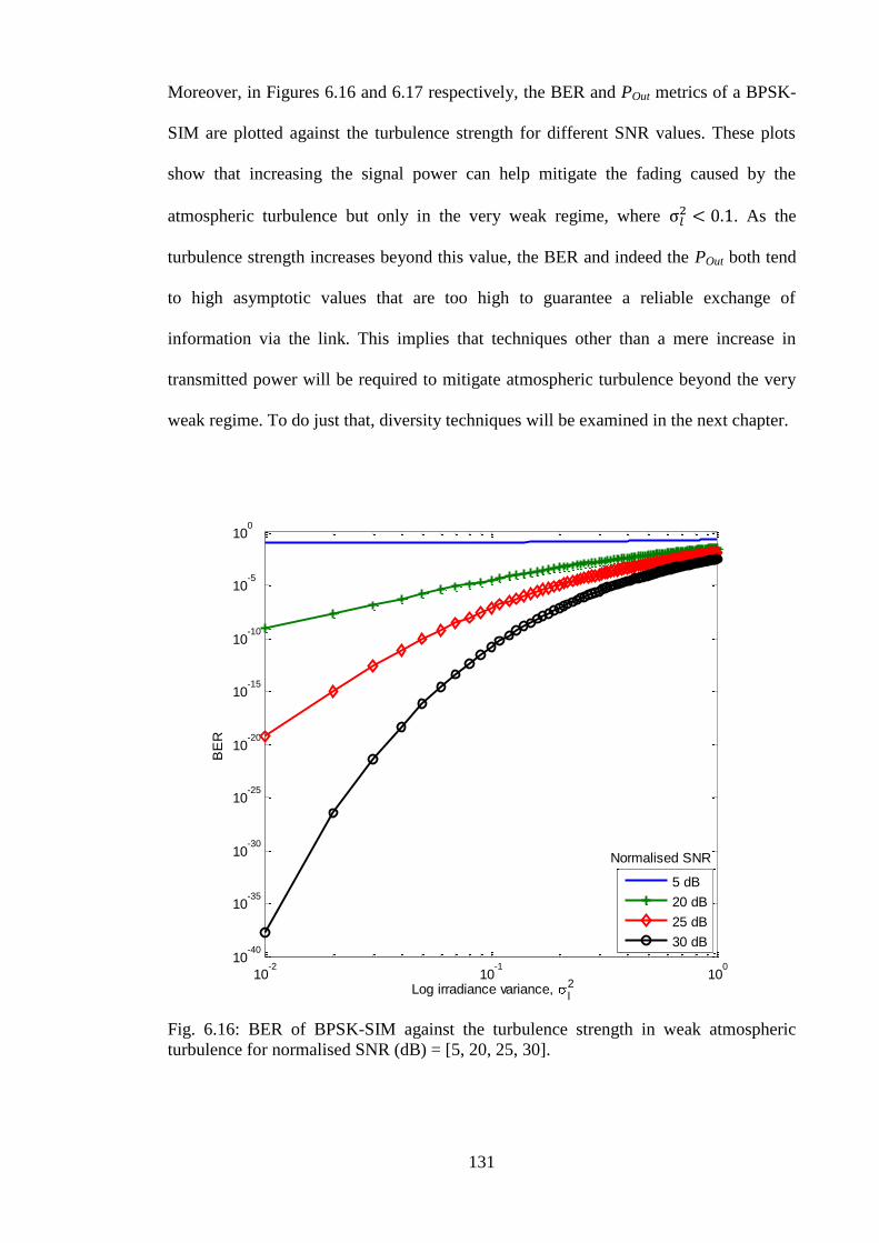
131

Moreover, in Figures 6.16 and 6.17 respectively, the BER and POut metrics of a BPSK-

SIM are plotted against the turbulence strength for different SNR values. These plots

show that increasing the signal power can help mitigate the fading caused by the

atmospheric turbulence but only in the very weak regime, where . As the

turbulence strength increases beyond this value, the BER and indeed the POut both tend

to high asymptotic values that are too high to guarantee a reliable exchange of

information via the link. This implies that techniques other than a mere increase in

transmitted power will be required to mitigate atmospheric turbulence beyond the very

weak regime. To do just that, diversity techniques will be examined in the next chapter.

10-2

10-1

100

10-40

10-35

10-30

10-25

10-20

10-15

10-10

10-5

100

Log irradiance variance, l2

BE

R

5 dB

20 dB

25 dB

30 dB

Normalised SNR

Fig. 6.16: BER of BPSK-SIM against the turbulence strength in weak atmospheric

turbulence for normalised SNR (dB) = [5, 20, 25, 30].

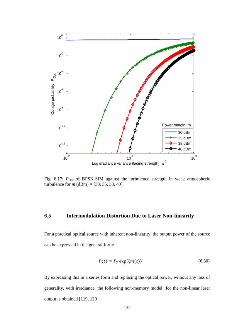
132

10-2

10-1

100

10-12

10-10

10-8

10-6

10-4

10-2

100

Log irradiance variance (fading strength), l2

Outa

ge p

robabili

ty,

PO

ut

30 dBm

35 dBm

38 dBm

40 dBm

Power margin, m

Fig. 6.17: POut of BPSK-SIM against the turbulence strength in weak atmospheric

turbulence for m (dBm) = [30, 35, 38, 40].

6.5 Intermodulation Distortion Due to Laser Non-linearity

For a practical optical source with inherent non-linearity, the output power of the source

can be expressed in the general form:

(6.30)

By expressing this in a series form and replacing the optical power, without any loss of

generality, with irradiance, the following non-memory model for the non-linear laser

output is obtained [119, 120].

133

(6.31)

The output irradiance I, and the constants , which describe the degree of optical

source on non-linearity are fixed for a given optical source at a specified driving

current. These values of are obtainable from the solution of the rate equation of

the particular optical source [121]. For an ideal laser source, the constants are all

equal to zero. The non-memory laser output model is valid for as long as: the difference

between the bias current and the modulation current amplitude is higher than the

threshold current, that is, no signal clipping; and the modulation frequency is well

below the resonance frequency of the laser source. When the laser is operated close to

its resonance frequency, the driving signal experiences increased distortion that is not

accurately accounted for by the non-memory model [122]. For a laser source, the innate

non linearity, which manifests itself as a kink in the output characteristic curve of the

optical source, originates from either: (a) the transverse motion of the near field [123] or

(b) the guiding properties of the laser [122, 124].

In a single subcarrier frequency system, the terms beyond the second term in (6.31)

generate the out-of-band signals, reducing it to the form used in (5.21). Conversely, for

multiple subcarriers, these terms result in signals with the in-band frequencies, which

then result in IMD. Moreover, for , becomes negligible and will henceforth not

be considered. Now, consider the general unity amplitude, PSK modulated multiple

subcarrier signals, , in which the subcarriers are separated

by an equal frequency Δω. That is, if the first and the last subcarriers are and ,

respectively then . The 2nd

and 3rd

intermodulation products are

generated by and in the following equations:

134

(6.32)

(6.33)

For a typical subcarrier at frequency , IMD occurs when the intermodulation

products fall within the frequency . That is when for the 2nd

order

intermodulation product (IMP2) and for the 3rd

order

intermodulation product (IMP3). It should be noted that if the subcarriers are integral

multiples of (orthogonal), then there will be no crosstalk/adjacent channel

interference in principle but the bandwidth requirement will be at least and

there exists several intermodulation distortion components comprising of both IMP2

and IMP3. However, by considering a single octave operation, in which the upper end

subcarrier frequency = 2 , the bandwidth requirement is reduced to and all the

IMP2 becomes out-of-band. In addition, only two of the possible seven IMP3 shown in

Table 6.4 are in-band. These in-band components are and .

The single octave operating condition therefore reduces the amount of IMD to contend

with considerably. It also results in negligible harmonic distortion, because the

harmonic components will all be out-of-band.

135

Table 6.4: Third order intermodulation products [120].

Term Type Number of Components per Term dB of Term above Harmonic

1 0

3 9.54

3 9.54

3 9.54

6 15.56

6 15.56

6 15.56

In the IMP3, that is the expansion of , there are six identical components making

up each term, if the indices x, y and z are all different. There are three identical terms

in IMP3 if any two of the indices x, y and z are equal in value as shown in Table 6.4.

The total third order intermodulation distortion (IMD3) is therefore given by:

(6.34)

where and are the numbers of each IMP3 contributing to the IMD3 at

, they can be readily obtained as [120]:

(6.35a)

(6.35b)

where represents the closest integer, smaller than or equal to x, for example,

. From these equations 6.35(a-b), whenever = k = 1 and the total number

of subcarrier frequencies N, is even, then and

136

. When N is odd and = k = 1, and

. In Table 6.5 the values of and , for different values of , k

and N = 12, are shown as an illustration. This table is useful during frequency planning,

as it helps to identify subcarriers with high number of in-band IMD so that they can be

avoided.

Table 6.5: Number of in-band intermodulation products for N = 12.

k

1

2

3

4

5

6

7

8

9

10

11

12

N2x - y

1 5 5 5 5 5 5 5 5 5 5 5 5

2 - 5 4 5 4 5 4 5 4 5 4 5

3 - - 4 4 4 4 4 4 4 4 4 4

4 - - - 4 3 4 3 4 3 4 3 4

5 - - - - 3 3 3 3 3 3 3 3

6 - - - - - 3 2 3 2 3 2 3

7 - - - - - - 2 2 2 2 2 2

8 - - - - - - - 2 1 2 1 2

9 - - - - - - - - 1 1 1 1

10 - - - - - - - - - 1 0 1

11 - - - - - - - - - - 0 0

12 - - - - - - - - - - - 0

Nx + y - z

1 25 30 34 37 39 40 40 39 37 34 30 25

2 - 20 25 28 31 32 33 32 31 28 25 20

3 - - 16 20 23 25 26 26 25 23 20 16

4 - - - 12 16 18 20 20 20 18 16 12

5 - - - - 9 12 14 15 15 14 12 9

6 - - - - - 6 9 10 11 10 9 6

7 - - - - - - 4 6 7 7 6 4

8 - - - - - - - 2 4 4 4 2

9 - - - - - - - - 1 2 2 1

10 - - - - - - - - - 0 1 0

11 - - - - - - - - - - 0 0

12 - - - - - - - - - - - 0

Furthermore in Fig. 6.18, the values of and are plotted against the

number of subcarriers for k = = 1. This graph further illustrates the relationship

137

between IMD3 and the number of subcarriers. It can thus be concluded that is

much greater than , and that the IMD3 increases as the square of the number of

subcarriers.

0 5 10 15 20 25 30 35 40 45 500

100

200

300

400

500

600

Number of subcarriers

Num

ber

of

in-b

and I

MD

Nx+y-x

N2x-y

Fig. 6.18: In-band intermodulation products against number of subcarriers for k = = 1.

The variance of the IMD3 can thus be obtained as:

(6.36)

where j = 2 if all the IMP3 add up coherently, this occurs when all the subcarrier are

carrying similar symbols, and j = 1 otherwise. In the general expansion of , there

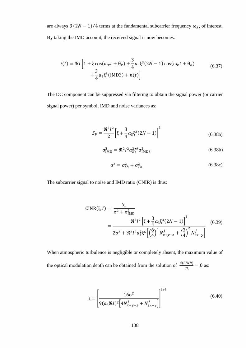
138

are always terms at the fundamental subcarrier frequency , of interest.

By taking the IMD account, the received signal is now becomes:

(6.37)

The DC component can be suppressed via filtering to obtain the signal power (or carrier

signal power) per symbol, IMD and noise variances as:

(6.38a)

(6.38b)

(6.38c)

The subcarrier signal to noise and IMD ratio (CNIR) is thus:

(6.39)

When atmospheric turbulence is negligible or completely absent, the maximum value of

the optical modulation depth can be obtained from the solution of as:

(6.40)

139

Equation (6.40) is plotted below in Fig. 6.19 for three different numbers of subcarriers.

As expected, as the number of subcarriers and the irradiance increase, the modulation

index decreases in order to keep the transmitter within its dynamic range.

14 16 18 20 22 24 26 28 30

0.2

0.3

0.4

0.5

0.6

0.7

0.8

0.9

Irradiance (dBm)

Modula

tion I

ndex

10

15

25

Number of

subcarriers

Fig. 6.19: Modulation index against the irradiance in the absence of atmospheric

turbulence for N = [10, 15, 25].

Since (6.40) does not take into account the irradiance fluctuation, the resulting

modulation index is referred to as the sub-optimum modulation index, . In the

presence of atmospheric turbulence, the irradiance level fluctuates and the average

subcarrier signal to noise and distortion ratio, CINRave, is therefore defined as the

average of over the scintillation statistics.

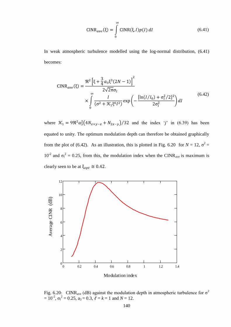
140

(6.41)

In weak atmospheric turbulence modelled using the log-normal distribution, (6.41)

becomes:

(6.42)

where and the index „j‟ in (6.39) has been

equated to unity. The optimum modulation depth can therefore be obtained graphically

from the plot of (6.42). As an illustration, this is plotted in Fig. 6.20 for N = 12, σ2

=

10-2

and σl2 = 0.25, from this, the modulation index when the CINRave is maximum is

clearly seen to be at .

Fig. 6.20: CINRave (dB) against the modulation depth in atmospheric turbulence for σ2

= 10-2

, σl2 = 0.25, a3 = 0.3, = k = 1 and N = 12.

0 0.2 0.4 0.6 0.8 1 1.2 1.40

2

4

6

8

10

12

Modulation index

Aver

age

CIN

R

(dB

)

141

For a BPSK pre-modulated multiple-SIM with IMD, the unconditional BER on any of

the subcarriers is given by:

(6.43)

The graph of this BER in weak scintillation is shown in Fig. 6.21 for N = 12, σ2

= 10-2

and σl2 = 0.25 as an example. From this graph, the modulation depth that

minimises the BER is obtained as 0.6 against 0.42 obtained previously (see Fig. 6.20)

when the CINRave was used.

Fig. 6.21: Unconditional BER against the modulation depth in atmospheric turbulence

for σ2

= 10-2

, σl2 = 0.25, a3 = 0.3, = k = 1 and N = 12.

0 0.2 0.4 0.6 0.8 1 1.21 10

4

1 103

0.01

0.1

1

Modulation Index

BE

R

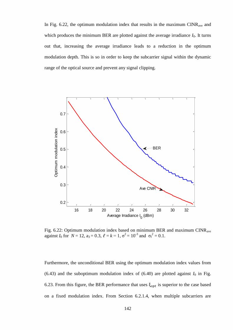
142

In Fig. 6.22, the optimum modulation index that results in the maximum CINRave and

which produces the minimum BER are plotted against the average irradiance I0. It turns

out that, increasing the average irradiance leads to a reduction in the optimum

modulation depth. This is so in order to keep the subcarrier signal within the dynamic

range of the optical source and prevent any signal clipping.

16 18 20 22 24 26 28 30 32

0.2

0.3

0.4

0.5

0.6

0.7

Average Irradiance I0 (dBm)

Optim

um

modula

tion index

Ave CNIR

BER

Fig. 6.22: Optimum modulation index based on minimum BER and maximum CINRave

against I0 for N = 12, a3 = 0.3, = k = 1, σ2

= 10-3

and σl2 = 0.1.

Furthermore, the unconditional BER using the optimum modulation index values from

(6.43) and the suboptimum modulation index of (6.40) are plotted against I0 in Fig.

6.23. From this figure, the BER performance that uses is superior to the case based

on a fixed modulation index. From Section 6.2.1.4, when multiple subcarriers are

143

considered with , there is always a 10logN (dB) penalty in I0. But as shown in

Fig. 6.23, this penalty is reduced by 7 dB and 4 dB, respectively with the use of and

, at a BER of 10-6

. The penalty is expected to increase as both a3 and the channel

fading strength increase. For a multiple-SIM system with different modulation

techniques on each subcarrier, the average BER is described as .

24 26 28 30 32 34 36

10-8

10-7

10-6

10-5

10-4

10-3

10-2

10-1

Average irradiance, (dBm)

BE

R

1/N

Optimum

Suboptimum

Modulation index

Fig. 6.23: BER of multiple SIM-FSO against I0 in atmospheric turbulence for N = 12,

a3 = 0.3, = k = 1, σ2

= 10-3

and σl2 = 0.1 using optimum and suboptimum modulation

index.

144

6.6 Summary

In this chapter, the BER and outage probability of subcarrier intensity modulated FSO

have been presented across all turbulence regimes representing short to very long range

systems. Based on the results presented, the SIM is recommended in atmospheric

turbulence against the fixed threshold OOK modulated FSO currently used in

commercial terrestrial FSO systems, primarily because it does not exhibit a BER floor

like the fixed threshold OOK. Multiple SIM has also been studied as a means of

increasing the system throughput/capacity but at an electrical SNR penalty of at least

20logN dB. The multiple SIM-FSO should therefore only be considered when the quest

to achieve a higher throughput outweighs the accompanying penalty. Also, the

intermodulation effect due to the optical source non-linearity has been analysed and the

in-band intermodulation products calculated. By choosing the subcarrier frequencies

carefully, the number of in-band intermodulation products can be reduced. Expressions

for the optimum modulation index based on average CNIR and unconditional BER have

equally been derived. Using the optimum modulation index can potentially reduce the

power penalty incurred due to IMD by up to 7 dB at a BER of 10-6

.

The atmospheric turbulence has been found to introduce power penalties in the system

and to guarantee a reliable communication link in this condition, the penalties must be

combated. This can be achieved by increasing the transmitted power but this is only

effective in the very weak turbulence regime when . Beyond this regime, the

technique fails and other methods will have to be adopted. In the next chapter, diversity

techniques which exploit both the spatial and temporal variations in the characteristics

of the turbulent atmospheric channel will be examined as means of ameliorating the

fading effect of the channel.

Chapter Seven

SIM-FSO with Spatial and Temporal

Diversity Techniques

7.1 Introduction

Fog, aerosols, rain and gases and other particles suspended in the atmosphere result in

laser irradiance attenuation. The coefficient of attenuation typically ranges from a few

dB/km in clear atmosphere to over 100 dB/km in a dense fog regime [20]. The huge

attenuation suffered during dense fog restricts the carrier class FSO links to ~500 m [1,

15]; extending the link range in such conditions requires alternative schemes such as

hybrid RF/FSO schemes [34, 125]. The thick fog which causes the most signal

146

attenuation is a short duration, localised event, which only occurs in few locations.

Another factor that accounts for the FSO performance degradation in clear atmosphere

is the irradiance and phase fluctuation. The signal fluctuation results from random index

of refraction variations along the propagation path due to atmospheric turbulence as

discussed in the preceding chapters. These phase and irradiance fluctuation suffered by

the traversing beam makes optical coherent detection less attractive, because it is

sensitive to both signal amplitude and phase. This informs the choice of direct detection

in terrestrial FSO links as it is not sensitive to the signal phase as mentioned in chapter

three. In direct detection systems, turbulence effects could result in deep irradiance

fades that lasts up to ~1-100 μs [44, 71]. For a link operating at say 1 Gbps, this could

result in a loss of up to 105 consecutive bits (burst error). To avoid this and reduce the

turbulence induced power penalty highlighted in chapter six, atmospheric turbulence

has to be mitigated.

Possible ways of reducing the fading duration and strength include the use of aperture

averaging, adaptive optics, error control and spatial diversity. In aperture averaging, the

receiver aperture needs to be far greater than the spatial coherence distance ρ0 of the

atmospheric turbulence in order to receive several uncorrelated signals. This condition

is not always achievable in FSO as the spatial coherence distance is of the order of

centimetres [29]. For coding to be effective in FSO, it must be robust enough to detect

and correct not only random errors but also burst errors because the temporal coherence

time, of atmospheric turbulence is much greater than the typical symbol duration. To

mitigate atmospheric turbulence effects, the use of convolution coding with hard-

decision Viterbi decoding has been investigated in [126], while a more efficient Turbo

code employing the maximum-likelihood decoding has been reported in [127]. In

addition, the work reported in [69] explored the use of a much more powerful low

147

density parity codes (LDPC) to detect and correct the burst error that results from

scintillation. In their work, the LDPC coded SIM in atmospheric turbulence was

reported to achieve a coding gain of more than 20 dB compared with similarly coded

OOK. It has also been reported in [70] that the use of space-time block code (STBC)

with coherent and differential detection improves the error performance of SIM in

atmospheric turbulence. However, invoking error control coding could introduce huge

processing delays and efficiency degradation in view of the number of redundant bits

that will be required [71].

The adaptive optics which is based on the phase conjugation principle is another viable

option. It has been used in FSO as reported in [68, 128] to reverse the wavefront

deformation effect of atmospheric turbulence. However, the complexity and cost of its

implementation is prohibitive. This perhaps is the reason why its use has only been

restricted to deep space FSO where the cost to benefit ratio is within acceptable limits.

In this chapter, the performance of a SIM-FSO with temporal diversity in a turbulent

atmospheric channel will be discussed. The spatial diversity analysis will be based on

the following linear combining techniques: equal gain combining (EGC), maximum

ratio combining (MRC) and selection combining (SelC). Subcarrier timed delay

diversity will also be introduced as an alternative channel fading mitigation technique

which can be used separately or with the spatial diversity. The receiver is assumed to

comprise of identical PIN photodetectors and unity modulation index under spatial

diversity. Inter-symbol interference will not be considered since terrestrial FSO is

basically a line-of-sight technology with negligible delay spread.

148

7.2 Receiver Diversity in Log-normal Atmospheric Channels

The idea of spatial diversity is premised on the fact that for a given separated

photodetectors, the chance that all the photodetectors will experience deep fade (due to

scintillation) simultaneously at any given instant is remote. An important consideration

in spatial diversity is the amount of correlation that exists between the signals received

by the different photodetectors. Apart from mitigating scintillation, the spatial diversity

in an FSO communication link is also advantageous in combating temporary link

blockage/outage due to birds or other small object flying cross the link path. It is also a

good means of combating misalignment when combined with wide divergence optical

sources, thereby circumventing the need for an active tracking. Moreover, it is much

easier to provide independent aperture averaging with a multiple aperture system, than

in a single aperture where the aperture size has to be far greater than the irradiance

spatial coherence distance [71]. In dense fog regime however, an FSO link with spatial

diversity offers limited advantage and an alternative configuration such as the hybrid

FSO/RF should be considered. In the following analysis, both instances of correlated

and uncorrelated received signals will be considered. Since the spatial coherence length

of the atmospheric channel only measures a few centimetres, it follows therefore that

the photodetectors only need to be separated by a few centimetres to achieve

uncorrelated reception. At the receiver, the beam footprint covers the entire field of

view (FOV) of all the detectors. The photocurrents , as shown in Fig. 7.1,

are then linearly combined before being sent to the coherent demodulator that separates

the composite signal into its constituent subcarriers and then demodulates each

subcarrier. The linear combining techniques considered are: MRC, EGC and SelC.

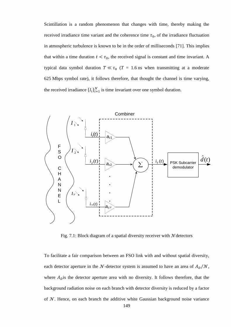
149

Scintillation is a random phenomenon that changes with time, thereby making the

received irradiance time variant and the coherence time , of the irradiance fluctuation

in atmospheric turbulence is known to be in the order of milliseconds [71]. This implies

that within a time duration , the received signal is constant and time invariant. A

typical data symbol duration (T = 1.6 ns when transmitting at a moderate

625 Mbps symbol rate), it follows therefore, that thought the channel is time varying,

the received irradiance is time invariant over one symbol duration.

F

S

O

C

H

A

N

N

E

L

PSK Subcarrier

demodulator

.

.

.

.

)(ˆ tdac2

ac1

Combiner

)(1 ti

)(2 ti )(tiT

acNiN (t)

1I

2I

IN

Fig. 7.1: Block diagram of a spatial diversity receiver with detectors

To facilitate a fair comparison between an FSO link with and without spatial diversity,

each detector aperture in the -detector system is assumed to have an area of ,

where is the detector aperture area with no diversity. It follows therefore, that the

background radiation noise on each branch with detector diversity is reduced by a factor

of . Hence, on each branch the additive white Gaussian background noise variance

150

will be . The thermal noise on each photodetector is however not reduced by a

factor of . The output of the individual detector during a symbol duration is given as:

(7.1)

The combiner shown in Fig. 7.1 scales the signal from each photodetector by a gain

factor, , before adding them together. Since the photodetectors are required to

be a few centimetres apart, and the link range a few kilometres, the difference in the

propagation delay across the receiver array becomes negligible. The combiner‟s output

thus become:

(7.2)

7.2.1 Maximum ratio combining (MRC)

In the MRC linear combiner, the gain factor is proportional to the received

irradiance. The weighted signals are then co-phased and summed coherently to obtain

the combiner‟s output current given by (7.2). Without any interference, the MRC is

optimal regardless of the fading statistics. This, according to [115], is because it results

in a maximum-likelihood receiver structure. On the other hand, MRC requires the

knowledge of the individual received irradiance and phase on each branch, making it

unsuitable for non-coherent demodulated subcarriers, such as the DPSK-SIM.

By substituting (7.1) into (7.2) and suppressing the DC components via filtering, the

MRC combiner output becomes:

151

(7.3)

The signal demodulation and the consequently extraction of the transmitted data is done

separately for each subcarrier; as such, the photocurrent at a particular subcarrier

frequency ωc is given by:

(7.4)

Since the coherence time of the turbulent atmospheric , the branch irradiance

is therefore time invariant over a period T. This leads to the following expression for

the signal power , at the subcarrier frequency of interest:

(7.5)

The overall noise is Gaussian, with a zero mean and a variance

. The electrical SNR at the demodulator input conditioned on the received

irradiance is thus derived as:

(7.6)

152

Applying Cauchy inequality [118], , to (7.6) results

in the following expression for the combiner‟s output SNR:

(7.7)

The left hand side of the Cauchy inequality is apparently equal to the right hand side

when . For a background noise limited FSO link, the noise variance on each

branch is proportional to the pupil receiver aperture area, and . It

should be noted that in arriving at (7.7), the intermodulation distortion due to the

inherent nonlinearity of the optical source discussed in section 6.3.3.1 has not been

considered. For an ideal optical source with a modulation index of one, the subcarrier

amplitude is constrained by the condition . The optimum electrical SNR for

each subcarrier frequency ωc now becomes:

(7.8)

where is the conditional SNR on each diversity branch. The average

SNR, , obtained by averaging (7.8) over the scintillation statistics is given as:

(7.9)

where is the joint pdf of scintillation, given by for

photodetectors receiving uncorrelated signals. Similarly, for a BPSK pre-modulated

subcarrier, the unconditional BER for the subcarrier at frequency ωc obtained by

averaging the conditional error rate over the statistics of the intensity fluctuation across

153

all branches is given by:

(7.10)

Solving (7.10) involves fold integrations if the classical definition of the Q-

function is used, but by using the alternative form of the Q-function and the Gauss-

Hermite quadrature integration described in section 6.2.1.1, this can be simplified to the

form below:

(7.11)

where and

. With , expression (7.11) expectedly reduces to (6.12), which is

the BER with no diversity.

7.2.2 Equal gain combining (EGC)

In implementing the EGC spatial diversity technique, the irradiance estimate on each

branch is not required but an estimate of the phase of all subcarrier signals on each

branch is still very much needed. The EGC combiner samples the photocurrents

and sums them coherently with equal weights , to produce the

decision statistics [115]. With the DC component suppressed via filtering, the

photocurrent at the output of the EGC combiner is given by:

154

(7.12)

The conditional SNR at the output of the EGC combiner obtained is thus obtained as:

(7.13)

From the foregoing, it is clear that . Since the noise variance is

proportional to the individual receiver aperture area

.

For a log normal distributed scintillation, the sum of moderate number of irradiances is

known to be another log normal variable [71, 129]. That is, the sum of independent

irradiance , where is normally distributed with mean and

variance . Equation (7.14) below gives the pdf of Z while its first and second

moments derived in Appendix B are given by (7.15). The application of central limit is

not appropriate here because the number of photodetectors is too small to justify its

use.

(7.14)

(7.15a)

(7.15b)

155

The average SNR and the unconditional BER for a BPSK pre-modulated subcarrier are

then given by (7.16) and (7.17) respectively:

(7.16)

(7.17)

where , wi and xi remain as previously defined in section 6.2.1.1.

With one photodetector, (7.17) gives the same result as (6.12) for the case with no

diversity.

7.2.3 Selection combining (SelC)

Both MRC and EGC spatial diversity techniques discussed thus far require the

irradiance level and/or the subcarrier signals phase estimates, also a separate receiver

chain is needed for each diversity branch thereby adding to the overall complexity of the

receiver. The SelC linear combiner on the other hand samples all the received signal and

selects the branch with the highest SNR or irradiance level, provided the photodetectors

receive same dose of background radiation. The output is equal to the signal on only

one of the branches and not the coherent sum of the individual photocurrents as is the

case in MRC and EGC. This makes SelC suitable for differentially modulated, non-

156

coherent demodulated subcarrier signals. In addition, the SelC is of reduced complexity

compared to the MRC and EGC and its conditional SNR is given by:

(7.18)

where . The pdf of the received irradiance, , given by

(7.19), is obtained by first determining its cumulative density function (cdf) and then

differentiating as detailed in Appendix C.

(7.19)

where . The average SNR and the unconditional BER, for a BPSK pre-

modulated subcarrier in a turbulent atmospheric channel, are given by:

(7.20)

(7.21)

where . For a binary DPSK pre-modulated SIM, the unconditional

bit error obtained using the Gauss-Hermite quadrature integration approach is derived

as:

(7.22)

157

where .

7.2.4 Effect of received signal correlation on error performance

For a receiver array system in which the photodetectors are separated by a spatial

distance, , which is less than the spatial coherence distance of the channel at the

receiver plane (i.e. ), the photodetectors will experience correlated irradiance

fluctuations. This means that the multiple receivers can all experience similar irradiance

fading at the same time. The effect of this on the system error performance will be

investigated by considering the best case scenario with an optimum MRC combiner and

only one subcarrier signal. The BER conditioned on the received irradiance is:

(7.23)

However in the presence of scintillation, the unconditional BER becomes Pe = E[Pec],

which is the average of (7.23) over the joint pdf of the irradiance fluctuation. Based on

Tatarski‟s [45] infinite power series expression for the correlation coefficient of an

optical wave travelling through a turbulent atmosphere given by (7.24), and shown

graphically in Fig. 7.2, it can be inferred that the correlation coefficient is inversely

proportional to the spatial separation whenever , where .

(7.24)

158

Fig. 7.2: Correlation coefficient for a weak turbulent field as a function of transverse

separation. Reproduced from [45].

From the foregoing, the following expression is obtained for the covariance matrix:

(7.25)

where is the spatial separation between photodetectors i and j and is the correlation

coefficient between two photodetectors with a spatial separation . The joint pdf of

the received irradiance is then given by:

(7.26)

where is a row matrix. The expression for the

unconditional BER is then obtained as:

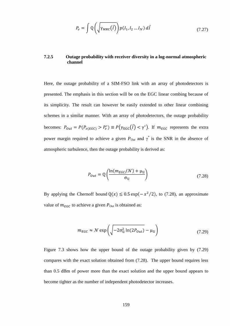
159

(7.27)

7.2.5 Outage probability with receiver diversity in a log-normal atmospheric

channel

Here, the outage probability of a SIM-FSO link with an array of photodetectors is

presented. The emphasis in this section will be on the EGC linear combing because of

its simplicity. The result can however be easily extended to other linear combining

schemes in a similar manner. With an array of photodetectors, the outage probability

becomes: . If represents the extra

power margin required to achieve a given POut and γ*

is the SNR in the absence of

atmospheric turbulence, then the outage probability is derived as:

(7.28)

By applying the Chernoff bound , to (7.28), an approximate

value of to achieve a given POut is obtained as:

(7.29)

Figure 7.3 shows how the upper bound of the outage probability given by (7.29)

compares with the exact solution obtained from (7.28). The upper bound requires less

than 0.5 dBm of power more than the exact solution and the upper bound appears to

become tighter as the number of independent photodetector increases.

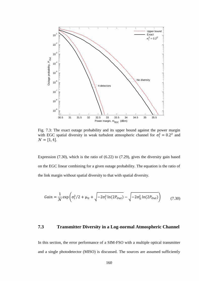
160

30.5 31 31.5 32 32.5 33 33.5 34 34.5 35 35.5

10-9

10-8

10-7

10-6

10-5

10-4

10-3

10-2

10-1

Power margin, mEGC

(dBm)

Outa

ge p

robabili

ty,

PO

ut

Upper bound

Exact

l2 = 0.22

4-detectors

No diversity

Fig. 7.3: The exact outage probability and its upper bound against the power margin

with EGC spatial diversity in weak turbulent atmospheric channel for and

.

Expression (7.30), which is the ratio of (6.22) to (7.29), gives the diversity gain based

on the EGC linear combining for a given outage probability. The equation is the ratio of

the link margin without spatial diversity to that with spatial diversity.

(7.30)

7.3 Transmitter Diversity in a Log-normal Atmospheric Channel

In this section, the error performance of a SIM-FSO with a multiple optical transmitter

and a single photodetector (MISO) is discussed. The sources are assumed sufficiently

161

spaced so that the photodetector receives uncorrelated optical radiations. To ensure a

fair comparison and to maintain a constant power requirement, it is assumed that the

power available for a single-transmitter system is equally shared among -laser

transmitters. This requirement is similar to that specified in the preceding section. As

such, the irradiance from each optical source is reduced by a factor of compared to a

single transmitter system. An alternative approach will be for each source in the array to

transmit the same power as in a single transmitter system, in this instance, the power

requirement is increased by a factor of . Based on the former, the received signal is

obtained as:

(7.31)

Since the optical sources in the array are only separated by few centimetres, the phase

shift experienced by the received irradiance due to the path difference is therefore

negligible. The SNR on each subcarrier, conditioned on the received irradiance is

derived as:

(7.32)

From the obvious similarity between (7.13) and (7.32), it can then be concluded that the

unconditional BER for a SIMO system is the same as that of single source with the

EGC combined multiple photodetectors.

162

7.4 Transmitter-Receiver Diversity in a Log-normal

Atmospheric Channel

Here, a multiple-source, multiple-photodetector (MIMO) SIM-FSO system will be

examined. In consistency with the earlier assumptions, the total transmitted power is

equal to the transmitted power when a single optical source is used with the same bit

rate. In addition, the combined aperture area of the photodetectors is the same as the

no spatial diversity case. Moreover, the optical sources and the photodetectors are

assumed well spaced to avoid any correlation in the received signals. First, the received

signals are combined using the EGC, and from the preceding section, a MISO system

with laser sources is said to be identical to an EGC combined SIMO with

photodetectors, these combined lead to the following as the conditional SNR of the

SIM-FSO in MIMO configuration:

(7.33)

This expression is the same as that of an EGC combiner with a total of

photodetectors. Hence, the unconditional BER is obtained by replacing in (7.17) by

.

If however, the received signals are combined using the MRC linear combining scheme,

the conditional SNR on each receiver branch will be:

(7.34)

163

Considering the fact that the sum of independent lognormal random variables is another

log-normal distribution [129], the unconditional BER becomes:

(7.35)

where and

, while and are as previously defined by (7.15) with

replaced by .

7.5 Results and Discussions of SIM-FSO with Spatial Diversity in

a Log-normal Atmospheric Channel

In order to analyse the results obtained so far, a 20th

order Hermite polynomial is

assumed while the log irradiance variance is assumed to vary between 0.22 and unity,

(i.e. ). By plotting the BER expressions against the normalised

, the link margin , defined as the ratio of required SNR with no

diversity to that with photodetectors at a BER of 10-6

and turbulence strength σl2, is

obtained. In Fig. 7.4, for BPSK-SIM is plotted against for the EGC and SelC

techniques for various values of σl2, while for a DPSK pre-modulated SIM is

plotted against the fading strength in Fig. 7.5.

164

1 2 3 4 5 6 7 8 9 10-10

-5

0

5

10

15

20

25

No of photodetectors

Lin

k m

arg

in a

t B

ER

= 1

0-6

(

dB

)

l2 = 0.22

l2 = 0.52

l2 = 0.72

l2 = 1

EGC

SelC

Fig. 7.4: BPSK-SIM link margin with EGC and SelC against number of photodetectors

for various turbulence levels and a BER of 10-6

.

In both situations, the use of SelC in weak turbulence results in negative link margins.

For instance, Fig. 7.5 shows that for , SelC spatial diversity results in between -

2 dB and -7 dB link margin for , similarly in Fig. 7.4, it results in a margin

of up to -5 dB at σl = 0.2. The negative link margin experienced with SelC can be

attributed to the fact that at a very low turbulence level, the effect of reducing the

received intensity by a factor of on each branch is dominant over the turbulence

induced intensity fluctuation.

165

0.1 0.2 0.3 0.4 0.5 0.6 0.7 0.8 0.9-10

-5

0

5

10

15

20

Log irradiance standard deviation, l

Lin

k M

arg

in

at

BE

R=

10

-6

(dB

)

2Rx

4Rx

6Rx

8Rx

10Rx

Fig. 7.5: DPSK-SIM with SelC spatial diversity link margin against turbulence strength

for .

However, as the turbulence level increases beyond , SelC spatial diversity starts

to yield a positive link margin; producing up to 9 dB link margin with two

photodetectors in a DPSK pre-modulated SIM link. And for in Fig. 7.4, SelC

proves worthwhile with positive link margins but the gains are still lower than that

obtainable from EGC by about ~1 to ~6 dB depending on the number of photodetectors

used. Based on the foregoing, SelC spatial diversity will not be recommended for use on

short link FSO experiencing weak irradiance fluctuation.

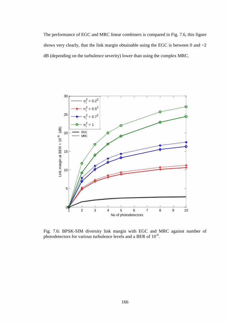
166

The performance of EGC and MRC linear combiners is compared in Fig. 7.6, this figure

shows very clearly, that the link margin obtainable using the EGC is between 0 and ~2

dB (depending on the turbulence severity) lower than using the complex MRC.

1 2 3 4 5 6 7 8 9 100

5

10

15

20

25

30

No of photodetectors

Lin

k m

arg

in a

t B

ER

= 1

0-6

(d

B)

l2 = 0.22

l2 = 0.52

l2 = 0.72

l2 = 1

EGC

MRC

Fig. 7.6: BPSK-SIM diversity link margin with EGC and MRC against number of

photodetectors for various turbulence levels and a BER of 10-6

.

167

Using two photodetectors with optimal MRC in atmospheric turbulence with

, has the potential to reduce the SNR required to achieve a BER of 10-6

by between ~2

and ~12 dB . With up to four independent photodetectors however, the theoretical link

margin for the MRC combiner increases to ~20 dB as shown in Fig. 7.6. Another

inference from this figure is that the spatial diversity gain (link margin) becomes more

pronounced as scintillation increases; using two detectors with MRC at turbulence level,

results in a link margin which is ~10 dB lower than at .

Also for , the marginal link margin per unit detector ( ) reduces

drastically as the graphs begin to flatten out. For instance, increasing from 4 to 10

with MRC across the turbulence levels only results in a meagre increase

of between 0 and ~6 dB link margin, while increasing from 1 to 4 over the same

turbulence range results in between ~3 and ~22 dB diversity gain.

The plot of the diversity gain (7.30) at a POut of 10-6

is shown in Fig. 7.7 for different

number of photodetectors and log intensity variance. This plot illustrates the gain based

on the outage probability metric. From the plot, using two photodetectors result in ~4

dB gain at σl2

= 0.72 and this rises to ~8 dB with . Beyond four photodetectors,

the graphs start to plateau, implying a reduction in the amount of gain recorded for each

additional photodetector.

168

1 2 3 4 5 6 7 8 9 100

2

4

6

8

10

12

14

16

Number of photodetectors

EG

C G

ain

at

PO

ut =

10

-6

(dB

)

l2 = 0.22

l2 = 0.52

l2 = 0.72

l2 = 1

Fig. 7.7: EGC diversity gain in log-normal atmospheric channel against the number of

photodetectors at POut of 10-6

and .

To illustrate the impact of signal correlation on the error performance, the combination

of (7.25) (7.26) and (7.27) is plotted in Fig. 7.8 for , ρ = [0, 0.1, 0.3, 0.6] and

. For instance at a BER of 10-6

, the use of two photodetectors with correlation

coefficients ρ = 0.3 and 0.6 requires additional ~1.6 dB and ~3 dB of SNR, respectively

compared to when ρ = 0. With three photodetectors, the additional SNR required to

achieve the same BER of 10-6

is ~2.4 dB and ~4.6 dB for ρ = 0.3 and 0.6, respectively.

This shows that the correlation effect results in a power penalty and this result, by

extension, buttresses the need for the photodetector separation to be greater than the

spatial coherence length , in order to get the most of the spatial diversity technique.

169

19 20 21 22 23 24 25 26 27 28

10-6

10-5

10-4

Normalised SNR (dB)

BE

R

= 0

= 0.1

= 0.3

= 0.6

3 Photodetectors

2 Photodetectors

Fig. 7.8: Error performance of BPSK-SIM at different values of correlation coefficient

for and .

Furthermore in Fig. 7.9, the plot of (7.35) against the normalised SNR is shown at a

turbulence level for different values of and . It can be inferred from the

plot that at a BER of 10-6

, using a 2 × 2 MIMO requires ~0.4 dB of SNR more than

employing a 1 × 4-MIMO configuration. However, spacing four photodetectors to

ensure that the received signals are uncorrelated is far more demanding and

cumbersome than spacing two photodetectors. Also, to achieve a BER of 10-6

, the use of

4 × 4-MIMO system requires about ~4 dB and 1 dB less SNR compared with using a

lone source with 4 and 8 photodetectors, respectively.

170

10 15 20 25 3010

-8

10-7

10-6

10-5

10-4

10-3

Normalised SNR (dB)

BE

R

4X4

2X2

1X4

1X8

1X5

1X1

MIMO

configuration

Fig. 7.9: Error performance of BPSK-SIM with MIMO configuration in turbulent

atmospheric channel for

.

7.6 SIM-FSO with Receiver Diversity in Gamma-gamma and

Negative Exponential Atmospheric Channels

In this section, the performance of SIM-FSO will be analysed in terms of BER and the

outage probability based on the gamma-gamma and negative exponential turbulence

models. While the results of the previous sections are valid for short FSO links

characterised by weak irradiance fluctuation only, the performance analysis of this

section will capture the performance of short to very long FSO links.

171

7.6.1 BER and outage probability of BPSK-SIM with spatial diversity

Following on from section 7.2, the general expression for the unconditional BER of an

FSO employing BPSK-SIM with an array of photodetectors can be written as:

(7.36)

where represents the post detection electrical SNR at the BPSK demodulator input

and is the joint pdf of the uncorrelated irradiance. In evaluating

, the EGC linear combining technique is considered because of its simplicity, but

other linear combining schemes can be used as well. The total noise variance is given by

, using a narrow band optical bandpass filter combined with

narrow field of view detectors, the background noise can be reduced considerably to

make the thermal noise dominant. Therefore, and . The post

detection for the thermal noise limited performance at the BPSK demodulator

input is thus obtained as:

(7.37)

The system performance analysis with spatial diversity in weak, moderate and strong

turbulence regimes will be based on the gamma-gamma model introduced in chapter

four. The gamma-gamma parameters representing each of the stated turbulence regimes

are as previously presented in Table 6.3. From the numerical solution of (7.36), the

BER can thus be obtained.

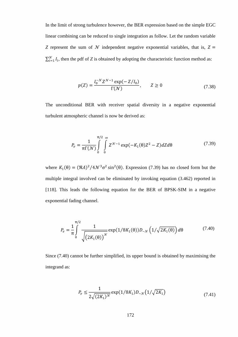
172

In the limit of strong turbulence however, the BER expression based on the simple EGC

linear combining can be reduced to single integration as follow. Let the random variable

Z represent the sum of independent negative exponential variables, that is,

, then the pdf of Z is obtained by adopting the characteristic function method as:

(7.38)

The unconditional BER with receiver spatial diversity in a negative exponential

turbulent atmospheric channel is now be derived as:

(7.39)

where . Expression (7.39) has no closed form but the

multiple integral involved can be eliminated by invoking equation (3.462) reported in

[118]. This leads the following equation for the BER of BPSK-SIM in a negative

exponential fading channel.

(7.40)

Since (7.40) cannot be further simplified, its upper bound is obtained by maximising the

integrand as:

(7.41)

173

where and Dρ is the parabolic cylinder function whose definition

is available in [118].

The outage probability in the fully developed speckle regime is given by the following:

(7.42)

Expression (7.42) is the cumulative distribution function of Z at the specified point and

by combining this with (7.38), the outage probability is obtained as:

(7.43)

Equation (7.43) above can be expressed as an implicit function in terms of the

incomplete gamma function γ(a, x) [118] or as a series as:

(7.44)

where the incomplete gamma function is defined as, .

174

7.6.1.1 Results and discussions

In Fig. 7.10, the BER of BPSK-SIM is plotted against the normalised SNR for two

photodetectors under different turbulence regimes. When compared to the results

obtained with no spatial diversity, the gain of spatial diversity in mitigating the effect of

turbulence induced irradiance fluctuation becomes very clear. A summary of the

resulting diversity gains, (i.e. reduction in the SNR), with two and three photodetectors

at a BER of 10-6

is presented in Table 7.1. As expected, the impact of diversity is least

in weak turbulence regime resulting in only 2.6 dB reductions in the SNR at a BER of

10-6

. Whereas in strong turbulence regime, the gain in SNR is ~12 dB, increasing to ~47

dB in the saturation regime.

15 20 25 30 35 40 45 50 55 60

10-7

10-6

10-5

10-4

10-3

10-2

10-1

Normalised SNR (dB)

BE

R

Saturation

(upperbound)

Saturation

(exact)

Weak

Moderate

Strong

Turbulence regime

Fig. 7.10: BPSK-SIM error rate against the normalised SNR in gamma-gamma and

negative exponential channels for two photodetectors.

175

As would be expected, the diversity gain is highest in extreme fading conditions since

adding more branches will greatly reduce the chance of a catastrophic fading from

happening

Table 7.1: Diversity gain at a BER of 10-6

in gamma-gamma and negative exponential

channels.

Figure 7.11 shows the extra power margin required to achieve a certain outage

probability POut with and without spatial diversity in negative exponential atmospheric

channels. The gain of employing diversity is apparent from the figure just as the case

under the BER performance metric. For instance at a POut of 10-6

, a diversity gain of

almost 30 dB is predicted and this increases to ~43 dB with four photodetectors. This

significant gain is down to the fact that with multiple photodetectors, more independent

irradiances are received.

Number of photodetectors

Spatial Diveristy Gain (dB)

Weak Strong Saturation 2 2.6 11.6 46.7

3 3.0 21.2 63.6

176

30 40 50 60 70 80 90 100

10-7

10-6

10-5

10-4

10-3

10-2

10-1

Power margin, mEGC

(dBm)

Outa

ge P

robabili

ty

= 1

= 2

= 4

N

N

N

Fig. 7.11: The outage probability as a function of power margin mEGC (dBm) for

in negative exponential channel.

For the sake of comparison, the predicted spatial diversity gains based on both metrics,

(BER and outage probability), are shown in Fig. 7.12 as a function of the number of

photodetectors. For both metrics, it is observed that as the number of photodetectors

increases beyond four, the diversity gains start to plateau. Although POut and BER are

different by definition, they both result in a similar conclusion. It should however be

mentioned that using an array of photodetectors adds to the cost and design complexity.

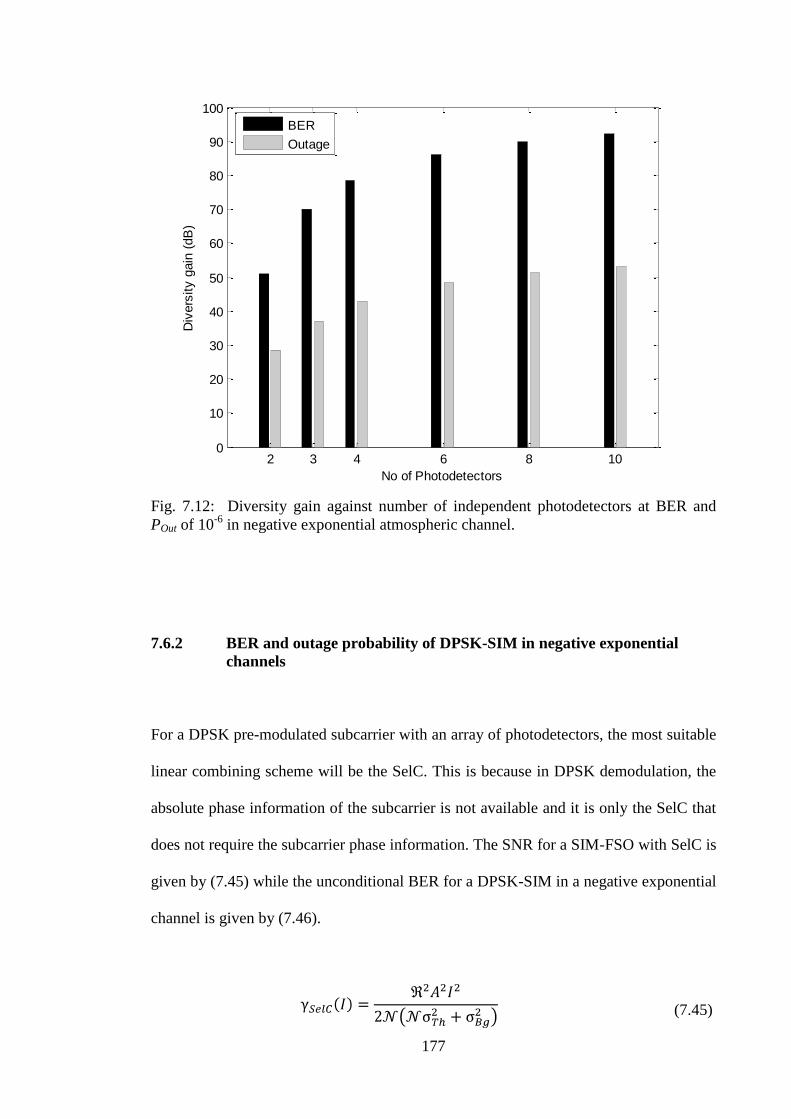
177

2 3 4 6 8 100

10

20

30

40

50

60

70

80

90

100

No of Photodetectors

Div

ers

ity g

ain

(dB

)

BER

Outage

Fig. 7.12: Diversity gain against number of independent photodetectors at BER and

POut of 10-6

in negative exponential atmospheric channel.

7.6.2 BER and outage probability of DPSK-SIM in negative exponential

channels

For a DPSK pre-modulated subcarrier with an array of photodetectors, the most suitable

linear combining scheme will be the SelC. This is because in DPSK demodulation, the

absolute phase information of the subcarrier is not available and it is only the SelC that

does not require the subcarrier phase information. The SNR for a SIM-FSO with SelC is

given by (7.45) while the unconditional BER for a DPSK-SIM in a negative exponential

channel is given by (7.46).

(7.45)

178

(7.46)

The pdf, in a negative exponential channel model given by

(7.47) is obtained by first finding the cumulative distribution function of Imax at an

arbitrary point and then differentiating. The resulting pdf is given by (7.47) and the

detailed proof presented in Appendix D.

(7.47)

The plot of the pdf of Imax is shown in Fig. 7.13 for different values of .

0 1 2 3 4 5 6 7 8 90

0.1

0.2

0.3

0.4

0.5

0.6

0.7

0.8

0.9

1

I

pdf

of

I max

= 1N

= 4N

N = 10

Fig. 7.13: The pdf, for , and I0 = 1 in a negative

exponential channel.

179

From the combination of (7.45), (7.46) and (7.47), an expression for the error

performance of a DPSK-SIM laser communication system in fully developed speckle

atmospheric channel is obtained as:

(7.48)

Now the received irradiance I0 needed to attain an outage probability

in a negative exponential atmospheric channel without diversity is given

by (7.49). In arriving at this equation, the threshold SNR has been taken as,

where I* is the receiver sensitivity required to attain the threshold BER

*.

(7.49)

With an array of PIN photodetectors employing SelC in a negative exponential

atmospheric channel, the received irradiance I0(SelC) needed to attain a given POut is

derived from the combination of (7.45), and (7.47), as:

(7.50)

From the foregoing, the diversity gain I0/I0SelC can thus be obtained.

180

7.6.2.1 Results and discussions

The numerical simulations presented in this section are based on the parameters of

Table 7.2. In Fig. 7.14, the error performance of DPSK-SIM in a negative exponential

channel, obtained from (7.48), is shown as a function of the average irradiance. This

plot brings to bear the potential gain of SelC in reducing the required sensitivity for a

given BER under very strong fading conditions. For example, to achieve a BER of 10-6

with no diversity, about 23 dBm of received irradiance is required while with two

photodetectors , about -1.7 dBm is needed to achieve the same level of performance.

Moreover, as the number of photodetectors increases, the attained diversity gain per

additional detector reduces. For instance, for , the gain per detector at a BER of

10-6

is ~12 dB and this reduces to about 5 and 4 dB for and 10, respectively.

These results are summarised in Table 7.3 for up to 10 photodetectors.

Table 7.2: Numerical simulation parameters

Parameter Value

Symbol rate Rb 155 – 625 Mbps

Spectral radiance of the sky N(λ) 10-3

W/cm2µmSr

Spectral radiant emittance of the sun W(λ) 0.055 W/cm2µm

Optical band-pass filter bandwidth Δλ @ λ = 850 nm 1 nm

PIN photodetector field of view FOV 0.6 rad

Radiation wavelength λ 850 nm

Number of Photodetectors 1 ≤ ≤ 10

Load resistance RL 50 Ω

PIN photodetector responsivity 1

Operating temperature Te 300 K

181

-20 -15 -10 -5 0

10-7

10-6

10-5

10-4

10-3

10-2

Average received irradiance, E[I] (dBm)

BE

R

= 2

= 4

= 6

= 8

= 10

= 1

N

N

N

N

N

N

Fig. 7.14: Error rate of DPSK-SIM against the average received irradiance with spatial

diversity in negative exponential channel for .

Table 7.3: Gain per photodetector at a BER of 10-6

1 2 4 6 8 10

Average

Irradiance (dBm)

23.1 -1.7 -12.5 -15.2 -16.2 -16.7

Gain (dB) per 0 12.4 8.9 6.4 4.9 4.0

In discussing the outage probability in negative exponential fading channels, (7.50) is

plotted in Fig. 7.15. In this plot, the threshold average irradiance I* is assumed to be 0

dBm. This graph shows that for a very long SIM-FSO link, whose channel fading is

modelled by the negative exponential distribution, achieving an outage probability of

10-6

or better will require a minimum of 60 dBm received irradiance without SelC.

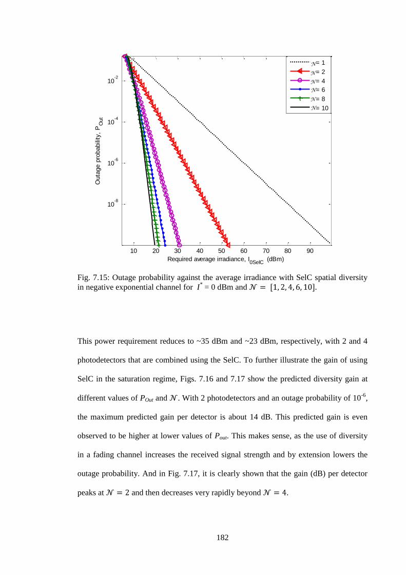
182

10 20 30 40 50 60 70 80 90

10-8

10-6

10-4

10-2

Required average irradiance, I0SelC

(dBm)

Outa

ge p

robabili

ty,

PO

ut

= 1

= 2

= 4

= 6

= 8

= 10N

N

N

N

N

N

Fig. 7.15: Outage probability against the average irradiance with SelC spatial diversity

in negative exponential channel for I* = 0 dBm and

This power requirement reduces to ~35 dBm and ~23 dBm, respectively, with 2 and 4

photodetectors that are combined using the SelC. To further illustrate the gain of using

SelC in the saturation regime, Figs. 7.16 and 7.17 show the predicted diversity gain at

different values of POut and . With 2 photodetectors and an outage probability of 10-6

,

the maximum predicted gain per detector is about 14 dB. This predicted gain is even

observed to be higher at lower values of Pout. This makes sense, as the use of diversity

in a fading channel increases the received signal strength and by extension lowers the

outage probability. And in Fig. 7.17, it is clearly shown that the gain (dB) per detector

peaks at and then decreases very rapidly beyond .

183

10-10

10-8

10-6

10-4

10-2

100

-5

0

5

10

15

20

25

Outage probability, POut

SelC

Div

ers

ity g

ain

(dB

) p

er

photo

dete

cto

r

= 1

= 2

= 4

= 6

= 8

= 10N

N

N

N

N

N

Fig. 7.16: Predicted SelC diversity gain per photodetector against Pout in saturation

regime for .

2 3 4 5 6 7 8 9 1010

0

101

Number of photodetectors

SelC

Gain

(dB

) per

photo

dete

cto

r

POut

= 10-2

POut

= 10-3

POut

= 10-6

Fig. 7.17: Predicted SelC diversity gain (dB) per photodetector for POut = [10

-6, 10

-3,

10-2

] in saturation regime.

184

Although up to 10 photodetectors have been shown in the results above, this is mainly

for illustration purpose. The use of such a large number of detectors will pose serious

implementation difficulties, as they all have to be spaced beyond the spatial coherence

distance in order to avoid any signal correlation. An interesting point to note from these

results is that, in contrast to the short range links where the use of SelC is not

worthwhile, it is highly recommended in very long range links, as it results in a

significant reduction in the required receiver sensitivity especially when the

photodetector is kept to a maximum of four. This is due to the fact that the irradiance

fading experienced in a fully developed speckle regime is dominant over the reduction

in the received irradiance due to the reduction in the receiver aperture area. Any scheme

that mitigates this dominant irradiance fading will clearly result in improved

performance. The predicted average irradiance and diversity gains presented above are

valid for as long as the photodetectors received signals are uncorrelated. That is,

where is the divergence angle of the optical source in milliradians and

L is the link length in kilometres. For , the received irradiances are correlated

and diversity gain is lower as previously discussed in section 7.2.4.

7.7 SIM-FSO with Subcarrier Time Delay Diversity

In the previous sections, spatial diversity has been discussed as a means of ameliorating

the deleterious impact of a turbulent atmosphere, an improvement of about 22 dB in

electrical SNR has been reported from the use of a four-detector system in weak

turbulence. But this gain is only achievable when the detectors are physically separated

by a distance greater than the turbulence coherence length, whose value is in the order

of centimetres and depends on the turbulence strength. Likewise, the use of aperture

averaging requires the receiver aperture to be several times the turbulence coherence

185

length. This does not only make the system bulky, it is cumbersome and not always

feasible.

In this section, subcarrier time delay diversity (TDD) is proposed as an alternative

means of mitigating channel fading in SIM-FSO links. The subcarrier TDD can equally

be used together with the spatial diversity techniques in order to achieve a more resilient

system. The conventional use of multiple subcarriers is to increase throughput/capacity

via subcarrier multiplexing. In the proposed TDD scheme however, dissimilar

subcarriers are used to transmit delayed copies of the original data as shown in Fig.

7.18. The proposed subcarrier TDD scheme has an advantage of simplicity and low

cost, to achieve a reasonable diversity gain compared to schemes such as the adaptive

optics or forward error correction. In addition, reduction in the throughout associated

with the temporal diversity scheme can be compensated for by employing subcarrier

multiplexing.

The TDD scheme relies solely on the statistical temporal variation of the atmospheric

turbulence induced fading. Turbulent eddies responsible for the fading are frozen in

space and only move across the beam path by the wind speed component perpendicular

to the propagation direction, this is according to Taylor frozen turbulence hypothesis

[45]. Thus from the knowledge of the average wind speed transverse to the direction of

beam propagation, the spatial statistics of turbulence can be translated into temporal

statistics. Following which the temporal covariance function of the irradiance

fluctuations can be obtained [130]. The temporal covariance is useful in determining the

correlation time τ0 defined as the point on the normalised covariance function. τ0

for weak turbulence has been reported in various experiments to measure between 3 ms

and 15 ms [130].

186

.

.

.

Σ Σ

bo

DC bias

Driv

er

circ

uit

d(t)

Modulator

at ωc1

Atm

op

sh

eric

ch

an

ne

l

Modulator

at ωc2

Modulator

at ωc3

Modulator

at ωc(U+1)U

2

.

.

.

(a)

TIA Σ

n(t)

Noise

OBPF

.

.

.

Demodulator

at ωc1

Demodulator

at ωc(U-1)

Demodulator

at ωcU

Demodulator

at ωc(U+1)U

.

.

.

)1(U

)2(U

Σ

De

cis

ion

circ

uit

)(ˆ td

(b)

Fig. 7.18: Proposed subcarrier TDD block diagram: (a) transmitter, and (b) receiver

187

Apart from re-transmitting the delayed version of the original data on different

subcarriers, other viable options include using different wavelengths or polarisations for

the retransmission. These two options have previously been investigated and reported in

[130-132].

7.7.1 Error performance with the subcarrier TDD

In the following analysis, it is assumed that . The minimum required buffer size

, which is now a part of the communication parameters, has to be determined prior

to transmission. To illustrate the system error performance with the proposed TDD, the

BPSK-SIM system with a single data carrying subcarrier and U-TDD paths will be

considered and the turbulent atmosphere modelled using the log-normal distribution.

During the jth

symbol, the received signal, prior to coherent demodulation on each

branch is given by:

1...2,1)())1((cos 2 UitniUtwIAdRi iicUiji , (7.51)

where . The standard RF coherent demodulator employed extracts the

reference carrier needed to down convert the received signal to its base band equivalent

from the incoming signal. The sum of the demodulator outputs is then fed into the

decision circuit, see Fig. 7.18. The electrical SNR is then derived from the foregoing as:

(7.52)

188

where and the noise variance , since there

are now demodulation paths associated with one PIN photodetector. It should

be noted that is the minimum modulation depth needed to avoid

clipping distortions with the addition of U-TDD paths. With the sum of independent

log-normal variables being another log-normal variable, replacing by in

(7.15) results in the following unconditional BER expression for the BPSK-SIM link

with U-TDD:

(7.53)

where . The penalty due to atmospheric turbulence induced fading at

a given BER with and without TDD can now be obtained from the plot of this equation.

The TDD is simple to implement but at the cost of increased communication latency

and an apparent reduction in throughput which is proportional to the number of

additional delay paths used. The use of subcarrier multiplexing can however

compensate for this reduction in throughput. A by-product of subcarrier TDD that is too

grave to be ignored is the IMD due to laser transmitter inherent non-linearity. The

impact of this on the error performance is discussed next.

189

7.7.2 Performance of multiple-SIM with TDD and intermodulation distortion

The effect of IMD when U additional subcarrier(s) is/are used per channel for

retransmission of delayed version of the data is examined here. The proposed TDD

technique apparently increases the amount of IMD, since the total number of subcarriers

is now increased to . Also the CINR and indeed the BER per subcarrier are

also impaired by the additional IMD from the U-delay paths, this is in contrast to the

multiple-SIM of Section 6.5, in which IMD resulted from the use of N subcarrier

channels only. Following the approach of section 6.5, the CINR with subcarrier TDD is

then be derived as:

(7.54)

In the above equation . The average CINR and the unconditional BER can be

obtained by substituting (7.54) in (6.41) and (6.43), respectively. An illustration of the

behaviour of the and BER as a function of the modulation depth is shown

in Fig. 7.19(a) for a 12-subcarrier FSO link with and without TDD. From this figure, the

optimum modulation index that either maximises the CINRave or minimises the BER

metric can be obtained. This figure is then used to arrive at the optimum BER graph of

Fig. 7.19(b), which shows very clearly the superiority of a SIM-FSO with TDD in terms

of BER over a SIM-FSO link with no TDD.

190

(a)

16 18 20 22 24 26 28 30 32

10-12

10-10

10-8

10-6

10-4

Average irradiance, I0 (dBm)

BE

R

1-TDD

No TDD

l2 = 0.301

(b)

Fig. 7.19: Performance of 12-subcarrier FSO link with and without TDD (a) average

CINR and BER as a function of modulation index at 14 dB SNR, and (b) optimum BER

against I0 for σl2

= 0.3, a3 = 0.3, and = k = 1.

0.2 0.4 0.6 0.8 10

2

4

6

8

10

12

CIN

Rave

(dB

)

0.2 0.4 0.6 0.8 110

-4

10-3

10-2

10-1

100

Modulation index

BE

R

No TDD

1-TDD

1-TDD

CINRav e

BER

a3=0.3

Log irradiance

variance = 0.3

SNR= 14 dB

191

7.7.3 Subcarrier TDD results and discussions

Based on the same simulation parameters given in Table 7.2, the error performance

with and without TDD as a function of the average irradiance I0 is shown in Fig. 7.20.

This plot shows that the required irradiance decreases as the number of temporal

diversity paths increases. To determining the optimum number of diversity paths

required, the diversity gain (difference in the average irradiance with and without TDD)

and the fading penalties (difference in the average irradiance with and without fading)

are summarised in Table 7.4. The table shows explicitly that at , the highest

TDD gain per additional path of 2 dB is obtained with 1-TDD. It is interesting to note

that the gain per unit path decreases as more paths are added.

-28 -26 -24 -22 -20 -18 -16

10-11

10-10

10-9

10-8

10-7

10-6

10-5

10-4

Average irradiance, I0 (dBm)

BE

R

No fading

No TDD

1-TDD

3-TDD

5-TDD

2-TDD6

l2 = 0.3

Fig. 7.20: Error performance of BPSK-SIM against I0 at 155 Mbps and with

no fading and with/without TDD.

192

This makes sense, because the modulation index has to be reduced as more paths are

added, in order to keep the laser within its dynamic range. The conclusion that single

retransmission is the optimum seems to be independent of how the TDD scheme is

implemented. A similar conclusion was previously reported when the delayed data was

retransmitted on different polarizations/wavelengths [130, 132]. Henceforth, only 1-

TDD will be considered because retransmitting a delayed copy of the data more than

once is less efficient in fading channels.

Table 7.4: Fading penalty and TDD gain at BER = 10-9

, , .

No TDD 1-TDD 2-TDD 3-TDD 5-TDD

I0 (dBm)

(no fading: -27.05)

-17.17 -19.17 -19.85 -20.13 -20.3

Fading penalty (dB) 9.88 7.88 7.2 6.92 6.75

Diversity gain (dB)

(gain / unit path)

0

(0)

2

(2)

2.68

(1.34)

2.96

(0.99)

3.13

(0.63)

Based on (7.53) with and N = 1, it is shown in Fig. 7.21 that for a

given level of error performance, the required average irradiance and indeed the

diversity gain both increase as the fading strength increases. However, the fading

penalties and diversity gains are independent of the data rate. For instance, at

the estimated gains and fading penalties with 1-TDD stand at 0.36 dB and ~4.2 dB

respectively for both symbol rates 155 Mbps and 625 Mbps and these increase to 3 dB

and ~11 dB at a fading strength of irrespective of the data rate.

193

0 0.1 0.2 0.3 0.4 0.5 0.6 0.7 0.8 0.9 1-30

-25

-20

-15

-10

-5

l2

Avera

ge irr

adia

nce

at

BE

R =

10

-9 (

dB

m)

0 0.1 0.2 0.3 0.4 0.5 0.6 0.7 0.8 0.9 10

2

4

6

8

10

1-T

TD

gain

(d

B)

No TDD

1-TDD

155Mbps

1-TDD gain

Average irradiance

625Mbps

Fig. 7.21: Average irradiance and 1-TDD gain for different turbulence strength,

Mbps and N = 1.

With IMD, there exists a certain that produces an optimal BER performance as

illustrated in Fig. 7.19, but evaluating this will require the system to be self

adaptive. That is, it will have to track the channel parameters in demodulating every

symbol. This will ultimately make the system more complex and less attractive, just as

the optimum OOK, thereby negating a major justification of SIM. In order to illustrate

the impact of IMD on the error performance with and without TDD, a fixed will be

considered. This leads to the result depicted in Fig. 7.22, from which it is observed that

IMD imposes a floor on the error performance, thereby limiting the achievable level of

performance.

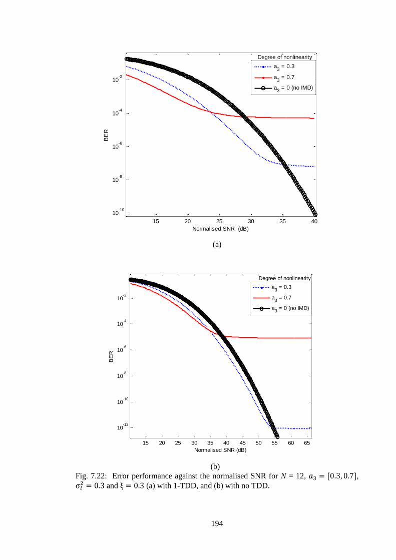
194

15 20 25 30 35 40

10-10

10-8

10-6

10-4

10-2

Normalised SNR (dB)

BE

R

a3 = 0.3

a3 = 0.7

a3 = 0 (no IMD)

Degree of nonlinearity

(a)

15 20 25 30 35 40 45 50 55 60 65

10-12

10-10

10-8

10-6

10-4

10-2

Normalised SNR (dB)

BE

R

a3 = 0.3

a3 = 0.7

a3 = 0 (no IMD)

Degree of nonlinearity

(b)

Fig. 7.22: Error performance against the normalised SNR for N = 12, ,

and (a) with 1-TDD, and (b) with no TDD.

195

The value of the BER floor depends, expectedly, on the degree of nonlinearity of the

optical source. For instance, with a nonlinearity degree and N = 12, the BER

floors for a link with 1-TDD and no TDD are ~10-4

and ~10-5

, respectively. These floor

values reduce to ~10-7

and 10-12

, respectively with a much more linear source with

. The BER floor for 1-TDD system under the influence of IMD is observed to

be higher than with no TDD simply because of the increased IMD accompanying the

TDD technique, although a SIM-FSO with 1-TDD still has higher CINR and lower

BER than without TDD before the floor is reached. It can thus be concluded that IMD

places a limit on the achievable link performance by imposing a BER floor on the

system. This further emphasises the desire and need for a linear laser transmitter in a

SIM-FSO system with multiple subcarriers.

7.8 Summary

In this chapter the error performance and outage probability of a SIM-FSO system

employing spatial diversity to combat the channel fading have been presented. The

following fading channel models have been considered: log-normal, gamma-gamma and

negative exponential. An expression for the unconditional BER of x -MIMO FSO

system that uses PSK subcarrier intensity modulation in turbulent atmosphere has

equally been derived. The error performance and the obtainable link margin using three

different linear combining techniques were also presented. Results showing clearly the

effect of correlated received irradiance on the system error performance have also been

given. In a single transmitter and 2-photodetector system at , a correlation

coefficient of 0.6 between the received irradiances results in additional ~3 dB of SNR to

achieve a BER of 10-6

. And this additional SNR increases as the correlation between the

196

received signals increases.

The use of SelC in a single source-multiple photodetector system in very weak

turbulence ( ) has been shown to result in a negative link margin and therefore

is not suggested as the sole means of mitigating scintillation. It has also been illustrated

that a multiple transmitter-single photodetector system is in effect a single transmitter-

multiple photodetector configuration employing EGC linear combining, and that a

reasonable number of independent photodetectors to mitigate scintillation without

overwhelming complexity can be put at between two and four. Using a 2 x 2-MIMO

system requires ~0.5 dB of SNR more than using 4-photodetector with single transmitter

at a BER of 10-6

but spacing an array of 4-photodetector sufficiently to ensure

uncorrelated irradiance reception is far more demanding than spacing 2-photodetector.

Also the use of 4 x 4-MIMO requires ~3 dB and ~0.8 dB of SNR less than using 4 and

8-photodetector, respectively with single optical transmitter at the same BER of 10-6

.

The subcarrier TDD as an alternative technique for ameliorating the channel fading has

equally been introduced and its error performance analysed. It has been shown that up

to 3 dB improvement in the receiver sensitivity can be achieved by re-transmitting the

delayed copy of the data five times in a channel of turbulence strength .

Retransmitting the delayed copy of the information just once is however found to be the

optimum with a gain of up to 4.5 dB in weak atmospheric turbulence. Expectedly, the

TDD gain was shown to be proportional to the fading strength but independent of the

data rate. It has also been shown that the IMD, caused by the optical source

nonlinearity, imposes a limit on the achievable BER of SIM-FSO. For SIM-FSO with

multiple subcarriers therefore, a linear laser source (one with negligible nonlinearity) is

much desired.

Chapter Eight

Link Budget Analysis

8.1 Introduction

The link budget is useful in estimating the theoretical power limited link range of a

communication system. In doing this, the various loss mechanisms experienced in a

terrestrial FSO link will be examined and discussed in this chapter. The principal source

of power loss in an FSO system, which is due to the constituents of the atmosphere, will

be discussed. Other losses mentioned in this chapter include the geometric loss, pointing

loss and optical loss due to imperfections in the lenses used in the design of the system.

Any other unforeseen power losses due to component ageing or component replacement

198

are catered for with the inclusion of link margin in the link budget analysis. Also the

expected level of performance, based on the outage probability or the BER performance

metrics, will be considered in determining the sensitivity of the receiver.

8.2 Power Loss

For optical radiation travelling through the atmospheric channel, the interaction between

the photons and the molecular constituent of the atmosphere cause some of the photons

to be extinguished while particulate constituents scatter the photons. These events

ultimately result in a power loss mechanism otherwise described by the Beer-Lambert

law. This law describes the transmittance of an optical field through the atmosphere as

function of the propagation distance. In addition, optical radiation traversing the

atmosphere spreads out due to diffraction, causing the size of the received beam to be

greater than the receiver aperture. These factors, combined with others herein discussed

are responsible for the difference between the transmitted and the received optical

powers.

8.2.1 Atmospheric channel loss

The atmospheric channel attenuates the field traversing it as a result of absorption and

scattering processes. The concentrations of matter in the atmosphere, which result in the

signal attenuation, vary spatially and temporally, and will depend on the current local

weather conditions. For a terrestrial FSO link transmitting an optical signal through the

atmosphere, the received irradiance at a distance L from the transmitter is related to the

transmitted irradiance by the Beer-Lambert‟s law as [79]:

199

(8.1)

where and represent the total attenuation/extinction coefficient (m-1

) and

the transmittance of the atmosphere at wavelength λ, respectively. The attenuation of

the optical signal in the atmosphere is due to the presence of molecular constituents

(gases) and aerosols. The aerosol is made up of tiny particles of various shapes ranging

from spherical to irregular shapes suspended in the atmosphere. The attenuation

coefficient is the sum of the absorption and the scattering coefficients from aerosols and

molecular constituents of the atmosphere, it follows therefore that [20]:

(8.2)

The first two terms represent the molecular and aerosol absorption coefficients,

respectively while the last two terms are the molecular and aerosol scattering

coefficients respectively.

a) Absorption – This takes place when there is an interaction between the

propagating photons and molecules (present in the atmosphere) along its path.

Some of the photons are extinguished and their energies converted into heat

[32]. The absorption coefficient depends very much on the type of gas molecules

and their concentration [79]. Absorption is wavelength dependent and therefore

selective. This leads to the atmosphere having transparent zones – range of

wavelengths with minimal absorptions – referred to as the transmission windows

as shown in Fig. 8.1. Since it is not possible to change the physics of the

atmosphere, the wavelengths used in FSO are basically chosen to coincide with

200

the atmospheric transmission windows [31]. The attenuation coefficient is

therefore dominated by scattering and as such .

Fig. 8.1: Atmospheric absorption transmittance over a sea level 1820 m horizontal path

[20].

b) Scattering – This results in angular redistribution of the optical field with and

without wavelength modification. The scattering effect depends on the radius

of the particles (fog, aerosol) encountered during propagation. One way of

describing this is to consider the size parameter . If , the

scattering process is classified as Rayleigh scattering [133]; if it is Mie

scattering and for , the scattering process can then be explained using the

diffraction theory (geometric optics). The scattering process for different

scattering particles present in the atmosphere is summarised in Table 8.1.

201

Table 8.1: Typical atmospheric scattering particles with their radii and scattering

process at λ = 850 nm

Type Radius (µm) Size Parameter x0 Scattering Process

Air molecules 0.0001 0.00074 Rayleigh

Haze particle 0.01 – 1 0.074 – 7.4 Rayleigh – Mie

Fog droplet 1 – 20 7.4 – 147.8 Mie – Geometrical

Rain 100 – 10000 740 – 74000 Geometrical

Snow 1000 – 5000 7400 –37000 Geometrical

Hail 5000–50000 37000 – 370000 Geometrical

8.2.1.1 Rayleigh scattering

A simplified expression describing Rayleigh scattering is given by [134]:

(8.3)

where is the number of particles per unit volume along the propagation path and

represents the cross-sectional area of scattering. The proportionality of the

Rayleigh scattering suggests that the shorter wavelengths get scattered more; this effect

is what is responsible for the blue colour of the sky during the day.

8.2.2.1 Mie scattering

Mie scattering occurs when the particle size is comparable to the beam size and as the

fog particle size compares very much with the wavelength band of interest in FSO (0.5

μm – 2 μm), this makes fog the major photon scatterer and Mie scattering the dominant

scattering process in terrestrial FSO systems. Based on the assumptions that the

scattered light has the same wavelength as the incident light, only single scattering

occurs while the multiple scattering effects are neglected, and that the particles are

spherical in shape and are acting independently with a complex refractive index in

space, the following expression for the Mie scattering was derived in [6] as:

202

(8.4)

where r is the particle (fog, aerosol etc.) radius in centimetres, Qd is the Mie scattering

efficiency, is real part of the complex refractive index and n(r) is the volume

concentration that is the number of fog particles per unit volume per unit increment in

radius. Here, is the specific attenuation measured in dB/km and is calculated by

summing up the attenuation effect of all the individual fog droplets present per unit

volume per unit increase in radius.

The particles encountered in the atmosphere have complex shapes and orientations and

applying the theory of Mie scattering to these atmospheric particles is therefore very

complicated. Henceforth, the description of attenuation due to scattering will be based

on reported empirical formulae. These empirical equations are often expressed in terms

of the visibility range V in km. The visibility range is the distance that a parallel

luminous beam travels through in the atmosphere until its intensity drops to 2% of its

original value [135]. It is measured with an instrument called the transmissiometer and a

commonly used empirical model for Mie scattering is given by:

(8.5)

where δ is given by (8.6) and Table 8.2 gives the international visibility range and

attenuation in the visible waveband for different weather conditions.

203

Kim model Kruse model

(8.6)

Table 8.2: International visibility range and attenuation coefficient in the visible

waveband for various weather conditions [78].

International Visibility Code

Weather

conditions

Precipitation

Visibility (m)

Attenuation

(dB/km) mm/hr

0

Dense fog 50 315

Thick fog

200 75

Moderate fog 500 28.9

Light fog

S

n

o

w

Storm 100 770 18.3

Very light fog

1,000 13.8

Strong rain 25 1,900 6.9

Light mist

2,000 6.6

Average rain 12.5 2,800 4.6

4,000 3.1

Very light mist Light rain 2.5 5,900 2

10,000 1.1

Clear air Drizzle 0.25 18,100 0.6

20,000 0.54

Very clear air 23,000 0.47

50,000 0.19

204

Recently, Al Naboulsi [36] in his work came up with equations 8.7(a-b) as a simple

relationship for estimating the advection and radiation (or convection) fog attenuation in

the 690 – 1550 nm wavelength band and 50 – 1000 m visibility range.

(8.7a)

(8.7b)

where λ is in nm and V is in metres. The power loss due to rain and snow are so low

compared to that due to the Mie scattering, they still have to be accounted for in the link

margin during the link budget analysis. A typical rainfall of 2.5 cm/hour could result in

an attenuation of ~6 dB/km [125] while a typical value for attenuation due to light snow

to blizzard is 3 dB/km to 30 dB/km [20]. In early 2008 in Prague, Czech Republic, the

fog attenuation was measured and compared with the empirical fog attenuation models.

This result is shown in Fig. 8.2, with a visibility of less than 200 m, corresponding to

thick fog, the attenuation at the location is ~200 dB/km. The empirical models provide a

reasonable fit to the measured values with a maximum of about 5 dB/km difference

between any two empirical models.

205

Fig. 8.2: Measured attenuation coefficient as a function of visibility range at λ = 830 nm

in early 2008, Prague, Czech Republic,[136].

8.2.2 Beam divergence

One of the main advantages of FSO systems is the ability to transmit a very narrow

optical beam, thus offering enhanced security, but due to diffraction, the beam spreads

out. This results in a situation in which the receiver aperture is only able to collect a

fraction of the beam and hence beam divergence loss.

206

AT

As

AR

Aim

Transmitter

apertureReceiver

aperture

Detector

Light

source

Lu

θ

Fig. 8.3: Beam divergence

Considering the arrangement of a free-space optical communication link of Fig. 8.3, and

by invoking the thin lens approximation to the diffuse optical source whose irradiance is

represented by Is, the amount of optical power focused on the detector is derived as

[137]:

(8.8)

where AT and AD are the transmitter and receiver aperture areas, respectively while As is

the area of the optical source. This clearly shows that a source with high radiance Is/As

and wide apertures are required in order to increase the received optical power.

For a non-diffuse, small source such as the laser, the size of the image formed at the

receiver plane is no longer given by the thin lens approximation; it is determined by

diffraction at the transmitter aperture. The diffraction pattern produced by a uniformly

illuminated circular aperture of diameter dT is known to consist of a set of concentric

rings. The image size is said to be diffraction limited when the radius of the first

207

intensity minimum or dark ring of the diffraction pattern becomes comparable in size

with the diameter dim of the normally focussed image [137]. That is:

(8.9)

Therefore,

(8.10)

The equation above shows that for diffraction to be the sole cause of beam divergence

(diffraction limited), the source diameter . A laser being inherently

collimated and coherent normally produces a diffraction-limited image. The diffraction

limited beam divergence angle in radians is thus given by . If the transmitter

and receiver effective antenna gains are respectively given by:

(8.11a)

(8.11b)

And the free-space path loss is given by:

(8.12)

The received optical power then becomes:

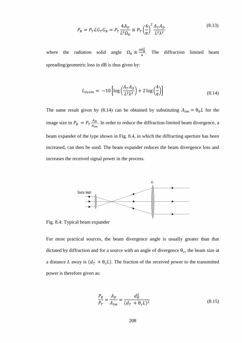
208

(8.13)

where the radiation solid angle . The diffraction limited beam

spreading/geometric loss in dB is thus given by:

(8.14)

The same result given by (8.14) can be obtained by substituting for the

image size in . In order to reduce the diffraction-limited beam divergence, a

beam expander of the type shown in Fig. 8.4, in which the diffracting aperture has been

increased, can then be used. The beam expander reduces the beam divergence loss and

increases the received signal power in the process.

AT

Source beam

Fig. 8.4: Typical beam expander

For most practical sources, the beam divergence angle is usually greater than that

dictated by diffraction and for a source with an angle of divergence , the beam size at

a distance L away is . The fraction of the received power to the transmitted

power is therefore given as:

(8.15)

209

The geometric loss in dB is thus:

(8.16)

The beam spreading loss for the diffraction limited source given by (8.14) is,

expectedly, lower than that of the non-diffraction limited case represented by (8.16),

this is because the image size is smaller by dT in the diffraction limited case.

From the foregoing, it is clear that a source with a very narrow angle of divergence is

preferable in terrestrial FSO systems. It should however be mentioned that, wide

divergence angle sources are desirable in short range FSO links to ease the alignment

requirement, compensate for building sway and eliminate the need for active tracking

systems at the expense of increased geometric loss apparently. A typical FSO

transceiver has optical beam divergence in the range of 2–10 mrad and 0.05–1.0 mrad

(equivalent to a beam spread of 2–10 m, and 5 cm to 1 m, respectively at 1 km link

range) for systems without and with tracking respectively.

8.2.3 Optical and window loss

This class of power loss includes losses due to imperfect lenses and other optical

elements used in the design of both the transmitter and receiver. It accounts for the

reflection, absorption and scattering due to the lenses in the system [20]. The value of

the optical loss , can be obtained from the component manufacturer. It apparently

depends on the characteristics of the equipments and quality of the lenses used. For FSO

transceivers installed behind windows within a building, there exists an additional

optical power loss due the window glass attenuation. Although (glass) windows allow

210

optical signals to pass through them, they contribute to the overall power loss of the

signal. Uncoated glass windows usually attenuate 4% per surface, because of reflection.

Coated windows display much higher losses and its magnitude is wavelength

dependent.

8.2.4 Pointing loss

Additional power penalty is usually incurred due lack of perfect alignment of the

transmitter and receiver. The resulting power loss is catered for by including

pointing/misalignment loss in the link budget analysis. For short FSO links (< 1 km),

this might not be an issue but for longer link ranges, this can certainly not be neglected.

Misalignments could result from building sway or strong wind effect on the FOS link

head stand.

8.3 The Link Budget

Based on the losses highlighted above, the received optical power in dBm can thus be

obtained from the link budget equation as:

(8.17)

The link margin LM is included in the link budget equation above to cater for other

losses such as changes in specification when a faulty component is replaced, ageing of

laser source, attenuation due to rain, snow and so on. One major importance of the link

budget equation is for determining the achievable link range, for a given receiver

sensitivity and link margin. The receiver sensitivity represents the minimum amount of

optical power needed for the system to achieve a specified level performance, for

211

example a BER of 10-9

. The receiver sensitivity depends on the modulation technique in

use, the noise level, fading/scintillation strength and the data rate. Higher data rates

simply implies shorter optical pulse duration, hence fewer photons that can be detected.

The noise could be from a combination of background radiation, the detection

process/quantum shot noise and the thermal noise caused by the thermal agitation of

electrons in the receiver electronic components. The receiver sensitivity for at any

desired level of performance can then be obtained from the results of Chapters Six and

Seven.

For a typical commercial FSO system whose specifications are given in Table 8.3, the

achievable link range as a function of link margin is shown in Fig. 8.5 for different

visibility values. The results in the figure are based on the Kim model of atmospheric

attenuation and the specifications are for non-turbulent atmospheric channels. By

operating the link at a 5 dB link margin in clear atmosphere, a range of about 3 km is

attainable at the specified data rate; doubling the link margin reduces the link range to

below 1.5 km.

Table 8.3: Typical link budget parameters

Parameter Typical Value

Receiver aperture diameter, dR 8 cm

Transmitter aperture diameter, dT 2.5 cm

Beam divergence, 2 mrad

Modulation technique/Bit rate On-Off keying/155Mbps

Transmitted power 14 dBm

Receiver sensitivity -30 dBm

Optical loss, Lop 1 dB

Pointing loss, LP 1 dB

Wavelength, λ 850 nm

212

-5 0 5 10 15 20 25 30

0.5

1

1.5

2

2.5

3

3.5

Link margin (dB)

Lin

k L

ength

(km

)

30 km

5 km

50 km

Visibility

Fig. 8.5: Link length against the available link margin for OOK-FSO in a channel with

visibility values 5, 30 and 50 km.

To illustrate the link budget analysis of a BPSK-SIM modulated FSO operating in

turbulent atmosphere, the analysis and results of the previous chapter will be

considered. For instance, from Figs. 7.9 and 7.20, the required average irradiance to

achieve a BER of 10-9

with and without diversity can be obtained, these values are

summarised in Table 8.4 below.

Table 8.4: Required irradiance to achieve a BER of 10-9

based on BPSK-SIM, Rb = 155

Mbps and .

No diversity 1-TDD 4 × 4 - MIMO

I0 (dBm) -17.2 -19.2 -28.8

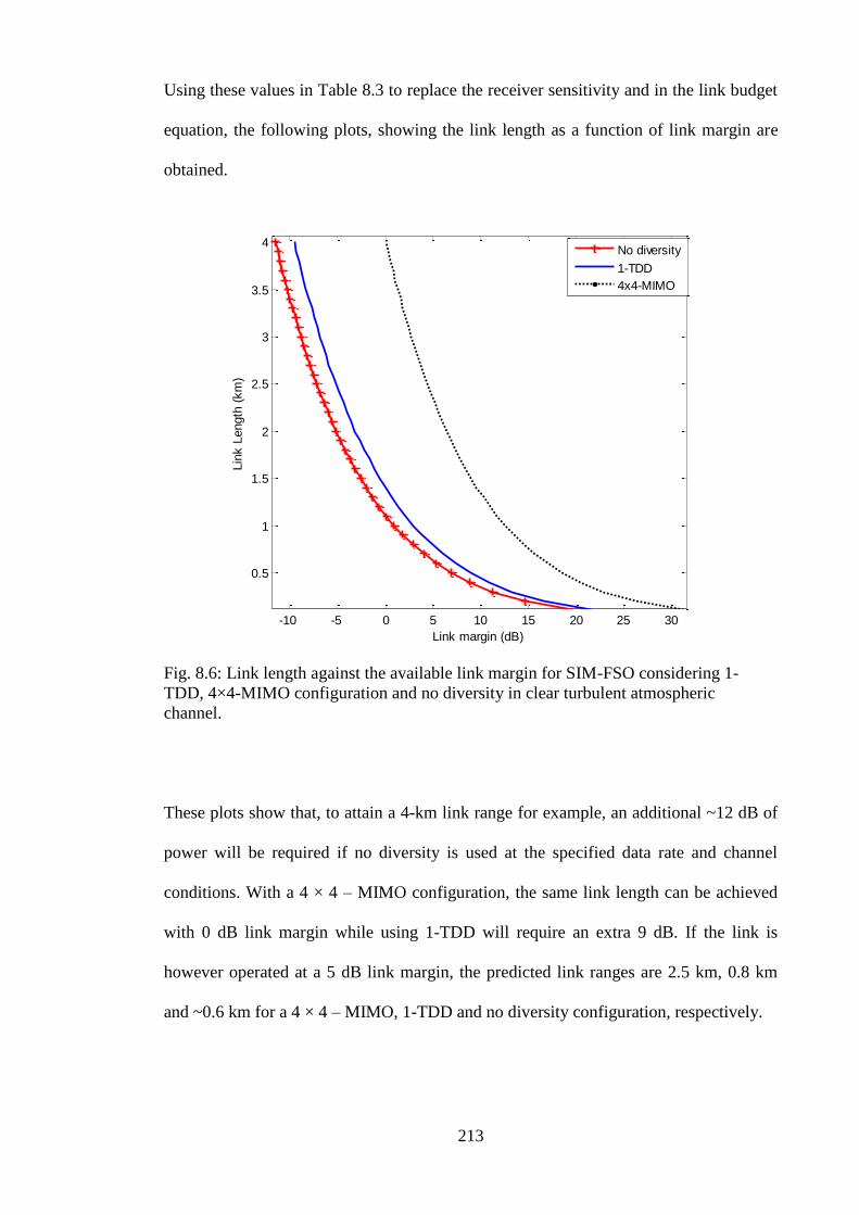
213

Using these values in Table 8.3 to replace the receiver sensitivity and in the link budget

equation, the following plots, showing the link length as a function of link margin are

obtained.

-10 -5 0 5 10 15 20 25 30

0.5

1

1.5

2

2.5

3

3.5

4

Link margin (dB)

Lin

k L

ength

(km

)

No diversity

1-TDD

4x4-MIMO

Fig. 8.6: Link length against the available link margin for SIM-FSO considering 1-

TDD, 4×4-MIMO configuration and no diversity in clear turbulent atmospheric

channel.

These plots show that, to attain a 4-km link range for example, an additional ~12 dB of

power will be required if no diversity is used at the specified data rate and channel

conditions. With a 4 × 4 – MIMO configuration, the same link length can be achieved

with 0 dB link margin while using 1-TDD will require an extra 9 dB. If the link is

however operated at a 5 dB link margin, the predicted link ranges are 2.5 km, 0.8 km

and ~0.6 km for a 4 × 4 – MIMO, 1-TDD and no diversity configuration, respectively.

214

8.4 Summary

In this chapter, the link budget equation, from which the attainable link length of

terrestrial FSO systems can be estimated, has been presented. In arriving at this

equation, various sources of power loss encountered in terrestrial FSO systems have

been discussed and accounted for. Out of all the losses, atmospheric scattering due to

fog is the most deleterious. This is because the wavelengths of interest in FSO (0.5 μm –

2 μm) are approximately the size as the particles making up the fog. Also, the estimated

link length is limited by the available power at the transmitter and the receiver

sensitivity. The available transmitted power is limited by safety standards while the

receiver sensitivity depends on the modulation type used, noise and atmospheric

turbulence.

Chapter Nine

Experimental Demonstration of

Scintillation Effect

9.1 Introduction

A turbulent atmospheric channel changes the power distribution profile, among other

things, of an optical beam travelling through it. Different models for describing this

phenomenon have been discussed in Chapter Four while theoretical analysis of its

(atmospheric turbulence) impact on the error performance of an FSO link, including

methods that can be used to mitigate its effects has already discussed in Chapters Five

to Seven. In this chapter, an experimental demonstration of the scintillation effect on an

FSO system will be discussed. The experiment involves the use of both OOK signalling

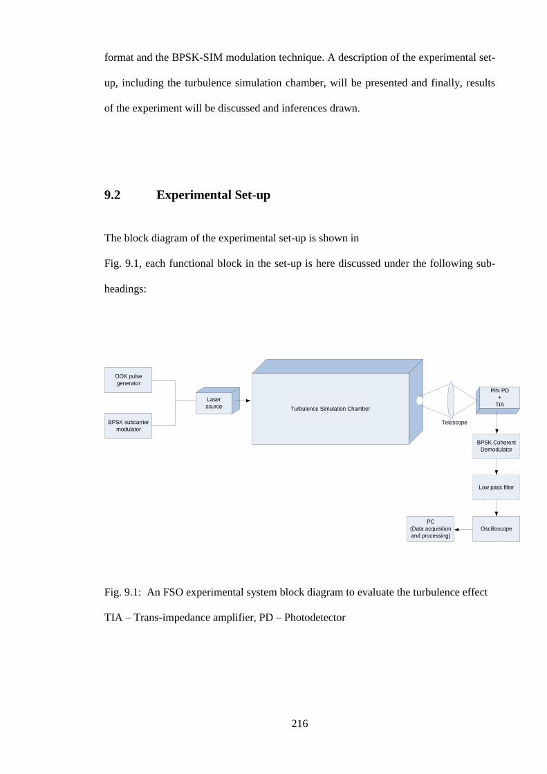
216

format and the BPSK-SIM modulation technique. A description of the experimental set-

up, including the turbulence simulation chamber, will be presented and finally, results

of the experiment will be discussed and inferences drawn.

9.2 Experimental Set-up

The block diagram of the experimental set-up is shown in

Fig. 9.1, each functional block in the set-up is here discussed under the following sub-

headings:

OOK pulse

generator

BPSK subcarrier

modulator

Turbulence Simulation Chamber

Laser

source

PIN PD

+

TIA

BPSK Coherent

Demodulator

Oscilloscope

PC

(Data acquisition

and processing)

Telescope

Low pass filter

Fig. 9.1: An FSO experimental system block diagram to evaluate the turbulence effect

TIA – Trans-impedance amplifier, PD – Photodetector

217

9.2.1 The transmitter

The optical source used in the experiment is a 850 nm „modulatable Beta-Tx‟ laser

source with a maximum output power of 3 mW. Near-infrared wavelength is chosen

because cheap matching photodetectors are readily available at this wavelength. The

laser source has its biased point factory-set midway along the linear section of its output

characteristic curve. In order for this laser source to operate within its linear region the

peak-to-peak amplitude of the input electrical signal must not exceed 500 mV. With this

in mind, the OOK signalling is generated by directly modulating the laser output with a

bipolar square wave signal.

The BPSK modulated subcarrier on the other hand is generated by using a MC 1496

multiplier integrated circuit. The schematic diagram of the BPSK modulator is shown in

Fig. 9.2, the subcarrier oscillator is a sinusoidal signal of a frequency 1MHz and an

amplitude 150 mVp-p while the modulating signal is a bipolar binary data sequence. In

this experiment, the aim is to investigate the scintillation effect on the symbol detection

threshold level, as such, less emphasis will be place on the data rate. For fair

comparison however, both modulation techniques under consideration will be operated

at the same data rate. The output impedance of the BPSK modulator of Fig. 9.2 is over

100 kΩ at the 1 MHz centre frequency. This is far higher than the 50 Ω input impedance

of the laser source. To ensure optimum power transfer therefore, an impedance

matching network shown in Fig. 9.3 is inserted between the subcarrier BPSK modulator

and the laser source as shown in Fig. 9.3.

218

MC1496

1k

6.8k

3.9k

1k 1k

3.9k

50k

51

51

10k 5110k

0.1µF

0.1µF

0.1µF

1

2 3

4

5

6

8

10

12

14

Modulating

Signal

Subcarrier

oscillator

Modulator

Output

VCC

12 V

VEE

-8 V

Fig. 9.2: Schematic diagram of the BPSK subcarrier modulator

0.1µF2N2222A

82K

100K 1K

0.1µF

Beta TX Laser Diode

Driver

12 V

Modulator Output

90 mALaser Diode

(850 nm, 3mW)

Optical

radiation

Fig. 9.3: Impedance matching network

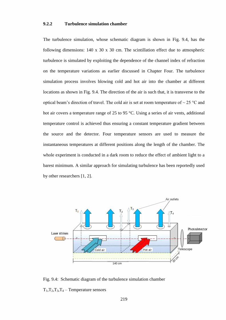
219

9.2.2 Turbulence simulation chamber

The turbulence simulation, whose schematic diagram is shown in Fig. 9.4, has the

following dimensions: 140 x 30 x 30 cm. The scintillation effect due to atmospheric

turbulence is simulated by exploiting the dependence of the channel index of refraction

on the temperature variations as earlier discussed in Chapter Four. The turbulence

simulation process involves blowing cold and hot air into the chamber at different

locations as shown in Fig. 9.4. The direction of the air is such that, it is transverse to the

optical beam‟s direction of travel. The cold air is set at room temperature of ~ 25 °C and

hot air covers a temperature range of 25 to 95 °C. Using a series of air vents, additional

temperature control is achieved thus ensuring a constant temperature gradient between

the source and the detector. Four temperature sensors are used to measure the

instantaneous temperatures at different positions along the length of the chamber. The

whole experiment is conducted in a dark room to reduce the effect of ambient light to a

barest minimum. A similar approach for simulating turbulence has been reportedly used

by other researchers [1, 2].

140 cm30

cm

Telescope

T2 T4

Fig. 9.4: Schematic diagram of the turbulence simulation chamber

T1,T2,T3,T4 – Temperature sensors

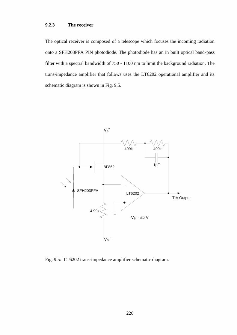
220

9.2.3 The receiver

The optical receiver is composed of a telescope which focuses the incoming radiation

onto a SFH203PFA PIN photodiode. The photodiode has an in built optical band-pass

filter with a spectral bandwidth of 750 - 1100 nm to limit the background radiation. The

trans-impedance amplifier that follows uses the LT6202 operational amplifier and its

schematic diagram is shown in Fig. 9.5.

SFH203PFA

BF862

499k

4.99k

499k

1pF

+

-

LT6202

VS+

VS--

VS = ±5 V

TIA Output

Fig. 9.5: LT6202 trans-impedance amplifier schematic diagram.

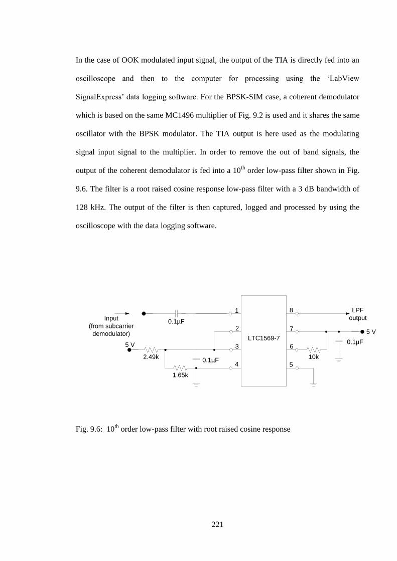
221

In the case of OOK modulated input signal, the output of the TIA is directly fed into an

oscilloscope and then to the computer for processing using the „LabView

SignalExpress‟ data logging software. For the BPSK-SIM case, a coherent demodulator

which is based on the same MC1496 multiplier of Fig. 9.2 is used and it shares the same

oscillator with the BPSK modulator. The TIA output is here used as the modulating

signal input signal to the multiplier. In order to remove the out of band signals, the

output of the coherent demodulator is fed into a 10th

order low-pass filter shown in Fig.

9.6. The filter is a root raised cosine response low-pass filter with a 3 dB bandwidth of

128 kHz. The output of the filter is then captured, logged and processed by using the

oscilloscope with the data logging software.

LTC1569-7

2.49k

1.65k

10k

0.1µF

0.1µF

0.1µF

5 V

5 V

Input

(from subcarrier

demodulator)

LPF

output1

2

3

4 5

6

7

8

Fig. 9.6: 10th

order low-pass filter with root raised cosine response

222

Since the emphasis in this experiment is on threshold level position rather than data rate,

the constraint imposed on the achievable data rate by the filter will hence have no

impact on the result of the experiment. In Fig. 9.7, the input and output signal

waveforms for the OOK modulated laser without turbulence are shown while Fig. 9.8

gives the input and the received signal waveforms for the BPSK subcarrier modulated

laser. The simulation parameters used to obtain these results are summarised in Table

9.1 and the picture of the experimental set-up is given in Fig. 9.9.

Input electrical signal,

100 mV p-p

Received signal at the

output of TIA, ~300

mV p-p

Time

Vo

lta

ge

y-axis 100 mV/division 50 mV/division

x-axis 10 µs/division 10 µs/division

Fig. 9.7: OOK modulated laser input and received signal waveforms without turbulence,

input signal 100 mV p-p, 40 kHz.

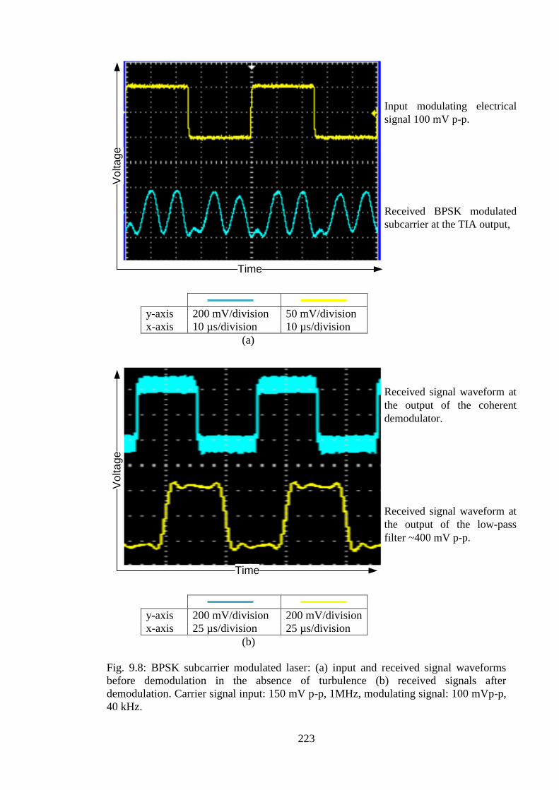
223

Input modulating electrical

signal 100 mV p-p.

Received BPSK modulated

subcarrier at the TIA output,

Time

Vo

lta

ge

y-axis 200 mV/division 50 mV/division

x-axis 10 µs/division 10 µs/division

(a)

Received signal waveform at

the output of the coherent

demodulator.

Received signal waveform at

the output of the low-pass

filter ~400 mV p-p.

Vo

lta

ge

Time

y-axis 200 mV/division 200 mV/division

x-axis 25 µs/division 25 µs/division

(b)

Fig. 9.8: BPSK subcarrier modulated laser: (a) input and received signal waveforms

before demodulation in the absence of turbulence (b) received signals after

demodulation. Carrier signal input: 150 mV p-p, 1MHz, modulating signal: 100 mVp-p,

40 kHz.

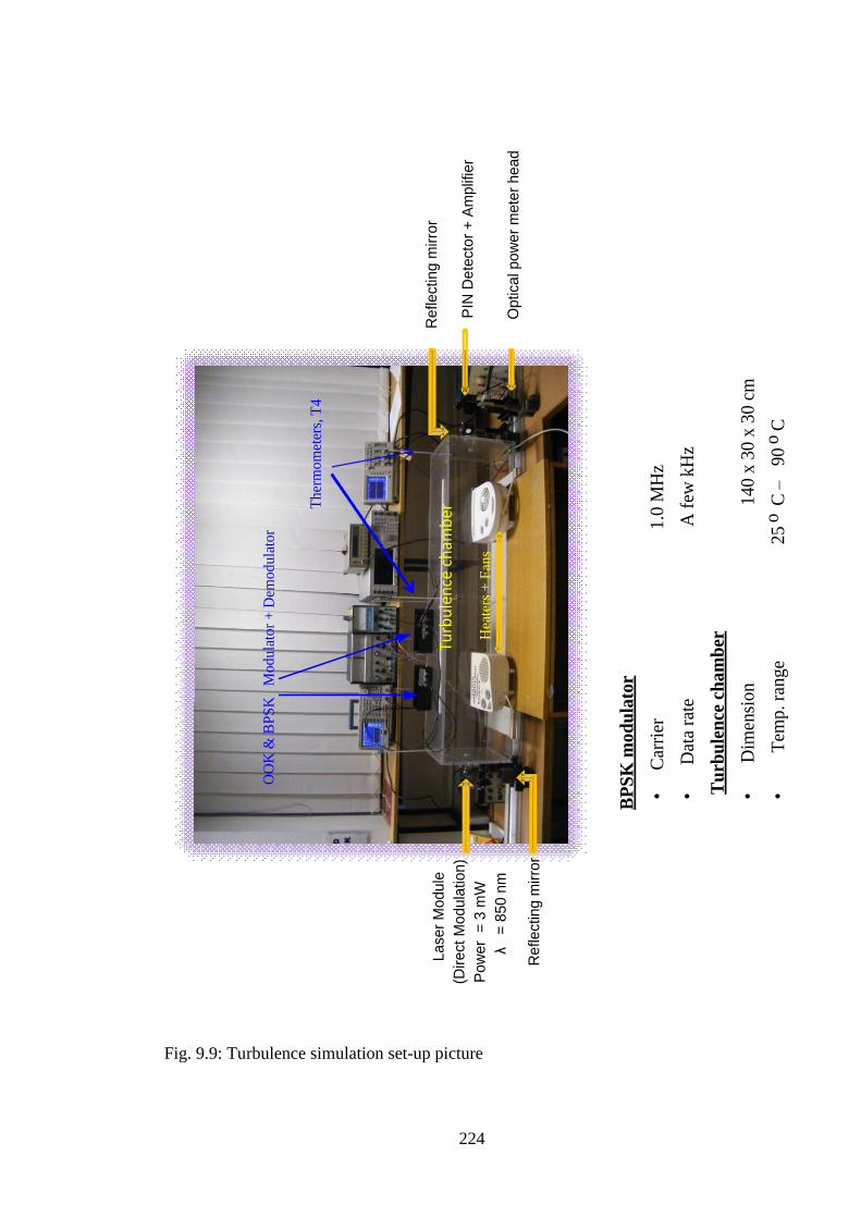
224

BP

SK

mo

du

lato

r

•C

arri

er

1.0

MH

z

•D

ata

rate

A f

ew k

Hz

Tu

rbu

len

ce c

ha

mb

er

•D

imen

sio

n1

40

x 3

0 x

30

cm

•T

emp

. ra

ng

e 2

5o

C –

90

oC

La

se

r M

od

ule

( Dire

ct M

od

ula

tio

n)

Po

we

r =

3 m

W

λ =

85

0 n

m

OO

K &

BP

SK

M

odula

tor

+ D

emodula

tor

PIN

De

tecto

r +

Am

plif

ier

Re

fle

ctin

g m

irro

r

Hea

ters

+ F

ans

Turb

ule

nce

ch

amb

er Ther

mo

met

ers,

T4

Re

fle

ctin

g m

irro

r

Op

tica

l p

ow

er

me

ter

he

ad

Fig. 9.9: Turbulence simulation set-up picture

225

Table 9.1: Parameters for the OOK and BPSK subcarrier modulation experiment.

Parameters Value

Laser type Modulatable Beta-Tx

Laser diode wavelength 850 nm

Laser maximum output power 3 mW

Laser beam size at aperture 5 mm × 2 mm

PIN detector (SFH203PFA) switching time 0.5 μs

PIN detector responsivity @ 850 nm 0.59 A/W

Modulation type OOK and BPSK-SIM

Optical band-pass filter 750 - 1100 nm

Turbulence simulation chamber 140×30×30 cm

Carrier signal (sinusoidal) frequency 1 MHz

Carrier signal (sinusoidal) amplitude 150 mV p-p

Modulating signal (square wave) amplitude 100 mV p-p

Modulating signal (square wave) pulse

duration

25 µs

Ambient temperature 25 °C

9.3 Characterisation of Simulated Turbulence

To evaluate the strength of the turbulence generated via this set-up, the intensity of laser

is directly modulated by a 1 MHz 200 mV peak to peak sinusoidal signal and the mean

values of the received signal without the locally generated turbulence logged over a

period of time. The process is then repeated with the turbulence simulator in operation

and the mean values acquired as well. While doing the experiment without turbulence,

the temperature across the turbulence simulation chamber is same as the ambient

temperature. With turbulence, the temperature at four different positions, T1 to T4 in

Fig. 9.4, are constantly changing, typical values are given in Table 9.2.

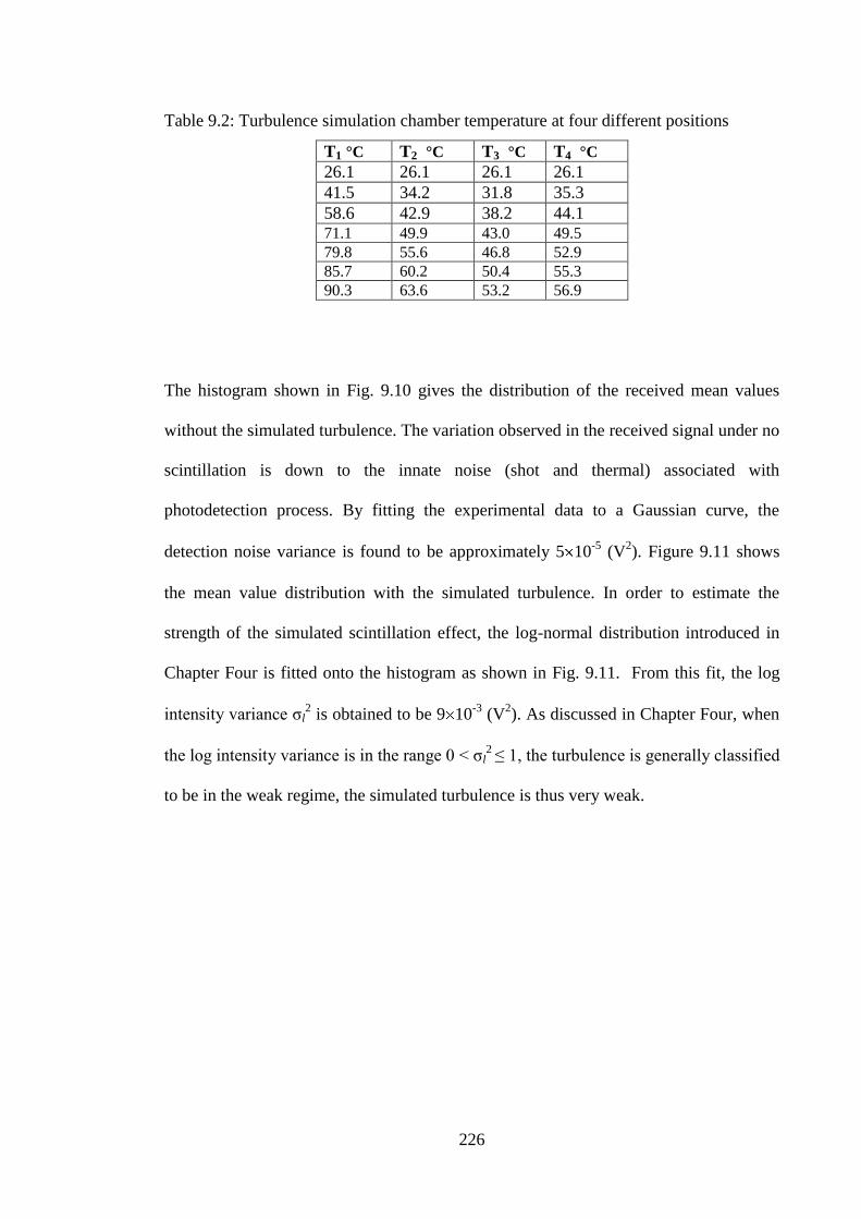
226

Table 9.2: Turbulence simulation chamber temperature at four different positions

T1 °C T2 °C T3 °C T4 °C

26.1 26.1 26.1 26.1

41.5 34.2 31.8 35.3

58.6 42.9 38.2 44.1 71.1 49.9 43.0 49.5

79.8 55.6 46.8 52.9

85.7 60.2 50.4 55.3

90.3 63.6 53.2 56.9

The histogram shown in Fig. 9.10 gives the distribution of the received mean values

without the simulated turbulence. The variation observed in the received signal under no

scintillation is down to the innate noise (shot and thermal) associated with

photodetection process. By fitting the experimental data to a Gaussian curve, the

detection noise variance is found to be approximately 5 10-5

(V2). Figure 9.11 shows

the mean value distribution with the simulated turbulence. In order to estimate the

strength of the simulated scintillation effect, the log-normal distribution introduced in

Chapter Four is fitted onto the histogram as shown in Fig. 9.11. From this fit, the log

intensity variance σl2 is obtained to be 9 10

-3 (V

2). As discussed in Chapter Four, when

the log intensity variance is in the range 0 < σl2

≤ 1, the turbulence is generally classified

to be in the weak regime, the simulated turbulence is thus very weak.

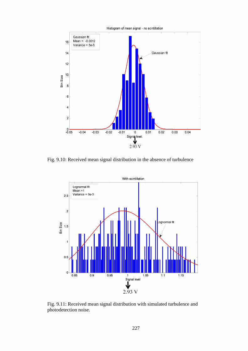
227

Fig. 9.10: Received mean signal distribution in the absence of turbulence

Fig. 9.11: Received mean signal distribution with simulated turbulence and

photodetection noise.

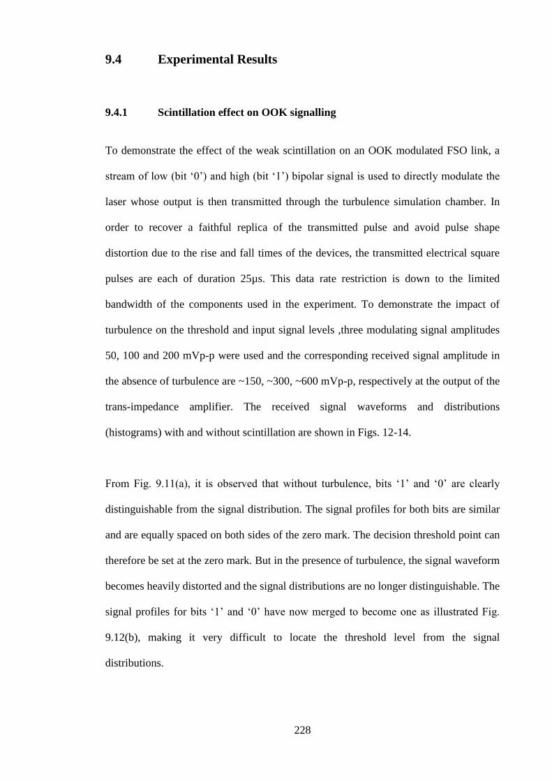
228

9.4 Experimental Results

9.4.1 Scintillation effect on OOK signalling

To demonstrate the effect of the weak scintillation on an OOK modulated FSO link, a

stream of low (bit „0‟) and high (bit „1‟) bipolar signal is used to directly modulate the

laser whose output is then transmitted through the turbulence simulation chamber. In

order to recover a faithful replica of the transmitted pulse and avoid pulse shape

distortion due to the rise and fall times of the devices, the transmitted electrical square

pulses are each of duration 25µs. This data rate restriction is down to the limited

bandwidth of the components used in the experiment. To demonstrate the impact of

turbulence on the threshold and input signal levels ,three modulating signal amplitudes

50, 100 and 200 mVp-p were used and the corresponding received signal amplitude in

the absence of turbulence are ~150, ~300, ~600 mVp-p, respectively at the output of the

trans-impedance amplifier. The received signal waveforms and distributions

(histograms) with and without scintillation are shown in Figs. 12-14.

From Fig. 9.11(a), it is observed that without turbulence, bits „1‟ and „0‟ are clearly

distinguishable from the signal distribution. The signal profiles for both bits are similar

and are equally spaced on both sides of the zero mark. The decision threshold point can

therefore be set at the zero mark. But in the presence of turbulence, the signal waveform

becomes heavily distorted and the signal distributions are no longer distinguishable. The

signal profiles for bits „1‟ and „0‟ have now merged to become one as illustrated Fig.

9.12(b), making it very difficult to locate the threshold level from the signal

distributions.

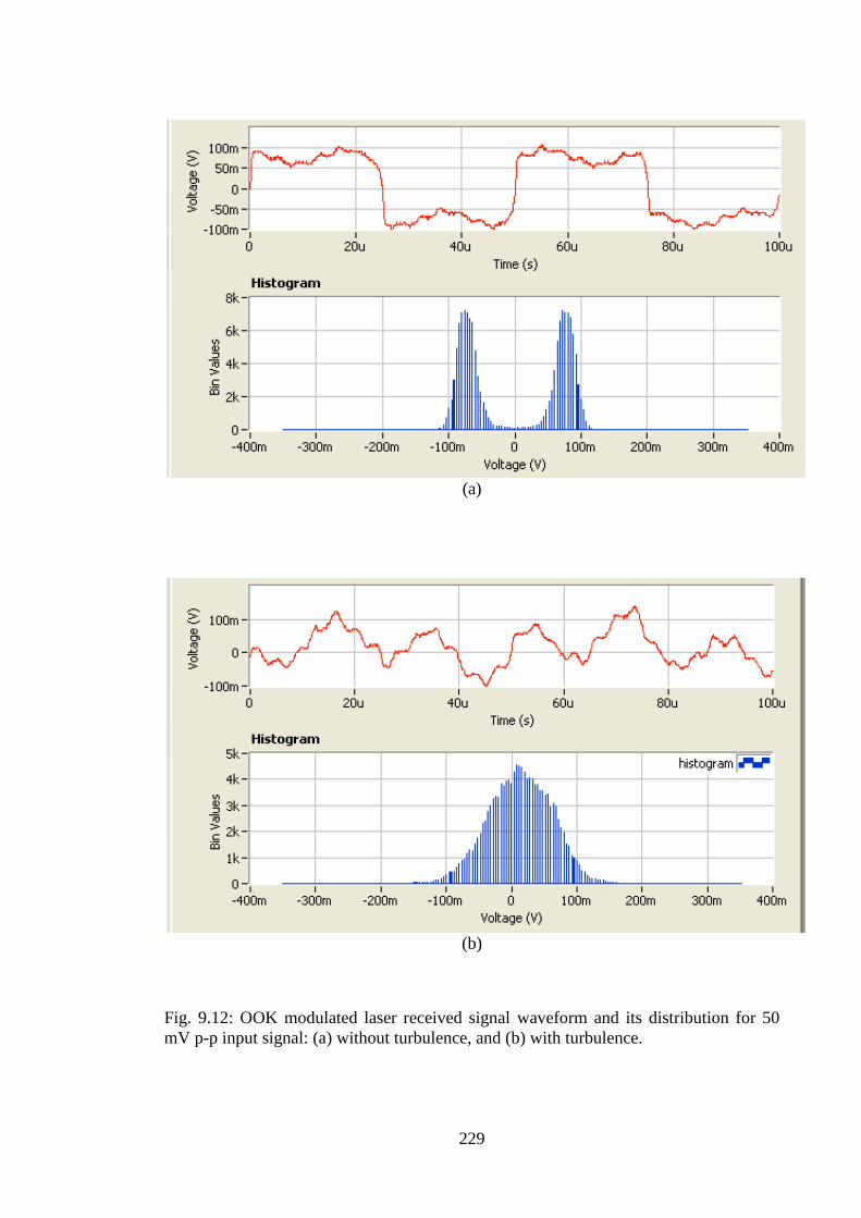
229

(a)

(b)

Fig. 9.12: OOK modulated laser received signal waveform and its distribution for 50

mV p-p input signal: (a) without turbulence, and (b) with turbulence.

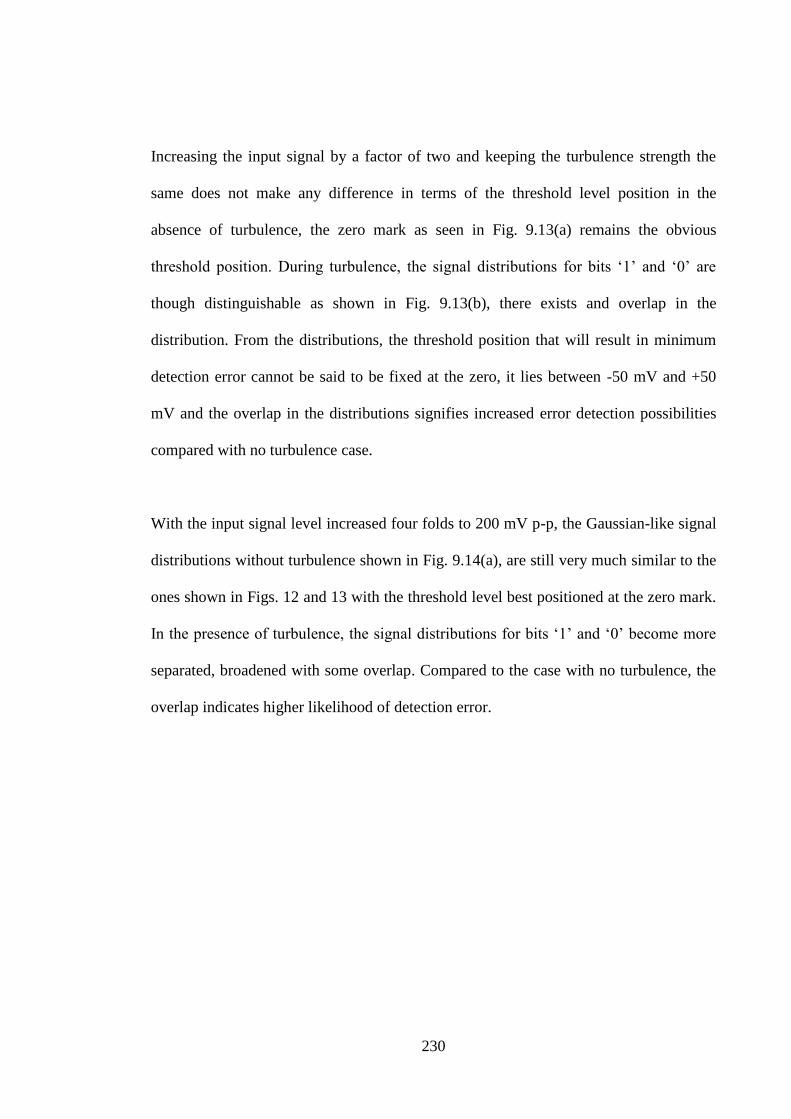
230

Increasing the input signal by a factor of two and keeping the turbulence strength the

same does not make any difference in terms of the threshold level position in the

absence of turbulence, the zero mark as seen in Fig. 9.13(a) remains the obvious

threshold position. During turbulence, the signal distributions for bits „1‟ and „0‟ are

though distinguishable as shown in Fig. 9.13(b), there exists and overlap in the

distribution. From the distributions, the threshold position that will result in minimum

detection error cannot be said to be fixed at the zero, it lies between -50 mV and +50

mV and the overlap in the distributions signifies increased error detection possibilities

compared with no turbulence case.

With the input signal level increased four folds to 200 mV p-p, the Gaussian-like signal

distributions without turbulence shown in Fig. 9.14(a), are still very much similar to the

ones shown in Figs. 12 and 13 with the threshold level best positioned at the zero mark.

In the presence of turbulence, the signal distributions for bits „1‟ and „0‟ become more

separated, broadened with some overlap. Compared to the case with no turbulence, the

overlap indicates higher likelihood of detection error.

231

(a)

(b)

Fig. 9.13: OOK modulated laser received signal waveform and its distribution for 100

mV p-p input signal: (a) without turbulence and (b) with turbulence.

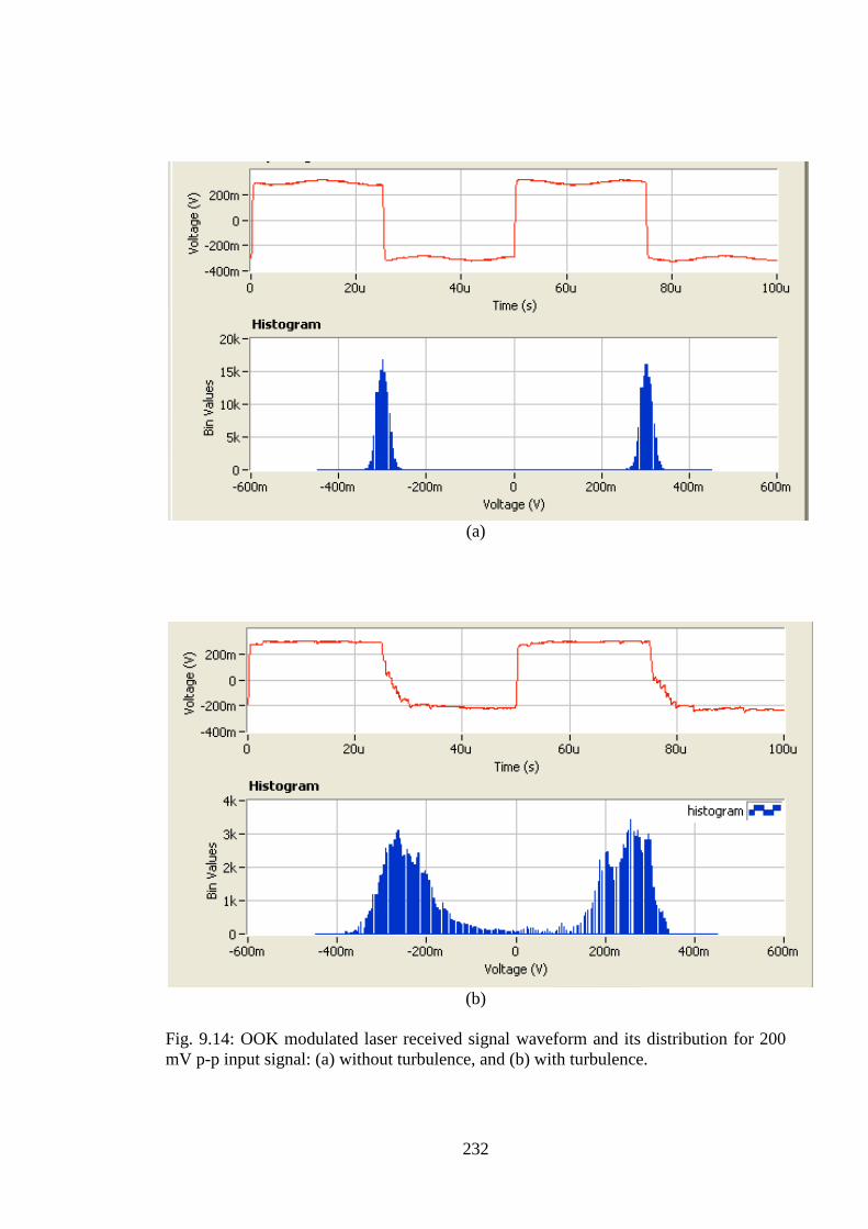
232

(a)

(b)

Fig. 9.14: OOK modulated laser received signal waveform and its distribution for 200

mV p-p input signal: (a) without turbulence, and (b) with turbulence.

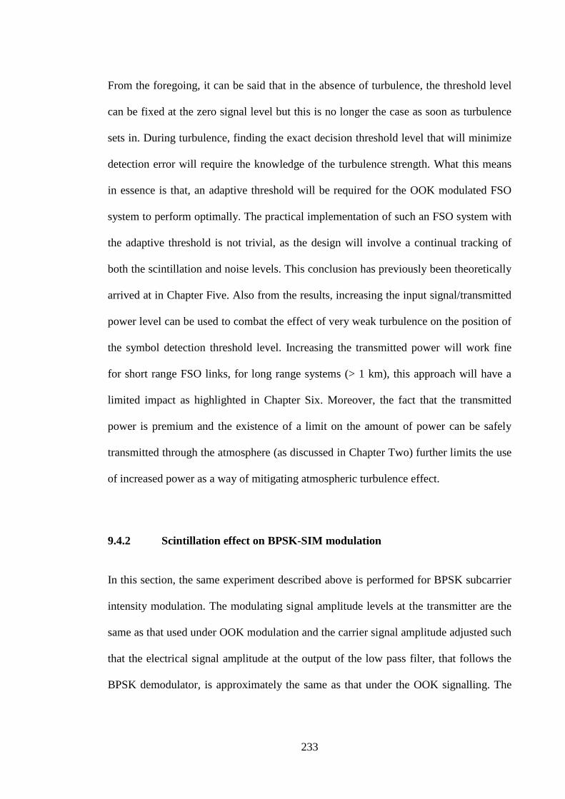
233

From the foregoing, it can be said that in the absence of turbulence, the threshold level

can be fixed at the zero signal level but this is no longer the case as soon as turbulence

sets in. During turbulence, finding the exact decision threshold level that will minimize

detection error will require the knowledge of the turbulence strength. What this means

in essence is that, an adaptive threshold will be required for the OOK modulated FSO

system to perform optimally. The practical implementation of such an FSO system with

the adaptive threshold is not trivial, as the design will involve a continual tracking of

both the scintillation and noise levels. This conclusion has previously been theoretically

arrived at in Chapter Five. Also from the results, increasing the input signal/transmitted

power level can be used to combat the effect of very weak turbulence on the position of

the symbol detection threshold level. Increasing the transmitted power will work fine

for short range FSO links, for long range systems (> 1 km), this approach will have a

limited impact as highlighted in Chapter Six. Moreover, the fact that the transmitted

power is premium and the existence of a limit on the amount of power can be safely

transmitted through the atmosphere (as discussed in Chapter Two) further limits the use

of increased power as a way of mitigating atmospheric turbulence effect.

9.4.2 Scintillation effect on BPSK-SIM modulation

In this section, the same experiment described above is performed for BPSK subcarrier

intensity modulation. The modulating signal amplitude levels at the transmitter are the

same as that used under OOK modulation and the carrier signal amplitude adjusted such

that the electrical signal amplitude at the output of the low pass filter, that follows the

BPSK demodulator, is approximately the same as that under the OOK signalling. The

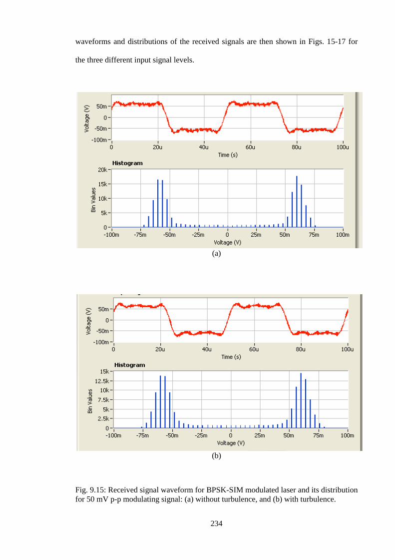
234

waveforms and distributions of the received signals are then shown in Figs. 15-17 for

the three different input signal levels.

(a)

(b)

Fig. 9.15: Received signal waveform for BPSK-SIM modulated laser and its distribution

for 50 mV p-p modulating signal: (a) without turbulence, and (b) with turbulence.

235

(a)

(b)

Fig. 9.16: BPSK-SIM modulated laser received signal waveform and its distribution for

100 mV p-p modulating signal: (a) without turbulence, and (b) with turbulence.

236

(a)

(b)

Fig. 9.17: Received signal waveform for BPSK-SIM modulated laser and its distribution

for 200 mV p-p modulating signal: (a) without turbulence, and (b) with turbulence.

With or without turbulence, it is observed from the figures that signal distribution for

bits „1‟ and „0‟ are similar and are equally spaced on either sides of the zero mark. This

is in contrast to when OOK signalling is used. The threshold position can therefore be

237

fixed at the zero mark and it is not affected by scintillation. This is a clear advantage of

BPSK-SIM over the simple OOK signalling. The results of this experiment can also be

explained in the spectral domain by noting that the scintillation noise power is

concentrated in very low frequencies below 100 Hz [3, 4]. This makes the OOK, which

has a significant portion of its power distribution within the low frequency, susceptible

to scintillation as demonstrated by the experiment. The SIM-BPSK based FSO on the

other hand does not suffer this same fate because its signal spectral distribution is

shifted away from the low frequency region to the frequency of the subcarrier, which is

1 MHz in this experiment.

It can therefore be inferred from the experiment and the analysis of Chapters Five and

Six that in turbulent atmospheric channels, an FSO system with the data directly

impressed on the intensity of the laser irradiance, as is the case in OOK, will suffer from

symbol decision difficulties which will eventually lead to detection errors. An

alternative approach will be to consider modulation schemes that will require no prior

knowledge of turbulence in deciding what symbol has been received. These schemes

include : i) PSK pre-modulated SIM, in which the information is not directly on the

laser intensity but on the phase of the subcarrier signal, ii) polarisation shift keying, in

which the information is placed on the polarization state of the optical beam, iii) or

pulse time modulation techniques, such as pulse position modulation, pulse width

modulation and pulse frequency modulation; in which the information is also not

directly on the beam intensity but on the pulse position, pulse width and the pulse

frequency respectively. The summary of key challenges, including atmospheric

turbulence, associated with optical wireless communication systems as a whole (indoor

and outdoor) are presented in Table 9.3.

238

Table 9.3: Challenges in optical wireless communications

Challenge Cause(s) Effects Mitigation Approach Channel

Inter symbol

interference

(ISI)

Multipath

Propagation

Poor transmission

quality (high BER)

Multipath distortion or

dispersion

Reduced date rates

Channel equalization

Indoor

Forward error control (FEC )

Spread spectrum techniques

Multiple subcarrier

Modulation (More bandwidth

efficient than a single-carrier

system)

OFDM

Multi-beam transmitter

Field of view controlling

Safety

Laser Radiation

Damage to eyes

and skin

Power efficient modulation

schemes: PPM, DPIM, etc.

Both

Use LED, Class 1 lasers,

and 1550 nm wavelength

Noise

Dark current

noise

Low Signal-to-noise

ratio and high BER

Optical and electrical filtering

Pre-amplification

FEC

Low noise post detection

amplifier

Small field of view optical

sources

Optical filter

Both

Shot noise

Background

noise

Thermal noise

Relative

intensity noise

Excess noise

(with APD)

ASE (only if

optical amplifier

is used)

Turbulence

Random

refractive index

variation

Phase and intensity

fluctuations

(scintillation)

FEC (LDPC, Turbo codes)

Robust modulation: SIM, PPM

MIMO

Diversity reception

(temporal and spatial)

Adaptive optics

Outdoor

Image dancing

Spatial coherence

degradation

Beam spreading

Reflection

index

Different

materials

Higher losses due to

reflection on surfaces

Higher transmit power Indoor

Blocking

Furniture

Temporary link outage

Diffuse link

Both Moving objects Cellular system

Walls Multi-beam

Birds Hybrid FSO/RF

Weather

effects

Fog, Rain,

Gases, Smoke,

Aerosols

Attenuations, Scattering

Link outage

Higher transmit power

Hybrid FSO/RF

Outdoor

Pointing,

Acquisition

and Tracking

(PAT)

Mobile link

heads

Building sway

Temporary/permanent

link outage

Power loss

Hybrid FSO/RF

Active tracking Adaptive

optics (beam steering and

tracking)

Outdoor

239

9.5 Summary

For an FSO system operating in a turbulent atmospheric channel, the effect of

scintillation on the receiver decision circuit – the circuit which decides what bit has

been received – has been experimentally verified. In the experiment, a turbulence

simulation chamber is used to mimic a turbulent atmospheric channel. The results of the

experiment show that for an FSO system operating in a turbulent atmospheric channel,

the prior knowledge of the channel fading strength or its statistics is not required in

demodulating and recovering the transmitted data in a BPSK-SIM based FSO system.

This is however not the case for an OOK-FSO, as the signal fluctuation caused by

turbulence affects the position of the symbol detection threshold level. To minimise

detection error in such systems will require increasing in the transmitted power or using

a complex decision circuit that can continually monitor and estimate the channel fading

and noise strengths.

It should be mentioned that in the experiment, the method used to simulate atmospheric

turbulence does not account for signal attenuation due to the molecular constituents of

the atmospheric channel. Also the short length (140 cm) of the turbulence simulation

chamber means that only very weak turbulence could be simulated.

Chapter Ten

Conclusions and Future work

10.1 Conclusions

The main objective for studying the terrestrial FSO communication system is to harness

its potential in addressing the „access network bottle-neck‟. The research reported in this

thesis supports this fundamental objective by investigating and analysing the use of

subcarrier intensity modulation for terrestrial FSO systems as against the prevailing

OOK signalling technique. The motivation behind this is the performance limitation of

OOK modulated FSO in atmospheric turbulence channels. The SIM-FSO has been

proven to overcome this limitation but not without its own shortcomings, which include

241

poor power efficiency and possibility of signal distortion due to intermodulation

distortion.

To be able to carry out the objectives of this research, the fundamental principles of

FSO and its building blocks had to be reviewed and discussed in Chapter Two.

Following this, optical detection was reviewed in Chapter Three, this is important in

understanding the statistical behaviour of transmitted photons. This chapter also

highlighted the process of converting photons to their corresponding electrical signals,

from which the transmitted data can then be extracted. Also, the different types of noise

encountered during optical detection were discussed with the view to understanding the

limit imposed on the system performance by each of them. The review work revealed

that the transmitted photons obey the Poisson distribution and this can be adequately

approximated as the tractable Gaussian distribution for large photoelectron counts as is

the case in terrestrial FSO systems.

A turbulent atmospheric channel causes the intensity of an optical beam travelling

through it to fluctuate randomly due to random changes in refractive index along the

beam‟s path. In Chapter Four, this atmospheric turbulence induced signal fluctuation

was reviewed and three most reported models (log-normal, Gamma-gamma and

negative exponential) were described and their respective pdfs presented. These models

were later used to model the statistical behaviour of the received signal for short to very

long range FSO systems.

In accordance with the research objectives, this thesis has focused on optimising the

system performance during atmospheric turbulence with the use of the phase shift

keying pre-modulated-SIM and in order to reduce the turbulence induced fading

242

penalty, spatial and subcarrier time delay diversity techniques have been explored. From

the BER performance analysis of terrestrial OOK-FSO in the presence of noise and

atmospheric turbulence, it was inferred that atmospheric turbulence: i) causes increased

SNR, which translates into increased transmitted optical power and ii) implies that an

adaptive threshold will be required for optimum performance, as the use of fixed

threshold resulted in a BER floor and sub-optimal error performance. This study also

revealed that in very weak turbulence situations (σl2 < 0.1), increasing the transmitted

power could be used to combat the channel fading. This approach does not work beyond

the very weak regime and alternative techniques will have to be sought.

In order to circumvent the performance limitation of OOK-FSO in turbulent

atmospheric channels and the poor spectral efficiency/requisite slot and symbol

synchronisation requirements of the PPM modulated systems, the SIM-FSO was

proposed and its error performance analysis presented in Chapter Six. The BER and the

outage probability of SIM-FSO across all turbulence regimes, representing short to very

long range systems, were presented in Chapter Seven. On the evidence of the results,

the SIM has been recommended in turbulent channels against the fixed threshold OOK

modulated FSO currently used in commercial terrestrial FSO systems. A SIM-FSO

system does not suffer from BER floor and its decision circuit does not need to track the

channel fading and noise levels continually in order to perform optimally. It has been

found that the turbulent atmosphere does impose power penalties on the system. For

instance, in weak atmospheric turbulence, a BPSK pre-modulated SIM-FSO system will

incur a power penalty of about 5 dB at a BER of 10-6

, and this penalty will rise to ~10

dB when the link error performance level is raised to a BER of 10-9

, this will continue to

rise as the error requirement level is raised. This suggests that the channel fading has to

be mitigated in order to reduce the penalty.

243

This led to the study of diversity techniques in Chapter Seven where the bit error and

outage probabilities of a SIM-FSO system employing spatial diversity to combat the

turbulence induced channel fading were presented. An expression for the BER of an

× -MIMO FSO system operating in a turbulent atmospheric channel was derived.

The error performance and the obtainable link margin using three different linear

combining techniques (MRC, EGC and SelC) were also presented. The use of SelC

linear combining technique in a multiple photodetector system operating in a very weak

turbulent atmospheric channel ( ) would result in negative link margins and is

therefore not suggested as a way of mitigating fading in short range (< 1 km) FSO links.

The MRC technique is optimum but complex to implement while the EGC is simpler to

implement. The diversity gain attainable with the EGC technique is less than 3 dB

inferior compared to the complex MRC. Hence in a photodetector array system, the

EGC is proposed as the preferred linear combining method.

With a turbulence induced fading of strength σl2 = 0.3 and a BER of 10

-6, using a 4 × 4

receiver/transmitter array reduced the required SNR from 25 dB to about 12 dB,

resulting in a gain of 13 dB. This gain will increase with the fading strength and as the

required bit error level is lowered. A reasonable number of independent photodetectors,

appropriate to mitigate scintillation without an overwhelming complexity, is between

two and four based on results presented in this thesis. Using a 2 × 2-MIMO system

required ~0.5 dB of SNR more than using four photodetectors with single transmitter at

BER of 10-6

but spacing an array of 4 photodetectors sufficiently to ensure uncorrelated

irradiance reception is far more demanding than spacing two photodetectors. Also the

use of 4 × 4-MIMO required ~3 dB and ~0.8 dB lower SNR than using four and eight

photodetectors, respectively with single optical transmitter at the same BER of 10-6

.

244

In strong atmospheric fading channels, using 1 × 2-MIMO configuration was predicted

to result in ~12 dB diversity gain and as the turbulence strength increases into the

saturation regime, the gain in electrical SNR exceeds 40 dB at the same BER of 10-6

.

However the diversity gain thus depends on the performance metric used, when the

outage probability metric is considered, the gain is generally lower. At a Pout of 10-6

during the saturation regime, the predicted gain was ~28 dB for a similar 1 × 2-MIMO

configured SIM-FSO but the general trend of the gain, with respect to the turbulence

strength and source/detector configuration, are the same for both the BER and Pout

metrics.

In the spatial diversity technique, whenever the photodetectors are closer together than

the spatial correlation distance of the field travelling through the turbulent channel, the

received signals become correlated. This raises the possibility of all the photodetectors

in the array experiencing deep fades simultaneously, thereby jeopardising the primary

aim of using spatial diversity. This effect has been verified and reported in chapter

seven, in a single transmitter and two photodetectors system at , a correlation

coefficient of 0.6 between the received signals was predicted to cause a 3 dB reduction

in the expected diversity gain at a BER of 10-6

. The reduction in the diversity gain

increased to over 4 dB in a SIM-FSO with 1 × 3-MIMO configuration and this penalty

is bound to increase as the received signals become more correlated.

The subcarrier TDD as an alternative/complementary technique for ameliorating the

channel fading was proposed in Chapter Seven. The idea is to retransmit delayed copies

of the data/information on different subcarriers. The results showed that up to 3 dB

improvement in receiver sensitivity can be achieved by retransmitting the delayed copy

of the data five times in a channel of turbulence strength . However,

245

retransmitting just once, on a different subcarrier frequency, was found to be the

optimum approach with a gain of up to 4.5 dB in weak atmospheric turbulence.

Expectedly, the TDD gain is proportional to the fading strength but independent of the

data rate.

In order to increase the system throughput/capacity, multiple SIM was also studied.

This however comes at a price, the SNR required to achieve say a BER of 10-6

with five

subcarriers is about 40 dB in a channel with a fading strength σl2 of 0.3. This increases

to about 46 dB with 10 subcarriers under the same conditions, depicting a (dB)

increment over the SNR required to attain the same level of error performance with a

single subcarrier. The multiple SIM-FSO should therefore only be considered when the

quest to achieve a higher throughput outweighs its accompanying power penalty.

In addition, the intermodulation effect due to the optical source non-linearity was

studied and the number of in-band intermodulation products calculated. This

investigation is particularly helpful in subcarrier frequency planning. The results of the

analysis can be used in leaving-out certain subcarrier frequencies (out of a range of

frequencies) that have high numbers of in-band intermodulation products. Also

presented were criteria that could be used to optimise the optical modulation index, this

is with the view to improving the system performance in the face of intermodulation

distortion and multiple subcarriers. It has been found out that IMD, caused by optical

source nonlinearity, imposes a limit on the achievable BER of a SIM-FSO. It should

hence be ensured that a linear laser source (one with negligible nonlinearity) is used to

transmit a multiple subcarrier multiplexed signal.

246

From the error performance analyses presented, the power required to achieve a given

level of performance could be obtained. These were then used in Chapter Nine to

estimate the power limited link range of a SIM-FSO. The results predicted that,

achieving a 4 km SIM-FSO link length with no diversity technique will require about 12

dB of power more than using a 4 × 4 – MIMO configured system with the same data

rate and channel conditions. If the link is however operated at a 5 dB link margin in

clear atmosphere, the predicted link ranges are 2.5 km, 0.8 km and 0.6 km for a 4 × 4 –

MIMO, 1-TDD and no diversity configuration respectively.

In Chapter Nine, a turbulence simulating chamber was used to demonstrate the

atmospheric turbulence effect on symbol detection with both OOK and BPSK-SIM

modulated FSO systems. From the experimental results for an OOK-FSO system, it was

observed that in the absence of turbulence, the threshold level can be fixed at the zero

signal level but this is no longer the case as soon as turbulence sets in. During

turbulence, finding the exact decision threshold level that will minimize detection error

will require knowledge of the turbulence strength. What this means in essence is that an

adaptive threshold will be required for the OOK modulated FSO system to perform

optimally. The practical implementation of such an FSO system with adaptive threshold

is not trivial, as the design will involve a continual tracking of both the scintillation and

noise levels. A similar inference was theoretically arrived at in Chapter Five. Moreover,

increasing the input signal/transmitted power level can be used to combat the effect of

very weak turbulence on the position of the symbol detection threshold level. Increasing

the transmitted power will work fine for short range FSO links, for long range systems

(> 1 km), this approach will have a limited impact and the fact that the transmitted

power is premium and the existence of a limit on the amount of power that can be safely

transmitted through the atmosphere further limits the use of increased power as a way of

247

mitigating atmospheric turbulence effect. For a BPSK pre-modulated SIM-FSO system

on the other hand, the experimental results confirmed that the position of the threshold

level is indeed independent of fading strength of the turbulent atmosphere. This is a

clear advantage of BPSK-SIM over an OOK modulated FSO link.

In conclusion, the performance of PSK pre-modulated SIM-FSO systems has been

investigated in the presence of atmospheric turbulence and its error rate/outage

probability expressions derived for different channel conditions. The SIM-FSO system

has been experimentally and theoretically compared with the classical OOK based FSO

systems in the presence of atmospheric turbulence. The SIM-FSO is advantageous in

that its decision circuit, unlike the OOK-FSO, does not require knowledge of the

atmospheric turbulence strength or its statistics to perform optimally. For FSO systems

spanning over 1 km, the effect of channel fading caused by atmospheric turbulence

becomes significant and can be mitigated (via diversity techniques) to prevent loss of

data, excessive power requirements, increased error rate and link outage.

10.2 Recommendations for Future Work

Although the objectives listed in chapter one of this thesis have been achieved, the work

was never envisaged to be self contained and comprehensive to cover the entire optical

wireless communications research areas. Since the amount of work and time required to

do so is beyond the scope of this thesis, the author will now be recommending further

works, which can be carried out to extend the work reported here.

Radio over FSO (RoFSO): As a straight forward progression of the work presented

here, the study and experimental demonstration of RoFSO could prove very useful.

248

This, potentially, will provide interesting findings regarding the integration of FSO with

radio over fibre signals and cable television networks. This RoFSO experiment, which

is in principle a multiple subcarrier system, can further prove the suitability/viability of

subcarrier modulated FSO as a tool for increasing communication systems capacity

and/or throughput.

Pulse interval modulated FSO: As an alternative solution to one of the findings

reported in this thesis - that encoding the data directly on the intensity of an optical

source, as is the case in OOK signalling technique, is sub-optimum in fading channels -

an investigation of pulse interval modulated FSO systems in turbulent channels will be

recommended. In pulse interval modulation, the data is encoded on the interval between

pulses, this technique might provide an alternative solution for the complex symbol

decision circuit needed for an optimum OOK-FSO system in turbulent atmospheric

channels.

Polarisation shift keying modulated FSO: It has been reported in this thesis that a

turbulent atmospheric channel does not result in change of polarisation state of a

traversing field. This fact can be explored by encoding data on the polarisation state of

an optical beam. The polarisation modulation technique has been studied in fibre

communication systems but is not very attractive in that area because an optical fibre

causes random changes in the polarisation state of an optical beam travelling through it.

Hybrid FSO/RF communication: The availability of FSO, especially links longer

than 1 km, depends so much on the atmospheric weather conditions. The attainment of

99.99 % availability during thick fog is still a challenge and to address this, one option

will be to combine an FSO link with an RF system as a back-up at reduced data rate.

Since the frequency range used in FSO is not licensed, it will be suggested that a licence

249

free frequency should be used for the RF back-up. This is to ensure the whole system

remains free from licence fee and bureaucracy.

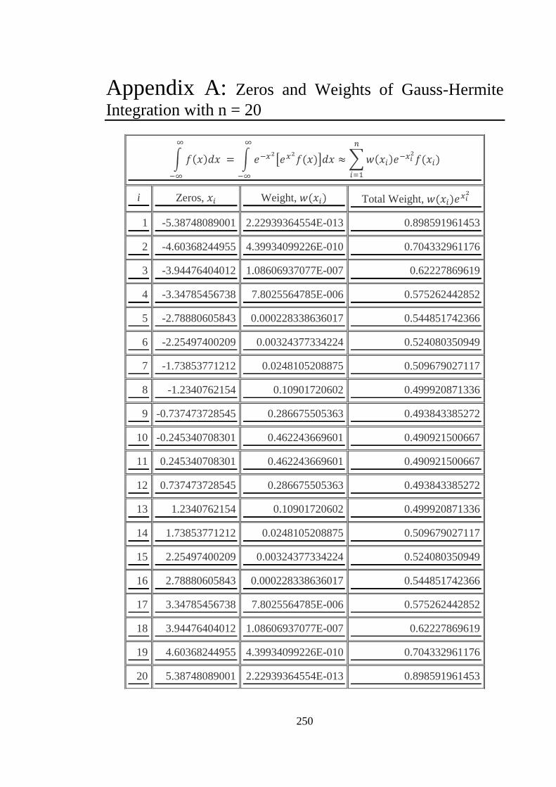
250

Appendix A: Zeros and Weights of Gauss-Hermite

Integration with n = 20

i Zeros, Weight, Total Weight,

1 -5.38748089001 2.22939364554E-013 0.898591961453

2 -4.60368244955 4.39934099226E-010 0.704332961176

3 -3.94476404012 1.08606937077E-007 0.62227869619

4 -3.34785456738 7.8025564785E-006 0.575262442852

5 -2.78880605843 0.000228338636017 0.544851742366

6 -2.25497400209 0.00324377334224 0.524080350949

7 -1.73853771212 0.0248105208875 0.509679027117

8 -1.2340762154 0.10901720602 0.499920871336

9 -0.737473728545 0.286675505363 0.493843385272

10 -0.245340708301 0.462243669601 0.490921500667

11 0.245340708301 0.462243669601 0.490921500667

12 0.737473728545 0.286675505363 0.493843385272

13 1.2340762154 0.10901720602 0.499920871336

14 1.73853771212 0.0248105208875 0.509679027117

15 2.25497400209 0.00324377334224 0.524080350949

16 2.78880605843 0.000228338636017 0.544851742366

17 3.34785456738 7.8025564785E-006 0.575262442852

18 3.94476404012 1.08606937077E-007 0.62227869619

19 4.60368244955 4.39934099226E-010 0.704332961176

20 5.38748089001 2.22939364554E-013 0.898591961453

251

Appendix B: Mean and variance of the sum of log-

normal distribution

By definition a log-normal distributed variable is given by , where l obeys

normal distribution. Let sum of independent log normal distributed irradiance be

another log normal distribution [129], that is:

(B1)

For identically distributed log normal random variable [129], and

.

From [47],

(B2)

Substituting (B2) into (B1) results in:

(B3)

The expectation of log normal random variable I is given by:

(B4)

Note that , therefore from which the log intensity mean, ,

is found as:

(B5)

It follows from the foregoing that:

252

And having normalising equation (B6) reduces to:

The second central moment of a log-normal random variable I is given by:

Substituting equation (B5) into (B8) and invoking the relation given by (B2) results in:

This implies that:

Hence:

And

(B6)

(B7)

(B8)

(B9)

(B10)

(B11)

(B12)

(B13)

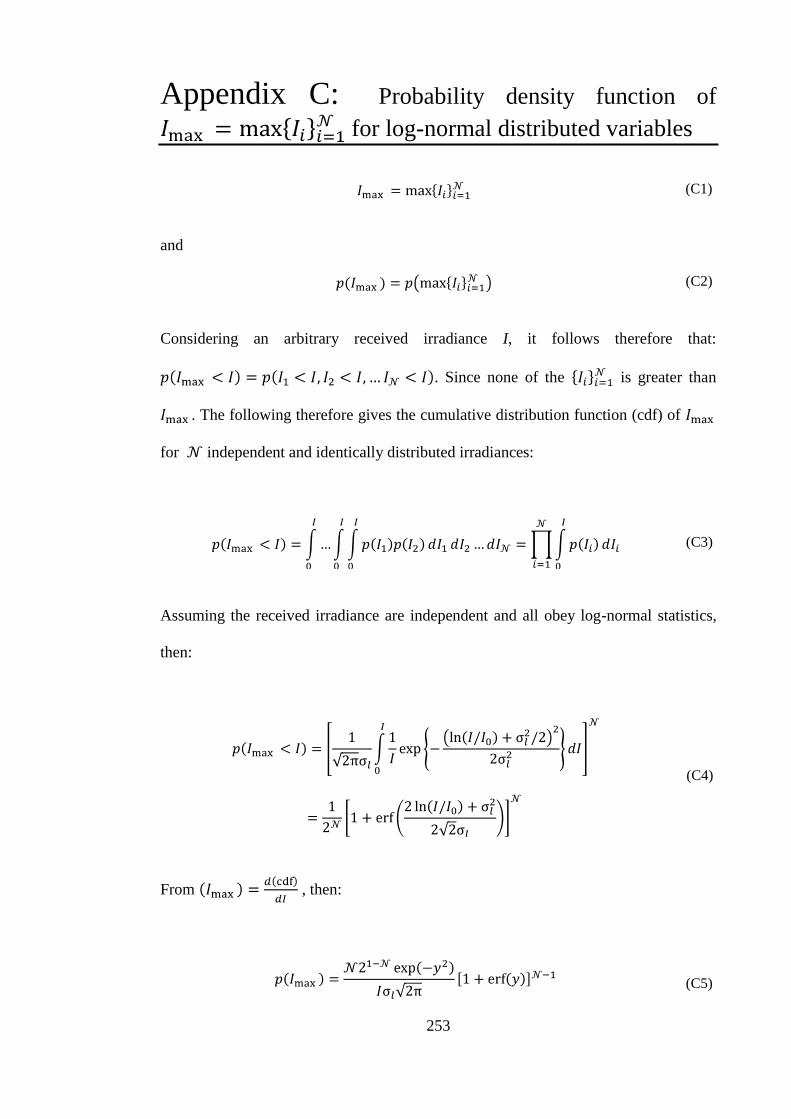
253

Appendix C: Probability density function of

for log-normal distributed variables

(C1)

and

(C2)

Considering an arbitrary received irradiance I, it follows therefore that:

. Since none of the is greater than

. The following therefore gives the cumulative distribution function (cdf) of

for independent and identically distributed irradiances:

(C3)

Assuming the received irradiance are independent and all obey log-normal statistics,

then:

(C4)

From , then:

(C5)

254

where . With equation (C5) returns the log-normal

distribution as would be expected.

255

Appendix D: Probability density function of

for negative exponential distributed variables

(D1)

and

(D2)

Considering an arbitrary received irradiance I, it follows therefore that:

. Since none of the is greater than

. The following therefore gives the cumulative distribution function (cdf) of

for independent and identically distributed irradiances:

(D3)

Assuming the received irradiance are independent and all obey negative exponential

statistics, then:

(D4)

From , then:

(D5)

256

With equation (D5) returns the negative exponential distribution as would be

expected.

257

References

[1] D. Killinger, "Free space optics for laser communication through the air," Optics

& Photonics News, vol. 13, pp. 36-42, Oct. 2002.

[2] A. G. Bell, "On the production and reproduction of sound by light," American

Journal of Sciences, vol. Series 3, pp. 305 - 324, Oct. 1880.

[3] F. E. Goodwin, "A review of operational laser communication systems,"

Proceedings of IEEE, vol. 58, pp. 1746-1752, Oct. 1970.

[4] H. Hemmati, "Interplanetary laser communications," Optics and Photonics

News, vol. 18, pp. 22-27, Nov. 2007.

[5] S. Zoran, F. Bernhard, and L. Hanspeter, "Free-space laser communication

cctivities in Europe: SILEX and beyond," IEEE Lasers and Electro-Optics

Society (LEOS ) 19th Annual Meeting pp. 78-79, Oct. 2006.

[6] H. Hemmati, "Deep Space Optical Communications," in Deep space

communications and navigation series Canifornia: Wiley-Interscience, 2006.

[7] S. Hardy, "Free-space optics systems are finding their niches," Lightwave pp.

33-36, Dec. 2005.

[8] C. P. Colvero, M. C. R. Cordeiro, G. V. de Faria, and J. P. von der Weid,

"Experimental comparison between far- and near infrared wavelenghts in free

space optical systems," Microwave and Optical Technology Letters, vol. 46, pp.

319-323, Aug. 2005.

[9] R. Dennis, L. Mark, G. Ganesh, P. Bruce, and N. Gerald, "Optical wireless

propagation, theory vs eperiment," Proceedings of SPIE: Optical Wireless

Communications III, vol. 4214, pp. 38-45, 2001.

[10] E. Korevaar, I. I. Kim, and B. McArthur, "Atmospheric propagation

characteristics of highest importance to commercial free space optics,"

Proceeding of SPIE, vol. 4976, pp. 1-12, 2003.

[11] D. Song, et al., "4 × 10 Gb/s terrestrial optical free space transmission over 1.2

km using an EDFA preamplifier with 100 GHz channel spacing," Optics

Express, vol. 7, pp. 280-284, Oct. 2000.

[12] B. Flecker, E. Leitgeb, S. Sheikh Muhammad, C. Chlestil, E. Duca, and V.

Carrozzo, "Measurement of light attenuation in fog and snow conditions for

terrestrial FSO links," 15th IST Mobile and Wireless Communications Summit,

June 2006.

[13] M. D‟Amico, A. Leva, and B. Micheli, "Free-space optics communication

systems: first results from a pilot field-trial in the surrounding area of Milan,

Italy," IEEE Microwave and Wireless Components Letters, vol. 13, pp. 305-307,

Aug. 2003.

[14] J. D. Montgomery, "Free-space optics seen as viable alternative to cable,"

Lightwave (Analyst Corner), pp. 43-44, April 2004.

[15] Isaac I. Kim, Bruce McArthur, and E. Korevaar, "Comparison of laser beam

propagation at 785 nm and 1550 nm in fog and haze for optical wireless

communications," SPIE Proceeding: Optical Wireless Communications III, vol.

4214, pp. 26-37, 2001.

[16] M. Bettayeb and S. F. A. Shah, "State of the art ultra-wideband technology for

communication systems: a review," Proceedings of the 10th IEEE International

258

Conference on Electronics, Circuits and Systems, (ICECS), vol. 3, pp. 1276 -

1279, 2003.

[17] J. N. Pelton, "Global satellite communications technology and systems,"

International Technology Research Institute, World Technology (WTEC)

Division, Baltimore Dec. 1998.

[18] I. Kim, "10 G FSO systems position technology for the future," Lightwaveonline

pp. 19-21, July 2009.

[19] K. Kazaura, K. Omae, T. Suzuki, M. Matsumoto, E. Mutafungwa, T. Murakami,

K. Takahashi, H. Matsumoto, K. Wakamori, and Y. Arimoto, "Performance

evaluation of next generation free-space optical communication system," IEICE

Transaction of Electronics, vol. E90-C, pp. 381-388, Feb. 2007.

[20] H. Willebrand and B. S. Ghuman, Free Space Optics: Enabling Optical

Connectivity in today's network. Indianapolis: SAMS publishing, 2002.

[21] BuddeComm, "Global - Broadband - FTTH overview & statistics," May 2009.

[22] C.-H. Cheng, "Signal processing for optical communication," IEEE Signal

Processing Magazime, pp. 88-94, Jan. 2006.

[23] C. C. Davis, I. I. Smolyaninov, and S. D. Milner, "Flexible optical wireless links

and networks," IEEE Communications Magazine, vol. 41, pp. 51-57, March

2003.

[24] A. Nordbotten, "LMDS systems and their application," IEEE Communications

Magazine, vol. 38, pp. 150 -154, 2000.

[25] R. C. Qiu, H. Liu, and X. Shen, "Ultra-wideband for multiple access

communications," IEEE Communications Magazine, vol. 43, pp. 80-87, 2005.

[26] D. Kedar and S. Arnon, "Optical wireless communication through fog in the

presence of pointing errors," Applied Optics, vol. 42, pp. 4946-4954, Aug. 2003.

[27] T. Kamalakis, T. Sphicopoulos, S. Sheikh Muhammad, and E. Leitgeb,

"Estimation of power scintillation statistics in free space optical links using the

multi canonical monte carlo method," IEEE International Symposium on

Communication Systems, Networks and Digital Signal Processing (CSNDSP)

pp. 629-633, July 2006.

[28] D. Kedar and S. Arnon, "Urban optical wireless communication networks: the

main challenges and possible solutions," IEEE Communications Magazine, vol.

42, pp. s2-s7, May 2004.

[29] X. Zhu and J. M. Kahn, "Free-space optical communication through atmospheric

turbulence channels," IEEE Transactions on Communications, vol. 50, pp. 1293-

1300, Aug. 2002.

[30] S. Karp, R. M. Gagliardi, S. E. Moran, and L. B. Stotts, Optical Channels:

fibers, clouds, water and the atmosphere. New York: Plenum Press, 1988.

[31] S. Bloom, E. Korevaar, J. Schuster, and H. Willebrand, "Understanding the

performance of free-space optics," Journal of Optical Networking, vol. 2, pp.

178-200, June 2003.

[32] W. K. Pratt, Laser Communication Systems, 1st ed. New York: John Wiley &

Sons, Inc., 1969.

[33] D. Kedar and S. Arnon, "Optical wireless communication through fog in the

presence of pointing errors," Applied Optics, vol. 42, pp. 4946-4954, Aug. 2003.

[34] S. Bloom and W. S. Hartley, "The last-mile solution: Hybrid FSO radio," in

AirFiber, Inc. White paper,

http://www.freespaceoptic.com/WhitePapers/Hybrid_FSO.pdf, last visited:

16th July 2007.

[35] B. Flecker, M. Geghart, E. Leitgeb, S. Sheikh Muhammad, and C. Chlestil,

"Results of attenuation-measurements for optical wireless channels under dense

259

fog conditions regarding different wavelengths " Prococeeding of SPIE vol.

6303, pp. 1-11, 2006.

[36] M. al Naboulsi and H. Sizun, "Fog attenuation prediction for optical and infrared

waves," Optical Engineering, vol. 23, pp. 319-329, 2004.

[37] E. Leitgeb, S. Sheikh Muhammad, B. Flecker, C. Chlestil, M. Geghart, and T.

Javornik, "The influence of dense fog on optical wireless systems, analysed by

measurements in Graz for improving the link-reliability," IEEE- ICTON

Conference, pp. 154-159, June 2006.

[38] E. J. McCartney, Optics of The Atmosphere. New York: J. Wiley and Sons,

1976.

[39] P. P. Smyth, P. L. Eardley, K. T. Dalton, D. R. Wisely, P. Mckee, and D. Wood,

"Optical wireless - a prognosis," Wireless Data Transmission, Proceeding of

SPIE, vol. 2601, pp. 212-225, 1995.

[40] J. T. Li and M. Uysal, "Optical wireless communications: System model,

capacity and coding," Vehicular Technology Conference, vol. 1, pp. 168-172,

2003.

[41] I. Hossein, E. Tamer, K. Vikas, D. Frank, and R. B. K, "High-availability free

space optical and RF hybrid wireless networks," IEEE Wireless

Communications vol. 10, pp. 45-53, April 2003.

[42] I. I. Kim, M. Mitchell, and E. J. Korevaar, "Measurement of scintillation for

free-space laser communication at 785 nm and 1550 nm," Optical Wireless

Communications II, Proceedings of SPIE, vol. 3850, pp. 49-52, 1999.

[43] I. I. Kim, J. Koontz, H. Hakakha, P. Adhikari, R. Stieger, C. Moursund, M.

Barclay, A. Stanford, R. Ruigrok, J. J. Schuster, and E. J. Korevaar,

"Measurement of scintillation and link margin for the TerraLink laser

communication system," Wireless Technology and Systems: Millimeter Wave

and Optical, Proceedings of SPIE, vol. 3232, pp. 100-118, 1997.

[44] V. W. S. Chan, "Free-space optical communications," IEEE Journal of

Lightwave Technology, vol. 24, pp. 4750-4762, Dec. 2006.

[45] G. R. Osche, Optical Detection Theory for Laser Applications. New Jersey:

Wiley, 2002.

[46] S. Karp, E. L. O'Neill, and R. M. Gagliardi, "Communication theory for the free-

space optical channel," Proceedings of the IEEE, vol. 58, pp. 1626-1650, 1970.

[47] J. W. Goodman, Statistical Optics. New York: John Wiley, 1985.

[48] M. Uysal, J. T. Li, and M. Yu, "Error rate performance analysis of coded free-

space optical links over gamma-gamma atmospheric turbulence channels," IEEE

Transactions on Wireless Communications, vol. 5, pp. 1229-1233, June 2006.

[49] L. C. Andrews, R. L. Phillips, and C. Y. Hopen, Laser beam scintillation with

applications. Bellingham: SPIE, 2001.

[50] L. C. Andrews and R. L. Phillips, Laser beam propagation through random

media, second ed. Washington: SPIE Press, 2005.

[51] X. Zhu and J. M. Kahn, "Performance bounds for coded free-space optical

communications through atmospheric turbulence channels," IEEE Transaction

on Communications, vol. 51, pp. 1233-1239, Aug. 2003.

[52] X. Zhu and J. M. Kahn, "Mitigation of turbulence-induced scintillation noise in

free-space optical links using temporal-domain detection techniques " IEEE

Photonics Technology Letters, vol. 15, pp. 623-625, 2003.

[53] I. B. Djordjevic, B. Vasic, and M. A. Neifeld, "Multilevel coding in free-space

optical MIMO transmission with Q-ary PPM over the atmospheric turbulence

channel," IEEE Photonics Technology Letters, vol. 18, pp. 1491-1493, 2006.

260

[54] K. Kiasaleh, "Performance of APD-based, PPM free-space optical

communication systems in atmospheric turbulence," IEEE Transactions on

Communications, vol. 53, pp. 1455-1461, Sept. 2005.

[55] S. G. Wilson, M. Brandt-Pearce, Q. Cao, and J. H. Leveque, "Free-space optical

MIMO transmission with Q-ary PPM," IEEE Transactions on Communications,

vol. 53, pp. 1402-1412, Aug. 2005.

[56] S. Sheikh Muhammad, T. Javornik, I. Jelovcan, Z. Ghassemlooy, and E.

Leitgeb, "Comparison of hard-decision and soft-decision channel coded M-ary

PPM performance over free space optical links," European Transaction on

Telecommunications, pp. 12, DOI: 10.1002/ett.1343, 2008.

[57] M. A. Al-Habash, L. C. Andrews, and R. L. Phillips, "Mathematical model for

the irradiance probability density function of a laser beam propagating through

turbulent media," Optical Engineering, vol. 40, pp. 1554-1562, 2001.

[58] A. Garcia-Zambrana, "Error rate performance for STBC in free-space optical

communications through strong atmospheric turbulence," IEEE Communication

Letters, vol. 11, pp. 390-392, May 2007.

[59] M. Uysal, S. M. Navidpour, and J. T. Li, "Error rate performance of coded free-

space optical links over stong turbulence channels," IEEE Communication

Letters, vol. 8, pp. 635-637, 2004.

[60] X. Zhu and J. M. Kahn, "Pairwise codeword error probability for coded free-

space optical communication through atmospheric turbulence channels," IEEE

International Conference on Communications (ICC), vol. 1, pp. 161-164, 2001.

[61] M. Razavi and J. H. Shapiro, "Wireless optical communications via diversity

reception and optical preamplification," IEEE Transaction on Communications,

vol. 4, pp. 975-983, 2005.

[62] S. M. Navidpour, M. Uysal, and L. Jing, "BER performance of MIMO free-

space optical links," 60th IEEE Vehicular Technology Conference, vol. 5, pp.

3378-3382, 2004.

[63] Q. Cao, M. Brandt-Pearce, S. G. Wilson, and L. C. Brown, "Free-space optical

MIMO system using an optical pre-amplifier," IEEE Global

Telecommunications Conference pp. 1-5, Nov. 2006.

[64] S. M. Navidpour, M. Uysal, and M. Kavehrad, "BER performance of free-space

optical transmission with spatial diversity," IEEE Transaction on

Communications, vol. 6, pp. 2813-2819, 2007.

[65] I. I. Kim, H. Hakakha, P. Adhikari, E. Korevaar, and A. K. Majumdar,

"Scintillation reduction using multiple transmitters," Proceeding of SPIE, vol.

2990, pp. 102-113, 1997.

[66] S. Rosenberg and M. C. Teich, "Photocounting array receivers for optical

communication through the lognormal atmospheric channel: error bound for M-

ary equal energy orthogonal signalling," IEEE Transaction on Information

Theory, vol. IT-19, pp. 807-809, Nov. 1973.

[67] M. Abtahi, P. Lemieux, W. Mathlouthi, and L. A. Rusch, "Supprression of

turbulence-induced scintillation in free-space optical communication systems

using saturated optical amplifiers," Journal of Lightwave Technology, vol. 24,

pp. 4966-4973, Dec. 2006.

[68] J. Elon Grave and S. Drenker, "Advancing Free space Optical communication

with Adaptive optics," Lightwaveonline, vol. 19, pp. 105-113, Sept. 2002.

[69] I. B. Djordjevic, B. Vasic, and M. A. Neifeld, "LDPC coded OFDM over the

atmospheric turbulence channel," Optical Express, vol. 15, pp. 6336-6350, 2007.

[70] H. Yamamoto and T. Ohtsuki, "Atmospheric optical subcarrier modulation

systems using space-time block code," in IEEE Global Telecommunications

Conference, (GLOBECOM '03) vol. 6, New York, pp.3326-3330, 2003.

261

[71] E. J. Lee and V. W. S. Chan, "Optical communications over the clear turbulent

atmospheric channel using diversity," IEEE Journal on Selected Areas in

Communications, vol. 22, pp. 1896-1906, Nov. 2004.

[72] D. Rockwell, A. and S. Mecherle, G., "Optical wireless: Low-cost, broadband,

optical access," www.freespaceoptic.com/WhitePapers/optical_wireless.pdf,

last visited 11 Sept. 2009.

[73] A. K. Majumdar and J. C. Ricklin, Free-Space Laser Communications:

Principles and Advances. New York: Springer, 2008.

[74] A. Pavelchek, R. G. Trissel, J. Plante, and S. Umbrasas, "Long-wave infrared

(10-μm) free-space optical communication system " Free-Space Laser

Communication and Active Laser Illumination III, vol. 5160, pp. 247-252, Jan.

2004.

[75] A. McCuaig, "Free-space optics: LEDs vs lasers," in Lightwaveonline:

PennWell, 2009.

[76] Practel, "Free space optics - from wireless fiber to visible light

communications," Practel, Inc. July 2009.

[77] G. Keiser, Optical Communications Essentials 1st ed. New York: McGraw-Hill

Professional, 2003.

[78] O. Bouchet, H. Sizun, C. Boisrobert, F. De Fornel, and P. Favennec, Free-Space

Optics: Propagation and Communication. London: ISTE Ltd, 2006.

[79] R. M. Gagliardi and S. Karp, Optical Communications, 2nd ed. New York: John

Wiley, 1995.

[80] AFGL, "AFGL Atmospheric Constituent Profiles (0–120 km), ," AFGL-TR-86-

0110, Air Force Geophysics Laboratory, Hanscom Air Force Base,

Massachusetts, 1986.

[81] M. Jeganathan and P. Ionov, "Multi-gigabits-per-second optical wireless

communications," Optical Crossing,

http://www.freespaceoptic.com/WhitePapers/Jeganathan%20%20(Optical%20C

rossing).pdf , last visited 20th May 2009.

[82] S. Betti, G. De marchis, and E. Iannone, Coherent Optical Communication

Systems, 1st ed. Canada: John Wiley and Sons Inc., 1995.

[83] S. Hranilovic, Wireless Optical Communication Systems vol. 1st. Boston:

Springer, 2005.

[84] IEC, "Safety of laser products - Part 1: Equipment classification and

requirements," 2nd ed: International Electrotechnical Commission, 2007.

[85] D. J. T. Heatley, D. R. Wisely, I. Neild, and P. Cochrane, "Optical wireless: The

story so far," IEEE Communications Magazine, vol. 36, pp. 72-82, Dec. 1998.

[86] K. Schröder, "Handbook on Industrial laser safety ": Technical University of

Vienna, 2000.

[87] J. M. Senior, Optical Fiber Communications Principles and Practice, 3rd ed.

Essex: Pearson Education Limited, 2009.

[88] G. Keiser, Optical Fiber Communications, 3rd ed. New York: McGraw-Hill

2000.

[89] N. S. Kopeika and J. Bordogna, "Background noise in optical communication

systems," Proceedings of the IEEE, vol. 58, pp. 1571-1577, 1970.

[90] S. F. Clifford, "The classical theory of wave propagation in a turbulent

medium," in Laser Beam Propagation in the Atmosphere, J. W. Strobehn, Ed.:

Springer-Verlag, 1978.

[91] A. Kolmogorov, "Turbulence," in Classic Papers on Statistical Theory, S. K.

Friedlander and L. Topper, Eds. New York: Wiley-Interscince, 1961.

262

[92] A. Kolmogorov, "The local structure of turbulence in incompressible viscous

fuid for very large Reynold numbers," Proceeding of Royal Society of London

Series A- Mathematical and Physical, vol. 434, pp. 9-13, 1991.

[93] V. I. Tatarski, Wave propagation in a turbulent medium. (Translated by R.A.

Silverman) New York: McGraw-Hill 1961.

[94] A. Ishimaru, "The beam wave case and remote sensing," in Topics in Applied

Physics: Laser Beam Propagation in the Atmosphere. vol. 25 p.134 New York:

Springer-Verlag, 1978.

[95] H. Hodara, "Laser wave propagation through the atmosphere," Proceedings of

the IEEE, vol. 54, pp. 368-375, March 1966.

[96] J. W. Strohbehn, "Line-of-sight wave propagation through the turbulent

atmosphere," Proceedings of the IEEE, vol. 56, pp. 1301-1318, Aug. 1968.

[97] J. W. Strobehn and S. F. Clifford, "Polarisation and angle of arrival fluctuations

for a plane wave propagated through turbulent medium," IEEE Transaction on

Antennas Propagation, vol. AP-15, p. 416, 1967.

[98] H. D.H., "Depolarisation of laser beam at 6328 Angstrom due to atmospheric

transmission," Applied Optics, vol. 8, p. 367, Feb. 1969.

[99] W. O. Popoola, Z. Ghassemlooy, and E. Leitgeb, "Free-space optical

communication using subcarrier modulation in gamma-gamma atmospheric

turbulence," 9th International Conference on Transparent Optical Networks

(ICTON '07) vol. 3, pp. 156-160, July 2007.

[100] J. H. Churnside and S. F. Clifford, "Log-normal Rician probability density

function of optical scintillations in the turbulent atmosphere," Journal of Optical

Society of America, vol. 4, pp. 1923-1930, Oct. 1987.

[101] L. C. Andrews and R. L. Phillips, "I-K distribution as a universal propagation

model of laser beams in atmospheric turbulence," Journal of optical society of

America A, vol. 2, p. 160, Feb. 1985.

[102] G. Parry and P. N. Pusey, "K distributions in atmopsheric propagation of laser

light," Journal of Optical Society of America, vol. 69, pp. 796-798, 1979.

[103] S. F. Clifford and R. J. Hill, "Relation between irradiance and log-amplitude

variance for optical scintillation described by the K distribution," Journal of

Optical Society of America, vol. 71, pp. 112-114, 1981.

[104] S. Sheikh Muhammad, W. Gappmair, and E. Leitgeb, "PPM channel capacity

evaluation for terrestrial FSO links," International Workshop on Satellite and

Space Communications, pp. 222-226, Sept. 2006.

[105] W. O. Popoola, Z. Ghassemlooy, M. S. Awan, and E. Leitgeb, "Atmospheric

channel effects on terrestrial free space optical communication links," 3rd

International Conference on Computers and Artificial Intelligence (ECAI 2009),

pp. 17-23, July 2009.

[106] W. O. Popoola, Z. Ghassemlooy, J. I. H. Allen, E. Leitgeb, and S. Gao, "Free-

space optical communication employing subcarrier modulation and spatial

diversity in atmospheric turbulence channel," IET Optoelectronic, vol. 2, pp. 16-

23, 2008.

[107] T. Ohtsuki, "Multiple-subcarrier modulation in optical wireless

communications," IEEE Communications Magazine, pp. 74-79, March 2003.

[108] I. B. Djordjevic and B. Vasic, "100-Gb/s transmission using orthogonal

frequency -division multiplexing," IEEE Photonics Technology Letters, vol. 18,

pp. 1576-1578, Aug. 2006.

[109] G. P. Agrawal, Fiber-Optic Communication Systems, 3rd ed. New york: Wiley-

Interscience, 2002.

263

[110] H. Rongqing, Z. Benyuan, H. Renxiang, T. A. Christopher, R. D. Kenneth, and

R. Douglas, "Subcarrier multiplexing for high-speed optical transmission,"

Journal of Lightwave Technology, vol. 20, pp. 417-424, 2002.

[111] R. You and J. M. Kahn, "Average power reduction techniques for multiple-

subcarrier intensity-modulated optical signals," IEEE Transaction on

Communications, vol. 49, pp. 2164-2171, 2001.

[112] S. Teramoto and T. Ohtsuki, "Multiple-subcarrier optical communication

systems with peak reduction carriers," in IEEE Global Telecommunications

Conference (GLOBECOM) vol. 6, pp. 3274-3278, 2003.

[113] S. Teramoto and T. Ohtsuki, "Multiple-subcarrier optical communication

systems with subcarrier signal-point sequence," IEEE Transactions on

Communications, vol. 53, pp. 1738-1743, 2005.

[114] J. G. Proakis, Digital Communications. New York: McGraw-Hill, 2004.

[115] M. K. Simon and M.-S. Alouini, Digital Communication Over Fading Channels,

2nd ed. New York: John Wiley & Sons Inc., 2004.

[116] M. Abramowitz and I. S. Stegun, Handbook of Mathematical functions with

formulars, graphs and mathematical tables: Dover, 1977.

[117] W. O. Popoola, Z. Ghassemlooy, and E. Leitgeb, "BER performance of DPSK

subcarrier modulated free space optics in fully developed speckle," in 6th

International Symposium on Communication Systems, Networks and Digital

Signal Processing, (CNSDSP), Graz, Austria, pp. 273-277, 2008.

[118] I. S. Gradshteyn and I. M. Ryzhik, Table of integrals, series, and products, 5th

ed. London: Academic Press, Inc., 1994.

[119] W. Huang and M. Nakagawa, "Nonlinear effect of direct-sequence CDMA in

optical transmission," Global Telecommunications Conference, GLOBECOM,

San Francisco, vol. 2, pp. 1185-1189, 1994.

[120] J. Daly, "Fiber optics intermodulation distortion," IEEE Transaction on

Communications, vol. COM-30, pp. 1954-1958, 1982.

[121] M. Abuelma'atti, "Carrier-to-intermodulation performance of multiple FM/FDM

carriers through a GaA1As hetrojunction laser diode," IEEE Transactions on

Communications, vol. 33, pp. 246-248, 1985.

[122] K. Stubkjaer and M. Danielsen, "Nonlinearities of GaAlAs lasers-Harmonic

distortion," IEEE Journal of Quantum Electronics, vol. QE-16, pp. 531-537,

1980.

[123] T. L. Paoli, "Nonlinearities in the emission characteristics of stripe-geometry

(AlGa)As double heterostructure junction lasers," IEEE Journal of Quantum

Electronics, vol. QE-12, pp. 770-776, 1976.

[124] J. Buus, "Multimode field theory explanation of kinks in the characteristics of

DH lasers," IEE Electronic Letters, vol. 14, pp. 127-128, 1978.

[125] I. I. Kim and E. Korevaar, "Availability of free space optics and hybrid FSO/RF

systems," Proceedings of SPIE: Optical Wireless Communications IV, vol. 4530,

pp. 84-95, 2001.

[126] J. P. Kim, K. Y. Lee, J. H. Kim, and Y. K. Kim, "A performance analysis of

wireless optical communication with convolutional code in turbulent

atmosphere," in International Technical Conference on Circuits Systems,

Computers and Communications (ITC-CSCC '97), Okinawa, pp.15-18, 1997.

[127] T. Ohtsuki, "Turbo-coded atmospheric optical communication systems," in

IEEE International Conference on Communications (ICC) New York, pp.2938-

2942, 2002.

[128] R. K. Tyson, " Bit-error rate for free-space adaptive optics laser communications

" Optical Society of America Journal, vol. 19, pp. 753-758 2002.

264

[129] R. L. Mitchell, "Permanence of the log-normal distribution," Journal of the

Optical Society of America, vol. 58, pp. 1267-1272, 1968.

[130] S. Trisno, I. I. Smolyaninov, S. D. Milner, and C. C. Davis, "Characterization of

time delayed diversity to mitigate fading in atmopheric turbulence channels,"

Proceeding of SPIE vol. 5892, pp. 589215.1-589215.10, 2005.

[131] S. Trisno, I. I. Smolyaninov, S. D. Milner, and C. C. Davis, "Delayed diversity

for fade resistance in optical wireless communications through turbulent media,"

Proceedings of SPIE, vol. 5596, pp. 385-394, 2004.

[132] C. H. Kwok, R. V. Penty, and I. H. White, "Link reliability improvement for

optical wireless communication systems with temporal domain diversity

reception," IEEE Photonics Technology Letters, vol. 20, pp. 700-702, 2008.

[133] D. R. Bates, "Rayleigh scattering by air," Planetary space Science, vol. 32, pp.

785-790, 1984.

[134] H. C. van de Hulst, Light scattering by small particles, (also Dover Publications,

Jan1, 1982) ed. New York: Wiley, 1957

[135] E. Leitgeb, M. Geghart, and U. Birnbacher, "Optical networks, last mile access

and applications," Journal of Optical and Fibre Communications Reports, vol.

2, pp. 56-85, 2005.

[136] M. Grabner and V. Kvicera, "Experimental study of atmospheric visibility and

optical wave attenuation for free-space optics communications," http://ursi-

france.institut-telecom.fr/pages/pages_ursi/URSIGA08/papers/F06p5.pdf, last

visited 2nd Sept. 2009.

[137] J. Gowar, Optical Communication Systems, 2nd ed.: Prentice Hall, 1993.