Cinderella Story: The Impact of College Athletic Success on Student Applications

By: Eric Tang

Northwestern University

MMSS Senior Thesis 2011

Advisor: Burton Weisbrod

I would like to thank Professor Burton Weisbrod for all his time, effort, guidance, and patience

as my senior thesis advisor. I also greatly appreciate the help I received from Chris Vickers

answering my questions regarding regressions in Stata.

2

ABSTRACT

Despite the abundance of literature on the topic, empirical studies have produced mixed results

on the relationship between college athletic success and student applications. Some studies have

lacked comprehensiveness by only analyzing a subset of Division I schools, while others have

failed to realize that different schools have different standards of “sports success.” This paper

captures breadth by analyzing all 346 Division I schools, but also factors in different

interpretations of sports success by distinguishing between three main groups of schools that are

well-known in the college athletic community: BCS schools, mid-major schools, and other

Division I schools. The study uses a range of representative sports success variables designed to

proxy the amount of national media attention a school receives from athletic success. The paper

finds that although there is generally a positive advertising effect of college athletics, the

relationship between sports success and student applications has weakened in the most recent

decade and is no longer statistically significant.

TABLE OF CONTENTS

I. Introduction………………………………………………………………………….…….3

II. Literature Review…………………………………………………………………….……5

III. Data Sources………………………………………………………………………………11

IV. Variables and Regressions…………………………………………………………………12

V. Results……………………………………………………………………………………18

VI. Limitations………………………………………………………………………………..24

VII. Conclusion and Future Research…………………………………………………………26

VIII. References………………………………………………………………………….…….30

3

I. Introduction

The excitement of competitive college athletics attracts millions of viewers each year.

Fans and alumni from across the United States regularly gather to support their college teams.

Due to this widespread appeal, college sports have seen an increased focus in the national media,

evident by the recent 14-year, multi-billion dollar television rights deal for the NCAA men’s

basketball tournament1. However, building a competitive athletic program comes at a substantial

cost for colleges and universities. Over the past decade, athletic budgets have skyrocketed at

alarming rates. Schools have gone on bidding wars to erect the best stadiums, secure the most

prominent coaches, and place into the highest revenue tournament and bowl games. According

to the recent Knight Commission report, the average of the top ten college athletic budgets has

increased over 55% from 2005 to 2009. This average budget of $69 million in 2005 is projected

to balloon to over a quarter-billion dollars by 20202.

This bidding war has been referred to as an “expenditure arms race” by some3. Robert

Frank contends that even though the “bids” have increased without bound, the rewards stay

relatively constant. No matter how many dollars are spent on college athletics, there will only be

a certain number of bowl games each year, a fixed number of teams that will make the NCAA

tournament, and still only one champion4. Therefore, only a limited number of schools are able

to reap the rewards. The Knight Commission reported that only about 15% of Division I and

Division II institutions operate their athletics programs with a profit5. According to a recent

USA Today study, just seven athletic programs out of hundreds have achieved a profit each of

the past five years. It should be noted that these statistics were presented in an excessively bleak 1 (Knight Commission on Intercollegiate Athletics, 2010), Page 3

2 (Knight Commission on Intercollegiate Athletics, 2010), Figure 4

3 (Frank, 2004), Page 11

4 (Weisbrod, Ballou, & Asch, 2008), Page 220 does show that the financial rewards for playing in bowl games have

also increased dramatically over the past 80 years 5 (Knight Commission on Intercollegiate Athletics, 2001), Page 16

4

manner, and Weisbrod et al. show that although aggregate profits of athletic programs may be

minimal or negative, schools with Division I FBS (formerly Division I-A) football teams

generate profits from men’s football and basketball programs that cover losses from other

sports6. Even so, overall athletic profits at these schools are minimal, and it raises the question

of whether universities should continue to dramatically increase expenditures to fund athletics.

From a pure numbers viewpoint, this university behavior to engage in high levels of

athletic expenditures for a low or sometimes negative return on investment seems irrational.

After all, expenditures could be better used towards academics to serve the greater educational

purpose of higher education institutions. Yet, proponents of college athletics argue that college

sports contribute greatly to the institution as a whole. They contend that there are numerous

spillover effects of college athletics that are not easily represented by numbers, such as bringing

unity to the student body and alumni and providing name recognition for the college. This latter

perspective, which has been referred to as the “advertising effect” of college sports, suggests that

sports success may have an effect on student applications. Sports success may increase the

quantity and quality of incoming students, resulting in a positive academic effect on the

institution and perhaps justifying such high levels of athletic expenditures. This belief has

prompted many empirical studies on the topic, outlined in the next section.

After covering previous empirical research, Section II explains how this paper contributes

to the overall literature. Section III covers the sources of data used in the study, while Section IV

discusses the variables in detail and provides the logic behind the regression models. Section V

gives the results of this empirical study, and Section VI discusses any shortfalls and limitations.

Section VII concludes by interpreting the impact of the findings in this study and offering areas

of future research.

6 (Weisbrod, Ballou, & Asch, 2008), Table 13.1

5

II. Literature Review

There has been a wide range of empirical research involving the impacts of college

athletic success on the quantity of school applications and the quality of the incoming freshman

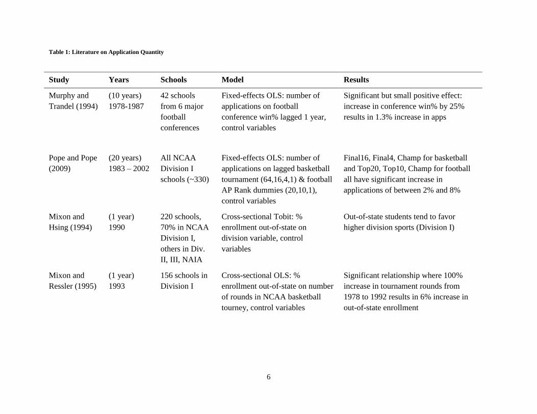
class. Table 1 provides a summary of the literature regarding application quantity. Two papers

have studied how sports success affects the total number of applications. Murphy and Trandel

(1994) examined a subset of Division I schools---55 schools from major football conferences---

and found a small but significant positive coefficient relating football conference winning % to

the number of applications. They concluded that an improvement in conference winning

percentage by 0.250 (i.e. from 50% to 75%) would increase applications an average of 1.3% the

following year. In a more recent and comprehensive study, Devin Pope and Jaren Pope (2009)

looked at all Division I schools from 1983-2002 and created several unique variables for sports

success. This paper used dummy variables for progression within the NCAA tournament for

basketball and dummy variables for AP rankings for football and created lagged dummy

variables for up to three years. The paper found significant and persistent increases in

applications of 2% to 8% for top-20 football schools and colleges that made the Sweet Sixteen of

the NCAA Tournament. Two other papers used basic cross-sectional OLS models and

discovered that schools in a higher-level athletic division and schools that performed better in

basketball had a higher proportion of out-of-state students.

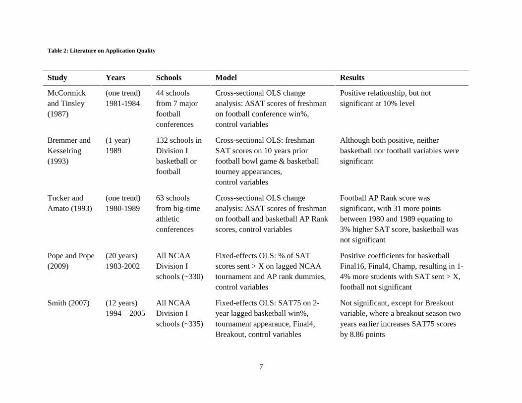
Table 2 provides a summary of the literature regarding application quality. McCormick

and Tinsley conducted one of the first empirical studies in 1987. Although they found that

football success had a positive correlation with incoming SAT scores among schools in the major

conferences, their results were not significant at the 10% level. The same Pope and Pope paper

6

Table 1: Literature on Application Quantity

Study Years Schools Model Results

Murphy and

Trandel (1994)

(10 years)

1978-1987

42 schools

from 6 major

football

conferences

Fixed-effects OLS: number of

applications on football

conference win% lagged 1 year,

control variables

Significant but small positive effect:

increase in conference win% by 25%

results in 1.3% increase in apps

Pope and Pope

(2009)

(20 years)

1983 – 2002

All NCAA

Division I

schools (~330)

Fixed-effects OLS: number of

applications on lagged basketball

tournament (64,16,4,1) & football

AP Rank dummies (20,10,1),

control variables

Final16, Final4, Champ for basketball

and Top20, Top10, Champ for football

all have significant increase in

applications of between 2% and 8%

Mixon and

Hsing (1994)

(1 year)

1990

220 schools,

70% in NCAA

Division I,

others in Div.

II, III, NAIA

Cross-sectional Tobit: %

enrollment out-of-state on

division variable, control

variables

Out-of-state students tend to favor

higher division sports (Division I)

Mixon and

Ressler (1995)

(1 year)

1993

156 schools in

Division I

Cross-sectional OLS: %

enrollment out-of-state on number

of rounds in NCAA basketball

tourney, control variables

Significant relationship where 100%

increase in tournament rounds from

1978 to 1992 results in 6% increase in

out-of-state enrollment

7

Table 2: Literature on Application Quality

Study Years Schools Model Results

McCormick

and Tinsley

(1987)

(one trend)

1981-1984

44 schools

from 7 major

football

conferences

Cross-sectional OLS change

analysis: ΔSAT scores of freshman

on football conference win%,

control variables

Positive relationship, but not

significant at 10% level

Bremmer and

Kesselring

(1993)

(1 year)

1989

132 schools in

Division I

basketball or

football

Cross-sectional OLS: freshman

SAT scores on 10 years prior

football bowl game & basketball

tourney appearances,

control variables

Although both positive, neither

basketball nor football variables were

significant

Tucker and

Amato (1993)

(one trend)

1980-1989

63 schools

from big-time

athletic

conferences

Cross-sectional OLS change

analysis: ΔSAT scores of freshman

on football and basketball AP Rank

scores, control variables

Football AP Rank score was

significant, with 31 more points

between 1980 and 1989 equating to

3% higher SAT score, basketball was

not significant

Pope and Pope

(2009)

(20 years)

1983-2002

All NCAA

Division I

schools (~330)

Fixed-effects OLS: % of SAT

scores sent > X on lagged NCAA

tournament and AP rank dummies,

control variables

Positive coefficients for basketball

Final16, Final4, Champ, resulting in 1-

4% more students with SAT sent > X,

football not significant

Smith (2007) (12 years)

1994 – 2005

All NCAA

Division I

schools (~335)

Fixed-effects OLS: SAT75 on 2-

year lagged basketball win%,

tournament appearance, Final4,

Breakout, control variables

Not significant, except for Breakout

variable, where a breakout season two

years earlier increases SAT75 scores

by 8.86 points

8

described above also examined the effects basketball and football success on SAT scores, again

finding a strong positive relationship between the two. However, the SAT scores used in this

study were the average scores sent to the schools by high school students after taking the SATs,

rather than the actual average SAT scores of the incoming freshman class. There are many steps

after sending the score (including applying, being accepted, and finally deciding to enroll) before

the institution actually capitalizes on any effect on student quality. Therefore, the SAT measure

used in the Pope and Pope paper may not be representative of incoming student quality. D.R.

Smith did a similar empirical study using actual SAT scores of incoming students. However, he

found that many sports success variables, such as win%, an NCAA tournament appearance, and

even reaching the Final4 had no significant effect on SAT scores. Smith did introduce a new

Breakout dummy variable, which equaled one if the school either 1) had a winning season 2)

made the NCAA tournament or 3) reached the Final Four, for the first time in 13 or more years.

Smith hypothesized that these breakout teams exemplified the type of “compelling stories”7 or

Cinderella stories that fueled media attention and produced the greatest advertising for the

institution as a whole. This breakout variable was found to be significant and positively related

to SAT scores; a breakout performance led to an average increase of nearly 10 points in the

freshman class average 75th-percentile SAT score two years later.

Empirical studies explaining the impact of sports success on student applications have

produced mixed results. Three primary reasons for these mixed findings include distinct subsets

of data, varying measures of athletic success, and different econometric models. The studies

outlined in the two tables above vary greatly by both the years of the study and the schools

included in the sample. Even though most models control for time effects within each study,

changing time periods across studies can certainly affect the advertising power of college sports,

7 Term originally referred to in (Toma & Cross, 1998), Page 653

9

thus creating different results depending on the time period of the study. Earlier studies

(McCormick and Tinsley, Tucker and Amato, Murphy and Trandel) also focused on a smaller

subset of Division I schools: schools from the major athletic conferences. These studies are

helpful in analyzing the schools with the largest athletic programs, but the results cannot be

generalized to provide a comprehensive picture of all Division I schools. Earlier studies also

included generic sports success variables such as conference winning % or bowl game and

tournament appearances. Although these variables provide a rough measure for athletic success,

they do not isolate or distinguish instances of extraordinary, impactful athletic success.

Therefore, such a generic sports success variable could miss out on compelling stories of athletic

success. For instance, this past season, the Connecticut Huskies basketball team had a mediocre

.500 conference record, but went on to become the NCAA Tournament Champion and the #1

team in the nation. Such a huge story for the university would be characterized as a mediocre

season by the conference winning % variables. Finally, differences in econometric specifications

can impact the results. Some studies, such as the Bremmer and Kesselring study and the two

papers on out-of-state %, used traditional OLS regressions with some control variables and

yearly fixed variables. Such an empirical framework only explains the correlation between sports

success and application quantity/quality, rather than the effect of sports success on applications.

There also remains the possibility of omitted variables that may affect applications, which could

dramatically change the results of these OLS regressions without institution fixed effects.

Some of the more recent papers (Smith, Pope and Pope) have solved many of the

problems of earlier studies. Both recent studies expand the sample to include all Division I

schools and a wider sample timeframe (12 years, 20 years) for a more comprehensive study. In

addition, they use more representative sports success variables, along with both year and

10

institution fixed effect variables to mitigate the effect of any omitted variables. However, both

studies group all Division I schools into one sample, with only the Pope paper running

regressions for public and private universities separately. By doing this generic grouping, the

studies are assuming that all schools within each grouping are equally affected by sports success.

The reality is not so simple. Although “sports success” is used as a universal term, it has

different definitions and interpretations among different schools. Schools that are historically

known for their athletic achievements may not necessarily define a Final16 appearance as a

successful season. Meanwhile, a less athletically-renowned institution may define a Final16 run

as a hugely successful season, capturing media headlines with their storybook run and winning

the hearts of fans in the process. The same level of sports success can have drastically different

interpretations depending on the institution, thus resulting in a divergent effect on applications.

Smith tries to account for this with his Breakout variable, but a broader breakdown of subgroups

is necessary.

This study looks at the two most popular and largest revenue-driving sports in college

athletics: men’s basketball and football. It examines all Division I schools in order to provide a

comprehensive study, but also distinguishes between the athletic level and sports success

expectations of the schools to establish more accurate results. It runs separate regressions for

three levels of schools that are well-known in the college sports community: BCS schools (from

the six major athletic conferences: ACC, Big 12, Big East, Bit Ten, Pac-10 and SEC), mid-major

schools (schools from 9 conferences that are a step below the athletic powerhouses: A-10, CAA,

C-USA, Horizon, MAC, MVC, MWC, WCC, WAC), and all other Division I schools8. In

general, the top BCS schools strive for at least a Final Four appearance or a BCS bowl game,

8 The current BCS schools are well-defined, while the nine mid-major conferences were taken from general

consensus and can be found at http://en.wikipedia.org/wiki/Mid-major. The subgroups used for college football

included BCS (and major independents) and Non-BCS schools

11

whereas the mid-major schools are hoping for a Sweet Sixteen or top 20 ranking, and the other

Division I schools are happy just to get into the tournament. Separate regressions for these

subgroups prevent dilution of certain sports success effects that may be present for a subgroup of

schools but not at the aggregate level. The study uses several representative sports success

variables designed to proxy the national media attention the college receives from its major

athletic programs, as well as some fixed effects and control variables that will be explained in the

upcoming sections.

III. Data Sources

This study covers all colleges and universities that were recognized as NCAA Division I

schools in 2010. Panel data is collected from 2000 to 2009 for 346 schools in Division I

basketball and 120 schools in Division I-FBS (football), resulting in 10 years of observations for

each institution. The primary datasets used for empirical analysis consist of two areas: sports

data and institution data. The sports dataset is a compilation of historic, end-of-year results for

college basketball and college football teams from 2000 to 2009. The data was taken from

Sports-Reference.com, a website that provides historical sports statistics. For each year, the

dataset includes the final regular season conference rankings and conference tournament results

of all 346 Division I teams, the end-of-year National Associated Press (AP) Poll College

Football rankings, the end-of-year (post-tournament) USA Today Poll rankings for college

basketball, and the number of games played in the NCAA Division I Basketball Tournament.

These sports variables were designed to measure sports success by serving as a proxy for the

amount of media attention the athletic success has brought to the institution over the past decade.

12

The institution dataset comes from the National Center for Education Studies (NCES)

Integrated Postsecondary Education Data System (IPEDS) Data Center, which provides a wide

variety of institutional data for every institution of higher education. The dataset includes

institution data from 2001 to 2009 for the 346 Division I schools. Institution variables include

the number of annual applications each school receives, the number of applications each school

admits, the number of students that enroll, the average SAT scores of these freshman enrollees,

as well as the state of migration for the entering class. The IPEDS website also provides other

university characteristics such as the sticker price, average professor salary, student-faculty ratio,

and total enrollment. Some annual state-specific control variables that were used include the

number of high school graduates and the median household income, gathered from NCES and

the U.S. Census Bureau, respectively. Finally, the National Association of College and

University Business Officers (NACUBO) provided the annual market value of endowments for

each institution. Many of these university characteristics have been widely used in past literature

to control for the quality of each institution. The specifics of the variables and how they

contribute to the regression model are discussed in more detail below.

IV. Variables and Regressions

There are three main groups of variables used in the regression model: sports variables,

institution control variables, and dependent variables. Sports variables are measures of athletic

success designed to capture the exposure a university receives from its sports success. An ideal

way to measure exposure is to calculate the total number of television viewers that watch NCAA

tournament and bowl games featuring the university. Unfortunately, such data could not be

obtained for this study. Therefore, several sports success variables were created that were

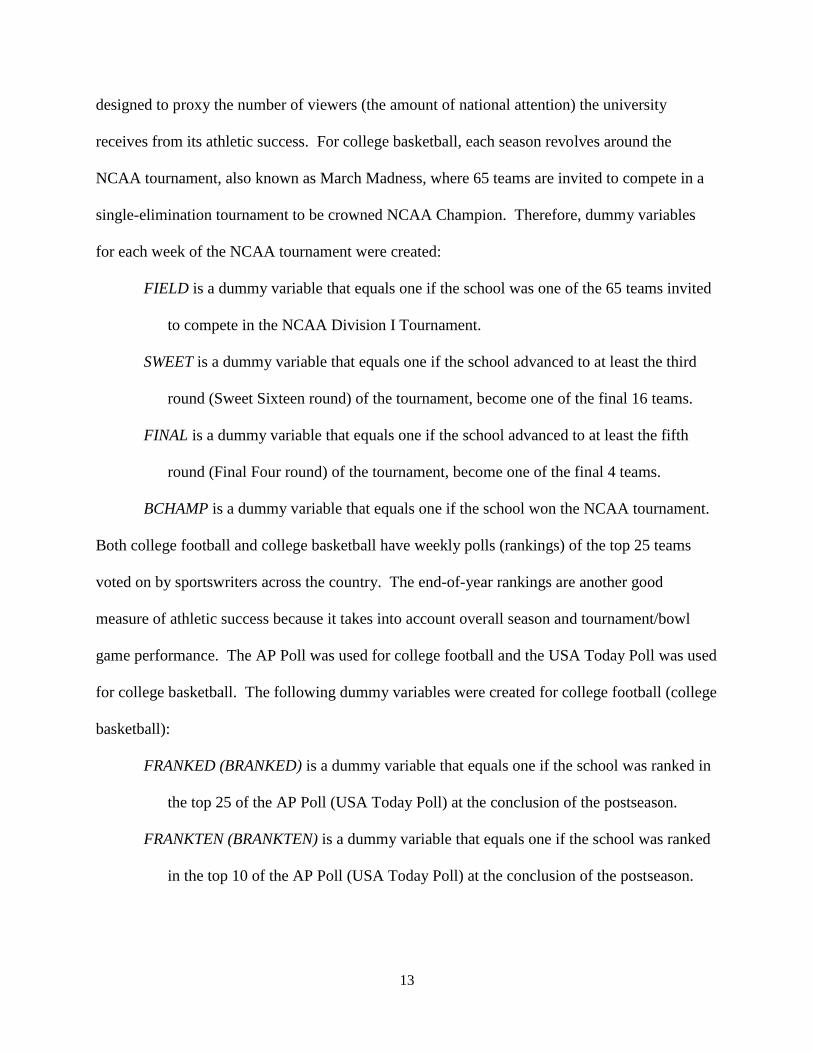
13

designed to proxy the number of viewers (the amount of national attention) the university

receives from its athletic success. For college basketball, each season revolves around the

NCAA tournament, also known as March Madness, where 65 teams are invited to compete in a

single-elimination tournament to be crowned NCAA Champion. Therefore, dummy variables

for each week of the NCAA tournament were created:

FIELD is a dummy variable that equals one if the school was one of the 65 teams invited

to compete in the NCAA Division I Tournament.

SWEET is a dummy variable that equals one if the school advanced to at least the third

round (Sweet Sixteen round) of the tournament, become one of the final 16 teams.

FINAL is a dummy variable that equals one if the school advanced to at least the fifth

round (Final Four round) of the tournament, become one of the final 4 teams.

BCHAMP is a dummy variable that equals one if the school won the NCAA tournament.

Both college football and college basketball have weekly polls (rankings) of the top 25 teams

voted on by sportswriters across the country. The end-of-year rankings are another good

measure of athletic success because it takes into account overall season and tournament/bowl

game performance. The AP Poll was used for college football and the USA Today Poll was used

for college basketball. The following dummy variables were created for college football (college

basketball):

FRANKED (BRANKED) is a dummy variable that equals one if the school was ranked in

the top 25 of the AP Poll (USA Today Poll) at the conclusion of the postseason.

FRANKTEN (BRANKTEN) is a dummy variable that equals one if the school was ranked

in the top 10 of the AP Poll (USA Today Poll) at the conclusion of the postseason.

14

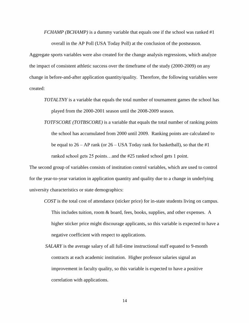
FCHAMP (BCHAMP) is a dummy variable that equals one if the school was ranked #1

overall in the AP Poll (USA Today Poll) at the conclusion of the postseason.

Aggregate sports variables were also created for the change analysis regressions, which analyze

the impact of consistent athletic success over the timeframe of the study (2000-2009) on any

change in before-and-after application quantity/quality. Therefore, the following variables were

created:

TOTALTNY is a variable that equals the total number of tournament games the school has

played from the 2000-2001 season until the 2008-2009 season.

TOTFSCORE (TOTBSCORE) is a variable that equals the total number of ranking points

the school has accumulated from 2000 until 2009. Ranking points are calculated to

be equal to 26 – AP rank (or 26 – USA Today rank for basketball), so that the #1

ranked school gets 25 points…and the #25 ranked school gets 1 point.

The second group of variables consists of institution control variables, which are used to control

for the year-to-year variation in application quantity and quality due to a change in underlying

university characteristics or state demographics:

COST is the total cost of attendance (sticker price) for in-state students living on campus.

This includes tuition, room & board, fees, books, supplies, and other expenses. A

higher sticker price might discourage applicants, so this variable is expected to have a

negative coefficient with respect to applications.

SALARY is the average salary of all full-time instructional staff equated to 9-month

contracts at each academic institution. Higher professor salaries signal an

improvement in faculty quality, so this variable is expected to have a positive

correlation with applications.

15

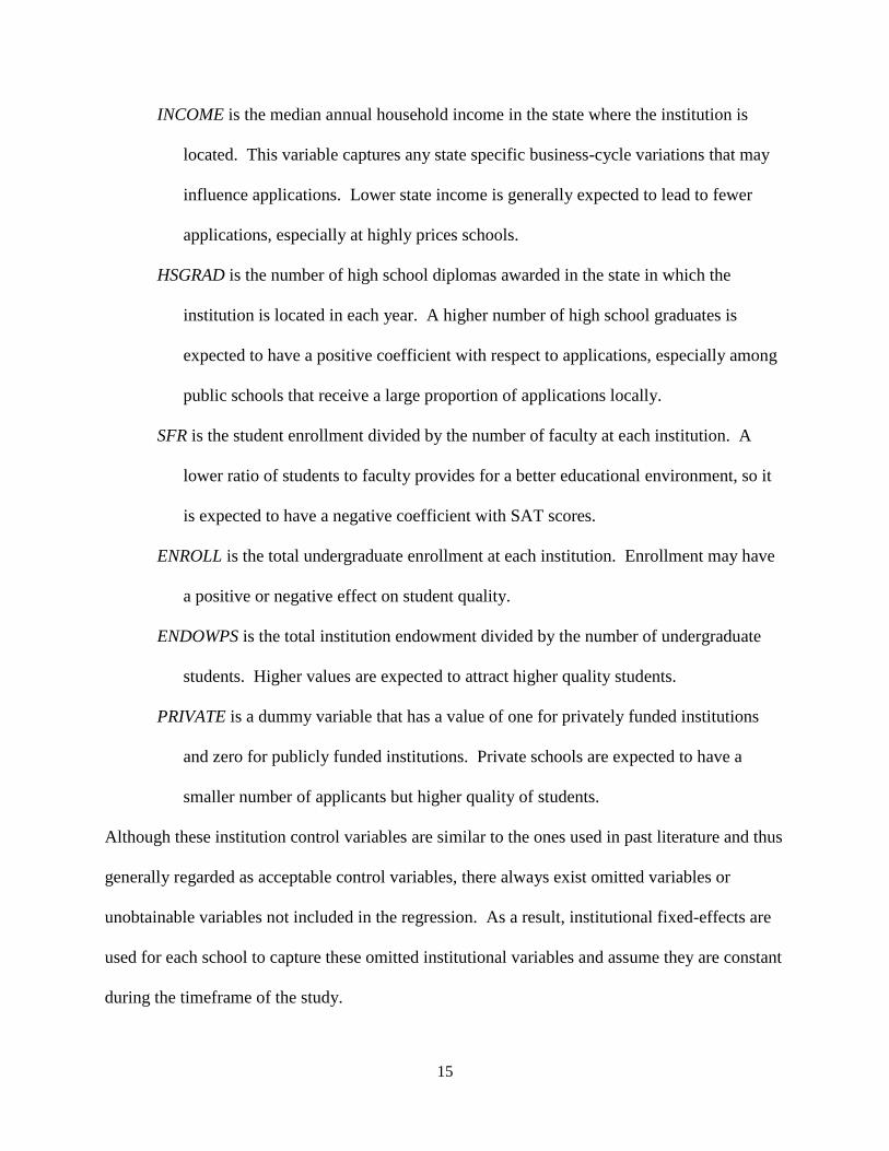
INCOME is the median annual household income in the state where the institution is

located. This variable captures any state specific business-cycle variations that may

influence applications. Lower state income is generally expected to lead to fewer

applications, especially at highly prices schools.

HSGRAD is the number of high school diplomas awarded in the state in which the

institution is located in each year. A higher number of high school graduates is

expected to have a positive coefficient with respect to applications, especially among

public schools that receive a large proportion of applications locally.

SFR is the student enrollment divided by the number of faculty at each institution. A

lower ratio of students to faculty provides for a better educational environment, so it

is expected to have a negative coefficient with SAT scores.

ENROLL is the total undergraduate enrollment at each institution. Enrollment may have

a positive or negative effect on student quality.

ENDOWPS is the total institution endowment divided by the number of undergraduate

students. Higher values are expected to attract higher quality students.

PRIVATE is a dummy variable that has a value of one for privately funded institutions

and zero for publicly funded institutions. Private schools are expected to have a

smaller number of applicants but higher quality of students.

Although these institution control variables are similar to the ones used in past literature and thus

generally regarded as acceptable control variables, there always exist omitted variables or

unobtainable variables not included in the regression. As a result, institutional fixed-effects are

used for each school to capture these omitted institutional variables and assume they are constant

during the timeframe of the study.

16

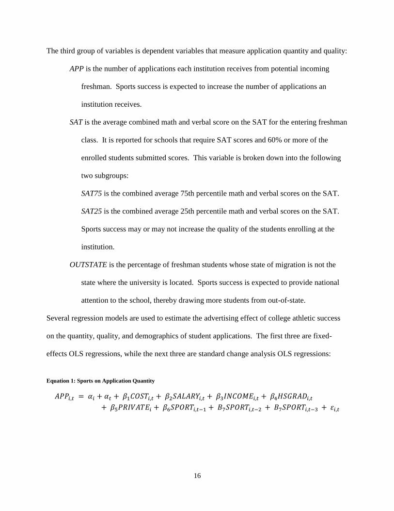
The third group of variables is dependent variables that measure application quantity and quality:

APP is the number of applications each institution receives from potential incoming

freshman. Sports success is expected to increase the number of applications an

institution receives.

SAT is the average combined math and verbal score on the SAT for the entering freshman

class. It is reported for schools that require SAT scores and 60% or more of the

enrolled students submitted scores. This variable is broken down into the following

two subgroups:

SAT75 is the combined average 75th percentile math and verbal scores on the SAT.

SAT25 is the combined average 25th percentile math and verbal scores on the SAT.

Sports success may or may not increase the quality of the students enrolling at the

institution.

OUTSTATE is the percentage of freshman students whose state of migration is not the

state where the university is located. Sports success is expected to provide national

attention to the school, thereby drawing more students from out-of-state.

Several regression models are used to estimate the advertising effect of college athletic success

on the quantity, quality, and demographics of student applications. The first three are fixed-

effects OLS regressions, while the next three are standard change analysis OLS regressions:

Equation 1: Sports on Application Quantity

17

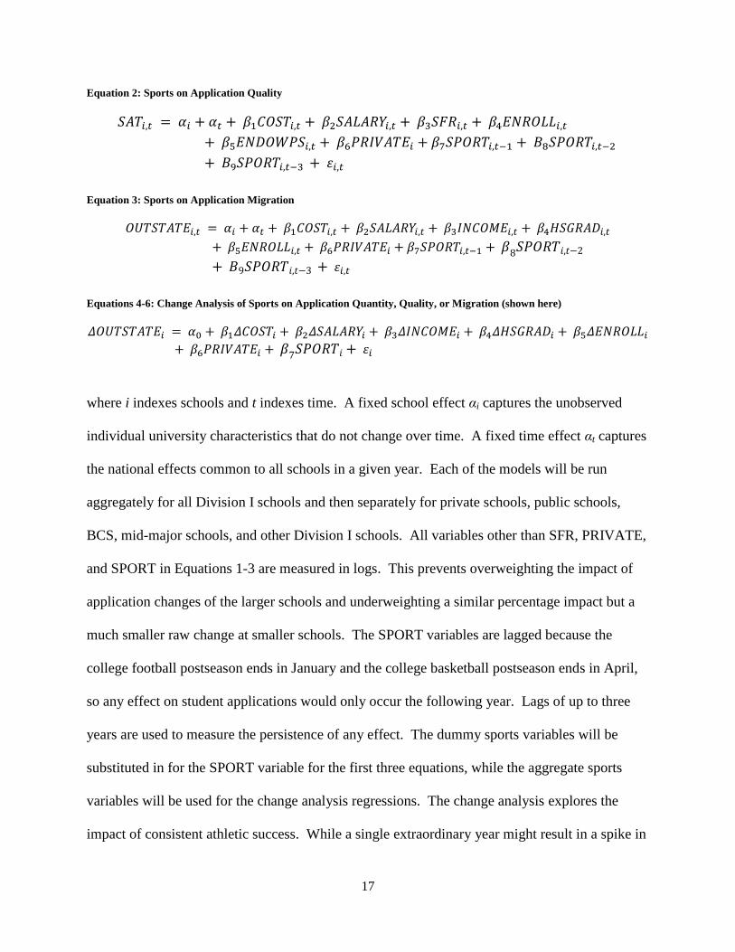
Equation 2: Sports on Application Quality

Equation 3: Sports on Application Migration

Equations 4-6: Change Analysis of Sports on Application Quantity, Quality, or Migration (shown here)

where i indexes schools and t indexes time. A fixed school effect αi captures the unobserved

individual university characteristics that do not change over time. A fixed time effect αt captures

the national effects common to all schools in a given year. Each of the models will be run

aggregately for all Division I schools and then separately for private schools, public schools,

BCS, mid-major schools, and other Division I schools. All variables other than SFR, PRIVATE,

and SPORT in Equations 1-3 are measured in logs. This prevents overweighting the impact of

application changes of the larger schools and underweighting a similar percentage impact but a

much smaller raw change at smaller schools. The SPORT variables are lagged because the

college football postseason ends in January and the college basketball postseason ends in April,

so any effect on student applications would only occur the following year. Lags of up to three

years are used to measure the persistence of any effect. The dummy sports variables will be

substituted in for the SPORT variable for the first three equations, while the aggregate sports

variables will be used for the change analysis regressions. The change analysis explores the

impact of consistent athletic success. While a single extraordinary year might result in a spike in

18

applications the following year, a consistently successful athletic program may develop a

positive reputation, resulting in a steady increase in college applications. The change analysis

variables are calculated by subtracting each institution’s 2009 value by the 2000 value.

V. Results

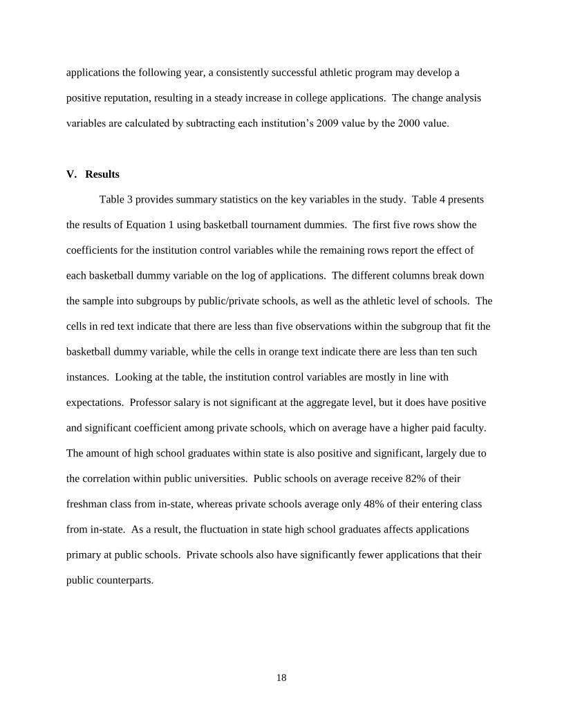
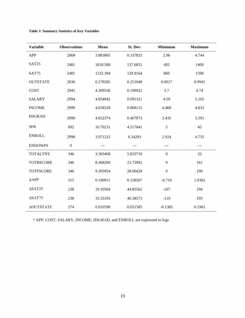
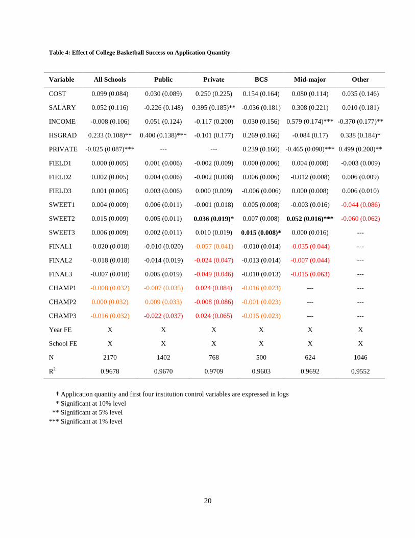
Table 3 provides summary statistics on the key variables in the study. Table 4 presents

the results of Equation 1 using basketball tournament dummies. The first five rows show the

coefficients for the institution control variables while the remaining rows report the effect of

each basketball dummy variable on the log of applications. The different columns break down

the sample into subgroups by public/private schools, as well as the athletic level of schools. The

cells in red text indicate that there are less than five observations within the subgroup that fit the

basketball dummy variable, while the cells in orange text indicate there are less than ten such

instances. Looking at the table, the institution control variables are mostly in line with

expectations. Professor salary is not significant at the aggregate level, but it does have positive

and significant coefficient among private schools, which on average have a higher paid faculty.

The amount of high school graduates within state is also positive and significant, largely due to

the correlation within public universities. Public schools on average receive 82% of their

freshman class from in-state, whereas private schools average only 48% of their entering class

from in-state. As a result, the fluctuation in state high school graduates affects applications

primary at public schools. Private schools also have significantly fewer applications that their

public counterparts.

19

Table 3: Summary Statistics of Key Variables

Variable Observations Mean St. Dev. Minimum Maximum

APP 2868 3.883805 0.337833 2.96 4.744

SAT25 2481 1018.568 137.6851 492 1400

SAT75 2481 1232.394 129.9164 860 1590

OUTSTATE 2036 0.278585 0.251048 0.0017 0.9941

COST 2945 4.309336 0.199922 3.7 4.74

SALARY 2994 4.834042 0.091321 4.59 5.165

INCOME 2999 4.658328 0.068115 4.468 4.833

HSGRAD 2999 4.832374 0.407873 3.435 5.591

SFR 692 16.70231 4.517641 5 45

ENROLL 2998 3.971232 0.34293 2.924 4.735

ENDOWPS 0 --- --- --- ---

TOTALTNY 346 3.303468 5.833719 0 33

TOTBSCORE 346 8.468208 23.75992 0 161

TOTFSCORE 346 9.395954 28.00428 0 190

ΔAPP 315 0.190911 0.158567 -0.716 1.0362

ΔSAT25 238 19.10504 44.85562 -107 194

ΔSAT75 238 19.33193 40.38573 -110 193

ΔOUTSTATE 274 0.010598 0.051585 -0.1385 0.1963

† APP, COST, SALARY, INCOME, HSGRAD, and ENROLL are expressed in logs

20

Table 4: Effect of College Basketball Success on Application Quantity

Variable All Schools Public Private BCS Mid-major Other

COST 0.099 (0.084) 0.030 (0.089) 0.250 (0.225) 0.154 (0.164) 0.080 (0.114) 0.035 (0.146)

SALARY 0.052 (0.116) -0.226 (0.148) 0.395 (0.185)** -0.036 (0.181) 0.308 (0.221) 0.010 (0.181)

INCOME -0.008 (0.106) 0.051 (0.124) -0.117 (0.200) 0.030 (0.156) 0.579 (0.174)*** -0.370 (0.177)**

HSGRAD 0.233 (0.108)** 0.400 (0.138)*** -0.101 (0.177) 0.269 (0.166) -0.084 (0.17) 0.338 (0.184)*

PRIVATE -0.825 (0.087)*** --- --- 0.239 (0.166) -0.465 (0.098)*** 0.499 (0.208)**

FIELD1 0.000 (0.005) 0.001 (0.006) -0.002 (0.009) 0.000 (0.006) 0.004 (0.008) -0.003 (0.009)

FIELD2 0.002 (0.005) 0.004 (0.006) -0.002 (0.008) 0.006 (0.006) -0.012 (0.008) 0.006 (0.009)

FIELD3 0.001 (0.005) 0.003 (0.006) 0.000 (0.009) -0.006 (0.006) 0.000 (0.008) 0.006 (0.010)

SWEET1 0.004 (0.009) 0.006 (0.011) -0.001 (0.018) 0.005 (0.008) -0.003 (0.016) -0.044 (0.086)

SWEET2 0.015 (0.009) 0.005 (0.011) 0.036 (0.019)* 0.007 (0.008) 0.052 (0.016)*** -0.060 (0.062)

SWEET3 0.006 (0.009) 0.002 (0.011) 0.010 (0.019) 0.015 (0.008)* 0.000 (0.016) ---

FINAL1 -0.020 (0.018) -0.010 (0.020) -0.057 (0.041) -0.010 (0.014) -0.035 (0.044) ---

FINAL2 -0.018 (0.018) -0.014 (0.019) -0.024 (0.047) -0.013 (0.014) -0.007 (0.044) ---

FINAL3 -0.007 (0.018) 0.005 (0.019) -0.049 (0.046) -0.010 (0.013) -0.015 (0.063) ---

CHAMP1 -0.008 (0.032) -0.007 (0.035) 0.024 (0.084) -0.016 (0.023) --- ---

CHAMP2 0.000 (0.032) 0.009 (0.033) -0.008 (0.086) -0.001 (0.023) --- ---

CHAMP3 -0.016 (0.032) -0.022 (0.037) 0.024 (0.065) -0.015 (0.023) --- ---

Year FE X X X X X X

School FE X X X X X X

N 2170 1402 768 500 624 1046

R2 0.9678 0.9670 0.9709 0.9603 0.9692 0.9552

† Application quantity and first four institution control variables are expressed in logs

* Significant at 10% level

** Significant at 5% level

*** Significant at 1% level

21

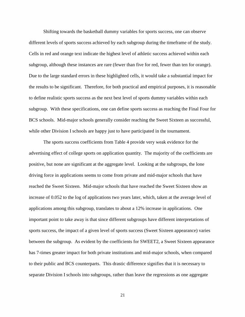
Shifting towards the basketball dummy variables for sports success, one can observe

different levels of sports success achieved by each subgroup during the timeframe of the study.

Cells in red and orange text indicate the highest level of athletic success achieved within each

subgroup, although these instances are rare (fewer than five for red, fewer than ten for orange).

Due to the large standard errors in these highlighted cells, it would take a substantial impact for

the results to be significant. Therefore, for both practical and empirical purposes, it is reasonable

to define realistic sports success as the next best level of sports dummy variables within each

subgroup. With these specifications, one can define sports success as reaching the Final Four for

BCS schools. Mid-major schools generally consider reaching the Sweet Sixteen as successful,

while other Division I schools are happy just to have participated in the tournament.

The sports success coefficients from Table 4 provide very weak evidence for the

advertising effect of college sports on application quantity. The majority of the coefficients are

positive, but none are significant at the aggregate level. Looking at the subgroups, the lone

driving force in applications seems to come from private and mid-major schools that have

reached the Sweet Sixteen. Mid-major schools that have reached the Sweet Sixteen show an

increase of 0.052 to the log of applications two years later, which, taken at the average level of

applications among this subgroup, translates to about a 12% increase in applications. One

important point to take away is that since different subgroups have different interpretations of

sports success, the impact of a given level of sports success (Sweet Sixteen appearance) varies

between the subgroup. As evident by the coefficients for SWEET2, a Sweet Sixteen appearance

has 7-times greater impact for both private institutions and mid-major schools, when compared

to their public and BCS counterparts. This drastic difference signifies that it is necessary to

separate Division I schools into subgroups, rather than leave the regressions as one aggregate

22

Table 5: Effect of College Football Success on Application Quantity

Variable All Schools Public Private BCS Non-BCS

COST 0.112 (0.096) 0.040 (0.090) 0.926 (0.580) 0.107 (0.152) 0.107 (0.137)

SALARY 0.070 (0.141) -0.109 (0.143) 0.802 (0.439)* -0.113 (0.172) 0.377 (0.251)

INCOME 0.213 (0.122)* 0.091 (0.120) 0.920 (0.467)* 0.021 (0.152) 0.437 (0.204)**

HSGRAD 0.176 (0.129) 0.310 (0.127)** -0.957 (0.451)** 0.266 (0.172) 0.124 (0.203)

PRIVATE 0.588 (0.244)** --- --- -0.099 (0.124) 0.622 (0.195)***

RANKED1 0.004 (0.006) 0.005 (0.006) -0.007 (0.023) 0.002 (0.006) 0.013 (0.018)

RANKED2 0.008 (0.006) 0.010 (0.006) -0.016 (0.021) 0.006 (0.006) 0.010 (0.017)

RANKED3 0.004 (0.006) 0.004 (0.006) -0.004 (0.020) 0.004 (0.006) 0.000 (0.018)

RANKTEN1 0.000 (0.009) -0.001 (0.009) 0.002 (0.039) 0.002 (0.009) -0.015 (0.028)

RANKTEN2 0.004 (0.009) 0.002 (0.009) 0.032 (0.043) 0.005 (0.009) -0.001 (0.033)

RANKTEN3 0.001 (0.009) 0.003 (0.008) -0.009 (0.042) 0.004 (0.008) -0.013 (0.034)

FCHAMP1 0.007 (0.021) 0.008 (0.023) 0.047 (0.059) 0.006 (0.019) ---

FCHAMP2 0.006 (0.020) 0.006 (0.025) 0.001 (0.045) 0.008 (0.019) ---

FCHAMP3 -0.002 (0.020) -0.017 (0.024) 0.028 (0.046) -0.006 (0.019) ---

Year FE X X X X X

School FE X X X X X

N 799 680 119 456 343

R2 0.9752 0.9795 0.9665 0.9643 0.9708

† Application quantity and first four institution control variables are expressed in logs

* Significant at 10% level

** Significant at 5% level

*** Significant at 1% level

23

Table 6: Effect of Sports Success on Change in Out-of-State %

Variable All Basketball All Basketball All Football

ΔCOST 0.08443 (0.06578) 0.08333 (0.06585) 0.20283 (0.14619)

ΔSALARY -0.02994 (0.07506) -0.02397 (0.07481) -0.04240 (0.11584)

ΔINCOME -0.02961 (0.10700) -0.03672 (0.10676) 0.07377 (0.16977)

ΔHSGRAD -0.61993 (0.09132)*** -0.62156 (0.09140)*** -0.57213 (0.15367)***

ΔENROLL 0.10340 (0.03914)*** 0.10155 (0.03913)*** 0.14880 (0.09867)

PRIVATE 0.01111 (0.00678) 0.01080 (0.00678) 0.00551 (0.01533)

TOTALTNY 0.00049 (0.00050)

TOTBSCORE

0.00007 (0.00012)

TOTFSCORE

0.00019 (0.00012)

N 265 265 102

R2 0.1797 0.1778 0.2050

† The first five institution control variables are expressed in changes in the underlying log values

* Significant at 10% level

** Significant at 5% level

*** Significant at 1% level

24

study, where any impacts of sports success would have been diluted and insignificant. Although

Sweet Sixteen two-year lags are significant for private and mid-major schools, no significant

effects are present in the 1-year lag and 3-year lag in applications, so there seems to be little

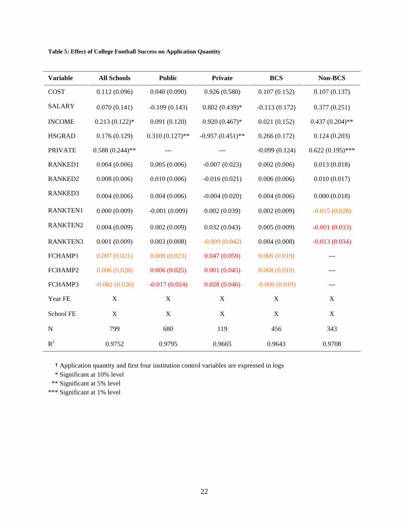
consistency and persistence in the results. Table 5 provides the results of Equation 1 using

football AP rank dummies. Again, although the majority of sports success dummies are positive,

none are significant. The results of football and basketball success on application quality reveal

similar results.

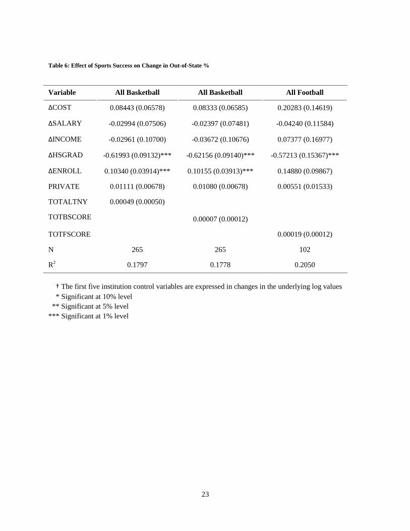
Table 6 provides the results for a change regression that shows the impact of consistent

sports success on the percentage of incoming students from out-of-state. Looking at the

institution control variables, the change in number of high school graduates in-state has a strong

negative coefficient with the percentage of incoming students from out-of-state. Changes in the

enrollment size of an institution are also positively related to the percentage of students

migrating from out-of-state. The three aggregate sports success measures all have a positive

coefficient with the percentage of out-of-state students, suggesting that sports success does

attract a broader demographic of students from around the country. However, none of the

sports variables are statistically significant, with the football sports variable falling just outside

the 10% p-level. In addition, the R-squared of these regressions are quite low, so much of the

variation in out-of-state% remains unexplained9.

VI. Limitations

This study strived to create a comprehensive study of the advertising effect of sports success on

student applications by including all 346 Division I schools over a ten year period. Such a large dataset is

bound to have some data imperfections. One can get an idea of some imperfections by referring to the

9 The R-squared for the change analysis regressions on applications and SAT scores were even lower (less than

10%)

25

summary statistics of key variables in Table 3. As one can see, student-faculty ratio is missing many

observations. This study was only able to gather data on SFR from IPEDS for the 2008 and 2009 school

years, so student-faculty ratio, along with endowment per student, was also not used in the regression

models involving application quality. The omission of these variables, along with other university

variables that might be correlated to incoming student quality (such as U.S. World News College

Rankings, library volumes, etc.), creates the possibility for omitted variable bias. The models used

institutional fixed effects to mitigate this problem by setting variables not used in the regressions as fixed,

but it would have been preferred to use actual year-by-year data in the regressions.

There were also some missing data among the variables that were used, causing the following

observations to be dropped. Eight institutions did not have application data, the three military schools did

not charge tuition, and other schools had missing data in SAT scores and migration patterns (out-of-state

variable). In addition, twenty-five schools joined Division I during the timeframe of the study, so only

their Division I observations were counted. Forty-five other schools switched conferences, five of which

switched from non-BCS conferences into the major athletic conferences, reflecting the mobility in college

sports, which may impact results.

The high school graduates variable gathered from NCES included projections of high school

graduates for years 2007-2009. Although these projections are fairly accurate since state trends are fairly

stable in the long run, there exists the possibility that these projections are not representative of actual

graduation outcomes. The state variables were thought to be a proxy of the local environment of the

institution, but this may not be representative. As shown in the study, the demographics of public and

private schools vary greatly, and certain schools are more heavily affected by local changes than others.

The regressions also featured lagged sports variables that reduced the number of sample years in

the study. Since the original timeframe of sports variables was relatively limited (nine years), this

significantly reduced the sample size of the regressions. Finally, there exists imperfections with the

athletic level subgroups that were used. Although the sports community splits colleges into these three

group: BCS, mid-major, and other Division I schools, there are schools within each subgroup that are not

26

representative of the typical athletic level common in the subgroup. For instance, the University of

Memphis is regarded as having a premier college basketball program, with four Sweet Sixteen

appearances in the timeframe of this study. However, it belongs in Conference USA, one of the mid-

major conferences. Meanwhile, schools such as the University of South Florida or Northwestern

University have traditionally weak college basketball teams. Yet, they are grouped along with the BCS

schools due to their participation in one of the six major athletic conferences. Even though mid-major

schools generally have a lower definition of sports success than BCS schools, there are instances where

this generalization breaks down.

VII. Conclusion and Further Research

This study found that although there seems to be some positive advertising effects of

college sports success on student applications, the evidence between 2000 and 2009 is weak and

not statistically significant. Previous studies have generally agreed on a positive relationship

between sports success and applications, but there have been mixed results on the statistical

significance of the relationship. Since there have been numerous studies across different

timeframes, the mixed results of the advertising power of college sports could be attributable to

the changing time periods across studies. Why then, has this advertising effect has tapered off in

the past decade?

College sports have always been extremely popular, and one could argue that today,

college sports have more widespread appeal than ever before, with expanding athletic budgets

and lucrative television deals. Based on this popularity, one would think that the advertising

effects of college sports would be greater than ever in the 2000s. However, this study suggests

just the opposite. A possible explanation of this phenomenon involves taking a broader look at

how the environment has changed across time periods.

27

The world has changed greatly from a television-dominant environment in the 1980s to a

much more connected world with widespread internet use in the 2000s. Today, there exists so

much more information available right at one’s fingertips. A prospective student can now go

online and learn limitless information about each college in the comfort of his or her bedroom.

While television was and still is a prime advertising technique backed by college sports, today’s

world provides an abundance of alternative sources of information. With the internet boom,

higher education institutions have digitalized their information onto university websites, while

other popular college information websites and forums have sprung up. College Confidential, a

popular forum where prospective students share information about topics ranging from

admissions, financial aid to college life, was founded in 2001. College guidebooks such as

College Prowler (founded 2002), which offered the inside scoop consisting of student opinions

and reviews, became instant successes, even being recognized among the fastest growing

companies within a few years of inception10

. Since the technology boom of the late 1990s and

2000s, the world has become much more connected and will be even more so as we enter into

the social media revolution. Although college athletics are key factors for some students when

deciding where to go to college, the inundation of college resources and easy access to

alternative sources of information may very well have permanently minimized the advertising

effect of college sports success on applications.

An alternative explanation for the weak advertising effect in this study revolves around

the sports environment of the 2000s. As Toma and Cross mention in their paper, not all

championships are given equal attention. Widespread media attention is usually given to

compelling “Cinderella” stories of unexpected, underdog teams making a storybook run against

the athletic powerhouses for the title. There were an abundance of Cinderella stories in the

10

Retrieved from Fast Company Magazine: http://www.fastcompany.com/fast50_05/winners

28

1980s and 1990s, including the 6th-seeded 1983 North Carolina State basketball team that

knocked off powerhouse Houston, the 1984 Boston College football squad famous for the Doug

Flutie Hail Mary, the 1985 Villanova basketball team, becoming the lowest seed (8) to ever win

a national championship, the 1995 Northwestern football team that reached the Rose Bowl,

etc…. All these stories garnered national headlines and led to substantial increase of

applications in subsequent years. Meanwhile, in the 2000s, there were only a few Cinderella

stories: mainly the 2006 Final Four run by George Mason’s basketball team and Boise State’s

upset victory over Oklahoma in the 2007 Fiesta Bowl. These two stories led to a respective 23%

and 18% jump in applications in subsequent years. However, the 2000s as a whole had fewer

Cinderella stories than in the past, and two big mid-major headline stories---back-to-back

Championship game appearances by Butler’s basketball team in 2009-2011 and Virginia

Commonwealth’s Final Four appearance in 2011---were not included in the sample because the

application effects of their successes had not been realized. The breakdown of subgroups within

the regressions were designed to test the Cinderella story effect, but a lack of such stories from

2000 to 2009 may have contributed to weaker than expected results.

Although this study did not find consistent statistical significance of an advertising effect

of college sports on applications, it was the first study to break down Division I teams by

subgroups based on athletic level. The results showed that different subgroups have different

measures of athletic success, so it would be faulty to generalize all Division I teams via an

aggregate regression. Such generalizations treat sports success as a universally consistent term,

which may dilute the true advertising effects among certain institutions. The subgroups used in

this study are not perfect, so further distinctions may be needed to ascertain more accurate

advertising effects. This study can also be improved upon by including more years in the sample

29

size and obtaining some of the missing institutional variables to better explain the variation in

applications. The advertising effect of college athletics remains an important area of research as

we enter into a changing environment, especially with college athletic budgets continuing to rise

to record-breaking levels.

30

VIII. References

Bremmer, D. S., & Kesselring, R. G. (1993). The Advertising Effect of University Athletic

Success: A Reappraisal of the Evidence. The Quarterly Review of Economics and Finance ,

33 (4), pp. 409-421.

College Basketball Statistics & History. (2011). Retrieved Spring 2011, from Sports Reference:

http://www.sports-reference.com/cbb/

College Football Statistics & History. (2011). Retrieved Spring 2011, from Sports Reference:

http://www.sports-reference.com/cfb/

Frank, R. H. (2004). Challenging the Myth: A Review of the Links Among College Athletic

Success, Student Quality, and Donations. Prepared for the Knight Foundation Commission

on Intercollegiate Athletics.

Income Data - State Median Income. (2011, January 4). Retrieved Spring 2011, from U.S.

Census Bureau: http://www.census.gov/hhes/www/income/data/index.html

Knight Commission on Intercollegiate Athletics. (2001). A Call to Action: Reconnecting College

Sports and Higher Education. Commission Report.

Knight Commission on Intercollegiate Athletics. (2010). Restoring the Balance: Dollars, Values,

and the Future of College Sports. Commission Report.

McCormick, R. E., & Tinsley, M. (1987, October). Athletics versus Academics? Evidence from

SAT Scores. The Jornal of Political Economy , 95 (5), pp. 1103-1116.

Mixon Jr., F. G., & Ressler, R. W. (1995). An empirical note on the impact of college athletics

on tuition revenues. Applied Economics Letters (2), pp. 383-387.

Murphy, R. G., & Trandel, G. A. (1994). The Relationship Between a University's Football

Record and the Size of Its Applicant Pool. Economics of Education Review , 13 (3), pp. 265-

270.

NCAA Members By Division. (n.d.). Retrieved Spring 2011, from National Collegiate Athletic

Association: http://web1.ncaa.org/onlineDir/exec/divisionListing

Pope, D. G., & Pope, J. C. (2009). The Impact of College Sports Success on the Quantity and

Quality of Student Applications. Southern Economic Journal , 75 (3), pp. 750-780.

Projection of Education Statistics to 2019. (2010, January). Retrieved Spring 2011, from

National Center for Education Statistics:

http://nces.ed.gov/programs/projections/projections2019/tables/table_14.asp

Smith, D. R. (2008). Big-Time College Basketball and the Advertising Effect: Does Success

Really Matter? Journal of Sports Economics , 9, pp. 387-406.

The IPEDS Data Center. (n.d.). Retrieved Spring 2011, from National Center for Education

Statistics: http://nces.ed.gov/ipeds/datacenter/Default.aspx

Toma, J. D., & Cross, M. (1998). Intercollegiate Athletics and Student College Choice:

Exploring the Impact of Championship Seasons on Undergraduate Applications. Research in

Higher Education , 39 (6), pp. 633-661.

31

Total Market Value of Endowments. (2010, February 19). Retrieved Spring 2011, from National

Association of College and University Business Officers:

http://www.nacubo.org/Research/NACUBO_Endowment_Study/Public_NCSE_Tables_/Tot

al_Market_Value_of_Endowments.html

Tucker, I., & Amato, L. (1993). Does Big-time Success in Football or Basketball Affect SAT

Scores? Economics of Education Review , 12 (2), pp. 177-181.

Weisbrod, B. A., Ballou, J. P., & Asch, E. D. (2008). Mission and Money: Understanding the

University. Cambridge University Press.