chumi viewer: compressive huge mesh interactive viewer
TRANSCRIPT
ARTICLE IN PRESS
Computers & Graphics 33 (2009) 542–553
Contents lists available at ScienceDirect
Computers & Graphics
0097-84
doi:10.1
� Corr
E-m
pierre-m
(S. Akko
journal homepage: www.elsevier.com/locate/cag
Technical Section
CHuMI viewer: Compressive huge mesh interactive viewer
Clement Jamin a,b,�, Pierre-Marie Gandoin a,c, Samir Akkouche a,b
a Universite de Lyon, CNRSb Universite Lyon 1, LIRIS, UMR5205, F-69622, Francec Universite Lyon 2, LIRIS, UMR5205, F-69676, France
a r t i c l e i n f o
Article history:
Received 21 December 2008
Received in revised form
21 March 2009
Accepted 28 March 2009
Keywords:
Lossless compression
Interactive visualization
Large meshes
Out-of-core
93/$ - see front matter & 2009 Elsevier Ltd. A
016/j.cag.2009.03.029
esponding author Tel.: +33 472448064.
ail addresses: [email protected] (C. J
[email protected] (P.-M. Gandoin), sa
uche).
a b s t r a c t
The preprocessing of large meshes to provide and optimize interactive visualization implies a complete
reorganization that often introduces significant data growth. This is detrimental to storage and network
transmission, but in the near future could also affect the efficiency of the visualization process itself,
because of the increasing gap between computing times and external access times. In this article, we
attempt to reconcile lossless compression and visualization by proposing a data structure that radically
reduces the size of the object while supporting a fast interactive navigation based on a viewing distance
criterion. In addition to this double capability, this method works out-of-core and can handle meshes
containing several hundred million vertices. Furthermore, it presents the advantage of dealing with any
n-dimensional simplicial complex, including triangle soups or volumetric meshes, and provides a
significant rate-distortion improvement. The performance attained is near state-of-the-art in terms of
the compression ratio as well as the visualization frame rates, offering a unique combination that can be
useful in numerous applications.
& 2009 Elsevier Ltd. All rights reserved.
1. Introduction
Mesh compression and mesh visualization are two fields ofcomputer graphics that are particularly active today, whoseconstraints and goals are usually incompatible, even contra-dictory. The reduction of redundancy often goes through signalcomplexification, because of prediction mechanisms whoseefficiency is directly related to the depth of the analysis. Thisadditional logical layer inevitably slows down the data access andcreates conflicts with the speed requirements of real-timevisualization. Conversely, for efficient navigation through a meshintegrating the user’s interactions dynamically, the signal must becarefully prepared and hierarchically structured. This generallyintroduces a high level of redundancy and sometimes comes withdata loss, if the original vertices and polyhedra are approximatedby simpler geometrical primitives. In addition to the on-diskstorage and network transmission issues, the data growth impliedby this kind of preprocessing could become detrimental to thevisualization itself since the gap between the processing timesand the access times from external memory is increasing.
In this article, we attempt to reconcile compression andinteractive visualization by proposing a method that combines
ll rights reserved.
amin),
good performance in terms of both the compression ratio and thevisualization frame rates. The interaction requirements of aviewer and a virtual reality system are quite similar in terms ofthe computational challenge but the two applications usedifferent criteria to decide how a model is viewed and updated.Our goal here is to take advantage of excellent view independentcompression and introduce distance-dependent updates of themodel during the visualization. As a starting point, the in-coreprogressive and lossless compression algorithm introduced byGandoin and Devillers [1] has been chosen. On top of itscompetitive compression ratios, out-of-core and LOD capabilitieshave been added to handle meshes with no size limitations andallow local refinements on demand by loading the necessary andsufficient data for an accurate real-time rendering of any subset ofthe mesh. To meet these goals, the basic idea consists insubdividing the original object into a tree of independent meshes.This partitioning is undertaken by introducing a primaryhierarchical structure (an nSP-tree) in which the original datastructures (a kd-tree coupled to a simplicial complex) areembedded, in a way that optimizes the bit distribution betweengeometry and connectivity and removes the undesirable blockeffects of kd-tree approaches.
After a study of related works (Section 2) focusing on themethod chosen as the starting point (Section 3), our contributionis introduced by an example (Section 4), then detailed in twocomplementary sections. First, the algorithms and data structuresof the out-of-core construction and compression are introduced(Sections 5 and 6), then the visualization point of view is adopted
ARTICLE IN PRESS
C. Jamin et al. / Computers & Graphics 33 (2009) 542–553 543
to complete the description (Section 7).Finally, experimentalresults are presented and the method is compared to prior art(Section 8).
2. Previous works
2.1. Compression
Mesh compression is a domain situated between computa-tional geometry and standard data compression. It consists inefficiently coupling geometry encoding (the vertex positions) andconnectivity encoding (the relations between vertices), and oftenaddresses manifold triangular surface models. We distinguishsingle-rate algorithms, which require full decoding to visualizethe object, and multiresolution methods that allow one to see themodel progressively refined while decoding. Although historicallygeometric compression began with single-rate algorithms, wehave chosen not to detail these methods here. The reader can referto surveys [2,3] for more information. For comparison purposes,since progressive and out-of-core compression methods are veryrare, Section 8 will refer to Isenburg and Gumhold’s well-knownsingle-rate out-of-core algorithm [4]. Similarly, lossy compression,whose general principle consists in a frequential analysis of themesh, is excluded from this study.
Progressive compression is based on the notion of refinement.At any time of the decoding process, it is possible to obtain aglobal approximation of the original model, which can be usefulfor large meshes or for network transmission. This research fieldhas been very productive for approximately 10 years, and ratherthan being exhaustive, here the choice has been to adopt ahistorical point of view. Early techniques of progressive visualiza-tion, based on mesh simplification, were not compression-oriented and often induced a significant increase in the file size,due to the additional storing cost of a hierarchical structure [5,6].Afterward, several single-resolution methods were extended toprogressive compression. For example, Taubin et al. [7] proposed aprogressive encoding based on Taubin and Rossignac’s algorithm[8]. Cohen-Or et al. [9] used techniques of sequential simplificationby vertex suppression for connectivity, combined with posi-tion prediction for geometry. Alliez and Desbrun [10] proposed analgorithm based on progressive removal of independent vertices,with a retriangulation step under the constraint of maintaining thevertex degrees around 6. Contrary to the majority of compressionmethods, Gandoin and Devillers [1] gave the priority to geometryencoding. Their algorithm, detailed in Section 3, gives competitivecompression rates and can handle simplicial complexes in anydimension, from manifold regular meshes to triangle soups. Pengand Kuo [11] took this paper as a basis to improve the compressionratios using efficient prediction schemes (sizes decrease by roughly15%), still limiting the scope to triangular models.
2.2. Large meshes processing
Working with huge data sets implies to develop out-of-coresolutions for managing, compressing or editing meshes. Lind-strom and Silva [12] proposed a simplication algorithm based on[13] whose memory complexity is neither dependent on the sizeof the input nor on the size of the output. Cignoni et al. [14]introduced a data structure called Octree-based External MemoryMesh (OEMM), which enable external memory management andsimplification of very large triangle meshes, by loading onlyselected sections in main memory. Isenburg et al. [15] developed astreaming file format for polygon meshes designed to work withlarge data sets. Isenburg et al. [16] proposed a single-rate
streaming compression scheme that encodes and decodesarbitrary large meshes using only minimal memory resources.Cai et al. [17] introduced the first progressive compressionmethod adapted to very large meshes, offering a way to addout-of-core capability to most of the existing progressivealgorithms based on octrees. The next section pays particularattention to out-of-core visualization techniques.
2.3. Visualization
Fast and interactive visualization of large meshes is a veryactive research field. Generally, a tree or a graph is built to handlea hierarchical structure which makes it possible to design out-of-core algorithms: at any moment, only necessary and sufficientdata are loaded into memory to render the mesh. Level of detail,view frustum and occlusion culling are widely used to adaptdisplayed data to the viewport. Rusinkiewicz and Levoy [18]introduced QSplat, the first out-of-core point-based renderingsystem, where the points are spread in a hierarchical structure ofbounding spheres. This structure can easily handle levels of detailand is well-suited to visibility and occlusion tests. Several millionpoints per second can thus be displayed using adaptive rendering.El-Sana and Chiang [19] proposed a technique to segment trianglemeshes into view-dependence trees, allowing external memorysimplification of models containing a few millions polygons, whilepreserving an optimal edge collapse order to enhance the imagequality. Later, Lindstrom [20] developed a method for interactivevisualization of huge meshes. An octree is used to dispatch thetriangles into clusters and to build a multiresolution hierarchy. Aquadric error metric is used to choose the representative pointpositions for each level of detail, and the refinement is guided byvisibility and screen space error. Yoon et al. [21] proposed asimilar algorithm with a bounded memory footprint: a clusterhierarchy is built, each cluster containing a progressive submeshto smooth the transition between the levels of detail. Cignoni et al.[22] used a hierarchy based on the recursive subdivision oftetrahedra in order to partition space and guarantee varyingborders between clusters during refinement. The initial construc-tion phase is parallelizable, and GPU is efficiently used to improveframe rates. Gobbetti and Marton [23] introduced the far voxels,capable of rendering regular meshes as well as triangles soups.The principle is to transform volumetric subparts of the modelinto compact direction-dependent approximations of theirappearance when viewed from a distance. A BSP tree is built,and nodes are discretized into cubic voxels containing theseapproximations. Again, the GPU is widely used to lighten the CPUload and improve performance. Cignoni et al. [24] proposeda general formalized framework that encompasses all thesevisualization methods based on batched rendering. Recently,Hu et al. [25] introduced the first highly parallel scheme forview-dependent visualization that is implemented entirely onprogrammable GPU. Although it uses a static data structurerequiring 57% more memory than an index triangle list, it allowsreal-time exploration of huge meshes.
2.4. Combined compression and visualization
Progressive compression methods are now mature (the ratesobtained are close to theoretical bounds) and interactivevisualization of huge meshes has been possible for several years.However, even if the combination of compression and visualiza-tion is often mentioned as a perspective, very few papers dealwith this problem, and the files created by visualizationalgorithms are often much larger than the original ones. In fact,compression favors a small file size to the detriment of fast data
ARTICLE IN PRESS
C. Jamin et al. / Computers & Graphics 33 (2009) 542–553544
access, whereas visualization methods focus on renderingspeed: the two goals oppose and compete with each other. Itmust be noted that there are a few counter-examples such as [26]where there is a reduction of redundancy without any run-timepenalty, but it remains unusual. Among the few works thatintroduce compression into visualization methods, Namane et al.[27] proposed a QSplat compressed version by using Huffmanand differential coding for spheres (position, radius) and normals.The compression ratio is approximately 50% compared to theoriginal QSplat files, but the scope is limited to point-basedrendering. More recently, Yoon and Lindstrom [28] introduced atriangle mesh compression algorithm that supports randomaccess to the underlying compressed mesh. However, theirfile format is not progressive and therefore inappropriate forglobal views of a model since it would require loading the fullmesh.
3. The starting point: kd-tree compression of vertex position andhierarchical connectivity coding
In this section, we briefly present the method originallyproposed by Gandoin and Devillers [1]. The algorithm, valid inany dimension, is based on a top-down kd-tree construction bycell subdivision. The root cell is the bounding box of the point setand the first output is the total number of points. Then, for eachcell subdivision, only the number of points in the first half-cell hasto be coded, the content of the second half-cell being easilydeduced. As the algorithm progresses, the cell size decreases andthe data transmitted provide a more accurate localization of thepoints. The subdivision process iterates until there is no longer anon-empty cell with a side greater than 1 spatial unit, such thatevery point is localized with the full mesh precision.
As soon as the points are separated, the connectivity of themodel is embedded (one vertex per cell) and the splitting processis run backwards: the cells are merged bottom-up and theirconnectivity is updated. The connectivity changes between twosuccessive versions of the model and is encoded by symbolsinserted between the geometry codes. The vertices are merged bythe two following decimating operators:
�
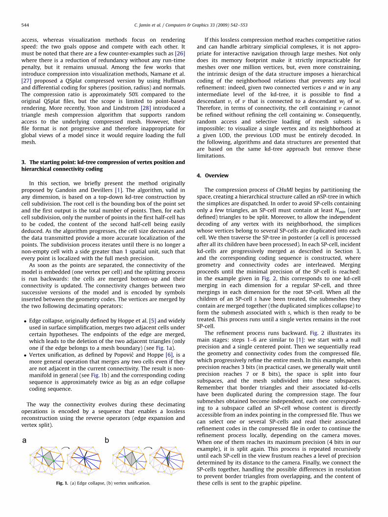
Edge collapse, originally defined by Hoppe et al. [5] and widelyused in surface simplification, merges two adjacent cells undercertain hypotheses. The endpoints of the edge are merged,which leads to the deletion of the two adjacent triangles (onlyone if the edge belongs to a mesh boundary) (see Fig. 1a). � Vertex unification, as defined by Popovic and Hoppe [6], is amore general operation that merges any two cells even if theyare not adjacent in the current connectivity. The result is non-manifold in general (see Fig. 1b) and the corresponding codingsequence is approximately twice as big as an edge collapsecoding sequence.
The way the connectivity evolves during these decimatingoperations is encoded by a sequence that enables a losslessreconstruction using the reverse operators (edge expansion andvertex split).
Fig. 1. (a) Edge collapse, (b) vertex unification.
If this lossless compression method reaches competitive ratiosand can handle arbitrary simplicial complexes, it is not appro-priate for interactive navigation through large meshes. Not onlydoes its memory footprint make it strictly impracticable formeshes over one million vertices, but, even more constraining,the intrinsic design of the data structure imposes a hierarchicalcoding of the neighborhood relations that prevents any localrefinement: indeed, given two connected vertices v and w in anyintermediate level of the kd-tree, it is possible to find adescendant vi of v that is connected to a descendant wj of w.Therefore, in terms of connectivity, the cell containing v cannotbe refined without refining the cell containing w. Consequently,random access and selective loading of mesh subsets isimpossible: to visualize a single vertex and its neighborhood ata given LOD, the previous LOD must be entirely decoded. Inthe following, algorithms and data structures are presented thatare based on the same kd-tree approach but remove theselimitations.
4. Overview
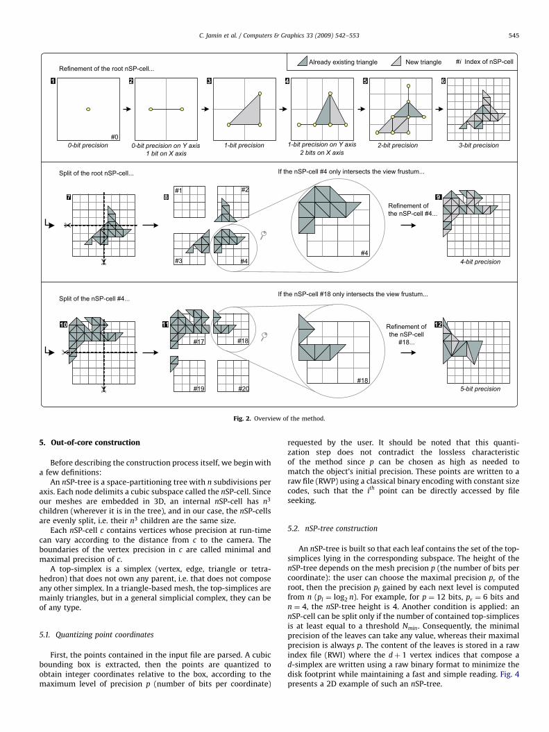
The compression process of CHuMI begins by partitioning thespace, creating a hierarchical structure called an nSP-tree in whichthe simplices are dispatched. In order to avoid SP-cells containingonly a few triangles, an SP-cell must contain at least Nmin (userdefined) triangles to be split. Moreover, to allow the independentdecoding of any vertex with its neighborhood, the simpliceswhose vertices belong to several SP-cells are duplicated into eachcell. We then traverse the SP-tree in postorder (a cell is processedafter all its children have been processed). In each SP-cell, incidentkd-cells are progressively merged as described in Section 3,and the corresponding coding sequence is constructed, wheregeometry and connectivity codes are interleaved. Mergingproceeds until the minimal precision of the SP-cell is reached:in the example given in Fig. 2, this corresponds to one kd-cellmerging in each dimension for a regular SP-cell, and threemergings in each dimension for the root SP-cell. When all thechildren of an SP-cell s have been treated, the submeshes theycontain are merged together (the duplicated simplices collapse) toform the submesh associated with s, which is then ready to betreated. This process runs until a single vertex remains in the rootSP-cell.
The refinement process runs backward. Fig. 2 illustrates itsmain stages: steps 1–6 are similar to [1]: we start with a nullprecision and a single centered point. Then we sequentially readthe geometry and connectivity codes from the compressed file,which progressively refine the entire mesh. In this example, whenprecision reaches 3 bits (in practical cases, we generally wait untilprecision reaches 7 or 8 bits), the space is split into foursubspaces, and the mesh subdivided into these subspaces.Remember that border triangles and their associated kd-cellshave been duplicated during the compression stage. The foursubmeshes obtained become independent, each one correspond-ing to a subspace called an SP-cell whose content is directlyaccessible from an index pointing in the compressed file. Thus wecan select one or several SP-cells and read their associatedrefinement codes in the compressed file in order to continue therefinement process locally, depending on the camera moves.When one of them reaches its maximum precision (4 bits in ourexample), it is split again. This process is repeated recursivelyuntil each SP-cell in the view frustum reaches a level of precisiondetermined by its distance to the camera. Finally, we connect theSP-cells together, handling the possible differences in resolutionto prevent border triangles from overlapping, and the content ofthese cells is sent to the graphic pipeline.
ARTICLE IN PRESS
+
+
21 3 4 5 6
7 8 9
10 11 12
Refinement of the root nSP-cell...
Split of the root nSP-cell...
Refinement of the nSP-cell #4...
#0
#2#1
#3 #4#4
Split of the nSP-cell #4...
Refinement of the nSP-cell
#18...#17
#19#18
Already existing triangle #i Index of nSP-cell
If the nSP-cell #4 only intersects the view frustum...
If the nSP-cell #18 only intersects the view frustum...
0-bit precision 1-bit precision 2-bit precision
5-bit precision
4-bit precision
1-bit precision on Y axis2 bits on X axis
0-bit precision on Y axis1 bit on X axis
New triangle
#18
#20
3-bit precision
Fig. 2. Overview of the method.
C. Jamin et al. / Computers & Graphics 33 (2009) 542–553 545
5. Out-of-core construction
Before describing the construction process itself, we begin witha few definitions:
An nSP-tree is a space-partitioning tree with n subdivisions peraxis. Each node delimits a cubic subspace called the nSP-cell. Sinceour meshes are embedded in 3D, an internal nSP-cell has n3
children (wherever it is in the tree), and in our case, the nSP-cellsare evenly split, i.e. their n3 children are the same size.
Each nSP-cell c contains vertices whose precision at run-timecan vary according to the distance from c to the camera. Theboundaries of the vertex precision in c are called minimal andmaximal precision of c.
A top-simplex is a simplex (vertex, edge, triangle or tetra-hedron) that does not own any parent, i.e. that does not composeany other simplex. In a triangle-based mesh, the top-simplices aremainly triangles, but in a general simplicial complex, they can beof any type.
5.1. Quantizing point coordinates
First, the points contained in the input file are parsed. A cubicbounding box is extracted, then the points are quantized toobtain integer coordinates relative to the box, according to themaximum level of precision p (number of bits per coordinate)
requested by the user. It should be noted that this quanti-zation step does not contradict the lossless characteristicof the method since p can be chosen as high as needed tomatch the object’s initial precision. These points are written to araw file (RWP) using a classical binary encoding with constant sizecodes, such that the ith point can be directly accessed by fileseeking.
5.2. nSP-tree construction
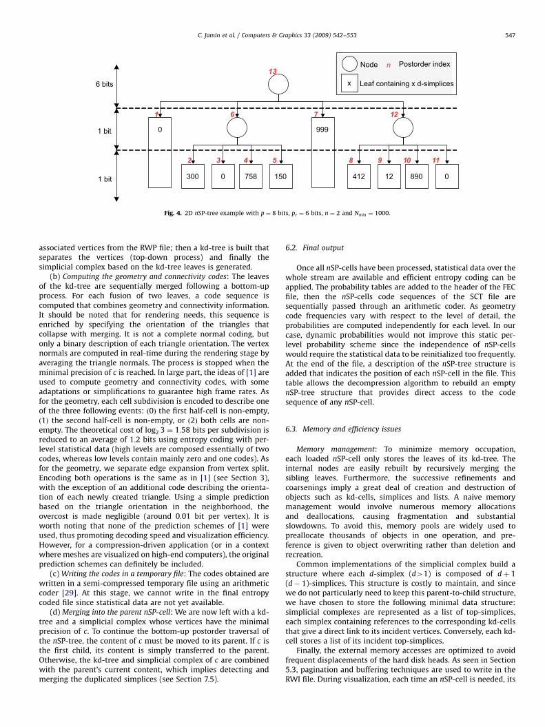
An nSP-tree is built so that each leaf contains the set of the top-simplices lying in the corresponding subspace. The height of thenSP-tree depends on the mesh precision p (the number of bits percoordinate): the user can choose the maximal precision pr of theroot, then the precision pl gained by each next level is computedfrom n (pl ¼ log2 n). For example, for p ¼ 12 bits, pr ¼ 6 bits andn ¼ 4, the nSP-tree height is 4. Another condition is applied: annSP-cell can be split only if the number of contained top-simplicesis at least equal to a threshold Nmin. Consequently, the minimalprecision of the leaves can take any value, whereas their maximalprecision is always p. The content of the leaves is stored in a rawindex file (RWI) where the dþ 1 vertex indices that compose ad-simplex are written using a raw binary format to minimize thedisk footprint while maintaining a fast and simple reading. Fig. 4presents a 2D example of such an nSP-tree.
ARTICLE IN PRESS
C. Jamin et al. / Computers & Graphics 33 (2009) 542–553546
Since an nSP-cell is only subdivided when it contains morethan Nmin triangles, the nSP-tree takes into account the localdensity of the mesh: sparse regions are hardly divided, whereashigh density areas are heavily splitted. This simple scheme hasbeen chosen because it combines adaptability and low encodingcost.
5.3. RWP and RWI file management
Even if the points and triangles are not ordered in the input file,it is likely that the different accesses to a given point of the RWPfile during the nSP-tree construction stage will be close in time.Consequently, the algorithm uses a cache in the main memory,based on a hash table, to minimize the disk accesses to vertexpositions. The hash keys are modulos of the point indices andguarantee a constant time access to cached points.
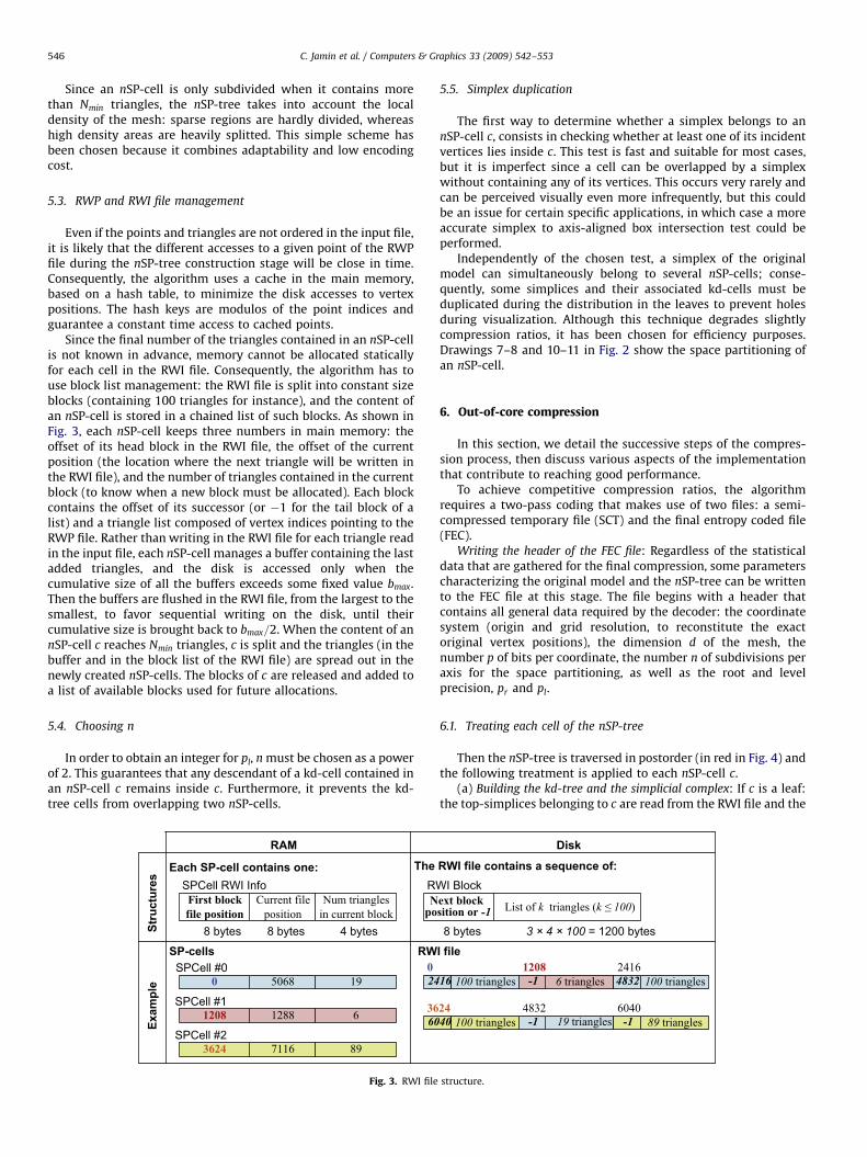
Since the final number of the triangles contained in an nSP-cellis not known in advance, memory cannot be allocated staticallyfor each cell in the RWI file. Consequently, the algorithm has touse block list management: the RWI file is split into constant sizeblocks (containing 100 triangles for instance), and the content ofan nSP-cell is stored in a chained list of such blocks. As shown inFig. 3, each nSP-cell keeps three numbers in main memory: theoffset of its head block in the RWI file, the offset of the currentposition (the location where the next triangle will be written inthe RWI file), and the number of triangles contained in the currentblock (to know when a new block must be allocated). Each blockcontains the offset of its successor (or �1 for the tail block of alist) and a triangle list composed of vertex indices pointing to theRWP file. Rather than writing in the RWI file for each triangle readin the input file, each nSP-cell manages a buffer containing the lastadded triangles, and the disk is accessed only when thecumulative size of all the buffers exceeds some fixed value bmax.Then the buffers are flushed in the RWI file, from the largest to thesmallest, to favor sequential writing on the disk, until theircumulative size is brought back to bmax=2. When the content of annSP-cell c reaches Nmin triangles, c is split and the triangles (in thebuffer and in the block list of the RWI file) are spread out in thenewly created nSP-cells. The blocks of c are released and added toa list of available blocks used for future allocations.
5.4. Choosing n
In order to obtain an integer for pl, n must be chosen as a powerof 2. This guarantees that any descendant of a kd-cell contained inan nSP-cell c remains inside c. Furthermore, it prevents the kd-tree cells from overlapping two nSP-cells.
RW
24
60
RAM
Current file position
SPCell RWI InfoNum triangles
in current block
36
5068SPCell #0
19
8 bytes
1288SPCell #1
6
7116SPCell #2
89
Npo
First block file position
0
1208
3624
0
Each SP-cell contains one:
RWSP-cells
Stru
ctur
esEx
ampl
e
The
8 bytes 4 bytes
Fig. 3. RWI file
5.5. Simplex duplication
The first way to determine whether a simplex belongs to annSP-cell c, consists in checking whether at least one of its incidentvertices lies inside c. This test is fast and suitable for most cases,but it is imperfect since a cell can be overlapped by a simplexwithout containing any of its vertices. This occurs very rarely andcan be perceived visually even more infrequently, but this couldbe an issue for certain specific applications, in which case a moreaccurate simplex to axis-aligned box intersection test could beperformed.
Independently of the chosen test, a simplex of the originalmodel can simultaneously belong to several nSP-cells; conse-quently, some simplices and their associated kd-cells must beduplicated during the distribution in the leaves to prevent holesduring visualization. Although this technique degrades slightlycompression ratios, it has been chosen for efficiency purposes.Drawings 7–8 and 10–11 in Fig. 2 show the space partitioning ofan nSP-cell.
6. Out-of-core compression
In this section, we detail the successive steps of the compres-sion process, then discuss various aspects of the implementationthat contribute to reaching good performance.
To achieve competitive compression ratios, the algorithmrequires a two-pass coding that makes use of two files: a semi-compressed temporary file (SCT) and the final entropy coded file(FEC).
Writing the header of the FEC file: Regardless of the statisticaldata that are gathered for the final compression, some parameterscharacterizing the original model and the nSP-tree can be writtento the FEC file at this stage. The file begins with a header thatcontains all general data required by the decoder: the coordinatesystem (origin and grid resolution, to reconstitute the exactoriginal vertex positions), the dimension d of the mesh, thenumber p of bits per coordinate, the number n of subdivisions peraxis for the space partitioning, as well as the root and levelprecision, pr and pl.
6.1. Treating each cell of the nSP-tree
Then the nSP-tree is traversed in postorder (in red in Fig. 4) andthe following treatment is applied to each nSP-cell c.
(a) Building the kd-tree and the simplicial complex: If c is a leaf:the top-simplices belonging to c are read from the RWI file and the
I Block
100 triangles 16 6 triangles-11208
100 triangles4832
100 triangles40 19 triangles -1
Disk
2416
24 483289 triangles -1
6040
8 bytes 3 × 4 × 100 = 1200 bytes
List of k triangles (k ≤ 100) ext block sition or -1
I file
RWI file contains a sequence of:
structure.
ARTICLE IN PRESS
0 999
412 12 890 0
6 bits
1 bit
1 bit 300 0 150
13
21761
1101985432
758
Node
Leaf containing x d-simplicesx
n Postorder index
Fig. 4. 2D nSP-tree example with p ¼ 8 bits, pr ¼ 6 bits, n ¼ 2 and Nmin ¼ 1000.
C. Jamin et al. / Computers & Graphics 33 (2009) 542–553 547
associated vertices from the RWP file; then a kd-tree is built thatseparates the vertices (top-down process) and finally thesimplicial complex based on the kd-tree leaves is generated.
(b) Computing the geometry and connectivity codes: The leavesof the kd-tree are sequentially merged following a bottom-upprocess. For each fusion of two leaves, a code sequence iscomputed that combines geometry and connectivity information.It should be noted that for rendering needs, this sequence isenriched by specifying the orientation of the triangles thatcollapse with merging. It is not a complete normal coding, butonly a binary description of each triangle orientation. The vertexnormals are computed in real-time during the rendering stage byaveraging the triangle normals. The process is stopped when theminimal precision of c is reached. In large part, the ideas of [1] areused to compute geometry and connectivity codes, with someadaptations or simplifications to guarantee high frame rates. Asfor the geometry, each cell subdivision is encoded to describe oneof the three following events: ð0Þ the first half-cell is non-empty,ð1Þ the second half-cell is non-empty, or ð2Þ both cells are non-empty. The theoretical cost of log2 3 ¼ 1:58 bits per subdivision isreduced to an average of 1:2 bits using entropy coding with per-level statistical data (high levels are composed essentially of twocodes, whereas low levels contain mainly zero and one codes). Asfor the geometry, we separate edge expansion from vertex split.Encoding both operations is the same as in [1] (see Section 3),with the exception of an additional code describing the orienta-tion of each newly created triangle. Using a simple predictionbased on the triangle orientation in the neighborhood, theovercost is made negligible (around 0:01 bit per vertex). It isworth noting that none of the prediction schemes of [1] wereused, thus promoting decoding speed and visualization efficiency.However, for a compression-driven application (or in a contextwhere meshes are visualized on high-end computers), the originalprediction schemes can definitely be included.
(c) Writing the codes in a temporary file: The codes obtained arewritten in a semi-compressed temporary file using an arithmeticcoder [29]. At this stage, we cannot write in the final entropycoded file since statistical data are not yet available.
(d) Merging into the parent nSP-cell: We are now left with a kd-tree and a simplicial complex whose vertices have the minimalprecision of c. To continue the bottom-up postorder traversal ofthe nSP-tree, the content of c must be moved to its parent. If c isthe first child, its content is simply transferred to the parent.Otherwise, the kd-tree and simplicial complex of c are combinedwith the parent’s current content, which implies detecting andmerging the duplicated simplices (see Section 7.5).
6.2. Final output
Once all nSP-cells have been processed, statistical data over thewhole stream are available and efficient entropy coding can beapplied. The probability tables are added to the header of the FECfile, then the nSP-cells code sequences of the SCT file aresequentially passed through an arithmetic coder. As geometrycode frequencies vary with respect to the level of detail, theprobabilities are computed independently for each level. In ourcase, dynamic probabilities would not improve this static per-level probability scheme since the independence of nSP-cellswould require the statistical data to be reinitialized too frequently.At the end of the file, a description of the nSP-tree structure isadded that indicates the position of each nSP-cell in the file. Thistable allows the decompression algorithm to rebuild an emptynSP-tree structure that provides direct access to the codesequence of any nSP-cell.
6.3. Memory and efficiency issues
Memory management: To minimize memory occupation,each loaded nSP-cell only stores the leaves of its kd-tree. Theinternal nodes are easily rebuilt by recursively merging thesibling leaves. Furthermore, the successive refinements andcoarsenings imply a great deal of creation and destruction ofobjects such as kd-cells, simplices and lists. A naive memorymanagement would involve numerous memory allocationsand deallocations, causing fragmentation and substantialslowdowns. To avoid this, memory pools are widely used topreallocate thousands of objects in one operation, and pre-ference is given to object overwriting rather than deletion andrecreation.
Common implementations of the simplicial complex build astructure where each d-simplex (d41) is composed of dþ 1(d� 1)-simplices. This structure is costly to maintain, and sincewe do not particularly need to keep this parent-to-child structure,we have chosen to store the following minimal data structure:simplicial complexes are represented as a list of top-simplices,each simplex containing references to the corresponding kd-cellsthat give a direct link to its incident vertices. Conversely, each kd-cell stores a list of its incident top-simplices.
Finally, the external memory accesses are optimized to avoidfrequent displacements of the hard disk heads. As seen in Section5.3, pagination and buffering techniques are used to write in theRWI file. During visualization, each time an nSP-cell is needed, its
ARTICLE IN PRESS
C. Jamin et al. / Computers & Graphics 33 (2009) 542–553548
complete code is read from the FEC file and put into a buffer toanticipate upcoming accesses.
Multi-core parallelization: The nSP-tree structure is intrinsicallyfavorable to parallelization. The compression has been multi-threaded to benefit from the emerging multi-core processors.While file I/O remain single-threaded to avoid costly randomaccesses to the hard disk, vertex splits and unifications, edgeexpansions and collapses, nSP-cell splits and mergings can beexecuted in parallel on different nSP-cells. To favor effectivesequential access to the hard drive and to avoid frequent locks ofthe other computing threads (file I/O are exclusive), the proces-sing of an SP-cell starts by loading the list of contained trianglesfrom RWI and RWP files into a buffer. Then the following steps(see Section 6.1) only require CPU and RAM operations and can beperformed by one thread running parallel to the other threads.Experimentally, a global increase in performance is observedbetween 1:5 and 2 with a dual-core CPU, and between 2 and 3with a quad-core CPU. This parallelization similarly benefits thedecompression and visualization stage, although the performanceincrease is more difficult to estimate.
21 21
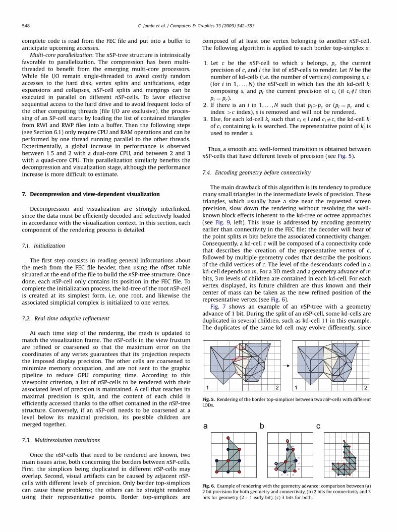
Fig. 5. Rendering of the border top-simplices between two nSP-cells with different
LODs.
Fig. 6. Example of rendering with the geometry advance: comparison between (a)
2 bit precision for both geometry and connectivity, (b) 2 bits for connectivity and 3
bits for geometry (2þ 1 early bit), (c) 3 bits for both.
7. Decompression and view-dependent visualization
Decompression and visualization are strongly interlinked,since the data must be efficiently decoded and selectively loadedin accordance with the visualization context. In this section, eachcomponent of the rendering process is detailed.
7.1. Initialization
The first step consists in reading general informations aboutthe mesh from the FEC file header, then using the offset tablesituated at the end of the file to build the nSP-tree structure. Oncedone, each nSP-cell only contains its position in the FEC file. Tocomplete the initialization process, the kd-tree of the root nSP-cellis created at its simplest form, i.e. one root, and likewise theassociated simplicial complex is initialized to one vertex.
7.2. Real-time adaptive refinement
At each time step of the rendering, the mesh is updated tomatch the visualization frame. The nSP-cells in the view frustumare refined or coarsened so that the maximum error on thecoordinates of any vertex guarantees that its projection respectsthe imposed display precision. The other cells are coarsened tominimize memory occupation, and are not sent to the graphicpipeline to reduce GPU computing time. According to thisviewpoint criterion, a list of nSP-cells to be rendered with theirassociated level of precision is maintained. A cell that reaches itsmaximal precision is split, and the content of each child isefficiently accessed thanks to the offset contained in the nSP-treestructure. Conversely, if an nSP-cell needs to be coarsened at alevel below its maximal precision, its possible children aremerged together.
7.3. Multiresolution transitions
Once the nSP-cells that need to be rendered are known, twomain issues arise, both concerning the borders between nSP-cells.First, the simplices being duplicated in different nSP-cells mayoverlap. Second, visual artifacts can be caused by adjacent nSP-cells with different levels of precision. Only border top-simplicescan cause these problems; the others can be straight renderedusing their representative points. Border top-simplices are
composed of at least one vertex belonging to another nSP-cell.The following algorithm is applied to each border top-simplex s:
1.
Let c be the nSP-cell to which s belongs, pc the currentprecision of c, and l the list of nSP-cells to render. Let N be thenumber of kd-cells (i.e. the number of vertices) composing s, ci(for i in 1; . . . ;N) the nSP-cell in which lies the ith kd-cell ki
composing s, and pi the current precision of ci (if ciel thenpi ¼ pc).
2.
If there is an i in 1; . . . ;N such that pi4pc or (pi ¼ pc and ciindex 4c index), s is removed and will not be rendered.
3. Else, for each kd-cell ki such that ci 2 l and ciac, the kd-cell k0iof ci containing ki is searched. The representative point of k0i isused to render s.
Thus, a smooth and well-formed transition is obtained betweennSP-cells that have different levels of precision (see Fig. 5).
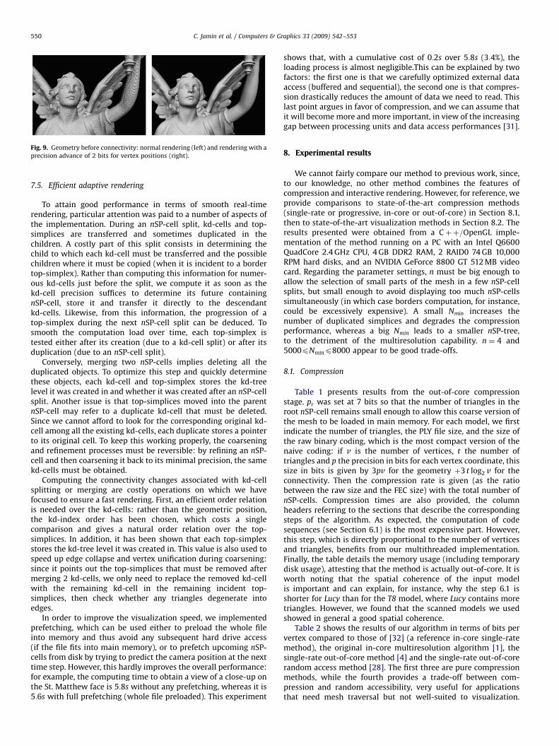
7.4. Encoding geometry before connectivity
The main drawback of this algorithm is its tendency to producemany small triangles in the intermediate levels of precision. Thesetriangles, which usually have a size near the requested screenprecision, slow down the rendering without resolving the well-known block effects inherent to the kd-tree or octree approaches(see Fig. 9, left). This issue is addressed by encoding geometryearlier than connectivity in the FEC file: the decoder will hear ofthe point splits m bits before the associated connectivity changes.Consequently, a kd-cell c will be composed of a connectivity codethat describes the creation of the representative vertex of c,followed by multiple geometry codes that describe the positionsof the child vertices of c. The level of the descendants coded in akd-cell depends on m. For a 3D mesh and a geometry advance of m
bits, 3 m levels of children are contained in each kd-cell. For eachvertex displayed, its future children are thus known and theircenter of mass can be taken as the new refined position of therepresentative vertex (see Fig. 6).
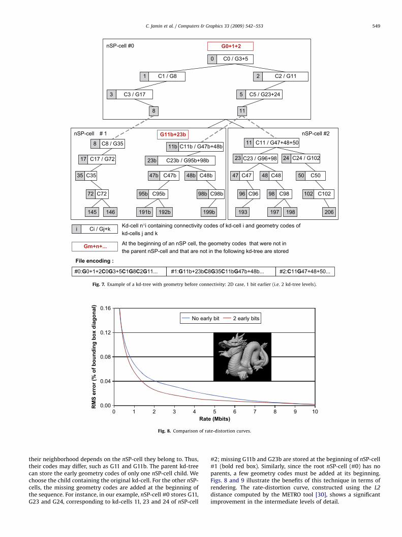
Fig. 7 shows an example of an nSP-tree with a geometryadvance of 1 bit. During the split of an nSP-cell, some kd-cells areduplicated in several children, such as kd-cell 11 in this example.The duplicates of the same kd-cell may evolve differently, since
ARTICLE IN PRESS
C0 / G3+5
nSP-cell #0
C1 / G8 C2 / G11
C3 / G17 C5 / G23+24
G0+1+2
nSP-cell # 1 nSP-cell #2
0
1 2
3 5
8 11
C17 / G7217 C23b / G95b+98b23b
C48b48bC47b47b
C23 / G96+9823 C24 / G10224
C4848 C5050C3535 C4747
G11b+23b
C7272 C95b95b C98b98b C9898 C102102C9696
Ci / Gj+ki Kd-cell n°i containing connectivity codes of kd-cell i and geometry codes of kd-cells j and k
Gm+n+... At the beginning of an nSP cell, the geometry codes that were not in the parent nSP-cell and that are not in the following kd-tree are stored
145 146 191b 192b 199b 193 197 198 206
C8 / G358 C11 / G47+48+5011C11b / G47b+48b11b
File encoding :
#0:G0+1+2C0G3+5C1G8C2G11... #1:G11b+23bC8G35C11bG47b+48b... #2:C11G47+48+50...
Fig. 7. Example of a kd-tree with geometry before connectivity: 2D case, 1 bit earlier (i.e. 2 kd-tree levels).
0.00
0.04
0.08
0.12
0.16
RM
S er
ror (
% o
f bou
ndin
g bo
x di
agon
al)
Rate (Mbits)
No early bit 2 early bits
0 1 2 3 4 5 6 7 8 9 10
Fig. 8. Comparison of rate-distortion curves.
C. Jamin et al. / Computers & Graphics 33 (2009) 542–553 549
their neighborhood depends on the nSP-cell they belong to. Thus,their codes may differ, such as G11 and G11b. The parent kd-treecan store the early geometry codes of only one nSP-cell child. Wechoose the child containing the original kd-cell. For the other nSP-cells, the missing geometry codes are added at the beginning ofthe sequence. For instance, in our example, nSP-cell #0 stores G11,G23 and G24, corresponding to kd-cells 11, 23 and 24 of nSP-cell
#2; missing G11b and G23b are stored at the beginning of nSP-cell#1 (bold red box). Similarly, since the root nSP-cell (#0) has noparents, a few geometry codes must be added at its beginning.Figs. 8 and 9 illustrate the benefits of this technique in terms ofrendering. The rate-distortion curve, constructed using the L2
distance computed by the METRO tool [30], shows a significantimprovement in the intermediate levels of detail.
ARTICLE IN PRESS
Fig. 9. Geometry before connectivity: normal rendering (left) and rendering with a
precision advance of 2 bits for vertex positions (right).
C. Jamin et al. / Computers & Graphics 33 (2009) 542–553550
7.5. Efficient adaptive rendering
To attain good performance in terms of smooth real-timerendering, particular attention was paid to a number of aspects ofthe implementation. During an nSP-cell split, kd-cells and top-simplices are transferred and sometimes duplicated in thechildren. A costly part of this split consists in determining thechild to which each kd-cell must be transferred and the possiblechildren where it must be copied (when it is incident to a bordertop-simplex). Rather than computing this information for numer-ous kd-cells just before the split, we compute it as soon as thekd-cell precision suffices to determine its future containingnSP-cell, store it and transfer it directly to the descendantkd-cells. Likewise, from this information, the progression of atop-simplex during the next nSP-cell split can be deduced. Tosmooth the computation load over time, each top-simplex istested either after its creation (due to a kd-cell split) or after itsduplication (due to an nSP-cell split).
Conversely, merging two nSP-cells implies deleting all theduplicated objects. To optimize this step and quickly determinethese objects, each kd-cell and top-simplex stores the kd-treelevel it was created in and whether it was created after an nSP-cellsplit. Another issue is that top-simplices moved into the parentnSP-cell may refer to a duplicate kd-cell that must be deleted.Since we cannot afford to look for the corresponding original kd-cell among all the existing kd-cells, each duplicate stores a pointerto its original cell. To keep this working properly, the coarseningand refinement processes must be reversible: by refining an nSP-cell and then coarsening it back to its minimal precision, the samekd-cells must be obtained.
Computing the connectivity changes associated with kd-cellsplitting or merging are costly operations on which we havefocused to ensure a fast rendering. First, an efficient order relationis needed over the kd-cells: rather than the geometric position,the kd-index order has been chosen, which costs a singlecomparison and gives a natural order relation over the top-simplices. In addition, it has been shown that each top-simplexstores the kd-tree level it was created in. This value is also used tospeed up edge collapse and vertex unification during coarsening:since it points out the top-simplices that must be removed aftermerging 2 kd-cells, we only need to replace the removed kd-cellwith the remaining kd-cell in the remaining incident top-simplices, then check whether any triangles degenerate intoedges.
In order to improve the visualization speed, we implementedprefetching, which can be used either to preload the whole fileinto memory and thus avoid any subsequent hard drive access(if the file fits into main memory), or to prefetch upcoming nSP-cells from disk by trying to predict the camera position at the nexttime step. However, this hardly improves the overall performance:for example, the computing time to obtain a view of a close-up onthe St. Matthew face is 5:8s without any prefetching, whereas it is5:6s with full prefetching (whole file preloaded). This experiment
shows that, with a cumulative cost of 0:2s over 5:8s (3:4%), theloading process is almost negligible.This can be explained by twofactors: the first one is that we carefully optimized external dataaccess (buffered and sequential), the second one is that compres-sion drastically reduces the amount of data we need to read. Thislast point argues in favor of compression, and we can assume thatit will become more and more important, in view of the increasinggap between processing units and data access performances [31].
8. Experimental results
We cannot fairly compare our method to previous work, since,to our knowledge, no other method combines the features ofcompression and interactive rendering. However, for reference, weprovide comparisons to state-of-the-art compression methods(single-rate or progressive, in-core or out-of-core) in Section 8.1,then to state-of-the-art visualization methods in Section 8.2. Theresults presented were obtained from a Cþþ=OpenGL imple-mentation of the method running on a PC with an Intel Q6600QuadCore 2.4 GHz CPU, 4 GB DDR2 RAM, 2 RAID0 74 GB 10,000RPM hard disks, and an NVIDIA GeForce 8800 GT 512 MB videocard. Regarding the parameter settings, n must be big enough toallow the selection of small parts of the mesh in a few nSP-cellsplits, but small enough to avoid displaying too much nSP-cellssimultaneously (in which case borders computation, for instance,could be excessively expensive). A small Nmin increases thenumber of duplicated simplices and degrades the compressionperformance, whereas a big Nmin leads to a smaller nSP-tree,to the detriment of the multiresolution capability. n ¼ 4 and5000pNminp8000 appear to be good trade-offs.
8.1. Compression
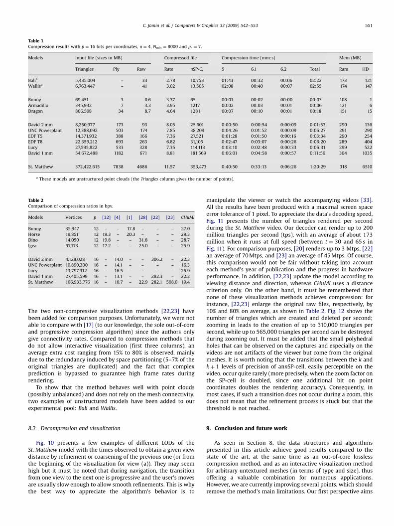
Table 1 presents results from the out-of-core compressionstage. pr was set at 7 bits so that the number of triangles in theroot nSP-cell remains small enough to allow this coarse version ofthe mesh to be loaded in main memory. For each model, we firstindicate the number of triangles, the PLY file size, and the size ofthe raw binary coding, which is the most compact version of thenaive coding: if v is the number of vertices, t the number oftriangles and p the precision in bits for each vertex coordinate, thissize in bits is given by 3pv for the geometry þ3 t log2 v for theconnectivity. Then the compression rate is given (as the ratiobetween the raw size and the FEC size) with the total number ofnSP-cells. Compression times are also provided, the columnheaders referring to the sections that describe the correspondingsteps of the algorithm. As expected, the computation of codesequences (see Section 6.1) is the most expensive part. However,this step, which is directly proportional to the number of verticesand triangles, benefits from our multithreaded implementation.Finally, the table details the memory usage (including temporarydisk usage), attesting that the method is actually out-of-core. It isworth noting that the spatial coherence of the input modelis important and can explain, for instance, why the step 6.1 isshorter for Lucy than for the T8 model, where Lucy contains moretriangles. However, we found that the scanned models we usedshowed in general a good spatial coherence.
Table 2 shows the results of our algorithm in terms of bits pervertex compared to those of [32] (a reference in-core single-ratemethod), the original in-core multiresolution algorithm [1], thesingle-rate out-of-core method [4] and the single-rate out-of-corerandom access method [28]. The first three are pure compressionmethods, while the fourth provides a trade-off between com-pression and random accessibility, very useful for applicationsthat need mesh traversal but not well-suited to visualization.
ARTICLE IN PRESS
Table 2Comparison of compression ratios in bpv.
Models Vertices p [32] [4] [1] [28] [22] [23] CHuMI
Bunny 35,947 12 – – 17.8 – – – 27.0
Horse 19,851 12 19.3 – 20.3 – – – 29.3
Dino 14,050 12 19.8 – – 31.8 – – 28.7
Igea 67,173 12 17.2 – – 25.0 – – 25.9
David 2 mm 4,128,028 16 – 14.0 – – 306.2 – 22.3
UNC Powerplant 10,890,300 16 – 14.1 – – – – 16.3
Lucy 13,797,912 16 – 16.5 – – – – 25.9
David 1 mm 27,405,599 16 – 13.1 – – 282.3 – 22.2
St. Matthew 166,933,776 16 – 10.7 – 22.9 282.1 508.0 19.4
Table 1Compression results with p ¼ 16 bits per coordinates, n ¼ 4, Nmin ¼ 8000 and pr ¼ 7.
Models Input file (sizes in MB) Compressed file Compression time (mm:s) Mem (MB)
Triangles Ply Raw Rate nSP-C. 5 6.1 6.2 Total Ram HD
Balia 5,435,004 – 33 2.78 10,753 01:43 00:32 00:06 02:22 173 121
Wallisa 6,763,447 – 41 3.02 13,505 02:08 00:40 00:07 02:55 174 147
Bunny 69,451 3 0.6 3.37 65 00:01 00:02 00:00 00:03 108 1
Armadillo 345,932 7 3.3 3.95 1217 00:02 00:03 00:01 00:06 121 6
Dragon 866,508 34 8.7 4.64 1281 00:07 00:10 00:01 00:18 151 15
David 2 mm 8,250,977 173 93 8.05 25,601 0:00:50 0:00:54 0:00:09 0:01:53 290 136
UNC Powerplant 12,388,092 503 174 7.85 38,209 0:04:26 0:01:52 0:00:09 0:06:27 291 290
EDF T5 14,371,932 388 166 7.36 27,521 0:01:28 0:01:50 0:00:16 0:03:34 290 254
EDF T8 22,359,212 693 263 6.82 31,105 0:02:47 0:03:07 0:00:26 0:06:20 289 404
Lucy 27,595,822 533 328 7.35 114,113 0:03:10 0:02:48 0:00:33 0:06:31 299 522
David 1 mm 54,672,488 1182 671 8.81 181,569 0:06:01 0:04:58 0:00:57 0:11:56 304 1035
St. Matthew 372,422,615 7838 4686 11.57 353,473 0:40:50 0:33:13 0:06:26 1:20:29 318 6510
a These models are unstructured point clouds (the Triangles column gives the number of points).
C. Jamin et al. / Computers & Graphics 33 (2009) 542–553 551
The two non-compressive visualization methods [22,23] havebeen added for comparison purposes. Unfortunately, we were notable to compare with [17] (to our knowledge, the sole out-of-coreand progressive compression algorithm) since the authors onlygive connectivity rates. Compared to compression methods thatdo not allow interactive visualization (first three columns), anaverage extra cost ranging from 15% to 80% is observed, mainlydue to the redundancy induced by space partitioning (5–7% of theoriginal triangles are duplicated) and the fact that complexprediction is bypassed to guarantee high frame rates duringrendering.
To show that the method behaves well with point clouds(possibly unbalanced) and does not rely on the mesh connectivity,two examples of unstructured models have been added to ourexperimental pool: Bali and Wallis.
8.2. Decompression and visualization
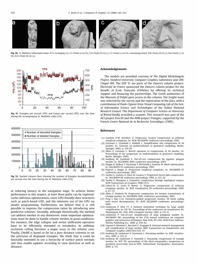
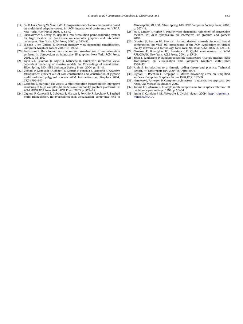
Fig. 10 presents a few examples of different LODs of theSt. Matthew model with the times observed to obtain a given viewdistance by refinement or coarsening of the previous one (or fromthe beginning of the visualization for view (a)). They may seemhigh but it must be noted that during navigation, the transitionfrom one view to the next one is progressive and the user’s movesare usually slow enough to allow smooth refinements. This is whythe best way to appreciate the algorithm’s behavior is to
manipulate the viewer or watch the accompanying videos [33].All the results have been produced with a maximal screen spaceerror tolerance of 1 pixel. To appreciate the data’s decoding speed,Fig. 11 presents the number of triangles rendered per secondduring the St. Matthew video. Our decoder can render up to 200million triangles per second (tps), with an average of about 173million when it runs at full speed (between t ¼ 30 and 65 s inFig. 11). For comparison purposes, [20] renders up to 3 Mtps, [22]an average of 70 Mtps, and [23] an average of 45 Mtps. Of course,this comparison would not be fair without taking into accounteach method’s year of publication and the progress in hardwareperformance. In addition, [22,23] update the model according toviewing distance and direction, whereas CHuMI uses a distancecriterion only. On the other hand, it must be remembered thatnone of these visualization methods achieves compression: forinstance, [22,23] enlarge the original raw files, respectively, by10% and 80% on average, as shown in Table 2. Fig. 12 shows thenumber of triangles which are created and deleted per second;zooming in leads to the creation of up to 310,000 triangles persecond, while up to 565,000 triangles per second can be destroyedduring zooming out. It must be added that the small polyhedralholes that can be observed on the captures and especially on thevideos are not artifacts of the viewer but come from the originalmeshes. It is worth noting that the transitions between the k andkþ 1 levels of precision of annSP-cell, easily perceptible on thevideo, occur quite rarely (more precisely, when the zoom factor onthe SP-cell is doubled, since one additional bit on pointcoordinates doubles the rendering accuracy). Consequently, inmost cases, if such a transition does not occur during a zoom, thisdoes not mean that the refinement process is stuck but that thethreshold is not reached.
9. Conclusion and future work
As seen in Section 8, the data structures and algorithmspresented in this article achieve good results compared to thestate of the art, at the same time as an out-of-core losslesscompression method, and as an interactive visualization methodfor arbitrary untextured meshes (in terms of type and size), thusoffering a valuable combination for numerous applications.However, we are currently improving several points, which shouldremove the method’s main limitations. Our first perspective aims
ARTICLE IN PRESS
Fig. 10. St. Matthew refinement times: 0.7 s to display (a), 1.2 s from (a) to (b), 2.0 s from (b) to (c), 1.7 s from (c) to (d); coarsening times: 0.8 s from (d) to (c), 0.6 s from (c) to
(b), 0.4 s from (b) to (a).
0
100
200
300
400
500
600
700
020406080
100120140160180200
FPS
TPS
(106 )
TPS
FPS
0 20 40 60 80 100
Fig. 11. Triangles per second (TPS) and frames per second (FPS) over the time
during the accompanying St. Matthew video [33].
0
100000
200000
300000
400000
500000
600000
0 10 20 30 40 50 60 70 80 90
Number of decoded trianglesNumber of deleted triangles
Fig. 12. Stacked column chart showing the number of triangles decoded/deleted
per second over the time during the St. Matthew video [33].
C. Jamin et al. / Computers & Graphics 33 (2009) 542–553552
at reducing latency in the navigation stage. To achieve betterperformance in this respect, at least three paths can be explored:cache-oblivious optimizations, more GPU-friendly data structuressuch as patch-based LOD, and the intensive use of the GPU viashader programming. Furthermore, we believe that it is stillpossible to improve the compression ratios by introducing newpredictive schemes. Secondly, although theoretically, the methodcan address meshes in any dimension, some important optimiza-tions must be done to handle volume meshes in good conditions.For instance, the edge collapse and vertex unification operatorshave to be efficiently extended to tetrahedra. In addition,occlusion culling becomes a major issue in the volume case.Finally, CHuMI is based so far on a pure distance criterion to setthe precision of displayed triangles. We think that it could befavorably extended to use a hierarchy of surface patch normalsand thus enable updates according to view direction as well asdistance.
Acknowledgements
The models are provided courtesy of The Digital Michelangelo
Project, Stanford University Computer Graphics Laboratory and UNC
Chapel Hill. The EDF Tx are parts of the Dancers column project:Electricite de France sponsored the Dancers column project for thebenefit of Ecole Franc-aise d’Athenes by offering its technicalsupport and financing the partnerships. The Greek authorities ofthe Museum of Delphi gave access to the column. The Insight teamwas selected for the survey and the registration of the data, with acontribution of Paolo Cignoni from Visual Computing Lab of the Inst.
of Information Science and Technologies of the Italian National
Research Council. The Department of Computer Science at University
of Bristol kindly provided a scanner. This research was part of theACI project Eros3D and the ANR project Triangles, supported by theFrench Centre National de la Recherche Scientifique (CNRS).
References
[1] Gandoin P-M, Devillers O. Progressive lossless compression of arbitrarysimplicial complexes. In: ACM SIGGRAPH conference proceedings, 2002.
[2] Gotsman C, Gumhold S, Kobbelt L. Simplification and compression of 3dmeshes. In: Tutorials on multiresolution in geometric modelling. Berlin:Springer; 2002. p. 319–61.
[3] Alliez P, Gotsman C. Recent advances in compression of 3d meshes. In:Proceedings of the symposium on multiresolution in geometric modeling.Berlin: Springer; 2003.
[4] Isenburg M, Gumhold S. Out-of-core compression for gigantic polygonmeshes. In: SIGGRAPH 2003 conference proceedings, 2003.
[5] Hoppe H, DeRose T, Duchamp T, McDonald J, Stuetzle W. Mesh optimization.In: SIGGRAPH 93 conference proceedings, 1993.
[6] Popovic J, Hoppe H. Progressive simplicial complexes. In: SIGGRAPH 97conference proceedings, 1997.
[7] Taubin G, Gueziec A, Horn W, Lazarus F. Progressive forest split compression.In: SIGGRAPH 98 conference proceedings, 1998. p. 123–32.
[8] Taubin G, Rossignac J. Geometric compression through topological surgery.ACM Transactions on Graphics 1998;17(2).
[9] Cohen-Or D, Levin D, Remez O. Progressive compression of arbitrarytriangular meshes. In: IEEE visualization 99 conference proceedings, 1999.p. 67–72.
[10] Alliez P, Desbrun M. Progressive compression for lossless transmission oftriangle meshes. In: SIGGRAPH 2001 conference proceedings; 2001.
[11] Peng J, Kuo C-CJ. Geometry-guided progressive lossless 3d mesh codingwith octree decomposition. In: ACM SIGGRAPH conference proceedings;2005.
[12] Lindstrom P, Silva CT. A memory insensitive technique for large modelsimplification. In: VIS ’01: Proceedings of the conference on visualization ’01.Washington, DC, USA: IEEE Computer Society; 2001. p. 121–6.
[13] Lindstrom P. Out-of-core simplification of large polygonal models. In:SIGGRAPH ’00: proceedings of the 27th annual conference on computergraphics and interactive techniques. New York, NY, USA: ACM Press, Addison-Wesley Publishing Co.; 2000. p. 259–62.
[14] Cignoni P, Montani C, Rocchini C, Scopigno R. External memory managementand simplification of huge meshes. IEEE Transactions on Visualization andComputer Graphics 2003;9(4):525–37.
[15] Isenburg M, Lindstrom P, Livermore L. Streaming meshes. In: IEEE visualiza-tion; 2005. p. 231–8.
[16] Isenburg M, Lindstrom P, Snoeyink J. Streaming compression of trianglemeshes. In: SGP ’05: proceedings of the third eurographics symposium ongeometry processing. Aire-la-Ville, Switzerland: Eurographics Association;2005. p. 111.
ARTICLE IN PRESS
C. Jamin et al. / Computers & Graphics 33 (2009) 542–553 553
[17] Cai K, Liu Y, Wang W, Sun H, Wu E. Progressive out-of-core compression basedon multi-level adaptive octree. In: ACM international conference on VRCIA.New York: ACM Press; 2006. p. 83–9.
[18] Rusinkiewicz S, Levoy M. Qsplat: a multiresolution point rendering systemfor large meshes. In: Conference on computer graphics and interactivetechniques. New York: ACM Press; 2000. p. 343–52.
[19] El-Sana J, jen Chiang Y. External memory view-dependent simplification.Computer Graphics Forum 2000;19:139–50.
[20] Lindstrom P. Out-of-core construction and visualization of multiresolutionsurfaces. In: Symposium on interactive 3D graphics. New York: ACM Press;2003. p. 93–102.
[21] Yoon S-E, Salomon B, Gayle R, Manocha D. Quick-vdr: interactive view-dependent rendering of massive models. In: Proceedings of visualization.Silver Spring, MD: IEEE Computer Society Press; 2004. p. 131–8.
[22] Cignoni P, Ganovelli F, Gobbetti E, Marton F, Ponchio F, Scopigno R. Adaptivetetrapuzzles: efficient out-of-core construction and visualization of giganticmultiresolution polygonal models. ACM Transactions on Graphics 2004;23(3):796–803.
[23] Gobbetti E, Marton F. Far voxels: a multiresolution framework for interactiverendering of huge complex 3d models on commodity graphics platforms. In:ACM SIGGRAPH. New York: ACM Press; 2005. p. 878–85.
[24] Cignoni P, Ganovelli F, Gobbetti E, Marton F, Ponchio F, Scopigno R. Batchedmulti triangulation. In: Proceedings IEEE visualization, conference held in
Minneapolis, MI, USA. Silver Spring, MD: IEEE Computer Society Press; 2005.p. 207–14.
[25] Hu L, Sander P, Hoppe H. Parallel view-dependent refinement of progressivemeshes. In: ACM symposium on interactive 3D graphics and games;2009.
[26] Oliveira JF, Buxton BF. Pnorms: platonic derived normals for error boundcompression. In: VRST ’06: proceedings of the ACM symposium on virtualreality software and technology. New York, NY, USA: ACM; 2006. p. 324–33.
[27] Namane R, Boumghar FO, Bouatouch K. Qsplat compression. In: ACMAFRIGRAPH. New York: ACM Press; 2004. p. 15–24.
[28] Yoon S, Lindstrom P. Random-accessible compressed triangle meshes. IEEETransactions on Visualization and Computer Graphics 2007;13(6):1536–43.
[29] Amir S. Introduction to arithmetic coding theory and practice. TechnicalReport, HP Labs report HPL-2004-76; April 2004.
[30] Cignoni P, Rocchini C, Scopigno R. Metro: measuring error on simplifiedsurfaces. Computer Graphics Forum 1998;17(2):167–74.
[31] Hennessy J, Patterson D. Computer architecture—a quantitative approach. LosAltos, CA: Morgan Kaufmann; 2007.
[32] Touma C, Gotsman C. Triangle mesh compression. In: Graphics interface 98conference proceedings; 1998. p. 26–34.
[33] Jamin C, Gandoin P-M, Akkouche S. CHuMI videos, 2009. hhttp://clementja-min.free.fr/CG/i.