chm 335 - physical chemistry laboratory course syllabus ... · chm 335 - physical chemistry...
TRANSCRIPT
CHM 335 - Physical Chemistry LaboratoryCourse Syllabus
Fall 2012
Contents
1 Instructors 4
2 Teaching Assistants 4
3 Text Book 4
4 Classroom 5
5 Laboratory Safety 5
6 Course Requirements 5
7 Data Collection 6
8 Grading 6
9 Outline of the Laboratory Procedure 7
10 Plagiarism 7
11 Schedule 8
12 The CHM 335 Web page 11
13 First Two Laboratory Projects 1413.1 Experiment 34 - Absorption Spectrum of a Conjugated Dye . . . . . . . . . 14
13.1.1 Reading Assignment . . . . . . . . . . . . . . . . . . . . . . . . . . . 1513.1.2 Experimental Notes . . . . . . . . . . . . . . . . . . . . . . . . . . . . 1513.1.3 Laboratory Reports . . . . . . . . . . . . . . . . . . . . . . . . . . . . 15
13.2 The Diffusion of Salt Solutions into Pure Water . . . . . . . . . . . . . . . . 16
1
13.2.1 Procedure . . . . . . . . . . . . . . . . . . . . . . . . . . . . . . . . . 1913.2.2 Laboratory Report . . . . . . . . . . . . . . . . . . . . . . . . . . . . 22
14 Second Two Laboratory Experiments 2314.1 Notes on Error Analysis . . . . . . . . . . . . . . . . . . . . . . . . . . . . . 23
14.1.1 Reading Assignment . . . . . . . . . . . . . . . . . . . . . . . . . . . 2314.1.2 Introduction . . . . . . . . . . . . . . . . . . . . . . . . . . . . . . . . 2314.1.3 Systematic and Random Errors . . . . . . . . . . . . . . . . . . . . . 2414.1.4 The Distribution of Random Errors - The Gaussian Distribution . . . 2414.1.5 Calculation of Random Errors for a Finite Set of Laboratory Measure-
ments . . . . . . . . . . . . . . . . . . . . . . . . . . . . . . . . . . . 2514.1.6 Error Propagation . . . . . . . . . . . . . . . . . . . . . . . . . . . . 2714.1.7 Errors from a Graphical Analysis of the Data . . . . . . . . . . . . . 31
14.2 Experiment 28a: The Intrinsic Viscosity of Polyvinyl Alcohol . . . . . . . . . 3414.2.1 Introduction and Reading Assignments . . . . . . . . . . . . . . . . . 3414.2.2 Theory . . . . . . . . . . . . . . . . . . . . . . . . . . . . . . . . . . . 3414.2.3 Experimental Procedure . . . . . . . . . . . . . . . . . . . . . . . . . 3514.2.4 Laboratory Report . . . . . . . . . . . . . . . . . . . . . . . . . . . . 35
14.3 Experiment 28b: The Intrinsic Viscosity of Polyvinyl Alcohol . . . . . . . . . 3714.3.1 Introduction . . . . . . . . . . . . . . . . . . . . . . . . . . . . . . . . 3714.3.2 Theory . . . . . . . . . . . . . . . . . . . . . . . . . . . . . . . . . . . 3714.3.3 Cleaning Procedure . . . . . . . . . . . . . . . . . . . . . . . . . . . . 3814.3.4 Laboratory Report . . . . . . . . . . . . . . . . . . . . . . . . . . . . 38
15 Format of Laboratory Reports for Final Four Experiments 39
16 Second Four Experiments 4016.1 Experiment Number 3 - Heat Capacity Ratio of Gases . . . . . . . . . . . . 40
16.1.1 Reading Assignment . . . . . . . . . . . . . . . . . . . . . . . . . . . 4016.1.2 Theoretical Discussion . . . . . . . . . . . . . . . . . . . . . . . . . . 4116.1.3 Experimental Notes . . . . . . . . . . . . . . . . . . . . . . . . . . . . 4516.1.4 Laboratory Report . . . . . . . . . . . . . . . . . . . . . . . . . . . . 45
16.2 Experiment 6 - The Heat of Combustion of Organic Compounds . . . . . . . 4616.2.1 Reading Assignment . . . . . . . . . . . . . . . . . . . . . . . . . . . 4616.2.2 Experimental Notes . . . . . . . . . . . . . . . . . . . . . . . . . . . . 4616.2.3 Error Analysis . . . . . . . . . . . . . . . . . . . . . . . . . . . . . . . 46
16.3 Experiment Number 9 - Partial Molar Volume . . . . . . . . . . . . . . . . . 4616.3.1 Reading Assignment . . . . . . . . . . . . . . . . . . . . . . . . . . . 4616.3.2 Experimental Notes . . . . . . . . . . . . . . . . . . . . . . . . . . . . 4616.3.3 Laboratory Reports . . . . . . . . . . . . . . . . . . . . . . . . . . . . 47
16.4 The Joule-Thomson Effect . . . . . . . . . . . . . . . . . . . . . . . . . . . . 4916.4.1 Reading Assignment . . . . . . . . . . . . . . . . . . . . . . . . . . . 4916.4.2 Procedure . . . . . . . . . . . . . . . . . . . . . . . . . . . . . . . . . 50
2
16.4.3 Calculations . . . . . . . . . . . . . . . . . . . . . . . . . . . . . . . . 5016.4.4 Error Analysis . . . . . . . . . . . . . . . . . . . . . . . . . . . . . . . 5016.4.5 Discussion . . . . . . . . . . . . . . . . . . . . . . . . . . . . . . . . . 50
17 Final Experiment - Experiment 25 - Surface Tension of Solutions 5117.1 Reading Assignment . . . . . . . . . . . . . . . . . . . . . . . . . . . . . . . 5117.2 Theory . . . . . . . . . . . . . . . . . . . . . . . . . . . . . . . . . . . . . . . 51
17.2.1 Experimental Notes . . . . . . . . . . . . . . . . . . . . . . . . . . . . 5617.3 Laboratory Report . . . . . . . . . . . . . . . . . . . . . . . . . . . . . . . . 56
18 Tables of Data 59
3
1 Instructors
1. Prof. Sze Yang (Wednesday and Friday’s Sections)Pastore 334401-207-9624Office Hours: Tu,Th 10e-mail:[email protected]
2. Prof. David L. Freeman (Tuesday and Thursday’s Sections)Pastore 333 (or 319)Ext. 4-5093Office Hours: MWF 10e-mail:[email protected]
2 Teaching Assistants
1. Meredith Matoian (Tuesday’s Section)Pastore 115Office Hours: M 10e-mail: [email protected]
2. Morgan Turano (Wednesday’s Section)201A PastoreOffice Hours: W 11e-mail: [email protected]
3. Maria Donnelly (Thursday’s Section)Pastore 217 7Office Hours: Tu 11e-mail: [email protected]
4. Lindsay McLennan (Friday’s Section)Pastore 233Office Hours: M 10e-mail: [email protected]
3 Text Book
Experiments in Physical Chemistry, 7th edition, Garland, Nibler and Shoemaker.
4
4 Classroom
316 Pastore
5 Laboratory Safety
You must wear safety glasses with side guards or safety goggles and have themon before you enter the laboratory. Of course, you must continue to wear themwhile in the lab. You must also wear a laboratory coat, and you may not wearopen-toed shoes or sandals. If you are ever in the laboratory without eye protectionor a lab coat, you will have 5 points deducted from your next laboratory report. Repeatedoffenses will result in failure in the course. Be sure to bring your eye protection and lab coatto the second class meeting, so that you will be allowed to perform the first experiment ofthe semester.
All students must complete the Department Safety and Environmental Compliance Form.All students must have their Medical Information Form with them during every laboratoryperiod.
6 Course Requirements
This semester you are to perform nine experiments. The nine experiments are dividedinto two groups of four plus a final experiment at the end of the semester. The first fourexperiments are designed to gradually teach each of you how to extract data and work up ananalysis as a laboratory report. Each of the first four experiments are performed by everymember of a section in the same laboratory period.
Some of the experiments are to be performed with a laboratory partner. Even thoughyou may collect data with a partner, you are responsible for your own labora-tory reports. Identical or nearly identical laboratory reports from two or morestudents are treated as cases of plagiarism.
In the first experiment you will study the spectrum of a conjugated dye. Again you willwork with partners. You will extract data by measuring the spectra and comparing thelocation of the wavelength maximum with theoretical predictions.
The second experiment is a study of the diffusion of ionic species in water. This ex-periment is performed with a partner. Each group studies the diffusion of a different ionicspecies. Your particular species is to be given to you by the TA. In this experiment youextract data and confirm that concentration gradients migrate with a particular functionaldependence on the time. Details are given in section 13.2.
In the third experiment you measure the viscosity of polyvinyl alcohol in water. Thepurpose of this experiment is to instruct you in the principles of experimental error. Yourepeat your measurements many times to observe the statistical distribution of error. Your
5
laboratory reports on this experiment emphasize the analysis of these errors. Details aregiven in Section 14.2.
In the final of the first four experiments, you again measure the viscosity of polyvinylalcohol solutions, but after chemical degradation. The purpose is to learn structural in-formation about the polymer from bulk measurements. The laboratory report from thisexperiment incorporates all sections learned in the first three experiments, and constitutesa complete laboratory report.
The second set of four experiments are performed with partners. Each of the four ex-periments is performed in every laboratory period by one set of partners. The equipmentis rotated among groups during this five week period. The experiments are 1) the Joule-Thomson effect; 2) the heat of combustion of an organic compound; 3) the partial molarvolume of a salt solution; and 4) heat capacity ratio of gases. Complete laboratory reportsare to be submitted for each of these experiments.
In the ninth and final experiment of the semester you study the surface tension of abutanol solution. Because of equipment limitations, only four students are able to performthe experiment in any one laboratory section. The experiment runs over a two week periodwithout partners to allow all students the opportunity to obtain data. Students not scheduledto perform an experiment in a given week during this period have no assignment. Thetime may be used to make up an experiment missed because of personal emergencies. Thelaboratory report for the surface tension experiment is written in the following week [seethe schedule, Section 11] in class during a four hour period. This laboratory report can beviewed as a kind of final exam where the questions are know ahead of time. Paper and graphpaper are provided for you.
7 Data Collection
Where possible, all data generated in the laboratory should be entered into a laboratorynotebook. Laboratory notebooks can be purchased in the bookstore, and the bookstorenotebooks generate carbonless copies, so that a copy of your data is automatically generated.In some instances the data you generate cannot be entered into the notebook. Your TA willinform you when the notebooks are not required. The copy of your data signed by your TAshould be included in the data portions of your laboratory reports.
8 Grading
Each of the laboratory report are worth 100 points. The reports are due exactly one weekafter the completion of a given experiment. If, because of a holiday, classes do not meet oneweek following the completion of a report, the report is due the day following the holiday oron the date the report would normally be due. For example, this semester there is no classon Tuesday, November 6. Reports from Tuesday’s section normally due on November 6 areare due on Wednesday, November 7 even though students in Tuesday’s section meet again
6
on Tuesday, November 13. In a similar fashion, if a class is cancelled because of weather (orany other reason) the report is due the day following the cancelled class or the next datethe University is officially open. Late reports will be accepted for grading up to oneweek after the due date. However, late reports are assessed a penalty of 2 pointsfor each day that they are late. Reports submitted more than one week past thedue date will not be accepted for grading, and such reports will receive a scoreof 0. The final laboratory report, written in class, is worth 200 points.
Your grades are determined on an absolute scale. The scale isA : 930 to 1000 pointsA- : 900 to 929B+ : 870 to 899B : 830 to 869B- : 800 to 829C+ : 770 to 799C : 730 to 769C- : 700 to 729D+ : 670 to 699D : 600 to 669F : < 600
9 Outline of the Laboratory Procedure
Before being allowed to begin any of the experiments in this course, you are required toprepare an outline of the experimental procedure. You should prepare the outline at home,and bring it to class with you. Your TA then signs and dates the outline before you begin theexperiment. The signed outline must be attached to your laboratory report. No laboratoryreports can be graded without the attached signed outline.
At the completion of an experiment, you must present your data to your TA. The TAthen signs and dates the data. The original signed data must be attached to your laboratoryreports for grading. No laboratory report can be graded without the signed data attached.
10 Plagiarism
One of our goals in this course is to reinforce the importance of scientific integrity. In recentyears, there have been numerous examples of established scientists generating falsified dataor copying material from another source. Acts of plagiarism both damage science and canhave important impacts on society. The possibly falsified data associated with the connectionbetween childhood vaccines and autism is an important recent example that has adverselyaffected both science and public health. Acts of plagiarism have destroyed many scientificcareers. Consequently, we want to make clear to you what plagiarism is and penalize acts ofplagiarism in a manner that makes clear its seriousness.
7
Your laboratory reports contain information about the purpose, theory and results ofyour experiments. Each of you prepares a laboratory report associated only with your name.By implication you are the sole author of that report, and no section of your report canbe identical (or nearly identical) to that of another person without attribution. Reports orsections of reports identical to any other source whether that source be another student, asection of a book, or information obtained from others on the web is treated as plagiarism.In CHM 335 the first instance of plagiarized sections are to receive a grade of 0. For repeatinstances of plagiarism, the entire report will receive a 0, and the incident will be referredto the Chair of the Chemistry Department and the Dean of your college.
In CHM 335 there is one exception to this policy. You often generate your data with alaboratory partner. The original data included in your reports, and only the original data,should be identical to that of your laboratory partners. The other sections of your reports,including all written work and all calculations cannot be identical to anyone including yourlaboratory partners.
As an example in the second experiment of the semester you determine the diffusivebehavior of ionic salts in water. The data from this experiment consists of a sheet of graphpaper with multiple curves in different colors generated as a function of time. At the end ofthe experiment each set of partners has one sheet of graph paper with the same curves. Thedata is then photocopied in color, and each partner receives either the original sheet or thephotocopy. This original data should be included in each partner’s laboratory report, andthe data are clearly identical for each partner.
To analyze this data each partner must separately generate numbers from the graphsusing a ruler and a set of points on the graph chosen by each individual in a manner tobe discussed later this semester. It is impossible for the generated numbers to be identicalbetween partners even though the curves are identical. Identical generated data from thisexperiment or any other experiment is an example of plagiarism.
Another possible source of plagiarism can occur if you do not analyze your data by your-self. Students often work together, and the plagiarism policy is not designed to discouragecollaborative learning. However, in the end, your calculations must be your own done inyour unique fashion. The sections of your reports containing the calculations must not beidentical or nearly identical to anyone else. From experience it is not possible for any twopeople analyzing the same data to obtain exactly the same set of calculations in the same or-der with the same final results. To avoid even the appearance of plagiarism, if you decide tostudy with another student, you must perform your calculations by yourself or with the helpof one of the instructors. Nearly identical calculation sections are examples of plagiarism.
11 Schedule
1. Week 1: Lecture and Orientation (Meet in 259 Pastore)Tuesday - Sept. 11Wednesday - Sept. 5
8

Thursday - Sept. 6Friday - Sept. 7
2. Week 2: Spectrum of a Conjugated DyeTuesday - Sept. 18Wednesday - Sept. 12Thursday - Sept. 13Friday - Sept. 14
3. Week 3: The Diffusion of Salt SolutionsTuesday - Sept. 25Wednesday - Sept. 19Thursday - Sept. 20Friday - Sept. 21
4. Week 4: The Viscosity of Polyvinyl Alcohol, Part a (Meet in 259 Pastore for a prelim-inary lecture)Tuesday - Oct. 2Wednesday - Sept. 26Thursday - Sept. 27Friday - Sept. 28
5. Week 5: The Viscosity of Polyvinyl Alcohol, Part bTuesday - Oct. 9Wednesday - Oct. 3Thursday - Oct. 4Friday - Oct. 5
6. Week 6: MakeupTuesday - Oct. 16Wednesday - Oct. 10Thursday - Oct. 11Friday - Friday - Oct. 12
7. Week 7: Group A - Heat Capacity Ratio of GasesGroup B - Joule-Thomson EffectGroup C - Partial Molar VolumeGroup D - Heat of CombustionTuesday - Oct. 23Wednesday - Oct. 17Thursday - Oct. 18Friday - Oct. 19
8. Week 8: Group B - Heat Capacity Ratio of GasesGroup C - Joule-Thomson Effect
9
Group D - Partial Molar VolumeGroup A - Heat of CombustionTuesday - Oct. 30Wednesday - Oct. 24Thursday - Oct. 25Friday - Oct. 26
9. Week 9: Group C - Heat Capacity Ratio of GasesGroup D - Joule-Thomson EffectGroup A - Partial Molar VolumeGroup B - Heat of CombustionTuesday - Nov. 7 (Wednesday)Wednesday - Oct. 31Thursday - Nov. 1Friday - Nov. 2
10. Week 10: Group D - Heat Capacity Ratio of GasesGroup A - Joule-Thomson EffectGroup B - Partial Molar VolumeGroup C - Heat of CombustionTuesday - Nov. 13Wednesday - Nov. 14Thursday - Nov. 8Friday - Nov. 9
11. Week 11: Group C,D make up,Group A,B Experiment 9, Surface TensionTuesday - Nov. 20Wednesday - Nov. 21Thursday - Nov. 15Friday - Nov. 16
12. Week 12: Group A,B make up, Group C,D Experiment 9, Surface TensionTuesday - Nov. 27Wednesday - Nov. 28Thursday - Nov. 29Friday - Nov. 30
13. Week 13: In Class Report Writing Session for Experiment 9 (259 Pastore)Tuesday - Dec. 4Wednesday - Dec. 5Thursday - Dec. 6Friday - Dec. 7
10
12 The CHM 335 Web page
It is expected that for most of you, success in this course will require some level of help beyondclassroom instruction. Because some of you may find it difficult to come to the scheduledoffice hours, we have installed web pages, including a page that can be used to submit ques-tions. Our course web page can be found at http://www.chm.uri.edu/courses/?chm335&1.Questions are submitted by anyone in the class by filling out a form on the web page, andanswers are distributed either to the entire class or only to the person asking the question.If the entire class is to receive a copy of the question and answer, the question is treated asanonymous; i.e. the person who asks the question is never identified. In fact, it is possibleto submit a question so that even the instructor does not know who submitted the question.Anonymous questions and responses by the instructor are distributed automatically to ev-eryone who has submitted their e-mail address to the instructor. With ordinary electronicmail, there is a private correspondence between the student and instructor. By using theweb page, the entire class has an opportunity to learn from the questions submitted.
The use of the web page does not preclude personal interaction between any of you andthe course instructor. Dr. Freeman, Dr. Yang and the teaching assistants all have regularoffice hours, and you are all encouraged to make use of these hours. Alternate meeting timescan be arranged by appointment. Additionally, you can contact the instructors by e-mail ortelephone. The e-mail addresses and phone numbers for all the instructors are given in thissyllabus.
If any of you have no access to electronic mail, please see Dr. Freeman. He can arrange anaccount for you on the Chemistry Department cluster of linux workstations. Alternatively,all URI students are entitled to an account on the University’s computers. If you wish to usethe University’s computer for e-mail, you should contact the User Services Department at theAcademic Computer Center in Tyler Hall. You can access a web browser using computersdistributed throughout the campus. If you need help with such access, see Dr. Freeman.
To receive copies of the submitted questions and the answers to the questions, you mustsubmit your e-mail address. There are two methods for subscribing to the CHM 335 list.In the first method send your e-mail address to [email protected]. The subject of themessage should be “CHM 335 e-mail list,” and the text should contain the e-mail addressyou would like to use. It is important to identify yourself as a student in CHM 335, so thatyour name is not added to the list associated with another course. The second method usesour web page. Go to our home page (http://www.chm.uri.edu/courses/?chm335&1) andclick on “Subscribe to the CHM 335 list.” On the resulting form, enter your e-mail address,click on the small ”subscribe” button and then click on the submit button. You can also usethis form to unsubscribe from the list in case you drop CHM 335.
Any student in CHM 335 can submit questions and comments to the instructors. Sub-mission of such comments or questions must be made using the WWW home page for thiscourse. The address (URL) of our home page ishttp://www.chm.uri.edu/courses/?chm335&1 . To submit a question to the list, you mustclick on the highlighted text that says “submit a question to the CHM 335 list.” As an
11
example of how to use the list, suppose a student in our class, Ms. Benzene Ring, wonders,“How do I propagate errors for ln p where p is the pressure?” (If you don’t know what thismeans, don’t worry. You will understand the question later in the semester). To obtain ananswer to her question, Ms. Ring links her web browser (e.g. Netscape or Microsoft InternetExplorer) to http://www.chm.uri.edu/courses/?chm335&1, and she then clicks on the textlinking her to the page for questions (i.e. the highlighted text that says “submit a questionto the CHM 335 list”). Ms. Ring then enters her e-mail address in the appropriate box andspecifies whether she wants her question to be answered to the entire CHM 335 class or toher alone. Ms. Ring then types in the large boxHow do I propagate errors for ln p where p is the pressure?
Ms. Ring then clicks the “send” button. Ms. Ring’s question is received by the course in-structors. One of the instructors then sends an e-mail message to the whole list that might be
Subject: errors
The question is: How do I propagate errors for ln p where p is the pressure?
Answer: Take the differential. Let y=ln p. Then dy = dp/p, and the error in
y (ln p) is given by e(y)=e(p)/p where e(y) means the error in y.
Now Ms. Ring and the entire class have an answer to her question.If the answer to the question can be sent to the entire list, the answer will not indicate
who asked the question. If Ms Ring wants to ask the question with full anonymity so thateven the instructors have no idea who asked the question, the e-mail portion of the form canbe left blank. Of course, if the e-mail section of the form is blank, the answer must be sentto the list and not just to the sender.
Because many questions may contain mathematical formulas, we need a notation tocommunicate the special symbols used in the course. To avoid confusion, it is most usefulif we agree on the same set of symbols. The symbols that follow are taken from a languagecalled LATEX. LATEX is a language that is frequently used to prepare scientific documents,and LATEX can be used to translate special symbols into simple text characters. By learningLATEX notation, you will learn a widely used method to communicate mathematical symbolsvia e-mail. The instructor plans to use these symbols in answering your questions, and it isasked that you use the same symbols in posing questions. The most important symbols arethe following:
1. Greek letters are represented by \ followed by the name of the letter. For exampleα is typed \alpha, β is typed \beta, and so on. A Greek letter is made upper caseby making the first letter of its name upper case. For example, the letter ∆ is typed\Delta.
2. Subscripts are represented by where the brackets contain the subscripts. For ex-ample, µij is typed \mu ij.
3. Superscripts are represented by where the brackets contain the superscripts. Forexample, β12 is typed \beta12.
12
4. Infinity (∞), is typed \infty.
5. The integral sign∫
is typed \int. The limits on a definite integral are included by intro-ducing subscripts and superscripts. As an example
∫∞0 e−x2
dx is typed \int 0\inftye-x2 dx.
6. The partial derivative symbol ∂ is typed \partial.
7. The summation sign∑
is typed \sum. The lower and upper limits of summation are in-cluded as subscripts and superscripts. As an example
∑∞n=0 1/n2 is typed \sum n=0\infty
1/n2.
8. Square roots√
a + b are typed \sqrta+b.
9. The arrow in chemical reactions → is typed --->. For example C+O2 → CO2 is typedC + O 2 ---> CO 2.
Let us now look at another example of a question submitted using the web. In this case,Ms. Ring has a question requiring an equation. This might be a real question. If you don’tunderstand the context, don’t worry. You will understand the details of the question laterin the course. Suppose Ms. Ring wants to ask
“In deriving the expression for the phase equilibrium line between gas and liquid, whenevaluating the integral expression
lnp2
p1
=∫ T2
T1
∆H
R
dT
T 2
∆H is taken outside the integral. What is the justification for this?”
To submit the question, Ms. Ring uses her web browser to attach tohttp://www.chm.uri.edu/courses/?chm335&1, clicks on the line that says, “submit a ques-tion to the CHM 335 list,” and then Ms. Ring enters the information requested by the form.If Ms. Ring wishes to remain anonymous, Ms. Ring leaves the e-mail box blank. Ms. Ringthen types into the large boxIn deriving the expression for the phase equilibrium line between gas and liquid,
when evaluating the integral expression
ln p 2/p 1 = \int T 1T 2 (\Delta H/R) dT/T2
\Delta H is taken outside the integral. What is the justification for this?
and clicks on the submit button. Ms. Ring’s question is received by the course instructors.The answer will be sent either to Ms. Ring alone, or preferably to the entire class if theappropriate box is checked. One of the instructors might reply
Subject: Experiment Number 13 Question
The question is:In deriving the expression for the phase equilibrium line between
13
gas and liquid, when evaluating the integral expression
ln p 2/p 1 = \int T 1T 2 (\Delta H/R) dT/T2
\Delta H is taken outside the integral.What is the justification for this?
The answer is: \Delta H is only weakly dependent on temperature. Then enthalpy
change can be taken outside the integral to a good approximation.
Remember, your first task is to subscribe to the CHM 335 list either by e-mail or fillingout the form on our web pages. You can then send questions and comments to the courseinstructors using your web browser starting at the URLhttp://www.chm.uri.edu/courses/?chm335&1
13 First Two Laboratory Projects
13.1 Experiment 34 - Absorption Spectrum of a Conjugated Dye
In general chemistry you have learned that the electrons in atoms and molecules occupydiscrete energy states called energy levels. The electrons fill the energy levels sequentially(called an aufbau) according to the Pauli Exclusion Principle where no more than two elec-trons can fill any one energy level. If two electrons occupy the same energy level, those twoelectrons must have the opposite spin. With the exception of the hydrogen atom, the valuesfor the energy levels available to the electrons have no analytic expression. Consequently, itis useful to use model systems to describe the energy states.
A good example of molecules whose energy levels can be represented by a simple modelare linear polyenes. The π-electrons in such systems can be modeled by the energy levels ofelectrons confined to move freely in a one-dimensional box. The energy levels for the particlein a box can be found analytically as explained in CHM 432, and the resultant expression is
En =n2π2h2
2mL2, (1)
where L is the box length, m is the particle mass (the mass of an electron in our problem),h = h/2π with h Planck’s constant (6.626 ×10⁻³⁴ Js), and n is called the quantum numberand can take on values = 1,2,3,. . .. The electrons in linear polyenes can be imagined tooccupy electronic energy levels with values given by Eq.(1). When using this particle in abox model, the box length is taken to be the linear distance the delocalized π-electrons canmove in the molecule.
Electronic energy states in atoms and molecules are often probed experimentally usingspectroscopy. In a spectroscopic experiment photons (particles of light) are either absorbedor emitted as the electrons “jump” between the available energy levels. In this experimentwhere absorption spectroscopy is used, the energy of the absorbed photons must equal thedifference in energy between the electron in the highest occupied energy level and the lowestunoccupied energy level. The purpose of this experiment is to measure the absorption
14
spectrum for a series of linear polyenes and determine the extent to which the particle in abox model describes the experimental data.
13.1.1 Reading Assignment
Textbook, Experiment number 34, pages 393-398. The actual procedure that is followed inthis experiment differs from the procedure outlined in the textbook. Your TA will providean explanation of the modifications.
13.1.2 Experimental Notes
1. Be sure to prepare the solutions in the fume hood and use rubber gloves. The dyesused in this experiment are toxic.
2. Your TA will give you detailed instructions about how to use the spectrometer.
13.1.3 Laboratory Reports
Your reports should include the following sections:
1. Cover Page: Include the title of the experiment, the date the experiment was performedand the name of you laboratory partner.
2. Introduction: You should discuss the purpose of the experiment and give an overviewof the key ideas. Make clear how the measurement of the absorption maximum enablesthe determination of information about the structure of the molecules.
3. Theory: Discuss the particle in a box model, and use the model to derive the keyformulas used to analyze the data.
4. Procedure: Attach the outline of the procedure that your TA’s signed in class.
5. Original Data: Attach the original data signed and dated by your TA.
6. Calculations:
(a) Use Eq. (6) in the textbook to calculate λmax for each dye studied. Choose α tomatch the experimental results for the dye specified by your TA. Then using thisvalue of α, determine λmax for the remaining dyes.
(b) Prepare a table that lists each compound, the value of p for the compound, anda comparison of the calculated values of λmax with the experimental ones.
7. Summary and Discussion: Briefly summarize the experiment and your findings. Includeall key numerical results including the value of α that you determined. Discuss theextent to which the particle in a box model is appropriate for the set of moleculesstudied in this experiment.
15
13.2 The Diffusion of Salt Solutions into Pure Water
When a drop of ink is placed in a beaker of water, the ink is observed to migrate fromthe initial location of the ink drop to the remainder of the water. This migration is calleddiffusion and continues until the ink concentration is uniform throughout the solution. Inthis experiment we study the time dependence of one property of the diffusion process.
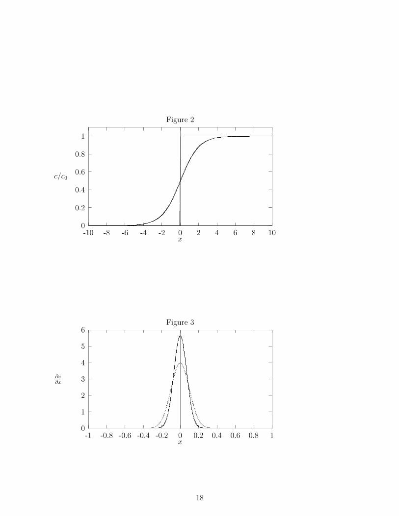
Instead of a drop of ink, you use an ionic solution and let it diffuse into pure waterto determine how the ionic concentration gradient depends on time. You begin with arectangular cell with the bottom half filled with the salt solution and the top half filled withwater as depicted in Figure 1. As time passes, the salt in the concentrated layer migratesto regions of low salt concentration. If the salt concentration c is measured as a functionof time t and coordinate x [See Figure 1 for the definition of x], the concentration profileappears as in Figure 2 [c0 is the initial salt concentration in the salt rich layer]. The two linesdrawn in Figure 2 represent concentration profiles at two different times. Can you tell whichof the two times is earlier? Using Fick’s Law of Diffusion [See Engel and Reid, Sections 17.2through 17.4], it is possible to show that
∂c
∂x= Ae−x2/2σ2(t) (2)
where A is a constant and σ is called the standard deviation. Equation (2) is often called aGaussian distribution. A graph of Eq.(2) is shown in Figure 3. The standard deviation σis a measure of the width of the distribution. It is possible to show that the area under aGaussian between −σ ≤ x ≤ σ comprises ∼68 % of the total area under the Gaussian curve.Therefore, if σ is large [the light line in Figure 3], the distribution is wide and if σ is small[the dark line in Figure 3] the distribution is narrow.
In this experiment you measure σ directly in a diffusion cell as a function of time. Youcan be expected to find that
σ = Ktα (3)
where K and α are constants. Relations of the form of Eq. (3) are often called power laws.You should find that α is particularly simple.
The method you will use to determine the concentration gradient of the solution as afunction of time is based on the refraction of light. When light travels from one medium toanother, the light bends. This bending of light is called refraction. In common experience,if a spoon is placed in a glass of water, it appears bent because of refraction. The amountthat light is bent is proportional to a property of a medium called the index of refractionn. In a salt solution, the index of refraction depends on the type of ionic species and theconcentration of the solution. In our cell where there is a concentration gradient, the indexof refraction depends on the coordinate x. Since the index of refraction is proportional tothe concentration, it is easy to see that
∂c
∂x= K ′∂n
∂x(4)
16
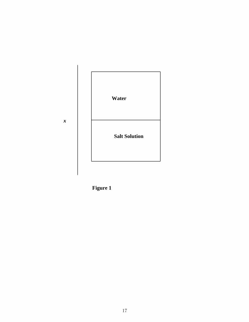
Salt Solution
Water
x
Figure 1
17
0
0.2
0.4
0.6
0.8
1
-10 -8 -6 -4 -2 0 2 4 6 8 10
c/c0
x
Figure 2
0
1
2
3
4
5
6
-1 -0.8 -0.6 -0.4 -0.2 0 0.2 0.4 0.6 0.8 1
∂c∂x
x
Figure 3
18
where K ′ is a constant of proportionality. We can then measure the concentration gradientby measuring the gradient of the index of refraction.
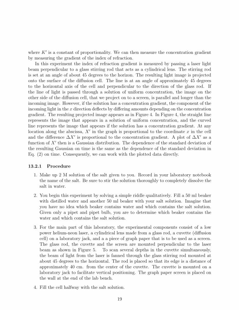
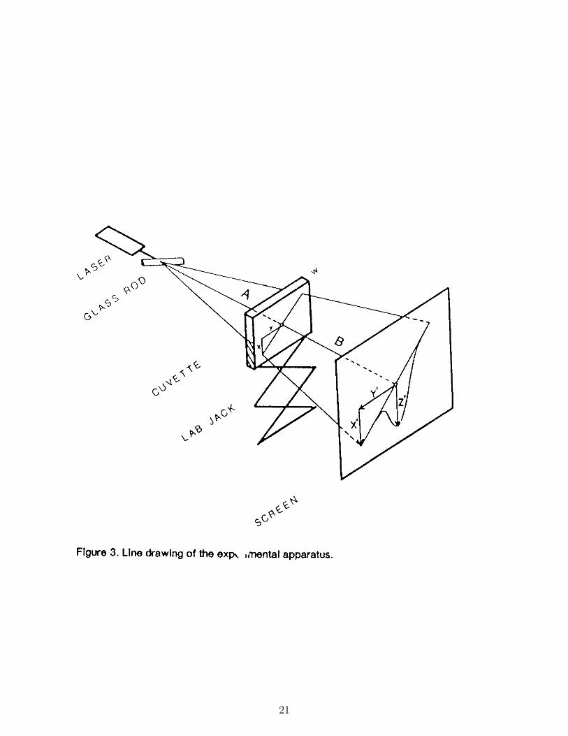
In this experiment the index of refraction gradient is measured by passing a laser lightbeam perpendicular to a glass stirring rod that acts as a cylindrical lens. The stirring rodis set at an angle of about 45 degrees to the horizon. The resulting light image is projectedonto the surface of the diffusion cell. The line is at an angle of approximately 45 degreesto the horizontal axis of the cell and perpendicular to the direction of the glass rod. Ifthe line of light is passed through a solution of uniform concentration, the image on theother side of the diffusion cell, that we project on to a screen, is parallel and longer than theincoming image. However, if the solution has a concentration gradient, the component of theincoming light in the x direction deflects by differing amounts depending on the concentrationgradient. The resulting projected image appears as in Figure 4. In Figure 4, the straight linerepresents the image that appears in a solution of uniform concentration, and the curvedline represents the image that appears if the solution has a concentration gradient. At anylocation along the abscissa, X ′ in the graph is proportional to the coordinate x in the celland the difference ∆X ′ is proportional to the concentration gradient. A plot of ∆X ′ as afunction of X ′ then is a Gaussian distribution. The dependence of the standard deviation ofthe resulting Gaussian on time is the same as the dependence of the standard deviation inEq. (2) on time. Consequently, we can work with the plotted data directly.
13.2.1 Procedure
1. Make up 2 M solution of the salt given to you. Record in your laboratory notebookthe name of the salt. Be sure to stir the solution thoroughly to completely dissolve thesalt in water.
2. You begin this experiment by solving a simple riddle qualitatively. Fill a 50 ml beakerwith distilled water and another 50 ml beaker with your salt solution. Imagine thatyou have no idea which beaker contains water and which contains the salt solution.Given only a pipet and pipet bulb, you are to determine which beaker contains thewater and which contains the salt solution.
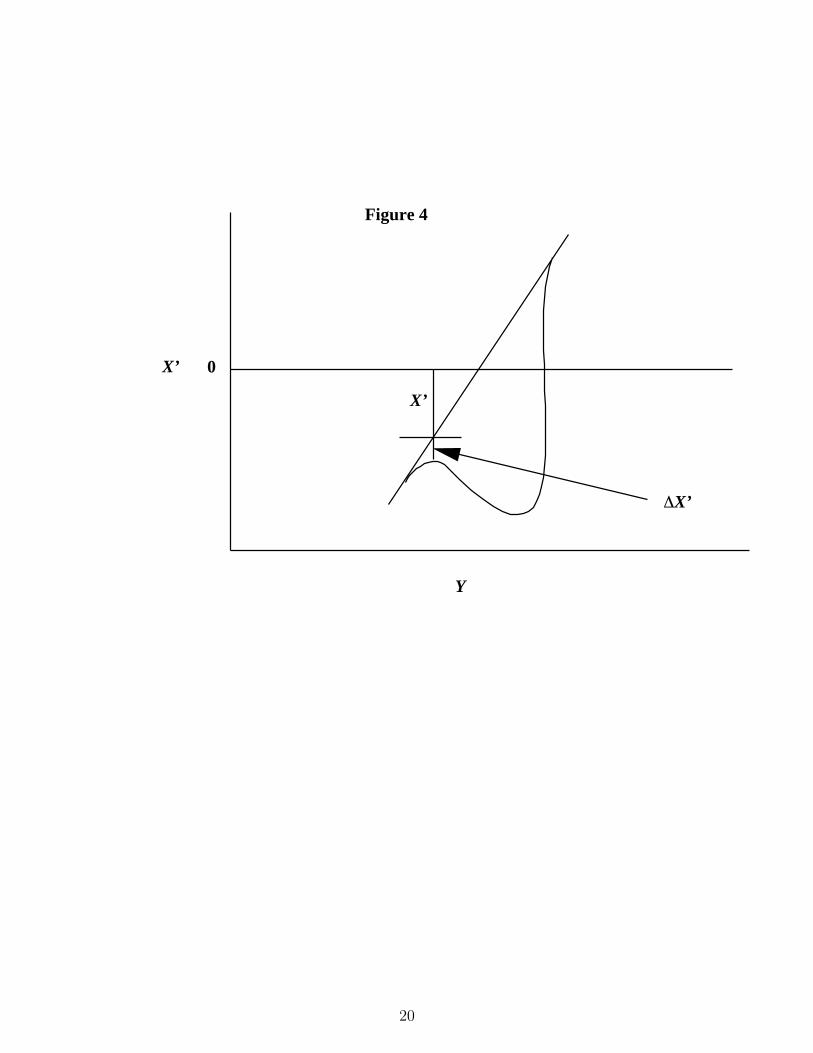
3. For the main part of this laboratory, the experimental components consist of a lowpower helium-neon laser, a cylindrical lens made from a glass rod, a cuvette (diffusioncell) on a laboratory jack, and a a piece of graph paper that is to be used as a screen.The glass rod, the cuvette and the screen are mounted perpendicular to the laserbeam as shown in Figure 5. To scan several depths in the cuvette simultaneously,the beam of light from the laser is fanned through the glass stirring rod mounted atabout 45 degrees to the horizontal. The rod is placed so that its edge is a distance ofapproximately 40 cm. from the center of the cuvette. The cuvette is mounted on alaboratory jack to facilitate vertical positioning. The graph paper screen is placed onthe wall at the end of the lab bench.
4. Fill the cell halfway with the salt solution.
19
X’
∆X’
X’ 0
Y
Figure 4
20
21
5. Raise or lower the cell until the laser hits the meniscus. A vertical line will appear onthe screen. Trace this line.
6. Slide the ring stand with the glass rod attached back so that the rod is between thecuvette and the laser making a line at a 45 degree angle. Trace the diagonal laser lineon the graph paper.
7. Add water to the cuvette by using a pipette and a floating cork. Make sure the wateris added slowly and directly on the cork so as not to disturb the interface. This processshould take a few minutes. You should start your stopwatches at the time you beginto add water to the cuvette.
8. When you have waited sufficient time so that a stable curve appears entirely on yourgraph paper, trace the curve on the graph paper and note the time.
9. Trace new lines at 5 minute intervals for 40 minutes.
13.2.2 Laboratory Report
Your reports should consist of the following parts:
1. A cover page giving the date the experiment was performed, the name of your labora-tory partner and the title of the experiment;
2. Your procedure signed by your TA;
3. A description of how you solved the riddle at the beginning of the experiment. Besure to include a description of the physical principals used to solve the riddle. Theseprincipals, of course, should relate to the rest of the experiment.
4. The raw data [in this case the original graph paper screen signed by your TA];
5. A table of 10 values of X ′ and ∆X ′ calculated from the graph paper for each time;
6. Graphs of ∆X ′ as a function of X ′ for each time;
7. A statement of the precise definition you used for the width w of each graph;
8. A table of w, t, ln w and ln t;
9. Plot the values of ln w as a function of ln t using the calculated points;
10. Draw a straight line that is your best estimate of the linear relationship between ln wand ln t;
11. Determine the slope of your graph;
22
12. Given that the slope is either an integer or a half integer, round off the value of yourslope to the nearest half integer;
13. Express the dependence of the the width as a power law. It is important to recognizethat the width w is proportional to the standard deviation σ of the Gaussian curves.
14. Summary and Discussion: Briefly summarize the experiment and your findings. Includeall key numerical results; e.g. power law. Examine Eq. (17.18) of the CHM 431textbook, and compare your measured value of α with the power law of the meansquared displacement in diffusion processes as a function of time.
14 Second Two Laboratory Experiments
14.1 Notes on Error Analysis
14.1.1 Reading Assignment
Text pages 29-32, 43-48 and 52-66.
14.1.2 Introduction
The study of the analysis of experimental error is an important goal of CHM 335. Theinstructors of this course feel error analysis to be sufficiently important that from 30% to40% of the grade on your later laboratory reports are based on this topic. We encourage youto learn this topic well as early in the semester as possible. Many aspects of error analysisare complex, and the lecture together with these course notes and the appropriate sectionsof the text book should be helpful. In preparing your reports we encourage you to come tothe instructors for help with error analysis to make sure you understand the key ideas.
To illustrate the importance of the analysis of errors, suppose a surveyor measures thedistance between Kingston and New York City, and reports the distance to be 150. miles.While stating the distance to be 150 miles might be sufficient for the Auto Club, from thepoint of view of the physical sciences the reported distance alone is inadequate. For example,the surveyor might mean 150 miles ± 1 mile or the surveyor might mean 150 miles ± 100miles. The first possibility tells us that it should take about 3 hours to drive to New Yorkwhile the latter is only a rough order of magnitude estimate. While the auto club probablyassumes something like 150 miles ± 1 mile, anyone in the sciences must provide not onlythe result of a measurement, but the extent to which the result is known as well. Startingwith the third experiment when you report an experimental result, you must include boththe value obtained as well as the error that provides information about how well you knowthe result reported.
23
14.1.3 Systematic and Random Errors
Experimental errors are often divided into two categories. The first category, usually calledsystematic errors, refers to mistakes inherent in a particular apparatus. For example, supposewe measure the length of the cover of your textbook with a metal ruler. The total lengthof the ruler expands and contracts depending on the temperature of the room. The rulermight be calibrated assuming the temperature is 20C, and if the actual room temperatureis 25C, the total length of the ruler must be longer than originally measured. Consequently,any measurement of length at the higher temperature can be expected to give a result that istoo short. It is important to recognize that systematic errors have a definite algebraic sign.In the case of our expanded ruler, the error is necessarily negative. There is some controlover such systematic errors. For example, if the coefficient of thermal expansion of the ruleris known, the measured length can be corrected to provide the true length. Associated withsystematic errors is the term accuracy. An apparatus is said to be accurate to the extentthat the systematic errors are minimized.
The second category of error is associated with inherent random fluctuations of any mea-surement apparatus, and consequently we refer to such errors as random errors. Again, wecan take the measurement of the length of the cover of our textbook as an example. If wemeasure the length of the book many times, we can expect to obtain a range of values thatfluctuates about a mean value. The fluctuations come from many sources. For example, youmight not place the bottom of the ruler at exactly the same place for each measurement.The thermal fluctuations of the atoms in the ruler change its length slightly providing an-other source. The temperature of the room also fluctuates changing the length of the rulerin a random way. Such random fluctuations are inherent, and cannot be eliminated. Byhypothesis, we assume the correct result (in the sense of random errors) for some measure-ment can be obtained from the arithmetic mean of an infinite set of measurements. Wecontrol random errors by increasing the number of measurements. Unlike systematic errors,random errors have no definite algebraic sign, and we denote the size of random errors with± notation. We use the term precision to express the magnitude of the random errors. Wecall a measurement precise if its random errors are small.
14.1.4 The Distribution of Random Errors - The Gaussian Distribution
An important theorem in probability theory, called the central limit theorem, states thatrandom, independent measurements of a quantity (call it x) must be distributed accordingto a Gaussian distribution that takes the form
P (x) =1√
2πσ2exp
−(x− µ)2
2σ2
. (5)
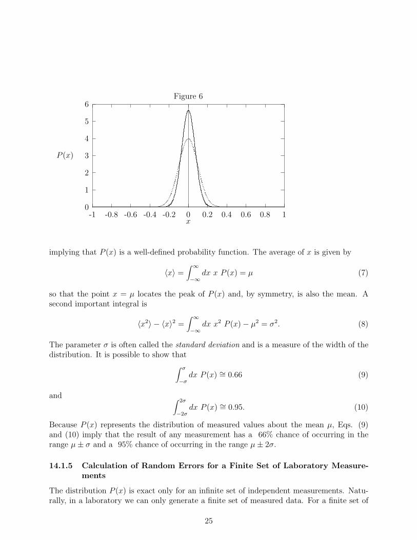
The meaning of the parameters σ and µ are given shortly. Equation (5) is plotted in Figure6 for the case that µ = 0 and σ = 1. (the broader peak) and µ = 0, σ = 0.5 (the narrowerpeak). The probability function P (x) is normalized in the sense that∫ ∞
−∞dxP (x) = 1 (6)
24
0
1
2
3
4
5
6
-1 -0.8 -0.6 -0.4 -0.2 0 0.2 0.4 0.6 0.8 1
P (x)
x
Figure 6
implying that P (x) is a well-defined probability function. The average of x is given by
〈x〉 =∫ ∞
−∞dx x P (x) = µ (7)
so that the point x = µ locates the peak of P (x) and, by symmetry, is also the mean. Asecond important integral is
〈x2〉 − 〈x〉2 =∫ ∞
−∞dx x2 P (x)− µ2 = σ2. (8)
The parameter σ is often called the standard deviation and is a measure of the width of thedistribution. It is possible to show that∫ σ
−σdx P (x) ∼= 0.66 (9)
and ∫ 2σ
−2σdx P (x) ∼= 0.95. (10)
Because P (x) represents the distribution of measured values about the mean µ, Eqs. (9)and (10) imply that the result of any measurement has a 66% chance of occurring in therange µ± σ and a 95% chance of occurring in the range µ± 2σ.
14.1.5 Calculation of Random Errors for a Finite Set of Laboratory Measure-ments
The distribution P (x) is exact only for an infinite set of independent measurements. Natu-rally, in a laboratory we can only generate a finite set of measured data. For a finite set of
25
measurements presumably distributed according to P (x), we estimate µ and σ. To estimateσ and µ for a finite set of measurements, we imagine the set of N measured values to bex1, x2, . . . , xN . The mean is given by the standard expression
µ =x1 + x2 + . . . + xN
N=
1
N
N∑i=1
xi. (11)
To determine the standard deviation we use
〈x2〉 =1
N
N∑i=1
x2i , (12)
so that
σ2 =1
N
N∑i=1
x2i −
(1
N
N∑i=1
xi
)2
. (13)
The standard deviation σ represents a measure of the fluctuations of x from a large setof measurements. Although σ is of interest, our principle concern is the fluctuations of thecalculated mean. It is not hard to show that the standard deviation of the mean itself σN isgiven by
σ2N =
σ2
N − 1(14)
(the N − 1 rather than N comes from the loss of one degree of freedom in the estimation ofthe mean). We then report our results in the form
x = µ± 2σN . (15)
From the discussion at the end of Section 14.1.4, there is a 95% probability that the correctresult is in the range given in Eq.(15).————————————————————————Exercise: A student measures the mass of an iron nail with a balance and obtainsthe following results: 5.500 g, 5.560g, 5.550g, 5.550g and 5.590g. Calculate the result thatthe student should report.
Answer: The average mass is found to be 5.550 grams, σ = .02898 grams, and σN = .01449grams. The reported result should be 5.55 ± .03 grams. Notice the first significant digit inthe error defines the number of significant figures that should be reported for the average.We don’t use simple first year chemistry rules for significant figures, but rather we use thecomputed error to define the number of significant figures to be reported.————————————————————————
The answer to the previous exercise requires rounding off to the last significant digit.The usual rule for rounding off digits is to increase by one digit if the next digit is greaterthan 5, do not increase by one digit if the next digit is less than 5, and increase by one digit
26
if the next digit is 5 and the result of the round off is even. For example 5.56 becomes 5.6,5.54 becomes 5.5 and 5.55 becomes 5.6. However 5.65 becomes 5.6.
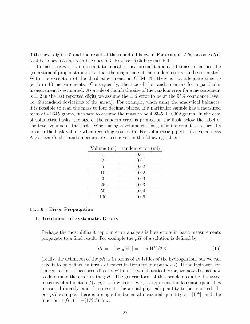
In most cases it is important to repeat a measurement about 10 times to ensure thegeneration of proper statistics so that the magnitude of the random errors can be estimated.With the exception of the third experiment, in CHM 335 there is not adequate time toperform 10 measurements. Consequently, the size of the random errors for a particularmeasurement is estimated. As a rule of thumb the size of the random error for a measurementis ± 2 in the last reported digit( we assume the ± 2 error to be at the 95% confidence level;i.e. 2 standard deviations of the mean). For example, when using the analytical balances,it is possible to read the mass to four decimal places. If a particular sample has a measuredmass of 4.2345 grams, it is safe to assume the mass to be 4.2345 ± .0002 grams. In the caseof volumetric flasks, the size of the random error is printed on the flask below the label ofthe total volume of the flask. When using a volumetric flask, it is important to record theerror in the flask volume when recording your data. For volumetric pipettes (so called classA glassware), the random errors are those given in the following table:
Volume (ml) random error (ml)1. 0.012. 0.015. 0.0210. 0.0220. 0.0325. 0.0350. 0.04100. 0.06
14.1.6 Error Propagation
1. Treatment of Systematic Errors
Perhaps the most difficult topic in error analysis is how errors in basic measurementspropagate to a final result. For example the pH of a solution is defined by
pH = − log10[H+] = − ln[H+]/2.3 (16)
(really, the definition of the pH is in terms of activities of the hydrogen ion, but we cantake it to be defined in terms of concentrations for our purposes). If the hydrogen ionconcentration is measured directly with a known statistical error, we now discuss howto determine the error in the pH. The generic form of this problem can be discussedin terms of a function f(x, y, z, . . .) where x, y, z, . . . represent fundamental quantitiesmeasured directly, and f represents the actual physical quantity to be reported. Inour pH example, there is a single fundamental measured quantity x =[H+], and thefunction is f(x) = −(1/2.3) ln x.
27
The total differential of a function provides the mathematics necessary to solve theproblem of error propagation. The total differential plays a central role in the studyof thermodynamics as well, and total differentials are discussed in detail in CHM 431.As a reminder, the total differential of a function f is defined by
df =
(∂f
∂x
)y,z,...
dx +
(∂f
∂y
)x,z,...
dy +
(∂f
∂z
)x,y,...
dz + . . . (17)
The total differential of f is the infinitesimal change in f that results from the in-finitesimal changes in its variables expressed as dx, dy, dz, . . .. In the case of errors,df is the error in f that arises from small errors dx, dy, dz, . . . in each of its variables.The interpretation of df just provided in terms of errors is valid for systematic errors.We shall discuss the modifications for random errors in Section 2. We first try theapplication of the total differential to our pH example. Using f = pH and x =[H+] wehave
f = −(
1
2.3
)ln x (18)
and
df = − dx
2.3 x. (19)
Then
ε(pH) = − ε([H+])
2.3[H+](20)
where the notation ε(x) denotes the systematic error in the variable x. The error inthe pH is not simply equal to the error in the hydrogen ion concentration itself, butrather the error in the pH is a function of the error in the hydrogen ion concentrationas well as other variables. The functional form of the expression for the error cannotbe guessed in any simple way, but must be derived from the expression for the totaldifferential. Because systematic errors have a definite algebraic sign, the systematicerror in the pH carries sign information.
Let us try another example. The density ρ of a substance is defined by
ρ =m
V(21)
where m is the mass and V is the volume. For the purpose of this exercise we take themass and the volume as the quantities actually measured in a laboratory, and we askhow the errors in the mass and volume propagate to give the final error in the density.Writing ρ = ρ(m, V ) The total differential of the density is given by
dρ =
(∂ρ
∂m
)V
dm +
(∂ρ
∂V
)m
dV (22)
=dm
V− m dV
V 2. (23)
28
The expression for the total differential in the density can be simplified by dividing theleft hand side of Eq.(23) by ρ and the right hand side of Eq.(23) by m/V resulting inthe expression
dρ
ρ=
dm
m− dV
V. (24)
The expression for the propagation of systematic errors then takes the form
ε(ρ)
ρ=
ε(m)
m− ε(V )
V. (25)
The right hand side of Eq.(25) contains sign information. A positive systematic errorin the mass results in a positive error in the density whereas a positive systematic errorin the volume results in a negative systematic error in the density. These signs makesense, because increasing the volume decreases the density (the volume term appearsin the denominator).
In this course we generally assume that there are no systematic errors. We have in-cluded the analysis of this section to provide the needed mathematics for the treatmentof random errors. In your laboratory reports you should focus on random errors, themethod for which is discussed in the next section.
2. Treatment of Random Errors
In the previous section the expressions for the propagated systematic errors containedsign information. Unlike systematic errors, random errors contain no signs. It ispossible to show that the expressions for systematic errors become valid for randomerrors if each term in the expression derived from the total differential is squared andaveraged so that cross terms are eliminated. The proof of this assertion is beyond thescope of this course. To make the procedure explicit, consider a function f of twomeasured quantities x and y. The total differential of f is given by
df =
(∂f
∂x
)y
dx +
(∂f
∂y
)x
dy. (26)
As before, we replace the differentials by errors
ε(f) =
(∂f
∂x
)y
ε(x) +
(∂f
∂y
)x
ε(y). (27)
Equation(27) is just the expression valid for the propagation of a systematic error. Wenow square both sides of Eq.(27) and average. By averaging, the cross terms containingterms of the form ε(x)ε(y) average to zero because each individual error can have bothpositive and negative signs. The final result for the propagated random error is then
ε(f)2 =
(∂f
∂x
)2
y
ε(x)2 +
(∂f
∂y
)2
x
ε(y)2. (28)
29
(We have replaced the symbol ε that represents a systematic error by the symbol ε torepresent a random error.) To apply the procedure to our density example, we canbegin with Eq.(25), square both sides and average to obtain(
ε(ρ)
ρ
)2
=
(ε(m)
m
)2
+
(ε(V )
V
)2
. (29)
Note: Students often mistakenly double a propagated error imagining that the prop-agated error must be at the single standard deviation (66 %) confidence level. Infact, the error in the fundamental measured quantities should already be expressed as2 standard deviations of the mean, and the propagated error represents 2 standarddeviations of the mean. No doubling of the propagated error is necessary.
————————————————————————
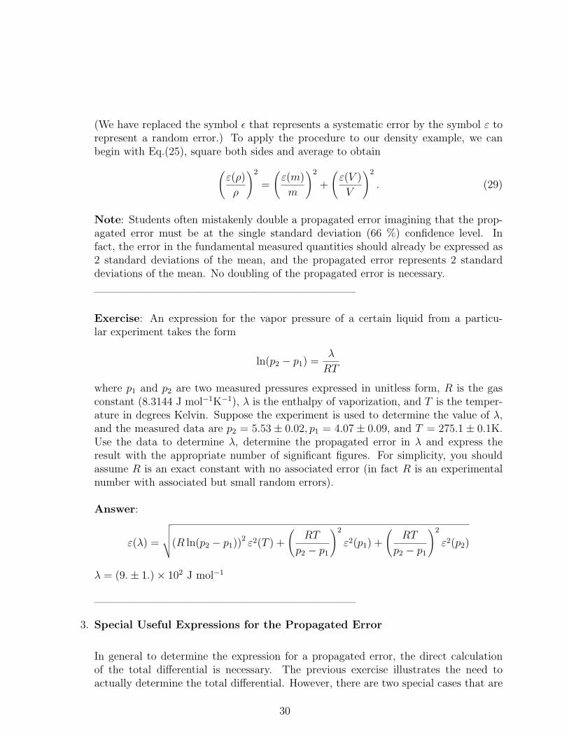
Exercise: An expression for the vapor pressure of a certain liquid from a particu-lar experiment takes the form
ln(p2 − p1) =λ
RT
where p1 and p2 are two measured pressures expressed in unitless form, R is the gasconstant (8.3144 J mol−1K−1), λ is the enthalpy of vaporization, and T is the temper-ature in degrees Kelvin. Suppose the experiment is used to determine the value of λ,and the measured data are p2 = 5.53± 0.02, p1 = 4.07± 0.09, and T = 275.1 ± 0.1K.Use the data to determine λ, determine the propagated error in λ and express theresult with the appropriate number of significant figures. For simplicity, you shouldassume R is an exact constant with no associated error (in fact R is an experimentalnumber with associated but small random errors).
Answer:
ε(λ) =
√√√√(R ln(p2 − p1))2 ε2(T ) +
(RT
p2 − p1
)2
ε2(p1) +
(RT
p2 − p1
)2
ε2(p2)
λ = (9.± 1.)× 102 J mol−1
————————————————————————
3. Special Useful Expressions for the Propagated Error
In general to determine the expression for a propagated error, the direct calculationof the total differential is necessary. The previous exercise illustrates the need toactually determine the total differential. However, there are two special cases that are
30
so common that is is useful to derive general expressions for future use. The first is afunction that depends only on the sums and differences of its variables. For examplef(x, y, z) = x + y − z The total differential of f is
df = dx + dy − dz. (30)
After replacing the differentials by errors and squaring and averaging, the result is
ε(f) =√
ε(x)2 + ε(y)2 + ε(z)2. (31)
In general the propagated random error for any function of only the sums and differ-ences of its variables is the square root of the sums of the squares of the errors in itsvariables.
The second important case is a generalization of our density example. Suppose f is afunction only of products and quotients of its variables. For example take f = xy/z.The total differential of f is
df =y
zdx +
x
zdy − xy
z2dz. (32)
Dividing the left hand side of Eq.(32) by f and the right hand side of Eq.(32) by xy/z,we obtain
df
f=
dx
x+
dy
y− dz
z. (33)
We next replace the differentials by errors and square and average to obtain
ε(f) = f
√√√√(ε(x)
x
)2
+
(ε(y)
y
)2
+
(ε(z)
z
)2
. (34)
We can interpret Eq.(34) by stating the relative error in f is the square root of thesum of the squares of the relative errors in each of its variables. This result can beextended to any number of variables as long as all variables appear as products orquotients only.
14.1.7 Errors from a Graphical Analysis of the Data
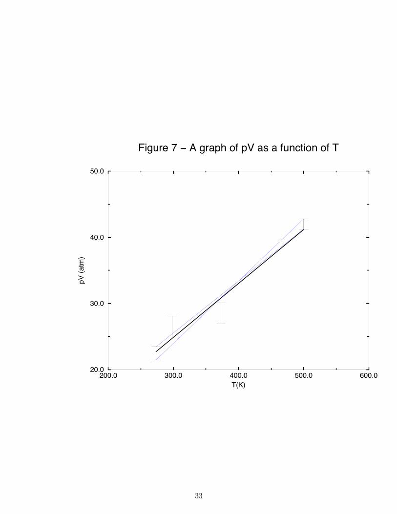
Frequently the physical result we seek in an experiment is extracted from the slope or theintercept of a linear graph obtained from a series of data. For example, suppose the goal ofan experiment is to determine a value of the gas constant R from pV T data obtained frommeasurements using one mole of an ideal gas. The value of R can be obtained from theslope of a graph of the product pV plotted as a function of the temperature T . An exampleof such data is shown in Figure 7. In the data shown in Figure 7, the random errors inthe temperature are smaller than the resolution of the graph. The random errors in the pVproduct are large and depicted by the vertical bar with the horizontal lines at the head and
31
foot associated with each data point. For example the first plotted point in Figure 7 is 22.4±1 l atm. A point is plotted at pV = 22.1 l atm and the vertical bar ranges from 21.1 l atmto 23.1 l atm. These vertical bars are called error bars. When plotting points containingrandom errors, associated with each point must be an error bar. There should be error barsparallel to both the x and y-axes, but in this example (and most of the experiments in thiscourse), the error bars for the data plotted on the x-axis are too small to see.
Perhaps the best way to determine the optimal line that connects a set of experimentalpoints is called linear regression. Linear regression is discussed in your textbooks, but inCHM 335 we use a simpler method. We draw the best straight line using a visual fit. Thebest straight line drawn in this way is depicted as the darkest solid line in Figure 7. Fromthis best fit line, the slope can be determined. The slope so determined is taken to be theslope to be reported in your laboratory experiment. For example, the slope of the best-fit(dark) line in Figure 7 is 0.0814 l atm K−1. We ask that you analyze your data in this wayusing graph paper rather than a computer. In the final experiment of the year, the reportsare written in class, and by preparing your graphs using graph paper rather than a computer,you have the necessary practice for the final laboratory project.
To obtain an estimate of the errors associated with the slope of a graph (or equivalentlythe intercept), the plotted error bars are used to obtain extreme values of the possible slopeand intercept. In this course we take the first and last plotted points, and connect thebottom of the first error bar to the top of the last error bar with a straight line. Similarly,we connect the top of the first error bar with the bottom of the last error bar with anotherstraight line. These two lines are depicted in Figure 7 as the two light solid lines. We callthe slope of the light solid line having the largest slope m+ and the slope of the light solidline having the smallest slope m−. We estimate the error in the slope to be
ε(m) =1
2(m+ −m−) (35)
For example, in Figure 7 m+ = 0.0942 l atm K−1, m− = 0.0784 l atm K−1 so that the erroris ε(m)=0.008 l atm K−1. We then report the gas constant to be R = 0.0814± 0.008 l atmmol−1 K−1. The error estimated in this fashion can often be an over estimate. Consequentlywe can take the error calculated in Eq.(35) to represent two standard deviations of the mean;i.e. at the 95% confidence level.
Although linear regression is capable of providing a more careful estimate of the errorin the slope from a set of data, the method expressed in Eq.(35) is more suitable for thepurposes of CHM 335.
The error in the intercept b is treated analogously.
ε(b) =1
2(b+ − b−) (36)
32
200.0 300.0 400.0 500.0 600.0T(K)
20.0
30.0
40.0
50.0
pV (
atm
)
Figure 7 − A graph of pV as a function of T
33
14.2 Experiment 28a: The Intrinsic Viscosity of Polyvinyl Alcohol
14.2.1 Introduction and Reading Assignments
In this and the next experiment, you use the measurement of the the viscosity of liquids toillustrate two things. In the first experiment you learn the methods of error analysis. Inthe experiment to be performed in the following week, you use viscosity measurements todiscover certain aspects of polymer structure. In the second part you learn the format of acomplete laboratory report as well. Before coming to the laboratory, be sure to read pages318 to 327 in your text book as well as pages 29 to 68 in your text. The latter readingassignment presents a discussion of error analysis.
14.2.2 Theory
When the instructors for this course were young (we won’t tell you how long ago) there wasa TV commercial for Prell Shampoo. To show how “wonderful” Prell was, the advertisementshowed two beakers, one filled with Prell and the other filled with water. A pearl was placedat the top of each solution and the rate at which the pearl reached the bottom of the beakerswas demonstrated. The pearl took much longer to reach the bottom in the beaker containingPrell than in the beaker containing water.
The difference in rate (which for some reason was supposed to show how good Prell is) isa measure of what we call viscosity. Another way of observing the effect of differing viscosityis to pass solutions through a pipe or a narrow capillary. The more viscous the solution thelonger it will take for the liquid to pass through the tube. This difference in flow rate is thebasic principle behind the Ostwald viscometer that we shall use in this experiment.
The physical origin of viscosity can be understood by imagining two trains of infinitelength running on parallel frictionless tracks. Suppose the train on the right track is movingat a higher speed than the train on the left track. Suppose the doors of the trains areopen and the passengers on each train participate in a game where they hop back and forthbetween the two trains at some rate. The passengers jump so that on average the numberof people on either train is constant. A person jumping from the fast train to the slow traintransfers momentum from the fast train to the slow train. A person jumping from the slowtrain to the fast train transfers negative momentum. This process of momentum transfertends to slow the fast train and speed up the slow train. To an observer too far from thetrain to see the jumping, the change in speed appears to be a frictional drag between thetwo trains.
Now consider a liquid flowing down a pipe. Imagine the fluid flowing down the pipe toconsist of concentric cylindrical layers of decreasing diameter starting at the wall of the pipeand ending at the axis of the pipe. It turns out that the layer adjacent to the wall of thepipe has zero speed and the speed increases from the wall to a maximum at the center ofthe pipe. Each layer is analogous to the trains described in the preceding paragraph and themolecules that jump between the layers (because of Brownian motion) are analogous to thepeople jumping between the trains. When we measure the properties of the fluid as it flows
34
down the pipe, we observe a frictional drag between the layers. This frictional drag is theviscosity.
The detailed theoretical background for the experiments is given in the reading assign-ments. It is useful to note that the key equation for the experiment is given as Eq. (3) inthe laboratory text
η
ρ= Bt (37)
where η is the viscosity, ρ is the solution density, B is a constant of proportionality and t isthe time necessary for a solution to pass through an Ostwald viscometer.
14.2.3 Experimental Procedure
In this first experiment you limit the measurements to determine the viscosity of the singlesolution of polyvinyl alcohol by comparison with the viscosity of water. Set up the experi-mental apparatus as in Figure 1 on page 320 of your text books. Measure the time it takesfor water to pass between the marks of the viscometer. You should repeat the measurementsfor water 10 times. Then perform 10 measurements of the flow time for the polyvinyl alcoholstock solution. Clean the Ostwald viscosimeter thoroughly with 3 portions of distilled waterafter your polyvinyl alcohol runs. Use a rubber bulb to force water through the capillarytube several times to remove polyvinyl alcohol from the capillary. After the cleaning, repeatthe viscosity measurement of distilled water twice. Record the water run time in your datasheet before you ask your TA to sign your data sheet. Fill the Ostwald viscosimeter withdistilled water at the end of the laboratory period.
14.2.4 Laboratory Report
In your report you have only three sections; a calculations section, an error analysis section,and a section summarizing your results. Tables of the density and viscosity of water neededfor your laboratory reports are found on the last page of this syllabus.
1. Include a cover page giving the title of the experiment and the date the experimentwas performed.
2. Include the signed outline of the experimental procedure.
3. Calculations
(a) Make a table consisting of the ten values of the flow time for the water measure-ments and the polyvinyl alcohol solution measurements.
(b) Calculate the average flow time for each species.
(c) Determine the density and viscosity of water using the tables at the end of thissyllabus. As an example, the density of water at 23.1C is 0.997514 g cm−3. Theviscosity of water at 23.C is 9.38 mP.
35
(d) Use the mean value for water and the known viscosity of water to determine theapparatus constant B.
(e) Using the determined value of B, calculate the viscosity of the polyvinyl alcoholsolution.
4. Error Analysis
(a) Calculate the standard deviation of the mean of the flow time for water.
(b) Calculate the standard deviation of the mean of the flow time for the polyvinylalcohol solution.
(c) Propagate errors to determine the error in B.
(d) Propagate errors to determine the error in the viscosity of the polyvinyl alcoholsolution.
5. Summarize your measured results including the calculated errors. Be sure to includethe proper number of significant figures and the proper units.
6. Remember to attach your original data signed by your TA.
Because you need additional experience in error propagation before attempting the nextlaboratory experiment, do the following exercises as the final section of your laboratoryreports:
1. A student has a sodium chloride solution having concentration 1.03 ± 0.02 molar. 50.0±0.1 ml of the solution are placed in a volumetric flask of volume 100.0 ± 0.2 ml,and the solution is mixed with water to the mark on the flask. Determine the finalconcentration along with its associated random error.
2. The final solution from problem 1 is again diluted in half with water using a pipetteand volumetric flask with the same specifications. Determine this final concentrationwith the associated random error.
3. Later in the semester, you will determine a quantity γ using pressure measurementshaving the form
γ =
P2
P1
− 1
P3
P1
− 1.
Suppose the measured pressures are P1 = 32.0 ± 0.2 torr, P2 = 43.2 ± 0.3 torr andP3 = 762. ± 1 torr. Calculate γ and the associated random error. Be careful. In thisproblem, taking the total differential is essential.
36
4. In the same experiment later this semester, you will determine a related expression forγ given by
γ =ln
P2
P1
lnP3
P1
.
Using the same data as in the previous problem, determine γ and the associated randomerror.
14.3 Experiment 28b: The Intrinsic Viscosity of Polyvinyl Alcohol
14.3.1 Introduction
In this follow-up experiment, you use the viscosity measurements to determine the fractionof polymer units that are connected in the so-called “head to head” arrangement. Theapproach is to use a reagent that cleaves the head to head connections exclusively. Thecleavage increases the number of molecules in solution and decreases the average molecularweight. This change is related to the viscosity. The experimental procedure that you useis identical to that given in the text book. The next subsection will contain a discussion ofsome of the theoretical ideas.
14.3.2 Theory
We define ∆ to be the fraction of bonds connecting monomer units in a strand of polyvinylalcohol that are connected “head to head.” Let W be the total mass of polyvinyl alcohol inthe solution. The total number of monomer units, N0, is equal to W divided by M0 whereM0 is the molecular weight of a monomer; i.e.
N0 = W/M0 (38)
Let Nn be the total number of polymer molecules in the solution before cleavage and N ′n
be the total number of polymer molecules in solution after cleavage. If Mn is the molecularweight of the polymer and M ′
n is the polymer molecular weight after cleavage, then
Nn = W/Mn (39)
andN ′
n = W/M ′n. (40)
Assuming the molecular weights of the polymers are high, to a vanishingly small error wecan then write
∆ =N ′
n −Nn
N0
(41)
=1/M ′
n − 1/Mn
1/M0
(42)
37
We can then determine ∆ from a knowledge of the molecular weights.We determine the molecular weights using changes in the viscosity that accompany the
cleavage process. In a polymer the viscosity increases with increasing molecular weight. Theprincipal reason is that the average volume of the polymer molecules in solution increaseswith chain length. The quantitative dependence on the molecular weight can be understoodby viewing the polymer in a spherical model as discussed in the text book. The final resultis found in Eq. (7) on page 323. Since the solution consists of a statistical ensemble, themolecular weights used are averages resulting in additional correction factors as given in Eq.(11) on page 324 of the text.
Please note that the second of the two equations listed as Eq. (7) on page 323 of the textis in error. You should use
M = 7.4× 10⁴[η]1.32.
14.3.3 Cleaning Procedure
As with the first part of this experiment, clean the Ostwald viscosimeter thoroughly with3 portions of distilled water after your polyvinyl alcohol runs. Use a rubber bulb to forcewater through the capillary tube several times to remove polyvinyl alcohol from the capillary.After the cleaning, repeat the viscosity measurement of distilled water twice. Record thewater run time in your data sheet before you ask your TA to sign your data sheet. Fill theOstwald viscosimeter with distilled water at the end of the laboratory period.
14.3.4 Laboratory Report
You write complete laboratory reports for this experiment. Before writing your reports, besure to read pages 10 to 25 in your text books. Your reports should contain the followingsections:
1. Title Page: Give the title of the experiment and the date the experiment was performed.
2. Abstract: This should be a 1 paragraph summary of what is to follow including theresults. It is suggested that you write the abstract after the rest of the report iscomplete.
3. Introduction: This should be a discussion of the purpose of the experiment.
4. Theory: This should provide a derivation of the key formulas used in the experimentand used in the analysis of the data. Make sure that all symbols used in this sectionare defined in words.
5. Procedure: Attach the outline of the procedure you brought to class and had signedby your TA.
6. Original Data: Attach the original data signed by your TA.
38
7. Results: Tabulate your data so that it can be used in the calculations to follow.
8. Calculations: Provide a sample calculation taking one from the original data to thefinal result.
9. Error Analysis: Use the standard deviations computed in last weeks experiment as anestimate of the error in the flow times. Determine the error in the specific viscosity bypropagation.
10. Graphical Analysis: Plot the specific viscosity divided by the concentration as a func-tion of concentration. Draw the best line through the data. Include error bars on thedata points. Use the limiting slope method to determine the intercept and the errorin the intercept.
11. Final Calculation: Determine the best average molecular weights for both the cleavedand uncleaved samples. Then calculate ∆. It is possible to determine the error in ∆and the average molecular weight by error propagation. However, we do not expectyou do determine these errors in this laboratory report.
12. Summary of Data: Summarize the final results. In particular include the averageintrinsic viscosity, the average molecular weight and the best estimate of ∆. Be sureto include the errors for the intrinsic viscosity when reporting your final results, andbe sure to report only the proper number of significant figures.
13. Conclusions: Discuss the significance of your results. Be sure to discuss the frequencyof the head to head connections and discuss the principal sources of error. Makesuggestions for how the experiment might be improved.
15 Format of Laboratory Reports for Final Four Ex-
periments
The laboratory reports for the final four experiments should all have the same format. Eachreport should have the following sections:
1. Title Page: Give the title of the experiment, the date the experiment was performedand the name of your laboratory partner (if any).
2. Abstract: This should be a 1 paragraph summary of what is to follow including theresults. It is suggested that you write the abstract after the rest of the report iscomplete.
3. Introduction: This should be a discussion of the purpose of the experiment.
39
4. Theory: This should provide a derivation of the key formulas used in the experimentand in the analysis of the data. Definitions must be provided for all symbols used inthis and subsequent sections.
5. Procedure: Attach the outline of the procedure you brought to class and had signedby your TA.
6. Original Data: Attach the original data signed by your TA.
7. Data Table: Tabulate your data so that it can be used in the calculations to follow.
8. Calculations: Provide a sample calculation taking one from the original data to thefinal results.
9. Graphical Analysis: If required, plot your data on a graph. Draw the best line throughthe data. Determine the slope and/or intercept of the graph as needed.
10. Error Analysis: Perform any necessary propagation of errors. You need show only oneexample of any one kind of propagation.
11. If a graph is needed use the calculated errors to include error bars on the graph. Usethe limiting slope method to determine the error in the slope and/or intercept.
12. Propagate the errors from the graph to give the errors in the final results.
13. Summary of Data: Summarize the final result with error bars included. Be sure toreport only the proper number of significant figures.
14. Conclusions: Discuss the significance of your results. Make suggestions for how theexperiment might be improved.
Special requirements for the last four experiments are summarized in the next section.
16 Second Four Experiments
16.1 Experiment Number 3 - Heat Capacity Ratio of Gases
16.1.1 Reading Assignment
Read experiment number 3, pages 104-112 in the text. The discussion that follows is some-what different and more complete than the discussion in the textbook.
40
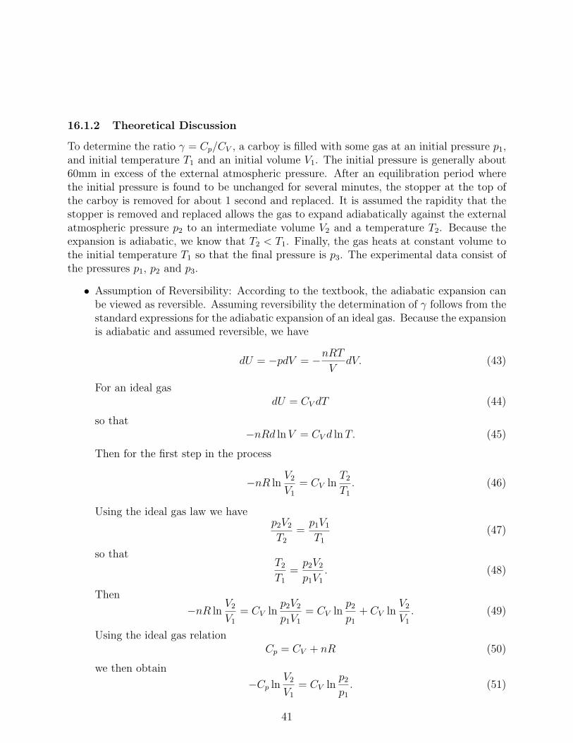
16.1.2 Theoretical Discussion
To determine the ratio γ = Cp/CV , a carboy is filled with some gas at an initial pressure p1,and initial temperature T1 and an initial volume V1. The initial pressure is generally about60mm in excess of the external atmospheric pressure. After an equilibration period wherethe initial pressure is found to be unchanged for several minutes, the stopper at the top ofthe carboy is removed for about 1 second and replaced. It is assumed the rapidity that thestopper is removed and replaced allows the gas to expand adiabatically against the externalatmospheric pressure p2 to an intermediate volume V2 and a temperature T2. Because theexpansion is adiabatic, we know that T2 < T1. Finally, the gas heats at constant volume tothe initial temperature T1 so that the final pressure is p3. The experimental data consist ofthe pressures p1, p2 and p3.
• Assumption of Reversibility: According to the textbook, the adiabatic expansion canbe viewed as reversible. Assuming reversibility the determination of γ follows from thestandard expressions for the adiabatic expansion of an ideal gas. Because the expansionis adiabatic and assumed reversible, we have
dU = −pdV = −nRT
VdV. (43)
For an ideal gasdU = CV dT (44)
so that−nRd ln V = CV d ln T. (45)
Then for the first step in the process
−nR lnV2
V1
= CV lnT2
T1
. (46)
Using the ideal gas law we havep2V2
T2
=p1V1
T1
(47)
so thatT2
T1
=p2V2
p1V1
. (48)
Then
−nR lnV2
V1
= CV lnp2V2
p1V1
= CV lnp2
p1
+ CV lnV2
V1
. (49)
Using the ideal gas relationCp = CV + nR (50)
we then obtain
−Cp lnV2
V1
= CV lnp2
p1
. (51)
41
In the second step of the process we heat the gas at constant volume to a final statedefined by the variables p3, V2 and T1. For this constant volume process the ideal gaslaw along with Eq. (48) give
T2
T1
=p2V2
p1V1
=p2
p3
(52)
so thatV2
V1
=
(p1
p2
)(p2
p3
)=
p1
p3
. (53)
Then−Cp ln
p1
p3
= CV lnp2
p1
(54)
or
γ =Cp
CV
=ln(p1/p2)
ln(p1/p3). (55)
• Irreversible Adiabatic Expansion: We now (perhaps more realistically) assume thatthe adiabatic expansion is an irreversible expansion of the gas against the constantexternal atmospheric pressure p2. Equating the irreversible work to the energy changefor an ideal gas, we obtain
CV (T2 − T1) = −p2(V2 − V1) (56)
= −p2
(nRT2
p2
− nRT1
p1
)(57)
= −nR
(T2 − T1
p2
p1
)(58)
or
CV
(T2
T1
− 1)
= −nR
(T2
T1
− p2
p1
). (59)
Using Eq. (48)
CV
(p2V2
p1V1
− 1
)= −nR
(p2V2
p1V1
− p2
p1
). (60)
The second step in the irreversible process is the same as the reversible case, and wecan again use Eq.(53) to obtain
CV
(p2p1
p1p3
− 1
)= −nR
(p2p1
p1p3
− p2
p1
)(61)
or from Eq.(50)
CV
(p2
p3
− 1
)= −(Cp − CV )
(p2
p3
− p2
p1
)(62)
42
or
−(γ − 1)
(p2
p3
− p2
p1
)=
(p2
p3
− 1
). (63)
After rearranging Eq. (63) and solving for γ we obtain the final result
γ =p1/p2 − 1
p1/p3 − 1. (64)
We can obtain Eq. (64) by expanding the numerator and denominator of Eq.(55) forsmall values of the argument. If we write
f(x) = ln x (65)
and expand f in a Taylor series about x = 1, we obtain
f(x) = f(1) + (x− 1)f ′(1) +1
2(x− 1)2f ′′(1) + . . . (66)
orln x = (x− 1) + . . . (67)
Then for (p1/p2−1) < 1 and (p1/p3−1) < 1 to leading order Eq.(55) becomes Eq.(64).
• Correct derivation allowing the escape of some of the gas: Let us now carefully deriveEq.(64). The steps in the process are:
1. an adiabatic irreversible expansion of the ideal gas from the state n1, p1, T1 andV1 against a constant external pressure p2 to the final state n1, p2, T2 and V2;
2. use of the initial volume of the container so that the state of the system is rep-resented by n2, p2, V1 and T2 - in this step some of the gas originally present isallowed to escape into the atmosphere;
3. constant volume heating to the initial temperature represented by the final staten2, V1, p3 and T1.
We let CV and Cp be the constant volume and constant pressure heat capacities permole. Then for step 1
n1CV (T2 − T1) = −p2
(n1RT2
p2
− n1RT1
p1
)(68)
= −n1RT2 + n1RT1p2
p1
. (69)
Solving for T2 we obtain
n1(R + CV )T2 = n1RT1p2
p1
+ n1CV T1 (70)
43
orCpT2 = RT1
p2
p1
+ CV T1 (71)
so that
T2 =R
Cp
T1p2
p1
+CV
Cp
T1 (72)
=Cp − Cv
Cp
T1p2
p1
+CV
Cp
T1 (73)
=
(1− 1
γ
)T1
p2
p1
+1
γT1 (74)
=T1
γ
[(γ − 1)
p2
p1
+ 1
]. (75)
In the second step, we remove n1 − n2 moles of gas from our system. The expressionfor n2 is
n2 =p2V1
RT2
(76)
=p2V1
R
γ
T1
[(γ − 1)
p2
p1
+ 1
] . (77)
In step 3, the gas remaining in the initial volume is heated to temperature T1 so thatits final pressure is p3. Solving for p3
p3 =n2RT1
V1
(78)
=(
RT1
V1
)(p2V1
R
)(γ/
T1
[(γ − 1)
p2
p1
+ 1
])(79)
orp3 =
p2γ
(γ − 1)p2
p1
+ 1. (80)
We next rearrange Eq.(80)
(γ − 1)p2
p1
+ 1 = γp2
p3
(81)
and solve for γ
γ
(p2
p1
− p2
p3
)=
p2
p1
− 1 (82)
or
γ =p1/p2 − 1
p1/p3 − 1(83)
in complete agreement with Eq.(64).
44
16.1.3 Experimental Notes
1. The adiabatic expansion method is used. Follow the procedure outlined in the text.
2. Our experimental design uses an electronic open ended manometer. Readings from anopen ended manometer gives the pressure relative to the atmospheric pressure. Theatmospheric pressure must be obtained by reading the electronic barometer. Ask yourTA for instructions.
16.1.4 Laboratory Report
1. Theory Section:
(a) Be sure to discuss the difference between the assumption of a reversible adiabaticexpansion and an irreversible expansion against a constant external pressure. Ex-plain which assumption is closest to the actual experimental situation.
2. Calculations:
(a) Calculate γ using both Eqs. (55) and (64).
3. Error Analysis:
(a) Assume an error of ± 2 in the last recorded figure from the electronic manometerand the electronic barometer.
(b) Although the reported values of γ are obtained by an average of the heat capacityration for three trials, choose only 1 of the 3 trials for each gas to propagate theerror in γ. Make sure to indicate carefully which of the three trials (for each gas)is used in your error propagation calculation. Carefully propagate errors in thepressure, the pressure ratios, the logarithms and the final ratios to obtain thepropagated error in the heat capacity ratio. Compute expressions and values forthe statistical error in γ from both Eqs. (55) and (64).
4. Conclusions:
(a) Compare γ ± ε(γ) using both the assumption of reversibility and irreversible adi-abatic expansions. Do the two values determined lie within their respective sta-tistical errors?
(b) Compare γ±ε(γ) with the theoretical values expected for an ideal monatomic anddiatomic gas. Do the theoretical results lie within your calculated experimentalerrors? If the results lie outside the experimental errors, discuss possible reasonsfor the lack of agreement.
45
16.2 Experiment 6 - The Heat of Combustion of Organic Com-pounds
16.2.1 Reading Assignment
Experiment 6, Pages 145-158, Text.
16.2.2 Experimental Notes
1. Follow the instructions in the textbook for the Parr instrument.
2. Our pressure gauge is calibrated in atmospheres. You must convert psi to atmospheresas discussed in the textbook.
3. You will determine the enthalpy of combustion for the compound assigned to you byyour TA in class.
16.2.3 Error Analysis
In determining the error in the enthalpy of combustion of your compound, include contri-butions only from a) the mass of the iron wire used, b) the mass of the sample used, c)the energies of combustion given in the text [± 2 in the last significant figure] and d) thetemperature change. It will be necessary to determine the error in the heat capacity of thecalorimeter from your first measurement, and then use this error by propagation to deter-mine the error in the final molar enthalpy of combustion. You may ignore any errors fromthe volume of water used in filling the calorimeter, and you may ignore any errors in the de-termination of the time of measurement. These errors are so small that they are insignificantfor our purposes.
16.3 Experiment Number 9 - Partial Molar Volume
16.3.1 Reading Assignment
Experiment 9 - Partial Molar Volume - Pages 172-178, text.
16.3.2 Experimental Notes
1. We use the Weld-type pycnometer. Read the note at the bottom of page 176, carefully.
2. Weigh your empty pycnometer. Make sure it is dry and clean before the measurementand use the Mettler balance. Accurate measurement is essential. If you have anyproblems with the balance, ask your TA.
3. Fill the pycnometer with the distilled water contained in the bottle in the heat bath.Place the pycnometer in a beaker in the bath and wait five minutes to make sure thetemperature is equilibrated.
46
4. Record the bath temperature and the room temperature. The temperature of the bathmust be greater than the room temperature. If this is not true, inform your TA atonce.
5. Remove the pycnometer from the bath, dry the exterior with a paper towel, and accu-rately weigh the full pycnometer with the Mettler balance.
6. Empty the pycnometer and dry it with acetone and the aspirator under the fume hood.
7. Fill the dry pycnometer with the stock NaCl solution. Place the pycnometer in abeaker in the bath for at least five minutes to equilibrate the temperature. Be sure torecord the molality of the stock solution and its associated error.
8. Remove the pycnometer, dry the exterior and weigh the pycnometer carefully.
9. Clean and dry the pycnometer with water and acetone as above.
10. Pipette 25.0 ml of the stock solution into a 50.0 ml volumetric flask. Add distilledwater slowly while mixing. Do not fill completely to the graduation mark. Place theflask in the heat bath to equilibrate for 5 minutes. After equilibration, add distilledwater from the bottle in the heat bath to the graduation mark.
11. Place this solution in the pycnometer and equilibrate using the same procedure outlinedabove.
12. After equilibration, weigh the pycnometer with diluted solution carefully as above.After the determination of the weight, do not dispose the diluted solution. Return thesolution to the volumetric flask. You will need the solution for the next dilution.
13. Repeat the process for a further dilution of the diluted NaCl solution by an additional50%.
14. Clean all glass ware before leaving the laboratory.
16.3.3 Laboratory Reports
1. Calculations: Perform all calculations to determine φ and√
m for the three measuredconcentrations. Please note that the relation between the molarity M of the solutionand the molality m is given by Eq. (24) in your textbook. Because the units associatedwith Eq. (24) of the textbook are confusing, a derivation of the connection now follows.
Consider a solution containing 1000. grams of solvent of known molality m. Followingthe notation in the textbook, we let M2 represent the molecular weight of the solutein units of grams per mole. Then the total mass in grams of solute and solvent in thesolution of molality m is 1000. g + mM2. The density d of the solution is then givenby
d =1000. g + mM2
V(84)
47
where V is the volume of the solution in cm3. By definition the molarity M is thenumber of moles of solute in 1 liter of solution, so that the volume of the solution inliters is given by
Ω =L
1000. cm3
1000. g + mM2
d. (85)
Because the number of moles of solute in our solution of 1000. grams of solvent is m,the molarity is given by
M =m
Ω(86)
=1000. cm3
L
md
1000. g + mM2
(87)
or
M =
(1000. cm3
L
)d
11000. g
m+ M2
. (88)
If we solve Eq.(88) for m in terms of M , we obtain
m = 1000. g1(
d
M
)(1000. cm3
L
)−M2
. (89)
Note that in the experiment M is decreased by a factor of 2 for each dilution. Therelation for m from the dilutions is more complex and must be calculated using Eq.(89).
2. Graphical Analysis: Plot your determined values of φ as a function of√
m. Youshould find a linear relationship. Plot the best straight line through the data pointsand determine the slope and the intercept φ0. Please note that the book uses sloppynotation for the slope. In Eqs. (21) and (22) you should interpret dφ/d
√m as the
derivative (i.e. slope) of your plotted line. The d represents differentiation in this case.In Eqs. (17) and (24) the d is the density.
3. Error Analysis: Propagate errors to determine the errors in φ and√
m for the lowestand the highest concentrations. Show all calculations. Tabulate all final results withassociated errors. Plot the error bars on your graph to determine the errors in theslope and intercept using the method of limiting slopes.
Hint: The formulas from which you determine error may appear complex. However, ifyou break the problem of determining errors into parts, the task can be made relativelyeasy. By breaking the problem into parts we introduce a small error that can be ignoredfor the purposes of this assignment. As an example, consider Eq. (17) in your text
φ =1
d
(M2 −
1000
m
W −W0
W0 −We
).
48
For our purposes, we can assume the error in M2 is too small to affect our results.Take the value of M2 to be 58.443 g mol−1 with no error. Define
a = W −W0
andb = W0 −We
The errors in a and b are given by
ε(a) =√
ε(W )2 + ε(W )20
andε(b) =
√ε(W0)2 + ε(We)2
Now let
c =1000
m
a
b
The error in c is given by
ε(c)
c=
√(ε(a)
a)2 + (
ε(b)
b)2 + (
ε(m)
m)2
Finally, the error in φ is given by
ε(φ)
φ=
√(
ε(c)
M2 − c)2 + (
ε(d)
d)2
For the other equations, use the same methods to break the problem of calculatingerrors into parts.
4. Summary of Final Results: Report the values of the slope and intercept with theassociated errors. Be sure to report the proper number of significant figures and theunits. Use Eqs. (21), (22), the determined values of φ0 and the slope to calculate thepartial molar volumes of water and NaCl as a function of m for m=0.5,1.0,1.5,2.0 and2.5. Plot the results for the partial molar volumes on a common graph.
5. Conclusions: Summarize your results.
16.4 The Joule-Thomson Effect
16.4.1 Reading Assignment
Experiment 2, pages 96-104
49
16.4.2 Procedure
Note: In this experiment, you measure the Joule-Thomson coefficient of CO2 only.
1. Place one thermocouple wire in the heat bath and the other wire in the exit of theJoule-Thomson cell. Make sure each wire is fixed in place, and make sure the wire inthe Joule-Thomson cell is near the bottom.
2. Ask your TA about the proper use of the regulator at the top of the gas tank.
3. Slowly open the needle valve of the regulator until the manometer records a pressuredifference of about 1900 millibar. Do not exceed 2000 millibar, because the manometeris limited to pressures less than 2 bar.
4. Wait 1 minute and record the pressure difference, the temperature of the bath, the celland the temperature difference once per minute for 5 minutes.
5. Decrease the pressure difference by about 100-200 millibar and repeat the measure-ments of the pressure and temperature differences. Again wait 1 minute before record-ing data and record data once per minute for 5 minutes.
6. Decrease the pressure difference 5 more times again by about 200 millibar.
7. When you have finished, make sure to close the regulator by turning off the main valve,and bleeding the system using the needle valve. Your final pressure difference shouldbe 0.
16.4.3 Calculations
1. Plot ∆T as a function of ∆P . Using
µJT =
(∂T
∂P
)H
determine the Joule-Thomson coefficient from the slope.
16.4.4 Error Analysis
1. Include error bars in ∆T for all measured points, and determine the error in the Joule-Thomson coefficient using the method of limiting slopes.
16.4.5 Discussion
1. Report the Joule-Thomson coefficient to the correct number of significant figures alongwith the statistical error. Because the Joule-Thomson coefficient is a function of tem-perature, the temperature associated with the measured value of µJT must be reportedas well.
50
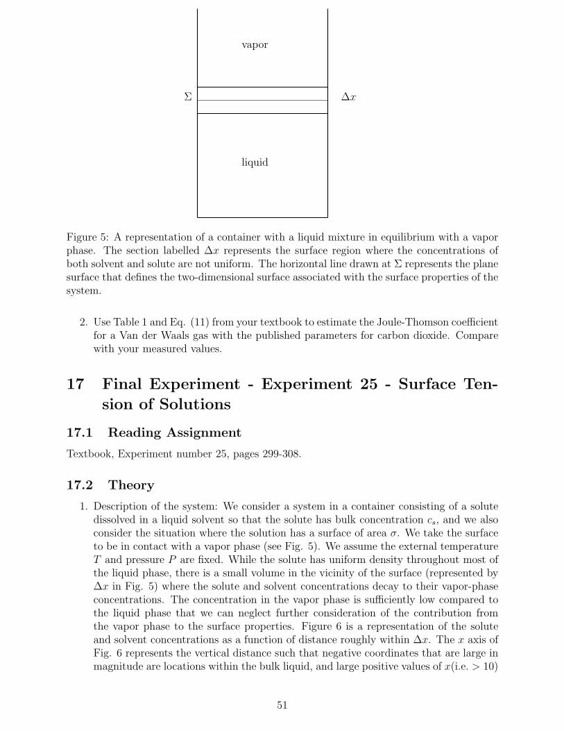
∆xΣ
liquid
vapor
Figure 5: A representation of a container with a liquid mixture in equilibrium with a vaporphase. The section labelled ∆x represents the surface region where the concentrations ofboth solvent and solute are not uniform. The horizontal line drawn at Σ represents the planesurface that defines the two-dimensional surface associated with the surface properties of thesystem.
2. Use Table 1 and Eq. (11) from your textbook to estimate the Joule-Thomson coefficientfor a Van der Waals gas with the published parameters for carbon dioxide. Comparewith your measured values.
17 Final Experiment - Experiment 25 - Surface Ten-
sion of Solutions
17.1 Reading Assignment
Textbook, Experiment number 25, pages 299-308.
17.2 Theory
1. Description of the system: We consider a system in a container consisting of a solutedissolved in a liquid solvent so that the solute has bulk concentration cs, and we alsoconsider the situation where the solution has a surface of area σ. We take the surfaceto be in contact with a vapor phase (see Fig. 5). We assume the external temperatureT and pressure P are fixed. While the solute has uniform density throughout most ofthe liquid phase, there is a small volume in the vicinity of the surface (represented by∆x in Fig. 5) where the solute and solvent concentrations decay to their vapor-phaseconcentrations. The concentration in the vapor phase is sufficiently low compared tothe liquid phase that we can neglect further consideration of the contribution fromthe vapor phase to the surface properties. Figure 6 is a representation of the soluteand solvent concentrations as a function of distance roughly within ∆x. The x axis ofFig. 6 represents the vertical distance such that negative coordinates that are large inmagnitude are locations within the bulk liquid, and large positive values of x(i.e. > 10)
51
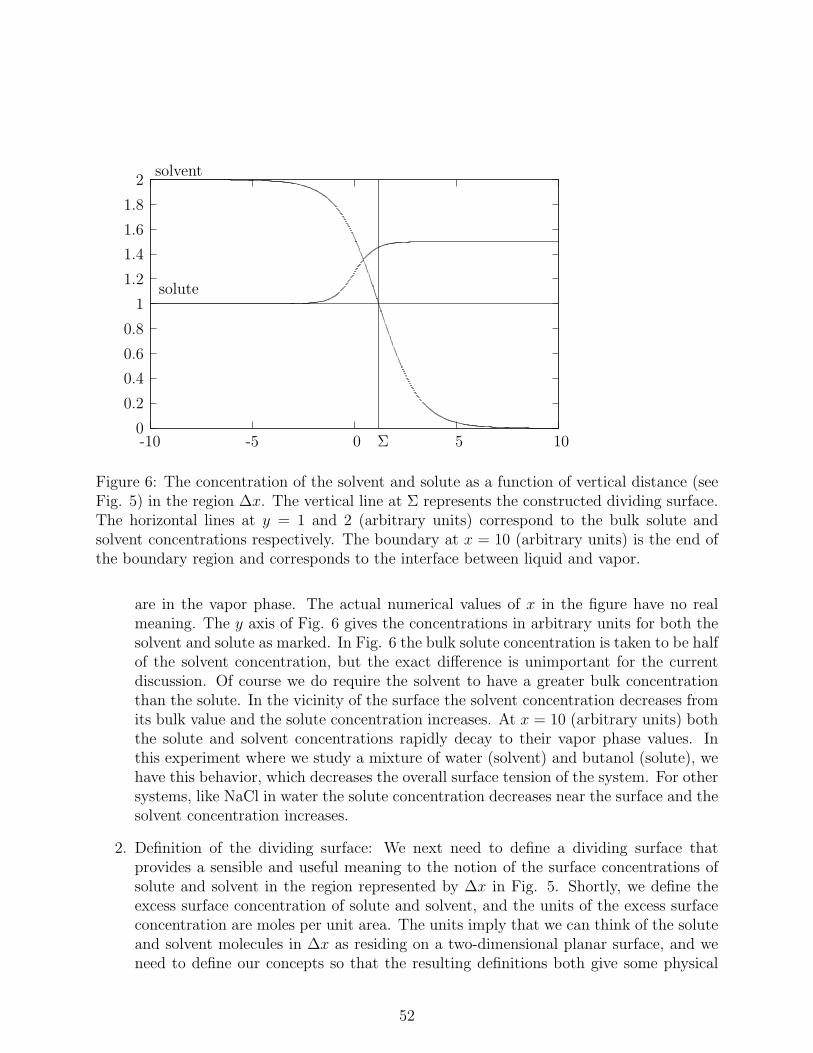
0
0.2
0.4
0.6
0.8
1
1.2
1.4
1.6
1.8
2
-10 -5 0 5 10Σ
solvent
solute
Figure 6: The concentration of the solvent and solute as a function of vertical distance (seeFig. 5) in the region ∆x. The vertical line at Σ represents the constructed dividing surface.The horizontal lines at y = 1 and 2 (arbitrary units) correspond to the bulk solute andsolvent concentrations respectively. The boundary at x = 10 (arbitrary units) is the end ofthe boundary region and corresponds to the interface between liquid and vapor.
are in the vapor phase. The actual numerical values of x in the figure have no realmeaning. The y axis of Fig. 6 gives the concentrations in arbitrary units for both thesolvent and solute as marked. In Fig. 6 the bulk solute concentration is taken to be halfof the solvent concentration, but the exact difference is unimportant for the currentdiscussion. Of course we do require the solvent to have a greater bulk concentrationthan the solute. In the vicinity of the surface the solvent concentration decreases fromits bulk value and the solute concentration increases. At x = 10 (arbitrary units) boththe solute and solvent concentrations rapidly decay to their vapor phase values. Inthis experiment where we study a mixture of water (solvent) and butanol (solute), wehave this behavior, which decreases the overall surface tension of the system. For othersystems, like NaCl in water the solute concentration decreases near the surface and thesolvent concentration increases.
2. Definition of the dividing surface: We next need to define a dividing surface thatprovides a sensible and useful meaning to the notion of the surface concentrations ofsolute and solvent in the region represented by ∆x in Fig. 5. Shortly, we define theexcess surface concentration of solute and solvent, and the units of the excess surfaceconcentration are moles per unit area. The units imply that we can think of the soluteand solvent molecules in ∆x as residing on a two-dimensional planar surface, and weneed to define our concepts so that the resulting definitions both give some physical
52
insight and simultaneously are consistent with the number of moles of each speciesin the volume defined by ∆x. The resulting definitions are physically artificial butmathematically consistent.
We draw a plane dividing surface within ∆x, which we label Σ, and we choose thelocation of Σ so that the excess number of moles of solvent on each side of Σ is 0. Tounderstand the notion of the excess number of surface moles of solvent, we let cS be thebulk solvent concentration assumed to be uniform from the bottom of the containerto the constructed surface at Σ. We let cS be the actual surface concentration thatis uniform from the bottom of the container until we reach ∆x and decays in ∆x aswe approach the vapor phase. The behavior of cS is depicted in Fig. 6. The excessnumber of moles of solvent is defined to be the difference between the deficit in thenumber of moles of solvent obtained from cS compared to cS below and above Σ. Tomake the concept clearer, we define the volume of the liquid phase, V` to be the volumeof solution from Σ to the bottom of the container. Then the excess number of molesof solvent, nΣ
S is defined to be
nΣS = cSV` − σ
∫ Σ
−bcSdx− σ
∫ ∞
ΣcSdx (90)
where −b is the coordinate at the bottom of the container. We choose the location ofΣ so that nΣ
S = 0. This choice of the location of Σ implies
cSV` = σ∫ ∞
−bcSdx; (91)
i.e. the total number of moles of solvent obtained by integrating the actual concentra-tion profile over the entire system is identical to the number of moles that would beobtained if a uniform concentration existed up to the surface defined by Σ.
We define the excess number of moles of solute in the same manner used to define thesolvent. Letting cs be the bulk solute concentration assumed to be uniform throughoutthe solution and cs be the actual solute concentration, we write for the excess numberof moles of solute
nΣs = csV` − σ
∫ Σ
−bcsdx− σ
∫ ∞
Σcsdx. (92)
While we have defined Σ so that nΣS = 0 by construction, in general the different
concentration profile for the solute implies that nΣs cannot generally vanish.
As discussed above, we now associate (i.e. pretend) that all the excess number of molesof solute nΣ
s are confined to a two-dimensional layer at Σ. We then define the excesssurface concentrations of both the solute and solvent by
Γs =nΣ
s
σ(93)
and
ΓS =nΣ
S
σ. (94)
53
By construction ΓS = 0, and our goal is to measure Γs assuming all the excess numberof moles of solute reside on the surface Σ. The measurement is possible by using theGibbs isotherm.
Before deriving the Gibbs isotherm it is useful to understand the notion of excess sur-face concentration with some definite physical models. We consider the case where∆x consists only of a single layer of solute molecules adsorbed onto a solvent. Suchfilms are called monolayers, and an example of such a system is oleic acid adsorbed onwater. In such a case we place Σ just at the interface between the solvent and solute.Clearly, the excess surface concentration of solvent is 0, because the solvent moleculesare completely absent from the monolayer. The resulting solute excess surface con-centration is just the number of moles of solute in the monolayer per unit area. Wesee that our definition of excess surface concentration of solute is consistent with ourexpectations for a monolayer. In another limit we consider the case that solute andsolvent are very similar (e.g. two completely miscible alcohols). In such a case Γs canbe expected to be very small; i.e. very little solute needs to be associated with ourartificial surface layer, because the concentration profiles of both solute and solvent in∆x have nearly the same functional form.
In the intermediate case between the two extremes outlined in the previous paragraph,the excess number of moles of solute can either be enhanced or diminished comparedto csV`. Work is required to form the surface owing to the breaking of bonds at theinterface (e.g. the hydrogen bonds for liquid water), and solutes having weaker bondsthan the solvent tend to have positive excess surface concentrations(e.g. butanol).Using similar reasoning solutes having stronger bonds than the solvent tend to havenegative excess surface concentrations(e.g. sodium chloride).
3. The Gibbs Isotherm: We let Gv be the Gibbs free energy of the vapor phase, G` be theGibbs free energy of the liquid phase and GΣ be the Gibbs free energy of the surfacephase. We allow all three phases to contain both solvent and solute. We can write forthe total differential of the entire Gibbs free energy function
dG = dGv + dG` + dGΣ. (95)
In each phase G is a function of T, P and the number of moles of both the solvent andsolute. Additionally, GΣ depends on the surface area σ. We can then write (at fixedtemperature and pressure)
dG = µsdnv,s + µSdnv,S + µsdn`,s + µSdn`,S + µsdnΣ,s + µSdnΣ,S + γdσ. (96)
where nv,s represents the number of moles of solute in the vapor, nv,S represents thenumber of moles of solvent in the vapor, n`,s represents the number of moles of solute inthe liquid, n`,S represents the number of moles of solvent in the liquid, nΣ,s representsthe number of moles of solute associated with the surface region, nΣ,S represents thenumber of moles of solvent associated with the surface region, and γ is the reversible
54
work per unit area to form the surface; i.e. the surface tension. In the vapor and liquidphases alone, we know that
dGv = µsdnv,s + µSdnv,S (97)
anddG` = µsdn`,s + µSdn`,S (98)
so that Eq. (96) becomes
dGΣ = µsdnΣ,s + µSdnΣ,S + γdσ. (99)
Because the number of moles of each species and the surface area are all extensivevariables with the chemical potentials and the surface tension intensive variables, byEuler’s theorem on homogeneous functions we can write
GΣ = µsnΣ,s + µSnΣ,S + γσ. (100)
After taking the total differential of Eq. (100) and subtracting Eq. (99), the result isa Gibbs-Duhem relation
−σdγ = nΣ,sdµs + nΣ,SdµS. (101)
or solving for the differential of the surface tension
−dγ = Γsdµs + ΓSdµS (102)
where we have recognized the excess surface concentrations as the number of moles ofsolute or solvent per unit area. As noted previously ΓS = 0 by construction, and weknow that
µs = µ + RT ln as (103)
where as is the activity of the solute defined so that the form of the chemical potentialmatches the ideal gas form. We can also write the activity in terms of the soluteconcentration
as = csφs (104)
where φs is called the activity coefficient. The activity coefficient can be shown toapproach unity as the concentration of solute becomes low. Taking the differential ofthe chemical potential
dµs = RTd ln as (105)
and substituting the differential into Eq. (102), we obtain
−dγs = RT Γs d ln a (106)
or
Γs = − 1
RT
dγ
d ln as
, (107)
55
which is the Gibbs isotherm. The excess solute surface concentration Γs depends onthe slope of the surface tension with solute activity, and to the extent that the relationbetween the surface tension and the logarithm of the activity is linear, we can assumethe excess solute concentration is independent of total concentration. Consequently,the Gibbs isotherm can provide a single excess solute surface concentration for alltotal solution concentrations. The location of the dividing surface Σ does vary withconcentration, but the location of Σ is not important to the overall interpretation.
In the textbook Eq. (107) is approximated by replacing the activity with the concen-tration; i.e. setting φ = 1. Equation (107) enables the determination of the excesssurface concentration of solute by measuring the surface tension as a function of con-centration. We determine the excess surface concentration of solute in this manner inthe current experiment.
17.2.1 Experimental Notes
1. We use the capillary rise method discussed in the textbook.
2. You make solutions of either n-butanol, iso-butanol, sec-butanol or tert-butanol. Askyour TA to assign the particular alcohol.
3. You are not to perform the NaCl experiment.
4. The approximately 0.8 M butanol stock solution will be provided. You are to usevolumetric methods to prepare the other solutions.
5. Be sure to record the temperature of the bath.
6. The surface tension of distilled water as a function of temperature is given in the Tablebelow. To determine the surface tension at your working temperature, you must useinterpolation methods.
Temperature (C) surface tension of water (dy cm−1)10. 74.2320. 72.7525. 72.0030. 71.20
17.3 Laboratory Report
1. Your reports are to be written in class during Week 13. Come to 259 Pastore for thereport writing session. You should bring calculators, your original signed data, youroriginal procedure, signed by your TA and pens or pencils. We supply paper and graphpaper. We also supply a copy of pages 299-308 from your text books as well as a copy ofthese notes. You may not use your own texts. We strongly recommend that you
56
prepare your laboratory reports at home for practice. Although you are notallowed to bring your home written reports with you to the report writingsession, the practice is essential in order to be able to finish the report inthe allotted time (4 hours). You may come to any one of the instructors in thecourse for help prior to the report writing session. In fact, we encourage you to come tous for help. Success in this assignment will only be possible with thorough preparation.
The laboratory report format is as follows:
(a) Title Page: Give the title of the experiment, and the date the experiment wasperformed.
(b) Abstract: This should be a 1 paragraph summary of what is to follow includingthe results. It is suggested that you write the abstract after the rest of the reportis complete.
(c) Introduction: This should be a discussion of the purpose of the experiment.
(d) Theory: This should provide a derivation of the key formulas used in the ex-periment and in the data analysis section. Definitions must be provided for allsymbols used in this and subsequent sections.
(e) Procedure: Attach the outline of the procedure you brought to class and hadsigned by your TA.
(f) Original Data: Attach the original data signed by your TA.
(g) Data Table: Tabulate your data so that it can be used in the calculations tofollow.
2. Calculations
(a) We assume that the density of water and butanol solutions are the same andunchanging during the course of the experiment. We can then determine thesurface tension of each solution, γs using
γs = γH2Ohs
hH2O
(108)
where γH2O is the surface tension of water obtained from the table, hs is thecapillary rise of the solution and hH2O is the capillary rise of pure water.
(b) Be sure to calculate the surface concentration in both units of mol cm−2 andmolecules per square angstrom as discussed in your textbooks.
(c) For the butanol calculations, use the activity coefficients given on page 302 of yourtextbooks. Alternatively, you can use the graph of the activity coefficient as afunction of concentration given Fig. 7. You may use the same activity coefficientsfor all forms of butanol.
57
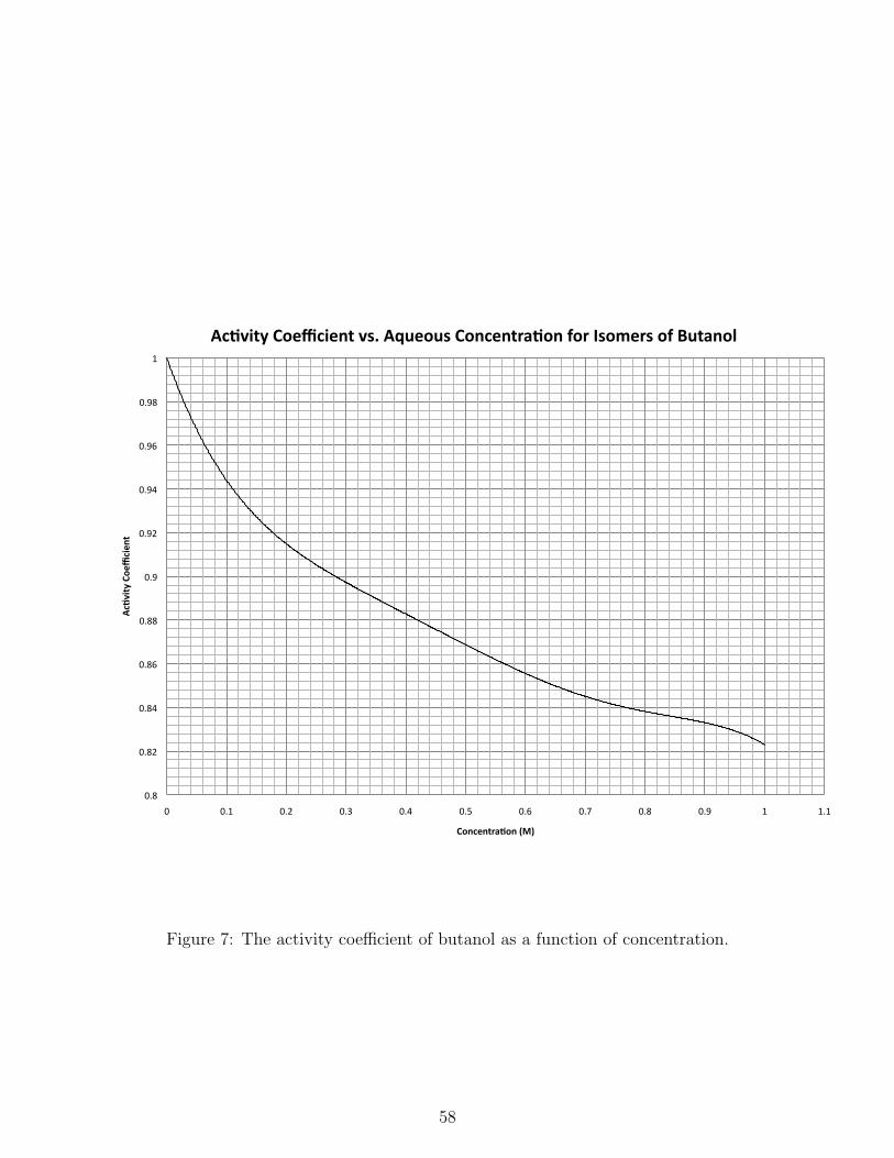
0.8$
0.82$
0.84$
0.86$
0.88$
0.9$
0.92$
0.94$
0.96$
0.98$
1$
0$ 0.1$ 0.2$ 0.3$ 0.4$ 0.5$ 0.6$ 0.7$ 0.8$ 0.9$ 1$ 1.1$
Ac#vity(Coe
fficien
t(
Concentra#on((M)(
Ac#vity(Coefficient(vs.(Aqueous(Concentra#on(for(Isomers(of(Butanol(
Figure 7: The activity coefficient of butanol as a function of concentration.
58
3. Error Analysis: Propagate the errors for only the first and last points on the graph ofthe surface tension as a function of the logarithm of the activity of the solution. Use thetwo calculated errors to determine the limiting slopes of your graph. Use the limitingslopes to estimate the error in your determined surface concentrations. Make sure toexpress the errors in both mol cm−2 and molecules A−2. A conversion is required.
18 Tables of Data
59
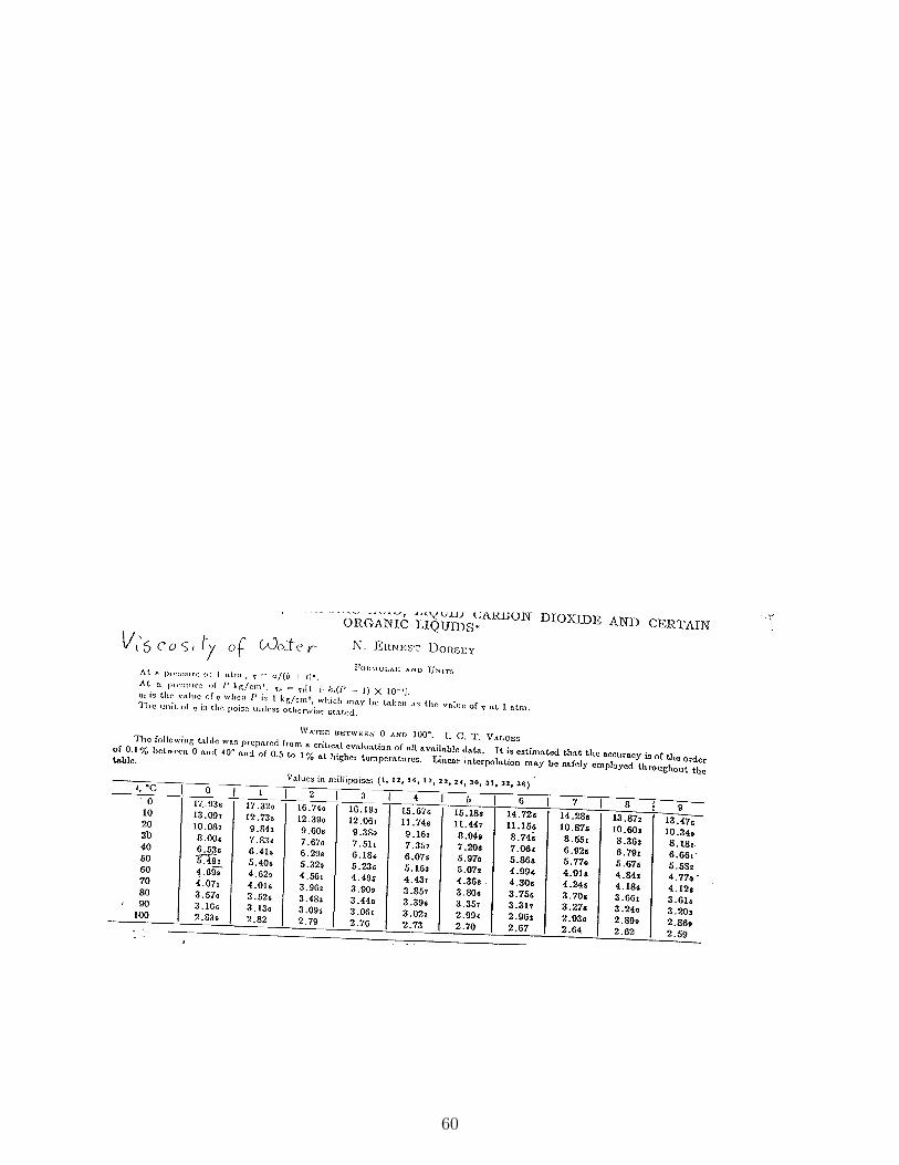
60
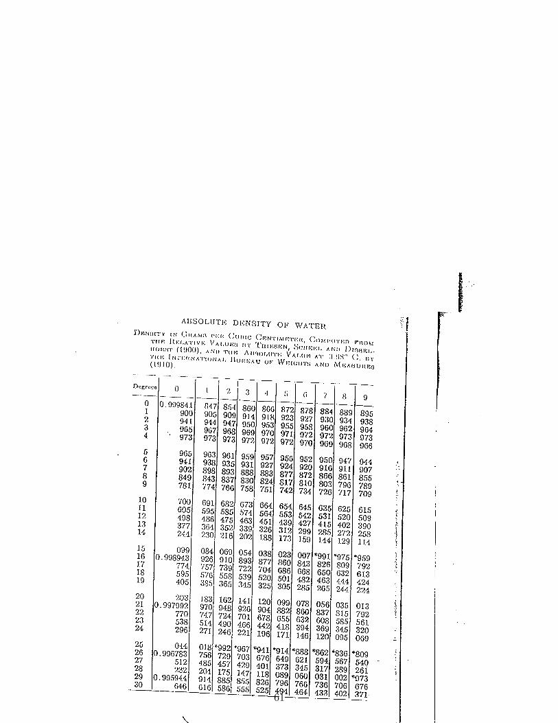
61