chemistry of marine water and sediments ||
TRANSCRIPT

Environmental Science Series editors: R. Allan . U. Forstner . W. Salomons

Springer-Verlag Berlin Heidelberg GmbH

Antonio Gianguzza . Ezio Pelizzetti Silvio Sammartano {Eds.}
Chemistry of Marine Water and Sediments
With 249 Figures and 106 Tables
Springer

Editors
Prof. Antonio Gianguzza
Dipartimento di Chimica Inorganica Universita di Palermo Via delle Scienze 1 -90128 Palermo, Italy
Prof. Ezio Pelizzetti
Dipartimento di Chimica Analitica Universita di Torino Via Pietro Giuria 5 1-10125 Torino, Italy
Prof. Silvio Sammartano
Dipartimento di Chimica Inorganica, Chimica Analitica e Chimica Fisica Universita di Messina Salita Sperone 31 1 -98166 Messina, Italy
Die Deutsche Bibliothek - CIP-Einheitsaufnahme
Chemistry of marine water and sediments: with 106 tables / Antonio Gianguzza ... (ed.). - Berlin; Heidelberg; New York ; Barcelona; Hong Kong; London; Milan; Paris; Tokyo: Springer, 2002
(Environmental science)
This work is subject to copyright. All rights are reserved, whether the whole or part of the material is concerned, specifically the rights of translation, reprinting, reuse of illustrations, recitation, broadcasting, reproduction on microfilms or in any other way, and storage in data banks. Duplication of this publication or parts thereof is permitted only under the provisions of the German Copyright Law of September 9, 1965, in its current version, and permission for use must always be obtained from Springer-Verlag. Violations are liable for prosecution under the German Copyright Law.
© Springer-Verlag Berlin Heidelberg 2002
Originally published by Springer-Verlag Berlin Heidelberg New York in 2002. Softcover reprint of the hardcover I st edition 2002
The use of general descriptive names, registered names, trademarks, etc. in this publication does not imply, even in the absence of a specific statement, that such names are exempt from the relevant protective laws and regulations and therefore free for general use.
Cover Design: Struve & Partner, Heidelberg
Dataconversion: Bliro Stasch (www.stasch.com) . Uwe Zimmermann, Bayreuth
SPIN: 10934449 30/3111 - 5 4 3 2 1 - Printed on acid-free paper
ISBN 978-3-642-07559-9 ISBN 978-3-662-04935-8 (eBook) DOI 10.1007/978-3-662-04935-8

Preface
This book is a collection of all the lectures by the professors attending the 3rd "International School on Marine Chemistry" held in Ustica (Palermo, Italy, September 2000),
under the auspices of the United Nations and the Italian Chemical Society. The School was organized by the University of Palermo in co-operation with the Natural Marine Reserve of Ustica Island.
The Organising Committee of the School wishes to thank the University of Messina, the University of Roma "La Sapienza:' the Italian University Consortium of Environmental Chemistry, and the Marine Reserve of Ustica Island for their financial support to the School.
This book has been printed with the financial support of the Environmental Research Centre CIRITA of the University of Palermo.
The editors thank all the professors whose outstanding scientific contributions have made it possible to publish this book.
Professor Antonio Gianguzza Professor Ezio Pelizzetti Professor Silvio Sammartano
Contents
Part I Biogeochemical Processes at the Air-Water and Water-Sediment Interface .............................................. .
1 Sea Water as an Electrolyte ................................................. 3 1.1 Introduction. . . . . . . . . . . . . . . . . . . . . . . . . . . . . . . . . . . . . . . . . . . . . . . . . . . . . . . . . . . . . . . . .. 3
1.1.1 Composition of Average Sea Water . . . . . . . . . . . . . . . . . . . . . . . . . . . . . . . . . . . .. 3 1.1.2 The Concept of Salinity . . . . . . . . . . . . . . . . . . . . . . . . . . . . . . . . . . . . . . . . . . . . . . .. 6 1.1.3 Causes of Major Components Not Being Conservative. . . . . . . . . . . . . . . . .. 8 1.1.4 Physical Properties of Natural Waters ................................. 12
1.2 Modelling the Physical Properties of Natural Waters ......................... 18 1.3 Estimating the Properties of Mixed Electrolytes ............................. 23 1.4 Estimating Transport Properties . . . . . . . . . .. . . . . . . . . . . . . . . . . . . . . . . . .. . . . . . . . .. 29
Acknowledgements. . . . . . . . . . . . . . . . . . . . . . . . . . . . . . . . . . . . . . . . . . . . . . . . . . . . . . . . .. 32 References. . . . . . . . . . . . . . . . . . . . . . . . . . . . . . . . . . . . . . . . . . . . . . . . . . . . . . . . . . . . . . . . . .. 32
2 The Chemical and Physical Properties of Marine Aerosols: An Introduction ............................................................ 35
2.1 Introduction. . . . . . . . . . . . . . . . . . . . . . . . . . . . . . . . . . . . . . . . . . . . . . . . . . . . . . . . . . . . . . . .. 35 2.1.1 Physical Characteristics of Aerosols ................................... 37 2.1.2 The Role of Clouds in the Aerosol Cycle. . . . . . . . . . . . . . . . . . . . . . . . . . . . . .. 39 2.1.3 The Global Distribution of Aerosols Over the Oceans ................. 41 2.1.4 Aerosol Composition ................................................. 45 2.1.5 Temporal Variability of Marine Aerosols .............................. 47
2.2 Sea Salt Aerosols . . . .. . . . . .. . . . . . . . . . . . . . . . . . . . . . . . . .. . . . . .. . . . . . . . . . . . . . . . ... 49 2.2.1 Sea Salt Production and Size Distribution. . . . . . . . . . . . . . . . . . . . . . . . . . . .. 49 2.2.2 The Contribution of Sea Salt to Submicrometre Aerosol. . . . . . . . . . . . . .. 50 2.2.3 Sea Salt Aerosol and New Particle Production ......................... 51
2.3 The Oceanic Atmospheric Sulphur Cycle ..................................... 51 2.3.1 Global Sulphur Budgets ............................................... 52 2.3.2 S02 and nss-SO~- . . . . . . . . . . . . . . . . . . . . . . . . . . . . . . . . . . . . . . . . . . . . . . . . . . . . .. 52 2.3.3 DMS and the Atmospheric Sulphur Cycle ............................. 54 2.3.4 MSA and nss-SO~- .................................................... 55 2.3.5 New-Particle Production from DMS over the Ocean ................... 55 2.3.6 Impact on Climat ..................................................... 58
2.4 The Oceanic Atmospheric Cycle of Nitrates and Ammonium. . . . . . . . . . . . . . . .. 58 2-4-1 Global Budgets of NOy and NHx ' . . . . . . . . . . . . . . . . . . . . . . . . . . . . . . . . . . . . .. 59

VIII Contents
2-402 Concentrations of Nitrate and Ammonium in the Marine Atmosphere ................................................... 61
2.4.3 Nitrate and Ammonium Aerosol Propertie ............................ 61 2.4.4 Organic Nitrogen Aerosol . . . . . . . . . . . . . . . . . . . . . . . . . . . . . . . . . . . . . . . . . . . .. 62 2-405 Trends in Nitrate and Ammonium in Pollution AerosoL ............... 62 2.4.6 Atmospheric Deposition and the Nitrogen-Nutrient Budget
in the Ocean .......................................................... 63 2.5 Mineral Dust in the Marine Atmosphere ..................................... 64
2.5.1 Global Distribution of Dust ........................................... 64 2.5.2 Sources of Dust ....................................................... 65 2.5.3 Elemental Composition ............................................... 67 2.5.4 Mineralogical Composition ........................................... 70 2.5.5 Deposition of Dust to the Oceans ..................................... 70 2.5.6 Impact of Dust on Marine Biogeochemistry Cycles .................... 72 2.5.7 The Impact of Mrican Deposition on the Nutrient Cycle ............ " 72
2.6 Other Aerosol Species and the Impact of Continental Source. . . . . . . . . . . . . . . .. 74 2.7 Conclusions ................................................................. 76
References . . . . . . . . . . . . . . . . . . . . . . . . . . . . . . . . . . . . . . . . . . . . . . . . . . . . . . . . . . . . . . . . . .. 77
3 Photochemical Processes in the Euphotic Zone of Sea Water: Progress and Problems. . . . . . . . . . . . . . . . . . . . . . . . . . . . . . . . . . . . . . . . . . . . . . . . . . . .. 83
3.1 Introduction. . . . . . . . . . . . . . . . . . . . . . . . . . . . . . . . . . . . . . . . . . . . . . . . . . . . . . . . . . . . . . . .. 83 3.2 General Framework ........................................................ " 84
3.2.1 Solar Flux. . . . . . . . . . . . . . . . . . . . . . . . . . . . . . . . . . . . . . . . . . . . . . . . . . . . . . . . . . . .. 84 3.2.2 Light Attenuation ..................................................... 84 3.2.3 Factors Influencing Photoreactions ................................... 86
3.3 Main Photoprocesses Occurring in Water and Air. . . . . . . . . . . . . . . . . . . . . . . . . . .. 87 3.3-1 Direct Photolysis .................................................... " 87 3.3.2 Indirect Photoreactions . . . . . . . . . . . . . . . . . . . . . . . . . . . . . . . . . . . . . . . . . . . . . .. 88
3.4 Role of Iron and Chlorine. . . . . . . . . . . . . . . . . . . . . . . . . . . . . . . . . . . . . . . . . . . . . . . . . . .. 95 3-401 Inorganic CI Formation in the Marine Environment .................. 95 3.4.2 Role ofIron in Surface Waters . . . . . . . . . . . . . . . . . . . . . . . . . . . . . . . . . . . . . . . .. 96 3.4.3 Interactions Between Iron and Chloride. . . . . . . . . . . . . . . . . . . . . . . . . . . . . .. 99 References. . ..... . . .... . . . ..... . . .... . . . .... . . . ... . . . . . ..... . . .... . . ....... 102
4 Sedimentary Organic Matter Preservation and Atmospheric O2 Regulation. . . . . . . . . . . . . . . . . . . . . . . . . . . . . . . . . . . . . . . . . . . . . . 105
4.1 Introduction. . . . . . . . . . . . . . . . . . . . . . . . . . . . . . . . . . . . . . . . . . . . . . . . . . . . . . . . . . . . . .. 105 4.2 Global Cycles of Carbon and Oxygen ...................................... 106 4.3 Organic Matter Preservation and Sediment Texture........................ 108 4-4 Oxygen Effects on Sedimentary Preservation.............................. 110 4.5 Maintaining Atmospheric O2 within Safe Bounds.......................... 114 4.6 The Mineral Conveyer Belt and Sedimentary Afterburner. . . . . . . . . . . . . . . . . . 119
Acknowledgements........................................................ 121 References ..................................................... '" . . . ...... 121

Contents IX
5 Particulate Organic Matter Composition and Fluxes in the Sea. . . . . . .. 125 5.1 Introduction. . . . . . . . . . . . . . . . . . . . . . . . . . . . . . . . . . . . . . . . . . . . . . . . . . . . . . . . . . . . . . . 125 5.2 Relation of Carbon Flux with Primary Production. . . . . . . . . . . . . . . . . . . . . . . .. 126
5.2.1 Spatial Relation. . . . . . . . . . . . . . . . . . . . . . . . . . . . . . . . . . . . . . . . . . . . . . . . . . . . . 126 5.2.2 Temporal Relation .................................................. 127
5.3 Relation of Carbon Flux with Depth ....................................... 130 5.4 Compositional Changes During Degradation . . . . . . . . . . . . . . . . . . . . . . . . . . . . .. 135
541 Initial Composition . . . . . . . . . . . . . . . . . . . . . . . . . . . . . . . . . . . . . . . . . . . . . . . .. 135 5.4.2 Diagenetic Indicators ............................................... 136 5.4.3 Heterotrophic Alteration. . . . . .. . . . . .. . . . .. . . . . . .. . . . . . . .. . . . . . . . . . .. 139 544 Uncharacterized Material. . . . . ... . . . .. . . . ... . . . . .. . . . . . . ... . . . .. . . .. 141 Acknowledgements. . . . . . . . . . . . . . .. . . .. .. . . . . .. . . . .. . . . . .. . . . . . . . .. . . . .. . .. 143 References. . . . . . . . . . . . . . . . . . . . . . . .. . . . . . . . . . . .. . . . .. . . . . . . .... . . . ... . . .. . .. 143
6 Diagenesis of Organic Matter at the Water-Sediment Interface........ 147 6.1 Introduction.. .. . . . . ... . . . . . . . . . ... . . . . ... . . . .. . . . .. . . . . . . ... . . . . .. . . . .. . .. 147 6.2 Controls on Organic Matter Diagenesis.................................... 148 6.3 Compositional Changes Resulting from Organic Matter Diagenesis. . . . . . .. 152
6.3.1 Elemental Compositions. . . . . .. . . . . . . . . . .. . . . . . . . . . . . . . .. . . . .. . . . ... 153 6.3.2 Biomarkers......................................................... 156
6.4 Overview.................................................................. 161 Acknowledgements........................................................ 162 References . . . . . . . . .. . . . . . . . . . . .. . . . . . .. . . . . . . . . . .. . . . . . .. . . . . . . .. . . . .. . . ... 162
7 Sedimentary Geochemistry of the Carbonate and Sulphide Systems and their Potential Influence on Toxic Metal Bioavailability............ 165
7.1 Introduction. . . . . . . . . . . . . . . . . . . . . . . . . . . . . . . . . . . . . . . . . . . . . . . . . . . . . . . . . . . . . . . 165 7.2 Basic Chemical Considerations............................................ 166
7.2.1 The Carbonic Acid and Hydrogen Sulphide Systems. . . . . . . . . . . . . . . .. 166 7.2.2 Redox Reactions .................................................... 168 7.2.3 Carbonate and Sulphide Minerals.................. ................. 171 7.2.4 Isotopes............................................................. 176
7.3 Sedimentary Geochemistry of Carbonate and Sulphide Systems ........... 178 7.3.1 "Normal" Marine Sediments........................................ 178 7.3.2 Carbonate-Rich Sediments.......................................... 182
7.4 Interactions of Toxic Metals with Sulphides in Anoxic Sediments .......... 184 7.4.1 General Considerations. . . . . .. . . . . .. . . . . .. . . . . . .. . . . . . .. . . . . .. . . . . .. 184 7.4.2 "Pyritization" of Trace Metals. . . . . . . . . . . . . . . . . . . . . . . . . . . . . . . . . . . . . .. 185 Acknowledgements. . . . . . . . . . . . . . . . . . . . . . . . . . . . . . . . . . . . . . . . . . . . . . . . . . . . . . .. 187 References. . . . . . . . . . . . . . . . . . . . . . . . . . . . . . . . . . . . . . . . . . . . . . . . . . . . . . . . . . . . . . . .. 187
Part II Chemical Equilibria and Speciation in Sea Water.................... 191
8 Speciation of Metals in Natural Water................................... 193 8.1 Introduction............................................................... 193

x Contents
8.2 Effect of Inorganic Speciation on the Solubility of Metals .................. 196 8.3 Estimation of the Activity Coefficients of Ions in Natural Waters. . ... . . . . .. 199 8.4 The MIAMI Ionic Interaction Model. . . . . . . . . . . . . . . . . . . . . . . . . . . . . . . . . . . . . .. 202 8.5 Reliability of the Model. . . . . . . . . . . . . . . . . . . . . . . . . . . . . . . . . . . . . . . . . . . . . . . . . . .. 203 8.6 Speciation of Metals ....................................................... 207 8.7 Formation of Metal Organic Complexes ................................... 211 8.8 Future of the Model ........................................................ 217
Acknowledgements. . . . . . . . . . . . . . . . . . . . . . . . . . . . . . . . . . . . . . . . . . . . . . . . . . . . . . .. 217 References . . . . . . . . . . . . . . . . . . . . . . . . . . . . . . . . . . . . . . . . . . . . . . . . . . . . . . . . . . . . . . . .. 217
9 Binding Ability of Inorganic Major Components of Sea Water toward some Classes of Ligands, Metal and Organometallic Cations.................................................. 221
9.1 Introduction. . ... . . . ... . . . . . .... . . . .... . . . ... .. . . . . . . . .... . . ... . . . ... . . . . .. 221 9.2 Artificial Sea Water.... . . . . ..... . . . .... . . .. .... . . . . ....... . . ... . . .... . . . . .. 221
9.2.1 The Major Components of Sea Water as a Single Sea Salt: The "Single Salt Approximation" . . .... . . . . ........ . . .... . . .... . . . .... 222
9.3 Interactions of Acid-Base Systems with the Components of Artificial Sea Water . . . . . . . . . . . . . . . . . . . . . . . . . . . . . . . . . . . . . . . . . . . . . . . . . . . . . . .. 225 9.3-1 Organic Ligands .................................................... 226 9.3.2 Inorganic Ligands................................................... 241 9.3-3 Metals and Organometallic Compounds ............................ 243
9.4 Discussion and Conclusions ............................................... 248 References . . . . . . . . . . . . . . . . . . . . . . . . . . . . . . . . . . . . . . . . . . . . . . . . . . . . . . . . . . . . . . . .. 250 Appendix. . . . . . . . . . . . . . . . . . . . . . . . . . . . . . . . . . . . . . . . . . . . . . . . . . . . . . . . . . . . . . . . .. 253 A9.1 Abbreviations and Formula . . . . . . . . . . . . . . . . . . . . . . . . . . . . . . . . . . . . . . . .. 253 A9.2 Tables............................................................... 255
10 Equilibrium Analysis, the Ionic Medium Method and Activity Factors. . . . . . . . . . . . . . . . . . . . . . . . . . . . . . . . . . . . . . . . . . . . . . . . . . . . . . . . . .. 263
10.1 Introduction............................................................... 263 10.2 Equilibrium Analysis ...................................................... 263 10.3 Activity Factors in Multi-Component Electrolyte Systems. . . . . . . . . . . . . . . . .. 266 10-4 The Pitzer and the Br0nsted-Guggenheim-Scatchard
Ion Interaction Models .................................................... 267 10.5 Comparison of the SIT and Pitzer Models. . . . . . . . . . . . . . . . . . . . . . . . . . . . . . . . .. 270 10.6 Determination of Interaction Parameters. . . . . . . . . . . . . . . . . . . . . . . . . . . . . . . . .. 277
References . . . . . . . . . . . . . . . . . . . . . . . . . . . . . . . . . . . . . . . . . . . . . . . . . . . . . . . . . . . . . . . .. 282
11 Acid-Base Equilibria in Saline Media: Application of the Mean Spherical Approximation ..................... 283
11.1 Introduction............................................................... 283 11.2 Acid-Base Equilibria in Saline Media ...................................... 283 11.3 pK' vs. Ionic Strength Equations. . . . . . . . . . . . . . . . . . . . . . . . . . . . . . . . . . . . . . . . . .. 285 11.4 The Mean Spherical Approximation: Estimation of Q(g) Term by
Use of the MSA Model . . . . . . . . . . . . . . . . . . . . . . . . . . . . . . . . . . . . . . . . . . . . . . . . . . . .. 286 11.5 Comparison with the Pitzer Model. . . . . . . .. . . . . . .. . . . . . . . .. . . . . . .. .. . . . . ... 288

Contents XI
11.6 Neutral Molecules ......................................................... 288 11.7 Data We Need for Working with the Mean Spherical Approximation ....... 289 11.8 An Example: Fitting pK* vs. I Plot by Use of MSA for an
Isocoulombic Equilibrium . . . . . . . . . .. . . . . . . . . . .. . . . . . . . . . . .. . . . . . . . .. . . . . .. 290 Acknowledgements . . . . . .. . . . .. . . . . . . .. . . . . . . . . . .. . . . . . . . . . . . . .. . . . . . .. . . .. 293 References . . . . . . . . . . . . . . . . . . . . . . . . . . . . . . . . . . . . . . . . . . . . . . . . . . . . . . . . . . . . . . . .. 293
12 Modelling of Natural Fluids: Are the Available Databases Adequate for this Purpose? . . . . . . . . . . . . .. 295
12.1 Introduction............................................................... 295 12.2 Equilibrium Analysis Applied to the Modelling of Natural Systems. . . . . . . .. 296 12.3 The Thermodynamic Database (TDB) Example............................ 297
12.3.1 1st Example: Uranium-Carbonate System ........................... 300 12.3.2 2nd Example: Lanthanides Hydrolysis............................... 301 References. . . . . . . . . . . . . . . . . . . . . . . . . . . . . . . . . . . . . . . . . . . . . . . . . . . . . . . . . . . . . . . .. 304
Part III Toxicants in Marine Environment. . . . . . . . . . . . . . . . . . . . . . . . . . . . . . . . . . .. 307
13 Endocrine-Disrupting Chemicals in Marine Environment .............. 309 13.1 Introduction............................................................... 309 13.2 Definition of Endocrine-Disrupting Chemicals... . . . . .. . . . . . ... . . . . .. . . ... 310 13.3 The Effects of Endocrine-Disrupting Chemicals in Invertebrates.. . . . . . . . .. 310
13.3.1 General Effects Excluding Imposex.................................. 310 13.3.2 Imposex ............................................................ 310
13.4 The Effects of Endocrine Disrupting Chemicals in Vertebrates. . ... . . . .. . .. 313 13.4.1 Fish................................................................. 313 13.4.2 Reptiles and Amphibians............................................ 315 13-4.3 Birds................................................................ 316 1344 Mammals........................................................... 317 13.4.5 Humans............................................................. 319 References . . . . . . . . . . . . . . . . . . . . . . . . . . . . . . . . . . . . . . . . . . . . . . . . . . . . . . . . . . . . . . . .. 319
14 Chemistry of Organic Toxicants in Marine Environment. . . ... . . ... . . . .. 325 References. . . . . . . . . . . . . . . . . . . . . . . . . . . . . . . . . . . . . . . . . . . . . . . . . . . . . . . . . . . . . . . .. 335
15 Toxic Effects of Organometallic Compounds towards Marine Biota. . . . . . . . . . . . . . . . . . . . . . . . . . . . . . . . . . . . . . . . . . . . . . . . . . . . . . . . . . . . .. 337
15.1 Organometallic Derivatives. . . . . . . . . . . . ... . . . . .. . . . . . . . . . . . . .. . . . . . . . . . . ... 337 15.2 Organoarsenic............................................................. 337
15.2.1 Organoarsenic Derivatives. . . . . . . . . . . . . . . . . . . . . . . . . . . . . . . . . . . . . . . . .. 337 15.2.2 Biotransformation of Arsenic....................................... 337 15.2.3 Organoarsenic in Marine Biota. . . . . .. . . . . . . . . . . . . . . . . . . . .. . . . . . . . .. 338
15.3 Organotin ................................................................. 352 15.3.1 Organotin Derivatives.............................................. 352 15.3.2 Organotin in the Marine Biota. . . . . . . . . . . . . . . . . . . . . . . . . . . . . . . . . . . . .. 353 Acknowledgements. . . . . . . . . . . . . . . . . . . . . . . . . . . . . . . . . . . . . . . . . . . . . . . . . . . . . . .. 379 References ......................... , . . . .. . . . . . . . . . . . . . . . . . . . . . . . . . . .. . . . . .. 379

XII Contents
Part IV Analytical and Bioanalytical Methodologies for Sea Water ........ 383
16 Flow Injection Techniques for the in situ Monitoring of Marine Processes . . . . . . . . . . . . . . . . . . . . . . . . . . . . . . . . . . . . . . . . . . . . . . . . . . . . . . . .. 385
16.1 Introduction............................................................... 385 16.1.1 Flow Injection Techniques .......................................... 385 16.1.2 Chemiluminescence Detection. . . . . . . . . . . . . . . . . . . . . . . . . . . . . . . . . . . . .. 387 16.1.3 Spectrophotometric Detection . . . . . . . . . . . . . . . . . . . . . . . . . . . . . . . . . . . . .. 388
16.2 FI -CL Determination ofIron in Sea Water ................................. 388 16.2.1 Marine Chemistry of Iron. . . . . . . . . . . . . . . . . . . . . . . . . . . . . . . . . . . . . . . . . .. 388 16.2.2 FI -CL Manifold for Iron . . . . . . . . . . . . . . . . . . . . . . . . . . . . . . . . . . . . . . . . . . . .. 390 16.2.3 Environmental Data. . . . . . . . . . . . . . . . . . . . . . . . . . . . . . . . . . . . . . . . . . . . . . . .. 391
16.3 FI-CL Determination of Copper in Sea Water.............................. 391 16.3.1 Marine Chemistry of Copper. . . . . . . . . . . . . . . . . . . . . . . . . . . . . . . . . . . . . . .. 391 16.3.2 FI -CL Manifold for Copper. . . . . . . . . . . . . . . . . . . . . . . . . . . . . . . . . . . . . . . . .. 392 16.3-3 Environmental Data. . . . . . . . . . . . . . . . . . . . . . . . . . . . . . . . . . . . . . . . . . . . . . . .. 394
16.4 FI-CL Determination of Cobalt in Sea Water............................... 394 16.4.1 Marine Chemistry of Cobalt. . . . . . . . . . . . . . . . . . . . . . . . . . . . . . . . . . . . . . . .. 394 16-4-2 FI-CL Manifold for Cobalt........................................... 395 16.4.3 Environmental Data. . . . . . . . . . . . . . . . . . . . . . . . . . . . . . . . . . . . . . . . . . . . . . . .. 396
16.5 FI-SPEC Determination of Nitrate in Sea Water............................ 398 16.5-1 Marine Chemistry of Nitrate. . . . . . . . . . . . . . . . . . . . . . . . . . . . . . . . . . . . . . .. 398 16.5-2 Submersible FI Monitor. . . . . . . . . . . . . . . . . . . . . . . . . . . . . . . . . . . . . . . . . . . .. 398 16.5.3 Environmental Data. . . . . . . . . . . . . . . . . . . . . . . . . . . . . . . . . . . . . . . . . . . . . . . .. 399
16.6 Conclusions ............................................................... 400 Acknowledgements. . . . . . . . . . . . . . . . . . . . . . . . . . . . . . . . . . . . . . . . . . . . . . . . . . . . . . .. 401 References . . . . . . . . . . . . . . . . . . . . . . . . . . . . . . . . . . . . . . . . . . . . . . . . . . . . . . . . . . . . . . . .. 401
17 Luminescence for the Analysis of Organic Compounds in Natural Waters. . . . . . . . . . . . . . . . . . . . . . . . . . . . . . . . . . . . . . . . . . . . . . . . . . . . . . . . . . .. 403
17.1 Introduction............................................................... 403 17.2 Immunoassays in Environmental Analysis. . . . . . . . . . . . . . . . . . . . . . . . . . . . . . . .. 403
17.2.1 Luminescent Immunoassays ........................................ 404 17.2.2 Applications ........................................................ 404
17.3 Luminescent Recombinant Cell-Based Biosensors in Environmental Analysis. . . . . . . . . . . . . . . . . . . . . . . . . . . . . . . . . . . . . . . . . . . . . . . . . . .. 408 17.3-1 Applications ........................................................ 409
17.4 Conclusions and Future Perspectives ...................................... 412 References. . . . . . . . . . . . . . . . . . . . . . . . . . . . . . . . . . . . . . . . . . . . . . . . . . . . . . . . . . . . . . . .. 412
18 Affinity Electrochemical Biosensors for Pollution Control.............. 415 18.1 Introduction............................................................... 415 18.2 Procedures................................................................. 415
18.2.1 Electrochemical Measurements. . . . . . . . . . . . . . . . . . . . . . . . . . . . . . . . . . . .. 415 18.2.2 DNA Sensor for Binding Compounds with an Affinity for DNA ..... 416 18.2.3 Analysis of River Water Sample ..................................... 417

Contents XIII
18.3 Results..................................................................... 417 18.3.1 DNA Sensor for Binding Compounds with an Affinity for DNA..... 417
18.4 Conclusions ............................................................... 419 References. . . . . . . . . . . . . . . . . . . . . . . . . . . . . . . . . . . . . . . . . . . . . . . . . . . . . . . . . . . . . . . .. 422
19 Palaeoenvironmental Reconstructions Using Stable Carbon Isotopes and Organic Biomarkers . . . . . . . . . . . . . . . . . . . . . .. 423
19.1 Introduction............................................................... 423 19.2 Stable Carbon Isotopes to Identify Organic Matter Sources ................ 423 19.3 Depositional Environment - Anoxygenic Photosynthesis .................. 429 19.4 Alkenone Palaeothermometer ............................................. 433 19.5 Alkenone Palaeobarometer ................................................ 437
Acknowledgements........................................................ 441 References. . . . . . . . . . . . . . . . . . . . . . . . . . . . . . . . . . . . . . . . . . . . . . . . . . . . . . . . . . . . . . . .. 441
20 Studies of Water Masses Mixing in the Ross Sea (Antarctica) Using Chemical Tracers. . . . . . . . . . . . . . . . . . . . . . . . . . . . . . . . . . . . . . . . . . . . . . . . . .. 445
20.1 Introduction............................................................... 445 20.2 Chemical Tracers in Oceanography. . . . . . . . . . . . . . . . . . . . . . . . . . . . . . . . . . . . . . .. 446
20.2.1 "NO" and "PO" as Chemical Tracers. . . . . . . . . . . . . . . . . . . . . . . . . . . . . . . .. 447 20.3 The Use of NO and PO as Chemical Tracers in Studying the Mixing
of Water Masses in the Ross Sea Shelf Area: A Field Study.................. 448 20.3.1 Sampling Area and Sea Water Sample Analysis . . . . . . . . . . . . . . . . . . . . .. 448 20.3.2 Distribution of NO and PO in Different Water Masses. . . . . . . . . . . . . .. 449 Acknowledgements. . . . . . . . . . . . . . . . . . . . . . . . . . . . . . . . . . . . . . . . . . . . . . . . . .. . . . .. 454 References . . . . . . . . . . . . . . . . . . . . . . . . . . . . . . . . . . . . . . . . . . . . . . . . . . . . . . . . . . . . . . . .. 454
21 Solid Speciation and Selective Extraction Procedures~ Trace Metal Distribution and Speciation in Coastal Sediments of the Adriatic Sea. . . . . . . . . . . . . . . . . . . . . . . . . . . . . . . . . . . . . . . . . . . . . . . . . . . . . . .. 455
21.1 Introduction............................................................... 455 21.2 Role of Marine Sediments in the Environment. . . . . . . . . . . . . . . . . . . . . . . . . . . .. 455 21.3 Selective Extractions. . . . . . . . . . . . . . . . . . . . . . . . . . . . . . . . . . . . . . . . . . . . . . . . . . . . . .. 456
21.3.1 Commonly Used Extraction Procedures. . . . . . . . . . . . . . . . . . . . . . . . . . . .. 456 21.4 Case Studies ............................................................... 457
21.4.1 PRISMA 2 Project. . . . . . . . . . . . . . . . . . . . . . . . . . . . . . . . . . . . . . . . . . . . . . . . . .. 457 21.4.2 Interreg Project. . . . . . . . . . . . . . . . . . . . . . . . . . . . . . . . . . . . . . . . . . . . . . . . . . . .. 461
21.5 Conclusions ............................................................... 464 Acknowledgements. . . . . . . . . . . . . . . . . . . . . . . . . . . . . . . . . . . . . . . . . . . . . . . . . . . . . . .. 466 References. . . . . . . . . . . . . . . . . . . . . . . . . . . . . . . . . . . . . . . . . . . . . . . . . . . . . . . . . . . . . . . .. 467
22 Organic Matter Sources and Dynamics in Northern Adriatic Coastal Water. . . . . . . . . . . . . . . . . . . . . . . . . . . . . . . . . . . . . . . .. 469
22.1 Introduction............................................................... 469 22.2 Analytical Methodologies. . . . . . . . . . . . . . . . . . . . . . . . . . . . . . . . . . . . . . . . . . . . . . . . .. 47l 22.3 Role of Organic Matter Dynamics in NA Environmental Problems......... 474

XIV Contents
22.4 Organic Matter Discharged by the Po River. . . . . . . . . . . . . . . . . . . . . . . . . . . . . . .. 478 22.5 Interannual Variability of DOC Concentrations in NA Coastal Waters. . . . .. 478 22.6 Composition of DOC ...................................................... 480
Acknowledgements. . .. .. . . . . . .. . . . . . . .. . . . . .. . . . . . . . .. . . . . . .. . . . .. .. . . . ... 482 References . . . . . . . . . . . . . . . . . . . . . . . . . . . . . . . . . . . . . . . . . . . . . . . . . . . . . . . . . . . . . . . .. 482
Index ...................................................................... 485
Contributors
Eric P. Achterberg (Dr.)
Department of Environmental Sciences
Plymouth Environmental Research Centre
University of Plymouth
Plymouth PL4 8AA, UK
Renato Barbieri (Professor of Inorganic Chemistry)
Dip. di Chimica Inorganica, Universita di Palermo
Viale delle Scienze, I -90128 Palermo, Italy
Phone: +39 091 590578
E-mail: [email protected]
Andrew R. Bowie (Dr.)
Department of Environmental Sciences
Plymouth Environmental Research Centre
University of Plymouth
Plymouth PL4 8AA, UK
Paola Calza (Researcher of Analytical Chemistry)
Dip. di Chimica Analitica, Universita di Torino
Via Pietro Giuria 5, I -10125 Torino
Phone: +39 011 6707630, Fax: +39 011 6707615
E-mail: [email protected]
Vincenzo Cannizzaro (Mr.)
Department of Environmental Sciences
Plymouth Environmental Research Centre
University of Plymouth
Plymouth PL4 8AA, UK
E-mail: [email protected]
Silvio Capri (Dr.)
Istituto di Ricerca sulle Acque
Consiglio Nazionale delle Ricerche
Via Reno 1,1-00198 Rome, Italy
Phone: +39 06 8841451
E-mail: [email protected]
Concetta De Stefano (Professor of Analytical Chemistry)
Dip. di Chimica Inorganica, Chimica Analitica e
Chimica Fisica, Universita di Messina
Salita Sperone 31, I -98166 Messina, Italy
Phone: +39 090 391354, Fax +39 090 392827
E-mail: [email protected]
Roberta Di Stefano (Ph.D. Chemistry)
Dip. di Chimica Inorganica, Universita di Palermo
Viale delle Scienze, 1-90128 Palermo, Italy
E-mail: [email protected]
Tiziana Fiore (Ph.D. Chemistry)
Dip. di Chimica Inorganica, Universita di Palermo
Viale delle Scienze, 1-90128 Palermo, Italy
E-mail: [email protected]
Claudia Foti (Professor of Analytical Chemistry)
Dip. di Chimica Inorganica, Chimica Analitica e
Chimica Fisica, Universita di Messina
Salita Sperone 31, 1-98166 Messina, Italy
Phone: +39 090 391354, Fax: +39 090 392827
E-mail: [email protected]

XVI
Roberto Frache (Professor of Analytical Chemistry)
Dip. di Chimica e Chimica Industriale
Universita di Genova
Via Dodecaneso 31, 1-16146 Genova, Italy
Phone: +39 010 3536186
E-mail: [email protected]
Paulo Gardolinski (Mr.)
Department of Environmental Sciences
Plymouth Environmental Research Centre
University of Plymouth
Plymouth PL4 8AA, UK
Antonio Gianguzza (Professor of Analytical Chemistry)
Centro Interdipartimentale di Ricerche sulla In
terazione Tecnologie-Ambiente (CIRITA)
Universita di Palermo
Viale delle Scienze, 1-90128 Palermo, Italy
Phone: +39 091 489409, Fax: +39 091 427584
E-mail: [email protected]
Ingmar Grenthe (Professor of Inorganic Chemistry)
Department of Chemistry, Inorganic Chemistry
Royal Institute of Technology
S-10044 Stockholm, Sweden
E-mail: [email protected]
Massimo Guardigli (Dr.)
Dip. di Scienze Farmaceutiche
Universita di Bologna
Via Belmeloro 6,1-40126 Bologna, Italy
Phone: +39 051343398, Fax: +39 051343398
E-mail: [email protected]
John 1. Hedges (Dr.)
School of Oceanography
University of Washington
Box 357940, Seattle, WA 98195-7940, USA
Phone: +1 (0)206 5430744, Fax: +1 (0)206 5436073
E-mail: [email protected]
Contributors
Carmela Ianni (Ph.D., Researcher of Analytical Chemistry)
Dip. di Chimica e Chimica Industriale
Universita di Genova
Via Dodecaneso 31, 1-16146 Genova, Italy
Phone: +39 010 3536180, Fax: +39 010 3536190
E-mail: [email protected]
Cindy Lee (Dr.)
Marine Science Research Center
State University of New York
Stony Brook, NY 11794-5000, USA
Phone: +1 (0)6316328741, Fax: +1 (0)6316328820
E-mail: [email protected]
Marco Mascini (Professor of Analytical Chemistry)
Dip. di Chimica
Universita di Firenze, Polo Scientifico
Via della Lastruccia 3
1-50019 Sesto Fiorentino (Firenze), Italy
Phone: +39 055 4573283, Fax: +39 055 4573384
E-mail: [email protected]
Frank J. Millero (Professor of Marine and Physical Chemistry)
Rosenstiel School of Marine and Atmospheric
Science, University of Miami
4600 Rickenbacker Causeway
Miami, Florida 33149, USA
Phone: +1 {o h05 3614707, Fax: +1 {o h05 3614144
E-mail: [email protected]
JohnW. Morse (Scherck Professor of Oceanography)
Texas A&M University, College Station
Texas 77843-3146, USA
Phone: +1 (0)409 8459630,Fax: +1 (0)409 8459631
E-mail: [email protected]
Patrizia Pasini (Ph.D. Chemistry)
Dip. di Scienze Farmaceutiche, Universita di Bologna
Via BeImeIoro 6,1-40126 Bologna, Italy
Phone: +39 051 343398, Fax: +39 051343398
E-mail: [email protected]
Contributors
Luisa Patrolecco (Dr.)
Istituto di Ricerca sulle Acque
Consiglio Nazionale delle Ricerche
Via Reno 1,1-00198 Rome, Italy
Phone +39 06 8841451
E-mail: [email protected]
Ezio Pelizzetti (Professor of Analytical Chemistry)
Dip. di Chimica Analitica
Universita di Torino
Via Pietro Giuria 5, 1-10125 Torino, Italy
Phone: +39 011 6707630, Fax: +39 011 6707615
E-mail: [email protected]
Claudia Pellerito (Ph.D. Chemistry)
Dip. di Chimica Inorganica, Universita di Palermo
Viale delle Scienze, 1-90128 Palermo, Italy
E-mail: [email protected]
Lorenzo Pellerito (Professor of Inorganic Chemistry)
Dip. di Chimica Inorganica,
Centro Interdiparti-mentale di Ricerche sulla
Interazione Tecnologie-Ambiente (CIRITA)
Universita di Palermo
Viale delle Scienze, 1-90128 Palermo, Italy
Phone: +39 091590367, Fax: +39 091 427584 E-mail: [email protected]
Valery S. Petrosyan (Professor of Organic Chemistry)
Department of Organic Chemistry
M.V. Lomonosov University
Moscow, 119 899, Russia
Phone: +7 (0)95 9395643
E-mail: [email protected]
Maurizio Pettine (Dr.)
Istituto di Ricerca sulle Acque
Consiglio Nazionale delle Ricerche
Via Reno 1,1-00198 Rome, Italy
Phone: +39 06 8841451
E-mail: [email protected]
XVII
Daniela Piazzese (Ph.D. Analytical Chemistry)
Dip. di Chimica Inorganica, Universita di Palermo
Viale delle Scienze, 1-90128 Palermo, Italy
Phone: +39 091 489409, Fax: +39 091 427584
E-mail: [email protected]
Denis Pierrot (Mr.)
Rosenstiel School of Marine and Atrnospheric Science
University of Miami
4600 Rickenbacker Causeway
Miami, Florida 33149, USA
Phone: +I (0 h05 3614680, Fax: +I (0 h05 3614144
E-mail: [email protected]
Martin R. Preston (Dr., B.Sc., Ph.D., MRSC, Chern.)
Oceanography Laboratories
University of Liverpool
Liverpool L69 3BX, UK
Phone: +44 (0 )1517944093, Fax: +44 (0 )1517944099
E-mail: [email protected]
Joseph M. Prospero (Professor)
Cooperative Institute of Marine and Atmospheric
Sciences (CIMAS), Rosenstiel School of Marine and
Atmospheric Sciences
University of Miami
4600 Rickenbacker Causeway
Miami, Florida 33149-1098, USA
Phone: +I (0)305 3614159, Fax: +I (0)305 3614457
E-mail: [email protected]
Paola Rivaro (Ph.D. in Marine Science)
Dip. di Chimica e Chimica Industriale
Universita di Genova
Via Dodecaneso 31, 1-16146 Genova, Italy
Phone: +39 0103536178, Fax: +39 010 3536190
vE_mail: [email protected]

XVIII
Aldo Roda (Professor of Analytical Chemistry)
Dip. di Scienze Farmaceutiche
Universita di Bologna
Via Belmeioro 6, 1-40126 Bologna, Italy
Phone: +39 051343398, Fax: +39 051343398
E-mail: [email protected]
Nicoletta Ruggieri (Dr.)
Dip. di Chimica e Chimica Industriale
Universita di Genova
Via Dodecaneso 31,1-16146 Genova, Italy
Phone: +39 010 3536173, Fax: +39 010 3536190
E-mail: [email protected]
Silvio Sammartano (Professor of Analytical Chemistry)
Dip. di Chimica Inorganica, Chimica Analitica e
Chimica Fisica, Universita di Messina
Salita Sperone 31, 1-98166 Messina, Italy
Phone: +39 090 393659, Fax +39 090 392827
E-mail: [email protected]
Richard Sandford (Mr.)
Department of Environmental Sciences
Plymouth Environmental Research Centre
University of Plymouth
Plymouth PL4 8AA, UK
Manuel Sastre de Vicente (Professor of Physical Chemistry)
Dep. de Quimica Fisica e Enxeneria Quimica
Universidad de La Coruna
CI Alejandro de la Sota 1, E-15071 La Coruna, Spain
Phone: +34 (0)981167000,Fax: +34(0)981167065
E-mail: [email protected]
Michelangelo Scopelliti (Mr.)
Dip. di Chimica Inorganica, Universita di Palermo
Viale delle Scienze, 1-90128 Palermo, Italy
E-mail: [email protected]
Fabio Triolo (Ph.D. Chemistry)
Mount Sinai School of Medicine
New York, NY 10029, USA or
Contributors
Dip. di Chimica Inorganica, Universita di Palermo
Viale delle Scienze, 1-90128 Palermo, Italy
E-mail: [email protected]
Teresa Vilarino (Assistant Professor)
Dep. de Quimica Fisica e Enxeneria
Quimica, Universidad de La Coruna
CI Alejandro de la Sota 1
E-15071 La Coruna, Spain
Phone: +34 (0)981 167000
Fax: +34(0)981 16706S
Stuart Wakeham (Dr.)
Skidaway Institute of Oceanography
10 Ocean Science Circle, SavannalI, GA 31411, USA
Phone: +I (0)912 5982310, Fax: +I (0)912 5982310
E-mail: [email protected]
Paul Worsfold (Professor of Analytical Chemistry)
Department of Environmental Sciences
Plymouth Environmental Research Centre
University of Plymouth
Plymouth PL4 8AA, UK
E-mail: [email protected]

Part I
Biogeochemical Processes at the Air-Water and Water-Sediment Interface

Chapter 1
Sea Water as an Electrolyte
F. J. Millero
1.1 Introduction
The composition of the major components of sea water has been measured by a number of researchers over the years. The relative molar concentration of the major cations (Na+, Mg2+, ci+, K+, Sr2+) and anions (Cr, SO~-, HCO;, Br-, CO~-, B(OH)4' F-) in the major oceans has been shown to be constant. These major components of sea water contribute to the physical chemical properties of the oceans. Since the major components of sea water are constant throughout the oceans (The Marcet Principle),.it is possible to treat ocean waters as an electrolyte solution (sea salt) with a dash of the non-electrolyte boric acid. This simplifies the physical chemistry of sea water solutions and other natural waters. Some minor components (Si02, NO; and PO~-) that are added to the oceans from the bacterial oxidation of plant material can also have a minor effect on the properties of deep waters. In this chapter, I will review how one treats sea water as a multi-component solution, and how the major components of sea water contribute to its physical and chemical properties. First we will examine the composition of sea water and the development of salinity.
1.1.1 Composition of Average Sea Water
The composition of the major components of sea water has been measured by a number of researchers over the years (Culkin 1965; Culkin and Cox 1966; Morris and Riley 1966; Riley and Tongudai 1967; Warner 1971; Carpenter and Manella 1973; Wilson 1975). The relative molar composition of the major cations (Na +, Mi+, Ca2+, K+, Sr2+) in the major oceans is shown in Fig. 1.1. Within the experimental error of the measurements, the relative composition of cations and anions is constant in the surface waters of the oceans. The relative composition of the cations in surface and deep waters is shown in Fig. 1.2. All the cations except Ca2+ are independent of the depth. This is shown more clearly in Fig. 1.3, where the concentration of ci+ normalized to a constant salinity is shown as a function of depth. This increase in ci+ is the result of the dissolution of CaC03 in deep ocean waters due to the effect of pressure on the solubility.
All of these measurements were made relative to the chlorinity (Cl) (the mass of halides in a given mass of sea water). It is determined by titrating sea water with AgN03
Sea water + AgN03 ~ AgCI(s) + AgBr(s) (1.1)

4
Fig. 1.1. The ratio of the concentration of major cations to the chlorinity in different oceans
0.6
0.5
0.4
0.3
0.2
0.1
o Na/CI
0.55
0.35
0.15
-0.05 oJ Atlantic
o Surface
o Deep
I K/CI
Pacific
r:~: ~ .:"
MgtCI
F. J. Millero
Indian Ocean
o NatCi o K/CI
Mg/CI
• Ca/Ci
CalCI
Fig. 1.2. The ratio of the concentration of major cations to the chlorinity in surface and deep waters
which precipitates all the major halides except F-. Average sea water has a chlorinity of 19.3740/00 (parts per thousand). To be consistent over the years, the silver used in the titrations on standard sea water (provided for calibrations) has come from the same bar used originally by Knudsen (1901), who set up the protocol. The relative composition (in grams per chlorinity, g/Cl(o/oo)) of average sea water at 25°C and pH = 8.1 is given in Table 1.1 (Millero 1996). These values of g/Cl(o/oo) can be used to determine the stoichiometry of the components of sea water at a given Cl as well as average sea water having a Cl(%o) = 19.374. The values of the total grams (gT = I,gi)' total moles (nT = l!2I,ni + nB), total equivalents (eT = l!2I,niZi) and ionic strength (I = 1!2I,niZ7) can be determined from the values of g/Cl(o/oo) (Table 1.1). This leads to the total molality given by:
mT = 28.903 Cl(%o) / [1000 - 1.8154 Cl(o/oo)] (1.2)
and total molal ionic strength (I = 1!2I,miZ7) given by:
IT= 35.99 Cl(%o) 1[1000 -1.8154 Cl(%o)] (1.3)

CHAPTER 1 • Sea Water as an Electrolyte
Normalized calcium (mM) Fig. 1.3. The normalized concentration (to S = 35) of Ca2+ in the Pacific Ocean as a function of depth (Millero 1996)
10.30 10.34 10.38 10.42
o
o 0 1000 I- o 80
2=[ 8 0
i 3= 00 00
0 4000 I- o 0
o 0 5000 I- 8 00
Table 1.1. Composition of one kilogram of natural sea water" and with a C/ = 19.3740/00 and pH = 8.1 (Millero 1996)
Species Molality (C/ = 19.374)
9/C/ M; 9; m; e; n;Z;2/C/
Na+ 0.556614 22.9898 10.7838 0.46907 0.46907 0.46907
Mg2+ 0.066260 24.3050 1.2837 0.05282 0.10563 0.21127 Ca2+ 0.021270 40.0780 0.4121 0.01028 0.02056 0.04113
K+ 0.020600 39.0983 0.3991 0.01021 0.01021 0.01021
5?+ 0.000410 87.6200 0.0079 0.00009 0.00017 0.00035
CI 0.998910 35.4527 19.3529 0.54588 0.54588 0.54588
50;- 0.140000 96.0636 2.7124 0.02824 0.05648 0.11295
HCO~ 0.005524 61.0171 0.1070 0.00175 0.00175 0.00175 -
Br 0.003470 79.9040 0.0672 0.00084 0.00084 0.00084
CO~- 0.000830 60.0092 0.0161 0.00027 0.00054 0.00107
B(OH)~ 0.000407 78.8404 0.0079 0.00010 0.00010 0.00010
F 0.000067 18.9984 0.0013 0.00007 0.00007 0.00007
OH 0.000007 17.0034 0.0001 0.00000 0.00000 0.00000
1/2L= 0.028895 35.1515 0.55981 0.60565 0.69735
B(OH)3 0.000996 61.8322 0.G193 0.00031 0.00031
L= 1.815402 35.171 0.56012 0.60596 0.69735
a For average sea water 5 = 35, CI = 19.374, pHsws = 8.1, TA = 2.400 mmol kg - 1, and t = 25 T .

6 F. J. Millero
The mean molecular weight (Mr) of sea salt is given by:
Mr = "LniMi = 62·793 (1.4)
These equations can be converted into functions of the salinity (S) using the approximate relationship:
S (%0) = 1.80655 CI(%o) (1.5)
The composition of the major components of sea water is summarized in Fig. 1.4.
The major sea salts include NaCI, Na2S04' MgCl2 and MgS04. The concept of salinity is discussed in more detail in the next section.
1.1.2 The Concept of Salinity
Salinity (S) was originally conceived as a measurement of the mass of dissolved salts in a given mass of sea water (the weight fraction in parts per thousand, ppt, %0). The experimental determination of the salt content of sea water by drying and weighing presents some difficulties. At the temperatures necessary to drive off the last traces of H20, the bicarbonates and carbonates are decomposed to oxides (M02, where M = Na or K), and some halides are lost when heating to dryness (HCI and HBr). One can prevent the loss of HCI by adding NaF before evaporation (Morris and Riley 1964). This led earlier researchers to use indirect methods to measure the salinity. A complete chemical analysis of sea water is the only reliable way to determine the true salinity of sea water (Sr)' This method, however, requires too much time, and cannot be used for routine work. The early work related the true salinity to chlorinity:
Sr = a CI(%o} (1.6)
where a = 1.8056 (Dittmar 1884) and 1.8148 (Lyman and Fleming 1940), which can be compared to the values of 1.8154 (Table 1.1). Earlier researchers suggested that CI(%o} could be used as a measure of salinity. Measurements of the chlorinity and evaporation salinity gave:
S (%0) = 0.030 + 1.805 CI(%o) (1.7)
For approximately 65 years, this formula was used in oceanography to determine salinity to an accuracy of 0.01%0 in S. "Normal" sea water of known CI(%o) (prepared for years in Copenhagen and now in Wormley, England) was used to calibrate the titration methods use to determine CI. Measurements of the physical properties of sea water such as density as a function of Cl(%o) could be used to calculate physical properties from CI measurements made at sea. The intercept was due to the use of Baltic Sea waters that have an input of river salts (Ca(HC03h) and little chloride. Since the salts of different rivers can vary, the intercept can vary for each estuarine system. The salinity of sea water can be determined by measuring a number of physical properties (listed below along with the estimated errors in salinity).

CHAPTER 1 • Sea Water as an Electrolyte
Fig. 1.4. The major cations and anions in sea water (Millero 1996)
1. Refractive Index 2. Sound Speed 3. Evaporation 4. Composition 5. Density 6. Chlorinity 7. Conductivity
±0.05 ±0.03 ±0.01 ±0.01 ±0.004 ±0.0002 ±0.0004
7
HCO]
B(OH)4
(1-
Due to the high precision, the salinity is presently determined from conductivity measurements. These measurements are made relative to a sample of known conductivity (R = CSamplel CStd)' Since the S = 35.000 at a CI = 19.374 (Eq.l.7), the earlier conductivity measurements.as a function of CI were converted using S = 1.80655 CI. Since the composition data for CI = 19.374 gives S = 35.171, 0.17 kg of carbonates and boric acid are lost during the evaporation.
The Practical Salinity Scale of 1978 was developed from measurements made of the conductivity of sea water of known CI (19.374) and S (35.000) relative to the conductivity of a given mass of KCl. This new scale breaks the CI-S relationship in favour of a salinity-conductivity ratio relationship. All waters with the same conductivity ratio

8 F. J. Millero
have the same salinity (even though the composition may differ). Since salinity is normally used to determine a physical property like density, this was thought to be the best method for determining the effect of changes in ionic composition. This is not always the case since non-electrolytes like Si02 are not detected by conductivity. The final equation is:
S = ao + aj Rjl2 + a2Rr + a3R~!2 + a4Ri + asRi/2 + ~S (1.8)
where
~S = [(t - 15) I (1+ k(t - 15))]bo + bj Rjl2 + b2Rr + b3Ri'2 + b4Ri + bsRi/2 (1.9)
and Rr = C (S, t, 0) I C (35, t, 0) at atmospheric pressure (p = 0). The coefficients are given in Table 1.2. The scale is valid from S = 2 to 42 and t = 0 to 40°C. Hill et al. (1986) have formulated equations that can be used in more dilute solutions. The practical salinity has no units.
1.1.3 Causes of Major Components Not Being Conservative
Although the major components of sea water are relatively constant, a number of factors can cause the waters to be non-conservative. They include processes that occur in (1) estuaries, anoxic basins, sediments, hydrothermal vents, and evaporated basins, and (2) by precipitation, dissolution, evaporation, freezing, and oxidation. Some examples will be briefly discussed.
The finding of hydrothermal vents has led to the discovery that a number of elements can be added (Ca, Cu, Zn, Mn, Si) and taken out (Mg, S04) of ocean waters. The loss of Mg for hydrothermal vent waters is shown in vent fluids of high Si02 in Fig. 1.5. The waters coming out of the vent at high temperatures are devoid of Mg. This is related to the formation of Mg silicates when the sea water reacts with molten basalt. As shown in Fig. 1.6, this deficiency of Mg changes the amount of Mg in deep Pacific waters.
Table 1.2. Coefficients needed to calculate the practical salin- Parameter Value Parameter Value ity of sea water from conductiv-ity measurements ao 0.0080 bo 0.0005
a1 -0.1692 b1 -0.0056
a2 25.3851 b2 -0.0066
a3 14.0941 b3 -0.0375
a4 -7.0261 b4 0.0636
as 2.7081 bs -0.0144
La;= 35.000 Lbj = 0.0000
k= 0.0162

CHAPTER 1 • Sea Water as an Electrolyte 9
Fig. 1.5. The concentration of 53 '"' ......,.<-~-~---.-----,--~--..----~--, Mg2+ vs. Si02 for hydrothermal vent waters (Millero 1996)
Fig. 1.6. The concentration of Mg2+ in deep waters of the Pacific
:f g 52 Cl ~
:[ ..r:: a. ~
Q
51' 0 o
52.4 0
500
1000
1500
2000
2500
3000
200 400 Si(IlM)
600
Magnesium (llmol kg-1)
52.6 52.8
3S00 f~ -0- Away from Vent
4000
53.0
800
The concentrations of salts in rivers are controlled by the nature of the rocks being weathered and the soil types yielding ground waters, which differ in chemical composition. The total solids in most rivers are less than 200 ppm or S = 0.2%0, and are mostly composed of Mg2+, Ca2+ and HCO;. The composition of average world water is compared with normal sea water in Fig. 1.7. The major river cation is Ca2+, and HCO; is the major anion. Most of the NaCI in river waters is recycled from sea salt aerosols. The Si02 is predominantly in the unionized form Si(OH)4 at the pH of most rivers (7.3 to 8.0). The major components of world river water (Ca2+ and HCO;) come from the weathering of CaC03• The mixing of river waters with a different composition of sea salts can result in an estuary composition different from sea water. This mixing

10
Fig. 1.7. A comparison of the composition of average river water with sea water (Millero 1996)
F. J. Millero
River water
K+
Seawater
Na+
K+ r= =--=---=2> .........
(1-
will result in a linear equation with intercepts equal to the values for sea salts as shown for the Baltic estuary in Figs. 1.8 and 1.9 (Millero 1978). The total grams of salts (gEst) in an estuary are given by:
gEst = gR + [(35.171 - gR) I 19.3741Cl(%o) (l.l0)

CHAPTER 1 • Sea Water as an Electrolyte
6
5
4
., ~ ~ 3 +" '" ~
2
o ~r-=~-L ____ -L ____ ~ ____ ~ ____ ~L-____ L-____ ~ ____ ~ ____ ~ ____ -L ____ ~
0.75 I ~
0.60
~ 0.45
~ ~
~ - 0.30
0.15
0.00 o 2 4 6
(/(%0)
8 10
11
6
5
4
~ 3;§ ~ «
2
o
Fig. 1.S. The concentration of cations in the baltic estuary as a function of chlorinity (Millero 1996)
where gR is the grams of river salts. The values of gi for conservative elements can be obtained from the measured values in the estuary (gE):
(gE - gsw) 19.374 g. =
! 19.374 - Cl(%o) (1.11)

12
Fig. 1.9. The concentration of anions in the baltic estuary as a function of chlorinity (Millero 1996)
3
2
F. J. Millero
-Br
-1 ~1 ~ __ ~~ __ L-~~ __ ~-L~~~~ __ L-~
o 2 4 6 8 10 12 (1(%0)
where gsw = k; Cl(%o} and k; is g/Cl for sea water (Table 1.1). For the Baltic, the present total salinity is given by
S = 0.044 + 1.8039 Cl(%o} (1.12)
which is different from the Knudsen (1901) relationship (Eq. 1.7). This is related to the increase of river salts due to a decrease in the dilution of rainwater or the increased weathering of CaC03 due to acid rain. Since the composition of brines (Fig. 1.10) can be different from sea water, its mixture with sea water will change the composition of the resulting mixture. The evaporation of sea water in isolated basins .can also change the composition due to the precipitation of a number of salts. This is shown in Figs. ·1.10 and 1.11 for the evaporation of a Mexican lagoon (Fernandez et al.1982). Ca2+, K+, HCO; and SO~- are lost from the solution during the initial evaporation at values of Cl near 40 (S = 74). This is due to the initial precipitation of CaC03 and later precipitation of CaS04. The loss of K+ may be related to its coprecipitation with CaC03 or CaS04.
1.1.4 Physical Properties of Natural Waters
The physical properties of natural waters can vary over a wide range of temperatures (0 to 400°C), salinities (0 to 350) and pressures (0 to 1000 bar). The most widely studied natural water is sea water (Millero 1982,1983, 2000b). Many of the physical properties of sea water are available as a function of t, Sand P (Millero 2000b; 2001). It has been shown in a number of studies that the physical properties of many dilute rivers, lakes and estuaries are the same as sea water diluted to the same salinity. This is due to the fact that the changes in the physical properties of dilute solutions are not a strong function of the added electrolyte. This is demonstrated for density in Fig. 1.12. The relative density (p - pO) of NaCI, Na2S04, MgCI2, and MgS04 is the same in dilute solutions. As the concentrations are increased, the relative densities of NaZS04' MgCI2, and MgS04 show positive deviations, while the values of NaCl are slightly lower than sea

CHAPTER 1 • Sea Water as an Electrolyte 13
_:1 :~: 0' 0: oN": 0: '~ 10 '1 -----.------,------r-----,------,------r-----.------.-----~
o Mg 2+
01 0 Q o---l ~ "-...D ______ 0 ___ 0 - - -0-0- __
-10 1 ()pl------~----~----~------~----~
i -] .. ~.~ "e~-.:~~-~--:-~. I
III QI
~ 10 II --.--------r---r--,-----r------.-----.-------.--~
Ca2+
o~--------------~
-10 f-
-20 f-
- 30 f-
20
\ \ \
I
40
-
\ !::,. !::,. \ !::,.\ - - - - - - ~- - -~ - - -
!::,. !::,. -
I I
60 80 100 CJ(%o)
Fig. 1.10. The changes in the cations during the evaporation of Mexican lagoon waters
water. Since most natural waters have NaCI as their major salt, the properties of this salt can be useful as a model for many of these waters.
The reliability of this dilution principle is demonstrated (for the measured relative density) for an estuarine system and sea water diluted to the same salinity (Fig. 1.13). The values of the density of sea water diluted to the same salinity are equal to within 3 ppm. More recently the density of Lake Tanganyika waters has been measured

14 F. J. Millero
Ji0i~' ~CI- : 0' '~ Br-
': ~ r::, (] 'r:;:;:] _10'~ ____ ~ ____ ~ ____ -L ____ ~ ____ ~ ______ L-____ i-____ ~ ____ ~
5 Ir-----,------.------r-----,------.------r-----,------.-----.
x 5
HCO; I '& O~:ts:n __ A A ~~-A __
~ - --6.-'....l....- -- -- -/:). -- -- ~
~ '0 Xl j
~
-s
10L o •
• -1 0 l
- 20 I-
- 30 I-
•• \ \
I
I
\ \ \ \ \
I
T
501-
_L
I I
-
-
\- -- --~ -- -- --. -- -- -.-- -- ---• • ••
-40 LI ----~------~----~----~--____ ~ ____ ~ ____ ~ ______ ~ ____ ~
20 40 60 80 100 (/(%0)
Fig. 1.11. The changes in the anions during the evaporation of Mexican lagoon waters
(Millero 2000a). The results as a function of temperature for the differences in the measured densities and compressibilities and the calculated values shown in Table 1.3 agree to within 2 ppm and 0.006 ppm, respectively, in density and compressibility. The measurements as a function of depth are compared to the calculated values in Fig. 1.14. The increases in the density in the deep waters are due to the addition of nutrients

CHAPTER 1 • Sea Water as an Electrolyte
10
8 I-
g 6 EJ b -x
~ 4 I
S.
2
ov o
Sea water 0 NaCl
0 MgCl2
• Na2S04
\l MgS04
2
15
\l
4 6 8 10 Salinity
Fig. 1.12. A comparison of the relative density of the major sea salts to sea water as a function of salinity
due to the mineralization of organic material. The increase in the salinity due to the addition of these elements can be adequately accounted for by increasing the salinity of the sea water.
The composition of deep waters in the oceans can change as the result of the mineralization of plant material and the dissolution of CaC03 (Connors and Weyl1968; Brewer and Bradshaw 1975; Millero et al. 1976a,b; Millero 1978; Millero and Kremling 1976; Poisson et al.1980, 1981). The increases in N03, P04, Si02, and alkalinity can change the physical properties of sea water (e.g. density and conductivity). Although these changes are small over small spatial scales, the changes can be important for largescale and ocean-to-ocean studies. The limitations of the Practical Salinity Scale for estuarine system (Parsons 1982; Sharp and Culberson 1982; Gieskes 1982; Millero 1984) have also been discussed. These studies point out the need to adjust the conductivity salinity for changes in the composition. Recently, Millero (2000b) has examined how these changes can be examined for the density of sea water and the results are briefly discussed below.
Brewer and Bradshaw (1975) were the first to estimate how changes in the composition of sea water would change the calculated density of ocean waters. They estimated that the changes in salinity could be 0.015 and the changes in density of 12 x 10 -6 g em -3. Using partial molar conductance (Poisson et al. 1979) and volume changes they found:
I1p = 5J.7I1TA - 9.6 11 TC02 + 4211Si02 (1.13)

16 F. J. Millero
Salinity 0 5 10 15 20 25 30 35
30
25
1: 20 v ~ '0 15 x
~ I
S 10
5 l / 10 Measured
Calculated
°C 0.0 0.2 0.4 0.6 0.8 1.0
Fraction of sea water
Fig. 1.13. A comparison of the measured densities for estuarine waters with those calculated at the same salinity
Table 1.3. Comparisons of the measured and calculated den- Ionic strength Salinity lip(Meas) -p(Calc) (ppm) sity of sea water at 25°C as a function of ionic strength and 0.11 5 -4 salinity
0.21 10 -7
0.31 15 -7
0.41 20 -5
0.51 25
0.61 30 11
0.72 35 24
0.83 40 34
where ~TA, ~TCa2' and ~Si02 are respectively the changes in total alkalinity, total carbon dioxide, and silica (mmol kg -I). It should be pointed out that the changes in TA and TCa2 are normalized to the values for the surface sea water used to determine the equation of state of sea water (TA = 2.332 and TCa2 = 2.226 mmol kg- I when S = 35). This equation was modified by Millero et al. (1976b), using more reliable partial molar volume for SiOz and considering the effect of added N03 as HN03• They obtained:

CHAPTER 1 • Sea Water as an Electrolyte 17
(p - pO) x 1 ()6 (bar1) Fig. 1.14. A comparison of the measured densities for Lake Tanganyika waters with those calculated at the same salinity
420 430 440 450 460 470 480 490 O.------.a.-...,---,----,----,--,-------,
200
400
]: 600
.c Q. <II 0 800
1400
1400
1400
o Measured
010
.0
Calculated 0
o
/l,.p = 53.7 /l,.TA - 9.6 /l,.TC02 + 45 /l,.Si02 + 24 /l,.N03 (1.14)
This equation was examined by Millero et al. (1976b), using directly measured density and conductivity of ocean waters. They found the values of /l,.p were 5 ±1.5 ppm in the North Atlantic and 16 ±3.6 in the North Pacific. These values differed with the calculated densities by ±2.7 ppm in the North Atlantic and ±4.0 in the North Pacific. Millero et al. (1978) made further density measurements on North Pacific waters and found that the measured values were in good agreement with their earlier measurements (Millero et al.1976b). They found that the measured results could be accounted for by assuming that the increase in density was due to the effect of the added solids on the density (/I,.p = 757 /l,.S). They found:
/l,.p = 37.9 /l,.TA + 72.8 /l,.Si02 + 47.7 /l,.N03 (1.15)
This equation yields results that agree with the measured values to ±4.3 ppm. These results indicate that the density changes in sea water due to changes in the composition can be accounted for by changes in the true salinity due to the mass of added dissolved solids:
/l,.S=IMi/l,.ni (1.16)
where Mi is the molecular weight and ni is the change in moles of solute i in 1 kg of sea water. This relationship holds only if the added solute has partial specific properties

18 F. J. Millero
similar to those of sea salt and the concentrations of added solutes are low (Poisson et al. 1980; Millero 1984).
More recently Millero (2000b) has shown that empirical relationships can also be used to fit the experimental measurements:
!!p = 10.2 + 43.9 !!TC02 «(J"= 4-2 ppm) (1.17)
!!p = 6.0 + 112 !!TA «(J" = 4.4 ppm) (1.18)
!!p = 1.9 + 100.5 !!Si02 «(J"= 4.1 ppm) (1.19)
!!p = 1.1 + 396 !!N03 «(J" = 4.1 ppm) (1.20 )
The intercept is close to zero except for TA and TC02, which is due to the difference in the surface values in the Atlantic and Pacific oceans. The individual slopes are larger than the theoretical values, because they include the changes due to all the constituents in the solution. Since nutrient data are more available than carbonate data, the equations using Si02 and N03 may be more useful. The changes in the density of estuarine waters may be different because of changes in the input of various chemicals from a given river (Poisson et al.1980, 1981; Millero 1984) and the precipitation of minerals such as CaC03•
1.2 Modelling the Physical Properties of Natural Waters
The ionic interactions in a mixed electrolyte solution like sea water can affect the physical properties (density, heat capacity, etc.) of natural waters. Since the composition of natural waters can be quite different, it is useful to have models that can be used to describe how the ionic components affect the physical properties. This requires knowledge of ionic interactions in the solutions of interest. Over the years, a great deal of progress has been made in interpreting and modelling the physico-chemical properties of mixed electrolyte solutions (Millero 2001). This has led to the development of models that can be used to estimate the properties of natural waters of known composition. These models consider the changes that occur due to ion-water interactions in dilute solutions and the resultant ion-ion interactions as one moves to more concentrated solutions. The ion-water interactions can be examined using the following models:
1. Continuum Model 2. Ion-Dipole Model 3. Ion Quadrupole Model 4. Ion-Water Structure Model 5. Hydration Model
The continuum model examines the interactions between an ion in a continuous dielectric medium. This can be represented by the transfer of an ion from a vacuum

CHAPTER 1 . Sea Water as an Electrolyte 19
to a solution that has no structure (Fig. 1.15). The free energy, enthalpy and entropy of transferring an ion for a vacuum to the solution can be determined from the equations:
LlGh (kcal mot l ) = _(Ne2Z2/ 2r)(1- 1 / D) = -163.9Z2 / r (1.21)
Mih (kcal mor l ) = (Niz2/ 2r)[l - 1/ D - T / D(alnD / aT)p] = -166.8Z2 / r (1.22)
LlSh (cal mot l K- l ) = (Ne2Z2/ 2r)(alnD / aT)p= -9.65Z2 / r (1.23)
where D is the dielectric constant, N is Avogadro's number, r is the radius (A = 1 X 10⁻⁸ cm), Z is the charge, e is the electrostatic charge, T is the absolute temperature and P is the pressure. The free energy of hydration for a number of cations as a function of Z2/r is shown in Fig. 1.16. The agreement is reasonable, but is better if the radius is increased by 0.85 A. This can be attributed to the average inter-sphere radius of the firmly bound waters of hydration. The ion-dipole and quadrupole models attempt to account for the interactions of water molecules with individual ions. A more simplistic model can be developed by examining the differences in the properties of the water molecules in the electrostricted region (Fig. 1.17) and the waters in the bulk solution. One can look at the electrostriction as the region where the volume is decreased due to the interactions of the water molecules with a given ion. If one uses the continuum model, the volume of electrostriction (cm3 morl ) is given by:
V(elect) = (Ne2Z2/ 2Dr)(alnD / ap}y= -4.2Z2/ r (1.24)
One can model the partial molal volume of an ion in water as being composed of two components:
V(ion) = V(int) + V(elect) = a? + bZ2 / r (1.25)
where the V(int) is related to the size of the ion in space = (4/3)Nllf = 2.52?, with r in A and V(elect) = -4.2Z2/ r. The fit of the measured values of V(ion) as a function of Z2/r in Fig. 1.18 gives values of a = 4.48 and b = -8. These values are larger than those
Fig. 1.15. The hydration of an ion
Vacuum
Solution
Na+

expected. This can be attributed to the void volume and dielectric saturation. The addition of a sphere to water increases the volume due to the inefficient packing of the water molecules around the ion. Since the water molecules firmly attached to an ion are not mobile, the dielectric constant is lower near the ion and is much smaller than the value in the bulk solution (increasing a). As with the solution properties, the addition of 0.085 to the radius improves the fit and gives a slope nearer to the continuum value. If one assumes that the water molecules in the electrostricted region are not

CHAPTER 1 • Sea Water as an Electrolyte
Fig. 1.17. The volume of electrostriction for ions in water
Electrostricted region
21
compressible (oV(int) / oP = -K(int) = 0), one can determine the number of water molecules hydrated to a given ion by:
V(elect) = h(VE - VB) (1.26)
where h is the hydration number, VE is the volume of water in the electrostricted region and VB is the volume of bulk water (18.015 cm3 morl).
The differentiation of Eq. 1.26 yields the compressibility of electrostriction:
K(elect) = K(ion) = -oV(elect) / oP = h(oVB/ oP) = -hVBf3s (1.27)
where f3s = -(1/ V B)(OVB / oP) (45.25 X 10⁻⁶ bar-I). By rearranging Eq. 1.27, one has:
h = -K{ion) / VBf3s (1.28)
Combining equations we have:
V(elect) = -[VE - VB) / VBf3s1K(ion) = -kK(ion) (1.29)
A plot of V(elect) as a function of K(ion) is shown in Fig. 1.19 and yields a value of k = 5000 bar, which is in reasonable agreement with the continuum model (4800 bar). This value of k yields a value of VE - VB = -3.9 cm3 mOrl. Using VB = 18 cm3 mor\ we obtain VE = 14 cm3 mor l for the volume of waters in the hydrated region. This is larger than the crystal volume of 6.6 cm3 morl or the volume corrected for packing of 11.8 cm3 mOrl. This means that the water molecules in the electrostricted region are not tightly packed. Hydration numbers calculated from Eq. 1.26 yield values of 3 to 4 for monovalent ions, 6 to 9 for divalent ions and 15 for trivalent ions (Millero 1996).

22
Fig. 1.18. A sketch of the electrostriction region around an ion
~ :;: ~ So
0
-20
-40
-60
- 80
- 100
M+
~" "'" ~" ' "
Bel+ o
M~+ " (r3+
~"""q)el+ Ln3+ 0'
Th4+
F. J, Millero
o A13+
_120L' __ L-~ __ -L __ ~ __ L-~ __ -L __ L-~L-~ __ J
or -20
~ -40
~ So -60
- 80 t-
I - 100
-120
o 2 4 6 8 10 12 14 16 18 20 Plrl
M+
~ Bel+
M2+
"- 0 " Th4+
0 2 4 6 8 10 P/(r + 0,85)
The ion-ion interactions can be examined using
1. Debye-Hiickel Theory 2. Ion Pairing Theory 3. Friedman Cluster Expansion Theory
The Debye-Hiickel Theory as with the Born Model considers the solution to be a dielectric medium. The free energy or activity coefficient (y) changes are related to the changes in the ionic strength:

CHAPTER 1 . Sea Water as an Electrolyte
Fig. 1.19. Correlation of the molal volume and compressibility of ions
40
20
0
, (5 E E - 20 ~
'S. -40
-60 o
o o
23
_80L' __ ~ __ L-~ __ -L __ -L __ ~ __ L-~ __ ~
-140 - 120 - 100 -80 -00 -40 - 20 0 20 40
/(D x 1()4 (em] mol-' bar')
Log Y= _AZ2[1/2 / (1 + B[1I2) (1.30)
where A = 0.51 and B = 0.33 at 25°C. The ion pairing model assumes that deviations from the Debye-Hiickel theory are due to the formation of interactions between ions of an opposite sign. The ion pairing model assumes that only the interactions between cations and anions are important in the solution and that these interactions can be strong enough to form a new ion-paired species. The Friedman cluster expansion model attempts to consider interactions of an opposite sign and those of the same sign (Fig. 1.20). The interactions in a mixed electrolyte solution like sea water are accounted for by examining the properties of single (NaCl) and binary electrolyte solutions with a common ion (NaCl + MgCI2). This latter model has proved to be useful in estimating the properties of mixed electrolyte solutions like sea water. The use of these methods is described in more detail in the next section.
1.3 Estimating the Properties of Mixed Electrolytes
This is done by using the apparent molal properties (41) of the solution (Fig. 1.21). The apparent molal property is related to the change that occurs when a salt is added to water. The apparent molal property is defined by:
41 = f'..p / n = (P - pO) / n (1.31)
where n is the number of moles or equivalents of added salt, P is the property of the solution, and pO is the property of water. The apparent molal property for a mixed elec-

24
Fig. 1.20. Types of ion-ion interactions
Fig. 1.21. Apparent molal properties of solutes in aqueous solutions.
1. Cation - Anion
2. Cation - Cation
3. Anion - Anion
Q + n sea salt
f$!
F. J. Millero
88 88 88
---. G p
cp =t.Pln=(P-f$!)ln
cP is apparent molal property t.P is change in property
trolyte solution is nearly equal to the weighted sum of the component electrolytes. This additivity, called Young's rule (Young and Smith 1954), is given by:
cI>= I.EirfJi (1.32)
where Ei = ni I nr (nr = I.ni) is the equivalent fraction of electrolyte i in the mixture and rfJi is the molal property of i at the ionic strength of the mixture. In terms of the ionic components of a mixed electrolyte solution, the equation becomes:
cI>= I.MI.xEMExrfJ(MX) (1.33)
where EM and Ex are the equivalent fractions of cations (M) and anions (X) and rfJ(MX) is the apparent property of electrolyte MX at the ionic strength of the mixture. For the major components of sea water, this sum can be made three ways:
cI>(SW) = ENaEc1rfJ(NaCI) + EMgEs04rfJ(MgS04)
cI>(SW) = ENaEso4rfJ(NazS04) + EMgEclrfJ(MgClz)
cI>(SW) = EN.EClrfJ(NaCI) + EN.Es04rfJ(MgS04) + EMgEClrfJ(MgClz) + EMgEs04rfJ(MgS04)
Experimentally, it is found that the third summation works best because it considers the weighted sum of all the possible cation-anion interactions in the solution. These

CHAPTER 1 . Sea Water as an Electrolyte 25
plus-minus interactions represent the major ionic interactions that occur in the mixture. Once the cp for the mixture is estimated, a given physical property can be determined from:
p= pO + lPnr (1.34)
For sea water, Eq. 1.33 can be broken down into terms for the individual major cations in the solution:
lP(SW) = ENacp(NaIXi) + EMgCP(MgIXi) + Ecacp(CaIXi ) + EKCP(KIXi)
+ Esrcp(SrIXi) (1.35)
The individual terms are given by:
cp(NaIXi) = ECl cp(NaCI) + ES04 CP(NazS04) + EHC03 cp(NaHC03) + EBrCP(NaBr)
+ EC03CP(NazC03) + EB(OH)4CP(Na(BOH)4) + EFCP(NaF) (1.36)
Similar equations can be written for EMgCP(MgIXi),Ecacp(CaIXi), etc. Since the apparent molal properties of individual electrolytes have been fitted to
equations of the form (Millero 1974,1975,2001):
cp(NaCI) = cpO(NaCI) + aII12 + bI + ... (1.37)
(a, b etc. are empirical constants), the values for sea water or other natural waters have the same form
lP(SW) = c.l,o(SW) + AJIIZ + BI + ... (1.38)
where the individual terms are given by:
#(SW) = LMLXEMExt/P(MX) (1.39)
A = LMLXEMExa(MX) (1.40 )
B = LMLxEMExb(MX) (1.41)
The superscript zero is to denote the values at infinite dilution or extrapolations to pure water. These extrapolations yield parameters that are only due to the ion-water interactions of the solution. The terms A and B are related to the ion-ion interactions of the solution. Combining Eqs. 1.34 and 1.38 gives:
p = rfJ + A'I + B'I3•Z (1.42)
where A' = AkI and B' = BkI (since nr = kI for a mixed electrolyte solution of fixed composition). This equation has been shown to reliably represent a number of physical

26 F. J. Millero
properties of sea water (Millero 1973a,b, 1975, 1982; Millero and Lepple 1973; Millero and Poisson 1981):
p = pO + Lion-water + Lion-ion interactions (1.43)
Thus, any physical property of sea water at a given ionic strength is equal to the property of pure water plus a term related to the weighted ion-water and ion-ion interactions. The second term is completely additive for the components of an electrolyte mixture.
These equations have been used to estimate the properties of sea water (Millero 1973a,b, 1974, 1975, 1978; Millero and Lepple 1973; Millero et al.1977), seas (Millero 1978; Millero and Chetirkin 1980; Millero et al.1982), lakes (Effler et al.1986; Millero 2000a), rivers (Millero 1975; Millero et al. 1976c, 1978); estuaries (Millero 1975; Millero and Kremling 1976; Millero et al. 1976a,c) and brines (Millero et al.1982). This includes the estimates of sound speeds (Millero et al. 1977), heat capacities (Millero et al. 1973a), enthalpies (Millero 1974), freezing points (Millero 1974), densities (Millero 1975), expansibilities (Millero 1973b), and compressibilites (Millero 1973b). Examples of the estimates of the densities and compressibilities of sea water using this simple additivity method are shown in Table 1.3. The calculated values are in good agreement with the measured values. At higher ionic strengths, the estimates are not as good. This is shown in more detail for the density comparisons of Red Sea Brine waters in Table 104-These larger errors at higher ionic strengths are related to excess mixing parameters due to the interactions of ions of the same sign (Na + _Mg2+, cr -soh. These excessmixing properties can be studied by mixing two electrolyte solutions at a constant ionic strength. For the mixing of the major sea salts, there are six possible mixtures that can be represented by the so-called cross square diagram Fig. 1.22)
The mixing of the salts around the sides of this diagram has either a common cation or anion during mixing. A number of studies by Young et al. (1957) have shown the excess mixing properties MEx follow some simple rules. They are:
1. The values of MEx in dilute solutions are not very large and can be assumed to be zero. This leads to the additivity of I/J or Young's first rule.
2. The values of MEx for mixtures with a common anion or cation are not strongly affected by the common ion. For example, the MEx for mixing NaCI and KCI is nearly the same as mixing NaBr and KBr.
MEiNaCI-KCI) = MEx(NaBr-KBr) (1.44)
Since this mixing process is largely related to cation-cation and anion-anion interactions, this means that as a first approximation, plus-plus and minus-minus interactions are independent of the other ions in the solutions.
3. The third rule is called the cross square rule and is given by:
LD=LX (1.45)
which states the sum of the excess mixing properties around the sides of the diagram given above is equal to the sum of the excess properties of the cross mixtures. For the major sea salts, this gives:

CHAPTER 1 . Sea Water as an Electrolyte 27
Table 1.4. Comparisons of the measured and calculated den- Ionic Strength L\p(Meas) -p(Calc) (ppm) sity of Red Sea Brines at 25 °C
Without L\VEX With L\VEX as a function of ionic strength
0.47 -18 -22
1.22 81 8
1.75 134 13
2.61 199 11
3.56 211 -29
4.23 235 -25
5.33 297 20
6.11 444 188
Fig. 1.22. Cross square dia- NaCI 71 MgCI2 gram for the mixing of the ma-
K
jar sea salts
Na2S04 MgS04
MEx(NaCl + Na2S04) + M Ex(MgCl2 + MgS04) + ~PEx(NaCl + MgCl2)
+ M Ex(MgS04 + Na2S04) = MEx(NaCl + MgS04) + MEx(Na2S04 + MgCl2) (1.46)
This simplifies the estimation of the MEx for a complicated mixture like sea water. The addition to Young's simple rule gives: .
I/J = LMLxEMEXI/J(MX) + ~PEx' nT
where MEx' nT is given by:
MEx' eT = (nT' 4)[LExENEM(ZM+ZX)(ZN+Zx)M(M,N)X
+ LExEyEM(ZM+ZX)(ZM+ Zy )M(X, y)M]
(1.47)
(1.48)
where Zi is the absolute charge on ion i, M(M,N)x is the excess mixing properties for MX + NX, and M(X,y)M is the excess mixing properties for MX + MY. This equation attempts to account for cation-cation and anion-anion interactions in the mixture by neglecting triplicate interaction (Young's third rule). Since the values of MEx are symmetrical around the ionic strength fraction (see Fig. 1.23), the values of ~P needed to estimate ~PM for the mixture can be the value near y = 0.5.

28 F. J. Millero
0.6 NaCI-Na2S04
0.4 MgCl2-Na2S04
/ -~--4t- --~-.~
\ ~ I I / .~
,>E 02 <l .
0.0
-0.2 NaCI-MgS04
MgCI2-NaCI
1.0 0.8 0.6 0.4 0.2 0.0 1.0 0.8 0.6 0.4 0.2 0.0 y y
Fig. 1.23. The volume change of mixing the major sea salts
The importance of using these mixing terms to estimate the physical properties of a mixture is demonstrated in Table 1.4. The estimated densities are in better agreement with the measured values when the excess mixing terms are considered (~VEx is in this case, the volume of mixing the major sea salts).
For most physical properties in dilute solutions, the estimates can be made without the !!.PEx term. When adding the excess mixing terms to the equations, one is dividing the ~ ion-ion into three terms:
~ ion-ion = D.H. + ~ Binary + ~ Ternary (1.49)
where D.H. is a Debye-Hiickel contribution, the ~ Binary term is related to the interactions of ions of opposite (Na-CI, Mg-CI) and like sign (Na-Na, CI-CI, Na-Mg) and the ~ Ternary term is related to triplet interactions (Na-Mg-CI, CI-S04-Na). The socalled Pitzer equations (Pitzer 1991) attribute the binary (Na-Na, CI-Cl) and ternar; interactions (Na-Na-CI) for single electrolytes (NaCl) to three terms /30, /31, and C . The binary (Na-Mg) interactions for mixtures (NaCl + MgClz) are related to (3, and the ternary interactions (Na-Mg-CI) are related to 'I'. The Pitzer's equations thus incorporate Young's rule and are embodied in the formulation of the Pitzer equations. This general approach, although somewhat complicated, can account for all the possible interactions in a stepwise manner. Computer codes have been written that can be used to estimate the physical chemical properties of natural waters over a wide range of temperature (o to 50°C) and ionic strength (o to 6 m).

CHAPTER 1 . Sea Water as an Electrolyte 29
1.4 Estimating Transport Properties
All of the properties discussed above were concerned with thermodynamic properties. It has been shown some time ago that the additivity principles discussed above can also be used to estimate the transport properties of mixed electrolyte solutions. For example, the viscosity of sea water has been estimated using these methods and the results are in good agreement with the experimental measurements (Millero 1974). More recently I have examined additivity methods to estimate the conductivity of natural waters (Millero 2000a). This is now necessary since the salinity of lakes and seas are frequently estimated from conductivity measurements made with the CTD (conductivity, temperature and depth) systems used in the oceans (Mcmanus et al. 1992). Since it has been shown above and elsewhere that the properties of lakes and seas are the same as sea water at the same salinity, it would be useful to be able to use these conductivity measurements to determine the total salinity of the lakes, etc. This salinity could be used to determine the physical chemical properties of the lake from equations for sea water. It is thus appropriate to briefly discuss the effect of composition on the conductivity of lakes and other natural waters.
The conductivity, unlike the density, responds only to the ionic components of the solution. The conductivity salinity is thus a strong function of the composition of the waters. This has been demonstrated (Millero 1984, 2000a) by using the equivalent conductances of the major components of sea water and river waters of different composition. The conductance of sea water in dilute solutions is larger than the values for "World" and St. Lawrence River waters. This is because the conductances of Na + and cr are larger than Mg2+, Ca2+ and RCO; : the major components of river water.
Since the effect of temperature and pressure on the physical chemical properties are not strong functions of the composition, the relationship between the conductivity and the density salinity can be approximated by measurements or calculations at 25°C. The easiest way to determine this relationship is to make direct conductivity and density measurements on samples from the lake. Recently this has been done (Jellison et al.1999) on samples from Mono Lake. This requires measurements of both conductivity and density as a function of temperature and composition of the lake waters of variable salinity. This is quite time consuming and essentially defines an equation of state for the lake independent of sea water.
A more useful approach is to make density and conductivity measurements at 25°C on the waters collected from the lake and sea water of known salinity. This will allow one to use a semi-empirical correlation to relate the sea water salinity determined by conductivity to the lake conductivity:
S(Lakekond = S(Sea waterkond + llCond (1.50 )
where llCond is an empirical function of the differences between the calculated salinity using the Practical Salinity Scale for the lake and sea water. If density measurements are also made, one can develop a relationship between the conductance salinity and total salinity derived from density measurements using the equation of state of sea water (Millero and Poisson 1981)

30 F. J. Millero
S{Lakeh= S{Lakebnd + ~(Dens - Cond) (1.51)
where ~(Dens - Cond) is a constant for function S{Lake>Cond' The methods outlined above can be used without any detailed knowledge of the
composition of the lake. If it is not possible to make conductivity and density measurements on lake waters, the next best thing to do is to make measurements on artificially made lake waters. As we have shown, measurements of artificial waters can provide reliable densities and conductivities of river, estuarine, brine and sea water of known composition (Millero 1973a,b; Millero and Lepple 1973; Millero et al.1976a, 1982; Millero and Chetirkin 1980).
If only composition data are available, one can determine the salinity from partial molal volume data as described above. The conductivity of the lake can be estimated from the conductivity of the components of the lake (Sorensen and Glass 1987; Wuest et al. 1996) and dilute solution measurements on pure electrolytes (Robinson and Stokes 1959). Wuest et al. (1996) have recently given equations for the equivalent conductivity of the major components of lakes as a function of temperature and composition. They have used these equations to estimate the conductivity of the waters from Lake Malawi. The validity of these methods needs to be examined by making direct measurements on waters of known composition as described above. To examine the approximate relationships between the conductivity of lakes and sea water, I have determined the equivalent conductance of sea water and the lakes considered in this paper using the infinite dilution ionic conductance taken from Robinson and Stokes (1959) and Wuest et al. (1996). The equivalent conductance of the mixture (Ao, flS cm-1 (eq/lfl) at infinite dilution is determined from:
Ao=LjEj~{i) (1.52 )
where Ej is the equivalent fraction and ~(i) is the equivalent conductance of ionic component i. The values of Ao at 25°C determined from this equation are given in Table 1.5. The lake values are lower largely due to the decrease in the concentration of Na+ and cr. The ratio of Ao{Lake)IAo{SW) at different temperatures are shown in Fig. 1.24. The ratios are second degree functions of temperature and vary from 0.80 to
Table 1.5. The cross-square LlVm Lll04Km rule for the volume and
compressibi-lity of the major sea.salts at 25°C Common ion mixtures
NaCI-Na2S04 0.56 1.65
Na2S04-MgS04 -0.11 -0.67
MgS04-MgCI 2 0.27 0.65
MgCI2-NaCI -0.22 -1.03
Total 0.50 0.60
Uncommon ion mixtures
NaCI-MgS04 -0.06 -1.34
MgCI2-Na2S04 0.59 1.98
Total 0.53 0.64
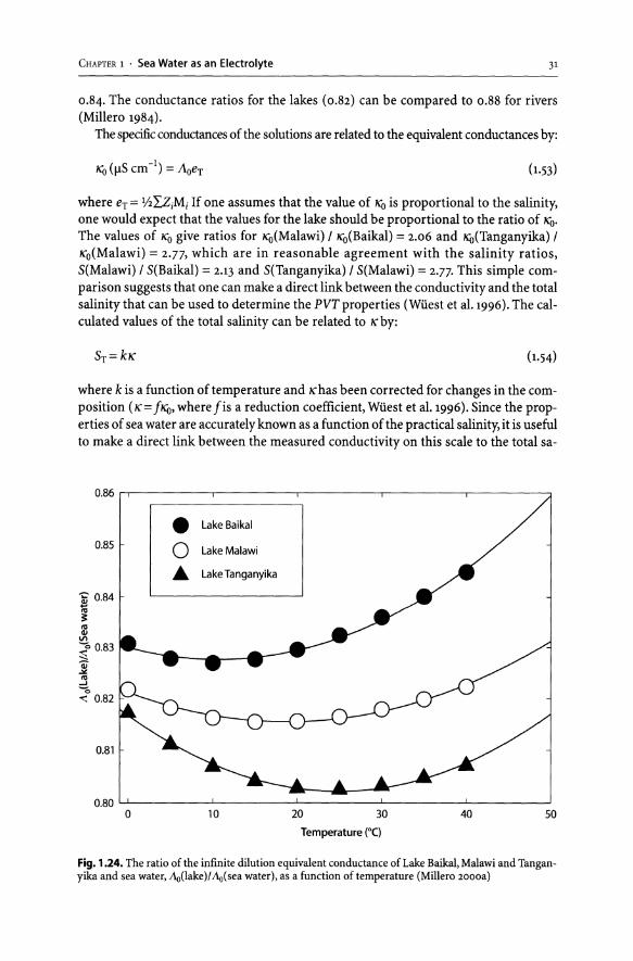
CHAPTER 1 • Sea Water as an Electrolyte 31
0.84. The conductance ratios for the lakes (0.82) can be compared to 0.88 for rivers (Millero 1984).
The specific conductances of the solutions are related to the equivalent conductances by:
I\{) (flS em-I) = Aoer (1.53)
where er = 0LZ;M; If one assumes that the value of I\{) is proportional to the salinity, one would expect that the values for the lake should be proportional to the ratio of I\{). The values of I\{) give ratios for I\{)(Malawi) /1\{)(Baikal) = 2.06 and I\{)(Tanganyika) / Ko(Malawi) = 2.77, which are in reasonable agreement with the salinity ratios, S(Malawi) / S(Baikal) = 2.13 and S(Tanganyika) / S(Malawi) = 2.77- This simple comparison suggests that one can make a direct link between the conductivity and the total salinity that can be used to determine the PVT properties (Wuest et al. 1996). The calculated values of the total salinity can be related to K by:
Sr=kK (1.54)
where k is a function of temperature and K has been corrected for changes in the composition (K= fl\{), where fis a reduction coefficient, Wuest et al. 1996). Since the properties of sea water are accurately known as a function of the practical salinity, it is useful to make a direct link between the measured conductivity on this scale to the total sa-
0.86 IrTI------------,------------,-----------,------------,------------,
0.85
~ 0.84
~ :B
VI
~ 0.83 '-' j j ~
"'" 0.82
0.81
• Lake Baikal
0 Lake Malawi
• Lake Tanganyika
0.80 ,-I -'----------''---------'--------'-------'--------' o 10 20 30 40 50
Temperature (OC)
Fig. 1.24. The ratio of the infinite dilution equivalent conductance of Lake Baikal, Malawi and Tanganyika and sea water, Ao(Iake)/ Ao(sea water), as a function of temperature (Millero 2oooa)

32 F. J. Millero
Table 1.6. The equivalence conductance of sea water and lake waters at 25°C. Calculated using the composition data for the lakes from the literature: Lake Baikal (Callender and Granina 1997; Falkner et al.1991); Lake Tanganyika (Degens et al. 1971; Edmond 1974); Lake Malawi (Wiiest et al.1996)
Ion }.,o{l1 E;}.,o{l1
Sea water Baikal Malawi Tanganyika
Na + 49.92 38.66 6.30 16.90 18.55
Mg 2+
53.04 9.25 10.89 12.62 23.91
Ca2+ 60.96 2.07 39.92 21.34 4.50
K+ 73.56 1.24 1.44 4.55 8.24
st 59.45 0.02 0.00 0.00 0.00
CI 76.41 68.87 0.77 4.14 6.47
SO~- 79.97 7.46 7.48 4.80 1.31
HCO; 44.50 0.13 39.62 39.75 39.64 -
Br 78.14 0.11
CO~- 69.83 0.06 0.30
F 44.50 0.01
B(OH)~ 55.40 0.01
Ao=LE;AuW 127.87 106.43 104.39 102.62
KD=AoeT 80.26 0.131 0.270 0.751
KD(SW)a 0.221 0.444 1.303
KD(5W)/KD(Lake) 1.68 l.64 1.73
a Seawater diluted to same total salinity of the lake (at ST = 35, eT = 0.6277).
linity determined from the composition. If sea water is diluted to the same total salinity (Table 1.6), the conductivity of sea water at 25°C is 1.68 ±O.03 larger than the values for the lakes. Direct measurements of the conductance are needed to determine if these methods are reliable.
Acknowledgements
The author would like to acknowledge the support of the Oceanographic Section of the National Science Foundation and the National Oceanic and Atmospheric Administration for supporting this work.
References
Brewer PG, Bradshaw A (1975) The effect of non-ideal composition of sea water on salinity and density. J Mar Res 33:157-175.
Callender E, Granina L (1997) Geochemical mass balances of major elements in Lake Baikal. Limnol Oceanogr 42:148-155

CHAPTER 1 . Sea Water as an Electrolyte 33
Carpenter JH, Manella ME (1973) Magnesium to chlorinity ratios in seawater. J Geophys Res 78:3621-3626 Connors DN, Weyl PK (1968) The partial equivalent conductance of salt in seawater and the density
conductance relationship. Limnol Oceanogr 13:39-50 Culkin F (1965) The major constituents of sea water. In: Riley P, Skirrow G (eds) Chemical oceanogra
phy, vol 1. Academic Press, New York, pp 121-161 Culkin F, Cox RA (1966) Sodium, potassium, magnesium, calcium and strontium in seawater. Deep-Sea
Res 13:789-804 Degens ET, Von Herzen RP, Wong H-K (1971) Lake Tanganyika: Water chemistry, sediments, geological
structure. Naturwissen 58:229-234 Dittmar W (1884) Report on researches into the composition of ocean water collected by H.M.S. Chal
lenger 1873-76. Sci. Res. Voyage "Challenger", 1873-76. Chern Phys 1:1-211 Edmond J (1974) Lake chemistry. In: Craig H (ed) Lake Tanganyika geochemical and hydrographic study.
University of California, San Diego (SIO Ref. Ser. 75-5, pp 1-64) Effler SW, Schimel K, Millero FJ (1986) Salinity, ionic strength, and chloride relationships in ion pol
luted Onondaga Lake N.Y. Wat Air Soil Pollut 27:169-180 Falkner KK, Measures CI, Herbelin SE, Edmond JM, Weiss RF (1991) The major and minor element
geochemistry of Lake Baikal. Limnol Oceanogr 36:413-423 Fernandez H, Vazquez F, Millero FJ (1982) The density and composition of hypersaline waters of a Mexi
can lagoon. Limnol Oceanogr 27:315-321 Gieskes JM (1982) The practical salinity scale 1978.A reply to comments byT. R. Parsons. Limnol Oceanogr
27:387-389 Hill KD, Dalphinee TM, Woods DJ (1986) The extension of the practical salinity scale 1978 to low salinities.
IEEE J Oceanic Eng OE-11:109 Jellison R, Macintyre S, Millero FJ (1999) Density and conductivity properties of Na-COr CI-S04 brine
from Mono Lake, USA. Int J Salt Lake Res 8:41-53 Knudsen M (1901) Hydrographical tables according to the measurings of Carl Forch, P. Jacobsen, Mar
tin Knudsen and S. P. L. Sorensen, G. E. C. Gad: Copenhagen. Williams Norgate, London Lyman J, Fleming RH (1940) Composition of seawater. J Mar Res 3:134-146 Mcmanus J, Collier RW, Chen CA, Dymond J (1992) Physical properties of Crater Lake, Oregon: A method
for the determination of a conductivity- and temperature-dependent expression for salinity. Limnol Oceanogr 37:41-53
Millero FJ (1973a) Theoretical estimates of the isothermal compressibility of seawater. Deep-Sea Res 20:101-105
Millero FJ (1973b) Seawater - a test of multicomponent electrolyte solution theories. 1. The apparent equivalent volume, expansibility and compressibility of artificial seawater. J Solution Chern 2:1-22
Millero FJ (1974) Seawater as a multicomponent electrolyte solution. In: Goldberg E (ed) The sea. Wiley, New York, pp 3-80
Millero FJ (1975) The physical chemistry of estuaries. In: Church TM (ed) Marine chemistry in the coastal environment. ACS, Washington, D.C. (ACS Symp. Ser.18, pp 25-55)
Millero FJ (1978) The physical chemistry of Baltic Sea waters. Thalassia JugosI14:1-46 Millero FJ (1982) The thermodynamics of seawater. Part 1: The PVT properties. Ocean Sci Eng 7:403-460 Millero FJ (1983) The thermodynamics of seawater. Part II: Thermochemical properties. Ocean Sci Eng
8:1-40 Millero FJ (1984) The conductivity-density-salinity-chlorinity relationship for estuarine waters.
Limnol Oceanogr 29:1317-1321 Millero FJ (1996) Chemical oceanography. CRC Press, Boca Raton, FL Millero FJ (2000a) The equation of state of lake waters. Aquatic Geochem 6:1-17 Millero FJ (2000b) Effect of changes in the composition of seawater on the density-salinity relation-
ship. Deep-Sea Res I 4]:1583-1590 Millero FJ (2001) The physical chemistry of natural waters. Wiley Scientific, N.Y. Millero FJ, Chetirkin PV (1980) The density of Caspian Sea waters. Deep-Sea Res 27:265-271 Millero FJ, Kremling K (1976) The densities of Baltic Sea waters. Deep-Sea Res 23:1129-1138 Millero FJ, Lepple FK (1973) The density and expansibility of artificial seawater solutions from 0 to 40°C
and 0 to 21%0 chlorinity. Mar Chern 1:89-104 Millero FJ, Poisson A (1981) International one atmosphere equation of state of seawater. Deep-Sea Res
28:625-629 Millero FJ, Perron G, Desnoyers JE (1973a) Heat capacity of seawater solutions from 5 to 35°C and 0.5 to
22%0 chlorinity. J Geophys Res 78:4499-4507 Millero FJ, Hansen LD, Hoff EV (1973b) The enthalpy of seawater from 0 to 30°C and 0 to 40%0 salinity.
J Mar Res 31:21-39 Millero FJ, Gonzalez A, Ward GK (1976a) The density of seawater solutions at one atmosphere as a func
tion of temperature and salinity. J Mar Res 34:61-93

34 EJ. Millero
Millero FJ, Gonzalez A, Brewer PG, Bradshaw A (1976b) The density of North Atlantic and North Pacific deep waters. Earth Planet Sci Lett 32:468-472
Millero FJ, Lawson D, Gonzalez A (1976c) The density of artificial river and estuarine waters. J Geophys Res 81:1177-1179
Millero FJ, Ward GK, Chetirkin PV (1977) Relative sound velocities of sea salts at 25°C. J Acoust Soc Am 61:1492-1498
Millero FJ, Forsht D, Means D, Gieskes J, Kenyon K (1978) The density of North Pacific Ocean waters. J Geophys Res 83:2359-2364
Millero FJ, Mucci A, Zullig J, Chetirkin P (1982) The density of Red Sea brines. Mar Chern 11:463-475 Morris AW, Riley JP (1964) The direct gravimetric determination of the salinity of seawater. Deep-Sea
Res 11:899-904 Morris AW, Riley JP (1966) The bromide/chlorinity and sulphate/chlorinity ratio in seawater. Deep-Sea
Res 13:699-705 Parsons TR (1982) The new physical definition of salinity: Biologists beware. Limnol Oceanogr 27=384-385 Pitzer KS (1991) Ion interaction approach: Theory and data collection. In: Pitzer KS (ed) Activity coeffi
cients in electrolyte solutions. CRS, Boca Raton, FL, pp 75-153 Poisson A, Perie M, Perie J, Chemla M (1979) Individual equivalent ionic conductances of the major ions
in seawater. J Solution Chern 8:377-394 Poisson A, Lebel J, Brunet C (1980) Influence of local variations in the ionic ratios on the density of
seawater in the St. Lawrence area. Deep-Sea Res 27:763-781 Poisson A, Lebel J, Brunet C (1981) The densities of western Indian Ocean, Red Sea and eastern Mediter
ranean surface waters. Deep-Sea Res 28:1161-1172 Riley JP, Tongudai M (1967) The major cation/chlorinity ratios in seawater of seawater. Chern Geol
2:263-269 . Robinson RA, Stokes RH (1959) Electrolyte solutions, 2nd edn. Butterworths, London, pp 455 Sharp JH, Culberson CH (1982) The physical definition of salinity: A chemical evaluation. Limnol
Oceanogr 27:385-387 Sorensen JA, Glass GE (1987) Ion and temperature dependence of electrical conductance for natural
waters. Anal Chern 59:1594-1597 Warner TB (1971) Normal fluoride content of seawater. Deep-Sea Res 18:1255-1263 Wilson TRS (1975) Salinity and the major element of sea water. In: Riley JP. Skirrow G (eds) Chemical
oceanography, vol 1, 2nd edn. Academic Press, New York, pp 365-413 Wiiest A, Piepke G, Halfman JD (1996) Combined effects of dissolve solids and temperature on the den
sity stratification of Lake Malawi. In: Johnson TC, Odada EO (eds) The limnology, climatology and paleoclimatology of the East African lakes. Gordon and Breach Scientific Pubs., PP 183-202
Young TF, Smith MB (1954) Thermodynamic properties of mixtures of electrolytes in aqueous solutions. J Phys Chern 58:716-724
Young TF, Wu Y-C, Krawetz AA (1957) Thermal effects of interaction between ions of like charge. Discuss Faraday Soc 24:37,77

Chapter 2
The Chemical and Physical Properties of Marine Aerosols: An Introduction
J. M. Prospero
2.1 Introduction
The atmosphere is an important pathway for the transport of particulate matter from the continents to the oceans. Although the magnitude of these wind-borne fluxes is not accurately known, there is evidence that some could be large enough to have a significant impact on chemical and biological processes in the oceans. In addition, windborne particles (i.e. aerosols) play an important role in climate-related processes which in turn can have a great impact on physical, chemical, and biological processes taking place in the oceans. Aerosols can affect climate directly by scattering and absorbing both solar radiation and that which is re-emitted from the surface of the Earth to the atmosphere. Aerosols playa critical role in water vapour nucleation processes. In this way, they can affect the concentration and size distribution of cloud droplets, which in turn can alter the radiate properties of clouds. The role of aerosols in cloud processes also affects the nature and distribution of rainfall and the subsequent distribution of clouds.
The role of aerosols in climate forcing has only recently received attention. Aerosols were largely ignored in the first Intergovernmental Panel on Climate Change (IPCC) assessment. It was only in the 1995 IPCC report (IPCC 1996) that the importance of aerosols was acknowledged and an effort was made to estimate the forcing due to anthropogenic particles. The report concluded that because of the many unknowns about the chemical, physical, and radiative properties of aerosols and their temporal and spatial variability, only very crude estimates could be made. The IPCC report and other studies have served to stimulate a broad research focus on aerosols and climate-related processes, both in the laboratory and in the field. We have learned much from these programmes, and it is now generally accepted that aerosols play an important role in climate. We are now better able to constrain the estimates of forcing or, at least, to better identify those parameters that must be better defined. Nonetheless, despite these advances, we still do not know enough about many aspects of aerosol properties and their role in climate to make a good assessment - indeed, our knowledge of aerosol processes is much worse than that of most greenhouse gases.
Another major change in the field is that we now have a better appreciation of the types of aerosols that are important. For many years, the aerosol community has focused largely on sulphur (and related) chemistry because of concerns about the impact of sulphur pollution emissions on the atmospheric sulphur cycle. It was not until the mid-90s that other aerosol species began to receive much attention. Today many "natural" species are included in climate assessments: sea salt, mineral dust, and biogenic organics. The inclusion of these species is necessary for two reasons: so that we

36 J. M. Prospero
can assess the relative impacts of anthropogenic and natural species and thereby to be able to partition changes that might occur in both through time; so that we can assess any changes in natural emissions that might occur as a result of human -induced climate change. Knowledge of these natural climate-related species also helps us to understand the factors that played a role in pre-human climate change. Motivated by these concerns, a very substantial part of the community effort is now devoted to a wide range of aerosol species.
The study of the role of aerosols is complicated by the fact that the physical and chemical properties of aerosols are highly variable in both time and space. In contrast, most common "greenhouse" gases (e.g. CO2, CH4, halocarbons) have relatively long lifetimes (months to years) in the atmosphere, and as a consequence, their distribution is relatively uniform over the Earth, and changes occur relatively slowly. Aerosols, on the other hand, have a residence time in the troposphere that ranges from a few days to a few weeks. Consequently, the concentration, composition and physical properties of particles in the atmosphere can vary greatly, depending on the distribution of sources, the meteorological processes in the source regions, the large scale circulation systems that subsequently control long-range transport, and finally, the various removal processes that act on the particles. In order to assess the transport of continental materials to the oceans and the general impact on climate, we must have \l good understanding of all these processes.
This paper is intended to be a brief review of the chemical and physical properties of aerosol species over the oceans. The emphasis is on those aerosol species that play an important role in marine biogeochemical and climate processes:
• Sea salt aerosols: Sea salt aerosols are produced by the bursting of bubbles at the surface of the ocean. In remote ocean regions, sea salt aerosol is often the primary light scattering aerosol component, and it is an important source of cloud-forming nuclei. Consequently, sea salt has a role in climate. Furthermore, over large areas of the ocean, sea salt aerosol offers a large surface area for chemical and physical interactions with other aerosol species and with gases; because of its large size and high settling velocity, sea salt aerosol can serve as a major sink for other atmospheric components.
• Non-sea-Salt (nss) sulphate aerosols: Nss-SO~- is that fraction of marine SO~- aerosol that is not derived from sea water aerosol droplets. Nss-SO~- plays a major role in radiation and cloud processes. As such, it is important to understand the factors affecting its distribution over the oceans. Nss-SO~- is the major acidic aerosol species in the atmosphere; over large areas of the world, the pH of aerosols and precipitation is largely controlled by the concentration of nss-SO~- and ammonium. NssSO~- aerosol over the oceans has two major sources: the oxidation of dimethyl-sulphide (DMS) emitted by marine organisms and pollution transported from the continents.
• Nitrate and ammonium: The global budgets of both these species have been hugely impacted by human activities. Ammonium is the major neutralizing species in the atmosphere. Both species can play an important role as nutrient inputs to coastal waters and oceans.

CHAPTER 2 • The Chemical and Physical Properties of Marine Aerosols: An Introduction 37
• Mineral dust: Mineral dust is a major aerosol species over many ocean regions. It is an important contributor to deep-sea sediments. The iron associated with dust is believed to be a limiting micronutrient over many remote ocean regions; as such, the dust cycle could be a major factor in the global oceanic carbon cycle. Other elements associated with dust could play an important role in the biogeochemistry of the oceans.
This paper can only serve as a brief overview of the field of aerosol chemistry. For those interested in further study, Hobbs (2000) and Jacob (1999) present excellent and concise introductions to the field of atmospheric chemistry. Graedel and Crutzen (1993) offer a broad and easily readable review of the fundamentals of atmospheric chemistry in climate processes, while Hobbs (1993) provides a good introduction to aerosolcloud-climate interactions; Charlson and Heintzenberg (1995) present broad coverage of the subject. Broader and more detailed coverage of atmospheric chemistry and aerosols can be found in the excellent texts by Finlayson-Pitts and Pitts (2000) and by Seinfeld and Pandis (1998).
2.1.1 Physical Characteristics of Aerosols
An aerosol is defined as a dispersion of solid or liquid particles in a gaseous phase -in this case, the atmosphere. The size of the particles can range from macromolecules to over 100 !lm diameter. In practice most of the aerosol mass that is normally of interest over the oceans is found in the size range under 10-20 !lm diameter. Larger particles have high settling velocities in the atmosphere, and consequently they are not carried far from their sources. (For example, a 20 !lm diameter particle with unit density has a settling velocity at sea level of 1.2 cm s -\, about 1 km per day.) While aerosols are usually thought of as a solid or liquid particle, in reality, in many regions most particles are complex mixtures of soluble and insoluble species, and depending on the relative humidity, they could consist of both solid and liquid phases.
Aerosols can be produced directly ("primary" aerosols) or as a product of the reactions of gases in the atmosphere ("secondary" aerosols). The mode of production affects the size distribution of the resulting aerosol. Figure 2.1 shows a schematic of the distribution of particle surface area of an idealized ensemble of aerosol particles formed by a variety of processes. (Seinfeld and Pandis 1998, Fig. 2.15, p. 101). Examples of primary aerosols are sea salt, mineral dust, soot emitted from smokestacks, diesel exhaust, and particles shed by plants (e.g. plant waxes, fibres). Physical processes (grinding of rocks, bursting bubbles) normally produce relatively large particles; as a result, the size distribution of primary particles places most of the mass above 1 !lm diameter as shown in Fig. 2.1; these are normally referred to as "coarse" particles. For example, the mass median diameter (MMD) of sea salt particles over the ocean is generally in the range of about 5-10 !lm diameter or greater (depending on wind conditions); nonetheless, a significant and important fraction of the sea salt mass lies below l!lm (O'Dowd et al.1997). The MMD of mineral dust particles over the source regions can be extremely large: many lO's of micro metres, but over the oceans it is typically only several!lm (Duce 1995).
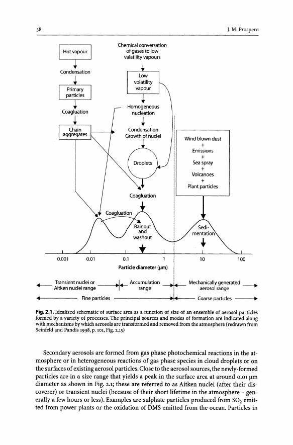
38
Condensation
0.001 0,01
Chemical conversation of gases to low
valatility vapours
Low volatility vapour
Homogeneous nucleation
+ Condensation
Growth of nuclei
.. 0.1 i
Particle diameter (J,lm) I i
Wind blown dust +
Emissions +
Sea spray +
Volcanoes +
Plant particles
10
J. M. Prospero
100
.--- Transient nuclei or __ ~+-- Accumulation ~.-- Mechanically generated ------. Aitken nuclei range ~ range i aerosol range
..... 1.. ... • Fine particles ,11··T ..... Coarse particles •
Fig. 2.1. Idealized schematic of surface area as a function of size of an ensemble of aerosol particles formed by a variety of processes. The principal sources and modes of formation are indicated along with mechanisms by which aerosols are transformed and removed from the atmosphere (redrawn from Seinfeld and Pandis 1998, p. 101, Fig. 2.15)
Secondary aerosols are formed from gas phase photochemical reactions in the atmosphere or in heterogeneous reactions of gas phase species in cloud droplets or on the surfaces of existing aerosol particles. Close to the aerosol sources, the newly-formed particles are in a size range that yields a peak in the surface area at around 0.01 flm diameter as shown in Fig. 2.1; these are referred to as Aitken nuclei (after their discoverer) or transient nuclei (because of their short lifetime in the atmosphere - generallya few hours or less). Examples are sulphate particles produced from S02 emitted from power plants or the oxidation of DMS emitted from the ocean. Particles in

CHAPTER 2 • The Chemical and Physical Properties of Marine Aerosols: An Introduction 39
this very fine particle mode are highly mobile. They rapidly coagulate to form larger particles that typically fall in the size range between 0.1 to 111m diameter (a size class referred to as the "accumulation" mode) or they can diffuse to the surface of cloud or fog droplets or to larger particles (e.g. sea salt, mineral dust).
Because of the various routes by which particles can be formed, the atmospheric aerosol is extremely complex and dynamic. Some classes of aerosols can be formed by both primary and secondary processes. For example, sulphate particles can be emitted directly from smokestacks; but in advanced technologies, the direct emission of particles contributes a relatively minor source because of emission controls. Furthermore, individual aerosol particles rarely exist as a pure type (e.g. a "pure" sea-salt droplet, a specific sulphate compound). Rather, most particles are comprised of a wide range of compounds with properties and atmospheric lifetimes that differ from those of their individual components. As a result, atmospheric particles often display a wide range of chemical and physical properties.
2.1.2 The Role of Clouds in the Aerosol Cycle
Clouds playa very important role in the aerosol cycle. Cloud droplets are an important patlIway for the reaction of gaseous species - for example, the oxidation of gasphase S02 to SO~- takes place largely in cloud droplets through the aqueous phase reaction with H20 2 (see below). But most clouds do not produce rain. Instead they evaporate, and the cloud droplets are converted to aerosol particles with sizes that typically fall in the range 0.1-1.0 11m diameter (i.e. in the "accumulation" mode; see Fig. 2.1).
Nonetheless, the small fraction of clouds that do precipitate play an important role in cleansing the atmosphere. Thus, clouds are important both in the formation of aerosols and in their removal from the atmosphere; the delicate balance between these processes has huge implications from the standpoint of climate. Consequently, cloud processes have the highest priority in climate studies.
The role of clouds in the atmospheric aerosol cycle is paradoxical: clouds are involved in the formation and removal of aerosols from that atmosphere, and yet clouds can not form without the presence of aerosols. At the water vapour supersaturations typically found in the atmosphere (only a few tenths of a percent), water vapour can only condense on hygroscopic aerosol particles (e.g. sulphate and nitrate aerosols, sea salt droplets). Thus, clouds and aerosols are involved in a complex and tightly coupled atmospheric cycle that results in the transformation, transport, and removal of aerosol particles (Wang and Prinn 2000). These processes are depicted schematically in Fig. 2.2: water vapour condensation on the aerosol particle, in-cloud reactions, droplet coalescence, and the formation of the precipitation, which then falls towards the ground. In many cases precipitation will evaporate before it reaches the Earth's surface; the particles so-produced are larger and more chemically complex than those which entered the cloud. Also, as indicated above, the cloud could evaporate before precipitation forms, a process that also yields a transformed aerosol ensemble. Clouds also play an important role in atmospheric nitrogen chemistry in that lighting associated with clouds is a significant source of nitrogen oxides (Wang and Prinn 2000).
Finally, clouds can also vent unreacted gases and particles to the middle and upper troposphere (Wang and Prinn 2000), as discussed below.

40
Drop continues to grow by collecting smallercloud droplets already acidified by nucleation scavenging and aqueous phase chemical reactions
Raindrop collects aerosol and absorbs/desorbs gases as it falls to ground (below cloud precipitationscavenging)
J. M. Pro spero
Cloud evaporates leaving behind a "cloud" of aerosol particles
Droplet grows by condensation. Ambient gases absorb in droplet and activity is increased by aqueous phase chemical reactions.
CCN dissolves in droplet
Cloud droplet nucleates on a CCN (nucleation scavenging)
Raindrops evaporate in dry air below cloud to produce aerosol
particles + * ____ ----~~~------
Fig. 2.2. Schematic diagram showing the role of clouds in aerosol processes. Aerosols (cloud condensation nuclei) adsorb water to form cloud droplets, which are subsequently modified by chemical reactions. If the cloud forms precipitation, the chemical species are deposited to the Earth's surface. Alternatively, the cloud can evaporate to produce a "cloud" of transformed aerosol in the middle and upper troposphere; also, the precipitation falling from raining clouds can evaporate to form aerosol in the lower atmosphere. (modified from Hobbs (2000), p. 112, Fig. 7.1)
The role of clouds is also central to the climate issue and the impact of humans on climate. The chemical and physical processes in clouds yield droplets which upon evaporation produce mostly accumulation-mode (0.1-1.0 !lm diameter) aerosols -particles that have dimensions comparable to that of visible light. Such particles are efficient scatters of light, and consequently they can have a strong effect on the radiative balance of the atmosphere. It is because of the strong scattering of solar radiation by fine particles that we see dense hazes in polluted atmospheres, hazes that can produce colourful light effects, for example brilliantly coloured sunsets. One of the major challenges in assessing the role of aerosols in climate is understanding how the properties of aerosols (their size distribution, chemical composition, index of refraction, etc.) effect the radiative properties of the atmosphere. This problem is made more difficult because of the extremely complex chemical and physical properties of aerosols that are a consequence of the great variety of sources and processes involved in their formation.
Because of the complexity of the aerosol formation processes and the relatively short residence time of particles in the atmosphere (typically 1-2 weeks in the lower troposphere), their properties and their distribution are highly variable in both time and

CHAPTER 2 • The Chemical and Physical Properties of Marine Aerosols: An Introduction 41
space. One of the major objectives in the field of aerosol studies today is to understand the factors affecting the variability of aerosols and to characterize that variability. There is a dearth of information about many aspects of the atmospheric aerosol cycle; this is especially true for the marine atmosphere. The study of marine aerosols presents a particularly great challenge because of the vast areas involved, the wide range of sources that impact on the marine atmosphere, and the many types of physical environments involved.
2.1.3 The Global Distribution of Aerosols Over the Oceans
Satellites provide us with graphic evidence of aerosol distributions over the oceans. An example is AVHRR (Advanced Very High Resolution Radiometer), which measures the radiation backscattered to space by aerosols over the oceans; these data are converted to equivalent aerosol optical thickness (EAOT), which is a measure of the column-integrated aerosol loading (Husar et al. 1997). Figure 2.3 shows the global average distribution of oceanic EAOT for the four seasons. Clear patterns are evident. First of all, the highest values of EAOT (and hence, the greatest column concentrations of aerosols) are found in regions close to the continents. This distribution affirms the fact that in many ocean regions the aerosol character is defined to a large extent by the transport of materials by winds from the continents. A second feature is that there are large seasonal differences in aerosol concentrations as can be seen by comparing the December-January distributions with June-August in Fig. 2.3. These differences are due to a variety of factors, including the seasonal variability of source emissions and meteorology. Third, some continents emit more aerosols than others, which suggests large differences in source and transport conditions. Especially notable is that large "plume" of high EAOT values over the tropical Atlantic. The plume extends from the coast of Africa to South America (in January) and to the Caribbean (in July); this plume is attributed to the transport of African dust. The large region of high EAOT over the Arabian Sea in June-August is due to dust carried from Africa and the Middle East. A large plume is seen off the western coast of southern Africa in June-August and in September-November; this is due to intense biomass burning in this region. Substantial plumes are seen over the North Atlantic during all seasons but winter; these are attributable to the transport of pollutants from North America and Europe. Similarly, large regions with high EAOT values are seen along the coast of Asia during most seasons; these are largely due to pollution transport. The Asian plume is most prominent in the spring when large quantities of soil dust are carried out of Asia along with pollution. The attribution of these plumes to these dominant aerosol types is supported by evidence from field studies in the regions covered by the plumes (Husar et al.1997).
The Total Ozone Mapping Spectrometer (TOMS) also provides information on the distribution of aerosols, especially absorbing species - predominantly mineral dust and smoke (Herman et al. 1997). The TOMS product is especially useful, because (in contrast to AVHRR) the system can detect aerosols over land as well as over water surfaces. Figure 2.4 shows the global frequency of occurrence (days per month) of moderate-to-high absorbing aerosol concentrations during January and July. Similarly to AVHRR, TOMS shows prominent plumes over the tropical North Atlantic (January and July) and the Arabian Sea (July) due to dust and the large plume in the South Atlantic in July due to smoke. In contrast to AVHRR, TOMS does not show large pollu-

42
~ " ~
o o 0 () . o~. o Q ¢J \:.?.,
J. M. Prospero
Q
Fig. 2.3 a,b. Aerosol distributions over the oceans derived from the National Oceanic and Atmospheric Administration (NOAA) advanced very high resolution radiometer (AVHRR) satellite (Husar et al.1997). Distributions are shown in units of equivalent aerosol optical thickness (BAOT) , which is derived from measurements of visible-spectrum solar radiation reflected from aerosols back to space; BAOT values are roughly proportional to the integrated column concentration of aerosol. Distributions are shown for each of the four seasons; a December-February; b March-May (Figure from R. Husar, personal communication, based on Husar et al.1997)
tion plumes emerging from Europe and Asia; this is because pollution plumes contain high concentrations of highly reflective aerosol (such as sulphates) that are detectable by AVHRR but only small amounts of absorbing aerosols (such as soot) that are detectable by TOMS.
Aerosol transport varies greatly from season to season. Consequently, any impacts that aerosol transport might have on ocean processes should also show a large seasonal and spatial variability. Especially notable is the large seasonal migration of the African dust plume. It reaches its northernmost position in July and August and its southernmost position in the low latitudes of the North Atlantic in the winter. The

CHAPTER 2 . The Chemical and Physical Properties of Marine Aerosols: An Introduction 43
:::,10
o .'0
~ ,,-- "'"""' ....... '~~r
Q
Fig. 2.3 (,d. Aerosol distributions over the oceans derived from the National Oceanic and Atmospheric Administration (NOAA) advanced very high resolution radiometer (AVHRR) satellite (Husar et al.1997). Distributions are shown in units of equivalent aerosol optical thickness (EAOn, which is derived from measurements of visible-spectrum solar radiation reflected from aerosols back to space; EAOT values are roughly proportional to the integrated column concentration of aerosol. Distributions are shown for each of the four seasons; (June-August; (September-November (Figure from R. Husar, personal communication, based on Husar et al.1997)
seasonal oscillation of the plume is consistent with the very large seasonal cycle of dust concentrations, as measured in South Florida, and Barbados, West Indies (Husar et al. 1997; Chiapello et al. 1999; Prospero 1999); indeed, during the summer months African dust has been measured over the eastern United States as far north as the New England states (Perry et al. 1997).
The TOMS aerosol distributions shown in Fig. 2.4 can be used to identify dust sources. In many cases, the distributions over land show a clearly defined geometry that can be matched to topographical features and geology. Note for example the isolated source "hot-spots" in North Africa and Australia in January and Central Asia in

44 J. M. Prospero
January 900N
6QoN
300N
0
30° 5 ./
60° 5
90° 5
180 120' W 600 W o 600 E 120" E 180
July
900 N
600 N
300 N
0
30" 5 ./
6O"S
90°5 180 1200W 600 W o 600 E 120" E 180
Number of days (AAI > 0.7)
o 7 14 21 28 31
Fig. 2.4. The distribution of absorbing aerosols derived from the Total Ozone Mapping Spectrometer (TOMS) satellite. The absorbing aerosol index (AAI) provides a measure of the concentration of dust and black carbon in the atmosphere. The figure shows the number of days in January (top) and July (bottom) when the TOMS AAI exceeded 0.7, a value associated with moderately high dust and smoke concentrations (redrawn from Prospero et al. 2002)
July. In a later section, the environmental characteristics of the dust source regions will be discussed. TOMS also is sensitive to biomass burning aerosols because of the presence of highly-absorbing soot. In Fig. 2.4, the large plume emerging from southern Africa in July is almost entirely due to biomass burning; in January the plume that emerges from equatorial Africa and extends across the Atlantic along the equator almost to Brazil is largely attributable to biomass burning, while the more northerly portion of the plume is mostly due to dust.

CHAPTER 2 . The Chemical and Physical Properties of Marine Aerosols: An Introduction 45
Figures 2.3 and 2.4 clearly show that the major sources of aerosols, both pollution and mineral dust, lie in the Northern Hemisphere. The contrast between the Northern and Southern Hemispheres is important both from the standpoint of climate issues and also the impact of aerosol transport on ocean biogeochemical processes.
2.1.4 Aerosol Composition
The large fraction of the aerosol mass over the ocean is comprised of a relatively small number of species as shown in Table 2.1, which presents a selection of aerosol concentrations at various mostly remote ocean sites. The annual means are compiled from long-term (multi-year) measurements made at ocean network stations operated by the aerosol group at the University of Miami (Prospero et al. 1989; Savoie et al. 1989a; Arimoto et al. 1995, 1996; Savoie et al. 1993, 1994). The sea salt aerosol concentration is calculated from the measured concentration of Na + in aerosol based on the ratio of the total concentration of salts in sea water to that ofNa + (i.e. sea salt aerosol = 3.256 x Na, by weight). The nss-SO~- fraction is calculated by measuring the Na + concentration in the aerosol; on the assumption that the SO~-INa + ratio in the sea-spray droplets is the same as that in bulk sea water, the Na + value is converted to a sea-salt SO~- by multiplying by 0.2517. This quantity is subsequently subtracted from total SO~- yield of the nss-SO~- concentration.
There are many other important marine-aerosol species that are not included in Table 2.1. In particular, organic materials can constitute a substantial fraction of the total aerosol mass (Jacobson et al. 2000). Most notable is soot ("black carbon" or "BC"), produced by fuel combustion and biomass burning. BC is found almost everywhere, even over the most remote oceans (Heintzenberg et al. 2000). In addition, as discussed below, over many ocean regions a large fraction of the aerosol mass remains uncharacterized (Quinn et al. 2000).
As one might expect, sea salt aerosol is a major constituent at most sites. (At some sites the high concentrations are attributable in part to local surf conditions, which are not representative of concentrations on larger scales.) Mineral dust shows an extremely wide range of concentrations. Note the very high concentrations in the tropical North Atlantic sites (Izana, Barbados) and the sites in the western North Pacific (Cheju, Okinawa, Hong Kong). These reflect the impact of dust transport from North Africa and China, respectively. Substantial dust concentrations are also noted in higher latitude stations in the North Atlantic (Bermuda). Annual mean dust concentrations over the central North Pacific (Shemya, Midway, Oahu) are low, but as will be shown below, iliey are significant. Dust concentrations in ilie souiliern oceans tend to be extremely low (for example, see American Samoa) due to the dearth of strong dust sources on ilie souiliern continents and the very great transport distances to ilie central ocean regions.
The impact of pollutant sources is evident at many sites in the Northern Hemisphere. Extremely high nss-SO~- and NO; concentrations are seen at the sites near the coast of Asia in the western Pacific; these are attributable to the high levels of atmospheric pollution found over much of Asia due to the limited use of emission controls. Moderately high pollutant levels are seen over the North Atlantic as well (Bermuda, Mace Head) as a result of emissions from North America and Europe. In contrast, the concentrations of NO;- and nss-SO~- at American Samoa and the Antarctic stations,

46 J. M. Pro spero
Table 2.1. Annual mean aerosol concentrations measured at remote ocean stations (Prospero et al.1989; Savoie et al. 1989a; Arimoto et al. 1995, 1996; Savoie et al. 1993, 1994)
Station Station Na Sea N03 nssS04 MSA NH4 AI Dust' V Sb Totald
Location a
salt b
Lat. Long. Mean Mean Mean Mean Mean Mean Mean Mean Mean Mean
'N 'E -3 -3 -3 -3 -3 -3 IIg m-3 Calc -3 -3 -3
IIgm IIg m IIgm IIg m IIgm IIg m ngm ngm IIgm
North Pacific
Western Pacific
Cheju, Korea 33.5 126.5 3.07 19.76 4.12 7.23 34.75 2.95 1.24 15.47 4.09 2.35 49.5
Okinawa 26.9 128.3 7.10 23.11 1.80 4.16 19.80 1.07 0.79 9.84 2.08 1.63 40.0
Taiwan 21.9 120.9 5.57 18.14 1.93 4.05 11.34 1.31 0.30 3.77 1.85 0.80 29.2
Hong Kong 22.6 114.3 3.01 9.79 3.03 7.41 23.11 2.79 1.05 13.13 6.20 2.05 36.2
Central Pacific
Shemya 52.9 174.1 20.72 67.47 0.20 0.33 58.56 0.13 0.11 1.33 0.50 69.5
Midway 28.2 -177.4 4.23 13.77 0.27 0.53 20.32 0.07 0.06 0.72 0.19 0.07 15.4
Oahu 21.3 -157.7 4.65 15.14 0.35 0.51 18.93 0.03 0.05 0.66 0.26 0.03 16.7
North Atlantic
Heimaey, Iceland 63.4 -20.3 8.79 28.62 0.23 0.65 38.37 0.38 29.9
Mace Head 53.3 -9.9 4.34 14.13 1.49 2.03 50.51 0.91 0.04 0.47 0.93 0.14 19.0
Izana, Tenerife 28.3 -16.5 0.38 1.25 0.77 0.92 4.58 0.33 1.78 22.28 2.86 0.08 25.5
Bermuda 32.3 -64.9 4.19 13.65 1.06 2.19 35.12 0.31 0.45 5.59 1.28 0.09 22.8
Barbados 13.2 -59.4 5.08 16.53 0.53 0.78 19.70 0.11 1.16 14.55 1.85 0.03 32.5
South Pacific
American Samoa - 14.3 -170.6 5.14 16.74 0.11 0.37 22.90 0.00 0.02 0.07 0.00 17.2
Antarctica
Mawson -67.6 62.5 0.10 0.33 0.03 0.09 22.90 0.00 0.5
Palmer Station -64.8 -64.1 1.20 3.91 0.02 0.10 48.80 0.02 4.0
a Station location: negative latitudes = Southern Hemisphere; negative longitudes = Western Hemisphere. b Sea salt calculated by multiplying Na concentration by 3.256, the sea saltlNa mass ratio in sea water. , Dust is calculated from the AI concentration assuming that AI is 8% of total as in average crustal material
(Taylor and McLennan 1985). d Total aerosol is the sum of sea salt, soil dust, nss-SO<\, NO] and NH4.
Mawson and Palmer, are extremely low; these levels are representative of conditions that one might expect under "natural" conditions over the oceans when there are no pollution impacts.
The presence of pollution aerosol is also reflected in the concentration of certain trace species. Table 2.1 shows the concentration of V and Sb as examples. Vanadium is emitted in a number of processes, and it is abundant in petroleum obtained from some sources. Antimony is present in the emissions from many types of industrial processes, especially smelters. The concentrations of V and Sb are very high in aerosols over the western North Pacific sites; in contrast, the concentrations at American Samoa are

CHAPTER 2 • The Chemical and Physical Properties of Marine Aerosols: An Introduction 47
extremely low, in most samples near the detection limit (Savoie et al. 1994). The great differences between the hemispheres is also reflected in the latitudinal distribution of NO; and nss-SO~- in marine aerosols based on data compiled from measurements made on islands and aboard ships (Heintzenberg et al. 2000).
The aerosol data in Table 2.1 are consistent with the picture that we obtain from satellites (Fig. 2.3 and Fig. 2.4). They show that the highest levels of aerosol are found in the Northern Hemisphere, that the continents are the dominant sources of the aerosol that is most visible in satellite products, that dust is one of the most dominant aerosol species, and that pollution aerosols are a major factor in many regions. In contrast, aerosol concentrations in the Southern Hemisphere are often extremely low.
2.1.5 Temporal Variability of Marine Aerosols
The satellite data in Figs. 2.3 and 2.4 show that aerosol concentrations are highly variable on a seasonal basis. They are also variable on shorter time scales. Figure 2.5 shows daily aerosol concentrations of nss-SO~-, NO; and MSA measured over a four year
_ 25 j
'i' E 20 CI :J. - 15 ~ -a 10 ;; ~ 5 l!!
01 ",11, '.~~WthillCII"" •. '9I(';' .... II'l'..II ..... '''''''' .. ,"" , .... ~ 2-Jan-91 3-Jul-91 2-Jan-92 2-Jul-92 1-Jan-93 3-Jul-93 ' -Jan-94 3-Jul-94 2-Jan-95
1.0 -r-----------,,--------------------, 0.9
;;;- 0.8 E 0.7 CI 0.6 3 0.5 « 0.4 ~ 0.3
0.2 0.1 0.0 I , " ,,~. " ....... - tt:::'lr. ,"II"':' ~ ~ , ..
2-Jan-91 3-Jul-91 2-Jan-92 2-Jul-92 l-Jan-93 3-Jul-93 l -Jan-94 3-Jul-94 2-Jan-95
6 Tj--------------------------------------------------------, ;;;- 5 E 4 CI
3 3 1\1
~ 2 .t:: Z 1
o 1 ,t.\o''''4~t "' ...... '1M ~d~ "I,~J 2-Jan-91 3-Jul-91 2-Jan-92 2-Jul-92 l -Jan-93 3-Jul-93 1-Jan-94 3-Jul-94 2-Jan-95
Fig. 2.5 a. Aerosol concentrations of nss-sulphate, MSA, and nitrate at the coastal site of Heimaey (Iceland), North Atlantic. Each point is data from a single daily sample collected when wind is blowing directly from the ocean to the sampling site (D. L. Savoie and J. M. Prospero, unpublished data)

48 J. M. Prospero
~ 18~1-------------------------------------------'----' E 16 ~ 14 a- 12 ~ 10 ~ 8 E- 6 ~ 4
~ 6 m~v~t;.!Il~rw:, ~.'~I~.;~ml'~.J,1 ~,!""'i.tn ":"'~·~·~1 2-Jan-91 3-Jul-91 2-Jan-92 2-Jul-92 Han-93 3-Jul-93 1-Jan-94 3-Jul-94 2-Jan-95
0.25 ~
;;;- 0.20 E ~ 0.15 2-< 0.10 VI
~~ . .
tJAl!1'.!, 'l7:t't~IIIT r''1''-J.Il~'IJ.·: 'r~ l-h.-f /fj,,,~ 0.00 , '" ,A '
~ 01 a-
.~ z
2-Jan-91 3-Jul-91 2-Jan-92 2-Jul-92 1-Jan-93 3-Jul-93 l-Jan-94 3-Jul-94 2-Jan-95
8, 7 6 5 4 3 2 1 or,'" ,",.,-,",,,.;' ·, ....... ft-,-h"·7·.r,·· ·1· ~""- · . -'r'.,. - lj~··--,r-""-V'1
2-Jan-91 3-Jul-91 2-Jan-92 2-Jul-92 , -Jan-93 3-Jul-93 1-Jan-94 3-Jul-94 2-Jan-95
Fig. 2.5 b. Aerosol concentrations of nss-sulphate, MSA, and nitrate at the coastal site of Bermuda, North Atlantic. Each point is data from a single daily sample collected when wind is blowing directly from the ocean to the sampling site (D. 1. Savoie and J. M. Prospero, unpublished data)
period (1991-1994) at three sites in the North Atlantic: Heimaey, an island that lies off the southern coast of Iceland; Bermuda; Barbados, and the West Indies. These figures clearly show the variability of concentrations on time scales ranging from annual to seasonal and day-to-day. Note that at Heimaey, the concentrations of nss-SO;- and NO; tend to be quite low most of the time, consistent with the relatively low annual mean concentrations shown in Table 2.1. However, there are occasional periods when concentrations increase sharply. These sharp "spikes", often lasting only a day or two, are associated with the transport of polluted air masses, usually from Europe (Prospero et al. 1995). Note that the large peaks in NO; concentrations match in time those in nss-SO~-. Compare the Heimaey time series of NO; and nss-SO~- with that at Bermuda and Barbados, both in terms of the peak concentrations, mean levels, and yearly variability. We might expect that the concentrations of other pollutants would also increase proportionately at such times. These data demonstrate the importance of meteorological factors in controlling the transport of pollutants (and natural materials) from the continents to the oceans.
The MSA aerosol concentration data from these three sites also show great differences. A large part of the variability is due to the seasonal character of DMS emissions from the ocean.

CHAPTER 2 . The Chemical and Physical Properties of Marine Aerosols: An Introduction 49
7- 6 E C\
5 3- 4 J!! 3 "' ~ Q. 2 "5 II> .:, '" I: 0
2-Jan-91 3-Jul-91 2-Jan-92 2-Jul-92 l -Jan-93 3-Jul-93 l-Jan-94 3-Jul-94 2-Jan-95
0.08 0.07
~ 0.06 C\ 0.05 3- 0.04 « 0.03 ::E 0.02
0.01 0.00
2-Jan-91 3-Jul-91 2-Jan-92 2-Jul-92 l -Jan-93 3-Jul-93 l-Jan-94 3-Jul-94 2-Jan-95
6 .. 5 E 4 C\ 3- 3 J!! l!! 2 .t:
1 Z
0 2-Jan-91 3-Jul-91 2-Jan-92 2-Jul-92 l -Jan-93 3-Jul-93 l -Jan-94 3-Jul-94 2-Jan-95
Fig. 2.S c. Aerosol concentrations of nss-sulphate, MSA, and nitrate at the coastal site of Barbados, North Atlantic. Each point is data from a single daily sample collected when wind is blowing directly from the ocean to the sampling site (D. L. Savoie and J. M. Prospero, unpublished data)
In the following sections, we will examine the factors affecting the concentration distribution of these and other aerosol species in the marine atmosphere.
2.2 Sea Salt Aerosols
2.2.1 Sea Salt Production and Size Distribution
Sea salt aerosols can be generated by a wide range of physical processes. The most effective mechanism is by the bursting of air bubbles entrained in the ocean surface during whitecap formation. The production of sea salt aerosol and its size distribution is very sensitive to wind speed and the sea state, among other factors. This makes it very difficult to estimate production rates of sea salt. There are a number of models that estimate the temporal and spatial distribution of sea salt over the global oceans (Gong et al. 1997; Erickson and Duce 1988; Tegen et al. 1997). These yield estimates are in the range of 1 000-3 000 Tg yr- l ; the large range indicates the difficulty of the modelling task.

50 J. M. Prospero
Bubble rupture produces aerosol droplets in a size range that extends from under about 0.01 11m diameter to more than 10 11m diameter (Fitzgerald 1991; O'Dowd et al. 1997). The concentration and size distribution of sea salt aerosols is dependent on a number of factors, especially the wind speed and the altitude above the sea surface (Fitzgerald 1991). Table 2.1 shows that on a mass basis, sea salt aerosol is dominant at all sites except Izana, which is located on a mountain (altitude 2360 m). As shown in Fig. 2.1, the size distribution of sea salt is such that the total surface area and volume distribution peaks in the supramicrometre size range (O'Dowd et al. 1997). Thus, sea salt aerosol offers a large surface area for chemical and physical reactions with other aerosol species and with gases (O'Dowd et al.1997). Such large particles have relatively high settling velocities. For example, a 10 11m diameter sea salt aerosol particle has a settling velocity of 0.307 cm S-1 (0.265 km d-1). Consequently, most of the sea salt mass has a relatively short residence time in the atmosphere, and much of the very large annual production rate (I 000-3 000 Tg yr-1) is rapidly returned to the ocean. As we shall see in a later section, sea salt aerosol can serve as a very effective mechanism for removing many atmospheric species, both gaseous and aerosol, from the marine boundary layer (MBL).
2.2.2 The Contribution of Sea Salt to Submicrometre Aerosol
Although most of the sea salt aerosol mass is in the size fraction above 1 11m diameter, a small but significant fraction of the sea salt aerosol is in the submicrometre fraction (O'Dowd et al. 1999). Quinn et al. (2000) report on measurements of submicrometre aerosol made in the Pacific Ocean. They collected the aerosol fraction below 111m diameter and analyzed it for a wide range of soluble components including nss-SO~- and sea salt.
Quinn et al. (2000) also weighed each of the filters so as to obtain a total aerosol mass below 111m. The total concentration of measured ions is always less than the total weighed mass; the difference is referred to as the "residual mass" which includes unanalyzed components such as mineral dust, organic material, soot, etc. Figure 2.6 shows the concentration of these three components (nss-SO~-, sea salt, and residual mass) for various latitude bands in the Pacific Ocean. A number of features stand out in the figure. First of all, in most latitude bands the concentration of submicrometre sea salt is comparable to that of nss-SO~-. The exceptions are in the mid-latitude North Pacific (20-400 N), where submicrometre sea salt is much lower and the high latitude (40-600 S) South Pacific, where it is much higher. The relative sea salt concentrations reflect the large differences in wind speeds in these latitude bands. In the case of nssSO~-, continental sources impact on the North Pacific, whereas over most of the South Pacific the only significant source of nss-SO~- is the oxidation of DMS (see below). The other notable feature of this figure is that the residual mass is very large in most latitude bands, usually comparable to (and in some cases greater than) those of nss-SO~- and sea salt. One might expect such a result for the North Pacific because of the impact of the transport of soil dust, soot, and organics from the continents, especially Asia as evident in Table 2.1. But the residual mass is also quite large in the South Pacific where there is relatively little land mass and the transport distances are very great.

CHAPTER 2 . The Chemical and Physical Properties of Marine Aerosols: An Introduction 51
0.70 '0 nss-S04
0.60 ... E C"I 0.50 ,a. "0 ~ 0.40 :v '" 0::
!? .!:! E .D :> VI
0.30
0.20
0.10
0.00
• Sea salt • Residual mass
4().-60· N 20-400 N 0-20· N 0-20· 5 20-40° 5
Lattitude (Pacific Ocean)
4().-6O°S 60-70· 5
Fig. 2.6. Latitudinal distribution of submicrometre aerosol concentrations over the Pacific Ocean (redrawn from Table 3 in Quinn et al. 2000)
2.2.3 Sea Salt Aerosol and New Particle Production
In remote ocean regions, the optical properties of the MBL are largely controlled by the concentration of sea salt aerosol and by nss-SO~- particles produced from the oxidation ofDMS emitted from the ocean (see the following section). For example, Quinn et al. (1998) show that in some areas, sea salt aerosol is the dominant light scattering aerosol. Sea salt is also important as a source of cloud condensation nuclei (O'Dowd and Smith 1993). Because of the importance of sea salt in climate, there is great interest in developing models that can accurately reproduce sea salt aerosol distributions on a global scale. But the development of such models is hampered by the dearth of accurate and precise sea salt size and concentration data on the oceans.
Although it is clear that nss-SO~- and sea salt aerosols are important, it is significant that a very large fraction of the radiatively important submicrometre aerosol over the oceans is largely uncharacterized as shown in Fig. 2.6. One of the major objectives in marine aerosol studies today is to focus on this important aerosol component.
2.3 The Oceanic Atmospheric Sulphur Cycle
There is great interest in the role of SO~- in aerosols because of its role in climate-related processes. As stated earlier, most of the SO~- aerosol mass produced from the oxidation of gaseous precursors (e.g. S02' DMS) is in the size range 0.1-1.0 Ilm diameter; particles in this size range are very efficient in the scattering and absorption of solar radiation. Also, because sulphate particles are hygroscopic, they can play an important role in cloud nucleation processes. Consequently, sulphates - both natural and anthropogenic - could have a large impact on climate.

52 J. M. Pro spero
Measurements of soi- over the oceans are complicated by that fact that sea water spray contains sulphate. Indeed, in aerosols over many remote regions of the ocean, the mass ratio of total SO~- to Na + is quite close to that of bulk sea water, 0.2517. However, as stated before, most of the sea salt aerosol surface area and mass is in the size range between 1-10 /lm diameter (Fig. 2.1), while nss-SO~- aerosol over the ocean is predominantly in the submicrometre size fraction (see for example, Li-Jones and Prospero 1998; Li et al. 1996).
2.3.1 Global Sulphur Budgets
The concentration of nss-SO~- in the marine environment is principally derived from two gaseous precursors: DMS produced by marine organisms and S02 from continental pollution sources and volcanoes. The global budget of sulphur from these sources is shown in Table 2.2 (Graf et al. 1997, Table 6; see also Benkovitz et al. 1996). The total global emissions of sulphur are 100 Tg S yr-'. Of this total, two-thirds is produced from anthropogenic sources. Thus, anthropogenic sulphur has dramatically impacted the global atmospheric sulphur cycle. It is for this reason that so much attention is focused on the possible implications of pollution emissions on climate processes. Prior to the human era, the atmospheric sulphur cycle was dominated by DMS from the oceans. Volcanic inputs are also important, but they are sporadic. Also, in most cases, the impact of volcanic eruptions is limited to regional scales; this is especially true for volcanoes wJlOse emissions are largely confined to the troposphere, where aerosol lifetimes are relatively short. In contrast, highly explosive volcanoes that inject material into the stratosphere can have long-range effects that can persist for years. In some cases, the effects can be global; for example, the eruption of Pinatubo in 1991 emitted 20 Tg S02, sharply increased the concentration of sulphate aerosol in the stratosphere and caused temperatures in the Northern Hemisphere to drop 0.2°C (Hansen et al. 1992). The effects of Pinatubo aerosols could be detected for several years after the eruption. In contrast, oceanic DMS sources are widely distributed, and emissions are relatively steady from year to year (Kettle et al. 1999). Note in Table 2.2 that biomass burning is a minor source of sulphur emissions but it is a major source of nitrogen species emissions (see below). In the following sections, we briefly consider some of the more important aspects of the chemistry of S02 and DMS in the marine atmosphere.
2.3.2 502 and nss-SO:-
Anthropogenic sulphur is emitted primarily in the form of S02' The principal sources are fossil fuel combustion (especially coal) and the smelting of ores. In the atmosphere, S02 is oxidized in the gas phase by the OH radical to produce H2S04, This reaction is rather slow; it yields an S02 atmospheric lifetime of 1-2 weeks. If the reaction with OH were the major controlling reaction for S02 in the atmosphere, then S02 would be transported over greater distances than is typically observed; indeed, under most conditions the concentration of pollutant-derived S02 over the oceans is generally quite

CHAPTER 2 • The Chemical and Physical Properties of Marine Aerosols: An Introduction 53
Table 2.2. Global annual mean sulphur budget (Graf et al. 1997) Source
Anthropogenic
Biomass burning
DMS
Volcanoes
Total
Sulfur emissions (T9 yr-')
65.6
2.5
18.2
13.7
100.0
low except close to continental sources. Under most conditions, the controlling reaction for S02 is that with H20 2 in cloud droplets; this reaction is very fast and results in the quantitative conversion of S02 to SO~- as long as sufficient H20 2 is present (and in most environments, it usually is).
The atmospheric chemistry of S02 dramatically demonstrates the critical role that clouds can play in atmospheric chemistry in general and the impact that these cloud processes have on climate.
• In the absence of clouds, S02 has a lifetime of 1-2 weeks; within clouds, minutes. • Other types of gases and particles are also incorporated into cloud droplets result
ing in a complex composition. • If the cloud evaporates (on a global average, the vast majority do), each droplet forms
a complex particle containing SO~-. • If the cloud precipitates, the SO~- is removed (along with other species) as precipi
tation; in regions affected by pollution, the precipitation is often very acidic because of the high concentrations of SO~-.
• Many types of clouds (convective clouds, fronts) pump air (and aerosol) into the middle and upper troposphere where particles have relatively long lifetimes (weeks to months) and where winds can carry them over great distances.
Sulphate in aerosol particles is initially present as sulphuric acid, which rapidly picks up ammonia to form ammonium sulphate and various intermediate compounds, depending on the amount of gaseous ammonia available. The molar ratio of NHrISO~varies widely, but the global average tends to be about one (Adams et al. 1999) - that is, equivalent to a "pure" particle with a composition {NH4)HS04• In reality, such pure particles are not normally found in the ambient atmosphere.
As a result of these processes, anthropogenic S02 does not directly playa prominent role in sulphur aerosol chemistry over the ocean. Most pollution S02 is deposited close to the sources on the continents. By the time polluted air masses reach the ocean, S02 has largely reacted to form sulphate. The primary processes that affect the distribution of anthropogenic SO~- particles over the oceans are the transport meteorology (visible as plumes in satellite imagery such as shown in Fig. 2.3) and the removal processes to the ocean (primarily in rainfall). Thus, the production of new sulphate particles over the ocean must come largely from the oxidation of oceanic DMS.

54 J. M. Pro spero
2.3.3 OMS and the Atmospheric Sulphur Cycle
Charlson et al. (1987), in their classic paper, suggested that in the pre-human era, the radiative properties of the marine atmosphere were strongly modulated by nss-SO~that was derived from the oxidation of DMS emitted by various marine organisms. Even today, in remote ocean regions, the production of new ultrafine sulphate particles is linked to DMS production. The precursor of DMS is DMSP (dimethylsulphonium propionate), an osmolyte produced by many phytoplankton species, especially dinoflagellates, prymnesiophytes (including coccolithophores), and chrysophytes. Two species in particular, Phaeocystis pouchetii and Emiliania huxleyi, are known to be very strong producers of DMSP. DMSP is released by these organisms during senescence or when grazed; in water DMSP is enzymatically cleaved to produce a variety of compounds including DMS. The concentration of DMS in the ocean follows in a general way the seasonal cycle of oceanic primary productivity. Accordingly in the mid and high latitudes of the Northern Hemisphere, DMS concentrations increase in March or April and peak in Mayor June then decrease rapidly; in the Southern Hemisphere, the cycle is shifted by six months (Kettle et al.1999). In contrast, in the tropics there is little evidence of a seasonal cycle. The concentration of MSA in the atmosphere mimics the seasonal cycle of DMS in the ocean. In Fig. 2.5, at Heimaey, Iceland, MSA shows a strong peak in June-July and very low concentrations during the remainder of the year. At Bermuda, the maximum MSA concentrations also occur during summer, but the peak is broader; winter concentrations are very low. At Barbados, the seasonal MSA cycle is even less evident; it is much broader and there is no well-defined winter minimum.
The cycle of DMS production and emission to the atmosphere is quite complex, and there is much that is not understood about the processes that affect DMS distributions in and over the oceans. Global surface-water DMS concentration data (over 10 000 measurements) were recently compiled and interpolated into a 1 x 1 monthly data set (Kettle et al. 1999), and the results compared to published fields of geophysical and biological parameters. Kettle et al. could not find any correlation between DMS and these parameters, and they could find no simple algorithm to create monthly fields of sea surface DMS concentrations based on these parameters. There clearly is much research to be done before we can understand the linkage between biological processes and the emission rate of DMS to the atmosphere.
The atmospheric chemistry of DMS is complex, and there are many unresolved issues (Berresheim et al. 1995; Ravishankara et al. 1997). Nonetheless, studies show that OH is the dominant oxidizing agent for DMS in unpolluted marine atmospheres where DMS has a lifetime of about 1 day. Reaction with OH can proceed by two dominant routes. Hydrogen can be abstracted by OH from the methyl group to form the radical group CH3SCHz, or OH can be added to the sulphur atom. The principal products are methanesulphonic acid (CH3S03H, MSA) and SO~-. Sulphate production is the higher energy route, and as a result, the relative yields of MSA and SO~- would be expected to be temperature dependent, yielding higher ratios of nss-SO;-/MSA in warmer climates.

CHAPTER 2 . The Chemical and Physical Properties of Marine Aerosols: An Introduction 55
2.3.4 MSA and nss-SO~-
In remote ocean regions, the concentrations of nss-SO~- and MSA are often correlated and yield a characteristic ratio that suggests a link between DMS emissions and nssSO~- production. Figure 2.7 shows scatter plots of nss-SO~- against MSA from three ocean stations: America Samoa (Savoie et al.1994), Mawson Station,Antarctica (Savoie et al. 1993) and Bermuda (Savoie and Prospero, unpublished data). At American Samoa and Mawson, remote sites where anthropogenic impacts are very small, the scatter plots yield relatively well-defined regression lines which suggest that the production of nss-SO~- is linked to DMS emissions. In the low and mid-latitudes, the mass ratio of nss-SO~-/MSA tends to be about 12-15; this is the case for the data from American Samoa (Fig. 2.7). In contrast, in the high latitudes it is about 3 as observed at Palmer Station (Fig. 2.7). The fact that the slopes of the regressions are markedly different reflects the different gas-to-particle conversion processes that apply in these two very different environments (i.e. tropical vs. the high latitudes). The fact that the ratio of nss-SO~-/MSA is relatively low in the high latitudes compared to that in the low and mid-latitudes is often cited as verification of the temperature dependence of the reaction of DMS with OR, although there is a continuing debate about the role of temperature in causing the observed differences (Berresheim et al. 1995).
At ocean sites impacted by transport from pollution sources, there is no clear relationship between MSA and nss-SO~-, because pollution-source SO~- overwhelms the contribution form oceanic sources. The lack of correlation between MSA and nss-SO~at North Atlantic sites is clearly evident in Fig. 2.5; the nss-SO~- time series at Reimaey appears very different from that of MSA and shows the dominance of pollution transport, which is evident as frequent "spikes" in the time series. The same situation is obtained at Bermuda (Fig. 2.5). Only at Barbados one can see at times a linkage between MSA and nss-SO~- in the time series (Fig. 2.5). Nonetheless, it is possible to discern the impact of oceanic DMS-SO~- at polluted sites such as Bermuda. Scatter plots usually show a well-defined lower boundary as seen in Fig. 2.7 for Bermuda. A line drawn along this boundary yields a nss-SO~-/MSA slope of about 15, similar to that shown for American Samoa in Fig. 2.7. Thus, when pollution levels are low, the ocean DMS source is still significant and detectable at Bermuda. Data from other sites in the North Atlantic (and from other oceanic regions impacted by pollution sources) yield scatter plots of nss-SO~-/MSA are similar to that shown for Bermuda in Fig. 2.7.
2.3.5 New-Particle Production from OMS over the Oceans
While it is now generally accepted that DMS plays a central role in the atmospheric sulphur cycle of the oceans, there are many uncertainties in the process and the ultimate impact on climate. The first problem has to do with the process of the biological processes in the water column that lead to the production of DMS and the physical processes that control the subsequent transfer from the ocean to the atmosphere. As

56
Fig. 2.7. Scatter plot of the daily concentrations of nss-S~against MSA from aerosol samples obtained at coastal stations in American Samoa, Palmer Station (Antarctica), and Bermuda (D. L. Savoie and J. M. Prospero, unpublished data; see also Savoie et al. 1993, 1994)
1.4
1.2
f'1.0 E g,
a 0.8 s III
i o.6 ::J III J. ~ 0.4
0.2
0.0 0.00
0.5
J. M. Prospero
• • • • •
•
~ . . ~
.. "'#.:~ •• : ••• ., . ~. -..
~ .. .. -.... • • • ~ American Samoa
• 0.02 0.04 0.06 0.08

CHAPTER 2 . The Chemical and Physical Properties of Marine Aerosols: An Introduction 57
stated above, Kettle et al. (1999) could not find any systematic relationships that could explain the observed distributions.
A second major uncertainty has to do with the chemical reactions of DMS in the atmosphere and the subsequent conversion of these products to the aerosol phase. DMS has a relatively short lifetime, about one day in the MBL under typical OH concentrations. Because of the high concentration (and large surface area) of sea salt aerosol in the MBL and the high mobility of the newly-formed ultrafine particles, DMS reaction products can rapidly diffuse to the existing aerosol phase as suggested in Fig. 2.1. Sievering et al. (1992) suggest that a large fraction of the DMS-SOz reacts directly with sea salt aerosols; because of the large settling velocity of these particles, this fraction of the DMS-SO~- is rapidly recycled back to the ocean surface. From the standpoint of climate processes, the critical question is: How much of the DMS-SOrSO~- goes into the formation of new aerosol particles in the size range of (roughly) 0.1-1.0 Ilm diameter - that is, particles that are efficient both as scatterers of light and as cloud-droplet nucleating particles? It is only through the production of new particles in this size range that DMS-SOrSO~- can have a significant impact on radiation and on cloud nucleating processes. If the DMS reaction products (i.e. SOz and SO~-) end up on the surfaces of existing particles, primarily sea salt particles, then the DMS-SO~- source will have little impact on climate. A number of major field campaigns have attempted to address this issue (Bates et al. 1998; Raes et al. 2000). The general feeling at this time is that under most conditions, there is relatively little production of new particles in the MBL from DMS oxidation, because a large fraction of the DMS-SO~- ends up on large sea-salt particles (Andreae et al. 1999, O'Dowd et al. 1997). However, recent work suggests that the direct reaction of SOz with sea salt is not as important as suggested by Sievering et al. (1992); van den Berg et al. (2000), using a sophisticated MBL chemical-physical model, found that the reaction of SOz with sea salt aerosol is quite complicated and that most SOz is oxidized in cloud droplets, not on sea salt aerosol.
The conclusion that new particle production is hindered in the MBL is generally consistent with recent studies that show that the concentration of nss-SO~- over the oceans cannot be readily related to ocean water concentrations of DMS. Furthermore, it has not been possible to relate year-to-year variations in the concentrations of MSA and nss-SO~- to observable climate changes. For example, measurements made over the equatorial Pacific throughout the 1980s and 1990S do not show any systematic change, despite the occurrence of major EI Nino events during that time period (Bates and Quinn 1997).
Studies suggest that new particle production from DMS takes place primarily in the outflow from clouds that tap into the MBL (Perry and Hobbs 1994, 1995; Clarke et al.1998). MBL air rising through the clouds is stripped of particles and reactive gases by cloud droplets. DMS, which is relatively insoluble and unreactive in the cloud environment, emerges from the top of the cloud into the middle and upper troposphere; here, because of the low particle concentrations and intense sunlight, the photochemical reaction products of DMS have a high probability of combining (condensing and coagulating) to form new particles. These newly-formed ultra-fine particles (smaller than about O.Olllm diameter) are subsequently brought down into the MBL by subsiding air. In the MBL, the particles can grow and ultimately serve as cloud-nucleating particles that can contribute to the formation of new clouds, thereby continuing

58 J. M. Pro spero
the cycle of particle production and transport. This process might well serve as the climate-controlling engine of the pre-human marine atmosphere and the present-day remote marine atmosphere.
2.3.6 Impact on Climate
A question that concerns us today is the degree to which humans have perturbed this natural aerosol production cycle over the world ocean and the impact on radiative processes. It has been clearly demonstrated that pollution aerosols modify cloud properties, often dramatically. This effect is readily visible as the appearance of "ship tracks" in stratus cloud over the ocean. These were first detected in satellite images (Coakley et al. 1987). It was noted that thin stratus cloud decks often were crossed by long thin lines of denser and brighter cloud. These tracks often appeared in regions where ship traffic was heavy. It was subsequently demonstrated that the exhaust from ships was entrained in clouds; the high concentration of exhaust aerosols resulted in a cloud that had higher concentrations of smaller droplets. This increased the scattering of sunlight and (hence) caused the clouds to appear "whiter". The increase in light scatter with increasing particle concentrations is known as the Twomey effect (Twomey 1991). This effect has been shown to be widespread, and it is central to the study of the role of anthropogenic aerosols in climate forcing.
There are still many unresolved issues about gas-to-particle conversion processes in the marine atmosphere. Although this discussion has focused on the DMS-SOrSO~aerosol system, it does demonstrate that there are many aspects of the aerosol formation process that are poorly characterized and that similar problems apply to other types of gas-aerosol systems.
The concern about the role of anthropogenic sulphate particles in climate has provided the impetus for a renewed interest in aerosol chemistry. The interest in marine SO~- stimulated a strong research effort into oceanic sources, in particular the role of D MS. After more than a decade of intensive research, there are still many unanswered questions about the marine sulphur cycle and the relative importance of natural and anthropogenic sources in the atmospheric chemistry of sulphur over the oceans. Of particular interest is the linkage between marine primary productivity and the impact that it has on the atmospheric sulphur cycle. If climate is indeed changing as a result of human activities (or natural ones for that matter), then we might expect some affects on ocean productivity. Thus, the possible feedback to the sulphur cycle has important implications for future climate trends.
2.4 The Oceanic Atmospheric Cycle of Nitrates and Ammonium
Nitrate and ammonium are important to marine chemistry because of their possible impact on the oceanic nutrient cycle. The important precursor species of aerosol NO; are NO and N02 (collectively referred to as NOx )' There are a number of organic nitrates that may playa significant role, in particular peroxyacetylnitrate (PAN). The entire ensemble of reactive gas phase N-species is generally referred to as NOy, which is defined as the sum of NOx, HN03, PAN and other related minor (mostly organic)
CHAPTER 2 . The Chemical and Physical Properties of Marine Aerosols: An Introduction 59
species. Most NOx is emitted into the atmosphere as NO, but there is rapid cycling in the atmosphere between NO and N02 on the time scale of a minute. Because of this rapid cycling, it is customary to think of the atmospheric chemistry of these species in terms of NOx, although at night-time (i.e. in the absence of sunlight), NOx is present entirely as N02• The main sink of NO x is oxidation to HN03. In the daytime, the reaction is through N02 with OH; at night it is through N02 with 0 3 to produce the N03-radical, which reacts with N02 to form N20 S' which subsequently reacts with H20 to from HN03. HN03 is extremely soluble in water and highly reactive. Consequently, it is rapidly removed from the atmosphere through precipitation and by direct deposition to surfaces. Over the ocean, HN03 reacts rapidly with sea-salt aerosol particles. It is because of these various factors, especially the latter, that the NOx-NO; system has relatively little impact on the radiative forcing of climate over the oceans, a subject discussed in greater detail below.
The dominant reduced nitrogen species in the atmosphere are NH: and NH3 (which, as a pair, are commonly referred to as NHx). Ammonia is important in atmospheric chemistry because it is by far the most important gaseous species available for the titration of acidic aerosol particles - primarily SO~- particles. It is important to note that in the atmosphere, there is relatively little conversion or exchange between NOxlNOy species and the NHx forms of nitrogen. In particular, NH3 is quite resistant to oxidation under normal circumstances, although in tropical regions model results suggest that significant amounts ofNH3 may be oxidized due to high OH and low sulphate concentrations (Dentener and Crutzen 1994).As a result, the NHx and NOx cycles follow quite different routes and have completely different fates in the marine aerosol cycle as discussed below. Also in contrast to the NOx cycle, where the ocean is invariably the sink (for NOx as NO;), the ocean can serve as either a source or a sink for NH3, depending on the relative concentrations in the ocean and in the atmosphere (Quinn et al. 1996).
2.4.1 Global Budgets of NOyand NHx
The global budget of NOy (see Prospero et al. 1996; Holland et al. 1999) is dominated by anthropogenic sources (Table 2.3). Energy production (combustion of coal, petroleum products, natural gas) produces about 20 Tg N yr- l as NOx' This source has been growing at a steady rate - from 1960 to 1986, at about 2.7% per year. The next largest source is biomass burning, which produces about 9 Tg Nyr- l . The primary natural sources of NO x are biological fixation (about 6 Tg Nyr- l ) and lightning (about 3 Tg N yr- l ). Note that in contrast to the sulphur cycle, which had a substantial oceanic source (i.e. DMS), there are no significant oceanic (water column) sources of NO x
On the other hand, lightning and the stratosphere can be substantial sources of NOx
over the oceans. The present-day emissions ofNOy are roughly 40 Tg Nyr-I, while the preindustrial rate was 8 Tg N yr- l . Thus, human activities have resulted in a five-fold increase in nitrogen emissions largely due to energy production and biomass burning.
Because of the highly reactive nature of NOx species, they have a relatively short residence time in the atmosphere: about one day. Consequently, pollutant NOx is not directly transported in large quantities over the oceans; the concentration of NOx is

60 J. M. Prospero
Table 2.3. Emissions of nitrogen species to the atmosphere (Pro spero et al. 1996)
Source
NOx (Tg N yr-')
Lightning
Soils (and crops)
Biomass burning
Stratospheric injection
Energy prod uction
Aircraft
Total
NH.(Tg N yr-')
Ocean
Soils (and fertilizer)
Biomass burning
Animal excretia
Total
Pre-industrial
3
3.6
0.8
0.6
0
0
8.0
3-13
10
0.5
2.5
16-26
Present day
3
5.5
8.5
0.6
21.3
0.5
39.4
3-13
20
5
32
60-70
Anthropogenic
1.9
7.7
21.3
0.5
31.4
10
4.5
29.5
44
low over the oceans except for those regions close to coastal urban complexes that emit large quantities of pollutants. However, pollutants do have a substantial impact on the NOx chemistry of the remote ocean through PAN. PAN is quite stable at cold temperatures - it has a lifetime of months at 250 K - but it decomposes rapidly at typical ambient temperatures. PAN produced in polluted continental regions can be transported long distances through the upper troposphere; when it is brought down to the surface, it decomposes to produce NOx; subsequent reactions produce the usual end product, HN03. PAN along with lightning and transport from the stratosphere are the major sources of NOx over the ocean (see Table 2.3); in many ocean areas, PAN pollution sources completely dominate natural sources.
As shown in Table 2.3, human activities have had a great impact on the mobilization of NH3 and NHt (Galloway et al. 1995; Bouwman et al. 1997; Benkovitz et al. 1996). The production of fertilizer converts about 80 Tg N yr-1 from Nz to NH3 with an annual rate of increase of 5.3% per year (Galloway et al. 1995); a substantial fraction of this NH3 (about 10 Tg N yr-1) is volatized directly from fertilized fields (Dentener and Crutzen 1994). The largest single source of ammonia (about 30 Tg Nyr-1) is from the excreta of domesticated animals; this source is estimated to be much greater today (about a factor of ten) than in preindustrial times because of the greatly increased world population and because of the increased consumption of meat in the diet (Dentener and Crutzen 1994; Prospero et al. 1996). Emissions of NH3 from biomass burning have also greatly increased, although amounts are only modest in the overall budget (Dentener and Crutzen 1994). The present day emissions ofNHx (including both natural and anthropogenic sources) is about 60-70 Tg Nyr-1 (Prospero et al. 1996). The total present-day emissions for both NOx and NHx is about 100-110 TgNyr-1 (Table 2.3).
Total preindustrial emission rates were about 24-34 Tg N yr-1• Considering all conti-

CHAPTER 2 • The Chemical and Physical Properties of Marine Aerosols: An Introduction 61
nental sources of the NHx budget, the emission rates today are about four to five times greater than the preindustrial rates, a factor similar to that found for NOx emissions.
2.4.2 Concentrations of Nitrate and Ammonium in the Marine Atmosphere
The impact of pollution sources of NO; and NH! is evident in Table 2.1. In remote ocean regions, nitrate aerosol concentrations are a few ten's of flg m -3 or less (see for example, American Samoa, Mawson, Palmer Station); in contrast, off the coast of Asia and in the North Atlantic, concentrations are ten to one hundred times greater. The same is true for NH! concentrations.
The NO; time series in Fig. 2.5 show dramatic evidence of the impact of polluted air masses in the form of sharp "spikes" in the NO; concentrations. These are most visible in the record from Heimaey where aerosol concentrations are quite low except on those occasions when polluted air is advected into the region, usually from Europe (Prospero et al. 1995). Note that the peaks in NO; concentrations coincide with those of nss-SO~-. The Bermuda aerosol time series also shows a lot of sharp peaks, much more than at Heimaey, because of transport from North American pollution sources; furthermore, there is little evidence of a seasonal cycle.
At Barbados (Fig. 2.5), the NO; time series is relatively smooth, although some sharp peaks are evident. Barbados is affected by pollution sources in Europe and North Africa; Savoie et al. (1989b) estimate that approximately half of the NO; and nss-SO~- is natural and half is anthropogenic. There is a clear seasonal cycle in NO; at Barbados; the spring maximum and sporadic peaks during winter are attributed to the transport of biomass burning products from Africa (Savoie et al. 1989b).
2.4.3 Nitrate and Ammonium Aerosol Properties
Aerosol nitrate has a more complex chemistry than sulphate, because under acid conditions NO; can be volatilized as HN03, which can subsequently undergo further chemical reactions (including photochemistry). In contrast, once SO~- enters the aerosol phase, it is essentially locked in the particle. Because of the volatility of NO;, the size distribution of NO; aerosol is very dependent on the chemical properties of the ambient aerosol. Under most conditions on the continents and almost invariably over the oceans, the submicrometre of aerosol is dominated by SO~-, which is only partially neutralized by NH;; as a consequence, NO; is found almost exclusively in the supramicrometre size distribution, where there is little SO~- and a relatively high concentration of basic material such as sea-salt and mineral dust. Over the ocean, the size distribution of NO; typically follows the surface area distribution of sea salt (Li-Jones and Prospero 1998; Murphy and Thomson 1997; Gard et a1.1998). Because of the higher settling velocities of large sea salt particles, the marine NO; aerosol has a shorter residence time than aerosol nss-SO~-. Per unit mass, coarse particles are less efficient light scatterers than submicrometre particles; thus, in general, over the oceans the radiative impact of nitrate is insignificant relative to that of sulphate (Yang et al. 1994; LiJones and Prospero 1998).

62 J. M. Pro spero
2.4.4 Organic Nitrogen Aerosols
Organic nitrogen could play an important role as an N-nutrient source. Measurements of dissolved organic nitrogen (DON) in precipitation from various continental and marine locations including the North Atlantic (Cornell et al. 1995) show that concentrations are often comparable to that of dissolved inorganic nitrogen (DIN, mainly NO; and NH;). Organic nitrogen in aerosols and precipitation can result from reactions of gas phase species and by mechanical processes that release particles directly (e.g. plant fragments, sea spray droplets). The protein in pollens or oceanic surface films can degrade in the atmosphere to lower molecular weight organic species such as amino acids or primary amines. Because many different techniques have been used to study organic nitrogen, it is difficult to make direct comparisons of results. Most research has focused on the DON fraction.
More recently, Neff et al. (2001) reviewed the atmospheric organic nitrogen (AON) cycle, including both reduced and oxidized forms. They found that AON comprises about 1/3 of the total nitrogen deposited to the surface but that this fraction varies widely from region to region. The sources of AON do not appear to be dominated by pollution; there are no strong correlations between fluxes of nitrate and AON or ammonium and AON. They suggest that the reduced and bacterially-related forms of AON do not appear to play an important role in the overall flux of AON to the surface of the EartlI; however, they suggest that both dust and organic nitrates such as PAN may be important. Neff et al. estimate a global AON flux between 10 and 50 Tg N yr-1.
These studies show that there are large unresolved uncertainties in the organic nitrogen cycle. Nonetheless, it is clear that organic nitrogen is an important aspect of local and global atmospheric nitrogen budgets.
2.4.5 Trends in Nitrate and Ammonium in Pollution Aerosols
There are certain regions in the world where the emissions of NOx and NH3 are very high relative to those of SOx. Examples are southern California, Western Europe and India. Under such conditions, the SO;- aerosol is neutralized by NH3, and NH4N03 is found in tlIe submicrometre size fraction. NH4N03 concentrations can exceed tlIose of (NH4hSO 4 and tlIereby play an important role in radiative forcing on regional scales (ten Brink et al. 1996). This has important implications about future trends in air quality and radiative forcing. Air quality regulations have been most effective in reducing tlIe emissions of SOx tlIan of NOx. This is largely because the major sources of SOx are industry and power plants that are easier to regulate than the principal sources of NOx, usually cars and trucks. Thus, the ratio of NOx/SOx in emissions will continue to increase as will the importance of NH4N03 aerosol. A substantial increase in the concentration of NH4N03 has already been observed in the European plume emerging over tlIe eastern NortlI Atlantic (Andreae et al. 2000; Raes et al. 2000). On a global scale over the coming decades, the emissions of NOx and NH3 are expected to increase, while tlIose of SOx are expected to remain relatively stable; tlIus, NH4N03 could play an increasingly important role in radiative processes. This factor could also be important witlI regard to the deposition of nutrients to tlIe ocean, especially in coastal waters and regional seas.

CHAPTER 2 • The Chemical and Physical Properties of Marine Aerosols: An Introduction 63
2.4.6 Atmospheric Deposition and the Nitrogen-Nutrient Budget in the Oceans
The primary productivity in surface waters of the ocean depends on the availability of nutrients (see for example, Levitus et a1.1993), the most important being phosphate and nitrate. Historically, the major sources of nutrients in the photic zone were considered to be the fixation of nitrogen in surface waters; the upward transport of nutrients from deeper waters; and the recycling of nutrients in the surface waters. However, Duce (1986) showed that atmospheric inputs could be important to some ocean regions. Using a simple model, he made some preliminary estimates of the possible impact of the deposition of various aerosol species on the surface waters and compared these atmospheric inputs to ocean sources such as upwelling. Duce found that in some oligotrophic regions, the atmospheric input of NO; and Fe could contribute a substantial and sometimes major fraction of these species to surface waters and thereby have an impact on biogeochemical processes. Of particular interest is the role of these species in primary productivity. In this section, we consider the possible significance of NOx and NHx species. In Section 2.5 we consider the role of Fe deposition on the ocean nutrient cycle.
The huge increase in anthropogenic emissions of NO x and NHx has resulted in major disruptions of the nitrogen-nutrient cycle over the continents, and there is concern about the impact of these inputs on coastal and ocean processes. It is known that pollutant nitrogen species such as NO; and NH! (Paerl199S) as well as various DON species (Seitzinger and Sanders 1999) can serve as a nutrients for microorganisms. The impact on coastal waters has been particularly notable (Paerl199S; Howarth et a1.1996) but the importance to the larger ocean has been more difficult to characterize. Recently, an effort was made to assess the nitrogen budgets for the North Atlantic and the surrounding watersheds (Galloway et a1.1996). Prospero et al. (1996) estimated that the total present-day (natural and anthropogenic) deposition of NOy to the North Atlantic Ocean (NAO) watershed, shelf, and open ocean is 670 Gmol yr-l, 79 Gmol yr-l, and 360 Gmol yr -1, respectively; in addition, the estimated deposition of NHx to these same regions is 390 Gmol yr-1, 55 Gmol yr-1, and 260 Gmol yr-1• In contrast, Michaels et al. (1996) estimate that the source of NO; within the main thermocline of the NAO due to N-fIxation is in the range of) 700 to 6400 Gmol yr-1• Thus, the total atmospheric deposition of nitrogen-nutrient species to the open ocean, about 600 Gmol yr-1, constitutes a substantial fraction (roughly 10-15%) of the estimate production above the thermocline. If the deposition of DON is comparable to that of NO; and NH! as suggested above, then the total nutrient-nitrogen deposition from the atmosphere is doubled and would constitute 20-30% of the open-ocean in-water source.
Thus, it appears that atmospheric transport and deposition has indeed had a major impact on the N-cycle in the NAO compared to pre-human times. Atmospheric transport has also impacted the N -cycle in other remote ocean regions. Figure 2.8 shows the deposition rate (mmol m-2 yr-1) of NOy and NHx in latitude bands extending from the western North Pacific across North America and the Atlantic to Europe and Africa. Huge amounts of NOx and NHx are deposited on the continents. Also, the deposition rate to the NAO is substantially higher than to the Pacific. Note also the ratio of NOxINHx' The ratio is much higher over North America compared to Europe. This reflects the very different character of the emissions from these two regions, a

64
L 60 >-
"I 50 E ~ 40
J /
E ' ~ 30 ___ -~ c ..._-.g 20 r--'-'iii &. 10 GI
J. M. Prospero
4
3 I: c 00
0,t:; 0,ij
"Vi "iii
2 &. &. GIGI "C"C O:r.~ zz
"C 0 I.--J......,...,.......,-;J· ,. ,. ,. ,. ,. ,. ,. 'I· ,. '. ,. 'I· I· ,. I. I. 'I 0 z I i I I I I I r I I i I I i I I I i
W175° 155° 135 " 5° 95° 75° 55°1 35° 15° E5° 25°
1 60
"I 50 E '0 40 E .§. 30 c .g 20 'iii &. 10 GI
North Pacific Ocean
North America
_-..... ---w ----._--.... ----.---... --.
North Atlantic Ocean
~ 0 1---='1----"1~1~I~i---,I.,I- ',- ',- '1- ',- 11_ ',--],- 1,- ',.
W175° 155° 135° "5° 95° North Pacific Ocean
75° 155° CIS
35° North
15°
Amer. I Atlantic Ocean
Longitude
Europe
4
31:C 00 :e:e "'''' 2 &. &. GIGI
"C"C o:r.~ zz
I ',- ',- ~- 1,- 'I 0 E5° 25°
Africa
Fig. 2.S. Estimated deposition rates of NOr (white bar, left axis) and NHx (black bar, left axis) across the North Pacific, North America, the North Atlantic and Europe (redrawn from Galloway et aI. 1996). The square symbols and connecting line show tlIe ratio of NOy to NHx (right axis)
factor that could have implications regarding aerosol chemistry and the role of deposited N species to the respective watersheds, coastal waters, and adjacent ocean regions.
2.5 Mineral Dust in the Marine Atmosphere
2.5.1 Global Distribution of Dust
Large amounts of soil dust are mobilized by winds, mostly in arid regions, and substantial quantities can be carried great distances. Of all the aerosol species discussed in this paper, mineral dust is the one that most clearly leaves its signature in the oceans in the form of terrigenous minerals in deep-sea sediments. Indeed, the importance of aeolian transport to oceanic processes was first suggested by studies of the mineral distributions in pelagic ocean sediments. It was noted that the concentration patterns of certain minerals (e.g. quartz, kaolinite, illite) in sediments off the coasts of some continents (e.g. the western coast of North Africa and North America, the eastern coast of Asia) were not related to fluvial sources but rather to the pattern of large scale wind fields (Prospero 1981). Various aspects of dust transport and its effects have been ex-

CHAPTER 2 • The Chemical and Physical Properties of Marine Aerosols: An Introduction 65
tensively studied during the past two decades. For reviews of various areas of research relevant to the ocean, see Andreae 1995; Prospero 1981, 1996a,b; Pye 1987; Middleton et al.1986; Duce et al.1991; Duce 1995; Goudie 1983; Leinen and Sarnthein 1989; Golitsyn and Gillette 1993; Guerzoni and Chester 1996.
Satellite images provide the most graphic evidence of the widespread occurrence of dust. In Figs. 2.3 and 2.4, huge plumes of dust are seen to emerge from arid continental regions and extend over large ocean areas. Indeed, excluding clouds, dust is the most prominent aerosol feature over the oceans. Dust plumes are much more prominent than pollution plumes; they cover larger areas and are more persistent. Because of the prominence of dust over such large regions, dust has become a major focus of climate studies. Dust is a strong absorber and scatterer of solar and terrestrial radiation (Sokolik and Toon 1999). Thus, dust can be an agent of climate change. Conversely, the generation of dust is strongly dependent on climatic factors such as aridity and wind conditions. Thus, there is a strong possibility that dust can provide strong feedback in the climate forcing system.
Satellite images show that the distribution of dust over the oceans is highly variable. The most prominent dust plumes are found in the Northern Hemisphere. Satellite images show a dust belt that extends from the western coast of North Africa, through the Middle East, into Central Asia and reaching into China almost to the Pacific coast. This huge dust belt dominates the global dust budget. In this belt, the largest sources by far are found in North Africa. In contrast, there are almost no major dust sources in the Southern Hemisphere. This is surprising in light of the widespread arid and desert regions in southern Africa, South America, and Australia. The absence of major dust sources in Australia, a continent where about 80% of the area is arid, is especially notable.
2.5.2 Sources of Dust
Mineral dust is a primary aerosol product; it is lifted directly from soils in the source regions by winds. Soil particles are produced by the chemical weathering of rocks and by mechanical processes (e.g. grinding, fracturing, impaction, etc.). These processes mostly produce particles that are relatively large, tens to hundreds of micrometres in diameter, but there is a substantial yield of smaller particles as well. When winds lift soil particles into the air, the suspended mass initially consists largely of particles with sizes greater than 10 11m (e.g. silt and sand particles) (Duce 1995). Such large particles have a very short residence time in the atmosphere because of their high settling velocity. For example, a sand particle (density 2.6 gm/cm3 ) with a diameter of 100 11m diameter has a Stokes settling velocity of 78.5 cm S-1 (67.9 km d-1). Because of the rapid fallout of large particles during transport, the peak in the suspended dust size distribution rapidly shifts to smaller particles; at distances of about 1 000 km or more from the source, the dust attains a relatively stable size distribution with a mass median diameter of several 11m (Duce 1995), consistent with the size distributions shown schematically in Fig. 2.1. Dust particles in this size range can be carried great distances by winds; for example; a dust particle 2 11m diameter has a settling velocity of 0.034 cm S-1
(0.029 km d-1).
There is considerable uncertainty as to the specific sources of dust. It is known that certain types of soil environments readily yield large amounts of dust. Prospero et al.

66 J. M. Prospero
(2002) used the TOMS satellite to identify the most active dust sources all over the Earth. They show that there is a clear geographical pattern to the frequency and intensity of dust activity. This relationship is apparent in Fig. 2.4, which shows the frequency of occurrence of high concentrations of dust (and smoke). Many of the source regions in Fig. 2-4 have a characteristic shape. These features (most clearly seen in the January distribution in Fig. 2.4) appear in TOMS year after year over a broad region of Africa, the Middle East and Asia. The pattern of activity in the most active dust sources can be closely matched to terrain contours and shows that the most active sites are located in topographical lows. Most of these regions had been inundated during pluvial periods in the Pleistocene/Holocene. Thus, these basins contain deep alluvial deposits, which in modern (arid) times are rapidly being deflated by winds. Finally, all major dust sources are located in regions where rainfall is less than about 200 mmyr-1•
As stated earlier, the most active dust sources are concentrated in a band that extends from the western coast of North Africa almost to the North Pacific coast of China. In contrast, there are many deserts and arid regions in southern Africa, North America, South America and Australia that produce so little dust that they are essentially insignificant in the global dust budget. The absence of major dust sources in Australia is especially notable. About 80% of the area of Australia is arid and there are extensive deserts and arid regions. Yet there is very little dust activity in Australia. Nonetheless, it is significant that dust activity in Australia largely takes place over the Lake Eyre basin, a region that has the characteristics that Prospero et al. (2002) identify as important: it is a topographical low that was inundated in the Pleistocene; it has deep fluvial deposits; and it is now in an arid region with rainfall in the range of about 100-200 mmyr-1•
Of all the dust regions identified in Prospero et al. (2002), North Africa is clearly the largest source of dust that can be transported great distances. Large amounts of dust are carried to the north across the Mediterranean to Europe (Guerzoni and Chester 1996) and to the west (Chiapello et al. 1995) across the North Atlantic to the Caribbean (Prospero and Nees 1986) and the eastern coast of North America (Prospero 1999; Perry et al. 1997). Figure 2.9 shows the monthly mean mineral dust concentration measured in the trade winds at Barbados starting in 1965. There is a clear seasonal cycle, which is linked to the seasonal shift in the large-scale wind patterns. Dust concentrations are relatively low during winter when dust from Africa is carried in the lower latitudes to South America (Prospero et al. 1981; Swap et al. 1992) as shown in the AVHRR (Fig. 2.3) and TOMS (Fig. 2.4) aerosol products.
Satellite imagery of aerosol optical thickness (BAOn such as that in Fig. 2.3 shows that the highest values of BAOT and the largest areal coverage over the oceans is clearly related to dust sources (Husar et al.1997). In contrast, the pollution plumes that emerge from the eastern coast of the United States and the western coast of Europe are relatively small and weak in comparison to the African dust plume. Furthermore, dense African dust plumes are highly visible all year long while the European and North American pollution plumes are prominent only during spring and summer.
Large amounts of dust are also transported out of Asia each spring (Prospero et al. 1989; Perry et al. 1999; Arimoto et al. 1996. Zhang et al. 1997). The dust is intermixed with substantial amounts of pollution aerosol as well (Savoie et al.1989b; Arimoto et al. 1996). The dust and pollution plume is clearly visible in the AVHRR aerosol optical

CHAPTER 2 . The Chemical and Physical Properties of Marine Aerosols: An Introduction 67
80 ~ 30
1: 25 • •• en 3- 20 t:
60-1-615
- flO '" III E ~ 5 en Co 3- « 0
~ 40 - 1.5 - 1 - 0.5 0 0.5
~ Lamb's Rainfall Index CI> c ~
20
o 1'-1",-"1·,', .... ,-! In
~ o 8;
In ......
'" ~ Sampling date
In
~ ~
Fig. 2.9. Monthly mean mineral dust concentrations (Ilg m-3) at Barbados, West Indies, 1965-1992. Inset is a scatter plot of mean annual August -September dust concentration at Barbados vs. the rainfall anomalies in the sub-SalIaran region of North Africa (Prospero et al. 1996)
depth product (Husar et al.1997) and in the TOMS absorbing aerosol product (Herman et al. 1997). Relatively high concentrations of mineral dust are measured at islands in the central North Pacific each spring (Prospero et al.1989; Perry et al.1999). Figure 2.10 shows the long term dust concentration record from Midway Island. Note the extremely high concentrations of dust in April 1998. This dust event was the largest ever observed over the North Pacific in the 20-year record of studies. Dust from this event was carried to the western and central United States; dust concentrations measured over the western coastal states was typically in the range 20-50 Ilg m -3 with local peaks over 100 Ilg m-3 (Husar et al. 2001).
The dust records at Barbados and Midway demonstrate that dust transport is extremely sensitive to a wide range of environmental factors; consequently, dust concentrations tend to be much more variable on a year to year basis than are the concentrations of other species, including pollutants. One might expect that this variability would be even greater over geological time scales because of the large extremes in climate.
2.5.3 Elemental Composition
The chemical and mineralogical composition of mineral dust over the oceans has been extensively studied and reviewed (see for example, Prospero 1981; Duce 1995; Guerzoni

68 J. M. Pro spero
20
18 • if' 16 E
• C\ 3- 14 <:
.!2 ~ 12 1; ~ 10
8 tii 8 =s -c ~
: 11 '" 1 •
<:
~
•
2
0
~~~~~~~~~~~~~~~~~~~ ~~~~~~~~~~~~~~~~~~~
Fig. 2.10. Mineral dust concentrations at Midway Island in the central North Pacific. Data points are concentrations obtained from one-week-long samples collected at a coastal site on the island (Prospero et al. 1989; unpublished data, R. Arimoto and D. 1. Savoie)
and Chester 1996; Pye 1987; Merrill et al.1994; Leinen and Sarnthein 1989). The elemental composition of the dust is broadly similar to that of average crustal material (Zhuang et al. 1992; Uematsu et al. 1985; Arimoto et al. 1989, 1990, 1992; Prospero 1981; Prospero et al. 1987, 1989; Talbot et al. 1986; Graham and Duce 1979; Spokes et al. 1994). Indeed, there is a remarkable consistency in composition of dust from specific source regions. As an example, Fig. 2.11 presents data on the elemental composition of dust samples collected from eight different large African dust events that passed over Barbados, West Indies, over a two year period. The figure shows the mean ratio of the concentration of a specific element (Fe, Ti, Cd, Sb, etc.) measured in the dust to that of Al in the dust; these mean ratios are plotted against the same ratio in average crustal material (Taylor and McLennan 1985). Aluminum is used as the normalizing element because it is a major component in the Earth's crust and there are no major anthropogenic sources of AI-rich aerosol; but other major elements could have been (and are) used (e.g. Fe, Ti, and Si). As can be seen in Fig. 2.11, most elements fall very close to the 1:1 line, which suggests that the composition of the dust is very similar to that of average crustal material. Indeed, the composition of the individual samples shows a very similar pattern, suggesting that there is very little difference in composition from one dust event to another. When element ratios deviate markedly from the 1:1 line (for example, As, Sb, and Cd in Fig. 2.11), it suggests that other sources or processes could be influencing the sample, for example, pollution (Guieu and Thomas 1996; Chester et al. 1996; Gullu et al. 1996). In comparing aerosol composition to hypothesized sources, it is convenient to use enrichment factors (EF). The EF is based on the ratio

CHAPTER 2 . The Chemical and Physical Properties of Marine Aerosols: An Introduction 69
1 x lao
1 x 10-'
C{ ., ~lX10-2
E '" w ~ ;:,
"tl <: 1 X 10⁻³ .. .., ~
1 o "tl .e 1 X 10⁻⁴ .. en
1 X 10⁻⁵
.. , ... , .... ,.,~ ... -., ' .. , ' ... ... ..... ~ ... -' .. .
As . ~~ .... ,........ "' £r .. "
C~~ . Pc Sc .... , ............. 6fn ..•.
Eu Cd.5b .... !~o
fIJI Ti
Dy ,
-li9J w
lr
'Mri Ba ~
"i······ AI Fe
n
. .. ~ ....... ,. -, ...... , .. .
........ ,., ......... -' .... .
lxl0~ :I~--~~~----__ ~~ ____ ~~+-______ ~~ __ ~~~--__ ~~~-lxl~ 1 X 10⁻⁵ 1 x 10⁻⁴ 1 X 10⁻³ 1 X 10⁻² 1 X 10-' 1 x lao
Taylor and McLennan: Element/AI
Fig. 2.11. Elemental concentrations in dust samples collected at Barbados, West Indies. Concentrations are normalized against Al and plotted against the ratio of these same elements in average crustal material as presented in Taylor and McLennan (1985) (Data courtesy of W. Landing, personal communication)
of the concentration of a specific element in the sample to that of a normalizing element (e.g. AI, Fe, Ti, and Si); the BP is calculated by dividing the sample ratio by the ratio in the hypothesized soil. That is, for soils, Al is used as the reference element.
BP = (X / Al) sample / (X / Al) soil
Figure 2.12 shows the BPs calculated for a large suite of elements in samples collected at sites in the Mediterranean (Gullu et al.1996). The samples were of two types: ones that contained high concentrations of African dust and ones that contained little (if any) dust. In the dust samples, most elements yield BPs close to 1, but many elements yield ratios a factor of 10 or higher. Some elements yielded ratios over 100 times higher. These elements are commonly associated with pollution sources (e.g. Cd, As, Sb, Se, and Hg). These large enrichments are attributed to the mixing of European pollution with the African dust prior to (or during) the collection phase.

70 J. M. Pro spero
10000,------------------------------------------------------,
1000
Fine particle mode «2.5 ~m diameter)
I. Non-dust - Dust 1
100
1O-J I·I •• t •••• : ••• :!tt.!.:.!.!.1.!
!I .. rI
0.1 ~[',-,-,-,r-r-r-r-r-r-r-r-r-.-.-,-,-,-,-,-,--r-r-r-r-.-.-.-.-.-.-.-,-,-,r-r-~
Th b ~ ~ ~ ~ ~ ~ K ~ 0 V ~ G ~ ~ G fu
Fig. 2.12. Element enrichment factors calculated for the fine fraction «2.5 f.lm diameter) of aerosol samples collected from Mediterranean air masses. Element concentrations are normalized to Al and compared to average crustal abundances. Data are plotted separately for African dust events and nondust events. The larger enrichment factors obtained from non-dust events reflects the impact of pollutants from Europe, but even the dust events show the effects of the add-mixing of pollutant aerosols. (redrawn from Gullu et al. 1996, Fig. 5). The square symbols are data from samples dominated by dust. The diamond symbols are data from samples that contain substantial pollution aerosol from European sources
2.5.4 Mineralogical Composition
The mineralogy of dust has been widely studied. For reviews that touch on this subject, see Pro spero 1981; Leinen and Sarnthein 1989; Guerzoni and Chester 1996; Pye 1987, 1989. Dusts typically contain minerals such as quartz, kaolinite, chlorite, illite, smectite, calcite, etc. The mineralogy of dust from specific source regions shows a consistency similar to that noted for elemental composition - for example, African dust carried to Barbados during the summer months (Glaccum and Pro spero 1980). But various studies have shown regional differences in dust composition. Dusts originating from lowlatitude dust sources (e.g. south of the Sahara in North Africa) tend to have more kaolinite than dusts from mid-latitude sources; conversely, mid-latitude sources tend to have more illite (Glaccum and Prospero 1980; Prospero 1981). The relative concentrations of these two minerals reflect climate differences that result in differences in mineral weathering processes. Indeed, differences in mineral composition can be used to broadly identify source regions, for example in North Africa (Herrmann et al. 1996; Molinaroli 1996). Similarly, large differences are noted for dusts transported over the North Pacific from sources in Asia and North America (Blank et al. 1985; Merrill et al. 1994; Leinen et al. 1994). The differences in mineralogy could conceivably be used to trace dust sources on a global scale, but this is difficult because the properties of potential soil sources are poorly characterized (Claquin et al. 1999).
2.5.5 Deposition of Dust to the Oceans
Estimates of the global dust budget vary widely, ranging from 1000 to 5000 Mt yr-1
(Duce 1995; Prospero 1996a). Because of the complexity of the generation and transport processes, it has been difficult to develop global dust models. A number of mod-

CHAPTER 2 • The Chemical and Physical Properties of Marine Aerosols: An Introduction 71
els have recently addressed this issue (see for example, Marticorena et al. 1997; Miller and Tegen 1998; Tegen and Miller 1998; Ginoux et al. 20m). Although these do replicate some features of the global dust cycle, there are major discrepancies. Most notable is that models tend to show very large amounts of dust transport in the Southern Hemisphere, whereas satellites show very little dust activity there (Pro spero et al. 2002). For example, most models show very large plumes of dust emerging from Australia, when in fact Australia is a very weak dust source. This is apparent from satellite images such as AVHRR (Fig. 2.3) and TOMS (Fig. 2.4). The development of better models will hinge on a better understanding of the factors affecting dust mobilization and a more complete knowledge of the physical environments in the source regions. They will also require more and better data on the distribution of dust over the oceans.
There are major issues to be resolved with regard to the temporal and spatial variability of dust transport and deposition. Over the open ocean where the mass median diameter is only a few micrometres at most, the dominant deposition mechanism is generally by precipitation (i.e. "wet" removal). Removal by "dry" processes (principally by sedimentation) could be important in coastal regions close to sources (such as along the western coast of North Africa) where the dust size distribution is skewed towards large particles. There are very few measurements of dust deposition rates to the ocean; consequently, they must be estimated. Estimates of wet deposition rates are based on calculations using scavenging ratios (defined as the concentration of a substance in rain divided by the corresponding concentration in air). Scavenging ratios are empirically derived from measurements made with collocated precipitation and aerosol samplers. However, because of the dearth of long-term measurements of dust in precipitation and aerosols (Prospero 1996a,b), it has been necessary to extrapolate scavenging ratios to the world ocean. The most recent and most comprehensive estimate of dust deposition to the oceans is presented in Duce et al. 1991. For various reasons, Duce et al. 1991, used a scavenging ratio of 200 for the North Atlantic; for the remainder of the world ocean, they used a ratio of 1 000 (which will yield a deposition flux that is five times that obtained with the 200 value, all other things being equal). The Duce et al. estimates are shown in Table 2.4. To demonstrate the sensitivity of the estimated global fluxes to the scavenging ratio, Table 2.4 also shows wet deposition rates obtained using a global scavenging ratio of 200. The difference in the global flux is almost a factor of three. Despite the large differences in the flux estimates, it is clear that the highest basin rates are in the northern North Atlantic, the northern Indian Ocean, and the North Pacific.
Ultimately, the estimates of dust deposition to the ocean must be reconciled with the accumulation rates in the deep-sea sediments. (However, it should be noted that a major shortcoming of such comparisons is that sediment accumulation rates are in effect long-term averages, while the atmospheric deposition estimates are based on present day conditions.) Rea (1994) estimated dust deposition rates based on the analysis of aeolian materials in pelagic sediment cores. Rea's measured accumulation rates for aeolian materials in Holocene sediments in the central North Pacific Ocean seem to be in reasonable agreement with the estimates by Duce et al. (1991). Data on the Atlantic are sparse and concentrated in the eastern equatorial regions; but here too, the agreement seems acceptable. In contrast, Rea finds that the Duce et al. deposition rates to the southern oceans are too high by a factor of 5 to 10; however, Rea's data

72 J. M. Pro spero
Table 2.4. Dust deposition rates to various ocean regions (after Duce et al.1991)'
Ocean Mean basin flux (g m-2 yr-')b Total basin deposition (Tg yr-')
Duce et al. (1991)b SR=200c
North Pacific 5.3 480 96
South Pacific 0.35 39 8
North Atlantic 4.0 220 220
South Atlantic 0.47 24 5
North Indian 7.1 100 20
South Indian 0.82 44 9
Global 2.5 910 358
a Prospero (1996a), Table 3.2. b Duce et al. (1991). Scavenging Ratio (SR) = 1 000 except for North Atlantic, where SR = 200. eDuce et al. (1991 J. Modified using SR = 200 globally.
density in these regions (especially in the Indian Ocean) is very sparse and does not warrant a strong conclusion in this regard.
2.5.6 Impact of Dust on Marine Biogeochemistry Cycles
Atmospheric dust could also supply other elements that might playa significant role in ocean biogeochemistry. For example, Measures and Vink (2000) surveyed data on the concentration of dissolved Al in surface waters from a wide range of ocean regions; they found that AI concentrations ranged over 3 orders of magnitude but were in good agreement with measurements (and estimates) of dust deposition to these ocean regions. Various studies (see Measures and Vink 2000) show that only a few percent of the Al in mineral aerosols is readily released in aqueous solutions. Nonetheless, dust deposition leaves a clearly discernible pattern in ocean surface waters. They suggest that Al could be used as a surrogate for dust deposition to the global ocean and thereby enable the study of the impact of other dust-borne species. For example, dust could be a significant source of rare-earth elements (REE) in ocean waters (Greaves et al. 1994; Sholkovitz et al. 1993). Approximately 1-3% of the REE in African dust is readily dissolved in surface waters in laboratory experiments (Greaves et al. 1994). Increased concentrations of REE were found in ocean surface waters in the western North Pacific, which yielded REE ratios similar to that of Asian soils (Greaves et al. 1999).
2.5.7 The Impact of African Deposition on the Nutrient Cycle
Much interest has focused on Fe in its role as an essential micronutrient. Pioneering work by J. H. Martin (Martin et al. 1994) showed that primary productivity could be significantly increased with the addition of soluble Fe to ocean surface waters. Martin suggested that the Fe carried by wind-borne dust could playa major role in control-

CHAPTER 2 • The Chemical and Physical Properties of Marine Aerosols: An Introduction 73
ling the primary productivity in vast ocean regions. Subsequent research has firmly established that Fe is an important micronutrient (Archer and Johnson 2000) and that Fe could play an important role in the Earth's carbon cycle, thereby mediating the ocean-atmosphere exchange of CO2 (Behrenfeld et al. 1996; Coale et al. 1996a,b; Falkowski 1997; Falkowski et al.1998; Fitzwater et al.1996; Gordon et al.1997). Furthermore, it is clear that except for coastal waters, the only significant source of Fe is that transported by winds from the continents (Johnson et al. 1997a,b).
The work cited above largely focuses on the results of laboratory experiments or on field experiments where Fe is added to ocean waters. Although there is considerable evidence to support the hypothesis that Fe plays an important role in the ocean primary productivity, it is difficult to estimate the importance of dust-Fe on the global ocean. Recently, Fung et al. (2000) presented an analysis of the iron budget in the upper ocean. They estimated the global distribution of annual iron assimilation by phytoplankton from satellite-derived estimates of oceanic primary production and on the measured ratios of FetC in cells. They took into account two sources of iron: that supplied by upwelling and mixing of ocean waters and that deposited from the atmosphere. On this basis, they computed the global assimilation rate of Fe by phytoplankton in the open ocean to be 12 x 109 mol Fe yr-1. They estimated that the total deposition of Fe in dust was 96 x 109 mol Fe yr-1 in the open ocean. The soluble fraction of Fe depends on a variety of factors, especially the pH of the solution (Desboeufs et al. 1999); solubilities at pH's commonly found in precipitation and cloud water are typically in the range of 1 and 10% (Zhu et al. 1997; Spokes et al. 1994, Spokes and Jickells 1996). Thus, the estimated Fe-dust flux yields a total available-Fe deposition rate in the range of 1 to 10 X 109 mol Fe yr-1• Thus, the estimated aeolian deposition rate of available Fe in dust could readily supply a substantial fraction of that required by phytoplankton. In comparison, the upwelling and entrainment supply of dissolved Fe to the upper ocean is relatively small: -0.7 x 10⁹ mol Fe yr-1• It should be noted that there are major uncertainties in the estimate of Fung et ai, as large as a factor of 5 to 10. The largest limitations in the calculations are due to the dearth of information on the transport rates of dust to the oceans, the chemical form of the Fe in the dust, and the availability of dust-Fe to organisms in the water column. These are areas ripe for research.
In an earlier section, I showed that huge amounts of dust are carried from North Africa to the Atlantic (Table 2.4). Thus, there is considerable interest in the impact of this transport of biogeochemical processes in this region. The nutrient budgets of the North Atlantic have been extensively studied, although major uncertainties remain (Galloway et al. 1996). Michaels et al. (1996) compiled an N-nutrient budget for the region. They found that the pool of N -nutrients was substantially greater than could be accounted for by conventional oceanic sources. They concluded that though the anthropogenic inputs of NOx and NHx were significant as discussed in an earlier section, the greatest impact was through the input of Fe associated with African dust. Michaels et al. attribute this high rate of N-fixation to the colonial cyanobacterium, Trichodesmium sp. Nitrogen fixation by Trichodesmium sp. requires a great deal more Fe than that required by organisms that utilize nitrate. The ratio of N:Fe in Trichodesmium sp. is about 1000 moles of N to 1 mole of Fe. Prospero et al. (1996) estimate the total deposition of dust to the latitude band 10° N to 40° N (excluding the areas near the coast of Africa) at about 44 x 1012 g yr-1. The concentration of Fe in African dust is close to the average crustal abundance, 3.5% by weight. Thus, the annual

74 J. M. Prospero
deposition of Fe in dust in this latitude band (which includes the Sargasso Sea where enhancedfixation is most prominent) is 2.8 x 10¹⁰ mol Fe yr-1• This amount of Fe could support an annual excess (i.e. "new") nitrate production of as much as 28 x 1012 mol N yr-1 if all the Fe were available to the Trichodesmium. Even if only a relatively small fraction of the Fe was available (about 10-25%), it could support a nitrate production comparable to the excess production observed in this region. This suggests that the excess nitrate in the North Atlantic may be largely controlled by dust transport and deposition.
If dust is playing a large role in nitrate nutrient production, then dust could cause large interannual changes in nitrate production (and primary productivity in general) in the North Atlantic. As shown in Fig. 2.9, there is a very large year-to-year variability in dust transport; Prospero and Nees (1986) showed that this variability was highly correlated to drought in sub-Saharan Africa (see also the inset in Fig. 2.9). Over the past three decades, dust concentrations in the Trade Winds has increased by a factor of three to four compared to dust transport during the mid-60s when rainfall rates were higher. Over longer time scales, the variability could be much larger. Palaeoclimate studies in North Africa show that this region has gone through extreme changes in climate. About 6-8 kyr B.P., the region experienced a pluvial phase which must have greatly reduced dust emissions. For example, the largest and most intense dust source on Earth today is found in northern Chad, in the Bodele Depression (Prospero et al. 2002). During the pluvial phase, the Bodele Depression was filled with water forming the palaeo Lake Chad, which covered a large area of the present -day country of Chad. Today Lake Chad covers a very small area far to the south of the depression. Further back in time, during glacial periods, dust activity must have been much greater than that today. Ice core studies in Greenland show that during the last glacial maximum, dust deposition rates were orders of magnitude greater than at present (Mahowald et al. 1999). Similarly, large changes in dust deposition have been observed in ice cores from the Antarctic; dust most likely was transported from sources in Australia and southern South America (Prospero et al. 2002).
2.6 Other Aerosol Species and the Impact of Continental Sources
This paper has focused on a limited number of species found in marine aerosols. There are many other species that could play an important role in the marine environment. Of particular interest are organic aerosols. Compared to the aerosol species discussed in this review, we know very little about the organic fraction. There are three major classes of primary organic aerosols: biological particles, carbonaceous material emitted by biomass burning, and particles emitted from anthropogenic sources. Secondary organic particles can be formed from the oxidation of volatile organic carbon (VOC) compounds that are emitted from biogenic and anthropogenic sources (Andreae and Crutzen 1997; Scholes and Andreae 2000). The chemical characterization or organic aerosols is extremely difficult because of the huge range of compounds present. Usually, only a small percentage of the total organic aerosol mass can be accounted for (Peltzer and Gagosian 1989). An alternative approach has been to broadly characterize the total organic carbon (OC) and that of an important subset of organics - BG. Both OC and BC can be measured relatively easily by a variety of techniques, although the data are subject to considerable uncertainty (Heintzenberg et al. 1997; Jacobson

CHAPTER 2 . The Chemical and Physical Properties of Marine Aerosols: An Introduction 75
et al. 2000; Huebert and Charlson 2000). Liousse et al. (1996) provide a summary of global Be and total De distributions. Typical concentrations at remote ocean sites are in the range of several hundred ng C m -3, except for some locations impacted by proximate sources. Be concentrations were substantially lower, mostly in the range of lO'S of ng C m-3 in the Northern Hemisphere and mostly below 10 ng C m-3 in the Southern Hemisphere.
There is great interest in Be because it is an extremely efficient absorber of solar radiation; consequently Be is believed to play major role in climate (Hansen et al. 2000). Aliliough measurements are limited, studies show that Be and De are important to climate related processes over the oceans. Extremely high concentrations of DC and Be (along with many oilier pollutant species) were measured in the Arabian Sea in air masses emerging from the Indian subcontinent; the radiative properties of the atmosphere were strongly affected by the organic component in the aerosol (Lelieveld et al. 2000; Satheesh et al. 1999). In haze layers, BC constituted as much as 17% of the fine particle mass (Novakov et al. 2000). A substantial fraction of the organic aerosol is water-soluble (Saxena and Hildemann 1996). Indeed, over the western North Atlantic, organic aerosols (and associated water) scattered more light than sulphate aerosol (Hegg et al. 1997).
The presence of Be and De over the oceans is clearly associated with the transport of continental aerosols to the marine environment. Recently, Heintzenberg et al. (2000) presented a review of ilie size distribution and chemical composition of marine aerosols. Figure 2.13 (Heintzenberg et al. 2000, Fig. 7) shows the latitude distribution of four aerosol species over the oceans: nss-SO~-, biogenic SO~-, Be, and metals. The top panel
Fig. 2.13. Global annual average latitudinal distributions of nss-So!-, black carbon, and metals. Also shown in the top (nss-So!-) panel is the contribution from biological sources (Le. DMS emissions) calculated from a model. The distribution of metals is given in units of the normalized (relative) latitudinal concentration of a suite of metals - see Heintzenberg et al. 2000 (modified after Heintzenberg et al. 2000, Fig. 7)
i C1 E. VI I: .2 ... ~ ... I: Qj v I: 0 v VI VI
'" ::E
3000rl----------------------r+-.-------,
2000
1000
0
200 I
150
100
50
0
0.8
0.6
0.4
0.2
Be
nss-S04
bio-S04
01 ---: 1
-90 -75 -60 -45 -30 -15 0 15 30 45 60 75 90
Lattitude (0)

76 J. M. Prospero
shows the measured distribution of nss-SO~-; also shown is the computed 'distribution of biogenic ally-produced (from DMS) nss-SO~-. This figure shows that the Northern Hemisphere is hugely impacted by continental anthropogenic sources and that the biogenic source is trivially small. The latitudinal distribution of Be (middle panel) is broadly similar to that of nss-SO~-; one subtle difference is the presence of a small Southern Hemisphere maximum in the mid-latitudes (30-45° S), which is attributed to biomass burning. Finally, the bottom panel shows the relative latitudinal distribution of "metals"; this category includes V, Cr, Ni, Cu, Zn, Cd, and Pb - all species that are closely identified with pollution sources. The distribution of these metals also shows a large maximum in the Northern Hemisphere mid-latitudes.
Thus, there is clear evidence of the widespread impact of anthropogenic aerosols over large areas of the global ocean. This impact is evident for a wide range of materials, both inorganic and organic. The chemistry of these complex aerosol mixtures is expected to be very different from that of aerosols in remote ocean regions where pollution impacts are minimal.
2.7 Conclusions
Research shows that aerosols can play an important role in a number of important marine biogeochemical processes and in climate. However, at this time it is difficult to quantify these impacts. There are huge areas of the ocean for which we have little or no detailed knowledge of aerosol physical and chemical properties. We also lack detailed knowledge of the processes by which aerosols can affect climate. As for the impact of aerosol material on ocean biogeochemical processes, there are two problems that preclude a clear assessment. First of all, we have only a very rough idea of how much aerosol material is actually deposited; estimates are largely based on models that thus far have yielded widely varying results. Secondly, we have a very poor understanding of the ways in which deposited aerosol materials participate in sea water chemistry and biology. For example, we have very little information on the rates at which dust-borne metals are released to the water column, the speciation and chemical properties of the released materials, and their bioavailability. These are all ripe areas for research.
This review could only cover a relatively short list of species. While these species make up a substantial fraction of the aerosol mass, in many ocean regions there is a large fraction of the marine aerosol mass that has not been characterized. For example, the work of Quinn et al. (2000) suggests that 9-45% of the submicrometre aerosol mass over the remote Pacific Ocean consists of species other than nss-SO~-, sea salt, NH;, and MSA. We know that in some regions mineral dust and organic materials could make up much of the balance of the mass. Nonetheless, it is clear that there is much work yet to be done in this regard. In particular, there is considerable evidence that organic materials are ubiquitous over the oceans and that much of this material is transported from the continents. Unfortunately, much of the data on organic aerosols is semiquantitative. Thus, there is a great need to characterize this aerosol component. In the absence of such data it is not possible to assess the impact of organic aerosols on marine biogeochemistry.

CHAPTER 2 . The Chemical and Physical Properties of Marine Aerosols: An Introduction 77
References
Adams PJ, Seinfeld JH, Koch DM (1999) Global concentrations of tropospheric sulfate, nitrate, and ammonium aerosol simulated in a general circulation model. J Geophys Res 104:13791-13823
Andreae MO (1995) Climatic effects of changing atmospheric aerosol levels. In: Henderson-Sellers A (ed) World survey of climatology, future climates of the World. Elsevier, Amsterdam (vol XVI, pp 341-392
Andreae MO, Crutzen PJ (1997) Atmospheric aerosols: Biogeochemical sources and role in atmospheric chemistry. Science 276:1052-1056
Andreae MO, Elbert W, Cai Y, Andreae TW, Gras J (1999) Non-sea-salt sulfate, methane sulfonate, and nitrate aerosol concentrations and size distributions at Cape Grim, Tasmania. J Geophys Res 104(DI7):21695-21706
Andreae MO, Elbert W, Gabriel R, Johnson DW, Osborne S, Wood R (2000) Soluble ion chemistry of the atmospheric aerosol and S02 concentrations over the eastern North Atlantic during ACE-2. Tellus 52B:1066-1087
Archer DE, Johnson K (2000) A model of the iron cycle in the ocean. Global Biogeochem Cycles 14:269-280
Arimoto R, Duce RA, Ray BJ (1989) Concentrations, sources, and air/sea exchange of trace elements in the atmosphere over the Pacific Ocean. In: Riley JP, Chester R, Duce RA (eds) Chemical oceanography. Academic Press, London (vol XX, pp 107-149)
Arimoto R, Ray BJ, Duce RA, Hewitt AD, Boldi R, Hudson A (1990) Concentrations, sources, and fluxes of trace elements in the atmosphere of New Zealand. J Geophys Res 95:22389-22405
Arimoto R, Duce RA, Savoie DL, Prospero JM (1992) Trace elements in aerosol particles from Bermuda and Barbados: Concentrations, sources, and relationships to aerosol sulfate. J Atmos Chern 14:439-457
Arimoto R, Duce RA, Ray BJ, Ellis WG Jr, Cullen JD, Merrill JT (1995) Trace elements in the atmosphere over the North Atlantic. J Geophys Res 100:1199-1214
Arimoto R, Duce RA, Savoie DL, Prospero JM, Talbot R, Cullen JD, Tomza U, Lewis NF, Ray BJ (1996) Relationships among aerosol constituents from Asia and the North Pacific during PEM-West A. J Geophys Res 101:2011-2024
Bates TS, Quinn PK (1997) Dimethylsulfide (DMS) in the equatorial Pacific Ocean (1982 to 1996): Evidence of a climate feedback? Geophys Res Lett 24(8):861-864
Bates TS, Huebert BJ, Gras JL, Griffiths FB, Durkee PA (1998) International Global Atmospheric Chemistry (IGAC) Project's First Aerosol Characterization Experiment (ACE 1): Overview. J Geophys Res 103(DDI3):16297-16318
Behrenfeld MJ, Bale AJ, Kolber ZS, Aiken J, Falkowski PG (1996) Confirmation of iron limitation of phytoplankton photosynthesis in the equatorial Pacific Ocean. Nature 383:508-511
Benkovitz CM, Scholtz MT, Pacyna J, Tarrason L, Dignon J, Voldner EC, Spiro PA, Logan JA, Graedel TE (1996) Global gridded inventories of anthropogenic emissions of sulfur and nitrogen. J Geophys Res 101:29239-29253
Berg A van den, Dentener F, Lelieveld J (2000) Modeling the chemistry of the marine boundary layer: Sulphate formation and the role of sea-salt aerosol particles. J Geophys Res 105(D9):11671-11698
Berresheim H, Wine P, Davis D (1995) Sulfur in the atmosphere. In: Singh H (ed) Composition, chemistry, and climate of the atmosphere. Van Nostrand Reinhold, New York, pp 251-307
Blank M, Leinen M, Prospero JM (1985) Major Asian aeolian inputs indicated by the mineralogy of aerosols and sediments in the western North Pacific. Nature 314:84-86
Bouwman AF, Lee DS, Asman WAH, Dentener FJ, Van Der Hoek KW, Olivier JGJ (1997) A global highresolution emission inventory for ammonia. Global Biochem Cycles 11:561-588
Brink HM ten, Veefkind JP, Waijers-Ijpelaan A, Hage JC van der (1996) Aerosol light-scattering in the Netherlands. Atmos Environ 30:4251-4261
Charlson RJ, Heintzenberg J (eds) (1995) DalJlem Workshop on Aerosol Forcing of Climate (1994: Berlin). John Wiley, Chichester
Charlson RJ, Lovelock JE, Andreae MO, Warren SG (1987) Oceanic phytoplankton, atmospheric sulphur, cloud albedo, and climate. Nature 326:655-661
Chester R, Nimmo M, Keyse S (1996) The influence of SalJaran and Middle Eastern desert-derived dust on the trace metal composition of Mediterranean aerosols and rainwaters: An overview. In: Guerzoni S, Chester R (eds) The impact of desert dust across the Mediterranean. Kluwer Academic Publishers, Dordrecht, pp 253-273
Chiapello I, Bergametti G,Gomes L, Chatenet B, Dulac F, Pimenta J, Santos Soares E (1995) An additional low layer transport of SalJelian and Saharan dust over the northeastern Tropical Atlantic. Geophys Res Lett 22:3191-3194

78 J. M. Prospero
Chiapello I, Prospero JM, Herman JR, Hsu NC (1999) Detection of mineral dust over the North Atlantic Ocean and Africa witll the Nimbus 7 TOMS. J Geophys Res 104:9277-9292
Clarke AD, Varner JL, Eisele F, Mauldin RL, Tanner D, Litchy M (1998) Particle production in the remote marine atmosphere: Cloud outflow and subsidence during ACE 1. J Geophys Res 103(DD13):16397-16410
Claquin T, Schulz M, Balkanski YJ (1999) Modeling the mineralogy of atmospheric dust sources. J Geophys Res 104(DI8):22243-22256
Coakley JA Jr, Bernstein RL, Durkee PA (1987) Effect of ship-stack effluents on cloud reflectivity. Science 237:1020-1022
Coale KH, Fitzwater SE, Gordon RM, Johnson KS, Barber RT (1996a) Control of community growth and export production by upwelled iron in the equatorial Pacific Ocean. Nature 379:621-624
Coale KH et al. (1996b) A massive phytoplankton bloom induced by an ecosystem-scale iron fertilization experiment in the equatorial Pacific Ocean. Nature 383:495-501
Cornell S, Rendell A, Jickells T (1995) Atmospheric inputs of organic nitrogen to the oceans. Nature 376:243-246
Dentener FJ, Crutzen PJ (1994) A tIlree dimensional model of tile global ammonia cycle. J Atmos Chern 19:331-369
Desboeufs KV, Losno R, Vimeux F, Cholbi S (1999) The pH-dependent dissolution of wind-transported Saharan dust. J Geophys Res 104(DI7):21287-21300
Duce RA (1986) The impact of atmospheric nitrogen, phosphorus, and iron species on marine biological productivity. In: Buat-Manard P (ed) The Role of air-sea exchange in geochemical cycling. Reidel, Dordrecht, pp 497-528
Duce RA (1995) Sources, distributions, and fluxes of mineral aerosols and tIleir relationship to climate. In: Charlson RJ, Heintzenberg J (eds) Dahlem Workshop on Aerosol Forcing of Climate. John Wiley, Chichester, pp 43-72
Duce RA, Liss PS, Merrill JT, Atlas EL, Buat-Menard P, Hicks BB, Miller JM, Prospero JM, Arimoto R, Church T, Ellis W, Galloway IN, Hansen L, Jickells TD, Knap AH, Reinhardt KH, Schneider B, Soudine A, Tokos JJ, Tsunogai S, Wollast R, Zhou M (1991) The atmospheric input of trace species to tile world ocean. Global Biogeochem Cycles 5:193-259
Erickson DJ III, Duce RA (1988) On tile global flux of atmospheric sea salt. J Geophys Res 93:14079-14088 Falkowski PG (1997) Evolution of tile nitrogen cycle and its influence on the biological sequestration of
CO2 in the ocean. Nature 387:272-275 Falkowski PG, Barber RT, Smetacek V (1998) Biogeochemical controls and feedbacks on ocean primary
production. Science 281:200-206 Finlayson-Pitts BJ, Pitts IN Jr (2000) Chemistry of the upper and lower atmosphere. Academic Press,
San Diego Fitzgerald JW (1991) Marine aerosols: A review. Atmos Environ 25A:533-545 Fitzwater SE, Coale KH, Gordon RM, Johnson KS, Ondrusek ME (1996) Iron deficiency and
phytoplankton growili in the Equatorial Pacific. Deep-Sea Res II 43:995-1015 Fung I, Meyn S, Tegen I, Doney SC, John J, Bishop JKB (2000) Iron supply and demand in tile upper
ocean. Global Biogeochem Cycles 14:281-296 Galloway IN, Schlesinger WH, Levy H II, Michaels A, Schnoor JL (1995) Nitrogen fixation: Anthropo
genic enhancement-environmental response. Global Biogeochem Cycles 9(2):235-252 Galloway IN, Howarth RW, Michaels AF, Nixon SW, Prospero JM, Dentener FJ (1996) Nitrogen and phos
phorous budgets of tile North Atlantic Ocean and its watershed. Biogeochemistry 35:3-25 Gard EE, Kleeman MJ, Gross DS, Hughes LS, Allen JO, Morrical BD, Fergenson DP, Dienes T, Galli, ME,
Johnson RJ, Cass GR, Glen R, Prather KA (1998) Direct observation of heterogeneous chemistry in tile atmosphere. Science 279:1184-1187
Ginoux P, Chin M, Tegen I, Herman J, Torres 0, Holben B (2001) Global modeling of mineral dust witll the Goddard transport model. J Geophys Res (to be published)
Glaccum RA, Prospero JM (1980) Saharan aerosols over tile tropical North Atlantic - mineralogy. Mar Geol 37:295-321
Golitsyn G, Gillette DA (1993) Introduction: A joint Soviet-American experiment for tile study of Asian desert dust and its impact on local meteorological conditions and climate. Atmos Environ 27 A:2467-2470
Gong SL, Barrie LA, Prospero JM, Savoie DL, Ayers GP, Blanchet J-p, Spacek L (1997) Modeling sea-salt aerosols in the atmosphere. 2. Atmospheric concentrations and fluxes. J Geophys Res 102:3819-3830
Gordon RM, Coale KH, Johnson KS (1997) Iron distributions in the Equatorial Pacific: Implications for new production. Limnol Oceanogr 42:419-431
Goudie AS (1983) Dust storms in space and time. Prog Phys Geog 7:502-530 Graedel TE, Crutzen PJ (1993) Atmospheric change: An Earth system perspective. W. H. Freeman and
Co., New York

CHAPTER 2 . The Chemical and Physical Properties of Marine Aerosols: An Introduction 79
Graf H-F, Feichter J, Langmann B (1997) Volcanic sulfur emissions: Estimates of source strength and its contribution to the global sulfate distribution. J Geophys Res 102:10727-10738
Grallam WF, Duce RA (1979) Atmospheric pathways of the phosphorus cycle. Geochim Cosmoschim Acta 43=1195-1208
Greaves MJ, Statham PJ, Elderfield H (1994) Rare earth element mobilization from marine atmospheric dust into seawater. Mar Chern 46:255-260
Greaves MJ, Elderfield H, Sholkovitz ER(1999) Aeolian sources of rare earth elements to the Western Pacific Ocean. Mar Chern 68:31-38
Guerzoni S, Chester R (eds) (1996) The impact of desert dust across the Mediterranean. Kluwer Academic Publishers, Dordrecht
Guieu C, Thomas AJ (1996) Saharan aerosols: From the soil to the ocean. In: Guerzoni S, Chester R (eds) The impact of desert dust across the Mediterranean. Kluwer Academic Publishers, Dordrecht, pp 207-216
Gullu GH, Olmez I, Tuncel G (1996) Chemical concentrations and elements size distributions of aerosols in the eastern Mediterranean during strong dust storms. In: . In: Guerzoni S, Chester R (eds) The impact of desert dust across the Mediterranean. Kluwer Academic Publishers, Dordrecht, pp 339-347
Hansen JE, Lacis A, Ruedy R, Sato M (1992) Potential climate impact of Mount Pinatubo eruption. Geophys Res Lett 19:215-218
Hansen JE, Sato M, Ruedy R, Lacis A, Oinas V (2000) Global warming in the twenty-first century: An alternative scenario. Proc Nat Acad Sci 97:9875-9880
Hegg DA, Livingston J, Hobbs PV, Novakov T, Russell P (1997) Chemical apportionment of aerosol column optical depth off the mid-Atlantic coast of the United States J Geophys Res 102(D21):25293-25304
Heintzenberg J, Charlson RJ, Clarke AD, Liousse C, Ramaswamy V, Shine KP, Wendisch M, Helas G (1997) Measurement and modeling of aerosol single scattering albedo: Progress, problems and prospects. Beitr Phys Atmosph 70:249-263
Heintzenberg J, Covert DC, Dingenen R Van (2000) Distribution and chemical composition of marine aerosols: A compilation and review. Tellus 52B:1104-1122
Herman JR, Bhartia PK, Torres 0, Hsu C, Seftor C, Celarier E (1997) Global distribution of UV-absorbing aerosols from Nimbus-7/TOMS data. J Geophys Res 102:16911-16922
Herrmann L, Jahn R, Stallr K (1996) Identification and quantification of dust additions in peri-Sallaran soils. In:. In: Guerzoni S, Chester R (eds) The impact of desert dust across the Mediterranean. Kluwer Academic Publishers, Dordrecht, pp 173-182
Hobbs PV (ed) (1993) Aerosol-cloud-climate interactions. Academic Press, San Diego Hobbs PV (2000) Introduction to atmospheric chemistry. Cambridge University Press, Cambridge Holland EA, Dentener FJ, Braswell BH, Sulzman JM (1999) Contemporary and pre-industrial global re-
active nitrogen budgets. Biogeochemistry 46:7-43 Howarth RW, Billen G, Swaney D, Townsend A, Jaworski N, Lajtha K, Downing JA, Elmgren R, Caraco N,
Jordan T, Berendse F, Freney J, Kudeyarov V, Murdoch P, Zhao-Liang Z (1996) Regional nitrogen budgets and riverine Nand P fluxes for the drainages to the North Atlantic Ocean: Natural and human influences. Biogeochemistry 35:75-139
Huebert BJ, Charlson RJ (2000) Uncertainties in data on organic aerosols. Tellus 52B:1249-1255 Husar RB, Pro spero JM, Stowe LL (1997) Characterization of tropospheric aerosols over the oceans with
the NOAA advanced very high resolution radiometer optical thickness operational product. J Geophys Res 102:16889-16909
Husar RB, Tratt DM, Schichtel BA et al. (2001) The Asian dust events of April 1998. J Geophys Res 106(DI6):18317-18330
IPCC (1996) Climate change 1995. In: Houghton JT, Meira Filho LG, Callander BA, Harris N, Kattenberg A, Maskell K (eds) The science of climate change. Cambridge University Press, Cambridge
Jacob DJ (1999) Introduction to atmospheric chemistry. Princeton Univ. Press, Princeton Jacobson MC, Hansson H -C, Noone KJ, Charlson RJ (2000) Organic atmospheric aerosols: Review and
state of the science. Rev Geophys 38:267-294 Johnson KS, Gordon RM, Coale KH (1997a) What controls dissolved iron in the world ocean? Mar Chern
57:137-161 Johnson KS, Gordon RM, Coale KH (1997b) What controls dissolved iron in the world ocean? Author's
closing comments. Mar Chern 57:181-186 Kettle AJ, Andreae MO, Amouroux D, Andreae TW, Bates TS, Berrresheim V, Bingemer H, Boniforti R,
Curran MAJ, DiTullio GR, Helas G, Jones GB, Keller MD, Kiene RP, Leck C, Levasseur M, Malin G, Maspero M, Matrai P, McTaggart AR, Mihalopoulos N, Nguyen NC, Novo A, Putaud JP, Rapsomanikis S, Roberts G, Schebeske G, Sharma S, Simo R, Staubes R, Turner S, Uher G (1999) A global database of sea surface dimethylsulfide (DMS) measurements and a procedure to predict sea surface DMS as a function of latitude, longitude and month. Global Biogeochem Cycles 13:399-444

80 J. M. Prospero
Leinen M, Sarnthein M (eds) (1989) Paleoclimatology and paleometeorology: Modern and past patterns of global atmospheric transport. Kluwer Academic Pubs., Norwell, Mass.
Leinen M, Prospero JM, Arnold E, Blank M (1994) Mineralogy of aeolian dust reaching the North Pacific Ocean 1. Sampling and analysis. J Geophys Res 99:21017-21023
Lelieveld J, Crutzen PJ, Ramanathan Y,Andreae MO, Brenninkmeijer CAM, Campos T, Cass GR, Dickerson RR, Fischer H, Gouw JA de, Hansel A, Jefferson A, Kley D, Laat ATJ de, Lal S, Lawrence MG, Lobert JM, Mayol-Bracero 0, MitraAP, Novakov T, Oltmans SJ, Prather KA, Reiner T, Rodhe H, Scheeren HA, Sikka D, Williams J (2001) The Indian Ocean experiment: Widespread air pollution from South and Southeast Asia. Science 291(5506):1031-1036
Levitus S, Conkright ME, Reid JL, Najjar RG, Mantyla A (1993) Distribution of nitrate, phosphate and silicate in the world oceans. Prog Oceanogr 31:245-273
Li X, Maring H, Savoie D, Voss K, Prospero JM (1996) Dominance of mineral dust in aerosol light scattering in the North Atlantic trade winds. Nature 380:416-419
Li-Jones X, Prospero JM (1998) Variations in the size distribution of non-sea-salt sulfate aerosol in the marine boundary layer at Barbados: Impact of African dust. J Geophys Res 103(DD13):16073-16084
Liousse C, Penner JE, Chuang C, Walton JJ, Eddleman H, Cachier H (1996) A global three-dimensional model study of carbonaceous aerosols. J Geophys Res 101(D14):19411-19432
MallOWald N, Kohfeld K, Hansson M, Balkanski Y, Harrison SP, Prentice IC, Schulz M, Rodhe H (1999) Dust sources and deposition during the last glacial maximum and current climate: A comparison of model results with paleodata from ice cores and marine sediments. J Geophys Res 104:15895-15916
Marticorena B, Bergametti G, Aumont B, Callot Y, N'Doume' C, Legrand M (1997) Modeling the atmospheric dust cycle. 2. Simulation of Saharan dust sources. J Geophys Res Atmos 102:4387-4404
Martin JH et al. (1994) Testing the iron hypothesis in ecosystems of the equatorial Pacific Ocean. Nature 371:123-129
Measures CI, Vink S (2000) On the use of dissolved aluminum in surface waters to estimate dust deposition to the ocean. Global Biogeochem Cycles 14(1):317-328
Merrill J, Arnold E, Leinen M, Weaver C (1994) Mineralogy of aeolian dust reaching the North Pacific Ocean. 2. Relationship of mineral assemblages to atmospheric transport patterns. J Geophys Res 99:21025-21032
Michaels AF, Olson D, Sarmineto JL,Ammerman W, Fanning K,Jalmke R, Knap AH, Lipschultz F, Prospero JM (1996) Inputs, losses and transformations of nitrogen and phosphorus in the pelagic North Atlantic Ocean. BiogeoclIem 35:181-226
Middleton NJ, Goudie AS, Wells GL (1986) The frequency and source areas of dust storms. In: Nickling WG (ed) Aeolian geomorphology. Allen and Unwin, N.Y., pp 237-259
Miller RL, Tegen I (1998) Climate response to soil dust aerosols. J CHm 11:3247-3267 Molinaroli E (1996) Mineralogical characteristics of SalIaran dust with a view to its final destination in
Mediterranean sediments. In: Guerzoni S, Chester R (eds) The impact of desert dust across the Mediterranean, Kluwer Academic Publishers, Dordrecht, pp 153-162
Murphy DM, Thomson DS (1997) Chemical composition of single aerosol particles at IdalIo Hill: Negative ion measurements. J Geophys Res 102:6353-6368
Neff JC, Holland EA, Dentener FJ, McDowell WH, Russell KM (2001) Atmospheric organic nitrogen: Implications for the global N cycle. Biogeochem (to be published)
Novakov T, Andreae MO, Gabriel R, Kirchstetter TW, Mayol-Bracero OL, Ramanathan V (2000) Origin of carbonaceous aerosols over the tropical Indian Ocean: Biomass burning or fossil fuels? Geophys Res Lett 27:4061-4064
O'Dowd CD, Smith MH (1993) Physico-chemical properties of aerosols over the Northeast Atlantic: Evidence for wind-speed-related sub-micron sea-salt aerosol production. J Geophys Res 98:1137-1149
O'Dowd CD, Smith MH, Consterdine IE, Lowe JA (1997) Marine aerosol, sea-salt, and the marine sulfur cycle: A short review. Atmos Environ 31:73-80
O'Dowd CD, Lowe JA, Smith MH, Kaye AD (1999) The relative importance of Nss-sulphate and sea-salt aerosol to the marine CCN population: An improved multi-component aerosol-cloud droplet parameterization. Quart J Roy Meteorol Soc 125(B):I295-1314
PaerI HW (1995) Coastal eutrophication in relation to atmospheric nitrogen deposition: Current perspectives. Ophelia 41:237-259
Peltzer ET, Gagosian RB (1989) Organic geochemistry of aerosols over the Pacific Ocean. In: Riley JP, Chester R, Duce RA (eds) Chemical oceanography, vol X. Academic Press, San Diego, pp 283-338
Perry KD, Hobbs PV (1994) Further evidence for particle nucleation in clear air adjacent to marine cumulus clouds. J Geophys Res 99(D11):22803-22818
Perry KD, Hobbs PV (1995) Correction to "Further evidence for particle nucleation in clean air adjacent to marine cumulus clouds". J Geophys Res 100(D9):18929-18929
Perry KD, Cahill TA, Eldred RA, Dutcher DD, Gill TE (1997) Long-range transport of North African dust to the eastern United States. J Geophys Res 102:11225-11238

CHAPTER 2 • The Chemical and Physical Properties of Marine Aerosols: An Introduction 81
Perry KD, Cahill TA, Schnell RC, Harris JM (1999) Long-range transport of anthropogenic aerosols to the National Oceanic and Atmospheric Administration baseline station at Mauna Loa Observatory, Hawaii. J Geophys Res 104(D15):I8521-18534
Prospero JM (1981) Aeolian transport to the World Ocean. In: Emiliani C (ed) The Sea, vol VII: The oceanic lithosphere. Wiley Interscience, New York, PP 801-974
Prospero JM (1996a) The atmospheric transport of particles to the ocean. In: Ittekkott V, Honjo S, Depetris PJ (eds) Particle flux in the ocean. John Wiley and Sons, New York (SCOPE Report 57, pp 19-52)
Prospero JM (1996b) Saharan dust transport over the north Atlantic Ocean and Mediterranean: An overview. In: Guerzoni S, Chester R (eds) The impact of desert dust across the Mediterranean. Kluwer Academic Pub., Dordrecht, pp 133-151
Prospero JM (1999) Long-term measurements of the transport of African mineral dust to the Southeastern United States: Implications for regional air quality. J Geophys Res 104:15917-15927
Prospero JM, Nees RT (1986) Impact of the North African drought and EI Nino on mineral dust in the Barbados trade winds. Nature 320:735-738
Prospero JM, Glaccum RA, Nees RT (1981) Atmospheric transport of soil dust from Africa to South America. Nature 289:570-572
Pro spero JM, Nees RT, Uematsu M (1987) Deposition rate of particulate and dissolved aluminum derived from Saharan dust in precipitation at Miami, Florida. J Geophys Res 92:14723-14731
Pro spero JM, Uematsu M, Savoie DL (1989) Mineral aerosol transport to the Pacific Ocean. In: Riley JP, Chester R, Duce RA (eds) Chemical oceanography, vol X. Academic Press, San Diego, pp 188-218
Prospero JM, Savoie DL,Arimoto R, Olafsson H, Hjartarson H (1995) Sources of aerosol nitrate and nonsea-salt (nss) sulfate in the Iceland region. Sci Tot Environ 1601161:181-191
Prospero JM, Barrett K, Church T, Dentener F, Duce RA, Galloway IN, Levy H II, Moody J, Quinn P (1996) Atmospheric deposition of nutrients to the North Atlantic basin. Biogeochem 35:27-73
Pro spero JM, Ginoux P, Torres 0, Nicholson S (2002) Environmental characterization of global sources of atmospheric soil dust derived from the NIMBUS-7 TOMS absorbing aerosol product. Rev Geophys (in press)
Pye K (1987) Aeolian dust and dust deposits. Academic Press, London Pye K (1989) Processes of fine particle formation, dust source regions, and climatic changes. In: Leinen
M, Sarnthein M (eds) Paleoclimatology and paleometeorology: Modern and past patterns of global atmospheric transport. Kluwer Academic Pubs., Dordrecht, pp 3-30
Quinn PK, Barrett KJ, Dentener FJ, Lipshcultz F, Six KD (1996) Estimation of the air/sea exchange of ammonia for the North Atlantic Basin. Biogeochem 35:275-304
Quinn PK, Coffman DJ, Kapustin VN, Bates TS, Covert DS (1998) Aerosol optical properties in the marine boundary layer during the First Aerosol Characterization Experiment (ACE 1) and the underlying chemical and physical aerosol properties. J Geophys Res 103:16547-16563
Quinn PK, Bates TS, Miller TL, Coffman DJ, Johnson JE, Harris JM, Ogren JA, Forbes G, Anderson TL, Covert DS, Rood MJ (2000) Surface submicron aerosol chemical composition: What fraction is not sulfate? J Geophys Res 1OS(D5):6785-6806
Raes F, Bates T, McGovern F, Liedekerke M Van (2000) The second Aerosol Characterization Experiment (ACE-2): General overview and main results Tellus 52B:111-125
Ravishankara AR, Rudich Y, Talukdar R, Barone SB (1997) Oxidation of atmospheric reduced sulphur compounds; perspective from laboratory studies. Philos Trans R Soc London 352(B):171-182
Rea DK (1994) The paleoclimatic record provided by eolian deposition in the deep sea - The geologic history of wind. Rev Geophys 32:159-195
Satheesh SK, Ramanathan V, Li-Jones X, Lobert JM, Podgorny lA, Prospero JM, Holben BN, Loeb NG (1999) A model for the natural and anthropogenic aerosols over the tropical Indian Ocean derived from Indian Ocean Experiment data. J Geophys Res 104(D22):27421-27440
Savoie DL, Pro spero JM, Saltzman ES (1989a) Nitrate, non-seasalt sulfate and methane sulfonate over the Pacific Ocean. In: Riley JP, Chester R, Duce RA (eds) Chemical oceanography, vol X. Academic Press, London, pp 219-250
Savoie DL, Prospero JM, Saltzman ES (1989b) Non-seasalt sulfate and nitrate in trade wind aerosols at Barbados: Evidence for long-range transport. J Geophys Res 94:5069-5080
Savoie DL, Prospero JM, Larsen RJ, Huang F, Izaguirre M, Huang T, Snowdon TH (1993) Nitrogen and sulfur species in Antarctic aerosols at Mawson, Palmer Station, and Marsh (King George Island), J Atmos Chern 17:95-122
Savoie DL, Prospero JM,Arimoto R, Duce RA (1994) Non-sea-salt sulfate and methanesulfonate at American Samoa. J Geophys Res 99(D2h587-3596
Saxena P, Hildemann LM (1996) Water soluble organics in atmospheric particles: A critical review of the literature and application of thermodynamics to identify candidate compounds. J Atmos Chern 2'f:57-109
Scholes M, Andreae MO (2000) Biogenic and pyrogenic emissions from Africa and their impact on the global atmosphere. Ambio 29:23-29

82 J. M. Prospero
Seinfeld JH, Pandis SN (1998) Atmosperhic chemistry and physics: From pollution to climate change. Wiley-Interscience, New York
Seitzinger SP, Sanders RW (1999) Atmospheric inputs of dissolved organic nitrogen stimulate estuarine bacteria and phytoplankton. Limnol Oceanogr 44:721-730
Sholkovitz ER, Church TM, Arimoto R (1993) Rare earth element composition of precipitation, precipitation particles, and aerosols. J Geophys Res 98:20587-20599
Sievering H, Boatman J, Gorman E, Kim Y, Anderson L, Ennis G, Luria M, Pandis S (1992) Removal of sulphur from the marine boundary layer by ozone oxidation in sea-salt aerosols. Nature 360:571-573
Sokolik IN, Toon OB (1999) Incorporation of mineralogical composition into models of the radiative properties of mineral aerosol from UV to IR wavelengths. J Geophys Res Atmos 104:9423-9444
Spokes LJ, Jickells TD (1996) Factors controlling the solubility of aerosol trace metals in the atmosphere and on mixing into seawater. Aquat Geochem 1:355-374
Spokes LJ, Jickells TD, Lim B (1994) Solubilisation of aerosol metals by cloud processing: A laboratory study. Geochim Cosmochim Acta 58(15):3281-3287
Swap R, Garstang M, Greco S, Talbot R, Kallberg P (1992) Sahara dust in the Amazon basin. Tellus 44B:133-149
Talbot RW, Harriss RC, Browell V, Gregory GL, Sebacher DI, Beck SM (1986) Distribution and geochemistry of aerosols in the tropical North Atlantic troposphere: Relationship to Saharan dust. J Geophys Res 91:5173-5182
Taylor SR, McLennan SM (1985) The continental crust: Its composition and evolution. Blackwells, Oxford
Tegen I, Miller R (1998) A general circulation model study of the inter-annual variability of soil dust aerosol. J Geophys Res Atmos 103:25975-25995
Tegen I, Hollrig P, Chin M, Fung I, Jacob D, Penner JE (1997) Contribution of different aerosol species to the global aerosol extinction optical thickness: Estimates from model results. J Geophys Res Atmos 102:23895-23915
Twomey S (1991) Aerosols, clouds, and radiation. Atmos Environ 25A:2435-2442 Uematsu M, Duce RA, Prospero JM (1985) Deposition of atmospheric mineral particles to the North
Pacific Ocean. J Atmos Chern 3:123-138 Wang C, Prinn RG (2000) On the roles of deep convective clouds in the tropospheric chemistry. J Geophys
Res 105:22269-22297 Yang Z, Young S, Kotamarthi V, Carmichael GR (1994) Photochemical oxidant processes in the presence
of dust: An evaluation of the impact of dust on particulate nitrate and ozone formation. J Appl Meteorol 33:813-824
Zhang XY, Arimoto R, An Z, Zhi S (1997) Dust emission from Chinese desert sources linked to variations in atmospheric circulation. J Geophys Res 102:28041-28047
Zhu XR, Prospero JM, Millero FJ (1997) Diel variability of soluble Fe(II) and soluble total Fe in North African dust in the trade winds at Barbados. J Geophys Res 102(DDI7):21297-21306
Zhuang G, Yi Z, Duce RA, Brown PR (1992) The chemistry of iron in marine aerosols. Global Biogeochem Cycles 6:153-171

Chapter 3
Photochemical Processes in the Euphotic Zone of Sea Water: Progress and Problems
E. Pelizzetti . P. Calza
3.1 Introduction
There has been an increasing interest in the photochemical processes that occur in the surface waters of the oceans and other natural waters. The sunlight aquatic environment, which includes the euphotic zone, aerosols, the surface microlayer and the sediment-water interface in shallow areas, is a likely site for photochemical transformations of dissolved and particulate non-living matter, both organic and inorganic (Zafiriou et al. 1984). The most obvious evidence of photoreaction in aquatic environments is the widespread presence of phytoplankton and other light-dependent underwater plants, and much effort has been directed towards the mathematical description of photosynthesis by freshwater as well as marine phytoplankton.
In addition to being naturally significant, the zone of surface waters is used as the receptacle for many liquid, solid and airborne wastes. This surface layer is also essential for recreation, transportation, material exchanges, and biology; these processes are more intense in this area than they are in deeper waters. A significant number of experimental studies recently have appeared that provide some efforts to understand the processes occurring, the substrates involved, their reaction rates, products and associated effects on the environment.
Considerably less attention has been paid to possible environmental significance of photoreactions of xenobiotics in water. As interest in transformation of xenobiotics in the environment has increased in recent years, so have efforts to quantitatively describe the dynamics of such transformations. The chemical structures of the chemical pollutants present in the water are often very different from those of natural substances and it may take therefore considerable periods of time to degrade these structures by biological pathways. Thus, even when part of the solar energy will be stored in biological systems present in aquatic environment, this energy will not be readily available for the breakdown of man -made pollutants. Although there are cases in which a clear distinction between biological breakdown and abiotic degradation cannot be made, there are cases where both these degradation types are complementary. Early studies (Leighton 1961; Howard 1975) paved the way for a quantitative understanding of photochemical smog formation and other atmospheric photoreactions.
Recent studies of the dynamics of photoreactions in water have demonstrated that adsorption of sunlight by xenobiotics can energize transformations that are surprisingly rapid. Direct photolysis half-lives of minutes or seconds have been observed in water for xenobiotics having a wide variety of molecular structures, such as nitrosamines, polycyclic aromatic compounds, various chlorinated organic compounds and metal complexes (Zepp 1980). Evidence has also begun to emerge that the natural com-

84 E. Pelizzetti . P. Calza
ponents of aquatic environments such as suspended sediments, aquatic humus and algae also have an important effect on photoreactions in water (Zepp and Wolfe 1987; Pelizzetti et al. 1990). In some cases, xenobiotics that do not react on exposure to sunlight in distilled water have been shown to rapidly react in natural water samples.
In the present chapter, after an overview on the principal light-induced processes occurring in the water, the attention will be focused on the role of two important constituents of sea water: iron and chloride. Iron is an essential metal, involved in the main redox reactions and electron transport, while chloride is an abundant constituent of sea water, and both may strongly influence the photoinduced processes.
3.2 General Framework
The spectral irradiance at depth depends on three factors: atmosphere-transmitted irradiance, which is incident on the water surface, transmission through the air-water interface and optical properties of water and dissolved and suspended materials, which determine the spectral attenuation properties of the water. The role of these three factors will be discussed below.
3.2.1 Solar Flux
The flux of solar energy that enters in the sea and is converted into other forms of energy by interaction with molecules is enormous. The global average (as photons) is roughly equal to the input of water in the form of rain (as molecules). These photons have energies (14.0-33.5 x 103 cm -I) in excess of the activation energies for most chemical reactions (Lee et al. 1977).
Values for intensity of the radiation with wavelengths of 390-800 nm can be obtained by calculations through data available for extraterrestrial solar irradiance, atmospheric transmissivity in respect to scattering (Leighton 1961) and absorption coefficient for ozone.
3.2.2 Light Attenuation
The photoprocesses occurring in the euphotic zone may be schematically represented as shown in Fig. 3-1.
Solar light can be reflected at the sea surface or can penetrate in sea water; in the second case, absorption and scattering can occur. Absorption and scattering of radiation cause an attenuation of the intensity of solar radiation, and the extent of attenuation may vary from one water body to another. Attenuation coefficients are usually wavelength-dependent, and the attenuation oflight intensity generally increases with decreasing wavelength in the visible and ultraviolet region.
The incident light is greatly absorbed by various chromophores, such as dissolved organic matter, living and dead inorganic and organic particulate matter, and water itself; however, the water itself is an important absorber only under highly transparent conditions. Inland surface waters contain dissolved organic matter, which prevents the sunlight from penetrating to large depths.
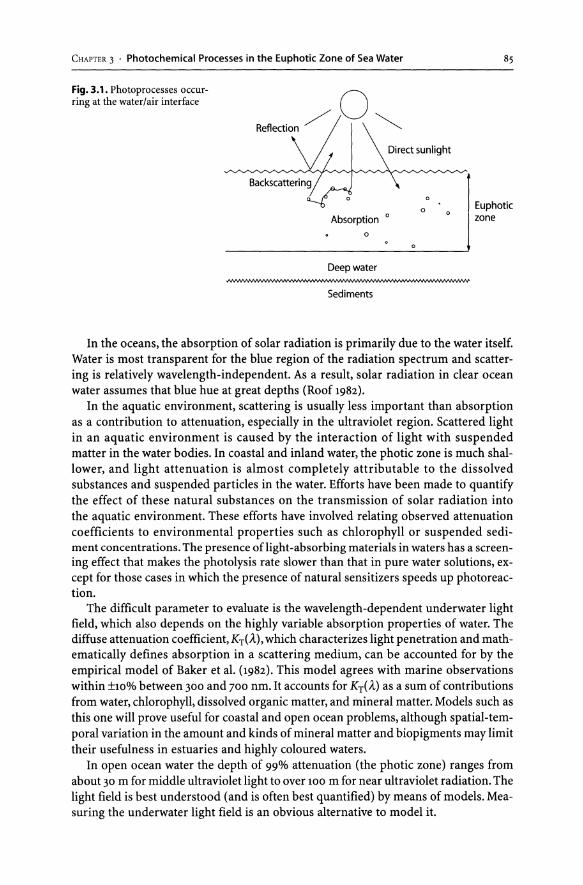
CHAPTER 3 . Photochemical Processes in the Euphotic Zone of Sea Water
Fig. 3.1. Photoprocesses occurring at the water/air interface
Backscattering
Absorption 0
o
85
o 1 Euphotic
1 zone
--------------------------------~
Deepwater
Sediments
In the oceans, the absorption of solar radiation is primarily due to the water itself. Water is most transparent for the blue region of the radiation spectrum and scattering is relatively wavelength-independent. As a result, solar radiation in clear ocean water assumes that blue hue at great depths (Roof 1982).
In the aquatic environment, scattering is usually less important than absorption as a contribution to attenuation, especially in the ultraviolet region. Scattered light in an aquatic environment is caused by the interaction of light with suspended matter in the water bodies. In coastal and inland water, the photic zone is much shallower, and light attenuation is almost completely attributable to the dissolved substances and suspended particles in the water. Efforts have been made to quantify the effect of these natural substances on the transmission of solar radiation into the aquatic environment. These efforts have involved relating observed attenuation coefficients to environmental properties such as chlorophyll or suspended sediment concentrations. The presence oflight-absorbing materials in waters has a screening effect that makes the photolysis rate slower than that in pure water solutions, except for those cases in which the presence of natural sensitizers speeds up photoreaction.
The difficult parameter to evaluate is the wavelength-dependent underwater light field, which also depends on the highly variable absorption properties of water. The diffuse attenuation coefficient, KrP") , which characterizes light penetration and mathematically defines absorption in a scattering medium, can be accounted for by the empirical model of Baker et al. (1982). This model agrees with marine observations within ±10% between 300 and 700 nm. It accounts for Kr(A) as a sum of contributions from water, chlorophyll, dissolved organic matter, and mineral matter. Models such as this one will prove useful for coastal and open ocean problems, although spatial-temporal variation in the amount and kinds of mineral matter and biopigments may limit their usefulness in estuaries and highly coloured waters.
In open ocean water the depth of 99% attenuation (the photic zone) ranges from about 30 m for middle ultraviolet light to over 100 m for near ultraviolet radiation. The light field is best understood (and is often best quantified) by means of models. Measuring the underwater light field is an obvious alternative to model it.

86 E. Pelizzetti . P. Calza
It is also possible to use light fields in the laboratory. Systems such as solar simulators can approximate surface sunlight at most wavelengths. Since the underwater light spectrum varies markedly with depth, broadband studies can accurately measure only the near-surface effects for optically thin samples or vertically integrated effects and absorption coefficients as a function of wavelength.
3.2.3 Factors Influencing Photoreactions
Photoreaction rates are determined by two factors:
1. The rate of absorption of light by the chromophores; 2. Quantum yield with which chemical change results after excitation of the
chromophore.
These factors may all vary over an enormous range, and accordingly the transformations involved vary enormously in their capacity to act as sources or sinks for different compounds. Compounds with a sufficiently high absorption coefficient and a very efficient photodecomposition rate (high quantum yield) for instance will generally have little chance of being detected at the water surface or in the euphotic zone, because their steady state concentration will be kept very low as a result of the extensive photochemical sink.
Basically, any solution photoprocess involves two, or often three relatively distinct steps:
1. Absorption of a single photon by a single chromophore C with the generation of an electronically excited state, C*;
2. Parallel and consecutive processes that degrade the electronic energy to heat, emitted radiation and primary photochemical products;
3. Secondary reactions of these primary photoproducts into the water.
It is frequently desired to measure or calculate the excitation rate of a chromophore under various conditions such as in situ or in an experimental apparatus simulating environmental light intensities and spectral distributions.
Several cases are possible. An example can be that of an optically thin layer near the water surface in which the excitation rate is a function only of the spectrum and intensity of the incident solar light and of the concentration and absorption spectrum of the chromophores. Consideration of this system can be simplified by neglecting reflection, backscattering, and internal scattering, so that in-air insolation measurements are assumed to represent the underwater light intensity.
An optically thick water layer that has a homogeneous chromophore and scatterer distribution may represent another case. In addition to the parameters involved in the optically thin case, the excitation rate now depends also on the optical properties of the water. Since all photons are absorbed, the excitation of a given chromophore depends on its ability to compete with all other chromophores for photons. The depth of such an optically thick layer may extend a few centimetres into turbid and/or absorbing waters, or nearly 100 m into relatively transparent oceanic waters.

CHAPTER 3 . Photochemical Processes in the Euphotic Zone of Sea Water 87
3.3 Main Photo processes Occurring in Water and Air
Solar radiation is fundamental to all the photochemical and photobiological processes of natural waters. The amount, spectral quality and spatial-temporal distribution of sunlight are key variables at the surface and within the water.
Various photoreactions occur in the environment; hydrogen peroxide forms in fresh and sea water, the free radical NO reaches detectable steady state levels in the equatorial Pacific, a photochemical rearrangement product is found in shallow-water encrusting corals (Look and FenicaI1984), and so on. On the one hand, solar radiation promotes photosynthesis processes and influences phytoplankton growth; on the other, light activated abiotic processes, through absorption by chromophores, can occur both by direct and indirect photoreactions.
3.3.1 Direct Photolysis
The direct photolysis of known dissolved molecules with known chromophores is the simplest type of photochemical reaction. The degree of spectral overlap between the electronic absorption spectrum of a chemical species and the emission spectrum of the light source is one of the primary determinant factors of direct photolysis rates. Compounds that strongly absorb at wavelengths greater than 320 nm have the potential to rapidly undergo direct photolysis in sunlight, especially if absorption extends into the visible region. On the other hand, if absorption is weak or non-existent at wavelengths greater than 300 nm, direct photolysis is usually negligible. Most xenobiotics absorb in the ultraviolet spectral region, but there are notable exceptions, such as dyes and certain nitroaniline herbicides, that absorb visible light. Electronic absorption spectra can be employed to compute direct photolysis rate constant in sunlight (Zepp 1978).
The simple inorganic components of natural waters are also generally transparent to sunlight. In the domain of particle-free water without dissolved organic chromophores, water absorbs nearly all the light. The rarity of direct photoreactions of inorganic chromophores is underscored by the fact that nitrite and nitrate are the only well-studied cases. Nitrogen oxides and OH radicals are photoproducts; nitrate is quite unreactive, while at the sea surface nitrite shows a net loss of about 10% per day. A few additional weak chromophores with some known photochemistry are iodate, uranyl ion, hydrogen peroxide and ferrous ions (Braterman et al. 1984).
It is not possible to derive much useful information about direct photolysis from theory, although the literature may indicate the most probable products and mechanisms. For these reasons, direct reactions are best studied experimentally in the medium of interest by monitoring starting material disappearance as well as product appearance. Simpler experiments may fail to reveal the true quantum yield because of unexpected products, or they may give unrealistic rates and product distributions ascribable to medium effects. The photolysis of complex organic chromophore molecules of unknown structures is particularly important in natural waters because simple natural chromophores are rare (Zika 1981; Zepp 1980; Zafiriou 1983). The most important chromophores seem to be diverse organic molecules of unknown structure and they may be partially colloidal. Harvey (1983) have extracted weakly coloured

88 E. Pelizzetti . P. Calza
hydrophobic organic materials called marine humus; these materials have chemical properties that suggest they are formed in situ by auto-oxidative reactions of plankton-derived organic compounds.
3.3.2 Indirect Photoreactions
Indirect photoprocesses are common and important because they can alter molecules resistant to direct photolysis, such as transparent species chromophores. There is evidence that dissolved substances in natural waters can photosensitize a variety of reactions; these photosensitized reactions are sometimes the dominant pathway for photochemical transformation, especially when direct photolysis is negligible.
In indirect photolysis, a reaction is initiated through light absorption by a chromophore other than the substrate itself. If the chromophore is regenerated, it plays a photocatalytic role; this occurs in energy transfer processes and in some cyclic redox reactions. If the chromophore changes irreversibly, it has undergone direct photolysis itself, which simultaneously causes indirect photolysis of other substances presented.
Various studies (Miller and Zepp 1979) have demonstrated that the photolysis rate of xenobiotics can be altered by the dissolved and suspended matter in the aquatic environment. The photolysis rate is effected by both physical and photochemical factors. Physical effects include light attenuation or scattering by natural substances. Changes in photochemistry occur through photosensitization by dissolved humic substances and other natural substances. Although semiconductor powder like Ti02
promotes rapid photocatalysed reactions of xenobiotics, some studies have shown that natural suspended sediments do not mediate such photoreactions. A few qualitative studies suggest that certain xenobiotics are more photolabile when absorbed to algae than when dissolved in distilled water (Zepp 1980).
In this chapter we will consider only the processes involving indirect photoreactions. In Fig. 3.2, the possible absorbers the photoreactant and the main factors that influence the photoprocesses are summarized. The most common light absorbers present in water are dissolved organic matter (DOM), semiconductors (SC) and inorganic anions, such as NO;. These absorbers, through photo-absorption, originate active species (B); the more common are the generation of radicals, such as hydroxyl radical and peroxy radical, and of oxidants, such as hydrogen peroxide and singlet oxygen.
The sources and sinks of those species will be discussed below. These species, reacting with an organic compound, give origin to a photo-transformed compound. The characteristics and concentration of the dissolved organic matter, concentration of dissolved oxygen and the quantity of the activated species photogene rated influence the rate of this process.
The known indirect photoreactions involve initial excitation of chromophore followed by energy transfer, by transfer of electrons or hydrogen atoms to or from other system components. The energy transfer reaction is the first recognized photoprocess in natural waters (Joussot-Dubien and Kadiri 1970) and has been widely studied; it almost represents the largest quantum yield as well. A significant fraction of ultraviolet sunlight absorbed in natural waters excites organic chromophores, particularly at wavelengths below 450 nm. Even processes with low efficiencies originating from these chromophores may be important because of these high excitation rates. Electronic
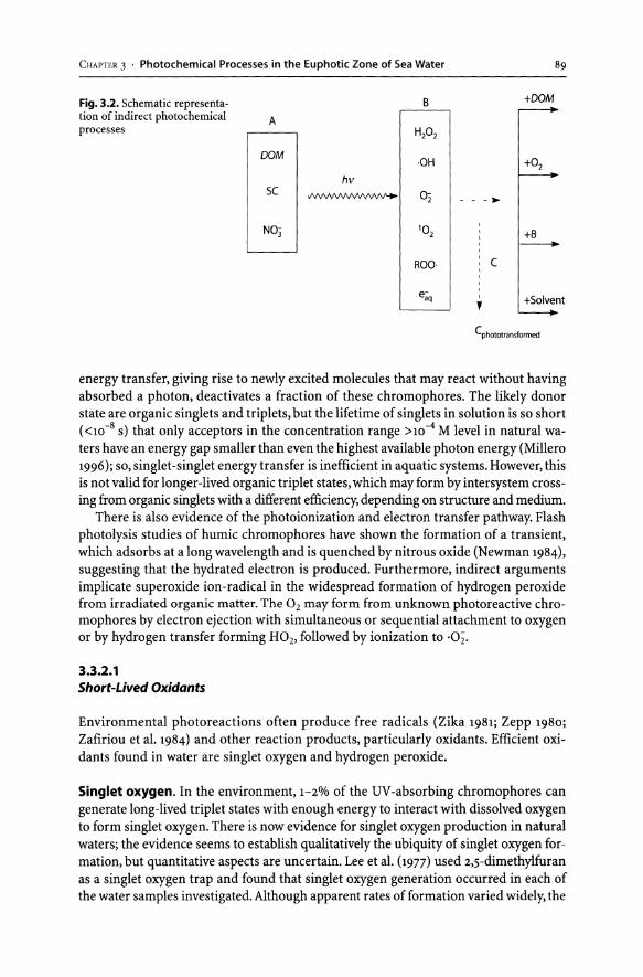
CHAPTER 3 . Photochemical Processes in the Euphotic Zone of Sea Water 89
Fig. 3.2. Schematic representa-tion of indirect photochemical A processes
Io:l hv
sc ~I
NO]
B
HP2
·OH
D2
1°2
I - - -~
+OOM
+°2
+B -ROO· I ,C
e~q , +Solvent
Cphototransformed
energy transfer, giving rise to newly excited molecules that may react without having absorbed a photon, deactivates a fraction of these chromophores. The likely donor state are organic singlets and triplets, but the lifetime of singlets in solution is so short «10-8 s) that only acceptors in the concentration range >10-4 M level in natural waters have an energy gap smaller than even the highest available photon energy (Millero 1996); so, singlet-singlet energy transfer is inefficient in aquatic systems. However, this is not valid for longer-lived organic triplet states, which may form by intersystem crossing from organic singlets with a different efficiency, depending on structure and medium.
There is also evidence of the photoionization and electron transfer pathway. Flash photolysis studies of humic chromophores have shown the formation of a transient, which adsorbs at a long wavelength and is quenched by nitrous oxide (Newman 1984), suggesting that the hydrated electron is produced. Furthermore, indirect arguments implicate superoxide ion-radical in the widespread formation of hydrogen peroxide from irradiated organic matter. The O2 may form from unknown photoreactive chromophores by electron ejection with simultaneous or sequential attachment to oxygen or by hydrogen transfer forming HOz, followed by ionization to ·0;:.
3.3.2.1 Short-Lived Oxidants
Environmental photoreactions often produce free radicals (Zika 1981; Zepp 1980; Zafiriou et al. 1984) and other reaction products, particularly oxidants. Efficient oxidants found in water are singlet oxygen and hydrogen peroxide.
Singlet oxygen. In the environment, 1-2% of the UV-absorbing chromophores can generate long-lived triplet states with enough energy to interact with dissolved oxygen to form singlet oxygen. There is now evidence for singlet oxygen production in natural waters; the evidence seems to establish qualitatively the ubiquity of singlet oxygen formation, but quantitative aspects are uncertain. Lee et al. (1977) used 2,5-dimethylfuran as a singlet oxygen trap and found that singlet oxygen generation occurred in each of the water samples investigated. Although apparent rates of formation varied widely, the

90 E. Pelizzetti . P. Calza
rate per unit of solution absorbency at 366 nm was less variable. The quantum yield for singlet oxygen formation ranged from l.4 to 9.3% with an average of 4.3%. Despite uncertainties, if these experiments indicate the correct order of magnitude, singlet oxygen formation is very active in many coastal, estuarine and fresh waters.
The chemistry of singlet oxygen has been widely studied (Foote and Clennan 1995). A large percentage of it simply returns to the ground state oxygen in a fast interaction (1.6 x 10⁻⁵ S-I) with the vibrational overtone bands of water (Rodgers and Snowden 1982). This fast reaction is the dominant singlet oxygen sink and the major reason why, even with high formation rates, singlet oxygen concentrations are always expected to be very low. Singlet oxygen is predominantly quenched to ground state oxygen by water; its half-life is about 3 fis. Nevertheless, some reactions might compete with water quenching to give significant chemical changes. Joussot-Dubien and Kadiri (1970) suggested that singlet oxygen might be involved in chemical nitrification, as the oxidation of ammonia. They showed that singlet oxygen in water would oxidize ammonia, but that this process is unlikely to compete effectively with biological ammonia sinks in surface waters. Thus, in bulk solution the rates of energy-transfer reactions of even the most reactive materials now seem constrained, on the one hand by physical quenching of singlet oxygen, and on the other by the strong competition with direct transfer to organics by O2, However, in oxygen-depleted or hydrophobic micro environments, such reactions could proceed with higher rates and affect properties such as the surface chemistry and the composition of particulate material.
Hydrogen peroxide. The finding of hydrogen peroxide in surface sea waters has strongly supported the notion that photochemical processes occur in the oceans. The sources of H20 2 can result from three major processes (Millero 1996):
1. Org + hv ~ Org* (3-1)
Org* ~ Org+ + e- (3.2)
O2 + e- ~·O; (3.3)
·0; + H+ ~ H02• (3-4)
H02• + H02• ~ H20 2 + O2 (3.5)
II. Org* + O2 ~ Org + + ·0; (3.6)
Org* + sub ~ Org- + sub+ (3-7)
Org* + sub ~ Org+ + sub- (3·8)
Org+ + sub ~ Org + sub+ (3.9)
Org- + O2 ~ Org + ·0; (3-10 )
sub- + O2 ~ sub + ·0; (3·n)

CHAPTER 3 . Photochemical Processes in the Euphotic Zone of Sea Water 91
III. MLn+ + hv~ M(n+l) + L- (3.12)
M(n-l) + O2 ~ MV+ + .0;: (3-13)
In all the considered pathways, the superoxide anion is a key intermediate in the formation of H20 2• Thus, all the reactions that lead to 0;: will increase the concentration of H20 2•
Studies by Zika et al. (1982) indicate that the formation of H20 2 is higher in coastal waters with higher humic concentrations than in oligotrophic waters. The production rates also appear to be directly related to the concentration of the humic in the water as measured by absorbance at 300 nm. These results support the notion that abiotic photochemical processes are responsible for the hydrogen peroxide in the surface waters of the oceans. The biological and non-photochemical processes known to form hydrogen peroxide are generally insignificant except in oligotrophic waters. The portion of the sunlight responsible for most of the formation of H20 2 is below 400 nm.
Since steady-state levels of H20 2 are found at 10-200 nM in surface water, the decay of H20 2 must be slow. Studies also indicate that the lifetimes are much longer in deep waters; these results indicate that particles or biological processes may control the lifetime of the decay. The decay appears to be partly related to biological particles, both living and dead cells. Nevertheless, further work is necessary to elucidate the decay mechanism of H20 2 and the role that cells have on the formation and destruction of H20 2• The decomposition is not affected by light and occurs in a matter of days. Enzymes as well as particles may be important. Although abiotic decomposition processes are small, they may be important in the open oceans.
3.3.2.2 Free Radicals
The involvement of radicals of various origins in natural waters has been suggested repeatedly (Swallow 1969; Zafiriou 1983) but not on the basis of strong evidence. However, recent research continues to suggest a nearly ubiquitous formation of a variety of radicals in natural waters. Many radicals live long enough to show a chemistry that is independent of their immediate sources, and some generalizations can be made about their chemical behaviours that are often interconnected.
Sources: Some studies (Sehgal et al. 1980) show that radical formation occur when ultrasound energy interacts with gas-satured aqueous solutions. The environmental impact of these processes has not been investigated at all, but is probably minor. A second potential source of radicals in natural waters is supply from the atmosphere of OH, H02,
CH30 2 or precursor species such as 03' HOOH and peroxy acetyl nitrate. Although a lack of evidence makes it impossible to estimate the fluxes of such radicals with confidence, approximate upper limits can be set by taking the expected concentrations of these species either from atmospheric measurements or from models, and then assuming that they deposit to water surface rapidly because of their high reactivity and/or high water solubility.
Biological emission of free radicals and their precursors is a little-understood source. Free radicals play key metabolic roles in vivo and may be responsible for cel-

92 E. Pelizzetti . P. Calza
lular malfunctions. It is unclear, however, whether their loss by active or passive processes is common for either healthy or senescent cells. A variety of thermal chemical processes may produce radicals. It has been suggested that thermal oxidation of phenols by Mn02 may generate humic materials (Shin do and Huang 1982).
Radical fate: The principal fate of many of the more reactive radicals is their transformation to a new radical; generally the daughter radical will be less reactive and more selective than its parent. This type of transformation is quite common and occurs during the reactions of radicals with the major constituents of fresh and natural waters, because these components are always light-element even-electron structures. Harvey (1983) has noted that marine humic materials may be primarily lipid-derived autoxidation/condensation products, formed in part from the action of thermally and photochemically generated radicals as well as other reactants with biogenic polyunsaturated triglycerides.
Finally, to a limited extent, less reactive radicals may simply accumulate in certain water systems until their steady state levels are significant. The fate of radicals in the environment may therefore be summarized as follows: transformation, redox stabilization, radical formation and possibly simple accumulation.
The oxidants participate in important non-radical reactions and also frequently generate new radicals, thus serving as radical reservoirs. The efforts to understand the role of photochemically produced free radicals in natural waters are complicated by several factors. Free radicals react readily with one another, with transition metals, and more slowly with many organic compounds.
The ·OH radical: the ·OH radical is the most reactive photochemically produced free radical in the atmosphere, while its role in an aqueous system is less clearly understood. Flash photolysis studies have demonstrated that it is formed in sea water. The possible sources of the ·OH radicals in sea water are N02, NO;, H20 2, Fe2+ and dissolved organic matter. The significant known sources and sinks, togeilier with typical daytime steadystate concentration of hydroxyl radical in atmospheric and surface waters are reported in Table 3.1.
Peroxy radicals and superoxide radical anion. In addition to the ·OH radical formation rate, Hoigne (1990) has demonstrated the formation and estimated the concentrations in some natural waters of other major radical types, as organic peroxy radicals and superoxide radical anion. They have suggested that the fastest ROO· secondary reactions would give half-lives of a few days at the surface for reactive compound classes, such as phenols, aromatics, amines and hydroquinones.
The major fonts of both radicals, together with their fates, are reported in Table 3.2.
3.3.2.3 Heterogeneous Photochemistry
All natural waters contain non-living organic particles, mineral particles and living organisms, as well as colloidal materials. In addition to iliese core materials, binding to particles by ions and solutes (especially hydrophobic organic compounds) also exposes the colloidal materials to ilie different and often enhanced reactivity of ilie particulate phase.

CHAPTER 3 . Photochemical Processes in the Euphotic Zone of Sea Water 93
Table 3.1. Sources and sinks for ·0 H radicals
Natural Water OH sources OH sinks Typical daytime steady-state aqueous concentrations
Continental clouds .OH(g) H .OH(aq)
Fe(ll) + HP2 ~ Fe(llI) + .0H(aq) + ·OH
03(aq) + .0; ~ ·OH(aq) + 202 2+ 2+
Fe(OH) + hv ~ Fe + .0H(aq)
DOC
HSO;/HSO;
CI-/8r-
1 x 10-14_1 X 10-12 M
Fresh surface waters
NO;+ hv ~ N02 + ·OH(aq)
NO;+ hv ~ N02 + ·OH DOC
HCO;/CO~-
1 xl 0-18 -1 X 10-15 M
Marine waters
NO;+ hv ~ NO + ·OH
Fe(ll) + H20 2 ~ Fe(lll) + ·OH + OH
NO; + hv ~ N02 + ·OH
NO; + hv~ NO + ·OH
DOC + hv ~ ·OH?
Fe(ll) + HP2~ Fe(lll) + ·OH + OH
8r-/CI- lxl0-19 _lxl0-17 M
DOC
HCO;/CO~-
Table 3.2. Sources and sinks form ·ROO and ·0; radicals
Natural water
Continental clouds
'ROO/'O; sources
·ROO(g) ~ .ROO(aq)
RC(O)R' + PhOH + hV(+02) ~.O; + products
Fresh and marine DOC + hv(+ 02) waters ~ .0; + oxidized DOC
Surface waters
·ROO/·a; sinks Typical daytime steady-state aqueous concentrations
. ROO(aq)/.O; 1 x 10⁻⁹ -4x 1O-8 M
Cu(lI)/Cu(l), Fe(l11)/Fe(l1) DOC .ROO(aq)/.O; 1 x10⁻⁹ -1 x 1 0-8 M?
Cu(lI)/Cu(I), DOC
Fundamental chemical considerations suggest many ways in which particulate or absorbed molecules differ from their dissolved forms. Highly significant spectral shifts occur for absorbed molecules (Leermakers et al. 1966), while the quenching of excited states of absorbed pesticides is observed (Hautala 1978).
Studies of xenobiotics in the presence of particulate materials, such as desert soils and sand, have shown bathochromic spectral shifts of sorbed anthracene, polychlorinated aromatic compounds and pesticides (Leermakers et al. 1966) moving photochemically active strong bands into the sunlight spectral region. There have been several general and mechanism-oriented studies on the effect of particulate on photoprocesses (Miller and Zepp 1979). In particular, there has been a great deal of interest in the possible involvement of semiconductor-type mechanisms in natural water photochemistry (Calza et al. 2001).

94 E. Pelizzetti . P. Calza
The possible photolysis of abundant hydrophobic and largely particulate monoand polyunsaturated fatty acids in the marine environment is of biogeochemical interest. Numerous pathways are known for such molecules once liberated from cells, and they are the suspected precursors of some humic and fulvic acid components.
Finally, there is evidence that the surfaces of algae (living and dead) are active in some photoprocesses. Heat-killed and ascorbate-washed cells also promote the reaction, so although the cells are living, the process does not appear to be metabolic. Similar effects have been seen for various other organophosphorus compounds.
3.3.2.4 Organic Compounds in Sea Water
Although the concentration of organic matter in the oceans is less than 0.01% of the total amount of salts, these compounds are important modifiers of many of the biological and chemical reactions that take place in the sea. They provide a nutritional and energy base for micro and macroorganisms, have a major impact on the speciation of many metals by such processes as complexation and adsorption, and are precursors of fossil fuels such as petroleum and oil shale. These organic compounds can also provide growth promoters and inhibitors that may control phytoplankton succession.
The source of most of the organic compounds in sea water is from primary production in the euphotic zone. Part of the organic matter from photosynthesis is partially metabolized in order to satisfy the energy requirements of phytoplankton. Much of the organic matter is consumed by organisms, but a significant amount is decomposed at the surface, while 1 to 12% of the annual production remains as a refractory fraction, quite resistant to biological and chemical transformations. The residence time of this residual dissolved organic matter in the sea has been estimated by Williams and Druffel (1987) to be 1310 yr for surface and 6240 yr for deep dissolved organic matter. Most of this residual organic carbon consists of humic substances. The other sources of input of organic matter to sea water, in addition to primary productivity by marine plankton, include terrestrial input by rivers and by the atmosphere, excretion by marine organisms and the resuspension of organic matter from marine sediments. The direct addition of organic matter due to oil spills is an additional source.
In aquatic systems, it is traditional to divide organic matter into two major categories: dissolved and particulate (DaM and paM). paM includes those species that will be retained by a glass fibre filter of 0.45 jlm.
Dissolved organic carbon (DOC) is about 50% of the DaM, and likewise particulate organic carbon (PaC) is about 50% of the value of paM. The concentration of dissolved organic carbon in sea water is typically significantly greater than that of pac. Seasonal variations of DOC and pac occur primarily in shallow waters and are similar to the variations in primary productivity. At depths below a few hundred metres, the average DOC is 40 jlM, while the average pac is 0.8 jlM (Millero 1996). The pac frequently goes through a maximum in the oxygen minimum zone. Some have suggested that this is a result of sinking particulate material having a density similar to water at a depth of 500 to 1000 m. The oxygen minimum is thus a result of bacteria oxidizing this material in this zone. The dissolved and particulate organic carbon, nitrogen and phosphorus levels in surface, deep, and coastal waters are compared to the levels at the oxygen minimum. The coastal levels are higher than those in surface wa-

CHAPTER 3 . Photochemical Processes in the Euphotic Zone of Sea Water 95
ters of the oceans. The levels of dissolved and particulate concentrations of all the organic compounds are much lower in deep waters than in surface waters.
Dissolved marine organic matter is such an extremely complex and dilute mixture of compound that only 10 to 20% can be full characterized. Measurements of dissolved organic carbon, nitrogen and phosphorus compounds are standard measurements used to obtain an understanding of the major types of organic compounds present in the oceans. The dissolved organic matter in sea water consists largely of humic substances and more labile compounds from the major biochemically important compound classes such as carbohydrates, steroids, alcohol, amino acids, hydrocarbons and fatty acids.
Particulate organic matter consists of a mixture of living and dead phytoplankton and zooplankton, bacteria, their degradation products and macroscopic aggregates. The distribution and nature of particulate organic matter has been found to be quite variable both geographically, vertically, diurnally, and seasonally, and it is influenced by a complex set of equilibria between sources, sinks and circulation patterns. In the euphotic zone, the major portion of paM is due to phytoplankton, the chemical composition of which will vary with species as well as with environmental conditions, hence, leading to significant variations in the nature of the paM. The metabolic products of phytoplankton can vary with changes in temperature, light intensity and nutrient availability. In the euphotic zone, the majority (90%) of poe is due to living matter, while at depths of 2 400 m and more, less than 1% of the poe is due to living organisms.
3.4 Role of Iron and Chlorine
Iron is an essential trace metal. In fact, as redox reactions and electron transport are two major functions of iron, it affects the enzyme systems. Iron, along with molybdenum, is also essential for nitrogen fixation and nitrate reduction and thus for the assimilation of the major nutrient nitrogen.
It is hypothesized that iron availability limits specific rates of phytoplankton growth (Martin et al. 1990; Brand 1991). Most marine photosynthetic organisms can only take up iron in the dissolved form. Under sea water conditions, the solubility of iron is extremely low. Careful analytical studies in the oceans have shown that the concentrations of total dissolved iron range from 0.02 to 10 nM.
The role of chloride in the marine environment is also crucial. Several classes of mechanisms for dechlorination of sea salt aerosol have been hypothesized. More than one kind of mechanism is probably operating in the marine boundary layer, and the relative importance of different mechanisms probably varies over space and time. An improved understanding of inorganic CI chemistry in the marine boundary layer is needed because of its potential importance for global chemistry (Keene 1995).
3.4.1 Inorganic (I Formation in the Marine Environment
The possible mechanisms for formation of atomic chlorine in the marine environment have been widely investigated, and several possible sources have been identified.

96 E. Pelizzetti . P. Calza
Reactions of sodium chloride, the major component of sea salt particles, with nitrogen oxides generate chlorine atom precursors. Chlorine atoms formed from the reactions of sea salt particles can destroy ozone and greenhouse gas through direct reactions. Alternatively, CI reacts rapidly with organic molecules, which can, in turn, lead to ozone formation in the presence of sufficient nitrogen oxides (Finlayson-Pitts and Pitts 1986).
The injection into the atmosphere of sea salt aerosol generated by breaking waves on the ocean surface is the major global source of tropospheric chlorine. Most of this material remains in the aerosol and is redeposited to the ocean surface, but important fractions ranging from averages of 3 to 35% are released from the aerosol as inorganic CI vapour (Keene 1995). Another precursor of atomic CI is HCI (Behnke et al. 1995). Although HN03 and H2S04 displace HCI from sea salt particles, this is not a significant source of atomic CI, because the subsequent reaction of HCI with OH is relatively slow (Singh and Kasting 1988).
Recent evidence indicates that other chemical processes may also dechlorinate sea salt aerosol. These processes generate highly reactive CI gases that during the daytime undergo rapid photochemical conversion to HCI via CI atoms. The aerosol eventually scavenges HCI. Processes involved in CI cycling are very uncertain, however, partially because of the difficulties in reliable measures of principal reactant and product species.
3.4.2 Role of Iron in Surface Waters
In waters several reductants coming from biodegradation of the biomasses are present. Among these, it has to be reminded of iron(II) and H2S. Even if those species are able to directly interact with the organic compounds, but usually through slow reactions, redox reactions in natural systems may occur more easily due to a microbial action and mediation through one or more electron transporter. The iron(III)/iron(II) system acts as a electron transporter. The oxido-reductive processes mediated by iron compounds are important, because in anaerobic conditions, such as sediments and deep waters, iron(III) oxides are the more abundant oxidant species. In various ecosystems the iron cycle depends on several physical, chemical and biological processes (Stumm 1992). The iron cycle is interdependent and often connected with the cycles of phosphorus, sulphur, heavy metals, oxygen and carbon; moreover, it is dependent on living matter and light intensity.
The importance of iron can be stressed by such considerations:
1. High quantities are present in rocks and it possesses a rapid rate of transformation. The ability of the species containing iron to oxidize or reduce and contemporary to precipitate or to be solubilized, links the iron cycle to the oxygen cycle (oxidant) and to the carbon cycle (reductant).
2. High surface areas of the iron oxides and their surface reactivity easily makes the adsorption of various solutes. This is one of the causes of interdependence between the iron cycle and the cycles of several other elements, such as heavy metals and phosphate.

CHAPTER 3 . Photochemical Processes in the Euphotic Zone of Sea Water 97
3. It is able to act as semiconductor and to participate with the redox photoreactions. In those reactions, the electromagnetic radiation is utilized either to conduct reactions thermodynamically not favoured (heterogeneous photosynthesis) or to catalyse a reaction thermodynamically favoured (heterogeneous photocatalysis).
The iron cycle includes the reductive solubilization of iron(IU) by organic ligands, a process that can also be photocatalysed in surface waters, and the oxidation of iron (II) by oxygen, a process catalysed by superficial interactions. During the iron(II) oxidation to iron(III), reactive compounds as heavy metals, phosphate ions and some organic compounds are linked to the precipitate surface. Those compounds are later released in solution during the reduction of iron oxides. The total balance of the cycle gives also the oxidation of organic matter by oxygen mediated by iron.
Fe(III) is also absorbed on external surfaces of humic materials, weakly bound octahedrally and easily complexed and reduced. When Fe(III) is added to the humic materials, most of the iron becomes bound to octahedral sites.
In Fig. 3.3 several important inorganic iron(III) species and their distribution as a function of pH are represented. While in acidic conditions, the there are several possible species (with cr, SO~- and F ligands), at the pH typical of sea water the only main species present at remarkable concentrations are the Fe-hydroxides. The hydrolysis of iron(III) is strongly dependent on pH. In particular, at strongly acidic pH, iron(III) is present in dissolved form and the prevalent species is Fe(OH)2+. At pH levels typical of sea water (-8), iron is prevalently present in a precipitate form (Fe(OHh).
Interesting findings have recently been reported with regard to the speciation of dissolved iron in oceanic surface waters (Gledhill and van den Berg 1995, van den Berg 1995, Rue and Bruland 1995). Organic ligands present in the euphotic zone of marine
Fig. 3.3. Speciation of iron(III) 100 ...... ...... -.- ..... I FeS01 / in sea water as function of pH Fe(OH}! ',,/' Fe(OHh , ....
FeCl2+ i i , , ,
10 , . / Fe(OH}4 ~ '.' , /. QJ / u. I'.
n; ;2 FeF2+ /f
/ !
!
/ \"\ II
FeOH2+
0.1 I 0 2 4 6 8 10
pH

98 E. Pelizzetti . P. Calza
waters form very stable complexes with dissolved Fe(III). Thus, it is most likely that the concentration of inorganic, dissolved Fe(III) species determines the upper limit for bioavailable Fe(III). The Fe(II) produced is likely to form less stable complexes with organic ligands present in the euphotic zone of sea water and hence is biologically more available than Fe(III). In the case of Fe(II), organic complexes may be rather weak, and hence ligands at the cell surface may form stronger complexes with Fe(II) than organic ligands in the medium (Anderson and Morel 1982).
3.4.2.1 Photoreactions Occurring on Iron
The speciation, and thus the biological availability, of redox-active metals are often strongly influenced by light.
In Fig. 3-4 the absorption spectra registered for several iron-complexes are reported. While Fe3+ gives no adsorption in the visible region, the absorption spectrum is extended in the visible zone in the presence of ligands, such as chloride and bromide. The extent of absorption is higher in the presence of bromine and the maximum lays in the visible light. So, light-induced reactions are favoured when iron is complexed, above all if it is linked to chlorine or bromine.
An important reaction taking place under light is the photo-reduction of Fe3+ to give ·OH; under the conditions here the most important photolabile form is the monohydroxy complex (Faust and Hoigne 1990) with a quantum yield of 0.14 at 313 nm and 0.017 at 360 nm:
FeOH2+ + hv~ Fe2+ + ·OH (3-14)
In the presence of hydrogen peroxide, the Fe 2+ formed in Eq. 3.14 generates additional ·OH via the Fenton reaction.
Because light affects to a larger extent the reduction of Fe(III), the concentration of Fe(II) in the euphotic zone of surface water is expected to depend on the light intensity and thus on the time of day. A diurnal variation in the Fe(II) concentration has
Fig. 3.4. Absorption spectra of 3000...,-------------------, Fe(III) species
., E u
~ 2000
.~
I ~ 1000
.!ll ~
i "\ ". FeBr2+ \ .... ,., \ .. .... _ .... );:--....... .. ... .. ...
\.. '" .. \
Fe(OH)2+ \.. \!eCl2+ ,., \'. " '. ... '. ...
o I --!:-3+ ................... , ... i - .................. ~~:::---j' ..
....,-",---.--
,., not to scale
300 350 400 Wavelength (nm)
450 500

CHAPTER 3 . Photochemical Processes in the Euphotic Zone of Sea Water 99
been observed by several research groups, not only in acidic lakes and rivers (McKnight et al.1988), but also in sea waters. The concentration of Fe(II) is much higher in acidic surface waters than in sea water because of the much slower oxidation of Fe(II) at low pH-values as compared to pH-values of sea water. Oxidation kinetics of Fe(II) by O2
and H20 2 depends in fact strongly on the Fe(II) speciation. Organically and inorganically complexed Fe(III) can be reduced under the influ
ence of sunlight. Although the average steady-state concentration of Fe(II) may be very low in the euphotic zone of sea water, considerably higher Fe(II) concentrations can be expected upon illumination with high intensity solar radiation.
The cycling of iron between its reduced and oxidized forms and between particulate and dissolved species in natural waters has a number of environmental consequences beyond iron's role as a nutrient and adsorbent. Iron photo-redox cycling has been shown to catalyse the oxidation of dissolved organic matter (Miles and Brezonik 1981). This process could represent a significant sink of biologically refractory materials, such as humic substances, and is closely coupled to the cycling of reactive transient species such as H20 2, ·OH, and H02/·O;:,(Faust and Zepp 1993).
Within the acidic pH range, the oxidation of dissolved Fe(II) by oxygen is expected to be very slow compared to other processes. However, the irradiation of humic substances in the presence of oxygen results in the formation ofH02/·0;: (Blough and Zepp 1995; Hoigne et al. 1989). The mechanism of this reaction is not known but may occur via reduction of oxygen by aqueous electrons or triplet state, both formed when humic substances are photo-excited. The end product of H02/·O;: dismutation is hydrogen peroxide. This reaction is catalysed by the presence of dissolved iron by the reactions:
H02/·O;: + Fe(II) -7 Fe(III) + H20 2 (3.15)
H02/·O;: + Fe(IIl) -7 Fe(II) + O2 (3.16)
The hydrogen peroxide formed from H02/·O;: is another potentially significant oxidant of Fe(II). It is clear that both iron and light have an accelerating effect on the oxidation of humic substances by oxygen. Voelker et al. (1997) have observed two photooxidation processes of fulvic acid. The first, which does not seem to require the presence of metals, results in the reduction of oxygen to H02/·O;:.
The second process, photo induced ligands to metal charge transfer reaction of Fe(III)-fulvate complex, occurs both in solution and on the surface of the iron oxide and results in the reduction of Fe(III). Dissolved Fe(III) is continuously supplied via re-oxidation of Fe(II) by both H02/·O;: and H20 2• The OH radicals produced by the reaction of Fe(II) with H20z further oxidize fulvic acid.
3.4.3 Interactions Between Iron and Chloride
Recently chlorine was identified and measured in coastal areas at concentrations up to 150 parts per trillion. This is a much larger concentration than can be attributed to known reactions of sea salt particles, suggesting that there must be an unrecognized source producing elz. Photocatalytic reactions involving metal oxides have been stud-

100 E. Pelizzetti . P. Calza
ied. Behnke et al. (1995) have produced, for example, chlorine during irradiation of most metal-oxide aerosol (Ti02, Fe20 3 and Si02) in the presence of HCI and 03' The authors postulate a photocatalytic mechanism involving electron transfer and free-radical reactions to explain these observations. Recently, we have observed that photocatalytic transformation of trichloromethane on titanium dioxide was inhibited by chloride and that tetrachlorometane is formed during the process (Minero et al.I997). The suggested mechanism involves the oxidation of chloride through reaction with the valence band holes, according to:
htB+cr ~·CI (3.17)
and subsequent reaction of ·CI with ·CCI3. Several oxides and chalcogenides that occur in the environment can be activated
by absorption of ground-level solar light, such as widely diffuse iron oxides. Fe203 is a semiconductor widely diffuse in nature and the photocatalytic halogenation with Fe203 may represent an important natural source of halogenated compounds in the environment.
The influence of iron (III) on the photoinduced transformations of phenol in the presence of halides can be adopted as a model system. The photodecomposition of phenol in the presence of Fe203 and NaBr at pH 7, together with evolution of bromophenols, is reported in Fig. 3.5. In this case, the formation of 2- and 4-bromophenol is observed.
The E~B potential for Fe203 is reported to be ca. 2.8 V (Gerisher 1979) and is able to guarantee the oxidation of Br-ion to the correspondent radical. This should allow the oxidation of bromide, according to Eq. 3.17, being EO=2.0 V for ·Br/Br- and 1.6 V for Brz/Br-., so both species result active in the halogenation of phenol.
Similarly, addition of chloride ions causes the formation of chlorophenols (Calza et al. 2001). In fact, EO=2.5 V for Cr/·CI and 2.3 V for CI2/Cr (Wardman 1989) should allow the oxidation of chloride in agreement with Eq. 3-17.
Interaction between iron and chloride can also occur in a homogeneous phase. Experiments conducted in conditions that simulate solar irradiation have shown that
Fig. 3.5. Photodegradation of phenol (2 x 10⁻⁴ M) and time evolution of bromophenols in presence of Fe203 and NaBr 0.01 M at pH 7
1.0
0.8
3' Q 0.6
'0 c: cu 0.4 ..c: c..
0.2
'" p-Bromophenol .......................... ~ , "
/ ""'" Phenol + 0.01 M Br
, , /
1*\ I. \ 'I \ " \
' .. , "'"
I, \ £' \ o-Bromophenol II ,
I It..
I
" "
"""
3.5
3.0 OJ
2.5 a ~
2.0 }
1.5 [ i:
1.0 IQ
.} 0.5
o. o 0 50 100 150
Irradation time (h)

CHAPTER 3 . Photochemical Processes in the Euphotic Zone of Sea Water 101
phenol, in the presence of iron(III) and halide ions gives the formation of halogenated phenols.
Photodecomposition of phenol and evolution of chlorophenols in the presence of Fe(III) and NaCI at pH 2 is reported in Fig. 3.6. At pH 2, the iron(III) is prevalently present in dissolved form so the process occurs in a homogeneous phase and Fe(OH)2+ is the predominant species (see Fig. 3.3). It is also a photoreactive species and can originate OH radicals through Eq. 3-14.
In such experimental conditions, quinone, cathecol and quinol have been identified as intermediates.
In the presence of halide X- ions (chloride or bromide ),also the following reactions take place:
FeH + X- H FeX2+ (3.18)
FeX2+ + hv~ Fe2+ + X· (3-19 )
Atomic CI reacts rapidly with many hydrocarbons and dimethylsulphide in an analogous manner to, but at different rates than, OH radicals. Phenol, 2- and 4-chlorophenol have been identified as shown in Fig. 3.6.
Interestingly, also at neutral and basic pH conditions, the halophenol formation is observed both in the presence of chloride and bromide (Calza et al. 2001).
From these results it emerges that the formation of chloro and bromophenols may occur under solar light in chloride and bromide rich environments in the presence of iron species. This process should be considered as a possible abiotic source of natural halogenation of organic matter at the air/sea water boundary. The widespread occurrence of chlorinated structures in humic substances provides another example of the difficulties in quantifying the role of different natural halogenation processes. However, the same type of reaction products can be expected in other chlorinating processes involving the formation of active chlorine species. This implies that at best, the environmental compartments responsible for the large-scale natural production of organohalogens can be identified, whereas much of the present uncertainty regarding the predominant reaction mechanism is likely to persist for a long time.
Fig. 3.6. Photo degradation of 1.0
/"----, p-Chlorophenol phenol (2 x 10 -4 M) and tim: evolution of chlorophenols In I , I \ I \ the presence of Fe(III) and 0.8 I \ NaCI 0.01 M at pH 2
J' _ .... --..... \
/ ',\ o-Chlorophenol g. 0.6 I \ \
I I , \ "0 f I- \ \ c : / \ \ GI
II \\ ..r:: 0.4 0.. J I \ II , I I \
0.2 II \ Phenol II ' ... /." l
20 2 o
~ 15 if
::I 2-
10 ~
25
5
o • 0 o 30 60 90
Irradation time (min)

102 E. Pelizzetti . P. Calza
References
Anderson MA, Morel FM (1982) The influence of aqueous iron chemistry on the uptake of iron by the coastal diatom Thalassiosira weissflogii. Limnol Oceanogr 27:789-813
Baker KS, Smith RC, Green AES (1982) Middle ultraviolet irradiance at the ocean surface: Measurements and models. LimnolOceanogr 27:500-509
Behnke W, Scheer V, Zetzsch C (1995) Production of photolytic precursor of atomic CI from aerosols and cr in the presence of 0 3, In: Grimvall A., Leer EWB de (eds) Naturally produced organohalogens. Kluwer Academic Publishers, Dordrecht, pp 375-384
Berg CMG Van den (1995) Evidence for organic complexation of iron in seawater. Mar Chern 50:139-157 Blough NY, Zepp RG (1995) Reactive oyxgen species in natural waters. In: Foote CS, Valentine JS (eds)
Active oxygen in chemistry. Chapman and Hall, New York, pp 280-333 Brand (1991) Minimum iron requirements of marine phytoplankton and the implications for
biogeochemical control of new production. Limnol Oceanogr 36:1756-1771 Braterman PS, Cairns-Smith AG, Sloper RW (1984) Photo-oxidation of iron(II) in water between pH 7.5
and 4.0. J Chern Soc Dalton Trans 1441-1445 Calza, P, Maurino V, Minero C, Pelizzetti E, Sega M, Vincenti M (2001) Chloro and bromophenols forma
tion from phenol and halides by simulated solar light irradiation in the presence of iron ions, iron oxides and cadmium sulfide. (to be published)
Faust BC, Hoigne J (1990) Photolysis of Fe(III)-hydroxy complexes as sources of OH radicals in clouds, fog and rain. Atmos Environ 23:235-240
Faust BC, Zepp RG (1993) PhotodIemistry of aqueous iron(III)-polycarboxylate complexes: roles in the chemistry of atmospheric and surface waters. Environ Sci Technol 27:2517-2522
Finlayson-Pitts BJ,Pitts IN Jr (1986) Atmospheric chemistry: Fundamentals and experimental techniques. Wiley, New York
Foote ST, Clennan EL (1995) Properties and reactions of synglet dioxygen. In: Foote CS, Valentine JS, Greenberg A, Liebman JF (eds) Active oxygen in chemistry, vol II. Blackie Academic and Professional, Glasgow, UK,pp 105-140
Gerisher H (1979) Solar photoelectrolysis with semiconductor electrodes. Appl Physics 31:115-172 Gledhill M, Berg CMG Van den (1995) Measurement of the redox speciation of iron in seawater by cata
lytic cathodic voltammetry. Mar Chern 50:51-61 Harvey GR (1983), Dissolved carbohydrates in the New York bight and the variability of marine organic
matter. Mar Chern 12:333-339 Hautala R (1978) U.S. Environmental Protection Agency. U.S. National Technical Information Service,
Springfield, VA. (EPA-600/3-78-060 Report PB-285) Hoigne J (1990) Formulation and calibration of environmental reaction kinetics; oxidation by aqueous
photooxidants as an example in aquatic chemical kinetics. In: Stumm W (ed) Reaction rates of processes in natural waters. Wiley Interscience, New York, pp 43-70
Hoigne J, Faust BC, Haag WR, Scully FE, Zepp RG (1989) Aquatic humic substances as sources and sinks of photochemically produced transient reactants. In: Suffert EM, Mac Carthy P (eds) Aquatic substances: Influence on fate and treatment of pollutants. American Chemical Society, Washington D.C., pp 363-381
Howard PH (1975) EPA report No. EPA-560/5-75-006. Washington, DC Joussot-Dubien J, Kadiri A (1970) Photosensitized oxidation of ammonia by singlet oxygen in aqueous
solution and in seawater. Nature 227:700-701 Keene WC (1995) Inorganic Cl cycling in the marine boundary layer: A review. In: Grimvall A, Leer WB
de (eds) Naturally-produced organohalogens. Kluwer Academic Publishers, DordredIt, pp 363-371 Lee WN, Zepp, RG, Gordon JA, Baughman GL, Cline DM (1977) Kinetics of chemical degradation of
malathion in water. Environ Sci Technol11(I):88-93 Leermakers PA, Thomas HT, Weis LD, James FC (1966) Spectra and photochemistry of molecules
adsorbed on silica gel IV. J Am Chern Soc 88:5075-5083 Leighton PA (1961) Photochemistry of air pollution. Academic Press, New York, pp 6-41 Look SA, Fenical W (1984) Erythrolides: Unique marine diterpenoids interrelated by a naturally occur
ring di-il-methane rearrangement. J Am Chern Soc 106:5026-5027 Martin JH, Fitzwater SE, Gordon RM (1990) Iron deficiency limits phytoplankton growth in Antartic
waters. Global Biogeochem Cycles 4:5-12 McKnight DM, Kimball BA, Bencala KE (1988) Iron photoreduction and oxidation in an acidic moun
tain stream. Science 240:637-640 Miles q, Brezonik PL (1981) Oxygen consumption in humic colored waters by a photochemical ferrous
ferric catalytic cycle. Environ Sci Technollp089-1095

CHAPTER 3 . Photochemical Processes in the Euphotic Zone of Sea Water 103
Miller GC, Zepp RG (1979) Effects of suspended sediments on photolysis rates of dissolved pollutants. Wat Res 13:453-485
Millero FJ (1996) Chemical oceanography, 2nd edn. CRC Press, Boca Raton Minero C, Maurino V, Calza P, Pelizzetti E (1997) Photocatalytic formation of tetrachloromethane from
chloroform and chloride ions. New J Chern 21:841-842 Newman L (ed) (1984) Gas-liquid chemistry of natural waters, vols I and II. Brookhaven National Labo
ratory, Upton, N.Y. (BNL 51757) Pelizzetti E, Minero C, Maurino V (1990) The role of colloidal particles in the photo degradation of or
ganic compounds of environmental concern in aquatic systems. Adv Colloid Interface Sci 32:271-316
Rodgers MAT, Snowden PT (1982) Lifetime of O2 elig) in liquid water as determined by time-resolved infrared luminescence measurements. J Amer Soc 104:5541-5561
Roof AAM (1982) Aquatic photochemistry. In: Hutzinger 0 (ed) The handbook of environmental chemistry, vol lIB: Reactions and processes. Springer-Verlag, Berlin, pp 43-65
Rue EL, Bruland KW (1995) Complexation of iron(III) by natural organic ligands in the Central North Pacific as determined by a new competitive ligand equilibration! adsorptive cathodic stripping voltammetric method. Mar Chern 50:117-138
Sehgal C, Sutherland RG, Verrall RE (1980) Optical spectra of sonoluminescence from transient and stable cavitation in water satured with various gases. J Phys Chern 84:388
Shindo H, Huang PM (1982) Role of manganese IV oxide in abiotic formation of humic substances in the environment. Nature 298:363
Singh HB, Kasting JF (1988) Chlorine-hydrocarbon photochemistry in the marine troposphere and lower stratosphere. J Atmos Chern 7:262-285
Stumm W (1992) Chemistry of the solid-water interface. John Wiley and Sons, New York Swallow JC (1969) Hydrated electrons in seawater. Nature 222:369-370 Voelker BM, Morel FMM, SuIzberger B (1997) Iron redox cycling in surface waters: Effects of humic sub
stances and light. Environ Sci TechnoI31(4):1004-1011 Wardman P (1989) Reduction potentials of one-electron couples involving free-radicals in aqueous so
lution. J Phys Chern Ref Data 18:1637-1755 Williams PM, Druffel ERM (1987) Radiocarbon in dissolved organic matter in the Central North Pacific
Ocean. Nature 330:246-248 Zafiriou OC (1983) Naturally water photochemistry. In: Riley JP, Chester R (eds) Chemical oceanogra
phy, vol VIII. Academic Press, New York, pp 339-379 Zafiriou OC, Joussot-Dubien J, Zepp RG, Zika R (1984) Photochemistry of natural waters. Environ Sci
TechnoI18(12l:358-371 Zepp RG (1978) Quantum yields for reaction of pollutants in dilute aqueous solution. Environ Sci Technol
12(3):327-329 Zepp RG (1980) Assessing the photochemistry of organic pollutants in aquatic environments. In: Haque
R (ed) Dynamics, exposure and hazard assessment of toxic chemicals. Ann Arbor Science, Ann Arbor, Mich., pp 69-110
Zepp RG, Wolfe NL (1987) Abiotic transformation of organic chemicals at the particle-water interface. In: Stumm W (ed) Aquatic surface chemistry. Wiley, New York, pp 423-455
Zika R (1981) Marine organic photochemistry. In: Duursma EK, Dawson R (eds) Marine organic chemistry. Elsevier, Amsterdam, The Netherlands, pp 299-326
Zika R, Salzman E, Chameides WL, Davis DD (1982) Hydrogen peroxide levels in rainwater collected in south Florida and the Bahamas Islands. J Geophys Res 87:5015-5017
Chapter 4
Sedimentary Organic Matter Preservation and Atmospheric O2 Regulation
J. 1. Hedges
4.1 Introduction
The global cycles of organic carbon (OC) and molecular oxygen (02) are inextricably linked by the fact that both substances are uniquely produced and destroyed in equimolar amounts by photosynthesis and respiration. These opposing processes have been balanced on the geochemical equivalent of a knife's edge for at least the last 600 million years, over which O2 dependent metazoans are continuously represented in the geologic record. Throughout this period, O2 release from the preservation of organic matter (-50 wt% OC) in marine sediments has been closely compensated for by simultaneous uptake of O2 during weathering of organic matter (and reduced inorganic minerals) in continental rocks. In this way, the atmospheric reservoir of O2 has been maintained within the relatively narrow concentration range (±50%), above which runaway vegetation fires occur and below which anoxia becomes deadly to multicellular life (Berner 1989). Given that the mean residence time of atmospheric O2 is four million years with respect to contemporary sedimentary OC burial, over the last 600 million years the Earth's global O2 control system has had roughly 300 chances to fail on either the side of conflagration and anoxia - and has not (Walker 1974; Watson et al. 1978; Garrels et al. 1976; Jones and Chaloner 1991). Such an extended planetary winning streak, at least from a human perspective, suggests the existence of an effective control system for global-scale cycling of bioactive elements for at least the most recent eighth of Earth history (Van Valen 1971; Petsch and Berner 1998).
This chapter lays forth the hypothesis that a tectonically-driven "mineral conveyer belt," modulated by a shifting "organic carbon compensation depth" along continental margins, has provided the basis for sensitive atmospheric O2 control over Phanerozoic time (0-0.6 billion years B.P.). In this scenario, flow of mineral debris from weathering mountains to depositing marine sediments physically links these geographically separate sinks and sources of O2 on a geologically short time scale. In an enmeshed cycle, "excess" organic matter depositing in marine sediments is oxidized by downward mixing of surface ocean waters, whose initial oxygen content is directly proportional to the current atmospheric O2 concentration. A small fraction of this depositing organic matter, however, escapes remineralization to be preserved in sediments, thereby releasing just enough O2 to compensate globally for weathering of continental rocks. This combination of mineral mass balance modulated by negative-feedback control during sedimentary organic matter preservation along continental margins appears to exhibit the capacity, sensitivity, and response time required to provide the Earth's hidden O2 safety net.

106 J. 1. Hedges
4.2 Global Cycles of Carbon and Oxygen
Photosynthesis, in its simplest chemical representation (excluding nutrients), can be thought of as the solar-powered conversion of carbon dioxide and water into organic matter (CH20) and molecular oxygen (02), The net result of this highly endothermic reaction is the production of one mole each of both the strongest naturally occurring reducing agent (organic matter) and oxidizing agent (molecular oxygen) on Earth.
CO2 + H20 ~ CH20 + O2 (4.1)
In this greatly simplified formulation, CH20 represents organic matter of all types and forms. Among all the reactants and products of photosynthesis, organic matter is unique in that it is predominantly: (a) nonvolatile, (b) solid, and (c) macroscopic. One outcome of this combination of characteristics is that in natural environments, particulate organic matter tends to sink and collect within a thin layer of solids deposited at the base of the atmosphere (in soils and peats) and ocean (in sediments). In contrast, oxidizing power represented by gaseous O2 primarily "floats" in the Earth's atmosphere (>99% of all O2) or as a minor dissolved component (-350 fLM at saturation) in the ocean, where -0.5% of all O2 resides (Fig. 4.1). One result of this separation of products is that oxic environments supporting multicellular life are restricted largely to a thin shell comprising the atmosphere, land surface and the surface
Net terrestrial 1 j pnmary 4.6 4.6 production
Land biota 11 (OC)
Terrestrial respiration
Atmospheric 02 37000
140 loJ exchange
I ! 140
Deep ocean 0 2 219
Net marine primary production
43
~iration ,
-0.4_____....
Surface marine respiration
3.9
Export production
0.01 lOC) preserv~tion 1 Organic
------Fig. 4.1. The global cycle of molecular oxygen and other redox active elements (adapted from Keeling et al.1993). All reservoirs and fluxes (per year) are in units of 1015 moles O2, In this figure, (Oe) indicates that the molar O2 equivalent occurs in the form of organic carbon, which inverts flux directions from their O2 counterpart. Molecular O2 is the only oxidizing agent whose major reservoir is the atmosphere

CHAPTER 4 . Sedimentary Organic Matter Preservation and Atmospheric O2 Regulation 107
millimetres to a few metres of marine sediments. The rest of the internal planet is anoxic, just as all the Earth was prior to photosynthesis (Des Marais 1997).
Respiration, the reverse of photosynthesis, releases solar energy stored in organic matter by reaction with molecular oxygen (Eq. 4.1 reversed). In contrast to photosynthesis, aerobic respiration can occur anywhere molecular oxygen and organic matter coexist in the presence of life. Respiration has thus allowed heterotrophic life to pervade deeply into soil profiles, sedimentary deposits and dark subterranean waters. Deep respiration is similarly constrained by O2 input from the lighted surface of the planet, although the delivery mechanisms for this gas depend largely on advection (or diffusion) in air and water. Once available O2 is consumed by respiration, organic matter degradation is carried out exclusively by single-cell organisms that often specialize both in the biochemical substrates and oxidizing agents they process. The general pattern for anaerobic microbial degradation is to employ electron acceptors in the order of their maximal free energy yield (e.g. NO; > Fe3+ > Mn02> SO~- > CO2), An attending pattern is toward decreasing flexibility in substrate utilization at lower free energy yield, such that sulphate and carbon dioxide reducers are heavily reliant on fermenters and other microorganisms to generate the simple substrates (e.g. acetate, formate, oxylate) they metabolize. A consequence of these combined trends is for structurally complex, hydrolysis-resistant organic substances such as lignin and algaenans (De Leeuw and Largeau 1993) to become increasingly difficult to metabolize under more reducing conditions.
Because preservation of organic carbon in marine sediments is essentially the only source for release of a molar equivalent of photosynthetically produced O2, it follows that ''An organic carbon paved is an O2 saved." The net global production rate of"saved" O2 can thus be estimated by multiplying the global average sediment accumulation rate by the average OC content of those deposits (Berner 1989; Hedges and Keil1995). The resulting flux is on the order of 0.15 x 10¹⁵ g OCyr-I, which is equivalent to -0.01 X 10¹⁵ moles OC and O2 per year (Fig. 4.1). To maintain a steady reservoir of atmospheric O2 (38 X 1018 moles; Van Cappellen and Ingall1996), O2 must be taken up at the same average rate by the weathering of continental rocks and oxidation of volcanic gases. The latter sink, however, presently accounts for only -1% of O2 uptake by rock weathering (Holland 1973). Among rocks, over 90% of O2 uptake is by sedimentary forms (largely shales), vs. granites and basalts (Walker 1974). Oxidation of organic matter, ferrous iron and sulphides accounts for most of the total oxygen uptake by sedimentary rocks (Broecker 1970). Although both climate and vegetation affect the weathering rate of sedimentary rocks, the long-term control must be the rate of continental uplift (Walker 1974; Berner and Canfield 1989; Des Marais 1997).
This close coupling presents a major challenge, because in the absence of appreciable O2 removal by volcanic gases, it is difficult to imagine how O2 concentrations might be linked to tectonics in a negative feedback loop that could explain the longterm stability of the atmospheric pool. An additional challenge is that preservation rates of organic carbon appear to have varied appreciably over the Phanerozoic, with an especially pronounced high 300 million years B.P. during the formation of PermoCarboniferous deposits (Berner 1987; Berner and Canfield 1989). Global uplift and weathering rates of sedimentary rocks are also likely to have varied widely over the last 600 million years. Any mechanism that might moderate atmospheric O2 fluctuations must therefore respond to substantially changing sources and sinks on a rela-

108 J. I. Hedges
tively short time scale (millions of years). A weathering sink whose magnitude varies with Oz concentration could help minimize atmospheric Oz fluctuations, but there is a paucity of evidence for fossil carbon in modern marine sediments (Emerson et al. 1987), or for a build-up of sedimentary DC over the Phanerozoic (Broecker 1970). Thus, it appears that oxidative weathering of sedimentary rocks is essentially complete in to day's world, and hence has limited potential for counteracting upswings in Oz concentration (Walker 1974). All indications, therefore, are that the control valve for the concentration of atmospheric Oz must operate on the source side during preservation of sedimentary organic matter. Nevertheless, a responsive link to fluctuating sinks on relatively remote continental surfaces appears necessary. In fact, research in the last five years (Hedges and Keil1995) points toward an effective communication link between the continental sinks and sea floor sources of Oz, as well as an Oz-based negative feedback control mechanism on sedimentary organic matter preservation (Hedges et al. 1999).
4.3 Organic Matter Preservation and Sediment Texture
Preservation in marine sediments is a rare fate for organic matter. Only one organic carbon in -1000 ultimately escapes respiration and recycling back to COz. Although the pelagic ocean accounts for over 80% of the surface area and primary production of the global ocean (Fig. 4.2), over 90% of contemporary DC preservation occurs within a relatively narrow band of shallow sediments flanking continental margins (Berner 1989; Hedges and Keil1995). The corresponding depth interval (-0-2000 m water depth) includes deltas, continental shelves, and upper continental slopes, which together are generally characterized by the relatively rapid accumulation of organic-rich sediments beneath oxygenated bottom waters. The observation that approximately twice as much total organic matter is presently delivered from land to the ocean than is preserved in all marine sediments (Smith and Mackenzie 1987) indicates that severe recycling mechanisms occur in the sea. Whatever processes are involved, they must allow extensive remineralization of intrinsically resistant terrigenous organic matter at sea and subsequent preservation of seemingly more labile marine-derived counterparts in marine sediments (Keil et al. 1997; Mayer et al. 1998). Thus, the key to understanding atmospheric Oz stabilization is to identify the mechanisms that modulate the minuscule leak of organic matter preserved in near-shore marine sediments over geologic time.
Fig. 4.2. The percentage distribution of area, productivity and organic carbon preservation among anoxic, coastal and open ocean marine waters. Although the coastal ocean accounts for only a small fraction of the ocean's area and primary productivity, it is the predominant site of sedimentary organic carbon preservation
Area(%)
0.1% 9.9%
Production (%)
81.5%
0.5%
Preservation (%)
90'86%
3.1% 6.3%
1- . - o~e~o~a~ - - D ~o:sta~- -6 u-p:-el~g-]

CHAPTER 4 ' Sedimentary Organic Matter Preservation and Atmospheric O2 Regulation 109
One of the most widely observed patterns in the composition of marine sediments is that their organic carbon content increases with decreasing mean particle size within deposits of a given depositional regime (Bordovskiy 1965; Premuzic et al. 1982), This relationship was once thought to occur because particles of organic matter and finer mineral grains are similarly sorted during transport and because the supply rate of oxidizing agents to organic debris is more restricted in clay-rich deposits. This earlier notion was fundamentally changed by the finding that organic matter and coexisting sedimentary minerals could not be physically separated hydrodynamically or with heavy liquids (e.g. Mayer et al. 1993; Keil et al. 1994a). Recognition that most sedimentary organic matter is directly associated with mineral grains has been one of the most formative conceptual breakthroughs in the study of organic matter distribution and preservation.
Mayer (1994a,b) demonstrated that the weight percentage of organic carbon (wt% DC) is directly correlated to the specific surface area (SA) of bulk sediments and soils, ratl1er than simply to texture. Moreover, he observed that coastal marine sediments depositing outside deltas typically exhibit ~C/SA ratios in the range of 0.5-1.0 mg DC m-2• This range corresponds to an organic carbon "loading" similar to that expected for average protein molecules adsorbed to mineral surfaces in a single layer, and was thus referred to as a "monolayer-equivalent" concentration. At the time, Mayer (1994a,b) stressed that this term refers to an equivalent concentration and not a mechanism, because the type and uniformity of organic molecule association with sedimentary minerals was unknown. Subsequent characterizations of mineral/organic associations by microscopic techniques (e.g. Ransom et al. 1998), gas adsorption energetics (Mayer 2000) and electron spectroscopy (Furukawa 2000) indicate that most sedimentary organic matter associated with minerals occurs in clumps rather than being distributed evenly in complete monolayers. This finding confirms intimate organic-mineral associations down to the nanometre scale (Furukawa 2000), but indicates that the molecules involved are not simply sorbed and thus may not have necessarily once been dissolved. Parallel studies in soils indicate that organic association is selective, dependent upon the surface characteristics of the mineral and often involves multivalent cation bridging (Kaiser and Guggenberger 2000; Baldock and Skjemstad 2000). The observation that organic matter separated from the mineral matrix of soils (Nelson et al.1994) and sediments (Keil et al.1994b) becomes orders of magnitude more reactive, also points toward a physical protection mechanism that would explain observed patterns in long-term preservation.
The wide range of ~C/SA ratios observed in marine sediments from contrasting depositional regimes (Fig. 4.3), however, indicates that surface area is not the only determinant of sedimentary DC preservation rates (Hedges and KeiI1995). In comparison to typical continental margin deposits, sediments accumulating beneath anoxic bottom waters usually have higher ~C/SA loadings (1-5 mg DC m-2), whereas those deposited under the open ocean (depth> 2000 m) almost always have lower ratios «0.5 mg DC m-2). Singling out the reasons for this nearly universal pattern is difficult, because many complex processes and properties covary in modern depositional settings. Primary production rates, water column depth, accumulation rates and varying degrees of biological mixing (bioturbation) and pumping (irrigation) are among frequently suggested causative factors. Particularly strong evidence has been presented that wt% DC increases with sediment accumulation rate (Heath et al. 1977;

lIO
Fig. 4.3. Weight percent organic carbon (%OC) vs. surface area for marine sediments from a range of depositional regimes (adapted from Hedges and Keil 1995). M and P represent data for samples from the Mexican and Peruvian margins, respectively. In general, organic carbon content decreases with increasing availability of O2, but varies directly with the surface area within different sedimentary regimes
~
J.I. Hedges
15 rl------~----,_------------~----------__,
10
5
p
p
M M
pP p p
MJI M P
'lO! M
M
p Low oxygen
Typical shelf
Deep ocean
o r:--_. · · ..... · l o 40 80 120
Surface area (m2 g-I )
Muller and Suess 1979) to the point where dilution by sand is observed (Doyle and Garrels 1985). This effect may result because high sedimentation rates decrease the time during which sediments are subjected to extensive biodegradation and strong oxidizing agents near the sediment-water interface (Henrichs 1992). In sharp contrast to the patterns in Fig. 4.3, and the parallel trends (Demaison and Moore 1980) observed for ancient rocks, Betts and Holland (1991) reported no significant correlation between DC burial efficiency and the O2 content of bottom waters in contemporary marine depositional environments. As discussed in the next section, this apparent contradiction may result from the fact that bottom water O2 contents do not directly indicate how long sedimentary particles are exposed to oxic degradation.
4.4 Oxygen Effects on Sedimentary Preservation
One of the strongest indications that molecular oxygen affects sedimentary organic matter preservation comes from unusual circumstances where DC-rich coastal sediments are transported within turbidity flows and redeposited at off-shore deep-ocean sites. The most studied example of such a phenomenon (Prahl et al. 1989, 1997) is the relict f-turbidite from the Madeira Abyssal Plain (MAP). This fine-grained deposit was emplaced approximately 140 000 years B.P., when an organic-rich deposit slumped off the continental slope of NW Africa and flowed down to spread as a 3-m thick deposit on the floor of the MAP region at -5500 m water depth (Thomson et al. 1993). After essentially instantaneous deposition, dissolved O2 diffused into the pore water at the surface sediment and reacted slowly across a sharp interface with organic matter and reducing minerals. After approximately 10 000 years, the reaction interface "burned

CHAPTER 4 . Sedimentary Organic Matter Preservation and Atmospheric O2 Regulation III
down" to a depth of -half a metre, at which time diffusive impedance through the accumulating surface sediment covering returned the entire deposit to anoxic conditions (Buckley and Cranston 1988). Mineralogical compositions above and below the preserved redox interface are essentially identical in two cored sections of the f-turbidite recovered -100 km apart in the MAP (Thomson et al. 1993), indicating that any differences in this initially uniform sequence should be attributable solely to their contrasting redox histories.
The pronounced compositional contrasts across the redox boundaries of the two MAP f-turbidite sequences give testament that long-term exposure to oxic conditions is sufficient to remineralize most forms of organic matter (Cowie et al. 1995). For example (Fig. 4.4),10000 years exposure to oxic pore water resulted in a loss of 80% of the DC and 100% of the physically recognizable pollen grains from the upper (oxidized) segment of this initially homogeneous deposit. Clearly, some aspect of prolonged exposure to oxic conditions decreased both components from concentrations characteristic of upper continental margin deposits to the low levels characteristic of the open ocean. To produce similar losses of DC and pollen in the laboratory, approximately 15 sequential treatments with heated H20 2 are necessary (Cowie 1990). The complete loss of pollen (Keil et al. 1994c) is particularly telling, because the covering of pollen grains, sporopollenin, is among the most resistant of all biopolymers to biodegrada-
o
o
%DC 0.2 0.4 0.6 0.8 1.0
P5
1000 Pollen (grains g-l)
2000
Depth (em)
700
740
780
820
860
900
o
o
%DC 0.2 0.4 0.6 0.8 1.0
I=:n
...................
Oxidized
.......................... ..... .... ,
Unoxidized ........... ,
P25
1000 Pollen (grains g-1)
\ \ , ~
2000
Fig. 4.4. Profiles of the weight percent organic carbon (%OC) contents and pollen abundances down two sequences of the f-turbidite from the Madeira Abyssal Plain (adapted from Keil et al. 1994; Cowie et al. 1995). Long-term exposure to oxic conditions on the surface of these deposits decreases organic carbon and pollen concentrations from values typical of continental margin deposits to low levels characteristic of the deep open ocean sediments

112 J, 1. Hedges
tion and typically persists for millions of years in anoxic deposits. These discrete particles (10-50 !lm) cannot be lost by diffusion and therefore must have been destroyed as a result of severe in situ degradation. Extensive degradation is substantiated by a pronounced increase in the percentage of nonprotein amino acids (f3-alanine plus r-aminobutyric acid) across the oxidation front. These two diagenetic products increase from low relative concentrations «10 mole%) typical of coastal sediments in the deeper turbidite to elevated sums (>30 mole%) in the oxidized surface horizon that are found only in deep ocean deposits (Cowie and Hedges 1994). Although the MAP turbidite demonstrates that conditions of long-term exposure to oxic conditions are sufficient to produce the low concentrations of highly degraded organic matter typical of open ocean sediments, they do not indicate how O2 exposure might affect the organic compositions of incrementally depositing sediments along continental margins, where essentially all OC preservation presently occurs.
To quantitatively assess the potential importance of oxicity on OC preservation in modern deposits, it is useful to estimate the average time period that particulate material at the sediment surface is exposed to oxic conditions before accumulating to a depth below local O2 penetration (Reimers 1989; Hartnett et al. 1998). This "oxygen exposure time" (OET) can be estimated (Fig. 4.5) for any given benthic site as ilie depth of O2 penetration divided by the average rate of sediment accumulation (Hedges and
Fig. 4.5. An illustration of the oxygen exposure time (OEn concept. OET combines both sediment accumulation rate and the presence of O2 into one measurable parameter
o
j
0 2 con centratio n
• Bottom water
" . -.. . .. ~ . - '
" ,
Oxygenated interval
Sediment ] Anoxic interval
25 50 7S 100
% Oxygen saturation
OET", Oxygenated interval
Sedimentation rate

CHAPTER 4 . Sedimentary Organic Matter Preservation and Atmospheric O2 Regulation 113
KeilI99S). Bioturbation sparingly affects OET, because particles should be mixed into and out of the thin oxic layer of continental margin sediments with comparable probabilities. OET incorporates the sediment accumulation rate as a prime determinant and is a direct indicator of oxic exposure within a sediment, as opposed to a remote proxy such as bottom water O2 concentration (Betts and Holland 1991). The first published test of this hypothesis was the demonstration by Hartnett et al. (1998) that the efficiency of organic carbon burial in surface sediments along the western Pacific margin is indirectly related to the log of OET, as would be expected for an oxic remineralization mechanism exhibiting first-order kinetics. This study indicated that burial efficiency (preservation rate divided by delivery rate to the sea floor) appears to be sensitive to oxic conditions on time scales of weeks to months, and thus that oxic degradation is important on short as well as long time scales.
A more detailed study of the role of O2 in organic matter preservation was later carried out for sediments depositing along a transect off the Washington State coast, USA (Hedges et al.1999). In this study, %OC, surface area, C/N, biochemical (individual amino acids, and carbohydrates) compositions and O2 penetration depths were measured in 16 sediment cores. For six of these cores, 013C compositions and 14C-based deposition rates were also determined. The measured elemental and stable carbon isotope compositions both indicate that all these sediments are predominantly marine derived and compositionally uniform with depth. Due to off-shore increases in O2 penetration depth and attending decreases in sediment accumulation rates, OETs increase exponentially off-shore in the six 14C-dated cores (Fig. 4.6a). Exposure periods ranged from decades on the continental shelf and upper continental slope, to hundreds of years on the lower continental slope, to approximately 1 000 years at the most off-shore sampling site. A corresponding plot of OC/SA vs. log OET gives a fit to a straight line with a slope corresponding to an approximate half-life of 150 years (Fig. 4.7). Although this result is largely constrained by the intrinsic time scale represented by the studied cores (Middelburg et al. 1993), a major fraction of the organic matter in these sediments appears to be remineralized under oxic conditions with a time constant on the order of 100 years.
To more extensively test the inference of progressive off-shore oxic degradation, the freshness of the organic matter in these deposits was tested by two different biochemical indicators and by an assessment of the percentage of total pollen grains showing physical evidence of degradation. Both molecular indicators of organic matter "freshness" (%(BALA + GABA), and the percent of glucose within the aldose suite) indicated that the remnant organic matter in farther off-shore sediments is more degraded. In contrast, progressive OC depletion and degradation were not observed downcore at individual sites. Organic matter degradation was therefore effectively complete below the shallow «3 cm) oxic surface horizons of these deposits. These observations indicate that most of the sedimentary organic matter remaining along the Washington continental margin is susceptible to remineralization under oxic conditions, but is degraded slowly, if at all, in the absence of molecular O2, This finding, and parallel results from the MAP turbidites, point towards a consistent oxic effect over a range of time scales. Such "02 sensitivity" does not necessarily hold for all organic matter, most of which (e.g. polysaccharides and proteins) is easily fermented and rapidly remineralized regardless of redox conditions (e.g. Lee 1992; Canfield 1989, 1994). Oxygen sensitive organic matter appears to concentrate in the latter stages of

114
Fig. 4.6. Plots of; a oxygen exposure time (OET); b average organic carbon/surface area (OC/SA) vs. distance off-shore from the Washington State coast (adapted from Hedges et al.1999). OET increases systematically off-shore in combined response to deeper O2
penetration depths and slower sediment accumulation rates, causing a pronounced decrease in the amount of organic matter that is preserved in association with mineral surfaces
Fig. 4.7. Plot of organic carbon/surface area (OC/SA) vs. the log of oxygen exposure time (OET) for the same Washington margin sediments in Fig. 4.6 (adapted from Hedges et al. 1999). The numbers correspond to core collection sites described in the original paper. Organic carbon loading decreases systematically in response to increasing OET, with an average half-life on the order of 102 yr.
~
1200
800
400
o I ~ 3 1
1.0
0.8
8
llt5
13 2 20 3
J.1. Hedges
a
9 19
b
:'i 0.6 6 j3 g
0.4 19
9 17 16 0.2
0.0 LI _---' __ .L..._--'-_---' __ .L..._--'-_---'_--'
o 50 100 150 200 Distance offshore (km)
1.2 r---,---,----.-----,----.------y----,--r---.
1.0
0.8
:'i 0.6 g 0.4
19
0.2
0.0 I 1'-
1.4 1.8 2.2 2.6 3.0
logOET(yr)
degradation where preservation extents, rather than degradation kinetics, are the key characteristics of preservation potential (Fig. 4.8).
Overall, the potential of modern continental margin sediments to preserve organic matter varies directly with the average surface area of the deposit (Fig. 4.3) and is modified greatly by O2 availability at the deposition site (Fig. 4.9). Given that mineral

CHAPTER 4 . Sedimentary Organic Matter Preservation and Atmospheric O2 Regulation 115
Fig. 4.8. Two hypothetical curves of percent remaining material (O/OR) vs. an arbitrary increase in diagenetic stage. This comparison illustrates the effect of a small resistant component on the overall extent, vs. the rate of organic matter degradation (adapted from Cowie et al. 1995). These two lines were generated for organic mixtures containing equal initial amounts of five components that are lost exponentially with fust -order rate constants, which vary from each other by a factor of two. The only difference between the two curves is that the most recalcitrant component in the mixture indicated by the solid line is twice as stable as the most recalcitrant component in the mixture corresponding to the dotted line. As in sedimentary mixtures, such differences are seen only at later stages of degradation, and are most evident as a contrast in reaction extent, as opposed to reaction kinetics
Fig. 4.9. A "degradation fan" plot of the average weight percentage of organic carbon (%OC) vs. surface area for the above suite of Washington coast sediments (adapted from Hedges et al. 1999) The arrow indicates increasing average mole percentages of J3-alanine plus ?,"antinobutyric acid, (BALA + GABA) in the same Washington margin sediments. The potential for organic matter preservation in these sediments increases in proportion to their average surface area, but decreases in response to increasing in situ oxic degradation, as indicated by increasing (BALA + GABA)
100
80
60 With recalcitra nt component
c: #-
40 Without recalcitrant component
20
0 ' ......... ;....... .. ....................... -a 0.2 0.4 0.6 0.8 1.0
Diagenetic stage.
3.5 r---r-"'T""'---,r---,-..,..--,--,--,--------,---,
3.0
2.5
~ 2.0
#-1.5 F. ...... ......... . _ ......... 1.0
0.5
10
11
l S
20 3
6 ........ ~.., 23'/
~ ~
~
~
~ ~
~
" .... ".... '3·7·· ··· ·· ~ .].·· ·· -9)6
20 30 40 Surface area (m2 g-l)
50
surface area and OET can both fluctuate by two orders of magnitude or more in nature (Hedges and Keil1995; Hedges et al. 1999), the combined effect of these two variables can have a dynamic range in excess of 104 for a given mass of sediment. Because of this range of response along continental margins, where essentially all OC burial presently occurs, mineral surface area and O2 availability have the combined poten-

116 J. 1. Hedges
tial to modulate the rate of O2 generation on a global scale. Because surface area delivery to coastal zones is ultimately controlled by continental uplift and O2 availability to the ocean floor is directly dependent upon the contemporary atmospheric concentration, a tectonic transmission and geochemical governor for a global O2 control apparatus appear to be in place.
4.5 Maintaining Atmospheric O2 within Safe Bounds
The geochemical challenge of maintaining relatively constant (within a factor or two) atmospheric concentrations of O2 (mean residence time -4 million years) over the last 600 million years has been recognized for several decades (Broecker 1970; Van Valen 1971). Twenty-five years ago, Walker (1974) pointed out that due to nearly complete remineralization of reduced elements during sedimentary rock weathering, the inferred global O2 control mechanism must operate on the source side within depositing marine sediments. The first comprehensive attempts to quantitatively model reservoir sizes and exchange rates among major redox-active elements in the Earth's surface (exogenic) cycle came in the mid 1970S (e.g. Holland 1973; Garrels and Perry 1974; Garrels et al. 1976). The latter authors demonstrated mathematically that the network of biogeochemical exchanges among the major reduced and oxidized forms of carbon (DC and CO2 + CaC03) and sulphur (SO~- and FeS2) at the Earth's surface appears to embody "effective feedback mechanisms" for controlling atmospheric COz and Oz. For example, they pointed out that an increase in continental erosion rates would decrease the partial pressure of atmospheric Oz, which would lead (through gas exchange) to lower O2 concentrations in sea water and (presumably) to more efficient sedimentary organic matter preservation (Fig. 4.1). The eventual system response would be a net release of more Oz to partially offset the initial atmospheric decrease. The functional relationships used in this model to determine the exchange fluxes of O2 and the various C and S forms, however, were largely empirical or presumed, with weak and incomplete mechanistic underpinnings.
It was also recognized about this time that large excursions in Oz and CO2 could be avoided if the Earth's exogenic redox cycles were confined largely among a select set of solid reactants and products. The overall global redox reaction can be represented as the reduction of carbon in carbonate and dolomite with sulphur in pyrite, to produce organic matter, iron oxide and sulphate (Garrels and Perry 1974).
4 FeS2 + CaC03 + 7 CaMg(C03h + 7 SiOz + 15 H20
H 15 CHzO + 8 CaS04 + 2 Fez03 + 7 MgSi03 (4.2)
This formulation bypasses the intermediary role of Oz and CO2 in photosynthesis/respiration and weathering and has the budgetary advantage that all the major electron exchangers occur predominantly in the rock reservoir. The masses of these redox-sensitive minerals in sedimentary rocks are so huge that any imbalance of the reaction network could rapidly change the comparably small amounts of sulphate and bicarbonate dissolved in the ocean, as well as of O2 and CO2 in the atmosphere. An illustration of the geological processes linking the key redox forms in Eq. 4.2 is given in

CHAPTER 4 . Sedimentary Organic Matter Preservation and Atmospheric O2 Regulation 117
Fig. 4.1 O. A schematic illustration of the long-term global cycles of carbon and sulphur (from Berner 1999). If stoichiometric fluxes are perfectly balanced between the four principal rock reservoirs, the relatively small amounts of bicarbonate and sulphate dissolved in tiIe ocean, and of CO2 and O2
in the atmosphere, will remain unchanged. The major compensation mechanism is to bury compensating masses of C and S in oxidized vs. reduced form
Rock OrganicC CaC03 organic
C burial burial
OrganicC
weathering Oceanic
bicarbonate
Pyrite and sulphate
weathering
Rock Pyrite CaS04
sulphide
5 burial burial
Rock
carbonate
C
CaCO,
weathering
CaS04
weathering
Rock
sulphate
5
Fig. 4.10. This reaction network exemplifies how massive fluxes of redox-active elements can cycle through the surface of the Earth without causing catastrophic changes in ocean and atmospheric chemistry, but it does not rule out such fluctuations.
Another advantage of the global redox cycle expressed in Eq. 4.2 is that the stable isotopic compositions of sedimentary carbon (8l3C) and sulphur (834S) can be incorporated into mass balances (Garrels and Lerman 1981,1984) to constrain the amounts of these elements in the major reservoirs and the fluxes between them (Fig. 4.10) over geologic time. The stable isotopic records of sea water sulphate (in gypsum) and carbonate (in marine limestones) have been particularly useful indicators of major shifts over the Phanerozoic among the four major rock reservoirs, whose original sizes are often poorly known. Berner (1987) later modified this isotopic budgetary approach by splitting each of the four rock reservoirs into younger (faster cycling) and older (slower cycling) compartments. An accompanying subroutine to this "rapid recycling" model was then used to estimate atmospheric O2 trends over geologic time. A major rationale for subdividing the rock reservoirs was that conventional model results for the then available 8l3e data for marine limestones indicated what would have been catastrophic fluctuations in atmospheric O2 concentrations. These calculations were incompatible with other geologic evidence that atmospheric O2 concentrations were maintained within 50% of present-day levels throughout the Phanerozoic (Berner 1987). Even with subdivided rock reservoirs, it was necessary in Berner's model to introduce an empirical feedback control on atmospheric O2 that operated on the sink (weathering) side (see Kump and Garrels 1986), which was at odds with the earlier inference of Garrels et al. (1976) that control must ultimately reside in the marine source region.
Subsequent generations of isotope/mass balance models have been formulated that account for additional factors such as redistribution of sediment type (Berner and

uS J. I. Hedges
Canfield 1989}, temporal trends in stable isotope composition (Lasaga 1989), and phosphorus limitation on marine primary production (Van Cappellen and Ingalll996; Petsch and Berner 1998). The latter constraint is based on the observation that burial of the limiting nutrient P is less efficient when ocean bottom waters are low in oxygen. The driving mechanism appears to be that a more oxidizing ocean leads to globally increased sequestration of phosphate into sedimentary iron oxyhydroxides (or bacteria). The net result is that an increase in atmospheric O2 leads, via increased downwelling of O2 enriched surface sea water, to a more oxidizing ocean floor, larger P uptake by sediments and a reduced reservoir of dissolved phosphate to support marine photosynthesis. Models incorporating this feedback mechanism (without a weathering counterpart) are able to generate numeric results that match in amplitude and duration the history of atmospheric O2 change inferred from the sedimentary record (Petsch and Berner 1998). Recognition of phosphate as a major constraint on the intermeshed cycles of carbon and oxygen is critical, because without this basic constraint, marine primary productivity has the potential to generate large amounts
1010
t Balance point
E I I I I I L
I Stability zone
I ...... -... ., ..
lOS
~ GoO
E .~ \ ...
GoO > 0 c
~ 1()6
-f-lo--" ...... ~
"" i"'--~ I'---
............
I Anoxia • ~ Wildfire I 1~
0.001 0.01 0.1 Organic carbon burial (moles 02 yr' x 1015)
Fig. 4.11. Turnover timer (r) of atmospheric O2 as a function of the magnitude of imbalances vs. the present-day rate of OC preservation and O2 production (-0.012 X 10¹⁵ moles yr-I ). Without other constraints (see text), the atmosphere of a photosynthetically dead Earth would lose its O2 in roughly 4 million years, whereas photosynthesis in the absence of respiration could (without P-control) double present atmospheric O2 levels in a matter of a tens of thousands of years

CHAPTER 4 . Sedimentary Organic Matter Preservation and Atmospheric O2 Regulation 119
of O2 in a short period of time (Fig. 4.11). Because the only long term source of P is rock weathering, and the ocean reservoir is relatively small and can be depleted in a matter of thousands of years (Broecker and Peng 1982), phosphate serves as a sensitive tectonic throttle for bioactive element cycling.
Another important constraint on O2 overproduction is that sulphate and carbon dioxide reduction convert insoluble sedimentary organic matter to dissolved sulphide and methane. In many coastal zones, these two reduction products diffuse upward into oxic zones where they remove the same amount of O2 that was generated when ilie parent organic matter was photosynthesized (Berner 1982). At extremely rapid sediment accumulation rates, this mechanism breaks down because sulphide and methane are buried faster than they can diffuse upward. Such conditions are rare, however, and at sediment accumulation rates less than approximately 1 g cm-2 yr-1 greater than 95% of the generated sulphide is diffusively lost and oxidized at the ultimate expense of atmospheric O2 (Morse and Berner 1995).
A recent modelling effort involving a detailed sulphur isotope record for Cenozoic sea water sulphate preserved in sedimentary barite (Payton and Arrigo 2000) demonstrated that the stable sulphur and carbon isotopic records are not consistent wiili atmospheric O2 control solely by burial of pyrite S and organic matter (Fig. 4.10). The difficulty with stable-isotope based models in general may be traced to their extreme sensitivity to the isotopic compositions of the C and S rock reservoirs (Fig. 4.10). The almost universal assumption in these models that isotopic fractionations have remained constant over the Phanerozoic as C and S are transferred among the major geologic reservoirs may simply not be realistic (Payton and Arrigo 2000). Additional mechanisms for constraining atmospheric O2 content over geologic time may well exist, and in fact be necessary.
4.6 The Mineral Conveyer Belt and Sedimentary Afterburner
The "mineral conveyer belt" model for control of atmospheric O2 (Fig. 4.12) combines the concept of mass balance in the weatlIering/deposition cycle (e.g. Van Capellen and Ingall1996) with a variant of Broecker's (1970) early concept for Oz-controlled marine sedimentary preservation. The assumption that mineral transport from weathering rocks to coastal marine sediments occurs wiili little net change in organic matter loading is based on the observation that most marine sediments deposited on upper continental margins exhibit a relatively uniform surface area "loading" of 0.5-1.0 mg OC m-2• Because the weight percentages of OC in ancient shales and nearshore fine-grained marine sediments are similar (Hunt 1996), this concentration factor has not changed greatly over the Phanerozoic. A key assumption of ilie conveyer belt model is that sedimentary rocks weather to primary particles that exhibit a surface area comparable to the mineral grains from which the rocks were originally formed. This assumption is critical only for the clay and silt fractions of sediments (primarily shales), which account for most of the total buried surface area (Keil et al. 1994a; Bergamaschi et al. 1997). The assumption that mineral surface area controls the maximal burial potential of sediments at a given stage of oxic degradation is consistent with field observations (e.g. Figs. 4.3 and 4.9) and does not conflict with previous inferences that phosphate may be co-limiting.

120 J. 1. Hedges
O2
Fig. 4.12. A schematic representation of the hypothetical "mineral conveyer belt:' The two cycles represent the transport of mineral surface area (squares with holes) with a typical organic matter loading (ball in holes) through the tectonic (anoxic) and weathering (oxic) cycles. The outer cycle represents deposition of organic-depleted sediments off-shore of the marine DC compensation depth (OCCD), where long term exposure to pore water O2 is sufficient to oxidize most of the mineral-associated organic matter. Surface area conservation during weathering and deposition modulated by a negative feedback mechanism involving oxic degradation could provide a sensitive, quantitatively ample and intrinsically stable control system for atmospheric O2
Although the idea that global marine sedimentary preservation is tied in a negative feedback loop to atmospheric O2 concentration is not new (Broecker 1970), evidence in support of this inference has increased substantially in the last few years (e.g. Hartnett et al. 1998; Hedges et al. 1999). As previously discussed, several observations point specifically toward the period of oxic exposure (OET) during sediment accumulation as the key determinant of preservation efficiency. Geochemists continue to debate whether OC preservation rates are controlled by primary production in the surface ocean (e.g. Calvert and Pedersen 1992) vs. conditions (such as OET) prevailing near the sea floor (Hedges and KeiI1995). This chicken-or-egg argument is circuitous to the extent that the delivery rate of organic reducing power to the sea floor ultimately is influenced by primary production, which must therefore be important. Although it has been speculated that more extensive remineralization under oxic conditions may result from the use of oxygen-specific enzymes (oxygenases and peroxi-

CHAPTER 4 . Sedimentary Organic Matter Preservation and Atmospheric O2 Regulation 121
dases) to degrade recalcitrant, carbon-rich substances such as lignin (Emerson and Hedges 1988), the specific mechanisms involved are presently unknown. Thus, the inferred "oxic effect" should be regarded as a general phenomenon that characteristically occurs in the presence of molecular O2, but does not necessarily involve this chemical species directly.
What is abundantly clear, however, is that deep open ocean sediments contain (Fig. 4.3) and bury (Fig. 4.2) very little organic matter (Premuzic et al. 1982). Where extensive off-shore gradients in sedimentary OC have been analyzed in detail, sharp decreases have been observed along lower (>2000 m) continental margins (Hedges and Keil1995; Van der Weijden et al.1999; Graneshram et al.1999). These trends, viewed within the context of an oxygen exposure model, suggest the existence of an "organic carbon compensation depth" (OCCD), much in parallel to the carbonate compensation depth (CCD) that has been recognized for decades on sea floor promontories (Broecker and Peng 1982). In both instances, slow external erosion appears to compete with sediment burial to determine preservation patterns that exhibit relatively sharp boundaries determined by bottom water conditions. In the case of the OCCD, however, the sharpness of the boundary and hence the sensitivity of the feedback mechanism may be enhanced by the sharp increase in OC preservation per unit surface area that typically occurs (Fig. 4.3) when bottom water O2 falls to low values as are now seen along the Peruvian and NW Mexican margins. Although no attempt is made here to numerically model the combined effects on atmospheric O2 concentrations that might result from a mineral conveyer belt operating in conjunction with a marine sedimentary "afterburner" (Fig. 4.12), such quantitative simulations should be possible. To understand the past expressions and the future functions of this proposed addition to the global safety net, it will be necessary to learn more about how organic matter becomes associated with sedimentary minerals and by what mechanism oxic degradation proceeds on land and in the ocean.
Acknowledgements
Cindy Lee and Kenia Whitehead made helpful comments on drafts of this chapter.
References
Baldock JA, Skjemstad JO (2000) Role of the soil matrix and minerals in protecting natural organic materials against biological attack. Org Geochem 31:697-710
Bergamaschi BA, Tsamakis E, Keil RG, Eglinton TI, Mont!uc;on DB, Hedges JI (1997) The effect of grain size and surface area on organic matter, lignin and carbohydrate concentrations and molecular compositions in Peru Margin sediments. Geochim Cosmochim Acta 61:1247-1260
Berner RA (1982) Models for carbon and sulfur cycles and atmospheric oxygen: Application to Paleozoic geologic history. Am J Sci 287:177-196
Berner RA (1987) Burial of organic carbon and pyrite sulfur in ilie modern ocean: Its geochemical and environmental significance. Am J Sci 282:451-473
Berner RA (1989) Biogeochemical cycles of carbon and sulfur and their effect on atmospheric oxygen over Phanerozoic time. Palaeogeogr Palaeoclimatol Palaeoecol 73:97-122
Berner RA (1999) Atmospheric oxygen over Phanerozoic time. Proc Nat! Acad Sci 96:10955-10957 Berner RA, Canfield DE (1989) A new model for atmospheric oxygen over Phanerozoic time. Am J Sci
289:333-361 Betts IN, Holland HD (1991) The oxygen content of ocean bottom waters, the burial efficiency of or
ganic carbon, and the regulation of atmospheric oxygen. Palaeogeogr Palaeoclimatol Palaeoecol 97:5-18

122 J. I. Hedges
Bordovskiy KO (1965) Accumulation and transformation of organic substances in marine sediments. Part I and II. Mar Geol 3:3-34
Broecker WS (1970) A boundary condition on the evolution of atmospheric oxygen. J Geophys Res 75:3553-3557 Broecker WS, Peng T-H (1982) Tracers in the Sea. Lamont-Doherty Geological Observatory, Palisades,
New York Buckley DE, Cranston RE (1988) Early diagenesis in deep-sea turbidities: The imprint of paleo-oxida
tion zones. Geochim Cosmochim Acta 52:2925-2939 Calvert SE, Pedersen TF (1992) Organic carbon accumulation and preservation in marine sediments:
How important is anoxia? In: Whelan J, Farrington JW (eds) Organic matter. University Press, New York, pp 231-263
Canfield DE (1989) Sulfate reduction and oxic respiration in marine sediments: implications for organic carbon preservation in euxinic environments. Deep-Sea Res 6:121-138
Canfield DE (1994) Factors influencing organic carbon preservation in marine sediments. Chern Geol 114:315-329
Capellen P Van, Ingall ED (1996) Redox stabilization of the atmosphere and oceans by phosphorus-limited marine productivity. Science 271:493-496
Cowie GL (1990) Marine organic diagenesis: A comparative study of amino acids, neutral sugars and lignin. PhD dissertation, University of Washington
Cowie GL, Hedges JI (1994) Biochemical indicators of diagenetic alteration in natural organic matter mixtures. Nature 369:304-307
Cowie GL, Hedges JI, Prahl FG, de Lange GJ (1995) Elemental and major biochemical changes across an oxidation front in a relict turbidite: An oxygen effect. Geochim Cosmochim Acta 59:33-46
Demaison GJ, Moore GT (1980) Anoxic environments and oil source bed genesis. Am Assoc Petrol Geol Bull 64:1179-1209
Des Marais DJ (1997) Isotopic evolution of the biogeochemical carbon cycle during the Proterozoic Eon. Org Geochem 27:185-193
Doyle LJ, Garrels RM (1985) What does percent organic carbon in sediments measure? Geo-Mar Let 5:51-53 Emerson S, Hedges JI (1988) Processes controlling the organic carbon content of open ocean sediments.
Paleoceanography 3:621-634 Emerson S, Stump C, Grootes PM, Stuiver M, Farwell GW, Schmidt FH (1987) Estimates of degradable
organic carbon in deep-sea sediments from 14C concentrations. Nature 329:51-53 Furukawa Y (2000) Energy-filtering transmission electron microscopy (EFTEM) and electron energy
loss spectroscopy (EELS) investigation of clay-organic matter aggregates in aquatic sediments. Org Geochem 31:735-744
Garrels RM, Lerman A (1981) Phanerozoic cycles of sedimentary carbon and sulfur. Proc Nat! Acad Sci 78:4652-4656
Garrels RM, Lerman A (1984) Coupling the sedimentary sulfur and carbon cycles-an improved mode. Am J Sci 284:989-1007
Garrels RM, Perry AE (1974) Cycling of carbon, sulfur and oxygen through geologic time. In: Goldberg ED (ed) The Sea, vol V. Wiley, New York, pp 303-316
Garrels RM, Lerman A, Mackenzie FT (1976) Controls on atmospheric O2 and CO2: Past, present, and future. Amer Sci 64:306-315
Graneshram RS, Calvert SE, Pedersen TF, Cowie GL (1999) Factors controlling the burial of organic carbon in laminated and bioturbated sediments of NW Mexico: Implications for hydrocarbon preservation. Geochim Cosmochim Acta 63:1723-1734
Hartnett HE, Keil RG, Hedges JI, Devol AH (1998) Influence of oxygen exposure time on organic carbon preservation in continental margin sediments. Nature 391:572-574
Heath GR, Moore TC, Dauphin JP (1977) Organic carbon in deep-sea sediments. In: Andersen NR Malahoff A (eds) The fate of fossil fuel CO2 in the Oceans. Plenum, New York, pp 605-625
Hedges JI, Keil RG (1995) Sedimentary organic matter preservation: An assessment and speculative synthesis. Mar Chern 49:81-115
Hedges JI, Hu FS, Devol AH, Hartnett HE, Keil RG (1999) Sedimentary organic matter preservation: A test for selective oxic degradation. Am J Sci 299:529-555
Henrichs SM (1992) The early diagenesis of organic matter in marine sediments: Progress and perplexity. Mar Chern 39:119-149
Holland HD (1973) Systematics of the isotope composition of sulfur in the oceans during the Phanerozoic and its implications for atmospheric oxygen. Geochim Cosmochim Acta 37:2605-2616
Hunt JM (1996) Petroleum geochemistry and geology. Freeman, New York Jones TP, Chaloner WG (1991) Fossil charcoal, its recognition and paleoatmospheric significance. Glo
bal Planet Change 97:39-50 Kaiser K, Guggenberger G (2000) The role of DOM sorption to mineral surfaces in the preservation of
organic matter in soils. Org Geochem 31:711-725

CHAPTER 4 . Sedimentary Organic Matter Preservation and Atmospheric O2 Regulation 123
Keeling RF, Najjar RP, Mender ML, Tans PP (1993) What atmospheric oxygen measurements can tell us about the global carbon cycle. Global Biogeochem Cycles 7:37-67
Keil RG, Tsamakis E, Fuh CB, Giddings JC, Hedges JI (1994a) Mineralogical and textural controls on organic composition of coastal marine sediments: Hydrodynamic separation using SPLITT fractionation. Geochim Cosmochim Acta 57:879-893
Keil RG, Montlu~on DB, Prahl FG, Hedges JI (1994b) Sorptive preservation of labile organic matter in marine sediments. Nature 370:549-552
Keil RG, Hu FS, Tsamakis E, Hedges JI (1994C) Pollen grains deposited in marine sediments are degraded only under oxic conditions. Nature 369:639-641
Keil RG, Mayer LM, Quay PD, Richey JE, Hedges JI (1997) Loss of organic matter from riverine particles in deltas. Geochim Cosmochim Acta 61:1507-1511
Kump LR, Garrels RM (1986) Modeling atmospheric O2 in the global sedimentary redox cycle. Am J Sci 286:337-360
Lasaga AC (1989) A new approach to isotopic modeling of the variation of atmospheric oxygen through the Phanerozoic. Am J Sci 289: 411-435
Lee C (1992) Controls on organic carbon preservation: The use of stratified water bodies to compare intrinsic rates of decomposition in oxic and anoxic systems. Geochim Cosmochim Acta 56:3323-3335
Leeuw JW de, Largeau C (1993) A review of macromolecular organic compounds that comprise living organisms and their role in kerogen, coal, and petroleum formation. In: Engle MH, Macko SA (eds) Organic geochemistry. New York, Plenum, pp 23-72
Mayer LM (1994a) Surface area control of organic carbon accumulation in continental shelf sediments. Geochim Cosmochim Acta 58:1271-1284
Mayer LM (1994b) Relationships between mineral surfaces and organic carbon concentrations in soils and sediments. Chern GeoI114:347-363
Mayer LM, Keil RG, Macko SA, Joye SB, Ruttenberg KC, Aller RC (1998) Importance of suspended particulates in riverine delivery of bioavailable nitrogen to coastal zones. Global Biogeochem Cycles 12:573-579
Mayer LM (2000) Extent of coverage of mineral surfaces by organic matter in marine sediments. Geochim Cosmochim Acta 63:207-215
Mayer LM, Jumars pJ, Taghon GL, Macko SA (1993) Low-density particles as potential nitrogenous food for benthos. J Mar Res 51:373-389
Middelburg JJ, Vlug T, Nat FJWA Van der (1993) Organic matter mineralization in marine systems. Global Planet Change 8:47-58
Morse JW, Berner RA (1995) What detemrines sedimentary CIS ratios? Geochim Cosmochim Acta 59:1073-1077 Millier pJ, Suess E (1979) Productivity, sedimentation rate, and sedimentary organic matter in the oceans.
I. Organic carbon preservation. Deep-Sea Res 26:1347-1362 Nelson PN, Dictor M-C, Soulsa G (1994) Availability of organic carbon in soluble and particle-size frac
tions from a soil profile. Soil Bioi Biochem 26:1549-1555 Payton A, Arrigo KR (2000) The sulfur-isotopic composition of Cenozoic seawater sulfate: Implications
for pyrite burial and atmospheric oxygen. Internat Geol Rev 42:1-8 Petsch ST, Berner RA (1998) Coupling the geochemical cycles of C, P, Fe, and S: The effect of atmos
pheric O2 and the isotopic records of carbon and sulfur. Amer J Sci 298:246-262 Prahl FG, Lange GJ de, Lyle M, Sparrow MA (1989) Post-depositional stability oflong-chain alkenones
under contrasting redox conditions. Nature 341:434-437 Prahl FG, Lange GJ de, Scholten S, Cowie GL (1997) A case of post-depositional aerobic degradation of
terrestrial organic matter in turbidite deposits from the Madeira Abyssal Plain Org Geochem 27:141-152 Premuzic ET, Benkovitz CM, Gaffney JS, Walsh JJ (1982) The nature and distribution of organic matter
in surface sediments of world oceans and seas. Org Geochem 4:63-77 Ransom B, Kim D, Kastner M, Wainwright S (1998) Organic matter preservation on continental slopes:
Importance of mineralogy and surface area. Geochim Cosmochim Acta 62:1329-1345 Reimers CE (1989) Control of benthic fluxes by particulate supply. In: Berger WH, Smetacek S, Wefer G
(eds) Productivity of the ocean: Present and past. John Wiley and Sons, New York, pp 217-233 Smith SV, Mackenzie FT (1987) The ocean as a net heterotrophic system: Implications for the carbon
biogeochemical cycle. Global Biogeochem Cycles 1:187-198 Thomson J, Higgs NC, Croudace IW, Colly S, Hydes DJ (1993) Redox zonation of elements at an
oxic/post-oxic boundary in deep-sea sediments. Geochim Cosmochim Acta 57:579-595 Valen L Van (1971) A history and stability of atmospheric oxygen. Science 171:439-443 Walker JCG (1974) Stability of atmospheric oxygen. Amer J Sci 274:193-214 Watson A, Lovelock JE, Margulis L (1978) Methanogenesis, fires and regulation of atmospheric oxygen.
Biosystems 19:293-298 Weijden CH Van der, Reichart GJ, Hendrik JV (1999) Enhanced preservation of organic matter in
sediments deposited within the oxygen minimum zone in the northeastern Arabian Sea. Deep-Sea Res 46:807-830

Chapter 5
Particulate Organic Matter Composition and Fluxes in the Sea
C.Lee
5.1 Introduction
For at least 40 years, the rain of particulate organic matter falling through the ocean has been known to exist and to constitute a source of food for organisms on the sea floor (Honjo 1990, 1996). Sinking of particulate material from the surface to deeper waters and the sea floor is one of the major pathways for the transport of carbon and other bioelements within the ocean, and a variety of biological, physical and chemical processes alter the organic and inorganic composition of particles as they sink. In the past four decades, marine geochemists have learned much about sinking particulate organic matter in the sea, yet many questions remain. This chapter reviews what is known about the quantity and quality of sinking particulate organic matter in the sea, describes how it varies in time and space, and considers several larger questions yet to be answered.
Organic compounds are synthesized from inorganic carbon in the sunlit surface layer of the world ocean, where primary production by phytoplankton is clearly the largest source of organic carbon. Heterotrophic consumption (or respiration) by zooplankton and bacteria removes most of the organic matter in the surface waters before it is exported below the euphotic zone. On a global average, only a small fraction (5-10%) of the total primary production sinks below the euphotic zone, and a small fraction of that (l-lO%) survives transport to the sea floor to be preserved in sediments. Thus, the majority of exported organic matter is remineralized (returned to inorganic form) on its way to the sea floor. Despite this great loss, the surface productivity signal can extend to the deep-sea floor and into the sediments, and the composition of organic matter in the deep ocean reflects its phytoplankton source. We can use organic biomarkers to investigate the sources of organic mater and specific diagenetic indicator compounds to ascertain the extent of its degradation. Complicating this picture, however, is the fact that the fraction of chemically uncharacterizable organic matter increases in importance with depth and makes up most of the bulk carbon in sediments. Explaining the fates of different classes of organic compounds, including the relationship between molecularly characterizable and uncharacterizable fractions of organic matter, is a central problem that will require the development and application of new indicators of source and degradation as well as new analytical tools.
A second question concerns the interaction between organic matter and minerals. Material exported from the euphotic zone leaves as large, fast-sinking particles (McCave 1975). Sinking particles include the biogenic mineral phases of planktonic diatoms, radiolaria, foraminifera, coccolithophorids, and pteropods and lithogenic minerals (e.g. from dust) (Honjo 1996); these minerals may serve as dense ballast to

126 C.Lee
allow the particles to sink. Sinking speed in turn influences the profile of organic matter remineralization with depth and the effectiveness of the deep ocean as a carbon sink. The deeper remineralization occurs, the longer recycled carbon is kept from contact with surface waters and the atmosphere. However, the extent to which dense mineral ballast determines how fast particles sink is currently unknown, and this is one of the critical, outstanding problems in the study of particulate matter in the sea.
5.2 Relation of Carbon Flux with Primary Production
Sediment traps capture large particles that sink in the water column and can be used to estimate the flux of these particles and their constituents (Honjo 1996). Sediment trap studies have demonstrated a direct correlation between primary production and the downward flux of bulk particulate organic carbon in regions of different average productivity and over time at individual sites with seasonally variable primary production. Below, details of these relations are investigated.
5.2.1 Spatial Relation
Early sediment trap studies suggested that carbon, and frequently mass fluxes, were dependent on total primary production. However, large variations in the nature of the relationship between flux and productivity were observed, depending on location (Fig. 5.1). It was quickly realized that carbon export from the euphotic zone is more closely related to "new production" (Eppley and Peterson 1979), and later models re-
Fig. 5.1. Sediment trap studies have shown a spatial correlation between the flux of bulk carbon (or mass) and primary production. Three different curves from the literature are shown here (after Suess 1980, Betzer et al.1984; Pace et al. 1987)
300~------------------------~
250
1 "I E 200 u E)
.~
.~ 150 v j
'tI
[ ~ 100 III
.S ct
50
i .. / I / I / I / I / ... / I / I / I / I / I / ... / I / I / I / ... / I
I i / I / I / I / ... / I / I / I / I / ... /1 /1 /1 /1 ,I
Betzer et al. (1984)
Pace et al. (1987)
Suess (1980)
o~r~---r-----r-----r----'-----.---~
o 5 10 15 20 25 30 Downward flux at 900 m (9 m-2 yrl)

CHAPTER 5 . Particulate Organic Matter Composition and Fluxes in the Sea 127
lated flux at depth to euphotic zone export (or new production) rather than to primary production (Martin et al. 1987; Pace et al. 1987). However, due to the effects of seasonality and complex food chains on flux, these models are not universally applicable.
Vertical fluxes of individual classes of biochemicals out of the surface ocean also directly reflect local primary production (Lee and Cronin 1984; Ittekkot et al. 1984a,b; Wakeham and Lee 1989, 1993). These relationships typically are much more variable than for organic carbon alone, reflecting their greater sensitivity to food-web dynamics, source and other factors.
Relationships between primary production and the fluxes of various classes of organic compounds and primary production are illustrated in Fig. 5.2. This comparison shows how different organic compound classes behave differently than total carbon. This difference could have several explanations. The flux of material from the euphotic zone reflects its production by phytoplankton; plankton growing in different areas could have varying relative amounts of certain biochemicals, for example, higher storage lipid contents in colder waters (Sargent 1976). Export from the euphotic zone is also dependent on the community of consumers present, because heterotrophs may preferentially degrade certain compounds over others. For example, bacteria may selectively degrade certain compounds compared to zooplankton. These factors also influence the variability of the flux-productivity relationship.
5.2.2 Temporal Relation
In addition to the spatial correlation of primary productivity with particle flux, there exists a well-defined temporal relationship. Close temporal coupling between phytoplankton blooms and particle flux maxima in the underlying water column clearly indicates rapid downward transport of biogenic debris (Deuser et al.1981, Ittekkot et al. 1984a,b, Deuser 1986). This close coupling can be seen in data showing carbon fluxes to a 3 2oo-m sediment trap in the Sargasso Sea (Fig. 5.3). Fluxes peak each spring about a month after the pigment maxima produced during the spring bloom, suggesting particle sinking rates of about a hundred metres per day. This seven-year record illustrates the importance of long-term sampling for detecting changes that occur from year to year. Clearly an unusual event in 1981 triggered higher fluxes than those normally observed. Observations at this site continue today (http://www.bbsr.edu/cintoo/ s202/s202_element/s2023Iement.html#flux) and have provided a wealth of data on seasonal and interannual variability in the North Atlantic. More recent work during the U.S. Global Ocean Flux Study (U.S. JGOFS) using time-series sediment traps has shown a similar general relation between flux and productivity over time and space in the Arabian Sea (Lee et al. 1998). However, temporal coupling between flux maxima and productivity events in the Arabian Sea is most pronounced when productivity is dominated by diatoms, indicating that biological community structure and/or composition strongly influence productivity-flux relations.
Specific organic compounds also show temporal productivity-flux relations. Amino acid and carbohydrate fluxes in the Sargasso Sea (Fig. 5.4) show the same close coupling with the spring peak in pigment concentrations observed for total organic carbon seen in the satellite data in Fig. 5.3. These relationships again will be affected by

128
Fig. S.2. Fluxes of poe, amino acids and fatty acids out of the euphotic zone (or the shallowest depth measured) in relation to primary production at various locations (reproduced from Wakeham and Lee 1993)
C. Lee
10000TI-----------------------------.
1000
100
Peru. VERTEX II
• • VERTEX I VERTEX III. • VERTEX IV
• PARFLUXE
• PARFLUXP
10+1-------.-------.-------.------~
0.1 10 100 1000 POCflux (mg m-2 d-1)
_ 10000,------------------------------, ~ 1: u
Peru • !!J 1000 VERTEX II. • VERTEX I
• VERTEX IV .~
'e ::I
~ Co
~ '" E ;t
• VERTEX III 100
• PARFLUXP
10+1-------.-------.-------,------~
10 100 1000 10000 Amino acid flux (mg m-2 d-1)
10000.------------------------------,
1000
100
VERTEX II •
VERTEX III •
Peru.
• VERTEX I • VERTEXIV
• PARFLUXE
• PARFLUXP
10+1-------.-------.-------,------~
10 100 1000 10000 100000 Fatty acid flux (mg m-2 d-1)
seasonal changes in biological community structure and in the production by phytoplankton of certain compounds relative to others.
Fluxes of specific organic compounds vary not only seasonally, but also on much shorter time scales. Diel patterns have been commonly observed for a wide variety of lipid compounds and amino acids as well as POC in the Peru upwelling area (Lee and Cronin 1982; Wakeham et al. 1983). Fluxes are usually much larger at night, and the particles collected then are dominated by faecal pellets, suggesting that these diel changes are related to zooplankton and anchovy vertical migration.

CHAPTER 5 . Particulate Organic Matter Composition and Fluxes in the Sea
Fig. 5.3. Variation with time in fluxes of organic and inorganic carbon measured in a sediment trap deployed at 3200 m in the Sargasso Sea, compared to satellite (CZCS)-derived pigment concentrations for the same time period (reproduced from Deuser et al. 1990). Dotted line signifies average timing of high and low particle mass flux at 3200m
0.3 '" ""
'1' E 0.2 C'I
S 1: Qj
§, 0.1 "., c::
0.0 6
'i 'tl N
4 E C'I
129
CZCS
Sediment trap 3200m
S )( ::J
2 c;: 2-0
U
0 ~, I~~~~~~~ ....... . ..... .,
12
Sediment trap 'i 3200m 'tl 'i' 8 E C'I
S )( ::J I.'. .'1.1 .', ,......,
ro;: 4 8"'
0 1979 1980 1981 1982 1983 1984 1985
Because the relation between productivity and flux is dependent on the production of organic matter by phytoplankton, one might not expect to see any specific relation between flux of non-biogenic inorganic materials and productivity. In fact, this is not the case. The major source of aluminum in particles is from terrestrial sources via atmospheric transport or direct land runoff. Yet, in the Sargasso Sea, which is roughly 1 800 km from North America and 5000 km from Africa, Al clearly shows the same flux peak each spring as in organic carbon and the biogenic inorganic elements, Ca, Sr, Mg, I, and Ba (Fig. 5.5). These biogenic elements are constituents of skeletal material or organic matter of both phytoplankton and zooplankton, so their relationship with productivity over time is not surprising. Although fluxes of all these elements exhibit a seasonal variation, concentrations of the elements of terrigenous origin (K, Ti, La, V, and Co) do not correlate with POC; they are present at close to crustal abundance relative to AI. Elements that have fluxes that vary with productivity over time but with concentrations that do not vary with POC must have sinking mechanisms in

130
Fig. SA. Fluxes of mass, organic C and individual compound classes to a 3200 m sediment trap in the Sargasso Sea (data from Ittekkot et a1. 1984a, reproduced from Wakeham and Lee 1993)
*' '1' E
50
o 2.0
r 1.0
~ u:: 0
0.2l 0.1
o
0.50 1 0.25
o
C.Lee
rrMMJsNlJ"M'MJSN!J' M M 'J '5 'N !J' M M 'J' '5' 'N I 1978 1979 1980 1981
common but different sources. Their most likely source is from atmospheric transport of lithogenic material. As expected, concentrations of biogenic elements (Ca, Sr, Mg, I, and Ba) correlate with C and hence deviate from their crustal abundances. The strong relation between inorganic element flux and the spring bloom likely occurs because clays entering the ocean from terrestrial sources sink with marine snow and zooplankton faecal pellets that form after the bloom. Marine snow is a conglomeration of particulate matter onto a sticky amorphous matrix that may be derived, for example, from senescing diatoms, gelatinous zooplankton or from bacterial exoenzymes (Silver and Alldredge 1981; Honjo 1996). Lithogenic material that is blown into the open ocean can then adhere to this sticky material and sink with it. Clay particles can also be incorporated into faecal pellets by direct ingestion of the clay or material that the clay is sticking to.
5.3 Relation of Carbon Flux with Depth
In addition to varying spatially and temporally with primary productivity, the distribution of particulate organic matter varies with depth. Because of dissolution, disag-

CHAPTER 5 . Particulate Organic Matter Composition and Fluxes in the Sea 131
Fig. 5.5. Changes over time in the fluxes of inorganic elements in particles sinking to 3200 m in the Sargasso Sea (reproduced from Deuser et al. 1981)
o
5000 o~ 0/
*' 4000
1: ~ 3000
c o 'B 2000
£ E
i o I .~ o ::l. ,."". " .
X\/X Mg .Il.-.Il.\ !
...
.." v .5 400 )( :s Ii:
t: 300 GI
/ \X~/l_.Il. .Il.,,:/.Il. .Il. __ :!
E GI i!i 200
100
o 'A'M' J 'J 'A' S'O' N'DIJ' F 'M'A'M' J 'J 'A' s'O'N'DIJ 'F'M'
1978 1979 1980
t 40 .Il.---\ /~ ~ \ -~ \ C \ ~ 30 \ u \
! -~ v~~\ \ iii_a Mn ~ 20 .Il. \ 1\ '-, \ ~ x Ii \- xTi
5i IIi / i ~ 10 o~~~O/"';\\U$ ~~:~o ~\x ~ /0_0 ......... 0"""-*// /0 o~ '/ / "'~~ '//0 I ~..,...o 0 __ /
o 0
o 'A'M' J 'J 'A' 5'0' N'DIJ' F 'M'A'M' J 'J 'A' s'O'N'DIJ 'F'M
1978 1979 1980
gregation and heterotrophic consumption by zooplankton and bacteria, this variation is usually a decrease in flux with depth. As mentioned above, comparisons of particle rain rates at various depths over the entire marine water column clearly demonstrate that typically <1% of the organic matter produced by phytoplankton in the surface ocean reaches the sea floor in the open ocean (e.g. Suess 1980; Martin et al. 1987).
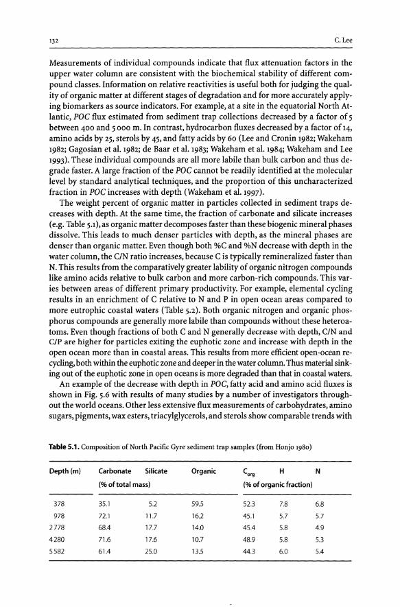
132 C.Lee
Measurements of individual compounds indicate that flux attenuation factors in the upper water column are consistent with the biochemical stability of different compound classes. Information on relative reactivities is useful both for judging the quality of organic matter at different stages of degradation and for more accuratelyapplying biomarkers as source indicators. For example, at a site in the equatorial North Atlantic, poe flux estimated from sediment trap collections decreased by a factor of 5 between 400 and 5 000 m. In contrast, hydrocarbon fluxes decreased by a factor of 14,
amino acids by 25, sterols by 45, and fatty acids by 60 (Lee and Cronin 1982; Wakeham 1982; Gagosian et al. 1982; de Baar et al. 1983; Wakeham et al. 1984; Wakeham and Lee 1993). These individual compounds are all more labile than bulk carbon and thus degrade faster. A large fraction of the poe cannot be readily identified at the molecular level by standard analytical techniques, and the proportion of this un characterized fraction in poe increases with depth (Wakeham et al. 1997).
The weight percent of organic matter in particles collected in sediment traps decreases with depth. At the same time, the fraction of carbonate and silicate increases (e.g. Table 5.1), as organic matter decomposes faster than these biogenic mineral phases dissolve. This leads to much denser particles with depth, as the mineral phases are denser than organic matter. Even though both %C and O/ON decrease with depth in the water column, the C/N ratio increases, because C is typically remineralized faster than N. This results from the comparatively greater lability of organic nitrogen compounds like amino acids relative to bulk carbon and more carbon-rich compounds. This varies between areas of different primary productivity. For example, elemental cycling results in an enrichment of C relative to Nand P in open ocean areas compared to more eutrophic coastal waters (Table 5.2). Both organic nitrogen and orsanic phosphorus compounds are generally more labile than compounds without these heteroatoms. Even though fractions of both C and N generally decrease with depth, C/N and e/P are higher for particles exiting the euphotic zone and increase with depth in the open ocean more than in coastal areas. This results from more efficient open-ocean recycling, both within the euphotic zone and deeper in the water column. Thus material sinking out of the euphotic zone in open oceans is more degraded than that in coastal waters.
An example of the decrease with depth in poe, fatty acid and amino acid fluxes is shown in Fig. 5.6 with results of many studies by a number of investigators throughout the world oceans. Other less extensive flux measurements of carbohydrates, amino sugars, pigments, wax esters, triacylglycerols, and sterols show comparable trends with
Table 5.1. Composition of North Pacific Gyre sediment trap samples (from Honjo 1980)
Depth (m) Carbonate Silicate Organic Corg H N
(% of total mass) (% of organic fraction)
378 35.1 5.2 59.5 52.3 7.8 6.8
978 72.1 11.7 16.2 45.1 5.7 5.7
2778 68.4 17.7 14.0 45.4 5.8 4.9
4280 71.6 17.6 10.7 48.9 5.8 5.3
5582 61.4 25.0 13.5 44.3 6.0 5.4

CHAPTER 5 . Particulate Organic Matter Composition and Fluxes in the Sea 133
Table S.2. Atomic ratios of C, N and P relative to P = 1 observed in sinking particles from the
Depth (m) Corg N P CoriN
northeast Pacific Ocean (from Coastal upwelling Knauer et al. 1979)
50 190 22 8.8
250 160 14 12
700 180 17 11
Coastal non-upwelling
50 260 27 9.9
250 330 33 10
700 370 25 15
Open ocean
75 410 29 14
575 460 34 13
1050 910 31 29
depth (Ittekkot 1984a,b; Repeta and Gagosian 1984; Wakeham 1982; Gagosian et al.1982). The lines shown in Fig. 5.6 are exponential regressions for flux data below 400 m. In analogy to half-lives, the Z1/2 values shown are calculated half-depths, the depth range over which half of the measured material has been lost. Compounds with smaller halfdepths are more rapidly degraded. Thus, the amino acids with Z1/2 of 600 m are lost more quickly than fatty acids with Z1/2 of 1 400 m, and both are lost more rapidly than bulk carbon with Z1/2 of 1700 m, as might be expected from their biochemical lability. This calculation of Z1/2 assumes first-order decomposition kinetics. If C is the flux of carbon, a compound class or an individual compound, then its loss with depth, z, is described as -d[C) I dz = k[C). Thus In [C) = -kz, and C = Coe-kz ,where Co is the initial flux. Then the half depth, 21/2' occurs when C I Co = 11 2. This sort of calculation makes many assumptions. First, we assume a constant sinking rate. In reality, different sized particles will sink at different rates. If we could assume that particle sinking rates, dzldt, were uniform with depth, we could estimate a decomposition rate, -d[C)ldt. However, particles originate from various sources and include different amounts of ballast materials (usually minerals), so that their sinking rates will vary greatly with location and even with depth as their ratio of organic matter to mineral content changes during decomposition and dissolution (see discussion above). Estimates of sinking rates for open ocean particles average 100-200 m d-1 (Honjo 1996). Other assumptions are that all flux is vertically downward. There is some evidence that particles rich in lipid materials can float, and if the contribution of upward to total flux were substantial, estimates of half-depths would be biased (Smith et al. 1989; Wakeham et al. 2000). Although virtually all primary production is limited to the euphotic zone, chemosynthesis can occur in anoxic parts of the water column to form new organic matter from CO2 (Karl et al. 1984). Individual compounds can also be synthesized from other compounds through alteration reactions (discussed below), resulting in local maxima or minima that are not easily modelled by first-order kinetics. A problem inherent to sediment trap methodology is that samples must be poisoned to prevent organic matter

134
Fig. 5.6. Fluxes of POC, amino acids and fatty acids for many locations (reproduced from Wakeham and Lee 1993). PARFLUX P and VERTEX IV are in the central Pacific Gyre, PARFLUX E the equatorial North Atlantic, PARFLUX S the Sargasso Sea, VERTEX I the California Current, and VERTEX II and III eastern tropical North Pacific. Lines and ZI/2 are explained in text
0 0
1000
2000
]: -£; 3000 c. QI
0
4000
5000
6000
0.01 0
1000
2000
]: -£; 3000 c. QI
Cl
4000
5000
I 6000
0.001 0
1000
2000
]: t 3000 QI
Cl
4000
5000
6000
C.Lee
POCflux (mg m-l d-') 10 100 1000 10000
o
i-
o
-z,n",1700m
.. o
Legend
• Peru Upwelling o PARFLUX P, '" PARFLUX E o VERTEX I o VERTEX II o VERTEX III • VERTEX IV o PARFLUXSz "l Panama Basin • Drake Passage
Amino acid flux (mg m-l d-') 0.1 1.0 10 100
0
Fatty acid flux (mg m-2 d-') 0.Q1
o
0.1
-o
-- zm .. l400m
10
1 10
1000
100

CHAPTER 5 . Particulate Organic Matter Composition and Fluxes in the Sea 135
decomposition before they are recovered. This treatment can result in an overestimated flux due to the collection of "swimmers:' that is, zooplankton or fish that swim into the trap and die from contact with the poison (Lee et al.1988). In shallow traps placed in coastal areas, much of the material collected can be swimmers. Technological changes in sediment traps address this problem (Peterson et al.1993; Buesseler et al. 2000).
The preferential removal of certain components, both organic and inorganic, from sinking particles leads to major changes in their composition. Decomposition and transformation rates vary depending on the molecular structure of individual compounds and their availability as substrates for heterotrophic metabolism.
5.4 Compositional Changes During Degradation
5.4.1 Initial Composition
Just as primary productivity affects the amount of material sinking in the ocean, compounds produced by plankton influence the composition of organic matter in sinking particles. Some of the organic matter produced in the euphotic zone does sink deep in the water column, eventually reaching the sediment, and the composition of this particulate organic matter can vary significantly depending on it original source. The fact that some of the original composition is preserved is the basis of using "molecular biomarkers" as indicators of the source of sedimentary organic matter. Variation in the complex biochemical composition of living organisms provides a variety of natural biomarkers. The great number and chemical diversity of biomarkers among the biochemicals typical of living organisms provides a "fingerprint" that can be used to determine sources of organic matter (Lee and Wakeham 1989; Wakeham and Lee 1989). Such fingerprints are intrinsic characteristics of organic matter; as concentrations relative to total carbon or as individual compound concentration ratios, they can be applied without many of the problems inherent in estimates of sediment trap fluxes. For example, just the presence of certain fatty acids and sterols in particles from such biologically diverse oceanic regimes as the highly-productive Peru upwelling area and the oligotrophic North Central Pacific reflects the different plankton communities found in these areas (Wakeham and Lee 1989). In addition, specific lipids can clearly distinguish marine from terrestrial sources; marine hydrocarbons and fatty acids typically have shorter carbon chain-lengths than their terrestrial counterparts. Compositional differences among carbohydrates and amino acids can also reflect biological sources, although these compound classes are usually not as source-specific as lipids and pigments. Carbohydrates and amino acids also make up a substantial amount of the organic matter in marine organisms. Some organisms like siliceous diatoms are reportedly characterized by elevated percentages of glycine and fucose, while organisms with carbonate tests like coccolithophores often exhibit unusually high concentrations of aspartic acid and arabinose (Mitterer 1968; Hecky et al. 1973; Ittekkot et al. 1984a,b). Although both plankton and bacteria are characterized by high relative abundances ofribose and fucose (Cowie and Hedges 1984), O-methyl sugars and uronic acids may provide a means of discriminating between these two important sources of organic matter (Mopper and Larsson 1978). In addition, muramic acid and certain

136 C. Lee
branched-chain fatty acids can serve as specific markers of bacteria (Lee et al. 1983; de Baar et al. 1983; Wakeham and Canuel 1988).
5.4.2 Diagenetic Indicators
Although phytoplankton producers initially dominate the organic composition of sinking particles, consumers can substantially alter this composition through degradation and alteration reactions. Not only can organic compounds be consumed, but waste products that are a structural portion of the original compound can be left behind. Or, bacteria colonizing a particle can synthesize new bacterial biomass either from the organic matter within the particle or by consuming DOC. A number of individual compounds indicate the freshness or diagenetic state of organic matter. For example, certain labile phytoplankton constituents, such as polyunsaturated fatty acids, are readily degraded in the environment and/or herbivore guts, and thus are depleted in more degraded particles (de Baar et al.1983; Wakeham and Canuel 1988). Preferential loss of labile algal fatty acids resulting in the enrichment of more stable components in the products of heterotrophic metabolism has been observed both in field studies and laboratory feeding experiments (Prahl et al. 1985; Wakeham and Canuel 1988; Harvey et al. 1987). Similarly, high relative percentages of nitrogen and carbon in the form of chromatographically-measured amino acids (Whelan 1977; Lee and Cronin 1984; Cowie and Hedges 1992) and carbohydrates (Cowie et al.1992; Cowie and Hedges 1992) are also indicative of relatively undegraded organic remains. Conversely, high relative concentrations of characteristic diagenetic products, such as the non-protein amino acids ornithine and f3-alanine can indicate the presence of bacterially degraded material (Lee and Cronin 1982,1984; Ittekkot et al. 1984a,b). Use of multiple compounds that indicate the stage of diagenesis provides a sensitive and consistent means of comparing the quality of organic matter in aquatic environments. For example, using a combination of only sixteen lipid, amino acid, pigment and carbohydrate compounds or groups of compounds, Wakeham et al. (1997) divided organic matter collected in the water column and sediment of the equatorial Pacific into four clearly-defined diagenetic classes that could be traced from sea surface to sediment (Fig. 5.7).
Freshness of organic matter can also be influenced by an intimately associated mineral or organic matrix. Resistant organic matrices may protect otherwise labile lipids. For example, waxy coatings common to land plants apparently protect higher plant alkanes, fatty acids, and fatty alcohols from degradation. Thus, terrestrial biomarkers are abundant in abyssal sediments, even though they are minor components of the particles produced in the overlying waters (Wakeham et al. 1984; Volkman et al. 1983; Gagosian et al. 1983). Marine-derived compounds seem to lack such a protective matrix and thus are preferentially degraded in the water column.
Several studies have reported that the adsorption of organic compounds serves to protect them from microbial degradation (Christensen and Blackburn 1980; Marshman and Marshall 1981; Gordon and Millero 1985). Mayer (1994) has recently postulated that adsorption of organic matter into micropores of inorganic sedimentary material might physically remove it from the action of hydrolyzing enzymes, which cannot function within the tiny pores. This mechanism may be responsible for the almost universal correlation between organic carbon content and mineral grain size observed in marine sedi-

CHAPTER 5 . Particulate Organic Matter Composition and Fluxes in the Sea
Fig. 5.7. Relative amounts of diagenetic indicators in plankton, sediment traps and sediment from the equatorial Pacific (Wakeham et al. 1997). Groups I-IV were categorized initially solely on the basis of their behaviour in the sample set, but clearly represent compounds of similar diagenetic fate. Compounds are: 1: chlorophyll a; 2: 22:6013 polyunsaturated fatty acid; 3: 20:5013 polyunsaturated fatty acid; 4: glucose; 5: 24-methylcholesta-5,24(28)-dien-3~ 01; 6: pheophorbide a; 7: galactose; 8: oleic acid; 9: cis-vaccenic acid; 10: anteiso-15:0 fatty acid; 11: 24-ethyl-choles-5-en-3~01; 12: bisnorhopane; 13: summed Cz4+C26+C28+C30 n-fatty acids; 14: summed C37+C38 methyl and ethyl, di- and tri-unsaturated alkenones; 15: glycine; 16: squalene
III IV ~ ~ r----l r----l
100
o I . II il II It. II., "'I II II
1234 5678 9101112 13141516
100
O'.UII!! U I I IY M il a II
9101112 13141516
100
~ cv 0 ' -111111 "11111 "lin II pi liE! !
~ 4 5678 9101112 13141516
'" "C § 100
.Ll <I::
0'1011 11 1111 ' " "'1" "IIpl
1 2 3 4 5 6 7 8 9101112 13141516
100
o g II ... I ' " II II "" II I I I I II J
1 2 3 4 5 6 7 8 9101112 13141516
100
o 1 2 3 4
• Pigment
9101112 13141516
Lipid 0 Sugar 0 Amino acid
137
Plankton
105m trap
l000m trap
>3500m trap
0-0.5 em sediment
10-12em sediment
ments. Hedges and Keil (1995) developed this idea further and suggested that organic matter in association with mineral material beyond that equivalent to a monolayer coating was at least partially protected from decomposition, possibly due to protection from oxygen.
Preservation of certain amino acids and sugars occurs in both siliceous and carbonate tests, as mentioned above. Organic matter is incorporated into silicate and carbonate tests during biological deposition of these minerals. For example, diatom cell walls contain a protein-silica complex (Hecky et a1.1973), whose preservation is thought to account for the increase in glycine and serine commonly observed with depth in marine particles (Siezen and Mague 1978; Lee and Cronin 1984; Muller et al. 1986).

138 C.Lee
Carbonates are often enriched in acidic amino acids, which are thought to participate in the carbonate precipitation mechanism (Lowenstam and Weiner 1989). These acidic amino acids and glycine are the dominant compounds found in deep equatorial Pacific sediment traps and sediment (Lee et aI. 2000). This material does not appear to be decomposed until it is released by dissolution of the mineral phase. The mechanism of association of organic matter to mineral grains is not well-understood and is probably multi-faceted. Simple adsorption undoubtedly plays a major role. If the mineral is terrestrially derived, adsorption could occur before deposition in the ocean; the organic coating could remain with the particle when the mineral grain enters the water, could be replaced by marine DOC, or further adsorption of marine DOC could occur. Recent work by Hedges and Keil (1999) and Keil et aI. (1997) demonstrate this process. Berner (1995) suggested that benthic animals might coat fine-grained minerals as they pass through animal guts; this process could also occur in the water column as particles pass through zooplankton guts. And, as mentioned above, organic matter could be contained within the inorganic skeletal matrices of organisms.
Individual changes with depth also occur in inorganic components of sinking particles, with material of marine and terrestrial sources behaving differently. In an example from the deep North Atlantic Ocean (Table 5.3), biogenic elements like Ca, I and Ba in particles decreased in concentration with depth. Concentrations of other biogenic elements increased slightly (Sr and Mg), or considerably (Si), but still decreased relative to AI. AI and the other terrestrial elements (K, Ti, La, V, and Co) all increased in weight percent with depth. This trend reflects the stability of lithogenic material to dissolution; this component has already been subjected to various leaching and dis-
Table 5.3. Elemental composition of sediment Element 389m 988m 3755m 5086m trap samples collected in the North Atlantic Ocean (from Si(%) 8.6 11.0 13.6 14.9 Brewer et al.198o)
AI(%) 0.8 1.3 2.9 3.6
Ca(%) 21.7 20.5 20.9 18.3
Mg(%) 0.6 0.6 0.8 0.8
Fe(%) 0.3 0.8 1.6 1.9
K(%) 0.2 0.4 0.7 0.8
Mn (ppm) 56 78 330 460
Sa (ppm) 670 658 511
Ti(ppm) 537 927 614 2176
Sr(ppm) 1354 1514 1581 1250
Cu (ppm) 29 80 129
V (ppm) 11 36 52 66
I (ppm) 219 169 132 135
La (ppm) 6.8 14.8 17.8 27.9
Sc (ppm) 0.9 2.5 4.9 6.6
Zn (ppm) 600 440 340 470
Co (ppm) 2.5 7.9 11.2

CHAPTER 5 . Particulate Organic Matter Composition and Fluxes in the Sea 139
solution processes on land and during transport. Most biogenic material, on the other hand, is formed in situ and readily begins to dissolve once the organism that formed it dies.
5.4.3 Heterotrophic Alteration
Degradation of organic matter in the sea occurs primarily through the action of bacteria and zooplankton. Biomarkers and diagenetic indicators can be used to distinguish between the presence and/or activity of each type of heterotroph.
5.4.3.1 Bacteria
Several organic compounds specific to bacteria such as muramic acid or anteiso-fatty acids can serve as specific source indicators of the presence of these organisms, as mentioned above. In the example from the equatorial Pacific shown in Fig. 5.7, several bacterial biomarkers were used to show the later stages (III and IV) of diagenesis, particularly cis-vaccenic acid and iso- and anteiso-15:0 fatty acids, which are known to have bacterial sources (Wakeham et al. 1997). These compounds were found in sinking particles throughout the water column but generally increased in relative abundance with depth. Bisnorhopane is also a bacterial biomarker, but is found only in sediments (Fig. 5-7). Bacterial biomarkers like muramic acid have been used to quantify bacterial biomass in particulate matter and sediments (King and White 1977; Moriarty 1977).
Other compounds, especially the organic nitrogen compounds, can be particularly useful as markers of bacterial alteration rather than indicators of bacterial biomass per se. For example, aspartic and glutamic acid, two commonly found amino acids in phytoplankton, decarboxylate as shown below to form non-protein amino acids that are not commonly found in phytoplankton and zooplankton. The ratios of protein to non-protein (*) amino acids (Fig. 5.8) have been used as indicators of bacterial activity in the Peru upwelling region (Lee and Cronin 1982) and the Sargasso Sea (Ittekkot et al. 1984a). These ratios can increase with depth in both water column particles and in sediments as bacteria degrade the original compounds. Another non -protein amino acid, ornithine, is a decomposition product of the protein amino acid arginine. Particulate ornithine fluxes increase with depth in the strong oxygen minimum off the coast of Mexico (Lee and Cronin 1984).
HOOC - CH2 - CH(NH2l - COOH
Aspartic acid
HOOC - CH2 - CH2 - CH(NH2l - COOH
Glutamic acid
-CO2 - H2N - CH2 - CH2 - COOH
f3-alanine*
-C02 H2N - CH2 - CH2 - CH2 - COOH
y-aminobutyric acid*
Fig. S.S. Decarboxylation of the protein amino acids, aspartic acid and glutamic acid to the nonprotein amino acids, J3-alanine and y-aminobutyric acid

140
5.4.3.2 Zooplankton
c. Lee
Consumption by zooplankton can lead to marked changes in composition between the phytoplankton food and excreted faecal pellets. Less than 5% of the carbon ingested by zooplankton ends up in faecal pellets (Copping and Lorenzen 1980), but pellets and other amorphous faecal material can be a significant part of the vertical flux, in some areas occasionally accounting for all of it (Honjo 1996). Some compounds are not altered extensively in composition during this process. Laboratory studies have shown, for example, that the amino acids in zooplankton faecal pellets are not very different from their algal food in composition (Cowey and Corner 1966; Tanoue et al.1982). Lipid compounds are much better indicators of zooplankton feeding processes. Zooplankton edit the composition of their food by selectively removing some compounds while adding others. For example, in studies using calanoid copepods feeding on a dinoflagellate, Harvey et al. (1987) found that most fatty acids in the food were assimilated, but the polyunsaturated components were preferentially metabolized. Sterols were removed less than the fatty acids, but unsaturated sterols were again removed preferentially. In similar laboratory feeding experiments, Prahl et al. (1984) also found unsaturated fatty acids and sterols to be preferentially removed from a green alga eaten by a calanoid copepod. Zooplankton faecal pellets can also be enriched in individual lipids over those present in the algal food. For example, the sterol cholesterol and wax esters, which are for the most part absent in phytoplankton, are found in faecal pellets produced by herbivores (Volkman et al. 1980; Prahl et al. 1984). These compounds are even more enriched in carnivores over their food source.
Perhaps the most well-known alteration reaction mediated by zooplankton is the conversion of chlorophyll to its degradation products, particularly pheophorbide (Shuman and Lorenzen 1975; Welschmeyer and Lorenzen 1985). Similar alteration reactions during zooplankton grazing hydrolyze the algal carotenoid esters, fucoxanthin and peridinin, to the corresponding alcohols fucoxanthinol and peridininol, as shown in Fig. 5.9 (Repeta and Gagosian 1984). These four compounds are the major carotenoids transported to the sea floor in sinking particles.
Fig. 5.9. Hydrolysis of the carotenoid pigment fucoxanthin to fucoxanthinol
Fucoxanthin
lEster hydrolysis (zooplankton)
ori-~'0 o II HO 0 HO OH
Fucoxanthinol

CHAPTER 5 . Particulate Organic Matter Composition and Fluxes in the Sea 141
5.4.4 Uncharacterized Material
In phytoplankton, most of the organic matter is made up of amino acids, carbohydrates and lipids that can be efficiently characterized at the molecular level with conventional chemical hydrolysis and chromatographic methods. Particles exported from the euphotic zone of the equatorial Pacific Ocean contain only a slightly lower proportion of characterizable material. However, the percentage of total organic matter in sinking particles that can be molecularly-characterized by conventional analysis decreases rapidly down the water column to become a minor component at depth (Fig. 5.10;
Wakeham et al.1997). Several hypotheses exist for this decrease in molecularly-resolvable organic matter during decomposition (Hedges et al. 2001). Labile intermediates released during microbial degradation ofbiomacromolecules (e.g. polysaccharides and proteins) may spontaneously recombine to form chemically complex "geopolymers" (de Leeuw and Largeau 1993). These geopolymers may be structurally too complex to analyze chemically, and they may increase preferentially with depth, because they do not degrade enzymatically. Alternatively, the biomacromolecules themselves may be in-
Fig. 5.10. Percent organic carbon in various biochemical classes within sinking particles in the equatorial Pacific Ocean (reproduced from Wakeham et al. 1997). Note the increase in the uncharacterized fraction
Plankton
105m trap
l000m trap
>3500m trap
0-0.5 cm sediment
10- 12cm sediment
Percent of organic carbon o 20 40 60 80 100
Amino acids Sugars Lipids Un characterized

142 C. Lee
trinsically resistant to biodegradation and thus may also be selectively preserved. It is also possible that refractory organic or inorganic matrices may protect intrinsically labile organic substances (Knicker et al. 1996). A key difference among these protection mechanisms is that humification and selective preservation should result in pronounced changes in organic structure, whereas protection does not require major compositional changes.
Hedges et al. (2001) used solid-state l3C NMR to investigate the composition of the bulk organic carbon used in the analyses shown in Figs. 5.7 and 5.10. They found that the major biochemical composition for bulk organic carbon was similar to that obtained by chromatographic analysis. This result fits more with the hypothesis of physical protection rather than selective preservation as described above. Several mechanisms could account for physical protection of organic matter by minerals. For example, as mentioned earlier, some organic matter is incorporated into silicate and carbonate tests during biological deposition of these minerals (Lowenstam and Weiner 1989). This material is entombed within the mineral matrix and will not be exposed to decomposing enzymes until it is released by dissolution of the mineral phase. Organic matter may also be protected on the surface of mineral particles if adsorption of the organic matter into. Mayer (1994) postulated that adsorption of organic matter into micropores of inorganic sedimentary material removes it physically from the action of large hydrolyzing enzymes. Inorganic matter makes up most of the total mass of sinking particles, so it would not be surprising if physical protection of the organic fraction by mineral components occurred.
The idea that minerals preserve associated organic matter and the fact that they are responsible for adding the ballast to particles that allows them to sink has suggested new concepts about organic matter fluxes in the ocean (Armstrong et al. 2002).
Typical mixes of organic carbon compounds have densities 1.1 times that of sea water, while the density of typical inorganic mineral ballast is about 2.5 times that of sea water. Since sinking velocities are proportional to the excess in density over that of the fluid through which particles sink, a particle that is half organic matter and half inorganic ballast will sink many times faster than a particle of comparable size composed totally of organic matter. Wind-blown dust particles, opaline silica (produced by diatoms and radiolarians), and calcium carbonate (produced by coccolithophorids and foraminifera) are the major types of mineral ballast in the world ocean (Honjo 1996). Dust, for example, does not dissolve appreciably with depth, so that organic matter adsorbed to dust will be protected during its transit to the sea floor. In contrast, organic matter external or internal to opal and carbonate tests will be subject to decomposition as the biomineral dissolves. The mineral phase with which organic material is associated may therefore affect organic carbon flux in two ways: through mineralspecific differences in the amount of organic carbon that can be protected per unit ballast mineral, and through differential dissolution of the ballast minerals themselves. These thoughts have been incorporated into a new model of organic matter decomposition in the ocean (Fig. 5.n; Armstrong et al. 2002). Considering mineral ballast and protection, a quantitative description of POC remineralization must account both for POC that is "protected" by its association with ballast and for POC that is "unprotected" from degradation. Both types of POC are assumed to be associated with the same sinking aggregates (flocs and/or faecal pellets); the same ballast would then provide the excess density needed for both types of carbon to sink. Only further research on organic-inorganic associations will allow progress in making quantitative and predic-

CHAPTER 5 . Particulate Organic Matter Composition and Fluxes in the Sea
Fig. 5.11. Depth profiles of total POC flux (solid line) and protected organic carbon flux (dashed line) are illustrated in a schematic representation. Protected flux is assumed to be proportional to ballast flux. The hatched area between the two curves is the flux of unprotected POC. Neither protected nor unprotected POC flux are measured directly; their magnitudes are inferred by fitting measured values to a model (Armstrong et al. 2002)
POCflux
143
tive models of organic matter flux that are useful over broad regions of the ocean and over seasonal and interannual time scales.
Acknowledgements
The author wishes to thank the Oceanographic Division of the u.s. National Science Foundation for supporting decades of study of particle fluxes, and Stuart Wakeham and John Hedges for their collaboration during these studies, and for constructive comments on this chapter.
References
Armstrong RA, Lee C, Hedges JI, Honjo S, Wakeham SG (2002) A new model for deep-ocean remineralization of organic carbon and mineral ballasts. Deep-Sea Res II 49:219-236
Baar HJW de, Farrington JW, Wakeham SG (1983) Vertical flux of fatty acids in the Nortil Atlantic Ocean. J Mar Res 41:19-41
Berner RA (1995) Sedimentary organic matter preservation: an assessment and speculative synthesis -a comment. Mar Chern 49:121-122
Betzer PR, Showers WJ, Laws EA, Winn CD, DiTullio GR, Kroopnik PM (1984) Primary productivity and particle fluxes on a transect of tile equator at 1530 W in the Pacific Ocean. Deep-Sea Res 31:1-11
Brewer P, Nozaki Y, Spencer DW, Fleer AP (1980) Sediment trap experiments in the deep Nortil Atlantic: Isotopic and elemental fluxes. J Mar Res 38:703-728
Buesseler KO, Steinberg DK et al. (2000) A comparison of the quantity and composition of material caught in a neutrally buoyant versus surface-tetilered sediment trap. Deep-Sea Res 47:277-294
Christensen D, Blackburn TH (1980) Turnover of tracer (C-14, H-3Iabeled) alanine in inshore marine sediments. Mar Bioi 58:97-103
Copping AE, Lorenzen CJ (1980) Carbon budget of a marine phytoplankton-herbivore system with carbon-14 as a tracer. Limnol Oceanogr 25:873-882

144 C.Lee
Cowey CB, Corner EDS (1966) The amino acid composition of certain unicellular algae, and of the faecal pellets produced by Calanus finmarchicus when feeding on them. In: Barnes H (ed) Some contemporary studies in marine science. Allen and Unwin, London, pp 225-231
Cowie GL,Hedges JI (1984) Carbohydrate sources in a coastal marine environment. Geochim Cosmochim Acta 48:2075-2087
Cowie GL, Hedges JI (1992) Sources and reactivities of amino acids in a coastal marine environment. Limnol Oceanogr 37:703-724
Cowie GL, Hedges JI, Calvert SE (1992) Sources and relative reactivities of amino acids, neutral sugars, and lignin in an intermittently anoxic marine environment. Geochim Cosmochim Acta 56:1963-1978
Deuser WG (1986) Seasonal and interannual variations in deep-water particle fluxes in the Sargasso Sea and their relation to surface hydrography. Deep-Sea Res 33:225-246
Deuser WG, Ross EH, Anderson FR (1981) Seasonality in supply of sediment to the deep Sargasso Sea and implications for the rapid transfer of matter to the deep ocean. Deep-Sea Res 28:495-505
Deuser WG, Muller-Karger FE, Evans RH, Brown OB, Esias WE, Feldman GC (1990) Surface-ocean color and deep-ocean carbon flux: How close a connection? Deep-Sea Res 37:1331-343
Eppley RW, Peterson BJ (1979) Particulate organic matter flux and planktonic new production in the deep ocean. Nature 282:677-680
Gagosian RB, SmitlI SO, Nigrelli GE (1982) Vertical transport of steroid alcohols and ketones measured in a sediment trap experiment in tlIe equatorial Atlantic Ocean. Geochim Cosmochim Acta 46:1163-1172
Gagosian RB, Volkman J, Nigrelli GE (1983) The use of sediment traps to determine sterol sources in coastal sediments off Peru. In: Bj0roy Met al. (eds) Advances in organic geochemistry 1981. John Wiley and Sons, New York, pp 369-379
Gordon AS, Millero FJ (1985) Adsorption mediated decrease in tlIe biodegradation rate of organic compounds. Microb Ecol11:289-298
Harvey JR, Eglinton G, O'Hara SCM, Corner EDS (1987) Biotransformation and assimilation of dietary lipids by Calanus feeding on a dinoflagellate. Geochim Cosmochim Acta 51:3031-3040
Hecky RE, Mopper K, Kilham P, Degens ET (1973) The amino acid and sugar composition of diatom cell-walls. Mar Bioi 19:323-331
Hedges JI, Keil RG (1995) Sedimentary organic matter preservation: an assessment and speculative syntlIesis. Mar Chern 49:81-115
Hedges JI, Keil RG (1999) Organic geochemical perspectives on estuarine processes: Sorption reactions and consequences. Mar Chern 65:55-65
Hedges JI, Baldock JA, Gelinas Y, Lee C, Peterson M, Wakeham SG (2001) Non-selective preservation of organic matter in sinking marine particles. Nature 409:801-804
Honjo S (1980) Material fluxes and modes of sedimentation in the mesopelagic and bathypelagic zones. J Mar Res 38:53-97
Honjo S (1990) Particle fluxes and modern sedimentation in the polar oceans. In: SmitlI WO (ed) Polar oceanography. Academic Press, New York, pp 687-739
Honjo S (1996) Fluxes of particles to tlIe interior of the open oceans. In: Ittekkot V, Schaefer P, Honjo S, Depetris PJ (eds) Particle flux in tlIe ocean. John Wiley and Sons, New York, pp 91-154
Ittekkot V, Deuser WG, Degens ET (1984a). Seasonality in the fluxes of sugars, amino acids, and amino sugars to tlIe deep ocean: Sargasso Sea. Deep-Sea Res 31:lO57-1069
Ittekkot V, Degens ET, Honjo S (1984b) Seasonality in the fluxes of sugars, amino acids, and amino sugars to tlIe deep ocean: Panama Basin. Deep-Sea Res 31:lO71-1083
Karl DM, Knauer GA, Martin JH, Ward BB (1984) Bacterial chemolithotropy in the ocean is associated witlI sinking particles. Nature 309:54-56
Keil RG, Mayer LM, Quay PD, Richey JE, Hedges JI (1997) Loss of organic matter from riverine particles in deltas. Geochim Cosmochim Acta 61:1507-1511
King JD, White DC (1977) Muramic acid as a measure of microbial biomass in estuarine and marine samples. Appl Environ MicrobioI33=777-783
Knauer GA, Martin JH, Bruland KW (1979) Fluxes of particulate carbon, nitrogen and phosphorus in tlIe upper water column of tlIe nortlIeast Pacific. Deep-Sea Res 26:97-lO8
Knicker H, Scaroni AW, Hatcher PG (1996) l3C and lSN NMR spectroscopic investigation on the formation of fossil algal residues. Org Geochem 24:661-669
Lee C, Cronin C (1982) The vertical flux of particulate organic nitrogen in the sea: decomposition of amino acids in tlIe Peru upwelling area and tlIe equatorial Atlantic. J Mar Res 40:227-251
Lee C, Cronin C (1984) Particulate amino acids in the sea: Effects of primary productivity and biological decomposition. J Mar Res 42:lO75-lO97
Lee C, Wakeham SG (1989) Organic matter in sea water: Biogeochemical processes. In: Riley JP (ed) Chemical oceanography, vol IX. Academic Press, New York, pp 1-51
Lee C, Wakeham SG, Farrington JW (1983) Variations in the composition of particulate organic matter in a time-series sediment trap. Mar Chern 13:181-194

CHAPTER 5 . Particulate Organic Matter Composition and Fluxes in the Sea 145
Lee C, Wakeham SG, Hedges JI (1988) The measurement of oceanic particle flux - Are swimmers a problem? Oceanography 1:34-36
Lee C, Wakeham SG, Hedges ]I (2000) Composition and flux of particulate amino acids and chloropigments in equatorial Pacific seawater and sediments. Deep-Sea Res I 47:1535-1568
Lee C et al. (1998) Particulate organic carbon fluxes: Compilation of results from the 1995 US JGOFS Arabian Sea Process Study. Deep-Sea Res 45:2489-2501
Leeuw JW de, Largeau C (1993) A review of macromolecular organic compounds that comprise living organisms an their role in kerogen, coal, and petroleum formation. In: Engel MH, Macko SA (eds) Organic geochemistry. Plenum Press, New York, pp 23-72
Lowenstam HA, Weiner S (1989) On biomineralization. Oxford University Press, New York Marshman NA, Marshall KC (1981) Bacterial growth on proteins in the presence of clay minerals. Soil
Bioi Biochem 13:127-134 Martin JW, Knauer GA, Karl DM, Broenkow WW (1987) VERTEX: Carbon cycling in the northeast Pa
cific. Deep-Sea Res 34: 267-285 Mayer LM (1994) Surface area control of organic carbon accumulation in continental shelf sediment.
Geochim Cosmochim Acta 58:1271-1284 McCave IN (1975) Vertical fluxes of particles in the ocean. Deep-Sea Res 22:491-502 Mitterer RM (1968) Amino acid composition of organic matrix in calcareous oolites. Science 162:1498-1499 Mopper K, Larsson K (1978) Uronic and other acids in Baltic Sea and Black Sea sediments. Geochim
Cosmochim Acta 42:153-163 Moriarty DJW (1977) Improved method using muramic acid to estimate biomass of bacteria in sediments.
Oecologia 26:317-323. Muller PJ, Suess E, Ungerer CA (1986) Amino acids and amino sugars of surface particulate and sedi
ment trap material from waters of the Scotia Sea. Deep-Sea Res 33:819-838 Pace ML, Knauer GA, Karl DM, Martin JH (1987) Primary production, new production and vertical flux
in the eastern Pacific Ocean Nature 325:803-804 Peterson ML, Hernes PJ, Thoreson DS, Hedges JI, Lee C, Wakeham SG (1993) Field evaluation of a valved
sediment trap. Limnol Oceanogr 38:1741-1761 Prahl FG, Eglinton G, Corner EDS, O'Hara SCM, Forsberg TEV (1984) Changes in plant lipids during
passage through the gut of Calanus. J Mar Bioi Assoc UK 64:317-334 Prahl FG, Eglinton G, Corner, EDS, O'Hara SCM (1985) Faecal lipids released by fish feeding on
zooplankton. J Mar Bioi Assoc UK 65:547-560 Repeta DJ, Gagosian RB (1984) Transformation reactions and recycling of carotenoids and chlorins in
the Peru upwelling region (150 S, 750 W). Geochim Cosmochim Acta 48:1265-1277 Sargent JR (1976) The structure, function and metabolism oflipids in marine organisms. In: Malins DC,
Sargent JR (eds) Biochemical and biophysical perspectives in marine biology, vol III. Academic Press, New York, pp 149-212
Shuman FR, Lorenzen CJ (1975) Quantitative degradation of chlorophyll by a marine herbivore. Limnol Oceanogr 20:580-586
Siezen RJ, Mague TH (1978) Amino acids in suspended particulate matter from oceanic and coastal waters of the Pacific. Mar Chern 6:215-231
Silver MW, Alldrege AL (1981) Bathypelagic marine snow: Deep-sea algal and detrital community. J Mar Res 39:501-530
Smith KL, Williams PM, Druffel ERM (1989) Upward fluxes of particulate organic-matter in the deep north Pacific. Nature 337:724-726
Suess E (1980) Particulate organic carbon flux in the oceans - surface productivity and oxygen utilization. Nature 288:260-263
Tanoue E, Handa N, Sakugawa H (1982) Difference of the chemical composition of organic matter between fecal pellet of Euphausia superba and its feed. Trans Tokyo Univ Fish 5:189-196
Volkman JK, Corner EDS, Eglinton G (1980) Transformations of biolipids in the marine food web and in underlying bottom sediments. In: CNRS (ed) Colloques internationaux du CNRS No 293. Editions CNRS, Paris, pp 185-197
Volkman JK, Farrington JW, Gagosian RB, Wakeham SG (1983) Lipid composition of coastal marine sediments from the Peru upwelling region. In: Bj0roy Met al. (eds) Advances in organic geochemistry 1981. John Wiley and Sons, New York, pp 228-240
Wakeham SG (1982) Organic matter from a sediment trap experiment in the equatorial North Atlantic: Wax esters, steryl esters, triacylglycerols and alkyldiacylglycerols. Geochem Cosmochim Acta 46:2239-2257
Wakeham SG, Canuel EA (1988) Organic geochemistry of particulate matter in the eastern tropical North Pacific Ocean: Implications for particle dynamics. J Mar Res 46:183-213
Wakeham SG, Lee C (1989) Organic geochemistry of particulate matter in the ocean: The role of particles in oceanic sedimentary cycles. Organic Geochem 14:83-96

146 C.Lee
Wakeham SG, Lee C (1993) Production, transport, and alteration of particulate organic matter in the marine water column. In: Engel MH, Macko SA (eds) Organic geochemistry. Plenum Press, New York, pp 145-169
Wakeham SG, Farrington JW, Volkman JK (1983) Fatty acids, wax esters, triacylglycerols, and alkyldiacylglycerols associated with particles collected in sediment traps in the Peru upwelling. In: Bj0roy Met al. (eds) Advances in organic geochemistry 1981. John Wiley and Sons, New York, pp 185-197
Wakeham SG, Lee C, Farrington JW, Gagosian RB (1984) Biogeochemistry of particulate organic matter in the oceans: Results from sediment trap experiments. Deep-Sea Res 31:509-528
Wakeham SG, Lee C, Hedges JI, Hernes PJ, Peterson ML (1997) Molecular indicators of diagenetic status in marine organic matter. Geochim Cosmochim Acta 61:5363-5369
Wakeham SG, Cowen JP, Burd BJ, Thomsen RE (2000) Lipid-rich ascending particles form the hydrothermal plume at Endeavour Segment, Juan de Fuca Ridge. Geochem Cosmochim Acta 65:923-939
Welschmeyer NA, Lorenzen CJ (1985) Chlorophyll budgets: Zooplankton grazing and phytoplankton growth in a temperate fjord and the Central Pacific Gyres. Limnol Oceanogr 30:1-21
Whelan JK (1977) Amino acids in a surface sediment core of the Atlantic abyssal plain. Geochim Cosmochim Acta 41:803-810

Chapter 6
Diagenesis of Organic Matter at the Water-Sediment Interface
S.Wakeham
6.1 Introduction
The water-sediment interface is an intense heterotrophic reactor through which organic matter must pass if it is to be preserved in sediments. The term "water-sediment interface" is not a simple descriptor. Strictly speaking, it implies a geometric surface between the water column and the sediments, but to a biogeo chemist it is the "zone in which organic matter is first accumulated from the water column and is initially metabolized by the sediment heterotrophic community" (Mayer 1993). The depth of this zone may range from millimetres to a metre or more, depending on the perspective of the biogeochemist and the processes involved.
The physical character of the interfacial zone is dictated by a combination of physical and chemical factors (Rhodes 1974). It is characterized by high water content, various forms of biological aggregations of mineral grains (faecal pellets, burrows etc.), horizontal and vertical mixing, resuspension, and elevated biological activity. Compared to underlying sediments, the interface is usually enriched in labile organic matter that has recently been delivered from the water column but has not yet been degraded. It is a very patchy environment on both macro- and microscales, and both chemically and biologically. Resuspension and bioturbation alter the topography and sedimentological character on a variety of time scales by mixing and redistributing particles. Living organisms are present at higher concentrations (on a volume basis) than in any other marine zone (Mayer 1993). Bacteria are present at lO3_lO4 times greater numbers and activities than in the overlying water column (Deming and Baross 1993). Most organisms in marine sediments are heterotrophs that rely on the settling of particulate organic matter from the water column and its accumulation at the interface. Feeding by macrofauna physically mixes sediments, and the degradation of organic matter by bacteria using various electron acceptors produces the marked biogeochemical zonation and gradients (redox, organic carbon content, chemical composition etc.) commonly observed in surface sediment layers. Biogeochemical processes at the water-sediment interface consume >90% of the organic carbon (DC) that rains down upon it, leaving <0.1% of the DC produced in the water column to be preserved in sediments. Chemical gradients are steep in the interfacial zone. The composition of the preserved material can be markedly different from that which is delivered.
Most changes in the concentration and composition of sedimentary organic matter take place in this interfacial zone, and it is the combined processes affecting these changes that is termed "diagenesis". Most remineralization and transformation reactions that accompany diagenesis occur because the processes yield energy for benthic organisms. Organic matter diagenesis is rapid on the geological scale, with most de-

148 S. Wakeham
composition occurring in the upper ten's of centimetres of the sediment column over time scales of months to centuries. The study of rates and mechanisms of organic matter alteration have broad implications related to energy transfer in the benthic community and organic carbon preservation and control of global atmospheric oxygen (Berner 1989).
This chapter describes some of the processes involved in diagenesis, using examples of alterations of organic matter that occur at the water-sediment interface and the types of information that these changes impart to organic biogeochemists.
6.2 Controls on Organic Matter Diagenesis
Organic matter remineralization in marine sediments (reviewed by Henrichs 1993) correlates closely with carbon rain rate, or the flux of OC to the sediments (Fig. 6.1). Rates of remineralization are higher in sediments receiving higher amounts of ~C, but the efficiency of remineralization is actually lower in rapidly accumulating sediments than in slowly depositing sediments. This inefficiency allows greater amounts of organic matter to pass through the diagenetic zone and become buried, helping to explain why many organic-rich sediments are deposited under highly productive surface waters. Further observations have found that ~C-rich sediments often are found under suboxic and anoxic waters. These findings have been interpreted as suggesting
103
102
l 1: 10' u .9 c: o ~ ~l()O ~ IV c: ~
10-' o
0 0 o
o o
o o
~~~~ o
rEP oQcg 0
~\o 000
cP 0
~o 00
o
o 0
08 o
10-2 ~I;:-;--.---r-'-''T''T'-''~'~' -;-,---" -'-, '--TI TI TI ~' f~---'----'---'rT-'I-'I-'I'TITI ~-"---r--r-'-'T'T'T'T"---'-~~ u "'" II 10-' 100 10' 102 103
Input (g C m-2 yr')
Fig. 6.1. Relationship between flux of organic carbon to the sea floor and organic carbon remineralization rate. Data are a compilation of measurements made globally (redrawn from Henrichs 1993)

CHAPTER 6 . Diagenesis of Organic Matter at the Water-Sediment Interface 149
that low bottom water oxygen concentrations retard decomposition, which then leads to accumulation of OC in sediments. The relative importance of these two factors -the supply of OC to the sea floor vs. bottom water oxygen concentration - has been hotly debated (e.g. Emerson and Hedges 1988; Calvert and Pedersen 1992; Lee 1992; Paropkari et al. 1992), and the debate has yet to be resolved (e.g. Keil and Cowie 1999; Cowie et al.1999; Granesham et al.1999). Nonetheless, there is reason to expect a coupling between the OC rain rate and water column oxygen, since higher availability of OC that can be remineralized leads to greater consumption of oxygen that produces suboxia and anoxia. An additional factor may be involved. Tegelaar et al. (1989) proposed that refractory macromolecules comprise the bulk of preserved organic matter. By this hypothesis, it is this recalcitrant macromolecular material that dominates the sedimentary OC that cannot be characterized at the molecular level (Wakeham et al. 1997; Hedges et al. 2000). In support of this concept is increasing evidence for a variety of biomacromolecules in algae and vascular plants that are resistant both to biodegradation and chemical analyses (de Leeuw and Largeau 1993). Thus, iliere may be molecular -structural factors iliat influence ilie intrinsic reactivity of organic substances.
Bacteria are major primary agents of early diagenesis (Deming and Baross 1993). They contain unique and versatile enzymes that can act on labile and refractory organic matter to satisfy their nutritional requirements. Acting in concert with each oilier and higher organisms, they produce powerful degradative systems beyond those of individual organisms. The classic description of diagenesis involves a stratification of sediments according to available oxidants that bacteria utilize in degrading organic matter to produce energy (Fig. 6.2). In reality, the situation is complicated by the fact that physiologically different types of bacteria degrade different classes of organic matter using specific oxidants, and there is considerable overlap and interaction of the zonation of the various respiratory functions, especially on the microscale. Because bacteria are unable to assimilate molecules larger than about 600 daltons, they must first hydrolyze complex molecules into simpler ones that can cross cellular membranes. End products from one functional group of bacteria are often substrates to be used by other groups in complex symbiotic relationships.
Recent research has expanded the number of mechanisms that may be involved in organic matter diagenesis to help explain changes in biochemical composition that occur during decomposition and preservation (reviewed by Hedges and Keil1995). A sorption preservation hypothesis has been developed in which intimate association of organic matter with mineral grains protects OC from degradation (Mayer 1994a,b; Keil et al. 1994a, and earlier papers cited therein). Sorption of organic matter to mineral surfaces occurs in nature and is widely used to explain both the behaviour of hydrophobic xenobiotics in nature and why otherwise labile compounds are not always rapidly degraded in sediments. The new findings show that there is covariation of %OC and sediment surface area (SA) for surface sediments from a wide variety of continental margin environments (Fig. 6.3), suggesting stabilization of intrinsically labile organic matter if it is intimately associated with mineral grains. Mayer (1994a,b) originally hypothesized that organic matter coats mineral grains in continental margin sediments in a uniform "monolayer equivalent" coating of 0.5-1.0 mg OC m-2• Sediments from non-continental margin areas have different %OCISA relationships. Some fraction of the organic matter might be found in mesopores that protect it from degradation, because the mesopores are smaller than the hydrolytic exoenzymes released
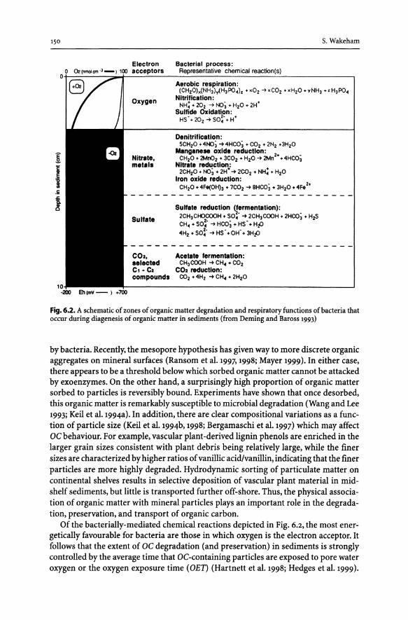
150
Electron acceptors
Oxygen
Nitrate, metals
Sulfate
C02, selected C, - C2 compounds
S. Wakeham
Bacterial process; Representative chemical reaction(s)
Aerobic respiration; (CHzOlx(NH3)y(H3P04)z + xOz -+ xCOz + xHzO + yNH3 + Z H3P04
Nitrification: NH: + 202 -+ NO; + HzO + 2H+
Sulfide Oxidation: HS' + 202 -+ SO~' + H+
Denitrification: SCH20 + 4NO; -+ 4HCO; + CO2 + 2N2 +3HzO
Manganese oxide reduction: 2+ _ CHzO + 2MnOz + 3C02 + H20 -+ 2Mn + 4HC03
Nitrate reduction: 2CH20 + NO; + 2H+ -+ 2C02 + NH: + H20
Iron oxide reduction: CHzO + 4~OHh + 7COz -+ 8HCO; + 3HzO • 4Fe 2+
Sulfata reduction (fermentation): 2CH3CHOCOOH + SO!- -+ 2CH3COOH + 2HCO; + HzS CH4 + SO~· -+ HCO; + HS' + HzO
4H2 + SO!· -+ HS' + OH-+ 3HzO
Acetate fermentation: CH3COOH -+ CH4 + CO2
C02 reduction: CO2 + 4H2 -+ CH4 + 2H20
Fig. 6.2. A schematic of zones of organic matter degradation and respiratory functions of bacteria that occur during diagenesis of organic matter in sediments (from Deming and Baross 1993)
by bacteria. Recently, the mesopore hypothesis has given way to more discrete organic aggregates on mineral surfaces (Ransom et al.1997, 1998; Mayer 1999). In either case, there appears to be a threshold below which sorbed organic matter cannot be attacked by exoenzymes. On the other hand, a surprisingly high proportion of organic matter sorbed to particles is reversibly bound. Experiments have shown that once desorbed, this organic matter is remarkably susceptible to microbial degradation (Wang and Lee 1993; Keil et al. 1994a). In addition, there are clear compositional variations as a function of particle size (Keil et al. 1994b, 1998; Bergamaschi et al. 1997) which may affect DC behaviour. For example, vascular plant-derived lignin phenols are enriched in the larger grain sizes consistent with plant debris being relatively large, while the finer sizes are characterized by higher ratios of vanillic acid/vanillin, indicating that the finer particles are more highly degraded. Hydrodynamic sorting of particulate matter on continental shelves results in selective deposition of vascular plant material in midshelf sediments, but little is transported further off-shore. Thus, the physical association of organic matter with mineral particles plays an important role in the degradation, preservation, and transport of organic carbon.
Of the bacterially-mediated chemical reactions depicted in Fig. 6.2, the most energetically favourable for bacteria are those in which oxygen is the electron acceptor. It follows that the extent of DC degradation (and preservation) in sediments is strongly controlled by the average time that DC-containing particles are exposed to pore water oxygen or the oxygen exposure time (DET) (Hartnett et al. 1998; Hedges et al. 1999).

CHAPTER 6 . Diagenesis of Organic Matter at the Water-Sediment Interface 151
8rl -------------------------------------------------------------------------,
C ",,,,' 61- .-'-
C ",,,,,"" .-.-.-
.-'-.-.-
~ 4 ~ ~.-//,-/ « ~ "tfe'f ( (fIt.
~ I!-"'- B 21- ~ .-
.","''''C .-
.-.-'- (=0.96
ssa .L.8 m = 0.76 mg OC m-2 ,.-1 oL5~ I
o ~ ~ ~ 100
Surface area (m2 g-l)
Fig. 6.3. Weight percent of organic carbon vs. mineral surface area for bulk (B), sand (S) silt (L), and clay (e) fractions of suspended sediment from the Columbia River estuary and the Washington continental margin (redrawn from Keil et al. 1994b; Hedges and Keil1995)
Several lines of evidence support the OET hypothesis. Studies of a deep-sea turbidite characterized by an oxidation front (the Madeira Abyssal Plain (MAP) f-turbidite) clearly implicate molecular oxygen as a key agent in organic matter degradation (Keil et al.1994c; Cowie et al.I995).As the MAP f-turbidite was laid down some 140 000 years ago, the slumping sediment was thoroughly mixed mineralogically and presumably chemically. Following deposition, the upper half-metre of the turbidite was exposed to bottom water oxygen for about 10000 years before being "capped" by the next deposit that returned the turbidite to a suboxic state. There has been marked degradation of organic matter in the oxidized zone compared to the unoxidized zone. Remineralization across the oxidation front of the MAP f-turbidite has removed >75% of the organic carbon initially deposited, producing sharp organic gradients across the redox front. The role of O2 in organic matter degradation has been strengthened by further study on recent continental margin sediments (Hedges and Keil1995; Hartnett et al.1998; Hedges et al.1999). In a transect across the Washington continental margin, slope and adjacent abyssal plain, measurements of penetration of O2 into surface sediment along with sediment accumulation rates allowed calculation of OET (Hedges et al. 1999). There was a marked increase in OETin the farther off-shore sediments (Fig. 6.4) that corresponded with decreased OC concentrations and organic carbon/surface area ratios. Combined with molecular analyses, these results clearly indicate that exposure of OC to oxygen and hence organic matter degradation increased off-shore. Although the implication is that molecular O2 ins the main oxidant, other electron acceptors (e.g. Fe and Mn) might also be involved and produce similar trends.

152
Fig. 6.4. Oxygen exposure times (GET) calculated for surface sediments off the coast of Washington State plotted vs. distance off-shore. Numbers refer to station numbers (redrawn from Hedges et al.1999)
1200
~ E ''::; 800 ~ ::I
I ON 400
0' lQ
0
S. Wakeham
19 ~
3
50 100 150 200 Distance offshore (kmJ
The relative reactivity or recalcitrance of organic matter seems to depend on intrinsic molecular structure. Unsaturated compounds tend to be more rapidly degraded than saturated ones; straight-chained molecules are more reactive than branched and cyclic compounds; the presence ofheteroatoms (N, S, and 0) sometimes inhibits decomposition. To better explain these trends, Hedges and Keil (1995) have described an oxygen-sensitive organic matter (OSOM) model in which there are (at least) three forms of organic matter in sediments. Materials such as charcoal are totally refractory. An oxygen sensitive fraction, lignin for example, degrades slowly in the presence of oxygen but not at all under anoxic conditions. Hydrolysable molecules such as proteins and polysaccharides are readily degraded regardless of conditions. Some combination of remineralization of these three types of ~C, albeit on very different time scales, is additive in proportion to their abundance, generating the DC profiles observed in sediments (Fig. 6.5). The OSOM model is an extension of earlier work (Skopintsev 1981) that had suggested that algal organic matter did not degrade as a single pool but rather as a composite of multiple rates among the various classes of organic components. Subsequent work by Westrich and Berner (1984) led to a multi-first order model (the multi G model) that described decomposition of multiple pools of carbon. Experimental evidence has strengthened the multi G model (e.g. Hedges and Keil1995; Sun and Wakeham 1994) and it is now widely used by biogeo chemists. Examples of diagenetic trends in molecular indicators are discussed below. Note that the OSOM model relies on molecular properties as a key determinant of organic degradation rates, whereas the sorption model is largely based on sediment surface area, although the two are certainly not mutually exclusive.
6.3 Compositional Changes Resulting from Organic Matter Diagenesis
Diagenetic alteration of organic matter can be tracked using bulk elemental parameters or by the behaviour of organic biomarkers in the sediments. Elemental compositions provide information on behaviour of bulk organic matter but offer relatively little insight into the fate of different biochemical fractions of the bulk material. Organic biomarkers offer the advantage of often being source-specific (de Leeuw and

CHAPTER 6 . Diagenesis of Organic Matter at the Water-Sediment Interface 153
%OC o 0.2
o
2
E 3 ..:!.
a ~ 4
5
6
7
0,
%OC o 0.2 0.4
Olf----
0.
3
4
5
6
7
%OC o 0.2 0.4
0ir- _ .. 1 o
Of
2 2
3 3
4 4
5 5
6 6
7 7
o Total%OC
0.2 0.4 0.6 0.8 1.0
>52
I ! I I I
I I I
I 1/2 o Zo,
Fig. 6.5. Model-derived profiles of percent organic carbon for three different organic carbon fractions, including refractory (0,), oxygen sensitive (Ox), and fermentable (Of) fractions (redrawn from Hedges and Kei11995)
Largeau 1993), and because analyses are made at the molecular level, it is often possible to follow the fate of specific compounds as they are either being degraded, produced, or structurally-altered during diagenesis. On the other hand, biomarkers often represent a very small fraction of the overall organic pool so that the picture obtained may be narrow in scope.
6.3.1 Elemental Compositions
Biogeochemists have long recognized that bulk organic carbon (OC) and total nitrogen (TN) concentrations and their atomic ratio [(CIN)a] could be used as indicators of diagenesis (e.g. Muller and Suess 1979). Typically OC and TN weight percentages decrease with increasing depth of burial as organic matter is remineralized. The atomic ratio C/N(a) increases as nitrogen-containing species are preferentially used relative to carbon.
An example of trends in OC and TN attending diagenesis in surface sediments and the potential role of oxygen availability in degradation can be found in a series of cores collected on the continental margin of the Black Sea (Cowie and Hedges 1991). Five box cores were collected along a 10 km transect that crossed the chemocline (redox boundary between oxic surface waters and anoxic bottom waters), thus giving a range of bottom water oxygen concentrations (Fig. 6.6). The assumption in this comparison, based on the proximity of the set of cores to each other, is that the organic matter

154
0.4
0.3
l c:
l c:
8.
S. Wakeham
- Inshore --. 4 14
0"""",
3 """"" CL""""
l' // //
.... ,,-/
13
12
e 0.2 .& ~ 2
.!:! /
// //
~ ·2 iii
~
0.1
c: III E' o //
b. ........ _-_._._._. __ ._ ..... _ .... .t:s.
___ Organic carbon
-0- Total nitrogen
··b·· (ON).
11
10
o o 9
Station B54-15
Depth (m) 198
Oxygen (mll-1) 0
B54-16B 160
0.05*
B54-16 128
0.68
B54-17 97
1.27
..
Fig. 6.6. Organic carbon and total nitrogen concentrations and atomic C/N ratios for fluff samples from sediment cores spanning the oxic/anoxic interface in the Black Sea. Also shown are the water depths and bottom water dissolved oxygen concentrations overlying the cores (redrawn from Cowie and Hedges 1991)
delivered to the sediments is uniform across the transect and differences in organic composition reflect different processes as a function of oxygen content. Decreasing OC and TN concentrations and increasing C/N(a) of interfacial "fluff" samples from the deepest, anoxic (BS4-15) to the shallowest, most oxygenated (BS4-17) coring stations are consistent with typical diagenetic trends. Accordingly, the extent of degradation in the fluff material varied with oxygen availability. OC and TN concentrations were also determined as a function of depth in the five cores (Fig. 6.7). OC and TN generally decreased with depth in the core and with bottom water oxygen present. For all five cores, there were substantial decreases in wt% OC and TN between the fluff layer and the underlying 0-0.5 em sediment, confirming that most degradation takes place near the water-sediment interface.
Laboratory simulations have been useful for evaluating changes in elemental composition during organic matter diagenesis and possible effects of oxic and anoxic conditions on decomposition, although results regarding oxygen have been equivocal (Henrichs 1993). In a recent study, Harvey et al. (1995) examined the decay of two marine phytoplankton, the diatom Thallasiosira weissflogii, and the cyanobacterium Synechococcus sp., by measuring particulate organic carbon (POC), particulate organic nitrogen (PON) and biochemical compositions (discussed below) in oxic and anoxic treatments over the 3-month time-course of the experiment. First order decay con-

CHAPTER 6 • Diagenesis of Organic Matter at the Water-Sediment Interface 155
a Organic carbon ('Yo) 0.0 1.0 2.0 3.0 4.0
Fluff I t.o Cl • J
E .!:!. ~
0-01 o
o I ( I Jt.-t' 'w:::: .
10
20
30
40
. &f' 4~6;" !! ~/ ~<:i.
,. I /1 I '91 O· I
: I I
i a. 90,' 1. : I : I : I [),
1 •
50 +1--~~--~~--r-~--r--+
b Total nitrogen ('Yo) 0.0 0.1 0.2 0.3 0.4
-AO-----o- n ox'.:J:' .::
. .,rt ~~:;':"
1// '-Ilia • :, I :. I
:6 I 1;)1 I • . I
/ 9. I
¢ . 4' : 0,' \ . i 1 : 1 : 1 0,
1 • _____ B54-15
- - e- - 854-26 •..• -{]-..... B54-16B - . -0- .- B54-16 ........ -6, ...... B54-17
o
10
20
30
40
• I 50
o "' 'S :::T
" ~
Fig. 6.7. Elemental compositions for Black Sea cores along a transect crossing the chemocline; a %OC; b %TN (redrawn from Cowie and Hedges 1991)
stants were significantly higher for both pac and paN under oxic conditions, and loss of nitrogenous material occurred preferentially to loss of carbon (Table 6.1). The absence of oxygen clearly resulted in slower decay for the phytoplankton and incomplete decomposition of the organic carbon pool, despite the observation that both bacterial abundances and metabolism were similar in the two treatments.
A very different approach was used by Lee (1992). Radiolabelled tracer compounds were used to compare aerobic and anaerobic microbial metabolism of organic substances. Differences in observed intrinsic rates of decomposition between the systems were small, but different compounds had very different labilities, suggesting a molecular structural effect. A significant observation was that high decomposition rates could occur when rate constants are low in situations when substrate concentrations are high. Thus, it is necessary to know botlI substrate concentrations and composition when decomposition rates are being calculated. Differences in apparent organic matter degradation between oxic and anoxic systems were postulated to be related to the presence of protozoa and meiofauna that graze bacteria (i.e. the microbial loop in sediments) in oxic systems and thus help increase the efficiency of remineralization. The absence of such grazers in anoxic systems may allow for greater sequestration of organic matter as bacterial biomass, thus leading to greater carbon preservation.

156 S. Wakeham
Table 6.1. Experimentally determined first order decay constants (k, yr -1) and regression coefficients for particulate organic carbon, nitrogen and major biochemical fractions during oxic and anoxic phytoplankton decay. Data from Harvey et al. (1995)
Biochemical fraction Oxic Anoxic
k(yr-') 2 k(yr-') 2 RatioO/A r r
T. weissflogii
POC 12.8 0.90 2.9 0.77 4.4
(19.5)a 0.97 (5.3)a 0.88 3.7
PON 17.3 0.95 3.5 0.88 4.9
(24.0)a 0.98 (5.4)a 0.93 4.4
Lipid 8.3 0.88 2.7 0.60 3.1
(13.1)a 0.96 (5.5)a 0.80 2.5
Protein 21.1 0.97 15.3 0.83 1.4
Carbohydrate 33.7 0.88 7.2 0.88 4.7
Synechococcus sp.
POC 15.3 0.91 2.5 0.85 6.2
PON 14.7 0.74 3.0 0.90 4.9
Lipid 8.2 0.82 2.3 0.79 3.6
Protein 22.0 0.85 6.2 0.90 3.5
Carbohydrate 34.2 0.84 4.1 0.65 8.3
a Initial decay constants observed over first 41 d for oxic decay and first 92 d of anoxic incubations.
6.3.2 Biomarkers
Compound-specific biochemical compositions provide further evidence of the effects and degree of diagenetic alteration of organic matter. Like %OC and TN, concentrations of amino acids, sugars and lipids generally decrease over time in laboratory experiments or with depth in the sediment. Normalizing amino acid, sugar and lipid concentrations to %OC provides a means of gauging the relative reactivities of these biochemical classes compared to OC. Doing so clearly shows that the classes are usually more labile than bulk OC - implying some unidentified fraction that is more stable in the bulk OC - and that they exhibit differential reactivities relative to one another (Cowie 1990; Cowie and Hedges 1991; Lee 1992; Harvey et al.1995). For example, in the Black Sea study of Cowie (1990), amino acids were preferentially degraded relative to OC in the fluff samples, but sugars were less affected. Amino acid and sugar concentrations were distinctly higher in fluff layers than in underlying sediments and concentrations gradually decreased with depth and under oxygenated bottom waters, providing further evidence of in situ sedimentary diagenesis. In the Harvey et al. (1995) laboratory study, carbohydrates were decomposed most rapidly under oxic conditions followed by protein and then lipids (Table 6.1). Under anoxic conditions, proteins were

CHAPTER 6 . Diagenesis of Organic Matter at the Water-Sediment Interface 157
most labile. The ratio of carbohydrate:protein metabolism decreased from 15 during aerobic decomposition to 3 during anaerobic decomposition. These trends were interpreted as resulting from a metabolic shift in microbial community under anoxic conditions in favour of protein metabolism over that of carbohydrates.
In a follow-up of the Harvey et al. (1995) study described above, Harvey and Macko (1997) reported on the kinetics oflipid decay at the molecular level. Aerobic degradation had a significantly greater effect on total lipids and individual compounds than anaerobic decomposition (Table 6.2). At the individual compound level, there were significant differences in behaviour that appear related in part to molecular structure. Unsaturated lipids degraded faster than saturated counterparts, and in the case of polyunsaturated fatty acids, removal was complete under both oxic and anoxic conditions. Unsaturation is certainly an important control that regulates the lability of many
Table 6.2. Experimentally determined first order decay constants (k, yr-1) and regression coefficients for particulate organic carbon, total lipid and major lipid classes during oxic and anoxic decay of dia-tom and cyanobacterial cells* (Data from Harvey and Macko 1997)
Biochemical fraction Oxic Anoxic RatioO/A
k (yr-') 2 k (yr-') 2 r r
T. weissflogii
POC 12.8 0.90 2.9 0.77 4.4
(19.5)a 0.97 (5.3)a 0.88 3.7
Total lipid 8.3 0.88 2.7 0.60 3.1
(13.1)a 0.96 (5.5)a 0.80 2.5
Algal fatty acids 30.1* 0.83 9.0' 0.84 3.4
Saturated 25.7 0.86 8.2 0.88 3.1
Monounsaturated 37.4 0.68 9.3 0.80 4.0
Polyunsaturated 34.3 0.82 13.6 0.82 2.5
Sterols 33.4 0.93 2.6 0.81 12.8
Phytol 31.9 0.88 3.0 0.64 10.6
Alkenes (21:6 - 21 :5) 41.6 0.73 10.5 0.88 4.0
Synechococcus sp.
POC 15.3 0.91 2.5 0.85 6.2
Total lipid 8.2 0.82 2.3 0.79 3.6
Algal fatty acids 23.0 0.84 4.2 0.88 5.5
Saturated 23.1 0.82 3.3 0.82 7
Monounsaturated 24.3 0.59 9.3 0.78 2.6
Phytol 15.2 0.82 3.4 0.75 4.5
Heptadecene 7.4 0.32 6.4 0.82 1.2
Regression calculations are based on cell death at day 5 and day 9 for T. weissfiogii and Synechococcus sp., respectively.
a Rate observed over the first 41 d for oxic and 92 d for anoxic incubations.
158 S. Wakeham
lipids. Sterols were generally more stable than fatty acids and displayed the largest reduction in degradation rate when oxygen was absent. These trends could help account for the fact that unsaturated lipids are particularly vulnerable to loss, and ratios of fatty acid:sterol decrease during diagenesis as observed in field studies (e.g. Kawamura et al.1980; Sun and Wakeham 1994; Canuel and Martens 1996). Remarkably, degradation patterns for lipids common to the two phytoplankton used by Harvey and Macko (1997) (Thallasiosira weissflogii and Synechococcus sp.) were not always similar, suggesting that factors other than molecular structure might affect the degradation rate. Furthermore, the proportion of total lipids that could be identified and quantified as individual compounds decreased with the degree of degradation, with the result that only a small fraction (18-24%) of lipids could be identified after the majority of pac and lipids were degraded. This loss of identifiable biochemicals has been described previously (e.g. Wakeham et al.1997; Hedges et al. 2000), to the extent that the origin, reactivity and fate of a large amount of OC remains obscure.
Diagenesis not only results in absolute loss of organic compounds via degradation, but it is accompanied by changes in ratios of compounds as a function of their relative lability or due to in-growth of diagenetic products at the expense of precursors. Organic matter degradation is accompanied, for example, by decreases in weight percentages of glucose among total aldoses, but increases in percentages of the deoxy sugars, rhamnose and fucose (Hamilton and Hedges 1988; Cowie et al. 1992). Increases in mole-percentages of the non-protein amino acids f3-alanine plus y-aminobutyric acid (Henrichs et al. 1984; Cowie et al. 1995) also occur. In a detailed study of amino acids in sediments from the Peru upwelling region, Henrichs et al. (1984) detected high concentrations of p-aminoglutaric acid, a nonprotein isomer of glutamic acid. Although a specific source was not identified, increasing ratios of f3-aminoglutaric acid:glutamic acid with depth in sediment cores (Fig. 6.8) strongly suggested an in situ bacterial source.
Among lipids, ratios of unsaturated to saturated fatty acids typically decrease down core (Fig. 6.9), because as noted above, unsaturated fatty acids that are derived from phytoplankton are more susceptible to degradation in sediments than are saturated acids (Kawamura et al.1980; Sun and Wakeham 1994; Canuel and Martens 1996). From profiles such as these, it is uncertain whether the unsaturated fatty acids are oxidized partially and removed from the fatty acid "analytical window:' remineralized completely to CO2, or hydrogenated in situ to their unsaturated analogs. Branched-chain fatty acids (e.g. iso- and anteiso-C1S and C17) that are common in bacterial cell membranes (Kaneda 1991) are often found to increase in relative abundance in sediments as diagenesis progresses. Enrichments in branched-chain fatty acids are widely used as indicators of bacterial alteration of organic matter (Perry et al. 1979). However, the reliance on branched-chain fatty acids as bacterial indicators must be tempered by the fact that many aerobic bacteria do not produce these compounds, so in situations where aerobic microbial decomposition is intense, branched-chain fatty acids may not be particularly abundant (Wakeham 1995). Branched-chain fatty acids at best may be semiquantitative indicators of bacterial biomass but are poor indicators of bacterial activity.
Sterols are popular biomarkers, because as a group they represent a wide variety of molecular structures that are remarkably useful as source indicators and because alterations to the sterol skeleton can be readily followed with the analytical tools avail-

CHAPTER 6 . Diagenesis of Organic Matter at the Water-Sediment Interface
J3-aminoglutaric / glutamic acid ratio
o 0.2 0.4 0.6 0.8 1.0 1.2 01 ix Lf 0
10
20
E 30 ~ .s::. a IV o 40
50
60
70
X .0 X <»
OX. "(5-
l
+ +
+
X 0
+ STA4 o STA5A X STA6 o STA8 • STA2A
o o
X + X
o
+
X +
0+
o
+
1.4
159
1.6 1.8
o
o X
o
+0
o
+
+
Fig. 6.8. Variation in the relative abundance of dissolved free glutamic acid and J3-aminoglutaric acid in sediment cores from the Peru upwelling region (redrawn from Henrichs et al. 1984)
Fig. 6.9. Ratios of unsaturated fatty acids to their saturated counterparts in sediments of Lake Haruna, Japan (adapted from Kawamura et al.1980) 3
5
~ 7 .t: a 9 IV
~ 11
813 15
Ratio of unsaturated to saturated fatty acid
0.1 0.5 1
Lake Haruna a-, ,
.-.-",",0
if"' .-
" o \
b .-0"
18:3 18:2 16:1 18:1 18:0 18:0 16:0 18:0
'0 .-
5
_-0
able to organic geochemists. Sterols are more reactive than bulk ~C, such that sterol concentrations decrease during diagenesis relative to total organic carbon. However, sterols are generally less reactive than fatty acids and alcohols. Sterol diagenesis is often

160 S. Wakeham
accompanied by bacterial conversion of stenols, the unsaturated biological form of most sterols, into stanols, the hydrogenated analogue (Gaskell and Eglinton 1975;
Nishimura 1978), and subsequently by dehydration of stanols to sterenes, the steroidal hydrocarbons (Wakeham et al. 1984). Stenol:stanol ratios that decrease with depth in sediments (Fig. 6.10) are generally interpreted in terms of production of the hydrogenated stanol product at the expense of the unsaturated precursor stenol. This transformation appears to occur more readily under reducing conditions than in oxidizing environments, and is often used as evidence that the sediments are anoxic. However, since low amounts of stanols are also present in phytoplankton, the same sediment profile might just as convincingly be interpreted as resulting from selective preservation of the more stable saturated stanols (Nishimura and Koyama 1977).
One strength of the biomarker approach is in the ability to determine detailed compound chemical structures that can be informative for tracing diagenetic alteration processes at the molecular level. However, relatively few examples of biogenic precursor-diagenetic product relationships have been reported. The sedimentary conversion offucoxanthin to loliolide (Repeta 1989) is one such case. Fucoxanthin (Fig. 6.11) is a major diatom carotenoid and a dominant pigment in diatomaceous sediments of the Peru upwelling region. Fucoxanthin concentrations decrease rapidly in upper layers of sediment cores. At first glance, the depth profile could be interpreted as being con-
Fig. 6.10. Down core changes in total organic carbon (TOC) concentration and the ratio of stenols to stanols in sediments of Lake $uwa, Japan (adapted from Nishi-mura and Koyama 1977)
E ~
!!! 0 u .5 .s::. .... Co Qj
0
50
100
150
Stenol/Stanol
3
3
TOC(%)
5
5
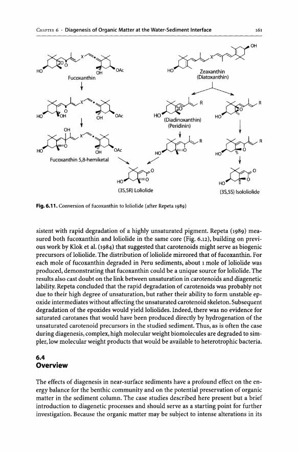
CHAPTER 6 . Diagenesis of Organic Matter at the Water-Sediment Interface 161
~X~·n "'0 ~ "'" " 0
HO OH OAe
Fucoxanthin
t
~X~·n :;/ """ "'" o ~
HO OH OH OAe
+
~x~OO HO~~ -
~eaxanthin (Dlatoxanthin)
~ ><q,},,/ R
HO~O~ -
(Diadinoxanthin) (Peridinin)
f ~R
HO~R ~
~OH X~.~ 111110"" M
HO OH OAe
Fucoxanthin 5,8-hemiketal ~
HO~II"b /
~R Ho~b -
t ~O
Ho~b ~O
HO~II"O (3S,5R) Loliolide
Fig. 6.11. Conversion of fucoxanthin to loliolide (after Repeta 1989)
(35,55) Isololiolide
sistent with rapid degradation of a highly unsaturated pigment. Repeta (1989) measured both fucoxanthin and loliolide in the same core (Fig. 6.12), building on previous work by Klok et al. (1984) that suggested that carotenoids might serve as biogenic precursors of loliolide. The distribution of loliolide mirrored that of fucoxanthin. For each mole of fucoxanthin degraded in Peru sediments, about 1 mole of loliolide was produced, demonstrating that fucoxanthin could be a unique source for loliolide. The results also cast doubt on the link between unsaturation in carotenoids and diagenetic lability. Repeta concluded that the rapid degradation of carotenoids was probably not due to their high degree of unsaturation, but rather their ability to form unstable epoxide intermediates without affecting the unsaturated carotenoid skeleton. Subsequent degradation of the epoxides would yield loliolides. Indeed, there was no evidence for saturated carotanes that would have been produced directly by hydrogenation of the unsaturated carotenoid precursors in the studied sediment. Thus, as is often the case during diagenesis, complex, high molecular weight biomolecules are degraded to simpler, low molecular weight products that would be available to heterotrophic bacteria.
6.4 Overview
The effects of diagenesis in near-surface sediments have a profound effect on the energy balance for the benthic community and on the potential preservation of organic matter in the sediment column. The case studies described here present but a brief introduction to diagenetic processes and should serve as a starting point for further investigation. Because the organic matter may be subject to intense alterations in its

162
Fig. 6.12. Distributions of fucoxanthin and loliolide in a sediment core from the Peru upwell-ing region (redrawn from Repeta 1989)
:[ "K ~
o Concentration (IImoles gdW-l)
1
01 ~ ~
5
10
Fucoxanthin(ol)
15
s. Wakeham
2
composition, it is critical to evaluate these changes and the environmental factors involved both in the context of contemporary biogeochemical cycles and as a means of coupling the aquatic water column with the underlying sediment record in order to obtain realistic palaeoenvironmental reconstructions. Vital information can be obtained both at the bulk elemental and at the molecular levels, although the perspectives they present can be clearly different. Bulk compositions provide a view of the behaviour of a large fraction of the organic matter but are incapable of describing what happens to specific biochemical fractions that often are highly variable in reactivity. Analyses of biomarkers point out how specific biochemical fractions behave, but because they are only a small part of the bulk material, biomarkers may provide a very narrow perspective to organic matter diagenesis. Clearly, however, both approaches are needed.
Acknowledgements
Cindy Lee provided valuable comments that improved this paper. Support by the National Science Foundation is acknowledged during the preparation of this review.
References
Bergarnaschi BA, Tsamakis E, Keil RG, Eglinton T, Montluyon DB, Hedges JI (1997) The effect of grain size and surface area on organic matter, lignin and carbohydrate concentrations and molecular compositions in Peru Margin sediments. Geochim Cosmochim Acta 61:1247-1260
Berner RA (1989) Biogeochemical cycles of carbon and sulfur and their effect on atmospheric oxygen over Phanerozoic time. Paleoceanogr Paleoclimatol Paleoecol 73:97-122

CHAPTER 6 . Diagenesis of Organic Matter at the Water-Sediment Interface 163
Billen G (1982) Modelling the processes of organic matter degradation and nutrients in sedimentary environments. In: Nedwell DB, Brown CM (eds) Sediment microbiology. Academic Press, New York, pp 15-52
Canuel EA, Martens CS (1996) Reactivity of recently deposited organic matter: Degradation of lipid compounds near tlIe sediment water interface. Geochim Cosmochim Acta 60:1793-1806
Calvert SE, Pedersen TF (1992) Organic carbon accumulation and preservation in marine sediments: How important is anoxia? In: Whelan J, Farrington JW (eds) Organic matter. Univ. Press, New York, pp 231-263
Cowie GL (1990) Marine organic diagenesis: A comparative study of amino acids, neutral sugars, and lignin. PhD dissertation, University of Washington, Seattle
Cowie GL, Hedges JI (1991) Organic carbon and nitrogen geochemistry of Black Sea surface sediments from stations spanning tlIe oxic/anoxic boundary. In: Izdar E, Murray JW (eds) Black Sea oceanography. Kluwer Academic Publishers, Dordrecht, pp 343-359
Cowie GL, Hedges JI, Calvert SE (1992) Sources and relative reactivities of amino acids, neutral sugars, and lignin in an intermittently anoxic sediment. Geochim Cosmochim Acta 56:1963-1978
Cowie GL, Hedges JI, PralIl FG, Lange GJ de (1995) Elemental and major biochemical changes across an oxidation from in a relict turbidite: A clear-cut oxygen effect. Geochim Cosmochim Acta 59:33-46
Cowie GL, Calvert SE, Pedersen TF, Schulz H, Rad U von (1999) Organic content and preservational controls in surficial shelf and slope sediments from tlIe Arabian Sea (Pakistan margin). Mar GeoI161:23-38
Deming JW, Barros JA (1993) The early diagenesis of organic mater: Bacterial activity. In: Engel MH, Macko SA (eds) Organic geochemistry - principles and applications. Plenum Press, New York, pp 119-144
Emerson S, Hedges JI (1988) Processes controlling the organic carbon content of open ocean sediments. Paleoceanogr 3:621-634
Gaskell SJ, Eglinton G (1975) Rapid hydrogenation of sterols in a contemporary lacustrine sediment. Nature 254:209-211
Graneshram RS, Calvert SE, Pederson TF, Cowie GL (1999) Factors controlling the burial of organic carbon in laminated and bioturbated sediments off NW Mexico: Implications for hydrocarbon preservation. Geochim Cosmochim Acta 63:1723-1734
Hamilton SE, Hedges JI (1988) The comparative geochemistries of lignins and carbohydrates in an anoxic fjord. Geochim Cosmochim Acta 52:129-142
Hartnett HE, Keil RG, Hedges JI, Devol AH (1998) Influence of oxygen exposure time on organic carbon preservation in continental margin sediments. Nature 391:572-574
Harvey HR, Macko SA (1997) Kinetics of phytoplankton decay during simulated sedimentation: changes in lipids under oxic and anoxic conditions. Org Geochem 27:129-140
Harvey HR, Tuttle JH, Bell JT (1995) Kinetics of phytoplankton decay during simulated sedimentation: Changes in biochemical composition and microbial activity under oxic and anoxic conditions. Geochim Cosmochim Acta 59:3367-3377
Hedges JI, Keil RG (1995) Sedimentary organic matter preservation: An assessment and speculative synthesis. Mar Chern 49:81-115
Hedges JI, Hu FS, Devol AH, Hartnett HE, Tsamakis E, KeiI RG (1999) Sedimentary organic matter preservation: A test for selective degradation under oxic conditions. Am J Sci 299:529-555
Hedges JI, Eglinton G., Hatcher PG et al. (2000) The molecularly-uncharacterized component of nonliving organic matter in natural environments. Org Geochem 31:945-958
Henrichs SM (1993) Early diagenesis of organic matter: The dynamics (rates) of cycling of organic compounds. In: Engel MH, Macko SA (eds) Organic geochemistry - principles and applications. Plenum Press, New York, pp 101-115
Henrichs SM, Farrington JW, Lee C (1984) Peru upwelling region sediments near IS° S. 2. Dissolved free and total hydrolyzable amino acids. Limnol Oceanogr 29:20-34
Kaneda T (1991) Iso and anteiso-fatty acids in bacteria: Biosynthesis, function, and taxonomic significance. Microbiol Rev 55:288-302
Kawamura K, Ishiwatari R, Yamazaki M (1980) Identification of polyunsaturated fatty acids in surface lacustrine sediments. Chern GeoI28:31-39
Keil RG, Cowie GL (1999) Organic matter preservation tlIrough the oxygen deficient zone of the NE Arabian Sea as discerned by organic carbon:mineral surface area ratios. Mar GeoI161:12-22
Keil RG, Montluc;:on DB, PralIl FG, Hedges JI (1994a) Sorptive preservation of labile organic matter in marine sediments. Nature 370:549-552
Keil RG, Tsamakis E, Fuh CB, Giddings JC, Hedges JI (1994b) Mineralogical and textural controls on organic composition of coastal marine sediments: Hydrodynamic separation using SPLITT fractionation. Geochim Cosmochim Acta 57:879-893
Keil RG, Hu FS, Tsamakis E, Hedges JI (1994c) Pollen degradation in marine sediments as an indicator of oxidation of organic matter. Nature 369:639-641

164 S. Wakeham
Keil RG, Tsamakis E, Giddings JC, Hedges JI (1998) Biochemical distribution (amino acids, neutral sugars and lignin phenols) among size classes of modern marine sediments from the Washington coast. Geochim Cosmochim Acta 62:1347-1364
Klok J, Baas M, Cox HC, Leeuw JW de, Rijpstra WIC, Schenck PA (1984) Loliolides and dihydroactinidiolides in a recent marine sediment probably indicate a major transformation pathway of carotenoids. Tetra Lett 1984:5577-5580
Lee C (1992) Controls on organic carbon preservation: The use of stratified water bodies to compare intrinsic rates of decomposition in oxic and anoxic systems. Geochim Cosmochim Acta 56:3323-3335
Leeuw JW de, Largeau C (1993) A review of macromolecular organic compounds that comprise living organisms and their role in kerogen, coal, and petroleum formation. In: Engel MH, Macko SA (eds) Organic geochemistry - principles and applications. Plenum Press, New York, pp 23-72
Mayer L M (1993) Organic matter at the sediment-water interface. In: Engel MH, Macko SA (eds) Organic geochemistry - principles and applications. Plenum Press, New York, pp 171-184
Mayer LM (1994a) Surface area control of organic carbon accumulation in continental shelf sediments. Geochim Cosmochim Acta 58:1271-1284
Mayer LM (1994b) Relationships between mineral surface and organic carbon concentrations in soils and sediments. Chern Geolll4:347-363
Mayer LM (1999) Extent of coverage of mineral surface by organic matter in marine sediments. Geochim Cosmochim Acta 63:207-215
Miiller PJ, Suess E (1979) Productivity, sedimentation rate, and sedimentary organic matter in the oceans 1. Organic carbon preservation. Deep-Sea Res 26:1347-1362
Nishimura M (1978) Geochemical characteristics of the high reduction zone of stenols in Suwa sediments and the environmental factors controlling the conversion of stenols into stanols. Geochim Cosmochim Acta 42:349-357
Nishimura M, Koyama T (1977) The occurrence of stanols in various living organisms and the behaviour of sterols in contemporary sediments. Geochim Cosmochim Acta 41:379-385
Paropkari AL, Prakash Babu C, Mascarenhas A (1992) A critical evaluation of depositional parameters controlling the variability of organic matter in Arabian Sea sediments. Mar GeoI107:213-226
Perry GA, Volkman JK,Johns RB (1979) Fatty acids of bacterial origin in contemporary marine sediments. Geochim Cosmochim Acta 43:1715-1725
Ransom B, Bennett RH, Baerwald R, Shea K (1997) TEM study of in situ organic matter on continental margins: occurrence and the "monolayer" hypothesis. Mar GeoI138:1-9
Ransom B, Kim D, Kastner M, Wainwright S (1998) Organic matter preservation on continental slopes: Importance of mineralogy and surface area. Geochim Cosmochim Acta 62:1329-1345
Repeta DJ (1989) Carotenoid diagenesis in recent marine sediments: II. Degradation of fucoxanthin to loliolide. Geochim Cosmochim Acta 53:699-707
Rhodes DC (1974) Organism-sediment relations on the muddy sea floor. In: Barnes H (ed) Annual reviews of oceanography and marine biology. George Allen and Unwin, London, pp 263-300
Skopintsev BA (1981) Decomposition of organic matter of plankton, humification and hydrolysis. In: Duursma EK, Dawson RA (eds) Marine organic chemistry. Elsevier, New York, pp 125-177
Sun M-Y, Wakeham SG (1994) Molecular evidence for degradation and preservation of organic matter in the anoxic Black Sea basin. Geochim Cosmochim Acta 58:395-3406
Tegelaar EW, Leeuw JW de, Derenne S, Largeau C (1989) A reappraisal of kerogen formation. Geochim Cosmochim Acta 53:3103-3106
Wakeham SG (1995) Lipid biomarkers for heterotrophic alteration of suspended particulate organic matter in oxygenated and anoxic water columns of the ocean. Deep-Sea Res 42:1749-1771
Wakeham SG, Gagosian RB, Farrington JW, Canuel EA (1984) Sterenes in suspended particulate matter in the eastern tropical North Pacific. Nature 308:840-843
Wakeham SG, Lee C, Hedges JI, Hernes PJ, Peterson ML (1997) Molecular indicators of diagenetic status in marine organic matter. Geochim Cosmochim Acta 61:5363-5369
Wang X-C, Lee C (1993) Adsorption and desorption of aliphatic amines, amino acids, and acetate by clay minerals and marine sediments. Mar Chern 44:1-23
Westrich JT, Berner RA (1984) The role of sedimentary organic matter in bacterial sulfate reduction: The G model tested. Limnol Oceanogr 29:236-249

Chapter 7
Sedimentary Geochemistry of the Carbonate and Sulphide Systems and their Potential Influence on Toxic Metal Bioavailability
J. W.Morse
7.1 . Introduction
Two of the most biogeo chemically dynamic and quantitatively important components of anoxic marine sediments are the carbonate and sulphide systems. They are in many ways remarkably similar (Fig. 7.1), as they are comprised of gases, are multiple species that are similarly dissolved, they form a variety of stable and metastable minerals, and they have widely used stable and radio isotopes. Both carbon and sulphur can occur in different redox states (Table 7.1), and because the dissolved systems include diprotic acids, they also exert a major influence on pH. Their dissolved concentrations can reach values of several millimoles. Carbonate and sulphide are thus generally regarded as the "master" components for controlling Eh-pH conditions in anoxic pore waters of marine sediments.
Many of the most important reactions in these systems are directly driven by organisms which may both oxidize and reduce components, adding further to their complexities. Sulphide is toxic to many organisms, but is actively consumed by others, while yet other organisms have developed various chemical "strategies" to protect themselves
Fig. 7.1. Major components of the CO2 and H2S systems in natural waters H2S(g)
I ~
H2S(aq)
1 HS- + H+
1 sz- + H+
I ~ (+ FeZ+)
FeS(s)
CO2(g)
I Atmosphere
~ Ocean
COz(aq)
1 (+HP)
HCOj +w
1 c03 +H+
I ~ (+Ca2+) Sediment
Caco3(s)

166 J. W.Morse
Table 7.1. Examples of common carbon and sulphur compounds in different valence states
Valence Carbon Sulphur
6 SO~- (sulphate)
5 *sulphane S in thiosulphate
4 CO2 (carbon dioxide) HCO; (bicarbonate)
50~- (sulphite)
2 CO (carbon monoxide) 520~- (thiosulphate average charge)
0 CO (graphite) SO (elemental 5) CHP (much organic matter) H5~ (polysulphides-mixed w -2)
-1 Fe52 (pyrite average charge) *sulphonate 5 in thiosulphate
-2 H25 (hydrogen sulphide)
-4 CH4 (methane)
from it. Therefore, sulphide plays a major role in benthic ecology. Carbonate and sulphide also have a major influence on the availability of toxic metals to benthic organisms by forming strong dissolved complexes, because of precipitation of low solubility toxic metal carbonate and sulphide minerals, and by coprecipitation and adsorption on authigenic calcium carbonate and iron sulphide minerals. In recent years, the study of these reactions and application of results to contaminated sediments has become one of the central themes in trying to relate metal concentrations to their effects on ecosystems.
The major elements of the sedimentary carbon-sulphur system that will be the focus of this chapter are shown schematically in Fig. 7.2. Although the relationships appear to be rather complex, they are in fact a substantial simplification of this dynamic biogeochemical system. The major elements, which will be discussed in more detail later can be divided into major interacting subsystems are:
1. The oxidation of metabolizable organic matter in which dissolved sulphate is used as the electron acceptor and which produces dissolved sulphide, bicarbonate and nutrients
2. The oxidation of sulphide to elemental sulphur, thiosulphate and sulphate 3. The reaction of dissolved sulphide with iron oxide minerals and dissolved iron to
form iron sulphide minerals and sulphate 4. The interaction of the sulphate reduction products with calcium and/or calcium
carbonate to either precipitate or dissolve calcium carbonate.
7.2 Basic Chemical Considerations
7.2.1 The Carbonic Acid and Hydrogen Sulphide Systems
The relations depicted in Fig. 7.1 for the CO2 and H2S systems can be described by a series of reactions and associated thermodynamic equilibrium constants (K; a is activity,f is fugacity). These are given below for 25°C and an activity of water equal to

CHAPTER 7 . Sedimentary Geochemistry of the Carbonate and Sulphide Systems
+ Organic ~ matter -----'L:J
+
167
r-;:I +~
Bacteria 1 1 Bacteria 1 [:J
, . +1 ~, I
+
+
HCOJ ,w HP~- ,NHt
+ ~
~ ~ ~~+ 101 +
~\~~ r-;;;;I Bacteria 0 ~
+ m + I:I~ 1 I
I c>" II c.co, I u I res,
1 1 [ CaC03 I I Ca2+, HCO) I Fig. 7.2. A schematic representation of the sedimentary sulphur-carbon system
unity (see Goldhaber and Kaplan 1974; Morse et al. 1987; Morse and Mackenzie 1990; and Rickard et al. 1995 for literature reviews and discussions on this topic).
Gas-Liquid Equilibrium:
COZ(g) H COZ(aq) K H,c02 = aC02(aq) I fc0 2 = 3.39 x 10-Z (7.1)
HzS(g) H HzS(aq) KH,H2S = aH2S(aq) I fH2S = 10.2 X 10-Z (7.2)
First Acid Dissociation Constant:
COZ(aq) + HzO H HCO; + H+ K]'C02 = (aHCOj" aH+) I aC02(aq) = 4.47 x 10⁻⁷ (7.3)
HzS H HS- + H+ K1,H2S = (aHS- aH+) I aH2S(aq) = 1.05 x 10⁻⁷ (7.4)

168 J. W.Morse
Second Acid Dissociation Constant:
HCO; H CO;- + H+ K1,c02 = (aCO~-aH+) I aHC03 = 4.68 x 10⁻¹¹ (7.5)
HS- HS1- + H+ K1,H2S= (aS2-aH+) I aHS- < 1 X 10 -17 (7.6)
In the above relationships, it is noteworthy that, while the solubilities of the gases and first acid dissociation constants are similar for both systems, the second dissociation constant for H1S is much smaller than for carbonic acid. It is in fact rather poorly known and may be orders of magnitude less than 10 -17 (Rickard et al. 1995). This presents major problems for understanding solid phase solubilities and the importance of metal-S ligand complexes. Over the pH ranges commonly encountered in marine sediments, bicarbonate is the dominant form of the carbon dioxide system, as is bisulphite for the hydrogen sulphide system in alkaline waters. However, as near neutral pH values are approached, H1S becomes an increasingly important component of the hydrogen sulphide system. It should also be kept in mind that the apparent constants for these systems in sea water are strongly influenced by temperature and salinity, and in the deep sea, by pressure.
7.2.2 Redox Reactions
Redox (oxidation-reduction) reactions are at the very heart of sedimentary carbon and sulphur systems and their interrelationships. Complicating things or making them interesting depending on your viewpoint, is the fact that many of these reactions are mediated by consortiums of bacteria, which in many cases are just beginning to be understood. In this section many of the basic redox reactions of general importance will be presented. It should be carefully noted that often these are only very simple approximations of what is occurring and should only be taken as "schematic" representations of processes. It will be useful to refer to Fig. 7.2 to keep the "big picture" in mind. Some of these redox processes will be treated in considerably more detail later in this chapter.
7.2.2.1 Important General (-0-5 Redox Reactions
The simple redox reaction (Eq. 7-7) for the CIS system that is most often used as an example is the reaction of two organic-Cs with sulphate to produce hydrogen sulphide and carbon dioxide system species. At temperatures typical of recent sediments, this reaction takes place only via the
2CH10 + SO~-~ HS- + 2HCO; + H+ (7.7)
activity of sulphate reducing bacteria such as Desulfovibrio (It is important to note that these organisms can only utilize relatively small organic compounds such as acetate that are produced in sediments by the breakdown of more complex organic matter by fermenters). Later, this important general reaction will be examined in a more com-

CHAPTER 7 . Sedimentary Geochemistry of the Carbonate and Sulphide Systems 169
plex form in the context of how it influences carbonate mineral dissolution and precipitation, nutrient regeneration and pore water pH.
Although organic-C of zero valence is generally assumed in sulphate reduction reactions, other forms are possible as well. For example, one of the more studied and still controversial reactions is where methane is used as the electron donor. This reaction can be simply written as in Eq. 7.8. However, it likely does not occur directly, and a consortium of bacteria, probably
CH4 + SO~- ~ HS- + HCO; + HzO (7.8)
causes the above net reaction to occur via two steps as in Eqs. 7.9 and /'.10 (Hoehler et al.1994).
CH4 + 3HzO ~ HCO~- + 4Hz + H+ (7·9)
4Hz + SO~- + H+ ~ HS- + 4HzO (7.10)
The sulphide that is produced by these reactions can meet a number of different fates. Generally, only a few percent of the produced sulphide survives to ultimately be buried, dominantly as pyrite-So The two primary ways in which the sulphide is lost both involve oxidation. This oxidation can be accomplished by S oxidizing bacteria, with entire ecosystems using sulphide as an energy source, such as in hydrothermal ridge vents and in cold "seep" vents. Oxidation can also result from reaction of hydrogen sulphide with metal oxides, with iron and manganese oxides generally being most important.
Some examples of important redox reactions largely involving sulphur and oxygen follow. Many of these reactions are largely driven by bacteria in sediments. Jorgensen (1990) has found the disproportionation reaction (Eq. 7.19) for thiosulphate to be of particular importance in anoxic marine sediments.
2HzS + Oz ~ 2So + 2HzO (7·u)
2HzS + 20z ~ SzO;- + HzO- + 2H+ (7.12)
2HzS + 30z~ 2S0~- + 4H+ (7.13)
HzS + 202 ~ SO~- + 2H+ (7.14)
HzS + (n - l)SO ~ S~z- + 2H+ (7.15)
2So + O2 + H20 ~ S20~- + 2H+ (7.16)
SO + O2 + H20 ~ SO;2- + 2H+ (7.17)
S032- + SO ~ S20~ (7.18)
SzO~- + HzO ~ SO~- + HzS (7.19 )
2S20~- + O2 ~ 2S0~- + 2S0 (7.20)

170 J. W.Morse
7.2.2.2 Reactions Involving Metals
Although it is possible to also write a large number of potential redox reactions between iron and manganese oxide minerals and assorted sulphur species (e.g. Aller and Rude 1988), the major reactions in sediments are almost certainly far more complex than these simple reactions would indicate. This is well-illustrated by the work of Pyzik and Summer (1981) on the sulphidization of goethite (FeOOH). They pointed out it could occur by four possible reactions (Eqs. 7.21-7.24):
2FeOOH + HS- + H20 ~ SO + 2 FeOH+ + 30W (7.21)
6 FeOOH + 4HS- + 2H20 ~ S~- + 6 FeOH+ + 80H- (7.22)
8FeOOH + 5HS- + 3H20 ~ S/- + 8 FeOH+ + 1l0H- (7.23)
8FeOOH + 2HS- + 3H20 ~ S20~- + 8 FeOH+ + 80W (7.24)
Mechanistically, there is an initial surface exchange of dissolved bisulphide for a surface hydroxyl group, followed by Eq. 7.21. Then there is a protonation of the surface hydroxide layer and dissolution of ferrous hydroxide to solution.
Other examples of types of redox reactions involving metals of concern to the sedimentary carbonate and sulphide systems include oxidation of iron sulphides, which produces acid that can result in carbonate mineral dissolution (Eq. 7.25) and use of metals oxides as electron acceptors for the oxidation of organic matter by bacteria resulting in the formation of metal carbonates (Eq. 7.26, siderite; Eq. 7.27 rhodochrosite).
4FeS2+ 1502+ 14H20 + 16CaC03~4Fe(OHh+ 8S0~- + 16 HCO; + 16Ca2+ (7.25)
2 Fe203 + CH20 + 6H+ ~ FeC03 + 3 Fe2+ + 4H20 (7.26)
2Mn02 + CH20 + 2H+ ~ MnC03 + Mn2+ + 2H20 (7.27)
7.2.2.3 Influence of Closed System Sulphate Reduction on the Carbonic Acid System
A more complete representation of the oxidation of organic matter via sulphate reduction given in Eq. 7.7 would include the other major components of organic matter Nand P. In marine plankton, these occur in a close to constant ratio of C:N:P of 106:16:1 known as the Redfield ratio (Redfield et al. 1963). When organic matter of this composition is oxidized via sulphate reduction, the nutrients phosphate and ammonia are also products (Eq. 7.28).
1/53 (CH20) 106(NH3) 16H3P04 + SO~-
~ CO2 + HCO; + HS- + 16/53 NH3 + 1/53 H3P04 + H20 (7.28)
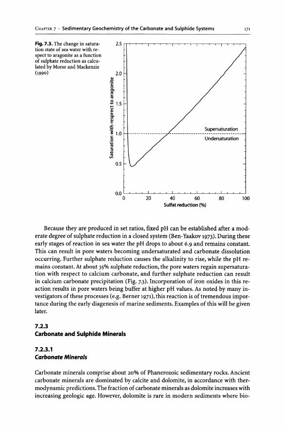
CHAPTER 7 . Sedimentary Geochemistry of the Carbonate and Sulphide Systems 171
Fig. 7.3. The change in satura- 2.5 rr Irr--,--,--,-,-,-,----r--,--,--,--,,.,,.-r-r-,--~.._.,...,
tion state of sea water with respect to aragonite as a function of sulphate reduction as calculated by Morse and Mackenzie (1990) 2.0
l!! 'c o en e .. B 15 i . a. ~
.r:. ...
. ~ 1.0 I: o .~
:::I 10 III
0.5
0.0 LI -,---,---,---'--,---,--,---'--,--,--,---'--,--,--,--'--,--,-.L....J
o 20 40 60 80 100
Sulfat reduction (%)
Because they are produced in set ratios, fixed pH can be established after a moderate degree of sulphate reduction in a closed system (Ben-Yaakov 1973). During these early stages of reaction in sea water the pH drops to about 6.9 and remains constant. This can result in pore waters becoming undersaturated and carbonate dissolution occurring. Further sulphate reduction causes the alkalinity to rise, while the pH remains constant. At about 35% sulphate reduction, the pore waters regain supersaturation with respect to calcium carbonate, and further sulphate reduction can result in calcium carbonate precipitation (Fig. 7.3). Incorporation of iron oxides in this reaction results in pore waters being buffer at higher pH values. As noted by many investigators of these processes (e.g. Berner 1971), this reaction is of tremendous importance during the early diagenesis of marine sediments. Examples of this will be given later.
7.2.3 Carbonate and Sulphide Minerals
7.2.3.1 Carbonate Minerals
Carbonate minerals comprise about 20% of Phanerozoic sedimentary rocks. Ancient carbonate minerals are dominated by calcite and dolomite, in accordance with thermodynamic predictions. The fraction of carbonate minerals as dolomite increases with increasing geologic age. However, dolomite is rare in modern sediments where bio-

172 J. W.Morse
genic carbonates strongly dominate. It is convenient to divide modern sedimentary carbonates into those found in relatively shallow waters and those being deposited on deep ocean basins. Sources, mineralogy and diagenetic processes are generally quite different in these environments. In this chapter, we will not be dealing with deep ocean sediments. In shallow water marine sediments, aragonite is usually the most common carbonate mineral, followed by high-magnesian calcite (e.g. Cao.87Mgo.13C03) and minor amounts of low-Mg calcite.
The pK (= -logK) values for calcite and aragonite solubility products (Eq. 7.29) are respectively at 25°C, 8.48 and 8.30. The solubility of high magnesian calcites is a complex and controversial topic (e.g. abiotic and biotic high magnesian calcites of the same composition appear to have different solubilities; see Morse and Mackenzie 1990 for extensive discussion of this topic).
CaC03 ~ Ca2+ + CO;- Ksp = aCa2+acoj- (7.29)
Observations of the composition of pore waters in carbonate-rich shallow water sediments have demonstrated that no single value for the calcium carbonate ion activity product widely occurs. This results in a moderate range of saturation states relative to aragonite (Fig. 7.4; Morse et al. 1985) that have been demonstrated to represent conditions of "dynamic equilibrium" between the pore waters and carbonates (Bernstein and Morse 1985). For equilibrium with aragonite in a S = 35 pore water at 25°C with normal Ca2+ concentration (aCa2+ == 2 X 10⁻³), the following approximate carbonic acid system parameter values at a pH of 7.2 (fairly typical of anoxic sediments) are total alkalinity about 2 x that of sea water (5 meq kg-I), and Pc02 about 10 matm. acoj- would then be about 2.5 x 10⁻⁶•
7.2.3.2 Iron Sulphide Minerals
Just as with the carbonates, there are several sulphide minerals that are found in modern sediments. However, unlike the sedimentary carbonate minerals, they are dominantly of authigenic rather than biogenic origin. Sedimentary sulphides are usually divided into acid volatile sulphide (AVS) and pyrite (FeS2)' which is the thermodynamically stable phase.
AVS comprises an "operationally defined" group of what are generally believed to be metastable iron sulphide minerals plus dissolved H2S species. Often, but with major exceptions, AVS is confined to a relatively small portion «10%) of total sedimentary sulphides. It can be ephemeral. Spatially, AVS often appears with a maximum in the top few cm of anoxic sediments and disappears rapidly with depth to close to undetectable concentrations within the top 20 cm or less. Temporally, it can exhibit major changes on a seasonal basis in the upper few cm of sediments. AVS has received considerable attention, because it is one of the most chemically reactive components of anoxic sediments during early diagenesis. AVS is readily oxidized within hours or less when anoxic sediments are exposed to oxic waters. The iron sulphide minerals amorphous-FeS, mackinawite (FeO.9S) and griegite (Fe3S4) that are generally purported to be the major components of AVS have also traditionally (e.g. Berner 1984) been held to be precursor phases necessary for the formation of the dominant and thermody-
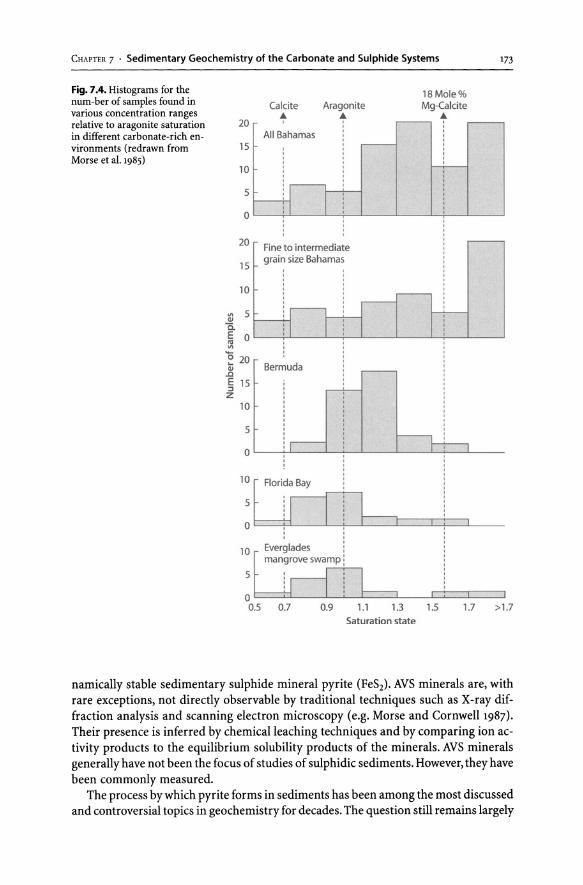
CHAPTER 7 . Sedimentary Geochemistry of the Carbonate and Sulphide Systems
Fig. 7.4. Histograms for the num-ber of samples found in various concentration ranges relative to aragonite saturation in different carbonate-rich environments (redrawn from Morse et al. 1985)
Calcite Aragonite
• • 20 0 r All Bahamas 15
10
5
0
20.- Fine to intermediate
15 I grain size Bahamas
10
VI 5 CIJ
c.. I I E 0 I ,
~ e 20 CIJ .0 E 15 :l z
10
5
0
Bermuda
10 r Florida Bay
5
0
10 Everglades r mangrove swamp 0
5
0.7 0.9 1.1 1.3 Saturation state
18 Mole% Mg-Calcite
•
1.S 1.7
173
>1.7
namically stable sedimentary sulphide mineral pyrite (FeS2)' AVS minerals are, with rare exceptions, not directly observable by traditional techniques such as X-ray diffraction analysis and scanning electron microscopy (e.g. Morse and Cornwell 1987). Their presence is inferred by chemical leaching techniques and by comparing ion activity products to the equilibrium solubility products of the minerals. AVS minerals generally have not been the focus of studies of sulphidic sediments. However, they have been commonly measured.
The process by which pyrite forms in sediments has been among the most discussed and controversial topics in geochemistry for decades. The question still remains largely

174 J. W.Morse
open, and no attempt will made to review the massive literature on the topic here. Instead, the major points on this topic in the review by Rickard et al. (1995) are briefly summarized and the reader should refer to this article for further details and referencing. The major problem in pyrite formation is how to produce the disulphide ligand and cause the Fe(II) to change from high spin in FeS to the low spin state found in pyrite. Different pathways have been proposed and demonstrated in laboratory experiments. These are:
1. The FeS oxidation pathway. Amorphous-FeS ages to mackinawite. Then under slightly oxidizing conditions, mackinawite converts to griegite and finally pyrite. This is the most often cited mechanism in the literature.
2. The polysulphide pathway. FeS (or FeSH+) reacts with polysulphides forming a complex that then breaks down producing FeS2' This reaction is relatively slow and does not necessarily involve a solid phase. It is a more realistic pathway than the classically cited schematic solid-solid reaction FeS + SO ~ FeS2'
3. The H2S pathway. FeS reacts with hydrogen sulphide producing hydrogen gas (FeS + H2S ~ FeS2 + H2). Because this reaction involves H2S, it is favoured at lower pH values and can be relatively rapid compared to the other pathways.
Pyrite occurs with different morphologies in sediments. Framboidal pyrite is most common and generally is assumed to be a relatively rapidly-formed early diagenetic product, whereas euhedral pyrite is usually presumed to form more slowly over long time periods during later stages of diagenesis.
Because of the large uncertainties in the value of the second dissociation constant for hydrogen sulphide, a special approach to representing metal sulphide solubility has been developed. This approach incorporates H+ in the reaction, resulting in the formation of bisulphide (Eq. 7.30) and is therefore a pH dependent solubility constant (*Ks' see Stumm and Morgan 1996 for discussion and examples).
MeS + H+ ~ Me2+ + HS- Ks=(aMe2+aHS-) / aH+ (7·30)
The pKs values for amorphous-FeS, mackinawite, griegite and pyrite are (using SO in the griegite and pyrite reactions), respectively, 2.95,3.6, 4.4, 16.4 (Davison 1991). Many of the preceding concepts have been incorporated into constructing Fig. 7.5. In this figure, the activity of HS- has been plotted vs. pH for a pore water of S = 35 at 25°C containing 20 ~M total H2S over a pH range typical of most anoxic marine sediments of 6.5 to 8. This was accomplished using Eq. 7.31. Then the activity of Fe2+ was calculated assuming
[( r ) ]-1
a _ YHS- a + HS- - YHS_LH2S - 2L +1
YH2S KI (7.31)
equilibrium with mackinawite according to Eq. 7.32 and also plotted against pH.
aFe2+ = * Ks(aH+ / aHS-) (7.32)

CHAPTER 7 . Sedimentary Geochemistry of the Carbonate and Sulphide Systems 175
Fig. 7.5. A plot of the activities ofbisulphite (solid line) and ferrous iron (dashed line) vs. pH for sea water S = 35, 25°C, IH2S = 20 f!M and equilibrium with mackina-wite (FeS). Dotted line is upper limit of ferrous iron concentration when limited by the solubility of siderite (FeC03) when aco;= 2.5 x 10⁻⁶
(see text) ~
20 I , I
\ '\
15 1-\ \ \ \ \ \ \ \
~ 10 \ \ \ \ a
5
o I ,
6.5
\ \ \
\ Upper limit for Fe1+ in equilibrium \ with respect to siderite (FeCO ) ................ _ ... " ........................................................ _ ............... _ .. _._ ............... 1 ...... .. , ,
'" Fe2+ in equilibrium with respect ',,~o mackinawite (FeS)
---------7 7.5
pH 8
Finally, the limiting activity of ferrous iron was calculated for a carbonate ion activity of 2.5 x 10⁻⁶ (see above). Even at this relatively low hydrogen sulphide concentration, low concentrations of ferrous iron are required over much of the pH range of anoxic marine sediments. Carbonate ion concentrations for equilibrium with aragonite also severely limit ferrous iron solubility.
7.2.3.3 Sulphide Minerals of Selected Toxic Metals
The association of trace metals enrichments with sulphidic sediments has long been known (e.g. Krauskopf 1956; Manheim 1961). Interest in these relationships has been sparked by studies that indicate trace metal-sulphide interactions, which may have a profound influence on the bioavailability of toxic metals in sediments (Di Toro et al. 1990,1992; Morse 1994). Direct evidence for the interactions of trace metals with sulphides in anoxic sediments from numerous locations is now available, and clear patterns of behaviour for different trace metals have emerged (e.g. Huerta-Diaz and Morse 1992; Morse et al. 1993). These will be discussed near the end of this chapter along with possible explanations.
It is worthwhile at this point to consider some basic relationships and concepts. In Table 7.2, p* Ks for simple metal sulphides and pKsp values for simple metal carbonates are presented. From these values, at 25°C and pH = 7.2, the activity of HS- has been calculated for the metals in simultaneous equilibrium with their carbonate and sulphide minerals at a carbonate ion activity of 2.5 x 10 -6 (aragonite equilibrium, see previous discussion). These results indicate that for most of the toxic metals (except Fe) considered, only extremely low bisulphite concentrations could occur under these conditions. Also calculated is the metal ion activity where carbonate is not con-

176 J. W.Morse
Table 7.2. Solubility relationships for different metal sulphides and carbonates (based on compilations by Morse and Mackenzie 1990 and Stumm and Morgan 1996)
Metal p*K, pK,p °Me-C03 °HS- °Fe
Cd 14.4 13.7 7.3 x 10⁻⁹ 3.8 X 10⁻¹⁴ 2.8 X 10⁻¹⁷
Co 7.4 9.7 8.4 x 10⁻⁵ 2.7 x 10⁻¹¹ 2.3 xl 0-10
Fe 3.6 10.9 4.9x 10⁻⁶ 3.2xl0-6 1.6 x 10⁻⁶
Ni 5.6 6.9 S.4x 10-2 2.9 x 10⁻¹² 1.6 X 10⁻⁸
Pb 14.0 12.2 2.8x10⁻⁷ 2.4 x 10⁻¹⁵ 6.8 x 10⁻¹⁷
Zn 10.9 10.0 4.0x 10⁻⁵ 1.9 X 10⁻¹⁴ 7.4 x 10⁻¹⁴
sidered and the concentration of total sulphide is set at 20 flM. Here again, with the exception of Fe, very low metal ion activities are permitted for equilibrium. A fairly regular relationship is shown in Fig. 7.6 between the values of p* Ks for metal sulphides and pKsp values for metal carbonates.
Unfortunately, the behaviour of trace metals in the real world is not so simple. Several different types of chemistry can occur (see Morse and Luther 1999 for discussion). These include formation of multiple different minerals (e.g. see Table 7.3 for Cu), coprecipitation reactions (Table 7.4) and largely irreversible adsorption. Often changes in metal valence occur (e.g. Cu(II) to Cu(I», further complicating the situation. In this chapter we shall not delve into the complex literature on this topic, but rather later give some specific examples from natural sediments along with possible interpretations of the chemistry involved.
7.2.4 Isotopes
Another major similarity between the sedimentary carbon and sulphur systems is the use of stable isotope ratios (13C/12C and 34SP2S) and radioisotopes e4C and 35S). Measurements of these isotopes in various components of sediments and injection of radioisotopes as tracers of chemical pathways and rates are major elements of the study of carbon and sulphur in sediments.
Variations in stable isotope ratios are usually reported as "del" (8) values (Eq. 7-41) which are in parts per mil (%0). The PDB fossil limestone is the primary C standard, and troilite from the Canyon Diablo meteorite is the generally accepted standard for S. The primary use of
[ (34 S /32 S )samPle _ 1] x 1000
834S - ) - (34 S /32 S standard
(J.41)

CHAPTER 7 . Sedimentary Geochemistry of the Carbonate and Sulphide Systems 177
Fig. 7.6. A plot of p* Ks for sulphide minerals vs. pKsp for carbonate minerals of the same metals
Table 7.3. Copper sulphide and iron-sulphide phases (based on Vaughan and Craig 1978; from Morse and Luther 1999)
16
14
12
Qj" "C :c 10 0.. :; ~ /
/
Zn / /
/ /
/
/ /
Pb /' Cd /
/
"::.t.~ 8 * 0.. // Co
/ 6 Ni //
/
4
2 6 8 10 12
pKsp (carbonate)
Copper sulfide minerals Copper-iron sulfide minerals
Chalcocite Cu 2S Chalcopyrite CuFeS2
Analite CU 7S4 Bornite CuleS4
Digenite CugSS Fukuchilite CuleSs
Djurleite CU 197S Talnakite CugFesS16
Geerite CU 16S Mooiheckite Cu9Fe9S16
Spionkopite CUl.3gS Haycockite Cu/esSs Yarrowite CU ,.12S Cubanite CuFe2S3
Covellite CuS Idaite CU SSFeS6S
Cubic CUS2
14
carbon stable isotopes in the study of carbon in sediments is to identify the relative importance of different carbon sources. For example, 8l3C values for biogenic carbonates are usually close to 0, for marine organic-C -22, for terrestrial organic-C -28 and often very negative, -40 or less for thermogenic methane. Later in this chapter the use of carbon stable isotopes to solve carbon-sulphur diagenetic processes in seagrass root zones (Eldridge and Morse 2000) will be described.
The use of sulphur stable isotopes in studying sedimentary sulphides has proven more challenging. This is because the extent of fractionation depends to a significant extent on the rates of bacterial sulphate reduction. The cycling of sulphur between different oxidation states further complicates matters, as does the extent to which sulphate is reduced under conditions approximating to different extents open and close systems (Fig. 7.7). (See Thode 1991 for extensive overview and discussion.)

178 J. W.Morse
Table 7.4. Possible reactions for the incorporation of metals into FeS and FeS2 phases. FeS2 reactions are given for those where the kinetics are well-described (Rickard 1975; Luther 1991; Rickard 1997; Rickard and Luther 1997; from Morse and Luther 1999)
Eq. FeS
7.33 Fe2+ + HS- ~ FeS + H+ (FeS formation)
7.34 FeS + Me2+ ~ Fe-S-Me2+ (Metal adsorption onto FeS)
7.35 Fe-S-Me2+ ~ Fe(Me)S + Fe2+ (Metal inclusion into FeS)
7.36 FeS + Me2+ ~ MeS + Fe2+ (Metathesis or metal exchange reaction)
FeS2
7.37 FeS or [Fe(Me)S] + S(O) ~ Fe(Me)S2 (Pyrite formation and metal inclusion)
7.38 FeS or [Fe(Me)S] + H2S ~ Fe(Me)S2 + H2
7.39 FeS2 + Me2+ ~ Fe-S-S-Me (Metal adsorption onto pyrite)
7.40 Fe-S-S-Me ~ Fe(Me)S2 (Metal inclusion into pyrite)
l4C is mostly used for two purposes. The first is for age dating and obtaining sediment accumulation rates. The second is incubation of 14C-Iabelled organic compounds in sediments in order make rate measurements on their decomposition. The primary use of 35S is to make measurements of the rates of sulphate reduction using radiolabelled sulphate (e.g. Jorgensen 1978). It is additionally widely used to investigate the biogeochemical cycling of sulphur (see review of Fossing 1995).
7.3 Sedimentary Geochemistry of Carbonate and Sulphide Systems
7.3.1 "Normal" Marine Sediments
7.3.1.1 Relationship Between Organic-C and pyrite-S Burial
The term "normal marine" is often used to describe fairly common coastal and even to some degree estuarine sediments as a depositional environment for sedimentary sulphides and carbon. Normal marine alone refers to sediments overlain by oxic sea water of typical oceanic salinity. The type of sediment of interest is typically a finegrained siliciclastic sediment. Excluded from the larger definition are coarse, sandy sediments, CaCOrrich sediments (hence the adjective "siliciclastic"), and sediments overlain by freshwater and anoxic marine waters (e.g. Berner 1982; Berner and Raiswell 1984). Because of the virtual absence of sulphur, also excluded are sediments that do not become sufficiently anoxic for sulphate reduction to become a major process near the sediment-water interface (e.g. many deep-sea sediments and sediments containing very low concentrations of organic-C).
Fine-grained, normal marine siliciclastic sediments have a relatively narrow range of CIS ratios. Consequently, organic-C and pyrite-S must covary in a close to linear
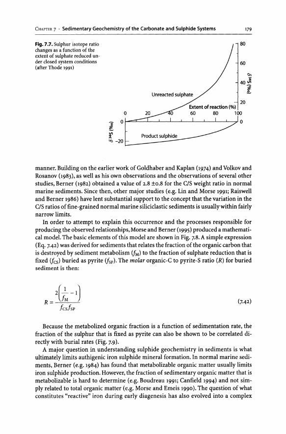
CHAPTER 7 . Sedimentary Geochemistry of the Carbonate and Sulphide Systems 179
Fig. 7.7. Sulphur isotope ratio I .., 80 changes as a function of the extent of sulphate reduced un-der closed system conditions / --j 60 (after Thode 1991)
Co
40 ~ l
20
o
l ~
o I ..--=-r: 7' 0
"<:l -20 L.-----
manner. Building on the earlier work of Goldhaber and Kaplan (1974) and Volkov and Rosanov (1983), as well as his own observations and the observations of several other studies, Berner (1982) obtained a value of 2.8 ±0.8 for the CIS weight ratio in normal marine sediments. Since then, other major studies (e.g. Lin and Morse 1991; Raiswell and Berner 1986) have lent substantial support to the concept that the variation in the CIS ratios of fine-grained normal marine siliciclastic sediments is usually within fairly narrow limits.
In order to attempt to explain this occurrence and the processes responsible for producing the observed relationships, Morse and Berner (1995) produced a mathematical model. The basic elements of this model are shown in Fig. 7.8. A simple expression (Eq. 7.42) was derived for sediments that relates the fraction of the organic carbon that is destroyed by sediment metabolism (fM) to the fraction of sulphate reduction that is fixed (fcs) buried as pyrite (fsp). The molar organic-C to pyrite-S ratio (R) for buried sediment is then:
( 1 ) 2 ~-l
R=~ fcsfsp
(7.42)
Because the metabolized organic fraction is a function of sedimentation rate, the fraction of the sulphur that is fixed as pyrite can also be shown to be correlated directly with burial rates (Fig. 7.9).
A major question in understanding sulphide geochemistry in sediments is what ultimately limits authigenic iron sulphide mineral formation. In normal marine sediments, Berner (e.g. 1984) has found that metabolizable organic matter usually limits iron sulphide production. However, the fraction of sedimentary organic matter that is metabolizable is hard to determine (e.g. Boudreau 1991; Canfield 1994) and not simply related to total organic matter (e.g. Morse and Emeis 1990). The question of what constitutes "reactive" iron during early diagenesis has also evolved into a complex

180
Fig. 7.8. Schematic flow diagram illustrating the relationships among the major components of the model. Note 02 respir. includes suboxic processes such as nitrate and metal oxide reduction as well as oxic respiration (redrawn from Morse and Berner 1995)
J. W.Morse
~ ~ • ~I~i~ / ~
~;5 Fig. 7.9. The log-log depend - 0 r-r--o"---.-----r-----r---r-r---.-,----.---,--,--,---,---.--.--.--.---,
ence of fsp on sediment burial rate in the Gulf of Mexico. The circled data point was not used in curve fitting or computations, as it is believed to represent slumped sediment from the upslope. The line is a linear least squares fit to data (after Morse and Berner 1995)
-1
... ..... '" C\ -2
..Q
-3
• •
-4 LI _L_L-L~~~~~~~L-~~~~~~-L_L_L~
-3 -2 -1 o log sed rate (em yrl)
question involving the reaction kinetics between dissolved sulphide and various iron oxides (e.g. Canfield 1988, 1989). It now can be argued that in sediments where dis-

CHAPTER 7 . Sedimentary Geochemistry of the Carbonate and Sulphide Systems 181
solved sulphide is present, "reactive" iron is limiting the rate of iron sulphide mineral formation. A further complication that is little discussed in the literature is that in sediments where dissolved sulphate is totally reduced in the top few cm of sediment, its rate of transport into the sediment is the limiting factor for sulphide production in the sediment (Arvidson and Morse, to be published). In the following section, the influence of biologically driven transport of oxidants on sedimentary sulphides and carbonates will be discussed.
7.3.1.2 Influences of Biologically-Driven Transport
Oxidation of sedimentary sulphides via reaction with iron and manganese oxides can be an important or even dominant reaction pathway (Aller and Rude 1988). However, the active transport of oxygen to several cm below the sediment-water interface by infaunal organisms (Fig. 7.10) can also be a very important process (e.g. Aller 1988). It is primarily through this process that most sulphides are often oxidized. Indeed, in measuring benthic oxygen demand, biologists often assume this is the major indirect pathway for oxygen consumption and that any sulphide not oxidized is of insignificant importance (e.g. Pamatmat 1971).
Just as the oxidation of pyrite in soils or sulphide minerals in mine tailings can lead to highly acidic waters, the oxidation of sedimentary sulphides produces acid as well (Eq. 7.14). This can lower the saturation state of pore waters with respect to carbonate minerals and lead to their extensive dissolution. Dissolution is highest in highly bioturbated and bioirrigated sediments, where these processes supply oxygen and remove accumulated alkalinity from dissolution (Aller 1982). In vegetated sediments, plants such a seagrasses can cause active transport of oxygen to sediments in their root zones. Based on extensive field data that included carbon isotope studies, Eldridge and Morse (2000) constructed a diagenetic model for this process. They found that the oxygen flux from roots was important for keeping sulphide concentrations below toxic levels for the seagrasses and that generally over half of the dissolved inorganic carbon (DIC) in the pore waters came from carbonate mineral dissolution rather than oxidation of organic matter.
Fig. 7.10. Schematic representation of burrow and its influence on sediment redox chemistry. Dark grey is sub oxic zone, black is zone of nitrate and manganese reduction (based on concepts in Aller 1988)
Oxic water

182 J. w. Morse
7.3.1.3 Carbonate Precipitation in Sulphidic Sediments
In Fig. 7.3, it was shown that sulphate reduction that initially results in a major decrease in pore water saturation with respect to calcium carbonate can lead again to supersaturation with increasing extent of sulphate reduction. In sediments and sedimentary rocks, this is a well-known mechanism for producing authigenic calcium carbonate. For example, the massive carbonate cap rocks on salt domes are a result of this process.
An example from modern sediments comes from Baffin Bay, Texas, which is a hypersaline negative estuary that has been studied because of its similarities to environments that may have existed in ancient epicontinental seas (Morse et al. 1992). Figure 7.11 shows the relationship of the loss of dissolved sulphate and calcium to the increase in total carbon dioxide. The decrease in dissolved calcium occurs because of the precipitation of calcium carbonate. If the loss of carbon dioxide from precipitation is corrected for by the loss of calcium, then a close to ideal two to one increase in dissolved carbon dioxide with sulphate loss is observed (Fig. 7.12).
For the precipitation of calcium carbonate to be quantitatively significant, it is necessary for there to be exceptionally high quantities of metabolizable organic matter available to produce the needed carbon dioxide. An example of such a situation is at hydrocarbon seeps in the Gulf of Mexico (Arvidson and Morse, to be published). There, the organic content of the sediments and concentration of calcium carbonate show a close association. (Fig. 7.13). Because large amounts of sulphide are also produced by this process, total dissolved hydrogen sulphide can exceed 10 mM.
7.3.2 Carbonate-Rich Sediments
During the last decade, Lynn Walter and her associates (Walter and Burton 1990; Walter et al. 1993; Ku et al. 1999) have done much to demonstrate the major quantitative importance of dissolution of calcium carbonate from shallow carbonate sediments (on the order of up to 50%) driven by the previously discussed sulphate reduction-sulphide oxidation process. Such sediments account for about a third of all ocean carbonate production (Milliman 1993) and are therefore of considerable significance in understanding the global carbon cycle and impact of fossil fuel CO2,
The basic "problem" for the sulphide system in calcium carbonate-rich sediments is the general lack of reactive iron to produce iron sulphide minerals. The sulphide that is produced by sulphate reduction then basically can only be buried in dissolved form in pore waters, be oxidized or diffuse out the sediments. For most carbonaterich sediments, the oxidative process strongly dominates the fate of the sulphide. This is not grossly unlike what also happens in "normal" marine sediments. However, no sulphide minerals are produced, and since these sediments are carbonate-rich they will remain relatively close to equilibrium between calcium carbonate and their pore waters (see Fig. 7.4; Morse et al. 1985).
Figure 7.14 (Walter et al. 1993) shows the strong relationship that generally occurs in carbonate muds from Florida Bay between total carbon dioxide, excess dissolved calcium and the amount of sulphate that has been reduced. This figure is similar to Fig. 7.11, except instead of calcium decreasing, it increases indicating dissolution rather

CHAPTER 7 ' Sedimentary Geochemistry of the Carbonate and Sulphide Systems 183
Fig. 7.11. The relationships of 0 the change in sulphate and
a calcium concentrations to the change in total dissolved car-bon dioxide in Baffin Bay, Texas
J • sediments, (From Morse et al, •• 1992)
•• ~
f •• .s • ... • 0
VI <I • • ..
-20 l- • 'I" I.' • • •
-30 I b
••• -5 ~ ••
f • • ~ • E • ~ •• III
U • <I • -, -10 l- • •
I." • • •• •
-151 0 10 20 30
&'.C02 (mM)
than precipitation. A probable explanation is that in the carbonate-rich sediments only typical for about 10% of the sulphate was reduced, whereas in the Baffin Bay, sediments close to total sulphate reduction often occurred. Referring to Fig. 7.3, it can be observed that the Florida Bay sediments are in the undersaturated region, whereas the Baffin sediments are in the supersaturated region. It is also noteworthy that the burrowed banks show much more extensive increases in calcium than the other mudbanks. This is in good agreement with the Aller and Rude (1988) observations for Long Island Sound sediments, that increased bioturbation leads to increased sulphide oxidation and carbonate dissolution.

184
Fig. 7.12. The relationship of the change in sulphate concentration to the change in total dissolved carbon dioxide in Baffin Bay, Texas sediments when calcium carbonate precipitation is corrected for. The line is the ideal 1:2 ratio (redrawn from Morse et al. 1992)
Fig. 7.13. The relationship be-tween organic-C and calcium carbonate in Gulf of Mexico cold seep communities (re-drawn from Arvidson and Morse, to be published)
7.4
J. W.Morse
o " -----------------------------------,
~ .s 0'"
-10
~ -20
-30 I 0
15
r ~ 10 £. I: 0 ..c :;; v v ·2 1\1
~ 5 0
(. oL
0
• 10 20 30 40
LUXO; (mMl
/ • /JI •
jy;#e
4 8 12 CaC03 (% wt.l
Interactions of Toxic Metals with Sulphides in Anoxic Sediments
7.4.1 General Considerations
The study of the relationship of toxic metals to sedimentary sulphides has primarily focused on three major areas. Early observations indicated that the concentrations of

CHAPTER 7 . Sedimentary Geochemistry of the Carbonate and Sulphide Systems
61 71
~4 5 "0
~ :l
~ 2
0" Vl
o
2
a
~~ ~o<:- • ~eOV •
~:?>,-e ~~~\l ~ ~e~o ••
Sulphide oxidation
&~~<; •• 0.0<; .:. • Mudbanks
0000 8 oQ 0 00 o~o
4 6
o Burrowed banks
8 10 12
rco; (mM)
14
• •
• • • • .' • -• • o 0 0
8 0 0 o 0 00
o 0.5 1.0
b
• Mudbanks o Burrowed banks
00 000
1.5 2.5
Excess Ca2+ (mM )
185
2.5
Fig. 7.14. The relationships of the change in sulphate to the change in; a total dissolved carbon dioxide; b calcium in Florida Bay sediments (redrawn from Walter et al. 1993)
toxic metals were often at elevated levels in sulphidic sediments (see Morse et al. 1987 for review). The observations of Di Toro et al. (1990) indicating that the toxicity of some metals was greatly reduced in sulphidic sediments stimulated interest in the topic Huerta-Diaz and Morse (1992) found that for many metals the "reactive" fraction was substantially "pyritized" during very early diagenesis. In the ensuing years, a rather vast literature has sprung up around this topic. This is in large part because of its practical application to assessing potential influences of toxic metals on ecosystems; a topic that remains highly controversial (e.g. Lee et al. 2000). Earlier (Sect. 7.2.3.3), it was pointed out that in sediments where there is both dissolved sulphide and carbonate, almost always the metal sulphides will limit metal solubility. Therefore, the discussion will be confined to metal sulphides here.
7.4.2 "Pyritization" of Trace Metals
Huerta-Diaz and Morse (1990) were able to determine trace metals that were coleached with pyrite-Fe using a modification of the pyrite-Fe extraction method of Lord (1982). Since the development of this technique, thousands of analyses have been performed on sediments from numerous locations (e.g. Huerta-Diaz and Morse 1992; Morse et al. 1993), and clear patterns of behaviour for different trace metals have emerged. For several trace metals, it has been observed that there is often a fairly regular increase in the concentration of the metal occurring in the pyrite-extracted fraction with depth below the sediment-water interface.
In interpreting this behaviour, it has been found useful to apply a measure of tile extent to which tile operationally defined "reactive" fraction has become transformed into tile fraction that extracts with pyrite-Fe. This is done in the same manner as the degree of pyritization (DOP) is calculated for Fe [DOP = pyrite-Fe I (pyrite-Fe + "reactive"-Fe)] and is referred to as the degree of trace metal pyritization (DTMP) (Huerta-Diaz and Morse 1990). Plots of DTMP against DOP have proven to be useful in establishing relationships for the relative degrees to which different metals are pyritized compared to for-
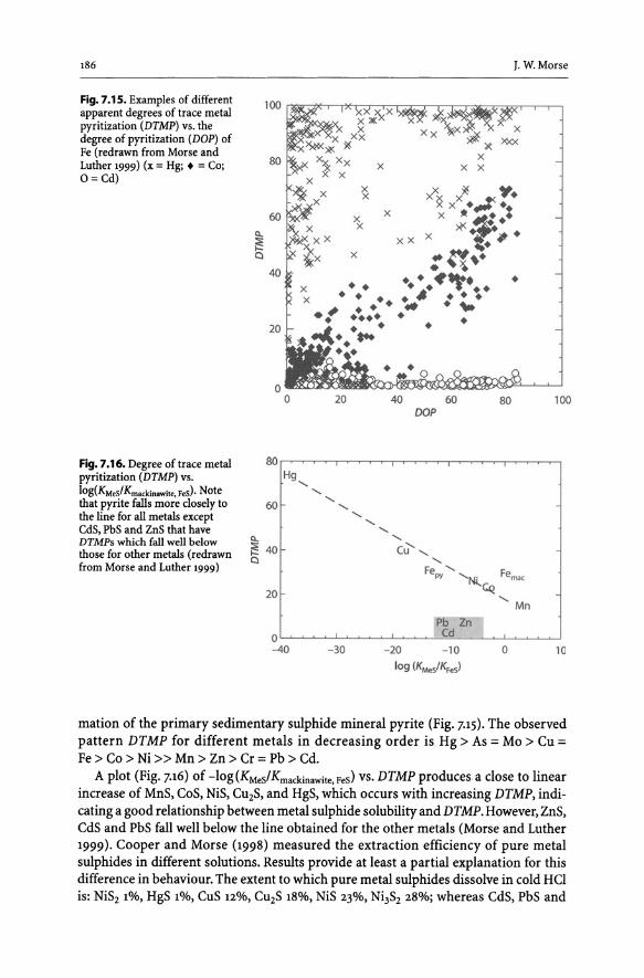
186
Fig. 7.1 s. Examples of different apparent degrees of trace metal pyritization (DTMP) vs. the degree of pyritization (DOP) of Fe (redrawn from Morse and Luther 1999) (x = Hg; • = Co; O=Cd)
Fig. 7.16. Degree of trace metal pyritization (DTMP) vs. log(KMesl Kmackinawite, FeS) ' Note that pyrite falls more closely to the line for all metals except CdS, PbS and ZnS that have DTMPs which fall well below those for other metals (redrawn from Morse and Luther 1999)
J. w. Morse
100~, IX~'>L~x~JS~. ~ ' ]
80 r _ _ v ,lL ' ~A X
X
~ X X X. · 60 R : X >iL/ • ..,r Y. ~ fX '" ,.S o XX X ·· X X ,.
40 - ~~ • • ~>+~. .. . ... ,. • • •• • • . ... . ~ .... 20 I- .....-. _.
o o
80 1 Hg,
60
~
~ 40 o
. ~ . . ... . . 20 40 60 80
DOP
'" "
" C', u ,
F ' Femac epy 'Ni.. CQ
, Mn 20
Pb Zn 0' Cd --40 - 30 - 20 -10 o
log (KMeSIK""s)
100
10
mation of the primary sedimentary sulphide mineral pyrite (Fig. 7.15). The observed pattern DTMP for different metals in decreasing order is Hg> As = Mo > Cu = Fe > Co > Ni > > Mn > Zn > Cr = Pb > Cd.
A plot (Fig. 7.16) of -log (KMeslKmackinawite, FeS) vs. DTMP produces a close to linear increase of MnS, CoS, NiS, CU2S, and HgS, which occurs with increasing DTMP, indicating a good relationship between metal sulphide solubility and DTMP. However, ZnS, CdS and PbS fall well below the line obtained for the other metals (Morse and Luther 1999). Cooper and Morse (1998) measured the extraction efficiency of pure metal sulphides in different solutions, Results provide at least a partial explanation for this difference in behaviour. The extent to which pure metal sulphides dissolve in cold HCI is: NiS2 1%, HgS 1%, CuS 12%, CU2S 18%, NiS 23%, Ni3S2 28%; whereas CdS, PbS and

CHAPTER 7 . Sedimentary Geochemistry of the Carbonate and Sulphide Systems 187
ZnS extract completely. For MeS compounds, this leads to Hg < Cu < Ni < < Zn = Pb = Cd. This is close to the relationship observed for DTMP. Therefore, if Zn, Cd and Pb largely make their own sulphide, they would appear to have a low DTMP because they extract in the HCI fraction. Unfortunately, this means that it is not possible to determine how extensively Zn, Cd and Pb are sulphidized. The other metals may be coprecipitates with pyrite or occur as discrete phases.
Acknowledgements
The US National Science Foundation, Office of Naval Research, and the Texas Sea Grant Program have supported much of the work presented in this chapter. Many colleagues, post -doctoral fellows, graduate and undergraduate students participated in these studies. Dr. Morse was supported in his efforts to prepare and produce this chapter by funds from the Louis and Elizabeth Scherck Chair in Oceanography.
References
Aller RC (1982) Carbonate dissolution in near-shore terrigenous muds: The role of physical and biological reworking. J GeoI90:79-95
Aller RC (1988) Benthic fauna and biogeochemical processes in marine sediments: The role of burrow structures. In: Blackburn TH, Sorensen J (eds) Nitrogen cycling in coastal marine environments. John Wiley and Sons, New York, pp 301-338
Aller RC, Rude PO (1988) Complete oxidation of solid phase sulfides by manganese and bacteria in anoxic marine sediments. Geochim Cosmochim Acta 52:751-765
Arvidson RS,Morse JW (to be published) Controls on rates of sulfate reduction in chemosynthetic cold seep communities, Gulf of Mexico, USA. Geochim Cosmochim Acta
Ben-Yaakov S (1973) pH buffering of pore water of recent anoxic sediments. Limnol Oceanogr 18:86-94 Berner RA (1971) Principles of chemical sedimentology. McGraw-Hill, New York Berner RA (1982) Burial of organic carbon and pyrite sulfur in the modern ocean: Its geochemical and
environmental significance. Am J Sci 282:451-473 Berner RA (1984) Sedimentary pyrite formation: An update. Geochim Cosmochim Acta 48:605-615 Berner RA, Raiswell R (1984) CIS method for distinguishing freshwater from marine sedimentary rocks.
Geology 12:365-368 Bernstein LO, Morse JW (1985) The steady-state calcium carbonate ion activity product of recent shal
low water carbonate sediments in seawater. Mar Chern 15:311-326 Boudreau BP (1991) On a reactive continuum representation of organic matter diagenesis. Am J Sci
291:507-538 Canfield OE (1988) Sulfate reduction and the diagenesis of iron in marine sediments. PhO dissertation,
Yale University Canfield OE (1989) Reactive iron in marine sediments. Geochim Cosmochim Acta 53:619-632 Canfield OE (1994) Factors influencing organic carbon preservation in marine sediments. Chern Geol
114:315-329 Cooper OC,Morse JW (1998) Biogeochemical controls on trace metal cycling in anoxic marine sediments.
Environ Sci TechnoI32:327-330 Oavison W (1991) The solubility of iron sulfides in synthetic and natural waters at ambient tempera
tures. Aquat Sci 53/54:309-329 Oi Toro OM, MalIony JO, Hansen OJ, Scott KJ, Hicks MB, Mayr SM, Redmond MS (1990) Toxicity of cad
mium in sediments: The role of acid volatile sulfide. Environ Sci Techno19:l487-1502 Oi Toro OM, MalIony JO, Hansen OJ, Scott KJ, Carlson AR,Ankley GT (1992) Acid volatile sulfide predicts
the acute toxicity of cadmium and nickel in sediments. Environ Sci TechnoI26:96-101 Eldridge PM, Morse JW (2000) A diagenetic model for sediment-seagrass interactions. Mar Chern
70:89-104 Fossing H (1995) 35S-radiolabeling to probe biogeochemical cycling of sulfur. In: Vairavamurthy MA,
Schoonen MAA (eds) Geochemical transformations of sedimentary sulfur. ACS Press, Washington, O.c. (ACS Symp. Ser 162, pp 348-364)
Goldhaber MM, Kaplan IR (1974) The sulfur cycle. In: Goldberg EO (ed) The sea, vol V. John Wiley and Sons, New York, pp 596-657

188 J. W.Morse
Hoehler TM, Alperin PI, Albert DB, Martens CS (1994) Field and laboratory studies of methane oxidation in an anoxic marine sediment: Evidence for a methanogen-sulfate reducer consortium. Global Biogeochem Cycles 8:451-463
Huerta-Diaz MA, Morse JW (1990) A quantitative method for determination of trace metal concentration in sedimentary pyrite. Mar Chern 29:119-144
Huerta-Diaz MA,Morse JW (1992) The pyritization of trace metals in anoxic marine sediments. Geochim Cosmochim Acta 56:2681-2702
Jorgensen BB (1978) A comparison of methods for the quantification of bacterial sulfate reduction in coastal marine sediments. 1. Measurement with radiotracer techniques. J Geomicrobiol1:11-27
Jorgensen BB (1990) The thiosulfate shunt in the sulfur cycle of marine sediments. Science 249:152-154 KrauskopfK B (1956) Factors controlling the concentrations of thirteen rare metals in sea-water. Geochim
Cosmochim Acta 9:1-32 Ku TCW, Walter LM, Coleman ML, Blake RE, Martini AM (1999) Coupling between sulfur recycling and
syndepositional carbonate dissolution: Evidence from oxygen and sulfur isotope composition of pore water sulfate, South Florida Platform, USA. Geochim Cosmochim Acta 63:2529-2546
Lee BG, Groscom SB, Lee JS, Choi HJ, Koh CH, Luoma SN, Fisher NS (2000) Influences of dietary uptake and reactive sulfides on metal bioavailability from aquatic sediments. Science 287:282-284
Lin S, Morse JW (1991) Sulfate reduction and iron sulfide mineral formation in Gulf of Mexico anoxic sediments. Am J Sci 291:55-89
Lord CJ III (1982) A selective and precise method for pyrite determination in sedimentary materials. J Sed Petrol 52:664-666
Luther GW III (1991) Pyrite synthesis via polysulfide compounds. Geochim Cosmochim Acta 55:2839-2849
Manheim FT (1961) A geochemical profile in the Baltic Sea. Geochim CosmoclJim Acta 25:52-70 Milliman JD (1993) Production and accumulation of calcium carbonate in the ocean: Budget of a
nonsteady state. Global Biogeochem Cycles 7:927-957 Morse JW (1994) Interactions of trace metals with authigenic sulfide minerals: Implications for their
bioavailability. Mar Chern 46:1-6 Morse JW, Berner, RA (1995) What controls sedimentary CIS ratios? Geochim Cosmochim Acta
59:1073-1077 Morse JW, Cornwell JC (1987) Analysis and distribution of iron sulfide minerals in recent anoxic ma
rine sediments. Mar Chern 22:55-69 Morse JW, Emeis KC (1990) Controls on CIS ratios in hemipelagic sediments. Am J Sci 290:1117-1135 Morse JW, Luther GW III (1999) Chemical influences on trace metal-sulfide interactions in anoxic
sediments. Geochim Cosmochim Acta 63:3373-3379 Morse JW, Mackenzie FT (1990) Geochemistry of sedimentary carbonates. Elsevier, Amsterdam Morse JW, Zullig JJ, Bernstein LD, Millero FJ, Milne P, Mucci A, Choppin GR (1985) Chemistry of calcium
carbonate-rich shallow water sediments in the Bal!amas. Am J Sci 285:147-185 Morse JW, Millero FJ, Cornwell J, Rickard D (1987) The chemistry of the hydrogen sulfide and iron sulfide
systems in natural waters. Earth-Sci Rev 24:1-42 Morse JW, Cornwell, JC, Arakaki T, Lin S, Huerta-Diaz MA (1992) Iron sulfide and carbonate mineral
diagenesis in Baffin Bay, Texas. J Sed Petrol 62:671-680 Morse JW, Presley BJ, Taylor RJ, Benoit G, Santschi P (1993) Trace metal chemistry of Galveston Bay:
Water, sediments and biota. Mar Environ Res 36:1-37 Pamatmat M (1971) Oxygen consumption by the seabed. IV. Shipboard and laboratory measurements.
Limnol Oceanogr 16:536-550 Pyzik AJ, Summer JE (1981) Sedimentary iron monosulfides: Kinetics and mechanism of formation.
Geochim Cosmochim Acta 45:687-698 Raiswell R, Berner RA (1986) Pyrite and organic matter in Phanerozoic normal marine shales. Geochim
Cosmochim Acta 50:1967-1976 Redfield AC, Ketchum BH, Rickard FA (1963) The influence of organisms on the composition of seawater.
In: Hill MN (ed) The Sea, vol II. John Wiley and Sons, NewYork,pp 27-77 Rickard DT (1975) Kinetics and meclJanism of pyrite formation at low temperatures. Am J Sci 275:636-652 Rickard DT (1997) Kinetics of pyrite formation by the H2S oxidation of iron (II) mono sulfide in aque
ous solutions between 25°C and 125°C: The rate equation. Geochim Cosmochim Acta 61:115-134 Rickard DT, Luther GW III (1997) Kinetics of pyrite formation by the H2S oxidation of iron(II)
mono sulfide in aqueous solutions between 25°C and 125 DC: The mechanism. Geochim Cosmochim Acta 61:135-147
Rickard DT, Schoonen MAA, Luther GW III (1995) Chemistry of iron sulfides in sedimentary environments. In: Vairavamurthy MA, Shoonen MAA (eds) Geochemical transformations of sedimentary sulfur. ACS Press, Washington, D.C. (ACS Symp. Ser 162, pp 168-193)
Stumm W, Morgan JJ (1996) Aquatic geochemistry. John Wiley and Sons, New York

CHAPTER 7 . Sedimentary Geochemistry of the Carbonate and Sulphide Systems 189
Thode HG (1991) Sulfur isotopes in nature and the environment: an overview. In: Krouse HR, Grinenko VA (eds) Stable isotopes: Natural and anthropogenic sulphur in the environment, Scope 43. John Wiley and Sons, New York, pp 1-26
Volkov II, Rosanov AG (1983) The sulfur cycle in the oceans. In: Volkov II, Rosanov AG (eds) The global biogeochemical sulfur cycle, Scope 19. John Wiley and Sons, New York pp 357-447
Walter LM, Burton EA (1990) Dissolution of recent platform carbonate sediments in marine pore fluids. Am J Sci 290:601-643
Walter LM, Bischof SA, Patterson WP, Lyons TW (1993) Dissolution and recrystallization in modern shelf carbonates: Evidence from pore water and solid phase chemistry. Phil Trans R Soc Lond A 344:27-36

c o .-.,. ra ·u c» Q
.
'" ." C
ra ra .-... .a .- .-::s
... eT
c» w
.,. -ra
eJ3:
:: ·e z ..
c» '"
~
.c c
_ u
._
Part II
Chemical Equilibria and Speciation in SeaWater

ChapterS
Speciation of Metals in Natural Waters
F. Millero . D. Pierrot
8.1 Introduction
The reactions of many trace metals in natural waters are affected by their speciation or form. This will affect the biological uptake (Anderson and Morel 1982) and toxicity (Sunda and Ferguson 1983) as well as the solubility (Liu and Millero 1999). For example, Fe(II) and Mn(II) are biologically available for marine organisms, while Fe(III) and Mn(IV) are not normally available. Although the form of an element in natural waters can be four phases (solid, gas, colloid and dissolved), we will only consider the form of a metal in the dissolved state. The definition of a dissolved metal is defined by the filter size used to separate solid and colloidal phases from the soluble form. In the past, this separation was made with a 0.45 Ilm filter, and in more recent work smaller size filters are used (-0.2 Ilm). The speciation of metals is controlled by ionic interactions of the metals with inorganic (Cr, OW, CO~-, etc.) and organic (fulvic and humic acids) ligands. The dissolved forms of a metal like Fe in sea water can include:
• Free ions: Fe2+, Fe3+ • Inorganically Complexed: Fe(OH)+, Fe(OH}z, FeC03 and Fe(C03)~-' FeCf+, FeCI;,
FeSO;, Fe(S04)~-' Fe(OH)2+, Fe(OH);, Fe(OHh, FeCOr, and Fe(C03)~-• Organically Complexed: FeL, where L can be a wide range of unknown natural ligands
(fulvic and humic acids, siderifores, etc.)
The speciation can also affect the rates of redox reactions (Millero 1990a,b) in natural water. Cu+ is rapidly oxidized with O2 or H20 2, while CuCI and CuC12 are nearly inert to the oxidation (Sharma and Millero 1988,1989). CuHS- is rapidly oxidized with 02' while Zn(HSh is not oxidized (Vasquez et al.1989). Cu2+ is rapidly reduced by H20 2, while CuC03 or Cu-EDTA is not reduced (Millero et al. 1991, 1992).
Some of the factors that can control the equilibrium speciation in natural waters are:
1. The oxidation potential (Eh) 2. The pH 3. The inorganic ligands (OW, CO~-) 4. The organic ligands (humics)
The ionic strength, temperature and pressure are also important. The importance of Eh on the speciation of Fe is shown in Fig. 8.1. At low pH and Eh, iron is predomi-
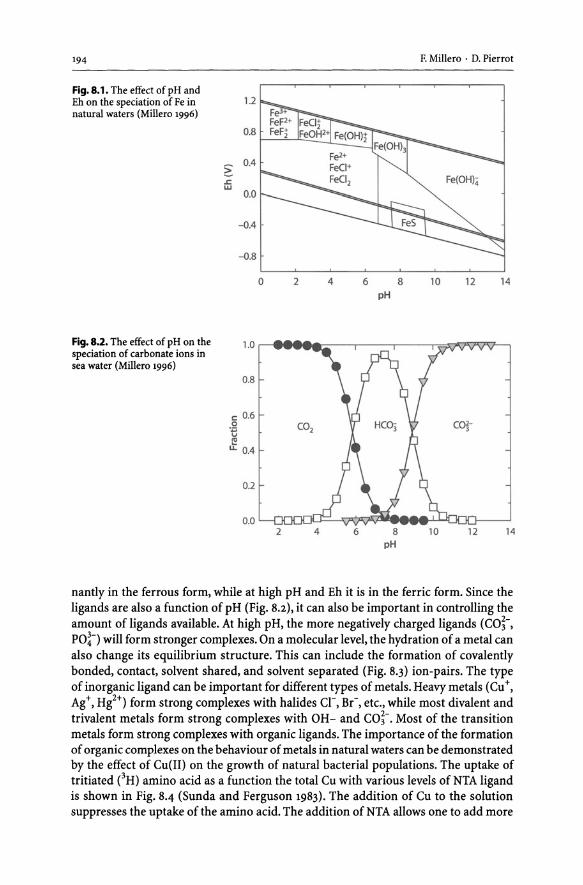
194
Fig. 8.1. The effect of pH and Eh on the speciation of Fe in natural waters (Millero 1996)
1.2
0.8
~ 0.4 2:-.s= w
0.0
-0.4
-0.8
o
F. Millero . D. Pierrot
2 4 6 8 10 12 14 pH
Fig. ~.~. The effect of PI:i on ~he 1.0 i.......... i 'HVVVVV ---, specIatIOn of carbonate IOns III sea water (Millero 1996)
0.8
c 0.6
.~ L CO2
.t 0.4
0.2
0.0 2 4 6 8
pH 10 12 14
nantly in the ferrous form, while at high pH and Eh it is in the ferric form. Since the ligands are also a function of pH (Fig. 8.2), it can also be important in controlling the amount of ligands available. At high pH, the more negatively charged ligands (CO~-, PO~-) will form stronger complexes. On a molecular level, the hydration of a metal can also change its equilibrium structure. This can include the formation of covalently bonded, contact, solvent shared, and solvent separated (Fig. 8.3) ion-pairs. The type of inorganic ligand can be important for different types of metals. Heavy metals (Cu +,
Ag +, Hg2+) form strong complexes with halides cr, Br-, etc., while most divalent and trivalent metals form strong complexes with OH- and CO;-. Most of the transition metals form strong complexes with organic ligands. The importance of the formation of organic complexes on the behaviour of metals in natural waters can be demonstrated by the effect of Cu(II) on the growth of natural bacterial populations. The uptake of tritiated eH) amino acid as a function the total Cu with various levels of NTA ligand is shown in Fig. 8.4 (Sunda and Ferguson 1983). The addition of Cu to the solution suppresses the uptake of the amino acid. The addition of NTA allows one to add more

CHAPTER 8 . Speciation of Metals in Natural Waters
Fig. 8.3. Types of ion-pairs for cation and anion interactions (Millero 1996)
Fig. 8.4. The uptake of tritiated amino acids in sea water by natural populations of bacteria as a function of added total Cu2+ (Sunda and Ferguson 1983)
~ I: o ~ ~ o u .5 "0 ·u "' o I: ·E "' j;.
120
100
80
60
40 r I -.- 4IJM NTA
-0- llJMNTA
2: t I ~ 0 IJM NTA
-8 -7 -6 log [Cu)y
195
Covalent binding
Contact pair
Solvent shared
Solvent separated
- 5

196 F. Millero . D. Pierrot
Fig. 8.5. The uptake of tritiated amino acids in sea water by natural populations of bacteria as a function offree Cu2+ (Sunda and Ferguson 1983)
120 I,-----~------r---_ _._---_,
ll00 '" 0
''::;
~ 80 0 e-o v :t .4iJM .S
""C o 2iJM 'u '" V OiJM 0
'" 'E '" 20 i-
o ~I --------~------~--______ ~ ______ _J
11 10 9 8 7 pCu
eu to the solution before the effect is seen. If one plots the effect as a function of the free eu (Fig. 8.5) in the solution, all of the results fall on the same curve (Sunda and Ferguson 1983). Thus, free copper is toxic to the natural bacterial population, while organically complexed eu is non-toxic.
8.2 Effect of Inorganic Speciation on the Solubility of Metals
The effect of the speciation of a metal on its solubility can be considered for Fe(III) in natural waters. The solubility of Fe(III) in sea water is controlled by (Byrne and Kester 1976; Millero et al. 1995):
Fe(OHh (s) + 3H+ H Fe3+ + 3H20 (8.1)
At equilibrium, the thermodynamic equilibrium constant is given by:
3/ 3 KFe(OH)3 == aFea H20 aH (8.2)
where ai == [i] Yi are the activities of species i ([ i] is the concentration and Yi is the activity coefficient of species i) and aRlO is the activity of water. At a given ionic strength, the value of aFe in sea water is given by
aFe == lFe [Fe3+] == lFe [Fe(III)] / (1 + I.13i1H+rn + KFex.[X i ]) I
(8·3)
where the values of [Fe3+] and [Fe(III)] are the concentrations of free iron and total dissolved iron, respectively. The cumulative thermodynamic hydrolysis reactions are given by:
131: Fe3+ + H20 == Fe(OH)2+ + H+ (8.4)

CHAPTER 8 . Speciation of Metals in Natural Waters 197
/3z: Fe3+ + 2HzO = Fe(OH)~ + 2H+ (B.S)
133: Fe3+ + 3HzO = Fe(OH)~ + 3H+ (B.6)
134: Fe3+ + 4HzO = Fe(OH)4 + 4H+ (B.7)
At a given ionic strength, hydrolysis constants are given by:
f3t= [Fe(OH)j3- j ))[H+]j I ah20[Fe3+] = f3j{ahzo'YFe l 'YFe(oH)jyh} (B.B)
where f3j is the thermodynamic hydrolysis constant, [i], ai' and y; are the concentration, activity and activity coefficient of species i in the ionic medium. The [H+] is defined on the free hydrogen ion molality scale (Byrne and Kester 1976; Millero 19B6).
One also needs to know the stability constants for the formation of Fe(III) complexes with cr, SO~-, coL etc.
Fe3+ + nXk= Fe(X·)3+nk I I n (B·9)
where Xi = cr, etc. The stability constant at a given ionic strength can be represented by:
Ktexi = [FeX;l1 [Fe3+] [Xit = KFeXi 'YFe y~/ 'YFeXi (B.lO)
where KFeXi is the thermodynamic stability constant. The equilibrium solubility of [Fe(III)] can be determined using:
[Fe(III)] = KFe(OHhY3H [H+]3 1 (aFea3H20'YFe) (B.n)
where the fraction of free Fe3+ is given by:
aFe = [Fe3+] I [Fe(III)] = 11 (1 + I.f3([H+ri + I.Ktex[X;l) I
(B.12)
The activity coefficient for free iron 'YFe can be estimated from measurements made in a solution where no complex formation occurs (NaCI04) at the same ionic strength of the solution or calculated from mean activity coefficient measurements in a solution that does not form strong interactions with Fe(III) (NaCl04 or NaCI). The equilibrium constant (KFe(OHh) for the formation of amorphous iron hydroxide, Fe(OHh, in various ionic media has been estimated by a number of researchers (Baes and Mesmer 1976; Millero et al.199S; Stumm and Morgan 1996; Liu and Millero 1999; Byrne and Luo 2000). The importance of the hydrolysis constants in controlling the solubility of Fe(III) in NaCI (0.7 m) and sea water (S = 35) is demonstrated in Figs. B.6 and B.7. The hydrolysis constants in NaCI give a reasonable representation of the solubility measurements (Liu and Millero 1999) over a wide range of pH values. The measurements for sea water (Byrne and Kester 1976; Kuma et al.1996) are also well represented by the model, but are restricted to pH values below B.5 due to the precipitation of Mg(OH}z(s).

198
Fig. 8.6. The effect of pH on the solubility of Fe(III) in 0.7 M NaCI at 25°C
Fig. 8.7. The effect of pH on the solubility of Fe(lII) in sea water at 25°C and s= 35
2
4
6
;¥ ';;, 8 0
"j'
10
12
o 2 4
2
1\ 4
Qj' 6
~ en 0
"j'
8
I
lO t 4
F. Millero . D. Pierrot
/.1.=10-15
/.Il= 10-15
/.I2=1(T6-50
6 8 10 12 14 pH
o Kuma et al. (1996) • Byrne and Kester (1976)
u~ /.I;. /.I;. /.Ii
.~
/.I; .Pi
6 8 10 12 pH
This brief examination of the method that can be used to determine the solubility of Fe(III) in natural waters points out the need to have methods that can be used to estimate the activity coefficients of ions as a function of composition and ionic strength. Once the stability constants are known at a given ionic strength, the fraction of the free metal, [Mh, and ligand, [Xh, can be calculated from:
aM= [M]P1 [Mlr= 11 (1 + LKfexj[Xih)
ax = [X]P I [Xlr = 11 (1 + LKfex· [Mi]P) I
(8.13)
(8.14)

CHAPTER 8 . Speciation of Metals in Natural Waters 199
The fraction of the metal and ligand complexed respectively to various ligands (Xi) and metals (Mi ) are given by:
aMX= aMK*MX[Xd I I
(8.15)
aMp<: = axKMjx[Md (8.16)
These equations can be solved by a series of iterations. Although trace metals do not affect the concentration of the major ligands in the solution (Cl, OH, S04' C03),
the major cations (Mg, Ca) must be considered. This is normally done first so that the concentration of the free major ligands can be estimated before the iteration of the trace metal speciation. In the next section, we will outline the model that we have developed to calculate the trace activity coefficients in natural waters over a wide range of composition (Na, Mg, Ca, K, Sr, Cl, S04' HC03, Br, C03, B(OH)4' F) with major (Cl, S04' C03) and trace (OH, P04) ligands.
8.3 Estimation of the Activity Coefficients of Ions in Natural Waters
To estimate the activity coefficients of ions in mixed electrolyte solutions, a self-consistent model valid over a wide range of ionic strengths and composition is needed (Millero 1982,2001). One would also like to know the form or speciation of metals in waters of interest. The estimation of the activity coefficients of ions in natural waters can be determined by using the ion pairing model (Garrels and Thompson 1962;
Truesdale and Jones 1969; van Breeman 1973; Dickson and Whitfield 1981; Turner et al. 1981; Millero and Schreiber 1982) and the specific interaction model (Pitzer 1979, 1991 Harvie and Weare 1980; Harvie et al. 1984; Millero 1982; Millero and Roy 1997; Millero and Pierrot 1998). The recent progress in using these models to estimate the activity of ionic solutes and speciation of metals is described elsewhere (Millero 2001). The specific interaction model as formulated by Pitzer (1979,1991) is used to estimate the activity coefficients in our model. The general equation is given by:
In}'; = D.H. + L.ijmimjB& + L.ijkmimjmkC &k (8.17)
where D.H. is a form of the Debye-Huckellimiting law. The Blj and Cljk parameters are related to the binary (ions i and j) and ternary (ions i,j and k) interactions and can be a function of ionic strength. The activity coefficient of a cation (M) in a mixed electrolyte is given by:
In I'M = z~F + 2 Lama(BMa + BCMa ) + Z~R + ZMS + Lcmc(2~c + Lama PMca )
+ LaLa,mama' Paa'M + Lcmc2E~c + Z~Rl + Z~R2
It can be attributed to six contributions:
(8.18)
1. The Debye-Huckel term (Z~F) is the limiting law, which is only a function of ionic strength.

200 F. Millero . D. Pierrot
2. The interaction parameters of M with the major anions (a) in the solution (2 Lam.(BMa + BeMa) are determined from binary solutions of Ma (e.g. NaCl).
3. The interaction parameters of M with the major cations (c) (Leme2 ~e) are determined from ternary solutions (Ma + ca) (e.g. NaCI-MgCI2).
4. The triplet interaction parameters of M with the major cations and anions (LemeLama P Mea and LaLa'mama' Paa'M) are determined from ternary solutions (Ma + ca).
5. The media terms for the major components (Z~R + ZMS) are determined from binary solutions of the major components of the solution.
6. The higher order electrical terms (Leme2E~e + Z~Rl + Z~R2) for the interactions of ions of different charge (Mg-Na) are a function of ionic strength.
As shown elsewhere (Millero 1982) for the trace components (H+, Cu2+, etc.) of the solution, only the major cation interaction parameters (2, 3, 4) are needed to make reasonable estimates of the "trace" activity coefficients (Millero 1982). The trace components of the solution do not contribute significantly to the media terms. Although this simplifies the estimation of the activity coefficients of trace constituents, many trace constituents form strong interactions with the major (SO~-) and minor components (OH-, CO~-, etc.) and cannot be accounted for using reasonable values for the interaction parameters. To correct for these strong interactions, one must consider the formation of an ion pair between the cation and anion. This leads to parameters for the ion pairs that are model dependent.
At a given temperature, the model requires the interaction terms f3'k., 13k, 13k., and ctx for all the major electrolytes (MX) that make up the solution. These parameters account for the binary interactions of the individual components of each electrolyte (M-M, X-X, and MX) in the mixture (Pitzer and Mayorga 1973,1974). The values of f3~, 13k, 13k., c4'MX for the major components of natural waters are available at 25°C and are tabulated elsewhere (Pitzer 1991). The Pitzer activity coefficient parameters for a number of electrolytes important in natural systems (HCI, NaCI, KCI, NaOH, MgCl2, CaCl2, Na2S04' K2S04, MgS04, CaS04) are known (M011er 1988; Greenberg and M011er 1989; Spencer et al. 1990; Pabalan and Pitzer 1987) over a wide range of temperatures (0 to 250°C) and have been fitted to equations of a form (Pabalan and Pitzer 1987; M011er 1988; Greenberg and M011er 1989) such as:
P(T) = al + ai1/ T -1/ TR) + a3ln(T / TR) + a4(T - TR) + asO·.,z - T~) (8.19)
Pis f3'k., 13k, or C"MX and TR is a reference temperature (298.15 K) and ai are adjustable parameters given elsewhere (Millero and Pierrot 1998). Data over a more limited temperature range (0 to 50°C) (Simonson et al. 1987a,b, 1988) are fitted to equations of the form:
f3'k.(T) = a + b(T - TR) + c(T - TR)2 (8.20)
One can make reasonable estimates of activity coefficients over smaller ranges of temperature (0 to 50°C) by using heat capacity (Criss and Millero 1996,1999) and enthalpy (Silvester and Pitzer 1978) data at 25°C (Millero 1979a). The

CHAPTER 8 . Speciation of Metals in Natural Waters 201
Pitzer parameter relative to a reference temperature TR (298.15 K) can be determined by:
13°= f3~+ ql (1/ T -1/ TR) + q2Cf2 - T~) (8.21)
where
ql = (f30J / 3)T~ - T~f3~L (8.22)
q2 = f3 0J /6 (8.23)
Similar equations can be derived for 131 and C<P (Millero and Pierrot 1998). The interactions of like charged ions (M-N and X-Y) are related to mixing param
eters (E\iN and E>xy), which are determined (Pitzer and Kim 1974; Pitzer 1975; Harvie and Weare 1980) from solubility or activity measurements on ternary solutions (MX + NX and MX + MY). The values of eij and '¥;jk terms are usually determined from regression analysis of experimental data from simple ternary systems for which the pure electrolyte parameters are known (Pitzer 1991). For a ternary mixture MX-NX, where M and N are cations and X is a common anion, the values of e ij and 'Pijk are determined from:
(In "YMx - In y~) / mN = E\iN + 1/2 (mM + mx) 'PMNX (8.24)
where y~x is the activity coefficient of MX calculated using only the pure electrolyte parameters and YMx is the experimental activity coefficient. The values of E\iN and E>xy are assumed to be independent of the common ion (X or Y and M or N) (called Young's Second Rule). Triplet interactions (M -N -X and M -X -Y) that may occurin these mixtures are accounted for by the addition of the parameters 'PMNX and 'PMXY' It should be pointed out that the E\iN and 'PMNX terms are normally not large and do not contribute much in dilute solutions (Millero 1982). The values of E\iN and 'PMNX are model dependent, since they require known values of 13k, 13k., 13k, dMX, f3'Nx, f3Nx, f3NX, and ctx and depend on the experimental data used for their evaluation (activity or solubility). It is thus important to take care in mixing the parameters determined by various researchers.
The activity coefficient of non-electrolytes (N) in mixed electrolyte solutions is determined from:
In}N = ~cmc(2ANc) + ~ama(2ANa)+~c~amcmaSNca (8.25)
The values of ANc> ANa and SNca are for the interactions of non-electrolytes (N) with various cations (c = Na+) and anions (a = en (Pitzer 1991; Harvie and Weare 1980; Millero 2001).
For a solution containing the major components of sea water (Na+, Mg2+, er, and SO~-), one needs to know 13 binary parameters (f3~aCl' f3~aCl' CtaCl; f3~a so , f3~a so ,
<P 130 131 <P 130 131 132 <P) d 2 4 2 4 C Na2S04; MgCl2, MgCl2, C MgCl2; MgS04, MgS04' MgS04' C MgS04 an 6 ternary parameters (~aMg, eClS04' 'PNaMgCl> 'PNaMgS04' 'PClS04Na, 'Pcls04Mg)' The addition of the other major

202 F. Millero . D. Pierrot
sea water components (K+, ci+, Sr2+, HCO;, Br-, CO~- and P-) requires more parameters, but they do not contribute much to the media term of the Pitzer equation.
8.4 The MIAMI Ionic Interaction Model
A sketch of the model we use is given in Pig. 8.8. The input can be any of the major components of sea water or the salinity. The detailed comments on the structure of our Pitzer model (Pitzer 1979, 1991) are given elsewhere (Millero and Pierrot 1998). The model is an extension of those developed by others (Harvie et a1.1984; Pelmy and Weare 1986; Millero 1982; Pabalan and Pitzer 1987; M0ller 1988; Greenberg and M0ller 1989; Spencer et al. 1990; Campbell et aI. 1993; Clegg and Whitfield 1991, 1995; Millero and Roy 1997; Millero and Pierrot 1998). The backbone of the model accounts for the interactions of the major cations (H+, Na +, K+, Mg2+, Ca2+, Sr2+) and anions (P-, cr, Br-, OW, HCO;, B(OH)4' soi-, CO;-, CO2, B(OHh, HP) of sea water from 0 to 50°C and 1= 0 to 6 m). Since parameters for the major components (Pabalan and Pitzer 1987;
Fig. 8.8. Sketch of ionic interactionmodel
Input
Temperature
composition
Calculation of activity coefficients for major components of the solution
Input pH I rco2 or TA
Calculation of the activity and
speciation of trace metals
Calculation of the solubility

CHAPTER 8 ' Speciation of Metals in Natural Waters 203
M0ller 1988; Greenberg and M0ller 1989) of sea water to 250°C are in the model, it can be used to make estimates for these ions at higher temperatures (Millero and Pierrot 1998), The model includes the formation of a number of ion pairs (HF, MgF+, CaF+, HS04, MgOH+, MgB(OH);, CaB(OH);, MgC03, CaC03, SrC03). Most of the binary terms (f3'lvIx, 13k, f3~, C~x) come from activity coefficient measurements (Pitzer 1991). The higher order interaction terms (eij, 'P;jk) have been determined from emf and solubility measurements. A number of other cations and anions (see Table 8.1) have been added to the model (Millero 1982; Millero and Pierrot 1998). In this paper, we report on the addition of a number of divalent (Millero and Hawke 1992) and trivalent (Millero 1992) metals to our model. The temperature coefficients come mainly from enthalpy and heat capacity data as discussed earlier. The ionic strength range is limited to 2 m due to the lack of data that can be used to determine the activity coefficients of the metal ion pairs. It should be pointed out that our model directly calculates activity coefficients as well as dissociation and association constants and speciation. It does not directly calculate the solubility of minerals.
The thermodynamic constants for the dissociation of acids and the formation of ion pairs have been fitted to equations of the form (Millero 1979b, 1995):
InK=A +BI T+ ClnT+DT (8.26)
where the parameters A, etc. are given elsewhere (Millero and Pierrot 1998; Millero 2001).
8.5 Reliability of the Model
The model has been used to estimate the activity coefficients of a number of cations and anions as a function of temperature for S = 35 sea water. The results for some cations and anions are given in Table 8.2. The values for most of the ions have large changes between 0 to 20°C, but do not change much above 25 0c, The reliability of these activity coefficients can be examined by comparing them with the measured values (Millero and Pierrot 1998). This can best be done for sea water solutions at 25°C, where a large number of studies have been made. The comparisons shown in Table 8.3 demonstrate that the model predicts reliable activity coefficients for a wide range of ions. Com-
Table 8.1. Ions considered in the Miami model
Monovalent cations H, Li, Na, K, Rb, Cs, NH4, Cu, Ag
Neutral solutes NH3, B(OH)3' Hl04, H2S, 503' CO2, HF
Divalent cations Be, Mg, Ca, Sr, Ba, Mn, Fe, Co, Ni, Cu, Zn, U02, Cd, Pb, Hg
Trivalent cations Fe, AI, Ga, In, La, Ce, Pr, Nd, Pm, Sm, Eu, Gd, Tb, Dy, Ho, Er, Tm, Yb, Lu, Y
Monovalent anions F, CI, Br, I, OH, HCOy B(OH)4' ClOy C104, Br03, CSN, N02, N03, HS04, HS, Hl04, H2As04, Acetate
Divalent anions 504' C03, 503' HP04, HAs04
Trivalent anions P04, As04

204 F. Millero . D. Pierrot
Table 8.2. Activity coefficients of some ions at different temperatures (Millero and Pierrot 1998)
Ion
H+
Li+
Na+
K+
Rb+
O·C
0.687
0.737
0.625
0.590
0.583
Cs+ 0.531
NH; 0.588
MgOH+ 0.918
Mg2+
ci+ 5r2+
F
CI Br-
OH
H5
NO;
NO~
HCO~
HSO~
H50~
B(OH)~
HlO~
H2AsO~
Acetate
0.222
0.203
0.203
0.313
0.684
0.709
0.753
0.312
0.691
0.660
0.604
0.592
1.062
0.818
0.386
0.537
0.819
0.672
0.120
0.161
0.052
0.060
0.113
5 ·C
0.664
0.733
0.630
0.592
0.586
0.535
0.592
0.913
0.218
0.206
0.201
0.314
0.688
0.712
0.755
0.304
0.691
0.656
0.611
0.593
0.999
0.801
0.391
0.537
0.816
0.668
0.118
0.153
0.050
0.060
0.111
10·C
0.641
0.729
0.634
0.594
0.588
0.538
0.595
0.908
0.215
0.205
0.199
0.316
0.690
0.715
0.757
0.296
0.690
0.653
0.617
0.594
0.941
0.785
0.394
0.536
0.812
0.665
0.116
0.145
0.049
0.060
0.109
15 ·C
0.615
0.725
0.637
0.595
0.590
0.541
0.597
0.903
0.211
0.203
0.197
0.318
0.691
0.716
0.758
0.288
0.689
0.650
0.622
0.594
0.889
0.769
0.397
0.536
0.807
0.661
0.114
0.138
0.047
0.059
0.106
20·C
0.588
0.721
0.638
0.596
0.591
0.543
0.599
0.898
0.207
0.200
0.195
0.319
0.692
0.717
0.759
0.281
0.688
0.647
0.627
0.595
0.842
0.754
0.398
0.535
0.803
0.657
0.112
0.131
0.045
0.059
0.104
25 ·C
0.559
0.717
0.639
0.596
0.592
0.544
0.601
0.892
0.203
0.198
0.193
0.321
0.692
0.718
0.759
0.273
0.687
0.643
0.630
0.596
0.799
0.739
0.399
0.534
0.799
0.653
0.110
0.125
0.043
0.059
0.102
30·C
0.528
0.713
0.639
0.595
0.592
0.546
0.602
0.887
0.199
0.195
0.190
0.322
0.692
0.718
0.758
0.266
0.686
0.640
0.633
0.596
0.761
0.725
0.398
0.533
0.795
0.649
0.107
0.118
0.042
0.058
0.099
35 ·C
0.495
0.709
0.639
0.595
0.593
0.546
0.604
0.881
0.195
0.191
0.187
0.324
0.691
0.717
0.757
0.259
0.684
0.636
0.635
0.596
0.726
0.711
0.396
0.532
0.790
0.645
0.105
0.112
0.040
0.058
0.097
40·C
0.462
0.704
0.638
0.594
0.592
0.547
0.604
0.876
0.191
0.188
0.184
0.325
0.690
0.716
0.755
0.253
0.682
0.632
0.636
0.597
0.694
0.698
0.392
0.531
0.786
0.641
0.102
0.107
0.039
0.057
0.094
50~-
50~
CO~
HPO~
HAsO~
PO!
AsO!
CO2
3.3 x 10-s 3.0 xl 0-5 2.9 xl 0-5 2.8 xl 0-5 2.6 xl 0-5 2.5 x 10⁻⁵ 2.5 xl 0-5 2.4 xl 0-5 2.3 xl 0-5
9.9 xl 0-4 9.5 x 10⁻⁴ 9.0 xl 0-4 8.6 xl 0-4 8.2 X 10⁻⁴ 7.8 X 10⁻⁴ 7.3 x 10⁻⁴ 6.9 xl 0-4 6.5 x 10⁻⁴
1.208 1.197 1.188 1.179 1.171 1.162 1.153 1.143 1.134
parisons over a wider range of temperature can be made for only a few ions (H+, Cr, NHt, OW, HCO;, CO~-, B(OH)4)' The most extensive and reliable measurements are

CHAPTER 8 . Speciation of Metals in Natural Waters 205
Table 8.3. Comparison of measured and calculated activity coefficients of ions in sea water at 25 DC and S = 35 (based on reI = 0.666) (Millero and Pier rot 1998)
Ion Measured Calculated L'1 Reference
H+ 0.590 0.581 0.009 Khoo et al. (1977a)
0.589 0.008 Dickson (1990b); Campbell et al. (1993)
Na+ 0.668 0.664 0.004 Johnson and Pytkowicz (1981)
0.670 0.006 Gieskes (1966)
0.678 0.014 Platford (1965)
K+ 0.625 0.619 0.006 Whitfield (1975)
NH: 0.616 0.624 -0.005 Khoo et al. (1977b)
0.592 0.032 Johansson and Wed borg (1980)
Mg2+ 0.240 0.219 0.021 Thompson (1966)
Ca2+ 0.203 0.214 -0.G11 Mucci (1983)
0.180 -0.034 Culberson et al. (1978)
5r2+ 0.190 0.208 -0.018 Culberson et al. (1978)
F 0.296 0.309 -0.013 Culberson et al. (1970)
CI 0.666 0.666 0 Assigned value
OH 0.255 0.263 -0.008 Millero (1995)
0.242 -0.021 Hansson (1972)
0.254 -0.009 Culberson and Pytkowicz (1973)
0.254 -0.009 Dickson and Riley (1979a)
H5 0.617 0.661 -0.044 Yao and Millero (1995)
HCO~ 0.570 0.574 -0.004 Mehrbach et al. (1973)
0.587 0.013 Hansson (1973)
0.586 0.012 Goyet and Poisson (1989)
0.583 0.009 Roy et al. (1993)
H50~ 0.782 0.770 0.012 Dickson (1990b)
B(OH)~ 0.390 0.384 0.006 Dickson (1990a)
0.419 0.Q35 Hansson (1973)
0.398 0.014 Byrne and Kester (1974)
0.351 -0.033 Millero et al. (1993)
HlO~ 0.453 0.514 -0.061 Yao and Millero (1995)
0.492 -0.022 Dickson and Riley (1979b)
0.352 -0.162 Kester and Pytkowicz (1967)
50:- 0.104 0.102 0.002 Khoo et al. (1977)
0.101 -0.001 Culberson et al. (1970)
0.112 0.010 Whitfield (1975)
0.121 0.019 Platford and Dafoe (1965)
0.121 0.019 Culberson et al. (1978)

206 F. Millero . D. Pierrot
Table 8.3. Continued
Ion Measured Calculated Ll Reference
CO;- 0.039 0.040 -0.001 Mehrbach et al. (1973)
0.039 -0.001 Hansson (1973)
0.037 -0.003 Roy et al. (1993)
0.037 -0.003 Goyet and Poisson (1989)
HPO~- 0.043 0.054 -0.011 Yao and Millero (1995)
PO!- 0.00002 0.00002 0 Yao and Millero (1995)
Table 8.4. Comparison of measured and calculated values of pK* (total scale) in sea water at 25°C and S=35
Acid Measured" Calculated Ll Reference
H2C03 pKo 1.547 1.546 0.001 Weiss (1974)
pK, 5.837 5.832 0.005 Mehrbach et al. (1973)
5.850 0.018 Hansson(1973)
5.849 0.017 Dickson and Millero (1987)
5.846 0.014 Goyet and Poisson (1989)
5.847 0.D15 Roy et al. (1993)
pK2 8.955 8.954 0.001 Mehrbach et al. (1973)
8.942 -0.012 Hansson(1973)
8.945 -0.009 Dickson and Millero (1987)
8.919 -0.D35 Goyet and Poisson (1989)
8.915 -0.039 Roy et al. (1993)
NH; 9.256 9.235 0.021 Yao and Millero (1995)
Hp 13.211 13.218 -0.007 Millero (1995)
H2S pK, 6.510 6.533 -0.023 Millero et al. (1988)
HF 2.611 2.552 0.059 Dickson and Riley (1979a)
H2S03 pK, 1.58 1.477 0.103 Millero et al.(1989)
pK2 6.13 6.159 -0.029 Millero et al.(1989)
B(OH)3 8.582 8.596 -0.014 Dickson (1990a)
HlO4 pK, 1.591 1.605 -0.014 Yao and Millero (1995)
pK2 5.955 6.003 -0.048 Yao and Millero (1995)
pK3 8.783 8.746 0.037 Yao and Millero (1995)
HSO~ 0.983 0.993 -0.010 Dickson (1990b)
Calcite 6.367 6.397 -0.030 Mucci (1983)
Aragonite 6.186 6.221 -0.035 Mucci (1983)
a Millero and Pierrot (1998).

CHAPTER 8 . Speciation of Metals in Natural Waters 207
for the mean activity coefficient for HCI in sea water. Emf measurements have been made in artificial sea water with (Khoo et al. 1977a; Dickson 1990b; Campbell et al.1993) and without S~- (Khoo et al. 1977a). The mean activity coefficient of HCI, ~(HCI) = ('lHYcl.5, determined from the model has been shown to be in good agreement with the measured values (Campbell et al. 1993). The deviations are generally within 0.005, with the exception of the 40°C data that is reproduced within ±0.01 units (Millero and Pierrot 1998).
The model yields reliable dissociation constants for the ionization of acids in sea water from 0 to 50°C (Millero and Roy 1997). Comparisons of the measured and calculated pKs for a number of acids at 25°C are given in Table 8.4. The differences are close to the experimental error of the measurements and demonstrate the reliability of the model. Comparisons of the measured (Mehrbach et al. 1973) and calculated values of the pKj and pK2 for carbonic acid in sea water as a function of salinity and temperature are shown in Figure 8.9. Again the comparisons are quite good over the salinity and temperature range of the measurements (0 to 35°C and S = 10 to 40).
8.6 Speciation of Metals
As stated earlier in this paper, we have added divalent and trivalent metals to the model. The metals added are listed in Table 8.1. The effect of temperature on the activity coefficients of metal cations is given in Table 8.5. As with the major cations, the changes in the activity coefficients with teinperature are much larger between 0 to 25 than 25 to 50°C. The calculations of the speciation of some metals in sea water are shown in Figs. 8.10 to 8.12. Pb2+, Cd2+, and Hg2+ form strong complexes with cr (Fig. 8.10). Be2+ is strongly complexed with OW, while UO~+ is highly complexed with CO~- (Fig. 8.u). The transition metals (Fig. 8.12) Mn, Fe, Co, Ni and Zn are not strongly complexed,
~pKl ~D n
0.00
40 I- -0.02 )
351- ) 0.00
f 301/0.02/
III 25 ~ 0.00
( 20
15 0.00
r T ~02
000 J ) ~.02
0.00
10' " £,
o 10 20 30 40 Temperature (OC)
~pK2
0 04 -0.02 0.06 -. /
/ 02 0.00 -0. ,--0.04/ /
o.oo~o.oo -0.02 /
0.00 0.00 /
~ 0.00 -002 ~ . 0.00 -0.02 ---=0.04 ---0.0~_0.02
o 10 20 30 40 Temperature (OC)
Fig. 8.9. Comparison of the measure (Millero and Roy 1997) and calculated pK's for carbonic acid in sea water obtained using the ionic interaction model

208 F. Millero . D. Pierrot
Table 8.5. Activity coefficients of some trace monovalent, divalent and trivalent metals in sea water (S = 35) at different temperatures
Ion
Lt Rb+
Cs+
Cu+
Mn2+
Fe2+
C02+
Ni2+
Cu2+
Zn2+
UO~+ Be2+
Cd2+
Pb2+
Hg2+
Bi+
La3+
Ce3+
Pr3+
Nd3+
Pm3+
5m3+
Eu3+
Gd3+
Tb3+
Dy'+ H03+
Er3+
Tm3+
Yb3+
Lu3+
y3+
A13+
Ga3+
In3+
Fe3+
O·C
0.7404
0.5862
0.5338
0.5345
0.2095
0.2302
0.2317
0.2373
0.2021
0.2162
0.2575
0.0860
0.0988
0.0322
0.0815
0.1812
0.0567
0.0588
0.0579
0.0577
0.0579
0.0585
0.0599
0.0605
0.0603
0.0609
0.0605
0.0609
0.0604
0.0607
0.0610
0.0605
0.0035
0.0035
0.0035
0.1066
S·C
0.7367
0.5888
0.5375
0.5318
0.2053
0.2255
0.2271
0.2323
0.1983
0.2120
0.2524
0.0843
0.0968
0.0315
0.0798
0.1806
0.0548
0.0571
0.0563
0.0560
0.0563
0.0569
0.0580
0.0585
0.0585
0.0590
0.0589
0.0590
0.0586
0.0588
0.0589
0.0589
0.0034
0.0034
0.0034
0.1027
10 ·C
0.7329
0.5910
0.5407
0.5290
0.2010
0.2209
0.2224
0.2272
0.1943
0.2077
0.2471
0.0825
0.0948
0.0309
0.0782
0.1795
0.0530
0.0554
0.0546
0.0544
0.0546
0.0553
0.0561
0.0565
0.0567
0.0571
0.0572
0.0570
0.0568
0.0568
0.0570
0.0571
0.0032
0.0032
0.0032
0.0987
1S·C
0.7126
0.5958
0.5494
0.5136
0.1776
0.1965
0.1979
0.2020
0.1738
0.1852
0.2199
0.0734
0.0844
0.0275
0.0696
0.1690
0.0442
0.0467
0.0460
0.0459
0.0460
0.0464
0.0469
0.0469
0.0472
0.0474
0.0477
0.0475
0.0474
0.0474
0.0473
0.0477
0.0025
0.0025
0.0025
0.0782
20·C
0.7250
0.5941
0.5457
0.5231
0.1919
0.2113
0.2128
0.2171
0.1863
0.1989
0.2364
0.0790
0.0907
0.0295
0.0748
0.1763
0.0494
0.0520
0.0512
0.0510
0.0512
0.0519
0.0524
0.0526
0.0529
0.0532
0.0535
0.0532
0.0531
0.0530
0.0531
0.0535
0.0029
0.0029
0.0029
0.0906
2S·C
0.7210
0.5950
0.5474
0.5200
0.1873
0.2064
0.2079
0.2121
0.1822
0.1944
0.2310
0.0771
0.0886
0.0288
0.0731
0.1742
0.0476
0.0503
0.0495
0.0493
0.0495
0.0501
0.0506
0.0507
0.0510
0.0513
0.0516
0.0513
0.0512
0.0512
0.0511
0.0516
0.0028
0.0028
0.0028
0.0864
30·C
0.7168
0.5956
0.5486
0.5169
0.1825
0.2015
0.2029
0.2071
0.1780
0.1898
0.2254
0.0753
0.0865
0.0282
0.0713
0.1717
0.0459
0.0485
0.0478
0.0476
0.0478
0.0483
0.0487
0.0488
0.0491
0.0493
0.0497
0.0494
0.0494
0.0493
0.0492
0.0497
0.0026
0.0026
0.0026
0.0823
35 ·C
0.7126
0.5958
0.5494
0.5136
0.1776
0.1965
0.1979
0.2020
0.1738
0.1852
0.2199
0.0734
0.0844
0.0275
0.0696
0.1690
0.0442
0.0467
0.0460
0.0459
0.0460
0.0464
0.0469
0.0469
0.0472
0.0474
0.0477
0.0475
0.0474
0.0474
0.0473
0.0477
0.0025
0.0025
0.0025
0.0782
40·C
0.7082
0.5956
0.5496
0.5102
0.1727
0.1914
0.1928
0.1969
0.1695
0.1805
0.2142
0.0715
0.0822
0.0268
0.0678
0.1659
0.0425
0.0450
0.0443
0.0442
0.0443
0.0445
0.0450
0.0451
0.0453
0.0454
0.0457
0.0456
0.0455
0.0456
0.0455
0.0457
0.0023
0.0023
0.0023
0.0741

CHAPTER 8 • Speciation of Metals in Natural Waters 209
CdCI 1--===== I HgCI2
Fig. 8.10. The speciation of Pb, Cd and Hg in sea water at 25°C and S = 35
BeOH
U02(C03)2
Fig. 8.11. The speciation of Be and V02 in sea water at 25°C and S = 35
Fe
Mn ----=o:o::J MnC03 r-~=::J:::::j FeOH
Co <:: =:J CoOH
CoC03
Ni Zn
K __ ICu(OH)2
CuOH Zn(OH)2
Fig. 8.12. The speciation of Mn, Fe, Co, Ni, Cu and Zn in sea water at 25°C and S = 35

210 F. Millero . D. Pier rot
while Cuz+ forms strong carbonate complexes. The effect of pH on the speciation of Fe(III) in NaCl and sea water as a function of pH is shown in Figs. 8.13 and 8.14. In NaCl above a pH = 2, hydrolysis dominates the speciation. At a pH - 8, the dominant forms are Fe(OH); and Fe(OH)4' In sea water at low pH, the speciation is affected by the formation of F- and SO~- complexes. Near a pH of 8, the Fe( OHh species appears to dominate. Since the hydrolysis constants for the formation ofFe(OH)4 are not known, this may be an artefact. If the /34 for NaCl is used for the sea water calculation, the Fe(OH)4 becomes important.
Fig. 8.13. The effect of pH on the speciation of Fe(III) in 1.0 0.7 mNaCl at 25 °C
I ~,,3~ / \ I Fe(OH)4
0.8
c 0.6 0 .... v
~ 0.4
0.2
0.0
l 0 2 4 6 8 10 12 14
pH
Fig. 8.14. The effect of pH on the speciation of Fe(III) in sea water at 25 °C and S = 35
'iij 100 Fe(OH)! Fe(OHh ...
~ ,. l I \
!! 80 I \
~ I \ : I \ .,
IV FeS04 '" .S: 60
'i' u. -~ ~[ \A i
Fe(OH)4 8 ",SO",' j ,
I .!!! \: FeOH2+ '. ~ FeCI2+ . I I ". I Q. 20 \: I·. VI /"'\; I'.
Fe3+, ~ /~. '. I .... J 'j
0' - -:::t-,' ~-- /j'"
0 2 4 6 8 10 12 pH

CHAPTER 8 . Speciation of Metals in Natural Waters 211
8.7 Formation of Metal Organic Complexes
When one examines the solubility of Fe(lII) in natural waters (Liu and Millero 1999, 2002) one finds that the solubility in S = 35 sea water (200 pM) is much greater than in 0.7 m NaCI (10 pM) at a pH near 8 (Fig. 8.15). Since measurements made in the major sea salts and artificial sea water (I = 0.7 m) are similar to the values in NaCI (Fig. 8.16),
one can attribute this to the effect of organic ligands (L) increasing the solubility due to the formation of Fe3+ complexes (FeL) (Liu and Millero 2002). The dilution of sea water with NaCI (Fig. 8.17) and the UV irradiation of sea water yield solubilities equal
Fig. 8.15. Comparison of the 2 solubility of Fe(III) in 0.7 M 0 o NaCI NaCI and sea water (S = 35) at 25°C '2. • Seawater
4
6 ~ ~ I '-CL 08 8' 8 T .... I e
lOr '0-" «(roo
"I 0 2 4 6 8 10 12 14
pH
Fig. 8.16. The solubility of 11.6 Fe(III) in the major sea salts and artificial sea water at 11.4 1 pH=8.1 1= 0.7 m, 25°C and pH = 8
11.2
~ 11.0 ,g. ~ 10.8
~ 10.6
10.4
10.2
10.0 NaCi Ca Mg S04 F ASW

212 F. Millero . D. Pierrot
to the values in NaCl, supporting this notion (Liu and Millero 2002). This example makes it clear that the formation of metal complexes with natural organics can affect the solubility as well as the toxicity shown earlier. With this in mind, we have made it possible to use our model to examine the competition of inorganic and organic ligands with various metals. Although natural organic ligands have an unknown structure, researchers (Mantoura et al. 1978; Sohn and Hughes 1981) have been able to determine stability constants for the formation of metals with humic type ligands and those of unknown structure. Much of our knowledge of the concentration and strength of the metal organic ligands in sea water has come from using voltametric methods (Gledhill and van den Berg 1994; Wu and Luther 1995; Rue and Bruland 1995; van den Berg 1995).
Before we discuss these results, it is useful to briefly examine the methods used to study the formation of the complexes in natural waters between a metal (M) and organic ligand (L):
M+L=ML (8.27)
Because the measurements are made directly in sea water, the formation constant used is defined in terms of easily measurable quantities:
KML = [ML) I [M'J[1') (8.28)
where [ML) is the concentration of the complex, [M') is the concentration of the metal not complexed by L, and [1') is the concentration of the free ligand not complexed by M. The values of [M') and [1') are related to the total concentrations by:
[Mh = [M') + [ML)
[Lh = [1') + [ML)
Fig. 8.17. The solubility of Fe(lII) in sea water (S = 35) diluted with 0.7 m NaCI at 25°C and pH=8
(8.29)
(8.30 )
800rl ----~------~----~----------~----_.
600
~ 400
~ 200
o
0.0 0.2 0.4 0.6 0.8 1.0 1.2 Dilution fraction

CHAPTER 8 . Speciation of Metals in Natural Waters 213
where the subscript T is used to denote the total analytical concentrations. The values of [M'] and [1'] are related to the free metal and ligand by:
[M'] = [Mn+] + IMX j (8.31)
[1'] = [Ln-] + INjL (8.32 )
where Xj are the inorganic ligands (OH-, CO~-, etc.) that complex the metal and Nj are the cations that can complex the ligand (Mgz+, Caz+, and other trace metals). Because natural organic ligands cannot normally be studied in simple solutions, it is not possible to determine the free ligand concentrations [L n-], and the values of [1'] are normally reported. The concentration of the free metal not complexed to inorganic ligands can be determined by the methods discussed above:
[Mn+] = [M'] aM (8·33)
where aM is the fraction of free metal in the solution without the organic ligand determined from:
aM = 1/ (1 + IKMX;[X];) (8.34)
To examine the competition between organic and inorganic ligands, it is more appropriate to use the stability constant defined in terms of the free metal:
KML = [ML] / [Mn+][1'] (8·35)
The free metal concentration in the solution with the organic ligand can be determined from:
[Mn+] = [Mlr~ (8·36)
where
£4 = 1/ (1 + IKMX;lXl; + KMd1']) (8·37)
Because the concentrations of the inorganic ligands are normally much higher than that of the organic ligands, one can use the fraction of free metals determined in sea water without organics to make a reasonable estimate of the value from:
KML"'KML£4. (8.38)
The values of £4, the fraction of free metal in sea water, with various concentrations of inorganic and organic ligands can be estimated from Eq. 8.37. For the organic complexes to dominate the speciation of a metal KMd1'] > IKMX; [XL. This can occur when KML or [1'] is large. In more simple terms, if the value of [1'] > 1 / KML or KML > 1/ [1'], or-

214 F. Millero . D. Pierrot
ganic complexation can be important. For example, if KML = 109 M-l, the concentration of [1'] must be greater than 1 nM to start to affect the speciation. The competition between inorganic and organic ligands can be examined quickly by using the speciation programmes described above in Visual Basic.
Because fulvic and humic acids are the most abundant organic material in natural waters, a number of researchers have determined the stability constants for the formation of metal complexes with extracted fulvics and humics. The constants are frequently determined at low concentration (0.01 M) and pH (6) in an ionic medium (NaCI04). Although these organics may not be the most important ligands in natural waters, they give one an idea of the magnitude of the effect organics can have on the speciation of metals. A summary of the average stability constants of metals with extracted organic matter is given in Fig. 8.18 (Mantoura et al. 1978). The stability constants for individual metals with different source material are in reasonable agreement. The results for a given extraction show a behaviour that is similar to that predicted by the Irving Williams order. Mercury forms quite strong complexes with humic material. Because the exact compositions of fulvic and humic acids are not known, it is not possible to discuss in detail the significance of these constants. One would expect that the known functional groups OH-, COOH-, and NH- are components of the portion of the humic complexes with the metals.
Recent voltametric studies have shown that a number of metals are strongly complexed with natural organic ligands present in sea water. The metals Cu2+, Fe3+, Zn2+, and Pb2+ are thought to be highly complexed (60-99%) with organic ligands in sea water. The most widely studied metals are Cu and Fe. The concentration and stability constants for the formation of the Cu complexes are given in Table 8.6. Many of the studies indicate that at least two Cu binding ligands (L1 = 2-60 nM and L2 = 10-300 nM) are present. The stronger ligand LI (logKI = 10-12) is present in surface waters, and the weaker ligand L2 (lOgK2 = 8.5-10.2) is present throughout the water column. The Ll ligand is thought to be related to the production of phytoplankton in surface waters. The effect of these organic ligands on the speciation of Cu can be demonstrated (Millero 1990b) by assuming the concentrations Ll = 5 nM and L2 = 150 nM with stability constants oflogKI = 12 and logK2 = 9. In sea water without organics at a pH = 8.1,
Fig. 8.18. Metal complexes with 22 humic material collected in
20[ various locations • Peats ~ 18 o Lakes 16 .. Seawater
14 f::" Soils
~l· 12
llO ~ 8
6
" ~ e e f::" 4 ~ • ft f::" 2 f::"
0 Ca Mg Mn Co Ni Cu Zn Cd Hg
Metal

CHAPTER 8 . Speciation of Metals in Natural Waters 215
the fractions of Cu2+ are acu = 0.039, aCuOH = 0.049, aCu(OHh = 0.022, lXcUS04 = 0.010, lXcuc03 = 0·738, lXcu(C03lz = 0.142, and lXcuHC03 = 0.001. Combining the estimates of the ligand concentrations and stability constants with the inorganic speciation, we get lXcu = 0.0002, lXcuc03 = 0.0034, lXcuLI = 0.9929, lXcuL2 = 0.0030, and lXcu(C03h = 0.0005. So in sea water without organics, 3.9% of Cu2+ is free, while natural organic ligands can lower this value to as low as 0.02%. As shown in Fig. 8.19, the difference between the speciation of Cu(II) with and without the inclusion of organic ligands is quite striking. We have added a provision to our computer code that allows one to input the concentration of a trace inorganic (HS-, PO~-) or organic ligand (humic), the concentration of the trace metal, and concentration of the ligand and the stability constant. This allows one to examine the competition between inorganic and organic ligands with some of the major anions (OW, CO;-).
A number of researchers (Gledhill and van den Berg 1994; Wu and Luther 1995; Rue and Bruland 1995; van den Berg 1995) have used voltammetric techniques to examine the concentration and strength of natural organic ligands capable of complexing Fe(III) in sea water. These studies (Table 8.7) yield ligand concentrations [LJr of 0.4-13 nM, total iron concentrations [FeJr of 0.2-8.5 nM, and apparent stability constants of KpeL = 1019_1023 . At high ligand concentrations and a pH near 8, Fe(III) is almost completely complexed with this ligand. As discussed above, this ligand is thought to be responsible for increasing the solubility of Fe(I1I) in sea water. The fraction of free Fe(I1I) in natural waters is a function of the pH, [LJr, and logK1• Near a pH of 8, the fractions of complexes can range from 70 to 99% depending on the levels of [LJr, [Fe(I1I)], and the logK selected (Millero 1998).
Bruland (1989) also determined the complexation of natural organic ligands with Zn in the North Pacific. He determined log KZnL = 11 and [1'] = 1.2 nM and estimated that more than 98% of dissolved zinc in surface waters is complexed by organic ligands. The concentration of the ligand was quite uniform from the surface to deep. Because the total dissolved Zn varies from 0.1 nM in the surface to 3 nM in the deep waters, the inorganic Zn2+ varies from 2 pM to 2 nM from the surface to deep. Future work is needed to determine the structure of the various natural organic ligands that complex trace metals in natural waters.
Bruland (1992) determined the complexation of natural organic ligands with Cd in the North Pacific. He found values oflogKcdL = 12 and [1'] = 0.1 nM. He estimated that 70% of dissolved Cd in surface waters is complexed to organic ligands. The organic
Table 8.6. Concentration and stability constants for metal organic complexes in sea water
Metal M(nM) Ll (nM) L2(nM) logKl logK2
Cu(ll)a 1-10 2-60 10-300 11-12 8.5-10.2
Cd(ll)b 0.002-0.8 0.1 12
Zn(ll)c 0.1-2 1.2 11
a Coale and Bruland (1988); Moffett and Zika (1987); Hering et al. (1987); Sunda and Hanson (1987); Sunda and Ferguson (1983); van den Berg (1984); Anderson et al. (1984); Sunda et al. (1984);
b Kramer and Duinker (1984); van den Berg (1982). Bruland (1992).
C Bruland (1989).

216
Fig. 8.19. The inorganic and organic speciation of Cu(II) in sea water at S = 35 and 25°C
Inorganic speciation of Cu2+
CuC03
Organic speciation of Cu2+
CULl
Cu2+ + Ll = CULl
Cu2+ + L2 = CuL2
Kl =1012
K2 = 109
F. Millero . D. Pierrot
CuC03 CuL2
Table 8.7. Concentration and stability constants for Fe(III) organic complexes in sea water
Region [L1T(nM) [FelT (nM) logKFeL Reference
Menai Straits 4-10 3.5-8.5 21.3 Gledhill and van der Berg (1994)
Atlantic 3-5 0.8-1.8 19.3 Gledhill and van der Berg (1994)
Atlantic 0.4-0.6 0.17-0.27 23.2 Wu and Luther (1995)
Pacific 0.4 0.2-0.8 23.1 Rue and Bruland (1995)
Mediterranean 4-13 3.1 21.8 van den Berg (1995)
ligand was only present in surface waters. Because the concentration of inorganic forms of Cd varies from 0.7 to 800 pM in surface to deep waters, the concentration of free Cd ranges from 20 fM in surface waters to 22 pM in the deep.

CHAPTER 8 . Speciation of Metals in Natural Waters 217
S.S Future ofthe Model
The present model provides reliable activity coefficients for a number of cations and anions from 0 to 50°C. It can also be used to determine the speciation of divalent and trivalent metals in natural waters. The effect of the addition of organic ligands with a known or estimated stability constant can also be examined. The model has been shown to be reliable for the major components of natural waters, but little data is available to examine the speciation of metals in natural waters. Solubility measurements of trace metal oxides and carbonates in sea water as a function of pH would be useful in testing the reliability of the model. New measurements of the stability constants for the complexation of OH-, CO~-, etc. with divalent and trivalent metals in NaCI solutions over a wide range of temperature (0 to 50°C) and ionic strength (0 to 6 m) are needed to derive more reliable Pitzer coefficients for trace metal ion pairs. Extensions of the model for the minor anions of natural waters at the present time are difficult due to the lack of reliable activity coefficient data for Na +, K+, Mg2+ and Ca2+ salts over a wide range of temperatures. The carbonic acid pK measurements of He and Morse (1993) can be used to extend the carbonate model to 100°C. More measurements of this kind are needed to extend the model to higher temperatures for other acids and trace metal ion pairs.
Acknowledgements
The authors would like to acknowledge the support of the Oceanographic Section of the National Science Foundation for supporting our marine physical chemistry work.
References
Anderson MA, Morel FM (1982) The influence of aqueous iron chemistry on the uptake of iron by the coastal diatom Thalassiosira weissflogii. Limnol Oceanogr 27:789-813
Baes CF, Mesmer RE (1976) The hydrolysis of cations. John Wiley and Sons, New York Berg CMG van den (1982) Determination of copper complexation with natural organic ligands in seawater
by equilibration with MnOz. II. Experimental procedures and application to surface seawater. Mar Chern 11:323-342
Berg CMG van den (1984) Determination of the complexing capacity and conditional stability constants of complexes of copper(Il) with natural organic ligands in seawater by cathodic stripping voltammetry of copper-catechol complexions. Mar Chern 15:1268-1274
Berg CMG van den (1995) Evidence for organic complexation of iron in seawater. Mar Chern 50:139-157 Breeman N van (1973) Calculation of activity coefficients in natural waters. Geochim Cosmochim Acta
37:101-107 Bruland KW (1989) Complexation of zinc by natural organic ligands in the central North Pacific. Limnol
Oceanogr 34:269-285 Bruland KW (1992) Complexation of cadmium by natural organic ligands in the central North Pacific.
Limnol Oceanogr 37:1008-1017 Byrne RH Jr, Kester DR (1974) Inorganic speciation of boron in seawater. J Mar Res 32:119-127 Byrne RH, Kester DR (1976) Solubility of hydrous ferric oxide and iron speciation in seawater. Mar Chern
4:255-274 Byrne RH, Luo Y-R (2000) Direct observations of nonintegral hydrous ferric oxide solubility products:
K*so= [FeH ][H+rZ.86• Geochim Cosmochim Acta 64:1873-1877 Campbell DM, Millero FJ, Roy R, Roy L, Lawson M, Vogel KM, Moore CP (1993) The standard potential
for the hydrogen - silver, silver chloride electrode in synthetic seawater. Mar Chern 44:221-233 Clegg SL, Whitfield M (1991) Activity coefficients in natural waters. In: Pitzer KS (ed) Activity coeffi
cients in electrolyte solutions. CRS, Boca Raton, FL, pp 279-434

218 F. Millero . D. Pier rot
Clegg SL, Whitfield M (1995) A chemical model of seawater including dissolved ammonia and the stoichiometric dissociation constant of ammonia in estuarine water and seawater from -2 to 40°C. Geochim Cosmochim Acta 59:2403-2421
Coale KH, Bruland KW (1988) Copper complexation in the Northeast Pacific. Linmol Oceanogr 33:1084-1101 Criss C, Millero FJ (1996) Modeling the heat capacities of aqueous 1-1 electrolyte solutions with Pitzer's
equations. J Phys Chern 91:1288-1294 Criss C, Millero FJ (1999) Modeling the heat capacities of high valence-type electrolyte solutions with
Pitzer's equations. J Solution Chern 28:849-864 Culberson C, Pytkowicz RM (1973) Ionization of water in seawater. Mar Chern 1:309-316 Culberson C, Pytkowicz RM, Hawley JE (1970) Seawater alkalinity determination by the pH method.
J Mar Res 28:15-21 Culberson C, Latham G, Bates RG (1978) Solubilities and activity coefficients of calcium and strontium
sulfates in synthetic seawater at 0.5 and 25°C. J Phys Chern 82:2693-2699 Dickson AG (1990a) Thermodynamics of the dissociation of boric acid in synthetic seawater from 273.15
to 318.15 K. Deep-Sea Res 37:755-766 Dickson AG (1990b) Standard potential of the reaction: AgCI(s) + I/2H2(g) = Ag(s) + HCI(aq), and the
standard acidity constant of the HSO"4 in synthetic sea water from 273.15 to 318.15 K. J Chern Thermodyn 22:113-127
Dickson AG, Riley JP (1979a) The estimation of acid dissociation constants in seawater from potentiometric titrations with strong base. I. The ion product of water - Kw. Mar Chern 7:89-99
Dickson AG, Riley JP (1979b) The estimation of acid dissociation constants in seawater from potentiometric titrations with strong base. II. The dissociation of phosphoric acid. Mar Chern 7:101-109
Dickson AG, Whitfield M (1981) An ion-association model for estimating acidity constants (at 25°C and 1 atm total pressure) in electrolyte mixtures related to seawater (ionic strength < 1 molkg-1 H20). Mar Chern 10:315-333
Felmy AR, Weare JH (1986) The prediction of borate mineral equilibria in natural waters: Application to Searles Lake, California. Geochim Cosmochim Acta 50:2771-2783
Garrels RM, Thompson ME (1962) A chemical model for seawater at 25°C and one atmosphere total pressure. Am J Sci 260:57-66
Gieskes JMT (1966) The activity coefficients of sodium chloride in mixed electrolyte solutions at 25°C. Physik Chemie Neue Folge 50:78-90
Gledhill M, Berg CMG van den (1994) Determination of complexation of iron(UI) with natural organic complexing ligands in seawater using cathodic stripping voltammetry. Mar Chern 47:41-54
Goyet C, Poisson A (1989) New determination of carbonic acid dissociation constants in seawater as a function of temperature and salinity. Deep-Sea Res 36:1635-1654
Greenberg JP, M011er N (1989) The prediction of mineral solubilities in natural waters: A chemical equilibrium model for the Na-K-Ca-CI-S04-H20 system to high concentration from 0 to 250°C. Geochim Cosmochim Acta 53:2503-2518
Hansson I (1972) An analytical approach to the carbonate system in seawater. PhD dissertation, University of Goteborg, Sweden
Hansson I (1973) A new set of acidity constants for carbonic acid and boric acid in seawater. Deep-Sea Res 20:461-478
Harvie CE, Weare JH (1980) The prediction of mineral solubilities in natural waters: The Na-K-Mg-CaS04-CI-H20 system from zero to high concentration at 25°C. Geochim Cosmochim Acta 44:981-997
Harvie CE, M011er N, Weare JH (1984) The prediction of mineral solubilities in natural waters: The NaK-Mg-Ca-H-CI-S04-0H-HCOrCOrCOrH20 system to high ionic strengths at 25°C. Geochim Cosmochim Acta 48:723-752
He S, Morse JW (1993) The carbonic acid system and calcite solubility in aqueous Na-K-Ca-Mg-CI-S04 solutions from 0 to 90°C. Geochim Cosmochim Acta 57:3533-3554
Hering JG, Sunda WG, Ferguson RL, Morel FMM (1987) A field comparison of two methods for the determination of copper complexation: Bacterial bioassay and fixed-potential amperometry. Mar Chern 20:299-312
Johansson 0, Wedborg M (1980) The ammonia-ammonium equilibrium in seawater at temperatures between 5 and 25°C. J Solution Chern 9:37-44
Johnson KE, Pytkowicz RM (1981) The activity of NaCI in seawater of 10-40%0 salinity and 5-25 °C at 1 atmosphere. Mar Chern 10:85-91
Kester DR, Pytkowicz RM (1967) Determination of the apparent dissociation constants of phosphoric acid in seawater. Limnol Oceanogr 12:243-252
Khoo KH, Ramette RW, Culberson CH, Bates RG (1977a) Determination of hydrogen ion concentrations in seawater from 5 to 40°C: standard potentials at salinities from 20 to 45%0. Anal Chern 49:29-34.
Khoo KH, Culberson CH, Bates RG (1977b) Thermodynamics of ammonium ion in seawater from 5 to 40°C. J Solution Chern 6:281-290

CHAPTER 8 . Speciation of Metals in Natural Waters 219
Kramer CJM, Duinker JC (1984) Complexation capacity and conditional stability constants for copper of sea and estuarine waters, sediment extracts and colloids. In: Kramer CJM, Duinker JC (eds) Complexation of trace metals in natural waters. Nijhoff/Junk, The Hague, The Netherlands, pp 217-228
Kuma K, Nishioka J, Matsunaga K (1996) Controls on iron(III) hydroxide solubility in seawater: The influence of pH and natural organic chelators. Limnol Oceanogr 41:396
Liu SX, Millero FJ (1999) The solubility of iron in sodium chloride solutions. Geochim Cosmochim Acta 63:3487-3497
Liu SX, Millero FJ (2002) The solubility of iron in seawater. Mar Chern 17:43-54 Mantoura RFC, Dickson A, Riley JP (1978) The complexation of metals with humic materials in natural
waters. Est Coastal Mar Sci 6:387-408 Mehrbach C, Culberson CH, Hawley JE, Pytkowicz RM (1973) Measurement of the apparent dissocia
tion constants of carbonic acid in seawater at atmospheric pressure. Limnol Oceanogr 18:897-907 Millero FJ (1979a) Effects of pressure and temperature on activity coefficients. In: Pytkowicz RM (ed)
Activity coefficients in electrolyte solutions, vol II. CRC Press, Boca Raton, FL, pp 63-151 Millero FJ (1979b) The thermodynamics of the carbonate system in seawater. Geochim Cosmochim Acta
43:1651- 1661 Millero FJ (1982) Use of models to determine ionic interactions in the natural waters. Thalassia
Jugoslavica 1-4:253-291 Millero FJ (1986) The pH of estuarine waters. Limnol Oceanogr 31(4):839-847 Millero FJ (1990a) Effect of speciation on the rates of oxidation of metals. In: Melchior D, Bassett R (eds)
Chemical modeling in aqueous systems II. ACS Books, Washington D.C., pp 447-460 Millero FJ (1990b) Marine solution chemistry and ionic interactions. Mar Chern 30:205-229 Millero FJ (1992) Stability constants for the formation of rare earth inorganic complexes as a function
of ionic strength. Geochim Cosmochim Acta 56:3123-3132 Millero FJ (1995) Thermodynamics of carbon dioxide system in the oceans. Geochim Cosmochim Acta
59:661-677 Millero FJ (1998) Solubility of Fe(III) in seawater. Earth Planet Sci Lett 154:323-330 Millero FJ (1996) Chemical oceanography. CRC Press, Boca Raton, FL Millero FJ (2001) The physical chemistry of natural waters. Wiley Scientific, N.Y. Millero FJ, Hawke DJ (1992) Ionic interactions of divalent metals in natural waters. Mar Chern 40:19-48 Millero FJ, Pierrot D (1998) A chemical model for natural waters. Aquatic Geochem 4:153-199 Millero FJ, Roy R (1997) A chemical model for the carbonate system in natural waters. Croatia Chemica
Acta 70:1-38 Millero FJ, Schreiber DR (1982) Use of the ion pairing model to estimate activity coefficients of the ionic
components of natural waters. Am J Sci 282:1508-1540 Millero FJ,Plese T, Fernandez M (1988) The dissociation of hydrogen sulfide in seawater. Limnol Oceanogr
33:269-274 Millero FJ, Sharma VK, Karn B (1991) The rate of reduction of Cu(II) with hydrogen peroxide in seawater.
Mar Chern 36:71-83 Millero FJ, Johnson R, Vega C, Sharma VK, Sotolongo S (1992) The effect of ionic interactions on the
rates of reduction of CU(II) with H20 2 in aqueous solutions. J Solution Chern 21:1271-1287 Millero FJ, Yao W,Aicher J (1995) The speciation ofFe(II) and Fe(I1I) in natural waters. Mar Chern 50:21-39 Moffett JW, Zika RG (1987) Solvent extraction of copper acetylacetonate in studies of copper (II)
speciation in seawater. Mar Chern 21:301-313 M0ller N (1988) The prediction of mineral solubilities in natural waters: A chemical equilibrium model
for the Na-Ca-Cl-S04-H20 system, to high temperature and concentration. Geochim Cosmochim Acta 52:821-837
Mucci A (1983) The solubility of calcite and aragonite in seawater at various salinities, temperatures and one atmosphere total pressure. Am J Sci 283:780-799
Pabalan RT, Pitzer KS (1987) Thermodynamics of concentrated electrolyte mixtures and the prediction of mineral solubilities to high temperature for mixtures in the system Na-K-Mg-Cl-S04-OH-H20. Geochim Cosmochim Acta 51:2429-2443
Pitzer KS (1975) Thermodynamics of electrolytes. Y. Effects of higher order electrostatic terms. J Solution Chern 3:249-265
Pitzer KS (1979) Theory: Ion interaction approach. In: Pytkowicz RM (ed) Activity coefficients in electrolyte solutions, vol I. CRC Press, Boca Raton, FL, pp 157-208
Pitzer KS (1991) Theory: Ion interaction approach: Theory and data collection. In: Pitzer KS (ed) Activity coefficients in electrolyte solutions, 2nd edn, vol I. CRC Press, Boca Raton, FL, pp 75-153
Pitzer KS, Kim JJ (1974) Thermodynamics of electrolytes. IY.Activity and osmotic coefficients for mixed electrolytes. J Am Chern Soc 96:5701-5707
Pitzer KS, Mayorga G (1973) Thermodynamics of electrolytes. II. Activity and osmotic coefficients for strong electrolytes with one or both ions univalent. J Phys Chern 77:2300-2308

220 F. Millero . D. Pier rot
Pitzer KS, Mayorga G (1974) Thermodynamics of electrolytes. III. Activity and osmotic coefficients for 2-2 electrolytes. J Solution Chern 3:539-546
Platford RF (1965) The activity coefficient of sodium chloride in seawater. J Mar Res 23:55-62 Platford RF, Dafoe T (1965) The activity coefficient of sodium sulfate in seawater. J Mar Res 23:63-68 Roy RN, Roy LN, Lawson M, Vogel KM, Porter-Moore C, Davis W, Millero FJ, Campbell DM (1993) The
dissociation constants of carbonic acid in seawater at salinities 5 to 45 and temperatures 0 to 45°C. Mar Chern 44:249-259
Rue EL, Bruland KW (1995) Complexation of iron (III) by natural organic ligands in the central North Pacific as determined by competitive equilibration/adsorptive cathodic stripping voltammetric method. Mar Chern 50:117-138
Sharma VK, Millero FJ (1988) Oxidation of Copper(I) in seawater. Environ Sci TechnoI22:768-771 Sharma VK, Millero FJ (1989) The oxidation of Curl) with H20 2 in natural waters. Geochim Cosmochim
Acta 53:2269-2276 Silvester LF, Pitzer KS (1978) Thermodynamic of electrolytes. X. Enthalpy and the effect of temperature
on the activity coefficients. J Solution Chern 7:327-337 Simonson JM, Roy RN, Gibbons JJ (1987a) Thermodynamics of aqueous mixed potassium carbonate,
bicarbonate, and chloride solutions to 368 K. J Chern Eng Data 32:41-45 Simonson JM, Roy RN, Connole J, Roy LN, Johnson DA (1987b) The thermodynamics of aqueous borate
solutions. II. Mixtures of boric acid with calcium or magnesium borate and chloride. J Solution Chern 16:791-803
Simonson JM, Roy RN, Mrad D, Lord P, Roy LN, Johnson DA, (1988) The thermodynamics of aqueous borate solutions, 1. Mixtures of boric acid with sodium or potassium borate and chloride. J Solution Chern 17:435-446
Sohn ML, Hughes MC (1981) Metal complex formation constants of some sedimentary humic acids with Zn(lI), Cu(lI) and Cd(lI). Geochim Cosmochim Acta 45=2393-2399
Spencer RJ,M011er N, Weare JH (1990) The prediction of mineral solubilities in natural waters: A chemical equilibrium model for the Na-K-Ca-Mg-CI-S04-H20 system at temperatures below 25°C. Geochim Cosmochim Acta 54:575-590
Stumm W, Morgan JJ (1996) Aquatic chemistry: Chemical equilibria and rates in natural waters, 3rd edn. Wiley-Interscience, New York
Sunda WG, Ferguson RL (1983) Sensitivity of natural bacterial communities to additions of copper and to cupric ion activity: A bioassay of copper complexation in seawater. In: Wong CS, Boyle E, Bruland KW, Burton JD, Goldberg ED (eds) Trace metals in seawater. Plenum Press, New York, pp 871-891
Sunda WG, Hanson AK (1987) Measurement of free cupric ion concentration in seawater by a ligand competition technique involving copper sorption onto C18 SEP-PAK cartridges. Limnol Oceanogr 32:537-551
Sunda WG, Klaveness D, Palumbo AV (1984) Bioassays of cupric ion activity and copper complexation. In: Kramer CJM, Duinker JC (eds) Complexation of trace metals in natural waters. Nijhoff/Junk, The Hague, The Netherlands, pp 399-409
Thompson ME (1966) Magnesium in sea water: An electrode measurement. Science 153:866-867 Truesdale AH, Jones BF (1969) Ion association of natural brines. Chern GeoI4:1-62 Turner DR, Whitfield M,Dickson AG (1981) The equilibrium speciation of dissolved components in fresh
water and seawater at 25°C and 1 atm pressure. Geochim Cosmochim Acta 45:855-881 Vazquez F, Zhang JZ, Millero FJ (1989) Effect of trace metals on the oxidation rates of H2S in seawater.
Geophys Res Lett 16:1363-1366 Whitfield M (1975) The extension of chemical models for seawater to include trace components. Geomim
Cosmochim Acta 39:1545-1557 Wu J, Luther GW (1995) Complexation of Fe(Ill) by natural organic ligands in the Northwest Atlantic
Ocean by a competitive ligand equilibration method and kinetic approach. Mar Chern 50:159-177 Yao W, Millero FJ (1995) The chemistry of the anoxic waters in the Framvaren Fjord, Norway. Aquatic
Chern 1:53-88

Chapter 9
Binding Ability of Inorganic Major Components of Sea Water towards some Classes of Ligands, Metal and Organometallic Cations C. De Stefano . C. Foti . A. Gianguzza . D. Piazzese . S. Sammartano
9.1 Introduction
"Sea water chemical system" can be thought of as a heterogeneous multi-component solution whose aqueous phase, which also contains particulate matter and colloids, is in contact with the sediments and the atmosphere (see Millero, this volume). In such a system, all chemical elements are present as different chemical species in a very wide range of concentrations, from nmol r 1 to mmol r 1. A possible classification of sea water components, based on the types of substances present (inorganic and organic ions and molecules, organometallic compounds, colloids, etc.) and on their concentrations, is shown in Table 9.1.
Most biogeochemical processes occur in surface sea water (up to a few hundred metres in depth) and involve dissolved and particulate organic matter (productivity and degradation) and nutrients, as well as essential trace metals. These processes are generally called "open processes:' because they depend on the environmental and geographical conditions of the seas. This means that the strength of these processes, as well as the amounts of substances involved ("non conservative components"), is extremely variable. Despite their importance to marine life and their high number, the total concentration of these components is generally low in aqueous solution (fig r1), contributing to sea water salinity by less than 0.5%.
The most abundant solutes in sea water are major and minor ions (Table 9.1). These are present in constant proportions ("conservative components"), because their concentrations are largely controlled by physical processes, such as evaporation/precipitation, by the transportation of water masses and by geological exchange processes between water and sediments. Taken together, these ions constitute over 99.5% of the total content of solutes dissolved in sea water, of which the major ions Na +, K+, Ca2+, Mg2+, cr, soi- make up 99.8%. The sodium and chloride ions alone account for 86%. Due to their abundance, the major ions cause sea water to have very high concentrations of positive and negative charges, which can determine electrostatic interactions both with each other (internal interactions) and with other acid-base systems present in the solution (external interactions).
9.2 Artificial Sea Water
Considering the above, it can be stated that an artificial solution containing major and minor ions (Table 9.1) can usefully represent total sea water salinity and can be used as a salt ionic medium for thermodynamic studies in sea water. Artificial sea water has been widely used over the past few decades for two main purposes: (a) as a refer-

222 C. De Stefano· C. Foti . A. Gianguzza . D. Piazzese . S. Sammartano
Table 9.1. Substances and their concentration range in sea water
Components
Conservative components
Major ions
Minor ions
Non conservative components
Nutrients
Trace metals Organometallic compounds Dissolved organic matter (DOM)
Particulate organic matter (POM)
Colloids
Substances and Ions
Na +, K+, ci+, Mg2+, CI-, 50~
Br-, F-, B(OH)3' 5r2+, HCO;
N-NH3' N-N02, N-N03, P-P04, 5i02
Fe, Mn, Zn, Cd, Cu, Co, Pb, etc. Rx5n(lV), RxHg(ll), R"As(l1l or V), Rx5b(V), etc. Amino-acids saccharydes, lipids, humic and fulvic acids
Phyto- and zooplankton, animal and vegetable dead tissues, clay, etc
Organic and/or inorganic
a Concentration values for sea water at 5 = 35. b Order of magnitude.
Concentration Range
11-550 mmoll-1 a
0.1-2 mmol 1-1a
IJg 1-' b
<0.05 IJmol r' b
ng 1-' to IJg 1-1 b
ng 1-' to IJg 1-' b
IJg 1-' to mg 1-1 b
ence solution in which to take salinity measurements (Lyman and Fleming 1940; Kester et al. 1967) and (b) as an ionic medium for equilibrium analysis (Culberson et al.1970; Dickson and Riley 1979; Fiol et al. 1995a,b; Garrels and Thompson 1962; Hansson 1972; Johnson and Pytkowicz 1979; Johansson and Wedborg 1985; Kester et al. 1967; Khoo et al. 1977; Millero 1996; Pytkowicz and Hawley 1974). Table 9.2 shows the composition (mol rl) of the most widely used artificial sea waters.
9.2.1 The Major Components of Sea Water as a Single Sea Salt: Theil Single Salt Approximation"
For equilibrium analysis studies of the acid-base systems about to be described, an artificial sea water containing the six major ions (Na +, K+, Ca2+, Mg2+, cr, SO~-) was used as an ionic medium. Table 9.3 shows the composition of artificial sea water (SSWE, Synthetic Sea Water for Equilibrium studies) for different salinities at 25°C.
As pointed out in the introduction, the high concentration of positive and negative charges of the ion components in this ionic medium (SSWE) produces a network of interactions (internal interactions), which must be examined before studying any acidbase equilibrium in the same ionic medium. Some investigations performed to evaluate the strength of these interactions (De Robertis et al. 1994; De Stefano et al. 1994), showed that: (a) very weak (NaClO, KClO, Na(OH)O and K(OH)O), (b) weak (MgCl+,CaCl+, Ca(OH)+ and Na(S04f), and (c) fairly stable (Mg(OHt, Mg(S04)O, Ca(S04)o and HS04) species are formed. As can be seen, without considering the hydroxo species of sodium, potassium and calcium and the protonated species of sulphate (these species are formed at pH values out of the range of natural fluids), at least 8 species have to be considered as the basic complexation model for every acid-base system in sea water.

CHAPTER 9 . Binding Ability of Inorganic Major Components of Sea Water 223
Table 9.2. Recipes for artificial sea water by different authors (S = 35; t = 25°C)
Component Composition (mol kg -1)
(a) (b) (e) (d) (e) (f) (g) (h) (i)
Na + 0.48527 0.4752 0.48532 0.49152 0.49528 0.4822 0.48617 0.4822 0.46893 Mg2+ 0.05529 0.0540 0.05522 0.05504 0.05595 0.05489 0.05475 0.05459 0.05282
Ca2+ 0.01049 0.0104 0.01071 0.01074 0.01036 0.01063 0.01065 0.01063 0.01028 K+ 0.D1013 0.0100 0.01026 0.01062 0.D1 058 0.01062 0.01021
5r2+ 0.00016 0.00009 0.00009 - 0.00009
CI 0.56572 0.5543 0.56579 0.56478 0.56988 0.5622 0.56825 0.5657 0.56725
Br 0.00082 0.00086 0.00087 0.00084
50~- 0.02914 0.0284 0.02925 0.02915 0.02901 0.02906 0.02927 0.02906 0.02824
F 0.00007 0.00005 0.00007 0.00007
HCO; 0.00241 0.00238 0.00241 0.00213 0.00205
CO~- 0.00024 - 0.00017
B(OH)) 0.00046 - 0.00044 - 0.00041
(a) Lyman and Fleming (1940); (b) Garrels and Thompson (1962); (e) Kester and Pytkowicz (1967); (d) Culberson et al. (1970); (e) Hansson (1972); (f) Pytkowicz and Hawley (1974); (g) Dickson and Riley (1979); (h) Johnson and Pytkowicz (1979); (i) Millero (1996).
Table 9.3. Composition of the six components artificial sea water at S= 35 and t= 25°C
Component C(molr1)
NaCI 0.4221 (0.42740)a
Na2S04 0.0288 (0.02919)
KCI 0.011 (0.01112)
CaCI 2 0.0111 (0.01121)
MgCI2 0.0548 (0.05552)
I 0.717 (0.726)
BA 0.5751 (0.58240)
a In parentheses the concentrations for 5 = 35 are expressed in mol kg-1; molalities at other salinities can be calculated by the equation: ms = m)5 27.565725 1(1000 -1.0057145)
In order to simplify the study of anion and cation interactions, it is useful to consider the major inorganic components of sea water as a single salt BA, whose cation Band anion A are representative of all major cations (Na+, K+, Ca2+ and Mg2+) and anions (Cr and SO~-), respectively. The concentration of the single salt BA (see Table 9.3) was calculated as a mean ionic concentration, and the resulting ionic charge was ±1.117 (De Stefano et al. 1998). The use of the single salt approximation allows us to considerably reduce the number of internal interactions between the components of the ionic medium and simplifies the calculations used to define the chemical model for SSWE.

224 C. De Stefano· C. Foti . A. Gianguzza . D. Piazzese . S. Sammartano
Indeed, only three species [BA, HA and B( OH)] have to be considered. Moreover, only the self association of BA plays a significant role in marine chemistry studies (at S = 35, -15% of the sea water salt is associated), since the protonation of anion A and the hydrolysis of cation B are outside the pH range under investigation. Table 9.4 shows equilibrium constants for the self association of the BA salt, 10gKBA' as well as protonation constants for the anion AZ-, 10gKHA> at different temperatures and salinities. The hydrolysis constant [species B(OH)] can be obtained by the simple equation:
10gKBoH = -12.75 + 0.234[1/2(2 + 3[1/2rl- 0.205[ (9.1)
The thermodynamic parameters in Table 9.4 allow us to complete the definition of the salt BA, and therefore, to calculate formation parameters for complexes formed by the minor and trace components of sea water (ligands and lor metal ions) with BZ+ and lor A z-, giving a general picture of the cumulative binding ability of the inorganic components of sea water.
Table 9.4. Thermodynamic parameters for the self association of BA, for the protonation of A z- and the hydrolysis of BZ+, at different temperatures and ionic strengths
Reaction logT K" DoH (kJ mor')" ~Cp(J K-' mor')"
BZ+ + AZ-= ABO -0.03 0 0
H+ + AZ-= HA(l-Z) 0.24 14.6 100
Bz+ = B(OH)(Z-l) + H+ -12.75 65.5 -102
T 5 logKsA logKHA T 5 logKsA logKHA
5 5 -0.27 -0.11 5 35 -0.34 -0.24
15 5 -0.27 -0.03 15 35 -0.36 -0.15
25 5 -0.27 0.06 25 35 -0.39 -0.07
35 5 -0.28 0.14 35 35 -0.41 0.02
45 5 -0.28 0.23 45 35 -0.43 0.10
5 15 -0.34 -0.18 5 45 -0.32 -0.25
15 15 -0.35 -0.10 15 45 -0.34 -0.16
25 15 -0.36 -0.01 25 45 -0.37 -0.08
35 15 -0.37 0.07 35 45 -0.40 0.01
45 15 -0.38 0.16 45 45 -0.43 0.09
5 25 -0.35 -0.22
15 25 -0.37 -0.13
25 25 -0.39 -0.05
35 25 -0.40 0.04
45 25 -0.42 0.12
a Att=25"Candl=Omoll-1.

CHAPTER 9 . Binding Ability of Inorganic Major Components of Sea Water 225
Table 9.5. Effective free concentrations rounded to the fourth decimal place, in mol (kg H20r1
5 [Na] [K] [Mg] [Cal [CI] [5°4] [BA]
5 0.092 0.065 0.0015 0.0066 0.0013 0.G78 0.0029 0.077
10 0.181 0.129 0.0029 0.0121 0.0025 0.153 0.0045 0.151
15 0.265 0.191 0.0043 0.0167 0.0035 0.225 0.0056 0.223
20 0.346 0.251 0.0056 0.0206 0.0043 0.296 0.0064 0.292
25 0.423 0.309 0.0069 0.0239 0.0051 0.365 0.0069 0.359
30 0.497 0.366 0.0081 0.0268 0.0057 0.431 0.0074 0.423
35 0.567 0.421 0.0093 0.0294 0.0063 0.496 0.0077 0.486
40 0.635 0.475 0.01 05 0.0316 0.0068 0.559 0.0080 0.546
45 0.701 0.527 0.0116 0.0337 0.0073 0.620 0.0083 0.604
In this picture, once the "internal interactions" have been defined, the effective free concentrations of the major components must be considered (see Table 9.5), in order to investigate the interactions of the ligands and/or trace metal ions in sea water. As can be seen, in comparison with the analytical concentration values at S = 35 (Table 9.3), free ion concentrations are much lower, particularly in regards to magnesium and sulphate ions, which are the most interactive of all the major sea water components.
9.3 Interactions of Acid-Base Systems with the Components of Artificial Sea Water
Micro and trace components of sea water interact to different extents with the major inorganic constituents (Na +, K+, Mg2+, ci+, cr and SO;-). Metal ions are complexed by cr, SO~- CO~- both as free ions (Martell and Smith 1997), i.e. MZ+' and as hydroxo species M(OH)~z-n) (these laboratories, unpublished results). Analogous behaviour is shown by some organometallic cations, such as organomercury(II) (De Robertis et al. 1998a) and organotin(IV) (De Stefano et al. 1999b,c, 2000a; Foti et al. 1999, 2000). O-ligands [(poly)carboxylate, phenols, hydroxycarboxylatesl form weak species with Na + and K+, and fairly stable complexes with Mg2+ and Ca2+ (Daniele et al. 1994 and references reported therein). Amines form weak complexes with cr and SO~- in their protonated form (Casale et a1.1998; Daniele et a1.1995; De Robertis et a1.1993) and with Mg2+ and ci+ (De Stefano et al. 1999a). Amino acids show an intermediate behaviour (De Stefano et al. 1995, 2000b).
These interactions have been quantified in two ways: (a) by studying the effect of the major components of sea water on the activity coefficients of metal ions and ligands (Pitzer 1991); (b) by building up appropriate complex formation models based on all significant binary interactions (Garrels and Thompson 1962; Millero 1974,1990). Hybrid models have also been proposed (Millero and Schreiber 1982). For these studies, the above artificial sea waters and others (Demianov et al. 1995; De Robertis et al. 1997; De Stefano et al. 1994; Fiol et al. 1995a,b) were used.

226 C. De Stefano . C. Foti . A. Gianguzza . D. Piazzese . S. Sammartano
Using results previously obtained from equilibrium analysis studies performed on various acid base-systems in artificial sea water (SSWE) both as six components and as single salt, we can now show a comprehensive picture of the binding capacity of SSWE towards 0- and N-ligands and organometallic cations, with the aim (a) of drawing up a rigorous speciation picture of the acid-base systems under investigation, and (b) of defining general relationships useful in estimating the behaviour of a whole class of ligands.
The interactions of carboxylate, amine, amino acid and phosphate classes ofligands and of organotin(IV) cations with the components of SSWE as a single salt BA will be discussed. The binding of some divalent cations by the anion of BA was also considered using predictive relationships.
9.3.1 Organic Ligands
9.3.1.1 Carboxylic Ligands
In speciation studies of natural waters, different classes of ligands have to be considered. Among these, carboxylates are the most common and ubiquitous naturally occurring organic complexants, present in all the fractions of natural organic matter, particularly in fulvic compounds (Buffle 1988). It can be estimated that the main binding sites of aquagenic refractory organic matter and fulvic acids are -COO(2-10 mmol g-l), often of aliphatic nature, and phenolic -OR (1-5 mmol g-l). A number (about 25 fig of C atoms rl) of carboxylic groups are also present in sea waters as both free and combined hydrolysable amino acids (Daumas 1976; Lee and Wakeham 1989; Stumm and Brauner 1975; Williams 1971) and as fatty acids (about 40 Ilg C r 1,
free and combined) (Stumm and Brauner 1975). Some important di- and tri-carboxylic acids such as pyruvic, succinic and citric acids are always present in natural waters and derive from the biochemical processes of living organisms. Therefore, the importance of carboxylic and polycarboxylic ligands in the general picture of organic complexation in natural waters is evident. A number of data concerning the binding capacity of carboxylic ligands (Martell and Smith 1997; SilIen and Martell 1964, 1971; Pettit and Powell 1997) are reported in literature, but no data are reported for the complex formation of these ligands in sea water. The binding capacity of carboxylic ligands towards alkali and alkaline earth metals has been extensively studied at different ionic strengths (Daniele et al. 1985, 1994 and references reported therein). The stability of different complexes of various polycarboxylic anions with Na +, Ca2+ and Mg2+ follows a regular trend with respect to the charges involved in the formation reaction, as shown in Fig. 9.1, where the formation constants of ML species are plotted vs. [(ZaZc)2/3 -1].
Linearity is quite good and ensures good predictive power. Moreover, this homogeneous trend indicates that sodium, magnesium and calcium cations have very similar binding capacities towards carboxylic anions.
With the aim of giving a comprehensive picture of the binding capacity of low molecular weight carboxylic ligands in sea water, apparent protonation constants and complex formation constants with the cationic macro components of sea water were determined for the following carboxylic ligands (see formulas and abbreviations in
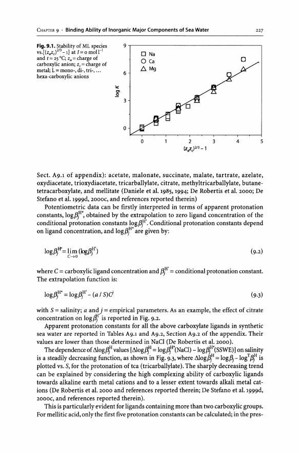
CHAPTER 9 . Binding Ability of Inorganic Major Components of Sea Water 227
Fig. 9.1. Stability of ML species vs.[(zazcl2l3 -1] at 1=0 moll-1
and t = 25°C; Za = charge of carboxylic anion; z, = charge of metal; L = mono-, di-, tri-, ... hexa-carboxylic anions
9,----------------------------------,
6
~
]' 3
o
DNa
o Ca .6. Mg
o 2 (Z~c)213 -1
3 4
o
5
Sect. A9.1 of appendix): acetate, malonate, succinate, malate, tartrate, azelate, oxydiacetate, trioxydiacetate, tricarballylate, citrate, methyltricarballylate, butanetetracarboxylate, and mellitate (Daniele et al. 1985, 1994; De Robertis et al. 2000; De Stefano et al. 1999d, 2000C, and references reported therein)
Potentiometric data can be firstly interpreted in terms of apparent protonation constants, 10gf3t, obtained by the extrapolation to zero ligand concentration of the conditional protonation constants 10gf3{. Conditional protonation constants depend on ligand concentration, and 10gf3t are given by:
H*. H' 10gf3· = 11m (1ogf3. )
J c-->o J (9.2)
where C = carboxylic ligand concentration and f3r = conditional protonation constant. The extrapolation function is:
10gf3t = 10gf3{ - (a / S)d (9.3)
with S = salinity; a and j = empirical parameters. As an example, the effect of citrate concentration on log[lf' is reported in Fig. 9.2.
Apparent protonation constants for all the above carboxylate ligands in synthetic sea water are reported in Tables A9.1 and A9.2, Section A9.2 of the appendix. Their values are lower than those determined in NaCI (De Robertis et al. 2000).
The dependence of Mogf3rvalues [Mogl1H = 10gf3t(NaCI) -logl1H*(SSWE)) on salinity is a steadily decreasing function, as shown in Fig. 9.3, where Mogf3r = 10gf3j _logT I1H is plotted vs. S, for the protonation of tca (tricarballylate). The sharply decreasing trend can be explained by considering the high complexing ability of carboxylic ligands towards alkaline earth metal cations and to a lesser extent towards alkali metal cations (De Robertis et al. 2000 and references reported therein; De Stefano et al. 1999d, 2000C, and references reported therein).
This is particularly evident for ligands containing more than two carboxylic groups. For mellitic acid, only the first five proton at ion constants can be calculated; in the pres-

228 C. De Stefano· C. Foti . A. Gianguzza . D. Piazzese . S. Sammartano
Fig. 9.2.logf3~' of citric acid at 4.5 ,'--------------------, different salinities vs, concentration
4.4 logf3~'
'=- / }4.3~
4,1 +I----.--~-___,-~--_---_I
Fig. 9.3. Mogf3r = log/3j _logT f3r vs. S1l2, for 1,2,3-propanetricarboxylate (t = 25 °C)
o
0.0
-0.6 ",.-<:Q.
8' <i -1.2
-1.8
o
4
2
8 Ceit
4 51/2
12
6
D j=1
o j=2 f:::" j=3
16
8
ence of the artificial sea water salt, the last carboxylic group behaves like a strong acid. The apparent protonation constants of mono, di and tri-carboxylic ligands can be expressed as a function of salinity by the equation:
10gf3t = 10gT f3r + atSliZ + azS + a3S31Z (9·4)
For tetra- and hexacarboxylic ligands Eq. 9.4 is inadequate, and it has been found that it is possible to use the relationship:
10gf3t = 10gTf3r+ btl + boz*log(l + bzl) (9.5)
with
z* = L( charge );eactants - L( charge )~roducts

CHAPTER 9 . Binding Ability of Inorganic Major Components of Sea Water 229
Table 9.6. Empirical parameters for the dependence on salinity of the apparent protonation constants of carboxylic ligands
Ligand logT t1; • • a 0, °2 °3
ae 4.75 -0.134 0.0213 -0.0015
mal 5.70 -0.423 0.0561 -0.0027
2 8.57 -0.550 0.0732 -0.0038
suee 5.64 -0.297 0.0419 -0.0021
2 9.85 -0.434 0.0631 -0.0036
mala 5.10 -0.301 0.0411 -0.0021
2 8.57 -0.439 0.0652 -0.0038
tar 4.43 -0.308 0.0411 -0.0020
2 7.46 -0.434 0.0603 -0.0033
aza 5.49 -0.268 0.0508 -0.0031
2 10.04 -0.398 0.0657 -0.0040
toda 1 4.25 -0.337 0.0459 -0.0023
2 7.56 -0.462 0.0629 -0.0034
tea 1 6.49 -0.434 0.0680 -0.0041
2 11.40 -0.608 0.0880 -0.0050
3 15.09 -0.602 0.0749 -0.0040
mtea 7.58 -0.439 0.0607 -0.0035
2 12.71 -0.630 0.0773 -0.0039
3 16.13 -0.634 0.0682 -0.0034
Ligand logT t1; b b , b b 2
b b 0
bte 7.18 0.0096 74 0.0720
2 13.01 0.0135 43 0.0720
3 17.54 0.0154 29 0.0720
4 20.92 0.0160 23 0.0720
mit 1 7.85 0.0097 2.2 X10s 0.0396
2 14.30 0.0103 7.5 xl 04 0.0396
3 19.39 0.0192 4.8x10⁴ 0.0396
4 22.86 0.0262 2.3 xl 04 0.0396
~ Eq. 9.4. Eq.9.5.
Values of empirical parameters ai' a2' a3' bo, bl and b2, are reported in Table 9.6. As concerns the empirical parameters of Eq. 9.4 for mono-, di- and tri-carboxylic
ligands, we observed a regular trend as a function of z*, according to the simplest re-

230 C. De Stefano· C. Foti . A. Gianguzza . D. Piazzese . S. Sammartano
lationship, valid for all the ligands:
aj= Cjz*
with
at = -0.00648 (±0.0029)Z* (9.4a)
a2 = -0.00872 (±0.00054) z* (9.4b)
a3 = -0.00047 (±0.00003) z* (9.4C)
The empirical parameters of Eq. 9.5 can very probably also be related to some specific parameters for carboxylic ligands; in particular, b2 can be related to the mean stability of the alkali and alkaline metal complexes of fully deprotonated or partially protonated ligands.
The sharp decrease in apparent protonation constants with increasing salinity can also be interpreted in terms of complex formation between the carboxylic anion and the cation B 1.117+ of artificial sea water. For all the systems, complex species are formed with both unprotonated and partially protonated ligands. Formation constants, reported in Table 9.7, are strictly related to the number of carboxylic groups involved in the co-ordination, n.
Table 9.7. Formation constants' for carboxylic ligand complexes with BI.l17+ (I = 0 mol t 1; t = 25 °C)
Ligand 10g/3110 log/3111 10g/3112 10g/3113 10g/3114 log/3210 10g/3121
ac 0030
mal 1.68 6.05 (OJ5)b -
succ 1.26 6.04 (0039)
mala 1.25 5037 (0.27)
tar 1.29 4.69 (0.26)
oda 1.80 4.69 (0033)
aza 0.95 6.00 (0.51)
toda 1.41 4.63 (0038)
tca 1.83 7.52 (1.03) 11.60 (0.19)b - 2.10 (OJ(
mtca 1.90 8.75 (1.17) 12.94 (0.23) 2.6 (0.7)
cit 3.24 7.82 (1.40) 11.30 (0.13) 3.57 (OJ)
btc 3.05 9.12 (1.94) 14.01 (1.00) 17.65 (0.11)b - 3.18 (0.13)
mit 7.05 13.00 (5.15) 18.22 (3.92) 22.28 (2.89) 25.26 (2.4)b 8.81 (1.76) 14.25 (1.25)d
a f3 . B1.117+ LZ- H+ B L H I1.117P+r-qz) pq' P + q + r H p q r .
b In parentheses partial formation constants (Kpqr) refer to the reaction: B1.117+ H Llr -z) B LH 11.1 17p+r-Z)
P + r H p r .
C Partial formation constants refer to the reaction: B 1.117+ + BL 11.117 -z) H Blz.234 -Z)
d Partial formation constants refer to the reaction: B1.117+ + BHLIZ.117-Z) H BzHLI3.234-Z).

CHAPTER 9 . Binding Ability of Inorganic Major Components of Sea Water 231
For example:
btc4- + Bl.l17+ = B(btc)2.883- n = 4
H3(mlt)3- + B1.l17+ = BH3(mlt)1.883- n = 3
The simplest relationship between 10gK and n is:
10gK = 0.37 (±om) n312 (1 ~ n ~ 5) (9.6)
Inspection of stability data revealed some other interesting trends: (i) stability is inversely proportional to the length of the alkyl chain. If we consider malonate, succinate and azelate we have /3110 = 48, 18 and 9 M-1, respectively: the decreasing function is not linear, owing to the higher flexibility of longer chains; (ii) the higher stability of oxydiacetate and trioxydiacetate is due to the involvement of the ethereal group in the co-ordination. This is consistent with previous findings on the stability of calcium complexes of oxydiacetate and trioxydiacetate (De Stefano et al. 1999d, 2000C).
Figure 9.4 shows the speciation diagram vs. pH for the tca system in artificial sea water (BA) at S = 35. In this system, it can be observed that all the species show high yields (>20%) and that at pH > 7, the sum of B(tca) 1.883- plus B2(tca)O.766- is >90%.
The same holds for the btc-BA system with a higher yield (except for the tri-protonated complex), and at pH> 7 we have -100% of the ligand as B(btc)2.883- and B2(btc) 1.766-. Formation percentages are strongly dependent on the number of carboxylic groups in the ligand; to illustrate this trend quantitatively, in Fig. 9.5 we plotted ~(species) % vs. salinity, at pH 8.2 for mono-, di-, tri- and tetra-carboxylic ligands. Percentages increase with n: for mellitate, at pH > 5, a 100% yield is always observed.
9.3.1.2 Phenols
A study carried out on the interaction of phenol and some of its derivatives in artificial sea water (Demianov et al. 1995) shows that phenols in artificial sea water form the weak species BLo. ll7+ (Table 9.8), with a mean stability of 1.3 M-1. This stability is somewhat lower than that of mono-carboxylic ligands, but is still comparable (same order of magnitude).
9.3.1.3 Amines
Amines are quite an important class of ligands, present as trace components in all biological fluids and natural waters. In particular, open chain polyamines have been widely studied owing to their strong ability to bind several metal cations (Perrin 1979; Pettit and Powell 1997; Martell and Smith 1997) and to form fairly stable species, in their protonated form, with organic and inorganic polyanions (Daniele et al. 1997). Amino compounds play an important role in reactions with sugars (or their derivatives) in natural waters leading to polymerized products (Bremmer 1967; Stevenson and Butler 1969) containing several amino groups along a linear chain, whose composition is

232 C. De Stefano . C. Foti . A. Gianguzza . D. Piazzese . S. Sammartano
Fig. 9.4. Speciation diagram of 100 " ----------------------, tca in artificial sea water singlesalt (S = 35, t= 25 °C); CBA = 0.5752 mol rl; Ctc.= 10-4 moll-I. Curves: 1. B(tca)H2; 2. B(tca)H; 3· B(tca); 4· B2(tca); S.lspecies%
Fig. 9.5. Sum of species percentages vs. salinity (S) of carboxylic ligands in SSWE as single salt, at pH = 8.2
Table 9.8. Formation constant
'j ~ 50
c?.!
100
[ 50 ~
5
3
4
5 8 pH
----b-- tea
-V- bte
\1-\1--\1-/", ___ ,, __ Z==E ,,/ ~ ________ O _____ O--O
0/0 ___ 0---0
.___0----0 -D-- ac 0""""""'- --0- mala
O+I----~--_r----~--_,--~~--,,~
o 15 30 45 5
for phenol complexes with Bl. ll7+ Ligand (1= 0 molrl; t= 25 °C)
logK a
phenol
o-cresol
p-cresol
o-nitrophenol
p-nitrophenol
Mean value
0.3
0.1
0.3
0.2
-0.1
0.15
a K refers to the reaction: B + L H BL.
very similar to that of the humic water-soluble fraction. Therefore, polyamines can be considered as a representative model of aminic sites in the humic acids, whose NMR

CHAPTER 9 . Binding Ability of Inorganic Major Components of Sea Water 233
spectra analysis shows intense dialkylamine bands (Mikita et al. 1981). Chloride and sulphate anions form weak complexes with partially or fully protonated polyamines, whose stability is strictly dependent on the charge of the polyammonium cation (Daniele et al. 1997). Mg2+ and Ca2+ also form complexes with polyamines (De Stefano et al. 1999a). The stability of these complexes is not very high and shows a regular increasing trend as a function of the number of amino groups. Moreover, for the reaction
M2+ + H;A;+ = M(H;A)(i+2)+
it is possible to express stability using the general equation:
10gK~ = bo + b, n + b2nH (9·7)
(with nH = i = number of protons in the complex species). The values of empirical parameters are for Mg2+ complexes: bo = 0.39, b, = 0.44 and b2 = -0.16; and for Ca2+ complexes: bo = -0·95, b, = 0.55 and b2 = -0.05.
In order to check the binding capacity of low molecular weight aminic ligands towards the major components of sea water, we examined the available literature data (Bates and Calais 1981; Bates and Erickson 1986; Czerminski et al. 1982) and the results of an extensive potentiometric investigation carried out at t = 25°C on the following amines in artificial sea water at different salinities (De Stefano et al. 2000d): ethylenediamine, diethylenetriamine, triethylenetetramine, tetraethylenepentamine and spermine (formulas and abbreviations are reported in Sect. A9.1 of appendix). Apparent proton at ion constant, or 10gf3r* values obtained from potentiometric data by extrapolation to zero ligand concentration are shown in Table A9.3 of the appendix (Sect. A9.2). As an example, apparent protonation constants of triethylenetetramine (nH = 1 to 4) are plotted as a function of ionic strength (Fig. 9.6).
For these ligands too, 10gK~* values can be expressed as a function of salinity by Eq. 9.4. Empirical parameters a" a2 and a3 are shown in Table 9.9, together with thermodynamic protonation constants 10gTKH.
Fig. 9.6. &ogt1i vs. total ionic strength for triethylenetetramine, at 25°C
".-co.. 8' <i
3
2
o I'k'="= D D D D tJ
0.0 0.2 0.4 0.6 0.8
r}'2 (mol 1-1)1/2
;=4
;=3
;=2
;=1
1.0

234 C. De Stefano· C. Foti . A. Gianguzza . D. Piazzese . S. Sammartano
Table 9.9. Parameters of Eq. 9.4 for the dependence on salinity of apparent protonation constants' of amines, at t= 25·C
Amine logTKiH °i °2 °3 en 9.91 0.003714
dien 9.80 0.003178
trien 9.67 0.001211
tetren 9.83 -0.000768
sper 10.70 0.000056
en 2 6.86 0.1594 -0.01958 0.00114b
dien 2 8.74 0.1481 -0.01865 0.00114
trien 2 8.87 0.1756 -0.02001 0.00114
tetren 2 9.01 0.1324 -0.01895 0.00114
sper 2 9.70 0.1260 -0.01932 0.00114
dien 3 3.66 0.4452 -0.06523 0.00344b
trien 3 6.12 0.3824 -0.06102 0.00344
tetren 3 7.73 0.3251 -0.05445 0.00344
sper 3 8.32 0.3368 -0.05403 0.00344
trien 4 2.38 0.8332 -0.1675 0.01095
tetren 4 3.90 0.7031 -0.1301 0.00812
sper 4 7.22 0.6003 -0.1114 0.00688
tetren 5 1.88 1.0958 -0.2321 0.01562
a Refer to the reaction: iH+ + A 0 ~ H/+. b The parameter 03 was constrained, for i = 2, 3, to be constant for all the amines.
The parameters of Eq. 9.4 depend on: (i) the protonation step (mainly), i.e. the charge of the protonated species; and (ii) the number of amino groups in the amine, nN' For i = 1, ... 3, we have the following relationships, which are valid for all the amines studied:
10gKr = 10gT Kr* + 5 (0.00722 - 0.00159 nN) (9.8)
log~* = 10gTKr + 5112 (0.179 - O.0077nN) - 0.02175 + 0.0014353/2 (9.8a)
10gKr = 10gTKr + 5112 (0.500 - 0.0346nN) - 0.05145 + 0.002465312 (9.8b)
The decrease in apparent protonation constants with increasing salinity was accounted for by considering the formation of complex species between protonated amines with A 1.117-. In all the amine-BA systems, the species B(am)I.117+ and (am)Alf/·ll7-i) (with i = 1, ... , n; n = number of aminogroups) are formed. Formation constants for amine-BA complex species are shown in Table 9.10.

CHAPTER 9 . Binding Ability of Inorganic Major Components of Sea Water 235
Table 9.10. Formation constants for amine complexes with the cation and the anion of marine salt BA, at! = 0 molt! and t= 25°C
Amine log f3;a 10gK;b 10gKBC Amine 10gf3;a 10gK;b 10gKB
C
en lOA 0.5 0.14 tetren 10.3 0.5 OA2
2 17.88 1.1 2 19.73 0.9
3 28.10 1.5
dien 10.3 0.5 0.18 4 32.98 2.5
2 19.60 1.1 5 35.92 3.6
3 24.23 2.0
sper 1 11.2 0.5 OAO
trien 1 10.2 0.5 0.35 2 21.23 0.8
2 19.77 1.2 3 30.31 1.6
3 26.59 1.9 4 38.28 2.3
4 29.96 2.9
a f3;: amO + iH+ + A1117-H (am)AH:;-1.117)
b K;:(am)H; + A1.117-H (am)AH/-l.l 17). c Ks:amo +Sl.l17+ H(am)S1.117+.
The relative formation constants of cation complexes are fairly low, ranging from 1.4 to 2.6 M-1• For anion complexes, real stability is given by the partial equilibrium between the protonated amine and the anion; the stability of these species is considerably higher than that of cationic ones, ranging from 3 to 4000 M-1• Moreover, logKi
is strictly dependent on i, i.e. on the charge of the protonated amine. The logKB constant for the formation of cationic species can be related to the rela
tive formation constants of amine complexes with Mg2+ and Ca2+. To this end, we may consider a mean formation constant for alkaline earth metal species, KMgCa' which takes into account the concentration of Mg2+ and Ca2+ in the artificial sea water:
KMgca = (KMgCMg + KCaCCa) / (CMg + CCa) (9.9)
having the following values: logKMgCa = 0.35,0.87,1.39,1.71,1.63 for en, dien, trien, tetren and sper, respectively. The simple relationship between the two constants is:
logKB = 0.27 logKMgca (9.10)
As regards to anionic species (am)AHY-l.ll7), for i> 1, their formation constants, logKi (Table 9.10) are strictly dependent on protonated amine charges, according to the relationship:
logKi = -0.65 + 0.817 I (9.11)
Further inspection of formation data for the different amines reveals the en - dien > trien > tetren > sper trend, which can be explained by considering the ratio

236 C. De Stefano· C. Foti . A. Gianguzza . D. Piazzese . S. Sammartano
RNlc = (number of aminogroups) / (number of -CHz-groups) = 1, 0.75, 0.67, 0.625, 0.4, for en, dien, trien, tetren and sper, respectively. By considering the RN/c term we obtain:
10gKi= -1.335 + 0.857i + 0.914RNlc (9.12)
By using the parameter RNiO it is also possible to obtain a general equation for apparent protonation constants. Calculations performed using all the protonation data for i ~ 2 made it possible to formulate the following general relationships for the empirical parameters of Eq. 9.4:
al = 0.0317 + O.Ol77 nN (9.4d)
a2 = -0.00507 nN+ 0.00379 RNlc (9.4e)
a3 = 0.000285 nN (9.4f)
Both apparent protonation constants and BA complex formation constants can be calculated from protonation constants at different ionic strengths and the formation constants of (am)ClHii- 1, (am)(S04)Hii-2, Mg(am)2+ and Ca(am)2+ complexes. This is certainly possible for 5 ~ 15 (IT~ 0.3 mol rl) and i ~ 3, but for higher salinities and for amines containing several amino groups, the probability of the formation of ternary species such as (am)CI(S04)H'i- 3 or MgCa(am)4+ becomes significant. For purposes of comparison, Table 9.11 shows experimentallogtJl* values and the relative calculated ones at 5 = 35. Deviation, 0 = logm*(calc) -logm*(exp)' increases consistently with i, and mean deviation, £, can be expressed as a linear function of z*, £ = 0.03 + 0.026 z*.
On the basis of the above observations, by way of example, Fig. 9.7 shows a speciation diagram for the spermine system in artificial sea water as a single salt (BA). High yields of complex species of different forms of protonated spermine with the sea water anion component (A) are observed in a wide range of pH values. The most important species in terms of formation percentages is the one with the higher amine charge,
Table 9.11. Differences be-tween experimental and calcu- Amine 8'
1 8'
2 8'
3 8'
4 8'
5 lated values of apparent proto-nation constants of amines en 0.05 0.11
dien 0.03 0.11 0.19
trien 0.02 0.07 0.14 0.20
tetren -0.01 0.01 O.OB 0.15 0.21
sper -0.03 0.01 0.09 0.20 b
0.03 0.06 0.l3 O.lB (0.21) e
a w- H~
8; = logf3; (calc) -logf3; (exp). b
e= mean values of 18;1.

CHAPTER 9 . Binding Ability of Inorganic Major Components of Sea Water 237
i.e. (sper)AH~·883. In our conditions for standard sea water (S = 35, pH = 8.2), 88% of total spermine is present as (sper)AH~·883 (-60%) and (sper)AH~·883 (-30%). Fully protonated spermine complexes are also present at pH > 8.5.
All the polyamines with amino groups separated by longer alkyl chains display the same behaviour as spermine (biogenic amines belong to this class of amines). As regards the unprotonated cationic species, significant yields only occur at very high pH values (pH> 10.5), and in the conditions necessary for the speciation of sea water their presence is negligible. In general, the total binding capacity of sea water salt towards amines is quite significant, as shown in Fig. 9.8, where Lspecies % (total percentage of complex species) is reported vs. S salinity, at pH = 8.2: for all the amines Lspecies % > 40 at S = 35.
The en < dien < tetren < trien < sper trend is mainly due to the presence, at pH = 8.2, of different protonated species of amines. The stability of (am)AHY-1.l17) com-
Fig. 9.7. Speciation diagram of 100 ,r-------------------~ spermine in artificial sea water, 35 salinity, vs. pH, at t = 25°C. Curves: 1. (sper)AH4; 2. (sper)AH3;
3. (sper)AH2; 4. (sper)AH; 5. B(sper)
~ lu 50 Co
'"
o I r<:: d"""":-"""""'" -6 ............... ' :l>
7 9 11 pH
Fig. 9.8. Ispecies % (total per- 100 ~-------------------~ centages of complex species) vs. salinity, at pH = 8.2
<f. .~ Co
v-l'"
75
50
25
o en
o dien D,. trien
\1 sper
<> tetren
O+I---------.----~--_,r---~----._~
o 15 30 45
5

238
Table 9.12. Formation con-stants of polyammonium cation complexes [(am)XHnl(n-z) with X= Al. ll7-, ct and Scn-, at! = 0
molt l and t=25°C
C. De Stefano· C. Foti . A. Gianguzza . D. Piazzese . S. Sammartano
Amine logKna
A1.117- cr SO~-
en 1.1 0.7 2.4
dien 2.0 1.5 3.8
trien 2.9 1.7 5.2
tetren 3.6 2.2 5.6
sper 2.3 1.5 3.9
a Refer to the reaction: Hn(am)"+ + Xz-H (am)XHn n-z; Xz-= A 1.1 17-, CI-, SO~- (n = maximum protonation degree).
plexes can be compared with that of analogous cr and SO~- complexes (De Robertis et al. 1998b). As an example, Table 9.12 shows the formation constants of (am)AH~n-l.ll7), (am)ClH~n-l), and (am)(S04)H~n-2) species.
The stability of BA sea salt complexes is intermediate between that of cr and SO~species, as expected on the basis of the electrostatic model for the binding of anions by polyammonium cations.
9.3.1.4 Amino Acids
Natural waters contain a wide range of individual (free amino acids, FAA) and hydrolysable combined amino acids (HAA) in solution, which constitute the most important fraction of the dissolved organic nitrogen matter. They can be found in natural waters as the excretion products of living organisms and/or as the hydrolysis products of pedogenic polypeptides. Moreover, FAA can be formed in natural waters by the reaction of ammonia, obtained during the biological fIxation process of elemental nitrogen, with some naturally occurring carboxylic acids, in the presence ofNADPH. Glutamic acid is formed from the reaction of ammonia with a-ketoglutaric acid, and most other amino acids can be formed from it by transamination: a-alanine, for example, is formed by the transamination of glutamic acid reacting with pyruvic acid. Therefore, amino acids are particularly abundant in waters with high productivity. In some oligotrophic lakes, dissolved hydrolysable amino acids are reported to make up 30-40% of total dissolved organic nitrogen (Tuschall and Brezonik 1980). Together with sugars, amino acids represent an important food and energy source for heterotrophic microorganisms (Campbell and Goldstein 1972). Accumulated amino acids participate in the synthetic and respiratory metabolism of the organisms. The assimilation and release of amino acids by marine organisms has been studied using 14C-Iabelled amino acids and by colourimetrically measuring their disappearance from the medium and their appearance in various chemical fractions of the different organisms, and vice versa (Stephens 1972). After hydrolysis, the following percentages of combined amino acids (HAA): 33,55-75,55.4 and 13-26 were measured with respect to dry organic matter in marine zoo- and phytoplankton, in bacteria, in molluscs, and in macrophytes, respectively (Buffle 1988). Salinity seems to be an important factor in regulating the
CHAPTER 9 . Binding Ability of Inorganic Major Components of Sea Water 239
assimilation of amino acids. Investigations carried out on some organism tests showed that uptake of glycine and a-alanine continues until salinity decreases to about 1/3 of normal sea water, i.e. a salinity of about 12. At lower salinities, the animals survive but can no longer acquire free amino acids from solution, probably because the osmotic and chloride regulation processes of the body fluid are reduced (Stephens 1972). Moreover, increasing salinity determines a lowering of amino acid assimilation, probably owing to their reduced availability due to complexation with the cation macro components of sea water. This last point further demonstrates the importance of chemical speciation studies in natural waters.
Besides their biological role, among the low molecular weight ligands present in natural waters, amino acids are interesting because of their acid-base behaviour, which can be considered to be intermediate between that of carboxylic acids and amines (De Stefano et al. 1995). Of the twenty amino acids that commonly occur in proteins, about half contain side chain donor atoms that are potentially capable of forming stable complex species with metal ions, and several studies have been described in literature on this subject (Silien and Martell 1964, 1971; Martell and Smith 1997). Most of these studies concern the co-ordination chemistry of transition metal ions, and relatively few data regarding their complexation with alkali and alkaline earth metal ions have been published (Evans and Guevremont 1979; Casale et al. 1989; De Robertis et al. 1991; De Stefano and Gianguzza 1991; De Stefano et al. 1995). While taking into account the above considerations on the dependence of amino acid assimilation on sea water salinity, because of their importance in defining the chemical speciation of amino acids in natural waters, we also thought it would be worthwhile examining the interactions of this class of compounds with sodium, calcium and magnesium (i.e. the cation macro constituents of natural waters).
The protonation constants of glycine, alanine, histidine, aspartic, glutamic and iminodiacetic acids were studied in different aqueous media and at different ionic strengths (De Stefano et al. 1995, 2000b). These studies showed that: (a) carboxylic groups interact weakly with Na + and rather strongly with Ca2+ and Mg2+, (b) unprotonated aminogroups interact weakly with Ca2+ and Mg2+ and (c) protonated aminogroups interact weakly with cr and SO~-. Moreover, by studying the dependence of protonation constants on ionic strength and complexing ability, amino acids were grouped into three different types: the first includes glycine, alanine and serine; the second lysine and histidine; and the third aspartic, glutamic and iminodiacetic acids.
Apparent protonation constants (logf3H*) for glycine, alanine, histidine, and glutamic and aspartic acids (De Stefano et al. 1995, 2000b) and for serine, valine, leucine, threonine and methionine (Fiol et al. 1995a,b, 1998) determined in artificial sea water are shown in Tables A9.4 and A9.5, respectively, in Sect. A9.2 of the appendix (in Sect. A9.1 of the appendix formulas and abbreviations of all amino acids considered here are reported).
The dependence on salinity of Mog f3r values [Mogf3r = 10gf3t(NaCI) -logf3t(SSWE)] is shown in Fig. 9.9, for the first (Fig. 9.9a) and the second (Fig. 9.9b) protonation step of glycine, histidine and glutamic acid. As can be seen, gly and his behave in a similar manner (in particular as regards 10gf3r\ whilst protonation constants for glutamic acid are significantly lower. This is due to the presence of a second carboxylic group, which binds cations (see formation constants for alkali and alkaline earth complexes below) more strongly than aminogroups.

240 C. De Stefano· C. Foti . A. Gianguzza . D. Piazzese . S. Sammartano
Fig. 9.9. Mogf3r values vs. SII2; 0.0 "------------------~ a for the first; b for the second protonation step of glycine (0), histidine (0 ~ and glutamic acid (.1.). ~ogf3j = 10gf3r' (NaCl)-10gf3j (SSWE)]
:r--CCl.. 8' -0.4 <i
-0.8
0.0 TI-----------------,
~-=9:=L J:'-<:0.. 8' -0.6 <i
-1.2 -+I-..,.-~-_._--_._--_,_--__.-~__r----j 2 3 4 5 6 7
5112
Apparent protonation constants obtained in artificial sea water can be expressed as a function of salinity by the equation:
logf3r = logT f3r + aS1I2 + bS (9.13)
The values of the empirical parameters of Eq. 9.13 were quite similar for the same amino acid class and the same protonation step. In particular, parameter b can be considered a "common parameter" for glycine and alanine and for aspartic and glutamic acids without any significant increment in the (j of fit. For parameters a and b it was also possible to give general parameters for each amino acid group:
type 1
type 3
al = -O.098±O.015 a2 =-O.105±O.019
al = -O.186±O.030 a2 = -O.292±O.027
a3 = -O·316±o.023
bI = O.009±O.003 b2 = O.009±O.003
bI = o.olO±O.oo5 b2 = O.019±O.005 b3 = O.022±O.oo4

CHAPTER 9 . Binding Ability of Inorganic Major Components of Sea Water 241
Table 9.13. Complex species formation of amino acid in SSWE as a single salt (BA), at 1=0 mol t 1 and t= 25°C
Reaction logK
gly ala his glu asp
B + L= BL 0.8 (0.7)' 0.65 (0.6)' 0.8 (0.6)' 1.34 (1.3)' 1.52 (1.6)'
B+HL=BHL 0.3 (0.2) 0.25 (0.2) 0.2 (0.1) 0.71 (0.6) 0.5 (0.4)
B + H2L = BH2L 0.1 0.0
H2L+ A= H2LA 0.4 0.4 0.6
HJL+ A = HJLA 0.7 -0.1 0.0
, In parentheses values calculated by using formation constants of weak complexes (see De Stefano et al. 1995).
The dependence on medium of protonation constants can be interpreted in terms of complex formation. We found the following species are formed: BL, BHL and H2LA (for L = gly and ala); BL, BHL, H2LA and H3LA (for L = his); BL, BHL and BH2L (for L = glu and asp). Formation constants are shown in Table 9.13.
The stability of BL and BHL species for gly, ala and his, and of BL, BHL and BH2L species for glu and asp is fairly constant, and the following mean values of formation constants can be used: 10gKBL = 0.75, 10gKBHL = 0.25 (for L = gly, ala and his); 10gKBL = 1.43, 10gKBHL = 0.605, and logKBH2L = 0.05 (for L = glu and asp). Table 9.13 also shows formation constant values for the simplest species BL and BHL, calculated from the formation constants of binary systems.
The calculated values are fairly similar to experimental ones but are consistently lower: this may indicate that ternary interaction cannot be neglected. As examples, the distribution diagrams of glycine, histidine and glutamic acid vs. pH are shown in Fig. 9.10.
At pH = 8, the complexation of gly and glu is higher than 50% and for his> 40%. For glycine, the most important species at the pH of natural waters is B(gly)H; for histidine, mainly B(his)H (with small percentages of A(his )H2 and B(his)) must be considered; for glutamic acid, B(glu)H (with small percentages of B(glu)H) predominates.
9.3.2 Inorganic ligands
9.3.2.1 Phosphates
The average concentration of phosphorus in sea water is about 2.5 flmol rl in the lower layers, while this falls to zero in the upper 100 m because of biological activity. In spite of its very low concentration, phosphorus can be considered a master element in the marine ecosystem, since it is involved in most important biological processes, such as

242
Fig. 9.10. Distribution diagram of; a glycine; b histidine; c glutamic acid vs. pH, in artificial sea water as a single salt BA and t = 25 0c. Species: a: 1. A(gly)H2•
2. B(gly)H,3.B(gly); b: 1. A(his)H3, 2. A(his)H2,J. B(his)H, 4. B(his); c: 1. A(glu)H3' 2. B(glu)H2,
3. B(glu)H, 4. B(glu). Curves relative to simple protonated species and free components are not reported
C. De Stefano . C. Foti . A. Gianguzza . D. Piazzese . S. Sammartano
75" -----------------------------------------,
~ 45
>-0-.
15
a
2
75" ----------------------------------,
b
~ 45
II! :c
15
75,.-------------------------------------,
c
3
~ 45
::l 0-.
15
5 9 pH
marine primary productivity (Fogg 1975; Spencer 1975). In that process, as well as in other biochemical processes, the reactive form of phosphorus is phosphate, which derives from both the particulate and the dissolved fraction. The latter exists as soluble inorganic phosphorus and as soluble organic phosphorus compounds. Soluble inorganic phosphate has been regarded as being present exclusively as orthophosphate, i.e. as H2P04 and HPO~-, with negligible amounts of PO~- and H3P04• Dissolved orthophosphate groups can also derive from the organic fraction (sugar phosphates,

CHAPTER 9 • Binding Ability of Inorganic Major Components of Sea Water 243
phospholipids, phosphonucleotides) as a consequence of enzymatic hydrolytic processes. Thus, the study of phosphorus compounds in sea water is mainly concerned with the chemical behaviour of the phosphate group. A comprehensive picture of the distribution of the different forms of phosphorus in sea water was drawn up by Armstrong (1965). Although there is no evidence of the presence of dissolved polyphosphates in sea water slowly leading to the formation of phosphate groups as a result of hydrolytic processes, it is well-known that phosphoric acid can undergo condensation to form poly-acids such as pyrophosphoric acid or poly-meta-phosphoric anions, (HP03 )n> with n = 3 up to 70 per chain. Polyphosphates can also be present in coastal sea waters containing sewage and industrial wastes. Therefore, these compounds too must be taken into account in chemical speciation studies of phosphorus compounds in sea water. Studies of the solution chemistry of the phosphate group in natural waters are complicated by interactions with macro constituent cations such as ci+ and Mg2+, which, under certain pH and free concentration conditions, can lead to the formation of insoluble species.
The speciation of phosphate in sea water has been investigated by few authors (Kester and Pytkowicz 1967; Atlas et al. 1976; Dickson and Riley 1979; Johansson and Wedborg 1979). The shift in the apparent protonation constants of phosphoric acid with changes in the composition of the ionic medium (containing macrocomponents of sea water, Na +, Mg2+ and Ca2+) was interpreted by the aut110rs in terms of the association of orthophosphate with medium cations using ion association models. Hershey et al. (1989) studied the ion pairing of phosphate with Mg2+ and evaluated Pitzer interaction parameters for the major components of sea water. Table A9.6 ~f the appendix (Sect. A9.2) shows apparent protonation constants, 10gfJj w, for p;ogtlb in SSWE. For purposes of comparison, speciation diagrams for different forms of phosphate ligand in SSWE (S = 35) and in NaCl (0.75 mol rl) are shown in Fig. 9.11.
As can be seen, curves for the different protonated species in SSWE have shifted significantly to lower pH values in comparison with those in the NaCI medium. The lowering effect on 10gf3t can be simply explained by takin&. into account the formation of simple and mixed protonated B 1.1 17+ - p;ogtl1) species (Table 9.14).
The speciation diagrams obtained by also including species formation as a result of the interaction of phosphate ligands with the sea water cation (B) are shown in Fig. 9.12.
9.3.3 Metals and Organometallic Compounds
9.3.3.1 Divalent Metal Ions
Trace metals interact significantly with both SO~- and cr. Many divalent cations, such as Mn2+, Fe2+, C02+, etc., form ion pairs witl1 SO~- (K = 400 m-1) and witl1 cr (K= 1 M-1).
The ion pairs CdCI+ and CdCI~, whose stability is much higher, constitute an exception. Moreover, most divalent and trivalent cations undergo strong hydrolysis and often hydrolytic species are very important at the pH value of sea water. To give an ex-

244 C. De Stefano· C. Foti . A. Gianguzza . D. Piazzese . S. Sammartano
100r, --~~----------------------,
2
~ ;; 50 CI..
~ 0' Cl..N
~ o
~
J L ~ 4 6 8 4 6 8
pH pH
6 pH pH
8 4 6 8
4 6 8 6 pH
8 pH
Fig. 9.11. Speciation diagrams for Pcfi, P20~- and P30io, by' considering the apparent protonation constants only, in SSWE (right) (S = 35), and in NaCl 0.75 moll-1 (left), at t= 25°C. Species: 1: HzL; 2:HL; 3: L
Table 9.14. Formation con-stants of B 1.117+ - PO~-, -P zO~-and -P30 105- complexes, at t = 25°C and 1= 0 mol rl
L log f3o' 10gf3/ 10gf3z'
pd-4 4.75 13.90 (1 .57)b 20.3 (Od
pp~ 5.81 12.82 (3.22) 17.96 (1.6)
pp~; 6.36 12.80 (3.36) 17.3 (1.4)
a Overall formation constants relative to the reaction (charges omitted): B + L + rH H BLH.
b In parentheses values of equilibrium constants for the reaction: B+HrLHBLHr·

CHAPTER 9 . Binding Ability of Inorganic Major Components of Sea Water 245
Fig. 9.12. Speciation diagrams for p~-, P20~- and P30io, by considering the formation of complexes with B1.1l7+, in SSWE, S = 35 and t = 25°C. Species: 1. H2L; 2. HL; 3. BH2L; 4. BHL; S.BL
100,1 ---------------------------------,
£. 0'" 50 0.
3 4
o ! ?:::7'""7C -----=;::::- t:=""""""---:: 4 6
pH 8
100" ---------------------------------==---~
l o 0.'"
l
100 I 6 50 0.'"
6
~
6
5
8 pH
/'
8 pH
ample of speciation for this class of trace components, we considered the divalent cations Mn2+, Fe2+, Co2+, Ni2+, Cu2+, Zn2+, Cd2+. In some cases, this group of cations is very homogeneous, but in general its speciation profiles display significant differences. Using the formation constants obtained for the cr and SO~- complexes of divalent cation under examination, it is quite simple to obtain formation constants for A 1.117-
complexes, as reported in Table 9.15. For Mn2+, Fe2+, Co2+, Ni2+, Cu2+ and Zn2+, stabil-
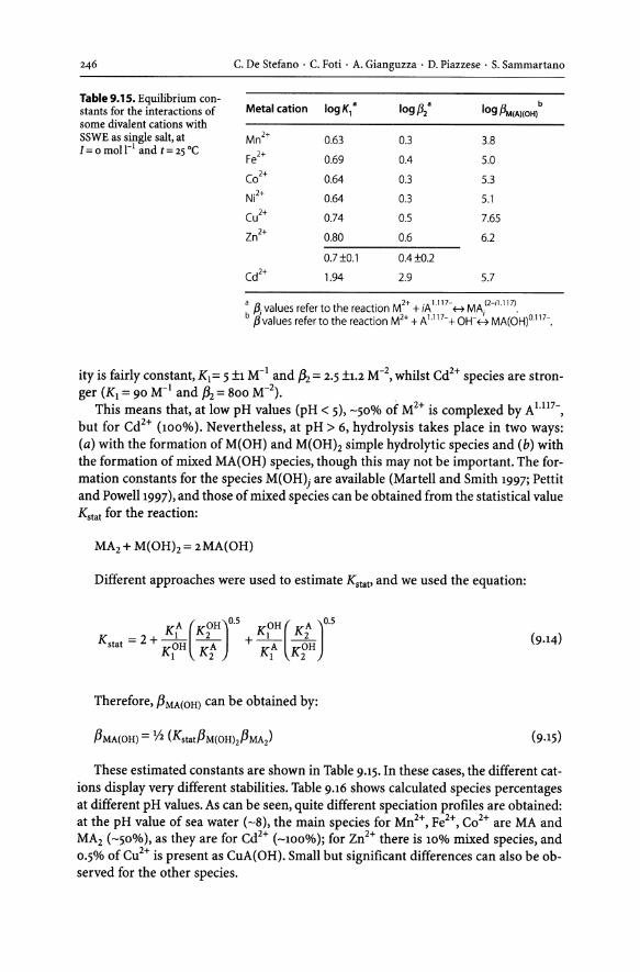
246 C. De Stefano . C. Foti . A. Gianguzza . D. Piazzese . S. Sammartano
Table 9.15. Equilibrium constants for the interactions of some divalent cations with SSWE as single salt, at
Metal cation 10gKl ' 10gf3/ log f3M(A)(OH) b
1= 0 moll-l and t= 2S oC Mn2+ 0.63 OJ 3.8
Fe2+ 0.69 0.4 5.0
C02+ 0.64 OJ 503
Ni2+ 0.64 OJ 5.1
Cu2+ 0.74 0.5 7.65
Zn2+ 0.80 0.6 6.2
0.7 to.1 O.4tO.2
Cd2+ 1.94 2.9 5.7
a f3i values refer to the reaction M2+ + iA 1.117-H MAi2-ill17) b f3values refer to the reaction M2+ + A 1.117-+ OW H MA(OH)o.117-.
ity is fairly constant, K1= 5 ±1 M-1 and ~ = 2.5 ±1.2 M-l , whilst Cdl + species are stron-ger (Kl = 90 M-1 and ~ = 800 M-l ). .
This means that, at low pH values (pH < 5), -50% of Ml+ is complexed by Al. ll7-,
but for Cd2+ (100%). Nevertheless, at pH> 6, hydrolysis takes place in two ways: (a) with the formation of M(OH) and M(OHh simple hydrolytic species and (b) with the formation of mixed MA(OH) species, though this may not be important. The formation constants for the species M(OH)j are available (Martell and Smith 1997; Pettit and Powell 1997), and those of mixed species can be obtained from the statistical value K stat for the reaction:
MAl + M(OHh = 2MA(OH)
Different approaches were used to estimate Kstat> and we used the equation:
A (OH}O'5 OH ( A }o.5 Kl Kl Kl Kl K stat = 2 + ----em -A- + ------p: OH
Kl Kl Kl K2 (9.14)
Therefore, f3MA(OH) can be obtained by:
f3MA(OH) = 0 (Kstatf3M(OHjzf3MAz) (9.15)
These estimated constants are shown in Table 9.15. In these cases, the different cations display very different stabilities. Table 9.16 shows calculated species percentages at different pH values. As can be seen, quite different speciation profiles are obtained: at the pH value of sea water (-8), the main species for Mnz+, Fez+, Coz+ are MA and MAz (-50%), as they are for Cdz+ (-100%); for Znz+ there is 10% mixed species, and 0.5% of Cuz+ is present as CuA(OH). Small but significant differences can also be observed for the other species.

CHAPTER 9 . Binding Ability of Inorganic Major Components of Sea Water 247
Table 9.16. Metal species percentages in SSWE as single salt, at different pH (S = 35)
Metal cation pH MA MA2 M(OHI M(OHI2 MA(OHI
Mn2+ 7 43.1 6.8 0.0
8 43.1 6.8 0.1 0.1
9 42.6 6.7 0.7 0.6
Fe2+ 7 45.7 7.9 0.1 0.1
8 45.0 7.8 0.8 0.8
9 39.0 6.8 7.3 0.1 7.4
C02+ 7 43.6 6.7 0.1 0.2
8 42.6 6.6 0.6 1.8
9 34.1 5.3 4.5 3.1 14.4
Ni2+ 7 43.6 6.7 0.1
8 43.0 6.6 0.4 1.1
9 37.1 5.7 3.1 2.2 9.9
Zn2+ 7 49.4 10.5 0.2 1.1
8 43.7 9.3 2.0 0.6 10.1
9 16.5 3.5 7.6 21.0 38.4
Cd2+ 7 24.2 74.4 0.0
8 24.1 74.3 0.1
9 23.9 73.5 0.1 1.3 Cu2+ 6 45.7 8.9 0.8 3.4
7 33.2 6.4 5.5 0.1 24.9
8 8.7 1.7 14.4 2.5 65.0
9 0.8 0.2 13.5 23.7 61.1
9.3.3.2 Organometallic Compounds
Among the organometallic compounds, organotin(IV) and organomercury(II) are the most widespread in the aquatic environment as a result of their use in industry (organotin in fungicides and acaricides in agriculture, in wood and stone preservatives, in antifouling agents in paints for ships, in stabilizers and catalysts in PVC and foam production; organomercury in fungicides for paper and wood and in antibacterial agents in medicine, etc.) and of the bioalkylation processes of inorganic metals by means of a variety of bacterial substrates (Craig and Miller 1997, and references therein).
Organotin(IV) compounds include a variety of organometallic moieties characterized by a central tin atom covalently bonded to various organic groups (methyl, ethyl, propyl, butyl, octyl, phenyl, etc.) through one or more carbon atoms. Their general formula can be written: RnSnX(4_n) (R = organic group; X = halide, nitrate, acetate, hydroxide, etc.; n = 1 to 4). Organotin cations in aqueous solution are considered as ac-

248 C. De Stefano . C. Foti . A. Gianguzza . D. Piazzese . S. Sammartano
ids of different hardness on the Lewis scale depending on the groups bonded to the tin(IV) (Tobias et al. 1966). They therefore show a strong tendency to hydrolysis in aqueous solution, resulting in some cases in condensation reactions of the monomeric conjugate bases with the formation of polynuclear hydroxo-complexes in solution according to the following general reaction (Tobias et al. 1966):
qRnSn(OH2)~+ + pH20 = PH30+ + (RnSn)q(OH)p(OH2);qz-P)+
The hydrolysis processes of mono-, di- and trimethyltin(IV) cations have recently been reviewed, extensively investigated and defined in different ionic media, including SSWE, in a wide range of ionic strengths and salinities (De Stefano et al. 1999b 1999C 2000aj Foti et al. 1999, 2000). Hydrolysis constants for mono-, di- and trimethyltin(IV) cations are shown in Table A9.7 of appendix (Sect. A9.2)
Once hydrolytic equilibria have been defined for all ilie organotin(IV) cations investigated, ilie interactions of simple and hydroxo-organotin(IV) species wiili ilie anion A of SSWE as a single salt can be considered. On ilie basis of the results obtained by potentiometric measurements, we formulated ilie complex formation model shown in Table 9.17.
Mixed hydroxo-species are formed in all the systems. This indicates the strength of the hydrolytic species to be stronger than the simple association of organotin cations with the anionic component A of SSWE. By way of example, Fig. 9.13 shows a speciation diagram for the species CH3Sn3+ in artificial sea water as a single salt (BA). As can be seen, the main species formed are mixed hydroxo species where the sea water anion (A) is representative of chloride and sulphate anions. In particular, at pH = 8 the predominant species is [(CH3SnhA(OHhlo.1l7- (more than 60% formation, Curve 6), while the simple hydrolytic species [CH3Sn(OHhlo achieves about 24% formation (Curve 2) at ilie same pH value, confirming the strengili of ilie hydrolysis processes.
9.4 Discussion and Conclusions
In the preceding sections, we illustrated two very important features of the interactions of low molecular weight ligands and metal cations, namely: (a) that these inter-
Table 9.17. Interactions of mono-, di- and triorganotin compounds in SSWE as single salt BA, at 1=0 mol rl and t= 25°C
System Species 10gf3" 10gK b
(CH3l3Sn-BA [(CH3l3Sn(Al]o.117- 0.15 0.15
(CH3l2Sn-BA [(CH3l2SnA]O.883+ 0.90 0.90
[(CH3l2SnA(OHl]Ol17- -3.05 -0.2
CH3Sn-BA [CH3SnA(OHl]0883+ 0.7
[CH3SnA(OHlll17- -1.45
[(CH3Snl2A(OHl/117- -5.80
a 13 refers to the reaction: M + Hp + A H M)OHll' with M = (CH)xSn(4-X)+.
b K refers to the reaction: M)OHly + A H M)OHl,A with M = (CH3lxSn(4-X)+.
2.2
2.0
1.89

CHAPTER 9 . Binding Ability of Inorganic Major Components of Sea Water 249
actions are quite significant, both in terms of stability constant values and in terms of the formation percentages of the various species; (b) that the behaviour of some major classes of ligands is generally homogeneous. To permit comparison of different ligands and metal cations, the percentages of complexes formed with the anion and the cation of the marine salts are reported in Pig. 9.14.
Only mono-carboxylic anions gave yields <50% whilst in the other cases, yields were always 2':50% and in some cases 100%. These percentages include protonated species for the different ligands and mixed hydroxo complexes for metal cations. Note that these speciation data are strictly valid only for the artificial sea water used (SSWE) and can differ significantly for other sea waters, in particular for those containing carbonate and fluoride. These differences are quite small for the ligands (amines in their protonated form interact with P-, RCO; and CO~-) (De Stefano et ai., work in progress)
Fig. 9.13. Speciation diagram for the system CH3SnH -BA at 25°C. CRSn3+ = 0.5 mM; CBA = 0.575 M. Species: 1. RSn(OHh; 2. RSn(OHh; 3. (RSnlz(OH)s; 4. RSnA(OH); 5. RSnA(OH}z; 6. RSn}zA(OHls
100
~ 50
0 r:: ~ 0 E'O oS 21
o Carboxylates
100rl----------------------------------~
l ;l; r::
l:Q
i9 r::
'0 "S Q) 0.
Amines
~ N ..., Q) Q) Q) 0.0. 0. Z'~ Z'
Amino acids
5
;l; r:: Vl r.'" U
pH
~ + + N N :::l"O UU
Metal cations
8
I 10
~v ct ~ 0.. 0.. 0..
Inorganic ligands
Fig. 9.14. Percentages of the component X (carboxylates, amines, amino acids, metal cations, inorganic ligands) complexed by the cation or the anion of marine salt BA, S = 35, at pH 8

250 C. De Stefano· C. Foti . A. Gianguzza . D. Piazzese . S. Sammartano
but can be considerable for the metallic and organometallic cations. A recent investigation (Foti et al. 2000) showed that the addition of carbonate ([CO~-] + [HCO;] = 2.7 mmol rl, for sea water 35 S) to the basic inorganic speciation model of organotins in synthetic sea water leads to the formation (at pH = 8) of a very stable mixed species (CH3)Sn(C03)(OHh in the monomethyltin system, whilst it is absolutely negligible for the other dimethyl and trimethyltin systems at the same pH value (see Table A9.8, Sect. A9.2 of appendix). Interactions of organotin cations and hydroxo species with floride ions ([F-] = 0.07 mmol rI, for sea water 35 S) are very weak, and no complex species are formed.
As concerns the possibility of having predictive relationships, we showed that polycarboxylic anions form complexes whose stability follows very regular trends. Moreover, apparent protonation constants can be expressed as a function of salinity by simple polynomial equations, whose empirical parameters mainly depend on the protonation step.
References
Armstrong FAJ (1965) Phosphorus. In: Riley JP, Skirrow G (eds) Chemical oceanography, 1st edn, vol I. Academic Press, New York, pp 323-364
Atlas E, Culberson C, Pytkowicz RM (1976) Phosphate association witii Na +, Ca2+ and Mg2+ in seawater. Mar Chern 4:243-254
Bates RG, Calais JG (1981) Thermodynamics of the dissociation of BisH+ in seawater from 5 to 40°C. J Sol Chern 10(4):269-279
Bates RG, Erickson WP (1986) Thermodynamics of the dissociation of 2-aminopyridinium ion in synthetic seawater and a standard for pH in marine systems. J Sol Chern 15(11):891-901
Bremmer JM (1967) In: Mc Laren AD, Peterson GH (eds) Soil Biochemistry, vol I. Marcel Dekker, New York
Buffle J (1988) Complexation reactions in aquatic systems - an Analytical approach. Ellis Horwood Series in Analytical Chemistry, Chichester, England
Campbell JW, Goldstein L (eds) (1972) Nitrogen metabolism and the environment. Academic Press, London
Casale A, De Robertis A, De Stefano C, Gianguzza A (1989) Thermodynamic parameters for tlIe formation of calcium a-alalinate complexes in aqueous solution. Thermochim Acta 140:59-66
Casale A, Foti C, Sammartano S, Signorino G (1998) Thermodynamic parameters for the protonation of some polyamines C(2n_2jNnH(Sn_2j in NaCI aqueous solution at different ionic strengtiis. Ann Chim (Rome) 88:55-70
Craig PJ, Miller D (1997) Analysis and speciation of organometallic compounds in tlIe marine environment. In: Gianguzza A, Pelizzetti E, Sammartano S (eds) Marine chemistry - an environmental analytical chemistry approach. Kluwer Academic, Dordrecht (Water Science and Technology Library, vol XXv, pp 161-172)
Culberson C, Pytkowicz RM, Hawley JE (1970) Seawater alkalinity determination by tlIe pH method. J Mar Res 28:15-21
Czerminski JB, Dickson AG, Bates RG (1982) Thermodynamics of tlIe dissociation of morpholinium ion in seawater: J Sol Chern 11(2):79-89
Daniele PG, De Robertis A, De Stefano C, Sammartano S, Rigano C (1985) On tlIe possibility of determining the thermodynamic parameters for the formation of weak complexes using a simple model for tlIe dependence on ionic strengtii of activity coefficients. Na +, K+ and Ca2+ complexes of low molecular weight ligands in aqueous solution. J Chern Soc Dalton Trans 2353-2361.
Daniele PG, De Stefano C, Prenesti E, Sammartano S (1994) Weak complex formation in aqueous solution. Curr Top Sol Chern 1:95-106
Daniele PG, Prenesti E, De Stefano C, Sammartano S (1995) Formation and stability of proton-amineinorganic anion complexes in aqueous solution. J Solution Chern 24:325-341
Daniele PG, Prenesti E, De Robertis A, De Stefano C, Foti C, Giuffre 0, Sammartano S (1997) Binding of inorganic and organic polyanions by protonated open chain polyamines in aqueous solution. Ann Chim (Rome) 87:415-447 (Errata corrige (1998) 88:447-448)

CHAPTER 9 . Binding Ability of Inorganic Major Components of Sea Water 251
Daumas RA (1976) Variations of particulate proteins and dissolved amino acids in coastal seawater. Mar Chern 4:225-242
Demianov P, De Stefano C, Gianguzza A, Sammartano S (1995) Equilibrium studies in natural waters: Speciation of phenolic compounds in synthetic seawater at different salinities. Env Tox Chern 14(5):767-773
De Robertis A, De Stefano C, Gianguzza A (1991) Salt effects on the protonation of L-histidine and L-aspartic acid: A complex formation model. Thermochim Acta 177:39-57
De Robertis A, De Stefano C, Patane G, Sammartano S (1993) Effects of salt on the protonation in aqueous solution of triethylenetetramine and tetraethylenepentamine. J Solution Chern 22:927-940
De Robertis A, De Stefano C, Sammartano S, Gianguzza A (1994) Equilibrium studies in natural fluids. A chemical speciation model for the major constituents of seawater. Chern Spec Bioav 6:65-84
De Robertis A, Foti C, Sammartano S, Gianguzza A (1997) Chemical speciation of some classes of low molecular weight ligands in seawater. In: Gianguzza A, Pellizzetti E, Sammartano S (eds) Marine chemistry - an environmental analytical chemistry approach. Kluwer Academic Publishers, Dordrecht, pp 59-69
De Robertis A, Foti C, Patane G, Sammartano S (1998a) Hydrolysis of (CH3)Hg+ in different ionic media: Salt effects and complex formation. J Chern Eng Data 43:957-960
De Robertis A, De Stefano C, Gianguzza A, Sammartano S (1998b) Binding of polyanions by biogenic amines. I. Formation and stability of protonated putrescine and cadaverine complexes with inorganic anions. Talanta 46:1085-1093
De Robertis A, De Stefano C, Foti C, Gianguzza A, Piazzese D, Sammartano S (2000) Protonation constants and association of polycarboxylic ligands with the major components of seawater J Chern Eng Data 45(6):996-1000
De Stefano C, Gianguzza A (1991) A complex formation model for the salt effects on the protonation of lysine in aqueous sodium and calcium chlorides and tetraethylammonium iodide solutions. Ann Chim (Rome) 81:119-130
De Stefano C, Foti C, Gianguzza A, Rigano C, Sammartano S (1994) Equilibrium studies in natural fluids. Use of synthetic seawater and other media as background salts. Ann Chim (Rome) 84:159-75
De Stefano C, Foti C, Gianguzza A, Sammartano S (1995) Chemical speciation of amino acids in electrolyte solutions containing major components of natural fluids. Chern Spec Bioavail7(1):1-8
De Stefano C, Foti C, Gianguzza A, Sammartano S (1998) The single salt approximation for the major components of seawater: Association and acid-base properties. Chern Spec BioavaiI1O(1):27-29
De Stefano C, Foti C, GianguzzaA, Sammartano S (1999a) Interaction of polyamines with Mg2+ and Ca2+. J Chern Eng Data 44(4):744-749
De Stefano C, Foti C, Gianguzza A, Marrone F, Sammartano S (1999b) Hydrolysis of ,ethyltin(IV) trichloride in aqueous NaCI and NaN03 solutions at different ionic strengths and temperatures. Appl Organomet Chern 13:805-811
De Stefano C, Foti C, Gianguzza A, Millero FJ, Sammartano S (1999c) Hydrolysis of (CH3hSn + in various salt media. J Solution Chern 28(7):959-972
De Stefano C, Gianguzza A, Piazzese D, Sammartano S (1999d) Speciation of low molecular weight carboxylic ligands in natural fluids: Protonation constants and association with major components of seawater of oxydiacetic and citric acids. Anal Chim Acta 398:103-110
De Stefano C, Foti C, Gianguzza A, Sammartano S.(2000a) Hydrolysis processes of organotin(IV) compounds in sea water. In: Gianguzza A, Pellizzetti E, Sammartano S (eds) Chemical processes in marine environments. Springer-Verlag, Berlin, pp 231-228
De Stefano C, Foti C, Gianguzza A, Sammartano S (2000b) The interaction of amino acids with the major constituents of natural waters at different ionic strengths. Mar Chern 72:61-76
De Stefano C, Gianguzza A, Piazzese D (2000C) Complexes of azelaic and diethylenetrioxydiacetic acids with Na +, Mg2+ and Ca2+ in NaCl aqueous solutions, at 25°C. J Chern Eng Data 45(1):15-19
De Stefano C, Foti C, Gianguzza A, Sammartano S (2000d) Speciation of low molecular weight ligands in natural fluids: Protonation constants and association of open chain polyamines with the major components of seawater. Anal Chim Acta 418:43-51
Dickson AG, Riley JP (1979) The estimation of acid dissociation constants in seawater media from potentiometric titrations with strong base. II The dissociation of phosphoric acid. Mar Chern 7:101-109
Evans CA, Guevremont R (1979) Metal complexes of aspartic acid and glutamic acid. In: Siegel H (ed) Metal ions in biological systems, vol IX. Marcel Dekker, New York, pp 41-69
Fiol S, Brandariz I, Sastre de Vicente ME (1995a) The protonation constants of glycine in artificial seawater at 25°C. Mar Chern 49:215-219
Fiol S, Brandariz I, Herrero RF, Vilarifto T, Sastre de Vicente ME (1995b) Protonation constants of amino acids in artificial sea water at 25°C. J Chern Eng Data 40:117-119

252 C. De Stefano· C. Foti . A. Gianguzza . D. Piazzese . S. Sammartano
Fiol S, Vilarifio T, Herrero RF, Sastre de Vicente ME, Arce F (1998) Protonation constants of valine, serine, and j3-alanine in artificial seawater at 25 DC. J Chern Eng Data 43:393-395
Fogg GF (1975) Primary productivity. In: Riley JP, Skirrow G (eds) Chemical oceanography, 2nd edn. Academic Press, New York, pp 346-444
Foti C, Gianguzza A, Millero FJ, Sammartano S (1999) The speciation of (CH3hSn2+ in electrolyte solution containing the major components of natural waters. Aquatic Geochem 5:381-398
Foti C, Gianguzza A, Piazzese D, Trifiletti G (2000) Inorganic speciation of organotin(IV) cations in natural waters with particular references to seawater. Chern Spec Bioavail12(2):1-12
Garrels RM, Thompson ME (1962) A chemical model for sea water at T = 25°C and one atmosphere total pressure. Am J Sci 260:57-66
Hansson I (1972) An analytical approach to the carbonate system seawater. Thesis, G0teborg Hershey JP, Millero FJ, Fernandez M (1989) The ionization of phosphoric acid in NaCI and NaMgCl so
lutions at 25°C. J Solution Chern 18:875-892 Johansson 0, Wedborg M (1979) Stability constants of phosphoric acid in seawater of 5-40%0 salinity
and temperatures of 5-25 °c. Mar Chern 8:57-69 Johansson 0, Wedborg M (1985) Determination of the stability constant for acetic acid in synthetic
seawater media at various temperatures and salinities. J Solution Chern 14:431-439 Johnson KS, Pytckowicz RM (1979) Activity coefficients in electrolyte solutions, vol I. CRC Press, Boca
Raton, FL, pp 1-61 Kester DR, Pytkowicz RM (1967) Determination of the apparent dissociation constants of phosphoric
acid in seawater. Limnol Oceanogr 12:243-252 Kester DR, Duedall IW, Connors DN, Pytkowicz RM (1967) Preparation of artificial seawater. Limnol
Oceanogr 12:176-178 Khoo KH, Ramette RW, Culberson CH, Bates RG (1977) Determination of hydrogen ion concentrations in
seawater from 5 to 40°C: Standard potentials at salinities from 20 to 45. Analytical Chern 49(1):29-34 Lee C, Wakeham SG (1989) Organic matter in sea water: Biogeochemical processes. In: Riley JP (ed)
Chemical oceanography, vol IX. Academic Press, New York Lyman J, Fleming RH (1940) Composition of seawater. J Mar Res J:l34-146 Martell AE, Smith RM (1997) Stability constants of metal complexes, NIST PC-based database. National
Institute of Standards and Technology, Gaithersburg, MD Mikita MA, Steenlink C, Wershaw RL (1981) Carbon-13 enriched Nuclear Magnetic Resonance method
for the determination of hydroxyl functionality in humic substances. Anal Chern 5J:l715 Millero FJ (1974) Seawater as a multi-component electrolyte solution. In: Goldberg ED (ed) The Sea, vol V.
Wiley, New York Millero FJ (1990) Marine solution chemistry and ionic interactions. Mar Chern 30:205-229 Millero FJ (1996) Chemical oceanography, 2nd edn. CRC Press, Boca Raton, FL Millero FJ, Schreiber DR (1982) Use of the ion pairing model to estimate activity coefficients of the ionic
components of natural waters. Am J Sci 282:1508-1540 Perrin DD (1979) Stability constants of metal ions complexes. Part B: Organic ligands. IUPAC (Chemi-
cal Data Series No. 22) Pettit LD, Powell KJ (1997) IUPAC stability constants database. Academic Software, Outlay, UK Pitzer KS (1991) Activity coefficients in electrolyte solutions, 2nd edn. CRC Press, Boca Raton, FL Pytkowicz RM, Hawley JE (1974) Bicarbonate and carbonate ion-pairs and a model of seawater at 25°C.
Limnol Oceanogr 19:223-234 Sillen LG, Martell AE (1964) Stability constants. The Chemical Society, London (Special Publication No. 17) Sillen LG, Martell AE (1971) Stability constants. The Chemical Society, London (Special Publication No. 25) Spencer CP (1975) The micronutrient elements. In: Riley JP, Skirrow G (eds) Chemical oceanography,
2nd edn. Academic Press, New York, pp 245-295 Stephens GC (1972) Amino acid accumulation and assimilation in marine organism. In: Campbell JW,
Goldstein L (eds) Nitrogen metabolism and the environment. Academic Press, London, pp 155-184 Stevenson FJ, Butler JHA (1969) In: Eglinton G, Murphy MTJ (eds) Organic geochemistry. Springer-Verlag,
Berlin Stumm W, Brauner PA (1975) Chemical speciation. In: Riley JP, Skirrow G (eds) Chemical oceanography,
2nd edn, vol I. Academic Press, New York, pp 173-234 Tobias RS, Farrer H, Hughes M, Nevett BA (1966) Hydrolysis of the aquo ions R3Sn+ and R2Sn2+: Steric
effects on the dissociation of aquo acids. Inorg Chern 5:2052-2055 Tuschall JR, Brezonik PL (1980) Characterization of organic nitrogen in natural water: Its molecular
size, protein content, and interaction with heavy metals. Limnol Oceanogr 25:495-504 Williams PM (1971) Organic compounds in aquatic environment. Marcel Dekker, New York

CHAPTER 9 . Binding Ability of Inorganic Major Components of Sea Water 253
Appendix
A9.1 Abbreviations and Formulas
A9.1.1 Carboxylate Ligands
Ligand name and abbreviation
Acetate
Malonate
Succinate
Malate
Tartrate
Nonanedioate (azelate)
Diglycolate (oxydiacetate)
Diethylenetrioxydiacetate
Citrate
1,2,3-Propanetricarboxylate (tricarbaliylate)
Methyltricarballylate
1,2,3,4-Butane-tetracarboxylate
Benzene-hexaca rboxylate
A9.1.2 Amine Ligands
ligand name and abbreviation
Ethylenediamine
Diethylenetriamine
Triethylenetetramine
T etraethylenepentami ne
Spermine
Formula and charge of the fully deprotonated ligand
ac [CH3COO)
mal [OOC-CH2-COOt
succ [OOC-(CH)2-COOt
mala [OOC-CH2-CH(OH)-COOt
tar [OOC-CH(OH)-CH(OH)-COOt
aza [OOC-(CH2)7-COot
oda [O(CH2COO))2-
toda [OOC-CH2-0(CH2)2-0-(CH2)2-0-CH2COO)2-
cit [HOC(COO)(CH2COO)2)3-
tca [OOC-CH2-CH(COO)-CH2COOt
mtca [OOC-CH(CH3)-CH(COO)-CHFOOt
btc [OOCCH2-(CHCOO)2-CH2COOt
mit [C6-(COO)6t
Formula
en H2NCHFH2NH2
dien H2NCH2CH2NHCH2CH2NH2
trien H2NCH2CH2NHCH2CH2NHCH2CH2NH2
tetren H2NCH2CH2NHCH2CH2NHCH2CH2NHCH2CH2NH2
sper H2N(CH2)3NH(CH2)4NH(CH2)3NH2

254 C. De Stefano . C. Foti . A. Gianguzza . D. Piazzese . S. Sammartano
A9.1.3 Amino Acid Ligands
ligand name and abbreviation Formula
Glycine gly H2NCH2C02H
Alanine ala H2NCH2CH2 C02H
Histidine his C6HgNP2
Aspartic acid asp H02CCH2CH(NH2)C02H
Glutamic acid glu H02CCH2CH2CH(NH2)C°2H
Iminodiacetic acid ida HN(CH2C02H)2
Serine ser OHCH2CH(NH2)C°2H
Valine val (CH3)2CHCH(NH2)C02H
Leucine leu (CH3)2CHCH2(NH2)C02H
Threonine thr CH3CH(OH)CH(NH2)C02H
Methionine met CH3SCH2CH2CH(NH2)C°2H

CHAPTER 9 . Binding Ability of Inorganic Major Components of Sea Water 255
A9.2 Tables
Table A9.1. Apparent proto- 5 H* H" 5 H* H*
nation constants' of mono and logK, logf32 logK, logf32
dicarhoxylic ligands in artificial ac tar sea water, at t= 25 DC
5 4.54 5 3.92 6.75
15 4.47 15 3.74 6.50
25 4.43 25 3.66 6.38
35 4.40 35 3.62 6.32
45 4.37 45 3.60 6.27
mal aza
5 5.00 7.66 5 5.11 9.43
15 4.75 7.32 15 5.04 9.26
25 4.64 7.17 25 5.04 9.19
35 4.59 7.08 35 5.05 9.15
45 4.56 7.02 45 5.06 9.12
succ toda
5 5.16 9.15 5 3.70 6.80
15 5.00 8.91 15 3.50 6.52
25 4.94 8.80 25 3.43 6.39
35 4.91 8.73 35 3.39 6.32
45 4.90 8.68 45 3.37 6.26
mala oda
5 4.61 7.87 5 3.57 6.34
15 4.43 7.63 15 3.28 5.96
25 4.36 7.53 25 3.17 5.80
35 4.33 7.46 35 3.10 5.68
45 4.30 7.41 40 3.08 5.65
a f3H f z- + j-z j re er to the reaction: L + jH H HjL .

256 C. De Stefano . C. Foti . A. Gianguzza . D. Piazzese . S. Sammartano
Table A9.2. Apparent proto-nation constants' of tri, tetra 5
H* 10gK,
H* logf32
H* logf33
H* log f34
H* 10gf3s and hexacarboxylic ligands in artificial sea water, at t = 25°C tca
5 5.81 10.42 14.07
15 5.60 10.08 13.65
25 5.51 9.93 13.45
35 5.45 9.84 13.31
45 5.41 9.77 13.21
mtca
5 6.86 11.64 15.01
15 6.59 11.21 14.51
25 6.46 11.00 14.24
35 6.37 10.87 14.06
45 6.30 10.78 13.93
cit
15 4.31 8.28 11.10
25 4.24 8.12 10.94
35 4.18 8.00 10.79
45 4.15 7.91 10.63
btc
5 5.74 10.74 14.81 18.03
15 5.56 10.36 14.34 17.47
25 5.55 10.31 14.23 17.35
35 5.57 10.28 14.20 17.30
45 5.56 10.31 14.18 17.28
mit
5 5.03 9.50 13.10 15.79 16.6
15 4.89 9.17 12.70 15.35 15.8
25 4.89 9.10 12.66 15.33 15.6
35 4.92 9.08 12.68 15.39 15.5
45 4.96 9.07 12.72 15.46 15.5
a fJH z- + j-z j refer to the reaction: L + jH ~ HjL .

CHAPTER 9 . Binding Ability of Inorganic Major Components of Sea Water 257
Table A9.3. Apparent proto-H* H* H* H* H*
nation constantsa of amines in Amine 5 10g,8, log,82 log,83 log ,84 log,85 artificial sea water, at t = 25°C
en 5 9.94 17.07
15 9.97 17.22
25 10.01 17.32
35 10.04 17.40
45 10.07 17.46
dien 5 9.82 18.82 23.20
15 9.86 18.95 23.55
25 9.88 19.04 23.72
35 9.91 19.11 23.84
45 9.94 19.18 23.93
trien 5 9.68 18.85 25.58 29.12
15 9.68 19.00 25.88 29.57
25 9.70 19.09 26.02 29.75
35 9.71 19.16 26.12 29.85
45 9.73 19.22 26.20 29.93
tetren 5 9.82 19.05 27.27 32.19 35.55
15 9.80 19.10 27.47 32.59 36.09
25 9.80 19.14 27.57 32.75 36.26
35 9.80 19.17 27.64 32.84 36.34
45 9.82 19.21 27.70 32.91 36.40
sper 5 10.70 20.60 29.44 37.53
15 10.69 20.65 29.66 37.91
25 10.69 20.68 29.77 38.07
35 10.70 20.71 29.85 38.16
45 10.72 20.74 29.92 38.23
a ,8;H refer to the reaction: iH+ + AO H H;A;+

258 C. De Stefano· C. Foti . A. Gianguzza . D. Piazzese . S. Sammartano
Table A9.4. Apparent protonation constants' of amino acids in artificial sea water at different salinities, at t= 25°C
LogrJ:*
5 Glycine Alanine Histidine Glutammic acid Aspartic acid
5 9.58 9.71 9.08 9.67 9.58
2 11.90 12.06 15.03 13.86 13.28
3 16.62 16.00 15.18
15 9.49 9.65 9.00 9.50 9.35
2 11.80 12.00 14.98 13.60 12.96
3 16.61 15.72 14.86
25 1 9.46 9.64 8.96 9.41 9.21
2 11.77 11.99 15.02 13.47 12.80
3 16.69 15.59 14.71
35 9.46 9.64 8.96 9.36 9.12
2 11.76 11.99 15.09 13.40 12.71
3 16.81 15.53 14.63
45 9.46 9.65 8.98 9.32 9.06
2 11.77 11.99 15.19 13.36 12.66
3 16.95 15.51 14.60
a Refer to the reaction: AZ- + iH+ H H;Az-'.

CHAPTER 9 • Binding Ability of Inorganic Major Components of Sea Water 259
Table A9.5. Apparent protonation constants of amino acids in SSWE at different salinities
5 Glycine a Serine b Valine b /3-alanine
b
logK, logK2 logK, logK2 logK, logK2 logK, logK2
5 2.426 9.496 2.292 9.072 2.341 9.480 3.495 9.923
5.5 2.393 9.539
9 2.252 9.011 2.276 9.465
10 2.363 9.447
10.6 3.448 9.907
12.5 2.371 9.447
14.5 2.247 8.951 2.297 9.431 3.515 9.853
17.5 2.186 8.773 2.286 9.393 3.472 9.866
20 2.210 8.791 2.315 9.287 3.451 9.905
21 8.883 2.298 9.340 3.465 9.852
22.6 2.186 8.858 2.276 9.361
24.7 8.845 2.304 9.341 3.498 9.884
25 2.365
26.5 2.370 9.339
29 2.172 8.727 2.281 9.338 3.488 9.837
32 2.124 8.821 2.332 9.378
35 2.358 9.392 2.177 8.793 2.316 9.319 3.476 9.836
5 a-alanine c Leucine c Threonine c Methionine c
logK, logK2 logK, logK2 logK, logK2 logK, logK2
4.5 2.478 9.715 2.424 9.583 2.293 8.985 2.251 9.087
13.5 2.415 9.626 2.414 9.514 2.261 8.842 2.271 9.010
22.5 2.414 9.614 2.388 9.474 2.223 8.767 2.261 8.973
27.7 2.422 9.581 2.396 9.452 2.290 8.791 2.272 8.963
32.4 2.465 9.589 2.473 9.482 2.342 8.790 2.384 9.001
a Fiol et al. (1995a). b Fiol et al. (1998). C Fiol et al. (1995b).

260 C. De Stefano· C. Foti . A. Gianguzza . D. Piazzese . S. Sammartano
Table A9.6. Apparent proto-nation constants' of phosphate, 5 109,8'- 109,82" 109,83" di-phosphate and tri-phosphate in synthetic sea water, at PO!-t = 25°C and at different salinities 5 9.10 15.73 17.61
15 8.93 15.40 17.12
25 8.91 15.34 16.96
35 8.92 15.34 16.89
45 8.94 15.36 16.85
Pp;-
5 6.54 11.58 13.15
15 6.48 11.37 12.62
25 6.51 11.39 12.47
35 6.55 11.45 12.42
45 6.60 11.53 12.41
PP~~ 5 5.79 10.29 12.06
15 5.71 9.94 11.48
25 5.75 9.91 11.34
35 5.80 9.96 11.31
45 5.86 10.04 11.32
a . 1i+2)-. + 1i+2-Jl-Referto the reaction: PP(3i+l) + JH f-7 HlP(3i+ 1) .
Table A9.7. Hydrolysis constants of (CH3)xSn(4-x)+ cations at 1=0 mol 1-1 and t= 25°C
Species I f3 a.b 09 pq
(pq) x=l x=2 x=3
1-1 -1.5 (12.5)b -2.86 (11.14) -6.14 (7.86)
1-2 -3.46 (24.54) -8.16 (19.84) -18.88 (9.12)
1-3 -9.09 (32.91) -19.35 (22.65)
1-4 -20.47 (35.53)
2-2 -4.99 (23.01)
2-3 -9.06 (32.94)
2-5 -7.69 (62.31)
a ,8pq refer to the reaction: pM + qHP f-7 Mp(OH)q + rH [M = methyltin(iV) cation; charges omitted].
b In parenthesis, formation constants refer to the reaction: pM + qOH f-7 Mp(OH)q.

CHAPTER 9 . Binding Ability of Inorganic Major Components of Sea Water
Table A9.8. Formation per-centages of organotin(IV) spe- Species pH x=l des in SSWE (as single salt, BA) -------------including carbonate ligand at (CH ) Sn-OHa
different pH values 1 x 4 7
6 5
8
(CH)xSn-Ab 4 64
6 5
8 <1
(CHl)XSn-COl C 4 <1
6 15
8 93
x=2
54
78
97
20
3
<1
19
19
3
x=3
18
97
32
28
<1
<1
261
a Sum of percentages of simple hydrolytic species. b Sum of percentages for the species containing A1.117- (including
mixed -OH species). C Sum of percentages for carbonate species (including mixed -A
and -OH species).

Chapter 10
Equilibrium Analysis, the Ionic Medium Method and Activity Factors
1. Grenthe
10.1 Introduction
Chemical models are used extensively to describe environmental systems, transport of pollutants, sorption phenomena, etc. The following chapter describes two different models for ionic medium/ionic strength corrections of equilibrium constants used in chemical speciation calculations. Published equilibrium constant data often refer to ionic media very different from those encountered in nature and in engineering systems, and they have therefore to be recalculated to the conditions relevant for the system under study. In addition, one may be interested to compare experimental data obtained in different ionic media in order to ascertain their quality. It is important to notice that models used in science and technology are provisional; they are used as tools, and it is their "practicality" that often decides which model one selects. The prime requirement of a model is that it has a scientific basis and that it is internally consistent. Before describing the scientific basis and structure of ion interaction theories, we will give a short discussion of equilibrium analysis, the method used to obtain precise information of the composition and equilibrium constants, i.e. the data used in speciation calculations.
10.2 Equilibrium Analysis
Equilibrium analysis is an analytical method used to study the species present in multicomponent solution systems, most commonly aqueous solutions where the different species are in rapid equilibrium with one another, as exemplified by the following twocomponent system:
pM + nLHMpLn; l~p~P and 1~ n~N (10.1)
The method has some similarity with the classical elemental analysis; the analytical data only provide information on constitution and the amounts of the different species, but not on their structure, the presence of isomers, etc. Equilibrium analysis is the first step in the scientific exploration of problems in solution co-ordination chemistry such as the structure of complexes, chemical bonding and reactivity. The results of equilibrium analysis is given as equilibrium constants, the numerical values of which are valid at a certain ionic strength/ionic medium composition and temperature. Data of this type are useful in many applications, e.g. to determine the chemical speciation of complex chemical systems, such as surface and ground waters, where the total con-

264 1. Grenthe
centrations of the components are known. In addition, one must have access to a chemical database that contains equilibrium constants for the predominant chemical reactions in the system. The chemical speciation describes the composition and the concentrations of the species as a function of one or more master variables such as the free hydrogen ion concentration, the free ligand concentration and the redox potential of the system.
When using an analytical tool, it is necessary to ascertain its range of validity, as well as its precision and accuracy; this is true also for equilibrium analysis. The following list indicates some of the factors necessary to consider when making equilibrium analytical experiments and when assessing the quality of equilibrium data reported in the scientific literature.
• Is the chemical system studied at equilibrium, or not? It is fairly easy to decide this in most experimental studies. It is much more difficult to do so in complex systems in engineering or in nature. Some equilibria may be rapidly attained, e.g. many complex formation reactions, while others may take a very long time, e.g. redox reactions involving the transfer of more than one electron and for which there are major changes in composition between the reduced and oxidized forms of a certain component. A typical example is the redox chemistry of sulphur, where most equilibrium reactions are extremely sluggish at room temperature.
• The equilibrium analysis provides information on the concentration of the species formed from experimental values of the total concentrations of the different components and the equilibrium concentration of one or more species, often the free metal ion or ligand concentration. The free concentration is often measured with an electrode that responds to the activity, and we must therefore be able to transform this quantity to concentrations. This is done using the following relationship:
aj= [Ad}'; (10.2)
where aj and}'; are the activity and the activity coefficient, respectively of species i. How can we design our experiments so that the activity and concentrations are equal, or related by a constant factor? This is where the ionic medium method enters the stage.
• The activity of the species present in solution varies with the total concentration of the components. It is well-known that:
limaj= [Ad; [Ad ~ 0 (10.3)
From Eq. 10.3, one must not draw the conclusion that an equilibrium analysis should be performed in very dilute solutions. In order to analyse even very simple equilibrium systems it is necessary to vary the concentrations of the components over a large concentration range, hence we cannot approach the limiting value of an extremely dilute solution. Instead, we add a strong electrolyte to the chemical system at a concentration that is much higher than that of the reactants. The strong electrolyte must not be a reactant, i.e. it must not interfere chemically in any significant way with the reaction studied. The activity coefficients of the reactants in these systems will then mainly be determined by the ionic medium electrolyte, as explained by the ion-ion interaction models described in the following text and in

CHAPTER 10 . Equilibrium Analysis, the Ionic Medium Method and Activity Factors 265
Sect. 10-4- As the concentration of the ionic medium varies fairly little in a properly designed equilibrium analytical experiment, we can assume that the activity coefficients of all reactants and products are constant. We define this constant as unity in a given ionic medium. This means that comparison of equilibrium constants determined in different ionic media is not trivial; it requires a method to calculate activity coefficients of all reactants and products. This will be discussed later.
• Equilibrium analytical methods are described by Rossotti and Rossotti\ and only a brief summary is given below, using a two-component system as an example: The experimental data consist of sets of total concentrations of the two components M, and L, and the concentration of the one or both of the concentrations of free M, and L, denoted m, and l. There are two mass-balance conditions:
M;= m + [MLl + [ML2l + ... + [MLN] = m(1+ f311 + f3i+ ... + f3NIN) (10.4)
L; = 1+ [MLl + 2 [ML2] + ... + N[MLNl = 1+ f311 + 2 f3i + ... + Nf3NIN (10.5)
where f3n in this example denotes the different stability constants for the different mononuclear complexes formed.
The stoichiometry and the equilibrium constants can be deduced using methods described in Rossotti and Rossotti (1961). Recently, the graphical methods have often been replaced by least-square techniques, where a chemical model consisting of stoichiometry and equilibrium constants for different assumed complexes is fitted to the experimental data. The least -square analysis provides a measure of the agreement between the model and the experimental data and an estimate of the precision of the deduced equilibrium constants. There are several reasons to be careful when using these methods: false minima may appear in the least-squares refinement, resulting in erroneous chemical conclusions; systematic errors in the experimental data may be described by introducing unrealistic chemical species. It is difficult to avoid such errors in equilibrium analytical experiments; an example is small variations in the activity coefficients resulting from the change in composition of the test solutions during an experiment. In order to ascertain the quality of equilibrium analytical data, it is essential to make an analysis of the amounts of the different complexes formed throughout the experiment. Complexes that are present in small amounts should be looked upon with suspicion, especially if they are formed in concentration ranges where large changes in the composition of the test solutions have been made. The least squares assigned uncertainty of the reported equilibrium constants are often underestimated. They depend on the weights of the individual measurements and the number of data points that are used to determine a particular equilibrium constant, and these factors are not always analysed. In addition, the uncertainty estimate represents an estimate of the precision of the experiment, not its accuracy. A measure of the latter can only be obtained by studying the same equilibrium system with different experimental methods. Recent advances in NMR-spectroscopy and laser-based spectroscopic methods and structure information based on synchrotron light sources (EXAFS) makes it possible to attain much more precise insight into equilibrium systems than offered by the "classical" methods; some examples are given by Szabo et al. 1997, Farkas et al. 2000, and Moll et al. 1999.

266 1. Grenthe
Conclusion: Users of equilibrium analytical data should be aware of the sources of error present in experiments of this type. The stoichiometric coefficients determined in an equilibrium analysis are not "fitting parameters;' they are related to the known co-ordination chemistry of the system, and one should therefore always investigate if the chemical model suggested by an equilibrium analysis is consistent with other types of chemical information or not. The users of tabulated equilibrium data are often faced with a number of different values of equilibrium constants, often determined in ionic media of different composition. In order to compare these data with one another, it is necessary to have a method for calculating activity coefficients. The same is true if one needs to use existing equilibrium constants for a certain metal complex determined, e.g. in 3 M NaCI04, to describe the chemistry in another system, e.g. marine waters.
10.3 Activity Factors in Multi-Component Electrolyte Systems
The ionic medium method dates back to the first decades of the last century (Bodlander and Storbek 1902a,bj Bodlander and Fittig 1902j Bodlander and Eberlin 1904j von Euler 1903a,b,cj Grossman 1905). The early use was based on empirics, which was later given a theoretical foundation through the work of Debye and Huckel (1923).
Theoretical background. All electrolyte models are based on macroscopic physicochemical descriptions of the interactions between dissolved ions, and sometimes between these and the solvent. However, all models used so far are provisional in the sense that they contain parameters that have to be determined experimentallyj an exception is the Debye-Huckellimiting law.
The classical Debye-Huckel model takes only electrostatic interactions between ions of opposite charge into account. It provides a fairly accurate description of the variation of the mean-activity coefficients of single charged 1:1 electrolytes up to concentrations of 0.01 Mj for higher charged electrolytes the range of validity is much smaller. The Debye-Huckellimiting law is:
logy± == -lz+z-IAv'J: (10.6)
where A is a known constant equal to 0.5100 morl12 kg1l2at 25° C. The range of validity of the Debye-Huckel model can only be extended to higher ionic strengths by the introduction of an electrolyte-dependent "effective" size of the ions. This parameter must be determined from experimental mean-activity coefficients. The extended Debye-Huckel equation is:
Iz+z_IAv'J: -log Y ± == 1 + Bad v'J: (10.7)

CHAPTER 10 • Equilibrium Analysis, the Ionic Medium Method and Activity Factors 267
where B is a constant determined by properties of the solvent (temperature, pressure, density and dielectric constant), and ad is the "effective" distance between anion and cation. The extended equation is valid up to 1m approx. 0.03 M for single charged 1:1 electrolytes.
In order to extend the range of validity of the Debye-Hiickel model further and to take experimentally observed individual electrolyte characteristics into account, the following methods have been used:
• Introduction of non-electrostatic short-range interactions by adding terms proportional to the concentrations of the various ions, or the ionic strength. An example is the Davies equation, written below for the single activity coefficient of an ion, Yi:
logYi = --o.5100Z2( Fm -0.31 1 l+Fm m (10.8)
The Davies equation works fairly well up to an ionic strength of 0.1 M, and has a formal resemblance to the expression for single ion activity coefficients obtained from the specific ion interaction model to be described later. However, the activity factor expression does not take electrolyte specific effects into account. To describe these, one is forced to introduce the concept of ion pairing, described by equilibrium constants between the single electrolyte anion and cations. In ionic media, it is sufficient to take only the complex formation between the reactants/products and the anion and cation of the ionic medium into account.
Helgeson et al. (1981) have developed more elaborate ion pairing models that have found extensive use for the modelling of geochemical systems.
• The individual characteristics of electrolytes may also be described by using specific ion-interaction models. We will discuss two of these: the Brensted-GuggenheimScatchard specific ion-interaction model, in the following denoted the SIT-model, and the Pitzer ion interaction model. Both are semi-empirical; they are extensions of the Debye-Huckel model, but contain parameters that take non-electrostatic interactions into account. The parameters have a theoretical basis; however, they cannot be calculated ab initio, but have to be determined from experimental, mean-activity or osmotic coefficient data. A more detailed description of the structure of these models is given in Sect. 10-4-
10.4 The Pitzer and the Brensted-Guggenheim-Scatchard Ion Interaction Models
Pitzer (1973, 1991) considered his model as an extension of the simple but general approach, presented by Guggenheim (1935), who proposed the following equation describing the concentration dependence of the activity coefficient of a cation M in a mixture:
AZ211/2 logYM = M 1/2 + 2,BMama
1 + 1 a
(10.9)
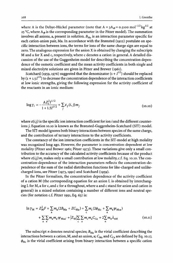
268 1. Grenthe
where A is the Debye-Hiickel parameter (note that A = 3Acp= 0.5100 mor1l2 kg 112 at 25°C, where Acp is the corresponding parameter in the Pitzer model). The summation involves all anions, a, present in solution. BMa is an interaction parameter specific for each cation-anion pair, Ma. In accordance with the Br0nsted (1922) postulate on specific interaction between ions, the terms for ions of the same charge sign are equal to zero. The analogous expression for the anion X is obtained by changing the subscripts M and a for X and c, respectively, where c denotes a cation in general. A detailed discussion of the use of the Guggenheim model for describing the concentration dependence of the osmotic coefficient and the mean activity coefficients in both single and mixed electrolyte solutions are given in Pitzer and Brewer (1961).
Scatchard (1959,1976) suggested that the denominator (1 + [112) should be replaced by (1 + 1.5[112) to decrease the concentration dependence of the interaction coefficients at low ionic strengths, giving the following expression for the activity coefficient of the reactants in an ionic medium:
AZ2[1I2 10gYi = ! 112 + }>y(i,j)mj
1+ l.S[ j (10.10)
where £(i,j) is the specific ion interaction coefficient for ion i and the different counterions j. Equation 10.10 is known as the Br0nsted-Guggenheim-Scatchard (SIT) model.
The SIT-model ignores both binary interactions between species of the same charge, and the contribution of ternary interactions to the activity coefficients.
The constancy of the ion interaction coefficients in the SIT -model at high molality was recognized long ago. However, the parameter is concentration-dependent at low molality (Pitzer and Brewer 1961; Pitzer 1973). These variations give only a small contribution to the accuracy of the calculated activity coefficients because of the product where £(i,j) mj makes only a small contribution at low molality, c.f. Eq. 10.10. The concentration-dependence of the interaction parameters reflects the concentration-dependence of the sum of the radial distribution functions for like-charged and unlikecharged ions, see Pitzer (1973,1991) and Scatchard (1959).
In the Pitzer formalism, the concentration dependence of the activity coefficient of a cation M (the corresponding equation for an anion L is obtained by interchanging L for M, a for c, and c for a throughout, where a and c stand for anion and cation in general) in a mixed solution containing a number of different ions and neutral species (for notation c.f. Pitzer 1991, Eq. 63) is:
In YM = Zf.tF + I, ma(2BMa + ZCMa ) + I, me (2<PMe + I,ma'l'Mea) a a
+ I, I, mama''I'Maa' + IZMII, I, memaCCa + 2I,mnAnM a a' can
(lO.n)
The subscript n denotes neutral species; BMa is the virial coefficient describing the interactions between a cation, M, and an anion, a; CMa and CCa are defined by Eq. 10.17,
<PMe is the virial coefficient arising from binary interaction between a specific cation

CHAPTER 10 . Equilibrium Analysis, the Ionic Medium Method and Activity Factors 269
and the other cations; A,nM is the virial coefficient representing the interactions between a specific cation and neutral species; ljIijk is the virial coefficient representing interactions between ions i,j, k (where i and j are different anions and k is a cation or when i and j are different cations and k is an anion). The parameters ljI and A, are assumed to be independent of ionic strength. The quantity F includes the Debye-Hiickel, f~ and other terms as follows:
F = F + I,I,mcmaB~c + I,I,mcmc'l/J~c' + I,I,mamA~a' (10.12) cae c' a a'
where
F = -Aq, J JIk, + ~ln(1 + b[I:)l 11 + b 1m b J (10.13)
and ¢I and B' are the ionic strength derivatives of I/J and B, respectively (see below). B and B' are equal to:
Z = I,mdZil (10.14) i
213(1) { } BMa = f3~~ + a~a 1- (1 + aI1I2)exp(-aII/2) = f3~~ + f3U~g(aI1I2) (10.15)
and
Ma = -2"2 1- (1 + aI1I2 + -)exp(-aII/2 ) = 13(1) g aI B' 2f3i.Va{ a21 } '( 112)
aI 2 Ma I (10.16)
Cca and the virial coefficient I/Jij are defined as follows:
C C<I> Ca=~
21ZcZa 111 2
CMa = C~a 21ZcZa 111 2
(10.17)
I/Jij = eij+Eei/I) (10.18)

270 1. Grenthe
C~a' are tabulated quantities for each cation-anion pair (Pitzer 1991), Eeij(I) is a function of the ionic strength only; it is zero except for unsymmetrical mixing of ions of the same sign, i.e. when the charges of i and j are of the same sign but different magnitude (this term is given by theory and its values can calculated numerically as described in (Pitzer 1991, Appendix B). g(aII12 ) and g'(art /2 ) are known functions of I; a is an empirical parameter equal to 2.0 kgl/2 mOrll2.
The features of the Pitzer and the SIT -models given above provide the rationale for the simplification of the Pitzer equations presented below.
10.5 Comparison of the SIT and Pitzer Models
How many empirical parameters is it advisable to use when calculating activity factors? It is wise to keep the old scholastic principle called Occam's razor in mind. This maxim says, "Entities are not to be multiplied without necessity:' or in Bertrand Russel's (1959) words: "If everything in some science can be interpreted without assuming this or that hypothetical entity, there is no ground assuming it:' In the following, we will discuss some possible simplifications of the Pitzer model. The most common simplification is to neglect the contribution of the third virial coefficient. Indeed, a check of the typical values of C<P from the available compilation (Pitzer 1991) shows that this contribution is significant only at high ionic strength, typically above 5-6 mol kg-I. Hence, C<P = 0 is a reasonable assumption when the concentrations of reactants/products are small in comparison with the ionic medium concentration.
Another simplification of the Pitzer model was proposed by Millero (1983), who suggested the estimate [3(l) = 0, for complexes. This simplification may lead to errors as discussed by Plyasunov et al. (1998) and illustrated by Fig. 10.1.
From Fig. 10.1 it is apparent that the one-parameter Pitzer model is inferior to the SIT-model. Another important observation is that the values of [3(0) obtained using
Fig. 10.1. The experimental and fitted mean activity coefficients of NaCl, MgCl2 and NdCl3
using Ifl) = 0 and neglecting triple ion interactions, plotted as a function of the ionic strength up to I = 3 mol kg-I. The thick full-drawn curves represent the experimental data. The calculated activity coefficients using the complete Pitzer model coincide with the experimental values within 0.2%. The short-dashed curve shows the mean activity coefficients calculated using the Pitzer model with only the pO) parameter. The long-dotted curves are calculated using the SIT-model with a fitted value of Er
+1 ?-.
1.0
0.8
• .•• NaCi
- - - - -~ 0.6
MgCl2
.-.-0.4
NdCl3
............
.. ~.~=-~--~-.-.---- .. -- .. ,--0.2
0.0 +I----,-r--r-,-~~----,~,-~~~___r-~~ 0.0 1.0 2.0
1m (mol kg-l)
3.0

CHAPTER 10 • Equilibrium Analysis, the Ionic Medium Method and Activity Factors 271
[3(1) = 0 always differ from the tabulated values from Pitzer (1991) given in parenthesis for the electrolytes in Fig. 10.1; NaCl: [3(0) = 0.110 (0.0765); MgCl2 : [3(0) = 0.557 (0.352)
and NdCl3: [3(0) = 1.247 (0.568). The error increases with the charge type of the electrolyte. To conclude: The Pitzer equations must be used with both the [3(0) and [3(1)
terms. An examination of the values of [3(1) at 298.15 K from Pitzer (1973) shows that they
are correlated with the charge type of the electrolyte: for most 1-1 electrolytes the values of {fJ) fall in a range 0.20 ±0.20, for most 2-1 electrolytes in the range 1.4 ±0.6, and for most 3-1 electrolytes in the range 5.2 ±1.2. These averages may be used as "fixed" values of [3(1) in the Pitzer equations, thus reducing the number of unknown parameters.
It may be important to be able to transfer parameters from one ion interaction model to the other. We will now demonstrate how this can be done in the ionic strength range, 0 < 1< 3-4 m, where the SIT and Pitzer models are approximately equivalent. The analytical statements for the mean activity coefficient in the Pitzer model without the CtP term is:
{ 11/2 2 }
lny± =-!ZMZL!AtP 1/2 +-In(1+bII12) 1 + bI b
2VM VL (2[3(0) + 2[3(1) X) +m-- ML ML V
(10.19)
where
X = - 1 + (1 + aI1I2 - -)exp(-aIlIz ) 1 { a 2I } a 2I 2
(10.20)
For the SIT-model we obtain:
A!ZMZL!I1IZ + m2VMVL £y(M,L) lny±=- 1+1.51112 v
(10.21)
Taking into account that A = 3AtP and making elementary transformations, we obtain:
Y = I/J M L _ I _ ~ln(l + bI1I2) A !Z Z !v{ 31112 112 }
4vM vLm 1 + 1.51112 1 + bI1I2 b
£ (M L) - ([3(0) - y , ) + [3(1) X - ML 2 ML (10.22)

272 i. Grenthe
X and Yare known quantities that depend only on the charge type of the electrolyte, the ionic strength/molality and A,p. The linear function Y of X has the intercept (f3fJL - €y(M,L) /2) and the slope 13m. The functions Y(X) are plotted in Fig. 10.2 for I-1,2-1 and 3-1 ion combinations.
The linearity is very good, indicating that the SIT-model is approximatelr equivalent to the Pitzer model without the C<P term and with a constant value of If! for each charge type. The relationships between the two sets of parameters given in Table 10.1
for different ion combinations may be used to convert the large set of er. values already available (Pitzer 1991, Guggenheim 1935) for complexes, into {f0) and If!) values. Note that e values, not e}' are tabulated in Pitzer (1991) and Guggenheim (1935); the relationship between them is ey= eln (10). The difference is due to the use of decadic and e logarithms, respectively.
The estimated values of If 0 for 3-1 and 4-1 interactions (If!) = 4.3 for 3-1 and 1-3,
and If 0 = 8.9 for 4-1 and 1-4 interactions) seem to be slightly lower than the "averaged" values from Pitzer (1991), If!) = 5.2 ±1.2 and If 0 = 11 ±2, respectively.
It is not straightforward to determine Pitzer parameters from experimental mean activity factors, and osmotic coefficient data. The interaction parameters are often strongly correlated, and different experiments may not always give concordant results. It is therefore advisable to investigate how sensitive the calculated activity coefficients are for variations in the Pitzer parameters. Example 1 demonstrates the use of the two models for a simple protolytic equilibrium and also how sensitive the Pitzer model is for the numerical values of the parameters.
Use of the Pitzer model in equilibrium analysis. Here we are faced with slightly different problems from those described above. Pitzer parameters for complexes can rarely be determined from mean activity coefficients; they have to be deduced from the ionic strength/ionic medium dependence of equilibrium constants. This requires a very large experimental effort and very precise values of the equilibrium constants. Very few data of this type are available. A simplifying factor for the Pitzer analysis is when the reactants/products are present in such a low concentration that the main ion-ion interactions are those between the medium ions themselves and between the medium ions and the reactants/products.
Complex formation equilibria are in general described using concentration equilibrium constants; these are "true" thermodynamic quantities as long as concentrations and activities for reactants/products are proportional to one another in the ionic medium used. Each ionic medium may thus be considered as a particular solvent. A practical way to compare equilibrium constants obtained in different ionic media is to use one reference medium, usually pure water. A simplified Pitzer model for the
Table 10.1. Quantitative (fP-£/2l rP) relationship between the Ion combination
Pitzer parameters {f0) and {fl) and the SIT parameter M+,X- 0.035 0.34 = 0.3 Erfor different ion combina-
M2+, X- and M+, X2- 0.150 1.56 = 1.6 tions M3+, X- and M+, X3- 0.366 4.29 ",,4.3
M4+, X- and M+, X4- 0.754 8.89",,8.9

CHAPTER 10 • Equilibrium Analysis, the Ionic Medium Method and Activity Factors 273
Fig. 1 O.2a-c. The relationship 1m (mol kg-l) between the SIT and Pitzer pa- 6.00 2.00 0.80 0.40 0.20 0.10 rameters for 1:1, 2:1 and 3:1 elec-trolytes
0.3 I a
0.2
~
0.1
0.0
-0.1 0.0 0.1 0.2 0.3 0.4 0.5 0.6 0.7
X
1m (mol kg-l)
9.00 2.00 0.75 0.40 0.20 0.10
1.4 r: 1.2
1.0
0.8 ~
0.6
0.4
0.2
0.0 0.0 0.1 0.2 0.3 0.4 0.5 0.6 0.7
X
1m (mol kg-l)
12.0 3.0 1.2 0.6 0.3 0.15
3.0
2.5
2.0
>- 1.5
1.0
0.5
0.0 0.0 0.1 0.2 0.3 0.4 0.5 0.6
X
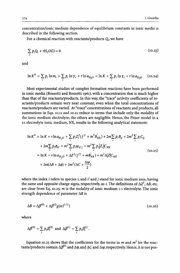
274 1. Grenthe
concentration/ionic medium dependence of equilibrium constants in ionic media is described in the following section.
For a chemical reaction with reactants/products Qi, we have
I, PiQi + rH20(l) = 0 i
and
(10.23)
InKO = I, Pi lnmi + I, Pi In Yi + rlnaH 0 = InK + I, Pi In Yi + rlnaH 0 (10.24) . . 2 . 2 I I I
Most experimental studies of complex formation reactions have been performed in ionic media (Rossotti and Rossotti 1961), with a concentration that is much higher than that of the reactants/products. In this way, the "trace" activity coefficients of reactants/products remain very near constant, even when the total concentrations of reactants/products are varied. At "trace" concentrations of reactants and products, all summations in Eqs. 10.11 and 10.12 reduce to terms that include only the molality of the ionic medium electrolyte; the others are negligible. Hence, the Pitzer model in a 1:1 electrolyte ionic medium, NX, results in the following analytical statement:
InKO = InK + rlnaH20 + I,PiZ;(jY + m2B~x) + 2m'i;.PiBij + 2m2I,PiCij I I I
+ 2mI,PilPu' + m2I,Pill'ii'j + m2I,pdZdCNX iii
2 r . 2 I I = InK + rlnaHzo + f).Z (f + mBNX ) + m I1ZCNX
+ 2m(/1B + M) + 2m2(I1C + 11",) 2
(10.25)
where the index i refers to species i, and i' and j stand for ionic medium ions, having the same and opposite charge signs, respectively, as i. The definitions of f).Z2, I1B, etc. are clear from Eq. 10.25; m is the molality of ionic medium 1-1 electrolyte. The ionic strength dependence of parameter /1B is
/1B = 11[3(0) + 11[3(l) g(aI1I2 ) (10.26)
where
11[3(0) = I, Pi[3~O) and 11[3(1) = I, Pi[3~I) . i i
Equation 10.25 shows that the coefficients for the terms in m and m2 for the reactants/products contain 11/1°) and 11f!>, and I1C and 11 "', respectively. Hence, it is not pos-

CHAPTER 10 • Equilibrium Analysis, the Ionic Medium Method and Activity Factors 275
sible to obtain the individual Pitzer parameters I1/iO) and I1C from this equation alone. When using Eq. 10.25 in a regression analysis, it is convenient to rewrite it as:
InKO = InK + rlnaH 20 + 11Z2(jY + m2B~x) + m2111ZICNX + 2mXI
+ 2mg(aI1/2 )X2 + 2m2X3
where XI = I1/iO) + 111jJ, X2 = 11/i1), X3 = I1C + 112111f1. The use of this equation is demonstrated in Example 2.
(10.27)
Using the SIT formalism, the concentration dependence of the equilibrium constant for Eq. 10.21, studied at trace concentration of the reaction participants in a constant ionic medium, is equal to:
112
InKo = InK + rlnaH 0 - AI 112 LPiZ; + mLPil::y(i,j) 2 1 + 1.51 i i
A/1Z211I2 = InK + rlnaH 0 - 1/2 + mi1£y
2 1 + 1.51 (10.28)
where m is the molality of the ionic medium electrolyte. The definitions of 11Z2 and l1£yare clear from Eq. 10.28.
It is not trivial to use this equation in a regression analysis as discussed in Plyasunov et al. (1998).
For chemical equilibria studied in the presence of an ionic medium (I < 4 mol kg -I ), one may neglect all parameters accounting for triple ionic interactions (CNX) and binary higher-order mixing terms (X3 ). These approximations will be discussed later. For 1-1 ionic media, Eq. 10.27 can be simplified to the following statement for the ionic medium dependence of InK:
[ 1112 2 ]
InKo = InK + rlnaH 0 _I1Z2 A<l> 112 + -In(1 + bI1/2 ) 2 1 + bI b
+I1Z2m2B~x + 2mXI + 2mg(aI1I2 )X2 (10.29)
The corresponding relation for the SIT-model is given by Eq. 10.28. After elementary transformations, we obtain:
1 [ 11/2 2 31112 1 ) y= A<l> 1I2+-ln(l+bII/2)- 1/2 -m2B~x 12m 1 + bI b 1 + 1.51
(10.30)
1 11£ X =-(X __ Y)+_2 g(aI1I2)
11Z2 I 2 11Z2

276 1. Grenthe
ie. Yis a linear function of g(aI1I2), with the slopeXzI !:,.ZZ and the intercept (Xl - Myl 2) I !:,.ZZ.
a is a fixed empirical Pitzer parameter equal to 2.0 kg1l2 morl12 for all electrolytes. Y can be calculated from the known ionic strength, the Debye-Hiickel parameter A,p and IJ.Ix, i.e. the known value of pI) for the 1-1 ionic medium electrolyte. The values of g(a[1I2) are obtained from the ionic strength of the solution.
In Fig. 10.3 we have plotted the values of Y for some common 1-1 ionic media. The linearity is goo~ for all electrolytes considered, and the values of the param
eters (Xl - M:yl 2) l/j"Zz and XzI !:,.ZZ determined for each electrolyte are given in Table 10.2. As these parameters, especially the slope, do not vary much with the nature of the 1-1 electrolyte, one can use all the data to determine one common set of parameters (see the last line of Table 10.2) where the uncertainties are given as 30'. This find-
Fig. 10.3. The relationship be-tween the SIT parameters !If
030
1
• NaCI04 and the Pitzer parameters !lifO) o NaCi and !llfl) for reactions studied .. KN03
in different 1:1 ionic media. The 0.25 • NaN03
symbols denote calculated val- e LiCI04
ues of Yas a function of g(Im) /:;, HCI04
using Eq. 10.30 0.20
~ ;' ~ «' ... .;'
)..
0.15
0.10
0.05
0.00 0.0 0.1 0.2 0.3 0.4 0.5 0.6 0.7
g(lm)
Table 10.2. Quantitative relationship between the Pitzer and SIT model parameters for chemical reactions in different ionic media at 298.15 K
1:1 ionic medium ele.ctrolyte (Xl -!If/ 2) , !lZ2 X2' !lZ2
NaCI04 0.031 0.340
LiCI04 0.038 0.348
Hcl°4 0.032 0.342
NaN03 0.026 0.334
KN03 0.019 0.327
NaCI 0.030 0.332
All data 0.029 ±O.OOS 0.337 ±0.014

CHAPTER 10 . Equilibrium Analysis, the Ionic Medium Method and Activity Factors 277
ing is very convenient for the estimation of the Pitzer parameter /1[f!) for reactions, because it only requires the value of the sum of squared charges of the ions participating in the reaction, /1Z2. One can show that for isocoulombic reactions, where /1Z2 = 0, the proposed result is consistent with /1[f!) = o.
Using the data in Table 10.2 we can now estimate the values of Xl and X2 ,
c.f. Example 2, for the protonation of sulphate, for which we obtain Xl = -0.11 ±0.07
and X2 = -1.35 ±0.05, in good agreement with the results in Table 1004-
Equation 10.25 was obtained by neglecting the contribution of the terms for higherorder electrostatic unsymmetrical mixing. By including these terms, the slope of the function Y is changed somewhat, particularly for ions of charge 3 or higher.
Because the determination of the Pitzer parameters for a reaction (or for complexes) from logK data is an ill-conditioned problem, it is rarely possible to determine more than one interaction parameter. We therefore suggest the following strategy when using logK data determined in 1-1 electrolyte ionic media to determine the Pitzer parameters for complexes:
1. Use the SIT equation to obtain logK>. 2. Estimate X2 from the /1Z2 value for the reaction if the charge of the reactants/prod
ucts do not exceed 2 and calculate Xl using X2 as a fixed parameter. The terms m2 /11 Z 1 CNX and higher-order electrostatic unsymmetrical mixing terms for the ionic medium ions should be included for data at high ionic strength.
3. Calculate the Pitzer parameters for the complexes from the values of with /1[f0) and with /1[fI) and the corresponding quantities [f0) and [f!) for the reactants.
4. In order to describe equilibrium data at higher ionic strengths or mixed electrolyte systems, it is necessary to determine additional interaction parameters. This can only be achieved by additional equilibrium constant measurements under these conditions.
10.6 Determination of Interaction Parameters
The interaction parameters in the two models must be determined from experimental mean activity coefficients, osmotic coefficients and/or concentration equilibrium constants. The accuracy of these data are typically ±0.005 in log y± or C/J, and ten to fifty times lower for concentration equilibrium constants. These constants have usually been determined at only a few ionic strengths. For the users of thermodynamic data, it is essential to be aware of the limitations of the methods used to make activity corrections and the consequences of approximations in the models. It is useful to find relationships, c.f. Eq. 10.22, between the interaction parameters in the two models and between the corresponding quantities for reactions. This is practical when one wishes to use the extensive compilations of Pitzer parameters for strong electrolytes together with the compilation of SIT parameters for complexes.
Examples of the use of the specific ion interaction models are in equilibrium analysis. In the following, I will present three examples of the use of specific ion interaction
methods.

278 1. Grenthe
Example 1. This is a comparison of the SIT and Pitzer models for the modelling of the ionic strength dependence for the reaction COiaq) + H20(l) ¢:::> HCO; + H+ in a NaCl medium.
We have:
log[(l = 10gK + 10glB+ + logIBco3 -logYc02(aq) -logaH2o
From the Pitzer equations, we obtain the following values for the single-ion activity coefficients:
log IB+ = F + mCl(2BH,CI + 2mCICH,CI) + mNa(2if>H,Na + mCI'l'H,Na,CI) + mNamCICNa,CI
log IBC03 = F + mNa (2BNa,HC03 + 2mNa CNa,HCO) + mCI (2I/>CI,HC03 + mNa'l'Na,CI,HC03 )
+ mNamCICNa,CI
where
F = - AtfJ J JIk + ~ ln~ + bJi:,)l + mnamClB' NaCl 11 + b 1m b J
logaH2o = CPvmMW /1000
where cP is the osmotic coefficient of the electrolyte, Mw the mol mass of water, and v = 2 for NaCl.
The activity coefficient for CO2(aq) is equal to:
log YC02(aq) = 2(Ac02,Na + Ac02,Cl)
where It represents the interaction coefficient between the ionic medium electrolyte ions and CO2(aq). All the necessary Pitzer parameters for the equations above are known and listed in Table 10.3.
Note that the various interaction parameters in the example can be determined from experimental mean activity data of the pure electrolytes. It is not necessary to deter-
Table 10.3. Pitzer parameters for the equations in Example 1
tiD) H,CI 0.1775 C~CI 0.00080 C~CI =0.00060
tiD) 0.0765 l) 0.2664 q,
=0.00127 Na,CI Na,CI CNa,CI
tiD) 0.0277 till 0.0411 q,
=0.0 Na,HCO~ Na,HC03 CNa.HC03
°H,Na 0.036 °CI,HC03 0.03
ljIH,Na,CI -0.004 ljINa,CI,HC03 -0.015
A.C02,Na + A.C02,(1 0.096

CHAPTER 10 • Equilibrium Analysis, the Ionic Medium Method and Activity Factors 279
mine them from experimental concentration equilibrium constants in various ionic media. However, the fitting is very sensitive even for small parameter variations. Figure 10.5 illustrates this.
The fit is not satisfactory without the mixing terms. The dotted line, obtained by including the mixing terms 8Cl04,HC03, 8Cl04,C03' 1i'Na,CI04,HX03 and 1i'Na,CI04,C03, which have been fitted to the experimental equilibrium constants, results in a good agreement between model and experimental data. One can discuss whether this is a satisfactory
Fig. 10.4. Comparison of experimental (symbols) and calculated equilibrium constants log K for the reaction CO2(aq) + H20(l) H HCO; + H+ in a NaCl medium using the SIT (dashed line) and Pitzer (julldrawn line) models
Fig. 10.5. Comparison of experimental and calculated ionic strength dependence of the first dissociation constant of carbonic acid. The full-drawn curve has been calculated using the Pitzer model with available literature values for the interaction parameters, but without including mixing terms for which no data are available. The dotted curve is obtained using mixing terms estimated from the experimental equilibrium constants. The dashed curve has been calculated using the SITmodel
6.5
6.4
6.3
:.c: := 6.2
C'I 0 'T
6.1
6.0
5.9
5.8 0
8.0
7.9
7.8
:.c: 7.7 o
g; 'T 7.6
7.5
7.4
H20(I) + COztaq) ~ H+ + HC03
o [45HARIBON) t:,. [73DYRlHAN) • [810HM/FOR) o [82THU/MIL)
• [87HED/SJO) • [93HE/MOR)
2 3 4 5 Molality of NaCI (mol kg-1)
6. [58FRY/NIL) D [76HIElHOG) o [81C1NFER) • [82BIUSCH) • [85SPA) ... [92BRU/STU) o [92BRUIWER) r'
;.' //'
/.,'
/ :;.::/ ...
.\. 0/ / ~.::..<"'" ''., - - - -6. ...... .
.. ' ...... -
1'*,,,,,
,,'
HzO(I) + C02(9) ~ H+ + HC03
• /0
6
~ ....................
7.3 +I---,-----,----,-----,-----,----,r--,---r--'
o 2 3 4 Molality of NaCI (mol kg-1)

280 I. Grenthe
method; in order to be confident about the mixing terms, they should be confirmed by an independent experiment.
The first example concerns a problem where we have a simple equilibrium system and where the equilibrium constant at zero ionic strength can be determined by a simple extrapolation method. The situation is very different if both equilibrium constants and Pitzer parameters have to be determined from experimental concentration equilibrium constants. The second example illustrates this:
Example 2. This example refers to the determination of IOgIO[(l and the Pitzer and SIT parameters from the experimental values of loglOK for the first protonation constant of the sulphate ion, H+ + SO~- ¢::} HS04, studied in NaCI04 media. References to the original data are given in Grenthe et al. (1997), where more details about the procedure are given.
The experimental data are fitted to an equation of type Eq. 10.23, which in this case is equal to:
InKo = InK + rlnaH20 +t.z2(F + mB~x) + m2t.IZICNX + 2mXI
+ 2mg(Im)X2 + 2m2X3
where
t,.Z2 = L viii; ~ Z I = LVi I Zi I
Xl = Ll/fol + t.cfJ = LVi/fOlij + LVicfJij'
X2 = t.lfll = LVif3~l)
X3= t.C + 112t.1fI= LViCij+ 1l2LVilflii'i
It is obvious that one cannot determine individual Pitzer parameters from these data, even if they are precise enough to permit the evaluation of all fitting terms. The results of different fitting models are given in Table 10.4 and Fig. 10.6.
• Model I. Determination of the whole set of parameters IOglo[(l, Xl' X2 and X3•
• Model II. Determination of the parameters IOglo[(l, Xl' and X2, neglecting ternary interactions.
• Model III. Determination of the parameters IOglO[(l,X1 and X3, assuming Ifl) = 0 for all species.
• Model IV. Determination of the whole set of parameters IOglO[(l and X I, the smallest number of parameters in the Pitzer model. The quantities Xl' X2 and X3 are in this case known by independent activity data. This is a situation that is rare.
The results of the various fitting models are shown in Fig. 10.6. The parametrization of the SIT and different choices of the Pitzer model are illus
trated below for the reaction H+ + SO~- ¢::} HS04 in NaCI04 ionic media at 25°C.

CHAPTER 10 • Equilibrium Analysis, the Ionic Medium Method and Activity Factors 281
Table 10.4. Regression data for the determination of Pitzer and SIT parameters
The SIT model The Pitzer model parameters for models I-IV
Parameter
-1091/= 1.989±0.084 109 1OKO
/:o.e = 0.003 ±0.084 Xl
Xl
Xl
Fig. 10.6. The parametrization of the SIT model and different choices of the Pitzer model for the reaction H+ + S~- H HSO:; in NaCl04 ionic media at 25°C
II
2.10±0.27 2.04±0.20
-0.45 ±0.88 -0.19±0.16
-0.46 ±3.40 -1.39 ±1.34
0.05 ±1.02 (0)
2.1
1.8
1.5 :0.::
0
Ci' 0 'T
1.2
0.9
0.6 0
III IV
2.1HO.13 2.23 ±O.ll
-0.S6±0.21 -0.34±0.08
(0) (0)
0.07 ±0.07 (0)
H+ + SO~- ~ HSG.\
The SIT model The Pitzer model
Variant I Variant II
Accepted values
l.987 ±0.009
-0.15 ±0.05
-0.995
-0.006 ±0.01 0
Variant III - - - - - -Variant IV
o
2 3 Molality of NaCI04 (mol kg-l)
~
o
4
An important problem in equilibrium analysis is to decide if a certain complex may be an artefact due to ionic medium variations, or not. An estimate of the variation of the activity coefficients of reactants and products provides important clues. It is evident that this problem is particularly important when weak complexes are formed. We can use the SIT and Pitzer models both to design the experiments and to evaluate the magnitude of the activity factor variations of reactants and products as a result of varying the composition of the equilibrium solutions.
Example 3. Assume that we are investigating the formation of fairly weak complexes, e.g. the cu(II)-cr system, using a Cu-reversible electrode. Should the experiment be made in a medium with constant ionic strength, constant concentration ofNa + or CI04? What is the magnitude of the variation of the activity factors if we exchange 25% of the NaCI04 ionic medium for NaCl? I will use the SIT model, because it demonstrates the principles without too much computational effort.

282 1. Grenthe
In the experiments, we measure the concentration of free or non-complex bound Cu2+ with the electrode. It is highly desirable that the activity coefficient for this species is constant throughout the experiment. Using the SIT single ion activity coefficient for Cu2+, we have:
logyc 2+ =-0.5100Zc2 2+ .Ji .JI+C(Cu2+,CI04")mclO +c(Cu2+,CnmCI U U 1 + 1.5 I 4
From this equation, we can see that the activity coefficient of Cu2+ will not be constant throughout the experiment. The interaction coefficients are c(Cu2+, CIO:!) = 0.32 and c(Cu2+, Cn '" 0.15. Hence, a replacement of 25% of a 3.5 molal NaCI04 ionic medium with NaCI will result in a change of 10glO YCu2+ equal to 0.14, which is not negligible. We could have studied the same system with a chloride electrode. In this case, it would have been advantageous to keep the sodium ion concentration constant, because the activity coefficients of a particular ion are mainly influenced by the ions of opposite charge. The example illustrates some of the problems encountered when interpreting equilibrium analytical data when large changes have been made in the ionic medium. An attempt to use the SIT method to interpret data in a mixed ionic medium is described in Grenthe and Lagerman (1993). A more detailed discussion of ionic medium effects with several different examples is given in Grenthe et al. (1997).
References
Bodliinder G, Storbeck 0 (1902a) Z Anorg Chern 31:1 Bodliinder G, Storbeck 0 (1902b) Z Anorg Chern 31:458 Bodlander G, Fittig R (1902) Z Physik Chern Leipzig 39:597 Bodliinder G, Eberlin W (1904) Z Anorg Chern 39:197 BfllInsted IN (1922) J Am Chern Soc 44:877 Debye P, Hiickel E (1923) Physik Z 24:185 Euler H von (1903a) Ber 36:1854 Euler H von (1903b) Ber 36:2878 Euler H von (1903c) Ber 36:3400 Farkas I, Banyai I, Szabo Z, Wahlgren U, Grenthe I (2000) Inorg Chern 39:799 Grenthe I, Lagerman B (1993) Radiochim Acta 61:169 Grenthe I, Spahiu K, Plyasunov A (1997) Estimation of medium effects on thermodynamic data. In:
Grenthe I, Puigdomenech I (eds) Modelling in aquatic chemistry. Nuclear Energy Agency, OECD, Paris Grossman H (1905) Z Anorg Chern 43=356 Guggenheim EA (1935) Philos Mag 19:588 Helgeson HC, Kirkham DH, Flowers GC (1981) Am J Sci 281:1249 Millero FJ (1983) Geochim Cosmochim Acta 47:2121 Moll H, Denneke MA, Ialilehvand F, Sandstrom M, Grenthe I (1999) Inorg Chern 38:1795 Pitzer KS (1973) J Phys Chern 77:268 Pitzer KS (1991) Ion interaction approach: Theory and data correlation. In: Pitzer KS (ed) Activity coef-
ficients in electrolyte solutions, 2nd edn. CRC Press, Boca Raton, FL, pp 75-153 Pitzer KS, Brewer L (1961) Revision of Lewis and Randall's thermodynamics. McGraw-Hill, New York Plyasunov A, Fanghanel T, Grenthe I (1998) Acta Chern Scand 52:250 Rossotti FIC, Rossotti H (1961) The determination of stability constants. McGraw-Hill, New York Russel B (1959) A history of western philosophy, 12th edn. Simon and Schuster Scatchard G (1959) The interpretation of activity and osmotic coefficients. In: Hamer WI (ed) The struc
ture of electrolytic solutions. Scatchard G (1976) Equilibrium in solution: Surface and colloid chemistry. Harvard University Press,
Cambridge, MA Szabo Z, Aas W, Grenthe I (1997) Inorg Chern 36:5369

Chapter 11
Acid-Base Equilibria in Saline Media: Application of the Mean Spherical Approximation
M. E. Sastre de Vicente . T. Vilarifio
11.1 Introduction
The simplest mathematical formulation of the hypothesis that chemical equilibrium exists in the bulk of a saline solution is based on the equilibrium constant, KT = K* Q{ }';), where KT is the thermodynamic equilibrium constant, K* the stoichiometric constant and Q{}';) the ratio of activity coefficients (}';) associated with the equilibrium. Studies on the effect of ionic strength on stoichiometric constants are based on modelling of the Q{}';) term (Sastre de Vicente 1997; Daniele et al. 1997).
With regard to this equation, the following points can be mentioned:
• Most treatments rely on the Debye-Hiickellimiting law, although their final purpose is their possible application to moderate and high ionic strengths, as shown through many studies devoted to the analysis of changes in activity and osmotic coefficients for strong electrolytes.
• The vast majority of the treatments lead to explicit expressions for pK* as a function of I, which is clearly an advantage; however, interpreting the parameters associated to the fitting of a pK* vs. I curve is often far from easy.
• This kind of study is carried out in a constant ionic medium, which has been traditionally employed as a synonym for "background electrolyte;" the principal weakness of the method arises from the assumption that the added salt is inert to the equilibria involved. If the background electrolyte cannot be considered as inert, ion association must be included and the equilibria redefined in the system.
11.2 Acid-Base Equilibria in Saline Media
For the case of acid-base equilibrium reactions in saline media, we should consider the most significant acid-base reactions that take place in solution, which can be classified as follows (Edsall 1943; Izatt et al. 1995):
• Type I:
AH=A- +H+ (n.l)
where the charge separation involved usually has a strong effect on H20 structure.

284 M. E. Sastre de Vicente· T. Vilarifto
• Type II:
AH~=AH+ H+ (11.2)
This reaction is usually termed "isocoulombic:' Because the net charge of reactants and products is the same, the change in water structure is usually small.
• Type III:
-AH~=AH+ H+ (11.3)
This reaction can be considered to be a particular case of Type I and involves the zwitterionic species -AH+, which usually behaves as a neutral molecule or as two separate ions depending on the separation between positive and negative charge.
• Type IV: Type IV refers to complex molecules. It is worth mentioning that the study of
the different aspects of the above simple equilibria I and II is the first step to encompass the analysis of acid-base equilibria of polyelectrolytic molecules.
The equilibrium constant for types I and II can be formulated as:
T _[A-][H+jY A- YH+ KI - [AHj hH
T _[AHj [H+)YAHYH' K II - [AH!J YAH!
Taking logarithms in Eqs. 11.4 and 11.5 yields
pK i = pK; _ log Y A- Y W YAH
T * YAHYW * YH+Yx-pK II = pK II -log = pK II - log YAH --'-'-----"--
YAH! YAH! Yx-
(11.4)
(n·5)
(11.6)
(1l.7)
As shown above, the dependence of pK* on the ionic strength is clearly a function of the way the Qi( y) term (i.e. the activity coefficient term), or rather its logarithm is modelled. Equations 11.4-11.7 include two types of activity coefficient, viz., that for the ions and that for neutral species. Obviously, the form of such coefficients used in the different theoretical approaches associated to the theory of electrolytes explicitly dictates the form of the final equation.

CHAPTER 11 • Acid-Base Equilibria in Saline Media: Application of the MSA 285
11.3 pK vs.lonic Strength Equations
In Table 11.1, it is shown that virtually all the expressions proposed over the years are of the type:
T * pK =pK + f( I,parameters) (11.8)
The different equations refer to the equilibria types I and II but based on different models for the activity coefficients logy; and logYneutral: Pitzer, Guggenheim, or other semi-empirical modifications of the Debye-Huckel equation. Also, a non-Debye-Huckel based equation is included at the bottom of the Table 11.1. This simple cubic-root equation is based on a classical quasi-lattice model, which exhibits this characteristic dependence.
Different authors(for example Grenthe and Plyasunov 1997; Millero and Pierrot 1998;
Salvatore et al. 1986; Partanen and Juusola 2000; Daniele et al. 1997; Sastre de Vicente
Table 11.1. pK vs. ionic strength dependence for equilibria I and II according to different models for activity coefficients
Modell (Pitzer)
{(4) = -0.392 [~ + 21n(1 + 1.N,!)1 , {(5) = -1 + (1 + 2/1 + 21 )e-2ft 1 + 1.2/1 1.2 J
Model II (Scatchard)
• T 1.018/1 2 3 pK, = pK, - Z------r. + p, 1 + 0, 1 + R, I
1+1.5,,1
Model III (Guggenheim)
pK;" =pKT +£, I-z 1.018/1 1 + 1.5/1
Model IV (De Stefano et al.)
• T 2/1 3/2 pK; = pK; - Z----r, + b, 1 + 0; 1 2 + 3,,1
Model V (quasi-lattice) • T 3r. pK; = pK; - z o;vl + b, 1
z=i-1
Taken from (Sastre de Vicente 1997).

286 M. E. Sastre de Vicente· T. Vilarino
1997; De Robertis et al.1997) some of which are contributors in this volume, traditionally have been using these equations to model pK* vs. ionic strength data.
Some authors have derived equations of the following type from studies over wide temperature and ionic strength ranges:
10gQ = f(I, T, param.) (11.9)
which includes the dependence on both the ionic strength and temperature (Kettler et al.I995)
With regard to these explicit equations in ionic strength, in particular Pitzer's, which are the more general and widely used, it must be stated that these equations:
• Are able to reproduce the measured properties within the experimental error; • Can be applied to single electrolytes and mixtures, i.e. natural waters (Millero and
Pierrot 1998), up to high concentrations; • However, coefficients obtained from linear regression analysis of pK* vs. I data have
no clear physical meaning. Other problems are for example ill-conditioning (Fiol et al. 1994), which leads to high errors in the regression parameters.
11.4 The Mean Spherical Approximation: Estimation of Q( y) Term by Use of the MSA Model
An alternative to modelling pK-I data is the mean spherical approximation (MSA) (Blum 1975; Friedman 1985), the application of acid-base equilibria on the basis of the "constant ionic medium" approach, is described below.
From a general point of view, in an electrolyte solution there must be a balance among different types of interactions (Israelichvili 1991):
a Forces of a purely electrostatic nature that arise from Coulomb's law (e.g. interactions between charges, permanent dipoles or quadrupoles, etc.);
b Polarization forces between dipoles induced by the action of permanent charges and dipoles on atoms and molecules. This type of force is present in any solvent medium (particularly in electrolyte solutions).
c Quantum mechanical forces consisting of an attractive part responsible for chemical bonding and a repulsive part of the steric type or in the form of exchange interactions that equilibrate attractive forces over very short distances.
A frequent way of describing such interactions in qualitative terms is based on the distinction between long-range (coulomb) interactions and short-range interactions. So, schematically, the interaction between two ions in solution can be expressed as:
Interaction between particles i, j = Coulomb Law + other kind of interactions (11.10 )

CHAPTER 11 . Acid-Base Equilibria in Saline Media: Application of the MSA 287
This dichotomy in the conceptualization of solution interactions has prevailed in modelling electrolyte solutions since the beginning of the development of theories early in this century.
Also, with MSA, the activity coefficient for an individual ionic species of charge Zi, diameter (ji and numerical density Pi in an arbitrary mixture can be resolved into two contributions, Fig. 11.1 (Blum and Hoye 1977; Corti 1987; Sanchez Castro and Blum 1989; Triolo et al. 1976; Turq et al. 1992; Waisman and Lebowitz 1972),
namely:
I I cl I hs nYi = nYi + nYi (n.n)
where the first term on the right-hand side describes the electrostatic contribution and the second the hard sphere contribution.
The use of MSA to estimate the log Q( Y) term entails estimating log Yi for each ionic species (AHr, A-, H+) involved in the particular acid-base equilibrium from electrostatic and hard-sphere contributions, the expressions for which in the general case of a mixture of charged hard spheres of arbitrary ionic radii ai and aj, and charges Zi and Zj' are (Cartallier et al. 1992) as shown in Fig. 11.1.
Electrostatic contribution Hard sphere contribution
In .el = _ a2z? _f_ _ a2z,.crj !.n.. + 1, 41t 1 + faj 4(1 + faj} tl
In yr' = -In tl + at Xo + 3 at X, + 3 0'12 tl +
1tCl.2a1 [1 1 1 P~ ~ 1 + fa j - 3" LY
[ n [z. _ 1t 2 ]2 112
2f= a 2LPj I 2tl crjPn I j= 1 (1 + fo j)2
p _ ~ ~ Pka~k n- n ~ (1 +fak)
k
a2 = 41t~e2 ~
1t Pka? n = 1 + 2tl L (1 + fak)
k
3 0'1 X,X2 + 9/2 crt xf tl2
+ 3 cr1 xi tl3
X =~ ~pak k 6 ~ /I tl=1-~S3
Sn=LPka{ (n=O, 1,2,3)
Fig. 11.1. Scheme where f3 is the reciprocal temperature, 11k T (where k is the Boltzmann constant and Tthe absolute temperature, in K), e the electron charge, t'Q the permittivity of free space, and e, the relative permittivity of the solvent

288 M. E. Sastre de Vicente . T. Vilarino
The most relevant aspect in the expression of log yby using the MSA is that all parameters appearing in the equations shown in Fig. 11.1 are an explicitly simple function of charges, diameters, concentrations, dielectric constant and temperature.
11.5 Comparison With the Pitzer Model
At this point, let us recall the expression for the activity coefficient of an ion, using, for example, a Pitzer equation.
The corresponding expression for the more general case of an electrolyte mixture is (Pitzer 1973,1991) given as:
InYM+ = z~F + 2I,[BMa + ttmz~MaJ+ 2I,mc8Mc a
+ I,I,mcma (z~Bca + zMCca + ljIMcJ (n.12) c a
1 (2 ' ) z~ , + - I, I, mama,\zM8aa' + ljIMaa' + - I, I, mcmc,8cc'
2 a a' 2 c c'
For a negative ion, it suffices to replace anions with cations. Function fYindudes long-range electrostatic interactions and is dependent on tile ionic
strengili, of which B is also a function - in contrast witil the previous theories, where all parameters were independent of 1. Parameter B takes account of dual interactions (e.g. BaM represents the interactions a-a, M-M and a-M), and C accounts for triple interactions in an electrolyte (e.g. CMa represents the interactions M-M-a and a-a-M). ljI, e and f! are mixing parameters; thus, 8 is associated with the interactions between two ions of the same sign (e.g. ~c accounts for the interactions M-c, M-M and c-c, M and c being two cations), while 8' is its derivative witil respectto tile ionic strengili (8' = d8 I dI).When chemical equilibria are involved, these parameters appear combined in the Q( y) term, and the meaning of the coefficients thus obtained become more difficult.
Conversely, the MSA approach entails the use, in all equations, of easily understandable parameters as charge, dielectric constant, diameters, concentration and temperature, and no direct mention to dual or triple interactions is done.
11.6 Neutral Molecules
Until now, we have described the activity coefficient of present ions. It should be noted that the activity coefficient for the neutral species (AH, A) is assumed to obey the Setschenow equation (Long and McDevitt 1952), i.e. to be a linear function of ionic strength and hence of the molar concentration:
logy. = ksc (11.13)

CHAPTER 11 . Acid-Base Equilibria in Saline Media: Application of the MSA
11.7 Data We Need for Working With the Mean Spherical Approximation
1. Electrical charges, Zj, are defined by the corresponding equilibrium model.
289
2. Numerical densities, Pj' Taking into account that a constant ionic medium requires that the supporting electrolyte be present at a much higher concentration than the substance whose ionization equilibria is being studied, the sole numerical densities that will appreciably contribute to the different parameters to be determined can be assumed to be those for the electrolyte ions.
3. Ionic diameters (O"j) Using the MSA model to calculate activity coefficients requires the prior knowledge of the diameters of all species present in the system: a Background electrolyte. The diameters of the ions that make up the most
usual electrolytes can be replaced with Pauling diameters as shown by Marcus (1988), who found ionic radii of dissolved species to be largely consistent with Pauling's crystal radii. Also, taking into account the well-known fact that cation sizes increase to a greater extent with increasing concentration than do anion sizes, the former are often assumed to vary with the concentration, while the latter remain constant and equal to Pauling values (Triolo et al. 1976,
1977. 1978).
O"+(c) = 0"0(1 + Lancn) (11.14)
where an are coefficients to be determined from experimental data. b Species involved in the equilibria. Owing to the few reported diameters (Kielland
1937) for the different ionic species that result from the ionization of organic compounds, we often estimate such diameters from Van der Waals volumes calculated from group contributions (Bondi 1964).
4. Dielectric constant Although the MSA model can use the dielectric constant for the medium at zero electrolyte concentration, the use of a dielectric constant dependent on the concentration of the particular electrolyte improves the results as it accounts for the fact that dielectric shielding must be smaller in the more concentrated solutions, where ions, on average, are closer to one another and hence less strongly shielded by the solvent.
The expression for the dielectric constant of an electrolyte solution is usually a simple polynomial, whether linear or slightly more complex (Barthel et al. 1998;
Fawcett and Tikanen 1996; Whitfield and Turner 1981), which relates £ to the molar concentration, hence considering the decrease in the constant with the increase in concentration.
£(c) = £0(1 + Lf3nCn) (11.15)
where f3n are coefficients to be determined from experimental data.

290 M. E. Sastre de Vicente . T. Vilarifto
11.8 An Example: Fitting pK vs.1 Plot by Use of MSA for an Isocoulombic Equilibrium
If we take as an example the isocoulombic equilibrium: AH+ = A + H+, the first step is always the estimation of the scaling parameter, r. The way of obtaining parameter 2T from the general expression (see Fig. 11.1) depends on the number of ions present in solution; the procedure usually involves solving an algebraic equation of a high order. Thus, the equation for a binary salt is of sixth order and must be resolved numerically. For this reason, various explicit approximations to Thave been developed, one of the most frequently used is the truncated expression:
JII2
2 n PiZi
2r = [ a2 ti(1 + rO"if (11.16)
which assumes that P n = 0, i.e. that ionic diameters are all identical. This expression holds in most cases - provided ionic sizes are fairly similar and/or the concentrations of the species involved are about or smaller than 1 M (Lee 1988; Sun et al. 1994).
Equation 11.16 can readily be solved either by using the Newton-Raphson method, by starting at very low concentrations, or by using an iterative method. In both cases, the inverse Debye length is used as the starting value:
[ ]112
2ro = 1(" = a2:tp;zl (11.17)
As can be seen from the previous expressions, estimating the scaling parameter requires the prior knowledge of both the dielectric constant, which is included in parameter a 2, and ion sizes.
As stated above, both the dielectric constant of the medium and the diameters of the different ions of the electrolytes present in it can be assumed to be fixed or concentration-dependent.
Moreover, it should be noted that the experimental data are given by the LewisRandall (LR) theory and that MSA expresses thermodynamic quantities in terms of molar concentrations in the framework of the McMillan-Mayer (MM) theory of solutions. Thus, data must be converted from LR to MM scales, that is to say from molality to molarity (Friedman 1972; Simonin 1996; Simonin and Blum 1996).
Once the electrolyte diameter and dielectric constant are known, the activity coefficients for the ionic species involved in the equilibria studied can readily be calculated from the MSA electrostatic and hard-sphere contributions, then we can rearrange the expressions for the equilibrium constants in order that the left-hand side of the resulting equation can be calculated numerically at each concentration. This yields to:
AH;=AH+ H+

CHAPTER 11 • Acid-Base Equilibria in Saline Media: Application of the MSA
[AH][H+]Y AHYH+ = K;Ql(Yi) K! = [AHr] YAH!
InK! = InK; + In Y AH± + In Y H+ -In YAH!
I l ellhs nYi = nYi + nYi
InyAH± = 2Am = A'CMX
T * I leI lhs leI lhs InKl = InKl + A CMX + nyH+ + nyH+ - nyAH! - nyAH!
PK* +_I_[lnyel -lnye! +lnyhS _lnyhS ]=PKT +A'C 1 IniO H+ AH! H+ AH! 1 MX
Y(O'Vdw(optim.)) = pK! + A' CMX
291
pK* values are obtained experimentally and the electrostatic and hard-sphere terms are worked out analytically by using MSA. Then, based on the tabulated salting coefficient for the neutral species, the diameters of the charged ions involved in the equilibrium are optimized in order to obtain the best fit of a plot of the left-hand side expression against the electrolyte concentration, which will provide the thermodynamic pKT as the intercept of the fitted line. As noted earlier, the initial diameters of organic species are calculated from Van der Waals volumes that are in turn derived from Bondi (Bondi 1964) tabulated data.
Once pKT has been calculated, experimental pK* vs. electrolyte concentration plots can readily be fitted.
One of the analyzed systems was the acid-base equilibria of glycine in artificial sea water (Vilarino and Sastre de Vicente 1999). Table 11.2 shows the recipe of sea water and other parameters used for calculations.
In Fig. 11.2 different aspects associated to MSA and other approaches are compared. Perhaps the most interesting difference between them is connected to the possibility of studying size effects.
Because the MSA expression for the activity coefficient consists of an electrostatic term and a hard-sphere term, the weight of each contribution to the overall value at variable ion sizes was studied. The electrostatic contribution increases very little with increasing diameter, consistent with the expectations, as it depends mostly on ion charges. On the other hand, the hard-sphere contribution increases markedly with increasing diameter and is roughly proportional to the ionic strength of the solution, similarly to salting coefficients.
In this context, it is worth mentioning that the most recent work of our group on this topic (Taboada-Pan et al. 2001) refers to the study of the isocoulombic equilibrium of three alkylamines in saline media. On the one hand in that study, the Pitzer

292 M. E. Sastre de Vicente· T. Vilariiio
Table 11.2. Recipe of sea water and other parameters used for calculations
Sea water ions Ionic Concentration c, (f= (fo + ac; + bc~ (molr') (fo (A) a(Amor'l) b(Amor2 12)
Na+ 0.92146 C'W 3.77 -0.190 0.0246
K+ 0.02034 C'W 3.42 -0.327 0.0503
Mg2+ 0.10573 C'W 6.41 -0.214 0.00448
ci+ 0.002068 C'W 5.78 -0.0107 0.0201
CI 1.08246 C'W 3.056
SO 0.05608 C'W 2.981
Dielectric constant: Er= Eo -8l, + b,3/2 with 8= 19.57 ±0.081 mol-' and b =4.6 ±0.1 13/2 mol-3/2 (from Vilarino and Sastre de Vicente 1999).
I Kl = II; O;(y;) I I Modeling Q;(y;) I I I
Semiempirical Models Statistical mechanical
· Pitzer (17) approaches
· Guggenheim (18) . Mean spherical · Scatchard (19) approximation · Quassi-Lattice (20,21)
Origin Debye-Huckel theory or Integral equation theories Quassi-Lattice model
Equation type Explicit functions in I Implicit (not functions in I)
Obtained parameters Coefficients from linear No coefficients regression Solution by Newton-Rhapson
Effect of physical-chemical Not straightforward Straightforward parameters:
· Charge · Concentration · Diameter (Volume, Surface) · Dielectric constant
Fitting of data Good Good
Numerical difficulty Low Low
Fig. 11.2. Comparison of different aspects associated to MSA and other approaches
theory is used for the calculation of the salting coefficient of amines from pK* data. On the other hand, the MSA approximation is applied to predict the size of alkylamines in that media, assuming a hard sphere contribution for the activity coefficient of the neutral molecule of alkylamine. These data are compared to those calculated from molar volumes proposed by several authors and taking neutral molecules as spheres.

CHAPTER 11 . Acid-Base Equilibria in Saline Media: Application of the MSA 293
As stated above, data show that the Bondi diameters are the closest values to those obtained from MSA calculations.
Finally, it should be mentioned that equations for the equilibria AH= AH + H+ and AH = A - + H+, typical of many processes (viz. those involving simple acid-base model systems such as carboxylic acids, amines and amino acids) were derived by using the mean spherical approximation. Detailed descriptions of those studies are provided in the references (Sastre de Vicente et al. 1998; Vilarifto and Sastre de Vicente 1996,1997, 1999; Vilarifto et al. 1997, 1998)
Acknowledgements
M. S. V. wishes to acknowledge the University of A Corufta and the Xunta de Galicia for their financial support of Projects XUGA l0303B90, XUGA 10303B92, XUGA 10303B94,XUGA 10310B97, PGIDTooPXh0308PR, and Dr. J. L. Barriada for his help with the word-processing.
References
Barthel JMG, Krienke H, Kunz W (1998) Physical chemistry of electrolyte Solutions. Steinkopff-Springer, Darmstadt
Blum L (1975) Mean spherical model for asymmetric electrolytes. 1. Method of solution. Mol Phys 30:1529-1535
Blum L, and H0ye JS (1977) Mean spherical model for asymmetric electrolytes. 2. Thermodynamic properties and the pair correlation function. J Phys Chern 81:1311-1316
Bondi A (1964) Van der Waals volumes and radii. J Phys Chern 68(3):441-451 Cartallier T, Turq P, Blum L, Condamine N (1992) Thermodynamics of ion association in the mean spheri
cal approximation. J Phys Chern 96:6766-6772 Corti HR (1987) Prediction of activity coefficients in aqueous electrolyte mixtures using the mean spheri
cal approximation. J Phys Chern 91:686-689 Daniele PG, De Stefano C, Foti C, Sammartano S (1997) The effect of ionic strength and ionic medium
on the thermodynamic parameters of protonation and complex formation. Current Topics in Solution Chemistry 2:253-274
De Robertis A, Foti C, Sammartano S, Gianguzza A (1997) Chemical speciation of some classes of low molecular weight ligands in seawater. In: Gianguzza A, Pelizzetti E, Sammartano S (eds.) Marine chemistry: An environmental analytical chemistry approach. Kluwer Academic Pub., Dordrecht, The Netherlands
Edsall JT (1943) Chap. 4. In: Cohn, Edsall (eds) Proteins, amino acids and peptides. Wiley, Reinhold, New York
Fawcett WR, Tikanen AC (1996) Role of solvent permittivity in estimation of electrolyte activity coefficients on the basis of the mean spherical approximation. J Phys Chern 100:4251-4255
Fiol S, Brandariz I, Herrero R, Vilarifto T, Sastre de Vicente M (1994) The protonation constants of glycine in NaCI at 25°C based on the Pitzer and Scatchard models: Data analysis by ridge regression. Ber Bunsen Phys Chern 98(2):164-171
Friedman HL (1972) Lewis-Randall to MCMillan-Mayer conversion for the thermodynamic solutions. J Solution Chern 1:387-431
Friedman HL (1985) A course in statistical mechanics. Prentice Hall, Englewood Cliffs, NJ, pp 137-156 Grenthe I, Plyasunov A (1997) On the use of semiempirical electrolyte theories for the modeling of so
lution chemical data. Pure Appl Chern 69(5):951-958 Israelichvili J (1991) Intermolecular and surface forces. Academic Press, London Izatt RM, Oscarson JL, Gillespie SE, Cheng X, Wang P, Watt GD (1995) A calorimetric study of ligand
interactions with protons and metal ions in the 100 to 400°C range. Pure Appl Chern 67:543-549 Kettler RM, Palmer DA, Wesolowsky DJ (1995) Dissociation quotient of benzoic acid in aqueous solution
chloride media to 250°C. J Solution Chern 24(4):385-407 Kielland J (1937) Individual activity coefficients of ions in aqueous solutions. J Am Chern Soc
59:1675-1678

294 M. E. Sastre de Vicente· T. Vilarifio
Lee LL (1988) Molecular thermodynamics of nonideal fluids. Butterworths Long FA, McDevit WF (1952) Activity coefficients of nonelectrolyte solutes in aqueous salt solutions. Chern
Rev 51:119-169 Marcus Y (1988) Ionic radii in aqueous solutions. Chern Rev 88:1475-1498 Millero FJ, Pierrot D (1998) A chemical equilibrium model for natural waters. Aquatic Geochem 4:153-199 Partanen JI, Juusola PM (2000) Comparison of different methods for calculation of the stoichiometric
dissociation constant of acetic acid from results of potentiometric titrations at 298.15 K in aqueous sodium or potassium chloride solutions. Fluid Phase Equilibria 169:149-166
Pitzer KS (1973) Thermodynamics of electrolytes. 1. Theoretical basis and general equations. J Phys Chern 77:268-277
Pitzer KS (1991) Ion interaction approach: Theory and data correlation. In: Pitzer KS (ed) Activity coefficients in electrolyte solutions, 2nd edn. CRC Press, Boca Raton, FL, pp 75-153
Salvatore F, Ferri D, Palombari R (1986) Salt effect on the dissociation constant of acid-base indicators. J Solution Chern 15(5):423-431
Sanchez-Castro C, Blum L (1989) Explicit approximation for the unrestricted mean spherical approximation for ionic solutions. J Phys Chern 93:7478-7482
Sastre de Vicente ME (1997) Ionic strength effects on acid-base equilibria. A review. Current Topics in Solution Chemistry 2:157-181
Sastre de Vicente ME, Vilarifio T, Brandariz I (1998) Application of the mean spherical approximation to the study of ionic strength effects on acid-base equilibria. Recent Res Devel Phys Chern 2:489-500
Simonin JP (1996) Study of experimental-to-McMillan-Mayer conversion of thermodynamic excess functions. J Chern Soc Faraday Trans 92:3519-3523
Simonin JP, Blum L (1996) Departures from ideality in pure ionic solutions using the mean spherical approximation. J Chern Soc Faraday Trans 92:1533-1536
Simonin JP, Blum L, Turq P (1996) Real ionic solutions in the mean spherical approximation. 1. Simple salts in the primitive model. J Phys Chern B 100:7704-7709
Sun T, Lenard JL, Teja AS (1994) A simplified mean spherical approximation for the prediction of the osmotic coefficients of aqueous electrolyte solutions. J Phys Chern 98:6870-6875
Taboada-Pan C, Brandariz I, Barriada JI., Vilarifio T, Sastre de Vicente ME (2001) The salting coefficient and size of alquilamines in saline media at different temperatures: estimation from Pitzer equations and the mean spherical approximation. Fluid Phase Equilibria 180:313-325
Triolo R, Grigera JR, Blum L (1976) Simple electrolytes in the mean spherical approximation. J Phys Chern 80:1858-1861
Triolo R, Blum I., Floriano MA (1977) Simple electrolytes in the mean spherical approximation. 3. A workable model for aqueous solutions. J Chern Phys 67:5956-5959
Triolo R, Blum L, Floriano MA (1978) Simple electrolytes in the mean spherical approximation. 2. Study of a refined model. J Phys Chern 82:1368-1370
Turq P, Barthel J, Chemla M (1992) Transport, relaxation and kinetic processes in electrolyte solutions. Springer-Verlag, Berlin (Lectures Notes in Chemistry 57, pp 74-109)
Vilarifio T, Sastre de Vicente ME (1996) Protonation of glycine in saline media: Evaluation of the effect of the ionic strength by use of the mean spherical approximation. J Phys Chern 100:16378-16384
Vilarifio T, Sastre de Vicente ME (1997) Theoretical calculation of the ionic strength dependence of the ionic product of water based on a mean spherical approximation. J Solution Chern 26 (9):833-846
Vilarifio T, Sastre de Vicente ME (1999) The mean spherical approximation methodology applied to the acid-base equilibria of glycine in artificial seawater. Phys Chern Chern Phys 1:2453-2456
Vilarifio T, Brandariz I, Fiol S, Armesto XL, Sastre de Vicente ME (1997) Study of the effect of ionic strength on the protonation eqUilibrium of various amino acids by using the mean spherical approximation. J Chern Soc Faraday Trans II 93:413-417
Vilarifio T, Alonso P, Armesto XL, Rodriguez P, Sastre de Vicente ME (1998) Effect of ionic strength on the kinetics of the oxidation of ascorbic acid by hexacyanoferrate(III): Comparison between specific interaction theories and the mean spherical approximation. J Chern Res (S) 9:558-559
Waisman E, Lebowitz JL (1972) Mean spherical model integral equation for charged hard spheres. J Chern Phys 56:3086-3099
Whitfield M, Turner DR (1981) Sea water as an electrochemical medium. In: Whitfield M, Turner DR (eds) Marine chemistry. A practical introduction. John Wiley and Sons, Rochester, pp 3-66

Chapter 12
Modelling of Natural Fluids: Are the Available Databases Adequate for this Purpose?
D. Ferri . C. Manfredi . E. Vasca . C. Fontanella . V. Caruso
12.1 Introduction
The research activity in our laboratory does not directly focus on marine chemistry. However it is mainly devoted to the study of equilibrium reactions that take place in natural systems, of which the sea is certainly one of the most important, and to determination of their behaviour.
Let us start by stating that the guidelines adopted in our laboratory are those developed by L. G. Sillen and his school in Stockholm. The primary rule we abide to is to pay greatest attention to experimental adequacy and accuracy, as we are convinced that bad data cannot be improved by any computerized treatment, powerful as it may be. The interpretation of good data can often be improved. Bad data remain bad. An obvious consequence of this creed of ours is a constant effort to optimize the experimental methods. To this crucial point we will return later.
Chemists are generally familiar with the terminology, the fields of pertinence, the investigation, and the interpretation methods adopted in Equilibrium Analysis (EA). But what is, in fact, equilibrium analysis? In answering this question, let us confine our interest to aqueous solutions. In water, chemical interactions mainly take place through acid-base, redox, precipitation or complexation reactions. The products may be species capable of individual existence. If so, they can be characterized by means of the classical analytical methods, which generally imply one or more separation steps prior to the analysis. Alternatively, the products formed may be complexes, i.e. species in a dynamic, often reversible chemical equilibrium, which obey the law of mass action and thus cannot be separated. In this case, they are characterized by measuring one or more physico-chemical properties of the solution (electrode potential, absorbance of electromagnetic radiation, solubility of solid phases, distribution between solvents, etc.) without perturbing the state of equilibriuml. It is obvious that to identify and to quantify the products of a reaction requires a totally different approach in the two cases. The experimental techniques and the methods of interpretation of the data developed for the study of chemical equilibria in aqueous solutions, particularly by Scandinavian chemists, constitute the basis of the equilibrium analysis.
To investigate a chemical equilibrium implies the determination of the composition of the species (complexes) formed by the reaction of one or more co-ordinating reagents with one or more ligands, as well as their formation constants. This is the
1 For the sake of completeness, the kinetic methods, based on the study of the relaxation, following the perturbation of the state of equilibrium, must also be mentioned.

296 D. Ferri· C. Manfredi· E. Vasca . C. Fontanella· V. Caruso
prelude to the speciation of the solution, i.e. its qualitative and quantitative description in terms of the stoichiometry of the complexes formed and their concentrations. It follows that a study of chemical speciation of a metal ion does not only provide its total analytical concentration but also a detailed knowledge of its partition among all the ligands in the solution. The speciation represents a fundamental requirement for the comprehension of the chemical and physical behaviour, as well as for the interpretation of the properties of the solution investigated, such as toxicity to living organisms, therapeutic efficiency and biological activity of chemical preparations. It further allows for understanding the role of the complexes in the genesis of minerals, for evaluating the possibility that toxic metals be transported in the biosphere, etc:'
We have now introduced a term, speciation, which was practically unknown three decades ago and is incorrectly and overly used today. However for the sake of clarity, we are dealing with a particular form of speciation of solutions: that which handles species coexisting under the condition of chemical equilibrium, defined by the law of mass action. Now let us attempt to place the few concepts cited above in a broader framework, without pretending to be exhaustive.
12.2 Equilibrium Analysis Applied to the Modelling of Natural Systems
Natural systems are too complex to be studied directly, thus we divide them into progressively simpler sub-systems, until they ultimately fit with the requisites and the limitations of idealized laboratory experiments, in which, for instance, the reactions of a single metal ion with one or more ligands, are investigated. The procedure is extended to all metals and to all ligands, with the aim of producing what we call a Thermodynamic Database. Finally, an approximate picture of the real system is obtained by reassembling the laboratory results, consisting of all the species found and their formation constants. This is modelling of which speciation is the first and essential step.
However speciation and consequently modelling are no better than the database on which they are founded. The databases are then the limiting parameter of the reliability of models. This is the crucial point mentioned above, on which a few comments have to be made. To delimit the boundaries of this theme, let us focus our attention on metals, as the central ions.
Vast collections of data have so far been reported by several authors, starting from Sillen and Martell's fundamental work: "Stability constants of metal-ion complexes" (Sillen and Martell 1964). However, these collections are seldom proposed as critical tables of thermodynamic parameters, and if they are, the criteria of selection are not clearly indicated. In a few cases, bad data are easily spotted. But generally the selection is not so straightforward. The reluctance of compilers of tables to recommend "the most reliable data" can be understood. But one must also realize that equilibrium analysis does not generally produce "fingerprint" evidence of the complexes claimed, rather it gives "probable" results. This means that the model (the stoichiometry of the complexes) that we propose to explain the experimental data may be not unique. The philosophy supporting EA recommends explaining the experimental data with the minimum number of complexes, which, for instance, produce the lowest value of the minimized function or the best fit in graphical approaches. Then, most obviously: the more accurate the experimental data, the more probable the results, in terms of the composition and formation constants of the complexes chosen.

CHAPTER 12 . Modelling of Natural Fluids: Are the Available Databases Adequate for this Purpose? 297
12.3 The Thermodynamic Database (TDB) Example
Recent compilations (Grenthe et al. 1992; Silva et al. 1995; Sandino and Osthols 1999; Lemire 2001) of critically reviewed thermodynamic parameters on the chemistry of solutions and solids of uranium and some actinides in their various oxidation states have been promoted by OECD/NEA (Organization for Economic Cooperation and Development/Nuclear Energy Agency), within a project currently referred to as the TDB (Thermodynamic Database) project (OstlIols 2000), which started in 1984. It states that "before that date a number of reviews had already been published, but none could reliably be used as a complete source data table to study the behaviour of radioelements in the environment." An international organization was then assembled (see Fig. 12.1).
Task groups were created to review the existing data and to propose a selection of the literature results or to suggest the acquisition of missing parameters, with the ultimate scope of realizing a model of migration to the biosphere of radionuclides from permanent repositories for radioactive wastes of nuclear reactors. The selection of the reliable data has been done with the greatest possible attention, often by re-elaborating the primary data and ignoring the articles that did not report experimental details. For each system that was validated, the referees were asked to justify their choice, which was then submitted to a higher Board for definitive approval. The TDB is still being assembled relatively to five elements, namely: uranium, americium, technetium, neptunium and plutonium and updated with the newly produced values of relevant parameters. To the complex formation equilibria of uranium, in the oxidation states +6, +5 and +4, witlI carbonate, oxalate and hydroxide ions, most frequently present in ground waters, a substantial contribution in the last two decades has been given by our laboratories and more recently by some of the Italian groups of thermodynamics of complexes.
To be adequate for performance assessment of the permanent repositories of radioactive wastes, the TDB (and thus the reviewers) had to comply with the following requisites:
• To contain data for all the elements of interest in radioactive waste disposal systems; • To document why and how the data were selected; • To document the sources of experimental data used; • To be internally consistent; • To treat all solids and aqueous species of the elements of interest.
Fig. 12.1. The organization of the NEA-TDB project
Review Team
Management Board and
Executive Group

298 D. Ferri . C. Manfredi . E. Vasca . C. Fontanella . V. Caruso
At the time (1984) when the TDB project started, none of the existing databases fulfilled all these criteria. The example of the TDB is a clear demonstration of two facts:
a Although the attempts, carried out by diligent authors to give order to the immense mess of the literature on equilibrium studies are greatly appreciated, we must admit that, at the first serious challenge to demonstrate their adequacy to model real systems, the existing compilations have badly failed. Much work is still to be done. The OECD/NEA project has shown that the right way to do the job is through international cooperation. The amount of labour for this enterprise demands for joint ventures, since we do not know the legendary Hercules' present address (read the sarcastic story of the mythical hero cleaning the stables (databases?) of king Augeas (Grenthe and Puigdomenech 1997, pp. 131-152)). While a deeply critical revision of the existing literature is indispensable, missing data must also be provided on mixed complex formation, on complexation of metals by large ligands as humic and fulvic acids, and on thermodynamic quantities, in addition to !J.G. Spectroscopic investigations (to gain structural information on the species found by the methods of equilibrium analysis) must also corroborate, when possible, the results of the equilibrium analysis. Finally, the results obtained in the presence of an ionic medium must be recalculated on other scales of activity or extrapolated to zero ionic strength, possibly by means of the Pitzer (Pitzer 1979) or the SIT (Br0ensted 1922; Br0ensted 1923; Scatchard 1936; Guggenheim 1966; Biedermann 1975; Ciavatta 1980) equations, which are the most reliable. The first is more precise (see Chapts. 1 and 8) but requests more parameters, which are rarely available. The second, which is simpler to apply, has proved to be the most advantageous choice. At this point it is evident that in our opinion the existing equilibrium data compilations must be considered generally inadequate as sources on which to base modelling. Somebody can suggest to begin amending the databases by eliminating from the literature the infesting data on applying a set of rules, by assigning, for instance, a weight to the experimental method of investigation. Whoever makes use of potentiometry and has experimented with its incomparable power, provided that an adequate electrode exists, would suggest the highest ranking for this method, but probably somebody would disagree. And yet the application of this rule would be only the first step. We should also ascribe different weights to the choice of the ionic medium (if there is one) and its concentration, to the type of electrochemical cell adopted (with or without liquid junction), to the type of glass electrode chosen (single or combined), to the number of free concentrations measured (if more than one is accessible) and so on. Then comes the delicate moment of the interpretation of the data in terms of stoichiometry of the complexes and their formation constants. Recently, May and Murray (2001)
discussed the possibility of building up a database that should achieve thermodynamic consistency automatically. But let us go back to the initial statements about the accuracy of the experimental data.
b The advent of high-speed computers and consequently of powerful programmes for the interpretation of the data has somehow favoured a dangerous tendency to use less effort in the acquisition of experimental data, for instance measuring a single free concentration (one electrode, usually the H+ glass membrane), when a deeper insight in the system could be attained by also measuring other electrodes (amalgam of the metal, second type electrodes for halogenides, oxalate, etc.). The choice

CHAPTER 12 . Modelling of Natural Fluids: Are the Available Databases Adequate for this Purpose? 299
of minimizing the time needed for the experimental part is particularly risky in polynuclear or multi-component systems, although extremely versatile computer programmes will suggest a possible interpretation of the data. But the probability that the interpretation might not be unique increases. We, conversely, believe that the utmost care must be reserved to the acquisition of data, bearing a dowry of information on the system investigated that is as rich as possible. As pointed out earlier, good data may always be reinterpreted by more powerful methods of calculation, as the TDB project has shown. Bad data cannot become good data, no matter how sophisticated the method of interpretation is. Bad data, since the first compilation of stability constants have always plagued the literature. However, we continue to produce bad data, whereas the utmost care should be used to design the experimental approach of an investigation, in order to measure as many parameters as possible with the highest accuracy. Time cannot be saved in this stage of the investigation. The amount of labour must instead be decreased by using fully automated acquisition systems that operate around the clock. In our laboratory, we have developed one which is capable of a precision of 10 microvolts, in the course of coulometric or volumetric titrations, performed into stainless steel air boxes, where the temperature is kept constant to within 0.02 DC, with the possibility of holding a free concentration (usually pH or pE) constant.
With the contributions of many solution chemists all over the world, EA has grown into a precise methodology for the study of equilibrium reaction with solid bases of thermodynamics. It is not obsolete because it thus far has not been replaced by any approach of comparable efficiency. Yet its role within the established chemical sectors is not well defined. It is not rare to find people who question the relevance of our work, on the basis of the contradictory and discrepant results reported in the literature, practic ally on all the systems studied. The project of realizing a thermodynamic database has even incited comments such as the following: "Metal speciation is the analytical chemist's answer for eternal employment" (Grenthe and Puigdomenech 1997, p. 132). However, the discipline EA is not to blame for this distrust. We think instead that to some extent, we the users of EA deserve this sarcastic attitude for the reasons discussed above. As pointed out earlier, most of the methods adopted in EA, because of their indirect nature, only produce probabilistic results that have often been questioned. There have been in the past decades people who did not believe in the existence of complexes in solutions, and they ascribed the deviations from ideal behaviour to variations of the activity coefficients. The development of the X-ray diffraction technique in concentrated solutions demonstrated the existence of complexes whose stoichiometric composition had been obtained by the methods of EA. Later on, other spectroscopic methods, such as NMR, Raman and, more recently, Mass Spectrometry and the possibility to carry out measurements in relatively dilute solutions using light of Synchrotron, offer means to corroborate the results of EA by producing, sometimes, even the structure of the complexes. But one must be careful, because witl10ut a prior knowledge of the speciation of the solution, spectroscopic data would be very difficult to interpret, for instance in a polynuclear system. Thus, spectroscopic measurements can provide essential information, particularly on the structure of the complexes, provided the speciation of the solution is known, and they should be carried out every time this is possible. In some way, a few scientific journals are already encouraging this trend

300 D. Ferri· C. Manfredi· E. Vasca . C. Fontanella· V. Caruso
and frequently suggest that the authors complete the studies submitted with spectroscopic data. We have so far discussed our views vs. the care one uses in following and performing the experimental stage. But the severe approach invoked must often come to a compromise:
a With the many difficulties which characterize the real systems and thus make their modelling problematic. The network of all the interactions within their reagents requests extremely versatile computer programmes able to refine many thermodynamic parameters contemporarily. Computer facilities for the speciation of natural fluids have been reviewed in 1997 by De Stefano et al. (see also references therein).
b With the fact that interactions between the components of natural fluids also give rise to weak complexes, involving alkaline and alkaline earth ions, which are generally neglected in defining chemical models of natural aqueous systems. The interpretation of data concerning the formation of complexes is a delicate and controversial subject, but necessary if we consider the high concentration of alkaline, alkaline earth and chloride ions in sea water or, even worse, in salt brines. An interesting review on weak complex formation has been carried out by Daniele et al. (1994).
c With the use of the available literature. We do not intend to absolve the bad data, but bad data sometimes may tell one how to plan an investigation to collect good data. We mean that there are grades of "bad." In the absence of other resources, partial, inaccurate, or badly designed experiments may give some primary information and help one plan a rigorous study.
As an application of what has been so far discussed, we propose two typical examples of our research, carried out following the guidelines exposed above. The examples are chosen among the studies carried out, either by the Royal Institute of Technology of Stockholm or by the University of Naples, to realize a thermodynamic database, within the Swedish project for the realization of a mathematical model for the migration of radionuclides, from permanent repositories to the biosphere.
12.3.1 1 st Example: Uranium-Carbonate System
A series of model studies (Aberg et al. 1983a; Aberg et al.1983b; Biedermann et al.1982; Bruno et al. 1986; Ciavatta et al. 1979; Ciavatta et al. 1981; Ciavatta et al. 1983; Ferri et al. 1981; Ferri et al. 1983; Ferri et al. 1993; Ferri et al. 1994; Ferri et al. 1988; Grenthe and Ferri 1981; Grenthe et al. 1984), on the complex formation between U, in the oxidation states +6, +5 and +4, and the carbonate ion was undertaken in the range 2 < pH < 12, in oxidizing as well as in reducing solutions, using potentiometric and spectrophotometric methods. A number of species were identified, which form the thermodynamic cycle of uranium in carbonate solutions, in function of pH and pE as it is shown in Fig. 12.2.
Particular attention was devoted to a species having a concentration ratio of carbonate to uranyl equal 2 (which was known and had traditionally been assigned the composition U02(C03)~-) that proved to have stoichiometry (U02h<C03)~-' Since this complex had never been reported, although it is the main species at 5.5 < pH < 7, we characterized it further by X-ray diffraction (Aberg et al. 1983a) in concentrated solu-

CHAPTER 12 • Modelling of Natural Fluids: Are the Available Databases Adequate for this Purpose? 301
Fig. 12.2. Thermodynamic U(C03)t 0( ) U02(C03)~ 0( ) U02.(C03)t cycle of U(VI, V and IV) in car-' . bonate solution at 2 < pH < 12
in oxidizing and reducing envi-ronment
UO'1"')'. (U02)3(S:°3)t
U02(C03)(aq)
OO'r
r 'Ie 'r uo2(S) 0( ) UOiOH)(s) 0( ) U03(S)
tions (up to 1 M). A single distance U-U was found, which implies an equilateral triangle geometry for the three uranium atoms. Further analyses by l3e NMR and by 170 NMR (Ferri et al. 1988; Aberg et al. 1983b) definitively confirmed the structure (Fig. 12.3).
It is interesting to know that rutherfordine, a natural uranyl carbonate, has a layer structure where one may recognize the (3,6) species, by shifting successive layers. The high solubility of uranyl carbonate, at pH around 5.5, can be explained by the small work requested on passing from the structure of the solid to that of the (3,6) complex.
Of course very seldom one meets with such a fortunate coincidence of favourable conditions to fully characterize a complex. However, on the one hand, works like this one add evidence that EA is an incomparable method for the determination of the stoichiometric composition of equilibrium complexes; on the other hand, this is an example of what we should do every time it is possible to validate our results.
12.3.2 2nd Example: Lanthanides Hydrolysis
The second example concerns investigations still in progress on the hydrolysis oflanthanides for two reasons: (a) to critically evaluate the relevant literature, (b) to obtain data of the quality requested by the TDB. In fact the chemical behaviour of the lan-

302
Fig. 12.3. Top: Suggested geometry for the trinuclear complex (U02h(C03)~- = (3,6); filled circles indicate uranyl groups, open circles stay for the carbonate groups. Bottom: Relation between the structures of the natural carbonate, U02C03 (,) Rutherfordine (a) and the trinuclear species (U02h(C03lt (b)
D. Ferri . C. Manfredi . E. Vasca . C. Fontanella . V. Caruso
~ --A~
•• -. - . :'.':
- ~
(a) (b)
thanides greatly resembles that of the actinides, mostly in the oxidation state +3, which are strongly radioactive. As such they give rise to radiolysis and produce heath, making their direct investigations problematic. The lanthanides are thus used to simulate the actinides in the same state of oxidation. But let us take a look at Table 12.1, showing the results of the studies on the hydrolysis of lanthanides reported in the literature (Pettit and Powell 2001)
As we can see, rarely two lanthanides exhibit the same mechanism of hydrolysis (-p,q). Considering the substantially identical reactions characterizing the trivalent lanthanides (a similarity which for many decades has rendered their separation very laborious), the enormous differences among the literature results look at least suspect. In addition, one must consider that the hydrolysis of the lanthanides seldom exceeds 2% of the total metal concentration. Since this is usually maintained below the 1 M level, it is easy to see that in favourable conditions we can reach a concentration of hydrolyzed species, which at most equals 0 .02 M. Some studies report measurements at lanthanide concentrations as low as 0.01 M, where the highest amount of hydrolyzed species hardly reaches the concentration level of 10 -4 M. At these levels, even using the most precise techniques available, it is impossible to distinguish with certainty between polynuclear species bearing 9 or 10 OH and 5 or 6 lanthanide atoms. We have studied 6 lanthanides (Eu, Gd, Dy, Ho, Er, Yb) (works to be published) by measuring the glass electrode potential with a precision of 0.01 m V, keeping the temperature in a termostatted air box at 25.00 ±0.02 °C and varying the composition of the solutions by using a coulometric technique that allows for the addition or withdrawal of a precise number of micromoles of electrons without introducing protolytic impurities. The interpretation of the data collected indicates that a single mechanism is sufficient to explain the hydrolysis, Eq. 12.1, of all the lanthanides we have so far studied:
qLn3+ + pH20 = Lnq(OH)/3q-P)+ + pH+ (12.1)
The mechanism corresponds to the following compositions (-p,q): (-1,1), (-2,2), (-9,5) and affords the best fit of the experimental data. But a few other mechanisms

CHAPTER 12 . Modelling of Natural Fluids: Are the Available Databases Adequate for this Purpose? 303
Table 12.1. Survey of the composition (-p,q) (see Eq.12.1) of the hydrolytic species of the lanthanides
ee3+ Pr3+ Nd3+ Pm3+ 5m 3+ Eu" Gd3+ Tb3+ DyH HOH ErH Tm 3+ Yb3+ Lu 3+
(-1,1) (-1,1) (-1,1) (-1,1) (-1,1) (-1,1) (-1,1) (-1,1) (-1,1) (-1,1) (-1,1) (-1,1) (-1,1) (-1,1)
(-2,1) (-1,2) (-2,2) (-2,1) (-2,1) (-2,1) (-2,1) (-2,1) (-2,1) (-2,1) (-4,1)
(-3,1) (-2,2) (-8,6) (-2,2) (-2,2) (-2,2) (-2,2) (-5,1)
(-5,3) (-3,1) (-12,6) (-3,1) (-3,1) (-3,1) (-6,1)
(-4,l) (-4,3) (-4,1) (-4,1)
(-5,3) (-5,3) (-5,1) (-5,1)
(-6,4) (-6,1) (-5,3)
(-9,5) (-6,1)
(-6,4)
4
I I
I ,. 3
"-I 8 2
o+,--------~--------~--------_.--------_,,_------~
~% 6.05 6.20 6.35 6.50 6.65 -Iogh
Fig. 12.4. Z(loghla Z = (h - H) I B where h = [H+], H = Total concentration of acid and B = [Ln(III)] =0.100 M
cannot be ruled out (due to the small amount of hydrolyzed products), although their fit is poorer. The present accuracy of the measurements does not allow one to distinguish with certainty among a few models that are slightly different. But we are sure that whatever the model, it fits all the lanthanides. This is what one would expect on the basis of the chemical similarity that characterizes the lanthanides. To corroborate this observation, we mixed the data relative to 0.1 M concentration level of the six lanthanides, as if they referred to a unique element. The fit was excellent as can be seen in Fig. 12-4- The next step will be to repeat this test by experimentally mixing up a number of different lanthanides. We have also found linear correlations between the formation constants of the species (2,2), as well as (9,5), and the ionic radius or the atomic number of the various lanthanides. Due to the extreme dilution of the solu-

304 D. Ferri· C. Manfredi· E. Vasca . C. Fontanella· V. Caruso
tions studied, we have not yet succeeded in producing spectroscopic evidence in support of the mechanism proposed, but we shall not give up.
We are presently striving to realize in solutions of oxalate the same cycle obtained for carbonate.
References
Aberg M, Ferri D, Glaser J, Grenthe I (1983a) Structure of the hydrated dioxouranium(VI) ion in aqueous solution. An X-ray diffraction and 1H NMR study. Inorg Chern 22:3986
Aberg M, Ferri D, Glaser J, Grenthe I (1983b) Studies on metal carbonate equilibria. 8. Structure of the exakis(carbonato )tris-dioxouranate(VI) ion in aqueous solution. An X-ray diffraction and 13C NMR study. Inorg Chern 22:3981
Biedermann G (1975) DalIlem Workshop on the Nature of Seawater. Dahlem Konferenzen, Berlin Biedermann G, Bruno J, Ferri D, Grenthe I, Salvatore F, SpalIiu K (1982) Modelling of the migration of
lanthanoids and actinoids in ground water: The medium dependence of equilibrium constants. Scientific Basis for Nuclear Waste Management V, Berlin, p 791
Bf0ensted IN (1922) Studies of solubility: IV. The principle of specific interaction of ions. J Am Chern Soc 44:877-898
Br0ensted IN (1923) The individual thermodynamic properties of ions. J Am Chern Soc 45:2898-2910 Bruno J, Ferri D, Grenthe I, Salvatore F (1986) Studies on metal carbonate equilibria. 13. On the solubil
ity of the uranium(IV) dioxide, U02(s). Acta Chern Scand A40:428 Ciavatta L (1980) Ann Chim 70:551 Ciavatta L, Ferri D, Grimaldi M, Palombari R, Salvatore F (1979) Dioxouranium(VI) carbonate complexes
in acid solution. J Inorg Nucl Chern 41:1175 Ciavatta L, Ferri D, Grenthe I, Salvatore F (1981) On the first acidification step of the triscarbonato
dioxouranate(VI) ion, U02(C03)t. Inorg Chern 20:463 Ciavatta L, Ferri D, Grenthe I, Salvatore F (1983) Studies on metal carbonate equilibria. 4. Reduction of
the tris( carbonato )dioxouranate(VI) ion, U02( C03)~-' in hydrogen carbonate solutions. Inorg Chern 22:2088
CODATA (1978) CODATA recommended key values for thermodynamics 1977- Committee on Data for Science and Technology (CODATA), Bulletin 28, International council for Scientific Unions, Paris
Daniele PG, De Stefano C, Prenesti E, Sammartano S (1994) Weak complex formation in aqueous solution. Current Topics in Sol Chern 1:95
De Stefano C, Sammartano S, Mineo P, Rigano C (1997) Computer tools for the speciation of natural fluids. In: Gianguzza A, Pellizzetti E, Sammartano S (eds) Marine chemistry - An environmental analytical chemistry approach. Kluwer Academic Publishers, Amsterdam, p 71
Ferri D, Glaser J, Grenthe I (1988) Confirmation of the Structure of (U02h(C03)~- by 170 NMR. Inorg Chim Acta 148:133
Ferri D, Grenthe I, Salvatore F (1981) Dioxouranium(VI) carbonate complexes in neutral and alkaline solutions. Acta Chern Scand A35:403
Ferri D, Grenthe I, Salvatore F (1983) Studies on metal carbonate equilibria. 7. Reduction of the tris(carbonato)dioxouranate(VI) ion, U02(C03)~- in carbonate solutions. Inorg Chern 22:3162
Ferri D, Salvatore F, Vasca E, Graser J, Grenthe I (1993) Complex formation in the U(VI)-OH--F- system. Acta Chern Scand 47:855
Ferri D, Salvatore F, Vasca E, Miranda R (1994) A combined potentiometric-coulometric method for the analysis of uranium in carbonate media. Ann Chim (Rome) 84:283
Grenthe I, Ferri D (1981), Actinide species in ground water Systems. Near-field phenomena in geologic repositories for radioactive wastes. NEA, Paris, p 21
Grenthe I, Puigdomenech I (eds) (1997) Modelling in aquatic chemistry. OECD-NEA, Paris Grenthe I, Ferri D, Riccio G, Salvatore F (1984) Studies on metal carbonate equilibria. 10. Solubility study
of the complex formation in the U(VI)-water-carbon dioxide system at 25°C. J Chern Soc Dalton Trans 11:2439
Grenthe I, Fuger J, Konings RJM, Lemire RJ, Muller AB, Nguyen-Trung C, Wanner H (1992) Chemical thermodynamics of uranium. In: Wanner H, Forest I (eds) Elsevier, Amsterdam
Guggenheim EA (1966) Applications of statistical mechanics. Clarendon Press, Oxford Lemire RJ (2001) Chemical thermodynamics of neptunium and plutonium. Elsevier, Amsterdam May PM, Murray K (2001) Database of chemical reactions designed to achieve thermodynamic consist
ency automatically. J Chern Eng Data 46:1035 bsthols E (2000) The NEA thermochemical database project. NEA-TDB, Issy-Ies-Moulineaux Pankratz LB (1982) Thermodynamic properties of elements and oxides. Bullettin, US Bureau of Mines

CHAPTER 12 . Modelling of Natural Fluids: Are the Available Databases Adequate for this Purpose? 305
Pettit D, Powell K (2001) IUPAC stability constants database. Academic Software, Otley, UK Pitzer KS (1979) Theory: Ion interaction Approach. In: Activity coefficients in electrolyte solutions, voir.
CRC Press, Boca Raton Sandino MC, Osthols E (eds) (1999) Chemical thermodynamics of technetium, vol III. Elsevier, Amster-
dam Scatchard G (1936) Concentrated solutions of strong electrolytes. Chern Rev 19:309-327 SilJen LG, Martell AE (1964) Stability constants of metal-ion complexes. Chemical Society, London Silva RJ, Bidoglio G, Rand MH, Robouch PB, Wanner H, Puigdomenech I (1995) Chemical thermody-
namics of americium. Elsevier, Amsterdam

.. c (II
E
c 0 .. . -> c w
(II c .-.. ca :E c .-'" ..
--c
-ca
.., U
J.
·x fa
0..
~
Part III
Toxicants in Marine Environment

Chapter 13
Endocrine-Disrupting Chemicals in Marine Environment
M. R. Preston
13.1 Introduction
The recognition that certain chemicals had oestrogenic activity dates back to the work of Dodds and co-workers in the 1930S (Dodds and Lawson 1938; Dodds et al.1938). The use of synthetic oestrogens in medicine began in the 1940S with the synthetic oestrogen diethylstilboestrol (DES) being widely used with the intention of preventing abortions and pregnancy complications in women. Its use was, however, largely counterproductive, and it was eventually found to increase abortions, neonatal deaths, premature births and a certain form of vaginal cancer (Herbst et al. 1971). The major use of synthetic hormones since this time has been in the contraceptive pill in the form of ethynyl derivatives of oestradiol.
During the 1990S, support began to grow for the hypothesis that a number of apparently unrelated changes within the environment and in human populations could be related to exposure to environmental chemicals, which has lead to specific damage to endocrine systems. Such changes included such 'classical' pollution problems as eggshell thinning in top predator birds, imposex in molluscs and reproductive disorders in seals, and more recently discovered phenomena as varying degrees of intersex/hermaphrodite occurrence in fish, reptiles and mammals. In human populations, incidences of a variety of cancers (particularly breast cancer) and disorders of the male reproductive system such as declines in sperm counts, cryptorchidism and hypospadias all have potential origins with environmental chemicals.
The linking factor governing these effects is that they are all related (either totally or in part) to problems within the endocrine system. Whilst there is now a growing body of evidence to suggest that certain types of endocrine-disrupting behaviour can be demonstrated by chemicals within the laboratory, only a few chemicals have been conclusively shown to have such effects in the open environment. The best known is probably the link between tributyltin compounds in antifouling paints and imposex in molluscs. In many cases, links between environmental chemicals and other effects remain fairly circumstantial, and a great deal of research effort is presently being placed into finding evidence for or against such connections.
This chapter reviews the present evidence base for endocrine-disrupting effects and extends beyond the marine environment into some discussion relating to human health effects and environmental chemicals. IEH (1995), Hester and Harrison (1999) and Vos et al. (2000) have recently published reviews of the topic, and the present work extends some aspects of these publications and introduces some more recent findings. It is not intended to be a monograph on the details of the endocrine system but rather a general review of the state of knowledge and uncertainty in the field.

310 M. R. Preston
13.2 Definition of Endocrine-Disrupting Chemicals
A considerable number of terms have been used to describe the chemicals that fall within the general category of endocrine-disrupting chemicals, which have largely reflected different aspects of their behaviour as understood at particular times. The terms include oestrogen mimics, oestrogenic chemicals, anti-oestrogens, environmental oestrogens, endocrine moderators, eco-oestrogens, xeno-oestrogens, anti-androgens, hormone-related toxicants, and probably other terms. More recently, the term 'endocrine disrupter' has become favoured, because it allows effects arising from changes in any part of the endocrine system including thyroid, thymic and pituitary hormones (Hester and Harrison 1999).
However, there are still a variety of definitions of endocrine-disrupting chemicals that are given in the literature, and some of these are given in Table 13.1 below. The complexity of these definitions reflects two problems. The first problem involves the difficulty in defining what is meant by 'adverse' in this context (i.e. how far outside the normal range of responses is adverse?). The second problem involves the need to distinguish between direct interference with endocrine systems and those caused as a secondary consequence of toxic effects manifest elsewhere within metabolic systems.
13.3 The Effects of Endocrine-Disrupting Chemicals in Invertebrates
13.3.1 General Effects Excluding Imposex
A considerable number of both inorganic and organic chemicals have been shown to cause endocrine-disrupting effects in invertebrates (Table 13.2).
The concentrations of endocrine-disrupting chemicals capable of causing such effects are low. For example, Billinghurst et al. (2000) found increased (doubled) cypris major protein concentrations in naupilus stage larvae of the barnacle Balanus amphitrite at concentrations of 1 Jlg rlof 4-n-nonyl phenol and 17f3-oestradiol. The range of effects noted in invertebrates is considerable, and examples are given in Table 13.3
13.3.2 Imposex
By far, the most widely studied aspect of the impact of endocrine-disrupting chemicals on invertebrates has been the phenomenon of ' impose x: Imposex is the chemically induced development of the physical characteristics of the opposite sex. The best example of this is the development of a penis and vas deferens in females of the dogwhelk Nucella lapillus as a result of exposure to the antifouling paint ingredient tributyltin (TBT) used on ships, boats and harbour equipment. This effect is widespread, and approximately 72 spp and 49 genera of prosobranchs are affected worldwide (Pinder and Pottinger cited in Depledge and Billinghurst 1999). The sensitivity of the organism to TBT varies considerably between species, but effects in N. lapillus

CHAPTER 13 . Endocrine-Disrupting Chemicals in Marine Environment 311
Table 13.1. Different definitions of endocrine disrupters and potential endocrine disrupters
Definition Source
An endocrine disrupter is an exogenous substance that causes adverse health EC (1997) effects in an intact organism, or its progeny, subsequent to changes in endocrine function
A potential endocrine disrupter is a substance that posseses properties that might EC (1997) be expected to lead to endocrine disruption in an intact organism
An endocrine disrupter is an exogenous agent that interferes with the synthesis, U.s. EPA (1997) secretion, transport, binding, action, or elimination of natural hormones in the body that are responsible for the maintenance of homeostasis, reproduction, development and/or behaviour
An endocrine disrupter is an exogenous substance or mixture that alters IPCS (1998) function(s) of the endocrine system and consequently causes adverse health effects in an intact organism or its progeny, or (sub)populations
A potential endocrine disrupter is an exogenous substance or mixture that IPCS (1998) posseses properties that might be expected to lead to endocrine disruption in an intact organism, or its progeny, or (sub)populations
An endocrine disrupter is an exogenous chemical substance or mixture that U.s. EPA (1998) alters the structure or function(s) of the endocrine system and causes adverse effects at the level of the organism, its progeny, populations, or sub-populations or organisms, based on scientific principles, data, weight-of-evidence, and the precautionary principle
Table 13.2. Chemicals having endocrine-disrupting effects in invertebrates (Depledge and Billingshurst 1999)
Class
Metals
Herbicides
PCBs
Alkylphenols
Natural and synthetic vertebrate steroids
Insecticides
Mixtures
Identified endocrine disrupting chemicals
Cadmium, selenium, zinc, mercury, lead, tributyltin
Diquat bromide, Atrazine, Simazine, Diuron
Clop hen A50, Aroclor 1254
Nonylphenol, pentylphenol
Diethylstilbestrol, testosterone
Pyriproxyfen, DDT, MCPA, Endrin, Toxaphene, Piperonyl butoxide, Methoprene, Endosulfan, pentachlorophenol, Diflubenzuron, Kelthane
Tannery effluent, paper and pulp mill effluent, crude oil derivatives, sewage effluent
can be induced at the remarkably low concentration of 1-2 ng rl, and complete sterilization occurs at concentrations in the 3-5 ng rl range (Gibbs et al. 1988). The relationship between TBT and imposex in N. lapillus has recently been reviewed by Gibbs and Bryan (1996)
Imposex in dogwhelks follows a number of identifiable phases (Alzieu 2000).
Phase 1 involves the formation of a vas deferens, a channel between prostate and penis present in males, appearance and growth of a penis (Phases 2-4), and finally ster-

312 M. R. Preston
Table 13.3. Examples of chemically induced changes in invertebrate development
Organism Chemical Effects References
Crustaceans Cd,Se Moulting changes Fingerman et al. (1996); Schultz et al. (1980)
Mussels Cd Impaired gonadal follicle Kluytmans et al. (1988) development
Sea urchins Stronglocentrotus Cd Oogenesis changes Khristoforova et al. (1984); intermedius Gnezdilova et al. (1985)
Sea star Asterias rubens Cd,Zn, PCBs Altered steroid metabolism, Voogt et al. (1987); reproductive anomalies Den Besten et al. (1989)
Estuarine crustaceans Difiubenzuron Development and moulting Cunningham (1986) inhibition
Shrimp Palaeomenetes pugio Endrin (30 ~g 1-1) Delayed spawning and reduced Tyler-Schroeder (1979) embryo viability
Crustaceans Methoprene Mimics juvenile hormone McKenney and Matthews (1990); Celestial and McKenney (1994)
ilization of the subject with blocking of the oviduct and accumulation of eggs within the gland (Phases 5 and 6). In the final stages, the female become sterile, and populations may drastically decline or disappear completely. The mechanism of imposex is still not well-understood but probably involves an increase in testosterone within females, while other hormones such as progesterone and 17p-oestradiol remain constant. The mode of action may be through the inhibition of cytochrome P450-dependent aromatase, causing a breakdown in the conversion of testosterone to 17/3-oestradiol and hence a build-up of testosterone (Alzieu 2000).
Imposex is a world-wide phenomenon associated most closely with proximity to ports or marinas (Batley 1996) and not generally extending far outside (Evans 1999). For example, occurrence of imposex has recently been reported in Australia (Reitsema and Spickett 1999), Singapore (Tan 1999) and Thailand (Bech 1999). Concern about the effects of TBT led to the ban on the use of paints containing it in 1982 (in the U.K., though somewhat later in other countries; Stewart 1996). A recommendation has been made by the Marine Environmental Protection Committee of the International Maritime Organization that TBT -based antifoulants should be completely banned from the year 2003. Although widespread, the effects of TBT are localized. This has led Evans (1999) to argue strongly that this ban is misguided and that the lack of suitable alternatives will impose both economic and environmental penalties (TBT antifoulants are estimated to save the shipping industry US$ 5.7 billion per year; Rouhi 1998), and annual fuel savings through TBT usage are estimated to be around 7.2 million tonnes (Bennett 1996)).
Where environmental concentrations ofTBT have fallen, there is an increasing body of evidence (see e.g. Evans 1999, Table 2) that, following bans, populations of a range of imposex impacted marine organisms have recovered as TBT concentrations have declined. At present there appear to be no clear successors to TBT antifoulants. Some alternatives such as the herbicide Irgarol1051 are already coming under suspicion as having non-target species effects (see e.g. Evans 2000; Okamura et al. 2000; OSPAR 1999).

CHAPTER 13 . Endocrine-Disrupting Chemicals in Marine Environment
13.4 The Effects of Endocrine Disrupting Chemicals in Vertebrates
13.4.1 Fish
313
The fact that certain observed changes in fish (including intersex, production of the female yolk precursor lipoprotein vitellogenin and abnormal testicular development in both adult male and juvenile fish) could be related to substances present in sewage and industrial effluent gave the first clear indications of an endocrine-disrupting chemical problem (Purdom et al. 1994; Harries et al. 1993; Jobling and Sumpter 1993; Sumpter and Jobling 1995; Jobling et al. 1996; Kime 1998; Vos et al. 2000). Such effects have been linked to oestrogenic hormones from human waste and from alkylphenols (Jobling et al. 1996). In the UK., a considerable number of studies have now also demonstrated a high prevalence (locally up to 100%) of intersex occurrence (Jobling et al. 1998). Table 13.4 provides some examples of the types of effects and associated contaminants in marine systems.
In the US., other effects have been observed, including delayed sexual development, altered blood sex hormone profiles, impaired reproductive performance, and masculinization in fish exposed to effluents from kraft pulp mill effluents (Hester and Harrison 1999). Tall oil, a major component of kraft mill effluent, contains 3% plant sterols, which are dominated by sitosterol and stigmastanol, but the link between this possible cause and the observed effects has not been established (Howell and Denton 1989), though j3-sitosterol is known to be oestrogenically active (Phillips and Harrison 1999).
The endocrine system in fish has similar features to that of mammals (Fig. 13.1; Kime 1999), though there are a number of important ways in which reproductive physiology is different between mammalian and non-mammalian animals (Dawson 1998). External stimuli such as seasonal changes in temperature or day length of the behaviour of a potential mate are processed by the brain, leading to the release of gonadotrophin releasing hormone (GnRH) by the hypothalamus. GnRH induces the pituitary gland to release gonadotrophin (GtH), which stimulates steroid synthesis in the gonads. Some fish are known to produce two gonadotrophins (GtH-l and GtH-2), which are analogous to the follicle stimulating and luteinising hormones (FSH and LH) that regulate the female cycle in mammals. In fish, GtH-l stimulates the ovary to produce oestradiol, which in turn induces production of a yolk protein (vitellogenin) by the liver. GtH -2 is most important prior to spawning when it stimulates ovarian synthesis of a progestogen (17,20-j3-dihydroXY-4-pregnen-3-one; 17,20j3P), which induces maturation of the oocytes prior to ovulation. This progestogen may playa role in the maturation of sperm, but there is no known role for progesterone, which is a key mammalian hormone. A further difference between fish and mammals is that the main hormone produced by the testis is ll-ketotestosterone rather than testosterone. However, both male and female fish produce testosterone, which may be involved in feedback signals to the pituitary. Fish gonads have some of the same functions as mammalian livers insofar as they are able to convert steroid hormones into metabolites that in some fish species may act as pheromones.
The interrelationships between the processes shown in Fig. 13.1 indicate that disruption of a single part of the system can lead to a profound overall disturbance.

314 M. R. Preston
Table 13.4. Possible endocrine-disrupting effects in fish (modified from Vos et al. 2000)
Effect/disorder Location Species Contaminants References
Raised blood U.K. estuaries and Flounder (Xeno)estrogens Allen et al. (1999); viteliogeneis in males; coastal waters (Platichthys f/esus) Manhiessen et al. ovotestis up to 20% (1998)
Raised blood Scotland, estuaries Flounder Sewage and industrial Lye et al. (1997) viteliogeneis in females; (Platichthys f/esus) waste, (xeno)estrogens testicular abnormalities
Reproductive U.s. Puget Sound English sole PCBs PAH Johnson et al. impairment (Parophrys vetulus) (1988,1997,
1998)
Reproductive U.s. San Francisco Bay Starry flounder Organic contaminants Spies and Rice impairment (Platichthys stellatus) (1988)
Decreased hatching Baltic Sea Baltic herring Chlorinated Hansen et al. success (C1upea hagengus) hydrocarbons (1985)
Decreased fecundity Baltic Sea Cod Lipophilic xenobiotics Petersen et al. (Gadus morhua) (1997)
Disruption of normal France, Brittany Plaice Amoco Cadiz oil spill Stott et al. (1983) ovarian cycle (Pleuronectes f/esus)
Premature vitellogenesis Netherlands, Texel Flounder Harbour dredge Janssen et al. (decreased turnover of (Platichthys flesus) contaminants (1997) steroids)
Elevated viteliogenin in U.s. Boston Harbour Winter flounder Unknown Pereira et al. female fish (Pleuronectes americanus) (1992)
Decreased age at first North Sea Plaice, sole Unknown Janssen et al. maturation (1997)
Changes in sex ratio North Sea Dab (Limanda limanda) Unknown Lang et al. (1995)
Reproductive disorder Baltic Sea Atlantic salmon Dietary vit B 1 Bengtsson et al. M74 syndrome (Salmo salra L.) deficiency (1999)
Immunodysfunction Puget Sound Chinook salmon (juveniles) PAH, PCBs Arkoosh et al. (estuary) (Oncorhynchus tshawytscha) (1998)
Serum viteliogenin U.K. estuaries Flounder nonylphenols + other Alien et al. (1999) (Platichthys flesus) organic chemicals
Changes in the function(s) of the endocrine system in fish can occur as a result of disruption of hypothalmic, pituitary or gonadal processes and also by changes in the steroid hormone deactivation function of the liver. Whilst such effects can be seen in laboratory experiments, identification of causative agents in the open environment is much more difficult. This is due not only to the complex mixture of potential endocrine-disrupting chemicals but also the fact that their behaviour may be antagonistic or synergistic in action. Thus, dose-response relationships are particularly hard to identify unambiguously. Kime (1999) and Vos et al. (2000) have reviewed the potential effects of endocrine-disrupting chemicals under a number of main headings, including changes in testicular structure and hormones, altered pheromone activity and decreased sperm viability in male fish. In female fish vitellogenin production may be reduced, abnormalities in the ovary may be observed (decreases in the numbers of

CHAPTER 13 . Endocrine-Disrupting Chemicals in Marine Environment
Thyroid
Metabolism Growth
Development? Migration
T TK
Liver
Metabolites
Reproduction
Feedback
Adrenal
Cortisol
Stress response (Immune system) Osmoregulation
Metabolism
315
Fig. 13.1. A schematic diagram of the endocrine system of fish (Kime 1999). TRH = thyrotrophin releasing hormone; GnRH = gonadotrophin releasing hormone; TSH = thyroid stimulating hormone; GtH = gonadotrophins I and II; ACTH = adrenocorticotrophic hormone; T4 = thyroxine; T3 = triiodothyronine; E2 = oestradiol; T = testosterone; IJ,20/3P = 17,2o/3-dihydroxY-4-pregnen-3-one; KT = 11-
keto testosterone; VTG = Vitellogenin
large, yolky eggs, increased numbers of immature oocytes), possible changes in spawning patterns, reduced egg numbers and/or viability and changes in secondary sexual characteristics.
It should be appreciated that the origins of hermaphrodite or intersex fish do not come about because of their adult exposure to environmental chemicals. It is far more likely that exposure at very early life stages is much more important, particularly at the critical points where structural differentiation of the gonads and sexual behavioural patterns are being laid down. Indeed, environmental chemicals may be used deliberately in aquaculture to produce monosex cultures (Foresti 2000). On the other hand, phenomena such as production of plasma vitellogen can be observed in adults (Harries et al. 1999).
13.4.2 Reptiles and Amphibians
The effects of endocrine-disrupting chemicals on reptiles have not been as widely studied as with other organisms, though there is an increasing evidence base that there are problems (Guillette 2000), and reptiles have been used as indicators ofbioindicators of environmental contaminants (Crain and Guillette 1998). The most widely cited example is that of alligators in Lake Apopka, Florida, which in 1980 was highly polluted by a spill of the chemical dicofol (contaminated with a variety of chemicals from the

316 M. R. Preston
DDT family) (Botham et al. 1999; Vos et al. 2000). This was introduced to a lake which, despite being already contaminated by agricultural runoff and sewage effluent, had a successful alligator population. By 1984 the juvenile alligator population had declined by around 90%. Eggs collected from the lake region had high contaminant concentrations, and abnormalities were also noted in the embryos and young. Males from Lake Apopka eggs had poorly organized testes with aberrant structures while six-monthold females had abnormal ovaries with prominent polyovular follicles and an unusually large number of multinucleated oocytes (Botham et al. 1999). Older animals also showed abnormalities that could be linked to endocrine disruption (Semenza et al. 1997). For example, concentrations of plasma testosterone were higher in females and lower in males than in cleaner environments, whilst 17/3-oestradiol were higher than normal in males. Males also showed a link between reduced penis length and androgen doses (Botham et al. 1999).
Less research has been performed on the influence of endocrine-disrupting chemicals and amphibians, though there is increasing concern about world-wide declines in amphibian populations (see e.g. Carey 2000). This is in part because of the complex sex determination factors in these animals that include temperature as a major parameter. Nevertheless, links have been made between the presence of endocrinedisrupting chemicals and various abnormalities in frogs (Xenopus laevis, Palmer and Palmer 1995; Acris crepitans, Reeder et al. 1998) and salamanders (Clark et al. 1998). Pickford and Morris (1999) have hypothesized that endocrine-disrupting chemicals may disrupt progesterone-induced oocyte maturation in the adult amphibian ovary and have tested this with the African clawed frog (Xenopus laevis) and the pro-oestrogenic pesticide methoxychlor. Effects were noted at very low concentrations (mean inhibitive concentration 72 nM), and the effects of the chemical were shown to be dosedependent, reversible and early acting.
Recently a number of researchers (e.g. Lutz and Kloas 1999; Kloas et a1.1999; Palmer et al. 1998) have examined the use of amphibians as a model to study endocrine-disrupting chemicals. Such models are based around the mechanisms of vitellogenin production, binding to liver receptors and in vivo effects on sexual development caused by larval exposure to chemicals. An overview of a workshop for detecting potential (anti- )oestrogenic/androgenic chemicals in wildlife has also recently been provided by Ankley et al. (1998).
13.4.3 Birds
The damaging effects of organochlorine pesticides (notably DDT/DDE, PCBs and the cyclodiene pesticides) on bird populations were firmly established after the major declines in top predator bird populations in many industrialized countries during the 1950S and 1960s (Botham et al.1999). Effects include eggshell thinning (Blus et al. 1997; Grasman et al.1998; Vos et al. 2000), female-female pairing (Hunt and Hunt 1977) and supernormal clutches (Fry and Toone 1981; Fryet al. 1987; Dawson 2000). Species such as peregrine falcons (Falco perigrinus), cormorants (e.g. Phalacrocorax auritus) and brown pelicans (Pelecanus occidentalis) have been shown to be particularly vulnerable though a variety of other species (e.g. dippers, Cinclus cinclus; Ormerod et al. 2000) may also be at risk. Whether such effects are due to endocrine-disruption mechanisms

CHAPTER 13 . Endocrine-Disrupting Chemicals in Marine Environment 317
seems open to debate with for example Bowerman et al. (2000) citing evidence for population level effects of hormone-disrupting chemicals in bald eagles (Halineetus leucocephalus) in the Great Lakes and Leatherland (1998), indicating that polyhalogenated aromatic hydrocarbons represent a significant threat to the thyroid hormone economy in both birds and seals. Conversely, Dawson (2000) argues that there is no evidence that avian wildlife has suffered endocrine disruption and refutes the link between eggshell thinning, supernormal clutches and endocrine disrupters. As part of the efforts to determine the validity of these opposing views, it is possible to identify the work of Berg et al. (1998), Fossi et al. (1999) and Halldin et al. (1999), who have examined methods for determining the effects of endocrine-disrupting chemicals on birds and that of Huet (2000), who has described the areas currently under active investigation by the OECD in this area.
13.4.4 Mammals
Much of the earlier work on the effects of endocrine disrupters on mammals focused on typicallaboratory test animals, particularly rats and mice (see e.g. Kelce et al.I995). Whilst such work is really outside the scope of this chapter, a useful comparative study of the relative potency of a number of natural and synthetic endocrine disrupters has been constructed by Nilsson (2000). Table 13.5 reproduces some key data.
Several groups of marine mammals have come under close scrutiny for evidence of endocrine disruption, including polar bears (Ursus maritimus). Polar bears are Arctic top predators and are known to accumulate particularly high concentrations of con-
Table 13.5. Relative potencies in vivo assays of selected synthetic as well as natural endocrine disrupters in comparison with 17/3-oestradiol (modified from Nilsson 2000)
Chemical"
17 j3-oestradiol
2,6,-cis-Diphenylhexamethylcyciotetrasiloxane
Coumestrol
Coumestrol
Genistein
Nonylphenol
Nonylphenol
Bisphenol-A
Octylphenol
Methoychlor
Methoxychlor
Methoxychlor
2',4',6' -T rich lorobi phenol
2',3 ',4',5' -T etrach loro-4-bi phenol
Approximate potency
l.0
0.03
0.01
0.01
0.001
0.0005
0.00001
0.0001
0.00001
0.0004
0.00001
0.0001
0.00001
0.00001
a Multiple entries are from different studies.

318 M. R. Preston
taminants, particularly chlorinated ones. A recently discovered phenomenon is that in some cases (e.g. chlordane and aHCH), bioaccumulation in polar bears, seals and cetaceans is enantioselective, and enantiomer ratios are important variables for sample groupings and for class separation of malelfemale seals and fat/liver tissues (Minh et al. 2000; Wiberg et al. 2000). The consequences of this observation are likely to be profound, and further research will clearly be necessary.
The distribution of contaminants in high latitudes is not uniform, and several researchers have reported temporal and geographical trends (see e.g. Norstrom et al. 1998; Muir and Norstrom 2000; Muir et al. 1999, 2000). The main source of these contaminants to polar bears is probably their food and in particular ringed seals (Phoca hispida) and harp seals (Phoca groenlandica) (Kleivane et al. 2000). Very high concentrations of PCBs have been reported in the literature in other top predators such as glaucus gulls (Henriksen et al. 2000). However, whilst there is growing evidence that immunotoxic effects such as changes in immunoglobulin levels are arising as a result, there is no evidence that there is a relationship between organochlorine concentrations and fertility (Bernhoft et al. 1997, 2000). Neverilieless, of considerable concern is ilie observation made by Wiig et al. (1998) iliat 4 of 269 animals examined exhibited female hermaphroditism. 'I\vo possible explanations for iliis phenomenon are (i) excessive androgen excretion by the moilier (possibly as a result of a tumour) and (ii) that there is endocrine disruption as a result of the presence of environmental pollutants.
Polar bears are thought to be particularly vulnerable to contaminant exposure, because iliey undergo one of the most extreme fasts known for any mammal (Polischuk et al. 1995). As organochlorine (and other lipophilic contaminants) are very largely stored in body fat, it is not surprising that contaminant concentration in both adipose tissue and milk increase as the fast progresses (Polischuk et al. 1995). The transfer of contaminants to cubs therefore also increases as the fast continues.
A second group of marine mammals that have been studied extensively are seals. Declines in populations of seals notably in the Baltic and North Sea areas have been evident over many years. As far back as 1976 Helle et al. (1976a,b) reported correlations between pathological changes in seals and PCB concentrations. A number of diseases have been linked to organochlorine contaminants, but the mechanisms are incompletely understood, and Vos et al. (2000) observed that it is conceivable iliat the disease syndrome is caused by several classes of persistent organohalogens and several independent mechanisms of action. It is also possible that the problems lie at least in part with metabolic or degradation products of the original compounds. For example, MeSOz-DDE apparently has a role in the etiology of adrenocortical hyperplasia in Baltic seals (Brandt et al.1992). Significant cytochrome P450-catalysed irreversible binding of MeSOz-DDE has also been observed in seals (Lund 1994). Vos et al. (2000) and Van Loveren et al. (2000) have concluded that both reproduction and immune functions in Baltic grey and ringed seals and Wadden Sea harbour seals are impaired by PCBs in the food chain. Damage to reproductive systems has led to population declines, and impairment of immune function has probably contributed to mass mortalities due to morbillivirus infections.
Experimental evidence relating to mammals such as dolphins suggests that there is the potential for damage as a result of exposure to contaminants (Wilson et al.1999). However, in the wild such conclusions are hard to validate because of the natural variability. So, for example, Wilson et al. (op. cit.) determined that there were no links be-

CHAPTER 13 . Endocrine-Disrupting Chemicals in Marine Environment 319
tween epidermal diseases and contaminants in four populations of dolphins but that there were highly significant correlations with oceanographic variables such as low salinity and temperature.
13.4.5 Humans
Although the focus of this chapter is on endocrine disruption in the marine environment, it is also pertinent to consider the effects on humans, particularly those who rely on the marine ecosystem for significant parts of their diet. That such effects may be relevant has recently been demonstrated by Fournier et al. (2000), who demonstrated that immunosuppression can be observed in mice fed on beluga whale meat from both the st. Lawrence Estuary and Arctic Sea. Recently, concerns have been expressed about the effects of environmental contaminants on general populations and particularly in high latitude indigenous peoples either directly in terms of their health or indirectly in terms of changes in cultural habits because of increased environmental risks (Ayotte et al.1996; Bard 1999; Dewailly et al. 2000;Hansen 2000; Kuhnlein et al. 1995; Kuhnlein and Chan 2000; Van Oostdam et al. 1999).
The types of human effects that have been attributed to endocrine disruption include decreasing sperm counts, cryptorchidism, malformations of the male genital tract, testicular cancer (Turner 1999) and breast cancer and effects on the cardiovascular system (IEH 1995). Much of the evidence available is circumstantial and subject to considerable disagreements as to methods or interpretation. For example, a very widely cited paper presenting evidence for declining semen quality during the past 50 years (Carlsen et al. 1992) has been widely criticized for both methodological and statistical inadequacies (e.g. Marmor et al. 1998; Gandini et al. 2000). Nevertheless, reports are still appearing, indicating both temporal and regional differences in sperm quality (Auger et al. 1995; Auger and Jouannet 1997). The debate on the relationship between environmental chemicals and health can be followed on a number of web sites including that of the Center for BioEnvironmental Research, Tulane and Xavier Universities (http://www.tmc.tulane.edu/ecme/eehomel) and the Introduction to Hormone Disrupting Chemicals run by Dr Michael Warhurst (http://website.lineone.net/ -mwarhurstl) .
References
Allen Y, Matthiessen P, Haworth S, Thain JE, Feist S (1999) Survey of estrogenic activity in United Kingdom estuarine and coastal waters and its effects on gonadal development of the flounder Platichthys flesus. Environ Toxicol Chern 18:1791-1800
Alzieu C (2000) Impact oftributyltin on marine invertebrates. Ecotoxicology 9:71-76 Ankley G, Mihaich E, Stalll R, Tillitt D, Colborn T, McMaster S, Miller R, Bantle J, Campbell P, Denslow N,
Dickerson R, Folmar L, Fry M, Giesy J, Gray LE, Guiney P, Hutchinson T, Kennedy S, Kramer V, LeBlanc G, Mayes M, Nimrod A, Patino, R, Peterson R, Purdy R, Ringer R, Thomas P, Touart L, Kraak G Van der, Zacharewski T (1998) Overview of a workshop on screening methods for detecting potential (anti- )estrogenic/androgenic chemicals in wildlife. Environ Toxicol Chern 17:68-87
Arkoosh MR, Casillas E, Huffman P, Clemons E, Evered J, Stein JE, Varanasi U (1998) Increased susceptibility of juvenile chinook salmon from a contaminated estuary to Vibrio anguillarum. Trans Am Fish Soc 127=360-374
Auger J, Jouannet P (1997) Evidence for regional differences of semen quality among fertile French men. Human Reproduction 12:740-745

320 M. R. Preston
Auger J, Kuntsmann JM, Czyglik F, Jouannet P (1995) Decline in semen quality among fertile men in Paris during the past 20 years. New Engl J Med 332:281-285
Ayotte P, Carrier G, Dewailly E (1996) Health risk assessment for Inuit newborns exposed to dioxin-like compounds through breast feeding. Chemosphere 32:531-542
Bard SM (1999) Global transport of anthropogenic contaminants and the consequences for the Arctic marine ecosystem. Mar Poliut Buli38:356-379
Batley G (1996) The distribution and fate of tributyltin in the marine environment. In: Mora SJ (ed) Tributyltin: Case study of an environmental contaminant. Cambridge University Press, Cambridge, pp 139-166
Bech M (1999) Increasing levels of tributyltin-induced imposex in muricid gastropods at Phuket Island, Thailand. Appl Organomet Chern 13:799-804
Bengtsson BE et al. (1999) Reproductive disturbances in Baltic fish: A synopsis of the FiRe project. Ambio 28(1):2-8
Bennett RF (1996) Industrial manufacture and applications of tributyltin compounds In: Mora SJ (ed) Tributyltin: Case study of an environmental contaminant. Cambridge University Press, Cambridge, pp 21-61
Berg C, Halldin K, Brunstrom B, Brandt I (1998) Methods for studying xenoestrogenic effects in birds. Toxicol Lett 103:671-676
Bernhoft A, Wiig 0, Skaare JU (1997) Organochlorines in polar bears (Ursus maritimus) at Svalbard. Environ Pollut 95=159-175
Bernhoft A, Skaare JU, Wiig 0, Derocher, Larsen HJS (2000) Possible immunotoxic effects of organochlorines in polar bears (Ursus maritimus) at Svalbard. J Toxicol Env Heal A 59:561-574
Billinghurst Z, Clare AS, Matsumura K, Depledge MH (2000) Induction of cypris major protein in barnacle larvae by exposure to 4-n-nonyl phenol and 17/3-oestradiol. Aquat ToxicoI47:203-212
Blus LJ, Wiemeyer SN, Bunck CM (1997) Clarification of effects of DDE on shell thickness, size, mass and shape of avian eggs. Environ Pollut 95:67-74
Botham C, Holmes P, Harrison P (1999) Endocrine disruption in mammals, birds, reptiles and amphibians. In: Hester RE, Harrison RM (eds) Endocrine disrupting chemicals. Royal Society of Chemistry, Cambridge (Issues in Environmental Science and Technology, No. 12, pp 61-82)
Bowerman WW, Best DA, Grubb TG, Sikarskie JG, Giesey JP (2000) Assessment of environmental endocrine disruptors in bald eagles of the Great lakes. Chemosphere 41:1569-1574
Brandt I, Jonsson C-J, Lund B-O (1992) Comparative studies on adrenocorticolytic DDT metabolites. Ambio 21:602-605
Carey C (2000) Infectious disease and world-wide declines of amphibian populations, with comments on emerging diseases in coral reef organisms and in humans. Environ Healtlt Persp 108:143-150
Carlsen E, Giwercman A, Keiding N, Skakkebaek NE (1992) Evidence for decreasing quality of semen during past 50 years. Brit Med J 305:609-613
Celestial DM, McKenney CL (1994) The influence of an insect growth regulator on the larval development of the mud crab Rhithropanopeus harrisii. Environ Pollut 85=169-173
Clark EJ, Norris DO, Jones RE (1998) Interactions of gonadal steroids and pesticides (DDT, DDE) on gonaduct growth in laval tiger salamanders, Ambystoma tigrinum. Gen Comp Endrocr 109:94-105
Crain DA, Guillette LJ (1998) Reptiles as models of contaminant-induced endocrine disruption. Anim Reprod Sci 53=77-86
Cunningham PA (1986) A review of toxicity testing and degradation studies used to predict the effects of Diflubenzuron (Dimilin) on estuarine crustaceans. Environ Pollut A 40:63-86
Dawson A (1998) Comparative reproductive physiology of nonmammalian species. Pure Appl Chern 70:1657-1669
Dawson A (2000) Mechanisms of endocrine disruption with particular reference to occurrence in avian wildlife: A review. Ecotoxicology 9:59-69
Depledge MH, Billinghurst Z (1999) Ecological significance of endocrine disruption in marine invertebrates. Mar Pollut Bull 39:32-38
Den Besten PJ, Herwig HJ, Zandee, Dr, Voogt PA (1989) Effects of cadmium and PCBs on reproduction of the sea star Asteria rubens: Aberrations in the early development. Ecotox Environ Safe 18:173-180
Dewailly E, Ayotte P, Bruneau S, Gingras S, Belles-Isles M, Roy R (2000) Susceptibility to infections and immune status in Inuit infants exposed to organochlorines. Environ Health Persp 108:205-211
Dodds EC, Lawson W (1938) Molecular structure in relation to oestrogenic activity: Compounds without a phenanthrene nucleus. Proc Roy Soc 125:222-232
Dodds EC, Goldberg L, Lawson W, Robinson R (1938) Oestrogenic activity of certain syntltetic compounds. Nature 141:247-248
EC (1997) European Commission DGXII, Report EUR 17549. European Workshop on the Impact of Endocrine Disrupters on Human Health and Wildlife, Brussels
Evans SM (1999) Tributyltinpollution: the catastrophe that never happened. Mar Pollut Bull 38:629-636
CHAPTER 13 . Endocrine-Disrupting Chemicals in Marine Environment 321
Evans SM (2000) Response to letter by Nichols. Mar Pollut Bull 40:713-715 Fingerman M, Devi M, Reddy PS, Katyayani R (1996) Impact of heavy metal exposure on the nervous
system and endocrine-mediated processes in crustaceans. Zool Stud 35:1-8 Fournier M et al. (2000) Immunosuppression in mice fed on diets containing beluga whale blubber from
the St. Lawrence Estuary and the Arctic populations. Toxicol Lett 112:311-317 Foresti F (2000) Biotechnology and fish culture. Hydrobiologia 420:45-47 Fossi MC, Casini S, Marsili L (1999) Non-destructive biomarkers of exposure to disrupting chemicals
in endangered species. Chemosphere 39:1273-1285 Fry DM, Toone CK (1981) DDT-induced feminisation of gull embryos. Science 213:922-924 Fry DM, Toone CK, Soeich SM, Peard RJ (1987) Sex ratio skew and breeding patterns of gulls: Demo
graphic and toxicological considerations. Stud Avian Bioi 10:26-43 Gandini L, Lombardo F, Culasso F, Dondero F, Lenzi A (2000) Myth and reality of the decline in semen
quality: An example of the relativity of data interpretation. J Endocrinol Invest 23:402-411 Gibbs PE, Bryan GW (1996) Reproductive failure in the gastropod N. lapillus caused by tributyltin pol
lution. A review. In: Champ MA, Seligman PF (eds) Organotin. Environmental Fate and Effects. Chapman and Hall, London, pp 259-280
Gibbs PE, Pascoe PL, Burt GR (1988) Sex change in the female dog-whelk Nucella lapillus induced by tributyltin from antifouling paints. J Mar Bioi Assoc UK 68:715-731
Gnezdilova SM, Khristoforova NK, Lipina IG (1985) Gonadotoxic and embryotoxic effects of cadmium in sea urchins. Symposia Biologica Hungarica 29:239-251
Grasman KA, Scanlon PF, Fox GA (1998) Reproductive and physiological effects of environmental contaminants in fish-eating birds of the Great Lakes: A review of historical trends. Environ Monit Assess 53=117-145
Guillette LJ (2000) Contaminant-induced endocrine disruption in wildlife. Growth Horm IGF Res 10:45-50
Halldin K, Berg C, Brandt I, Brunstrom B (1999) Sexual behaviour in Japanese quail as test end point for endocrine disruption: Effects of in ovo exposure to ethinyloestradiol and diethylstilbestrol. Environ Health Persp 107:861-866
Hansen JC (2000) Environmental contaminants and human health in the Arctic. Toxicol Lett 112:119-125 Hansen PD, Vonwesternhagen H, Rosenthal H (1985) Chlorinated hydrocarbons and hatching success
in Baltic herring spring spawners. Mar Environ Res 15(1):59-76 Harries JE, Sheaman DA, Jobling S, Matthiessen P, Neall P Routledge, EJ, Rycroft R, Sumpter JP, Tylor T
(1996) A survey of estrogenic activity in United Kingdom inland waters. Environ Toxicol Chern 15=1993-2002
Harries JE, Janbakhsh A, Jobling S, Matthiessen P, Sumpter JP, Tyler CR (1999) Estrogenic potency of effluent from two sewage treatment works in the United Kingdom. Environ Toxicol Chern 18:932-937
Helle E, Olsson M, Jensen S (1976a) DDT and PCB levels and reproduction in ringed seals from the Bothnian Bay. Ambio 5=188-189
Helle E, Olsson M, Jensen S (1976b) PCB levels correlated with pathological changes in seal uteri. Ambio 5:261-263
Henriksen EO, Gabrielsen GW, Trudeau S, Wolkers J, Sagerup K, Skaare JU (2000) Organochlorines and possible biochemical effects in glaucous gulls (Larus hyperboreus) from Bjornoya, the Barents Sea. Arch Environ Con Tox 38:234-243
Herbst AL Ulfelder H, Poskanzer DC (1971) Adenocarcinoma of the vagina. Association of maternal stilbestrol therapy with tumour appearance in young women. New Engl J Med 284:878-881
Hester RE, Harrison RM (eds.) (1999) Endocrine disrupting chemicals. Royal Society of Chemistry, Cambridge (Issues in Environmental Science and Technology, No. 12)
Howell WM, Denton TE (1989) Gonopodial morphogenesis in female mosquitofish, Gambusia afftnus, mascilinized by exposure to degradation products from plant sterols. Environ Bioi Fish 24:43-51
Huet MC (2000) OECD activity on endocrine disrupters test guidelines development. Ecotoxicology 9:77-84
Hunt GL, Hunt MW (1977) Female-female pairing in western gulls (Laurus occidentalis) in southern California. Science 196:1466-1467
IEH (1995) IEH assessment on environmental oestrogens: Consequences to human health and wildlife. Institute for Environment and Health, Leicester
IPCS (1998) International Programme on Chemical Safety, Report of IPCS/OECD Scoping Meeting on Endocrine Disruptors (EDCs), 16-18 March, Washington
Janssen PAH, Lambert JGD, Vethaak AD, Goos HJT (1997) Environmental pollution causes elevated concentrations of estrogens and vitellogenin in the female flounder Platichthys flesus L. Aquat Toxicol 39:195-214
Jobling S, Sumpter JP (1993) Detergent components in sewage effluent are weakly oestrogenic to fish: An in vitro study using rainbow trout (Oncorhynchus mykiss) hepatocytes. Aquat Toxicol 27:361-372

322 M. R. Preston
Jobling S, Sheahan DA, Osborne JA, Matthiessen P, Sumpter JP (1996) Inhibition of testicular growth in rainbow trout (Oncorhynchus mykiss) exposed to estrogenic alkylphenolic chemicals. Environ Toxicol Chern 15:194-202
Jobling S, Tyler CR, Nolan M, Sumpter JP (1998) The identification of estrogenic effects in wild fish. R&D Technical Report W119, Environment Bristol UK (cited in Vos et al. 2000)
Johnson LL, Casillas E, Collier TK, McCain BB, Varanasi U (1988) Contaminant effects on ovarian development in English sole (Parophrys vetulus) from Puget Sound, Washington. Can J Fish Aquat Sci 45:3133-2146
Johnson LL, Sol SY, Lomax DP, Nelson GM, Sloan CA, Casillas E (1997) Precocious sexual maturation and other reproductive anomalies in English sole from an urban waterway. ICES CM 19971U:07
Johnson LL, Landahl JT, Kubin LA, Horness BH, Myers MS, Collier TK, Stein JE (1998) Assessing the effects of anthropogenic stressors on Puget Sound flatfish populations. J Sea Res 39:125-137
Kelce WR, Stone CR, Laws SC, Gray LE, Kemppainen JA, Wilson EM (1995) Persistent DDT metabolite· pp'DDE is a potent androgen receptor antagonist. Nature 375:581-585
Kime DE (1998) Endocrine disruption in fish. Kluwer, Boston Kime DE (1999) Environmentally induced endocrine abnormalities in fish. Royal Society of Chemistry,
London (Issues in Environmental Science and Technology, 12, pp 1-151) Kleivane L, Severinsen T, Skaare JU (2000) Biological transport and mammal to mammal transfer of
organochlorines in Arctic fauna. Mar Environ Res 49:343-357 Kloas W, Lutz I, Einspanier R (1999) Amphibians as a model to study endocrine disruptors: II. Estrogenic
activity of environmental chemicals in vitro and in vivo. Sci Total Environ 225:59-68 Kluytmans JH, Brands F, Jandee DI (1988) Interactions of cadmium with the reproductive cycle of Mytilus
edulis. Mar Environ Res 24:189-192 Khristoforova NK, Gnezdilova SM, Vlasova GA (1984) Effect of cadmium on gametogenesis and offspring
of the sea urchin Stronglocentrotus intermedius. Mar Ecol Prog Ser 17:9-14 Kuhnlein HV, Receveur 0, Muir DCG, Chan HM, Soueida R (1995) Arctic indigenous women consume
greater-than acceptable levels of organochlorines. J Nutr 125:2501-25lO Kuhnlein HV, Chan HM (2000) Environment and contaminants in traditional food systems of north
ern indigenous peoples. Annu Rev Nutr 20:595-626 Lang T, Damm U,Dethlefsen V (1995) Changes in the sex ratio of North Sea dab (Limanda limanda) in
the period 1981-1995. ICES CM 1995/G:25 Ref E Leatherland JF (1998) Changes in thyroid hormone economy following consumption of environmen
tally contaminated Great Lakes fish. Toxicol Ind Health 14:41-57 Loveren H van, Ross PS, Osterhaus ADME, Vos JG (2000) Contaminant-induced immunosuppression
and mass mortalities among harbor seals. Toxicol Lett 112:319-324 Lund B-O (1994) In Vitro adrenal bioactivation and effects on steroid metabolism of DDT, PCBs and
their metabolites in the grey seal (Halichoerus grypus). Environ Toxicol Chern 13:911-917 Lutz I, Kloas W (1999) Amphibians as a model to study endocrine disruptors: 1. Environmental pollu
tion and estrogen receptor binding. Sci Total Environ 225:49-57 Lye CM, Frid CLJ, Gill ME, McCormick D (1997) Abnormalities in the reproductive health of flounder
Platichthys flesus exposed to effluent from a sewage treatment works. Mar Pollut Bull 34:34-41 Marmor D, Izard V, Schahmaneche D, benoit G, Jardin A (1998) Is male fertility really declining? Presse
Medicale 27:1484-1490 Matthiessen P, Allen Y, Allchin CR, Feist SW, Kirby MF, Law RJ, Scott AP, Thain JE, Thomas KV (1998)
Estrogenic endocrine disruption in flounder (Platichthys flesus 1.) from UK estuarine and marine waters. CEFAS, Lowestoft (Science Series Technical Reports 107)
McKenney CL, Matthews E (1990) Influence of an insect growth regulator on the larval development of an estuarine shrimp. Environ Pollut 64:169-178
Minh TB, Nakate H, Watanabe M, Tanabe S, Miyazaki N, Jefferson TA, Prudente M, Subramanian A (2000) Isomer-specific accumulation and toxic assessment of polychlorinated biphenyls, including coplanar congeners, in cetaceans from the North Pacific and Asian coastal waters. Arch Environ Con Tox 39:398-410
Muir DCG, Norstrom RJ (2000) Geographical differences and time trends of persistent organic pollutants in the Arctic. Toxicol Lett 112:93-101
Muir DCG, Braune B, DeMarch B, Norstrom R, Wagemann R, Lockhart L, Hargrave B, Bright D, Addison R, Payne J, Reimer K (1999) Spatial and temporal trends and effects of contaminants in the Canadian Arctic marine ecosystem: A review. Sci Total Environ 230:83-144.
Muir DCG, Born EW, Koczansky K, Stern GA (2000) Temporal and spatial trends of persistent organochlorines in Greenland walrus (Odobenus rosmarus rosmarus). Sci Total Environ 245:73-86
Nilsson R (2000) Endocrine modulators in the food chain and environment. Toxicol PathoI28:420-431 Norstrom RJ, Belikov, SE, Born EW, Garner GW, Malone B, Olpinski S, Ramsay MA, Schliebe S, Stirling I,
Stishov MS, Taylor MK, Wiig 0 (1998) Chlorinated hydrocarbon contaminants in polar bears from

CHAPTER 13 . Endocrine-Disrupting Chemicals in Marine Environment 323
eastern Russia, North America, Greenland and Svalbard: Biomonitoring of Arctic pollution. Arch Environ Con Tox 3n54-367
Okamura H, Aoyama I, Takami T, Maruyama T, Suzuki Y, Matsumoto M, Katsuyama I, Hamada J, Beppu T, Tanaka 0, Maguire RJ, Liu D, Lau YL, Pacepavicius GJ (2000) Phytotoxicity of the new antifouling compound Irgarol1051 and a major degradation product. Mar Pollut Bull 40:754-763
Oostdam J van, Gilman A, Dewailly E, Usher P, Wheatley B, Kuhnlein H, Neve S, Walker J, Tracy B, Feeley M, Jerome V, Kwavnick B (1999) Human health implications of environmental contaminants in Arctic Canada: A review. Sci Total Environ 230:1-82
Ormerod SJ, Tyler SJ, Juttner I (2000) Effects of point-source PCB contamination on breeding performance and post-fledging survival in the dipper Cinclus cinclus. Environ Pollut 110:505-513
OSPAR (1999) Organic tin compounds. OSPAR Consortium for the Protection of the Marine Environment of the North-East Atlantic. Report of the Working Group on Diffuse Sources (DIFF), Berne, 18-22 October 1999 (cited in Evans 2000)
Palmer BD, Palmer SK (1995) Vitellogenin induction by xenobiotic estrogens in the red-eared turtle and african clawed frog. Environ Health Persp 103:19-25
Palmer BD, Huth LK, Pieto DL, Selcer KW (1998) Vitellogenin as a biomarker for xenobiotic estrogens in an amphibian model system. Environ Toxicol Chem 17:30-36
Pereira JJ, Ziskowski J, Mercaido-Allen R, Kuropat C, Luedke D, Gould E (1992) Vitellogenin in winter flounder (Pleuronectes americanus) from Long Island Sound and Boston Harbor. Estuaries 15:289-297 .
Petersen GI, Gerup J, Nilsson L, Larsen JR, Schneider R (1997) Body burdens of lipophilic xenobiotics and reproductive success in Baltic cod (Gadus morhua L.) ICES CM 1997/U:1O
Phillips B, Harrison P (1999) Overview of the endocrine disrupters issues. In: Hester RE, Harrison RM (eds) Endocrine disrupting chemicals. Royal Society of Chemistry, Cambridge (Issues in Environmental Science and Technology, No. 12, pp 1-26)
Pickford DB, Morris ID (1999) Effects of endocrine-disrupting contaminants on amphibian oogenesis: Methoxychlor inhibits progesterone-induces maturation of Xenopus laevis oocytes in vitro. Environ Health Persp 107:285-292
Polischuk SC, Letcher RJ, Norstrom RJ, Ramsay MA (1995) Preliminary results of fasting on the kinetics of organochlorines in polar bears (Ursus maritimus). Sci Total Environ 161:465-472
Purdom CE, Hardiman PA, Bye VJ, Eno NC, Tyler CR, Sumpter JP (1994) Estrogenic effects of effluents from sewage treatment works. Chem Ecol 8:275-285
Reeder AL, Foley GL, Nichols, DK, Hanssen LG, Wikoff B, Faeh S, Eisold J, Wheeler MB, Warner R, Murphy JE, Beasley VR (1998) Forms and prevalence of intersexuality and effects of environmental contaminants on sexuality in cricket frogs (Acris crepitans). Environ Health Persp 106:261-266
Reitsema TJ, Spickett JT (1999) Imposex in Morula granulata as bioindicator of tributyltin (TBT) contamination in the Dampier Archipelago, Western Australia. Mar Pollut Bull 39:280-284
Rouhi AM (1998) The squeeze of tributyltins. Chem Eng News 76:41-42 Schultz TW, Freeman SR, Dumont IN (1980) Uptake, depuration and distribution of selenium in Daphnia
and its effect on survival and ultrastructure. Arch Environ Can Tax 9:23-40 Semenza JC, Tolbert PE, Rubin CH, Guillette LJ, Jackson RJ (1997) Reproductive toxins and alligator ab
normalities at Lake Apopka, Florida. Environ Health Persp 105:1030-1032 Spies RB, Rice DW (1988) Effects of organic contaminants on reproduction of starry flounder (Platichthys
stellatus) in San Francisco Bay. Mar Bioi 98:191-200 Stewart C (1996) The efficacy oflegislation in controlling tributyltin in the marine environment. In: Mora
SJ (ed) Tributyltins: Case study of an environmental contaminant. Cambridge University Press, Cambridge, pp 264-297
Stott GG, Haensly WE, Neff JM, Sharp JR (1983) Histopathologic survey of ovaries of plaice, Pleuronectes pia tess L. from Aber wrac'h and Aber benoit, Brittany, France: Long-term effects of the Amoco Cadiz crude oil spill. ) Fish Dis 6:429-437
Sumpter JP, Jobling S (1995) Vitellogenesis as a biomarker for estrogenic contaminantion of the aquatic environment. Environ Health Persp 103:173-178
Tan KS (1999) Imposex in Thais gradata and Chicoreus capucinus (Mollusca,Neogastropoda, Muricidae) from the Straits of Johor. A case study using penis length, area and weight as measures of imposex severity. Mar Pollut Bull 39:295-303
Turner KJ (1999) Oestrogens, environmental oestrogens and male reproduction In: Hester RE, Harrison RM (eds) Endocrine disrupting chemicals. Royal Society of Chemistry, Cambridge (Issues in Environmental Science and Technology, No. 12, pp 83-108)
Tyler-Schroeder DB (1979) Use of grass shrimp Palaeomenetes pugio in a life-cycle toxicity test. UAS American Society for Testing and Materials, Philadelphia
US EPA (1997) Special Report on Environmental Endocrine Disruption: An effects assessment and analysis. EPA, Washington (Report No EPA/630/R-96/012)

324 M. R. Preston
US EPA (1998) Endocrine Disrupter Screening and Testing Advisory Committee, Final Report. EPA, Washington
Voogt PA, Den Besten PJ, Kusters GCM, Messing MWJ (1987) Effects of cadmium and zinc on steroid metabolism and steroid level in the sea star Asteria rubens L. Comp Biochem Phys C 86:83-89
Vos JG, Dybing E, Greim HA, Ladefoged 0, Lambre C, Tarazona Jv, Brandt I, Vethaak AD (2000) Health effects of endocrine-disrupting chemicals on wildlife, with special reference to the European situation. Crit Rev ToxicoI30:71-133
Wiberg K, Letcher RJ, Dandau CD, Norstrom RJ, Tysklind M, Bidleman TF (2000) The enantioselective bioaccumulation of chiral chlordane and alpha-HCH contaminants in the polar bear food chain. Environ Sci Technol 34:2668-2674
Wiig 0, Derocher AE, Cronin, Skaare JU (1998) Female hermaphrodite polar bears at Svalbard. J Wildlife Dis 34:792-796
Wilson, B, Arnold H, Bearzi G, Fortuna CM, Gaspar R, Ingram S, Liret C, Pribanic S, Read AJ, Ridoux V, Schneider K, Urian KW, Wells RS, Wood C, Thompson PM, Hammond PS (1999) Epidermal diseases in bottlenose dolphins: Impacts of natural and anthropogenic factors. Proc Roy Soc Lond B Bio 266:1077-1083

Chapter 14
Chemistry of Organic Toxicants in Marine Environment
V. S. Petrosyan
The problems of environmental pollution with the persistent organic compounds are of great importance both on national and international levels. Many of the persistent organic pollutants (POPs) are toxic, and this is why their chemistry and toxicology in different environmental media (aquatic ecosystems, soils, atmosphere, biota, etc.) are under the detailed investigations.
In this paper, some of the important POPs entering the marine environment, their properties and behaviour in various compartments of the marine ecosystems (water, sediments), the problems of qualitative and quantitative assessments, and the ways of detoxification of POPs by means of naturally occurring humic substances will be considered.
First of all, it is important to mention the most toxic POPs, the polychlorinated dibenzodioxins (PCDDs, I) and dibenzofuranes (PCDFs, II), which are today widely known as "dioxins" (Fig. 14.1).
The congeners (isomers) of these important ecotoxicants occupy the first thirteen positions in the World Health Organization's (WHO) list of the most toxic organic compounds. Four of these congeners (III- VI) are given in Fig. 14.2.
Unfortunately, these days there are many sources of PCDDs and PCDFs in the environment: incineration of wastes, containing various types of organochlorine compounds, polyvinylchloride (PVC, VII, Fig. 14.3) and related products, organochlorine pesticides (like timber preservative 2,4,5-trichlorophenol (VIII) and defoliant 2,4,5-T (IX)) (see Fig. 14.4).
In the following discussion, we will see that substantial amounts of "dioxins" appear in the marine environment, negatively affecting the aquatic biota.
CI.-©()fJJ-a. (In (In
o o
PCDDs(l) PCDFs(l1)
Fig. 14.1. Persistant organic pollutants (POPs). (I) Polychlorinated dibenzodioxins (PCDDs), (II) polychlorinated dibenzofuranes (PCDFs)

326
(I~O~CI
CI~O~CI
2,3,7,8-TCDD (III)
CI
CI~O~CI )Q( a
o CI
CI
l,2,3,6,7,8-HxCDD (V)
Fig. 14.2. Congeners (isomers) of PCDDs and PCDFs
Fig. 14.3. Polyvinylchloride (PVC)
(I
I OH
CI/ '(
CI
(VIII)
CI
~ O(H2COOH /"
- 2 (I(H2COOH
(I/T
(I
(IX)
V. S. Petrosyan
CI CI
CI CI
(I
2,3A,7,8-PeCDF (IV)
(I CI
(I CI
CI (I
CI
l,2,3A,7,8,9-HpCDF (VI)
- (-(H2 - (H(I- )n -
(VII)
:::©(°nCI
o (I
(III)
Fig. 14.4. Organochlorine pesticides: 2,4,5-trichlorophenol (VIII) and 2,4,5-T (IX)
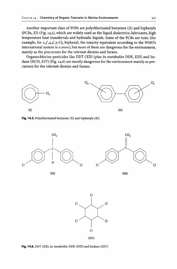
CHAPTER 14 . Chemistry of Organic Toxicants in Marine Environments 327
Another important class of POPs are polychlorinated benzenes (X) and biphenyls (PCBs, XI) (Fig. 14.5), which are widely used as the liquid dielectrics, lubricants, high temperature heat transferrals and hydraulic liquids. Some of the PCBs are toxic (for example, for 2,3',4,4',5-Cls biphenyl, the toxicity equivalent according to the WHO's international system is 0.0001), but most of them are dangerous for the environment, mainly as the precursors for the relevant dioxins and furans.
Organochlorine pesticides like DDT (XII) (plus its metabolite DDE, XIII) and lindane (HCH, XIV) (Fig. 14.6) are mostly dangerous for the environment mainly as precursors for the relevant dioxins and furans.
©r Cl"
Cln Cln
(X) (XI)
Fig. 14.5. Polychlorinated benzenes (X) and biphenyls (XI)
CCI3 CCl2
I II
ffI~ CI CI
ffC~ CI CI
(XII) (XIII)
CI
CI CI
CI CI
CI
(XIV)
Fig. 14.6. DDT (XII), its metabolite DDE (XIII) and lindane (XIV)

328 V. S. Petrosyan
Usually the models evaluating transport and accumulation of POPs consider the following compartments: air, soil, sea, vegetation and litterfall (Pekar et al. 1998). For example, in the recent joint report (Pekar et al. 1999) of the Meteorological Synthesizing Centre-East and Norwegian Institute for Air Research, it is assumed that initially emitted POPs enter the atmospheric air. The exchange of POPs takes place between gaseous and aerosol phases (Fig. 14.7), while the atmospheric transport is accomplished. Then in the course of wet and dry depositions of gaseous and aerosol phases, POPs enter soil, sea and vegetation. The dry deposition process of the pollutant gasphase is considered to be reversible, directly allowing one in the modelling course to consider the reemission process, which is important for some pollutants. From vegetation with fallen leaves, POPs enter the litterfall where they sometimes find their way to the soil. The accumulation in compartments decreases due to POPs degradation in the course of chemical, photochemical and biochemical reactions.
The total depositions and deposition densities of PCBs (XI), benzo(a)pyrene (XV), 2,3,4,7,8-PeCDF (IV) and lindane (XIV) have been estimated for some of the regional seas using the above-mentioned model (Pekar et al. 1999), and the calculated values for the Mediterranean, Baltic and North seas are given in Tables 14.1 and 14.2.
According to the calculation results, the highest depositions of the POPs considered fell in the area of the Mediterranean Sea. If we consider mean deposition density on the sea basins, then the highest intensity is accounted for on the Baltic Sea. Comparative diagrams of total depositions and their densities on the Mediterranean, Baltic and North Seas are presented in Figs. 14.8-14.11.
The recent analysis (Shatalov et al. 2000) of calculated spatial distribution of selected POPs in 1997 gave the preliminary estimates of contamination levels in different media. The data obtained for the European seas are given in Table 14.3.
D E G R A D A T I ...... f-----I o N
....
Exchange
~
~ Atmospheric transport
Exchange ----'1 Aerosol phase J
Wet deposition
Dry deposition
(aeros. phase)
Fig. 14.7. Scheme of POPs exchange between the various environmental compartments

CHAPTER 14 . Chemistry of Organic Toxicants in Marine Environments 329
Table 14.1. Total depositions of PCBs, benzo(a)pyrene, 2,3>4,7,8-PeCDF and lindane for 1996
Compounds Unit Mediterranean Sea Baltic Sea North Sea
PCBs kg yr -1
1623 715 594
B[a]P t yr -1
30 7 12
2,3A),8-PeCDF 9 I-Teqyr -1
492 65 101
Lindane t yr -1
56 18 26
Table 14.2. Deposition densities of PCBs, benzo(a)pyrene, 2,3>4,7,8-PeCDF and lindane for 1996
Compounds Unit Mediterranean Sea Baltic Sea North Sea
PCBs -2 -1
472 1843 886 ngm yr
B[a]P -2 -1
9 18 18 flgm yr
2,3A),8-PeCDF pg I-Teq m -2 -1
143 167 151 yr
Lindane -2 -1
16 46 38 flgm yr
f 30 40 >-
. j ~ ~r~ I .-1: 25 i 35 ~------ I ------------ [;l Ol !:: 30 . -------. .. .. ---- ------------ --- -----.. • Dry ..;; 20
.§ 25 ~ .~ 15 .~ 20 Qj 0
~ 10 ~ 15 0 'U
.;::; 1§ 10 'Vi 5 0 {2 5 Q. Qj 0 0 0
Mediterranean Baltic Sea North Sea Mediterranean Baltic Sea North Sea Sea Sea
Fig. 14.8. Total depositions (right) and deposition densities (left) oflindane on regional seas for 1996
Back to 1990-91 during the oceanography expeditions on the research vessel Moskovsky Universitet, we were measuring in particular the contamination of the Adriatic, Ionic, Mediterranean, Tirrenian and Black seas with organic pollutants both in waters and sediments (Petrosyan and Gianguzza 1999). In the spring of 1990, the expedition, headed by the author of this paper, started in Casablanca (Marocco) and ended in Sebastopol (U.S.S.R.), and there were 19 stations in the Mediterranean, Ionic, Adriatic and Black Seas (Fig. 14.12).
The data on the contamination of waters with hydrocarbons and phthalates have been obtained by Drs. P. I. Demyanov and A. N. Fedotov (M. V. Lomonosov University, Moscow) by means of high-resolution gas chromatography and presented in Table 14.4. These results show that the three most contaminated aquatic zones were evidently situated next to ilie estuaries of rivers Rhone (Station 3), Po (Station 11) and Danube (Station 19).

330
1. 1100 r-, ----------------,
1: 900 01 ..;; 700 r ··············· ~ ':£ 500 QI
~ 300 o
:€ 100 [ I ...... ----.. - '.... I - U I QI -100 L. ___ ----1 ____ .1.-___ ...J
o Mediterranean Baltic Sea North Sea Sea
V. S. Petrosyan
~ 1100 -L
900 >-~ I: .2
700
.t: 500 '" 0 Q. QI 300 "0
] 100 ~
- 100 ,'-___ -'-____ ...J-___ ---'
Mediterranean Baltic Sea North Sea Sea
• Wet gas 0 Wet part • Dry gas 0 Dry part I
Fig. 14.9. Total depositions (right) and deposition densities (left) of PCB on regional seas for 1996
~ 4.0 -,---~ 35
1 3:0 '" 2: 25 ~ .
.~ 2.0
~ 1.5 c .g 1.0
10.5 ~ 0.0 ' - -
Mediterranean Baltic Sea Sea
North Sea
12 ,,-------------,
'[ 10
'" § 8 1-·· ............... .
i 6
'" -c 4 ] {2
0 ' - 'GI - .... Mediterranean Baltic Sea
Sea North Sea
• Wet gas 0 Wet part • Dry gas 0 Dry part
Fig. 14.10. Total depositions (right) and deposition densities (left) ofbenzo(a)pyrene on regional seas for 1996
1. >. 7 120 " --------------, E 2" 100 fT ~ 801- ·
~60 .~ 40 -c 15 20
'.;::0 '&. 0 I - ,. I ! , _
~ Mediterranean Baltic Sea Sea
North Sea
~ 240 f' -~----------
2"200 fT $160
.§ 120 .".::
&. 60 .. ~ 20
;§ 0 ' - M!;F;4
Mediterranean Sea
...... r=J =='.,
Baltic Sea North Sea
• Wet gas 0 Wet part • Dry gas 0 Dry part
Fig. 14.11. Total depositions (right) and deposition densities (left) of 2,3,4,7,8-PeCDF on regional seas for 1996

CHAPTER 14 . Chemistry of Organic Toxicants in Marine Environments 331
Table 14.3. Concentrations of organic toxicants in European countries (sea water, ng m-3, 1997)
Country PCB B[a]P HCH Country PCB B[a]P HCH
Albania 32.9 574.7 2668.5 Latvia 66.3 693.8 2487.7
Azerbaidjan 8.3 907.2 123.8 Lithuania 74.8 985.7 2742.7
Belgium 157.4 1228.8 24220.0 Malta 15.4 137.2 2275.8
Bosnia and Herzegovina 46.8 1075.2 3024.1 Macedonia (The FYR) 34.4 651.0 2535.4
Bulgaria 28.3 714.8 1565.8 Moldova 37.7 119l.0 2101.1
Croatia 54.9 870.4 4621.0 Netherlands 150.9 891.9 12927.0
Cyprus 5.0 101.7 389.4 Norway 36.1 147.3 906.3
Denmark 122.7 738.3 3931.5 Poland 116.5 1539.3 3868.4
Estonia 74.2 627.6 2139.3 Portugal 15.3 121.2 2239.7
Finland 59.9 418.3 1497.7 Romania 29.3 773.0 1 646.3
France 73.4 472.4 18485.0 Russia 30.9 674.7 853.3
Georgia 24.4 1 332.4 368.7 Slovenia 98.0 1004.1 8372.5
Germany 181.9 1149.1 5577.7 Spain 27.5 205.3 5587.2
Greece 14.6 333.9 1405.3 Sweden 62.6 401.4 2183.8
Iceland 8.3 24.5 132.6 Turkey 14.4 370.7 680.8
Ireland 20.7 110.0 1251.7 Ukraine 31.5 1182.4 1459.3
Italy 45.5 462.2 6080.4 U.K. 43.7 356.1 4605.0
Kazakhstan 7.7 296.3 241.6 Yugoslavia 39.0 731.6 2673.9
40 ;9"
~ 1,2
30 o 10 20 3!\ 40
Fig. 14.12. Sampling stations within the 1990 Mediterranean, Ionic, Adriatic, and Black Sea expedition

332 V. S. Petrosyan
Table 14.4. Contamination of Mediterranean, Ionic, Adriatic and Black Sea waters with hydrocarbons and phthalates (ngrl)
Organics No. of stations
(-15
(-16
(-17
(-18
(-19
(-20
(-21
(-22
(-23
(-24
(-25
(-26
(-27
(-28
(-29
(-30
(-31
(-32
C-33
(-34
(-35
(-36
(-37
(-38
(-39
(-40
Sum of alkenes
BuPht
OctPht
2 3
10 4
26 18
12 7
23 18
9 4
15 10
11 6
18 11
15 10
24 16
121 33
58 40
73 51
77 58
89 77
117 76
119 74
110 67
106 56
89 37
62 29
49 21
39 14
28 16
30 15
30
4
6
12
11
15
12
18
14
18
16
19
37
29
22
52
31
27
21
15
11
6
4
3
3
4
4
5
5
14
8
14
5
6
5
7
8
11
13
12
11
10
10
7
6
4
7
11
19
16
21
14
13
12
9
16
19
19
24
23
23
21
23
15
11
10
6
4
5
16
10
2
13
4
16
4
10
4
12
12
17
19
30
30
41
47
45
46
47
43
29
23
20
16
19
16
13
11 12
18 7
27 25
298 13
21 24
28 7
24 13
18 8
50 17
61 18
93 36
114 30
136 39
113 39
136 41
113 80
116 39
87 37
77 32
61 29
36 20
32 18
26 12
20 11
25 14
20 11
19 10
13
12
13
12
11
25
36
51
59
66
62
60
57
41
33
36
23
12
11
9
8
13
8
6
15
7
23
12
11
11
18
11
17
17
23
23
23
21
17
16
12
11
8
5
3
3
2
3
6
16
7
16
10
16
5
6
5
5
6
6
8
8
9
10
10
9
9
6
6
6
4
5
4
5
19
8
10
96
7
6
3
2
2
8
2
2
2
3
2
2
1 360 768 410 156 334 578 1 764 620 635 313 181 160
66 47 132 62 63 30 7367 70 56 136 171 2870
773 190 412 130 146 250 554 318 179 231 94 24
The data demonstrate particularly that the petroleum hydrocarbons were mostly in the estuary of River Po and in the area south of Balearic Islands (Station 2). It was interesting to see that the highest concentrations of the individual alkanes have been obtained for the hydrocarbons with 25-33 carbon atoms. In regards to the phthalates, it was very interesting to see that butyl phthalate had been contaminating the waters in the Adriatic and Black seas next to the estuaries of rivers Po and Danube. Contrary

CHAPTER 14 • Chemistry of Organic Toxicants in Marine Environments 333
to this, octyl phthalate was not found in substantial amounts at these stations, but the highest concentration of this compound has been found in the vicinity of Balearic Islands.
In the spring of 1991, the joint Russian-Italian expedition headed by Professor A. Gianguzza (University of Palermo) and the author of this paper started in Palermo, and all 33 stations were within the Tirrenian Sea (Fig. 14.13).
The concentrations of organic contaminants in the Tirrenian Sea waters were measured by means of high-resolution gas chromatography (Drs. P. I. Demyanov, A. N. Fedotov, M. V. Lomonosov University, Moscow), and are presented in Table 14.5.
Sea waters with hydrocarbons and phthalates at most of the stations were at the same levels, but the contents of alkanes, dibutyl phthalate and other dialkyl phthalates were much higher at Station 1. The changes in concentrations of all the compounds that had been found in the Tirrenian Sea waters are shown graphically in Fig. 14.14.
Drs. 1. de Domenico and G. Magazzu (Oceanography Institute, CNR, Messina) obtained the data on the contamination of the Tirrenian Sea sediments with polycyclic aromatic hydrocarbons (PAHs), using two different standards (chrysene and crude oil). The results obtained are presented in Table 14.6.
42
Z 40 L
'" "C :J ... E ~
38
9 10 11 12 13 14 15
· · · 16
· .
17
· . : l __________ ~ 42
~~~~,~----E-:--]:;:_~;----: ~~:-~,-------:-:-------~ -ff: ~:-~-:l::::::-::l-----~~r~----l',';;-;,~---.:~"
• ::: 21* ' .... : \ 16 ,
9 .... ~ .~.~~.::i~~~=~~ ~~~~,:.-. ---;----f -------;t~:-~;--t:: ;~~t:'ici.d; •. _- .... - , 8 7 "" ::-1'''''·2 , 'alermo; 14 . ___ ':\::' Calabria
: ---- -.L ' __ t:~'~---- · r-----r - I . ---------~----:: : SiCilia . :
: : : , : j:
: : : : , .'.-----:-----' , , 'J__ , ' , , -'---------- , , ---------~--- -i----------i----- i ii ' , , " ,
40
38
r iii i : 136 ' , , " I I i : : I I I I I I I I I I i I 36 I I I I I I I I I I
9 10 11 12 13 longitude (0 E)
14
Fig. 14.13. Sampling stations within the 1991 Tirrenian Sea expedition
15 16 17

334 v. S. Petrosyan
Table 14.5. Pollution of the Tirrenian sea waters with some of the organic contaminants (l1g rl)
No. of stations Organics
Alkanes
2.60
3 0.84
13 0.61
15 0.69
19 0.74
22 0.23
24 0.93
31 0.49
33 0.49
a OBP: dibutylphthalate. b OEHP: di(ethyl)hexylphthalate. , OAP: dialkylphthalates.
5
4.5
4 , en 3.5 3-c 3 .2
2.5 ~ c 2 QI v c 8
Squalene DBP'
0.40 3.80
0.41 0.45
0.12 0.08
0.43 0.14
0.16 0.09
0.11 0.05
0.13 0.14
0.13 0.09
0.08 0.09
33
DEHPb DAP'
0.32 4.70
0.31 0.83
0.22 0.33
0.51 0.73
0.15 0.26
0.07 0.13
0.13 0.38
0.09 0.18
0.09 0.18
Dialkylphthalates (total content)
DEHP
Fig. 14.14. The concentrations of organic contaminants in the Tirrenian Sea waters
It is evident from the results of Table 14.6 that the data obtained with two different standards are quite different: the values in the last column (which are in our opinion more reliable) are 7-8 times higher than the figures from the middle column.

CHAPTER 14 . Chemistry of Organic Toxicants in Marine Environments 335
Table 14.6. Contamination of the Tirrenian sea sediments with polycyclic aromatic compounds (fig tl)
No. of stations Content of PACs
With chrysene (as a standard) With crude oil (as a standard)
10 0.05 0.38
11 0.15 1.10
12 0.22 1.64
13 0.06 0.43
14 0.10 0.78
15 0.06 0.45
16 0.13 0.96
17(1 s) 0.08 0.54
17(2s) 4.87 36.13
18 0.69 4.93
19(1s) 0.13 0.86
19(2s) 0.08 0.65
20(ls) 0.07 0.47
20(2s) 0.05 0.40
20(3s) 0.13 l.04
30 1.06 7.22
We have shown (Petrosyan et al. 1994) that the ecotoxicological effects of various types of contaminants are diminished by means of their binding by humic substances (humic and fulvic acids) contained in the aquatic ecosystems. Particularly, the humic substances detoxify different PAHs (Perminova et al.1999), increasing the binding and detoxification constants in the same series (e.g. anthracene < fluoranthene < pyrene).
References
Pekar M, Gusev A, Pavlova N, Strukov B, Erdman L, Ilyin I, Dutchak S (1998) Long-range transport of selected POPs: Development of transport models. EMEP/MSC-E Report 2/1998, Part 1
Pekar M, Pavlova N, Gusev A, Shatalov V, Vulikh N, Ioannisian D, Dutchak S, Berg T, Hjellbrekke A-G (1999) Long-range transport of selected POPs: Development of transport models. EMEP/MSC-E and CCC Report 411999
Perminova IV, Grechishcheva NY, Petrosyan VS (1999) Relationships between structure and binding affinity of humic substances for polycyclic aromatic hydrocarbons: Relevance of molecular descriptors. Environ Sci TechnoI33:3781-3789
Petrosyan V, Gianguzza A (1999) Contamination of Adriatic, Ionic, Mediterranean, Tirrenian and Black Seas with heavy metals and organic pollutants. Proceedings of 2nd Symposium on the "Protection of groundwater from pollution and seawater intrusion". Bari, September 27-0ctober 1, (1999)
Petrosyan VS, Perminova IV, Danchenko NN, Yashchenko NY, Lebedeva GF, Kovalevsky DV, Kulikova NA, Filippova or, Venedictov PS, Polynov VA (1994) Detoxification of heavy metals, polyaromatic hydrocarbons and pesticides by humic substances in waters and soils. Proceedings of the International Congress "Water: Ecology and technology". Moscow, pp 1136-1142
Shatalov V, Malanichev A, Berg T, Larsen R (2000) Investigation and assessment of POP transboundary transport and accumulation in different media. EMEP/MSC-E and CCC Report 4/2000, Part I

Chapter 15
Toxic Effects of Organometallic Compounds towards Marine Biota
1. Pellerito . R. Barbieri· R. Di Stefano· M. Scopelliti . C. Pellerito· T. Fiore· F. Triolo
15.1 Organometallic Derivatives
Organometallic derivatives are compounds containing a direct (J or 1T: carbon metal linkage. Furthermore, the concept of the metallic atom must be extended to all the elements that are less negative than the carbon atom. As a consequence, taking into account all elements that are less negative than carbon and the number of existing organic compounds, it is possible to synthesize millions of organometallic derivatives. Several of these are extensively used in organic syntheses; others may find application in agriculture and in many other fields as pesticides, fire retardants, wood preservatives, antifouling agents, etc. In general, the organic derivatives of the metals are more toxic than the parent inorganic metal, with the alkyl derivatives bearing greater toxicity than the aryl ones. Furthermore, the mechanism of toxicity depends on the co-ordination atoms present in the attached biological molecule.
This review will focus on a limited number of organometallic compounds, i.e. those whose presence and toxicity have been evidenced in marine biota.
15.2 Organoarsenic
15.2.1 Organoarsenic Derivatives
Arsenic occurs mainly as inorganic arsenate in sea water (2-3 Jlg dm -3) and in marine biota (up to 100 Jlg kg-1 of wet weight), as arsenobetaine in marine animals (Fig. 15.1) and as dimethylarsinylribosides (Fig. 15.1) in marine algae, in which arsenobetaine is absent. The arsenical derivatives are mainly used as industrial chemicals (wood preservatives), agricultural chemicals (herbicides and desiccants), fining agents in glass manufacturing, metallic arsenic in non-ferrous alloys, high-purity metallic arsenic for the electronics industry, and finally a small amount of arsenic is used as additive in animal food (Ishiguro 1992).
15.2.2 Biotransformation of Arsenic
The biotransformation of arsenic in marine ecosystems has been reported in several recent papers (Kaise and Fukui 1992; Francesconi et al. 1992; Garman et al. 1993). Owing to the fact that the phosphate/arsenate concentrations may be close to equimolar

338 L. Pellerito· R. Barbieri· R. Di Stefano· M. Scopelliti . C. Pellerito· T. Fiore· F. Triolo
Phytoplankton, Algae Marine animals
0-
CH3 OH ("*0 Hc-L~ ~ 3
H3C --L+ Arsenobetaine I Arsenocholine I "'& CH3
CH3 CH3
t I
H3C-As= 0
Trimethylarsine oxide lH 3
Arsenosugars
~ CH3 .. Dimethylarsinic acid I Sea water
OH OH OH
H3C-~S-OH
I I I 0
HO-As-OH HO-As-OH ~ HC-As-OH ¥'
II 3 II 0 0
Inorganic arsenic(V) Inorganic arsenic(lIl) Methanearsonic acid
Fig. 15.1. A tentative arsenic cycle in marine ecosystems
in the coastal boundary zone, the discrimination between arsenate and phosphate by phytoplankton is relatively poor, the concentrations differing only by a factor two to ten. As a consequence, arsenic is accumulated in marine organisms mainly in the form of organoarsenic compounds (Hanaoka et al. 1992a), in particular arsenobetaine, dimethylarsinic acid, methanearsonic acid, etc. (Fig. 15.1), which may be interconverted according to the following tentative scheme.
15.2.3 Organoarsenic in Marine Biota
Water-soluble arsenic compounds in several bivalves (Mytilus coruscum, Meretrix fusaria, Tapes japanica, Tresus keenae, etc.) (Shibata and Morita 1992) were extracted with 1:1 methanol/water and analysed with a high performance liquid chromatograph, combined with an inductively coupled argon plasma mass spectrometer. The results obtained are reported in Table 15.1.

CHAPTER 15 . Toxic Effects of Organometallic Compounds towards Marine Biota 339
The study evidenced that Meretrix lusoria, Tapes japonica and Tresus keenae contain not only arsenobetaine, but also the arsenosugar derivative reported in Fig. 15.2a, while Mytilus edulis, Mytilus coruscum, Cassostrea gigas, Anadara broughtonii, and Corbicula japonica contain either one or both of the arsenosugars of Fig. 15.2a,b. Since these bivalves are plankton-feeders, one can hypothesize that algae are one of the possible sources of the above-mentioned arsenosugars, while arsenobetaine could be er-
Table 15.1. Arsenic species in bivalves, adapted from Shibata and Morita (1992)
Sample Arsenic concentration (lIg As 9 -1 fresh tissue)"
(Japanese name) Arsenobetaine Tetramethyl- Arsenosugar Others e
arsonium
Fig.1S.2a Fig.1S.2b
Meretrix fusoria (Hamaguri)
Whole 1 0.78 0.17 0.92 0.1
Whole 2 0.33 0.25 0.17 0.03 0.57
Adductor muscle 2.06 0.24 0.57 0.34
Foot l.82 0.46 0.65 0.16
Digestive glandb 1.39 2.07 1.58
Mantle l.03 1.35 1.12 0.1
Mantle edge 0.26 1.34 1.14 0.1
Gill 0.14 6.07 2.44
Tapesjaponica (Asari)
Whole 1 0.63 0.67 0.07 0.57
Whole 2 0.75 0.70 0.07 0.59
Whole 3 0.49 0.46 0.05 0.48
Whole 4 0.73 1.48 0.15 0.73
Corbicufa japonica (Yamatosijimi)
Mix( 0.54 0.14 0.68
Mix 2d 0.53 0.22 0.06
Anadara broughtonii (Akagai)
Whole 1.03 0.11 0.05
Tresus keenae (Mirukui)
Whole 0.57 0.03 0.16 0.26
Spisufa sachafinensis (Hokkigai)
Whole 0.66 0.15

340 L. Pellerito . R. Barbieri . R. Di Stefano . M. Scopelliti . C. Pellerito . T. Fiore . F. Triolo
Table 15.1. Continued
Sample Arsenic concentration (Ilg As 9 -1 fresh tissue)"
(Japanese name) Arsenobetaine Tetramethyl- Arsenosugar Others e
arsonium
Fig. 15.2a Fig. 15.2b
Mytilus coruscum (lgai)
Adductor muscle 2.57 0.01 0.02
Foot 0.81 0.05 0.11
Digestive gland 1.35 0.06 0.13 0.03 0.18
Remaining part of the 1.41 0.02 0.06 0.12 body
Mantle 0.90 0.03 0.15
Mantle edge 1.36 0.04 0.03 0.09
Gill 0.93 0.06 0.08 0.05
a Column, Asahipak GS220; buffer, 25 mmol dm -3 tetramethylammonium, 25 mmol dm3 malonic acid (pH 6.8 adjusted by NH3).
b _, not detected (detection limit is less than 0.01 ~g As g -1 fresh tissue for any species). C Including soft tissues surrounding digestive gland. d Including whole tissues of three bivalves. e Others: I: AsO!-; II: AsO~-; III: CH3AsO~-; IV: (CH3)2AsO;; V: (CH3)3AsO; VI: (CH3)4As +CH2CHPH; VII:
(CH3)2As(O)CH2CHpH.
roneously accumulated by mussels because of its chemical similarity with the glycinebetaine used by the same organisms for osmo-regulation. The absence of arsenobetaine in Corbicula japonica could be due either to a lower amount of arsenobetaine in the food or to a lower amount of osmo-regulator necessary for Corbicula japonica, a mussel living in low-salinity regions. It has been demonstrated in vitro that microorganisms occurring in sediments induce the formation of arsenobetaine from arsenocholine (Hanaoka et al. 1992b). In particular, two or three metabolites, Fig. 15.3a,b, have been isolated from two different culture media (115 ZoBell 2216E and an aqueous solution of inorganic salts, respectively), after the addition of synthetic arsenocholine to 1 g of the sediment and incubation at 25°C in the dark.
The metabolites have been identified by high performance liquid chromatography, thin layer chromatography, FAB mass spectrometry, and a combination of gas chromatography and selected-ion monitoring mass spectrometry. The metabolites were structurally identified as arsenobetaine, trimethylarsine and dimethylarsinic acid, which led the AA to conclude that the cycle of Fig. 15.1 could only be carried out by the microorganisms.
An in vitro investigation of the chemical form and acute toxicity of arsenic compounds in sixty specimens of marine organisms has been carried out by Kaise and Fukui (1992). The chemical form of arsenic compounds in Demospongia, Coelenterata, Echinodermata, Mollusca, herbivorous and carnivorous Conches, plankton feeder Bivalvia, herbivorous, carnivorous and plankton feeder fish (Squalus brevirostris and Mustelus manazo), Crustacea and seaweed (Phaeophyceae (Lamina ria japonica,
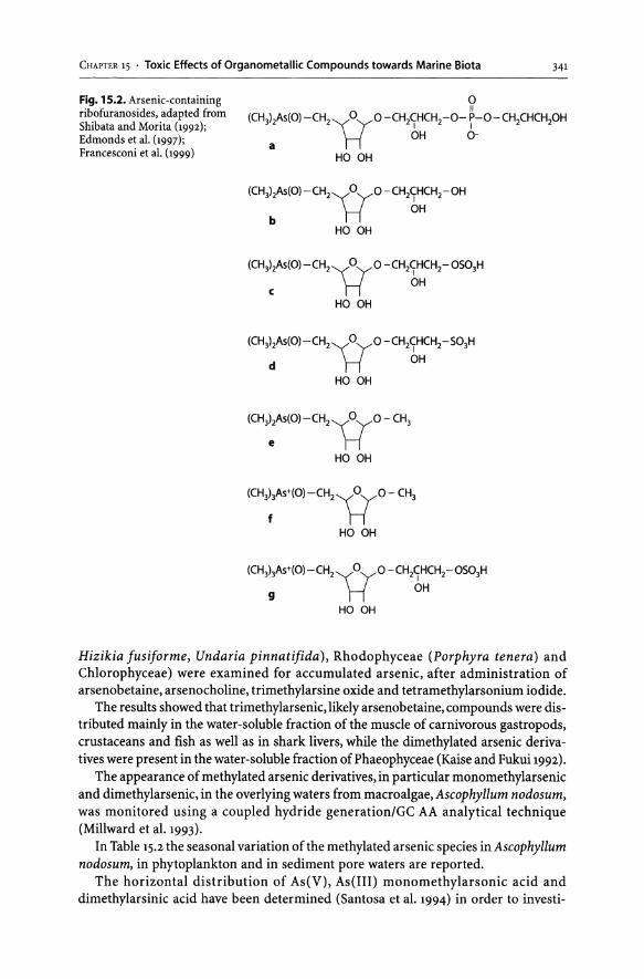
CHAPTER 15 • Toxic Effects of Organometallic Compounds towards Marine Biota 341
Fig. 1 S.2. Arsenic-containing ribofuranosides, adapted from Shibata and Morita (1992); Edmonds et al. (1997); Francesconi et al. (1999)
o II
(CH3hAs(O) -CH2 V O 0 - CH2CHCH2-O- P-O - CH2CHCHPH I I OH 0-
a HO OH
(CH3hAS(O}-CH2VO O-CH2~HCH2-0H OH
b HO OH
(CH3l2As(Ol -CH2VO 0 -CH2~HCH2-OS03H
OH c
HO OH
(CH3hAS(Ol-CH2,,(0yO -CH2~HCH2-S03H
d r-i OH
HO OH
(CH3~AS(Ol-CH2VO - CH3
HO OH
(CH3:3AS+(Ol-CH2V
O- CH3
HO OH
(CH3hAS+(Ol-CH2,,(0yO -CH2~HCH2-0S03H
g r-i OH
HO OH
Hizikia fusiforme, Undaria pinnatifida), Rhodophyceae (Porphyra tenera) and Chlorophyceae) were examined for accumulated arsenic, after administration of arsenobetaine, arsenocholine, trimethylarsine oxide and tetramethylarsonium iodide.
The results showed that trimethylarsenic, likely arsenobetaine, compounds were distributed mainly in the water-soluble fraction of the muscle of carnivorous gastropods, crustaceans and fish as well as in shark livers, while the dimethylated arsenic derivatives were present in the water-soluble fraction of Phaeophyceae (Kaise and Fukui 1992).
The appearance of methylated arsenic derivatives, in particular monomethylarsenic and dimethylarsenic, in the overlying waters from macro algae, Ascophyllum nodosum, was monitored using a coupled hydride generation/GC AA analytical technique (Millward et al. 1993).
In Table 15.2 the seasonal variation of the methylated arsenic species in Ascophyllum nodosum, in phytoplankton and in sediment pore waters are reported.
The horizontal distribution of As(V), As(III) monomethylarsonic acid and dimethylarsinic acid have been determined (Santosa et al. 1994) in order to investi-

342 L. Pellerito . R. Barbieri· R. Di Stefano . M. Scopelliti . C. Pellerito . T. Fiore . F. Triolo
<II ~~ 0·-
~~ <II U EO~
~~~ ~;e "'~ ... I: 0 I: en .... 0
0V; to v cC 6,.= ~ "V; ~cC
.s~ o~
a
b
Inorganic salt medium ZoBell medium
60
40
20
5 10 14 0 5 10
Incubation period (days) Incubation period (days)
l00.n Inorganic salt medium
80 1 \ Arsenocholine
60 2 l -'\. .-/"-~ Trimet~ylarsine '5 ~ 40 ~ oXide \. .0:: '" 0 li 15 20 ~ ~! La~ .,.-- DimethylarsinicaOd ~ ~o 0 ~ ~ ::: 0 5 10 15 20 25 30 enOl: ._ .... 0 111- u cC"'l:
t5 'iii 100 x :li ,y Arsenocholine
c( 6,.- f\ ZoBell medium
§ t5 80 Trimethylarsine
60
40
20
o
oxide \.
o 5 10 15 20 25 30 Incubation period (days)
14
Fig. 1 S.3. Conversion of arsenocholine into metabolites during aerobic incubation at 25°C in an inorganic medium and a ZoBell medium added to the sediment collected; a in May 1990; b in July 1990, adapted from Hanaoka et aI. (1992b)
gate their distribution and the cycle of the arsenic derivatives in the marine environment. In particular, during the cruises of the Shirase and Hakuho-maru ships as well as of the tanker Japan Violet, the Indian Pacific Oceanic (Santosa et al. 1994) surface

CHAPTER 15 • Toxic Effects of Organometallic Compounds towards Marine Biota 343
was being investigated, while vertical distribution was being determined in the west Pacific Ocean. The concentrations of the biologically produced species, namely monomethylarsonic acid and dimethylarsinic acid, were extremely low in the Antarctic and southwest Pacific waters (8 and 22 ng dm -3, and 12 and 25 ng dm -3, respectively). In all the other regions (East Indian Ocean, northwestern Pacific Ocean), the concentrations of monomethylarsonic acid (MMAA) and dimethylarsinic acid (DMAA) were very similar to each other (Fig. 15.4).
Three more cruises were performed by the same authors in the 1993-95 period, extending the determinations to inorganic and organometallic germanium derivatives (Table 15.3) (Santosa et al. 1997).
Polyphysa peniculus, a marine unicellular alga, is capable of metabolize arsenate, arsenite and monomethylarsonate, yielding as excreted metabolites, respectively, arsenite and dimethylarsenite, dimethylarsenite, trace amounts of monomethylarsonate,
Table 15.2. Seasonal variation of methylated arsenic species in waters (lower Tamar Estuary), adapted from Millward et al. (1993)
Source DMA (~g dm -3) MMA (~g dm -3)
Summer Winter Summer Winter
Macroalgae 0.08 0.G1 0.01 <0.01
Phytoplankton 0.04 0 0 0
Sediment porewaters <0.01 <0.01 <0.01 0.03
Region
Northwest Pacific . 1 • China Sea • Indonesia Archipelago . J • North Indian Ocean .. I • East Indian Ocean f------*l
;1 1 : Southwest Pacific [As(V) + As(lll)]
Antarctic I • 100 80 40 20 0 400 800 1200 1400
Portion of each species (%) Total arsenic (ng dm-3)
I DMAA o MMAA o AS(III) o AS(V)
Fig. 15.4. Total dissolved arsenic and the percentage of each species in a variety of ocean surface waters, adapted from Santosa et al. (1994)

344 L. Pellerito . R. Barbieri· R. Di Stefano . M. Scopelliti . C. Pellerito . T. Fiore· F. Triolo
Table 15.3. Average concentration of monomethylarsonic acid (MMAA), dimethylarsinic acid (DMAA), monomethylgermanium (MMGe) in the surface zone « 100 m) of three sampling stations in the Pacific Ocean, adapted from Santosa et aI. (1997)
Sampling station Arsenic Species (ng dm-3)
Germanium species (ng dm-3)
Inorg.As MMAA DMAA Inorg.Ge MMGe
North-west Pacific (LM-6) 1483 11.8 47.7 2.5 15.9
Central north Pacific gyre (C) 1110 15.9 184.5 2.0 165
Central Pacific equatorial 1450 12.4 53.3 <0.7 15.8 Region (D2)
Table 15.4. Arsenic distribution in aqueous extracts of cells determined by HG GC AA (Ilg g-l, dry weight), adapted from Cullen et aI. (1994)
Arsenic Arsenic species Cells treated with 10 ppm Cell treated with 0.9 ppm exposed founds in cells arsenicals arsenicals
Aa Bb Aa Bb
Arsenate Arsenate 12.8 ±0.8 9.7 ±0.7 0 5.1 ±0.3
Arsenite 25.1 ±1.3 0 26.3 ±1.6 0
MMAA 0 0 0 0
DMAA 1.9 ±0.2 0 21.7 ±2.0 0
Total 39.8 9.7 48.0 5.1
Arsenite Arsenate 8.0 ±05 0 1.8±0.1 0
Arsenite 37.7 ±25 2.3 ±0.2 65 ±0.4 1.2 ±0.1
MMAA 3.1 ±0.2 0.4 ±0.03 1.0 ±0.1 0
DMAA 0.8±0.1 0.8±0.08 5.4 ±0.5 0.8±0.1
Total 49.6 35 14.7 2.0
MMAA Arsenate 0 0.3 ±0.03 0 0
Arsenite 0 0.9±0.07 0 0
MMAA 5.3 ±0.3 0.8 ±0.06 1.4±0.1 0
DMAA 65 ±0.6 2.7 ±0.3 1.6±0.2 0
Total 11.8 4.7 3.0 0
MMAA Arsenate 1.6 ±0.1 0 0 0
Arsenite 0 0 0 0
MMAA 0.6±0.04 0.1 ±0.01 0.7 ±0.04 0
DMAA 28.1 ±2.5 3.6 ±0.3 20.4 ±1.8 2.5 ±0.3
Total 30.3 3.7 21.1 2.5
a Seven days after the cells were exposed to arsenicals. b Seven days after the cells were transferred to fresh media.

CHAPTER 15 • Toxic Effects of Organometallic Compounds towards Marine Biota 345
and finally dimethylarsinate. Polyphysa peniculus did not metabolize dimethylarsinic acid when it was used as substrate (Cullen et al. 1994) (Table 15.4).
The data reported in Table 15.4 strongly support the biomethylation pathway of Fig. 15.5 for the microbial process.
According to the proposed model (Cullen et al. 1994), the arsenate is taken up from the medium, via the phosphate transport system, into the algal cells. The arsenate is reduced to arsenite inside the cells by thiols and/or dithiols, and the cells excrete most of the arsenite into the growth medium by means of an active transport system.
Subsequently, methylation of the en do cellular arsenite to MMAA occurs by using SAM; because of its low passive diffusion coefficient, the endocellular MMAA is not excreted in the growth medium, rather it remains in the cells, where it is reduced and further methylated to DMAA. Possessing a greater diffusion coefficient, DMAA passively diffuses into the growth medium.
According to an in vitro investigation of the blue mussel Mytilus edulis carried out by Gailer et al. (1995) exposure to arsenite, arsenate, methylarsonic acid, dimethylarsinic acid, arsenobetaine, arsenocholine, trimethylarsine oxide, tetramethylarsonium iodide or dimethyl-( -hydroxyethyl)arsine oxide (100 Ilg As dm-3 in sea water, for 10 days), results in conversion of arsenobetaine and arsenocholine to trimethylarsine oxide,
Golgi apparatus
Rough endoplasmatic reticulum
Chloroplast Nucleus
" :: " II
Phosphate :: Thiols and/or !! Active transport Arsenate • :: Arsenate" d· h· I • Arsenite" :: system • Arsenitei'
transport system 11 It 10 S !~
Arsenitei' _~~~~~~!~0sport system----....
11 I.
:: 2 e 2 e :: Passive b :: Arsenite" ~M MMAA-=:-=+M DMAA":: d.ffu . .. DMAA II e+ e+ II I sion
il !!
Fig. 15.5. Proposed model for biomethylation of arsenate in marine alga Polyphysa peniculus, adapted from Cullen et al. (1994)

346 L. Pellerito . R. Barbieri . R. Di Stefano . M. Scopelliti . C. Pellerito· T. Fiore . F. Triolo
whereas trimethylarsine oxide and tetramethylarsonium iodide remain unaltered. None of the other arsenic derivatives are significantly accumulated. Furthermore, arsenobetaine, arsenocholine and tetramethylarsonium iodide are accumulated by the mussel, although arsenobetaine is accumulated more efficiently. Finally, following exposure to arsenobetaine or arsenocholine, the accumulated arsenic is present in the tissue as arsenobetaine (Table 15.5).
Cytotoxicity of arsenobetaine, arsenocholine, trimethylarsine oxide and tetramethylarsonium iodide derivatives, which are contained in fishery products, has been investigated by Kaise et al. (1998) in mammalian cells, see Table 15.6.
Arsenobetaine, arsenocholine and trimethylarsine oxide did not inhibit cell growth (BALB/c 3T3 cells) at a concentration ~1O mg cm-3• Chromosome aberrations, consist-
Table 15.5. Total arsenic (Ilg) in 12 mussels at the end of accu- Arsenic compound mulation, adapted from Gailer et al. (1995)
Control
Arsenobetaine
Tetramethylarsonium Iodide
Control
Arsenocholine
After accumulation in whole animal
Range Mean
15.4-38
456-1201
49-113
13-41
99-317
24.5
727
82
24
197
Table 15.6. Toxicity of arsenic compounds in experimental animals and cultured cells, adapted from Kaise et al. (1998)
Arsenical
Arsenite
Arsenate
Methylarsonic acid
Dimethylarsinic acid
Trimethylarsine oxide
Arsenobetaine
Arsenocholine
Tetramethylarsonium
Arsenosugar f
a 50% lethal dose. b 50% growth inhibition. C Percent of aberrant.
BALBlc HT cells
LDso' (g kg_l)
ICsob
(mgcm-3)
0.0345 0.0007
0.006
1.8 1.2
1.2 0.32
10.6 >10
>10 >10
6.5 >10
0.9 8
2
d Sister chromatid exchange (SCE) metaphase. ; Not induced.
See Kaise et al. (1996).
Chromosomal aberrations on cultured human fibroblast
(%)c Concentration SCEd
(mg cm-3) (mg cm-3 ceWl)
20 0.001 O.OOl e
33 0.02 0.02e
37 O.5e
90 0.5 0.1 e
42 2 1.0e
18 10 1.0e
15 10 1.0e
24 10 1.0e
15 5 1.0e

CHAPTER 15 • Toxic Effects of Organometallic Compounds towards Marine Biota 347
ing in chromatid gaps, chromatid breaks and, rarely, disruption of centromeres, were provoked by arsenite, arsenate, methylarsonic acid and trimethylarsine oxide. Arsenocholine, arsenobetaine and tetramethylarsonium iodide were less toxic than inorganic arsenic (Kaise et al. 1998).
Arsenobetaine may be decomposed into trimethylarsine oxide, dimethylarsinic acid and inorganic arsenic(V) by microorganisms occurring in particles, which are present in deep sea at 1100-3500 m (Hanaoka et al.1997). The arsenic transformations in short marine food chains were investigated by HPLC-ICP MS (Edmonds et al.1997). In particular, the organisms studied were the copepod Gladioferens imparipes fed on the diatom Chaetoceros concavicornis cultured under axenic conditions, the amphipod Allorchestes compressa, the Antarctic krill Euphausia superba, the abalone Haliotis roeii, and finally the teleosts fish silver drummer Kyphosus sydneyanus. The experiments were designed to provide information on the ability of marine animals to convert arsenosugars to arsenobetaine, and to determine whether absorption from water is the source of arsenobetaine in herbivorous animals (Table 15.7).
Chaetoceros concavicornis accumulated the arsenosugar of Fig. 15.2C to a concentration dependent on its degree of exposure to inorganic arsenate in sea water; this suggests that the conversion is part of a detoxification process. A high concentration of arsenate was detected in extracts of copepods fed with algal cells that had been grown in water containing 1 mg kg- 1 of arsenate. Arsenobetaine was absent from the muscle of the silver drummer Kyphosus sydneyanus, although trimethylarsine oxide was present (Edmonds et al. 1997).
Arsenobetaine was absent both in the copepods Gladioferens imparipes fed only with the diatom Chaetoceros concavicornis, grown in axenic culture, and from the muscle of the silver drummer Kyphosus sydneyanus, although trimethylarsine oxide was present (Edmonds et al. 1997).
Liver samples of pinnipedes (nine ringed seals (Phoca hispida), one bearded seal (Erginathus barbatus) and cetaceans (two pilot whales (Globicephalus melas), one beluga whale (Deliphinapterus leucus)) contained arsenobetaine as the predominant arsenic derivative (0.052-1.67 mg As kg-1 wet mass); arsenocholine was also present at 0.005-0.044 mg As kg- 1 wet mass; dimethylarsinic acid ranged between <0.001 to 0.109 mg As kg- 1 wet mass and finally methylarsonic acid was below the detection limit «0.001 to 0.025 mg As kg- 1 wet mass), (Table 15.8) (Goessler et al. 1998).
As determined by HPLC-GFAA and HPLC-ICP MS, arsenobetaine was the major arsenic compound extracted from the water-soluble fraction of jellyfish Aurelia aurita and Carybdea rastonii (Fig. 15.6) (Hanaoka et al. 1999a). Arsenocholine and tetramethylarsonium ions were also present.
Animals of higher trophic levels generally do not eat jellyfish. As a consequence, the arsenobetaine that accumulates in the latter may not be passed directly to these higher-level animals. Instead, microorganisms occurring in sediments, suspended substances, macro algae, etc., could degrade arsenobetaine in a multi-step process to inorganic arsenic, so that the arsenic may circulate in a smaller ecosystem composed of sea water, plankton, small fish and jellyfish rather than in a general ecosystem that includes animals of all trophic levels.
After feeding Crangon crangon shrimp with dimethyl- and trimethylarsenosugars, the muscle, midgut gland, gills and the remainder tissue of the crustacean were

348 L. Pellerito . R. Barbieri· R. Di Stefano . M. Scopelliti . C. Pellerito . T. Fiore . F. Triolo
Table 15.7. Arsenic compounds detected in various samples and approximate percentage that each compound contributed to the total arsenic in each organism, adapted from Edmonds et al. (1997)
Sample
Chaetoceros in normal sea water
Chaetoceros with elevated arsenic
Chaetoceros in artificial (reduced arsenic) sea water
Cope pods fed Chaetoceros from normal sea water
Cope pods fed Chaetoceros with elevated arsenic
Copepods fed Chaetoceros from artificial sea water
Amphipods
Antarctic krill
Silver drummer muscle
Silver drummer gut 1 (stomach)
Silver drummer gut 2
Silver drummer gut 3
Abalone foot muscle
Abalone digestive gland
Abalone fore-gut contents
Abalone hind-gut contents (faeces)
Abalone food (algae)
Arsenic compounds detected"
Arsenosugar of Fig. 15.2a (2%), arsenosugar of Fig. 15.2c (90%), unknown compounds(5%)
Arsenosugar of Fig. 15.2c (>99%)
Arsenosugar of Fig. 15.2a (2%), arsenosugar of Fig. 15.2c (60%), unknown compounds(30%)
Arsenosugar of Fig. 15.2c (70%), trimethylarsine oxide (10%), unknown compounds (> 15%)
As(V) (40%), trimethylarsine oxide (25%), arsenosugar of Fig. 15.2c (20%), unknown compounds (> 1 0%)
Trimethylarsine oxide (70%), arsenosugar of Fig. 15.2c (20%), unknown compounds (>5%)
Arsenobetaine (60%), arsenosugar of Fig. 15.2a (5%), Fig. 15.2b (7%), Fig. 15.2c (5%), Fig. 15.2d (1 %)
Arsenobetaine (60%), arsenosugar of Fig. 15.2a (5%), Fig. 15.2b (1 %), Fig. 15.2d (1 %), DMAAb (20%)
Trimethylarsine oxide (>95%), tetramethylarsonium ion (3%), arsenosugars of Fig. 15.2a and of Fig. 15.2c (1 %)
Trimethylarsine oxide (65%), arsenosugar of Fig. 15.2a (5%), Fig. 15.2b (2%), Fig. 15.2c (1 %), Fig. 15.2d (10%)
Trimethylarsine oxide (50%), arsenosugar of Fig. 15.2a (10%), Fig. 15.2b (15%), Fig. 15.2c (1 %), Fig. 15.2d (15%)
Trimethylarsine oxide (90%), arsenosugar of Fig. 15.2a (2%), Fig. 15.2b (2%), Fig. 15.2d (2%)
Arsenobetaine (90%), tetramethylarsonium ion(l %), arsenosugar of Fig. 15.2a (3%), Fig. 15.2b (2%), Fig. 15.2c (1 %)
Arsenobetaine (40%), tetramethylarsonium ion (1 %), arsenosugar of Fig. 15.2a (10%), Fig. 15.2b (35%), Fig. 15.2c «1%), Fig. 15.2d (10%)
Unknown compounds (60%), arsenosugar of Fig. 15.2a (5%), Fig. 15.2b (30%), Fig. 15.2d (2%)
Unknown compounds (35%), arsenosugar of Fig. 15.2a (5%), Fig. 15.2b (50%), Fig. 15.2d (5%)
Unknown compounds (30%), arsenosugar Fig. 15.2a(25%), Fig. 15.2b (10%), Fig. 15.2c(5%), Fig. 15.2d (25%)
a Approx. percentages in parentheses b DMAA, dimethylarsinic acid.
analysed by HPLC-I CP MS for their arsenical metabolites, see Fig. 1pa -g (Francesconi et al. 1999). The aim of the investigation was to ascertain the possible role of the arsenosugars as precursors to arsenobetaine. The obtained results showed that while only 0.9% of dimethylarsenosugar was accumulated by the shrimps, giving dimethyl-

CHAPTER 15 . Toxic Effects of Organometallic Compounds towards Marine Biota 349
Table 15.8. Concentrations of Organoarsenic compounds in liver samples of whales and seals determined by HPLC-HHPN-ICP-MS, adapted from Goessler et al. (1998)
Species Concentration of arsenic compounds· (mg As kg -1 wet mass)
Arsenobetaine Arsenocholine DMAA MMAA
Pilot whale 0.887 0.005 0.004 0.003
Pilot whale 0.147 0.005 <0.001 <0.001
Ringed seal 0.337 0.005 0.021 <0.001
Ringed seal 1.67 0.020 0.109 <0.001
Ringed seal 1.02 0.012 0.040 <0.001
Ringed seal 1.46 0.G15 0.067 <0.001
Ringed seal 0.764 0.008 0.032 <0.001
Ringed seal 1.17 0.G11 0.G18 <0.001
Ringed seal 0.702 0.G25 0.028 <0.001
Ringed seal 0.417 0.021 0.036 0.001
Ringed seal 0.386 0.044 0.021 <0.001
Ringed seal 0.684 0.G18 0.004 0.G25
Beluga whale 0.0502 0.002 0.016 0.002
Bearded seal 0.0156 0.016 0.021 0.004
a Mean of two different extracts.
arsinate and dimethylarsinoylethanol as major metabolites, about half of the accumulated 4.2% of trimethylarsenosugars were converted to arsenobetaine. Shrimps fed with arsenobetaine retained S7% of the dose (Table IS.9). The main conclusion from these results is that the dimethyl and trimethyl arsenosugars do not represent the major source of betaine for wild Crangon.
The investigation of the structure of the lipid-soluble arsenic compound is important for the elucidation of arsenic circulation in the marine ecosystem.
Phosphatidyl arsenocholine and phosphatidyl arsenosugar, -OCR! and -OCR2 being fatty acyl groups (Hanaoka et al. 1999b) (Fig. IS.7) were extracted and identified in several tissues of five demersal sharks, in particular, the starspotted shark Mustelus manazo.
In particular, the muscle, kidneys and brains contained alkali-labile arsenic derivatives; the livers; stomaches, hearts and gallbladders contained alkali-stable derivatives; finally, the intestines, skin, dark muscle, spleens and bones contained both types of arsenic compounds, as shown in Fig. IS.S.
Further hydrolysis has been carried out on the above-mentioned derivatives obtained from muscle and liver. The HPLC-I CP-MS analysis showed the occurrence of arsenocholine, suggesting that arsenolecithins were present in the tissues, as shown in Fig. IS.9.
Finally, the presence of dimethylated arsenolipids in the liver was evidenced from the detection of dimethylarsinic acid in liver hydrolysates (Fig. IS.lO) (Hanaoka et al. 1999b).
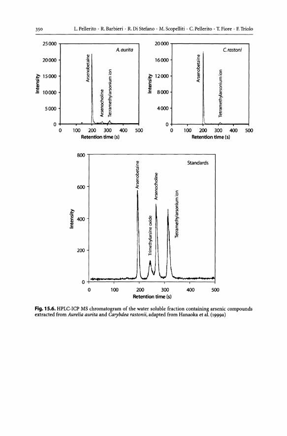
350 L. Pellerito . R. Barbieri· R. Di Stefano . M. Scopelliti . C. Pellerito . T. Fiore· F. Triolo
25000 20000 Aaurita c.rastoni
QJ QJ
20000 -I c: 16000 c: 'i;j 'i;j ii) 1l .0 0 c: 0 c: c: .Q c: .2 {15000] ~ ~ 12000 QJ
E ~ E « " 'Vi « " '2 c: '2 $ 0 $ 0
..5 10000 QJ ~ c: 8000 ~ .!: '" - '" 0 >- >-.r::. idj .r::. ii) ~
5000 -I c: E 4000 E ~ ~ ~
« ~ ~ 0 0
0 100 200 300 400 500 0 100 200 300 400 500 Retention time (5) Retention time (5)
800 QJ Standards c:
'i;j
600
1l QJ
0 c: c: ~ ~ .r::.
u « 0 c: c:
~ .2 E " '2
~ 'Vi !4OO ..5
0 ~
! '"
~ ~ ~ ~ ii)
~ E ~
.~
~ III >-~
200 E ~
l Nu~ --_._,-- . T .----'
o , ... , .....", -...""t
o 100 200 300 400 500 Retention time (5)
Fig. 15.6. HPLC-ICP MS chromatogram of the water soluble fraction containing arsenic compounds extracted from Aurelia aurita and Carybdea rastonii, adapted from Hanaoka et aI. (1999a)

CHAPTER 15 . Toxic Effects of Organometallic Compounds towards Marine Biota 351
Table 15.9. Retention (0/0) of three arsenic compounds in individual tissues and whole shrimp fed 951lg As (normalized see Francesconi et al. 1999) over 19 days. The proportion of arsenic body burden in each tissue is shown in parentheses. Values for midgut gland and gills are based on arsenic contents of pooled tissues
Tissue Me2As-sugar group Me3As-sugar group Arsenobetain group
Tail muscle 0.32 (0.355) 1.08 (0.258) 27.6 (0.488)
Midgut gland 0.02 (0.022) 0.40 (0.096) 2.1 (0.038)
Gills 0.03 (0.035) 0.12 (0.029) 1.1 (0.019)
Remaindera 0.53 (0.588) 2.58 (0.617) 25.7 (0.455)
Whole animal 0.9 (1.00) 4.2 (1.00) 57 (1.00)
a Not including haemolymph and other fluids lost during dissection. Values have been rounded to two significant figures.
o II
C1HP -OC-R1
II CHO -C-Rz
I 0 C~ II I
CH 0 -P-O- CH CH -As+- CH z I Z Z I 3
0- CH3
o II
CH O-C- R I 2 0 1
II CHO-C- R2
I 0 CH3 II I
CH20 - P-O- CH2CHOHCHP HO CH2-As = 0 I I 0- CH3
HO OH
Fig. 15.7. The molecular structures of phosphatidylarsenocholine and phosphatidyl arsenosugar. -OCR 1
and -OCR2: fatty acyl groups, adapted from Hanaoka et al. (1999b)
250
, :§" 200 g. ... 1\1
8. .!?) 150
~ t:: 0 . .-:; (!! 100 ~ I v t:: 0 v III
<C 50
0
3
I
Alkali-stable arsenolipid
.-J
Alkali-labile arsenolipid 4
)
1 Stomach
2 Heart
3 Liver
4 Gallbladder
5 Intestine
6 Skin
7 Dark muscle
8 Spleen
9 Bone
10 White muscle
11 Kidney
12 Brain
Fig. 15.8. Distribution of alkali-labile and alkali-stable arsenolipids in the tissue and organs of starspotted shark, adapted from Hanaoka et al. (1999b)

352 L. Pellerito· R. Barbieri· R. Di Stefano . M. Scopelliti . C. Pellerito . T. Fiore . F. Triolo
12000 •• --------------, Standards AB
9000 AC
Tetra l:' .~ 6000 $ E
3000
0 ,~UL
0 2 4 6 8 Retention time
2500 .,-------------,
2000
l:' 1500 ·iii c: $ E 1000
500
o I. o
AC
2 4 6 8 Retention time
Fig. 15.9. HPLC-ICP-MS chromatograms of standards and the water soluble arsenic residues obtained after severe acid hydrolysis of alkali-labile arsenic fraction prepared from ordinary muscle, adapted from Hanaoka et al. (1999b)
20000 20000 As(lll) Standards
DMA J DMA
15000 MA 15000 As(V)
.~ l:' III ·iii c: 10000 ~ 10000 ~
5000 5000
o 1M I I" II i (I iii i IIIII i IIII iii j; 1IIII1 Ii III'
1J~ o 11111111111111
0 2 4 6 8 10 12 14 16 0 2 4 6 8 10 12 14 16 Retention time (min) Retention time (min)
Fig. 15.10. HPLC-ICP-MS chromatograms of standards and the water soluble arsenic residues obtained after severe alkaline hydrolysis of alkali-stable arsenic fraction prepared from the liver, adapted from Hanaoka et al. (1999b)
15.3 Organotin
15.3.1 Organotin Derivatives
Organotin(IV} derivatives have been widely studied for several reasons. Their extensive world-wide use is evident in industry as PVC stabilizers; in agriculture as agrochemicals (fungicides, acaricides), disinfectants (biocides, bactericides) and preservatives (cellulose, wood and stonework); and in the marine environment as antifouling agents (algaecides, molluscicides). Books and reviews have been published in the last few years, covering almost all applications and chemical and biological proper-

CHAPTER 15 • Toxic Effects of Organometallic Compounds towards Marine Biota 353
ties of these compounds (Patai 1995; Abel et al. 1995; Champ and Seligman 1996; De Mora 1996; Smith 1998; Barbieri et al. 2000). As a consequence, organotin(IV) compounds are extensively present in natural and marine waters, marine biota, and sediments. Several good books covering the toxic effects of organometallics and comprising organotin(IV) derivatives have been published recently (Arakawa and Wada 1993; Mennie and Craig 1993; Crompton 1998). Again, for the scope of this review, we will describe the toxic effects of organotin(IV) derivatives on marine biota reported in the last ten years.
15.3.2 Organotin in the Marine Biota
The level of tributyltin(IV)oxide (TBTO) in sediments and in Mytilus galloprovincialis sampled in the harbour area of Taranto, where mussel cultures are highly developed, has been detected by electrothermal atomic absorption after n-hexane/methylene chloride mixture extraction in 4 different sampling stations and purification of the extract with a sodium hydroxide wash. The TBTO levels obtained in sediments and mussels were in the range of 15-47 ng g-l (wet weight) and 11-30 ng g-l (wet weight), respectively (Cardellicchio et al. 1992) (Fig. 15.11).
When exposed to 10-5 and lO -7 mol dm -3 diorganotin(IV)dichloride and triorganotin(IV)chloride solutions for different times, the gastropod Truncatella subcylindrica suffered the following chromosomal structural lesions: (1) breakages, (2) bridging, (3) irregular outline and (4) light areas after staining with acetic orcein, see Figs. 15.12 and 15.13, Table 15.10 (Vitturi et al. 1992).
The experimental evidence shows that tributyltin(IV)chloride is more toxic to this organism than diorganotin(IV)dichloride.
Effects of the exposure to 10-4 and lO -5 mol dm -3 dibutyltin(IV) derivatives of carbohydrates solutions as D( - )sorbitol, D( + )glucose, D( - )fructose and D( + )glyceraldehyde (Mansueto et al. 1993b), Fig. 15.14, on different stages of Ciona intestinalis development, larval movements and metamorphosis have been tested in vivo.
The results are summarized in Table 15.11, where it is possible to note that the twocell stage embryos, if incubated for 1 hour in the organotin(IV) solutions, stopped cleavage, which was restored when the embryos were transferred in organotin-free sea water.
Fig. 15.11. Distribution of TBTO average concentrations in mussels and sediments in the four sampling stations, adapted from Cardellicchio et al. (1992)
, Iso $ C\ 40 ..s g 30 .~
~ 20 OJ
~ 10 8 ~ 0 I- 2 3
Sampling station
• Sediments o Mussels
4

354 L. Pellerito . R. Barbieri· R. Di Stefano . M. Scopelliti . C. Pellerito . T. Fiore . F. Triolo
2 3 4
Fig. 15.12. Truncatella subcylindrica and its representative karyotype, adapted from Vitturi et aI. (1992)
Fig. 15.13. Diakinetic bivalents of Truncatella subcylindrica treated with BU3SnCl for 72 h (single arrow indicates a breakage and double arrow indicates the bridging), adapted from Vitturi et aI. (1992)
H ~OH OH H 0 H 0 H
H H OH H OH H H~ HO OH
H OH H OH
a b
H
~OH
H 0
H H OH
HO OH
OH H
c
:X:H H~OH
H
d
Fig. 15.14. Structures of; a D(-)sorbitol; b D(+)glucose; c D (-)fructose; d D(+)glyceral-dehydes

CHAPTER 15 . Toxic Effects of Organometallic Compounds towards Marine Biota 355
Table 15.10. Spermatocyte chromosome alterations in Truncatella subcylindrica. Dibutyltin{IV) and tributyltin{IV) chloride concentrations, incubation times and percentages of different categories of anomalous spreads observed during analysis of 100 spreads per specimen, adapted from Vitturi et al. (1992)
Anomaly Time interval 3h 24h 48h 144 h
Organometal DBTD TBTC DBTD TBTC DBTD TBTC DBTD
No. of specimens 3 2 4 2
Cone. (mol dm -3) 10-4 10-4 10-4 10-4 10-4 10-4 10-4
Irregular outlines Norm. 45 45 86 82 91 86
Breakages Norm. 19 20 37 40 35 28
Chromosome bridging Norm. 24 26 40 32 36 35
Light stained areas Norm. 3 43 78 67 86 84
No. of specimens 3 6 6 2
Cone. (mol dm -3) 10-7 10-7 10-7 10-7 10-7 10-7 10-7
Irregular outlines Norm. Norm. 7 55 42 85 78
Breakages Norm. Norm. 3 21 15 38 45
Chromosome bridging Norm. Norm. 3 19 15 39 32
Light stained areas Norm. Norm. 5 50 33 80 65
No. of specimens 3 6 6 2
Cone. (mol dm -3) 10-9 10-9 10-9 10-9 10-9 10-9 10-9
Irregular outlines Norm. Norm. Norm. 46 16 60 35
Breakages Norm. Norm. Norm. 14 7 21 15
Chromosome bridging Norm. Norm. Norm. 16 10 26 18
Light stained areas Norm. Norm. Norm. 44 15 48 35
No. of specimens 3 6 6 2
Cone. (mol dm -3) 10-11 10-11 10-11 10-11 10-11 10-11 10-11
Irregular outlines Norm. Norm. Norm. 12 Norm. 38 25
Breakages Norm. Norm. Norm. 8 Norm. 20 15
Chromosome bridging Norm. Norm. Norm. 10 Norm. 19 16
Light stained areas Norm. Norm. Norm. 11 Norm. 35 22
OBTD = dibutyltin(lV)dichloride ; TBTC = tributyltin(lV)chloride; The term Norm. (= Normal) indicates no difference from the control. As 100 spreads of each specimen were examined, the percentage values in this table are calculated from n observations in each case, where n = 100 No. of specimens.
The gastrula stage was seriously affected by exposure to 10-4 mol dm -3 solutions of the previously-mentioned complexes: 85% of the embryos were anomalous neurulae with open neural folds; 5% were twisted larvae. The gastrulae, if incubated in 10 -5 mol dm-3 solutions, developed twisted larvae in ovular envelopes and immobile larvae with twisted tails. Finally, larvae treated with both 10 -4 and 10 -5 mol dm -3 solutions stopped swimming, did not metamorphose and underwent cytolysis, as shown in Fig. 15.15.

356 L. Pellerito . R. Barbieri . R. Di Stefano . M. Scopelliti . C. Pellerito . T. Fiore . F. Triolo
Table 15.11. Development of Ciona intestinalis embryos after incubation in solutions of organometallic com-plexes in sea water for a limited time (1 h) and after transferring to normal sea water, after Mansueto et al. (1993)a
Compound Cone. Development stage
(moldm-J ) Twoeells Gastrula Neurula Late neurula Larva
AG1 10-4 Larvae,90 Anomalous embryos, Delayed larvae, 90 Delayed larvae, 90 Immobility 85
10-5 Larvae,90 Delayed, twisted Delayed larvae, 90 Larvae, 90 Immobility larvae, 90
AG2 10-4 Larvae,90 Anomalous embryos, Larvae, 90 Twisted, 60 immobile, Immobility 85 twisted larvae, 5 10 anomalous
larvae, 20 10-5 Larvae,90 Delayed larvae, 90 Larvae, 90 Larvae, 90
AG3 10-4 Delayed Delayed twisted Larvae, 90 Larvae, 90 Immobility larvae,90 larvae,90
10-5 Delayed Delayed larvae, 90 Larvae, 90 Larvae, 90 larvae,90
AG7 10-4 Anomalous Anomalous embryos, Anomalous larvae,80 Twisted larvae,60 immobility neurulae, 80 twisted larvae, 10 immobile larvae, 10 anomalous larvae, 20 80 twisted immobile larva, 10 larvae, 10
10-5 Delayed Delayed, twisted Delayed larvae, 90 Delayed larvae, 90 Immobility larvae, 90 larvae, 90
a Data refer to 14 experiments and show the percentage of developed or arrested embryos. Control developed >90% of swimming larvae.AG7 = Bu1Sn-D-(-)sorbitol;AG2 = Bu1Sn-D-(+)glucose;AG3 = Bu1Sn-D-(-)fructose; AG7 = Bu1Sn-D-(+)glyceraldehyde.
Fig. 15.15. Ciona intestinalis gastrulae incubated for 1 h in 10-5 moldm-J BU2 Sn-D-(-) sorbitol solution. The embryos developed into twisted larvae in ovular envelopes and immobile larvae with twisted tails (magnification 40X), after Mansueto et al. (1993)

CHAPTER 15 . Toxic Effects of Organometallic Compounds towards Marine Biota 357
Exposure to lO -5 and lO -7 mol dm -3 bis( dimethyltin(IV)chloro )protoporphyrin(IX), Fig. 15.16, of early developing embryos of Anilocra physodes 1. (Crustacea, Isopoda), a parasite of various fish, for different exposure times, produced abnormal metaphase and anaphase figures, which depended on the concentration and not the exposure time (Vitturi et al. 1993) (Table 15.12).
According to the reported data, it may be concluded that the bis( dimethyltin(IV)chloro )protoporphyrin(IX) interferes with the formation of the mitotic spindle and acts directly on metaphase chromosome structure (Vitturi et al. 1993).
The above-reported effects are also observed in embryos of the ascidian Ciona intestinalis upon exposure to 10-5 and 10-7 mol dm -3 solutions of tributyltin(IV)chloride (Mansueto et al. 1993a).
o~ 0
I H3C ".... CI 5n-
H3C ~I ~ 0,
0
o
o
H3C "" .. I
f N-H
H ~5n -CI
3C I
o r
, N
/ N,
Fig. 15.16. Structure of bis( dimethyltin{IV)chloro )protoporphyrin(IX)
/~ I
H-N , '\~
/ II

Tabl
e 15
.12.
Gen
otox
ic a
ctiv
ity. M
etap
hase
and
ana
phas
e ch
rom
osom
al d
amag
e in
Ani
/acT
a ph
ysad
es e
arly
-dev
elop
ing
embr
yos
trea
ted
wit
h bi
s(di
met
hyit
in(I
V)
chio
ro)p
roto
porp
hyri
n(IX
), a
dapt
ed f
rom
Vit
turi
et a
l. (1
993)
Co
mp
ou
nd
T
ime
N
o. o
f em
bry
os
To
tal
No
rma
lb
Ab
no
rma
l T
ota
l co
nce
ntr
ati
on
in
terv
al
em
plo
ye
d
spre
ad
s·
me
tap
ha
ses
me
ta p
ha
ses
spre
ad
s (m
old
m-'
) (h
) a
na
ph
ase
s a
na
ph
ase
s
Fra
gm
en
ts
Bri
dg
es
c d
c d
c d
c d
e
0.95
6 x
10
-5
24
11
22
0 10
2
59
3 4
6
10
104
18
98
48
9
180
8 4
8
2 36
14
80
16
8
4
2.07
X 1
0-7
2
4
10
20
0
20
12
50
38
14
87
24
89
48
8
160
23
10
46
4
14
19
62
33
65
1 x
10
-9
24
12
24
0 63
59
10
5
9 2
4
78
78
84
48
8
160
35
42
13
5 10
4
8
52
60
Co
ntr
ol
12
270
71
78
2 73
79
88
a 20
spr
eads
pe
r e
mb
ryo
we
re a
naly
sed.
b
Th
e te
rm "
no
rma
l" in
dic
ate
s n
o d
iffe
ren
ce fr
om
th
e c
on
tro
l. ~
Nu
mb
er o
f met
apha
ses.
N
um
be
r of a
na p
hase
s.
e N
um
be
r of p
rop
ha
ses
of w
hic
h c
hro
mo
som
e a
berr
atio
ns w
ere
no
t de
tect
ed
.
:::: 00
.. "" ~ '" .. S· ?"
til ~ !:!. ?" ~
r;' §' 0 ~
(/)
.g ~ a: 0 "" ~ '" .. ::1
-' 0 H
'T
I o· .. '" :-r1 ::;l o· 0'
Tab
le 1
5.12
. Gen
otox
ic a
ctiv
ity. M
etap
hase
and
ana
phas
e ch
rom
osom
al d
amag
e in
Ani
locr
a ph
ysod
es e
arly
-dev
elop
ing
embr
yos
trea
ted
wit
h bi
s( di
met
hylt
in{I
V)
chlo
ro)p
roto
porp
hyri
n(IX
), a
dapt
ed f
rom
Vit
turi
et a
l. (1
993)
Co
mp
ou
nd
T
ime
N
o. o
f em
bry
os
To
tal
No
rma
lb
Ab
no
rma
l T
ota
l co
nce
ntr
atio
n
inte
rva
l e
mp
loye
d
spre
ads"
m
etap
hase
s m
eta
phas
es
spre
ads
(mo
ldm
-')
(h)
anap
hase
s an
apha
ses
Fra
gm
en
ts
Bri
dg
es
c d
c d
c d
c d
e
0.95
6 x
10
-5
24
11
2
20
10
2
59
3
46
1
0
10
4
18
9
8
48
9
18
0
8 4
8
2 3
6
14
8
0
16
8
4
2.07
x 1
0-7
2
4
10
2
00
20
12
5
0
38
1
4
87
2
4
89
48
8
16
0
23
10
4
6
4 1
4
19
6
2
33
65
1 X
10
-9
24
12
2
40
63
59
10
5
9 2
4
78
78
8
4
48
8
160
35
42
13
5
10
4
8
52
60
Co
ntr
ol
12
27
0
71
78
2 73
7
9
88
a 20
spr
eads
pe
r e
mb
ryo
we
re a
na
lyse
d.
b T
he
term
'no
rma
l' in
dic
ate
s n
o d
iffe
ren
ce fr
om
th
e c
on
tro
l.
~ N
um
be
r o
f me
ta p
hase
s.
Nu
mb
er o
f ana
phas
es.
e N
um
be
r o
f pro
ph
ase
s o
f wh
ich
ch
rom
oso
me
ab
err
atio
ns
we
re n
ot d
ete
cte
d.
:::: 00
r" '"" ~ '" ... s" ?"
o:l ~ ::l. ?" ~ it ~ 0 ~
(/)
.g ~ a: \1 '"" ~ '" ... ::;:
0 H
'TI o· ... '" "" ::;l o· 0

CHAPTER 15 . Toxic Effects of Organometallic Compounds towards Marine Biota 359
In vivo observations showed that cleavage of fertilized eggs was inhibited and embryo blastomeres gave rise to cellular masses not delimited by plasma membranes. Furthermore, electron-dense precipitates, probably due to inorganic tin, were evidenced by transmission electron microscopy (TEM) in the egg cytoplasm of cellular masses. The same type of precipitate was also present in mitochondria, whose structure appeared to be highly modified, indicative of a degenerative process of the embryos after incubation in TBT chloride (Fig. 15.17).
The cytotoxic activity of diorganotin(IV) and triorganotin(IV) derivatives of penicillin G, and of [meso-tetra(4-sulphonatophenyl)porphine], of chloramphenicol, cycloserine and of orotic acid, see Fig. 15.18a-e, has been tested in Ciona intestinalis fertilized eggs at different stages of development (Maggio et al. 1994; Pellerito et al.1997b, 1998; Lencioni et al.1999) and in Aphanius Jasciatus (Vitturi et al. 1994).
The genotoxicity of all the organotin(IV)-penicillin G and triorganotin(IV)[mesotetra(4-sulphonatophenyl)porphinate] derivatives correlates with the blockage of Ciona intestinalis fertilized eggs at early stages of development. The results obtained from the in vivo investigation of Ciona intestinalis developing embryos, Fig. 15.19a,b and Table 15.13, suggested the following considerations:
1. All the organotin(IV) derivatives are toxic, like the organotin(IV) parents; 2. The triorganotin(IV) derivatives are more toxic than the diorganotin(IV) deriva
tives; 3. In the triorganotin(IV) series, the tributyltin(IV) is the most toxic.
At least two major nonexclusive hypotheses may explain the results:
Fig. 15.17. Electron-dense precipitates ofTBT chloride in the cell masses. The mitochondria ultrastructure, m, is highly modified (magnification 18 500X), adapted from Mansueto, Gianguzza et aI. (1993)

360 L. Pellerito . R. Barbieri· R. Di Stefano . M. Scopelliti . C. Pellerito . T. Fiore . F. Triolo
o H H - II :!S CH3 O-"y-:C-HNJf~~
NH3 0 H
H03S S03H
a b
o H II
02N-o-~ I tCCHCl2 C-C
_ I I-CHPH
HO H
H NW '\ / 3
H .... ··C-CH
/ \ o C-O-
~N~
c d
o
tl HN3 SI
,f'~ 1 6 COOH o N I H
e
Fig. 15.18. Structures of; a penicillin G: b [meso-tetra(4-sulphonatophenyl)porphine; c chloramphenicol; d cycloserine; e orotic acid, adapted from Maggio et aI. (1994); Pellerito et aI. (1997b); Pellerito et aI. (1998); Lencioni et aI. (1999)
a Consistent ultrastructural damage, including mitochondrial organelles and cytomembranes may be caused by the organotin{IV)-penicillin G derivatives;
b Irregular cleaving processes may reflect damage affecting chromosome structure.
The latter hypothesis is supported by studies that showed that chromosome damages occur in Aphanius fasciatus after exposure to the above-mentioned chemicals (Vitturi et al.1994) and in Rutilus rubilio after exposure to diorganotin(IV)amoxicillin derivatives (Vitturi et al.1995) (Fig. 15.20). The results reported in Tables 15.14 and 15.15 and Figs. 15.21 and 15.22 show that all chromosome abnormalities may be classifiable in Aphanius fasciatus as irregular staining, breakages, side-arm bridges or pseudochiasmata of chromosomes, while differentially stained chromosome areas, granular deeply stained zones along the chromosomal body, arm breakage and finally side-arm bridges {pseudo chiasmata) were observed in Rutilus rubilio chromosomes after exposure to 10-5 and 10-7 mol dm -3 solutions of diorganotin{IV)amoxicillin derivatives (Pellerito et al. 1995).

CHAPTER 15 . Toxic Effects of Organometallic Compounds towards Marine Biota 361
a b
Fig. 15.19. a Anomalous embryos derived from gastrulae incubated for 1 h in lO -7 mol dm-3 Bu3Sn(IV)ClpenGNa (magnification 50X); b Anomalous two-cell stage incubated in lO-5 mol dm-3
• (Bu3Sn)4TPPS solution, adapted from Maggio et aI. (1994); Pellerito et aI. (1997b)
Table 15.13. Results of development of Ciona intestinalis fertilized eggs incubated in the solution of H4TPPS, (R2Snh TPPS e (R3Sn)4TPPS, (H4 TPPS = [meso-tetra (4-sulphonatophenyl)porphine]; R = Me, Bu and Ph) from 2-cell stage. The controls give rise to 90% swimming larvae. Percentage of developed or arrested eggs (average of 5 experiments), adapted from Pellerito et aI. (1997b)
(om pound (one. Development stages (moldm-')
Blastomere Early Anomalous Undifferentiated Anomalous Swimming gastrulae neurulae embryos larvae larvae
2 4 8-16
H4TPPS 10-5 100 10-7 100
(Me2Sn)2TPPS 10-5 100
10-7 100
(Bu2Sn)2 TPPS 10-5 50 50
10-7 50 50
(Ph2Sn)2TPPS 10-5 100
10-7 100
(MejSn)4 TPPS 10-5 100
10-7 50 50
(BUjSn)4TPPS 10-5 100
10-7 100
(PhjSn)4TPPS 10-5 50 50
10-7 50 50

362 L. Pellerito· R. Barbieri· R. Di Stefano . M. Scopelliti . C. Pellerito . T. Fiore . F. Triolo
Fig. 1 S.20. Structure of arnoxicillin, adapted from Pellerito et aI. (1995)
Fig. 1 S.21. Chromosome aberrations obtained from different giemsa stained spreads of treated Aphanius Jasciatus specimens; A = chromosomes with irregular staining; B = chromosomes with black granular regions; C = breakages; D = chromosomes with arms different in length and E = chromosomes with pseudochiasmata, adapted from Vitturi et al. (1994)
OH
H~'l' 6'1 . 5'
H ~4' 0 H ~ 5 CH
II NJjCt :Sq2 CHJ 3Hp - C- C- Hs 6 3 11 3 H 110 9 7 N4 COO-
NH! 0 H
Exposure to different concentrations of butyltin(IV)chlorides affected phagocytic activity of Ciona intestinalis and of Botryllus schlosseri haemocytes, mainly by influencing cellular calcium homeostasis by interacting with calcium pumps (Cima et al. 1995), while dibutyltin(IV)dichloride, triphenyltin(IV)chloride and diphenyltin(IV)dichloride did not show significant effects on phagocytosis (Cooper et al. 1995) (Figs. 15.23 and 15.24).
On the other hand, tributyltin(IV) derivatives induced apoptosis (Fig. 15.25) in Botryllus schlosseri haemocytes (Cima and Ballarin 1999), as evidenced by: (i) chro-

CHAPTER 15 . Toxic Effects of Organometallic Compounds towards Marine Biota 363
Table 15.14. Genotoxic activity: mitotic metaphase chromosomal damage in Aphanius Jasciatus speci-mens treated with RzSnClz, RzSnClpenG, R3SnCI and R3SnCIpenGNa (penG = penicillin G; R = methyl, butyl and phenyl), adapted from Vitturi et al. (1994)
Compound Conc. Time (mol dm -J) interval (h)
No. of meta phases
Normal Fragments Irregular Pseudo- Irregular Total outlines chiasmata staining spreads
MezSnClpenG 10-5 24 4 30 28 40 70
48 32 8 39
10-7 24 4 52 22 36 60
48 26 6 36
MezSnClz 10-5 24 18 23 22 30
48 16 25 18 40 10-7 24 12 44 32 28 80
48 40 39 38 70
MeJSnClpenGNa 10-5 Died after a treatment of 3 hours 10-7 24 15 16 25 36
48 5 22 23 32 42
MeJSnCI 10-5 Died after a treatment of 3 hours 10-7 24 2 12 20 18 38
48 18 24 20 40
BuzSnClpenG 10-5 24 4 2 40 16 32 50
48 4 3 30 8 36 40 10-7 24 16 46 4 40 80
48 40 15 36 50
BUzSnClz 10-5 24 4 41 16 32 50
48 2 28 23 18 35 10-7 24 10 50 10 44 64
48 4 35 8 40 50
BuJSnClpenGNa 10-5 Died after a treatment of 3 hours 10-7 24 12 15 20 30
48 14 18 24 28
BuJ5nCI 10-5 Died after a treatment of 3 hours 10-7 24 30 18 36 28 46
48 Died after a treatment of 40 hours
Phz5nClpenG 10-5 24 8 4 50 8 30 60
48 6 9 8 10 10-7 24 42 29 22 50
48 48 27 25 58

364 1. Pellerito . R. Barbieri· R. Di Stefano . M. Scopelliti . C. Pellerito . T. Fiore . F. Triolo
Table 15.14. Continued
Cone. Time Compound (mol dm -J) interval (h)
Ph2SnCI2 10-5 24
48
10-7 24
48
PhJSnClpenGNa 10-5
10-7 24
48
PhJSnCI 10-5
10-7 24
48
Fig. 15.22. Giemsa-stained metaphase of Rutilus rubilio treated with 10-7 mol drn -3 BU2 SnClamox'2H20 for 48 h, adapted from Vitturi et al. (1995)
No. of meta phases
Normal Fragments Irregular Pseudo- Irregular Total outlines chiasmata staining spreads
15 6 15 23
19 10 18 25
10 4 10 20
4 12 12 15 22
Died after a treatment of 3 hours
10 8 12
10 14 12 18
Died after a treatment of 3 hours
12 15 32 36 50
13 18 25 40 45

CHAPTER 15 ' Toxic Effects of Organometallic Compounds towards Marine Biota 365
Table 15.15. Genotoxic activity: mitotic metaphase chromosomal damage in Rutilus rubilio specimens treated with amox'3HzO, RzSnCIamox'2HzO and RzSnamoxz'2HzO (R = methyl, butyl and phenyl), adapted from Vitturi et ai, (1995)
Compound Cone. Time interval No. of metaphases (moldm-3) (h)
Normal Irregular Granular Breakages Side-arm Total staining zones bridges spreads
Controls 326 333
Amox,3Hp 10-5 24 12 15
48 17 4 28
10-7 24 8 22 2 31
48 10 26 6 42
MelSnClamox' 2HlO 10-5 24 12 10 6 2 3 24
48 8 6 3 18
10-7 24 23 4 36
48 7 18 7 12 40
Me2Snamox2,2HP 10-5 24 Died after a treatment of 13-14 hours
48
10-7 24 22 6 4 29
48 13 8 4 4 25
Bu2SnClamox'2Hp 10-5 24 16 21
48 20 4 32
10-7 24 3 28 12 6 11 51
48 2 34 16 7 16 66
BulSnamoxl' 2H2O 10-5 24 Died after a treatment of 2-3 hours
48 10-7 24 14 8 11 27
48 16 13 6 14 43
Ph2SnClamox'2H20 10-5 24 13 4 17
48 13 14 5 29
10-7 24 7 23 12 40
48 4 25 17 44
Ph2Snamox2,2HP 10-5 24 Died after a treatment of 2-3 hours
48
10-7 24 12 24
48 19 16 10 9 48
matin condensation, with Acridine Orange nuclear staining, (ii) DNA fragmentation, with the TUNEL reaction, (iii) PS translocation, with the annexin-V assay; and (iv) loss of membrane permeability with the Trypan Blue diffusion assay.

366 L. Pellerito . R. Barbieri· R. Di Stefano . M. Scopelliti . C. Pellerito . T. Fiore . F. Triolo
a b c
Fig. 15.23. Phagocytizing haemocytes, showing; a positivity for Ca2+ -ATPase (arrowhead); b localized internal calcium rise in normal conditions (arrowhead); c diffuse internal calcium rise in the presence of TBT. Bars: 10 f1Il1, adapted from Cima et al. (1995)
Fig. 15.24. Phagocytosis of Ciona intestinalis haemocytes after incubation (90 min) with different concentrations of organotin compounds; (a) 1.51LM, (b) 0.15 fLM, (c) 0.015 ILM, (d) 0.0015 fLM and (e) MS = marine solution, adapted from Cooper et al. (1995)
so
l '" .~ 40 >. u o C\
'" ..c IJ. 30 '0 <II C\ !9 I: ~ 20
~
10
o TBT DBT TPT DPT MS
An ultrastructural study carried out by Gianguzza et al. (1996), by exposing embryos of the asci dian Ciona intestinalis to tributyltin(IV)chloride solutions, at two different stages of development (1) before hatching (coiled larval stage) and (2) 2 h after hatching (swimming larval stage) led to the following conclusions:

CHAPTER 15 . Toxic Effects of Organometallic Compounds towards Marine Biota
Fig. 15.25. Apoptotic index of Botryllus schlosseri exposed to 10 f!M TBT for 1 and 2 h as detected with the annexin-V assay (grey bars) and the TUNEL reaction (black bars). The white bars represent the unexposed haemocytes, adapted from Cima et al. (1995)
21
18
~ 15 -c c 'u 12
'15 g. 9 a. 0{
6
3
o -'--'---'------'
Time (h)
367
2
a The embryos at the coiled larval stage do not hatch after exposure to TBT chloride; b Severe anomalies in the swimming larva occur and include alteration of tail mor
phology, which appears to be twisted and squatted less than the control.
Furthermore, TEM of tail muscle cells correlated alterations of mitochondrial and myofibrillar ultrastructure with loss of larval mobility (Fig. 1p6a,b).
To correlate these embryonic arrests with cell biochemistry, and especially to understand the molecular details underlying the chemical damages of cellular organelles, fertilized eggs exposed to 10-5 and 10-7 mol dm -3 tributyltin(IV)[meso-tetra(4-carboxyphenyl)porphinate], were assayed for DNA, RNA, protein, glucose, lipids and ATP contents, comparing the obtained values with those of control fertilized eggs (Fig. 15.27) (Mansueto et a!. 2000).
The greater reduction of the content of all tested compounds was induced by 10 -5 mol dm -3 tributyltin(IV)[meso-tetra{4-carboxyphenyl)porphinatel solution, while 10-7 mol dm-3 solution still inhibited cleavage, but reduced only lipid and ATP content. A possible explanation may be that cleavage did not occur because of lack of energy, or an ATP shortage provoked a cAMP deficiency. Independently of the molecular mechanism underlying the block of the fertilized egg cleavage, the primary effect seems to be the damage to the organellar or cellular membrane, or both.
Cytotoxicity of triorganotin{IV) derivatives towards the sea urchin Paracentrotus lividus (Echinodermata) have been gathered by exposure to triorganotin(IV)-Lhomocysteate derivatives as well as to the parent triorganotin{IV)chlorides, while the free L-homocysteic acid exerted no significant toxic activity (Pellerito et al. 1997a). Comparative analysis of mitotic chromosomes from untreated embryos and embryos treated with 10-5 and 10-7 mol dm -3 solutions of the above-mentioned organotin(IV) derivatives are reported in Fig. 15.28a-d and Table 15.16.
As expected, the tributyltin- and triphenyltin{IV)-L-homocysteate were the most toxic, while the trimethytin(IV)-L-homocysteate exerted the lowest cytotoxicity. The main defects evidenced were: (1) suppression of stretch between sister chromatids at

368
a
L. Pellerito· R. Barbieri· R. Di Stefano· M. Scopelliti . C. Pellerito· T. Fiore· F. Triolo
p /1\
b
Fig. 15.26. a Ciona intestinalis swimming larva incubated for 1 h in 10-7 mol dm -3 TBT solution and then transferred to sea water. The larva, vitally stained with Nile Blue sulphate, presents severe anomalies in the tail (ta) which is strongly twisted; it makes weak and brief movements, and the larva is not able to swim; b Ciona intestinalis swimming larva incubated for 1 h in 10 -7 mol dm -3 TBT solution. Longitudinal section of the muscle cell. Owing to folding, several sectors of myofibrils (m *j) appear as point structures. Some mitochondria (m*) show a strongly modified ultrastructure. The cells of the ectodermal layer present a large nucleus (N), yolk granules (G) and are very rich in r.e.r. vesicles (er). (Bar = 1 flm), adapted from Gianguzza et al. (1996)
100 990 ±45 970 ±50 1 000
« 80 800 Z 70±6 't: 0 67±5 \C
C'I 634 "C :::L 60 56±6
~ 600S --'tl
ll~ ~
.:: 48 i5 ~. :::>
IT~ 0 40B 37;1;4 Co 40 400 ;B E 0 0 u z C'I 18 i 2
l> :::L 20 200
3tO.2 2tO.2 ltO.l
0 ',' ',' ',' 0 C H L C H L C H L C H L C H L
AlP Gucose Lipids RNA Proteins
Fig. 15.27. ATP/DNA, glucoselDNA, lipids/DNA, RNA/DNA and proteins/DNA ratios determined at two different concentrations of tributyltin(IV)[meso-tetra(4-carboxyphenyl)porphinate): H = 10-5 mol dm-\ L = 10 -7 mol dm - 3; and C = control, adapted from Mansueto et al. (2000)
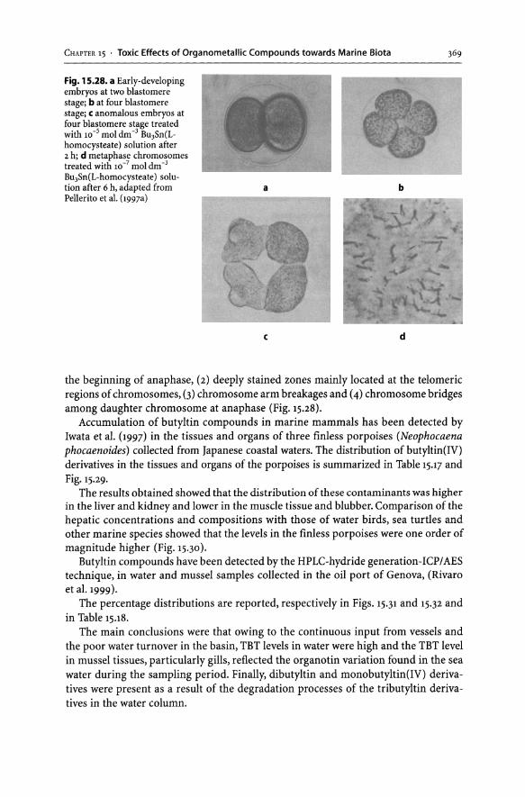
CHAPTER 15 • Toxic Effects of Organometallic Compounds towards Marine Biota
Fig. 1 S.28. a Early-developing embryos at two blastomere stage; b at four blastomere stage; c anomalous embryos at four blastomere stage treated with 10-5 mol dm -3 Bu3Sn(Lhomocysteate) solution after 2 h; d metaphase chromosomes treated with 10-7 mol dm-3
BU3Sn(L-homocysteate) solution after 6 h, adapted from Pellerito et al. (1997a)
a
c
369
b
d
the beginning of anaphase, (2) deeply stained zones mainly located at the telomeric regions of chromosomes, (3) chromosome arm breakages and (4) chromosome bridges among daughter chromosome at anaphase (Fig. 15.28).
Accumulation of butyltin compounds in marine mammals has been detected by Iwata et al. (1997) in the tissues and organs of three finless porpoises (Neophocaena phocaenoides) collected from Japanese coastal waters. The distribution of butyltin(IV) derivatives in the tissues and organs of the porpoises is summarized in Table 15.17 and Fig. 15.29.
The results obtained showed that the distribution of these contaminants was higher in the liver and kidney and lower in the muscle tissue and blubber. Comparison of the hepatic concentrations and compositions with those of water birds, sea turtles and other marine species showed that the levels in the finless porpoises were one order of magnitude higher (Fig. 15.30).
Butyltin compounds have been detected by the HPLC-hydride generation-ICP/AES technique, in water and mussel samples collected in the oil port of Genova, (Rivaro et al. 1999).
The percentage distributions are reported, respectively in Figs. 15.31 and 15.32 and in Table 15.18.
The main conclusions were that owing to the continuous input from vessels and the poor water turnover in the basin, TBT levels in water were high and the TBT level in mussel tissues, particularly gills, reflected the organotin variation found in the sea water during the sampling period. Finally, dibutyltin and monobutyltin(IV) derivatives were present as a result of the degradation processes of the tributyltin derivatives in the water column.

370 1. Pellerito· R. Barbieri· R. Di Stefano . M. Scopelliti . C. Pellerito . T. Fiore· F. Triolo
Table 15.16. Genotoxic activity: mitotic metaphase and anaphase chromosomal damage in Paracentrotus lividus embryos treated with R3SnCl and R3SnL-HCA (L-HCA = L-homocysteic acid; R = methyl, butyl and phenyl), adapted from Pellerito et aI. (1997a)
Compound Concentration Time interval No. of spreads (moldm-3) (h)
Normal Irregular Granular Colchicinized-like Total staining zones chromosome spreads
Controls 71 74
6-8 110 4 114
18-20 258 3 264
Me3Sn(L-HCA) 10-5 Arrest
6-8
18-20
10-7 6 8 8 20 42
6-8 4 6 25 38
18-20 5 5
Me3SnCI 10-5 Arrest
6-8
18-20
10-7 2 4 10 12 15 41
6-8 4 4 5 20 33
18-20 3 7 10
nBujSn(L-HCA) 10-5 Arrest
6-8
18-20
10-7 2 4 6 6 12 28
6-8 0 20 28
18-20 Arrest
nBu3SnCl 10-5 2 Arrest
6-8
18-20
10-7 7 12 6 15 40
6-8 4 4 26 36
18-20 Arrest
Ph3Sn(L -HCA) 10-5 2 Arrest
6-8
18-20
10-7 Arrest
6-8
18-20

CHAPTER 15 . Toxic Effects of Organometallic Compounds towards Marine Biota
Table 15.16. Continued
Compound Concentration Time interval No. of spreads (mol dm-3) (h)
Normal Irregular Granular Colchicinized-like staining zones chromosome
PhJSnCI 10-5 Arrest
6-8
18-20
10-7 2 Arrest
6-8
18-20
371
Total spreads
Table 15.17. Concentrations (ng ofbutyltin ion per g, wet weight basis) ofbutyltins in tissues and or-gans of higher trophic animals, adapted from Iwata et al. (1997)
Sample Sampling location Tissues and MBT DBT TBT LBTs organs
Finless porpoise, Ise Bay Muscle 22 38 420 480 1994 Blubber 73 20 120 213
Liver 680 1800 810 3290 Kidney 55 340 510 905 Heart 12 41 640 693 Lung 90 59 160 309 Stomach 18 64 130 212 Brain 9 40 350 399 Adrenal gland 130 350 250 730 Spleen 33 98 69 200 Bonea 14 21 33 68 Esophagus 19 36 49 104 Pancreas 72 130 220 422 Intestine 9 70 66 145 Urinary bladder 26 67 56 149 Eye <5 12 35 47 Blood 82 640 95 817 Intestine content 6 47 150 203
Ginkgo-toothed Japan Sea Muscle 20 8 19 47 beaked whale, Blubber 20 10 33 63 1993 Liver 120 130 76 326
Kidney 66 34 42 132
Largha seal. Western coast of Muscle 14 6 20 40 1992 Hokkaido Blubber 14 1 4 19
Liver 96 200 32 328 Kidney 27 55 28 110
Common cormorant, North Pacific Liver 150 180 19 349 1993
Loggerhead turtle, Tosashimizu Liver 68 60 2.4 130 1990
a The bone marrow of a rib was analysed.

372 L. Pellerito . R. Barbieri . R. Di Stefano . M. Scopelliti . C. Pellerito . T. Fiore . F. Triolo
Muscle Blubber
Liver Kidney
Heart
Lung
Stomach
Brain Adrenal gland
Spleen Bone
Esophagus
Pancreas Intestine
Urinary bladder
Eye
Blood
Intestine content
"'{\
-~ '-/
'" :::. ,-'-/ ...
"'~ .- '-/
... -.-
",-
o
-~-r '-'
... ... -~
... ;-
'" " '-'
" 20
--'" -- ~
" ~ '-/ - --... --" ..
'-/ .. --- {\
~ '":, C"L- .~ '-'" ~ ,,'-" -- ... TBT '-'
-" - o DBT - ~'-/ • MBT - '-' --r--""" -
40 60 80 100
Composition (%)
Fig. 15.29. Butyltin compositions in tissues and organs of a finless porpoise collected from Ise Bay, adapted from Iwata et al. (1997)
Caprella1
Blue mussel2
Horseshoe crab3
Japanese sea bass4
Loggerhead turtle
Largha seal
Finless porpoise
Ginkgo-toothed beaked whale
Common cormorant
Laysan albatross
---- -
- -----
La
o 2000
-
-
4000 6000 8000 10000 12000 Concentration (ng (g wwt)-l)
Fig. 15.30. Interspecies comparison ofbutyltin concentrations in livers, adapted from Iwata et aI. (1997); (1) Caprella: whole body; (2) Blue mussel: soft tissue, (J) see Kannan K et al (1995) Arch Environ Toxicol 28:40, (4) see Suzuki T et al. (1992) J Agric Food Chern 40:1437

CHAPTER 15 . Toxic Effects of Organometallic Compounds towards Marine Biota 373
a b
c d
Fig. 15.31. Nile tilapia livers of control and TPTH-treated groups after four months of exposure (400X); a Control (water) showing normal hepatocytes and sinusoids; b Control (0.0015% DMSO), showing small hyaline droplets in hepatocytes. P, exocrine pancreas; c Treated with 1 mg 1-1 TPTH, showing congestions of sinusoids (S) and central vein. Note marked increase in lipid vacuolation (L); d Treated with 3 mg rl TPTH showing more severe sinusoidal congestion (S) and lipid vacuolation (L), adapted from Visoottiviseth et al. (1999)
Triphenyltin(IV)hydroxide provoked histopathological anomalies in the liver, kidney and gill of Oreochromis nilotica (Nile tilapia) (Visoottiviseth et al. 1999). In par-

374 1. Pellerito . R. Barbieri· R. Di Stefano . M. Scopelliti . C. Pellerito . T. Fiore . F. Triolo
Fig. 15.32. Nile tilapia kidneys of control and TPTH-treated groups after four months of exposure (400X); a control (water), showing normal appearance of glomerulus (G) and renal corpuscle (C). Hyaline droplets (arrowhead) in the first proximal epithelial cells (PI) are observed; b treated with 1 mg t 1 TPTH, showing more severe glomerulus contraction (G) and widening of Bowman's capsules (arrowhead). First proximal epithelial cells (PI) are filled with large hyaline droplets (arrow); c treated with 3 mg t 1 TPTH, showing numerous large hyaline droplets (arrowhead) in epithelial cells of first proximal tubules, adapted from Visoottiviseth et al. (1999)
b
a
c
ticular, the hepatocytes underwent congestion and dilatation of sinusoidal spaces, cytoplasmic pallor, vacuolation and accumulation of hyaline droplets, subcapsular and scattered focal necrosis (Fig. 15.31).
Hydropic degeneration, accumulation of hyaline droplets in the tubular epithelial cells, congestion of peritubular capillaries and detachment of tubular epithelial cells were observed in the kidney, in addition to collapse of the glomerular capillary in more severe cases (Fig. 15.32).
Finally, hyperplasia of the covering gill epithelium, congestion of gill capillaries and vessel and aneurismal formation of gill lamellar capillaries have been noted (Fig. 15.33).
Imposex or masculinization of the muricid Thais distinguenda was induced by tributyltin contamination around the major harbours of Phuket Island, Thailand (Bech 1999).50 specimens of Thais distinguenda were collected in 21 stations in the 1996-1998 period and analysed for imposex (Table 15.19).

CHAPTER 15 . Toxic Effects of Organometallic Compounds towards Marine Biota 375
Table 1 S.18. Concentration, ng rl for whole molecule, ofbutyltin compounds in sea water and mussel tissue samples from Genova oil Port (adapted from Rivaro et al. 1999)
July September October December February May 1977 1977 1977 1997 1998 1998
Unfiltered
Total butyltin 1308 1843 1237 314 1906 680
TBT 528 ±15 1200 ±21 734 ±28 225±18 629 ±14 297 ±4
DBT 571 ±12 518 ±29 290±7 41 ±4 1029 ±19 21O±8
MBT 209 ±21 124±14 213 ±13 48±3 249±2 173 ±15
Filtered
Total butyltin 603 1541 1175 288 1471 580
TBT 161 ±20 1041 ±95 724±3 200±9 394 ±37 222 ±15
DBT 296 ±30 384 ±38 238 ±16 40±2 872 ±1 185 ±10
MBT 146±15 116 ±10 213 ± 11 48 ±4 205 ±6 173±15
Whole tissues
Total butyltin 4.61 11.03 8.46 3.62 6.85 2.18
TBT 2.50 ±0.25 5.79 ±0.28 3.29 ±0.33 0.73 ±0.07 3.36 ±0.02 0.89 ±0.08
DBT 1.57 ±0.14 3.08 ±0.01 3.72 ±0.07 1.04 ±0.11 2.84 ±0.12 0.69 ±0.06
MBT 0.54 ±0.01 2.19 ±0.12 1.45 ±0.03 1.85 ±0.18 0.65 ±0.01 0.60 ±0.01
Gills
Total butyltin 13.73 16.03 11.40 7.07 12.46 3.63
TBT 6.52 ±0.13 7.59 ±0.56 6.02 ±0.22 2.54 ±0.11 5.94 ±0.03 1.21 ±0.06
DBT 3.70 ±0.03 5.84 ±0.37 3.38 ±0.18 2.32 ±0.24 5.40 ±0.03 0.84 ±0.04
MBT 3.51 ±0.03 2.60 ±0.01 2.00 ±0.06 2.21 ±0.01 1.12 ±0.12 1.58 ±0.08
Digestive glands
T ota I butylti n 6.47 4.46 3.82 3.70 6.68 2.50
TBT 2.76 ±0.11 2.46 ±0.08 2.03 ±0.02 1.66 ±0.17 2.75 ±0.02 1.20 ±0.10
DBT 2.05 ±0.16 1.15 ±0.07 0.83 ±0.04 0.19 ±0.04 3.34 ±0.04 0.52 ±0.06
MBT 1.66 ±0.10 0.85 ±0.01 0.95 ±0.01 1.85 ±0.02 0.69 ±0.03 0.78 ±0.03
Table 15.19 clearly shows that both the incidence and distribution of imposex dramatically increased from 1996 to 1998, from 10 stations up to 18 stations. A similar trend was found using Thais bitubercularis and Morula musiva as indicators.
Butyltin derivatives, namely tributyltin and its degradation products, dibutyltin and monobutyltin, were present in higher concentrations in the kidney, with respect to the liver, of striped dolphins (Stenella coeruleoalba), bottlenose dolphins (Tursiops truncatus) and in a fetus of the common dolphin (Delphinus delphi) found stranded along the western Italian and Greek coasts in the 1992-1994 period (Table 15.20) (Focardi et al. 2000).

376 L. Pellerito . R. Barbieri· R. Di Stefano . M. Scopelliti . C. Pellerito . T. Fiore . F. Triolo
a b
, ~_ <II
I
c d
Fig. 15.33. Nile tilapia gills of control and TPTH-treated groups after one month of exposure; a control (water), showing normal appearance of gill filament (F) and lamellae (L). Note stratified squamous epithelium covering gill filaments and thin single-layer epithelium of gill lamellae (200X); b control (0.0015% DMSO), showing normal gills (200X); c treated with 1 mg I-I TPTH, showing slightly thickened epithelium of filament (arrowhead) (400X); d treated with 3 mg rl TPTH, showing slightly thickened epithelium of filament (arrowhead) (400X), adapted from Visoottiviseth et al. (1999)
From the reported data it was possible to conclude that bottlenose dolphins have lower butyltin concentrations than striped dolphins, while the fetus had a higher concentration in the liver, suggesting that butyltins were transferred from mother to fetus.

CHAPTER 15 . Toxic Effects of Organometallic Compounds towards Marine Biota 377
Table 15.19. Imposex incidence of Thais distinguenda from 21 sites, of Thais bitubercularis and Morula musiva in 1996 and 1998, adapted from Bech (1999)
Station name Thais distinguenda Thais bitubercularis Morula musiva
1996 1998 1996 1998 1996 1998
Laem Nga 0 0 21 79 0 0
Laem Mai Phai 0 62
Laem Phap Pha 57.4 83 42 100 a 10
Phuket Harbour 89.67 100 100 100 19 62.5
Laem Nam Bor 84 91 41.4 100 a a Deep-sea port 65.79 100
Tin smelting plant 34.38 68
Taphao Yai (west) 7.1 74
Taphao Yai (south) 0 62
Koh Taphao Noi 0 32
Hotel Cape Panwa 0 63
Laem Panwa 0 58
Laem Yam Yen 50 71
Laem Wing 22.2 62
Chalong Bay (East) 57 58 100 100 0 5
Koh Thanan 0 34
Koh Lon (East) 0 14
Koh Aew a 2
Koh Hey 0 0
Koh Maiton 0 a
Table 15.20. Concentrations (ng g-l wet wt) of butyltin species in the liver and kidneys of Mediterranean dolphins (Mean and range of concentrations; N.d. = not detected, below detection limit of 2 ngg-1 wwt), adapted from Focardi et al. (2000)
Species Tissue MBT DBT TBT 1:BTs
Stenella coeruleoalba Liver,8 97 (4.7-205) 115 (10-434) 67 (N.d.-386) 259 (15-1025)
Kidney, 7 1661 (772-6596) 86 (Nd-468) 200 (8.0-990) 2230 (783-8055)
Tursiops truncatus Liver, 2 3.0; 12 36 4.1; 15 27;43
Kidney, 2 1003; 1968 16 5.3;46 1024; 2014
Delphinus delphi a Liver, 1 5.5 333 4014 4352
Kidney, 1 2622 400 193 3215
a Fetus.

378 L. Pellerito· R. Barbieri . R. Di Stefano . M. Scopelliti . C. Pellerito . T. Fiore . F. Triolo
An analogous investigation has been carried out by using GC-MS on the livers of 21 beluga whales found dead and stranded along the shores of st. Lawrence Estuary and Hudson Strait (northern Quebec), during the 1995-1998 period (St-Louis et al. 2000).
Table 15.21. Concentrations of butyltin compounds in beluga liver samples
Sample" Concentration (n9 Sn 9-' dwt)
MBT DBT TBT ~BTs TBTIDBT
St.Lawrence Estuary
9507, M, 0,199 132 111 244 0.8
9508, F, 0, 157 7 57 67 130 1.2
9509, M, 1.5,247 26 735 116 877 0.2
9511, M, 26+,419 399 282 84 764 0.3
9512, M, 11,400 6 53 8 66 0.2
9601, F, 21+, 427 9 250 22 281 0.1
9602, F, 5, 325 9 45 0 54
9604, M, 16+,420 0 96 0 96
9607, M, 24+, 399 11 100 0 111
9608,F,1,2,216 17 137 0 153
9609, M, 23++, 393 23 188 0 210
9701, M, 8, 396 7 229 101 336 0.4
9702, F, 28,5, 338 7 141 58 205 0.4
9703, F, 21 +, 363 6 1613 467 2085 0.3
9704b, M, 0,139 9 12 15 36 1.2
9705, M, 7.5, 378 14 160 40 214 0.3
9706, F, 31.5+, 385 10 716 308 1034 0.4
9802, M, N/A, 401 9 294 14 316 0.1
9803, F, N/A, 377 27 289 27 342 0.1
9804, F, N/A, 356 16 208 0 224
9806, F, N/ A, 388 16 54 28 98 0.5
Hudson Strait
98348,M, 17, N/ A N.d. N.d. N.d.
98349,F, 11, N/ A N.d. N.d. N.d.
98358, M, N/A, N/A N.d. N.d. N.d.
98359, F, > 15, N/ A N.d. N.d. N.d.
98482, F, N/A, N/A N.d. N.d. N.d.
~ The first two digits indicate the year when the whale was found stranded. This beluga whale was a neonate.
NIA = not available. N.d. = not detected, adapted from St-Louis et al. (2000).

CHAPTER 15 . Toxic Effects of Organometallic Compounds towards Marine Biota 379
Table 15.21 summarizes the data obtained, from which it was possible to conclude that: (1) the liver was contaminated with concentrations of butyltin ranging from to 0.04 to 2.1 mg Sn kg-Ion a dry weight basis, and (2) the contamination with tributyltin derivatives of the mammals of the St. Lawrence did not decrease in the last 10 years after regulating the use of TBT-based antifoulants on small crafts.
Acknowledgements
Financial support by the Ministero dell'Istruzione, dell'Universita e della Ricerca (M.LU.R), Roma, and by Universita di Palermo, is gratefully acknowledged.
References
Abel EW, Stone FGA, Wilkinson G (eds) (1995) Comprehensive organometallic chemistry II. Pergamon, Oxford
Arakawa Y, Wada S (1993) Biological properties of alkyltin compounds. In: Sigel H, Sigel A (eds) Metal ions in biological systems, vol XXIX. Marcel Dekker Inc., New York, pp 101-136
Barbieri R, Pellerito L, Ruisi G, Barbieri-Paulsen A, Barone G, Posante S, Rossi M (2000) 119Sn Mossbauer spectroscopy studies on the interaction of organotin(IV) salts and complexes with biological systems and molecules. In: Gianguzza A, Pelizzetti E, Sammartano S (eds) Chemical processes in marine environments. Springer-Verlag, Berlin, pp 229-244
Bech M (1999) Increasing levels of tributyl-induced imposex in muricid gastropods at Phuket Island, Thailand. Appl Organomet Chern 13:799-804
Cardellicchio N, Geraci S, Marra C, Paterno P (1992) Determination of tributyltin oxide in coastal marine sediments and mussels by electrothermal atomic absorption spectrometry. Appl Organomet Chern 6:241-246
Champ MA, Seligman PF (eds) (1996) Organotin: Environmental fate and effects. Chapman and Hall, London
Cima F, Ballarin L (1999) TBT - induced apoptosis in tunicate haemocytes. Appl Organomet Chern 13:697-703 Cima F, Ballarin L, Bressa G, Sabbadin A (1995) Immunotoxicity ofbutyltins in tunicates.Appl Organomet
Chern 9:567-572 Cooper EL,Arizza V, Cammarata M, Pellerito L, Parrinello N (1995) Tributyltin affects phagocytic activ
ity of Ciona intestinalis hemocytes. Comp Biochem Physiol112C:285-289 Crompton TR (1998) Occurrence and analysis of organometallic compounds in the environment. John
Wiley and Sons, Chichester Cullen WR, Harrison LG, Li H, Hewitt G(1994) Bioaccumulation and excretion of arsenic compounds
by a marine unicellular alga, Polyphysa peniculus. Appl Organomet Chern 8:313-324 De Mora SJ (ed) (1996) Tributyltin: Case history of an environmental contaminant. Cambridge Univer
sity Press, Cambridge Edmonds JS, Shibata Y, Francesconi KA, Rippingale RJ, Morita M (1997),Arsenic transformations in short
marine food chains studied by HPLC-ICP MS. Appl Organomet Chern 11:281-288 Focardi S, Corsolini S,Aurigi S, Pecetti G, Sanchez-Hernandez JC (2000) Accumulation ofbutyltin com
pounds in dolphins stranded along the Mediterranean coasts. Appl Organomet Chern 14:48-56 Francesconi KA, Edmonds JS, Stick RV (1992), Arsenocholine from anaerobic decomposition of a
trimethylarsonioriboside. Appl Organomet Chern 6:247-249 Francesconi KA, Hunter DA, Bachmann B, Raber G, Goessler W (1999) Uptake and transformation of
arsenosugars in the shrimp crangon. Appl Organomet Chern 13:669-680 Gailer J, Francesconi KA, Edmonds JS, Irgolic KJ (1995) Metabolism of arsenic compounds by the blue
mussel Mytilus edulis after accumulation from seawater spiked with arsenic compounds. Appl Organomet Chern 9:341-356
Garman GD, Pillai MC, Cherr GN (1993) Inhibition of cellular events during early algal gametophyte development: Effects of select metals and an aqueous petroleum waste. Aquat ToxicoI28(1-2):127-144
Gianguzza M, Dolcemascolo G, Mansueto C, Pellerito L (1996), Effects of tributyltin(IV) chloride exposure on larvae of Ciona intestinalis (Urochordata): An ultrastructural study. Appl Organomet Chern lO:405-413
Goessler W, Rudorfer A, Mackey EA, Becker PR, Irgolic KJ (1998) Determination of arsenic compounds in marine mammals with high-performance liquid chromatography and an inductively coupled plasma mass spectrometer as element-specific detector. Appl Organomet Chern 12:491-502

380 L. Pellerito· R. Barbieri· R. Di Stefano· M. Scopelliti . C. Pellerito· T. Fiore· F. Triolo
Hanaoka K, Tagawa S, Kaise T (1992a) The fate of organoarsenic compounds in marine ecosystems. Appl Organomet Chern 6:139-146
Hanaoka K, Satow T, Tagawa S, Kaise T (1992b) Formation of arsenobetain from arsenocholine by microorganisms occurring in the sediments. Appl Organomet Chern 6:375-382
Hanaoka K, Kaise T, Kai N, Kawasaki Y, Miyasita H, Kakimoto K, Tagawa S (1997) Arsenobetain-decomposing ability of marine microorganisms occurring in particles collected at depths of 1100 and 3500 meters. Appl Organometal Chern 11:265-272
Hanaoka K, Goessler W, Kaise T, Ohno H, Nakatani Y, Ueno S, Kuehnelt D, Schlagenhaufen C, Irgolic KJ (1999a) Occurrence of a few organo-arsenicals in jellyfish. Appl Organomet Chern 13:95-100
Hanaoka K, Goessler W, Yoshida K,Fujitaka Y,Kaise T, Irgolic KJ (1999b) Arsenocholine- and dimethylated arsenic-containing lipids in starspotted shark mustelus manazo. Appl Organomet Chern 13:765-770
Ishiguro S (1992) Industries using arsenic and arsenic compounds. Appl Organomet Chern 6:323-331 Iwata H, Tanabe S, Mizuno T, Tatsukawa R (1997) Bioaccumulation of butyltin compounds in marine
mammals: The specific tissue distribution and composition. Appl Organomet Chern 11:257-264 Kaise T, Fukui S (1992) The chemical form and acute toxicity of arsenic compounds in marine organ
isms. Appl Organomet Chern 6:155-160 Kaise T, Oya-Ohta Y, Ochi T, Okubo T, Hanaoka K, Irgolic KJ, Sakurai T, Matsubara C (1996) Toxicologi
cal study of organic arsenic compound in marine algae using mammalian cell culture technique. J Food Hyg Soc Jap 37:135-141
Kaise T, Ochi T, Oya-Ohta Y, Hanoka K, Sakurai T, Saitoh T, Matsubara C (1998) Cytotoxicological aspects of organic arsenic compounds contained in marine products using the mammalian cell culture technique. Appl Organomet Chern 12:137-144
Lencioni S, Pellerito A, Fiore T, Giuliani AM, Pellerito L, Cambria MT, Mansueto C (1999) Organometallic complexes with biological molecules. X. Dialkyltin(IV} and trialkyltin(IV} orotates: Spectroscopic and in vivo investigations. Appl Organomet Chern 13:145-157
Maggio F, Pellerito A, Pellerito L, Grimaudo S, Mansueto C, Vitturi R (1994) Organometallic complexes with biological molecules. II. Synthesis, solid-state characterization and in vivo cytotoxicity of diorganotin(IV}chloro and triorganotin(IV}chloro derivatives of penicillin G.Appl Organomet Chern 8:71-85
Mansueto C, Gianguzza M, Dolcemascolo G, Pellerito L (1993a) Effects of tributyltin(IV} chloride exposure on early embryonic stages of ciona intestinalis: In vivo and ultrastructural investigations. Appl Organomet Chern 7:391-399
Mansueto C, Lo Valvo M, Pellerito L, Girasolo MA (1993b) Organometallic complexes in ascidian embryonic development: II. Effects on different stages and larvae. Appl Organomet Chern 7:95-107
Mansueto C, Puccia E, Maggio F, Di Stefano R, Fiore T, Pellerito C, Triolo F, Pellerito L (2000) Organometallic complexes with biological molecules. XIV. Biological activity of dialkyl and trialkyltin(IV)[meso-tetra(4-carboxyphenyl} porphinatel derivatives. Appl Organomet Chern 14:229-235
Mennie D, Craig PJ (1993) Analysis of organometallic compounds in the environment. In: Sigel H, Sigel A (eds) Metal ions in biological systems, vol XXIX. Marcel Dekker Inc., New York, pp 37-78
Millward GE, Ebdon L, Walton AP (1993) Seasonality in estuarine sources of methylated arsenic. Appl Organomet Chern 7:499-512
Patai S (ed) (1995) The chemistry of organic germanium, tin and lead compounds. Wiley, Chichester Pellerito L, Maggio F, Consiglio M, Pellerito A, Stocco GC, Grimaudo S (1995) Organometallic complexes
with biological molecules. IV. Di- and triorganotin(IV}-amoxiciliin derivatives: Solid-state and solution-phase spectroscopic investigations. Appl Organomet Chern 9:227-239
Pellerito A, Fiore T, Giuliani AM, Maggio F, Pellerito L, Vitturi R, Colomba MS, Barbieri R (1997a) Organometallic complexes with biological molecules. VIII. Synthesis, solid state and in vivo investigation of triorganotin(IV} derivatives of L-homocysteic acid. Appl Organomet Chern 11:601-616
Pellerito A, Fiore T, Giuliani AM, Maggio F, Pellerito L, Mansueto C (1997b) Organometallic complexes with biological molecules: IX. Diorgano- and triorganotin(IV)[meso-tetra(4-sulfonatophenyl}porphinatel derivatives: Solid-state and in vivo effects. Appl Organomet Chern 11:707-719
Pellerito A, Fiore T, Pellerito C, Fontana A, Di Stefano R, Pellerito L, Cambria MT, Mansueto C (1998) Organometallic complexes with biological molecules. XI. Solid state and in vivo investigations of some diorganotin(IV}-chloramphenicol and cycloserine derivatives. J Inorg Biochem 72:115-125
Rivaro P, Pensiero G, Frache R (1999) Occurrence of butyltin compounds in water and mussel samples collected in an oil port. Appl Organomet Chern 13:727-732
Santosa SJ, Wada S, Tanaka S (1994) Distribution and cycle of arsenic compounds in the ocean. Appl Organomet Chern 8:273-283
Santosa SJ, Wada S, Mokudai H, Tanakas (1997) The contrasting behaviour of arsenic and germanium in seawater. Appl Organomet Chern 11:403-412
Shibata Y,Morita M (1992) Characterization of organic arsenic compounds in bivalves. Appl Organometal Chern 6:343-349

CHAPTER 15 . Toxic Effects of Organometallic Compounds towards Marine Biota 381
Smith PI (ed) (1998) Chemistry of tin. Blackie Acad and Prof, London St-Louis R, Mora S de, Pelletier E, Doidge B, Leclair D, Mikaelian I, Martineau D (2000) Hepatic butyltin
concentration in beluga whales (Delphinapterus leucas) from the St. Lawrence Estuary and Northern Quebec, Canada. Appl Organomet Chern 14:218-226
Visoottiviseth P, Thamamaruitkun T, Sahaphong S, Riengrojpitak S, Kruatrachue M (1999) Histopathological effects of triphenyl hydroxide on liver, kidney and gill of Nile Tilapia (Oreochromis nilotica). Appl Organomet Chern 13:749-763
Vitturi R,Mansueto C, Catalano E, Pellerito L, Girasolo MA (1992) Spermatocyte chromosome alterations in Truncatella subcylindrica (L., 1767) (mollusca, mesogastropoda) following exposure to dibutyltin(IV) and tributyltin(IV)chloride. Appl Organomet.Chem 6:525-532
Vitturi R, Catalano E, Lo Conte MR, Pellerito L (1993) Chemically induced chromosome damage in earlydeveloping embryos of Ani/ocra physodes L. (crustacea, isopoda) following exposure to bis(dimethyl(IV)chloro)protoporphyrin(IX). Appl Organomet Chern 7:295-302
Vitturi R, Mansueto C, Gianguzza A, Maggio F, Pellerito A, Pellerito L (1994) Organometallic complexes with biological molecules, part 3. In vivo cytotoxicity of diorganotin(IV)chloro and triorganotin(IV)chloro derivatives of penicillin G on chromosomes of Aphanius Jasciatus (Pisces, Cyprinodontiformes). Appl Organomet Chern 8:509-515
Vitturi R, Zava B, Colomba MS, Pellerito A, Maggio F, Pellerito L (1995) Organometallic complexes with biological molecules. V. In vivo cytotoxicity of diorganotin(IV)-amoxicillin derivatives in mitotic chromosomes of Rutilus rubilio (Pisces, Cyprinidae). Appl Organomet Chern 9:561-566

.. -G
I
"'~
u '"
~3:
-'" '"
G
I C
'"
~ ..
=.2
-0
; c·-
",tn
_
0
",
u 0
>
._-0 -
~o
...., _
.c
... '" ~
~
C
GI
_ c:c:E
Part IV
Analytical and Bioanalytical Methodologies for Sea Water

Chapter 16
Flow Injection Techniques for the in situ Monitoring of Marine Processes
P. J. Worsfold . E. P. Achterberg . A. R. Bowie . R. Sandford· V. Cannizzaro . P. Gardolinski
16.1 Introduction
16.1.1 Flow Injection Techniques
Flow injection (PI) analysis has become established as an important tool for sample presentation and on-line treatment in the laboratory environment. It is now being increasingly considered for deployment outside of the laboratory, in both process and environmental locations (Andrew et al. 1994).
FI has been described as an unsegmented flow technique in which a volume of liquid sample is inserted into a moving liquid carrier stream, whereupon it undergoes physical dispersion as it is transported to a flow-through detector for measurement (Ruzicka and Hansen 1981). The transient response is usually in the form of a peak, with a sharp rising edge and a more gradual decay, the shape being due to axial dispersion and radial diffusion of the sample zone as it travels through the FI manifold. ' The height and area of the peak are usually directly related to analyte concentration, but for convenience, peak height is usually the measured parameter. The degree of sample dispersion is controlled by factors such as sample volume, carrier flow rate, length and diameter of the manifold tubing and manifold geometry and under most conditions is highly reproducible (relative standard deviations are typically less than 5%). The technique is now widely used in analytical laboratories for the automation of wet chemical methods and has considerable potential for use on board ships (Worsfold et al. 2000) and in submersible analysers (David et al. 1998)
A block diagram of a simple single channel PI manifold is shown in Fig. 16.1 and typically consists of a means of propulsion (e.g. a peristaltic pump), a rotary injection valve for sample introduction (similar to HPLC valves but low pressure) and a flow-through detector (e.g. a spectrophotometer). In this manifold, the carrier stream transports the sample to the detector. PTFE tubing (typically 0.8 mm i.d.) is used throughout the manifold for sample and reagent transport, with tightly-wound coils often included to enhance mixing. If the method requires more than one reagent, additional streams can be merged with the carrier stream at suitable points in the manifold. Similarly, if in-line physical treatment of the sample is required, the necessary components can easily be incorporated. These include:
• Solid phase chelating micro columns for matrix removal and analyte pre-concentration, e.g. 8-hydroxyquinoline for the removal of the major sea water ions and simultaneous preconcentration of trace metals;

386 P. J. Worsfold . E. P. Achterberg· A. R. Bowie· R. Sandford· V. Cannizzaro· P. Gardolinski
• Gas dialysis for the diffusion of a gaseous analyte from a carrier (donor) stream through a microporous membrane into a reagent (acceptor) stream, e.g. for the selective extraction of ammonia from sea water;
• Solid phase reaction columns, in which the injected sample reacts with a solid material, e.g. an immobilized enzyme packed in a column.
Reagent consumption is generally low in FI systems (an important factor for shipboard and submersible applications) and can be reduced still further by using a reagent injection manifold, whereby a discrete volume of reagent is injected into a continuously flowing sample stream. This option is suitable for applications in which the sample is in abundant supply (as in many marine situations) and is particularly beneficial when expensive reagents are required. Simultaneous FI determinations can be performed by designing manifolds in which the sample is injected into more than one flow channel, undergoing different reaction chemistries in each. FI systems are easily automated, using off-the-shelf components and a notebook PC to control the operation of the valves, pumps, data acquisition, and processing. A schematic of an automated FI manifold including the facility for on board calibration is shown in Fig. 16.2.
In the laboratory, FI has been coupled with most detection systems, but this chapter focuses on shipboard (and submersible) deployment of FI instrumentation in order to utilize its ability to acquire high quality analytical data with excellent temporal and/or spatial resolution. The following sections describe examples of FI with chemiluminescence (CL) (Bowie et al. 1996) and spectrophotometric (SPEC) detection, respectively, for the determination of trace metals and nutrients in marine waters.
Pump
Carrier system I to I
Sample
Injection valve
01
'" c o ~ 01 c:
Fig. 16.1. Block diagram of a single channel flow injection manifold
Detector
Data output ,
•
Time(s}
Waste

CHAPTER 16 • Flow Injection Techniques for the in situ Monitoring of Marine Processes 387
Reagents
P
Sample
"'"d,", J& Control
Reaction manifold
Computer
Data output
& Waste
Data acquisition
Fig. 16.2. Block diagram of an automated flow injection manifold incorporating a facility for on board calibration
16.1.2 Chemiluminescence Detection
CL is the production of light by a chemical reaction. In solution, CL has manyanalytical applications including the determination of metal ions in environmental matrices. The advantages of CL include high sensitivity, a wide linear dynamic range and simple instrumentation. For analytical applications, the rapid and transient nature of solution phase CL emission requires rapid and reproducible mixing of sample and reagent, for which FI is well-suited.
The measured CL emission intensity (lCL) is dependent on the rate of reaction and the efficiency of the reaction at generating molecules in an excited state (expressed as the quantum yield). CL reactions commonly used in analysis have quantum yields of 0.001-0.1,
but the almost complete absence of background emission (no light source) means that even very inefficient reactions with quantum yields <0.001 can be exploited. Because ICL is proportional to the rate of reaction, any of the reaction components (substrate, oxidant, "catalyst;' co-factor or sensitizer) can be determined by adjusting concentrations such that the analyte is the limiting reactant, i.e. all other reagents are present in excess.
For a reaction to emit CL, an excited state molecule must be produced during the course of the reaction. The observed emission arises from the ejection of a photon from this excited state. Three essential features are therefore necessary:
• The reaction must be exothermic in order to generate sufficient energy for formation of the electronically excited state (for emission in the visible region the minimum energy requirement is 180 kJ morl ).

388 P. J. Worsfold . E. P. Achterberg· A. R. Bowie . R. Sandford· V. Cannizzaro· P. Gardolinski
• A pathway must exist for the formation of the electronically excited state. • The excited state must be capable of deactivation by the emission of radiation or
energy transfer to a fluorophore.
There are empirical guidelines for predicting CL behaviour. For instance, if an analyte itself or an oxidation product is fluorescent, then oxidation of the molecule may produce CL. There are, however, many exceptions to this principle, and in many cases, CL reactions cannot be predicted. Nonetheless, many solution phase CL reactions involve the oxidation of aromatic substances. One of the most commonly used is the reaction involving the oxidation of luminol (5-amino-2,3-dihydrophthalazine-1,4-dione or 5-aminophthalhydrazide), an acyl hydrazide, in basic solution (pH 10-11). The reaction is catalysed by haeme-containing enzymes (e.g. peroxidase) and several metal ions of which Co(Il), Cu(II) and Fe(II) are particularly effective. In addition, hexacyanoferrate(III) can act as catalyst/co-oxidant in the reaction. Due to the rapid and transient CL emission from this reaction, it is ideally suited to incorporation within an FI manifold.
16.1.3 Spectrophotometric Detection
Spectrophotometry was the first detection system used in conjunction with FI (Ruzicka and Hansen 1981) and remains the most popular in terms of applications and published papers. The determination of nutrients in natural waters is the most common environmental application of the technique. In recent years, the advent of solid-state detectors has made FI -SPEC a viable system for deployment in the field, including shipboard use. Its compact nature means that it can also be deployed as a submersible device when incorporated in a suitable housing. This provides the possibility of autonomous operation at remote sites for days, or even weeks at a time, which would give high temporal data resolution during transient events such as storms.
16.2 FI-CL Determination of Iron in Sea Water
16.2.1 Marine Chemistry of Iron
Iron (Fe) is the fourth most abundant element in the Earth's crust (-5.6%), but like other reactive trace elements, dissolved Fe levels in open-oceanic waters are often subnanomolar. The marine biogeochemistry of Fe is complicated by its redox speciation, low solubility and involvement in biological cycles. Improvements to the understanding of the redox cycling of Fe are required, and chemical nature of Fe associated with various operationally defined parameters (e.g. labile, dissolved, colloidal, organically bound, particulate) needs further clarification.
The major sources of Fe to the world's oceans are atmospheric, fluvial, hydrothermal, and continental shelf regeneration and upwelling of Fe-enriched subsurface waters. In remote areas, the ocean receives the majority of surface water Fe from atmospheric dusts, and the true impact of suspended aerosols on trace element levels can

CHAPTER 16 . Flow Injection Techniques for the in situ Monitoring of Marine Processes 389
only be made by direct measurements. Iron removal in surface waters is thought to be dominated by biological processes. A schematic of sources, transport and reactivity of Fe in the marine environment is shown in Fig. 16.3.
Fe(III) is the thermodynamically stable form in oxygenated sea water, existing predominantly as insoluble oxyhydroxides or colloidal matter. Fe(II) is a transient species in surface oxic waters, existing via chemical or photochemical reduction or through atmospheric wet or dry deposition and is oxidized rapidly by O2 and H20 2 species at sea water pH. Recently, dissolved Fe has been shown to be strongly complexed to organic material in the marine environment (Gledhill and van den Berg 1994). Laboratory studies have shown that phytoplankton are able to utilize only dissolved Fe(II) or Fe(III) species; uptake of the colloidal or particulate forms is only possible via a thermal or photochemical dissolution pathway. Figure 16.4 illustrates the photoredox cycling of Fe.
c=J Dry deposition Wet deposition
V Riverine Desorption ........ . hC Fe2+ ==" FeLx .......... .
Fe = iron hv = Light
. <§>,Fe A~n Fe3+.)Oz £)<>-~ Sinking f . "'( Trophic
. I Fel {1 Grazing? recycling Contlnenta -y '>
shelf Sedimentation
L = Organic ligands Anaerobic Upwelling (A sediments , U
Deep Ocean Hydrothermal vents
Fig. 16.3. Schematic biogeochemical cycle for iron
Fig. 16.4. Schematic photoredox cycle for iron in the marine environment
°z.H+
Bioavailable Fez+
) UV and organic ligands
8~ ~) Colloidal Fe
Rapid Light.
HzOz ~ .
Oxy-hydroxide speCies
8~ \HYdrOIYSis
( Fe oxides
Bioavailable Fe3+

390 P. J. Worsfold . E. P. Achterberg· A. R. Bowie· R. Sandford· V. Cannizzaro· P. Gardolinski
Iron is an essential micronutrient for biological organisms and limits phytoplankton growth in certain high-nutrient, low-chlorophyll (HNLC) areas of the world's oceans, which may have important implications for global carbon cycles. Such hypotheses have recently been tested in the under-productive waters of the equatorial Pacific (Coale et al. 1996) and Southern Ocean (Boyd et al. 2000), where seeding an expanse of surface water with low concentrations of dissolved Fe triggered a massive phytoplankton bloom, and resulted in a significant drawdown of surface water nitrate and atmospheric CO2, The ongoing debate about the effect of Fe limitation on phytoplankton communities has highlighted how little is actually known about the complex marine speciation of Fe and uptake mechanisms for the growth of microorganisms. Similar mesoscale iron enrichment experiments are planned for different regions of the HNLC Southern Ocean.
16.2.2 FI-CL Manifold for Iron
The manifold for the Fe monitor, shown in Fig. 16.5 (Bowie et al. 1998), utilizes the luminol reaction (see Sect. 16.1.2) and a chelating microcolumn of 8-hydroxyquinoline (8-HQ) immobilized on a commercial hydrophilic vinyl co-polymer (Toyopearl TSK gel, HW 75F, 32-63 micron fine, Toso Haas Co.). After Fe(III) reduction by sulphite to the Fe(II) species, the 8-HQ resin extracts and preconcentrates the Fe from the sea water sample as it flows through the column. Elution is then performed using a HCI stream, which is mixed with the luminol reagent inside a quartz flow cell, emitting light that is detected by a photomultiplier tube and the output sent to a flatbed chart recorder. The analytical figures of merit for this manifold are given in Table 16.1 and show that it is suitable for the determination of Fe(II + III) in coastal and open ocean waters.
UHP water rinse
Acid wash
Sample PumpS
1.5
Acetate buffer I 0.2
PumpC 0.09 M Hel eluent
1.5
Luminol 1.5
mlmin-1
V2
8-HQ colu.mn
Waste
Chart recorder
Fig. 16.5. Flow injection manifold with chemiluminescence detection for the determination of Fe(II + III) in the marine environment

CHAPTER 16 . Flow Injection Techniques for the in situ Monitoring of Marine Processes 391
Table 16.1. Analytical figures of merit for the Fe(II + III) FICL manifold. The time for sample quantification includes two standard additions with analysis of each solution in triplicate
16.2.3 Environmental Data
LOD
RSD (n=5)
Linear Range
Time for one analytical cycle (n = 3)
Time for sample quantification
0.04 nM
3-6% for 1.0 nM Fe
0.04-10 nM (R2 = 0.9976)
9min
28min
The Atlantic Meridional Transect (AMT)-3 (Aiken et al. 2000) provided an excellent opportunity to map Fe distributions in the upper water column from Portsmouth (U.K.) to Stanley (FI) on board the RRS James Clark Ross during September/October 1996. The ship's track crossed a range of ecosystems where oceanic conditions ranged polar to tropical, from productive European shelf seas to oligotrophic mid-Atlantic gyres. The transect from 50° N to 50° S passed through a diverse range biogeochemical provinces with distinct Fe surface water inputs mechanisms. The results from shipboard analysis of the CRM, whilst participating in AMT-3, and a laboratory based analysis were 1.95 ±0.14 nM and 2.01 ±0.12 nM, respectively. This was in good agreement with the NASS 4 certified value of 1.88 ±0.29 nM.
Figures 16.6a and b show the distribution of total dissolvable Fe (II+III), fluorescence, temperature and salinity through the upper water column at Station A308, on September 29,1996 (24°41' N, 21°24' W). Unfiltered samples were taken at 8 depths through the upper 200 m of the ocean and acidified prior to analysis. Total dissolvable Fe concentrations may include an input from colloidal and labile particulate species present in the sea water. Daily station work showed iliat Fe concentrations through the upper mixed layer were highly correlated with Fe input mechanisms, hydrography and biological activity. At Station A309, high surface water levels of -1.2 nM exist due to Fe-laden atmospheric depositions off the West African continent. The Fe content then decreases through the euphotic zone to reach a sharp minimum (-0.4 nM) at the chlorophyll fluorescence maximum. Increased Fe concentrations are then noted below 100 m where biological activity is reduced.
16.3 FI-CL Determination of Copper in Sea Water
16.3.1 Marine Chemistry of Copper
Copper (Cu) is an essential micronutrient (e.g. as an electron donor/acceptor in enzymatic reactions and electron transport mechanisms in photosynthesis), but at enhanced concentrations the dissolved cupric ion can also be toxic to marine biota. At low concentrations, Cu can inhibit growili of dinoflagellates at concentrations <10-13 M, causing a decrease in fecundity and even death (Gledhill et al. 1997). Natural inputs (riverine, aeolian and hydrothermal venting) and anthropogenic inputs (e.g. mine

392 P. J. Worsfold . E. P. Achterberg· A. R. Bowie· R. Sandford· V. Cannizzaro· P. Gardolinski
0
40
:§: 80
..r: a. CLI
o 120
160
200
0 [Total Fe] (nM)
1 2 36.4 Salinity / Fluorescence
36.8 37.2
.......... Salinity' ..... \ , \ Fluorescence "/" , ,
\..... " \. I .. .-
... "
L~l~D'~ ;1,
•... / /1 ............ >/
( ................... ~// I Temperature
.... I I
o 10 20 Temperature rC)
Fig. 16.6. Depth profile and associated hydrographic data for Fe(II + III) in the North East Atlantic
30
waste, sewage and antifouling paints) can elevate Cu levels in marine waters, particularly in coastal ecosystems.
The speciation of Cu is an important factor, determining its role in marine ecosystems, including its toxicity to marine species. The bioavailable form, and thus the potentially toxic form, is the dissolved free hydrated Cu2+ ion (Campbell 1995). Ambient concentrations of dissolved Cu in the open ocean range from 0.5-6 nM, of which >98% is reported to be organically complexed (Coale and Bruland 1988, 1990). The organic ligands have been classified as either weak (conditional stability constants of KCuL = 107-10 -11), which are usually restricted to the upper or mixed layers of the oceans, or strong (conditional stability constants of KCuL = 10 12 -10 15), usually found throughout the water column (Moffet et a1.1990). Contemporary modelling of the biogeochemical cycling of Cu in marine ecosystems is limited by the ability to accurately measure in situ the concentrations of individual Cu species. Thus, a shipboard analytical method for the determination of Cu(II) at sub-nM levels in sea water would help our understanding of the biogeochemical cycling of Cu and its role in surface redox processes by providing high quality analytical data with good temporal and/or spatial resolution.
16.3.2 FI-CL Manifold for Copper
CL emission is generated in solution by the Cu(II) catalysed oxidation of 1,10-phenanthroline, which produces an excited diformyl species as an intermediate. The 1,lO-phenanthroline combines with copper to form a chelate [Cu-phennf+ (n = 1 or 2). The bound copper then catalyses the decomposition of hydrogen peroxide to produce

CHAPTER 16 . Flow Injection Techniques for the in situ Monitoring of Marine Processes 393
superoxide radicals, which oxidize the 1,10-phenanthroline to the excited intermediate state 3,3' -diformyl-2,2 dipyridyl (the primary CL emitter) and eventually to 2' -dipyridyl-3,3' -dicarboxylic acid (Federova et al. 1982). A cationic surfactant, cetyldimethylethylenediamine bromide (CEDAB), creates a less polar micellar environment than the aqueous phase for the uncharged 1,IO-phenanthroline, and a positively charged surface for the anionic superoxide radical to migrate to. Thus, a microenvironment is created that allows a higher excitation efficiency and aids decomposition of the excited 1,2-dioxetane so formed. Tetraethylenepentamine (TEPA) is used to reduce the interference (noise) generated from trace metal contamination of the reagents. TEPA is a strong complexing agent for Cu but with slower kinetics than the main CL reaction and thus does not inhibit the primary CL emission.
Many CL reactions are unselective with respect to the metal ions that catalyse them and interfering species alter the quantitative relationship between the CL yield and the analyte concentration in the sample. Significant quenching of the CL signal for Cu(ll) from the 1,IO-phenanthroline reaction has been observed with some species, e.g. Na(I) (51%), Cr(Ill) (78%), Mn(ll) (83%), and bicarbonate (12.2%) and significant enhancement with others, e.g. K(I) (271%), Mg(ll) (143%) and chloride (131%) (all data normalized to 100% for the response for 10 nM Cu). These observations highlight the need for matrix separation when analysing sea water (Coale et al. 1992). A chelating microcolumn of 8-HQ (see Sect. 16.2.2) can be incorporated into the FI manifold (Fig. 16.7) for in-line, solid phase matrix separation and preconcentration. This pre concentrates Cu(II) and removes possible interferents from the sea water matrix, thereby permitting sub-nanomolar determination of Cu(II) in sea water. The analytical figures of merit for this manifold are given in Table 16.2 and show that it is suitable for the determination of Cu(II) in coastal and open ocean waters. The FI-CL analyser can also be easily automated to minimize contamination, improve reproducibility and facilitate continuous monitoring.
Water rinse
Citrate (0.2 M)
Eluent (0.2 M Hel)
H20 2 (8%)
1,10-Phenenthroline,
CEDAB, NaOH, TEPA
Pumps
Waste
Fig. 16.7. Flow injection manifold with chemiluminescence detection for the determination of Cu(II) in the marine environment

394 P. J. Worsfold . E. P. Achterberg· A. R. Bowie· R. Sandford· V. Cannizzaro· P. Gardolinski
Table 16.2. Analytical figures of merit for the Cu(II) PI -CL manifold. The time for sample quantification includes two standard additions with analysis of each solution in triplicate
16.3.3 Environmental Data
LOD
RSD (n = 5)
Linear Range
Time for one analytical cycle (n = 3)
Time for sample quantification
0.01 nM
<5%
0.01-50 nM (R2 = 0.9548) 0.01-10 nM (R2 = 0.9941)
8min
26min
The FI-CL analyser was validated by analysis of the open ocean CRM NASS 5 and by comparison with voltammetric analysis of an Irish Sea sample. The results from shipboard analysis of the CRM, whilst participating in AMT-9 (September 1999) in the North East Atlantic on RRS James Clark Ross as well as a laboratory based analysis were 4.70 ±0.28 nM and 4.37 ±0.17 nM, respectively. This was in good agreement with the NASS 5 certified value of 4.68 ±0.7 nM. A value of 11.5 nM Cu(lI) was obtained in the Irish sea water sample using FI-CL, which compared well with the 10.9 nM Cu(II) that was determined by using cathodic stripping voltammetry. A depth profile for Cu(lI) from AMT Station A905 in the North East Atlantic (38.78° N, 19.99° W) is shown in Fig. 16.8 as an example of shipboard measurements. The sample was collected using clean sampling protocols with a trace metal clean rosette system. The profile shows good agreement with previously reported data for this region (Danielsson et al. 1985).
16.4 FI-CL Determination of Cobalt in Sea Water
16.4.1 Marine Chemistry of Cobalt
Cobalt (Co) is an essential micronutrient for aquatic organisms. For example, it acts as a co-factor in the vitamin B12 complex and is an essential element in some metalloproteins. Co is only toxic to plants and mammals at relatively high concentrations (>17 flM), which are rarely observed in the aquatic environment (Schrauzer 1991). The oceanic concentrations of Co are extremely low (pM), and processes that control Co geochemistry in sea water are not yet well-understood. Depth profiles of Co in oceanic waters do not display the nutrient-like features seen for other micronutrient trace elements such as Cu, Ni or Zn. Instead, they show uniform or decreasing concentrations with depth (Jickells and Burton 1988; Johnson et al. 1988). Donat and Bruland (1995) reported vertical distributions of Co in the open ocean with maxima in surface waters (4-50 pM) and depleted concentrations to less than 20 pM at depth. The surface water maxima have been explained by atmospheric Co inputs (Jickells and Burton 1988). The decrease in Co concentration with depth is has been attributed to redox processes analogous or related to the geochemistry of Mn, leading to enhanced scavenging in mid and deep oceanic waters (Jickells and Burton 1988). Co scavenging in the water column may be due to the oxidation of soluble Co(II) to particle reactive
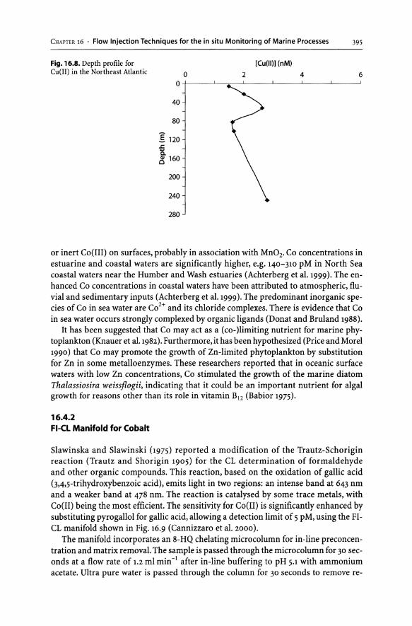
CHAPTER 16 . Flow Injection Techniques for the in situ Monitoring of Marine Processes 395
Fig. 16.8. Depth profile for Cu(II) in the Northeast Atlantic
0
40
80
]: 120
a ~ 160
200
240
280
[Cu(lI)] (nM)
0 2 4 6
or inert Co(IlI) on surfaces, probably in association with MnOz. Co concentrations in estuarine and coastal waters are significantly higher, e.g. 140-310 pM in North Sea coastal waters near the Humber and Wash estuaries (Achterberg et al. 1999). The enhanced Co concentrations in coastal waters have been attributed to atmospheric, fluvial and sedimentary inputs (Achterberg et aI. 1999). The predominant inorganic species of Co in sea water are Coz+ and its chloride complexes. There is evidence that Co in sea water occurs strongly complexed by organic ligands (Donat and Bruland 1988).
It has been suggested that Co may act as a (co-)limiting nutrient for marine phytoplankton (Knauer et aI.1982). Furthermore, it has been hypothesized (Price and Morel 1990) that Co may promote the growth of Zn-limited phytoplankton by substitution for Zn in some metalloenzymes. These researchers reported that in oceanic surface waters with low Zn concentrations, Co stimulated the growth of the marine diatom Thalassiosira weissflogii, indicating that it could be an important nutrient for algal growth for reasons other than its role in vitamin Bl2 (Babior 1975).
16.4.2 FI-CL Manifold for Cobalt
Slawinska and Slawinski (1975) reported a modification of the Trautz-Schorigin reaction (Trautz and Shorigin 1905) for the CL determination of formaldehyde and other organic compounds. This reaction, based on the oxidation of gallic acid (3,4,5-trihydroxybenzoic acid), emits light in two regions: an intense band at 643 nm and a weaker band at 478 nm. The reaction is catalysed by some trace metals, with Co(II) being the most efficient. The sensitivity for Co(II) is significantly enhanced by substituting pyrogallol for gallic acid, allowing a detection limit of 5 pM, using the FICL manifold shown in Fig. 16.9 (Cannizzaro et al. 2000).
The manifold incorporates an 8-HQ chelating micro column for in-line preconcentration and matrix removal. The sample is passed through the microcolumn for 30 seconds at a flow rate of 1.2 ml min-1 after in-line buffering to pH 5.1 with ammonium acetate. Ultra pure water is passed through the column for 30 seconds to remove re-

396 P. J. Worsfold . E. P. Achterberg· A. R. Bowie . R. Sandford· V. Cannizzaro . P. Gardolinski
Pump
MQW Waste
8-HQcolumn Buffer
Sample 1.2 I §' I Injection valve 4-way
valve
Hel • I 1.2
NaOH, Methanol 1.2
Pyrogallol, 1.2
HlOl, GAB Flow cell PMT
mlmin- 1
Waste
Fig. 16.9. Flow injection manifold with chemiluminescence detection for the determination of Co(Il) in the marine environment
sidual alkali and alkali-earth metals (e.g. Mg and Ca) from the column. The eluant (HCI) is then passed through the column at a flow rate of 1.2 ml min- l in the reverse direction to the sample loading, mixed with the reagent solutions (pumped at 1.2 ml min-I) and the resulting mixture introduced into the CL flowcell after heating to 80°C in a 5 m reaction coil. The analytical figures of merit for this manifold are given in Table 16.3 and show that it is suitable for the determination of Co(II) in coastal and open ocean waters. The accuracy of the method is shown for three marine CRMs and an Irish Sea water sample in Table 16.4.
16.4.3 Environmental Data
The FI-CL Co(II) system has been deployed at sea during the IMPACT cruise (CH 148) on board the RRS Challenger in the North Sea (September 16-27, 1999). Samples were collected using ultra-clean sampling protocols with modified Teflon-coated Niskin samplers. Sea water samples were filtered (0.2 11m polycarbonate membrane filters) and acidified (pH 2, quartz-distilled HCI) prior to analysis on board ship. A typical depth profile for Co in the coastal waters of the North Sea (Station 28; 54.02° N,01.52° E) is shown in Fig. 16.10. Co concentrations ranged between ca. 140 and 190 pM at Station 28, with highest concentrations in the bottom waters. The observed concentrations are in good agreement with values observed previously in this area (between ca. 100 and 200 pM; Achterberg et al.1999). The salinity profile shows a surface minimum, with a well-mixed water column below ca. 10 m depth. The surface minimum is possi-

CHAPTER 16 . Flow Injection Techniques for the in situ Monitoring of Marine Processes 397
Table 16.3. Analytical figures of merit for the Co(II) FI-CL manifold. The time for sample quantification includes two standard additions with analysis of each solution in triplicate
LOD
RSD (n = 5)
Linear Range
Time for one analytical cycle (n = 3)
Time for sample quantification
0.005 nM
<5%
0.005-1 nM (R2 = 0.996S)
S min
26 min
Table 16.4. Laboratory based determination of Co in three marine certified reference materials and an Irish Sea water sample. Error bars represent ±3 s
Sample
NASS-4
CASS-3
SLEW-2
Irish SW
0
20
]: 40 .r:. .... a. CI)
60 c
SO
100
0
34.0
FI-CL (nMJ
0.16±0.01
0.60±0.09
0.93 ±0.13
0.35 ±0.02
100
34.2
Certified value (nM)
0.15 ±0.02
0.6S±0.11
0.S7 ±0.21
200
34.4
Co (pM)
300
Salinity
Fig. 16.10. Depth profile for Co (II) in the North Sea
Cathodic stripping voltammetry (nMJ
0.34 ±0.01
400 500 600
34.6 34.8 35.0
bly due to rain inputs. The Co profile shows a surface minimum (150 pM) coinciding with the salinity minimum and a maximum near the bottom of the water column. The deep water maximum can probably be explained by a sedimentary flux of Co into the overlaying waters. Remobilization of Co from sediments of the North Sea was reported by Burton et al. (1993) and Tappin et al. (1995), following a reduction of the redox potential at the sediment-water interface as a result of mineralization of biogenic material.

398 P. J. Worsfold . E. P. Achterberg· A. R. Bowie· R. Sandford· V. Cannizzaro· P. Gardolinski
16.5 FI-SPEC Determination of Nitrate in Sea Water
16.5.1 Marine Chemistry of Nitrate
The elemental gas (N2) is the most abundant form of nitrogen in estuarine and coastal waters. For biogeochemical processes, however, the most important species are the dissolved inorganic forms (nitrate, nitrite and ammonia) and organic nitrogen compounds (in dissolved and particulate forms), of which the predominant species in oxic waters is nitrate.
Nitrate plays an important role in primary production in euphotic surface waters, and as a growth-limiting nutrient, it can directly affect the quality of freshwater and marine environments. Therefore, an accurate and reliable technique for determining nutrient concentrations is essential, and a field deployable instrument is desirable to minimize sample degradation and provide high temporal and spatial resolution monitoring.A submersible FI monitor incorporating spectrophotometric (SPEC) detection is therefore a potentially attractive approach.
16.5.2 Submersible FI Monitor
A prototype instrument has been described (David et al. 1998, 1999). The current design is contained within a pressure housing engineered from a single block of PVC in which the FI manifold (Fig. 16.11) is mounted, together with control and processing boards. The FI monitor consists of two battery powered 12 V ISMATEC peristaltic pumps, two switching valves, one acrylic "T" piece for mixing reagents, a sample loop, reduction column, flow cell and detector. Figure 16.12 shows a photograph of the complete monitor, including pressure housing.
For total oxidized nitrogen (TON) determination, the FI chemistry is based on the reduction of nitrate to nitrite in a copperized cadmium column followed by diazotisation
Carrier
Sulphanilamide
N1NED 0.16
Waste
Detector/ Flow cell
Fig. 16.11. Flow injection manifold with spectrophotometric detection for the determination of total oxidized nitrogen in the marine environment

CHAPTER 16 . Flow Injection Techniques for the in situ Monitoring of Marine Processes 399
Fig. 16.12. Photograph of the submersible nitrate monitor showing the flow injection manifold (left) and the pressure housing (right)
and subsequent coupling with sulphanylamide and N-(l-naphthyl)ethylenediamine (N1NED) to produce a pink-purple azo dye (Amax= 540 nm). This is quantified using a flow-through, solid-state detector incorporating an ultrabright green light emitting diode (LED) as the light source and a photo diode to detect the transmitted radiation. When a sample or standard is injected into the FI manifold, the baseline value and transient peak maximum are recorded. The TON concentration, sample identification, date and time are then stored in protected memory. The analytical figures of merit achieved for the FI-SPEC monitor in the laboratory (Table 16.5) show that the limit of detection is sufficiently low for deployment in most marine environments.
16.5.3 Environmental Data
In situ application of the submersible FI system for monitoring of TON in the Tamar Estuary and the North Sea has been described (David et al. 1998, 1999). In addition, the monitor has been used on board the RRS Challenger during the North Sea Impact Cruise in September 1999. The main objective of this cruise was to study contaminant behaviour in the North Sea in order to predict potential toxic effects of contaminants. The monitor was deployed successfully for nine days, operating on a 30 min cycle time, and provided high quality results for more than 100 samples. The analytical figures of merit of the FI-SPEC monitor during the cruise are summarized in Table 16.6 and show that the limit of detection and linear range can be easily adjusted during the cruise to suit local conditions by, e.g. varying the optical path length. A typical moni-

400 P. J. Worsfold . E. P. Achterberg. A. R. Bowie· R. Sandford· V. Cannizzaro· P. Gardolinski
Table 16.5. Analytical figures of merit for the FI-SPEC submersible nutrient monitor in the laboratory with a 20 mm path length flow cell. The time for sample quantification includes analysis of a sample and an on board standard in triplicate and data processing time
Table 16.6. Shipboard analytical figures of merit for the FISPEC nutrient monitor during the Impact cruise. The time for sample quantification includes analysis of a sample and an on board standard in triplicate and data processing time
LOD
RSD (n = 3)
Linear Range
Time for one analytical cycle (n = 3)
Time for sample quantification
LOD (20 mm path length)
LOD (10 mm path length)
RSD (n =3)
Linear Range (20 cm path length)
Linear Range (10 cm path length)
Time for one analytical cycle (n=3)
Time for sample quantification
0.5 iJM
<5%
0-10 iJM (R2 = 0.993)
9min
30min
0.6iJM
3.6iJM
<5%
0-7.1 iJM (R2 = 0.994)
3.6-140 iJM (R2 = 0.997)
9min
30min
tor profile for TON and salinity during a tidal cycle deployment in the mouth of Humber Estuary (53.32° N, 00.05° E) on 25th September 1999 is shown in Fig. 16.13.
An intercomparison exercise for nutrients in sea water was performed by the National Oceanic and Atmospheric Administration - National Research Council of Canada, when sea water samples (MOOS-I) were analysed by 32 laboratories for nutrients (TON, nitrite, phosphate and silicate). The consensus mean and standard deviation for TON were 22.5 and 3.1 j-lM, respectively. These samples were also analysed using the submersible FI monitor and the results, 25.1 and 2.0 j-lM, respectively for the mean and standard deviation were in good agreement with the consensus data when using the z-scoring system for assessing bias (z < 2). The results obtained for the same samples using a laboratory segmented continuous flow analyser were also in good agreement with the FI-SPEC monitor (P = 0.05), demonstrating that the submersible FI data can be directly compared with historical laboratory data for TON.
16.6 Conclusions
Flow injection techniques are well-suited to marine analytical chemistry applications, particularly as shipboard systems for high temporal and/or spatial resolution monitoring. Chemiluminescence is a robust and sensitive means of detection for certain trace metals (e.g. Fe, Cu, Co) and can be made selective by the incorporation of solid phase microcolumns containing immobilized chelating reagents such as 8-hydroxyquinoline. Solid state spectrophotometric detectors can also be incorporated within flow injection systems for the in situ determination of a wide range of analytes, including total oxidized nitrogen. With suitable engineering, such systems can be configured for reliable, long-term submersible deployment. Flow injection in its various forms therefore provides a valuable tool for marine analytical chemists and has the

CHAPTER 16 . Flow Injection Techniques for the in situ Monitoring of Marine Processes
Fig. 16.13. Tidal cycle for nitrate and salinity in the North Sea
95
85
75
~ 65
-= 55 ~ e 45
35
7 8 25 L~~---::--~-=:------;:~~~'i 15 I
o 2 3 4 Time (h)
5 6
401
33.0
32.5
32.0 II> ..
31.5 §' ;::;: '<
31.0
30.5
30.0
potential to provide high quality analytical data to support developments in chemical oceanography.
Acknowledgements
PJW, EPA, ARB, VC and RS acknowledge the European Union for funding (MEMOSEA contract MAS3-CT97-0143 and IRONAGES contract EVK2-CT-1999-00031). PG would like to thank CNPq, Brazil, for financial support. RS would like to thank the University of Plymouth and Plymouth Marine Laboratory for financial support.
References
Achterberg EP, Colombo C, Berg CMG van den (1999) The distribution of dissolved Cu, Zn, Ni, Co and Cr in English coastal surface waters. Cont Shelf Res 19:537-558
Aiken J, Rees N, Hooker S, Holligan P, Bale A, Robins D, Moore G, Harris R, Pilgrim D (2000) The Atlantic meridional transect: Overview and syniliesis of data. Prog Oceanogr 45:257-312
Andrew KN, Blundell NJ, Price D, Worsfold PJ (1994) Flow injection techniques for water monitoring. Anal Chern 66:916A-922A
Babior BM (ed) (1975) Cobalamin: Biochemistry and pailiophysiology. Wiley, New York Bowie AR,Achterberg EP,Mantoura RFC, Worsfold PJ (1998) Determination of sub-nanomolar levels of
iron in seawater using flow injection with chemiluminescence detection. Anal Chim Acta 361:189-200 Bowie AR, Sanders MG, Worsfold PJ (1996) Analytical applications ofliquid phase chemiluminescence
reactions - a review. J Biolumin Chemilum 11:61-90 Boyd PW, Watson AJ, Law CS et al. (2000) Mesoscale iron fertilisation elevates phytoplankton stocks in
the polar Southern Ocean. Nature 407:695-702 Burton JD, Althaus M, Millward GE, Morris AW, Stailiam PJ, Tappin AD, Turner A (1993) Processes influ
encing the fate of trace metals in the North Sea. Philos T Roy Soc 343:557-568 Campbell PGC (1995) Interactions between trace metals and aquatic organisms: A critique of ilie free ion
activity model. In: Tessier A, Turner DR (eds) Metal speciation and bioavailability in aquatic systems. John Wiley and Sons, New York, pp 45-103
Cannizzaro V, Bowie AR, Sax A, Achterberg EP, Worsfold PJ (2000) Determination of cobalt and iron in estuarine and coastal waters using flow injection with chemiluminescence detection. Analyst 125:51-57
Coale KH, Bruland KW (1988) Copper complexation in ilie Norilieast Pacific. Limnol Oceanogr 33:1084-1101 Coale KH, Bruland KW (1990) Spatial and temporal variability in copper complexation in ilie Norili Pa
cific. Deep-Sea Res 47:317-336 Coale KH, Johnson KS, Stout PM, Sakamoto CM (1992) Determination of copper in sea water using a
flow-injection meiliod wiili chemiluminescence detection. Anal Chim Acta 266:345-351 Coale KH, Johnson KS, Fitzwater SE et al. (1996) A massive phytoplankton bloom induced by an
ecosystem-scale iron fertilisation experiment in the equatorial Pacific Ocean. Nature 383:495-501

402 P. J. Worsfold . E. P. Achterberg· A. R. Bowie· R. Sandford· V. Cannizzaro· P. Gardolinski
Danielsson L-G, Magnusson B, Westerlund S (1985) Cadmium, copper, iron, nickel and zinc in the Northeast Atlantic Ocean. Mar Chern 17:23-41
David ARJ, McCormack T, Morris AW, Worsfold PJ (1998) Submersible flow injection-based sensor for the determination of total oxidised nitrogen in coastal waters. Anal Chim Acta 361:63-72
David ARJ, McCormack T, Worsfold PJ (1999) A submersible battery-powered flow injection (FI) sensor for the determination of nitrate in estuarine and coastal waters. J Auto Meth Man Chern 21:1-9
Donat JR, BruIand KW (1988) Direct determination of dissolved cobalt and nickel in seawater by differential pulse cathodic stripping voltammetry preceded by adsorptive collection of their nioxime complexes. Anal Chern 60:240-244
Donat JR, Bruland KW (1995) Trace elements in the oceans. In: Salbu B, Steinnes E (eds) Trace elements in natural waters. CRC Press, Boca Raton, pp 247-281
Federova OS, Olkin SE, BerdnikovVM (1982) The chemiluminescence mechanism in 1,1O-phenanthroline during catalytic decomposition of hydrogen peroxide. Z Phys Chemie 263:529-549
Gledhill M, Berg CMG van den (1994) Determination of complexation of iron(III) with natural organic complexing ligands in seawater using cathodic stripping voltammetry. Mar Chern 47:41-54
Gledhill M, Nimmo M, Hill SJ, Brown MT (1997) Toxicity of Cu(II) species to marine algae, with particular reference to macroalgae. J Phycol 33:2-11
Jickells TD, Burton JD (1988) Cobalt, copper, manganese and nickel in the Sargasso Sea. Mar Chern 23:131-144
Johnson KS, Stout PM, Berelson WM, Sakamoto-Arnold eM (1988) Cobalt and copper distributions in the water of Santa Monica basin, California. Nature 332:527-530
Knauer GA, Martin JH, Gordon RM (1982) Cobalt in Northeast Pacific waters. Nature 297:49-51 Moffet JW, Brand LE, Zika RG. (1990) Distribution and potential sources and sinks of copper chelators
in the Sargasso Sea. Deep Sea Res I 37:27-36 Price NM, Morel FMM (1990) Cadmium and cobalt substitution for zinc in a marine diatom. Nature
344:658- 660 Ruzicka J, Hansen EH (1981) Flow injection analysis. Wiley Interscience, New York Schrauzer GN (1991) Cobalt. In: Merian E (ed) Metals and their compounds in the environment:
Occurrence, analysis, and biological relevance. VCH, Heidelberg, pp 879-892 Slawinska D, Slawinski I (1975) Chemiluminescent flow method for the determination of formaldehyde.
Anal Chern 47:2101-2109 Tappin AD,Millward GE, Statham PJ, Burton JD,Morris AW (1995) Trace metals in the Central and South
ern North Sea. Estuar Coast Shelf S 41:275-323 Trautz M, Schorigin P (1905) Z Wiss Photogr Photochem 121:3 Worsfold PJ, Achterberg EP, Bowie AR, Sandford RC, Mantoura RFC (2000) Flow injection with chemi
luminescence detection for the shipboard monitoring of trace metals. In: Varney MS (ed) Chemical sensors in oceanography. Gordon and Breech, Amsterdam, pp 71-94
Chapter 17
Luminescence for the Analysis of Organic Compounds in Natural Waters
A. Roda . P. Pasini . M. Guardigli
17.1 Introduction
Many widely used synthetic chemicals, as well as industrial by-products, are continuously emitted into the environment. Even if present in low quantities, some of these substances or their degradation products represent a threat for the health of humans and wildlife. Sometimes they accumulate in living organisms and target organs (bioaccumulation) so that their concentrations increase along the food chain. Natural waters (rivers, lakes, seas, and ground waters) are among the most endangered environments, since in many cases these substances are directly released in them. Moreover, natural waters represent an important way by which pollutants travel along long distances. Molecules with low water solubility, i.e. with high lipophilicity (pesticides, aromatic hydrocarbons and their derivatives, surfactants, oestrogen-like compounds, etc.) could be present in the particulate matter of fresh and marine water. The analysis of organic compounds in natural waters is therefore of crucial importance in the monitoring of pollution and in risk assessing for humans and environment. This requires rapid and sensitive analytical procedures for the detection of organic pollutants that should be suitable for performing screening analysis of a large number of samples.
Separative chromatographic and hyphenated techniques (such as GC-MS and HPLC-MS) are the most diffused conventional analytical procedures used for the analysis of organic compounds in environmental samples. However, these analytical procedures always require sample preparations, even in the case of environmental matrices as simple as drinking water. Sample preparations are frequently time-consuming, and due to the numerous and sometimes complicated processes involved, errors and sample losses are most likely to occur in this step. In addition, extraction of samples for chromatographic analysis usually requires the use of organic solvents, which frequently poses problems in handling, storage and disposal. A further disadvantage of these techniques is that they are not generally suitable for performing parallel analysis of a large number of samples.
17.2 Immunoassays in Environmental Analysis
In recent years, the expansion of immunochemical detection methods moved beyond the clinical diagnostic field to applications in environmental monitoring. Nowadays, immunoassay is a widely-used analytical method for the detection and quantitation of environmental pollutants. Immunochemical analytical methods have gained favour

404 A. Roda . P. Pasini . M. Guardigli
in environmental analytical processes beginning in the 1980s, when they were recognized as useful screening techniques for the detection of compounds of environmental regulatory concern in many countries (Van Emon 1987; Van Emon and Gerlach 1995). The U.S. Food and Drug Administration (FDA) joined the U.S. Environmental Protection Agency (EPA) in researching immunochemical detection methods for a variety of regulatory and monitoring applications. The high specificity of antibodies used as biospecific recognition elements in immunochemical methods allows for the reduction in the number of pre-analytical steps, and little or no nonaqueous solvents are used. When complex matrix samples have to be analyzed, a separation step of the analyte from the matrix is still required before performing the quantitative step. On the other hand, on samples with a relatively simple and stable matrix with low component variability, such as natural waters, the factors affecting the quantitative procedure can be minimized and kept under control, so that immunoassay can be carried out directly on the sample without any dean-up procedure. Moreover, immunological methods can be easily developed or converted in high throughput screening (HTS) formats (for example, in 96- or 384-well microtitre plates), and optimized to provide quick results in field applications.
17.2.1 Luminescent Immunoassays
The most common immunoassay format in environmental analysis is the ELISA (Enzyme-Linked ImmunoSorbent Assay). Enzyme immunoassays, in which a suitable enzyme is used as a label, allow signal amplification due to the enzyme-catalysed reaction, thus obtaining a high sensitivity. Quantitation by ELISA has become more accepted in the past decade and is now a laboratory standard for environmental analysis, frequently surpassing traditional chromatographic methods in sensitivity, selectivity and cost (Van Emon and Lopez-Avila 1992). Due to the low molecular weight of most of the organic pollutants, competitive immunoassays are the preferred format in environmental analysis. In a typical competitive indirect heterogeneous ELISA, the analyte contained in the sample and an analyte derivative immobilized on a solid support (e.g. a well of a 96-wells microtitre plate) compete for an enzyme-labelled antibody. After the immunoreaction and the washing steps, the enzyme-labelled antibody bound to the solid support is quantified by means of the enzyme-catalysed reaction; the amount of analyte contained in the sample is inversely proportional to the fraction of bound enzyme-labelled antibody. In an alternative format (direct heterogeneous ELISA), the antibody is immobilized on the solid phase, and an enzyme-labelled analyte derivative is used.
Most of the environmental applications involve the determination of a compound or group of compounds present in trace concentrations. Immunoassays commonly used in environmental analysis rely on colourimetric detection procedures, i.e. quantitation is performed through the use of a chromogenic enzyme substrate. The intrinsic detectability of immunoassays can be further improved by the use of luminescent labels such as enzymes detectable by bio- or chemiluminescent (CL) substrates or lanthanide chelates detectable by time-resolved fluorescence (TRF) techniques.
Chemiluminescent detection is probably the most sensitive detection principle for enzyme labels, and the analytical sensitivity of chemiluminescent immunoassays is

CHAPTER 17 . Luminescence for the Analysis of Organic Compounds in Natural Waters 405
usually higher than that of colourimetric immunoassays. In many cases, the sensitivity of chemiluminescent immunoassays is comparable to or even better than that obtained with radioactive labels. This trend was clearly demonstrated by the comparison of the detection limits obtained in the colourimetric, luminescent and radio-immunological determination of steroids in real samples, like plasma and saliva (Roda et al. 1984). It should be noted that saliva has a composition resembling quite closely that of surface waters, thus suggesting the convenient applicability of chemiluminescent immunoassays to natural water samples. In addition, luminescent detection is generally characterized by a rapid response, and its dynamic range can be linear for up to 5 decades of concentration. Electrochemiluminescence represents an alternative way to implement luminescent detection in immunoassays. This technique offers the advantage that the luminescent signal is triggered by the application of a suitable potential rather than by the addition of a chemiluminescent reagent, thus reducing problems related to signal handling or to the background emission shown by some chemiluminescent substrates. Time-resolved fluorescence measurement techniques represent an improvement over the conventional fluorescent detection. Fluorescence potentially allows a high detectability, but its sensitivity is reduced by the presence of a background emission, which is mainly due to the excitation of the biological components of the sample. Time-resolved fluorescence detection, in which the measurement of the emission is delayed with respect to the excitation of the sample and long-lived luminescent labels are used, allows one to efficiently suppress the background emission, thus increasing the detectability of the luminescent probe.
17.2.2 Applications
Most of the luminescent immunoassays developed for analysis of environmental water samples are used for the detection and quantitation of pesticides (Table 17.1).
Benzo(a)pyrene was detected in environmental water samples using immunoassay methods. It was found that the immunological method could be used for the direct
Table 17.1. Luminescent immunoassays for the detection of organic compounds in water samples
Analyte Detection principle Reference
Benzo(a)pyrene Time-resolved fluorescence Ius et al. (1992)
Phthalate esters Time-resolved fluorescence Ius et al. (1993)
Paraoxon, Aldicarb Chemiluminescence Roda et al. (1994)
Chlortoluron Chemiluminescence Kameth et al. (1996)
Triazine,2A-Dichlorophenoxyacetic Chemiluminescence Weller et al. (1999) acid, Trinitrotoluene
2A-Dichlorophenoxyacetic acid Chemiluminescence Dzgoev et al. (1997)
Atrazine Electrochemiluminescence Wilson et al. (1997)
2,4-Dichlorophenoxyacetic acid Electrochemiluminescence Marquette and Blum (1998)
Atrazine, Terbuthyilazine, Ametryn Chemiluminescence Samsonova et al. (1999)

406 A. Roda . P. Pasini . M. Guardigli
analysis of both freshwater and sea water samples, since the salt content of the sea water did not interfere in the assay (Roda et al. 1991). Instead, a preliminary desalting procedure was necessary if the sea water sample was preconcentrated before analysis.
A time-resolved fluoroimmunoassay was developed for the detection of benzo(a)pyrene (Ius et al. 1992) on the basis of the previously reported work. This direct heterogeneous immunoassay was developed using a specific antibody labelled with an isothiocyanatophenyl-EDTA-Eu complex. After the immunoreaction, the lanthanide complex was dissociated, and the amount of metal ion in solution was determined via a time-resolved fluorescence measurement upon addition of an enhancement solution forming a luminescent europium complex. The detection limit (about 0.5 ng rnI-1)
was low enough for the application of the method on water samples without preliminary extraction or concentration procedures. Phthalate esters, widely used as plastifiers, were determined in a direct competitive immunoassay based on a time-resolved fluorescence measurement using rabbit antibodies against phthalate esters (Ius et al.1993). The bound antibodies were detected using a biotinylated anti-rabbit antibody and a BCPDA-Iabelled streptavidin. Metal luminescence intensity was then measured in the time-resolved mode upon addition of an excess of europium ion. This assay was able to detect as low as 0.5 pmol mrl of the most diffused phthalate esters.
A chemiluminescent flow sensor was developed for the determination of organophosphorus (Paraoxon) and carbamate (Aldicarb) pesticides in water (Roda et al.1994). The flow sensor relies on the inhibition of acetylcholinesterase (either in solution or immobilized on a solid support) due to pesticides. A series of coupled enzymatic reactions, catalysed by the enzymes choline oxidase and peroxidase immobilized on a solid support, was used in order to allow the chemiluminescent measurement of the acetylcholinesterase activity. Detection limits of 0.75 flg rl and 4 flg rl were reported for Paraoxon and Aldicarb, respectively.
The water sample content of the herbicide chlortoluron was determined using an enhanced chemiluminescent immunoassay (Kameth et al. 1996) in which the chemiluminescence signal was detected by means of a camera luminometer, providing a semiquantitative assay based on a photographic record of the luminescent end point. This assay could represent a rapid, simple and portable means of monitoring multiple water samples for the presence of chlortoluron or other pesticides. In the reported example, the assay was able to identify and quantitate the herbicide with good accuracy at or above the European limit for individual pesticides in drinking water.
Detection of atrazine in water was also performed by means of an electrochemiluminescence flow injection immunoassay based on anti-atrazine antibodies labelled with glucose oxidase (Wilson et al. 1997). This competitive electrochemiluminescent immunoassay used transparent aminosilanized indium tin oxide-coated glass electrodes, derivatized with aminodextran covalently linked to a triazine derivative. It was possible to detect less than 0.1 ppb of atrazine, thus below the precautionary limit for pesticides in drinking water recommended by the European Commission.
A flow analysis system coupled with an immunosensor exploiting the electrogenerated chemiluminescence of luminol was used for the detection of 2,4-dichlorophenoxyacetic acid (2,4-D) in drinking water (Marquette and Blum 1998). The immunosensor is based on a competitive immunoreaction, in which 2,4-D contained in the water sample and 2,4-D immobilized on the surface of a glassy carbon electrode compete for a luminol-Iabelled anti-2,4-D antibody. After the immunoreaction, the amount

CHAPTER 17 • Luminescence for the Analysis of Organic Compounds in Natural Waters 407
of bound antibody is detected by applying a suitable potential to the electrode, in order to obtain the luminollabel electro chemiluminescence. An innovative aspect of this device with respect to other 2,4-D immunosensors reported in the literature is the novel immobilization procedure used to obtain the 2,4-D antigen-coated glassy carbon electrode, which allowed multiple (up to 50 times) regenerations of the immunosensor. This immunosensor was able to detect as low as 0.21lg rl of free 2,4-D, which is close to the accepted level in drinking water in the European Union (O.lllg rl).
A chemiluminescent competitive multianalyte immunoassay based on a combination of mono- and polyclonal antibodies was developed for the detection of three crossreacting s-triazine pesticides (atrazine, terbuthylazine and ametryn) in water samples (Samsonova et al. 1999). Detection of single s-triazines using immunological methods is a difficult task, because even monoclonal antibodies against such small analytes are often unable to efficiently discriminate between structurally similar molecules. The simultaneous use of three polyclonal and two monoclonal antibodies with different specificities towards s-triazines allowed for the development of a multianalyte assay in which antibody cross-reactivity is exploited to identify and quantify the three analytes. The antibodies were immobilized in separate wells of an eight -well microtitre strip, and horseradish peroxidase, which was detected with the enhanced chemiluminescence reaction, was used as a label for antigens. Measurement of the chemiluminescence intensities was performed by using a small, battery-powered portable luminometer, which is of practical importance from the on-site monitoring point of view. The data obtained with the chemiluminescent immunoassays were processed using a neural network, and the best parameters for the correct identification of an individual s-triazine in a mixture and the estimation of its amount were found. When this assay was applied to environmental samples containing various s-triazine mixtures, it was able to correctly classify the analytes in most cases, suggesting that it can be proposed as an alternative field test for multianalyte environmental monitoring. In all the luminescent immunoassays described above, luminescence measurements were performed using conventional photomultiplier tube-based luminometers or timeresolved fiuorometers. Imaging devices, which are able not only to measure the intensity but also to evaluate the spatial distribution of the luminescence emission from a sample, represent a significant improvement in luminescence measurement. These devices allow for the simultaneous measurement of the luminescent signals from a whole 96- or 384-well microtitre plate, thus being more rapid than conventional luminometers that measure light output well by well or strip by strip. They also represent the detectors used for the development of multiarray affinity devices, in which several different biospecific reagents are immobilized in an array arrangement on a suitable surface. This sensor design allows for the parallel processing of many immunoassays, allowing simultaneous determination of different analytes in the same sample, using reagents volumes much smaller than those needed to perform separate immunoassays for each analyte of interest. Quantitation of the analyte content of the sample is performed by using image analysis techniques: the localization of the CL signal on the target surface and its intensity are related to the identity and the concentration of the analyte, respectively.
The development of a parallel affinity sensor array based on chemiluminescent labels for the detection of environmental contaminants in water has been reported (Weller et al. 1999). The required reagents (antibodies or haptens) were immobilized

408 A. Roda . P. Pasini . M. Guardigli
as spots on a glass slide, obtaining a biochip with an array containing up to 1 600 spots. The glass slide was inserted in a flow cell in which the immunoreactions took place and, after addition of the chemiluminescent substrate, the CL signal was acquired by means of a CCD imaging device. The biochip was used to develop model systems for the simultaneous detection and quantitation of triazine, trinitrotoluene and 2,4-D in water samples based on immunoassays either in direct (antibody-immobilized) or indirect (hapten-immobilized) formats. Both formats proved to be able to detect and quantitate the analytes, offering the possibility of many regeneration cycles of the biochip. This device could thus represent a potential analytical tool for performing multiple analyses on one sample in parallel, also including the identification of the analytes.
The development and optimization of a chemiluminescent ELISA for the simultaneous determination of 2,4-D in multiple samples, using innovative solid supports represented by gold-coated surfaces and glass capillaries with CCD imaging of the chemiluminescent signal has been reported (Dzgoev et al.1997). The authors observed that such solid supports offered advantages with respect to other supports used in the development of multiarray devices such as the "flat-wells" obtained by thick-film technology' but the analytical sensitivity was still lower than that of the single sample determination assay.
The perception of immunoassay has changed in the past decade from considering it to be an environmental analytical alternative to accepting it as a reliable quantitative method. Luminescent immunoassays represent a valuable alternative to the conventional radiometric or colourimetry ones. They are more sensitive than colourimetry immunoassays, and can be as sensitive as radioimmunoassays, without all the problems related to storage, handling and disposal of radioactive materials. This feature, combined with the rapidity of response and the possibility of performing simultaneous analysis of several samples in a 96- or 384-well microtitre plate format, makes these assays suitable for the development of HTS analytical methods and for extensive automation. New refinements of immunoassay technology, such as biochip-based methods and multianalyte immunoassays, while still in research, will certainly take their place among other environmental monitoring techniques of the future.
17.3 Luminescent Recombinant Cell-Based Biosensors in Environmental Analysis
A different bioanalytical approach has been made possible by the use of recombinant DNA techniques in analytical chemistry, which led to the development of luminescent whole-cell biosensors. Luminescence-based reporter genes have been used to develop efficient bioassays for the specific detection of several inorganic and organic compounds, which are applied especially in the environmental analysis field (Kohler et al. 2000). These biosensors are based on the ability of genetically engineered microorganisms (bacteria and yeast) or mammalian cells to emit visible light in response to specific substances. Such transformed cells are constructed by recombinant DNA techniques, using a plasmid vector containing the luminescent reporter gene under transcriptional control of a specific gene sequence, whose expression is regulated very precisely. The presence of the analyte induces the expression of the specific gene se-

CHAPTER 17 . Luminescence for the Analysis of Organic Compounds in Natural Waters 409
quence and consequently of the reporter gene in a quantitative manner, followed by the synthesis of the corresponding protein. Luc and lux genes encoding firefly and marine bacteria luciferases, respectively, are widely used as reporters. When the corresponding luciferin substrate is either added or produced by the recombinant cells, a luciferin/luciferase-mediated light output occurs. The light emission intensity is proportional to the analyte concentration, which allows quantitative analysis to be performed. The use of enzymes as reporter molecules permits the analytical signal amplification, which combined with the high detectability of bioluminescent reactions, lowers the detection limit of the system. Recently, the genes encoding two naturally occurring and recombinantly produced luminescent proteins from the jellyfish Aequorea victoria, i.e. aequorin and green fluorescent protein (GFP), have been used as reporter genes in the development of recombinant cell-based biosensors. Aequorin is naturally bioluminescent upon binding to Ca2+ ions and has virtually no associated background signal, thus allowing highly sensitive detection. GFP is an autofluorescent protein that does not require addition of substrates or co-factors. These characteristics made the use of these photoproteins very attractive in diverse analytical applications (Shetty et al. 1999; Lewis and Daunert 2000).
17.3.1 Applications
Luminescent recombinant cell-based biosensors for the detection of organic pollutants in natural waters were reported (Table 17.2).
Bacteria are commonly used as test organisms because of their large population sizes, rapid growth rates and easy maintenance. In addition, many natural occurring bacteria are provided with genetically coded detoxifying systems for a given contaminant, and such specific DNA sequences are quite easy to be transformed in other microorganisms. A bacterial biosensor for naphthalene was developed by fusing the nahG promoter from the naphthalene degradation pathway of Pseudomonas fluorescens to Vibrio fischeri's luxCDABE gene and was applied in waste water and ground water
Table 17.2. Luminescent recombinant cell-based biosensors for the detection of organic compounds in water samples
Analyte Recombinant cell (reporter gene) Reference
Naphthalene Pseudomonas fluorescens (fuxCDABE) King et al. (1990)
Naphthalene Pseudomonas fluorescens (fuxCDABE) Heitzer et al. (1994)
Middle-chain alkanes Escherichia coli (fuxAB) Sticher et al. (1997)
Estrogen-like compounds MCF-7 breast cancer cell line (fuc) and Balaguer et'al. (1999) HeLa cells (fuc)
Estrogen-like compounds T47D breast cancer cell line (fuc) Legler et al. (1999)
Estrogen-like compounds Saccharomyces cerevisiae (fac-Z) Pasini et al. (2001)
Polyhalogenated aromatic Rat hepatoma cell line (fue) Murk et al. (1996) hyd roca rbons

410 A. Roda . P. Pasini . M. Guardigli
monitoring (King et al. 1990). A bioluminescent whole-cell biosensor for specific online monitoring of naphthalene and its degradation product salicylate was developed by immobilizing the reporter bacteria in calcium alginate (Heitzer et al. 1994). A microbial sensor for the detection of middle-chain alkanes was constructed by introducing in Escherichia coli a plasmid containing a fusion between the promoter of alkB and luxAB of V. fischeri and a separate plasmid bearing the regulatory gene alkS from Pseudomonas oleovorans. The biosensor was induced by n-alkanes from pentane to decane and was applied to the analysis of contaminated ground water samples (Sticher et al. 1997).
As concerns the detection of some organic compounds, their ability to bind specific nuclear receptors is exploited to construct recombinant cell-based biosensors. Upon binding an active ligand, the ligand-occupied receptor interacts with specific DNA sequences (responsive elements) carried by an expression plasmid to modulate gene transcription. This causes the expression of the reporter gene and the synthesis of the reporter protein, which is detected by luminescent techniques.
A very wide range of synthetic chemicals and natural compounds have been found to be oestrogenic. These endocrine-disrupting compounds (EDCs) include pesticides, plasticizers, breakdown products of surfactants, synthetic oestrogens used as drugs and phyto-oestrogens, most of which are often detectable in many surface waters. The majority of these molecules exhibit different molecular structures, while sharing the ability to bind the human oestrogen receptors (hER). A reporter gene bioassay was developed using a breast cancer cell line (MCF-7), which naturally expressed the endogenous oestrogen receptor and was stably transfected with an oestrogen-regulated firefly luciferase gene (Pons et al. 1990). Recently, this cell line along with newly developed ones, with detection limits of 1-5 pM oestradiol, was used to detect oestrogenic activity in wastewater sewage treatment plant influents and effluents. The direct analysis of the water samples, after sterile filtration on 0.2 flm membranes, showed that the oestrogenic activity was equivalent to 60-100 pM oestradiol in the influent and was reduced by a factor 4-10 in the effluent, thus suggesting that effluents from sewage treatment works are an important potential source of oestrogenic compounds contaminating the aquatic environment (Balaguer et al. 1999). An oestrogen receptormediated, chemical-activated luciferase reporter gene-expression bioassay (ERCALUX) was developed by transfection of the firefly luciferase luc gene in the T47D breast cancer cell line. The system was tested on single oestrogen-like compounds or combinations and exhibited a detection limit of 0.5 pM oestradiol (Legler et al.1999).
Other reporter gene bioassays for oestrogenic activity assessment are based on recombinant yeast cells. This cellular model is often used because yeast cells are easily engineered and cultured, and have rapid growth rates, thus providing a very robust model suitable for wide-scale screening. Most yeast-based systems use the f3-galactosidase coding sequence as a reporter gene with the enzyme activity detected by colourimetric methods, which are often time-consuming and poorly sensitive, providing detection limits inadequate for the direct analysis of environmental aqueous samples (Rehmann et al. 1999). In our laboratory, a chemiluminescent whole cell biosensor based on recombinant yeast cells was developed and optimized for environmental monitoring of oestrogen-like compounds. A recombinant yeast strain (Saccharomyces cerevisiae) was used in which the DNA sequence of the human oestrogen receptor was stably integrated into the main chromosome. The yeast cells also contained an expression plasmid carrying oestrogen-responsive sequences and the reporter gene

CHAPTER 17 • Luminescence for the Analysis of Organic Compounds in Natural Waters 411
lac-Z, encoding the enzyme f3-galactosidase (Routledge and Sumpter 1996). The activity of the analyte-induced enzyme was detected by a chemiluminescent l,2-dioxetane-f3-D-galactopyranoside substrate. The CL detection proved to be much more rapid than the colourimetric one, allowing for the achievement of a detection limit of 10 pmol rl oestradiol after incubating the cells with the analyte for 24 hours compared to at least 72 hours required with the colourimetric detection. The applicability of the chemiluminescent biosensor to the analysis of natural water samples was preliminarily checked by assessing samples from influent and effluent of an activated sludge sewage treatment plant (Pasini et al. 2001).
A different receptor-mediated, chemical-activated luciferase reporter gene-expression bioassay (CALUX) was developed for the detection of aryl hydrocarbon receptor-active compounds, such as polyhalogenated aromatic hydrocarbons, which include polychlorodibenzo-p-dioxins (PCDDs), polychlorodibenzofuranes (PCDFs) and polychlorobiphenyls (PCBs). These substances either derive from combustion or industrial processes as by-products, or are used in productive processes (e.g. plastics manufacture) and are included in a list of 16 persistent organic pollutants (POPs) identified to be monitored at international level. A rat hepatoma cell line, which naturally expresses the aryl hydrocarbon receptor (AhR), was stably transfected with a plasmid containing the dioxin-responsive elements sequence and the luciferase luc reporter gene. The biosensor had a detection limit of 1 pM 2,3,7,8-tetrachlorodibenzo-p-dioxin (TCDD) and was applied to the analysis of sediments and pore water. In the case of pore water, only a simple and rapid extraction procedure was needed, without additional clean-up (Murk et al. 1996).
In addition to the previously described specific or group-selective luminescent reporter gene bioassays, a number of total toxicity luminescent tests have been developed. The most widely accepted microbial toxicity test system is based on the wildtype luminescent bacterium Vibrio fischeri. Bacterial bioluminescence has proved to be a convenient measure of cellular metabolism and consequently a reliable sensor for measuring the presence of toxic chemicals in aquatic samples (De Zwart and Sloof 1981). Sample toxicity is assessed from the decrease in luminescence following a short exposure to several concentrations of the sample. This system is commercially established and marketed as Microtox. It is commonly used to assess the general toxicity of potentially contaminated water samples, e.g. in wastewater treatment plant effluent testing for protection of receiving waters, in surface water monitoring for identification of pollution sources, and in monitoring raw drinking water for contamination due to spills or pollution sources. A recombinant bacterial sensor, in which the DNA damage-inducible promoter recN from Escherichia coli was fused to the lux operon of V. fischeri and introduced into Salmonella typhimurium, was developed for genotoxicity assessment (Verschaeve et al. 1999). Also this system is now commercially available as the Vitotox test. A different approach for toxicity assessment was based on a set of E. coli strains harbouring different plasmids, each carrying a different stress promoter:lux fusion. The panel included an oxidative stress sensor, a DNA damage sensor (genosensor) and two general stress sensors. The system allowed for the evaluation of different toxic effects in industrial wastewater samples (Belkin et al. 1997). These luminescent biosensors, though rapid, well-standardized and often ready-to-use, provide information on the sample total toxicity only, giving no indication on the chemical nature of contaminants.

412 A. Roda . P. Pasini . M. Guardigli
In conclusion, rapid and sensitive detection of the bio-chemiluminescence deriving from transformed cells, together with the selectivity and specificity of the gene regulation, has allowed efficient bioanalytical methods to be developed for the detection of pollutants in environmental aquatic samples. Such methods are usually carried out in 96-well microtitre plates and can be adapted to a 384-well microtitre format and easily automated, thus allowing high throughput screening. Advantages inherent in biological detection systems lie in their ability to indicate bioavailability and report effects on living organisms, thus providing preliminary information on the sample toxicity. The relatively inexpensive and easy handling of recombinant cell-based biosensors make their development and application even more attractive.
17.4 Conclusions and Future Perspectives
The reported bioanalytical methods could be very useful tools for the first -level monitoring of environmental and biological samples. Only positive samples will undergo further investigations, using more accurate analytical techniques such as GC-MS and HPLC-MS to detect and quantify the individual analytes. Since the percentage of negative samples is usually high, the availability of these rapid, sensitive first-level screening tests should allow considerable savings in terms of instrumentation, personnel and reagents costs, and operator time. A possible application of these first-level screening tests could be the systematic study of large and complex natural water systems (rivers, lakes, seas), which implies the analysis of numerous samples; several representative sampling points have to be selected in order to cover the whole aqueous system and to monitor the known possible sources of pollutants; in addition, the sampling has to be performed over a long period of time to evaluate the effects of meteorological variables.
Luminescent immunoassays and recombinant cell-based biosensors could also be advantageously applied in epidemiologic studies involving the analysis of biological samples to assess human exposure to contaminants and in food analysis to find out possible contamination sources.
Finally, continuous advancements in immunoassay and biosensor technology will lead to the development of miniaturized and biochip-based devices, which could further improve the analytical throughput and allow continuous environmental monitoring by carrying out on-site analysis.
References
Balaguer P, Fran<;ois F, Comunale F, Fenet H, Boussioux AM, Pons M, Nicolas JC, Casellas C (1999) Reporter cell lines to study the estrogenic effects of xenoestrogens. Sci Tot Environ 233:47-56
Belkin S, Smulski DR, Danon S, Vollmer AC, Dyk TK van, LaRossa RA (1997) A panel of stress-responsive luminous bacteria for the detection of selected classes of toxicants. Wat Res 31:3009-3016
De Zwart D, SloofW (1981) The Microtox as an alternative assay in the acute toxicity assessment of water pollutants. Aquat Toxicol 4:129-138
Dzgoev A, Mecklenburg M, Xie B, Miyabayashi A, Larsson PO, Danielsson B (1997) Optimization of a charge coupled device imaging enzyme linked immuno sorbent assay and supports for the simultaneous determination of multiple 2,4-D samples. Anal Chim Acta 347:87-93
Emon JM Van(1987) Interim report on development and demonstration of immunoassay detection systems for rapid screening at superfund sites. EPAl600/X-87/414

CHAPTER 17 . Luminescence for the Analysis of Organic Compounds in Natural Waters 413
Emon JM Van, Gerlach CL (1995) A status report on field-portable immunoassays. Environ Sci Technol 29:312A-317A
Emon JM Van, Lopez-Avila V (1992) Immunochemical methods for environmental analysis. Anal Chern 64:79A- 88A
Heitzer A, Malachowsky K, Thonnard JE, Bienkowski PR, Sayler GS (1994) Optical sensor for environmental on-line monitoring of naphthalene and salicylate bioavailability with an immobilized bioluminescent catabolic reporter bacterium. Appl Environ Microbiol 60:1487-1494
Ius A, Bacigalupo MA, Roda A, Vaccari C (1992) Development of a time-resolved fluorimmunoassay of benzo(a)pyrene in water. Fres J Anal Chern 343:55-56
Ius A, Bacigalupo MA, Meroni G, Pistillo A, Roda A (1993) Development of a time-resolved fluoroimmunoassay for phthalate esters in water. Fres J Anal Chern 345:589-591
Kameth MF, Aherne GW, Stevenson D (1996) Development and evaluation of a chemiluminescent immunoassay for chlortoluron using a camera luminometer. Analyst 121:329-332
King JMH, DiGrazia PM, Applegate B, Burlage R, Sanseverino J, Dunbar P, Larimer F, Sayler GS (1990) Rapid, sensitive bioluminescent reporter technology for naphthalene exposure and biodegradation. Science 249:778-781
Kohler S, Belkin S, Schmid RD (2000) Reporter gene bioassays in environmental analysis. Fres J Anal Chern 366:769-779
Legler J, Brink CE van den, Brouwer A, Murk AJ, Saag PT van der, Vethaak AD, Burg B van der (1999) Development of a stably transfected estrogen receptor-mediated luciferase reporter gene assay in the human T 47D breast cancer line. Toxicol Sci 48:55-66
Lewis JC, Daunert S (2000) Photoproteins as luminescent labels in binding assays. Fres J Anal Chern 366:760-768
Marquette CA, Blum LJ (1998) Electrochemiluminescence ofluminol for 2,4-D optical immunosensing in a flow injection analysis system. Sensor Actuat B 51:100-106
Murk AJ, Legler J, Denison MS, Giesy JP, Guchte C van de, Brouwer A (1996) Chemical-activated luciferase gene expression (CALUX): A novel in vitro bioassay for Ah receptor active compounds in sediments and pore water. Fund Appl ToxicoI3J:149-160
Pasini P, Gentilomi G, Guardigli M, Baraldini M, Musiani M, Roda A (2001) A chemiluminescent whole cell biosensor for assessing estrogenic activity. In: Case JF, Herring PJ, Robison BH, Haddock SHD, Kricka LJ, Stanley PE (eds) Bioluminescence and chemiluminescence 2000. World Scientific Publishing Company, Singapore, pp 327-330
Pons M, Gagne D, Nicolas JC, Mehtali M (1990) A new cellular model of response to estrogens: A bioluminescent test to characterize (anti)estrogen molecules. BioTechniques 9:450-459
Rehmann K, Schramm K-W, Kettrup AA (1999) Applicability of a yeast oestrogen screen for the detection of oestrogen-like activities in environmental samples. Chemosphere 38:3303-3312
Roda A, Girotti S, Lodi S, Preti S (1984) Development of a sensitive immunoassay for plasma and salivary steroids. Talanta 31:895-900
Roda A, Bacigalupo MA, Ius A, Minutello A (1991) Development and applications of an ultrasensitive quantitative enzyme immunoassay for benzo(a}pyrene in environmental samples. Environ Technol 12:1027-1035
Roda A, Rauch P, Ferri E, Girotti S, Ghini S, Carrea G, Bovara R (1994) Chemiluminescent flow sensor for the determination of Paraoxon and Aldicarb pesticides. Anal Chim Acta 294:35-42
Routledge EJ, Sumpter JP (1996) Estrogenic activity of surfactants and some of their degradation products assessed using a recombinant yeast screen. Environ Toxicol Chern 15:241-248
Samsonova JV, Rubtsova MY, Kiseleva AV, Ezhov AA, Egorov AM (1999) Chemiluminescent multiassay of pesticides with horseradish peroxidase as a label. Biosens Bioelectron 14:273-281
Shetty RS, Ramanathan S, Badr IH, Wolford JL, Daunert S (1999) Green fluorescent protein in the design of a living biosensing system for L-arabinose. Anal Chern 71:763-768
Sticher P, Jaspers MCM, Stemmler K, Harms H, Zehneder AJB, Meer JR van der (1997) Development and characterization of a whole-cell bioluminescent sensor for bioavailable middle-chain alkanes in contaminated groundwater samples. Appl Environ Microbiol 63:4053-4060
Verschaeve L, Gompel J Van, Thilemans L, Regniers L, Vanparys P, Lelie D van der (1999) VITOTOX bacterial genotoxicity and toxicity test for the rapid screening of chemicals. Environ Mol Mutagen 33=240-248
Weller MG, Schuetz AJ, Winklmair M, Niessner R (1999) Highly parallel affinity sensor for the detection of environmental contaminants in water. Anal Chim Acta 393:29-41
Wilson R, Barker MH, Schiffrin DJ, Abuknesha R (1997) Electrochemiluminescence flow injection immunoassay for atrazine. Biosens Bioelectron 12:277-286

Chapter 18
Affinity Electrochemical Biosensors for Pollution Control
M.Mascini
18.1 Introduction
DNA electrochemical biosensors, realized by immobilizing an oligonucleotide sequence of the calf thymus DNA on a suitable electrode surface, are simple to assemble and can provide reliable results; such DNA biosensors hold enormous potential for environmental monitoring (Wang et al. 1997a,b).
A major application of a DNA biosensor will be the testing of water, food, soil, and plant samples for the presence of analytes (carcinogens, drugs, mutagenic pollutants, etc.) with binding affinities for the structure of DNA. Binding of small molecules to DNA and general DNA damage by ionizing radiation, dimethyl sulphate etc. has been described through the variation of the electrochemical signal of guanine (Mecklenburg et al.1997; Wang et al. 1996a,b,c; Jelen et al.1997a,b).
The objective of our work was to develop a disposable electrochemical DNA sensor to evaluate the presence of small DNA binding compounds by measuring changes of the electrochemical signal of guanine in calf thymus DNA extract. Single-use sensors have several advantages, such as avoidance of contamination among samples, constant sensitivity and reproducibility, and ease of use (Del Carlo et al. 1997).
This biosensor was realized by immobilizing calf thymus DNA onto the electrode surface (Wang et al.1997b; Marrazza et al.1999a,b). The DNA biosensor was then immersed in the sample solution containing the analyte. After two minutes of interaction, the DNA sensor was washed, immersed in a suitable clean buffer and a chronopotentiometric analysis (PSA) was carried out to evaluate the oxidation of guanine residues on the electrode surface. We report some preliminary experiments showing clear electrochemical effects due to the presence of genotoxic compounds. We can extrapolate and evaluate such electrochemical signals as resulting from potentially genotoxic compounds present in real water samples.
18.2 Procedures
18.2.1 Electrochemical Measurements
All electrochemical measurements were carried out at room temperature in 2 ml Teflon beakers. Potentiometric stripping analysis at a constant current (PSA) was performed with the following parameters; the potentials were sampled at a frequency of 33 kHz, and the derivative signal (dt/dE) was recorded vs. the potential.

416 M.Mascini
The electrodes modified by calf thymus ssDNA immobilization were examined in 0.2 M acetate buffer pH 5.0, using an initial potential of +0.5 V and a constant current of +6 flA. The guanine peak area following baseline fitting was used as the analytical signal.
18.2.2 DNA Sensor for Binding Compounds with an Affinity for DNA
The procedure consisted of the following steps: calf thymus DNA immobilization on the electrode surface, dipping the electrode in the sample/blank solution, and electrochemical interrogation of the surface.
Calf thymus immobilization consisted of an electrochemical oxidation (+1.6 V VS. SCE for 1 min in 0.2 M acetate buffer pH 5.0); then the electrode was immersed in a stirred buffer solution containing 10-20 mg rl of single stranded or double stranded calf thymus DNA. This immobilization step lasted for 2 min, holding the electrode surface at a potential of +0.5 V vs. SCE. The electrode was then washed with buffer solution for 10 s. The modified electrode was placed in a sample solution for 2 min. A chronopotentiogram was carried out in 0.2 M acetate buffer pH 5.0 by using an initial potential of +0.5 V and a constant current of +6 flA; the guanine peak area was obtained at around +1 V (see Fig. 18.1).
Fig. 18.1. Chronopotentiograms for modified screen printed electrodes calf thymus dsDNA obtained increasing the daunomycin concentrations (a) 1 mg rl, (b) 2.5 mg rl, (e) 5 mgrl. Calf thymus dsDNA immobilization: 10 mg r' dsDNA for 2 min at +0.5 V vs. AgI AgCI. PSA transduction: in 0.2 M acetate buffer pH 5.0 with a stripping constant current of +1 f.LA and an initial potential of +0.5V
4
3
~ ~
~ ..... .1Q 2
0.7
"VI .§. 250
~ ftI
~ 200
~
0.8 E(V)
0.9

CHAPTER 18 • Affinity Electrochemical Biosensors for Pollution Control 417
This area was compared with the area obtained when the analyte concentration in the sample solution was zero.
In some cases, the sample solvent was up to 10% methanol to allow analyte dissolution.
18.2.3 Analysis of River Water Sample
A preconcentration step of river water was found necessary to obtain some signals through this technique. The water samples were prefiltered through a 0.45 Ilm filter to clarify the water. Then 11 of sample water was passed through an Isolute column SPE. The organic compounds extracted were eluted using 500 III ethyl acetate. The obtained samples were dried, then 10 ml of phosphate buffer containing 3% v/v methanol were added. The analysis was carried out as described before. The extracts of the water samples were also analyzed using a standard method with a Varian 3400 gas chromatograph coupled to a Finnigan Mat 800 ion trap detector mass spectrometer (GC-ITDMS).
18.3 Results
18.3.1 DNA Sensor for Binding Compounds with an Affinity for DNA
Preliminary studies were performed to identify general assay conditions that affected the electrochemical signal of the guanine oxidation peak, like ionic strength, pH, buffer composition, DNA concentration and form (single-stranded and double-stranded). Figure 18.2 reports the guanine peak area obtained as a function of single-stranded calf thymus concentration. The area increases linearly with concentrations up to 20 mg rl, then levels off. This value was generally used.
Table 18.1 reports the values of the guanine peak area as a function of the stripping oxidation current value. The area is smaller with larger currents, but the peak appeared very broad and not reproducible (a large RSD). 6 IlA was then generally used.
The guanine peak appears very sharp in acetate buffer; the baseline at this high potential value was lower than in other buffer. The modified electrode performance was tested in buffer solution containing methanol up to 10% v/v, and we observed any variation of the electrochemical signal of guanine peak. Methanol is useful for dissolving some organic compounds.
We performed several preliminary experiments for evaluating the variation of the area of the guanine peak obtained using single-stranded or double-stranded DNA immobilized when the sample contained different compounds of environmental interest.
Table 18.2 summarizes these experiments, showing that the guanine peak is higher for single-stranded DNA (ssDNA); the guanine base in single-stranded DNA is obviously more readily available for oxidation than in double-stranded DNA (dsDNA).
Buffer solution: 0.2 M acetate buffer solution pH 5.0 with 10% v/v of methanol. The area is reported with each measurement repeated four times.
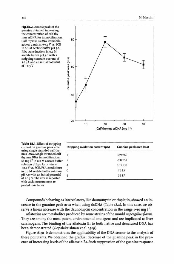
418
Fig.18.2. Anodic peak of the guanine obtained increasing the concentration of calf thymus ssDNA for immobilization. Calf thymus ssDNA immobilization: 2 min at +0.5 V VS. SCE in 0.2 M acetate buffer pH 5.0. PSA transduction: in 0.2 M acetate buffer pH 5.0 with a stripping constant current of +6 flA and an initial potential of +0.5 V
Table 18.1. Effect of stripping
80
Vi" E-ta ~60 ta -"
~ <II c 'i: ta j
1.7
40
M. Mascini
20~1'----L---~---L--~~--~--~---J--~
10 20 30 40 Calf thymus ssDNA (mg 1-1)
current on guanine peak area Stripping oxidation current (IlA) Guanine peak area (ms) using single stranded calf thy-mus DNA. Single stranded calf thymus DNA immobilization: 20 mg rl in 0.2 M acetate buffer 2 solution pH 5.0 for 2 min. at 4 +0.5 V VS. SCE. PSA conditions: in 0.2 M acetate buffer solution 6 pH 5.0 with an initial potential 8 of +0.5 V. The area is reported with each measurement re-peated four times
339±60
268±51
103±33
78±5
32±7
Compounds behaving as intercalators, like daunomycin or cisplatin, showed an increase in the guanine peak area when using dsDNA (Table 18.2). In this case, we observe a linear increase with the daunomycin concentration in the range 1-10 mg rl.
Aflatoxins are metabolites produced by some strains of the mould Aspergillus flavus. They are among the most potent environmental mutagens and are implicated as liver carcinogens. The binding of the aflatoxin B1 to both native and denatured DNA has been demonstrated (Gopalakrishnan et al. 1989).
Figure 18.3a-b demonstrates the applicability of the DNA sensor to the analysis of these pollutants. We obtained the gradual decrease of the guanine peak in the presence of increasing levels of the aflatoxin B1. Such suppression of the guanine response

CHAPTER 18 . Affinity Electrochemical Biosensors for Pollution Control 419
Table 18.2. Compounds tested with single-stranded or double-stranded calf thymus DNA immobilized on screen printed electrodes. Calf thymus DNA immobilization: 20 mg t 1 of single stranded or double stranded calf thymus DNA in 0.2 M acetate buffer solution pH 5.0 for 2 min. at +0.5 V VS. SeE. PSA conditions: in 0.2 M acetate buffer solution pH 5.0 with a stripping current of +6 f1A and an initial potential of +0.5 V
Compounds tested
Buffer solution
Daunomycin
Phthalates mixture (20 mg 1-')
Atrazine (50 mg 1-')
Bisphenol (100 mg 1-')
PCB 105 (0.4 mg 1-')
PCB mixture (Aroclor 1260) (20 mg 1-')
PCB mixture (Aroclor 1016) (20 mg 1-')
Aflatoxin B1 (10 mg 1-')
Cisplatin (30 mg 1-')
Hydrazine (20 mg 1-')
Guanine peak area (ms) using calf thymus dsDNA immobilized
36±7
52±6
39±16
66±39
76±13
54±8
39±5
43±8
36±8
58±14
22±4
Guanine peak area (ms) using calfthymus ssDNA immobilized
89±13
86±3
80±26
85±11
85±17
68±7
99±7
95±17
77±7
78±6
73±6
results in a well-defined concentration dependence and offers convenient quantification oflow levels of aflatoxin. The signal was observed within 10-30 mg rl (Fig. 18.3b).
In the most of the compounds, ssDNA gave greater effects. The peak area of guanine decreased even when low concentrations were present (PCB 0.2 mg rl). This can be explained by the binding of the compounds with guanine in a short time (2 min) and a lower availability of guanine for oxidation at the electrode surface.
PCBs have been recognized for several years as ubiquitous environmental pollutants. The high toxicity of some of the PCB congeners represents a public health risk, as these molecules are still present in the environment, even though the production of PCB has been banned. The screen-printed electrodes modified with single-stranded calf thymus DNA were used to detect PCB 105. Figure 18.4a-b displays the chronopotentiometric response of the calf thymus ssDNA modified electrode followed by increasing PCB 105 concentrations.
A decrease of the guanine peak area could be detected with some water samples (Fig. 18.5, Curves b, c, d). By HPLC analysis, we obtained the results reported in Table 18.3.
It seems that there is an approximate relationship between the two sets of analysis. The sensor is not able to distinguish between compounds of environmental concern but could be conveniently used as a screening tool of toxicity.
18.4 Conclusions
The potential of DNA biosensors for detection of toxic compounds has been demonstrated. This kind of procedure offers a sensitive, rapid and portable tool for field monitoring of several environmentally and toxicologically significant compounds.

420
Fig. 18.3. a Chronopotentiograms for (a) calf thymus ssDNA modified screen printed electrodes and followed increasing aflatoxin BI concentrations; (b) 10 mg rl; (c) 20 mg rl; (c) 30 mgrl; b Calibration curves obtained increasing the concentration of aflatoxin BI .
The results correspond to the difference between the guanine peak area after interaction with aflatoxin BI minus that obtained for the buffer solution. Calf thymus ssDNA immobilization: 20 mg I-I calf thymus ssDNA for 2 min at +0.5 V vs. SCE. PSA transduction: in 0.2 M acetate buffer pH 5.0 with a stripping constant current of +6 j.lA and an initial potential of +0.5 V
M. Mascini
1.20 r, --------------------,
a
a
~ $
~ ..... ~
1.00 1.05 1.10 1.15 E(V)
b
i°'1~ ~ -30 I \!J
-45 t, 30 20
10 1-1) 0
Aflatoxin Bl (mg
Moreover, we found that the calf thymus ssDNA biosensor interacts with low-molecular mass substances of environmental concern, and it can be used as a general indicator.
The DNA biosensor, realized by immobilization of the calf thymus extract on suitable electrode surface, is a simple tool to assemble and obtains reliable results. This therefore opens the possibility of rapid evaluation as a screening tool of toxicity of water samples.

CHAPTER 18 . Affinity Electrochemical Biosensors for Pollution Control
Fig. 18.4. a Chronopotentiograrns for (a) calf thymus ssDNA modified screen printed electrodes and followed by an increasing PCB 105 concentration, (b) 0.2mgr',(c) 0.6mgr', (d) 1 mg r'; b Calibration curves obtained increasing the concentration of PCB 105. The results correspond to the difference between the guanine peak area after interaction with PCB 105 minus that obtained for the buffer solution. Calf thymus ssDNA immobilization: 20 mg r', calf thymus ssDNA for 2 min at +0.5 V vs. SCE. PSA transduction: in 0.2 M acetate buffer pH 5.0 with a stripping constant current of +6 flA and an initial potential of +0.5 V
Table 18.3. Results of the water samples obtained using a standard method with a Varian 3400 gas chromato-graph coupled to a Finningan Mat 800 ion trap detector mass spectrometer (GC-ITDMS)
1.20
:=- 0.80 :> ~
~ .!Q
0;-
S !II ~ !II
..><:
0.40
10
o
al Co -10 <] ClJ c:: .i: !II :::l I.!l -20
1.00 1.05
E(V) 1.10
b
~ 1----1
-30 '~ __ ~~ __ ~ __ L-~ __ L-~ __ ~~ __ -L~
0.0 0.2 0.4 0.6 0.8 1.0
PCB 105 (mg 1-')
a
b(ngr') c(ngr') d(ngr')
Desetil-terbutilazine 0 12 21
Carbofuran 0 210 101
Simazine 0 0 23
Terbutilazine 79 28 81
Etofu mesate 6 184 83
Alachlor 0 0 27
Metolachlor 7 14 225
421
1.15

422
Fig. 18.5. Chronopotentiograms obtained using calf thymus ssDNA modified screen printed electrode with: (a) blank solution, (b), (e) and (d) river water (100 times concentrated). Calf thymus ssDNA immobilization: 20 mg t l calf thymus ssDNA for 2 min at +0.5 V vs. SCE. PSA transduction: in 0.2 M acetate buffer pH 5.0 with a stripping constant current of +6 flA and an initial potential of +0.5 V
References
~ ~
~ ..... ~
M.Mascini
1.60 " ---------------------,
0.95 1.00
a
1.05
E(V)
a Peakarea:89±13ms b Peak area: 94 ± 7 ms c Peak area: 61 ± 8 ms d Peak area: 48 ± 9 ms
1.10 1.15
Del Carlo M, Lionti I, Taccini M, Cagnini A, Mascini M (1997) Disposable screen-printed electrodes for the immunochemical detection of polychlorinated biphenyls. Anal Chim Acta 342:189
Gopalakrishnan S, Byrd S, Stone MP, Harris TM (1989) Carcinogen-nucleic acid interactions: Equilibrium binding studies of aflatoxin BI with the oligodeoxynucleotide d(ATGCATh and with plasmid pBR322 support intercalative association with the B-DNA helix. Biochemistry 28:726
Marrazza G, Chianella I, Mascini M (1999a) Disposable DNA electrochemical sensor for hybridization detection. Biosensors and Bioelectronics 14:43
Marrazza G, Chianella I, Mascini M (1999b) Disposable DNA electrochemical biosensors for environmental monitoring. Anal Chim Acta 387:297
Mecklenburg M, Grauers A, Rees Jonsson B, Weber A, Danielsson B (1997) A strategy for the broad range detection of compounds with affinity for nucleic acids. Anal Chim Acta 347:79
Jelen F, Fojta M, Palecek E (1997a) Voltammetry of native double-stranded, denatured and degraded DNAs. J Electroanal Chern 427:49
Jelen F, Tomoschik M, Palecek E (1997b) Adsorptive stripping square-wave voltammetry of DNA. J Electroanal Chern 423:141
Wang J, Rivas G, Cai X, Shiraishi H, Farias PAM, Dontha N, Luo D (1996a) Accumulation and trace measurements of phenothiazine drugs at DNA-modified electrodes. Anal Chim Acta 332:139
Wang J, Chicharro M, Rivas G, Cai X, Dontha N, Farias PAM, Shiraishi H (1996b) DNA biosensor for the detection of hydrazines. Anal Chern 68(13):2251
Wang J, Rivas G, Luo D, Cai X, Valera FS, Dontha N (1996c) DNA-modified electrode for the detection of aromatic amines. Anal Chern 68(24):4365
Wang J, Cai X, Rivas G, Shiraishi H, Dontha N (1997a) Nucleic-acid immobilization, recognition and detection at chronopotentiometric DNA chips. Biosensors and Bioelectronics 12(7):587
Wang J, Rivas G, Palecek E, Nielsen P, Shiraishi H, Dontha N, Luo D, Parrado C, Chicharro M, Farias PAM, Valera FS, Grant DH, Ozsoz M (1997b) DNA electrochemical biosensors for environmental monitoring. A review. Anal Chim Acta 347:1

Chapter 19
Palaeoenvironmental Reconstructions Using Stable Carbon Isotopes and Organic Biomarkers
S.Wakeham
19.1 Introduction
Aquatic sediments carry the potential of preserving a historical record, or some remnant thereof, of past environmental conditions. The stratigraphic record has long been a tool for elucidating the character of the Earth and the forces that have altered its face and determined the nature, distributions and fate of living organisms. There have been dramatic changes in the Earth's climate in the past. Increasing levels of atmospheric CO2 attributed to combustion of biomass and fossil fuels coupled with deforestation have heightened societal and scientific concerns about global warming, a reduction in ice volume and a rise in sea level. These issues have generated a greater interest in understanding past natural and present anthropogenic processes that influence global climate change and in developing predictive capabilities about future climate.
Studies of palaeoenvironment have varied in scope. They can range from qualitative descriptions and interpretation of conditions at a given time in the geological past to quantitative investigations concerned with the nature and the rate of change during specific time intervals. Organic biomarkers, molecules whose molecular structures point to specific biological sources, are proving to be quite valuable for palaeoenvironmental reconstructions. The utility of biomarkers derives from two features. First, organisms that inhabit specific ecological niches may biosynthesize unique biomarker compounds that can be used as indicators of the source organisms and their habitat. Second, organisms often possess an ability to regulate patterns of constituent biochemicals in order to remain viable under changing environmental conditions, so that environmental characteristics may be inferred from these patterns. To be a robust palaeoenvironmental proxy, the signal carried by biomarkers must survive during deposition and burial in sediments over the time frame of interest.
This chapter discusses several ways that palaeoenvironmental records may be obtained from organic geochemical studies, in particular from biomarker records in the sediment. The case studies represent only a few of the many applications that are presently accumulating in the literature and are by no means an exhaustive survey. Readers are referred to the references cited in the respective examples for further reading.
19.2 Stable Carbon Isotopes to Identify Organic Matter Sources
The biological source of sedimentary organic matter may be deduced from chemical studies on the structure of individual compounds (biomarkers) extracted from sedi-

424 S. Wakeham
ments. A second means of inferring source and ecological setting is through light (C, N, H, S) stable isotope tracers. Carbon fixation during photosynthesis results in a differential partitioning (fractionation) of isotopes of different atomic masses, yielding different ratios of isotope abundances (for definitions and background, see Degens 1969; Fogel and Cifuentes 1993; Hayes 1993). Isotope ratios can be indicative of physiological processes occurring during photosynthetic fixation of inorganic carbon into organic matter and during assimilation of organic compounds up the food chain. The stable isotopic composition of bulk organic matter is an integrative signal. It will reflect isotope fractionation resulting from the range of metabolic processes and environmental conditions that occurred over the life of the organism or multiple organisms that biosynthesized the organic matter and over the time frame during which the organism(s) lived and the sediments deposited. Interpreting isotope ratios for bulk organic material can thus be ambiguous. Isotopic compositions of individual compounds, on the other hand, have the potential of isolating specific biosynthetic sources and metabolic events in the life of an organism, although the biochemical mechanisms and environmental factors determining isotopic fractionation are complex and the subject of continuing research. Carbon isotopes have received the widest attention, because potentially all organic matter and compounds carry a carbon isotopic signal. Isotopes of nitrogen, sulphur, oxygen, and hydrogen have generally been less widely used because of difficulties in analytical procedures (Fogel and Cifuentes 1993), but this is rapidly changing.
Early studies of carbon isotopes found that there were metabolic controls on the photosynthetic isotope fraction (lOp) that could be used to elucidate organic carbon (OC) sources in geochemistry. As a consequence of different carbon fixation pathways and fractionations, there is a wide range of isotopic compositions in various types of living organisms (Fig. 19.1) and in different biochemical constituents (Degens 1969). Most plants use the enzyme ribuiose-l,s-biphosphate-carboxyiase (RuBP-carboxylase) during photosynthesis to produce a 3-carbon compound, hence the Crpathway. It is the RuBP-carboxylase reaction that is responsible for the fractionation of carbon isotopes during photosynthesis, which is about 20-30%0. To a first approximation, land plants are isotopically lighter (depleted in l3C relative to 12C with del-values (ol3C) of about -25 to -30%0 according to the nomenclature; Degens 1969) than marine plankton (013C -18 to -22%0). This difference results in part from isotopic fractionation and input from isotope differences for the source carbon, atmospheric CO2 for land plants vs. dissolved CO2 for plankton. Recent work has shown that photosynthetic isotope fractionation in the ocean is in fact quite complicated and the range of isotopic compositions considerably wider (ol3C -18 to -28%0). Photosynthtic isotope fractionation by marine plankton depends of the concentration of dissolved CO2, the phytoplankton species physiology (do the cells take up CO2 by passive diffusion across the cell membrane or do they actively pump CO2 or HC03), cellular volume, and cellular growth rate, to name a few (see Popp et al. 1999 and references therein).
A few plants (e.g. grasses, sugarcane, corn) utilize the C4 pathway that employs an alternate enzyme, phosphoenol-pyruvate-carboxylase (PEP carboxylates), and produces a 4-carbon product. This reaction has a smaller isotope fractionation (-2%0). Land plants fixing carbon by the C4-pathway are isotopically heavier (enriched in l3C; ol3C -12 to -16%0) than plants employing the Crpathway.

CHAPTER 19 • Palaeoenvironmental Reconstructions
-10 -15
+ / CO2
Yeast
-20 813e -25
• + 1\
-30
Lactate
-35
425
-40
Tropical land plants
Common land plants
Lacustrine higher plants
Fresh water plankton
Marine vertebrates
Marine invertebrates
Marine higher plants
Marine plankton (+22 °C)
Marine plankton (+ 1 0c)
Marine sulphate reducing bacteria
Marine chemautotrophic bacteria
Fig. 19.1. Ranges of stable carbon isotope values for total OC in living organisms. Redrawn from Degens (1969)
Stable carbon isotopes are frequently used to estimate contributions from marine and terrigenous sources of organic matter in marine sediments. Early work (e.g. Hedges and Parker 1976; Gearing et al. 1977) showed a trend in 013e of bulk OC as one progresses from continental shelf (ol3e -26%0) to off-shore sediments (013e -19 to -21%0) in the Gulf of Mexico. Most terrigenous OC would be deposited on the inner shelves, and little is transported to outer shelves and continental slopes, indicating a minimal contribution of land-derived OC to surface sediments of the Gulf. Other studies (e.g. Prahl and Muelhausen 1989; Gofii et al.1998) have suggested that a

426 S. Wakeham
significant amount of terrigenous OC is deposited in off-shore sediments. In part, this difference in interpretation arises from the fact that organic matter delivered by rivers to continental shelves may not necessarily have a uniform carbon isotopic composition, and this composition may change over time as the ecosystem in the catchment basin changes, for example in response to climate change. In the case of the Gulf of Mexico, a continental end-member value of -26%0 assumes input primarily from C3
vascular plants and neglects C4 plants (Golli et al. 1998). However, material carried by the Mississippi River into the Gulf of Mexico includes contributions by both C3 (trees and shrubs) and C4 (grasses) plants on the North American continent. Different soil provenances display different 8l3C values, ranging from --19 to -230/00 for C4 grasslands to -26%0 for C3 forests (Fig. 19.2; Onstad et al. 2000). Particulate matter delivered to the Gulf is relatively enriched in l3C (813C -19 to - 24%0). Thus, 8l3c values of -20 to - 220/00 for OC in Gulf of Mexico sediments (Golli et al. 1998) might in fact result from significant inputs of terrigenous C4-derived OC rather than strictly marine OC. If so, then the terrigenous contribution to these sediments would be higher than previously believed, possibly greater than 50% (Golli et al. 1998).
Part of the uncertainty in interpreting isotopic data for bulk organic carbon arises from the inclusion of organic materials originating from a variety of photosynthetic sources that individually imprint different 8l3C signals depending on their carbon source, degree of photosynthetic isotope fractionation, and differing response to environmental factors. Analyses of individual biomarker distributions in conjunction with bulk isotopic compositions help resolve these complications (Prahl et al. 1994;
Fig. 19.2. Stable carbon isotope value for riverine suspended particulate matter in the United States. The stippled areas are C4 grasslands. From Onstadt et al. (2000)

CHAPTER 19 . Palaeoenvironmental Reconstructions 427
Gofii et al. 1998). However, significantly different results may be obtained depending on the choice of biomarker(s). For example, Prahl et al. (1994) estimated that terrigenous OC is a minor component (::;10%) in continental slope sediments on the Washington (USA) margin based on lignin phenol concentrations and l3C of bulk ~C, but a calculation using n-alkane concentrations and l3C of bulk OC suggested a significantly higher input (30%).
Better still is measurement of biomarker specific isotopic compositions (Hayes et al. 1990). Compound-specific isotope analyses (CSIA) are now a common tool employed by organic geochemists. A powerful application of CSIA has been in using n-alkanes for tracking the anthropogenically-driven shifts in vegetation, for example in northern Australia over the past 6000 years (Bird et al. 1995). European settlement of the region in the late 19th century resulted in the replacement of the original C3 forests by a C4 ecosystem of grasses (and ultimately including cultivated sugarcane). The principle behind the Bird et al. analysis is that n-alkanes (1) are robust biomarkers for vascular plants, (2) are stable against diagenesis and hence well-preserved in sediments, and (3) record the stable carbon isotope values of their C3 (8l3C - -280/00) vs. C4
(813C - -12%0) plant sources. Figure 19.3 shows carbon isotope values for n-alkanes in a set of sediments from the Johnstone River, North Queensland, and a marine sediment core off the mouth of the Johnstone River. Among the river sediments, the sample from tlIe forested area (JR-8B) was the most depleted in 13C (813C -27.9%0), while the sample from a sugarcane cultivating region (JR4) was most enriched (813C -20.90/00).
-26. Terrestrial samples
--0- JR4 «(4); -20.9%, 5.4% (
-28 ~ n // ~ --0- Burdekin «(4); -22.3%, 0.23% (
---- JR8B (C3); -27.9%,4.2% (
-30 ~ ~ '" -/.'~ 1 Marine samples
, -32 t 1
-.to-- 0-5 cm; -19.8%, 0.59% (
--.-- 0-9 cm;-20.6%, 0.57% (
--0-- 10-20cm;-21.8%,0.58%( 00 -34
--A-- 4O-50cm;-21.4%,0.58%(
-36 ~ ~ 1 -6:- 65-85 cm; -22.0%, 0.65% (
--.-- 10()"'120 cm;-21.9%,0.49%(
-+-- 16()"'180 cm;-22.3%,0.61 % (
-~ r ~ ] 20()'" 220 em; -22.2%,0.56% ( --.---40 _ 1,1 ~rro: II --A- 28()"'300 cm;-22.0%,0.56%(
28 29 30 31 32 33 34 n-alkane carbon number
Fig. 19.3. Carbon isotopic compositions of n-alkanes from sediments from the Johnstone River, North Queensland, Australia, and a 3-m marine sediment core off the mouth of the Johnstone R. The ol3C values of bulk organic carbon are given in the legend. Redrawn from Bird et al. (1995)
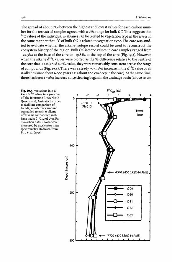
428 s. Wakeham
The spread of about 8%0 between the highest and lowest values for each carbon number for the terrestrial samples agreed with a 7%0 range for bulk OC. This suggests that 13e values of the individual n-alkanes can be related to vegetation type in the rivers in the same manner that 13e of bulk OC is related to vegetation type. The core was studied to evaluate whether the alkane-isotope record could be used to reconstruct the ecosystem history of the region. Bulk OC isotope values in core samples ranged from -22.3%0 at the base of the core to -19.8%0 at the top of the core (Fig. 19.3). However, when the alkane 013e values were plotted as the %-difference relative to the centre of the core that is assigned a 0%0 value, they were remarkably consistent across the range of compounds (Fig. 19.4). There was a steady -1-1.5%0 increase in the 013e value of all n-alkanes since about 6 000 years B.P. (about 200 cm deep in the core). At the same time, there has been a -2%0 increase since dearing began in the drainage basin (above 10 cm
Fig. 19.4. Variations in n-alkane OBC values in a 3-m core off the Johnstone River, North Queensland, Australia. In order to facilitate comparison of trends, an arbitrary amount was added to each n-alkane OBC value so that each n-alkane had a o BCdiff of 00/00. Radiocarbon dates shown were measured by accelerator mass spectrometry. Redrawn from Bird et al. (1995)
E ~
~ v .5
-= Co
~
o13ed11f (%0)
-3 -2 -1 o 1 2 3 4
o I r:::w:JaO" •
....... Error
100
+- 4540 ±400 B.P. ((-14 AMS)
- (-29 200 (-30
-0- (-31
(-32
-a- (-33
+- 7720±470B.P.«(-14AMS)
300 , ....... &......jL.......!--..I ....... --1~......J.~--1. ........ ....J.. ........ .J
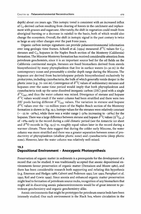
CHAPTER 19 . Palaeoenvironmental Reconstructions 429
depth) about 100 years ago. This isotopic trend is consistent with an increased influx of C4-derived carbon resulting from clearing of forests in the catchment and replacement with grasses and sugarcane. Alternately, the shift in vegetation could result from aboriginal burning or a decrease in rainfall to the basin, both of which would also change the ecosystem. Overall, the shift in isotopic signal in the past century is twice as large as any other changes over the past 8000 years.
Organic carbon isotope signatures can provide palaeoenvironmental information over long geologic time frames. Schoell et al. (1994) measured 8 13C values for C27
steranes and C35 hopanes in the Naples Beach section of the Monterey (California) formation. The Miocene Monterey formation has received considerable attention from petroleum geochemists, since it is an important source bed for the oil fields on the California continental margin. Steranes are fossil biomarkers derived from sterols biosynthesized by many phytoplankton that live in surface waters (0-30 m) in the contemporary ocean and presumably a similar depth range during the Miocene. The hopanes are derived from bacteriohopane polyols biosynthesized exclusively by prokaryotes, including cyanobacteria, the bulk of which generally reside deeper in the photic zone (e.g. 70-100 m). Convergence of 813C values of sedimentary steranes and hopanes over the same time period would imply that both phytoplankton and cyanobacteria took up the same dissolved inorganic carbon (DIC) pool with a single 813CDIc> and thus the water column was mixed. Divergence of sterane and hopane 813C values would result if the water column had been stratified and there were two DIC pools having different 8 13CDIC values. The variation in sterane and hopane 813C values over the -22 million years of the Naples Beach section of the Monterey formation is shown in Fig. 19.5. Isotope values for the steranes were relatively constant ( - -25 to -26%0), while there was a wider range (-31%0 increasing to -26%0) for the hopanes. There was a large difference between sterane and hopane 813C values (~13CH_S) of -6%0 early in the record during a cold climatic period (see the Antarctic ice sheet and 8180 records in Fig. 19.5) vs. roughly equal values later in the record during a warmer climate. These data suggest that during the colder early Miocene, the water column was more stratified and there was a greater separation between zones of productivity of phytoplankton (shallow photic zone) and cyanobacteria (deep photic zone). However, later the water column was relatively well-mixed.
19.3 Depositional Environment - Anoxygenic Photosynthesis
Preservation of organic matter in sediments is a prerequisite for the development of a record that can be studied. It was traditionally accepted that anoxic depositional environments favour preservation of organic matter (Demaison and Moore 1980), and there has been considerable research both supporting and refuting this hypothesis (e.g. Emerson and Hedges 1988; Calvert and Pederson 1992; Lee 1992; Paropkari et al. 1992; Keil and Cowie 1999). Since anoxia and enhanced organic matter preservation might lead to formation of petroleum source rocks, recognition of any biomarkers that might aid in discerning anoxic palaeoenvironments would be of great interest to petroleum geochemistry and organic geochemistry alike.
Anoxic environments that might be prototypes for petroleum source beds have been intensely studied. One such environment is the Black Sea, where circulation in the

430 S. Wakeham
A Permanent East Antarctica On-Off East Antarctica ice sheet ~ glaciations
-221lIic~ilftf;;f¥';kfrpfrr:u l -23 , T
c:a -24 c 0.. -25 en =
!11.3 12.6 I J .O
C27 Sterane Shallow photic zone
~ -26 t 25 Today ···j··········· 4!) •.•• .••• m i
=- -27 (140C) · e -28 ... 4!)
.e: -29 (.)
~ -30 to
-31
-32
-33
B 2 1 Stratified --+- Photic zone -+- Mixed
E 0
... -1 II) Q, -2 en :C -3
(.) M -4 ~
<] -5 -6
Low ........ [C02{aq) ]
warmer
j High
[C02(aq)] cooler
Warmer 1.0 :::-
E 1.5 ~ -c 2.070
2.5 Colder
-7 « , ! I, ! , , ! , , I j ! I ! , ! I I , .3.0 6 8
Late M
10
.1 I
o
12 14 16 18 20 22 Age (Ma)
Middle C E
I
N
Early E
Fig. 19.5. a C27 steranes and C35 hopanes 813C values for the Naples Beach section of the Monterey formation (Naples Beach, California), indicating changing water masses in the shallow and deep euphotic zone. The scope of the Antarctic ice sheet represents relative climatic conditions; b Isotopic difference e:,.13CH_S between CZ7 steranes and C35 hopanes. The lower solid line is as measured; the upper solid line is e:,. I3CH_S corrected by 1.~o/oo for the difference (e:,.13CDIcl in the photic zone of contemporary Santa Monica Bay. The interpretation is that in the late Miocene, the water column was stratified but in the early Miocene it was mixed. The wavy ribbon is the Miocene 8180 record from benthic foraminifera. From Schoell et al. (1994)

CHAPTER 19 . Palaeoenvironmental Reconstructions 431
2 200-m deep basin is restricted, and bottom waters (:<:120 m) are permanently anoxic. During a cruise to the Black Sea in 1988, organic geochemists and microbiologists were surprised to discover that the oxic-anoxic boundary in the water column (the "chemodine") was located well within in the photic zone (Murray et al.1989). Associated with the chemodine were concentration maxima for bacteriochlorophyll e and carotenoid pigments, notably isorenieratene (1, Fig. 19.6) that are characteristic of an oxygenic primary production by photoautotrophic bacteria, Chlorobrium sp. (Repeta and Simpson 1991). These brown sulphur bacteria typically live as strict anaerobes in bacterial plates at shallow oxic/anoxic interfaces. Blooms of C. phaeobacteriodes frequently occur in shallow meromictic lakes, where hydrogen sulphide produced in anoxic sediments and bottom waters rises into the euphotic zone (Parkin and Brock 1980); viable of C. phaeobacteriodes have also been isolated from surface sediments underlying anoxic water columns (Herbert and Tanner 1977). The high concentrations of bacteriochlorophylls and isorenieratene at the chemodine in the Black Sea generated significant interest among organic geochemists. These pigments and their diagenetic and catagenic products have been found in a wide variety of ancient sediments (Koopmans et al. 1996a), making them potentially excellent biomarkers for anoxic waters reaching into the photic zone.
Distributions of isorenieratene in sediments of the Black Sea have been used to reconstruct the record of anoxygenic primary production over the past 8200 years (Repeta 1993). Downcore concentrations of isorenieratene ranged from non-detectable to >70 Ilg g-l or up to 11lg mg-1 TOC (Fig. 19.7). There are distinct episodes of intense burial of isorenieratene that suggest temporal variations in the depth of the H2S chemodine. Maxima in sedimentary isorenieratene should represent periods of a shallow H2S chemodine, while the absence of isorenieratene should correspond to the chemodine being located below the photic zone. The depth of the chemodine in the water column has significant implications to the balance of freshwater inflow to the Black Sea from adjacent landmasses and through the Bosphorus. The freshwater balance in turn is related to dimatic variations throughout the Holocene.
Fig. 19.6. Structures of isorenieratene (1), f3,~carotane (II) and octahydroisorenieratene (III)
II
III

432
Fig. 19.7. Concentrations of isorenieratene in a Black Sea core covering the past 8000 years. Redrawn from Repeta (1993)
~ }
10
20
30
S. Wakeham
Box core 5 (119 isorenieratene mg roc-I) 1 2
The highly unsaturated nature of carotenoid pigments such as isorenieratene renders these compounds remarkably reactive. In anoxic sediments, they preferentially accumulate in macromolecular fractions, usually through loss of double and incorporation of inorganic sulphur (Sinninghe Damste et al. 1990; Wakeham et al. 1995). Sulphurization (inter- and intra-molecular cross-linking between S and C) may provide a mechanism that protects otherwise labile molecules from degradation by sequestration into a less reactive polar macromolecule. Chemical release of S-bound {3,f3-carotane and octahydroisorenieratene (II and III, Fig. 19.6), fully and partially unsaturated derivatives of isorenieratene, by desulphurization of polar macromolecular material extracted from Black Sea sediments produced a historical record (Sinninghe Damste et al. 1993) similar to that derived from isorenieratene described above. Diagenesis and ultimately catagenesis of isorenieratene generates a wide range of aromatic and S-containing isoprenoids (Koopmans et al. 1996a) that can being applied as indicators of photic zone anoxia in ancient environments. In the Messinian (upper Miocene) evaporitic sequence of the Veno del Gesso Basin (Italy), distributions of Sbound isorenieratane (a derivative of isorenieratene) and the pentacyclic triterpenoid gammacerane have been used to reconstruct the palaeo depositional environment (Fig. 19.8). Gammacerane is thought to derive from anaerobic bacterivorous ciliates living at or just below the chemocline and is an indicator of water column stratification; isotopic evidence suggests that the ciliates were feeding on sulphur bacteria that produced isorenieratene (Sinninghe Damste et al. 1995b). In sequences where both isorenieratane and gammacerane were present, the water column was stratified and the chemocline was in the photic zone. When gammacerane was present but iso-

CHAPTER 19 . Palaeoenvironmental Reconstructions
isorenleratane
Xio !iiil iiiZ¥~iifl "
'Xc
:~: I : f 'I ~::: kFZZZ:rz,~=~wi=ZI Vile F ' Vllb ~
~:: Eii VI>
Vc V. v. ,V, 'v. IV.
::~ fW1W¥ ~
gammacerane
_ marl _ selenitic gypsum concentration (mglg bitumen)
Situation A chemochne in phOlic zone
Situation B chemocline in water column
but not in photic zone
Situation C chemocllne in sediment
433
Fig. 19.8. Concentrations of isorenieratane and gammacerane in the Veno del Gesso marl sequence. Also shown are the reconstructed water columns based on these biomarker distributions. From Sinninghe Damste et al. (1995a)
renieratane absent, the chemocline was below the photic zone but still in the water column, because the ciliates do not live in sediments. When both were absent, the water column was unstratified and there was no anoxic zone. Although carotenoid derivatives are now widely used as indicators of photic zone anoxia, they must be used with caution, however, and should not be made without complementary l3C isotopic analysis (Koopmans et al. 1996b).
19.4 Alkenone Palaeothermometer
Series oflong chain C3T> C3S-' and C39-di-, tri- and tetra-unsatursated methyl and ethyl ketones (see Fig. 19.9 for the C37 alkenones) were first observed nearly two decades ago in Miocene to Pleistocene sediments (Boon et al. 1978). The geographic range of alkenones is now known to encompass sediments from all oceans (Brassell 1993). At the time that the structures of the alkenones were first determined (de Leeuw et al. 1980; see also Rechka and Maxwell 1988a,b), they were also found to be abundant in unicellular algae of the Prymnesiophyceae, namely Emiliania huxleyi (Volkman et al. 1980). Alkenones have now been found in a number of prymnesiophytes (now classified as haptophytes), of which the calcifying E. huxleyi and Gephyrocapsa oceanica and the noncalcifying Crysotilla and Isochrysis are the most important in the oceans (Conte et al. 1994, 1995; Volkman et al. 1995). No other sources of alkenones are presently known, making them powerful and unusually unambiguous biomarkers. In addition to the limited species distribution of alkenones among phytoplankton, it was also discovered that they might be sensitive to the temperature at which they are biosynthesized and thus have a potential palaeotemperature application (Brassell et al. 1986).

434 S. Wakeham
I. Diunsaturated compounds 0
II. Triunsaturated compounds
I (CH21n - C
\ R
o I
(CH21n - C
\ III.Tetraunsaturated compounds 0
Fig. 19.9. Structures of the 37:2, 37:3 and 37:4 unsaturated alkenones
I (CH21n - C
\ R
37:2
37:3
37:4
Variations in the proportions of di-, tri- and tetra-unsaturated alkenones in cultures and sediments (Fig. 19.10) led to an alkenone unsaturation index (Brassell et al.1986):
U~7 = ([37:2]- [37:4]) / ([37:2] + [37=3] + [37:4])
which simplifies to
u~/ = ([37=2] / ([37:2] + [37:3])
in the absence of 37:4. Culture experiments showed a linear relationship between U~7 (or U~7') and growth temperature (Brassell et al. 1986; Prahl and Wakeham 1987; Prahl et al.1988) that could be transformed into a U~7 vs. temperature calibration. There have been many calibrations reported in the literature due to apparent variability in alkenone biosynthesis by different strains of haptophytes (Brassell 1993; Conte et al. 1994,1995). However, analysis of core tops and comparison with sea surface temperatures in many regions of the ocean has produced a relatively robust and "universal" calibration (Fig. 19.11; MUller et al. 1998; see also references cited for numerous recent U~/-temperature calibrations), at least for typical open ocean regimes. Two important caveats must be kept in mind when calculating temperatures from alkenone unsaturation patterns. First, there is significant regional variability in U~/ -temperature calibrations, especially in coastal areas such that a universal open ocean calibration may not always be inappropriate. Second, there remains an issue about whether U~/ -derived temperatures more accurately reflect sea surface temperatures or mixed layer temperatures depending on the depth at which the alkenone-producers live.
Alkenone thermometry has nonetheless become a widely used tool by palaeoceanographers. Sea surface temperature records have been reconstructed over time scales of years to hundreds of kiloyears. For example, alkenone unsaturation patterns in sediments of the Peruvian margin provide information about El Nino events in the eastern Pacific that can be related to Peruvian palaeoclimate over the past several centuries. McCaffrey et al. (1990) found alkenone unsaturation to be positively correlated with periods of greater or lesser El Nino activity as described by Quinn et al. (1987).

CHAPTER 19 ,Palaeoenvironmental Reconstructions
Fig. 19.10. Gas chromatograms of alkenones in cultures of Emiliania huxleyi at 25 and 10°C, Redrawn from Prahl and Wakeham (1987)
1 ~ 'Vi c: !l oS
37:2
37:3
~J *
37:3
I 37:2
37:4 *
38:2 Et
I ~»2M' 38:3 Et , A
38:2 Et
38:3 Me
38:3 Et ~ *
Time
38:2 Me
435
25 ·C Culture
39:2
10°C Culture
• Increased sea surface temperatures are associated with El Nino conditions (Fig. 19.12), because the intensity of coastal upwelling of colder subsurface water in the eastern tropical Pacific decreases. The "very strong" EI Nino events of Quinn et al. (1987) had sea surface temperature anomalies of 7-l2 °C, considerably higher than the sea surface temperature derived from alkenone analyses (e.g. about 2°C for the 1982 El Nino). This temperature difference may be related to the fact that the alkenone-producing haptophytes may better record the average temperature of the cooler mixed layer rather than that at the warmer sea surface,

436
1.0
0.9
0.8
0.7
0.6
~0.5
0.4
0.3
0.2 t+ 0.1
0.0 0
00 +
++" "+ " ,I"" /0
Atlantic --+-1 ~ + + ,1"a-o +' ~ Indic
+ 0 .. " "'~(jo + ' +""':A>o .y.{ -¥. -;r::J" 0
0''::1 ,." 0 ,,0 0
,~
~,.! qa 0 Pacific
'+ ,," ,. , , .A , "', "0 0
1(,' 0
+' !;IJ , , DO
o 0 <>
5 10 15
Annual mean SST,O m (OC)
+ o o
20
S. Wakeham
+
Atlantic Ocean
Indian Ocean
Pacific Ocean
25 30
Fig. 19.11. "Global" calibration of u~/ vs. sea surface temperature derived from a compilation of core top data throughout the ocean. Redrawn from Muller et al. (1998)
On a longer scale, for example, the sea surface temperature history over the past 80 ka was determined by Zhao et al. (1995), who used high resolution (-200-500 years) U~/ records from cores off northwest Africa to track effects of glacial-interglacial transitions of sea surface temperatures in the subtropical eastern Atlantic. The derived U~/ sea surface temperatures had a range from -18°C during the last glacial (10-75 ka B.P.; Fig. 19.13) to -21.5 °C during the early Holocene «10 ka B.P.). In addition to the significant glacial vs. interglacial temperature difference recorded in these cores (and numerous others in the literature) is the rapidity of temperature change. In some cases, temperature changes of 3-4 °C occur in the space of a century, for example after Heinrich events H2 and H4 for core 658C in Fig. 19.13. These apparent rapid alkenonederived temperature changes are in good agreement with oxygen isotope (180 ) records of temperature inferred from ice volume. The very rapid temperature shifts that coincide with Heinrich events are thought to indicate ice sheet surges during periods of
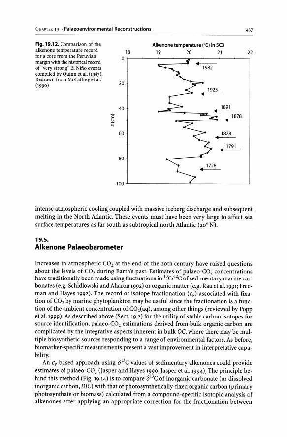
CHAPTER 19 . Palaeoenvironmental Reconstructions
Fig. 19.12. Comparison of the alkenone temperature record for a core from the Peruvian margin with the historical record of "very strong" El Nino events compiled by Quinn et al. (1987). Redrawn from McCaffrey et aI. (1990)
E ~
'"
Alkenone temperature (DC) in SC3
18 19 20 21 o I ... ...
1982
20 1925
...
40
60 1828 ..---... 1791
I .-80
100 •
437
22
intense atmospheric cooling coupled with massive iceberg discharge and subsequent melting in the North Atlantic. These events must have been very large to affect sea surface temperatures as far south as subtropical north Atlantic (200 N).
19.5. Alkenone Palaeobarometer
Increases in atmospheric CO2 at the end of the 20th century have raised questions about the levels of CO2 during Earth's past. Estimates of palaeo-C02 concentrations have traditionally been made using fluctuations in 13CJ12C of sedimentary marine carbonates (e.g. Schidlowski and Aharon 1992) or organic matter (e.g. Rau et al.1991; Freeman and Hayes 1992). The record of isotope fractionation (£p) associated with fixation of CO2 by marine phytoplankton may be useful since the fractionation is a function of the ambient concentration of CO2(aq), among other things (reviewed by Popp et al.1999). As described above (Sect. 19.2) for the utility of stable carbon isotopes for source identification, palaeo-C02 estimations derived from bulk organic carbon are complicated by the integrative aspects inherent in bulk OC, where there may be multiple biosynthetic sources responding to a range of environmental factors. As before, biomarker-specific measurements present a vast improvement in interpretative capability.
An £p-based approach using 813C values of sedimentary alkenones could provide estimates of palaeo-C02 (Jasper and Hayes 1990, Jasper et al. 1994). The principle behind this method (Fig. 19.14) is to compare 813c of inorganic carbonate (or dissolved inorganic carbon, DIC) with that of photosynthetically-fixed organic carbon (primary photosynthate or biomass) calculated from a compound-specific isotopic analysis of alkenones after applying an appropriate correction for the fractionation between

438 S. Wakeham
22 +I------~.-----~-.--~~----~------~-----.~----~--.---~
21
20 p - 19
~ !<" 18 ~'"
17
16
15 I 2 o 10 20 30
3
40
Age (kyr)
658°C
~
5
50 60 70 80
22 +I----~~----~_r--~----~------~--_.~-----L_.--~
21
20
P - 19 ~ ;1;; 18
17
16
2 3 4 5 15 +I------~~----._~--~------_r------,_----~r_----_.--~--~ o 10 20 30 40
Age (kyr) 50 60 70 80
Fig. 19.13. Reconstructed U~/ sea surface temperature records over the past 80 ka derived from cores in the subtropical southeast Atlantic. Arrows mark sea surface temperature maxima that correlate with Heinrich events (see text). Redrawn from Zhao et al. (1995)
813Cbiomass and 813Calkenone' This gives an estimate of the isotope fractionation (lOp, %0) that occurs during photosynthesis. The resulting lOp is then placed on a calibration plot relating lOp and the sea water concentration of dissolved CO2 [C02(aq) 1 to give an estimated Pco2• Application of Hemy's Law allows calculation of the equilibrium atmospheric Pco2•
Jasper and Hayes (1990) applied their approach to calculate the history of lOp, surface water Pe02 and atmospheric Pe02 for the northern Gulf of Mexico over the past 100 ka using sediments from the Pigmy Basin (Fig. 19.15). Palaeo-Peo2 trends were compared with the Peo2 record obtained directly by measuring CO2 in gas bubbles from the Vostok (Antarctica) ice core. The alkenone-based and ice core records are remarkably similar, showing reduced levels of atmospheric CO2 during the last glacial. In contrast, the Pco2 record that would be obtained from 813C of total organic carbon was significantly different from and more poorly tracked the Vostok record. This discrepancy provides a strong argument for using specific biomarkers for palaeo-C02 reconstructions rather than bulk OC.

CHAPTER 19 . Palaeoenvironmental Reconstructions 439
18
Nd""'~ 0
+ Em/d(T) -5
'()
~ 16 0. "l
14
+~m/f
---, Op (Dissolved (02) -10 12
013( t-15 (%oPDB)
I Ep= 13.9%
-20
,--+ 1 ~'e (Photo""'''''') +3.8% -25
10 5.4 6 7 8 9 10
Dissolved CO2 (Ilmoll-')
1 180 210 240 270 300 340
L- pC02 (Ilatm) (37
Alkadienone
Fig. 19.14. Schematic of the method used to calculate palaeo-pco, (sea water) and Pco, (atmosphere) from 013C of carbonate, OC, or alkenones. Redrawn from Jasper and Hayes (1990)
Alkenone-based palaeo-C02 histories are rapidly accumulating in the literature (e.g. Jasper et al. 1994; Muller et al. 1998; Pagani et al. 1999). In a study of the Angola Current over the last 200 ka, Muller et al. (1998) derived the Pe02 record for surface waters using isotopic compositions of alkenones extracted from cores in the Angola Basin off western Africa. As in the Pigmy Basin in the Gulf of Mexico, there was substantial variability in Peo2 in the Angola Basin over the time scale covered by the cores. Pcoz trends in surface waters were compared to the Vostok ice core record to determine the disequilibrium between the ocean and atmosphere (Fig. 19.16). The magnitude of the difference between sea water and atmosphere (I:!.peo) determines the flux of CO2 across the air-sea interface, while the sign of the difference determines the direction of the flux. This exercise suggests that surface waters in the eastern Angola Basin were generally a CO2 source during the past 200 ka (sea water Peozlevels were higher than Pco2 in the atmosphere; note that a 70 flatm correction was used in Fig. 19.16 to facilitate comparison of trends). The strength of the flux from the sea surface to atmosphere was reduced during glacial compared to interglacial times (Peo2 - 70 flatm for glacial times (20-70 ka and 130-180 ka) vs. 100-120 flatm for interglacial periods (15 ka to present and 70-130 ka». Presumably, this difference was related to lower sea surface temperatures and higher biological productivity during glacial periods that would draw down concentrations of dissolved CO2 and reduce the flux-driving gradient between the sea surface and atmosphere.
Alkenone palaeo barometry is a relatively new tool, and additional investigation is required to minimize uncertainty that presently exists in this or any other biomarkerbased CO2 proxy. For example, variability in Ep and oJ3C of inorganic carbon and

440 S. Wakeham
360.-----------------------------------------------------.
N. Gulf of Mexico
320
280
I 8~
Q. 240
200
160 I i I 3 I 4 Sa 5b 5c? o W 40 i 60 80 100
Age (ka B.P.)
Fig. 19.15. Atmospheric Pco, over the last 100 ka derived from ol3C of alkenones extracted from sediments of the Pigmy Basin, compared to the record from the Vostok ice core and a record that would be obtained from bulk OC. Redrawn from Jasper and Hayes (1990)
400
350
E 300 '!Q ,a.
8 Q. 250
200
Estimated surface water Peo at Site 1016-3,Angola Basin·
Vostoc ice core Peo +70atm
--6- after Rau et al. (1991) ------ after Popp et al. (1989)
150+1--.--.-'r-.--.--.--r--r-.--.--.--.--.--r-'--.-~--r--r-.
o 50 100
Age (ka) 150 200
Fig. 19.16. Estimated surface water Pco, derived from a core from the Angola Basin. The record obtained from the Vostok ice core is shown for comparison and has been adjusted by the average glacial sediment-ice difference of 70 l1atm to facilitate comparison. This presentation emphasizes the disequilibrium during the period between 60 and 130 ka. Redrawn from Miiller et al. (1998)

CHAPTER 19 . Palaeoenvironmental Reconstructions 441
biomarkers can be caused by many factors, most of which are poorly constrained in palaeoenvironmental studies but which are being intensely studied in the contemporary ocean (e.g. Popp et al. 1999). Carbon isotope fractionation is strongly influenced by several factors in addition to dissolved CO2, One must be certain that the source of the specific biomarker being used is as unambiguous as possible. The limited sources of alkenones in open ocean settings - E. huxleyi and G. oceanica - makes these compounds among the best in the organic geochemists' toolbox to date. The carbon uptake mechanism and cellular geometry of source organisms must be known, because they affect the lOp that is imprinted into organic matter. Microalgal growth rate is another important factor affecting lOp that cannot be easily determined in ancient environments. Cd/Ca ratios might be a proxy for surface water phosphate, which could be used to infer primary production and perhaps growth rates. It is thus important to use a multi-proxy approach - e.g. lOp determined from sedimentary alkenones and inorganic carbonate from planktonic foraminifera along with Cd/Ca measurements -in order to improve confidence in the results.
Acknowledgements
The support of the National Science Foundation during the preparation of this paper is gratefully acknowledged. C. Lee provided helpful comments to improve the manuscript.
References
Bird MI, Summons RE, Gagan MK, Roksandic Z, Dowling L, Head J, Fifield LK, Cresswell RG, Johnson DP (1995) Terrestrial vegetation change inferred from n-alkane "l3C analysis in the marine environment. Geochim Cosmochim Acta 59:2853-2857
Boon JJ, Meer FW van der, Lange F de, Leeuw JW de, Schenck PA, Burlingame AL (1978) In: Initial reports of the Deep-Sea Drilling Project, vols 38,39,40 and 41, Supplement, Walvis Ridge DSDP Leg 40. U.S. Government Printing Office, Washington, pp 627-637
Brassell SC (1993) Applications of biomarkers for delineating marine paleoclimate fluctuations during the Pleistocene. In: Engel MH, Macko SA (eds) Organic geochemistry - principles and applications. Plenum Press, New York, pp 699-738
Brassell SC, Eglinton G, Marlowe IT, pflaumann U, Sarnthein M (1986) Molecular stratigraphy: A new tool for climate assessment. Nature 320:129-133
Calvert SE, Pederson TF (1992) Organic carbon accumulation and preservation in marine sediments: How important is anoxia? In: Whelan J, Farrington JW (eds) Organic matter. Univ. Press, New York, pp 231- 263
Conte MH, Volkman JK, Eglinton G (1994) Lipid biomarkers of the Haptophyta. In: Green JC, Leadbeater BSC (eds) The haptophyte algae. Clarendon Press, Oxford, pp 351-377
Conte MH, Thompson A, Eglinton G, Green JC (1995) Lipid biomarkers diversity in the coccolithophoride Emiliania huxleyi (Prymnesiophyceae) and the related species Gephyrocapsa oceanica. J Phycol 31:272- 282
Degens, ET (1969) Biogeochemistry of stable carbon isotopes. In: Eglinton G, Murphy MTJ (eds) Organic geochemistry. Springer-Verlag, New York, pp 304-329
Demaison GJ, Moore GT (1980) Anoxic environments and oil source bed genesis. AAPG Bull 64:1179-1209
Emerson S, Hedges JI (1988) Processes controlling the organic carbon content of open ocean sediments. Paleoceanogr 3:621-634
Freeman KH, Hayes JM (1992) Fractionation of carbon isotopes by phytoplankton and estimates of ancient CO2 levels. Global Biogeochem Cycles 6:185-198
Fogel ML, Cifuentes LA (1993) Isotope fractionation during primary production. In: Engel MH, Macko SA (eds) Organic geochemistry - principles and applications. Plenum Press, New York, pp 73-98
Gearing P, Plucker FE, Parker PL (1977) Organic carbon stable isotope ratios in continental sediments. Mar Chern 5:251-266

442 S. Wakeham
Goni MA, Ruttenberg KC, Eglington T (1998) A reassessment of the sources and importance of landderived organic matter in surface sediments from the Gulf of Mexico. Geochim Cosmochim Acta 62:3055-3075
Hayes JM (1993) Factors controlling BC contents of sedimentary organic compounds: Principles and evidence. Mar GeoI113:m-125
Hayes JM, Freeman KH, Popp BN, Hoham CH (1990) Compound-specific isotopic analyses: A novel tool for reconstruction of ancient biogeochemical processes. Org Geochem 16:1115-1128
Hedges JI, Parker PL (1976) Land-derived organic matter in surface sediments from the Gulf of Mexico. Geochim Cosmochim Acta 40:1019-1029
Herbert R, Tanner A (1977) The isolation and some characteristics of photosynthetic bacteria (Chlorobiacae, Chromatiaceae) from Antarctic marine sediments. J Appl BacterioI43:437-447
Jasper JJ, Hayes JM (1990) A carbon isotope record of CO2 levels during the quaternouy. Nature 347:462-464 Jasper JP, Hayes JM, Mix AC, Prahl FG (1994) Photosynthetic fractionation of BC and concentrations of
.C02 in the central equatorial Pacific during the last 225000 years. Paleoceanogr 9:781-898 Keil RG, Cowie GL (1999) Organic matter preservation through the oxygen deficient zone of the NE
Arabian Sea as discerned by organic carbon:mineral surface area ratios. Mar GeoI161:12-22 Koopmans MP, Koster J, Kaam-Peters HME van, Kenig F, Schouten S, Hartgers WA, Leeuw JW de,
Sinninghe Damste JS (1996a) Diagenetic and molecular products of isorenieratene: Molecular indicators for photic zone anoxia. Geochim Cosmochim Acta 60:4467-4496
Koopmans MP, Schouten S, Kohnen S, Sinninghe Damste JS (1996b) Restricted utility of aryl isoprenoids as indicators for photic zone anoxia. Geochim Cosmochim Acta 60:4873-4876
Lee C (1992) Controls on organic carbon preservation: The use of stratified water bodies to compare intrinsic rates of decomposition in oxic and anoxic systems. Geochim Cosmochim Acta 56:3323-3335
Leeuw JW de, Meer FW van der, Rijpstra WIC (1980) On the occurrence and structural identification of long-chain unsaturated ketones and hydrocarbons in sediments. In: Douglas AG, Maxwell JR (eds) Advances in organic geochemistry. Pergamon Press, New York, pp 211-217
McCaffrey MA, Farrington JW, Repeta DJ (1990) The organic geochemistry of Peru margin sediments. 1. A comparison of the C37 alkenone and historical El Nino records. Geochim Cosmochim Acta 54:1671-1682
Miiller PJ, Kirst G, Ruhland G, Storch I von, Rosell-Mele A (1998) Calibration of the alkenone paleotemperature index U37 K' based on core tops from the eastern South Atlantic and the global ocean (600 N-600 S). Geochim Cosmochim Acta 62:1757-1772
Murray JW, Jannasch HW, Honjo S, Anderson RF, Reeburgh WS, Top Z, Frederich GE, Codispoti LA, Izdar E (1989) Unexpected changes in the oxic/anoxic interface in the Black Sea. Nature 338:411-413
Onstad G, Canfield DE, Quay PD, Hedges JI (2000) Sources of particulate organic matter in rivers from the continental USA: Lignin phenol and stable isotope compositions. Geochim Cosmochim Acta 64:3539-3546
Pagani M, Arthur MA, Freeman KH (1999) Miocene evolution of atmospheric carbon dioxide. Paleoceanogr 14:273-292
Parkin TB, Brock TD (1980) The effect of light quality on the growth of phototrophic bacteria in lakes. Arch MicrobioI125=l9-27
Paropkari AL, Prakash Babu C, Mascarenhas A (1992) A critical evaluation of depositional parameters controlling the variability of organic matter in Arabian Sea sediments. Mar GeoI107:213-226
Popp, BN, Hanson KL, Dore JE, Bidigare RR, Laws EA, Wakeham SG (1999) Controls on the carbon isotopic composition of phytoplankton: Paleoceanographic perspectives. In: Abrantes F, Mix A, (eds) Reconstructing ocean history: A window into the future. Kluwer Academic, New York, pp 381-398
Prahl FG, Muelhausen LA (1989) Lipid biomarkers as geochemical tools for paleoceanographic study. In: Berger WH et al. (eds) Productivity of the ocean: Present and past. Wiley, New York, pp 271-289
Prahl FG, Wakeham SG (1987). Calibration of unsaturation patterns in long-chain ketone compositions for paleotemperature assessment. Nature 330:367-369
Prahl FG, Muelhausen LA, Zahnle DL (1988) Further evaluation of long-chain alkenones as indicators of paleoceanographic conditions. Geochim Cosmochim Acta 52:2303-2310
Prahl FG, Ertel JR, Goni MA, Sparrow MA, Eversmeyer B (1994) Terrestrial organic carbon contributions to sediments on the Washington margin. Geochim Cosmochim Acta 58:3035-3048
Quinn WH, Neal VT, Antunez de Mayolo SE (1987) El Nino occurrences over the past four and a half centuries. J Geophys Res 92:14449-14461
Rau GH, Froelich PN, Takahashi T, Des Marais DJ (1991) Does sedimentary organic "BC record variations in quaternary ocean [C02(aq)]? Paleoceanogr 6:339-347
Rechka JA, Maxwell JR (1988a) Unusual long-chain ketones of algal origin. Tetrahedron Lett 29:2599-2600 Rechka JA, Maxwell JR (1988b) Characterization of alkenone temperature indicators in sediments and
organisms. In: Mattavelli L, Novelli L (eds) Advances in organic geochemistry 1987. Org Geochem 13:727-734

CHAPTER 19 . Palaeoenvironmental Reconstructions 443
Repeta DJ (1993) A high resolution record of Holocene anoxygenic primary production in the Black Sea. Geochim Cosmochim Acta 57:4337-4342
Repeta DJ, Simpson DJ (1991) The distribution and recycling of chlorophyll, bacteriochlorophyll and carotenoids in the Black Sea. Deep-Sea Res. 38(SuppI2):S969-S984
Schidlowski M, Aharon P (1992) Carbon cycle and carbon isotope record: Geochemical impact of life over 3.8 Ga of Earth history. In: Schidlowski M et al. (eds) Earth organic evolution: Implications for mineral and energy resources. Springer-Verlag, Berlin, pp 147-175
Schoell M, Scouten S, Sinninghe Damste JS, Leeuw JW de, Summons RE (1994) A molecular organic carbon isotope record of Miocene climate changes. Science 263:1122-1125
Sinninghe Damste JS, Rijpstra WIC, Kock van-Dalen AC, Leeuw JW de, Schenck PA (1990) Characterization of organically bound sulfur in high-molecular-weight, sedimentary organic matter using flash pyrolysis and Raney Ni desulfurization. In: Orr WL, White CM (eds) Geochemistry of sulfur in fossil fuels. American Chemical Society (ACS Symposium 249, pp 486-528)
Sinninghe Damste JS, Wakeham SG, Kohnen MEL, Hayes JM, Leeuw JW de (1993) A 6000 year molecular record of chemocline excursions in the Black Sea. Nature 362:827-829
Sinninghe Damste JS, Frewin NL, Kenig F, Leeuw LW de (1995a) Molecular indicators for paleoenvironmental change in a Messinian evaporitic sequence (Vena del Gesso, Italy). I: Variations in extractable organic matter from ten cyclically deposited marl beds. Org Geochem 23:471-483
Sinninghe Damste JS, Kenig F, Koopmans ME, Koster J, Schouten S, Hayes JM, Leeus JW de (1995b) Evidence for gammacerane as an indicator of water column stratification. Geochim Cosmochim Acta 59:1895-1990
Volkman JK, Eglinton G, Corner EDS, Forsberg TEV (1980) Long-chain alkenes and alkenones in the marine coccolithophoprid Emiliania huxleyi. Phytochem 19:2619-2622
Volkman JK, Barrett SK, Blackburn SI, Sikes EL (1995) Alkenones in Gephyrocapsa oceanica: Implications for studies of paleoclimate. Geochim Cosmochim Acta 59:513-520
Wakeham SG, Kohnen MEL, Sinninghe Damste JS, Leeuw JW de (1995) Organic sulfur compounds formed during early diagenesis in Black Sea sediments. Geochim Cosmochim Acta 59:521-533
Zhao M, Beveridge NAS, Shackleton NJ, Sarnthen M, Eglinton G (1995) Molecular stratigraphy of cores off northwest Africa: Sea surface temperature history over the last 80 ka. Paleoceanogr 10:661-675

Chapter 20
Studies of Water Masses Mixing in the Ross Sea (Antarctica) Using Chemical Tracers
P. Rivaro . R. Frache
20.1 Introduction
Recent oceanographic observations near the Antarctic continent renewed interest about the role of the high latitudes in climatic changes. In fact, the production of dense waters in the ocean at polar regions has a significant effect on the global deep ocean circulation (Whitworth et al. 1998). These water masses, which have relatively high concentrations of oxygen acquired from the atmosphere, flow away from Antarctic regions and sink. introducing water with near-surface characteristics into deep ocean. This process, called ventilation, is associated with important fluxes of heat, salt, nutrients and gases.
The Antarctic Ross Sea (Fig. 20.1) is an interesting area, where different important aspects such as ice melting, water mass formation, mixing, and spreading can be observed and studied.
The Ross Sea is a wide continental shelf, with an area of about 500 000 km2, bounded west by the Victoria Land coast and east by Edward VII Land; the northern boundary can be considered the line from Cape Adare to Cape Colbeck, and the southern boundary is the Ross Ice Shelf (RIS). The RIS extends over nearly half the continental shelf and is about 250 m thick on its northernmost side (Jacobs 1989). The Ross Ice Shelf limits only the uppermost waters, while the deeper waters can circulate freely under the ice shelf (Budillon et al.1999).
The topography of the continental shelf is locally modified by canyons and banks, and the mean depth is about 450 m (Picco et al. 1999).
The characteristics of the water masses of the Ross Sea have been described by several authors (Jacobs et al. 1985; Locarnini 1994).
The available evidence indicates that most of the dense deep-water production in high southern latitudes originates on the continental shelf and onto the continental slope, mixing with ambient water. If this mixed fluid becomes equal to the ambient density of the ocean at a given level, it will leave the vicinity of the continental slope and settle at this particular level.
If instead it reaches the bottom of the slope, it may become Antarctic Bottom Water (AABW) (Baines and Condie 1998).
Many of the details of the processes of dense water formation on the continental shelf and its flow down the slope are still obscure, and these details probably vary from location to location.
Dense waters are primarily formed on the Antarctic continental shelf by the formation of sea ice in autumn and winter with the consequent rejection of brine, which produces salty water at ~ -1.85 °C potential temperature at the freezing point. This pro-

446
Fig. 20.1. The Ross Sea Map and bathymetry (from Budillon et al.1999, modified)
P. Rivaro . R. Frache
... I,!_ (L \t 70"00' ,. ': \. (."" \f ~ I§ - I\- .'~. \' "", I\'~" ~'" I ..
'-'~ I . • J-' r \ I "" .
~, ' , : 71";1 \\ ~ ·f, - 71 ·00'
_72°00'
- 73"00'
GI "C -74.00' i :3
- 75°00'
- 76"00'
-n ·oo'
- 7S·00'
160·00'
t ~ ~1 ,,""- , (\
\~,'\. ; "") \ /"\ 'i \ l./~ ) --....., r~' J 711 ....... L L ,,'
170"00'
i\ ·v./ j I
\l i (i l (J.:r "i .
I ... .
'j
r: ,l -""
~i %\
~ I \ % '
,i" % i I '.' I ". ,
\..,,\ ~ '"' \ .. - ... 1 - "r. I
'\ ~ ,-._\~ .... "'-.... '-.J ~~,~
lS0·00'
Longitude
.,,~
- 1 70°00' - 160·00'
cess is assisted by the presence of coastal polynyas that are formed and maintained by the off-shore; these are directed drainage winds from the continent, which are generally stronger and colder in winter. The rejected brine increases the salinity of the subsurface waters, forming the densest waters in the Southern Ocean. These waters, with salinity values that increase with depth from 4.75 to 35 are named High Salinity Shelf Waters (HSSW).
Some of these dense waters may be modified (made colder and fresher, but generally less dense) by ice melting at the underside of deep ice shelves, which produce water (Ice Shelf Water, ISW) colder than -1.85 °C (to about -2.3 0C), because the pressure at depth lowers the melting point of ice.
All these processes produce a heterogeneous mixture of dense water that may be cold or salty or both, relative to its environment (Baines and Condie 1998).
It may accumulate in the depressions on the shelf and eventually spill over the sill at the shelf break, or find paths down canyons or other openings to the deep sea.
Shelf waters can mix with a warmer (>0 °C) water mass named Circumpolar Deep Water (CDW), the most voluminous water mass of the Southern Ocean, which is carried around Antarctica by the Antarctic Circumpolar Current (ACC). CDW is generally separated from the shelf waters by a front, the Antarctic Slope Front (ASF), a common feature near the continental shelf break, which is supposed to be an important source or sink region of nutrients, particulate matter and heat (Jacobs 1991).
20.2 Chemical Tracers in Oceanography
Traditionally, temperature and salinity have been used as tracers of water masses in order to differentiate between melting, freezing, and mixing processes and to define the water type.

CHAPTER 20 • Studies of Water Masses Mixing in the Ross Sea (Antarctica) 447
More recently, isotopes and other chemicals such as tritium, 3Helium and chlorofluorocarbons (CFC) have been used as transient tracers of water mass formation processes and circulation.
They do not have any biogeochemical activities, and they enter the marine environment through inputs from atmosphere.
Their time-dependent input into oceanic surface waters can be used in model studies to derive renewal rates of deep water from near-surface waters as well as exchange rates between individual deep-water masses (Mensch et al. 1998).
However, their sampling and measurements are very complicated due to their low concentrations in the water column, atmosphere contamination possibility, and instrumentation not readily available in oceanographic laboratories.
Oxygen and nutrients (nitrate, nitrite, ammonia, phosphate, silicate), which are the most determined oceanographic parameters, are involved in the production and degradation of organic matter, and therefore they are in themselves limited as water mass tracers.
Surface oxygen concentration varies from about 350 flM in surface waters at 0 °C to 200 flM in warm tropical waters due to the change of solubility of oxygen with temperature. However, because a number of effects such as phytoplanktonic activity, the surface concentration is generally supersaturated.
Below the depth of the photic zone, oxygen is consumed by the oxidation of organic matter. The average rate of consumption varies with depth and geographical location (Minster 1989).
For nutrients, the picture is similar. The values at the surface waters are mostly determined by a competition between residence time of the waters, subtraction due to biological activities and regeneration processes, which contribute to their concentrations in the deep layers of the water column.
20.2.1 "NO" and "PO" as Chemical Tracers
Broeker introduced a linear combination of the concentrations of oxygen and nitrate and of oxygen and phosphate, such as the observed changes in concentrations as a result of biological production or degradation, which in principle cancel each other out (Broeker 1974).
Biological studies have shown that for each mole of O2 consumed, roughly 1/9th of a mole of bound N is released as nitrate ion.
Thus, the combination of 9 N03 + O2 (termed NO) and of 135 P04 + O2 (termed PO) should be nearly conservative.
The qualification "nearly" is introduced because the coefficient 9 and 135, based on the estimation of Redfield ratio, undoubtedly varies from place to place in the sea.
Evidence that NO is appropriate as a conservative water mass tracer is shown by a plot of NO, N03 and O2 vs. salinity, reported in Fig. 20.2. It can be seen that the concentration of O2 and N03 shows a non linear variation as a function of salinity, and that the curvature in the oxygen and nitrate vs. salinity profile are largely removed in the NO vs. salinity plot (Broecker 1974).
NO and PO have been used in global ocean circulation studies for identifying waters of southern and northern origin in the deep Atlantic (Broecker 1974). More re-

448
Fig. 20.2. Plot of NO, N03 and O2 values vs. salinity, in the At-1antic Ocean (from Broecker 1974, modified)
510
500
~ 490 2-.§ 480 ... ~ 1: 470 <II v c: 8 460
450
440 34.3 34.45 34.6
Salinity (%0)
P. RivarD . R. Frache
34.7 34.9
cently, these tracers were applied for studying the mixing of different water masses in the Weddel Sea (Antarctica), involved in the bottom water formation (Lindegren and Anderson 1991; Lindegren and Josefson 1998). NO distribution observed in a section towards the Fiichner Ice Shelf in the Weddel Sea showed that the chemical signature of the entrained Warm Deep Water had to be found in the NO minimum (480 11M), which coincided with the temperature maximum (Lindegren and Anderson 1991).
Nevertheless, in the Arctic Ocean, NO and PO and the combined derivative NO/PO have been used to investigate the source of relatively shallow waters (Wilson and Wallace 1990; Anderson and Jones 1992; Cooper et al. 1999).
20.3 The Use of NO and PO as Chemical Tracers in Studying the Mixing of Water Masses in the Ross Sea Shelf Area: A Field Study
As part of an interdisciplinary field project performed during the austral summer 1997-98 devoted to examining the physical and biogeochemical characteristics of the Ross Sea, a study of the interaction between the Shelf Waters and the Circumpolar Deep Water in correspondence to the shelf break was carried out.
These investigations were carried out in the framework of the activities of the Climate Long-Term Interaction for the Mass balance in Antarctica (CLIMA) project of the Italian National Program for Antarctic Research (PNRA) in the Ross Sea.
In this study, the distribution of oxygen and nutrients were considered, together with conservative tracers NO and PO related to the physical variables, to characterize, from a chemical point of view, the mixing processes occurring in correspondence to the shelf break.
20.3.1 Sampling Area and Sea Water Sample Analysis
The sampling area was selected in correspondence to the shelf break in the centre of the Ross Sea basin (latitude 75°54'06" S ,longitude 177°44'04" W), on the basis of pre-

CHAPTER 20 • Studies of Water Masses Mixing in the Ross Sea (Antarctica) 449
vious surveys (1995 CLIMA Project Cruise). In this area, a mesoscale experiment was carried out after a large-scale synoptic survey aimed at monitoring the general hydrological characteristics of the Ross Sea.
The map with the bathymetry of the 53 stations sampled in five days of the experiment is shown in Fig. 20.3.
The hydrological casts were carried out using a Sea Bird Electronics SBE 9/11 Plus with double temperature and conductivity sensors coupled with a Carousel water sampler SBE 32 carrying 24 bottles of 12litres each. Water samples were collected at different depths, according to CTD profiles.
Dissolved oxygen measurements were made aboard ship using automated microtritations, according to the Winkler method (Strickland and Parson 1972).
The subsamples for the determination of nutrients were collected directly from the Niskin bottle, filtered through a 0.7 Ilm GFF filter and stored at -30°C in 100 ml LDPE (Low Density PolyEthylene) containers, until analysis.
Measurements of nutrients were performed by an Autoanalyser Technicon II, according to the Hansen and Grasshoff methods (1983).
Estimated detection limits for nitrate, nitrite, ammonium, phosphate and silicate were 0.05,0.01,0.05,0.05, 0.1 IlM, respectively.
20.3.2 Distribution of NO and PO in Different Water Masses
On the basis of an accurate e/s analysis, the stations were clustered, according to the characteristics of the water masses (Bergamasco et al. 1998). In Fig. 20.4, the threedimensional plot of the minimum temperature, chosen to assess the ISW presence in the studied area, is shown.
'i \ l-\%()'~
-~~
"b~~ , .,. ~ ,,"" ------~~
, "..,. ,...,. .~'~ ,. ""..,. ~--.'~
4()o~c.>&' ~.
Fig. 20.3. Mesoscale experiment sampling station position and bathymetry of the area
!<:-~ ';-.
k-~ ".
I
I ",I!!o-<!i' ".

450
~<>~Q(o
P. Rivaro . R. Frache
noel
0.60
0.40
0.20
0.00
- 0.20
-0.40
-0.60
- 1.00
- 1.20
-1.40
- 1.60
- 1.80
- 2.00
- 2.20
Fig. 20.4. Three dimensional plot of the distribution of the minimum temperature
In particular, in some stations on the shelf the presence of ISW, as indicated by a temperature minimum near the bottom (about 500 metres depth) was assessed; while off-shore CDW was singled out by a temperature maximum between 300 and 600 metres. The minimum temperature trend allowed us to establish the presence of a mass of ISW, which mixes with the southern limits of CDW (Bergamasco et al. 1998).
Between Station 181 and 195, the Antarctic Slope Front is located, characterized by a sharp gradient of temperature from about -0.90 °C until +1.38 °C along the continental slope.
Temperature is the best indicator of the presence on the Antarctic Slope Front, with lateral gradients exceeding 3 °C in 25 km, as reported by Jacobs (1991). At any rate, the gradients can be less pronounced where tongues of warm water intrude onto the continental shelf, as in the case we reported.
The distribution of oxygen is reported in Fig. 20.5. It can be seen that oxygen minimum values (about 200 jlM) were found in stations
195,194,181 at 411, 800, 240 m depth, respectively. Moreover, the same depths showed the highest nutrient concentrations in the sections, as shown by the nitrate three-dimensional plot reported in Fig. 20.6. Values fall in the same range as those previously reported in literature for Circumpolar Deep Water (Catalano et al. 1999).
The highest oxygen concentrations, apart from those relative to the surface, were found at bottom depth in some stations in the shelf and in the slope areas, where low values of nutrients (i.e. 25 jlM nitrate) were detected. This layer of 100 m thickness presents the characteristics of super-cooled water, and it is colder, lower in nutrients and higher in oxygen than the overlying deep water, features deriving from continental shelf waters. Furthermore, southernmost stations of the mesoscale area, located on the shelf edge, had oxygen concentrations higher than 230 jlM.

CHAPTER 20 • Studies of Water Masses Mixing in the Ross Sea (Antarctica)
1
451
02 (jJM)
297
287
277
267
257
247
237
227
217
207
197
Fig. 20.5. Three dimensional plot of the distribution of oxygen concentration found at the minimum temperature
(I
l .~ ~~ \
,:,-... <!i"~ ,:,-" 'Ii'
~.,
..... "'. ~.,:-"'~ , -:-..;.
;s> ~ .,..
,",,' ':"
N03 (jJM)
33
32
1 _ 31
H 30
I ' 29
.~oli' D 28 .,.. 27 ;'l
11 26 25
24
Fig. 20.6. Three dimensional plot of the distribution of nitrate concentration found at the minimum temperature
Comparing the distributions of oxygen and nitrate with a minimum temperature trend, it can be seen that these two parameters are not good chemical tracers of the mixing processes, particularly in the case of nitrate. In fact, chemical gradients are less

452 P. Rivaro . R. Frache
pronounced than physical ones, where tongues of warmer water intrude onto the continental shelf.
In Fig. 20.7, the distribution of the values of the conservative tracer NO found at the minimum temperature on the shelf break is reported.
It is possible to see that NO maximum levels, higher than 570 IlM, were found in those stations close to the Ross Ice Shelf. This maximum coincided with the lowest temperatures found in the studied area, and it reflects the high oxygen concentrations found at the same depths on the shelf. Moreover, the two maxima in the NO section have very nearly the same concentration, and therefore they can be treated as being part of the same water mass.
The lowest NO concentrations (448 and 496 IlM) were found respectively in Station 197 and 204, where temperatures higher than 0.5 °C were determined.
The NO values fall in the same range as those calculated for the Weddel Sea (Lindegren and Anderson 1991). In fact, for Ice Shelf Water, NO value was estimated at about 575 IlM while a minimum "NO" level of 480 IlM was calculated for WDW.
As previously reported by Lindegren for the Weddel Sea, the NO minimum coincided with the temperature maximum.
A NO high level water mass, represented in dark grey, can be observed on the shelf area; it presents the physical features of Deep Ice Shelf Water, which was found at about 500 m depth. Moreover, the presence of two water lenses, which were not put in evidence by the oxygen distribution analysis, seems to be confirmed by the NO distribution.
These masses overflowed along the slope, where mixing processing with the intruding CDW, (bright grey) signed by a lower NO level, occurred.
~ \ i ,.,) ,~ -l
9" ..... ~ <0 ;-;.;i> "';s.
~ ~. ~
....... ~"fi' ~ ~ ..!!Y
<..",. ,:,"" ~ , ~..., " ","P ~ ~!->~
",. '" ~ >
? '.<:;0':;-.,..
NO (IlM)
570
560
550
540
. 530
~ ~~~ 500
490
480
470
460
450
440
Fig. 20.7. Three dimensional plot of the distribution of NO values found at the minimum temperature
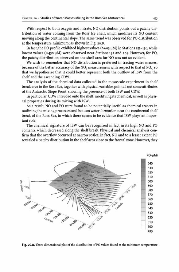
CHAPTER 20 • Studies of Water Masses Mixing in the Ross Sea (Antarctica) 453
With respect to both oxygen and nitrate, NO distribution points out a patchy distribution of water coming from the Ross Ice Shelf, which modifies its NO content moving along the continental slope. The same trend was observed for PO distribution at the temperature minimum, as shown in Fig. 20.S.
In fact, the PO profile exhibited highest values (>603 jlM) in Stations 153-156, while lowest values «450 jlM) were observed near Stations 197 and 204. However, for PO, the patchy distribution observed on the shelf area for NO was not so evident.
We wish to remember that NO distribution is preferred in tracing water masses, because of the better accuracy of the N03 measurement with respect to that of P04, so that we hypothesize that it could better represent both the outflow of ISW from the shelf and the ascending CDW.
The analysis of the chemical data collected in the mesoscale experiment in shelf break area in the Ross Sea, together with physical variables pointed out some attributes of the Antarctic Slope Front, showing the presence of both ISW and CDW.
In particular, CDW intruded onto the shelf, modifying its chemical, as well as physical properties during its mixing with ISW.
As a result, NO and PO were found to be potentially useful as chemical tracers in outlining the mixing processes and bottom water formation near the continental shelf break of the Ross Sea, in which there seems to be evidence that ISW plays an important role.
The chemical signature of ISW can be recognized in fact in its high NO and PO contents, which decreased along the shelf break. Physical and chemical analysis confirm that the overflow occurred at narrow scales; in fact, NO and to a lesser extent PO revealed a patchy distribution in the shelf area close to the frontal zone. However, they
PO (11M)
640
630 620
610
~ ~ _.; - -- .... ,,;:,. 'h,,-
~ ~ i'\ ~" -p; r-- . - 590 -L ... ~~.. , - E # "7 /. ,~ , .... ,,~, ~-" . .- . //:/jjf:;;'~ ~..:.s-.. :~ _~.,. .. 580
570 560 550 540 530 520 510 500 490
Fig. 20.S. Three dimensional plot of the distribution of PO values found at the minimum temperature

454 P. Rivaro . R. Frache
cannot provide additional information on mixing processes without a better understanding of the mixing evolution.
Acknowledgements
This study was performed as a part of the Italian National Program for Research in Antarctica and was financially supported by ENEA through a joint research programme.
The authors are indebted to Prof. Giancarlo Spezie, responsible for the scientific expedition and to Prof. Enrico Zambian chi and Dr. Andrea Bergamasco for their helpful comments and suggestions.
References
Anderson LG, Jones P (1992) Tracing upper waters of the Nansen basin in the Arctic Ocean. Deep Sea Res 39(2):S425-S433
Baines PG, Condie S (1998) Observations and modelling of antarctic downslope flows: A review. Antarctic Res Ser 75:29-49
Bergamasco A, Spezie G, Paschini E, Zambianchi E, Rivaro P, Bottinelli C, Grotti M, (1998). H meso CLIMA 98 experiment: Preliminary analysis and data interpretation. Final Proceedings I Convegno Nazionale delle Scienze del Mare, Ischia, (Italy) 11-14.11.1998
Broecker WS (1974) NO as a conservative water-mass tracer. Earth Planet Sci Lett 23:100-107 Budillon G, Tucci S, Artegiani A, Spezie G (1999) Water masses and suspended matter characteristics of
the western Ross Sea. In: Faranda FM, Guglielmo L, Ianora A (eds) Ross Sea ecology. Springer-Verlag, Berlin, pp 63-93
Catalano G, Benedetti F, Predonzani S, Goffart A, Ruffini S, Rivaro P, Falconi C (1999) Spatial and tem. poral patterns of nutrient distributions in the Ross Sea. In: Faranda FM, Guglielmo L, Ianora A (eds)
Ross Sea ecology. Springer-Verlag, Berlin, pp 107-120 Cooper LW, Cota GF, Pomeroy LR (1999) Modification of NO, PO, and NO/PO during flow across the
Bering and Chukchi shelves: Implications for use as Arctic water mass tracers. J Geophys Res 104(C4l:7827-7836
Hansen HP, Grasshoff H (1983) Automated chemical analysis. In: Grasshoff K, Ehrardt M, Kremling K (eds) Methods of sea water analysis. VCh, Weinheim, pp 347-379
Jacobs SS (1989) Marine controls on modern sedimentation on the Antarctic continental shelf. Mar Geol 85=121- 153
Jacobs SS (1991) On the nature and significance of the Antarctic Slope Front. Mar Chern 35:9-24 Jacobs SS, Fairbanks RC, Horibe Y (198a) Oriljin and evolution of water masses near the Antarctic con
tinental margin: Evidence from H2 BO/H2 60 ratios in sea water. Antarctic Res Ser 43:59-85 Lindegren R, Anderson LG (1991. "NO" as conservative tracer in the Weddel Sea. Mar Chern 35:179-187 Lindegren R, Josefson M (1998) Bottom water formation in the Weddel Sea resolved by principal
components analysis and target estimation. Chemom Intell Lab Sys 44:403-409 Locarnini RA (1994) Water masses and circulation in the Ross Gyre and environs. PhD dissertation, Texas
University, College Station, Texas Mensch M, Simon A, Bayer R (1998) Tritium and CFC input functions for the Weddel Sea. J Geophys Res
103:15923-15937 Minster JF (1989) Introduction to chemical tracers of the ocean circulation. In: Anderson DLT, Willebrand
J (eds) Oceanic circulation models: Combining data and dynamics. Kluwer Academic Publisher, Dordrecht, pp 345-376
Picco P, Bergamasco A, Demicheli L, Manzella G, Meloni R, Paschini E (1999) Large scale circulation features in the central and western Ross Sea (Antarctica). In: Faranda FM, Guglielmo L, Ianora A (eds) Ross Sea ecology. Springer-Verlag, Berlin, pp 95-106
Strickland JDH, Parson TR (1972) A practical handbook of sea water analysis. Bull Fish Res Board Can 167-310
Whitworth T III, Orsi AH, Kim SJ, Nowlin WD Jr (1998) Water masses and mixing near the antarctic slope front. Antarctic Res Ser 75:1-27
Wilson C, Wallace DWR (1990) Using the nutrient ratio NO/PO as a tracer of continental shelf waters in the central Arctic ocean. J Geophys Res 95(C12):22193-22208

Chapter 21
Solid Speciation and Selective Extraction Procedures: Trace Metal Distribution and Speciation in Coastal Sediments of the Adriatic Sea
C. Ianni· N. Ruggieri
21.1 Introduction
Studies on distribution and speciation of heavy metals in sediments can not only provide information on the degree of pollution, but also on the effective environmental impact, metal bioavailability, and their origin. Sediments, in fact, are important sinks for various substances including heavy metals, but they can also be a metal source. The extension of the phenomena depends on the association of the metals with the different phases of the sediments, defined as "solid speciation;' which is usually determined by utilizing selective sequential extraction procedures.
In this work, some case studies concerning determination of metal speciation in coastal sediments of Adriatic Sea will be shown, in order to better explain the importance of solid speciation in environmental studies better. The data presented are part of different projects: the former is a quasi-synoptic research project for the safeguard of the Adriatic Sea (PRISMA 2), in particular of the sector "Physical, chemical and biological oceanography;' undertaken in 1996-98. The latter is an INTERREG II project involving Italy and Greece for the monitoring of the southern Adriatic and Ionic Sea, undertaken in 1999 and still in progress.
21.2 Role of Marine Sediments in the Environment
Marine sediments are caused by unconsolidated accumulations of particles brought to the ocean by rivers, glaciers and winds, mixed with shells and skeletons of marine organisms (Yen and Tang 1977). They are the final destination of trace metals, as a result of adsorption, desorption, precipitation, diffusion, chemical reactions, biological activity and a combination of those phenomena. When some physical disturbance occurs, or because of diagenesis and/or changes in pH or redox potential, sediments can act as a source of metals, releasing them in the overlying water column. This phenomenon can occur even long after the end of direct discharge (Jones and Turki 1997),
and its extension depends on the metal association with the different mineralogical fractions of the sediment. Therefore, metal behaviour and availability strictly depends on their chemical form and thus on their speciation. Determination of solid speciation, defined as the identification and quantification of the different species, forms or phases present in a sediment, has become increasingly important. The measurement of total content, in fact, is not sufficient to get information on the potential availability of metals (whether toxic or essential) to biota under various environmental conditions (Davidson et al. 1994).

456 C. Ianni· N. Ruggieri
21.3 Selective Extractions
To date, it has generally been accepted that the most appropriate methods to evaluate solid speciation are selective sequential extraction procedures (Kot and Namiesnik 2000), which are widely used to assess the long-term emission potential of pollutants and to study the distribution of pollutants among the geochemical phases (Rauret 1998). One must keep in mind that selective sequential extractions give, as a result, "operationally defined species" (Tessier et al. 1979), which depend on the different procedures used. It is not possible to obtain specific chemical associations, because the reagents utilized are often insufficiently specific to exclusively dissolve the "target" phase conditions (Davidson et al.1994) and results obtained can vary widely when different experimental conditions are used (Tipping et al. 1985; Rauret et al. 1989). Nevertheless, useful information can be gained from such studies; in fact, a large number of selective extraction methods have been studied and reported, many of which are variants of the Tessier procedure (Tessier et al.1979). Selective extractions have also been proven to be adequate for determining the metals associated wiili source constituents in sedimentary deposits (van der Sloot et al. 1997). Moreover, according to Rubio et al. (1991), metals with an anthropogenic origin are mainly obtained in the first extractions, while in the last stage of the process, the residual fraction is obtained, corresponding to metals with lithogenic origins.
Recently, studies on selective extractions have received new emphasis with the availability of a sediment reference material, certified by the SM&T programme of the European Union (Quevauviller et al.1997) following a less aggressive procedure. In fact, the increasing performances of the analytical techniques used for element determination in an extract, together with the increasing evidence that exchangeable metals better correlate with plant uptake, has led extraction methods to evolve towards the use of less and less aggressive solutions (Gupta and Aten 1993).
21.3.1 Commonly Used Extraction Procedures
The fractions obtained when applying selective extraction schemes are related to exchangeable metals, metals mainly bound to carbonates, metals released in reducible conditions such as those bound to hydrous oxides of Fe and Mn, metals bound to oxidizable components such as organic matter, and sulphides and residual fraction. The reagents more commonly used in sequential extraction procedures are usually applied according to the following order: unbuffered salts, weak acids, reducing agents, oxidizing agents and strong acids. Exchangeable fraction uses an electrolyte at pH 7 to avoid oxide and carbonate solubilization and to prevent oxyhydroxide precipitation. The carbonate fraction generally uses acetic acid or a buffer acetic acid- sodium acetate at pH 5. These reagents are not able to dissolve all the carbonates, nor can they attack carbonate selectively, as they also remove labile organically bound metals (Rauret 1998; Baffi et al.1998). The reducible fraction is mainly related to metals bound to Fe and Mn oxides. Hydroxylamine in acid solution is the reducing agent most widely used to solubilize these oxides, although iron oxide is not completely dissolved. Ammonium oxalate seems more effective if used in the dark, even if some precipitation

CHAPTER 21 • Solid Speciation and Selective Extraction Procedures 457
of metals oxalate can occur, also at low pH. Dithionite-citrate reagent dissolves oxides and hydroxides, but can also attack iron rich silicates. Therefore, no reducing agent is either selective or completely efficient. Oxidizing agents destroy organic matter and transform sulphides into sulphates. The reagents most widely used are acidic hydrogen peroxide and sodium hypochlorite, and to a less extent, 8 M nitric acid. Residual fraction is usually extracted using the same reagents utilized for the total solubilization, a mixture of strong acids, with or without fluoridric acid, in closed systems at high temperature (usually microwaves ovens). Alternatively, the amount of metals bonded to the residue can be estimated by the difference between the total content and the sum of the amount extracted in the various selective steps.
21.4 Case Studies
Some case studies will be described and commented on to show how selective extraction can be a useful indication concerning metal solid speciation and how this information completes data on the metal content of marine sediments. In some cases, data on granulometric composition and on organic matter content were also available and supported the discussion of the results. In Fig. 21.1, the location of the three areas studied is reported.
21.4.1 PRISMA 2 Project
This project was undertaken to obtain information and to study the physical and biogeochemical mechanisms that influence and determine the transport and diffusion
Fig. 21.1. Map of the studied areas 45.40
44.70
44.00
Z 43.30 L <II
"C
E 42.60 "f j
41.90
41.20
40.50
., ' co·
12.7013.40 14.1014.80 15.50 16.2016.90 17.60 longitude (0 E)
[[]

458 C. Ianni· N. Ruggieri
of the substances (pollutants and others) introduced in the marine environment by the freshwaters of the Po River. The aim of the work on sediments was to provide information on the distribution, enrichment and speciation of some trace metals in the surface sediments of two areas of the Adriatic Sea: Chioggia and Ancona. Chioggia was chosen because of the predominance of fluvial inputs, while Ancona was chosen because the freshwaters follow the coast until Conero Mount (near Ancona). The examples reported are of course only a part of the work regarding this project (Ianni et al. 2000).
21.4.1.1 Methods
Total attack. The samples were treated in microwave Teflon vessels with aqua regia and heated in microwave oven.
Selective extraction. Fraction 1. Exchangeable and carbonates. Ammonium acetate 1 M (pH 5) was added to the sediment, which was shaken overnight at room temperature. The extracts were separated from the residues by centrifugation.
Fraction 2. Bound to Fe and Mn oxides. Hydroxylamine hydrochloride 1 M and acetic acid 25% (1:1) were added to the residue, and the same procedure of the first extraction was performed.
Fraction 3. Bound to organic matter and sulphides. The residue of the second extraction was put in a microwave Teflon vessel and after the addition of 8 M nitric acid, heated in microwave oven.
The metal content of the residual phase was obtained by the difference between the total content and the sum of the Fractions 1, 2 and 3.
21.4.1.2 Results
In both areas, metals total concentration are comparable with those found in other coastal areas of Mediterranean Sea (Donazzolo et al. 1981, 1984; Martincic et al. 1990; Rapin et al. 1979) and are lower respect to very polluted areas, as for example the Gulf of Naples (De Rosa et al. 1983). Chioggia presents, for some elements, higher concentrations, due to the relevant input of freshwaters from the Po River.
As regard speciation, in both areas for all the samples, the reducible fraction is poor of all the elements, and especially of Fe, which should be a major component of the phase. The negative Eh of these sediments (Colantoni, personal communication) outlines that these sediments are in reducing conditions, particularly rich in sulphides and organic matter (Fabiano, personal communication) and poor of oxides. Generally, all the elements studied, except Cd and Pb, which are found at some extent in the labile fraction (exchangeable, carbonates and/or labile organic matter), are associated prevalently to the oxidizable fraction. This renders the elements in these sediments not immediately available, but can be released if redox conditions change, for example for aeration caused by dredging operations.
In Fig. 21.2, the grain size distribution, together with distribution of Pb total content is shown in the area of Chioggia. Beside Pb, even Cd, Sn and Hg present the same

CHAPTER 21 • Solid Speciation and Selective Extraction Procedures
a
Z 45.00 L QI
" :::>
'f ~ 44.80
b
Z 45.00 L QI
" :::>
'f ~ 44.80
12.30
12.30
12.60 12.90 13.20
Longitude (" E)
:G
12.60 12.90 13.20
longitude (0 E)
Fig. 21.2. Area of Chioggia, spatial distribution of; a grain size; b Pb (Ilg t')
459
Silty clay
Clayey silt
Silt
Clayey sand
Silty sand
Sand
50
40
30
20
10
trend of the grain size, with a higher concentration in the central part of the area, where pelite is predominant. Instead, Cu together with Zn and Fe present a decreasing gradient from the coast towards open sea (Fig. 21.3), which is related to freshwater inputs (Po River).
The same trend has been observed for organic matter, particularly for carbohydrates, proteins and lipids (Fabiano, personal communication), by another group working on the same project. Being that all these elements act as micronutrients, it is probable that they are largely associated to organic phases. Cu, in fact, is principally associated to the organic phase and to the labile biologic matter that can be extracted with the first attack (Baffi et al. 1998; Rauret 1998), and that is highly present in these sediments. In fact, high values of the proteins/carbohydrates ratio have been found (Fabiano, personal communication), and this indicates sediments rich of organic matter of recent origin (excretions, dead organism, etc.), being that bacteria use the proteins more rapidly than the carbohydrates. The association of the copper extracted by the acetate buffer with the labile organic matter is confirmed by the same decreasing trend, as shown in Fig. 21.3. Cd presents also the same trend in step 1, although total Cd follows grain size. Moreover, it is the only element found in great percentage in the acetate buffer extract (20-60%); this is partly explained because this element can also

460 C. Ianni· N. Ruggieri
a
18
Z 45.00 . ~. ~G L
15
12
12.30 12.60 12.90 13.20
Longitude (0 El 9
b 8.0
Z 45.00 ° 6.0 ., " ~ 'f ~ 44.80 4.0
I ~( 1I-L904 4 103 7
12.30 12.60 12.90 13.20 2.0
Longitude (0 El
0.0
Fig. 21.3. Area of Chioggia, spatial distribution of; a Cu (fig rl); b Cu (fig rl) in Fraction 1
be found as carbonate (Span and Gaillard 1986), but it is also bonded with labile organic matter, being that the higher percentage (so-60%) is found near the coast.
In Fig. 21.4, the speciation oflead in the northern transect and in Station 71 is shown to highlight how using only total content to obtain information on environmental impact can bring one to a careless conclusion. The total content of Station 71 is SSjlg g-I, while the concentration range found in the transect is IS-30 jlg g -I. Nevertheless, the percentage of Pb present in the first fraction (more available) is 20% for Station 71 and 3S-S0% for the transect. Therefore, the availability in the two cases is the same, and the high percentage present in the Station 71 residue (so%) outlines that, according to Rubio et al. (1991), the Pb has prevalently a lithogenic origin, while in the northern transect it has prevalently an anthropogenic origin (S-20% in residue).
As regards the Ancona area, the distribution of Pb in fraction 1 is partially overlapping the total one, which follows grain size (see Fig. 21.S), especially in the two south transects, and presents an area of greater concentration in the central part and in Stations 83 and 8S. The grain size distribution (Fig. 21.S) shows that this central part and the mentioned stations are rich of pelites. Therefore, we can suppose that the Pb obtained from the first extraction is prevalently adsorbed on small particles, and so is

CHAPTER 21 • Solid Speciation and Selective Extraction Procedures 461
Fig. 21.4. Speciation of Pb in the northern transect and in 100 Station 71 in the area of Chioggia
75
i :c 50 0..
25
o ... I<:.....:=~---..!
2 3 lG 2G 3G
100 ( .1 02
i 75 r /i iJ 03 .R
:c 50 0..
25
0 71
particularly mobile. Moreover, the amount of Pb in fraction 1 is not negligible, being around 20-30% of the total amount. Fortunately, as was mentioned earlier, the lead content, especially in the Ancona area, is not particularly high, so the bioavailable fraction is low enough to be considered not dangerous.
Even in this area, Cd is present at very high levels in the labile fraction (40-60%), indicating its recent origin with respect to the other metals and its relatively higher bioavailability. Moreover, as shown in Fig. 21.6, the distribution of Cd in this fraction follows the grain size trend, so as Pb, it is probably adsorbed on fine particles, and the same consideration as above can be made.
The distribution of Cu in Fraction 1 (Fig. 21.6) follows a decreasing gradient from the coast towards the open sea, as seen for Chioggia, which indicates a recent coastal input, probably in association with labile organic matter. The maximum concentration in this phase is found in Stations 76 and 80 of the south transect, which are relatively lacking in the other elements, whereas the total content is greater in the other two stations (83,85). In this transect, the recent coastal input is remarkable if related to the total content.
21.4.2 Interreg Project
The aim of Interreg project is the monitoring and the characterization of the Apulian coast, in order to individuate degradation caused by anthropic activities, and on the other hand, to individuate zones of particular ecological interest, where in the future

462
a
44.00
z ~
~ 43.70 ~ .£ j
43.40
b
44.00
z ~
~ 43.70 ~ Of j
43.40
13.20
13.20
C. Ianni . N. Ruggieri
Silty clay
Clayey silt
Silt
5 Clayey sand
Silty sand
13.50 13.80 14.10
Longitude (0 E) Sand
9.2
8.0
6.8
5 S.6
4.4
13.50 13.80 14.10
Longitude (0 E) 3.2
Fig. 21.5. Area of Ancona; a grain size; b spatial distribution of Pb (Ilg rl) in Fraction 1
protected marine areas can be created. The project is still in progress, and it foresees the determination and speciation of heavy metals and some organic compounds in the coastal sediments to evaluate the degree of pollution.
21.4.2.1 Methods
Total attack. As described in Sect. 21-4-1.1.

CHAPTER 21 • Solid Speciation and Selective Extraction Procedures
a
44.00
z ~
~ 43.70
.~ ~
43.40
b
44.00
z ~
~ 43.70 Z '= ~
43.40
13.20
13.20
13.50 13.80 14.10
longitude (0 E)
13.50 13.80 14.10
longitude (O E)
3.5
2.5
1.5
0.5
0.20
0.16
0.12
0.08
Fig. 21.6. Spatial distribution in Fraction 1 in the area of Ancona; a Cu (fig I-I); b Cd (fig tl)
Selective extraction. Modified SM&T protocol (accuracy tested on CRM).
463
Fraction 1. Exchangeable and acid soluble. Acetic acid 0.11 M (pH 2.8) was added to the sediment, which was shaken overnight at room temperature. The extracts were separated from the residues by centrifugation.
Fraction 2. Easily reducible phase. Hydroxylamine hydrochloride 0.1 M adjusted to pH 2
with nitric acid was added to the residue with the same procedure as the first extraction. Fraction 3. Bound to organic matter and sulphides. The residue was put in a micro
wave Teflon vessel, and after the addition of 8.8 M hydrogen peroxide, left at room tem-

464 C. Ianni· N. Ruggieri
perature for one hour, then treated at 50°C in an ultrasound bath for two hours. A further aliquot of hydrogen peroxide was added, and the vessels were heated in a microwave oven. After cooling, 2 M ammonium acetate (pH 2) was added, and the procedure was carried out as for Steps 1 and 2.
The metal content of the residual phase was obtained by the difference between the total content and the sum of the Fractions 1, 2 and 3.
21.4.2.2 Results
In this area, total metal content is generally lower than or similar to natural levels, except for Cr and Zn in all samples, and for Pb and Cd only in some particular stations. No fluvial inputs interest this part of the coast, and as it can be seen by the distribution of the fine fraction «63 flm) in Fig. 21.7, near the coast we find a high amount of coarse particles, while the fine particles are found off-shore.
Prior to analysis, the sediments were subdivided in two granulometric fractions « and >63 flm). All the metals in the >63 flm fraction present increasing gradients towards off-shore; in the <63 flm fraction the elements have the same trend (in Fig. 21.7 distribution of Cu is reported as an example), except Cd and Pb, which present an opposite behaviour, as shown in Fig. 21.7 for Pb.
Selective extractions, which were performed on the fine fraction, indicate for Cd and Pb in the area where their concentration is higher (Transects 4 and 6), indicate that both are present, Pb in all stations and Cd in the coastal ones, in the oxidizable fraction (see Fig. 21.8). This phase is not easily mobilizable, but can be oxidized in different environmental conditions. Moreover, Cd is present in the more available fraction, with increasing percentages from the coast towards the open sea. Nevertheless, considering the small percentage of fine fractions in this zone, the concentration of heavy metals in the bulk of the sediment is still low. At any rate, these results outline an evident coastal input, probably associated to organic matter, not present for the other elements.
In all the other cases, selective extractions outlined that metals are present in very low amounts in the three fractions extracted and up to 80% in the residue. As an example, speciation of Cu and Cr in two transects where their total content was particularly high is reported in Fig. 21.9.
As far as this set of data can indicate, these sediments don't seem particularly polluted, even if in some cases variations in physical and chemical conditions can cause negative impacts on the environment. Even in this case, these are some examples drawn from the work, which being still in progress, foresees other sampling and analysis. It will be interesting, for example, to evaluate the results of selective extractions performed on the coarse fraction, which in some cases presents higher contents with respect to the fine fraction.
21.S Conclusions
The case studies reported confirmed that selective extractions are a very useful and versatile technique to investigate on environmental impact, bioavailability and metal origin in marine sediments. Obviously, for a complete understanding of enrichment,

CHAPTER 21 • Solid Speciation and Selective Extraction Procedures
a 40.80
Z L 40.70 III
"0 ::> ... 'f ~
40.60
b 40.80
Z L 40.70 III 'tI ::l
'f ~
40.60
c 40.80
Z L 40.70 III 'tI
.€ t:: ~
40.60
I
I
l~fG
I
~9E
17.90 18.00 18.10 longitude (0 E)
.:3H e4H
17.90
17.90
t:E 18.00
Longitude (0 E)
18.00 longitude (0 E)
18.10
18.10
Fig. 21.7. Area of Brindisi; spatial distribution of; a fine fraction; b Pb (f1g rl); c Cu (f1g rl)
100
80
60
40
20
o
120
90
70
50
40
30
20
19
16
13
10
465
diffusion and speciation mechanisms, when possible, knowledge of parameters for grain size, mineralogy, organic matter content, and so on, is of great usefulness. For

466 C. Ianni . N. Ruggieri
Fig. 21.S. Speciation of Ph and Cd in Transect 4 in the area of 100 Brindisi
80
l60 .0 CL.
40
20
0 4E 4F 4G 4H
~ 100
80
l60 "1J u
40
20
0 4E 4F 4G 4H
.1 02.3 OR
example, the correspondence between a metal distribution in the labile fraction and the fine fraction indicates that the metal is prevalently found in the exchangeable phase. Correlation with organic matter content can indicate that an element in the oxidizable phase is bound to organics rather than to sulphides.
Therefore, as selective extraction procedures are so essential for environmental studies and considering the recent improvements in these analytical methods and the availability of reference material, their utilization is strongly advisable.
Acknowledgements
This work was fmancially supported by the Italian National "Programma di Ricerca e Sperimentazione per il Mare Adriatico" 2nd phase (PRISMA 2) and by the CE project "INTERREG II Italia - Grecia"

CHAPTER 21 . Solid Speciation and Selective Extraction Procedures 467
Fig. 21.9. Speciation of Cu and Cr in Transects 4 and 8 in the 100 area of Brindisi
80
l 60
::l
U 40
20
o I" ( 4E 4F 4G 4H
100
80
l 60
U 40
20
0 8F 8G 8H
.1 0 2 .3 DR
References
Baffi F, Ianni C, Ravera M, Soggia F, Magi E (1998) Evaluation of the acetate buffer attack of a sequential extraction scheme for marine particulate metal speciation studies by scanning electron microscopy with energy dispersive X-ray analysis. Anal Chim Acta 360:27-34
Davidson CM, Thomas RP, McVey SE, Perala R, Littlejohn D, Ure AM (1994) Evaluation of a sequential extraction procedure for the speciation of heavy metals in sediment. Anal Chim Acta 291:277-286
De Rosa S,Damiani V, Serena F (1983) Studio dei sedimenti del Golfo di Pozzuoli: Livelli di contaminazione da metalli pesanti. Atti V Congr Naz AIOL, Stresa, pp 437-447
Donazzolo R, Hieke Merlin 0, Menegazzo Vitturi L, Orio AA, Pavoni B (1981) Heavy metal contamination in surface sediments from the Gulf of Venice, Italy. Mar Pollut Bull 12:417-425
Donazzolo R, Hieke Merlin 0, Menegazzo Vitturi L (1984) Heavy metal content and lithological properties of recent sediments in the northern Adriatic. Mar Pollut Bull 3:93-101
Gupta SK, Aten C (1993) Comparison and evaluation of extraction media and their suitability in a simple model to predict the biological relevance of heavy metal concentrations in contaminated soils. Int J Environ Anal Chern 51:25-46

468 C. Ianni· N. Ruggieri
Ianni C, Magi E, Rivaro P, Ruggieri N (2000) Trace metals in Adriatic coastal sediments: Distribution and speciation pattern. Toxic Environ Chern 78:73-92
Jones B, Turki A (1997) Distribution and speciation of heavy metals in surficial sediments from the Tees Estuary, north-east England. Mar Pollut Bull 34:768-779
Kot A, Namiesnik J (2000) The role of speciation in analytical chemistry. Trends Anal Chern 19:69-79 Martincic D, Kwokal Z, Branica M (1990) Distribution of zinc, lead, cadmium and copper between dif
ferent size fractions of sediments. II. The Krka River estuary and the Kornati Islands (central Adriatic Sea). Science Total Environ 95:217-225
Quevauviller P, Rauret G, LopeZ-Sanchez JF, Rubio R, Ure AM, Muntau H (1997) The certification of extractable contents (mass fractions) of Cd, Cr, Ni, Pb and Zn in sediment following a three-step sequential extraction procedure. European Commission, Bruxelles (Report EUR 17554 EN)
Rapin F, Fernex F, Favarger PY, Vernet JP, Dievoet E van(1979) Repartition du mercure dans Ie sediments marins superficiels du plateau continental de la Cote d' Azur (France, Mediterranee). Rev Int Oceanog Med 53:41-49
Rauret G (1998) Extraction procedures for the determination of heavy metals in contaminated soil and sediment. Talanta 46:449-455
Rauret G, Rubio R, Lopez-Sanchez JF, Casassas E (1989) Specific procedure for metal solid speciation in heavily polluted river sediments. Int J Environ Anal Chern 35:89-100
Rubio R, Lopez-Sanchez JF, Rauret G (1991) La especiacion solida de trazas de metales en sedimentos. Aplicacion a sedimentos muy contaminados. Anal De Quim 87:599-605
Sloot HA van der, Heasman L, Quevauviller P (eds) (1997) Harmonization of leaching/extraction test. Elsevier Science, Amsterdam, pp 75-99.
Span D, Gaillard JF (1986) An investigation of a procedure for determining carbonate-bound trace metals. Chern Geol 56:135
Tessier A, Campbell PGC, Bisson M (1979) Sequential extraction procedure for the speciation of particulate trace metals. Anal Chern 51:844-850
Tipping E, Hetherington NB, Hilton J, Thompson DW, Bowles E, Hamilton-Taylor J (1985) Artifacts in the use of selective chemical extraction to determine the distributions of heavy metals between oxides of manganese and iron. Anal Chern 57:1944-1946
Yen TF, Tang TIS (1977) Chemical aspects of marine sediments. In: Yen TF (ed) Chemistry of marine sediments. Ann Arbor Science, Ann Arbor, Mich., pp 1-38

Chapter 22
Organic Matter Sources and Dynamics in northern Adriatic Coastal Waters
M. Pettine . L. Patrolecco . S. Capri
22.1 Introduction
Organic matter in marine environments results from both autochthonous and allochthonous sources. Phytoplanktonic production is responsible for the internal production of organic matter, which according to dominant biological processes, distributes between the particulate and dissolved phases. Photosynthetic activity transforms, in the presence of inorganic nutrients and light, inorganic carbon into particulate organic matter (POM), of which more than 30% consists of carbon (POC) according to the Redfield stoichiometry and its revisitation by Morel and Hudson (1985). During photosynthetic processes, a variable percentage of photosynthates is released in the surrounding water as dissolved substances (DOM), consisting of monomeric and low molecular weight polymeric compounds. Other than being directly released by phytoplankton, DOM may be indirectly produced through sloppy feeding (i.e. the release of dissolved compounds following the breaking of large preyed cells that cannot be ingested whole by the zooplankton), dissolution of faecal pellets and marine snow, and virus-induced bacteria cell lysis.
Dissolved organic carbon (DOC) is by far the major carbon pool in oceans, outweighing any other marine source of organic carbon by at least a factor of 10 (Kepkay 1994). Furthermore, although algal biomass in oceans is only 0.2% of that of terrestrial plants, annual phytoplankton photosynthesis is roughly equivalent to that of plants, since algae have duplication rates on the order of days compared to month to years for plants (Chisholm 1992). Therefore, the fate of carbon in oceans not only influences the trophic food chain but also affects the exchange of carbon at the sea water-atmosphere interface.
In addition to the autochthonous sources, external inputs may further supply organic matter for marine ecosystems. On a world scale, terrestrial sources contribute about 10% to the total sea water DOM, while on a local scale their contribution may be much more important. Riverine inputs either directly discharge organic matter into sea water or indirectly provide new organic matter through the discharge of nutrients that feed primary production.
External inputs have markedly increased the productivity of the shallow and small northern Adriatic over the oligotrophic features of the Mediterranean. External annual contributions of nutrients in this basin have been estimated to be of the same order of magnitude as the regeneration rate, thus giving similar contributions to primary production from new and regenerated material (Degobbis and Gilmartin 1990). This evaluation strengthens the vulnerability of the northern Adriatic to external inputs and therefore to water management of rivers that discharge into this basin. An-

470 M. Pettine . L. Patrolecco . S. Capri
nualloads of organic matter directly discharged into northern Adriatic waters account for more than 30% of the annual phytoplankton production in its most productive region along the western side (Pettine et al. 1998).
Responses of plankton biomass and productivity to riverine discharged nutrients and organic matter have been studied in many coastal ecosystems including the Hudson River, Narragansett Bay, northern Gulf of Mexico, Chesapeake Bay, Columbia River estuary, and the Baltic Sea (Benner et al. 1992; Maske 1994; Malone 1994; Cloern 1996; Harding et al. 1999; Kemp et al. 1999; Malone et al. 1999; Klinkhammer et al. 2000).
River-induced eutrophication is a general observed phenomenon involving a number of negative consequences such as excess phytoplankton growth, increased frequency of blooms, seasonal decline of oxygen in bottom waters, and changes in the trophic structure (Harding et al.1999). However, the severity of these problems and in particular the fate of DOM resulting from both autochthonous and allochthonous sources may be strongly dependent on seasonal variations of freshwater flow, the geomorphology of the receiving systems and the dominant circulation pattern.
This was clearly disclosed by a recent thorough comparison (Malone et al. 1999) between the Chesapeake Bay (CB) and northern Adriatic (NA). Both of these systems are dominated by a single river, the Susquehanna in CB and the Po in NA; however, despite some similarities in terms of freshwater and nutrient loading, they exhibit significantly different trophic status. CB waters appear to be much more efficient in sequestering nutrients and retaining and recycling phytoplankton biomass than NA waters (Harding et al. 1999); in this latter system the export of nutrients due to water mass exchanges between the northern and middle basins, favoured by the counterclockwise circulation pattern during most of the year, and the confinement of regenerated nutrients, due to the strong vertical stratification during summer, reduce its capacity to retain nutrients on time and scale that promote primary and secondary productivity (Harding et al. 1999).
NA waters exhibit markedly lower average productivity levels than CB waters, although they experience large trophic gradients from coastal eutrophic to off-shore oligotrophic waters. However, the dynamics of DOM in this basin has resulted in the formation of a large quantity of sticky mucilaginous masses with serious problems for tourists and fishery activities; in 1989, the damages amounted to billion of dollars according to Italian authorities' estimations. This phenomenon is not reported for CB waters (Malone et al. 1999), while both the CB and NA systems experiment seasonal oxygen decline; anoxic problems are, however, much more severe in the former compared to the latter system.
There is now wide consensus that mucilaginous aggregates consist of organic and inorganic material entrapped in a gelatinous polysaccharides matrix (Degobbis et al. 1995), although timing and evolution of mucilaginous aggregates, trigger mechanisms, and biological species possibly involved in the formation of aggregates are still largely unknown (Funari et al. 1999). The mean percent values and related standard deviation (±x) of organic carbon, nitrogen, phosphorus, silicon and sulphur in aggregates collected in the summer of 1991 from surface and deep northern Adriatic waters were 24.0 ±7.2, 2.9 ±1.1, 0.26 ±0.12, 6.4 ±4.5 and 1.1 ±0.5, respectively (Pettine et al. 1995).

CHAPTER 22 • Organic Matter Sources and Dynamics in Adriatic Coastal Waters 471
The scarce information available on the distribution and variability of dissolved organic matter and its important components in the northern Adriatic is one of the restrictions on the understanding of the mucilage occurrences.
In an attempt to improve our knowledge on sources, concentrations and variability of organic matter in coastal waters, we have determined organic matter loads discharged by the Po River in the dissolved and particulate phases, and the concentrations of dissolved (DOC) and colloidal (COC) organic carbon, together with those of total dissolved carbohydrates (TDCHO), free (DFAA) and total dissolved (TDAA) amino acids in two frontal regions of the northern Adriatic system (see Fig. 22.2). Polymeric organic compounds that are included in the colloidal fraction and in the TDCHO and TDAA variables are of particular interest in northern Adriatic waters for their involvement in the formation of micro- and macro aggregates.
This paper summarizes the results obtained in previous investigations (Pettine et al. 1998, 1999, 2001) highlighting an interannual variability in seasonal changes of DOC concentrations, which is strongly dependent on the hydrological regime of the Po River. Experimental findings also point out contrasting behaviours of mucilage and seasonal changes in DOC, COC and TDCHO concentrations, which strengthen the importance of the qualitative character of DOM, rather than its quantitative concentrations in triggering the formation of large mucilaginous aggregates.
22.2 Analytical Methodologies
Dissolved Organic Carbon. Samples were filtered through precombusted (4 hours at 480°C) and preweighed Whatman GF/F glass fibre filters (0.7Ilm nominal pore size). For freshwater samples, filtration was performed in a laboratory within a few hours from collection: in this case about 1 I samples were filtered under negative pressure and the filters, washed with 20 ml milli Q water, were stored at -20°C for the analysis of Poe. Filtered freshwater samples for DOC analysis were stored in high density polyethylene (HDPE) bottles as in the case of filtered sea water samples (see after) while the filtration procedure was different. For sea water samples, the filtration was performed aboard, and we were not interested in the analysis of POC: about 100 ml were filtered in this case by using a disposable polycarbonate syringe and a polypropylene filter holder (Nucleopore). Filtered samples were stored in duplicate into 25 ml HDPEbottles (previously treated with HN03 1.2 M at 50°C for 1 h), which were quickly frozen in an aluminum block at -20°C. The suitability of HDPE containers for the storage of DOC samples was proved by recent findings (Norrman 1993; Tupas et al. 1994; Yoro et al. 1999), and confirmed by our preliminary tests. For DOC analysis, filtered samples were thawed in the laboratory, acidified to pH 2 with ultrapure HCI and purged with Nz for about 10 minutes to remove inorganic carbon. Dissolved organic carbon (DOC) was assayed by high temperature catalytic oxidation (HTCO) and infrared detection using a Shimadzu TOC-5000 A analyser. Carbon concentrations were determined against potassium hydrogen phthalate standards after correction for total blank. This value, which is the analytical system blank plus a Milli Q water blank, was approximately 10-15 IlM C under our experimental conditions and was mostly due to the

472 M. Pettine . L. Patrolecco . S. Capri
experimental system. Samples were measured in triplicate with a fixed c.v. of 2%; otherwise, further replicates were automatically carried by the instrument.
Particulate Organic Carbon. For pac analysis, the filters were dried at 60°C overnight, re-weighed to determine particle loading and homogenized in an agate mortar mill. Blank filters were processed the same way. Powered, homogenized samples (10-15 mg) were accurately weighed (±0.01 mg) into tin or silver cups (9 x 5 mm) to determine particulate nitrogen (PN), total particulate carbon (PC) or particulate organic carbon (PaC). Samples in silver cups were acidified with 20 fJl5 M ultrapure HCl and kept at 50-60°C for 30 min to remove inorganic carbon. Care was taken to ensure complete saturation of the sample with HCl and to avoid sample loss. Acid treatment was repeated until effervescence was no longer observed (generally three times). PC, pac and PN were determined by high temperature oxidation using a Carlo Erba NA 1500 series 2 C/H/N/O/S analyser. Samples were run in duplicate. The sulphanylamide standard was used to construct the calibration curve. Carbon and nitrogen contents were expressed as percentage of total solid and as concentration (mg tl) of filtered water sample. Average blank levels were 2.5 ±0.8 flg C and <0.5 flg N; detection limits (calculated as three times the standard deviation of the blank for carbon, and according to sensitivity of the instrument for nitrogen) were 2 and 0.5 flg for carbon and nitrogen, respectively, corresponding to 0.02% C and 0.005% N for a 10 mg sample. Analytical precision was ±2.3 and ±1.8% of the measured values for total and organic carbon and ±1.6% for nitrogen. Particulate inorganic carbon (PIC) was determined by the difference between PC and poe. Only pac data will be discussed in this paper.
Colloidal Organic Carbon. A limited number of sea water samples were processed with a tangential flow ultrafiltration (UF) system (Amicon DC10LA) to investigate the molecular weight distribution of the DaM pool. For DOC fractionation, about 30 1 samples were filtered aboard, immediately after collection, through 0.4 flm polycarbonate filters (Nucleopore, 0 142 mm) in a closed pressurized system (N2), using a Sartorius Teflon -covered apparatus. To avoid contamination, the first 1-2 I of the filtrate were discharged. Filtered samples were then passed in cascade through two polysulphone membranes, which have nominal molecular weight cut -offs of 10 kDa (hollow-fibre cartridge, Amicon, HlOPlO) and 1 kDa (spiral-wound cartridge, Amicon, SlONl), respectively. Operating pressures were 20-25 psi at the inlet and 10-15 psi at the outlet of the system. UF cartridges were thoroughly cleaned, recirculating sequentially 0.1 N NaOH and 0.01 N HCl solutions for at least 30 min before and between samples and rinsing several times with about 5 1 Milli-Q water. Finally, after conditioning the UF cartridges with about 11 filtered sample, about 20 1 of sample were processed and the concentrated colloidal fraction was reduced to about 21, thus achieving a lO-fold concentration factor.
Following this procedure, we fractionated the DOCpool into a low-molecular-weight or "truly dissolved" fraction (DOC < 1 kDa) and two colloidal size classes, operationally defined as low-molecular-weight COC (1 kDa < LCOC < 10 kDa) and high-molecular weight COC (10 kDa < HCOC < 0.4 flm). Each sample was stored frozen in duplicate into 25 ml high density polyethylene (HDPE) bottles (as previously described for DOC). In the laboratory, DOC analyses were performed on 0.4 flm polycarbonate filtered samples and their four different molecular weight fractions (>10 kDa; <10 kDa; 1-10 kDa; <1 kDa), in order to calculate partial mass balances on each cartridge. DOC

CHAPTER 22 • Organic Matter Sources and Dynamics in Adriatic Coastal Waters 473
recovery (R, as a percentage of the initial DOC) was calculated according to Dai et al. (1998). For the 1 kDa cartridge, R % ranged from 87 to 120% (with an average of 101 ±8%), while for the 10 kDa cartridge, R % ranged from 83 to 117% (with an average of 100 ±8%). Overall recovery in our ultrafiltration system was close to 100% (±1O%) and was within the ranges reported in the literature (Guo et al.1994; Benner et al.1997; Dai et al. 1998), indicating that contamination or loss of organic carbon were minimal. While this fractionation procedure is probably the best one available at the moment and the most widely used, we must note that interactions at membrane surface may lead to conformation changes, irreversible adsorption and lor self-coagulation of small molecules resulting in an overestimation of COC (Buftle and Leppard 1995; Guo et al. 2000).
Dissolved Free (DFAA) and Total Dissolved (TDAA) Amino Acids. Samples for total dissolved amino acids (TDAA) were analyzed after liquid hydrolysis in 6 N HCl at 110°C for 22 h (modified from Parson et al. 1984). 2 ml samples were placed in glass ampoules (acid washed and muffled for 3 hours at 500°C), sealed under a flow of N2• Each vial was spiked with a-aminoadipic acid, norvaline and hydroxylysine as recovery standards of the acidic, neutral and basic classes, respectively (Cowie and Hedges 1992), and 2 ml of ultrapure 12 N HCl. Hydrolysates were vacuum dried and then redissolved in milli-Q water to achieve a neutral pH. DFAA were analyzed without preliminary hydrolysis of the samples.
DFAA and TDAA were determined by high performance liquid chromatography (HPLC-Perkin Elmer Series IV) and fluorimetric detection (Perkin Elmer LS4) with a gradient system of methanolltetrahydrofuran (90:10 v/v) acetate buffer, following derivatization with o-phthaldialdehyde (OPA) and 2-mercaptoethanol (Lindroth and Mopper 1979, as modified in Pettine et al.I999); 21 individual amino acids were separated according to this procedure (see Fig. 22.1). Daily standards in aged sea water, samples and blanks (aged sea water) were run in triplicate. The average TDAA blank amounted to 62 ±40 nM and was mainly due to glycine, aspartic acid, serine and alanine. Recovery for most of the amino acids was within ±1O% except for asparagine, glutamine, tryptophane, histidine and methionine. In the analysis of free amino acids, glutamic acid, glutamine, aspartic acid and asparagine are separated into four distinct peaks, but the acid hydrolysis performed for analyzing total dissolved amino acids causes the deamination of asparagine (asn) and glutamine (gIn) to form aspartic acid (asp) and glutamic acid (glu) plus ammonium. Therefore, in the TDAA analysis, the amino acids pairs (asn + asp and gIn + glu) give only two peaks instead of four. Tryptophane is unstable during acid hydrolysis and may not be detected. Histidine is also partially modified by acid hydrolysis and the recovery is only 20-30% (Keil and Kirchman 1991). DFAA and TDAA are expressed as individual amino acids (nM) and as the sum of the amino acidic molar carbon (DFAA-C or TDAA-C) and nitrogen (DFAA-N or TDAA-N) units.
Total Dissolved Carbohydrates. Total dissolved carbohydrates (TDCHO), including mono-, oligo- and polysaccharides, were analyzed by the MBTH method after a preliminary hydrolysis with 0.09 N HCl (20 h at 100°C) (Burney and Sieburth 1977). This hydrolysis procedure was preferred to the stronger H2S04 attack more recently proposed (Pakulski and Benner 1992; Mopper et al. 1992), mainly because it has been extensively used in estuarine and coastal waters, thus making the comparison with previous find-

474
Fig. 22.1. An example of HPLC spectrum of amino acids in a sea water sample; 1: aspartic acid; 2: glutamic acid; 3: aspar- . agine; 4: serine; s: histidine; 6: glutamine; To glycine; 8: threonine; 9: arginine; 10: alanine; 11: tyrosine; 12: r-aminobutyric acid (internal standard); 13: valine; 14: phenylalanine; IS: isoleucine; 16: leucine; 17: ornithine; 18: lysine; methioninsulphone, methionine, tryptophane and norvaline were not detected in this sample
4
7
2
5 10 15
M. Pettine . 1. Patrolecco . S. Capri
8
10
20
t(min)
i.s. 12
25
13 14
16
30
17
35
ings feasible (see Pettine et al. 1999 for more details). Furthermore, polysaccharides determined by this method would more directly reflect changes in the concentration of exuded polymers (Benner 1998), which include transparent exopolymer particles actively involved in the aggregate formation (Passow and Alldredge 1994; Passow 2000). Samples were analyzed in triplicate against glucose standard solutions, and results were expressed in terms of glucose-carbon equivalents (TDCHO-C), by assuming 6 moles of carbon per mole of hexose. The relative standard deviation between replicate samples was usually below 5%.
22.3 Role of Organic Matter Dynamics in NA Environmental Problems
The dynamics of the DOC pool in the northern Adriatic basin are involved in hypoxic and anoxic crises in bottom waters and massive occurrences of mucilaginous aggregates in the water column.
Anoxic phenomena occur during summer in the western coastal waters, which are influenced by the Po River discharge. Since 1975, when nutrient loads discharged by the Po showed an abrupt increase (Marchetti 1990) as happened in other European rivers (Kempe et al.1991), large algal blooms have occurred regularly, causing episodes of diffused anoxia at the sea bottom, which resulted in mass mortalities of benthic organisms. The spatial and temporal extensions of areas affected by anoxia have diminished in recent years (Degobbis et al. 1999), probably as a consequence of the reduction and banning of phosphorus in Italian detergents. Toxic algal species on occasion also developed, causing severe damages to mollusc cultures and threatening human health. In addition to these environmental deterioration problems that are typical of eutrophicated systems, the northern Adriatic has experienced a peculiar phe-

CHAPTER 22 • Organic Matter Sources and Dynamics in Adriatic Coastal Waters 475
nomenon consisting of massive occurrences of mucilaginous aggregates. In 1989, these aggregates covered a large part of the entire surface of the NA basin (Stachowitsch et al. 1990) and drew the attention of public and scientific opinion. Large quantities of sticky mucilaginous masses affected biological, chemical and physical characteristics of the ecosystem (Degobbis et al.1999). Part of the material floating on the sea surface was deported on beaches by wind and currents, reducing their suitability for bathing and threatening tourism. Suspended and sinking mucilaginous aggregates created serious problems for fisheries and biota. Benthic organisms suffered in many areas from suffocation due to their covering by aggregates.
The impressive mucilage events of 1989-91 stimulated many studies aimed at understanding the possible causes responsible for this phenomenon and its triggering mechanisms; however, in spite of these efforts, this phenomenon remains substantially unknown (Funari et al. 1999). Although it was reported that episodes of massive mucilage formation have been recorded for over a century (Fonda-Umani et al.1988), the similarities between past and recent phenomena in terms of triggering factors and spatial extensions remain in doubt.
We speculated on the strict temporal parallelism between massive aggregate occurrences and changes in the formulation of detergents (Pettine et al. 1995). In 1988, in fact, phosphorus was banned from domestic detergents and substituted by zeolite A particles and about doubled polycarboxylate concentrations. These changes have further increased the NIP ratio in coastal waters, which was already unbalanced, and probably they were responsible for the shift in the phytoplankton population from dinoflagellate to diatom blooms recently reported (Degobbis et al. 1999).
Therefore, P-substitutes, while contributing to diminish the frequency and extension of anoxia in NA coastal waters, apparently cause an external forcing on biological and chemical processes, which could favour an intensification of macroaggregate occurrences. Possible effects may be on a large scale (changes in algal succession from dinoflagellate to diatoms and on their released chemical compounds; limitation of the bacterial activity due to further increase in NIP ratio and consequently increased residence time for DOM) as well as on a micro scale (changes in sorption, partitioning and gelling of polymers, due to the inclusion in colloidal matter of zeolite A particles and polycarboxylates).
22.4 Organic Matter Discharged by the Po River
Concentrations of dissolved and particulate organic carbon (DOC, POC) were measured in samples taken monthly for a year at two stations in the lower Po River (Figs. 22.2 and 22.3). Samples were collected at each station at two depths (about 0.5 m from surface and 2 m above the bottom) to evaluate possible variations in the water column that may affect the transport. Two major interrelated variables, solid transport and flow conditions, influenced the variability of organic matter concentrations in the water and solid phases, while the water column was reasonably homogeneous (Pettine et al. 1998).
Mass fluxes of DOC and POC to the northern Adriatic basin were calculated by four different methods. They were based on: (a) the mean of products of the instantaneous concentrations and the mean daily discharge of the sampling day; (b) the product of

476 M. Pettine . L. Patrolecco . S. Capri
30' 12° 30' 13° 30' 14°
30'
45°
30'
44°
Fig. 22.2. Location of the study area. In the Po River, only the Pila station is shown; the other (Pontelagoscuro) is upstream of the river stretch plotted. In the NA system, the two investigated frontal regions, one in the north (N) and the other in the south (S), are shown
the arithmetic means of the concentrations and discharges; (c) the product of discharge-weighted concentrations and the mean annual discharge; and (d) the sum of the products of daily discharge and concentration resulting from the concentration vs. flow equation, extended to a whole year. Methods a and b, which use the arithmetic mean of instantaneous loads or arithmetic means of concentrations and discharges, give equal weight to each pair of variables. This may introduce a major bias in calcu-

CHAPTER 22 • Organic Matter Sources and Dynamics in Adriatic Coastal Waters
Fig. 22.3. Monthly average organic carbon concentration in the lower stretch of the Po River
8
-;'7 .s c: 6 o
·s 5 c: <II v
5 4 v c:
~ 3 el
.!:! 2 c:
E> o
o ~ ~ >. c
:;E ~ ~ ~
fOOOCl ~
- ~ c. 1:: ~ <I: ~ 0
1) :rl Z 0
477
c: ~
..0 ~
lations, since concentrations measured at low discharge have the same importance as those at peak discharge. Method c reduces this bias and improves the evaluation of mass transport by use of discharge-weighted means; while Method d, based on the total discharge curve, is the more accurate has a better correlation between concentration and discharge. In our case, these different methods provided reasonably close estimations; however, results by Method c are more appropriate and gave fluxes of 13.4 x 10⁴ and 12.1 x 10⁴ tonnes year-I for POC and DOC, respectively.
These loads may be compared with those discharged by the Rhone River, which shows some similarities with the Po River. Both these rivers originate from the Alps, drain large catchment areas (Rhone 96000 km2 and Po 70091 km2), have reasonably similar solid transport (about 5 x 10⁶tonnes year-I) and water discharge (55 km3year-1
in the Rhone vs. 47 km\ear- I in the Po). The TOC load for the Rhone was estimated to be 15 x 104 tonnes year-I, one third of which is POC (Kempe et al.I991). Thus, in terms of TOC, the Po export rate (25.5 x 10⁴ tonnes year-I) is about 1.7 times higher than that of the Rhone, making the former river the largest contributor of organic matter to the Mediterranean. The Nile River, which is another large river discharging into the Mediterranean, is extensively exploited for irrigation, hence its discharge into the sea is strongly reduced.
Organic carbon appears to be preferentially transported in the solid phase in the Po compared with the Rhone (DOC discharges are in fact similar, while POC discharges are markedly different), and this different partitioning reflects a high carbon content in the particulate matter transported by the Po, since solid transport in the two rivers is similar. These differences in the particulate and total transport of organic carbon are strongly related to marked differences in population densities in the watersheds of these rivers (232 and 84 inhabitants km-2 for the Po and the Rhone, respectively).
However, the TOC export rate by the Po (3.57 tonnes km-2 year -I), which is given by the ratio between the calculated load and the surface extension of the river catchment, is slightly lower than the average export rate estimated for major temperate rivers

478 M. Pettine . L. Patrolecco . S. Capri
(4 tonnes km -2 year -1; MeybeckI 982). Therefore, although the Po exhibits a higher TOC discharge compared to other Mediterranean rivers, its TOC export rate does not suggest a marked alteration by anthropogenic activity, pointing out that the self-purification capacity of the river is able to maintain organic matter concentrations at a low level in the lower stretch.
22.S Interannual Variability of DOC Concentrations in NA Coastal Waters
DOC concentrations have been measured on more than 400 samples from surface and deep waters at different distances from the Po mouth in two frontal regions, (Pettine et al. 1999 and 2001). The location of these frontal regions, which could move depending on the seasonal period, is exemplified in Fig. 22.2 for the June 1996 cruise. The overall ranges of DOC concentrations and salinity resulting from all the four cruises were 70 to 280 flM and 30 to 38, respectively. Average DOC values in the four cruises carried out in the northern region, under the direct influence of the Po river, are shown in Fig. 22.4. In winter, deep waters assume a typical background value of 76 ±10 flM, averaged from all the available data in both the northern and southern region. This average value is well within the range 50-92 flM characteristic of deep and surface western Mediterranean (Copin-Montegut and Avril 1993), and is also very close to concentrations typical of surface oceanic waters (70-80 flM; Guo et al.1995). These low winter concentrations suggest that the Adriatic system has a good capacity to react to external forces through degradation processes and water mass exchange between the northern and middle basins.
Surface values in winter show only a slight increase with respect to the background value, while during summer, changes appear much more marked. However, seasonal changes were found to strongly depend on the hydrological regime of the Po River, which is responsible for over 50% of the total riverine discharge into the northern Adriatic system.
In June 1996, average surface values were a factor of 2.6 and 2.1 higher than the background value (76 ±10 J.1M) in the northern and southern regions, respectively. In June 1997 the corresponding increasing factors were 1.7 and 1.3. This interannual vari-
Fig. 22.4. Average DOC con- 200 centrations in the northern frontal region of the four cru~~ 100
~ 120 ~
~ 80
40
o J96
~ ~ F97 J97 F98

CHAPTER 22 • Organic Matter Sources and Dynamics in Adriatic Coastal Waters 479
ability reflects changes in the Po discharge curve during these two years: in 1996, many peaks preceded the June cruise, while in 1997 a long low flow period prevailed before the June cruise (Fig. 22.5). Accordingly, temporal patterns of chI a concentrations in the receiving coastal waters pointed out a much higher productivity in the spring of 1996 than in 1997, which was responsible for the higher increasing factors observed for DOC concentrations in the former year compared to the latter (Pettine et al. 2001).
Contrary to the increase in DOC concentrations that were stronger in 1996 than in 1997 (Fig. 22.6), mucous aggregates showed a much stronger occurrence in June 1997
8~.------------------------------------------------------.
6000
"1,
14000
~ u::
2000
o D
I·· ... ··:~ I
F M A
" ',:
M A S o N D F
Fig. 22.5. Discharge curves of the Po River in 1996 and 1997. The two arrows indicate the two-year cruise period
Fig. 22.6. Calculated increments (liM) in DOC concentrations over the background winter value of 76 liM in June 1996 and June 1997
120r---------------------------~
~ 2: 80 ~ c: ~ ~ v .= ~ 40 o
0+1-----' J 96 J 97

480 M. Pettine . L. Patrolecco . S. Capri
compared to June 1996. This was confirmed by the use of the remote observing vehicle (ROV) during the cruises. The scavenging effect exerted in the water column by mucous macroaggregates may partially explain an inverse relationship between macroaggregates and dissolved DOC concentrations. However, these findings point out that high DOC levels, as in the case of June 1996, do not necessarily produce macroaggregates, strengthening the importance of the qualitative characteristics of the DOC pool in the mass transfer between DOC, COC and the mucous fraction.
The conclusion by Passow (2000) that TEP-precursors, which consist of strongly sulphated polysaccharides actively involved in aggregation processes, appear to be a distinct group of polysaccharides, whose production and standing stocks are uncoupled from bulk carbohydrates, further remarks the importance of the qualitative characteristics of DOM in the formation of aggregates. The higher sulphur level found in macroaggregates in our previous investigations (Pettine et a1.199S) is consistent with a large role played by TEP in the formation of macroaggregate.
22.6 Composition of DOM
Dissolved organic matter in the northern Adriatic system is characterized by the presence of a high colloidal fraction with a shift in the molecular weight distribution toward the large size fraction and a high contribution of carbohydrates to dissolved organic matter (Pettine et al. 1999 and 2001).
The average values (11M) calculated from all the data were 67 ±14 for the overall colloidal organic fraction (>1 kDa) and 39 ±13 for the truly dissolved organic fraction (DOC> 1 kDa). Differences between the June and February cruises were very small (Fig. 22.7). The colloidal organic carbon pool consisted of high (>10 kDa, HCOC) and low (1 to 10 kDa, LCGC) molecular weight classes. The HCGC fraction accounted for
Fig. 22.7. Distribution of dissolved organic matter «0.7 flIll) between the high (HCaC) and low (LCaC) colloidal classes LCaC 41 % and truly dissolved components in the June and February cruises
LCOC46%
June cruises
truly DOC 38%
HCOC21%
February cruises
truly DOC 36%
HCOC18%

CHAPTER 22 • Organic Matter Sources and Dynamics in Adriatic Coastal Waters 481
21 ±5 and 18 ±6% of DOC in the June and February cruises, respectively. The LCOC fraction contributed 41 ±7 and 46 ±6% to the overall DOC in the June and February cruises. Both these colloidal classes were tightly correlated to DOC (Pettine et al. 2001).
Total dissolved carbohydrate concentrations from the two investigated areas and various cruises ranged from 6.0 to 72.4 JlM in terms of carbon (average 18.3 ±12.0) and were tightly correlated to DOC. The entire data set (JlM) was described by (p < 0.001):
TDCHO = -10.46 (±2.22) + 0.28 (±0.02) DOC; n = 155; r = 0.74; s.d. = 8.07 (22.1)
The percent contributions of TDCHO to DOC were 20.3 ±1O.7; 15-1 ±4.9; 18.4 ±4.3 and 14.2 ±5.0 in June 1996, February 1997, June 1997 and February 1998, respectively, with average values of 19.1 ±7.3% in the June cruises and 14.5 ±4.9% in the February cruises (Fig. 22.8).
According to the slope of Eq. 22.1, TDCHO is responsible for 28% of the DOC variations over the study period. This slope is in the high range of values reported for
Other 78.9%
Other 84%
June 1996
February 1997
TOCHO 20.3%
0.8%
TDCHO 15.1%
Other 81.3%
Other 85.4%
June 1997
February 1998
TDCHO 18.4%
TOCHO 14.2%
Fig. 22.8. Contributions of total dissolved carbohydrates (TDCHO) and free amino acids (DFAA -C) to DOC in the various cruises

482 M. Pettine . L. Patrolecco . S. Capri
TDCHO vs. DOC slopes, which have been found to vary from 0.09 to 0.29 (Burney and Sieburth 1977; Senior and Chevolot 1991; Pakulski and Benner 1994).
Contrary to colloidal and carbohydrate components, DFAA varied within the approximate range 100-400 nM reported for marine waters (Thurman 1985) and contributed <1% to DOC in the various cruises. However, based on a limited data set available for total dissolved amino acids (TDAA), they gave average carbon concentrations (11M) of 3.9 ±0.7, 5.1 ±2·5 and 2.4 ±2.1 in February 1997, June 1997 and February 1998, contributing 4.5, 4.9 and 2.9% to DOC, respectively.
Further investigations are needed to improve our knowledge of the qualitative characteristics of DOM, with particular emphasis on dominant polymeric compounds that are included in the colloidal fraction and may give rise to coagulation processes leading to the f(}rmation of macroaggregates.
Acknowledgements
The studies summarized in this paper were carried out in the framework of the multidisciplinary project on the Adriatic Sea (PRISMA) supported by the Ministry of University and Scientific Research (MURST).
References
Benner RH (1998) Cycling of dissolved organic matter in the ocean. In: Hessen DO, Tranvick L (eds) Ecol Stud 133:317-331
Benner RH, Chin-Leo G, Gardner W, Eadie B, Cotner J (1992) The fates and effects of riverine and shelfderived DOM on Mississippi River plume/Gulf shelf processes. Proceedings of the workshop "Nutrient enhanced coastal ocean productivity". National Oceanic and Atmospheric Administration, Coastal Ocean Program Office, pp 84-94
Benner RH, Biddanda B, Black B, McCarthy M (1997) Abundance, size distribution and stable carbon and nitrogen isotopic compositions of marine organic matter isolated by tangential-flow ultrafiltration. Mar Chern 57:243-263
Buffle J, Leppard GG (1995) Characterization of aquatic colloids and macromolecules 2. Key role of physical structures on analytical results. Environ Sci Technol 29:2176-2184
Burney CM, Sieburth J (1977) Dissolved carbohydrates in sea water. II. A spectrophotometric procedure for total carbohydrate analysis and polysaccharide estimation. Mar Chern 5:15-28
Chisholm S (1992) What limits phytoplankton growth? Oceanus 35(3):36-46 Cloern JE (1996) Phyfoplankton bloom dynamics in coastal ecosystem: A review with some generalles
sons from sustained investigation of San Francisco Bay, California. Rev Geophys 34:127-168 Copin-Montegut G, Avril B (1993) Vertical distribution and temporal variation of dissolved organic car
bon in the north-western Mediterranean Sea. Deep-Sea Res 40(10):1963-1972 Cowie GL, Hedges JI (1992) Improved amino acids quantification in environmental samples: Charge
matched recovery standards and reduced analysis time. Mar Chern 37:223-238 Dai M, Buesseler KO, Ripple P, Andrews J, Belastock RA, Gustafsson 0, Moran SB (1998) Evaluation at
two cross-flow ultrafiltration membranes for isolating marine organic colloids. Mar Chern 62:117-136 Degobbis D, Gilmartin M (1990) Nitrogen, phosphorus and biogenic silicon budgets for the northern
Adriatic sea. Oceanol Acta 13:31-45 Degobbis D, Fonda-Umani S, Franco P, Malej A, Precali R, Smodlaka N (1995) Changes in northern Adri
atic ecosystem and the hypertrophic appearance of gelatinous aggregates. Sci Total Environ 165:43-58 Degobbis D, Malej A, Fonda Umani S (1999) The mucilage phenomenon in the northern Adriatic sea. A
critical review of the present scientific hypotheses. Annali Istituto Superiore di Sanita (ISSN) 35(3l:373-381
Fonda-Umani S, Ghirardelli E, Specchi M (1988) II fenomeno del "mare sporco" nell'Adriatico. In: Brambati A (ed) Consiglio Nazionale delle Ricerche, Progetto Strategico Oceanografia e Tecnologie Marine, pp 37-42
Funari E, Farooq A, Fonda Umani S, Pagnotta R (1999) State of the art and new scientific hypotheses on the phenomenon of mucilages in the Adriatic sea. Annali Istituto Superiore di Sanita (ISSN) 35(3):353-425
CHAPTER 22 . Organic Matter Sources and Dynamics in Adriatic Coastal Waters 483
Guo L, Coleman CH Jr, Santschi PH (1994) The distribution of colloidal and dissolved organic carbon in the Gulf of Mexico. Mar Chern 45:105-119
Guo L, Santschi PH, Warnken KW (1995) Dynamics of dissolved organic carbon (DOC) in oceanic environments. Limnol Oceanogr 40(8):1392-1403
Guo L, Wen LS, Tang D, Santshi PH (2000) Re-examination of cross-flow ultrafiltration for sampling aquatic colloids: Evidence from molecular probes. Mar Chern 69:75-90
Harding LW Jr, Degobbis D, Precali R (1999) Production and fate of phytoplankton: Annual cycles and interannual variability. In: Malone TC, Malej A, Harding LW Jr, Smodlaka N, Turner RE (eds) Ecosystems at the land-sea margin. Drainage basin to coastal sea. American Geophysical Union, Washington DC (Coastal and estuarine studies, 55, pp 131-172)
Keil RG, Kirchman DL (1991) Dissolved combined amino acids in marine waters as determined by a vapor-phase hydrolysis method. Mar Chern 33:242-259
Kemp WP, Faganeli J, Puskaric S, Smith EM, Boynton WR (1999) Pelagic-benthic coupling and nutrient cycling. In: Malone TC, Malej A, Harding LW J r, SmodIaka N, Turner RE (eds) Ecosystems at the landsea margin. Drainage basin to coastal sea. American Geophysical Union, Washington DC (Coastal and estuarine studies, 55, pp 295-337)
Kempe S, Pettine M, Cauwet G (1991) Biogeochemistry of European rivers. In: Degens ET, Kempe S, Richey JE (eds) Biogeochemistry of major World rivers. Wiley, New York, pp 169-211
Kepkay PE (1994) Particle aggregation and the biological reactivity of colloids. Mar Ecol Prog Ser 109:293-304
Klinkhammer GP, McManus J, Colbert D, Rudnicki MD (2000) Behaviour of terrestrial dissolved organic matter at the continent-ocean boundary from high-resolution distributions. Geochim Cosmochim Acta 64(16):2765-2774
Lindroth P, Mopper K (1979) High performance liquid chromatographic determination of subpicomole amounts of amino acids by precolumn fluorescence derivatization with o-phthaldehyde. Anal Chern 51(11):1667-1674
Malone TC (1994) Anthropogenic nitrogen loading and assimilation capacity of the Hudson River estuarine system, USA. In: Kennedy VS (ed) The estuary as a filter. Academic Press, New York, pp 291-312
Malone TC, Maley A, Harding LW Jr, SmodIaka N, Turner RE (1999) Ecosystems at the land-sea margin. Drainage basin to coastal sea. American Geophysical Union, Washington DC (Coastal and estuarine studies)
Maske H (1994) Long-term trend in seston and chlorophyll a in a Kiel Bight, Western Baltic. Contin Shelf Res 14:791-801
Marchetti R (1990) Algal bloom and gel production in the Adriatic sea. In: Barth H, Fegan L (eds) Eutrophicated-related phenomena in the Adriatic Sea and in other Mediterranean coastal zones. Commission of the European Communities (Water Pollution Research Report, 16, CEE-EUR 12978, pp 21-42)
Meybeck M (1982) Carbon, nitrogen and phosphorus transport by world rivers. Am J Sci 282:401-450 Mopper K, Schultz CA, Chevolot L, Germain C, Revuelta R, Dawson R (1992) Determination of sugars in
un concentrated seawater and other natural waters by liquid chromatography and pulsed amperometric detection. Environ Sci TechnoI26:133-138
Morel FMM, Hudson JM (1985) The geobiological cycle of trace elements in aquatic systems: Redfield revisited. In: Stumm W (ed) Chemical processes in lakes. John Wiley and Sons, New York, pp 251-281
Norrman B (1993) Filtration of water samples for DOC studies. Mar Chern 41:239-242 Pakulski DJ, Benner R (1992) An improved method for the hydrolysis and MBTH analysis of dissolved
and particulate carbohydrates in seawater. Mar Chern 40:143-160 Pakulski DJ, Benner R (1994) Abundance and distribution of carbohydrates in the ocean. Limnol
Oceanogr 39(4):30-940 Parson TR, Maita YR, Lalli CM (1984) A manual of chemical and biological methods for seawater analy
sis, 2nd edn. Pergamon Press, New York, p 173 Passow U (2000) Formation of transparent exopolymer particles, TEP, from dissolved precursor mate
rial. Mar Ecol Prog Ser 192:1-11 Passow U, Alldredge AL (1994) Distribution, size and bacterial colonization on transparent exopolymer
particles (TEP) in the ocean. Mar Ecol Progr Ser 113:185-198 Pettine M, Pagnotta R, Liberatori A (1995) Composition of mucilaginous macro aggregates and hypoth
eses for their formation. Ann Chim 85:431-441 Pettine M, Patrolecco L, Camusso M, Crescenzio S (1998) Transport of carbon and nitrogen to the North
ern Adriatic Sea by the River Po. Estuar Coast Shelf S 46:127-142 Pettine M, Patrolecco L, Manganelli M, Capri S, Farrace MG (1999) Characterization of dissolved or
ganic matter in the northern Adriatic Sea. Mar Chern 64:153-169 Pettine M, Capri S, Manganelli M, Patrolecco L, Puddu A, Zoppini A (2001) The dynamics of DOM in the
northern Adriatic sea. Estuar Coast Shelf S 52:471-489

484 M. Pettine . 1. Patrolecco . S. Capri
Senior W, Chevolot L (1991) Studies of carbohydrates (or carbohydrate-like substance) in an estuarine environment. Mar Chern 32:19-35
Stachowitsch M, Fanuko N, Richter M (1990) Mucus aggregates in the Adriatic Sea: An overview of stages and occurrences. Mar Ecol11(4):327-350
Thurman EM (1985) Organic Geochemistry of natural waters. NijhofflJunk The Hague, The Netherlands, pp 158-163
Tupas LM, Brian NP, Karl DM (1994) Dissolved organic carbon in oligotrophic waters: Experiments on sample preservation, storage and analysis. Mar Chern 45:207-216
Yoro SC, Panahgiotopoulos C, Sempere R (1999) Dissolved organic carbon contamination induced by filters and storage bottles. Wat Res 33(8):1956-1959

Index
Symbols
13C NMR 140, 301 17,20-f3-dihydroxY-4-pregnen-3-one (17,20{3P)
313,315 170 NMR 301 2,3,7,8-tetrachlorodibenzo-p-dioxin (TCDD) 411 3H 194,196- 197 4-bromophenol 100 8-hydroxyquinoline (8-HQ) 390,393,395
A
a-ketoglutaric acid 238 AABW see Antarctic bottom water AAI see absorbing aerosol index absorbance 35, 41, 44, 85-86, 88-89, 91, 93, 97,
295 -, electromagnetic radiation 295
absorbency 90 absorber 65,74,84,88 absorbing aerosol index (AAI) 44 absorption 51, 84-88, 98, 100, 347, 353
-, coefficient 84, 86 -, radiation 84
-, solar 51, 85 acaricide 247, 352 ACC see antarctic circumpolar current accumulation 39-40,71,108-109,111-114,119,
147-148,151,178,181,312,328,338,340, 346-348,374,439,455
-, organic carbon in sediment 149 -, rate 71,109,113-114,151,178
-, sediment 71,113-114,151,178 acetate 107,168,247,395,416-419,421-422,456,
459, 464, 473 acetylcholinesterase 406 acetic acid 463 acid
-, amino 62, 95, 112, 128, 132-137, 139-140, 156,158,195,226,238-239,258-259,293, 471, 473-474, 482 -, flux 132 -, sediment 158
-, aspartic (asp) 135,139,239,241,473,474 -, carbonic 168, 172, 207, 217, 279 -, citric 226
-, dicarboxylic 255, 393 -, distribution 341
-, dimethylarsinic (DMAA) 338,340-341, 344-345, 347 -, distribution 341
-, fatty 95,128,132-133,135-136,139,157-159, 226 -, flux 132 -, polyunsaturated 94,136,157
-, fulvic 193, 214 -, glutamic 139,158-159,238-242,473-474 -, glutamic (glu) 139,158-159,238-242,
473-474 -, humic 193, 214 -, iminodiacetic 239 -, ionization 207 -, mellitic 227 -, methane arsonic 338 -, methane sulfonic (MSA) 47-49, 54-57, 76,
286-292 -, distribution 341
-, monomethylarsonic (MMAA) 341,344 -, distribution 341
-, muramic 139 -, nitric 457-458,463 -, orotic 359-360 -, phosphoric 243 -, pyruvic 226, 238 -, rain 12
-, succinic 226 -, tricarboxylic 226 -, vanillic 150 -, volatile sulphide (AVS) 172
Acris crepitans 316 actinide 297, 302 activity
-, coefficient, ion 199,205 -, water 166, 196
Adriatic Sea 329,331-332,455,458,469-471, 474-475,478,480,482 -, coastal sediment 455 -, coastal water 469 -, northern (NA) 470
adsorption 94, 98, 109, 136, 138, 166, 176, 455, 473
advanced very high resolution radiometer (AVHRR) 41-43,66

486
advection 61, 107 aerobic 107,155,157,342
-, decomposition 157 aerosol 9,35-53,56-59,61-66,68,71-72,74-76,
83,95-96,100,328,388 -, anthropogenic 58, 75 -, chemical properties 35 -, composition 45 -, concentration 41, 45-47, 51, 61 -, cycle 39, 41, 59 -, equivalent optical thickness (EAOT)
41-43,66 -, global distribution 41 -, mass 37, 45, 50, 74, 76 -, nitrogen, organic 62 -, non-sea salt sulphate (nss-Soi-) 36, 45,
47-52, 54-5h 61,75-76 -, organic 74-75 -, physical characteristics 37 -, physical properties 35 -, pollution 46-47 -, primary 37 -, radiative properties 35 -, sea salt 9, 36, 45, 49-52, 57, 95-96
-, concentration 50 -, size distribution 50
-, secondary 38 -, spatial variability 35 -, submicrometre, concentration 51 -, temporal variability 35,47
aflatoxin 418, 420 Africa 41-42,44,63-69,71-73,110,391,439
-, deposition 72 -,dust 41-42,66,68-69,72-73
-, rare-earth element (REE) 72 -, southern 41, 44, 65-66
African clawed frog (Xenopus laevis) 316 afterburner 119 age dating 178 aggregate 95, 142, 150, 470-471, 474-475,
479-480 -, macro 471, 475, 480, 482
aggregation 147, 480 agriculture 247,316,337, 352 agrochemical 352 AhR see aryl hydrocarbon receptor Aitken nuclei 38 AI see aluminum ala see alanine alanine (ala) 112,136,158,238-239,241,473-474 alcohol 95, 136, 140, 159 aldose 113, 158 algae 84,88,136,140,149,152,337,339,343,345,
347, 395, 433, 469, 474-475 -, bloom 474 -, cell 345,347 -, fatty acid 136 -, macro- 341,347 -, marine 337 -, toxic 474
algaecide 352
alkali -, ion 300 -, metal 226
alkaline -, earth ion 300 -, earth metal 226, 396
alkalinity 15-16,171-172,181 alkane 136,333,410,427-428 alkB 410 alkenone 433-435, 437, 439, 440
-, palaeobarometry 439 -, thermometry 434
alkylamine 291 alkylphenol 313 alligator 315 Allorchestes compressa 347 aluminum 46, 68, 72, 129, 138 amalgam 298
Index
America 41, 45, 47, 55-56, 61, 63-66,70, 74, 426 American Samoa 46-47, 55-56, 61 americium 297 amine 62, 92, 233-237, 239, 249, 257, 292-293 amino acid 62,95,112,128,132-137,139-140,156,
158, 195, 226, 238-239, 258-259, 293, 471, 473-474, 482 -, acidic 138 -, dissolved free (DFAA) 471,473, 482 -, flux 132 -, hydrolysable combined (HAA) 238 -, sediment 158 -, total dissolved (TDAA) 471,473,482 -, tritiated 194
amino sugar 133 amino dextran 406 aminogroup 234, 236, 239 ammonia 53, 59-60, 62, 90, 170, 238, 386, 398, 447 ammonium 36, 53, 58-64, 76, 204, 395, 449, 464,
473 -, atmospheric cycle 58 -, concentration in marine atmosphere 61
amoxicillin 360, 362 amphibian 315-316 amphipod 347 Anadara broughtonii 339 anaerobes 431 anaerobic 96,107,155,157,432
-, decomposition 157 -, microbial degradation 107
analyte 385-388,393,400,404,407-408,411-412, 415,417
anaphase 357-358, 369-370 anchovy 128
-, vertical migration 128 Ancona 458,460,462-463 androgen 316, 318
-, excretion 318 Angola 439-440
-, Basin 439-440 Ani/oCTa physodes 357-358 animal 60, 138, 239, 313, 316, 318, 337, 347, 371
-, marine 337,347

Index
anion 3,7,9,12,14,23-24,26-27,88,91-92,195, 200-203, 215, 217, 223, 226-227, 230, 233, 235-236,248-250,267-270,288-289,393
anoxia 105, 149, 429, 432, 474-475 anoxic 8,107-109, lll-l12, 120, 133, 148, 152-157,
160,165,169,172,174-175,178,429,431-432, 470,474 -, basin 8 -, bottom water 109, 153 -, pore water 165 -, sediment 172, 175, 431, 432
Antarctic 46, 74, 343, 347, 430, 445-446, 448, 450,453 -, bottom water (AABW) 445 -, circumpolar current (ACC) 446 -, krill 347 -, slope front (ASF) 446
Antarctica 56,445-446,448,454 anthracene 93,335 anthropogenic 35-36, 51-53, 58-60, 63, 68,
73-75,391,423,456,460,478 -, aerosol 58, 75 -, emission
-,NHx 63 -,NOx 63
-, particle 35 -, sulphur 52
antibacterial 247 antibody 404, 406-407 antifoulant 312, 379 antifouling 247, 310, 337, 352, 392
-, agent 247,337, 352 -, paint 310, 392
antigen 407 antimony 46 AON see atmospheric organic nitrogen Aphanius fasciatus 359-360, 362-363 apoptosis 365 Apulia 461 aquaculture 315 Arabian Sea 41, 74, 127 aragonite 172, 175
-, solubility products 172 Arctic 317, 319, 448
-, Ocean 448 -, Sea 319
arginine 139, 474 argon 338 arid 64-66
-, region 64, 66 aridity 65 aromatase 312 aromatics 92 arsenate 337-338, 343, 345, 347
-, inorganic 337,347 arsenic 337, 339, 341, 348
-, accumulation in marine organism 338 -, As(III) 341
-, distribution 341 -, As(V) 341,347
-, distribution 341
-, circulation in marine ecosystem 349 arsenite 343,345, 347 arsenobetaine 337-341,345-348 arsenocholine 340, 342, 345-346, 349
-, phosphatidyl 349 arsenolipid 351 arsenosugar 339,347-349,351
-, phosphatidyl 349
487
artificial sea water (SSWE) 207,2ll-223, 225-226, 228, 230-233, 235-237, 239-240, 242, 248-249,255-258,291
aryl hydrocarbon receptor (AhR) 4ll Ascophyllum nodosum 341 ASF see Antarctic slope front Asia 41-42,45,50,61,65-66,70,72
-, Central 65 asn see asparagine asp see aspartic acid asparagine (asn) 473-474 aspartic acid (asp) 135,139,239,241,473-474 Aspergillus flavus 418 assimilation 72, 95, 238, 424 Atlantic 17-18,41-42,44-45,47-49,55,61-64,
66,71-73,75,127,132,134,138,391-392, 394-395,436,438,447 -, tropical 41
atmosphere 35-40, 44, 49, 52-55, 57-59, 62-63, 65,72-74,84,91-92,94,96,106, ll6-ll8, 126, 221, 325, 439, 445, 447, 469 -, marine
-, ammonium 61 -, nitrate 61
-, mineral dust 64 -, oxygen concentration 108 -, pollution 40 -, radiative balance 40
atmospheric 8, 36-37, 39, 41, 45, 52-55, 58-59, 62-63,71,84,91-92,105,107-108, ll4, ll6-121, 130,148,328,388-391,394,423-424,437-438 -, chemistry, DMS 54 -, nitrogen 39 -, O2 105
-, regulation 105 -, organic nitrogen (AON) 62 -, sulphur cycle 54 -, transport 63, 130, 328
atmospheric organic nitrogen (AON), source 62 atom 54,88,96,239,247,301-302,337 ATP 367-368 atrazine 406
-, detection 406 attenuation 84-85, 88, 132
-, spectral properties of water 84 Aurelia aurita 347, 350 Australia 65-66, 74, 312, 427-428 autoxidation 92 availability 63,73,95,98, 1l0, ll4, 135, 149, 153,
166,239,412,419,455-456,460,466 -, toxic metal 166
AVHRR see advanced very high resolution radiometer

488
Avogadro's number 19 AVS see acid volatile sulphide azelate 231
B
backbone 202 backscattering 41, 86 bacteria 3,95,117,125,130-131,136,139,147,149,
150,155,158,160,168-170,177,194-195,238, 247,408-409,411,431-432,459,469,475 -, brown sulphur 431 -, degradation of organic matter 147 -, photoautotrophic 431
bacterial -, biomarker 139 -, biomass 136,139,155,158 - activity 139, 158, 475
bactericide 352 bacteriochlorophyll 431
-, e 431 bacteriohopane 429
-, polyol 429 Baffin Bay (Texas) 182-184 Balanus amphitrite 310 bald eagles (Halineetus leucocephalus) 317 Balearic Islands 332 Baltic Sea 6,318, 328, 470 Baltic seals, adrenocortical hyperplasia 318 Barbados 43,48-49,54-55,66-69 barite 119 barnacle 310 basalt 8, 107 base 94, 106, 222, 226, 239, 283-284, 286-287,
291,293,295,298-299,315,417,428 basin 8, 12, 66, 71, 172, 328, 369, 426, 428, 431,
448,469-470,474-475,478 -, evaporation 8
bathymetry 449 beluga whale (Deliphinapterus leucus) 319,378 benthic 112, 138, 148, 161, 166, 181, 430, 474
-, animal 138 -, community 148, 161 -, organism 166
-, availability of toxic metals 166 -, oxygen demand 181
benzene 327 benzo(a)pyrene 328-330,406
-, detection 406 Bermuda 45, 48, 54-56, 61 betaine 349 bicarbonate 6,116-117,168,393 binding capacity 226, 233, 237
-, carboxylic ligands 226 bioaccumulation 318, 403 bioalkylation 247 bioassay 408, 410-411 bioavailability 76, 98, 175, 392, 412, 455, 461, 464 biochemical 127, 135, 158, 423 biochemistry 367 biochip 408, 412 biocide 352
biodegradation 96, 110, 112, 140, 149 bioelement 125
Index
biogenic 74-75,92,127,130,138,160,172,177, 237,397 -, polyunsaturated triglyceride 92
biogeochemistry 37, 388 bioindicator 315 biological
-, community structure 127-128 -, deposition 137, 141 -, emission of free radical 91 -, fIxation 59, 238
bioluminescence 409-410 biomacromolecule 140, 149 biomarker 125,132,135-136,139,152,158,160,
162, 423, 426, 429, 431, 433, 437-439 -, fossil 429 -, organic 152, 423
biomass 41, 44, 45, 59, 60, 74, 75, 96, 136, 139, 155,158,423,437,469-470 -, burning 41,44-45,59-60,74-75
-, NH3 emission 60 -, combustion 423
biomethylation 345 biomineral 142 biopigment 85 biopolymer III
biosensor 408-412,415,420 -, DNA 415, 419-420 -, pollution control 415
biosphere 296-297,300 bioturbation 109, 147, 181, 183 biphenyl 327 bird 309, 316, 369
-, eggshell thinning 309 -, population 316 -, predator 309
birth 309 bis( dimethyltin(IV)chloro )protoporphyrin(IX)
357-358 bisnorhopane 139 bisulphide 170 bisulphite 168 bivalve 338-339 Black Sea 153-156,329,331-332,429,431-432 blastomere 359,369 blood 313 bloom 127, 130,390, 470, 474-475
-, algae 474 -, diatom 475 -, phytoplankton 127 -, spring 127, 130
Bodele Depression 74 Bondi diameters 293 bone 349 Born model 22 Bosphorus 431 Botryllus schlosseri 362,365,367
-,haemocytes 362,365 bottlenose dolphins (Tursiops truncatus) 375 brain 313, 349 breast cancer 309,319,410

Index
bromide 98, 100, 101, 393 -, cetyldimethylethylenediamine (CEDAB)
393 -, oxidation 100
bromine 3, 98, 100, 194, 199, 202 bromophenol 100-101 Bf0nsted-Guggenheim-Scatchard model (SIT)
267-268,270-273,275-282,298 brown pelicans (Pelecanus occidentalis) 316 bubble 36-37, 49-50 burial, efficiency 110, 113 bursting, air bubbles 49 butyltin 362,369,371-372,375-376,378-379
-, (IV) 362, 369 -, (IV)chloride 362
c cadmium 68-69,75,186,207,215,243,246,398,
458,461,463-464,466-467 calcite 69,171-172
-, solubility products 172 calcium 3,5-6, 8-9, 12, 25, 29, 116, 130, 138, 142,
166,171-172,182-185,199-200,202,213,217, 221-222,225-226,231,233,235-236,239,243, 362, 396, 410 -, carbonate 9,12,15,18,116,142,166,
171-172,178,182,184,203 -, precipitation 182
calf 415-422 -, thymus DNA 415-416, 418-419
-, immobilization 416, 418 California 62, 134, 429, 430 CALUX see chemical-activated luciferase
reporter gene-expression bioassay cancer 309,319,410
-, testicular 319 -, vaginal 309
Canyon Diablo meteorite 176 Cape
-, Adare 445 -, Colbeck 445
capillaries 374, 408 carbamate 406 carbohydrate 95,127,132,135-136,140,156,353,
459, 471, 480, 482 -, total dissolved (TDCHO) 471,474,481
carbon -, colloidal organic (COC) 471, 473, 480 -, cycle 37, 72, 182, 390 -, dioxide (C02) 16,36,72,106-107,116-118,
133,158,166-168,170,182-185,202, 278-279,390,423-424,437-439
-, dissolved inorganic (DIC) 429, 437 -, dissolved organic (DOC) 94, 136, 138, 469,
471-472,474-475,477-482 -, analysis 471
-, fixation 424 -, photosynthesis 424
-, flux 126, 130 -, global cycle 106, 182, 390 -, inorganic 125,129,424, 429, 437, 439, 469, 472
489
-, isotopes 424 -, organic (OC) 74,94-95,105-116,118-120,
125-127,140-141,147-153,155-160,179, 424-428,437-440,469,471-473,475,47h 480 -, concentration 154 -, degradation 113 -, depletion 113 -, preservation 108, 148 -, preservation rate 109,119 -, terrigenous 425, 427
-, particulate (PC) 386, 472 -, particulate inorganic (PIC) 472 -, particulate organic (PaC) 94-95, 126,
128-129,132,142,156-158,469,471-472, 475,477 -, analysis 472 -, flux 132
-, rain rate 148 -, stable isotope 423 -, total organic (TOC) 74,127,159-160,438,
477 carbonate 7,18,116,121,135,137,141-142,165-166,
169-172,175-177,181-185,194,210,217,249, 261, 297, 300-302, 304, 437, 439, 456, 458, 460, 472 -, compensation depth (CCD) 121,408 -, mineral 171 -, production, ocean 182 -, sediment 182
carbonic acid 168, 172, 207, 217, 279 carboxylate 225-227 carboxylic acid
-, di- 226,255,393 -, tri- 226
carcinogen 415, 418 cardiovascular system 319 Caribbean 41, 66 carnivores 140 carotenoid 140, 160, 431, 432
-, degradation 161 -, ester 140 -, pigment 431, 432
carrier 385, 386 Carybdea rastonii 347,350 Casablanca (Marocco) 329 Cassostrea gigas 339 catagenesis 432 catalyst 247,387-388 cation 3-4,7,9,11,13,19,23-27,109,195,199-203,
207, 213, 217, 223, 225-227, 230-231, 235, 238-239,243,246-249,260,267-270,288-289
CB see Chesapeake Bay CCD see carbonate compensation depth CDW see circumpolar deep water 446, 450, 453 CEDAB see cetyldimethylethylenediamine
bromide cell 72,91-92,94,98,107,137,157,298,345-347,
359,361,367-368,374,398,408-412,424,469 -, growth 346
cellulose 352 -, preservative 352

490
Cenozoic 119 centrifugation 463 centromere 347 cetacean 318 cetyldimethylethylenediamine bromide (CEDAB)
393 CFC see chlorofluorocarbon Chad 74 Chaetoceros concavicornis 347 chalcogenide 100 chelate 392 chemical-activated luciferase reporter gene
expression bioassay (CALUX) 410-411 chemiluminescence (CL) 386,390,393,396,
404,406-408,410,412 -, detection 387, 404 -, emission intensity (JeL) 387 -, immunoassay 404, 407
chemocline 153,155,431-432 chemosynthesis 133 Chesapeake Bay (CB) 470 China 65-66 chloramphenicol 359-360 chlordane 318 chloride 6,84,95,98,100-101,221,239,248,
282,300,353,355,357,359,362, 366-367, 393, 395 -, ion 100, 221, 300
chlorine 3-7,12,26,28-30,95-97,100-101, 193-194,197,199,201-202,204-205, 207, 221-223,225,236,238-239,243,278,281-282 -, cycling 96 -, inorganic, vapour 96
chlorinity (Cl) 4, 6 chlorite 69,99-100,201 Chlorobrium sp. 431
-, C. phaeobacteriodes 431 chlorofluorocarbon (CFC) 447 chlorophenol 100-101
-, evolution 101 -, formation 100
chlorophyll 85, 137, 140, 390-391 -, a (chi a) 479
chlortoluron 406 choline 406 chromatid 347,367 chromatin 365 chromatograph 338, 417, 421 chromatography 140-141,329,333,340,
403-404,473 chromium 75, 393, 464
-, Cr(I1l) 393 chromophore 86-89
-,C 86 cllromosome 346, 360, 362, 367, 369 chronopotentiogram 416, 420, 422 chronopotentiometric analysis (PSA) 415-416,
418-419,421-422 chrysene 333 chrysophytes 54 ciliates 432
-, bacterivorous 432
Index
CincIus cincIus 316 Ciona intestinalis 356-357,359,361-362,366,368 circumpolar deep water (CDW) 446,450,453 cis-vaccenic acid 139 cisplatin 418 citrate 227, 457 citric acid 226 CI see chlorinity clay 109, 119, 130, 151 CLIMA see climate long-term interaction for
the mass balance in Antarctica climate 35-37,39-40,45,51-53,55,57-59,65,67,
69, 74, 76, 107, 423, 426, 429 -, change 36, 57, 65, 423, 426
climate long-term interaction for the mass balance in Antarctica (CLIMA) 448-449
cloud 35-40, 51, 53, 57-58, 73 -, aerosol cycle 39 -, condensation nuclei 40, 51 -, convective 53 -, distribution 35 -, droplet, size distribution 35 -, radiate properties 35 -, stratus 58
coagulation 39, 57, 473, 482 coal 59 coast 41,45,47-49,56,60-62,64-67,71-73,85,
90-91,99,108-110,112,114,119,132,139,152, 178,338,369,375,392-393,395-396,398, 434-435, 445-446, 455, 458-459, 460-461, 464,470-471,473-475,479 -, sediment 455
-, Adriatic Sea 455 -, water 62, 64, 72, 91, 132, 369, 395-396, 398,
471, 473-475, 479 coat 138, 149 coating 136-138,149 cobalt 138, 186, 207, 243, 246,388,390,394-397,
400 -, (II) 388,394-397 -, (III) 395
COC see colloidal organic carbon coccolithophores 54, 135 coccolithophorids 142 colloid 87,92,193,221,389,391,471-472,475,
480,482 colloidal organic carbon (COC) 471, 473, 480 colourimetry 238, 404-405, 408, 410
-, immunoassay 405 Columbia River 151, 470 combustion 45, 59, 411, 423
-, biomass 423 common dolphin (Delphinus delphi) 375 community 36,127-128,135,147-148,157,161,
184,390 -, biological structure 127, 128
complexation 94, 214-215, 217, 222, 226, 239, 241, 295, 298 -, reaction 295
concept -, of ion pairing 267 -, of salinity 6

Index
condensation 40, 51, 57, 92, 243,365 conductance, partial molar 15 conductivity 7,8, IS, 17, 29-32, 449
-, lake 30 -, river 30 -, sea water 30
conflagration 105 congener 325,419 conglomeration 130 conjunction 121,388, 426 consumption 60, 125, 131, 149, 181, 386, 447
-, oxygen 181 -, zooplankton 139
contaminant 313,315,318-319,333-335,369,399, 407,409,411-412
contamination 166,315,328-329,333,379,393, 410-412,415,447,472-473 -, water
-, hydrocarbon 329 -, phthalate 329
continental -, pollution sources 52 -, shelf 150,426 -, slope 110, 113, 425, 427, 445, 450, 453
continuum model 18-19,21 contraceptive pill 309 contraction 374 copepod 347
-, calanoid 140 copper 8,75,176,186,193-194,200,210,214,
216,245-246,281-282,388,391-395,400, 459-461, 463-465 -, Cu(I) 176 -, Cu(II) 176, 194, 215-216, 281, 388, 392-395
coprecipitation 12, 166, 176, 187 coral 87 Corbicula japonica 339 core 71,74,92,113, lIS, 153-155, 158-160, 162,
427-428,432,434,436-440 cormorant 316 Coulomb's law 286 coupling 107, 127, 149, 162, 399 Crangon crangon 347 cross square rule 26 crust 68,388
-, material 68 Crustacea 341, 347, 357 cryptorchidism 309,319 current 398,416-419,421-422,475 cyanobacteria 73, 157, 429 cycle 37,39, 41, 43, 52, 54, 55, 58-59, 62-63, 66,
70,72,96-97,105-106,116-120,162,182, 300-301,304,313,338,340,342,388-390,399, 401,408 -, aerosol 39, 41, 59 -, atmospheric
-, ammonium 58 -, nitrate 58
-, deposition 119 -, DMS production 54 -, methanesulphonic acid (MSA) 54 -, NHx 59
-, NOx 59 -,oxygen 96 -, primary productivity 54 -,sulphur 52,55,58,59 -, weathering 119
cyclodiene 316 -, pesticide 316
cycloserine 359-360 cytochrome 312, 318
-, P 450 312,318 cytolysis 355 cytoplasm 359, 374 cytotoxic 359 cytotoxicity 346
o D( + )glucose 353-354 D( + )glyceraldehyde 353-354 Danube 329 daunomycin 416, 418 Davies equation 267 DDE 316,318,327 DDT 316,327 deamination 473 decane 410 decarboxylate 139 dechlorination 95 decomposition 91,133,137,139-140,142,
148-149,152,154-155,157,392 -, aerobic 157 -, anaerobic 157 -, rate 133,155
defoliant 325 deforestation 423 degeneration 374
491
degradation 83,95,107,110,112-113,115,119-121, 125,132-133,136,140,142,147,149,150,152-153, 155-158,161,221,318,328,369,375,398,403, 409, 432, 447, 461, 478 -, anaerobic, microbial 107 -, naphthalene 409 -, organic matter, bacteria 147 -, oxic 110, 113, 119-121
degree of pyritization (DOP) 185-186 degree of trace metal pyritization (DTMP)
185-186 dehydration, stanol 160 Delphinus delphi 375 delta 109 density 6,12-13,15-18,26-30,37,65,141,267,
287, 289, 328-330, 445, 471, 477 -, ocean water 15 -, river 30 -, sea water 30
deposit 66,91,105,107,109-114,116,148, lSI, 456 -, alluvial 66 -, fluvial 66
deposition 40,53,62-64,70-74,76,105-106, 109-110,112-114,116,119-120,137,141,148, 150-151,172,328-330,389,391,423-425 -, biological 137, 141

492
-, cycle 119 -, dry 328, 389 -, dust, ocean 70 -, iron 63 -, NHx 63 -, NOy , rate 63
depression 74, 446 depth 3,5,14,29,84-86,94-95,105,109-110,
112-114,120-121, 125-128,130,132,137-140, 142,147,153-154,156,158,160,172,185,221, 391,394, 396, 429, 434, 445-447, 449-450, 452,475
DES see oestrogen diethylstilboestrol desert 65-66, 93 desorption 150,455 destruction 91 Desulfovibrio 168 desulphurization 432 detection, spectrophotometric (SPEC) 386, 388,
398-400 detoxification 325,335,347, 409
-, POPs 325 DFAA see dissolved free amino acids diagenesis 136,139,147-150,153-154,156,
158-159,161,172,174,179,185,455 -, organic matter 147
-, control 148 dialkylamine 233 dialysis 386 diatom 127,130,135,137,142,157,160,347,395,475
-, bloom 475 -, cell wall 137
diazotisation 398 dibenzodioxin 325 dibenzofuranes (PCDFs) 325-326,411 dibutyltin 353, 362, 369, 375
-, (IV) 353,362 -, (IV)dichloride 362
DIC see dissolved inorganic carbon dicofol 315 diethylenetriamine 233 diethylstilboestrol 309 dimethylarsenic 341 dimethylarsenite 343 dimethylarsenosugar 348 dimethylarsinate 345,349 dimethylarsinic acid, distribution 341 dimethylarsinic acid (DMAA) 338,340-341,
344-345,347 dimethylarsinoylethanol 349 dimethylarsinylribosides 337 dimethylsulphate (DMS) 415
-, oxidation 38, 50-51 dimethylsulphide (DMS) 38,48,50-55,57-59,101
-, atmospheric chemistry 54 -, distribution 54 -, DMSO 373,376 -,DMSP 54 -, emission 48, 55 -, production 54
dimethylsulphonium 54 DIN see dissolved inorganic nitrogen
dinoflagellate 54,391, 475 diorganotin(IV)amoxicillin 360 diorganotin(IV)dichloride 353 dioxide 16,100,106-107,118,168,182-185 dioxin 325, 411 diphenyltin(IV)dichloride 362 disease 318,319 disinfectant 352 dismutation 99 dispersion 37,385 disrupter 310-311,317
Index
disruption 63, 309-310, 313, 316, 318-319, 347 dissociation 167-168,406 dissolved
-, free amino acids (DFAA) 471,473,482 -, inorganic carbon (DIC) 429,437 -, inorganic nitrogen (DIN) 62 -, organic carbon (DOC) 94, 136, 138, 469,
471-472,474-475,477-482 -, analysis 471
-, organic matter (DOM) 84-85, 88, 92, 94-95,99,469-472,475,480,482 -, dynamics 470
-, organic nitrogen (DON) 62-63, 238 disturbance 313, 455 disulphide 174 dithiol 345 DMAA see dimethylarsinic acid DMS see dimethyl sulphide DNA 365,367-368,408-411,415-420
-, biosensor 415,419-420 -, electrochemical 415
-, double-stranded (dsDNA) 416-418 -, fragmentation 365 -, recombinant techniques 408 -, structure 415
DOC see dissolved organic carbon dogwhelk (Nucella lapillus) 310-311 dolomite 116, 171 dolphin 319,375-376
-, striped (Stenella coeruleoalba) 375- 376 DOM see dissolved organic matter DON see dissolved organic nitrogen DOP see degree of pyritization double-stranded DNA (dsDNA) 416-418 downwelling 117 drainage 428, 446 drainage basin 1 dredging 458 drinking water 403, 406, 407, 411
-, 2,4-dichlorophenoxyacetic acid (2,4-D) 406
-, level, European Union 407 drop 52,171 droplet 35, 36, 38-40, 45, 50, 53, 57-58, 62,
373-374 drug 404, 410, 415 dry deposition 328, 389 dsDNA see double-stranded DNA DTMP see degree of trace metal pyritization dust 37,39,41-42,44-45,47,50,61,64-73,76,
125,142

Index
-, African, rare-earth element (REE) 72 -, belt 65 -, composition 69 -, concentration 43, 67-68, 73 -, global budget 65-66, 70 -, global cycle 70 -, global distribution 64 -, mineral 37, 39, 41, 45, 50, 61, 64, 66-67, 76
-, concentration 66-67 -, marine atmosphere 64
-, region 66 -, soil 41, 50, 64 -, source 65 -,sources 65-66,69 -, transport 67, 70, 73
E
EA see equilibrium analysis eagle 317 EAOT see equivalent aerosol optical thickness Earth 39-40,68,72,105-106,116,388,423,437 ecosystem 96, 166, 169, 185, 241, 319, 325, 335,
338, 34h 349, 391-392, 426, 428, 469-470, 475 ecotoxicant 325 ecotoxicological 335 ectodermal 368 EOCs see endocrine-disrupting compounds Edward VII Land 445 EF see enrichment factor effect, Twomey 58 effluent 313, 316, 410-411 egg 312,315-316, 359, 361, 367 eggshell 309,316
-, thinning 309, 316 -, top predator birds 309
Eh 165, 194, 458 El Niiio 57, 434, 437 electrochemiluminescence 405- 406 electrolyte 3, 12, 18, 23-26, 29, 199-201, 264,
266-268,271-272,274-278,283,286-289, 290- 291, 456 -, mixed solution, transport property 29
electron 84, 88-89, 92, 95-96, 99-100, 107, 109, 116,147,150,169-170, 173, 264> 287, 302, 359, 391 -,transport 84,95-96,391
electrostriction 19,21-22 ELISA see enzyme-linked immunosorbent assay elucidation 349, 423 embryo 316, 356-359, 361, 366-367, 369-370 Emiliania huxleyi 54, 433, 435, 441 emission 36,39, 41, 45-46, 48, 52, 54-55, 59, 60,
62-63, 74> 87, 91, 387-388, 392, 405, 407, 409, 456 -, biological, free radical 91 -, dimethylsulphide (OMS) 48,55 -, NH3, biomass burning 60 -,NHx 60 -, NOx 61
emitter 393 enantiomer 318 endocrine 309-311,313-316,318-319, 410
-, disruption 316-319
493
-, system 309-310, 313-314 endocrine-disrupting compounds (EOCs) 410 enrichment factor (EF) 68-69 enthalpy 26, 200, 203 enzyme 91,95,386,404,410,424
-, exo- 130, 149 -, immunoassay 404
enzyme-linked immunosorbent assay (ELISA) 404,408
EPA see U.S. Environmental Protection Agency epithelium 374,376 epoxide 161 equator 44, 57, 72, 87, 132, 134, 136-140, 390
-, Africa 44 equilibrium, isocoulombic 290, 291 equilibrium analysis (EA) 263, 295-296, 299, 301 equivalence 32 equivalent aerosol optical thickness (EAOT)
41-43,66 ER-CALUX see oestrogen receptor-mediated,
chemical-activated luciferase reporter geneexpression bioassay
erosion 116, 121 eruption 52 Escherichia coli 410-411
-, recN 411 ester 133, 140, 406 estuarine 6,13,15-16,18,30,90,178,395,398,473
-, system 6, 13, 15 estuary 8-9,11-12,26,85,151,182,329,395,470 ethylenediamine 233, 399 etiology 318 Euphausia superba 347 euphotic zone 83-84, 86, 94-95, 97-99, 125-128,
132-133,135,140,391,430-431 Europe 41-42, 45, 61-64, 66, 69, 328, 331, 391,
406-407, 456, 474 European Commission 406 European Union, drinking water level 407 europium 406 eutrophic 132, 470 eutrophication 470, 474 evaporation 6-8, 12-14, 40, 221
-, basin 8 excreta, domesticated animals 60 excretion 94, 139, 238, 318, 343, 459 exocrine 373 exoenzyme 130,149 exopolymer 474 extraction, selective method 456 extraterrestrial 84
F
FAA see free amino acids faecal 128, 130, 139, 142, 147, 469
-, pellets 128, 130, 139, 142, 147, 469 Falco perigrinus 316 falcon 316 fallout 65 fatty acid 95,128,132-133,135-136,139,157-159,226
-, flux 132

494
FDA see U.S. Food and Drug Administration fecundity 391 female 310,312-314,316, 318 Fenton reaction 98 fermenter 107, 168 fertility 318 fertilizer 60 fertilizing 60, 359, 361, 367
-, field 60 fetus 375-376 PI see flow injection analysis 385-388, 390-400 fibre 37,94,471-472 filament 376 Filchner Ice Shelf (Weddel Sea) 448 filtration 471 fingerprint 135, 296 fire retardant 337 firefly 409-410
-, luciferase luc gene 410 fish 309, 313-315, 341, 347, 357
-, hermaphrodite 309, 315 -, intersex 309,315 -, masculinization 313
fishery 346,470,475 fixation, biological 59, 238 floes 142 Florida 43, 185,315
-, Bay 185 flow injection analysis (FI) 385-388,390-400 fluff, layer 156 fluorescence 388, 391, 405-406 fluoride 249 fluorine 3-4,97,193,198-199,202,249,269,278,
376,471 fluoroimmunoassay 406 fluorometer 407 fluorophore 388 flux 71,84,106-107,126-127,129-132,139,142,
148, 181, 439 -, amino acid 132 -, fatty acid 132 -, solar 84 -, solar energy 84
foam 247 fog 39 follicle 313-316 follicle stimulating hormone (FSH) 313 food chain 127, 347, 403, 424, 469 foraminifera 142, 430 forest 426, 429 formaldehyde 395 foron 328 fossil 94, 108, 176, 182, 423, 429
-,biomarker 429 -, fuel 94, 423
free amino acids (FAA) 238,473 freezing 8, 26, 446 freshwater 83, 178, 398, 406, 431, 458-459, 470-471 Friedman Cluster Expansion Theory 22 frog 316 FSH see follicle stimulating hormone fucose 135, 158
fucoxanthin 140,160-162 -, concentration 160
fucoxanthinol 140 fuel 45, 94, 182,312,423
-, combustion 45 -, fossil 94, 423
fugacity 166 fulvic 193, 214, 226, 298, 335
-, acid 193, 214 fungicide 247,352
G
galactose 137 gallbladder 349 gammacerane 432-433
Index
gas 36-39, 53, 55, 57-59, 62, 91, 96, 107, 109, 116, 165, 168, 174, 193,328-329,333,340, 398, 41h 421,445 -, dialysis 386
gastropod 341, 353 gastrula 356,361 gel 390 gene 35,37-38,52,55,57-58,71,86-87,91-92,
108,132,139,154,156,158-159,165,169,172, 174, 176, 207, 221, 249, 295-296, 298,300,312, 347,386, 403, 405, 408-412, 417, 424, 429, 439, 446,456,464,472
genosensor 411 genotoxicity 359, 411 Genova 369, 375 geometry 301-302,385, 441 geomorphology 470 geopolymer 140 Gephyrocapsa oceanica 433, 441 germanium 343 GFP see green fluorescent protein gill 347,351,369, 373-374, 376 glacial 436, 438-440 glacier 455 Gladioferens imparipes 347 global 37, 41, 49, 52-53, 59, 62, 65-66, 70-72,
74-75,84,96, 105-106,116-117,119,121,125, 148, 182, 390, 423, 445, 447 -, budget
-, dust 65-66, 70 -,NHx 59 -,NOy 59 -, sulphur 52
-, cycle -, carbon 106, 182, 390 -, dust 70 -, molecular oxygen (02) 105 -, organic carbon (OC) 105
-, oxygen 106 -, redox 116
-, distribution -, aerosol 41 -, dust 64
-, uplift 107 -, warming 423
glomerulus 374

Index
glucose 113, 137, 158, 353-354, 367-368, 406, 474 -, oxidase 406
glutamic acid (glu) 139,158-159,238-242, 473-474
glutamine (gIn) 473-474 glycine (gly) 135, 137, 239-242, 291, 473-474 glycinebetaine 340 GnRH see gonadotrophin releasing hormone goethite 170 gonad 313,315 gonadotrophin (GtH) 313 gonadotrophin releasing hormone (GnRH) 313 grain 109, 111, 113, 119, 138, 147, 149, 458-462, 465
-, size distribution 458, 460 granite 107 grass 426,429 grasslands 426 grazer 155 grazing, zooplankton 140 Great Lakes 317 Greece 375, 455 green fluorescent protein (GFP) 409 griegite (Fe3S4) 172, 174 ground water 9, 297, 403, 409 growth 94-95, 158, 194, 311, 346, 390-391, 395,
398,409,410,424,434,470 GtH see gonadotrophin guanine 415-421 Guggenheim model 268 Gulf of Mexico 180,182, 184, 425, 439, 470
-, sediment 426 Gulf of Naples 458 gull 318 gut 136,138 gypsum 116 gyre 132, 134, 391
H
H20 2, formation 91 HAA see hydrolysable combined amino acids habitat 423 haemocyte 362,365,367 halide 4, 100-101, 194, 247 Halineetus leucocephalus 317 Haliotis roeii 347 halocarbon 36 halogenation 100-101 halogenide 298 halophenol 101 hapten 407 haptophytes 433-435 harbour 353 harp seal (Phoca groenlandica) 318 haze, layer 74 HCI 96, 100, 186, 200, 207, 390, 396, 472-473 HDPE see high density polyethylene health 319,403, 419, 474 heart 168, 349 heat 18, 26, 86, 200, 203, 32h 445-446
-, capacity 18, 200, 203 -, transferral, high temperature 327
heating 111, 396, 458, 464 heavy metal 96-97, 455, 462, 464 Heinrich events 436, 438 helium 447 Henry's Law 438 hepatocyte 373-374 hepatoma 411 hER see human oestrogen receptor herbicide 87, 312, 337, 406
-, Irgarol1051 312 herbivores 136 hermaphrodite
-, fish 309 -, mammals 309 -, reptiles 309
hermaphroditism 318 heteroatom 132, 152 heterotrophic 107, 131, 135-136, 147, 238
-, consumption 125 -, metabolism 135-136 -, microorganism 238
heterotrophs 147 hexacyanoferrate(III) 388 hexose 474 high density polyethylene (HDPE) 471 high salinity shelf water (HSSW) 446
495
high throughput screening (HTS) 404,408 high-nutrient, low-chlorophyll areas (HNLC) 390 histidine (his) 179, 187, 239-242, 295, 473-474 HNLC see high-nutrient, low-chlorophyll areas Holocene 66, 71, 431, 436 homeostasis 362 hopane 429-430 horizon 112-113 hormone 309-310,312-314,317
-, pituitary 310 -, thymic 310 -, thyroid 310
horseradish 407 HSSW see high salinity shelf water HTS see high throughput screening Hudson Strait 378 human 36, 40, 52, 54, 58-60, 63, 105, 309, 313,
319, 403, 410, 412, 474 -, oestrogen receptor (hER) 410 -, population 309
Humber Estuary 400 humic acid 193, 214 humidity 37 humification 140 humus, marine 88 hydration 18, 21, 89, 392
-, metal 194 -, model 18
hydraulic liquids 327 hydrazide 388 hydride 341, 369 hydrocarbon 95, 101, 132, 135, 160, 182, 317, 329,
332-333, 403, 411 -, aromatic 317, 333, 403, 411 -, contamination of water 329
hydrochloride 458, 463
496
hydrogen 54,90,166 -, H+ 90,167-169,174,197,200,202,204,
278-281,284, 28h 290,293,298,303 -, peroxide 39,53, 87-92, 98-99-, 111, 193,389,
392, 457, 463 -, sulphide 96,166-169,174-175,182,431
hydrogenation 158, 160 hydrography 391 hydrolysable combined amino acids (HAA) 238 hydrolysate 473 hydrolysis 97,140,197,224,238,243,248,301-302,
352,473 -, constant 197 -, lanthanide 301
hydro quinone 92 hydroxide 97, 170, 197, 247, 297, 353, 373, 457 hydroxycarboxylate 225 hydroxylamine 456, 458, 463
-, hydrochloride 458, 463 hydroxylysine 473 hyperplasia 318, 374
-, adrenocortical 318 hypochlorite 457 hypospadias 309 hypothalamus 313
ice 445-446, 448, 452-453 -, shelf water (ISW) 446, 449-450, 452-453 -, volume reduction 423
iceberg 437 Iceland 47-48,54 leL see chemiluminescence, emission intensity illite 64, 69 iminodiacetic acid 239 immobilization 386,390, 400, 404, 406-407,
410,415-422 immunoassay 403-408, 412
-, chemiluminescent 404, 407 -, colourimetric 405 -, ELISA 404, 408 -, environmental analysis 403 -, enzyme 404 -, fluoro- 406 -, luminescent 405, 408, 412 -, radio- 408
immunochemical detection methods 403 immunoglobulin 318 immunoreaction 404, 406, 408 immunosensor 406 immunosuppression 319 imposex 309- 312, 375
-, dogwhelks 311 -, molluscs 309 -, N. lapillus 311
incorporation 53,117,130,137,141-142,171,174, 385,387-388,393,398-400
incubation 340,342,355-356, 359, 361, 368, 411 index 40,44,274,36h434 India 62 Indian Ocean 71,343
indium 406 industrial 46,316, 337, 403, 411 industry 62, 247, 312, 352 ingestion 130, 139, 469 inhibition 312, 406 inhibitor 94 insolation 86 intercalator 418
Index
Intergovernmental Panel on Climate Change (IPCC) 35
intersex 309, 313, 315 -, fish 309 -, mammals 309 -, reptiles 309
intestines 349 invertebrates 310
-, effects of endocrine disruption 310 iodate 87 iodide 346-347 ion 18-23,26,28,50,87,92,97,100-101,193-194,
199-201,203-205,221-222,224-225,266-270, 272,274,277-278,282,284,286,288-291, 296-297,300,347,387-388,393 -, activity coefficient, estimation 199 -, alkali 300 -, alkaline earth 300 -, counter- 268 -, ferrous 87 -, inorganic 221 -, organic 221 -, quadrupole model 18 -, uranyl 87
ion pair, trace metal 217 ion pairing 23, 199, 243, 267
-, model 23, 199, 267 ion-dipole model 19 Ionic Sea 329, 455 ionic strength 4, 16, 23-24, 26-28, 197-200,
203, 217, 224, 226, 233, 236, 239, 248, 263, 266-270,272,276-281,283-286,288,291,298
ionization 89, 207, 289 -, acid 207
IPCC see Intergovernmental Panel on Climate Change
irgarol 312 Irish Sea 396 iron 37,63,68,72-73,84,95-101,107,116-117,
151,166,169,170-172,174-177,179,181-182, 185-186,193-194,196-197,207,210-212, 214-216,388-392,400,456,458-459 -, availability 95 -, cycle 96-97 -, deposition 63 -, Fe(II) 96-99, 174, 193,388-392 -, Fe(III) 96-101,193,196-197,210-212,
215-216, 389-392 -, Fe2+ 92, 101, 174, 193, 243, 246 -, Fe3+ 98,101, 107,193,196-197,211,214 -, griegite (Fe3S4) 172, 174 -, ion 87 -, oxide 97, 100, 171, 180 -,sulphide 166,170,172,179,182

Index
-, minerals 172 -, production 179
irradiance, spectral 84 irradiation 99-100, 211 irrigation 109, 477 Irving Williams order 214 island 47-48 isoleucine 474 isomer 158,263,325,326 isopoda 357 isoprenoids 432 isorenieratane 432-433 isorenieratene 431-432 isotope 113,117,119,165,176-177,179,181,424,
425-427, 429, 436-438, 441, 447 -, radio- 176 -, ratio 424
ISW see ice shelf water Italian National Program for Antarctic Research
(PNRA) 448 Italy 297, 375, 432, 448, 454-455, 466, 470, 474
J
Japan 159-160,342,369 jellyfish 347 Johnstone River 427-428
K
kaolinite 64, 69 karyotype 354 Kenia 121 ketone 433 kidney 349,369,373-375 krill 347 Kyphosus sydneyanus 347
L
lagoon 12-14 lake 12, 26, 29-32, 99, 238, 403, 412, 431
-, Apopka (Florida) 315 -, Baikal 31-32 -, Eyre 66 -, Malawi 32 -, meromictic 431 -, Mono 29 -, oligotrophic 238 -, Tanganyika 13, 17, 32
lamellae 376 land 41, 50, 106, 108, 121, 136, 139, 424-425 landmasses 431 lanthanide 301-302,406
-, hydrolysis 301 larvae 310, 316, 356, 361, 366-368 LDPE see low density poly-ethylene lead 75, 187, 458-462, 464-467
-, Pb2+ 207, 214 -, PbS 186
leucine 239, 474 Lewis-Randall theory (LR) 290
LH see luteinising hormone lifetime 36, 38-39, 52-54, 57, 89 light 36, 40, 57-58, 61, 65, 75, 83-88, 91-92,
95-96,98,100-101,265,299,353,387,395, 399,407-408,424,469 -, absorption, chromophore 88 -, attenuation 84 -, scattering 36, 51 -, visible 40, 87, 98, 408
lignin 120,150,152,427 limestone 116, 176
-, marine 116
497
limitation 45,52,73-74,92,108,117,133,203,277, 296,337,356,390,433,441,447,472,475,482
limiting 37, 117, 119, 175, 181, 199, 264, 266, 283, 296,387,395, 398 -, micronutrient 37 -, nutrient 117,395, 398
lindane 327-329 lipid 92,128,133,135-136,140,156-158,349,
367-368, 373, 459 -, unsaturated 157
lipophilicity 403 liquid 37, 83, 109, 298, 327, 338, 340, 385, 473
-, dielectrics 327 lithogenic 130, 138, 456, 460 litterfall 328 liver 313, 316, 318, 341, 349, 352, 369, 372-373,
375-376,378-379,418 loliolide 160-162
-, distribution 161 Long Island Sound 183 low density poly-ethylene (LDPE) 449 LR see Lewis-Randall theory lubricant 327 luciferase 409-411 lucifer in 409 luminescence 403-405, 408-409, 412
-, analysis, organic compounds 403 -, immunoassay 405, 408, 412
luminol 388, 390, 406 luminometer 406-407 luteinising hormone (LH) 313 luxAB 410 lysine 239, 474 lysis 469
M
mackinawite 172, 174 macroaggregate 471, 475, 480, 482 macro algae 341, 347 macrofauna 147 macroorganism 94 macrophytes 238 Madeira 110, III
-, Abyssal Plain (MAP) 110, lll, 112, 113, 151 magnesium 8, 25, 28, 130, 138, 172, 199-200, 222,
225-226,236,239,393,396 -, Mg2+ 3,9,26,29,201-202,213,217,221-223,
225-226,233,235,239,243 male 309, 311, 313-314, 316, 318-319

498
-, genital tract 319 malformation 319 malfunction 92 malonate 231 mammals 309, 313, 318, 346, 369, 379, 394, 408
-, hermaphrodite 309 -, intersex 309
management, coastal 1
manganese 8,151,169-170,181,193,207,213, 243,246,393-394,456,458 -, Mn(lI) 193,393 -, Mn(IV) 193
MAP see Madeira Abyssal Plain Marcet principle 3 marine boundary layer (MBL) 51, 57, 95 marine snow 130, 469 masculinization 313,374
-, fish 313 -, Thais distinguenda 374
mass median diameter (MMD) 37,65,70 maturation 313
-, oocyte 313 -, sperm 313
MBL see marine boundary layer McMillan-Mayer theory (MM) 290 mean spherical approximation (MSA) 47-49,
54-57, 76, 286-293 meat 60,319 medicine 247,309 Mediterranean Sea 66,328-329,331-332,458,
477-478 meiofauna 155 mellitic acid 227 melting 437, 445-446 membrane 149,298,359,365,386,396,424,
472-473 -, loss of permeability 365
mercury 186, 214 -, Hg2+ 194, 207
Meretrix lusoria 338-339 mesopore 149 metabolism 135-136,155,157,179,238,411
-, heterotrophic 135-136 metabolite 313, 327, 340, 342-343, 348, 418 metal 75-76,83-84,92,94-99,166,168-170,
174-176,180,184-186,193-194,196,198-199, 203,207-208,212-215,217,221,224-227, 230-231,235,243,247-249,264,266,296, 298,302, 33h386-388, 393-396, 400, 406, 455-458,461-462,464 -, alkali 226, 396 -, alkaline earth 226, 396 -, complex 83, 212, 230 -, heavy 96-97, 455, 462, 464 -, hydration 194 -, ion 225 -, organic complexes, formation 211 -, organic derivatives 337 -,toxic 166,175,184,296
-, bioavailability 165 -, transition 92, 194, 207
metalloprotein 394
metamorphose 355 metaphase 357, 363-365, 369-370 metazoans 105 meteorite 176
-, Canyon Diablo 176 meteorological 36, 48
-, processes 36 meteorology 41, 53 methane 36, 169, 177 methanearsonic acid 338
Index
methanesulphonic acid (MSA) 47-49, 54-57, 76, 286-292 -, seasonal cycle 54
methanol 338, 417, 473 methionine 239, 473-474 methioninsulphone 474 methoxychlor 316 methylation 341, 343 Mexico 12-14, 110, 121, 139, 180, 182, 184, 425,
439,470 Miami 45, 203 MIAMI ionic interaction model 202 micro aggregate, formation 471 microbial 96, 107, 136, 140, 150, 155, 157,345, 410
-, degradation 107, 136, 140, 150 microcolumn 385,390, 393, 395, 400 microlayer 83 micronutrient 37,72,390-391,394,459
-, limiting 37 microorganism 107, 238, 340, 347, 390, 408-409
-, heterotrophic 238 microwave 457-458, 463 Middle East 41, 65-66 migration 42, 128, 297, 300
-, vertical 128 -, anchovy 128 -, zooplankton 128
milk 318 mill 313, 472 mineral 18,37,39, 41, 45, 50, 61, 64, 66-67, 69,
72,76,85,92,105,109-110,114,116,119-121, 125,133,136-137,141,147,149,151,165-166, 169-172,175-176,181-182,296 -, dust 37,39, 41, 45, 50, 61, 64, 66-67, 76
-, concentration 66-67 -, marine atmosphere 64
-, sulphide 166,172,175,181-182 Mineral Conveyer Belt 119 mineralization 15,397 mineralogy 69, 172, 465 Miocene 429, 430, 432-433
-, Monterey formation 429 Mississippi River 426 mitochondria 359,367-368 mitotic 357,363,365,367,370 mixing 9, 26-28, 69, 73, 109, 147, 201, 270, 275,
277, 279, 288, 303, 385, 387, 398, 445-446, 448, 451, 453-454 -, horizontal 147 -, vertical 147 -, water masses 448
MM see McMillan-Mayer theory

Index
MMAA see monomethylarsonic acid MMD see mass median diameter mobilization 60, 64, 464 model 13,18-19,21,23,49,57,59,63,70,75-76,
85,91,100,116-117,119-120,126,142,152, 179-181,199-203, 207,212,217,222,225,232, 243,248,250,263-268,270- 272,274-275, 277-281,285-286,289,293,296-298,300, 303,316,328,345,408,410,447 -, Born 22 -, Br0nsted-Guggenheim-Scatchard (SIT)
267-268,270-273,275-282,298 -, continuum 18-19,21 -, Debye-Hiickel 266-267 -, Guggenheim 268 -, hydration 18 -, ion pairing 23, 199, 267 -, ion quadrupole 18-19 -, ion-dipole 18-19 -, ion-water structure 18 -, MIAMI ionic interaction 202 -, multi G 152 -,OSOM 152 -, Pitzer 202, 267-268, 270, 272, 274,
278- 281 -, specific interaction 199
modelling 18, 295, 296 -, natural fluids 295 -, physical properties, natural water 18
molecular oxygen (02) 105-106 mollusc 238,309, 474 molluscicide 352 molybdenum 95 Mono Lake 29 monobutyltin 369, 375 monolayer 109, 137, 149 monomethylarsenic 341 monomethylarsonate 343 monomethylarsonic acid (MMAA) 341, 344
-, distribution 341 monomethyltin 250 monosex 315 mortality 474 MOTula musiva 375 mould 418 mountain 50, 105 mouse 319 mouth 400, 427, 478 MSA see mean spherical approximation or
methanesulfonic acid mucilage 470-471, 474-475 mudbank 183 multi G model 152 muramic acid 139 muricid 374 muscle 341,347,349,352,367-369 mussel 340,346,353,369,372,375 Mustelus manazo 349, 351 mutagen 418 mutagenic 415 myofibrils 367-368 Mytilus
-, edulis 339 -, COTuscum 338-339 -, gal/opTovincialis 353
N
NA see northern Adriatic Sea NADPH 238 NAO see North Atlantic Ocean naphthalene 409
-, degradation 409 Naples 300, 429-430, 458 Narragansett Bay 470
499
National Oceanic and Atmospheric Administra-tion (NOAA) 32, 42-43, 400
naupilus 310 NEA see Nuclear Energy Agency necrosis 374 neonatal 309
-, death 309 Neophocaena phocaenoides 369 neptunium 297 network 45, 116, 222, 300, 407 NHx 59-60, 63, 73
-, anthropogenic emission 63 -, cycle 59 -, deposition 63
-, rate 63 -, emission 60 -, global budget 59
niche, ecological 423 nickel 186, 245 Nile
-,River 368,373-374,376,477 -, tilapia 373-374,376
nitrate 58, 61,398 -, atmospheric cycle 58 -, concentration in marine atmosphere 61
nitric acid 457-458, 463 nitrification 90 nitrite 87,398, 400, 447, 449 nitro aniline 87 nitrogen 6, 12, 19, 24-25, 27, 39, 50, 58-59, 60,
62-63,73,95-96,132- 133,136,139,152- 154, 156,170,200-201,214,226,238,263,265,311, 329, 333, 368, 391,394,396, 398, 400, 424, 43h 44h472-473,475-476 -, atmospheric 39 -, cycle 63 -, dissolved inorganic (DIN) 62 -, dissolved organic (DON) 62-63, 238 -, fixation, surface water 63 -, N2 60,398,472,473 -, NO distribution 448-449, 453 -, N02 58,92 -, N03 3,15-18,45,47-48,58-59,61-64,88,
92, 107, 447, 453 -, organic aerosol 62 -, oxide 39, 96 -, particulate (PN) 472 -, total (TN) 62,153-156
-, concentration 154

500
-, total oxidized (TON) 398-400 -, concentration 399
NMR 140,301 -, \3C 140,301 _, 170 301
NOAA see National Oceanic and Atmospheric Administration
non-sea salt sulphate aerosol (nss-SO~-) 36,45, 47-52,54-57,61,75-76
North Africa 64-67,69,71,73-74 North America 41,45,63-64,66,70,426 North Atlantic Ocean (NAO) 17,41-42,45,47-49,
55,61-64,66,71,73,75, 127,132,134,138,437 North Pacific 17,50,63-64,66-67,70-72,132,
134, 215 North Sea 318, 328, 395-397, 399, 401 Northern Hemisphere 45,47,52,54,65,74-75 norvaline 473-474 Norway 328 NOx 58-60, 62-63, 73
-, anthropogenic emission 63 -, concentration 59 -, cycle 59 -, emissions 61
NOy 58-59, 63 -, deposition rate 63 -, global budget 59
nss-SO~- see non-sea salt sulphate aerosol NTA 194 Nucella lapillus 310-311 Nuclear Energy Agency (NEA) 297-298 nucleation 35,51, 57 nuclei, transient 38 nucleus 36,38, 40, 51, 368 nutrient 14, 18, 58, 62-63, 73, 95, 99, 106, 117,
169,170,221,386,388,390,394-395,398,400, 445-450,469-470,474 -, cycle 63 -, determination 386 -, inorganic 469 -, limiting 117,395, 398 -, nitrogen 62, 73 -, recycling 63
o o-phthaldialdehyde (OPA) 473 OC see organic carbon Occam's razor 270 OCCD see organic carbon compensation depth ocean 3-4,15,18,29,35-37,41-43,45-46,48-49,
52-55,57-59,61,64-67,70-74,76,83,85, 90-91, 94-95, 132, 388, 390, 392, 433, 469 -, floor 117 -, nutrient cycle 63
oceanography 6, 32, 329, 401, 455 octahydroisorenieratene 431-432 OECD see Organization for Economic Coopera
tion and Development oestradiol 309-310,312-313,315-316,410-411
-, ethynyl derivative 309 oestrogen 309-310, 403, 410
Index
-, diethylstilboestrol (DES) 309 -, eco- 310 -, hormone 313 -, receptor, human (hER) 410
oestrogen receptor-mediated, chemical-activated luciferase reporter gene-expression bioassay (ER-CALUX) 410
OH 3,9,52,54-55,57,59,87,91-92,96-99,101, 170,193-194,196-197,199-200,202,204,207, 213-215, 217, 222, 225-226, 246, 248, 250, 302 -,OH- 193-194,200,202,204,207,213-215,217 -, radical 87, 92, 101
oil 94, 313, 333, 369, 375, 429 oligonucleotide 415 oligotrophic 63, 91, 135, 238, 391, 470
-, lake 238 oocyte 313,315-316
-, maturation 313 OPA see o-phthaldialdehyde opal 142 opaline silica 142 operon 411 orcein 353 Oreochromis nilotica 373 organ 351,369,371-372,403 organelles 367 organic carbon (OC) 74,94-95,105-116,118-120,
125-127,140-141,147-153,155-160,179, 424-428,437-440,469,471-473,475,47h480 -, compensation depth (OCCD) 120,121 -, concentration 154 -, degradation 113 -, depletion 113 -, global cycle 105 -, marine 120, 426
-, preservation 108, 148 -, rate 109,119
-, terrigenous 425, 427 -, total (TOC) 74,127,159-160,438,477
organic matter 106, 116, 170 -, concentration 94 -, degradation 113,158
-, bacteria 147 -, diagenesis 147
-, control 148 -, dissolved (DOM) 84-85, 88, 92, 94-95, 99,
469-472,475,480,482 -, particulate (POM) 94-95, 106, 125, 130,
135, 147, 221, 469 -, remineralization 148 -, sedimentary, preservation 105 -, sorption to mineral surfaces 149 -, sources 469
organics 35,50,74,212-214,466 organism 52, 54, 73, 92, 94-95, 107, 125, 135,
138-139,147,165,168,181,193,226,238,296, 312,315,338,340,347-348,353,390,394,403, 409, 412, 423-425, 441, 455, 459, 474 -, marine 52, 94, 135, 193, 238,312,338, 455
Organization for Economic Cooperation and Development (OECD) 297-298
organoarsenic 337-338, 349

Index
-, marine biota 338 organochlorine 316,318,325
-, compound 325 -, contaminant 318 -, pesticide 316, 325
organohalogen 101, 318 organomercury 225, 247 organometallic 221, 243, 247,337, 353
-, compound 221, 247, 337 -, toxic effect 337
-, derivative 337 organophosphorus 94,406 organotin 225, 247-248, 250, 261, 353, 359, 367, 369
-, (IV) 225, 247-248, 261, 353, 359, 367 -, marine biota 353
ornithine 136, 139, 474 orotic acid 359, 360 orthophosphate 242-243 osmolyte 54 osmotic coefficient 268, 272, 278, 283 OSOM see oxygen-sensitive organic matter model outflow 57, 453 ovary 313-314,316 overproduction 118 oviduct 312 ovular 356 ovulation 313 oxalate 297-298,304, 457 oxicity 112 oxidant 88-89,96,99,149,151,181,387-388 oxidase 406 oxidation 3, 8, 36, 38-39, 50-51, 53, 57, 59, 74, 90,
92,97,99-100, 107,112,151,168-169,170,174, 177,181-183,193,297,300,302,388,392, 394-395,415-417,419,447,472 -, bromide 100 -, DMS 38, 50-51 -, pyrite 181 -, sedimentary sulphide 181 -, volatile organic carbon (VOC) 74
oxide 39,87,89,96-97,99,100,116,169,170-171, 180-181, 217, 345-347, 353, 406, 456, 458
oxydiacetate 231 oxygen 50-51,57,88-90,96-97,99,105-107,110,
112,114-115,117,120,137,148-150,152-154,158, 168-169,181,225-226,424,436,445,447-453, 470,472 -, atmospheric concentration 108 -, availability 114 -, concentration 107, 113, 116-117, 119, 121
-, bottom water 113,149,151, 153 -, sea water 116
-, consumption 181 -, content, bottom water 110 -, cycle 96 -, exposure time (OET) 112-115,119 -, global cycle 106 -, molecular (02) 89-91,93,99,105-108,110,
112-114,116-121,151, 169,180,193,389,447 -, global cycle 105
-, 0; 89, 90, 91, 93, 99 -, singlet, chemistry 90
501
oxygen-sensitive organic matter (OSOM) model 152 oxyhydroxide 117,389,456 oxylate 107 ozone 41,44
p
p*Ks 175 Pacific Ocean 5,8-9,17-18,45,50-51,57,63-67,
70-72,76,87,113,132-140,215,342,390,434 PAHs see polycyclic aromatic hydrocarbons paint 247, 310, 312, 392 palaeo
-, barometer 437 -, barometry 439 -, climate 73 -, environment 429 -, temperature 433 -, thermometer 433
Palermo 379 Palmer Station 55-56, 61 Pamatmat 181 PAN see peroxyacetylnitrate pancreas 373 Paracentrotus lividus 370 parasite 357 partial molar conductance 15 particle, anthropogenic 35 particulate
-, carbon (PC) 386, 472 -, inorganic carbon (PIC) 472 -, matter, transport 35 -, nitrogen (PN) 472 -, organic carbon (POC) 94-95,126,128-129,
132,142,156-158,469,471-472,475,477 -, analysis 472 -, flux 132
-, organic matter (PaM) 94-95, 106, 125, 130, 135, 147, 221, 469
Pauling -, crystal radii 289 -, diameter 289
PC see particulate carbon PCBs see polychlorobiphenyls PCDDs see polychlorodibenzo-p-dioxins PCDFs see dibenzofuranes PCDFs see polychlorodibenzofurans Pco, 172, 438-440 pE 299-300 Pelecanus occidentalis 316 pelican 316 pelite 459-460 penetration 85,112-114,151 penicillin 359-360,363 penis 310-311, 316 pentane 410 peregrine falcon (Falco perigrinus) 316 peridinin 140 peridininol 140 permeability, membrane, loss 365 peroxidase 120, 388, 406-407 peroxide 87-91, 98-99,392, 457, 463

502
peroxy radical 92 peroxyacetylnitrate (PAN) 58 persistent organic pollutants (POPs) 325,
327-328, 411 -, degradation 328 -, detoxification 325 -, spatial distribution 328
Peru 110,121,128,135,139,158-160,162,434,437 -, palaeoclimate 434 -, area 128, 135 -, region 139,158-160,162
pesticide 93, 316, 325-326, 337, 403, 405-407, 410 petroleum 46, 59, 94, 332, 429 peusochiasmata 362 pH 4-5, 9, 36, 73, 97, 99-101, 165, 168-169, 171-172,
174-175,194,210-212,214-215,217,222,231-232, 236-237,241-243,246,248,250,261,299-302, 388-389,395-396,416-419,421-422,455-456, 463-464,473
Phaeocystis pouchetii 54 Phaeophyceae 341 phagocytosis 362 Phalacrocorax auritus 316 phenol 92,100-101,150,225,231-232,310,427
-, photodecomposition 101 phenols, halogenated, formation 101 phenylalanine 474 pheophorbide 137, 140 pheromone 313-314 Phoca
-, groenlandica 318 -, hispida 318
phosphate 63,97,117,119,170,241-243,260,338, 345, 400, 417, 447, 449 -, dissolved 117
phosphatidyl -, arsenocholine 349, 351 -,arsenosugar 349
phospholipid 243 phosphonucleotide 243 phosphoric acid 243 phosphorus 95-96, 117, 132, 241, 474-475
-, concentration 241 -, limitation, primary production 117 -, P04 15,199,447,453 -, PO{- 3,194,215,242,244-245 -, uptake by sediment 117
photic zone 63, 85, 429-432, 447 photo-absorption 88 photochemical
-, processes 83, 89-91 -, euphotic zone 83
-, reaction 38 -, transformation 83
photochemistry 61, 87-88, 93 photodecomposition 86, 100
-, phenol 101 photodegradation 100-101 photolysis 85, 87-88, 92, 94
-, direct 87 -, indirect 88 -, rate 85, 87-88
photon 84, 86, 89 photoproduct 86-87 photoprotein 409 photoreactant 88 photoreaction 83-85, 87-89
-, indirect 88 -, iron 98 -, xenobiotic 83
photosensitization 88 photosynthate 437, 469
Index
photosynthesis 83,94,105-107,116-118,391,424, 438,469 -,anoxygenic 429 -, phytoplankton 83
phthalate 329, 332-333 -, contamination of water 329
phyto-oestrogen 410 phytoplankton 54,72,83,94-95,125,127-128,
131,136,139-140,155-156,158,160,214,238, 338,341,389-390,395,424,429,433,43h 469-470,475 -, bloom 127 -, growth 95, 390, 470
-, rate 95 -, photosynthesis 83 -, primary production 125
PIC see particulate inorganic carbon pigment 127,129,133,135-136,160,431-432 Pigmy Basin 439-440 Pitzer 28, 199-202, 217, 225, 243, 267-268,
270-281,285-286,288,291,298 -, coefficients 217 -, equations 28 -,model 202,267-268,270,272,274,278-281 -,parameter 201,272-273,275-278,280
pK 172, 206-207, 217, 283-286, 290-292 p~ 206,283-286,290-292 pKs 174-175,207 pKsp 175 plankton 88, 94, 127, 135, 137, 170, 339, 347, 424, 470
-, community 135 -, marine 94, 170, 424
plant 3,15,37-38,62,83,136,149-150,181,313, 394, 411, 415, 424, 426-427, 456, 469 -, C3 42 6 -, C4 42 6 -, underwater 83 -,vascular 149,426
plasma 315-316,338,359,405 plasmid 408, 410-411
-, vector 408 plastic 411 plasticizer 410 Pleistocene 66, 433 plume 41-42, 44, 53, 62, 65-66 plutonium 297 PN see particulate nitrogen PNRA see Italian National Program for
Antarctic Research Po River 329,458-459,470-471,474-479 POC see particulate organic carbon polar 318,391, 393, 432, 445

Index
polar bear 318 pollen 62, 111, 113
-, grain 111, 113 pollutant 41, 45, 48, 52, 59, 67, 74, 83, 263, 318,
325,328-329,403-404,409,411-412,415, 418-419, 456, 458 -,organic 325,329,403-404,409,411
pollution 41-42,45-47,52-53,55,61,65-66, 68-69, 75, 309, 325, 403, 411, 455 -, aerosol 46-47 -, atmosphere 40 -, continental sources 52 -, control, biosensor 415
polyamine 231, 237 polyammonium 233, 238 polyanion 231 polycarbonate 396,471-472 polycarboxylate 475 polychlorinated benzenes 327 polychlorobiphenyls (PCBs) 316,318,327-329,
411,419 polychlorodibenzo-p-dioxins (PCDDs) 325-326,
411 polychlorodibenzofurans (PCDFs) 325-326,411 polycyclic aromatic hydrocarbons (PAHs) 333,
335 polyethylene 471 polymer 474-475 polynyas 446 polypeptide 238 polyphosphate 243 Polyphysa peniculus 343, 345 polypropylene 471 polysaccharide 113,140,152,474,480 polysulphide 174 polysulphone 472 polyvinylchloride (PVC) 325 POM see particulate organic matter POPs see persistent organic pollutants population 60,194-195,309,312,316,318-319,
409,475,477 pore 110-111,120,165,169,171-172,174,181-182,
341, 411, 471 -, water 110, 111, 120, 165, 169, 171, 172, 174,
181, 182, 341, 411 -, oxic 111
porpoise 369, 372 potassium 3,12,202,217,221-223,225 Practical Salinity Scale 7, 29 precipitation 8, 12, 18, 36, 39-40, 53, 62, 71, 73,
138, 166, 169, 171, 182, 184, 221, 295, 455-456 -, calcium carbonate 182 -, reaction 295
predator 309,316-318 -, bird 309
premature 309 -, births 309
preservation -, rate 107, 109, 113, 119 -, sedimentary organic matter 105
preservative 337, 352 -, cellulose 352
50 3
-, stonework 352 -, wood 337,352
pressure 8, 12, 19, 29, 116, 267, 385, 398-399, 446, 471-472
primary production -, limitation, phosphorus 117 -, phytoplankton 125 -, rate 109
primary productivity 54,58,63,72-73,94,108, 118, 127, 130, 135, 242, 470 -, seasonal cycle 54 -, surface water 63
PRISMA project 455, 457, 466, 482 producer 54,136,434 production 37,49,53-55,57-60,63,72-73,89,
91,94,101,106,109,117-118,125-128,133,160, 179, 182, 214, 247, 313-316, 387, 398, 419, 431, 445, 44h 469, 470, 480 -, dimethylsulphide (DMS) 54 -, energy 59 -, fertilizer 60 -, rate, sea salt 49 -, sea salt 49 -, sulphide 179
productivity 54,58,63,72-73,94,108,118, 125-127,129-130,135,221,238,242,429,439, 470,479
progesterone 312-313 progestogen 313 prokaryote 429 promoter 94, 409, 411
-, nahG 409 prostate 311 protein 62, 109, 113, 136-137, 139-140, 152, 156,
158,239,310,313,367-368,409-410,459 -, autofluorescent 409 -, non-, amino acid 136, 139, 158
proton 233 protonation 170, 224, 226-227, 229-230, 233-234,
236, 239-240, 243-244, 250,255-260, 27h280 protozoa 155 prymnesiophytes 54, 433 PSA see chronopotentiometric analysis pseudo chiasmata 360 Pseudomonas
-, fluorescens 409 -, oleovorans, alkS 410
PVC see polyviny1chloride pyrite 116,119,169,173-174,178-179,181,185-187
-, -Fe 185 -, oxidation 181
pyritization 185-186 pyrogallol 395 pyruvic acid 226, 238
Q
quadrupole 18 quantum yield 86-88, 90, 387 quartz 64, 69, 396 Quebec 378 Queensland 427-428

50 4
R
rabbit 406 radiation 35-36, 40-43, 51, 57, 65, 74, 84-87, 99,
295, 388, 399, 415 -, absorption 84 -, electromagnetic 295 -, scattering 84
radical 54,87-89,91-93, 100-10l, 393 -, ·OH, source 92 -, free, biological emission 91 -, peroxy 92 -, superoxide anion 92
radiocarbon 428 radioelement 297 radioimmunoassay 408 radioisotope 176 radiolaria 142 radiolysis 302 radiometer 42-43 radionuclides 297, 300 rain 12,39-40,71,84,125,131,147-148,397
-, -water 12 -, particulate organic matter 125
rainfall 35,53, 66-67,73, 429 -, distribution 35
rare-earth element (REE) 72 -, African dust 72
rat 411 rate
-, accumulation 71, 109, 113-114, 151, 178 -, bacterial sulphate reduction 177 -, continental uplift 107 -, decomposition 133,155 -, sediment accumulation 71,113-114,151,178 -, weathering, sedimentary rocks 107
receptor 316, 410-411 recombinant 408-410,412
-, cell-based biosensor 409 Red Sea 26, 27 Redfield 170, 447, 469
-, ratio 170, 447 -, stoichiometry 469
redox 84,88,95-96,116,168-170,193,264,295, 397,455 -, global cycle 116 -, potential 264,397, 455 -, reaction 84,88,95-96,168-170,193,264,
295 REE see rare-earth element refraction 40 refractive index 7 remainder tissue 347 remineralization 108,113,116,125-126,142,148,
152-153,155,158 remote observing vehicle (ROV) 480 reporter gene 408, 410-411 reptile 309, 315 reptiles 309
-, hermaphrodite 309 -, intersex 309
reservoir 105-107,116-117,119
Index
residence time 36, 40, 59, 61, 65, 94, 105, 114, 447,475
respiration 105, 107, 116, 118, 125, 180 retardant 337 retention 351 rhamnose 158 rhodochrosite 170 Rhone 329, 477 ribofuranoside 341 ribulose-1,5-biphosphate-carboxylase 424 ringed seal 318 RIS see Ross Ice Shelf river 6, 9, 10, 12, 18, 26, 29-31, 94, 99, 329, 403,
412,41h422,426-42h455,470,474,476-478 -, Columbia 151, 470 -, conductivity 30 -, density 30 -, Johnstone 427-428 -, Mississippi 426 -,~ile 368,373-374,376,477 -, Po 329, 458-459, 470-471, 474-479 -, Rhone 329, 477 -, salt, concentration 9 -, St. Lawrence 29
R~A 367-368 rock 9,37,65,96,105,107,110,116-119,171,182,
429 -, sedimentary 107, 116, 119, 171
Ross Ice Shelf (RIS) 445, 452-453 Ross Sea (Antarctica) 445, 448, 453 ROV see remote observing vehicle RUBP-carboxylase see ribulose-1,5-biphos-
phate-carboxylase runoff 316 rutherfordine 30l Rutilus rubilio 360,364-365
5
SA see sediment surface area 109,113-115,149 Saccharomyces cerevisiae 410 Sahara 69 salicylate 410 salinity 3,6-8,12-13,15-17,29-31,178,202,207,
221-222,227-234,236-240,248,250,258-260, 319,340,391,396,400-401,446-478 -, concept of 6
Salmonella typhimurium 411 salt 3,6,9,12-13,15,23,26-28,3°,36-37,39,45,
49-52, 57, 61, 76, 94-96, 99, 182, 211, 217, 223-224,226,228,232,235-238,241-242, 248- 249,261,283,290,300,340,406,445,456 -, concentration, river 9 -, dome 182
Samoa 46-47,55-56, 61 sand 65, 93, 110, 151
-, particle 65 Sargasso Sea 73,127,129-131,134,139 satellite 41-44, 47, 53, 58, 72, 127, 129 saturation 20,106,152,157-160,172,181,472
-, pore water 181 SC see semiconductor 88

Index
scatterer 57, 61, 65, 86 scattering 35,36,40,51,58,75,84-86,88,374
-, internal 86 -, light 40 -, radiation 84 -, solar radiation 40 -, sunlight 58
scavenging 71, 394, 480 -, ratio 71
SCE 416,418-419,421-422 sea 26, 29, 62, 182, 221, 328-330, 391, 403, 412
-, floor 108,113,121,125,131,140,142,148-149 -, salt 3,6,9,15,26-28,30,36-37,39,45,
49-52, 57, 61, 76, 95-96, 99, 211, 238 -, aerosol 9,36,45,49-52, 57, 95-96 -, spatial distribution 49 -, temporal distribution 49
sea level, rise 423 sea water
-, composition 3, 15 -, conductivity 30 -, density 30 -, major components 3,6,8,24,29,201-202,
225,233,243 seagrass 177, 181 seal 309,317-318, 349
-, harp (Phoca groenlandica) 318 -, reproductive disorders 309 -, ringed (Phoca hispida) 318
Sebastopol (U.S.S.R.) 329 secondary productivity 470 sediment 8,37,64,71,83-85,88,94,96,105-106,
108-117,119-120,125-127,129-130,132,135-139, 147-156,158-162,165-166,168-185,221,325, 329, 333, 335, 340-342, 347, 353, 397, 411, 423-425,427,429,431-434,440,455-459, 463-464 -, accumulation rate 71,113-114,151,178 -, afterburner 119, 121 -, coastal, Adriatic Sea 455 -, core 71,154,158-160 -, marine 94,105,107-110,116,119,147-148,
165,168-169,172,174-175,179,182,425, 457,464
-, siliciclastic 178 -, sulphidic 173, 175, 185 -, surface area (SA) 109,113-115,149 -, trap 126-127,129-130,132,135,137-138
sedimentation 71, 110, 179 semiconductor (SC) 88,93,100 senescence 54,130 serine 137, 239, 473-474 settling velocity 36-37, 65
-, Stokes 65 sewage 316, 392, 410-411 sex 310, 313, 316 shark 341, 349, 351
-, starspotted (Mustelus manazo) 349, 351 sheet 430, 436 shelf 63,113,150,386,388,391,425,445-446,
448, 450, 452-453 shell 106, 455
shore 378 shrimp 347,351 shrub 426 siderifore 193 siderite 170 silica 16, 137, 142 silicate 8, 137, 141, 400, 447, 449, 457 silicia 8-9, 68, 138, 312 silt 65,119,151 silver 4, 347, 472 silver drummer 347 Singapore 312 single salt approximation 223 single-stranded DNA (ssDNA) 416-422 singlet 88-90
-,oxygen 89-90 -, formation 89
505
sinking 125,127,129,131-133,135-136,138-140, 142,475 -, rate 127, 133 -, velocity 142
SIT see Bf0nsted-Guggenheim-Scatchard model sitosterol 313 skeleton 158,455 skin 349 sludge 411 smectite 69 smelter 46 smoke 41,44 smokestacks 37,39 snow 130, 469 sodium 3, 25-26, 28-30, 45, 52, 199-202, 217,
221-222,225-226,239,243,278-279,281-282, 353, 393, 456 -, chloride 6, 9, 12, 23-28, 101, 197, 200-201,
210-212, 217, 222, 227, 239, 240, 243-244, 270-271,278-279,281-282
-, hypochlorite 457 soil 9,41,50,64-65,70,72,93,106-107,109,181,
325,328,415,426 -, dust 41, 50, 64 -, particle 65 -, type 9
solar 40,83-85,107 -,energy 83,84,107 -, flux 84 -, radiation 40, 85
-, transmission 85 -, scattering 40
solubility 73,91,95,166,168,172-173,175, 185-186,193,196-197,201,203,211-212,215, 295,301,388,403
solubilization 96-97, 456 soot 45 sorbitol 353-354, 356 sorption 149, 263, 475
-, organic matter 149 sound speed 7 South America 41, 65-66, 74 South Atlantic 41 South Florida 43 South Pacific 50

506
Southern Hemisphere 45 SOx 62 spawning 313,315 SPEC see spectrophotometric detection specific interaction model 199, 267 specific surface area (SA) 109 spectrometer 41, 44 spectrometry 299 spectrophotometer 385 spectrophotometry 388 spectroscopy 109,265 speed 26, 49-50, 85, 126, 298 sperm 309,313-314,319
-, maturation 313 -, quality 319
sperm counts 309, 319 -, decline 309 -, decreasing 319
spermatocyte 355 spermine 233, 236-237 sporopollenin 111
spray 45, 52, 62 ssDNA see single-stranded DNA SSWE see synthetic sea water for equilibrium
studies or artificial sea water St. Lawrence 29, 319
-, Estuary 319 -, River 29
stakeholder 1 stanol 160 starspotted shark 349,351 Stenella coeruleoalba 375-376 stenol 160 sterane 429, 430
-, 813c value 429 sterene 160 sterilization 311-312 steroid 95, 313, 405 sterol 132-133,135,158,313,429 stigmastanol 313 stomache 349 stone 247 stonework, preservative 352 storage 127, 403, 408 strain 410-411, 418, 434 stratification 432, 470 stratosphere 52, 59 stratus cloud 58 stream 385-386, 390 streptavidin 406 striped dolphins (Stenella coeruleoalba) 375-376 suboxia 149 substrate 83,88,107,135,149,155,247,345,387,
404-405,408-409,411 succinate 231 succinic acid 226 suffocation 475 sugar 133,137,156,158,231,238,242
-, -cane 427 -, phosphate 242
sulphanylamide 399, 472
Index
sulphate 2-3, 8, 12, 26, 28, 36, 38-39, 42, 45, 47-49,50-59,61-62,75-76,97,107,116-119, 166,168-171,177-179,181-185,193,197,199, 200-202,207,221-223,225,236,238-239,243, 248,277,280-281,368, 415, 457 -, dimethyl- 415 -, particle 38-39, 51, 53, 58 -, reduction 166,169-171,177-179,182
sulphide 107,118,165-166,168-170,172,174-179, 181-184,186,431,456,458,463,466 -, mineral 166, 172, 175, 181-182 -, oxidation 181 -, production 179
sulphidization 170 sulphite 390 sulphur 52-55,58-59,96,116-117,119,165-166,
168-170,174,176-179,264,424,431-432,480 -, anthropogenic 52 -, atmospheric cycle 54 -, cycle 52, 55, 58-59 -, global budget 52
sulphurization 432 sunlight 57-59, 83-84, 86-88, 91, 93, 99
-, scattering 58 superoxide 89,91-92,393
-, radical anion 92 supersaturation 171 surfactant 393, 403, 410 sustainable development 1 swimming 355,361, 366-368 Synechococcus sp. 158 synthetic sea water for equilibrium studies
(SSWE) 222,226-227,232,239-241,243-245, 248-249,259,261
T
tail 356,367-368 Tapes japonica 338, 339 TBT see tributyltin TBTO see tributyltin(IV}oxide TCDD see 2,3,7,8-tetrachlorodibenzo-p-dioxin TCOz 15, 16, 17, 18 TDAA see total dissolved amino acids TDB see thermodynamic database project TDCHO see total dissolved carbohydrates technetium 297 tectonic 107, 118, 120 teleosts 347 TEM see transmission electron microscopy temperature 6, 8, 12, 14, 19, 28-31, 52, 55, 95, 168,
200, 203-204,207-208,21h 224,263-264,26h 286-288, 299,302,313,316,319,327,391,433-434. 436-439,446,448-453,457,463-464, 472
TEP see transparent exopolymer particle TEPA see tetraethylenepentamine Tessier procedure 456 testicular cancer 319 testis 313, 316 testosterone 312-313,315-316 tetrachlorometane 100 tetraethylenepentamine (TEPA) 393

Index
tetramethylarsonium 346-347 -, iodide 346-347
tetren 235, 237 Texas 182-184,187 Thailand 312 Thais
-, bitubercularis 375, 377 -, distinguenda 374,377
-, masculinization 374 Thallasiosira weissflogii 158 thermocline 63 thermodynamic 297, 299
-, database (TDB) project 296-297, 299-301 -, hydrolysis constant 197 -, stability constant 197
thermometry 434 -, alkenone 434
thiol 345 thiosulphate 169 threonine 239, 474 thymus 415-422 thyroid hormone 317 timber preservative 325 tin 247-248,359, 406, 472 Tirrenian Sea 329, 333-335 tissue 318,346-347,349,351,369,371-372,375 titanium 100 TN see total nitrogen TOC see total organic carbon TOMS see total ozone mapping spectrometer TON see total oxidized nitrogen tongue 450, 452 topography 147, 445 total dissolved amino acids (TDAA) 471,473,482 total dissolved carbohydrates (TDCHO) 471,
474,481 total nitrogen (TN) 62,153-156
-, concentration 154 total organic carbon (TOC) 74,127,159-160,
438,477 total oxidized nitrogen (TON) 398-400
-, concentration 399 total ozone mapping spectrometer (TOMS) 41,
44,66 tourism 470,475 toxic 165, 175, 184, 337, 474
-, algae 474 -, effect, organometallic compound 337 -, metal 166, 175, 184, 296
-, bioavailability 165 toxic metal, availability, benthic organism 166 toxicant 307, 325
-, marine environment 307,325 toxicity 185,193,212,296,327,337,392,411-412,
419-420 -, living organism 296
toxicology 325 trace metal 95,175-176,185-186,193,199,213,
215, 217, 221, 225, 386, 393-395, 400, 455, 458 -, determination 386 -, distribution 455 -, ion pairs 217
tracer 155,176,424,446-448,451-453 -, chemical 445-448
transamination 238 transcription 408, 410 transduction 416, 418, 421, 422 transfection 410-411
507
transformation 38-40, 83, 86, 88, 92, 94, 96, 100, 135, 160, 185, 271, 347, 408-409, 412, 434 -, photochemical 83 -, xenobiotics 83
transition 92, 194, 207, 436 -, metal 92, 194, 207
translocation 365 transmission 84-85,359, 399
-, electron microscopy (TEM) 359,367 -, solar radiation 85
transmissivity 84 transparent exopolymer particle (TEP) 474,480 trap 89, 126-127, 129-130, 132, 135, 137-138, 417, 421 tree 426 Tresus keenae 338-339 triacylglycerol 133 triazine 406-408 tributyltin (TBT) 311-312,353,355,357,359,
365-369,375,379 -, chloride 353,357, 359, 366-367 -, oxide (TBTO) 353 -, concentration 312
tricarballylate 227 trichloromethane 100 Trichodesmium sp. 73 triethylenetetramine 233 triglyceride 92
-, polyunsaturated, biogenic 92 trimethylarsenic 341 trimethylarsenosugar 347 trimethylarsine 340, 345-347
-, oxide 345-347 trimethyltin 248, 250 trinitrotoluene 408 triorganotin 353,359
-, chloride 353 trioxydiacetate 231 triphenyltin(IV)
-, hydroxide 373 -, chloride 362
triplet 28, 89, 99, 200 triterpenoid 432 tritium eH) 447
-, amino acid 194 troilite 176 tropics 54 troposphere 36,39-40, 52-53, 57
-,lower 40 -, middle 39-40, 53, 57 -, upper 39-40, 53, 57
Truncatella subcylindrica 353-355 Trypan Blue 365 tryptophane 473-474 tumour 318 TUNEL reaction 365, 367 turbidite 110-113,151

508
turbidity uo turnover time (r) u8 Tursiops truncatus 375 turtle 369 Twomey effect 58 tyrosine 474
u UF see ultrafiltration U~7 434, 436, 438 ultrafiltration (UF) 472-473 United Kingdom (U.K.) 312-313,391 United States (U.S.) 66-67,127,313,329,404,
426-427 -, Environmental Protection Agency (EPA)
401,404 -, Food and Drug Administration (FDA) 404
unsaturation 157, 434 uptake 105,107,117,193-195,239,389-390,441,
456 upwelling 63,73, l28, 135, 139, 158-160, 162, 388,
435 uranium, thermodynamic cycle 300 urban 60 Ursus maritimus 318 UV 89,211
v vacuolation 373-374 vacuum 473 vaginal cancer 309 Van der Waals volume 289, 291 vanadium 46 vanillic acid 150 vapour 35, 96
-, inorganic chlorine 96 -, water 35, 39
vascular 149-150,426 -, plant 149, 426
vegetation 105, 107, 328, 428 vein 373 velocity 36-37, 61, 65, 142 Veno del Gesso 432-433
-, Basin (italy) 432 -, marl sequence 433
vent 8-9, 39, 169 -,hydrothermal 8
ventilation 445 vesicle 368 Vibrio fischeri 409-410
-, alkB 410 -,luxAB 410 -,luxCDABE 409
Victoria Land 445 viscosity 29 vitamin 394-395 vitellogen 315 vitellogenin (VTG) 313-316 volatile organic carbon (VaG), oxidation 74 volatility 61
volcano 52 voltammetry 394 Vostok ice core (Antarctica) 439-440 VTG see vitellogenin vulnerability 158, 316, 318
w waste 83, 136, 297, 313, 325, 392, 409
-, water 411 water vapour 35, 39 watershed 63-64, 477 wave 96 wavelength 84-89 wax 37,133
-, ester 133 weather 9, 119
Index
weathering 9,12,65,69,105,107, U6-U7, 119-120 -, cycle 119 -, oxidative, sedimentary rock 108 -, rate, sedimentary rocks 107
Weddel Sea (Antarctica) 448, 452 West Indies 48, 67-68 whale 319,349, 378
-, beluga (Deliphinapterus leucus) 319,378 whitecap formation 49 WHO see World Health Organization wind 35, 47-50, 53, 64-66, 72, 446, 455, 475
-, speed 49-50 women 309 wood 247, 337, 352
-, preservative 337, 352 World Health Organization (WHO) 325,327
x xeno-oestrogen 310 xenobiotic 83-84, 87-88, 93, 149
-, transformation 83 Xenopus laevis 316
y
yeast 408, 410 yolk 313, 368 Young's rule 24, 28
z zeolite 475 zinc 8, 75, 187, 193, 207, 214-215, 245-246, 394,
459,464 zooplankton 95, l25, 128, 130-131, 138-140, 469
-, faecal pellet 130, 140 -, grazing 140 -, vertical migration l28

Loo.ation : http ://www .spring(>r .d(>/g(>oscil
You are one click away from a world of geoscience information!
Come and visit Springer's
Geosciences Online Library Books • Search the Springer website cata logue • Subscribe to our free alerting service for new books • Look through the book series profiles
You want to order? Email to:[email protected]
T Journals I . Get abstracts, ToC's free of charge to everyone
• Use our powerful seaf(h eng ine LINK Seaf(h • Subscribe to our free alerting service LINK Alert • Read full-text artides (ava ilable only to subscribers of the paper version of a journal)
You want to subscribe? Email to:[email protected]
You have a quest.ion on an elect ron ic product?
Electronic Media • Get more information on our software and CD-ROMs
Email to: [email protected]
................ Bookmark now:
www.springer.de/geosci/ Spring<f -c ......... Sorvk. Holberltr.7· 0-69126 Htktelbtrg. Germ<ll'l)' Tel, -MUll ' J.45-217ma· F.,.: -M9 6111 34S-119 d.tp ' 006'10. OOl:l.- lc
" Springer