chemical dynamics, thermochemistry, and quantum...

Physical Chemistry

Laboratory Experiments

Chemistry 361 & 362

Chemical Dynamics,Thermochemistry, andQuantum Chemistry

Jay Baltisberger

Fall 2000 – Spring 2001

2

Table of ContentsLABORATORY 1 (QUANTITATIVE COMPUTATION)............................................................................................4

ERROR BARS AND ERROR ANALYSIS ......................................................................................................................4

LABORATORY 2 (LITERATURE WORK) ..................................................................................................................7

CURRENT ARTICLE REVIEW....................................................................................................................................7

LABORATORY 3 (THERMOCHEMISTRY)................................................................................................................8

DETERMINATION OF THE HEAT CONTENT OF COAL................................................................................................8

LABORATORY 4 (THERMOCHEMISTRY/SPECTROSCOPY) ............................................................................12

THERMODYNAMICS OF RHODAMINE B LACTONE-ZWITTERION EQUILIBRIUM .....................................................12

LABORATORY 5 (THERMOCHEMISTRY)..............................................................................................................15

THE BINARY LIQUID-SOLID PHASE DIAGRAM OF NAPHTHALENE AND P-DICHLOROBENZENE.............................15


A LIQUID BINARY PHASE SYSTEM........................................................................................................................18

LABORATORY 7 (DYNAMICS)...................................................................................................................................21

A SIMPLE REDUCTION/OXIDATION REACTION AND CHEMICAL KINETICS USING VISIBLE SPECTROSCOPY.........21

LABORATORY 8 (DYNAMICS/SPECTROSCOPY) .................................................................................................24

MEASUREMENT OF LONGITUDINAL RELAXATION TIMES (T1) FOR13C IN ETHYLBENZENE ...................................24


MEASUREMENT OF THE NO2 DIMERIZATION EQUILIBRIUM CONSTANT ...............................................................30

LABORATORY 10 (QUANTUM CHEMISTRY) ........................................................................................................33

DETERMINATION OF MOLECULAR STRUCTURE OF HCL / DCL / CH4 ...................................................................33


PARTICLE IN A BOX, HÜCKEL MOLECULAR ORBITAL AND GAUSSIAN98 ANALYSIS OF CYANINE DYE

MOLECULE SPECTRA ............................................................................................................................................38


DETERMINATION OF THE POTENTIAL ENERGY SURFACE OF I2 ..............................................................................42

LABORATORY 13 (STATISTICAL MECHANICS) ..................................................................................................47

3D ISING SPIN LATTICE MODEL FOR PHASE TRANSITIONS...................................................................................47

LABORATORY 14 (DYNAMICS/SPECTROSCOPY) ...............................................................................................56

EXCHANGE RATE MEASUREMENT ON N,N DIMETHYLACETAMIDE USING SPIN SATURATION NMRSPECTROSCOPY .....................................................................................................................................................56

LABORATORY 15 (DYNAMICS/SPECTROSCOPY) ...............................................................................................61

IMAGING AND DIFFUSION MEASUREMENTS USING PULSED FIELD GRADIENTS WITH NMR SPECTROSCOPY .......61

LABORATORY 16 (THERMOCHEMISTRY)............................................................................................................64

MEASUREMENT OF THE HEAT CAPACITY RATIO FOR A NON-IDEAL GAS USING THE ADIABATIC EXPANSION

METHOD ...............................................................................................................................................................64


A SIMPLE MEASUREMENT OF FLUORESCENCE QUENCHING OF QUININE WITH NACL .........................................67

3


STRUCTURE ANALYSIS OF A STEROID MOLECULE USING MULTI-DIMENSIONAL PFG NMR SPECTROSCOPY ......68


QUADRUPOLAR INTERACTIONS IN NMR SPECTROSCOPY.....................................................................................72


DIPOLAR COUPLINGS MEASURED IN PARTIALLY-ORIENTED SOLUTIONS USING NMR SPECTROSCOPY..............78


STRONGLY J-COUPLED SPIN SYSTEMS IN NMR SPECTROSCOPY..........................................................................80

LABORATORY 22 (THERMOCHEMISTRY)............................................................................................................82

MEASUREMENT OF THE JOULE-THOMPSON COEFFICIENT.....................................................................................82

REFERENCES .................................................................................................................................................................85

4

Laboratory 1 (Quantitative Computation)

Error Bars and Error Analysis

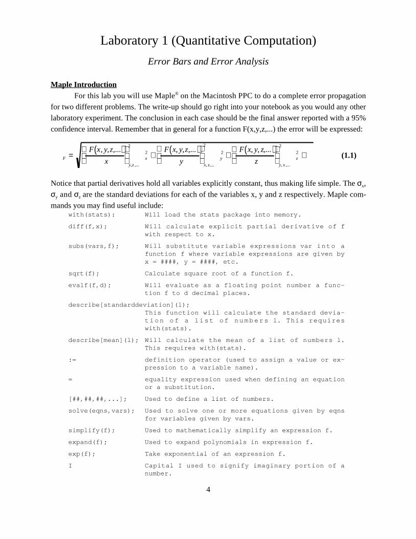
Maple IntroductionFor this lab you will use Maple® on the Macintosh PPC to do a complete error propagation

for two different problems. The write-up should go right into your notebook as you would any other

laboratory experiment. The conclusion in each case should be the final answer reported with a 95%

confidence interval. Remember that in general for a function F(x,y,z,...) the error will be expressed:

F =F x, y,z,...( )

x

y,z ,...

2

x2 +

F x, y,z,...( )y

x, z,...

2

y2 +

F x, y, z,...( )z

y, x ,...

2

z2 + (1.1)

Notice that partial derivatives hold all variables explicitly constant, thus making life simple. The σx,

σy and σz are the standard deviations for each of the variables x, y and z respectively. Maple com-

mands you may find useful include:with(stats): Will load the stats package into memory.

diff(f,x); Will calculate explicit partial derivative of fwith respect to x.

subs(vars,f); Will substitute variable expressions var into afunction f where variable expressions are given byx = ####, y = ####, etc.

sqrt(f); Calculate square root of a function f.

evalf(f,d); Will evaluate as a floating point number a func-tion f to d decimal places.

describe[standarddeviation](l);This function will calculate the standard devia-tion of a list of numbers l. This requireswith(stats).

describe[mean](l); Will calculate the mean of a list of numbers l.This requires with(stats).

:= definition operator (used to assign a value or ex-pression to a variable name).

= equality expression used when defining an equationor a substitution.

[##,##,##,...]; Used to define a list of numbers.

solve(eqns,vars); Used to solve one or more equations given by eqnsfor variables given by vars.

simplify(f); Used to mathematically simplify an expression f.

expand(f); Used to expand polynomials in expression f.

exp(f); Take exponential of an expression f.

I Capital I used to signify imaginary portion of anumber.

5

int(f,x=a..b); Integrate a function f with respect to variable xfrom limits a to b (which may even be Infinity).

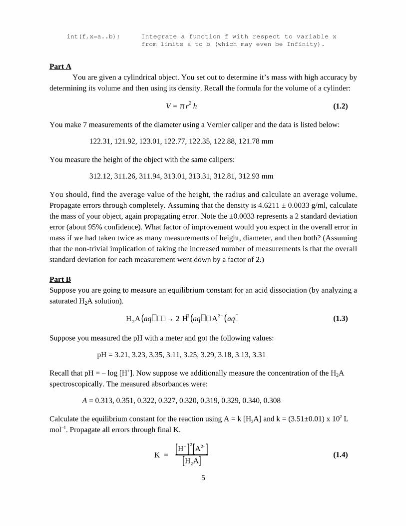
Part AYou are given a cylindrical object. You set out to determine it’s mass with high accuracy by

determining its volume and then using its density. Recall the formula for the volume of a cylinder:

V = π r2 h (1.2)

You make 7 measurements of the diameter using a Vernier caliper and the data is listed below:

122.31, 121.92, 123.01, 122.77, 122.35, 122.88, 121.78 mm

You measure the height of the object with the same calipers:

312.12, 311.26, 311.94, 313.01, 313.31, 312.81, 312.93 mm

You should, find the average value of the height, the radius and calculate an average volume.

Propagate errors through completely. Assuming that the density is 4.6211 ± 0.0033 g/ml, calculate

the mass of your object, again propagating error. Note the ±0.0033 represents a 2 standard deviation

error (about 95% confidence). What factor of improvement would you expect in the overall error in

mass if we had taken twice as many measurements of height, diameter, and then both? (Assuming

that the non-trivial implication of taking the increased number of measurements is that the overall

standard deviation for each measurement went down by a factor of 2.)

Part BSuppose you are going to measure an equilibrium constant for an acid dissociation (by analyzing a

saturated H2A solution).

H 2A aq( ) → 2 H+ aq( ) + A2− aq( ) (1.3)

Suppose you measured the pH with a meter and got the following values:

pH = 3.21, 3.23, 3.35, 3.11, 3.25, 3.29, 3.18, 3.13, 3.31

Recall that pH = – log [H+]. Now suppose we additionally measure the concentration of the H2A

spectroscopically. The measured absorbances were:

A = 0.313, 0.351, 0.322, 0.327, 0.320, 0.319, 0.329, 0.340, 0.308

Calculate the equilibrium constant for the reaction using A = k [H2A] and k = (3.51±0.01) x 102 L

mol–1. Propagate all errors through final K.

K = H+[ ]2

A2-[ ]H2A[ ] (1.4)

6

As in part A, determine which measurement is giving the greatest contribution to the overall error

observed for the equilibrium constant, K. Describe how the value for K and its error might change

if this measurement were improved by a factor of 3 (reduce the standard deviation of this measure-

ment by a factor of 3.)

Part CGiven the formula below :

A = b2 eC / d1 / 2 (1.5)

The value of b was measured to be (cm):

5.231, 5.331, 6.011, 5.112, 5.523, 5.911, 5.783, 5.651

The value of c was measured to be (unitless):

0.5231, 0.4412, 0.4951, 0.3991, 0.5123, 0.5411, 0.4801, 0.4512

The value of d was measured to be (cm2):

102.52, 103.21, 104.51, 100.13, 110.23, 99.23, 95.21, 111.23, 115.23

Using this data calculate the average values for b, c and d as well as standard deviations for these. In

addition calculate the average value for A as well as a 95% confidence interval for this value.

Consider a calibration data set previously generated for A (cm) as a function of t (hrs) given below.

A = 4.634 8.312 11.852 15.152 18.621 22.092 25.907 30.012

t = 1.00 2.00 3.00 4.00 5.00 6.00 7.00 8.00

Using Statview calculate the time at which the data was collected (estimate error appropriately). As

in the previous part A and B, you should determine which measurement is responsible for the larg-

est portion of the error in the final time measurement. Describe what you might do to try to im-

prove this situation and get a better measurement for the final value of time.

7

Laboratory 2 (Literature Work)

Current Article ReviewSelf directed literature search.

You will find a paper concerning a topic in Physical Chemistry.

Journals suggested are the Journal of Chemical Education, Journal of the American

Chemical Society, Journal of Physical Chemistry, Science or Nature.

You will read the paper and discuss it amongst yourselves (groups of 3).

You may discuss the paper with me.

You will present (1 week from today) a talk of length 15 minutes on this topic.

Your talk should address the following points

Overall idea of experiment

What sort of apparatus was used and how did it work

What sort of data analysis was conducted

What overall conclusions are reached

What problems exist in the article

You shall copy the article so everyone in the class has a copy of it.

8

Laboratory 3 (Thermochemistry)

Determination of the Heat Content of Coal

Introduction

This experiment is an adaptation of one published by Mueller and McCorkle1. A traditional

physical chemistry experiment is to determine the heat of combustion of a substance using a Parr

oxygen bomb and a technique called bomb calorimetry. It is particularly useful to know the heat of

combustion (∆CH) of a fossil fuel such as coal, especially if one is involved in industry. It is impor-

tant to be able to predict how effective coal is as an energy source. Coal is used to generate heat to

boil water and ultimately produce electricity (recall Carnot cycles and impact this had on the in-

dustrial revolution in England), therefore it is essential to be able to predict how much coal is

needed to produce a certain amount of heat. Bomb calorimetry is a good method to measure the

heat of combustion of coal. Since the technique is essentially the same no matter what the sample,

this experiment will also provide training that will be applicable whenever it is necessary to meas-

ure the heat of combustion or formation of another substance.

Experimental ProcedureSample pellets may be prepared by grinding the naphthalene or benzoic acid standard or

coal unknown into a powder using a grinder or mortar and pestle. Then the powder can be placed

into a gelatin capsule to be used as a sample pellet in the bomb. An alternative method for preparing

the samples is to use a pellet press to compress the sample into a tight tablet shaped pellet which can

be burned in the bomb. It should be noted that the coal pellets have a tendency to fall apart which

would affect your data, thus the capsule should be used. Once these pellets have been prepared the

bomb calorimeter operation procedure below can be followed.

Calorimeter1. Make sure both the bomb and bucket are clean and dry. May use acetone to clean the stain-

less steel bomb, however, all vapor must be allowed to evaporate before tests are conducted.

2. Get exactly 2.000 L of distilled water in volumetric flask(s) and fill bucket.

3. Set up digital thermometer for monitoring the temperature of water in the bucket. If stirrer isavailable, set this up in bucket as well.

4. Prepare a standard sample of 0.8±0.1 g benzoic acid (∆CU = – 26.412 kJ / g and ∆CH =–26.422 kJ / g) or 0.5±1 g naphthalene (∆CU = – 39.581 kJ / g and ∆CH = –40.232 kJ / g).Normally pellets are prepared, however a gelatin capsule may be used as well. If a gelatincapsule is to be used, two empty capsule runs must be completed in addition to the two stan-dard runs before attempting any unknown material.

9

5. Wire must be weighed carefully both before and after each run, to determine the mass whichhas been oxidized. The heat of combustion (complete oxidation) of the fuse wire is ∆U =–5.89 kJ / g.

6. A 1.000 mL drop of distilled water should be placed in the bottom of the bomb calorimeterbefore the start of the experiment, this insures that there will be no additional water vaporproduced in the combustion reaction (all water produced will be in the liquid form, whichhas a heat of formation of –243.83 kJ / mol).

7. Prepare fuse and pellet in holder. Wire should barely touch the top of the pellet or capsule.Make certain that the fuse holder contains the wire securely. The combustion crucibleshould be tilted to point away from the electrodes and the top of the bomb to prevent igni-tion of these parts.

8. Seal the bomb itself by screwing the top until hand tight. DO NOT USE A WRENCH FORTHIS.

9. Fill the bomb with O2 to a pressure of 25-35 atm. To do this, first turn the main regulator forthe O2 cylinder on, making sure that the main pressure valve is closed. Make sure that theexit port on the bomb is closed and the adapter is attached properly. Upon filling once to 25atm, the bomb should be vented slowly and refilled to 25 atm. This will have the effect ofdiluting the N2 in the bomb by a factor of 625 = 252 rather than just 25. This means that theN2 percentage (the most abundant gas impurity) should be less than 0.2%.

10. Carefully place the bomb in the bucket. Attaching the ignition leads to the correct terminals(note the grounded terminal is the one on the left when reading the number correctly and hasa small “g” symbol near it.) Take care to avoid splashing any water out and around thebucket as this could change the effective heat capacity.

11. Record the temperature of the bomb/calorimeter system every 30 seconds for approximately5 to 10 minutes, allowing the bomb and water to equilibrate. This will allow you to establishan initial temperature baseline (it is acceptable if this has a slight rise or fall by a few de-grees).

12. Press the ignition switch and hold it down for 2 seconds. The indicator light should come onbriefly and then go back off. It comes on to indicate that the circuit is complete and that cur-rent is passing through the ignition wire. It goes out when ignition begins and the wireburns/breaks.

13. Continue to record the temperature. Readings should be taken approximately every 30 sec-onds. The temperature should within a minute or so undergo a 1 to 2 degree jump. Continuemonitoring the temperature for a 5 to 10 minute period following this jump. Do not stopmonitoring temperature until the slope of the temperature versus time curve is reasonablyconstant (i.e. each time step the temperature changes by a constant increment).

14. The bomb should be allowed to cool for about 10 minutes then the pressure should be re-leased VERY slowly. Once released, you may open the bomb and check to see that combus-tion was complete. Rinse all parts first with deionized water and then acetone to remove anyacid formed from nitrogen or sulfur atoms in the combusted molecule as well as any residual

10

carbon deposits. In theory there should be no char left in the vessel, if there is, this repre-sents a potential source of error from incomplete combustion.

15. The remaining wire from the fuse should be carefully removed and reweighed. Weigh onlythe unoxidized portion of the wire (not the metal oxide balls you may find in the container).This mass will be used to compute the heat released due to combustion of the wire.

Experimental Procedure1. Run a calorimeter standardization using benzoic acid or naphthalene as per the above in-

structions.

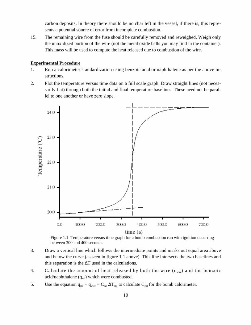
2. Plot the temperature versus time data on a full scale graph. Draw straight lines (not neces-sarily flat) through both the initial and final temperature baselines. These need not be paral-lel to one another or have zero slope.

3. Draw a vertical line which follows the intermediate points and marks out equal area aboveand below the curve (as seen in figure 1.1 above). This line intersects the two baselines andthis separation is the ∆T used in the calculations.

4. Calculate the amount of heat released by both the wire (qwire) and the benzoicacid/naphthalene (qstd) which were combusted.

5. Use the equation qstd + qwire = Ccal ∆Tstd to calculate Ccal for the bomb calorimeter.

Figure 1.1 Temperature versus time graph for a bomb combustion run with ignition occurringbetween 300 and 400 seconds.

11

6. Run the same experiment and measure ∆Tcoal for an unknown coal sample (approximately0.2 to 0.5 g sample).

7. All ∆Tcoal measurements should be conducted two or three times for averaging purposes.You may calculate the qcoal (which is ∆CU) from the equation qwire + qcoal = Ccoal ∆Tcoal usingthe unknown ∆Tcoal.

8. To convert to ∆CH from ∆CU you need to consider the ∆p V portion. First convert from ∆CUto ∆CUm using the initial mass of the sample. Second, look at the balanced equation and de-termine the number of gas phase product molecules minus the number of gas phase reactantmolecules. The ideal gas law tells us that ∆p V = ∆(nRT) which means if we assume tem-perature is constant (roughly true) then ∆p V = RT ∆n. Where ∆n is the change in number ofgas molecules, that is ∆CHm = ∆CUm + RT ∆n. For the coal sample, you will need to make anassumption about the approximate molecular formula of coal (C200H400) so that you can writea balanced equation which accounts for the number of carbon dioxide and water productmolecules.

9. Then error analysis should be completed, propagating all errors completely. The final resultshould summarize the ∆CH and ∆fH of coal (using in both kJ / g and kJ / mol) and give 95%confidence error limits.

12

Laboratory 4 (Thermochemistry/Spectroscopy)

Thermodynamics of Rhodamine B Lactone-Zwitterion Equilibrium

Introduction

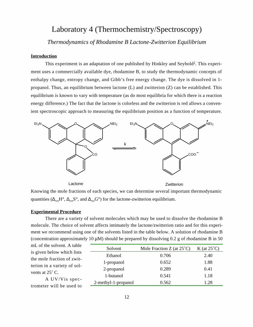
This experiment is an adaptation of one published by Hinkley and Seybold2. This experi-

ment uses a commercially available dye, rhodamine B, to study the thermodynamic concepts of

enthalpy change, entropy change, and Gibb’s free energy change. The dye is dissolved in 1-

propanol. Thus, an equilibrium between lactone (L) and zwitterion (Z) can be established. This

equilibrium is known to vary with temperature (as do most equilibria for which there is a reaction

energy difference.) The fact that the lactone is colorless and the zwitterion is red allows a conven-

ient spectroscopic approach to measuring the equilibrium position as a function of temperature.

Knowing the mole fractions of each species, we can determine several important thermodynamic

quantities (∆rxnH°, ∆rxnS°, and ∆rxnG°) for the lactone-zwitterion equilibrium.

Experimental ProcedureThere are a variety of solvent molecules which may be used to dissolve the rhodamine B

molecule. The choice of solvent affects intimately the lactone/zwitterion ratio and for this experi-

ment we recommend using one of the solvents listed in the table below. A solution of rhodamine B

(concentration approximately 10 µM) should be prepared by dissolving 0.2 g of rhodamine B in 50

mL of the solvent. A table

is given below which lists

the mole fraction of zwit-

terion in a variety of sol-

vents at 25˚ C.

A UV/Vis spec-

trometer will be used to

O

COO

NEt2Et2N

k

O

CO

NEt2Et2N

O

Lactone Zwitterion

Solvent Mole Fraction Z (at 25˚C) K (at 25˚C)

Ethanol 0.706 2.40

1-propanol 0.652 1.88

2-propanol 0.289 0.41

1-butanol 0.541 1.18

2-methyl-1-propanol 0.562 1.28

13

find the absorbance of the rhodamine B solution over a range of temperatures from 15 °C to 60 °C

and over a range of wavelengths containing the maximum absorbance. An electronically controlled

water bath is used to control the temperature of the solution in the spectrometer sample compart-

ment.

A table should be generated that includes the following data at each temperature: A (absor-

bance), xZ, xL, K, and ∆rxnG°. Also all calculations should be shown and include graphs used to de-

termine the temperature independent assumed parameters ∆rxnH° and ∆rxnS°. The following equa-

tions relate the absorbances measured to the various parameters.

A 100%( ) =A 25˚C( )

%Z 25˚C( )(4.1)

where A(100%) is the absorbance one would measure if all of the sample were in the colored zwit-

terion form. The concentration of the zwitterion form (labeled Z), is given by the equation:

Z[ ] =A T( ) 25˚C( )A 100%( ) T( ) RhB[ ] (4.2)

where ρ(25°C) and ρ(T) are solvent densities at 25°C and some temperature T respectively. The dif-

ference in densities is assumed to be negligible, that is ρ(25°C) ≈ ρ(T). Assuming that the density is

constant over the temperature range of which the experiment is performed [Z] becomes:

Z[ ] =A T( )

A 100%( ) RhB[ ]

L[ ] = RhB[ ] − Z[ ](4.3)

The equilibrium constant, K, can be easily seen from the equilibrium equation to be:

K =Z[ ]L[ ]

=Z[ ]

RhB[ ] − Z[ ]=

xZ

1− xZ

xZ =Z[ ]

RhB[ ]

(4.4)

Then ∆rxnG° can be calculated by the following:

∆Go = –RT ln K

The following equation can be compared to the least squared line of the plot ln K vs. 1/T in order to

determine ∆rxnH˚ and ∆rxnS˚ using the equation below:

ln K =∆So

R−

∆H o

RT(4.6)

14

Errors should be calculated as per standard error propagation for K (at each temperature), ∆rxnH°,

∆rxnS°, and ∆rxnG° (at each temperature) of the lactone-zwitterion equilibrium.

15


The Binary Liquid-Solid Phase Diagram ofNaphthalene and p-Dichlorobenzene

Introduction

This experiment is an adaptation of one published by Blanchette3 and another by Calvert et

al.4 This is also described in a standard physical chemistry laboratory manual5. In this experiment,

we are interested in studying the heterogeneous equilibrium between the liquid and the solid phase

in a two component system. The naphthalene and p-dichlorobenzene are chosen because they are

inexpensive, safe chemicals and their melting points are accessible with boiling water bath. This

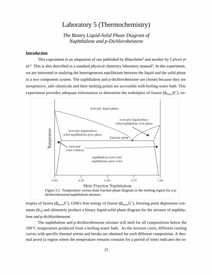
experiment provides adequate information to determine the enthalpies of fusion (∆fusionH˚), en-

tropies of fusion (∆fusionS˚), Gibb's free energy of fusion (∆fusionG˚), freezing point depression con-

stants (K f) and ultimately produce a binary liquid-solid phase diagram for the mixture of naphtha-

lene and p-dichlorobenzene.

The naphthalene and p-dichlorobenzene mixture will melt for all compositions below the

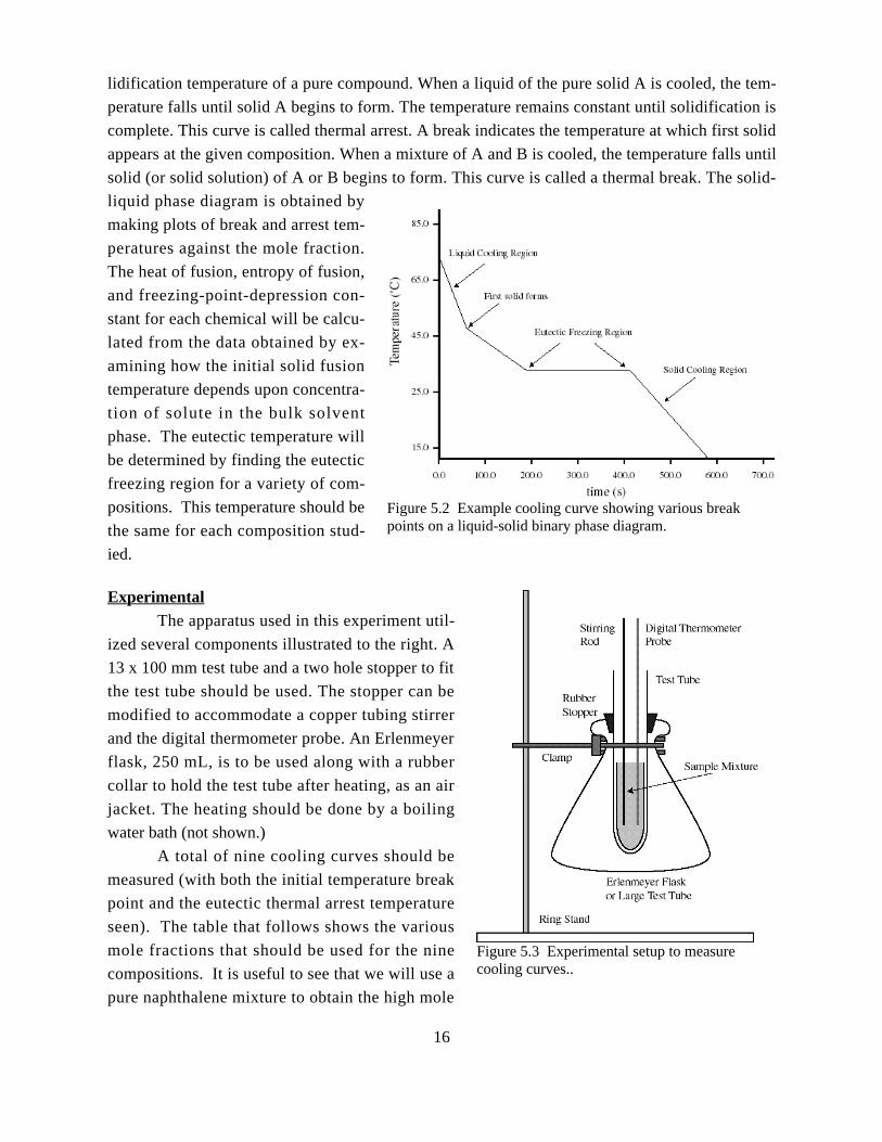
100˚C temperature produced from a boiling water bath. As the mixture cools, different cooling

curves with specific thermal arrests and breaks are obtained for each different composition. A ther-

mal arrest (a region where the temperature remains constant for a period of time) indicates the so-

Figure 5.1 Temperature versus mole fraction phase diagram in the melting region for a p-dichlorobenzene/naphthalene mixture.

16

lidification temperature of a pure compound. When a liquid of the pure solid A is cooled, the tem-

perature falls until solid A begins to form. The temperature remains constant until solidification is

complete. This curve is called thermal arrest. A break indicates the temperature at which first solid

appears at the given composition. When a mixture of A and B is cooled, the temperature falls until

solid (or solid solution) of A or B begins to form. This curve is called a thermal break. The solid-

liquid phase diagram is obtained by

making plots of break and arrest tem-

peratures against the mole fraction.

The heat of fusion, entropy of fusion,

and freezing-point-depression con-

stant for each chemical will be calcu-

lated from the data obtained by ex-

amining how the initial solid fusion

temperature depends upon concentra-

tion of solute in the bulk solvent

phase. The eutectic temperature will

be determined by finding the eutectic

freezing region for a variety of com-

positions. This temperature should be

the same for each composition stud-

ied.

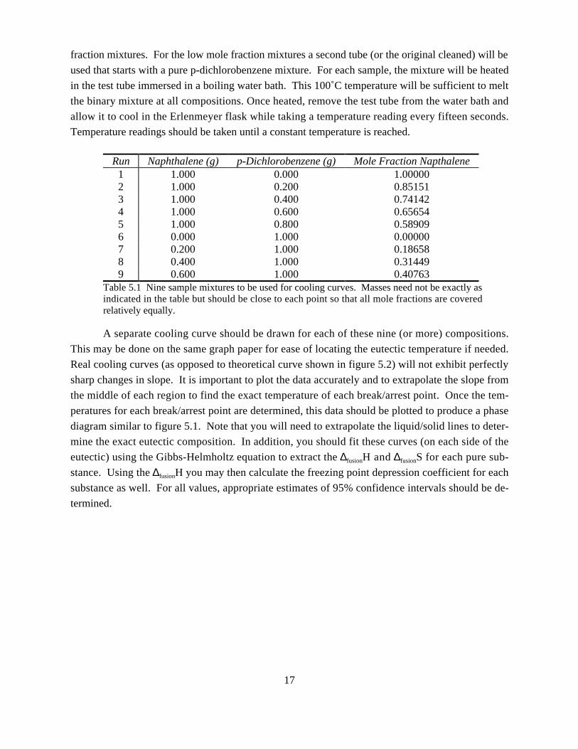
ExperimentalThe apparatus used in this experiment util-

ized several components illustrated to the right. A

13 x 100 mm test tube and a two hole stopper to fit

the test tube should be used. The stopper can be

modified to accommodate a copper tubing stirrer

and the digital thermometer probe. An Erlenmeyer

flask, 250 mL, is to be used along with a rubber

collar to hold the test tube after heating, as an air

jacket. The heating should be done by a boiling

water bath (not shown.)

A total of nine cooling curves should be

measured (with both the initial temperature break

point and the eutectic thermal arrest temperature

seen). The table that follows shows the various

mole fractions that should be used for the nine

compositions. It is useful to see that we will use a

pure naphthalene mixture to obtain the high mole

Figure 5.2 Example cooling curve showing various breakpoints on a liquid-solid binary phase diagram.

Figure 5.3 Experimental setup to measurecooling curves..

17

fraction mixtures. For the low mole fraction mixtures a second tube (or the original cleaned) will be

used that starts with a pure p-dichlorobenzene mixture. For each sample, the mixture will be heated

in the test tube immersed in a boiling water bath. This 100˚C temperature will be sufficient to melt

the binary mixture at all compositions. Once heated, remove the test tube from the water bath and

allow it to cool in the Erlenmeyer flask while taking a temperature reading every fifteen seconds.

Temperature readings should be taken until a constant temperature is reached.

A separate cooling curve should be drawn for each of these nine (or more) compositions.

This may be done on the same graph paper for ease of locating the eutectic temperature if needed.

Real cooling curves (as opposed to theoretical curve shown in figure 5.2) will not exhibit perfectly

sharp changes in slope. It is important to plot the data accurately and to extrapolate the slope from

the middle of each region to find the exact temperature of each break/arrest point. Once the tem-

peratures for each break/arrest point are determined, this data should be plotted to produce a phase

diagram similar to figure 5.1. Note that you will need to extrapolate the liquid/solid lines to deter-

mine the exact eutectic composition. In addition, you should fit these curves (on each side of the

eutectic) using the Gibbs-Helmholtz equation to extract the ∆fusionH and ∆fusionS for each pure sub-

stance. Using the ∆fusionH you may then calculate the freezing point depression coefficient for each

substance as well. For all values, appropriate estimates of 95% confidence intervals should be de-

termined.

Run Naphthalene (g) p-Dichlorobenzene (g) Mole Fraction Napthalene1 1.000 0.000 1.000002 1.000 0.200 0.851513 1.000 0.400 0.741424 1.000 0.600 0.656545 1.000 0.800 0.589096 0.000 1.000 0.000007 0.200 1.000 0.186588 0.400 1.000 0.314499 0.600 1.000 0.40763

Table 5.1 Nine sample mixtures to be used for cooling curves. Masses need not be exactly asindicated in the table but should be close to each point so that all mole fractions are coveredrelatively equally.

18


A Liquid Binary Phase System

Introduction

The procedure for the experiment of solubilities of liquids in a binary two-phase system is

taken from an article by Arthur M. Halperm and Saeed Gozashti6 The classic example of a two

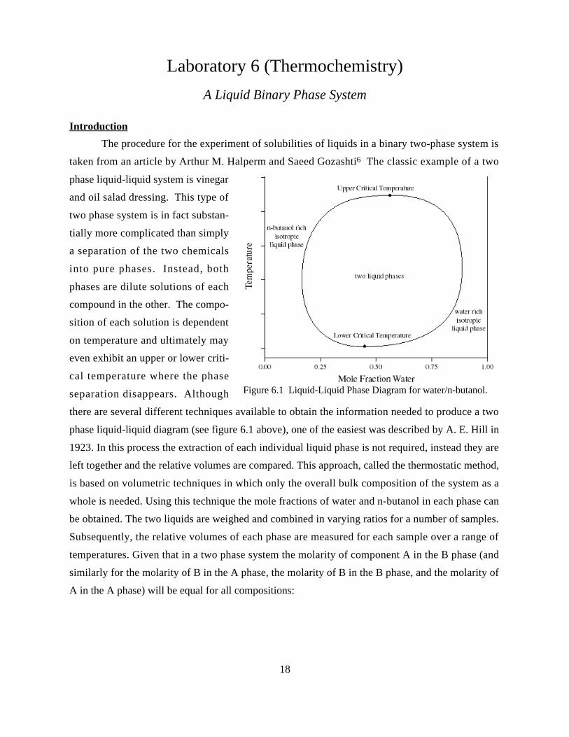
phase liquid-liquid system is vinegar

and oil salad dressing. This type of

two phase system is in fact substan-

tially more complicated than simply

a separation of the two chemicals

into pure phases. Instead, both

phases are dilute solutions of each

compound in the other. The compo-

sition of each solution is dependent

on temperature and ultimately may

even exhibit an upper or lower criti-

cal temperature where the phase

separation disappears. Although

there are several different techniques available to obtain the information needed to produce a two

phase liquid-liquid diagram (see figure 6.1 above), one of the easiest was described by A. E. Hill in

1923. In this process the extraction of each individual liquid phase is not required, instead they are

left together and the relative volumes are compared. This approach, called the thermostatic method,

is based on volumetric techniques in which only the overall bulk composition of the system as a

whole is needed. Using this technique the mole fractions of water and n-butanol in each phase can

be obtained. The two liquids are weighed and combined in varying ratios for a number of samples.

Subsequently, the relative volumes of each phase are measured for each sample over a range of

temperatures. Given that in a two phase system the molarity of component A in the B phase (and

similarly for the molarity of B in the A phase, the molarity of B in the B phase, and the molarity of

A in the A phase) will be equal for all compositions:

Figure 6.1 Liquid-Liquid Phase Diagram for water/n-butanol.

19

NMCP = 1MA

B = 2MAB = 3MA

B = 4MAB = 5MA

B = MAB

1MBB = 2MB

B = 3MBB = 4MB

B = 5MBB = MB

B

1MAA = 2MA

A = 3MAA = 4MA

A = 5MAA = MA

A

1MBA = 2MB

A = 3MBA = 4MB

A = 5MBA = MB

A

(6.1)

where N signifies the sample identification, P the phase, and C the component. Thus:

nc = McpV p + Mc

pV p(6.2)

na = MAAV A + MA

BV B (6.3)

nb = MBAVA + MB

BV B (6.4)

where nc is the number of moles of component c in a given sample, P defines the phase, Mcp is the

molarity, and VP is the volume. By measuring the molarities of the components and the volumes of

the phases the moles and the mole fractions can be found. Thus, a phase diagram can be produced.

Procedure

A series of five samples should be prepared in which the mole fraction of n-butanol in water

ranges from 0.200 to 0.800. You should not prepare samples with mole fractions outside this range

since at elevated temperatures these may form a single phase which would necessitate not using

data from that sample from that temperature and above. The samples should be carefully weighed

so that you know exactly how many moles of both n-butanol and water are present in each. Each

sample will be placed in a high precision (better than ±0.1 mL precision) 10 mL graduated cylinder

fitted with a glass top. It is recommended that no more than about 7 mL total be filled into each

graduated cylinder to make sure that expansion does not increase the volume above the 10 mL

maximum for each cylinder. These five samples should be sealed with the glass tops and parafilm

to ensure that material enters or leaves the graduated cylinders over the course of the experiment.

For each temperature, the five cylinders will be immersed in a temperature controlled water

bath. It is critical that the cylinders be maintained at a constant temperature and allowed to equili-

brate for at least 10 minutes before any measurements are conducted. In addition at the lower tem-

peratures, it is important that the samples be inverted to stir the solutions to guarantee that there are

no concentration gradients present in the sample as the system achieves equilibrium concentrations.

At the higher temperature, thermal convection will help to stir the mixtures and the increased solu-

bilities of the water and n-butanol will help to guarantee equilibrium is reached faster. An alterna-

tive approach is to use an ultrasonic stirring bath as a temperature controlled bath if one is available

that can hold all five samples. For increased accuracy, a sixth graduated cylinder should be in-

20

cluded which contains a known quantity of water so that you may determine the expansion coeffi-

cient for the graduated cylinders as you raise the temperature (and account for this in your final

phase diagram.) Once temperature equilibrium is established for each cylinder, you should read the

volumes (to a precision of ±0.01 mL via interpolation if possible) of both phases in the tube. You

should take care to note which is the water rich and which is the n-butanol rich phase (the relative

positions of these phases will not change from tube to tube or temperature to temperature.) This

process should be repeated at temperatures of 20˚C, 30˚C, 40˚C, 50˚C, 60˚C and 80˚C.

Data Analysis

When you review equations 6.3 and 6.4 you may note that these may be transformed in the

following manner:

na

V A = MAA + MA

B VB

V A(6.5)

nb

V A = MBA + MB

B VB

V A(6.6)

This form suggests that a graph of nB / VA or nA / VA versus the ratio of the volumes, VB / VA. If these

plots are done for the five data points, the slope and intercept will give the concentrations of water

and n-butanol for each of the phases. This should be reported with appropriate error bars using

StatView, Excel or other similar program. These concentrations should then be compiled into a

phase diagram similar to the one in figure 6.1.

21

Laboratory 7 (Dynamics)

A Simple Reduction/Oxidation Reaction and Chemical KineticsUsing Visible Spectroscopy

Introduction:

This experiment is an adaptation of one published by Elias and Arden7. The experiment

discussed in this paper is a simple oxidation of iodide ions by peroxodisulfate ions. The reaction is

quick and easy to perform; this experiment has advantages in that one can directly observe the in-

crease in absorbance over time due to the formation of the I3− ion by using a standard visible spec-

trometer (such as a Spectronics 20.) The reaction between iodide and the peroxodisulfate ion is

S2O82− + 2I− → 2SO4

2 − + I2 (7.1)

Subsequently each I2 reacts with the excess I– to produce a triiodide ion, I3

− .

I2 + I− → I3− (7.2)

This experiment can be performed effectively by obtaining the Spec 20 absorbances of each solu-

tion (made with differing concentrations of peroxodisulfate and iodide ions) at 353nm. The build up

curves will appear essentially linear (rather than showing any curvature due to changes in concen-

trations of the peroxodisulfate and iodide ions) since the molar absorptivity of the triiodide is so

high and the reaction is relatively slow, maintaining I3−[ ] << I−[ ] for the initial moments of the re-

action. This initial rate will relate to a rate law of the form given below:

d I2[ ]dt

= k S2O82-[ ]n

I−[ ]m(7.3)

where the rate constant, k, as well as the rate law exponents, n and m, will be determined from this

experiment.

Procedure:

You should first prepare solu-

tions of 0.1M KNO3 (to be used as a

diluting agent to maintain constant

ionic strength in all solutions,) 0.02M

K2S2O8 in 0.1M KNO3, and 0.04M KI

in 0.1M KNO3. The wavelength on

Sample 0.02 M K2S2O8 0.04 M KI 0.1 M KNO3

A 4 mL 1 mL 3 mLB 4 mL 2 mL 2 mLC 4 mL 3 mL 1 mLD 4 mL 4 mL 0 mLE 1 mL 4 mL 3 mLF 2 mL 4 mL 2 mLG 3 mL 4 mL 1 mL

Table 7.1 Sample mixtures suggested for rate law determination ofK2S2O8 / KI reaction (note all have identical total volume and iden-tical ionic strengths.

22

the Spec 20 should be adjusted to 353nm and the instrument should be set to 100% transmission

using 0.1 M KNO3 as the blank. Seven or more experiments should be preformed (as suggested in

table 7.1) In experiments A-D the peroxodisulfate concentration is held constant and the iodide ion

concentration is varied. In experiments D-G, the iodide ion concentrations are held constant and the

peroxodisulfate ion concentration is varied. Note that the sample labeled D is used in both sets. In

each experiment, the 0.1 M KNO3 was first added to the cuvet, the 0.02 M K2S2O8 was added next,

and the 0.04 M KI was added last. The KI should always be added last since once the solution is

mixed it begins to react immediately to produce triiodide ions. After the addition of the KI, the cu-

vet was inverted once and then quickly placed in the Spec 20 and the reaction's absorbance was

measured every thirty seconds for five minutes.

Data and Analysis:

The time resolved absorbances should be plotted using a program such as Statview or Excel.

These graphs should be roughly linear (with slight curvature at the higher concentrations). The ini-

tial slope of this line (which has units of absorbance per unit time) should be extrapolated back to

zero time and determined along with appropriate error bars. The rate equation 7.3 can be manipu-

lated below:

lnd I2[ ]

dt

= lnk + n ln S2O8

2-[ ] + m ln I−[ ] (7.4)

Modifying this by using the knowledge that A = [ I3− ] b where e is the molar absorptivity of I3

− and

b is the pathlength for the cell. This allows us to modify equation 7.4 below:

lnd I2[ ]

dt

= ln

d A b( )dt

= ln

dAdt

− ln b( )

lndA

dt

= ln k b( ) + nln S2O8

2−[ ] + mln I−[ ](7.5)

This suggests that by plotting the logarithm of the rate versus either the logarithm of the peroxodi-

sulfate ion (samples D-G) or the iodide ion (A-D). The slope of the resulting line will be either the

n or m respectively. Ideally the error bars on these parameters should allow you to identify the

closest integer value for both n and m. If these parameters are well established, the multi-step rate

law may or may not be identified. Once the n and m values are determined the plot of rates versus

the concentration product S2O82−[ ]n

I−[ ]m. The slope of this line will correspond to the product k b.

The product of b may be measured by mixing 0.100 mL of the 0.02 M K2S2O8 solution with 5.0

mL of the 0.04 M KI solution and dilute the solution to a total volume of 8.0 mL with the 0.1 M

23

KNO3 solution (allow this to stand for at least 15 minutes for the reaction to proceed to comple-

tion.) The final triiodide concentration will then be 2.5x10–4 M and the produce b may be deter-

mined by taking the observed absorbance of this solution and dividing by the final triiodide con-

centration. Your conclusion should report the complete rate law, including the rate constant along

with error bars on the appropriate parameters.

24

Laboratory 8 (Dynamics/Spectroscopy)

Measurement of Longitudinal Relaxation Times (T1)For13C in Ethylbenzene

Introduction:

This experiment is an adaptation of one published by Fuson and others8,9. The measure-

ment of relaxation times in NMR spectroscopy is an important experiment to learn a number of

things about a molecule. First off, when running NMR spectra the time that must be waited for re-

laxation to occur limits the ultimate rate of data acquisition and ultimately the signal-to-noise ratio

which may be achieved. Secondly, the relaxation times give insight into the molecular motions pre-

sent in a molecule as well as the bulk reorientation of a molecule in solution. For 1H NMR spectra,

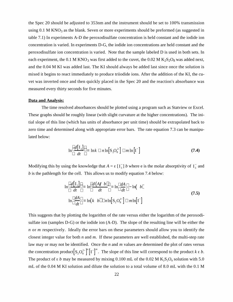
the T1 relaxation times are normally in the 2-10 s time range whereas the 13C NMR T1 relaxation

times are much longer (in the 10-60 s range).

It is surprising to think that such a low energy

event as a nuclear spin flip requires such a

long time to reach equilibrium after a pertur-

bation. The answer to this problem stems

from the difference in rates of spontaneous

versus stimulated emission. As demonstrated

by the Einstein coefficients, the rate of spon-

taneous emission increases greatly with en-

ergy of that emission. In a very low energy

situation (flipping nuclear spins) the rate of

spontaneous emission is essentially zero. For

nuclear spins to reestablish equilibrium

populations, there must be photons present at

exactly the Larmor frequency which can

cause stimulated emission. This radiation frequency arising from black body radiation is very low

in intensity (black body radiation has maximum intensity in the infrared region at room tempera-

ture.) The source of radiation to cause relaxation must therefore arise from non-black body mecha-

nisms (i.e. specific molecular motions.)

Ethylbenzene provides an excellent test case to gain insight into relaxation processes. This

molecule has a very well established and easily interpreted NMR spectrum and possesses both

Figure 8.1 Relaxation time as a function of tem-perature. The minimum in the T1 curve arises whenthe spectral density cuts out at the Larmor frequency.

25

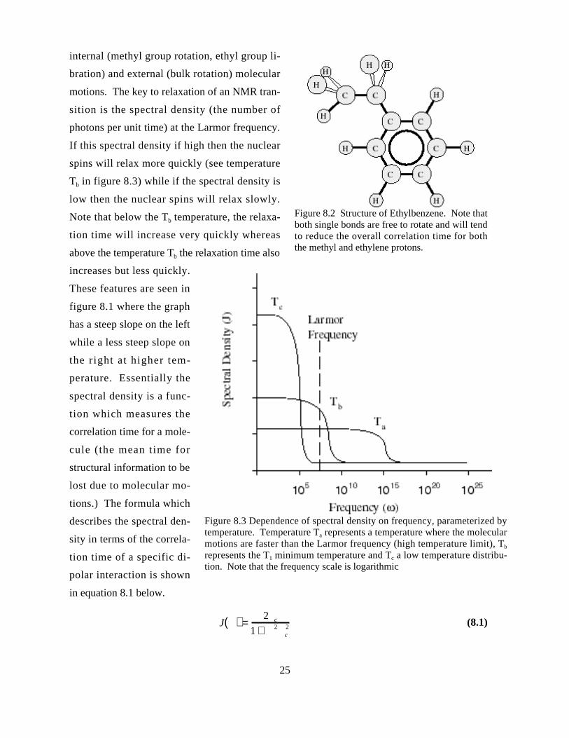
internal (methyl group rotation, ethyl group li-

bration) and external (bulk rotation) molecular

motions. The key to relaxation of an NMR tran-

sition is the spectral density (the number of

photons per unit time) at the Larmor frequency.

If this spectral density if high then the nuclear

spins will relax more quickly (see temperature

Tb in figure 8.3) while if the spectral density is

low then the nuclear spins will relax slowly.

Note that below the Tb temperature, the relaxa-

tion time will increase very quickly whereas

above the temperature Tb the relaxation time also

increases but less quickly.

These features are seen in

figure 8.1 where the graph

has a steep slope on the left

while a less steep slope on

the right at higher tem-

perature. Essentially the

spectral density is a func-

tion which measures the

correlation time for a mole-

cule (the mean time for

structural information to be

lost due to molecular mo-

tions.) The formula which

describes the spectral den-

sity in terms of the correla-

tion time of a specific di-

polar interaction is shown

in equation 8.1 below.

J( ) =2 c

1 + 2c2 (8.1)

Figure 8.3 Dependence of spectral density on frequency, parameterized bytemperature. Temperature Ta represents a temperature where the molecularmotions are faster than the Larmor frequency (high temperature limit), Tb

represents the T1 minimum temperature and Tc a low temperature distribu-tion. Note that the frequency scale is logarithmic

Figure 8.2 Structure of Ethylbenzene. Note thatboth single bonds are free to rotate and will tendto reduce the overall correlation time for boththe methyl and ethylene protons.

26

This expression is essentially related to a black box model in which oscillators from zero frequency

up to some frequency approximately 1/τc are roughly equally populated. In systems which have

different molecular subunits (such as methyl groups) which have a second correlation time different

than the overall isotropic correlation time will have a modified formula for the overall spectral den-

sity at a given nuclear position. This spectral density relates to the overall longitudinal relaxation

time for a given site, T1,i, due to random fluctuations of like spins (protons relaxing other protons)

by formula 8.2 below, where 0 is the Larmor frequency.

1

T1,i

=3

24 2I I +1( ) J ik 0( ) + Jik 2 0( )

k∑ (8.2)

If the spins are heteronuclear (relaxation of a carbon site by a proton) then the equation for the re-

laxation time is modified.

1

T1, I

=3

2 I2

S2 2S S +1( ) 1

12 J IS I,0 − S ,0( ) + 32 J IS I, 0( ) + 3

4 J IS I,0 + S ,0( )[ ]s∑ (8.3)

For each nuclear site in the molecule the T1 will be strongly affected by the spectral density at that

site. For a molecule like ethylbenzene, the spectral density will be different for the methyl group

than the aromatic portions. In particular, it is expected that the effective correlation time for a

methyl group will be much shorter than other regions and this short correlation time will result in a

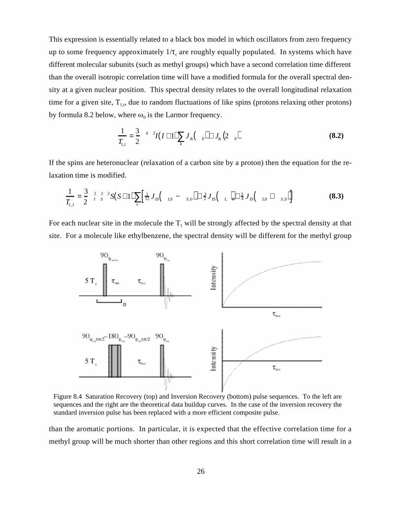
Figure 8.4 Saturation Recovery (top) and Inversion Recovery (bottom) pulse sequences. To the left aresequences and the right are the theoretical data buildup curves. In the case of the inversion recovery thestandard inversion pulse has been replaced with a more efficient composite pulse.

27

wider frequency range for the spectral density and an overall reduced spectral density. This will

reduce the transition rate for the methyl group relative to the aromatic region.

Experimental:

The experimental NMR methods used to study relaxation times are either an inversion re-

covery sequence or a saturation recovery sequence, shown in figure 8.4. Note that the inversion re-

covery sequence is actually a modified version in which the initial 180˚ pulse has been replaced by

a composite pulse. The saturation recovery method is the easiest to understand. The series of

pulses applied at the beginning of the sequence are used to saturate the spin transitions of interest

(i.e. the protons on ethylbenzene). By applying a series of pulses the spins are continually dis-

turbed. Note that for a stimulate absorption/emission event, there must be a population difference

between the two energy levels. After a large number of pulses, the rate of emission and absorption

will be effectively averaged as the populations of the energy levels are equalized. The delay that

follows is referred to as the recovery delay. During this period of time, the spins return (to some

degree) to their equilibrium populations. By observing the signal recovered as a function of this

delay we may map out a saturation recovery curve (shown to the right of the pulse sequence in fig-

ure 8.4) Since we are merely destroying the population difference the equilibrium buildup curve

will follow a simple exponential growth model leading to the equation 8.4 which describes this

buildup curve.

S rec( ) = S ∞( ) 1 − e− rec T 1[ ] (8.4)

In the case of the inversion recovery sequence, the theory is somewhat more complicated. First, the

inversion recovery sequence is coherent, meaning we actually track the magnetization and not just

the population difference. The initial pulse inverts the magnetization from the +z to the –z axis.

While the magnetization is initially aligned in the –z direction, it immediately begins to return to its

equilibrium position in the +z direction. This recovery follows an exponential buildup in much the

same way as the saturation recovery method. The equation 8.5 is modified to account for the initial

inversion as opposed to the saturation.

S rec( ) = S ∞( ) 1 − 2e− rec T1[ ] (8.5)

The sequence shown in figure 8.4 is one that includes a composite pulse to replace the standard

180˚ inversion pulse. You may notice that this composite pulse is actually three pulses applied in

rapid succession with phase shifts (90x – 180y – 90x). The effect of this pulse is identical for an on

resonance spin (the magnetization is rotated from the +z to –z axis). The benefit of the composite

28

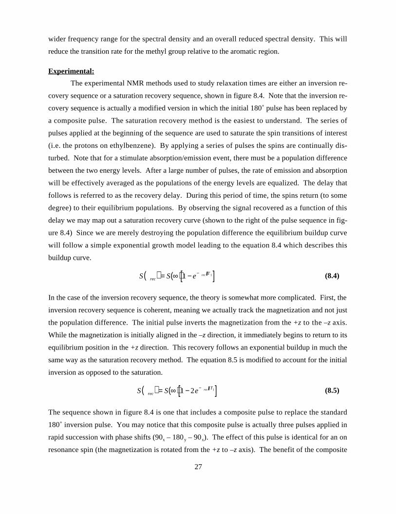
pulse is seen when comparing the overall magnetization rotation for an off-resonance spin versus a

non-composite pulse. For the straight 180X pulse, the off resonance magnetization is rotated about

an axis slighly tilted towards the Z axis from the X axis. The effect is that the magnetization ap-

pears to over-rotate beyond 180 degrees and misses the bottom of the sphere (the –z direction) and

instead actually passes the bottom and starts to go up giving an inversion population of this spin of

less than 100% (in some bad case is may be much less than 100%). This will seriously affect the

measured T1 values since the initial starting signal will not be equal and opposite to the infinite time

one. By using a composite pulse sequence made up of a 90X then 180Y then 90X pulse, you may

actually achieve a nearly 100% inver-

sion for even very large offsets. In

the figure 8.5 you will notice that the

magnetization of the off resonance

spin moves away from the Y axes to-

wards the X axis initially. This would

be bad if we completed the 180 de-

grees of rotation but instead, we stop

at 90. The second pulse rotates this

from the +x side to the –x side along

the surface of the sphere. From this

final point, the last 90X pulse can ro-

tate the magnetization towards the –z

axis . The 180Y pulse added just

enough compensation so that the sec-

ond 90X pushed the magnetization

nearly perfectly onto the –z axis.

The overall use of composite pulses will improve the fitting of the experimental inversion

recovery data substantially. If the inversion were less than 100% the equation 8.5 would need to be

modified with the addition of a third adjustable parameter (inversion efficiency) which ranges from

0 to 2 and precedes the exponential term. For the experiment you will conduct, the 13C and 1H re-

laxation times of ethylbenzene shall be measured using the composite pulse inversion recovery se-

quence described. The data will be analyzed on the NMR spectrometer using the software available

on the instrument. Once you have the T1 values for each spin site in the molecule, you can then

construct the effective spectral densities for each site. As a simplification, we can assume for a

small molecule such as this that we are in the fast motion limit (from equation 8.1, ω τc << 1) and

Figure 8.5 Composite pulse inversion using a 90X–180Y–90X

sequence. Note that on resonance this is identical to a 180X, butfor an off resonance spin, the magnetization follows a somewhatmore complicated trajectory. This trajectory still leads to nearlyperfect inversion which an off-resonance 180 would fail to do.

29

therefore the spectral density for a given site is effectively constant over the range of frequencies

used in NMR (i.e. J(ω 0) = J(2 ω0) for both the 300 MHz 1H and 75MHz 13C sties). Once the vari-

ous spectral densities are tabulated for each site, a mean correlation time may be determined for

each portion of the molecule. Note than in the case of specific sites in the molecules you will need

to sum up a number of spectral density contributions from various spin pairs within the molecule.

30


Measurement of the NO2 Dimerization Equilibrium Constant

Introduction:

This experiment is an adaptation of one published by Wettack and modified by others10.

The reaction of nitrogen monoxide with oxygen gas produces nitrogen dioxide that then dimerizes

to form the brown dinitrogen tetroxide. This is a major source of visual irritation in locations of

heavy pollution as well as reacting with water to produce acid rain.

2 N Og( ) + O2 g( ) → 2NO 2 g( ) (9.1)

2 N O2 g( ) ← → N 2O4 g( ) (9.2)

In a constant volume container, the relative quantities of nitrogen dioxide and dinitrogen tetroxide

will shift as the temperature is changed due to the change in the ∆rxnG for the reaction 9.2 following

the well known equation ∆rxnG = –RT ln K.

Experimental:

To generate a reaction vessel with known quantities of both NO2 (g) and N2O4 (g), we must

be careful to use volumetric gas handling and not allow the NO (g) to contact O2 (g) until the proper

time in the experiment. The reaction we will use to generate the NO (g) is between copper metal

and concentrated nitric acid.

6H + aq( ) + 3Cu s( ) + 2 H N O3 g( ) → 2 N Og( ) + 3Cu2 + aq( ) + 4H 2O l( ) (9.3)

This reaction will produce pure NO (g) but this gas will react with any O2 (g) present in the reaction

vessel immediately to produce the NO2 (g). Essentially we need to keep producing NO (g) in ex-

cess until all available O2 (g) is reacted. In this manner we can effectively dilute out any produced

NO2 (g) or N2O4 (g) and thus collect nearly pure NO (g). An alternative approach is to bubble the

NO (g) through concentrated base (NaOH or KOH) and thus eliminate any of the NO2 (g) or N2O4

(g). This NO (g) will be collected in a gas tight syringe (approximately 4 mL) and will be tem-

perature regulated to 25˚ C. A second gas tight syringe will be filled with O2 (g) directly from a

99.99% pure gas cylinder; this syringe should the same volume of O2 (g) as is in the NO (g) sy-

ringe. From reaction 9.1, the stoichiometry of these two is exactly 1:1 and when equal volumes of

these are mixed, the product will be exactly the same volume of NO2 (g). This product will almost

31

immediately begin to dimerize to form N2O4 (g) and a faint brown color should appear. By main-

taining the product in an airtight syringe and monitoring the volume change as a function of tem-

perature, we may extract the equilibrium constant for the reaction 9.2.

Kp =pN2 O4

pNO2

2 =xN 2 O4

ptotal

xNO2

2 ptotal2 =

xN2 O4

xNO2

2 ptotal

=ntotal nN2 O4

nNO2

2 ptotal

=nN 2O 4

nNO2

2

Vtotal

RT=

nNO 2 ,0 − nNO2( )

nNO2

2

Vtotal

2RT

(9.4)

The total number of moles of gas will change as the temperature changes and the equilibrium shifts

and this will produce a change in the volume (since the overall pressure is maintained throughout

the experiment.)

nNO2 ,0 =ptotal VNO

RT= nNO 2

+nN2O 4

2

ntotal =ptotal Vtotal

RT= nNO 2

+ nN2 O4

(9.5)

Combining these equations, we may solve for the number of moles of NO2 (g) in terms of the initial

volume of NO (g), VNO, and the equilibrated volume of the mixture, Vtotal.

nNO2=

ptotal 2VNO − Vtotal( )RT

(9.6)

This may be then substituted back into equation 9.4 to give an expression for the equilibrium con-

stant in terms of the two volumes, VNO and Vtotal.

Kp =

ptotal VNO

RT−



2

Vtotal

2RT=

Vtotal − VNO( )Vtotal

2 ptotal 2VNO − Vtotal( )2 (9.7)

This expression is now suitable for calculating the equilibrium constant Kp for each temperature.

The only caveat is that the volumes must be all standardized to a single initial temperature. There-

fore for reaction mixtures studied at higher or lower temperature must have the total volumes modi-

fied using the ideal gas law per equation 9.8.

Vtotaladj =

ntotalRT adj

ptotal

= Vtotal

T adj

T(9.8)

32

The adjusted volumes may then be used for all calculations of equilibrium constants per equation

9.7. It is clear that the adjusted volumes should never exceed the original volume of NO (g) nor

should it be less than one-half the original volume. If either of these data events were to occur, it

would more than likely indicate that your initial reaction mixture contained some impurities (nor-

mally O2 or H2O). The second of these (H2O) is particularly insideous as it will react with NO2 (g)

to produce nitric (HNO3) and nitrous acid (HNO2) which is soluble in water and therefore will ef-

fectively cause a gas phase mass imbalance. In either case, we may account for these impurities as

long as they do not change over time (i.e. as long as there is no leak into or out of the reaction sy-

ringe.)

Data Analysis:

Once the equilibrium constants, Kp, have been determined at each temperature, these may be

converted into ∆rxnG at each temperature. By making a graph of the ∆rxnG versus T, we expect to

see a straight line with a slope of –∆rxnS and an intercept of ∆rxnH (assuming both of these are con-

stant over the temperature range being studied.) Alternatively, a plot of ln Kp versus 1 / T will give

a slope of –∆rxnH / R and an intercept of ∆rxnS / R. In either case, the relative errors for each of

these thermodynamic state functions may be extracted from Statview or Excel as appropriate. This

procedure is very similar to that used in laboratory 4, the study of the rhodamine B equilibrium.

33

Laboratory 10 (Quantum Chemistry)

Determination of Molecular Structure of HCl / DCl / CH4

Introduction:

This experiment is an adaptation of one published in a standard physical chemistry labora-

tory manual5,11-14. The determination of bond distances and strengths dates back to the beginning

of chemistry. In early chemistry courses students are given data describing atomic and ionic radii.

These data were collected in a variety of ways, such as crystallographic studies with both X-rays

and neutrons and spectroscopic studies. In this laboratory you will study the molecular structure of

CH4 and/or 1H35Cl, 1H37Cl, 2H35Cl and 2H37Cl with infra-red and near infra-red spectroscopy tech-

niques. This laboratory has been extensively used in many physical chemistry courses by many dif-

ferent instructors.1-6 The data collected will allow the calculation of the bond length and force con-

stant for each of these molecules.

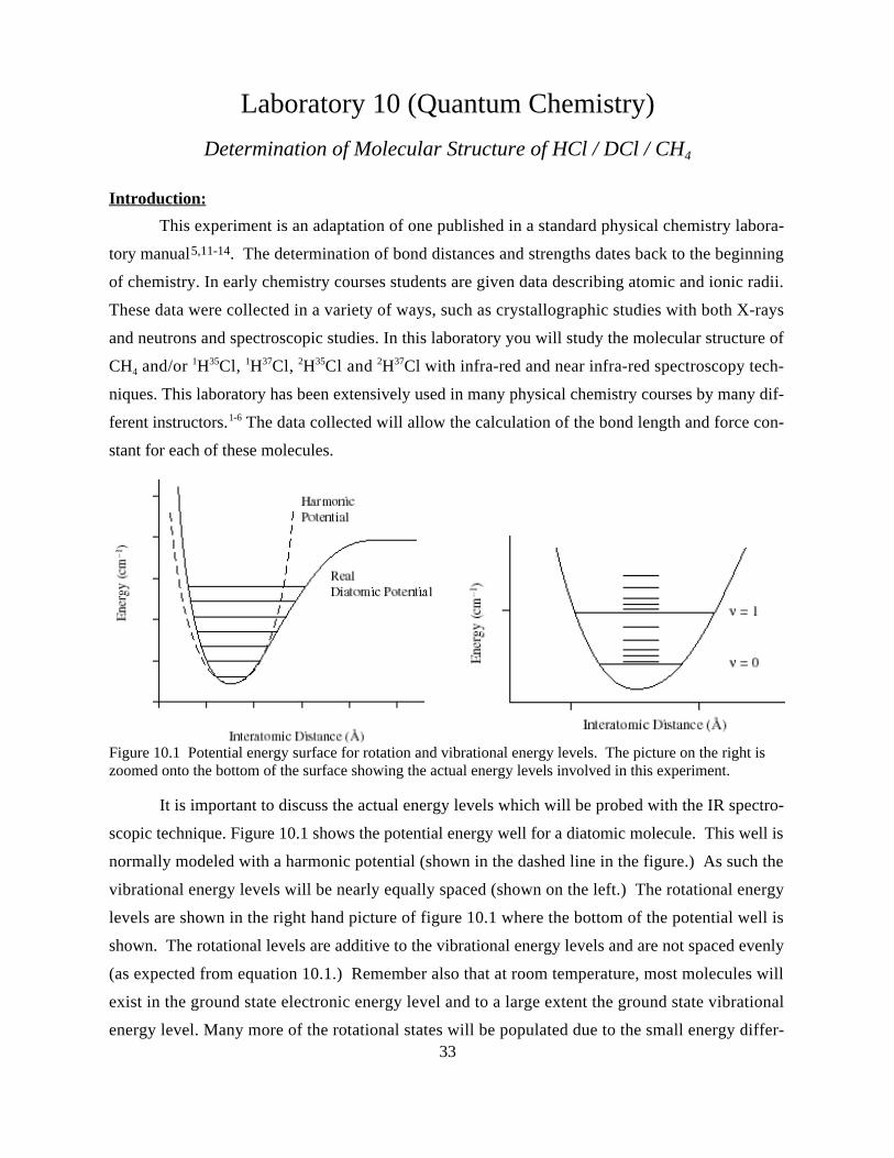
It is important to discuss the actual energy levels which will be probed with the IR spectro-

scopic technique. Figure 10.1 shows the potential energy well for a diatomic molecule. This well is

normally modeled with a harmonic potential (shown in the dashed line in the figure.) As such the

vibrational energy levels will be nearly equally spaced (shown on the left.) The rotational energy

levels are shown in the right hand picture of figure 10.1 where the bottom of the potential well is

shown. The rotational levels are additive to the vibrational energy levels and are not spaced evenly

(as expected from equation 10.1.) Remember also that at room temperature, most molecules will

exist in the ground state electronic energy level and to a large extent the ground state vibrational

energy level. Many more of the rotational states will be populated due to the small energy differ-

Figure 10.1 Potential energy surface for rotation and vibrational energy levels. The picture on the right iszoomed onto the bottom of the surface showing the actual energy levels involved in this experiment.

34

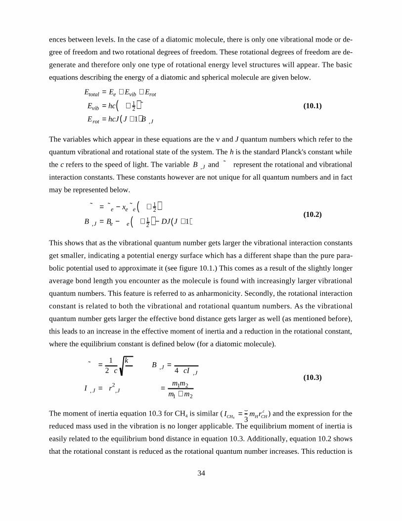
ences between levels. In the case of a diatomic molecule, there is only one vibrational mode or de-

gree of freedom and two rotational degrees of freedom. These rotational degrees of freedom are de-

generate and therefore only one type of rotational energy level structures will appear. The basic

equations describing the energy of a diatomic and spherical molecule are given below.

Etotal = Ee + Evib + Erot

Evib = hc + 12( ) ˜

Erot = hcJ J +1( )B ,J

(10.1)

The variables which appear in these equations are the and J quantum numbers which refer to the

quantum vibrational and rotational state of the system. The h is the standard Planck's constant while

the c refers to the speed of light. The variable B ,J and ˜ represent the rotational and vibrational

interaction constants. These constants however are not unique for all quantum numbers and in fact

may be represented below.

˜ = ˜ e − xe

˜ e + 1

2( )B ,J = Be − e + 1

2( ) − DJ J +1( )(10.2)

This shows that as the vibrational quantum number gets larger the vibrational interaction constants

get smaller, indicating a potential energy surface which has a different shape than the pure para-

bolic potential used to approximate it (see figure 10.1.) This comes as a result of the slightly longer

average bond length you encounter as the molecule is found with increasingly larger vibrational

quantum numbers. This feature is referred to as anharmonicity. Secondly, the rotational interaction

constant is related to both the vibrational and rotational quantum numbers. As the vibrational

quantum number gets larger the effective bond distance gets larger as well (as mentioned before),

this leads to an increase in the effective moment of inertia and a reduction in the rotational constant,

where the equilibrium constant is defined below (for a diatomic molecule).

˜ = 12 c

k B ,J =

4 cI ,J

I , J = r ,J2 =

m1m2

m1 + m2

(10.3)

The moment of inertia equation 10.3 for CH4 is similar ( ICH4=

8

3mHrCH

2 ) and the expression for the

reduced mass used in the vibration is no longer applicable. The equilibrium moment of inertia is

easily related to the equilibrium bond distance in equation 10.3. Additionally, equation 10.2 shows

that the rotational constant is reduced as the rotational quantum number increases. This reduction is

35

called the centrifugal distortion and is due to the added force that pulls the atoms apart as the angu-

lar momentum is increased. This is much like the merry-go-round effect where as the velocity is

increased the children are increasingly prone to fly off the wheel. This larger effective intermo-

lecular radius again causes the effective inertia to increase and reduces the rotational constant. In

general the centrifugal distortion term, D, in equation 2 will be dependent on which vibrational

state the molecule is in as well, since higher vibrational states are more susceptible to centrifugal

distortion. This term may be shown (see Herzberg7) to be approximately equal to 4 Be3 ˜

e2 . Addi-

tional terms may be included, however for the accuracy and precision of the data collected in this

experiment, these formulae are sufficient to completely describe the system.

In this experiment, since most of the molecules occur in the ground state vibrational energy

level ( = 0) the only transition we can observe is the = +1. The selection rules for the rotational

levels are more complex, since J = ±1, ±2 or 0 may all be observed in one way or another. The

J = ±2 refer to the Raman transitions and will not be discussed here but the other two refer to the

P, Q and R branches observed in a rotationally resolved IR spectrum. The selection rules are related

to the usual transition dipole moments calculated from the integral below.

fi = −e ∗f , J f( )r i , Ji( )d∫ (10.4)

These dipole moments squared lead to the intensity of a given transition. When each of the transi-

tions moments are evaluated in the case of HCl it is found that only the = +1, J = ±1 are ob-

served. The J = 0 transition is forbidden because the initial and final wavefunctions will have

identical rotational components which will cancel in the integral in equation 4 while the vibrational

wavefunctions will be orthogonal and lead to a zero integral.

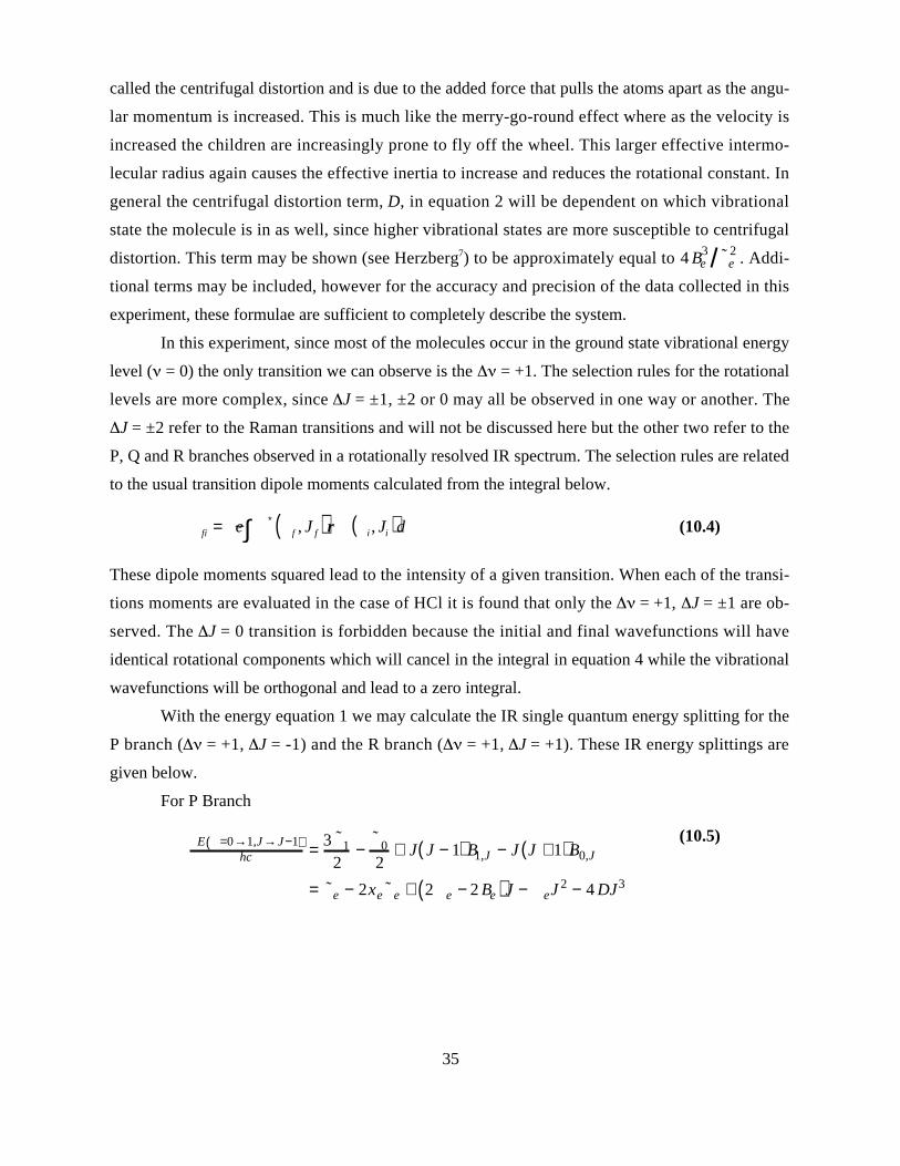
With the energy equation 1 we may calculate the IR single quantum energy splitting for the

P branch ( = +1, J = -1) and the R branch ( = +1, J = +1). These IR energy splittings are

given below.

For P Branch

E =0→1,J→J−1( )hc = 3 ˜ 1

2−

˜ 02

+ J J − 1( ) B1,J − J J +1( )B0,J

= ˜ e − 2xe ˜ e + 2 e − 2 Be( )J − eJ 2 − 4 DJ3

(10.5)

36

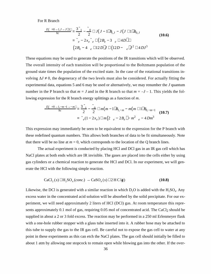
For R Branch

E =0→1,J→J+1( )hc =

3 ˜ 12

−˜ 02

+ J J − 1( ) B1,J − J J +1( )B0, J

= ˜ e − 2xe

˜ e + 2Be − 3 e + 4D( ) +

2Be − 4 e +12 D( )J + 12D − e( )J 2 + 4 DJ3

(10.6)

These equations may be used to generate the positions of the IR transitions which will be observed.

The overall intensity of each transition will be proportional to the Boltzmann population of the

ground state times the population of the excited state. In the case of the rotational transitions in-

volving J ≠ 0, the degeneracy of the two levels must also be considered. For actually fitting the

experimental data, equations 5 and 6 may be used or alternatively, we may renumber the J quantum

number in the P branch so that m = J and in the R branch so that m = –J – 1. This yields the fol-

lowing expression for the R branch energy splittings as a function of m.

E =0→1,−m −1→− m( )hc = 3 ˜ 1

2−

˜ 02

+ m m −1( )B1,−m − m m + 1( ) B0, −m−1

= ˜ e(1 − 2xe ) + m 2 e − 2Be( ) − m2e − 4 Dm3

(10.7)

This expression may immediately be seen to be equivalent to the expression for the P branch with

these redefined quantum numbers. This allows both branches of data to be fit simultaneously. Note

that there will be no line at m = 0, which corresponds to the location of the Q branch lines.

The actual experiment is conducted by placing HCl and DCl gas in an IR gas cell which has

NaCl plates at both ends which are IR invisible. The gases are placed into the cells either by using

gas cylinders or a chemical reaction to generate the HCl and DCl. In our experiment, we will gen-

erate the HCl with the following simple reaction.

CaCl2 (s) + H2SO4 (conc.) → CaSO4 (s) + 2 H C l (g) (10.8)

Likewise, the DCl is generated with a similar reaction in which D2O is added with the H2SO4. Any

excess water in the concentrated acid solution will be absorbed by the solid precipitate. For our ex-

periment, we will need approximately 2 liters of HCl (DCl) gas. At room temperature this repre-

sents approximately 0.1 mol of gas, requiring 0.05 mol of concentrated acid. The CaCl2 should be

supplied in about a 2 or 3 fold excess. The reaction may be performed in a 250 ml Erlenmeyer flask

with a one-hole rubber stopper with a glass tube inserted into it. A rubber hose may be attached to

this tube to supply the gas to the IR gas cell. Be careful not to expose the gas cell to water at any

point in these experiments as this can etch the NaCl plates. The gas cell should initially be filled to

about 1 atm by allowing one stopcock to remain open while blowing gas into the other. If the over-

37

all pressure in the cell is too great and no isotopic substructure may be seen in the IR spectrum, it

may be necessary to use vacuum rack techniques to fill the cell with less than 1 atm of HCl gas.

The IR spectrum may be taken in either absorption or transmission mode in the region of

interest (about 2800 cm-1 for HCl and about 2100 cm-1 for DCl). It should be possible to observe at

least ten distinct lines (perhaps twenty if the resolution of the spectrophotometer is capable of dis-

tinguishing the 35Cl from 37Cl isotopes) in both the P and R branches. The spectrum should be

taken with maximum resolution and expansion for accurate measurement of the peak positions.

Once the peaks have been measured, the spectrum should be assigned and then fit to the energy

function given in equation 7. The four basic spectroscopic constants ( e, Be, e, D) may then be

used to calculate the interatomic distances and bond strengths for each vibrational state as well as

the shape of the potential energy surface near the minimum. Errors should be fully propagated to

determine the overall accuracy of this method. These numbers may then be compared to those

given by Herzberg.7

38


Particle in a Box, Hückel Molecular Orbitaland GAUSSIAN98 Analysis of Cyanine Dye Molecule Spectra

Introduction:

This experiment is an adaptation of one published in various forms15-17 as well as being pre-

sented in the standard physical chemistry laboratory manual5. The purpose of this lab is to acquire

the UV/Vis spectra for a series of cyanine dye molecules and then attempt to interpret these spectra

in terms of various levels of theory ranging from the particle in a box model, the Hückel approxi-

mations for molecular orbits and finally full blown ab initio calculations with Gaussian94. The ba-

sic theory for each of these methods of analysis will not be detailed here, but rather only a rough

outline of the overall procedure will be given.

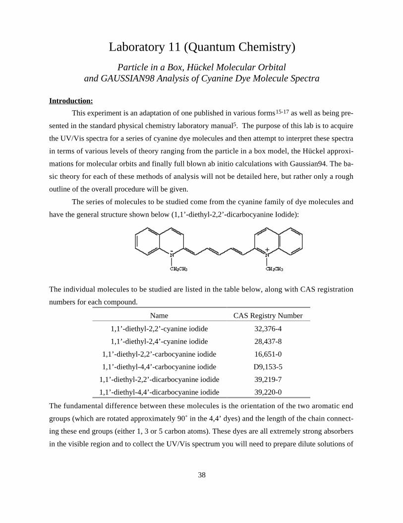
The series of molecules to be studied come from the cyanine family of dye molecules and

have the general structure shown below (1,1’-diethyl-2,2’-dicarbocyanine Iodide):

The individual molecules to be studied are listed in the table below, along with CAS registration

numbers for each compound.

Name CAS Registry Number

1,1’-diethyl-2,2’-cyanine iodide 32,376-4

1,1’-diethyl-2,4’-cyanine iodide 28,437-8

1,1’-diethyl-2,2’-carbocyanine iodide 16,651-0

1,1’-diethyl-4,4’-carbocyanine iodide D9,153-5

1,1’-diethyl-2,2’-dicarbocyanine iodide 39,219-7

1,1’-diethyl-4,4’-dicarbocyanine iodide 39,220-0

The fundamental difference between these molecules is the orientation of the two aromatic end

groups (which are rotated approximately 90˚ in the 4,4’ dyes) and the length of the chain connect-

ing these end groups (either 1, 3 or 5 carbon atoms). These dyes are all extremely strong absorbers

in the visible region and to collect the UV/Vis spectrum you will need to prepare dilute solutions of

39

each. Concentration is not critical, as we will not be determining any molar absorptivity values. All

spectra should be acquired at 25˚ C for standardization purposes.

Once the spectra have been collected, you should identify the λmax in each. This is assumed

to be the highest wavelength peak and hopefully will correspond to the transition from the HOMO

(highest occupied molecular orbit) to the LUMO (lowest unoccupied molecular orbit). To calculate

the energy splitting between these energy levels we shall use three methods, first will be the particle

in a box model. In this model we assume that the electrons (π only) are resonant in a box which

extends linearly over the length of a molecule. The length of this one-dimensional box is deter-

mined by assuming an average bond length and calculating the number of bonds over which the

electrons are delocalized. The standard energy expression for the one-dimensional particle in a box

is given by

En =h2n2

8ml2(11.1)

where n is the quantum number (1, 2, 3, ...), m is the mass of the electron and l is the length of the

box. The observed transition will be calculated by looking at the number of π electrons and placing

two in each of the levels until you reach the HOMO. For example, if you have 20 π electrons then

the first 10 orbits will be filled and the HOMO will be the n = 10 level. The LUMO will be the

nHOMO + 1 level, giving a transition energy of

∆En→n +1 =h2 n +1( )2

8ml2−

h2 n2

8ml2=

h2 2n +1( )8ml2

(11.2)

where n is the HOMO level. Calculate the wavelength of the HOMO-LUMO transition for each of

the six dye molecules (making appropriate approximations on the length of the “box” parameter, l).

Compare these calculations to the observed λmax for each molecule.

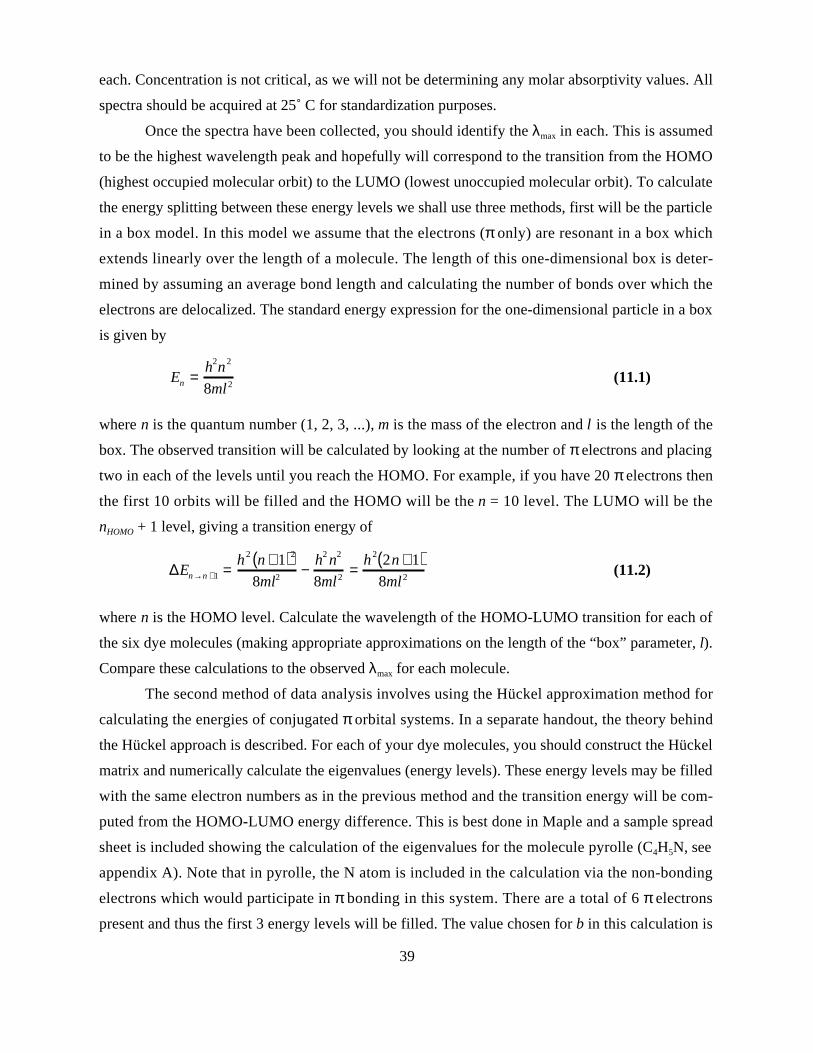
The second method of data analysis involves using the Hückel approximation method for

calculating the energies of conjugated π orbital systems. In a separate handout, the theory behind

the Hückel approach is described. For each of your dye molecules, you should construct the Hückel

matrix and numerically calculate the eigenvalues (energy levels). These energy levels may be filled

with the same electron numbers as in the previous method and the transition energy will be com-

puted from the HOMO-LUMO energy difference. This is best done in Maple and a sample spread

sheet is included showing the calculation of the eigenvalues for the molecule pyrolle (C4H5N, see

appendix A). Note that in pyrolle, the N atom is included in the calculation via the non-bonding

electrons which would participate in π bonding in this system. There are a total of 6 π electrons

present and thus the first 3 energy levels will be filled. The value chosen for b in this calculation is

40

one which represents an average exchange integral value of 77.5 kcal/mol. The matrices which are

required to calculate the energy of a cyanine dye molecule are substantially larger (20+ individual

eigenvalues) and will require a great deal of care to make sure that the elements are correct. In this

problem, the π bonding difference between an sp2 carbon and an sp2 pyrollic nitrogen are included

by changing the diagonal and off-diagonal elements for integrals involving the nitrogen atoms. The

calculated wavelengths for each dye molecule should again be compared to the experimental values

as well as the values calculated with the particle in a box model.

The third model will be to do a full ab initio calculation on the dye molecule of your choice

using GAUSSIAN98. This is a computer program on the Pentium II LINUX workstation which can

calculate wavefunctions and energy levels using the full Hamiltonian of the molecule within the

Born-Oppenheimer approximation using a density functional theory (DFT) approach. The compu-

tation time will take multiple hours at a reasonable level of theory and thus you will only study one

molecule with this program. The results will be given in a lengthy output file which contains more

information then you will need. Dr. Baltisberger will aid in extracting the energy levels of the

HOMO and LUMO and will help you convert the values into a wavelength which may be com-

pared to the other two methods.

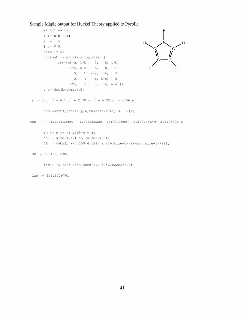
41

Sample Maple output for Hückel Theory applied to Pyrollewith(linalg):

e := n*b + a:

k := 1.5:

l := 0.8:

size := 5:

huckmat := matrix(size,size, [

a+(k*b)-e, l*b, 0, 0, l*b,

l*b, a-e, b, 0, 0,

0, b, a-e, b, 0,

0, 0, b, a-e, b,

l*b, 0, 0, b, a-e ]):

y := det(huckmat/b);

y := 1.5 n4 - 4.5 n2 + 2.78 - n5 + 4.28 n3 - 3.56 n

ans:=sort([fsolve(y,n,maxsols=size,-3..3)]);

ans := [ -1.618033989, -1.008258220, .6180339887, 1.188674649, 2.319583570 ]

an := p -> -ans[p]*b + a:

an(1+(size+1)/2)-an((size+1)/2):

DE := subs(b=(-77550*4.184),an(1+(size+1)/2)-an((size+1)/2));

DE := 185155.3185

lam := 6.626e-34*3.00e8*1.00e9*6.022e23/DE;

lam := 646.5129761

C

C

C

C

NH H

HH

H

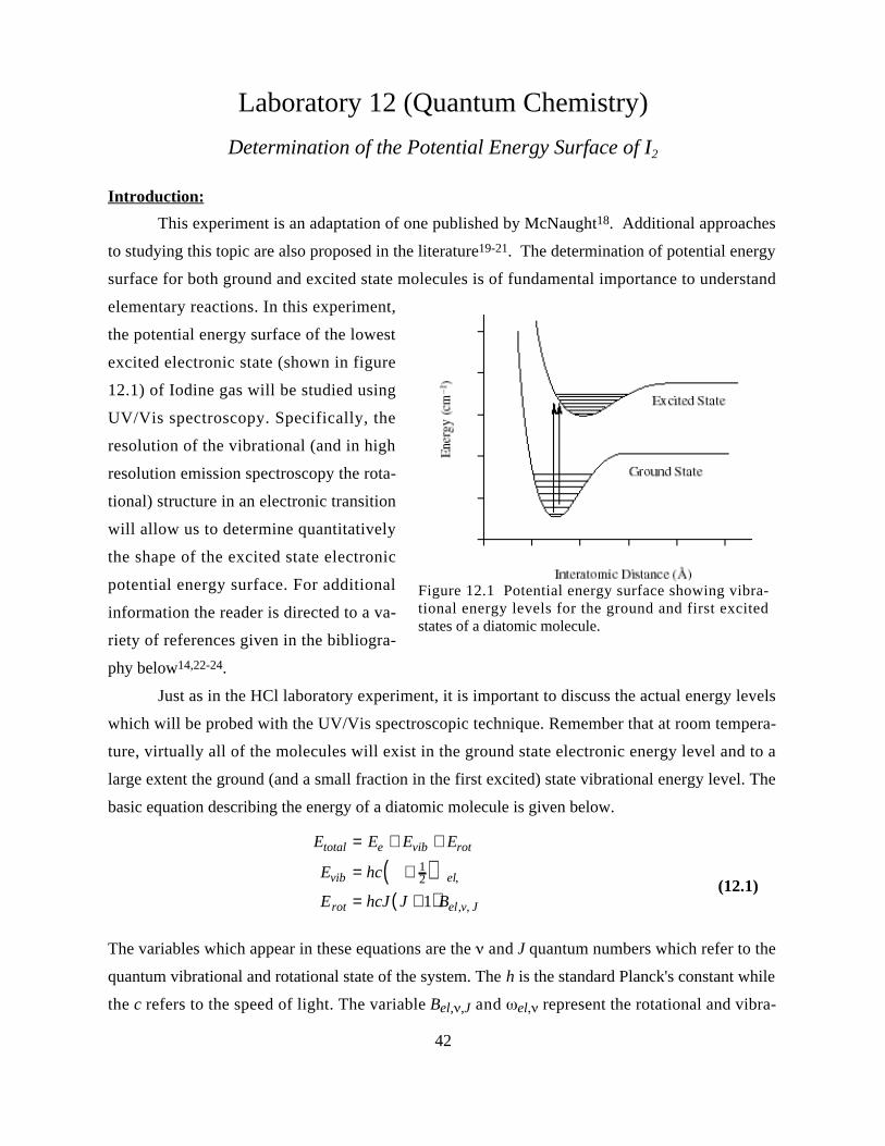
42


Determination of the Potential Energy Surface of I2

Introduction:

This experiment is an adaptation of one published by McNaught18. Additional approaches

to studying this topic are also proposed in the literature19-21. The determination of potential energy

surface for both ground and excited state molecules is of fundamental importance to understand

elementary reactions. In this experiment,

the potential energy surface of the lowest

excited electronic state (shown in figure

12.1) of Iodine gas will be studied using

UV/Vis spectroscopy. Specifically, the

resolution of the vibrational (and in high

resolution emission spectroscopy the rota-

tional) structure in an electronic transition

will allow us to determine quantitatively

the shape of the excited state electronic

potential energy surface. For additional

information the reader is directed to a va-

riety of references given in the bibliogra-

phy below14,22-24.

Just as in the HCl laboratory experiment, it is important to discuss the actual energy levels

which will be probed with the UV/Vis spectroscopic technique. Remember that at room tempera-

ture, virtually all of the molecules will exist in the ground state electronic energy level and to a

large extent the ground (and a small fraction in the first excited) state vibrational energy level. The

basic equation describing the energy of a diatomic molecule is given below.

Etotal = Ee + Evib + Erot

Evib = hc + 12( ) el,

Erot = hcJ J +1( )Bel,v, J

(12.1)

The variables which appear in these equations are the and J quantum numbers which refer to the

quantum vibrational and rotational state of the system. The h is the standard Planck's constant while

the c refers to the speed of light. The variable Bel, ,J and el represent the rotational and vibra-

Figure 12.1 Potential energy surface showing vibra-tional energy levels for the ground and first excitedstates of a diatomic molecule.

43

tional interaction constants. Remember that these constants are not unique for all quantum numbers

and in fact the vibrational frequency may be represented below.

el, = el − xel el + 12( ) − yel el + 1

2( )2− (12.2)

Notice that the vibrational constants in this equation actually refer to equilibrium for each electronic

state (there are separate el, etc. for each different electronic energy level). Also, as in the first

laboratory experiment, these equations show that as the vibrational quantum number gets larger the

vibrational interaction constants get smaller, indicating a potential energy surface which has a dif-

ferent shape than the pure parabolic potential used to approximate it. This feature is referred to as

anharmonicity, which may be seen in figure 12.1. As the interatomic radius is reduced, the potential

grows rapidly as the inner electrons begin to interact strongly (and ultimately as the nuclei begin to

interact). As the radius is increased, the potential levels off at a constant value. This is the dissocia-

tion energy above which the molecule dissociates into atomic species. It may be seen that the cur-

vature of the right hand side of the potential energy surface goes from concave up to concave down,

indicating a change in sign of the second derivative of the potential at some point. This may be ap-

proximated using the higher order terms in equation 12.2. Additional terms may be included, how-

ever for the accuracy and precision of the data collected in this experiment, these formulae are suf-

ficient to completely describe the system.

In this experiment, since most of the molecules exist in the ground state vibrational level of

the ground electronic state, X 1g , the primary transition we observe is from the = 0 vibrational

level of the X state to any of the higher vibrational levels of the excited electronic state, B 30u+ . It

may be shown in the usual manner that there will be no restriction on . The selection rules for the

rotational states are the same as in the first laboratory ( J = ±1). These energy levels will have the

effect of broadening the observed vibronic transition because of the range of energies which are ob-

served for the P and R branches of a rotation/vibration spectrum. In addition, at higher temperatures

the higher energy = 1 and = 2 vibrational levels of the X state will be increasingly populated and

will lead to two additional bands of transitions to vibrational states of the B state. The usual transi-

tion dipole moment integral may be used to calculate the intensity for each of the observed vibra-

tional bands.

fi = −e B*

f , J f( ) r X i , Ji( )d∫ (12.4)

The X and B subscripts on the wavefunctions refer to the respective electronic states. The intensity

of lines within each of the three observed bands will be determined from equation 12.4. These inte-

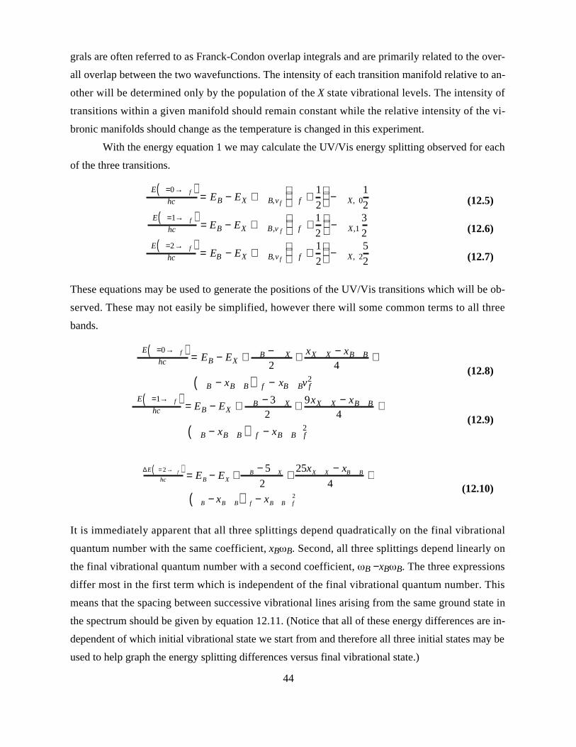
44

grals are often referred to as Franck-Condon overlap integrals and are primarily related to the over-

all overlap between the two wavefunctions. The intensity of each transition manifold relative to an-

other will be determined only by the population of the X state vibrational levels. The intensity of

transitions within a given manifold should remain constant while the relative intensity of the vi-

bronic manifolds should change as the temperature is changed in this experiment.

With the energy equation 1 we may calculate the UV/Vis energy splitting observed for each

of the three transitions.

E =0→ f( )hc = EB − EX + B,v f f +

1

2

− X, 0

1

2 (12.5)

E =1→ f( )hc = EB − EX + B,v f f +

1

2

− X,1

3

2 (12.6)

E =2→ f( )hc = EB − EX + B,v f f +

1

2

− X, 2

5

2 (12.7)

These equations may be used to generate the positions of the UV/Vis transitions which will be ob-

served. These may not easily be simplified, however there will some common terms to all three

bands.

E =0→ f( )hc = EB − EX + B − X

2+ xX X − xB B

4+

B − xB B( ) f − xB Bv f2

(12.8)

E =1→ f( )hc = EB − EX + B − 3 X

2+ 9xX X − xB B

4+

B − xB B( ) f − xB B f2

(12.9)

∆E = 2→ f( )hc = EB − EX + B − 5 X

2+

25xX X − xB B

4+

B − xB B( ) f − xB B f2

(12.10)

It is immediately apparent that all three splittings depend quadratically on the final vibrational

quantum number with the same coefficient, xB B. Second, all three splittings depend linearly on

the final vibrational quantum number with a second coefficient, B −xB B. The three expressions

differ most in the first term which is independent of the final vibrational quantum number. This

means that the spacing between successive vibrational lines arising from the same ground state in

the spectrum should be given by equation 12.11. (Notice that all of these energy differences are in-

dependent of which initial vibrational state we start from and therefore all three initial states may be

used to help graph the energy splitting differences versus final vibrational state.)

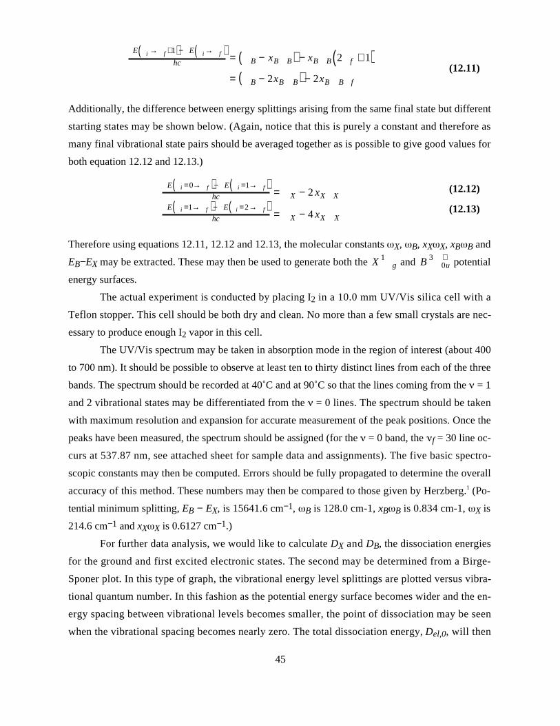
45

E i → f +1( )− E i → f( )hc

= B − xB B( ) − xB B 2 f + 1( )= B − 2xB B( ) − 2xB B f

(12.11)

Additionally, the difference between energy splittings arising from the same final state but different

starting states may be shown below. (Again, notice that this is purely a constant and therefore as

many final vibrational state pairs should be averaged together as is possible to give good values for

both equation 12.12 and 12.13.)

E i =0→ f( )− E i =1→ f( )hc = X − 2 xX X

(12.12)

E i =1→ f( )− E i =2→ f( )hc = X − 4 xX X

(12.13)

Therefore using equations 12.11, 12.12 and 12.13, the molecular constants X, B, xX X, xB B and

EB−EX may be extracted. These may then be used to generate both the X 1g and B 3

0u+ potential

energy surfaces.

The actual experiment is conducted by placing I2 in a 10.0 mm UV/Vis silica cell with a

Teflon stopper. This cell should be both dry and clean. No more than a few small crystals are nec-

essary to produce enough I2 vapor in this cell.

The UV/Vis spectrum may be taken in absorption mode in the region of interest (about 400

to 700 nm). It should be possible to observe at least ten to thirty distinct lines from each of the three

bands. The spectrum should be recorded at 40˚C and at 90˚C so that the lines coming from the = 1

and 2 vibrational states may be differentiated from the = 0 lines. The spectrum should be taken

with maximum resolution and expansion for accurate measurement of the peak positions. Once the

peaks have been measured, the spectrum should be assigned (for the = 0 band, the f = 30 line oc-

curs at 537.87 nm, see attached sheet for sample data and assignments). The five basic spectro-

scopic constants may then be computed. Errors should be fully propagated to determine the overall

accuracy of this method. These numbers may then be compared to those given by Herzberg.1 (Po-

tential minimum splitting, EB − EX, is 15641.6 cm−1, B is 128.0 cm-1, xB B is 0.834 cm-1, X is

214.6 cm−1 and xX X is 0.6127 cm−1.)

For further data analysis, we would like to calculate DX and DB, the dissociation energies

for the ground and first excited electronic states. The second may be determined from a Birge-

Sponer plot. In this type of graph, the vibrational energy level splittings are plotted versus vibra-

tional quantum number. In this fashion as the potential energy surface becomes wider and the en-

ergy spacing between vibrational levels becomes smaller, the point of dissociation may be seen

when the vibrational spacing becomes nearly zero. The total dissociation energy, Del,0, will then

46

represent the sum of all of these splittings, or the area under the curve. To a good approximation

this curve will be nearly linear and may be approximated as such. Note that this dissociation energy

is from the = 0 level, which is not the bottom of the potential energy well and therefore this disso-

ciation energy is labeled DB,0. To get DB from this, we need to add on the zero point energy B / 2.

To calculate the energy from the bottom of the ground electronic state to the dissociation point of

the first excited electronic state, E*, we need to add together the electronic splitting EB − EX and

DB,0. The difference between the ground state dissociation products and the excited state products

in the I2 dissociation will be the final state of one of the I product atoms. This atom will be in an

excited electronic state which is 7598 cm-1 higher in energy than a ground state iodine atom. The

dissociation energy, DX,0, for the ground electronic state from the = 0 vibrational level will be

given by the difference between E* and the atomic iodine excitation energy, 7598 cm-1. Again, this

dissociation energy must be corrected by the zero point vibrational energy, X / 2, to yield the cor-

rect value of DX.

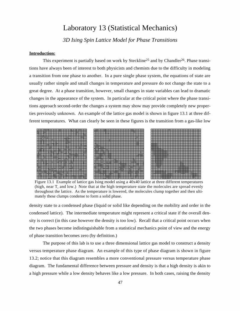
47

Laboratory 13 (Statistical Mechanics)

3D Ising Spin Lattice Model for Phase Transitions

Introduction:

This experiment is partially based on work by Steckline25 and by Chandler26. Phase transi-

tions have always been of interest to both physicists and chemists due to the difficulty in modeling

a transition from one phase to another. In a pure single phase system, the equations of state are

usually rather simple and small changes in temperature and pressure do not change the state to a

great degree. At a phase transition, however, small changes in state variables can lead to dramatic

changes in the appearance of the system. In particular at the critical point where the phase transi-

tions approach second-order the changes a system may show may provide completely new proper-

ties previously unknown. An example of the lattice gas model is shown in figure 13.1 at three dif-

ferent temperatures. What can clearly be seen in these figures is the transition from a gas-like low

density state to a condensed phase (liquid or solid like depending on the mobility and order in the

condensed lattice). The intermediate temperature might represent a critical state if the overall den-

sity is correct (in this case however the density is too low). Recall that a critical point occurs when

the two phases become indistinguishable from a statistical mechanics point of view and the energy

of phase transition becomes zero (by definition.)

The purpose of this lab is to use a three dimensional lattice gas model to construct a density

versus temperature phase diagram. An example of this type of phase diagram is shown in figure

13.2; notice that this diagram resembles a more conventional pressure versus temperature phase

diagram. The fundamental difference between pressure and density is that a high density is akin to

a high pressure while a low density behaves like a low pressure. In both cases, raising the density

Figure 13.1 Example of lattice gas Ising model using a 40x40 lattice at three different temperatures(high, near Tc and low.) Note that at the high temperature state the molecules are spread evenlythroughout the lattice. As the temperature is lowered, the molecules clump together and then ulti-mately these clumps condense to form a solid phase.

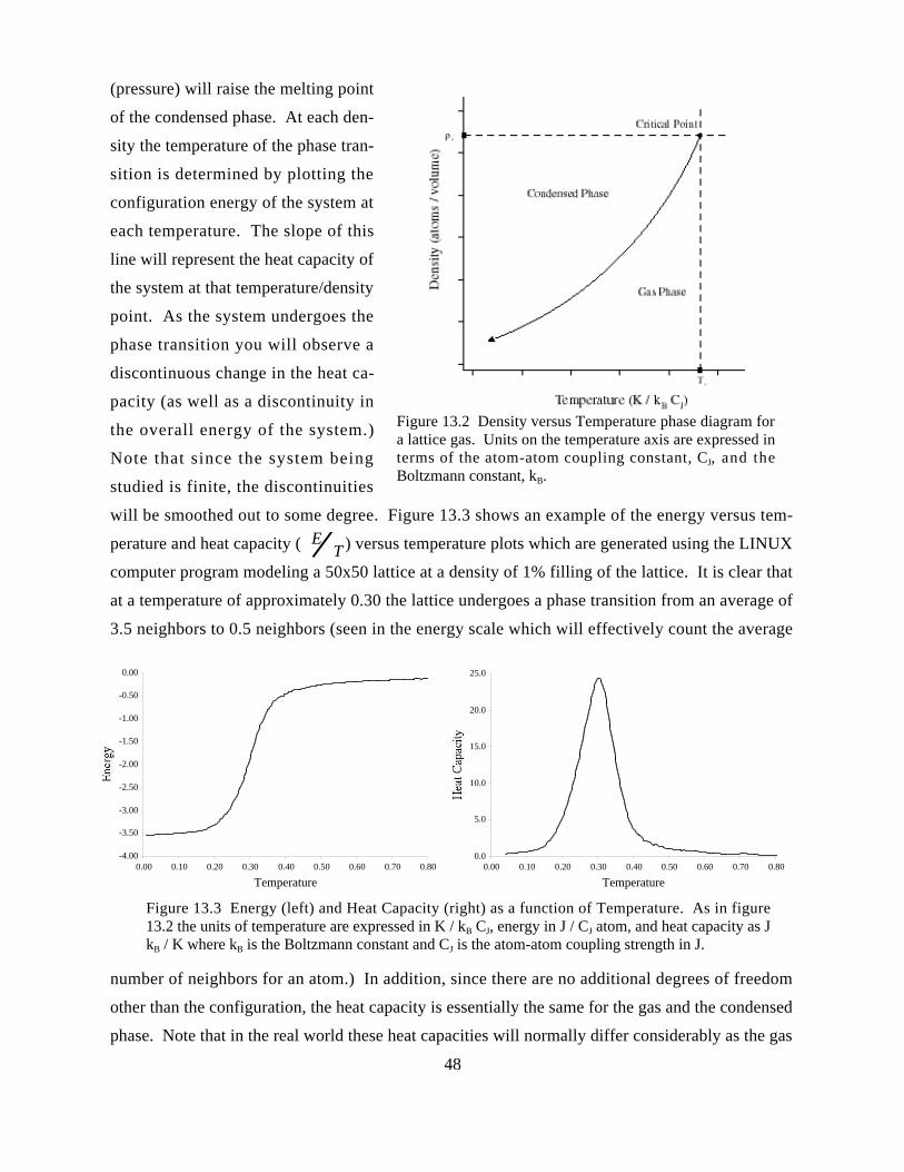
48

(pressure) will raise the melting point

of the condensed phase. At each den-

sity the temperature of the phase tran-

sition is determined by plotting the

configuration energy of the system at

each temperature. The slope of this

line will represent the heat capacity of

the system at that temperature/density

point. As the system undergoes the

phase transition you will observe a

discontinuous change in the heat ca-

pacity (as well as a discontinuity in

the overall energy of the system.)

Note that since the system being

studied is finite, the discontinuities

will be smoothed out to some degree. Figure 13.3 shows an example of the energy versus tem-

perature and heat capacity ( ET ) versus temperature plots which are generated using the LINUX

computer program modeling a 50x50 lattice at a density of 1% filling of the lattice. It is clear that

at a temperature of approximately 0.30 the lattice undergoes a phase transition from an average of

3.5 neighbors to 0.5 neighbors (seen in the energy scale which will effectively count the average

number of neighbors for an atom.) In addition, since there are no additional degrees of freedom

other than the configuration, the heat capacity is essentially the same for the gas and the condensed

phase. Note that in the real world these heat capacities will normally differ considerably as the gas

Figure 13.2 Density versus Temperature phase diagram fora lattice gas. Units on the temperature axis are expressed interms of the atom-atom coupling constant, CJ, and theBoltzmann constant, kB.

-4.00

-3.50

-3.00

-2.50

-2.00

-1.50

-1.00

-0.50

0.00

0.00 0.10 0.20 0.30 0.40 0.50 0.60 0.70 0.80

Temperature

Ene

rgy

0.0

5.0

10.0

15.0

20.0

25.0

0.00 0.10 0.20 0.30 0.40 0.50 0.60 0.70 0.80

Temperature

Hea

t Cap

acity

Figure 13.3 Energy (left) and Heat Capacity (right) as a function of Temperature. As in figure13.2 the units of temperature are expressed in K / kB CJ, energy in J / CJ atom, and heat capacity as JkB / K where kB is the Boltzmann constant and CJ is the atom-atom coupling strength in J.

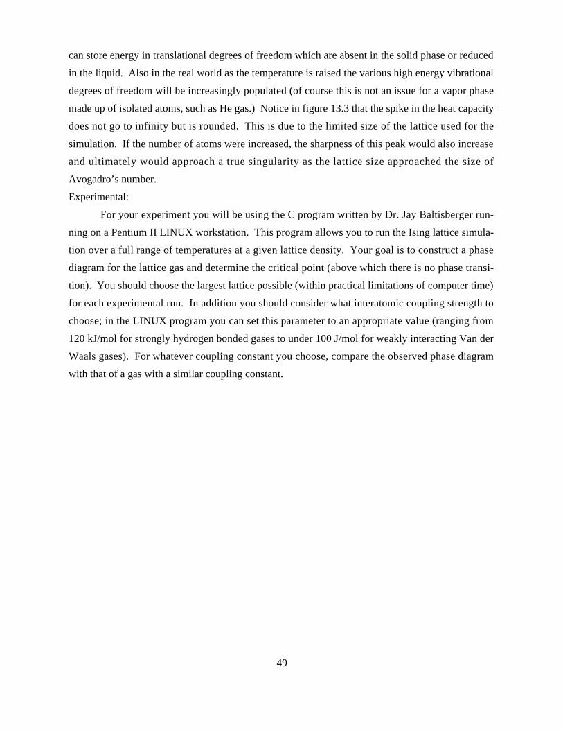
49

can store energy in translational degrees of freedom which are absent in the solid phase or reduced

in the liquid. Also in the real world as the temperature is raised the various high energy vibrational

degrees of freedom will be increasingly populated (of course this is not an issue for a vapor phase

made up of isolated atoms, such as He gas.) Notice in figure 13.3 that the spike in the heat capacity

does not go to infinity but is rounded. This is due to the limited size of the lattice used for the

simulation. If the number of atoms were increased, the sharpness of this peak would also increase

and ultimately would approach a true singularity as the lattice size approached the size of

Avogadro’s number.

Experimental:

For your experiment you will be using the C program written by Dr. Jay Baltisberger run-

ning on a Pentium II LINUX workstation. This program allows you to run the Ising lattice simula-

tion over a full range of temperatures at a given lattice density. Your goal is to construct a phase

diagram for the lattice gas and determine the critical point (above which there is no phase transi-

tion). You should choose the largest lattice possible (within practical limitations of computer time)

for each experimental run. In addition you should consider what interatomic coupling strength to

choose; in the LINUX program you can set this parameter to an appropriate value (ranging from

120 kJ/mol for strongly hydrogen bonded gases to under 100 J/mol for weakly interacting Van der

Waals gases). For whatever coupling constant you choose, compare the observed phase diagram

with that of a gas with a similar coupling constant.

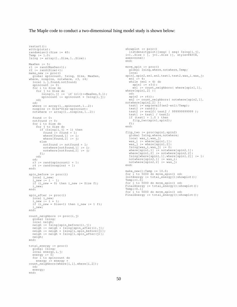
50

The Maple code to conduct a two-dimensional Ising model study is shown below:

restart():with(plots):randomize():Size := 40:Temp := 1.0:Ising := array(1..Size,1..Size):

MaxDen := 5:r1 := rand(MaxDen+1):r2 := rand(Size)+1:make_new := proc() global spincount, Ising, Size, MaxDen,where, nospins, notwhere, r3, r4; local i,j,found,notfound; spincount := 0: for i to Size do for j to Size do Ising[i,j] := `if`(r1()>=MaxDen,0,1); spincount := spincount + Ising[i,j]; od; od; where := array(1..spincount,1..2): nospins := Size*Size-spincount: notwhere := array(1..nospins,1..2):

found := 0: notfound := 0: for i to Size do for j to Size do if (Ising[i,j] = 1) then found := found + 1; where[found,1] := i; where[found,2] := j; else notfound := notfound + 1; notwhere[notfound,1] := i; notwhere[notfound,2] := j; fi; od; od; r3 := rand(spincount) + 1: r4 := rand(nospins) + 1:end:

spin_before := proc(i) local i_new; i_new := i - 1; if (i_new = 0) then i_new := Size fi; i_new;end:

spin_after := proc(i) local i_new; i_new := i + 1; if (i_new = Size+1) then i_new := 1 fi; i_new;end:

count_neighbors := proc(i,j) global Ising; local neigh; neigh := Ising[spin_before(i),j]; neigh := neigh + Ising[spin_after(i),j]; neigh := neigh + Ising[i,spin_before(j)]; neigh := neigh + Ising[i,spin_after(j)]; neigh;end:

total_energy := proc() global Ising; local energy,i,j; energy := 0; for i to spincount do energy := energy +count_neighbors(where[i,1],where[i,2]); od; energy;end:

showplot := proc() listdensityplot([seq( [ seq( Ising[i,j],i=1..Size ) ], j=1..Size )], style=PATCH,axes=none);end:

move_spin := proc() global Ising,where,notwhere,Temp; localspin1,spin2,en1,en2,test1,test2,was_i,was_j; en1 := 4: while (en1 = 4) do spin1 := r3(): en1 := count_neighbors( where[spin1,1],where[spin1,2] ): od: spin2 := r4(): en2 := count_neighbors( notwhere[spin2,1],notwhere[spin2,2] ): test1 := exp(evalf(en2-en1)/Temp); test2 := rand(); test2 := evalf( test2 / 999999999999 ); test1 := test1 / test2; if (test1 > 1.0 ) then flip_two(spin1,spin2); fi;end:

flip_two := proc(spin1,spin2) global Ising,where,notwhere; local was_i,was_j; was_i := where[spin1,1]: was_j := where[spin1,2]: Ising[was_i,was_j] := 0: where[spin1,1] := notwhere[spin2,1]: where[spin1,2] := notwhere[spin2,2]: Ising[where[spin1,1],where[spin1,2]] := 1: notwhere[spin2,1] := was_i: notwhere[spin2,2] := was_j:end:

make_new():Temp := 10.0;for i to 5000 do move_spin() od:InitEnergy := total_energy();showplot();Temp:=1.0;for i to 5000 do move_spin() od:FinalEnergy := total_energy();showplot();Temp:=0.1;for i to 5000 do move_spin() od:FinalEnergy := total_energy();showplot();

The C program to perform the three-dimensional Ising model study is shown below:

/* Ising model for 3D lattice gas*/#include <stdio.h>#include <stdlib.h>#include <time.h>#include <math.h>

/* Defines */

/* Globals */double temp,j_coup,j_coup_kb;long int ***data_array;long int **spin_positions;long int size,energy,spins,idum;

/* structures */

/* Prototypes */long int count_spins(void);double ran2(long int idum[]);long int get_energy(void);long int **matrix(long int nrh,long int nch);long int ***lattice(long int nrh,long int nch,long int ndh);long int count_neighbors(long int i, long int j, long int h);double *array(long int size);long int randim(void);long int ranspin(void);long int flip_spins(long int flips);void init_data(void);

/* Main program */void main(void) { long int i,iterations,flips,num_total; long int num_temps,num_tem2; char ans; char filename[25],errfilenm[25]; FILE *output; double *temps,*errs,*energies,temp_min,temp_max,run_energy,temp_spacing; double total_energy,total_eng2;

printf("What is size of array (NxNxN, with N < 2500)?\n"); scanf("%li",&size); if (size>2500) size = 2500; printf("The array will be %li x %li x %li\n",size,size,size); printf("What is number of gas spins (must be less than %5li)?\n",size*size*size/2); scanf("%li",&spins); if (spins>3*size*size*size/4) spins = 3*size*size*size/4; printf("The array will be filled with %li spins\n",spins);

data_array = lattice(size+1,size+1,size+1); spin_positions = matrix(spins+2,5); idum = -time(NULL); printf("Random seed: %li\n",idum); if (idum>=0) idum = - idum - 1; ran2(&idum);

printf("How many spins to flip per energy check?\n"); scanf("%li",&flips); if (flips<=100) flips = 100; if (flips>=size*size*size) flips = size*size*size; printf("%li spins will be flipped each reporting period.\n",flips);

printf("How many iterations of spin flips?\n"); scanf("%li",&iterations); if (iterations<=10) iterations = 10; if (iterations>=500) iterations = 500; printf("%li reporting periods will be averaged over.\n",iterations);

printf("Do you want to choose your temperature or use a range [y/r]?\n"); scanf("%1s",&ans); if (ans != 'r' && ans != 'R') ans = 'y'; num_temps = 1; num_tem2 = 0; if (ans == 'r' || ans == 'R') { printf("What is the highest temperature you want (K)?\n"); scanf("%lf",&temp_max); if (temp_max<0) temp_max = 2.0; printf("What is the lowest temperature you want (K)?\n"); scanf("%lf",&temp_min); if (temp_min<0) temp_min = 0.1;

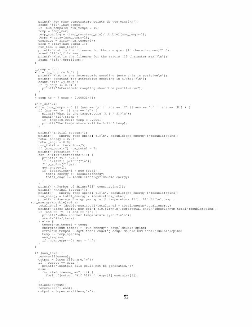
52

printf("How many temperature points do you want?\n"); scanf("%li",&num_temps); if (num_temps<0) num_temps = 10; temp = temp_max; temp_spacing = (temp_max-temp_min)/(double)(num_temps-1); temps = array(num_temps+1); energies = array(num_temps+1); errs = array(num_temps+1); num_tem2 = num_temps; printf("What is the filename for the energies [15 character max]?\n"); scanf("%15s",filename); printf("What is the filename for the errors [15 character max]?\n"); scanf("%15s",errfilenm); }

j_coup = 0.0; while (j_coup <= 0.0) { printf("What is the interatomic coupling (note this is positive\n"); printf("constant for attractive coupling in kJ/mol)?\n"); scanf("%lf",&j_coup); if (j_coup <= 0.0) { printf("Interatomic coupling should be positive.\n"); } } j_coup_kb = j_coup / 0.00831441;

init_data(); while (num_temps > 0 || (ans == 'y' || ans == 'Y' || ans == 'r' || ans == 'R') ) { if (ans == 'y' || ans == 'Y') { printf("What is the temperature (k T / J)?\n"); scanf("%lf",&temp); if (temp<=0.0001) temp = 0.0001; printf("The temperature will be %lf\n",temp); }

printf("Initial Status:"); printf(" Energy (per spin): %lf\n",-(double)get_energy()/(double)spins); total_energy = 0.0; total_eng2 = 0.0; num_total = iterations/5; if (num_total<7) num_total = 7; printf("Iteration "); for (i=1;i<=iterations;i++) { printf(" #%li ",i); if (!(i%12)) printf("\n"); flip_spins(flips); get_energy(); if (iterations-i < num_total) { total_energy += (double)energy; total_eng2 += (double)energy*(double)energy; } } printf("\nNumber of Spins:%li",count_spins()); printf("\nFinal Status:"); printf(" Energy (per spin): %lf\n",-(double)get_energy()/(double)spins); run_energy = total_energy / (double)num_total; printf("\nAverage Energy per spin (@ temperature %lf): %10.8lf\n",temp,-run_energy/(double)spins); total_eng2 = (double)num_total*total_eng2 - total_energy*total_energy; printf("Error Energy per spin: %10.8lf\n\n",sqrt(total_eng2)/(double)num_total/(double)spins); if (ans == 'y' || ans == 'Y') { printf("\nRun another temperature [y/n]?\n\n"); scanf("%1s",&ans); } else { temps[num_temps] = temp; energies[num_temps] = -run_energy*j_coup/(double)spins; errs[num_temps] = sqrt(total_eng2)*j_coup/(double)num_total/(double)spins; temp -= temp_spacing; num_temps--; if (num_temps==0) ans = 'n'; } }

if (num_tem2) { remove(filename); output = fopen(filename,"w"); if ( output == NULL ) printf("\nOutput file could not be generated."); else { for (i=1;i<=num_tem2;i++) { fprintf(output,"%lf %lf\n",temps[i],energies[i]); } } fclose(output); remove(errfilenm); output = fopen(errfilenm,"w");

53

if ( output == NULL ) printf("\nOutput file could not be generated."); else { for (i=1;i<=num_tem2;i++) { fprintf(output,"%lf %lf %lf\n",temps[i],energies[i],errs[i]); } } fclose(output); }}

long int randim(void) { return( size*ran2(&idum) + 1 );}

long int ranspin(void) { return( spins*ran2(&idum) + 1 );}

void init_data(void) { long int i,j,k,h; for (i=1;i<=size;i++) { for (j=1;j<=size;j++) { for (h=1;h<=size;h++) { data_array[i][j][h] = 0; } } } for (i=1;i<=spins;i++) { j = randim(); k = randim(); h = randim(); while ( data_array[j][k][h] == 1 ) { j = randim(); k = randim(); h = randim(); } data_array[j][k][h] = 1; spin_positions[i][0] = j; spin_positions[i][1] = k; spin_positions[i][2] = h; }}

long int flip_spins(long int flips) { long int total,new,old,h1,i,j,h,k,i1,j1,choosespin; double test;

total = 0; for (k=1;k<=flips;k++) { choosespin = ranspin(); i = spin_positions[choosespin][0]; j = spin_positions[choosespin][1]; h = spin_positions[choosespin][2]; i1 = randim(); j1 = randim(); h1 = randim(); while ( data_array[i1][j1][h1] == 1 ) { i1 = randim(); j1 = randim(); h1 = randim(); } if (i==i1 && j==j1 && h==h1) { exit(EXIT_FAILURE); } old = count_neighbors(i,j,h); new = count_neighbors(i1,j1,h1); test = ( (double) (new-old) ) * j_coup_kb / temp; test = exp( test ) / ran2(&idum); if (test >= 1.0) { data_array[i][j][h] = 0; data_array[i1][j1][h1] = 1; total++; spin_positions[choosespin][0] = i1; spin_positions[choosespin][1] = j1; spin_positions[choosespin][2] = h1; } } return(total);}

long int count_neighbors(long int i, long int j, long int h) { long int neighbors = 0;

if (j==size) { neighbors = data_array[i][1][h]; } else { neighbors = data_array[i][j+1][h]; }

54

if (i==size) { neighbors += data_array[1][j][h]; } else { neighbors += data_array[i+1][j][h]; }

if (h==size) { neighbors += data_array[i][j][1]; } else { neighbors += data_array[i][j][h+1]; }

if (j==1) { neighbors += data_array[i][size][h]; } else { neighbors += data_array[i][j-1][h]; }

if (i==1) { neighbors += data_array[size][j][h]; } else { neighbors += data_array[i-1][j][h]; }

if (h==1) { neighbors += data_array[i][j][size]; } else { neighbors += data_array[i][j][h-1]; } return(neighbors);}

long int get_energy(void) { long int i,j,h,count;

energy = 0; for (i=1;i<=size;i++) { for (j=1;j<=size;j++) { for (h=1;h<=size;h++) { if (data_array[i][j][h] == 1) { energy += count_neighbors(i,j,h); } } } } return(energy);}

long int count_spins(void) { long int i,j,h,count;

count = 0; for (i=1;i<=size;i++) { for (j=1;j<=size;j++) { for (h=1;h<=size;h++) { if (data_array[i][j][h] == 1) { count++; } } } } return(count);}

long int **matrix(long int nrh,long int nch) { long int i,j; long int **m;

m = (long int **) malloc( (nrh+2)*sizeof(long int*)); if(m ==NULL) { printf("\nMalloc failed (2nd dim of 2d array)"); exit(EXIT_FAILURE); }

for(i=0;i<=nrh;i++) { m[i]=(long int *) malloc( (nch+2)*sizeof(long int)); if(m ==NULL) { printf("\nMalloc failed (2nd dim of 2d array)"); exit(EXIT_FAILURE); } } for(i=0;i<=nrh;i++) { for(j=0;j<=nch;j++) m[i][j] = 0; } return(m);}

long int ***lattice(long int nrh,long int nch,long int ndh) { long int i,j,k; long int ***m;

m = (long int ***) malloc( (nrh+2)*sizeof(long int**)); if(m ==NULL) { printf("\nMalloc failed (1st dim of 3d array)"); exit(EXIT_FAILURE); }

55

for(i=0;i<=nrh;i++) { m[i] = (long int **) malloc( (nch+2)*sizeof(long int*)); if(m[i] ==NULL) { printf("\nMalloc failed (2nd dim of 3d array)"); exit(EXIT_FAILURE); } for(j=0;j<=ndh;j++) { m[i][j] = (long int *) malloc( (ndh+2)*sizeof(long int)); if(m[i][j] ==NULL) { printf("\nMalloc failed (3rd dim of 3d array)"); exit(EXIT_FAILURE); } } } for(i=0;i<=nrh;i++) { for(j=0;j<=nch;j++) { for(k=0;k<=ndh;k++) m[i][j][k] = 0; } } return(m);}

double *array(long int size) { double *m; long int i;

m = (double *) malloc( (size+3)*sizeof(double));

if ( m == NULL ) { printf("\nMalloc failed (1d Array)"); exit(EXIT_FAILURE); }

for(i=0;i<=size;i++) m[i] = 0.0;

return(m);}

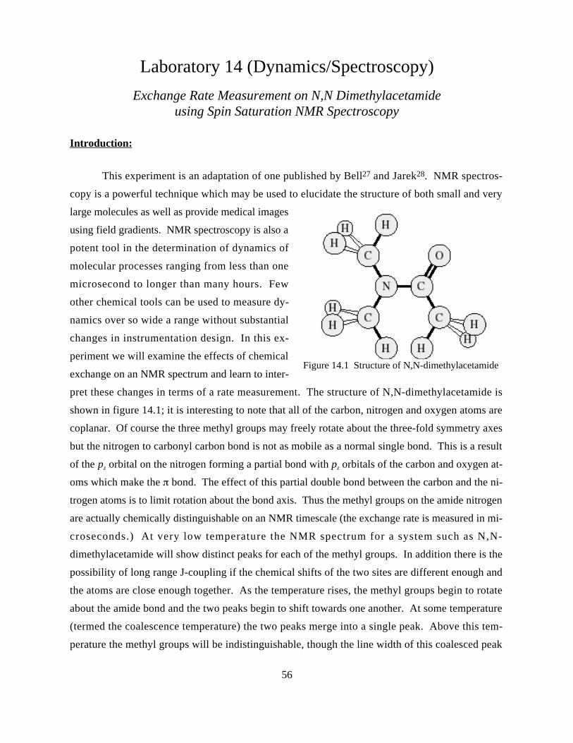
56


Exchange Rate Measurement on N,N Dimethylacetamideusing Spin Saturation NMR Spectroscopy

Introduction:

This experiment is an adaptation of one published by Bell27 and Jarek28. NMR spectros-

copy is a powerful technique which may be used to elucidate the structure of both small and very

large molecules as well as provide medical images

using field gradients. NMR spectroscopy is also a

potent tool in the determination of dynamics of

molecular processes ranging from less than one

microsecond to longer than many hours. Few

other chemical tools can be used to measure dy-

namics over so wide a range without substantial

changes in instrumentation design. In this ex-

periment we will examine the effects of chemical

exchange on an NMR spectrum and learn to inter-

pret these changes in terms of a rate measurement. The structure of N,N-dimethylacetamide is

shown in figure 14.1; it is interesting to note that all of the carbon, nitrogen and oxygen atoms are

coplanar. Of course the three methyl groups may freely rotate about the three-fold symmetry axes

but the nitrogen to carbonyl carbon bond is not as mobile as a normal single bond. This is a result

of the pz orbital on the nitrogen forming a partial bond with pz orbitals of the carbon and oxygen at-

oms which make the bond. The effect of this partial double bond between the carbon and the ni-

trogen atoms is to limit rotation about the bond axis. Thus the methyl groups on the amide nitrogen

are actually chemically distinguishable on an NMR timescale (the exchange rate is measured in mi-

croseconds.) At very low temperature the NMR spectrum for a system such as N,N-

dimethylacetamide will show distinct peaks for each of the methyl groups. In addition there is the

possibility of long range J-coupling if the chemical shifts of the two sites are different enough and

the atoms are close enough together. As the temperature rises, the methyl groups begin to rotate

about the amide bond and the two peaks begin to shift towards one another. At some temperature

(termed the coalescence temperature) the two peaks merge into a single peak. Above this tem-

perature the methyl groups will be indistinguishable, though the line width of this coalesced peak

Figure 14.1 Structure of N,N-dimethylacetamide

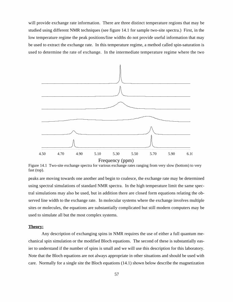
57

will provide exchange rate information. There are three distinct temperature regions that may be

studied using different NMR techniques (see figure 14.1 for sample two-site spectra.) First, in the

low temperature regime the peak positions/line widths do not provide useful information that may

be used to extract the exchange rate. In this temperature regime, a method called spin-saturation is

used to determine the rate of exchange. In the intermediate temperature regime where the two

peaks are moving towards one another and begin to coalesce, the exchange rate may be determined

using spectral simulations of standard NMR spectra. In the high temperature limit the same spec-

tral simulations may also be used, but in addition there are closed form equations relating the ob-

served line width to the exchange rate. In molecular systems where the exchange involves multiple

sites or molecules, the equations are substantially complicated but still modern computers may be

used to simulate all but the most complex systems.

Theory:

Any description of exchanging spins in NMR requires the use of either a full quantum me-

chanical spin simulation or the modified Bloch equations. The second of these is substantially eas-

ier to understand if the number of spins is small and we will use this description for this laboratory.

Note that the Bloch equations are not always appropriate in other situations and should be used with

care. Normally for a single site the Bloch equations (14.1) shown below describe the magnetization

4.50 4.70 4.90 5.10 5.30 5.50 5.70 5.90 6.10

Frequency (ppm)Figure 14.1 Two-site exchange spectra for various exchange rates ranging from very slow (bottom) to veryfast (top).

58

vector (MX,A, MY,A, MZ,A) in the Larmor frequency ( ) rotating frame and have two types of terms,

those that relate to the chemical shift of the site A ( ) and those that relate to the relaxation (T1,A,

T2,A).

˙ M Z ,A = 1

T1, A

MZ, A,0 − MZ, A( )

˙ M X , A = 0 − A( ) MY , A −1

T2, A

MX , A

˙ M Y, A = 0 − A( ) MX , A −1

T2, A

MY ,A

(14.1)

This is a fairly complicated set of coupled differential equations, but the terms are relatively easy to

understand qualitatively. The T1,A relaxation term essentially restores the original equilibrium mag-

netization, MZ,A,0 when the magnetization vector has been disturbed from equilibrium. This is a fa-

miliar exponential growth equation which is independent of the other two vector components. In

fact we studied T1,a measurements in laboratory 8 and you may return there for additional informa-

tion. The T2,A terms are line broadening terms that essentially exponentially damp out the magneti-

zation in the x-y plane. The chemical shift terms serve to rotate the magnetization about the x-y

plane at a frequency . In the presence of chemical exchange, the Bloch equations for site A are

modified as shown below (note that in the case of exchange there are now two spins labeled A and

B). Similar equations can be written for the B site.

˙ M Z ,A = 1

T1, A

MZ, A,0 − MZ, A( )

˙ M X , A = 0 − A( ) MY , A −1

T2, A

MX , A + kBMX, B − kAMX , A

˙ M Y, A = 0 − A( ) MX , A −1

T2, A

MY ,A + kBMY ,B − kAMY , A

(14.2)

The additional terms involve rate constants kA and kB which are the rates for exchange from A to B

and B to A respectively. Note that these are not independent and will relate to one another via the

equilibrium populations of the two sites such that pA kA = pB kB. The effect of this exchange on the

Bloch equations is rather mathematically challenging since we now have six coupled differential

equations to simultaneously solve. The net outcome from these equations is that an equation for the

lineshape may be written below.

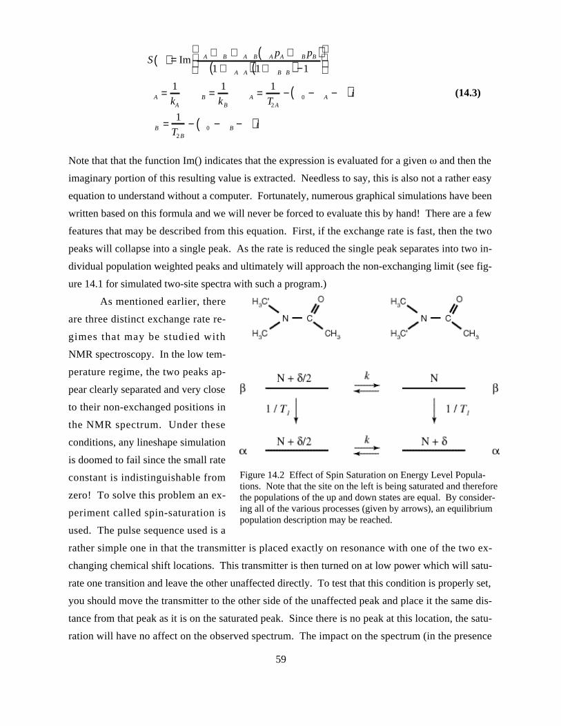
59

S ( ) = Im A + B + A B A pA + B pB( )1 + A A( ) 1+ B B( ) −1

A =1

kAB =

1

kBA =

1

T2 A

− 0 − A −( ) i

B =1

T2 B

− 0 − B −( ) i

(14.3)

Note that that the function Im() indicates that the expression is evaluated for a given and then the

imaginary portion of this resulting value is extracted. Needless to say, this is also not a rather easy

equation to understand without a computer. Fortunately, numerous graphical simulations have been

written based on this formula and we will never be forced to evaluate this by hand! There are a few

features that may be described from this equation. First, if the exchange rate is fast, then the two

peaks will collapse into a single peak. As the rate is reduced the single peak separates into two in-

dividual population weighted peaks and ultimately will approach the non-exchanging limit (see fig-

ure 14.1 for simulated two-site spectra with such a program.)

As mentioned earlier, there

are three distinct exchange rate re-

gimes that may be studied with

NMR spectroscopy. In the low tem-

perature regime, the two peaks ap-

pear clearly separated and very close

to their non-exchanged positions in

the NMR spectrum. Under these

conditions, any lineshape simulation

is doomed to fail since the small rate

constant is indistinguishable from

zero! To solve this problem an ex-

periment called spin-saturation is

used. The pulse sequence used is a

rather simple one in that the transmitter is placed exactly on resonance with one of the two ex-

changing chemical shift locations. This transmitter is then turned on at low power which will satu-

rate one transition and leave the other unaffected directly. To test that this condition is properly set,

you should move the transmitter to the other side of the unaffected peak and place it the same dis-

tance from that peak as it is on the saturated peak. Since there is no peak at this location, the satu-

ration will have no affect on the observed spectrum. The impact on the spectrum (in the presence

Figure 14.2 Effect of Spin Saturation on Energy Level Popula-tions. Note that the site on the left is being saturated and thereforethe populations of the up and down states are equal. By consider-ing all of the various processes (given by arrows), an equilibriumpopulation description may be reached.

60

of slow exchange) is that the unsaturated exchanging peak will be reduced in amplitude from the

equilibrium intensity. In the case of N,N-dimethylacetamide, the three methyl groups all should

have equal intensity initially (and show no J-coupling). Under the spin saturation experiment, the

non-exchanging methyl group will remain the original intensity while the other peaks are reduced

(one in fact disappears under saturation). The effect of spin saturation is shown in figure 14.2

where the two peaks will develop different population differences than a normal equilibrium popu-

lation difference in the absence of spin saturation. The mathematics of evaluating the various rate

constants in this figure are somewhat complicated (since it will be a system of coupled first order

differential equations) but straightforward in solution. By comparing the height of the exchange

peak to the non-exchange peak, the rate constant for the exchange process may be extracted via

equation 14.4 (the solution to the coupled equations).

k =I0 − I

I T1(14.4)

Where I is the intensity of the peak in the presence of spin saturation and I0 is the intensity of the

non-exchanging methyl group. The T1 is the spin lattice relaxation time (as measured identically to

laboratory 8) of the exchanging methyl group. For greater accuracy, the T1 for the exchanging site

should also be measured under spin-saturation of the other exchange site before substitution into

equation 14.4. If this is not done, you can expect approximately 5 to 10% errors in the measured

exchange rate constant, k.

Experiment:

For the experiment, you will conduct a series of T1 and spin saturation measurements at a

minimum of four different temperatures. Our NMR spectrometer is capable of covering tempera-

ture ranges from -40˚ C up to over 100˚ C. By measuring the rate constants using the procedure

outlined in the theory section, you can examine the rates as a function of temperature. By plotting

the ln k versus temperature, you may determine the activation energy of the rotational process, that

is to say the energy needed to rotate the methyl group by 90˚ (half-way to exchange). This infor-

mation is useful because it will give you insight into the amount of double bond character present

between the amide nitrogen and the carbonyl carbon atoms.

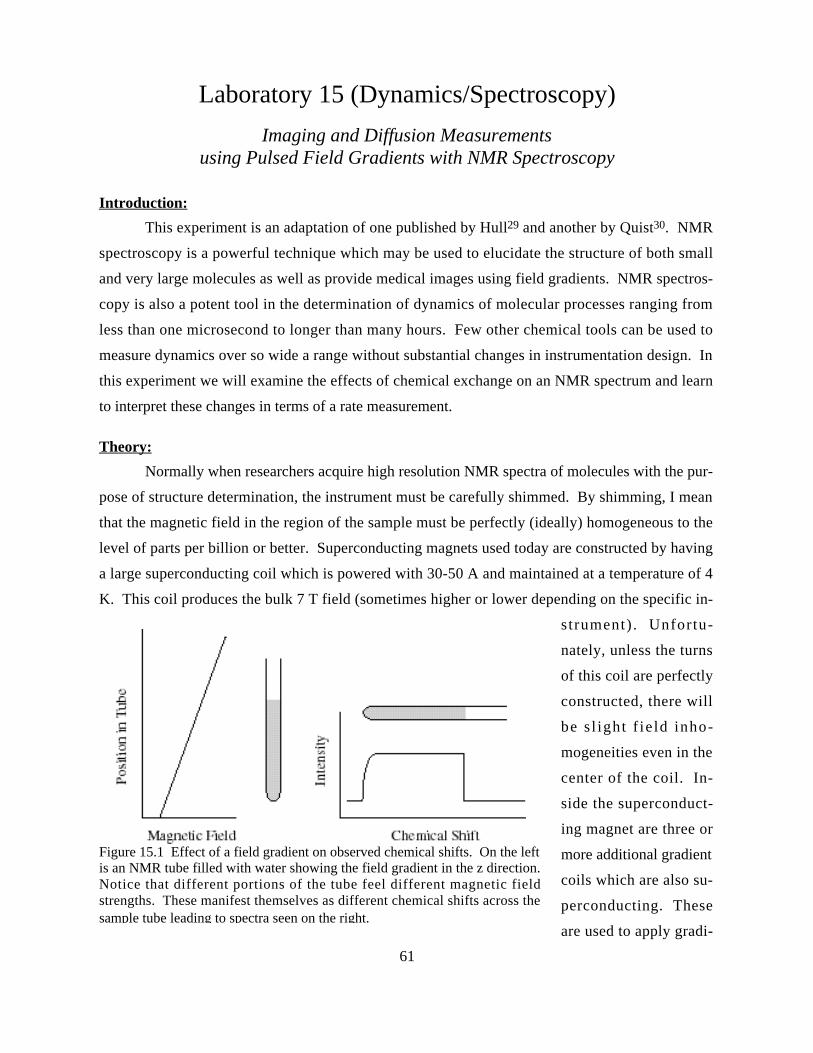
61


Imaging and Diffusion Measurementsusing Pulsed Field Gradients with NMR Spectroscopy

Introduction:

This experiment is an adaptation of one published by Hull29 and another by Quist30. NMR

spectroscopy is a powerful technique which may be used to elucidate the structure of both small

and very large molecules as well as provide medical images using field gradients. NMR spectros-

copy is also a potent tool in the determination of dynamics of molecular processes ranging from

less than one microsecond to longer than many hours. Few other chemical tools can be used to

measure dynamics over so wide a range without substantial changes in instrumentation design. In

this experiment we will examine the effects of chemical exchange on an NMR spectrum and learn

to interpret these changes in terms of a rate measurement.

Theory:

Normally when researchers acquire high resolution NMR spectra of molecules with the pur-

pose of structure determination, the instrument must be carefully shimmed. By shimming, I mean

that the magnetic field in the region of the sample must be perfectly (ideally) homogeneous to the

level of parts per billion or better. Superconducting magnets used today are constructed by having

a large superconducting coil which is powered with 30-50 A and maintained at a temperature of 4

K. This coil produces the bulk 7 T field (sometimes higher or lower depending on the specific in-

strument) . Unfortu-

nately, unless the turns

of this coil are perfectly

constructed, there will

be s l ight f ie ld inho-

mogeneities even in the

center of the coil. In-

side the superconduct-

ing magnet are three or

more additional gradient

coils which are also su-

perconducting. These

are used to apply gradi-

Figure 15.1 Effect of a field gradient on observed chemical shifts. On the leftis an NMR tube filled with water showing the field gradient in the z direction.Notice that different portions of the tube feel different magnetic fieldstrengths. These manifest themselves as different chemical shifts across thesample tube leading to spectra seen on the right.

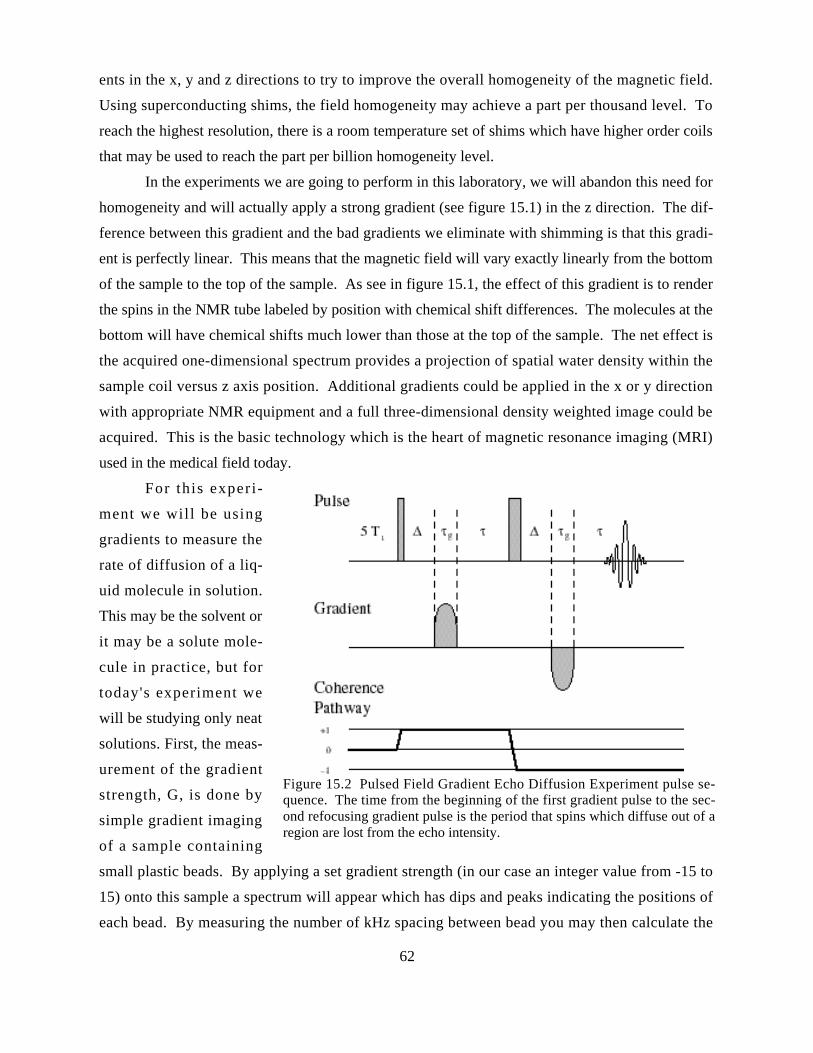
62

ents in the x, y and z directions to try to improve the overall homogeneity of the magnetic field.

Using superconducting shims, the field homogeneity may achieve a part per thousand level. To

reach the highest resolution, there is a room temperature set of shims which have higher order coils

that may be used to reach the part per billion homogeneity level.

In the experiments we are going to perform in this laboratory, we will abandon this need for

homogeneity and will actually apply a strong gradient (see figure 15.1) in the z direction. The dif-

ference between this gradient and the bad gradients we eliminate with shimming is that this gradi-

ent is perfectly linear. This means that the magnetic field will vary exactly linearly from the bottom

of the sample to the top of the sample. As see in figure 15.1, the effect of this gradient is to render

the spins in the NMR tube labeled by position with chemical shift differences. The molecules at the

bottom will have chemical shifts much lower than those at the top of the sample. The net effect is

the acquired one-dimensional spectrum provides a projection of spatial water density within the

sample coil versus z axis position. Additional gradients could be applied in the x or y direction

with appropriate NMR equipment and a full three-dimensional density weighted image could be

acquired. This is the basic technology which is the heart of magnetic resonance imaging (MRI)

used in the medical field today.

For this experi -

ment we will be using

gradients to measure the

rate of diffusion of a liq-

uid molecule in solution.

This may be the solvent or

it may be a solute mole-

cule in practice, but for

today's experiment we

will be studying only neat

solutions. First, the meas-

urement of the gradient

strength, G, is done by

simple gradient imaging

of a sample containing

small plastic beads. By applying a set gradient strength (in our case an integer value from -15 to

15) onto this sample a spectrum will appear which has dips and peaks indicating the positions of

each bead. By measuring the number of kHz spacing between bead you may then calculate the

Figure 15.2 Pulsed Field Gradient Echo Diffusion Experiment pulse se-quence. The time from the beginning of the first gradient pulse to the sec-ond refocusing gradient pulse is the period that spins which diffuse out of aregion are lost from the echo intensity.

63

gradient strength (after converting from kHz to T using the gyromagnetic ratio of the sample.) The

basic idea which we will use to measure diffusion is to use gradients to encode spins with specific

z-axis position information (in the form of an evolved chemical shift.) By using a 180˚ pulse to re-

focus the chemical shift interaction and applying a second gradient pulse, only those spins which

have not moved will be effectively refocused. The pulse sequence described is shown in figure

15.2. Note that the gradient pulses are relatively short with a long delay in between them. By

varying this delay (τ), the number of molecules which diffuse away from their starting locations

changes. Alternately, varying the gradient strength may achieve the same effect by providing

changing sensitivity to position. This approach in fact has the advantage of having a constant re-

laxation contribution to the overall echo intensity. The dependence on the diffusion constant is

shown below:

lnIg

I0

= − 2

g2 G2 + ∆+

2 g

3

D (15.1)

Where γ is the gyromagnetic ratio of the sample (γ = 2.675x108 T–1 s–1 for 1H in water,) G is the

gradient strength (measured in T / m,) and Ig and I0 are the echo intensities in the presence and ab-

sence of gradients respectively. In fact this equation suggests that the best way to measure the dif-

fusion constant is to plot the ln(Ig/ I0) as a function of G2. This plot would then be linear with a

slope of the form:

− 2g2 + ∆ +

2 g

3

D (15.2)

By inserting the appropriate values for the delays, this would then give an experimental measure of

the diffusion constant which might be compared against accepted values or theory:

D = kB T / 6 π η r (15.3)

where kB is the Boltzmann constant, T is the absolute temperature, r is the molecular radius and η is

the viscosity.

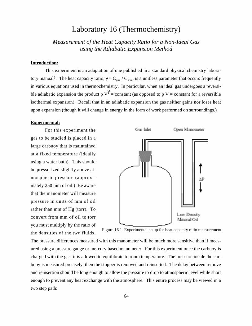
64


Measurement of the Heat Capacity Ratio for a Non-Ideal Gasusing the Adiabatic Expansion Method

Introduction:

This experiment is an adaptation of one published in a standard physical chemistry labora-

tory manual5. The heat capacity ratio, γ = Cp,m / CV,m, is a unitless parameter that occurs frequently

in various equations used in thermochemistry. In particular, when an ideal gas undergoes a reversi-

ble adiabatic expansion the product p Vγ = constant (as opposed to p V = constant for a reversible

isothermal expansion). Recall that in an adiabatic expansion the gas neither gains nor loses heat

upon expansion (though it will change in energy in the form of work performed on surroundings.)

Experimental:

For this experiment the

gas to be studied is placed in a

large carbuoy that is maintained

at a fixed temperature (ideally

using a water bath). This should

be pressurized slightly above at-

mospheric pressure (approxi-

mately 250 mm of oil.) Be aware

that the manometer will measure

pressure in units of mm of oil

rather than mm of Hg (torr). To

convert from mm of oil to torr

you must multiply by the ratio of

the densities of the two fluids.

The pressure differences measured with this manometer will be much more sensitive than if meas-

ured using a pressure gauge or mercury based manometer. For this experiment once the carbuoy is

charged with the gas, it is allowed to equilibrate to room temperature. The pressure inside the car-

buoy is measured precisely, then the stopper is removed and reinserted. The delay between remove

and reinsertion should be long enough to allow the pressure to drop to atmospheric level while short

enough to prevent any heat exchange with the atmosphere. This entire process may be viewed in a

two step path:

Figure 16.1 Experimental setup for heat capacity ratio measurement.

65

S1( p1, V1,m, T1 ) expands to S2( p2, V2,m, T2 ) (16.1)

S2( p2, V2,m, T2 ) is heated to S3( p3, V2,m, T1 ) (16.2)

Note that the external pressure will be p2 and the external temperature will be T1. This path will in-

deed be adiabatic since during the expansion no heat will enter the gas through the thick carbuoy

walls. Since this is an adiabatic expansion, the final temperature, T2, will be lower than the initial

temperature, T1. Note that the molar volume is constant during the last step since the carbuoy is

plugged during this time of reheating to room temperature. These various state variables do of

course relate to one another. If we assume a perfect gas behaviour, then the first step will be gov-

erned by the ideal gas law (p Vm / T = R) as follows:

p1 V1,m / T1 = p2 V2,m / T2 (16.3)

Similarly for the second step we may write:

p2 V2,m / T2 = p3 V2,m / T1 (16.4)

Combining equations 16.3 and 16.4, we may arrive at the relation below:

p1 / p3 = V2,m / V1,m (16.5)

In addition for the first step (which is adiabatic) the initial and final pressures and volumes must be

related via an adiabat (p Vγ = constant) giving the equation below:

ln (p1 / p2) = γ ln (V2,m / V1,m) (16.6)

Combining equation 16.5 and 16.6, we can write a closed form for the heat capacity ratio:

γ = ln (p1 / p2) / ln (p1 / p3) (16.7)

This expression is valid for an ideal gas but will be reasonable for a non-ideal gas for which the in-

teractions between molecules are not huge or where the pressure is not large. Note that p1 > p3 > p2

and therefore this expression will generate a γ greater than 1 (as is required.) When performing the

actual experiment, be certain to remember to add the atmospheric pressure to the measured ∆p (p1 =

p2 + ∆p1 and p3 = p2 + ∆p2) for each experimental cycle (release pressure/equilibrate). You should

repeat the release/equilibrate cycle multiple times until the differential pressure, ∆p, is too small to

be measured effectively. Calculate the γ for each cycle (note that the end point of the previous cy-

cle acts as the initial point for the subsequent cycle.) An alternative derivation of the heat capacity

66

ratio in which the expansion is not viewed as reversible gives a somewhat different relation shown

below:

γ = (p1 / p2 – 1) / (p1 / p3 – 1) (16.8)

Notice that this expression is very similar to 16.7 and is in fact related via a power law expansion.

You should calculate the heat capacity ratios with this formula as well and compare all results to

the accepted literature values. In addition, errors should be propagated fully and you should answer

the question whether you can effectively distinguish the 16.7 and 16.8 heat capacity ratios.

67


A Simple Measurement of Fluorescence Quenching of Quinine with NaCl

Introduction:

This experiment is an adaptation of one published by Sacksteder et al.31 The purpose of this

is to understand the physical process of fluorescence and to learn how a quenching agent changes

that process.

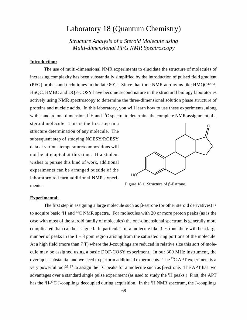
68


Structure Analysis of a Steroid Molecule usingMulti-dimensional PFG NMR Spectroscopy

Introduction:

The use of multi-dimensional NMR experiments to elucidate the structure of molecules of

increasing complexity has been substantially simplified by the introduction of pulsed field gradient

(PFG) probes and techniques in the late 80’s. Since that time NMR acronyms like HMQC32-34,

HSQC, HMBC and DQF-COSY have become second nature in the structural biology laboratories

actively using NMR spectroscopy to determine the three-dimensional solution phase structure of

proteins and nucleic acids. In this laboratory, you will learn how to use these experiments, along

with standard one-dimensional 1H and 13C spectra to determine the complete NMR assignment of a

steroid molecule. This is the first step in a

structure determination of any molecule. The

subsequent step of studying NOESY/ROESY

data at various temperature/compositions will

not be attempted at this time. If a student

wishes to pursue this kind of work, additional

experiments can be arranged outside of the

laboratory to learn additional NMR experi-

ments.

Experimental:

The first step in assigning a large molecule such as β-estrone (or other steroid derivatives) is

to acquire basic 1H and 13C NMR spectra. For molecules with 20 or more proton peaks (as is the

case with most of the steroid family of molecules) the one-dimensional spectrum is generally more

complicated than can be assigned. In particular for a molecule like β-estrone there will be a large

number of peaks in the 1 – 3 ppm region arising from the saturated ring portions of the molecule.

At a high field (more than 7 T) where the J-couplings are reduced in relative size this sort of mole-

cule may be assigned using a basic DQF-COSY experiment. In our 300 MHz instrument, the

overlap is substantial and we need to perform additional experiments. The 13C APT experiment is a

very powerful tool35-37 to assign the 13C peaks for a molecule such as β-estrone. The APT has two

advantages over a standard single pulse experiment (as used to study the 1H peaks.) First, the APT

has the 1H-13C J-couplings decoupled during acquisition. In the 1H NMR spectrum, the J-couplings

O

HO

Figure 18.1 Structure of -Estrone.

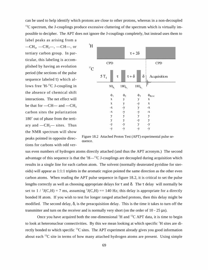
69

can be used to help identify which protons are close to other protons, whereas in a non-decoupled13C spectrum, the J-couplings produce excessive cluttering of the spectrum which is virtually im-

possible to decipher. The APT does not ignore the J-couplings completely, but instead uses them to

label peaks as arising from a

—CH3, —CH2—, —CH—, or

tertiary carbon group. In par-

ticular, this labeling is accom-

plished by having an evolution

period (the sections of the pulse

sequence labeled τ) which al-

lows free 1H-13C J-coupling in

the absence of chemical shift

interactions. The net effect will

be that for —CH— and —CH3

carbon sites the polarization

180˚ out of phase from the terti-

ary and —CH2— sites. Thus

the NMR spectrum will show

peaks pointed in opposite direc-

tions for carbons with odd ver-

sus even numbers of hydrogen atoms directly attached (and thus the APT acronym.) The second

advantage of this sequence is that the 1H—13C J-couplings are decoupled during acquisition which

results in a single line for each carbon atom. The solvent (normally deuterated pyridine for ster-

oids) will appear as 1:1:1 triplets in the aromatic region pointed the same direction as the other even

carbon atoms. When reading the APT pulse sequence in figure 18.2, it is critical to set the pulse

lengths correctly as well as choosing appropriate delays for τ and δ. The τ delay will normally be

set to 1 / 1J(C,H) = 7 ms, assuming 1J(C,H) == 140 Hz; this delay is appropriate for a directly

bonded H atom. If you wish to test for longer ranged attached protons, then this delay might be

modified. The second delay, δ, is the preacquisition delay. This is the time it takes to turn off the

transmitter and turn on the receiver and is normally very short (on the order of 10 - 25 µs).

Once you have acquired both the one-dimensional 1H and 13C APT data, it is time to begin

to look at heteronuclear connectivities. By this we mean looking at which specific 1H sites are di-

rectly bonded to which specific 13C sites. The APT experiment already gives you good information

about each 13C site in terms of how many attached hydrogen atoms are present. Using simple

Figure 18.2 Attached Proton Test (APT) experimental pulse se-quence.

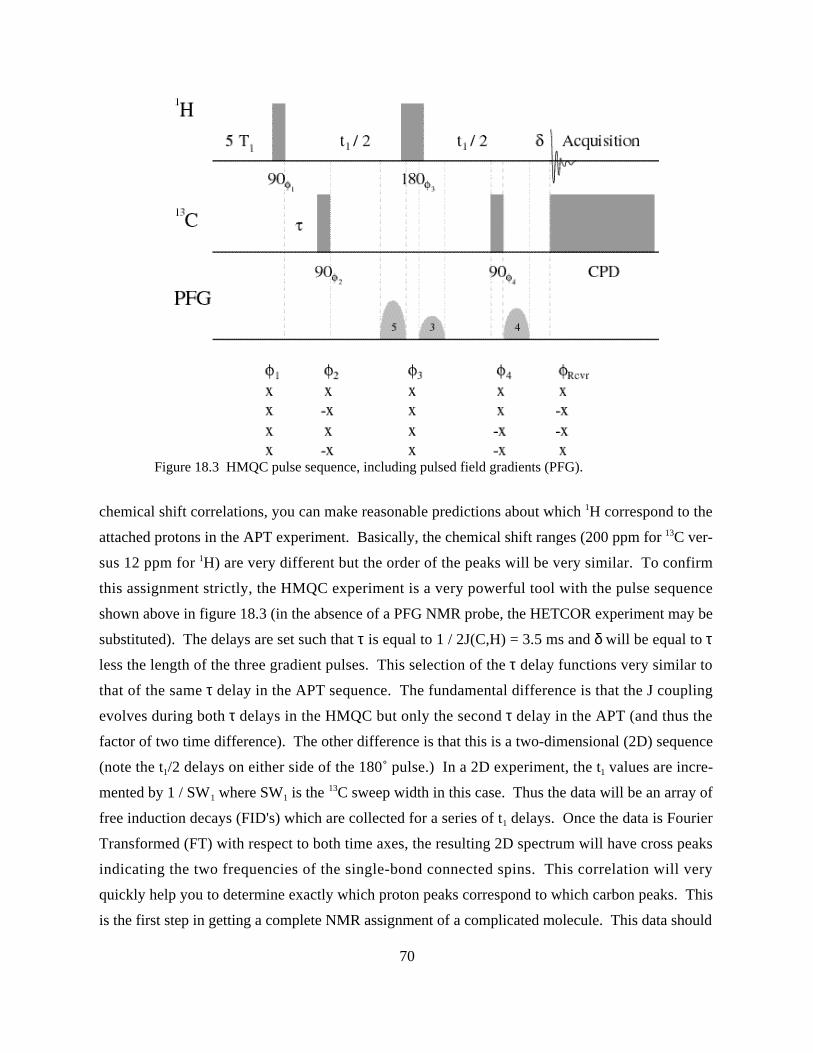
70

chemical shift correlations, you can make reasonable predictions about which 1H correspond to the

attached protons in the APT experiment. Basically, the chemical shift ranges (200 ppm for 13C ver-

sus 12 ppm for 1H) are very different but the order of the peaks will be very similar. To confirm

this assignment strictly, the HMQC experiment is a very powerful tool with the pulse sequence

shown above in figure 18.3 (in the absence of a PFG NMR probe, the HETCOR experiment may be

substituted). The delays are set such that τ is equal to 1 / 2J(C,H) = 3.5 ms and δ will be equal to τ

less the length of the three gradient pulses. This selection of the τ delay functions very similar to

that of the same τ delay in the APT sequence. The fundamental difference is that the J coupling

evolves during both τ delays in the HMQC but only the second τ delay in the APT (and thus the

factor of two time difference). The other difference is that this is a two-dimensional (2D) sequence

(note the t1/2 delays on either side of the 180˚ pulse.) In a 2D experiment, the t1 values are incre-

mented by 1 / SW1 where SW1 is the 13C sweep width in this case. Thus the data will be an array of

free induction decays (FID's) which are collected for a series of t1 delays. Once the data is Fourier

Transformed (FT) with respect to both time axes, the resulting 2D spectrum will have cross peaks

indicating the two frequencies of the single-bond connected spins. This correlation will very

quickly help you to determine exactly which proton peaks correspond to which carbon peaks. This

is the first step in getting a complete NMR assignment of a complicated molecule. This data should

Figure 18.3 HMQC pulse sequence, including pulsed field gradients (PFG).

71

be tabulated in a spread sheet (such as Excel) so that you can clearly see which sites have which

chemical shift values. The HMBC is analagous to the HMQC with the first 13C pulse replaced by a

90-τ2-90 sequence which is tuned to detect two and three bond J couplings (τ2 = 1 / 2 nJ(C,H) = 60

ms where nJ(C,H) is a long range two or three bond J coupling.) The net effect is that the cross

peaks observed in the HMBC will arise from one, two and three bond correlations. The added

benefit is that the 13C is not decoupled at the end and thus the one bond cross peaks will be split in

the proton dimension by 140 Hz. Therefore it is clear whether a given peak is a short or long range

correlation. By using the HMBC data, you may begin to connect the dots so to speak. By choosing

a peak which you clearly know (i.e. a methyl group for instance,) you may then look for HMBC

cross peaks to protons which are near this methyl peak. Once you determine the neighboring pro-

tons, you may use the HMQC to determine to which carbons these correspond. This process is re-

peated as you cycle around the entire molecule. A different experiment (DQF-COSY) may be used

to obtain the same correlation data but the drawback with this experiment is that both dimensions

are 1H. Since the 1H spectrum is rather crowded in the 1 - 3 ppm region, the cross peaks will over-

lap very strongly and thus the connectivity information will be rather difficult to extract.

72


Quadrupolar Interactions in NMR Spectroscopy

Introduction:

A vast majority of the atoms on the periodic table possess nuclear spin greater than 1/2. For

these nuclei, the charge distribution is non-spherical and thus interacts with local field gradients

present at the nucleus. In general these non-spherical nuclei may interact with even higher order

terms in the expansion of the electric potential energy but in general the quadrupolar terms will

dominate all others. The reason the quadrupolar terms are the largest arises since these second or-

der terms do not produce any direct forces on the nucleus (other than some torque on the nucleus).

The first order dipolar term is generally going to be zero since the nuclear location will always be at

a minimum in the potential energy field (i.e. the location where the first derivative is zero.) The ze-

roeth order term will merely act as an energy offset term on all nuclear energy levels and this con-

stant offset will not appear in any NMR energy expressions. Therefore the quadrupolar interaction

remains as the largest electric field – nuclear interaction.

Theory:

Quadrupolar interactions arise when expanding electromagnetic energies using a Taylor ex-

pansion. In general the electric field gradient may be represented as a 3 x 3 tensor of elements.

V =V

,

,

(19.1)

Vxx Vyx Vzx

Vxy Vyy Vzy

Vxz Vyz Vzz

(19.2)

This tensor may always be rewritten in an axis system which renders it diagonal. In this frame the

3 x 3 tensor is reduced to three diagonal components Vxx, Vyy, V zz. These three components must

obey the Poisson equation which demands that the field gradient tensor be traceless, i.e. Vxx + Vyy

+ Vzz = 0. Thus the quadrupolar interactions will ultimate depend only on the two parameters, Vzz

and η, where the second term is defined below.

=Vxx − Vyy

Vzz

(19.3)

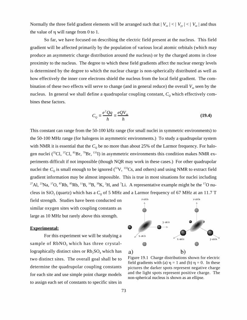
73

Normally the three field gradient elements will be arranged such that | Vxx | < | Vyy | < | Vzz | and thus

the value of will range from 0 to 1.

So far, we have focused on describing the electric field present at the nucleus. This field

gradient will be affected primarily by the population of various local atomic orbitals (which may

produce an asymmetric charge distribution around the nucleus) or by the charged atoms in close

proximity to the nucleus. The degree to which these field gradients affect the nuclear energy levels

is determined by the degree to which the nuclear charge is non-spherically distributed as well as

how effectively the inner core electrons shield the nucleus from the local field gradient. The com-

bination of these two effects will serve to change (and in general reduce) the overall Vzz seen by the

nucleus. In general we shall define a quadrupolar coupling constant, CQ which effectively com-

bines these factors.

CQ =e2Qq

h=

eQVzz

h(19.4)

This constant can range from the 50-100 kHz range (for small nuclei in symmetric environments) to

the 50-100 MHz range (for halogens in asymmetric environments.) To study a quadrupolar system

with NMR it is essential that the CQ be no more than about 25% of the Larmor frequency. For halo-

gen nuclei (35Cl, 37Cl, 81Br, 79Br, 131I) in asymmetric environments this condition makes NMR ex-

periments difficult if not impossible (though NQR may work in these cases.) For other quadrupolar

nuclei the CQ is small enough to be ignored (51V, 133Cs, and others) and using NMR to extract field

gradient information may be almost impossible. This is true in most situations for nuclei including27Al, 23Na, 17O, 87Rb, 85Rb, 11B, 10B, 39K, 2H, and 7Li. A representative example might be the 17O nu-

cleus in SiO2 (quartz) which has a CQ of 5 MHz and a Larmor frequency of 67 MHz at an 11.7 T

field strength. Studies have been conducted on

similar oxygen sites with coupling constants as

large as 10 MHz but rarely above this strength.

Experimental:

For this experiment we will be studying a

sample of RbNO3 which has three crystal-

lographically distinct sites or Rb2SO4 which has

two distinct sites. The overall goal shall be to

determine the quadrupolar coupling constants

for each site and use simple point charge models

to assign each set of constants to specific sites in

Figure 19.1 Charge distributions shown for electricfield gradients with (a) = 1 and (b) = 0. In thesepictures the darker spots represent negative chargeand the light spots represent positive charge. Thenon-spherical nucleus is shown as an ellipse.

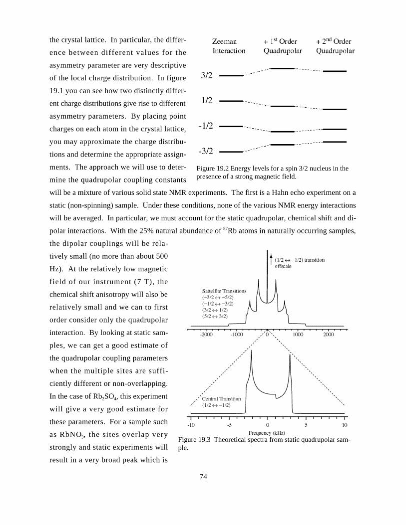
74

the crystal lattice. In particular, the differ-

ence between different values for the

asymmetry parameter are very descriptive

of the local charge distribution. In figure

19.1 you can see how two distinctly differ-

ent charge distributions give rise to different

asymmetry parameters. By placing point

charges on each atom in the crystal lattice,

you may approximate the charge distribu-

tions and determine the appropriate assign-

ments. The approach we will use to deter-

mine the quadrupolar coupling constants

will be a mixture of various solid state NMR experiments. The first is a Hahn echo experiment on a

static (non-spinning) sample. Under these conditions, none of the various NMR energy interactions

will be averaged. In particular, we must account for the static quadrupolar, chemical shift and di-

polar interactions. With the 25% natural abundance of 87Rb atoms in naturally occurring samples,

the dipolar couplings will be rela-

tively small (no more than about 500

Hz). At the relatively low magnetic

field of our instrument (7 T), the

chemical shift anisotropy will also be

relatively small and we can to first

order consider only the quadrupolar

interaction. By looking at static sam-

ples, we can get a good estimate of

the quadrupolar coupling parameters

when the multiple sites are suffi-

ciently different or non-overlapping.

In the case of Rb2SO4, this experiment

will give a very good estimate for

these parameters. For a sample such

as RbNO3, the sites overlap very

strongly and static experiments will

result in a very broad peak which is

Figure 19.2 Energy levels for a spin 3/2 nucleus in thepresence of a strong magnetic field.

Figure 19.3 Theoretical spectra from static quadrupolar sam-ple.

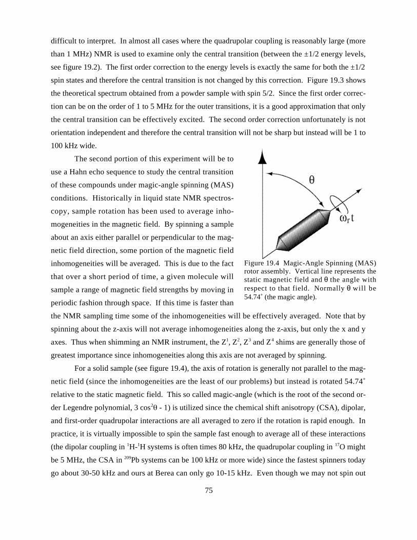
75

difficult to interpret. In almost all cases where the quadrupolar coupling is reasonably large (more

than 1 MHz) NMR is used to examine only the central transition (between the ±1/2 energy levels,

see figure 19.2). The first order correction to the energy levels is exactly the same for both the ±1/2

spin states and therefore the central transition is not changed by this correction. Figure 19.3 shows

the theoretical spectrum obtained from a powder sample with spin 5/2. Since the first order correc-

tion can be on the order of 1 to 5 MHz for the outer transitions, it is a good approximation that only

the central transition can be effectively excited. The second order correction unfortunately is not

orientation independent and therefore the central transition will not be sharp but instead will be 1 to

100 kHz wide.

The second portion of this experiment will be to

use a Hahn echo sequence to study the central transition

of these compounds under magic-angle spinning (MAS)

conditions. Historically in liquid state NMR spectros-

copy, sample rotation has been used to average inho-

mogeneities in the magnetic field. By spinning a sample

about an axis either parallel or perpendicular to the mag-

netic field direction, some portion of the magnetic field

inhomogeneities will be averaged. This is due to the fact

that over a short period of time, a given molecule will

sample a range of magnetic field strengths by moving in

periodic fashion through space. If this time is faster than

the NMR sampling time some of the inhomogeneities will be effectively averaged. Note that by

spinning about the z-axis will not average inhomogeneities along the z-axis, but only the x and y

axes. Thus when shimming an NMR instrument, the Z1, Z2, Z3 and Z4 shims are generally those of

greatest importance since inhomogeneities along this axis are not averaged by spinning.

For a solid sample (see figure 19.4), the axis of rotation is generally not parallel to the mag-

netic field (since the inhomogeneities are the least of our problems) but instead is rotated 54.74˚

relative to the static magnetic field. This so called magic-angle (which is the root of the second or-

der Legendre polynomial, 3 cos2 - 1) is utilized since the chemical shift anisotropy (CSA), dipolar,

and first-order quadrupolar interactions are all averaged to zero if the rotation is rapid enough. In

practice, it is virtually impossible to spin the sample fast enough to average all of these interactions

(the dipolar coupling in 1H-1H systems is often times 80 kHz, the quadrupolar coupling in 17O might

be 5 MHz, the CSA in 209Pb systems can be 100 kHz or more wide) since the fastest spinners today

go about 30-50 kHz and ours at Berea can only go 10-15 kHz. Even though we may not spin out

Figure 19.4 Magic-Angle Spinning (MAS)rotor assembly. Vertical line represents thestatic magnetic field and θ the angle withrespect to that field. Normally θ will be54.74˚ (the magic angle).

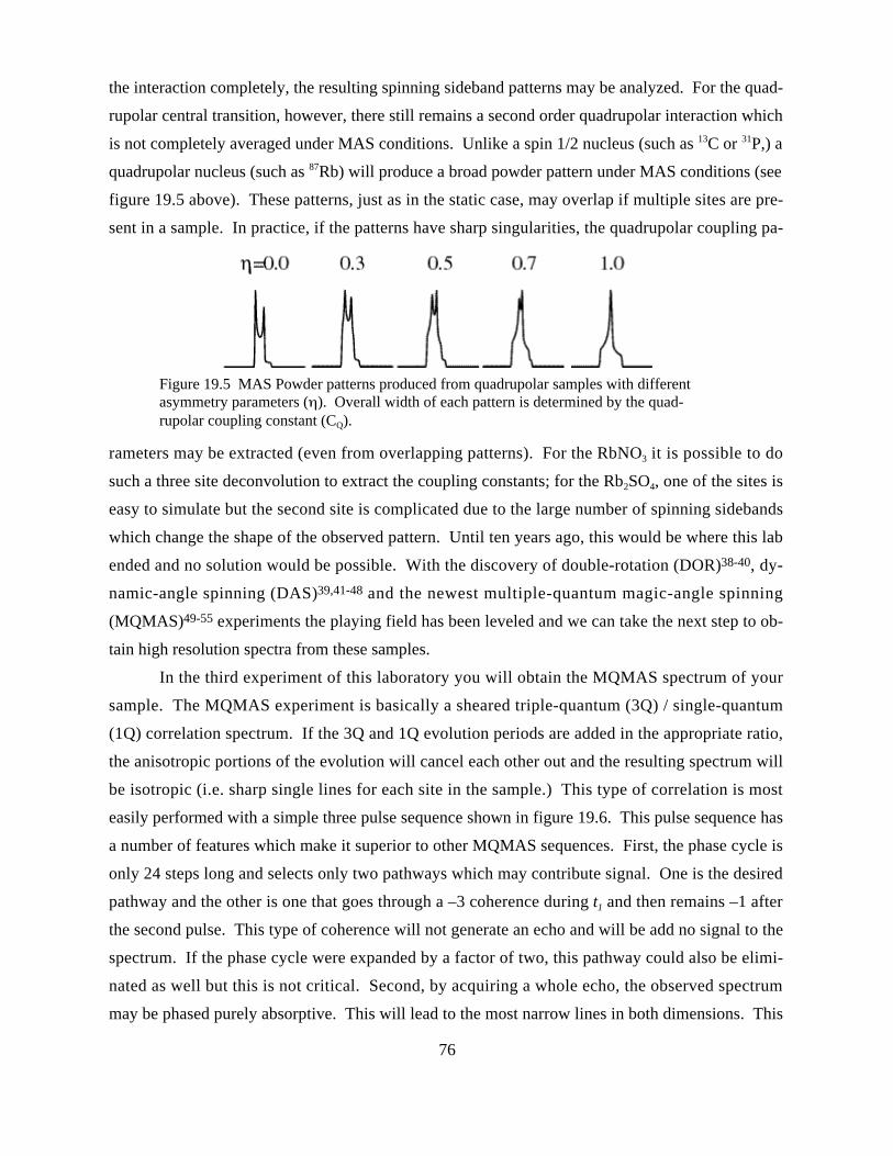
76

the interaction completely, the resulting spinning sideband patterns may be analyzed. For the quad-

rupolar central transition, however, there still remains a second order quadrupolar interaction which

is not completely averaged under MAS conditions. Unlike a spin 1/2 nucleus (such as 13C or 31P,) a

quadrupolar nucleus (such as 87Rb) will produce a broad powder pattern under MAS conditions (see

figure 19.5 above). These patterns, just as in the static case, may overlap if multiple sites are pre-

sent in a sample. In practice, if the patterns have sharp singularities, the quadrupolar coupling pa-

rameters may be extracted (even from overlapping patterns). For the RbNO3 it is possible to do

such a three site deconvolution to extract the coupling constants; for the Rb2SO4, one of the sites is

easy to simulate but the second site is complicated due to the large number of spinning sidebands

which change the shape of the observed pattern. Until ten years ago, this would be where this lab

ended and no solution would be possible. With the discovery of double-rotation (DOR)38-40, dy-

namic-angle spinning (DAS)39,41-48 and the newest multiple-quantum magic-angle spinning

(MQMAS)49-55 experiments the playing field has been leveled and we can take the next step to ob-

tain high resolution spectra from these samples.

In the third experiment of this laboratory you will obtain the MQMAS spectrum of your

sample. The MQMAS experiment is basically a sheared triple-quantum (3Q) / single-quantum

(1Q) correlation spectrum. If the 3Q and 1Q evolution periods are added in the appropriate ratio,

the anisotropic portions of the evolution will cancel each other out and the resulting spectrum will

be isotropic (i.e. sharp single lines for each site in the sample.) This type of correlation is most

easily performed with a simple three pulse sequence shown in figure 19.6. This pulse sequence has

a number of features which make it superior to other MQMAS sequences. First, the phase cycle is

only 24 steps long and selects only two pathways which may contribute signal. One is the desired

pathway and the other is one that goes through a –3 coherence during t1 and then remains –1 after

the second pulse. This type of coherence will not generate an echo and will be add no signal to the

spectrum. If the phase cycle were expanded by a factor of two, this pathway could also be elimi-

nated as well but this is not critical. Second, by acquiring a whole echo, the observed spectrum

may be phased purely absorptive. This will lead to the most narrow lines in both dimensions. This

Figure 19.5 MAS Powder patterns produced from quadrupolar samples with differentasymmetry parameters ( ). Overall width of each pattern is determined by the quad-rupolar coupling constant (CQ).

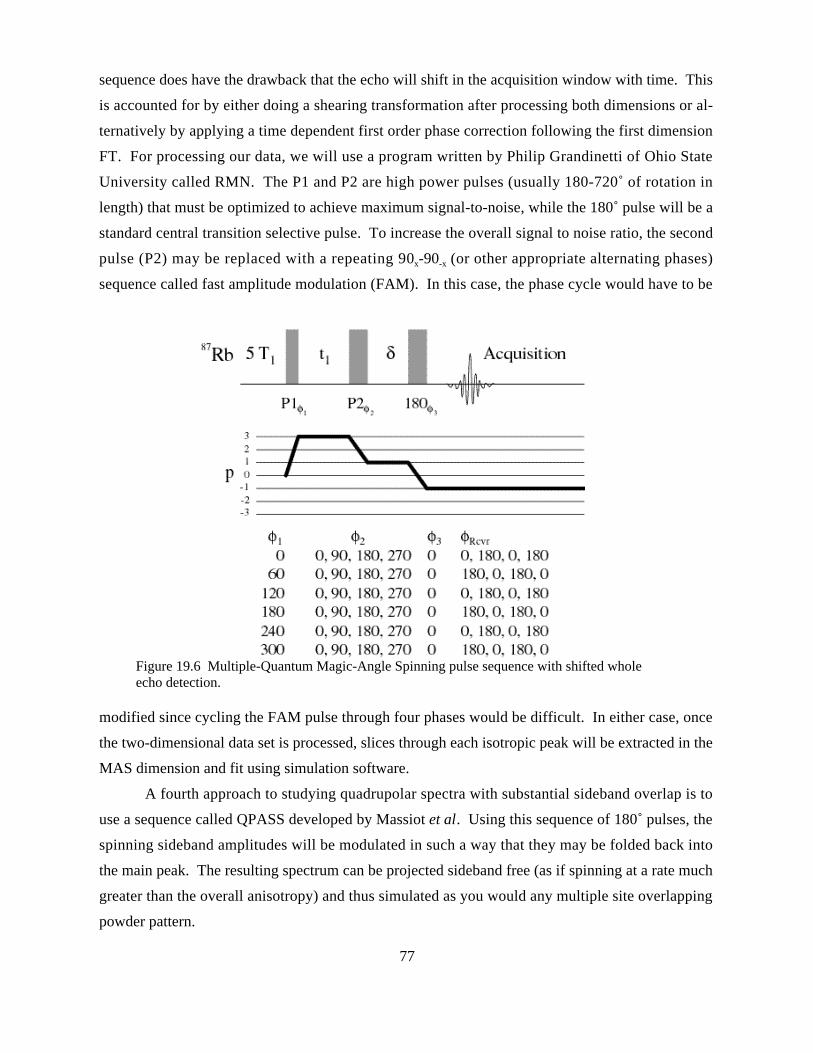
77

sequence does have the drawback that the echo will shift in the acquisition window with time. This

is accounted for by either doing a shearing transformation after processing both dimensions or al-

ternatively by applying a time dependent first order phase correction following the first dimension

FT. For processing our data, we will use a program written by Philip Grandinetti of Ohio State

University called RMN. The P1 and P2 are high power pulses (usually 180-720˚ of rotation in

length) that must be optimized to achieve maximum signal-to-noise, while the 180˚ pulse will be a

standard central transition selective pulse. To increase the overall signal to noise ratio, the second

pulse (P2) may be replaced with a repeating 90x-90-x (or other appropriate alternating phases)

sequence called fast amplitude modulation (FAM). In this case, the phase cycle would have to be

modified since cycling the FAM pulse through four phases would be difficult. In either case, once

the two-dimensional data set is processed, slices through each isotropic peak will be extracted in the

MAS dimension and fit using simulation software.

A fourth approach to studying quadrupolar spectra with substantial sideband overlap is to

use a sequence called QPASS developed by Massiot et al. Using this sequence of 180˚ pulses, the

spinning sideband amplitudes will be modulated in such a way that they may be folded back into

the main peak. The resulting spectrum can be projected sideband free (as if spinning at a rate much

greater than the overall anisotropy) and thus simulated as you would any multiple site overlapping

powder pattern.

Figure 19.6 Multiple-Quantum Magic-Angle Spinning pulse sequence with shifted wholeecho detection.

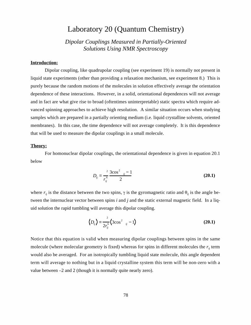
78


Dipolar Couplings Measured in Partially-OrientedSolutions Using NMR Spectroscopy

Introduction:

Dipolar coupling, like quadrupolar coupling (see experiment 19) is normally not present in

liquid state experiments (other than providing a relaxation mechanism, see experiment 8.) This is

purely because the random motions of the molecules in solution effectively average the orientation

dependence of these interactions. However, in a solid, orientational dependences will not average

and in fact are what give rise to broad (oftentimes uninterpretable) static spectra which require ad-

vanced spinning approaches to achieve high resolution. A similar situation occurs when studying

samples which are prepared in a partially orienting medium (i.e. liquid crystalline solvents, oriented

membranes). In this case, the time dependence will not average completely. It is this dependence

that will be used to measure the dipolar couplings in a small molecule.

Theory:

For homonuclear dipolar couplings, the orientational dependence is given in equation 20.1

below

Dij =2

rij6

3cos2ij − 1

2(20.1)

where rij is the distance between the two spins, is the gyromagnetic ratio and ij is the angle be-

tween the internuclear vector between spins i and j and the static external magnetic field. In a liq-

uid solution the rapid tumbling will average this dipolar coupling.

Dij =2

2rij6 3cos2

ij − 1 (20.1)

Notice that this equation is valid when measuring dipolar couplings between spins in the same

molecule (where molecular geometry is fixed) whereas for spins in different molecules the rij term

would also be averaged. For an isotropically tumbling liquid state molecule, this angle dependent

term will average to nothing but in a liquid crystalline system this term will be non-zero with a

value between –2 and 2 (though it is normally quite nearly zero).

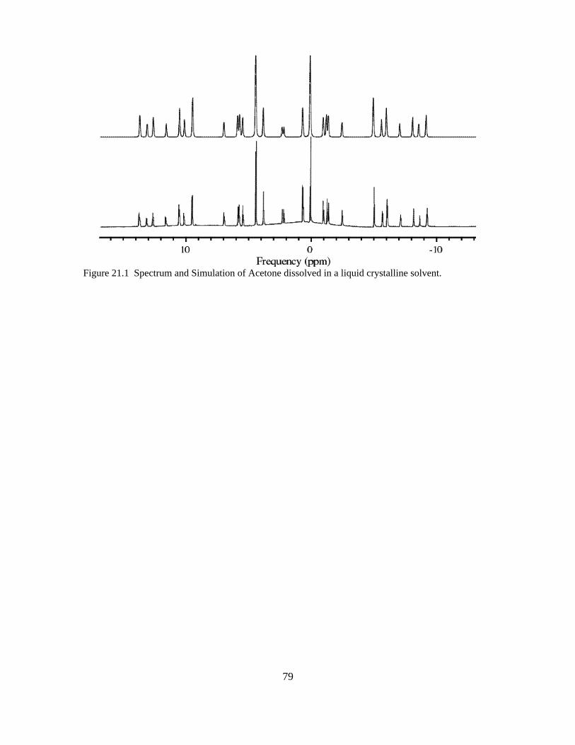
79

Figure 21.1 Spectrum and Simulation of Acetone dissolved in a liquid crystalline solvent.

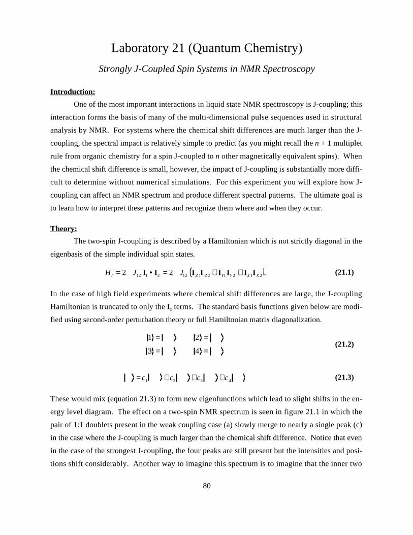
80


Strongly J-Coupled Spin Systems in NMR Spectroscopy

Introduction:

One of the most important interactions in liquid state NMR spectroscopy is J-coupling; this

interaction forms the basis of many of the multi-dimensional pulse sequences used in structural

analysis by NMR. For systems where the chemical shift differences are much larger than the J-

coupling, the spectral impact is relatively simple to predict (as you might recall the n + 1 multiplet

rule from organic chemistry for a spin J-coupled to n other magnetically equivalent spins). When

the chemical shift difference is small, however, the impact of J-coupling is substantially more diffi-

cult to determine without numerical simulations. For this experiment you will explore how J-

coupling can affect an NMR spectrum and produce different spectral patterns. The ultimate goal is

to learn how to interpret these patterns and recognize them where and when they occur.

Theory:

The two-spin J-coupling is described by a Hamiltonian which is not strictly diagonal in the

eigenbasis of the simple individual spin states.

HJ = 2 J12 I1 • I2 = 2 J12 IZ 1I Z 2 + IY1IY 2 + IX 1IX 2( ) (21.1)

In the case of high field experiments where chemical shift differences are large, the J-coupling

Hamiltonian is truncated to only the Iz terms. The standard basis functions given below are modi-

fied using second-order perturbation theory or full Hamiltonian matrix diagonalization.

1 = 2 =

3 = 4 =(21.2)

= c1 + c2 + c3 + c4 (21.3)

These would mix (equation 21.3) to form new eigenfunctions which lead to slight shifts in the en-

ergy level diagram. The effect on a two-spin NMR spectrum is seen in figure 21.1 in which the

pair of 1:1 doublets present in the weak coupling case (a) slowly merge to nearly a single peak (c)

in the case where the J-coupling is much larger than the chemical shift difference. Notice that even

in the case of the strongest J-coupling, the four peaks are still present but the intensities and posi-

tions shift considerably. Another way to imagine this spectrum is to imagine that the inner two

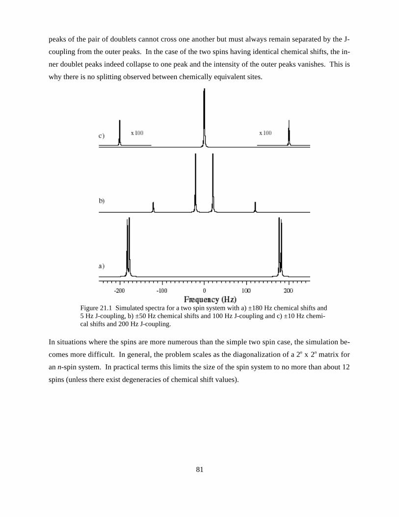
81

peaks of the pair of doublets cannot cross one another but must always remain separated by the J-

coupling from the outer peaks. In the case of the two spins having identical chemical shifts, the in-

ner doublet peaks indeed collapse to one peak and the intensity of the outer peaks vanishes. This is

why there is no splitting observed between chemically equivalent sites.

In situations where the spins are more numerous than the simple two spin case, the simulation be-

comes more difficult. In general, the problem scales as the diagonalization of a 2n x 2n matrix for

an n-spin system. In practical terms this limits the size of the spin system to no more than about 12

spins (unless there exist degeneracies of chemical shift values).

Figure 21.1 Simulated spectra for a two spin system with a) ±180 Hz chemical shifts and5 Hz J-coupling, b) ±50 Hz chemical shifts and 100 Hz J-coupling and c) ±10 Hz chemi-cal shifts and 200 Hz J-coupling.

82


Measurement of the Joule-Thompson Coefficient

Introduction:

The determination of various gas constants has been one of the standard experiments per-

formed in physical chemistry laboratories for most of the history of the subject. We recognize that

these experiments measure constants the form the basis of the rest of physical chemistry (recall that

all chemical potentials are related to one another via the chemical potential in the gas phase). The

Joule-Thompson coefficient is measured normally using an adiabatic expansion through a mem-

brane or porous plug (see figure 22.1). This laboratory has been modified throughout the years, but

fundamentally has remained the

same adiabatic expansion. You

will be using this approach to

determine the Joule-Thompson

coefficient for three gases (CO2,

He and N2) and comparing this

result to both theoretical (via the

Van der Waals equation) and

other experimental values.

Theory:

The basic theory used to

measure the Joule-Thompson

coefficient is to consider an

adiabatic expansion through a

porous plug (see figure 22.2).

The basic idea is that the gas

expands (from a high pressure region to a low pressure region) in an adiabatic fashion (meaning no

heat is transferred to the gas from the surroundings). Consider the implications of such an expan-

sion as a two step process. In the first process, the gas is compressed under constant pressure on

the high pressure side of the porous plug and then is expanded under lower pressure on the low

pressure side of the plug. The work done to compress the gas on the high pressure side will be

simply wH = p1 V1. On the low pressure side the work of expansion will be wL = – p2 V2. Now if

we consider the system as a whole ∆U = U2 – U1 = p1 V1 – p2 V2. This equation may be rewritten to

Figure 22.1 Joule-Thompson Expansion Experimental Setup.

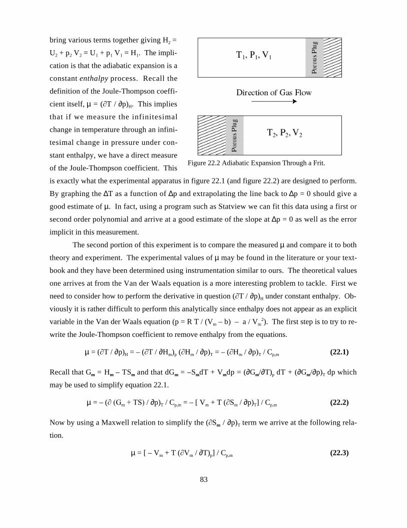
83

bring various terms together giving H2 =

U2 + p2 V2 = U1 + p1 V1 = H1. The impli-

cation is that the adiabatic expansion is a

constant enthalpy process. Recall the

definition of the Joule-Thompson coeffi-

cient itself, µ = ( T / ∂p)H. This implies

that if we measure the infinitesimal

change in temperature through an infini-

tesimal change in pressure under con-

stant enthalpy, we have a direct measure

of the Joule-Thompson coefficient. This

is exactly what the experimental apparatus in figure 22.1 (and figure 22.2) are designed to perform.

By graphing the ∆T as a function of ∆p and extrapolating the line back to ∆p = 0 should give a

good estimate of µ. In fact, using a program such as Statview we can fit this data using a first or

second order polynomial and arrive at a good estimate of the slope at ∆p = 0 as well as the error

implicit in this measurement.

The second portion of this experiment is to compare the measured µ and compare it to both

theory and experiment. The experimental values of µ may be found in the literature or your text-

book and they have been determined using instrumentation similar to ours. The theoretical values

one arrives at from the Van der Waals equation is a more interesting problem to tackle. First we

need to consider how to perform the derivative in question ( T / ∂p)H under constant enthalpy. Ob-

viously it is rather difficult to perform this analytically since enthalpy does not appear as an explicit

variable in the Van der Waals equation (p = R T / (Vm – b) – a / Vm2). The first step is to try to re-

write the Joule-Thompson coefficient to remove enthalpy from the equations.

µ = ( T / ∂p)H = – ( T / ∂Hm)p ( Hm / ∂p)T = – ( Hm / ∂p)T / Cp,m (22.1)

Recall that Gm = Hm – TSm and that dGm = –SmdT + Vmdp = (∂Gm/∂T)p dT + (∂Gm/∂p)T dp which

may be used to simplify equation 22.1.

µ = – ( m / ∂p)T / Cp,m = – [ Vm + T ( m / ∂p)T] / Cp,m (22.2)

Now by using a Maxwell relation to simplify the ( m / ∂p)T term we arrive at the following rela-

tion.

µ = [ – Vm + T ( m / ∂T)p] / Cp,m (22.3)

Figure 22.2 Adiabatic Expansion Through a Frit.

84

The only difficulty here lies in taking the partial derivative ( m / ∂T)p due to the impossibility of

solving the Van der Waals equation explicitly for Vm. To simplify our lives we may rewrite this

derivative below.

( m / ∂T)p = – ( m / ∂p)T ( p / ∂T)V = – ( p / ∂T)V / ( p / ∂ m)T (22.4)

Of course this leaves us a pair of derivatives of pressure as a function of T and Vm which are

straightforward to perform for the Van der Waals equation of state.

( m / ∂T)p = – (R / (Vm – b) ) / ( – RT / (Vm – b)2 + 2 a / Vm3) (22.5)

This is then used in equation 22.3 to give the expression below.

µ = { – Vm – [(R T / (Vm – b) ) / ( – RT / (Vm – b)2 + 2 a / Vm3)] } / Cp,m (22.6)

An ambitious mathematics problem might be to try to rewrite this expression in terms of p and T

instead of Vm and T. In any case, to determine the theoretical value of the Joule-Thompson coeffi-

cient you need to insert the appropriate values for Vm and T under the conditions of the experiment

(you will need to use a computer to solve for Vm). The only constants you will need to have are the

a, b and Cp,m values for a specific gas under the given conditions.

Experimental:

For this experiment you will simply attach the gas to be studied (CO2, N2 or He) to the ex-

perimental apparatus as shown in figure 22.1. You will measure a series of temperature differences

as a function of pressure drops and should begin with a low pressure drop and slowly increase this

until the ∆p is a maximum value of about 60 psi. You will need to let the system equilibrate at each

pressure drop for about 10 minutes (or longer if the temperature difference is not stable). It is sug-

gested that you do pressure drops of 10, 20, 30, 40, 50 and 60 psi for each gas. Once you have the

data, you should convert to standard units and graph the ∆T as a function of ∆p. From the zero

pressure drop slope you may obtain the values for the Joule-Thompson coefficient (see theory sec-

tion for additional details). Errors should be propagated for all variables in this experiment to de-

termine if your values agree with theory and other experiments.

85

References

1 M. R. Mueller and K. L. McCorckle, Journal of Chemical Education 71, 169 (1994).

2 D. A. Hinckley and P. G. Seybold, Journal of Chemical Education 64, 362 (1987).

3 P. P. Blanchette, Journal of Chemical Education 64, 267 (1987).

4 D. Calvert, M. J. Smith, and E. Falcào, Journal of Chemical Education 76, 668 (1999).

5 D. P. Shoemaker, C. W. Garland, and J. W. Nibler, Experiments in Physical Chemistry, 6th ed.(McGraw-Hill, New York, NY, 1996).

6 A. M. Halperm and S. Gozashti, Journal of Chemical Education 65, 500 (1988).

7 H. Elias and A. P. Zipp, Journal of Chemical Education 65, 737 (1988).

8 M. M. Fuson, Journal of Chemical Education 71, 126 (1994).

9 D. J. Wink, Journal of Chemical Education 66, 810 (1989).

10 F. S. Wettack, Journal of Chemical Education 49, 556 (1972).

11 H. W. Thompson, A Course in Chemical Spectroscopy (Oxford University Press, London, England,1938).

12 F. Daniels and e. al., Experimental Physical Chemistry, 6th ed. (McGraw-Hill, New York, NY,1962).

13 C. F. Meyer and A. A. Levin, Physical Review 34, 44 (1929).

14 G. Herzberg, Molecular Spectra and Molecular Structure I. Spectra of Diatomic Molecules, 2nd ed.(D. Van Nostrand Co., Princeton, NJ, 1950).

15 K. M. Jinks, Journal of Chemical Education 52, 312 (1975).

16 R. S. Moog, Journal of Chemical Education 68, 506 (1991).

17 B. D. Anderson, Journal of Chemical Education 74, 985 (1997).

18 I. J. McNaught, Journal of Chemical Education 57, 101 (1980).

19 R. B. Snadden, Journal of Chemical Education 64, 919 (1987).

20 G. Long, D. Sauder, G. M. Shalhoub, R. Stout, M. H. Towns, and T. J. Zielinski, Journal of Chemi-cal Education 76, 841 (1999).

21 C. J. Pursell and L. Doezema, Journal of Chemical Education 76, 839 (1999).

22 G. Herzberg, Molecular Spectra and Molecular Structure III. Electronic Spectra of PolyatomicMolecules (D. Van Nostrand Co., Princeton, NJ, 1966).

23 F. E. Stafford, Journal of Chemical Education 39, 626 (1962).

24 R. D'alterio, R. Mattson, and R. Harris, Journal of Chemical Education 51, 283 (1974).

25 V. S. Steckline, Journal of Chemical Education 47, 128 (1970).

26 D. Chandler, Introduction to Modern Statistical Mechanics (Oxford University Press, New York,NY, 1987).

27 H. M. Bell, Journal of Chemical Education 53, 665 (1976).

86

28 R. L. Jarek, R. J. Flesher, and S. K. Shin, Journal of Chemical Education 74, 978 (1997).

29 L. A. Hull, Journal of Chemical Education 67, 782 (1990).

30 P.-O. Quist, Journal of Chemical Education 73, 751 (1996).

31 L. Sacksteder, R. M. Ballew, E. A. Brown, J. N. Demas, D. Nesselrodt, and B. A. DeGraff, Journalof Chemical Education 67, 1065 (1990).

32 J. Ruiz-Cabello, G. W. Vuister, C. T. W. Moonen, P. van Gelderen, J. S. Cohen, and P. C. M. vanZijl, Journal of Magnetic Resonance 100, 282-303 (1992).

33 R. E. Hurd and B. K. John, Journal of Magnetic Resonance 91, 648-653 (1991).

34 W. Wilker, D. Leibfritz, R. Kerssebaum, and W. Bermel, Magnetic Resonance in Chemistry 31, 287-292 (1993).

35 A. M. Torres, T. T. Nakashima, and R. E. D. McClung, Journal of Magnetic Resonance Series A101, 285-294 (1993).

36 J. C. Madsen, H. Bildsøe, H. Jakobsen, and O. W. Sørensen, Journal of Magnetic Resonance 67,243-257 (1986).

37 S. Patt and J. N. Shoolery, Journal of Magnetic Resonance 46, 535-539 (1982).

38 B. F. Chmelka, K. T. Mueller, A. Pines, J. Stebbins, Y. Wu, and J. W. Zwanziger, Nature 339, 42-43(1989).

39 K. T. Mueller, B. Q. Sun, G. C. Chingas, J. W. Zwanziger, T. Terao, and A. Pines, Journal of Mag-netic Resonance 86, 470-487 (1990).

40 K. T. Mueller, Ph.D., University of California, Berkeley, 1991.

41 A. Llor and J. Virlet, Chemical Physics Letters 152, 248-253 (1988).

42 K. T. Mueller, E. W. Wooten, and A. Pines, Journal of Magnetic Resonance 92, 620-627 (1991).

43 K. T. Mueller, G. C. Chingas, and A. Pines, Review of Scientific Instruments 62, 1445-1452 (1991).

44 K. T. Mueller, Y. Wu, B. F. Chmelka, J. Stebbins, and A. Pines, Journal of the American ChemicalSociety 113, 32-38 (1991).

45 E. W. Wooten, K. T. Mueller, and A. Pines, Accounts of Chemical Research 25, 209-215 (1992).

46 P. J. Grandinetti, Y. K. Lee, J. H. Baltisberger, B. Q. Sun, and A. Pines, Journal of Magnetic Reso-nance A 102, 195-204 (1993).

47 P. J. Grandinetti, J. H. Baltisberger, A. Llor, Y. K. Lee, U. Werner, M. A. Eastman, and A. Pines,Journal of Magnetic Resonance A 103, 72-81 (1993).

48 S. L. Gann, J. H. Baltisberger, and A. Pines, Chemical Physics Letters 210, 405-410 (1993).

49 L. Frydman and J. S. Harwood, Journal of the American Chemical Society 117, 5367- (1995).

50 A. Medek, J. S. Harwood, and L. Frydman, Journal of the American Chemical Society 117, 12779-12787 (1995).

51 J. H. Baltisberger, Z. Xu, J. F. Stebbins, S. H. Wang, and A. Pines, Journal of the American Chemi-cal Society 118, 7209-7214 (1996).

52 G. Wu, D. Rovnyak, and R. G. Griffin, Journal of the American Chemical Society 118, 9326-9332(1996).

87

53 A. Samoson, Chemical Physics Letters 247;, 203-206 (1995).

54 G. Wu, D. Rovnyank, B. Sun, and R. G. Griffin, Chemical Physics Letters 249, 210-217 (1995).

55 D. Massiot, B. Touzo, D. Trumeau, J. P. Coutures, J. Virlet, P. Florian, and P. J. Grandinetti, SolidState Nuclear Magnetic Resonance 6, 73-83 (1996).

chemical dynamics, thermochemistry, and quantum...

Documents