chebyshev interpolation for parametric - arxiv · problem for polynomial interpolation on an...

arX

iv:1

505.

0464

8v2

[q-

fin.

CP]

8 J

ul 2

016

Chebyshev Interpolation for Parametric

Option Pricing∗

Maximilian Gaß1,†, Kathrin Glau1,

Mirco Mahlstedt1,†, Maximilian Mair1

1Technical University of Munich, Germany

July 11, 2016

Abstract

Recurrent tasks such as pricing, calibration and risk assessment need to beexecuted accurately and in real-time. Simultaneously we observe an increasein model sophistication on the one hand and growing demands on the qual-ity of risk management on the other. To address the resulting computationalchallenges, it is natural to exploit the recurrent nature of these tasks. Weconcentrate on Parametric Option Pricing (POP) and show that polynomialinterpolation in the parameter space promises to reduce run-times while main-taining accuracy. The attractive properties of Chebyshev interpolation and itstensorized extension enable us to identify criteria for (sub)exponential conver-gence and explicit error bounds. We show that these results apply to a varietyof European (basket) options and affine asset models. Numerical experimentsconfirm our findings. Exploring the potential of the method further, we empir-ically investigate the efficiency of the Chebyshev method for multivariate andpath-dependent options.

Keywords Multivariate Option Pricing, Complexity Reduction, (Tensorized)Chebyshev Polynomials, Polynomial Interpolation, Fourier TransformMethods, MonteCarlo, Affine Processes2000 MSC 91G60, 41A10

∗We like to thank Jonas Ballani, Behnam Hashemi, Daniel Kressner and Nick Trefethen for fruit-ful discussions on Chebyshev interpolation. Moreover, we gratefully acknowledge valuable feedbackfrom Christian Bayer, Ernst Eberlein, Dilip Madan, Christian Potz, Peter Tankov and Ralf Werner.For further we thank Paul Harrenstein and Pit Forster. Additionally, we thank the participantsof the conferences Advanced Modelling in Mathematical Finance, A conference in honour of ErnstEberlein, Kiel. May 20–22, 2015, Stochastic Methods in Physics and Finance, 2015 in Heraklion,MoRePas2015: Model Reduction of Parametrized Systems III, held in Trieste and the 12th Ger-man Probability and Statistic Days 2016 in Bochum. Furthermore we thank the participants of theresearch seminars Seminar Stochastische Analysis und Stochastik der Finanzmarkte, Technical Uni-versity Berlin. May 28, 2015 and the Groupe de Travail MathfiProNum: Finance mathematique,probabilites numeriques et statistique des processus, Universite Diderot, Paris. June 11, 2015.

†We thank the KPMG Center of Excellence in Risk Management for their support.

1

http://arxiv.org/abs/1505.04648v2

1 Introduction

The development of fast and accurate computational methods for parametric modelsis one of the central issues in computational finance. Financial institutions dedi-cated to trading or assessment of financial derivatives have to cope with the dailytasks of computing numerous characteristic financial quantities. Examples of in-terest are prices, sensitivities and risk measures for products on different modelsand for varying parameter constellations. With regard to the ever growing mar-ket activities, more and more of these evaluations need to be delivered in real-time. In addition we face a constantly rising model sophistication since the originalwork of Black and Scholes (1973) and Merton (1973). From the early nineties on,stochastic volatility and Levy models as well as models based on further classesof stochastic processes have been developed that reflect the observed market datain a more appropriate way. For asset models see e.g. Heston (1993), Eberlein,Keller and Prause (1998), Duffie, Filipovic and Schachermayer (2003), Cuchiero,Keller-Ressel and Teichmann (2015). In the case of fixed income models see e.g.Eberlein and Ozkan (2005), Keller-Ressel, Papapantoleon and Teichmann (2013),Filipovic, Larsson and Trolle (2014). The aftermath of the financial crisis 2007–2009, moreover, has lead to a new generation of more complex models, for instanceby incorporating more risk factors. The usefulness of a pricing model critically de-pends on how well it captures the relevant aspects of market reality in its numericalimplementation. Exploiting new ways to deal with the rising computational com-plexity therefore supports the evolution of pricing models and touches a core concernof present mathematical finance.

A large body of computational tasks in finance needs to be repeatedly performedin real-time for a varying set of parameters. Prominent examples are option pricingand hedging of different option sensitivities, e.g. delta and vega, that also need to becalculated in real-time. In particular for optimization routines arising in model cal-ibration, large parameter sets come into play. Further examples arise in the contextof risk control and assessment, such as for quantification and monitoring of risk mea-sures. The following question serves as a starting point of our investigations: Howto systemically exploit the recurrent nature of parametric computational problems infinance with the approached objective to gain efficiency? Looking for answers to thisquestion, we focus on Parametric Option Pricing (POP) in the sequel.

In the present literature on computational methods in finance, complexity reduc-tion for parametric problems has largely been addressed by applying Fourier tech-niques following the seminal works of Carr and Madan (1999) and Raible (2000).See also the monograph Boyarchenko and Levendorskii (2002). Research in thisarea concentrates on adopting fast Fourier transform (FFT) methods and variantsfor option pricing. Lee (2004) accurately describes pricing European options withFFT. Further developments are for instance provided by Lord, Fang, Bervoets andOosterlee (2008) for early exercise options and by Feng and Linetsky (2008) andKudryavtsev and Levendorskii (2009) for barrier options. Another path to efficientlyhandle large parameter sets that has been pursued in finance relies on reduced basismethods. These are techniques to solve parametrized partial differential equations.Sachs and Schu (2010), Cont, Lantos and Pironneau (2011), Pironneau (2011) andHaasdonk, Salomon and Wohlmuth (2012) and Burkovska, Haasdonk, Salomon and

2

Wohlmuth (2015) applied this approach to price European, American plain vanillaoptions and European baskets. FFT methods on the one hand can be highly ben-eficial when the prices are required in a large number of Fourier variables, e.g. fora large set of strikes of European plain vanillas. On the other hand numerical ex-periments have shown a promising gain in efficiency of reduced basis methods whenan accurate PDE solver is readily available. In essence all these approaches revealan immense potential of complexity reduction by targeting parameter dependence.Hereto, they exploit the functional architecture of the underlying pricing techniquefor varying parameters.

Financial institutions have to deal simultaneously with a diversity of models,a multitude of option types, and—as a consequence—a wide variety of underlyingpricing techniques. It is therefore worthwhile to explore the possibility of a genericcomplexity reduction method that is independent of the specific pricing technique.To do so, we focus on the set of option prices and the set of parameters of interest,disregard on purpose the pricing technology and view the option price as a functionof the parameters. The core idea is now to introduce interpolation of option pricesin the parameter space as a complexity reduction technique for POP.

The resulting procedure naturally splits into two phases: Pre-computation andreal-time evaluation. The first one is also called offline phase while the second isalso called online phase. In the pre-computation phase the prices are computedfor some fixed parameter configurations, namely the interpolation nodes. Here, anyappropriate pricing method—for instance based on Fourier, PDE or even MonteCarlo techniques—can be chosen. The real-time evaluation phase then consists ofthe evaluation of the interpolation. Provided that the evaluation of the interpolationis faster than the benchmark tool, the scheme permits a gain in efficiency in all caseswhere accuracy can be maintained. Then, we distinguish two use cases:

• In comparison to the benchmark pricing routine, the fast evaluation of theinterpolation will eventually outweigh the expensive pre-computation phase, ifpricing is a task repeatedly employed. Optimization procedures are an obviousinstance where this feature becomes advantageous.

• Even if the number of price computations is limited, we can still benefit fromthe separation of the procedure into its two phases. In this way, e.g., idle timesin the financial industry can be put to good use by preparing the interpolationfor whenever real-time pricing is needed during business activities.

The question arising at this stage is: Under what circumstances can we hope to findan interpolation method that delivers both reliable results and a considerable gain inefficiency?

One could now be tempted to proceed in a naive manner and first define anequidistant grid and then interpolate piecewise linearly in the parameter space.Numerical experiments for Black&Scholes call prices as function of the volatility,for instance, would then provide convincing evidence that the number of nodesneeded for a given accuracy is considerably high. Increasing the polynomial degreemight lead to better results. However, convergence might not be guaranteed. Runge(1901) showed that polynomial interpolation on equispaced grids may diverge—evenfor analytic functions. Second, the evaluation of the polynomial interpolants maybe numerically problematic, as it is shown in Runge (1901) that ”the interpolation

3

problem for polynomial interpolation on an equidistant grid is exponentially ill-conditioned”, a formulation we borrow from Trefethen (2011). For these reasons weabstain from polynomial interpolation with equidistant grids. Rather we take a stepback and ask: Which methods for the interpolation of prices as functions of modeland payoff parameters are numerically promising in terms of convergence, stabilityand implementational ease?

Regarding this research question, we need to take into consideration both theset of interpolation methods as such and the specific features of the functions weinvestigate. It is well-known that the efficiency of interpolation methods criticallydepends on the degree of regularity of the approximated function. For the core prob-lem of our study—European (basket) options—we investigate the regularity of theoption prices as functions of the parameters. We find that these functions are indeedanalytic for a large set of option types, models and parameters. Taking the perspec-tive of approximation theory, this inspires the hope to find suitable interpolationmethods.

Empirically, we observe that parameters of interest often range within boundedintervals. One interpolation method that is highly effective for analytic functionson bounded intervals is Chebyshev interpolation. This intensively studied methodenjoys excellent numerical properties—in stark contrast to polynomial interpolationon equally spaced nodal points. The interpolation nodes are known beforehand, im-plementation is straightforward and the method is numerically stable. For univariatefunctions that are several times differentiable, the method converges polynomiallyand for univariate analytic functions convergence is exponential. In a remarkablemonograph, Trefethen (2013) gives a comprehensive review of Chebyshev interpola-tion. Its appealing theoretical properties are indeed of practical use as the softwaretool Chebfun1 demonstrates. In this implemention Platte and Trefethen (2008) aim“to combine the feel of symbolics with the speed of numerics”. Therefore Chebyshevinterpolation is our method of choice.2

Exploring the potential of interpolation methods for more than one single free pa-rameter, we choose a tensorized version of Chebyshev interpolation: For parametersp ∈ RD, where D ∈ N denotes the dimensionality of the parameter space, the pricePricep is approximated by tensorized Chebyshev polynomials Tj with pre-computedcoefficients cj , j ∈ J , as follows,

Pricep ≈∑

j∈JcjTj(p).

Chebyshev interpolation is a standard numerical method that has proven tobe extremely useful for applications in such diverse fields as physics, engineering,statistics and economics. Nevertheless, for pricing tasks in mathematical financeChebyshev interpolation still seems to be rarely used and its potential is yet to beunfolded. Pistorius and Stolte (2012) use Chebyshev interpolation of Black&Scholesprices in the volatility as an intermediate step to derive a pricing methodology for

1Chebfun is an open-source software system, see http://www.chebfun.org2Chebyshev interpolation shares its good properties with for instance Legendre transformation,

for which we expect similarly positive results. We refer to Trefethen (2013), who states: ”It is theclustering near the ends of the interval that makes the difference, and other sets of points withsimilar clustering, like Legendre points [...] have similarly good behaviour.”

4

http://www.chebfun.org

a time-changed model. Independently from us, Pachon (2016) recently proposedChebyshev interpolation as a quadrature rule for the computation of option priceswith a Fourier type representation, which is comparable to the cosine method.

Our main results are the following:

• Theorem 3.2 provides accessible sufficient conditions on options and models

that guarantee an asymptotic error decay of order O(−

D√N)in the total

number N of interpolation nodes where > 1 is given by the domain ofanalyticity and D is the number of varying parameters.

• More specific conditions for parametric European options in Levy models areprovided in Corollary 3.6, while Corollary 3.9 provides the framework for para-metric basket options in affine models.

These results establish an error analysis that is based on the domain of analyticityof the prices as functions of the parameters. Observing that typical payoff functionsare not smooth, we cannot expect an exponential error decay for interpolation witharbitrarily small maturities. Small maturities thus serve as an example that domainsof analyticity need to be carefully studied.

• The investigations in Sections 3.2–4.2 show that for a large set of relevant(basket) options, models and free parameters a domain of analyticity can in-deed be identified. This gives examples of relevant financial applications where(sub)exponential error decay is guaranteed.

To numerically validate the theoretical results we compare prices obtained by Cheby-shev interpolation to benchmark prices by Fourier techniques.

• Numerical experiments in affine models confirm the theoretical error decay em-pirically for European call options (Figure 5.3) and digital down&out options(Figure 5.4). For the considered model examples of Black&Scholes, Merton,CGMY and Heston we observe L∞-error levels of order 10−10 using not morethan N = (25 + 1)2 Chebyshev interpolation nodes when D = 2 parametersare varied.

Numerical results show that already a small number of nodes leads to high accuracy.This motivates us to further explore the potential of the Chebyshev method formultivariate options. Here we deliberately go beyond the scope of our theoreticalresults and consider additional features like path-dependency.

• For multivariate basket and path-dependent options in the Black&Scholes,Heston and Merton model we use Monte Carlo as reference method. In allof our settings in Section 5.2 Chebyshev interpolation achieves an accuracythat is similar to the accuracy of the Monte Carlo simulation itself (10−3) forD = 2.

In addition we present empirical results demonstrating the efficiency of the Cheby-shev method.

• The gain in efficiency in comparison to Fourier techniques is first validated forbivariate options of European type in Section 5.3.1.

5

• Secondly, the explicit gains in efficiency in comparison to Monte Carlo methodsare shown in Section 5.3.2 taking multivariate lookback options in the Hestonmodel as examples.

The remainder of the article is organized as follows. In Section 2 we intro-duce Chebyshev interpolation in detail and present the general convergence results.Section 3 establishes a convergence analysis of Chebyshev interpolation for POP.We formulate analyticity conditions for the payoff profiles and models that guaran-tee (sub)exponential convergence of the method. These conditions are verified inSection 4 for different option types, models and free parameters. The numericalexperiments in Section 5 confirm these findings using Fourier techniques. Pricingbasket options, the gain in efficiency is numerically investigated. Experiments basedon Monte Carlo and finite differences moreover suggest to further explore the po-tential of the approach beyond the scope of the theoretical investigations from theprevious sections. The resulting conclusion and outlook are presented in Section 6.Finally, the appendix provides the proof of the multivariate convergence result.

2 Chebyshev Polynomial Interpolation

In this section we introduce the notation for Chebyshev interpolation. FollowingTrefethen (2013), the one-dimensional version is shown. Then we present the mul-tivariate extension and convergence results. Consider an option price with a singlevarying parameter

Pricep, p ∈ [−1, 1].(2.1)

An interpolation of Pricep with Chebyshev polynomials of degree N is of the form

IN (Price(·))(p) :=

N∑

j=0

cjTj(p),(2.2)

with coefficients

cj :=210<j<N

N

N∑

k=0

′′Pricepk cos

(jπ

k

N

), j ≤ N,(2.3)

and basis functions

Tj(p) := cos(j arccos(p)

)for p ∈ [−1, 1] and j ≤ N(2.4)

where∑ ′′

indicates that the first and last summands are halved. The Chebyshevnodes pk = cos

(π kN

)may conveniently be displayed in a graph, see Figure 2.1.

For an arbitrary compact parameter interval [p, p], interpolation (2.2) needs to beadjusted by the appropriate linear transformation.

6

-1 -0.5 0 0.5 10

0.2

0.4

0.6

0.8

1Chebyshev nodes for D=1

Figure 2.1: A set of Chebyshev points pk ∈ [−1, 1] (blue) for degree N = 20 and equidistantlyspaced auxiliary construction points (red) on the semi-circle.

2.1 Multivariate Chebyshev Interpolation

The Chebyshev polynomial interpolation (2.2)–(2.4) has a tensor based extension tothe multivariate case, see e.g. Sauter and Schwab (2004). In order to obtain a nicenotation, consider the interpolation of prices

(2.5) Pricep, p ∈ [−1, 1]D.

For a more general hyperrectangular parameter space P = [p1, p

1]×. . .×[p

D, pD], the

appropriate linear transformations need to be performed. Let N := (N1, . . . , ND)with Ni ∈ N0 for i = 1, . . . ,D. The interpolation with

∏Di=1(Ni + 1) summands is

given by

(2.6) IN (Price(·))(p) :=

∑

j∈JcjTj(p),

where the summation index j is a multiindex ranging over J := (j1, . . . , jD) ∈ ND0 :

ji ≤ Ni for i = 1, . . . ,D, i.e.

(2.7) IN (Price(·))(p) =

N1∑

j1=0

. . .

ND∑

jD=0

c(j1,...,jD)T(j1,...,jD)(p).

The basis functions Tj for j = (j1, . . . , jD) ∈ J are defined by

(2.8) Tj(p1, . . . , pD) =

D∏

i=1

Tji(pi).

The coefficients cj for j = (j1, . . . , jD) ∈ J are given by

(2.9) cj =( D∏

i=1

210<ji<Ni

Ni

) N1∑

k1=0

′′. . .

ND∑

kD=0

′′Pricep

(k1,...,kD)D∏

i=1

cos

(jiπ

kiNi

),

7

where∑ ′′

indicates that the first and last summand are halved and the Chebyshevnodes pk for multiindex k = (k1, . . . , kD) ∈ J are given by

(2.10) pk = (pk1 , . . . , pkD)

with the univariate Chebyshev nodes pki = cos(π kiNi

)for ki = 0, . . . , Ni and i =

1, . . . ,D. A set ofD-variate Chebyshev nodes p(k1,...,kD) forD = 2 andN1 = N2 = 20is depicted in Figure 2.2.

pk1

-1 -0.5 0 0.5 1

pk2

-1

-0.8

-0.6

-0.4

-0.2

0

0.2

0.4

0.6

0.8

1Chebyshev nodes for D=2

Figure 2.2: A set of D-variate Chebyshev points pk ∈ [−1, 1]D for D = 2 and N1 = N2 = 20.

2.2 Convergence of Multivariate Chebyshev Interpolation

In the univariate case, it is well known that the error of approximation with Cheby-shev polynomials decays polynomially for differentiable functions and exponentiallyfor analytic functions. Let f be analytic in [−1, 1] then it has an analytic extensionto some Bernstein ellipse B([−1, 1], ) with parameter > 1, defined as the openregion in the complex plane bounded by the ellipse with foci ±1 and semiminor andsemimajor axis lengths summing up to . This and the following result traces backto the seminal work of Bernstein (1912).

Theorem 2.1. Trefethen (2013, Theorem 8.2) Let a function f be analytic in theopen Bernstein ellipse B([−1, 1], ), with > 1, where it satisfies |f | ≤ V for someconstant V > 0. Then for each N ≥ 0,

‖f − IN (f)‖L∞([−1,1]) ≤ 4V−N

− 1.

8

In the multivariate case we will extend a convergence result from Sauter and Schwab(2004). We consider parametric option prices of form

Pricep for p ∈ P(2.11)

with P ⊂ RD of hyperrectangular structure, i.e. P = [p1, p

1]× . . .× [p

D, pD] with real

pi≤ p

ifor all i = 1, . . . ,D. We define the D-variate and transformed analogon of

a Bernstein ellipse around the hyperrectangle P with parameter vector ∈ (1,∞)D

as

B(P, ) := B([p1, p

1], 1)× . . .×B([p

D, pD], D)(2.12)

with B([p, p], ) := τ[p,p] B([−1, 1], ), where for p ∈ C we have the transform

τ[p,p](ℜ(p)

):= p +

p−p2

(1 − ℜ(p)

)and τ[p,p]

(ℑ(p)

):=

p−p2 ℑ(p). We call B(P, )

generalized Bernstein ellipse if the sets B([−1, 1], i) are Bernstein ellipses for i =1, . . . ,D.

Theorem 2.2. Let P ∋ p 7→ Pricep be a real valued function that has an analyticextension to some generalized Bernstein ellipse B(P, ) for some parameter vector ∈ (1,∞)D and supp∈B(P,) |Pricep| ≤ V . Then

maxp∈P

∣∣Pricep − IN (Price(·))(p)

∣∣ ≤ 2D2+1 · V ·

D∑

i=1

−2Ni

i

D∏

j=1

1

1− −2j

12

.

The proof of the theorem is provided in Appendix A.

Corollary 2.3. Under the assumptions of Theorem 2.2 there exists a constant C > 0such that

maxp∈P


∣∣ ≤ C−N ,(2.13)

where = min1≤i≤D

i and N = min1≤i≤D

Ni.

Remark 2.4. In particular, under the assumptions required by Theorem 2.2 withN =

∏Di=1(Ni + 1) denoting the total number of nodes, Corollary 2.3 shows that the

error decay is of (sub)exponential order O(−

D√N)for some > 1.

In the setting of Theorem 2.2 additionally the derivatives of Pricep are ap-proximated by the according derivatives of the Chebyshev interpolation. The one-dimensional result is shown in Tadmor (1986) and a multivariate result is derived inCanuto and Quarteroni (1982) for functions in Sobolev spaces. These results allowus to obtain the Chebyshev approximation of derivatives with no additional cost.To state the according convergence results we follow Canuto and Quarteroni (1982)and introduce the weighted Sobolev spaces for σ ∈ N by

(2.14) W σ,ω2 (P) =

φ ∈ L2(P) : ‖φ‖Wσ,ω

2 (P) <∞,

with norm

(2.15) ‖φ‖2Wσ,ω2 (P) =

∑

|α|≤σ

∫

P|∂αφ(p)|2ω(p) dp,

9

wherein α = (α1, . . . , αD) ∈ ND0 is a multiindex and ∂α = ∂α1 · · · ∂αD and the weight

function ω on P given by

ω(x) :=D∏

j=1

ω(τ−1[p

j,pj ]

(xj)), ω(τ−1[p

j,pj ]

(xj)) := (1− τ−1[p

j,pj ]

(xj)2)−

12

with τ[pj,pj ]

(p) = pj+pj−p2

(1−p

). Then we apply the result of Canuto and Quarteroni

(1982, Theorem 3.1) in the following corollary.

Corollary 2.5. Under the assumptions of Theorem 2.2 for any D2 < σ ∈ N and

any σ ≥ µ ∈ N0 there exists a constant C > 0 such that

‖Price(·) − IN (Price(·))(·)‖Wµ,ω

2 (P) ≤ CN2µ−σ‖Price(·)‖Wσ,ω2 (P),

Proof. In our setting we have P ⊂ RD of hyperrectangular structure. Under theassumptions of Theorem 2.2 it follows that p 7→ Pricep ∈ W σ

2 (P) and therewithp 7→ Pricep ∈ W σ,ω

2 (P). Before we apply Canuto and Quarteroni (1982, Theorem3.1), which assumes P = [−1, 1]D , we investigate how the linear transformation τP ,as introduced in the proof of Theorem 2.2, influences the derivatives. Let p 7→ Pricep

be a function on P. We set h(p) = Pricep τP(p). Further, let IN (h)(p) be the

Chebyshev interpolation of h(p) on [−1, 1]D . Then, it directly follows

Pricep − IN (Price(·))(p) =

(h(·)− IN (h)(·)

) τ−1

P (p).

First, let us assume D = 1, i.e. P = [p, p], and let α ∈ N0. For the partial derivativesit holds

∂αPricep − ∂αIN (Price(·))(p) = ∂α

(Pricep − IN (Price

(·))(p))

= ∂α((h(·)− IN (h)(·)

) τ−1

P (p))

= ∂α−1(∂1h(τ−1

P (p))− ∂1IN (h(·))(τ−1

P (p)))

= ∂α−1 2

p− p

([∂1h

](τ−1

P (p))−[∂1IN (h

(·))](τ−1

P (p))).

Repeating this step iteratively yields

∂αPricep − ∂αIN (Price(·))(p) =

2α

(p− p)α

([∂αh

](τ−1

P (p))−[∂αIN (h

(·))](τ−1

P (p))).

Therewith, the error on [−1, 1] is scaled with a factor 2α

(p−p)α . Extending this to

the D-variate case with, this analogously results with α = (α1, . . . , αD) ∈ ND0 is a

multiindex and ∂α = ∂α1 · · · ∂αD

∂αPricep − ∂αIN (Price(·))(p) =

D∏

i=1

2|αi|

(pi − pi)|αi|

([∂αh

](τ−1

P (p))−[∂αIN (h

(·))](τ−1

P (p))).

10

From Theorem 3.1 in Canuto and Quarteroni (1982) the assertion follows directlyfor h(·) on P = [−1, 1]D , i.e. for any D

2 < σ ∈ N and any σ ≥ µ ∈ N0 there exists a

constant C > 0 such that

‖h(·)− IN (h)(·)‖Wµ,ω2 (P) ≤ CN2µ−σ‖h(·)‖Wσ,ω

2 (P),(2.16)

For arbitrary P the constant from 2.16 has to be multiplied with the according factorresulting from the linear transformation τP .

The result in Corollary 2.5 is given in terms of weighted Sobolev norms. In thefollowing remark we connect the approximation error in the weighted Sobolev normto the C l(P) norm, where C l(P) is the Banach space of all functions u in P suchthat u and ∂αu with |α| ≤ l are uniformly continuous in P and the norm

‖u‖Cl(P) = max|α|≤l

maxp∈P

|∂αu(p)|

is finite.

Corollary 2.6. Under the assumptions of Theorem 2.2 for any D2 < σ ∈ N and any

σ ≥ µ ∈ N0 and l ∈ N0 with µ− l > D2 , there exists a constant C(σ) > 0 depending

on σ, such that

‖Price(·) − IN (Price(·))(·)‖Cl(P) ≤ C(σ)N2µ−σ max

|α|≤σsupp∈P

|∂αPricep|.

Proof. In the setting of Corollary 2.5, we start with the estimation of the approxi-mation error in the weighted Sobolev norms,


2 (P) ≤ CN2µ−σ‖Price(·)‖Wσ,ω2 (P).(2.17)

On P it holds that w(p) ≥ 1 and therewith we can deduce for the Sobolev normwith a constant weight of 1,


2 (P) ≥ ‖Price(·) − IN (Price(·))(·)‖Wµ,1

2 (P).

With W µ2 (P) the usual Sobolev space,

W µ2 (P) =

φ ∈ L2(P) : ‖φ‖Wµ

2 (P) <∞, ‖φ‖2Wµ

2 (P) =∑

|α|≤µ

∫

P|∂αφ(p)|2 dp,

Corollary 6.2 from Wloka (1987) directly yields that for any l with µ− l > D2 there

exists a constant C such that

‖Price(·) − IN (Price(·))(·)‖Cl(P) ≤ C‖Price(·) − IN (Price

(·))(·)‖Wµ2 (P).(2.18)

In formula (2.18) we have derived a lower bound for the left hand side of expression(2.17). Next, we will find an upper bound for the right hand side of (2.17). Fromthe definition of the weighted Sobolev norm, see (2.15), it follows

‖Price(·)‖Wσ,ω2 (P) =

√√√√∑

|α|≤σ

∫

P|∂αPricep|2ω(p) dp

≤√√√√∑

|α|≤σsupp∈P

|∂αPricep|2∫

Pω(p) dp.

11

Here, we apply∫P ω(p) dp = πD and that there exists a constant α2(σ) depending

on σ such that

‖Pricep‖Wσ,ω2 (P) ≤

√α2(σ) max

|α|≤σsupp∈P

|∂αPricep|2πD

= α(σ) max|α|≤σ

supp∈P

|∂αPricep|πD2 .(2.19)

Finally, using (2.18) and (2.19) in (2.17) yields an estimate of the approximationerror in the C l(P) norm,

1

C‖Price(·) − IN (Price

(·))(·)‖Cl(P) ≤ CN2µ−σα(σ) max|α|≤σ

supp∈P

|∂αPricep|πD2 .

Collecting all constants in C(σ), we achieve

‖Price(·) − IN (Price(·))(·)‖Cl(P) ≤ C(σ)N2µ−σ max

|α|≤σsupp∈P

|∂αPricep|.

3 Exponential Convergence of Chebyshev

Interpolation for POP

In this section we embed the multivariate Chebyshev interpolation into the optionpricing framework. We provide sufficient conditions under which option prices de-pend analytically on the parameters.

Analytic properties of option prices can be conveniently studied in terms ofFourier transforms. First, Fourier representations of option prices are explicitlyavailable for a large class of both option types and asset models. Second, Fouriertransformation unveils the analytic properties of both the payoff structure and thedistribution of the underlying stochastic quantity in a beautiful way. By contrast, ifoption prices are represented as expectations, their analyticity in the parameters ishidden. For example the function K 7→ (ST−K)+ is not even differentiable, whereasthe Fourier transform of the dampened call payoff function evidently is analytic inthe strike, compare Table 4.1 on page 19.

3.1 Conditions for Exponential Convergence

Let us first introduce a general option pricing framework. We consider option pricesof the form

Pricep=(p1,p2) = E(fp

1(Xp2)

)(3.1)

where fp1is a parametrized family of measurable payoff functions fp

1: Rd → R+

with payoff parameters p1 ∈ P1 and Xp2 is a family of Rd-valued random variableswith model parameters p2 ∈ P2. The parameter set

p = (p1, p2) ∈ P = P1 × P2 ⊂ RD(3.2)

12

is again of hyperrectangular structure, i.e. P1 = [p1, p

1] × . . . × [p

m, pm] and P2 =

[pm+1

, pm+1

]×. . .×[pD, pD] for some 1 ≤ m ≤ D and real p

i≤ p

ifor all i = 1, . . . ,D.

Typically we are given a parametrized Rd-valued driving stochastic process Hp′

with Sp′being the vector of asset price processes modeled as an exponential of Hp′ ,

i.e.

Sp′,it = Sp

′,i0 exp(Hp′,i

t ), 0 ≤ t ≤ T, 1 ≤ i ≤ d,(3.3)

and Xp2 is an FT -measurable Rd-valued random variable, possibly depending onthe history of the d driving processes, i.e. p2 = (T, p′) and

Xp2 := Ψ(Hp′

t , 0 ≤ t ≤ T),

where Ψ is an Rd-valued measurable functional.We now focus on the case that the price (3.1) is given in terms of Fourier trans-

forms. This enables us to provide sufficient conditions under which the parametrizedprices have an analytic extension to an appropriate generalized Bernstein ellipse. Formost relevant options, the payoff profile fp

1is not integrable and its Fourier trans-

form over the real axis is not well defined. Instead, there exists an exponentialdampening factor η ∈ Rd such that e〈η,·〉 fp

1 ∈ L1(Rd). We therefore introduceexponential weights in our set of conditions and denote the Fourier transform ofg ∈ L1(Rd) by

g(z) :=

∫

Rd

ei〈z,x〉 g(x) dx

and we denote the Fourier transform of e〈η,·〉 f ∈ L1(Rd) by f(·−iη). The exponentialweight of the payoff will be compensated by exponentially weighting the distributionof Xp2 and that weight will reappear in the argument of ϕp

2, the characteristic

function of Xp2 .

Conditions 3.1. Let parameter set P = P1 × P2 ⊂ RD of hyperrectangularstructure as in (3.2). Let ∈ (1,∞)D and denote 1 := (1, . . . , m) and 2 :=(m+1, . . . , D) and let weight η ∈ Rd.

(A1) For every p1 ∈ P1 the mapping x 7→ e〈η,x〉 fp1(x) is in L1(Rd).

(A2) For every z ∈ Rd the mapping p1 7→ fp1(z − iη) is analytic in the general-ized Bernstein ellipse B(P1, 1) and there are constants c1, c2 > 0 such that

supp1∈B(P1,1) |fp1(−z − iη)| ≤ c1ec2|z| for all z ∈ Rd.

(A3) For every p2 ∈ P2 the exponential moment condition E(e−〈η,Xp2 〉 ) < ∞

holds.

(A4) For every z ∈ Rd the mapping p2 7→ ϕp2(z+ iη) is analytic in the generalized

Bernstein ellipse B(P2, 2) and there are constants α ∈ (1, 2] and c1, c2 > 0such that supp2∈B(P2,2) |ϕp

2(z + iη)| ≤ c1 e

−c2|z|α for all z ∈ Rd.

Conditions (A1)–(A4) are satisfied for a large class of payoff functions and assetmodels, see Sections 4.1 and 4.2.

13

Theorem 3.2. Let ∈ (1,∞)D and weight η ∈ Rd. Under conditions (A1)–(A4)we have

maxp∈P


∣∣ ≤ 2D2+1 · V ·

D∑

i=1

−2Ni

i

D∏

j=1

1

1− −2j

12

.

The proof of the theorem builds on the following proposition that can be derivedfrom Eberlein, Glau and Papapantoleon (2010, Theorem 3.2), observing that the

proof solely uses that z 7→ fp1(−z − iη)ϕp2(z + iη) belongs to L1(Rd) instead of

the slightly stronger assumption that z 7→ ϕp2(z + iη) belongs to L1(Rd) which is

imposed there.

Proposition 3.3. Assume conditions (A1), (A3) and that the mapping z 7→ fp1(−z−

iη)ϕp2(z + iη) belongs to L1(Rd) for every p = (p1, p2) ∈ P, then the option

prices (3.1) have for every p = (p1, p2) ∈ P the Fourier transform based repre-sentation

Pricep =1

(2π)d

∫

Rd+iηfp1(−z)ϕp2(z) dz.(3.4)

We are now in a position to prove Theorem 3.2.

Proof of Theorem 3.2. In view of Theorem 2.2, it suffices to show that the mappingp 7→ Pricep has an analytic extension to the generalized Bernstein ellipse B(P, ).Thanks to Proposition 3.3, we have the following Fourier representation of the optionprices,

Pricep =1

(2π)d

∫

Rd+iηfp1(−z)ϕp2(z) dz.

Due to assumptions (A2) and (A4) the mapping

p = (p1, p2) 7→ fp1(−z)ϕp2(z)

has an analytic extension to B(P, ). Let γ be a contour of a compact triangle in theinterior of B([p

i, pi], i) for arbitrary i = 1, . . . ,D. Then thanks to assumption (A2)

and (A4) we may apply Fubini’s theorem and obtain

∫

γPrice(p1,...,pD)(z) dpi =

1

(2π)d

∫

γ

∫

Rd+iηfp1(−z)ϕp2(z) dz dpi

=1

(2π)d

∫

Rd+iη

∫

γfp1(−z)ϕp2(z) dpi dz = 0.

Moreover, thanks to assumptions (A2) and (A4), dominated convergence showscontinuity of p 7→ Pricep in B(P, ) which yields the analyticity of p 7→ Pricep

in B(P, ) thanks to a version of Morera’s theorem provided in Janich (2004, Satz8).

14

Similar to Corollary 2.5 in the setting of Theorem 3.2 additionally the accordingderivatives are approximated as well by the Chebyshev interpolation. A very in-teresting application of this result in finance is the computation of sensitivities likedelta or vega of an option price for risk assessment purposes. Theorem 3.2 togetherwith Corollary 2.5 yield the following corollary.

Corollary 3.4. Under the assumptions of Theorem 3.2, for all l ∈ N, µ and σ withσ > D

2 , 0 ≤ µ ≤ σ and µ− l > D2 there exist a constant C, such that

‖Pricep − IN (Price(·))(p)‖Cl(P) ≤ CN2µ−σ‖Pricep‖Wσ

2 (P),

where the spaces and norms are defined in Section 2.2.

Remark 3.5. The upper bound in condition (A2) is tailored to the application topayoff profiles with varying option parameters, compare Section 4.1 and particularlyTable 4.1, below. Examples of (time-inhomogeneous) Levy processes satisfying theupper bound in (A4) for P2 = [T , T ] ⊂ (0,∞) are provided in Glau (2016), wherealso its connection to the parabolicity of the Kolmogorov equation of the process isinvestigated. In a fix parameter setting, condition (A3) for α ∈ (1, 2] in Glau (2016)translates to our upper bound in (A4). This condition is satisfied for a large varietyof models.

3.2 Convergence Results for Selected Option Prices

In the previous subsection, Conditions 3.1 and Theorem 3.2 introduced a frameworkin which the Chebyshev approximation achieves (sub)exponential error decay. Nowwe relate this abstract framework to two specific settings.

3.2.1 European Options in Univariate Levy Models

Let r be the deterministic and constant interest rate. We consider the parametrizedfamily of asset prices,

Sπt := S0 eLπt(3.5)

with t ≥ 0. For fixed π = (σ, b) let Lπ be a Levy process with characteristics(σ2, b, F ) and

∫|x|>1 |x|F (dx) < ∞. Due to the Theorem of Levy-Khintchine we

have the following representation of the characteristic function of the parametrizedLevy process

E(eizL

πt)= etψ

π(z), ψπ(z) = −σ2z2

2+ ibz +

∫

R

(eizx−1− izx

)F (dx).(3.6)

We assume Lπ is defined under a risk neutral measure. Therefore, for every π ∈ Πwe assume E(eL

πt ) <∞ for some and equivalently all t > 0 and the drift condition

b = b(r, σ) = r − σ2

2−∫

R

(ex−1− x

)F (dx),(3.7)

to ensure that the discounted asset price process is a martingale. Denoting

ψ(z) :=

∫

R

(eizx−1− izx

)F (dx),(3.8)

15

the pure jump part of the exponent of the characteristic function, this reads as

b = b(r, σ) = r − σ2

2− ψ(−i).(3.9)

The fair value at time t = 0 of a European option with payoff function fK forK ∈ P1 := [K,K] ⊂ R with maturity T ∈ [T , T ] ⊂ (0,∞) is given by

Price(r,K,S0,T,π) = e−rT E(fK(S0 e

LπT )).(3.10)

In order to guarantee (sub)exponential convergence of the Chebyshev interpolation,in the following corollary, we translate the exponential moment condition (A3), theanalyticity condition and the upper bound in (A4) to conditions on the cumulantgenerating function ψπ.

Corollary 3.6. Let Conditions (A1) and (A2) be satisfied for weight η ∈ R and1 > 1 and set P1 = [K,K]. Moreover, let P2 = [S0, S0] × [T , T ] ⊂ R2 withS0, T > 0. Assume

∫

|x|>1(e−ηx ∨ ex)F (dx) <∞(3.11)

and there exist constants C1, C2 > 0 and β < 2 such that∣∣∣ℑ(ψ(z + iη)

)∣∣∣ ≤ C1 + C2|z|β for all z ∈ R.(3.12)

If additionally one of the following conditions is satisfied,

(i) σ > 0,

(ii) there exist α ∈ (1, 2] with β < α and constants C1, C2 > 0 such that

ℜ(ψ)(z + iη) ≤ C1 − C2|z|α for all z ∈ R,

then there exist constants C > 0 and > 1 such that

maxp∈P1×P2


∣∣ ≤ C−N ,(3.13)

where N = min1≤i≤3

N3.

Proof. In view of Theorem 3.2 and Corollary 2.3, under the hypothesis of thiscorollary, it suffices to verify Conditions (A3) and (A4). Thanks to the expo-nential moment condition (3.11), Sato (1999, Theorem 25.17) implies that thevalidity of the Levy-Khintchine formula (3.6) extends to the complex strip U :=R+ i

([0, 1] ∪

(sgn(η)[0, |η|]

)), i.e. for every π ∈ Π and every t > 0,

E(eizL

πt)= etψ

π(z) for every z ∈ U.(3.14)

In particular, E(e−ηLπt ) = etψ

π(iη) < ∞ for every π ∈ Π, which yields (A3). Denotes0 := log(S0). The assumptions of the corollary yield for every z ∈ U the analyticityof

(s0, t) 7→ ϕp2=(es0 ,t)(z) = Siz0 etψ

π(z)

16

on the generalized Bernstein ellipse B(P2, 2) for some parameter 2 ∈ (1,∞)2, i.e.the validity of the analyticity Condition in (A4). Next we consider

∣∣ϕp2(z + iη)∣∣ ≤

∣∣ eis0(z+iη)∣∣∣∣ etψπ(z+iη)

∣∣≤ exp

−s0η −ℑ(s0)z + ℜ(t)ℜ

(ψπ(z + iη)

)−ℑ(t)ℑ

(ψπ(z + iη)

).

An elementary manipulation shows for every z ∈ R,

ℜ(ψπ(z + iη)

)= ψπ(iη) − σ2z2

2+

∫

R

(cos(zx)− 1

)e−ηx F (dx)

which in combination with the assumption on the imaginary part of ψ yields theupper bound in Condition (A4) under assumption (ii). In view of

∫

R

(cos(zx)− 1

)e−ηx F (dx) ≤ 0,

condition (A4) also follows under assumption (i).

Let us notice that for the Merton model, Condition (3.11) is satisfied for ev-ery η ∈ R and Condition (3.12) is satisfied with β = 1. Examples of Levy jumpdiffusion modes, i.e. examples satisfying condition (i) of Corollary 3.6 are e.g. theBlack&Scholes and the Merton model. Examples of pure jump Levy models sat-isfying condition (ii) of Corollary 3.6 are provided in Glau (2016), compare alsoRemark 3.5 and Table 4.2 below.

For simplicity and in accordance with our numerical experiments, we fixed themodel parameters π. The analysis can be extended to varying model parameters π.

Remark 3.7. Assuming (3.11), we observe that the mappings

(r, σ) 7→ b(r, σ) = r − σ2

2−∫

R

(ex−1− x

)F (dx)(3.15)

and (r, σ) 7→ ψπ=(b(r,σ),σ)(z) for every z ∈ U are holomorphic. Moreover, (r, σ) 7→b(r, σ) is bounded on every generalized Bernstein ellipse B([r, r] × [σ, σ], ) with ∈ (1,∞)2.

Remark 3.8. Corollary 3.6 allows us to determine explicit error bounds for calloptions in Levy models. The fair price at t = 0 of a call option with strike K andmaturity T with deterministic interest rate r ≥ 0 is

CallS0,KT = e−rT E

(S0 e

LT −K)+

(3.16)

under a risk-neutral probability measure. Noticing that

CallS0,KT = e−rT KE

((S0/K) eLt −1

)+,(3.17)

it suffices to interpolate the function

(T, S0) 7→ CallS0,1T(3.18)

17

on [T , T ] × [S0/K,S0/K ] in order to approximate the prices CallS0,KT for values

(T, S0,K) ∈ [T , T ]× [S0, S0]× [K,K] ⊂ (0,∞)3. This effectively reduces the dimen-sionality D of the interpolation problem by one.

Let us fix some η < −1 and let P = [T , T ] × [S0/K,S0/K], ζ1 =S0K+S0K

S0K−S0Kand

ζ2 = T+T

T−T , then for every j ∈ (1, ζj +√

(ζj)2 − 1) for j = 1, 2, let = (1, 2) and

V := sup(T,S0)∈B(P,)

∣∣∣CallS0,1T

∣∣∣ ,

then

max(T,S0)∈P

∣∣CallS0,1T − IN1,N2(Call

(·),1(·) )(T, S0)

∣∣ ≤ 4V

(−2N11 + −2N2

2

(1− −21 ) · (1− −2

2 )

) 12

.

In particular, there exists a constant C > 0 such that

max(T,S0)∈P

∣∣CallS0,1T − IN1,N2(Call

(·),1(·) )(T, S0)

∣∣ ≤ C−N ,(3.19)

where = min1, 2 and N = minN1, N2.Additionally, when fixing the maturity T , letting ζ =

S0K+S0K

S0K−S0K, we obtain the expo-

nential error decay

maxS0/K≤S0≤S0/K

∣∣CallS0,1T − IN (Call

(·),1T )(S0)

∣∣ ≤ 4V−N

− 1,(3.20)

for some ∈ (1, ζ +√ζ2 − 1) and V = sup

S0∈B([S0/K,S0/K],)

∣∣∣CallS0,1T

∣∣∣.

3.2.2 Basket Options in Affine Models

Let Xπ′be a parametric family of affine processes with state space D ⊂ Rd for

π′ ∈ Π′ such that for every π′ ∈ Π′ there exists a complex-valued function νπ′and a

Cd-valued function φπ′such that

ϕp2=(t,x,π′)(z) = E

(ei〈z,X

π′

t 〉 ∣∣Xπ′

0 = x)= eν

π′(t,iz)+〈φπ′

(t,iz),x〉,(3.21)

for every t ≥ 0, z ∈ Rd and x ∈ D. Under mild regularity conditions, the functionsνπ

′and φπ

′are determined as solutions to generalized Riccati equations. We refer

to Duffie, Filipovic and Schachermayer (2003) for a detailed exposition. The richclass of affine processes comprises the class of Levy processes, for which νπ

′(t, iz) =

tψπ′(z) with ψπ

′given as some exponent in the Levy-Khintchine formula (3.6) and

φπ′(t, iz) ≡ 0. Moreover, many popular stochastic volatility models such as the

Heston model as well as stochastic volatility models with jumps, e.g. the modelof Barndorff-Nielsen and Shephard (2001) and time-changed Levy models, see Carr,Geman, Madan and Yor (2003) and Kallsen (2006), are driven by affine processes.

Consider option prices of the form

Price(K,T,x,π′) = E

(fK(Xπ′

T )|Xπ′

0 = x)

(3.22)

where fK is a parametrized family of measurable payoff functions fK : Rd → R+

for K ∈ P1.

18

Corollary 3.9. Under the conditions (A1)–(A3) for weight η ∈ Rd, ∈ (1,∞)D

and P = P1 × P2 ⊂ RD of hyperrectangular structure assume

(i) for every parameter p2 = (t, x, π′) ∈ P2 ⊂ RD−m that the validity of the affineproperty (3.21) extends to z = R+ iη, i.e. for every z ∈ R+ iη,

ϕp2=(t,x,π′)(z) = E

(ei〈z,X

π′

t 〉 ∣∣Xπ′

0 = x)= eν

π′(t,iz)+〈φπ′

(t,iz),x〉,

(ii) for every z ∈ Rd that the mappings (t, π′) 7→ νπ′(t, iz − η) and (t, π′) 7→

φπ′(t, iz − η) have an analytic extension to the Bernstein ellipse B(Π′, ′) for

some parameter ′ ∈ (1,∞)D−m−1,

(iii) there exist α ∈ (1, 2] and constants C1, C2 > 0 such that uniformly in theparameters p2 = (t, x, π′) ∈ B(P2, ˜2) for some generalized Bernstein ellipsewith ˜2 ∈ (1,∞)D−m

ℜ(νπ

′(t, iz − η) + 〈φπ′

(t, iz − η), x〉)≤ C1 − C2|z|α for all z ∈ R.

Then there exist constants C > 0, > 1 such that

maxp∈P1×P2


∣∣ ≤ C−N .

Proof. Thanks to Theorem 3.2 and Corollary 2.3 and in view of the assumed validityof Conditions (A1)–(A3), it suffices to verify Condition (A4). While assumptions(i) and (ii) together yield the analyticity condition in (A4), part (iii) provides theupper bound in (A4).

The existence of exponential moments of affine processes has been investigated byKeller-Ressel and Mayerhofer (2015), where also criteria are provided under whichformula (3.21) and the related generalized Riccati system can be extended to complexexponential moments z ∈ Cd. The question has already been treated for importantspecial cases, which allow for more explicit conditions. Filipovic and Mayerhofer(2009) consider affine diffusions and Cheridito and Wugalter (2012) investigate affineprocesses with killing when the jump measures possess exponential moments of allorders.

4 Analyticity Properties

4.1 Analyticity Properties of Selected Payoff Profiles

We first list in Table 4.1 a selection of payoff profiles fK for option parameter Kas function of the logarithm of the underlying. As we have seen in Proposition 3.3,we can represent option prices under certain conditions by their Fourier transform.

Therefore, the table provides the Fourier transform fK of the respective optionpayoff, as well. All examples in Table 4.1 are special cases by k := log(K) of thefollowing lemma that has a straightforward proof.

19

Type Payoff Weight Fourier transform fK holomor-

f(x) η fK(z − iη) phic in log(K)

Call (ex−K)+ < −1 Kiz+1+η

(iz+η)(iz+1+η) X

Put (K − ex)+ > 0 Kiz+1+η

(iz+η)(iz+1+η) X

Digital 1x>log(K) < 0 −Kiz+η

iz+η X

down&out

Asset-or-nothing ex 1x>log(K) < −1 −Kiz+1+η

iz+1+η X

down&out

Table 4.1: Examples of payout profiles of a single underlying.

Proposition 4.1. Let R×Rd ∋ (k, x) 7→ fk(x) be of form fk(x) = h(k)f0(τk(x)

)

with a transform τk(x)j = xj + αjk with αj ∈ R for every j = 1, . . . , d and aholomorphic function h. Let η ∈ Rd such that x 7→ e〈η,x〉 fk(x) belongs to L1(Rd)for every k ∈ R. Then

(i) the mapping k 7→ fk(z − iη) has a holomorphic extension and

(ii) |fk(z − iη)| ≤ |h(k)| e|η||k| e|ℑ(k)||z| for every k ∈ C.

Proof. Both assertions are immediate consequences of

f(τk)(z − iη) = exp

− k

d∑

j=1

αj(izj − η)

f(z − iη)

for all z ∈ Rd and all k ∈ C.

Example 4.2 (Call on the minimum of several assets). The payoff profile of a calloption on the minimum of d assets is defined as

(4.1) fK(x) = (ex1 ∧ ex2 ∧ · · · ∧ exd −K)+ ,

for x = (x1, . . . , xd) ∈ Rd and strike K ∈ R+. With dampening constant η ∈(−∞,−1)d we have x 7→ e〈η,x〉 fK(x) ∈ L1(Rd). Proposition 4.1 shows that K 7→fK(z − iη) has a holomorphic extension.

For some payoff profiles it is not possible to transform them to integrable func-tions by a multiplication with an exponential dampening factor. Thus we split theminto summands which can be appropriately dampened. Therefore, we decompose

the unity, 1 =∑2d

j=1 1Oj(x) a.e. with the distinct orthants Oj of Rd. More precisely,

for j = 1, . . . , 2d let ζj := (ζj1 , . . . , ζjd) with ζ

ji ∈ −1, 1 for the 2d different possible

configurations and let

(4.2) Oj :=(x1, . . . , xd) ∈ R

d∣∣ ζji xi ≥ 0 for all i = 1, . . . , d

.

20

For each j = 1, . . . , 2d we choose for the call, respectively put, profile

(4.3) ηj := −(1 + ε)ζj, respectively ηj := εζj

for some ε > 0 for each j = 1, . . . , 2d.The following proposition enables us to prove analytic dependence of prices of

basket put and call options on the strike.

Proposition 4.3. For every j = 1, . . . , 2d let Oj and ηj as defined in (4.2) and (4.3).Then for each k ∈ R the payoff profile fk of a basket on a call, respectively put, isof the form fk(x) =

(ex1 + . . . + exd − ek

)+, respectively fk(x) =

(ek − ex1 − . . . −

exd)+

, and

fk(x) =2d∑

j=1

fkj (x)(4.4)

with fkj (x) := fk(x)1Oj (x) for a.e. x = (x1, . . . , xd) ∈ Rd. Moreover, for every

j = 1, . . . , 2d and every k ∈ R we have that x 7→ e〈ηj ,x〉 fkj (x) ∈ L1(Rd) and for

every z ∈ Rd the mapping

k 7→ fkj (z − iηj)(4.5)

has a holomorphic extension.

Proof. We show the claim for the call option. The put option case is proved anal-ogously. For every j = 1, . . . , 2d, under the assumptions of the proposition it iselementary to show that x 7→ e〈η

j ,x〉 fkj (x) ∈ L1(Rd). Moreover, letting u := z − iηj

with z ∈ Rd we have

fkj (u) =

∫

Oj

ei〈u,x〉 fk(x) dx

= ek ei〈u,~k〉∫

A(k)ei〈u,x〉

(ex1 + . . .+ exd −1

)dx1 . . . dxd(4.6)

with ~k = (k, . . . , k) ∈ Rd and A(k) := (Oj − ~k) ∩ x ∈ Rd : f0(x) > 0. From thegeometry of A(k) and the holomorphicity of the integrand in (4.6) we can deducethat the integral in (4.6) is holomorphic in k and thus obtain the assertion of theproposition.

4.2 Analyticity Properties of Asset Models

In this section, we shortly introduce a range of asset models and present analyticityproperties of their Fourier transforms. For some models and some parameters, thedomain of analyticity is immediately observable. For some non-trivial cases, we statethe domain briefly. Throughout the section, T > 0 denotes the time to maturity ofthe option while r > 0 refers to the constant risk-free interest rate.

21

4.2.1 Multivariate Black&Scholes Model

In the multivariate Black&Scholes model, the characteristic function of LπT , themultivariate analogon of (3.5), with π = (b, σ) is given by

(4.7) ϕp2=(T,b,σ)(z) = exp

(T

(i〈b, z〉 − 1

2〈z, σz〉

)),

with covariance matrix σ ∈ Rd×d such that det(σ) > 0 and drift b ∈ Rd adhering tothe drift condition

(4.8) bi = r − 1

2σii, i = 1, . . . , d.

In the Black&Scholes model, analyticity in the parameters is immediately con-firmed, i.e. p2 7→ ϕp

2(z), given in (4.7), is holomorphic for every z ∈ Rd. The ad-

missible parameter domain, however, is restricted to parameter constellations suchthat σ is a covariance matrix.

Remark 4.4. Let η ∈ Rd be the chosen weight in Conditions 3.1 and let the openset U be given by

(4.9) U ⊆ (0,∞)×R×~σ ∈ R

d(d+1)/2∣∣ σ(~σ) positive definite

,

where σ : Rd(d+1)/2 → Rd×d is defined by σ(~σ)ij = σ(maxi,j−1)maxi,j/2+mini,j,

i, j ∈ 1, . . . , d, for ~σ ∈ Rd(d+1)/2. By construction, σ(~σ) is symmetric for any~σ ∈ Rd(d+1)/2.

Then for every z ∈ Rd, (T, b, ~σ) 7→ ϕp2=(T,b,σ(~σ))(z+iη) given by (4.7) is analytic

on U . Note that U does not depend on η.

4.2.2 Univariate Merton Jump Diffusion Model

As second Levy model we state the Merton Jump Diffusion model by Merton (1976).The logarithm of the asset price process follows a jump diffusion with volatility σ2

enriched by jumps arriving at a rate λ > 0 with normally N (α, β2) distributed jumpsizes. Here, the characteristic function of LπT in (3.5) with π = (b, σ, α, β, λ) is givenby

(4.10) ϕp2=(T,b,σ,α,β,λ)(z) = exp

(T

(ibz − σ2

2z2 + λ

(eizα−

β2

2z2 − 1

)))

with drift condition (3.7) turning into

(4.11) b = r − σ2

2− λ

(eα+

β2

2 − 1

),

where σ > 0, α ∈ R and β ≥ 0. Since the characteristic function in the MertonJump Diffusion model is composed of analytic functions, it is itself analytic on thewhole parameter domain.

22

4.2.3 Univariate CGMY Model

We consider the CGMY model by Carr, Geman, Madan and Yor (2002), which isa special case of the extended Koponen’s family of Boyarchenko and Levendorskii(2000), with characteristic function (3.6) of LπT in (3.5) with π = (b, C,G,M, Y )

ϕp2=(T,b,C,G,M,Y )(z)

= exp(T(ibz + CΓ(−Y )

[(M − iz)Y −MY + (G+ iz)Y −GY

])),

(4.12)

where C > 0, G > 0, M > 0, 0 < Y < 2 and Γ(·) denotes the Gamma function. Thedrift b ∈ R is set to

(4.13) b = r − CΓ(−Y )[(M − 1)Y −MY + (G+ 1)Y −GY

]

to comply with the drift condition (3.7) for martingale pricing.

Remark 4.5. For weight η ∈ R from Conditions 3.1, choose an open set U(η) with

U(η) ⊆ (0,∞) ×R× (0,∞)

×(G,M) ∈ (0,∞)2

∣∣ G− η > 0, M + η > 0× (0, 2).

(4.14)

Then for every z ∈ R, (T, b, C,G,M, Y ) 7→ ϕp2=(T,b,C,G,M,Y )(z + iη) for the charac-

teristic function ϕp2of the CGMY model (4.12) is analytic on U(η).

Table 4.2 displays for selected Levy models conditions on the weight η ∈ R andthe index α ∈ (1, 2] that guarantee (A3) and the upper bound in (A4) for a fixedmodel parameter constellation.

Class(A3) and the upper bound in (A4) hold for

η such that and α such that

Brownian Motion α = 2with drift

Merton Jump Diffusion α = 2

Levy jump diffusion with∫|x|>1 e

|η||x| F (dx) <∞ α = 2

characteristics (b, σ, F )

univariate CGMY with η ∈ (−minG,M, maxG,M) α = Yparameters (C,G,M, Y )with Y > 1

Table 4.2: Conditions on η and α for (A3) and the upper bound in (A4) to hold for a fixed modelparameter constellation. The selected Levy models are described in more detail in Sections 4.2.1–4.2.3.

For the CGMY model with parameters C,G,M > 0 and Y < 2 it is obviousthat (3.11) is statisfied for every η ∈ R with G > η and M > −η. Moreover,equation (4.12) in Glau (2015) shows that for Y ≤ 1, (3.12) is satisfied with β = 1.

23

4.2.4 Heston Model for Two Assets

Here we state the two asset version of the multivariate Heston model in the specialcase of having a single, univariate driving volatility process vtt≥0. The two assetprice processes are modeled as

(4.15) S1t = S1

0eH1

t and S2t = S2

0eH2

t , for t ≥ 0,

where H = (H1,H2) solves the following system of SDEs,

dH1t =

(r − 1

2σ21

)dt+ σ1

√vt dW

1t ,

dH2t =

(r − 1

2σ22

)dt+ σ2

√vt dW

2t ,

dvt = κ(θ − vt) dt+ σ3√vt dW

3t ,

where the Brownian motions Wi, i = 1, 2, 3, are correlated according to 〈W 1,W 2〉 =ρ12, 〈W 1,W 3〉 = ρ13, 〈W 2,W 3〉 = ρ23. Following Eberlein, Glau, Papapantoleon (2010),the characteristic function of HT in this framework is

ϕp2=(T,v0,κ,θ,σ1,σ2,σ3,ρ12,ρ13,ρ23)(z)

= exp

(T i

⟨(rr

), z

⟩)exp

(v0σ23

(a− c)(1 − exp(−cT ))1− g exp(−cT )

+κθ

σ23

[(a− c)T − 2 log

(1− g exp(−cT )

1− g

)]),

(4.16)

with auxiliary functions

ζ = ζ(z) = −(⟨

z,

(σ21 ρ12σ1σ2

ρ12σ1σ2 σ22

)z

⟩+

⟨(σ1σ2

), iz

⟩)

−(σ21z

21 + σ22z

22 + 2ρ12σ1σ2z1z2 + iσ21z1 + iσ22z2

),

a = a(z) = κ− iρ13σ1σ3z1 − iρ23σ2σ3z2,

c = c(z) =√a(z)2 − σ23ζ(z),

g = g(z) =a(z) − c(z)

a(z) + c(z),

(4.17)

and positive parameters v0, κ, θ and σ3 fulfilling the Feller condition

(4.18) σ23 ≤ 2κθ,

ensuring an almost surely non-negative volatility process (vt)t≥0. Obviously, for

each z ∈ Rd, the characteristic function ϕp2=(T,v0,κ,θ,σ1,σ2,σ3,ρ12,ρ13,ρ23)(z) of (4.16)

is analytic in v0 and θ. Let us additionally mention that the analiticity in z hasalready been investigated by Levendorskii (2012, Section 2.3, Lemma 2.1) for theunivariate Heston model.

24

5 Numerical Experiments

We apply the Chebyshev interpolation method to parametric option pricing con-sidering a variety of option types in different well known option pricing models.Moreover, we conduct both an error analysis as well as a convergence study. Thefirst focuses on the accuracy that can be achieved with a reasonable number ofChebyshev interpolation points. The latter confirms the theoretical order of conver-gence derived in Section 3, when the number of Chebyshev points increases. Finally,we study the gain in efficiency for selected multivariate options.

We measure the numerical accuracy of the Chebyshev method by comparingderived prices with prices coming from a reference method. We employ the referencemethod not only for computing reference prices but also for computing prices at

Chebyshev nodes Pricep(k1,...,kD)

with (k1, . . . , kD) ∈ J during the precomputationphase of the Chebyshev coefficients cj , j ∈ J , in (2.9). Thereby, a comparabilitybetween Chebyshev prices and reference prices is maintained.

We implemented the Chebyshev method for applications with two parameters.To that extent we pick two free parameters pi1 , pi2 out of (3.2), 1 ≤ i1 < i2 ≤ D,in each model setup and fix all other parameters at reasonable constant values.We then evaluate option prices for different products on a discrete parameter gridP ⊆ [p

i1, pi1 ]× [p

i2, pi2 ] defined by

P =(pki1i1, pki2i2

), ki1 , ki2 ∈ 0, . . . , 100

,

pkijij

= pij+kij100

(pij − p

ij

), kij ∈ 0, . . . , 100, j ∈ 1, 2.

(5.1)

Once the prices have been derived on P , we compute the discrete L∞(P) and L2(P)error measures,

εL∞(N) = maxp∈P

∣∣∣Pricep − IN (Price(·))(p)

∣∣∣ ,

εL2(N) =

√√√√∆P∑

p∈P

∣∣∣Pricep − IN (Price(·))(p)

∣∣∣2,

(5.2)

where ∆P =(pi1−pi1 )

100

(pi2−pi2 )100 , to interpret the accuracy of our implementation and

of the Chebyshev method as such.

5.1 European Options

We consider a plain vanilla European call option on one asset as well as a Europeandigital down&out option, first. Both derivatives have been introduced in Table 4.1.For these products we investigate the performance of the Chebyshev interpolationmethod for the Heston model and the Levy models of Black&Scholes, Merton and theCGMY model. We keep the strike parameter constant, p1 = k = log(K) for K = 1.As previously discussed in Remark 3.8, this is no restriction of generality. We alsodisregard interest rates, setting r = 0. For the three Levy models we vary the matu-rity T (in years) as well as the option moneyness S0/K. All three models fall withinthe scope of Corollary 3.8, where the error is analyzed explicitly. Thus we expect

25

Model fixed parameters free parametersp1 p2 p1 p2

BS K = 1 σ = 0.2 S0/K ∈ [0.8, 1.2] T ∈ [0.5, 2]

Merton K = 1 σ = 0.15, S0/K ∈ [0.8, 1.2] T ∈ [0.5, 2]α = −0.04,β = 0.02,λ = 3

CGMY K = 1 C = 0.6, S0/K ∈ [0.8, 1.2] T ∈ [0.5, 2]G = 10,M = 28,Y = 1.1

Heston K = 1 T = 2, S0/K ∈ [0.8, 1.2] v0 ∈ [0.12, 0.42]κ = 1.5,θ = 0.22,σ = 0.25,ρ = 0.1

Table 5.1: Parametrization of models and European call option.

(sub)exponential convergence for the three Levy models. For the Heston model wevary S0/K and let v0 as one of the model parameters float. Due to the analyticityof the Fourier transform of the payoff in S0/K and of the characteristic function ofthe process in v0, compare Section 4.2.4, we expect this convergence for the Hestonmodel as well. A detailed overview of the realistically chosen parametrization isgiven by Table 5.1. For numerical integration in Fourier pricing we use Matlab’squadgk routine over the interval [0,∞) with absolute precision bound of ε < 10−14.

The first question we address concerns the achievable accuracy with a fixednumber of Chebyshev polynomials. We set N1 = N2 = 10 and precompute theChebyshev coefficients as defined in (2.9) with D = 2 using the parametrizationof Table 5.1 for the models therein. We evaluate the resulting polynomial over aparameter grid of dimension D = 2 and compute the approximate European optionprices in each node. As a comparison, we also compute the respective Fourier pricevia numerical integration of the accordingly parametrized integrand in (3.4). Fig-ure 5.1 shows the results for the European call option. The accuracy achieved byN = N1 = N2 = 10 shows a significant spread over the four different models butreaches very satisfying error levels from 10−7 to 10−10. Increasing the number ofChebyshev points further improves the accuracy. Since at its core the implemen-tation of the Chebyshev method consists of summing up matrices, this refinementcomes at virtually no additional cost.

In the same parametrization setting we price a European digital down&out op-tion. While a call payoff profile is not differentiable but at least continuous, thedigital payoff function is not even continuous, compare Table 4.1. This reduc-tion in smoothness of the payoff function reduces the accuracy of the interpola-tion p 7→ Price(p) as well. We compare the Chebyshev interpolation again with

26

21.5

Chebyshev price error, BS

T

10.50.8

1

S0/K

×10-8

0

5

-51.2

∆Price

21.5

Chebyshev price error, Merton

T

10.50.8

1

S0/K

×10-7

2

-2

0

1.2

∆Price

21.5

Chebyshev price error, CGMY

T

10.50.8

1

S0/K

×10-8

0

5

-51.2

∆Price

1.2

Chebyshev price error, Heston

S0/K

10.8

0.05v0

0.1

×10-9

0.15-2

0

2

∆Price

Figure 5.1: Absolute pricing error for a European call option with strike K = 1 in various models.We compare the Chebyshev interpolation with N = N1 = N2 = 10 to classic Fourier pricing bynumerical integration. The parametrization of the models and the option has been chosen accordingto Table 5.1. We observe that the achieved accuracy varies significantly between the models. Theorder of accuracy of Black&Scholes prices is identical to the accuracy for the CGMY case. TheMerton model falls behind by one order of magnitude, while the Heston model shows a very strongfit between prices and their approximation by the Chebyshev method.

N1 = N2 = 10 to classic Fourier pricing by numerical integration. The parametriza-tion of the models and the option has been chosen again according to Table 5.1,where K = 1 now denotes the parameter of the digital option. Figure 5.2 shows theresults. Comparing the results of the call option pricing in Figure 5.1 to the resultsof the digital option pricing in Figure 5.2 we observe that the accuracy achievedby N1 = N2 = 10 is reduced by a factor 101 to 102. This demonstrates how littlethe reduced smoothness of the payoff profile effects the accuracy of the Chebyshevmethod in these cases. Furthermore we conduct an empirical convergence study forthis very same setting of option and model parametrization. For an increasing de-gree N = N1 = N2, the Chebyshev polynomial is set up and prices over a parametergrid of structure (5.19) are computed. Again, Fourier pricing serves as a comparison.For each N ∈ 1, . . . , 30, the error measures εL∞ and εL2 , defined by (5.2) on thediscrete parameter grid P defined in (5.19), are evaluated. We observe exponentialconvergence for all four models. Figure 5.3 shows the decay for the European calloption while Figure 5.4 does so for the European digital down&out option.

Defining ζ = T+T

T−T and setting = ζ+√ζ2 − 1, the theoretical convergence analysis

predicts a slope of the error decays in both Figure 5.3 as well as Figure 5.4 of at

27

21.5

Chebyshev price error, BS

T

10.50.8

1

S0/K

×10-7

0

5

-51.2

∆Price

21.5

Chebyshev price error, Merton

T

10.50.8

1

S0/K

×10-6

0

5

-51.2

∆Price

21.5

Chebyshev price error, CGMY

T

10.50.8

1

S0/K

×10-7

-5

0

5

1.2

∆Price

1.2

Chebyshev price error, Heston

S0/K

10.8

0.05v0

0.1

×10-8

0.15

0

1

-1

∆Price

Figure 5.2: Absolute pricing error for a European digital down&out option with K = 1 in variousmodels. The plots of this figure correspond to the plots of Figure 5.1 where a Europan call optionwas priced instead. We compare again the performance of the Chebyshev method for N = N1 =N2 = 10. All four price surfaces lose between one to two orders of magnitude in accuracy comparedto their call option counterparts.

Chebyshev N0 5 10 15 20 25 30

error

10-20

10-18

10-16

10-14

10-12

10-10

10-8

10-6

10-4

10-2

100Chebyshev error decay

εL∞ (bs)

εL2 (bs)

εL∞ (merton)

εL2 (merton)

εL∞ (cgmy)

εL2 (cgmy)

εL∞ (heston)

εL2 (heston)

Figure 5.3: Convergence study for the Black&Scholes, Merton, CGMY and the Heston model forprices of a European call option parametrized as stated in Table 5.1. The reference price is derivedby Fourier pricing and numerical integration with an absolute accuracy of 10−14, which is reachedby all models for N = N1 = N2 ≈ 25 the latest. The error decay for the three Levy models ofBlack&Scholes, Merton and the CGMY model roughly coincide, extending the findings from Figure5.1.

28

Chebyshev N0 5 10 15 20 25 30

error

10-20

10-18

10-16

10-14

10-12

10-10

10-8

10-6

10-4

10-2

100Chebyshev error decay

εL∞ (bs)

εL2 (bs)

εL∞ (merton)

εL2 (merton)

εL∞ (cgmy)

εL2 (cgmy)

εL∞ (heston)

εL2 (heston)

Figure 5.4: Convergence study for prices of a European digital down&out option in theBlack&Scholes, Merton, CGMY and the Heston model parametrized as stated in Table 5.1. Theresults of this figure correspond to the results shown in Figure 5.3 where the error decay of pricesof a European call option in the same model setup was analyzed. Now higher N and thus moreChebyshev nodes are needed to reach the same levels of accuracy as before.

leastS = log10 () ≈ −0.48

or steeper. Note that ζ2 =S0K+S0K

S0K−S0Kleads to a higher and for this analysis we

compare the slope to the minimal value as in Corollary 2.3. Empirically, we observea slope for the Black&Scholes model of about SBS = −0.64, for the Merton modelof SMerton = −0.61 and for the CGMY model of SCGMY = −0.61. Thus, the errorin each Levy model empirically confirms the theoretical claim of Remark 3.8.

5.2 Basket and Path-dependent Options

In this section we use the Chebyshev method to price basket and path-dependentoptions. First, we apply the method to interpolate Monte-Carlo estimates of pricesof financial products and check the resulting accuracy. To this aim we exemplar-ily choose basket, barrier and lookback options in 5-dimensional Black&Scholes,Heston and Merton models. Second, we combine the Chebyshev method with aCrank-Nicolson finite difference solver with Brennan Schwartz approximation, seeBrennan and Schwartz (1977), for pricing a univariate American put option in theBlack&Scholes model.

In our Monte-Carlo simulation we use 106 sample paths, antithetic variates asvariance reduction technique and 400 time steps per year. The error of the Monte-Carlo method cannot be computed directly. We thus turn to statistical error analysisand use the well-known 95% confidence bounds to determine the accuracy. Followingthe assumption of a normally distributed Monte-Carlo estimator with mean equal

29

to the estimator’s value and variance equal to the empirical variance of the payoffon the Monte-Carlo samples these bounds are derived. The confidence bounds thenyield a range around the mean that includes the true price with 95% probability.We pick two free parameters pi1 , pi2 out of (3.2), 1 ≤ i1 < i2 ≤ D, in each modelsetup and fix all other parameters at reasonable constant values. In this section wedefine the discrete parameter grid P ⊆ [p

i1, pi1 ]× [p

i2, pi2 ] by

P =(pki1i1, pki2i2

), ki1 , ki2 ∈ 0, . . . , 40

,

pkijij

= pij+kij40

(pij − p

ij

), kij ∈ 0, . . . , 40, j ∈ 1, 2,

(5.3)

and call P test grid. On this test grid the largest confidence bound is 0.025 anon average lees than 0.013. For the finite difference method we find that the abso-lute error between numerical approximation and option price is below 0.005 on allcomputed parameter tuples in P . This error bound was computed by comparingeach approximation to the limit of the sequence of finite difference approximationswith increasing grid size. In our calculations we work with a grid size in time aswell as in space (log-moneyness) of 50 · max1, T and compared the result to theresulting prices using grid sizes of 1000 ·max1, T. This grid size has been deter-mined as sufficient for the limit due to hardly any changes compared to grid sizes of500 ·max1, T.

Here, our main concern is the accuracy of the Chebyshev interpolation when wevary for each option the parameters strike and maturity analogously to the previoussection. For N ∈ 5, 10, 30, we precompute the Chebyshev coefficients as definedin (2.9) with D = 2 where always N1 = N2 = N . An overview of fixed and freeparameters in our model selection is given in Table 5.2. For computational simplicityin the Monte-Carlo simulation, we assume uncorrelated underlyings.

Let us briefly define the payoffs of the multivariate basket and path-dependentoptions. The payoff profile of a basket option for d underlyings is given as

fK(S1T , . . . , S

dT

)=

1

d

d∑

j=1

SjT

−K

+

.

We denote St = (S1t , . . . , S

dt ), S

jT := min0≤t≤T S

jt and S

jT := max0≤t≤T S

jt . A

lookback option for d underlyings is defined as

fK(S1T , . . . , S

dT

)=

1

d

d∑

j=1

SjT

−K

+

.

As a multivariate barrier option on d underlyings we define the payoff

fK(S(t)0≤t≤T

)=

1

d

d∑

j=1

SjT

−K

+

· 1SjT≥80, j=1,...,d.

For an American put option the payoff is the same as for a European put,

fK(St)= (K − St)

+ ,

30

Model fixed parameters free parametersp1 p2 p1 p2

BS Sj0 = 100, σj = 0.2 K ∈ [83.33, 125] T ∈ [0.5, 2]r = 0.005

Heston Sj0 = 100, κj = 2, K ∈ [83.33, 125] T ∈ [0.5, 2]r = 0.005 θj = 0.22,

σj = 0.3,ρj = −0.5,vj,0 = 0.22

Merton Sj0 = 100, σj = 0.2, K ∈ [83.33, 125] T ∈ [0.5, 2]r = 0.005 αj = −0.1,

βj = 0.45,λj = 0.1

Table 5.2: Parametrization of models, basket and path-dependent options. The model parametersare given for j = 1, . . . , d to reflect the multivariate setting with free parameters strike K andmaturity T . Note that in contrast to the two dimensional Heston model described in Section 4.2.4we use here in the numerical experiments a multivariate Heston model in which the volatility ofeach underlying is driven by its own volatility process.

but the option holder has the right to exercise the option at any time t up to matu-rity T .

Model Option εL∞ MC price MC conf. bound CI price

BS Basket 1.338 · 10−1 8.6073 1.171 · 10−2 8.4735Heston Basket 9.238 · 10−2 0.0009 1.036 · 10−4 0.0933Merton Basket 9.815 · 10−2 8.8491 1.552 · 10−2 8.7510

BS Lookback 2.409 · 10−1 9.4623 9.861 · 10−3 9.2213Heston Lookback 5.134 · 10−1 0.0314 6.472 · 10−4 -0.4820Merton Lookback 2.074 · 10−1 1.0919 9.568 · 10−3 0.8844

BS Barrier 1.299 · 10−1 1.0587 5.092 · 10−3 1.1887Heston Barrier 1.073 · 10−1 2.7670 9.137 · 10−3 2.6597Merton Barrier 9.916 · 10−2 1.3810 1.102 · 10−2 1.4802

Table 5.3: Interpolation of exotic options with Chebyshev interpolation. N = 5 and d = 5 in allcases. In addition to the L∞ errors the table displays the Monte-Carlo (MC) prices, the Monte-Carlo confidence bounds and the Chebyshev Interpolation (CI) prices for those parameters at whichthe L∞ error is realized.

We now turn to the results of our numerical experiments. In order to evaluatethe accuracy of the Chebyshev interpolation we look for the worst case error εL∞ .The absolute error of the Chebychev interpolation method can be directly computedby comparing the interpolated option prices with those obtained by the referencenumerical algorithm i.e. either the Monte-Carlo or the Finite Difference method.

31



BS Lookback 2.861 · 10−2 0.9827 4.197 · 10−3 0.9541Heston Lookback 1.098 · 10−1 2.0559 4.826 · 10−3 2.1656Merton Lookback 3.221 · 10−2 4.7072 1.264 · 10−2 4.7394





BS Lookback 3.766 · 10−3 25.9007 1.032 · 10−2 25.9045Heston Lookback 1.914 · 10−3 16.4972 9.754 · 10−3 16.4991Merton Lookback 3.646 · 10−3 27.1018 1.623 · 10−2 27.1054



Since the Chebychev interpolation matches the reference method on the Chebychevnodes, we will use the out-of-sample test grid as in (5.3). Table 5.3 shows thenumerical results for the basket and path-dependent options for N = 5, Table 5.4for N = 10 and Table 5.5 for N = 30. In addition to the L∞ errors the tablesdisplay the Monte-Carlo (MC) prices, the Monte-Carlo confidence bounds and theChebyshev Interpolation (CI) prices for those parameters at which the L∞ error isrealized.

The results show that for N = 30 the accuracy is for all selected options ata level of 10−3. We see that the Chebyshev interpolation error is dominated bythe Monte-Carlo confidence bounds to a degree which renders it negligible in acomparison between the two. For basket and barrier options the L∞ error alreadyreaches satisfying levels of order 10−3 at N = 10 already. Again, the Chebyshevapproximation falls within the confidence bounds of the Monte-Carlo approximation.Thus, Chebyshev interpolation with only 121 = (10+1)2 nodes suffices for mimicking

32

the Monte Carlo pricing results. This statement does not hold for lookback options,where the L∞ error still differs noticeably when comparing N = 10 to N = 30.As can be seen from Table 5.3 Chebyshev interpolation with N = 5 may yieldunreliable pricing results. For lookback options in the Heston model we even observenegative prices in individual cases. Chebyshev pricing of American options in the

N εL∞ FD price CI price

5 3.731 · 10−3 1.9261 1.922410 1.636 · 10−3 12.0730 12.074630 3.075 · 10−3 6.3317 6.3286

Table 5.6: Interpolation of one-dimensional American puts with Chebyshev interpolation in theBlack&Scholes model. In addition to the L∞ errors the table displays the Finite Differences (FD)prices and the Chebyshev Interpolation (CI) prices for those parameters at which the L∞ error isrealized.

Black&Scholes model is even more accurate as illustrated in Table 5.6. Here, alreadyfor N = 5 the accuracy of the reference method is achieved. We conclude that theChebyshev interpolation is highly promising for the evaluation of multivariate basketand path-dependent options. Yet the accuracy of the interpolation critically dependson the accuracy of the reference method at the nodal points which motivates furtheranalysis that we perform in the subsequent subsection.

5.2.1 Interaction of Approximation Errors at Nodal Points and Inter-polation Errors

The Chebyshev method is most promising for use cases, where computationally in-tensive pricing methods are required. Then, for computing the prices at the Cheby-shev nodes in order to set up the interpolation, the issue of distorted prices at theChebyshev nodes and their consequences rises naturally. The observed noisy pricesat the Chebyshev nodes are

Pricep(k1,...,kD)

ε = Pricep(k1,...,kD)

+ εp(k1,...,kD)

,

where εp(k1,...,kD)

is the approximation error introduced by the underlying numericaltechnique at the Chebyshev nodes. Due to linearity, the resulting interpolation is ofthe form

(5.4) IN (Price(·)ε )(p) = IN (Price

(·))(p) + IN (ε(·))(·)

with the error function

(5.5) ε(p) =

ND∑

jD=0

. . .

N1∑

j1=0

cεj1,...,jDTj1,...,jD(p),

with the coefficients cεj for j = (j1, . . . , jD) ∈ J given by

(5.6) cεj =( D∏

i=1

210<ji<Ni

Ni

) N1∑

k1=0

′′. . .

ND∑

kD=0

′′εp

(k1,...,kD)D∏

i=1

cos

(jiπ

kiNi

).

33

If εp(k1,...,kD) ≤ ε for all Chebyshev nodes p(k1,...,kD), we obtain

(5.7) |ε(p)| ≤ 2D εD∏

i=1

(Ni + 1),

since the Chebyshev polynomials are bounded by 1. This yields the following remark.

Remark 5.1. Let P ∋ p 7→ Pricep be given as in Theorem 2.2 and assume thatεp

(k1,...,kD) ≤ ε for all Chebyshev nodes p(k1,...,kD). Then

maxp∈P

∣∣Pricep − IN (Price(·)ε )(p)

∣∣

≤ 2D2+1 · V ·

D∑

i=1

−2Ni

i

D∏

j=1

1

1− −2j

12

+ 2Dε

D∏

i=1

(Ni + 1).

(5.8)

The following example shall illustrate the practical consequences of Remark 5.1.In the setting of Corollary 3.8 we set [S0/K,S0/K] = [0.8, 1.2], [T , T ] = [0.5, 2].This results in ζ1 = 2.5

1.5 = 53 and ζ2 = 2

0.4 = 5. Thus, for 1 = 2.9 ∈ (1, 3) and

2 = 9.8 ∈ (1, 5 +√24), Remark 5.1 yields with N1 = N2 = 6,

maxp∈P


∣∣ ≤ 0.0072 + 196 · ǫ.

In this example, the accuracy of the reference method has to reach a level of 10−5

to guarantee an overall error of order 10−3. This demonstrates a trade-off betweenincreasing N1 and N2 compared to the accuracy of the reference method. The errorbound above is rather conservative. Our experiments from the previous section sug-gest that this bound highly overestimates the errors empirically observed. However,the presented error bound from Remark 5.1 can guarantee a desired accuracy by de-termining an adequate number of Chebyshev nodes and the corresponding accuracyof the reference method used at the Chebyshev nodes. For practical implementationwe suggest the following procedure. For a prescribed accuracy the Ni, i = 1, . . . ,D,can be determined from the first term in (5.8) by choosing Ni, i = 1, . . . ,D, as smallas possible such that the prescribed accuracy is attained. Accordingly, the accuracythat the reference method needs to achieve is bounded by the second term. A veryaccurate reference method in combination with small Ni, i = 1, . . . ,D, promise bestresults. With this rule of thumb in mind the experiments of Section 5.3.2 belowhave been conducted.

5.3 Study of the gain of efficiency

In the previous section we investigated the accuracy of the Chebyshev polynomialinterpolation method using Fourier, Monte-Carlo and Finite Difference as referencepricing methods. Finally, we investigate the gain in efficiency achieved by the methodin comparison with Fourier pricing as well as in comparison to Monte Carlo pricing.In Section 5.3.1 we compute the results on a standard PC with an Intel i5 CPU,2.50 GHz with cache size 3 MB. In Section 5.3.2 we used a PC with Intel Xeon CPUwith 3.10 GHz with 20 MB SmartCache. All codes are written in Matlab R2014a.

34

5.3.1 Comparison to Fourier pricing

Here, we compare the method to Fourier pricing. We choose the pricing problem ofa call option on the minimum of two assets as an example. Today’s values of theunderlying two assets are fixed at

(5.9) S10 = 1, S2

0 = 1.2.

Modeling the future development of the underlyings, (Sjt )t≥0, j ∈ 1, 2, we con-sider two bivariate models, separately. First, the two assets will be driven by thebivariate Black&Scholes model of Section 4.2.1. The bivariate Black&Scholes modelis parametrized by a covariance matrix σ ∈ R2×2 that we choose to be given by

(5.10) σ11 = 0.22, σ12 = 0.01, σ22 = 0.252.

In a second efficiency study, asset movements follow the more involved bivariate Hes-ton model in the version of Section 4.2.4 above for which we choose the parametriza-tion

(5.11)

v0 = 0.05, σ1 = 0.15, ρ13 = 0.01,

κ = 0.4963, σ2 = 0.2, ρ12 = 0,

θ = 0.2286, σ3 = 0.1, ρ23 = 0.02.

In both cases we neglect interest rates, thus setting r = 0. The benchmark method,that is Fourier pricing, is evaluated using Matlab’s quad2d routine. We prescribean absolute and relative accuracy of at least 10−8 from the integration result andintegrate the Fourier integrand over the domain Ω = [−50, 50]× [0, 50], with a maxi-mum number of 4000 function evaluations. We use Fourier integration with the sameaccuracy specifications at the Chebyshev nodes to set up the Chebyshev method forpricing based on strike K and maturity T as the two free parameters taking valuesin the intervals

(5.12)K ∈ [Kmin, Kmax], Kmin = 0.8, Kmax = 1.2,

T ∈ [Tmin, Tmax], Tmin = 0.5, Tmax = 2.

For a fair comparison, the number of Chebyshev polynomials is chosen such thatChebyshev interpolation prices yield an accuracy that matches the accuracy of thebenchmark method resulting in

(5.13) NBSCheby = 11 and NHeston

Cheby = 23,

for the bivariate Black&Scholes model and the bivariate Heston model, respectively.Figure 5.5 illustrates the absolute errors over the whole K × T domain of inter-est between Fourier pricing and the Chebyshev method for both models, with theChebyshev interpolator being based on NBS

Cheby+1 polynomials in the Black&Scholes

model case and NHestonCheby + 1 polynomials in the Heston model case.

In order to set up an efficiency study, we will compute sets of prices with in-creasing number of parameter tupels. To this end, when the offline phase of theChebyshev method has been completed we compute 98 pricing surfaces, that is for

35

21.5

Chebyshev accuracy, BS

T

10.50.8

1

K

×10-8

-2

0

2

1.2

∆Price

21.5

Chebyshev accuracy, Heston

T

10.50.8

1

K

×10-8

0

5

-51.2

∆Price

Figure 5.5: Left: Difference between prices from the Fourier method and Chebyshev interpolationin the bivariate Black&Scholes model over the whole parameter domain of interest. The modelis parametrized as indicated by (5.10). Chebyshev interpolation is based on NBS

Cheby + 1 = 12Chebyshev polynomials. Right: The respective plot for the Heston model parametrized as in (5.11).Here, Chebyshev interpolation is based on NHeston

Cheby + 1 = 24 Chebyshev polynomials. We achievean absolute accuracy of order 10−8 in both cases, thus matching the accuracy that the benchmarkmethod Fourier pricing reaches.

each M ∈ 3, . . . , 100 we compute prices for all parameter tuples from ΘM definedby

ΘM =(KM

i , TMj )∣∣ KM

i = Kmin +i− 1

M − 1(Kmax −Kmin),

TMj = Tmin +j − 1

M − 1(Tmax − Tmin), for 1 ≤ i, j ≤M

.(5.14)

The computation time consumed by the Chebyshev offline phase is stored. Also,for eachM ∈ 3, . . . , 100, run-times for deriving all |ΘM | =M2 prices are measuredand stored for both routines, the Fourier pricing method and the Chebyshev inter-polation algorithm. Figure 5.6 depicts these run-time measurements and Table 5.7provides a second perspective.

In the Black&Scholes model case, the offline phase required TBSoffline = 8 seconds

for deriving option prices at all (NBSCheby + 1)2 = 144 Chebyshev nodes. The Heston

model required THestonoffline = 101 seconds for the (NHeston

Cheby + 1)2 = 576 supportingprices. Taking this initial investment into account deems pricing with the Chebyshevmethod rather costly when only few option prices are derived after the offline phasehas been completed. Yet, as Figure 5.6 shows, the increase in pricing speed that isachieved once the Chebyshev algorithm has been set up eventually outpaces Fourierpricing. From our experiments we conclude that the Chebyshev method alreadyoutruns its benchmark Fourier pricing in terms of total run-times when the numberof prices to be computed exceeds (NBS

Cheby + 1)2 or (NHestonCheby + 1)2, respectively.

Additionally, Table 5.7 highlights that in both models for a total number of 502

parameter tuples, the Chebyshev method exhibits a significant decrease in (total)pricing run-times. For the maximal number investigated, i.e. 1002 parameter tuples,pricing in the Black&Scholes model results in 95% of run-time savings and 90% run-time savings in the Heston model case in our implementation. This results from thefact the online phase in the Chebyshev method consist of computationally cheappolynomial evaluations and elementary assembling.

36

M (evaluation of M 2 different parameter pairs)5 15 25 35 45 55 65 75 85 95

evaluationtime(secon

ds)

0

100

200

300

400

500

600Black&Scholes Call option: Offline + online time

Fourier

Chebyshev

M (evaluation of M 2 different parameter pairs)5 15 25 35 45 55 65 75 85 95


ds)

0

200

400

600

800

1000

1200

1400

1600

1800Heston Call option: Offline + online time

Fourier

Chebyshev

Figure 5.6: Comparison of pricing times between Fourier pricing and the Chebyshev method for acall option on the minimum of two assets in the Black&Scholes model (left) and the Heston model(right). For each M ∈ 3, . . . , 100, run-times for deriving option prices for all M2 parametertupels from ΘM defined by (5.14) are depicted. In both model cases, computation times for theChebyshev method contain the duration of the offline phase that has to be conducted once in thebeginning. The Fourier and the Chebyshev curves roughly intersect when M = NBS

Cheby +1 = 12 forthe Black&Scholes model and when M = NHeston

Cheby + 1 = 24 for the Heston model, respectively.

BS HestonM 10 50 75 100 10 50 75 100

TChebyonline (s) 0.18 4.54 10.20 18.11 0.70 17.58 39.66 69.82

TChebyoffline+online (s) 8.06 12.42 18.07 25.98 101.96 118.85 140.92 171.08

TFourier (s) 5.34 131.96 301.82 528.74 17.60 442.62 991.33 1788.08

TChebyoffline+online

TFourier151% 9.41% 5.99% 4.91% 579.27% 26.85% 14.22% 9.57%

Table 5.7: Efficiency study for the bivariate Black&Scholes model and the bivariate Heston model:A selection of the results fully depicted in Figure 5.6. With increasing number of computed prices,the Chebyshev algorithm increasingly profits from the initial investment of the offline phase.

37

5.3.2 Comparison to Monte-Carlo pricing

In this section we choose a multivariate lookback option in the Heston model, basedon 5 underlyings, as example. For the efficiency study we first vary one parameter,then we vary two.Variation of one model parameterFor the multivariate lookback option in the Heston model the following parametersare fixed with j = 1, . . . , 5 as

(5.15)Sj0 = 100, r = 0.005, K = 100, T = 1,

κj = 2, θj = 0.22, ρj = −0.5, vj,0 = 0.22.

As free parameter in the Chebyshev interpolation we pick the volatility of the volatil-ity coefficient σ = σj, j = 1, . . . , 5,

(5.16) σ ∈ [σmin, σmax], σmin = 0.1, σmax = 0.5.

The benchmark method is the Monte-Carlo pricing, again with 106 sample paths,antithetic variates as variance reduction technique and 400 time steps per year. Werefer to this setting as benchmark setting.

Following the discussion from Section 5.2.1, for the evaluation of the prices atthe nodal points we guarantee a small ε by the Monte-Carlo method we enrichthe Monte-Carlo setting to 5 · 106 sample paths, antithetic variates and 400 timesteps per year. In Table 5.8 we present the accuracy results for the Chebyshevinterpolation with NHeston

Cheby = 6 based on the enriched Monte-Carlo setting. To thisaim, we compare the absolute differences of the Chebyshev prices and the enrichedMonte-Carlo prices on the test grid P ⊆ [p, p],

P =(σk), k ∈ 0, . . . , 20

,

σk = σmin +k

20(σmax − σmin) , k ∈ 0, . . . , 20.

(5.17)

The highest observed error on the test grid is at a level of 10−2. On the sametest grid the benchmark Monte-Carlo setting has a worst case confidence bound of1.644 · 10−2 and by comparing the benchmark Monte-Carlo prices to the enrichedMonte-Carlo prices on this test grid, the maximal absolute error is 7.361 · 10−3.Therefore, we conclude that the Monte-Carlo benchmark setting and the presentedChebyshev interpolation method have a roughly comparable accuracy and on thebasis of this accuracy study we now turn to the comparison of run-times.

We compare run-times of the Chebyshev interpolation withNHestonCheby = 6, in which

the offline phase is based on the enriched Monte-Carlo setting, to the run-times ofthe Monte-Carlo benchmark setting described above.

Table 5.9 provides the respective results. The results for M = 1 have beenempirically measured, all others have been extrapolated from that since for eachparameter set, the same amount of computation time would have to be invested.The table indicates that fromM = 50 onwards interpolation by Chebyshev is faster.In Figure 5.7 we present additionally for each M = 1, . . . , 100 the run-times ofthe Chebyshev interpolation method, including the offline phase, compared to theMonte-Carlo method. Here we observe that for M = 35 both lines intersect and for

38

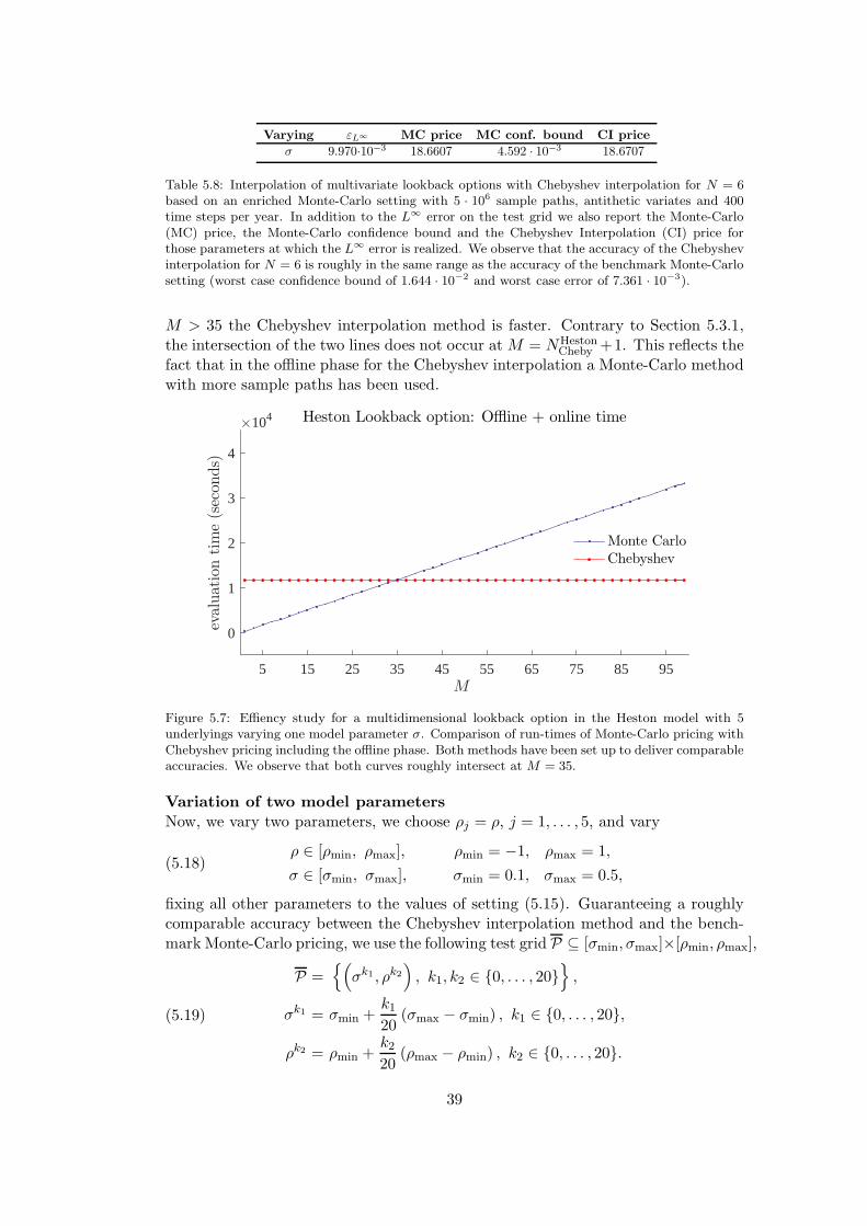
Varying εL∞ MC price MC conf. bound CI price

σ 9.970·10−3 18.6607 4.592 · 10−3 18.6707

Table 5.8: Interpolation of multivariate lookback options with Chebyshev interpolation for N = 6based on an enriched Monte-Carlo setting with 5 · 106 sample paths, antithetic variates and 400time steps per year. In addition to the L∞ error on the test grid we also report the Monte-Carlo(MC) price, the Monte-Carlo confidence bound and the Chebyshev Interpolation (CI) price forthose parameters at which the L∞ error is realized. We observe that the accuracy of the Chebyshevinterpolation for N = 6 is roughly in the same range as the accuracy of the benchmark Monte-Carlosetting (worst case confidence bound of 1.644 · 10−2 and worst case error of 7.361 · 10−3).

M > 35 the Chebyshev interpolation method is faster. Contrary to Section 5.3.1,the intersection of the two lines does not occur atM = NHeston

Cheby +1. This reflects thefact that in the offline phase for the Chebyshev interpolation a Monte-Carlo methodwith more sample paths has been used.

5 15 25 35 45 55 65 75 85 95M

0

1

2

3

4


ds)

×104 Heston Lookback option: Offline + online time

Monte CarloChebyshev

Figure 5.7: Effiency study for a multidimensional lookback option in the Heston model with 5underlyings varying one model parameter σ. Comparison of run-times of Monte-Carlo pricing withChebyshev pricing including the offline phase. Both methods have been set up to deliver comparableaccuracies. We observe that both curves roughly intersect at M = 35.

Variation of two model parametersNow, we vary two parameters, we choose ρj = ρ, j = 1, . . . , 5, and vary

(5.18)ρ ∈ [ρmin, ρmax], ρmin = −1, ρmax = 1,

σ ∈ [σmin, σmax], σmin = 0.1, σmax = 0.5,

fixing all other parameters to the values of setting (5.15). Guaranteeing a roughlycomparable accuracy between the Chebyshev interpolation method and the bench-mark Monte-Carlo pricing, we use the following test grid P ⊆ [σmin, σmax]×[ρmin, ρmax],

P =(σk1 , ρk2

), k1, k2 ∈ 0, . . . , 20

,

σk1 = σmin +k120

(σmax − σmin) , k1 ∈ 0, . . . , 20,

ρk2 = ρmin +k220

(ρmax − ρmin) , k2 ∈ 0, . . . , 20.

(5.19)

39

M 1 10 50 100

TChebyonline (s) 2.7·10−5 2.7·10−4 1.4·10−3 2.7·10−3

TChebyoffline+online (s) 1.2·104 1.2·104 1.2·104 1.2·104

TMonte-Carlo (s) 3.4·102 3.4·103 1.7·104 3.4·104


TMonte-Carlo3473.4% 347.3% 69.5% 34.73%

Table 5.9: Efficiency study for a multivariate lookback option in the Heston model based on 5underlyings. Here, we vary one model parameter and compare the Chebyshev results to Monte-Carlo. Both methods have been set up to deliver comparable accuracies. With increasing numberof computed prices, the Chebyshev algorithm increasingly profits from the initial investment of theoffline phase.

Varying εL∞ MC price MC conf. bound CI price

σ, ρ 5.260 · 10−2 5.239 1.428 · 10−2 5.292

Table 5.10: Interpolation of multivariate lookback options with Chebyshev interpolation for N = 6based on an enriched Monte-Carlo setting with 5 · 106 sample paths, antithetic variates and 400time steps per year. In addition to the L∞ error on the test grid we also report the Monte-Carlo(MC) price, the Monte-Carlo confidence bound and the Chebyshev Interpolation (CI) price forthose parameters at which the L∞ error is realized. We observe that the accuracy of the Chebyshevinterpolation N = 6 is roughly in the same range as the accuracy of the benchmark Monte-Carlosetting (worst case confidence bound of 6.783 · 10−2 and worst case error of 2.791 · 10−2).

In Table 5.10 we present the accuracy results for the Chebyshev interpolation withNHeston

Cheby = 6 based on the enriched Monte-Carlo setting. Comparing the benchmarkMonte-Carlo setting and the enriched Monte-Carlo setting on this test grid, weobserve that the maximal absolute error is 2.791 · 10−2 and the confidence boundsof the benchmark Monte-Carlo setting do not exceed 6.783 · 10−2.

For a run-time comparison, we show for different values of M the run-timesnecessary to compute the prices for M2 parameter tupels. Again, the run-times aremeasured for M = 1 and extrapolated for other values of M . Table 5.11 presentsthe results. In Figure 5.8 for each M = 1, . . . , 100 the run-times of the Chebyshevinterpolation method, including the offline phase, compared to the Monte-Carlomethod are presented. We observe that for M = 15 both lines intersect and forM > 15 the Chebyshev method outperforms its benchmark. Contrary to the case ofvarying only one parameter, the intersection of both lines occurs at a significantlylower value of M due to the fact that for each M pricing for M2 parameter tupelsis performed.

Additionally, Table 5.11 highlights that for a total number of 502 parametertuples, the Chebyshev method exhibits a significant decrease in (total) pricing run-times. For the maximal number of 1002 parameter tuples that we investigated,pricing in either model resulted in more than 97% of run-time savings in our im-plementation. While the computation of 1002 Heston prices via the Monte-Carlomethod consumes up to 39 days, the Chebyshev method computes the very sameprices in 23 hours only. Note that only 7 seconds of this time span are consumed byactual pricing during the online phase.

40

HestonM 1 10 50 100

TChebyonline (s) 7.1·10−4 7.1·10−2 1.8 7.1

TChebyoffline+online (s) 8.2·104 8.2·104 8.2·104 8.2·104

TMonte-Carlo (s) 3.4·102 3.4·104 8.4·105 3.4·106


TMonte-Carlo24313.9% 243.1% 9.7% 2.4%

Table 5.11: Efficiency study for a multivariate lookback option in the Heston model based on 5underlyings. Here, we vary two model parameters and compare the Chebyshev results to Monte-Carlo. Both methods have been set up to deliver comparable accuracies. With increasing numberof computed prices, the Chebyshev algorithm increasingly profits from the initial investment of theoffline phase.

5 15 25 35 45 55 65 75 85 95M (evaluation of M2 different parameter pairs)

-0.5

0

0.5

1

1.5

2

2.5

3

3.5


ds)

×106 Heston Lookback option: Offline + online time

Monte CarloChebyshev

Figure 5.8: Effiency study for a multivariate lookback option in the Heston model based on 5underlyings, varying the two model parameters σ and ρ. Comparison of run-times for Monte-Carlo pricing and Chebyshev pricing including the offline phase. Both methods have been set up todeliver comparable accuracies. We observe that the Monte-Carlo and the Chebyshev curves roughlyintersect at M = 15.

41

6 Conclusion and Outlook

This article focuses on applying the Chebyshev method to European option pricing.Within this scope, Sections 2–4 establish theoretical convergence results and numer-ical case studies in Section 5 confirm these findings. Moreover, in experiments withFourier pricing an accuracy of 10−5 is observed with less than ten Chebyshev nodesin each parameter, see Figure 5.3. The financial implications of the high precisionachieved with such a small number of interpolation nodes are twofold. First, it showsthat there are interesting cases in which we observe an accuracy in the range of ma-chine precision. In this comfortable situation without methodological risk we canignore the fact that approximations are implemented. Second, compared with othersources of risk, already errors from a much lesser accuracy level can be ignored. Ifwe agree that an accuracy of 10−4 is satisfactory, already 36–49 interpolation nodesfor the approximation of call option prices as reported in Figure 5.3 are sufficient.

Additionally, also the numerical experiments for American, barrier and lookbackoptions display promising results. A theoretical error analysis for nonlinear pricingproblems is beyond the scope of the present article, while we are convinced that fur-ther investigations in this direction are valuable. For instance our analytic approachbased on examinations of the Fourier representations can be adopted to barrier op-tions in Levy models leading to the involvement of Wiener-Hopf factorizations, seeEberlein et al. (2011). In general we expect the regularity analysis to become morechallenging in the presence of nonlinearities. For American options the current workof Teichmann (2015) may lead to regularity assertions for American options that areinherited from their corresponding European counterparts.

The theoretical and experimental results of our case studies show that the methodcan perform considerably well when few parameters are varied. As a consequence,we recommend the interpolation method for this case and also when solely thestrike of a plain vanilla option is varied and fast Fourier methods are available. Forcalibration purposes for example, strikes are not given in a discrete logarithmic scale,which makes an additional interpolation necessary in order to apply FFT. Here,Chebyshev polynomials offer an attractive alternative. In particular, the maturitycan be used as supplementary free variable. Moreover, for models with a low numberof parameters, another path could be beneficial: Interpolating the objective functionof the parameters directly. Then the optimization would boil down to a minimizationof a tensorized polynomial, which could be exploited in further research. As may beseen from Armenti et al. (2015), where the present article is applied for the first time,this advantage can also be exploited for other optimization procedures in finance forexample in risk allocation.

The multivariate construction of the interpolation and the theoretical error anal-ysis suggest that the empirically observed error behaviour extends to three and morevarying parameters, as well, as long as analyticity is provided. More precisely, in

case of analyticity, the rate is of order ρ−D√N for some constant ρ depending on

the domain of analyticity and N the total number of interpolation nodes. For mul-tivariate polynomial interpolation, the introduction of sparsity techniques promisehigher efficiency, as for instance by compression techniques for tensors as reviewedby Kolda and Bader (2009). We address the issue of curse of dimensionality fur-ther in Gaß, Glau and Mair (2015), where we take a different route by replacing the

42

Chebyshev interpolation with an empirical interpolation for Fourier pricing methods.

A Proof of Theorem 2.2

Proof. In Sauter and Schwab (2004, Proof of Lemma 7.3.3) the proof is given forthe following error bound:

maxp∈P

∣∣f − IN (f)∣∣ ≤

√D2

D2+1V −Nmin(1− −2

min)−D

2 ,

where N is the number of interpolation points in each of the D dimensions, min :=minDi=1 i and V the bound of f on B(P, ) with P = [−1, 1]D. Here, we extend theproof by incorporating the different values of Ni, i = 1, . . . ,D, as well as expressingthe error bound with the different i, i = 1, . . . ,D.

In general we work with a parameter space P of hyperrectangular structure,P = [p

1, p

1] × . . . × [p

D, pD]. With the introduced linear transformation in Section

2.1 we have a transformation τP : [−1, 1]D → P with

τP(p) =

(pi +

pi− pi

2(1− p)

)D

i=1

.

Let p 7→ Pricep be a function on P. We set Pricep = Pricep τP(p). Further, let

IN (Price(·))(p) be the Chebyshev interpolation of Pricep on [−1, 1]D . Then it holds

IN (Price(·))(p) = IN (Price

(·))(·) τ−1

P (p).

Therewith, it directly follows

Pricep − IN (Price(·))(p) =

(Price − IN (Price

(·))(·)) τ−1

P (p).

Applying the error estimation from Sauter and Schwab (2004, Lemma 7.3.3) results

∣∣Price − IN (Price(·))(·)

∣∣C0(P)

=∣∣Price − IN (Price

(·))(·)∣∣C0([−1,1]D)

≤√D2

D2+1V −Nmin(1− −2

min)−D

2

=√D2

D2+1V −Nmin(1− −2

min)−D

2 ,

where V = supp∈B([−1,1]D,) Pricep, V = supp∈B(P,) Price

p. Summarizing, the

transformation τP : [−1, 1]D → P does not affect the error analysis, only by ap-plying the transformation as described in Section 2.1,

B(P, ) := B([p1, p

1], 1)× . . . ×B([p

D, pD], D),(A.1)

with B([p, p], ) := τ[p,p] B([−1, 1], ). Note that i is not the radius of the ellipse

B([pi, pi], i) but of the normed ellipse B([−1, 1], i). Therefore, in the following it

suffices to show the proof for P = [−1, 1]D.

43

As in Sauter and Schwab (2004, Proof of Lemma 7.3.3) we introduce the scalarproduct

〈f, g〉 :=∫

B(P,)

f(z)g(z)∏Di=1

√|1− z2i |

dz

and the Hilbert space

L2(B(P, )) := f : f is analytic in B(P, ) and ||f ||2 := 〈f, f〉 <∞.Following Sauter and Schwab (2004, Proof of Lemma 7.3.3), we define a completeorthonormal system for L2(B(P, )) w.r.t. the scalar product 〈·, ·〉 by the scaledChebyshev polynomials

Tµ(z) := cµTµ(z) with cµ :=

(2

π

)D2

D∏

i=1

(2µii + −2µii )−

12 , for all µ ∈ N

D0 .

Then, for any arbitrary bounded functional E on L2(B(P, )) we have

|E(f)| ≤ ||E||||f ||,(A.2)

where ||E|| denotes the operator norm. Due to the orthonormality of(Tµ

)µ∈ND

0

it

follows that

||E|| = supf∈L2(B(P,))\0

|E(f)|‖f‖

=√∑

µ∈ND0

|E(Tµ)|2.

In the following let E be the error of the Chebyshev polynomial interpolation at afix p ∈ P,

E(f) := |f(p)− IN (f(·))(p)|.Starting with (A.2), we first focus on ||E||,

‖E‖2 =∑

µ∈ND0

|E(Tµ)|2 =∑

µ∈ND0

c2µ|E(Tµ)|2.

At this step we apply Lemma A.1 and obtain∑

µ∈ND0

c2µ|E(Tµ)|2 =∑

µ∈ND0 ,∃i:µi>Ni

c2µ|E(Tµ)|2 ≤∑


4c2µ.

Overall, using(∏D

j=1 2µjj + x

)−1≤(∏D

j=1 2µjj

)−1=∏Dj=1

−2µjj for x > 0, µj ∈

N0 and j = 1, . . . ,D and this leads to

‖E‖2 ≤ 4∑


c2µ ≤ 4

(2

π

)D D∑

i=1

∑

µ∈ND0 ,µi>Ni

D∏

j=1

−2µjj

≤ 4

(2

π

)D D∑

i=1

−2Ni

i

∑

µ∈ND0 ,µi>Ni

−2(µi−Ni)i

D∏

j=1,j 6=i−2µjj

≤ 4

(2

π

)D D∑

i=1

−2Ni

i

∑

µ∈ND0

D∏

j=1

−2µjj

.

44

From this point on we use the convergence of the geometric series since |−2j | <

1, j = 1, . . . ,D,

‖E‖2 ≤ 4

(2

π

)D D∑

i=1

−2Ni

i

∞∑

µ1=0

. . .

∞∑

µD=0

D∏

j=1

−2µjj

= 4

(2

π

)D D∑

i=1

−2Ni

i

∞∑

µ1=0

. . .

∞∑

µD−1=0

D−1∏

j=1

−2µjj

∞∑

µD=0

−2µDD

= 4

(2

π

)D D∑

i=1

−2Ni

i

∞∑

µ1=0

. . .

∞∑

µD−1=0

D−1∏

j=1

−2µjj

1

1− −2D

= . . . = 4

(2

π

)D D∑

i=1

−2Ni

i

D∏

j=1

1

1− −2j

.

Recalling (A.2), we have to estimate ‖f‖,

‖f‖2 =∫

B(P,)

f(z)f(z)∏Di=1

√|1− z2i |

dz ≤(

supz∈B(P,)

|f(z)|)2

‖1‖2.

From πD2 T0 = 1 it directly follows that ‖1‖2 =

(π

D2

)2‖T0‖2 = πD and therewith

‖f‖2 ≤ πD · V 2.

Combining the results leads to

|E(f)| = |f(p)− IN (f(·))(p)∣∣ ≤

πD · V 2 · 4

(2

π

)D D∑

i=1

−2Ni

i

D∏

j=1

1

1− −2j

12

= 2D2+1V

D∑

i=1

−2Ni

i

D∏

j=1

1

1− −2j

12

.

The following lemma shows that the Chebyshev interpolation of a polynomialwith a degree as most as high as the degree of the interpolating Chebyshev polyno-mial is exact and furthermore determines an upper bound for interpolating Cheby-shev polynomials with a higher degree.

Lemma A.1. For x ∈ [−1, 1]D it holds

|Tµ(x)− IN (Tµ(·))(x)| = 0 ∀µ ∈ ND0 : µi ≤ Ni, i = 1, . . . ,D,(A.3)

|Tµ(x)− IN (Tµ(·))(x)| ≤ 2 ∀µ ∈ ND0 : ∃i ∈ 1, . . . ,D : µi > Ni.(A.4)

45

Proof. Uniqueness properties of the Chebyshev interpolation directly imply (A.3).The proof of (A.4) is similar to Sauter and Schwab (2004, Proof of Hilfssatz 7.3.1).They use the zeros of the Chebyshev polynomial as interpolation points, whereas weuse the extreme points and therefore, we use a different orthogonality property in thisproof. We first focus on the one-dimensional case. Recalling (2.2), the Chebyshevinterpolation of Tµ, µ > N , is given as

IN (Tµ)(x) =

N∑

j=0

cjTj(x) with cj =210<j<N

N

N∑

k=0

′′Tµ(xk)Tj(xk), j ≤ N,

where xk denotes the k-th extremum of TN . Here, we can apply the followingorthogonality (Rivlin (1990, p.54)),

N∑

k=0

′′Tµ(xk)Tj(xk) =

0, µ+ j 6= 0 mod (2N) and |µ − j| 6= 0 mod (2N),

N, µ+ j = 0 mod (2N) and |µ − j| = 0 mod (2N),N2 , µ+ j = 0 mod (2N) and |µ − j| 6= 0 mod (2N),N2 , µ+ j 6= 0 mod (2N) and |µ − j| = 0 mod (2N).

(A.5)

For j ≤ N and µ > N this yields the existence of γ ≤ N such that

IN (Tµ) = Tγ .(A.6)

(A.6) follows elementarily from the case that for any µ > N only for one 0 ≤ j ≤ Nthe orthogonality can lead to a coefficient cj > 0.

Proving the claim, we distinguish several cases. In all of these cases we assumethat there exists 0 ≤ j ≤ N such that

∑Nk=0

′′Tµ(xk)Tj(xk) 6= 0. We will then show

that for all other 0 ≤ i ≤ N, i 6= j it follows∑N

k=0′′Tµ(xk)Tj(xk) = 0.

Firstly, assume there exists j such that µ + j = 0 mod (2N) and µ − j =0 mod (2N). Then it directly follows for all 0 ≤ i ≤ N , i 6= j that µ + i 6=0 mod (2N) and µ− i 6= 0 mod (2N).

Secondly, assume there exists j such that µ + j = 0 mod (2N) and µ − j 6=0 mod (2N). Analogously, for all 0 ≤ i ≤ N , i 6= j we have µ+ i 6= 0 mod (2N) andadditionally from µ+ j = 0 mod (2N) it follows that µ+ j− 2N = 0 mod (2N) andtherewith for all 0 ≤ i ≤ N , i 6= j we have µ − i > µ + j − 2N which is equivalentto µ− i 6= 0 mod (2N).

Similar argumentation holds for the third case µ+j 6= 0 mod (2N) and |µ−j| =0 mod (2N).

Therewith, (A.6) holds and it directly follows that |Tµ − IN (Tµ)| ≤ |Tµ| +|IN (Tµ)| ≤ 1 + 1 = 2. Thus (A.4) holds in the one-dimensional case. The extensionto the multivariate case follows analogously by applying the triangle inequality andinserting the one-dimensional result to each tensor component.

References

Armenti, Y., S. Crepey, S. Drapeau, and A. Papapantoleon (2015). Multivariateshortfall risk allocation. available on http://arxiv.org/abs/1507.05351.

46

http://arxiv.org/abs/1507.05351

Barndorff-Nielsen, O. E. and N. Shephard (2001). Non-Gaussian Ornstein–Uhlenbeck-based models and some of their uses in financial economics. Journalof the Royal Statistical Society, Series B 63, 167–241.

Bernstein, S. N. (1912). Sur l’ordre de la meilleure approximation des fonctionscontinues par des polynomes de degre donne, mimoires acad. Academie Royale deBelgique. Classe des Sciences. Memoires 4.

Black, F. and M. Scholes (1973). The pricing of options and corporate liabilities.Journal of Political Economy 81 (3), 637–654.

Boyarchenko, S. I. and S. Z. Levendorskii (2000). Option pricing for truncatedlevy processes. International Journal of Theoretical and Applied Finance 3 (03),549–552.

Boyarchenko, S. I. and S. Z. Levendorskii (2002). Non-Gaussian Merton-Black-Scholes Theory, Volume 9. World Scientific.

Brennan, M. J. and E. S. Schwartz (1977). The valuation of American put options.The Journal of Finance 2 (32), 449–462.

Burkovska, O., B. Haasdonk, J. Salomon, and B. Wohlmuth (2015). Reduced basismethods for pricing options with the Black-Scholes and Heston models. SIAMJournal on Financial Mathematics 6 (1), 685–712.

Canuto, C. and A. Quarteroni (1982). Approximation results for orthogonal poly-nomials in sobolev spaces. Mathematics of Computation 38 (157), 67–86.

Carr, P., H. Geman, D. B. Madan, and M. Yor (2002). The fine structure of assetreturns: An empirical investigation. Journal of Business 75 (2), 305–332.

Carr, P., H. Geman, D. B. Madan, and M. Yor (2003). Stochastic volatility for Levyprocesses. Mathematical Finance 13, 345–382.

Carr, P. and D. B. Madan (1999). Option valuation and the fast Fourier transform.Journal of Computional Finance 2 (4), 61–73.

Cheridito, P. and A. Wugalter (2012). Pricing and hedging in affine models withpossibility of default. SIAM Journal on Financial Mathematics 3 (1), 328–350.

Cont, R., N. Lantos, and O. Pironneau (2011). A reduced basis for option pricing.SIAM Journal on Financial Mathematics 2 (1), 287–316.

Cuchiero, C., M. Keller-Ressel, and J. Teichmann (2012). Polynomial processes andtheir applications to mathematical finance. Finance and Stochastics 4 (16).

Duffie, D., D. Filipovic, and W. Schachermayer (2003). Affine processes and appli-cations in finance. Annals of Applied Probability 13 (3), 984–1053.

Eberlein, E., K. Glau, and A. Papapantoleon (2010). Analysis of Fourier transformvaluation formulas and applications. Applied Mathematical Finance 17 (3), 211–240.

47

Eberlein, E., K. Glau, and A. Papapantoleon (2011). Analyticity of the Wiener–Hopffactorization and valuation of exotic options in Levy models. In G. Di Nunno andB. Øksendal (Eds.), Advanced Mathematical Methods for Finance, pp. 223 – 245.Springer.

Eberlein, E., U. Keller, and K. Prause (1998). New insights into smile, mispricingand value at risk: the hyperbolic model. Journal of Business 71 (3), 371–405.

Eberlein, E. and F. Ozkan (2005). The Levy LIBOR model. Finance and Stochas-tics 9 (3), 327–348.

Feng, L. and V. Linetsky (2008). Pricing discretely monitored barrier options anddefaultable bonds in Levy process models: A fast Hilbert transform approach.Mathematical Finance 18 (3), 337–384.

Filipovic, D., M. Larsson, and A. Trolle (2014). Linear-rational term structuremodels. Preprint.

Filipovic, D. and E. Mayerhofer (2009). Affine diffusion processes: Theory andapplications. In Advanced Financial Modelling, Volume 8 of Radon Series onComputational and Applied Mathematics, pp. 125–164. de Gruyter.

Gaß, M., K. Glau, and M. Mair (2015). Magic Points Fourier Transform OptionPricing – Polynomial and Empirical Interpolation. Working paper.

Glau, K. (2015). Classification of Levy processes with parabolic Kolmogorov back-ward equations. forthcoming in SIAM journal Theory of Probability.

Glau, K. (2016). Feynman-Kac formula for Levy processes with discontionuouskilling rate. forthcoming in Finance and Stochastics.

Haasdonk, B., J. Salomon, and B. Wohlmuth (2013). A reduced basis method forthe simulation of American options. In Numerical Mathematics and AdvancedApplications 2011, pp. 821–829. Springer.

Heston, S. L. (1993). A closed-form solution for options with stochastic volatilitywith applications to bond and currency options. Review of Financial Studies 6 (2),327–343.

Janich, K. (2004). Funktionentheorie: eine Einfuhrung. Springer-Lehrbuch.Springer.

Kallsen, J. (2006). A didactic note on affine stochastic volatility models. In Y. Ka-banov, R. Lipster, and J. Stoyanov (Eds.), From Stochastic Calculus to Mathe-matical Finance: The Shiryaev Festschrift, pp. 343–368. Springer.

Keller-Ressel, M. and E. Mayerhofer (2015). Exponential moments of affine pro-cesses. The Annals of Applied Probability 25, 714–752.

Keller-Ressel, M., A. Papapantoleon, and J. Teichmann (2013). The affine libormodels. Mathematical Finance 23 (4), 627–658.

48

Kolda, T. G. and B. W. Bader (2009). Tensor decompositions and applications.SIAM Review 51 (3), 455–500.

Kudryavtsev, O. and S. Z. Levendorskii (2009). Fast and accurate pricing of barrieroptions under Levy processes. Finance and Stochastics 13 (4), 531–562.

Lee, R. W. (2004). Option pricing by transform methods: Extensions, unification,and error control. Journal of Computational Finance 7 (3), 51–86.

Levendorskii, S. Z. (2012). Efficient pricing and reliable calibration in the Hestonmodel.

Lord, R., F. Fang, F. Bervoets, and C. W. Oosterlee (2008). A fast and accurateFFT-based method for pricing early-exercise options under Levy processes. SIAMJournal on Scientific Computing 30 (4), 1678–1705.

Merton, R. C. (1973). Theory of rational option pricing. The Bell Journal ofEconomics and Management Science 4 (1), 141–183.

Merton, R. C. (1976). Option pricing when underlying stock returns are discontin-uous. Journal of Financial Economics 3, 125–144.

Pachon, R. (2016). Numerical pricing of European options with arbitrary payoffs.Available at SSRN: http://ssrn.com/abstract=2712402.

Pironneau, O. (2011). Reduced basis for vanilla and basket options. Risk andDecision Analysis 2 (4), 185–194.

Pistorius, M. and J. Stolte (2012). Fast computation of vanilla prices in time-changedmodels and implied volatilities. International Journal of Theoretical and AppliedFinance 15 (4), 1250031–1250031.

Platte, R. B. and N. L. Trefethen (2008). Chebfun: A new kind of numerical com-puting, pp. 69–86. Springer.

Raible, S. (2000). Levy Processes in Finance: Theory, Numerics, and EmpiricalFacts. Ph. D. thesis, Universitat Freiburg.

Rivlin, T.-J. (1990). Chebyshev polynomials. John Wiley & Sons, Inc., copublishedin the United States with John Wiley &.

Runge, C. (1901). Uber empirische Funktionen und die Interpolation zwischenaquidistanten Ordinaten. Zeitschrift fur Mathematik und Physik 46, 224–243.

Sachs, E. W. and M. Schu (2010). Reduced order models in PIDE constrainedoptimization. Control and Cybernetics 39 (3), 661–675.

Sato, K.-I. (1999). Levy Processes and Infinitely Divisible Distributions. CambridgeUniversity Press.

Sauter, S. and C. Schwab (2004). Randelementmethoden: Analyse, Numerik undImplementierung schneller Algorithmen. Vieweg+ Teubner Verlag.

49

http://ssrn.com/abstract=2712402

Tadmor, E. (1986). The exponential accuracy of fourier and chebyshev differencingmethods. SIAM Journal on Numerical Analysis 23 (1), 1–10.

Teichmann, J. (2015). Tractable american options prob-lems. Talk at ETH Zurich, September 2015, available onhttps://people.math.ethz.ch/~jteichma/its_talks/teichmann_talk_zurich_sep2015.pdf.

Trefethen, L. N. (2011). Talk: Six myths of polynomial interpolation and quadrature.https://people.maths.ox.ac.uk/trefethen/mythstalk.pdf.

Trefethen, L. N. (2013). Approximation Theory and Approximation Practice. SIAMbooks.

Wloka, J. (1987). Partial Differential Equations. Cambridge University Press.

50

https://people.math.ethz.ch/~jteichma/its_talks/teichmann_talk_zurich_sep2015.pdf

https://people.maths.ox.ac.uk/trefethen/mythstalk.pdf

chebyshev interpolation for parametric - arxiv · problem for polynomial interpolation on an...

Documents