characterizing spatial and seasonal variability of carbon dioxide and water vapour fluxes above a...

Characterizing spatial and seasonal variability of carbondioxide and water vapour fluxes above a tropical mixed

mangrove forest canopy, India

Abhra Chanda1,∗, Anirban Akhand

1, Sudip Manna1, Sachinandan Dutta

1,Sugata Hazra

1, Indrani Das2 and V K Dadhwal

3

1School of Oceanographic Studies, Jadavpur University, 188, Raja S. C. Mullick Road,Kolkata 700 032, West Bengal, India.

2Department of Botany, Midnapore College, Midnapore 721 101, West Bengal, India.3National Remote Sensing Centre, Department of Space, Government of India,

Balanagar, Hyderabad 500 037, Andhra Pradesh, India.∗Corresponding author. e-mail: [email protected]

The above canopy carbon dioxide and water vapour fluxes were measured by micrometeorological gra-dient technique at three distant stations, within the world’s largest mangrove ecosystem of Sundarban(Indian part), between April 2011 and March 2012. Quadrat analysis revealed that all the three studysites are characterized by a strong heterogeneity in the mangrove vegetation cover. At day time the for-est was a sink for CO2, but its magnitude varied significantly from −0.39 to −1.33 mg m−2 s−1. Thestation named Jharkhali showed maximum annual fluxes followed by Henry Island and Bonnie Camp.Day time fluxes were higher during March and October, while in August and January the magnitudeswere comparatively lower. The seasonal variation followed the same trend in all the sites. The spatialvariation of CO2 flux above the canopy was mainly explained by the canopy density and photosyntheticefficiency of the mangrove species. The CO2 sink strength of the mangrove cover in different stationsvaried in the same way with the CO2 uptake potential of the species diversity in the respective sites. Therelationship between the magnitude of day time CO2 uptake by the canopy and photosynthetic photonflux was defined by a non-linear exponential curve (R2 ranging from 0.51 to 0.60). Water vapour fluxesvaried between 1.4 and 69.5 mg m−2 s−1. There were significant differences in magnitude between dayand night time water vapour fluxes, but no spatial variation was observed.

1. Introduction

Forest patches are considered to be a complexecosystem by virtue of the variability in theircomposition and structure (Noe et al. 2011).These terrestrial ecosystems play a decisive rolein regulating the atmospheric composition andhence the climate, by means of exchanging tracegases between the atmosphere and the biosphere

(Magnani et al. 2007; Misson et al. 2007). Everyyear, terrestrial plants fix one eighth of the atmo-spheric carbon dioxide (CO2) by means of photo-synthesis, while respiration, decay and soil organ-ism activity return back a similar fraction, thatis why, the key to accurately predict future levelsof atmospheric CO2 is in understanding how theterrestrial biosphere and atmosphere exchangeCO2 (Reich 2010). Recent estimates revealed that

Keywords. Carbon dioxide fluxes; water vapour fluxes; photosynthetic photon flux; spatial variation; mangrove forests;

Sundarban.

J. Earth Syst. Sci. 122, No. 2, April 2013, pp. 503–513c© Indian Academy of Sciences 503

504 Abhra Chanda et al.

the terrestrial gross primary production (GPP) isthe largest global CO2 flux (∼123 ± 8 Pg C year−1)driving several ecosystem functions (Beer et al.2010).

Micrometeorological techniques made continu-ous monitoring and frequent collection of data pos-sible without disturbing the environment aroundthe plant canopy (Baldocchi et al. 1988). Severalendeavours have been undertaken to study theexchange dynamics of greenhouse gases over trop-ical terrestrial forests but a comparatively lesserattention has been paid on the mangrove forestsat the land ocean boundary. Mangroves are oneof the most productive and bio-diverse ecosystemsdeveloped along estuaries, sea coasts and rivermouths in the tropical and subtropical intertidalzones. In general, the mangrove ecosystem includ-ing the below- and above-ground compartmentsact as sinks for CO2, but the water column andthe sediment are largely found to emit the same(Borges et al. 2003). The present carbon burial ratewithin the mangrove systems has been assessed tobe ≈18.4 Tg C yr−1 based on the global mangrovecover of 160,000 km2 (Bouillon et al. 2009).

Sundarban is the largest continuous stretch ofmangrove forests of the world covering about2.84% of the global mangrove area (15×104 km2)and having a unique bio-climatic zone in theland–ocean margin of the Bay of Bengal, outof which 40% lies within India and the rest inBangladesh counterpart. In the year 1989, Sun-darban Biosphere Reserve was constituted in theIndian Sundarban part, after the core area of theSundarban Tiger Reserve, i.e., Sundarban NationalPark received the recognition of UNESCO WorldHeritage Site. Few studies were undertaken inthe past in selected locations of the Sundarbandeltaic system, which revealed dual character ofthis ecosystem in terms of source and sink forCO2. Mukhophadhya et al. (2000) carried out ashort term survey in Jambu Island and observedthe environment to be a sink for CO2 in the pre-monsoon season at a rate of 24 × 109 kg C year−1

while the same authors conducted another studyat Lothian Island which reflected the source char-acter with an emission rate of 1.51 × 106 mgday−1 (Mukhophadhya et al. 2001). Long termannual studies conducted later at the LothianIsland also confirmed a source character for CO2

as reported by Mukhophadhya et al. (2002),while at the same Lothian Island and Sajnekhali,Ganguly et al. (2008) observed a mean net influxof −48.3 g m−2 day−1 and total sink strength of206 Gg day−1 was estimated for the entire reserveforest area (4264 km2). All the observations madeso far tried to illustrate the holistic scenario ofthe ecosystem based on the results obtained fromthe particular study sites, but no prior attempts

have been taken to discuss the spatial variability ofthe CO2 exchange within the same time frame insuch a complex and heterogeneous gigantic man-grove ecosystem. The structure and functioning ofmangrove forests are influenced by several physico-chemical and bio-geographical factors like soil type,availability of water table, vapour pressure deficit,photosynthetic photon flux which again vary overdifferent spatial and temporal scales (Duke et al.1998). Apart from these factors, species diver-sity along with the species specific carbon uptakepotential, determines the sink strength of a forestcover and canopy density also plays a crucial rolebehind the spatial variation of fluxes.

The present study aims to investigate the natureand magnitude of the atmosphere–biosphere CO2

and H2O fluxes above the forest canopy at threeselected locations situated at the northern, mid-dle and southern parts of the Indian Sundarbans.Micrometeorological techniques were implementedto carry out the investigation throughout a com-plete annual cycle. The study also strives to findout the relationship between the micrometeorolog-ical variables and the gas exchange, along with theeffect of species composition, if any.

2. Materials and methods

2.1 Site description

The mangrove forest of Indian Sundarbans is sit-uated between 21◦32′ and 22◦40′N latitudes andbetween 88◦05′ and 89◦E longitudes comprisingan area of 9630 km2 out of which 4264 km2 isunder the arena of reserve forest. It extends tillthe Bay of Bengal towards south and stretchesup to the Dampier–Hodges line in the north. Theclimate in this part of the continent is grosslydemarcated as monsoon (June–September), post-monsoon (October–January) and pre-monsoon(February–May). In order to understand the spa-tial variability in CO2 and H2O dynamics above theforest canopy, flux measurements were carried outat three sites located at the northern, middle andsouthern parts of the Indian Sundarbans (figure 1).Jharkhali Island (22◦01′16′′N, 88◦41′4.75′′E) atthe confluence of Bidya and Herobhanga rivers(northern station), Bonnie Camp (21◦49′47.87′′N,88◦37′22.33′′E) almost 30 km downstream (mid-dle station) from Jharkhali and Henry Island(21◦34′27.11′′N, 88◦17′34.06′′E) at the southern-most tip of the Sundarbans (southern station) werechosen for this study (hereafter referred to as Stn1,Stn2 and Stn3, respectively). Out of these threestations, Stn3 has a tower of 16 m height and therest two have towers of 20 m height.

CO2 and H2O flux above a mixed mangrove forest 505

Figure 1. The location of the study sites shown in the mapof Indian Sundarbans.

In Stn1, Avicenia marina (Forssk.) Vierh.together with Avicenia alba Blume dominatethe canopy cover, while Excoecaria agallocha L.,Phoenix paludosa Roxb. and Bruguiera gymnor-rhiza are also found in patches. A large abun-dance of Phoenix paludosa is observed in Stn2 fol-lowed by Avicenia marina with few patches ofAegiceras corniculatum and Agialites rotundifolia.The top canopy layer in Stn3 is mainly com-prised of Avicenia officinalis L., other dominantspecies in the lower strata are Aegiceras cornicula-tum (L.) Blanco and Agialites rotundifolia Roxb.In the interior parts, Avicenia alba and Bruguieragymnorrhiza (L.) Lam. are also found to thrive.

2.2 Instrumentation and sampling strategy

All observations were made in every month at eachsite, for a continuous 24 hour diurnal cycle, fromApril 2011 to March 2012. In order to examinethe diurnal variation, all the data were logged atevery 1 hour interval. CO2 and H2O fluxes weremonitored at half hourly intervals and averaged to1 hour. Difficulties in accessing Stn2 all round theyear has compelled us to study this site bimonthly.In Stn3, flux calculations were made from the

difference in concentration at 6 and 16 m respec-tively, whereas, in the other two stations fluxeswere calculated from the difference in concentra-tion between 10 and 20 m. In all the cases, the top-most forest canopy layer was well below the lowerheight from which the air samples were drawn.Stn1 had a uniform canopy height of 8–9 m, whilethe other two stations had a comparatively lowercanopy height ranging between 4 and 5 m, as Stn1is dominated with species which can grow tallercompared to those dominant in Stn2 and Stn3.Air samples from the respective measuring heightsof the tower were pumped and passed through atthe rate of 0.5 litre min−1 (with the help of aportable air sampler) to the closed path LI-840ACO2/H2O Gas Analyzer (Li-Cor, Inc. USA) to getthe ambient concentration of CO2 (in ppm). Inorder to minimise the effect of fluctuations, a 5-minute average for CO2 values were used to calcu-late the flux. The analyzer was calibrated beforeand after the completion of each diurnal cycle withthe help of three gases, one having CO2-free airand the other two having a certified reference stan-dard of known concentration (300 and 600 ppm inN2 medium) of CO2 (Indian Refrigeration Stores,Kolkata, West Bengal, India). The relative uncer-tainties (standard deviation relative to mean value)were observed to be ±0.04 for CO2 concentrationmeasurements and ±0.09 for H2O concentrations.

Micrometeorological parameters like air tem-perature, atmospheric pressure, relative humidity,wind velocity and its direction were recorded withthe help of weather stations (La Crosse Technol-ogy, WS-2350) mounted at the respective towers.The precision of measurements are 0.1◦C for airtemperature, 1 m bar for atmospheric pressure, 1%relative humidity and 0.1 m s−1 for wind velocity,respectively. The photosynthetic active radiation(PAR) is measured with the help of a PAR Sensor(LI-190, Li-Cor, Inc. USA) fitted at the top of thetowers. The precision of measurement was 0.1 μmolm−2 s−1. In Stn1 and Stn2, the fetch of the for-est stand extends to almost 1 km in all directionsfrom the tower, but in Stn3 there is a void spacein the forest patch in the south–south eastern sec-tion. Flux measurement was skipped for this sitewhen wind had a direction between 105◦ and 155◦

from that end.

2.3 Flux calculations

The exchange of trace gases were calculated bymicrometeorological methods (gradient technique),using the formula:

FCO2 = Kc · ΔCi, (1)

where FCO2 denotes the atmosphere–biosphereflux (mg m−2 s−1), ΔCi is the difference in


concentration of trace gases (mg m−3) at therespective heights mentioned above and Kc is theexchange velocity which is further defined as:

Kc =1

(Ra + Rs), (2)

where Ra and Rs stand for aerodynamic and sur-face layer resistance, respectively (Barrett 1998).Fluxes towards the canopy are noted with a neg-ative sign; while fluxes away from the canopytowards the atmosphere are given with a positivesign.

Surface layer resistance (Rs) was calculated fromsurface transfer function (B−1) and friction veloc-ity (u∗), following the relations:

kB−1 = 2(

K

Dc

)2/3

(3)

and

Rs =B−1

u∗ , (4)

where k is the Von Karman constant, K is thermaldiffusivity of air and

Dc (molecular diffusivity) = 0.115 (T2/273)1.5,

(5)

where T2 is the temperature at 20 m height(Wesely and Hicks 1977). Friction velocity

(u∗) = k(u10 − u20)/0.693, (6)

where u10 and u20 are wind speed at 10 and 20 mheight respectively. The equation

Ra =(

ln(

Z

Z0

)− Ψm

)/k u∗ (7)

is used to calculate the aerodynamic resistancewhere Z0 represents the roughness length andΨm stands for the atmospheric stability correctionfunction (Wesely and Hicks 1977). Z0 was obtainedfrom the y-intercept (ln Z0) of the straight linefrom the plot of ln Z vs. u. The atmospheric cor-rection functions were evaluated based on the out-put of Z/L where L stands for the Obukhov scalelength.

Obukhov scale length is a metric of atmosphericstability and is approximately the height at whichbuoyancy starts to dominate over mechanicallygenerated turbulence.

L = − (u ∗ θv) /k · g (ω′θ′v)s , (8)

where θv is the mean virtual potential tempera-ture. The potential temperature for air is generallyexpressed as:

θ = T (P0/P )R/Cp (9)

where T is the absolute temperature of the parcelof air, R and Cp are the universal gas constant andspecific heat capacity at constant pressure of air,respectively. P stands for the instantaneous atmo-spheric pressure and P0 is the standard referencepressure taken as 1000 m bar. Using the similaritytheory approximation (ω′θ′

v)s = −u∗ θ∗, where θ∗is proportional to θ10– θ20, i.e., the vertical differ-ence in potential virtual temperature, the Obukhovlength reduces to

L = (u∗2 θv)/k · g θ∗ . (10)

For stable conditions (i.e., Z/L > 0),

Ψm = 4.7 Z/L (11a)

and for unstable condition (i.e., Z/L < 0),

Ψm = −2 ln(1 + x)/2 − ln(1 + x2)/2+ 2 tan−1(x) − π/2, (11b)

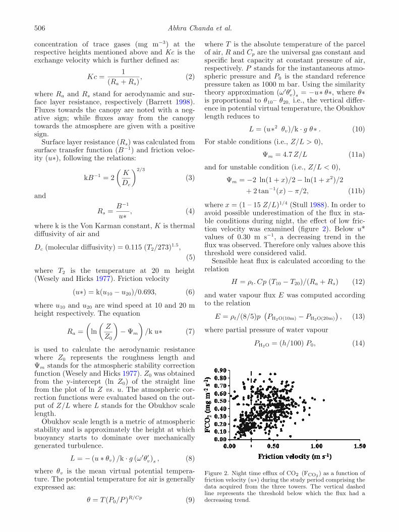
where x = (1 – 15 Z/L)1/4 (Stull 1988). In order toavoid possible underestimation of the flux in sta-ble conditions during night, the effect of low fric-tion velocity was examined (figure 2). Below u*values of 0.30 m s−1, a decreasing trend in theflux was observed. Therefore only values above thisthreshold were considered valid.

Sensible heat flux is calculated according to therelation

H = ρt. Cp (T10 − T20)/(Ra + Rs) (12)

and water vapour flux E was computed accordingto the relation

E = ρt/(8/5)p(PH2O(10m) − PH2O(20m)

), (13)

where partial pressure of water vapour

PH2O = (h/100) P0, (14)

Figure 2. Night time efflux of CO2 (FCO2) as a function offriction velocity (u∗) during the study period comprising thedata acquired from the three towers. The vertical dashedline represents the threshold below which the flux had adecreasing trend.


h being the relative humidity and P0 is the vapourpressure at a given temperature obtained from therelation

ln P0 = − 0.493048 + 0.07263769t

− 0.000294549t2 + 9.79832 × 10−7t3

− 1.86536 × 10−9t. (15)

Latent heat flux is evaluated as per the relation

HL = EL, (16)

where L is the latent heat of vapourization(Ganguly et al. 2008).

During static conditions, i.e., when wind velocitywere found to be near zero, the molecular diffusionflux was also calculated by applying Fick’s first lawand using the relation

FCO2 = −Dd dC/dZ, (17)

where Dd is the inter-diffusion coefficient for CO2

and dC/dZ is the concentration gradient along theheight. Dd is computed according to the formula

Dd = 1.325 + 0.009t(◦C) (18)

(Lerman 1979). To identify the layer of frictionalinfluence adjoining the earth’s surface, the heightof Planetary Boundary Layer (PBL) was calculatedusing the formula

h = 0.25 u ∗ /f, (19)

given f = 2ΩsinΦ is the Coriolis parameter, Ωand Φ being the rotational speed of the earth andlatitude, respectively (Ganguly et al. 2008).

2.4 Quadrat analysis

The species composition of the sites was studiedby performing quadrat analysis in Stn1 and Stn3.It could not be done in Stn2, as it is situated inthe core area of Sundarban Tiger Reserve (STR);entry in the forest area was strictly prohibited dueto safety reasons. In Stn1 and Stn3, quadrat sur-veys were conducted in the months of Octoberand February in 10 plots (10 m × 10 m) at eachsite, randomly covering the fetch of the vegetationcover. By means of species count, the dominantspecies of the sites were marked and their relativeabundance was calculated from the composite aver-age of all the quadrat plots. Since the main focusof the present study was related to canopy photo-synthesis, special care was taken to include onlythose species (in computing relative abundance)whose canopy lied in the top layer receiving unin-terrupted sunlight. The plants lying in the lowerstrata were excluded from the species count. Thecanopy density was measured with the help of aspherical densiometer (Robert E Lemmon, ModelA, Forest Densiometers).

3. Results and discussion

3.1 Meteorological conditions

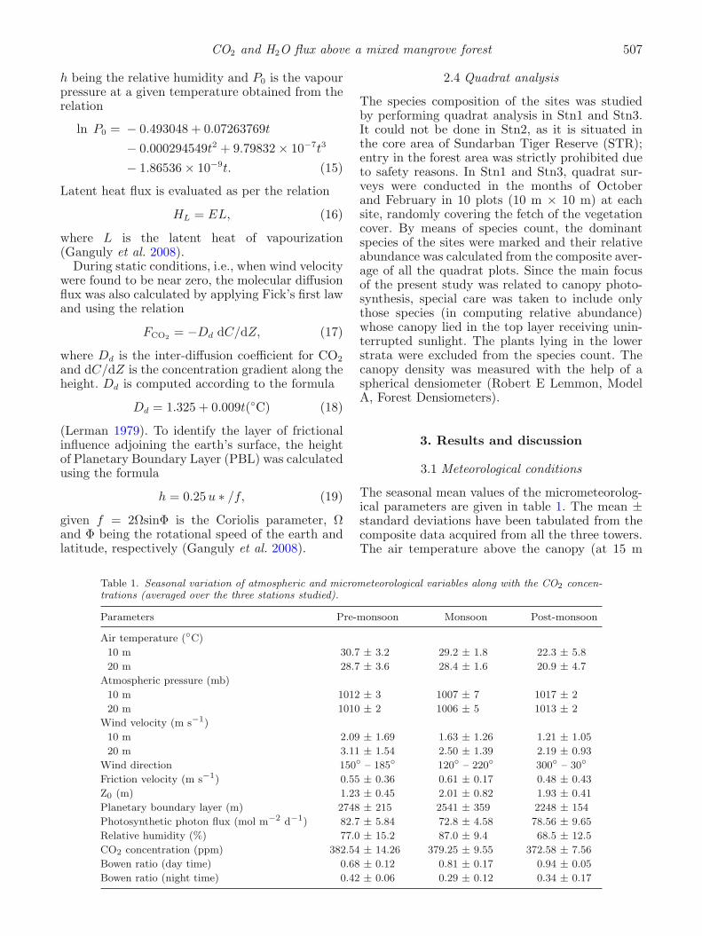
The seasonal mean values of the micrometeorolog-ical parameters are given in table 1. The mean ±standard deviations have been tabulated from thecomposite data acquired from all the three towers.The air temperature above the canopy (at 15 m

Table 1. Seasonal variation of atmospheric and micrometeorological variables along with the CO2 concen-trations (averaged over the three stations studied).

Parameters Pre-monsoon Monsoon Post-monsoon

Air temperature (◦C)

10 m 30.7 ± 3.2 29.2 ± 1.8 22.3 ± 5.8

20 m 28.7 ± 3.6 28.4 ± 1.6 20.9 ± 4.7

Atmospheric pressure (mb)

10 m 1012 ± 3 1007 ± 7 1017 ± 2

20 m 1010 ± 2 1006 ± 5 1013 ± 2

Wind velocity (m s−1)

10 m 2.09 ± 1.69 1.63 ± 1.26 1.21 ± 1.05

20 m 3.11 ± 1.54 2.50 ± 1.39 2.19 ± 0.93

Wind direction 150◦ – 185◦ 120◦ – 220◦ 300◦ – 30◦

Friction velocity (m s−1) 0.55 ± 0.36 0.61 ± 0.17 0.48 ± 0.43

Z0 (m) 1.23 ± 0.45 2.01 ± 0.82 1.93 ± 0.41

Planetary boundary layer (m) 2748 ± 215 2541 ± 359 2248 ± 154

Photosynthetic photon flux (mol m−2 d−1) 82.7 ± 5.84 72.8 ± 4.58 78.56 ± 9.65

Relative humidity (%) 77.0 ± 15.2 87.0 ± 9.4 68.5 ± 12.5

CO2 concentration (ppm) 382.54 ± 14.26 379.25 ± 9.55 372.58 ± 7.56

Bowen ratio (day time) 0.68 ± 0.12 0.81 ± 0.17 0.94 ± 0.05

Bowen ratio (night time) 0.42 ± 0.06 0.29 ± 0.12 0.34 ± 0.17


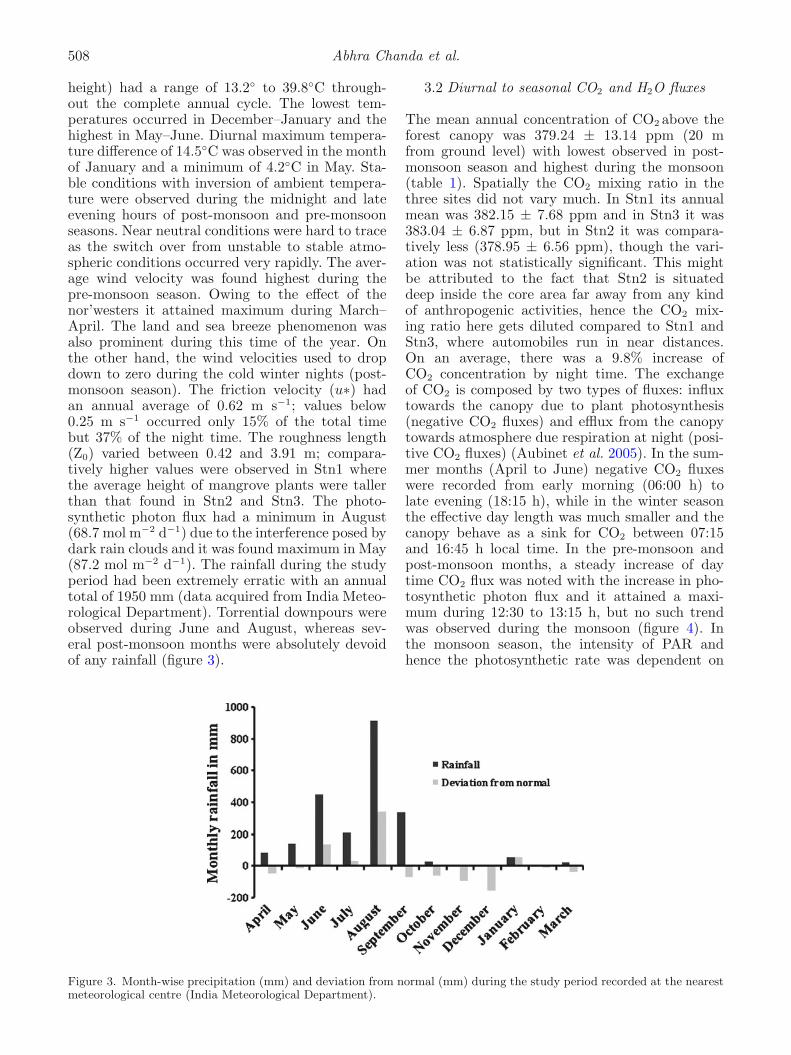
height) had a range of 13.2◦ to 39.8◦C through-out the complete annual cycle. The lowest tem-peratures occurred in December–January and thehighest in May–June. Diurnal maximum tempera-ture difference of 14.5◦C was observed in the monthof January and a minimum of 4.2◦C in May. Sta-ble conditions with inversion of ambient tempera-ture were observed during the midnight and lateevening hours of post-monsoon and pre-monsoonseasons. Near neutral conditions were hard to traceas the switch over from unstable to stable atmo-spheric conditions occurred very rapidly. The aver-age wind velocity was found highest during thepre-monsoon season. Owing to the effect of thenor’westers it attained maximum during March–April. The land and sea breeze phenomenon wasalso prominent during this time of the year. Onthe other hand, the wind velocities used to dropdown to zero during the cold winter nights (post-monsoon season). The friction velocity (u∗) hadan annual average of 0.62 m s−1; values below0.25 m s−1 occurred only 15% of the total timebut 37% of the night time. The roughness length(Z0) varied between 0.42 and 3.91 m; compara-tively higher values were observed in Stn1 wherethe average height of mangrove plants were tallerthan that found in Stn2 and Stn3. The photo-synthetic photon flux had a minimum in August(68.7 mol m−2 d−1) due to the interference posed bydark rain clouds and it was found maximum in May(87.2 mol m−2 d−1). The rainfall during the studyperiod had been extremely erratic with an annualtotal of 1950 mm (data acquired from India Meteo-rological Department). Torrential downpours wereobserved during June and August, whereas sev-eral post-monsoon months were absolutely devoidof any rainfall (figure 3).

3.2 Diurnal to seasonal CO2 and H2O fluxes

The mean annual concentration of CO2 above theforest canopy was 379.24 ± 13.14 ppm (20 mfrom ground level) with lowest observed in post-monsoon season and highest during the monsoon(table 1). Spatially the CO2 mixing ratio in thethree sites did not vary much. In Stn1 its annualmean was 382.15 ± 7.68 ppm and in Stn3 it was383.04 ± 6.87 ppm, but in Stn2 it was compara-tively less (378.95 ± 6.56 ppm), though the vari-ation was not statistically significant. This mightbe attributed to the fact that Stn2 is situateddeep inside the core area far away from any kindof anthropogenic activities, hence the CO2 mix-ing ratio here gets diluted compared to Stn1 andStn3, where automobiles run in near distances.On an average, there was a 9.8% increase ofCO2 concentration by night time. The exchangeof CO2 is composed by two types of fluxes: influxtowards the canopy due to plant photosynthesis(negative CO2 fluxes) and efflux from the canopytowards atmosphere due respiration at night (posi-tive CO2 fluxes) (Aubinet et al. 2005). In the sum-mer months (April to June) negative CO2 fluxeswere recorded from early morning (06:00 h) tolate evening (18:15 h), while in the winter seasonthe effective day length was much smaller and thecanopy behave as a sink for CO2 between 07:15and 16:45 h local time. In the pre-monsoon andpost-monsoon months, a steady increase of daytime CO2 flux was noted with the increase in pho-tosynthetic photon flux and it attained a maxi-mum during 12:30 to 13:15 h, but no such trendwas observed during the monsoon (figure 4). Inthe monsoon season, the intensity of PAR andhence the photosynthetic rate was dependent on

Figure 3. Month-wise precipitation (mm) and deviation from normal (mm) during the study period recorded at the nearestmeteorological centre (India Meteorological Department).


Figure 4. Mean daily cycles of CO2 flux (FCO2) above the forest canopy in the three stations (Stn1, Stn2 and Stn3)during the pre-monsoon (Pre M), monsoon (M) and post-monsoon (Post M) seasons. The vertical bars denote the standarddeviation from the mean of the corresponding hourly fluxes.

the cloud cover rather than on the time of day.Despite the fact that highest photosynthetic pho-ton flux was recorded in the month of May, thehighest average day time CO2 flux was observedin March (table 2). In the beginning of the post-monsoon season an average increase in CO2 uptakeis noticed. This may be due to the increased canopydensity with the formation of new leaves after theheavy showers of June and July (monsoonal rain).The night time CO2 flux had no significant sea-sonality. The largest uncertainties in the presentedresults are related to the determination of night

time fluxes especially during cold winter months(having friction velocity as low as 0.07–0.18 m s−1).The computed molecular diffusion fluxes rangedbetween 0.13 and 0.26 mg m−2 s−1, which wascomparatively much lower than that observed dur-ing conditions having friction velocity >0.3 m s−1.Under these circumstances the estimated flux val-ues were substituted by values calculated from theoverall relation between night time flux and ambi-ent temperature as per Lindroth et al. (1998). Inthe warmer months, the night time fluxes werecomparatively higher than that found in winter. In

Table 2. Monthly average of CO2 influx towards canopy (during day time) and efflux of CO2 away from the canopy (duringnight time) in the three stations.

Stn1 Stn2 Stn3

Month Day Night Day Night Day Night

April −1.42 ± 0.57 0.62 ± 0.10 −0.82 ± 0.40 0.40 ± 0.16

May −1.57 ± 0.50 0.56 ± 0.07 −0.57 ± 0.07 0.38 ± 0.12 −0.91 ± 0.35 0.41 ± 0.10

June −1.47 ± 0.39 0.46 ± 0.15 −0.95 ± 0.18 0.32 ± 0.14

July −1.33 ± 0.40 0.46 ± 0.11 −0.46 ± 0.17 0.37 ± 0.15 −0.87 ± 0.41 0.45 ± 0.19

August −1.22 ± 0.19 0.57 ± 0.09 −0.85 ± 0.32 0.60 ± 0.15

September −1.51 ± 0.43 0.59 ± 0.17 −0.61 ± 0.21 0.41 ± 0.09 −0.97 ± 0.33 0.51 ± 0.14

October −1.61 ± 0.45 0.62 ± 0.12 −1.13 ± 0.42 0.48 ± 0.12

November −1.34 ± 0.34 0.48 ± 0.14 −0.70 ± 0.15 0.32 ± 0.16 −1.02 ± 0.30 0.58 ± 0.11

December −1.16 ± 0.29 0.51 ± 0.07 −0.81 ± 0.16 0.46 ± 0.07

January −0.92 ± 0.28 0.34 ± 0.06 −0.40 ± 0.14 0.23 ± 0.10 −0.50 ± 0.27 0.25 ± 0.06

February −1.37 ± 0.38 0.64 ± 0.13 −0.74 ± 0.41 0.27 ± 0.10

March −1.79 ± 0.67 0.55 ± 0.16 −0.64 ± 0.10 0.42 ± 0.05 −1.23 ± 0.44 0.39 ± 0.20


winter mornings, especially after long nights hav-ing very stable conditions with the formation offog just above the forest canopy, positive CO2 fluxwas observed even after the appearance of sun raysabove the horizon. This shows the release of storedCO2 as observed by Pilegaard et al. (2001).

The water vapour flux in an ecosystem is prin-cipally the sum of evaporation and transpirationwith the surface condensation of water vapourbeing subtracted from it (Meiresonne et al. 2003).The water vapour fluxes were found positivethroughout the year but there were significantdifferences in their magnitude between day andnight time (figure 5). During day time the fluxesincreased steadily with the increment in ambi-ent temperature and attained the maximum dur-ing 11:30–12:15 h. The lowest water vapour fluxes(1.3 mg m−2 s−1) were observed during the mid-nights of monsoon season whereas in the scorchingnoon of summer it was as high as 69.5 mg m−2 s−1.In the pre-monsoon season, the difference betweenmean day and night time evapotranspiration rateswas observed to be the least (20.5 mg m−2 s−1).

3.3 Spatial variability of CO2 and H2O fluxes

Scrutinizing the dataset acquired from all the sitesthroughout the year, it is found that 42% of the

night time data were not of good quality, but 83%of the day time data did pass through the qualityfilters set on the basis of threshold friction veloc-ity and proper wind direction. One-way ANOVAon the diurnal averaged CO2 fluxes from the threetowers reveal significant differences in magnitude(F = 8.2, p < 0.005, n = 246). The mean CO2

uptake was maximum in Stn1 (−1.33 mg m−2 s−1),followed by Stn3 (−0.88 mg m−2 s−1). An annualmean CO2 influx of −0.39 mg m−2 s−1 wasobserved in Stn2. Ray et al. (2011) observed anet community CO2 exchange rate of 1.00 ±0.66 mg m−2 s−1 working in several sites of Sundar-ban. The number of valid data in Stn2 was almosthalf in comparison to the other two sites, even thenthe monthly variation was found statistically sig-nificant (F = 9.68, p = 0.000, n = 144). Thoughthe CO2 fluxes were of varying magnitude, theaverage water vapour fluxes as well as the sensibleand latent heat fluxes did not show any differenceamong the three towers as observed by Milden-berger et al. (2009). The measurement of flux atStn3 were made at different heights compared tothe other two sites, but it is considered to have noinfluence on the difference of CO2 fluxes, becausewith in the PBL fluxes are nonvariant with height,if the fetch remains uniform (Foken 2006).

Latent heat flux was found to be the dominantcomponent as the measured Bowen ratio’s showed

Figure 5. Mean daily cycles of H2O flux (E) above the forest canopy in the three stations (Stn1, Stn2 and Stn3) during thepre-monsoon (Pre M), monsoon (M) and post-monsoon (Post M) seasons. The vertical bars denote the standard deviationfrom the mean of the corresponding hourly fluxes.


values less than one throughout the year. Moreover,a significant lowering in Bowen ratio values duringthe night time showed that evaporation overruledtranspiration in all the sites. As transpiration fromthe plant leaves and CO2 exchange by means ofphotosynthesis are a strongly coupled process, itis expected to observe a closely associated watervapour flux with that of CO2 flux (Mildenbergeret al. 2009). Since we have detected a spatial vari-ability of CO2 flux along with a constant H2O flux,it further strengthens the fact that transpirationhas a minor contribution towards the overall watervapour flux.

3.4 Influence of species compositionon the CO2 fluxes

The month-wise variation in the averaged day timeCO2 uptake followed the same trend in all the threesites; became maximum during March and thendecreased in the monsoon months, again increaseda bit in October–November and became minimumin December–January. This might be due to thefact that PAR was high during the pre-monsoonmonths and it decreased during the monsoon owingto the effect of dark clouds. Moreover, the scat-ter plots between the magnitude of day time CO2

uptake and photosynthetic photon flux obtainedfrom the three towers were of similar nature(figure 6). The relationship between the twoparameters was best defined by a trend line of anexponential curve (R2 ranging from 0.51 to 0.60).Other atmospheric factors like ambient tempera-ture, relative humidity and CO2 mixing ratios didnot have any relationship with CO2 flux. Therefore,the main reason that can be attributed to the dif-ference in magnitude of CO2 uptake over the year isthe varying photosynthetic efficiency of the speciescomposition.

The photosynthetic efficiency of homogeneousmono-species vegetation is easier to assess andcompare, but in this case the plant cover in all thethree sites are randomly heterogeneous. The mixedvegetation cover in these sites includes almost eightto ten different mangrove species in varying propor-tion. The most challenging part of this study was tofind out the site specific dominance of the speciesand their relative abundance. It was observed thatfive to six species contributed more than 90% ofthe canopy cover. The relative abundance foundin Stn1 was of the order: A. marina (33%) > A.alba (28%) > E. agallocha (18%) > B. gymnorhiza(11%) > P. paludosa (5%), whereas in Stn3, itwas in the sequence: A. officinalis (37%) > A.rotundifolia (23%) > A. corniculutum (17%) > E.agallocha (15%) > P. paludosa (4%). Though wecould not perform the quadrat analysis in Stn2, it

Figure 6. Relationship between the magnitude of day timeCO2 influx (FCO2) and photosynthetic photon flux (PAR)in the three stations (Stn1, Stn2 and Stn3) for the entirestudy period. The curves are non-linear least square fits foran exponential function.

was clearly visible from the tower, that the adja-cent vegetation cover is principally dominated byP. paludosa. On the basis of eye estimation, itwas roughly assessed that P. paludosa comprisesalmost 50% of the vegetation cover followed by A.marina, with the association of A. rotundifolia andA. corniculutum.

Nandy (Datta) and Ghose (2001) carried outan exhaustive study on the dominant mangrovespecies of the Indian Sundarbans identifying theinter-specific variation in the rate of photosynthe-sis and water use efficiency. According to them(among the species found to be dominant in thepresent study sites), A. marina has the highestphotosynthetic rate (11.8 μmol m−2 s−1) and the


lowest in case of P. paludosa (3.69 μmol m−2 s−1).Based on the relative abundance of species in thethree sites and the photosynthesis efficiency tab-ulated in the paper of Nandy (Datta) and Ghose(2001), a weighed average was calculated for eachsite. The CO2 uptake potential for Stn1 was esti-mated to be the highest (9.43 μmol m−2 s−1), fol-lowed by Stn3 (7.25 μmol m−2 s−1) and the leastwas observed in Stn2 (4.34 μmol m−2 s−1). Theannual mean day time CO2 flux above the canopywas found to correlate in the same order. Theabundance of A. marina in Stn1 has led to theincreased CO2 uptake throughout the year, and P.paludosa being short and stunted in structure andhaving much lesser photosynthetic rate comparedto other species has attributed to the low CO2 fluxrecorded in Stn2. Moreover, the canopy densitymeasured in bimonthly intervals (in Stn1 and Stn3)showed that it ranged between 74 and 81% in Stn1and between 65 and 72% in Stn3. No significantseasonal variation was detected in any of the sitesduring the sampling. The Stn2 though could besurveyed, it was clearly visible from the tower thatthe forest was not that dense compared to Stn1 andStn3. Hence it could be inferred from the presentanalysis that the maximum flux at Stn1 could bedue to the combined effect of species diversity hav-ing greater CO2 sequestration potential and highercanopy density.

4. Conclusion

During the annual study, CO2, water vapour, sensi-ble and latent heat fluxes were measured above theforest canopy with the main intention to charac-terize the spatial variability in the trace gas fluxesand identifying the factors regulating the flux. CO2

fluxes above the forest canopy showed significantspatial variability. Overall, the spatial distributionof the dominant species along with their relativeabundance in each site strongly correlated with themagnitude of day time CO2 influx. Amongst allthe micrometeorological variables studied, like at-mospheric temperature, pressure, relative humidityand photosynthetic photon flux, it was only photo-synthetic photon flux which showed a strong expo-nential relationship with the day time CO2 fluxtowards the biosphere. Our results further indicatethat the variability in utilization of the photosyn-thetic photon flux together with the canopy den-sity mainly determines the CO2 uptake potential ofeach site. From the measured differences in Bowenratio between day and night times along with itsspatial non-variance, it could be concluded thatevaporation played major contribution in the watervapour fluxes compared to transpiration.

Acknowledgements

The authors are grateful to National RemoteSensing Centre, (NRSC), Department of Space,Government of India for funding the research work.A Chanda is grateful to Department of Scienceand Technology, Govt. of India for providing theINSPIRE fellowship.

References

Aubinet M, Berbigier P, Berndorfer C, Cescatti A,Feigenwinter C, Granier A, Grunwald T, HavrankovaK, Heinesch B, Longdoz B, Marcolla B, Montagnani Land Sedlak P 2005 Comparing CO2 storage and advec-tion conditions at night at different CARBOEUROFLUXsites; Bound.-Layer. Meteorol. 116 63–94.

Baldocchi D D, Hicks B B and Meyers T P 1988 Mea-suring biosphere–atmosphere exchanges of biologicallyrelated gases with micrometeorological methods; Ecology69 1331–1340.

Barrett K 1998 Oceanic ammonia emissions in the Europeand their trans boundary fluxes; Atmos. Environ. 32(3)381–391.

Beer C, Reichstein M, Tomelleri E, Ciais P, Jung M,Carvalhais N, Rodenbeck C, AltafArain M, BaldocchiD, Bonan G B, Bondeau A, Cescatti A, Lasslop G,Lindroth A, Lomas M, Luyssaert S, Margolis H, OlesonK W, Roupsard O, Veenendaal E, Viovy N, Williams C,IanWoodward F and Papale D 2010 Terrestrial gross car-bon dioxide uptake: Global distribution and covariationwith climate; Science 329 834–838.

Borges A V, Djenidi S, Lacroix G, Theate J, Delille B andFrankignoulle M 2003 Atmospheric CO2 flux from man-grove surrounding waters; Geophys. Res. Lett. 30(11)1–4.

Bouillon S, Rivera-Monroy V H, Twilley R R and KairoJ G 2009 Mangroves; In: The management of naturalcoastal carbon sinks (eds) Laffoley D d’A and GrimsditchG (IUCN, Gland, Switzerland), 15p.

Duke N C, Ball M C and Ellison J C 1998 Factors influ-encing the biodiversity and distributional gradients inmangroves; Global Ecol. Biogeog. Lett. 7 27–47.

Foken T 2006 Angewandte Meteorologie–Mikrometeorolo-gische Methoden; Springer, Berlin, 2. Auflage, 325 S.

Ganguly D, Dey M, Mandal S K, Dey T K and Jana T K2008 Energy dynamics and its implication to biosphere–atmosphere exchange of CO2, H2O and CH4 in a tropicalmangrove forest canopy; Atmos. Environ. 42 4172–4184.

Lerman A 1979 Geochemical processes: Water and sedimentenvironment, John Wiley, New York.

Lindroth A, Grelle A and Moren A-S 1998 Long-term mea-surements of boreal forest carbon balance reveal largetemperature sensitivity; Global Change Biol. 4 443–450.

Magnani F, Mencuccini M, Borghetti M, Berbigier P,Berninger F, Delzon S, Grelle A, Hari P, Jarvis P G,Kolari P, Kowalski A S, Lankreijer H, Law B E,Lindroth A, Loustau D, Manca G, Moncrieff J B,Rayment M, Tedeschi V, Valentini R and Grace J 2007The human footprint in the carbon cycle of temperateand boreal forests; Nature 447 849–851.

Meiresonne L, Sampson D A, Kowalski A S, Janssens I A,Nadeshdina N, Cermak J, Van Slycken J and CeulemansR 2003 Water flux estimates from a Belgian Scots pinestand: A comparison of different approaches; J. Hydrol.270 230–252.


Mildenberger K, Beiderwieden E, Hsia Y-J and Klemm O2009 CO2 and water vapour fluxes above a subtropicalmountain cloud forest – The effect of light conditions andfog; Agric. For. Meteorol. 149 1730–1736.

Misson L, Baldocchi D D, Black T A, Blanken P D, BrunetY, Curiel Yuste J, Dorsey J R, Falk M, Granier A,Irvine M R, Jarosz N, Lamaud E, Launiainen S, LawB E, Longdoz B, Loustau D, McKay M, Paw U K T,Vesala T, Vickers D, Wilson K B and Goldstein A H2007 Partitioning forest carbon fluxes with overstory andunderstory eddy-covariance measurements: A synthesisbased on FLUXNET data; Agric. For. Meteorol. 14414–31.

Mukhophadhya S K, Jana T K, De T K and Sen S 2000Measurement of exchange of CO2 in mangrove forest ofSundarbans using micrometeorological method; Trop.Ecol. 41 57–60.

Mukhophadhya S K, Biswas H, Das K L, De T K andJana T K 2001 Diurnal variation of carbon dioxide andmethane exchange above Sundarbans mangrove forest, inNW coast of India; Indian J. Mar. Sci. 30 70–74.

Mukhophadhya S K, Biswas H, De T K, Sen B K, Sen Sand Jana T K 2002 Impact of Sundarban mangrove bio-sphere on the carbon dioxide and mixing ratios at theNE coast of Bay of Bengal, India; Atmos. Environ. 36629–638.

Nandy (Datta) P and Ghose M 2001 Photosynthesis andwater-use efficiency of some mangroves from Sundarbans,India; J. Plant Biol. 44 213–219.

Noe S M, Kimmel V, Huve K, Copolovici L, Portillo-Estrada M, Puttsepp U, Jogiste K, Niinemets U, HortnaglL and Wohlfahrt G 2011 Ecosystem-scale biosphere–atmosphere interactions of a hemiboreal mixed foreststand at Jarvselja, Estonia; Forest Ecol. Manag. 26271–81.

Pilegaard K, Hummelshøj P, Jensen N O and Chen Z 2001Two years of continuous CO2 eddy-flux measurementsover a Danish beech forest; Agric. For. Meteorol. 10729–41.

Ray R, Ganguly D, Chowdhury C, Dey M, Das S, DuttaM K, Mandal S K, Majumdar N, De T K, MukhopadhyayS K and Jana T K 2011 Carbon sequestration and annualincrease of carbon stock in a mangrove forest. Atmos.Environ. 45 5016–5024.

Reich P B 2010 The carbon dioxide exchange; Science 329774–775.

Stull R B 1988 An introduction to boundary layer mete-orology (Dordrecht, Boston, London: Kluwer AcademicPublishers).

Wesely M L and Hicks B B 1977 Some factors that affectthe deposition rates of sulfur dioxide and similar gases onvegetation; J. Air Pollut. Control. Assoc. 27 1110–1116.

MS received 27 August 2012; revised 5 November 2012; accepted 12 November 2012

characterizing spatial and seasonal variability of carbon dioxide and water vapour fluxes above a...

Documents