Characterization of SINR Region for Multiple

Interfering Multicast in Power-Controlled

Systems

Yi Chen and Chi Wan Sung

Abstract

This paper considers a wireless communication network consisting of multiple interfering multicast

sessions. Different from a unicast system where each transmitter has only one receiver, in a multicast

system, each transmitter has multiple receivers. It is a well known result for wireless unicast systems

that the feasibility of an signal-to-interference-plus-noise power ratio (SINR) without power constraint

is decided by the Perron-Frobenius eigenvalue of a nonnegative matrix. We generalize this result and

propose necessary and sufficient conditions for the feasibility of an SINR in a wireless multicast system

with and without power constraint. The feasible SINR region as well as its geometric properties are

studied. Besides, an iterative algorithm is proposed which can efficiently check the feasibility condition

and compute the boundary points of the feasible SINR region.

Index Terms

Wireless multicast system, power control, signal-to-interference-plus-noise power ratio (SINR),

SINR feasibility, SINR region, Perron-Frobenius eigenvalue.

I. INTRODUCTION

In wireless communication systems, interference is an inherent phenomenon. Due to the

broadcast nature of wireless channels, interference arises whenever multiple transmitter-receiver

Yi Chen is with Department of Information Engineering, The Chinese University of Hong Kong. Email:

chelseachenyi@gmail.com. Chi Wan Sung is with Department of Electronic Engineering, City University of Hong Kong. Email:

albert.sung@cityu.edu.hk. This work was supported in part by a grant from the University Grants Committee of the Hong Kong

Special Administrative Region, China under Project AoE/E-02/08, and in part by a grant from the Research Grants Council of

the Hong Kong Special Administrative Region, China under Project CityU 121713.

arX

iv:1

505.

0688

2v1

[cs

.IT

] 2

6 M

ay 2

015

pairs are active concurrently in the same frequency band, and each receiver is only interested

in retrieving information from its own transmitter. For a particular receiver, the received signal

is a superposition of its desired signal, interfering signals and background noise. SINR, defined

as the power of desired signal divided by the sum of the power of interfering signals and the

power of noise, is a widely used performance measure for wireless communication systems. It is

analogous to signal-to-noise ratio (SNR) used for single user communication, which has clearly

understood implication on the bit error rate (BER) and capacity for additive white Gaussian

noise (AWGN) channels. Using SINR as a surrogate for BER and capacity implicitly assumes

that the interference is an AWGN. Although there are limitations of this assumption, as reported

in [1], [2], the importance of SINR has never been doubted.

For a system consisting of multiple point-to-point communication sessions, also referred to as

unicast system, the SINRs of all receivers form a vector. The feasible SINR region includes all

the SINR vectors that can be achieved by some transmission powers. The geometric properties

of feasible SINR region has been studied in [3]–[5]. Reference [3] proves that in the case of

unlimited transmission power, the feasible SINR region is log-convex. In [4], it is shown that

under a total power constraint, the infeasible SINR region is not convex. Reference [5] considers

a system with only three transmitter-receiver pairs without power constraint, and shows that the

feasible SINR region is concave. It also provides certain technical conditions under which a

concavity result for systems with a general number of users is established. In [6], for the cases

that the transmission powers are subject to arbitrary linear constraints, a mathematical expression

for the boundary points of the SINR region is obtained.

In this paper, we consider the feasible SINR region for systems consisting of multiple point-

to-multipoint communication sessions, also referred to as multicast system. Multicast enables

data to be delivered from a source node to multiple destination nodes. Practical examples of

such configurations include cellular networks and two-way relay networks. In cellular networks,

a base station multicasts a file to multiple mobile devices that request the file at the same time

[7]. In two-way relay networks, when network coding is applied, a relay multicasts the coded

packets to two sink nodes [8]. The power control and scheduling for wireless multicast systems

have been studied in [9]–[12] and the references therein. All these works aim to either minimize

the system power or maximize the system throughput, subject to the constraint that the SINR

of all receivers are larger than a given threshold. The feasibilities of the problems, however, are

unknown.

For a wireless unicast system, the feasibility of an SINR vector without power constraint

is determined by the Perron-Frobenius eigenvalue of a nonnegative matrix [13], [14]. In this

paper, we generalize this result to a wireless multicast system. We first propose a necessary and

sufficient condition under which an SINR is achievable without power limitation. Based on this

condition, we figure out the feasible SINR region by giving its boundary points. The approach

is to find the farthest point of the feasible SINR region from the origin in a given direction.

An iterative algorithm is proposed to find the farthest point, which is also a distributed power

control algorithm to solve the power balancing problem [13] aimed to maximize the minimal

SINR of all receivers.

Then we analyse the geometric properties of the feasible and infeasible SINR regions. It is

found that the feasible SINR region of a multicast system is in fact the intersection of the feasible

SINR regions of all its embedded unicast systems. Based on the results in [3]–[5] for unicast

systems, we show that the feasible SINR region of a multicast system is log-convex, and the

infeasible SINR region of a multicast system with two multicast sessions is convex. We also

show by an example that, the convexity property of the infeasible SINR region does not hold

for a general multicast system with more than two multicast sessions.

Later, the necessary and sufficient condition for the feasibility of an SINR in a multicast system

is extended to include linear constraints on the power. This result generalizes the results in [6]

for unicast systems. Besides, in [6], the zero-outage SINR region for a time-varying system is

also considered, where the channel gains are selected from a finite set. Suppose the transmission

powers are not allowed to vary with the channel gains, we establish a reduction that maps any

instance of the zero-outage SINR problem in a time-varying unicast system to a corresponding

instance of the feasible SINR problem in a time-invariant multicast system. The idea is to regard

the multiple receivers in a multicast session as an identical receiver that can experience a finite

set of channel gains.

The rest of the paper is organized as follows: In Section II, the system model and problem

formulation are presented. The necessary and sufficient condition on the feasibility of an SINR

vector is provided in Section III. Section IV gives the characterizations of the SINR region and

proposes an iterative algorithm. Section V studies the geometric properties of the feasible SINR

region. Section VI extends the study to include power constraints. Finally, the paper is concluded

T1 T2

R11 R2

1 R12 R2

2

Fig. 1: Example of a multicast network consisting of two multicast sessions. Transmitter T1

wants to transmit data to both R11 and R2

1. Transmitter T2 wants to transmit data to both R12 and

R22. Their transmitted signals interfere with each other. The solid lines represent intended links

and the dashed lines represent interfering links.

in Section VII.

Notation: The following notations are used throughout this paper. Vectors are denoted in bold

small letter, e.g., x, with their ith entry denoted by xi. They are regarded as column vectors unless

stated otherwise. Matrices are denoted by bold capitalized letters, e.g., X, with Xij denoting

the (i, j)th entry. Vector and matrix inequalities are component-wise inequalities, e.g., x ≥ y if

xi ≥ yi for all i; X ≥ Y if Xij ≥ Yij for all i and j. The cardinality of a set is denoted by

“| · |”. The Euclidean norm of a vector is denote by “|| · ||” . The transpose of a vector or matrix

is denoted by (·)T . I represents an identity matrix with compatible size. 0 represents a vector

with compatible size whose entries are all zero.

II. SYSTEM MODEL

Consider a general wireless communication network consisting of N multicast sessions. The

N transmitters are denoted by Ti for i = 1, . . . , N . Each Ti wants to multicast common data

packets to Ki receivers, denoted by Rkii for ki = 1, . . . , Ki. Without loss of generality assume

Ki ≥ 1. If Ki = 1 for all i, the scenario reduces to the unicast case. The total number of

receivers in the system is K =∑N

i Ki. Define Ki = 1, 2, . . . , Ki for i = 1, . . . , N . Fig. 1

illustrates an example of such network. Let pi be the transmission power of transmitter Ti and

p = [p1, . . . , pN ]T . The channel gain between Tj and Rkii is denoted by g

rkii ,tj

. All the multicast

sessions share the same channel and thus interfere with each other. We assume that interference

caused by simultaneous transmissions is treated as AWGN with variance identical to the received

power. The SINR of receiver Rkii is given by

γkii (p) =grkii ,ti

pi∑j 6=i grkii ,tj

pj + σ2, (1)

where σ2 is the variance of the background noise and without loss of generality, it is assumed

to be identical for all receivers. We define the SINR of the i-th multicast session as

γi(p) = minki∈Ki

γkii (p)

.

The SINR vector of the system is

Γ(p) = [γ1(p), γ2(p), . . . , γN(p)].

In this paper, we analyze the feasible SINR region of a multicast system, that is,

Υ =

Γ(p) ∈ RN : p ≥ 0,p ∈ RN.

Proposition 1. Given a vector µ ∈ RN . There exists a power vector p∗ ≥ 0 such that Γ(p∗) = µ,

if and only if there exits a power vector p′ ≥ 0 such that Γ(p′) ≥ µ.

Proof: The “only if” part is trivial and we show the “if” part. Suppose γi(p′) > µi for

some i. Fix such an i. Since γi(p) is monotonically decreasing as pi is decreasing, we can find

a 0 < p(1)i < p′i and let p(1) = [p′1, . . . , p

′i−1, p

(1)i , p′i+1, . . . , p

′N ]T such that γi(p(1)) = µi. On

the other hand, since γj(p) for j 6= i is monotonically increasing as pi is decreasing, we have

γj(p(1)) ≥ µj . By keeping on decreasing the power of transmitters that achieve higer SINR than

µ, we obtain a sequence p(1)i , p

(2)i , . . . , p

(t)i , . . . for each i = 1, . . . , N . It can be seen that these

sequences are monotonically decreasing and lower bounded by zero, so they are convergent.

Denote the limit point by p∗. For any arbitrarily small δ > 0 and for all i, since γi(p) is

continuous with p, there exists a sufficiently large T , when t > T , |γi(p∗) − γi(p(t))| < δ.

Meanwhile, since γi(p(t′)) = µi for some t′ ≥ T , we have |γi(p∗)−µi| < δ. Therefore γi(p∗) =

µi for all i.

By Proposition 1, we say that an SINR vector µ = [µ1, . . . , µN ] is feasible if and only if there

exists a power vector p ≥ 0 such that

pi −∑j 6=i

µigrkii ,tj

grkii ,ti

pj ≥ µiσ2

grkii ,ti

,∀ki ∈ Ki,∀i. (2)

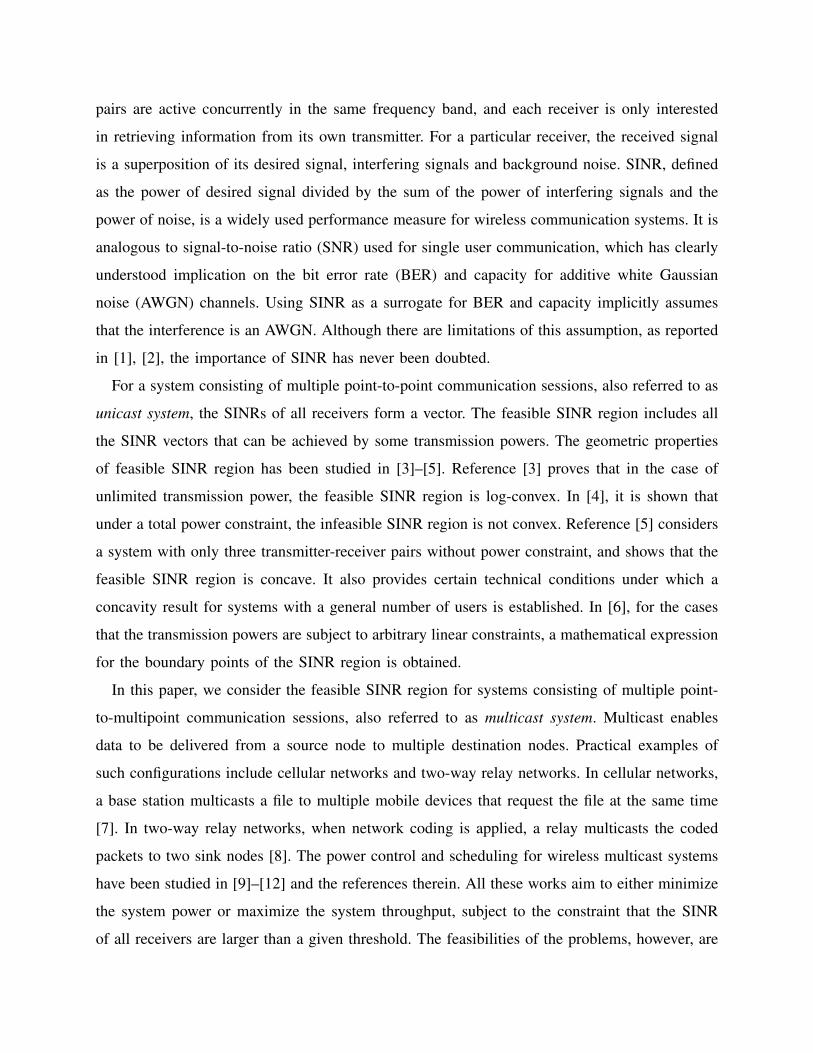
In matrix form, it is

A(µ)p ≥ n(µ), (3)

where

A(µ) =

1 −µ1

gr11 ,t2

gr11 ,t1

··· −µ1

gr11 ,tN

gr11 ,t1

1 −µ1

gr21 ,t2

gr21 ,t1

··· −µ1

gr21 ,tN

gr21 ,t1

...... . . . ...

1 −µ1

grK11 ,t2

grK11 ,t1

··· −µ1

grK11 ,tN

grK11 ,t1

−µ2

gr12 ,t1

gr12 ,t2

1 ··· −µ2

gr12 ,tN

gr12 ,t2

...... . . . ...

−µ2

grK22 ,t1

grK22 ,t2

1 ··· −µ2

grK22 ,tN

grK22 ,t2

...... . . . ...

−µNgrKNN

,t1grKNN

,tN

−µNgrKNN

,t2grKNN

,tN

··· 1

=

a11

a21

...

aK11

a12

...

aK22

...

aKNN

∈ RK×N

and

n(µ) =[ K1︷ ︸︸ ︷µ1σ

2

gr11 ,t1

,µ1σ

2

gr21 ,t1

. . . ,µ1σ

2

grK11 ,t1

, . . . ,

KN︷ ︸︸ ︷µNσ

2

gr1N ,tN

, . . . ,µNσ

2

grKNN ,tN

]T= [n1

1, n21 . . . , n

K11 , . . . , n1

N , . . . , nKNN ]T ∈ RK×1.

Each row of A(µ) corresponds to a receiver. For the convenience of discussion, we use akii ∈ RN

to denote the row of A(µ) that corresponds to receiver Rkii . As in the form (3), the feasibility

of µ can be checked through linear programming [15]. However, in a different way, we propose

a necessary and sufficient condition on the feasibility, which generalizes the Perron-Frobenius

eigenvalue criteria for unicast systems (square matrices). This condition is used to explicitly

characterize the feasible SINR region Υ and to prove some geometric properties of it. Before

further discussion, we given some definitions.

Define set

G(µ) =G =

ak1

1

ak22

...

akNN

∈ RN×N : ki ∈ Ki for i = 1, . . . , N.

Notice that, for each G ∈ G(µ), only one receiver is involved for each transmitter, which is a

unicast scenario. So G(µ) is the set including all the embedded unicast systems and its size is∏Ni=1Ki. Considering the example in Fig. 1, the four embedded unicast systems are

G(µ) =

a1

1

a12

,a2

1

a12

,a1

1

a22

,a2

1

a22

.

In subsequent discussion, we also use k = (k1, k2, . . . , kN) to specify a G ∈ G(µ). Let nG =

[nk11 , n

k22 , . . . , n

kNN ]T denote the noise vector with entries of n(µ) that correspond to the receivers

in G. For the simplicity of notation, we sometimes drop the argument µ of A, n and G when

the context is clear.

Definition 1. [16] A matrix X is called nonnegative if X ≥ 0. A nonnegative square matrix X

is irreducible if for every pair (i, j) of its index set, there exists a positive integer n ≡ n(i, j)

such that X(n)ij > 0, where X(n)

ij is the (i, j)th entry of Xn.

Definition 2. [16] Let X be an irreducible nonnegative square matrix. The Perron-Frobenius

eigenvalue of X is the maximum of the absolute value of eigenvalues of X, and is denoted by

λ(X).

Let 1 = [1, . . . , 1] be a vector whose components are all 1. For each G ∈ G(1), I−G is the

normalized interference link gain matrix of the corresponding embedded unicast system.

Definition 3. A multicast system is called irreducible if and only if the matrices I − G for

G ∈ G(1) are all irreducible.

It needs to be mentioned that if a multicast system is irreducible, as long as µ > 0, the

matrices I − G for G ∈ G(µ) are all irreducible. Throughout the paper, we assume that the

multicast system is irreducible.

III. FEASIBILITY CONDITION FOR SINR

In this section, we give a necessary and sufficient condition for the feasibility of an SINR

vector in a wireless multicast system. Recall that in a wireless unicast system, the following

theorem from [13], [17] is the fundamental results that characterize the feasibility.

Theorem 1. [17] Consider a unicast network setting G and assume I−G is irreducible. The

following statements are equivalent:

1) There exists a power vector p ≥ 0 such that Gp ≥ 0.

2) λ(I−G) < 1.

3) G−1 =∑∞

k=0(I−G)k exists and is positive component-wise, with limk→∞(I−G)k = 0.

Moreover, there exists p ≥ 0 such that Gp = 0 if and only if λ(I−G) = 1.

For a multicast system, the main result of this paper is the following theorem.

Theorem 2. Consider a multicast network setting A(µ) and assume it is irreducible, i.e., the

matrices I−G for G ∈ G(µ) are all irreducible. There exists a power vector p ≥ 0 such that

A(µ)p ≥ n(µ) if and only if maxG∈G(µ)λ(I−G) < 1.

Theorem 2 basically says that for a wireless multcast system, an SINR vector µ is feasible if

and only if µ is feasible to any of its embedded unicast system.

Corollary 1. When there are only two multcast sessions, i.e., N = 2, the feasibility of µ is

determined by the unicast system specified by

G∗ =

ak∗11

ak∗22

where k∗i = arg maxki∈Ki

µigrkii ,tj

grkii ,ti

, i = 1, 2, j 6= i.

That is, µ is feasible if and only if λ(I−G∗) < 1.

Corollary 1 follows straightforwardly from Theorem 2. Note that when N = 2, for any G ∈ G,

we have

λ(I−G) =

õ1

grk11 ,t2

grk11 ,t1

× µ2

grk22 ,t1

grk22 ,t2

. (4)

So maxG∈Gλ(I−G) = λ(I−G∗).

The proof of the necessary condition for Theorem 2 is straightforward. Suppose there exists

a power vector p ≥ 0 such that Ap ≥ n. Then for any G ∈ G, we have Gp ≥ nG ≥ 0. By

Theorem 1, λ(I−G) < 1 for all G, which implies maxG∈Gλ(I−G) < 1.

In the rest of this section, we prove the sufficient condition and assume that maxG∈Gλ(I−

G) < 1. By Theorem 1, it indicates that for each G ∈ G, G−1 ≥ 0 exists, and thus p =

G−1nG ≥ 0 exists. For each receiver, define

Akii =p ∈ RN : akii p ≥ nkii ,p ≥ 0

.

Note that akii is a row vector as defined before. Akii is an intersection of half-spaces and thus is

convex. Our proof is based on Helly’s theorem given below.

Theorem 3. (Helly’s theorem) [18]. Let F be a finite collection of convex sets in RN . The

intersection of all the sets of F is non-empty if and only if any N + 1 of them has non-empty

intersection.

In our case,

F =Akii : i = 1, . . . , N, ki ∈ Ki

. (5)

There are in total K convex sets in F . If any N+1 of them have non-empty intersection, then all

of them have non-empty intersection, i.e., the SINR is feasible. The number of all combinations

of such N + 1 sets is(KN+1

). We first show the proof for N = 2. Then we use the mathematical

induction to prove the general case.

Lemma 2. Suppose X = (Xij) is an N ×N matrix satisfying Xij = 1 for i = j and Xij ≤ 0

for i 6= j. Let S be a subset of 1, . . . , N and X′ be the matrix by removing the i-th row and

i-th column of X for all i ∈ S. If λ(I−X) < 1, then λ(I−X′) < 1.

Proof: Since λ(I−X) < 1, by Theorem 1, there exists a vector p ≥ 0 such that Xp ≥ 0.

Let p′ ∈ RN−|S| be the vector constructed by removing the i-th entry in p for all i ∈ S . Since

Xij ≤ 0 for i 6= j, it can be verified that X′p′ ≥ 0, which implies λ(I−X′) < 1.

Lemma 3. Consider G, G ∈ G such that G differs from G only in one row. i.e., ki 6= ki for

one i ∈ 1, . . . , N and kj = kj for j 6= i. Let p = G−1nG and p = G−1nG. There exists

p ∈ p, p such that Gp ≥ nG and Gp ≥ nG.

Proof: Since p = G−1nG and p = G−1nG, we have Gp = nG and Gp = nG. If p = p,

automatically we have Gp = nG and Gp = nG. In the following discussion, we consider the

case when p 6= p. Without loss of generality, assume that G and G differ in the first row, that

is, k1 6= k1 and kj = kj for j 6= 1. Let us partition G into four blocks as follows.

G =

1 −µ1

grk11 ,t2

grk11 ,t1

· · · −µ1

grk11 ,tN

grk11 ,t1

−µ2

grk22 ,t1

grk22 ,t2

1 · · · −µ2

grk22 ,tN

grk22 ,t2

...... . . . ...

−µNgrkNN

,t1

grkNN

,tN

−µNgrkNN

,t2

grkNN

,tN

· · · 1

=

1 A

C D

.

Similarly, G is partitioned into four blocks as G =

1 B

C D

. Note that G and G share the

same three blocks: 1, C and D. We consider Gp − nG and Gp − nG. Since akii = akii and

nki = nki for i = 2, . . . , N , akii p = akii p = nki = nki and akii p = akii p = nki = nki for

i = 2, . . . , N . If ak11 p = nk1

or ak11 p = nk1

, then Gp = nG or Gp = nG, which implies p = p.

Therefore when p 6= p, we must have ak11 p 6= nk1

and ak11 p 6= nk1

. In the following we prove

that, either ak11 p > nk1

or ak11 p > nk1

but not both, that is, (ak11 p− nk1

)(ak11 p− nk1

) < 0.

Since G−1 > 0 exists, by Theorem 1 and Lemma 2, D−1 exists. By block-wise inversion

[19], the inverse of G can be written as

G−1 =

a −aAD−1

−D−1Ca D−1 +D−1CaAD−1

,where a = (1−AD−1C)−1 > 0. G−1 is in the same form by replacing A with B and replacing

a with b = (1−BD−1C)−1 > 0. Denote nG =

nk1

n′

and nG =

nk1

n′

where n′ ∈ RN−1. We

have

ak11 p− nk1

=[1 B

]G−1nG − nk1

=[1 B

] a −aAD−1

−D−1Ca D−1 +D−1CaAD−1

nk1

n′

− nk1

= ank1−BD−1Cank1

− aAD−1n′ +BD−1n′ +BD−1CaAD−1n′ − nk1

= ank1(1−BD−1C)− (1−BD−1C)aAD−1n′ +BD−1n′ − nk1

= −ab−1(AD−1n′ − nk1) + (BD−1n′ − nk1

).

Similarly, we have

ak11 p− nk1

= −ba−1(BD−1n′ − nk1) + (AD−1n′ − nk1

).

Then

(ak11 p− nk1

)(ak11 p− nk1

)

= −ab−1(AD−1n′ − nk1)2 − ba−1(BD−1n′ − nk1

)2 + 2(AD−1n′ − nk1)(BD−1n′ − nk1

)

= −[√

ab−1(AD−1n′ − nk1)−√ba−1(BD−1n′ − nk1

)]2

≤ 0.

Further, since ak11 p 6= nk1

and ak11 p 6= nk1

, (ak11 p − nk1

)(ak11 p − nk1

) < 0. In summary, there

exists p ∈ p, p such that Gp ≥ nG and Gp ≥ nG.

A. Two Multicast Sessions N = 2

If K = 2, i.e., K1 = K2 = 1, it is the unicast scenario and Theorem 2 is true straightforwardly.

If K1 = 1, K2 = 2 or K1 = 2, K2 = 1 or K1 = K2 = 2, then any three subsets of F must be

A1i ,A2

i ,Akjj for i = 1 or 2 and j 6= i. Let

G =

a1i

akjj

and G =

a2i

akjj

.By Lemma 3, there exists p such that Gp ≥ nG and Gp ≥ nG, which implies p ∈ (A1

i ∩

A2i ∩A

kjj ). Further by Helly’s theorem, the intersection of all sets in F is non-empty. For other

values of K1 and K2, we divide the(K1+K2

3

)combinations of three sets of F into two parts:

1) two sets belong to transmitter Ti and one set belongs to transmitter Tj where j 6= i; 2) three

sets belong to the same transmitter Ti for i = 1 or 2. In the first case, the three sets could

be Akii ,Ak′ii ,A

kjj . We use the same argument as before, and conclude that the three sets have a

non-empty intersection. In the second case, the three sets could be Akii ,Ak′ii ,A

k′′ii . It is easy to

verified that pi = maxnkii , nk′ii , n

k′′ii and pj = 0 is one of their intersection points. Overall, we

prove that any three sets of F have a non-empty intersection, and thus the intersection of all

sets is non-empty.

B. Multicast Sessions with general N

We use mathematical induction to prove Theorem 2. We already show that it is true when

N = 2. Assume that the theorem holds for all numbers less than or equal to N − 1 and now we

prove that it also holds for N . If Ki = 1 for all i, it is the unicast scenario and Theorem 2 is

true. Otherwise, we categorize the combinations of N + 1 sets of F into N parts: 1) Receivers

of N transmitters are involved: Ak11 ,Ak2

2 , . . . ,AkNN ,Ak

′ii . 2) Receivers of N − 1 transmitters are

involved: Ak11 , . . . ,A

kj−1

j−1 ,Akj+1

j+1 , . . . ,AkNN ,Ak

′ii ,A

k′ll where i, l 6= j. · · · D) Receivers of N−D+1

transmitters are involved. · · · N) Receivers of 1 transmitter is involved.

We prove the first part. Let

G =

ak11

...

akii...

aNj

N

and G =

ak11

...

ak′ii

...

aNj

N

.

By Lemma 3, there exists p such that Gp ≥ nG and Gp ≥ nG, which implies p ∈ (∩Nj=1Akjj ∩

Ak′ii ).

We prove the D) part for D = 2, . . . , N . Suppose the D − 1 transmitters whose receivers

are not involved in the N + 1 sets, are d1, d2, . . . , dD−1 ∈ 1, · · · , N. We simply let pd1 =

pd2 = · · · = pdD−1= 0. The resulting system is equivalent to having N − D + 1 multicast

sections characterized by matrix A′, which is constructed by removing the rows in A that

corresponds to the receivers of transmitter d and the d-th column of A, for d = d1, . . . , dD−1.

Define G ′ ⊂ R(N−D+1)×(N−D+1) for A′. For any G′ ∈ G ′, we can find a G ∈ G such that, G′

is constructed by removing the d-th row and d-th column of G for all d = d1, . . . , dD−1. Since

λ(I−G) < 1 for all G ∈ G, by Lemma 2, λ(I−G′) < 1, and therefore maxG′∈G′λ(I−G′) < 1.

By the inductive hypothesis, we can apply Theorem 2 when N − D + 1 < N , and thus there

exists p′ ≥ 0 such that A′p′ ≥ n′, where n′ is obtained by removing the entries that correspond

to the receivers of transmitter Td for d = d1, . . . , dD−1. By inserting 0 back into p′ at the position

of transmitter Td for all d = d1, . . . , dD−1, we get a power p ≥ 0 which is in the N + 1 subsets.

Overall, we have proved that any N+1 subsets of F has a non-empty intersection. By Helly’s

theorem, all subsets in F has an intersection. This completes the proof of Theorem 2.

IV. FEASIBLE SINR REGION AND ALGORITHM

In this section, we characterize the feasible SINR region of a wireless multicast system by

analytically obtaining its boundary points. By Proposition 1, we know that the feasible SINR

region is downward comprehensive. That is, if µ is feasible, then any µ′ satisfying 0 ≤ µ′ ≤ µ

is also feasible. Therefore, finding the boundary points is enough to figure out the feasible

SINR region. Our approach is to find the farthest point from the origin in a given direction. In

mathematics, the problem is formulated as

supp

β

s.t. A(βµ)p ≥ n(βµ)

p ≥ 0,

where µ is a given direction. By Theorem 2, there is a feasible solution to the above problem

if and only if

maxG∈G(βµ)

λ(I−G) = β · maxG∈G(µ)

λ(I−G) < 1.

That is

β <1

maxG∈G(µ)λ(I−G).

Therefore, the optimal value is

β∗(µ) =1

maxG∈G(µ)λ(I−G).

β∗(µ)µ is a boundary point of the SINR region.The open line segment defined by αµ : 0 <

α < β∗(µ) is in the feasible SINR region Υ, but αµ is not in the feasible region if α > β∗(µ).

We note that the size of G is∏N

i=1Ki, which grows exponentially with N . It is not an efficient

method to calculate the Perron-Frobenius eigenvalue of all the embedded unicast systems and

find out the maximum one. Next, we propose an iterative algorithm to compute β∗(µ). For

i = 1, 2, . . . , N , let ei denote the N -dimensional column vector such that the i-th component of

ei is 1 while the others are 0. The algorithm is described in Algorithm 1.

For receiver Rkii , (eTi −akii )p(k) is the sum of the interference power. The power of transmitter

Ti is updated by the maximum interference power experienced by the receivers in its multicast

session. This idea is similar to the distributed power control algorithm for unicast systems [20]

to solve the power balancing problem. Recall that in [20], given a normalized interference link

Algorithm 1 Iterative algorithm

1: Choose p(0) ∈ RN > 0 and k ← 0

2: repeat

3: for i = 1 to N do

4: y(k)i ← maxki∈Ki

(eTi − akii

)p(k)

5: end for

6: β(k) ← minNi=1

p

(k)i

y(k)i

7: p(k+1) ← y(k)

||y(k)||

8: k ← k + 1

9: until convergence

10: return β(k)

gain matrix I−G, the algorithm works as p(k+1) = (I−G)p(k)

||(I−G)p(k)|| , where k is the iteration index. It

is well known that when I−G is primitive (to be defined later), ||(I−G)p(k)|| converges to the

Perron-Frobenius eigenvalue of I−G, and p(k) converges to the corresponding eigenvector. In

our proposed algorithm, we are dealing with multicast systems. For notation simplicity, define

Z(µ) = Z = I−G : G ∈ G(µ). (6)

Z includes the normalized interference link gain matrices of all the embedded unicast systems

and Z ≥ 0 for all Z ∈ Z . Given any p > 0, due to the structure of G(µ), there always exists

Z ∈ Z such that Zp ≥ Zp for all Z ∈ Z . Our algorithm works as p(k+1) = Z(k)p(k)

||Z(k)p(k)|| , where

Z(k) ∈ Z is chosen such that Z(k)p(k) ≥ Zp(k) for all Z ∈ Z . In the rest of this section, we

show the convergence of the algorithm.

Lemma 4. The sequence β(k) generated by Algorithm 1 is monotonically increasing and

bounded above by 1maxG∈G(µ)λ(I−G) = 1

maxZ∈Z(µ)λ(Z) , and thus is convergent.

Proof: By Algorithm 1, we have y(k) ≥ Zp(k) for all Z ∈ Z , and p(k) ≥ β(k)y(k). Then

Zp(k+1) = Zy(k)

||y(k)||≤ Z

p(k)

β(k)||y(k)||≤ y(k)

β(k)||y(k)||=

p(k+1)

β(k).

Since the above inequality holds for all Z ∈ Z , we have

β(k) ≤ minZ∈Z

N

mini=1

p(k+1)i

[Zp(k+1)T ]i

=

N

mini=1

p

(k+1)i

y(k+1)i

= β(k+1).

That is, β(k) is monotonically increasing. On the other hand, since p(k) ≥ β(k)y(k) ≥ β(k)Zp(k)

for all Z ∈ Z , that is (I − β(k)Z)p(k) ≥ 0, we have λ(β(k)Z) ≤ 1 by Theorem 1. Therefore

β(k) ≤ 1maxZ∈Z(µ)λ(Z) , and thus β(k) is convergent.

Denote limk→∞ β(k) = β∗. Before we proceed to show that β∗ = 1

maxZ∈Z(µ)λ(Z) , we introduce

the concept of primitive matrix and primitive set.

Definition 4. [16] A square nonnegative matrix X is called primitive if there exists a positive

integer n such that Xn > 0.

The class of primitive matrices is a subclass of irreducible matrices. If X is primitive, then

its Perron-Frobenius eigenvalue is strictly greater than all other eigenvalues in absolute value.

The primitive condition guarantees the convergence of the aforementioned distributed power

control algorithm for unicast systems. In our multicast case, we need to use the concept of

primitive set, which replaces a single matrix and powers of that matrix with a set of matrices

and inhomogeneous products of matrices from the set.

Definition 5. [21] Let Z be a set of N × N nonnegative matrices. For a positive integer n,

let Θ(n) be an arbitrary product of n matrices from Z , with any ordering and with repetitions

permitted. Define Z to be a primitive set if there is a positive integer n such that every Θ(n) is

positive.

It can be seen that a necessary condition for Z to be primitive is that Z is primitive for all

Z ∈ Z . One of the sufficient conditions for Z to be primitive is that for any Z ∈ Z , in each row

and each column of Z, there are more than half of the entries that are positive [21]. Interested

readers can refer to [21] for more information of the primitive set. It needs to be mentioned that

when the system is composed of two multicast sessions, Z ∈ Z are always non-primitive, and

therefore Z cannot be primitive. However, for this case, Corollary 1 already gives an explicit

and simple solution to the feasible SINR region. Algorithm 1 works for systems with more than

two multicast sessions and with Z being primitive.

2 4 6 8 10 12 140.6

0.8

1

1.2

1.4

1.6

1.8

2

iteration step k

β(k

)

Fig. 2: Convergence of Algorithm 1. In this example, there are four multicast sessions and each

has three receivers. The link gains are randomly drawn from a uniform distribution on [0, 1).

Theorem 4. If the matrix set Z(µ) defined in (6) is primitive, then β(k) converges to β∗ =

1maxZ∈Z(µ)λ(Z) for an arbitrary initial value p(0) > 0. Moreover, p(k) converges to a power

vector p∗ such that limα→∞ Γ(αp∗) achieves the boundary point β∗µ.

The proof is provided in Appendix A. Fig. 2 illustrates the typical behavior of Iterative

Algorithm 1. In this example, there are four multicast sessions and each has three receivers.

The link gains are randomly drawn from a uniform distribution on [0, 1). As we can see, β(k)

converges within a small number of iterations. By using Algorithm 1, we can efficiently check

the feasibility of an SINR vector µ by checking the value of β∗(µ). If β∗(µ) < 1, µ is infeasible,

and vice versa. Besides, Algorithm 1 can be used to find the optimal solution of the classic power

balancing problem for multicast systems, which is in the following form

supp

N

mini=1

γi(p)

s.t. p ≥ 0,

and the solution is β∗(1).

V. GEOMETRIC PROPERTIES OF THE FEASIBLE SINR REGION

In this section, we discuss the geometric properties of the feasible SINR region. Let D(µ)

denote the diagonal matrix constructed by

D(µ) =

µ1 0 · · · 0

0 µ2 · · · 0...

... . . . ...

0 · · · 0 µN

.By Theorem 2, the feasible SINR region is equivalent to

Υ =

µ ∈ RN : max

Z∈Z(µ)λ(Z) < 1

=

µ ∈ RN : max

Z∈Z(1)

λ(D(µ)Z

)< 1

=

⋂Z∈Z(1)

µ ∈ RN : λ

(D(µ)Z

)< 1.

That is, the feasible SINR region of a multicast system is the intersection of the feasible SINR

regions of all its embedded unicast systems. Let Υc = RN+ \Υ denote the complement of Υ in RN

+ ,

i.e., the infeasible SINR region. Next, we investigate the convexity of Υc and the log-convexity

of Υ.

A. Convexity of Υc

For unicast systems, it has been proved in [5] that the infeasible SINR regions of a general two

user system and a general three user system are convex. It is also shown in [4] that the convexity

of the infeasible SINR region does not hold for a general four user system. For multicast systems,

we have the following observation.

Theorem 5. The infeasible SINR region of a general system consisting of two multicast sessions

is convex. The convexity property does not hold for a general system consisting of more than

two multicast sessions.

When there are two multicast sessions, by Corollary 1, the feasible SINR region is

Υ =

[µ1, µ2] ∈ R2+ : µ1µ2 <

grk∗11 ,t1

grk∗11 ,t2

·grk∗22 ,t2

grk∗22 ,t1

.

It is ready to verify that Υc is convex.

When there are more than two multicast sessions, Υc is the union of the infeasible SINR

regions of all the embedded unicast systems and is in general non-convex. Fig. 3 illustrates the

Υc for a system consisting of three multicast sessions, where the link gain matrix is given by

T1 T2 T3

R11 1 0.5 0.1

R21 1 0.1 0.5

R12 0.5 1 0.1

R22 0.1 1 0.5

R13 0.5 0.1 1

R23 0.1 0.5 1

.

It can be seen that its Υc is non-convex.

B. Log-convexity of Υ

We first introduce the notion of log-convexity. Let log(µ) = [log µ1, log µ2, . . . , log µN ] and

log(Υ) = log(µ) : µ ∈ Υ. We say a set Υ is log-convex if log(Υ) is convex. Since log(·) :

Υ→ log(Υ) is a bijective mapping, we have

log(Υ) =⋂

Z∈Z(1)

log(µ) ∈ RN : λ

(D(µ)Z

)< 1.

It has been proved in [3] that the feasible SINR region of a unicast system is log-convex. So

log(Υ), the intersection of the SINR regions of all its embedded unicast, is also log-convex. We

conclude this by the following theorem.

Theorem 6. The feasible SINR region of a multicast system is log-convex. In other words, the

feasible SINR, expressed in decibels, is a convex set.

VI. FEASIBILITY OF SINR WITH POWER CONSTRAINTS

So far, we have discussed the feasibility of SINR for a multicast system in the case of unlimited

power. In this section, we consider that besides p ≥ 0, the power vector are also subject to the

linear constraints ∑i∈Ωm

pi ≤ pΩm ,m = 1, . . . ,M,

0

1

2

3

4

5

0

1

2

3

4

5

0

2

4

6

γ1

γ2

γ 3

Fig. 3: Infeasible SINR region of a three-multicast-session system.

where Ωm ⊆ 1, . . . , N and M is the number of constraints. When Ωm = 1, . . . , N, it is

a constraint on the total power. When Ωm = i, it is a constraint on the individual power of

transmitter Ti. Define the power set by

P = p ≥ 0 and∑i∈Ωm

pi ≤ pΩm ,m = 1, . . . ,M.

Now the feasibility of SINR vector µ is decided by whether there exists p ∈ P such that

A(µ)p = n(µ). Note that the power vectors in P are downward comprehensive. That is, if

p′ ∈ P , then p ∈ P if 0 ≤ p ≤ p′. Hence using the same argument as in Proposition 1, we

know that µ is feasible if and only if there exits p ∈ P such that A(µ)p ≥ n(µ). Our results

generalize the feasibility condition derived in [6] for a unicast system to a multicast system.

Definition 6. For a matrix X ∈ RK×N , a vector y ∈ RK and a set Ω ⊆ 1, . . . , N, ψ(X,y,Ω)

is the operation to add y to the j-th column of X, for all j ∈ Ω. That is, Z = ψ(X,y,Ω), where

Zij = Xij + yi for all i ∈ 1, . . . , K and j ∈ Ω, and Zij = Xij for the else.

Theorem 7. Consider a multicast network setting A(µ) and assume the matrices I − G for

G ∈ G(µ) are all irreducible. There exists a power vector p ∈ P such that A(µ)p ≥ n(µ) if

and only if

maxG∈G(µ)

maxm∈1,...,M

λ(ψ(I−G,

nG

pΩm

,Ωm

))≤ 1.

Proof: It is already known from [6] that, for a unicast system G, there exists p ∈ P

such that Gp ≥ nG if and only if maxm∈1,...,Mλ(ψ(I −G, nG

pΩm,Ωm)) ≤ 1. We first prove

the necessary condition. Suppose there exists p ∈ P such that A(µ)p ≥ n(µ). Then for any

G ∈ G(µ), Gp ≥ nG, which implies maxm∈1,...,Mλ(ψ(I−G, nG

pΩm,Ωm)) ≤ 1. Regarding all

G ∈ G(µ), we have maxG∈G(µ) maxm∈1,...,Mλ(ψ(I−G, nG

pΩm,Ωm))leq1.

Next we prove the sufficient condition. For any G ∈ G(µ), since 0 ≤ I − G < ψ(I −

G, nG

pΩm,Ωm) for all m, by the Perron-Frobenius Theorem for irreducible matrices [16], λ(I −

G) < λ(ψ(I−G, nG

pΩm,Ωm)) ≤ 1. This implies that G−1 exists and p = G−1nG ∈ P . The rest

of the proof follows the same argument as the proof of Theorem 2.

Note that

maxG∈G(µ)

maxm∈1,...,M

λ(ψ(I−G,

nG

pΩm

,Ωm

))= max

m∈1,...,Mmax

G∈G(µ)

λ(ψ(I−G,

nG

pΩm

,Ωm

)).

Similar to (6), for each of the M linear constraints, define

ZΩm(µ) =

ψ(I−G,

nG

pΩm

,Ωm

): G ∈ G(µ)

.

By using Algorithm 1 with ZΩm(µ), we can find a supremum β∗Ωm(µ). The farthest point of

the SINR region in direction µ is then minMm=1β∗Ωm(µ)µ. By this approach, the feasible SINR

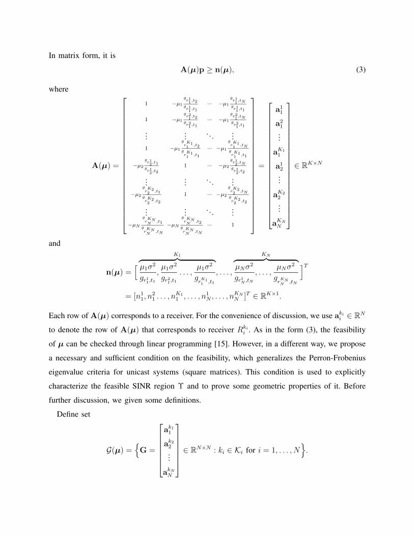
region is characterized. On the other hand, if minMm=1β∗Ωm(µ) ≥ 1, µ is feasible. Fig. 4 plots

the feasible SINR region of the network example in Fig. 1, with a power constraint on the total

power. In this example, the link gain matrix is

T1 T2

R11 0.5326 0.6801

R21 0.5539 0.3672

R12 0.2393 0.8669

R22 0.5789 0.4068

,and the power constraint is p1 + p2 ≤ 2. The four dashed lines are the boundary of the feasible

SINR regions of four embedded unicast systems and the solid line is the boundary of the multicast

system. It can be seen that under power contraint, the infeasible SINR region is not necessary

to be convex even for a multicast system with two multicast sessions.

0 0.2 0.4 0.6 0.8 1 1.2 1.4 1.60

0.2

0.4

0.6

0.8

1

1.2

1.4

1.6

µ2

µ1

Fig. 4: Feasible SINR region for a multcast system with two multicast sessions, under a total

power constraint. The dashed lines correspond to the four embedded unicast systems and the

solid line corresponds to the multicast system.

In the end of this section, we introduce an application of our multicast model to a time varying

unicast system. Consider a unicast system consisting of N transmitter-receiver pairs, where the

channel gains among them vary with time due to the mobility of the receivers. Let hi(t) for

i = 1, . . . , N denote the link gain vector from N transmitters to the i-th receiver at time t. As

argued in [6], hi(t) can be modeled with discrete states, that is, hi(t) is randomly selected from

a finte set h1i ,h

2i , . . . ,h

Kii for all i. An SINR vector µ is said to be zero-outage if there exists

a power such that no matter what the link gain realization is, the SINR is achievable all the time.

Such a zero-outage SINR problem can be mapped to a feasible SINR problem of a multicast

system. The idea is to let one receiver Ri pretend to be Ki receivers, i.e., R1i , . . . , R

Kii , and Rki

i

only experiences the link gain hkii . The feasible SINR region of this artificial multicast system

is exactly the zero-outage SINR region of the original time-varying unicast sytem. Theorem 2

and Theorem 7 can be applied. It needs to be mentioned that the scenario considered here is

different from that in [6]. In [6], the power can change with the channel states and is subject to

an average power constraint. In our model, the power is universal for all possible channel states.

VII. CONCLUSION

In this paper, we characterize the feasibility condition of an SINR vector for a multicast

system, which generalizes the Perron-Frobenius Theorem for a unicast system. We also propose

an iterative algorithm which can efficiently check the condition and compute the boundary

points of the feasible SINR region. According to the earlier mentioned Gaussian interference

assumption, by describing the feasible SINR region, we directly obtain the feasible rate region

by applying the Shannon Capacity formula for AWGN channels that maps the SINR to the rate.

APPENDIX A

PROOF OF THEOREM 4

Proof: Let Z(k) denote one of the matrices at the k-th iteration such that Z(k)p(k) ≥ Zp(k)

for all Z ∈ Z . From the construction of the algorithm, we have

Z(k)p(k) ≤ 1

β(k)p(k) for all k ∈ N. (7)

Moreover, there exists 1 ≤ i ≤ N such that [Z(k)p(k)]i = 1β(k) [p

(k)]i. We note that each vector

p(k) is a unit vector, as ||p(k)|| = 1. By the Bolzano-Weierstrass Theorem and the compactness

of the unit ball in RN , there exists a convergent subsequence, that is, p(kj) → p∗. By Lemma

4, β(kj) → β∗. Suppose at p∗, Z∗ ∈ Z is one of the matrices that satisfy Z∗p∗ ≥ Zp∗ for

all Z ∈ Z . Taking the limit of (7) with respect to the subsequence indexed by kj , we have

Z∗p∗ ≤ 1β∗p∗. If Z∗p∗ = 1

β∗p∗, since Z∗ is irreducible, β∗ = 1

λ(Z∗)≥ 1

maxZ∈Z(µ)λ(Z) . On the

other hand, β∗ ≤ 1maxZ∈Z(µ)λ(Z) by Lemma 4. Therefore, β∗ = 1

maxZ∈Z(µ)λ(Z) .

If Z∗p∗ 6= 1β∗p∗, since Z is primitive, there exists integer n such that an arbitrary product

of n matrices from Z is positive, i.e., Θ(n) > 0, and therefore Θ(n)Z∗p∗ < Θ(n) 1β∗p∗. By

the continuity of the mapping, there exists p(k) close enough to p∗ such that Θ(n)Z∗p(k) <

Θ(n) 1β∗p(k) and Z(k) = Z∗. We now apply the algorithm for n more iterations from p(k). For

i = 0, 1, . . . , n− 1 we have the following inequalities

Z(k+i+1)p(k+i) ≤ Z(k+i)p(k+i) (8)

due to that the selection matrix satisfies Z(k+i)p(k+i) ≥ Zp(k+i) for all Z ∈ Z . Meanwhile by

Algorithm 1,

p(k+i) =y(k+i−1)

||y(k+i−1)||=

Z(k+i−1)p(k+i−1)

||Z(k+i−1)p(k+i−1)||=

Z(k+i−1) · · ·Z(k+1)Z(k)p(k)

||Z(k+i−1) · · ·Z(k+1)Z(k)p(k)||.

By substituting p(k+i) into (8), we get

Z(k+i+1)Z(k+i−1)Z(k+i−2) · · ·Z(k+1)Z(k)p(k) ≤ Z(k+i)Z(k+i−1)Z(k+i−2) · · ·Z(k+1)Z(k)p(k). (9)

Let us take a look at these inequalities step by step. By (8) for i = 0, Z(k+1)p(k) ≤ Z(k)p(k). By

multiplying Z(k+2) on both side of the inequality, we have

Z(k+2)Z(k+1)p(k) ≤ Z(k+2)Z(k)p(k). (10)

By (9) for i = 1, Z(k+2)Z(k)p(k) ≤ Z(k+1)Z(k)p(k). Along with (10), we have

Z(k+2)Z(k+1)p(k) ≤ Z(k+1)Z(k)p(k).

By multiplying Z(k+3) on both side of the above inequality, we have Z(k+3)Z(k+2)Z(k+1)p(k) ≤

Z(k+3)Z(k+1)Z(k)p(k). By (9) for i = 2, Z(k+3)Z(k+1)Z(k)p(k) ≤ Z(k+2)Z(k+1)Z(k)p(k). So

Z(k+3)Z(k+2)Z(k+1)p(k) ≤ Z(k+2)Z(k+1)Z(k)p(k).

By repeating this procedure for n− 1 times, we can finally get

Z(k+n)Z(k+n−1) · · ·Z(k+1)p(k) ≤ Z(k+n−1)Z(k+n−2) · · ·Z(k+1)Z(k)p(k). (11)

Since Θ(n)Z∗p(k) < Θ(n) 1β∗p(k) holds for arbitrary Θ(n), we let Θ(n) = Z(k+n)Z(k+n−1) · · ·Z(k+1).

Along with (11), we have

Z(k+n)Z(k+n−1) · · ·Z(k+1)Z∗p(k) = Θ(n)Z∗p(k)

< Θ(n)1

β∗p(k)

=1

β∗Z(k+n)Z(k+n−1) · · ·Z(k+1)p(k)

≤ 1

β∗Z(k+n−1)Z(k+n−2) · · ·Z(k+1)Z∗p(k).

By multiplying 1||Z(k+n−1)···Z(k+1)Z∗p(k)|| on both side of the inequality, we have

Z(k+n)p(k+n) = Z(k+n) Z(k+n−1) · · ·Z(k+1)Z∗p(k)

||Z(k+n−1) · · ·Z(k+1)Z∗p(k)||

<1

β∗Z(k+n−1) · · ·Z(k+1)Z∗p(k)

||Z(k+n−1) · · ·Z(k+1)Z∗p(k)||

=1

β∗p(k+n).

This implies β(k+n) > β∗, which contradicts with that β∗ is the limit. Hence there must have

Z∗p∗ = 1β∗p∗.

We prove p(k) → p∗ by contradiction. Suppose there exists another subsequence such that

pk′j → p′ and p∗ 6= p′. Then Z∗p′ ≤ 1

β∗p′. Meanwhile we already have Z∗p∗ = 1

β∗p∗. By the

Subinvariance Theorem in [16] (pp. 23), p∗ = p′, which contradicts with the assumption that

p∗ 6= p′. Therefore p(k) converges to p∗.

Since Z∗p∗ = 1β∗p∗ and Zp∗ ≤ 1

β∗p∗ for all Z ∈ Z(µ), it is ready to see that limα→∞ γi(αp

∗) =

minZ∈Z(1) p∗i[Zp∗]i

= β∗µi for all i = 1, . . . , N . So limα→∞ Γ(αp∗) = β∗µ.

REFERENCES

[1] Y. Chen and W. S. Wong, “Power control for non-Gaussian interference,” IEEE Trans. Wireless Commun., vol. 10, no. 8,

pp. 2660–2669, August 2011.

[2] Y. Chen, S. Yang, and W. S. Wong, “Exact non-Gaussian interference model for fading channels,” IEEE Trans. Wireless

Commun., vol. 12, no. 1, pp. 168–179, Jan. 2013.

[3] C. W. Sung, “Log-convexity property of the feasible sir region in power-controlled cellular systems,” IEEE Commun. Lett.,

vol. 6, no. 6, pp. 248–249, June 2002.

[4] S. Stanczak and H. Boche, “The infeasible SIR region is not a convex set,” IEEE Trans. Commun., vol. 54, no. 11, pp.

1905–1907, Nov 2006.

[5] W. S. Wong, “Concavity of the feasible signal-to-noise ratio region in power control problems,” IEEE Trans. Inf. Theory,

vol. 57, no. 4, pp. 2143–2150, April 2011.

[6] H. Mahdavi-Doost, M. Ebrahimi, and A. Khandani, “Characterization of SINR region for interfering links with constrained

power,” IEEE Trans. Inf. Theory, vol. 56, no. 6, pp. 2816–2828, June 2010.

[7] H. Won, H. Cai, D. Y. Eun, K. Guo, A. Netravali, I. Rhee, and K. Sabnani, “Multicast scheduling in cellular data networks,”

IEEE Trans. Wireless Commun., vol. 8, no. 9, pp. 4540–4549, Sept. 2009.

[8] Y. Chen and C. W. Sung, “Resource allocation for two-way relay cellular networks with and without network coding,” in

Proc. ICCS’14, Nov. 2014, pp. 600–604.

[9] K. Wang, C. F. Chiasserini, R. Rao, and J. Proakis, “A distributed joint scheduling and power control algorithm for

multicasting in wireless ad hoc networks,” in Proc. IEEE ICC’03, vol. 1, May 2003, pp. 725–731.

[10] E. Karipidis, N. Sidiropoulos, and L. Tassiulas, “Joint QoS multicast power / admission control and base station assignment:

A geometric programming approach,” in Proc. IEEE Sensor Array and Multichannel Signal Processing Workshop (SAM

2008), July 2008, pp. 155–159.

[11] I. Rubin, C.-C. Tan, and R. Cohen, “Joint scheduling and power control for multicasting in cellular wireless networks,”

EURASIP Journal on Wireless Commun. and Networking, vol. 2012, no. 1, pp. 1–16, 2012.

[12] A. Argyriou, “Link scheduling for multiple multicast sessions in distributed wireless networks,” IEEE Wireless Commun.

Lett., vol. 2, no. 3, pp. 343–346, June 2013.

[13] J. M. Aein, “Power balancing in systems employing frequency reuse,” in Comsat Tech. Rev., vol. 3, no. 2, 1973.

[14] J. Zander, “Performance of optimum transmitter power control in cellular radio systems,” IEEE Trans. Veh. Tech., vol. 41,

no. 1, pp. 57–62, Feb. 1992.

[15] P.-C. Lin, “Feasibility problem of channel spatial reuse in power-controlled wireless communication networks,” in Proc.

IEEE WCNC’13, April 2013, pp. 591–596.

[16] E. Seneta, Non-negative Matrices and Markov Chains. Springer, 2006.

[17] M. Chiang, P. Hande, T. Lan, and C. W. Tan, “Power control in wireless cellular networks,” Foundations and Trends in

Networking, vol. 2, no. 4, pp. 381–533, 2008.

[18] B. Alexander, A Course in Convexity. American Mathematical Society, 2002, vol. 54.

[19] D. S. Bernstein, Matrix Mathematics: Theory, Facts, and Formulas. Princeton Univ. Press, 2009.

[20] S. Grandhi, R. Vijayan, and D. Goodman, “Distributed power control in cellular radio systems,” IEEE Trans. Commun.,

vol. 42, no. 234, pp. 226–228, Feb 1994.

[21] J. E. Cohen and P. H. Sellers, “Sets of nonnegative matrices with positive inhomogeneous products,” Journal Linear

Algebra Appl., vol. 47, pp. 185–192, 1982.