characterization of multiple spiral wave dynamics as a...

Characterization of multiple spiral wave dynamics as a stochastic predator-prey system

Niels F. Otani,1,* Alisa Mo,1 Sandeep Mannava,1,† Flavio H. Fenton,1 Elizabeth M. Cherry,1

Stefan Luther,2,‡ and Robert F. Gilmour, Jr.11Department of Biomedical Sciences, Cornell University, Ithaca, New York 14853, USA

2Laboratory of Atomic and Solid State Physics, Cornell University, Ithaca, New York 14853, USAReceived 29 April 2008; revised manuscript received 13 June 2008; published 29 August 2008

A perspective on systems containing many action potential waves that, individually, are prone to spiral wavebreakup is proposed. The perspective is based on two quantities, “predator” and “prey,” which we define as thefraction of the system in the excited state and in the excitable but unexcited state, respectively. These quantitiesexhibited a number of properties in both simulations and fibrillating canine cardiac tissue that were found to beconsistent with a proposed theory that assumes the existence of regions we call “domains of influence,” eachof which is associated with the activity of one action potential wave. The properties include i a propensity torotate in phase space in the same sense as would be predicted by the standard Volterra-Lotka predator-preyequations, ii temporal behavior ranging from near periodic oscillation at a frequency close to the spiral waverotation frequency “type-1” behavior to more complex oscillatory behavior whose power spectrum is com-posed of a range of frequencies both above and, especially, below the spiral wave rotation frequency “type-2”behavior, and iii a strong positive correlation between the periods and amplitudes of the oscillations of thesequantities. In particular, a rapid measure of the amplitude was found to scale consistently as the square root ofthe period in data taken from both simulations and optical mapping experiments. Global quantities such aspredator and prey thus appear to be useful in the study of multiple spiral wave systems, facilitating the posingof new questions, which in turn may help to provide greater understanding of clinically important phenomenasuch as ventricular fibrillation.

DOI: 10.1103/PhysRevE.78.021913 PACS numbers: 87.19.Hh, 87.10.e, 87.18.Nq, 05.65.b

I. INTRODUCTION

Cardiac rhythm disorders such as ventricular fibrillationare a major source of mortality in the United States. Many ofthese disorders may be caused by rotating action potentialwaves called spiral waves and their subsequent breakup intoadditional spiral waves. Much progress has been made on themicroscopic dynamics underlying cardiac rhythm i.e., ionchannel dynamics and intermediate-scale dynamics i.e., in-dividual spiral waves. However, characterization of themacroscopic dynamics, including the global behavior ofmultiple spiral waves, remains elusive.

Others have studied systems containing many waves. Bubet al. 1 observed a transition from no spiral waves, to smallnumbers of spiral centers with a constant interbeat interval,to fractured, multiple spirals in cultured cell monolayers asthe plating density or intercellular connectivity was changed.Jung et al. 2 described a statistics-based method for char-acterizing spatiotemporal turbulence. When applied to a cel-lular excitable medium model or astrocyte syncytium 3, itrevealed a power-law scaling of the size distribution of co-herent space-time structures for the state of spiral turbulence.Xie et al. 4 studied the coexistence of stable spiral waveswith independent frequencies in a heterogeneous excitablemedium and concluded that multiple spiral waves could co-

exist because they are “insulated” from each other by chaoticregions generated by wave conduction block. Samie et al. 5showed evidence that multiple reentrant circuits with differ-ent frequencies can exist in the heart during ventricular fi-brillation.

The present study continues research on the multiple-spiral-wave system from a large-scale perspective, with thegoal of identifying features that are characteristic of the sys-tem as a whole. Our goal was to develop improved intuitioninto the complex behavior of these systems for possible ap-plication to the study and diagnosis of cardiac tissue duringfibrillation. Accordingly, we focused our study on two quan-tities that are defined from the state of the entire system. Thetwo quantities bear a resemblance to the classical predatorand prey quantities. Predator-prey-based models originatedfrom studies in ecosystems, but have since been applied todiverse fields such as tumor cell dynamics 6, the immuneresponse 7–9, epidemiology 10, and economics 11.Even excitable media have been studied using predator-preymodels, but only at the microscopic level to the best of ourknowledge e.g., Savill and Hogeweg 12, Biktashev et al.13. Here, we apply the predator-prey concept at the mac-roscopic level to the complete system. In our model, thecollection of all cells within all the action potentials plays therole of the predator, while the excitable cells play the role ofthe prey.

The paper is organized as follows: In Sec. II, we discussthe computer simulations we use, the definitions of thepredator and prey quantities, and the diagnostics employed.In Sec. III, we demonstrate that the system of spiral wavesbehaves quite differently depending on the amplitude of theoscillation of the predator and prey quantities. The behaviorsobserved are linked to electrical restitution dynamics and are

*[email protected]†Currently at: SUNY Upstate Medical University, Syracuse, NY

13210, USA.‡Currently at: Max-Planck-Institute for Dynamics and Self-

Organization, Burgerstrasse 10, D-37073 Göttingen, Germany.

PHYSICAL REVIEW E 78, 021913 2008

1539-3755/2008/782/02191317 ©2008 The American Physical Society021913-1

http://dx.doi.org/10.1103/PhysRevE.78.021913

labeled as “type-1” during small amplitude oscillation and“type-2” when the amplitude is large. We also describe thebehavior of trajectories in predator-prey phase space, includ-ing its propensity towards one sense of rotation as opposedto the other. We also show a remarkable relationship betweenthe amplitude and frequency of the oscillation of the predatorquantity that appears over both short and long time scales. InSec. IV, we suggest possible theoretical explanations for thebehavior observed. We introduce a concept we call “domainsof influence” and discuss how the wave dynamics withinthese domains can lead to rotation in phase space, the twotypes of behavior, and the amplitude versus frequency rela-tionship. Finally, in Sec. V, we offer a summary and somepossible future directions.

II. METHODS

Our study is based on the data generated by two differentcomputer simulation models of action potential propagationand on data from optical mapping experiments on caninehearts. Separate definitions for our predator and prey quanti-ties were developed for each of these three systems, allowingthem to be tailored to the nature of the action potential pro-files exhibited by each. The two quantities were then studiedusing a variety of tools borrowed largely from the field ofnonlinear dynamics.

A. Simulations

The two simulations employed in this study differ prima-rily in the local dynamical models used to represent the ionchannel dynamics. These simulations were run with a varietyof parameters to provide some confidence that key resultsapply generally to excitable media. In varying these param-eters, we kept in mind that our primary interest was to de-velop insight into what could be potentially applicable tofibrillation. Thus, we concentrated on parameter regimes inwhich individual rotating waves are susceptible to spiralwave breakup, thought to be a necessary ingredient in thedevelopment of fibrillatory activity.

For a large number of our simulations, we employed Fen-ton and Karma’s 3V-SIM model 14. Many of these simu-lations were conducted with a set of parameters we call the“default” parameters. These parameters were chosen tomaximize the propensity for spiral waves to break as theyrotated, while at the same time minimizing the tendency ofthe spiral wave cores to meander. These were determined foran earlier project 15 to be gfi=1.75, r=33.83, si=29, o=12.5, v

+=7.99, v2− =312.5, v1

− =9.8, w+ =870, w

− =41, uc=0.13, uv=0.04, ucsi=0.861, k=10, and D=0.002 cm2 /mswith d=c /gfi, where c, the membrane capacitance per unitarea, is equal to 1 F /cm2. Note that the definitions of v1

−

and v2− here and in 16 are interchanged compared to the

definitions in 14. Also, note that these default parametervalues differ from those in the original paper 14. Time isin units of ms, space quantities are defined in units of cm,and conductances are in mS /cm2.

Some simulations employed the model of Fox, McHarg,and Gilmour FMG 17, which is a more detailed ion chan-

nel model of canine cardiac ventricular muscle. The param-eters used here were the same as those described in 17 withthe exception of GKr, which was set to 0.0068 mS /F, halfits published value. This was done to promote vigorous spiralwave breakup.

Our main interest was the dynamics of the spiral wavesthemselves; accordingly, for the system geometry, we em-ployed a simple square system large enough to support manywaves. The equations for both models were thus solved on arectangular spatial grid with time advances calculated usingthe forward Euler method. The spatial coupling term D2uwas approximated at each grid point i , j using a standardfive-point differencing scheme, where u is the membrane po-tential. For the 3V-SIM model, we set D=0.002 cm2 /ms andused a fixed time-step size t=0.1 ms, with grid spacings ofx=y=0.03 in the x and y directions, respectively. Unlessotherwise stated, the system size for the 3V-SIM simulationswas 6 cm square. For the FMG model a fixed time step oft=0.02 ms was used with a grid spacing x=y=0.015 cm and diffusion coefficient D=0.001 cm2 /ms.

All simulations were started with no-flow boundary con-ditions i.e., u /n=0, where n represents the direction nor-mal to the boundary. A single spiral wave was initiated inthe 3V-SIM system using the standard cross-field stimulationtechnique. In the FMG simulations spiral waves were initi-ated by setting a portion of the system back to the restingstate while a plane wave was propagating across the system,thus creating a wave break. The wave then rotated aroundthis point, thus creating a spiral wave. Other methods werealso used to initiate a spiral wave in a few of the 3V-SIMsimulations. No dependence of the long-term behavior of thesystem on the method used to initiate the first spiral wavewas noted.

Following the creation of the spiral wave, we waited forapproximately three spiral wave rotation periods, allowingthe spiral wave to establish itself. Then, at time t=650 ms3V-SIM or t=600 ms FMG, we switched the boundaryconditions from no-flow to periodic i.e., ux=0,y=ux=L ,y for all y and ux ,y=0=ux ,y=L for all x, L beingthe system size in the x or y directions for the remainder ofthe simulation. Systems with periodic boundary conditionseffectively have no boundaries—action potentials that propa-gate out one boundary seamlessly reenter the simulationfrom the opposite boundary. This was done because we werenot interested in the interactions between spiral waves andboundaries, only in interactions between spiral waves andthemselves.

To generate many simulations within the same 3V-SIMdynamical system, we randomized how the spiral wave wasstarted from one simulation to the next. The width of thestrip associated with the second stimulus used in cross-fieldstimulation was randomly chosen between 33.3% and 83.3%of the total horizontal width of the simulation region. Addi-tionally, the timing of the second stimulus was randomlychosen to be between 349.6 ms and 361.6 ms after the firststimulus. The ranges of both random choices were chosen soas to guarantee that a spiral wave would be formed.

B. Optical mapping experiments

To perform the optical mapping experiments, adult beaglecanine hearts were prepared in vitro using experimental pro-

OTANI et al. PHYSICAL REVIEW E 78, 021913 2008

021913-2

cedures that have been approved by the Institutional AnimalCare and Use Committee of the Center for Research AnimalResources at Cornell University. Briefly, the right coronaryartery was cannulated at its origin using polyethylene tubing.The right atrial and ventricular myocardium perfused by thatartery were then excised. The preparation was then sus-pended in a heated tissue chamber with either the endocar-dial or epicardial surface of the right ventricle facing up to-wards the camera. Oxygenation was established through bothsuperfusion and perfusion via the coronary artery using Ty-rode solution. Following equilibration, the preparation wasstained with the voltage-sensitive dye Di-4-ANEPPS10 M. Ventricular fibrillation was induced by rapid pac-ing cycle lengths=80–200 ms via a bipolar electrodepressed against the surface of the preparation. For purposesof imaging, reduction of mechanical motion was accom-plished either through reduction of the Tyrode calcium con-centration to 0.125 mM or through the introduction of theelectromechanical uncoupler blebbistatin 20 M 18. Op-tical recordings were created using excitation light producedby 16 high-performance light-emitting diodes Luxeon IIIstar, LXHL-FM3C, wavelength 53020 nm, coupled tocollimator lenses Luxeon, LXHL-NX05 and driven by alow-noise constant-current source. The fluorescence emis-sion light was collected by a Navitar lens DO-2595, focallength 25 mm, F-stop 0.95, passed through a long-pass filter610 nm, and imaged by a 128128 back-illuminatedEMCDD array electron-multiplied charge coupled device,Photometrics Cascade 128+. The signal was digitized with a16-bit analog-to-digital A/D converter at a frame rate of511 Hz full frame, 128128 pixels, representing a typicalfield of view of 66 cm2. The PCI interface provided high-bandwidth uninterrupted data transfer to the host computer.

The data were divided into records 200 time sampleslong. The time record of each pixel was normalized to theunit interval. A moving average of length five time sampleswas then calculated, and spatial averaging was applied usingthe four nearest neighbors. The records were then renormal-ized to the interval 0,1 and subtracted from 1, so that 0 and1 corresponded to the lowest and highest membrane poten-tials, respectively. This study concentrated on either the epi-cardial or endocardial surface of the right ventricle; accord-ingly, all pixels outside this region of interest were maskedout prior to analysis.

C. Predator and prey quantities

We define the predator quantity Dt to be the fraction ofsystem cells in the excited state—that is, inside an actionpotential—at time t. Similarly, we define the prey quantityYt to be the fraction of cells that are excitable, but notexcited i.e., not in an action potential and not refractory attime t. The idea here is that cells in the action potential i.e.,the predator cells are all capable of exciting “eating” ex-citable cells i.e., the prey cells. Without prey around, preda-tor cells will eventually die off, as is the case along thetrailing edge of the action potential. Following a refractoryperiod, dead cells will spontaneously regenerate, becomingprey cells again. This analogy suggests that the fraction of

excited and excitable cells should behave roughly like thepredator and prey variables in the well-known predator-preysystem of ordinary differential equations; see, for example,19.

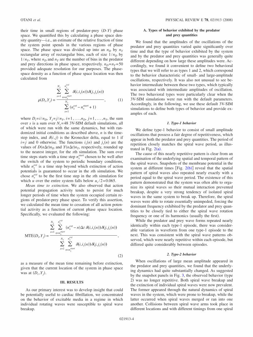
In our optical mapping data, we defined pixels to be in thepredator i.e., excited state if their values were greater than0.60 as illustrated in Fig. 1. The choice of 0.60 was some-what arbitrary; we found that the dynamics of the predatorquantity was generally not sensitive to the exact choice—thus, any reasonable choice for the definition of “excited”could have been used. Similarly, pixels with values less than0.20 or 0.12, depending on the appearance of the data, weredefined to be in the prey state.

For the 3V-SIM model, we defined cells to be in thepredator state if the membrane potential u was greater thanor equal to 0.7, since u1 corresponded to a fully excitedcell, while u0 in the resting state. Similarly, when the gat-ing variable v was greater than 0.6 and u0.6, we consid-ered the cell to be sufficiently recovered to be labeled as“excitable” and thus part of the prey population.

For the FMG model, cells with membrane potentialgreater than −20 mV were considered to be in the predatorstate. Cells were defined to be in the prey state when themembrane potential was decreasing with time and had valueless than −80 mV.

D. Diagnostics

Diagnostics for this study included standard plots of thepredator and prey quantities versus time, the predator andprey quantities versus each other i.e., phase space plots,and snapshots of the membrane potential V vs x and y atvarious times. We also employed the following two types ofdiagnostics.

Phase space density. The predator and prey quantitiesDt and Yt were sometimes observed to spend most of

Predatorcutofflevel

Preycutofflevel

Membranepotential Predator

PreyTime

1.0

0.0

FIG. 1. Color online Definitions of the predator and prey statesas applied to the time record of a single pixel taken from typicalfiltered optical mapping data. The pixel was considered to be in thepredator or prey state when the optical signal, assumed to representthe membrane potential, was above or below fixed cutoff levels.Here the data were normalized and inverted so that 0.0 and 1.0represented the minimum and maximum observed membrane po-tentials, respectively, for the given pixel. The predator and preyquantities Dt and Yt, at any given time t, were then defined to bethe fraction of cells in the predator and prey states at time t.

CHARACTERIZATION OF MULTIPLE SPIRAL WAVE … PHYSICAL REVIEW E 78, 021913 2008

021913-3

their time in small regions of predator-prey D-Y phasespace. We quantified this by calculating a phase space den-sity quantity—i.e., an estimate of the relative fraction of timethe system point spends in the various regions of phasespace. The phase space was divided up into an nD by nYrectangular array of rectangular bins, each of size 1 /nD by1 /nY, where nD and nY are the number of bins in the predatorand prey directions in phase space, respectively. nD=nY =50provided adequate resolution for our purposes. The phase-space density as a function of phase space location was thencalculated from

Di,Y j =

s=1

Ns

n=ns

start

nsext

„i,isn…„j, jsn…

s=1

Ns

nsext − ns

start + 1

, 1

where Di= i /nD, Y j = j /nY, i=1, . . . ,nD, j=1, . . . ,nY, the sumover s is a sum over Ns=48 3V-SIM default simulations, allof which were run with the same dynamics, but with ran-domized initial conditions as described above, n is the time-step index, and i , j is the Kronecker delta, equal to 1 ifi= j and 0 otherwise. The functions isn and jsn are thevalues of DntnD and YntnY, respectively, rounded upto the nearest integer, for the sth simulation. The sum overtime steps starts with a time step ns

start chosen to be well afterthe switch of the system to periodic boundary conditions,while ns

ext is a time step beyond which extinction of actionpotentials is guaranteed to occur in the sth simulation. Wechose ns

ext to be the first time step in the sth simulation forwhich u over the entire system falls below uc /2=0.065.

Mean time to extinction. We also observed that actionpotential propagation activity tends to persist for muchlonger periods of time when the system occupied certain re-gions of predator-prey phase space. To verify this assertion,we calculated the mean time to cessation of all action poten-tial activity as a function of current phase space location.Specifically, we evaluated the following:

MTEDi,Y j =

s=1

Ns

n=ns

start

nsext

nsext − nt „i,isn…„j, jsn…

s=1

Ns

n=ns

start

nsext

„i,isn…„j, jsn…

,

2

as a measure of the mean time remaining before extinction,given that the current location of the system in phase spacewas at Di ,Y j.

III. RESULTS

As our primary interest was to develop insight that couldbe potentially useful to cardiac fibrillation, we concentratedon the behavior of excitable media in a regime in whichindividual rotating waves were susceptible to spiral wavebreakup.

A. Types of behavior exhibited by the predatorand prey quantities

We found that the amplitudes of the oscillations of thepredator and prey quantities varied quite significantly overtime and that the type of behavior exhibited by the systemand by the predator and prey quantities was generally quitedifferent depending on how large these amplitudes were. Ac-cordingly, we found it convenient to define two behavioraltypes that we will refer to as types 1 and 2, which correspondto the behavior characteristic of small- and large-amplitudeoscillations, respectively. It was also not unusual to see be-havior intermediate between these two types, which typicallywas associated with intermediate amplitudes of oscillation.The two behavioral types were particularly clear when the3V-SIM simulations were run with the default parameters.Accordingly, in the following, we use these default 3V-SIMsimulations to define both types of behavior and provide ex-amples of each.

1. Type-1 behavior

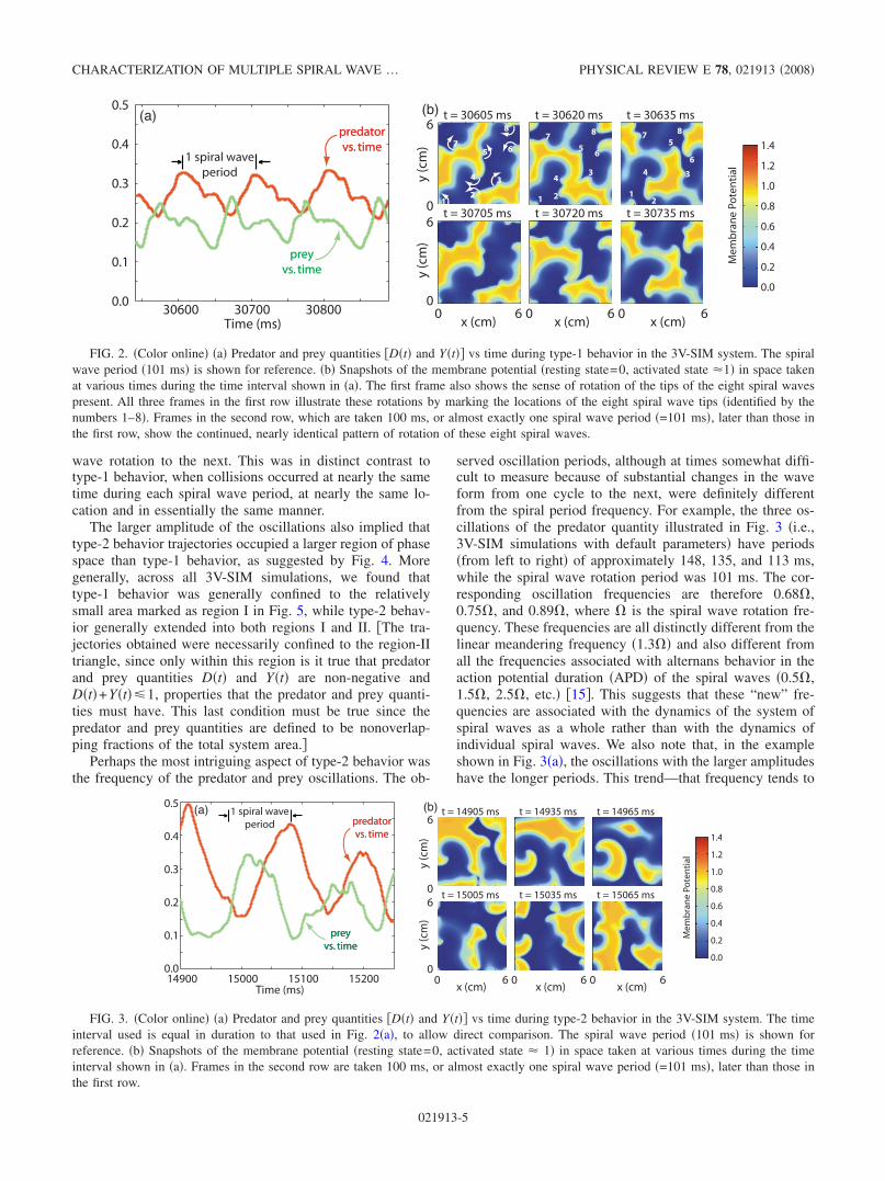
We define type-1 behavior to consist of small amplitudeoscillations that possess a fair degree of repetitiveness, whichappear in both the predator and prey quantities. The period ofrepetition closely matches the spiral wave period, as illus-trated in Fig. 2a.

The cause of this nearly repetitive pattern is clear from anexamination of the underlying spatial and temporal pattern ofthe spiral waves. Snapshots of the membrane potential in thesystem at different times Fig. 2b reveal that the spatialpattern of spiral waves also repeated nearly exactly with aperiod equal to the spiral wave period. The existence of thispattern demonstrated that the system was often able to orga-nize its spiral waves so their mutual interaction preventedbreakup, despite a very strong tendency of isolated spiralwaves in the same system to break up. Therefore, the spiralwaves were able to rotate essentially unimpeded, forcing thedominant frequency exhibited by the predator and prey quan-tities to be closely tied to either the spiral wave rotationfrequency or one of its harmonics usually the first.

While the predator and prey wave forms repeated nearlyidentically within each type-1 episode, there was consider-able variation in waveform from one type-1 episode to thenext. This was consistent with the spiral wave patterns ob-served, which were nearly repetitive within each episode, butdiffered quite considerably between episodes.

2. Type-2 behavior

When oscillations of large mean amplitude appeared inthe predator and prey quantities, we found that the underly-ing dynamics had quite substantially changed. As suggestedby the snapshot panels in Fig. 3, the observed behavior type2 was no longer repetitive. Both spiral wave breakup andthe extinction of individual spiral waves were now prevalent.The former appeared through the natural dynamics of spiralwaves in the system, which were prone to breakup, while thelatter occurred when spiral waves merged or ran into oneanother. Collisions between spiral wave arms took place indifferent locations and with different timings from one spiral


021913-4

wave rotation to the next. This was in distinct contrast totype-1 behavior, when collisions occurred at nearly the sametime during each spiral wave period, at nearly the same lo-cation and in essentially the same manner.

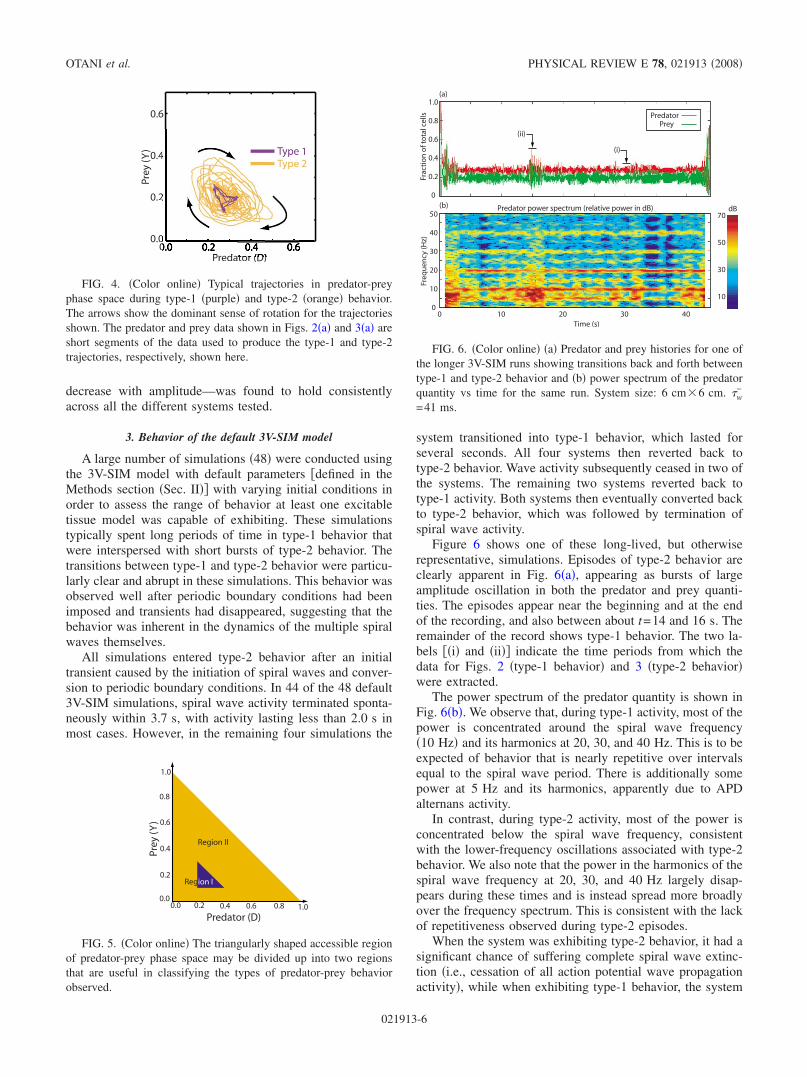
The larger amplitude of the oscillations also implied thattype-2 behavior trajectories occupied a larger region of phasespace than type-1 behavior, as suggested by Fig. 4. Moregenerally, across all 3V-SIM simulations, we found thattype-1 behavior was generally confined to the relativelysmall area marked as region I in Fig. 5, while type-2 behav-ior generally extended into both regions I and II. The tra-jectories obtained were necessarily confined to the region-IItriangle, since only within this region is it true that predatorand prey quantities Dt and Yt are non-negative andDt+Yt1, properties that the predator and prey quanti-ties must have. This last condition must be true since thepredator and prey quantities are defined to be nonoverlap-ping fractions of the total system area.

Perhaps the most intriguing aspect of type-2 behavior wasthe frequency of the predator and prey oscillations. The ob-

served oscillation periods, although at times somewhat diffi-cult to measure because of substantial changes in the waveform from one cycle to the next, were definitely differentfrom the spiral period frequency. For example, the three os-cillations of the predator quantity illustrated in Fig. 3 i.e.,3V-SIM simulations with default parameters have periodsfrom left to right of approximately 148, 135, and 113 ms,while the spiral wave rotation period was 101 ms. The cor-responding oscillation frequencies are therefore 0.68 ,0.75 , and 0.89 , where is the spiral wave rotation fre-quency. These frequencies are all distinctly different from thelinear meandering frequency 1.3 and also different fromall the frequencies associated with alternans behavior in theaction potential duration APD of the spiral waves 0.5 ,1.5 , 2.5 , etc. 15. This suggests that these “new” fre-quencies are associated with the dynamics of the system ofspiral waves as a whole rather than with the dynamics ofindividual spiral waves. We also note that, in the exampleshown in Fig. 3a, the oscillations with the larger amplitudeshave the longer periods. This trend—that frequency tends to

Time (ms)

predatorvs. time

predatorvs. time

preyvs. time

preyvs. time

0.0

0.1

0.2

0.3

0.4

0.5

30600 30700 30800x (cm)

0 66

t = 30720 ms

1 spiral waveperiod

0.2

0.0

0.4

0.6

0.8

1.0

1.2

1.4

Mem

bra

ne

Pote

nti

aly(c

m)

0

6

y(c

m)

x (cm)

00

6t = 30705 ms

x (cm)0 6

t = 30735 ms

t = 30620 mst = 30605 ms t = 30635 ms(a) (b)

2 2 2

33 34 4

4

5 55

6 66

77 7

8 8 8

1 11

FIG. 2. Color online a Predator and prey quantities Dt and Yt vs time during type-1 behavior in the 3V-SIM system. The spiralwave period 101 ms is shown for reference. b Snapshots of the membrane potential resting state=0, activated state 1 in space takenat various times during the time interval shown in a. The first frame also shows the sense of rotation of the tips of the eight spiral wavespresent. All three frames in the first row illustrate these rotations by marking the locations of the eight spiral wave tips identified by thenumbers 1–8. Frames in the second row, which are taken 100 ms, or almost exactly one spiral wave period =101 ms, later than those inthe first row, show the continued, nearly identical pattern of rotation of these eight spiral waves.

Time (ms)

predatorvs. time

predatorvs. time

preyvs. time

preyvs. time

0.0

0.1

0.2

0.3

0.4

0.5

1500014900 15100 15200x (cm)

0 66

t = 15035 ms

0.2

0.0

0.4

0.6

0.8

1.0

1.2

1.4

Mem

bra

ne

Pote

nti

aly(c

m)

0

6

y(c

m)

x (cm)

00

6t = 15005 ms

x (cm)0 6

t = 15065 ms

t = 14935 mst = 14905 ms t = 14965 ms(b)(a) 1 spiral waveperiod

FIG. 3. Color online a Predator and prey quantities Dt and Yt vs time during type-2 behavior in the 3V-SIM system. The timeinterval used is equal in duration to that used in Fig. 2a, to allow direct comparison. The spiral wave period 101 ms is shown forreference. b Snapshots of the membrane potential resting state=0, activated state 1 in space taken at various times during the timeinterval shown in a. Frames in the second row are taken 100 ms, or almost exactly one spiral wave period =101 ms, later than those inthe first row.


021913-5

decrease with amplitude—was found to hold consistentlyacross all the different systems tested.

3. Behavior of the default 3V-SIM model

A large number of simulations 48 were conducted usingthe 3V-SIM model with default parameters defined in theMethods section Sec. II with varying initial conditions inorder to assess the range of behavior at least one excitabletissue model was capable of exhibiting. These simulationstypically spent long periods of time in type-1 behavior thatwere interspersed with short bursts of type-2 behavior. Thetransitions between type-1 and type-2 behavior were particu-larly clear and abrupt in these simulations. This behavior wasobserved well after periodic boundary conditions had beenimposed and transients had disappeared, suggesting that thebehavior was inherent in the dynamics of the multiple spiralwaves themselves.

All simulations entered type-2 behavior after an initialtransient caused by the initiation of spiral waves and conver-sion to periodic boundary conditions. In 44 of the 48 default3V-SIM simulations, spiral wave activity terminated sponta-neously within 3.7 s, with activity lasting less than 2.0 s inmost cases. However, in the remaining four simulations the

system transitioned into type-1 behavior, which lasted forseveral seconds. All four systems then reverted back totype-2 behavior. Wave activity subsequently ceased in two ofthe systems. The remaining two systems reverted back totype-1 activity. Both systems then eventually converted backto type-2 behavior, which was followed by termination ofspiral wave activity.

Figure 6 shows one of these long-lived, but otherwiserepresentative, simulations. Episodes of type-2 behavior areclearly apparent in Fig. 6a, appearing as bursts of largeamplitude oscillation in both the predator and prey quanti-ties. The episodes appear near the beginning and at the endof the recording, and also between about t=14 and 16 s. Theremainder of the record shows type-1 behavior. The two la-bels i and ii indicate the time periods from which thedata for Figs. 2 type-1 behavior and 3 type-2 behaviorwere extracted.

The power spectrum of the predator quantity is shown inFig. 6b. We observe that, during type-1 activity, most of thepower is concentrated around the spiral wave frequency10 Hz and its harmonics at 20, 30, and 40 Hz. This is to beexpected of behavior that is nearly repetitive over intervalsequal to the spiral wave period. There is additionally somepower at 5 Hz and its harmonics, apparently due to APDalternans activity.

In contrast, during type-2 activity, most of the power isconcentrated below the spiral wave frequency, consistentwith the lower-frequency oscillations associated with type-2behavior. We also note that the power in the harmonics of thespiral wave frequency at 20, 30, and 40 Hz largely disap-pears during these times and is instead spread more broadlyover the frequency spectrum. This is consistent with the lackof repetitiveness observed during type-2 episodes.

When the system was exhibiting type-2 behavior, it had asignificant chance of suffering complete spiral wave extinc-tion i.e., cessation of all action potential wave propagationactivity, while when exhibiting type-1 behavior, the system

00.0

0.2

0.4

0.6

Pre

y(Y

)

2

Predator (D)

FIG. 4. Color online Typical trajectories in predator-preyphase space during type-1 purple and type-2 orange behavior.The arrows show the dominant sense of rotation for the trajectoriesshown. The predator and prey data shown in Figs. 2a and 3a areshort segments of the data used to produce the type-1 and type-2trajectories, respectively, shown here.

Prey

(Y)

Predator (D)

1.0

1.0

Region II

0.80.60.40.2

0.2

0.4

0.6

0.8

0.00.0

Region I

FIG. 5. Color online The triangularly shaped accessible regionof predator-prey phase space may be divided up into two regionsthat are useful in classifying the types of predator-prey behaviorobserved.

10

30

50

70dB

0 10 20 30 40Time (s)

0

10

20

30

40

50

Freq

uen

cy(H

z)

Predator power spectrum (relative power in dB)

0

0.2

0.4

0.6

0.8

1.0

PredatorPrey

(a)

(b)

(i)

(ii)

Frac

tio

no

fto

talc

ells

FIG. 6. Color online a Predator and prey histories for one ofthe longer 3V-SIM runs showing transitions back and forth betweentype-1 and type-2 behavior and b power spectrum of the predatorquantity vs time for the same run. System size: 6 cm6 cm. w

−

=41 ms.


021913-6

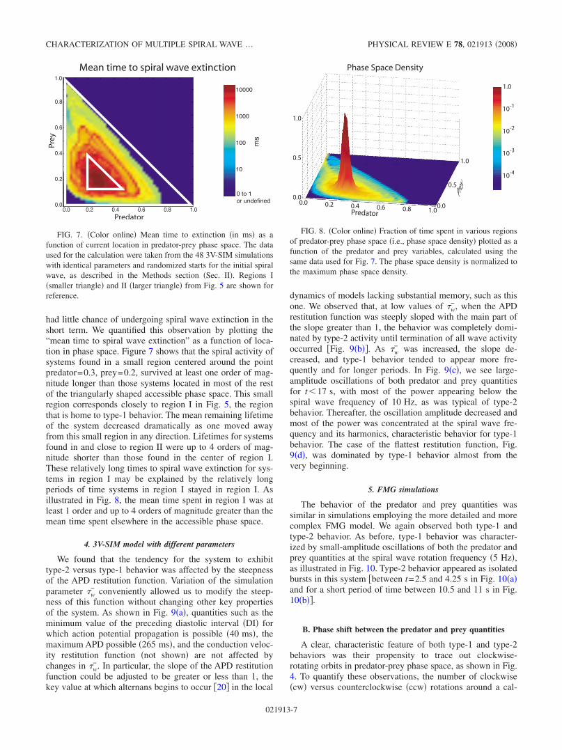
had little chance of undergoing spiral wave extinction in theshort term. We quantified this observation by plotting the“mean time to spiral wave extinction” as a function of loca-tion in phase space. Figure 7 shows that the spiral activity ofsystems found in a small region centered around the pointpredator=0.3, prey=0.2, survived at least one order of mag-nitude longer than those systems located in most of the restof the triangularly shaped accessible phase space. This smallregion corresponds closely to region I in Fig. 5, the regionthat is home to type-1 behavior. The mean remaining lifetimeof the system decreased dramatically as one moved awayfrom this small region in any direction. Lifetimes for systemsfound in and close to region II were up to 4 orders of mag-nitude shorter than those found in the center of region I.These relatively long times to spiral wave extinction for sys-tems in region I may be explained by the relatively longperiods of time systems in region I stayed in region I. Asillustrated in Fig. 8, the mean time spent in region I was atleast 1 order and up to 4 orders of magnitude greater than themean time spent elsewhere in the accessible phase space.

4. 3V-SIM model with different parameters

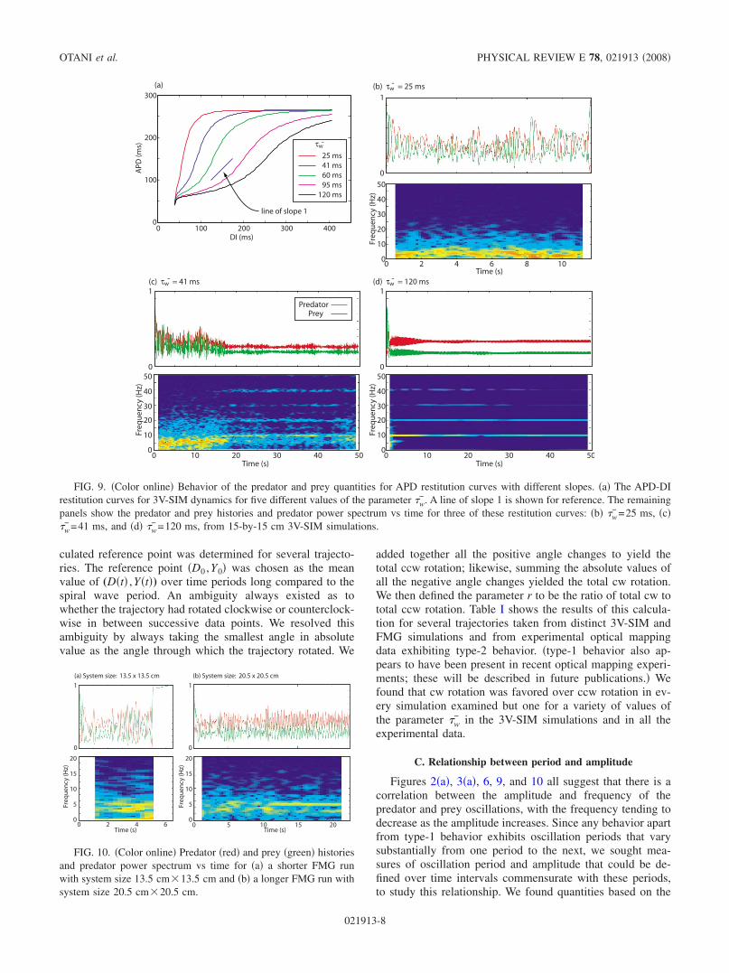
We found that the tendency for the system to exhibittype-2 versus type-1 behavior was affected by the steepnessof the APD restitution function. Variation of the simulationparameter w

− conveniently allowed us to modify the steep-ness of this function without changing other key propertiesof the system. As shown in Fig. 9a, quantities such as theminimum value of the preceding diastolic interval DI forwhich action potential propagation is possible 40 ms, themaximum APD possible 265 ms, and the conduction veloc-ity restitution function not shown are not affected bychanges in w

−. In particular, the slope of the APD restitutionfunction could be adjusted to be greater or less than 1, thekey value at which alternans begins to occur 20 in the local

dynamics of models lacking substantial memory, such as thisone. We observed that, at low values of w

−, when the APDrestitution function was steeply sloped with the main part ofthe slope greater than 1, the behavior was completely domi-nated by type-2 activity until termination of all wave activityoccurred Fig. 9b. As w

− was increased, the slope de-creased, and type-1 behavior tended to appear more fre-quently and for longer periods. In Fig. 9c, we see large-amplitude oscillations of both predator and prey quantitiesfor t17 s, with most of the power appearing below thespiral wave frequency of 10 Hz, as was typical of type-2behavior. Thereafter, the oscillation amplitude decreased andmost of the power was concentrated at the spiral wave fre-quency and its harmonics, characteristic behavior for type-1behavior. The case of the flattest restitution function, Fig.9d, was dominated by type-1 behavior almost from thevery beginning.

5. FMG simulations

The behavior of the predator and prey quantities wassimilar in simulations employing the more detailed and morecomplex FMG model. We again observed both type-1 andtype-2 behavior. As before, type-1 behavior was character-ized by small-amplitude oscillations of both the predator andprey quantities at the spiral wave rotation frequency 5 Hz,as illustrated in Fig. 10. Type-2 behavior appeared as isolatedbursts in this system between t=2.5 and 4.25 s in Fig. 10aand for a short period of time between 10.5 and 11 s in Fig.10b.

B. Phase shift between the predator and prey quantities

A clear, characteristic feature of both type-1 and type-2behaviors was their propensity to trace out clockwise-rotating orbits in predator-prey phase space, as shown in Fig.4. To quantify these observations, the number of clockwisecw versus counterclockwise ccw rotations around a cal-

10

100

1000

10000

0 to 1

or undefined

Predator

Prey

0.0 0.2 0.4 0.6 0.8 1.0

1.0

0.8

0.6

0.4

0.2

0.0

ms

Mean time to spiral wave extinction

FIG. 7. Color online Mean time to extinction in ms as afunction of current location in predator-prey phase space. The dataused for the calculation were taken from the 48 3V-SIM simulationswith identical parameters and randomized starts for the initial spiralwave, as described in the Methods section Sec. II. Regions Ismaller triangle and II larger triangle from Fig. 5 are shown forreference.

Predator

Prey

Phase Space Density

1.0

1.0

10-1

10-2

10-3

10-4

1.0

1.00.80.60.40.20.00.0

0.5

0.5

0.0

FIG. 8. Color online Fraction of time spent in various regionsof predator-prey phase space i.e., phase space density plotted as afunction of the predator and prey variables, calculated using thesame data used for Fig. 7. The phase space density is normalized tothe maximum phase space density.


021913-7

culated reference point was determined for several trajecto-ries. The reference point D0 ,Y0 was chosen as the meanvalue of (Dt ,Yt) over time periods long compared to thespiral wave period. An ambiguity always existed as towhether the trajectory had rotated clockwise or counterclock-wise in between successive data points. We resolved thisambiguity by always taking the smallest angle in absolutevalue as the angle through which the trajectory rotated. We

added together all the positive angle changes to yield thetotal ccw rotation; likewise, summing the absolute values ofall the negative angle changes yielded the total cw rotation.We then defined the parameter r to be the ratio of total cw tototal ccw rotation. Table I shows the results of this calcula-tion for several trajectories taken from distinct 3V-SIM andFMG simulations and from experimental optical mappingdata exhibiting type-2 behavior. type-1 behavior also ap-pears to have been present in recent optical mapping experi-ments; these will be described in future publications. Wefound that cw rotation was favored over ccw rotation in ev-ery simulation examined but one for a variety of values ofthe parameter w

− in the 3V-SIM simulations and in all theexperimental data.

C. Relationship between period and amplitude

Figures 2a, 3a, 6, 9, and 10 all suggest that there is acorrelation between the amplitude and frequency of thepredator and prey oscillations, with the frequency tending todecrease as the amplitude increases. Since any behavior apartfrom type-1 behavior exhibits oscillation periods that varysubstantially from one period to the next, we sought mea-sures of oscillation period and amplitude that could be de-fined over time intervals commensurate with these periods,to study this relationship. We found quantities based on the

0

100

200

300

0 100 200 300 400DI (ms)

APD

(ms)

line of slope 1

25 ms41 ms60 ms95 ms

120 ms

τw-

(a) (b) τw = 25 ms-

(d) τw = 120 ms-(c) τw = 41 ms-

0

1

0

1

0

1

0

10

20

30

40

50

Freq

uen

cy(H

z)

0

10

20

30

40

50Fr

equ

ency

(Hz)

0

10

20

30

40

50

Freq

uen

cy(H

z)

0 10 20 30 40 50Time (s)

Time (s)

Time (s)0 10 20 30 40 50

0 2 4 6 8 10

PredatorPrey

FIG. 9. Color online Behavior of the predator and prey quantities for APD restitution curves with different slopes. a The APD-DIrestitution curves for 3V-SIM dynamics for five different values of the parameter w

−. A line of slope 1 is shown for reference. The remainingpanels show the predator and prey histories and predator power spectrum vs time for three of these restitution curves: b w

− =25 ms, cw

− =41 ms, and d w− =120 ms, from 15-by-15 cm 3V-SIM simulations.

(a) System size: 13.5 x 13.5 cm (b) System size: 20.5 x 20.5 cm

0

1

0

1

0

5

10

15

20

Freq

uen

cy(H

z)

0

5

10

15

20

Freq

uen

cy(H

z)

00 2 4 6Time (s) Time (s)

5 10 15 20

FIG. 10. Color online Predator red and prey green historiesand predator power spectrum vs time for a a shorter FMG runwith system size 13.5 cm13.5 cm and b a longer FMG run withsystem size 20.5 cm20.5 cm.


021913-8

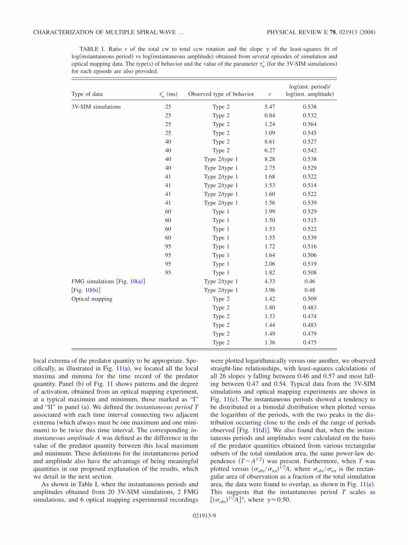
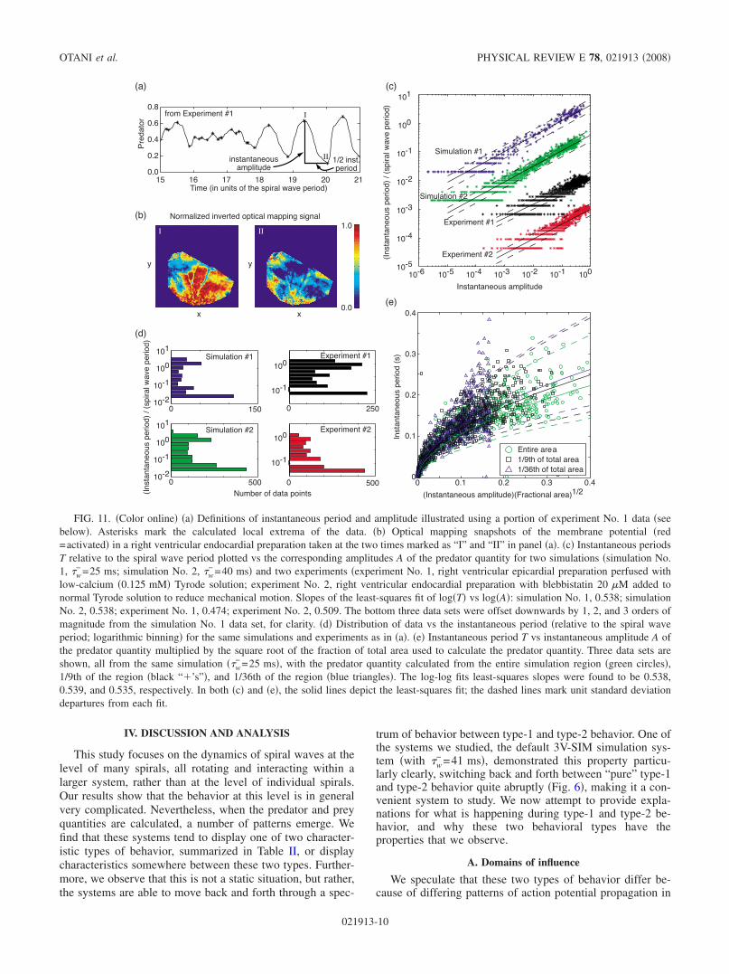
local extrema of the predator quantity to be appropriate. Spe-cifically, as illustrated in Fig. 11a, we located all the localmaxima and minima for the time record of the predatorquantity. Panel b of Fig. 11 shows patterns and the degreeof activation, obtained from an optical mapping experiment,at a typical maximum and minimum, those marked as “I”and “II” in panel a. We defined the instantaneous period Tassociated with each time interval connecting two adjacentextrema which always must be one maximum and one mini-mum to be twice this time interval. The corresponding in-stantaneous amplitude A was defined as the difference in thevalue of the predator quantity between this local maximumand minimum. These definitions for the instantaneous periodand amplitude also have the advantage of being meaningfulquantities in our proposed explanation of the results, whichwe detail in the next section.

As shown in Table I, when the instantaneous periods andamplitudes obtained from 20 3V-SIM simulations, 2 FMGsimulations, and 6 optical mapping experimental recordings

were plotted logarithmically versus one another, we observedstraight-line relationships, with least-squares calculations ofall 26 slopes falling between 0.46 and 0.57 and most fall-ing between 0.47 and 0.54. Typical data from the 3V-SIMsimulations and optical mapping experiments are shown inFig. 11c. The instantaneous periods showed a tendency tobe distributed in a bimodal distribution when plotted versusthe logarithm of the periods, with the two peaks in the dis-tribution occurring close to the ends of the range of periodsobserved Fig. 11d. We also found that, when the instan-taneous periods and amplitudes were calculated on the basisof the predator quantities obtained from various rectangularsubsets of the total simulation area, the same power-law de-pendence TA1/2 was present. Furthermore, when T wasplotted versus obs /tot1/2A, where obs /tot is the rectan-gular area of observation as a fraction of the total simulationarea, the data were found to overlap, as shown in Fig. 11e.This suggests that the instantaneous period T scales asobs1/2A, where 0.50.

TABLE I. Ratio r of the total cw to total ccw rotation and the slope of the least-squares fit ofloginstantaneous period vs loginstantaneous amplitude obtained from several episodes of simulation andoptical mapping data. The types of behavior and the value of the parameter w

− for the 3V-SIM simulationsfor each episode are also provided.

Type of data w− ms Observed type of behavior r

loginst. period/loginst. amplitude

3V-SIM simulations 25 Type 2 5.47 0.538

25 Type 2 0.84 0.532

25 Type 2 1.24 0.564

25 Type 2 1.09 0.545

40 Type 2 8.61 0.527

40 Type 2 6.27 0.542

40 Type 2/type 1 8.28 0.538

40 Type 2/type 1 2.75 0.529

41 Type 2/type 1 1.68 0.522

41 Type 2/type 1 1.53 0.514

41 Type 2/type 1 1.60 0.522

41 Type 2/type 1 1.56 0.539

60 Type 1 1.99 0.529

60 Type 1 1.50 0.515

60 Type 1 1.53 0.522

60 Type 1 1.55 0.539

95 Type 1 1.72 0.516

95 Type 1 1.64 0.506

95 Type 1 2.06 0.519

95 Type 1 1.82 0.508

FMG simulations Fig. 10a Type 2/type 1 4.33 0.46

Fig. 10b Type 2/type 1 3.96 0.48

Optical mapping Type 2 1.42 0.509

Type 2 1.80 0.483

Type 2 1.33 0.474

Type 2 1.44 0.483

Type 2 1.49 0.479

Type 2 1.36 0.475


021913-9

IV. DISCUSSION AND ANALYSIS

This study focuses on the dynamics of spiral waves at thelevel of many spirals, all rotating and interacting within alarger system, rather than at the level of individual spirals.Our results show that the behavior at this level is in generalvery complicated. Nevertheless, when the predator and preyquantities are calculated, a number of patterns emerge. Wefind that these systems tend to display one of two character-istic types of behavior, summarized in Table II, or displaycharacteristics somewhere between these two types. Further-more, we observe that this is not a static situation, but rather,the systems are able to move back and forth through a spec-

trum of behavior between type-1 and type-2 behavior. One ofthe systems we studied, the default 3V-SIM simulation sys-tem with w

− =41 ms, demonstrated this property particu-larly clearly, switching back and forth between “pure” type-1and type-2 behavior quite abruptly Fig. 6, making it a con-venient system to study. We now attempt to provide expla-nations for what is happening during type-1 and type-2 be-havior, and why these two behavioral types have theproperties that we observe.

A. Domains of influence

We speculate that these two types of behavior differ be-cause of differing patterns of action potential propagation in

100

10010-110-210-310-410-510-6

10-1

10-2

10-3

10-4

10-5

101

100

10-1

100

10-1

100

10-1

10-2

101

100

10-1

10-2

101

(Instantaneousperiod)/(spiralwaveperiod)


Instantaneousperiod(s)

Number of data points

Instantaneous amplitude

(Instantaneous amplitude)(Fractional area)1/2

Simulation #1

Simulation #2

Experiment #1

Experiment #2

00

0 150

0 500

0 250

0 500

0.1

0.2

0.3

0.4

(b)

(c)(a)

(d)

(e)

0.1 0.2 0.3 0.4

Simulation #1

Time (in units of the spiral wave period)

Predator

150.0

0.2

0.4

0.6

0.8

16 17 18 19 20 21

Simulation #2

Experiment #1

Experiment #2

Entire area

1/9th of total area

1/36th of total area

1.0

0.0xx

y y

Normalized inverted optical mapping signal

I II

from Experiment #1 I

IIinstantaneousamplitude

1/2 inst.period

FIG. 11. Color online a Definitions of instantaneous period and amplitude illustrated using a portion of experiment No. 1 data seebelow. Asterisks mark the calculated local extrema of the data. b Optical mapping snapshots of the membrane potential red=activated in a right ventricular endocardial preparation taken at the two times marked as “I” and “II” in panel a. c Instantaneous periodsT relative to the spiral wave period plotted vs the corresponding amplitudes A of the predator quantity for two simulations simulation No.1, w

− =25 ms; simulation No. 2, w− =40 ms and two experiments experiment No. 1, right ventricular epicardial preparation perfused with

low-calcium 0.125 mM Tyrode solution; experiment No. 2, right ventricular endocardial preparation with blebbistatin 20 M added tonormal Tyrode solution to reduce mechanical motion. Slopes of the least-squares fit of logT vs logA: simulation No. 1, 0.538; simulationNo. 2, 0.538; experiment No. 1, 0.474; experiment No. 2, 0.509. The bottom three data sets were offset downwards by 1, 2, and 3 orders ofmagnitude from the simulation No. 1 data set, for clarity. d Distribution of data vs the instantaneous period relative to the spiral waveperiod; logarithmic binning for the same simulations and experiments as in a. e Instantaneous period T vs instantaneous amplitude A ofthe predator quantity multiplied by the square root of the fraction of total area used to calculate the predator quantity. Three data sets areshown, all from the same simulation w

− =25 ms, with the predator quantity calculated from the entire simulation region green circles,1/9th of the region black “’s”, and 1/36th of the region blue triangles. The log-log fits least-squares slopes were found to be 0.538,0.539, and 0.535, respectively. In both c and e, the solid lines depict the least-squares fit; the dashed lines mark unit standard deviationdepartures from each fit.


021913-10

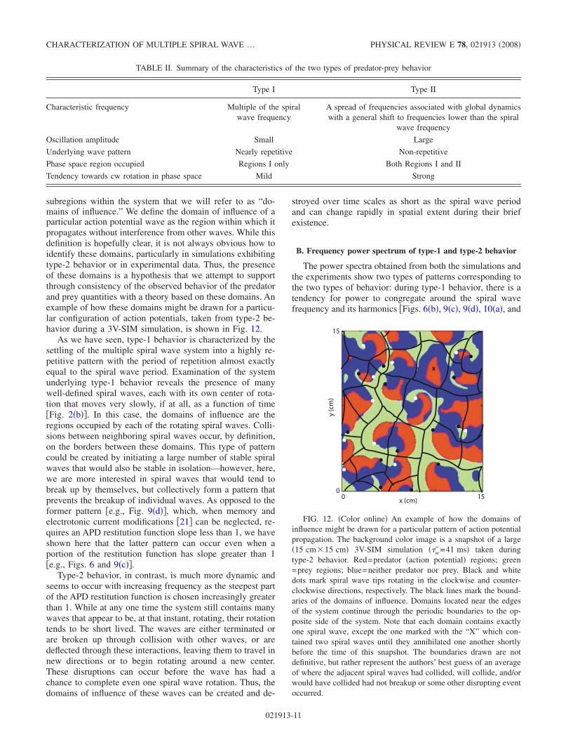
subregions within the system that we will refer to as “do-mains of influence.” We define the domain of influence of aparticular action potential wave as the region within which itpropagates without interference from other waves. While thisdefinition is hopefully clear, it is not always obvious how toidentify these domains, particularly in simulations exhibitingtype-2 behavior or in experimental data. Thus, the presenceof these domains is a hypothesis that we attempt to supportthrough consistency of the observed behavior of the predatorand prey quantities with a theory based on these domains. Anexample of how these domains might be drawn for a particu-lar configuration of action potentials, taken from type-2 be-havior during a 3V-SIM simulation, is shown in Fig. 12.

As we have seen, type-1 behavior is characterized by thesettling of the multiple spiral wave system into a highly re-petitive pattern with the period of repetition almost exactlyequal to the spiral wave period. Examination of the systemunderlying type-1 behavior reveals the presence of manywell-defined spiral waves, each with its own center of rota-tion that moves very slowly, if at all, as a function of timeFig. 2b. In this case, the domains of influence are theregions occupied by each of the rotating spiral waves. Colli-sions between neighboring spiral waves occur, by definition,on the borders between these domains. This type of patterncould be created by initiating a large number of stable spiralwaves that would also be stable in isolation—however, here,we are more interested in spiral waves that would tend tobreak up by themselves, but collectively form a pattern thatprevents the breakup of individual waves. As opposed to theformer pattern e.g., Fig. 9d, which, when memory andelectrotonic current modifications 21 can be neglected, re-quires an APD restitution function slope less than 1, we haveshown here that the latter pattern can occur even when aportion of the restitution function has slope greater than 1e.g., Figs. 6 and 9c.

Type-2 behavior, in contrast, is much more dynamic andseems to occur with increasing frequency as the steepest partof the APD restitution function is chosen increasingly greaterthan 1. While at any one time the system still contains manywaves that appear to be, at that instant, rotating, their rotationtends to be short lived. The waves are either terminated orare broken up through collision with other waves, or aredeflected through these interactions, leaving them to travel innew directions or to begin rotating around a new center.These disruptions can occur before the wave has had achance to complete even one spiral wave rotation. Thus, thedomains of influence of these waves can be created and de-

stroyed over time scales as short as the spiral wave periodand can change rapidly in spatial extent during their briefexistence.

B. Frequency power spectrum of type-1 and type-2 behavior

The power spectra obtained from both the simulations andthe experiments show two types of patterns corresponding tothe two types of behavior: during type-1 behavior, there is atendency for power to congregate around the spiral wavefrequency and its harmonics Figs. 6b, 9c, 9d, 10a, and

TABLE II. Summary of the characteristics of the two types of predator-prey behavior

Type I Type II

Characteristic frequency Multiple of the spiralwave frequency

A spread of frequencies associated with global dynamicswith a general shift to frequencies lower than the spiral

wave frequency

Oscillation amplitude Small Large

Underlying wave pattern Nearly repetitive Non-repetitive

Phase space region occupied Regions I only Both Regions I and II

Tendency towards cw rotation in phase space Mild Strong

x

00

15

15x (cm)

y(c

m)

FIG. 12. Color online An example of how the domains ofinfluence might be drawn for a particular pattern of action potentialpropagation. The background color image is a snapshot of a large15 cm15 cm 3V-SIM simulation w

− =41 ms taken duringtype-2 behavior. Red=predator action potential regions; green=prey regions; blue=neither predator nor prey. Black and whitedots mark spiral wave tips rotating in the clockwise and counter-clockwise directions, respectively. The black lines mark the bound-aries of the domains of influence. Domains located near the edgesof the system continue through the periodic boundaries to the op-posite side of the system. Note that each domain contains exactlyone spiral wave, except the one marked with the “X” which con-tained two spiral waves until they annihilated one another shortlybefore the time of this snapshot. The boundaries drawn are notdefinitive, but rather represent the authors’ best guess of an averageof where the adjacent spiral waves had collided, will collide, and/orwould have collided had not breakup or some other disrupting eventoccurred.


021913-11

10b, while when the system is exhibiting type-2 behaviorthe tendency is for power to spread out both above and es-pecially below the spiral wave frequency Figs. 6b, 9b,9c, and 10b. These two power spectrum patterns are con-sistent with the types of behaviors we hypothesize are takingplace within the domains of influence; that is, during type-1behavior, waves are primarily executing spiral wave rotationwithin their respective domains of influence, and thus mostof the power will be expected to be concentrated around thespiral wave frequency and its harmonics. In contrast, duringtype-2 behavior, waves execute only a portion of a spiralwave rotation or are propagating in some more complicatedpattern within their domains. Thus, in this case, we wouldexpect the power spectrum to be characterized by frequen-cies that are commensurate with the inverse of the lifetimesof the domains of influence or by the typical time it takes forthe resident wave to cross its domain. These frequenciescould extend above the spiral wave rotation frequency whenthe domains last shorter than a spiral wave period or whenthe wave takes less than a spiral wave period to traverse itsdomain. This situation is typical of the experimental data,where the behavior is type-2-like, and transit times of wavesacross the entire preparation are small compared to the spiralwave rotation period. In contrast, frequencies would be ex-pected to be found more often below the spiral wave fre-quency when the system is composed largely of waves thattake more than one spiral wave period to cross their domains.This scenario is more typical of many of our 3V-SIM simu-lations, where study of the system during type-2 behaviorreveals the presence of waves that are traveling relativelylong distances across the system.

1. Self-organization during type-1 behavior

Perhaps the most important question we can ask abouttype-1 behavior has to do with the nature of the self-organization the system exhibits. When individual spiralwaves are not prone to breakup, the ability for the system tomaintain a particular spatial pattern of spiral waves from onespiral wave rotation period to the next is not all thatsurprising—without breakup, we generally only see driftingand/or meandering of the spiral wave centers, both of whichare slow processes compared to spiral wave rotation. Theexistence of type-1 behavior is much more surprising whenbreakup is an inherent property of individual spiral waves. Inthis case, the system must somehow organize its spiral wavesso that their mutual interaction inhibits their tendency tobreak up, as we saw in the 3V-SIM simulations. The processby which this occurs is, at the moment, unknown, althoughwe can make some modest observations. We see, for ex-ample, that during type-1 behavior the arm of each spiralappears to collide with other waves repeatedly at a locationwhere breakup might otherwise be expected to occur. We canspeculate, therefore, that breakup is being inhibited by theserepeated collisions.

Once we accept the near-repetitive spatial pattern oftype-1 behavior, it is not too difficult to understand most ofthe other type-1 properties. If type-1 behavior were exactlyrepetitive from one spiral wave period to the next, then alldynamical quantities, including the predator and prey quan-

tities, would also be necessarily repetitive with the same pe-riod. Thus, it is not surprising that the near repetition oftype-1 behavior would yield near-repetitive behavior in thepredator and prey quantities and that the period of repetitionwould be the spiral wave period. Also, we should not be toosurprised that the oscillation amplitude of the predator andprey quantities is relatively small, since simple rotation of aspiral wave would be expected to have a smaller impact onthe fraction of tissue activated at any one time, in contrast tothe larger fluctuation one would anticipate resulting from an-nihilation and formation of action potential waves, as rou-tinely takes place during type-2 behavior.

2. Type-2 behavior as a less organized, “searching” mode

Type-2 behavior appears to lack the same degree of theself-organization and near-repetitive dynamics present intype-1 behavior; thus, the spatial pattern of spiral waves isfree to change during type-2 behavior, allowing the system tosample one pattern of spiral waves after the next. We cantherefore think of a system exhibiting type-2 behavior asbeing engaged in a “searching” mode, as it looks for oppor-tunities to either coalesce into self-organization type-1 orprogress into behavior that will lead to complete action po-tential extinction. We have seen that systems involved intype-2 behavior are actually able to change spiral wave pat-terns fairly quickly, perhaps even on a time scale approach-ing the spiral wave period cf. Fig. 3. This allowed the sys-tem to conduct its search relatively rapidly, sampling newspatial patterns of spiral waves in quick succession. Further-more, for our default 3V-SIM system, it seemed fairly easyfor type-2 behavior to find spiral wave patterns that self-organized into the nearly repetitive behaviors characteristicof type-1 behavior. It also seemed relatively easy for type-2behavior to generate patterns of spiral waves that involvednear total activation of the tissue, corresponding to a highvalue of the predator quantity, or near total recovery of thetissue high prey value, both of which corresponded to en-tering into region II in Fig. 5. This translated into large am-plitudes in the oscillation of the predator quantity and alsoincreased the tendency for type-2 behavior to end in extinc-tion of all spiral wave activity e.g., the ends of the simula-tions shown in Figs. 6a, 9b, and 10a. These tendenciesexplain the large disparities in the mean time to spiral waveextinction Fig. 7 and phase space densities Fig. 8 we ob-tain for type-1 versus type-2 behavior.

C. Clockwise rotation in phase space

We believe the observed tendency towards clockwise ro-tation in predator-prey phase space, when it occurs, is basedon the fact that rotation will always appear when both dy-namical variables are oscillatory with the same frequencyand the phase shift between the two variables is somethingother than a multiple of 180°. This type of behavior iscommon in the analysis of electronic signals, where the ro-tating pattern is generally called a Lissajous figure e.g.,22. In our case, we suggest that the observed clockwiserotation is caused by approximately oscillatory behavior ofboth the predator and prey quantities, with the predator quan-


021913-12

tity lagging behind the prey quantity by less than half anoscillation period.

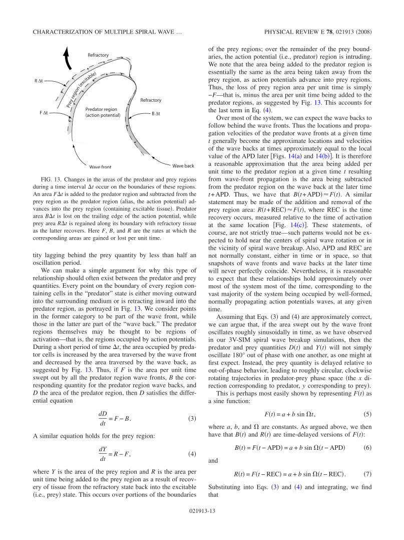
We can make a simple argument for why this type ofrelationship should often exist between the predator and preyquantities. Every point on the boundary of every region con-taining cells in the “predator” state is either moving outwardinto the surrounding medium or is retracting inward into thepredator region, as portrayed in Fig. 13. We consider pointsin the former category to be part of the wave front, whilethose in the latter are part of the “wave back.” The predatorregions themselves may be thought to be regions ofactivation—that is, the regions occupied by action potentials.During a short period of time t, the area occupied by preda-tor cells is increased by the area traversed by the wave frontand decreased by the area traversed by the wave back, assuggested by Fig. 13. Thus, if F is the area per unit timeswept out by all the predator region wave fronts, B the cor-responding quantity for the predator region wave backs, andD the area of the predator region, then D satisfies the differ-ential equation

dD

dt= F − B . 3

A similar equation holds for the prey region:

dY

dt= R − F , 4

where Y is the area of the prey region and R is the area perunit time being added to the prey region as a result of recov-ery of tissue from the refractory state back into the excitablei.e., prey state. This occurs over portions of the boundaries

of the prey regions; over the remainder of the prey bound-aries, the action potential i.e., predator region is intruding.We note that the area being added to the predator region isessentially the same as the area being taken away from theprey region, as action potentials advance into prey regions.Thus, the loss of prey region area per unit time is simply−F—that is, minus the area per unit time being added to thepredator regions, as suggested by Fig. 13. This accounts forthe last term in Eq. 4.

Over most of the system, we can expect the wave backs tofollow behind the wave fronts. Thus the locations and propa-gation velocities of the predator wave fronts at a given timet generally become the approximate locations and velocitiesof the wave backs at times approximately equal to the localvalue of the APD later Figs. 14a and 14b. It is thereforea reasonable approximation that the area being added perunit time to the predator region at a given time t resultingfrom wave-front propagation is the area being subtractedfrom the predator region on the wave back at the later timet+APD. Thus, we have that Bt+APDFt. A similarstatement may be made of the addition and removal of theprey region area: Rt+RECFt, where REC is the timerecovery occurs, measured relative to the time of activationat the same location Fig. 14c. These statements, ofcourse, are not strictly true—such patterns would not be ex-pected to hold near the centers of spiral wave rotation or inthe vicinity of spiral wave breakup. Also, APD and REC arenot normally constant, either in time or in space, so thatsnapshots of wave fronts and wave backs at the later timewill never perfectly coincide. Nevertheless, it is reasonableto expect that these relationships hold approximately overmost of the system most of the time, corresponding to thevast majority of the system being occupied by well-formed,normally propagating action potentials waves, at any giventime.

Assuming that Eqs. 3 and 4 are approximately correct,we can argue that, if the area swept out by the wave frontoscillates roughly sinusoidally in time, as we have observedin our 3V-SIM spiral wave breakup simulations, then thepredator and prey quantities Dt and Yt will not simplyoscillate 180° out of phase with one another, as one might atfirst expect. Instead, the prey quantity is delayed relative toout-of-phase behavior, leading to roughly circular, clockwiserotating trajectories in predator-prey phase space the x di-rection corresponding to predator, y corresponding to prey.

This is perhaps most easily shown by representing Ft asa sine function:

Ft = a + b sin t , 5

where a, b, and are constants. As argued above, we thenhave that Bt and Rt are time-delayed versions of Ft:

Bt = Ft − APD = a + b sin t − APD 6

and

Rt = Ft − REC = a + b sin t − REC . 7

Substituting into Eqs. 3 and 4 and integrating, we findthat

Predator region(action potential)

Prey

regi

on(e

xcitable)

R ∆t

F ∆t B ∆t

Refractory

Refractory

Wave front Wave back

FIG. 13. Changes in the areas of the predator and prey regionsduring a time interval t occur on the boundaries of these regions.An area Ft is added to the predator region and subtracted from theprey region as the predator region alias, the action potential ad-vances into the prey region containing excitable tissue. Predatorarea Bt is lost on the trailing edge of the action potential, whileprey area Rt is regained along its boundary with refractory tissueas the latter recovers. Here F, B, and R are the rates at which thecorresponding areas are gained or lost per unit time.


021913-13

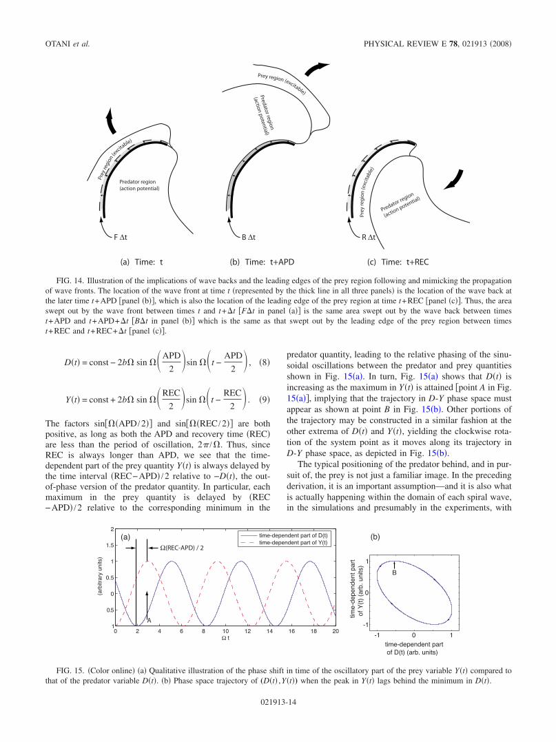
Dt = const − 2b sin APD

2sin t −

APD

2 , 8

Yt = const + 2b sin REC

2sin t −

REC

2 . 9

The factors sin APD /2 and sin REC /2 are bothpositive, as long as both the APD and recovery time RECare less than the period of oscillation, 2 / . Thus, sinceREC is always longer than APD, we see that the time-dependent part of the prey quantity Yt is always delayed bythe time interval REC−APD /2 relative to −Dt, the out-of-phase version of the predator quantity. In particular, eachmaximum in the prey quantity is delayed by REC−APD /2 relative to the corresponding minimum in the

predator quantity, leading to the relative phasing of the sinu-soidal oscillations between the predator and prey quantitiesshown in Fig. 15a. In turn, Fig. 15a shows that Dt isincreasing as the maximum in Yt is attained point A in Fig.15a, implying that the trajectory in D-Y phase space mustappear as shown at point B in Fig. 15b. Other portions ofthe trajectory may be constructed in a similar fashion at theother extrema of Dt and Yt, yielding the clockwise rota-tion of the system point as it moves along its trajectory inD-Y phase space, as depicted in Fig. 15b.

The typical positioning of the predator behind, and in pur-suit of, the prey is not just a familiar image. In the precedingderivation, it is an important assumption—and it is also whatis actually happening within the domain of each spiral wave,in the simulations and presumably in the experiments, with

Predator region(action potential)

Prey

regi

on(e

xcitable)

Predator region

(actionp

otential)

Prey region (excitable)

Predator region

(action potential)

Prey

reg

ion

(exc

itabl

e)

(a) Time: t (b) Time: t+APD (c) Time: t+REC

F ∆t R ∆tB ∆t

FIG. 14. Illustration of the implications of wave backs and the leading edges of the prey region following and mimicking the propagationof wave fronts. The location of the wave front at time t represented by the thick line in all three panels is the location of the wave back atthe later time t+APD panel b, which is also the location of the leading edge of the prey region at time t+REC panel c. Thus, the areaswept out by the wave front between times t and t+t Ft in panel a is the same area swept out by the wave back between timest+APD and t+APD+t Bt in panel b which is the same as that swept out by the leading edge of the prey region between timest+REC and t+REC+t panel c.

0 2 4 6 8 10 12 14 16 18 201

0.5

0

0.5

1

1.5

2

Ω t

time-dependent part of D(t)

time-dependent part of Y(t)Ω(REC-APD) / 2

A

time-dependent part

of D(t) (arb. units)

time-dependentpart

ofY(t)(arb.units)

-1

-1

0

0

1

1

(b)(a)

B

(arbitraryunits)

FIG. 15. Color online a Qualitative illustration of the phase shift in time of the oscillatory part of the prey variable Yt compared tothat of the predator variable Dt. b Phase space trajectory of (Dt ,Yt) when the peak in Yt lags behind the minimum in Dt.


021913-14

the predator action potential chasing or moving into theexcitable tissue prey.

Another assumption used in this derivation—that of sinu-soidal behavior at the spiral wave frequency—was not foundto be universally true in the simulations. It was not unusualfor the predator and prey quantities to deviate substantiallyfrom this behavior. In fact, during type-1 behavior, we evenfound predator and prey wave forms that more closely re-sembled two complete sinusoidal oscillations per spiral waveperiod than one. Nevertheless, a majority of the time, wefound that the peaks and valleys of the predator wave formtended to lag behind those of the prey by less than half aspiral wave period, leading to the observed dominance ofclockwise rotation in predator-prey phase space.

D. Dependence of instantaneous period on amplitude

The origin of the approximate dependence of the instan-taneous period on amplitude as TA1/2 in both the simula-tions and experiments remains unclear. However, we havebeen able to devise a simple system that reproduces thisquantitative dependence and also exhibits qualitative simi-larities to other observed statistical features. We simplymodel the local predator quantity Di in the ith domain as

Dit = CTi2tsin it , 10

where C is a constant, it+t=it+2t /Tit, and t=2 ms. The time-varying periods Tit were calculated inde-pendently for each domain according to the following:

ln Tit + t = ln Tit + 0.05t/Titr − rit1/2,

11

where r is randomly chosen with equal probability between 0and 1, and rit varies slightly to either side of 0.5, so as toalways favor return of Tt to a value of about 0.0316=10−1.5. Specifically, r0t= ln Tt−ln Tmin / ln Tmax−ln Tmin, where Tmax and Tmin were chosen to be 10−1.5+100

and 10−1.5−100, respectively. In other words, each of the do-main predator quantities oscillates with an amplitude propor-tional to the square of its period, and these periods varyslowly and randomly about a value of 10−1.5 and indepen-dently of one another.

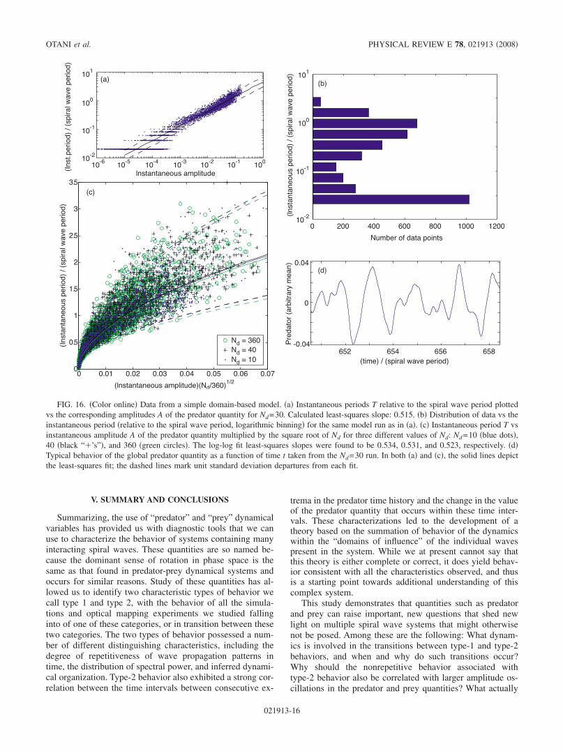
When simulations of this simple model were conducted,the results in Fig. 16 were obtained. As shown in Fig. 16a,calculation of the instantaneous periods and amplitudes givesthe same TA1/2 dependence obtained from the spiral wavesimulations and optical mapping experiments. We also findthat the distribution of the data in amplitude-period space isnot unlike that seen in the main simulations and experiments.In particular, we see a flare in the spread of instantaneousamplitudes for the smaller periods. The distribution of dataversus the logarithm of the periods Fig. 16b also bearsqualitative resemblance to the corresponding distribution inthe main simulations and experiments Fig. 11d. Specifi-cally, we see that both graphs show the tendency for most ofthe periods to congregate at both ends of the main range overwhich the period varies, in a bimodal distribution. The datawere also found to overlap Fig. 16c for different numbersof domains, Nd, when plotted versus the amplitude times

Nd1/2, just as in the experiments and simulations cf. Fig.

11e. Finally, we also observe qualitative similarities in thewave form of the predator quantities. Comparing Fig. 16dwith Figs. 2a and 3a, we observe that both displaysmooth, sinusoidal-like undulations, with smaller short-period oscillations often superimposed on a larger, longer-period pattern. Qualitatively similar wave forms are also ob-served in the experimental predator data not shown.

If we assume that this model is indeed representative ofwhat is happening, the next question to answer is, what typeof dynamics might underlie such a model? The answer isunclear at present. However, we can make the following ob-servations and speculations. First, the proportionality of theamplitude of the individual domain predator quantities Ditto the square of the periods Tit suggests that the amplitudeof the oscillation of these predator quantities’ second deriva-tive, d2Dit /dt2, is approximately independent of the peri-ods, since d2Dit /dt2−42Csin it, from Eq. 10, if wecan assume a small time step t and slow variation in theperiods 1 /TitdTi /dt1. Plots of the second time de-rivatives of both individual Dit’s and the total predatorquantity from simulations of Eq. 10 confirm the approxi-mate constancy of these amplitudes, once fluctuations above1 /10th the Nyquist frequency are filtered out. Second, if thearea inside a spiral wave, and thus, the area used to calculateone of the Di’s, can be represented as xfrontt−xbacktl /S,where the x direction is oriented in the direction of propaga-tion of the wave, xfront and xback are the wave-front and wave-back locations, respectively, l is the length of the wave front,and S is the area of the domain, then d2Dit /dt2 would thenbe proportional to d2xfront /dt2−d2xback /dt2—that is, the dif-ference between the wave-front and wave-back accelera-tions. These changes in velocity of the wave front and waveback, in turn, are often thought to be governed by the DIencountered by the wave front as it propagates. Thus, theacceleration of the wave front, for example, is given by

dvDIdt

= vDIdDI

dt= vDI

dxfront

dt

dDIdx

= vDIvDIdDI

dx, 12

where vDI is the wave-front velocity, dependent on thepreceding DI i.e., conduction velocity restitution function,and vDI is the slope of this function. Both vDI andvDI can be expected to be characterized by “typical” val-ues during the continual, rapid activation of tissue that domi-nates spiral wave turbulence. This leaves us to try to under-stand the nature of the gradient of DIs in such a system.Severe gradients in DIs are thought not to exist in systemsentertaining action potential propagation—they are quicklyeroded over a number of different length scales, discussed byEchebarria and Karma 23. Thus, we can suppose that pat-terns of multiple spiral waves will become increasingly com-plex until gradients in DIs up to this theoretical value arereached and would subsequently level off. Thus, there issome rationale for the existence of a characteristic amplitudefor the oscillation of the d2Di /dt2, although obviously thisargument remains highly speculative.


021913-15

V. SUMMARY AND CONCLUSIONS

Summarizing, the use of “predator” and “prey” dynamicalvariables has provided us with diagnostic tools that we canuse to characterize the behavior of systems containing manyinteracting spiral waves. These quantities are so named be-cause the dominant sense of rotation in phase space is thesame as that found in predator-prey dynamical systems andoccurs for similar reasons. Study of these quantities has al-lowed us to identify two characteristic types of behavior wecall type 1 and type 2, with the behavior of all the simula-tions and optical mapping experiments we studied fallinginto of one of these categories, or in transition between thesetwo categories. The two types of behavior possessed a num-ber of different distinguishing characteristics, including thedegree of repetitiveness of wave propagation patterns intime, the distribution of spectral power, and inferred dynami-cal organization. Type-2 behavior also exhibited a strong cor-relation between the time intervals between consecutive ex-

trema in the predator time history and the change in the valueof the predator quantity that occurs within these time inter-vals. These characterizations led to the development of atheory based on the summation of behavior of the dynamicswithin the “domains of influence” of the individual wavespresent in the system. While we at present cannot say thatthis theory is either complete or correct, it does yield behav-ior consistent with all the characteristics observed, and thusis a starting point towards additional understanding of thiscomplex system.

This study demonstrates that quantities such as predatorand prey can raise important, new questions that shed newlight on multiple spiral wave systems that might otherwisenot be posed. Among these are the following: What dynam-ics is involved in the transitions between type-1 and type-2behaviors, and when and why do such transitions occur?Why should the nonrepetitive behavior associated withtype-2 behavior also be correlated with larger amplitude os-cillations in the predator and prey quantities? What actually

0 200 400 600 800 1000 1200

(Inst.period)/(spiralwaveperiod)

Number of data points

0

0

0.01

652 654 656 658

0.02 0.03 0.04

0.04

-0.04

0.05 0.06 0.070

0.5

1

1.5

2

2.5

3

3.5

(lnstantaneous amplitude)(Nd/360)1/2

(time) / (spiral wave period)

(lnstantaneousperiod)/(spiralwaveperiod)

lnstantaneous amplitude


Predator(arbitrarymean)

Nd = 360

Nd = 40

Nd = 10

10-6

10-5

10-4

10-3

10-2

10-1

10010

-2

10-1

100

101

10-2

10-1

100

101

(a)

(c)

(d)

(b)

FIG. 16. Color online Data from a simple domain-based model. a Instantaneous periods T relative to the spiral wave period plottedvs the corresponding amplitudes A of the predator quantity for Nd=30. Calculated least-squares slope: 0.515. b Distribution of data vs theinstantaneous period relative to the spiral wave period, logarithmic binning for the same model run as in a. c Instantaneous period T vsinstantaneous amplitude A of the predator quantity multiplied by the square root of Nd for three different values of Nd: Nd=10 blue dots,40 black “’s”, and 360 green circles. The log-log fit least-squares slopes were found to be 0.534, 0.531, and 0.523, respectively. dTypical behavior of the global predator quantity as a function of time t taken from the Nd=30 run. In both a and c, the solid lines depictthe least-squares fit; the dashed lines mark unit standard deviation departures from each fit.


021913-16

is responsible for the square-root dependence between in-stantaneous amplitude and instantaneous period? What ishappening during those time intervals when the trajectorydoes not rotate clockwise in phase space? What new dynam-ics are responsible for the new frequencies observed duringtype-2 behavior? The answers to these questions will hope-fully result in new insight into the large-scale dynamics ofthese systems.

ACKNOWLEDGMENTS

This work was supported in part by the National Institutesof Health under Grants No. HL075515–S03, HL075515–S04F.H.F. and HL075515 R.F.G.. This research also was sup-ported in part by the National Science Foundation throughTeraGrid resources provided by Pittsburgh SupercomputingCenter.

1 G. Bub, A. Shrier, and L. Glass, Phys. Rev. Lett. 94, 0281052005.

2 P. Jung, J. Wang, R. Wackerbauer, and K. Showalter, Phys.Rev. E 61, 2095 2000.

3 P. Jung, A. Cornell-Bell, K. S. Madden, and F. Moss, J. Neu-rophysiol. 79, 1098 1998.

4 F. Xie, Z. Qu, J. N. Weiss, and A. Garfinkel, Phys. Rev. E 63,031905 2001.

5 F. H. Samie, O. Berenfeld, J. Anumonwo, S. F. Mironov, S.Udassi, J. Beaumont, S. Taffet, A. M. Pertsov, and J. Jalife,Circ. Res. 89, 1216 2001.

6 R. R. Sarkar and S. Banerjee, Math. Biosci. 196, 65 2005.7 J. Lello, R. A. Norman, B. Boag, P. J. Hudson, and A. Fenton,

Am. Nat. 171, 176 2008.8 S. S. Pilyugin and R. Antia, Bull. Math. Biol. 62, 869 2000.9 E. Hauben, M. G. Roncarolo, E. Draghici, and U. Nevo,

Transpl Immunol. 18, 122 2007.10 N. Bairagi, P. K. Roy, and J. Chattopadhyay, J. Theor. Biol.

248, 10 2007.11 C. H. Anderton, Rev. Dev. Econ. 71, 15 2003.12 N. J. Savill and P. Hogeweg, Theor Popul. Biol. 56, 243

1999.13 V. N. Biktashev, J. Brindley, A. V. Holden, and M. A. Tsyga-

nov, Chaos 14, 988 2004.14 F. Fenton and A. Karma, Chaos 8, 20 1998.15 D. Allexandre and N. F. Otani, Phys. Rev. E 70, 061903

2004.16 F. H. Fenton, E. M. Cherry, H. M. Hastings, and S. J. Evans,

Chaos 12, 852 2002.17 J. J. Fox, J. L. McHarg, and R. F. Gilmour, Jr., Am. J. Physiol.

Heart Circ. Physiol. 282, H516 2002.18 V. V. Fedorov, I. T. Lozinsky, E. A. Sosunov, E. P.

Anyukhovsky, M. R. Rosen, C. W. Balke, and I. R. Efimov,Heart Rhythm 4, 619 2007.

19 P. Blanchard, R. L. Devaney, and G. R. Hall, DifferentialEquations Brooks/Cole, Pacific Grove, CA, 1997.

20 M. R. Guevara, G. Ward, A. Shrier, and L. Glass, in Proceed-ings of the 11th Computers in Cardiology Conference IEEEComputer Society, Los Angeles, 1984, p. 167.

21 E. M. Cherry and F. H. Fenton, Am. J. Physiol. Heart Circ.Physiol. 286, H2332 2004.

22 Radio Amateur’s Handbook, 54th ed. American Radio RelayLeague, Newington, CT, 1977, p. 524.

23 B. Echebarria and A. Karma, Phys. Rev. Lett. 88, 2081012002.


021913-17

characterization of multiple spiral wave dynamics as a...

Documents