characteristic formulae for mechanized program verification
TRANSCRIPT
UNIVERSITÉ PARIS.DIDEROT (Paris 7)
ÉCOLE DOCTORALE : Sciences Mathématiques de Paris Centre
Ph.D in Computer Science
Characteristic Formulae forMechanized Program Verification
Arthur Charguéraud
Advisor: François POTTIER
Defended on December 16, 2010
Jury
Claude Marché ReviewerGreg Morrisett ReviewerRoberto di Cosmo ExaminerYves Bertot ExaminerMatthew Parkinson ExaminerFrançois Pottier Advisor
AbstractThis dissertation describes a new approach to program verification,based on characteristic formulae. The characteristic formula of a pro-gram is a higher-order logic formula that describes the behavior of thatprogram, in the sense that it is sound and complete with respect tothe semantics. This formula can be exploited in an interactive theoremprover to establish that the program satisfies a specification expressedin the style of Separation Logic, with respect to total correctness.
The characteristic formula of a program is automatically generatedfrom its source code alone. In particular, there is no need to annotate thesource code with specifications or loop invariants, as such informationcan be given in interactive proof scripts. One key feature of characteristicformulae is that they are of linear size and that they can be pretty-printed in a way that closely resemble the source code they describe, eventhough they do not refer to the syntax of the programming language.
Characteristic formulae serve as a basis for a tool, called CFML, thatsupports the verification of Caml programs using the Coq proof assis-tant. CFML has been employed to verify about half of the content ofOkasaki’s book on purely functional data structures, and to verify sev-eral imperative data structures such as mutable lists, sparse arrays andunion-find. CFML also supports reasoning on higher-order imperativefunctions, such as functions in CPS form and higher-order iterators.
Remerciements
Je tiens tout d’abord à remercier chaleureusement mon directeur de thèse, FrançoisPottier. Toujours disponible, François excelle tout autant dans l’art de travailler àl’intuition que dans l’art de vérifier la correction des détails techniques. Par ailleurs,je resterai marqué par son impressionnante productivité ainsi que sa haute récepti-vité au travail d’autrui, deux ingrédients qui font la force des grands chercheurs. Safaçon de travailler restera pour moi un modèle.
Je tiens à remercier tout particulièrement Claude Marché et Greg Morrisett pourleur minutieuse relecture de cette thèse. Je remercie également Yves Bertot, Robertodi Cosmo et Matthew Parkinson de me faire l’honneur d’être dans mon jury.
La manière dont j’ai abordé ma thèse a été significativement influencée par mespremiers pas dans le monde de la recherche. Le premier pas fut un stage de sixsemaines avec Didier Rémy. Ce stage a directement guidé le domaine ainsi que le lieude ma thèse. Le second pas fut un stage d’un semestre à l’université de Pennsylvanieavec Benjamin Pierce et Stephanie Weirich. Écrire mon premier papier de rechercheavec eux s’est révélé extrêmement formateur.
Au cours de ces dernières années passées à l’INRIA-Rocquencourt, j’ai eu lachance d’avoir été en contact direct avec des grands gourous du “Bat.8 virtuel” :Damien Doligez, Gérard Huet, Xavier Leroy, Jean-Jacques Lévy, Luc Maranget,François Pottier, Didier Rémy, et Francesco Zappa-Nardelli. Ce fut un plaisir dedécouvrir non seulement leur vision de la recherche (la technique), mais aussi leurvision du monde de la recherche (la politique).
Je me souviendrai également des nombreuses discussions avec mes co-thésards aucoin café (où je n’ai d’ailleurs jamais bu un seul café), d’abord avec les thésards de lapremière vague : Alain, Yann, Zaynah, Boris, Benoît, et surtout Jean-Baptiste ; puisavec ceux de la seconde vague : Benoît, Tahina, Alexandre, Nicolas, et Jonathan.Par ailleurs, j’ai eu la chance de discuter à de nombreuses reprises de preuve deprogramme avec les membres du projet Proval et de tactiques Coq avec les membresdu projet 𝜋𝑟2. Je tiens à les remercier.
Pour finir, je souhaite remercier très fort ceux à qui je dois presque tout : mesparents, ma famille et Josefa.
3
Contents
1 Introduction 81.1 Approaches to program verification . . . . . . . . . . . . . . . . . . . 81.2 Overview . . . . . . . . . . . . . . . . . . . . . . . . . . . . . . . . . 121.3 Implementation . . . . . . . . . . . . . . . . . . . . . . . . . . . . . . 171.4 Contribution . . . . . . . . . . . . . . . . . . . . . . . . . . . . . . . 201.5 Research and publications . . . . . . . . . . . . . . . . . . . . . . . . 211.6 Structure of the dissertation . . . . . . . . . . . . . . . . . . . . . . . 21
2 Overview and specifications 232.1 Characteristic formulae for pure programs . . . . . . . . . . . . . . . 23
2.1.1 Example of a characteristic formula . . . . . . . . . . . . . . . 232.1.2 Specification and verification . . . . . . . . . . . . . . . . . . 25
2.2 Formalizing purely functional data structures . . . . . . . . . . . . . 282.2.1 Specification of the signature . . . . . . . . . . . . . . . . . . 282.2.2 Verification of the implementation . . . . . . . . . . . . . . . 312.2.3 Statistics on the formalizations . . . . . . . . . . . . . . . . . 34
3 Verification of imperative programs 373.1 Examples of imperative functions . . . . . . . . . . . . . . . . . . . . 37
3.1.1 Notation for heap predicates . . . . . . . . . . . . . . . . . . . 373.1.2 Specification of references . . . . . . . . . . . . . . . . . . . . 383.1.3 Reasoning about for-loops . . . . . . . . . . . . . . . . . . . . 393.1.4 Reasoning about while-loops . . . . . . . . . . . . . . . . . . 41
3.2 Mutable data structures . . . . . . . . . . . . . . . . . . . . . . . . . 423.2.1 Recursive ownership . . . . . . . . . . . . . . . . . . . . . . . 423.2.2 Representation predicate for references . . . . . . . . . . . . . 433.2.3 Representation predicate for lists . . . . . . . . . . . . . . . . 443.2.4 Focus operations for lists . . . . . . . . . . . . . . . . . . . . . 463.2.5 Example: length of a mutable list . . . . . . . . . . . . . . . . 473.2.6 Aliased data structures . . . . . . . . . . . . . . . . . . . . . . 493.2.7 Example: the swap function . . . . . . . . . . . . . . . . . . . 50
3.3 Reasoning on loops without loop invariants . . . . . . . . . . . . . . 513.3.1 Recursive implementation of the length function . . . . . . . 52
4
CONTENTS 5
3.3.2 Improved characteristic formulae for while-loops . . . . . . . . 533.3.3 Improved characteristic formulae for for-loops . . . . . . . . . 54
3.4 Treatment of first-class functions . . . . . . . . . . . . . . . . . . . . 553.4.1 Specification of a counter function . . . . . . . . . . . . . . . 553.4.2 Generic function combinators . . . . . . . . . . . . . . . . . . 563.4.3 Functions in continuation passing-style . . . . . . . . . . . . . 573.4.4 Reasoning about list iterators . . . . . . . . . . . . . . . . . . 58
4 Characteristic formulae for pure programs 614.1 Source language and normalization . . . . . . . . . . . . . . . . . . . 614.2 Characteristic formulae: informal presentation . . . . . . . . . . . . . 62
4.2.1 Characteristic formulae for the core language . . . . . . . . . 634.2.2 Definition of the specification predicate . . . . . . . . . . . . 644.2.3 Specification of curried n-ary functions . . . . . . . . . . . . . 654.2.4 Characteristic formulae for curried functions . . . . . . . . . . 67
4.3 Typing and translation of types and values . . . . . . . . . . . . . . . 684.3.1 Erasure of arrow types and recursive types . . . . . . . . . . . 684.3.2 Typed terms and typed values . . . . . . . . . . . . . . . . . 694.3.3 Typing rules of weak-ML . . . . . . . . . . . . . . . . . . . . 704.3.4 Reflection of types in the logic . . . . . . . . . . . . . . . . . 704.3.5 Reflection of values in the logic . . . . . . . . . . . . . . . . . 72
4.4 Characteristic formulae: formal presentation . . . . . . . . . . . . . . 724.4.1 Characteristic formulae for polymorphic definitions . . . . . . 734.4.2 Evaluation predicate . . . . . . . . . . . . . . . . . . . . . . . 734.4.3 Characteristic formula generation with notation . . . . . . . . 74
4.5 Generated axioms for top-level definitions . . . . . . . . . . . . . . . 754.6 Extensions . . . . . . . . . . . . . . . . . . . . . . . . . . . . . . . . . 77
4.6.1 Mutually-recursive functions . . . . . . . . . . . . . . . . . . . 774.6.2 Assertions . . . . . . . . . . . . . . . . . . . . . . . . . . . . . 774.6.3 Pattern matching . . . . . . . . . . . . . . . . . . . . . . . . . 78
4.7 Formal proofs with characteristic formulae . . . . . . . . . . . . . . . 814.7.1 Reasoning tactics: example with let-bindings . . . . . . . . . 824.7.2 Tactics for reasoning on function applications . . . . . . . . . 834.7.3 Tactics for reasoning on function definitions . . . . . . . . . . 854.7.4 Overview of all tactics . . . . . . . . . . . . . . . . . . . . . . 86
5 Generalization to imperative programs 885.1 Extension of the source language . . . . . . . . . . . . . . . . . . . . 88
5.1.1 Extension of the syntax and semantics . . . . . . . . . . . . . 885.1.2 Extension of weak-ML . . . . . . . . . . . . . . . . . . . . . . 90
5.2 Specification of locations and heaps . . . . . . . . . . . . . . . . . . . 915.2.1 Representation of heaps . . . . . . . . . . . . . . . . . . . . . 915.2.2 Predicates on heaps . . . . . . . . . . . . . . . . . . . . . . . 92
5.3 Local reasoning . . . . . . . . . . . . . . . . . . . . . . . . . . . . . . 93
6 CONTENTS
5.3.1 Rules to be supported by the local predicate . . . . . . . . . . 935.3.2 Definition of the local predicate . . . . . . . . . . . . . . . . . 945.3.3 Properties of local formulae . . . . . . . . . . . . . . . . . . . 955.3.4 Extraction of invariants from pre-conditions . . . . . . . . . . 96
5.4 Specification of imperative functions . . . . . . . . . . . . . . . . . . 975.4.1 Definition of the predicates AppReturns and Spec . . . . . . . 975.4.2 Treatment of n-ary applications . . . . . . . . . . . . . . . . . 995.4.3 Specification of n-ary functions . . . . . . . . . . . . . . . . . 99
5.5 Characteristic formulae for imperative programs . . . . . . . . . . . . 1015.5.1 Construction of characteristic formulae . . . . . . . . . . . . . 1015.5.2 Generated axioms for top-level definitions . . . . . . . . . . . 103
5.6 Extensions . . . . . . . . . . . . . . . . . . . . . . . . . . . . . . . . . 1035.6.1 Assertions . . . . . . . . . . . . . . . . . . . . . . . . . . . . . 1035.6.2 Null pointers and strong updates . . . . . . . . . . . . . . . . 104
5.7 Additional tactics for the imperative setting . . . . . . . . . . . . . . 1065.7.1 Tactic for heap entailment . . . . . . . . . . . . . . . . . . . . 1065.7.2 Automated application of the frame rule . . . . . . . . . . . . 1085.7.3 Other tactics specific to the imperative setting . . . . . . . . 109
6 Soundness and completeness 1106.1 Additional definitions and lemmas . . . . . . . . . . . . . . . . . . . 111
6.1.1 Interpretation of Func . . . . . . . . . . . . . . . . . . . . . . 1116.1.2 Reciprocal of decoding: encoding . . . . . . . . . . . . . . . . 1116.1.3 Substitution lemmas for weak-ML . . . . . . . . . . . . . . . 1136.1.4 Typed reductions . . . . . . . . . . . . . . . . . . . . . . . . . 1136.1.5 Interpretation and properties of AppEval . . . . . . . . . . . . 1166.1.6 Substitution lemmas for characteristic formulae . . . . . . . . 1176.1.7 Weakening lemma . . . . . . . . . . . . . . . . . . . . . . . . 1186.1.8 Elimination of n-ary functions . . . . . . . . . . . . . . . . . . 118
6.2 Soundness . . . . . . . . . . . . . . . . . . . . . . . . . . . . . . . . . 1206.2.1 Soundness of characteristic formulae . . . . . . . . . . . . . . 1206.2.2 Soundness of generated axioms . . . . . . . . . . . . . . . . . 123
6.3 Completeness . . . . . . . . . . . . . . . . . . . . . . . . . . . . . . . 1246.3.1 Labelling of function closures . . . . . . . . . . . . . . . . . . 1256.3.2 Most-general specifications . . . . . . . . . . . . . . . . . . . 1276.3.3 Completeness theorem . . . . . . . . . . . . . . . . . . . . . . 1286.3.4 Completeness for integer results . . . . . . . . . . . . . . . . . 131
6.4 Quantification over Type . . . . . . . . . . . . . . . . . . . . . . . . . 1316.4.1 Case study: the identity function . . . . . . . . . . . . . . . . 1316.4.2 Formalization of exotic values . . . . . . . . . . . . . . . . . . 132
CONTENTS 7
7 Proofs for the imperative setting 1347.1 Additional definitions and lemmas . . . . . . . . . . . . . . . . . . . 134
7.1.1 Typing and translation of memory stores . . . . . . . . . . . . 1347.1.2 Typed reduction judgment . . . . . . . . . . . . . . . . . . . . 1357.1.3 Interpretation and properties of AppEval . . . . . . . . . . . . 1367.1.4 Elimination of n-ary functions . . . . . . . . . . . . . . . . . . 137
7.2 Soundness . . . . . . . . . . . . . . . . . . . . . . . . . . . . . . . . . 1387.3 Completeness . . . . . . . . . . . . . . . . . . . . . . . . . . . . . . . 144
7.3.1 Most-general specifications . . . . . . . . . . . . . . . . . . . 1457.3.2 Completeness theorem . . . . . . . . . . . . . . . . . . . . . . 1477.3.3 Completeness for integer results . . . . . . . . . . . . . . . . . 154
8 Related work 1568.1 Characteristic formulae . . . . . . . . . . . . . . . . . . . . . . . . . . 1568.2 Separation Logic . . . . . . . . . . . . . . . . . . . . . . . . . . . . . 1588.3 Verification Condition Generators . . . . . . . . . . . . . . . . . . . . 1608.4 Shallow embeddings . . . . . . . . . . . . . . . . . . . . . . . . . . . 1628.5 Deep embeddings . . . . . . . . . . . . . . . . . . . . . . . . . . . . . 166
9 Conclusion 1709.1 Characteristic formulae in the design space . . . . . . . . . . . . . . 1709.2 Summary of the key ingredients . . . . . . . . . . . . . . . . . . . . . 1719.3 Future work . . . . . . . . . . . . . . . . . . . . . . . . . . . . . . . . 1749.4 Final words . . . . . . . . . . . . . . . . . . . . . . . . . . . . . . . . 177
Chapter 1
Introduction
The starting point of this dissertation is the notion of correctness of aprogram. A program is said to be correct if it behaves according to itsspecification. There are applications for which it is desirable to establishprogram correctness with a very high degree of confidence. For large-scale programs, only mechanized proofs, i.e., proofs that are verified bya machine, can achieve this goal. While several decades of research onthis topic have brought many useful ingredients for building verificationsystems, no tool has yet succeeded in making program verification aroutine exercise. The matter of this thesis is the development of a newapproach to mechanized program verification. In this introduction, Iexplain where my approach is located in the design space and give ahigh-level overview of the ingredients involved in my work.
1.1 Approaches to program verification
Motivation Computer programs tend to become involved in a growing number ofdevices. Moreover, the complexity of those programs keeps increasing. Nowadays,even a cell phone typically relies on more than ten million lines of code. One majorconcern is whether programs behave as they are intended to. Writing a programthat appears to work is not so difficult. Producing a fully-correct program hasshown to be astonishingly hard. It suffices to get one single character wrong amongmillions of lines of code to end up with a buggy program. Worse, a bug may remainundetected for a long time before the particular conditions in which the bug showsup are gathered. If you are playing a game on your cell phone and a bug causesthe game to crash, or even causes the entire cell phone to reboot, it will probablybe upsetting but it will not have dramatic consequences. However, think of theconsequences of a bug occurring in the cruise control of an airplane, a bug in theprogram running the stock exchange, or a bug in the control system of a nuclearplant.
Testing can be used to expose bugs, and a coverage analysis can even be used to
8
1.1. APPROACHES TO PROGRAM VERIFICATION 9
check that all the lines from the source code of a program have been tested at leastonce. Yet, although testing might expose many bugs, there is no guarantee that itwill expose all the bugs. Static analysis is another approach, which helps detectingall the bugs of a certain form. For example, type-checking ensures that no absurdoperation is being performed, like reading a value in memory at an address thathas never been allocated by the program. Static analysis has also been successfullyapplied to array bound checking, and in particular to the detection of buffer overflowvulnerabilities (e.g., [84]). Such static analyses can be almost entirely automatedand may produce a reasonably-small number of false positives.
Program verification Neither testing nor static analysis can ensure the totalabsence of errors. More advanced tools are needed to prove that programs alwaysbehave as intended. In the context of program verification, a program is said to becorrect if it satisfies its specification. The specification of a program is a descriptionof what a program is intended to compute, regardless of how it computes it. Thegeneral problem of computing whether a given program satisfies a given specificationis undecidable. Thus, a general-purpose verification tool must include a way for theprogrammer to guide the verification process.
In traditional approaches based on a Verification Condition Generator (VCG),the transfer of information from the user to the verification system takes the formof invariants that annotate the source code. Thus, in addition to annotating everyprocedure with a precise description of what properties the procedure can expect ofits input data and of what properties it guarantees about its output data, the useralso needs to include intermediate specifications such as loop invariants. The VCGtool then extracts a set of proof obligations from such an annotated program. If allthose proof obligations can be proved correct, then the program is guaranteed tosatisfy its specification.
Another approach to transferring information from the user to the verificationtool consists in using an interactive theorem prover. An interactive theorem prover,also called a proof assistant, allows one to state a theorem, for instance a mathemat-ical result from group theory, and to prove it interactively. In an interactive proof,the user writes a sequence of tactics and statements for describing what reasoningsteps are involved in the proofs, while the proof assistant verifies in real-time thateach of those steps is legitimate. There is thus no way to fool the theorem prover:if the proof of a theorem is accepted by the system, then the theorem is certainlytrue (assuming, of course, that the proof system itself is sound and correctly im-plemented). Interactive theorem provers have been significantly improved in thelast decade, and they have been successfully applied to formalize large bodies ofmathematical theories.
The statement “this program admits that specification” can be viewed as a theo-rem. So, one could naturally attempt to prove statements of this form using a proofassistant. This high-level picture may be quite appealing, yet it is not so immediateto implement. On the one hand, the source code of a program is expressed in some
10 CHAPTER 1. INTRODUCTION
programming language. On the other hand, the reasoning about the behavior of thatprogram is carried out in terms of a mathematical logic. The challenge is to find away of building a bridge between a programming language and a mathematical logic.For example, one of the main issue is the treatment of mutable state. In a program,a variable 𝑥 may be assigned to the value 5 at one point, and may later updated tothe value 7. In mathematics, on the contrary, when 𝑥 has the value 5 at one point, ithas the value 5 forever. Devising a way to describe program behaviors in terms of amathematical logic is a central concern of my thesis. Several approaches have beeninvestigated in the past. I shall recall them and explain how my approach differs.
Interactive verification The deep embedding approach involves a direct axioma-tization of the syntax and of the semantics of the programming language in the logicof the theorem prover. Through this construction, programs can be manipulated inthe logic just as any other data type. In theory, this natural approach allows provingany correct specification that one may wish to establish about a given program. Inpractice, however, the approach is associated with a fairly high overhead, due to theclumsiness of explicit manipulation of program syntax. Nonetheless, this approachhas enabled the verification of low-level assembly routines involving a small numberof instructions that perform nontrivial tasks [65, 25].
Rather than relying on a representation of programs as a first-order data type,one may exploit the fact that the logic of a theorem prover is actually a sort ofprogramming language itself. For example, the logic of Coq [18] includes functions,algebraic data structures, case analysis, and so on. The idea of the shallow embed-ding approach is to relate programs from the programming language with programsfrom the logic, despite the fact that the two kinds of programs are not entirelyequivalent.
There are basically three ways to build on this idea. A first technique consistsin writing the code in the logic and using an extraction mechanism (e.g., [49]) totranslate the code into a conventional programming language. For example, Leroy’scertified C compiler [47] is developed in this way. The second technique works inthe other direction: a piece of conventional source code gets decompiled into a setof logical definitions. Myreen [58] has employed this technique to verify a machine-code implementation of a LISP interpreter. Finally, with the third approach, onewrites the program twice: once in a deep embedding of the programming language,and once directly in the logic. A proof can then be conducted to establish thatthe two programs match. Although this approach requires a bigger investment thanthe former two, it also provides a lot of flexibility. This third approach has beenemployed in the verification of a microkernel, as part of the Sel4 project [46].
All approaches based on shallow embedding share one big difficulty: the needto overcome the discrepancies between the programming language and the logicallanguage, in particular with respect to the treatment of partial functions and ofmutable state. One of the most developed techniques for handling those features ina shallow embedding has been developed in the Ynot project [17]. Ynot, which is
1.1. APPROACHES TO PROGRAM VERIFICATION 11
based on Hoare Type Theory (HTT) [63], relies on a dependently-typed monad fordescribing impure computations.
The approach developed in this thesis is quite different: given a conventionalsource code, I generate a logical proposition that describes the behavior of thatcode. In other words, I generate a logical formula that, when applied to a speci-fication, yields a sufficient condition for establishing that the source code satisfiesthat specification. This sufficient condition can then be proved interactively. Bynot representing explicitly program syntax, I avoid the technical difficulties relatedto the deep embedding approach. By not relying on logical functions to representprogram functions, I avoid the difficulties faced by the shallow embedding approach.
Characteristic formulae The formula that I generate for a given program is asound and almost-complete description of the behavior of that program, hence it iscalled a characteristic formula. Remark: a characteristic formula is only “almost-complete” because it does not reveal the exact addresses of allocated memory cellsand it does not allow specifying the exact source code of function closures. Instead,functions have to be specified extensionally. The notion of characteristic formu-lae dates back to the 80’s and originates in work on process calculi, a model forparallel computations. There, characteristic formulae are propositions, expressedin a temporal logic, that are generated from the syntactic definition of a process.The fundamental result about those formulae is that two processes are behaviorallyequivalent if and only if their characteristic formulae are logically equivalent [70, 57].Hence, characteristic formulae can be employed to prove the equivalence or the dis-equivalence of two given processes.
More recently, Honda, Berger and Yoshida [40] adapted characteristic formulaefrom process logic to program logic, targetting PCF, the “Programming languagefor Computable Functions”. PCF can be seen as a simplified version of languagesof the ML family, which includes languages such as Caml and SML. Honda et algive an algorithm that constructs the “total characteristic assertion pair” of a givenPCF program, that is, a pair made of the weakest pre-condition and of the strongestpost-condition of the program. (Note that the PCF program is not annotated withany specification nor any invariant, so the algorithm involved here is not the sameas a weakest pre-condition calculus.) This notion of most-general specification ofa program is actually much older, and originates in work from the 70’s on thecompleteness of Hoare logic [31]. The interest of Honda et al’s work is that it showsthat the most general specification of a program can be expressed without referringto the programming language syntax.
Honda et al also suggested that characteristic formulae could be used to provethat a program satisfies a given specification, by establishing that the most-generalspecification entails the specification being targeted. This entailment relation canbe proved entirely at the logical level, so the program verification process can beconducted without the burden of referring to program syntax. Yet, this appealingidea suffered from one major problem. The specification language in which total
12 CHAPTER 1. INTRODUCTION
characteristic assertion pairs are expressed is an ad-hoc logic, where variables denotePCF values (including non-terminating functions) and where equality is interpretedas observational equality. As it was not immediate to encode this ad-hoc logic intoa standard logic, and since the construction of a theorem prover dedicated to thatnew logic would have required an tremendous effort, Honda et al’s work remainedtheoretical and did not result in an effective program verification tool.
I have re-discovered characteristic formulae while looking for a way to enhancethe deep embedding approach, in which program syntax is explicitly representedin the theorem prover. I observed that it was possible to build logical formulaecapturing the reasoning that can be done through a deep embedding, yet withoutexposing program syntax at any time. In a sense, my approach may be viewed asbuilding an abstract layer on top of a deep embedding, hiding the technical detailswhile retaining its benefits. Contrary to Honda, Berger and Yoshida’s work, thecharacteristic formulae that I build are expressed in terms of standard higher-orderlogic. I have therefore been able to build a practical program verification tool basedon characteristic formulae.
1.2 Overview
The characteristic formula of a term 𝑡, written J𝑡K, relates a description of the inputheap in which the term 𝑡 is executed with a description of the output value and ofthe output heap produced by the execution of 𝑡. Characteristic formulae are closelyrelated to Hoare triples [29, 36]. A total correctness Hoare triple {𝐻} 𝑡 {𝑄} assertsthat, when executed in a heap satisfying the predicate 𝐻, the term 𝑡 terminatesand returns a value 𝑣 in a heap satisfying 𝑄𝑣. Note that the post-condition 𝑄is used to specify both the output value and the output heap. When 𝑡 has type𝜏 , the pre-condition 𝐻 has type Heap → Prop and the post-condition 𝑄 has type⟨𝜏⟩ → Heap → Prop, where Heap is the type of a heap and where ⟨𝜏⟩ is the Coqtype that corresponds to the ML type 𝜏 .
The characteristic formula J𝑡K is a predicate such that J𝑡K𝐻 𝑄 captures exactlythe same proposition as the triple {𝐻} 𝑡 {𝑄}. There is however a fundamental dif-ference between Hoare triples and characteristic formulae. A Hoare triple {𝐻} 𝑡 {𝑄}is a three-place relation, whose second argument is a representation of the syntaxof the term 𝑡. On the contrary, J𝑡K𝐻 𝑄 is a logical proposition, expressed in termsof standard higher-order logic connectives, such as ∧, ∃, ∀ and ⇒, which does notrefer to the syntax of the term 𝑡. Whereas Hoare-triples need to be established byapplication of derivation rules specific to Hoare logic, characteristic formulae canbe proved using only basic higher-order logic reasoning, without involving externalderivation rules.
In the rest of this section, I present the key ideas involved in the constructionof characteristic formulae, focusing on the treatment of let bindings, of functionapplications, and of function definitions. I also explain how to handle the framerule, which enables local reasoning.
1.2. OVERVIEW 13
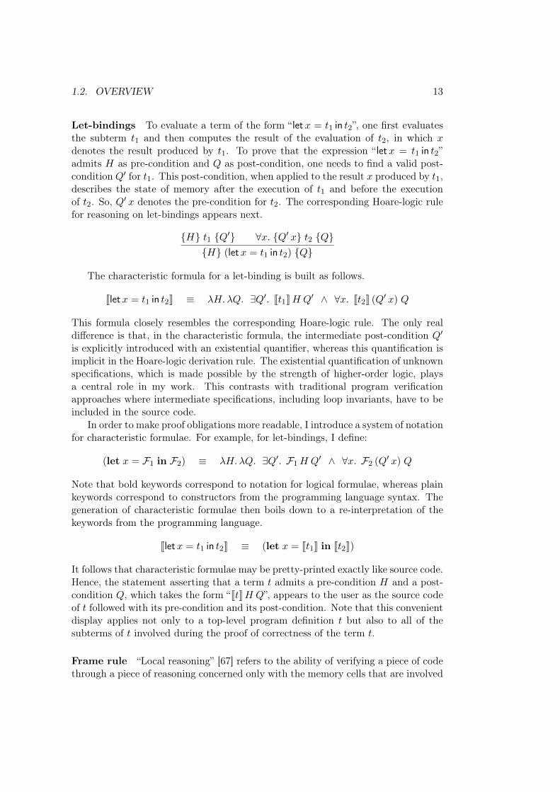
Let-bindings To evaluate a term of the form “ let𝑥 = 𝑡1 in 𝑡2”, one first evaluatesthe subterm 𝑡1 and then computes the result of the evaluation of 𝑡2, in which 𝑥denotes the result produced by 𝑡1. To prove that the expression “ let𝑥 = 𝑡1 in 𝑡2”admits 𝐻 as pre-condition and 𝑄 as post-condition, one needs to find a valid post-condition 𝑄′ for 𝑡1. This post-condition, when applied to the result 𝑥 produced by 𝑡1,describes the state of memory after the execution of 𝑡1 and before the executionof 𝑡2. So, 𝑄′ 𝑥 denotes the pre-condition for 𝑡2. The corresponding Hoare-logic rulefor reasoning on let-bindings appears next.
{𝐻} 𝑡1 {𝑄′} ∀𝑥. {𝑄′ 𝑥} 𝑡2 {𝑄}{𝐻} (let𝑥 = 𝑡1 in 𝑡2) {𝑄}
The characteristic formula for a let-binding is built as follows.
Jlet𝑥 = 𝑡1 in 𝑡2K ≡ 𝜆𝐻. 𝜆𝑄. ∃𝑄′. J𝑡1K𝐻 𝑄′ ∧ ∀𝑥. J𝑡2K (𝑄′ 𝑥) 𝑄
This formula closely resembles the corresponding Hoare-logic rule. The only realdifference is that, in the characteristic formula, the intermediate post-condition 𝑄′
is explicitly introduced with an existential quantifier, whereas this quantification isimplicit in the Hoare-logic derivation rule. The existential quantification of unknownspecifications, which is made possible by the strength of higher-order logic, playsa central role in my work. This contrasts with traditional program verificationapproaches where intermediate specifications, including loop invariants, have to beincluded in the source code.
In order to make proof obligations more readable, I introduce a system of notationfor characteristic formulae. For example, for let-bindings, I define:
(let 𝑥 = ℱ1 in ℱ2) ≡ 𝜆𝐻. 𝜆𝑄. ∃𝑄′. ℱ1𝐻 𝑄′ ∧ ∀𝑥. ℱ2 (𝑄′ 𝑥) 𝑄
Note that bold keywords correspond to notation for logical formulae, whereas plainkeywords correspond to constructors from the programming language syntax. Thegeneration of characteristic formulae then boils down to a re-interpretation of thekeywords from the programming language.
Jlet𝑥 = 𝑡1 in 𝑡2K ≡ (let 𝑥 = J𝑡1K in J𝑡2K)
It follows that characteristic formulae may be pretty-printed exactly like source code.Hence, the statement asserting that a term 𝑡 admits a pre-condition 𝐻 and a post-condition 𝑄, which takes the form “J𝑡K𝐻 𝑄”, appears to the user as the source codeof 𝑡 followed with its pre-condition and its post-condition. Note that this convenientdisplay applies not only to a top-level program definition 𝑡 but also to all of thesubterms of 𝑡 involved during the proof of correctness of the term 𝑡.
Frame rule “Local reasoning” [67] refers to the ability of verifying a piece of codethrough a piece of reasoning concerned only with the memory cells that are involved
14 CHAPTER 1. INTRODUCTION
in the execution of that code. With local reasoning, all the memory cells that arenot explicitly mentioned are implicitly assumed to remain unchanged. The conceptof local reasoning is very elegantly captured by the “frame rule”, which originates inSeparation Logic [77]. The frame rule states that if a program expression transformsa heap described by a predicate 𝐻1 into heap described by a predicate 𝐻 ′
1, then,for any heap predicate 𝐻2, the same program expression also transforms a heap ofthe form 𝐻1 *𝐻2 into a state described by 𝐻 ′
1 *𝐻2, where the star symbol, calledseparating conjunction, captures a disjoint union of two pieces of heap.
For example, consider the application of the function incr, which increments thecontents of the memory cell, to a location 𝑙. If (𝑙 →˓ 𝑛) describes a singleton heapthat binds the location 𝑙 to the integer 𝑛, then an application of the function increxpects a heap of the form (𝑙 →˓ 𝑛) and produces the heap (𝑙 →˓ 𝑛+1). By the framerule, one can deduce that the application of the function incr to 𝑙 also takes a heapof the form (𝑙 →˓ 𝑛) * (𝑙′ →˓ 𝑛′) towards a heap of the form (𝑙 →˓ 𝑛 + 1) * (𝑙′ →˓ 𝑛′).Here, the separating conjunction asserts that 𝑙′ is a location distinct from 𝑙. The useof the separating conjunction gives us for free the property that the cell at location𝑙′ is not modified when the contents of the cell at location 𝑙 is incremented.
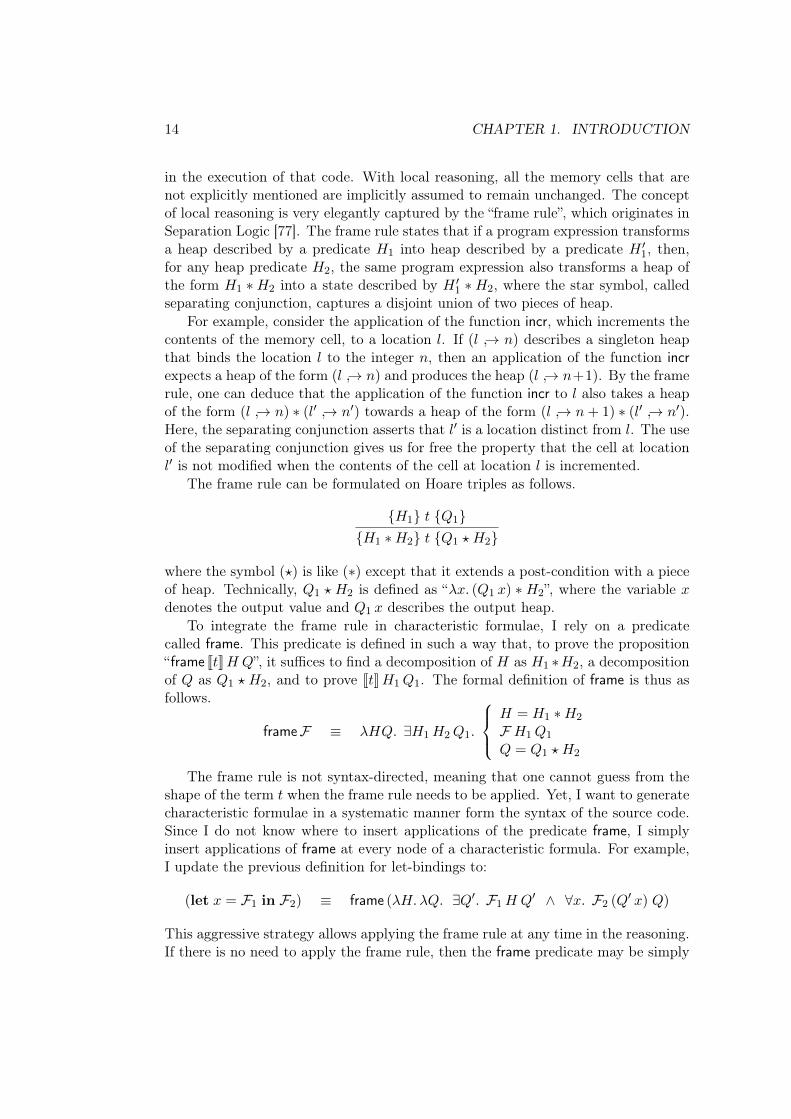
The frame rule can be formulated on Hoare triples as follows.
{𝐻1} 𝑡 {𝑄1}{𝐻1 *𝐻2} 𝑡 {𝑄1 ⋆ 𝐻2}
where the symbol (⋆) is like (*) except that it extends a post-condition with a pieceof heap. Technically, 𝑄1 ⋆ 𝐻2 is defined as “𝜆𝑥. (𝑄1 𝑥) * 𝐻2”, where the variable 𝑥denotes the output value and 𝑄1 𝑥 describes the output heap.
To integrate the frame rule in characteristic formulae, I rely on a predicatecalled frame. This predicate is defined in such a way that, to prove the proposition“frame J𝑡K𝐻 𝑄”, it suffices to find a decomposition of 𝐻 as 𝐻1 *𝐻2, a decompositionof 𝑄 as 𝑄1 ⋆ 𝐻2, and to prove J𝑡K𝐻1𝑄1. The formal definition of frame is thus asfollows.
frameℱ ≡ 𝜆𝐻𝑄. ∃𝐻1𝐻2𝑄1.
𝐻 = 𝐻1 *𝐻2
ℱ 𝐻1𝑄1
𝑄 = 𝑄1 ⋆ 𝐻2
The frame rule is not syntax-directed, meaning that one cannot guess from theshape of the term 𝑡 when the frame rule needs to be applied. Yet, I want to generatecharacteristic formulae in a systematic manner form the syntax of the source code.Since I do not know where to insert applications of the predicate frame, I simplyinsert applications of frame at every node of a characteristic formula. For example,I update the previous definition for let-bindings to:
(let 𝑥 = ℱ1 in ℱ2) ≡ frame (𝜆𝐻. 𝜆𝑄. ∃𝑄′. ℱ1𝐻 𝑄′ ∧ ∀𝑥. ℱ2 (𝑄′ 𝑥) 𝑄)
This aggressive strategy allows applying the frame rule at any time in the reasoning.If there is no need to apply the frame rule, then the frame predicate may be simply
1.2. OVERVIEW 15
ignored. Indeed, given a formula ℱ , the proposition “ℱ 𝐻 𝑄” is always a sufficientcondition for proving “frameℱ 𝐻 𝑄”. It suffices to instantiate 𝐻1 as 𝐻, 𝑄1 as 𝑄and 𝐻2 as a specification of the empty heap.
The approach that I have described here to handle the frame rule is in fact gener-alized so as to also handle applications of the rule of consequence, for strengtheningpre-conditions and weakening post-conditions, and to allow discarding memory cells,for simulating garbage collection.
Translation of types Higher-order logic can naturally be used to state propertiesabout basic values such as purely-functional lists. Indeed, the list data structure canbe defined in the logic in a way that perfectly matches the list data structure fromthe programming language. However, particular care is required for specifying andreasoning on program functions. Indeed, programming language functions cannotbe directly represented as logical functions, because of a mismatch between thetwo: program functions may diverge or crash whereas logical functions must alwaysterminate. To address this issue, I introduce a new data type, called Func, usedto represent functions. The type Func is presented as an abstract data type to theuser of characteristic formulae. In the proof of soundness, a value of type Func isinterpreted as the syntax of the source code of a function.
Another particularity of the reflection of Caml values into Coq values is thetreatment of pointers. When reasoning through characteristic formulae, the typeand the contents of memory cells are described explicitly by heap predicates, sothere is no need for pointers to carry the type of the memory cell they point to. Allpointers are therefore described in the logic through an abstract data type calledLoc. In the proof of soundness, a value of type Loc is interpreted as a store location.
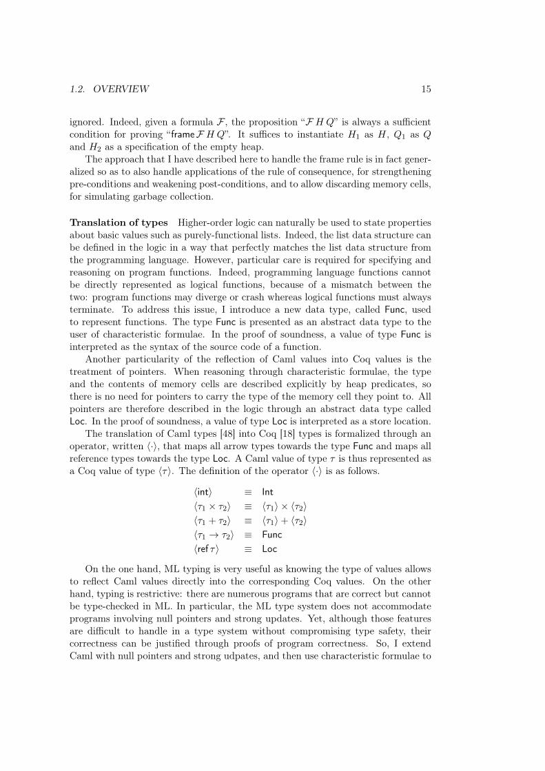
The translation of Caml types [48] into Coq [18] types is formalized through anoperator, written ⟨·⟩, that maps all arrow types towards the type Func and maps allreference types towards the type Loc. A Caml value of type 𝜏 is thus represented asa Coq value of type ⟨𝜏⟩. The definition of the operator ⟨·⟩ is as follows.
⟨int⟩ ≡ Int⟨𝜏1 × 𝜏2⟩ ≡ ⟨𝜏1⟩ × ⟨𝜏2⟩⟨𝜏1 + 𝜏2⟩ ≡ ⟨𝜏1⟩ + ⟨𝜏2⟩⟨𝜏1 → 𝜏2⟩ ≡ Func⟨ref 𝜏⟩ ≡ Loc
On the one hand, ML typing is very useful as knowing the type of values allowsto reflect Caml values directly into the corresponding Coq values. On the otherhand, typing is restrictive: there are numerous programs that are correct but cannotbe type-checked in ML. In particular, the ML type system does not accommodateprograms involving null pointers and strong updates. Yet, although those featuresare difficult to handle in a type system without compromising type safety, theircorrectness can be justified through proofs of program correctness. So, I extendCaml with null pointers and strong udpates, and then use characteristic formulae to
16 CHAPTER 1. INTRODUCTION
justify that null pointers are never dereferenced and that reads in memory alwaysyield a value of the expected type.
The correctness of this approach is however not entirely straightforward to jus-tify. On the one hand, characteristic formulae are generated from typed programs.On the other hand, the introduction of null pointers and strong updates may jeop-ardize the validity of types. To justify the soundness of characteristic formulae, Iintroduce a new type system called weak-ML. This type system does not enjoy typesoundness. However, it carries all the type information and invariants needed togenerate characteristic formulae and to prove them sound.
In short, weak-ML corresponds to a relaxed version of ML that does not keeptrack of the type of pointers or functions, and that does not impose any constrainton the typing of dereferencing and applications. The translation from Caml typesto Coq types is in fact conducted in two steps: a Caml type is first translated intoa weak-ML type, and this weak-ML type it then translated into a Coq type.
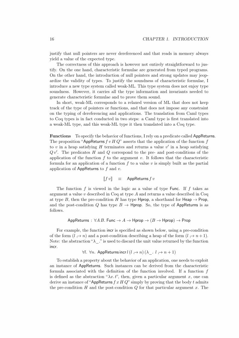
Functions To specify the behavior of functions, I rely on a predicate called AppReturns.The proposition “AppReturns 𝑓 𝑣 𝐻 𝑄” asserts that the application of the function 𝑓to 𝑣 in a heap satisfying 𝐻 terminates and returns a value 𝑣′ in a heap satisfying𝑄𝑣′. The predicates 𝐻 and 𝑄 correspond to the pre- and post-conditions of theapplication of the function 𝑓 to the argument 𝑣. It follows that the characteristicformula for an application of a function 𝑓 to a value 𝑣 is simply built as the partialapplication of AppReturns to 𝑓 and 𝑣.
J𝑓 𝑣K ≡ AppReturns 𝑓 𝑣
The function 𝑓 is viewed in the logic as a value of type Func. If 𝑓 takes asargument a value 𝑣 described in Coq at type 𝐴 and returns a value described in Coqat type 𝐵, then the pre-condition 𝐻 has type Hprop, a shorthand for Heap → Prop,and the post-condition 𝑄 has type 𝐵 → Hprop. So, the type of AppReturns is asfollows.
AppReturns : ∀𝐴𝐵. Func → 𝐴 → Hprop → (𝐵 → Hprop) → Prop
For example, the function incr is specified as shown below, using a pre-conditionof the form (𝑙 →˓ 𝑛) and a post-condition describing a heap of the form (𝑙 →˓ 𝑛+ 1).Note: the abstraction “𝜆_.” is used to discard the unit value returned by the functionincr.
∀𝑙. ∀𝑛. AppReturns incr 𝑙 (𝑙 →˓ 𝑛) (𝜆_. 𝑙 →˓ 𝑛 + 1)
To establish a property about the behavior of an application, one needs to exploitan instance of AppReturns. Such instances can be derived from the characteristicformula associated with the definition of the function involved. If a function 𝑓is defined as the abstraction “𝜆𝑥. 𝑡”, then, given a particular argument 𝑥, one canderive an instance of “AppReturns 𝑓 𝑥𝐻 𝑄” simply by proving that the body 𝑡 admitsthe pre-condition 𝐻 and the post-condition 𝑄 for that particular argument 𝑥. The
1.3. IMPLEMENTATION 17
characteristic formula of a function definition (let rec 𝑓 = 𝜆𝑥. 𝑡 in 𝑡′) is defined asfollows.
Jlet rec 𝑓 = 𝜆𝑥. 𝑡 in 𝑡′K ≡𝜆𝐻𝑄. ∀𝑓. (∀𝑥𝐻 ′𝑄′. J𝑡K𝐻 ′𝑄′ ⇒ AppReturns 𝑓 𝑥𝐻 ′𝑄′) ⇒ J𝑡′K𝐻 𝑄
Observe that the formula does not involve a specific treatment of recursivity.Indeed, to prove that a recursive function satisfies a given specification, it sufficesto conduct a proof by induction that the function indeed satisfies that specification.The induction may be conducted on a measure or on a well-founded relation, usingthe induction facility from the theorem prover. So, there is no need to strengthenthe characteristic formula in any way for supporting recursive functions. A similarobservation was also made by Honda et al [40].
1.3 Implementation
I have implemented a tool, called CFML, short for “Characteristic Formulae for ML”,that targets the verification of Caml programs [48] using the Coq proof assistant [18].This tool comprises two parts. The CFML generator is a program that translatesCaml source code into a set of Coq definitions and axioms. The CFML library isa Coq library that contains notation, lemmas and tactics for manipulating charac-teristic formulae. In this section, I describe precisely the fragment of the OCamllanguage supported by CFML, as well as the exact logic in which the reasoning oncharacteristic formulae is taking place. I also give an overview of the architecture ofCFML, and comment on its trusted computing base.
Source language I have focused on a subset of the OCaml programming lan-guage, which is a sequential, call-by-value, high-level programming language. Thecurrent implementation of CFML supports the core 𝜆-calculus, including higher-order functions, recursion, mutual recursion and polymorphic recursion. It supportstuples, data constructors, pattern matching, reference cells, records and arrays. Iprovide an additional Caml library that adds support for null pointers and strongupdates.
For the sake of simplicity, I model machine integers as mathematical integers,thus making the assumption that no arithmetic overflow ever occurs. Moreover, I donot include floating-point numbers, whose formalization is associated with numeroustechnical difficulties. Also, I assume the source language to be deterministic. Thisdeterminacy requirement might in fact be relaxed, but the formal developments wereslightly simpler to conduct under this assumption.
Lazy expressions are supported under the condition that the code would termi-nate without any lazy annotation. Although this restriction does not enable reason-ing on infinite data structures, it covers some uses of laziness, such as computationscheduling, which is exploited in particular in Okasaki’s data structures [69]. Infact, CFML simply ignores any annotation relative to laziness. Indeed, if a program
18 CHAPTER 1. INTRODUCTION
satisfies its specification when evaluated without any lazy annotation, then it alsosatisfies its specification when evaluated with lazy annotations. (The reciprocal isnot true.)
Moreover, CFML includes an experimental support for Caml modules and func-tors, which are reflected as Coq modules and functors. This development is stillconsidered experimental because of several limitations of the current module systemof Coq.1 Yet, the support for modules has shown useful in the verification of datastructures implemented using Caml functors.
Thereafter, I refer to the subset of the OCaml language supported by CFML as“Caml”.
Target logic When verifying programs through characteristic formulae, both thespecification process and the verification process take place in the logic. The logictargeted by CFML is the logic of Coq. More precisely, I work in the Calculusof Inductive Constructions, strengthened with the following standard extensions:functional extensionality, propositional extensionality, classical logic, and indefinitedescription (also called Hilbert’s epsilon operator). Note that the proof irrelevanceproperty is derivable in this setting.
Those axioms are all compatible with the standard boolean model of type theory.They are not included by default in Coq but they are integrated in other higher-order logic proof assistants such as Isabelle/HOL and HOL4. Remark: althoughthe CFML library is implemented in the Coq proof assistant, the developments itcontains could presumably be reproduced in another general-purpose proof assistantbased on higher-order logic.
The CFML generator The CFML generator starts by parsing a Caml sourcefile. This source code need not be annotated with any specification nor invariant.The tool then normalizes the source code in order to assign names to intermediateexpressions, that is, to make sequencing explicit. It then type-checks the code andgenerates a Coq file. This Coq file contains a set of declarations reflecting everytop-level declaration from the source code.
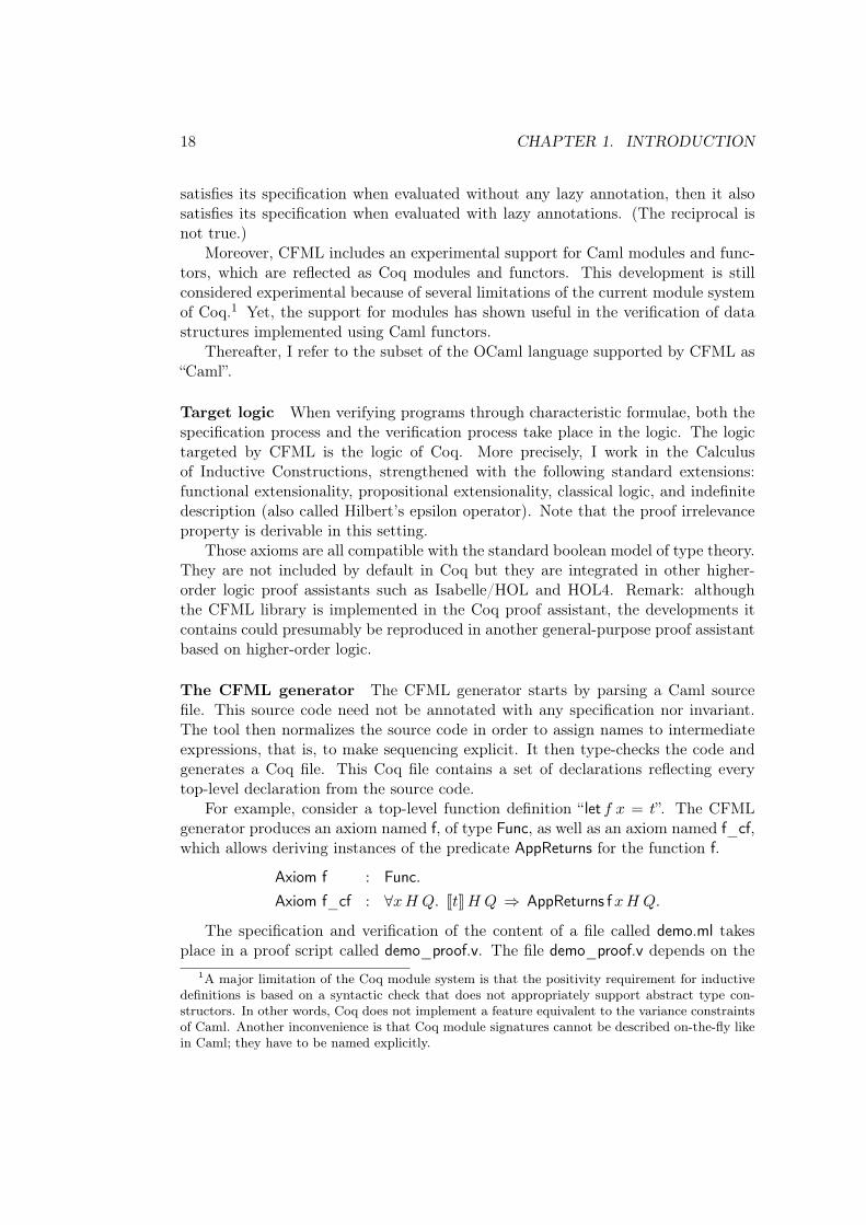
For example, consider a top-level function definition “ let 𝑓 𝑥 = 𝑡”. The CFMLgenerator produces an axiom named f, of type Func, as well as an axiom named f_cf,which allows deriving instances of the predicate AppReturns for the function f.
Axiom f : Func.Axiom f_cf : ∀𝑥𝐻 𝑄. J𝑡K𝐻 𝑄 ⇒ AppReturns f𝑥𝐻 𝑄.
The specification and verification of the content of a file called demo.ml takesplace in a proof script called demo_proof.v. The file demo_proof.v depends on the
1A major limitation of the Coq module system is that the positivity requirement for inductivedefinitions is based on a syntactic check that does not appropriately support abstract type con-structors. In other words, Coq does not implement a feature equivalent to the variance constraintsof Caml. Another inconvenience is that Coq module signatures cannot be described on-the-fly likein Caml; they have to be named explicitly.
1.3. IMPLEMENTATION 19
generated file, which is called demo_ml.v. When the source file demo.ml is modified,the CFML generator needs to be executed again, producing an updated demo_ml.vfile. The proof script from demo_proof.v, which records the arguments explainingwhy the previous version of demo.ml was correct, may need to be updated. To findout where modifications are required, it suffices to run the Coq proof assistant onthe proof script until the first point where a proof breaks. One can then fix theproof script so as to reflect the changes made in the source code.
The CFML library The CFML library is made of three main parts. First, itincludes a system of notation for pretty-printing characteristic formulae. Second, itincludes a number of lemmas for reasoning on the specification of functions. Third,it includes the definition of high-level tactics that are used to efficiently manipulatecharacteristic formuale.
The CFML library is built upon three axioms. The first one asserts the existenceof a type Func, which is used to represent functions. The second one asserts theexistence of a predicate AppEval, a low-level predicate in terms of which the predicateAppReturns is defined. Intuitively, the proposition AppEval 𝑓 𝑣 ℎ 𝑣′ ℎ′ corresponds tothe big-step reduction judgment for functions: it is equivalent to (𝑓 𝑣)/ℎ ⇓ 𝑣′/ℎ′ . Thethird axiom asserts that AppEval is deterministic: in the judgment AppEval 𝑓 𝑣 ℎ 𝑣′ ℎ′,the last two arguments are uniquely determined by the first three. The libraryalso includes axioms for describing the specification of the primitive functions formanipulating references. Through the proof of soundness, I establish that all thoseaxioms can be given a sound interpretation.
Trusted computing base The framework that I have developed aims at provingprograms correct. To trust that CFML actually establish the correctness of a pro-gram, one needs to trust that the characteristic formulae that I generate and thatI take as axioms are accurate descriptions of the programs they correspond to, andthat those axioms do not break the soundness of the target logic.
The trusted computing base of CFML also includes the implementation of theCFML generator, which I have programmed in OCaml, the implementation of theparser and of the type-checker of OCaml, and the implementation of the Coq proofassistant. To be exhaustive, I shall also mention that the correctness of the frame-work indirectly relies on the correctness of the complete OCaml compiler and on thecorrectness of the hardware.
The main priority of my thesis has been the development and implementation ofa practical tool for program verification. For this reason, I have not yet invested timein trying to construct a mechanized proof of the soundness of characteristic formulae.In this dissertation, I only give a detailed paper proof justifying that all the axiomsinvolved can be given a concrete interpretation in the logic. An interesting directionfor future work consists in trying to replace the axioms with definitions and lemmas,which would be expressed in terms of a deep embedding of the source language.
20 CHAPTER 1. INTRODUCTION
1.4 Contribution
The thesis that I defend is summarized in the following statement.
Generating the characteristic formula of a program and ex-ploiting that formula in an interactive proof assistant providesan effective approach to formally verifying that the programsatisfies a given specification.
A characteristic formula is a logical predicate that precisely describes the set ofspecifications admissible by a given program, without referring to the syntax ofthe programing language. I have not invented the general concept of characteristicformulae, however I have turned that concept into a practical program verificationtechnique. More precisely, the main contributions of my thesis may be summarizedas follows.
I show that characteristic formulae can be expressed in terms of a standardhigher-order logic. Moreover, I show that characteristic formulae can be pretty-printed just like the source code they describe. Hence, compared with Honda etal’s work, the characteristic formulae that I generate are easy to read and can bemanipulated within an off-the-shelf theorem prover. I also explain how characteristicformulae can support local reasoning. More precisely, I rely on separation-logicstyle predicates for specifying memory states, and the characteristic formulae that Igenerate take into account potential applications of the frame rule.
I demonstrate the effectiveness of characteristic formulae through the imple-mentation of a tool called CFML that accepts Caml programs and produces Coqdefinitions. I have used CFML to verify a collection of purely-functional data struc-tures taken from Okasaki’s book on purely-functional data structures [69]. Someadvanced structures, such as bootstrapped queues, had never been formally verifiedpreviously.
I have investigated the treatment of higher-order imperative functions. In par-ticular, I have verified the following functions: a higher-order iterator for lists, afunction that manipulates a list of counters in which each counter is a function thatcarries its own private state, the generic combinator compose, and Reynolds’ CPS-append function [77]. More recently, I have verified three imperative algorithms: animplementation of Dijkstra’s shortest path algorithm (the version of the algorithmthat uses a priority queue), an implementation of Tarjan’s Union-Find data structure(specified with respect to a partial equivalence relations), and an implementation ofsparse arrays (as described in the first task from the Vacid-0 challenge [78]). Thosedevelopments, which are not described in this manuscript, can be found online2.
2Proof scripts: http://arthur.chargueraud.org/research/2010/thesis/
1.5. RESEARCH AND PUBLICATIONS 21
1.5 Research and publications
During my thesis, I have worked on three main projects. First, I have studied atype system based on linear capabilities for describing mutable state. This typesystem has been described in an ICFP’08 paper, and it is not included in my disser-tation. Second, I have worked on a deep embedding of the pure fragment of Camlin Coq. This deep embedding is described in a research paper which has not beenpublished. The work on the deep embedding led me to characteristic formulae forpurely-functional Caml programs. This work has appeared as an ICFP’10 paper.Most of the content of that paper is included in my dissertation. I have recentlyextended characteristic formulae to imperative programs, reusing in particular ideasthat had been developed for the type system based on capabilities. At the time ofwriting, the extension of characteristic formulae to the imperative setting has notyet been submitted as a conference paper.
Previous research papers:
− Functional Translation of a Calculus of Capabilities,Arthur Charguéraud and François Pottier,International Conference on Functional Programming (ICFP), 2008.
− Verification of Functional Programs Through a Deep Embedding,Arthur Charguéraud,Unpublished, 2009.
− Program Verification Through Characteristic Formulae,Arthur Charguéraud,International Conference on Functional Programming (ICFP), 2010.
1.6 Structure of the dissertation
The thesis is structured as follows. Examples of verification through characteristicformulae is described in Chapter 2 for pure programs, and in Chapter 3 for imper-ative programs. The construction of characteristic formulae for pure programs isdeveloped in Chapter 4. This construction is then generalized to imperative pro-grams in Chapter 5. The proof of soundness and completeness of characteristicformulae for pure programs is the matter of Chapter 6. Those proofs are then ex-tended to an imperative setting in Chapter 7. Finally, related work is discussed inChapter 8, and conclusions are given in Chapter 9.
Notice: several predicates are used with a different meaning in the context ofpurely-functional programs than in the context of imperative programs. For ex-ample, the big-step reduction judgment for pure programs takes the form 𝑡 ⇓ 𝑣,whereas the judgment for imperative programs takes the form 𝑡/𝑚 ⇓ 𝑣′/𝑚′ . Simi-larly, reasoning on applications in a purely-functional setting involves the predicate
22 CHAPTER 1. INTRODUCTION
“AppReturns 𝑓 𝑣 𝑃 ”, whereas in an imperative setting the same predicate takes theform “AppReturns 𝑓 𝑣 𝐻 𝑄”. This reuse of predicate names, which makes the presen-tation lighter and more uniform, should not lead to confusion since a given predicateis always used in a consistent manner in each chapter.
Chapter 2
Overview and specifications
The purpose of this overview is to give some intuition on how to constructa characteristic formula and how to exploit it. To that end, I considera small but illustrative purely-functional function as running example.Another goal of the chapter is to explain the specification language uponwhich I rely. Specifications take the form of Coq lemmas, stated usingspecial predicates as well as a layer of notation. The specification ofmodules and functors is illustrated through the presentation of a casestudy on purely-functional red-black trees.
2.1 Characteristic formulae for pure programs
In a purely-functional setting, the characteristic formulae J𝑡K associated with a term𝑡 is such that, for any given post-condition 𝑃 , the proposition “J𝑡K𝑃 ” holds if andonly if the term 𝑡 terminates and returns a value satisfying the predicate 𝑃 . Notethat reasoning on the total correctness of pure programs can be conducted with-out pre-conditions. In terms of types, the characteristic formula associated with aterm 𝑡 of type 𝜏 applies to a post-condition 𝑃 of type ⟨𝜏⟩ → Prop and produces aproposition, so J𝑡K admits the type (⟨𝜏⟩ → Prop) → Prop. In terms of a denotationalinterpretation, J𝑡K corresponds to the set of post-conditions that are valid for theterm 𝑡. I next describe an example of a characteristic formula.
2.1.1 Example of a characteristic formula
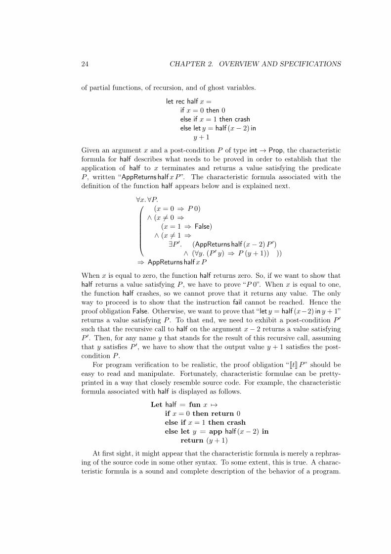
Consider the following recursive function, which divides by two any non-negativeeven integer. For the interest of the example, the function diverges when called on anegative integer and crashes when called on an odd integer. Through this example, Ipresent the construction of characteristic formulae and also illustrate the treatment
23
24 CHAPTER 2. OVERVIEW AND SPECIFICATIONS
of partial functions, of recursion, and of ghost variables.
let rec half 𝑥 =if 𝑥 = 0 then 0else if 𝑥 = 1 then crashelse let 𝑦 = half (𝑥− 2) in
𝑦 + 1
Given an argument 𝑥 and a post-condition 𝑃 of type int → Prop, the characteristicformula for half describes what needs to be proved in order to establish that theapplication of half to 𝑥 terminates and returns a value satisfying the predicate𝑃 , written “AppReturns half𝑥𝑃 ”. The characteristic formula associated with thedefinition of the function half appears below and is explained next.
∀𝑥. ∀𝑃.
(𝑥 = 0 ⇒ 𝑃 0)∧ (𝑥 ̸= 0 ⇒
(𝑥 = 1 ⇒ False)∧ (𝑥 ̸= 1 ⇒
∃𝑃 ′. (AppReturns half (𝑥− 2)𝑃 ′)∧ (∀𝑦. (𝑃 ′ 𝑦) ⇒ 𝑃 (𝑦 + 1)) ))
⇒ AppReturns half𝑥𝑃
When 𝑥 is equal to zero, the function half returns zero. So, if we want to show thathalf returns a value satisfying 𝑃 , we have to prove “𝑃 0”. When 𝑥 is equal to one,the function half crashes, so we cannot prove that it returns any value. The onlyway to proceed is to show that the instruction fail cannot be reached. Hence theproof obligation False. Otherwise, we want to prove that “ let 𝑦 = half (𝑥−2) in 𝑦 + 1”returns a value satisfying 𝑃 . To that end, we need to exhibit a post-condition 𝑃 ′
such that the recursive call to half on the argument 𝑥− 2 returns a value satisfying𝑃 ′. Then, for any name 𝑦 that stands for the result of this recursive call, assumingthat 𝑦 satisfies 𝑃 ′, we have to show that the output value 𝑦 + 1 satisfies the post-condition 𝑃 .
For program verification to be realistic, the proof obligation “J𝑡K𝑃 ” should beeasy to read and manipulate. Fortunately, characteristic formulae can be pretty-printed in a way that closely resemble source code. For example, the characteristicformula associated with half is displayed as follows.
Let half = fun 𝑥 ↦→if 𝑥 = 0 then return 0else if 𝑥 = 1 then crashelse let 𝑦 = app half (𝑥− 2) in
return (𝑦 + 1)
At first sight, it might appear that the characteristic formula is merely a rephras-ing of the source code in some other syntax. To some extent, this is true. A charac-teristic formula is a sound and complete description of the behavior of a program.
2.1. CHARACTERISTIC FORMULAE FOR PURE PROGRAMS 25
Thus, it carries no more and no less information than the source code of the pro-gram itself. However, characteristic formulae enable us to move away from programsyntax and conduct program verification entirely at the logical level. Characteristicformulae thereby avoid all the technical difficulties associated with manipulation ofprogram syntax and make it possible to work directly in terms of higher-order logicvalues and formulae.
2.1.2 Specification and verification
One of the key ingredients involved in characteristic formulae is the abstract pred-icate AppReturns, which is used to specify functions. Because of the mismatch be-tween program functions, which may fail or diverge, and logical functions, whichmust always be total, we cannot represent program functions using logical func-tions. For this reason, I introduce an abstract type, named Func, to representprogram functions. Values of type Func are exclusively specified in terms of thepredicate AppReturns. The proposition “AppReturns 𝑓 𝑥𝑃 ” states that the applica-tion of the function 𝑓 to an argument 𝑥 terminates and returns a value satisfying𝑃 . Hence the type of AppReturns, shown below.
AppReturns : ∀𝐴𝐵. Func → 𝐴 → (𝐵 → Prop) → Prop
Observe a function 𝑓 is described in Coq at the type Func, regardless of Caml type ofthe function 𝑓 . Having Func as a constant type and not a parametric type allows fora simple treatment of polymorphic functions and of functions that admit a recursivetype.
The predicate AppReturns is used not only in the definition of characteristicformulae but also in the statement of specifications. One possible specification forhalf is the following: if 𝑥 is the double of some non-negative integer 𝑛, then theapplication of half to 𝑥 returns an integer equal to 𝑛. The corresponding higher-order logic statement appears next.
∀𝑥. ∀𝑛. 𝑛 ≥ 0 ⇒ 𝑥 = 2 * 𝑛 ⇒ AppReturns half𝑥 (= 𝑛)
Remark: the post-condition (= 𝑛) denotes a partial application of equality: it isshort for “𝜆𝑎. (𝑎 = 𝑛)”. Here, the value 𝑛 corresponds to a ghost variable: it appearsin the specification of the function but not in its source code. The specificationthat I have considered for half might not be the simplest one, however it is useful toillustrate the treatment of ghost variables.
The next step consists in proving that the function half satisfies its specification.This is done by exploiting its characteristic formula. I first give the mathematicalpresentation of the proof and then show the corresponding Coq proof script. Thespecification is proved by induction on 𝑥. Let 𝑥 and 𝑛 be such that 𝑛 ≥ 0 and𝑥 = 2 *𝑛. We apply the characteristic formula to prove “AppReturns half𝑥 (= 𝑛)”. If𝑥 is equal to 0, we conclude by showing that 𝑛 is equal to 0. If 𝑥 is equal to 1, weshow that 𝑥 = 2 * 𝑛 is absurd. Otherwise, 𝑥 ≥ 2. We instantiate 𝑃 ′ as “= 𝑛 − 1”,
26 CHAPTER 2. OVERVIEW AND SPECIFICATIONS
and prove “AppReturns half (𝑥 − 2)𝑃 ′” using the induction hypothesis. Finally, weshow that, for any 𝑦 such that 𝑦 = 𝑛 − 1, the proposition 𝑦 + 1 = 𝑛 holds. Thiscompletes the proof. Note that, through this proof by induction, we have provedthat the function half terminates when it is applied to a non-negative even integer.
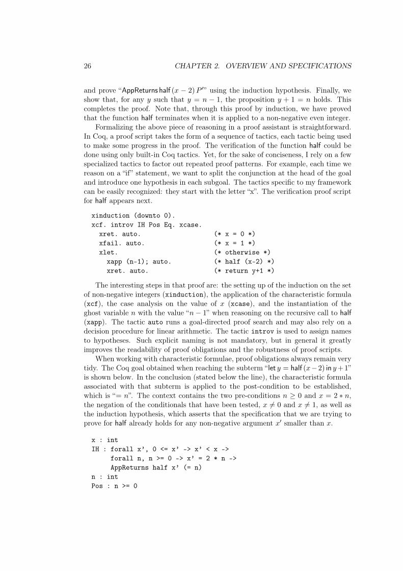
Formalizing the above piece of reasoning in a proof assistant is straightforward.In Coq, a proof script takes the form of a sequence of tactics, each tactic being usedto make some progress in the proof. The verification of the function half could bedone using only built-in Coq tactics. Yet, for the sake of conciseness, I rely on a fewspecialized tactics to factor out repeated proof patterns. For example, each time wereason on a “if” statement, we want to split the conjunction at the head of the goaland introduce one hypothesis in each subgoal. The tactics specific to my frameworkcan be easily recognized: they start with the letter “x”. The verification proof scriptfor half appears next.
xinduction (downto 0).xcf. introv IH Pos Eq. xcase.
xret. auto. (* x = 0 *)xfail. auto. (* x = 1 *)xlet. (* otherwise *)
xapp (n-1); auto. (* half (x-2) *)xret. auto. (* return y+1 *)
The interesting steps in that proof are: the setting up of the induction on the setof non-negative integers (xinduction), the application of the characteristic formula(xcf), the case analysis on the value of 𝑥 (xcase), and the instantiation of theghost variable 𝑛 with the value “𝑛− 1” when reasoning on the recursive call to half(xapp). The tactic auto runs a goal-directed proof search and may also rely on adecision procedure for linear arithmetic. The tactic introv is used to assign namesto hypotheses. Such explicit naming is not mandatory, but in general it greatlyimproves the readability of proof obligations and the robustness of proof scripts.
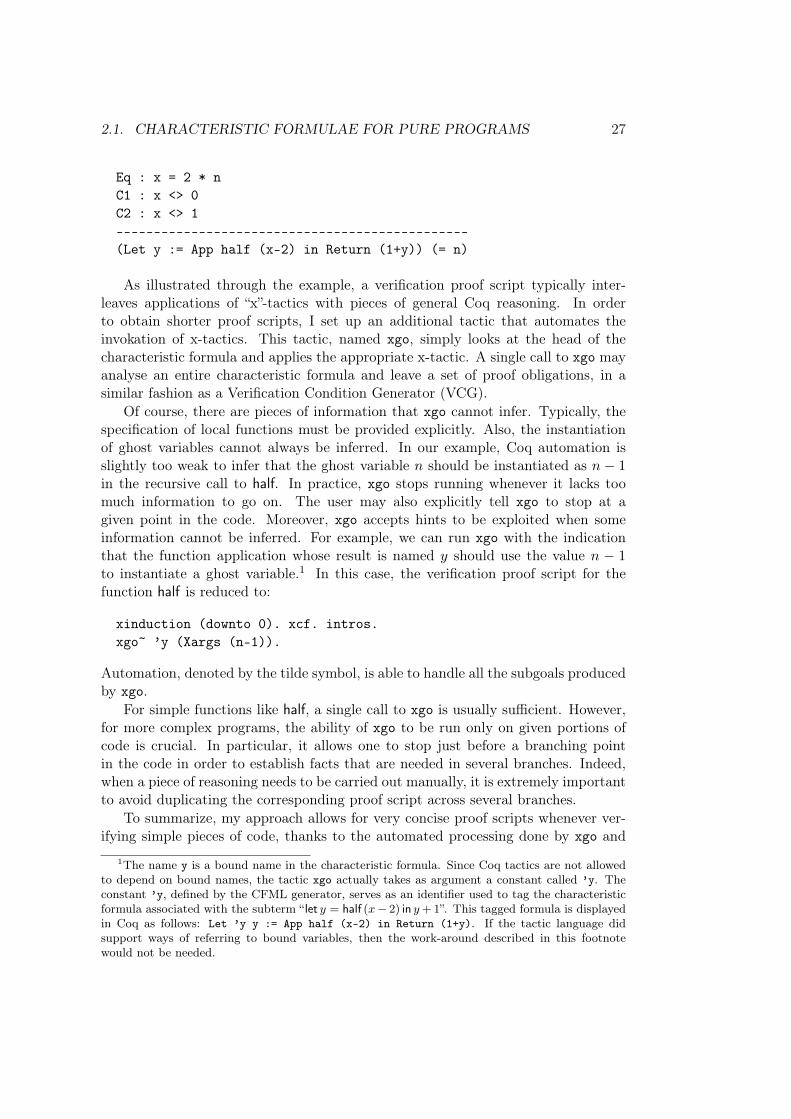
When working with characteristic formulae, proof obligations always remain verytidy. The Coq goal obtained when reaching the subterm “ let 𝑦 = half (𝑥−2) in 𝑦+ 1”is shown below. In the conclusion (stated below the line), the characteristic formulaassociated with that subterm is applied to the post-condition to be established,which is “= 𝑛”. The context contains the two pre-conditions 𝑛 ≥ 0 and 𝑥 = 2 * 𝑛,the negation of the conditionals that have been tested, 𝑥 ̸= 0 and 𝑥 ̸= 1, as well asthe induction hypothesis, which asserts that the specification that we are trying toprove for half already holds for any non-negative argument 𝑥′ smaller than 𝑥.
x : intIH : forall x’, 0 <= x’ -> x’ < x ->
forall n, n >= 0 -> x’ = 2 * n ->AppReturns half x’ (= n)
n : intPos : n >= 0
2.1. CHARACTERISTIC FORMULAE FOR PURE PROGRAMS 27
Eq : x = 2 * nC1 : x <> 0C2 : x <> 1-----------------------------------------------(Let y := App half (x-2) in Return (1+y)) (= n)
As illustrated through the example, a verification proof script typically inter-leaves applications of “x”-tactics with pieces of general Coq reasoning. In orderto obtain shorter proof scripts, I set up an additional tactic that automates theinvokation of x-tactics. This tactic, named xgo, simply looks at the head of thecharacteristic formula and applies the appropriate x-tactic. A single call to xgo mayanalyse an entire characteristic formula and leave a set of proof obligations, in asimilar fashion as a Verification Condition Generator (VCG).
Of course, there are pieces of information that xgo cannot infer. Typically, thespecification of local functions must be provided explicitly. Also, the instantiationof ghost variables cannot always be inferred. In our example, Coq automation isslightly too weak to infer that the ghost variable 𝑛 should be instantiated as 𝑛− 1in the recursive call to half. In practice, xgo stops running whenever it lacks toomuch information to go on. The user may also explicitly tell xgo to stop at agiven point in the code. Moreover, xgo accepts hints to be exploited when someinformation cannot be inferred. For example, we can run xgo with the indicationthat the function application whose result is named 𝑦 should use the value 𝑛 − 1to instantiate a ghost variable.1 In this case, the verification proof script for thefunction half is reduced to:
xinduction (downto 0). xcf. intros.xgo~ ’y (Xargs (n-1)).
Automation, denoted by the tilde symbol, is able to handle all the subgoals producedby xgo.
For simple functions like half, a single call to xgo is usually sufficient. However,for more complex programs, the ability of xgo to be run only on given portions ofcode is crucial. In particular, it allows one to stop just before a branching pointin the code in order to establish facts that are needed in several branches. Indeed,when a piece of reasoning needs to be carried out manually, it is extremely importantto avoid duplicating the corresponding proof script across several branches.
To summarize, my approach allows for very concise proof scripts whenever ver-ifying simple pieces of code, thanks to the automated processing done by xgo and
1The name y is a bound name in the characteristic formula. Since Coq tactics are not allowedto depend on bound names, the tactic xgo actually takes as argument a constant called ’y. Theconstant ’y, defined by the CFML generator, serves as an identifier used to tag the characteristicformula associated with the subterm “ let 𝑦 = half (𝑥− 2) in 𝑦+1”. This tagged formula is displayedin Coq as follows: Let ’y y := App half (x-2) in Return (1+y). If the tactic language didsupport ways of referring to bound variables, then the work-around described in this footnotewould not be needed.
28 CHAPTER 2. OVERVIEW AND SPECIFICATIONS
module type Fset = sig | module type Ordered = sigtype elem | type ttype fset | val lt: t -> t -> boolval empty: fset | endval insert: elem -> fset -> fset |val member: elem -> fset -> bool |
end |
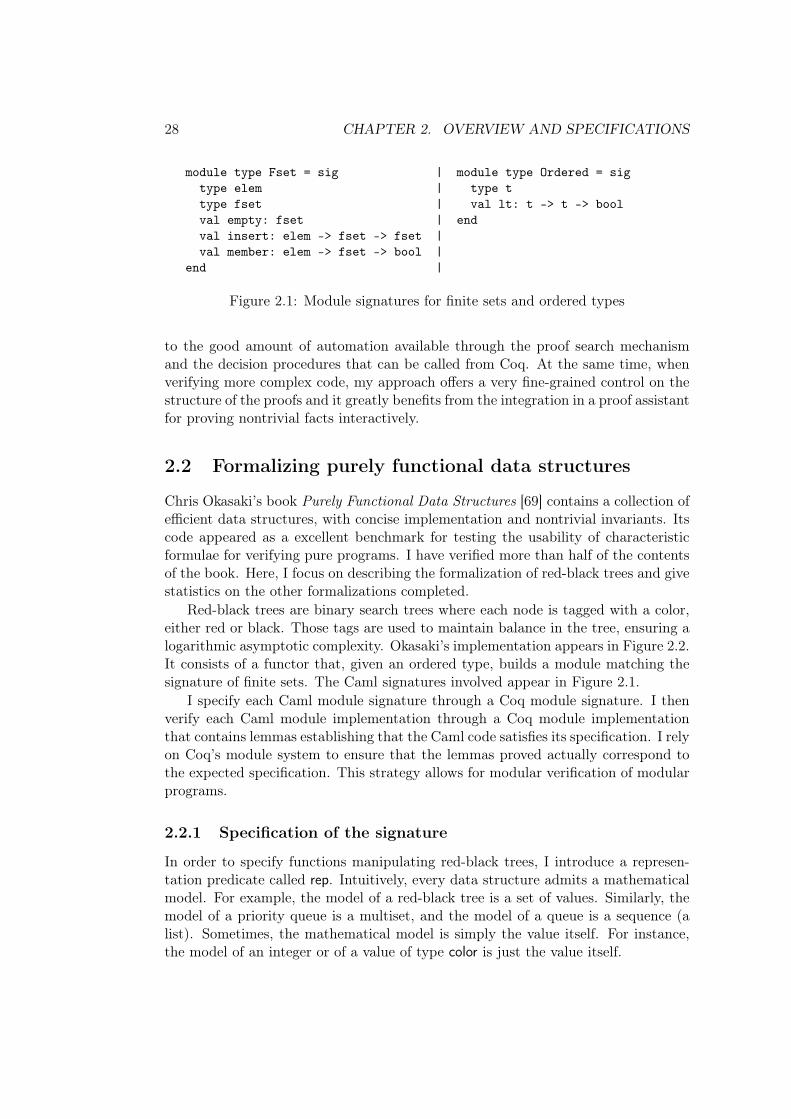
Figure 2.1: Module signatures for finite sets and ordered types
to the good amount of automation available through the proof search mechanismand the decision procedures that can be called from Coq. At the same time, whenverifying more complex code, my approach offers a very fine-grained control on thestructure of the proofs and it greatly benefits from the integration in a proof assistantfor proving nontrivial facts interactively.
2.2 Formalizing purely functional data structures
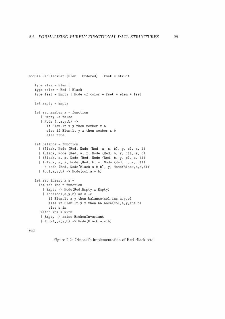
Chris Okasaki’s book Purely Functional Data Structures [69] contains a collection ofefficient data structures, with concise implementation and nontrivial invariants. Itscode appeared as a excellent benchmark for testing the usability of characteristicformulae for verifying pure programs. I have verified more than half of the contentsof the book. Here, I focus on describing the formalization of red-black trees and givestatistics on the other formalizations completed.
Red-black trees are binary search trees where each node is tagged with a color,either red or black. Those tags are used to maintain balance in the tree, ensuring alogarithmic asymptotic complexity. Okasaki’s implementation appears in Figure 2.2.It consists of a functor that, given an ordered type, builds a module matching thesignature of finite sets. The Caml signatures involved appear in Figure 2.1.
I specify each Caml module signature through a Coq module signature. I thenverify each Caml module implementation through a Coq module implementationthat contains lemmas establishing that the Caml code satisfies its specification. I relyon Coq’s module system to ensure that the lemmas proved actually correspond tothe expected specification. This strategy allows for modular verification of modularprograms.
2.2.1 Specification of the signature
In order to specify functions manipulating red-black trees, I introduce a represen-tation predicate called rep. Intuitively, every data structure admits a mathematicalmodel. For example, the model of a red-black tree is a set of values. Similarly, themodel of a priority queue is a multiset, and the model of a queue is a sequence (alist). Sometimes, the mathematical model is simply the value itself. For instance,the model of an integer or of a value of type color is just the value itself.
2.2. FORMALIZING PURELY FUNCTIONAL DATA STRUCTURES 29
module RedBlackSet (Elem : Ordered) : Fset = struct
type elem = Elem.ttype color = Red | Blacktype fset = Empty | Node of color * fset * elem * fset
let empty = Empty
let rec member x = function| Empty -> false| Node (_,a,y,b) ->
if Elem.lt x y then member x aelse if Elem.lt y x then member x belse true
let balance = function| (Black, Node (Red, Node (Red, a, x, b), y, c), z, d)| (Black, Node (Red, a, x, Node (Red, b, y, c)), z, d)| (Black, a, x, Node (Red, Node (Red, b, y, c), z, d))| (Black, a, x, Node (Red, b, y, Node (Red, c, z, d)))
-> Node (Red, Node(Black,a,x,b), y, Node(Black,c,z,d))| (col,a,y,b) -> Node(col,a,y,b)
let rec insert x s =let rec ins = function
| Empty -> Node(Red,Empty,x,Empty)| Node(col,a,y,b) as s ->
if Elem.lt x y then balance(col,ins a,y,b)else if Elem.lt y x then balance(col,a,y,ins b)else s in
match ins s with| Empty -> raise BrokenInvariant| Node(_,a,y,b) -> Node(Black,a,y,b)
end
Figure 2.2: Okasaki’s implementation of Red-Black sets
30 CHAPTER 2. OVERVIEW AND SPECIFICATIONS
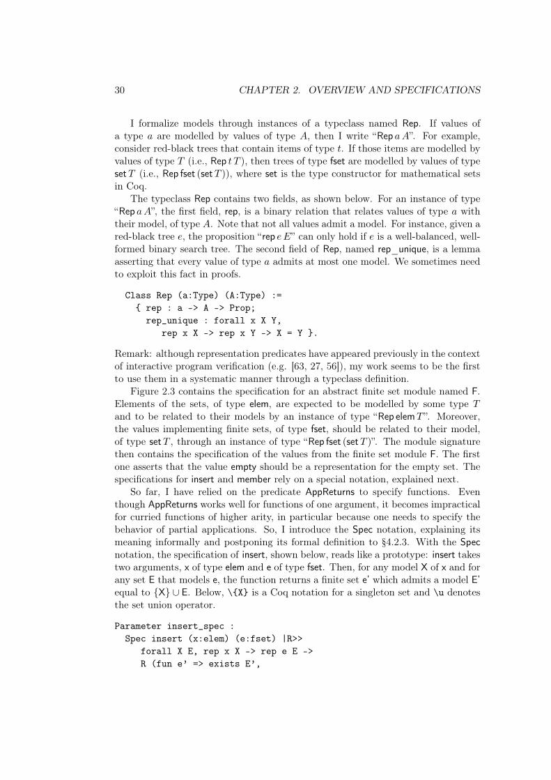
I formalize models through instances of a typeclass named Rep. If values ofa type 𝑎 are modelled by values of type 𝐴, then I write “Rep 𝑎𝐴”. For example,consider red-black trees that contain items of type 𝑡. If those items are modelled byvalues of type 𝑇 (i.e., Rep 𝑡 𝑇 ), then trees of type fset are modelled by values of typeset𝑇 (i.e., Rep fset (set𝑇 )), where set is the type constructor for mathematical setsin Coq.
The typeclass Rep contains two fields, as shown below. For an instance of type“Rep 𝑎𝐴”, the first field, rep, is a binary relation that relates values of type 𝑎 withtheir model, of type 𝐴. Note that not all values admit a model. For instance, given ared-black tree 𝑒, the proposition “rep 𝑒𝐸” can only hold if 𝑒 is a well-balanced, well-formed binary search tree. The second field of Rep, named rep_unique, is a lemmaasserting that every value of type 𝑎 admits at most one model. We sometimes needto exploit this fact in proofs.
Class Rep (a:Type) (A:Type) :={ rep : a -> A -> Prop;
rep_unique : forall x X Y,rep x X -> rep x Y -> X = Y }.
Remark: although representation predicates have appeared previously in the contextof interactive program verification (e.g. [63, 27, 56]), my work seems to be the firstto use them in a systematic manner through a typeclass definition.
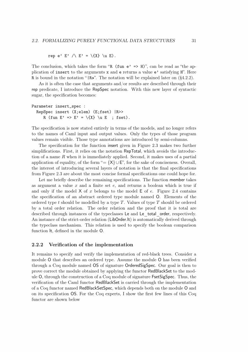
Figure 2.3 contains the specification for an abstract finite set module named F.Elements of the sets, of type elem, are expected to be modelled by some type 𝑇and to be related to their models by an instance of type “Rep elem𝑇 ”. Moreover,the values implementing finite sets, of type fset, should be related to their model,of type set𝑇 , through an instance of type “Rep fset (set𝑇 )”. The module signaturethen contains the specification of the values from the finite set module F. The firstone asserts that the value empty should be a representation for the empty set. Thespecifications for insert and member rely on a special notation, explained next.
So far, I have relied on the predicate AppReturns to specify functions. Eventhough AppReturns works well for functions of one argument, it becomes impracticalfor curried functions of higher arity, in particular because one needs to specify thebehavior of partial applications. So, I introduce the Spec notation, explaining itsmeaning informally and postponing its formal definition to §4.2.3. With the Specnotation, the specification of insert, shown below, reads like a prototype: insert takestwo arguments, x of type elem and e of type fset. Then, for any model X of x and forany set E that models e, the function returns a finite set e’ which admits a model E’equal to {X} ∪ E. Below, \{X} is a Coq notation for a singleton set and \u denotesthe set union operator.
Parameter insert_spec :Spec insert (x:elem) (e:fset) |R>>
forall X E, rep x X -> rep e E ->R (fun e’ => exists E’,
2.2. FORMALIZING PURELY FUNCTIONAL DATA STRUCTURES 31
rep e’ E’ /\ E’ = \{X} \u E).
The conclusion, which takes the form “R (fun e’ => H)”, can be read as “the ap-plication of insert to the arguments x and e returns a value e’ satisfying H”. HereR is bound in the notation “|R»”. The notation will be explained later on (§4.2.2).
As it is often the case that arguments and/or results are described through theirrep predicate, I introduce the RepSpec notation. With this new layer of syntacticsugar, the specification becomes:
Parameter insert_spec :RepSpec insert (X;elem) (E;fset) |R>>
R (fun E’ => E’ = \{X} \u E ; fset).
The specification is now stated entirely in terms of the models, and no longer refersto the names of Caml input and output values. Only the types of those programvalues remain visible. Those type annotations are introduced by semi-columns.
The specification for the function insert given in Figure 2.3 makes two furthersimplifications. First, it relies on the notation RepTotal, which avoids the introduc-tion of a name 𝑅 when it is immediately applied. Second, it makes uses of a partialapplication of equality, of the form “= {X}∪E”, for the sake of conciseness. Overall,the interest of introducing several layers of notation is that the final specificationsfrom Figure 2.3 are about the most concise formal specifications one could hope for.
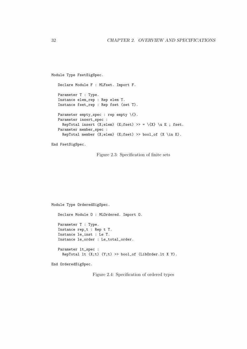
Let me briefly describe the remaining specifications. The function member takesas argument a value 𝑥 and a finite set 𝑒, and returns a boolean which is true ifand only if the model X of 𝑥 belongs to the model E of 𝑒. Figure 2.4 containsthe specification of an abstract ordered type module named O. Elements of theordered type 𝑡 should be modelled by a type 𝑇 . Values of type 𝑇 should be orderedby a total order relation. The order relation and the proof that it is total aredescribed through instances of the typeclasses Le and Le_total_order, respectively.An instance of the strict-order relation (LibOrder.lt) is automatically derived throughthe typeclass mechanism. This relation is used to specify the boolean comparisonfunction lt, defined in the module O.
2.2.2 Verification of the implementation
It remains to specify and verify the implementation of red-black trees. Consider amodule O that describes an ordered type. Assume the module O has been verifiedthrough a Coq module named OS of signature OrderedSigSpec. Our goal is then toprove correct the module obtained by applying the functor RedBlackSet to the mod-ule O, through the construction of a Coq module of signature FsetSigSpec. Thus, theverification of the Caml functor RedBlackSet is carried through the implementationof a Coq functor named RedBlackSetSpec, which depends both on the module O andon its specification OS. For the Coq experts, I show the first few lines of this Coqfunctor are shown below
32 CHAPTER 2. OVERVIEW AND SPECIFICATIONS
Module Type FsetSigSpec.
Declare Module F : MLFset. Import F.
Parameter T : Type.Instance elem_rep : Rep elem T.Instance fset_rep : Rep fset (set T).
Parameter empty_spec : rep empty \{}.Parameter insert_spec :
RepTotal insert (X;elem) (E;fset) >> = \{X} \u E ; fset.Parameter member_spec :
RepTotal member (X;elem) (E;fset) >> bool_of (X \in E).
End FsetSigSpec.
Figure 2.3: Specification of finite sets
Module Type OrderedSigSpec.
Declare Module O : MLOrdered. Import O.
Parameter T : Type.Instance rep_t : Rep t T.Instance le_inst : Le T.Instance le_order : Le_total_order.
Parameter lt_spec :RepTotal lt (X;t) (Y;t) >> bool_of (LibOrder.lt X Y).
End OrderedSigSpec.
Figure 2.4: Specification of ordered types
2.2. FORMALIZING PURELY FUNCTIONAL DATA STRUCTURES 33
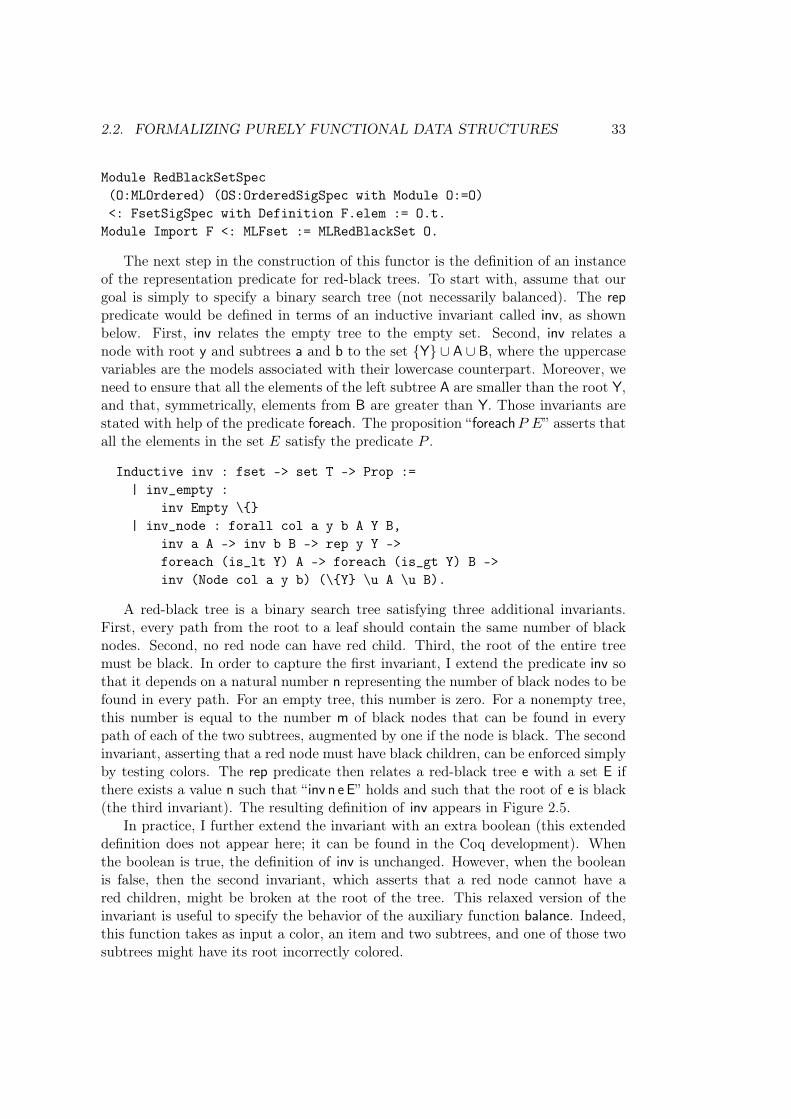
Module RedBlackSetSpec(O:MLOrdered) (OS:OrderedSigSpec with Module O:=O)<: FsetSigSpec with Definition F.elem := O.t.
Module Import F <: MLFset := MLRedBlackSet O.
The next step in the construction of this functor is the definition of an instanceof the representation predicate for red-black trees. To start with, assume that ourgoal is simply to specify a binary search tree (not necessarily balanced). The reppredicate would be defined in terms of an inductive invariant called inv, as shownbelow. First, inv relates the empty tree to the empty set. Second, inv relates anode with root y and subtrees a and b to the set {Y} ∪ A ∪ B, where the uppercasevariables are the models associated with their lowercase counterpart. Moreover, weneed to ensure that all the elements of the left subtree A are smaller than the root Y,and that, symmetrically, elements from B are greater than Y. Those invariants arestated with help of the predicate foreach. The proposition “foreach𝑃 𝐸” asserts thatall the elements in the set 𝐸 satisfy the predicate 𝑃 .
Inductive inv : fset -> set T -> Prop :=| inv_empty :
inv Empty \{}| inv_node : forall col a y b A Y B,
inv a A -> inv b B -> rep y Y ->foreach (is_lt Y) A -> foreach (is_gt Y) B ->inv (Node col a y b) (\{Y} \u A \u B).
A red-black tree is a binary search tree satisfying three additional invariants.First, every path from the root to a leaf should contain the same number of blacknodes. Second, no red node can have red child. Third, the root of the entire treemust be black. In order to capture the first invariant, I extend the predicate inv sothat it depends on a natural number n representing the number of black nodes to befound in every path. For an empty tree, this number is zero. For a nonempty tree,this number is equal to the number m of black nodes that can be found in everypath of each of the two subtrees, augmented by one if the node is black. The secondinvariant, asserting that a red node must have black children, can be enforced simplyby testing colors. The rep predicate then relates a red-black tree e with a set E ifthere exists a value n such that “ inv n e E” holds and such that the root of e is black(the third invariant). The resulting definition of inv appears in Figure 2.5.
In practice, I further extend the invariant with an extra boolean (this extendeddefinition does not appear here; it can be found in the Coq development). Whenthe boolean is true, the definition of inv is unchanged. However, when the booleanis false, then the second invariant, which asserts that a red node cannot have ared children, might be broken at the root of the tree. This relaxed version of theinvariant is useful to specify the behavior of the auxiliary function balance. Indeed,this function takes as input a color, an item and two subtrees, and one of those twosubtrees might have its root incorrectly colored.
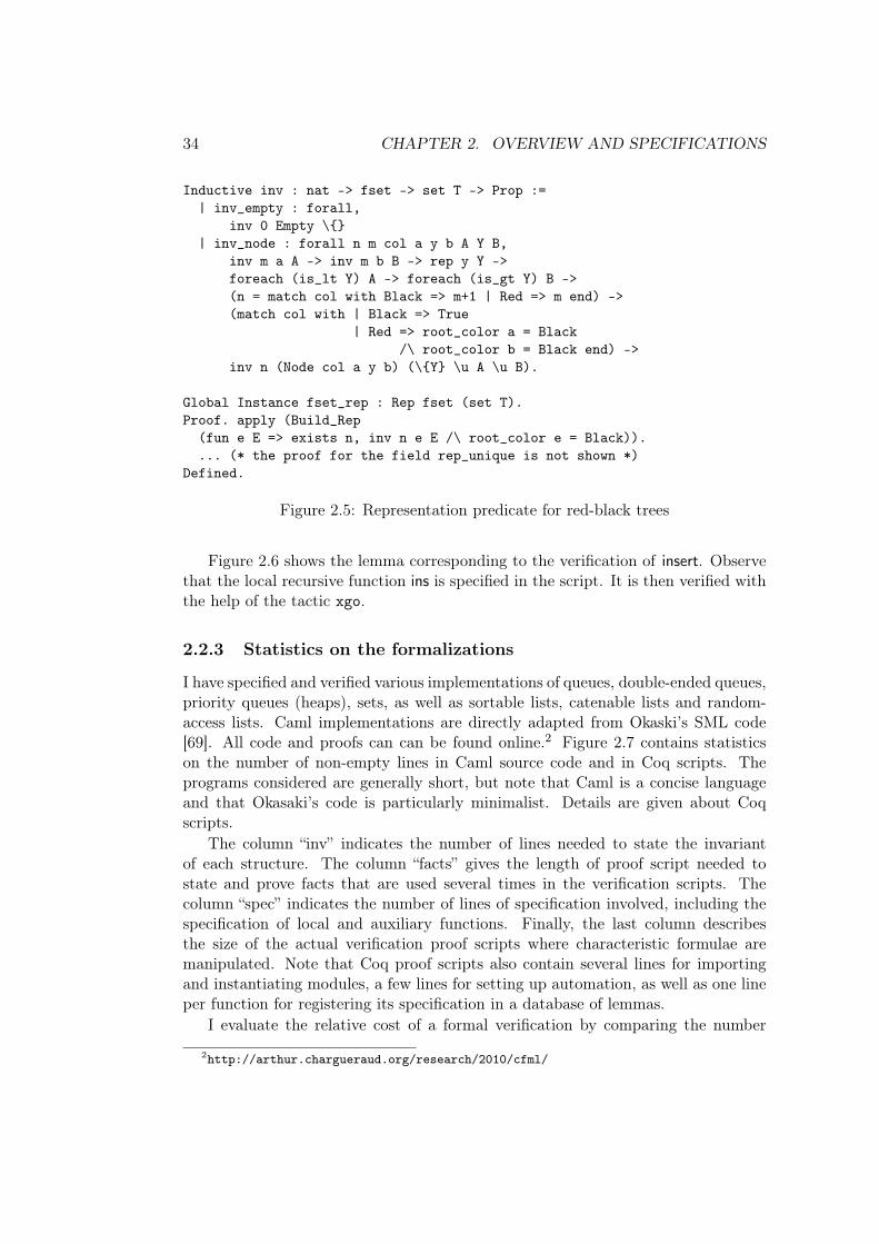
34 CHAPTER 2. OVERVIEW AND SPECIFICATIONS
Inductive inv : nat -> fset -> set T -> Prop :=| inv_empty : forall,
inv 0 Empty \{}| inv_node : forall n m col a y b A Y B,
inv m a A -> inv m b B -> rep y Y ->foreach (is_lt Y) A -> foreach (is_gt Y) B ->(n = match col with Black => m+1 | Red => m end) ->(match col with | Black => True
| Red => root_color a = Black/\ root_color b = Black end) ->
inv n (Node col a y b) (\{Y} \u A \u B).
Global Instance fset_rep : Rep fset (set T).Proof. apply (Build_Rep
(fun e E => exists n, inv n e E /\ root_color e = Black)).... (* the proof for the field rep_unique is not shown *)
Defined.
Figure 2.5: Representation predicate for red-black trees
Figure 2.6 shows the lemma corresponding to the verification of insert. Observethat the local recursive function ins is specified in the script. It is then verified withthe help of the tactic xgo.
2.2.3 Statistics on the formalizations
I have specified and verified various implementations of queues, double-ended queues,priority queues (heaps), sets, as well as sortable lists, catenable lists and random-access lists. Caml implementations are directly adapted from Okaski’s SML code[69]. All code and proofs can can be found online.2 Figure 2.7 contains statisticson the number of non-empty lines in Caml source code and in Coq scripts. Theprograms considered are generally short, but note that Caml is a concise languageand that Okasaki’s code is particularly minimalist. Details are given about Coqscripts.
The column “inv” indicates the number of lines needed to state the invariantof each structure. The column “facts” gives the length of proof script needed tostate and prove facts that are used several times in the verification scripts. Thecolumn “spec” indicates the number of lines of specification involved, including thespecification of local and auxiliary functions. Finally, the last column describesthe size of the actual verification proof scripts where characteristic formulae aremanipulated. Note that Coq proof scripts also contain several lines for importingand instantiating modules, a few lines for setting up automation, as well as one lineper function for registering its specification in a database of lemmas.
I evaluate the relative cost of a formal verification by comparing the number
2http://arthur.chargueraud.org/research/2010/cfml/
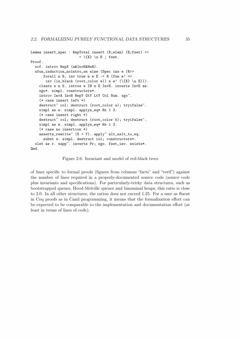
2.2. FORMALIZING PURELY FUNCTIONAL DATA STRUCTURES 35
Lemma insert_spec : RepTotal insert (X;elem) (E;fset) >>= \{X} \u E ; fset.
Proof.xcf. introv RepX (n&InvE&HeB).xfun_induction_nointro_on size (Spec ins e |R>>
forall n E, inv true n e E -> R (fun e’ =>inv (is_black (root_color e)) n e’ (\{X} \u E))).
clears s n E. intros e IH n E InvE. inverts InvE as.xgo*. simpl. constructors*.introv InvA InvB RepY GtY LtY Col Num. xgo~.(* case insert left *)destruct~ col; destruct (root_color a); tryifalse~.ximpl as e. simpl. applys_eq* Hx 1 3.(* case insert right *)destruct~ col; destruct (root_color b); tryifalse~.ximpl as e. simpl. applys_eq* Hx 1 3.(* case no insertion *)asserts_rewrite~ (X = Y). apply~ nlt_nslt_to_eq.
subst s. simpl. destruct col; constructors*.xlet as r. xapp~. inverts Pr; xgo. fset_inv. exists*.
Qed.
Figure 2.6: Invariant and model of red-black trees
of lines specific to formal proofs (figures from columns “facts” and “verif”) againstthe number of lines required in a properly-documented source code (source codeplus invariants and specifications). For particularly-tricky data structures, such asbootstrapped queues, Hood-Melville queues and binominal heaps, this ratio is closeto 2.0. In all other structures, the ration does not exceed 1.25. For a user as fluentin Coq proofs as in Caml programming, it means that the formalization effort canbe expected to be comparable to the implementation and documentation effort (atleast in terms of lines of code).
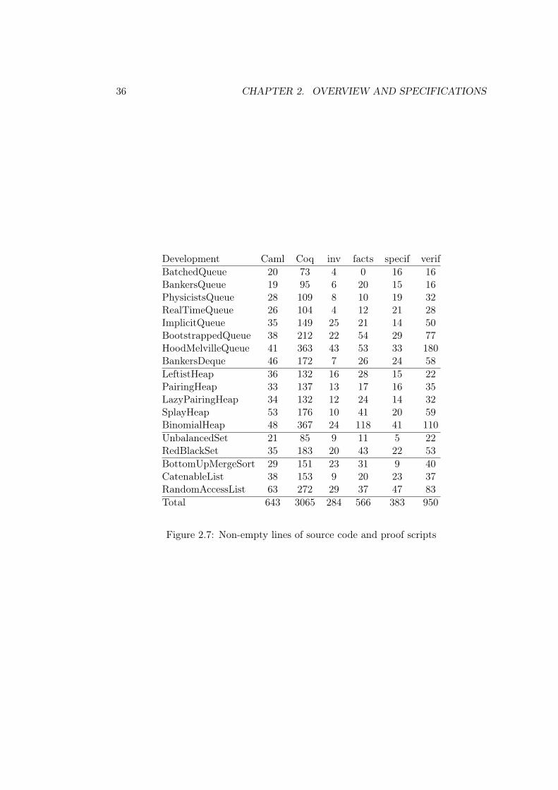
36 CHAPTER 2. OVERVIEW AND SPECIFICATIONS
Development Caml Coq inv facts specif verifBatchedQueue 20 73 4 0 16 16BankersQueue 19 95 6 20 15 16PhysicistsQueue 28 109 8 10 19 32RealTimeQueue 26 104 4 12 21 28ImplicitQueue 35 149 25 21 14 50BootstrappedQueue 38 212 22 54 29 77HoodMelvilleQueue 41 363 43 53 33 180BankersDeque 46 172 7 26 24 58LeftistHeap 36 132 16 28 15 22PairingHeap 33 137 13 17 16 35LazyPairingHeap 34 132 12 24 14 32SplayHeap 53 176 10 41 20 59BinomialHeap 48 367 24 118 41 110UnbalancedSet 21 85 9 11 5 22RedBlackSet 35 183 20 43 22 53BottomUpMergeSort 29 151 23 31 9 40CatenableList 38 153 9 20 23 37RandomAccessList 63 272 29 37 47 83Total 643 3065 284 566 383 950
Figure 2.7: Non-empty lines of source code and proof scripts
Chapter 3
Verification of imperativeprograms
This chapter contains an overview of the treatment of imperative pro-grams. After introducing some notation for specifying heaps, I presentthe specification of the primitive functions for manipulating references,and I explain the treatment of for-loops and while-loops, using loop in-variants. I then introduce representation predicates for mutable datastructures, focusing on mutable lists to illustrate the definition and ma-nipulation of such predicates. I study the example of a function thatcomputes the length of a mutable list and explain why reasoning onloops using invariants does not take advantage of local reasoning. I thenpresent a different treatment of loops. Finally, I explain the treatmentof higher-order functions and that of functions with local state.
3.1 Examples of imperative functions
3.1.1 Notation for heap predicates
I start by describing informally the combinators for constructing heap predicates,which have type Hprop. Formal definitions are postponed to §5.2.1. The emptyheap is written [ ] and the spatial conjunction of two heaps is written 𝐻1 *𝐻2. Thepredicate “𝑙 →˓𝒯 𝑣” describes a reference cell 𝑙 whose contents is described in Coqas the value 𝑣 of type 𝒯 . Since the type 𝒯 can be deduced from the value 𝑣, Ioften omit it and write “𝑙 →˓ 𝑣”. A more general predicate for describing mutabledata structures, written “𝑙 𝑇 𝑣”, is explained further on. I lift propositions andexistentials into heap predicates as follows. The predicate [𝑃 ] holds of the emptyheap when the proposition 𝑃 is true. The predicate ∃∃𝑥.𝐻 holds of a heap ℎ ifthere exists a value 𝑥 such that the predicate 𝐻 holds of ℎ (note that 𝑥 is bound in𝐻). The corresponding ASCII notations, which are used in Coq statements, appearbelow.
37
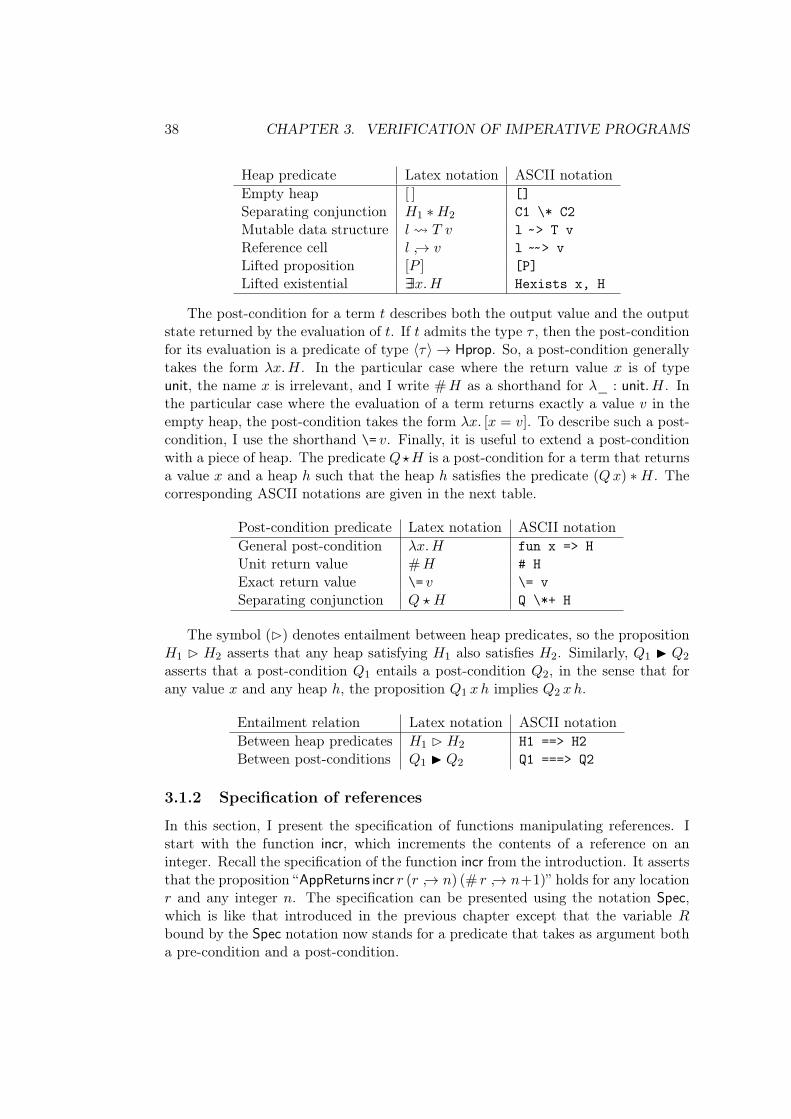
38 CHAPTER 3. VERIFICATION OF IMPERATIVE PROGRAMS
Heap predicate Latex notation ASCII notationEmpty heap [ ] []Separating conjunction 𝐻1 *𝐻2 C1 \* C2Mutable data structure 𝑙 𝑇 𝑣 l ˜> T vReference cell 𝑙 →˓ 𝑣 l ˜̃ > vLifted proposition [𝑃 ] [P]Lifted existential ∃∃𝑥.𝐻 Hexists x, H
The post-condition for a term 𝑡 describes both the output value and the outputstate returned by the evaluation of 𝑡. If 𝑡 admits the type 𝜏 , then the post-conditionfor its evaluation is a predicate of type ⟨𝜏⟩ → Hprop. So, a post-condition generallytakes the form 𝜆𝑥.𝐻. In the particular case where the return value 𝑥 is of typeunit, the name 𝑥 is irrelevant, and I write #𝐻 as a shorthand for 𝜆_ : unit. 𝐻. Inthe particular case where the evaluation of a term returns exactly a value 𝑣 in theempty heap, the post-condition takes the form 𝜆𝑥. [𝑥 = 𝑣]. To describe such a post-condition, I use the shorthand \= 𝑣. Finally, it is useful to extend a post-conditionwith a piece of heap. The predicate 𝑄⋆𝐻 is a post-condition for a term that returnsa value 𝑥 and a heap ℎ such that the heap ℎ satisfies the predicate (𝑄𝑥) *𝐻. Thecorresponding ASCII notations are given in the next table.
Post-condition predicate Latex notation ASCII notationGeneral post-condition 𝜆𝑥.𝐻 fun x => HUnit return value #𝐻 # HExact return value \= 𝑣 \= vSeparating conjunction 𝑄 ⋆ 𝐻 Q \*+ H
The symbol (B) denotes entailment between heap predicates, so the proposition𝐻1 B 𝐻2 asserts that any heap satisfying 𝐻1 also satisfies 𝐻2. Similarly, 𝑄1 I 𝑄2
asserts that a post-condition 𝑄1 entails a post-condition 𝑄2, in the sense that forany value 𝑥 and any heap ℎ, the proposition 𝑄1 𝑥ℎ implies 𝑄2 𝑥ℎ.
Entailment relation Latex notation ASCII notationBetween heap predicates 𝐻1 B 𝐻2 H1 ==> H2Between post-conditions 𝑄1 I 𝑄2 Q1 ===> Q2
3.1.2 Specification of references
In this section, I present the specification of functions manipulating references. Istart with the function incr, which increments the contents of a reference on aninteger. Recall the specification of the function incr from the introduction. It assertsthat the proposition “AppReturns incr 𝑟 (𝑟 →˓ 𝑛) (# 𝑟 →˓ 𝑛+1)” holds for any location𝑟 and any integer 𝑛. The specification can be presented using the notation Spec,which is like that introduced in the previous chapter except that the variable 𝑅bound by the Spec notation now stands for a predicate that takes as argument botha pre-condition and a post-condition.
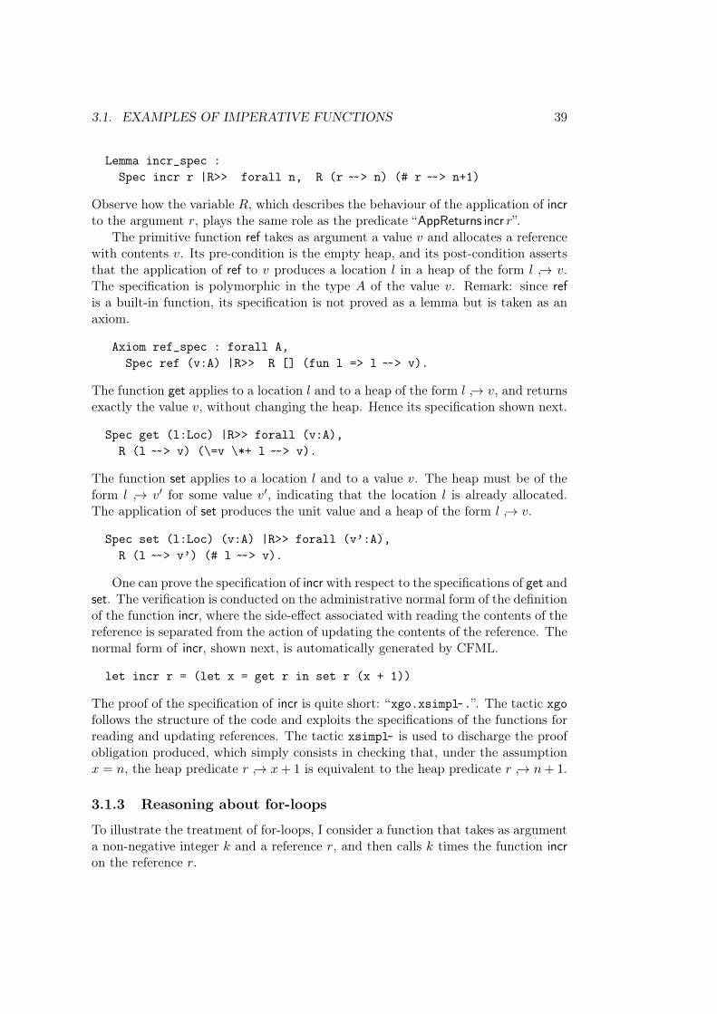
3.1. EXAMPLES OF IMPERATIVE FUNCTIONS 39
Lemma incr_spec :Spec incr r |R>> forall n, R (r ˜̃ > n) (# r ˜̃ > n+1)
Observe how the variable 𝑅, which describes the behaviour of the application of incrto the argument 𝑟, plays the same role as the predicate “AppReturns incr 𝑟”.
The primitive function ref takes as argument a value 𝑣 and allocates a referencewith contents 𝑣. Its pre-condition is the empty heap, and its post-condition assertsthat the application of ref to 𝑣 produces a location 𝑙 in a heap of the form 𝑙 →˓ 𝑣.The specification is polymorphic in the type 𝐴 of the value 𝑣. Remark: since refis a built-in function, its specification is not proved as a lemma but is taken as anaxiom.
Axiom ref_spec : forall A,Spec ref (v:A) |R>> R [] (fun l => l ˜̃ > v).
The function get applies to a location 𝑙 and to a heap of the form 𝑙 →˓ 𝑣, and returnsexactly the value 𝑣, without changing the heap. Hence its specification shown next.
Spec get (l:Loc) |R>> forall (v:A),R (l ˜̃ > v) (\=v \*+ l ˜̃ > v).
The function set applies to a location 𝑙 and to a value 𝑣. The heap must be of theform 𝑙 →˓ 𝑣′ for some value 𝑣′, indicating that the location 𝑙 is already allocated.The application of set produces the unit value and a heap of the form 𝑙 →˓ 𝑣.
Spec set (l:Loc) (v:A) |R>> forall (v’:A),R (l ˜̃ > v’) (# l ˜̃ > v).
One can prove the specification of incr with respect to the specifications of get andset. The verification is conducted on the administrative normal form of the definitionof the function incr, where the side-effect associated with reading the contents of thereference is separated from the action of updating the contents of the reference. Thenormal form of incr, shown next, is automatically generated by CFML.
let incr r = (let x = get r in set r (x + 1))
The proof of the specification of incr is quite short: “xgo.xsimpl̃ .”. The tactic xgofollows the structure of the code and exploits the specifications of the functions forreading and updating references. The tactic xsimpl̃ is used to discharge the proofobligation produced, which simply consists in checking that, under the assumption𝑥 = 𝑛, the heap predicate 𝑟 →˓ 𝑥 + 1 is equivalent to the heap predicate 𝑟 →˓ 𝑛 + 1.
3.1.3 Reasoning about for-loops
To illustrate the treatment of for-loops, I consider a function that takes as argumenta non-negative integer 𝑘 and a reference 𝑟, and then calls 𝑘 times the function incron the reference 𝑟.
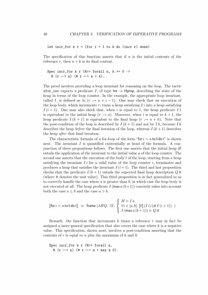
40 CHAPTER 3. VERIFICATION OF IMPERATIVE PROGRAMS
let incr_for k r = (for i = 1 to k do (incr r) done)
The specification of this function asserts that if 𝑛 is the initial contents of thereference 𝑟, then 𝑛 + 𝑘 is its final content.
Spec incr_for k r |R>> forall n, k >= 0 ->R (r ˜̃ > n) (# r ˜̃ > n + k).
The proof involves providing a loop invariant for reasoning on the loop. The tacticxfor_inv expects a predicate 𝐼, of type Int → Hprop, describing the state of theheap in terms of the loop counter. In the example, the appropriate loop invariant,called 𝐼, is defined as 𝜆𝑖. (𝑟 →˓ 𝑛 + 𝑖 − 1). One may check that an execution ofthe loop body, which increments 𝑟, turns a heap satisfying 𝐼 𝑖 into a heap satisfying𝐼 (𝑖 + 1). One may also check that, when 𝑖 is equal to 1, the heap predicate 𝐼 1is equivalent to the initial heap (𝑟 →˓ 𝑛). Moreover, when 𝑖 is equal to 𝑘 + 1, theheap predicate 𝐼 (𝑘 + 1) is equivalent to the final heap (𝑟 →˓ 𝑛 + 𝑘). Note thatthe post-condition of the loop is described by 𝐼 (𝑘 + 1) and not by 𝐼 𝑘, because 𝐼 𝑘describes the heap before the final iteration of the loop, whereas 𝐼 (𝑘 + 1) describesthe heap after that final iteration.
The characteristic formula of a for-loop of the form “for 𝑖 = 𝑎 to 𝑏 do 𝑡” is shownnext. The invariant 𝐼 is quantified existentially at head of the formula. A con-junction of three propositions follows. The first one asserts that the initial heap 𝐻entails the application of the invariant to the initial value 𝑎 of the loop counter. Thesecond one asserts that the execution of the body 𝑡 of the loop, starting from a heapsatisfying the invariant 𝐼 𝑖 for a valid value of the loop counter 𝑖, terminates andproduces a heap that satisfies the invariant 𝐼 (𝑖+ 1). The third and last propositionchecks that the predicate 𝐼 (𝑏 + 1) entails the expected final heap description 𝑄 tt(where tt denotes the unit value). This third proposition is in fact generalized so asto correctly handle the case where 𝑎 is greater than 𝑏, in which case the loop body isnot executed at all. The heap predicate 𝐼 (max 𝑎 (𝑏+1)) concisely takes into accountboth the case 𝑎 ≤ 𝑏 and the case 𝑎 > 𝑏.
Jfor 𝑖 = 𝑎 to 𝑏 do 𝑡K ≡ frame (𝜆𝐻𝑄. ∃𝐼.
𝐻 B 𝐼 𝑎∀𝑖 ∈ [𝑎, 𝑏]. J𝑡K (𝐼 𝑖) (# 𝐼 (𝑖 + 1))𝐼 (max 𝑎 (𝑏 + 1)) B 𝑄 tt
)
Remark: the function that increments 𝑘 times a reference 𝑟 may in fact beassigned a more general specification that also covers the case where 𝑘 is a negativevalue. This specification, shown next, involves a post-condition asserting that thecontents of 𝑟 is equal to 𝑛 plus the maximum of 𝑘 and 0.
Spec incr_for k r |R>> forall n,R (r ˜̃ > n) (# r ˜̃ > n + max k 0).
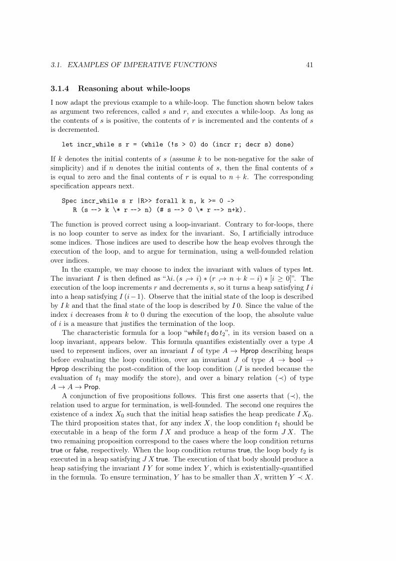
3.1. EXAMPLES OF IMPERATIVE FUNCTIONS 41
3.1.4 Reasoning about while-loops
I now adapt the previous example to a while-loop. The function shown below takesas argument two references, called 𝑠 and 𝑟, and executes a while-loop. As long asthe contents of 𝑠 is positive, the contents of 𝑟 is incremented and the contents of 𝑠is decremented.
let incr_while s r = (while (!s > 0) do (incr r; decr s) done)
If 𝑘 denotes the initial contents of 𝑠 (assume 𝑘 to be non-negative for the sake ofsimplicity) and if 𝑛 denotes the initial contents of 𝑠, then the final contents of 𝑠is equal to zero and the final contents of 𝑟 is equal to 𝑛 + 𝑘. The correspondingspecification appears next.
Spec incr_while s r |R>> forall k n, k >= 0 ->R (s ˜̃ > k \* r ˜̃ > n) (# s ˜̃ > 0 \* r ˜̃ > n+k).
The function is proved correct using a loop-invariant. Contrary to for-loops, thereis no loop counter to serve as index for the invariant. So, I artificially introducesome indices. Those indices are used to describe how the heap evolves through theexecution of the loop, and to argue for termination, using a well-founded relationover indices.
In the example, we may choose to index the invariant with values of types Int.The invariant 𝐼 is then defined as “𝜆𝑖. (𝑠 →˓ 𝑖) * (𝑟 →˓ 𝑛 + 𝑘 − 𝑖) * [𝑖 ≥ 0]”. Theexecution of the loop increments 𝑟 and decrements 𝑠, so it turns a heap satisfying 𝐼 𝑖into a heap satisfying 𝐼 (𝑖−1). Observe that the initial state of the loop is describedby 𝐼 𝑘 and that the final state of the loop is described by 𝐼 0. Since the value of theindex 𝑖 decreases from 𝑘 to 0 during the execution of the loop, the absolute valueof 𝑖 is a measure that justifies the termination of the loop.
The characteristic formula for a loop “while 𝑡1 do 𝑡2”, in its version based on aloop invariant, appears below. This formula quantifies existentially over a type 𝐴used to represent indices, over an invariant 𝐼 of type 𝐴 → Hprop describing heapsbefore evaluating the loop condition, over an invariant 𝐽 of type 𝐴 → bool →Hprop describing the post-condition of the loop condition (𝐽 is needed because theevaluation of 𝑡1 may modify the store), and over a binary relation (≺) of type𝐴 → 𝐴 → Prop.
A conjunction of five propositions follows. This first one asserts that (≺), therelation used to argue for termination, is well-founded. The second one requires theexistence of a index 𝑋0 such that the initial heap satisfies the heap predicate 𝐼 𝑋0.The third proposition states that, for any index 𝑋, the loop condition 𝑡1 should beexecutable in a heap of the form 𝐼 𝑋 and produce a heap of the form 𝐽 𝑋. Thetwo remaining proposition correspond to the cases where the loop condition returnstrue or false, respectively. When the loop condition returns true, the loop body 𝑡2 isexecuted in a heap satisfying 𝐽 𝑋 true. The execution of that body should produce aheap satisfying the invariant 𝐼 𝑌 for some index 𝑌 , which is existentially-quantifiedin the formula. To ensure termination, 𝑌 has to be smaller than 𝑋, written 𝑌 ≺ 𝑋.
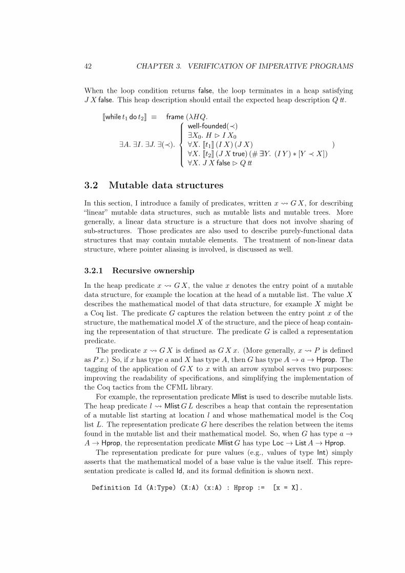
42 CHAPTER 3. VERIFICATION OF IMPERATIVE PROGRAMS
When the loop condition returns false, the loop terminates in a heap satisfying𝐽 𝑋 false. This heap description should entail the expected heap description 𝑄 tt .
Jwhile 𝑡1 do 𝑡2K ≡ frame (𝜆𝐻𝑄.
∃𝐴. ∃𝐼. ∃𝐽. ∃(≺).
well-founded(≺)∃𝑋0. 𝐻 B 𝐼 𝑋0
∀𝑋. J𝑡1K (𝐼 𝑋) (𝐽 𝑋)∀𝑋. J𝑡2K (𝐽 𝑋 true) (#∃∃𝑌. (𝐼 𝑌 ) * [𝑌 ≺ 𝑋])∀𝑋. 𝐽 𝑋 false B 𝑄 tt
)
3.2 Mutable data structures
In this section, I introduce a family of predicates, written 𝑥 𝐺𝑋, for describing“linear” mutable data structures, such as mutable lists and mutable trees. Moregenerally, a linear data structure is a structure that does not involve sharing ofsub-structures. Those predicates are also used to describe purely-functional datastructures that may contain mutable elements. The treatment of non-linear datastructure, where pointer aliasing is involved, is discussed as well.
3.2.1 Recursive ownership
In the heap predicate 𝑥 𝐺𝑋, the value 𝑥 denotes the entry point of a mutabledata structure, for example the location at the head of a mutable list. The value 𝑋describes the mathematical model of that data structure, for example 𝑋 might bea Coq list. The predicate 𝐺 captures the relation between the entry point 𝑥 of thestructure, the mathematical model 𝑋 of the structure, and the piece of heap contain-ing the representation of that structure. The predicate 𝐺 is called a representationpredicate.
The predicate 𝑥 𝐺𝑋 is defined as 𝐺𝑋 𝑥. (More generally, 𝑥 𝑃 is definedas 𝑃 𝑥.) So, if 𝑥 has type 𝑎 and 𝑋 has type 𝐴, then 𝐺 has type 𝐴 → 𝑎 → Hprop. Thetagging of the application of 𝐺𝑋 to 𝑥 with an arrow symbol serves two purposes:improving the readability of specifications, and simplifying the implementation ofthe Coq tactics from the CFML library.
For example, the representation predicate Mlist is used to describe mutable lists.The heap predicate 𝑙 Mlist𝐺𝐿 describes a heap that contain the representationof a mutable list starting at location 𝑙 and whose mathematical model is the Coqlist 𝐿. The representation predicate 𝐺 here describes the relation between the itemsfound in the mutable list and their mathematical model. So, when 𝐺 has type 𝑎 →𝐴 → Hprop, the representation predicate Mlist𝐺 has type Loc → List𝐴 → Hprop.
The representation predicate for pure values (e.g., values of type Int) simplyasserts that the mathematical model of a base value is the value itself. This repre-sentation predicate is called Id, and its formal definition is shown next.
Definition Id (A:Type) (X:A) (x:A) : Hprop := [x = X].
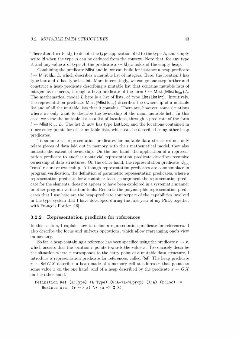
3.2. MUTABLE DATA STRUCTURES 43
Thereafter, I write Id𝐴 to denote the type application of Id to the type 𝐴, and simplywrite Id when the type 𝐴 can be deduced from the context. Note that, for any type𝐴 and any value 𝑥 of type 𝐴, the predicate 𝑥 Id𝐴 𝑥 holds of the empty heap.
Combining the predicate Mlist and Id, we can build for instance a heap predicate𝑙 Mlist IdInt 𝐿, which describes a mutable list of integers. Here, the location 𝑙 hastype Loc and 𝐿 has type List Int. More interestingly, we can go one step further andconstruct a heap predicate describing a mutable list that contains mutable lists ofintegers as elements, through a heap predicate of the form 𝑙 Mlist (Mlist IdInt)𝐿.The mathematical model 𝐿 here is a list of lists, of type List (List Int). Intuitively,the representation predicate Mlist (Mlist IdInt) describes the ownership of a mutablelist and of all the mutable lists that it contains. There are, however, some situationswhere we only want to describe the ownership of the main mutable list. In thiscase, we view the mutable list as a list of locations, through a predicate of the form𝑙 Mlist IdLoc 𝐿. The list 𝐿 now has type List Loc, and the locations contained in𝐿 are entry points for other mutable lists, which can be described using other heappredicates.
To summarize, representation predicates for mutable data structures not onlyrelate pieces of data laid out in memory with their mathematical model, they alsoindicate the extent of ownership. On the one hand, the application of a represen-tation predicate to another nontrivial representation predicate describes recursiveownership of data structures. On the other hand, the representation predicate IdLoc“cuts” recursive ownership. Although representation predicates are commonplace inprogram verification, the definition of parametric representation predicates, where arepresentation predicate for a container takes as argument the representation predi-cate for the elements, does not appear to have been exploited in a systematic mannerin other program verification tools. Remark: the polymorphic representation predi-cates that I use here are the heap-predicate counterpart of the capabilities involvedin the type system that I have developed during the first year of my PhD, togetherwith François Pottier [16].
3.2.2 Representation predicate for references
In this section, I explain how to define a representation predicate for references. Ialso describe the focus and unfocus operations, which allow rearranging one’s viewon memory.
So far, a heap containing a reference has been specified using the predicate 𝑟 →˓ 𝑥,which asserts that the location 𝑟 points towards the value 𝑥. To concisely describethe situation where 𝑥 corresponds to the entry point of a mutable data structure, Iintroduce a representation predicate for references, called Ref. The heap predicate𝑟 Ref𝐺𝑋 describes a heap made of a memory cell at address 𝑟 that points tosome value 𝑥 on the one hand, and of a heap described by the predicate 𝑥 𝐺𝑋on the other hand.
Definition Ref (a:Type) (A:Type) (G:A->a->Hprop) (X:A) (r:Loc) :=Hexists x:a, (r ˜̃ > x) \* (x ˜> G X).
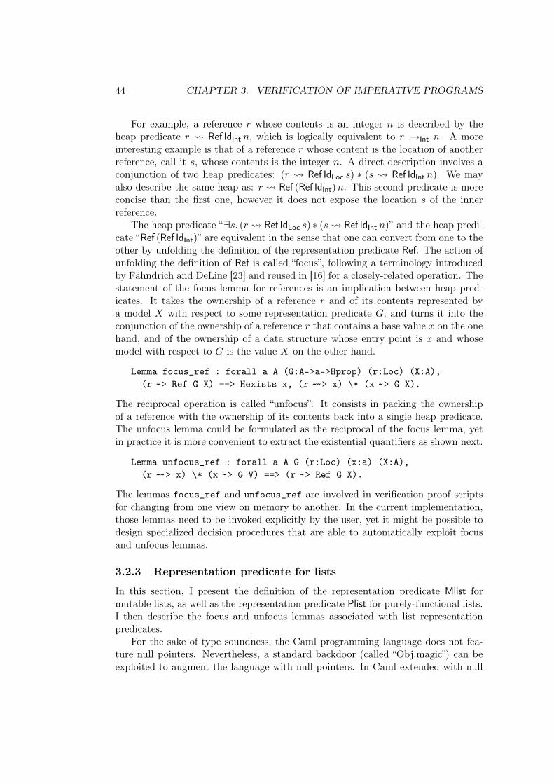
44 CHAPTER 3. VERIFICATION OF IMPERATIVE PROGRAMS
For example, a reference 𝑟 whose contents is an integer 𝑛 is described by theheap predicate 𝑟 Ref IdInt 𝑛, which is logically equivalent to 𝑟 →˓Int 𝑛. A moreinteresting example is that of a reference 𝑟 whose content is the location of anotherreference, call it 𝑠, whose contents is the integer 𝑛. A direct description involves aconjunction of two heap predicates: (𝑟 Ref IdLoc 𝑠) * (𝑠 Ref IdInt 𝑛). We mayalso describe the same heap as: 𝑟 Ref (Ref IdInt)𝑛. This second predicate is moreconcise than the first one, however it does not expose the location 𝑠 of the innerreference.
The heap predicate “∃∃𝑠. (𝑟 Ref IdLoc 𝑠) * (𝑠 Ref IdInt 𝑛)” and the heap predi-cate “Ref (Ref IdInt)” are equivalent in the sense that one can convert from one to theother by unfolding the definition of the representation predicate Ref. The action ofunfolding the definition of Ref is called “focus”, following a terminology introducedby Fähndrich and DeLine [23] and reused in [16] for a closely-related operation. Thestatement of the focus lemma for references is an implication between heap pred-icates. It takes the ownership of a reference 𝑟 and of its contents represented bya model 𝑋 with respect to some representation predicate 𝐺, and turns it into theconjunction of the ownership of a reference 𝑟 that contains a base value 𝑥 on the onehand, and of the ownership of a data structure whose entry point is 𝑥 and whosemodel with respect to 𝐺 is the value 𝑋 on the other hand.
Lemma focus_ref : forall a A (G:A->a->Hprop) (r:Loc) (X:A),(r ˜> Ref G X) ==> Hexists x, (r ˜̃ > x) \* (x ˜> G X).
The reciprocal operation is called “unfocus”. It consists in packing the ownershipof a reference with the ownership of its contents back into a single heap predicate.The unfocus lemma could be formulated as the reciprocal of the focus lemma, yetin practice it is more convenient to extract the existential quantifiers as shown next.
Lemma unfocus_ref : forall a A G (r:Loc) (x:a) (X:A),(r ˜̃ > x) \* (x ˜> G V) ==> (r ˜> Ref G X).
The lemmas focus_ref and unfocus_ref are involved in verification proof scriptsfor changing from one view on memory to another. In the current implementation,those lemmas need to be invoked explicitly by the user, yet it might be possible todesign specialized decision procedures that are able to automatically exploit focusand unfocus lemmas.
3.2.3 Representation predicate for lists
In this section, I present the definition of the representation predicate Mlist formutable lists, as well as the representation predicate Plist for purely-functional lists.I then describe the focus and unfocus lemmas associated with list representationpredicates.
For the sake of type soundness, the Caml programming language does not fea-ture null pointers. Nevertheless, a standard backdoor (called “Obj.magic”) can beexploited to augment the language with null pointers. In Caml extended with null
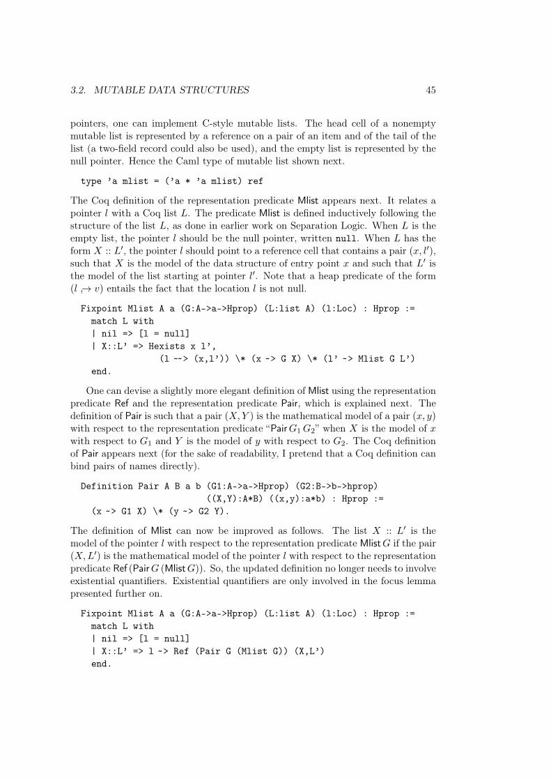
3.2. MUTABLE DATA STRUCTURES 45
pointers, one can implement C-style mutable lists. The head cell of a nonemptymutable list is represented by a reference on a pair of an item and of the tail of thelist (a two-field record could also be used), and the empty list is represented by thenull pointer. Hence the Caml type of mutable list shown next.
type ’a mlist = (’a * ’a mlist) ref
The Coq definition of the representation predicate Mlist appears next. It relates apointer 𝑙 with a Coq list 𝐿. The predicate Mlist is defined inductively following thestructure of the list 𝐿, as done in earlier work on Separation Logic. When 𝐿 is theempty list, the pointer 𝑙 should be the null pointer, written null. When 𝐿 has theform 𝑋 :: 𝐿′, the pointer 𝑙 should point to a reference cell that contains a pair (𝑥, 𝑙′),such that 𝑋 is the model of the data structure of entry point 𝑥 and such that 𝐿′ isthe model of the list starting at pointer 𝑙′. Note that a heap predicate of the form(𝑙 →˓ 𝑣) entails the fact that the location 𝑙 is not null.
Fixpoint Mlist A a (G:A->a->Hprop) (L:list A) (l:Loc) : Hprop :=match L with| nil => [l = null]| X::L’ => Hexists x l’,
(l ˜̃ > (x,l’)) \* (x ˜> G X) \* (l’ ˜> Mlist G L’)end.
One can devise a slightly more elegant definition of Mlist using the representationpredicate Ref and the representation predicate Pair, which is explained next. Thedefinition of Pair is such that a pair (𝑋,𝑌 ) is the mathematical model of a pair (𝑥, 𝑦)with respect to the representation predicate “Pair𝐺1𝐺2” when 𝑋 is the model of 𝑥with respect to 𝐺1 and 𝑌 is the model of 𝑦 with respect to 𝐺2. The Coq definitionof Pair appears next (for the sake of readability, I pretend that a Coq definition canbind pairs of names directly).
Definition Pair A B a b (G1:A->a->Hprop) (G2:B->b->hprop)((X,Y):A*B) ((x,y):a*b) : Hprop :=
(x ˜> G1 X) \* (y ˜> G2 Y).
The definition of Mlist can now be improved as follows. The list 𝑋 :: 𝐿′ is themodel of the pointer 𝑙 with respect to the representation predicate Mlist𝐺 if the pair(𝑋,𝐿′) is the mathematical model of the pointer 𝑙 with respect to the representationpredicate Ref (Pair𝐺 (Mlist𝐺)). So, the updated definition no longer needs to involveexistential quantifiers. Existential quantifiers are only involved in the focus lemmapresented further on.
Fixpoint Mlist A a (G:A->a->Hprop) (L:list A) (l:Loc) : Hprop :=match L with| nil => [l = null]| X::L’ => l ˜> Ref (Pair G (Mlist G)) (X,L’)end.
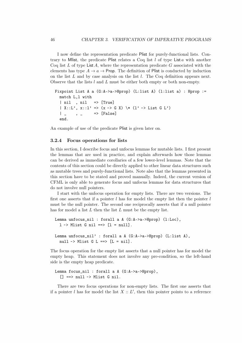
46 CHAPTER 3. VERIFICATION OF IMPERATIVE PROGRAMS
I now define the representation predicate Plist for purely-functional lists. Con-trary to Mlist, the predicate Plist relates a Coq list 𝑙 of type List 𝑎 with anotherCoq list 𝐿 of type List𝐴, where the representation predicate 𝐺 associated with theelements has type 𝐴 → 𝑎 → Prop. The definition of Plist is conducted by inductionon the list 𝐿 and by case analysis on the list 𝑙. The Coq definition appears next.Observe that the lists 𝑙 and 𝐿 must be either both empty or both non-empty.
Fixpoint List A a (G:A->a->Hprop) (L:list A) (l:list a) : Hprop :=match L,l with| nil , nil => [True]| X::L’, x::l’ => (x ˜> G X) \* (l’ ˜> List G L’)| _ , _ => [False]end.
An example of use of the predicate Plist is given later on.
3.2.4 Focus operations for lists
In this section, I describe focus and unfocus lemmas for mutable lists. I first presentthe lemmas that are used in practice, and explain afterwards how those lemmascan be derived as immediate corollaries of a few lower-level lemmas. Note that thecontents of this section could be directly applied to other linear data structures suchas mutable trees and purely-functional lists. Note also that the lemmas presented inthis section have to be stated and proved manually. Indeed, the current version ofCFML is only able to generate focus and unfocus lemmas for data structures thatdo not involve null pointers.
I start with the unfocus operation for empty lists. There are two versions. Thefirst one asserts that if a pointer 𝑙 has for model the empty list then the pointer 𝑙must be the null pointer. The second one reciprocally asserts that if a null pointerhas for model a list 𝐿 then the list 𝐿 must be the empty list.
Lemma unfocus_nil : forall a A (G:A->a->Hprop) (l:Loc),l ˜> Mlist G nil ==> [l = null].
Lemma unfocus_nil’ : forall a A (G:A->a->Hprop) (L:list A),null ˜> Mlist G L ==> [L = nil].
The focus operation for the empty list asserts that a null pointer has for model theempty heap. This statement does not involve any pre-condition, so the left-handside is the empty heap predicate.
Lemma focus_nil : forall a A (G:A->a->Hprop),[] ==> null ˜> Mlist G nil.
There are two focus operations for non-empty lists. The first one asserts thatif a pointer 𝑙 has for model the list 𝑋 :: 𝐿′, then this pointer points to a reference
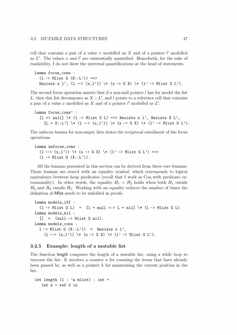
3.2. MUTABLE DATA STRUCTURES 47
cell that contains a pair of a value 𝑥 modelled as 𝑋 and of a pointer 𝑙′ modelledas 𝐿′. The values 𝑥 and 𝑙′ are existentially quantified. Henceforth, for the sake ofreadability, I do not show the universal quantifications at the head of statements.
Lemma focus_cons :(l ˜> Mlist G (X::L’)) ==>Hexists x l’, (l ˜̃ > (x,l’)) \* (x ˜> G X) \* (l’ ˜> Mlist G L’).
The second focus operation asserts that if a non-null pointer 𝑙 has for model the list𝐿, then this list decomposes as 𝑋 :: 𝐿′, and 𝑙 points to a reference cell that containsa pair of a value 𝑥 modelled as 𝑋 and of a pointer 𝑙′ modelled as 𝐿′.
Lemma focus_cons’ :[l <> null] \* (l ˜> Mlist G L) ==> Hexists x l’, Hexists X L’,
[L = X::L’] \* (l ˜̃ > (x,l’)) \* (x ˜> G X) \* (l’ ˜> Mlist G L’).
The unfocus lemma for non-empty lists states the reciprocal entailment of the focusoperations.
Lemma unfocus_cons :(l ˜̃ > (x,l’)) \* (x ˜> G X) \* (l’ ˜> Mlist G L’) ==>(l ˜> Mlist G (X::L’)).
All the lemmas presented in this section can be derived from three core lemmas.Those lemmas are stated with an equality symbol, which corresponds to logicalequivalence between heap predicates (recall that I work in Coq with predicate ex-tensionality). In other words, the equality 𝐻1 = 𝐻2 holds when both 𝐻1 entails𝐻2 and 𝐻2 entails 𝐻1. Working with an equality reduces the number of times thedefinition of Mlist needs to be unfolded in proofs.
Lemma models_iff :(l ˜> Mlist G L) = [l = null <-> L = nil] \* (l ˜> Mlist G L).
Lemma models_nil :[] = (null ˜> Mlist G nil).
Lemma models_cons :l ˜> Mlist G (X::L’)) = Hexists x l’,
(l ˜̃ > (x,l’)) \* (x ˜> G X) \* (l’ ˜> Mlist G L’).
3.2.5 Example: length of a mutable list
The function length computes the length of a mutable list, using a while loop totraverse the list. It involves a counter 𝑛 for counting the items that have alreadybeen passed by, as well as a pointer ℎ for maintaining the current position in thelist.
let length (l : ’a mlist) : int =let n = ref 0 in
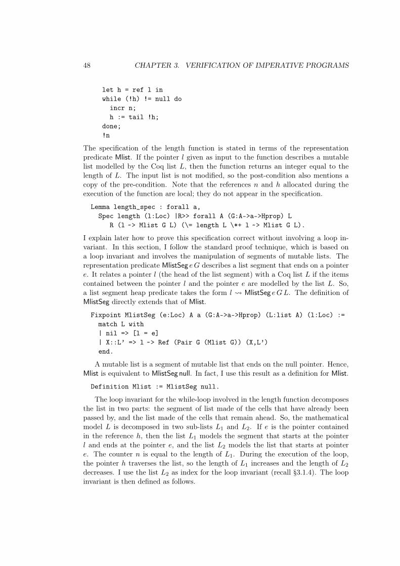
48 CHAPTER 3. VERIFICATION OF IMPERATIVE PROGRAMS
let h = ref l inwhile (!h) != null do
incr n;h := tail !h;
done;!n
The specification of the length function is stated in terms of the representationpredicate Mlist. If the pointer 𝑙 given as input to the function describes a mutablelist modelled by the Coq list 𝐿, then the function returns an integer equal to thelength of 𝐿. The input list is not modified, so the post-condition also mentions acopy of the pre-condition. Note that the references 𝑛 and ℎ allocated during theexecution of the function are local; they do not appear in the specification.
Lemma length_spec : forall a,Spec length (l:Loc) |R>> forall A (G:A->a->Hprop) L
R (l ˜> Mlist G L) (\= length L \*+ l ˜> Mlist G L).
I explain later how to prove this specification correct without involving a loop in-variant. In this section, I follow the standard proof technique, which is based ona loop invariant and involves the manipulation of segments of mutable lists. Therepresentation predicate MlistSeg 𝑒𝐺 describes a list segment that ends on a pointer𝑒. It relates a pointer 𝑙 (the head of the list segment) with a Coq list 𝐿 if the itemscontained between the pointer 𝑙 and the pointer 𝑒 are modelled by the list 𝐿. So,a list segment heap predicate takes the form 𝑙 MlistSeg 𝑒𝐺𝐿. The definition ofMlistSeg directly extends that of Mlist.
Fixpoint MlistSeg (e:Loc) A a (G:A->a->Hprop) (L:list A) (l:Loc) :=match L with| nil => [l = e]| X::L’ => l ˜> Ref (Pair G (Mlist G)) (X,L’)end.
A mutable list is a segment of mutable list that ends on the null pointer. Hence,Mlist is equivalent to MlistSeg null. In fact, I use this result as a definition for Mlist.
Definition Mlist := MlistSeg null.
The loop invariant for the while-loop involved in the length function decomposesthe list in two parts: the segment of list made of the cells that have already beenpassed by, and the list made of the cells that remain ahead. So, the mathematicalmodel 𝐿 is decomposed in two sub-lists 𝐿1 and 𝐿2. If 𝑒 is the pointer containedin the reference ℎ, then the list 𝐿1 models the segment that starts at the pointer𝑙 and ends at the pointer 𝑒, and the list 𝐿2 models the list that starts at pointer𝑒. The counter 𝑛 is equal to the length of 𝐿1. During the execution of the loop,the pointer ℎ traverses the list, so the length of 𝐿1 increases and the length of 𝐿2
decreases. I use the list 𝐿2 as index for the loop invariant (recall §3.1.4). The loopinvariant is then defined as follows.
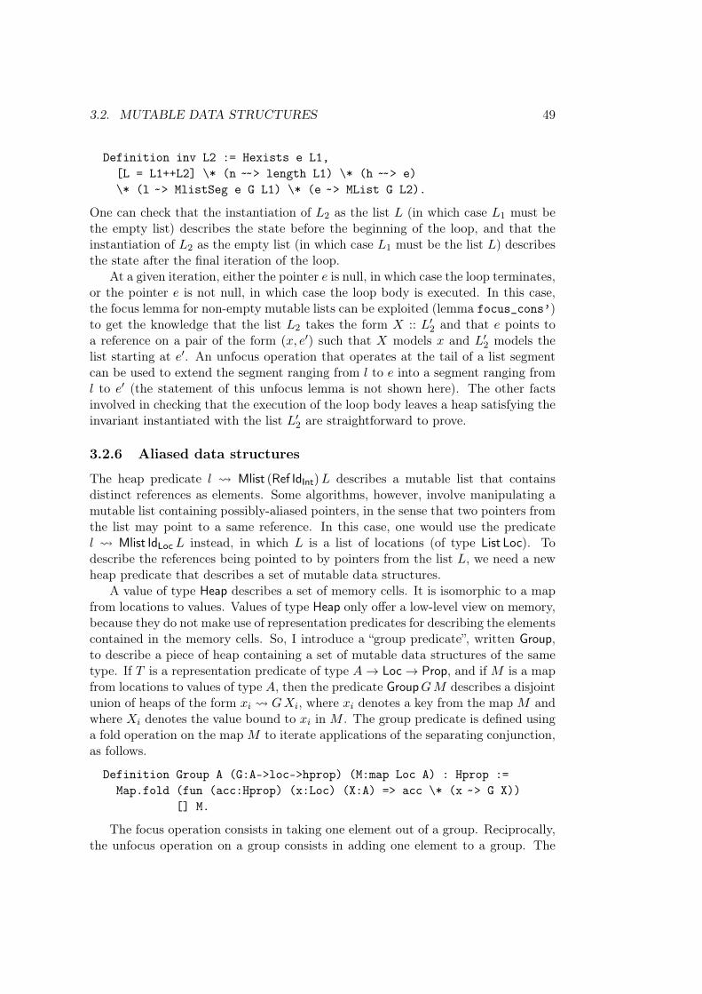
3.2. MUTABLE DATA STRUCTURES 49
Definition inv L2 := Hexists e L1,[L = L1++L2] \* (n ˜̃ > length L1) \* (h ˜̃ > e)\* (l ˜> MlistSeg e G L1) \* (e ˜> MList G L2).
One can check that the instantiation of 𝐿2 as the list 𝐿 (in which case 𝐿1 must bethe empty list) describes the state before the beginning of the loop, and that theinstantiation of 𝐿2 as the empty list (in which case 𝐿1 must be the list 𝐿) describesthe state after the final iteration of the loop.
At a given iteration, either the pointer 𝑒 is null, in which case the loop terminates,or the pointer 𝑒 is not null, in which case the loop body is executed. In this case,the focus lemma for non-empty mutable lists can be exploited (lemma focus_cons’)to get the knowledge that the list 𝐿2 takes the form 𝑋 :: 𝐿′
2 and that 𝑒 points toa reference on a pair of the form (𝑥, 𝑒′) such that 𝑋 models 𝑥 and 𝐿′
2 models thelist starting at 𝑒′. An unfocus operation that operates at the tail of a list segmentcan be used to extend the segment ranging from 𝑙 to 𝑒 into a segment ranging from𝑙 to 𝑒′ (the statement of this unfocus lemma is not shown here). The other factsinvolved in checking that the execution of the loop body leaves a heap satisfying theinvariant instantiated with the list 𝐿′
2 are straightforward to prove.
3.2.6 Aliased data structures
The heap predicate 𝑙 Mlist (Ref IdInt)𝐿 describes a mutable list that containsdistinct references as elements. Some algorithms, however, involve manipulating amutable list containing possibly-aliased pointers, in the sense that two pointers fromthe list may point to a same reference. In this case, one would use the predicate𝑙 Mlist IdLoc 𝐿 instead, in which 𝐿 is a list of locations (of type List Loc). Todescribe the references being pointed to by pointers from the list 𝐿, we need a newheap predicate that describes a set of mutable data structures.
A value of type Heap describes a set of memory cells. It is isomorphic to a mapfrom locations to values. Values of type Heap only offer a low-level view on memory,because they do not make use of representation predicates for describing the elementscontained in the memory cells. So, I introduce a “group predicate”, written Group,to describe a piece of heap containing a set of mutable data structures of the sametype. If 𝑇 is a representation predicate of type 𝐴 → Loc → Prop, and if 𝑀 is a mapfrom locations to values of type 𝐴, then the predicate Group𝐺𝑀 describes a disjointunion of heaps of the form 𝑥𝑖 𝐺𝑋𝑖, where 𝑥𝑖 denotes a key from the map 𝑀 andwhere 𝑋𝑖 denotes the value bound to 𝑥𝑖 in 𝑀 . The group predicate is defined usinga fold operation on the map 𝑀 to iterate applications of the separating conjunction,as follows.
Definition Group A (G:A->loc->hprop) (M:map Loc A) : Hprop :=Map.fold (fun (acc:Hprop) (x:Loc) (X:A) => acc \* (x ˜> G X))
[] M.
The focus operation consists in taking one element out of a group. Reciprocally,the unfocus operation on a group consists in adding one element to a group. The
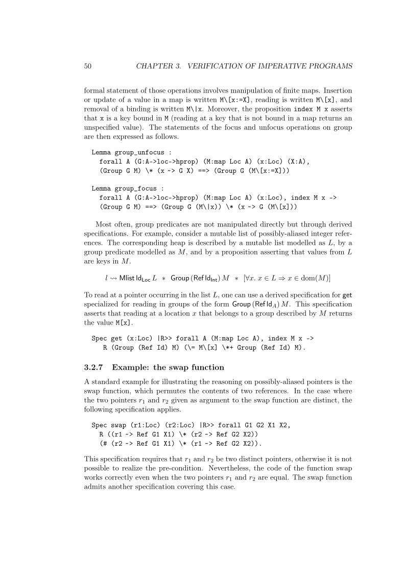
50 CHAPTER 3. VERIFICATION OF IMPERATIVE PROGRAMS
formal statement of those operations involves manipulation of finite maps. Insertionor update of a value in a map is written M\[x:=X], reading is written M\[x], andremoval of a binding is written M\|x. Moreover, the proposition index M x assertsthat x is a key bound in M (reading at a key that is not bound in a map returns anunspecified value). The statements of the focus and unfocus operations on groupare then expressed as follows.
Lemma group_unfocus :forall A (G:A->loc->hprop) (M:map Loc A) (x:Loc) (X:A),(Group G M) \* (x ˜> G X) ==> (Group G (M\[x:=X]))
Lemma group_focus :forall A (G:A->loc->hprop) (M:map Loc A) (x:Loc), index M x ->(Group G M) ==> (Group G (M\|x)) \* (x ˜> G (M\[x]))
Most often, group predicates are not manipulated directly but through derivedspecifications. For example, consider a mutable list of possibly-aliased integer refer-ences. The corresponding heap is described by a mutable list modelled as 𝐿, by agroup predicate modelled as 𝑀 , and by a proposition asserting that values from 𝐿are keys in 𝑀 .
𝑙 Mlist IdLoc 𝐿 * Group (Ref IdInt)𝑀 * [∀𝑥. 𝑥 ∈ 𝐿 ⇒ 𝑥 ∈ dom(𝑀)]
To read at a pointer occurring in the list 𝐿, one can use a derived specification for getspecialized for reading in groups of the form Group (Ref Id𝐴)𝑀 . This specificationasserts that reading at a location 𝑥 that belongs to a group described by 𝑀 returnsthe value M[x].
Spec get (x:Loc) |R>> forall A (M:map Loc A), index M x ->R (Group (Ref Id) M) (\= M\[x] \*+ Group (Ref Id) M).
3.2.7 Example: the swap function
A standard example for illustrating the reasoning on possibly-aliased pointers is theswap function, which permutes the contents of two references. In the case wherethe two pointers 𝑟1 and 𝑟2 given as argument to the swap function are distinct, thefollowing specification applies.
Spec swap (r1:Loc) (r2:Loc) |R>> forall G1 G2 X1 X2,R ((r1 ˜> Ref G1 X1) \* (r2 ˜> Ref G2 X2))(# (r2 ˜> Ref G1 X1) \* (r1 ˜> Ref G2 X2)).
This specification requires that 𝑟1 and 𝑟2 be two distinct pointers, otherwise it is notpossible to realize the pre-condition. Nevertheless, the code of the function swapworks correctly even when the two pointers 𝑟1 and 𝑟2 are equal. The swap functionadmits another specification covering this case.
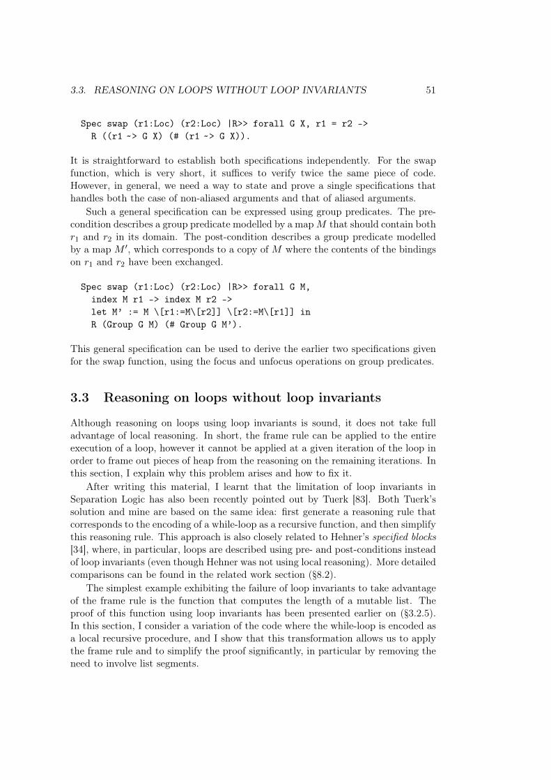
3.3. REASONING ON LOOPS WITHOUT LOOP INVARIANTS 51
Spec swap (r1:Loc) (r2:Loc) |R>> forall G X, r1 = r2 ->R ((r1 ˜> G X) (# (r1 ˜> G X)).
It is straightforward to establish both specifications independently. For the swapfunction, which is very short, it suffices to verify twice the same piece of code.However, in general, we need a way to state and prove a single specifications thathandles both the case of non-aliased arguments and that of aliased arguments.
Such a general specification can be expressed using group predicates. The pre-condition describes a group predicate modelled by a map 𝑀 that should contain both𝑟1 and 𝑟2 in its domain. The post-condition describes a group predicate modelledby a map 𝑀 ′, which corresponds to a copy of 𝑀 where the contents of the bindingson 𝑟1 and 𝑟2 have been exchanged.
Spec swap (r1:Loc) (r2:Loc) |R>> forall G M,index M r1 -> index M r2 ->let M’ := M \[r1:=M\[r2]] \[r2:=M\[r1]] inR (Group G M) (# Group G M’).
This general specification can be used to derive the earlier two specifications givenfor the swap function, using the focus and unfocus operations on group predicates.
3.3 Reasoning on loops without loop invariants
Although reasoning on loops using loop invariants is sound, it does not take fulladvantage of local reasoning. In short, the frame rule can be applied to the entireexecution of a loop, however it cannot be applied at a given iteration of the loop inorder to frame out pieces of heap from the reasoning on the remaining iterations. Inthis section, I explain why this problem arises and how to fix it.
After writing this material, I learnt that the limitation of loop invariants inSeparation Logic has also been recently pointed out by Tuerk [83]. Both Tuerk’ssolution and mine are based on the same idea: first generate a reasoning rule thatcorresponds to the encoding of a while-loop as a recursive function, and then simplifythis reasoning rule. This approach is also closely related to Hehner’s specified blocks[34], where, in particular, loops are described using pre- and post-conditions insteadof loop invariants (even though Hehner was not using local reasoning). More detailedcomparisons can be found in the related work section (§8.2).
The simplest example exhibiting the failure of loop invariants to take advantageof the frame rule is the function that computes the length of a mutable list. Theproof of this function using loop invariants has been presented earlier on (§3.2.5).In this section, I consider a variation of the code where the while-loop is encoded asa local recursive procedure, and I show that this transformation allows us to applythe frame rule and to simplify the proof significantly, in particular by removing theneed to involve list segments.
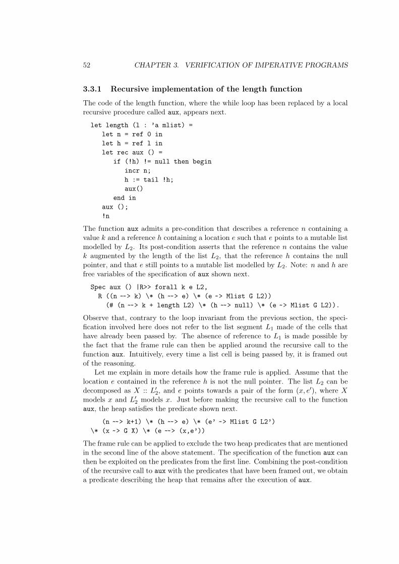
52 CHAPTER 3. VERIFICATION OF IMPERATIVE PROGRAMS
3.3.1 Recursive implementation of the length function
The code of the length function, where the while loop has been replaced by a localrecursive procedure called aux, appears next.
let length (l : ’a mlist) =let n = ref 0 inlet h = ref l inlet rec aux () =
if (!h) != null then beginincr n;h := tail !h;aux()
end inaux ();!n
The function aux admits a pre-condition that describes a reference 𝑛 containing avalue 𝑘 and a reference ℎ containing a location 𝑒 such that 𝑒 points to a mutable listmodelled by 𝐿2. Its post-condition asserts that the reference 𝑛 contains the value𝑘 augmented by the length of the list 𝐿2, that the reference ℎ contains the nullpointer, and that 𝑒 still points to a mutable list modelled by 𝐿2. Note: 𝑛 and ℎ arefree variables of the specification of aux shown next.
Spec aux () |R>> forall k e L2,R ((n ˜̃ > k) \* (h ˜̃ > e) \* (e ˜> Mlist G L2))
(# (n ˜̃ > k + length L2) \* (h ˜̃ > null) \* (e ˜> Mlist G L2)).
Observe that, contrary to the loop invariant from the previous section, the speci-fication involved here does not refer to the list segment 𝐿1 made of the cells thathave already been passed by. The absence of reference to 𝐿1 is made possible bythe fact that the frame rule can then be applied around the recursive call to thefunction aux. Intuitively, every time a list cell is being passed by, it is framed outof the reasoning.
Let me explain in more details how the frame rule is applied. Assume that thelocation 𝑒 contained in the reference ℎ is not the null pointer. The list 𝐿2 can bedecomposed as 𝑋 :: 𝐿′
2, and 𝑒 points towards a pair of the form (𝑥, 𝑒′), where 𝑋models 𝑥 and 𝐿′
2 models 𝑥. Just before making the recursive call to the functionaux, the heap satisfies the predicate shown next.
(n ˜̃ > k+1) \* (h ˜̃ > e) \* (e’ ˜> Mlist G L2’)\* (x ˜> G X) \* (e ˜̃ > (x,e’))
The frame rule can be applied to exclude the two heap predicates that are mentionedin the second line of the above statement. The specification of the function aux canthen be exploited on the predicates from the first line. Combining the post-conditionof the recursive call to aux with the predicates that have been framed out, we obtaina predicate describing the heap that remains after the execution of aux.
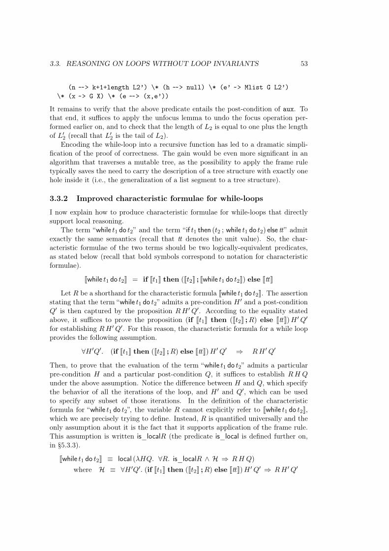
3.3. REASONING ON LOOPS WITHOUT LOOP INVARIANTS 53
(n ˜̃ > k+1+length L2’) \* (h ˜̃ > null) \* (e’ ˜> Mlist G L2’)\* (x ˜> G X) \* (e ˜̃ > (x,e’))
It remains to verify that the above predicate entails the post-condition of aux. Tothat end, it suffices to apply the unfocus lemma to undo the focus operation per-formed earlier on, and to check that the length of 𝐿2 is equal to one plus the lengthof 𝐿′
2 (recall that 𝐿′2 is the tail of 𝐿2).
Encoding the while-loop into a recursive function has led to a dramatic simpli-fication of the proof of correctness. The gain would be even more significant in analgorithm that traverses a mutable tree, as the possibility to apply the frame ruletypically saves the need to carry the description of a tree structure with exactly onehole inside it (i.e., the generalization of a list segment to a tree structure).
3.3.2 Improved characteristic formulae for while-loops
I now explain how to produce characteristic formulae for while-loops that directlysupport local reasoning.
The term “while 𝑡1 do 𝑡2” and the term “ if 𝑡1 then (𝑡2 ; while 𝑡1 do 𝑡2) else tt” admitexactly the same semantics (recall that tt denotes the unit value). So, the char-acteristic formulae of the two terms should be two logically-equivalent predicates,as stated below (recall that bold symbols correspond to notation for characteristicformulae).
Jwhile 𝑡1 do 𝑡2K = if J𝑡1K then (J𝑡2K ; Jwhile 𝑡1 do 𝑡2K) else JttK
Let 𝑅 be a shorthand for the characteristic formula Jwhile 𝑡1 do 𝑡2K. The assertionstating that the term “while 𝑡1 do 𝑡2” admits a pre-condition 𝐻 ′ and a post-condition𝑄′ is then captured by the proposition 𝑅𝐻 ′𝑄′. According to the equality statedabove, it suffices to prove the proposition (if J𝑡1K then (J𝑡2K ;𝑅) else JttK)𝐻 ′𝑄′
for establishing 𝑅𝐻 ′𝑄′. For this reason, the characteristic formula for a while loopprovides the following assumption.
∀𝐻 ′𝑄′. (if J𝑡1K then (J𝑡2K ;𝑅) else JttK)𝐻 ′𝑄′ ⇒ 𝑅𝐻 ′𝑄′
Then, to prove that the evaluation of the term “while 𝑡1 do 𝑡2” admits a particularpre-condition 𝐻 and a particular post-condition 𝑄, it suffices to establish 𝑅𝐻 𝑄under the above assumption. Notice the difference between 𝐻 and 𝑄, which specifythe behavior of all the iterations of the loop, and 𝐻 ′ and 𝑄′, which can be usedto specify any subset of those iterations. In the definition of the characteristicformula for “while 𝑡1 do 𝑡2”, the variable 𝑅 cannot explicitly refer to Jwhile 𝑡1 do 𝑡2K,which we are precisely trying to define. Instead, 𝑅 is quantified universally and theonly assumption about it is the fact that it supports application of the frame rule.This assumption is written is_local𝑅 (the predicate is_local is defined further on,in §5.3.3).
Jwhile 𝑡1 do 𝑡2K ≡ local (𝜆𝐻𝑄. ∀𝑅. is_local𝑅 ∧ ℋ ⇒ 𝑅𝐻 𝑄)
where ℋ ≡ ∀𝐻 ′𝑄′. (if J𝑡1K then (J𝑡2K ;𝑅) else JttK)𝐻 ′𝑄′ ⇒ 𝑅𝐻 ′𝑄′
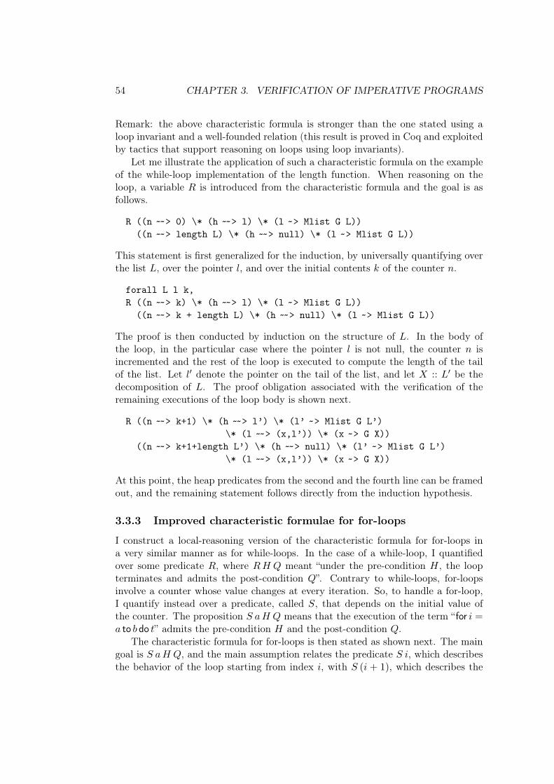
54 CHAPTER 3. VERIFICATION OF IMPERATIVE PROGRAMS
Remark: the above characteristic formula is stronger than the one stated using aloop invariant and a well-founded relation (this result is proved in Coq and exploitedby tactics that support reasoning on loops using loop invariants).
Let me illustrate the application of such a characteristic formula on the exampleof the while-loop implementation of the length function. When reasoning on theloop, a variable 𝑅 is introduced from the characteristic formula and the goal is asfollows.
R ((n ˜̃ > 0) \* (h ˜̃ > l) \* (l ˜> Mlist G L))((n ˜̃ > length L) \* (h ˜̃ > null) \* (l ˜> Mlist G L))
This statement is first generalized for the induction, by universally quantifying overthe list 𝐿, over the pointer 𝑙, and over the initial contents 𝑘 of the counter 𝑛.
forall L l k,R ((n ˜̃ > k) \* (h ˜̃ > l) \* (l ˜> Mlist G L))
((n ˜̃ > k + length L) \* (h ˜̃ > null) \* (l ˜> Mlist G L))
The proof is then conducted by induction on the structure of 𝐿. In the body ofthe loop, in the particular case where the pointer 𝑙 is not null, the counter 𝑛 isincremented and the rest of the loop is executed to compute the length of the tailof the list. Let 𝑙′ denote the pointer on the tail of the list, and let 𝑋 :: 𝐿′ be thedecomposition of 𝐿. The proof obligation associated with the verification of theremaining executions of the loop body is shown next.
R ((n ˜̃ > k+1) \* (h ˜̃ > l’) \* (l’ ˜> Mlist G L’)\* (l ˜̃ > (x,l’)) \* (x ˜> G X))
((n ˜̃ > k+1+length L’) \* (h ˜̃ > null) \* (l’ ˜> Mlist G L’)\* (l ˜̃ > (x,l’)) \* (x ˜> G X))
At this point, the heap predicates from the second and the fourth line can be framedout, and the remaining statement follows directly from the induction hypothesis.
3.3.3 Improved characteristic formulae for for-loops
I construct a local-reasoning version of the characteristic formula for for-loops ina very similar manner as for while-loops. In the case of a while-loop, I quantifiedover some predicate 𝑅, where 𝑅𝐻 𝑄 meant “under the pre-condition 𝐻, the loopterminates and admits the post-condition 𝑄”. Contrary to while-loops, for-loopsinvolve a counter whose value changes at every iteration. So, to handle a for-loop,I quantify instead over a predicate, called 𝑆, that depends on the initial value ofthe counter. The proposition 𝑆 𝑎𝐻 𝑄 means that the execution of the term “for 𝑖 =𝑎 to 𝑏 do 𝑡” admits the pre-condition 𝐻 and the post-condition 𝑄.
The characteristic formula for for-loops is then stated as shown next. The maingoal is 𝑆 𝑎𝐻 𝑄, and the main assumption relates the predicate 𝑆 𝑖, which describesthe behavior of the loop starting from index 𝑖, with 𝑆 (𝑖 + 1), which describes the
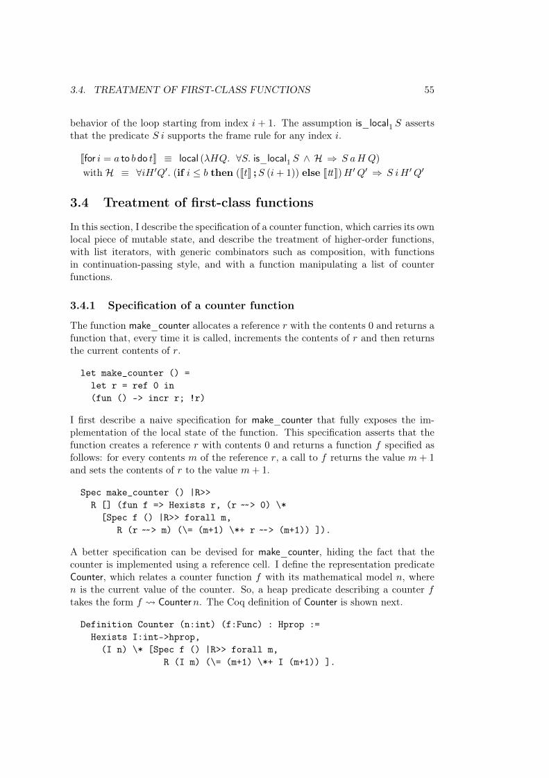
3.4. TREATMENT OF FIRST-CLASS FUNCTIONS 55
behavior of the loop starting from index 𝑖 + 1. The assumption is_local1 𝑆 assertsthat the predicate 𝑆 𝑖 supports the frame rule for any index 𝑖.
Jfor 𝑖 = 𝑎 to 𝑏 do 𝑡K ≡ local (𝜆𝐻𝑄. ∀𝑆. is_local1 𝑆 ∧ ℋ ⇒ 𝑆 𝑎𝐻 𝑄)
with ℋ ≡ ∀𝑖𝐻 ′𝑄′. (if 𝑖 ≤ 𝑏 then (J𝑡K ;𝑆 (𝑖 + 1)) else JttK)𝐻 ′𝑄′ ⇒ 𝑆 𝑖𝐻 ′𝑄′
3.4 Treatment of first-class functions
In this section, I describe the specification of a counter function, which carries its ownlocal piece of mutable state, and describe the treatment of higher-order functions,with list iterators, with generic combinators such as composition, with functionsin continuation-passing style, and with a function manipulating a list of counterfunctions.
3.4.1 Specification of a counter function
The function make_counter allocates a reference 𝑟 with the contents 0 and returns afunction that, every time it is called, increments the contents of 𝑟 and then returnsthe current contents of 𝑟.
let make_counter () =let r = ref 0 in(fun () -> incr r; !r)
I first describe a naive specification for make_counter that fully exposes the im-plementation of the local state of the function. This specification asserts that thefunction creates a reference 𝑟 with contents 0 and returns a function 𝑓 specified asfollows: for every contents 𝑚 of the reference 𝑟, a call to 𝑓 returns the value 𝑚 + 1and sets the contents of 𝑟 to the value 𝑚 + 1.
Spec make_counter () |R>>R [] (fun f => Hexists r, (r ˜̃ > 0) \*
[Spec f () |R>> forall m,R (r ˜̃ > m) (\= (m+1) \*+ r ˜̃ > (m+1)) ]).
A better specification can be devised for make_counter, hiding the fact that thecounter is implemented using a reference cell. I define the representation predicateCounter, which relates a counter function 𝑓 with its mathematical model 𝑛, where𝑛 is the current value of the counter. So, a heap predicate describing a counter 𝑓takes the form 𝑓 Counter𝑛. The Coq definition of Counter is shown next.
Definition Counter (n:int) (f:Func) : Hprop :=Hexists I:int->hprop,
(I n) \* [Spec f () |R>> forall m,R (I m) (\= (m+1) \*+ I (m+1)) ].
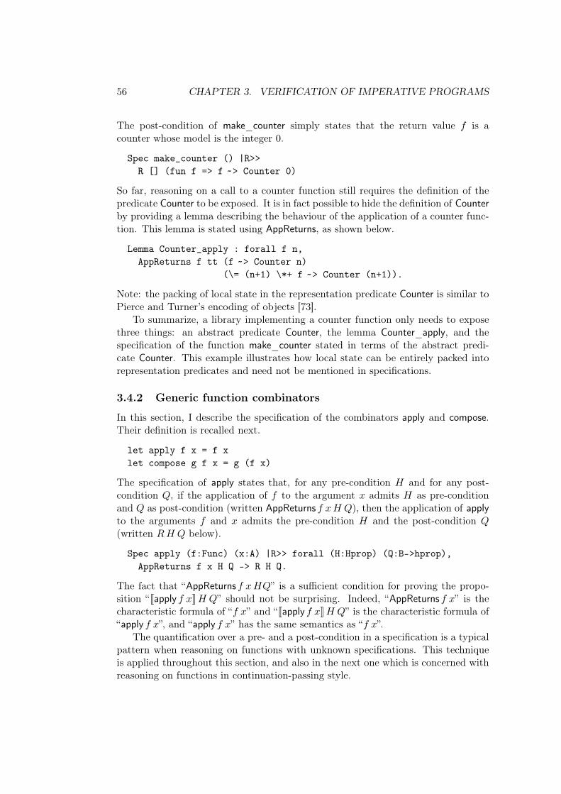
56 CHAPTER 3. VERIFICATION OF IMPERATIVE PROGRAMS
The post-condition of make_counter simply states that the return value 𝑓 is acounter whose model is the integer 0.
Spec make_counter () |R>>R [] (fun f => f ˜> Counter 0)
So far, reasoning on a call to a counter function still requires the definition of thepredicate Counter to be exposed. It is in fact possible to hide the definition of Counterby providing a lemma describing the behaviour of the application of a counter func-tion. This lemma is stated using AppReturns, as shown below.
Lemma Counter_apply : forall f n,AppReturns f tt (f ˜> Counter n)
(\= (n+1) \*+ f ˜> Counter (n+1)).
Note: the packing of local state in the representation predicate Counter is similar toPierce and Turner’s encoding of objects [73].
To summarize, a library implementing a counter function only needs to exposethree things: an abstract predicate Counter, the lemma Counter_apply, and thespecification of the function make_counter stated in terms of the abstract predi-cate Counter. This example illustrates how local state can be entirely packed intorepresentation predicates and need not be mentioned in specifications.
3.4.2 Generic function combinators
In this section, I describe the specification of the combinators apply and compose.Their definition is recalled next.
let apply f x = f xlet compose g f x = g (f x)
The specification of apply states that, for any pre-condition 𝐻 and for any post-condition 𝑄, if the application of 𝑓 to the argument 𝑥 admits 𝐻 as pre-conditionand 𝑄 as post-condition (written AppReturns 𝑓 𝑥𝐻 𝑄), then the application of applyto the arguments 𝑓 and 𝑥 admits the pre-condition 𝐻 and the post-condition 𝑄(written 𝑅𝐻 𝑄 below).
Spec apply (f:Func) (x:A) |R>> forall (H:Hprop) (Q:B->hprop),AppReturns f x H Q -> R H Q.
The fact that “AppReturns 𝑓 𝑥𝐻𝑄” is a sufficient condition for proving the propo-sition “Japply 𝑓 𝑥K𝐻 𝑄” should not be surprising. Indeed, “AppReturns 𝑓 𝑥” is thecharacteristic formula of “𝑓 𝑥” and “Japply 𝑓 𝑥K𝐻 𝑄” is the characteristic formula of“apply 𝑓 𝑥”, and “apply 𝑓 𝑥” has the same semantics as “𝑓 𝑥”.
The quantification over a pre- and a post-condition in a specification is a typicalpattern when reasoning on functions with unknown specifications. This techniqueis applied throughout this section, and also in the next one which is concerned withreasoning on functions in continuation-passing style.
3.4. TREATMENT OF FIRST-CLASS FUNCTIONS 57
The specification of compose is shown next. It quantifies over an initial pre-condition 𝐻, over a final post-condition 𝑄, and also over an intermediate post-condition 𝑄′, which describes the output of the application of the argument 𝑓 to theargument 𝑥.
Spec compose (g:Func) (f:Func) (x:A) |R>> forall H Q Q’,AppReturns f x H Q’ ->(forall y, AppReturns g y (Q’ y) Q) ->R H Q.
The hypotheses closely resemble the premises of the reasoning rule for let-bindings. Indeed, the term “compose 𝑔 𝑓 𝑥” has the same semantics as the term“ let 𝑦 = 𝑓 𝑥 in 𝑔 𝑦”. In fact, we can use the notation for characteristic formulae togive a more concise specification to the function compose, as shown below. Thebold keywords associated with notation for characteristic formulae are written inCoq using capitalized keywords. In particular, App is a notation for the predicateAppReturns.
Spec compose (g:Func) (f:Func) (x:A) |R>> forall H Q,(Let y = (App f x) In (App g y)) H Q -> R H Q.
With this specification, reasoning on an application of the function compose producesexactly the same proof obligation as if the source code of the function compose wasinlined. In general, code inlining is not a satisfying approach to verifying higher-order functions because it is not modular. However, the source code of the functioncompose is so basic that its specification is not more abstract that its source code.
3.4.3 Functions in continuation passing-style
The CPS-append function has been proposed as a verification challenge by Reynolds[77]. This function takes three arguments: two lists 𝑥 and 𝑦 and a continuation 𝑘.Its purpose is to call the continuation 𝑘 on the list obtained by concatenation ofthe lists 𝑥 and 𝑦. The function is implemented recursively, so as to compute theconcatenation of 𝑥 and 𝑦 using the function itself. I study first the purely-functionalversion of CPS-append, and then the corresponding imperative version that usesmutable lists.
The source code of the pure CPS-append function is shown next.
let rec cps_app (x:’a list) (y:’a list) (k:’a list->’b) : ’b =match x with | [] -> k y
| v::x’ -> cps_app x’ y (fun z -> k (v::z))
An example where 𝑥 is instantiated as a singleton list of the form “𝑣 :: nil” helpsunderstand the working of the function.
cps_app (𝑣 :: nil) 𝑦 𝑘 = cps_app nil 𝑦 (𝜆𝑧. 𝑘(𝑣 :: 𝑧)) = (𝜆𝑧. 𝑘(𝑣 :: 𝑧)) 𝑦 = 𝑘(𝑣 :: 𝑦)
58 CHAPTER 3. VERIFICATION OF IMPERATIVE PROGRAMS
The specification of the function asserts that if the application of the continuation𝑘 to the concatenation of 𝑥 and 𝑦 admits a pre-condition 𝐻 and a post-condition 𝑄,then so does the application of the CPS-append function to the arguments 𝑥, 𝑦 and𝑘. (For the sake of simplicity, I here assume the lists to contain purely-functionalvalues, thereby avoiding the need for representation predicates.)
Spec cps_app (x:list a) (y:list a) (k:Func) |R>>forall H Q, AppReturns k (x++y) H Q -> R H Q.
This specification is proved by induction on the structure of the list 𝑥.The imperative version of the CPS-append function is shown next. The func-
tion tail and set_tail are used to obtain and to update the tail of a mutable list,respectively.
let rec cps_app’ (x:’a mlist) (y:’a mlist) (k:’a mlist->’b) : ’b =if x == null
then k yelse cps_app’ (tail x) y (fun z -> set_tail x z; k x)
The specification is slightly more involved than in the purely-functional case becauseit involves representation predicates for the list and for the elements of that list. Thepre-condition asserts that the pointers 𝑥 and 𝑦 are starting points of lists modelledas 𝐿 and 𝑀 , respectively. It also mentions a heap predicate 𝐻 covering the rest ofthe heap. We need 𝐻 because the frame rule does not apply when reasoning withCPS functions, as the entire heap usually needs to be passed on to the continuation.In the imperative CPS-append function, the continuation 𝑘 is called on a pointer 𝑧that points to a list modelled as the concatenation of 𝐿 and 𝑀 . In addition to therepresentation predicate associated with 𝑧, the pre-condition of 𝑘 also mention theheap predicate 𝐻. The post-condition of the function, called 𝑄, is then the same asthe post-condition of the continuation. The complete specification appears next.
Spec cps_app’ (x:Loc) (y:Loc) (k:Func) |R>>forall (G:a->A->hprop) (L M:list A) H Q,(forall z, AppReturns k z (z ˜> Mlist G (L++M) \* H) Q) ->R (x ˜> Mlist G L \* y ˜> Mlist G M \* H) Q.
This specification is proved by induction on the structure of the list 𝐿.
3.4.4 Reasoning about list iterators
In this section, I show how to specify the iter function on purely-functional lists, andillustrate the use of this specification for reasoning on the manipulation of a list ofcounter functions.1
1Due to lack of time, I do not describe the specification of the functions fold and map, nor thespecification of iterators on imperative maps. I will add those later on.
3.4. TREATMENT OF FIRST-CLASS FUNCTIONS 59
The specification of the function iter shares a number of similarities with thetreatment of loops. Again, I want to avoid the introduction of a loop invariant anduse a presentation that takes advantage of local reasoning, because I want to be ableto reason about the application of the function iter to a function 𝑓 and to a list 𝑙without asserting that some prefix of the list 𝑙 has been treated by the function 𝑓while the remaining segment of the list 𝑙 has not yet been treated.
Recall the recursive implementation of the function iter.
let rec iter f l = match l with| [] -> ()| x::l -> f x; iter f l
The function iter is quite similar to the recursive encoding of a for-loop, in the sensethat the argument changes at every recursive call. So, I quantify over a predicate,called 𝑆, that depends on the argument 𝑙. The proposition 𝑆 𝑙𝐻 𝑄 asserts thatthe application of “ iter 𝑓 ” to the list 𝑙 admits the pre-condition 𝐻 and the post-condition 𝑄.
In the specification shown below, 𝑙0 denotes the initial list passed to iter, and 𝑙 de-notes a sublist of 𝑙0. The term “ iter 𝑓 𝑙0” admits 𝐻 and 𝑄 as pre- and post-conditions,written 𝑅𝐻 𝑄 (where 𝑅 is bound by the Spec notation), if the proposition 𝑆 𝑙0𝐻 𝑄does hold. The hypothesis given about 𝑆 is a slightly simplified version of thecharacteristic formula associated with the body of the function iter.
Spec iter (f:val) (l0:list a) |R>>(forall (S:(list a)->hprop->(unit->hprop)->Prop),
is_local_1 S ->(forall l H’ Q’,
match l with| nil => (H’ ==> Q’ tt)| x::l’ => (App f x ;; S l’) H’ Q’end ->
S l H’ Q’) ->S l0 H Q) ->
R H Q.
To check the usability of the specification of the function iter, I consider anexample. The function step_all, whose code appears below, takes as argument alist of distinct counter functions (recall §3.4.1), and makes a call to each of thosecounters for incrementing their local state. To keep the example simple, the resultsproduced by the invocation of the counter functions are simply ignored.
let step_all (l:list(unit->int)) =List.iter (fun f => ignore (f())) l
A list of counters is modelled using the application of the representation predicatePlist to the representation predicate Counter. More precisely, if 𝑙 is a list of functions
60 CHAPTER 3. VERIFICATION OF IMPERATIVE PROGRAMS
and 𝐿 is a list of integers, then the predicate 𝑙 Plist Counter𝐿 asserts that 𝐿contains the integer values describing the current state of each of the counters fromthe list 𝑙. A call to the function step_all on the list 𝑙 increments the state of everycounter, so the model of 𝑙 evolves from the list 𝐿 to a list 𝐿′. The list 𝐿′ is obtainedby applying the successor function to the elements of 𝐿, written map (𝜆𝑛. 𝑛 + 1)𝐿,where map denotes the map function on Coq lists. Hence the specification shownnext.
Spec step_all (l:list Func) |R>> forall (L:list int),R (l ˜> List Counter L)
(# l ˜> List Counter (map (fun n => n+1) L)).
Chapter 4
Characteristic formulae for pureprograms
This chapter describes the construction, pretty-printing and manipula-tion of characteristic formulae for purely-functional programs. I startwith the presentation of a set of informal rules explaining, for each con-struct from the source programming language, what logical formula de-scribes it. I then focus on the specification of n-ary functions and for-mally define the predicate Spec and the notation associated with it. Theformal presentation of a characteristic formula generator follows. Com-pared with the informal presentation, it involves direct support for n-aryfunctions and n-ary applications, it describes the lifting of program valuesto the logical level, and it shows how polymorphism is handled. Finally,I explain how to build a set of tactics for reasoning on characteristicformulae.
4.1 Source language and normalization
Before generating the characteristic formula of a program, I apply a transforma-tion on the source code so as to put the program in a administrative normal form.Through this process, the program is arranged so that all intermediate results andall functions become bound by a let-definition. One notable exception is the appli-cation of simple total functions such as addition and subtraction; for example, theapplication “𝑓 (𝑣1 + 𝑣2)” is considered to be in normal form although “𝑓 (𝑔 𝑣1 𝑣2)” isnot in normal form in general. Without such a special treatment of basic operators,programs in normal form tend to be hard to read.
The normalization process, which is similar to 𝐴-normalization [28], preservesthe semantics and greatly simplifies formal reasoning on programs. Moreover, it isstraightforward to implement. Similar transformations have appeared in previouswork on program verification (e.g., [40, 76]). I omit a formal description of thenormalization process because it is relatively standard and because its presentation
61
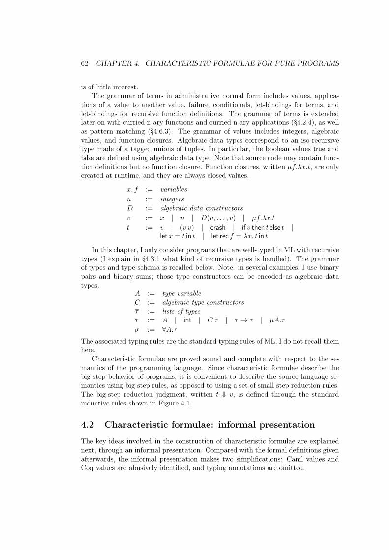
62 CHAPTER 4. CHARACTERISTIC FORMULAE FOR PURE PROGRAMS
is of little interest.The grammar of terms in administrative normal form includes values, applica-
tions of a value to another value, failure, conditionals, let-bindings for terms, andlet-bindings for recursive function definitions. The grammar of terms is extendedlater on with curried n-ary functions and curried n-ary applications (§4.2.4), as wellas pattern matching (§4.6.3). The grammar of values includes integers, algebraicvalues, and function closures. Algebraic data types correspond to an iso-recursivetype made of a tagged unions of tuples. In particular, the boolean values true andfalse are defined using algebraic data type. Note that source code may contain func-tion definitions but no function closure. Function closures, written 𝜇𝑓.𝜆𝑥.𝑡, are onlycreated at runtime, and they are always closed values.
𝑥, 𝑓 := variables𝑛 := integers𝐷 := algebraic data constructors𝑣 := 𝑥 | 𝑛 | 𝐷(𝑣, . . . , 𝑣) | 𝜇𝑓.𝜆𝑥.𝑡
𝑡 := 𝑣 | (𝑣 𝑣) | crash | if 𝑣 then 𝑡 else 𝑡 |let𝑥 = 𝑡 in 𝑡 | let rec 𝑓 = 𝜆𝑥. 𝑡 in 𝑡
In this chapter, I only consider programs that are well-typed in ML with recursivetypes (I explain in §4.3.1 what kind of recursive types is handled). The grammarof types and type schema is recalled below. Note: in several examples, I use binarypairs and binary sums; those type constructors can be encoded as algebraic datatypes.
𝐴 := type variable𝐶 := algebraic type constructors𝜏 := lists of types𝜏 := 𝐴 | int | 𝐶 𝜏 | 𝜏 → 𝜏 | 𝜇𝐴.𝜏
𝜎 := ∀𝐴.𝜏The associated typing rules are the standard typing rules of ML; I do not recall themhere.
Characteristic formulae are proved sound and complete with respect to the se-mantics of the programming language. Since characteristic formulae describe thebig-step behavior of programs, it is convenient to describe the source language se-mantics using big-step rules, as opposed to using a set of small-step reduction rules.The big-step reduction judgment, written 𝑡 ⇓ 𝑣, is defined through the standardinductive rules shown in Figure 4.1.
4.2 Characteristic formulae: informal presentation
The key ideas involved in the construction of characteristic formulae are explainednext, through an informal presentation. Compared with the formal definitions givenafterwards, the informal presentation makes two simplifications: Caml values andCoq values are abusively identified, and typing annotations are omitted.
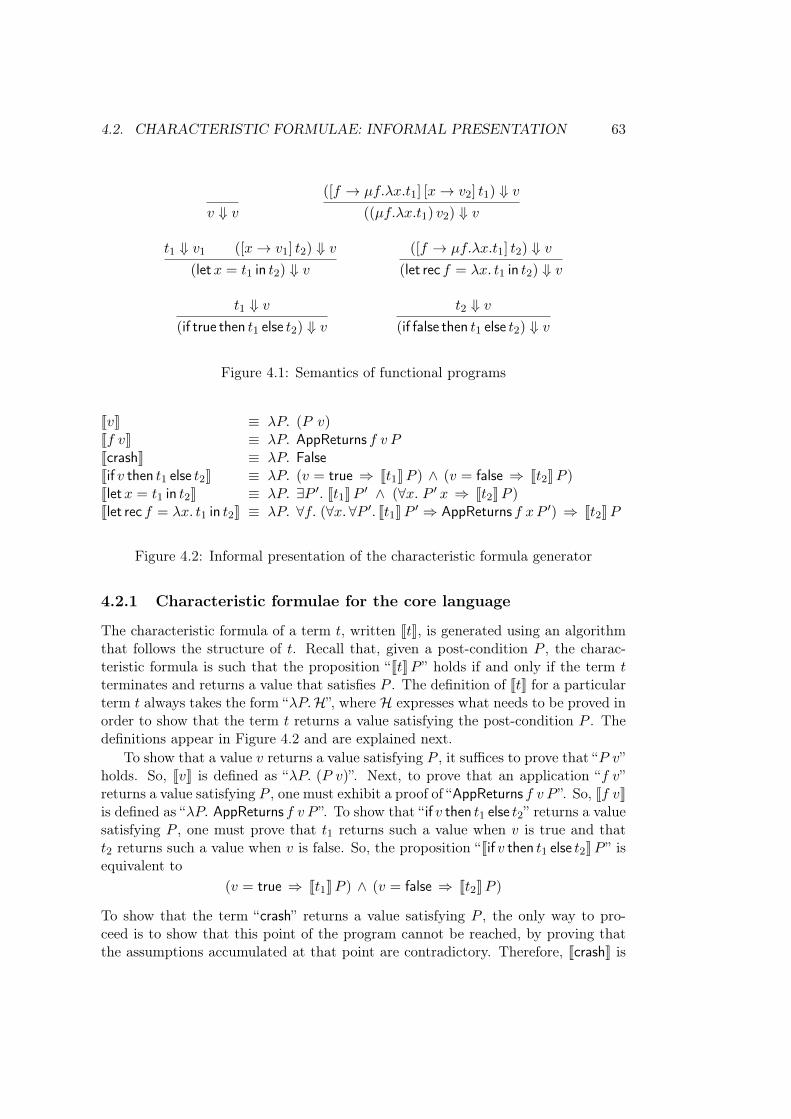
4.2. CHARACTERISTIC FORMULAE: INFORMAL PRESENTATION 63
𝑣 ⇓ 𝑣
([𝑓 → 𝜇𝑓.𝜆𝑥.𝑡1] [𝑥 → 𝑣2] 𝑡1) ⇓ 𝑣
((𝜇𝑓.𝜆𝑥.𝑡1) 𝑣2) ⇓ 𝑣
𝑡1 ⇓ 𝑣1 ([𝑥 → 𝑣1] 𝑡2) ⇓ 𝑣
(let𝑥 = 𝑡1 in 𝑡2) ⇓ 𝑣
([𝑓 → 𝜇𝑓.𝜆𝑥.𝑡1] 𝑡2) ⇓ 𝑣
(let rec 𝑓 = 𝜆𝑥. 𝑡1 in 𝑡2) ⇓ 𝑣
𝑡1 ⇓ 𝑣
(if true then 𝑡1 else 𝑡2) ⇓ 𝑣
𝑡2 ⇓ 𝑣
(if false then 𝑡1 else 𝑡2) ⇓ 𝑣
Figure 4.1: Semantics of functional programs
J𝑣K ≡ 𝜆𝑃. (𝑃 𝑣)J𝑓 𝑣K ≡ 𝜆𝑃. AppReturns 𝑓 𝑣 𝑃JcrashK ≡ 𝜆𝑃. FalseJif 𝑣 then 𝑡1 else 𝑡2K ≡ 𝜆𝑃. (𝑣 = true ⇒ J𝑡1K𝑃 ) ∧ (𝑣 = false ⇒ J𝑡2K𝑃 )Jlet𝑥 = 𝑡1 in 𝑡2K ≡ 𝜆𝑃. ∃𝑃 ′. J𝑡1K𝑃 ′ ∧ (∀𝑥. 𝑃 ′ 𝑥 ⇒ J𝑡2K𝑃 )Jlet rec 𝑓 = 𝜆𝑥. 𝑡1 in 𝑡2K ≡ 𝜆𝑃. ∀𝑓. (∀𝑥.∀𝑃 ′. J𝑡1K𝑃 ′ ⇒ AppReturns 𝑓 𝑥𝑃 ′) ⇒ J𝑡2K𝑃
Figure 4.2: Informal presentation of the characteristic formula generator
4.2.1 Characteristic formulae for the core language
The characteristic formula of a term 𝑡, written J𝑡K, is generated using an algorithmthat follows the structure of 𝑡. Recall that, given a post-condition 𝑃 , the charac-teristic formula is such that the proposition “J𝑡K𝑃 ” holds if and only if the term 𝑡terminates and returns a value that satisfies 𝑃 . The definition of J𝑡K for a particularterm 𝑡 always takes the form “𝜆𝑃.ℋ”, where ℋ expresses what needs to be proved inorder to show that the term 𝑡 returns a value satisfying the post-condition 𝑃 . Thedefinitions appear in Figure 4.2 and are explained next.
To show that a value 𝑣 returns a value satisfying 𝑃 , it suffices to prove that “𝑃 𝑣”holds. So, J𝑣K is defined as “𝜆𝑃. (𝑃 𝑣)”. Next, to prove that an application “𝑓 𝑣”returns a value satisfying 𝑃 , one must exhibit a proof of “AppReturns 𝑓 𝑣 𝑃 ”. So, J𝑓 𝑣Kis defined as “𝜆𝑃. AppReturns 𝑓 𝑣 𝑃 ”. To show that “ if 𝑣 then 𝑡1 else 𝑡2” returns a valuesatisfying 𝑃 , one must prove that 𝑡1 returns such a value when 𝑣 is true and that𝑡2 returns such a value when 𝑣 is false. So, the proposition “Jif 𝑣 then 𝑡1 else 𝑡2K𝑃 ” isequivalent to
(𝑣 = true ⇒ J𝑡1K𝑃 ) ∧ (𝑣 = false ⇒ J𝑡2K𝑃 )
To show that the term “crash” returns a value satisfying 𝑃 , the only way to pro-ceed is to show that this point of the program cannot be reached, by proving thatthe assumptions accumulated at that point are contradictory. Therefore, JcrashK is
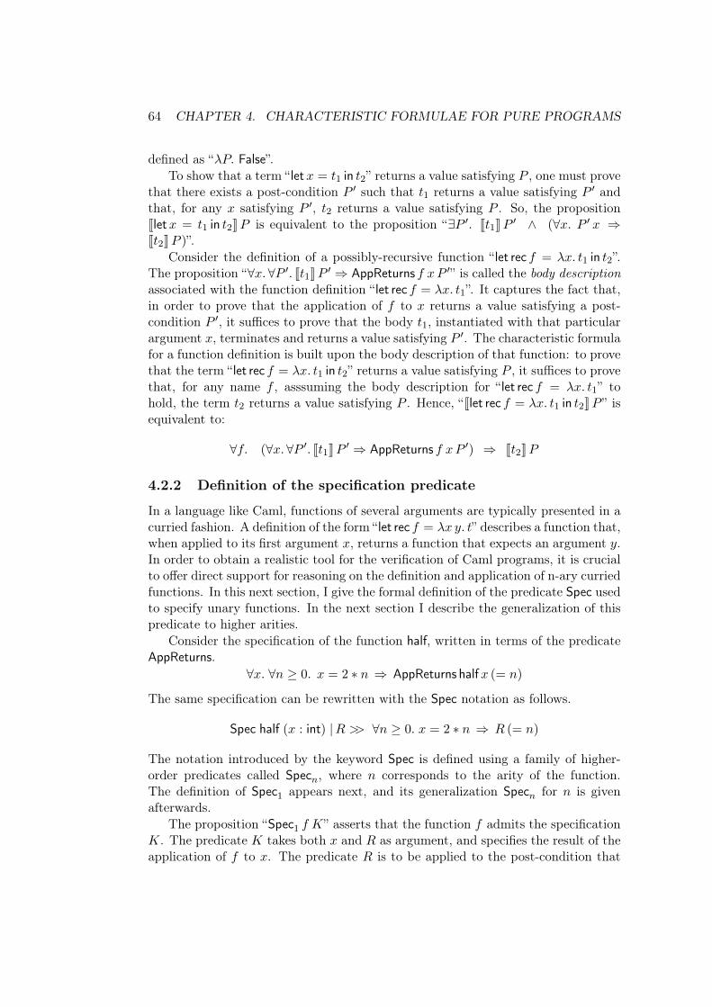
64 CHAPTER 4. CHARACTERISTIC FORMULAE FOR PURE PROGRAMS
defined as “𝜆𝑃. False”.To show that a term “ let𝑥 = 𝑡1 in 𝑡2” returns a value satisfying 𝑃 , one must prove
that there exists a post-condition 𝑃 ′ such that 𝑡1 returns a value satisfying 𝑃 ′ andthat, for any 𝑥 satisfying 𝑃 ′, 𝑡2 returns a value satisfying 𝑃 . So, the propositionJlet𝑥 = 𝑡1 in 𝑡2K𝑃 is equivalent to the proposition “∃𝑃 ′. J𝑡1K𝑃 ′ ∧ (∀𝑥. 𝑃 ′ 𝑥 ⇒J𝑡2K𝑃 )”.
Consider the definition of a possibly-recursive function “ let rec 𝑓 = 𝜆𝑥. 𝑡1 in 𝑡2”.The proposition “∀𝑥.∀𝑃 ′. J𝑡1K𝑃 ′ ⇒ AppReturns 𝑓 𝑥𝑃 ′” is called the body descriptionassociated with the function definition “ let rec 𝑓 = 𝜆𝑥. 𝑡1”. It captures the fact that,in order to prove that the application of 𝑓 to 𝑥 returns a value satisfying a post-condition 𝑃 ′, it suffices to prove that the body 𝑡1, instantiated with that particularargument 𝑥, terminates and returns a value satisfying 𝑃 ′. The characteristic formulafor a function definition is built upon the body description of that function: to provethat the term “ let rec 𝑓 = 𝜆𝑥. 𝑡1 in 𝑡2” returns a value satisfying 𝑃 , it suffices to provethat, for any name 𝑓 , asssuming the body description for “ let rec 𝑓 = 𝜆𝑥. 𝑡1” tohold, the term 𝑡2 returns a value satisfying 𝑃 . Hence, “Jlet rec 𝑓 = 𝜆𝑥. 𝑡1 in 𝑡2K𝑃 ” isequivalent to:
∀𝑓. (∀𝑥. ∀𝑃 ′. J𝑡1K𝑃 ′ ⇒ AppReturns 𝑓 𝑥𝑃 ′) ⇒ J𝑡2K𝑃
4.2.2 Definition of the specification predicate
In a language like Caml, functions of several arguments are typically presented in acurried fashion. A definition of the form “ let rec 𝑓 = 𝜆𝑥 𝑦. 𝑡” describes a function that,when applied to its first argument 𝑥, returns a function that expects an argument 𝑦.In order to obtain a realistic tool for the verification of Caml programs, it is crucialto offer direct support for reasoning on the definition and application of n-ary curriedfunctions. In this next section, I give the formal definition of the predicate Spec usedto specify unary functions. In the next section I describe the generalization of thispredicate to higher arities.
Consider the specification of the function half, written in terms of the predicateAppReturns.
∀𝑥. ∀𝑛 ≥ 0. 𝑥 = 2 * 𝑛 ⇒ AppReturns half𝑥 (= 𝑛)
The same specification can be rewritten with the Spec notation as follows.
Spec half (𝑥 : int) |𝑅 >> ∀𝑛 ≥ 0. 𝑥 = 2 * 𝑛 ⇒ 𝑅 (= 𝑛)
The notation introduced by the keyword Spec is defined using a family of higher-order predicates called Spec𝑛, where 𝑛 corresponds to the arity of the function.The definition of Spec1 appears next, and its generalization Spec𝑛 for 𝑛 is givenafterwards.
The proposition “Spec1 𝑓 𝐾” asserts that the function 𝑓 admits the specification𝐾. The predicate 𝐾 takes both 𝑥 and 𝑅 as argument, and specifies the result of theapplication of 𝑓 to 𝑥. The predicate 𝑅 is to be applied to the post-condition that
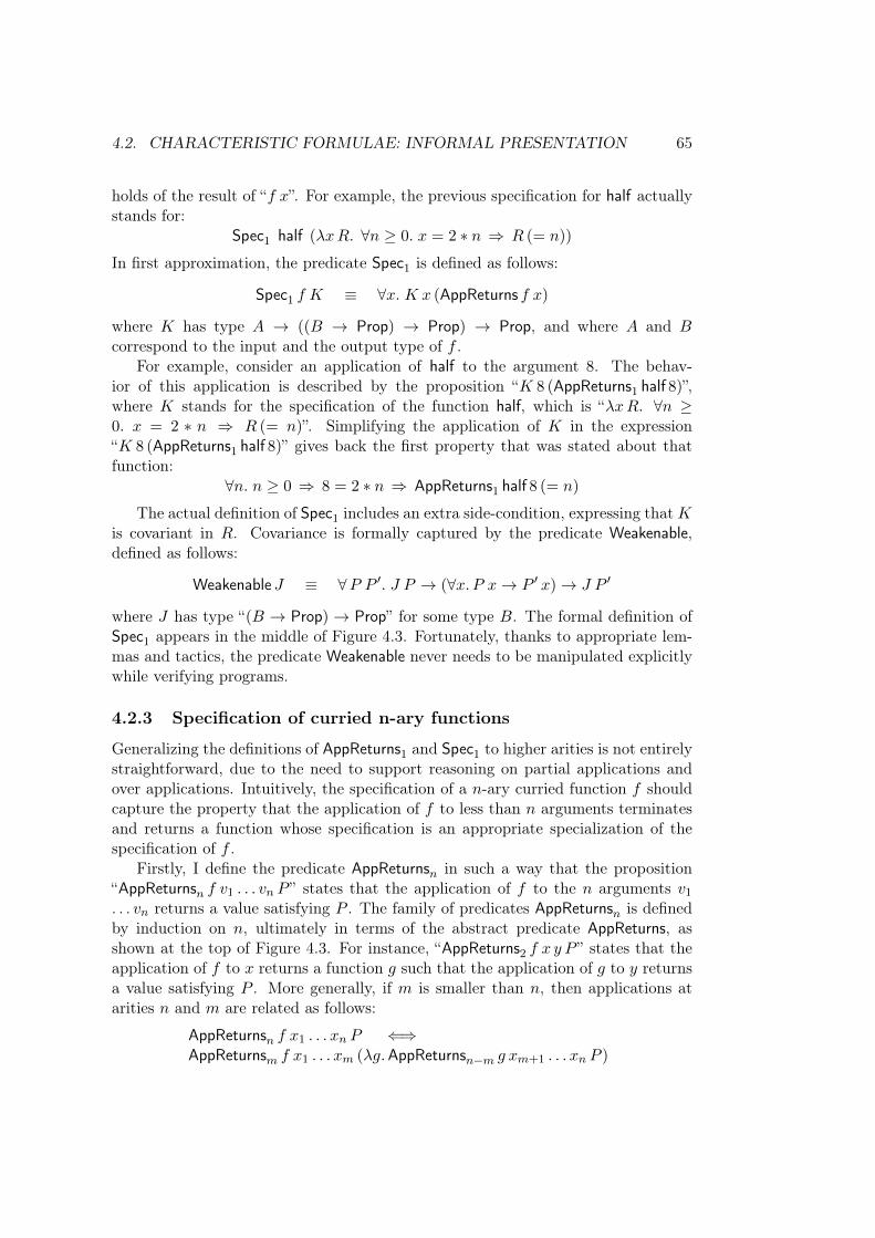
4.2. CHARACTERISTIC FORMULAE: INFORMAL PRESENTATION 65
holds of the result of “𝑓 𝑥”. For example, the previous specification for half actuallystands for:
Spec1 half (𝜆𝑥𝑅. ∀𝑛 ≥ 0. 𝑥 = 2 * 𝑛 ⇒ 𝑅 (= 𝑛))
In first approximation, the predicate Spec1 is defined as follows:
Spec1 𝑓 𝐾 ≡ ∀𝑥. 𝐾 𝑥 (AppReturns 𝑓 𝑥)
where 𝐾 has type 𝐴 → ((𝐵 → Prop) → Prop) → Prop, and where 𝐴 and 𝐵correspond to the input and the output type of 𝑓 .
For example, consider an application of half to the argument 8. The behav-ior of this application is described by the proposition “𝐾 8 (AppReturns1 half 8)”,where 𝐾 stands for the specification of the function half, which is “𝜆𝑥𝑅. ∀𝑛 ≥0. 𝑥 = 2 * 𝑛 ⇒ 𝑅 (= 𝑛)”. Simplifying the application of 𝐾 in the expression“𝐾 8 (AppReturns1 half 8)” gives back the first property that was stated about thatfunction:
∀𝑛. 𝑛 ≥ 0 ⇒ 8 = 2 * 𝑛 ⇒ AppReturns1 half 8 (= 𝑛)
The actual definition of Spec1 includes an extra side-condition, expressing that 𝐾is covariant in 𝑅. Covariance is formally captured by the predicate Weakenable,defined as follows:
Weakenable 𝐽 ≡ ∀𝑃 𝑃 ′. 𝐽 𝑃 → (∀𝑥. 𝑃 𝑥 → 𝑃 ′ 𝑥) → 𝐽 𝑃 ′
where 𝐽 has type “(𝐵 → Prop) → Prop” for some type 𝐵. The formal definition ofSpec1 appears in the middle of Figure 4.3. Fortunately, thanks to appropriate lem-mas and tactics, the predicate Weakenable never needs to be manipulated explicitlywhile verifying programs.
4.2.3 Specification of curried n-ary functions
Generalizing the definitions of AppReturns1 and Spec1 to higher arities is not entirelystraightforward, due to the need to support reasoning on partial applications andover applications. Intuitively, the specification of a 𝑛-ary curried function 𝑓 shouldcapture the property that the application of 𝑓 to less than 𝑛 arguments terminatesand returns a function whose specification is an appropriate specialization of thespecification of 𝑓 .
Firstly, I define the predicate AppReturns𝑛 in such a way that the proposition“AppReturns𝑛 𝑓 𝑣1 . . . 𝑣𝑛 𝑃 ” states that the application of 𝑓 to the 𝑛 arguments 𝑣1. . . 𝑣𝑛 returns a value satisfying 𝑃 . The family of predicates AppReturns𝑛 is definedby induction on 𝑛, ultimately in terms of the abstract predicate AppReturns, asshown at the top of Figure 4.3. For instance, “AppReturns2 𝑓 𝑥 𝑦 𝑃 ” states that theapplication of 𝑓 to 𝑥 returns a function 𝑔 such that the application of 𝑔 to 𝑦 returnsa value satisfying 𝑃 . More generally, if 𝑚 is smaller than 𝑛, then applications atarities 𝑛 and 𝑚 are related as follows:
AppReturns𝑛 𝑓 𝑥1 . . . 𝑥𝑛 𝑃 ⇐⇒AppReturns𝑚 𝑓 𝑥1 . . . 𝑥𝑚 (𝜆𝑔.AppReturns𝑛−𝑚 𝑔 𝑥𝑚+1 . . . 𝑥𝑛 𝑃 )
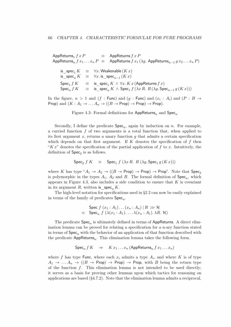
66 CHAPTER 4. CHARACTERISTIC FORMULAE FOR PURE PROGRAMS
AppReturns1 𝑓 𝑥𝑃 ≡ AppReturns 𝑓 𝑥𝑃AppReturns𝑛 𝑓 𝑥1 . . . 𝑥𝑛 𝑃 ≡ AppReturns 𝑓 𝑥1 (𝜆𝑔. AppReturns𝑛−1 𝑔 𝑥2 . . . 𝑥𝑛 𝑃 )
is_spec1𝐾 ≡ ∀𝑥.Weakenable (𝐾 𝑥)is_spec𝑛𝐾 ≡ ∀𝑥. is_spec𝑛−1 (𝐾 𝑥)
Spec1 𝑓 𝐾 ≡ is_spec1𝐾 ∧ ∀𝑥.𝐾 𝑥 (AppReturns 𝑓 𝑥)Spec𝑛 𝑓 𝐾 ≡ is_spec𝑛𝐾 ∧ Spec1 𝑓 (𝜆𝑥𝑅. 𝑅 (𝜆𝑔. Spec𝑛−1 𝑔 (𝐾 𝑥)))
In the figure, 𝑛 > 1 and (𝑓 : Func) and (𝑔 : Func) and (𝑥𝑖 : 𝐴𝑖) and (𝑃 : 𝐵 →Prop) and (𝐾 : 𝐴1 → . . . 𝐴𝑛 → ((𝐵 → Prop) → Prop) → Prop).
Figure 4.3: Formal definitions for AppReturns𝑛 and Spec𝑛
Secondly, I define the predicate Spec𝑛, again by induction on 𝑛. For example,a curried function 𝑓 of two arguments is a total function that, when applied toits first argument 𝑥, returns a unary function 𝑔 that admits a certain specificationwhich depends on that first argument. If 𝐾 denotes the specification of 𝑓 then“𝐾 𝑥” denotes the specification of the partial application of 𝑓 to 𝑥. Intuitively, thedefinition of Spec2 is as follows.
Spec2 𝑓 𝐾 ≡ Spec1 𝑓 (𝜆𝑥𝑅. 𝑅 (𝜆𝑔. Spec1 𝑔 (𝐾 𝑥)))
where 𝐾 has type “𝐴1 → 𝐴2 → ((𝐵 → Prop) → Prop) → Prop”. Note that Spec2is polymorphic in the types 𝐴1, 𝐴2 and 𝐵. The formal definition of Spec𝑛, whichappears in Figure 4.3, also includes a side condition to ensure that 𝐾 is covariantin its argument 𝑅, written is_spec𝑛𝐾.
The high-level notation for specifications used in §2.2 can now be easily explainedin terms of the family of predicates Spec𝑛.
Spec 𝑓 (𝑥1 : 𝐴1) . . . (𝑥𝑛 : 𝐴𝑛) |𝑅 >> ℋ≡ Spec𝑛 𝑓 (𝜆(𝑥1 : 𝐴1). . . . 𝜆(𝑥𝑛 : 𝐴1). 𝜆𝑅. ℋ)
The predicate Spec𝑛 is ultimately defined in terms of AppReturns. A direct elim-ination lemma can be proved for relating a specification for a n-ary function statedin terms of Spec𝑛 with the behavior of an application of that function described withthe predicate AppReturns𝑛. This elimination lemma takes the following form.
Spec𝑛 𝑓 𝐾 ⇒ 𝐾 𝑥1 . . . 𝑥𝑛 (AppReturns𝑛 𝑓 𝑥1 . . . 𝑥𝑛)
where 𝑓 has type Func, where each 𝑥𝑖 admits a type 𝐴𝑖, and where 𝐾 is of type𝐴1 → . . . 𝐴𝑛 → ((𝐵 → Prop) → Prop) → Prop, with 𝐵 being the return typeof the function 𝑓 . This elimination lemma is not intended to be used directly;it serves as a basis for proving other lemmas upon which tactics for reasoning onapplications are based (§4.7.2). Note that the elimination lemma admits a reciprocal,
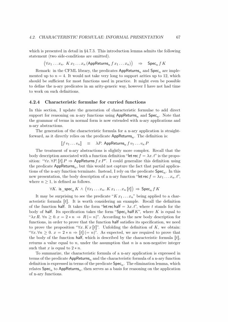
4.2. CHARACTERISTIC FORMULAE: INFORMAL PRESENTATION 67
which is presented in detail in §4.7.3. This introduction lemma admits the followingstatement (two side-conditions are omitted).Ä
∀𝑥1 . . . 𝑥𝑛. 𝐾 𝑥1 . . . 𝑥𝑛 (AppReturns𝑛 𝑓 𝑥1 . . . 𝑥𝑛)ä
⇒ Spec𝑛 𝑓 𝐾
Remark: in the CFML library, the predicates AppReturns𝑛 and Spec𝑛 are imple-mented up to 𝑛 = 4. It would not take very long to support arities up to 12, whichshould be sufficient for most functions used in practice. It might even be possibleto define the n-ary predicates in an arity-generic way, however I have not had timeto work on such definitions.
4.2.4 Characteristic formulae for curried functions
In this section, I update the generation of characteristic formulae to add directsupport for reasoning on n-ary functions using AppReturns𝑛 and Spec𝑛. Note thatthe grammar of terms in normal form is now extended with n-ary applications andn-ary abstractions.
The generation of the characteristic formula for a n-ary application is straight-forward, as it directly relies on the predicate AppReturns𝑛. The definition is:
J𝑓 𝑣1 . . . 𝑣𝑛K ≡ 𝜆𝑃. AppReturns𝑛 𝑓 𝑣1 . . . 𝑣𝑛 𝑃
The treatment of n-ary abstractions is slightly more complex. Recall that thebody description associated with a function definition “ let rec 𝑓 = 𝜆𝑥. 𝑡” is the propo-sition: “∀𝑥. ∀𝑃. J𝑡K𝑃 ⇒ AppReturns 𝑓 𝑥𝑃 ”. I could generalize this definition usingthe predicate AppReturns𝑛, but this would not capture the fact that partial applica-tions of the n-ary function terminate. Instead, I rely on the predicate Spec𝑛. In thisnew presentation, the body description of a n-ary function “ let rec 𝑓 = 𝜆𝑥1 . . . 𝑥𝑛. 𝑡”,where 𝑛 ≥ 1, is defined as follows.
∀𝐾. is_spec𝑛𝐾 ∧Ä∀𝑥1 . . . 𝑥𝑛. 𝐾 𝑥1 . . . 𝑥𝑛 J𝑡K
ä⇒ Spec𝑛 𝑓 𝐾
It may be surprising to see the predicate “𝐾 𝑥1 . . . 𝑥𝑛” being applied to a char-acteristic formula J𝑡K. It is worth considering an example. Recall the definitionof the function half. It takes the form “ let rec half = 𝜆𝑥. 𝑡”, where 𝑡 stands for thebody of half. Its specification takes the form “Spec1 half𝐾”, where 𝐾 is equal to“𝜆𝑥𝑅. ∀𝑛 ≥ 0. 𝑥 = 2 * 𝑛 ⇒ 𝑅 (= 𝑛)”. According to the new body description forfunctions, in order to prove that the function half satisfies its specification, we needto prove the proposition “∀𝑥.𝐾 𝑥 J𝑡K”. Unfolding the definition of 𝐾, we obtain:“∀𝑥.∀𝑛 ≥ 0. 𝑥 = 2 * 𝑛 ⇒ J𝑡K (= 𝑛)”. As expected, we are required to prove thatthe body of the function half, which is described by the characteristic formula J𝑡K,returns a value equal to 𝑛, under the assumption that 𝑛 is a non-negative integersuch that 𝑥 is equal to 2 * 𝑛.
To summarize, the characteristic formula of a n-ary application is expressed interms of the predicate AppReturns𝑛 and the characteristic formula of a n-ary functiondefinition is expressed in terms of the predicate Spec𝑛. The elimination lemma, whichrelates Spec𝑛 to AppReturns𝑛, then serves as a basis for reasoning on the applicationof n-ary functions.
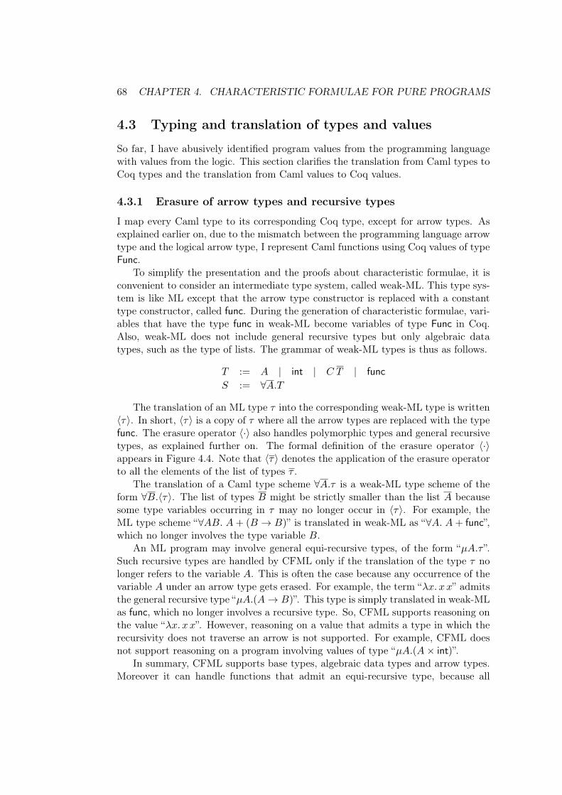
68 CHAPTER 4. CHARACTERISTIC FORMULAE FOR PURE PROGRAMS
4.3 Typing and translation of types and values
So far, I have abusively identified program values from the programming languagewith values from the logic. This section clarifies the translation from Caml types toCoq types and the translation from Caml values to Coq values.
4.3.1 Erasure of arrow types and recursive types
I map every Caml type to its corresponding Coq type, except for arrow types. Asexplained earlier on, due to the mismatch between the programming language arrowtype and the logical arrow type, I represent Caml functions using Coq values of typeFunc.
To simplify the presentation and the proofs about characteristic formulae, it isconvenient to consider an intermediate type system, called weak-ML. This type sys-tem is like ML except that the arrow type constructor is replaced with a constanttype constructor, called func. During the generation of characteristic formulae, vari-ables that have the type func in weak-ML become variables of type Func in Coq.Also, weak-ML does not include general recursive types but only algebraic datatypes, such as the type of lists. The grammar of weak-ML types is thus as follows.
𝑇 := 𝐴 | int | 𝐶 𝑇 | func𝑆 := ∀𝐴.𝑇
The translation of an ML type 𝜏 into the corresponding weak-ML type is written⟨𝜏⟩. In short, ⟨𝜏⟩ is a copy of 𝜏 where all the arrow types are replaced with the typefunc. The erasure operator ⟨·⟩ also handles polymorphic types and general recursivetypes, as explained further on. The formal definition of the erasure operator ⟨·⟩appears in Figure 4.4. Note that ⟨𝜏⟩ denotes the application of the erasure operatorto all the elements of the list of types 𝜏 .
The translation of a Caml type scheme ∀𝐴.𝜏 is a weak-ML type scheme of theform ∀𝐵.⟨𝜏⟩. The list of types 𝐵 might be strictly smaller than the list 𝐴 becausesome type variables occurring in 𝜏 may no longer occur in ⟨𝜏⟩. For example, theML type scheme “∀𝐴𝐵. 𝐴 + (𝐵 → 𝐵)” is translated in weak-ML as “∀𝐴. 𝐴 + func”,which no longer involves the type variable 𝐵.
An ML program may involve general equi-recursive types, of the form “𝜇𝐴.𝜏 ”.Such recursive types are handled by CFML only if the translation of the type 𝜏 nolonger refers to the variable 𝐴. This is often the case because any occurrence of thevariable 𝐴 under an arrow type gets erased. For example, the term “𝜆𝑥. 𝑥 𝑥” admitsthe general recursive type “𝜇𝐴.(𝐴 → 𝐵)”. This type is simply translated in weak-MLas func, which no longer involves a recursive type. So, CFML supports reasoning onthe value “𝜆𝑥. 𝑥 𝑥”. However, reasoning on a value that admits a type in which therecursivity does not traverse an arrow is not supported. For example, CFML doesnot support reasoning on a program involving values of type “𝜇𝐴.(𝐴× int)”.
In summary, CFML supports base types, algebraic data types and arrow types.Moreover it can handle functions that admit an equi-recursive type, because all
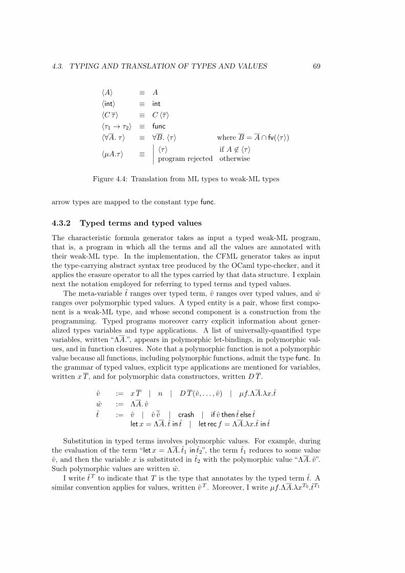
4.3. TYPING AND TRANSLATION OF TYPES AND VALUES 69
⟨𝐴⟩ ≡ 𝐴
⟨int⟩ ≡ int⟨𝐶 𝜏⟩ ≡ 𝐶 ⟨𝜏⟩⟨𝜏1 → 𝜏2⟩ ≡ func⟨∀𝐴. 𝜏⟩ ≡ ∀𝐵. ⟨𝜏⟩ where 𝐵 = 𝐴 ∩ fv(⟨𝜏⟩)
⟨𝜇𝐴.𝜏⟩ ≡∣∣∣∣∣ ⟨𝜏⟩ if 𝐴 ̸∈ ⟨𝜏⟩
program rejected otherwise
Figure 4.4: Translation from ML types to weak-ML types
arrow types are mapped to the constant type func.
4.3.2 Typed terms and typed values
The characteristic formula generator takes as input a typed weak-ML program,that is, a program in which all the terms and all the values are annotated withtheir weak-ML type. In the implementation, the CFML generator takes as inputthe type-carrying abstract syntax tree produced by the OCaml type-checker, and itapplies the erasure operator to all the types carried by that data structure. I explainnext the notation employed for referring to typed terms and typed values.
The meta-variable 𝑡 ranges over typed term, 𝑣 ranges over typed values, and �̂�ranges over polymorphic typed values. A typed entity is a pair, whose first compo-nent is a weak-ML type, and whose second component is a construction from theprogramming. Typed programs moreover carry explicit information about gener-alized types variables and type applications. A list of universally-quantified typevariables, written “Λ𝐴.”, appears in polymorphic let-bindings, in polymorphic val-ues, and in function closures. Note that a polymorphic function is not a polymorphicvalue because all functions, including polymorphic functions, admit the type func. Inthe grammar of typed values, explicit type applications are mentioned for variables,written 𝑥𝑇 , and for polymorphic data constructors, written 𝐷𝑇 .
𝑣 := 𝑥𝑇 | 𝑛 | 𝐷𝑇 (𝑣, . . . , 𝑣) | 𝜇𝑓.Λ𝐴.𝜆𝑥.𝑡
�̂� := Λ𝐴. 𝑣
𝑡 := 𝑣 | 𝑣 𝑣 | crash | if 𝑣 then 𝑡 else 𝑡let𝑥 = Λ𝐴. 𝑡 in 𝑡 | let rec 𝑓 = Λ𝐴.𝜆𝑥.𝑡 in 𝑡
Substitution in typed terms involves polymorphic values. For example, duringthe evaluation of the term “ let𝑥 = Λ𝐴. 𝑡1 in 𝑡2”, the term 𝑡1 reduces to some value𝑣, and then the variable 𝑥 is substituted in 𝑡2 with the polymorphic value “Λ𝐴. 𝑣”.Such polymorphic values are written �̂�.
I write 𝑡𝑇 to indicate that 𝑇 is the type that annotates by the typed term 𝑡. Asimilar convention applies for values, written 𝑣 𝑇 . Moreover, I write 𝜇𝑓.Λ𝐴.𝜆𝑥𝑇0 .𝑡𝑇1
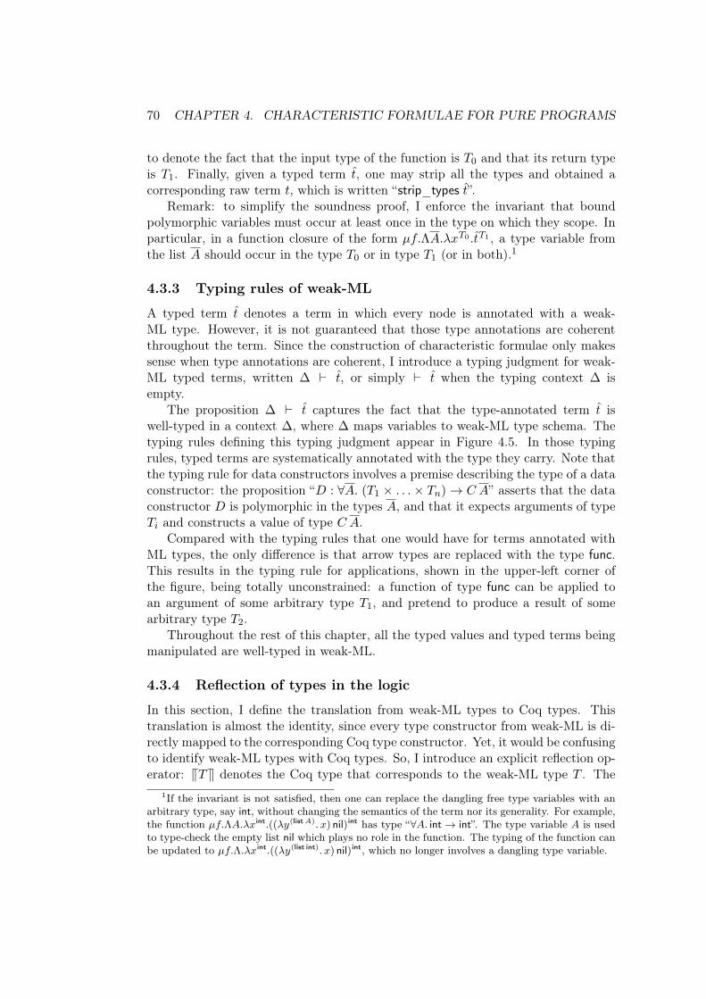
70 CHAPTER 4. CHARACTERISTIC FORMULAE FOR PURE PROGRAMS
to denote the fact that the input type of the function is 𝑇0 and that its return typeis 𝑇1. Finally, given a typed term 𝑡, one may strip all the types and obtained acorresponding raw term 𝑡, which is written “strip_types 𝑡”.
Remark: to simplify the soundness proof, I enforce the invariant that boundpolymorphic variables must occur at least once in the type on which they scope. Inparticular, in a function closure of the form 𝜇𝑓.Λ𝐴.𝜆𝑥𝑇0 .𝑡𝑇1 , a type variable fromthe list 𝐴 should occur in the type 𝑇0 or in type 𝑇1 (or in both).1
4.3.3 Typing rules of weak-ML
A typed term 𝑡 denotes a term in which every node is annotated with a weak-ML type. However, it is not guaranteed that those type annotations are coherentthroughout the term. Since the construction of characteristic formulae only makessense when type annotations are coherent, I introduce a typing judgment for weak-ML typed terms, written ∆ ⊢ 𝑡, or simply ⊢ 𝑡 when the typing context ∆ isempty.
The proposition ∆ ⊢ 𝑡 captures the fact that the type-annotated term 𝑡 iswell-typed in a context ∆, where ∆ maps variables to weak-ML type schema. Thetyping rules defining this typing judgment appear in Figure 4.5. In those typingrules, typed terms are systematically annotated with the type they carry. Note thatthe typing rule for data constructors involves a premise describing the type of a dataconstructor: the proposition “𝐷 : ∀𝐴. (𝑇1 × . . .× 𝑇𝑛) → 𝐶 𝐴” asserts that the dataconstructor 𝐷 is polymorphic in the types 𝐴, and that it expects arguments of type𝑇𝑖 and constructs a value of type 𝐶 𝐴.
Compared with the typing rules that one would have for terms annotated withML types, the only difference is that arrow types are replaced with the type func.This results in the typing rule for applications, shown in the upper-left corner ofthe figure, being totally unconstrained: a function of type func can be applied toan argument of some arbitrary type 𝑇1, and pretend to produce a result of somearbitrary type 𝑇2.
Throughout the rest of this chapter, all the typed values and typed terms beingmanipulated are well-typed in weak-ML.
4.3.4 Reflection of types in the logic
In this section, I define the translation from weak-ML types to Coq types. Thistranslation is almost the identity, since every type constructor from weak-ML is di-rectly mapped to the corresponding Coq type constructor. Yet, it would be confusingto identify weak-ML types with Coq types. So, I introduce an explicit reflection op-erator: V𝑇W denotes the Coq type that corresponds to the weak-ML type 𝑇 . The
1If the invariant is not satisfied, then one can replace the dangling free type variables with anarbitrary type, say int, without changing the semantics of the term nor its generality. For example,the function 𝜇𝑓.Λ𝐴.𝜆𝑥int.((𝜆𝑦(list𝐴). 𝑥) nil)int has type “∀𝐴. int → int”. The type variable 𝐴 is usedto type-check the empty list nil which plays no role in the function. The typing of the function canbe updated to 𝜇𝑓.Λ.𝜆𝑥int.((𝜆𝑦(list int). 𝑥) nil)int, which no longer involves a dangling type variable.
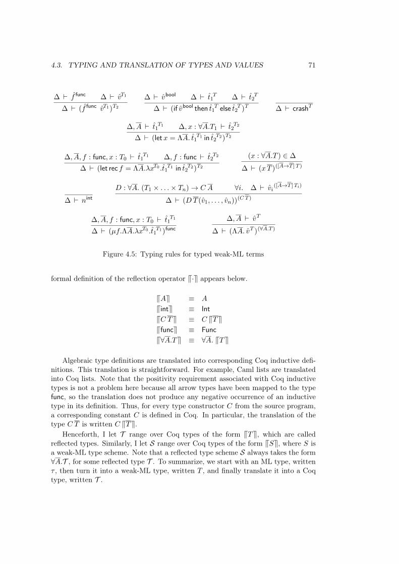
4.3. TYPING AND TRANSLATION OF TYPES AND VALUES 71
∆ ⊢ 𝑓 func ∆ ⊢ 𝑣𝑇1
∆ ⊢ (𝑓 func 𝑣𝑇1)𝑇2
∆ ⊢ 𝑣bool ∆ ⊢ 𝑡1𝑇 ∆ ⊢ 𝑡2
𝑇
∆ ⊢ (if 𝑣bool then 𝑡1𝑇 else 𝑡2𝑇 )𝑇 ∆ ⊢ crash𝑇
∆, 𝐴 ⊢ 𝑡1𝑇1 ∆, 𝑥 : ∀𝐴.𝑇1 ⊢ 𝑡2
𝑇2
∆ ⊢ (let𝑥 = Λ𝐴. 𝑡1𝑇1 in 𝑡2𝑇2)𝑇2
∆, 𝐴, 𝑓 : func, 𝑥 : 𝑇0 ⊢ 𝑡1𝑇1 ∆, 𝑓 : func ⊢ 𝑡2
𝑇2
∆ ⊢ (let rec 𝑓 = Λ𝐴.𝜆𝑥𝑇0 .𝑡1𝑇1 in 𝑡2𝑇2)𝑇2
(𝑥 : ∀𝐴.𝑇 ) ∈ ∆
∆ ⊢ (𝑥𝑇 )([𝐴→𝑇 ]𝑇 )
∆ ⊢ 𝑛int
𝐷 : ∀𝐴. (𝑇1 × . . .× 𝑇𝑛) → 𝐶 𝐴 ∀𝑖. ∆ ⊢ 𝑣𝑖([𝐴→𝑇 ]𝑇𝑖)
∆ ⊢ (𝐷𝑇 (𝑣1, . . . , 𝑣𝑛))(𝐶 𝑇 )
∆, 𝐴, 𝑓 : func, 𝑥 : 𝑇0 ⊢ 𝑡1𝑇1
∆ ⊢ (𝜇𝑓.Λ𝐴.𝜆𝑥𝑇0 .𝑡1𝑇1)func
∆, 𝐴 ⊢ 𝑣𝑇
∆ ⊢ (Λ𝐴. 𝑣𝑇 )(∀𝐴.𝑇 )
Figure 4.5: Typing rules for typed weak-ML terms
formal definition of the reflection operator V·W appears below.
V𝐴W ≡ 𝐴
VintW ≡ IntV𝐶 𝑇W ≡ 𝐶 V𝑇WVfuncW ≡ FuncV∀𝐴.𝑇W ≡ ∀𝐴. V𝑇W
Algebraic type definitions are translated into corresponding Coq inductive defi-nitions. This translation is straightforward. For example, Caml lists are translatedinto Coq lists. Note that the positivity requirement associated with Coq inductivetypes is not a problem here because all arrow types have been mapped to the typefunc, so the translation does not produce any negative occurrence of an inductivetype in its definition. Thus, for every type constructor 𝐶 from the source program,a corresponding constant 𝐶 is defined in Coq. In particular, the translation of thetype 𝐶 𝑇 is written 𝐶 V𝑇W.
Henceforth, I let 𝒯 range over Coq types of the form V𝑇W, which are calledreflected types. Similarly, I let 𝒮 range over Coq types of the form V𝑆W, where 𝑆 isa weak-ML type scheme. Note that a reflected type scheme 𝒮 always takes the form∀𝐴.𝒯 , for some reflected type 𝒯 . To summarize, we start with an ML type, written𝜏 , then turn it into a weak-ML type, written 𝑇 , and finally translate it into a Coqtype, written 𝒯 .
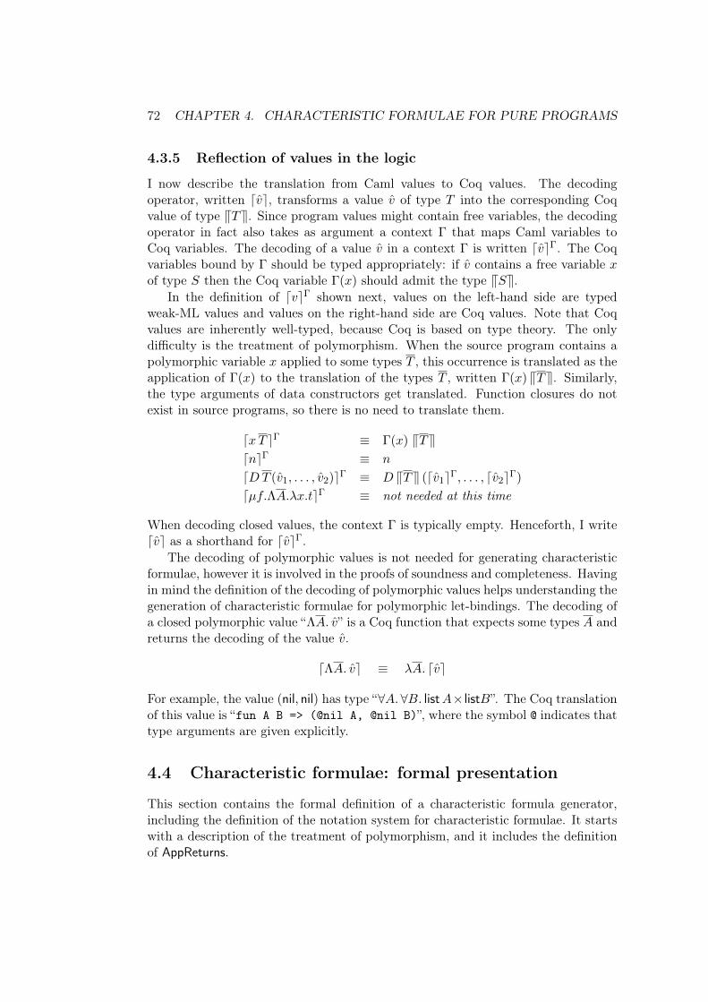
72 CHAPTER 4. CHARACTERISTIC FORMULAE FOR PURE PROGRAMS
4.3.5 Reflection of values in the logic
I now describe the translation from Caml values to Coq values. The decodingoperator, written ⌈𝑣⌉, transforms a value 𝑣 of type 𝑇 into the corresponding Coqvalue of type V𝑇W. Since program values might contain free variables, the decodingoperator in fact also takes as argument a context Γ that maps Caml variables toCoq variables. The decoding of a value 𝑣 in a context Γ is written ⌈𝑣⌉Γ. The Coqvariables bound by Γ should be typed appropriately: if 𝑣 contains a free variable 𝑥of type 𝑆 then the Coq variable Γ(𝑥) should admit the type V𝑆W.
In the definition of ⌈𝑣⌉Γ shown next, values on the left-hand side are typedweak-ML values and values on the right-hand side are Coq values. Note that Coqvalues are inherently well-typed, because Coq is based on type theory. The onlydifficulty is the treatment of polymorphism. When the source program contains apolymorphic variable 𝑥 applied to some types 𝑇 , this occurrence is translated as theapplication of Γ(𝑥) to the translation of the types 𝑇 , written Γ(𝑥) V𝑇W. Similarly,the type arguments of data constructors get translated. Function closures do notexist in source programs, so there is no need to translate them.
⌈𝑥𝑇 ⌉Γ ≡ Γ(𝑥) V𝑇W⌈𝑛⌉Γ ≡ 𝑛
⌈𝐷𝑇 (𝑣1, . . . , 𝑣2)⌉Γ ≡ 𝐷 V𝑇W (⌈𝑣1⌉Γ, . . . , ⌈𝑣2⌉Γ)
⌈𝜇𝑓.Λ𝐴.𝜆𝑥.𝑡⌉Γ ≡ not needed at this time
When decoding closed values, the context Γ is typically empty. Henceforth, I write⌈𝑣⌉ as a shorthand for ⌈𝑣⌉Γ.
The decoding of polymorphic values is not needed for generating characteristicformulae, however it is involved in the proofs of soundness and completeness. Havingin mind the definition of the decoding of polymorphic values helps understanding thegeneration of characteristic formulae for polymorphic let-bindings. The decoding ofa closed polymorphic value “Λ𝐴. 𝑣” is a Coq function that expects some types 𝐴 andreturns the decoding of the value 𝑣.
⌈Λ𝐴. 𝑣⌉ ≡ 𝜆𝐴. ⌈𝑣⌉
For example, the value (nil, nil) has type “∀𝐴.∀𝐵. list𝐴× list𝐵”. The Coq translationof this value is “fun A B => (@nil A, @nil B)”, where the symbol @ indicates thattype arguments are given explicitly.
4.4 Characteristic formulae: formal presentation
This section contains the formal definition of a characteristic formula generator,including the definition of the notation system for characteristic formulae. It startswith a description of the treatment of polymorphism, and it includes the definitionof AppReturns.
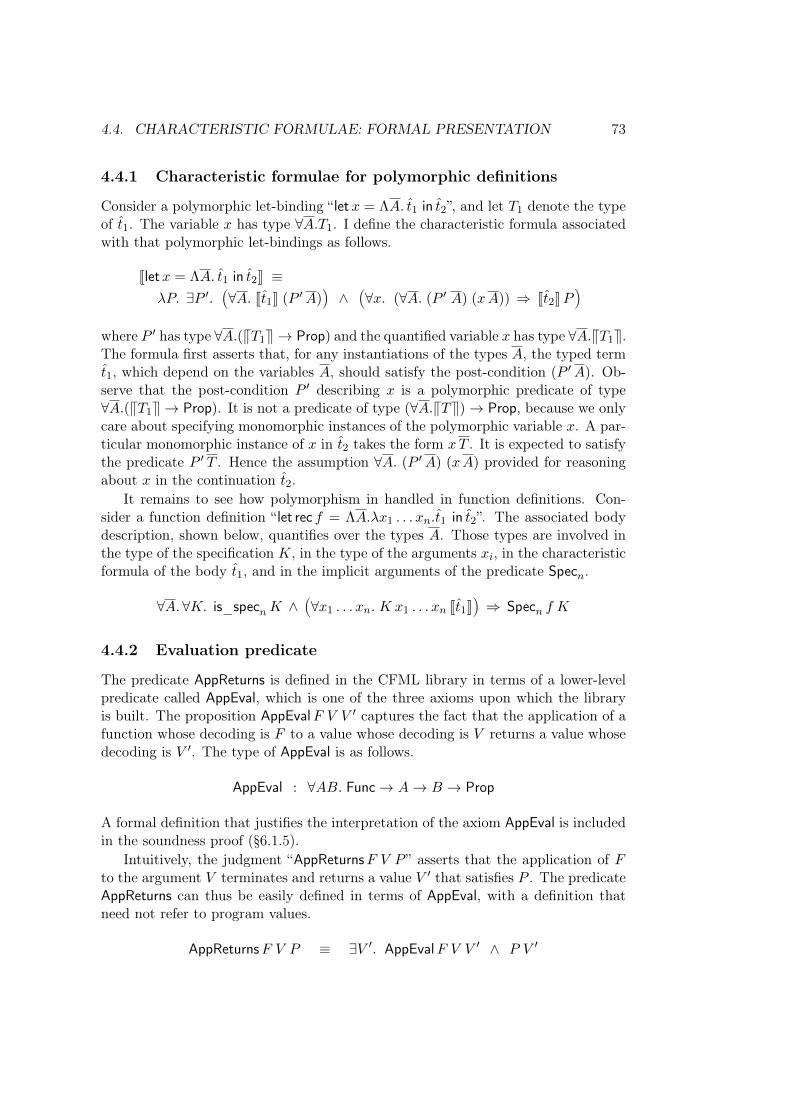
4.4. CHARACTERISTIC FORMULAE: FORMAL PRESENTATION 73
4.4.1 Characteristic formulae for polymorphic definitions
Consider a polymorphic let-binding “ let𝑥 = Λ𝐴. 𝑡1 in 𝑡2”, and let 𝑇1 denote the typeof 𝑡1. The variable 𝑥 has type ∀𝐴.𝑇1. I define the characteristic formula associatedwith that polymorphic let-bindings as follows.
Jlet𝑥 = Λ𝐴. 𝑡1 in 𝑡2K ≡𝜆𝑃. ∃𝑃 ′.
Ä∀𝐴. J𝑡1K (𝑃 ′𝐴)
ä∧Ä∀𝑥. (∀𝐴. (𝑃 ′ 𝐴) (𝑥𝐴)) ⇒ J𝑡2K𝑃
äwhere 𝑃 ′ has type ∀𝐴.(V𝑇1W → Prop) and the quantified variable 𝑥 has type ∀𝐴.V𝑇1W.The formula first asserts that, for any instantiations of the types 𝐴, the typed term𝑡1, which depend on the variables 𝐴, should satisfy the post-condition (𝑃 ′𝐴). Ob-serve that the post-condition 𝑃 ′ describing 𝑥 is a polymorphic predicate of type∀𝐴.(V𝑇1W → Prop). It is not a predicate of type (∀𝐴.V𝑇W) → Prop, because we onlycare about specifying monomorphic instances of the polymorphic variable 𝑥. A par-ticular monomorphic instance of 𝑥 in 𝑡2 takes the form 𝑥𝑇 . It is expected to satisfythe predicate 𝑃 ′ 𝑇 . Hence the assumption ∀𝐴. (𝑃 ′𝐴) (𝑥𝐴) provided for reasoningabout 𝑥 in the continuation 𝑡2.
It remains to see how polymorphism in handled in function definitions. Con-sider a function definition “ let rec 𝑓 = Λ𝐴.𝜆𝑥1 . . . 𝑥𝑛.𝑡1 in 𝑡2”. The associated bodydescription, shown below, quantifies over the types 𝐴. Those types are involved inthe type of the specification 𝐾, in the type of the arguments 𝑥𝑖, in the characteristicformula of the body 𝑡1, and in the implicit arguments of the predicate Spec𝑛.
∀𝐴.∀𝐾. is_spec𝑛𝐾 ∧Ä∀𝑥1 . . . 𝑥𝑛. 𝐾 𝑥1 . . . 𝑥𝑛 J𝑡1K
ä⇒ Spec𝑛 𝑓 𝐾
4.4.2 Evaluation predicate
The predicate AppReturns is defined in the CFML library in terms of a lower-levelpredicate called AppEval, which is one of the three axioms upon which the libraryis built. The proposition AppEval𝐹 𝑉 𝑉 ′ captures the fact that the application of afunction whose decoding is 𝐹 to a value whose decoding is 𝑉 returns a value whosedecoding is 𝑉 ′. The type of AppEval is as follows.
AppEval : ∀𝐴𝐵. Func → 𝐴 → 𝐵 → Prop
A formal definition that justifies the interpretation of the axiom AppEval is includedin the soundness proof (§6.1.5).
Intuitively, the judgment “AppReturns𝐹 𝑉 𝑃 ” asserts that the application of 𝐹to the argument 𝑉 terminates and returns a value 𝑉 ′ that satisfies 𝑃 . The predicateAppReturns can thus be easily defined in terms of AppEval, with a definition thatneed not refer to program values.
AppReturns𝐹 𝑉 𝑃 ≡ ∃𝑉 ′. AppEval𝐹 𝑉 𝑉 ′ ∧ 𝑃 𝑉 ′
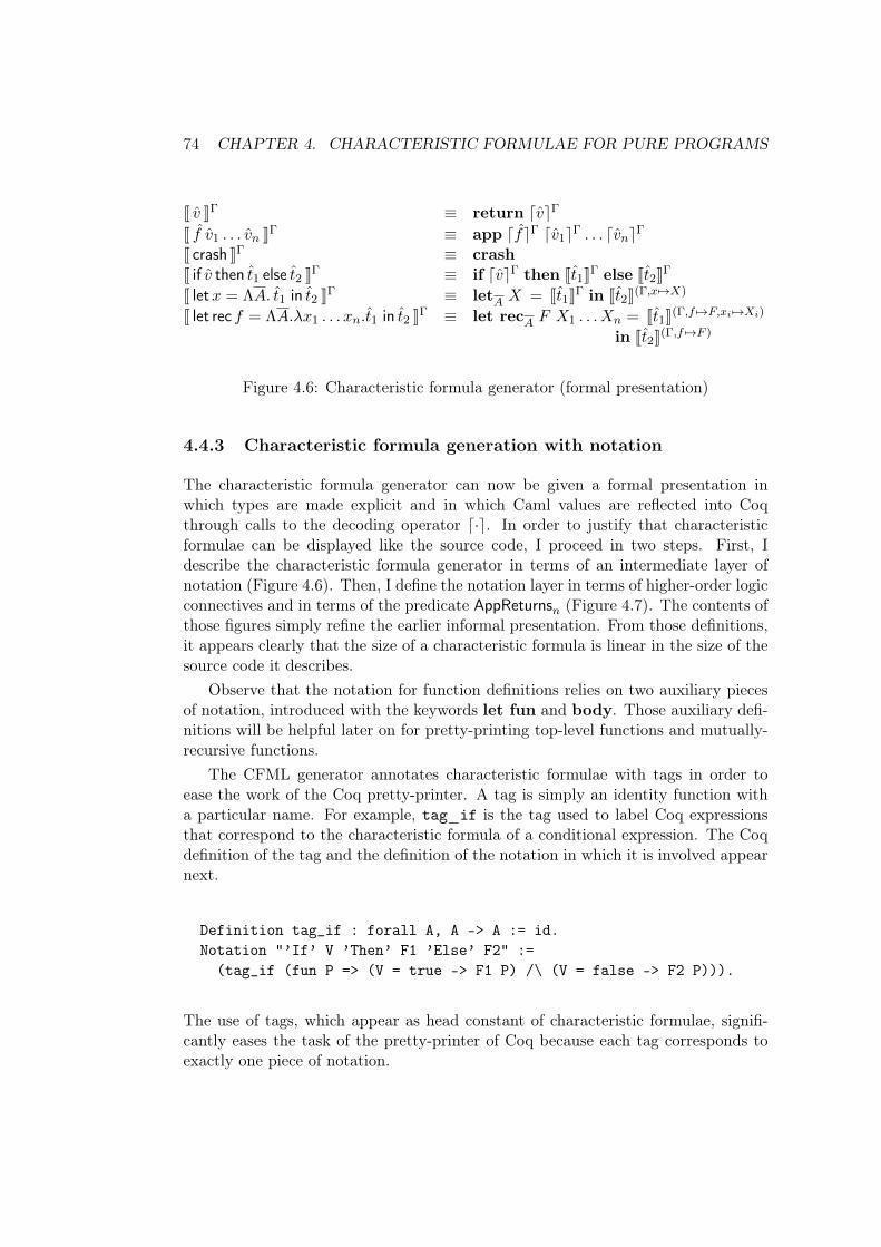
74 CHAPTER 4. CHARACTERISTIC FORMULAE FOR PURE PROGRAMS
J 𝑣 KΓ ≡ return ⌈𝑣⌉ΓJ 𝑓 𝑣1 . . . 𝑣𝑛 KΓ ≡ app ⌈𝑓⌉Γ ⌈𝑣1⌉Γ . . . ⌈𝑣𝑛⌉ΓJ crash KΓ ≡ crashJ if 𝑣 then 𝑡1 else 𝑡2 KΓ ≡ if ⌈𝑣⌉Γ then J𝑡1KΓ else J𝑡2KΓ
J let𝑥 = Λ𝐴. 𝑡1 in 𝑡2 KΓ ≡ let𝐴 𝑋 = J𝑡1KΓ in J𝑡2K(Γ,𝑥 ↦→𝑋)
J let rec 𝑓 = Λ𝐴.𝜆𝑥1 . . . 𝑥𝑛.𝑡1 in 𝑡2 KΓ ≡ let rec𝐴 𝐹 𝑋1 . . . 𝑋𝑛 = J𝑡1K(Γ,𝑓 ↦→𝐹,𝑥𝑖 ↦→𝑋𝑖)
in J𝑡2K(Γ,𝑓 ↦→𝐹 )
Figure 4.6: Characteristic formula generator (formal presentation)
4.4.3 Characteristic formula generation with notation
The characteristic formula generator can now be given a formal presentation inwhich types are made explicit and in which Caml values are reflected into Coqthrough calls to the decoding operator ⌈·⌉. In order to justify that characteristicformulae can be displayed like the source code, I proceed in two steps. First, Idescribe the characteristic formula generator in terms of an intermediate layer ofnotation (Figure 4.6). Then, I define the notation layer in terms of higher-order logicconnectives and in terms of the predicate AppReturns𝑛 (Figure 4.7). The contents ofthose figures simply refine the earlier informal presentation. From those definitions,it appears clearly that the size of a characteristic formula is linear in the size of thesource code it describes.
Observe that the notation for function definitions relies on two auxiliary piecesof notation, introduced with the keywords let fun and body. Those auxiliary defi-nitions will be helpful later on for pretty-printing top-level functions and mutually-recursive functions.
The CFML generator annotates characteristic formulae with tags in order toease the work of the Coq pretty-printer. A tag is simply an identity function witha particular name. For example, tag_if is the tag used to label Coq expressionsthat correspond to the characteristic formula of a conditional expression. The Coqdefinition of the tag and the definition of the notation in which it is involved appearnext.
Definition tag_if : forall A, A -> A := id.Notation "’If’ V ’Then’ F1 ’Else’ F2" :=
(tag_if (fun P => (V = true -> F1 P) /\ (V = false -> F2 P))).
The use of tags, which appear as head constant of characteristic formulae, signifi-cantly eases the task of the pretty-printer of Coq because each tag corresponds toexactly one piece of notation.
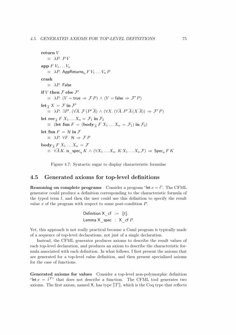
4.5. GENERATED AXIOMS FOR TOP-LEVEL DEFINITIONS 75
return 𝑉
≡ 𝜆𝑃. 𝑃 𝑉
app 𝐹 𝑉1 . . . 𝑉𝑛
≡ 𝜆𝑃. AppReturns𝑛 𝐹 𝑉1 . . . 𝑉𝑛 𝑃
crash≡ 𝜆𝑃. False
if 𝑉 then ℱ else ℱ ′
≡ 𝜆𝑃. (𝑉 = true ⇒ ℱ 𝑃 ) ∧ (𝑉 = false ⇒ ℱ ′ 𝑃 )
let𝐴 𝑋 = ℱ in ℱ ′
≡ 𝜆𝑃. ∃𝑃 ′. (∀𝐴. ℱ (𝑃 ′𝐴) ∧ (∀𝑋. (∀𝐴.𝑃 ′𝐴 (𝑋 𝐴)) ⇒ ℱ ′ 𝑃 )
let rec𝐴 𝐹 𝑋1 . . . 𝑋𝑛 = ℱ1 in ℱ2
≡ (let fun 𝐹 = (body𝐴 𝐹 𝑋1 . . . 𝑋𝑛 = ℱ1) in ℱ2)
let fun 𝐹 = ℋ in ℱ≡ 𝜆𝑃. ∀𝐹. ℋ ⇒ ℱ 𝑃
body𝐴 𝐹 𝑋1 . . . 𝑋𝑛 = ℱ≡ ∀𝐴𝐾. is_spec𝑛𝐾 ∧ (∀𝑋1 . . . 𝑋𝑛. 𝐾 𝑋1 . . . 𝑋𝑛ℱ) ⇒ Spec𝑛 𝐹 𝐾
Figure 4.7: Syntactic sugar to display characteristic formulae
4.5 Generated axioms for top-level definitions
Reasoning on complete programs Consider a program “ let𝑥 = 𝑡”. The CFMLgenerator could produce a definition corresponding to the characteristic formula ofthe typed term 𝑡, and then the user could use this definition to specify the resultvalue 𝑥 of the program with respect to some post-condition 𝑃 .
Definition X_cf := J𝑡K.Lemma X_spec : X_cf 𝑃.
Yet, this approach is not really practical because a Caml program is typically madeof a sequence of top-level declarations, not just of a single declaration.
Instead, the CFML generator produces axioms to describe the result values ofeach top-level declaration, and produces an axiom to describe the characteristic for-mula associated with each definition. In what follows, I first present the axioms thatare generated for a top-level value definition, and then present specialized axiomsfor the case of functions.
Generated axioms for values Consider a top-level non-polymorphic definition“ let𝑥 = 𝑡𝑇 ” that does not describe a function. The CFML tool generates twoaxioms. The first axiom, named X, has type V𝑇W, which is the Coq type that reflects
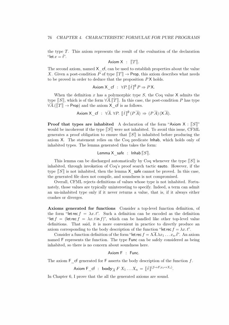
76 CHAPTER 4. CHARACTERISTIC FORMULAE FOR PURE PROGRAMS
the type 𝑇 . This axiom represents the result of the evaluation of the declaration“ let𝑥 = 𝑡”.
Axiom X : V𝑇W.
The second axiom, named X_cf, can be used to establish properties about the value𝑋. Given a post-condition 𝑃 of type V𝑇W → Prop, this axiom describes what needsto be proved in order to deduce that the proposition 𝑃 X holds.
Axiom X_cf : ∀𝑃. J 𝑡 K∅ 𝑃 ⇒ 𝑃 X.
When the definition 𝑥 has a polymorphic type 𝑆, the Coq value X admits thetype V𝑆W, which is of the form ∀𝐴.V𝑇W. In this case, the post-condition 𝑃 has type∀𝐴.(V𝑇W → Prop) and the axiom X_cf is as follows.
Axiom X_cf : ∀𝐴. ∀𝑃. J 𝑡 K∅ (𝑃 𝐴) ⇒ (𝑃 𝐴) (X𝐴).
Proof that types are inhabited A declaration of the form “Axiom X : V𝑆W”would be incoherent if the type V𝑆W were not inhabited. To avoid this issue, CFMLgenerates a proof obligation to ensure that V𝑆W is inhabited before producing theaxiom X. The statement relies on the Coq predicate Inhab, which holds only ofinhabited types. The lemma generated thus takes the form:
Lemma X_safe : Inhab V𝑆W.
This lemma can be discharged automatically by Coq whenever the type V𝑆W isinhabited, through invokation of Coq’s proof search tactic eauto. However, if thetype V𝑆W is not inhabited, then the lemma X_safe cannot be proved. In this case,the generated file does not compile, and soundness is not compromised.
Overall, CFML rejects definitions of values whose type is not inhabited. Fortu-nately, those values are typically uninteresting to specify. Indeed, a term can admitan un-inhabited type only if it never returns a value, that is, if it always eithercrashes or diverges.
Axioms generated for functions Consider a top-level function definition, ofthe form “ let rec 𝑓 = 𝜆𝑥. 𝑡”. Such a definition can be encoded as the definition“ let 𝑓 = (let rec 𝑓 = 𝜆𝑥. 𝑡 in 𝑓)”, which can be handled like other top-level valuedefinitions. That said, it is more convenient in practice to directly produce anaxiom corresponding to the body description of the function “ let rec 𝑓 = 𝜆𝑥. 𝑡”.
Consider a function definition of the form “ let rec 𝑓 = Λ𝐴.𝜆𝑥1 . . . 𝑥𝑛.𝑡”. An axiomnamed F represents the function. The type Func can be safely considered as beinginhabited, so there is no concern about soundness here.
Axiom F : Func.
The axiom F_cf generated for F asserts the body description of the function 𝑓 .
Axiom F_cf : body𝐴 𝐹 𝑋1 . . . 𝑋𝑛 = J 𝑡 K(𝑓 ↦→𝐹,𝑥𝑖 ↦→𝑋𝑖).
In Chapter 6, I prove that the all the generated axioms are sound.
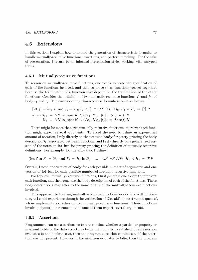
4.6. EXTENSIONS 77
4.6 Extensions
In this section, I explain how to extend the generation of characteristic formulae tohandle mutually-recursive functions, assertions, and pattern matching. For the sakeof presentation, I return to an informal presentation style, working with untypedterms.
4.6.1 Mutually-recursive functions
To reason on mutually-recursive functions, one needs to state the specification ofeach of the functions involved, and then to prove those functions correct together,because the termination of a function may depend on the termination of the otherfunctions. Consider the definition of two mutually-recursive functions 𝑓1 and 𝑓2, ofbody 𝑡1 and 𝑡2. The corresponding characteristic formula is built as follows.
Jlet 𝑓1 = 𝜆𝑥1. 𝑡1 and 𝑓2 = 𝜆𝑥2. 𝑡2 in 𝑡K ≡ 𝜆𝑃. ∀𝑓1.∀𝑓2. ℋ1 ∧ ℋ2 ⇒ J𝑡K𝑃
where ℋ1 ≡ ∀𝐾. is_spec𝐾 ∧ (∀𝑥1. 𝐾 𝑥1 J𝑡1K) ⇒ Spec 𝑓1𝐾ℋ2 ≡ ∀𝐾. is_spec𝐾 ∧ (∀𝑥2. 𝐾 𝑥2 J𝑡2K) ⇒ Spec 𝑓2𝐾
There might be more than two mutually-recursive functions, moreover each func-tion might expect several arguments. To avoid the need to define an exponentialamount of notation, I rely directly on the notation body for pretty-printing the bodydescription ℋ𝑖 associated with each function, and I rely directly on a generalized ver-sion of the notation let fun for pretty-printing the definition of mutually-recursivedefinitions. For example, for the arity two, I define:
(let fun 𝐹1 = ℋ1 and 𝐹2 = ℋ2 in ℱ) ≡ 𝜆𝑃. ∀𝐹1. ∀𝐹2. ℋ1 ∧ ℋ2 ⇒ ℱ 𝑃
Overall, I need one version of body for each possible number of arguments and oneversion of let fun for each possible number of mutually-recursive functions.
For top-level mutually-recursive functions, I first generate one axiom to representeach function, and then generate the body description of each of the functions. Thosebody descriptions may refer to the name of any of the mutually-recursive functionsinvolved.
This approach to treating mutually-recursive functions works very well in prac-tice, as I could experience through the verification of Okasaki’s “bootstrapped queues”,whose implementation relies on five mutually-recursive functions. Those functionsinvolve polymorphic recursion and some of them expect several arguments.
4.6.2 Assertions
Programmers can use assertions to test at runtime whether a particular property orinvariant holds of the data structures being manipulated is satisfied. If an assertionevaluates to the boolean true, then the program execution continues as if the asser-tion was not present. However, if the assertion evaluates to false, then the program
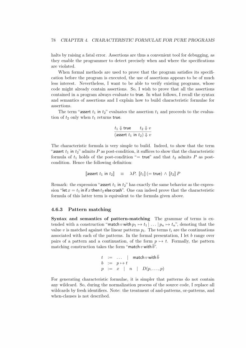
78 CHAPTER 4. CHARACTERISTIC FORMULAE FOR PURE PROGRAMS
halts by raising a fatal error. Assertions are thus a convenient tool for debugging, asthey enable the programmer to detect precisely when and where the specificationsare violated.
When formal methods are used to prove that the program satisfies its specifi-cation before the program is executed, the use of assertions appears to be of muchless interest. Nevertheless, I want to be able to verify existing programs, whosecode might already contain assertions. So, I wish to prove that all the assertionscontained in a program always evaluate to true. In what follows, I recall the syntaxand semantics of assertions and I explain how to build characteristic formulae forassertions.
The term “assert 𝑡1 in 𝑡2” evaluates the assertion 𝑡1 and proceeds to the evalua-tion of 𝑡2 only when 𝑡1 returns true.
𝑡1 ⇓ true 𝑡2 ⇓ 𝑣
(assert 𝑡1 in 𝑡2) ⇓ 𝑣
The characteristic formula is very simple to build. Indeed, to show that the term“assert 𝑡1 in 𝑡2” admits 𝑃 as post-condition, it suffices to show that the characteristicformula of 𝑡1 holds of the post-condition “= true” and that 𝑡2 admits 𝑃 as post-condition. Hence the following definition:
Jassert 𝑡1 in 𝑡2K ≡ 𝜆𝑃. J𝑡1K (= true) ∧ J𝑡2K𝑃
Remark: the expression “assert 𝑡1 in 𝑡2” has exactly the same behavior as the expres-sion “ let𝑥 = 𝑡1 in if𝑥 then 𝑡2 else crash”. One can indeed prove that the characteristicformula of this latter term is equivalent to the formula given above.
4.6.3 Pattern matching
Syntax and semantics of pattern-matching The grammar of terms is ex-tended with a construction “match 𝑣with 𝑝1 ↦→ 𝑡1 | . . . | 𝑝𝑛 ↦→ 𝑡𝑛”, denoting that thevalue 𝑣 is matched against the linear patterns 𝑝𝑖. The terms 𝑡𝑖 are the continuationsassociated with each of the patterns. In the formal presentation, I let 𝑏 range overpairs of a pattern and a continuation, of the form 𝑝 ↦→ 𝑡. Formally, the patternmatching construction takes the form “match 𝑣with 𝑏”.
𝑡 := . . . | match 𝑣with 𝑏𝑏 := 𝑝 ↦→ 𝑡𝑝 := 𝑥 | 𝑛 | 𝐷(𝑝, . . . , 𝑝)
For generating characteristic formulae, it is simpler that patterns do not containany wildcard. So, during the normalization process of the source code, I replace allwildcards by fresh identifiers. Note: the treatment of and-patterns, or-patterns, andwhen-clauses is not described.
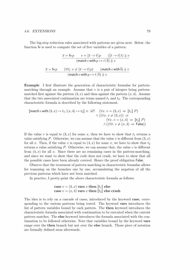
4.6. EXTENSIONS 79
The big-step reduction rules associated with patterns are given next. Below, thefunction fv is used to compute the set of free variables of a pattern.
𝑥 = fv 𝑝 𝑣 = [𝑥 → 𝑣] 𝑝 ([𝑥 → 𝑣] 𝑡) ⇓ 𝑣
(match 𝑣with 𝑝 ↦→ 𝑡 | 𝑏) ⇓ 𝑣
𝑥 = fv 𝑝 (∀𝑣𝑖. 𝑣 ̸= [𝑥 → 𝑣] 𝑝) (match 𝑣with 𝑏) ⇓ 𝑣
(match 𝑣with 𝑝 ↦→ 𝑡 | 𝑏) ⇓ 𝑣
Example I first illustrate the generation of characteristic formulae for pattern-matching through an example. Assume that 𝑣 is a pair of integers being pattern-matched first against the pattern (3, 𝑥) and then against the pattern (𝑥, 4). Assumethat the two associated continuation are terms named 𝑡1 and 𝑡2. The correspondingcharacteristic formula is described by the following statement.
Jmatch 𝑣with (3, 𝑥) ↦→ 𝑡1 | (𝑥, 4) ↦→ 𝑡2K ≡ 𝜆𝑃. (∀𝑥. 𝑣 = (3, 𝑥) ⇒ J𝑡1K 𝑃 )∧ ((∀𝑥. 𝑣 ̸= (3, 𝑥)) ⇒
(∀𝑥. 𝑣 = (𝑥, 4) ⇒ J𝑡2K 𝑃 )∧ ((∀𝑥. 𝑣 ̸= (𝑥, 4) ⇒ False))
If the value 𝑣 is equal to (3, 𝑥) for some 𝑥, then we have to show that 𝑡1 returns avalue satisfying 𝑃 . Otherwise, we can assume that the value 𝑣 is different from (3, 𝑥)for all 𝑥. Then, if the value 𝑣 is equal to (4, 𝑥) for some 𝑥, we have to show that 𝑡2returns a value satisfying 𝑃 . Otherwise, we can assume that, the value 𝑣 is differentfrom (4, 𝑥) for all 𝑥. Since there are no remaining cases in the pattern-matching,and since we want to show that the code does not crash, we have to show that allthe possible cases have been already covered. Hence the proof obligation False.
Observe that the treatment of pattern matching in characteristic formulae allowsfor reasoning on the branches one by one, accumulating the negation of all theprevious patterns which have not been matched.
In practice, I pretty-print the above characteristic formula as follows:
case 𝑣 = (3, 𝑥) vars 𝑥 then J𝑡1K elsecase 𝑣 = (𝑥, 4) vars 𝑥 then J𝑡2K else crash
The idea is to rely on a cascade of cases, introduced by the keyword case, corre-sponding to the various patterns being tested. The keyword vars introduces thelist of pattern variables bound by each pattern. The then keyword introduces thecharacteristic formula associated with continuation to be executed when the currentpattern matches. The else keyword introduces the formula associated with the con-tinuation to be followed otherwise. Note that variables bound by the keyword varsrange over the then branch but not over the else branch. Those piece of notationare formally defined soon afterwards.
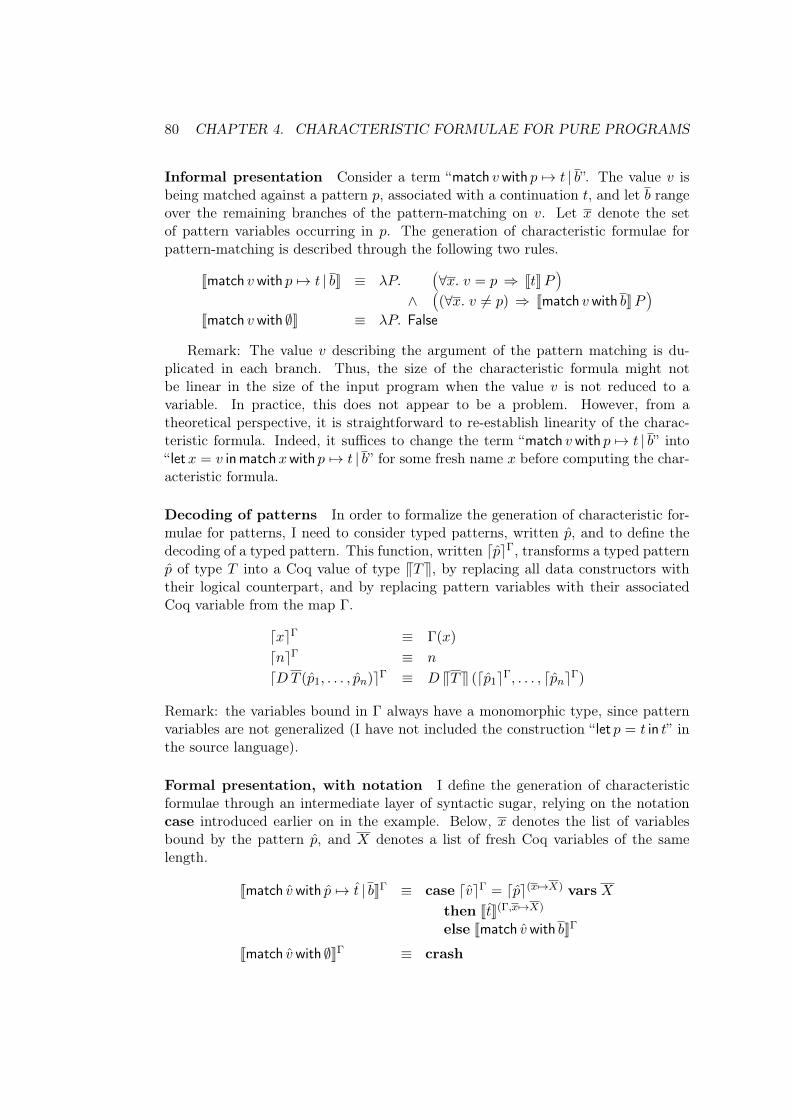
80 CHAPTER 4. CHARACTERISTIC FORMULAE FOR PURE PROGRAMS
Informal presentation Consider a term “match 𝑣with 𝑝 ↦→ 𝑡 | 𝑏”. The value 𝑣 isbeing matched against a pattern 𝑝, associated with a continuation 𝑡, and let 𝑏 rangeover the remaining branches of the pattern-matching on 𝑣. Let 𝑥 denote the setof pattern variables occurring in 𝑝. The generation of characteristic formulae forpattern-matching is described through the following two rules.
Jmatch 𝑣with 𝑝 ↦→ 𝑡 | 𝑏K ≡ 𝜆𝑃.Ä∀𝑥. 𝑣 = 𝑝 ⇒ J𝑡K𝑃
ä∧Ä(∀𝑥. 𝑣 ̸= 𝑝) ⇒ Jmatch 𝑣with 𝑏K𝑃
äJmatch 𝑣with ∅K ≡ 𝜆𝑃. False
Remark: The value 𝑣 describing the argument of the pattern matching is du-plicated in each branch. Thus, the size of the characteristic formula might notbe linear in the size of the input program when the value 𝑣 is not reduced to avariable. In practice, this does not appear to be a problem. However, from atheoretical perspective, it is straightforward to re-establish linearity of the charac-teristic formula. Indeed, it suffices to change the term “match 𝑣with 𝑝 ↦→ 𝑡 | 𝑏” into“ let𝑥 = 𝑣 in match𝑥with 𝑝 ↦→ 𝑡 | 𝑏” for some fresh name 𝑥 before computing the char-acteristic formula.
Decoding of patterns In order to formalize the generation of characteristic for-mulae for patterns, I need to consider typed patterns, written 𝑝, and to define thedecoding of a typed pattern. This function, written ⌈𝑝⌉Γ, transforms a typed pattern𝑝 of type 𝑇 into a Coq value of type V𝑇W, by replacing all data constructors withtheir logical counterpart, and by replacing pattern variables with their associatedCoq variable from the map Γ.
⌈𝑥⌉Γ ≡ Γ(𝑥)
⌈𝑛⌉Γ ≡ 𝑛
⌈𝐷𝑇 (𝑝1, . . . , 𝑝𝑛)⌉Γ ≡ 𝐷 V𝑇W (⌈𝑝1⌉Γ, . . . , ⌈𝑝𝑛⌉Γ)
Remark: the variables bound in Γ always have a monomorphic type, since patternvariables are not generalized (I have not included the construction “ let 𝑝 = 𝑡 in 𝑡” inthe source language).
Formal presentation, with notation I define the generation of characteristicformulae through an intermediate layer of syntactic sugar, relying on the notationcase introduced earlier on in the example. Below, 𝑥 denotes the list of variablesbound by the pattern 𝑝, and 𝑋 denotes a list of fresh Coq variables of the samelength.
Jmatch 𝑣with 𝑝 ↦→ 𝑡 | 𝑏KΓ ≡ case ⌈𝑣⌉Γ = ⌈𝑝⌉(𝑥 ↦→𝑋) vars 𝑋
then J𝑡K(Γ,𝑥 ↦→𝑋)
else Jmatch 𝑣with 𝑏KΓ
Jmatch 𝑣with ∅KΓ ≡ crash
4.7. FORMAL PROOFS WITH CHARACTERISTIC FORMULAE 81
where the notation case is formally defined as follows:
(case 𝑉 = 𝑉 ′ vars 𝑋 then ℱ else ℱ ′) ≡𝜆𝑃. (∀𝑋. 𝑉 = 𝑉 ′ ⇒ ℱ 𝑃 ) ∧ ((∀𝑋. 𝑉 ̸= 𝑉 ′) ⇒ ℱ ′ 𝑃 )
Remark: in the characteristic formula, the value ⌈𝑣⌉Γ appears under the scopeof the pattern variables 𝑥, although this was not the case in the program sourcecode. So, if the value 𝑣 contains a variable with the same name as a variable boundin the pattern 𝑝, then we need to alpha-rename the pattern variable in conflict.Alternatively, we may first bind the value 𝑣 to a fresh variable 𝑥, building the term“ let𝑥 = 𝑣 in match𝑥with 𝑝 ↦→ 𝑡 | 𝑏”, in which the value being matched, namely 𝑥, isguaranteed to be distinct from all the pattern variables. The implementation ofCFML performs this transformation whenever the value 𝑣 contains a free variablethat clashes with one of the pattern variables involved in the pattern matching.
Exhaustive patterns By default, the OCaml type-checker checks for exhaustive-ness of coverage in pattern-matching constructions, through an analysis based ontypes. If there exists a value that might not match any of the patterns, then theCaml compiler issues a warning. There are cases where the invariants of the programguarantee that the given set of branches actually covers all the possible cases. Insuch a case, the user may ignore the warning produced by the compiler.
When the compiler’s analysis recognizes a pattern matching as exhaustive, then itis safe to modify the characteristic formula so as to remove the proof-obligation thatcorresponds to exhaustiveness. In such a case, I replace the formula crash, whichis defined as “𝜆𝑃.False”, with the formula done, which is defined as “𝜆𝑃.True”.Through this change, a nontrivial proof obligation “crash𝑃 ” is replaced with atrivial proof obligation “done𝑃 ”. In practice, most patterns are exhaustive, so theamount of work required in interactive proofs is greatly reduced by this optimizationwhich exploits the strength of the exhaustiveness decision procedure.
Conclusion and extensions In summary, characteristic formulae rely on equal-ities and disequalities to reason on pattern matching. The branches of a patterncan be studied one by one, following the execution flow of the program. The CFMLlibrary also includes a tactic that applies to the characteristic formula of a patternwith 𝑛 branches and directly generates 𝑛 subgoals, plus one additional subgoal whenthe pattern is not recognized as exhaustive. The treatment of for alias patterns (ofthe form “𝑝 as𝑥”) and of top-level or-patterns is not described here but is imple-mented in CFML. The treatment of when-clauses and general or-patterns is left tofuture work.
4.7 Formal proofs with characteristic formulae
In this section, I explain how to reason about programs through characteristic for-mulae. While it is possible to manipulate characteristic formulae directly, I have
82 CHAPTER 4. CHARACTERISTIC FORMULAE FOR PURE PROGRAMS
found it much more effective to design a set of high-level tactics. Moreover, the useof high-level tactics means that the user does not need to know about the details ofthe construction of characteristic formulae.
4.7.1 Reasoning tactics: example with let-bindings
Definition of the core tactic To start with, assume we want to show that a term“ let𝑥 = 𝑡1 in 𝑡2” returns a value satisfying a predicate 𝑃 . The goal to be established,“Jlet𝑥 = 𝑡1 in 𝑡2K𝑃 ”, is equivalent to the proposition shown next.
∃𝑃 ′. J𝑡1K𝑃 ′ ∧ (∀𝑋. 𝑃 ′𝑋 ⇒ J𝑡2K(𝑥 ↦→𝑋) 𝑃 )
On this goal, a call to the tactic xlet with an argument 𝑃1 instantiates 𝑃 ′ as 𝑃1
and produces two subgoals. The first subgoal, “J𝑡1K𝑃1”, corresponds to the body ofthe let-binding. The second subgoal consists in proving “J𝑡2K(𝑥 ↦→𝑋) 𝑃 ” in a contextextended with a free variable named 𝑋 and an hypothesis 𝑃1𝑋.
The Coq implementation of the tactic xlet is straightforward. First, it providesits argument P1 as a witness, with a call to “exists𝑃1”. Then, it splits the con-junction, with the tactic split. Finally, in the second subgoal, it introduces 𝑋 aswell as the hypothesis about 𝑋, calling the tactic intro twice. The correspondingCoq tactic definition appears next.
Tactic Notation "xlet" constr(P1) :=exists P1; split; [ | intro; intro ].
Inference of specification The tactic xlet described so far requires the inter-mediate specification 𝑃1 to be provided explicitly. Yet, it is very often the case thatthis post-condition can be automatically inferred when solving the goal “J𝑡1K𝑃1”.For example, if 𝑡1 is the application of a function, then the post-condition 𝑃1 getsunified with the post-condition of that function. So, I also define a tactic xlet thatdoes not expect any argument, and that simply instantiates 𝑃1 with a fresh unifica-tion variable. As soon as this unification variable is instantiated in the first subgoalJ𝑡1K𝑃1, the hypothesis “𝑃1𝑋” from the second subgoal becomes fully determined.
The implementation of this alternative tactic xlet relies on a call to the tactic“exists_”, where the underscore symbol indicates that a fresh unification variableshould be created.
Tactic Notation "xlet" :=exists _; split; [ | intro; intro ].
Generation of names Choosing appropriate names for variables and hypothesesis extremely important in practice for conducting interactive proofs. Indeed, a proofscript that relies on generated names such as H16 is very brittle, because any changeto the program or to the proof may shift the names and result in H16 being renamed,for example into H19. Moreover, proof obligations are much easier to read when they
4.7. FORMAL PROOFS WITH CHARACTERISTIC FORMULAE 83
involve only meaningful names. I have invested particular care in developing twoversions of every tactic: one version where the user explicitly provides a name fora variable or an hypothesis, and one version that tries and picks a clever nameautomatically. As a result, it is possible to obtain robust proof scripts and readableproof obligations at a reasonable cost, by providing only a few names explicitly.
Let me illustrate this with the tactic xlet. A call to the tactic intro movesa universally-quantified variable or a hypothesis from the head of the goal into theproof context. The name 𝑋 that appears in the characteristic formula of a let-binding comes from the source code of the program, after it has been put in normalform. When the name 𝑋 comes from the original source code, it makes sense to reusethat name. However, when 𝑋 corresponds to a variable that has been introducedduring the normalization process (for assigning names to intermediate expressionsfrom the source code), it is sometimes better to use a more meaningful name thanthe one that has been generated automatically. A call of the form “xlet as X”enables one to specify the name that should be used for 𝑋.
The tactic xlet also needs to come up with a name for the hypothesis “𝑃1𝑋”.By default, the tactic picks the name HX, which is obtained by placing the letter Hin front of the name of the variable. However, it is also possible to specify the nameto be used explicitly, by providing it as extra argument to xlet. This possibility isparticularly useful when the hypothesis “𝑃1𝑋” needs to be decomposed in severalconjuncts. For example, if the post-condition 𝑃1 of the term 𝑡1 takes the form“(𝜆𝑋. ∃𝑌. 𝐻1 𝑌 ∧𝐻2 𝑌 )”, then a call to the tactic “xlet as X (Y&M1&M2)” leaves inthe second subgoal a proof context containing a variable Y, an hypothesis M1 of type“𝐻1 𝑌 ” and an hypothesis M2 of type “𝐻2 𝑌 ”. Without such a convenient feature,one would have to write instead something of the form “xlet as X. destruct HXas (Y&M1&M2)”, or to rely on a more evolved tactic language such as SSReflect [30].
Overall, there are five ways to call the tactic xlet, as summarized below.
xlet.xlet P1 as X.xlet P1 as X HX.xlet as X.xlet as X HX.
All of the tactics implemented in CFML offer a similar degree of flexibility.
4.7.2 Tactics for reasoning on function applications
The process of proving a specification for a function 𝑓 and then exploiting thatspecification for reasoning on applications of that function is as follows. First, onestates the specification of 𝑓 as a lemma of the form Spec𝑛 𝑓 𝐾. Second, one provesthis lemma using the characteristic formula describing the behavior of 𝑓 . Third,one registers that lemma in a database of specification lemmas, so that the nameof the lemma does not need to be mentioned explicitly in the proof scripts. Then,when reasoning on a piece of code that involves an application of the function 𝑓 , a
84 CHAPTER 4. CHARACTERISTIC FORMULAE FOR PURE PROGRAMS
proof obligation of the form AppReturns𝑚 𝑓 𝑥1 . . . 𝑥𝑚 𝑃 is involved. The tactic xapphelps proving that goal. The implementation of the tactic depends on whether thefunction is applied to the exact number of arguments it expects (𝑚 = 𝑛), or whethera partial-application is involved (𝑚 < 𝑛), or whether an over-application is involved(𝑚 > 𝑛). Note that all the lemmas about Spec𝑛 mentioned thereafter are proved inCoq.
Normal applications The elimination lemma for the predicate Spec𝑛 (introducedin §4.2.3) can be used to deduce a proposition about AppReturns𝑛 𝑓 from the spec-ification Spec𝑛 𝑓 𝐾. However, it does not directly have a conclusion of the formAppReturns𝑚 𝑓 𝑥1 . . . 𝑥𝑛 𝑃 . So, the implementation of the tactic xapp relies on acorollary of the elimination lemma, shown next.®
Spec𝑛 𝑓 𝐾∀𝑅. Weakenable𝑅 ⇒ 𝐾 𝑥1 . . . 𝑥𝑛𝑅 ⇒ 𝑅𝑃
⇒ AppReturns𝑛 𝑓 𝑥1 . . . 𝑥𝑛 𝑃
Let me illustrate the working of this lemma through an example. Suppose thata value 𝑥 is a non-negative multiple of 4 (i.e. 𝑥 = 4 * 𝑘 for some 𝑘 > 0), and let meshow that the application of the function half to 𝑥 returns an even value, that is,“AppReturns1 half𝑥 even”. The proof obligation is:
∀𝑅. Weakenable𝑅 ⇒ (∀𝑛 ≥ 0. 𝑥 = 2 * 𝑛 ⇒ 𝑅 (= 𝑛)) ⇒ 𝑅 even
By instantiating the hypothesis with 𝑛 = 2*𝑘 and checking that 𝑥 = 2*𝑛, we derivethe fact “𝑅 (= 2*𝑘)”. The conclusion, namely “𝑅 even”, follows: since 𝑅 is compatiblewith weakening, it suffices to check that the proposition “∀𝑦. 𝑦 = 2 * 𝑘 ⇒ even 𝑦”holds.
Partial applications Partial application occurs when the function 𝑓 is applied tofewer arguments than it normally expects. The result of such a partial applicationis another function, call it 𝑔, whose specification is an appropriate specializationof the specification of 𝑓 . For example, if 𝐾 is the specification of 𝑓 , then thepartial application of 𝑓 to an argument 𝑥 admits the specification 𝐾 𝑥. So, to showthat the partial application of 𝑓 to arguments 𝑥1 . . . 𝑥𝑛 satisfies a post-condition𝑃 , one needs to prove that the specification 𝑃 is a consequence of the specification𝐾 𝑥1 . . . 𝑥𝑛. The following result is exploited by the tactic xapp for reasoning onpartial applications (𝑛 > 𝑚).®
Spec𝑛 𝑓 𝐾∀𝑔. Spec𝑛−𝑚 𝑔 (𝐾 𝑥1 . . . 𝑥𝑚) ⇒ 𝑃 𝑔
⇒ AppReturns𝑚 𝑓 𝑥1 . . . 𝑥𝑚 𝑃
Over-applications Over-application occurs when the function 𝑓 is applied tomore arguments that it normally expects. This situation typically occurs withhigher-order combinators, such as compose, that return a function. The case of over-applications can be viewed as a particular case of a normal applications. Indeed, a
4.7. FORMAL PROOFS WITH CHARACTERISTIC FORMULAE 85
𝑚-ary application can be viewed as a 𝑛-ary application that returns a function of“𝑚−𝑛” arguments. More precisely, when 𝑚 > 𝑛, the goal AppReturns𝑚 𝑓 𝑥1 . . . 𝑥𝑚 𝑃can be rewritten into the goal shown below.
AppReturns𝑛 𝑓 𝑥1 . . . 𝑥𝑛 (𝜆𝑔.AppReturns𝑚−𝑛 𝑔 𝑥𝑛+1 . . . 𝑥𝑚 𝑃 )
Hence, the reasoning on over-applications relies on the following lemma.®Spec𝑛 𝑓 𝐾∀𝑅. Weakenable𝑅 ⇒ 𝐾 𝑥1 . . . 𝑥𝑛𝑅 ⇒ 𝑅 (𝜆𝑔.AppReturns𝑚−𝑛 𝑔 𝑥𝑛+1 . . . 𝑥𝑚 𝑃 )
⇒ AppReturns𝑚 𝑓 𝑥1 . . . 𝑥𝑚 𝑃
4.7.3 Tactics for reasoning on function definitions
Reasoning by weakening The tactic xweaken allows proving a specificationSpec𝑛 𝐹 𝐾 ′ from an existing specification Spec𝑛 𝐹 𝐾. Using weakening, one mayderive several specifications for a single function without verifying the code of thatfunction more than once. The targeted specification 𝐾 ′ must be weaker than theexisting specification 𝐾 in the sense that 𝐾 𝑥1 . . . 𝑥𝑛𝑅 has to imply 𝐾 ′ 𝑥1 . . . 𝑥𝑛𝑅for any predicate 𝑅 compatible with weakening. Notice that 𝐾 ′ has to be a validspecification in the sense that it should satisfy the predicate is_spec𝑛 .
Spec𝑛 𝑓 𝐾∀𝑥1 . . . 𝑥𝑛𝑅. Weakenable𝑅 ⇒ (𝐾 𝑥1 . . . 𝑥𝑛𝑅 ⇒ 𝐾 ′ 𝑥1 . . . 𝑥𝑛𝑅)is_spec𝑛𝐾
′
⇒ Spec𝑛 𝑓 𝐾 ′
For example, from the specification of the function half we can deduce a weakerspecification that captures the fact that when the input is of the form 4 * 𝑚 thenthe output is a non-negative integer.
Spec1 half (𝜆𝑥𝑅. ∀𝑚. 𝑚 ≥ 0 ⇒ 𝑥 = 4 *𝑚 ⇒ 𝑅 (𝜆𝑦. 𝑦 ≥ 0))
In this case, the proof obligation is:
∀𝑥𝑅. Weakenable𝑅 ⇒Ä∀𝑛. 𝑛 ≥ 0 ⇒ 𝑥 = 2 * 𝑛 ⇒ 𝑅 (= 𝑛)
ä⇒Ä∀𝑚. 𝑚 ≥ 0 ⇒ 𝑥 = 4 *𝑚 ⇒ 𝑅 (𝜆𝑦. 𝑦 ≥ 0)
äConsider a particular value of 𝑥, 𝑅 and 𝑚. The goal is to show 𝑅 (𝜆𝑦. 𝑦 ≥ 0), and wehave the assumptions Weakenable𝑅 and
Ä∀𝑛. 𝑛 ≥ 0 ⇒ 𝑥 = 2 * 𝑛 ⇒ 𝑅 (= 𝑛)
äand
𝑚 ≥ 0 and 𝑥 = 4*𝑚. If we instantiate 𝑛 with 2*𝑚 in the second assumption about𝑅, we get 𝑅 (= 2*𝑚). Since 𝑅 is compatible with weakening, we can prove the goal𝑅 (𝜆𝑦. 𝑦 ≥ 0) simply by showing that any value 𝑦 equal to 2 * 𝑚 is non-negative.This property holds because 𝑚 is non-negative.
86 CHAPTER 4. CHARACTERISTIC FORMULAE FOR PURE PROGRAMS
Reasoning by induction The purpose of the tactic xinduction is to establishby induction that a function 𝑓 admits a specification 𝐾. More precisely, it statesthat, to prove Spec𝑛 𝑓 𝐾, it suffices to show that 𝐾 is a correct specification for theapplication of 𝑓 to an argument 𝑥 under the assumption that 𝐾 is already a correctspecification for applications of 𝑓 to smaller arguments.
In the particular case of a function of arity one, calling the tactic xinductionon an argument (≺), which denotes a well-founded relation used to argue for termi-nation, transforms a goal of the form Spec1 𝑓 𝐾 into the goal:
Spec1 𝑓 (𝜆𝑥𝑅. Spec1 𝑓 (𝜆𝑥′𝑅′. 𝑥′ ≺ 𝑥 ⇒ 𝐾 𝑥′𝑅′) ⇒ 𝐾 𝑥𝑅)
The tactic xinduction relies on the following lemma.ÖSpec𝑛 𝑓 (𝜆𝑥1 . . . 𝑥𝑛𝑅.
Spec𝑛 𝑓 (𝜆𝑥′1 . . . 𝑥′𝑛𝑅
′. (𝑥′1, . . . , 𝑥′𝑛) ≺ (𝑥1, . . . , 𝑥𝑛) ⇒ 𝐾 𝑥′1 . . . 𝑥
′𝑛𝑅
′)⇒ 𝐾 𝑥1 . . . 𝑥𝑛𝑅)
⇒ Spec𝑛 𝑓 𝐾
where 𝑓 has type Func, 𝐾 has type 𝐴1 → . . . 𝐴𝑛 → ((𝐵 → Prop) → Prop) → Prop,and (≺) is a well-founded binary relation over values of type 𝐴1 × . . .×𝐴𝑛.
Advanced reasoning by induction The induction lemma can be used to estab-lish the specification of a function by induction on a well-founded relation over thearguments of that function. However, it does not support induction over the struc-ture of the proof of an inductive proposition. The purpose of the tactic xintrosis to change a goal of the form Spec𝑛 𝑓 𝐾 into a goal with a conclusion aboutAppReturns𝑛 𝑓 , thereby making it possible to conduct advanced forms of induction.
The implementation of the tactic xintros relies on an introduction lemma forspecifications, which is a form of reciprocal to the elimination lemma: it allowsproving the specification of a function 𝑓 in terms of a description of the behaviorof applications of 𝑓 to some arguments. This introduction lemma is formalized asfollows.
∀𝑥1 . . . 𝑥𝑛. 𝐾 𝑥1 . . . 𝑥𝑛 (AppReturns𝑛 𝑓 𝑥1 . . . 𝑥𝑛)Spec𝑛 𝑓 (𝜆𝑥1 . . . 𝑥𝑛𝑅.True)is_spec𝑛𝐾
⇒ Spec𝑛 𝑓 𝐾
The lemma involves two side-conditions. The first one asserts that 𝑓 is a n-arycurried function, meaning that the application to the 𝑛 − 1 first arguments alwaysterminates. The second hypothesis asserts that 𝐾 is a valid specification, in thesense that it is compatible with weakening.
4.7.4 Overview of all tactics
The CFML library includes one tactic for each construction of the language. I havealready presented the tactic xlet for let-bindings and the tactic xapp for applica-tions. Four other tactics are briefly described next. The tactic xret is used to reason
4.7. FORMAL PROOFS WITH CHARACTERISTIC FORMULAE 87
on a value. It simply unfolds the notation return, changing a goal “(return 𝑉 ) 𝑃 ”into “𝑃 𝑉 ”. The tactic xif helps reasoning on a conditional. It applies to a goal ofthe form “(if 𝑉 then ℱ else ℱ ′) 𝑃 ” and produces two subgoals: first “ℱ 𝑃 ”, with anhypothesis 𝑉 = true, and second “ℱ 𝑃 ”, with an hypothesis 𝑉 = false. The syntax“xif as H” allows specifying how to name those new hypotheses. The tactic xfunS applies to a goal of the form “(let fun 𝐹 = ℋ in ℱ) 𝑃 ”. It leaves two subgoals.The first goal requires proving the proposition 𝑆, which is typically of of the formSpec𝐹𝐾, under the assumption ℋ, which is the body description for 𝐹 . The secondgoal corresponds to the continuation: it requires proving ℱ 𝑃 under the assumption𝑆, which can be used to reason about applications of the function 𝐹 .
For pattern matching, I provide the tactic xmatch that produces one goal for eachbranch of the pattern matching. In case the completeness of the pattern matchingcould not be established automatically, the tactic produces an additional goal as-serting that the pattern matching is complete (recall §4.6.3). I also provide a tactic,called xcase, for reasoning on the branches one by one. This strategy allows ex-ploiting the assumption that a pattern has not been matched for deriving a fact thatneeds to be exploited through the reasoning on the remaining branches. Thereby,the tactic xcase helps factorizing pieces of proof involved in the verification of anontrivial pattern matching.
The remaining tactics have already been described. They are briefly summarizednext. The tactic xweaken allows establishing a specification from another specifica-tion, xinduction is used for proving a specification by induction on a well-foundedrelation, and xintros is used for proving a specification by induction on the proof ofan inductively-defined predicate. The tactic xcf applies the characteristic formula ofa top-level definition. The tactic xgo automatically applies the appropriate x-tactic,and stops when a specification of a local function is needed or when a ghost variableinvolved in an application cannot be inferred.
Chapter 5
Generalization to imperativeprograms
In this chapter, I explain how to generalize the ingredients from the pre-vious chapter in order to support imperative programs. First, I describea data structure for representing heaps, and define Separation Logic con-nectives for concisely describing those heaps. Second, I define a predicatetransformer called local that supports in particular applications of theframe rule. Third, I introduce the predicates used to specify imperativefunctions. I then explain how to build characteristic formulae for imper-ative programs using those ingredients. Finally, I describe the treatmentof null pointers and strong updates.
5.1 Extension of the source language
5.1.1 Extension of the syntax and semantics
To start with, I briefly describe the syntax and the semantics of the source languageextended with imperative features. Compared with the pure language from the pre-vious chapter, the grammar of values is extended with memory locations, written 𝑙.The null pointer is just a particular location that never gets allocated. Values arealso extended with primitive functions for allocating, reading and updating refer-ence cells, and with a primitive function for comparing pointers. The unit value,written tt , is defined as a particular algebraic data type definition with a uniquedata constructor. The grammar of terms is extended with sequence, for-loops andwhile-loops. The grammar of ML types is extended with reference types.
𝑙 := locations𝑣 := . . . | 𝑙 | ref | get | set | cmp𝑡 := . . . | 𝑡 ; 𝑡 | for𝑥 = 𝑣 to 𝑣 do 𝑡 | while 𝑡 do 𝑡𝜏 := . . . | ref 𝜏
88

5.1. EXTENSION OF THE SOURCE LANGUAGE 89
𝑣/𝑚 ⇓ 𝑣/𝑚
([𝑓 → 𝜇𝑓.𝜆𝑥.𝑡] [𝑥 → 𝑣] 𝑡)/𝑚 ⇓ 𝑣′/𝑚′
((𝜇𝑓.𝜆𝑥.𝑡) 𝑣)/𝑚 ⇓ 𝑣′/𝑚′
𝑡1/𝑚1⇓ tt/𝑚2
𝑡2/𝑚2⇓ 𝑣′/𝑚3
(𝑡1 ; 𝑡2)/𝑚1⇓ 𝑣′/𝑚3
𝑡1/𝑚1⇓ 𝑣/𝑚2
([𝑥 → 𝑣] 𝑡2)/𝑚2⇓ 𝑣′/𝑚3
(let𝑥 = 𝑡1 in 𝑡2)/𝑚1⇓ 𝑣′/𝑚3
𝑡1/𝑚 ⇓ 𝑣′/𝑚′
(if true then 𝑡1 else 𝑡2)/𝑚 ⇓ 𝑣′/𝑚′
𝑡2/𝑚 ⇓ 𝑣′/𝑚′
(if false then 𝑡1 else 𝑡2)/𝑚 ⇓ 𝑣′/𝑚′
𝑙 = 1 + max(dom(𝑚))
(ref 𝑣)/𝑚 ⇓ 𝑙/𝑚⊎[𝑙 ↦→𝑣]
𝑙 ∈ dom(𝑚)
(get 𝑙)/𝑚 ⇓ (𝑚[𝑙])/𝑚
𝑙 ∈ dom(𝑚)
(set 𝑙 𝑣)/𝑚 ⇓ tt/(𝑚[𝑙 ↦→𝑣])
𝑙1 = 𝑙2
(cmp 𝑙1 𝑙2)/𝑚 ⇓ true/𝑚
𝑙1 ̸= 𝑙2
(cmp 𝑙1 𝑙2)/𝑚 ⇓ false/𝑚
𝑎 ≤ 𝑏 ([𝑖 → 𝑎] 𝑡)/𝑚1⇓ tt/𝑚2
(for 𝑖 = 𝑎 + 1 to 𝑏 do 𝑡)/𝑚2⇓ tt/𝑚3
(for 𝑖 = 𝑎 to 𝑏 do 𝑡)/𝑚1⇓ tt/𝑚3
𝑎 > 𝑏
(for 𝑖 = 𝑎 to 𝑏 do 𝑡)/𝑚 ⇓ tt/𝑚
𝑡1/𝑚 ⇓ false/𝑚′
(while 𝑡1 do 𝑡2)/𝑚 ⇓ tt/𝑚′
𝑡1/𝑚1⇓ true/𝑚2
𝑡2/𝑚2⇓ tt/𝑚3
(while 𝑡1 do 𝑡2)/𝑚3⇓ tt/𝑚4
(while 𝑡1 do 𝑡2)/𝑚1⇓ tt/𝑚4
Figure 5.1: Semantics of imperative programs
Remark: I write the application of the primitive function set in the form “set 𝑙 𝑣”, asif set was a function of two arguments. However, it is simpler for the proof to viewset as a function of one argument that expects a pair of values, as this avoids theneed to consider partially-applied primitive functions.
A memory store, written 𝑚, maps locations to program values. The reductionjudgment takes the form 𝑡/𝑚 ⇓ 𝑣′/𝑚′ , asserting that the evaluation of the term 𝑡 ina store 𝑚 terminates and returns a value 𝑣′ in a store 𝑚′. The definition of thisbig-step judgment is standard. In the rules shown in Figure 5.1, 𝑚[𝑙] denotes thevalue stored in 𝑚 at location 𝑙, 𝑚[𝑙 ↦→ 𝑣] describes a memory update at location 𝑙and 𝑚⊎ [𝑙 ↦→ 𝑣] describes a memory allocation at location 𝑙. More generally, 𝑚1⊎𝑚2
denotes the disjoint union of two stores 𝑚1 and 𝑚2.
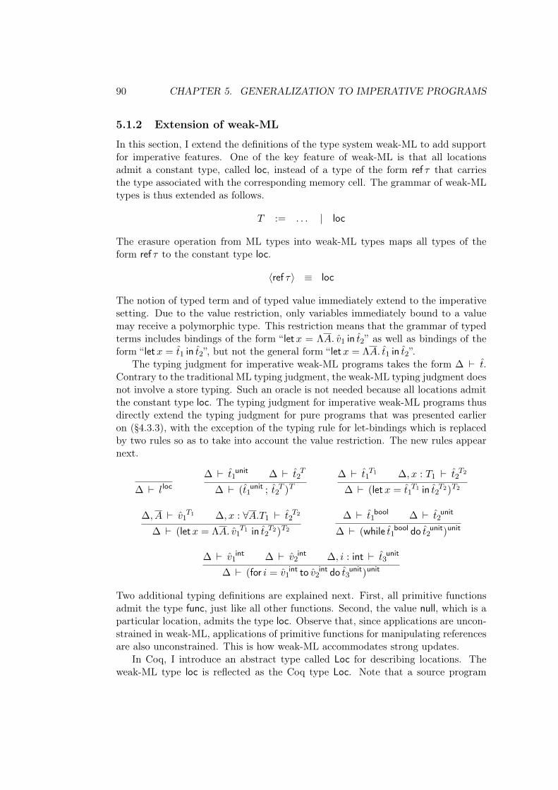
90 CHAPTER 5. GENERALIZATION TO IMPERATIVE PROGRAMS
5.1.2 Extension of weak-ML
In this section, I extend the definitions of the type system weak-ML to add supportfor imperative features. One of the key feature of weak-ML is that all locationsadmit a constant type, called loc, instead of a type of the form ref 𝜏 that carriesthe type associated with the corresponding memory cell. The grammar of weak-MLtypes is thus extended as follows.
𝑇 := . . . | loc
The erasure operation from ML types into weak-ML types maps all types of theform ref 𝜏 to the constant type loc.
⟨ref 𝜏⟩ ≡ loc
The notion of typed term and of typed value immediately extend to the imperativesetting. Due to the value restriction, only variables immediately bound to a valuemay receive a polymorphic type. This restriction means that the grammar of typedterms includes bindings of the form “ let𝑥 = Λ𝐴. 𝑣1 in 𝑡2” as well as bindings of theform “ let𝑥 = 𝑡1 in 𝑡2”, but not the general form “ let𝑥 = Λ𝐴. 𝑡1 in 𝑡2”.
The typing judgment for imperative weak-ML programs takes the form ∆ ⊢ 𝑡.Contrary to the traditional ML typing judgment, the weak-ML typing judgment doesnot involve a store typing. Such an oracle is not needed because all locations admitthe constant type loc. The typing judgment for imperative weak-ML programs thusdirectly extend the typing judgment for pure programs that was presented earlieron (§4.3.3), with the exception of the typing rule for let-bindings which is replacedby two rules so as to take into account the value restriction. The new rules appearnext.
∆ ⊢ 𝑙 loc
∆ ⊢ 𝑡1unit ∆ ⊢ 𝑡2
𝑇
∆ ⊢ (𝑡1unit ; 𝑡2
𝑇 )𝑇∆ ⊢ 𝑡1
𝑇1 ∆, 𝑥 : 𝑇1 ⊢ 𝑡2𝑇2
∆ ⊢ (let𝑥 = 𝑡1𝑇1 in 𝑡2𝑇2)𝑇2
∆, 𝐴 ⊢ 𝑣1𝑇1 ∆, 𝑥 : ∀𝐴.𝑇1 ⊢ 𝑡2
𝑇2
∆ ⊢ (let𝑥 = Λ𝐴. 𝑣1𝑇1 in 𝑡2𝑇2)𝑇2
∆ ⊢ 𝑡1bool ∆ ⊢ 𝑡2
unit
∆ ⊢ (while 𝑡1bool do 𝑡2unit)unit
∆ ⊢ 𝑣1int ∆ ⊢ 𝑣2
int ∆, 𝑖 : int ⊢ 𝑡3unit
∆ ⊢ (for 𝑖 = 𝑣1int to 𝑣2int do 𝑡3unit)unit
Two additional typing definitions are explained next. First, all primitive functionsadmit the type func, just like all other functions. Second, the value null, which is aparticular location, admits the type loc. Observe that, since applications are uncon-strained in weak-ML, applications of primitive functions for manipulating referencesare also unconstrained. This is how weak-ML accommodates strong updates.
In Coq, I introduce an abstract type called Loc for describing locations. Theweak-ML type loc is reflected as the Coq type Loc. Note that a source program
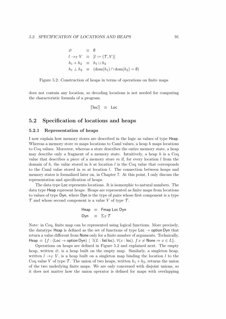
5.2. SPECIFICATION OF LOCATIONS AND HEAPS 91
∅ ≡ ∅𝑙 →𝒯 𝑉 ≡ [𝑙 := (𝒯 , 𝑉 )]
ℎ1 + ℎ2 ≡ ℎ1 ∪ ℎ2
ℎ1 ⊥ ℎ2 ≡ (dom(ℎ1) ∩ dom(ℎ2) = ∅)
Figure 5.2: Construction of heaps in terms of operations on finite maps
does not contain any location, so decoding locations is not needed for computingthe characteristic formula of a program.
VlocW ≡ Loc
5.2 Specification of locations and heaps
5.2.1 Representation of heaps
I now explain how memory stores are described in the logic as values of type Heap.Whereas a memory store 𝑚 maps locations to Caml values, a heap ℎ maps locationsto Coq values. Moreover, whereas a store describes the entire memory state, a heapmay describe only a fragment of a memory state. Intuitively, a heap ℎ is a Coqvalue that describes a piece of a memory store 𝑚 if, for every location 𝑙 from thedomain of ℎ, the value stored in ℎ at location 𝑙 is the Coq value that correspondsto the Caml value stored in 𝑚 at location 𝑙. The connection between heaps andmemory states is formalized later on, in Chapter 7. At this point, I only discuss therepresentation and specification of heaps.
The data type Loc represents locations. It is isomorphic to natural numbers. Thedata type Heap represent heaps. Heaps are represented as finite maps from locationsto values of type Dyn, where Dyn is the type of pairs whose first component is a type𝒯 and whose second component is a value 𝑉 of type 𝒯 .
Heap ≡ Fmap Loc DynDyn ≡ Σ𝒯 𝒯
Note: in Coq, finite map can be represented using logical functions. More precisely,the datatype Heap is defined as the set of functions of type Loc → option Dyn thatreturn a value different from None only for a finite number of arguments. Technically,Heap ≡ {𝑓 : (Loc → option Dyn) | ∃(𝐿 : list loc). ∀(𝑥 : loc). 𝑓 𝑥 ̸= None ⇒ 𝑥 ∈ 𝐿}.
Operations on heaps are defined in Figure 5.2 and explained next. The emptyheap, written ∅, is a heap built on the empty map. Similarly, a singleton heap,written 𝑙 →𝒯 𝑉 , is a heap built on a singleton map binding the location 𝑙 to theCoq value 𝑉 of type 𝒯 . The union of two heaps, written ℎ1 + ℎ2, returns the unionof the two underlying finite maps. We are only concerned with disjoint unions, soit does not matter how the union operator is defined for maps with overlapping
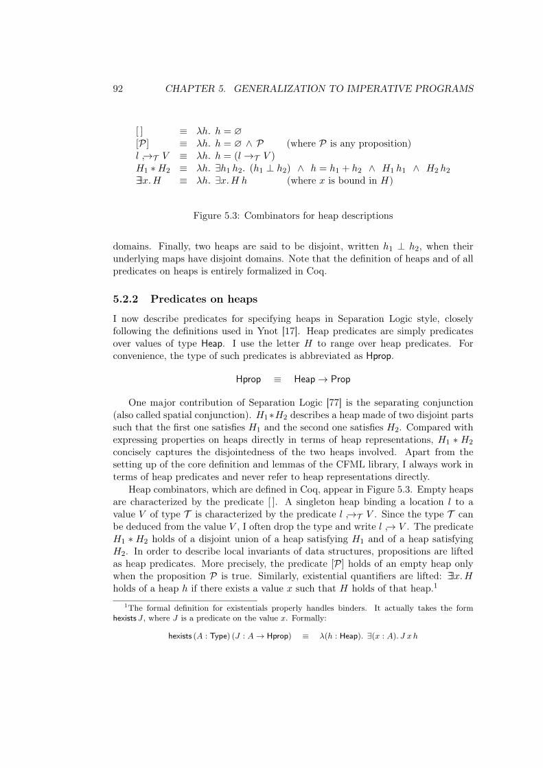
92 CHAPTER 5. GENERALIZATION TO IMPERATIVE PROGRAMS
[ ] ≡ 𝜆ℎ. ℎ = ∅[𝒫] ≡ 𝜆ℎ. ℎ = ∅ ∧ 𝒫 (where 𝒫 is any proposition)𝑙 →˓𝒯 𝑉 ≡ 𝜆ℎ. ℎ = (𝑙 →𝒯 𝑉 )𝐻1 *𝐻2 ≡ 𝜆ℎ. ∃ℎ1 ℎ2. (ℎ1 ⊥ ℎ2) ∧ ℎ = ℎ1 + ℎ2 ∧ 𝐻1 ℎ1 ∧ 𝐻2 ℎ2∃∃𝑥.𝐻 ≡ 𝜆ℎ. ∃𝑥.𝐻 ℎ (where 𝑥 is bound in 𝐻)
Figure 5.3: Combinators for heap descriptions
domains. Finally, two heaps are said to be disjoint, written ℎ1 ⊥ ℎ2, when theirunderlying maps have disjoint domains. Note that the definition of heaps and of allpredicates on heaps is entirely formalized in Coq.
5.2.2 Predicates on heaps
I now describe predicates for specifying heaps in Separation Logic style, closelyfollowing the definitions used in Ynot [17]. Heap predicates are simply predicatesover values of type Heap. I use the letter 𝐻 to range over heap predicates. Forconvenience, the type of such predicates is abbreviated as Hprop.
Hprop ≡ Heap → Prop
One major contribution of Separation Logic [77] is the separating conjunction(also called spatial conjunction). 𝐻1*𝐻2 describes a heap made of two disjoint partssuch that the first one satisfies 𝐻1 and the second one satisfies 𝐻2. Compared withexpressing properties on heaps directly in terms of heap representations, 𝐻1 * 𝐻2
concisely captures the disjointedness of the two heaps involved. Apart from thesetting up of the core definition and lemmas of the CFML library, I always work interms of heap predicates and never refer to heap representations directly.
Heap combinators, which are defined in Coq, appear in Figure 5.3. Empty heapsare characterized by the predicate [ ]. A singleton heap binding a location 𝑙 to avalue 𝑉 of type 𝒯 is characterized by the predicate 𝑙 →˓𝒯 𝑉 . Since the type 𝒯 canbe deduced from the value 𝑉 , I often drop the type and write 𝑙 →˓ 𝑉 . The predicate𝐻1 * 𝐻2 holds of a disjoint union of a heap satisfying 𝐻1 and of a heap satisfying𝐻2. In order to describe local invariants of data structures, propositions are liftedas heap predicates. More precisely, the predicate [𝒫] holds of an empty heap onlywhen the proposition 𝒫 is true. Similarly, existential quantifiers are lifted: ∃∃𝑥.𝐻holds of a heap ℎ if there exists a value 𝑥 such that 𝐻 holds of that heap.1
1The formal definition for existentials properly handles binders. It actually takes the formhexists 𝐽 , where 𝐽 is a predicate on the value 𝑥. Formally:
hexists (𝐴 : Type) (𝐽 : 𝐴 → Hprop) ≡ 𝜆(ℎ : Heap). ∃(𝑥 : 𝐴). 𝐽 𝑥 ℎ
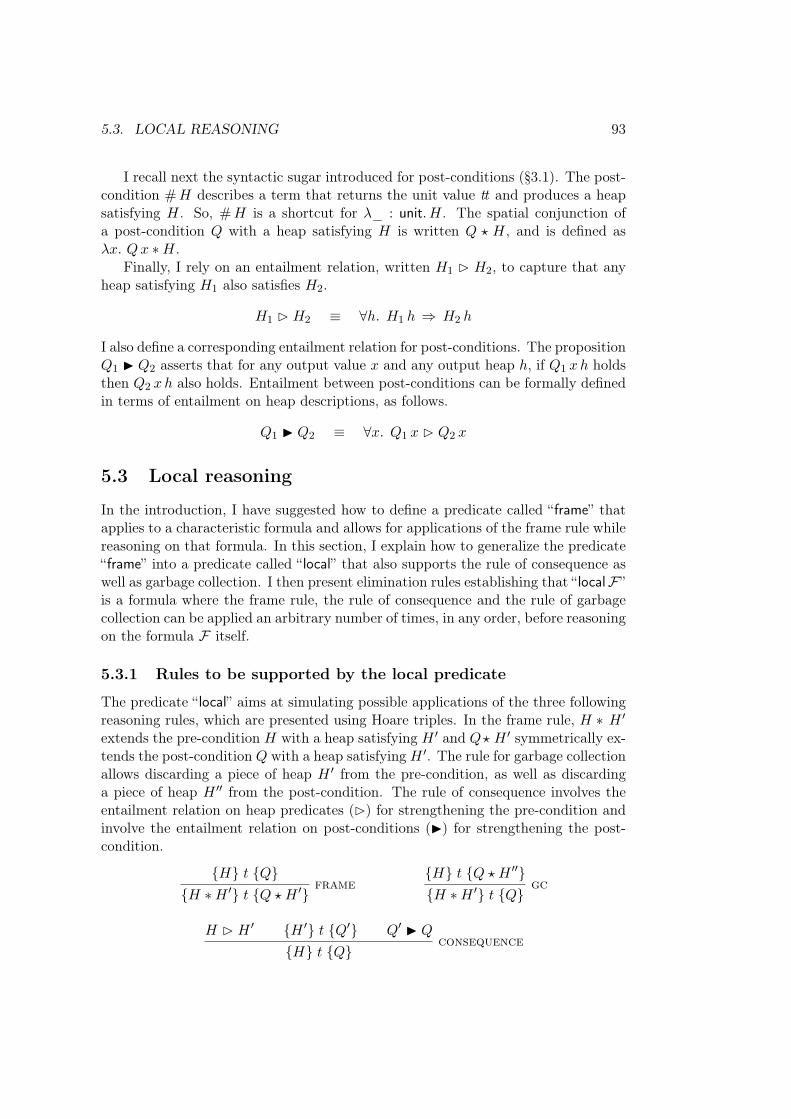
5.3. LOCAL REASONING 93
I recall next the syntactic sugar introduced for post-conditions (§3.1). The post-condition #𝐻 describes a term that returns the unit value tt and produces a heapsatisfying 𝐻. So, #𝐻 is a shortcut for 𝜆_ : unit. 𝐻. The spatial conjunction ofa post-condition 𝑄 with a heap satisfying 𝐻 is written 𝑄 ⋆ 𝐻, and is defined as𝜆𝑥. 𝑄𝑥 *𝐻.
Finally, I rely on an entailment relation, written 𝐻1 B 𝐻2, to capture that anyheap satisfying 𝐻1 also satisfies 𝐻2.
𝐻1 B 𝐻2 ≡ ∀ℎ. 𝐻1 ℎ ⇒ 𝐻2 ℎ
I also define a corresponding entailment relation for post-conditions. The proposition𝑄1 I 𝑄2 asserts that for any output value 𝑥 and any output heap ℎ, if 𝑄1 𝑥ℎ holdsthen 𝑄2 𝑥ℎ also holds. Entailment between post-conditions can be formally definedin terms of entailment on heap descriptions, as follows.
𝑄1 I 𝑄2 ≡ ∀𝑥. 𝑄1 𝑥 B 𝑄2 𝑥
5.3 Local reasoning
In the introduction, I have suggested how to define a predicate called “frame” thatapplies to a characteristic formula and allows for applications of the frame rule whilereasoning on that formula. In this section, I explain how to generalize the predicate“frame” into a predicate called “ local” that also supports the rule of consequence aswell as garbage collection. I then present elimination rules establishing that “ localℱ”is a formula where the frame rule, the rule of consequence and the rule of garbagecollection can be applied an arbitrary number of times, in any order, before reasoningon the formula ℱ itself.
5.3.1 Rules to be supported by the local predicate
The predicate “ local” aims at simulating possible applications of the three followingreasoning rules, which are presented using Hoare triples. In the frame rule, 𝐻 * 𝐻 ′
extends the pre-condition 𝐻 with a heap satisfying 𝐻 ′ and 𝑄⋆ 𝐻 ′ symmetrically ex-tends the post-condition 𝑄 with a heap satisfying 𝐻 ′. The rule for garbage collectionallows discarding a piece of heap 𝐻 ′ from the pre-condition, as well as discardinga piece of heap 𝐻 ′′ from the post-condition. The rule of consequence involves theentailment relation on heap predicates (B) for strengthening the pre-condition andinvolve the entailment relation on post-conditions (I) for strengthening the post-condition.
{𝐻} 𝑡 {𝑄}{𝐻 *𝐻 ′} 𝑡 {𝑄 ⋆ 𝐻 ′}
frame{𝐻} 𝑡 {𝑄 ⋆ 𝐻 ′′}{𝐻 *𝐻 ′} 𝑡 {𝑄}
gc
𝐻 B 𝐻 ′ {𝐻 ′} 𝑡 {𝑄′} 𝑄′ I 𝑄
{𝐻} 𝑡 {𝑄}consequence
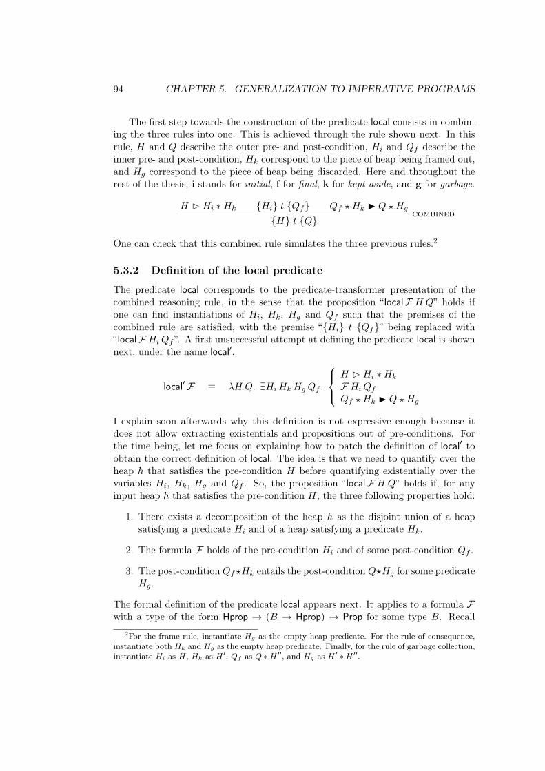
94 CHAPTER 5. GENERALIZATION TO IMPERATIVE PROGRAMS
The first step towards the construction of the predicate local consists in combin-ing the three rules into one. This is achieved through the rule shown next. In thisrule, 𝐻 and 𝑄 describe the outer pre- and post-condition, 𝐻𝑖 and 𝑄𝑓 describe theinner pre- and post-condition, 𝐻𝑘 correspond to the piece of heap being framed out,and 𝐻𝑔 correspond to the piece of heap being discarded. Here and throughout therest of the thesis, i stands for initial, f for final, k for kept aside, and g for garbage.
𝐻 B 𝐻𝑖 *𝐻𝑘 {𝐻𝑖} 𝑡 {𝑄𝑓} 𝑄𝑓 ⋆ 𝐻𝑘 I 𝑄 ⋆ 𝐻𝑔
{𝐻} 𝑡 {𝑄}combined
One can check that this combined rule simulates the three previous rules.2
5.3.2 Definition of the local predicate
The predicate local corresponds to the predicate-transformer presentation of thecombined reasoning rule, in the sense that the proposition “ localℱ 𝐻 𝑄” holds ifone can find instantiations of 𝐻𝑖, 𝐻𝑘, 𝐻𝑔 and 𝑄𝑓 such that the premises of thecombined rule are satisfied, with the premise “{𝐻𝑖} 𝑡 {𝑄𝑓}” being replaced with“ localℱ 𝐻𝑖𝑄𝑓 ”. A first unsuccessful attempt at defining the predicate local is shownnext, under the name local′.
local′ℱ ≡ 𝜆𝐻 𝑄. ∃𝐻𝑖𝐻𝑘 𝐻𝑔 𝑄𝑓 .
𝐻 B 𝐻𝑖 *𝐻𝑘
ℱ 𝐻𝑖𝑄𝑓
𝑄𝑓 ⋆ 𝐻𝑘 I 𝑄 ⋆ 𝐻𝑔
I explain soon afterwards why this definition is not expressive enough because itdoes not allow extracting existentials and propositions out of pre-conditions. Forthe time being, let me focus on explaining how to patch the definition of local′ toobtain the correct definition of local. The idea is that we need to quantify over theheap ℎ that satisfies the pre-condition 𝐻 before quantifying existentially over thevariables 𝐻𝑖, 𝐻𝑘, 𝐻𝑔 and 𝑄𝑓 . So, the proposition “ localℱ 𝐻 𝑄” holds if, for anyinput heap ℎ that satisfies the pre-condition 𝐻, the three following properties hold:
1. There exists a decomposition of the heap ℎ as the disjoint union of a heapsatisfying a predicate 𝐻𝑖 and of a heap satisfying a predicate 𝐻𝑘.
2. The formula ℱ holds of the pre-condition 𝐻𝑖 and of some post-condition 𝑄𝑓 .
3. The post-condition 𝑄𝑓 ⋆𝐻𝑘 entails the post-condition 𝑄⋆𝐻𝑔 for some predicate𝐻𝑔.
The formal definition of the predicate local appears next. It applies to a formula ℱwith a type of the form Hprop → (𝐵 → Hprop) → Prop for some type 𝐵. Recall
2For the frame rule, instantiate 𝐻𝑔 as the empty heap predicate. For the rule of consequence,instantiate both 𝐻𝑘 and 𝐻𝑔 as the empty heap predicate. Finally, for the rule of garbage collection,instantiate 𝐻𝑖 as 𝐻, 𝐻𝑘 as 𝐻 ′, 𝑄𝑓 as 𝑄 *𝐻 ′′, and 𝐻𝑔 as 𝐻 ′ *𝐻 ′′.

5.3. LOCAL REASONING 95
that 𝐻𝑖 is the “initial” heap, 𝑄𝑓 describes the “final” post-condition, 𝐻𝑘 is the heapbeing “kept aside”, and 𝐻𝑔 is the “garbage” heap.
localℱ ≡ 𝜆𝐻 𝑄. ∀ℎ. 𝐻 ℎ ⇒ ∃𝐻𝑖𝐻𝑘 𝐻𝑔 𝑄𝑓 .
(𝐻𝑖 *𝐻𝑘)ℎℱ 𝐻𝑖𝑄𝑓
𝑄𝑓 ⋆ 𝐻𝑘 I 𝑄 ⋆ 𝐻𝑔
Notice that the definition of local refers to a heap representation ℎ. This heaprepresentation never needs to be manipulated directly in proofs, as all the work canbe conducted through the high-level elimination lemmas that are explained in therest of this section.
Remark: the definition of the predicate local shows some similarities with thedefinition of the “STsep” monad from Hoare Type Theory [61], in the sense thatboth aim at baking the Separation Logic frame condition into a system defined interms of heaps describing the whole memory.
5.3.3 Properties of local formulae
The first useful property about the predicate transformer local is that it may beignored during reasoning. More precisely, if the goal is to prove “ localℱ 𝐻 𝑄”, thenit suffices to prove “ℱ 𝐻 𝑄”. (To check this implication, instantiate 𝐻𝑖 as 𝐻, 𝑄𝑓 as𝑄, and 𝐻𝑘 and 𝐻𝑔 as the empty heap predicate.) Formally:
∀𝐻 𝑄. ℱ 𝐻 𝑄 ⇒ localℱ 𝐻 𝑄
Another key property of local is its idempotence: iterated applications of local areredundant. In other words, a proposition of the form “ local (localℱ)𝐻 𝑄” is al-ways equivalent to the proposition “ localℱ 𝐻 𝑄”. With predicate extensionality, theidempotence property can be stated very concisely, as follows.
∀ℱ . localℱ = local (localℱ)
It remains to explain how to exploit the predicate local in reasoning on char-acteristic formulae. Let me start with the case of the frame rule. The followingstatement is a direct consequence of the definition of the predicate local.
ℱ 𝐻1𝑄1 ⇒ localℱ (𝐻1 *𝐻2) (𝑄1 ⋆ 𝐻2)
Yet, applying this lemma would result in consuming the occurrence of local at thehead of the formula, preventing us from subsequently applying other rules. Fortu-nately, thanks to the idempotence of the predicate local, it is possible to derive alemma where the local modifier is preserved.
localℱ 𝐻1𝑄1 ⇒ localℱ (𝐻1 *𝐻2) (𝑄1 ⋆ 𝐻2)
In practice, I have found it more convenient with respect to tactics to reformulatethe lemma in the following form.
is_localℱ ∧ ℱ 𝐻1𝑄1 ⇒ ℱ (𝐻1 *𝐻2) (𝑄1 ⋆ 𝐻2)
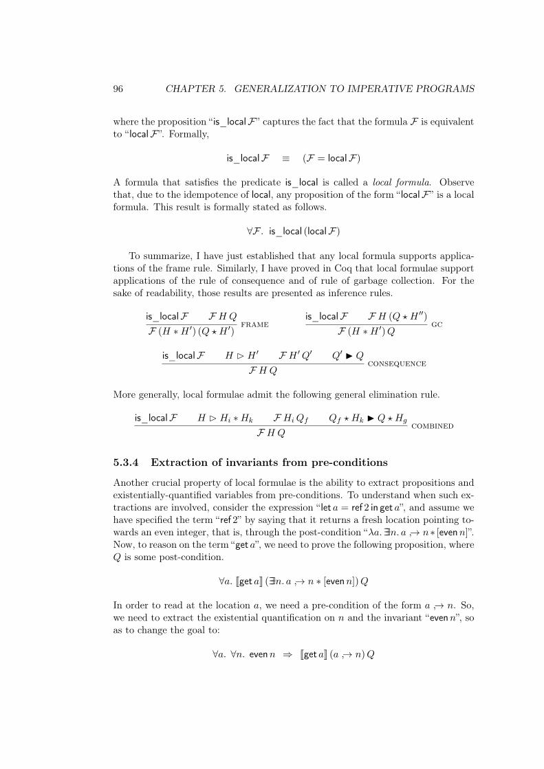
96 CHAPTER 5. GENERALIZATION TO IMPERATIVE PROGRAMS
where the proposition “ is_localℱ” captures the fact that the formula ℱ is equivalentto “ localℱ”. Formally,
is_localℱ ≡ (ℱ = localℱ)
A formula that satisfies the predicate is_local is called a local formula. Observethat, due to the idempotence of local, any proposition of the form “ localℱ” is a localformula. This result is formally stated as follows.
∀ℱ . is_local (localℱ)
To summarize, I have just established that any local formula supports applica-tions of the frame rule. Similarly, I have proved in Coq that local formulae supportapplications of the rule of consequence and of rule of garbage collection. For thesake of readability, those results are presented as inference rules.
is_localℱ ℱ 𝐻 𝑄
ℱ (𝐻 *𝐻 ′) (𝑄 ⋆ 𝐻 ′)frame
is_localℱ ℱ 𝐻 (𝑄 ⋆ 𝐻 ′′)
ℱ (𝐻 *𝐻 ′)𝑄gc
is_localℱ 𝐻 B 𝐻 ′ ℱ 𝐻 ′𝑄′ 𝑄′ I 𝑄
ℱ 𝐻 𝑄consequence
More generally, local formulae admit the following general elimination rule.
is_localℱ 𝐻 B 𝐻𝑖 *𝐻𝑘 ℱ 𝐻𝑖𝑄𝑓 𝑄𝑓 ⋆ 𝐻𝑘 I 𝑄 ⋆ 𝐻𝑔
ℱ 𝐻 𝑄combined
5.3.4 Extraction of invariants from pre-conditions
Another crucial property of local formulae is the ability to extract propositions andexistentially-quantified variables from pre-conditions. To understand when such ex-tractions are involved, consider the expression “ let 𝑎 = ref 2 in get 𝑎”, and assume wehave specified the term “ref 2” by saying that it returns a fresh location pointing to-wards an even integer, that is, through the post-condition “𝜆𝑎.∃∃𝑛. 𝑎 →˓ 𝑛* [even𝑛]”.Now, to reason on the term “get 𝑎”, we need to prove the following proposition, where𝑄 is some post-condition.
∀𝑎. Jget 𝑎K (∃∃𝑛. 𝑎 →˓ 𝑛 * [even𝑛])𝑄
In order to read at the location 𝑎, we need a pre-condition of the form 𝑎 →˓ 𝑛. So,we need to extract the existential quantification on 𝑛 and the invariant “even𝑛”, soas to change the goal to:
∀𝑎. ∀𝑛. even𝑛 ⇒ Jget 𝑎K (𝑎 →˓ 𝑛)𝑄
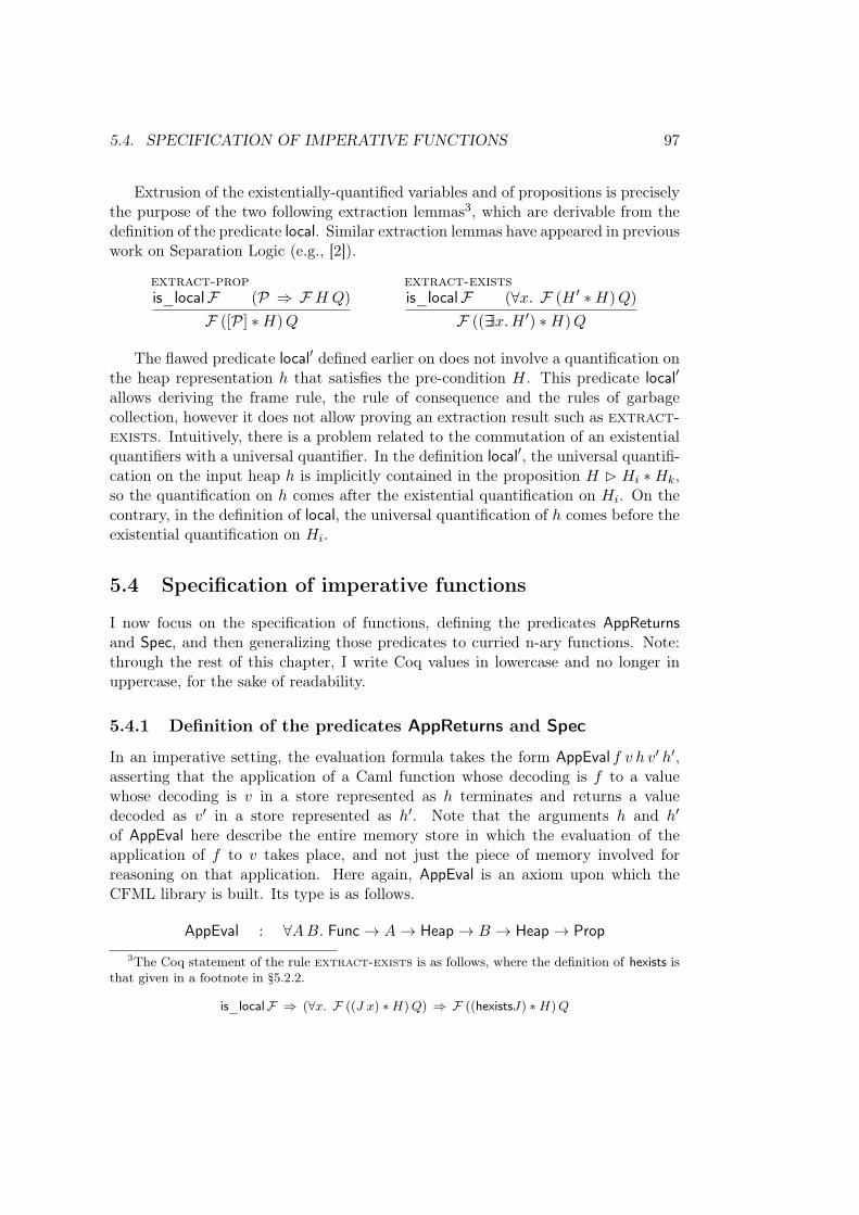
5.4. SPECIFICATION OF IMPERATIVE FUNCTIONS 97
Extrusion of the existentially-quantified variables and of propositions is preciselythe purpose of the two following extraction lemmas3, which are derivable from thedefinition of the predicate local. Similar extraction lemmas have appeared in previouswork on Separation Logic (e.g., [2]).
extract-propis_localℱ (𝒫 ⇒ ℱ 𝐻 𝑄)
ℱ ([𝒫] *𝐻)𝑄
extract-existsis_localℱ (∀𝑥. ℱ (𝐻 ′ *𝐻)𝑄)
ℱ ((∃∃𝑥.𝐻 ′) *𝐻)𝑄
The flawed predicate local′ defined earlier on does not involve a quantification onthe heap representation ℎ that satisfies the pre-condition 𝐻. This predicate local′
allows deriving the frame rule, the rule of consequence and the rules of garbagecollection, however it does not allow proving an extraction result such as extract-exists. Intuitively, there is a problem related to the commutation of an existentialquantifiers with a universal quantifier. In the definition local′, the universal quantifi-cation on the input heap ℎ is implicitly contained in the proposition 𝐻 B 𝐻𝑖 *𝐻𝑘,so the quantification on ℎ comes after the existential quantification on 𝐻𝑖. On thecontrary, in the definition of local, the universal quantification of ℎ comes before theexistential quantification on 𝐻𝑖.
5.4 Specification of imperative functions
I now focus on the specification of functions, defining the predicates AppReturnsand Spec, and then generalizing those predicates to curried n-ary functions. Note:through the rest of this chapter, I write Coq values in lowercase and no longer inuppercase, for the sake of readability.
5.4.1 Definition of the predicates AppReturns and Spec
In an imperative setting, the evaluation formula takes the form AppEval 𝑓 𝑣 ℎ 𝑣′ ℎ′,asserting that the application of a Caml function whose decoding is 𝑓 to a valuewhose decoding is 𝑣 in a store represented as ℎ terminates and returns a valuedecoded as 𝑣′ in a store represented as ℎ′. Note that the arguments ℎ and ℎ′
of AppEval here describe the entire memory store in which the evaluation of theapplication of 𝑓 to 𝑣 takes place, and not just the piece of memory involved forreasoning on that application. Here again, AppEval is an axiom upon which theCFML library is built. Its type is as follows.
AppEval : ∀𝐴𝐵. Func → 𝐴 → Heap → 𝐵 → Heap → Prop
3The Coq statement of the rule extract-exists is as follows, where the definition of hexists isthat given in a footnote in §5.2.2.
is_localℱ ⇒ (∀𝑥. ℱ ((𝐽 𝑥) *𝐻)𝑄) ⇒ ℱ ((hexists𝐽) *𝐻)𝑄
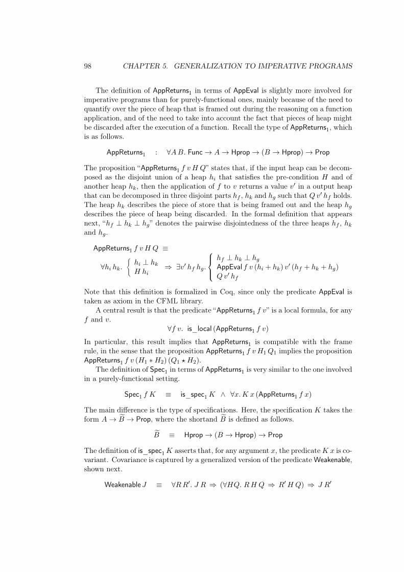
98 CHAPTER 5. GENERALIZATION TO IMPERATIVE PROGRAMS
The definition of AppReturns1 in terms of AppEval is slightly more involved forimperative programs than for purely-functional ones, mainly because of the need toquantify over the piece of heap that is framed out during the reasoning on a functionapplication, and of the need to take into account the fact that pieces of heap mightbe discarded after the execution of a function. Recall the type of AppReturns1, whichis as follows.
AppReturns1 : ∀𝐴𝐵. Func → 𝐴 → Hprop → (𝐵 → Hprop) → Prop
The proposition “AppReturns1 𝑓 𝑣 𝐻 𝑄” states that, if the input heap can be decom-posed as the disjoint union of a heap ℎ𝑖 that satisfies the pre-condition 𝐻 and ofanother heap ℎ𝑘, then the application of 𝑓 to 𝑣 returns a value 𝑣′ in a output heapthat can be decomposed in three disjoint parts ℎ𝑓 , ℎ𝑘 and ℎ𝑔 such that 𝑄𝑣′ ℎ𝑓 holds.The heap ℎ𝑘 describes the piece of store that is being framed out and the heap ℎ𝑔describes the piece of heap being discarded. In the formal definition that appearsnext, “ℎ𝑓 ⊥ ℎ𝑘 ⊥ ℎ𝑔” denotes the pairwise disjointedness of the three heaps ℎ𝑓 , ℎ𝑘and ℎ𝑔.
AppReturns1 𝑓 𝑣 𝐻 𝑄 ≡
∀ℎ𝑖 ℎ𝑘.®
ℎ𝑖 ⊥ ℎ𝑘𝐻 ℎ𝑖
⇒ ∃𝑣′ ℎ𝑓 ℎ𝑔.
ℎ𝑓 ⊥ ℎ𝑘 ⊥ ℎ𝑔AppEval 𝑓 𝑣 (ℎ𝑖 + ℎ𝑘) 𝑣′ (ℎ𝑓 + ℎ𝑘 + ℎ𝑔)𝑄𝑣′ ℎ𝑓
Note that this definition is formalized in Coq, since only the predicate AppEval istaken as axiom in the CFML library.
A central result is that the predicate “AppReturns1 𝑓 𝑣” is a local formula, for any𝑓 and 𝑣.
∀𝑓 𝑣. is_local (AppReturns1 𝑓 𝑣)
In particular, this result implies that AppReturns1 is compatible with the framerule, in the sense that the proposition AppReturns1 𝑓 𝑣 𝐻1𝑄1 implies the propositionAppReturns1 𝑓 𝑣 (𝐻1 *𝐻2) (𝑄1 ⋆ 𝐻2).
The definition of Spec1 in terms of AppReturns1 is very similar to the one involvedin a purely-functional setting.
Spec1 𝑓 𝐾 ≡ is_spec1𝐾 ∧ ∀𝑥.𝐾 𝑥 (AppReturns1 𝑓 𝑥)
The main difference is the type of specifications. Here, the specification 𝐾 takes theform 𝐴 → ‹𝐵 → Prop, where the shortand ‹𝐵 is defined as follows.‹𝐵 ≡ Hprop → (𝐵 → Hprop) → Prop
The definition of is_spec1𝐾 asserts that, for any argument 𝑥, the predicate 𝐾 𝑥 is co-variant. Covariance is captured by a generalized version of the predicate Weakenable,shown next.
Weakenable 𝐽 ≡ ∀𝑅𝑅′. 𝐽 𝑅 ⇒ (∀𝐻𝑄. 𝑅𝐻 𝑄 ⇒ 𝑅′𝐻 𝑄) ⇒ 𝐽 𝑅′
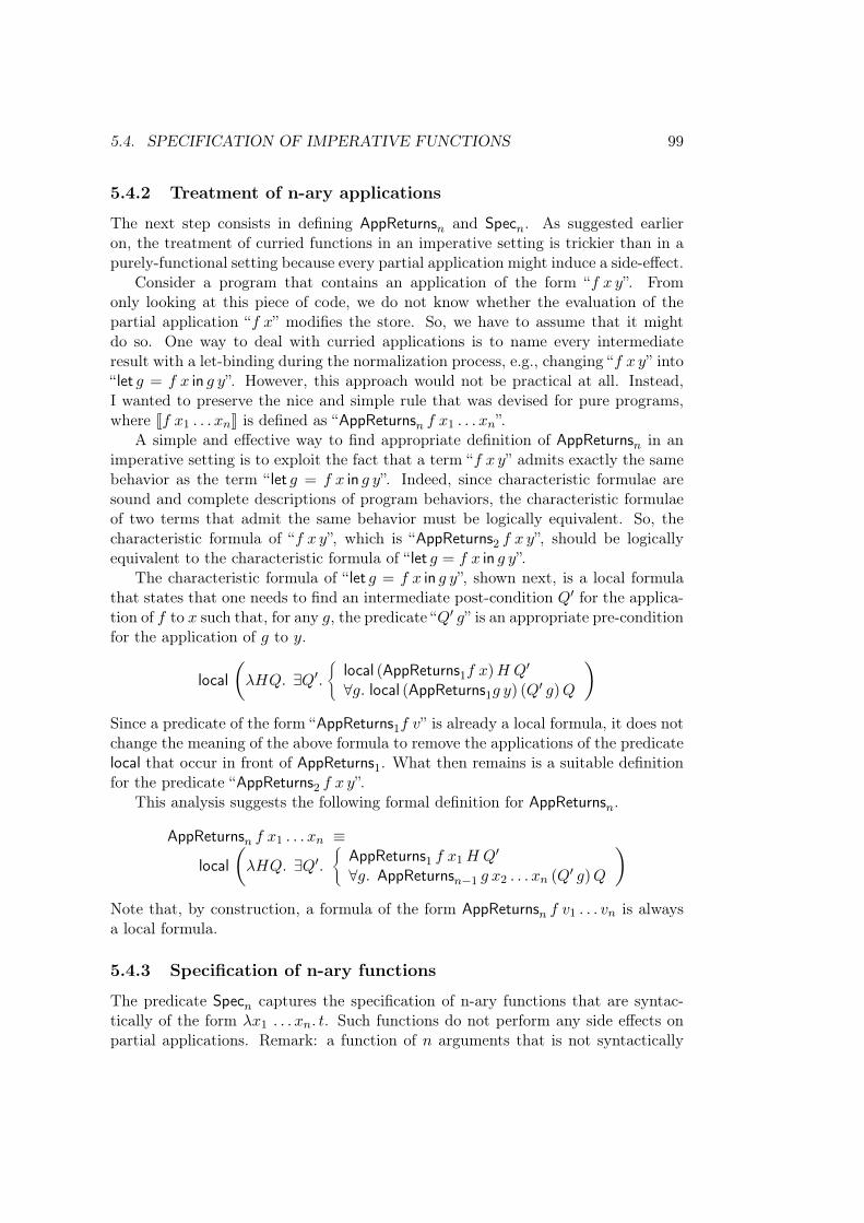
5.4. SPECIFICATION OF IMPERATIVE FUNCTIONS 99
5.4.2 Treatment of n-ary applications
The next step consists in defining AppReturns𝑛 and Spec𝑛. As suggested earlieron, the treatment of curried functions in an imperative setting is trickier than in apurely-functional setting because every partial application might induce a side-effect.
Consider a program that contains an application of the form “𝑓 𝑥 𝑦”. Fromonly looking at this piece of code, we do not know whether the evaluation of thepartial application “𝑓 𝑥” modifies the store. So, we have to assume that it mightdo so. One way to deal with curried applications is to name every intermediateresult with a let-binding during the normalization process, e.g., changing “𝑓 𝑥 𝑦” into“ let 𝑔 = 𝑓 𝑥 in 𝑔 𝑦”. However, this approach would not be practical at all. Instead,I wanted to preserve the nice and simple rule that was devised for pure programs,where J𝑓 𝑥1 . . . 𝑥𝑛K is defined as “AppReturns𝑛 𝑓 𝑥1 . . . 𝑥𝑛”.
A simple and effective way to find appropriate definition of AppReturns𝑛 in animperative setting is to exploit the fact that a term “𝑓 𝑥 𝑦” admits exactly the samebehavior as the term “ let 𝑔 = 𝑓 𝑥 in 𝑔 𝑦”. Indeed, since characteristic formulae aresound and complete descriptions of program behaviors, the characteristic formulaeof two terms that admit the same behavior must be logically equivalent. So, thecharacteristic formula of “𝑓 𝑥 𝑦”, which is “AppReturns2 𝑓 𝑥 𝑦”, should be logicallyequivalent to the characteristic formula of “ let 𝑔 = 𝑓 𝑥 in 𝑔 𝑦”.
The characteristic formula of “ let 𝑔 = 𝑓 𝑥 in 𝑔 𝑦”, shown next, is a local formulathat states that one needs to find an intermediate post-condition 𝑄′ for the applica-tion of 𝑓 to 𝑥 such that, for any 𝑔, the predicate “𝑄′ 𝑔” is an appropriate pre-conditionfor the application of 𝑔 to 𝑦.
localÇ𝜆𝐻𝑄. ∃𝑄′.
®local (AppReturns1𝑓 𝑥)𝐻 𝑄′
∀𝑔. local (AppReturns1𝑔 𝑦) (𝑄′ 𝑔)𝑄
åSince a predicate of the form “AppReturns1𝑓 𝑣” is already a local formula, it does notchange the meaning of the above formula to remove the applications of the predicatelocal that occur in front of AppReturns1. What then remains is a suitable definitionfor the predicate “AppReturns2 𝑓 𝑥 𝑦”.
This analysis suggests the following formal definition for AppReturns𝑛.
AppReturns𝑛 𝑓 𝑥1 . . . 𝑥𝑛 ≡
localÇ𝜆𝐻𝑄. ∃𝑄′.
®AppReturns1 𝑓 𝑥1𝐻 𝑄′
∀𝑔. AppReturns𝑛−1 𝑔 𝑥2 . . . 𝑥𝑛 (𝑄′ 𝑔)𝑄
åNote that, by construction, a formula of the form AppReturns𝑛 𝑓 𝑣1 . . . 𝑣𝑛 is alwaysa local formula.
5.4.3 Specification of n-ary functions
The predicate Spec𝑛 captures the specification of n-ary functions that are syntac-tically of the form 𝜆𝑥1 . . . 𝑥𝑛. 𝑡. Such functions do not perform any side effects onpartial applications. Remark: a function of 𝑛 arguments that is not syntactically
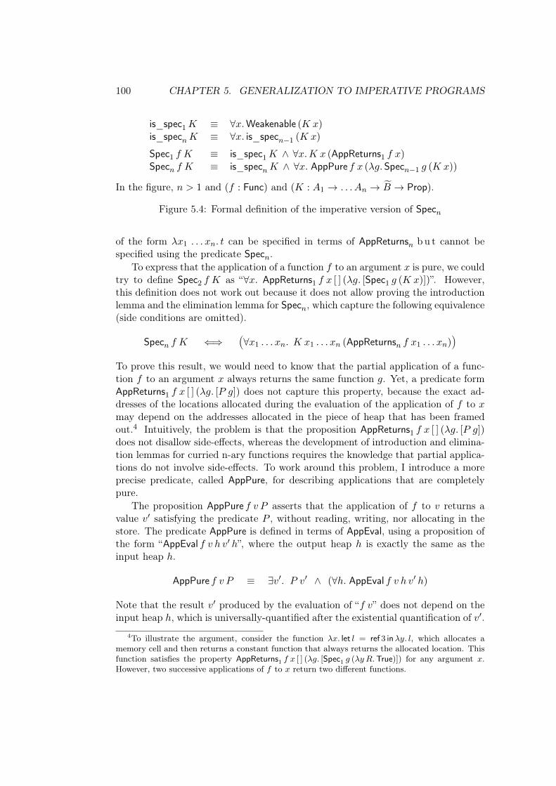
100 CHAPTER 5. GENERALIZATION TO IMPERATIVE PROGRAMS
is_spec1𝐾 ≡ ∀𝑥.Weakenable (𝐾 𝑥)is_spec𝑛𝐾 ≡ ∀𝑥. is_spec𝑛−1 (𝐾 𝑥)
Spec1 𝑓 𝐾 ≡ is_spec1𝐾 ∧ ∀𝑥.𝐾 𝑥 (AppReturns1 𝑓 𝑥)Spec𝑛 𝑓 𝐾 ≡ is_spec𝑛𝐾 ∧ ∀𝑥. AppPure 𝑓 𝑥 (𝜆𝑔. Spec𝑛−1 𝑔 (𝐾 𝑥))
In the figure, 𝑛 > 1 and (𝑓 : Func) and (𝐾 : 𝐴1 → . . . 𝐴𝑛 → ‹𝐵 → Prop).
Figure 5.4: Formal definition of the imperative version of Spec𝑛
of the form 𝜆𝑥1 . . . 𝑥𝑛. 𝑡 can be specified in terms of AppReturns𝑛 b u t cannot bespecified using the predicate Spec𝑛.
To express that the application of a function 𝑓 to an argument 𝑥 is pure, we couldtry to define Spec2 𝑓 𝐾 as “∀𝑥. AppReturns1 𝑓 𝑥 [ ] (𝜆𝑔. [Spec1 𝑔 (𝐾 𝑥)])”. However,this definition does not work out because it does not allow proving the introductionlemma and the elimination lemma for Spec𝑛, which capture the following equivalence(side conditions are omitted).
Spec𝑛 𝑓 𝐾 ⇐⇒Ä∀𝑥1 . . . 𝑥𝑛. 𝐾 𝑥1 . . . 𝑥𝑛 (AppReturns𝑛 𝑓 𝑥1 . . . 𝑥𝑛)
äTo prove this result, we would need to know that the partial application of a func-tion 𝑓 to an argument 𝑥 always returns the same function 𝑔. Yet, a predicate formAppReturns1 𝑓 𝑥 [ ] (𝜆𝑔. [𝑃 𝑔]) does not capture this property, because the exact ad-dresses of the locations allocated during the evaluation of the application of 𝑓 to 𝑥may depend on the addresses allocated in the piece of heap that has been framedout.4 Intuitively, the problem is that the proposition AppReturns1 𝑓 𝑥 [ ] (𝜆𝑔. [𝑃 𝑔])does not disallow side-effects, whereas the development of introduction and elimina-tion lemmas for curried n-ary functions requires the knowledge that partial applica-tions do not involve side-effects. To work around this problem, I introduce a moreprecise predicate, called AppPure, for describing applications that are completelypure.
The proposition AppPure 𝑓 𝑣 𝑃 asserts that the application of 𝑓 to 𝑣 returns avalue 𝑣′ satisfying the predicate 𝑃 , without reading, writing, nor allocating in thestore. The predicate AppPure is defined in terms of AppEval, using a proposition ofthe form “AppEval 𝑓 𝑣 ℎ 𝑣′ ℎ”, where the output heap ℎ is exactly the same as theinput heap ℎ.
AppPure 𝑓 𝑣 𝑃 ≡ ∃𝑣′. 𝑃 𝑣′ ∧ (∀ℎ. AppEval 𝑓 𝑣 ℎ 𝑣′ ℎ)
Note that the result 𝑣′ produced by the evaluation of “𝑓 𝑣” does not depend on theinput heap ℎ, which is universally-quantified after the existential quantification of 𝑣′.
4To illustrate the argument, consider the function 𝜆𝑥. let 𝑙 = ref 3 in𝜆𝑦. 𝑙, which allocates amemory cell and then returns a constant function that always returns the allocated location. Thisfunction satisfies the property AppReturns1 𝑓 𝑥 [ ] (𝜆𝑔. [Spec1 𝑔 (𝜆𝑦 𝑅.True)]) for any argument 𝑥.However, two successive applications of 𝑓 to 𝑥 return two different functions.

5.5. CHARACTERISTIC FORMULAE FOR IMPERATIVE PROGRAMS 101
The predicate Spec2 can now be defined in terms of AppPure and Spec1. Com-pared with the definition of Spec2 from the purely-functional setting, the only dif-ference is the replacement of the predicate AppReturns with the predicate AppPure.
Spec2 𝑓 𝐾 ≡ is_spec2𝐾 ∧ ∀𝑥. AppPure 𝑓 𝑥 (𝜆𝑔. Spec1 𝑔 (𝐾 𝑥))
The general definitions of Spec𝑛 and of is_spec𝑛 appear in Figure 5.4.
5.5 Characteristic formulae for imperative programs
5.5.1 Construction of characteristic formulae
The algorithm for constructing characteristic formulae for imperative programs ap-pears in Figure 5.5, and are explained next. For the sake of clarity, contexts anddecoding of values are left implicit. I have set up a notation layer for pretty-printingcharacteristic formulae for imperative programs, in a very similar way as describedin the previous chapter for purely-functional programs. I omit the details here.
As explained in the introduction, an application of the predicate local is intro-duced at every node of a characteristic formula. A value 𝑣 admits a pre-condition𝐻 and a post-condition 𝑄 if the current heap, which by assumption satisfies thepredicate 𝐻, also satisfies the predicate 𝑄𝑣. This entailment is written 𝐻 B 𝑄𝑣.The application of a n-ary function is described through the predicate AppReturns𝑛.Here, the application of local in front of AppReturns𝑛 is redundant, yet I leave itfor the sake of uniformity. The treatment of crash, of conditionals and of functiondefinitions is quite similar to the treatment given for the purely-functional setting.In short, it suffices to replace occurrences of a post-condition 𝑃 with a pre-condition𝐻 and a post-condition 𝑄. In practice, it is useful to consider a direct constructionfor the characteristic formulae of terms of the form “ if 𝑡0 then 𝑡1 else 𝑡2”.
Jif 𝑡0 then 𝑡1 else 𝑡2K ≡local (𝜆𝐻𝑄. ∃𝑄′. J𝑡0K𝐻 𝑄′ ∧ J𝑡1K (𝑄′ true)𝑄 ∧ J𝑡2K (𝑄′ false)𝑄)
One can prove that this direct formula is logically equivalent to the characteristicformula of the term “ let𝑥 = 𝑡0 in if𝑥 then 𝑡1 else 𝑡2”.
The treatment of let-bindings has already been described in the introduction.In a term “ let𝑥 = 𝑡1 in 𝑡2”, the post-condition 𝑄′ of 𝑡1 is quantified existentially,and then 𝑄′ 𝑥 describes the pre-condition for 𝑡2. Sequences are a particular case oflet-bindings, where the result of 𝑡1 is of type unit and thus need not be named.
For a polymorphic let-binding, the bound term must be a syntactic value, due tothe value restriction. Consider the typed term “ let𝑥 = �̂�1 in 𝑡2”, where �̂�1 stands fora possibly-polymorphic value. The construction of the corresponding characteristicformula is formally described as follows.
Jlet𝑥 = �̂�1 in 𝑡2KΓ ≡ local (𝜆𝐻𝑄. ∀𝑋. 𝑋 = ⌈�̂�1⌉ ⇒ J𝑡2K(Γ,𝑥 ↦→𝑋)𝐻 𝑄)
If 𝑆 denotes the type of �̂�1, then the formula universally quantifies over a value 𝑋 oftype V𝑆W, and provides the assumption “𝑋 = ⌈�̂�1⌉”, which asserts that the logical
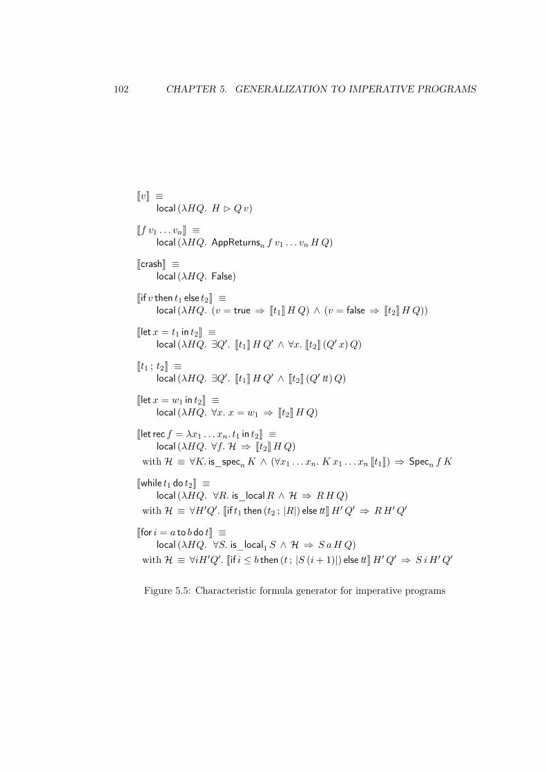
102 CHAPTER 5. GENERALIZATION TO IMPERATIVE PROGRAMS
J𝑣K ≡local (𝜆𝐻𝑄. 𝐻 B 𝑄𝑣)
J𝑓 𝑣1 . . . 𝑣𝑛K ≡local (𝜆𝐻𝑄. AppReturns𝑛 𝑓 𝑣1 . . . 𝑣𝑛𝐻 𝑄)
JcrashK ≡local (𝜆𝐻𝑄. False)
Jif 𝑣 then 𝑡1 else 𝑡2K ≡local (𝜆𝐻𝑄. (𝑣 = true ⇒ J𝑡1K𝐻 𝑄) ∧ (𝑣 = false ⇒ J𝑡2K𝐻 𝑄))
Jlet𝑥 = 𝑡1 in 𝑡2K ≡local (𝜆𝐻𝑄. ∃𝑄′. J𝑡1K𝐻 𝑄′ ∧ ∀𝑥. J𝑡2K (𝑄′ 𝑥)𝑄)
J𝑡1 ; 𝑡2K ≡local (𝜆𝐻𝑄. ∃𝑄′. J𝑡1K𝐻 𝑄′ ∧ J𝑡2K (𝑄′ tt)𝑄)
Jlet𝑥 = 𝑤1 in 𝑡2K ≡local (𝜆𝐻𝑄. ∀𝑥. 𝑥 = 𝑤1 ⇒ J𝑡2K𝐻 𝑄)
Jlet rec 𝑓 = 𝜆𝑥1 . . . 𝑥𝑛. 𝑡1 in 𝑡2K ≡local (𝜆𝐻𝑄. ∀𝑓. ℋ ⇒ J𝑡2K𝐻 𝑄)
with ℋ ≡ ∀𝐾. is_spec𝑛𝐾 ∧ (∀𝑥1 . . . 𝑥𝑛. 𝐾 𝑥1 . . . 𝑥𝑛 J𝑡1K) ⇒ Spec𝑛 𝑓 𝐾
Jwhile 𝑡1 do 𝑡2K ≡local (𝜆𝐻𝑄. ∀𝑅. is_local𝑅 ∧ ℋ ⇒ 𝑅𝐻 𝑄)
with ℋ ≡ ∀𝐻 ′𝑄′. Jif 𝑡1 then (𝑡2 ; |𝑅|) else ttK𝐻 ′𝑄′ ⇒ 𝑅𝐻 ′𝑄′
Jfor 𝑖 = 𝑎 to 𝑏 do 𝑡K ≡local (𝜆𝐻𝑄. ∀𝑆. is_local1 𝑆 ∧ ℋ ⇒ 𝑆 𝑎𝐻 𝑄)
with ℋ ≡ ∀𝑖𝐻 ′𝑄′. Jif 𝑖 ≤ 𝑏 then (𝑡 ; |𝑆 (𝑖 + 1)|) else ttK𝐻 ′𝑄′ ⇒ 𝑆 𝑖𝐻 ′𝑄′
Figure 5.5: Characteristic formula generator for imperative programs
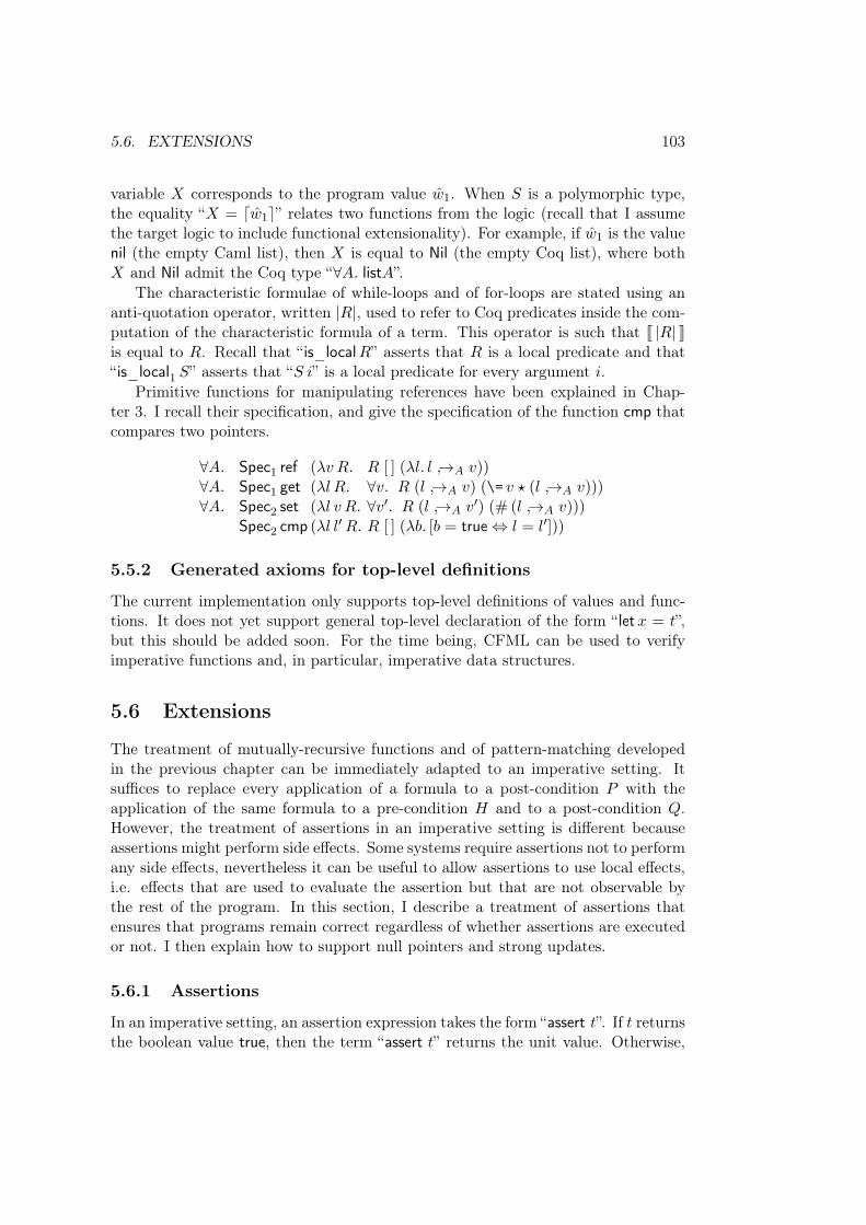
5.6. EXTENSIONS 103
variable 𝑋 corresponds to the program value �̂�1. When 𝑆 is a polymorphic type,the equality “𝑋 = ⌈�̂�1⌉” relates two functions from the logic (recall that I assumethe target logic to include functional extensionality). For example, if �̂�1 is the valuenil (the empty Caml list), then 𝑋 is equal to Nil (the empty Coq list), where both𝑋 and Nil admit the Coq type “∀𝐴. list𝐴”.
The characteristic formulae of while-loops and of for-loops are stated using ananti-quotation operator, written |𝑅|, used to refer to Coq predicates inside the com-putation of the characteristic formula of a term. This operator is such that J |𝑅| Kis equal to 𝑅. Recall that “ is_local𝑅” asserts that 𝑅 is a local predicate and that“ is_local1 𝑆” asserts that “𝑆 𝑖” is a local predicate for every argument 𝑖.
Primitive functions for manipulating references have been explained in Chap-ter 3. I recall their specification, and give the specification of the function cmp thatcompares two pointers.
∀𝐴. Spec1 ref (𝜆𝑣 𝑅. 𝑅 [ ] (𝜆𝑙. 𝑙 →˓𝐴 𝑣))∀𝐴. Spec1 get (𝜆𝑙 𝑅. ∀𝑣. 𝑅 (𝑙 →˓𝐴 𝑣) (\= 𝑣 ⋆ (𝑙 →˓𝐴 𝑣)))∀𝐴. Spec2 set (𝜆𝑙 𝑣 𝑅. ∀𝑣′. 𝑅 (𝑙 →˓𝐴 𝑣′) (# (𝑙 →˓𝐴 𝑣)))
Spec2 cmp (𝜆𝑙 𝑙′𝑅. 𝑅 [ ] (𝜆𝑏. [𝑏 = true ⇔ 𝑙 = 𝑙′]))
5.5.2 Generated axioms for top-level definitions
The current implementation only supports top-level definitions of values and func-tions. It does not yet support general top-level declaration of the form “ let𝑥 = 𝑡”,but this should be added soon. For the time being, CFML can be used to verifyimperative functions and, in particular, imperative data structures.
5.6 Extensions
The treatment of mutually-recursive functions and of pattern-matching developedin the previous chapter can be immediately adapted to an imperative setting. Itsuffices to replace every application of a formula to a post-condition 𝑃 with theapplication of the same formula to a pre-condition 𝐻 and to a post-condition 𝑄.However, the treatment of assertions in an imperative setting is different becauseassertions might perform side effects. Some systems require assertions not to performany side effects, nevertheless it can be useful to allow assertions to use local effects,i.e. effects that are used to evaluate the assertion but that are not observable bythe rest of the program. In this section, I describe a treatment of assertions thatensures that programs remain correct regardless of whether assertions are executedor not. I then explain how to support null pointers and strong updates.
5.6.1 Assertions
In an imperative setting, an assertion expression takes the form “assert 𝑡”. If 𝑡 returnsthe boolean value true, then the term “assert 𝑡” returns the unit value. Otherwise,
104 CHAPTER 5. GENERALIZATION TO IMPERATIVE PROGRAMS
if 𝑡 returns false, then the program crashes. In general, assertions are allowed toaccess and even modify the store, as asserted by the reduction rule for assertions.
𝑡/𝑚 ⇓ true/𝑚′
(assert 𝑡)/𝑚 ⇓ tt/𝑚′
Let me first give a characteristic formula that corresponds closely to this re-duction rule. Let 𝐻 be a pre-condition and 𝑄 be a post-condition for the term“assert 𝑡”. The term 𝑡 is evaluated in a heap satisfying 𝐻. It must return a valueequal to the boolean true, that is, satisfying the predicate (= true). The output heapshould satisfy the predicate “𝑄 tt”. So, the post-condition for 𝑡 is \= true ⋆ (𝑄 tt). Tosummarize, the characteristic formulae associated with an assertion may be built asfollows.
Jassert 𝑡K ≡ 𝜆𝐻𝑄. J𝑡K𝐻 (\= true ⋆ (𝑄 tt))
The above formula only asserts that the program is correct when assertions areexecuted. Yet, most programmers expect their code to be correct regardless ofwhether assertions are executed or not. I next explain how to build a characteristicformula for assertions that properly captures the irrelevance of assertions, while stillallowing assertions to access and modify the store, as this possibility can be usefulin general.
To that end, I impose that the execution of the assertion “assert 𝑡” producesan output heap that satisfies the same invariant as the input heap it receives. If 𝐻denotes the pre-condition of the term 𝑡, then the post-condition of 𝑡 is \= true⋆𝐻. Thepost-condition 𝑄 of the term “assert 𝑡” describes the same heap as 𝐻, so the predicate𝐻 should entail the predicate “𝑄 tt”. The appropriate characteristic formula forassertions is thus as follows.
Jassert 𝑡K ≡ 𝜆𝐻𝑄. J𝑡K𝐻 (\= true ⋆ 𝐻) ∧ 𝐻 B 𝑄𝑡𝑡
With such a characteristic formula, although an assertion cannot break the in-variants satisfied by the heap, it may modify values stored in the heap. For example,the expression “assert (set𝑥 4 ; true)” updates the heap at location 𝑥, but it doesnot break an invariant asserting that the location 𝑥 contains an even integer, e.g.“∃∃𝑛. 𝑥 →˓ 𝑛 * [even𝑛]”. So, technically, the final result computed by a program maydepend on whether assertions are executed or not. However, this result always sat-isfies the specification of the program, regardless of whether assertions are executedor not.
5.6.2 Null pointers and strong updates
Motivation The ML type system guarantees type soundness: a well-typed pro-gram can never crash or get stuck. In particular, if a program involves a location 𝑙 oftype ref 𝜏 , then the store indeed contains a value of type 𝜏 at location 𝑙. To achievethis soundness result, ML gives up on at least two popular features from C-like lan-guages: null pointers and strong updates. Null pointers are typically used to encode
5.6. EXTENSIONS 105
empty data structures. In Caml, an explicit option type is generally used to trans-late C programs using null pointers, and this encoding has a small but measurablecost in terms of execution speed and memory consumption. Strong updates allowreusing a same memory location at several types, which is again a useful feature forsaving some memory space. Strong updates are also convenient for initializing cyclicdata structures. In this section, I explain how to recover null pointers and strongupdate in Caml while still being able to prove programs correct using characteristicformulae.
Null pointers To support null pointers, I introduce a constant location null in theprogramming language, implemented as the memory address 0. I also introduce inthe logic a corresponding constant of type Loc, called Null. The decoding operationfor locations is such that ⌈null⌉ is equal to Null.
A singleton heap predicate of the form “𝑙 →˓𝒯 𝑉 ” should imply that 𝑙 is not anull pointer. To that end, I update the definition of the singleton heap predicatewith an assumption 𝑙 ̸= Null, as follows.
𝑙 →˓𝒯 𝑉 ≡ 𝜆ℎ. ℎ = (𝑙 →𝒯 𝑉 ) ∧ 𝑙 ̸= Null
With this new definition, the specification of ref, recalled next, ensures that thelocation 𝑙 being returned by a call to ref is distinct from the null location.
∀𝐴. Spec1 ref (𝜆𝑣 𝑅. 𝑅 [ ] (𝜆𝑙. 𝑙 →˓𝐴 𝑣))
The pointer comparison function cmp can be used to test at runtime whether agiven pointer is null. For example, one can define a function is_null that expects alocation 𝑙 and returns a boolean 𝑏 that is true if and only if the location 𝑙 is the nulllocation. The specification of is_null appears below.
Spec1 is_null (𝜆𝑙 𝑅. 𝑅 [ ] (𝜆𝑏. [𝑏 = true ⇔ 𝑙 = Null]))
Strong updates Characteristic formulae accommodate strong updates quite nat-urally because the type of memory cells is not carried by the type of pointers, sinceall pointers admit the constant type loc in weak-ML. Instead, the type of the con-tents of a memory cell appears in a heap predicate of the form 𝑙 →˓𝒯 𝑉 , which assertsthat the location 𝑙 contains a Caml value that corresponds to the Coq value 𝑉 oftype 𝒯 . Remark: earlier work on the logic of Bunched Implication [42], a precursorof Separation Logic [77], has pointed out the fact that working with heap predicatesallows reasoning on strong updates [9]. This possibility was exploited in Hoare TypeTheory [61], which builds upon Separation Logic.
To support strong updates, it therefore suffices to generalize the specification ofthe primitive function set, allowing the type 𝐴 of the argument to differ from thetype 𝐴′ of the previous contents of the location. This generalized specification isformally stated as follows.
∀𝐴. Spec2 set (𝜆 𝑙 𝑣 𝑅. ∀𝐴′. ∀(𝑣′ : 𝐴′). 𝑅 (𝑙 →˓𝐴′ 𝑣′) (# (𝑙 →˓𝐴 𝑣)))
106 CHAPTER 5. GENERALIZATION TO IMPERATIVE PROGRAMS
When the type of memory cells is allowed to evolve through the execution of aprogram, it is generally useful to be able to cast a pointer from a type to another. Asubtyping rule of the form “ref 𝜏 ≤ ref 𝜏 ′” would here make sense. This subtyping ruleis obviously unsound in ML, but it does not break the soundness of characteristicformulae because both the type ref 𝜏 and the type ref 𝜏 ′ are reflected in the logicas the type Loc. To encode the subtyping rule in Caml, I introduce a coercionfunction called cast, of type “ref 𝜏 → ref 𝜏 ′”, which behaves like the identity function.Applications of the function cast are eliminated on-the-fly by the CFML generator,immediately after type-checking.
Implementation in Caml Null references and strong references can be imple-mented in Caml with the help of the primitive function Obj.magic, of type ’a ->’b. This function allows fooling the type system by arbitrarily changing the type ofexpressions. Remark: this encoding of strong references and null pointers in Camlis a standard trick.
Figure 5.6 contains the signature and the implementation of a library for C-style manipulation of pointers. The module includes functions sref and sget andsset for manipulating a Caml reference at a different type than that carried by thepointer. It also includes the function cmp for comparing pointers of different types,the function cast for changing the type of a pointer, the constant null which denotesthe null reference, and the function is_null which is a specialization of the comparisonfunction cmp for testing whether a given pointer is null.
Remark: it is also possible to build a library where all pointers admit a constanttype called sref. For example, in this setting, the function ref admits the type∀𝐴.𝐴 → sref and the function get admits the type ∀𝐴. sref → 𝐴. This alternativepresentation can be more convenient in some particular developments, however itseems that, in general, the use of a constant type for pointers requires a greaternumber of type annotation in source code than the use of type-carrying pointers.
To conclude, characteristic formulae allow for a safe and practical integration ofadvanced pointer manipulations in a high-level programming language like Caml.
5.7 Additional tactics for the imperative setting
In this section, I describe the tactics for manipulating characteristic formulae that arespecific to the imperative setting. I start with a core tactic that helps proving heapentailment relations. I then explain how the frame rule is automatically applied bythe tactic that handles reasoning about applications. Finally, I give a brief overviewof the other tactics involved.
5.7.1 Tactic for heap entailment
The tactic hsimpl helps proving goals of the form 𝐻1 B 𝐻2. It works modulo associa-tivity and commutativity of the separating conjunction, and it is able to instantiate
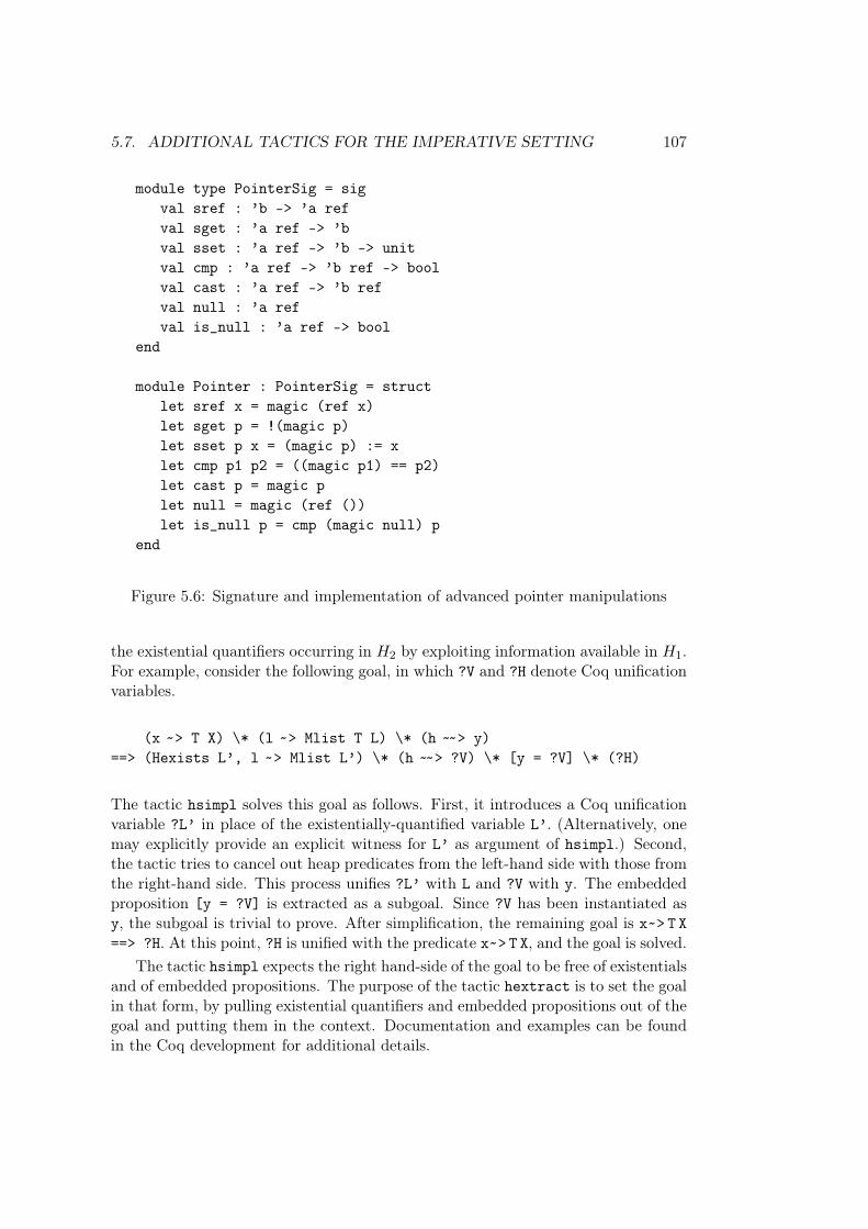
5.7. ADDITIONAL TACTICS FOR THE IMPERATIVE SETTING 107
module type PointerSig = sigval sref : ’b -> ’a refval sget : ’a ref -> ’bval sset : ’a ref -> ’b -> unitval cmp : ’a ref -> ’b ref -> boolval cast : ’a ref -> ’b refval null : ’a refval is_null : ’a ref -> bool
end
module Pointer : PointerSig = structlet sref x = magic (ref x)let sget p = !(magic p)let sset p x = (magic p) := xlet cmp p1 p2 = ((magic p1) == p2)let cast p = magic plet null = magic (ref ())let is_null p = cmp (magic null) p
end
Figure 5.6: Signature and implementation of advanced pointer manipulations
the existential quantifiers occurring in 𝐻2 by exploiting information available in 𝐻1.For example, consider the following goal, in which ?V and ?H denote Coq unificationvariables.
(x ˜> T X) \* (l ˜> Mlist T L) \* (h ˜̃ > y)==> (Hexists L’, l ˜> Mlist L’) \* (h ˜̃ > ?V) \* [y = ?V] \* (?H)
The tactic hsimpl solves this goal as follows. First, it introduces a Coq unificationvariable ?L’ in place of the existentially-quantified variable L’. (Alternatively, onemay explicitly provide an explicit witness for L’ as argument of hsimpl.) Second,the tactic tries to cancel out heap predicates from the left-hand side with those fromthe right-hand side. This process unifies ?L’ with L and ?V with y. The embeddedproposition [y = ?V] is extracted as a subgoal. Since ?V has been instantiated asy, the subgoal is trivial to prove. After simplification, the remaining goal is x˜> T X==> ?H. At this point, ?H is unified with the predicate x˜> T X, and the goal is solved.
The tactic hsimpl expects the right hand-side of the goal to be free of existentialsand of embedded propositions. The purpose of the tactic hextract is to set the goalin that form, by pulling existential quantifiers and embedded propositions out of thegoal and putting them in the context. Documentation and examples can be foundin the Coq development for additional details.
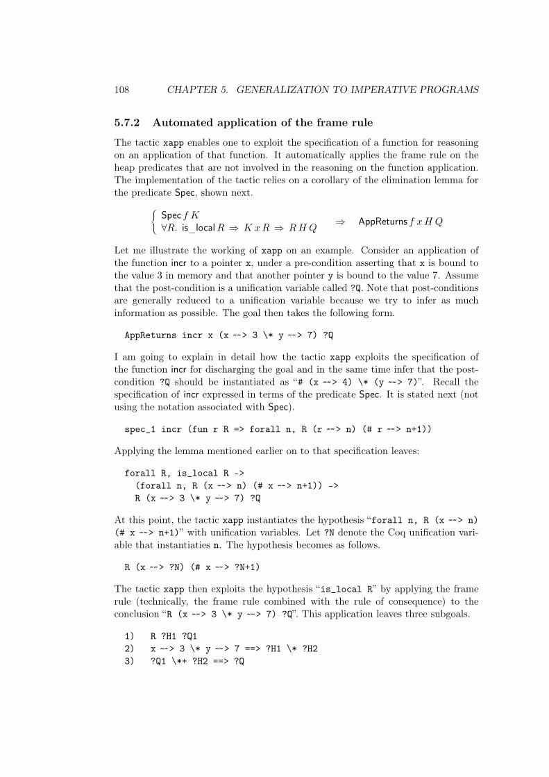
108 CHAPTER 5. GENERALIZATION TO IMPERATIVE PROGRAMS
5.7.2 Automated application of the frame rule
The tactic xapp enables one to exploit the specification of a function for reasoningon an application of that function. It automatically applies the frame rule on theheap predicates that are not involved in the reasoning on the function application.The implementation of the tactic relies on a corollary of the elimination lemma forthe predicate Spec, shown next.®
Spec 𝑓 𝐾∀𝑅. is_local𝑅 ⇒ 𝐾 𝑥𝑅 ⇒ 𝑅𝐻 𝑄
⇒ AppReturns 𝑓 𝑥𝐻 𝑄
Let me illustrate the working of xapp on an example. Consider an application ofthe function incr to a pointer x, under a pre-condition asserting that x is bound tothe value 3 in memory and that another pointer y is bound to the value 7. Assumethat the post-condition is a unification variable called ?Q. Note that post-conditionsare generally reduced to a unification variable because we try to infer as muchinformation as possible. The goal then takes the following form.
AppReturns incr x (x ˜̃ > 3 \* y ˜̃ > 7) ?Q
I am going to explain in detail how the tactic xapp exploits the specification ofthe function incr for discharging the goal and in the same time infer that the post-condition ?Q should be instantiated as “# (x ˜̃ > 4) \* (y ˜̃ > 7)”. Recall thespecification of incr expressed in terms of the predicate Spec. It is stated next (notusing the notation associated with Spec).
spec_1 incr (fun r R => forall n, R (r ˜̃ > n) (# r ˜̃ > n+1))
Applying the lemma mentioned earlier on to that specification leaves:
forall R, is_local R ->(forall n, R (x ˜̃ > n) (# x ˜̃ > n+1)) ->R (x ˜̃ > 3 \* y ˜̃ > 7) ?Q
At this point, the tactic xapp instantiates the hypothesis “forall n, R (x ˜̃ > n)(# x ˜̃ > n+1)” with unification variables. Let ?N denote the Coq unification vari-able that instantiaties n. The hypothesis becomes as follows.
R (x ˜̃ > ?N) (# x ˜̃ > ?N+1)
The tactic xapp then exploits the hypothesis “is_local R” by applying the framerule (technically, the frame rule combined with the rule of consequence) to theconclusion “R (x ˜̃ > 3 \* y ˜̃ > 7) ?Q”. This application leaves three subgoals.
1) R ?H1 ?Q12) x ˜̃ > 3 \* y ˜̃ > 7 ==> ?H1 \* ?H23) ?Q1 \*+ ?H2 ==> ?Q
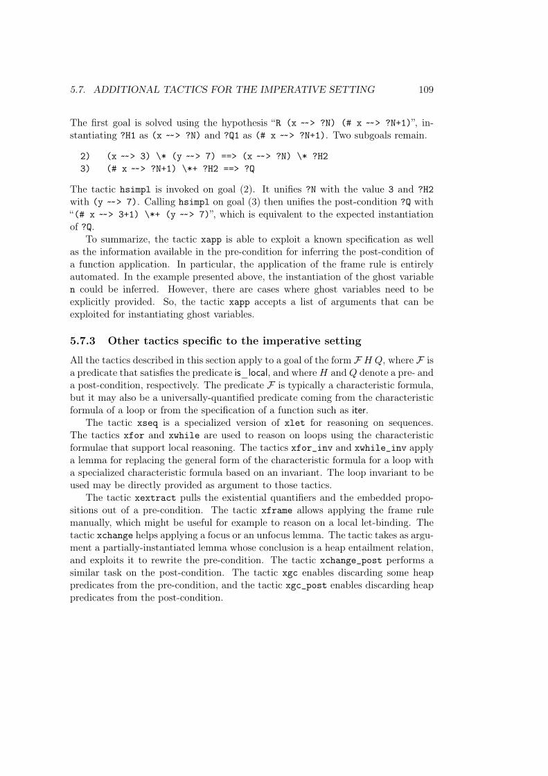
5.7. ADDITIONAL TACTICS FOR THE IMPERATIVE SETTING 109
The first goal is solved using the hypothesis “R (x ˜̃ > ?N) (# x ˜̃ > ?N+1)”, in-stantiating ?H1 as (x ˜̃ > ?N) and ?Q1 as (# x ˜̃ > ?N+1). Two subgoals remain.
2) (x ˜̃ > 3) \* (y ˜̃ > 7) ==> (x ˜̃ > ?N) \* ?H23) (# x ˜̃ > ?N+1) \*+ ?H2 ==> ?Q
The tactic hsimpl is invoked on goal (2). It unifies ?N with the value 3 and ?H2with (y ˜̃ > 7). Calling hsimpl on goal (3) then unifies the post-condition ?Q with“(# x ˜̃ > 3+1) \*+ (y ˜̃ > 7)”, which is equivalent to the expected instantiationof ?Q.
To summarize, the tactic xapp is able to exploit a known specification as wellas the information available in the pre-condition for inferring the post-condition ofa function application. In particular, the application of the frame rule is entirelyautomated. In the example presented above, the instantiation of the ghost variablen could be inferred. However, there are cases where ghost variables need to beexplicitly provided. So, the tactic xapp accepts a list of arguments that can beexploited for instantiating ghost variables.
5.7.3 Other tactics specific to the imperative setting
All the tactics described in this section apply to a goal of the form ℱ 𝐻 𝑄, where ℱ isa predicate that satisfies the predicate is_local, and where 𝐻 and 𝑄 denote a pre- anda post-condition, respectively. The predicate ℱ is typically a characteristic formula,but it may also be a universally-quantified predicate coming from the characteristicformula of a loop or from the specification of a function such as iter.
The tactic xseq is a specialized version of xlet for reasoning on sequences.The tactics xfor and xwhile are used to reason on loops using the characteristicformulae that support local reasoning. The tactics xfor_inv and xwhile_inv applya lemma for replacing the general form of the characteristic formula for a loop witha specialized characteristic formula based on an invariant. The loop invariant to beused may be directly provided as argument to those tactics.
The tactic xextract pulls the existential quantifiers and the embedded propo-sitions out of a pre-condition. The tactic xframe allows applying the frame rulemanually, which might be useful for example to reason on a local let-binding. Thetactic xchange helps applying a focus or an unfocus lemma. The tactic takes as argu-ment a partially-instantiated lemma whose conclusion is a heap entailment relation,and exploits it to rewrite the pre-condition. The tactic xchange_post performs asimilar task on the post-condition. The tactic xgc enables discarding some heappredicates from the pre-condition, and the tactic xgc_post enables discarding heappredicates from the post-condition.
Chapter 6
Soundness and completeness
In this chapter, I prove that characteristic formulae for pure programsare sound and complete. The soundness theorem states that if one canprove that the characteristic formula of a term 𝑡 holds of a post-condition𝑃 then the term 𝑡 terminates and returns a value that satisfies 𝑃 . Char-acteristic formulae are built from the source code in a compositional wayand that they can even be displayed in a way that closely resemble sourcecode, thus, intuitively, proving the soundness of a characteristic formulawith respect to the source code it describes should be relatively direct.The syntactic soundness proof that I give is indeed quite simple.
The completeness theorem states that if a term 𝑡 evaluates to a value𝑣 then the characteristic formula for 𝑡 holds of the most-general spec-ification for 𝑣. If the value 𝑣 does not contain any first-class function,then its most-general specification is simply the predicate “being equalto 𝑣”. The case where 𝑣 contains functions is slightly more subtle, sincecharacteristic formulae only allow specifying the extensional behavior offunctions and do not enable stating properties about the source code ofa function closure. In this chapter, I explain how to take that restrictioninto account in the statement of the completeness theorem.
The last part of this chapter is concerned with justifying the soundnessof the treatment of polymorphism. In characteristic formulae, I quantifytype variables over the sort Type, which corresponds to the set of all Coqtypes, instead of restricting the quantification to the set of Coq typesthat correspond to some weak-ML type. It is more convenient in practiceto quantify over Type because it is the default sort in Coq. I explain inthis chapter why the quantification over Type is correct.
110
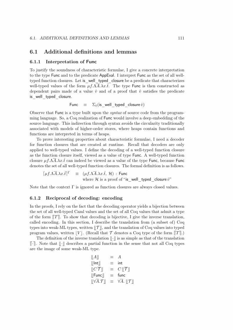
6.1. ADDITIONAL DEFINITIONS AND LEMMAS 111
6.1 Additional definitions and lemmas
6.1.1 Interpretation of Func
To justify the soundness of characteristic formulae, I give a concrete interpretationto the type Func and to the predicate AppEval. I interpret Func as the set of all well-typed function closures. Let is_well_typed_closure be a predicate that characterizeswell-typed values of the form 𝜇𝑓.Λ𝐴.𝜆𝑥.𝑡. The type Func is then constructed asdependent pairs made of a value 𝑣 and of a proof that 𝑣 satisfies the predicateis_well_typed_closure.
Func ≡ Σ𝑣(is_well_typed_closure 𝑣)
Observe that Func is a type built upon the syntax of source code from the program-ming language. So, a Coq realization of Func would involve a deep embedding of thesource language. This indirection through syntax avoids the circularity traditionallyassociated with models of higher-order stores, where heaps contain functions andfunctions are interpreted in terms of heaps.
To prove interesting properties about characteristic formulae, I need a decoderfor function closures that are created at runtime. Recall that decoders are onlyapplied to well-typed values. I define the decoding of a well-typed function closureas the function closure itself, viewed as a value of type Func. A well-typed functionclosure 𝜇𝑓.Λ𝐴.𝜆𝑥.𝑡 can indeed be viewed as a value of the type Func, because Funcdenotes the set of all well-typed function closures. The formal definition is as follows.
⌈𝜇𝑓.Λ𝐴.𝜆𝑥.𝑡⌉Γ ≡ (𝜇𝑓.Λ𝐴.𝜆𝑥.𝑡, ℋ) : Funcwhere ℋ is a proof of “ is_well_typed_closure 𝑣”
Note that the context Γ is ignored as function closures are always closed values.
6.1.2 Reciprocal of decoding: encoding
In the proofs, I rely on the fact that the decoding operator yields a bijection betweenthe set of all well-typed Caml values and the set of all Coq values that admit a typeof the form V𝑇W. To show that decoding is bijective, I give the inverse translation,called encoding. In this section, I describe the translation from (a subset of) Coqtypes into weak-ML types, written T𝒯 U, and the translation of Coq values into typedprogram values, written ⌊𝑉 ⌋. (Recall that 𝒯 denotes a Coq type of the form V𝑇W.)
The definition of the inverse translation T·U is as simple as that of the translationV·W. Note that T·U describes a partial function in the sense that not all Coq typesare the image of some weak-ML type.
T𝐴U ≡ 𝐴
TIntU ≡ intT𝐶 𝒯 U ≡ 𝐶 T𝒯 UTFuncU ≡ funcT∀𝐴.𝒯 U ≡ ∀𝐴. T𝒯 U
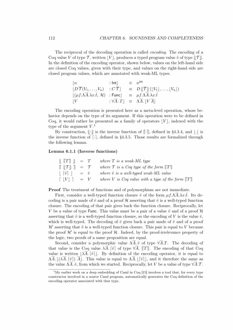
112 CHAPTER 6. SOUNDNESS AND COMPLETENESS
The reciprocal of the decoding operation is called encoding. The encoding of aCoq value 𝑉 of type 𝒯 , written ⌊𝑉 ⌋, produces a typed program value 𝑣 of type T𝒯 U.In the definition of the encoding operator, shown below, values on the left-hand sideare closed Coq values, given with their type, and values on the right-hand side areclosed program values, which are annotated with weak-ML types.
⌊𝑛 : Int⌋ ≡ 𝑛int
⌊𝐷 𝒯 (𝑉1, . . . , 𝑉𝑛) : 𝐶 𝒯 ⌋ ≡ 𝐷 T𝒯 U (⌊𝑉1⌋, . . . , ⌊𝑉𝑛⌋)⌊(𝜇𝑓.Λ𝐴.𝜆𝑥.𝑡, ℋ) : Func⌋ ≡ 𝜇𝑓.Λ𝐴.𝜆𝑥.𝑡
⌊𝑉 : ∀𝐴. 𝑇 ⌋ ≡ Λ𝐴. ⌊𝑉 𝐴⌋
The encoding operation is presented here as a meta-level operation, whose be-havior depends on the type of its argument. If this operation were to be defined inCoq, it would rather be presented as a family of operators ⌊𝑉 ⌋, indexed with thetype of the argument 𝑉 .1
By construction, T·U is the inverse function of V·W, defined in §4.3.4, and ⌊·⌋ isthe inverse function of ⌈·⌉, defined in §4.3.5. Those results are formalized throughthe following lemma.
Lemma 6.1.1 (Inverse functions)
T V𝑇W U = 𝑇 where 𝑇 is a weak-ML typeV T𝒯 U W = 𝒯 where 𝒯 is a Coq type of the form V𝑇W⌊ ⌈𝑣⌉ ⌋ = 𝑣 where 𝑣 is a well-typed weak-ML value⌈ ⌊𝑉 ⌋ ⌉ = 𝑉 where 𝑉 is Coq value with a type of the form V𝑇W
Proof The treatment of functions and of polymorphism are not immediate.First, consider a well-typed function closure 𝑣 of the form 𝜇𝑓.Λ𝐴.𝜆𝑥.𝑡. Its de-
coding is a pair made of 𝑣 and of a proof ℋ asserting that 𝑣 is a well-typed functionclosure. The encoding of that pair gives back the function closure. Reciprocally, let𝑉 be a value of type Func. This value must be a pair of a value 𝑣 and of a proof ℋasserting that 𝑣 is a well-typed function closure, so the encoding of 𝑉 is the value 𝑣,which is well-typed. The decoding of 𝑣 gives back a pair made of 𝑣 and of a proofℋ′ asserting that 𝑣 is a well-typed function closure. This pair is equal to 𝑉 becausethe proof ℋ′ is equal to the proof ℋ. Indeed, by the proof-irrelevance property ofthe logic, two proofs of a same proposition are equal.
Second, consider a polymorphic value Λ𝐴. 𝑣 of type ∀𝐴.𝑇 . The decoding ofthat value is the Coq value 𝜆𝐴. ⌈𝑣⌉ of type ∀𝐴. V𝑇W. The encoding of that Coqvalue is written ⌊𝜆𝐴. ⌈𝑣⌉⌋. By definition of the encoding operator, it is equal toΛ𝐴. ⌊(𝜆𝐴. ⌈𝑣⌉) 𝐴⌋. This value is equal to Λ𝐴. ⌊⌈𝑣⌉⌋, and it therefore the same asthe value Λ𝐴. 𝑣, from which we started. Reciprocally, let 𝑉 be a value of type ∀𝐴.𝒯 .
1My earlier work on a deep embedding of Caml in Coq [15] involves a tool that, for every typeconstructor involved in a source Caml program, automatically generates the Coq definition of theencoding operator associated with that type.
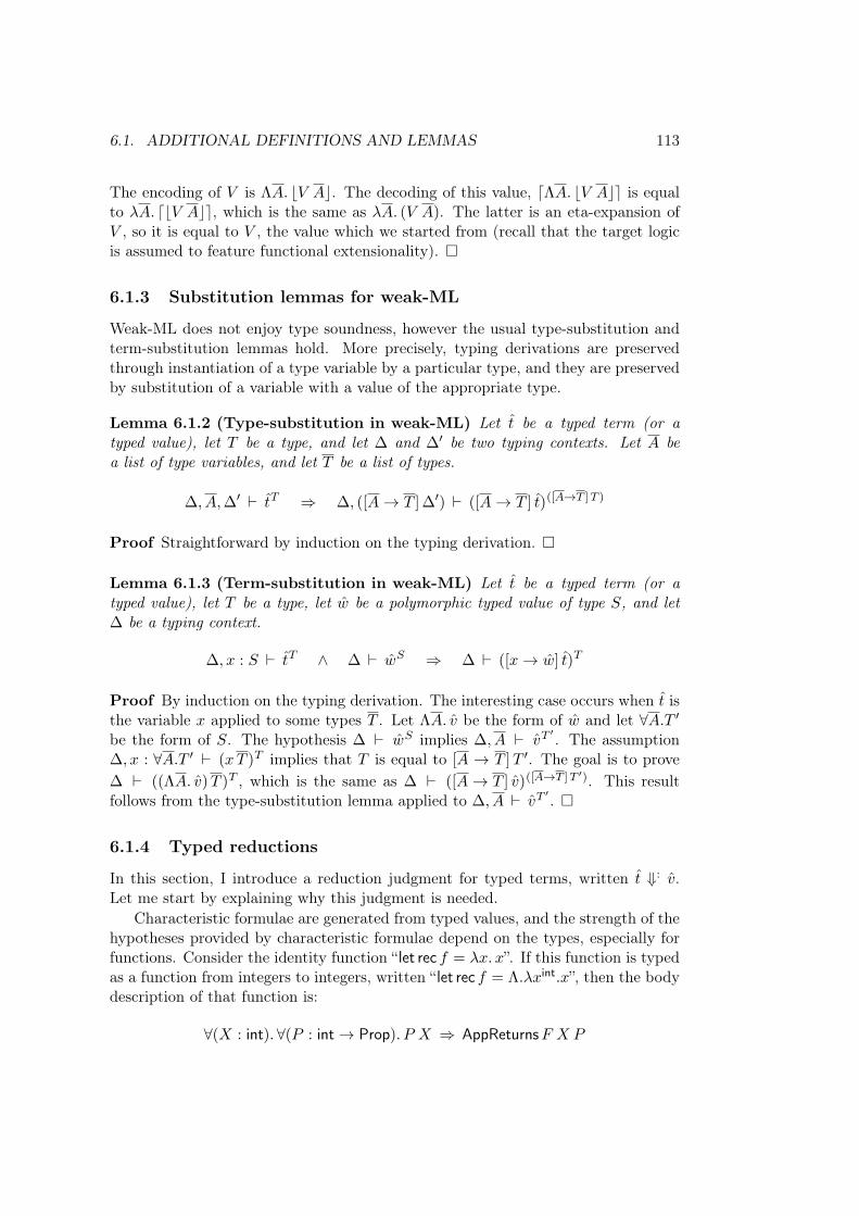
6.1. ADDITIONAL DEFINITIONS AND LEMMAS 113
The encoding of 𝑉 is Λ𝐴. ⌊𝑉 𝐴⌋. The decoding of this value, ⌈Λ𝐴. ⌊𝑉 𝐴⌋⌉ is equalto 𝜆𝐴. ⌈⌊𝑉 𝐴⌋⌉, which is the same as 𝜆𝐴. (𝑉 𝐴). The latter is an eta-expansion of𝑉 , so it is equal to 𝑉 , the value which we started from (recall that the target logicis assumed to feature functional extensionality). �
6.1.3 Substitution lemmas for weak-ML
Weak-ML does not enjoy type soundness, however the usual type-substitution andterm-substitution lemmas hold. More precisely, typing derivations are preservedthrough instantiation of a type variable by a particular type, and they are preservedby substitution of a variable with a value of the appropriate type.
Lemma 6.1.2 (Type-substitution in weak-ML) Let 𝑡 be a typed term (or atyped value), let 𝑇 be a type, and let ∆ and ∆′ be two typing contexts. Let 𝐴 bea list of type variables, and let 𝑇 be a list of types.
∆, 𝐴,∆′ ⊢ 𝑡𝑇 ⇒ ∆, ([𝐴 → 𝑇 ] ∆′) ⊢ ([𝐴 → 𝑇 ] 𝑡)([𝐴→𝑇 ]𝑇 )
Proof Straightforward by induction on the typing derivation. �
Lemma 6.1.3 (Term-substitution in weak-ML) Let 𝑡 be a typed term (or atyped value), let 𝑇 be a type, let �̂� be a polymorphic typed value of type 𝑆, and let∆ be a typing context.
∆, 𝑥 : 𝑆 ⊢ 𝑡𝑇 ∧ ∆ ⊢ �̂�𝑆 ⇒ ∆ ⊢ ([𝑥 → �̂�] 𝑡)𝑇
Proof By induction on the typing derivation. The interesting case occurs when 𝑡 isthe variable 𝑥 applied to some types 𝑇 . Let Λ𝐴. 𝑣 be the form of �̂� and let ∀𝐴.𝑇 ′
be the form of 𝑆. The hypothesis ∆ ⊢ �̂�𝑆 implies ∆, 𝐴 ⊢ 𝑣𝑇′ . The assumption
∆, 𝑥 : ∀𝐴.𝑇 ′ ⊢ (𝑥𝑇 )𝑇 implies that 𝑇 is equal to [𝐴 → 𝑇 ]𝑇 ′. The goal is to prove∆ ⊢ ((Λ𝐴. 𝑣)𝑇 )𝑇 , which is the same as ∆ ⊢ ([𝐴 → 𝑇 ] 𝑣)([𝐴→𝑇 ]𝑇 ′). This resultfollows from the type-substitution lemma applied to ∆, 𝐴 ⊢ 𝑣𝑇
′ . �
6.1.4 Typed reductions
In this section, I introduce a reduction judgment for typed terms, written 𝑡 ⇓: 𝑣.Let me start by explaining why this judgment is needed.
Characteristic formulae are generated from typed values, and the strength of thehypotheses provided by characteristic formulae depend on the types, especially forfunctions. Consider the identity function “ let rec 𝑓 = 𝜆𝑥. 𝑥”. If this function is typedas a function from integers to integers, written “ let rec 𝑓 = Λ.𝜆𝑥int.𝑥”, then the bodydescription of that function is:
∀(𝑋 : int).∀(𝑃 : int → Prop). 𝑃 𝑋 ⇒ AppReturns𝐹 𝑋 𝑃
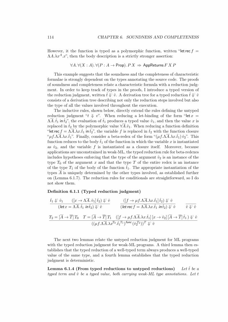
114 CHAPTER 6. SOUNDNESS AND COMPLETENESS
However, it the function is typed as a polymorphic function, written “ let rec 𝑓 =Λ𝐴.𝜆𝑥𝐴.𝑥”, then the body description is a strictly stronger assertion:
∀𝐴. ∀(𝑋 : 𝐴).∀(𝑃 : 𝐴 → Prop). 𝑃 𝑋 ⇒ AppReturns𝐹 𝑋 𝑃
This example suggests that the soundness and the completeness of characteristicformulae is strongly dependent on the types annotating the source code. The proofsof soundness and completeness relate a characteristic formula with a reduction judg-ment. In order to keep track of types in the proofs, I introduce a typed version ofthe reduction judgment, written 𝑡 ⇓: 𝑣. A derivation tree for a typed reduction 𝑡 ⇓: 𝑣consists of a derivation tree describing not only the reduction steps involved but alsothe type of all the values involved throughout the execution.
The inductive rules, shown below, directly extend the rules defining the untypedreduction judgment “𝑡 ⇓ 𝑣”. When reducing a let-binding of the form “ let𝑥 =Λ𝐴. 𝑡1 in 𝑡2”, the evaluation of 𝑡1 produces a typed value 𝑣1, and then the value 𝑥 isreplaced in 𝑡2 by the polymorphic value ∀𝐴.𝑣1. When reducing a function definition“ let rec 𝑓 = Λ𝐴.𝜆𝑥.𝑡1 in 𝑡2”, the variable 𝑓 is replaced in 𝑡2 with the function closure“𝜇𝑓.Λ𝐴.𝜆𝑥.𝑡1”. Finally, consider a beta-redex of the form “(𝜇𝑓.Λ𝐴.𝜆𝑥.𝑡1) 𝑣2”. Thisfunction reduces to the body 𝑡1 of the function in which the variable 𝑥 is instantiatedas 𝑣2, and the variable 𝑓 is instantiated as a closure itself. Moreover, becauseapplications are unconstrained in weak-ML, the typed reduction rule for beta-redexesincludes hypotheses enforcing that the type of the argument 𝑣2 is an instance of thetype 𝑇0 of the argument 𝑥 and that the type 𝑇 of the entire redex is an instanceof the type 𝑇1 of the body of the function 𝑡1. The appropriate instantiation of thetypes 𝐴 is uniquely determined by the other types involved, as established furtheron (Lemma 6.1.7). The reduction rules for conditionals are straightforward, so I donot show them.
Definition 6.1.1 (Typed reduction judgment)
𝑡1 ⇓: 𝑣1 ([𝑥 → Λ𝐴. 𝑣1] 𝑡2) ⇓: 𝑣
(let𝑥 = Λ𝐴. 𝑡1 in 𝑡2) ⇓: 𝑣
([𝑓 → 𝜇𝑓.Λ𝐴.𝜆𝑥.𝑡1] 𝑡2) ⇓: 𝑣
(let rec 𝑓 = Λ𝐴.𝜆𝑥.𝑡1 in 𝑡2) ⇓: 𝑣 𝑣 ⇓: 𝑣
𝑇2 = [𝐴 → 𝑇 ]𝑇0 𝑇 = [𝐴 → 𝑇 ]𝑇1 ([𝑓 → 𝜇𝑓.Λ𝐴.𝜆𝑥.𝑡1] [𝑥 → 𝑣2] [𝐴 → 𝑇 ] 𝑡1 ) ⇓: 𝑣
((𝜇𝑓.Λ𝐴.𝜆𝑥𝑇0 .𝑡1𝑇1)func (𝑣2
𝑇2))𝑇 ⇓: 𝑣
The next two lemmas relate the untyped reduction judgment for ML programswith the typed reduction judgment for weak-ML programs. A third lemma then es-tablishes that the typed reduction of a well-typed term always produces a well-typedvalue of the same type, and a fourth lemma establishes that the typed reductionjudgment is deterministic.
Lemma 6.1.4 (From typed reductions to untyped reductions) Let 𝑡 be atyped term and 𝑣 be a typed value, both carrying weak-ML type annotations. Let 𝑡
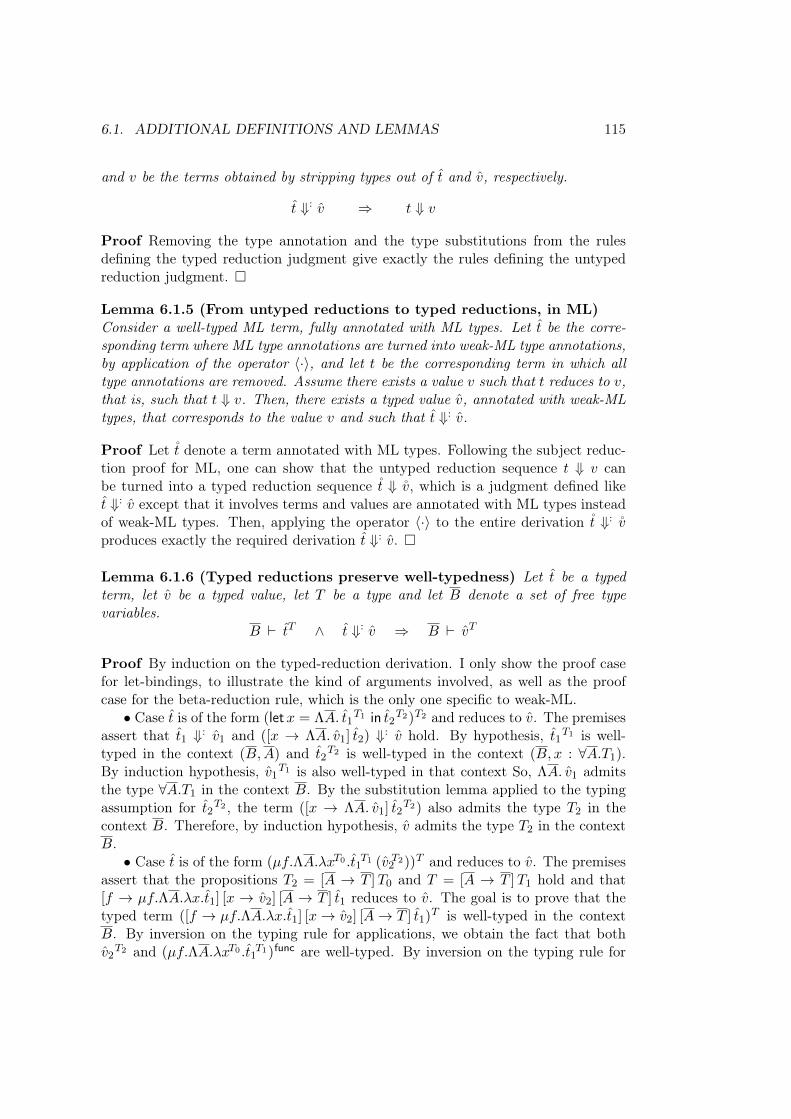
6.1. ADDITIONAL DEFINITIONS AND LEMMAS 115
and 𝑣 be the terms obtained by stripping types out of 𝑡 and 𝑣, respectively.
𝑡 ⇓: 𝑣 ⇒ 𝑡 ⇓ 𝑣
Proof Removing the type annotation and the type substitutions from the rulesdefining the typed reduction judgment give exactly the rules defining the untypedreduction judgment. �
Lemma 6.1.5 (From untyped reductions to typed reductions, in ML)Consider a well-typed ML term, fully annotated with ML types. Let 𝑡 be the corre-sponding term where ML type annotations are turned into weak-ML type annotations,by application of the operator ⟨·⟩, and let 𝑡 be the corresponding term in which alltype annotations are removed. Assume there exists a value 𝑣 such that 𝑡 reduces to 𝑣,that is, such that 𝑡 ⇓ 𝑣. Then, there exists a typed value 𝑣, annotated with weak-MLtypes, that corresponds to the value 𝑣 and such that 𝑡 ⇓: 𝑣.
Proof Let �̊� denote a term annotated with ML types. Following the subject reduc-tion proof for ML, one can show that the untyped reduction sequence 𝑡 ⇓ 𝑣 canbe turned into a typed reduction sequence �̊� ⇓ �̊�, which is a judgment defined like𝑡 ⇓: 𝑣 except that it involves terms and values are annotated with ML types insteadof weak-ML types. Then, applying the operator ⟨·⟩ to the entire derivation �̊� ⇓: �̊�produces exactly the required derivation 𝑡 ⇓: 𝑣. �
Lemma 6.1.6 (Typed reductions preserve well-typedness) Let 𝑡 be a typedterm, let 𝑣 be a typed value, let 𝑇 be a type and let 𝐵 denote a set of free typevariables.
𝐵 ⊢ 𝑡𝑇 ∧ 𝑡 ⇓: 𝑣 ⇒ 𝐵 ⊢ 𝑣𝑇
Proof By induction on the typed-reduction derivation. I only show the proof casefor let-bindings, to illustrate the kind of arguments involved, as well as the proofcase for the beta-reduction rule, which is the only one specific to weak-ML.
∙ Case 𝑡 is of the form (let𝑥 = Λ𝐴. 𝑡1𝑇1 in 𝑡2𝑇2)𝑇2 and reduces to 𝑣. The premises
assert that 𝑡1 ⇓: 𝑣1 and ([𝑥 → Λ𝐴. 𝑣1] 𝑡2) ⇓: 𝑣 hold. By hypothesis, 𝑡1𝑇1 is well-
typed in the context (𝐵,𝐴) and 𝑡2𝑇2 is well-typed in the context (𝐵, 𝑥 : ∀𝐴.𝑇1).
By induction hypothesis, 𝑣1𝑇1 is also well-typed in that context So, Λ𝐴. 𝑣1 admitsthe type ∀𝐴.𝑇1 in the context 𝐵. By the substitution lemma applied to the typingassumption for 𝑡2
𝑇2 , the term ([𝑥 → Λ𝐴. 𝑣1] 𝑡2𝑇2) also admits the type 𝑇2 in the
context 𝐵. Therefore, by induction hypothesis, 𝑣 admits the type 𝑇2 in the context𝐵.
∙ Case 𝑡 is of the form (𝜇𝑓.Λ𝐴.𝜆𝑥𝑇0 .𝑡1𝑇1 (𝑣2
𝑇2))𝑇 and reduces to 𝑣. The premisesassert that the propositions 𝑇2 = [𝐴 → 𝑇 ]𝑇0 and 𝑇 = [𝐴 → 𝑇 ]𝑇1 hold and that[𝑓 → 𝜇𝑓.Λ𝐴.𝜆𝑥.𝑡1] [𝑥 → 𝑣2] [𝐴 → 𝑇 ] 𝑡1 reduces to 𝑣. The goal is to prove that thetyped term ([𝑓 → 𝜇𝑓.Λ𝐴.𝜆𝑥.𝑡1] [𝑥 → 𝑣2] [𝐴 → 𝑇 ] 𝑡1)
𝑇 is well-typed in the context𝐵. By inversion on the typing rule for applications, we obtain the fact that both𝑣2
𝑇2 and (𝜇𝑓.Λ𝐴.𝜆𝑥𝑇0 .𝑡1𝑇1)func are well-typed. By inversion on the typing rule for
116 CHAPTER 6. SOUNDNESS AND COMPLETENESS
function closures, we obtain the typing assumption “𝐵,𝐴, 𝑓 : func, 𝑥 : 𝑇0 ⊢ 𝑡1𝑇1”.
By the type substitution lemma, this implies “𝐵, 𝑓 : func, 𝑥 : ([𝐴 → 𝑇 ]𝑇0) ⊢([𝐴 → 𝑇 ] 𝑡1)
([𝐴→𝑇 ]𝑇1)”. Exploiting the two assumptions 𝑇2 = [𝐴 → 𝑇 ]𝑇0 and 𝑇 =[𝐴 → 𝑇 ]𝑇1, we can rewrite this proposition as “𝐵, 𝑓 : func, 𝑥 : 𝑇2 ⊢ ([𝐴 → 𝑇 ] 𝑡1)
𝑇 ”.The conclusion, which is “𝐵 ⊢ ([𝑓 → 𝜇𝑓.Λ𝐴.𝜆𝑥.𝑡1] [𝑥 → 𝑣2] [𝐴 → 𝑇 ] 𝑡1)
𝑇 ”, can thenbe deduced by applying the substitution lemma twice, once for 𝑥 and once for 𝑓 . �
Lemma 6.1.7 (Determinacy of typed reductions) Let 𝑡 be a typed term, andlet 𝑣1 and 𝑣2 be two typed values.
𝑡 ⇓: 𝑣1 ∧ 𝑡 ⇓: 𝑣2 ⇒ 𝑣1 = 𝑣2
Proof By induction on the first hypothesis and case analysis on the second one.The nontrivial case is that of applications, for which we need to establish that thelist of types 𝑇 is uniquely determined. Consider a list 𝑇 such that 𝑇2 = [𝐴 → 𝑇 ]𝑇0
and 𝑇 = [𝐴 → 𝑇 ]𝑇1, and another list 𝑇 ′ such that 𝑇2 = [𝐴 → 𝑇 ′]𝑇0 and 𝑇 = [𝐴 →𝑇 ′]𝑇1. Then, [𝐴 → 𝑇 ]𝑇0 = [𝐴 → 𝑇 ′]𝑇0 and [𝐴 → 𝑇 ]𝑇1 = [𝐴 → 𝑇 ′]𝑇1. Since thefree variables 𝐴 are included in the union of the set of free type variables of 𝑇0 andof that of 𝑇1, the list 𝑇 ′ must be equal to the list 𝑇 . �
6.1.5 Interpretation and properties of AppEval
Recall that AppEval is the low-level predicate in terms of which AppReturns is defined.In this section, I give an interpretation of AppEval in terms of the typed semanticsof the source language. The type of AppEval is recalled next.
AppEval : ∀𝐴𝐵. Func → 𝐴 → 𝐵 → Prop
The proposition AppEval𝐹 𝑉 𝑉 ′ asserts that the application of a Caml functionreflected as 𝐹 in the logic to a value reflected as 𝑉 in the logic terminates and returnsa Caml value reflected as 𝑉 ′ in the logic. This can be reformulated using encoders,saying that the application of the encoding of 𝐹 to the encoding of 𝑉 terminates andreturns the encoding of 𝑉 ′. Hence the following definition of the predicate AppEval.
Definition 6.1.2 (Definition of AppEval) Let 𝐹 be a value of type Func, 𝑉 is avalue of type 𝒯 and 𝑉 ′ is a value of type 𝒯 ′.
AppEval𝐹 𝑉 𝑉 ′ ≡ (⌊𝐹 ⌋ ⌊𝑉 ⌋) ⇓: ⌊𝑉 ′⌋
Remark: one can also present this definition as an inductive rule, as follows.
(𝑓 𝑣) ⇓: 𝑣′
AppEval ⌈𝑓⌉ ⌈𝑣⌉ ⌈𝑣′⌉
The semantics of the source language is assumed to be deterministic. SinceAppEval lifts the semantics of function application to the level of Coq values, forevery function 𝐹 and argument 𝑉 there is at most one result value 𝑉 ′ for whichthe relation AppEval𝐹 𝑉 𝑉 ′ holds. This property is formally captured through thefollowing lemma.
6.1. ADDITIONAL DEFINITIONS AND LEMMAS 117
Lemma 6.1.8 (Determinacy of AppEval) For any types 𝒯 and 𝒯 ′, for any Coqvalue 𝐹 of type Func, any Coq value 𝑉 of type 𝒯 , and any two Coq values 𝑉 ′
1 and𝑉 ′2 of type 𝒯 ′,
AppEval𝐹 𝑉 𝑉 ′1 ∧ AppEval𝐹 𝑉 𝑉 ′
2 ⇒ 𝑉 ′1 = 𝑉 ′
2
Proof By definition of AppEval, the hypotheses are equivalent to (⌊𝐹 ⌋ ⌊𝑉 ⌋) ⇓: ⌊𝑉 ′1⌋
and (⌊𝐹 ⌋ ⌊𝑉 ⌋) ⇓: ⌊𝑉 ′2⌋. By determinacy of typed reductions (Lemma 6.1.7), ⌊𝑉 ′
1⌋ isequal to ⌊𝑉 ′
2⌋. The equality between 𝑉 ′1 and 𝑉 ′
2 then follows from the injectivity ofencoders. �
Remark: ideally, the soundness theorem for characteristic formulae should beproved without exploiting the determinacy assumption on the source language. How-ever, the proof appears to become slightly more complicated when this assumptionis not available. For this reason, I leave the generalization of the soundness proof toa non-deterministic language for future work.
6.1.6 Substitution lemmas for characteristic formulae
The substitution lemma for characteristic formulae is used both in the proof ofsoundness and in the proof of completeness. It explains how a substitution of avalue for a variable in a term commutes with the computation of the characteristicformula for that term. The proof of the substitution lemma involves a correspondingsubstitution lemma for the decoding operator. It also relies on two type-substitutionlemmas, one for characteristic formulae and one for the decoding operator, presentednext.
Lemma 6.1.9 (Type-substitution lemmas) Let 𝑣 be a well-typed value and 𝑡be a well-typed term in a context (∆, 𝐴). Let Γ be a decoding context with typescorresponding to those in ∆. Let 𝑇 be a list of weak-ML types of the same arity as𝐴.
⌈[𝐴 → 𝑇 ] 𝑣⌉Γ = [𝐴 → V𝑇W ] ⌈𝑣⌉Γ
J [𝐴 → 𝑇 ] 𝑡 KΓ = [𝐴 → V𝑇W ] J 𝑡 KΓ
Proof By induction on the structure of 𝑣 and 𝑡. �
A useful corollary to the type-substitution lemma for decoders describes the applica-tion of the decoding of a polymorphic value. Recall that �̂� ranges over polymorphicvalues. I use the notation �̂� 𝑇 to denote the type application of �̂� to the types 𝑇 :if �̂� is of the form Λ𝐴. 𝑣, then �̂� 𝑇 is equal to [𝐴 → 𝑇 ] 𝑣. Using this notation, thecommutation of decoding with type applications of polymorphic values is formalizedas follows.
Lemma 6.1.10 (Application of the decoding of polymorphic value)Let �̂� be a closed polymorphic value of type ∀𝐴.𝑇 , and let 𝑇 be a list of types of thesame arity as 𝐴.
⌈�̂� 𝑇 ⌉ = ⌈�̂�⌉ V𝑇W
118 CHAPTER 6. SOUNDNESS AND COMPLETENESS
Proof Let Λ𝐴. 𝑣 be the form of �̂�. The left-hand side is equal to ⌈[𝐴 → 𝑇 ] 𝑣⌉. Theright-hand side is equal to “(𝜆𝐴. ⌈𝑣⌉) V𝑇W”, which is the same as [𝐴 → V𝑇W] ⌈𝑣⌉.The conclusion then follows from the type-substitution lemma (Lemma 6.1.9). �
Lemma 6.1.11 (Substitution lemma for decoding) Let 𝑣 be a value of type 𝑇with a free variable 𝑥 of type 𝑆, let �̂� be a closed value of type 𝑆, and let Γ be adecoding context. Then,
⌈ [𝑥 → �̂�] 𝑣 ⌉Γ = ⌈ 𝑣 ⌉(Γ,𝑥 ↦→⌈�̂�⌉)
Proof By induction on the structure of 𝑣. The interesting case is when 𝑣 is anoccurrence of the variable 𝑥. An occurrence of 𝑥 in 𝑣 take the form of a typeapplication 𝑥𝑇 . On the left-hand side, the substitution of 𝑥 by �̂� gives �̂� 𝑇 . Thisvalue is then decoded as ⌈�̂� 𝑇 ⌉. On the right-hand side, 𝑥𝑇 is directly decoded as⌈�̂�⌉ V𝑇W, since 𝑥 is mapped to ⌈�̂�⌉ is the decoding context (Γ, 𝑥 ↦→ ⌈�̂�⌉). Using theprevious lemma, we can conclude that both sides yield equal values. �.
Lemma 6.1.12 (Substitution lemma for characteristic formulae) Let 𝑡 be awell-typed term with a free variable 𝑥 of type 𝑆, and let �̂� be a closed typed value oftype 𝑆. Then,
J [𝑥 → �̂�] 𝑡 KΓ = J 𝑡 K(Γ,𝑥 ↦→⌈�̂�⌉)
Proof By induction on the structure of 𝑡, invoking the previous lemma when reach-ing values. �
6.1.7 Weakening lemma
The following weakening lemma is involved in the proof of completeness.
Lemma 6.1.13 (Weakening for characteristic formulae)For any well-typed term 𝑡, for any post-conditions 𝑃 and 𝑃 ′, and for any context Γ,
(∀𝑋. 𝑃 𝑋 ⇒ 𝑃 ′𝑋) ∧ J 𝑡 KΓ 𝑃 ⇒ J 𝑡 KΓ 𝑃 ′
Proof By induction on 𝑡. The only nontrivial case is that for applications, where,given a function 𝐹 and an argument 𝑉 , we must show that AppReturns𝐹𝑉 𝑃 impliesAppReturns𝐹𝑉 𝑃 ′. By definition of AppReturns, the assumption ensures the existenceof a value 𝑉 ′ such that AppEval𝐹 𝑉 𝑉 ′ and 𝑃 𝑉 ′. Therefore, the same value 𝑉 ′ issuch that AppEval𝐹 𝑉 𝑉 ′ and 𝑃 ′ 𝑉 ′. Thus the proposition AppReturns𝐹𝑉 𝑃 ′ holds.�
6.1.8 Elimination of n-ary functions
For the sake of verifying programs in practice, I have introduced a direct treatment ofn-ary functions, with the predicate Spec. However, for the sake of conducting proofs,it is much simpler to consider only unary functions, with characteristic formulae
6.1. ADDITIONAL DEFINITIONS AND LEMMAS 119
expressed directly in terms of AppReturns. In this section, I formally justify that theequivalence between the two presentations.
For functions of arity one, I show the equivalence between the body descriptionof a function “ let rec 𝑓 = 𝜆𝑥. 𝑡” stated in terms of Spec1 and the body descriptionof that same function stated in terms of AppReturns1. In the corresponding lemma,shown below, (𝐺𝑥) denotes the characteristic formula of the body 𝑡 of the function“ let rec 𝑓 = 𝜆𝑥. 𝑡” (the characteristic formula of 𝑡 indeed depends on the variable 𝑥).
Lemma 6.1.14 (Spec1-to-AppReturns1)
(∀𝐾. is_spec1𝐾 ∧ (∀𝑥. 𝐾 𝑥 (𝐺𝑥)) ⇒ Spec1𝑓𝐾)⇐⇒ (∀𝑥𝑃. (𝐺𝑥)𝑃 ⇒ AppReturns1 𝑓 𝑥𝑃 )
Proof The proof is not entirely straightforward, so I have also carried it out inCoq. To prove the proposition “AppReturns1 𝑓 𝑣 𝑃 ” under the assumption “(𝐺𝑣)𝑃 ”,we instantiate 𝐾 as “𝜆𝑥𝑅. 𝑥 = 𝑣 ⇒ 𝑅𝑃 ” and we are left proving is_spec1𝐾,which holds because 𝐾 is covariant in 𝑅, as well as “∀𝑥. 𝐾 𝑥 (𝐺𝑥)”, which isequivalent to “𝑥 = 𝑣 ⇒ (𝐺𝑥)𝑃 ”. The latter directly follows from the assump-tion “(𝐺𝑣)𝑃 ”. Reciprocally, we need to prove “Spec1𝑓𝐾” under the assumptions“ is_spec1𝐾” and “∀𝑥. 𝐾 𝑥 (𝐺𝑥)” and “∀𝑥𝑃. (𝐺𝑥)𝑃 ⇒ AppReturns1 𝑓 𝑥𝑃 ”. Bydefinition of Spec1, and given that is_spec1𝐾 is true by assumption, it suffices toprove “∀𝑥. 𝐾 𝑥 (AppReturns1 𝑓 𝑥)”. The hypothesis “ is_spec1𝐾” asserts that 𝐾 iscovariant in its second argument. So, exploiting the assumption “∀𝑥. 𝐾 𝑥 (𝐺𝑥)”, itremains to prove “∀𝑥𝑃. (𝐺𝑥)𝑃 ⇒ AppReturns1 𝑓 𝑥𝑃 ”, which corresponds exactlyto one of the assumptions. �
For a function of arity two, I show the equivalence between the body descriptionof a function “ let rec 𝑓 = 𝜆𝑥 𝑦. 𝑡” and the body description of the function “ let rec 𝑓 =𝜆𝑥. (let rec 𝑔 = 𝜆𝑦. 𝑡 in 𝑦)”. This encoding of n-ary functions as unary function can beeasily extended to higher arities. In the corresponding lemma, shown below, (𝐺𝑥𝑦)denotes the characteristic formula of the body 𝑡.
Lemma 6.1.15 (Spec2-to-AppReturns1)
(∀𝐾. is_spec2𝐾 ∧ (∀𝑥 𝑦. 𝐾 𝑥 𝑦 (𝐺𝑥𝑦)) ⇒ Spec2𝑓𝐾)⇐⇒ (∀𝑥𝑃. (∀𝑔. ℋ ⇒ 𝑃 𝑔) ⇒ AppReturns1 𝑓 𝑥𝑃 )
where ℋ ≡ (∀𝑦 𝑃 ′. (𝐺𝑥𝑦)𝑃 ′ ⇒ AppReturns1 𝑔 𝑦 𝑃 ′)
The proof of this lemma is even more technical than the previous one because itinvolves exploiting the determinacy of partial applications. So, I do not show thedetails and refer the reader to the Coq proof for further details. Note that thetreatment of arities higher than two does not involve further difficulties. It simplyinvolves additional proof steps for reasoning on iterated partial applications.
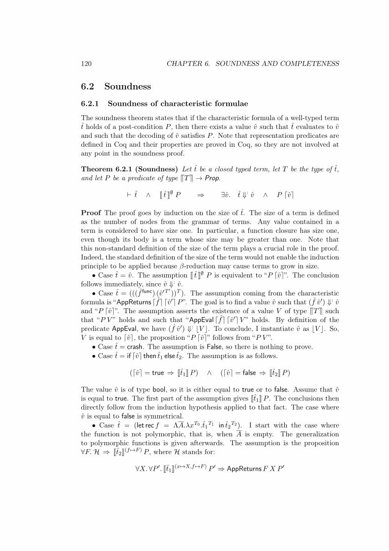
120 CHAPTER 6. SOUNDNESS AND COMPLETENESS
6.2 Soundness
6.2.1 Soundness of characteristic formulae
The soundness theorem states that if the characteristic formula of a well-typed term𝑡 holds of a post-condition 𝑃 , then there exists a value 𝑣 such that 𝑡 evaluates to 𝑣and such that the decoding of 𝑣 satisfies 𝑃 . Note that representation predicates aredefined in Coq and their properties are proved in Coq, so they are not involved atany point in the soundness proof.
Theorem 6.2.1 (Soundness) Let 𝑡 be a closed typed term, let 𝑇 be the type of 𝑡,and let 𝑃 be a predicate of type V𝑇W → Prop.
⊢ 𝑡 ∧ J 𝑡 K∅ 𝑃 ⇒ ∃𝑣. 𝑡 ⇓: 𝑣 ∧ 𝑃 ⌈𝑣⌉
Proof The proof goes by induction on the size of 𝑡. The size of a term is definedas the number of nodes from the grammar of terms. Any value contained in aterm is considered to have size one. In particular, a function closure has size one,even though its body is a term whose size may be greater than one. Note thatthis non-standard definition of the size of the term plays a crucial role in the proof.Indeed, the standard definition of the size of the term would not enable the inductionprinciple to be applied because 𝛽-reduction may cause terms to grow in size.
∙ Case 𝑡 = 𝑣. The assumption J 𝑡 K∅ 𝑃 is equivalent to “𝑃 ⌈𝑣⌉”. The conclusionfollows immediately, since 𝑣 ⇓: 𝑣.
∙ Case 𝑡 = (((𝑓 func) (𝑣′𝑇′))𝑇 ). The assumption coming from the characteristic
formula is “AppReturns ⌈𝑓⌉ ⌈𝑣′⌉𝑃 ”. The goal is to find a value 𝑣 such that (𝑓 𝑣′) ⇓: 𝑣and “𝑃 ⌈𝑣⌉”. The assumption asserts the existence of a value 𝑉 of type V𝑇W suchthat “𝑃 𝑉 ” holds and such that “AppEval ⌈𝑓⌉ ⌈𝑣′⌉𝑉 ” holds. By definition of thepredicate AppEval, we have (𝑓 𝑣′) ⇓: ⌊𝑉 ⌋. To conclude, I instantiate 𝑣 as ⌊𝑉 ⌋. So,𝑉 is equal to ⌈𝑣⌉, the proposition “𝑃 ⌈𝑣⌉” follows from “𝑃 𝑉 ”.
∙ Case 𝑡 = crash. The assumption is False, so there is nothing to prove.∙ Case 𝑡 = if ⌈𝑣⌉ then 𝑡1 else 𝑡2. The assumption is as follows.
(⌈𝑣⌉ = true ⇒ J𝑡1K𝑃 ) ∧ (⌈𝑣⌉ = false ⇒ J𝑡2K𝑃 )
The value 𝑣 is of type bool, so it is either equal to true or to false. Assume that 𝑣is equal to true. The first part of the assumption gives J𝑡1K𝑃 . The conclusions thendirectly follow from the induction hypothesis applied to that fact. The case where𝑣 is equal to false is symmetrical.
∙ Case 𝑡 = (let rec 𝑓 = Λ𝐴.𝜆𝑥𝑇0 .𝑡1𝑇1 in 𝑡2𝑇2). I start with the case where
the function is not polymorphic, that is, when 𝐴 is empty. The generalizationto polymorphic functions is given afterwards. The assumption is the proposition∀𝐹. ℋ ⇒ J𝑡2K(𝑓 ↦→𝐹 ) 𝑃 , where ℋ stands for:
∀𝑋.∀𝑃 ′. J𝑡1K(𝑥↦→𝑋,𝑓 ↦→𝐹 ) 𝑃 ′ ⇒ AppReturns𝐹 𝑋 𝑃 ′
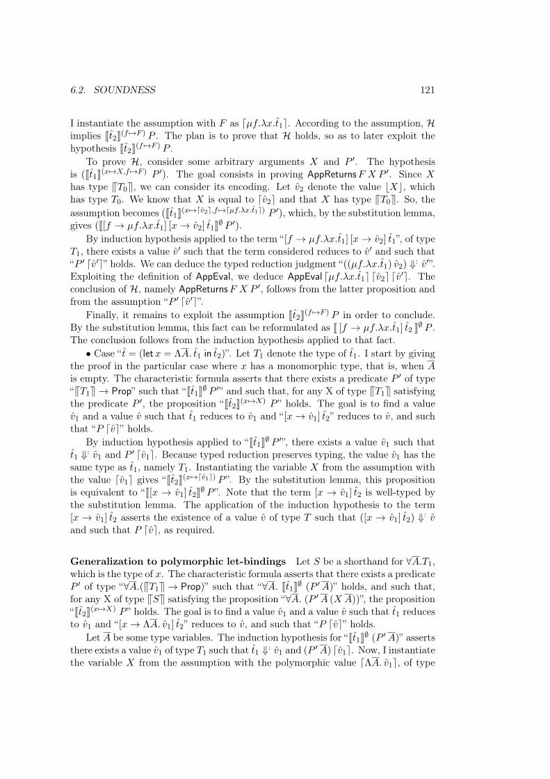
6.2. SOUNDNESS 121
I instantiate the assumption with 𝐹 as ⌈𝜇𝑓.𝜆𝑥.𝑡1⌉. According to the assumption, ℋimplies J𝑡2K(𝑓 ↦→𝐹 ) 𝑃 . The plan is to prove that ℋ holds, so as to later exploit thehypothesis J𝑡2K(𝑓 ↦→𝐹 ) 𝑃 .
To prove ℋ, consider some arbitrary arguments 𝑋 and 𝑃 ′. The hypothesisis (J𝑡1K(𝑥 ↦→𝑋,𝑓 ↦→𝐹 ) 𝑃 ′). The goal consists in proving AppReturns𝐹 𝑋 𝑃 ′. Since 𝑋has type V𝑇0W, we can consider its encoding. Let 𝑣2 denote the value ⌊𝑋⌋, whichhas type 𝑇0. We know that 𝑋 is equal to ⌈𝑣2⌉ and that 𝑋 has type V𝑇0W. So, theassumption becomes (J𝑡1K(𝑥 ↦→⌈𝑣2⌉,𝑓 ↦→⌈𝜇𝑓.𝜆𝑥.𝑡1⌉) 𝑃 ′), which, by the substitution lemma,gives (J[𝑓 → 𝜇𝑓.𝜆𝑥.𝑡1] [𝑥 → 𝑣2] 𝑡1K∅ 𝑃 ′).
By induction hypothesis applied to the term “[𝑓 → 𝜇𝑓.𝜆𝑥.𝑡1] [𝑥 → 𝑣2] 𝑡1”, of type𝑇1, there exists a value 𝑣′ such that the term considered reduces to 𝑣′ and such that“𝑃 ′ ⌈𝑣′⌉” holds. We can deduce the typed reduction judgment “((𝜇𝑓.𝜆𝑥.𝑡1) 𝑣2) ⇓: 𝑣′”.Exploiting the definition of AppEval, we deduce AppEval ⌈𝜇𝑓.𝜆𝑥.𝑡1⌉ ⌈𝑣2⌉ ⌈𝑣′⌉. Theconclusion of ℋ, namely AppReturns𝐹 𝑋 𝑃 ′, follows from the latter proposition andfrom the assumption “𝑃 ′ ⌈𝑣′⌉”.
Finally, it remains to exploit the assumption J𝑡2K(𝑓 ↦→𝐹 ) 𝑃 in order to conclude.By the substitution lemma, this fact can be reformulated as J [𝑓 → 𝜇𝑓.𝜆𝑥.𝑡1] 𝑡2 K∅ 𝑃 .The conclusion follows from the induction hypothesis applied to that fact.
∙ Case “𝑡 = (let𝑥 = Λ𝐴. 𝑡1 in 𝑡2)”. Let 𝑇1 denote the type of 𝑡1. I start by givingthe proof in the particular case where 𝑥 has a monomorphic type, that is, when 𝐴is empty. The characteristic formula asserts that there exists a predicate 𝑃 ′ of type“V𝑇1W → Prop” such that “J𝑡1K∅ 𝑃 ′” and such that, for any X of type V𝑇1W satisfyingthe predicate 𝑃 ′, the proposition “J𝑡2K(𝑥 ↦→𝑋) 𝑃 ” holds. The goal is to find a value𝑣1 and a value 𝑣 such that 𝑡1 reduces to 𝑣1 and “[𝑥 → 𝑣1] 𝑡2” reduces to 𝑣, and suchthat “𝑃 ⌈𝑣⌉” holds.
By induction hypothesis applied to “J𝑡1K∅ 𝑃 ′”, there exists a value 𝑣1 such that𝑡1 ⇓: 𝑣1 and 𝑃 ′ ⌈𝑣1⌉. Because typed reduction preserves typing, the value 𝑣1 has thesame type as 𝑡1, namely 𝑇1. Instantiating the variable 𝑋 from the assumption withthe value ⌈𝑣1⌉ gives “J𝑡2K(𝑥 ↦→⌈𝑣1⌉) 𝑃 ”. By the substitution lemma, this propositionis equivalent to “J[𝑥 → 𝑣1] 𝑡2K∅ 𝑃 ”. Note that the term [𝑥 → 𝑣1] 𝑡2 is well-typed bythe substitution lemma. The application of the induction hypothesis to the term[𝑥 → 𝑣1] 𝑡2 asserts the existence of a value 𝑣 of type 𝑇 such that ([𝑥 → 𝑣1] 𝑡2) ⇓: 𝑣and such that 𝑃 ⌈𝑣⌉, as required.
Generalization to polymorphic let-bindings Let 𝑆 be a shorthand for ∀𝐴.𝑇1,which is the type of 𝑥. The characteristic formula asserts that there exists a predicate𝑃 ′ of type “∀𝐴.(V𝑇1W → Prop)” such that “∀𝐴. J𝑡1K∅ (𝑃 ′𝐴)” holds, and such that,for any X of type V𝑆W satisfying the proposition “∀𝐴. (𝑃 ′𝐴 (𝑋 𝐴))”, the proposition“J𝑡2K(𝑥 ↦→𝑋) 𝑃 ” holds. The goal is to find a value 𝑣1 and a value 𝑣 such that 𝑡1 reducesto 𝑣1 and “[𝑥 → Λ𝐴. 𝑣1] 𝑡2” reduces to 𝑣, and such that “𝑃 ⌈𝑣⌉” holds.
Let 𝐴 be some type variables. The induction hypothesis for “J𝑡1K∅ (𝑃 ′𝐴)” assertsthere exists a value 𝑣1 of type 𝑇1 such that 𝑡1 ⇓: 𝑣1 and (𝑃 ′𝐴) ⌈𝑣1⌉. Now, I instantiatethe variable 𝑋 from the assumption with the polymorphic value ⌈Λ𝐴. 𝑣1⌉, of type
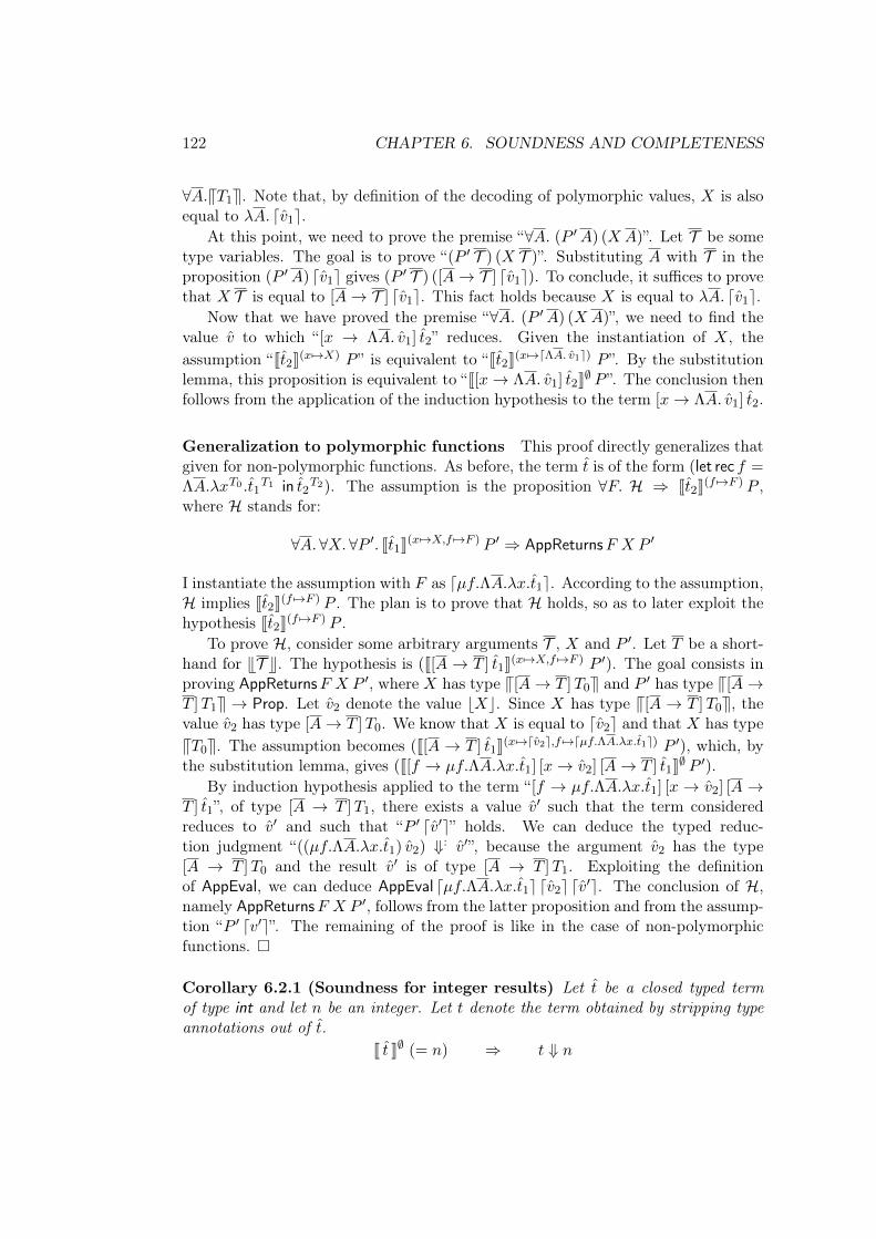
122 CHAPTER 6. SOUNDNESS AND COMPLETENESS
∀𝐴.V𝑇1W. Note that, by definition of the decoding of polymorphic values, 𝑋 is alsoequal to 𝜆𝐴. ⌈𝑣1⌉.
At this point, we need to prove the premise “∀𝐴. (𝑃 ′𝐴) (𝑋 𝐴)”. Let 𝒯 be sometype variables. The goal is to prove “(𝑃 ′ 𝒯 ) (𝑋 𝒯 )”. Substituting 𝐴 with 𝒯 in theproposition (𝑃 ′𝐴) ⌈𝑣1⌉ gives (𝑃 ′ 𝒯 ) ([𝐴 → 𝒯 ] ⌈𝑣1⌉). To conclude, it suffices to provethat 𝑋 𝒯 is equal to [𝐴 → 𝒯 ] ⌈𝑣1⌉. This fact holds because 𝑋 is equal to 𝜆𝐴. ⌈𝑣1⌉.
Now that we have proved the premise “∀𝐴. (𝑃 ′𝐴) (𝑋 𝐴)”, we need to find thevalue 𝑣 to which “[𝑥 → Λ𝐴. 𝑣1] 𝑡2” reduces. Given the instantiation of 𝑋, theassumption “J𝑡2K(𝑥 ↦→𝑋) 𝑃 ” is equivalent to “J𝑡2K(𝑥 ↦→⌈Λ𝐴. 𝑣1⌉) 𝑃 ”. By the substitutionlemma, this proposition is equivalent to “J[𝑥 → Λ𝐴. 𝑣1] 𝑡2K∅ 𝑃 ”. The conclusion thenfollows from the application of the induction hypothesis to the term [𝑥 → Λ𝐴. 𝑣1] 𝑡2.
Generalization to polymorphic functions This proof directly generalizes thatgiven for non-polymorphic functions. As before, the term 𝑡 is of the form (let rec 𝑓 =Λ𝐴.𝜆𝑥𝑇0 .𝑡1
𝑇1 in 𝑡2𝑇2). The assumption is the proposition ∀𝐹. ℋ ⇒ J𝑡2K(𝑓 ↦→𝐹 ) 𝑃 ,where ℋ stands for:
∀𝐴.∀𝑋.∀𝑃 ′. J𝑡1K(𝑥 ↦→𝑋,𝑓 ↦→𝐹 ) 𝑃 ′ ⇒ AppReturns𝐹 𝑋 𝑃 ′
I instantiate the assumption with 𝐹 as ⌈𝜇𝑓.Λ𝐴.𝜆𝑥.𝑡1⌉. According to the assumption,ℋ implies J𝑡2K(𝑓 ↦→𝐹 ) 𝑃 . The plan is to prove that ℋ holds, so as to later exploit thehypothesis J𝑡2K(𝑓 ↦→𝐹 ) 𝑃 .
To prove ℋ, consider some arbitrary arguments 𝒯 , 𝑋 and 𝑃 ′. Let 𝑇 be a short-hand for T𝒯 U. The hypothesis is (J[𝐴 → 𝑇 ] 𝑡1K(𝑥 ↦→𝑋,𝑓 ↦→𝐹 ) 𝑃 ′). The goal consists inproving AppReturns𝐹 𝑋 𝑃 ′, where 𝑋 has type V[𝐴 → 𝑇 ]𝑇0W and 𝑃 ′ has type V[𝐴 →𝑇 ]𝑇1W → Prop. Let 𝑣2 denote the value ⌊𝑋⌋. Since 𝑋 has type V[𝐴 → 𝑇 ]𝑇0W, thevalue 𝑣2 has type [𝐴 → 𝑇 ]𝑇0. We know that 𝑋 is equal to ⌈𝑣2⌉ and that 𝑋 has typeV𝑇0W. The assumption becomes (J[𝐴 → 𝑇 ] 𝑡1K(𝑥 ↦→⌈𝑣2⌉,𝑓 ↦→⌈𝜇𝑓.Λ𝐴.𝜆𝑥.𝑡1⌉) 𝑃 ′), which, bythe substitution lemma, gives (J[𝑓 → 𝜇𝑓.Λ𝐴.𝜆𝑥.𝑡1] [𝑥 → 𝑣2] [𝐴 → 𝑇 ] 𝑡1K∅ 𝑃 ′).
By induction hypothesis applied to the term “[𝑓 → 𝜇𝑓.Λ𝐴.𝜆𝑥.𝑡1] [𝑥 → 𝑣2] [𝐴 →𝑇 ] 𝑡1”, of type [𝐴 → 𝑇 ]𝑇1, there exists a value 𝑣′ such that the term consideredreduces to 𝑣′ and such that “𝑃 ′ ⌈𝑣′⌉” holds. We can deduce the typed reduc-tion judgment “((𝜇𝑓.Λ𝐴.𝜆𝑥.𝑡1) 𝑣2) ⇓: 𝑣′”, because the argument 𝑣2 has the type[𝐴 → 𝑇 ]𝑇0 and the result 𝑣′ is of type [𝐴 → 𝑇 ]𝑇1. Exploiting the definitionof AppEval, we can deduce AppEval ⌈𝜇𝑓.Λ𝐴.𝜆𝑥.𝑡1⌉ ⌈𝑣2⌉ ⌈𝑣′⌉. The conclusion of ℋ,namely AppReturns𝐹 𝑋 𝑃 ′, follows from the latter proposition and from the assump-tion “𝑃 ′ ⌈𝑣′⌉”. The remaining of the proof is like in the case of non-polymorphicfunctions. �
Corollary 6.2.1 (Soundness for integer results) Let 𝑡 be a closed typed termof type int and let 𝑛 be an integer. Let 𝑡 denote the term obtained by stripping typeannotations out of 𝑡.
J 𝑡 K∅ (= 𝑛) ⇒ 𝑡 ⇓ 𝑛
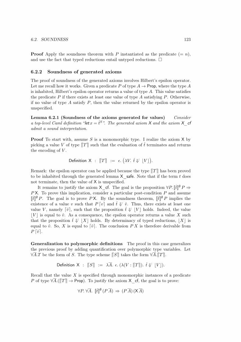
6.2. SOUNDNESS 123
Proof Apply the soundness theorem with 𝑃 instantiated as the predicate (= 𝑛),and use the fact that typed reductions entail untyped reductions. �
6.2.2 Soundness of generated axioms
The proof of soundness of the generated axioms involves Hilbert’s epsilon operator.Let me recall how it works. Given a predicate 𝑃 of type 𝐴 → Prop, where the type 𝐴is inhabited, Hilbert’s epsilon operator returns a value of type 𝐴. This value satisfiesthe predicate 𝑃 if there exists at least one value of type 𝐴 satisfying 𝑃 . Otherwise,if no value of type 𝐴 satisfy 𝑃 , then the value returned by the epsilon operator isunspecified.
Lemma 6.2.1 (Soundness of the axioms generated for values) Considera top-level Caml definition “ let𝑥 = 𝑡𝑆”. The generated axiom X and the axiom X_cfadmit a sound interpretation.
Proof To start with, assume 𝑆 is a monomorphic type. I realize the axiom X bypicking a value 𝑉 of type V𝑇W such that the evaluation of 𝑡 terminates and returnsthe encoding of 𝑉 .
Definition X : V𝑇W := 𝜖.Ä𝜆𝑉. 𝑡 ⇓: ⌊𝑉 ⌋
ä.
Remark: the epsilon operator can be applied because the type V𝑇W has been provedto be inhabited through the generated lemma X_safe. Note that if the term 𝑡 doesnot terminate, then the value of X is unspecified.
It remains to justify the axiom X_cf. The goal is the proposition ∀𝑃. J𝑡K∅ 𝑃 ⇒𝑃 X. To prove this implication, consider a particular post-condition 𝑃 and assumeJ𝑡K∅ 𝑃 . The goal is to prove 𝑃 X. By the soundness theorem, J𝑡K∅ 𝑃 implies theexistence of a value 𝑣 such that 𝑃 ⌈𝑣⌉ and 𝑡 ⇓: 𝑣. Thus, there exists at least onevalue 𝑉 , namely ⌈𝑣⌉, such that the proposition 𝑡 ⇓: ⌊𝑉 ⌋ holds. Indeed, the value⌊𝑉 ⌋ is equal to 𝑣. As a consequence, the epsilon operator returns a value 𝑋 suchthat the proposition 𝑡 ⇓: ⌊𝑋⌋ holds. By determinacy of typed reductions, ⌊𝑋⌋ isequal to 𝑣. So, 𝑋 is equal to ⌈𝑣⌉. The conclusion 𝑃 𝑋 is therefore derivable from𝑃 ⌈𝑣⌉.
Generalization to polymorphic definitions The proof in this case generalizesthe previous proof by adding quantification over polymorphic type variables. Let∀𝐴.𝑇 be the form of 𝑆. The type scheme V𝑆W takes the form ∀𝐴.V𝑇W.
Definition X : V𝑆W := 𝜆𝐴. 𝜖. (𝜆(𝑉 : V𝑇W). 𝑡 ⇓: ⌊𝑉 ⌋).
Recall that the value 𝑋 is specified through monomorphic instances of a predicate𝑃 of type ∀𝐴.(V𝑇W → Prop). To justify the axiom X_cf, the goal is to prove:
∀𝑃. ∀𝐴. J𝑡K∅ (𝑃 𝐴) ⇒ (𝑃 𝐴) (X𝐴)
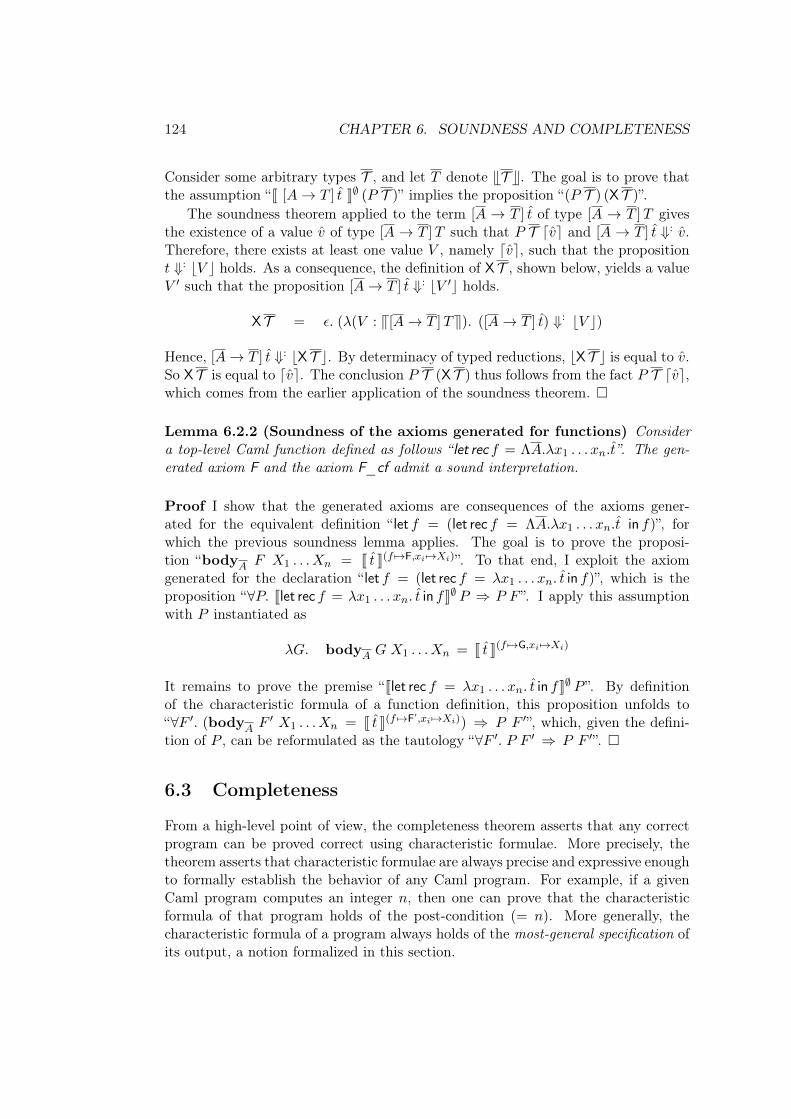
124 CHAPTER 6. SOUNDNESS AND COMPLETENESS
Consider some arbitrary types 𝒯 , and let 𝑇 denote T𝒯 U. The goal is to prove thatthe assumption “J [𝐴 → 𝑇 ] 𝑡 K∅ (𝑃 𝒯 )” implies the proposition “(𝑃 𝒯 ) (X 𝒯 )”.
The soundness theorem applied to the term [𝐴 → 𝑇 ] 𝑡 of type [𝐴 → 𝑇 ]𝑇 givesthe existence of a value 𝑣 of type [𝐴 → 𝑇 ]𝑇 such that 𝑃 𝒯 ⌈𝑣⌉ and [𝐴 → 𝑇 ] 𝑡 ⇓: 𝑣.Therefore, there exists at least one value 𝑉 , namely ⌈𝑣⌉, such that the proposition𝑡 ⇓: ⌊𝑉 ⌋ holds. As a consequence, the definition of X 𝒯 , shown below, yields a value𝑉 ′ such that the proposition [𝐴 → 𝑇 ] 𝑡 ⇓: ⌊𝑉 ′⌋ holds.
X 𝒯 = 𝜖. (𝜆(𝑉 : V[𝐴 → 𝑇 ]𝑇W). ([𝐴 → 𝑇 ] 𝑡) ⇓: ⌊𝑉 ⌋)
Hence, [𝐴 → 𝑇 ] 𝑡 ⇓: ⌊X 𝒯 ⌋. By determinacy of typed reductions, ⌊X 𝒯 ⌋ is equal to 𝑣.So X 𝒯 is equal to ⌈𝑣⌉. The conclusion 𝑃 𝒯 (X 𝒯 ) thus follows from the fact 𝑃 𝒯 ⌈𝑣⌉,which comes from the earlier application of the soundness theorem. �
Lemma 6.2.2 (Soundness of the axioms generated for functions) Considera top-level Caml function defined as follows “ let rec 𝑓 = Λ𝐴.𝜆𝑥1 . . . 𝑥𝑛.𝑡”. The gen-erated axiom F and the axiom F_cf admit a sound interpretation.
Proof I show that the generated axioms are consequences of the axioms gener-ated for the equivalent definition “ let 𝑓 = (let rec 𝑓 = Λ𝐴.𝜆𝑥1 . . . 𝑥𝑛.𝑡 in 𝑓)”, forwhich the previous soundness lemma applies. The goal is to prove the proposi-tion “body𝐴 𝐹 𝑋1 . . . 𝑋𝑛 = J 𝑡 K(𝑓 ↦→F,𝑥𝑖 ↦→𝑋𝑖)”. To that end, I exploit the axiomgenerated for the declaration “ let 𝑓 = (let rec 𝑓 = 𝜆𝑥1 . . . 𝑥𝑛. 𝑡 in 𝑓)”, which is theproposition “∀𝑃. Jlet rec 𝑓 = 𝜆𝑥1 . . . 𝑥𝑛. 𝑡 in 𝑓K∅ 𝑃 ⇒ 𝑃 𝐹 ”. I apply this assumptionwith 𝑃 instantiated as
𝜆𝐺. body𝐴 𝐺 𝑋1 . . . 𝑋𝑛 = J 𝑡 K(𝑓 ↦→G,𝑥𝑖 ↦→𝑋𝑖)
It remains to prove the premise “Jlet rec 𝑓 = 𝜆𝑥1 . . . 𝑥𝑛. 𝑡 in 𝑓K∅ 𝑃 ”. By definitionof the characteristic formula of a function definition, this proposition unfolds to“∀𝐹 ′. (body𝐴 𝐹 ′ 𝑋1 . . . 𝑋𝑛 = J 𝑡 K(𝑓 ↦→F’,𝑥𝑖 ↦→𝑋𝑖)) ⇒ 𝑃 𝐹 ′”, which, given the defini-tion of 𝑃 , can be reformulated as the tautology “∀𝐹 ′. 𝑃 𝐹 ′ ⇒ 𝑃 𝐹 ′”. �
6.3 Completeness
From a high-level point of view, the completeness theorem asserts that any correctprogram can be proved correct using characteristic formulae. More precisely, thetheorem asserts that characteristic formulae are always precise and expressive enoughto formally establish the behavior of any Caml program. For example, if a givenCaml program computes an integer 𝑛, then one can prove that the characteristicformula of that program holds of the post-condition (= 𝑛). More generally, thecharacteristic formula of a program always holds of the most-general specification ofits output, a notion formalized in this section.
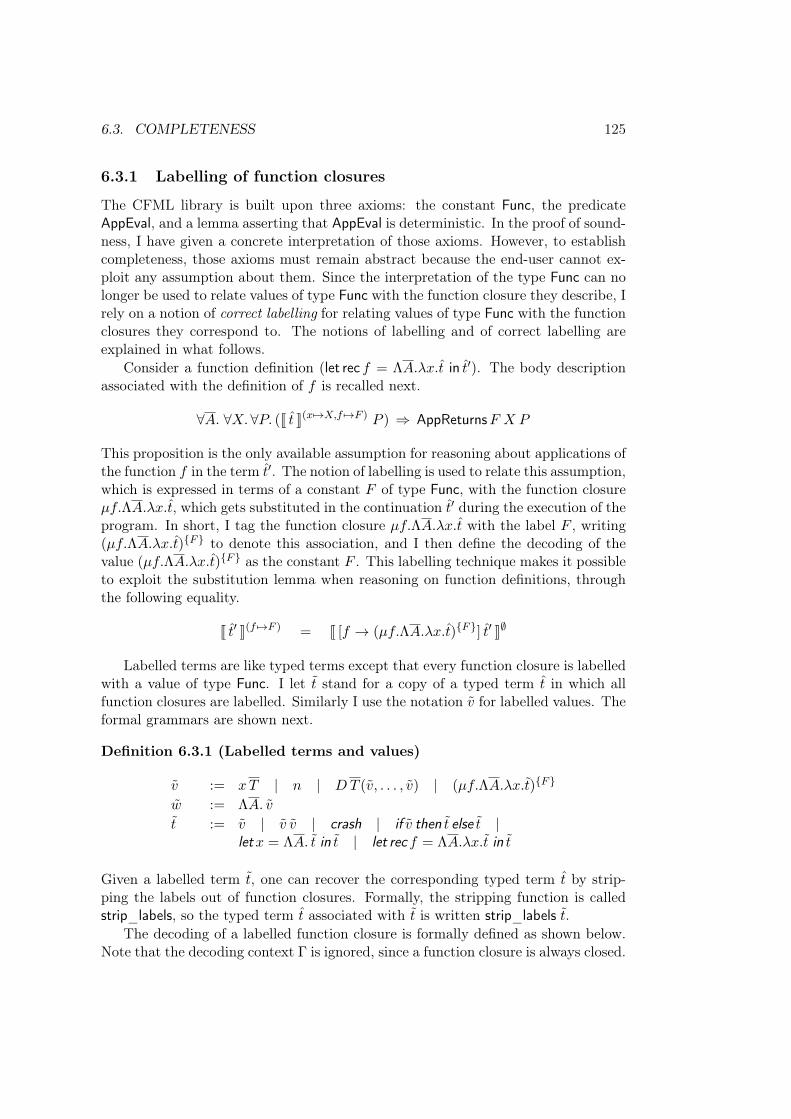
6.3. COMPLETENESS 125
6.3.1 Labelling of function closures
The CFML library is built upon three axioms: the constant Func, the predicateAppEval, and a lemma asserting that AppEval is deterministic. In the proof of sound-ness, I have given a concrete interpretation of those axioms. However, to establishcompleteness, those axioms must remain abstract because the end-user cannot ex-ploit any assumption about them. Since the interpretation of the type Func can nolonger be used to relate values of type Func with the function closure they describe, Irely on a notion of correct labelling for relating values of type Func with the functionclosures they correspond to. The notions of labelling and of correct labelling areexplained in what follows.
Consider a function definition (let rec 𝑓 = Λ𝐴.𝜆𝑥.𝑡 in 𝑡′). The body descriptionassociated with the definition of 𝑓 is recalled next.
∀𝐴. ∀𝑋.∀𝑃. (J 𝑡 K(𝑥↦→𝑋,𝑓 ↦→𝐹 ) 𝑃 ) ⇒ AppReturns𝐹 𝑋 𝑃
This proposition is the only available assumption for reasoning about applications ofthe function 𝑓 in the term 𝑡′. The notion of labelling is used to relate this assumption,which is expressed in terms of a constant 𝐹 of type Func, with the function closure𝜇𝑓.Λ𝐴.𝜆𝑥.𝑡, which gets substituted in the continuation 𝑡′ during the execution of theprogram. In short, I tag the function closure 𝜇𝑓.Λ𝐴.𝜆𝑥.𝑡 with the label 𝐹 , writing(𝜇𝑓.Λ𝐴.𝜆𝑥.𝑡){𝐹} to denote this association, and I then define the decoding of thevalue (𝜇𝑓.Λ𝐴.𝜆𝑥.𝑡){𝐹} as the constant 𝐹 . This labelling technique makes it possibleto exploit the substitution lemma when reasoning on function definitions, throughthe following equality.
J 𝑡′ K(𝑓 ↦→𝐹 ) = J [𝑓 → (𝜇𝑓.Λ𝐴.𝜆𝑥.𝑡){𝐹}] 𝑡′ K∅
Labelled terms are like typed terms except that every function closure is labelledwith a value of type Func. I let 𝑡 stand for a copy of a typed term 𝑡 in which allfunction closures are labelled. Similarly I use the notation 𝑣 for labelled values. Theformal grammars are shown next.
Definition 6.3.1 (Labelled terms and values)
𝑣 := 𝑥𝑇 | 𝑛 | 𝐷𝑇 (𝑣, . . . , 𝑣) | (𝜇𝑓.Λ𝐴.𝜆𝑥.𝑡){𝐹}
�̃� := Λ𝐴. 𝑣
𝑡 := 𝑣 | 𝑣 𝑣 | crash | if 𝑣 then 𝑡 else 𝑡 |let𝑥 = Λ𝐴. 𝑡 in 𝑡 | let rec 𝑓 = Λ𝐴.𝜆𝑥.𝑡 in 𝑡
Given a labelled term 𝑡, one can recover the corresponding typed term 𝑡 by strip-ping the labels out of function closures. Formally, the stripping function is calledstrip_labels, so the typed term 𝑡 associated with 𝑡 is written strip_labels 𝑡.
The decoding of a labelled function closure is formally defined as shown below.Note that the decoding context Γ is ignored, since a function closure is always closed.
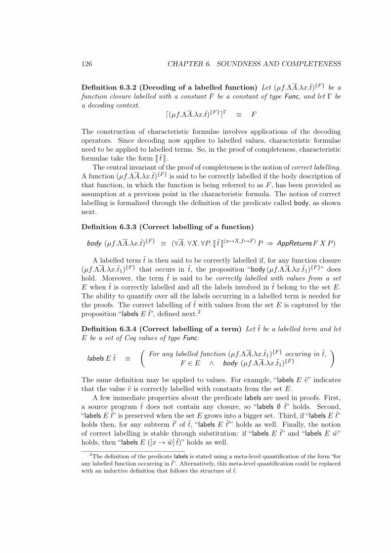
126 CHAPTER 6. SOUNDNESS AND COMPLETENESS
Definition 6.3.2 (Decoding of a labelled function) Let (𝜇𝑓.Λ𝐴.𝜆𝑥.𝑡){𝐹} be afunction closure labelled with a constant 𝐹 be a constant of type Func, and let Γ bea decoding context.
⌈(𝜇𝑓.Λ𝐴.𝜆𝑥.𝑡){𝐹}⌉Γ ≡ 𝐹
The construction of characteristic formulae involves applications of the decodingoperators. Since decoding now applies to labelled values, characteristic formulaeneed to be applied to labelled terms. So, in the proof of completeness, characteristicformulae take the form J 𝑡 K.
The central invariant of the proof of completeness is the notion of correct labelling.A function (𝜇𝑓.Λ𝐴.𝜆𝑥.𝑡){𝐹} is said to be correctly labelled if the body description ofthat function, in which the function is being referred to as 𝐹 , has been provided asassumption at a previous point in the characteristic formula. The notion of correctlabelling is formalized through the definition of the predicate called body, as shownnext.
Definition 6.3.3 (Correct labelling of a function)
body (𝜇𝑓.Λ𝐴.𝜆𝑥.𝑡){𝐹} ≡ (∀𝐴. ∀𝑋.∀𝑃. J 𝑡 K(𝑥 ↦→𝑋,𝑓 ↦→𝐹 ) 𝑃 ⇒ AppReturns𝐹 𝑋 𝑃 )
A labelled term 𝑡 is then said to be correctly labelled if, for any function closure(𝜇𝑓.Λ𝐴.𝜆𝑥.𝑡1)
{𝐹} that occurs in 𝑡, the proposition “body (𝜇𝑓.Λ𝐴.𝜆𝑥.𝑡1){𝐹}” does
hold. Moreover, the term 𝑡 is said to be correctly labelled with values from a set𝐸 when 𝑡 is correctly labelled and all the labels involved in 𝑡 belong to the set 𝐸.The ability to quantify over all the labels occurring in a labelled term is needed forthe proofs. The correct labelling of 𝑡 with values from the set 𝐸 is captured by theproposition “ labels 𝐸 𝑡”, defined next.2
Definition 6.3.4 (Correct labelling of a term) Let 𝑡 be a labelled term and let𝐸 be a set of Coq values of type Func.
labels 𝐸 𝑡 ≡Ç
For any labelled function (𝜇𝑓.Λ𝐴.𝜆𝑥.𝑡1){𝐹} occuring in 𝑡,
𝐹 ∈ 𝐸 ∧ body (𝜇𝑓.Λ𝐴.𝜆𝑥.𝑡1){𝐹}
åThe same definition may be applied to values. For example, “ labels 𝐸 𝑣” indicatesthat the value 𝑣 is correctly labelled with constants from the set 𝐸.
A few immediate properties about the predicate labels are used in proofs. First,a source program 𝑡 does not contain any closure, so “ labels ∅ 𝑡” holds. Second,“ labels 𝐸 𝑡” is preserved when the set 𝐸 grows into a bigger set. Third, if “ labels 𝐸 𝑡”holds then, for any subterm 𝑡′ of 𝑡, “ labels 𝐸 𝑡′” holds as well. Finally, the notionof correct labelling is stable through substitution: if “ labels 𝐸 𝑡” and “ labels 𝐸 �̃�”holds, then “ labels 𝐸 ([𝑥 → �̃�] 𝑡)” holds as well.
2The definition of the predicate labels is stated using a meta-level quantification of the form “forany labelled function occurring in 𝑡”. Alternatively, this meta-level quantification could be replacedwith an inductive definition that follows the structure of 𝑡.
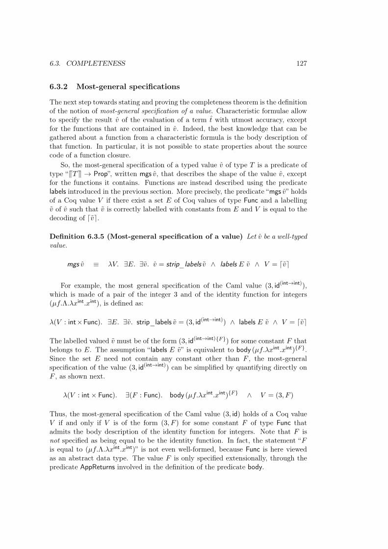
6.3. COMPLETENESS 127
6.3.2 Most-general specifications
The next step towards stating and proving the completeness theorem is the definitionof the notion of most-general specification of a value. Characteristic formulae allowto specify the result 𝑣 of the evaluation of a term 𝑡 with utmost accuracy, exceptfor the functions that are contained in 𝑣. Indeed, the best knowledge that can begathered about a function from a characteristic formula is the body description ofthat function. In particular, it is not possible to state properties about the sourcecode of a function closure.
So, the most-general specification of a typed value 𝑣 of type 𝑇 is a predicate oftype “V𝑇W → Prop”, written mgs 𝑣, that describes the shape of the value 𝑣, exceptfor the functions it contains. Functions are instead described using the predicatelabels introduced in the previous section. More precisely, the predicate “mgs 𝑣” holdsof a Coq value 𝑉 if there exist a set 𝐸 of Coq values of type Func and a labelling𝑣 of 𝑣 such that 𝑣 is correctly labelled with constants from 𝐸 and 𝑉 is equal to thedecoding of ⌈𝑣⌉.
Definition 6.3.5 (Most-general specification of a value) Let 𝑣 be a well-typedvalue.
mgs 𝑣 ≡ 𝜆𝑉. ∃𝐸. ∃𝑣. 𝑣 = strip_labels 𝑣 ∧ labels 𝐸 𝑣 ∧ 𝑉 = ⌈𝑣⌉
For example, the most general specification of the Caml value (3, id(int→int)),which is made of a pair of the integer 3 and of the identity function for integers(𝜇𝑓.Λ.𝜆𝑥int.𝑥int), is defined as:
𝜆(𝑉 : int×Func). ∃𝐸. ∃𝑣. strip_labels 𝑣 = (3, id(int→int)) ∧ labels 𝐸 𝑣 ∧ 𝑉 = ⌈𝑣⌉
The labelled valued 𝑣 must be of the form (3, id(int→int){𝐹}) for some constant 𝐹 thatbelongs to 𝐸. The assumption “ labels 𝐸 𝑣” is equivalent to body (𝜇𝑓.𝜆𝑥int.𝑥int){𝐹}.Since the set 𝐸 need not contain any constant other than 𝐹 , the most-generalspecification of the value (3, id(int→int)) can be simplified by quantifying directly on𝐹 , as shown next.
𝜆(𝑉 : int × Func). ∃(𝐹 : Func). body (𝜇𝑓.𝜆𝑥int.𝑥int){𝐹} ∧ 𝑉 = (3, 𝐹 )
Thus, the most-general specification of the Caml value (3, id) holds of a Coq value𝑉 if and only if 𝑉 is of the form (3, 𝐹 ) for some constant 𝐹 of type Func thatadmits the body description of the identity function for integers. Note that 𝐹 isnot specified as being equal to be the identity function. In fact, the statement “𝐹is equal to (𝜇𝑓.Λ.𝜆𝑥int.𝑥int)” is not even well-formed, because Func is here viewedas an abstract data type. The value 𝐹 is only specified extensionally, through thepredicate AppReturns involved in the definition of the predicate body.
128 CHAPTER 6. SOUNDNESS AND COMPLETENESS
6.3.3 Completeness theorem
Theorem 6.3.1 (Completeness in terms of most-general specifications)Let 𝑡 be a closed, well-typed term of type 𝑇 that does not contain any function closure,and let 𝑣 be a value.
𝑡 ⇓: 𝑣 ⇒ J 𝑡 K∅ (mgs 𝑣)
Proof I prove by induction on the derivation of the typed reduction judgment 𝑡 ⇓: 𝑣that, for any correct labelling 𝑡 of 𝑡 using constants for some set 𝐸, under theassumption that 𝑡 is well-typed, the characteristic formula of 𝑡 holds of the most-general specification of 𝑣.
𝑡 ⇓: 𝑣 ⇒ ∀𝐸. ∀𝑡. 𝑡 = strip_labels 𝑡 ∧ labels 𝐸 𝑡 ∧ (⊢ 𝑡) ⇒ J 𝑡 K∅ (mgs 𝑣)
There is one proof case for each possible reduction rule. In each proof case, I describethe form of the term 𝑡 and the premises of the assumption 𝑡 ⇓: 𝑣.
∙ Case 𝑡 = 𝑣. By hypothesis, there exists a labelling 𝑡 of the term 𝑡 such that“ labels 𝐸 𝑡” holds. Since 𝑡 is equal to 𝑣, there also exists a labelling 𝑣 of the value 𝑣such that “ labels 𝐸 𝑣” holds. The goal is (mgs 𝑣) ⌈𝑣⌉. By definition, this propositionis equivalent to the following proposition, which is true.
∃𝐸. ∃𝑣. strip_labels 𝑣 = 𝑣 ∧ labels 𝐸 𝑣 ∧ ⌈𝑣⌉ = ⌈𝑣⌉
∙ Case 𝑡 = (let rec 𝑓 = Λ𝐴.𝜆𝑥.𝑡1 in 𝑡2), with a premise asserting that the term“[𝑓 → 𝜇𝑓.Λ𝐴.𝜆𝑥.𝑡1] 𝑡2” reduces to 𝑣. By hypothesis, there exists a set 𝐸, a la-belling 𝑡1 of 𝑡1 and a labelling 𝑡2 of 𝑡2 such that the propositions “ labels 𝐸 𝑡1” and“ labels 𝐸 𝑡2” hold. The proof obligation is “∀𝐹. ℋ ⇒ J𝑡2K(𝑓 ↦→𝐹 ) (mgs 𝑣)”, whereℋ, the body description of the function, corresponds exactly to the propositionbody (𝜇𝑓.Λ𝐴.𝜆𝑥.𝑡1)
{𝐹}.Given a particular variable 𝐹 of type Func, the goal simplifies to
body (𝜇𝑓.Λ𝐴.𝜆𝑥.𝑡1){𝐹} ⇒ J𝑡2K(𝑓 ↦→𝐹 ) (mgs 𝑣)
Since the decoding of (𝜇𝑓.Λ𝐴.𝜆𝑥.𝑡1){𝐹} is equal to 𝐹 , the substitution lemma
(adapted to labelled terms) allows us to rewrite the formula J𝑡2K(𝑓 ↦→𝐹 ) into J[𝑓 →(𝜇𝑓.Λ𝐴.𝜆𝑥.𝑡1)
{𝐹}] 𝑡2K∅.It remains to invoke the induction hypothesis on the reduction sequence [𝑓 →
𝜇𝑓.Λ𝐴.𝜆𝑥.𝑡1] 𝑡2 ⇓: 𝑣. To that end, it suffices to check that [𝑓 → (𝜇𝑓.Λ𝐴.𝜆𝑥.𝑡1){𝐹}] 𝑡2
is correctly labelled with values from the set 𝐸∪{𝐹}. Indeed, a label occurring in theterm [𝑓 → (𝜇𝑓.Λ𝐴.𝜆𝑥.𝑡1)
{𝐹}] 𝑡2 either occurs in 𝑡1, which is labelled with constantsfrom 𝐸, or occurs in 𝑡2, which is also labelled with constants from 𝐸, or is equal tothe label 𝐹 .
∙ Case 𝑡 = ((𝜇𝑓.Λ𝐴.𝜆𝑥𝑇0 .𝑡1𝑇1) (𝑣2
𝑇2))𝑇 , with a premise asserting that the term“[𝑓 → 𝜇𝑓.Λ𝐴.𝜆𝑥.𝑡1] [𝑥 → 𝑣2] [𝐴 → 𝑇 ] 𝑡1” reduces to 𝑣, and two premises relatingtypes: 𝑇2 = [𝐴 → 𝑇 ]𝑇0 and 𝑇 = [𝐴 → 𝑇 ]𝑇1. Let 𝑡 be the labelling of 𝑡. Thehypothesis “ labels 𝐸 𝑡” implies that there exist a set 𝐸, a value 𝐹 from that set,
6.3. COMPLETENESS 129
and two labellings 𝑡1 and 𝑣2 such that the following facts are true: (𝜇𝑓.Λ𝐴.𝜆𝑥.𝑡1)is labelled with 𝐹 in 𝑡, the proposition body (𝜇𝑓.Λ𝐴.𝜆𝑥.𝑡1)
{𝐹} holds, “ labels 𝐸 𝑡1”holds, and “ labels 𝐸 𝑣2” holds.
Since the decoding of the labelled value (𝜇𝑓.Λ𝐴.𝜆𝑥.𝑡1){𝐹} is the constant 𝐹 ,
the goal J 𝑡 K∅ (mgs 𝑣) is equivalent to “AppReturns𝐹 ⌈𝑣2⌉ (mgs 𝑣)”. To prove thisgoal, I apply the assumption body (𝜇𝑓.Λ𝐴.𝜆𝑥.𝑡1)
{𝐹}, which asserts the followingproposition.
∀𝐴. ∀𝑋.∀𝑃. (J𝑡1K(𝑥↦→𝑋,𝑓 ↦→𝐹 ) 𝑃 ) ⇒ AppReturns𝐹 𝑋 𝑃
The types 𝐴 are instantiated as V𝑇W, 𝑋 is instantiated as ⌈𝑣2⌉ and 𝑃 is instanti-ated as (mgs 𝑣). It remains to prove the premise, which is the proposition “J[𝐴 →𝑇 ] 𝑡1K(𝑥 ↦→⌈𝑣2⌉,𝑓 ↦→𝐹 ) (mgs 𝑣)”. Through the substitution lemma, it becomes “J[𝑓 →(𝜇𝑓.Λ𝐴.𝜆𝑥.𝑡1)
{𝐹}] [𝑥 → 𝑣2] [𝐴 → 𝑇 ] 𝑡1K∅ (mgs 𝑣)”. This proposition follows from theinduction hypothesis applied to the typed term “[𝑓 → 𝜇𝑓.Λ𝐴.𝜆𝑥.𝑡1] [𝑥 → 𝑣2] [𝐴 →𝑇 ] 𝑡1”. This term is well-typed and admits the type 𝑇 because the type of 𝑣2 is equalto [𝐴 → 𝑇 ]𝑇0 and because 𝑇 is equal to [𝐴 → 𝑇 ]𝑇1. Note that the set of labelsoccurring in “[𝑓 → (𝜇𝑓.Λ𝐴.𝜆𝑥.𝑡1)
{𝐹}] [𝑥 → 𝑣2] [𝐴 → 𝑇 ] 𝑡1” is included in the set oflabels occurring in 𝑡, which is of the form ((𝜇𝑓.Λ𝐴.𝜆𝑥.𝑡1)
{𝐹} 𝑣2).∙ Case 𝑡 = (if 𝑣 then 𝑡1 else 𝑡2). Because 𝑡 is well-typed, the value 𝑣 has type bool,
so it is either equal to true or false. In both cases, the conclusion follows from theinduction hypothesis.
∙ Case 𝑡 = (let𝑥 = Λ𝐴. 𝑡1 in 𝑡2), with two premises asserting “𝑡1 ⇓: 𝑣1” and“([𝑥 → Λ𝐴. 𝑣1] 𝑡2) ⇓: 𝑣”. By hypothesis, there exist a set 𝐸, a labelling 𝑡1 of 𝑡1 anda labelling 𝑡2 of 𝑡2 such that the propositions “ labels 𝐸 𝑡1” and “ labels 𝐸 𝑡2” hold.Let me start with the case where 𝑥 admits a monomorphic type, that is, assuming𝐴 to be empty. In this case, the goal is:
∃𝑃 ′. J𝑡1K∅ 𝑃 ′ ∧ (∀𝑋. 𝑃 ′𝑋 ⇒ J𝑡2K(𝑥 ↦→𝑋) (mgs 𝑣))
To prove this goal, I instantiate 𝑃 ′ as the predicate mgs 𝑣1. The first subgoal,“J𝑡1K∅ (mgs 𝑣1)”, follows from the induction hypothesis applied to the reduction “𝑡1 ⇓:
𝑣1” and to the set 𝐸.It remains to prove the second subgoal. Let 𝑇1 be the type of the variable 𝑥,
and let 𝑋 be a value of type V𝑇1W such that “mgs 𝑣1𝑋” holds. By definition ofmgs, there exists a set 𝐸′ and a labelling 𝑣1 of 𝑣1 such that “ labels 𝐸′ 𝑣1” and“𝑋 = ⌈𝑣1⌉”. The goal is to prove J𝑡2K(𝑥 ↦→𝑋) (mgs 𝑣). By the substitution lemma,the formula “J𝑡2K(𝑥 ↦→𝑋)” is equivalent to “J[𝑥 → 𝑣1] 𝑡2K∅”. So it remains to prove“J[𝑥 → 𝑣1] 𝑡2K∅ (mgs 𝑣)”. This proposition follows from the induction hypothesisapplied to the reduction derivation “([𝑥 → 𝑣1] 𝑡2) ⇓: 𝑣” and to the 𝐸 ∪𝐸′, which weknow correctly labels the term [𝑥 → 𝑣1] 𝑡2 thanks to the hypotheses “ labels 𝐸′ 𝑣1”and “ labels 𝐸 𝑡2”.
130 CHAPTER 6. SOUNDNESS AND COMPLETENESS
Generalization to polymorphic let-bindings The variable 𝑥 admits the poly-morphic type ∀𝐴. 𝑇1. The goal is:
∃𝑃 ′.
®∀𝐴. J 𝑡1 K∅ (𝑃 ′𝐴)
∀𝑋. (∀𝐴. (𝑃 ′𝐴 (𝑋 𝐴))) ⇒ J 𝑡2 K(𝑥 ↦→𝑋) (mgs 𝑣)
I instantiate 𝑃 ′ as 𝜆𝐴.mgs 𝑣1, which admits the type ∀𝐴.(V𝑇1W → Prop), as ex-pected. For the first subgoal, let 𝒯 be some arbitrary types and let 𝑇 denote thelist T𝑇U. We have to prove J [𝐴 → 𝑇 ] 𝑡1 K∅ (𝑃 ′ 𝒯 ). The post-condition 𝑃 ′ 𝒯 is equalto [𝐴 → 𝒯 ] (mgs 𝑣1). It is straightforward to show that this proposition is equalto mgs ([𝐴 → 𝑇 ] 𝑣1). The proof obligation J [𝐴 → 𝑇 ] 𝑡1 K∅ (mgs ([𝐴 → 𝑇 ] 𝑣1)), isobtained by applying the induction hypothesis to “([𝐴 → 𝑇 ] 𝑡1) ⇓: ([𝐴 → 𝑇 ] 𝑣1)”,which is a direct consequence of the hypothesis “𝑡1 ⇓: 𝑣1”.
The second proof obligation is harder to establish. Let 𝑋 be a Coq value oftype ∀𝐴. V𝑇1W that satisfies the proposition ∀𝐴. (𝑃 ′𝐴 (𝑋 𝐴)). The goal is to proveJ 𝑡2 K(𝑥 ↦→𝑋) (mgs 𝑣). The difficulty comes from the fact that we do not have an as-sumption about the polymorphic value 𝑋, but instead have different assumptionsfor every monomorphic instances of 𝑋. For this reason, the proof involves reasoningseparately on each of the occurrences of the polymorphic variable 𝑥 in the term𝑡2. So, let 𝑡′2 be a copy of 𝑡2 in which the occurrences of 𝑥 have been renamedusing a finite set of names 𝑥𝑖, such that each 𝑥𝑖 occurs exactly once in 𝑡′2. Thegoal becomes “J 𝑡′2 K(𝑥1 ↦→𝑋,...,𝑥𝑛 ↦→𝑋) (mgs 𝑣)”. The plan is to build an family of la-bellings (𝑣𝑖1)𝑖∈[1..𝑛] for the value 𝑣1 such that the goal can be rewritten in the form“J[𝑥𝑖 → 𝑣𝑖1] 𝑡
′2K∅ (mgs 𝑣)”.
Consider a particular occurrence of the variable 𝑥𝑖 in 𝑡′2. It takes the form ofa type application “𝑥𝑖 𝑇 ”, for some types 𝑇 . The decoding of this occurrence gives“𝑋 𝑇 ”. Let 𝒯 stand for the list of Coq types V𝑇W. Instantiating the hypothesisabout 𝑋 on the types 𝒯 gives (𝑃 ′ 𝒯 ) (𝑋 𝒯 ). By definition of 𝑃 ′, the value 𝑋 𝒯 thussatisfies the predicate [𝐴 → 𝒯 ] (mgs 𝑣1), which is the same as mgs ([𝐴 → 𝑇 ] 𝑣1). So,there exist a set 𝐸𝑖 and a labelling 𝑣𝑖1 of the value 𝑣1 such that “ labels 𝐸𝑖 𝑣
𝑖1” holds
and such that 𝑋 𝒯 is equal to ⌈𝑣𝑖1⌉.To summarize the reasoning of the previous paragraph, the decoding of the
occurrence of the variable 𝑥𝑖 in the context (𝑥1 ↦→ 𝑋, . . . , 𝑥𝑛 ↦→ 𝑋) is the sameas the decoding of the labelled value 𝑣𝑖1 in the empty context. It follows that thecharacteristic formula “J 𝑡′2 K(𝑥1 ↦→𝑋,...,𝑥𝑛 ↦→𝑋)” can be rewritten into “J[𝑥𝑖 → 𝑣𝑖1] 𝑡
′2K∅”.
Furthermore, there exists a family of sets (𝐸𝑖)𝑖∈[1..𝑛] such that “ labels 𝐸𝑖 𝑣𝑖1” holds
for every index 𝑖.It remains to prove “J[𝑥𝑖 → 𝑣𝑖1] 𝑡
′2K∅ (mgs 𝑣)”. This conclusion follows from the
induction hypothesis applied to the term [𝑥 → Λ𝐴. 𝑣1] 𝑡2 and to the set 𝐸 ∪ (⋃
𝑖𝐸𝑖).Indeed, the term [𝑥𝑖 → Λ𝐴. 𝑣𝑖1] 𝑡
′2 is a labelling of the term [𝑥 → Λ𝐴. 𝑣1] 𝑡2. Also,
a label that occurs in the labelled term [𝑥𝑖 → 𝑣𝑖1] 𝑡′2 belongs to the set 𝐸 ∪ (
⋃𝑖𝐸𝑖).
Indeed such a label occurs either in 𝑡2 (which contains the same labels as 𝑡′2) or inone of the labelled values 𝑣𝑖1, and we have “ labels 𝐸 𝑡2” as well as “ labels 𝐸𝑖 𝑣
𝑖1” for
every index 𝑖. �
6.4. QUANTIFICATION OVER TYPE 131
6.3.4 Completeness for integer results
A simpler statement of the completeness theorem can be devised for a program thatproduces an integer. If a term 𝑡 evaluates to an integer 𝑛 that satisfies a predicate𝑃 , then the characteristic formula of 𝑡 holds of 𝑃 .
Corollary 6.3.1 (Completeness for integer results) Consider a program well-typed in ML and that admits the type int. Let 𝑡 be the term obtained by replacing MLtype annotations with the corresponding weak-ML type annotations in that program,and let 𝑡 denote the corresponding raw term. Let 𝑛 be an integer and let 𝑃 be apredicate on integers. Then,
𝑡 ⇓ 𝑛 ∧ 𝑃 𝑛 ⇒ J 𝑡 K∅ 𝑃
Proof The reduction 𝑡 ⇓ 𝑛 starts on a term well-typed in ML, So there exists acorresponding typed reduction 𝑡 ⇓: 𝑛. The completeness theorem applied to thisassumption gives “J 𝑡 K∅ (mgs 𝑛)”. To show “J 𝑡 K∅ 𝑃 ”, I apply the weakening lemmafor characteristic formulae. I remains to show that, for any value 𝑉 of type int, theproposition “mgs 𝑛𝑉 ” implies “𝑃 𝑉 ”. By definition of mgs, there exists a set 𝐸 anda labelling �̃� of 𝑛 such that labels 𝐸 �̃� and 𝑉 = 𝑛. Since 𝑛 is an integer, the labellingcan be ignored completely. So, 𝑉 = ⌈𝑛⌉ and the conclusion “𝑃 𝑉 ” then follows fromthe hypothesis 𝑃 𝑛. �
6.4 Quantification over Type
Polymorphism has been treated by quantifying over logical type variables. I havenot yet discussed what exactly is the sort of these variables in the logic. A temptingsolution would be to assign them the sort Type. In Coq, Type is the sort of all typesfrom the logic. However, type variables used to represent polymorphism are onlymeant to range over reflected types, i.e. types of the form V𝑇W. Thus, it seems thatone ought to assign type variables the sort RType, defined as {𝐴 : Type | ∃𝑇.𝐴 =V𝑇W }.
Of course, I would provide RType as an abstract definition, since the fact thattypes correspond to reflected types need not be exploited in proofs. A questionnaturally arises: since RType is an abstract type, would it remain sound and completeto use the sort Type instead of the sort RType as a sort for type variables? The answeris positive. The purpose of this section is to justify this claim.
6.4.1 Case study: the identity function
To start with, I consider an example suggesting how replacing the quantification overRType with a quantification over Type affects characteristic formulae. Consider theidentity function id, defined as 𝜆𝑥. 𝑥. This function is polymorphic: it admits thetype “∀𝐴.𝐴 → 𝐴” in Caml. Hence, the assumption provided by a characteristic
132 CHAPTER 6. SOUNDNESS AND COMPLETENESS
formula for this function involves a universal quantification over the type 𝐴.
∀(𝐴 : RType). ∀(𝑋 : 𝐴). ∀(𝑃 : 𝐴 → Prop). 𝑃 𝑋 ⇒ AppReturns id𝑋 𝑃
For the sake of studying this formula, let me reformulate it into the following equiv-alent proposition3, which is expressed in terms of the predicate AppEval instead ofthe high-level predicate AppReturns.
∀(𝐴 : RType). ∀(𝑋 : 𝐴). AppEval id𝑋𝑋
Is this statement still sound if we change the sort of 𝐴 from RType to Type?Let me first recall why the statement with RType is sound. Let 𝐴 be a type of
sort RType and let 𝑋 be a Coq value of type 𝐴. The goal is to prove AppEval id𝑋𝑋.By definition of AppEval, it is equivalent to the proposition (⌊id⌋ ⌊𝑋⌋) ⇓: ⌊𝑋⌋. Theencoding of 𝑋, written ⌊𝐴⌋, is a well-typed program value 𝑣. Thus, ⌊𝑋⌋ is equalto 𝑣. The goal then simplifies to ((𝜆𝑥. 𝑥) 𝑣) ⇓: 𝑣, which is correct according to thesemantics.
Now, if 𝐴 is of sort Type and 𝑋 is an arbitrary Coq value of type 𝐴, then theredoes not necessarily exist a program value 𝑣 that corresponds to 𝑋. Intuitively,however, it would make sense to say that applying the identify function to someexotic object returns the exact same object. The object in question is not a realprogram value, but this is not a problem because it is never inspected in any way bythe polymorphic identity function. The purpose of the next section is to formallyjustify this intuition.
6.4.2 Formalization of exotic values
I extend the grammar of program values with exotic values, in such a way as toobtain a bijection between the set of all Coq values and the set of all well-typedprogram values, for a suitably-defined notion of typing of exotic values. First, thegrammar of values is extended with exotic values, written “exoT𝑉 ”, where T standsfor a Coq type and 𝑉 is a Coq value of type T. Note that T ranges over all Coqtypes, whereas 𝒯 only ranges over Coq types of the form V𝑇W. The grammar ofweak-ML types is extended with exotic types, written “ExoticT”.
𝑣 := . . . | exoT𝑉𝑇 := . . . | ExoticT
A Coq type T is said to be exotic, written “ is_exoticT”, if the head constructor of𝐴 does not correspond to a type constructor that exists in weak-ML. Let C denote
3Given the definition of AppReturns, the equivalence to be established is
AppEval id𝑋𝑋 ⇐⇒ (∀𝑃. 𝑃 𝑋 ⇒ (∃𝑌.AppEval id𝑋 𝑌 ∧ 𝑃 𝑌 ))
From left to right, instantiate 𝑌 as 𝑋. From right to left, instantiate 𝑃 as 𝜆𝑌. (𝑌 = 𝑋).
6.4. QUANTIFICATION OVER TYPE 133
the set of type constructors introduced through algebraic data type definitions. Thedefinition of is_exotic is formalized as follows.4
is_exoticT ≡
T ̸= IntT ̸= Func∀𝐶 ∈ C . ∀T. T ̸= 𝐶 T
An exotic value “exoT𝑉 ” admits the type “ExoticT” if and only if the Coq type Tis exotic.
is_exoticT∆ ⊢ (exoT𝑉 )(ExoticT)
Let T be an exotic Coq type. The programming language type “ExoticT” isreflected in the logic as the type T. The decoding of an exotic value “exoT𝑉 ” is 𝑉 ,and, reciprocally, the encoding of a Coq value 𝑉 of some exotic type T is the exoticvalue “exoT𝑉 ”.
VExoticTW ≡ TTTU ≡ ExoticT⌈exoT𝑉 ⌉ ≡ 𝑉
⌊𝑉 : T⌋ ≡ exoT𝑉
when “ is_exoticT” holds
Observe that the side-condition “ is_exoticT” ensures that the definition of TTUand of ⌊𝑉 : T⌋ do not overlap with existing definitions. The soundness of theintroduction of exotic values is captured through the following lemma.
Lemma 6.4.1 (Inverse functions with exotic values) Under the definitions ex-tended with exotic types and exotic values, the operator T·U is the inverse of V·W and⌊·⌋ is the inverse of ⌈·⌉.
Proof Follows directly from the definitions of the operations on exotic types andexotic values. �
To summarize, the treatment of exotic values described in this section allowsfor a bijection to be established between the set of all Coq types and the set ofall weak-ML types, and between the set of all Coq values and the set of all typedprogram values. This bijection justifies the quantification over the sort Type of thetype variables that occur in characteristic formulae.
4Technically, one should also check that the type constructors are applied to list of types of theappropriate arity. Partially-applied type constructors are also treated as exotic values.
Chapter 7
Proofs for the imperative setting
Through the previous chapter, I have established the soundness and com-pleteness of characteristic formulae for pure programs. The matter of thischapter is the generalization of those results to the case of imperativeprograms. To that end, the theorems need to be extended with heapdescriptions. Two additional difficulties related to the treatment of mu-table state arise. Firstly, the statement of the soundness theorem needsto quantify over the pieces of heap that have been framed out beforereasoning on a given characteristic formula. Secondly, the statement ofthe completeness theorem needs to account for the fact that characteris-tic formulae do not reveal the actual address of the memory cells beingallocated. The most general post-condition that can be proved from acharacteristic formula is thus a specification of the output value and ofthe output heap up to renaming of locations.
7.1 Additional definitions and lemmas
7.1.1 Typing and translation of memory stores
Reasoning on characteristic formulae involves the notion of typed memory store,written �̂�, and that of well-typed memory stores. I define those notions next, andthen describe the bijection between the set of well-typed memory stores and the setof values of type Heap.
A memory store 𝑚 is a map from locations to closed values. A typed store �̂�is a map from locations to typed values. So, if 𝑙 is a location in the domain of �̂�,then �̂�[𝑙] denotes the typed value stored in �̂� at that location. A typed store �̂� issaid to be well-typed in weak-ML, written ⊢ �̂�, if all the values stored in �̂� arewell-typed. Formally,
(⊢ �̂�) ≡ ∀𝑙 ∈ dom(�̂�). (⊢ �̂�[𝑙])
A well-typed memory store �̂� can be decoded into a value of type Heap. To thatend, it suffices to decode each of the values stored in �̂�. Reciprocally, a value of
134
7.1. ADDITIONAL DEFINITIONS AND LEMMAS 135
type Heap can be encoded into a well-typed memory store by encoding all the valuesthat it contains. The formalization of this definition is slightly complicated by thefact that Heap is actually a map from locations to dependent pairs made of a Coqtype and of a Coq value of that type. The formal definition is shown next. Notethat the decoding of typed stores only applies to well-typed stores.
Definition 7.1.1 (Decoding and encoding of memory stores)
⌈�̂�⌉ ≡ ℎ where®
dom(ℎ) = dom(�̂�)�̂�[𝑙] = 𝑣𝑇 ⇒ ℎ[𝑙] = (V𝑇W, ⌈𝑣𝑇 ⌉)
⌊ℎ⌋ ≡ �̂� where®
dom(�̂�) = dom(ℎ)ℎ[𝑙] = (𝒯 , 𝑉 : 𝒯 ) ⇒ �̂�[𝑙] = ⌊𝑉 ⌋
It is straightforward to check that ⌊⌈�̂�⌉⌋ is equal to �̂� for any well-typed memorystore �̂�, and that ⌈⌊ℎ⌋⌉ is equal to ℎ for any heap ℎ.
Remark: for the presentation to be complete, the decoding and the encodingoperations needs to be extended to locations, as follows.
VlocW ≡ LocTLocU ≡ loc
⌈𝑙loc⌉ ≡ (𝑙 : Loc)
⌊𝑙 : Loc⌋ ≡ 𝑙loc
7.1.2 Typed reduction judgment
The typed version of the reduction judgment is defined in a similar manner as inthe purely functional setting, except that it now involves typed memory stores. Thejudgment takes the form 𝑡/�̂� ⇓: 𝑣′/�̂�′ , asserting that the evaluation of the typed 𝑡in the typed store �̂� terminates and returns the typed value 𝑣′ in the typed store�̂�′. The inductive rules appear in Figure 7.1. Observe that the semantics of theprimitive functions ref, get and set consists in reading and writing typed values in atyped store. The reduction rule for get includes a premise asserting that the valueat location 𝑙 in the store has the same type as the term “get 𝑙”.
As before, the typed reduction judgment is deterministic and preserves typing.
Lemma 7.1.1 (Determinacy of typed reductions)
𝑡/�̂� ⇓: 𝑣′1/�̂�′1
∧ 𝑡/�̂� ⇓: 𝑣′2/�̂�′2
⇒ 𝑣′1 = 𝑣′2 ∧ �̂�′1 = �̂�′
2
Proof Similar proof as in the purely-functional setting (Lemma 6.1.7). �
Lemma 7.1.2 (Typed reductions preserve typing) Let 𝑡 be a typed term,let 𝑣 be a typed value, let �̂� and �̂� be two typed stores, let 𝑇 be a type and let𝐵 denote a list of free type variables.
𝐵 ⊢ 𝑡𝑇 ∧ ⊢ �̂� ∧ 𝑡/�̂� ⇓: 𝑣/�̂�′ ⇒ 𝐵 ⊢ 𝑣𝑇 ∧ ⊢ �̂�′
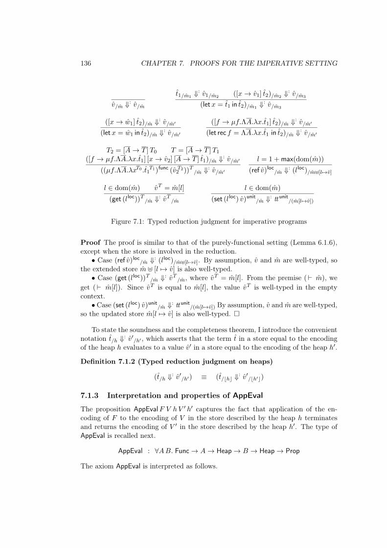
136 CHAPTER 7. PROOFS FOR THE IMPERATIVE SETTING
𝑣/�̂� ⇓: 𝑣/�̂�
𝑡1/�̂�1⇓: 𝑣1/�̂�2
([𝑥 → 𝑣1] 𝑡2)/�̂�2⇓: 𝑣/�̂�3
(let𝑥 = 𝑡1 in 𝑡2)/�̂�1⇓: 𝑣/�̂�3
([𝑥 → �̂�1] 𝑡2)/�̂� ⇓: 𝑣/�̂�′
(let𝑥 = �̂�1 in 𝑡2)/�̂� ⇓: 𝑣/�̂�′
([𝑓 → 𝜇𝑓.Λ𝐴.𝜆𝑥.𝑡1] 𝑡2)/�̂� ⇓: 𝑣/�̂�′
(let rec 𝑓 = Λ𝐴.𝜆𝑥.𝑡1 in 𝑡2)/�̂� ⇓: 𝑣/�̂�′
𝑇2 = [𝐴 → 𝑇 ]𝑇0 𝑇 = [𝐴 → 𝑇 ]𝑇1
([𝑓 → 𝜇𝑓.Λ𝐴.𝜆𝑥.𝑡1] [𝑥 → 𝑣2] [𝐴 → 𝑇 ] 𝑡1)/�̂� ⇓: 𝑣/�̂�′
((𝜇𝑓.Λ𝐴.𝜆𝑥𝑇0 .𝑡1𝑇1)func (𝑣2
𝑇2))𝑇 /�̂� ⇓: 𝑣/�̂�′
𝑙 = 1 + max(dom(�̂�))
(ref 𝑣)loc/�̂� ⇓: (𝑙 loc)/�̂�⊎[𝑙 ↦→𝑣]
𝑙 ∈ dom(�̂�) 𝑣𝑇 = �̂�[𝑙]
(get (𝑙 loc))𝑇 /�̂� ⇓: 𝑣𝑇 /�̂�
𝑙 ∈ dom(�̂�)
(set (𝑙 loc) 𝑣)unit/�̂� ⇓: tt unit
/(�̂�[𝑙 ↦→𝑣])
Figure 7.1: Typed reduction judgment for imperative programs
Proof The proof is similar to that of the purely-functional setting (Lemma 6.1.6),except when the store is involved in the reduction.
∙ Case (ref 𝑣)loc/�̂� ⇓: (𝑙 loc)/�̂�⊎[𝑙 ↦→𝑣]. By assumption, 𝑣 and �̂� are well-typed, so
the extended store �̂� ⊎ [𝑙 ↦→ 𝑣] is also well-typed.∙ Case (get (𝑙 loc))𝑇 /�̂� ⇓: 𝑣𝑇 /�̂�, where 𝑣𝑇 = �̂�[𝑙]. From the premise (⊢ �̂�), we
get (⊢ �̂�[𝑙]). Since 𝑣𝑇 is equal to �̂�[𝑙], the value 𝑣𝑇 is well-typed in the emptycontext.
∙ Case (set (𝑙 loc) 𝑣)unit/�̂� ⇓: tt unit
/(�̂�[𝑙 ↦→𝑣]) By assumption, 𝑣 and �̂� are well-typed,so the updated store �̂�[𝑙 ↦→ 𝑣] is also well-typed. �
To state the soundness and the completeness theorem, I introduce the convenientnotation 𝑡/ℎ ⇓: 𝑣′/ℎ′ , which asserts that the term 𝑡 in a store equal to the encodingof the heap ℎ evaluates to a value 𝑣′ in a store equal to the encoding of the heap ℎ′.
Definition 7.1.2 (Typed reduction judgment on heaps)
(𝑡/ℎ ⇓: 𝑣′/ℎ′) ≡ (𝑡/⌊ℎ⌋ ⇓: 𝑣′/⌊ℎ′⌋)
7.1.3 Interpretation and properties of AppEval
The proposition AppEval𝐹 𝑉 ℎ𝑉 ′ ℎ′ captures the fact that application of the en-coding of 𝐹 to the encoding of 𝑉 in the store described by the heap ℎ terminatesand returns the encoding of 𝑉 ′ in the store described by the heap ℎ′. The type ofAppEval is recalled next.
AppEval : ∀𝐴𝐵. Func → 𝐴 → Heap → 𝐵 → Heap → Prop
The axiom AppEval is interpreted as follows.
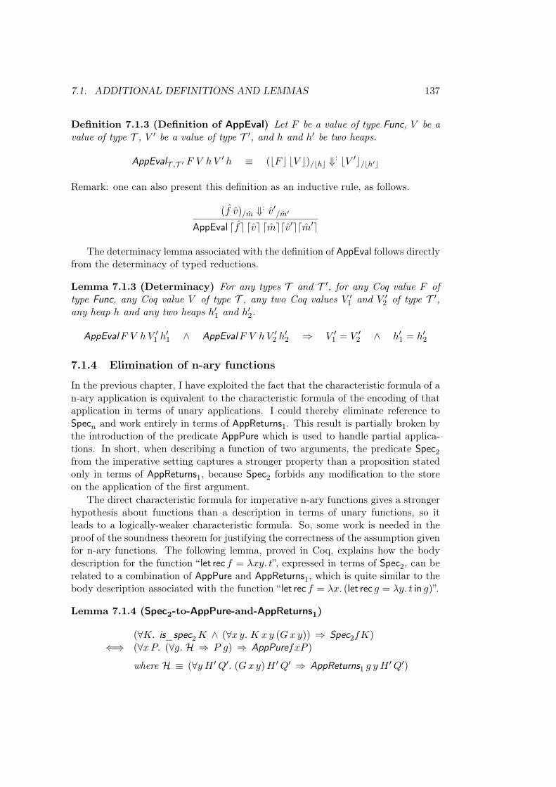
7.1. ADDITIONAL DEFINITIONS AND LEMMAS 137
Definition 7.1.3 (Definition of AppEval) Let 𝐹 be a value of type Func, 𝑉 be avalue of type 𝒯 , 𝑉 ′ be a value of type 𝒯 ′, and ℎ and ℎ′ be two heaps.
AppEval𝒯 ,𝒯 ′ 𝐹 𝑉 ℎ𝑉 ′ ℎ ≡ (⌊𝐹 ⌋ ⌊𝑉 ⌋)/⌊ℎ⌋ ⇓: ⌊𝑉 ′⌋/⌊ℎ′⌋
Remark: one can also present this definition as an inductive rule, as follows.
(𝑓 𝑣)/�̂� ⇓: 𝑣′/�̂�′
AppEval ⌈𝑓⌉ ⌈𝑣⌉ ⌈�̂�⌉⌈𝑣′⌉⌈�̂�′⌉
The determinacy lemma associated with the definition of AppEval follows directlyfrom the determinacy of typed reductions.
Lemma 7.1.3 (Determinacy) For any types 𝒯 and 𝒯 ′, for any Coq value 𝐹 oftype Func, any Coq value 𝑉 of type 𝒯 , any two Coq values 𝑉 ′
1 and 𝑉 ′2 of type 𝒯 ′,
any heap ℎ and any two heaps ℎ′1 and ℎ′2.
AppEval𝐹 𝑉 ℎ𝑉 ′1 ℎ
′1 ∧ AppEval𝐹 𝑉 ℎ𝑉 ′
2 ℎ′2 ⇒ 𝑉 ′
1 = 𝑉 ′2 ∧ ℎ′1 = ℎ′2
7.1.4 Elimination of n-ary functions
In the previous chapter, I have exploited the fact that the characteristic formula of an-ary application is equivalent to the characteristic formula of the encoding of thatapplication in terms of unary applications. I could thereby eliminate reference toSpec𝑛 and work entirely in terms of AppReturns1. This result is partially broken bythe introduction of the predicate AppPure which is used to handle partial applica-tions. In short, when describing a function of two arguments, the predicate Spec2from the imperative setting captures a stronger property than a proposition statedonly in terms of AppReturns1, because Spec2 forbids any modification to the storeon the application of the first argument.
The direct characteristic formula for imperative n-ary functions gives a strongerhypothesis about functions than a description in terms of unary functions, so itleads to a logically-weaker characteristic formula. So, some work is needed in theproof of the soundness theorem for justifying the correctness of the assumption givenfor n-ary functions. The following lemma, proved in Coq, explains how the bodydescription for the function “ let rec 𝑓 = 𝜆𝑥𝑦. 𝑡”, expressed in terms of Spec2, can berelated to a combination of AppPure and AppReturns1, which is quite similar to thebody description associated with the function “ let rec 𝑓 = 𝜆𝑥. (let rec 𝑔 = 𝜆𝑦. 𝑡 in 𝑔)”.
Lemma 7.1.4 (Spec2-to-AppPure-and-AppReturns1)
(∀𝐾. is_spec2𝐾 ∧ (∀𝑥 𝑦. 𝐾 𝑥 𝑦 (𝐺𝑥𝑦)) ⇒ Spec2𝑓𝐾)⇐⇒ (∀𝑥𝑃. (∀𝑔. ℋ ⇒ 𝑃 𝑔) ⇒ AppPure𝑓𝑥𝑃 )
where ℋ ≡ (∀𝑦 𝐻 ′𝑄′. (𝐺𝑥𝑦)𝐻 ′𝑄′ ⇒ AppReturns1 𝑔 𝑦 𝐻 ′𝑄′)
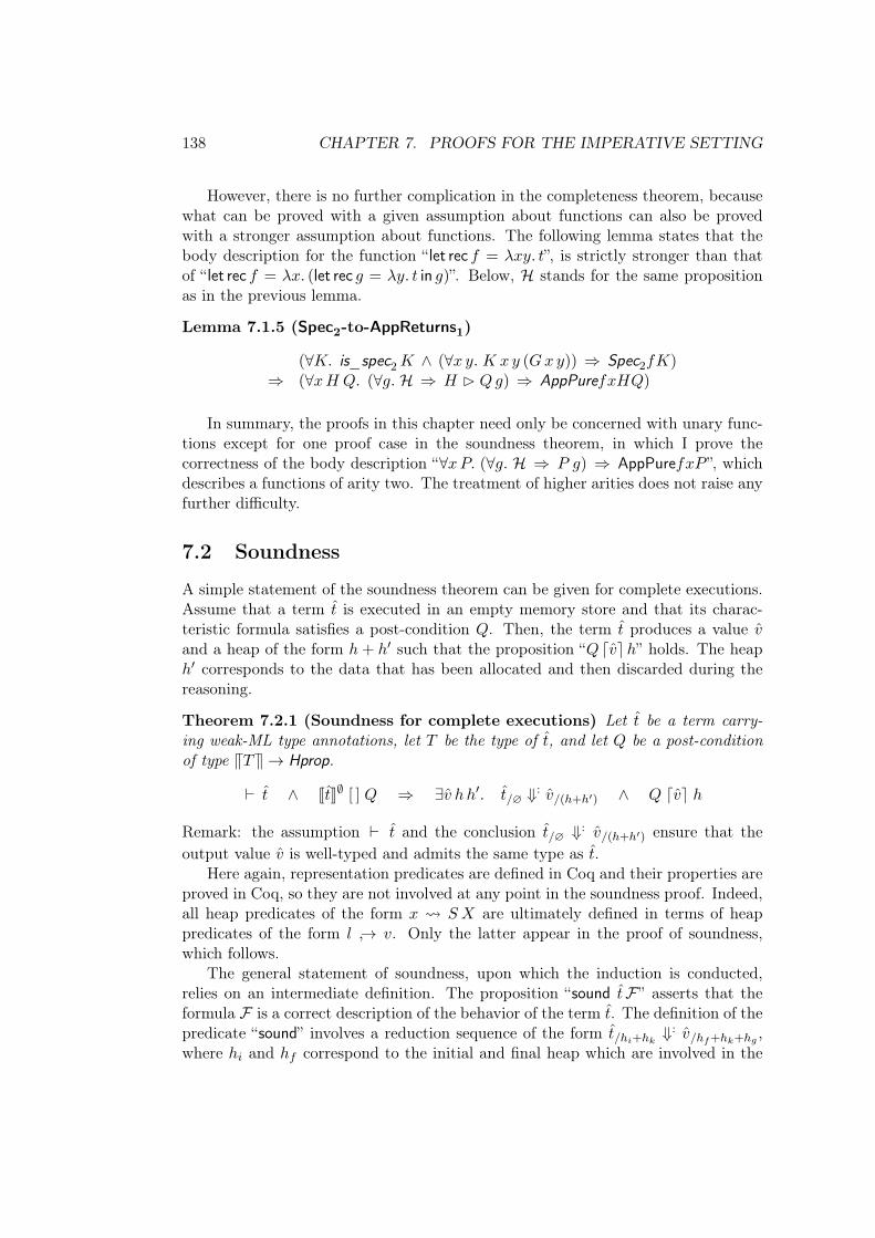
138 CHAPTER 7. PROOFS FOR THE IMPERATIVE SETTING
However, there is no further complication in the completeness theorem, becausewhat can be proved with a given assumption about functions can also be provedwith a stronger assumption about functions. The following lemma states that thebody description for the function “ let rec 𝑓 = 𝜆𝑥𝑦. 𝑡”, is strictly stronger than thatof “ let rec 𝑓 = 𝜆𝑥. (let rec 𝑔 = 𝜆𝑦. 𝑡 in 𝑔)”. Below, ℋ stands for the same propositionas in the previous lemma.
Lemma 7.1.5 (Spec2-to-AppReturns1)
(∀𝐾. is_spec2𝐾 ∧ (∀𝑥 𝑦. 𝐾 𝑥 𝑦 (𝐺𝑥𝑦)) ⇒ Spec2𝑓𝐾)⇒ (∀𝑥𝐻 𝑄. (∀𝑔. ℋ ⇒ 𝐻 B 𝑄𝑔) ⇒ AppPure𝑓𝑥𝐻𝑄)
In summary, the proofs in this chapter need only be concerned with unary func-tions except for one proof case in the soundness theorem, in which I prove thecorrectness of the body description “∀𝑥𝑃. (∀𝑔. ℋ ⇒ 𝑃 𝑔) ⇒ AppPure𝑓𝑥𝑃 ”, whichdescribes a functions of arity two. The treatment of higher arities does not raise anyfurther difficulty.
7.2 Soundness
A simple statement of the soundness theorem can be given for complete executions.Assume that a term 𝑡 is executed in an empty memory store and that its charac-teristic formula satisfies a post-condition 𝑄. Then, the term 𝑡 produces a value 𝑣and a heap of the form ℎ + ℎ′ such that the proposition “𝑄 ⌈𝑣⌉ℎ” holds. The heapℎ′ corresponds to the data that has been allocated and then discarded during thereasoning.
Theorem 7.2.1 (Soundness for complete executions) Let 𝑡 be a term carry-ing weak-ML type annotations, let 𝑇 be the type of 𝑡, and let 𝑄 be a post-conditionof type V𝑇W → Hprop.
⊢ 𝑡 ∧ J𝑡K∅ [ ] 𝑄 ⇒ ∃𝑣 ℎ ℎ′. 𝑡/∅ ⇓: 𝑣/(ℎ+ℎ′) ∧ 𝑄 ⌈𝑣⌉ ℎ
Remark: the assumption ⊢ 𝑡 and the conclusion 𝑡/∅ ⇓: 𝑣/(ℎ+ℎ′) ensure that theoutput value 𝑣 is well-typed and admits the same type as 𝑡.
Here again, representation predicates are defined in Coq and their properties areproved in Coq, so they are not involved at any point in the soundness proof. Indeed,all heap predicates of the form 𝑥 𝑆 𝑋 are ultimately defined in terms of heappredicates of the form 𝑙 →˓ 𝑣. Only the latter appear in the proof of soundness,which follows.
The general statement of soundness, upon which the induction is conducted,relies on an intermediate definition. The proposition “sound 𝑡ℱ” asserts that theformula ℱ is a correct description of the behavior of the term 𝑡. The definition of thepredicate “sound” involves a reduction sequence of the form 𝑡/ℎ𝑖+ℎ𝑘
⇓: 𝑣/ℎ𝑓+ℎ𝑘+ℎ𝑔,
where ℎ𝑖 and ℎ𝑓 correspond to the initial and final heap which are involved in the
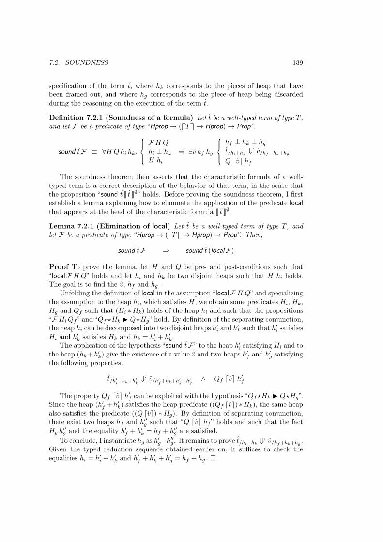
7.2. SOUNDNESS 139
specification of the term 𝑡, where ℎ𝑘 corresponds to the pieces of heap that havebeen framed out, and where ℎ𝑔 corresponds to the piece of heap being discardedduring the reasoning on the execution of the term 𝑡.
Definition 7.2.1 (Soundness of a formula) Let 𝑡 be a well-typed term of type 𝑇 ,and let ℱ be a predicate of type “Hprop → (V𝑇W → Hprop) → Prop”.
sound 𝑡ℱ ≡ ∀𝐻 𝑄ℎ𝑖 ℎ𝑘.
ℱ 𝐻 𝑄ℎ𝑖 ⊥ ℎ𝑘𝐻 ℎ𝑖
⇒ ∃𝑣 ℎ𝑓 ℎ𝑔.
ℎ𝑓 ⊥ ℎ𝑘 ⊥ ℎ𝑔𝑡/ℎ𝑖+ℎ𝑘
⇓: 𝑣/ℎ𝑓+ℎ𝑘+ℎ𝑔
𝑄 ⌈𝑣⌉ ℎ𝑓
The soundness theorem then asserts that the characteristic formula of a well-typed term is a correct description of the behavior of that term, in the sense thatthe proposition “sound 𝑡 J 𝑡 K∅” holds. Before proving the soundness theorem, I firstestablish a lemma explaining how to eliminate the application of the predicate localthat appears at the head of the characteristic formula J 𝑡 K∅.
Lemma 7.2.1 (Elimination of local) Let 𝑡 be a well-typed term of type 𝑇 , andlet ℱ be a predicate of type “Hprop → (V𝑇W → Hprop) → Prop”. Then,
sound 𝑡ℱ ⇒ sound 𝑡 (localℱ)
Proof To prove the lemma, let 𝐻 and 𝑄 be pre- and post-conditions such that“ localℱ 𝐻 𝑄” holds and let ℎ𝑖 and ℎ𝑘 be two disjoint heaps such that 𝐻 ℎ𝑖 holds.The goal is to find the 𝑣, ℎ𝑓 and ℎ𝑔.
Unfolding the definition of local in the assumption “ localℱ 𝐻 𝑄” and specializingthe assumption to the heap ℎ𝑖, which satisfies 𝐻, we obtain some predicates 𝐻𝑖, 𝐻𝑘,𝐻𝑔 and 𝑄𝑓 such that (𝐻𝑖 *𝐻𝑘) holds of the heap ℎ𝑖 and such that the propositions“ℱ 𝐻𝑖𝑄𝑓 ” and “𝑄𝑓 ⋆𝐻𝑘 I 𝑄⋆𝐻𝑔” hold. By definition of the separating conjunction,the heap ℎ𝑖 can be decomposed into two disjoint heaps ℎ′𝑖 and ℎ′𝑘 such that ℎ′𝑖 satisfies𝐻𝑖 and ℎ′𝑘 satisfies 𝐻𝑘 and ℎ𝑘 = ℎ′𝑖 + ℎ′𝑘.
The application of the hypothesis “sound 𝑡ℱ” to the heap ℎ′𝑖 satisfying 𝐻𝑖 and tothe heap (ℎ𝑘 +ℎ′𝑘) give the existence of a value 𝑣 and two heaps ℎ′𝑓 and ℎ′𝑔 satisfyingthe following properties.
𝑡/ℎ′𝑖+ℎ𝑘+ℎ′
𝑘⇓: 𝑣/ℎ′
𝑓+ℎ𝑘+ℎ′
𝑘+ℎ′
𝑔∧ 𝑄𝑓 ⌈𝑣⌉ ℎ′𝑓
The property 𝑄𝑓 ⌈𝑣⌉ ℎ′𝑓 can be exploited with the hypothesis “𝑄𝑓 ⋆𝐻𝑘 I 𝑄⋆𝐻𝑔”.Since the heap (ℎ′𝑓 +ℎ′𝑘) satisfies the heap predicate ((𝑄𝑓 ⌈𝑣⌉) *𝐻𝑘), the same heapalso satisfies the predicate ((𝑄 ⌈𝑣⌉) *𝐻𝑔). By definition of separating conjunction,there exist two heaps ℎ𝑓 and ℎ′′𝑔 such that “𝑄 ⌈𝑣⌉ ℎ𝑓 ” holds and such that the fact𝐻𝑔 ℎ
′′𝑔 and the equality ℎ′𝑓 + ℎ′𝑘 = ℎ𝑓 + ℎ′′𝑔 are satisfied.
To conclude, I instantiate ℎ𝑔 as ℎ′𝑔+ℎ′′𝑔 . It remains to prove 𝑡/ℎ𝑖+ℎ𝑘⇓: 𝑣/ℎ𝑓+ℎ𝑘+ℎ𝑔
.Given the typed reduction sequence obtained earlier on, it suffices to check theequalities ℎ𝑖 = ℎ′𝑖 + ℎ′𝑘 and ℎ′𝑓 + ℎ′𝑘 + ℎ′𝑔 = ℎ𝑓 + ℎ𝑔. �
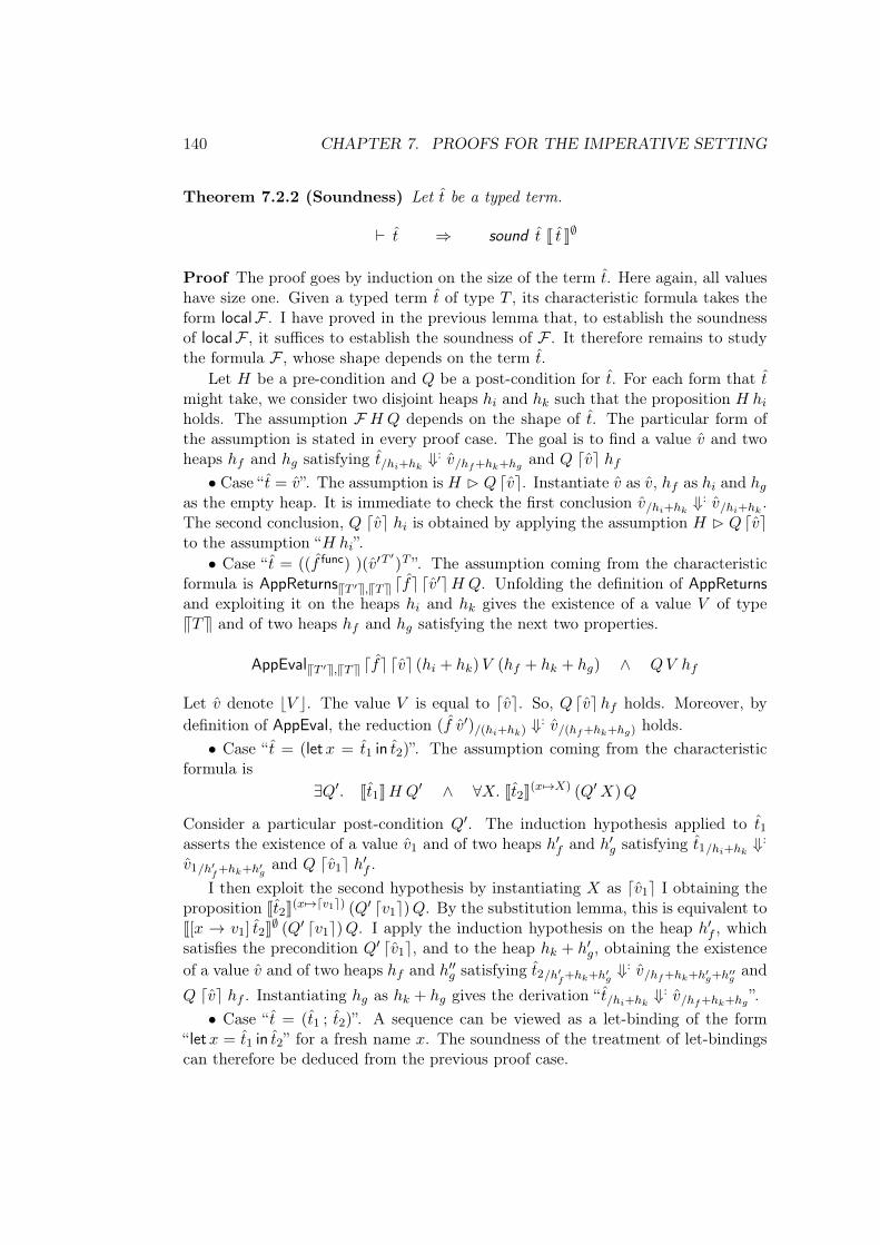
140 CHAPTER 7. PROOFS FOR THE IMPERATIVE SETTING
Theorem 7.2.2 (Soundness) Let 𝑡 be a typed term.
⊢ 𝑡 ⇒ sound 𝑡 J 𝑡 K∅
Proof The proof goes by induction on the size of the term 𝑡. Here again, all valueshave size one. Given a typed term 𝑡 of type 𝑇 , its characteristic formula takes theform localℱ . I have proved in the previous lemma that, to establish the soundnessof localℱ , it suffices to establish the soundness of ℱ . It therefore remains to studythe formula ℱ , whose shape depends on the term 𝑡.
Let 𝐻 be a pre-condition and 𝑄 be a post-condition for 𝑡. For each form that 𝑡might take, we consider two disjoint heaps ℎ𝑖 and ℎ𝑘 such that the proposition 𝐻 ℎ𝑖holds. The assumption ℱ 𝐻 𝑄 depends on the shape of 𝑡. The particular form ofthe assumption is stated in every proof case. The goal is to find a value 𝑣 and twoheaps ℎ𝑓 and ℎ𝑔 satisfying 𝑡/ℎ𝑖+ℎ𝑘
⇓: 𝑣/ℎ𝑓+ℎ𝑘+ℎ𝑔and 𝑄 ⌈𝑣⌉ ℎ𝑓
∙ Case “𝑡 = 𝑣”. The assumption is 𝐻 B 𝑄 ⌈𝑣⌉. Instantiate 𝑣 as 𝑣, ℎ𝑓 as ℎ𝑖 and ℎ𝑔as the empty heap. It is immediate to check the first conclusion 𝑣/ℎ𝑖+ℎ𝑘
⇓: 𝑣/ℎ𝑖+ℎ𝑘.
The second conclusion, 𝑄 ⌈𝑣⌉ ℎ𝑖 is obtained by applying the assumption 𝐻 B 𝑄 ⌈𝑣⌉to the assumption “𝐻 ℎ𝑖”.
∙ Case “𝑡 = ((𝑓 func) )(𝑣′𝑇′)𝑇 ”. The assumption coming from the characteristic
formula is AppReturnsV𝑇 ′W,V𝑇W ⌈𝑓⌉ ⌈𝑣′⌉𝐻 𝑄. Unfolding the definition of AppReturnsand exploiting it on the heaps ℎ𝑖 and ℎ𝑘 gives the existence of a value 𝑉 of typeV𝑇W and of two heaps ℎ𝑓 and ℎ𝑔 satisfying the next two properties.
AppEvalV𝑇 ′W,V𝑇W ⌈𝑓⌉ ⌈𝑣⌉ (ℎ𝑖 + ℎ𝑘)𝑉 (ℎ𝑓 + ℎ𝑘 + ℎ𝑔) ∧ 𝑄𝑉 ℎ𝑓
Let 𝑣 denote ⌊𝑉 ⌋. The value 𝑉 is equal to ⌈𝑣⌉. So, 𝑄 ⌈𝑣⌉ℎ𝑓 holds. Moreover, bydefinition of AppEval, the reduction (𝑓 𝑣′)/(ℎ𝑖+ℎ𝑘) ⇓
: 𝑣/(ℎ𝑓+ℎ𝑘+ℎ𝑔) holds.∙ Case “𝑡 = (let𝑥 = 𝑡1 in 𝑡2)”. The assumption coming from the characteristic
formula is∃𝑄′. J𝑡1K𝐻 𝑄′ ∧ ∀𝑋. J𝑡2K(𝑥 ↦→𝑋) (𝑄′𝑋)𝑄
Consider a particular post-condition 𝑄′. The induction hypothesis applied to 𝑡1asserts the existence of a value 𝑣1 and of two heaps ℎ′𝑓 and ℎ′𝑔 satisfying 𝑡1/ℎ𝑖+ℎ𝑘
⇓:
𝑣1/ℎ′𝑓+ℎ𝑘+ℎ′
𝑔and 𝑄 ⌈𝑣1⌉ ℎ′𝑓 .
I then exploit the second hypothesis by instantiating 𝑋 as ⌈𝑣1⌉ I obtaining theproposition J𝑡2K(𝑥 ↦→⌈𝑣1⌉) (𝑄′ ⌈𝑣1⌉)𝑄. By the substitution lemma, this is equivalent toJ[𝑥 → 𝑣1] 𝑡2K∅ (𝑄′ ⌈𝑣1⌉)𝑄. I apply the induction hypothesis on the heap ℎ′𝑓 , whichsatisfies the precondition 𝑄′ ⌈𝑣1⌉, and to the heap ℎ𝑘 + ℎ′𝑔, obtaining the existenceof a value 𝑣 and of two heaps ℎ𝑓 and ℎ′′𝑔 satisfying 𝑡2/ℎ′
𝑓+ℎ𝑘+ℎ′
𝑔⇓: 𝑣/ℎ𝑓+ℎ𝑘+ℎ′
𝑔+ℎ′′𝑔
and𝑄 ⌈𝑣⌉ ℎ𝑓 . Instantiating ℎ𝑔 as ℎ𝑘 + ℎ𝑔 gives the derivation “𝑡/ℎ𝑖+ℎ𝑘
⇓: 𝑣/ℎ𝑓+ℎ𝑘+ℎ𝑔”.
∙ Case “𝑡 = (𝑡1 ; 𝑡2)”. A sequence can be viewed as a let-binding of the form“ let𝑥 = 𝑡1 in 𝑡2” for a fresh name 𝑥. The soundness of the treatment of let-bindingscan therefore be deduced from the previous proof case.
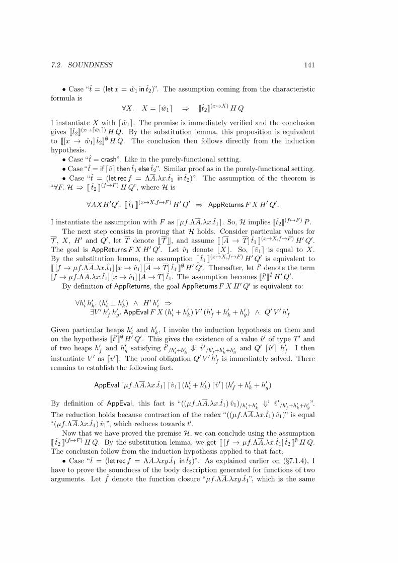
7.2. SOUNDNESS 141
∙ Case “𝑡 = (let𝑥 = �̂�1 in 𝑡2)”. The assumption coming from the characteristicformula is
∀𝑋. 𝑋 = ⌈�̂�1⌉ ⇒ J𝑡2K(𝑥 ↦→𝑋)𝐻 𝑄
I instantiate 𝑋 with ⌈�̂�1⌉. The premise is immediately verified and the conclusiongives J𝑡2K(𝑥 ↦→⌈�̂�1⌉)𝐻 𝑄. By the substitution lemma, this proposition is equivalentto J[𝑥 → �̂�1] 𝑡2K∅𝐻 𝑄. The conclusion then follows directly from the inductionhypothesis.
∙ Case “𝑡 = crash”. Like in the purely-functional setting.∙ Case “𝑡 = if ⌈𝑣⌉ then 𝑡1 else 𝑡2”. Similar proof as in the purely-functional setting.∙ Case “𝑡 = (let rec 𝑓 = Λ𝐴.𝜆𝑥.𝑡1 in 𝑡2)”. The assumption of the theorem is
“∀𝐹. ℋ ⇒ J 𝑡2 K(𝑓 ↦→𝐹 )𝐻 𝑄”, where ℋ is
∀𝐴𝑋𝐻 ′𝑄′. J 𝑡1 K(𝑥 ↦→𝑋,𝑓 ↦→𝐹 )𝐻 ′𝑄′ ⇒ AppReturns𝐹 𝑋 𝐻 ′𝑄′.
I instantiate the assumption with 𝐹 as ⌈𝜇𝑓.Λ𝐴.𝜆𝑥.𝑡1⌉. So, ℋ implies J𝑡2K(𝑓 ↦→𝐹 ) 𝑃 .The next step consists in proving that ℋ holds. Consider particular values for
𝒯 , 𝑋, 𝐻 ′ and 𝑄′, let 𝑇 denote T𝒯 U, and assume J [𝐴 → 𝑇 ] 𝑡1 K(𝑥 ↦→𝑋,𝑓 ↦→𝐹 )𝐻 ′𝑄′.The goal is AppReturns𝐹 𝑋 𝐻 ′𝑄′. Let 𝑣1 denote ⌊𝑋⌋. So, ⌈𝑣1⌉ is equal to 𝑋.By the substitution lemma, the assumption J 𝑡1 K(𝑥 ↦→𝑋,𝑓 ↦→𝐹 )𝐻 ′𝑄′ is equivalent toJ [𝑓 → 𝜇𝑓.Λ𝐴.𝜆𝑥.𝑡1] [𝑥 → 𝑣1] [𝐴 → 𝑇 ] 𝑡1 K∅𝐻 ′𝑄′. Thereafter, let 𝑡′ denote the term[𝑓 → 𝜇𝑓.Λ𝐴.𝜆𝑥.𝑡1] [𝑥 → 𝑣1] [𝐴 → 𝑇 ] 𝑡1. The assumption becomes J𝑡′K∅𝐻 ′𝑄′.
By definition of AppReturns, the goal AppReturns𝐹 𝑋 𝐻 ′𝑄′ is equivalent to:
∀ℎ′𝑖 ℎ′𝑘. (ℎ′𝑖 ⊥ ℎ′𝑘) ∧ 𝐻 ′ ℎ′𝑖 ⇒∃𝑉 ′ ℎ′𝑓 ℎ
′𝑔. AppEval𝐹 𝑋 (ℎ′𝑖 + ℎ′𝑘)𝑉 ′ (ℎ′𝑓 + ℎ′𝑘 + ℎ′𝑔) ∧ 𝑄′ 𝑉 ′ ℎ′𝑓
Given particular heaps ℎ′𝑖 and ℎ′𝑘, I invoke the induction hypothesis on them andon the hypothesis J𝑡′K∅𝐻 ′𝑄′. This gives the existence of a value 𝑣′ of type 𝑇 ′ andof two heaps ℎ′𝑓 and ℎ′𝑔 satisfying 𝑡′/ℎ′
𝑖+ℎ′𝑘⇓: 𝑣′/ℎ′
𝑓+ℎ′
𝑘+ℎ′
𝑔and 𝑄′ ⌈𝑣′⌉ ℎ′𝑓 . I then
instantiate 𝑉 ′ as ⌈𝑣′⌉. The proof obligation 𝑄′ 𝑉 ′ ℎ′𝑓 is immediately solved. Thereremains to establish the following fact.
AppEval ⌈𝜇𝑓.Λ𝐴.𝜆𝑥.𝑡1⌉ ⌈𝑣1⌉ (ℎ′𝑖 + ℎ′𝑘) ⌈𝑣′⌉ (ℎ′𝑓 + ℎ′𝑘 + ℎ′𝑔)
By definition of AppEval, this fact is “((𝜇𝑓.Λ𝐴.𝜆𝑥.𝑡1) 𝑣1)/ℎ′𝑖+ℎ′
𝑘⇓: 𝑣′/ℎ′
𝑓+ℎ′
𝑘+ℎ′
𝑔”.
The reduction holds because contraction of the redex “((𝜇𝑓.Λ𝐴.𝜆𝑥.𝑡1) 𝑣1)” is equal“(𝜇𝑓.Λ𝐴.𝜆𝑥.𝑡1) 𝑣1”, which reduces towards 𝑡′.
Now that we have proved the premise ℋ, we can conclude using the assumptionJ 𝑡2 K(𝑓 ↦→𝐹 )𝐻 𝑄. By the substitution lemma, we get J [𝑓 → 𝜇𝑓.Λ𝐴.𝜆𝑥.𝑡1] 𝑡2 K∅𝐻 𝑄.The conclusion follow from the induction hypothesis applied to that fact.
∙ Case “𝑡 = (let rec 𝑓 = Λ𝐴.𝜆𝑥𝑦.𝑡1 in 𝑡2)”. As explained earlier on (§7.1.4), Ihave to prove the soundness of the body description generated for functions of twoarguments. Let 𝑓 denote the function closure “𝜇𝑓.Λ𝐴.𝜆𝑥𝑦.𝑡1”, which is the same
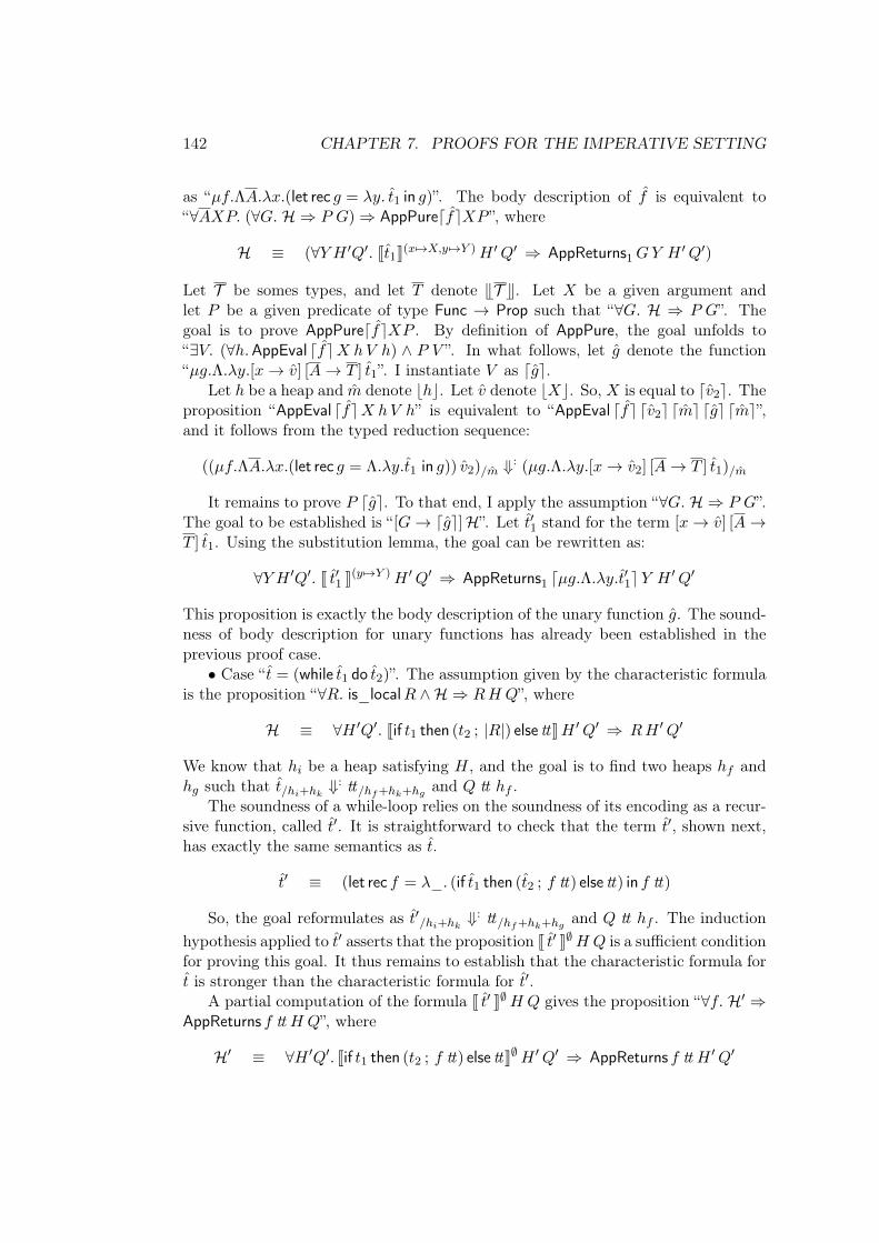
142 CHAPTER 7. PROOFS FOR THE IMPERATIVE SETTING
as “𝜇𝑓.Λ𝐴.𝜆𝑥.(let rec 𝑔 = 𝜆𝑦. 𝑡1 in 𝑔)”. The body description of 𝑓 is equivalent to“∀𝐴𝑋𝑃. (∀𝐺. ℋ ⇒ 𝑃 𝐺) ⇒ AppPure⌈𝑓⌉𝑋𝑃 ”, where
ℋ ≡ (∀𝑌 𝐻 ′𝑄′. J𝑡1K(𝑥 ↦→𝑋,𝑦 ↦→𝑌 )𝐻 ′𝑄′ ⇒ AppReturns1𝐺𝑌 𝐻 ′𝑄′)
Let 𝒯 be somes types, and let 𝑇 denote T𝒯 U. Let 𝑋 be a given argument andlet 𝑃 be a given predicate of type Func → Prop such that “∀𝐺. ℋ ⇒ 𝑃 𝐺”. Thegoal is to prove AppPure⌈𝑓⌉𝑋𝑃 . By definition of AppPure, the goal unfolds to“∃𝑉. (∀ℎ.AppEval ⌈𝑓⌉𝑋 ℎ𝑉 ℎ) ∧ 𝑃 𝑉 ”. In what follows, let 𝑔 denote the function“𝜇𝑔.Λ.𝜆𝑦.[𝑥 → 𝑣] [𝐴 → 𝑇 ] 𝑡1”. I instantiate 𝑉 as ⌈𝑔⌉.
Let ℎ be a heap and �̂� denote ⌊ℎ⌋. Let 𝑣 denote ⌊𝑋⌋. So, 𝑋 is equal to ⌈𝑣2⌉. Theproposition “AppEval ⌈𝑓⌉𝑋 ℎ𝑉 ℎ” is equivalent to “AppEval ⌈𝑓⌉ ⌈𝑣2⌉ ⌈�̂�⌉ ⌈𝑔⌉ ⌈�̂�⌉”,and it follows from the typed reduction sequence:
((𝜇𝑓.Λ𝐴.𝜆𝑥.(let rec 𝑔 = Λ.𝜆𝑦.𝑡1 in 𝑔)) 𝑣2)/�̂� ⇓: (𝜇𝑔.Λ.𝜆𝑦.[𝑥 → 𝑣2] [𝐴 → 𝑇 ] 𝑡1)/�̂�
It remains to prove 𝑃 ⌈𝑔⌉. To that end, I apply the assumption “∀𝐺. ℋ ⇒ 𝑃 𝐺”.The goal to be established is “[𝐺 → ⌈𝑔⌉]ℋ”. Let 𝑡′1 stand for the term [𝑥 → 𝑣] [𝐴 →𝑇 ] 𝑡1. Using the substitution lemma, the goal can be rewritten as:
∀𝑌 𝐻 ′𝑄′. J 𝑡′1 K(𝑦 ↦→𝑌 )𝐻 ′𝑄′ ⇒ AppReturns1 ⌈𝜇𝑔.Λ.𝜆𝑦.𝑡′1⌉𝑌 𝐻 ′𝑄′
This proposition is exactly the body description of the unary function 𝑔. The sound-ness of body description for unary functions has already been established in theprevious proof case.
∙ Case “𝑡 = (while 𝑡1 do 𝑡2)”. The assumption given by the characteristic formulais the proposition “∀𝑅. is_local𝑅 ∧ℋ ⇒ 𝑅𝐻 𝑄”, where
ℋ ≡ ∀𝐻 ′𝑄′. Jif 𝑡1 then (𝑡2 ; |𝑅|) else ttK𝐻 ′𝑄′ ⇒ 𝑅𝐻 ′𝑄′
We know that ℎ𝑖 be a heap satisfying 𝐻, and the goal is to find two heaps ℎ𝑓 andℎ𝑔 such that 𝑡/ℎ𝑖+ℎ𝑘
⇓: tt/ℎ𝑓+ℎ𝑘+ℎ𝑔and 𝑄 tt ℎ𝑓 .
The soundness of a while-loop relies on the soundness of its encoding as a recur-sive function, called 𝑡′. It is straightforward to check that the term 𝑡′, shown next,has exactly the same semantics as 𝑡.
𝑡′ ≡ (let rec 𝑓 = 𝜆_. (if 𝑡1 then (𝑡2 ; 𝑓 tt) else tt) in 𝑓 tt)
So, the goal reformulates as 𝑡′/ℎ𝑖+ℎ𝑘⇓: tt/ℎ𝑓+ℎ𝑘+ℎ𝑔
and 𝑄 tt ℎ𝑓 . The inductionhypothesis applied to 𝑡′ asserts that the proposition J 𝑡′ K∅𝐻 𝑄 is a sufficient conditionfor proving this goal. It thus remains to establish that the characteristic formula for𝑡 is stronger than the characteristic formula for 𝑡′.
A partial computation of the formula J 𝑡′ K∅𝐻 𝑄 gives the proposition “∀𝑓. ℋ′ ⇒AppReturns 𝑓 tt 𝐻 𝑄”, where
ℋ′ ≡ ∀𝐻 ′𝑄′. Jif 𝑡1 then (𝑡2 ; 𝑓 tt) else ttK∅𝐻 ′𝑄′ ⇒ AppReturns 𝑓 tt 𝐻 ′𝑄′
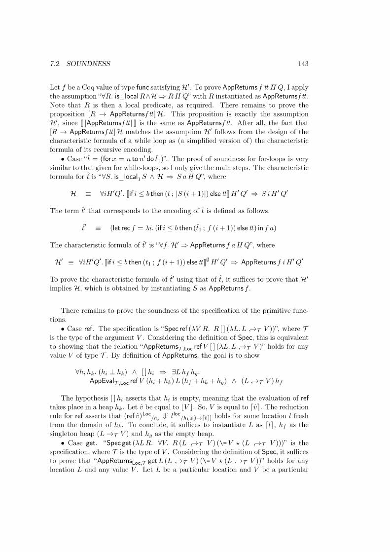
7.2. SOUNDNESS 143
Let 𝑓 be a Coq value of type func satisfying ℋ′. To prove AppReturns 𝑓 tt 𝐻 𝑄, I applythe assumption “∀𝑅. is_local𝑅∧ℋ ⇒ 𝑅𝐻 𝑄” with 𝑅 instantiated as AppReturns𝑓 tt .Note that 𝑅 is then a local predicate, as required. There remains to prove theproposition [𝑅 → AppReturns𝑓 tt ]ℋ. This proposition is exactly the assumptionℋ′, since J |AppReturns𝑓 tt | K is the same as AppReturns𝑓 tt . After all, the fact that[𝑅 → AppReturns𝑓 tt ]ℋ matches the assumption ℋ′ follows from the design of thecharacteristic formula of a while loop as (a simplified version of) the characteristicformula of its recursive encoding.
∙ Case “𝑡 = (for𝑥 = 𝑛 to𝑛′ do 𝑡1)”. The proof of soundness for for-loops is verysimilar to that given for while-loops, so I only give the main steps. The characteristicformula for 𝑡 is “∀𝑆. is_local1 𝑆 ∧ ℋ ⇒ 𝑆 𝑎𝐻 𝑄”, where
ℋ ≡ ∀𝑖𝐻 ′𝑄′. Jif 𝑖 ≤ 𝑏 then (𝑡 ; |𝑆 (𝑖 + 1)|) else ttK𝐻 ′𝑄′ ⇒ 𝑆 𝑖𝐻 ′𝑄′
The term 𝑡′ that corresponds to the encoding of 𝑡 is defined as follows.
𝑡′ ≡ (let rec 𝑓 = 𝜆𝑖. (if 𝑖 ≤ 𝑏 then (𝑡1 ; 𝑓 (𝑖 + 1)) else tt) in 𝑓 𝑎)
The characteristic formula of 𝑡′ is “∀𝑓. ℋ′ ⇒ AppReturns 𝑓 𝑎𝐻 𝑄”, where
ℋ′ ≡ ∀𝑖𝐻 ′𝑄′. Jif 𝑖 ≤ 𝑏 then (𝑡1 ; 𝑓 (𝑖 + 1)) else ttK∅𝐻 ′𝑄′ ⇒ AppReturns 𝑓 𝑖𝐻 ′𝑄′
To prove the characteristic formula of 𝑡′ using that of 𝑡, it suffices to prove that ℋ′
implies ℋ, which is obtained by instantiating 𝑆 as AppReturns 𝑓 .
There remains to prove the soundness of the specification of the primitive func-tions.
∙ Case ref. The specification is “Spec ref (𝜆𝑉 𝑅. 𝑅 [ ] (𝜆𝐿.𝐿 →˓𝒯 𝑉 ))”, where 𝒯is the type of the argument 𝑉 . Considering the definition of Spec, this is equivalentto showing that the relation “AppReturns𝒯 ,Loc ref𝑉 [ ] (𝜆𝐿.𝐿 →˓𝒯 𝑉 )” holds for anyvalue 𝑉 of type 𝒯 . By definition of AppReturns, the goal is to show
∀ℎ𝑖 ℎ𝑘. (ℎ𝑖 ⊥ ℎ𝑘) ∧ [ ]ℎ𝑖 ⇒ ∃𝐿ℎ𝑓 ℎ𝑔.AppEval𝒯 ,Loc ref𝑉 (ℎ𝑖 + ℎ𝑘)𝐿 (ℎ𝑓 + ℎ𝑘 + ℎ𝑔) ∧ (𝐿 →˓𝒯 𝑉 )ℎ𝑓
The hypothesis [ ]ℎ𝑖 asserts that ℎ𝑖 is empty, meaning that the evaluation of reftakes place in a heap ℎ𝑘. Let 𝑣 be equal to ⌊𝑉 ⌋. So, 𝑉 is equal to ⌈𝑣⌉. The reductionrule for ref asserts that (ref 𝑣)Loc
/ℎ𝑘⇓: 𝑙 loc
/ℎ𝑘⊎[𝑙 ↦→⌈𝑣⌉] holds for some location 𝑙 freshfrom the domain of ℎ𝑘. To conclude, it suffices to instantiate 𝐿 as ⌈𝑙⌉, ℎ𝑓 as thesingleton heap (𝐿 →𝒯 𝑉 ) and ℎ𝑔 as the empty heap.
∙ Case get. “Spec get (𝜆𝐿𝑅. ∀𝑉. 𝑅 (𝐿 →˓𝒯 𝑉 ) (\=𝑉 ⋆ (𝐿 →˓𝒯 𝑉 )))” is thespecification, where 𝒯 is the type of 𝑉 . Considering the definition of Spec, it sufficesto prove that “AppReturnsLoc,𝒯 get𝐿 (𝐿 →˓𝒯 𝑉 ) (\=𝑉 ⋆ (𝐿 →˓𝒯 𝑉 ))” holds for anylocation 𝐿 and any value 𝑉 . Let 𝐿 be a particular location and 𝑉 be a particular
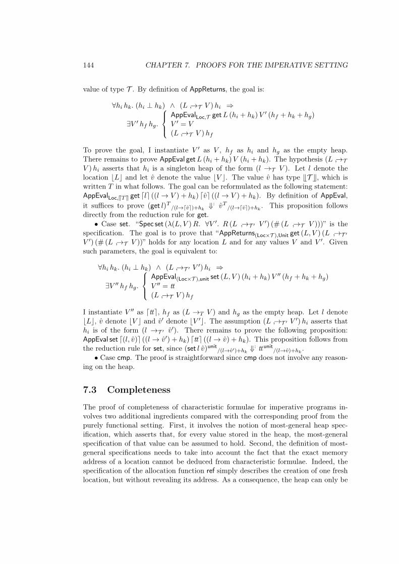
144 CHAPTER 7. PROOFS FOR THE IMPERATIVE SETTING
value of type 𝒯 . By definition of AppReturns, the goal is:
∀ℎ𝑖 ℎ𝑘. (ℎ𝑖 ⊥ ℎ𝑘) ∧ (𝐿 →˓𝒯 𝑉 )ℎ𝑖 ⇒
∃𝑉 ′ ℎ𝑓 ℎ𝑔.
AppEvalLoc,𝒯 get𝐿 (ℎ𝑖 + ℎ𝑘)𝑉 ′ (ℎ𝑓 + ℎ𝑘 + ℎ𝑔)
𝑉 ′ = 𝑉(𝐿 →˓𝒯 𝑉 )ℎ𝑓
To prove the goal, I instantiate 𝑉 ′ as 𝑉 , ℎ𝑓 as ℎ𝑖 and ℎ𝑔 as the empty heap.There remains to prove AppEval get𝐿 (ℎ𝑖 + ℎ𝑘)𝑉 (ℎ𝑖 + ℎ𝑘). The hypothesis (𝐿 →˓𝒯𝑉 )ℎ𝑖 asserts that ℎ𝑖 is a singleton heap of the form (𝑙 →𝒯 𝑉 ). Let 𝑙 denote thelocation ⌊𝐿⌋ and let 𝑣 denote the value ⌊𝑉 ⌋. The value 𝑣 has type T𝒯 U, which iswritten 𝑇 in what follows. The goal can be reformulated as the following statement:AppEvalLoc,V𝑇W get ⌈𝑙⌉ ((𝑙 → 𝑉 ) + ℎ𝑘) ⌈𝑣⌉ ((𝑙 → 𝑉 ) + ℎ𝑘). By definition of AppEval,it suffices to prove (get 𝑙)𝑇 /(𝑙→⌈𝑣⌉)+ℎ𝑘
⇓: 𝑣𝑇 /(𝑙→⌈𝑣⌉)+ℎ𝑘. This proposition follows
directly from the reduction rule for get.∙ Case set. “Spec set (𝜆(𝐿, 𝑉 )𝑅. ∀𝑉 ′. 𝑅 (𝐿 →˓𝒯 ′ 𝑉 ′) (# (𝐿 →˓𝒯 𝑉 )))” is the
specification. The goal is to prove that “AppReturns(Loc×𝒯 ),Unit get (𝐿, 𝑉 ) (𝐿 →˓𝒯 ′
𝑉 ′) (# (𝐿 →˓𝒯 𝑉 ))” holds for any location 𝐿 and for any values 𝑉 and 𝑉 ′. Givensuch parameters, the goal is equivalent to:
∀ℎ𝑖 ℎ𝑘. (ℎ𝑖 ⊥ ℎ𝑘) ∧ (𝐿 →˓𝒯 ′ 𝑉 ′)ℎ𝑖 ⇒
∃𝑉 ′′ ℎ𝑓 ℎ𝑔.
AppEval(Loc×𝒯 ),unit set (𝐿, 𝑉 ) (ℎ𝑖 + ℎ𝑘)𝑉 ′′ (ℎ𝑓 + ℎ𝑘 + ℎ𝑔)
𝑉 ′′ = tt(𝐿 →˓𝒯 𝑉 )ℎ𝑓
I instantiate 𝑉 ′′ as ⌈tt⌉, ℎ𝑓 as (𝐿 →𝑇 𝑉 ) and ℎ𝑔 as the empty heap. Let 𝑙 denote⌊𝐿⌋, 𝑣 denote ⌊𝑉 ⌋ and 𝑣′ denote ⌊𝑉 ′⌋. The assumption (𝐿 →˓𝒯 ′ 𝑉 ′)ℎ𝑖 asserts thatℎ𝑖 is of the form (𝑙 →𝒯 ′ 𝑣′). There remains to prove the following proposition:AppEval set ⌈(𝑙, 𝑣)⌉ ((𝑙 → 𝑣′) + ℎ𝑘) ⌈tt⌉ ((𝑙 → 𝑣) + ℎ𝑘). This proposition follows fromthe reduction rule for set, since (set 𝑙 𝑣)unit
/(𝑙→𝑣′)+ℎ𝑘⇓: tt unit
/(𝑙→𝑣)+ℎ𝑘.
∙ Case cmp. The proof is straightforward since cmp does not involve any reason-ing on the heap.
7.3 Completeness
The proof of completeness of characteristic formulae for imperative programs in-volves two additional ingredients compared with the corresponding proof from thepurely functional setting. First, it involves the notion of most-general heap spec-ification, which asserts that, for every value stored in the heap, the most-generalspecification of that value can be assumed to hold. Second, the definition of most-general specifications needs to take into account the fact that the exact memoryaddress of a location cannot be deduced from characteristic formulae. Indeed, thespecification of the allocation function ref simply describes the creation of one freshlocation, but without revealing its address. As a consequence, the heap can only be
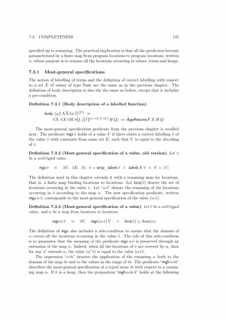
7.3. COMPLETENESS 145
specified up to renaming. The practical implication is that all the predicates becomeparameterized by a finite map from program locations to program locations, written𝛼, whose purpose is to rename all the locations occurring in values, terms and heaps.
7.3.1 Most-general specifications
The notion of labelling of terms and the definition of correct labelling with respectto a set 𝐸 of values of type Func are the same as in the previous chapter. Thedefinition of body description is also the the same as before, except that it includesa pre-condition.
Definition 7.3.1 (Body description of a labelled function)
body (𝜇𝑓.Λ𝐴.𝜆𝑥.𝑡){𝐹} ≡∀𝐴. ∀𝑋.∀𝐻.∀𝑄. (J 𝑡 K(𝑥 ↦→𝑋,𝑓 ↦→𝐹 )𝐻 𝑄) ⇒ AppReturns𝐹 𝑋 𝐻 𝑄
The most-general specification predicate from the previous chapter is recallednext. The predicate mgs 𝑣 holds of a value 𝑉 if there exists a correct labelling 𝑣 ofthe value 𝑣 with constants from some set 𝐸, such that 𝑉 is equal to the decodingof 𝑣.
Definition 7.3.2 (Most-general specification of a value, old version) Let 𝑣be a well-typed value.
mgs 𝑣 ≡ 𝜆𝑉. ∃𝐸. ∃𝑣. 𝑣 = strip_labels 𝑣 ∧ labels 𝐸 𝑣 ∧ 𝑉 = ⌈𝑣⌉
The definition used in this chapter extends it with a renaming map for locations,that is, a finite map binding locations to locations. Let locs(𝑣) denote the set oflocations occurring in the value 𝑣. Let “𝛼 𝑣” denote the renaming of the locationsoccurring in 𝑣 according to the map 𝛼. The new specification predicate, writtenmgv 𝛼 𝑣, corresponds to the most-general specification of the value (𝛼 𝑣).
Definition 7.3.3 (Most-general specification of a value) Let 𝑣 be a well-typedvalue, and 𝛼 be a map from locations to locations.
mgv 𝛼 𝑣 ≡ 𝜆𝑉. mgs (𝛼 𝑣)𝑉 ∧ locs(𝑣) ⊆ dom(𝛼)
The definition of mgv also includes a side-condition to ensure that the domain of𝛼 covers all the locations occurring in the value 𝑣. The role of this side-conditionis to guarantee that the meaning of the predicate mgv 𝛼 𝑣 is preserved through anextension of the map 𝛼. Indeed, when all the locations of 𝑣 are covered by 𝛼, thenfor any 𝛼′ extends 𝛼, the value (𝛼′ 𝑣) is equal to the value (𝛼 𝑣).
The expression “𝛼 �̂�” denotes the application of the renaming 𝛼 both to thedomain of the map �̂� and to the values in the range of �̂�. The predicate “mgh𝛼 �̂�”describes the most-general specification of a typed store �̂� with respect to a renam-ing map 𝛼. If ℎ is a heap, then the proposition “mgh𝛼 �̂�ℎ” holds at the following
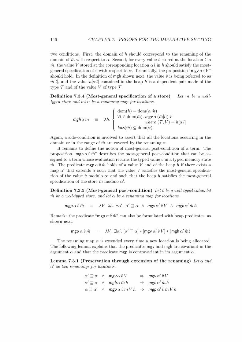
146 CHAPTER 7. PROOFS FOR THE IMPERATIVE SETTING
two conditions. First, the domain of ℎ should correspond to the renaming of thedomain of �̂� with respect to 𝛼. Second, for every value 𝑣 stored at the location 𝑙 in�̂�, the value 𝑉 stored at the corresponding location 𝛼 𝑙 in ℎ should satisfy the most-general specification of 𝑣 with respect to 𝛼. Technically, the proposition “mgv 𝛼 𝑣𝑉 ”should hold. In the definition of mgh shown next, the value 𝑣 is being referred to as�̂�[𝑙], and the value ℎ[𝛼 𝑙] contained in the heap ℎ is a dependent pair made of thetype 𝒯 and of the value 𝑉 of type 𝒯 .
Definition 7.3.4 (Most-general specification of a store) Let 𝑚 be a well-typed store and let 𝛼 be a renaming map for locations.
mgh𝛼 �̂� ≡ 𝜆ℎ.
dom(ℎ) = dom(𝛼 �̂�)∀𝑙 ∈ dom(�̂�). mgv 𝛼 (�̂�[𝑙])𝑉
where (𝒯 , 𝑉 ) = ℎ[𝛼 𝑙]locs(�̂�) ⊆ dom(𝛼)
Again, a side-condition is involved to assert that all the locations occurring in thedomain or in the range of �̂� are covered by the renaming 𝛼.
It remains to define the notion of most-general post-condition of a term. Theproposition “mgp 𝛼 𝑣 �̂�” describes the most-general post-condition that can be as-signed to a term whose evaluation returns the typed value 𝑣 in a typed memory state�̂�. The predicate mgp 𝛼 𝑣 �̂� holds of a value 𝑉 and of the heap ℎ if there exists amap 𝛼′ that extends 𝛼 such that the value 𝑉 satisfies the most-general specifica-tion of the value 𝑣 modulo 𝛼′ and such that the heap ℎ satisfies the most-generalspecification of the store �̂� modulo 𝛼′.
Definition 7.3.5 (Most-general post-condition) Let 𝑣 be a well-typed value, let�̂� be a well-typed store, and let 𝛼 be a renaming map for locations.
mgp 𝛼 𝑣 �̂� ≡ 𝜆𝑉. 𝜆ℎ. ∃𝛼′. 𝛼′ ⊒ 𝛼 ∧ mgv 𝛼′ 𝑣 𝑉 ∧ mgh𝛼′ �̂� ℎ
Remark: the predicate “mgp 𝛼 𝑣 �̂�” can also be formulated with heap predicates, asshown next.
mgp 𝛼 𝑣 �̂� = 𝜆𝑉. ∃∃𝛼′. [𝛼′ ⊒ 𝛼] * [mgv 𝛼′ 𝑣 𝑉 ] * (mgh𝛼′ �̂�)
The renaming map 𝛼 is extended every time a new location is being allocated.The following lemma explains that the predicates mgv and mgh are covariant in theargument 𝛼 and that the predicate mgp is contravariant in its argument 𝛼.
Lemma 7.3.1 (Preservation through extension of the renaming) Let 𝛼 and𝛼′ be two renamings for locations.
𝛼′ ⊒ 𝛼 ∧ mgv 𝛼 𝑣 𝑉 ⇒ mgv 𝛼′ 𝑣 𝑉
𝛼′ ⊒ 𝛼 ∧ mgh𝛼 �̂�ℎ ⇒ mgh𝛼′ �̂� ℎ
𝛼 ⊒ 𝛼′ ∧ mgp 𝛼 𝑣 �̂� 𝑉 ℎ ⇒ mgp 𝛼′ 𝑣 �̂� 𝑉 ℎ
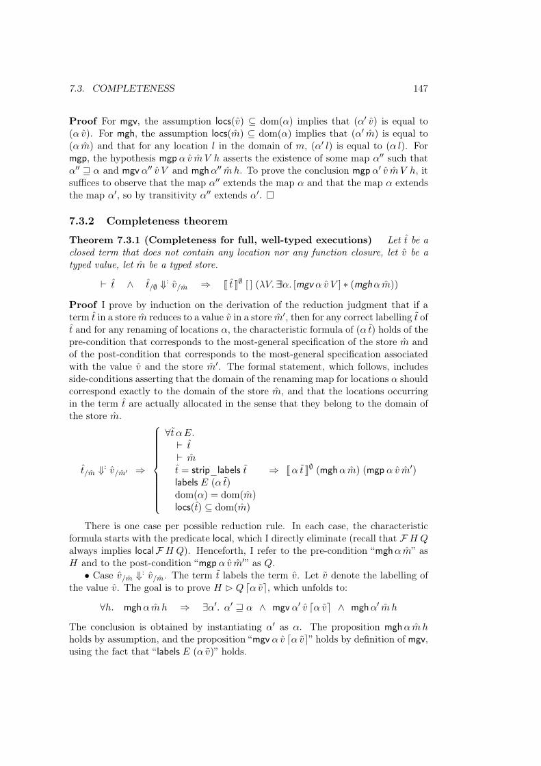
7.3. COMPLETENESS 147
Proof For mgv, the assumption locs(𝑣) ⊆ dom(𝛼) implies that (𝛼′ 𝑣) is equal to(𝛼 𝑣). For mgh, the assumption locs(�̂�) ⊆ dom(𝛼) implies that (𝛼′ �̂�) is equal to(𝛼 �̂�) and that for any location 𝑙 in the domain of 𝑚, (𝛼′ 𝑙) is equal to (𝛼 𝑙). Formgp, the hypothesis mgp 𝛼 𝑣 �̂� 𝑉 ℎ asserts the existence of some map 𝛼′′ such that𝛼′′ ⊒ 𝛼 and mgv 𝛼′′ 𝑣 𝑉 and mgh𝛼′′ �̂� ℎ. To prove the conclusion mgp 𝛼′ 𝑣 �̂� 𝑉 ℎ, itsuffices to observe that the map 𝛼′′ extends the map 𝛼 and that the map 𝛼 extendsthe map 𝛼′, so by transitivity 𝛼′′ extends 𝛼′. �
7.3.2 Completeness theorem
Theorem 7.3.1 (Completeness for full, well-typed executions) Let 𝑡 be aclosed term that does not contain any location nor any function closure, let 𝑣 be atyped value, let �̂� be a typed store.
⊢ 𝑡 ∧ 𝑡/∅ ⇓: 𝑣/�̂� ⇒ J 𝑡 K∅ [ ] (𝜆𝑉.∃∃𝛼. [mgv 𝛼 𝑣 𝑉 ] * (mgh𝛼 �̂�))
Proof I prove by induction on the derivation of the reduction judgment that if aterm 𝑡 in a store �̂� reduces to a value 𝑣 in a store �̂�′, then for any correct labelling 𝑡 of𝑡 and for any renaming of locations 𝛼, the characteristic formula of (𝛼 𝑡) holds of thepre-condition that corresponds to the most-general specification of the store �̂� andof the post-condition that corresponds to the most-general specification associatedwith the value 𝑣 and the store �̂�′. The formal statement, which follows, includesside-conditions asserting that the domain of the renaming map for locations 𝛼 shouldcorrespond exactly to the domain of the store �̂�, and that the locations occurringin the term 𝑡 are actually allocated in the sense that they belong to the domain ofthe store �̂�.
𝑡/�̂� ⇓: 𝑣/�̂�′ ⇒
∀𝑡 𝛼𝐸.
⊢ 𝑡⊢ �̂�
𝑡 = strip_labels 𝑡labels 𝐸 (𝛼 𝑡)dom(𝛼) = dom(�̂�)
locs(𝑡) ⊆ dom(�̂�)
⇒ J𝛼 𝑡 K∅ (mgh𝛼 �̂�) (mgp 𝛼 𝑣 �̂�′)
There is one case per possible reduction rule. In each case, the characteristicformula starts with the predicate local, which I directly eliminate (recall that ℱ 𝐻 𝑄always implies localℱ 𝐻 𝑄). Henceforth, I refer to the pre-condition “mgh𝛼 �̂�” as𝐻 and to the post-condition “mgp 𝛼 𝑣 �̂�′” as 𝑄.
∙ Case 𝑣/�̂� ⇓: 𝑣/�̂�. The term 𝑡 labels the term 𝑣. Let 𝑣 denote the labelling ofthe value 𝑣. The goal is to prove 𝐻 B 𝑄 ⌈𝛼 𝑣⌉, which unfolds to:
∀ℎ. mgh𝛼 �̂�ℎ ⇒ ∃𝛼′. 𝛼′ ⊒ 𝛼 ∧ mgv 𝛼′ 𝑣 ⌈𝛼 𝑣⌉ ∧ mgh𝛼′ �̂� ℎ
The conclusion is obtained by instantiating 𝛼′ as 𝛼. The proposition mgh𝛼 �̂�ℎholds by assumption, and the proposition “mgv 𝛼 𝑣 ⌈𝛼 𝑣⌉” holds by definition of mgv,using the fact that “ labels 𝐸 (𝛼 𝑣)” holds.
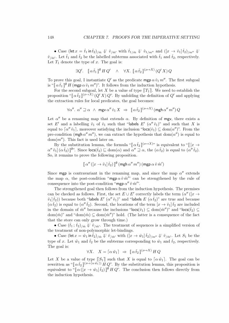
148 CHAPTER 7. PROOFS FOR THE IMPERATIVE SETTING
∙ Case (let𝑥 = 𝑡1 in 𝑡2)/�̂� ⇓: 𝑣/�̂�′ with 𝑡1/�̂� ⇓: 𝑣1/𝑚′′ and ([𝑥 → 𝑣1] 𝑡2)/𝑚′′ ⇓:
𝑣/�̂�′ . Let 𝑡1 and 𝑡2 be the labelled subterms associated with 𝑡1 and 𝑡2, respectively.Let 𝑇1 denote the type of 𝑥. The goal is:
∃𝑄′. J𝛼 𝑡1 K∅𝐻 𝑄′ ∧ ∀𝑋. J𝛼 𝑡2 K(𝑥↦→𝑋) (𝑄′𝑋)𝑄
To prove this goal, I instantiate 𝑄′ as the predicate mgp 𝛼 𝑣1𝑚′′. The first subgoal
is “J𝛼 𝑡1 K∅𝐻 (mgp 𝛼 𝑣1𝑚′′)”. It follows from the induction hypothesis.
For the second subgoal, let 𝑋 be a value of type V𝑇1W. We need to establish theproposition “J𝛼 𝑡2 K(𝑥 ↦→𝑋) (𝑄′𝑋)𝑄”. By unfolding the definition of 𝑄′ and applyingthe extraction rules for local predicates, the goal becomes:
∀𝛼′′. 𝛼′′ ⊒ 𝛼 ∧ mgv 𝛼′′ 𝑣1𝑋 ⇒ J𝛼 𝑡2 K(𝑥 ↦→𝑋) (mgh𝛼′′𝑚′′)𝑄
Let 𝛼′′ be a renaming map that extends 𝛼. By definition of mgv, there exists aset 𝐸′ and a labelling 𝑣1 of 𝑣1 such that “ labels 𝐸′ (𝛼′′ 𝑣1)” and such that 𝑋 isequal to ⌈𝛼′′ 𝑣1⌉, moreover satisfying the inclusion “ locs(𝑣1) ⊆ dom(𝛼′′)”. From thepre-condition (mgh𝛼′′𝑚′′), we can extract the hypothesis that dom(𝛼′′) is equal todom(𝑚′′). This fact is used later on.
By the substitution lemma, the formula “J𝛼 𝑡2 K(𝑥 ↦→𝑋)” is equivalent to “J [𝑥 →𝛼′′ 𝑣1] (𝛼 𝑡2) K∅”. Since locs(𝑡2) ⊑ dom(𝛼) and 𝛼′′ ⊒ 𝛼, the (𝛼 𝑡2) is equal to (𝛼′′ 𝑡2).So, it remains to prove the following proposition.
J𝛼′′ ([𝑥 → 𝑣1] 𝑡2) K∅ (mgh𝛼′′𝑚′′) (mgp 𝛼 𝑣 �̂�′)
Since mgp is contravariant in the renaming map, and since the map 𝛼′′ extendsthe map 𝛼, the post-condition “mgp 𝛼 𝑣 �̂�′” can be strengthened by the rule ofconsequence into the post-condition “mgp 𝛼′′ 𝑣 �̂�′”.
The strengthened goal then follows from the induction hypothesis. The premisescan be checked as follows. First, the set 𝐸 ∪ 𝐸′ correctly labels the term (𝛼′′ ([𝑥 →𝑣1] 𝑡2)) because both “ labels 𝐸′ (𝛼′′ 𝑣1)” and “ labels 𝐸 (𝛼 𝑡2)” are true and because(𝛼 𝑡2) is equal to (𝛼′′ 𝑡2). Second, the locations of the term [𝑥 → 𝑣1] 𝑡2 are includedin the domain of �̂�′′ because the inclusions “ locs(𝑣1) ⊆ dom(�̂�′′)” and “ locs(𝑡2) ⊆dom(�̂�)” and “dom(�̂�) ⊆ dom(�̂�′′)” hold. (The latter is a consequence of the factthat the store can only grow through time.)
∙ Case (𝑡1 ; 𝑡2)/�̂� ⇓: 𝑣/�̂�′ . The treatment of sequences is a simplified version ofthe treatment of non-polymorphic let-bindings.
∙ Case (let𝑥 = �̂�1 in 𝑡2)/�̂� ⇓: 𝑣/�̂�′ with ([𝑥 → �̂�1] 𝑡2)/𝑚′′ ⇓: 𝑣/�̂�′ . Let 𝑆1 be thetype of 𝑥. Let �̃�1 and 𝑡2 be the subterms corresponding to �̂�1 and 𝑡2, respectively.The goal is:
∀𝑋. 𝑋 = ⌈𝛼 �̃�1⌉ ⇒ J𝛼 𝑡2 K(𝑥 ↦→𝑋)𝐻 𝑄
Let 𝑋 be a value of type V𝑆1W such that 𝑋 is equal to ⌈𝛼 �̃�1⌉. The goal can berewritten as “J𝛼 𝑡2 K(𝑥 ↦→⌈𝛼 �̃�1⌉)𝐻 𝑄”. By the substitution lemma, this proposition isequivalent to “J𝛼 ([𝑥 → �̃�1] 𝑡2) K∅𝐻 𝑄”. The conclusion then follows directly fromthe induction hypothesis.
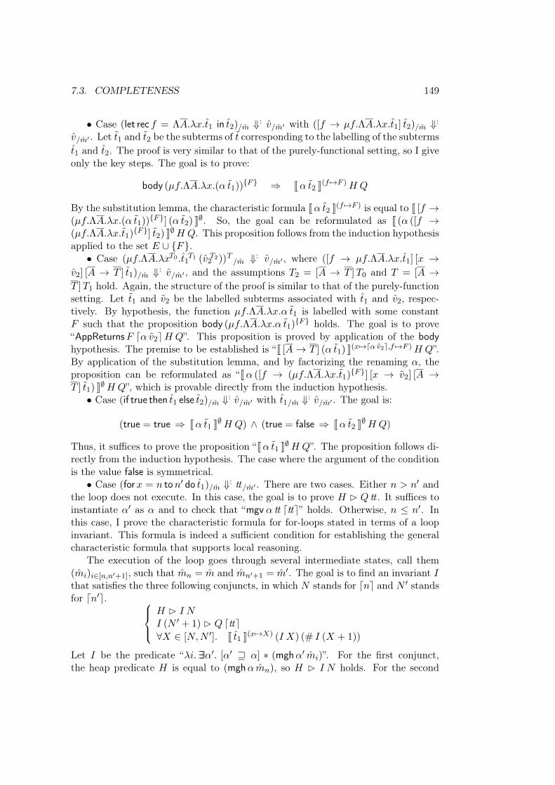
7.3. COMPLETENESS 149
∙ Case (let rec 𝑓 = Λ𝐴.𝜆𝑥.𝑡1 in 𝑡2)/�̂� ⇓: 𝑣/�̂�′ with ([𝑓 → 𝜇𝑓.Λ𝐴.𝜆𝑥.𝑡1] 𝑡2)/�̂� ⇓:
𝑣/�̂�′ . Let 𝑡1 and 𝑡2 be the subterms of 𝑡 corresponding to the labelling of the subterms𝑡1 and 𝑡2. The proof is very similar to that of the purely-functional setting, so I giveonly the key steps. The goal is to prove:
body (𝜇𝑓.Λ𝐴.𝜆𝑥.(𝛼 𝑡1)){𝐹} ⇒ J𝛼 𝑡2 K(𝑓 ↦→𝐹 )𝐻 𝑄
By the substitution lemma, the characteristic formula J𝛼 𝑡2 K(𝑓 ↦→𝐹 ) is equal to J [𝑓 →(𝜇𝑓.Λ𝐴.𝜆𝑥.(𝛼 𝑡1))
{𝐹}] (𝛼 𝑡2) K∅. So, the goal can be reformulated as J (𝛼 ([𝑓 →(𝜇𝑓.Λ𝐴.𝜆𝑥.𝑡1)
{𝐹}] 𝑡2) K∅𝐻 𝑄. This proposition follows from the induction hypothesisapplied to the set 𝐸 ∪ {𝐹}.
∙ Case (𝜇𝑓.Λ𝐴.𝜆𝑥𝑇0 .𝑡1𝑇1 (𝑣2
𝑇2))𝑇 /�̂� ⇓: 𝑣/�̂�′ , where ([𝑓 → 𝜇𝑓.Λ𝐴.𝜆𝑥.𝑡1] [𝑥 →𝑣2] [𝐴 → 𝑇 ] 𝑡1)/�̂� ⇓: 𝑣/�̂�′ , and the assumptions 𝑇2 = [𝐴 → 𝑇 ]𝑇0 and 𝑇 = [𝐴 →𝑇 ]𝑇1 hold. Again, the structure of the proof is similar to that of the purely-functionsetting. Let 𝑡1 and 𝑣2 be the labelled subterms associated with 𝑡1 and 𝑣2, respec-tively. By hypothesis, the function 𝜇𝑓.Λ𝐴.𝜆𝑥.𝛼 𝑡1 is labelled with some constant𝐹 such that the proposition body (𝜇𝑓.Λ𝐴.𝜆𝑥.𝛼 𝑡1)
{𝐹} holds. The goal is to prove“AppReturns𝐹 ⌈𝛼 𝑣2⌉𝐻 𝑄”. This proposition is proved by application of the bodyhypothesis. The premise to be established is “J [𝐴 → 𝑇 ] (𝛼 𝑡1) K(𝑥 ↦→⌈𝛼𝑣2⌉,𝑓 ↦→𝐹 )𝐻 𝑄”.By application of the substitution lemma, and by factorizing the renaming 𝛼, theproposition can be reformulated as “J𝛼 ([𝑓 → (𝜇𝑓.Λ𝐴.𝜆𝑥.𝑡1)
{𝐹}] [𝑥 → 𝑣2] [𝐴 →𝑇 ] 𝑡1) K∅𝐻 𝑄”, which is provable directly from the induction hypothesis.
∙ Case (if true then 𝑡1 else 𝑡2)/�̂� ⇓: 𝑣/�̂�′ with 𝑡1/�̂� ⇓: 𝑣/�̂�′ . The goal is:
(true = true ⇒ J𝛼 𝑡1 K∅𝐻 𝑄) ∧ (true = false ⇒ J𝛼 𝑡2 K∅𝐻 𝑄)
Thus, it suffices to prove the proposition “J𝛼 𝑡1 K∅𝐻 𝑄”. The proposition follows di-rectly from the induction hypothesis. The case where the argument of the conditionis the value false is symmetrical.
∙ Case (for𝑥 = 𝑛 to𝑛′ do 𝑡1)/�̂� ⇓: tt/�̂�′ . There are two cases. Either 𝑛 > 𝑛′ andthe loop does not execute. In this case, the goal is to prove 𝐻 B 𝑄 tt . It suffices toinstantiate 𝛼′ as 𝛼 and to check that “mgv 𝛼 tt ⌈tt⌉” holds. Otherwise, 𝑛 ≤ 𝑛′. Inthis case, I prove the characteristic formula for for-loops stated in terms of a loopinvariant. This formula is indeed a sufficient condition for establishing the generalcharacteristic formula that supports local reasoning.
The execution of the loop goes through several intermediate states, call them(�̂�𝑖)𝑖∈[𝑛,𝑛′+1], such that �̂�𝑛 = �̂� and �̂�𝑛′+1 = �̂�′. The goal is to find an invariant 𝐼that satisfies the three following conjuncts, in which 𝑁 stands for ⌈𝑛⌉ and 𝑁 ′ standsfor ⌈𝑛′⌉.
𝐻 B 𝐼 𝑁𝐼 (𝑁 ′ + 1) B 𝑄 ⌈tt⌉∀𝑋 ∈ [𝑁,𝑁 ′]. J 𝑡1 K(𝑥 ↦→𝑋) (𝐼 𝑋) (# 𝐼 (𝑋 + 1))
Let 𝐼 be the predicate “𝜆𝑖. ∃∃𝛼′. [𝛼′ ⊒ 𝛼] * (mgh𝛼′ �̂�𝑖)”. For the first conjunct,the heap predicate 𝐻 is equal to (mgh𝛼 �̂�𝑛), so 𝐻 B 𝐼 𝑁 holds. For the second
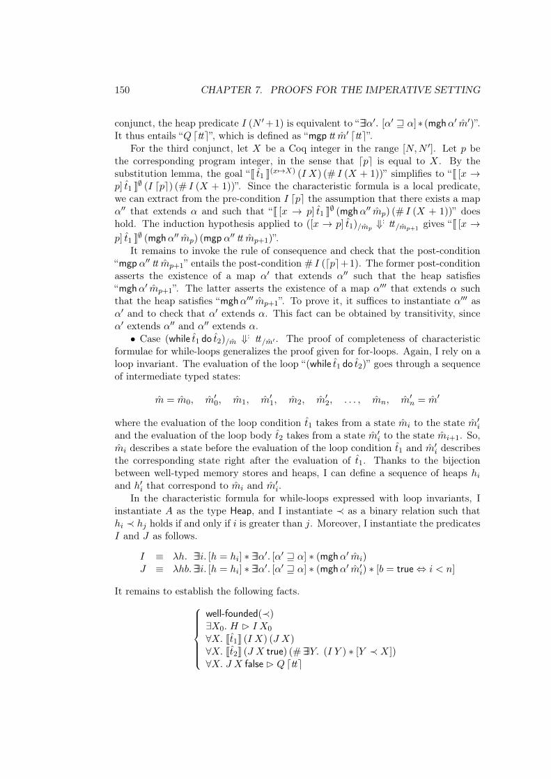
150 CHAPTER 7. PROOFS FOR THE IMPERATIVE SETTING
conjunct, the heap predicate 𝐼 (𝑁 ′ +1) is equivalent to “∃∃𝛼′. [𝛼′ ⊒ 𝛼]* (mgh𝛼′ �̂�′)”.It thus entails “𝑄 ⌈tt⌉”, which is defined as “mgp tt �̂�′ ⌈tt⌉”.
For the third conjunct, let 𝑋 be a Coq integer in the range [𝑁,𝑁 ′]. Let 𝑝 bethe corresponding program integer, in the sense that ⌈𝑝⌉ is equal to 𝑋. By thesubstitution lemma, the goal “J 𝑡1 K(𝑥 ↦→𝑋) (𝐼 𝑋) (# 𝐼 (𝑋 + 1))” simplifies to “J [𝑥 →𝑝] 𝑡1 K∅ (𝐼 ⌈𝑝⌉) (# 𝐼 (𝑋 + 1))”. Since the characteristic formula is a local predicate,we can extract from the pre-condition 𝐼 ⌈𝑝⌉ the assumption that there exists a map𝛼′′ that extends 𝛼 and such that “J [𝑥 → 𝑝] 𝑡1 K∅ (mgh𝛼′′ �̂�𝑝) (# 𝐼 (𝑋 + 1))” doeshold. The induction hypothesis applied to ([𝑥 → 𝑝] 𝑡1)/�̂�𝑝
⇓: tt/�̂�𝑝+1gives “J [𝑥 →
𝑝] 𝑡1 K∅ (mgh𝛼′′ �̂�𝑝) (mgp 𝛼′′ tt �̂�𝑝+1)”.It remains to invoke the rule of consequence and check that the post-condition
“mgp 𝛼′′ tt �̂�𝑝+1” entails the post-condition # 𝐼 (⌈𝑝⌉+1). The former post-conditionasserts the existence of a map 𝛼′ that extends 𝛼′′ such that the heap satisfies“mgh𝛼′ �̂�𝑝+1”. The latter asserts the existence of a map 𝛼′′′ that extends 𝛼 suchthat the heap satisfies “mgh𝛼′′′ �̂�𝑝+1”. To prove it, it suffices to instantiate 𝛼′′′ as𝛼′ and to check that 𝛼′ extends 𝛼. This fact can be obtained by transitivity, since𝛼′ extends 𝛼′′ and 𝛼′′ extends 𝛼.
∙ Case (while 𝑡1 do 𝑡2)/�̂� ⇓: tt/�̂�′ . The proof of completeness of characteristicformulae for while-loops generalizes the proof given for for-loops. Again, I rely on aloop invariant. The evaluation of the loop “(while 𝑡1 do 𝑡2)” goes through a sequenceof intermediate typed states:
�̂� = �̂�0, �̂�′0, �̂�1, �̂�′
1, �̂�2, �̂�′2, . . . , �̂�𝑛, �̂�′
𝑛 = �̂�′
where the evaluation of the loop condition 𝑡1 takes from a state �̂�𝑖 to the state �̂�′𝑖
and the evaluation of the loop body 𝑡2 takes from a state �̂�′𝑖 to the state �̂�𝑖+1. So,
�̂�𝑖 describes a state before the evaluation of the loop condition 𝑡1 and �̂�′𝑖 describes
the corresponding state right after the evaluation of 𝑡1. Thanks to the bijectionbetween well-typed memory stores and heaps, I can define a sequence of heaps ℎ𝑖and ℎ′𝑖 that correspond to �̂�𝑖 and �̂�′
𝑖.In the characteristic formula for while-loops expressed with loop invariants, I
instantiate 𝐴 as the type Heap, and I instantiate ≺ as a binary relation such thatℎ𝑖 ≺ ℎ𝑗 holds if and only if 𝑖 is greater than 𝑗. Moreover, I instantiate the predicates𝐼 and 𝐽 as follows.
𝐼 ≡ 𝜆ℎ. ∃∃𝑖. [ℎ = ℎ𝑖] * ∃∃𝛼′. [𝛼′ ⊒ 𝛼] * (mgh𝛼′ �̂�𝑖)𝐽 ≡ 𝜆ℎ𝑏.∃∃𝑖. [ℎ = ℎ𝑖] * ∃∃𝛼′. [𝛼′ ⊒ 𝛼] * (mgh𝛼′ �̂�′
𝑖) * [𝑏 = true ⇔ 𝑖 < 𝑛]
It remains to establish the following facts.
well-founded(≺)∃𝑋0. 𝐻 B 𝐼 𝑋0
∀𝑋. J𝑡1K (𝐼 𝑋) (𝐽 𝑋)
∀𝑋. J𝑡2K (𝐽 𝑋 true) (#∃∃𝑌. (𝐼 𝑌 ) * [𝑌 ≺ 𝑋])∀𝑋. 𝐽 𝑋 false B 𝑄 ⌈tt⌉
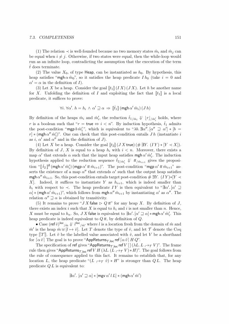
7.3. COMPLETENESS 151
(1) The relation ≺ is well-founded because no two memory states �̂�𝑖 and �̂�𝑗 canbe equal when 𝑖 ̸= 𝑗. Otherwise, if two states were equal, then the while-loop wouldrun as an infinite loop, contradicting the assumption that the execution of the term𝑡 does terminate.
(2) The value 𝑋0, of type Heap, can be instantiated as ℎ0. By hypothesis, thisheap satisfies “mgh𝛼 �̂�0”, so it satisfies the heap predicate 𝐼 ℎ0 (take 𝑖 = 0 and𝛼′ = 𝛼 in the definition of 𝐼).
(3) Let 𝑋 be a heap. Consider the goal J𝑡1K (𝐼 𝑋) (𝐽 𝑋). Let ℎ be another namefor 𝑋. Unfolding the definition of 𝐼 and exploiting the fact that J𝑡1K is a localpredicate, it suffices to prove:
∀𝑖. ∀𝛼′. ℎ = ℎ𝑖 ∧ 𝛼′ ⊒ 𝛼 ⇒ J𝑡1K (mgh𝛼′ �̂�𝑖) (𝐽 ℎ)
By definition of the heaps �̂�𝑖 and �̂�′𝑖, the reduction 𝑡1/�̂�𝑖
⇓: ⌊𝑟⌋/�̂�′𝑖
holds, where𝑟 is a boolean such that “𝑟 = true ⇔ 𝑖 < 𝑛”. By induction hypothesis, 𝑡1 admitsthe post-condition “mgp 𝑏 �̂�′
𝑖 ”, which is equivalent to “𝜆𝑏.∃∃𝛼′′. [𝛼′′ ⊒ 𝛼′] * [𝑏 =𝑟] * (mgh𝛼′′ �̂�′
𝑖)”. One can check that this post-condition entails 𝐽 ℎ (instantiate 𝑖as 𝑖, 𝛼′ and 𝛼′′ and in the definition of 𝐽).
(4) Let 𝑋 be a heap. Consider the goal J𝑡2K (𝐽 𝑋 true) (#∃∃𝑌. (𝐼 𝑌 ) * [𝑌 ≺ 𝑋]).By definition of 𝐽 , 𝑋 is equal to a heap ℎ𝑖 with 𝑖 < 𝑛. Moreover, there exists amap 𝛼′ that extends 𝛼 such that the input heap satisfies mgh𝛼′ �̂�′
𝑖. The inductionhypothesis applied to the reduction sequence 𝑡2/�̂�′
𝑖⇓: tt/�̂�𝑖+1
gives the proposi-tion “J 𝑡2 K∅ (mgh𝛼′ �̂�′
𝑖) (mgp 𝛼′ tt �̂�𝑖+1)”. The post-condition “mgp 𝛼′ tt �̂�𝑖+1” as-serts the existence of a map 𝛼′′ that extends 𝛼′ such that the output heap satisfiesmgh𝛼′′ �̂�𝑖+1. So, this post-condition entails target post-condition # ∃∃𝑌. (𝐼 𝑌 )*[𝑌 ≺𝑋]. Indeed, it suffices to instantiate 𝑌 as ℎ𝑖+1, which is indeed smaller thanℎ𝑖 with respect to ≺. The heap predicate 𝐼 𝑌 is then equivalent to “∃∃𝛼′. [𝛼′ ⊒𝛼] * (mgh𝛼′ �̂�𝑖+1)”, which follows from mgh𝛼′′ �̂�𝑖+1 by instantiating 𝛼′ as 𝛼′′. Therelation 𝛼′′ ⊒ 𝛼 is obtained by transitivity.
(5) It remains to prove “𝐽 𝑋 false B 𝑄 tt” for any heap 𝑋. By definition of 𝐽 ,there exists an index 𝑖 such that 𝑋 is equal to ℎ𝑖 and 𝑖 is not smaller than 𝑛. Hence,𝑋 must be equal to ℎ𝑛. So, 𝐽 𝑋 false is equivalent to ∃∃𝛼′. [𝛼′ ⊒ 𝛼] *mgh𝛼′ �̂�′
𝑖. Thisheap predicate is indeed equivalent to 𝑄 tt , by definition of 𝑄.
∙ Case (ref 𝑣)loc/�̂� ⇓: 𝑙 loc
/�̂�′ where 𝑙 is a location fresh from the domain of �̂� and�̂�′ is the heap �̂� ⊎ [𝑙 ↦→ 𝑣]. Let 𝑇 denote the type of 𝑣, and let 𝒯 denote the Coqtype V𝑇W. Let 𝑣 be the labelled value associated with 𝑣, and let 𝑉 be a shorthandfor ⌈𝛼 𝑣⌉ The goal is to prove “AppReturns𝒯 ,loc ref ⌈𝛼 𝑣⌉𝐻 𝑄”.
The specification of ref gives “AppReturns𝒯 ,loc ref𝑉 [ ] (𝜆𝐿.𝐿 →˓𝒯 𝑉 )”. The framerule then gives “AppReturns𝒯 ,loc ref𝑉 𝐻 (𝜆𝐿. (𝐿 →˓𝒯 𝑉 )*𝐻)”. The goal follows fromthe rule of consequence applied to this fact. It remains to establish that, for anylocation 𝐿, the heap predicate “(𝐿 →˓𝒯 𝑣) * 𝐻” is stronger than 𝑄𝐿. The heappredicate 𝑄𝐿 is equivalent to:
∃∃𝛼′. [𝛼′ ⊒ 𝛼] * [mgv 𝛼′ 𝑙 𝐿] * (mgh𝛼′ �̂�′)
152 CHAPTER 7. PROOFS FOR THE IMPERATIVE SETTING
Let 𝐿 be a location and ℎ′ be a heap satisfying the predicate (𝐿 →˓𝒯 𝑣)*𝐻. Thegoal is to prove that the above heap predicate also applies to ℎ′. Then, to prove thegoal, I instantiate 𝛼′ as 𝛼 ⊎ [𝑙 ↦→ ⌊𝐿⌋]. The first subgoal 𝛼′ ⊒ 𝛼 holds by definitionof 𝛼′. The second subgoal “mgv 𝛼′ 𝑙 𝐿” simplifies to “𝐿 = 𝛼′ 𝑙”, which is also true bydefinition of 𝛼′. It remains to prove the third subgoal, which asserts that ℎ′ satisfiesthe heap predicate (mgh𝛼′ �̂�′).
Because ℎ′ satisfies (𝐿 →˓𝒯 𝑣) *𝐻, the heap ℎ′ decomposes as a singleton heapsatisfying (𝐿 →˓𝒯 𝑣) and as a heap ℎ satisfying 𝐻, which was defined as “mgh𝛼 �̂�”.The assumptions given by “mgh𝛼 �̂�ℎ” are as follows.
dom(ℎ) = dom(𝛼 �̂�)∀𝑙′ ∈ dom(�̂�). mgv 𝛼 (�̂�[𝑙′])𝑉 ′ where (𝒯 ′, 𝑉 ′) = ℎ[𝛼 𝑙′]locs(�̂�) ⊆ dom(𝛼)
To prove (mgh𝛼′ �̂�′ ℎ′), we need to establish the following facts.dom(ℎ′) = dom(𝛼′ �̂�′)∀𝑙′ ∈ dom(�̂�′). mgv 𝛼′ (�̂�′[𝑙′])𝑉 ′ where (𝒯 ′, 𝑉 ′) = ℎ′[𝛼′ 𝑙′]locs(�̂�′) ⊆ dom(𝛼′)
The first and the third facts are easy to verify. For the second fact, let 𝑙′ be alocation in the domain of �̂�′. If 𝑙′ is equal to 𝑙, then (𝛼 𝑙′) is equal to 𝐿 andthe goal is “mgv 𝛼′ (�̂�′[𝑙])𝑉 ”. The proposition simplifies to “mgv 𝛼′ 𝑣 (𝛼 𝑣)”, whichfollows from the tautology “mgv 𝛼 𝑣 (𝛼 𝑣)”, by covariance of mgs in the 𝛼-renamingmap. Otherwise, if 𝑙′ is not equal to 𝑙, then 𝑙′ belongs to the domain of �̂� and thecovariance of mgv in the 𝛼-renaming map can be used to derive “mgv 𝛼′ (�̂�[𝑙′])𝑉 ′”from “mgv 𝛼 (�̂�[𝑙′])𝑉 ′”.
∙ Case (get 𝑙)𝑇 /�̂� ⇓: 𝑣𝑇 /�̂� where 𝑣𝑇 = �̂�[𝑙]. Let 𝒯 stand for V𝑇W and let 𝐿stand for ⌈𝛼 𝑙⌉. The goal is “AppReturnsloc,𝒯 get𝐿 (mgh𝛼 �̂�) (mgp 𝛼 𝑣 �̂�)”. We coulduse the frame rule like in the previous proof case to prove this goal, however theproof is simpler when we directly unfold the definition of AppReturns and work withthe predicate AppEval. The goal then reformulates as follows.
∀ℎ𝑖 ℎ𝑘. mgh𝛼 �̂�ℎ𝑖 ⇒ ∃𝑉 ℎ𝑓 ℎ𝑔.
®AppEval get𝐿 (ℎ𝑖 + ℎ𝑘)𝑉 (ℎ𝑓 + ℎ𝑘 + ℎ𝑔)mgp 𝛼 𝑣 �̂� 𝑉 ℎ𝑓
From the specification of get applied to the location 𝐿, we get:
∀𝑉. AppReturnsloc,𝒯 get𝐿 (𝐿 →˓𝒯 𝑉 ) (𝜆𝑉 ′. [𝑉 ′ = 𝑉 ] * (𝐿 →˓𝒯 𝑉 ))
Reformulating this proposition in terms of AppEval gives:
∀𝑉 ℎ′𝑖 ℎ′𝑘. (𝐿 →˓𝒯 𝑉 )ℎ′𝑖 ⇒ ∃𝑉 ′ ℎ′𝑓 ℎ
′𝑔.
AppEval get𝐿 (ℎ′𝑖 + ℎ′𝑘)𝑉 ′ (ℎ′𝑓 + ℎ′𝑘 + ℎ′𝑔)
𝑉 ′ = 𝑉(𝐿 →˓𝒯 𝑉 ′)ℎ′𝑓
7.3. COMPLETENESS 153
It remains to find the suitable instantiations for proving the goal by exploit-ing the above proposition. Since 𝑙 belongs to the domain of �̂� and since the hy-pothesis mgh𝛼 �̂�ℎ𝑖 holds, we know that 𝐿 belongs to the domain of ℎ𝑖 and thatmgv 𝛼 (�̂�[𝑙]) (ℎ𝑖[𝑙]) holds. Let 𝑉 stand for the value ℎ𝑖[𝑙]. The assertion reformulatesas mgv 𝛼 𝑣 𝑉 . Moreover, there exists a heap ℎ𝑟 such that the heap ℎ𝑖 decomposes asthe disjoint union of the singleton heap 𝐿 →𝒯 𝑉 and of ℎ𝑟. Let ℎ′𝑖 be instantiatedas 𝐿 →𝒯 𝑉 , and let ℎ′𝑘 be instantiated as ℎ𝑟 + ℎ𝑘. The union ℎ′𝑖 + ℎ′𝑘 equal to theunion ℎ𝑖 + ℎ𝑘.
We can check the premise (𝐿 →˓𝒯 𝑉 )ℎ′𝑖, and obtain the existence of 𝑉 ′, ℎ′𝑓 andℎ′𝑔 satisfying the three conclusions derived from the specification of get. The sec-ond conclusion ensures that 𝑉 ′ is equal to 𝑉 . The third conclusion, (𝐿 →˓𝒯 𝑉 )ℎ′𝑓asserts that ℎ′𝑓 is a singleton heap of the form 𝐿 →𝒯 𝑉 , so it is the same as ℎ′𝑖.In particular, the union ℎ′𝑓 + ℎ′𝑘 is equal to the union ℎ𝑖 + ℎ𝑘. The first conclu-sion, AppEval get𝐿 (ℎ′𝑖 + ℎ′𝑘)𝑉 ′ (ℎ′𝑓 + ℎ′𝑘 + ℎ′𝑔), is then equivalent to the propositionAppEval get𝐿 (ℎ𝑖 + ℎ𝑘)𝑉 (ℎ𝑖 + ℎ𝑘 + ℎ′𝑔).
To conclude, it remains to instantiate 𝑉 as 𝑉 , ℎ𝑓 as ℎ𝑖, ℎ𝑔 as ℎ′𝑔, and toprove mgp 𝛼 𝑣 �̂� 𝑉 ℎ𝑖. Instantiating 𝛼′ as 𝛼 in this proposition, we have to provemgh 𝛼�̂�ℎ𝑖, which holds by assumption, and to prove mgv 𝛼 𝑣 𝑉 , a fact which hasbeen extracted earlier on from the assumption mgh𝛼 �̂�ℎ𝑖.
∙ Case (set 𝑙 𝑣)unit/�̂� ⇓: tt unit
/�̂�′ where 𝑙 belongs to the domain of 𝑙 and �̂�′ standsfor �̂�[𝑙 ↦→ 𝑣]. Let 𝑇 be the type of 𝑣 and let 𝒯 stand for V𝑇W. By assumption, thereexists a labelled value 𝑣 that corresponds to 𝑣, such that labels 𝐸 𝑣. Let 𝑉 standfor ⌈𝛼 𝑣⌉, and let 𝐿 stand for ⌈𝛼 𝑙⌉. The goal is:
AppReturns(loc×𝒯 ),unit set (𝐿, 𝑉 ) (mgh𝛼 �̂�) (mgp 𝛼 tt �̂�)
As in the previous proof case, we can rewrite this goal in terms of AppEval. Thestatement shown next takes into account the fact that the return value is the unitvalue.
∀ℎ𝑖 ℎ𝑘. mgh𝛼 �̂�ℎ𝑖 ⇒ ∃ℎ𝑓 ℎ𝑔.®
AppEval set (𝐿, 𝑉 ) (ℎ𝑖 + ℎ𝑘) tt (ℎ𝑓 + ℎ𝑘 + ℎ𝑔)mgp 𝛼 tt �̂�′ ⌈tt⌉ℎ𝑓
From the specification of set applied to the location 𝐿, we get:
∀𝑉 𝒯 ′ 𝑉 ′. AppReturns(loc×𝒯 ),unit set (𝐿, 𝑉 ) (𝐿 →˓𝒯 ′ 𝑉 ′) (# (𝐿 →˓𝒯 ′ 𝑉 ))
Reformulating this proposition in terms of AppEval gives:
∀𝑉 𝒯 ′ 𝑉 ′ ℎ′𝑖 ℎ′𝑘.
(𝐿 →˓𝒯 ′ 𝑉 ′)ℎ′𝑖⇒ ∃ℎ′𝑓 ℎ′𝑔.
®AppEval set (𝐿, 𝑉 ) (ℎ′𝑖 + ℎ′𝑘) tt (ℎ′𝑓 + ℎ′𝑘 + ℎ′𝑔)
(𝐿 →˓𝒯 𝑉 )ℎ′𝑓
It remains to find the suitable instantiations. Since 𝑙 belongs to the domain of �̂�and since the hypothesis mgh𝛼 �̂�ℎ𝑖 holds, we know that 𝐿 belongs to the domainof ℎ𝑖 and that mgv 𝛼 (�̂�[𝑙]) (ℎ𝑖[𝑙]). Let 𝑉 ′ denote the value ℎ𝑖[𝑙]. There exists a heapℎ𝑟 such that the heap ℎ𝑖 decomposes as the disjoint union of the singleton heap
154 CHAPTER 7. PROOFS FOR THE IMPERATIVE SETTING
𝐿 →𝒯 ′ 𝑉 ′ and of ℎ𝑟. Let ℎ′𝑖 be instantiated as 𝐿 →𝒯 ′ 𝑉 ′, and let ℎ′𝑘 be instantiatedas ℎ𝑟 + ℎ𝑘. The union ℎ′𝑖 + ℎ′𝑘 equal to the union ℎ𝑖 + ℎ𝑘.
We can check the premise (𝐿 →˓𝒯 ′ 𝑉 ′) (𝐿 →𝒯 ′ 𝑉 ′), and obtain the existenceof ℎ′𝑓 and ℎ′𝑔 satisfying the two conclusions derived from the specification of set.The second conclusion, (𝐿 →˓𝒯 𝑉 )ℎ′𝑓 asserts that ℎ′𝑓 is a singleton heap of theform 𝐿 →𝒯 𝑉 . Let ℎ𝑓 be instantiated as ℎ′𝑓 + ℎ𝑟. In particular, the unionℎ′𝑓 + ℎ′𝑘 is equal to the union ℎ𝑓 + ℎ𝑘. Moreover, let ℎ𝑔 be instantiated as ℎ′𝑔.The first conclusion, AppEval get𝐿 (ℎ′𝑖 + ℎ′𝑘)𝑉 ′ (ℎ′𝑓 + ℎ′𝑘 + ℎ′𝑔) is then equivalent toAppEval get𝐿 (ℎ𝑖 + ℎ𝑘)𝑉 (ℎ𝑓 + ℎ𝑘 + ℎ𝑔).
It remains to prove mgp 𝛼 tt �̂�′ ⌈tt⌉ℎ𝑓 . Instantiating 𝛼′ as 𝛼 in this predicate,it remains to prove mgv 𝛼 tt tt , which is true, and mgh𝛼 �̂�′ ℎ𝑓 . To prove the latter,let 𝑙′ be a location in the domain of �̂�′, which is the same as the domain of �̂�. Wehave to prove mgv 𝛼 (�̂�[𝑙′]) (ℎ𝑓 [⌈𝛼 𝑙′⌉]). There are two cases. If 𝑙′ is not the location𝑙, then �̂�′[𝑙′] is equal to �̂�[𝑙′] and ℎ𝑓 [⌈𝛼 𝑙′⌉] is equal to ℎ𝑖[⌈𝛼 𝑙′⌉], so the assumption“mgh𝛼 �̂�ℎ𝑖” can be used to conclude. Otherwise, if 𝑙′ is the location 𝑙, then �̂�′[𝑙]is equal to 𝑣 and ℎ[⌈𝛼 𝑙⌉] is equal to 𝑉 (because 𝑉 stands for ℎ[𝐿] and 𝐿 has beendefined as ⌈𝛼 𝑙⌉), so the goal is to prove mgv 𝛼 𝑣 𝑉 , which holds because 𝑉 has beendefined ⌈𝛼 𝑣⌉ and labels 𝐸 𝑣 holds by assumption.
∙ Case (cmp 𝑙 𝑘′)/�̂� ⇓: �̂�bool/�̂�. The proof is straightforward since cmp does not
involve any reasoning on the heap. �
7.3.3 Completeness for integer results
A simpler statement of the completeness theorem can be given in the case of aprogram that admits the type int in ML. To lighten the presentation, I identifyCaml integers with Coq integers.
Theorem 7.3.2 (Completeness for ML programs with integer results)Consider a closed ML program of type int. Let 𝑡 denote the corresponding term typedin weak-ML, and let 𝑡 denote the corresponding raw term. Let 𝑛 be an integer, let 𝑃be a Coq predicate on integers, and let 𝑚 be a memory store.
𝑡/∅ ⇓ 𝑛/𝑚 ∧ 𝑃 𝑛 ⇒ J 𝑡 K∅ [ ] (𝜆𝑛. [𝑃 𝑛])
Proof Since the term 𝑡 is well-typed in ML, the reduction derivation 𝑡/∅ ⇓ 𝑛/𝑚 canbe turned into a typed reduction derivation 𝑡int
/∅ ⇓: 𝑛int/�̂�. By the completeness
theorem applied to that derivation, there exists a renaming 𝛼 such that:
J 𝑡 K∅ [ ] (𝜆𝑉.∃∃𝛼. [mgv 𝛼𝑛𝑉 ] * (mgh𝛼𝑚))
The characteristic formula is a local predicate, so we can apply the rule of garbagecollection to ignore the post-condition about the final store 𝑚. It gives:
J 𝑡 K∅ [ ] (𝜆𝑉.∃∃𝛼. [mgv 𝛼𝑛𝑉 ])
7.3. COMPLETENESS 155
To prove the conclusion, we apply the rule of consequence, and there remains toestablish an implication between the post-conditions:
∀𝑉. (∃𝛼.mgv 𝛼𝑛𝑉 ) ⇒ 𝑃 𝑉
The hypothesis “mgv 𝛼𝑛𝑉 ” asserts the existence of a correct labelling �̃� of 𝑛 suchthat 𝑉 = ⌈𝛼 �̃�⌉. Since the integer 𝑛 does not contain any function nor any location,the hypothesis simplifies to 𝑉 = 𝑛. The conclusion 𝑃 𝑉 then follows directly fromthe assumption 𝑃 𝑛. �
Chapter 8
Related work
The discussion of related work is organized around five sections. Thefirst one is concerned with the origins of characteristic formulae andthe comparison with the program logics developed by Honda, Berger,and Yoshida. In a second part, I focus on Separation Logic. I thendiscuss approaches based on Verification Condition Generators (VCG),approaches based on shallow embeddings, and approaches based on deepembeddings.
8.1 Characteristic formulae
Characteristic formulae in process calculi The notion of characteristic for-mula originates in process calculi. The characterization theorem [70, 57] states thattwo processes are bisimilar if and only if they satisfy the same set of formulae inHennessy-Milner logic [35]. In this context, a formula 𝐹 is said to be the characteris-tic formula of a process 𝑝 if the set of processes that satisfy 𝐹 matches exactly the setof processes that are bisimilar to 𝑝. Graf and Sifakis [32] described an algorithm forconstructing the characteristic formulae of a process from the syntactic definition ofthat process. More precisely, they explained how to build a modal logic formula thatcharacterizes the equivalence class of a given CCS process (for processes that do notinvolve recursion). Aceto and Ingólfsdóttir [1] later described a similar generationalgorithm for translating regular CCS processes into their characteristic formulae,which are there expressed in Hennessy-Milner logic extended with recursion.
The behavioral equivalence or dis-equivalence of two processes can be establishedby comparing their characteristic formulae. Such proofs can be conducted in a high-level temporal logic rather than through reasoning on the syntactic definition ofthe processes. Somewhat similarly, the characteristic formulae developed in thisthesis allow reasoning on a program to be conducted on higher-order logic formulae,without referring to the source code of that program at any time.
156
8.1. CHARACTERISTIC FORMULAE 157
Total characteristic assertion pairs The first development of a program-logiccounterpart to process-logic characteristic formulae is due to recent work by Honda,Berger and Yoshida [40]. This work originates in the study of a correspondencebetween process logics and program logics [38], where Honda showed how an encod-ing of a high-level programming language into the 𝜋-calculus can be used to turna logic for the 𝜋-calculus with linear types into a compositional program logic fora higher-order functional programming language. This program logic, which is de-scribed in detail in [41], was later extended to an imperative programming languagewith global state [10], and then further extended to support reasoning on aliasing[39] and reasoning on local state [87].
In the logics for higher-order imperative programs, the specification judgmenttake the form of a Hoare triple {𝐶} 𝑡 :𝑥{𝐶 ′}, where 𝑡 is a term, 𝐶 and 𝐶 ′ areassertions about the initial heap and the final heap, and 𝑥 is a bound name used torefer to the result produced by 𝑡 in the post-condition 𝐶 ′. So, the interpretation ofthe judgment {𝐶} 𝑡 :𝑥{𝐶 ′} is essentially the same as that of the triple {𝐶} 𝑡 {𝜆𝑥.𝐶 ′},which follows the presentation that I have used so far. The specification of functionsand higher-order functions involves a ternary predicate, called evaluation formulaand written “𝑣1 ∙ 𝑣2 == 𝑣3”, which asserts that the application of the value 𝑣1 to thevalue 𝑣2 returns the value 𝑣3. The specification thus takes place in a first-order logicextended with this ad-hoc evaluation predicate. Another specificity of the assertionlogic is that its values are the values of the programming language (i.e., PCF values),including in particular non-terminating functions. Moreover, in the assertion logic,equality is interpreted as observational equivalence. All those constructions makethe assertion logic nonstandard, making it difficult to reuse existing proof tools.
The series of work on program logics by Honda, Berger and Yoshida culminatedin the development of total characteristic assertion pairs [40], abbreviated as TCAP,which corresponds to the notion of most-general Hoare triple. A most-general Hoaretriple, also called most-general formula, is made of the weakest pre-condition, whichcorresponds to the minimal requirement for safe execution, and of the strongest post-condition, which precisely relates the output heap to the input heap. Most-generalformulae were introduced by Gorelick in 1975 [31] for establishing a completenessresult for Hoare logic. Yet, this theoretical result does not help verify programs inpractice, because most-general formulae were there expressed in terms of the syntaxand the semantics of the source program. The total characteristic assertion pairs(TCAPs) developed by Honda, Berger and Yoshida [40] precisely solve that problem,as TCAPs express the weakest pre-condition and the strongest post-condition in theassertion logic, without any reference to program syntax. Moreover, the TCAP of aprogram can be constructed automatically by application of a simple algorithm.
As those researchers point out, TCAPs suggest a new approach to proving thata program satisfies a given specification. Indeed, rather than building a derivationusing the reasoning rules of the Hoare program logic, one may simply prove thatthe pre-condition of the specification implies the weakest pre-condition and thatthe post-condition of the specification is implied by the strongest post-condition.The verification of those two implications can be conducted entirely at the logical
158 CHAPTER 8. RELATED WORK
level. Yet, this appealing idea was never implemented, mainly because the treatmentof first-class functions and of evaluation formulae in the assertion logic makes thelogic nonstandard and precludes the use of a standard theorem prover. A centralcontribution of this thesis has been to show how to reconcile first-class functionsand evaluation formulae with a standard logic, by representing functions in the logicthrough the deep embedding of their code (with the type Func) and by defining anevaluation formula (the predicate AppEval) in terms of the deep embedding of thesemantics of the source programming language.
The presentation of characteristic formulae that I build also differ in severalways from TCAPs. First, characteristic formulae rely on existential quantificationof intermediate specifications and loop invariants. This was not the case in TCAPs,which are expressed in first-order logic. Second, I have shown that characteristicformulae could be pretty-printed just like source code. This possibility was notpointed out in the work on TCAPs, even though, in principle, it should be possibleto apply a similar notation system to TCAPs. Third, TCAPs rely on a reachabilitypredicate for reasoning on dynamic allocation, whereas I have based on my workupon standard technique from Separation Logic, whose effectiveness has alreadybeen demonstrated. In particular, I introduced the predicate local to integrate theframe rule directly inside characteristic formulae.
8.2 Separation Logic
Tight specifications and the frame rule Separation Logic has been developedinitially by Reynolds [77] and by O’Hearn and Yang [67, 86], and subsequently bymany others. It builds on earlier work by Burstall [14], on work by Bornat [12],and on the logic of Bunched Implications developed by O’Hearn, Ishtiaq and Pym[66, 42]. The starting point of Separation Logic is the tight interpretation of Hoaretriples. The tight interpretation of a triple {𝐻} 𝑡 {𝑄} asserts that the execution ofthe term 𝑡 is only allowed to modify memory cells that are described by the pre-condition 𝐻. This interpretation is the key to the soundness of the frame rule, whichenables local reasoning.
Following the traditional presentation of Hoare logic, Separation Logic allows thelocal variables of a program to be modified, even though it does not require localvariables to be described with an assertion of the form 𝑥 →˓ 𝑣. In other words, inSeparation Logic assertions, the name of a local variable is confused with the currentvalue of that variable. For this reason, the frame rule is usually presented with aside-condition, as shown below. In this rule, 𝑐 denotes a command, and 𝑝, 𝑞 and 𝑟are assertions about the heap.
{𝑝} 𝑐 {𝑞}{𝑝 * 𝑟} 𝑐 {𝑞 * 𝑟}
Çwhere no variable occurringfree in 𝑟 is modified by 𝑐.
åCharacteristic formulae require a frame rule without side condition because they
cannot refer to program syntax. As observed by O’Hearn [68], the side-condition is
8.2. SEPARATION LOGIC 159
not needed in a language such as Caml, where mutation is only allowed for heap-allocated data. More generally, it would suffice to distinguish the name of localvariables from their contents in order to avoid the side-condition in the frame rule.
Separation Logic tools A number of verification tools have been built upon ideasfrom Separation Logic. For example, Smallfoot, developed by Berdine, Calcagno andO’Hearn [8], is an automated verification tool specialized for programs manipulatinglinked data structures. Also, Yang et al [85] have developed an automated tool forverifying dozens of thousands of lines of source code for device drivers, which mainlyinvolve linked lists.
Because fully-automated tools are inherently limited in scope, other researchershave investigated the possibility to exploit Separation Logic inside interactive proofassistants. The first such embedding of Separation Logic appears to be the oneby Marti and Affeldt [52, 53]. Yet, these researchers conducted their Coq proofsby unfolding the definition of the separating conjunction, which breaks the nicelevel of abstraction brought by this operator. Appel [2] has shown how to buildreasoning tactics that do not break the abstraction layer, obtaining significantly-shorter proof scripts. Further Separation Logic tactics were subsequently developedin many research projects, e.g., [24, 82, 62, 17, 55, 59].
Most of those tactics exploit an hypothesis of the form 𝐻 ℎ for proving a goalof the form 𝐻 ′ ℎ. One exception is a recent version of Ynot [17], where the tacticsdirectly handles goals of the form 𝐻 B 𝐻 ′, without involving a heap variable ℎ inthe proof. This approach allows working entirely at the level of heap predicates andit allows for the development of more efficient tactics. This is why I have followedthat approach in the implementation of my tactic hsimpl (§5.7.1).
Local reasoning and while loops The traditional Hoare logic reasoning rule forwhile loops is expressed using loop invariants. This rule can be used in the contextof Separation Logic. However, it does not take full advantage of local reasoning (asexplained in §3.3). I came accross the limitation of loop-invariants, found a way toaddress it, and then learnt that Tuerk had made the same observation and discussedit in a workshop paper [83]. I present his solution and then compare it with mine.
In Tuerk’s presentation, the deduction rule that does involve a loop invariant isas shown below. In this partial-correctness reasoning rule, 𝑏 is a boolean condition,𝑐 is a set of commands, and 𝐼 is an invariant.
{𝑏 ∧ 𝐼} 𝑐 {𝐼}{𝐼} (while 𝑏 do 𝑐) {¬𝑏 ∧ 𝐼}
His generalized rule is shown next. There, 𝑃 denotes a predicate (the invariantbecomes parameterized by an index), and 𝑥 and 𝑦 denote indices for 𝑃 . Observethat the premise involves a quantification over all the programs 𝑐′ that admit a givenspecification. The variable 𝑐′ intuitively denotes the remaining iterations of the loop.
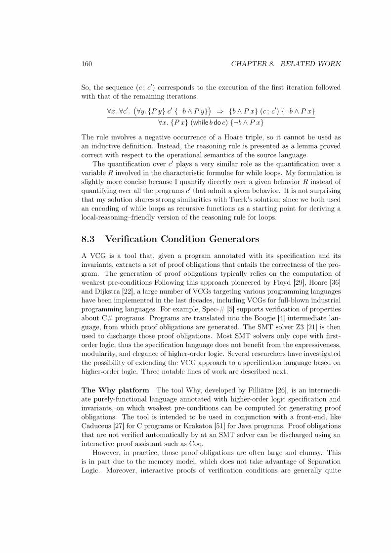
160 CHAPTER 8. RELATED WORK
So, the sequence (𝑐 ; 𝑐′) corresponds to the execution of the first iteration followedwith that of the remaining iterations.
∀𝑥. ∀𝑐′.Ä∀𝑦. {𝑃 𝑦} 𝑐′ {¬𝑏 ∧ 𝑃 𝑦}
ä⇒ {𝑏 ∧ 𝑃 𝑥} (𝑐 ; 𝑐′) {¬𝑏 ∧ 𝑃 𝑥}
∀𝑥. {𝑃 𝑥} (while 𝑏 do 𝑐) {¬𝑏 ∧ 𝑃 𝑥}
The rule involves a negative occurrence of a Hoare triple, so it cannot be used asan inductive definition. Instead, the reasoning rule is presented as a lemma provedcorrect with respect to the operational semantics of the source language.
The quantification over 𝑐′ plays a very similar role as the quantification over avariable 𝑅 involved in the characteristic formulae for while loops. My formulation isslightly more concise because I quantify directly over a given behavior 𝑅 instead ofquantifying over all the programs 𝑐′ that admit a given behavior. It is not surprisingthat my solution shares strong similarities with Tuerk’s solution, since we both usedan encoding of while loops as recursive functions as a starting point for deriving alocal-reasoning–friendly version of the reasoning rule for loops.
8.3 Verification Condition Generators
A VCG is a tool that, given a program annotated with its specification and itsinvariants, extracts a set of proof obligations that entails the correctness of the pro-gram. The generation of proof obligations typically relies on the computation ofweakest pre-conditions Following this approach pioneered by Floyd [29], Hoare [36]and Dijkstra [22], a large number of VCGs targeting various programming languageshave been implemented in the last decades, including VCGs for full-blown industrialprogramming languages. For example, Spec-# [5] supports verification of propertiesabout C# programs. Programs are translated into the Boogie [4] intermediate lan-guage, from which proof obligations are generated. The SMT solver Z3 [21] is thenused to discharge those proof obligations. Most SMT solvers only cope with first-order logic, thus the specification language does not benefit from the expressiveness,modularity, and elegance of higher-order logic. Several researchers have investigatedthe possibility of extending the VCG approach to a specification language based onhigher-order logic. Three notable lines of work are described next.
The Why platform The tool Why, developed by Filliâtre [26], is an intermedi-ate purely-functional language annotated with higher-order logic specification andinvariants, on which weakest pre-conditions can be computed for generating proofobligations. The tool is intended to be used in conjunction with a front-end, likeCaduceus [27] for C programs or Krakatoa [51] for Java programs. Proof obligationsthat are not verified automatically by at an SMT solver can be discharged using aninteractive proof assistant such as Coq.
However, in practice, those proof obligations are often large and clumsy. Thisis in part due to the memory model, which does not take advantage of SeparationLogic. Moreover, interactive proofs of verification conditions are generally quite
8.3. VERIFICATION CONDITION GENERATORS 161
brittle because the proof obligations are quite sensitive to changes in either the sourcecode or its invariants. So, although interactive verification of programs with higher-order logic specifications is made possible by the tool Why, it involves a significantcost. As a consequence, the verification of large programs with Why appears to bewell-suited only for programs that require a small number of interactive proofs.
With characteristic formulae, a slightly smaller degree of automation is achiev-able than with a VCG, however proof obligations always remain tidy and can beeasily related to the point of the program they arise from. Characteristic formulaeoffer some possibility for partially automating the reasoning, through calls to thetactic xgo and through the invokation of decision procedures from Coq. When rea-soning on the code becomes more involved and requires a lot of intervention from theuser, the verification of the code can be conducted step-by-step in a fully-interactivemanner. Moreover, by investing a little extra effort in explicitly naming the hy-potheses that need to be referred to in the proof scripts, one can build very robustproof scripts.
Jahob The tool Jahob [88], mainly developed by Zee, Kuncak and Rinard, targetsthe verification of programs written in a subset of Java, and accommodates specifi-cations expressed in higher-order logic. The tool has been successfully employed toverify mutable linked data structures, such as lists and trees. For discharging proofobligations, Jahob relies on a translation from (a subset of) higher-order logic intofirst order logic, as well as on automated theorem provers extended with specializeddecision procedures for reasoning on lists, trees, sets and maps.
A key feature of Jahob is its integrated proof language, which allows includingproof hints directly inside the source code. Those hints are used to guide automatedtheorem provers, in particular by indicating how existential variables should beinstantiated. Although it is not clear how this approach would extend beyond theverification of list and set data structures for which powerful decision procedurescan be devised, the programs verified in Jahob exhibit both high-level specificationsand an impressive degree of automation.
Yet, the impressively-small number of hints written in a program often covers upthe extensive amount of time required for coming up with the appropriate hints. Thedevelopment process involves running the tool, waiting for the output of automatedtheorem provers, reading the proof obligations to try and understand why proofobligations could not be discharged automatically, and finally starting over with aslightly different proof hint. This process turns out to be quite time-consuming.Moreover, guessing what hints may work seems to require a good understanding ofthe working of the automated theorem provers and of the encoding of higher-orderlogic that is applied before the provers are called.
Carrying out interactive proofs using characteristic formulae certainly also re-quires some expertise with the interactive theorem prover and its proof-search fea-tures. However, interactive proofs give near-instantaneous feedback, saving overalla lot of time in the verification process. In the end, an interactive proof script might
162 CHAPTER 8. RELATED WORK
involve more lines than the integrated proof hints of Jahob, however those linesmight take a lot less time to come up with.
Pangolin Pangolin, developed by Régis-Gianas and Pottier [76] is the first VCGtool that targets a higher-order, purely-functional programming language. The keyinnovation of this work is the treatment of first-class functions: a function getsreflected in the logic as the pair of its pre-condition and of its post-condition. Morerecently, the tool Who [44], by Kanig and Filliâtre, builds upon the same idea forextending Why [26] with imperative higher-order functions. I have followed a verydifferent approach to lifting functions to the logical level. In my work, functions arerepresented as values of the abstract data type Func and specified using the abstractpredicate AppReturns. This approach has three benefits compared with representingfunctions as pairs of a pre- and a post-condition.
Firstly, the predicate AppReturns allows assigning several specifications to thesame functions, whereas in Pangolin the specification of a function is hooked into thetype of the function. Assigning multiple specifications to a same function turns outto be particularly useful for higher-order functions, which typically admit a complexmost-general specification and a series of simpler, specialized specifications.
Secondly, the fact that functions are uniformly represented as a data type Funcrather than as a pair of a pre- and a post-condition makes it simpler to reason aboutfunctions stored in data-structures. For example, in my approach a list of functionsis reflected as the type “List Func” while in Pangolin the same list would have a typeof the form “List (∃𝐴𝐵. (𝐴 → Prop) × (𝐵 → Prop))”, involving dependent types.
Thirdly, specification of functions through the predicate AppReturns interactsbetter with ghost variables, as the reflection of a function 𝑓 as a logical value of type“(𝐴 → Prop) × (𝐵 → Prop)” does not take ghost variables into account. AlthoughPangolin offers syntactic sugar for specifying functions with ghost variables, thissyntactic sugar has to be ultimately eliminated, leading to duplication of hypothesesin pre- and post-conditions or in proof obligations.
8.4 Shallow embeddings
Program verification with a shallow embedding consists in relating the source codeof the program that is executed with a program written in the logic of a theoremprover. This approach can take several forms.
Programming in type theory with ML types Leroy’s formally-verified Ccompiler [47] is, for the most part, programmed directly in Coq. The extractionmechanism of Coq is used to obtain OCaml source code out of the Coq definitions.This translation is mainly a matter of adapting the syntax. Because the logic ofCoq includes only pure total functions, the compiler is implemented without anyimperative data structure, and the termination of all the recursive functions involvedis justified through a simple syntactic criteria. Although those restrictions appeared
8.4. SHALLOW EMBEDDINGS 163
acceptable for writing a program such as a compiler, there are many programs thatcannot accommodate such restrictions.
The source code of Leroy’s compiler involves only basic ML types. Typically, adata structure is represented using algebraic types, and the properties of a value oftype 𝑇 are specified through a predicate of type 𝑇 → Prop. There exists anotherstyle of programming, detailed next, which consists in using dependent types toenforce invariants of values, for example relying on the type “ list𝑛” to describe listsof length 𝑛.
Programming in type theory with dependent types Programming with de-pendent types has been investigated in particular in Epigram [54], Adga [19] andRussell [81]. The latter is an extension to Coq, which behaves as a permissive sourcelanguage which elaborates into Coq terms. In Russell, establishing invariants, jus-tifying termination of recursive functions and proving the inaccessibility of certainbranches from a pattern matching can be done through interactive Coq proofs.Those features make it easier in particular to write programs featuring nontrivialrecursion (even though the proofs about such dependently-typed functions mightturn out to be more technical).
When dependent types are used, Coq functions manipulate values and proofs inthe same time. So, the work of the extraction mechanism is more involved than whenprogramming with ML types, because the proof-specific entities need to be separatedfrom the values with computational content. Recognizing proof-specific elements isfar from trivial. With the current implementation of Coq, some ghost variablesmight fail to be recognized as computationally irrelevant. Such variables remainin the extracted code, leading to runtime inefficiencies and, possibly to incorrectasymptotic complexity [81]. The Implicit Calculus of Constructions [6] could solvethat problem, as it allows tagging ghost variables manually, however this system isnot yet implemented.
Hoare Type Theory and Ynot The two approaches described so far do not sup-port imperative features. The purpose of Hoare Type Theory (HTT) [61, 63], devel-oped by Nanevski, Morrisett and Birkedal, is precisely to extend the programminglanguage from the logic with an axiomatic monad for describing impure features suchas side-effects and non-termination. HTT is implemented in a tool called Ynot [17]and it has been recently re-implemented by Nanevksi et al [64]. Both developments,implemented in Coq, allow for the extraction of code that performs side effects. Thetype of the monad involved takes the form “ST𝑃 𝑄”, which is a partial-correctnessHoare triple asserting that a term of that type admits the pre-condition 𝑃 and thepost-condition 𝑄. On top of the monadic type ST is built a Separation Logic-stylemonad, of type “STsep𝑃 𝑄”, which supports local reasoning.
In HTT, verification proofs thus take the form of Coq typing derivations forthe source code. So, program verification is done at the same time as writing thesource code. This is a significant difference with characteristic formulae, which
164 CHAPTER 8. RELATED WORK
allow verifying programs after they have been written, without requiring the sourcecode to be modified in any way. Moreover, characteristic formulae can target anexisting programming language, whereas the Ynot programming language has to fitinto the logic it is implemented in. For example, supporting handy features such asalias-patterns and when-clauses would be a real challenge for Ynot, because patternmatching is so deeply hard-wired in Coq that it is not straightforward to extend it.
Another technical difficulty faced by HTT is the treatment of ghost variables.A specification of the form “ST𝑃 𝑄” does not naturally allow for ghost variables tobe used for sharing information between the pre- and the post-condition. Indeed, if𝑃 and 𝑄 both refer to a ghost variable 𝑥 quantified outside of the type “ST𝑃 𝑄”,then 𝑥 is considered as a computationally-relevant value and thus it appears in theextracted code (indeed, 𝑥 is typically not of type Prop). Ynot [17] relies on a hack forsimulating the Implicit Calculus of Constructions [6], which, as mentioned earlier on,allows to tag ghost variables explicitly. A danger of this approach is that forgettingto tag a variable as ghost does not produce any warning yet results in the extractedcode being inefficient. HTT [63, 64] takes a different approach and implements post-conditions as predicate over both the input heap and the output heap. This makesit possible to eliminate ghost variables by duplicating the pre-condition inside thepost-condition. Typically, “∀𝑥. ST𝑃 𝑄” gets encoded as “ST (∃𝑥. 𝑃 ) (∀𝑥. 𝑃 ⇒ 𝑄)”.Tactics are then developed to avoid the duplication of proof obligations, howeverthe duplication remains visible in specifications. It might be possible to also hidethe duplication in specifications with a layer of notation, however such a notationsystem does not appear to have been implemented.
Translation of code into logical definitions The extraction mechanism in-volved in the aforementioned approaches take a program described as a logical defi-nition and translate it into a conventional programming language. It is also possibleto consider a translation that goes instead in the other direction, from a piece ofcode towards a higher-order logic definition.
The LOOP compiler [43] takes Java programs and compiles them into PVSdefinitions. It supports a fairly large fragment of the Java language and features ad-vanced PVS tactics for reasoning on generated definitions. In particular, it includesa weakest-precondition calculus mechanism that allows achieving a high degree ofautomation, despite being limited in the size of the fragment of code that can beautomatically verified. However, interactive proofs require a lot of expertise fromthe user: LOOP requires not only to master the PVS tool but also to understand thecompilation scheme involved [43]. By contrast, the tactics manipulating character-istic formulae appear to allow conducting interactive proofs of correctness withoutdetailed knowledge on the construction of those formulae.
Myreen and Gordon [60, 58] decompile machine code into HOL4 functions. Thelemmas proved interactively about the generated HOL4 functions can then be auto-matically transformed into lemmas about the behavior of the corresponding piecesof machine code. This approach has been applied to verify a complete LISP inter-
8.4. SHALLOW EMBEDDINGS 165
preter implemented in machine code. The translation into HOL4 is possible onlybecause the functional translation of a while loop is a tail-recursive function. In-deed, tail-recursive functions can be accepted as logical definitions in HOL4 withoutcompromising the soundness of the logic, even when the function is non-terminating[50]. Without exploiting this peculiarity of tail-recursive functions, the automatedtranslation of source code into HOL4 would not be possible. For this reason, itseems hard to apply this decompilation-based approach to the verification of codefeaturing general recursion and higher-order functions.
SeL4 The goal of the seL4 project [46, 45] is the machine-checked verification ofthe seL4 microkernel. The microkernel is implemented in a subset of C, and alsoincludes lines of assembly code. The development involves two layers of specifica-tion. First, abstract logical specifications, describing the high-level invariants thatthe microkernel should satisfy, have been stated in Isabelle/HOL. Second, a modelof the microkernel has been implemented in a subset of Haskell. This executablespecification is automatically translated into Isabelle/HOL definitions, via a shallowembedding.
The proof of correcteness is two-step. First, it involves relating the translation ofthe executable Haskell specification with a deep embedding of the C code. This taskcan be partially automated with the help of specialized tactics. Second, the proofinvolves relating the abstract specification with the translation of the executablespecification. This task is mostly carried out at the logical level, and thus does notinvolve referring to the low-level representation of data-structures such as doubly-linked lists.
To summarize, this two-step approach involves a shallow embedding of somesource code. This code is not the low-level C code that is ultimately compiled, butrather the source code of an abstract version of that code, expressed in a higher-levelprogramming language, namely Haskell. The shallow embedding approach applieswell in seL4 because the code of the executable specification was written in sucha way as to avoid any nontrivial recursion [45]. Overall, the approach is fairlysimilar to that of Myreen and Gordon [60, 58], except that the low-level code is notdecompiled automatically but instead decompiled by hand, and this decompilationis proved correct using semi-automated tactics.
The KeY system The KeY system [7] is a fairly successful approach to theverification of Java programs. Contrary to the aforementioned approaches, the KeYsystem does not target a standard mathematical logic, but instead relies on a logicspecialized for reasoning on imperative programs, called Dynamic Logic. DynamicLogic [33] is a particular kind of modal logic in which program code appears insidemodalities such as the mix-fix operator ⟨·⟩. For example, “𝐻1 → ⟨𝑡⟩𝐻2” is a DynamicLogic formula asserting that, in any heap satisfying 𝐻1, the sequence of commands 𝑡terminates and produces a heap satisfying 𝐻2. This formula thus has the sameinterpretation as the proposition “J𝑡K𝐻1 (#𝐻2)”. Reasoning rules of Dynamic Logic
166 CHAPTER 8. RELATED WORK
enable symbolic execution of source code that appears inside a modality. Reasoningon loops and recursive functions can be conducted by induction. Local reasoning issupported in the KeY methodology thanks to the recent addition of a feature calledDynamic Frames [79].
Despite being based on very different logics, the characteristic formulae approachand the KeY approach to program verification show a lot of similarities regarding thehigh-level interactions between the user and the system. Indeed, KeY features a GUIinterface where the user can view the current formula and make progress by writinga proof script made of tactics (called “taclets”). It also relies on existential variablesfor delaying the instantiations of particular intermediate invariants. Thanks to thosesimilarities, the approach based on characteristic formulae can presumably leverageon the experience acquired through the KeY project and take inspiration from thenice features developed for the KeY system. In the same time, by being implementedin terms of a mainstream theorem prover rather than a custom one, characteristicformulae can leverage on the fast development of that theorem prover and benefitfrom the mathematical libraries that are developed for it.
8.5 Deep embeddings
A fourth approach to formally reasoning on programs consists in describing thesyntax and the semantics of a programming language in the logic of a proof assistant,using inductive definitions. In theory, the deep embedding approach can be used toverify programs written in any programming language, and without any restrictionin terms of expressiveness (apart from those of the proof assistant).
Proof of concept by Mehta and Nipkow Mehta and Nipkow [56] have setup the first proof-of-concept of program verification through a deep embedding ina general-purpose theorem prover. The authors axiomatized the syntax and thesemantics of a basic procedural language in Isabelle/HOL. Then, they proved Hoare-style reasoning rules correct with respect to the semantics of that language. Finally,they implemented in ML a VCG tactic for automatically applying the reasoningrules. The VCG tactic, when applied to a source code annotated with specificationand invariants, produces a set of proof obligations that entails the correctness ofthe source code. The approach was validated through the verification of a short yetcomplex program, the Schorr-Waite graph-marking algorithm. Although Mehta andNipkow’s work is conducted inside a theorem prover, it remains fairly close to thetraditional VCG-based approach.
To reason about data that are chained in the heap, Mehta and Nipkow adapteda technique from Bornat [12]. They defined a predicate “List𝑚𝑙𝐿” to express thefact that, in a memory store 𝑚, there exists a path that goes from the location 𝑙to the value null by traversing the locations mentioned in the list 𝐿. Mehta andNipkow observed that the definition of the predicate List allows for some form oflocal reasoning, in the sense that the proposition “List𝑚𝑙𝐿” remains true when
8.5. DEEP EMBEDDINGS 167
modifying a pointer that does not belong to the list 𝐿. However, the predicate Listrefers to the entire heap 𝑚, so it does not support application of the frame rule.
The frameworks XCAP and SCAP The frameworks XCAP [65] and SCAP[25], developed by Shao et al, rely on deep embeddings for reasoning in Coq aboutassembly programs. They support reasoning on advanced patterns such as strongupdates, embedded code pointers, or longjump/setjump. Those frameworks havebeen used to verify short but complex assembly routines, whose proof involves hun-dreds of lines per instruction.
One of the long-term goals of the Flint project headed by Shao is to develop thetechniques required to formally prove correct the kernel of an operating system. Sucha development involves reasoning at different abstraction levels. Typically, a threadscheduler or a garbage collector needs to have a lower-level view of memory, whereasthreads that are executed by the scheduler and that use the garbage collection facilitymight have a much higher-level view of memory. So, it makes sense to develop variouslogics for reasoning at each abstraction layer. Yet, at some point, all those logicsmust be related to each other.
As Shao et al have argued, the key benefits of using a deep embedding is thatit allows for a foundational approach to program verification, in which all thoselogics are ultimately defined in terms of the semantics of machine code. In thisthesis, I have focused on reasoning on programs written in a high-level programminglanguage, so the challenge is quite different. Applying such a foundational approachto characteristic formulae would involve establishing a formal connection between acharacteristic formula generator and a formally-verified compiler.
From a deep embedding of pure-Caml to characteristic formulae Thedevelopment of the characteristic formulae presented in this thesis originates in aninvestigation of the use of a deep embedding for proving purely-functional programs.In the development of this deep embedding, I did formalize in Coq the syntax and thesemantics of the pure fragment of Caml. The specification predicate took the form“𝑡 ⇓|𝑃 ”, asserting that the execution of the term 𝑡 terminates and returns a valuesatisfying the predicate 𝑃 . The reasoning rules, which take the form of lemmasproved correct with respect to the axiomatized semantics, were used to establishjudgments of the form “𝑡 ⇓|𝑃 ”.
I relied on tactics to help applying those reasoning rules. Those tactics behavedin a similar way as the x-tactics developed for characteristic formulae, althoughthe implementation of those tactics was much more involved (I explain why furtheron). With this deep embedding, I was able to verify the implementation of thelist library of OCaml and to prove correct a bytecode compiler and interpreter formini-ML. The resulting verification proof scripts were actually quite similar to thoseinvolved when working with characteristic formulae. Further details can be foundin the corresponding technical report [15]. I next explain how the deep embeddingreasoning rules led to characteristic formulae, an what improvements were brought
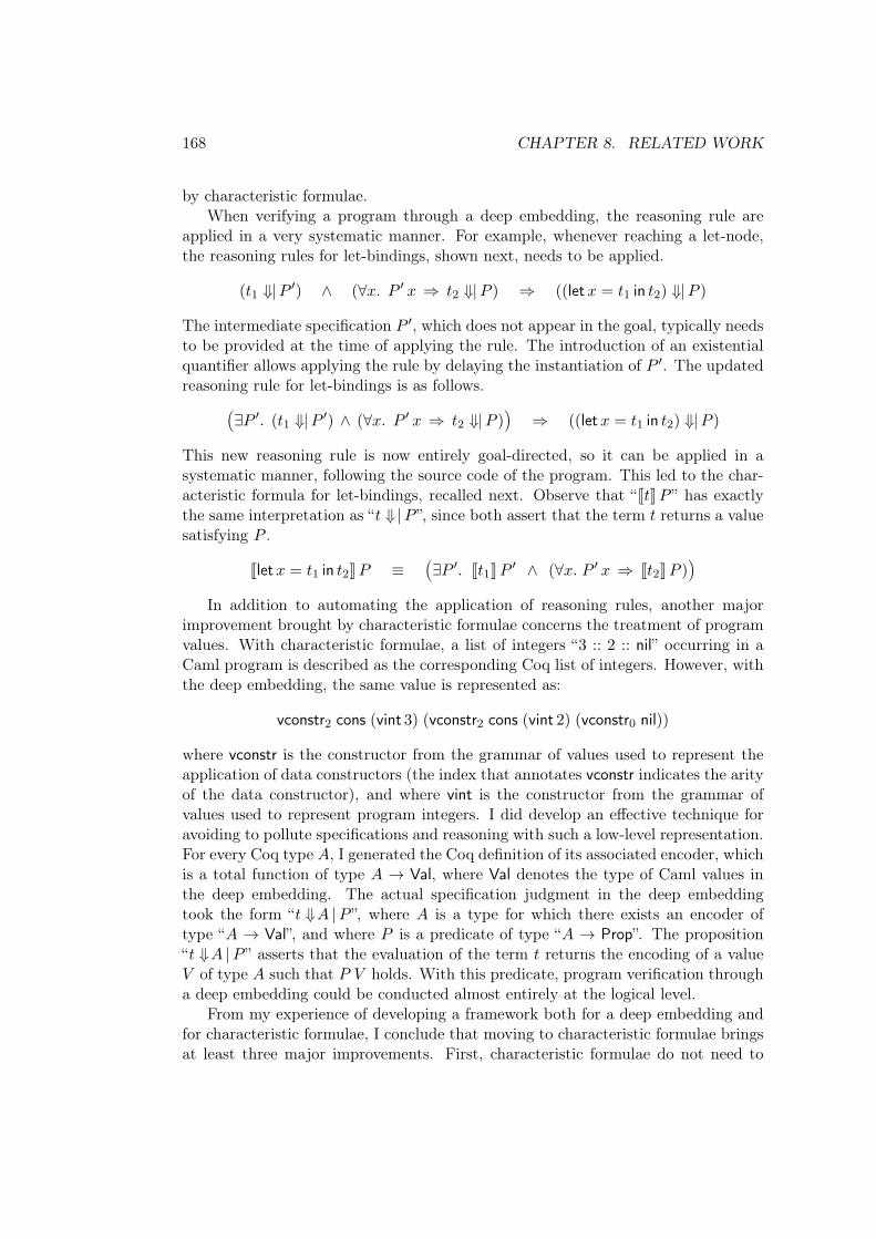
168 CHAPTER 8. RELATED WORK
by characteristic formulae.When verifying a program through a deep embedding, the reasoning rule are
applied in a very systematic manner. For example, whenever reaching a let-node,the reasoning rules for let-bindings, shown next, needs to be applied.
(𝑡1 ⇓|𝑃 ′) ∧ (∀𝑥. 𝑃 ′ 𝑥 ⇒ 𝑡2 ⇓|𝑃 ) ⇒ ((let𝑥 = 𝑡1 in 𝑡2) ⇓|𝑃 )
The intermediate specification 𝑃 ′, which does not appear in the goal, typically needsto be provided at the time of applying the rule. The introduction of an existentialquantifier allows applying the rule by delaying the instantiation of 𝑃 ′. The updatedreasoning rule for let-bindings is as follows.Ä
∃𝑃 ′. (𝑡1 ⇓|𝑃 ′) ∧ (∀𝑥. 𝑃 ′ 𝑥 ⇒ 𝑡2 ⇓|𝑃 )ä
⇒ ((let𝑥 = 𝑡1 in 𝑡2) ⇓|𝑃 )
This new reasoning rule is now entirely goal-directed, so it can be applied in asystematic manner, following the source code of the program. This led to the char-acteristic formula for let-bindings, recalled next. Observe that “J𝑡K𝑃 ” has exactlythe same interpretation as “𝑡 ⇓|𝑃 ”, since both assert that the term 𝑡 returns a valuesatisfying 𝑃 .
Jlet𝑥 = 𝑡1 in 𝑡2K𝑃 ≡Ä∃𝑃 ′. J𝑡1K𝑃 ′ ∧ (∀𝑥. 𝑃 ′ 𝑥 ⇒ J𝑡2K𝑃 )
äIn addition to automating the application of reasoning rules, another major
improvement brought by characteristic formulae concerns the treatment of programvalues. With characteristic formulae, a list of integers “3 :: 2 :: nil” occurring in aCaml program is described as the corresponding Coq list of integers. However, withthe deep embedding, the same value is represented as:
vconstr2 cons (vint 3) (vconstr2 cons (vint 2) (vconstr0 nil))
where vconstr is the constructor from the grammar of values used to represent theapplication of data constructors (the index that annotates vconstr indicates the arityof the data constructor), and where vint is the constructor from the grammar ofvalues used to represent program integers. I did develop an effective technique foravoiding to pollute specifications and reasoning with such a low-level representation.For every Coq type 𝐴, I generated the Coq definition of its associated encoder, whichis a total function of type 𝐴 → Val, where Val denotes the type of Caml values inthe deep embedding. The actual specification judgment in the deep embeddingtook the form “𝑡 ⇓𝐴 |𝑃 ”, where 𝐴 is a type for which there exists an encoder oftype “𝐴 → Val”, and where 𝑃 is a predicate of type “𝐴 → Prop”. The proposition“𝑡 ⇓𝐴 |𝑃 ” asserts that the evaluation of the term 𝑡 returns the encoding of a value𝑉 of type 𝐴 such that 𝑃 𝑉 holds. With this predicate, program verification througha deep embedding could be conducted almost entirely at the logical level.
From my experience of developing a framework both for a deep embedding andfor characteristic formulae, I conclude that moving to characteristic formulae bringsat least three major improvements. First, characteristic formulae do not need to
8.5. DEEP EMBEDDINGS 169
represent and manipulate program syntax. Thus, they avoid many technical diffi-culties, in particular those associated with the representation of binders. Moreover,I observed that the repeated computations of substitutions that occur during theverification of a deeply-embedded program can lead to the generation of proof termsof quadratic size, which can be problematic for scaling up to larger programs.
Second, with characteristic formulae there is no need to apply reasoning rulesof the program logic, because the applications of those rules is automatically donethrough the construction of the characteristic formulae. In particular, characteristicformulae saves the need to compute reduction contexts. With a deep embedding,to prove a goal of the form “𝑡 ⇓ |𝑃 ”, one must first rewrite the goal in the form“𝐶[𝑡1] ⇓ |𝑃 ”, where 𝐶 is a reduction context and where 𝑡1 is the subterm of 𝑡 inevaluation position. More generally, by moving to characteristic formulae, tacticscould be given a much simpler and a much more efficient implementation.
Third and last, characteristic formulae, by lifting values at the logical level onceand for all at the time of their construction, completely avoid the need to refer tothe relationship between program values and logical values. Contrary to the deepembedding approach, characteristic formulae do not require encoders to be involvedin specifications and proofs; encoders are only involved in the proof of soundnessof characteristic formulae. The removal of encoders leads to simpler specifications,simpler reasoning rules, and simpler tactics.
The fact that characteristic formulae outperform deep embeddings is after all nota surprise: characteristic formulae can be seen as an abstract layer built on the topof a deep embedding, so as to hide details related to the representation of values andto retain only the essence of the reasoning rules supported by the deep embedding.
Chapter 9
Conclusion
This last chapter begins with a summary of how the various approachesto program verification try to avoid referring to program syntax. I thenrecall the main ingredients involved for constructing a practical verifi-cation tool upon the idea of characteristic formulae. Finally, I discussdirections for future research, and conclude.
9.1 Characteristic formulae in the design space
The correctness of a program ultimately refers to the semantics of the programminglanguage in which that program is written. The reduction judgment describing thesemantics, written 𝑡/𝑚 ⇓ 𝑣′/𝑚′ in the thesis, directly refers to the input memorystate 𝑚 and to the output memory state 𝑚′. Hoare-triples, here written {𝐻} 𝑡 {𝑄},allow for abstraction in specifications. While a memory state 𝑚 describes exactlywhat values lie in memory, the heap descriptions involved in Hoare triples allow tostate properties about the values stored in memory, without necessarily revealing theexact representation of those values. Separation Logic later suggested an enhancedinterpretation of Hoare triples, according to which any allocated memory cell that isnot mentioned in the pre-condition of a term is automatically guaranteed to remainunchanged through the evaluation of that term. Separation Logic thereby allows forlocal reasoning, in the sense that the verification of a program component can beconducted independently of the pieces of state owned by other components.
By moving from a judgment of the form 𝑡/𝑚 ⇓ 𝑣′/𝑚′ to a judgment of the form{𝐻} 𝑡 {𝑄}, Hoare logic and Separation Logic avoid a direct reference to the mem-ory states 𝑚 and 𝑚′. However, the reference to the source code 𝑡 still remains. Inthe traditional VCG approach, this is not an issue: when the code is annotatedwith sufficiently-many specifications and invariants, it is possible to automaticallyextract a set of verification conditions. Proving the verification condition then en-sures that the program satisfies its specification. Although the VCG approach workssmoothly when the verification conditions can be discharged by fully-automated the-orem provers, verification conditions are not as well-suited for interactive proofs.
170
9.2. SUMMARY OF THE KEY INGREDIENTS 171
One alternative to building Hoare-logic derivations automatically consists inbuilding them by hand, through interactive proofs. To build the derivation of aHoare triple {𝐻} 𝑡 {𝑄} manually, one has to refer to the source code 𝑡 explicitly.The description of source code in the logic involves a deep embedding of the program-ming language. Program verification through a deep embedding is possible, howeverit requires a significant effort, mainly because values from the programming languageneeds to be explicitly lifted at the logical level, and because reasoning on reductionsteps involves computing substitutions in the deep embedding of the source code.
The main motivation for verifying programs with a shallow embedding is pre-cisely to avoid the reference to programming language syntax. There are severalways in which a shallow embedding can be exploited in program verification, butthey all rely on the same idea: building a logical definition that corresponds to thesource code of the program to be verified. These techniques relies on the fact thatthe logic of a theorem prover actually contains a small programming language. Yet,the shallow embedding approach suffers from restrictions related to the fact thatsome features of the host logical language are carved in stone.
I have followed a different approach to removing direct reference to the sourcecode of the program to be verified. It consists in generating a logical formula thatcharacterizes the behavior of the source code. This concept of characteristic formulaeis not new: it was first developed in process calculi [70, 57] and was later adaptedto PCF programs by Honda, Berger and Yoshida [40]. Yet, those characteristicformulae for PCF programs work did not lead to a practical verification system,because the specification language relied on a nonstandard logic.
In this thesis, I have shown how to construct characteristic formulae expressed ina standard higher-order logic. The characteristic formula of a term 𝑡 is a predicate,written J𝑡K, such that J𝑡K𝐻 𝑄 implies that the term 𝑡 admits 𝐻 as pre-conditionand 𝑄 as post-condition. I have implemented a tool for generating Coq character-istic formulae for Caml programs, and I have developed a Coq library that includesdefinitions, lemmas and tactics for proving programs through their characteristicformula. Finally, I have applied this tool for specifying and verifying nontrivial pro-grams. The key ingredients involved for turning the idea of characteristic formulaeinto a practical verification system are summarized next.
9.2 Summary of the key ingredients
Characteristic formulae The starting point of this thesis is the notion of char-acteristic formula, which is a higher-order logic formulae that characterizes the setof total-correctness specifications that a given program admits. A characteristic for-mula is built compositionally from the source code of the program it describes, andit has a size linear in that of the program. The program does not need to be an-notated with specification and invariants, as unknown specifications and invariantsget quantified existentially in characteristic formulae.
172 CHAPTER 9. CONCLUSION
Notation layer If ℱ is the characteristic formula of a term 𝑡, the proof obligationtakes the form “ℱ 𝐻 𝑄”, where 𝐻 is the pre-condition and 𝑄 is the post-condition.I have devised a system of notation for pretty-printing characteristic formulae ina way that closely resemble the source code that the formula describes. So, theproof obligation “ℱ 𝐻 𝑄” reads like the term 𝑡 being applied to the pre- and thepost-conditions, in the form “𝑡𝐻 𝑄”. Since characteristic formulae are built compo-sitionally, the ability to easily read proof obligations applies not only to the initialterm 𝑡 but also to all of its subterms.
Reflection of values The values involved in the execution of a program are spec-ified using values from the logic. For example, if a Caml function expects a list ofintegers, then its pre-condition is a predicate about Coq list of integers. This reflec-tion of Caml values as Coq values works for all values except for functions, becauseCoq functions can only describe total functions. I have introduced the abstract typeFunc to represent functions, as well as the abstract predicate AppEval for specifyingthe behavior of function applications. In the soundness proof, a value of type Funcis interpreted as the deep embedding of the source code of some function. Thisinterpretation avoids the need to rely on a nonstandard logic, as done in the workof Honda, Berger and Yoshida [40].
Ghost variables The specification of a function generally involves ghost vari-ables, in particular for sharing information between the pre-condition and the post-condition. In order to state general lemmas about function specifications, such asthe induction lemma which inserts an induction hypothesis into given specification,I have introduced the predicate Spec. The proposition Spec𝑓𝐾 asserts that thefunction 𝑓 admits the specification 𝐾, where 𝐾 is an higher-order predicate able tocapture the quantification over an arbitrary number of ghost variables.
N-ary functions Caml programs typically define functions of several argumentsin a curried fashion. Partial applications are commonplace, and over-applicationsare also possible. In theory, a function of two arguments can always be specified asa function of one argument that returns another function of one argument. Yet, ahigher-level predicate that captures the specification of a function of two argumentsin a more direct way is a must-have for practical verification. For that purpose, Ihave defined a family of predicates AppReturns𝑛 and Spec𝑛, which are all ultimatelydefined in terms of the core predicate AppReturns.
Heap predicates Characteristic formulae, which were first set up for purely func-tional programs, could easily be extended to an imperative setting by adding heapdescriptions. I exploited the techniques of Separation Logic for describing heapsin a concise way, and followed the Coq definitions of Separation Logic connectivesdeveloped in Ynot [17]. In particular, heap predicates of the form 𝐿 →˓𝒯 𝑉 supportreasoning on strong updates. One novel ingredient for handling Separation Logic in
9.2. SUMMARY OF THE KEY INGREDIENTS 173
characteristic formulae is the definition of the predicate local, which is inserted atevery node of a characteristic formula, thereby allowing for application of the framerule at any time.
Bounded recursive ownership The use of representation predicates is a stan-dard technique for relating imperative data structures with their mathematicalmodel. I have extended this technique to polymorphic representation predicates: arepresentation predicate for a container takes as argument the representation pred-icate describing the elements stored in that container. Depending on the represen-tation predicate given for the elements, one can describe either a situation wherethe container owns its elements, or a situation where the container does not own itselements and simply views them as base values.
Weak-ML ML types greatly help in program verification because they allow re-flecting basic Caml values directly as their Coq counterpart. Yet, for the sake of typesoundness, the ML type system keeps track of the type of functions, and it enforcesthe invariant that a location of type ref 𝜏 contains a value of type 𝜏 at any time.Since program verification is a much more accurate analysis than ML type-checking,it need not suffer from the restrictions imposed by ML. The introduction of the typesystem weak-ML serves two purposes. First, it relaxes the restrictions associatedwith ML, in particular through a totally-unconstrained typing rule for applications.Second, it simplifies the proof of soundness of characteristic formulae, by allowing toestablish a bijection between well-typed weak-ML values and a subset of Coq values,and by avoiding the need to involve a store typing oracle.
High-level tactics I have developed a set of tactics for reasoning on character-istic formulae in Coq. Those tactics not only shorten proof scripts, they also makeit possible to verify programs without knowledge of the details of the constructionof characteristic formulae. The end-user only needs to learn the various syntaxesfor CFML tactics, in particular the optional arguments for specifying how variablesand hypotheses should be named. Furthermore, in the verification of imperativeprograms, tactics play a key role by supporting application of lemmas modulo asso-ciativity and commutativity of the separating conjunction, and by automating theapplication of the frame rule on function calls.
Implementation The CFML generator parses Caml code and produces Coq def-initions. It reuses the parser and the type-checker of the OCaml compiler, andinvolves about 3, 000 lines of OCaml for constructing characteristic formulae. TheCFML library contains notations, lemmas and tactics for manipulating characteris-tic formulae. It is made of about 4, 000 lines of Coq. Note that the CFML librarywould have been significantly easier to implement if Coq did feature a slightly moreevolved tactic language.
174 CHAPTER 9. CONCLUSION
9.3 Future work
Formal verification of characteristic formulae Defenders of a foundationalapproach to program verification argue that we ought to try and reduce the trustedcomputing base as much as possible. There are at least two ways of proceeding.The first one involves building a verified characteristic formula generator and thenconducting a machine-checked proof of the soundness theorem for characteristicformulae. An alternative approach consists in developing a program that, insteadof generating axioms to reflect every top-level declaration from the source Camlprogram, directly generates lemmas and their proofs. Those proofs would be carriedout in terms of a deep embedding of the source program. Note that the programgenerating the lemmas and their proofs would not need to be itself proved correct,because its output would be validated by the Coq proof-checker. I expect both ofthose approaches to involve a lot of effort if a full-blown programming language isto be supported.
Non-determinism In this thesis, I have assumed the source language to be deter-ministic. This assumption makes definitions and proofs slightly simpler, in particularfor the treatment of partial functions and polymorphism, however it does not seem tobe essential to the development. One could probably replace the predicate AppEvalwith two predicates: a deterministic predicate describing only the evaluation of par-tial applications of curried functions, and a non-deterministic predicate describingthe evaluation of general function applications.
Exceptions It should be straightforward to add support for throwing and catchingof exceptions. Currently, a post-condition has the type “𝐴 → Hprop”, describing boththe result value of type 𝐴 and the heap produced. Support for exceptions can beadded by generalizing the result type to “(𝐴 + exn) → Hprop”, where exn denotesthe type of exceptions. Such a treatment of exceptions has been implemented forexample in Ynot [17]. Characteristic formulae would then involve a left injection todescribe a normal result and involve a right injection to describe the throwing of anexception.
Arithmetic So far, I have completely avoided the difficulties related to fixed-size representations of numbers: I have assumed arbitrary-precision integers andI have not provided any support for floating-point numbers. One way to obtaincorrect programs without wasting time reasoning on modulo arithmetic consists inrepresenting all integers using the BigInt library. Alternatively, one could targetfixed-size integers, yet at the cost of proving side-conditions for every arithmeticoperation involved in the source program. For floating-point numbers, the problemappears to be harder. Nevertheless, it should be possible to build upon the recentbreakthroughs in formal reasoning on numerical routines [11, 3] and achieve a highdegree of automation.
9.3. FUTURE WORK 175
Fields as arrays The frame rule can be made even more useful if the ownershipof an array of records can be viewed as the ownership of a record of arrays. Such are-organization of memory allows to invoke the frame rule on particular fields of arecord. One can then obtain for free the property that a function that needs onlyaccess one field of a record does not modify the other fields. It should be possibleto define heap predicates that capture the field-as-array methodology.
Hidden state Modules can be used to abstract the definition of the invariantsof private pieces of heap. One may want to go further and hide altogether theexistence of such a private piece of state. This is precisely the purpose of the anti-frame rule developed by Pottier [75, 80]. For example, assume that a module exportsa heap predicate 𝐼 of type Hprop and a function 𝑓 that admits the pre-condition𝐻 * 𝐼 and the post-condition 𝑄⋆ 𝐼. Assume that the module also contains a privateinitialization code that allocates a piece of heap satisfying the invariant 𝐼. Then,the module can be viewed from the outside world as simply exporting a function 𝑓that admits the pre-condition 𝐻 and the post-condition 𝑄, removing any referenceto the invariant 𝐼. Integrating the anti-frame rule would allow exporting cleanerspecifications for modules such as a random-number generator, a hash-consing datastructure, a memoization module, and, more generally, for any imperative datastructure that exposes a purely-functional interface.
Concurrency The verification of concurrent programs is a obvious direction forfuture research. A natural starting point would be to try and extend characteristicformulae with the reasoning rules developed for Concurrent Separation Logic, whichwas initially devised by O’Hearn and Brookes [13, 68], and later also developed byother researchers [72, 37].
Module systems In the experimental support for modules and systems, I havemapped Caml modules to Coq modules. However, limitations in the current modulesystem of Coq make it difficult to verify nontrivial Caml functors. The enhancementof modules for Coq is a largely-open problem. In fact, one may argue that even themodule system of Caml is not entirely satisfying. I hope that, in the near future,an expressive and practical module system that fits both Caml and Coq will beproposed. Such a common module system would be very helpful for carrying outmodular verification of modular programs without having to hack around severallimitations.
Low-level languages It would be very interesting to implement a characteristicformula generator for a lower-level programming language such as C or assembly.Features such as pointer arithmetic should not be too difficult to handle. The treat-ment of general “goto” instructions may be tricky to handle, however the treatmentof “break” and “continue” instructions appears to be straightforward to integrate
176 CHAPTER 9. CONCLUSION
in the characteristic formulae for loops. Characteristic formulae for low-level pro-grams should also bring strong guarantees about total collection, ensuring that allthe memory allocated by a program is freed at some point.
Object-oriented languages It would also be worth investigating how charac-teristic formulae may be adapted to an object-oriented programming language likeJava or C#. The object presentation naturally encourages ghost variables, whichdescribes the mathematical model of an object, to be laid out as ghost fields. Thistreatment may reduce the number of existentially-quantified variables and therebyallow more goals to be solved by automated theorem provers. Yet, a number ofdifficult problems arise when moving to an object-oriented language, in particularwith respect to the specification of collaborating classes and thus need to share acommon invariant, and with respect to the inheritance of specifications. It wouldbe interesting to see whether characteristic formulae can integrate the notion ofdynamic specification that has been developed by Parkinson and Bierman [71] tohandle inheritance in Java.
Partial correctness The characteristic formulae that I have developed targettotal correctness, which offers a stronger guarantee than partial correctness. Yet,some programs, such as web-servers, are not intended to terminate. A partial-correctness Hoare triple whose post-condition is the predicate False asserts thata program diverges, because the program is proved never to crash and never toterminate. Divergence cannot be specified in a total correctness setting. So, onecould be interested in trying to build characteristic formulae that target partialcorrectness, possibly reusing ideas developed by Honda et al [40].
Lazy evaluation The treatment of lazy evaluation that I relied on for verifyingOkasaki’s data structures is quite limited. Indeed, verifying a program by remov-ing all the lazy keywords for the source code is sound but not complete. I havestarted to work on an explicit treatment of suspended computations, aiming for aproper model of the implementation of laziness in Caml. More challenging would bethe reasoning on Haskell programs, where laziness is implicit. The specification ofHaskell programs would probably involve the specification of partially-defined datastructures, as suggested by Danielsson et al [20].
Complexity analysis One could generalize characteristic formulae into predicatesthat, in addition to a pre- and a post-condition, also applies to a bound on thenumber of reduction steps. Proof obligations would then take the form “ℱ 𝑁 𝐻 𝑄”,where ℱ is a characteristic formula and 𝑁 is a natural number. Another possibleapproach, suggested by Pottier, consists in keeping proof obligations in the form“ℱ 𝐻 𝑄” and adding an artificial heap predicate of the form “credit𝑁 ”, which denotesthe ownership of “the right to perform 𝑁 reduction steps”. Note that a credit of theform “credit (𝑁+𝑀)” can be split at any time into a conjunction “credit𝑁*credit𝑀 ”.
9.4. FINAL WORDS 177
This suggestion has been studied by Pilkiewicz and Pottier [74] in a type systemthat extends the type system developed by Pottier and myself [16]. It should notbe difficult to modify characteristic formulae so as to impose that atomic operationsconsume exactly one credit, in the sense that they expect “credit 1” in the pre-condition and do not give this credit back in the post-condition. Combined with atreatment of laziness, this approach based on credits would presumably enable theformalization of the advanced complexity analyses involved in Okasaki’s book [69].
9.4 Final words
I would like to conclude by speculating on the role of interactive theorem provers infuture developments of program verification. Research on artificial intelligence hashad limited success in automated theorem proving, and, in spite of the impressiveprogress made by SMT solvers, the verification of nontrivial programs still requiresa good amount of user intervention in addition to the writing of specifications.Being established that some form of interaction between the user and the machineis required, proof assistants appear as a fairly effective way for users to providethe high-level arguments of a proof and for the system to give real-time feedback.My thesis has focused on the development of characteristic formulae, which aim atsmoothly integrating program verification within proof assistants. Proof assistantshave undergone tremendous improvements in the last decade. Undoubtedly, theywill continue to be improved, making interactive proofs, and, in particular, programverification, more largely applicable and more accessible.
Bibliography
[1] L. Aceto and A. Ingolfsdottir. Characteristic formulae: from automata to logic.Bulletin of the European Association for Theoretical Computer Science, 91:57,2007. Columns: Concurrency.
[2] Andrew W. Appel. Tactics for separation logic. Unpublished draft,http://www.cs.princeton.edu/appel/papers/septacs.pdf, 2006.
[3] Ali Ayad and Claude Marché. Multi-prover verification of floating-point pro-grams. In Jürgen Giesl and Reiner Hähnle, editors, International Joint Con-ference on Automated Reasoning, Lecture Notes in Artificial Intelligence, Edin-burgh, Scotland, 2010. Springer.
[4] Mike Barnett, Bor-Yuh Evan Chang, Robert DeLine, Bart Jacobs, and K. Rus-tan M. Leino. Boogie: A modular reusable verifier for object-oriented programs.In Formal Methods for Components and Objects (FMCO) 2005, Revised Lec-tures, volume 4111 of LNCS, pages 364–387, New York, NY, 2006. Springer-Verlag.
[5] Mike Barnett, Rob DeLine, Manuel Fähndrich, K. Rustan M. Leino, and Wol-fram Schulte. Verification of object-oriented programs with invariants. Journalof Object Technology, 3(6), 2004.
[6] Bruno Barras and Bruno Bernardo. The implicit calculus of constructions as aprogramming language with dependent types. In Roberto M. Amadio, editor,FoSSaCS, volume 4962 of LNCS, pages 365–379. Springer, 2008.
[7] Bernhard Beckert, Reiner Hähnle, and Peter H. Schmitt. Verification of Object-Oriented Software: The KeY Approach, volume 4334 of LNCS. Springer-Verlag,Berlin, 2007.
[8] Josh Berdine, Cristiano Calcagno, and Peter W. O’Hearn. Smallfoot: Modularautomatic assertion checking with separation logic. In International Symposiumon Formal Methods for Components and Objects, volume 4111 of LNCS, pages115–137. Springer, 2005.
[9] Josh Berdine and Peter W. O’Hearn. Strong update, disposal, and encapsula-tion in bunched typing. In Mathematical Foundations of Programming Seman-
178
BIBLIOGRAPHY 179
tics, volume 158 of Electronic Notes in Theoretical Computer Science, pages81–98. Elsevier Science, 2006.
[10] Martin Berger, Kohei Honda, and Nobuko Yoshida. A logical analysis of aliasingin imperative higher-order functions. In ACM International Conference onFunctional Programming (ICFP), pages 280–293, 2005.
[11] Sylvie Boldo and Jean-Christophe Filliâtre. Formal verification of floating-pointprograms. In IEEE Symposium on Computer Arithmetic, pages 187–194. IEEEComputer Society, 2007.
[12] Richard Bornat. Proving pointer programs in Hoare logic. In InternationalConference on Mathematics of Program Construction (MPC), volume 1837 ofLNCS, pages 102–126. Springer, 2000.
[13] Stephen D. Brookes. A semantics for concurrent separation logic. In PhilippaGardner and Nobuko Yoshida, editors, CONCUR, volume 3170 of LNCS, pages16–34. Springer, 2004.
[14] R. M. Burstall. Some techniques for proving correctness of programs which alterdata structures. In B. Meltzer and D. Mitchie, editors, Machine Intelligence 7,pages 23–50. Edinburgh University Press, Edinburgh, Scotland., 1972.
[15] Arthur Charguéraud. Verification of call-by-value functionalprograms through a deep embedding. 2009. Unpublished.http://arthur.chargueraud.org/research/2009/deep/.
[16] Arthur Charguéraud and François Pottier. Functional translation of a calculusof capabilities. In ACM International Conference on Functional Programming(ICFP), 2008.
[17] Adam Chlipala, Gregory Malecha, Greg Morrisett, Avraham Shinnar, and RyanWisnesky. Effective interactive proofs for higher-order imperative programs. InACM International Conference on Functional Programming (ICFP), 2009.
[18] The Coq Development Team. The Coq Proof Assistant Reference Manual, Ver-sion 8.2, 2009.
[19] Thierry Coquand. Alfa/agda. In Freek Wiedijk, editor, The Seventeen Proversof the World, Foreword by Dana S. Scott, volume 3600 of LNCS, pages 50–54.Springer, 2006.
[20] Nils Anders Danielsson, John Hughes, Patrik Jansson, and Jeremy Gibbons.Fast and loose reasoning is morally correct. In ACM Symposium on Principlesof Programming Languages (POPL), pages 206–217, 2006.
[21] Leonardo de Moura and Nikolaj Bjørner. Z3: An efficient SMT solver. In Toolsand Algorithms for the Construction and Analysis (TACAS), volume 4963 ofLNCS, pages 337–340, Berlin, 2008. Springer-Verlag.
180 BIBLIOGRAPHY
[22] Edsger W. Dijkstra. A Discipline of Programming. Prentice-Hall, 1976.
[23] Manuel Fähndrich and Robert DeLine. Adoption and focus: practical lineartypes for imperative programming. In ACM Conference on Programming Lan-guage Design and Implementation (PLDI), pages 13–24, 2002.
[24] Xinyu Feng, Rodrigo Ferreira, and Zhong Shao. On the relationship betweenconcurrent separation logic and assume-guarantee reasoning. In Rocco DeNicola, editor, ESOP, volume 4421 of LNCS, pages 173–188. Springer, 2007.
[25] Xinyu Feng, Zhong Shao, Alexander Vaynberg, Sen Xiang, and Zhaozhong Ni.Modular verification of assembly code with stack-based control abstractions.In ACM Conference on Programming Language Design and Implementation(PLDI), pages 401–414, 2006.
[26] Jean-Christophe Filliâtre. Verification of non-functional programs using inter-pretations in type theory. Journal of Functional Programming, 13(4):709–745,2003.
[27] Jean-Christophe Filliâtre and Claude Marché. Multi-prover verification of Cprograms. In Formal Methods and Software Engineering, 6th ICFEM 2004,volume 3308 of LNCS, pages 15–29. Springer-Verlag, 2004.
[28] Cormac Flanagan, Amr Sabry, Bruce F. Duba, and Matthias Felleisen. Theessence of compiling with continuations. In ACM Conference on ProgrammingLanguage Design and Implementation (PLDI), pages 237–247, 1993.
[29] R. W. Floyd. Assigning meanings to programs. In Mathematical Aspects ofComputer Science, volume 19 of Proceedings of Symposia in Applied Mathe-matics, pages 19–32. American Mathematical Society, 1967.
[30] Georges Gonthier and Assia Mahboubi. A small scale reflection extension forthe Coq system. Research Report 6455, Institut National de Recherche enInformatique et en Automatique, Le Chesnay, France, 2008.
[31] G. A. Gorelick. A complete axiomatic system for proving assertions about recur-sive and non-recursive programs. Technical Report 75, University of Toronto,1975.
[32] Susanne Graf and Joseph Sifakis. A modal characterization of observationalcongruence on finite terms of CCS. Information and Control, 68(1-3):125–145,1986.
[33] David Harel, Dexter Kozen, and Jerzy Tiuryn. Dynamic Logic. The MIT Press,Cambridge, Massachusetts, 2000.
[34] Eric C. R. Hehner. Specified blocks. In Bertrand Meyer and Jim Woodcock,editors, VSTTE, volume 4171 of LNCS, pages 384–391. Springer, 2005.
BIBLIOGRAPHY 181
[35] M. C. B. Hennesy and R. Milner. Algebraic laws for nondeterminism andconcurrency. Journal of the ACM, 32(1):137–161, 1985.
[36] C. A. R. Hoare. An axiomatic basis for computer programming. Communica-tions of the ACM, 12(10):576–580, 583, 1969.
[37] Aquinas Hobor, Andrew W. Appel, and Francesco Zappa Nardelli. Oracle se-mantics for concurrent separation logic. In Sophia Drossopoulou, editor, ESOP,volume 4960 of LNCS, pages 353–367. Springer, 2008.
[38] Kohei Honda. From process logic to program logic. In Chris Okasaki andKathleen Fisher, editors, ICFP, pages 163–174. ACM, 2004.
[39] Kohei Honda, Martin Berger, and Nobuko Yoshida. An observationally com-plete program logic for imperative higher-order functions. In Proceedings ofthe Twentieth Annual IEEE Symposium on Logic in Computer Science (LICS),pages 280–293, 2005.
[40] Kohei Honda, Martin Berger, and Nobuko Yoshida. Descriptive and relativecompleteness of logics for higher-order functions. In M. Bugliesi, B. Preneel,V. Sassone, and I. Wegener, editors, Automata, Languages and Programming,33rd International Colloquium, ICALP 2006, Venice, Italy, July 10-14, 2006,Proceedings, Part II, volume 4052 of LNCS. Springer, 2006.
[41] Kohei Honda and Nobuko Yoshida. A compositional logic for polymorphichigher-order functions. In International ACM Conference on Principles andPractice of Declarative Programming (PPDP), pages 191–202, 2004.
[42] Samin Ishtiaq and Peter W. O’Hearn. BI as an assertion language for mutabledata structures. In ACM Symposium on Principles of Programming Languages(POPL), pages 14–26, London, United Kingdom, 2001.
[43] Bart Jacobs and Erik Poll. Java program verification at nijmegen: Develop-ments and perspective. In Kokichi Futatsugi, Fumio Mizoguchi, and NaokiYonezaki, editors, ISSS, volume 3233 of LNCS, pages 134–153. Springer, 2003.
[44] Johannes Kanig and Jean-Christophe Filliâtre. Who: a verifier for effectfulhigher-order programs. In ML’09: Proceedings of the 2009 ACM SIGPLANworkshop on ML, pages 39–48, New York, NY, USA, 2009. ACM.
[45] Gerwin Klein, Philip Derrin, and Kevin Elphinstone. Experience report: seL4:formally verifying a high-performance microkernel. In Graham Hutton andAndrew P. Tolmach, editors, ICFP, pages 91–96. ACM, 2009.
[46] Gerwin Klein, Kevin Elphinstone, Gernot Heiser, June Andronick, David Cock,Philip Derrin, Dhammika Elkaduwe, Kai Engelhardt, Rafal Kolanski, MichaelNorrish, Thomas Sewell, Harvey Tuch, and Simon Winwood. seL4: Formalverification of an OS kernel. In Proceedings of the 22nd Symposium on Operating
182 BIBLIOGRAPHY
Systems Principles (22nd SOSP’09), Operating Systems Review (OSR), pages207–220, Big Sky, MT, 2009. ACM SIGOPS.
[47] Xavier Leroy. Formal certification of a compiler back-end or: programming acompiler with a proof assistant. In ACM Symposium on Principles of Program-ming Languages (POPL), pages 42–54, 2006.
[48] Xavier Leroy, Damien Doligez, Jacques Garrigue, Didier Rémy, and JérômeVouillon. The Objective Caml system, 2005.
[49] Pierre Letouzey. Programmation fonctionnelle certifiée – l’extraction de pro-grammes dans l’assistant Coq. PhD thesis, Université Paris 11, 2004.
[50] Panagiotis Manolios and J Strother Moore. Partial functions in ACL2. 2003.
[51] Claude Marché, Christine Paulin Mohring, and Xavier Urbain. The Krakatoatool for certification of Java/JavaCard programs annotated in JML. JLAP,58(1–2):89–106, 2004.
[52] Nicolas Marti, Reynald Affeldt, and Akinori Yonezawa. Towards formal verifi-cation of memory properties using separation logic, 2005.
[53] Nicolas Marti, Reynald Affeldt, and Akinori Yonezawa. Verification of the heapmanager of an operating system using separation logic. In Proceedings of theThird SPACE, pages 61–72, Charleston, SC, USA, 2006.
[54] Conor McBride and James McKinna. The view from the left. Journal ofFunctional Programming, 14(1):69–111, 2004.
[55] Andrew McCreight. Practical tactics for separation logic. In Stefan Berghofer,Tobias Nipkow, Christian Urban, and Makarius Wenzel, editors, TPHOLs, vol-ume 5674 of LNCS, pages 343–358. Springer, 2009.
[56] Farhad Mehta and Tobias Nipkow. Proving pointer programs in higher-orderlogic. In Franz Baader, editor, Automated Deduction - CADE-19, 19th Inter-national Conference on Automated Deduction Miami Beach, FL, USA, July 28- August 2, 2003, Proceedings, volume 2741 of LNCS, pages 121–135. Springer,2003.
[57] R. Milner. Communication and Concurrency. Prentice-Hall, 1989.
[58] Magnus O. Myreen. Formal Verification of Machine-Code Programs. PhDthesis, University of Cambridge, 2008.
[59] Magnus O. Myreen. Separation logic adapted for proofs by rewriting. In MattKaufmann and Lawrence C. Paulson, editors, ITP, volume 6172 of LNCS, pages485–489. Springer, 2010.
BIBLIOGRAPHY 183
[60] Magnus O. Myreen and Michael J. C. Gordon. Verified LISP implementationson ARM, x86 and powerPC. In Stefan Berghofer, Tobias Nipkow, ChristianUrban, and Makarius Wenzel, editors, TPHOLs, volume 5674 of LNCS, pages359–374. Springer, 2009.
[61] A. Nanevski and G. Morrisett. Dependent type theory of stateful higher-orderfunctions. Technical report, Citeseer, 2005.
[62] Aleksandar Nanevski, Greg Morrisett, Avi Shinnar, Paul Govereau, and LarsBirkedal. Ynot : Reasoning with the awkward squad. In ACM InternationalConference on Functional Programming (ICFP), 2008.
[63] Aleksandar Nanevski, J. Gregory Morrisett, and Lars Birkedal. Hoare typetheory, polymorphism and separation. Journal of Functional Programming,18(5-6):865–911, 2008.
[64] Aleksandar Nanevski, Viktor Vafeiadis, and Josh Berdine. Structuring the ver-ification of heap-manipulating programs. In Manuel V. Hermenegildo and JensPalsberg, editors, Proceedings of the 37th ACM SIGPLAN-SIGACT Symposiumon Principles of Programming Languages, POPL 2010, Madrid, Spain, January17-23, 2010, pages 261–274. ACM, 2010.
[65] Zhaozhong Ni and Zhong Shao. Certified assembly programming with embed-ded code pointers. In ACM Symposium on Principles of Programming Lan-guages (POPL), 2006.
[66] Peter O’Hearn and David Pym. The logic of bunched implications. Bulletin ofSymbolic Logic, 5(2):215–244, 1999.
[67] Peter O’Hearn, John Reynolds, and Hongseok Yang. Local reasoning aboutprograms that alter data structures. In Proceedings of CSL’01, volume 2142 ofLNCS, pages 1–19, Berlin, 2001. Springer-Verlag.
[68] Peter W. O’Hearn. Resources, concurrency and local reasoning. TheoreticalComputer Science, 375(1–3):271–307, 2007.
[69] Chris Okasaki. Purely Functional Data Structures. Cambridge University Press,1999.
[70] David Park. Concurrency and automata on infinite sequences. In Peter Deussen,editor, Theoretical Computer Science: 5th GI-Conference, Karlsruhe, volume104 of LNCS, pages 167–183, Berlin, Heidelberg, and New York, 1981. Springer-Verlag.
[71] Matthew J. Parkinson and Gavin M. Bierman. Separation logic, abstractionand inheritance. In George C. Necula and Philip Wadler, editors, POPL, pages75–86. ACM, 2008.
184 BIBLIOGRAPHY
[72] Matthew J. Parkinson, Richard Bornat, and Peter W. O’Hearn. Modular ver-ification of a non-blocking stack. In Martin Hofmann and Matthias Felleisen,editors, POPL, pages 297–302. ACM, 2007.
[73] Benjamin C. Pierce and David N. Turner. Simple type-theoretic foundations forobject-oriented programming. Journal of Functional Programming, 4(2):207–247, 1994.
[74] Alexandre Pilkiewicz and François Pottier. The essence of monotonic state.In Proceedings of the Sixth ACM SIGPLAN Workshop on Types in LanguageDesign and Implementation (TLDI’11), Austin, Texas, 2011.
[75] Fran cois Pottier. Hiding local state in direct style: A higher-order anti-framerule. In LICS, pages 331–340. IEEE Computer Society, 2008.
[76] Yann Régis-Gianas and François Pottier. A Hoare logic for call-by-value func-tional programs. In International Conference on Mathematics of Program Con-struction (MPC), 2008.
[77] John C. Reynolds. Separation logic: A logic for shared mutable data structures.In IEEE Symposium on Logic in Computer Science (LICS), pages 55–74, 2002.
[78] K. Rustan, M. Leino, and M. Moskal. VACID-0: Verification of Ample Cor-rectness of Invariants of Data-structures, Edition 0. 2010.
[79] Peter H. Schmitt, Mattias Ulbrich, and Benjamin Weiß. Dynamic frames in Javadynamic logic. In Bernhard Beckert and Claude Marché, editors, Proceedings,International Conference on Formal Verification of Object-Oriented Software(FoVeOOS 2010), volume 6528 of LNCS, pages 138–152. Springer, 2011.
[80] Jan Schwinghammer, Hongseok Yang, Lars Birkedal, François Pottier, andBernhard Reus. A semantic foundation for hidden state. In C.-H. L. Ong, editor,Proceedings of the 13th International Conference on Foundations of SoftwareScience and Computational Structures (FOSSACS 2010), volume 6014 of LNCS,pages 2–17. Springer, 2010.
[81] Matthieu Sozeau. Program-ing finger trees in coq. SIGPLAN Not., 42(9):13–24,2007.
[82] Harvey Tuch, Gerwin Klein, and Michael Norrish. Types, bytes, and separationlogic. In Martin Hofmann and Matthias Felleisen, editors, POPL, pages 97–108.ACM, 2007.
[83] Thomas Tuerk. Local reasoning about while-loops. In VSTTE LNCS, 2010.
[84] David Wagner, Jeffrey S. Foster, Eric A. Brewer, and Alexander Aiken. A firststep towards automated detection of buffer overrun vulnerabilities. In NDSS.The Internet Society, 2000.
BIBLIOGRAPHY 185
[85] Hongseok Yang, Oukseh Lee, Josh Berdine, Cristiano Calcagno, Byron Cook,Dino Distefano, and Peter W. O’Hearn. Scalable shape analysis for systemscode. In Aarti Gupta and Sharad Malik, editors, CAV, volume 5123 of LNCS,pages 385–398. Springer, 2008.
[86] Hongseok Yang and Peter W. O’Hearn. A semantic basis for local reasoning.In Mogens Nielsen and Uffe Engberg, editors, FoSSaCS, volume 2303 of LNCS,pages 402–416. Springer, 2002.
[87] Nobuko Yoshida, Kohei Honda, and Martin Berger. Logical reasoning forhigher-order functions with local state. In International Conference on Foun-dations of Software Science and Computation Structures (FOSSACS), volume4423 of LNCS, pages 361–377. Springer, 2007.
[88] Karen Zee, Viktor Kuncak, and Martin C. Rinard. An integrated proof languagefor imperative programs. In Michael Hind and Amer Diwan, editors, PLDI,pages 338–351. ACM, 2009.