chapter three soil strength and soil forces. 3.1 introduction in terms of soil mechanics, there are...
TRANSCRIPT
CHAPTER THREE
SOIL STRENGTH AND SOIL FORCES
3.1 INTRODUCTION
In terms of Soil Mechanics, there are two groups of soil properties:
3.1.1 Internal properties: i) Friction in the soil is a factor and depends on
the normal load. It is between soil and soil and is called angle of
shearing resistance or internal friction ( ) ii) The force of adherence between the particles of
the soil - cohesion. The cohesion(C) is the attraction of soil properties
for each other.
External Soil Properties
i) Friction between soil and an external material e.g. a moldboard plough.
This is called external friction or soil metal friction. The symbol is
ii) Adhesion: The attraction between soil and some other material e.g. plough.
The symbol is Ca. These four properties control the soil behaviour as a mechanical entity.
Measurement of Soil Mechanical Properties
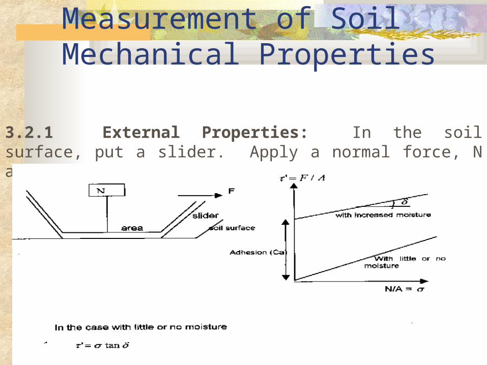
3.2.1 External Properties: In the soil surface, put a slider. Apply a normal force, N and apply a shear force, F.
Measurement of External Soil Properties Contd.
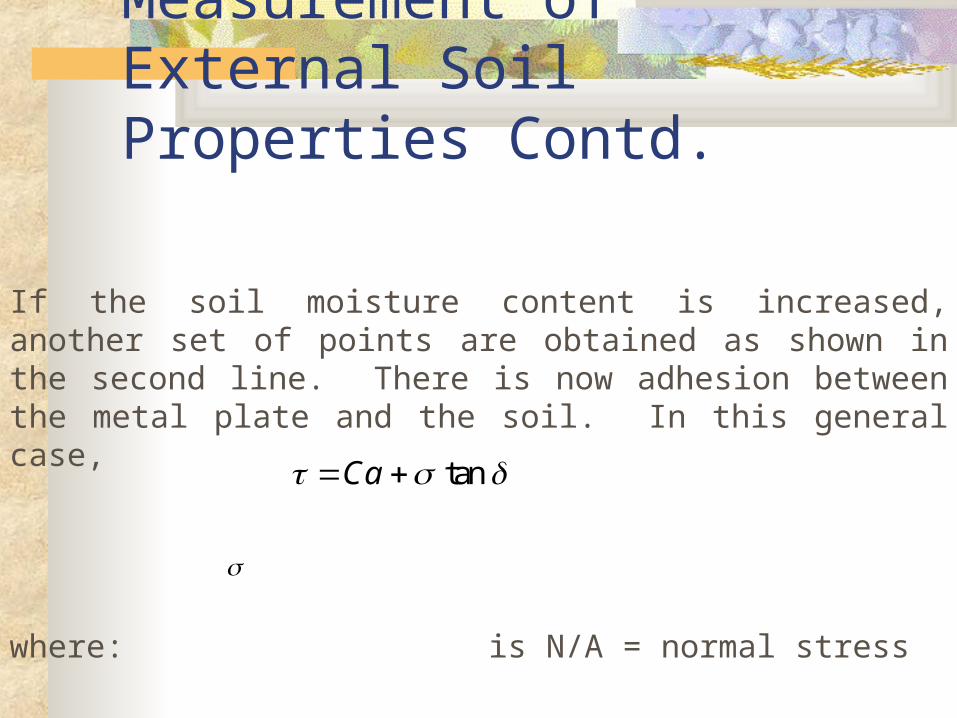
If the soil moisture content is increased, another set of points are obtained as shown in the second line. There is now adhesion between the metal plate and the soil. In this general case,
where: is N/A = normal stress
Ca tan
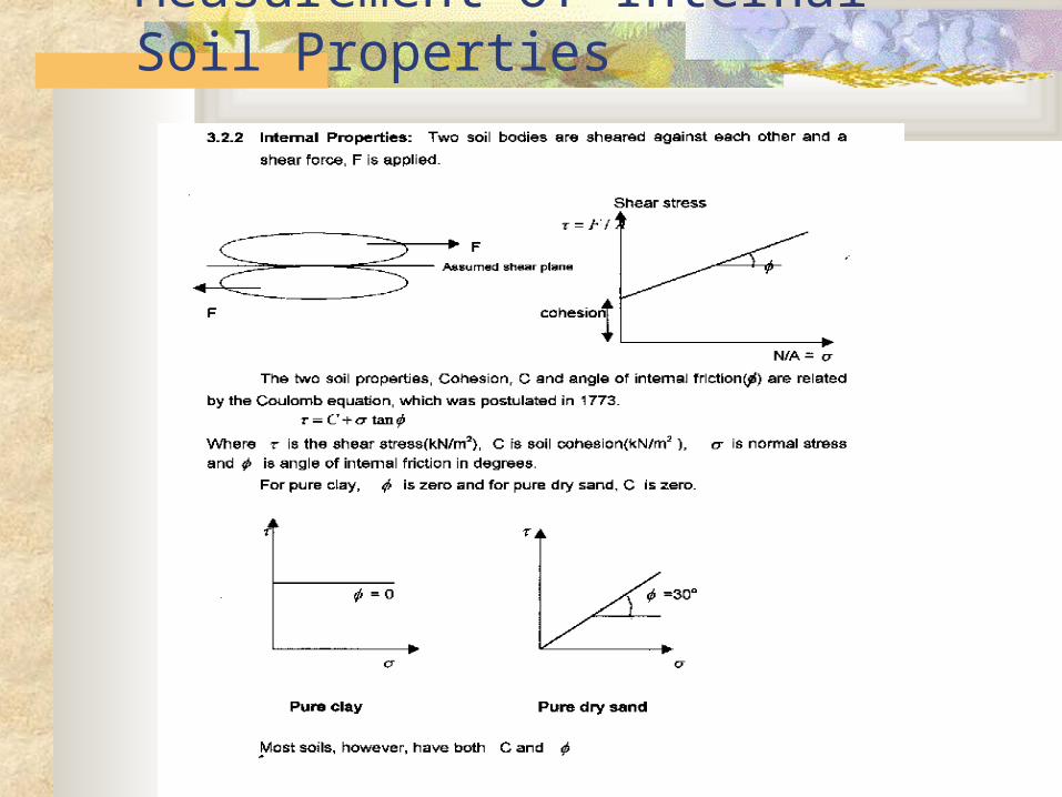
Measurement of Internal Soil Properties
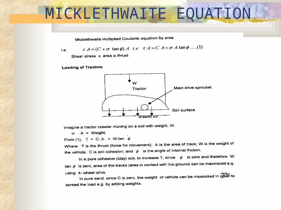
MICKLETHWAITE EQUATION
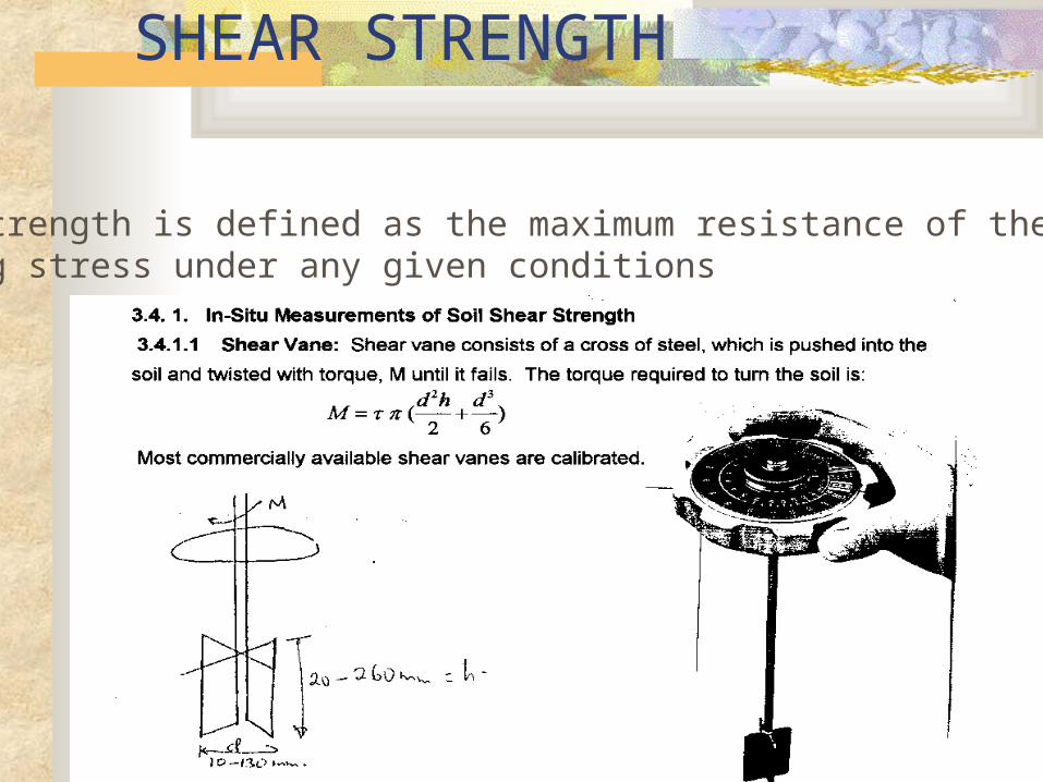
SHEAR STRENGTH
Shear Strength is defined as the maximum resistance of the soil toshearing stress under any given conditions
Triaxial Compression Test Apparatus
This is the most common method used to determine soil shear strength.
A soil specimen is extruded from a 37.5 mm diameter cutting tube, capped top and bottom and covered with a rubber membrane to minimize loss of moisture.
The sample is placed in position (see diagram) and pressure head is applied to the water in the transparent cylinder surrounding the specimen.
This pressure is applied to the soil and is called lateral pressure or cell pressure and is termed minimum principal stress.
A vertical load is now applied to the sample at a constant rate of strain until the sample fails.
Triaxial Compression Test Apparatus Contd.
The vertically applied stress at failure, called the deviatoric stress, may be measured on the proving ring, and when added to the cell pressure gives the maximum principal stress.
With the maximum ( 1) and minimum principal stresses (3) be drawn.
The procedure is repeated with different cell pressures( 3 ) and a series of Mohr circles drawn.
These circles have a common tangent called the Mohr envelope which defines the Coulomb equation.
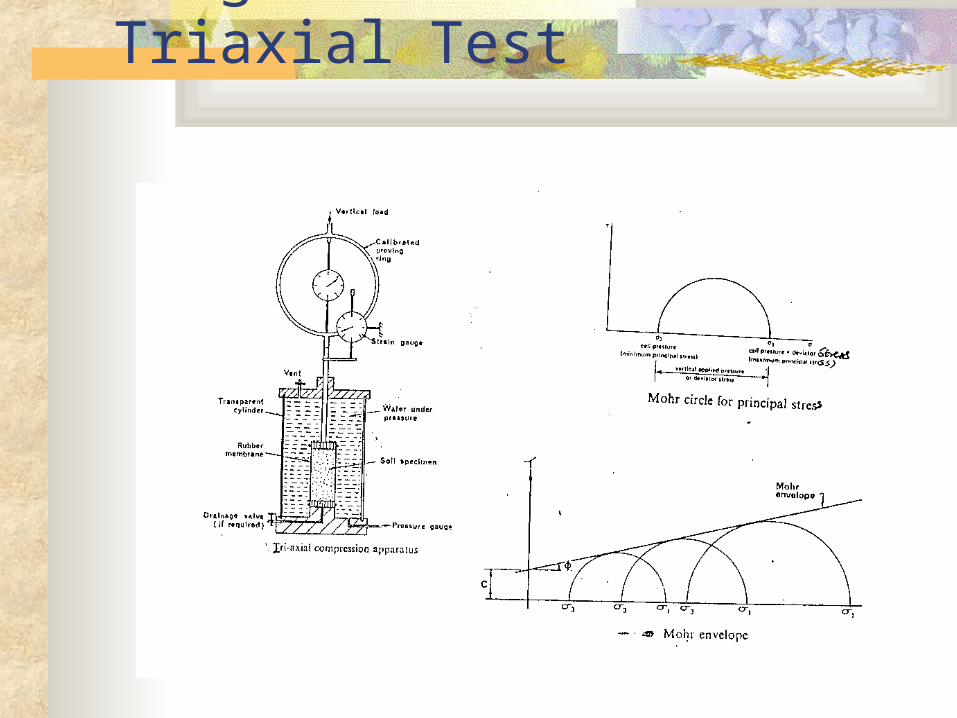
Diagrams of the Triaxial Test
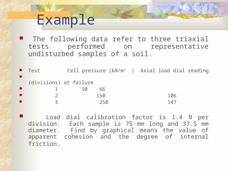
Example The following data refer to three triaxial tests
performed on representative undisturbed samples of a soil.
Test Cell pressure (kN/m2 ) Axial load dial reading (divisions) at failure 1 50 66 2 150 106 3 250 147
Load dial calibration factor is 1.4 N per division. Each sample is 75 mm long and 37.5 mm diameter. Find by graphical means the value of apparent cohesion and the degree of internal friction.
Solution
xmm m
37 5
41104 0 001104
22 2.
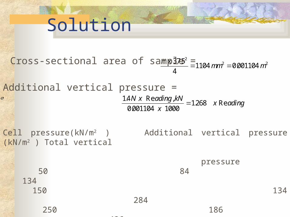
. Cross-sectional area of sample =
Additional vertical pressure =
Cell pressure(kN/m2 ) Additional vertical pressure (kN/m2 ) Total vertical pressure 50 84 134 150 134 284 250 186 436
14
0 001104 10001268
. Re ,
.. Re
N x ading kN
xx ading
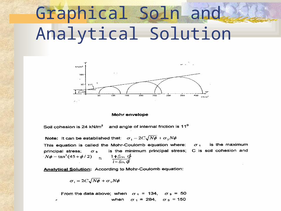
Graphical Soln and Analytical Solution
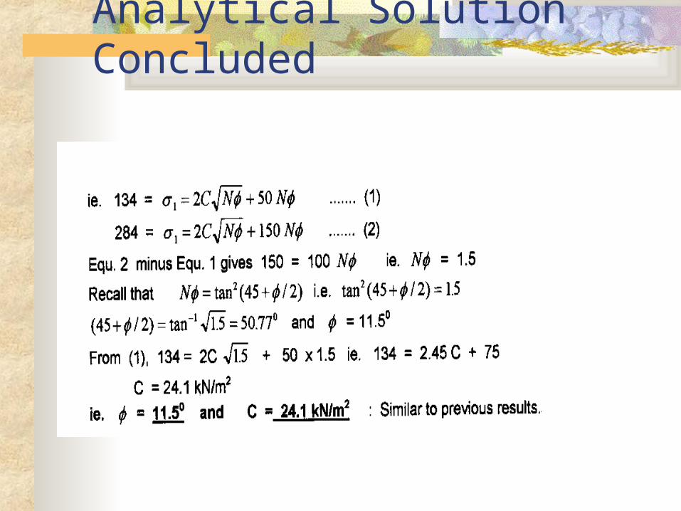
Analytical Solution Concluded
Types of Triaxial Test
The types of Triaxial Test that we can do depend on the drainage conditions of the soils to be tested.
i) Undrained Test: There is no dissipation of
pore pressure during the application of of cell pressure or deviatoric stress.
No hole or connection is at the bottom plate of the soil cylinder.
The pore pressure is then difficult to dissipate.
Undrained Test Contd.
This is called the quick undrained test and involves the total stress analysis.
This applies to fast soil failures where there is insufficient time for drainage to occur eg. tillage and rapid construction of a large embankment.
It is also the standard test for bearing capacity of foundation which is a short term case, since after initial loading, the soil will consolidate and gain in strength.
(ii) Consolidated-Undrained Test or Consolidated Slow Quick Test:
Drainage is permitted during the application of the cell pressure .
Pore pressure that builds up during the application of cell pressure is allowed to drain.
The sample becomes fully consolidated. No drainage is allowed during the application of the deviatoric stress.
The effective stress analysis applies and may apply to a building which has consolidated as drainage has taken place and the building fails eg. the failure of footings or foundations with suddenly applied load.
iii) Drained Test
Drainage is permitted during the application of the cell pressure and the deviatoric stress.
It is a slow test as the pore pressures are allowed to dissipate.
This is called the slow test and the effective stress analysis applies.
This pattern applies to the soil slope failure which is slow.
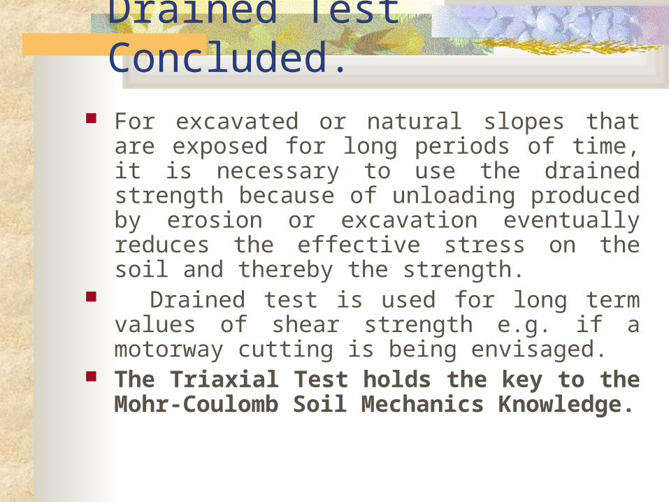
Drained Test Concluded. For excavated or natural slopes that are
exposed for long periods of time, it is necessary to use the drained strength because of unloading produced by erosion or excavation eventually reduces the effective stress on the soil and thereby the strength.
Drained test is used for long term values of shear strength e.g. if a motorway cutting is being envisaged.
The Triaxial Test holds the key to the Mohr-Coulomb Soil Mechanics Knowledge.
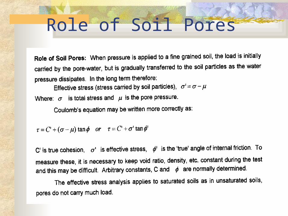
Role of Soil Pores
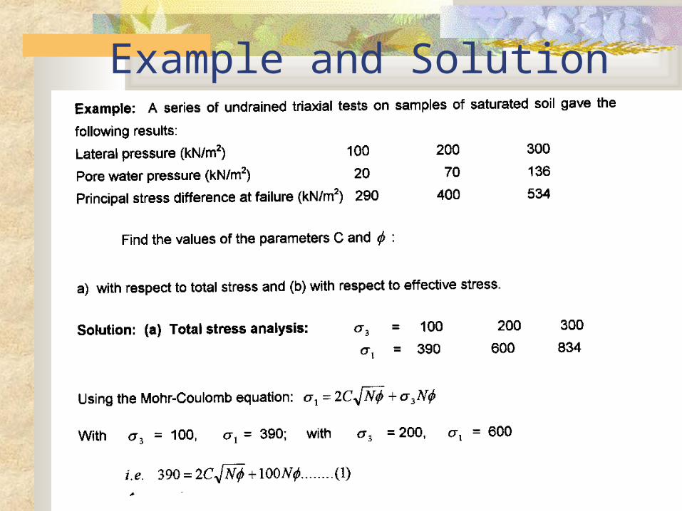
Example and Solution
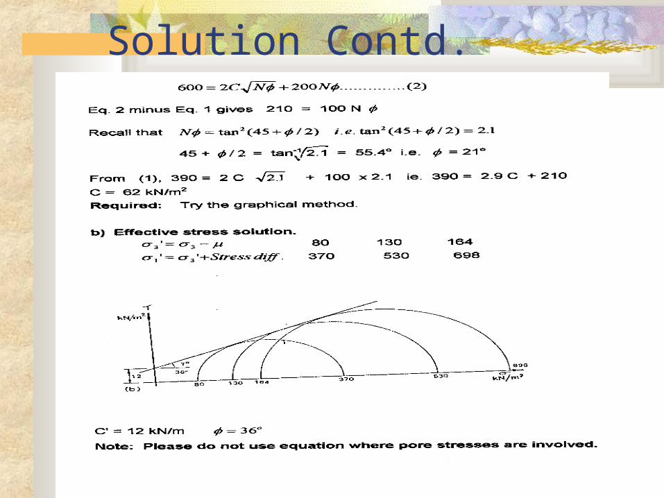
Solution Contd.
ACTIVE AND PASSIVE RANKINE STATES
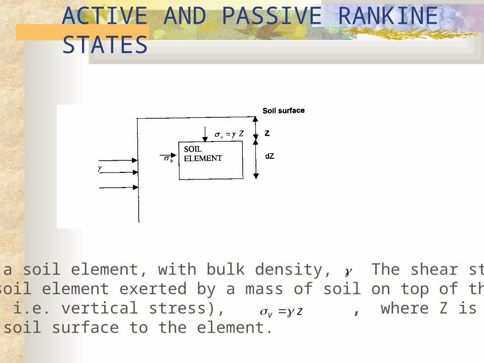
Consider a soil element, with bulk density, . The shear stress on the soil element exerted by a mass of soil on top of the element ( i.e. vertical stress), , where Z is the distance from the soil surface to the element.
zV
ACTIVE AND PASSIVE RANKINE STATES CONTD.
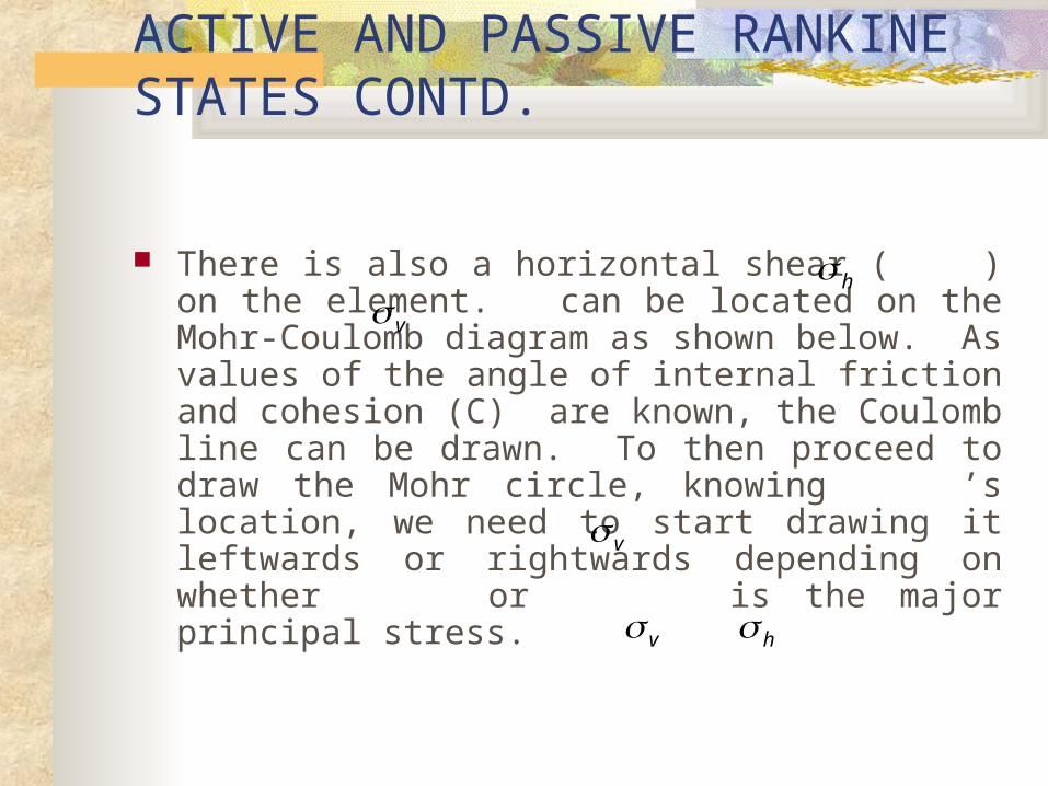
There is also a horizontal shear ( ) on the element. can be located on the Mohr-Coulomb diagram as shown below. As values of the angle of internal friction and cohesion (C) are known, the Coulomb line can be drawn. To then proceed to draw the Mohr circle, knowing ’s location, we need to start drawing it leftwards or rightwards depending on whether or is the major principal stress.
hv
v
v h
ACTIVE AND PASSIVE RANKINE STATES CONTD
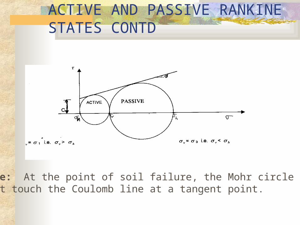
Note: At the point of soil failure, the Mohr circle will just touch the Coulomb line at a tangent point.
ACTIVE AND PASSIVE RANKINE STATES CONTD
If is the major principal stress ( i..e. > ), the circle will go leftwards as
= . being larger than means that the major force causing failure on the soil element is the vertical stress and then the soil above the element is referred to as being ACTIVE (See figure above) because it was doing the work. If is larger like the bulldozer blade, then the soil above the soil element acts as if it is dormant waiting for a horizontal stress to shear it. The soil is then said to be PASSIVE.
v v
h v
1 h
h
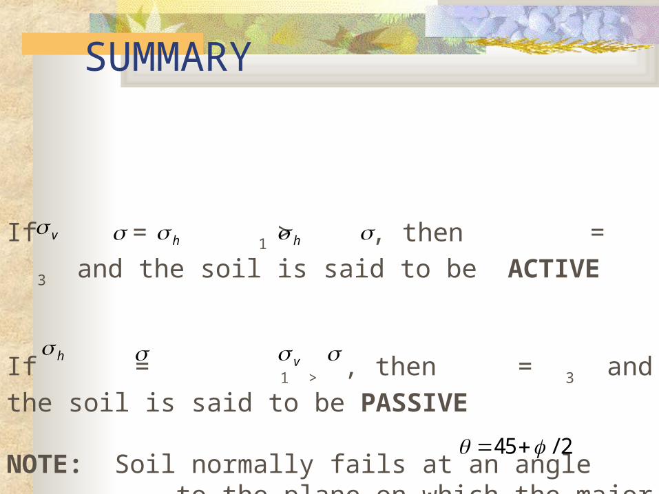
SUMMARY
If = 1 > , then = 3 and the soil is said to
be ACTIVE
If = 1 > , then = 3 and the soil is said to be
PASSIVE
NOTE: Soil normally fails at an angle to the plane on which the major principal stress acts.
h h
h
v
v
45 2/
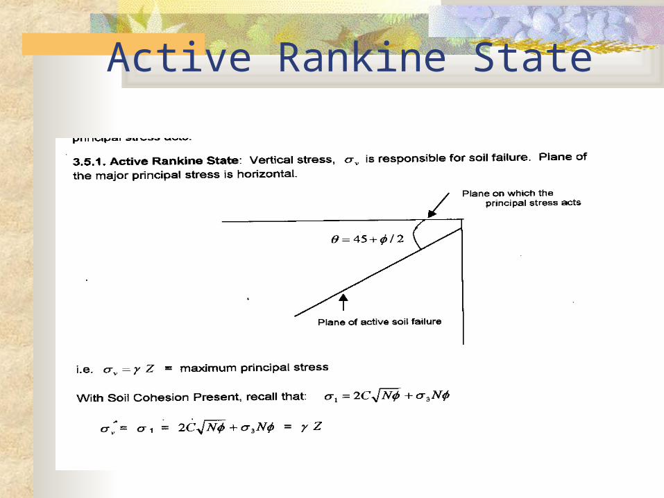
Active Rankine State
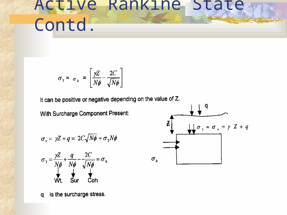
Active Rankine State Contd.
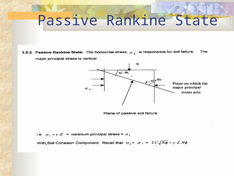
Passive Rankine State
Active and Passive Earth Forces
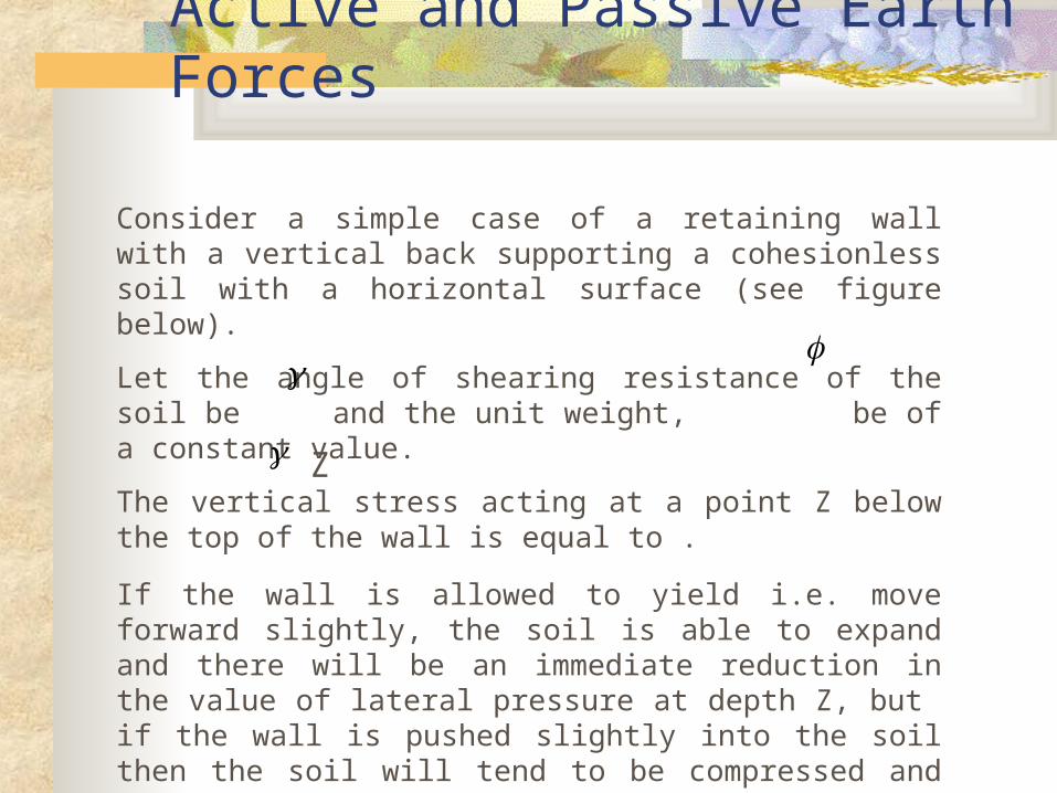
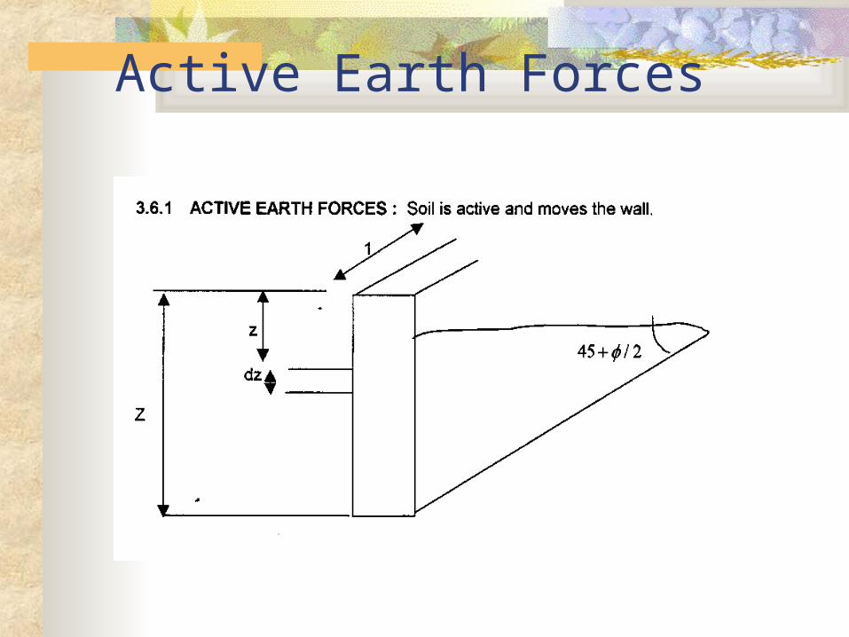
Consider a simple case of a retaining wall with a vertical back supporting a cohesionless soil with a horizontal surface (see figure below).
Let the angle of shearing resistance of the soil be and the unit weight, be of a constant value.
The vertical stress acting at a point Z below the top of the wall is equal to .
If the wall is allowed to yield i.e. move forward slightly, the soil is able to expand and there will be an immediate reduction in the value of lateral pressure at depth Z, but if the wall is pushed slightly into the soil then the soil will tend to be compressed and there will be an increase in the value of the
lateral pressure.
Z
Active and Passive Earth Forces Contd.
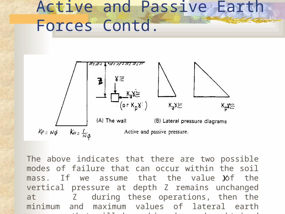
The above indicates that there are two possible modes of failure that can occur within the soil mass. If we assume that the value of the vertical pressure at depth Z remains unchanged at Z during these operations, then the minimum and maximum values of lateral earth pressure that will be achieved can be obtained from the Mohr circle diagram below.
Active and Passive Earth Forces Contd.
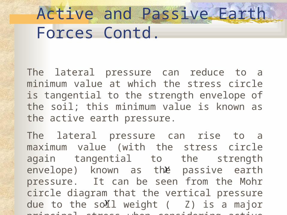
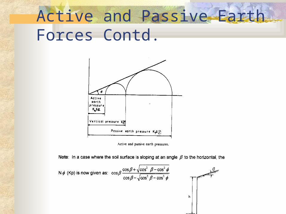
The lateral pressure can reduce to a minimum value at which the stress circle is tangential to the strength envelope of the soil; this minimum value is known as the active earth pressure.
The lateral pressure can rise to a maximum value (with the stress circle again tangential to the strength envelope) known as the passive earth pressure. It can be seen from the Mohr circle diagram that the vertical pressure due to the soil weight ( Z) is a major principal stress when considering active pressure and that when considering passive pressure, the vertical pressure due to the soil weight ( Z) is a minor principal stress.
Active and Passive Earth Forces Contd.
Active Earth Forces
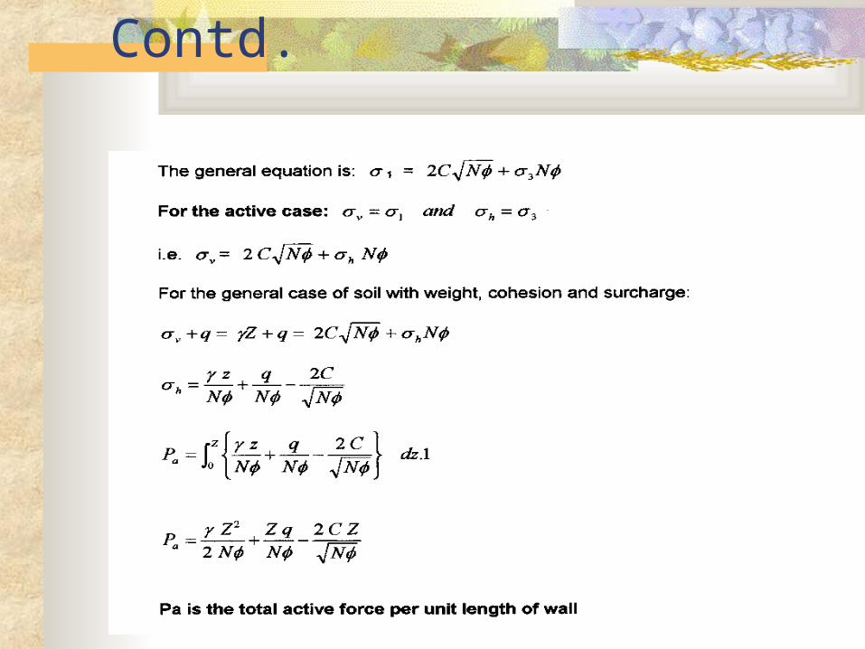
Active Earth Forces Contd.
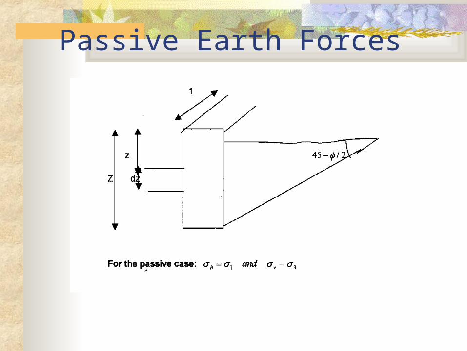
Passive Earth Forces
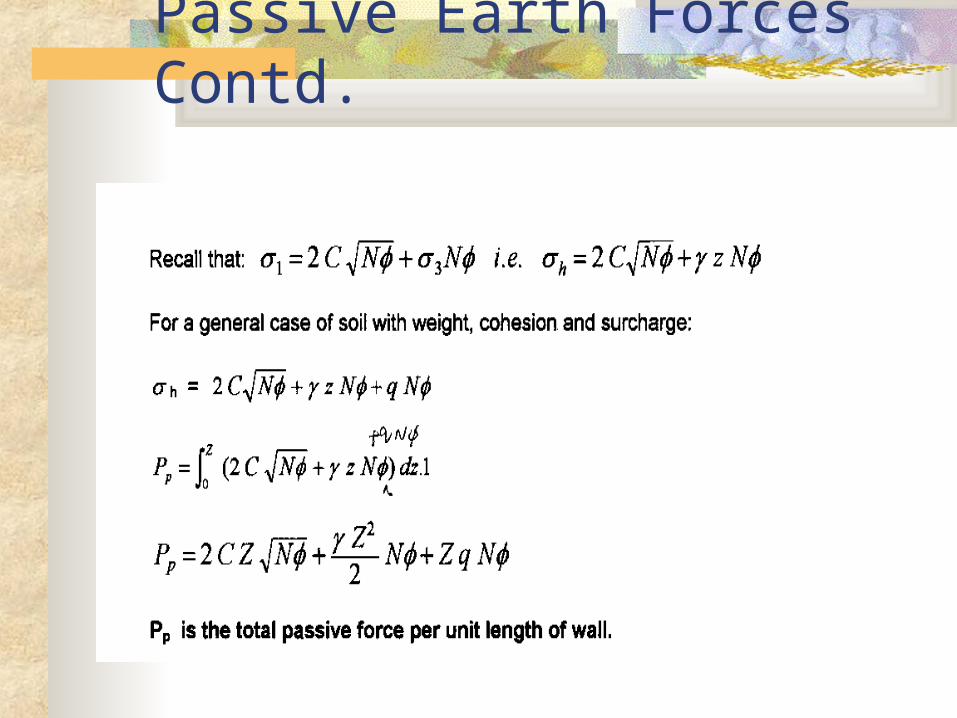
Passive Earth Forces Contd.
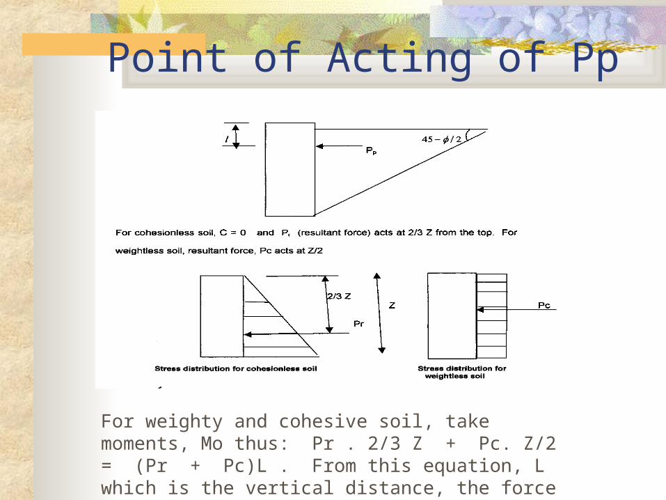
Point of Acting of Pp
For weighty and cohesive soil, take moments, Mo thus: Pr . 2/3 Z + Pc. Z/2 = (Pr + Pc)L . From this equation, L which is the vertical distance, the force acts, can be obtained.
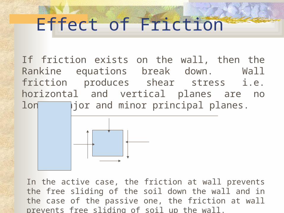
Effect of Friction
If friction exists on the wall, then the Rankine equations break down. Wall friction produces shear stress i.e. horizontal and vertical planes are no longer major and minor principal planes.
In the active case, the friction at wall prevents the free sliding of the soil down the wall and in the case of the passive one, the friction at wall prevents free sliding of soil up the wall.
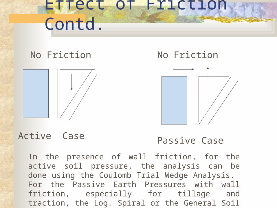
Effect of Friction Contd.
No Friction No Friction
Active Case Passive Case
In the presence of wall friction, for the active soil pressure, the analysis can be done using the Coulomb Trial Wedge Analysis. For the Passive Earth Pressures with wall friction, especially for tillage and traction, the Log. Spiral or the
General Soil Mechanics Equation can be used.
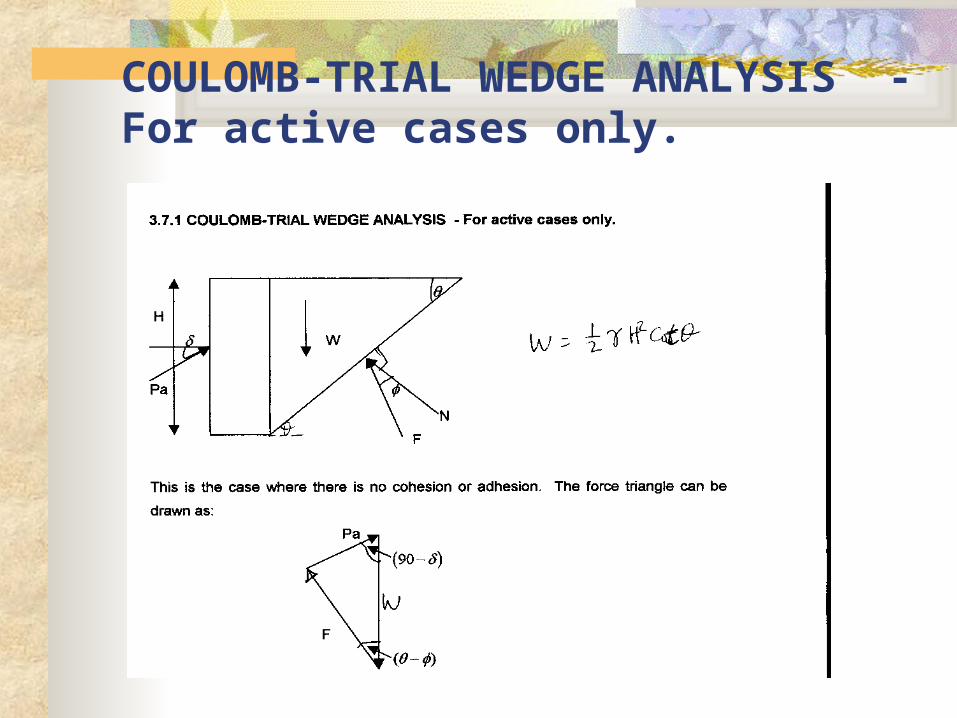
COULOMB-TRIAL WEDGE ANALYSIS - For active cases only.
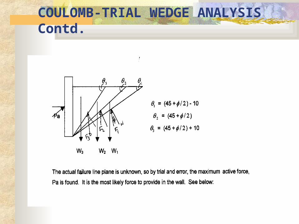
COULOMB-TRIAL WEDGE ANALYSIS Contd.
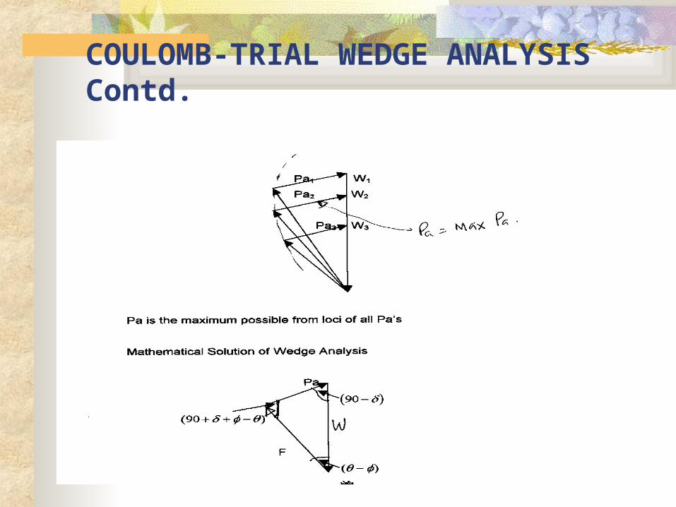
COULOMB-TRIAL WEDGE ANALYSIS Contd.
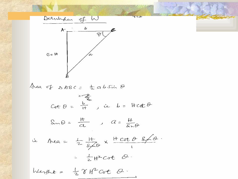
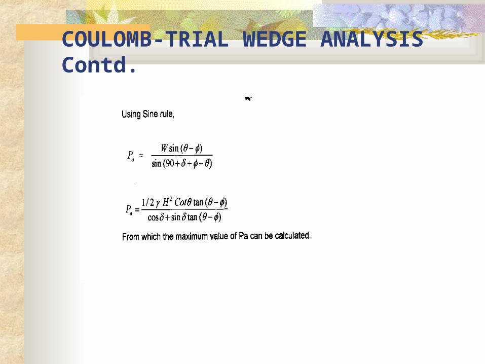
COULOMB-TRIAL WEDGE ANALYSIS Contd.
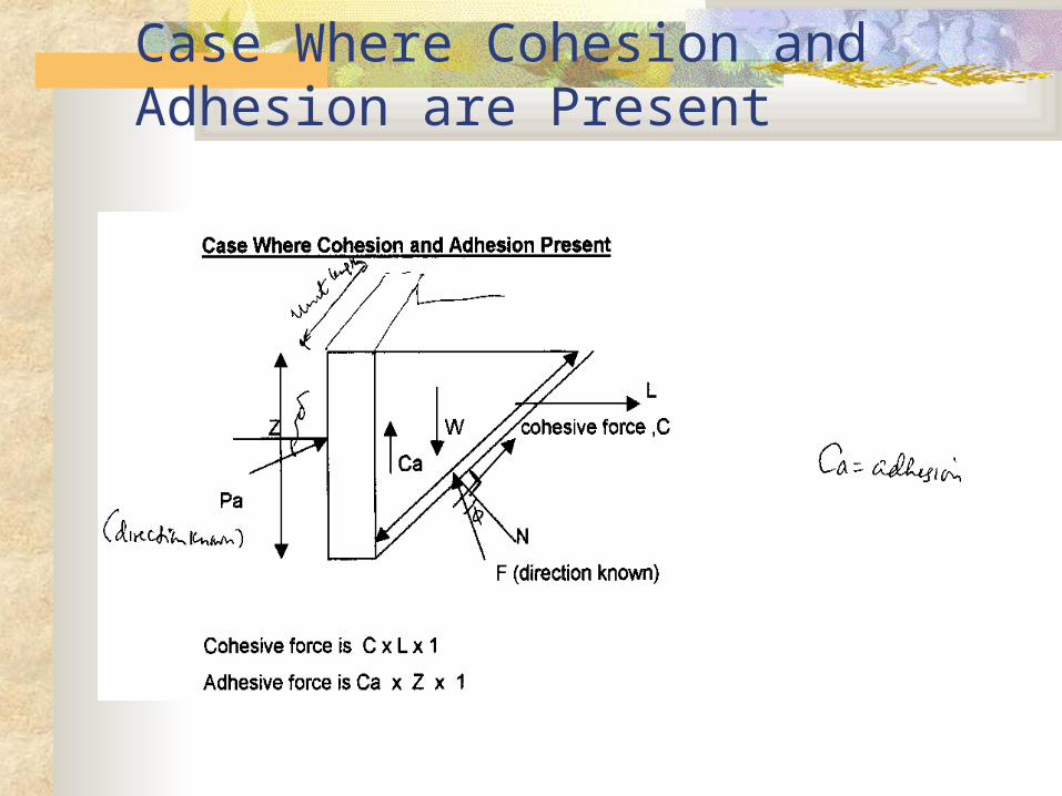
Case Where Cohesion and Adhesion are Present
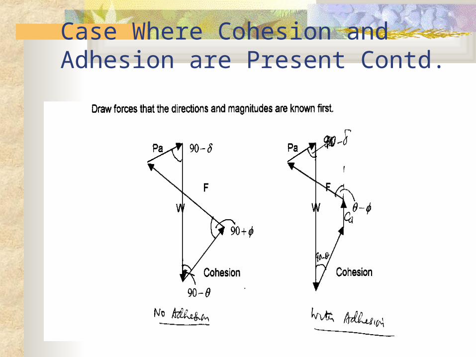
Case Where Cohesion and Adhesion are Present Contd.
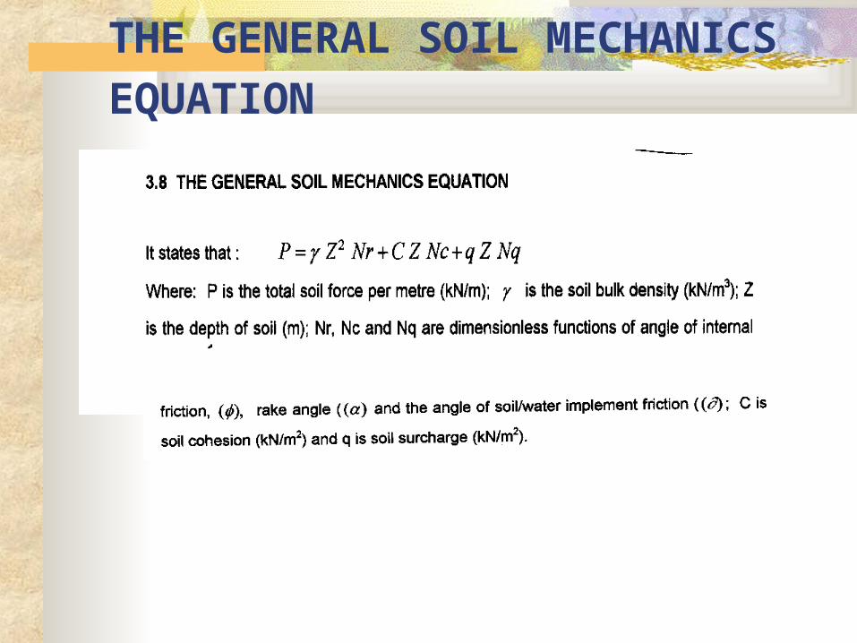
THE GENERAL SOIL MECHANICS
EQUATION
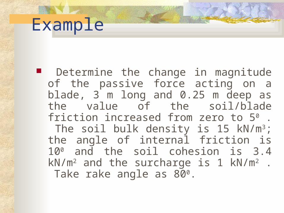
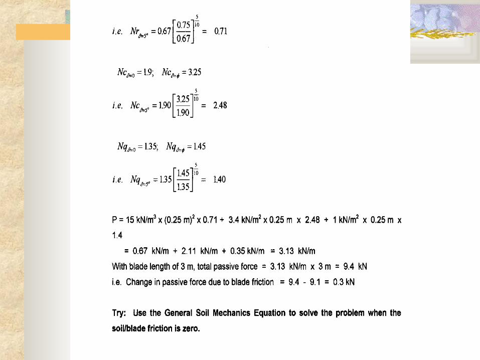
Example
Determine the change in magnitude of the passive force acting on a blade, 3 m long and 0.25 m deep as the value of the soil/blade friction increased from zero to 50 . The soil bulk density is 15 kN/m3; the angle of internal friction is 100 and the soil cohesion is 3.4 kN/m2 and the surcharge is 1 kN/m2 . Take rake angle as 800.
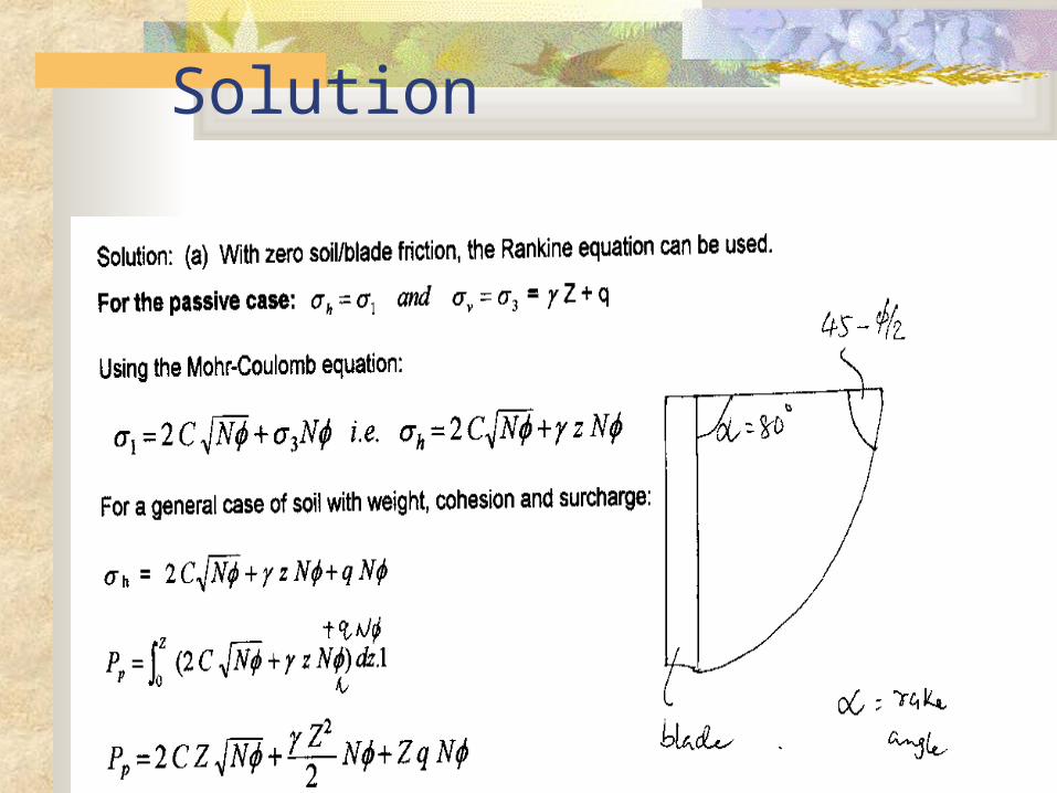
Solution
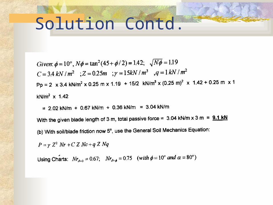
Solution Contd.