Chapter Fourteen

1

CHAPTER 14A Dynamic Model of Aggregate Demand

And Aggregate Supply

®

A PowerPointTutorial

To Accompany

MACROECONOMICS, 7th. EditionN. Gregory Mankiw

Tutorial written by:

Mannig J. SimidianB.A. in Economics with Distinction, Duke University

M.P.A., Harvard University Kennedy School of GovernmentM.B.A., Massachusetts Institute of Technology (MIT) Sloan School of

Management

Chapter Fourteen

2

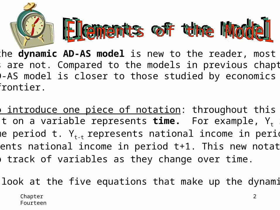
Although the dynamic AD-AS model is new to the reader, most of itscomponents are not. Compared to the models in previous chapters, thedynamic AD-AS model is closer to those studied by economics at theresearch frontier.

We need to introduce one piece of notation: throughout this chapter, asubscript t on a variable represents time. For example, Yt representsGDP in time period t. Yt-t represents national income in period t-1 andYt+1 represents national income in period t+1. This new notation allowsus to keep track of variables as they change over time.

Let’s now look at the five equations that make up the dynamic AD-ASmodel.

Chapter Fourteen

3

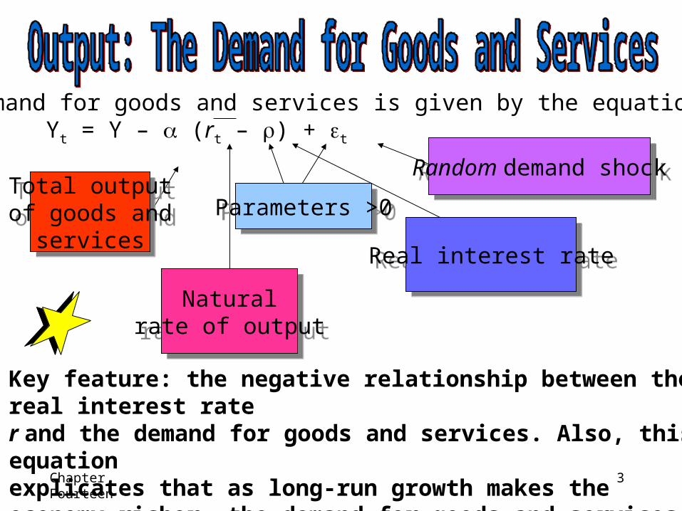
The demand for goods and services is given by the equation:Yt = Y – (rt – ) + t

Total outputof goods and

services

Total outputof goods and

services

Naturalrate of output

Naturalrate of output

Parameters >0Parameters >0

Real interest rateReal interest rate

Random demand shockRandom demand shock

Key feature: the negative relationship between the real interest rate r and the demand for goods and services. Also, this equation explicates that as long-run growth makes the economy richer, the demand for goods and services grows proportionally.

Chapter Fourteen

4

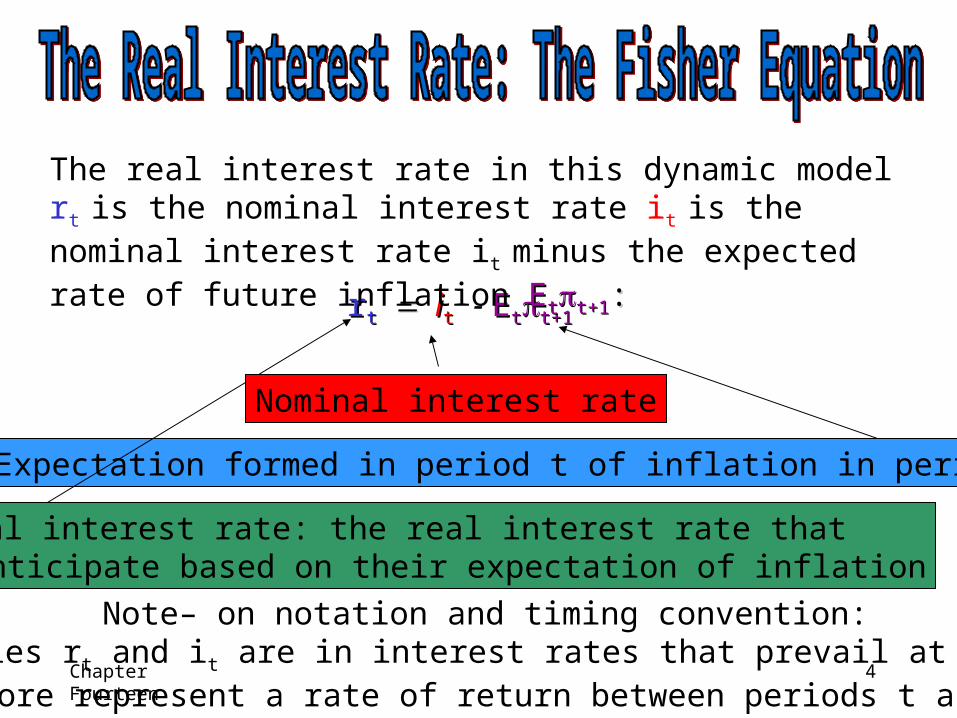
rrttiitt - EEttt+1t+1

The real interest rate in this dynamic model rt is the nominal interest rate it is the nominal interest rate it minus the expected rate of future inflation EEttt+1t+1::

Expectation formed in period t of inflation in period t + 1

Ex ante real interest rate: the real interest rate that people anticipate based on their expectation of inflation

Nominal interest rate

Note– on notation and timing convention:The variables rt and it are in interest rates that prevail at time t and

therefore represent a rate of return between periods t and t+1.

Chapter Fourteen

5

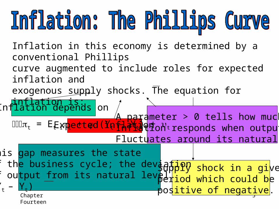
Inflation in this economy is determined by a conventional Phillipscurve augmented to include roles for expected inflation andexogenous supply shocks. The equation for inflation is:

t = Et-1t + (Yt – Yt) + t

Inflation depends on

Expected inflationA parameter > 0 tells how muchInflation responds when outputFluctuates around its natural level

This gap measures the stateof the business cycle; the deviationof output from its natural level(Yt – Yt)

Supply shock in a givenperiod which could bepositive of negative.

Chapter Fourteen

6

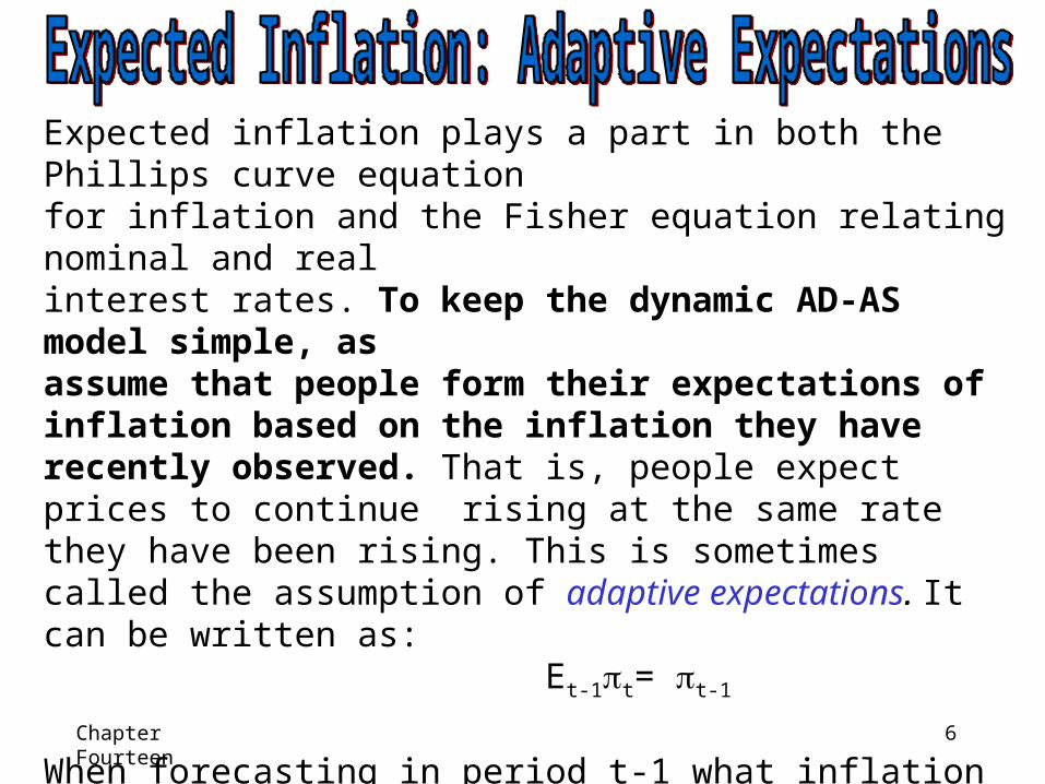
Expected inflation plays a part in both the Phillips curve equationfor inflation and the Fisher equation relating nominal and real interest rates. To keep the dynamic AD-AS model simple, as assume that people form their expectations of inflation based on the inflation they have recently observed. That is, people expect prices to continue rising at the same rate they have been rising. This is sometimes called the assumption of adaptive expectations. It can be written as:

Et-1t= t-1

When forecasting in period t-1 what inflation rate will prevail in prevail in period t, people simply look at inflation in period t-1 andextrapolate it forward. The same assumption applies in every period. Thus once inflation is observed in period t, people will expect that rate to continue. Therefore, Et+1t= t

Chapter Fourteen

7

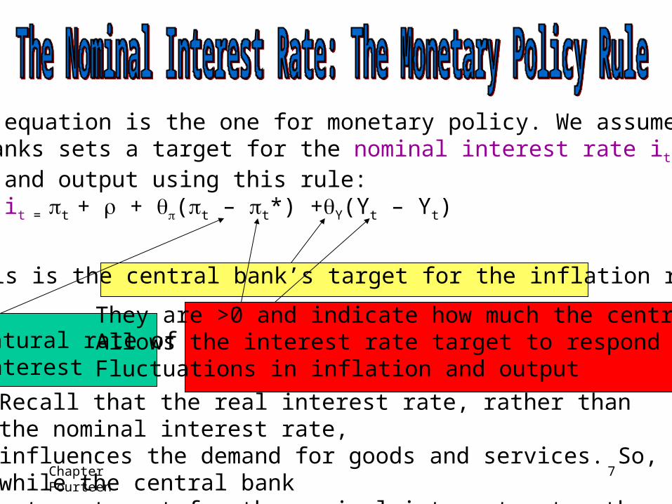
The final equation is the one for monetary policy. We assume that thecentral banks sets a target for the nominal interest rate it based on inflation and output using this rule:

it = t + + (t – t*) +Y(Yt – Yt)

This is the central bank’s target for the inflation rate

They are >0 and indicate how much the central bankAllows the interest rate target to respond toFluctuations in inflation and output

Natural rate ofinterest

Recall that the real interest rate, rather than the nominal interest rate, influences the demand for goods and services. So, while the central banksets a target for the nominal interest rate, the bank’s influence is via the real interest rate.

Chapter Fourteen

8

Interest rate or the Money Supply?• The main advantage of using the interest rate,

rather than the money supply, as the policy instrument AD-AS model is that it is more realistic. Today most central banks, including the Federal Reserve, set a short-term target for the nominal interest rate.

• Keep in mind that hitting that target requires adjustments in the money supply.

• So, when a central bank decides to change the interest, it is also committing itself to adjust the money supply accordingly.

Chapter Fourteen

9

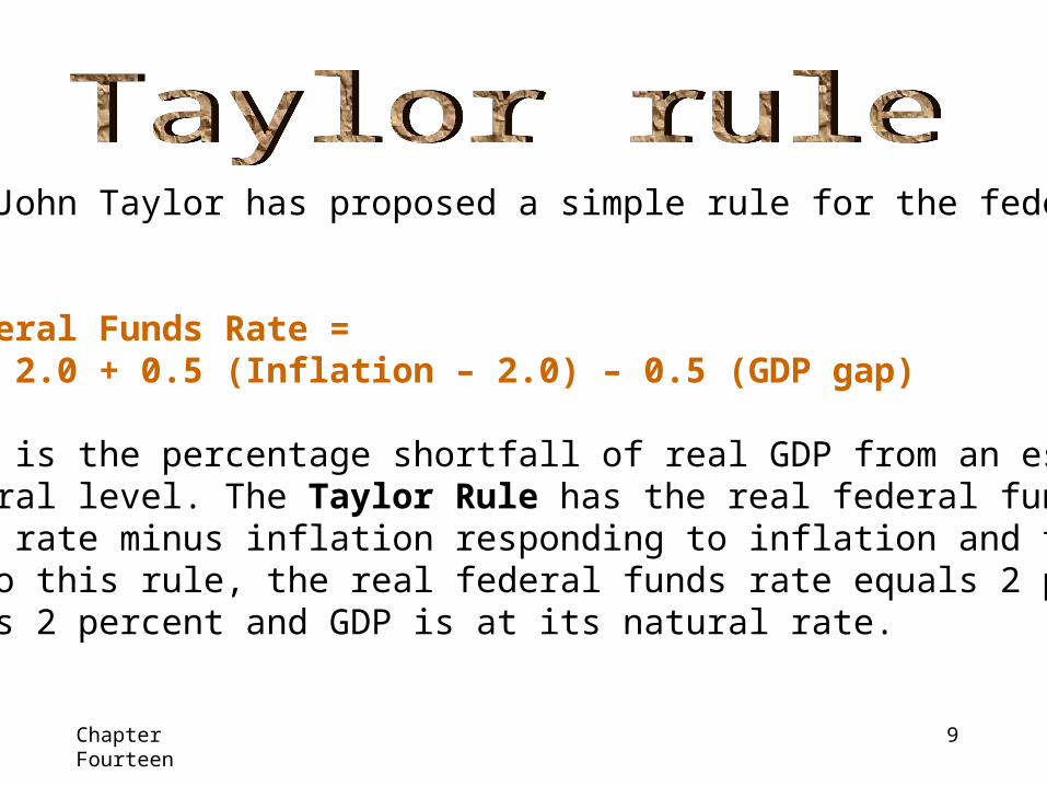
Economist, John Taylor has proposed a simple rule for the federalfunds rate:

Nominal Federal Funds Rate = Inflation + 2.0 + 0.5 (Inflation – 2.0) – 0.5 (GDP gap)

The GDP gap is the percentage shortfall of real GDP from an estimateof its natural level. The Taylor Rule has the real federal funds rate— the nominal rate minus inflation responding to inflation and the GDP gap.According to this rule, the real federal funds rate equals 2 percent wheninflation is 2 percent and GDP is at its natural rate.

Chapter Fourteen

10

The previous 5 equations we went over on the last few slides: The Demand for Goods and Services, The Fisher Equation, The Phillips Curve, Adaptive Expectations, The Monetary Policy Rule determine the Model’s five endogenous variables: output, the real interest rate,inflation and the nominal interest rate.

We are almost ready to put these pieces together to see how variousshocks to the economy influences the paths of these variables overtime. Before doing so, however, we need to establish the starting point for our analysis: the economy’s long-run equilibrium.

Chapter Fourteen

11

• The long-run equilibrium represents the normal state around whichthe economy fluctuates. It occurs when there are no shocks andinflation has stabilized.• In words, the long-run equilibrium is described as follows: Outputand the real interest rate are at their natural values, inflation and expected inflation are at the target rate of inflation, and the nominalinterest rate equals the natural rate of interest plus target inflation.• The long-run equilibrium is described as follows: Output and thereal interest rate are at their natural values, inflation and expected inflation are at the target rate of inflation, and the nominal interestrate equals the natural rate of interest plus target inflation.• The long-run equilibrium of this model two related principles: the classicdichotomy and monetary neutrality. Continue to understand this on thenext slide….

Chapter Fourteen

12

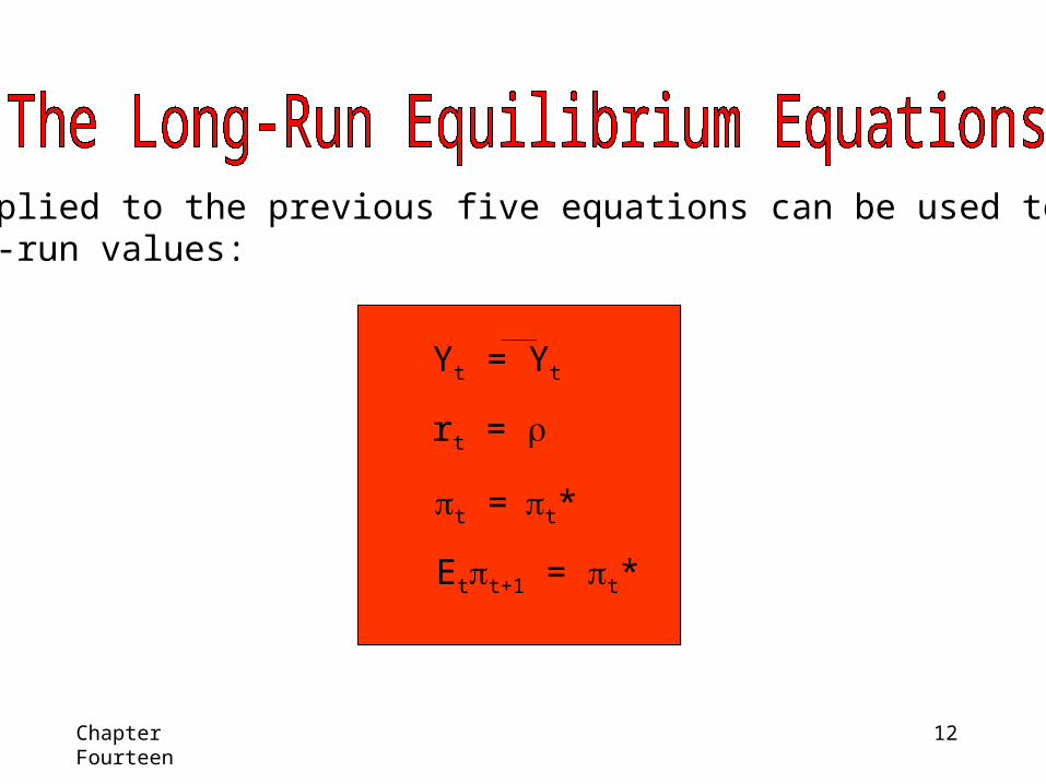
Yt = Yt

rt =

t =t*

Ett+1 = t*

Algebra applied to the previous five equations can be used to verifythese long-run values:

Chapter Fourteen

13

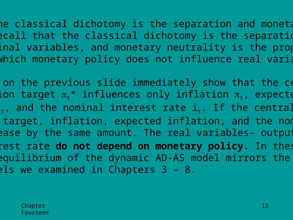
Recall that the classical dichotomy is the separation and monetaryneutrality. Recall that the classical dichotomy is the separation ofreal from nominal variables, and monetary neutrality is the propertyAccording to which monetary policy does not influence real variables.

The equations on the previous slide immediately show that the centralbank’s inflation target t* influences only inflation t, expected inflation Ett+1, and the nominal interest rate it. If the central bank raisesits inflation target, inflation, expected inflation, and the nominal interestrate all increase by the same amount. The real variables– output Yt andthe real interest rate do not depend on monetary policy. In these ways,the long-run equilibrium of the dynamic AD-AS model mirrors theClassical models we examined in Chapters 3 – 8.

Chapter Fourteen

14

Inflation, t

Income, Output, Yt

DASt

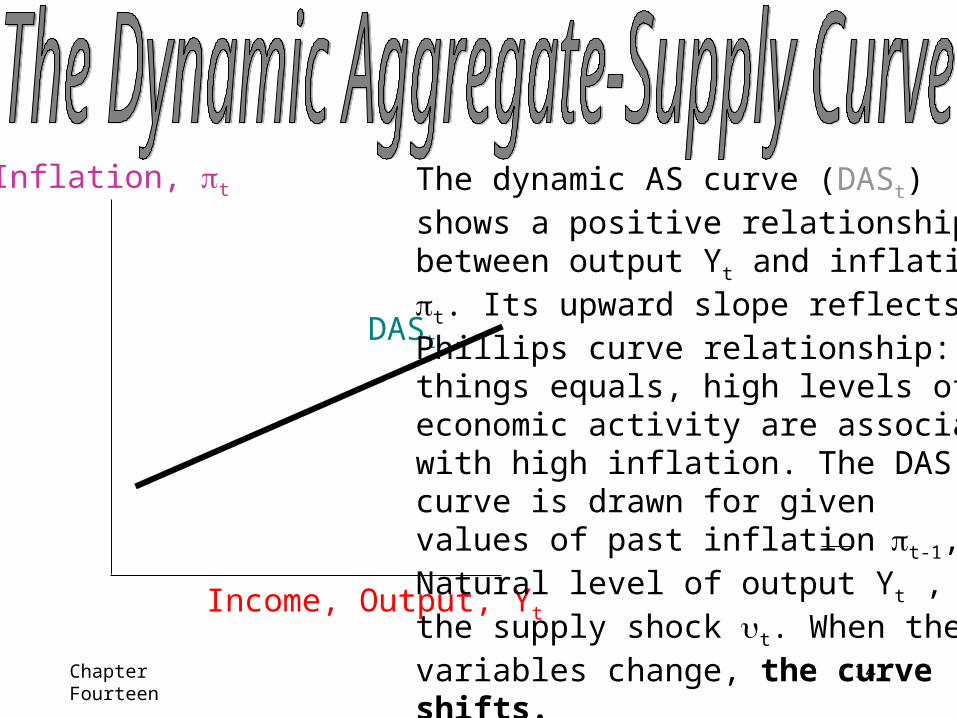
The dynamic AS curve (DASt)shows a positive relationship between output Yt and inflationt. Its upward slope reflects thePhillips curve relationship: otherthings equals, high levels of economic activity are associatedwith high inflation. The DAScurve is drawn for givenvalues of past inflationt-1, theNatural level of output Yt , andthe supply shock t. When thesevariables change, the curveshifts.

Chapter Fourteen

15

Inflation, t

Income, Output, Yt

DADt

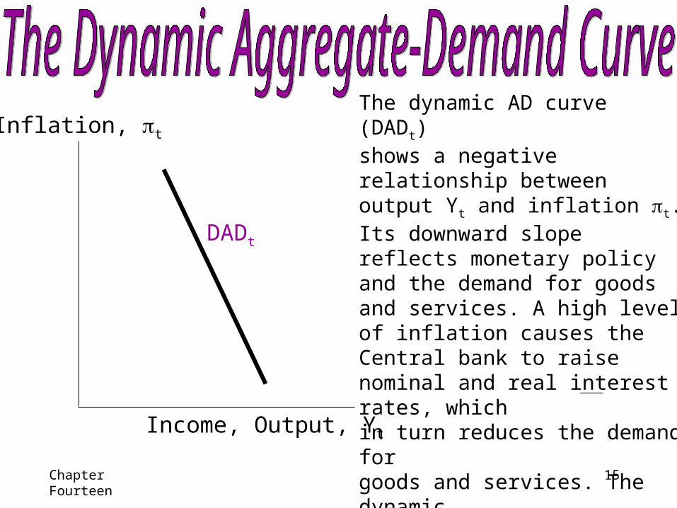
The dynamic AD curve (DADt)shows a negative relationship between output Yt and inflation t. Its downward slope reflects monetary policy and the demand for goods and services. A high level of inflation causes the Central bank to raise nominal and real interest rates, whichin turn reduces the demand forgoods and services. The dynamicAD curve is drawn for givenValues of the natural level ofOutput Yt , the inflation target t*and the demand shock t. WhenThese exogenous variables shift,the curve shifts.

Chapter Fourteen

16

Inflation, t

Income, Output, Yt

DASt

DADt

Yt

Short-runEquilibrium

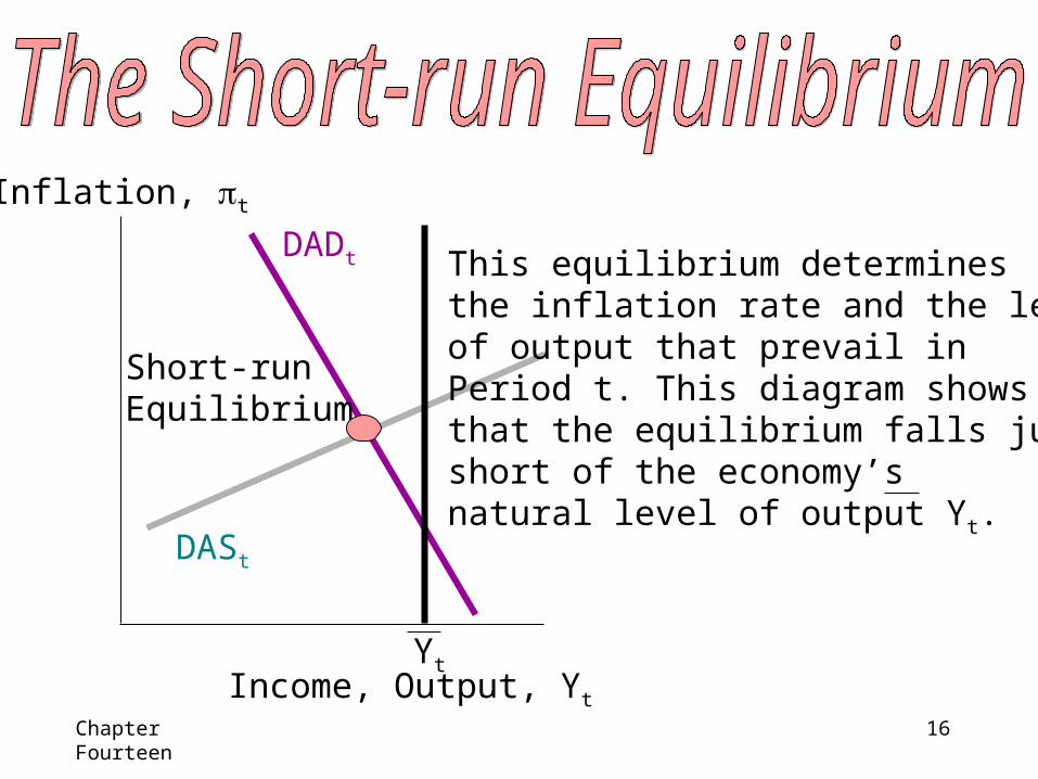
This equilibrium determinesthe inflation rate and the levelof output that prevail inPeriod t. This diagram showsthat the equilibrium falls justshort of the economy’snatural level of output Yt.

Chapter Fourteen

17

Inflation, t

Income, Output, Yt

DASt

DADt

Yt

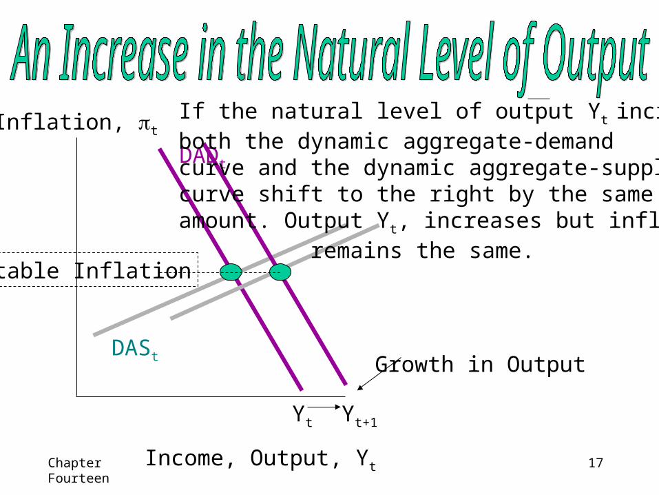
Stable Inflation

Yt+1

Growth in Output

If the natural level of output Yt increases,both the dynamic aggregate-demandcurve and the dynamic aggregate-supplycurve shift to the right by the same amount. Output Yt, increases but inflation

remains the same.

Chapter Fourteen

18

Inflation, t

Income, Output, Yt

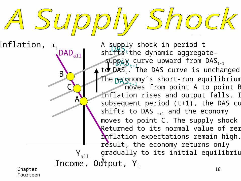
DAStDADall

Yall

A

B

C

DASt+1

DASt-1

A supply shock in period t shifts the dynamic aggregate- supply curve upward from DASt-1

to DASt. The DAS curve is unchanged.The economy’s short-run equilibrium

moves from point A to point B.inflation rises and output falls. In thesubsequent period (t+1), the DAS curve shifts to DAS t+1 and the economy moves to point C. The supply shock hasReturned to its normal value of zero, butinflation expectations remain high. As aresult, the economy returns only gradually to its initial equilibrium, pointA.

Chapter Fourteen

19

Inflation, t

Income, Output, Yt

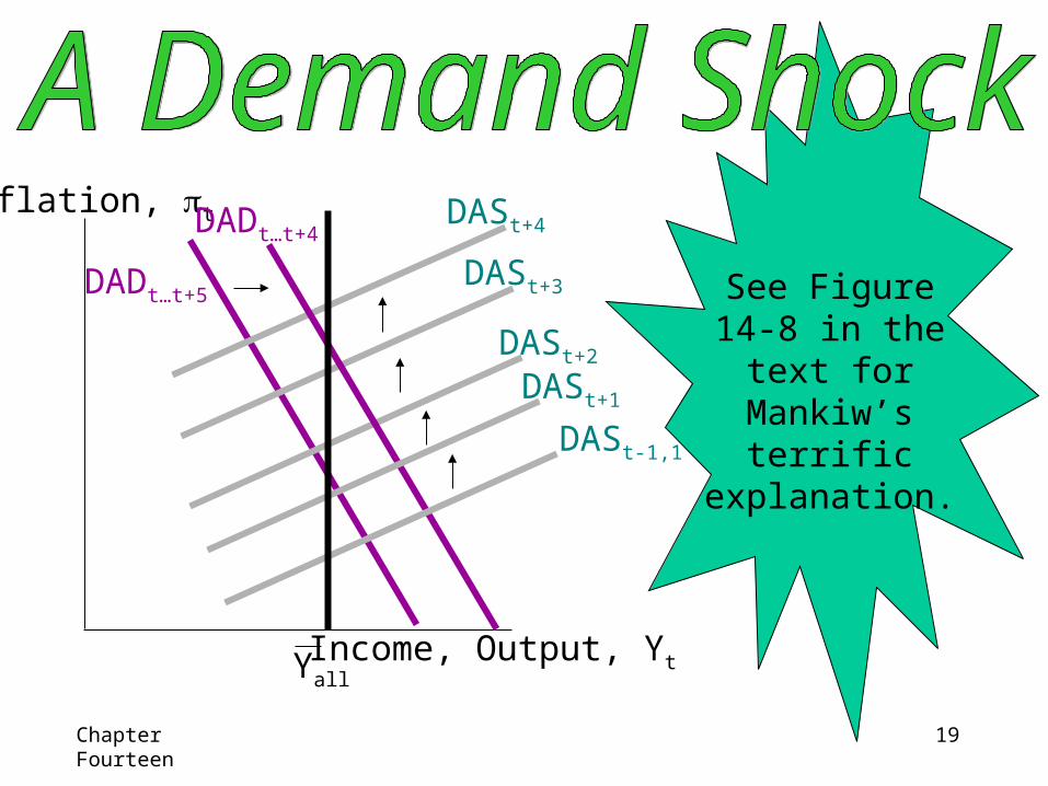
DASt+4

DADt…t+5

Yall

DASt+3

DASt+2

DADt…t+4

DASt+1

DASt-1,1

See Figure 14-8 in the text for Mankiw’s

terrific explanation.

Chapter Fourteen

20

Taylor ruleTaylor principle

Taylor ruleTaylor principle