chapter 6 selective harmonic elimination of single phase...
TRANSCRIPT
139
CHAPTER 6
SELECTIVE HARMONIC ELIMINATION OF SINGLE
PHASE VOLTAGE SOURCE INVERTER USING
ALGEBRAIC HARMONIC ELIMINATION APPROACH
6.1 INTRODUCTION
The problem of eliminating harmonics in switching converters has
been the focus of research for many years. Present day available PWM
schemes can be broadly classified as carrier modulated sine PWM and
precalculated programmed pulse width modulation (PPWM) schemes. If the
switching losses in an inverter are not a concern (i.e., switching on the order
of a few kHz is acceptable), then the sine-triangle PWM method and its
variants are very effective for controlling the inverter (Mohan et al 2004).
This is because the generated harmonics are beyond the bandwidth of the
system being actuated and therefore these harmonics do not dissipate power.
On the other hand, for systems where high switching efficiency is of utmost
importance, it is desirable to keep the switching frequency much lower. In this
case, another approach is to choose the switching times (angles) such that a
desired fundamental output is generated and specifically chosen harmonics of
the fundamental are suppressed (Pate1 and Hoft 1973, Enjeti et al 1990, Sun
and Grotstollen 1994). This is referred to as selective harmonic elimination or
programmed harmonic elimination as the switching angles are chosen
(programmed) to eliminate specific harmonics. This is also called as
Computed Pulse Width Modulation (CPWM) or Programmed Pulse Width
Modulation (PPWM). The Programmed PWM techniques optimize a
140
particular objective function such as to obtain minimum losses, reduced
torque pulsations, selective elimination of harmonics and therefore the most
effective means of obtaining high performance results. It is interesting to note
that the various objective functions are chosen to generate a particular
programmed PWM technique essentially constitutes the minimization of
unwanted effects due to the harmonics present in the inverter output spectra.
In view of this, little or no difference between each one of the programmed
techniques is observed when significant number of low order harmonics is
eliminated. However, each one of the programmed PWM techniques is
associated with the difficult task of computing specific PWM switching
instants to optimize a particular objective function. This difficulty is
particularly encountered at lower output frequency range due to the necessity
of large number of PWM switching instants. Also in most cases only a local
minimum can be obtained after considerable computational effort. Despite
these difficulties programmed PWM exhibit several distinct advantages In
comparison to the conventional carrier modulated sine PWM schemes which
are listed below:
1. For a given inverter switching frequency, the first
uneliminated harmonic is almost double that for a natural or
regular-sampled PWM scheme, thus resulting in a far superior
pole switching waveform harmonic spectrum.
2. A much higher pole switching waveform fundamental
amplitude is attainable before the minimum pulse-width limit
of the inverter is reached.
3. About 50% reduction in the inverter switching frequency is
achieved when compared with the conventional carrier
modulated sine PWM scheme.

141
4. Higher voltage gain due to over modulation is possible. This
contributes to higher utilization of the power conversion
process.
5. Due to the high quality of the output voltage and current, the
ripple in the DC link current is also small. Thus a reduction in
the size of the DC link filter components is achieved.
6. The reduction in switching frequency contributes to the
reduction in switching losses of the inverter and permits the
use of GTO switches for high power converters.
7. Elimination of lower order harmonics causes no harmonic
interference such as, resonance with external line filtering
networks typically employed in inverter power supplies.
8. The use of precalculated optimized programmed PWM
switching patterns avoids on line computations and provides
straightforward implementation of a high performance
technique.
In this chapter a simple new algebric approach using MATLAB is
proposed to obtain the notching angles and it is applied to a single phase
voltage source inverter for selective harmonic elimination. The simulated
results are compared with the developed PIC microcontroller (PIC 18F452)
based hardware model.
6.2 PRINCIPLES OF HARMONIC ELIMINATION
TECHNIQUE
The two-state output waveform of the single-phase inverter is
approached from an analytical point of view and a generalized method for
theoretically eliminating any number of harmonics is developed. The basic
square wave is chopped a number of times and a fixed relationship between

142
the number of chops and possible number of harmonics that can be eliminated
is derived. Figure 6.1 shows a generalized output waveform with N chops per
half-cycle. It is assumed that the periodic waveform has half-wave symmetry
and unit amplitude.
Figure 6.1 Generalized output waveform of the single phase inverter
(magnitude normalized)
Therefore,
( ) ( )f t f t (6.1)
where, )( tf is a two state periodic function with N chops per half cycle.
Let M2321 .,,.........,, define the N chops as shown in Figure 6.1.
A Fourier series can represent the waveform as follows:
1
( ) sin( ) cos( )n nn
f t a n t b n t
(6.2)
where
2
0
1 ( )sin( )na f t n t d t
(6.3)
143
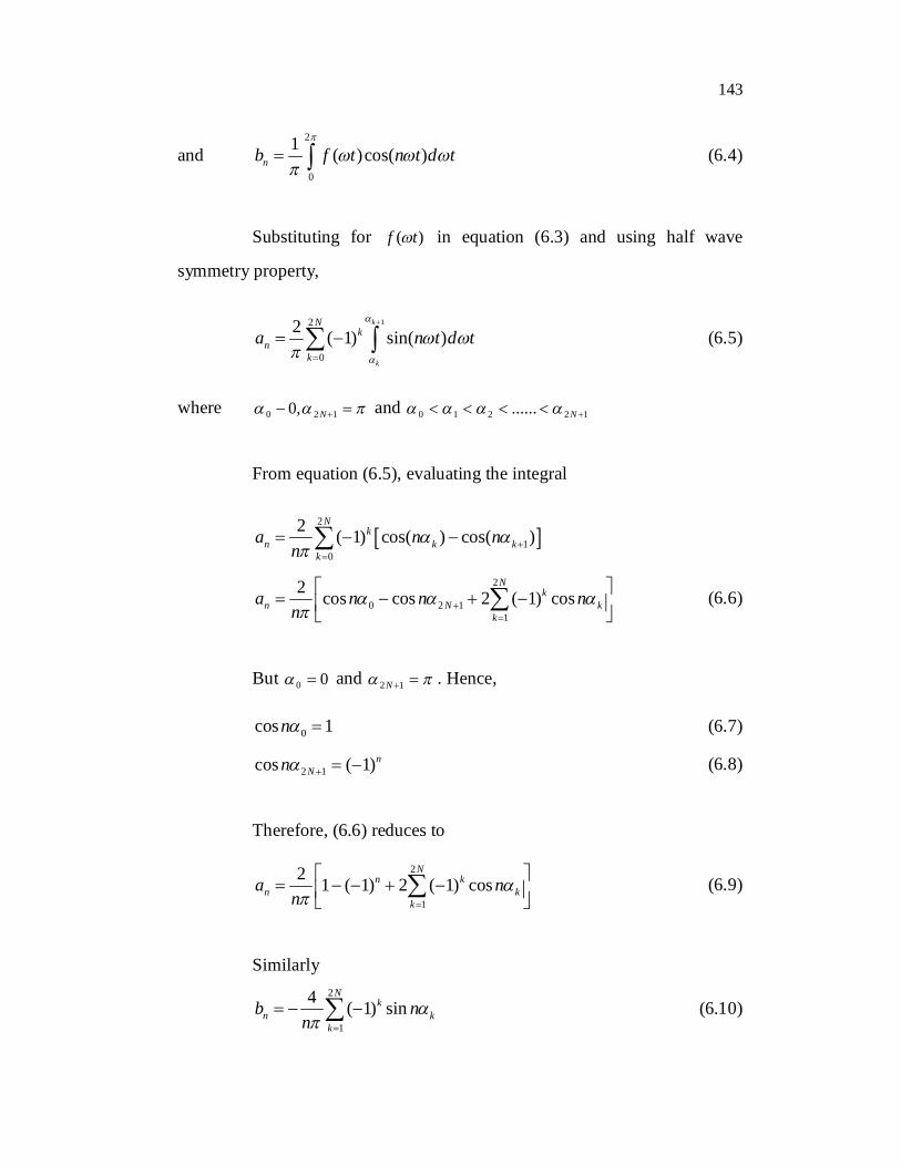
and 2
0
1 ( )cos( )nb f t n t d t
(6.4)
Substituting for )( tf in equation (6.3) and using half wave
symmetry property,
12
0
2 ( 1) sin( )k
k
Nk
nk
a n t d t
(6.5)
where 120 ,0 N and 12210 ...... N
From equation (6.5), evaluating the integral
2
10
2 ( 1) cos( ) cos( )N
kn k k
k
a n nn
2
0 2 11
2 cos cos 2 ( 1) cosN
kn N k
ka n n n
n
(6.6)
But 00 and 12 N . Hence,
0cos 1n (6.7)
2 1cos ( 1)nNn (6.8)
Therefore, (6.6) reduces to
2
1
2 1 ( 1) 2 ( 1) cosN
n kn k
ka n
n
(6.9)
Similarly
2
1
4 ( 1) sinN
kn k
k
b nn
(6.10)
144
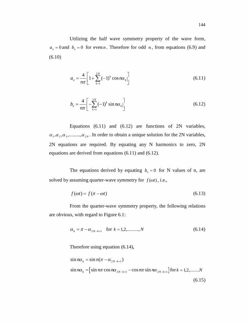
Utilizing the half wave symmetry property of the wave form,
0na and 0nb for even n . Therefore for odd n , from equations (6.9) and
(6.10)
2
1
4 1 ( 1) cosN
kn k
ka n
n
(6.11)
2
1
4 ( 1) sinN
kn k
kb n
n
(6.12)
Equations (6.11) and (6.12) are functions of 2N variables,
N2321 .,,.........,, . In order to obtain a unique solution for the 2N variables,
2N equations are required. By equating any N harmonics to zero, 2N
equations are derived from equations (6.11) and (6.12).
The equations derived by equating 0nb for N values of n, are
solved by assuming quarter-wave symmetry for )( tf , i.e.,
( ) ( )f t f t (6.13)
From the quarter-wave symmetry property, the following relations
are obvious, with regard to Figure 6.1:
2 1k N k for Nk .,,.........2,1 (6.14)
Therefore using equation (6.14),
2 1sin sin ( )k N kn n
2 1 2 1sin sin cos cos sink N k N kn n n n n for Nk ,........2,1
(6.15)
145
For odd n
sin 0,cos 1n n
Substituting in equation (6.15)
2 1sin sink N kn n , for Nk ,........2,1 (6.16)
Substituting equation (6.16) in equation (6.12),
12 1
1
4 ( 1) sin sin 0N
kn k N k
k
b n nn
(6.17)
From equation (6.14)
2 1cos cos ( )k N kn n , for Nk ,........2,1 (6.18)
For odd n , equation (6.18) becomes
2 1cos cosk N kn n , for Nk ,........2,1 (6.19)
Substituting equation (6.19) in equation (6.11)
1
4 1 2 ( 1) cosN
kn k
ka n
n
(6.20)
For a two-state waveform of the type shown in Figure. 6.1, any N
harmonics can be eliminated by solving the N+1 equations obtained from
setting equation (6.20) to zero. The waveform is chopped N times per half-
cycle and is constrained to possess odd quarter-wave symmetry.

146
6.3 ALGEBRAIC APPROACH FOR SOLVING HARMONIC
ELIMINATION EQUATIONS
Mathematical analyses play a vital role in most of the process
implementations. In power electronic circuits, one of the main problems is the
formulation of the gate pulse for switching of the power electronic devices.
When the gate pulse is a pulse of constant duty cycle, the problem becomes
simpler. But in the case of a pulse width modulated (PWM) waveform, there
is a great deal of calculations and they vary according to the PWM generation
method used.
Mathematical analysis is used in this chapter to solve the non-linear
simultaneous harmonic equations. The non-linear equations are the
transcendental equations of the switching instants of the PWM waveform.
These transcendental equations have to be solved either as such or by suitable
transforms (Sun and Grotstollen 1994) in order to obtain the final refined
angles to be used in the generation of PWM pulses for the elimination of
desired harmonics. Some non-linear iterative methods are used to generate the
angles by finding the solutions of the given set of equations. The whole
procedure is finally automated using MATLAB programs.
6.3.1 Harmonic Elimination Equations
The generalized harmonic equation of power electronic inverters is
of the form given by the expression
2 10
4 cos(2 1)(2 1)
Ndc
k i ii
VV h kk
(6.21)

147
where V - Voltage output of the inverter
Vdc - Magnitude of the DC input voltage
hi - Change of waveform level
α - Switching (notching) angle of the inverter
N - The number of harmonic equations
k - Switching angle number (varies from 0 to N-1)
The equation (6.21) is obtained from the Fourier series expansion
of the inverter voltage equation (Sun et al 1994). In general,
Number of harmonic equations to be solved (N) = Number of
harmonics to be eliminated (N)+1.
The additional equation is for the fundamental component of the
waveform. The change of waveform level implies the difference between the
final value of the PWM pulse at an instant and the value of the wave before
switching. This point can be made clear by assuming an exemplary waveform
with three notch angles as shown in Figure 6.2. It is obvious that only the first
two lower order harmonics can be eliminated using the three equations. The
even order harmonics automatically get eliminated due to the symmetry of the
wave.
Figure 6.2 An exemplary PWM waveform for N=3
148
The constraint to be satisfied by the waveform (Sun and Beineke
1996) in Figure 6.2 is that,
1 2 3 2 (6.22)
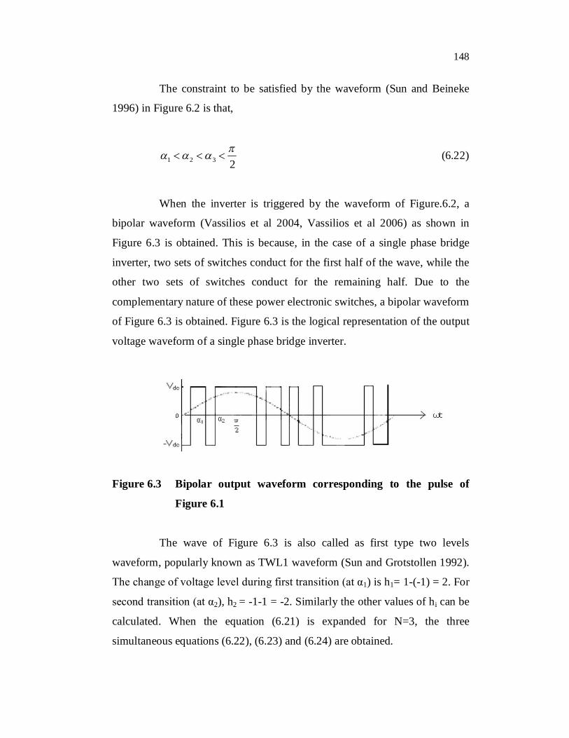
When the inverter is triggered by the waveform of Figure.6.2, a
bipolar waveform (Vassilios et al 2004, Vassilios et al 2006) as shown in
Figure 6.3 is obtained. This is because, in the case of a single phase bridge
inverter, two sets of switches conduct for the first half of the wave, while the
other two sets of switches conduct for the remaining half. Due to the
complementary nature of these power electronic switches, a bipolar waveform
of Figure 6.3 is obtained. Figure 6.3 is the logical representation of the output
voltage waveform of a single phase bridge inverter.
Figure 6.3 Bipolar output waveform corresponding to the pulse of
Figure 6.1
The wave of Figure 6.3 is also called as first type two levels
waveform, popularly known as TWL1 waveform (Sun and Grotstollen 1992).
The change of voltage level during first transition (at α1) is h1= 1-(-1) = 2. For
second transition (at α2), h2 = -1-1 = -2. Similarly the other values of hi can be
calculated. When the equation (6.21) is expanded for N=3, the three
simultaneous equations (6.22), (6.23) and (6.24) are obtained.
149
1 2 31 2cos 2cos 2cos 04M (6.22)
1 2 31 2cos3 2cos3 2cos3 0 (6.23)
1 2 31 2cos5 2cos5 2cos5 0 (6.24)
where M=V1 denotes that the magnitude of the fundamental component is set
to a pre-specified level M. Also the second and third equations are equated to
zero, which denotes that the voltage level of the harmonics to be eliminated
(third and fifth harmonics in this case) should be zero. In other words, the
harmonic content pertaining to these two harmonic should not be present in
the output waveform, once the converter/inverter is triggered with a PWM
generated using the solution of the above equations. In order to solve the
above equations, numerical methods are used.
6.3.2 Solution by Numerical Methods
It is found that the solving of the above transcendental (or
trigonometric) functions of trigger angles is not possible as such. There are
two popular and successful methods of solving non-linear transcendental
equations. They are Seidel’s method and Newton’s method
(www.math.fullerton.edu). But Seidel’s method can be applied only if all the
simultaneous equations are functions of the same trigger angle. In simple
words, Seidel suggests a method to assume the trigonometric function as a
simple variable (i.e., A=cos (a), B=cos (b) and so on). The procedure then
involves solving the equations for the variables (A, B, etc.) by trial and error.
Finally, the inverse trigonometric functions are applied to the variables to get
the final solutions (since a=cos-1(A), b=cos-1(B) and so on). But this method is
not applicable for the set of equations obtained from the harmonic equations.
This is because the first set of equations are the cosine functions of the trigger
150
angle itself, whereas the second and third set of equations are cosine functions
of 3rd and 5th multiples of the angles in first equation. So even if Seidel
method were applied, it would only worsen the problem by creating a set of 3
equations with 9 unknowns. As a result, Newton’s method is adopted for
obtaining the solution for the equations.
6.3.3 Initial Switching Angle Generation Any iterative mathematical method cannot be evaluated without the
usage of initial values of the unknown parameter. Newton’s method is no
exception to this rule. As a result, the convergence of Newton’s method and
hence its effectiveness solely depends on the quality of initial guess. If the
initial guess is too far from the final solution, then the Newton’s method may
not even converge to the final value. So it is of utmost importance to not only
provide the Newton’s method with an initial guess, but also provide it with a
good enough guess. A very good guess consequently reduces the number of
iterations and hence improves the speed of the whole method. This is very
useful in real-time implementation of the method.
The real problem is that there is no clue to decide a good initial
guess for Newton’s method. So the problem becomes quite challenging and
the method becomes a trial and error method if the initial guesses are not
known. So the initial angles are generated by converting the equation into a
Cauchy problem (Sun and Grotstollen 1992) and then plotting a set of
trajectories of triggering angles as a function of the preset level of the
fundamental (M). This helps in the generation of good initial angles for a
given value of M. These initial values are then passed into Newton’s method
and finally the accurate trigger angles are obtained. This section can be further
sub-divided into two parts, namely, the conversion of the equations into
Cauchy problem and linearising the curves by using the method of least
squares.
151
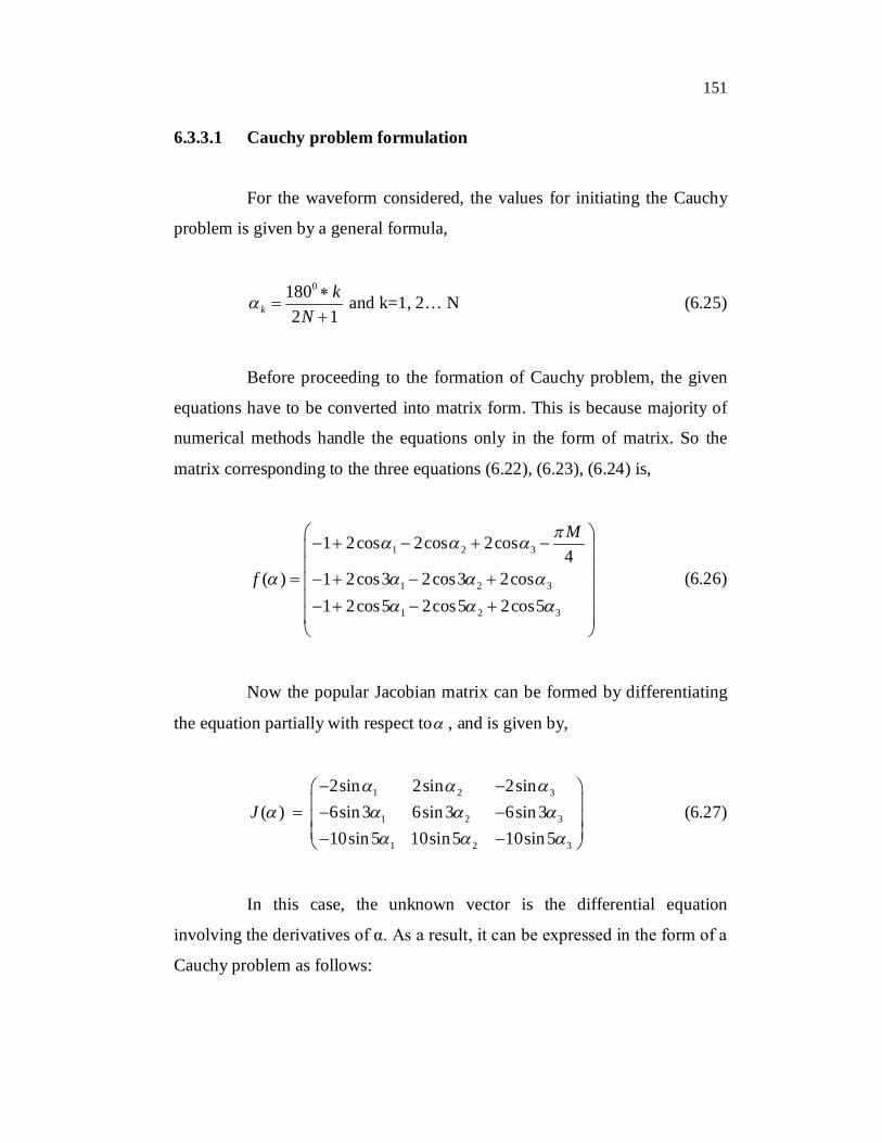
6.3.3.1 Cauchy problem formulation
For the waveform considered, the values for initiating the Cauchy
problem is given by a general formula,
0180
2 1kk
N
and k=1, 2… N (6.25)
Before proceeding to the formation of Cauchy problem, the given
equations have to be converted into matrix form. This is because majority of
numerical methods handle the equations only in the form of matrix. So the
matrix corresponding to the three equations (6.22), (6.23), (6.24) is,
1 2 3
1 2 3
1 2 3
1 2cos 2cos 2cos4
( ) 1 2cos3 2cos3 2cos1 2cos5 2cos5 2cos5
M
f
(6.26)
Now the popular Jacobian matrix can be formed by differentiating
the equation partially with respect to , and is given by,
1 2 3
1 2 3
1 2 3
2sin 2sin 2sin( ) 6sin 3 6sin 3 6sin 3
10sin 5 10sin5 10sin 5J
(6.27)
In this case, the unknown vector is the differential equation
involving the derivatives of α. As a result, it can be expressed in the form of a
Cauchy problem as follows:
152
( ). 1 0 0,.....0 TdJ bdM
(6.28)
where 0 0M M and
8b for TWL1 waveform.
or this can be expressed more elaborately as,
1 2 3 1
1 2 3 2
1 2 3 3
sin sin sin / /8sin 3 sin3 sin 3 / 0sin 5 sin5 sin 5 / 0
d dMd dMd dM
(6.29)
In this case, the trigger angles are initiated by using the equation
(6.25). So the values are,
0
1180
7 ,
0
2360
7 and
0
3540
7 (6.30)
at M = M0 = 0
If the above values are chosen, then it can be proved that the
fundamental, third and fifth harmonics have zero amplitudes for these initial
angles. The equation (6.28) can be called as a typical Cauchy problem. Here,
if the value of increment for M is small enough, then the method proves to be
pretty effective. So the increment value for M is chosen as 0.001, though the
value could be less than this value. As a result ΔM will be nearly equal to dM
(Sun and Grotstollen 1992). Now the following steps are to be followed to get
the trajectories of α versus M:
1. Initially, set M=M0=0,12
1800
N
kk , k=1 to N.
2. Solve the equation (6.29) to get the next points of α.
153
3. Increment the value of M, by ΔM=0.001, so
that MMM kk 1 . The next value is dkk 1 , where
dMdMd .
4. Again jump to step (2). Repeat this until .0k αk > 0.
The above procedure is developed in the form of a M-file program.
The program accepts the number of harmonic equations (N) as input, and
generates a set of trajectories of α1, α2 and α3 as a function of M. It was found
that the trajectories tend to zero, as M reaches the value 1.068. This is the
limiting value of M for the case of N=3. This value varies according to the
number of harmonics to be eliminated.
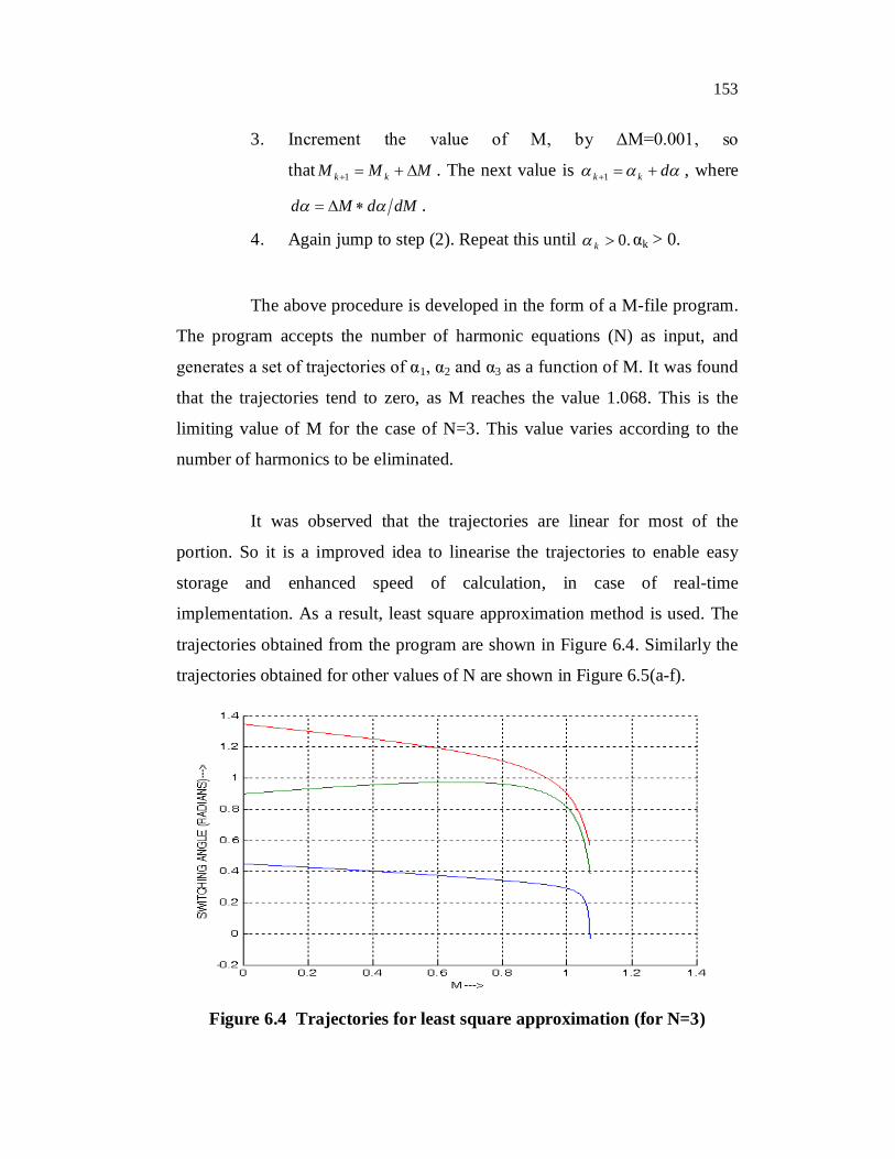
It was observed that the trajectories are linear for most of the
portion. So it is a improved idea to linearise the trajectories to enable easy
storage and enhanced speed of calculation, in case of real-time
implementation. As a result, least square approximation method is used. The
trajectories obtained from the program are shown in Figure 6.4. Similarly the
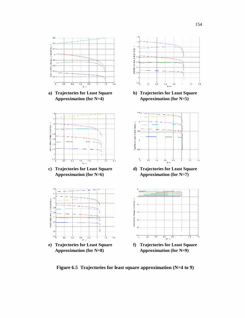
trajectories obtained for other values of N are shown in Figure 6.5(a-f).
Figure 6.4 Trajectories for least square approximation (for N=3)
154
a) Trajectories for Least Square b) Trajectories for Least Square Approximation (for N=4) Approximation (for N=5)
c) Trajectories for Least Square d) Trajectories for Least Square Approximation (for N=6) Approximation (for N=7)
e) Trajectories for Least Square f) Trajectories for Least Square Approximation (for N=8) Approximation (for N=9)
Figure 6.5 Trajectories for least square approximation (N=4 to 9)

155
6.3.3.2 Linearising by least square approximation
As seen from Figure 6.4, the trajectories are linear to almost the
whole region. Linearization of these trajectories is carried out from least
square curve fitting technique. Finally, the linear equation (Sun et al 1994)
obtained will contain α as a linear or scalar function of M.
The method of least squares gives two normal equations for
linearising any non-linear curve given by:
A X Bn Y and
2A X B X XY (6.30)
where A and B are the unknown variables to be found, and (X, Y) is the
coordinates of the curve at selected points of the curve and n represents the
number of data points.
The greater the number of (X, Y) coordinates, the greater is the
accuracy of the method. In this case,
MX and ,iY where i = 1, 2, N.
It should be noted that the value of n of in equation (6.30) denotes
the no. of (X, Y) coordinates, while the N used throughout this chapter
denotes the no. of harmonic equations.
As a result, the new set of harmonic normal equations is,
iA M Bn and
2iA M B M M (6.31)

156
In this case, the actual coordinates of (M, α) are obtained from the
Cauchy problem implementation procedure itself, rather than from the actual
procedure of inferring the Y coordinates from X in the graph. This is to
increase the accuracy of the initial points. The linear equations for the case of
N=3, have been found to be
1 0.4660 0.1693M
2 0.9704 0.0866M
3 1.4105 0.4428M (6.32)
Now it is clear that the value of α can be found for a given value of
M. Also, in this case, the value of M should be less than that of Mmax = 1.068
for N=3.For M=1, the values of α can be calculated from equation (6.32).
These values are as follows:
α1 = 0.2967 radians (16.99º)
α2 = 0.8838 radians (50.63º)
α3 = 0.9677 radians (55.45º) (6.33)
These values represent the radians or in degrees and they can be
converted to the actual time instant of switching of the wave as follows:
(sec ) ( ) 2s radT
or (sec ) (deg ) 0180s reesT (6.34)
where T represents the time period of the wave.
For example, for a fundamental frequency of 50 Hz, the time period
is 0.02 seconds. So the value T=0.02 seconds. The equation (6.33) can be
used to find the α values in seconds, to be used in actual PWM pulse

157
formulation. These radian or degree values can be converted to any other
frequency value. This is an extremely important feature, because it destroys
the country boundaries and enables the method to be used in any country and
for device functioning at virtually any frequency.
6.3.4 Generation of Final Notching Angles
The initial angles found in the section 6.3.3.2 have to be used to
initialize the Newton’s method to generate the final accurate notch angles. If
these initial angles are fed as such, then the harmonics are not completely
eliminated due to the error in the initial angles. Only if these angles are
refined further to the maximum extent, the PWM wave can be generated and
applied to the actual circuit. So here, the Newton’s method is used to refine
the initial angles with the help of Gauss elimination method. The Gauss
elimination method is used only as a sub-set of Newton’s procedure, in order
to solve the simultaneous equations. It should be noted that the Gauss
elimination method is used during each iteration of the Newton’s method. The
maximum no. of iterations is automatically fixed by the program, depending
upon the value of error which can be tolerated.
6.3.4.1 Newton’s iterative method
This is a popularly known procedure and is also referred to as
Newton-Raphson’s iterative method. This method is well known for its fast
convergence, provided that the method is supported by good initial guesses.
The Newton’s method defines the solution procedure for the set of
equations given by,
( ) ( )J f (6.35)

158
Then the iteration procedure is as follows:
1. The values of initial angles 0 are substituted in the
matrices J and f.
2. The value of is found by,
)()( 1 fJ (6.36)
using Gauss elimination procedure.
3. The values of obtained are compared with the tolerance
error value.
4. If the value of is lesser than the error tolerance, then exit
the loop.
5. If not, the new values of α are found by )()( oldnew .
6. The new values of are substituted in the matrices J and f.
Then the loop is repeated from step (2).
The working of Gauss elimination can be studied in brief in the
next section. This is because the Gauss elimination method is the central part
of Newton’s method. So, one should know the purpose of employing the
Gauss elimination, before going into a deep study of its working. Now after
knowing the working of Newton’s method, it would be easier to understand
the working of Gauss elimination method.
6.3.4. 2 Gauss elimination method
There are a plenty of methods used for solving simultaneous
equations. These include Gauss elimination method, Gauss Seidel method,
relaxation method, and so on. Gauss elimination method is chosen because of
its simplicity and ease of programming. Also many methods have an
important requirement that the equations must be diagonally dominant, which

159
is not a problem in Gauss elimination. These reasons make Gauss elimination
method, the best choice for our application.
This method works on the principle of back-substitution of values
of variables. The method is used to solve the simultaneous equations by
formulating them into an augmented matrix formed by adjoining the known
matrices on the left and right hand sides. Then the augmented matrix is
reduced to an upper triangular matrix and then back substituted to find the
unknown variables.
Let the set of simultaneous equations to be solved, is in the form of
equation (6.35).
The procedure for solving using Gauss elimination is as follows:
1. Substitute the values of α available from Newton’s method in
matrices J and f.
2. Formulate the augmented matrix by adjoining the matrices
)(J and )(f . Let the augmented matrix be
)(:)()( fJA (6.37)
3. The augmented matrix is reduced to an upper triangular matrix
by appropriate row transformations. Here, upper triangular
matrix refers to a matrix that contains the lower part of the
matrix (below the diagonal, to the lower-left of the matrix)
with all zeroes. For such a matrix the last row contains only
the last variable (the last variable, in this case is α3). So the
value of the last variable can be found directly by dividing the
last element of the last row, by the element just to the left of it
in the last row.
160
4. Now the back substitution is used to find the rest of the
variables. This is done by substituting the values of known
variables in each row, moving from the last row to the first.
If there are N harmonic equations, then the order of the augmented
matrix will be N by N+1. In other words, the matrix A will contain N rows
with (N+1) columns. The first N columns are the elements of the matrix J,
while the (N+1)th column is the matrix f. As a result, after step 3, the matrix A
will be of the form in which, the ith row will be a function of the last (i-1)
variables. So as the row number increases, the no. of variables involved
decreases. So the problem is solved from the last row to the first row. It would
be obvious that the last row will be a function of the last variable alone, while
the first row will be a function of all the variables.
When the combination of Newton’s and Gauss elimination methods
are applied, the final refined angles are obtained. In this case, the final values
of α were found to be,
α1 = 0.2916 rad (16.707º) (6.38)
α2 = 0.8113 rad (46.48º) (6.39)
α3 = 0.8976 rad (51.43º) (6.40)
These values are converted to a wave of any frequency using
equation (6.34). The effectiveness of Newton’s method can be known from
the trajectories plotted by the program. The trajectories are shown in
Figure 6.6.
161
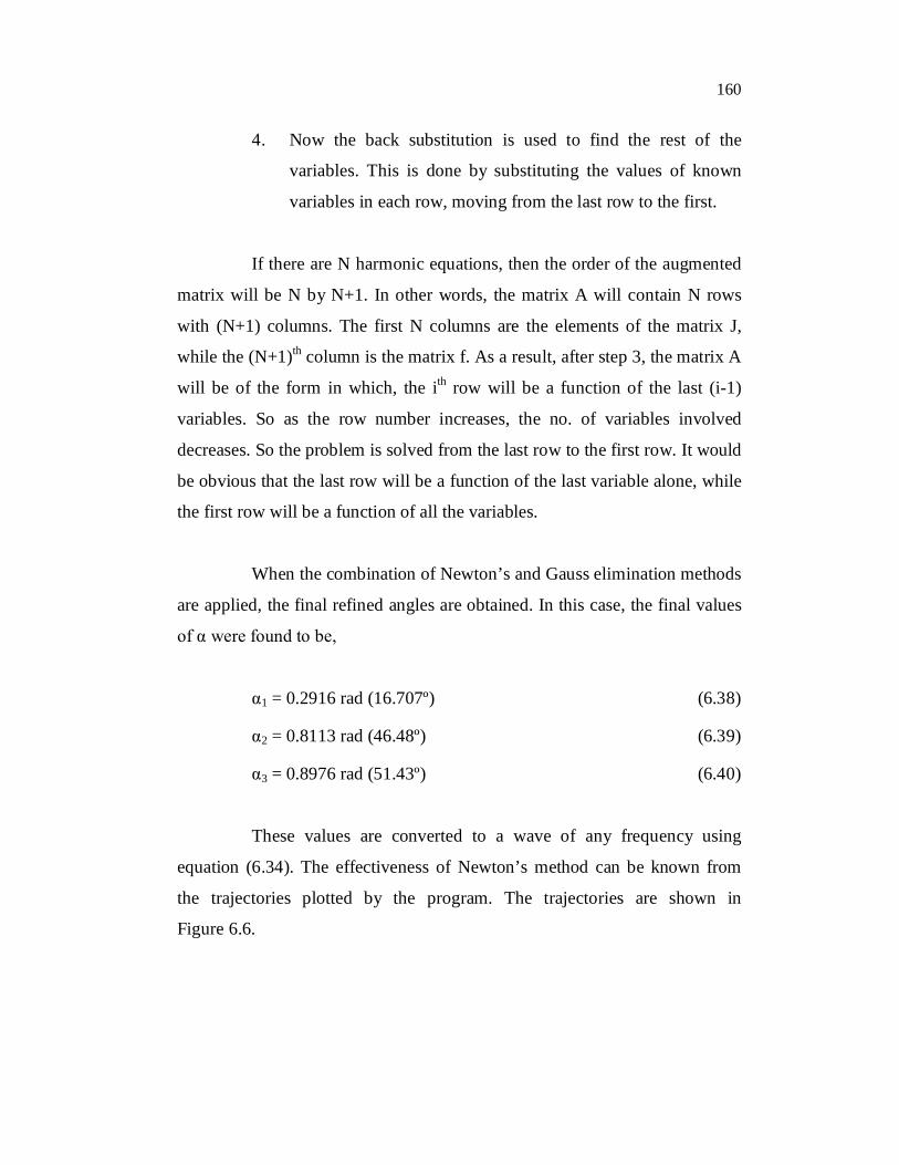
Figure 6.6 Effectiveness (Rate of convergence) of Newton’s method
It is seen from the trajectories that the method converges in just 4 to
5 iterations. This re-establishes the fact that the choice of Newton’s method is
indeed useful in the real-time implementation of the method. Though the
iterations are less, the difference between the initial and final values of trigger
angles is significant. It is only this difference that makes the harmonic content
to zero (if not, at least to the lowest possible value).
6.4 IMPLEMENTATION OF COMPUTED PULSE WIDTH
MODULATION
The term “computed PWM” (CPWM) is coined because the
generation of PWM by this method is just by computing an interpolated
repeated sequence and directly using these values to generate the waveform.
As a result, large number of trials is involved in this method. Also the time
required to form the interpolated sequence is far less than that required for the
sine-triangular comparison method. Since there are no direct tools for creating
the wave form that is needed for this work, the required wave is created from
the zero-crossings of a variable frequency triangular wave, which switches at
pre-specified or programmed instants (Enjeti et al 1990). This method has

162
been found to simple but effective method to generate a wave of required
shape.
6.4.1 Implementation in MATLAB (SIMULINK)
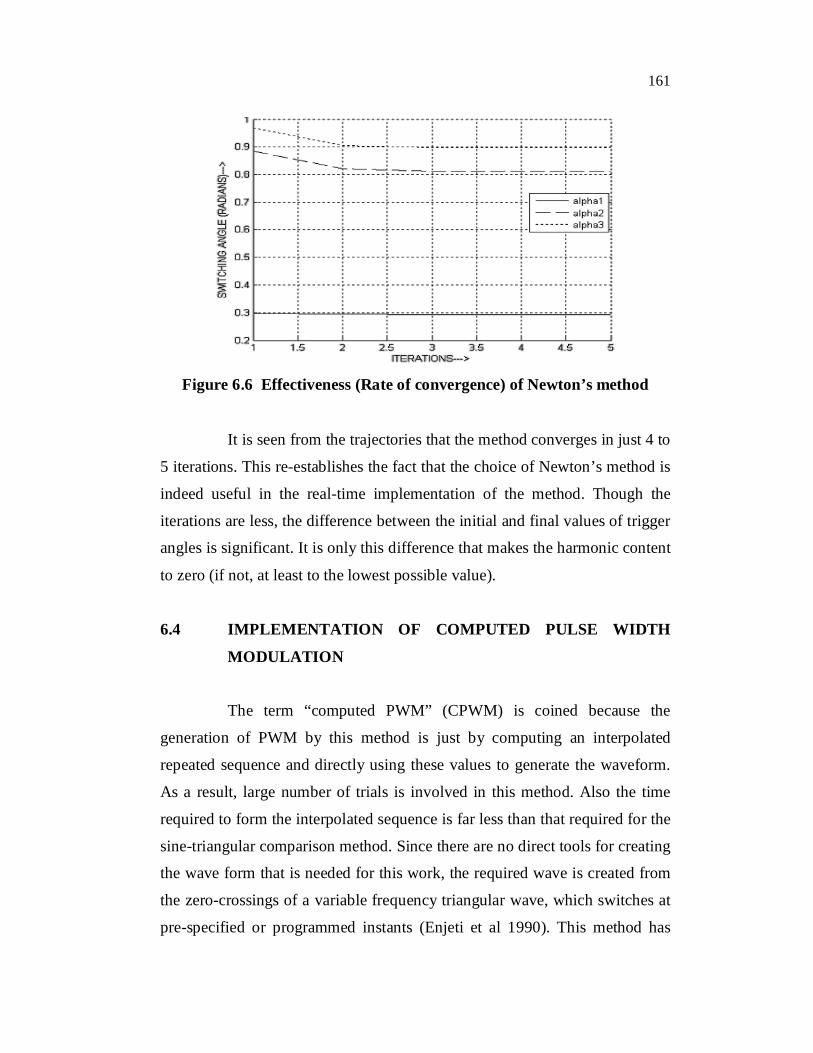
To find out the notching angles a program is developed as per the
flowchart shown in Figure 6.7. The notching angles are obtained for a given
value of N and modulation index (M). The notching angles are directly loaded
into Simulink model and then it is executed. The main block (core) in the
implementation of this method is the “repeated sequence interpolated” block
of SIMULINK. The output from this block is compared with a constant of
zero value. This implies that the zero-crossings of the sequence are detected.
The coordinates of the sequence are formulated from the shape of the desired
PWM wave. The basic logic is to form the quasi-triangular sequence such that
its zero crossings generate a transition in the PWM level, i.e., a notch. The
SIMULINK implementation of this method is shown in Figure 6.8.
The “repeated sequence interpolated” generates a quasi-triangular
waveform, which is sent to a multiplexer along with the constant of zero
value. These two signals are again compared using a relational operator and
then converted to “double” data type, in order to aid in the triggering of the
output pulse to the converter/inverter circuit. Finally a 2nd order digital filter is
used to verify whether the generated output is a modulated version of a wave
of required frequency. It has to be noted that any modulated wave, on low
pass filtering, gives the reference (sine wave in this case) signal, which has
been modulated. The output of the model of Figure 6.8 is given in Figure 6.9.
The output waveform may resemble the waveform obtained from sine PWM
in overall shape, but the values of notch angles are accurately the same as that
of those obtained from the calculations.
163
Figure 6.7 Flow chart for the mathematical analysis
Figure 6.8 Simulink representation of the CPWM approach
START
INPUT N
LINEARISE THE CURVES BY LEAST SQUARE APPROX.
REFINE ANGLES USING NEWTON’S METHOD
SOLVE SIMULTANEOUS EQNS. USING GAUSS ELIMINATION
OUTPUT FINAL NOTCH ANGLES
STOP
GENERATE CURVES OF α Vs M USING CAUCHY THEORY

164
Figure 6.9 Output PWM versus Time period for CPWM approach
The method used in here uses a reverse process of formation of triangular wave from PWM wave, in order to get the PWM wave itself. The
PWM waveform cannot be directly generated using SIMULINK. There is a
block called “timer”, which enables the generation of any given pulse form, but it can only generate the pulse once. But here the necessity is to generate
the pulse over and over again for the specified time period. On the other hand,
the “repeated sequence interpolated” block can generate the waveform of specified period and repeat it, the constraint being that it can only generate
triangular waveform. So the only way out is to generate a triangular
waveform and use its zero-crossings to generate a PWM of required shape. But the accuracy of the method depends solely upon the sampling time of the
“repeated sequence interpolated”. But the accuracy of the method was best,
with a sampling period of 10 microseconds. So this value of sampling interval is used.
6.4.2 Simulink Model Parameters
The formulation of triangular wave may be slightly difficult for the
first time. But with a little practice, the method proves quite easy to use. The formation of the coordinates for triangular wave involves writing down the
values of notch angles for one time period and creating a notch of triangular
165
wave for the mid-points of the adjacent points of PWM, the output changing from 1 to 0 and then to -1 and then again to 0 and to 1, and so on.
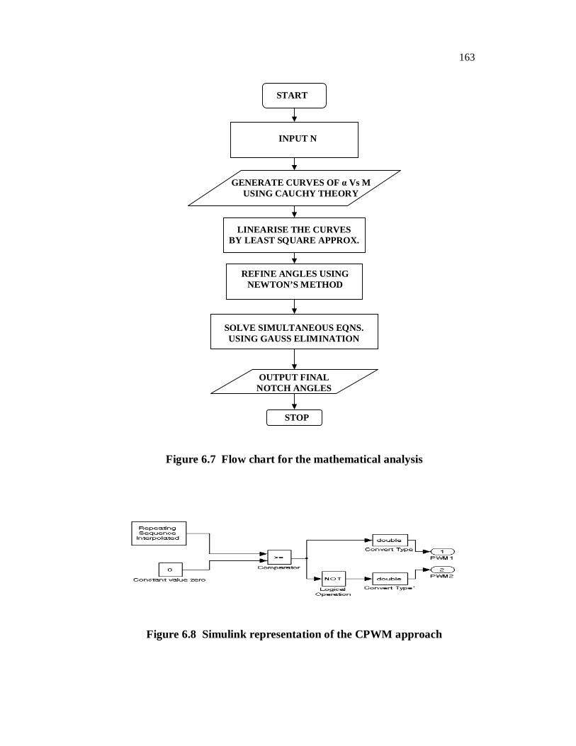
The method can be made clear by taking the case of N=3 and forming a triangular wave sequence for it. Now the Table 6.1 shows the notch
angles of the desired PWM waveform and its corresponding destination
output levels. This is formed from Figure 6.9. Here T is the time period of the desired waveform.
Now from these values, it is needed that the triangle should attain its peak values (-1 or +1) in between two notches and should cross zero line,
at every notch. So the triangular wave has essentially 15 zero crossings in this
case. Now the triangular wave sequence can be formulated as in Table 6.2. It is seen from the Table that the zero crossings occur at the points mentioned in
Table 6.1, while the values 1 and -1 alternate about it.
Table 6.1 Sequence to obtain desired PWM waveform (N=3)
S. No. Time Period (secs) Logic Output Level 1 0 0 2 α1 1 3 α2 0 4 α3 1 5 0.5T – α3 0 6 0.5T – α2 1 7 0.5T – α1 0 8 0.5T 1 9 0.5T + α1 0 10 0.5T + α2 1 11 0.5T + α3 0 12 T – α3 1 13 T – α2 0 14 T – α1 1 15 T 0

166
Figure 6.10 shows the block properties window (SIMULINK) of the “repeated sequence interpolated” block. It can be clearly seen that the values in the Table 6.2 are fed as such in the Figure 6.10. The values of trigger angles can be fed as such in the form of actual numbers, but it would hinder the understanding of the method. So the variables alpha1, alpha2, etc. are used. These variables have to be initialized before executing the model file. The initialization can be done from the “model properties” window of SIMULINK. The computed values are assigned to the variable using the “model initialization” section of the model properties, as shown in Figure 6.11.
Table 6.2 Sequence for the Quasi-triangular wave
S. No. Time Period (secs) Logic Output Level 1 0 0 2 α1/2 -1 3 α1 0 4 (α1+ α2)/2 1 5 α2 0 6 (α2+ α3)/2 -1 7 α3 0 8 T/4 1 9 (T-2* α3)/2 0 10 (T- α2- α3)/2 -1 11 (T-2* α2)/2 0 12 (T- α1- α2)/2 1 13 (T-2* α1)/2 0 14 (T- α1)/2 -1 15 0.5T 0 16 (T+ α1)/2 1 17 (T+2* α1)/2 0 18 (T+ α1+ α2)/2 -1 19 (T+2* α2)/2 0 20 (T+ α2+ α3)/2 1 21 (T+2* α3)/2 0 22 0.75*T -1 23 T- α3 0 24 (2*T- α2- α3)/2 1 25 T- α2 0 26 (2*T- α1- α2)/2 -1 27 T- α1 0 28 (2*T- α1)/2 1 29 T 0

167
Figure 6.10 Block parameters of ‘Repeated sequence interpolated’ block
Figure 6.11 Model properties window for the computed PWM model
It is clear that the CPWM method is far better than the sine-
triangular comparison method in terms of speed of formulation, ease of
implementation and the accuracy of waveform. So the CPWM method is
indeed the best suited method for this kind of application. Further this method
can be easily implemented in hardware, which is an added advantage.
6.5 SIMULATION AND HARDWARE RESULTS
Based on the developed algebraic approach the notching angles are
generated to selectively eliminate the harmonics produced by the inverters.

168
A Computed PWM waveform is generated using these angles. This waveform
is then applied to the Simulated PWM inverter as shown in Figure 6.12 for
different values of N and modulation index (M). The specifications of the
inverter circuit are as follows:
DC input voltage : 230V
Load Resistance : 400 Ohms
Figure 6.12 Simulink model of a single phase voltage source inverter
The circuit consists of four IGBT’s: IGBT1, IGBT2, IGBT3, and
IGBT4 which are connected as shown in the Figure 6.12. Pulse generator 1
triggers IGBT1 and IGBT2 during positive half cycles of the output wave.
During negative cycles of output IGBT3 and IGBT4 are triggered by pulse
generator2.
To corroborate the results obtained in the simulation, a hardware
prototype model using microcontroller is implemented to selectively eliminate

169
the harmonics. The block diagram of the proposed hardware model is shown
in Figure 6.13. The power circuit is designed for a output voltage of 230V
with a output frequency of 50 Hz and the rated output power is 500 watts.
Four IGBTs, (IRG4BC20S) are used as the main switches which are
connected in full bridge configuration. The power circuit diagram is shown in
Figure 6.14. To generate computed PWM signals PIC microcontroller (PIC
18F452) is used. The microcontroller based implementation of computed
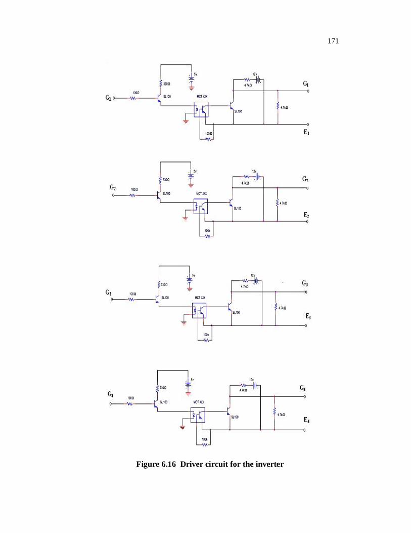
PWM generation is shown in Figure 6.15. The driver circuit for the inverter is
shown in Figure 6.16. The load connected to the output terminals is 400
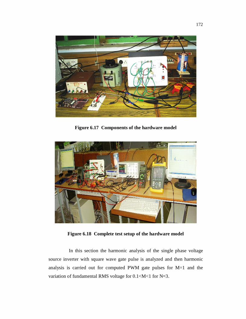
ohms. The components of the hardware are shown in Figure 6.17. The
complete test setup shown in the Figure 6.18. To capture the waveforms the
four channel digital storage oscilloscope (GWINSTEK, GDS2104) is used.
For measuring gate voltages the oscilloscope probes are directly connected.
For output voltage measurements differential module is used along with the
oscilloscope and the multiplication of the differential module is 400. For
voltage measurements true RMS meters (Tektronix, TX1) are used. For
harmonic analysis and measurement the Fluke 434 power quality analyzer is
used.
Figure 6.13 Block diagram of the microcontroller based single phase
inverter model

170
Figure 6.14 Power circuit diagram of the inverter model
Figure 6.15 Microcontroller based implementation of computed PWM
171
Figure 6.16 Driver circuit for the inverter
172
Figure 6.17 Components of the hardware model
Figure 6.18 Complete test setup of the hardware model
In this section the harmonic analysis of the single phase voltage
source inverter with square wave gate pulse is analyzed and then harmonic
analysis is carried out for computed PWM gate pulses for M=1 and the
variation of fundamental RMS voltage for 0.1<M<1 for N=3.

173
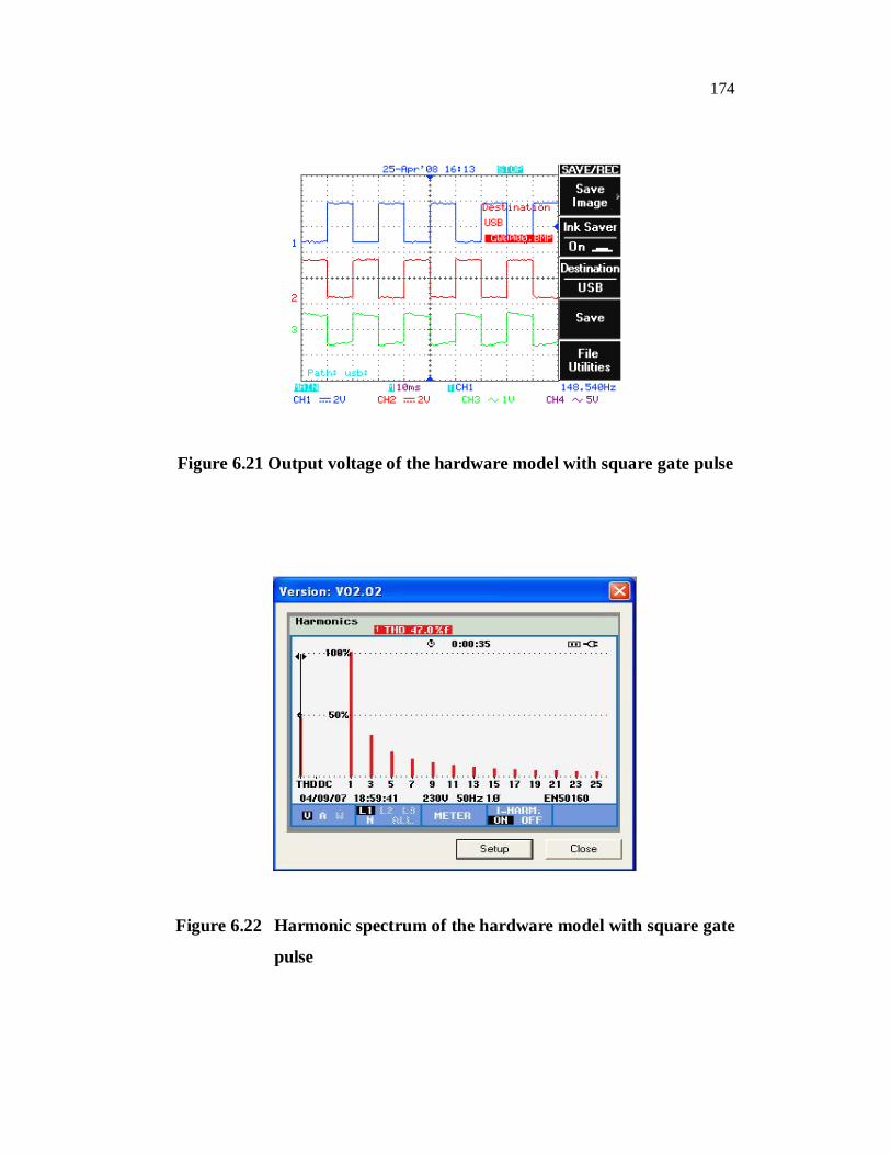
6.5.1 Harmonic Analysis of Inverter Circuit with Square Gate Pulse
The proposed simulink and hardware model was tested for a simple square wave gate pulse. The switching waveforms and output voltage waveform and harmonic spectrum of the output voltage of the simulation model are shown in Figures 6.19 and 6.20 respectively. The output voltage
waveform and harmonic spectrum of the output voltage of the hardware model are shown in Figures 6.21 and 6.22 respectively. Table 6.3 shows the harmonic content expressed as a percentage of fundamental for each order of the harmonic.
Figure 6.19 Switching waveforms and output voltage waveforms
Figure 6.20 Harmonic analysis of pulse triggered single phase inverter
174
Figure 6.21 Output voltage of the hardware model with square gate pulse
Figure 6.22 Harmonic spectrum of the hardware model with square gate
pulse

175
Table 6.3 Harmonic analysis of single phase square pulse triggered
inverter circuit
S. No. Harmonic Order Magnitude (% of Fundamental) 1 1 100.00 2 3 33.32 3 5 20.02 4 7 14.31 5 9 11.15 6 11 9.14 7 13 7.75 8 15 6.73 9 17 5.95
10 19 5.34 11 21 4.85 12 23 4.44
Thus from the Table 6.3, it is observed that as the order of the
harmonic increases the magnitude of the harmonic content expressed as a
percentage of the fundamental decreases. Also from the spectrum analysis it is
observed that the magnitudes harmonic order of 3rd, 5th, 7th, 9th, 11th etc., are
higher and they are detrimental to the operation of critical equipments. Thus if
these order of harmonics can be eliminated, it is possible to operate the
critical equipments with better performance. In the subsequent sections the
selective harmonic elimination of the harmful harmonic levels using
computed PWM waveforms are discussed in detail.
6.5.2 Elimination of the First Two Odd Harmonics
For eliminating first two lower order harmonics three values of
notch angles need to be calculated; one for fundamental component and the
176
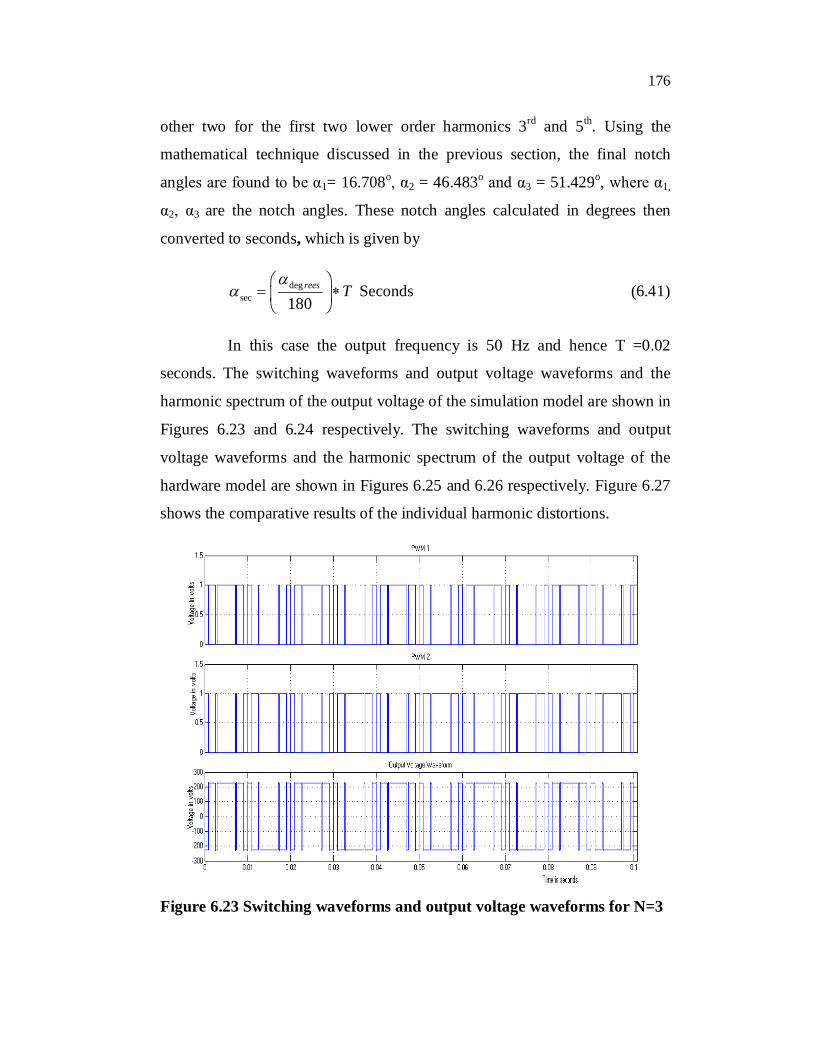
other two for the first two lower order harmonics 3rd and 5th. Using the
mathematical technique discussed in the previous section, the final notch
angles are found to be α1= 16.708o, α2 = 46.483o and α3 = 51.429o, where α1,
α2, α3 are the notch angles. These notch angles calculated in degrees then
converted to seconds, which is given by
degsec 180
rees T
Seconds (6.41)
In this case the output frequency is 50 Hz and hence T =0.02
seconds. The switching waveforms and output voltage waveforms and the
harmonic spectrum of the output voltage of the simulation model are shown in
Figures 6.23 and 6.24 respectively. The switching waveforms and output
voltage waveforms and the harmonic spectrum of the output voltage of the
hardware model are shown in Figures 6.25 and 6.26 respectively. Figure 6.27
shows the comparative results of the individual harmonic distortions.
Figure 6.23 Switching waveforms and output voltage waveforms for N=3

177
Figure 6.24 Harmonic spectrum of the output voltage (for N=3)
Figure 6.25 Switching waveforms and output voltage waveforms of the
hardware model for N=3
Figure 6.26 Harmonic spectrum of the output voltage of the hardware
model (N=3)
178
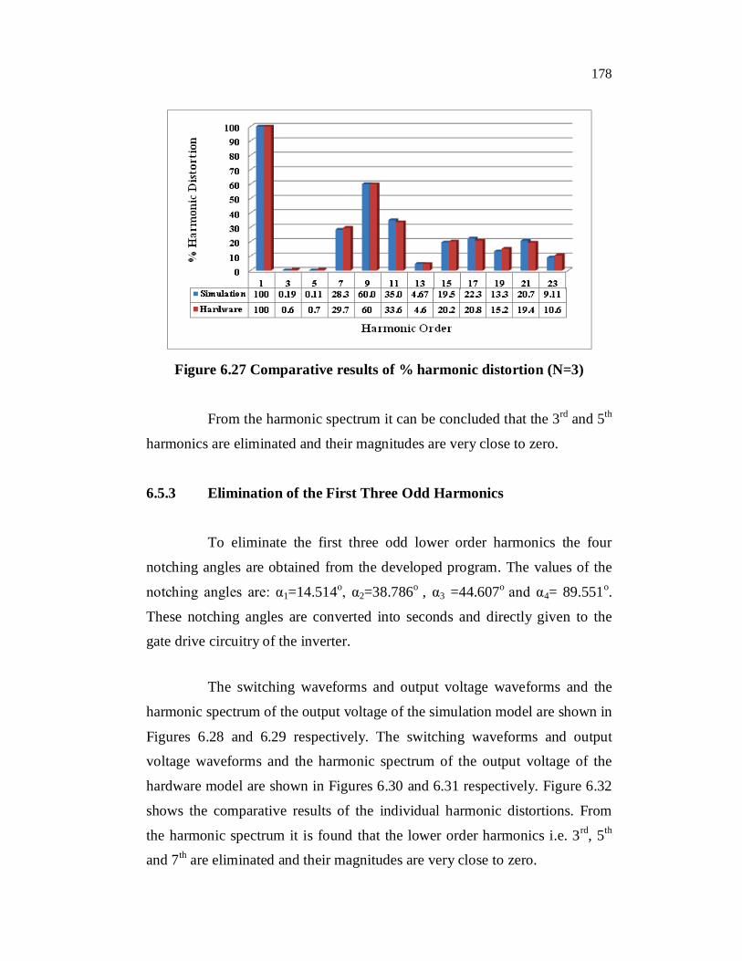
Figure 6.27 Comparative results of % harmonic distortion (N=3)
From the harmonic spectrum it can be concluded that the 3rd and 5th
harmonics are eliminated and their magnitudes are very close to zero.
6.5.3 Elimination of the First Three Odd Harmonics
To eliminate the first three odd lower order harmonics the four
notching angles are obtained from the developed program. The values of the
notching angles are: α1=14.514o, α2=38.786o , α3 =44.607o and α4= 89.551o.
These notching angles are converted into seconds and directly given to the
gate drive circuitry of the inverter.
The switching waveforms and output voltage waveforms and the
harmonic spectrum of the output voltage of the simulation model are shown in
Figures 6.28 and 6.29 respectively. The switching waveforms and output
voltage waveforms and the harmonic spectrum of the output voltage of the
hardware model are shown in Figures 6.30 and 6.31 respectively. Figure 6.32
shows the comparative results of the individual harmonic distortions. From
the harmonic spectrum it is found that the lower order harmonics i.e. 3rd, 5th
and 7th are eliminated and their magnitudes are very close to zero.

179
Figure 6.28 Switching waveforms and output voltage waveforms for N=4
Figure 6.29 Harmonic spectrum of the output voltage (for N=4)
180
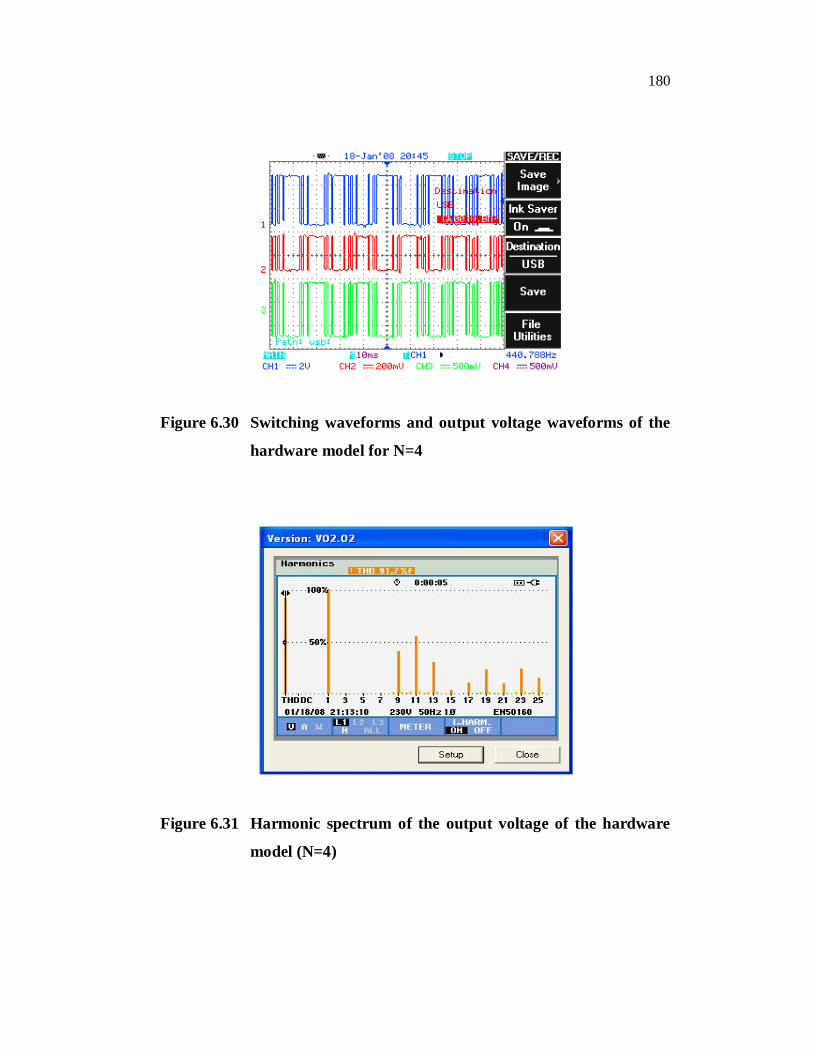
Figure 6.30 Switching waveforms and output voltage waveforms of the
hardware model for N=4
Figure 6.31 Harmonic spectrum of the output voltage of the hardware
model (N=4)

181
Figure 6.32 Comparative results of % harmonic distortion (N=4)
6.5.4 Elimination of the First Four Odd Harmonics
For eliminating the first four odd lower order harmonics the five
notching angles are obtained from the developed program. The values of the
notching angles are: α1= 12.171o, α2 = 30.77o , α3 = 36.876o, α4= 60.983o and
α5= 62.643o. These notching angles are converted into seconds and directly
give to the gate drive circuitry of the inverter.
The switching waveforms and output voltage waveforms and the
harmonic spectrum of the output voltage of the simulation model are shown in
Figures 6.33 and 6.34 respectively. The switching waveforms and output
voltage waveforms and the harmonic spectrum of the output voltage of the
hardware model are shown in Figures 6.35 and 6.36 respectively. Figure 6.37
shows the comparative results of the individual harmonic distortions. Based
on the harmonic spectrum, it is found that the lower order harmonics i.e. 3rd,
5th, 7th, and 9th are eliminated.
182
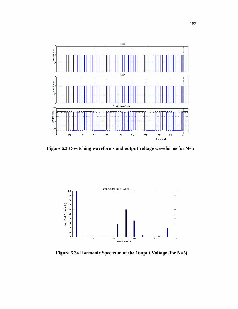
Figure 6.33 Switching waveforms and output voltage waveforms for N=5
Figure 6.34 Harmonic Spectrum of the Output Voltage (for N=5)

183
Figure 6.35 Switching waveforms and output voltage waveforms of the
hardware model for N=5
Figure 6.36 Harmonic spectrum of the output voltage of the hardware model (N=5)
Figure 6.37 Comparative results of % harmonic distortion (N=5)

184
6.5.5 Elimination of the First Five Odd Harmonics
For eliminating the first five odd lower order harmonics the six
notching angles are obtained from the developed program. The values of the
notching angles are: α1= 10.896o, α2 =26.867o , α3 = 32.985o, α4= 53.799o
α5=56.111o and α6= 89.829o. These notching angles are converted into
seconds and directly give to the gate drive circuitry of the inverter.
The switching waveforms and output voltage waveforms and the
harmonic spectrum of the output voltage of the simulation model are shown in
Figures 6.38 and 6.39 respectively. The switching waveforms and output
voltage waveforms and the harmonic spectrum of the output voltage of the
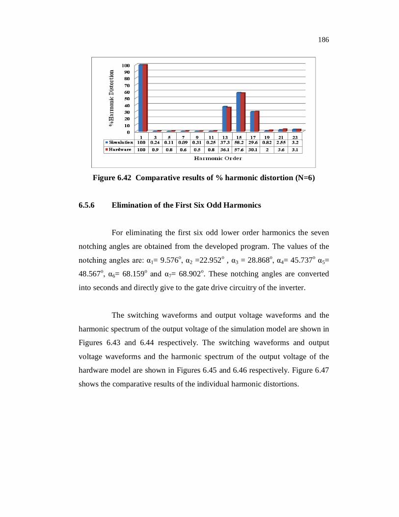
hardware model are shown in Figures 6.40 and 6.41 respectively. Figure 6.42
shows the comparative results of the individual harmonic distortions. Based
on the harmonic spectrum, it is found that the lower order harmonics i.e. 3rd,
5th, 7th, 9th and 11th are eliminated.
Figure 6.38 Switching waveforms and output voltage waveforms for N=6
185
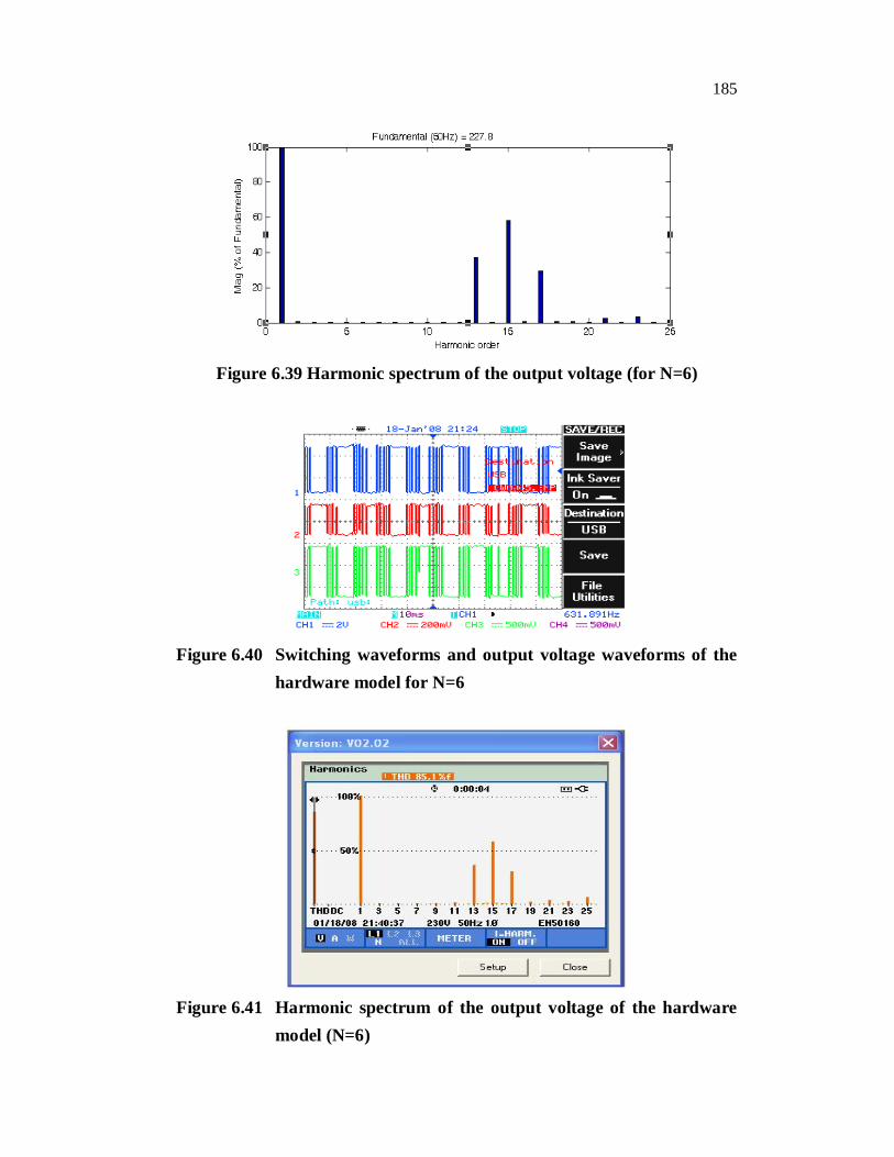
Figure 6.39 Harmonic spectrum of the output voltage (for N=6)
Figure 6.40 Switching waveforms and output voltage waveforms of the
hardware model for N=6
Figure 6.41 Harmonic spectrum of the output voltage of the hardware
model (N=6)
186
Figure 6.42 Comparative results of % harmonic distortion (N=6)
6.5.6 Elimination of the First Six Odd Harmonics
For eliminating the first six odd lower order harmonics the seven
notching angles are obtained from the developed program. The values of the
notching angles are: α1= 9.576o, α2 =22.952o , α3 = 28.868o, α4= 45.737o α5=
48.567o, α6= 68.159o and α7= 68.902o. These notching angles are converted
into seconds and directly give to the gate drive circuitry of the inverter.
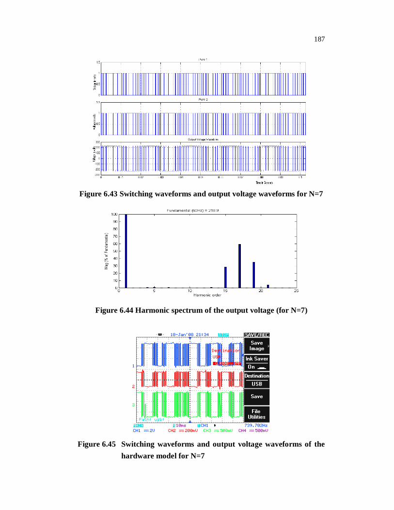
The switching waveforms and output voltage waveforms and the
harmonic spectrum of the output voltage of the simulation model are shown in
Figures 6.43 and 6.44 respectively. The switching waveforms and output
voltage waveforms and the harmonic spectrum of the output voltage of the
hardware model are shown in Figures 6.45 and 6.46 respectively. Figure 6.47
shows the comparative results of the individual harmonic distortions.
187
Figure 6.43 Switching waveforms and output voltage waveforms for N=7
Figure 6.44 Harmonic spectrum of the output voltage (for N=7)
Figure 6.45 Switching waveforms and output voltage waveforms of the hardware model for N=7

188
Figure 6.46 Harmonic spectrum of the output voltage of the hardware model (N=7)
Figure 6.47 Comparative results of % harmonic distortion (N=7)
Based on the harmonic spectrum, it is found that the lower order harmonics i.e. 3rd, 5th, 7th, 9th, 11th and 13th are eliminated.
6.5.7 Elimination of the First Seven Odd Harmonics
For eliminating the first seven odd lower order harmonics the eight
notching angles are obtained from the developed program. The values of the notching angles are: α1= 8.748o, α2 =20.620o , α3 = 26.351o, α4= 41.218o , α5= 44.321o, α6= 61.904o α7= 63.043o and α8= 89.917o. These notching angles

189
are converted into seconds and directly give to the gate drive circuitry of the inverter.
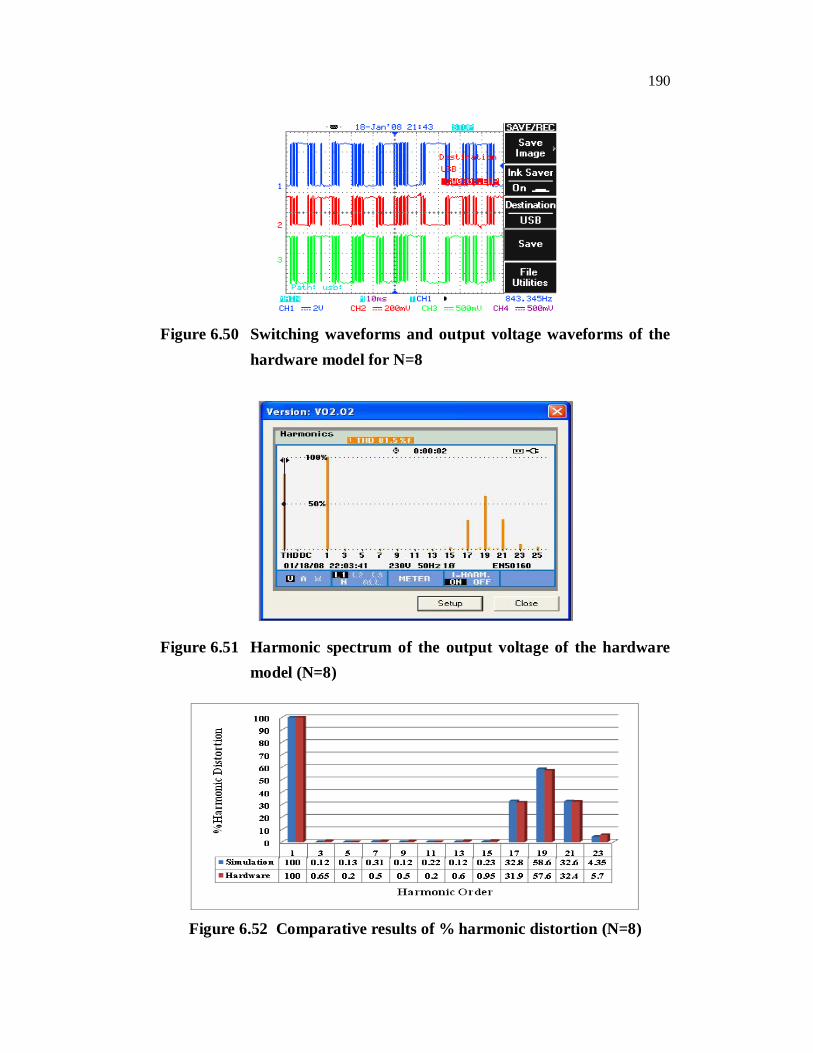
The switching waveforms and output voltage waveforms and the harmonic spectrum of the output voltage of the simulation model are shown in Figures 6.48 and 6.49 respectively. The switching waveforms and output
voltage waveforms and the harmonic spectrum of the output voltage of the hardware model are shown in Figures 6.50 and 6.51 respectively. Figure 6.52 shows the comparative results of the individual harmonic distortions.
Figure 6.48 Switching waveforms and output voltage waveforms for N=8
Figure 6.49 Harmonic spectrum of the output voltage (for N=8)
190
Figure 6.50 Switching waveforms and output voltage waveforms of the hardware model for N=8
Figure 6.51 Harmonic spectrum of the output voltage of the hardware model (N=8)
Figure 6.52 Comparative results of % harmonic distortion (N=8)
191
Based on the harmonic spectrum, it is found that the lower order
harmonics i.e 3rd, 5th, 7th, 9th, 11th, 13th and 15th are eliminated.
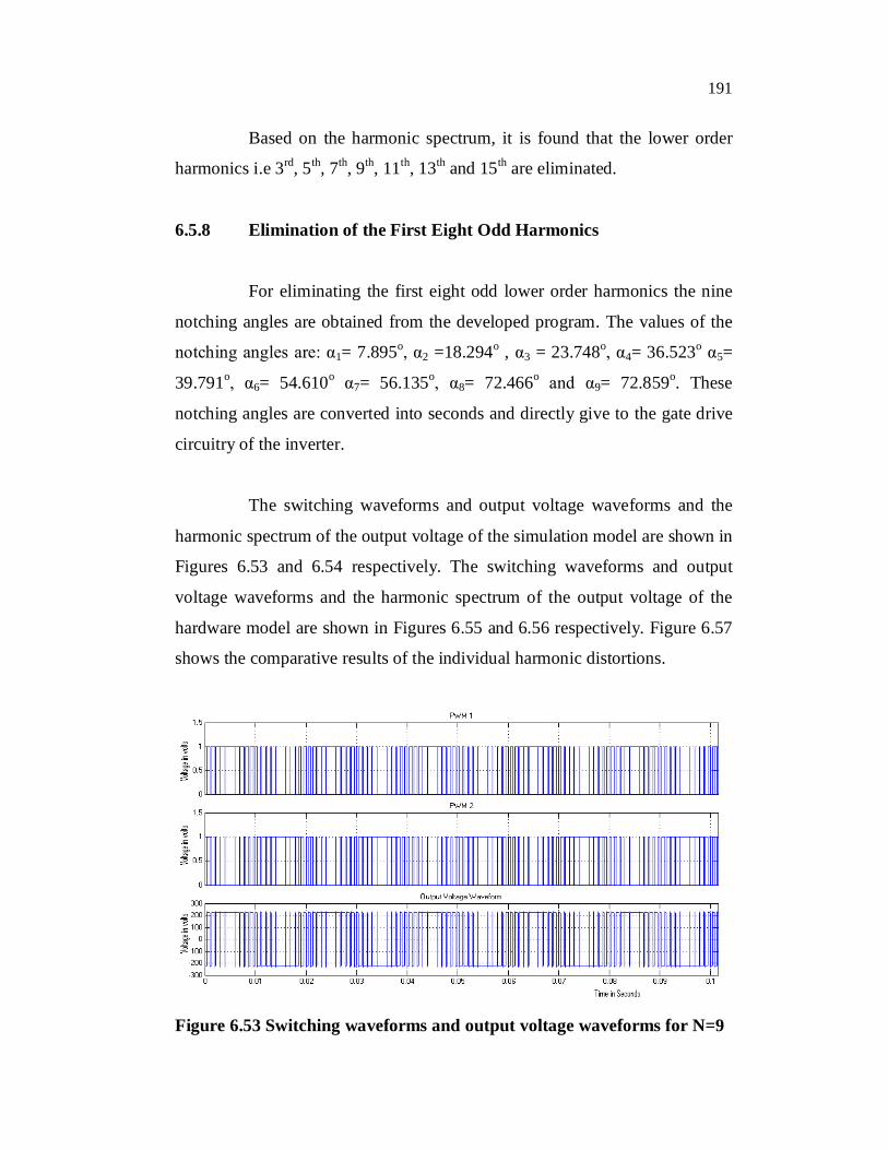
6.5.8 Elimination of the First Eight Odd Harmonics
For eliminating the first eight odd lower order harmonics the nine
notching angles are obtained from the developed program. The values of the
notching angles are: α1= 7.895o, α2 =18.294o , α3 = 23.748o, α4= 36.523o α5=
39.791o, α6= 54.610o α7= 56.135o, α8= 72.466o and α9= 72.859o. These
notching angles are converted into seconds and directly give to the gate drive
circuitry of the inverter.
The switching waveforms and output voltage waveforms and the
harmonic spectrum of the output voltage of the simulation model are shown in
Figures 6.53 and 6.54 respectively. The switching waveforms and output
voltage waveforms and the harmonic spectrum of the output voltage of the
hardware model are shown in Figures 6.55 and 6.56 respectively. Figure 6.57
shows the comparative results of the individual harmonic distortions.
Figure 6.53 Switching waveforms and output voltage waveforms for N=9

192
Figure 6.54 Harmonic Spectrum of the output voltage (for N=9)
Figure 6.55 Switching waveforms and output voltage waveforms of the
hardware model for N=9
Figure 6.56 Harmonic spectrum of the output voltage of the hardware
model (N=9)

193
Figure 6.57 Comparative results of % harmonic distortion (N=9)
Based on the harmonic spectrum, it is found that the lower order
harmonics i.e. 3rd, 5th , 7th , 9th , 11th , 13th, 15th and 17th are eliminated.
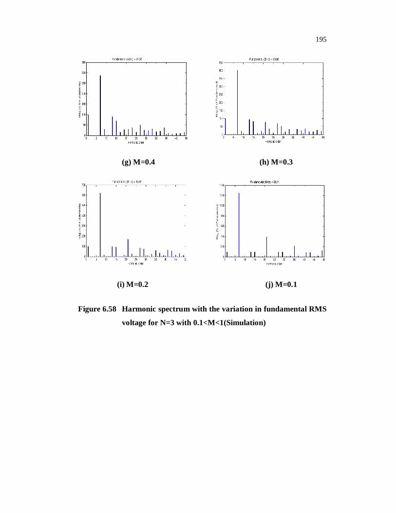
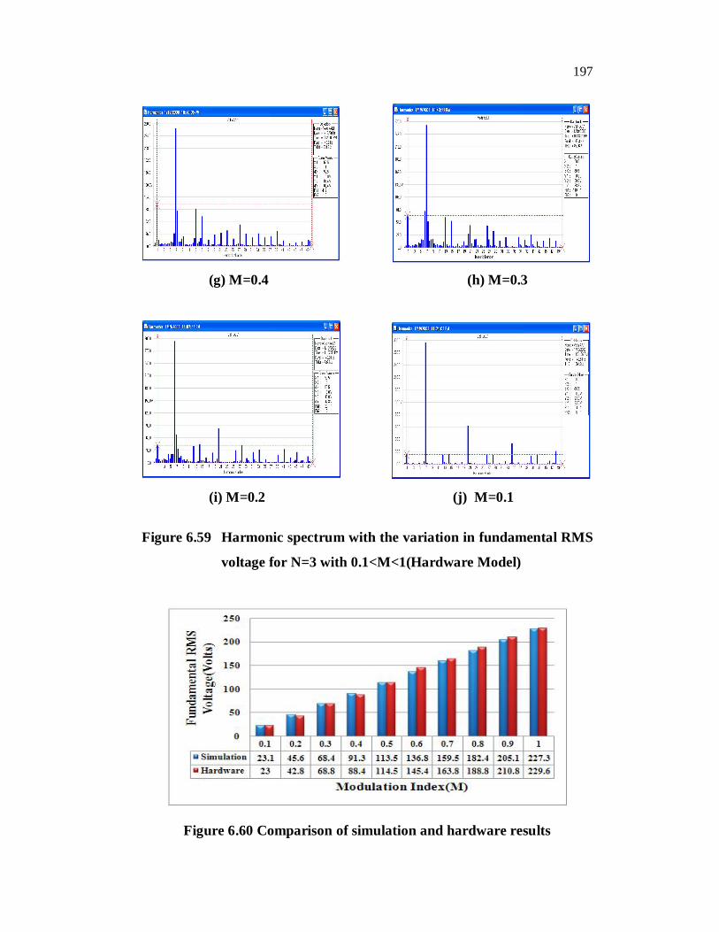
6.5.9 Variation in the Fundamental Voltage for Different Modulation
Indexes
The proposed simulated and hardware model can be tested with
various modulation index values varied from 0.1 to 1 for 3<N<9. Whenever
the modulation index varies for a particular value of N correspondingly the
fundamental RMS is also varied. The variation of the fundamental RMS
voltage for N=3 with modulation index varies from 0.1 to 1 is shown in
Figures 6.58(a-j) and 6.59(a-j) for both simulated and hardware models.
Figure 6.60 represents the comparison of simulation and hardware results for
fundamental RMS voltage. The simulated results are very close to the
hardware results.

194
(a) M=1 (b) M=0.9
(c) M=0.8 (d) M=0.7
(e) M=0.6 (f) M=0.5
Figure 6.58 (Continued)
195
(g) M=0.4 (h) M=0.3
(i) M=0.2 (j) M=0.1
Figure 6.58 Harmonic spectrum with the variation in fundamental RMS
voltage for N=3 with 0.1<M<1(Simulation)

196
(a) M=1.0 (b) M=0.9
(c) M=0.8 (d) M=0.7
(e) M=0.6 (f) M=0.5
Figure 6.59 (Continued)
197
(g) M=0.4 (h) M=0.3
(i) M=0.2 (j) M=0.1
Figure 6.59 Harmonic spectrum with the variation in fundamental RMS
voltage for N=3 with 0.1<M<1(Hardware Model)
Figure 6.60 Comparison of simulation and hardware results

198
6.6 CONCLUSION
A simple and effective, minimization technique to solve the
selective harmonic elimination using computed PWM control method for
single phase voltage source inverters has been discussed in this chapter. By
solving the harmonic equations, the values of notch angles are obtained,
which control the switching instants of the PWM wave. The switching angles
obtained by these methods to eliminate harmonics are not as accurately as
obtained through the computed PWM technique. The PWM wave generated
by the computed PWM technique takes less time when compared to the sine-
triangular comparison method. They do not involve any ‘trial and error’
procedures and the PWM pulse can triggered accurately at the desired values
of the notch angles.
The computed method was applied to developed inverter with
3<N<9 the modulation index of 1.0. The selective harmonic elimination was
carried out effectively for all the values of N. The same thing can be extended
for other values of modulation index values. The variation of the fundamental
RMS voltage for the modulation index value between 0.1 and 1.0 for N=3 is
shown and it was found that it is decreasing as the modulations decreases. All
the simulation results were upheld with hardware results.