chapter 5 : nonlinear eigenvalue problems · chapter 5 : nonlinear eigenvalue problems ......
TRANSCRIPT
CHAPTER 5 : NONLINEAR EIGENVALUEPROBLEMS
Heinrich [email protected]
Hamburg University of TechnologyInstitute of Mathematics
TUHH Heinrich Voss Nonlinear eigenvalue problems Eigenvalue problems 2012 1 / 58

Examples
Nonlinear eigenvalue problem
The term nonlinear eigenvalue problem is not used in a unique way in theliterature
On the one hand: Parameter dependent nonlinear (with respect to the statevariable) operator equations
T (λ,u) = 0
are discussed concerning— positivity of solutions— multiplicity of solution— dependence of solutions on the parameter; bifurcation— (change of ) stability of solutions
TUHH Heinrich Voss Nonlinear eigenvalue problems Eigenvalue problems 2012 2 / 58
Examples
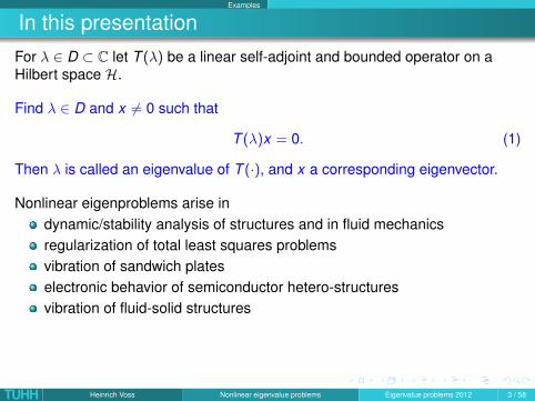
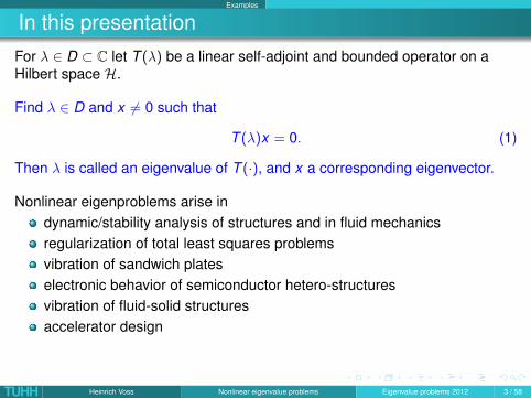
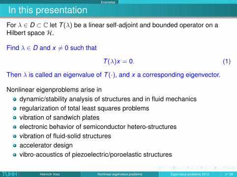
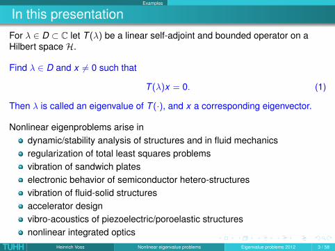
In this presentationFor λ ∈ D ⊂ C let T (λ) be a linear self-adjoint and bounded operator on aHilbert space H.
Find λ ∈ D and x 6= 0 such that
T (λ)x = 0. (1)
Then λ is called an eigenvalue of T (·), and x a corresponding eigenvector.
Nonlinear eigenproblems arise indynamic/stability analysis of structures and in fluid mechanicsregularization of total least squares problemsvibration of sandwich plateselectronic behavior of semiconductor hetero-structuresvibration of fluid-solid structuresaccelerator designvibro-acoustics of piezoelectric/poroelastic structuresnonlinear integrated optics
TUHH Heinrich Voss Nonlinear eigenvalue problems Eigenvalue problems 2012 3 / 58
Examples
In this presentationFor λ ∈ D ⊂ C let T (λ) be a linear self-adjoint and bounded operator on aHilbert space H.
Find λ ∈ D and x 6= 0 such that
T (λ)x = 0. (1)
Then λ is called an eigenvalue of T (·), and x a corresponding eigenvector.
Nonlinear eigenproblems arise indynamic/stability analysis of structures and in fluid mechanics
regularization of total least squares problemsvibration of sandwich plateselectronic behavior of semiconductor hetero-structuresvibration of fluid-solid structuresaccelerator designvibro-acoustics of piezoelectric/poroelastic structuresnonlinear integrated optics
TUHH Heinrich Voss Nonlinear eigenvalue problems Eigenvalue problems 2012 3 / 58
Examples
In this presentationFor λ ∈ D ⊂ C let T (λ) be a linear self-adjoint and bounded operator on aHilbert space H.
Find λ ∈ D and x 6= 0 such that
T (λ)x = 0. (1)
Then λ is called an eigenvalue of T (·), and x a corresponding eigenvector.
Nonlinear eigenproblems arise indynamic/stability analysis of structures and in fluid mechanicsregularization of total least squares problems
vibration of sandwich plateselectronic behavior of semiconductor hetero-structuresvibration of fluid-solid structuresaccelerator designvibro-acoustics of piezoelectric/poroelastic structuresnonlinear integrated optics
TUHH Heinrich Voss Nonlinear eigenvalue problems Eigenvalue problems 2012 3 / 58
Examples
In this presentationFor λ ∈ D ⊂ C let T (λ) be a linear self-adjoint and bounded operator on aHilbert space H.
Find λ ∈ D and x 6= 0 such that
T (λ)x = 0. (1)
Then λ is called an eigenvalue of T (·), and x a corresponding eigenvector.
Nonlinear eigenproblems arise indynamic/stability analysis of structures and in fluid mechanicsregularization of total least squares problemsvibration of sandwich plates
electronic behavior of semiconductor hetero-structuresvibration of fluid-solid structuresaccelerator designvibro-acoustics of piezoelectric/poroelastic structuresnonlinear integrated optics
TUHH Heinrich Voss Nonlinear eigenvalue problems Eigenvalue problems 2012 3 / 58
Examples
In this presentationFor λ ∈ D ⊂ C let T (λ) be a linear self-adjoint and bounded operator on aHilbert space H.
Find λ ∈ D and x 6= 0 such that
T (λ)x = 0. (1)
Then λ is called an eigenvalue of T (·), and x a corresponding eigenvector.
Nonlinear eigenproblems arise indynamic/stability analysis of structures and in fluid mechanicsregularization of total least squares problemsvibration of sandwich plateselectronic behavior of semiconductor hetero-structures
vibration of fluid-solid structuresaccelerator designvibro-acoustics of piezoelectric/poroelastic structuresnonlinear integrated optics
TUHH Heinrich Voss Nonlinear eigenvalue problems Eigenvalue problems 2012 3 / 58
Examples
In this presentationFor λ ∈ D ⊂ C let T (λ) be a linear self-adjoint and bounded operator on aHilbert space H.
Find λ ∈ D and x 6= 0 such that
T (λ)x = 0. (1)
Then λ is called an eigenvalue of T (·), and x a corresponding eigenvector.
Nonlinear eigenproblems arise indynamic/stability analysis of structures and in fluid mechanicsregularization of total least squares problemsvibration of sandwich plateselectronic behavior of semiconductor hetero-structuresvibration of fluid-solid structures
accelerator designvibro-acoustics of piezoelectric/poroelastic structuresnonlinear integrated optics
TUHH Heinrich Voss Nonlinear eigenvalue problems Eigenvalue problems 2012 3 / 58
Examples
In this presentationFor λ ∈ D ⊂ C let T (λ) be a linear self-adjoint and bounded operator on aHilbert space H.
Find λ ∈ D and x 6= 0 such that
T (λ)x = 0. (1)
Then λ is called an eigenvalue of T (·), and x a corresponding eigenvector.
Nonlinear eigenproblems arise indynamic/stability analysis of structures and in fluid mechanicsregularization of total least squares problemsvibration of sandwich plateselectronic behavior of semiconductor hetero-structuresvibration of fluid-solid structuresaccelerator design
vibro-acoustics of piezoelectric/poroelastic structuresnonlinear integrated optics
TUHH Heinrich Voss Nonlinear eigenvalue problems Eigenvalue problems 2012 3 / 58
Examples
In this presentationFor λ ∈ D ⊂ C let T (λ) be a linear self-adjoint and bounded operator on aHilbert space H.
Find λ ∈ D and x 6= 0 such that
T (λ)x = 0. (1)
Then λ is called an eigenvalue of T (·), and x a corresponding eigenvector.
Nonlinear eigenproblems arise indynamic/stability analysis of structures and in fluid mechanicsregularization of total least squares problemsvibration of sandwich plateselectronic behavior of semiconductor hetero-structuresvibration of fluid-solid structuresaccelerator designvibro-acoustics of piezoelectric/poroelastic structures
nonlinear integrated optics
TUHH Heinrich Voss Nonlinear eigenvalue problems Eigenvalue problems 2012 3 / 58
Examples
In this presentationFor λ ∈ D ⊂ C let T (λ) be a linear self-adjoint and bounded operator on aHilbert space H.
Find λ ∈ D and x 6= 0 such that
T (λ)x = 0. (1)
Then λ is called an eigenvalue of T (·), and x a corresponding eigenvector.
Nonlinear eigenproblems arise indynamic/stability analysis of structures and in fluid mechanicsregularization of total least squares problemsvibration of sandwich plateselectronic behavior of semiconductor hetero-structuresvibration of fluid-solid structuresaccelerator designvibro-acoustics of piezoelectric/poroelastic structuresnonlinear integrated optics
TUHH Heinrich Voss Nonlinear eigenvalue problems Eigenvalue problems 2012 3 / 58
Examples
Example 1: Vibration of structures
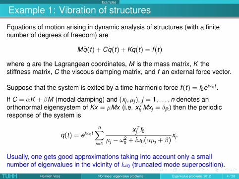
Equations of motion arising in dynamic analysis of structures (with a finitenumber of degrees of freedom) are
Mq(t) + Cq(t) + Kq(t) = f (t)
where q are the Lagrangean coordinates, M is the mass matrix, K thestiffness matrix, C the viscous damping matrix, and f an external force vector.
Suppose that the system is exited by a time harmonic force f (t) = f0eiω0t .
If C = αK + βM (modal damping) and (xj , µj ), j = 1, . . . ,n denotes anorthonormal eigensystem of Kx = µMx (i.e. xT
k Mxj = δjk ) then the periodicresponse of the system is
q(t) = eiω0tn∑
j=1
xTj f0
µj − ω20 + iω0(αµj + β)
xj .
Usually, one gets good approximations taking into account only a smallnumber of eigenvalues in the vicinity of iω0 (truncated mode superposition).
TUHH Heinrich Voss Nonlinear eigenvalue problems Eigenvalue problems 2012 4 / 58
Examples
Example 1: Vibration of structures
Equations of motion arising in dynamic analysis of structures (with a finitenumber of degrees of freedom) are
Mq(t) + Cq(t) + Kq(t) = f (t)
where q are the Lagrangean coordinates, M is the mass matrix, K thestiffness matrix, C the viscous damping matrix, and f an external force vector.
Suppose that the system is exited by a time harmonic force f (t) = f0eiω0t .
If C = αK + βM (modal damping) and (xj , µj ), j = 1, . . . ,n denotes anorthonormal eigensystem of Kx = µMx (i.e. xT
k Mxj = δjk ) then the periodicresponse of the system is
q(t) = eiω0tn∑
j=1
xTj f0
µj − ω20 + iω0(αµj + β)
xj .
Usually, one gets good approximations taking into account only a smallnumber of eigenvalues in the vicinity of iω0 (truncated mode superposition).
TUHH Heinrich Voss Nonlinear eigenvalue problems Eigenvalue problems 2012 4 / 58
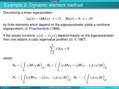
Examples
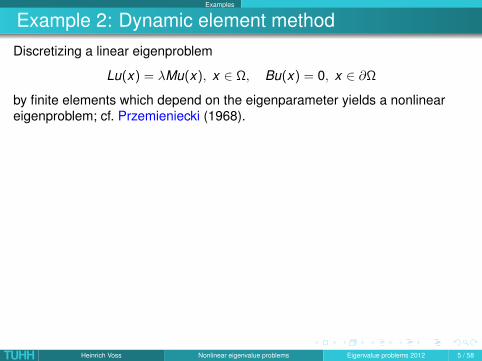
Example 2: Dynamic element methodDiscretizing a linear eigenproblem
Lu(x) = λMu(x), x ∈ Ω, Bu(x) = 0, x ∈ ∂Ω
by finite elements which depend on the eigenparameter yields a nonlineareigenproblem; cf. Przemieniecki (1968).
If the ansatz functions φj (x) + λψj (x) depend linearly on the eigenparameterthen one obtains a cubic eigenvalue problem (cf. V. 1987)
3∑j=0
λjAjx = 0
where
A3 =(∫
Ω
ψjMψk dx)
jk, A2 =
(∫Ω
(ψjMφk + φjMψk − ψjLψk ) dx)
jk
A1 =(∫
Ω
(φjMφk − φjLψk − ψjLφk ) dx)
jk, A0 = −
(∫Ω
φjLφk dx)
jk
TUHH Heinrich Voss Nonlinear eigenvalue problems Eigenvalue problems 2012 5 / 58
Examples
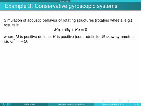
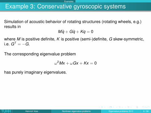
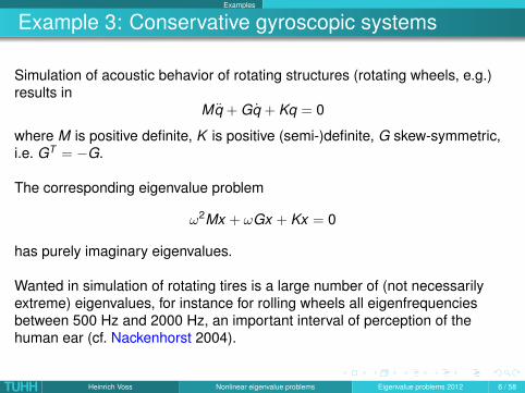
Example 3: Conservative gyroscopic systems
Simulation of acoustic behavior of rotating structures (rotating wheels, e.g.)results in
Mq + Gq + Kq = 0
where M is positive definite, K is positive (semi-)definite, G skew-symmetric,i.e. GT = −G.
The corresponding eigenvalue problem
ω2Mx + ωGx + Kx = 0
has purely imaginary eigenvalues.
Wanted in simulation of rotating tires is a large number of (not necessarilyextreme) eigenvalues, for instance for rolling wheels all eigenfrequenciesbetween 500 Hz and 2000 Hz, an important interval of perception of thehuman ear (cf. Nackenhorst 2004).
TUHH Heinrich Voss Nonlinear eigenvalue problems Eigenvalue problems 2012 6 / 58
Examples
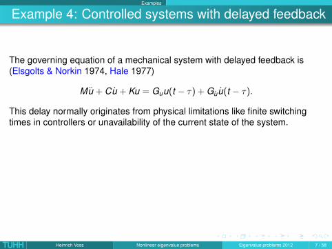
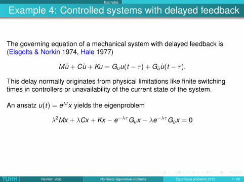
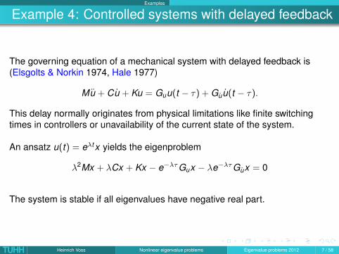
Example 4: Controlled systems with delayed feedback
The governing equation of a mechanical system with delayed feedback is(Elsgolts & Norkin 1974, Hale 1977)
Mu + Cu + Ku = Guu(t − τ) + Guu(t − τ).
This delay normally originates from physical limitations like finite switchingtimes in controllers or unavailability of the current state of the system.
An ansatz u(t) = eλtx yields the eigenproblem
λ2Mx + λCx + Kx − e−λτGux − λe−λτGux = 0
The system is stable if all eigenvalues have negative real part.
TUHH Heinrich Voss Nonlinear eigenvalue problems Eigenvalue problems 2012 7 / 58
Examples
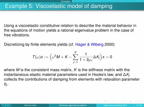
Example 5: Viscoelastic model of damping
Using a viscoelastic constitutive relation to describe the material behavior inthe equations of motion yields a rational eigenvalue problem in the case offree vibrations.
Discretizing by finite elements yields (cf. Hager & Wiberg 2000)
T (ω)x :=(ω2M + K −
K∑j=1
11 + bjω
∆Kj
)x = 0
where M is the consistent mass matrix, K is the stiffness matrix with theinstantaneous elastic material parameters used in Hooke’s law, and ∆Kjcollects the contributions of damping from elements with relaxation parameterbj .
TUHH Heinrich Voss Nonlinear eigenvalue problems Eigenvalue problems 2012 8 / 58
Examples
Example 5: Viscoelastic model of damping
Using a viscoelastic constitutive relation to describe the material behavior inthe equations of motion yields a rational eigenvalue problem in the case offree vibrations.
Discretizing by finite elements yields (cf. Hager & Wiberg 2000)
T (ω)x :=(ω2M + K −
K∑j=1
11 + bjω
∆Kj
)x = 0
where M is the consistent mass matrix, K is the stiffness matrix with theinstantaneous elastic material parameters used in Hooke’s law, and ∆Kjcollects the contributions of damping from elements with relaxation parameterbj .
TUHH Heinrich Voss Nonlinear eigenvalue problems Eigenvalue problems 2012 8 / 58
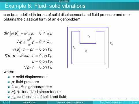
Examples
Example 6: Fluid–solid vibrationscan be modelled in terms of solid displacement and fluid pressure and oneobtains the classical form of an eigenproblem
div [σ(u)] + ω2ρsu = 0 in Ωs,
∆p +ω2
c2 p = 0 in Ωf ,
σ(u) · n − pn = 0 on ΓI ,
∇p · n + ω2ρf u · n = 0 on ΓI ,
u = 0 on ΓD,
∇p · n = 0 on ΓN ,
ΓO
ΓI
Ωs
Ωf
whereu: solid displacementp: fluid pressureλ = ω2: eigenparameterσ(u): linearized stress tensorρs, ρf : densities of solid and fluid
TUHH Heinrich Voss Nonlinear eigenvalue problems Eigenvalue problems 2012 9 / 58
Examples
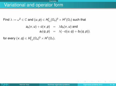
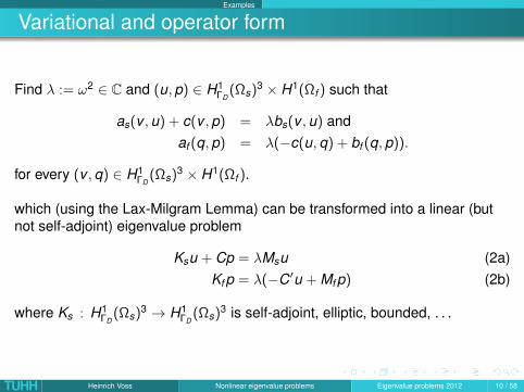
Variational and operator form
Find λ := ω2 ∈ C and (u,p) ∈ H1ΓD
(Ωs)3 × H1(Ωf ) such that
as(v ,u) + c(v ,p) = λbs(v ,u) andaf (q,p) = λ(−c(u,q) + bf (q,p)).
for every (v ,q) ∈ H1ΓD
(Ωs)3 × H1(Ωf ).
which (using the Lax-Milgram Lemma) can be transformed into a linear (butnot self-adjoint) eigenvalue problem
Ksu + Cp = λMsu (2a)Kf p = λ(−C′u + Mf p) (2b)
where Ks : H1ΓD
(Ωs)3 → H1ΓD
(Ωs)3 is self-adjoint, elliptic, bounded, . . .
TUHH Heinrich Voss Nonlinear eigenvalue problems Eigenvalue problems 2012 10 / 58
Examples
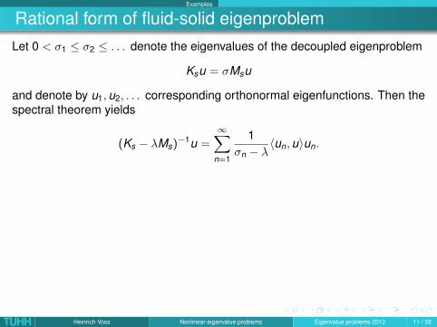
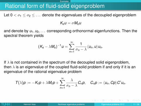
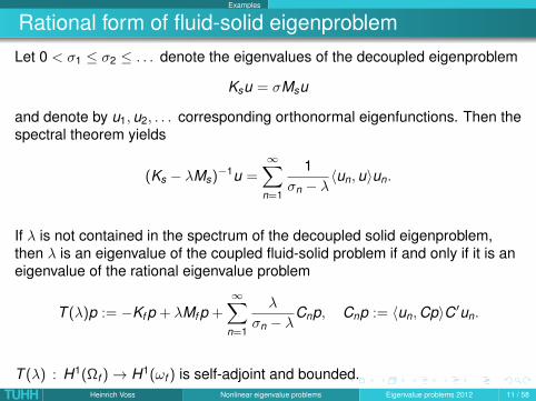
Rational form of fluid-solid eigenproblemLet 0 < σ1 ≤ σ2 ≤ . . . denote the eigenvalues of the decoupled eigenproblem
Ksu = σMsu
and denote by u1,u2, . . . corresponding orthonormal eigenfunctions. Then thespectral theorem yields
(Ks − λMs)−1u =∞∑
n=1
1σn − λ
〈un,u〉un.
If λ is not contained in the spectrum of the decoupled solid eigenproblem,then λ is an eigenvalue of the coupled fluid-solid problem if and only if it is aneigenvalue of the rational eigenvalue problem
T (λ)p := −Kf p + λMf p +∞∑
n=1
λ
σn − λCnp, Cnp := 〈un,Cp〉C′un.
T (λ) : H1(Ωf )→ H1(ωf ) is self-adjoint and bounded.
TUHH Heinrich Voss Nonlinear eigenvalue problems Eigenvalue problems 2012 11 / 58
Examples
Rational form of fluid-solid eigenproblemLet 0 < σ1 ≤ σ2 ≤ . . . denote the eigenvalues of the decoupled eigenproblem
Ksu = σMsu
and denote by u1,u2, . . . corresponding orthonormal eigenfunctions. Then thespectral theorem yields
(Ks − λMs)−1u =∞∑
n=1
1σn − λ
〈un,u〉un.
If λ is not contained in the spectrum of the decoupled solid eigenproblem,then λ is an eigenvalue of the coupled fluid-solid problem if and only if it is aneigenvalue of the rational eigenvalue problem
T (λ)p := −Kf p + λMf p +∞∑
n=1
λ
σn − λCnp, Cnp := 〈un,Cp〉C′un.
T (λ) : H1(Ωf )→ H1(ωf ) is self-adjoint and bounded.TUHH Heinrich Voss Nonlinear eigenvalue problems Eigenvalue problems 2012 11 / 58
Examples
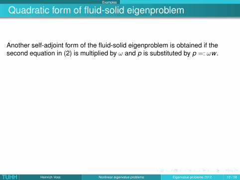
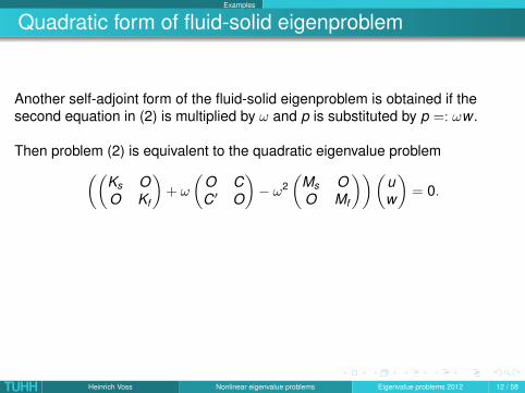
Quadratic form of fluid-solid eigenproblem
Another self-adjoint form of the fluid-solid eigenproblem is obtained if thesecond equation in (2) is multiplied by ω and p is substituted by p =: ωw .
Then problem (2) is equivalent to the quadratic eigenvalue problem((Ks OO Kf
)+ ω
(O CC′ O
)− ω2
(Ms OO Mf
))(uw
)= 0.
TUHH Heinrich Voss Nonlinear eigenvalue problems Eigenvalue problems 2012 12 / 58
Examples
Quadratic form of fluid-solid eigenproblem
Another self-adjoint form of the fluid-solid eigenproblem is obtained if thesecond equation in (2) is multiplied by ω and p is substituted by p =: ωw .
Then problem (2) is equivalent to the quadratic eigenvalue problem((Ks OO Kf
)+ ω
(O CC′ O
)− ω2
(Ms OO Mf
))(uw
)= 0.
TUHH Heinrich Voss Nonlinear eigenvalue problems Eigenvalue problems 2012 12 / 58

Examples
Example 7: Electronic structure of quantum dots
Semiconductor nanostructures have attracted tremendous interest in the pastfew years because of their special physical properties and their potential forapplications in micro– and optoelectronic devices.
In such nanostructures, the free carriers are confined to a small region ofspace by potential barriers, and if the size of this region is less than theelectron wavelength, the electronic states become quantized at discreteenergy levels.
The ultimate limit of low dimensional structures is the quantum dot, in whichthe carriers are confined in all three directions, thus reducing the degrees offreedom to zero.Therefore, a quantum dot can be thought of as an artificial atom.
TUHH Heinrich Voss Nonlinear eigenvalue problems Eigenvalue problems 2012 13 / 58
Examples
Example 7: Electronic structure of quantum dots
Electron Spectroscopy Group, Fritz-Haber-Institute, BerlinTUHH Heinrich Voss Nonlinear eigenvalue problems Eigenvalue problems 2012 14 / 58
Examples
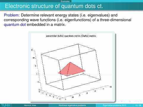
Electronic structure of quantum dots ct.Problem: Determine relevant energy states (i.e. eigenvalues) andcorresponding wave functions (i.e. eigenfunctions) of a three-dimensionalquantum dot embedded in a matrix.
TUHH Heinrich Voss Nonlinear eigenvalue problems Eigenvalue problems 2012 15 / 58
Examples
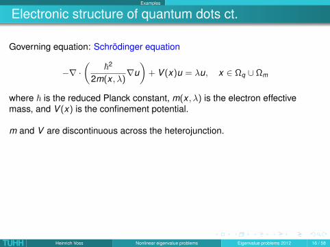
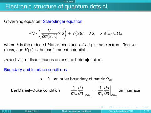
Electronic structure of quantum dots ct.
Governing equation: Schrödinger equation
−∇ ·(
~2
2m(x , λ)∇u)
+ V (x)u = λu, x ∈ Ωq ∪ Ωm
where ~ is the reduced Planck constant, m(x , λ) is the electron effectivemass, and V (x) is the confinement potential.
m and V are discontinuous across the heterojunction.
Boundary and interface conditions
u = 0 on outer boundary of matrix Ωm
BenDaniel–Duke condition1
mm
∂u∂n
∣∣∣∣∂Ωm
=1
mq
∂u∂n
∣∣∣∣∂Ωq
on interface
TUHH Heinrich Voss Nonlinear eigenvalue problems Eigenvalue problems 2012 16 / 58
Examples
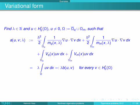
Variational form
Find λ ∈ R and u ∈ H10 (Ω), u 6= 0, Ω := Ωq ∪ Ωm, such that
a(u, v ;λ) :=~2
2
∫Ωq
1mq(x , λ)
∇u · ∇v dx +~2
2
∫Ωm
1mm(x , λ)
∇u · ∇v dx
+
∫Ωq
Vq(x)uv dx +
∫Ωm
Vm(x)uv dx
= λ
∫Ω
uv dx =: λb(u, v) for every v ∈ H10 (Ω)
TUHH Heinrich Voss Nonlinear eigenvalue problems Eigenvalue problems 2012 17 / 58
Examples
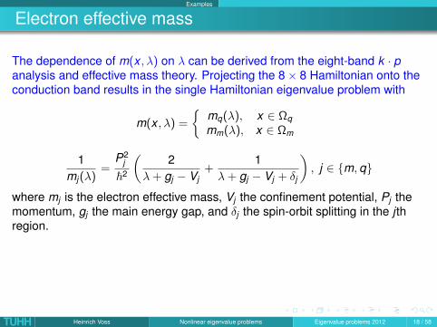
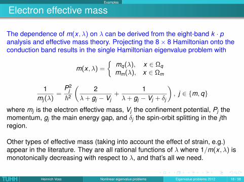
Electron effective mass
The dependence of m(x , λ) on λ can be derived from the eight-band k · panalysis and effective mass theory. Projecting the 8× 8 Hamiltonian onto theconduction band results in the single Hamiltonian eigenvalue problem with
m(x , λ) =
mq(λ), x ∈ Ωqmm(λ), x ∈ Ωm
1mj (λ)
=P2
j
~2
(2
λ+ gj − Vj+
1λ+ gj − Vj + δj
), j ∈ m,q
where mj is the electron effective mass, Vj the confinement potential, Pj themomentum, gj the main energy gap, and δj the spin-orbit splitting in the j thregion.
Other types of effective mass (taking into account the effect of strain, e.g.)appear in the literature. They are all rational functions of λ where 1/m(x , λ) ismonotonically decreasing with respect to λ, and that’s all we need.
TUHH Heinrich Voss Nonlinear eigenvalue problems Eigenvalue problems 2012 18 / 58
Examples
Electron effective mass
The dependence of m(x , λ) on λ can be derived from the eight-band k · panalysis and effective mass theory. Projecting the 8× 8 Hamiltonian onto theconduction band results in the single Hamiltonian eigenvalue problem with
m(x , λ) =
mq(λ), x ∈ Ωqmm(λ), x ∈ Ωm
1mj (λ)
=P2
j
~2
(2
λ+ gj − Vj+
1λ+ gj − Vj + δj
), j ∈ m,q
where mj is the electron effective mass, Vj the confinement potential, Pj themomentum, gj the main energy gap, and δj the spin-orbit splitting in the j thregion.
Other types of effective mass (taking into account the effect of strain, e.g.)appear in the literature. They are all rational functions of λ where 1/m(x , λ) ismonotonically decreasing with respect to λ, and that’s all we need.
TUHH Heinrich Voss Nonlinear eigenvalue problems Eigenvalue problems 2012 18 / 58
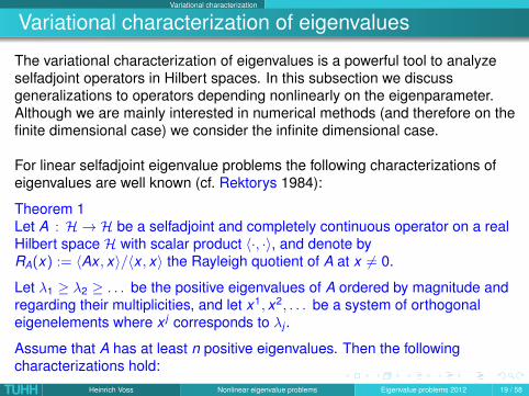
Variational characterization
Variational characterization of eigenvalues
The variational characterization of eigenvalues is a powerful tool to analyzeselfadjoint operators in Hilbert spaces. In this subsection we discussgeneralizations to operators depending nonlinearly on the eigenparameter.Although we are mainly interested in numerical methods (and therefore on thefinite dimensional case) we consider the infinite dimensional case.
For linear selfadjoint eigenvalue problems the following characterizations ofeigenvalues are well known (cf. Rektorys 1984):
Theorem 1Let A : H → H be a selfadjoint and completely continuous operator on a realHilbert space H with scalar product 〈·, ·〉, and denote byRA(x) := 〈Ax , x〉/〈x , x〉 the Rayleigh quotient of A at x 6= 0.
Let λ1 ≥ λ2 ≥ . . . be the positive eigenvalues of A ordered by magnitude andregarding their multiplicities, and let x1, x2, . . . be a system of orthogonaleigenelements where x j corresponds to λj .
Assume that A has at least n positive eigenvalues. Then the followingcharacterizations hold:
TUHH Heinrich Voss Nonlinear eigenvalue problems Eigenvalue problems 2012 19 / 58
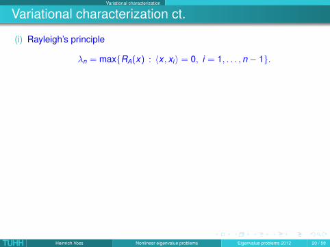
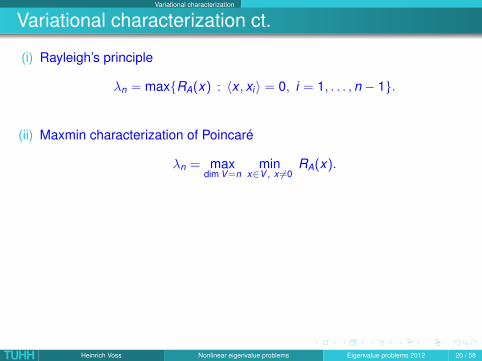
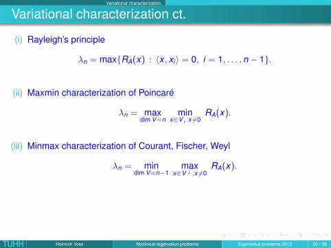
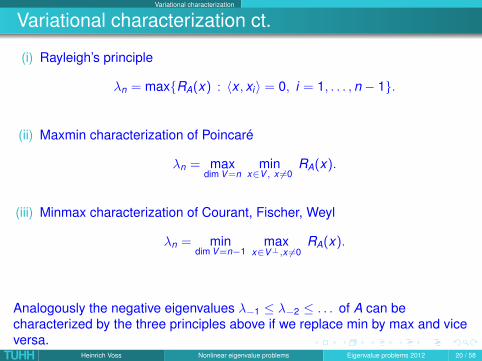
Variational characterization
Variational characterization ct.
(i) Rayleigh’s principle
λn = maxRA(x) : 〈x , xi〉 = 0, i = 1, . . . ,n − 1.
(ii) Maxmin characterization of Poincaré
λn = maxdim V =n
minx∈V , x 6=0
RA(x).
(iii) Minmax characterization of Courant, Fischer, Weyl
λn = mindim V =n−1
maxx∈V⊥,x 6=0
RA(x).
Analogously the negative eigenvalues λ−1 ≤ λ−2 ≤ . . . of A can becharacterized by the three principles above if we replace min by max and viceversa.
TUHH Heinrich Voss Nonlinear eigenvalue problems Eigenvalue problems 2012 20 / 58
Variational characterization
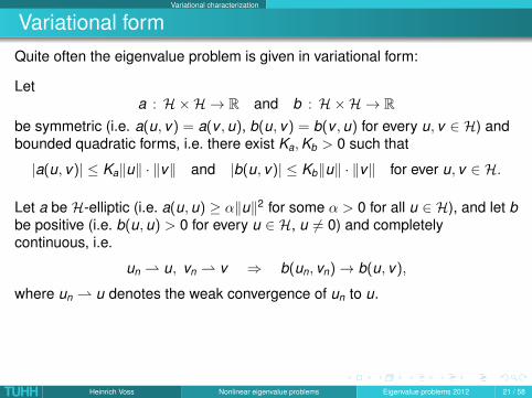
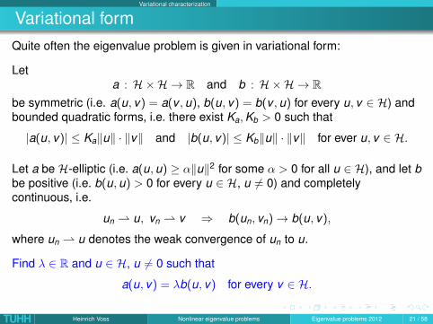
Variational formQuite often the eigenvalue problem is given in variational form:
Leta : H×H → R and b : H×H → R
be symmetric (i.e. a(u, v) = a(v ,u), b(u, v) = b(v ,u) for every u, v ∈ H) andbounded quadratic forms, i.e. there exist Ka,Kb > 0 such that
|a(u, v)| ≤ Ka‖u‖ · ‖v‖ and |b(u, v)| ≤ Kb‖u‖ · ‖v‖ for ever u, v ∈ H.
Let a be H-elliptic (i.e. a(u,u) ≥ α‖u‖2 for some α > 0 for all u ∈ H), and let bbe positive (i.e. b(u,u) > 0 for every u ∈ H, u 6= 0) and completelycontinuous, i.e.
un u, vn v ⇒ b(un, vn)→ b(u, v),
where un u denotes the weak convergence of un to u.
Find λ ∈ R and u ∈ H, u 6= 0 such that
a(u, v) = λb(u, v) for every v ∈ H.
TUHH Heinrich Voss Nonlinear eigenvalue problems Eigenvalue problems 2012 21 / 58
Variational characterization
Variational form ct.
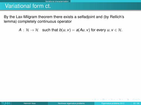
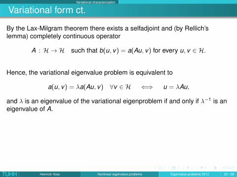
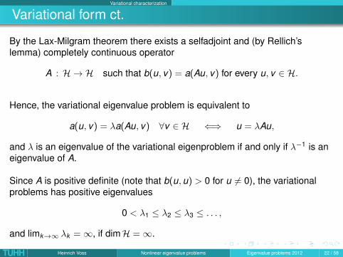
By the Lax-Milgram theorem there exists a selfadjoint and (by Rellich’slemma) completely continuous operator
A : H → H such that b(u, v) = a(Au, v) for every u, v ∈ H.
Hence, the variational eigenvalue problem is equivalent to
a(u, v) = λa(Au, v) ∀v ∈ H ⇐⇒ u = λAu,
and λ is an eigenvalue of the variational eigenproblem if and only if λ−1 is aneigenvalue of A.
Since A is positive definite (note that b(u,u) > 0 for u 6= 0), the variationalproblems has positive eigenvalues
0 < λ1 ≤ λ2 ≤ λ3 ≤ . . . ,
and limk→∞ λk =∞, if dimH =∞.
TUHH Heinrich Voss Nonlinear eigenvalue problems Eigenvalue problems 2012 22 / 58
Variational characterization
Variational form ct.
By the Lax-Milgram theorem there exists a selfadjoint and (by Rellich’slemma) completely continuous operator
A : H → H such that b(u, v) = a(Au, v) for every u, v ∈ H.
Hence, the variational eigenvalue problem is equivalent to
a(u, v) = λa(Au, v) ∀v ∈ H ⇐⇒ u = λAu,
and λ is an eigenvalue of the variational eigenproblem if and only if λ−1 is aneigenvalue of A.
Since A is positive definite (note that b(u,u) > 0 for u 6= 0), the variationalproblems has positive eigenvalues
0 < λ1 ≤ λ2 ≤ λ3 ≤ . . . ,
and limk→∞ λk =∞, if dimH =∞.
TUHH Heinrich Voss Nonlinear eigenvalue problems Eigenvalue problems 2012 22 / 58
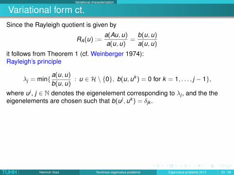
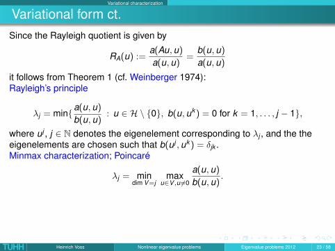
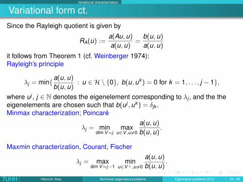
Variational characterization
Variational form ct.Since the Rayleigh quotient is given by
RA(u) :=a(Au,u)
a(u,u)=
b(u,u)
a(u,u)
it follows from Theorem 1 (cf. Weinberger 1974):
Rayleigh’s principle
λj = mina(u,u)
b(u,u): u ∈ H \ 0, b(u,uk ) = 0 for k = 1, . . . , j − 1,
where uj , j ∈ N denotes the eigenelement corresponding to λj , and the theeigenelements are chosen such that b(uj ,uk ) = δjk .Minmax characterization; Poincaré
λj = mindim V =j
maxu∈V ,u 6=0
a(u,u)
b(u,u).
Maxmin characterization, Courant, Fischer
λj = maxdim V =j−1
minu∈V⊥,u 6=0
a(u,u)
b(u,u).
TUHH Heinrich Voss Nonlinear eigenvalue problems Eigenvalue problems 2012 23 / 58
Variational characterization
Variational form ct.Since the Rayleigh quotient is given by
RA(u) :=a(Au,u)
a(u,u)=
b(u,u)
a(u,u)
it follows from Theorem 1 (cf. Weinberger 1974):Rayleigh’s principle
λj = mina(u,u)
b(u,u): u ∈ H \ 0, b(u,uk ) = 0 for k = 1, . . . , j − 1,
where uj , j ∈ N denotes the eigenelement corresponding to λj , and the theeigenelements are chosen such that b(uj ,uk ) = δjk .
Minmax characterization; Poincaré
λj = mindim V =j
maxu∈V ,u 6=0
a(u,u)
b(u,u).
Maxmin characterization, Courant, Fischer
λj = maxdim V =j−1
minu∈V⊥,u 6=0
a(u,u)
b(u,u).
TUHH Heinrich Voss Nonlinear eigenvalue problems Eigenvalue problems 2012 23 / 58
Variational characterization
Variational form ct.Since the Rayleigh quotient is given by
RA(u) :=a(Au,u)
a(u,u)=
b(u,u)
a(u,u)
it follows from Theorem 1 (cf. Weinberger 1974):Rayleigh’s principle
λj = mina(u,u)
b(u,u): u ∈ H \ 0, b(u,uk ) = 0 for k = 1, . . . , j − 1,
where uj , j ∈ N denotes the eigenelement corresponding to λj , and the theeigenelements are chosen such that b(uj ,uk ) = δjk .Minmax characterization; Poincaré
λj = mindim V =j
maxu∈V ,u 6=0
a(u,u)
b(u,u).
Maxmin characterization, Courant, Fischer
λj = maxdim V =j−1
minu∈V⊥,u 6=0
a(u,u)
b(u,u).
TUHH Heinrich Voss Nonlinear eigenvalue problems Eigenvalue problems 2012 23 / 58
Variational characterization
Variational form ct.Since the Rayleigh quotient is given by
RA(u) :=a(Au,u)
a(u,u)=
b(u,u)
a(u,u)
it follows from Theorem 1 (cf. Weinberger 1974):Rayleigh’s principle
λj = mina(u,u)
b(u,u): u ∈ H \ 0, b(u,uk ) = 0 for k = 1, . . . , j − 1,
where uj , j ∈ N denotes the eigenelement corresponding to λj , and the theeigenelements are chosen such that b(uj ,uk ) = δjk .Minmax characterization; Poincaré
λj = mindim V =j
maxu∈V ,u 6=0
a(u,u)
b(u,u).
Maxmin characterization, Courant, Fischer
λj = maxdim V =j−1
minu∈V⊥,u 6=0
a(u,u)
b(u,u).
TUHH Heinrich Voss Nonlinear eigenvalue problems Eigenvalue problems 2012 23 / 58
Variational characterization
Nonlinear eigenvalue problem
Consider a family of bounded and selfadjoint operators
T (λ) : H → H, λ ∈ J,
where J ⊂ R is an open interval which may be unbounded.
Letf : J ×H → R, (λ, x) 7→ 〈T (λ)x , x〉
be continuous, and assume that for every fixed x ∈ H, x 6= 0, the real equation
f (λ, x) = 0 (2)
has at most one solution in J.
Then equation (2) implicitly defines a functional p on some subset D ofH \ 0 which we call the Rayleigh functional, and which is exactly theRayleigh quotient in case of a linear eigenproblem T (λ) = λI − A.
TUHH Heinrich Voss Nonlinear eigenvalue problems Eigenvalue problems 2012 24 / 58
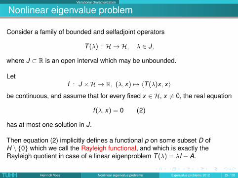
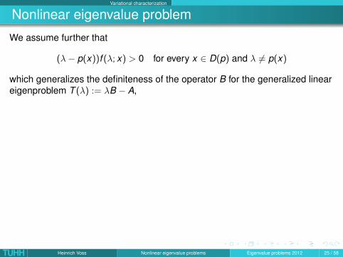
Variational characterization
Nonlinear eigenvalue problem
We assume further that
(λ− p(x))f (λ; x) > 0 for every x ∈ D(p) and λ 6= p(x)
which generalizes the definiteness of the operator B for the generalized lineareigenproblem T (λ) := λB − A,
and which is satisfied if T is differentiable and
∂
∂λf (λ, x)
∣∣λ=p(x)
> 0 for every x ∈ D (3)
The implicit function theorem gives that D is an open set and p is continuouslydifferentiable on D.
Differentiating the governing equation
f (p(x), x) = 〈T (p(x)x , x〉 ≡ 0
yields that the eigenelements of problem T (·) are the stationary vectors of theRayleigh functional p.
TUHH Heinrich Voss Nonlinear eigenvalue problems Eigenvalue problems 2012 25 / 58
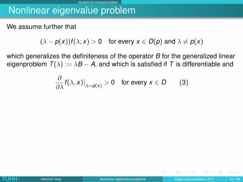
Variational characterization
Nonlinear eigenvalue problem
We assume further that
(λ− p(x))f (λ; x) > 0 for every x ∈ D(p) and λ 6= p(x)
which generalizes the definiteness of the operator B for the generalized lineareigenproblem T (λ) := λB − A, and which is satisfied if T is differentiable and
∂
∂λf (λ, x)
∣∣λ=p(x)
> 0 for every x ∈ D (3)
The implicit function theorem gives that D is an open set and p is continuouslydifferentiable on D.
Differentiating the governing equation
f (p(x), x) = 〈T (p(x)x , x〉 ≡ 0
yields that the eigenelements of problem T (·) are the stationary vectors of theRayleigh functional p.
TUHH Heinrich Voss Nonlinear eigenvalue problems Eigenvalue problems 2012 25 / 58
Variational characterization
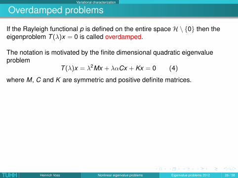
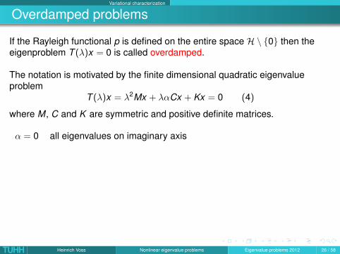
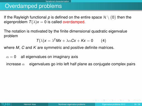
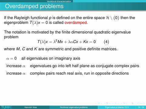
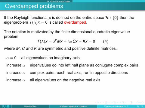
Overdamped problems
If the Rayleigh functional p is defined on the entire space H \ 0 then theeigenproblem T (λ)x = 0 is called overdamped.
The notation is motivated by the finite dimensional quadratic eigenvalueproblem
T (λ)x = λ2Mx + λαCx + Kx = 0 (4)
where M, C and K are symmetric and positive definite matrices.
α = 0 all eigenvalues on imaginary axis
increase α eigenvalues go into left half plane as conjugate complex pairs
increase α complex pairs reach real axis, run in opposite directions
increase α all eigenvalues on the negative real axis
increase α all eigenvalues going to the left are smallerthan all eigenvalues going to the rightsystem is overdamped
TUHH Heinrich Voss Nonlinear eigenvalue problems Eigenvalue problems 2012 26 / 58
Variational characterization
Quadratic overdamped problems
For quadratic overdamped systems the two solutions
p±(x) =1
2〈Mx , x〉
(−α〈Cx , x〉 ±
√α2〈Cx , x〉2 − 4〈Mx , x〉〈Kx , x〉
).
of the quadratic equation
〈T (λ)x , x〉 = λ2〈Mx , x〉+ λα〈Cx , x〉+ 〈Kx , x〉 = 0 (5)
are real, and they satisfy supx 6=0 p−(x) < infx 6=0 p+(x).
Hence, equation (5) defines two Rayleigh functionals p− and p+
corresponding to the intervals
J− := (−∞, infx 6=0
p+(x)) and J+ := (supx 6=0
p−(x),∞).
TUHH Heinrich Voss Nonlinear eigenvalue problems Eigenvalue problems 2012 27 / 58
Variational characterization
Rayleigh’s principle
For general (not necessarily quadratic) overdamped problems Hadeler (1967for the finite dimensional case, and 1968 for dimH =∞) generalizedRayleigh’s principle proving that the eigenvectors are orthogonal with respectto the generalized scalar product
[x , y ] :=
⟨
T (p(x))− T (p(y))
p(x)− p(y)x , y
⟩, if p(x) 6= p(y)
〈T ′(p(x))x , y〉, if p(x) = p(y)(6)
which is symmetric, definite and homogeneous, but in general is not bilinear.
TUHH Heinrich Voss Nonlinear eigenvalue problems Eigenvalue problems 2012 28 / 58
Variational characterization
Rayleigh’s principle
Theorem 2 (Hadeler)Let T (λ) : H → H, λ ∈ J be a family of selfadjoint and bounded operators.Assume that the problem T (λ)x = 0 is overdamped and that for every λ ∈ Jthere exists ν(λ) > 0 such that T (λ)− ν(λ)I is completely continuous.
Then problem T (λ)x = 0 has at most a countable set of eigenvalues in Jwhich we assume to be ordered by magnitude λ1 ≥ λ2 ≥ . . . regarding theirmultiplicities.
The corresponding eigenvectors x1, x2, . . . can be chosen orthonormally withrespect to the generalized scalar product (6),and the eigenvalues can bedetermined recursively by
λn = maxp(x) : [x , xi ] = 0, i = 1, . . . ,n − 1, x 6= 0. (7)
TUHH Heinrich Voss Nonlinear eigenvalue problems Eigenvalue problems 2012 29 / 58
Variational characterization
minmax and maxmin for overdamped problems
Poincaré’s maxmin characterization was first generalized by Duffin (1955) tooverdamped quadratic eigenproblems of finite dimension, and for moregeneral overdamped problems of finite dimension it was proved by Rogers(1964).
Infinite dimensional eigenvalue problems were studied by Turner (1967),Langer (1968), and Weinberger (1969) who proved generalizations of both,the maxmin characterization of Poincaré and of the minmax characterizationof Courant, Fischer and Weyl for quadratic (and by Turner (1968) forpolynomial) overdamped problems.
The corresponding generalizations for general overdamped problems ofinfinite dimension were derived by Hadeler (1968). Similar results (weakeningthe compactness or smoothness requirements) are contained in Rogers(1968), Werner (1971), Abramov (1973), Hadeler (1975), Markus (1985),Maksudov & Gasanov (1992), and Hasanov (2002).
TUHH Heinrich Voss Nonlinear eigenvalue problems Eigenvalue problems 2012 30 / 58
Variational characterization
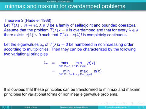
minmax and maxmin for overdamped problems
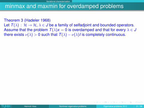
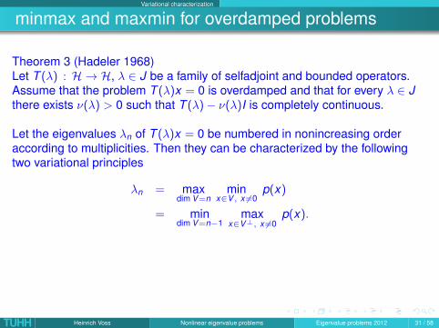
Theorem 3 (Hadeler 1968)Let T (λ) : H → H, λ ∈ J be a family of selfadjoint and bounded operators.Assume that the problem T (λ)x = 0 is overdamped and that for every λ ∈ Jthere exists ν(λ) > 0 such that T (λ)− ν(λ)I is completely continuous.
Let the eigenvalues λn of T (λ)x = 0 be numbered in nonincreasing orderaccording to multiplicities. Then they can be characterized by the followingtwo variational principles
λn = maxdim V =n
minx∈V , x 6=0
p(x)
= mindim V =n−1
maxx∈V⊥, x 6=0
p(x).
It is obvious that these principles can be transformed to minmax and maxminprinciples for variational forms of nonlinear eigenvalue problems.
TUHH Heinrich Voss Nonlinear eigenvalue problems Eigenvalue problems 2012 31 / 58
Variational characterization
minmax and maxmin for overdamped problems
Theorem 3 (Hadeler 1968)Let T (λ) : H → H, λ ∈ J be a family of selfadjoint and bounded operators.Assume that the problem T (λ)x = 0 is overdamped and that for every λ ∈ Jthere exists ν(λ) > 0 such that T (λ)− ν(λ)I is completely continuous.
Let the eigenvalues λn of T (λ)x = 0 be numbered in nonincreasing orderaccording to multiplicities. Then they can be characterized by the followingtwo variational principles
λn = maxdim V =n
minx∈V , x 6=0
p(x)
= mindim V =n−1
maxx∈V⊥, x 6=0
p(x).
It is obvious that these principles can be transformed to minmax and maxminprinciples for variational forms of nonlinear eigenvalue problems.
TUHH Heinrich Voss Nonlinear eigenvalue problems Eigenvalue problems 2012 31 / 58
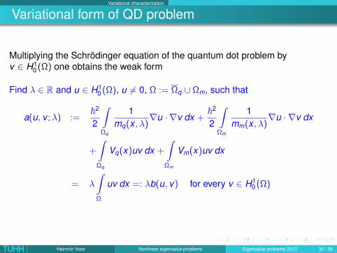
Variational characterization
Variational form of QD problem
Multiplying the Schrödinger equation of the quantum dot problem byv ∈ H1
0 (Ω) one obtains the weak form
Find λ ∈ R and u ∈ H10 (Ω), u 6= 0, Ω := Ωq ∪ Ωm, such that
a(u, v ;λ) :=~2
2
∫Ωq
1mq(x , λ)
∇u · ∇v dx +~2
2
∫Ωm
1mm(x , λ)
∇u · ∇v dx
+
∫Ωq
Vq(x)uv dx +
∫Ωm
Vm(x)uv dx
= λ
∫Ω
uv dx =: λb(u, v) for every v ∈ H10 (Ω)
TUHH Heinrich Voss Nonlinear eigenvalue problems Eigenvalue problems 2012 32 / 58
Variational characterization
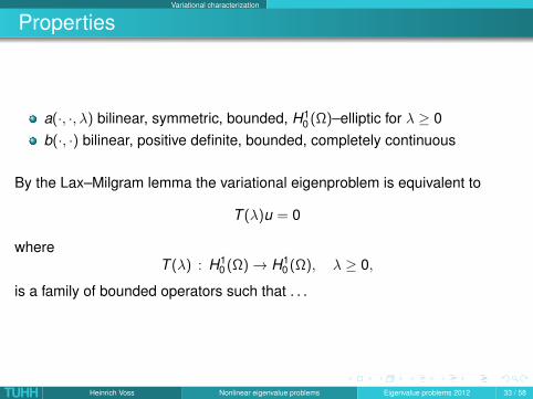
Properties
a(·, ·, λ) bilinear, symmetric, bounded, H10 (Ω)–elliptic for λ ≥ 0
b(·, ·) bilinear, positive definite, bounded, completely continuous
By the Lax–Milgram lemma the variational eigenproblem is equivalent to
T (λ)u = 0
whereT (λ) : H1
0 (Ω)→ H10 (Ω), λ ≥ 0,
is a family of bounded operators such that . . .
TUHH Heinrich Voss Nonlinear eigenvalue problems Eigenvalue problems 2012 33 / 58
Variational characterization
Properties ct.
Forf (λ; u) := 〈T (λ)u,u〉 = λb(u,u)− a(u,u;λ)
it holdsf (0; u) < 0 < lim
λ→∞f (λ; u) =∞ for every u 6= 0
∂∂λ f (λ; u) > 0 for every u 6= 0 and λ ≥ 0
For fixed λ ≥ 0 the eigenvalues of the linear eigenproblem T (λ)u = µusatisfy a maxmin characterization.
Hence, the nonlinear Schrödinger equation has an infinite number ofeigenvalues which can be characterized as minmax values of the Rayleighfunctional.
TUHH Heinrich Voss Nonlinear eigenvalue problems Eigenvalue problems 2012 34 / 58
Variational characterization Nonoverdamped eigenvalue problems
Nonoverdamped systems
For nonoverdamped eigenproblems the natural ordering to call the largesteigenvalue the first one, the second largest the second one, etc., is notappropriate.
This is obvious if we make a linear eigenvalue
T (λ)x := (λI − A)x = 0
nonlinear by restricting it to an interval J which does not contain the largesteigenvalue of A.
Then all conditions are satisfied, p is the restriction of the Rayleigh quotientRA to D := x 6= 0 : RA(x) ∈ J, and supx∈D p(x) will not be an eigenvalue.
TUHH Heinrich Voss Nonlinear eigenvalue problems Eigenvalue problems 2012 35 / 58
Variational characterization Nonoverdamped eigenvalue problems
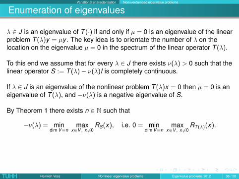
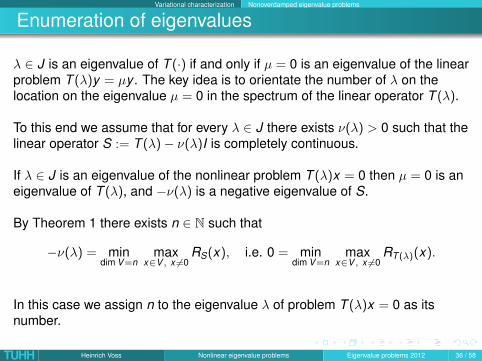
Enumeration of eigenvalues
λ ∈ J is an eigenvalue of T (·) if and only if µ = 0 is an eigenvalue of the linearproblem T (λ)y = µy . The key idea is to orientate the number of λ on thelocation on the eigenvalue µ = 0 in the spectrum of the linear operator T (λ).
To this end we assume that for every λ ∈ J there exists ν(λ) > 0 such that thelinear operator S := T (λ)− ν(λ)I is completely continuous.
If λ ∈ J is an eigenvalue of the nonlinear problem T (λ)x = 0 then µ = 0 is aneigenvalue of T (λ), and −ν(λ) is a negative eigenvalue of S.
By Theorem 1 there exists n ∈ N such that
−ν(λ) = mindim V =n
maxx∈V , x 6=0
RS(x), i.e. 0 = mindim V =n
maxx∈V , x 6=0
RT (λ)(x).
In this case we assign n to the eigenvalue λ of problem T (λ)x = 0 as itsnumber.
TUHH Heinrich Voss Nonlinear eigenvalue problems Eigenvalue problems 2012 36 / 58
Variational characterization Nonoverdamped eigenvalue problems
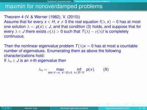
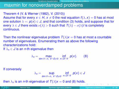
maxmin for nonoverdamped problems
Theorem 4 (V. & Werner (1982), V. (2010))Assume that for every x ∈ H, x 6= 0 the real equation f (λ, x) = 0 has at mostone solution λ =: p(x) ∈ J, and that condition (3) holds, and suppose that forevery λ ∈ J there exists ν(λ) > 0 such that T (λ)− ν(λ)I is completelycontinuous.
Then the nonlinear eigenvalue problem T (λ)x = 0 has at most a countablenumber of eigenvalues. Enumerating them as above the followingcharacterizations hold:If λn ∈ J is an n-th eigenvalue then
λn = maxdim V =n, V∩D 6=∅
infx∈D∩V
p(x). (8)
If converselyλn = sup
dim V =n, V∩D 6=∅inf
x∈D∩Vp(x) ∈ J
then λn is an n-th eigenvalue of T (λ)x = 0 and (8) holds.
TUHH Heinrich Voss Nonlinear eigenvalue problems Eigenvalue problems 2012 37 / 58
Variational characterization Nonoverdamped eigenvalue problems
maxmin for nonoverdamped problems
Theorem 4 (V. & Werner (1982), V. (2010))Assume that for every x ∈ H, x 6= 0 the real equation f (λ, x) = 0 has at mostone solution λ =: p(x) ∈ J, and that condition (3) holds, and suppose that forevery λ ∈ J there exists ν(λ) > 0 such that T (λ)− ν(λ)I is completelycontinuous.
Then the nonlinear eigenvalue problem T (λ)x = 0 has at most a countablenumber of eigenvalues. Enumerating them as above the followingcharacterizations hold:If λn ∈ J is an n-th eigenvalue then
λn = maxdim V =n, V∩D 6=∅
infx∈D∩V
p(x). (8)
If converselyλn = sup
dim V =n, V∩D 6=∅inf
x∈D∩Vp(x) ∈ J
then λn is an n-th eigenvalue of T (λ)x = 0 and (8) holds.
TUHH Heinrich Voss Nonlinear eigenvalue problems Eigenvalue problems 2012 37 / 58
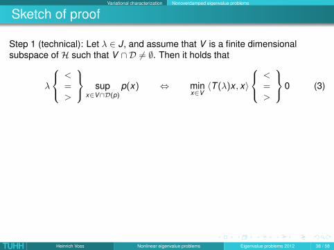
Variational characterization Nonoverdamped eigenvalue problems
Sketch of proof
Step 1 (technical): Let λ ∈ J, and assume that V is a finite dimensionalsubspace of H such that V ∩ D 6= ∅. Then it holds that
λ
<=>
supx∈V∩D(p)
p(x) ⇔ minx∈V〈T (λ)x , x〉
<=>
0 (3)
Step 2: If λn is an n-th eigenvalue, then µn(λn) = 0, and
µn(λn) = maxdim V =n
minx∈V , ‖x‖=1
〈T (λn)x , x〉 = minx∈V , ‖x‖=1
〈T (λn)x , x〉.
Hence, minx∈V ,‖x‖=1〈T (λn)x , x〉 ≤ 0 for every V with dim V = n, and (3)implies
supx∈V∩D
p(x) ≥ λn = supx∈V∩D
p(x).
Hence, λn is a minmax value of p.
TUHH Heinrich Voss Nonlinear eigenvalue problems Eigenvalue problems 2012 38 / 58
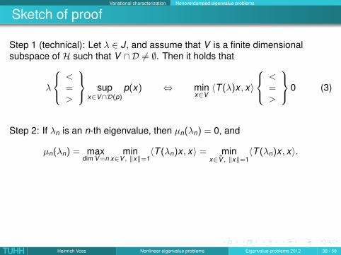
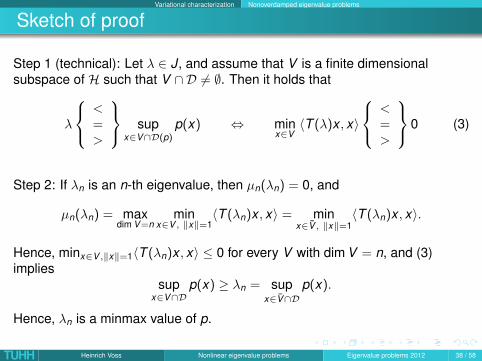
Variational characterization Nonoverdamped eigenvalue problems
maxmin for nonoverdamped problems ct.
Theorem 5Under the conditions of Theorem 4 let supv∈D p(v) ∈ J and assume that thereexists W ∈ Hn such that
W ∩ D 6= ∅ and infv∈W∩D
p(v) ∈ J.
Then for j = 1, . . . ,n every V ∈ Hj with
V ∩ D 6= ∅ and λj = infv∈V∩D
p(v)
is contained in D, and the maxmin characterization of λj can be replaced by
λj = maxV∈Hj , V\0⊂D
minv∈V\0
p(v).
TUHH Heinrich Voss Nonlinear eigenvalue problems Eigenvalue problems 2012 39 / 58
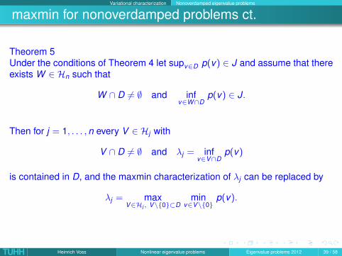
Variational characterization Nonoverdamped eigenvalue problems
minmax for nonoverdamped problemsTheorem 6 (V. (2003))Assume that for every x ∈ H, x 6= 0 the real equation f (λ, x) = 0 has at mostone solution λ =: p(x) ∈ J, and that condition (3) holds, and suppose that forevery λ ∈ J there exists ν(λ) > 0 such that T (λ)− ν(λ)I is completelycontinuous.
Then the nonlinear eigenvalue problem T (λ)x = 0 has at most a countablenumber of eigenvalues. Enumerating them as above the followingcharacterizations hold:If problem T (λ)x = 0 has an n-th eigenvalue λn then
λn = mindim V =n−1, V⊥∩D 6=∅
supx∈D∩V⊥
p(x).
Proof takes advantage of the following Lemma:
Let λ ∈ J, and let V be a finite dimensional subspace of H such thatV⊥ ∩ D 6= ∅. Then it holds that
λ
<=>
infx∈V⊥∩D(p)
p(x) ⇔ maxx∈V⊥, ‖x‖=1
〈T (λ)x , x〉
<=>
0
TUHH Heinrich Voss Nonlinear eigenvalue problems Eigenvalue problems 2012 40 / 58
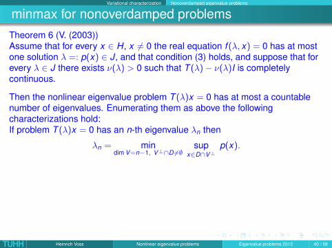
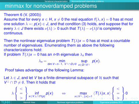
Variational characterization Nonoverdamped eigenvalue problems
Further literature
Variational characterizations for non-overdamped nonlinear eigenvalueproblems were proved (independently from our work) by
Barston (1974) for some extreme eigenvalues of finite dimensionalquadratic eigenproblems
and for the infinite dimensional case by
Griniv & Meln’ik (1996): T (λ) = A(λ)− I, A(λ) compactBinding, Eschwé & H. Langer (2000)Eschwé & M. Langer (2004) unbounded operators
TUHH Heinrich Voss Nonlinear eigenvalue problems Eigenvalue problems 2012 41 / 58
Variational characterization Nonoverdamped eigenvalue problems
Further literature
Variational characterizations for non-overdamped nonlinear eigenvalueproblems were proved (independently from our work) by
Barston (1974) for some extreme eigenvalues of finite dimensionalquadratic eigenproblems
and for the infinite dimensional case by
Griniv & Meln’ik (1996): T (λ) = A(λ)− I, A(λ) compact
Binding, Eschwé & H. Langer (2000)Eschwé & M. Langer (2004) unbounded operators
TUHH Heinrich Voss Nonlinear eigenvalue problems Eigenvalue problems 2012 41 / 58
Variational characterization Nonoverdamped eigenvalue problems
Further literature
Variational characterizations for non-overdamped nonlinear eigenvalueproblems were proved (independently from our work) by
Barston (1974) for some extreme eigenvalues of finite dimensionalquadratic eigenproblems
and for the infinite dimensional case by
Griniv & Meln’ik (1996): T (λ) = A(λ)− I, A(λ) compactBinding, Eschwé & H. Langer (2000)
Eschwé & M. Langer (2004) unbounded operators
TUHH Heinrich Voss Nonlinear eigenvalue problems Eigenvalue problems 2012 41 / 58
Variational characterization Nonoverdamped eigenvalue problems
Further literature
Variational characterizations for non-overdamped nonlinear eigenvalueproblems were proved (independently from our work) by
Barston (1974) for some extreme eigenvalues of finite dimensionalquadratic eigenproblems
and for the infinite dimensional case by
Griniv & Meln’ik (1996): T (λ) = A(λ)− I, A(λ) compactBinding, Eschwé & H. Langer (2000)Eschwé & M. Langer (2004) unbounded operators
TUHH Heinrich Voss Nonlinear eigenvalue problems Eigenvalue problems 2012 41 / 58
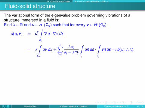
Variational characterization Nonoverdamped eigenvalue problems
Fluid-solid structureThe variational form of the eigenvalue problem governing vibrations of astructure immersed in a fluid is:Find λ ∈ R and u ∈ H1(Ω0) such that for every v ∈ H1(Ω0)
a(u, v) := c2∫Ω0
∇u · ∇v dx
= λ
∫Ω0
uv dx +∑j=1
λρ0
kj − λmj
∫Γj
un ds ·∫Γj
vn ds =: b(u, v ;λ).
Obviously, f (λ,u) := b(u,u;λ)− a(u,u) is monotonically increasing for everyfixed u 6= 0, and therefore f (λ,u) = 0 defines a Rayleigh functional in everyreal interval J which does not contain a pole kj/mj .
For J0 := (0,minkj/mj : j = 1, . . . , ` the infimum of the Rayleigh functionalis contained in J0, and Theorem 5 applies (i.e. the eigenvalues can beenumerated in the natural way), for further intervals the enumerationaccording to their location in the spectrum of the linear eigenproblems isrelevant in Theorem 4.
TUHH Heinrich Voss Nonlinear eigenvalue problems Eigenvalue problems 2012 42 / 58
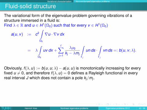

Variational characterization Nonoverdamped eigenvalue problems
A priori bound for CMS
Theorem 5 can be used to derive an a priori bound for CMS (cf. Elssel & V.2006).
We already obtained in Chapter 12 the Craig-Bampton form of an eigenvalueproblemΩ1 0 0
0 Ω2 00 0 Kii
x1x2x3
= λ
I 0 M`i1
0 I M`i2
Mi`1 Mi`2 Mii
x1x2x3
(1)
and that this problem is reduced to(Ω2 00 Kii
)y = λ
(I M`i2
Mi`2 Mii
)y (2)
in the component mode synthesis method, where all diagonal elements of Ω1are greater than the cut-off frequency ω, and all eigenvalues in Ω2 are lessthan ω.
TUHH Heinrich Voss Nonlinear eigenvalue problems Eigenvalue problems 2012 43 / 58
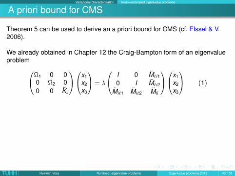
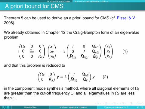
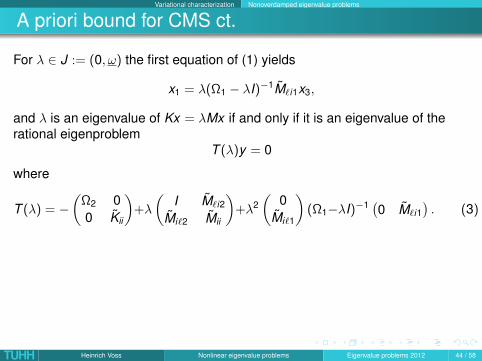
Variational characterization Nonoverdamped eigenvalue problems
A priori bound for CMS ct.
For λ ∈ J := (0, ω) the first equation of (1) yields
x1 = λ(Ω1 − λI)−1M`i1x3,
and λ is an eigenvalue of Kx = λMx if and only if it is an eigenvalue of therational eigenproblem
T (λ)y = 0
where
T (λ) = −(
Ω2 00 Kii
)+λ
(I M`i2
Mi`2 Mii
)+λ2
(0
Mi`1
)(Ω1−λI)−1 (0 M`i1
). (3)
Let λ1 ≤ λ2 ≤ · · · ≤ λn denote the eigenvalues of problem (1) ordered bymagnitude, and let m ∈ N such that λm < ω ≤ λm+1.
Then λ1, . . . , λm ∈ J are the eigenvalues of the nonlinear eigenproblem (1) inJ.
TUHH Heinrich Voss Nonlinear eigenvalue problems Eigenvalue problems 2012 44 / 58
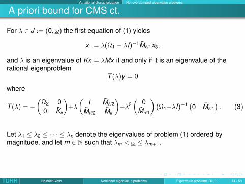
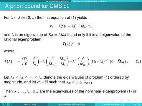
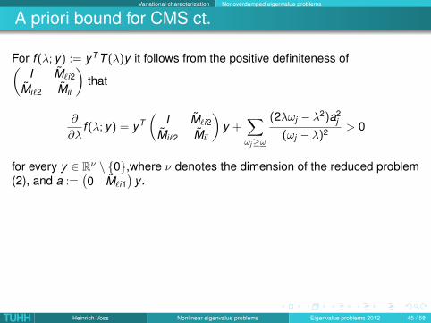
Variational characterization Nonoverdamped eigenvalue problems
A priori bound for CMS ct.
For f (λ; y) := yT T (λ)y it follows from the positive definiteness of(I M`i2
Mi`2 Mii
)that
∂
∂λf (λ; y) = yT
(I M`i2
Mi`2 Mii
)y +
∑ωj≥ω
(2λωj − λ2)a2j
(ωj − λ)2 > 0
for every y ∈ Rν \ 0,where ν denotes the dimension of the reduced problem(2), and a :=
(0 M`i1
)y .
Hence, due to the monotonicity of f (λ; y) for every y ∈ Rν \ 0 the realequation f (λ; y) = 0 has at most one solution p(y) ∈ J, and the condition
∂
∂λf (λ, y)
∣∣λ=p(y)
> 0 for every y ∈ D
holds.
TUHH Heinrich Voss Nonlinear eigenvalue problems Eigenvalue problems 2012 45 / 58
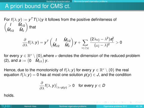
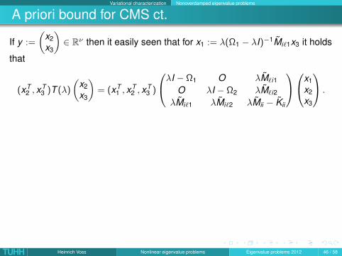
Variational characterization Nonoverdamped eigenvalue problems
A priori bound for CMS ct.
If y :=
(x2x3
)∈ Rν then it easily seen that for x1 := λ(Ω1 − λI)−1Mi`1x3 it holds
that
(xT2 , x
T3 )T (λ)
(x2x3
)= (xT
1 , xT2 , x
T3 )
λI − Ω1 O λM`i1
O λI − Ω2 λM`i2
λMi`1 λMi`2 λMii − Kii
x1x2x3
.
Hence,(
x2x3
)∈ D if and only if the Rayleigh quotient R of the linear
eigenproblem (1) at x := (xT1 , x
T2 , x
T3 )T is contained in J, and p(y) = R(x).
In particularinf
y∈Dp(y) = inf
x∈Rn, x 6=0R(x) = λ1 ∈ J,
and the eigenvalues λ1, . . . , λm of problem (3) satisfy the minmaxcharacterization.
TUHH Heinrich Voss Nonlinear eigenvalue problems Eigenvalue problems 2012 46 / 58
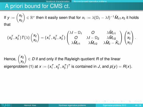
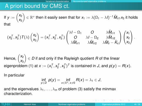
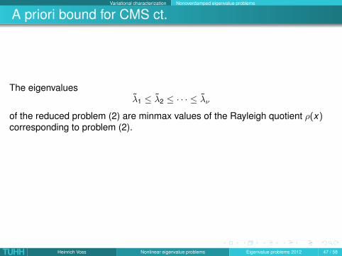
Variational characterization Nonoverdamped eigenvalue problems
A priori bound for CMS ct.
The eigenvaluesλ1 ≤ λ2 ≤ · · · ≤ λν
of the reduced problem (2) are minmax values of the Rayleigh quotient ρ(x)corresponding to problem (2).
Comparing p and ρ on appropriate subspaces of Rν we arrive at the followinga priori bound for the relative errors of the CMS approximations λj to λj .
TUHH Heinrich Voss Nonlinear eigenvalue problems Eigenvalue problems 2012 47 / 58
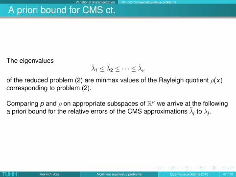

Variational characterization Nonoverdamped eigenvalue problems
Theorem
Let K ,M ∈ Rn×n be symmetric and positive definite, and letλ1 ≤ λ2 ≤ · · · ≤ λn be the eigenvalues of problem (1), which we assume to beordered by magnitude.
Denote by λ1 ≤ λ2 ≤ · · · ≤ λν the eigenvalues of the CMS approximation (2)of problem (1) corresponding to some partition of the graph |K |+ |M| andsome cut-off threshold ω.
Assume that the interval (0, ω) contains m eigenvalues λ1, . . . , λm of (1).
Then it holds
0 ≤λj − λj
λj≤
λj
ω − λj≤
λj
ω − λj, j = 1, . . . ,m.
Hence, for eigenvalues which are far away from the cut-off threshold we mayexpect accurate approximations by the CMS method.
TUHH Heinrich Voss Nonlinear eigenvalue problems Eigenvalue problems 2012 48 / 58

Variational characterization Nonoverdamped eigenvalue problems
Proof
The left inequality, i.e. λj ≤ λj , is trivial since CMS is a projection method. Theright inequality follows from the monotonicity of the function λ 7→ λ/(ω − λ).
To prove the inequality in the middle denote by V ∈ Sj , V \ 0 ⊂ D the jdimensional subspace of Rν such that
λj = maxy∈V , y 6=0
p(y).
Then p(y) ≤ λj for every y ∈ V , y 6= 0, and therefore it follows from themonotonicity of the function f (λ; y) with respect to λ
−yT(
Ω2 00 Kii
)y + λjyT
(I M`i2
Mi`2 Mii
)y
+λ2j yT
(0
Mi`1
)(Ω1 − λj I)−1 (0 M`i1
)y ≥ 0.
TUHH Heinrich Voss Nonlinear eigenvalue problems Eigenvalue problems 2012 49 / 58
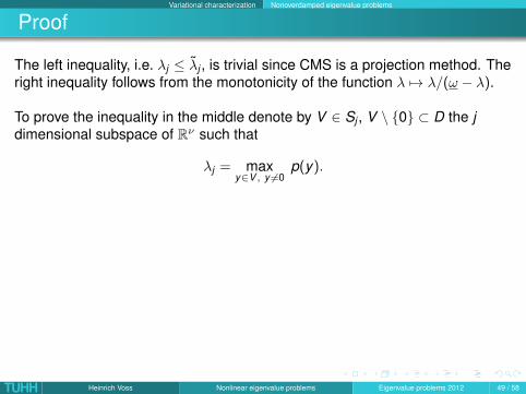
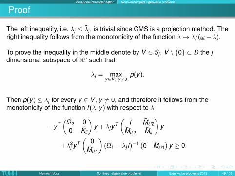
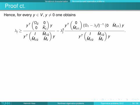
Variational characterization Nonoverdamped eigenvalue problems
Proof ct.Hence, for every y ∈ V , y 6= 0 one obtains
λj ≥yT(
Ω2 00 Kii
)y
yT
(I M`i2
Mi`2 Mii
)y− λ2
j
yT(
0Mi`1
)(Ω1 − λj I)−1
(0 M`i1
)y
yT
(I M`i2
Mi`2 Mii
)y
.
In particular for y ∈ V such that ρ(y) = maxy∈V , y 6=0 ρ(y) we have
λj ≥ maxy∈V , y 6=0
ρ(y)− λ2j
yT(
0Mi`1
)(Ω1 − λj I)−1
(0 M`i1
)y
yT
(I M`i2
Mi`2 Mii
)y
≥ λj −λ2
j
ω − λjmax
y∈Rn,y 6=0
yT(
0Mi`1
)(0 M`i1
)y
yT
(I M`i2
Mi`2 Mii
)y
. (4)
TUHH Heinrich Voss Nonlinear eigenvalue problems Eigenvalue problems 2012 50 / 58
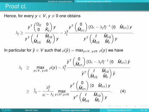
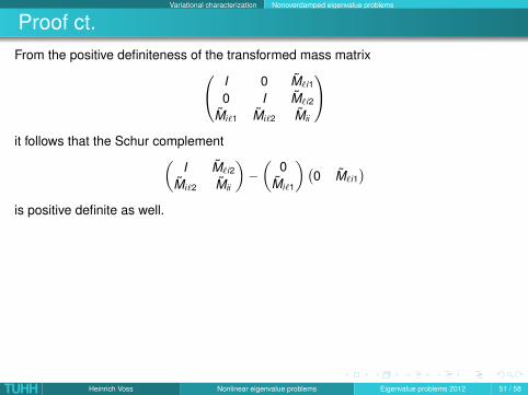
Variational characterization Nonoverdamped eigenvalue problems
Proof ct.From the positive definiteness of the transformed mass matrix I 0 M`i1
0 I M`i2
Mi`1 Mi`2 Mii
it follows that the Schur complement(
I M`i2
Mi`2 Mii
)−(
0Mi`1
)(0 M`i1
)is positive definite as well.
Thus,
maxy∈Rn,y 6=0
yT(
0Mi`1
)(0 M`i1
)y
yT
(I M`i2
Mi`2 Mii
)y
≤ 1,
and inequality (4) yields
λj ≥ λj −λ2
j
ω − λj
which completes the proof.
TUHH Heinrich Voss Nonlinear eigenvalue problems Eigenvalue problems 2012 51 / 58
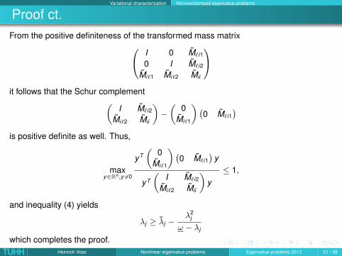
Variational characterization Nonoverdamped eigenvalue problems
Proof ct.From the positive definiteness of the transformed mass matrix I 0 M`i1
0 I M`i2
Mi`1 Mi`2 Mii
it follows that the Schur complement(
I M`i2
Mi`2 Mii
)−(
0Mi`1
)(0 M`i1
)is positive definite as well. Thus,
maxy∈Rn,y 6=0
yT(
0Mi`1
)(0 M`i1
)y
yT
(I M`i2
Mi`2 Mii
)y
≤ 1,
and inequality (4) yields
λj ≥ λj −λ2
j
ω − λj
which completes the proof.TUHH Heinrich Voss Nonlinear eigenvalue problems Eigenvalue problems 2012 51 / 58

Variational characterization Nonoverdamped eigenvalue problems
Example
Consider the model of a container ship with 10 substructures which has 1960DoFs on the interfaces.
We solved the eigenproblem by the CMS method using a cut-off bound of20,000 (about 10 times the largest wanted eigenvalue λ50 ≈ 2183).
329 eigenvalues of the substructure problems were less than our threshold,and the dimension of the resulting projected problem was 2289.
The following figure shows the relative errors for the smallest 50 eigenvalues(lower crosses in blue) and the error bounds (upper crosses in red).
TUHH Heinrich Voss Nonlinear eigenvalue problems Eigenvalue problems 2012 52 / 58
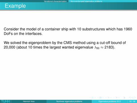
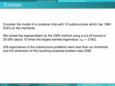
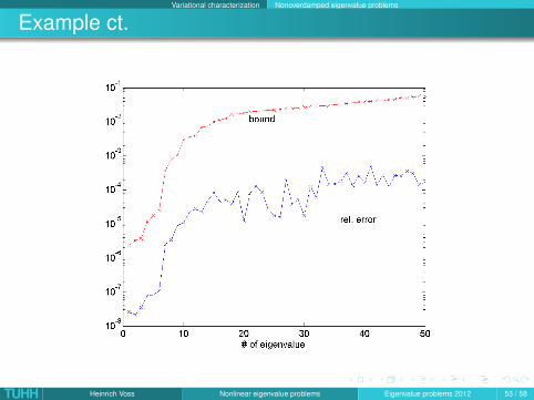
Variational characterization Nonoverdamped eigenvalue problems
Example ct.
TUHH Heinrich Voss Nonlinear eigenvalue problems Eigenvalue problems 2012 53 / 58

Variational characterization Nonoverdamped eigenvalue problems
A priori bound
In the example the relative error is overestimated by two or three orders ofmagnitude.
ω 0 00 1 00 0 1
x1x2x3
= λ
1 0 m0 1 0m 0 1
x1x2x3
with ω > 1 and m ∈ (0,1) demonstrates that the a priori bound can not beimproved without further assumptions.
If x1 and x2 are the local degrees of freedom, and x3 is the interface variable,then with cut-off frequency ω the minimum eigenvalue of the reduced problemis λ1 = 1.
Letting m→ 1− 0 l’Hospital’s rule yields
limm→1−0
λ1 − λ1
λ1=
1ω
= limm→1−0
λ1
ω − λ1.
TUHH Heinrich Voss Nonlinear eigenvalue problems Eigenvalue problems 2012 54 / 58
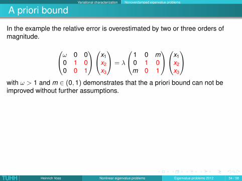
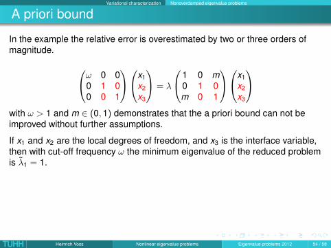
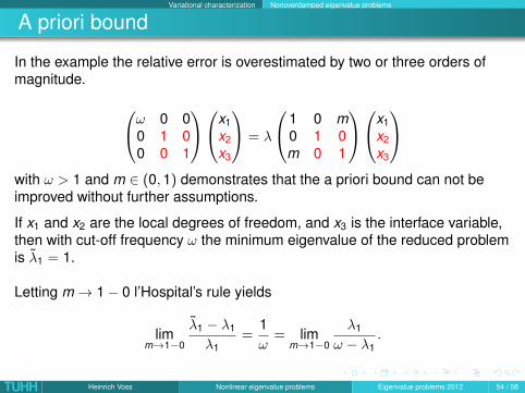

Variational characterization Nonoverdamped eigenvalue problems
A priori bound for AMLSAMLS can be understood as a sequence of ` consecutive CMS steps and aterminating spectral truncation. It is clear how to obtain an a priori bound forthe general AMLS method.
Hence, if λ(ν)j denotes the eigenvalues of the reduced eigenvalue problem
corresponding to the ν–th level ordered by magnitude, then it holds
λ(ν)j ≤ λ(ν−1)
j
(1 +
λ(ν−1)j
ων − λ(ν−1)j
), ν = 1,2, . . . ,p + 1.
where on the ν-th level eigenvalues exceeding ων are neglected.
Thus, it follows for all λj ≤ minν=1,...,p ων
λ(`+1)j ≤ λj
p∏ν=0
(1 +
λ(ν)j
ων+1 − λ(ν)j
),
and the following theorem follows.
TUHH Heinrich Voss Nonlinear eigenvalue problems Eigenvalue problems 2012 55 / 58
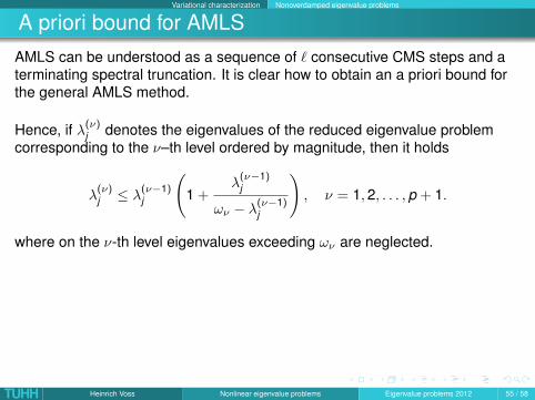
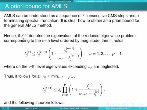
Variational characterization Nonoverdamped eigenvalue problems
A priori bound for AMLSAMLS can be understood as a sequence of ` consecutive CMS steps and aterminating spectral truncation. It is clear how to obtain an a priori bound forthe general AMLS method.
Hence, if λ(ν)j denotes the eigenvalues of the reduced eigenvalue problem
corresponding to the ν–th level ordered by magnitude, then it holds
λ(ν)j ≤ λ(ν−1)
j
(1 +
λ(ν−1)j
ων − λ(ν−1)j
), ν = 1,2, . . . ,p + 1.
where on the ν-th level eigenvalues exceeding ων are neglected.
Thus, it follows for all λj ≤ minν=1,...,p ων
λ(`+1)j ≤ λj
p∏ν=0
(1 +
λ(ν)j
ων+1 − λ(ν)j
),
and the following theorem follows.TUHH Heinrich Voss Nonlinear eigenvalue problems Eigenvalue problems 2012 55 / 58
Variational characterization Nonoverdamped eigenvalue problems
TheoremLet K , M and λj , j = 1, . . . ,n be given as in the last theorem. Let the graph of|K |+ |M| be substructured with ` levels, and denote by λ(ν)
1 ≤ λ(ν)2 ≤ . . . the
eigenvalues obtained by AMLS with cut-off threshold ων on level ν.
If m ∈ N such thatλm < min
ν=0,...,pων ≤ λm+1
then it holds
λj − λj
λj≤
p∏ν=0
(1 +
λ(ν)j
ων − λ(ν)j
)− 1, j = 1, . . . ,m.
Since the final problem is a projection of each of the intermediateeigenproblems in the AMLS reduction, it follows from the minmaxcharacterization that λ(ν)
j ≤ λj for ν = 0, . . . ,p. Therefore the a priori boundcan be replaced by the computable bound
λj − λj
λj≤
p∏ν=0
(1 +
λj
ων − λj
)− 1, j = 1, . . . ,m.
TUHH Heinrich Voss Nonlinear eigenvalue problems Eigenvalue problems 2012 56 / 58
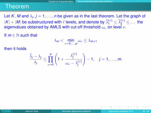
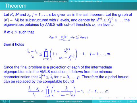
Variational characterization Nonoverdamped eigenvalue problems
Example
We substructured the FE model of the container ship by Metis with 4 levels ofsubstructuring.
Neglecting eigenvalues exceeding 20,000 and 40,000 on all levels AMLSproduced a projected eigenvalue problem of dimension 451 and 911,respectively.
The relative errors and the bounds are shown in the following figure where thelower and upper crosses correspond to the threshold 40,000, and the lowerand upper circles to 20,000.
TUHH Heinrich Voss Nonlinear eigenvalue problems Eigenvalue problems 2012 57 / 58
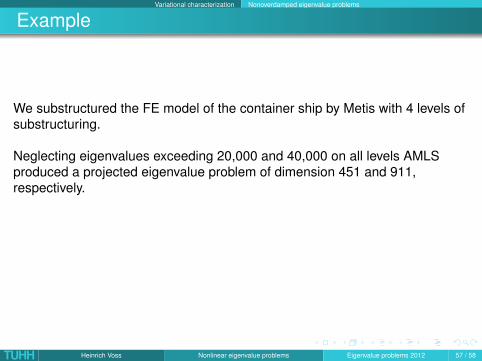
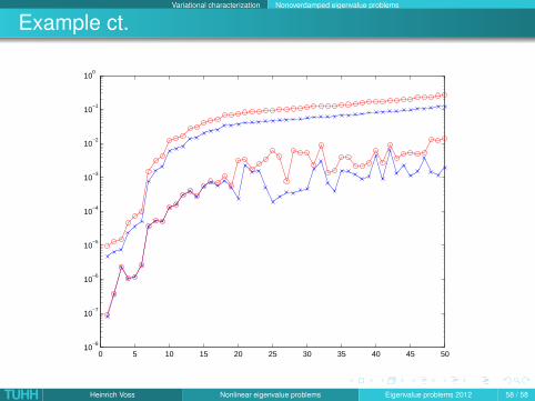
Variational characterization Nonoverdamped eigenvalue problems
Example ct.
0 5 10 15 20 25 30 35 40 45 5010
−8
10−7
10−6
10−5
10−4
10−3
10−2
10−1
100
TUHH Heinrich Voss Nonlinear eigenvalue problems Eigenvalue problems 2012 58 / 58