chapter 4 some counting problems; cients, the …jean/cis160/cis160slides6.pdfchapter 4 some...
TRANSCRIPT
Chapter 4
Some Counting Problems;Multinomial Coe�cients, TheInclusion-Exclusion Principle,Sylvester’s Formula, The SieveFormula
4.1 Counting Permutations and Functions
In this short section, we consider some simple countingproblems.
Let us begin with permutations. Recall that apermutation of a set, A, is any bijection between A anditself.
427
428 CHAPTER 4. SOME COUNTING PROBLEMS; MULTINOMIAL COEFFICIENTS
If A is a finite set with n elements, we mentioned earlier(without proof) that A has n! permutations, where thefactorial function, n 7! n! (n 2 N), is given recursivelyby:
0! = 1
(n + 1)! = (n + 1)n!.
The reader should check that the existence of the func-tion, n 7! n!, can be justified using the Recursion Theo-rem (Theorem 2.5.1).
Proposition 4.1.1 The number of permutations of aset of n elements is n!.
Let us also count the number of functions between twofinite sets.
Proposition 4.1.2 If A and B are finite sets with|A| = m and |B| = n, then the set of function, BA,from A to B has nm elements.
4.1. COUNTING PERMUTATIONS AND FUNCTIONS 429
As a corollary, we determine the cardinality of a finitepower set.
Corollary 4.1.3 For any finite set, A, if |A| = n,then |2A| = 2n.
Computing the value of the factorial function for a fewinputs, say n = 1, 2 . . . , 10, shows that it grows very fast.For example,
10! = 3, 628, 800.
Is it possible to quantify how fast factorial grows com-pared to other functions, say nn or en?
Remarkably, the answer is yes. A beautiful formula dueto James Stirling (1692-1770) tells us that
n! ⇠p2⇡n
⇣n
e
⌘n,
which means that
limn!1
n!p2⇡n
�ne
�n = 1.
430 CHAPTER 4. SOME COUNTING PROBLEMS; MULTINOMIAL COEFFICIENTS
Figure 4.1: Jacques Binet, 1786-1856
Here, of course,
e = 1 +1
1!+
1
2!+
1
3!+ · · · + 1
n!+ · · ·
the base of the natural logarithm.
It is even possible to estimate the error. It turns out that
n! =p2⇡n
⇣n
e
⌘ne�n,
where1
12n + 1< �n <
1
12n,
a formula due to Jacques Binet (1786-1856).
Let us introduce some notation used for comparing therate of growth of functions.
4.1. COUNTING PERMUTATIONS AND FUNCTIONS 431
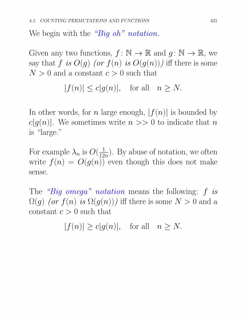
We begin with the “Big oh” notation .
Given any two functions, f : N ! R and g : N ! R, wesay that f is O(g) (or f (n) is O(g(n))) i↵ there is someN > 0 and a constant c > 0 such that
|f (n)| c|g(n)|, for all n � N.
In other words, for n large enough, |f (n)| is bounded byc|g(n)|. We sometimes write n >> 0 to indicate that nis “large.”
For example �n is O( 112n). By abuse of notation, we often
write f (n) = O(g(n)) even though this does not makesense.
The “Big omega” notation means the following: f is⌦(g) (or f (n) is ⌦(g(n))) i↵ there is some N > 0 and aconstant c > 0 such that
|f (n)| � c|g(n)|, for all n � N.
432 CHAPTER 4. SOME COUNTING PROBLEMS; MULTINOMIAL COEFFICIENTS
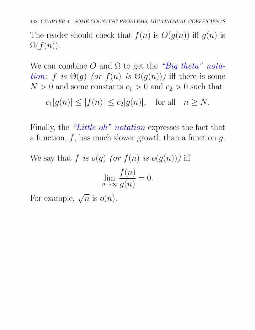
The reader should check that f (n) is O(g(n)) i↵ g(n) is⌦(f (n)).
We can combine O and ⌦ to get the “Big theta” nota-tion : f is ⇥(g) (or f (n) is ⇥(g(n))) i↵ there is someN > 0 and some constants c1 > 0 and c2 > 0 such that
c1|g(n)| |f (n)| c2|g(n)|, for all n � N.
Finally, the “Little oh” notation expresses the fact thata function, f , has much slower growth than a function g.
We say that f is o(g) (or f (n) is o(g(n))) i↵
limn!1
f (n)
g(n)= 0.
For example,p
n is o(n).
4.2. COUNTING SUBSETS OF SIZE K; MULTINOMIAL COEFFICIENTS 433
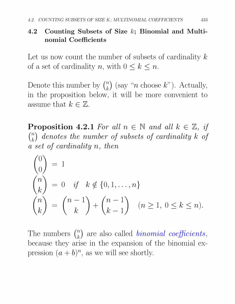
4.2 Counting Subsets of Size k; Binomial and Multi-nomial Coe�cients
Let us now count the number of subsets of cardinality kof a set of cardinality n, with 0 k n.
Denote this number by�n
k
�(say “n choose k”). Actually,
in the proposition below, it will be more convenient toassume that k 2 Z.
Proposition 4.2.1 For all n 2 N and all k 2 Z, if�nk
�denotes the number of subsets of cardinality k of
a set of cardinality n, then✓0
0
◆= 1
✓n
k
◆= 0 if k /2 {0, 1, . . . , n}
✓n
k
◆=
✓n � 1
k
◆+
✓n � 1
k � 1
◆(n � 1, 0 k n).
The numbers�n
k
�are also called binomial coe�cients ,
because they arise in the expansion of the binomial ex-pression (a + b)n, as we will see shortly.
434 CHAPTER 4. SOME COUNTING PROBLEMS; MULTINOMIAL COEFFICIENTS
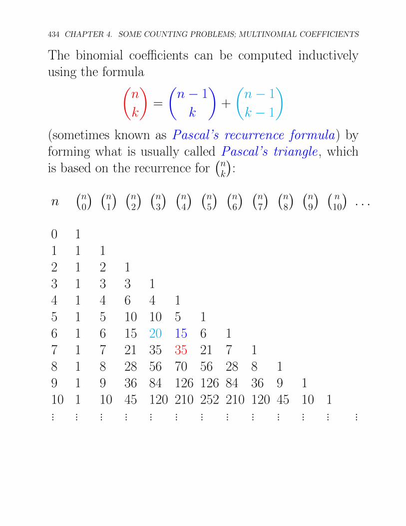
The binomial coe�cients can be computed inductivelyusing the formula
✓n
k
◆=
✓n � 1
k
◆+
✓n � 1
k � 1
◆
(sometimes known as Pascal’s recurrence formula) byforming what is usually called Pascal’s triangle , whichis based on the recurrence for
�nk
�:
n�n
0
� �n1
� �n2
� �n3
� �n4
� �n5
� �n6
� �n7
� �n8
� �n9
� � n10
�. . .
0 11 1 12 1 2 13 1 3 3 14 1 4 6 4 15 1 5 10 10 5 16 1 6 15 20 15 6 17 1 7 21 35 35 21 7 18 1 8 28 56 70 56 28 8 19 1 9 36 84 126 126 84 36 9 110 1 10 45 120 210 252 210 120 45 10 1... ... ... ... ... ... ... ... ... ... ... ... ...
4.2. COUNTING SUBSETS OF SIZE K; MULTINOMIAL COEFFICIENTS 435
Figure 4.2: Blaise Pascal, 1623-1662
We can also give the following explicit formula for�n
k
�in
terms of the factorial function:
Proposition 4.2.2 For all n, k 2 N, with 0 k n,we have ✓
n
k
◆=
n!
k!(n � k)!.
Then, it is very easy to see that✓n
k
◆=
✓n
n � k
◆.
Remarks:
(1) The binomial coe�cients were already known in thetwelfth century by the Indian Scholar Bhaskra. Pas-cal’s triangle was taught back in 1265 by the Persianphilosopher, Nasir-Ad-Din.
436 CHAPTER 4. SOME COUNTING PROBLEMS; MULTINOMIAL COEFFICIENTS
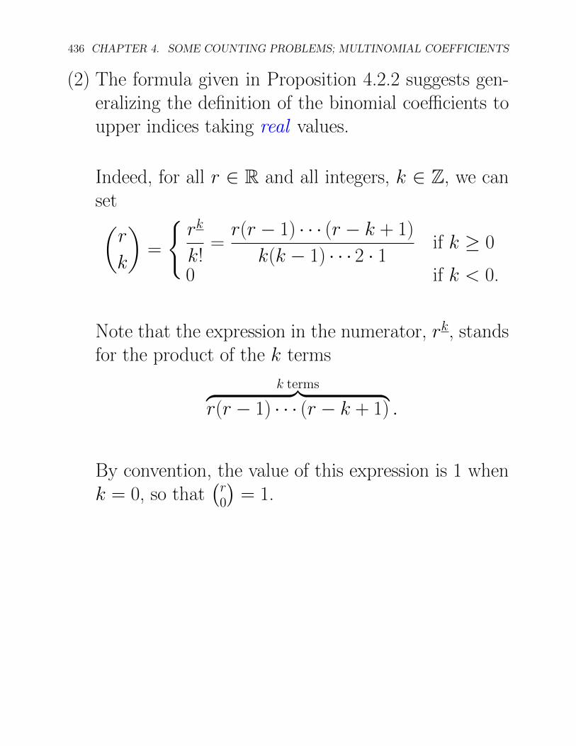
(2) The formula given in Proposition 4.2.2 suggests gen-eralizing the definition of the binomial coe�cients toupper indices taking real values.
Indeed, for all r 2 R and all integers, k 2 Z, we canset✓
r
k
◆=
(rk
k!=
r(r � 1) · · · (r � k + 1)
k(k � 1) · · · 2 · 1 if k � 0
0 if k < 0.
Note that the expression in the numerator, rk, standsfor the product of the k terms
k termsz }| {r(r � 1) · · · (r � k + 1) .
By convention, the value of this expression is 1 whenk = 0, so that
�r0
�= 1.
4.2. COUNTING SUBSETS OF SIZE K; MULTINOMIAL COEFFICIENTS 437
The expression�rk
�can be viewed as a polynomial of
degree k in r. The generalized binomial coe�cientsallow for a useful extension of the binomial formula(see next) to real exponents.
However, beware that the symmetry identity fails whenr is not a natural number and that the formula inProposition 4.2.2 (in terms of the factorial function)only makes sense for natural numbers.
We now prove the “binomial formula” (also called “bino-mial theorem”).
438 CHAPTER 4. SOME COUNTING PROBLEMS; MULTINOMIAL COEFFICIENTS
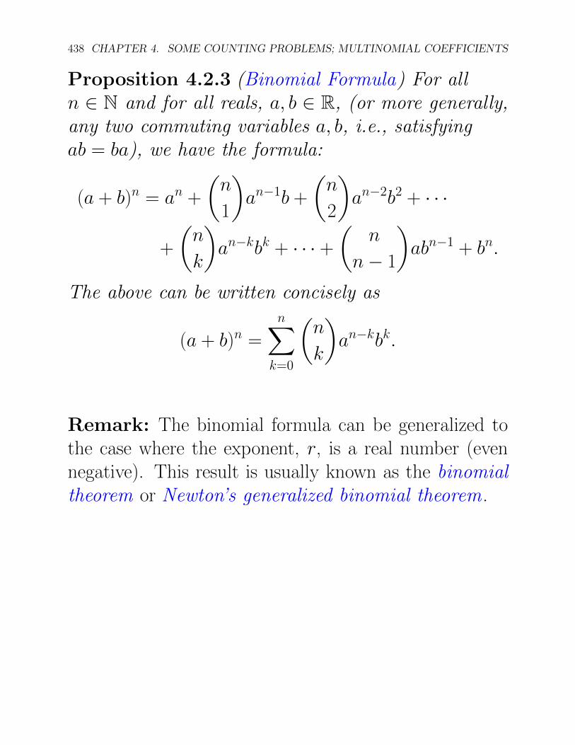
Proposition 4.2.3 (Binomial Formula) For alln 2 N and for all reals, a, b 2 R, (or more generally,any two commuting variables a, b, i.e., satisfyingab = ba), we have the formula:
(a + b)n = an +
✓n
1
◆an�1b +
✓n
2
◆an�2b2 + · · ·
+
✓n
k
◆an�kbk + · · · +
✓n
n � 1
◆abn�1 + bn.
The above can be written concisely as
(a + b)n =nX
k=0
✓n
k
◆an�kbk.
Remark: The binomial formula can be generalized tothe case where the exponent, r, is a real number (evennegative). This result is usually known as the binomialtheorem or Newton’s generalized binomial theorem .
4.2. COUNTING SUBSETS OF SIZE K; MULTINOMIAL COEFFICIENTS 439
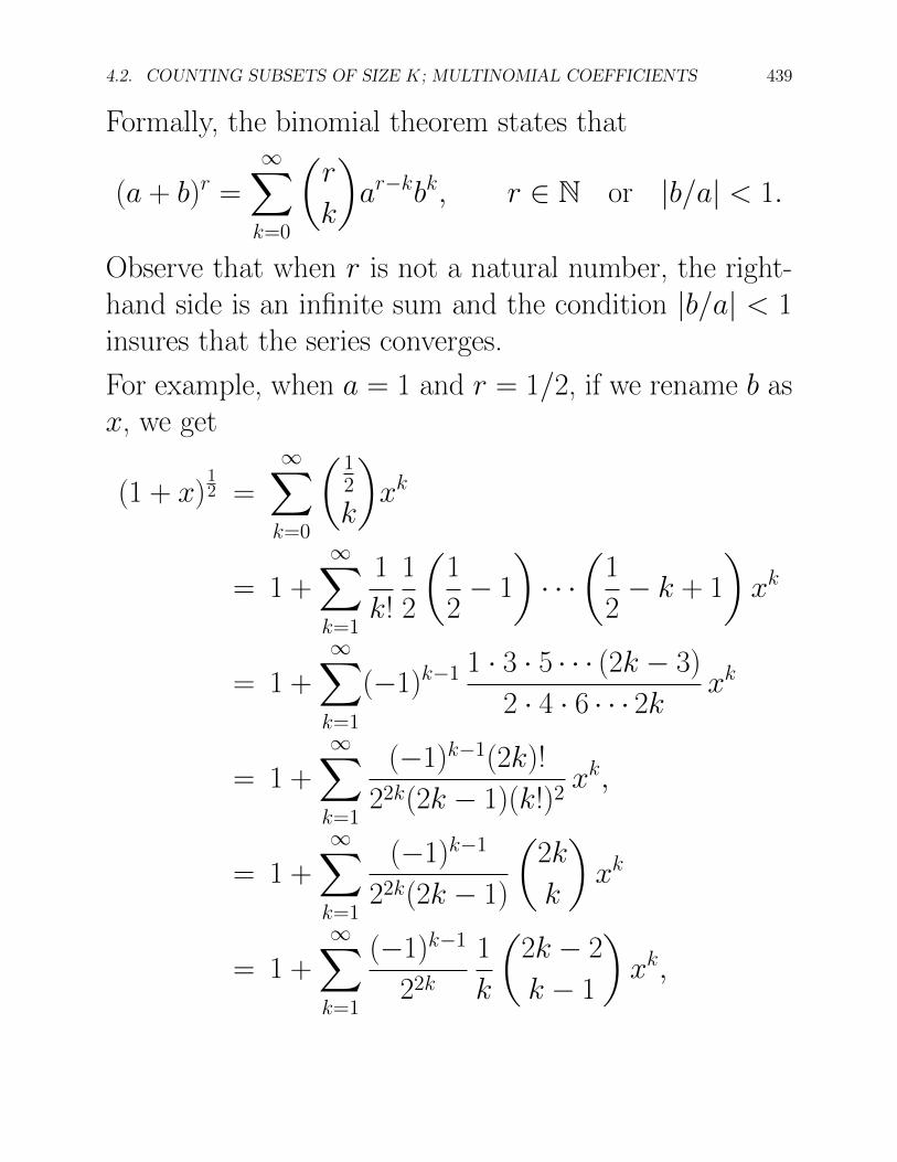
Formally, the binomial theorem states that
(a + b)r =1X
k=0
✓r
k
◆ar�kbk, r 2 N or |b/a| < 1.
Observe that when r is not a natural number, the right-hand side is an infinite sum and the condition |b/a| < 1insures that the series converges.
For example, when a = 1 and r = 1/2, if we rename b asx, we get
(1 + x)12 =
1X
k=0
✓12
k
◆xk
= 1 +1X
k=1
1
k!
1
2
✓1
2� 1
◆· · ·✓1
2� k + 1
◆xk
= 1 +1X
k=1
(�1)k�1 1 · 3 · 5 · · · (2k � 3)
2 · 4 · 6 · · · 2k xk
= 1 +1X
k=1
(�1)k�1(2k)!
22k(2k � 1)(k!)2xk,
= 1 +1X
k=1
(�1)k�1
22k(2k � 1)
✓2k
k
◆xk
= 1 +1X
k=1
(�1)k�1
22k
1
k
✓2k � 2
k � 1
◆xk,
440 CHAPTER 4. SOME COUNTING PROBLEMS; MULTINOMIAL COEFFICIENTS
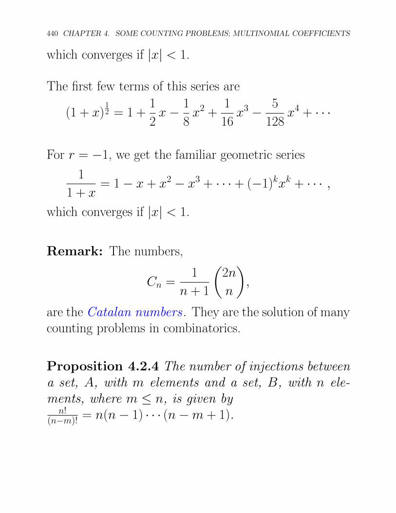
which converges if |x| < 1.
The first few terms of this series are
(1 + x)12 = 1 +
1
2x � 1
8x2 +
1
16x3 � 5
128x4 + · · ·
For r = �1, we get the familiar geometric series
1
1 + x= 1 � x + x2 � x3 + · · · + (�1)kxk + · · · ,
which converges if |x| < 1.
Remark: The numbers,
Cn =1
n + 1
✓2n
n
◆,
are the Catalan numbers . They are the solution of manycounting problems in combinatorics.
Proposition 4.2.4 The number of injections betweena set, A, with m elements and a set, B, with n ele-ments, where m n, is given by
n!(n�m)! = n(n � 1) · · · (n � m + 1).
4.2. COUNTING SUBSETS OF SIZE K; MULTINOMIAL COEFFICIENTS 441
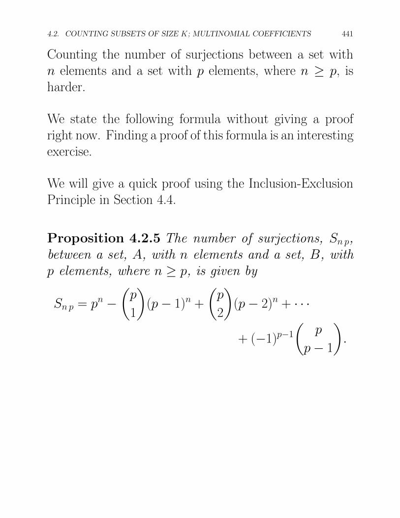
Counting the number of surjections between a set withn elements and a set with p elements, where n � p, isharder.
We state the following formula without giving a proofright now. Finding a proof of this formula is an interestingexercise.
We will give a quick proof using the Inclusion-ExclusionPrinciple in Section 4.4.
Proposition 4.2.5 The number of surjections, Sn p,between a set, A, with n elements and a set, B, withp elements, where n � p, is given by
Sn p = pn �✓
p
1
◆(p � 1)n +
✓p
2
◆(p � 2)n + · · ·
+ (�1)p�1
✓p
p � 1
◆.
442 CHAPTER 4. SOME COUNTING PROBLEMS; MULTINOMIAL COEFFICIENTS
Remarks:
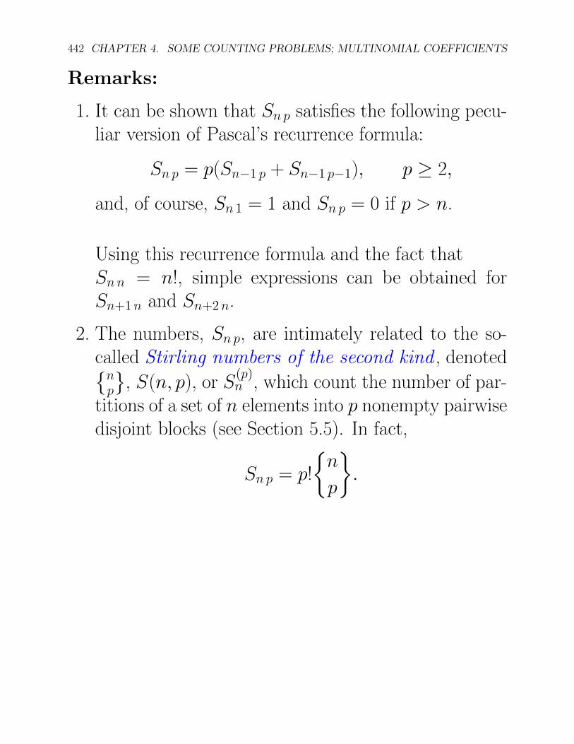
1. It can be shown that Sn p satisfies the following pecu-liar version of Pascal’s recurrence formula:
Sn p = p(Sn�1 p + Sn�1 p�1), p � 2,
and, of course, Sn 1 = 1 and Sn p = 0 if p > n.
Using this recurrence formula and the fact thatSn n = n!, simple expressions can be obtained forSn+1 n and Sn+2 n.
2. The numbers, Sn p, are intimately related to the so-called Stirling numbers of the second kind , denoted�n
p
, S(n, p), or S(p)
n , which count the number of par-titions of a set of n elements into p nonempty pairwisedisjoint blocks (see Section 5.5). In fact,
Sn p = p!
⇢n
p
�.
4.2. COUNTING SUBSETS OF SIZE K; MULTINOMIAL COEFFICIENTS 443
The Stirling numbers,�n
p
, satisfy a recurrence equa-
tion which is another variant of Pascal’s recurrenceformula:⇢
n
1
�= 1
⇢n
n
�= 1
⇢n
p
�=
⇢n � 1
p � 1
�+ p
⇢n � 1
p
�(1 p < n).
The total numbers of partitions of a set with n � 1elements is given by the Bell number ,
bn =nX
p=1
⇢n
p
�.
There is a recurrence formula for the Bell numbersbut it is complicated and not very useful because theformula for bn+1 involves all the previous Bell num-bers.
A good reference for all these special numbers is Graham,Knuth and Patashnik [9], Chapter 6.
444 CHAPTER 4. SOME COUNTING PROBLEMS; MULTINOMIAL COEFFICIENTS
Figure 4.3: Eric Temple Bell, 1883-1960 (left) and Donald Knuth, 1938- (right)
The binomial coe�cients can be generalized as follows.For all n, m, k1, . . . , km 2 N, with k1+ · · ·+km = n andm � 2, we have the multinomial coe�cient ,
✓n
k1 · · · km
◆,
which counts the number of ways of splitting a set of nelements into an ordered sequence of m disjoint subsets,the ith subset having ki � 0 elements.
Such sequences of disjoint subsets whose union is {1, . . . , n}itself are sometimes called ordered partitions .
Beware that some of the subsets in an ordered partitionmay be empty, so we feel that the terminology “partition”is confusing since as will see in Section 5.5, the subsetsthat form a partition are never empty.
4.2. COUNTING SUBSETS OF SIZE K; MULTINOMIAL COEFFICIENTS 445
Note that when m = 2, the number of ways of splittinga set of n elements into two disjoint subsets where thefirst subset has k1 elements and the second subset hask2 = n � k1 elements is precisely the number of subsetsof size k1 of a set of n elements, that is
✓n
k1 k2
◆=
✓n
k1
◆.
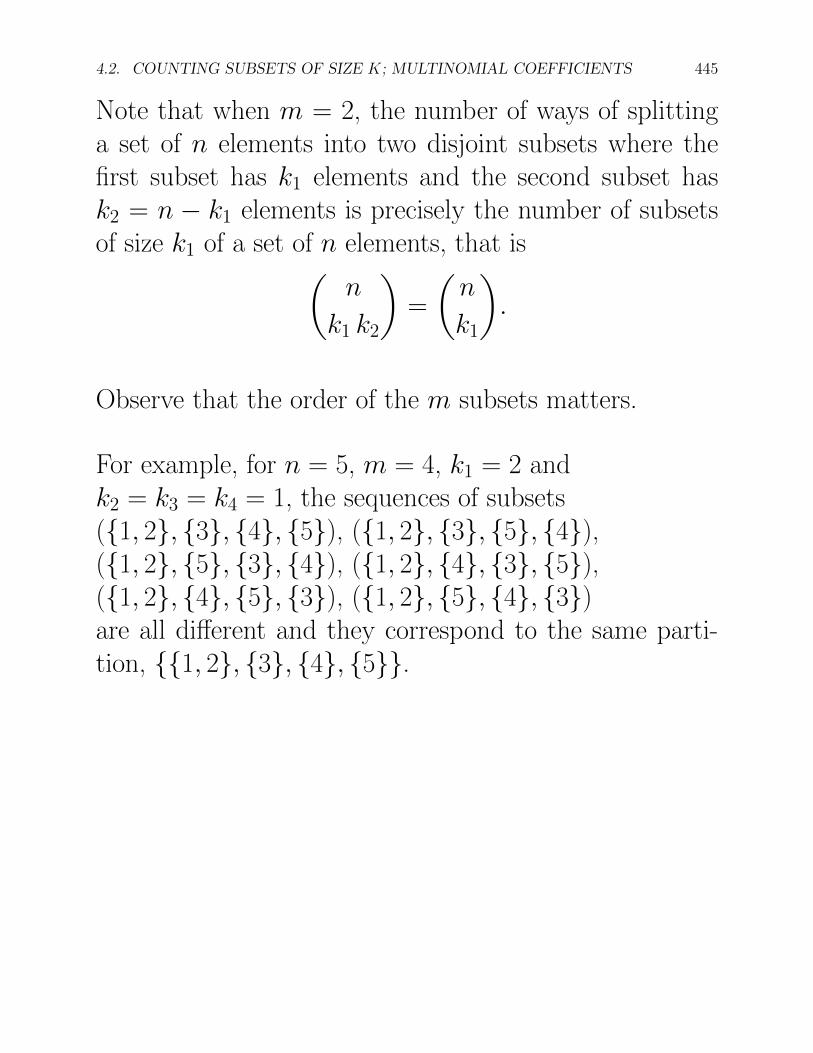
Observe that the order of the m subsets matters.
For example, for n = 5, m = 4, k1 = 2 andk2 = k3 = k4 = 1, the sequences of subsets({1, 2}, {3}, {4}, {5}), ({1, 2}, {3}, {5}, {4}),({1, 2}, {5}, {3}, {4}), ({1, 2}, {4}, {3}, {5}),({1, 2}, {4}, {5}, {3}), ({1, 2}, {5}, {4}, {3})are all di↵erent and they correspond to the same parti-tion, {{1, 2}, {3}, {4}, {5}}.
446 CHAPTER 4. SOME COUNTING PROBLEMS; MULTINOMIAL COEFFICIENTS
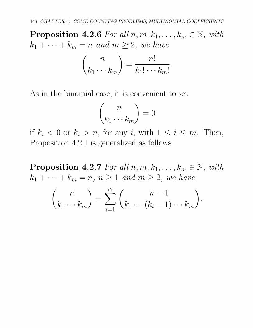
Proposition 4.2.6 For all n, m, k1, . . . , km 2 N, withk1 + · · · + km = n and m � 2, we have
✓n
k1 · · · km
◆=
n!
k1! · · · km!.
As in the binomial case, it is convenient to set✓
n
k1 · · · km
◆= 0
if ki < 0 or ki > n, for any i, with 1 i m. Then,Proposition 4.2.1 is generalized as follows:
Proposition 4.2.7 For all n, m, k1, . . . , km 2 N, withk1 + · · · + km = n, n � 1 and m � 2, we have
✓n
k1 · · · km
◆=
mX
i=1
✓n � 1
k1 · · · (ki � 1) · · · km
◆.
4.2. COUNTING SUBSETS OF SIZE K; MULTINOMIAL COEFFICIENTS 447
Remark: Proposition 4.2.7 shows that Pascal’s trianglegeneralizes to “higher dimensions”, that is, to m � 3.
Indeed, it is possible to give a geometric interpretationof Proposition 4.2.7 in which the multinomial coe�cientscorresponding to those k1, . . . , km with k1+ · · ·+km = nlie on the hyperplane of equation x1 + · · · + xm = n inRm, and all the multinomial coe�cients for which n N ,for any fixed N , lie in a generalized tetrahedron called asimplex .
When m = 3, the multinomial coe�cients for whichn N lie in a tetrahedron whose faces are the planesof equations, x = 0; y = 0; z = 0; and x + y + z = N .
We have also the following generalization of Proposition4.2.3:
448 CHAPTER 4. SOME COUNTING PROBLEMS; MULTINOMIAL COEFFICIENTS
Proposition 4.2.8 (Multinomial Formula) For alln, m 2 N with m � 2, for all pairwise commutingvariables a1, . . . , am, we have
(a1 + · · · + am)n =
X
k1,...,km�0k1+···+km=n
✓n
k1 · · · km
◆ak1
1 · · · akmm .
How many terms occur on the right-hand side of themultinomial formula?
After a moment of reflexion, we see that this is the numberof finite multisets of size n whose elements are drawn froma set of m elements, which is also equal to the number ofm-tuples, k1, . . . , km, with ki 2 N and
k1 + · · · + km = n.
Proposition 4.2.9 The number of finite multisets ofsize n � 0 whose elements come from a set of sizem � 1 is ✓
m + n � 1
n
◆.
4.3. SOME PROPERTIES OF THE BINOMIAL COEFFICIENTS 449
4.3 Some Properties of the Binomial Coe�cients
The binomial coe�cients satisfy many remarkable identi-ties.
If one looks at the Pascal triangle, it is easy to figure outwhat are the sums of the elements in any given row
It is also easy to figure out what are the sums of n�m+1consecutive elements in any given column (starting fromthe top and with 0 m n).
What about the sums of elements on the diagonals? Again,it is easy to determine what these sums are.
Here are the answers, beginning with sums of the elementsin a column.
(a) Sum of the first n � m + 1 elements in column m(0 m n).
450 CHAPTER 4. SOME COUNTING PROBLEMS; MULTINOMIAL COEFFICIENTS
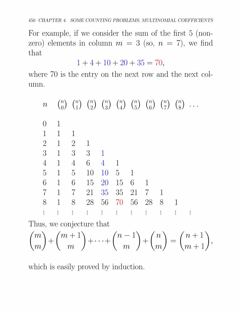
For example, if we consider the sum of the first 5 (non-zero) elements in column m = 3 (so, n = 7), we findthat
1 + 4 + 10 + 20 + 35 = 70,
where 70 is the entry on the next row and the next col-umn.
n�n
0
� �n1
� �n2
� �n3
� �n4
� �n5
� �n6
� �n7
� �n8
�. . .
0 11 1 12 1 2 13 1 3 3 14 1 4 6 4 15 1 5 10 10 5 16 1 6 15 20 15 6 17 1 7 21 35 35 21 7 18 1 8 28 56 70 56 28 8 1... ... ... ... ... ... ... ... ... ... ...
Thus, we conjecture that✓m
m
◆+
✓m + 1
m
◆+ · · ·+
✓n � 1
m
◆+
✓n
m
◆=
✓n + 1
m + 1
◆,
which is easily proved by induction.
4.3. SOME PROPERTIES OF THE BINOMIAL COEFFICIENTS 451
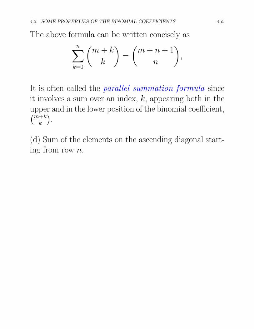
The above formula can be written concisely as
nX
k=m
✓k
m
◆=
✓n + 1
m + 1
◆,
or even as
nX
k=0
✓k
m
◆=
✓n + 1
m + 1
◆,
since� km
�= 0 when k < m.
It is often called the upper summation formula since itinvolves a sum over an index, k, appearing in the upperposition of the binomial coe�cient,
� km
�.
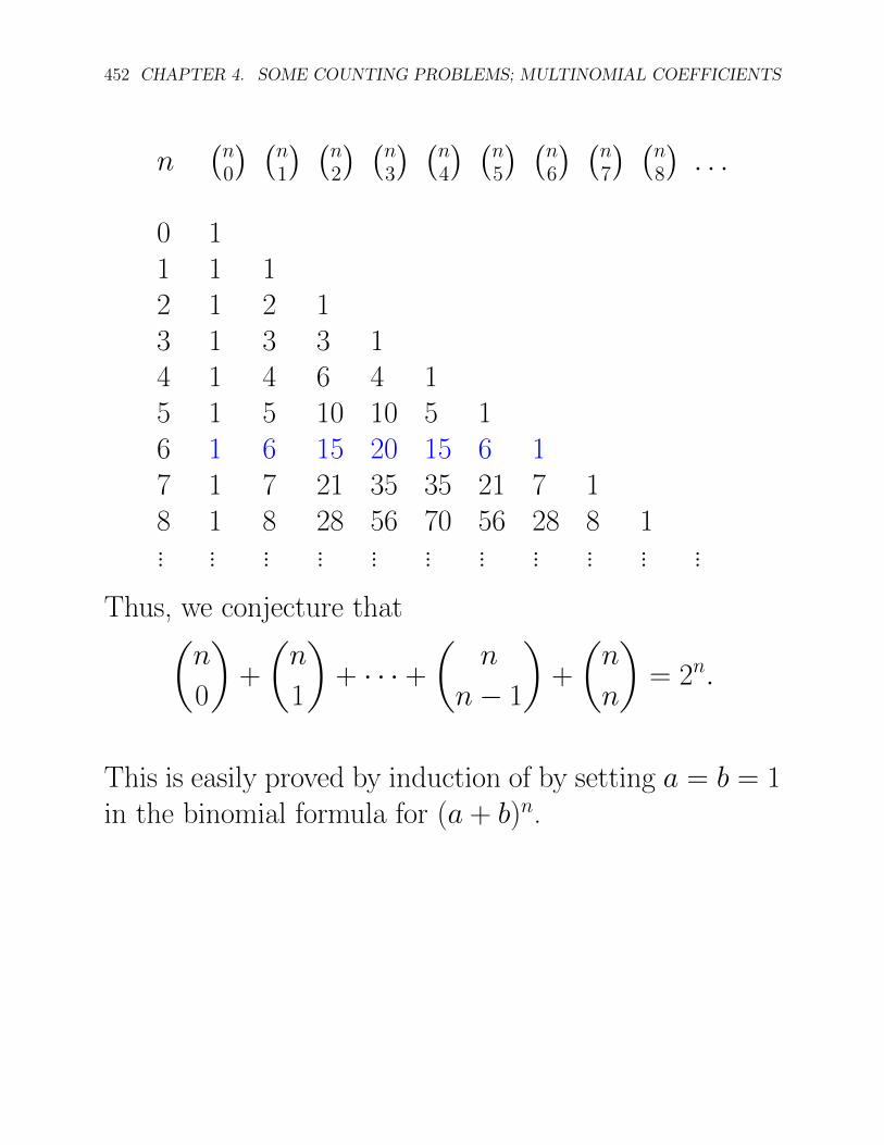
(b) Sum of the elements in row n.
For example, if we consider the sum of the elements inrow n = 6, we find that
1 + 6 + 15 + 20 + 15 + 6 + 1 = 64 = 26.
452 CHAPTER 4. SOME COUNTING PROBLEMS; MULTINOMIAL COEFFICIENTS
n�n
0
� �n1
� �n2
� �n3
� �n4
� �n5
� �n6
� �n7
� �n8
�. . .
0 11 1 12 1 2 13 1 3 3 14 1 4 6 4 15 1 5 10 10 5 16 1 6 15 20 15 6 17 1 7 21 35 35 21 7 18 1 8 28 56 70 56 28 8 1... ... ... ... ... ... ... ... ... ... ...
Thus, we conjecture that✓
n
0
◆+
✓n
1
◆+ · · · +
✓n
n � 1
◆+
✓n
n
◆= 2n.
This is easily proved by induction of by setting a = b = 1in the binomial formula for (a + b)n.
4.3. SOME PROPERTIES OF THE BINOMIAL COEFFICIENTS 453
Unlike the columns for which there is a formula for thepartial sums, there is no closed form formula for the par-tial sums of the rows.
However, there is a closed form formula for partial al-ternating sums of rows. Indeed, it is easily shown byinduction that
mX
k=0
(�1)k✓
n
k
◆= (�1)m
✓n � 1
m
◆,
if 0 m n. For example
1 � 7 + 21 � 35 = �20.
Also, for m = n, we getnX
k=0
(�1)k✓
n
k
◆= 0.
(c) Sum of the first n + 1 elements on the descendingdiagonal starting from row m.
454 CHAPTER 4. SOME COUNTING PROBLEMS; MULTINOMIAL COEFFICIENTS
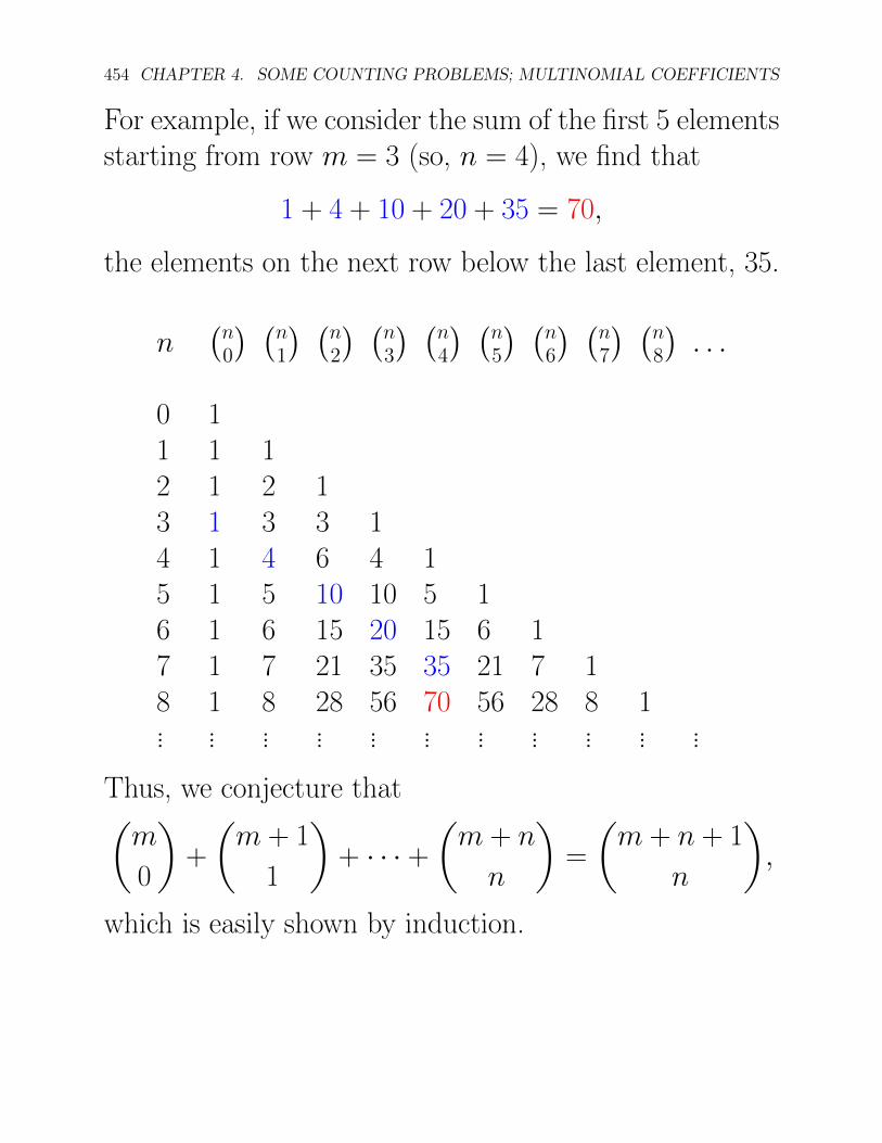
For example, if we consider the sum of the first 5 elementsstarting from row m = 3 (so, n = 4), we find that
1 + 4 + 10 + 20 + 35 = 70,
the elements on the next row below the last element, 35.
n�n
0
� �n1
� �n2
� �n3
� �n4
� �n5
� �n6
� �n7
� �n8
�. . .
0 11 1 12 1 2 13 1 3 3 14 1 4 6 4 15 1 5 10 10 5 16 1 6 15 20 15 6 17 1 7 21 35 35 21 7 18 1 8 28 56 70 56 28 8 1... ... ... ... ... ... ... ... ... ... ...
Thus, we conjecture that✓
m
0
◆+
✓m + 1
1
◆+ · · · +
✓m + n
n
◆=
✓m + n + 1
n
◆,
which is easily shown by induction.
4.3. SOME PROPERTIES OF THE BINOMIAL COEFFICIENTS 455
The above formula can be written concisely asnX
k=0
✓m + k
k
◆=
✓m + n + 1
n
◆,
It is often called the parallel summation formula sinceit involves a sum over an index, k, appearing both in theupper and in the lower position of the binomial coe�cient,�m+k
k
�.
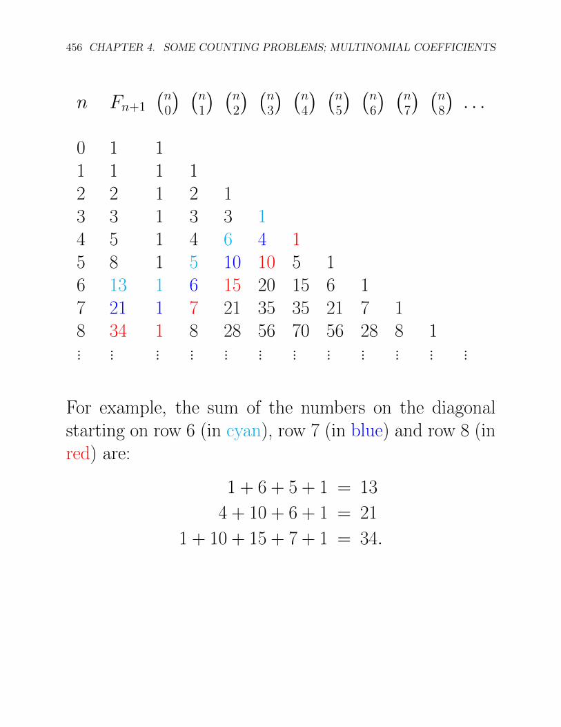
(d) Sum of the elements on the ascending diagonal start-ing from row n.
456 CHAPTER 4. SOME COUNTING PROBLEMS; MULTINOMIAL COEFFICIENTS
n Fn+1
�n0
� �n1
� �n2
� �n3
� �n4
� �n5
� �n6
� �n7
� �n8
�. . .
0 1 11 1 1 12 2 1 2 13 3 1 3 3 14 5 1 4 6 4 15 8 1 5 10 10 5 16 13 1 6 15 20 15 6 17 21 1 7 21 35 35 21 7 18 34 1 8 28 56 70 56 28 8 1... ... ... ... ... ... ... ... ... ... ... ...
For example, the sum of the numbers on the diagonalstarting on row 6 (in cyan), row 7 (in blue) and row 8 (inred) are:
1 + 6 + 5 + 1 = 13
4 + 10 + 6 + 1 = 21
1 + 10 + 15 + 7 + 1 = 34.
4.3. SOME PROPERTIES OF THE BINOMIAL COEFFICIENTS 457
We recognize the Fibonacci numbers , F7, F8 and F9,what a nice surprise!
Recall that F0 = 0, F1 = 1 and
Fn+2 = Fn+1 + Fn.
Thus, we conjecture that
Fn+1 =
✓n
0
◆+
✓n � 1
1
◆+
✓n � 2
2
◆+ · · · +
✓0
n
◆.
The above formula can indeed be proved by induction,but we have to distinguish the two case where n is evenor odd.
We now list a few more formulae which are often used inthe manipulations of binomial coe�cients.
They are among the “top ten binomial coe�cient iden-tities” listed in Graham, Knuth and Patashnik [9], seeChapter 5.
458 CHAPTER 4. SOME COUNTING PROBLEMS; MULTINOMIAL COEFFICIENTS
(e) The equation✓
n
i
◆✓n � i
k � i
◆=
✓k
i
◆✓n
k
◆,
holds for all n, i, k, with 0 i k n.
This is because, we find that after a few calculations,✓
n
i
◆✓n � i
k � i
◆=
n!
i!(k � i)!(n � k)!=
✓k
i
◆✓n
k
◆.
Observe that the expression in the middle is really thetrinomial coe�cient✓
n
i k � i n � k
◆.
For this reason, the equation (e) is often called trinomialrevision .
4.3. SOME PROPERTIES OF THE BINOMIAL COEFFICIENTS 459
For i = 1, we get
n
✓n � 1
k � 1
◆= k
✓n
k
◆.
So, if k 6= 0, we get the equation✓
n
k
◆=
n
k
✓n � 1
k � 1
◆, k 6= 0.
This equation is often called the absorption identity .
(f) The equation✓
m + p
n
◆=
mX
k=0
✓m
k
◆✓p
n � k
◆
holds for m, n, p � 0 such that m + p � n.
This equation is usually known as Vandermonde convo-lution .
460 CHAPTER 4. SOME COUNTING PROBLEMS; MULTINOMIAL COEFFICIENTS
An interesting special case of Vandermonde convolutionarises when m = p = n. In this case, we get the equation
✓2n
n
◆=
nX
k=0
✓n
k
◆✓n
n � k
◆.
However,�n
k
�=� nn�k
�, so we get
nX
k=0
✓n
k
◆2
=
✓2n
n
◆,
that is, the sum of the squares of the entries on row n ofthe Pascal triangle is the middle element on row 2n.
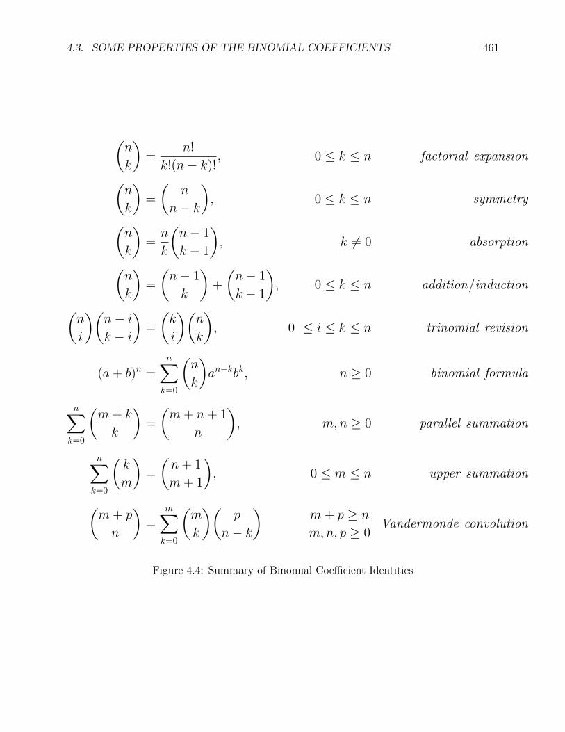
A summary of the top nine binomial coe�cient identitiesis given in Figure 4.4.
4.3. SOME PROPERTIES OF THE BINOMIAL COEFFICIENTS 461
✓n
k
◆=
n!
k!(n � k)!, 0 k n factorial expansion
✓n
k
◆=
✓n
n � k
◆, 0 k n symmetry
✓n
k
◆=
n
k
✓n � 1
k � 1
◆, k 6= 0 absorption
✓n
k
◆=
✓n � 1
k
◆+
✓n � 1
k � 1
◆, 0 k n addition/induction
✓n
i
◆✓n � i
k � i
◆=
✓k
i
◆✓n
k
◆, 0 i k n trinomial revision
(a + b)n =nX
k=0
✓n
k
◆an�kbk, n � 0 binomial formula
nX
k=0
✓m + k
k
◆=
✓m + n + 1
n
◆, m, n � 0 parallel summation
nX
k=0
✓k
m
◆=
✓n + 1
m + 1
◆, 0 m n upper summation
✓m + p
n
◆=
mX
k=0
✓m
k
◆✓p
n � k
◆m + p � n
m, n, p � 0Vandermonde convolution
Figure 4.4: Summary of Binomial Coe�cient Identities
462 CHAPTER 4. SOME COUNTING PROBLEMS; MULTINOMIAL COEFFICIENTS
Remark: Going back to the generalized binomial coef-ficients,
�rk
�, where r is a real number, possibly negative,
the following formula is easily shown:✓
r
k
◆= (�1)k
✓k � r � 1
k
◆,
where r 2 R and k 2 Z.
If r < 0 and k � 1 then k � r � 1 > 0, so the formulashows how a binomial coe�cient with negative upper in-dex can be expessed as a binomial coe�cient with positiveindex.
For this reason, this formula is known as negating theupper index .
4.3. SOME PROPERTIES OF THE BINOMIAL COEFFICIENTS 463
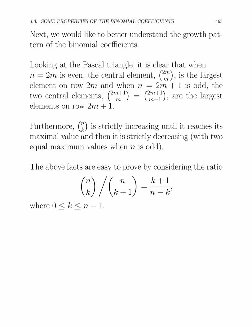
Next, we would like to better understand the growth pat-tern of the binomial coe�cients.
Looking at the Pascal triangle, it is clear that whenn = 2m is even, the central element,
�2mm
�, is the largest
element on row 2m and when n = 2m + 1 is odd, thetwo central elements,
�2m+1
m
�=�
2m+1m+1
�, are the largest
elements on row 2m + 1.
Furthermore,�n
k
�is strictly increasing until it reaches its
maximal value and then it is strictly decreasing (with twoequal maximum values when n is odd).
The above facts are easy to prove by considering the ratio✓
n
k
◆�✓n
k + 1
◆=
k + 1
n � k,
where 0 k n � 1.
464 CHAPTER 4. SOME COUNTING PROBLEMS; MULTINOMIAL COEFFICIENTS
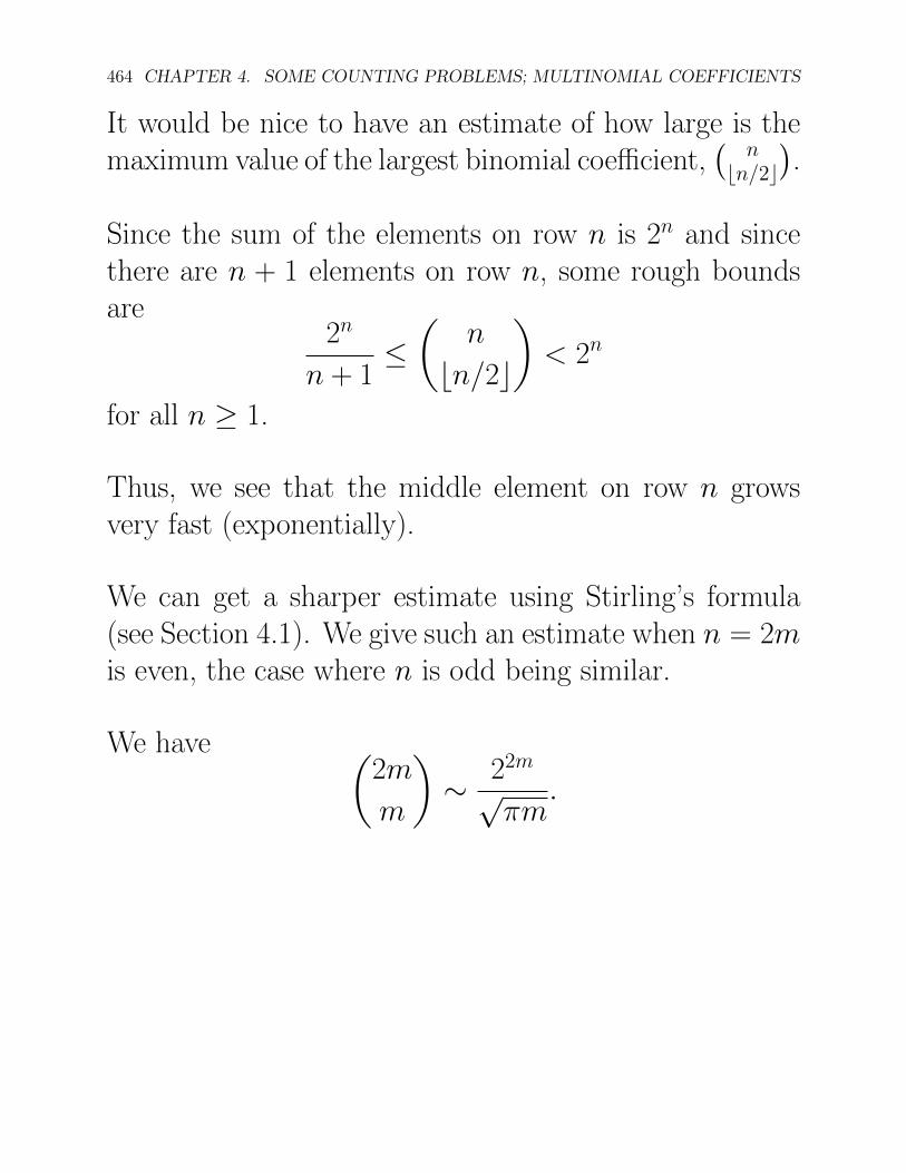
It would be nice to have an estimate of how large is themaximum value of the largest binomial coe�cient,
� nbn/2c
�.
Since the sum of the elements on row n is 2n and sincethere are n + 1 elements on row n, some rough boundsare
2n
n + 1✓
n
bn/2c◆
< 2n
for all n � 1.
Thus, we see that the middle element on row n growsvery fast (exponentially).
We can get a sharper estimate using Stirling’s formula(see Section 4.1). We give such an estimate when n = 2mis even, the case where n is odd being similar.
We have ✓2m
m
◆⇠ 22m
p⇡m
.
4.3. SOME PROPERTIES OF THE BINOMIAL COEFFICIENTS 465
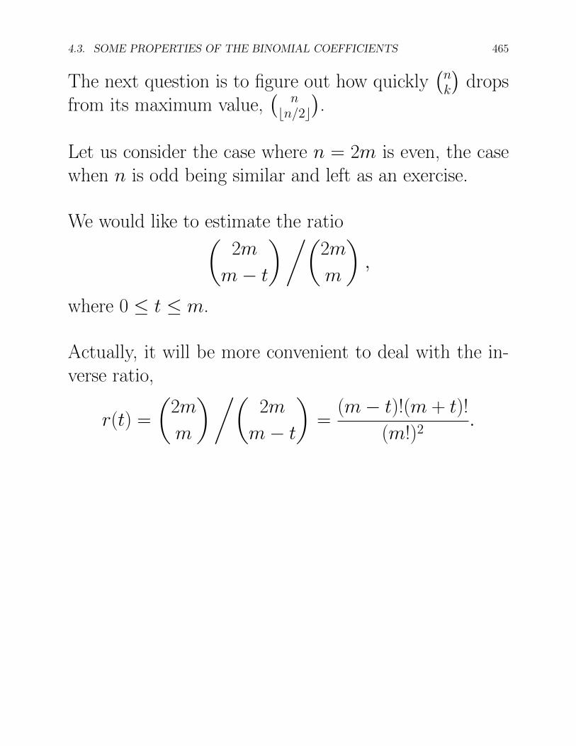
The next question is to figure out how quickly�n
k
�drops
from its maximum value,� nbn/2c
�.
Let us consider the case where n = 2m is even, the casewhen n is odd being similar and left as an exercise.
We would like to estimate the ratio✓2m
m � t
◆�✓2m
m
◆,
where 0 t m.
Actually, it will be more convenient to deal with the in-verse ratio,
r(t) =
✓2m
m
◆�✓2m
m � t
◆=
(m � t)!(m + t)!
(m!)2.
466 CHAPTER 4. SOME COUNTING PROBLEMS; MULTINOMIAL COEFFICIENTS
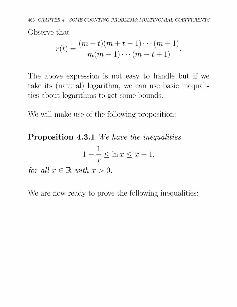
Observe that
r(t) =(m + t)(m + t � 1) · · · (m + 1)
m(m � 1) · · · (m � t + 1).
The above expression is not easy to handle but if wetake its (natural) logarithm, we can use basic inequali-ties about logarithms to get some bounds.
We will make use of the following proposition:
Proposition 4.3.1 We have the inequalities
1 � 1
x ln x x � 1,
for all x 2 R with x > 0.
We are now ready to prove the following inequalities:
4.3. SOME PROPERTIES OF THE BINOMIAL COEFFICIENTS 467
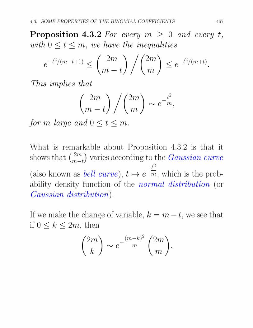
Proposition 4.3.2 For every m � 0 and every t,with 0 t m, we have the inequalities
e�t2/(m�t+1) ✓
2m
m � t
◆�✓2m
m
◆ e�t2/(m+t).
This implies that✓
2m
m � t
◆�✓2m
m
◆⇠ e� t2
m,
for m large and 0 t m.
What is remarkable about Proposition 4.3.2 is that itshows that
�2mm�t
�varies according to the Gaussian curve
(also known as bell curve), t 7! e� t2
m , which is the prob-ability density function of the normal distribution (orGaussian distribution).
If we make the change of variable, k = m� t, we see thatif 0 k 2m, then
✓2m
k
◆⇠ e�(m�k)2
m
✓2m
m
◆.
468 CHAPTER 4. SOME COUNTING PROBLEMS; MULTINOMIAL COEFFICIENTS
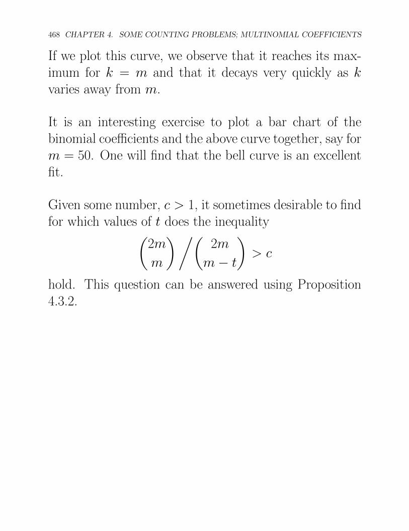
If we plot this curve, we observe that it reaches its max-imum for k = m and that it decays very quickly as kvaries away from m.
It is an interesting exercise to plot a bar chart of thebinomial coe�cients and the above curve together, say form = 50. One will find that the bell curve is an excellentfit.
Given some number, c > 1, it sometimes desirable to findfor which values of t does the inequality
✓2m
m
◆�✓2m
m � t
◆> c
hold. This question can be answered using Proposition4.3.2.
4.3. SOME PROPERTIES OF THE BINOMIAL COEFFICIENTS 469
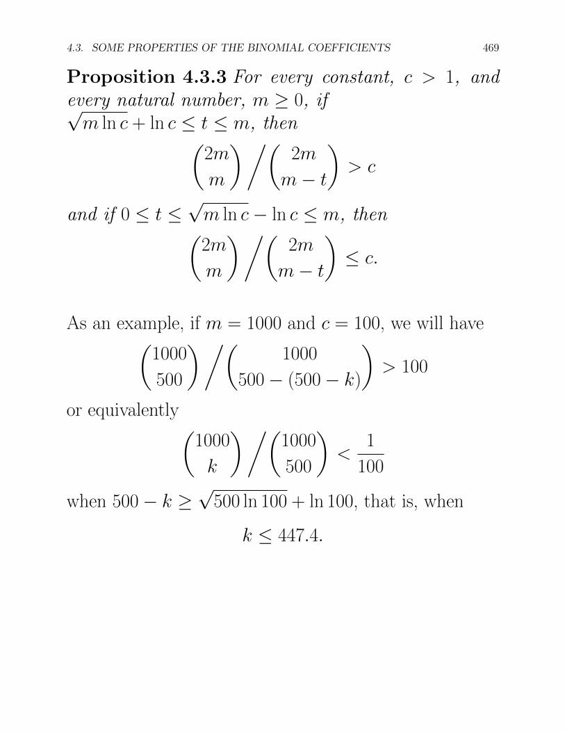
Proposition 4.3.3 For every constant, c > 1, andevery natural number, m � 0, ifp
m ln c + ln c t m, then✓2m
m
◆�✓2m
m � t
◆> c
and if 0 t pm ln c � ln c m, then
✓2m
m
◆�✓2m
m � t
◆ c.
As an example, if m = 1000 and c = 100, we will have✓1000
500
◆�✓1000
500 � (500 � k)
◆> 100
or equivalently✓1000
k
◆�✓1000
500
◆<
1
100
when 500 � k � p500 ln 100 + ln 100, that is, when
k 447.4.
470 CHAPTER 4. SOME COUNTING PROBLEMS; MULTINOMIAL COEFFICIENTS
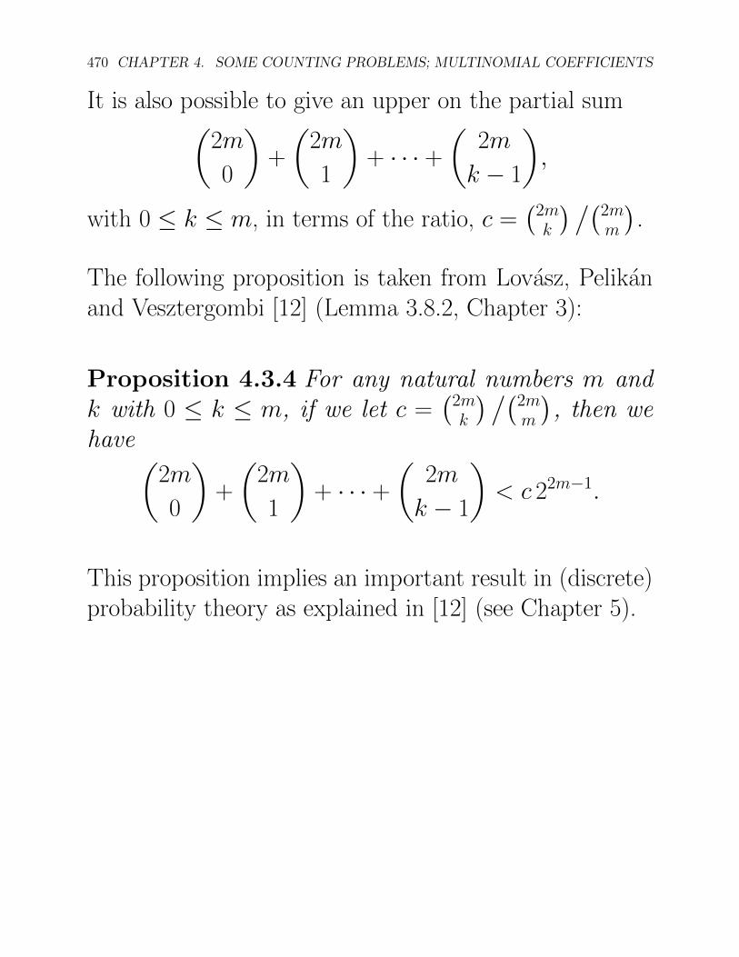
It is also possible to give an upper on the partial sum✓2m
0
◆+
✓2m
1
◆+ · · · +
✓2m
k � 1
◆,
with 0 k m, in terms of the ratio, c =�
2mk
� ��2mm
�.
The following proposition is taken from Lovasz, Pelikanand Vesztergombi [12] (Lemma 3.8.2, Chapter 3):
Proposition 4.3.4 For any natural numbers m andk with 0 k m, if we let c =
�2mk
� ��2mm
�, then we
have ✓2m
0
◆+
✓2m
1
◆+ · · · +
✓2m
k � 1
◆< c 22m�1.
This proposition implies an important result in (discrete)probability theory as explained in [12] (see Chapter 5).
4.3. SOME PROPERTIES OF THE BINOMIAL COEFFICIENTS 471
Observe that 22m is the sum of all the entries on row 2m.
As an application, if k 447, the sum of the first 447numbers on row 1000 of the Pascal triangle makes up lessthan 0.5% of the total sum and similarly for the last 447entries.
Thus, the middle 107 entries account for 99% of the totalsum.
472 CHAPTER 4. SOME COUNTING PROBLEMS; MULTINOMIAL COEFFICIENTS
4.4 The Inclusion-Exclusion Principle, Sylvester’s For-mula, The Sieve Formula
We close this chapter with the proof of a poweful formulafor determining the cardinality of the union of a finitenumber of (finite) sets in terms of the cardinalities of thevarious intersections of these sets.
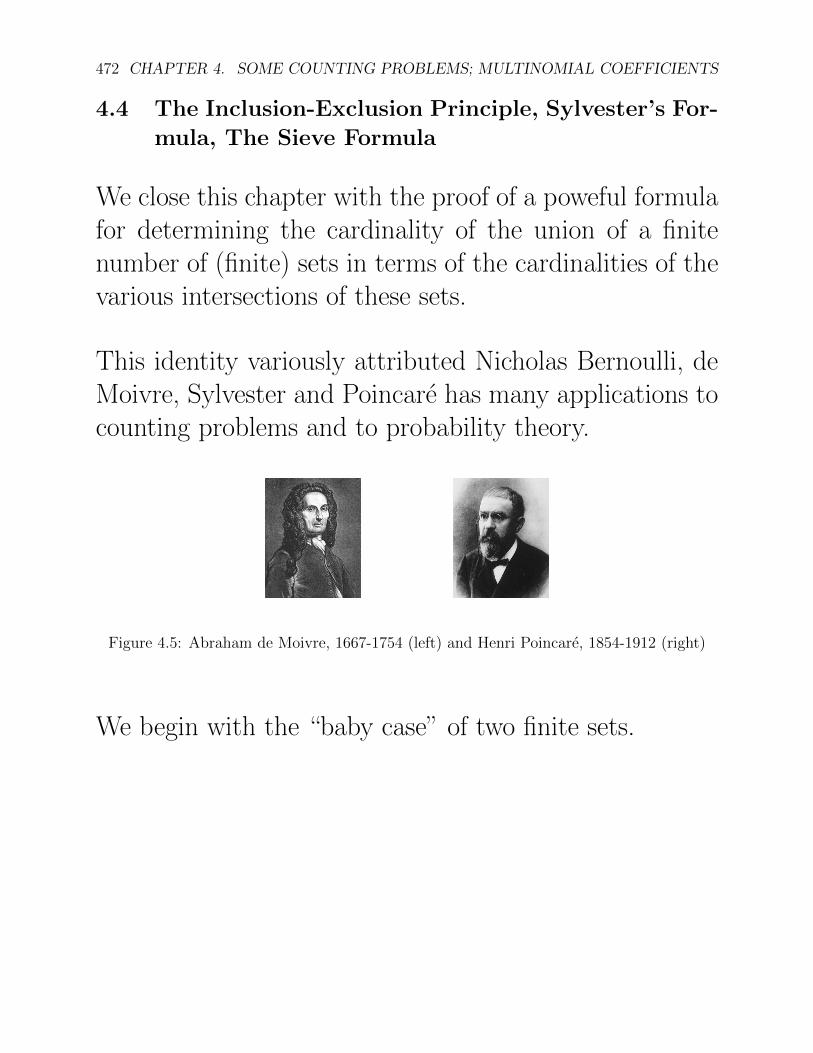
This identity variously attributed Nicholas Bernoulli, deMoivre, Sylvester and Poincare has many applications tocounting problems and to probability theory.
Figure 4.5: Abraham de Moivre, 1667-1754 (left) and Henri Poincare, 1854-1912 (right)
We begin with the “baby case” of two finite sets.
4.4. THE INCLUSION-EXCLUSION PRINCIPLE 473
Proposition 4.4.1 Given any two finite sets, A, andB, we have
|A [ B| = |A| + |B| � |A \ B|.
We would like to generalize the formula of Proposition4.4.1 to any finite collection of finite sets, A1, . . . , An.
A moment of reflexion shows that when n = 3, we have
|A[B[C| = |A|+|B|+|C|�|A\B|�|A\C|�|B\C|+ |A \ B \ C|.
One of the obstacles in generalizing the above formula ton sets is purely notational: We need a way of denotingarbitrary intersections of sets belonging to a family ofsets indexed by {1, . . . , n}.
474 CHAPTER 4. SOME COUNTING PROBLEMS; MULTINOMIAL COEFFICIENTS
We can do this by using indices ranging over subsets of{1, . . . , n}, as opposed to indices ranging over integers.
So, for example, for any nonempty subset, I ✓ {1, . . . , n},the expression
Ti2I Ai denotes the intersection of all the
subsets whose index, i, belongs to I .
Theorem 4.4.2 (Inclusion-Exclusion Principle) Forany finite sequence, A1, . . . , An, ofn � 2 subsets of a finite set, X, we have
�����
n[
k=1
Ak
����� =X
I✓{1,...,n}I 6=;
(�1)(|I|�1)
�����\
i2I
Ai
����� .
As an application of the Inclusion-Exclusion Principle, letus prove the formula for counting the number of surjec-tions from {1, . . . , n} to {1, . . . , p}, with p n, given inProposition 4.2.5.
4.4. THE INCLUSION-EXCLUSION PRINCIPLE 475
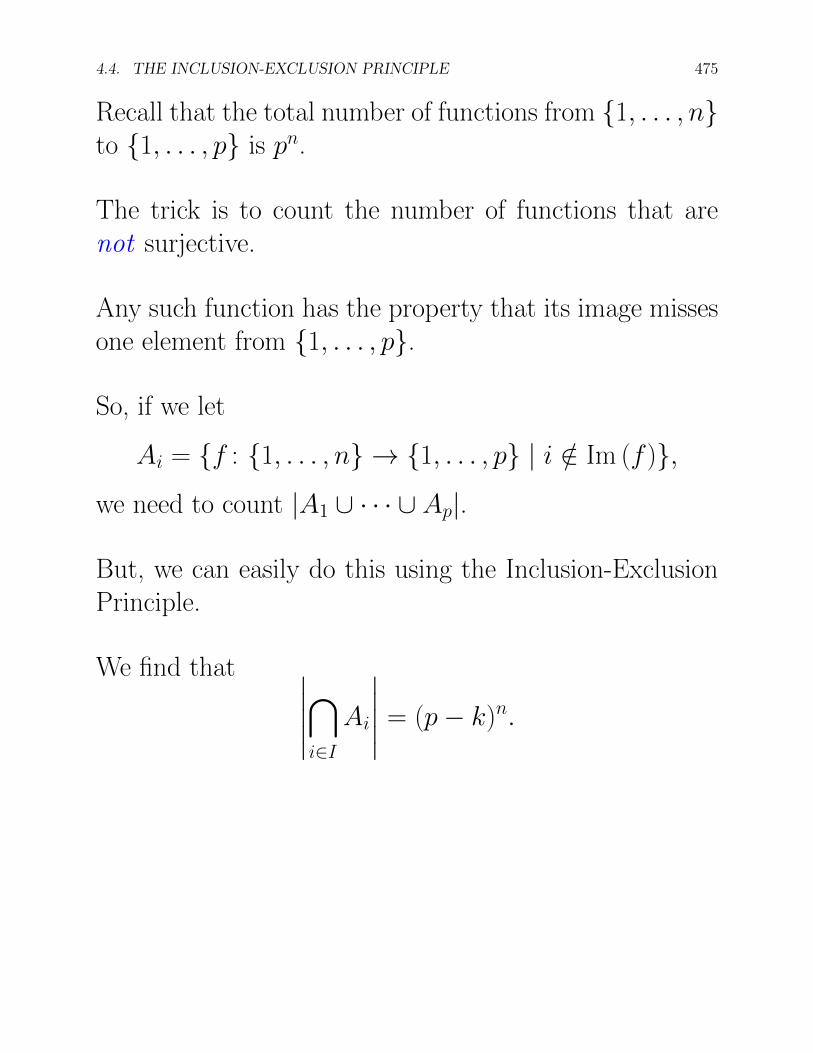
Recall that the total number of functions from {1, . . . , n}to {1, . . . , p} is pn.
The trick is to count the number of functions that arenot surjective.
Any such function has the property that its image missesone element from {1, . . . , p}.
So, if we let
Ai = {f : {1, . . . , n} ! {1, . . . , p} | i /2 Im (f )},
we need to count |A1 [ · · · [ Ap|.
But, we can easily do this using the Inclusion-ExclusionPrinciple.
We find that �����\
i2I
Ai
����� = (p � k)n.
476 CHAPTER 4. SOME COUNTING PROBLEMS; MULTINOMIAL COEFFICIENTS
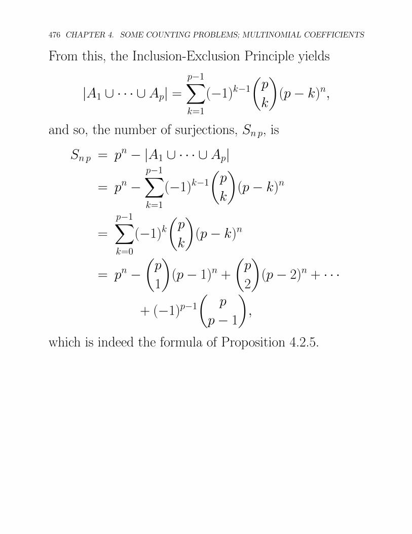
From this, the Inclusion-Exclusion Principle yields
|A1 [ · · · [ Ap| =p�1X
k=1
(�1)k�1
✓p
k
◆(p � k)n,
and so, the number of surjections, Sn p, is
Sn p = pn � |A1 [ · · · [ Ap|
= pn �p�1X
k=1
(�1)k�1
✓p
k
◆(p � k)n
=p�1X
k=0
(�1)k✓
p
k
◆(p � k)n
= pn �✓
p
1
◆(p � 1)n +
✓p
2
◆(p � 2)n + · · ·
+ (�1)p�1
✓p
p � 1
◆,
which is indeed the formula of Proposition 4.2.5.
4.4. THE INCLUSION-EXCLUSION PRINCIPLE 477
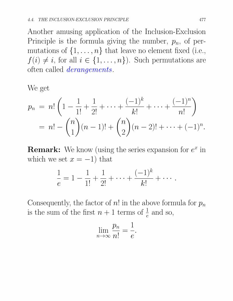
Another amusing application of the Inclusion-ExclusionPrinciple is the formula giving the number, pn, of per-mutations of {1, . . . , n} that leave no element fixed (i.e.,f (i) 6= i, for all i 2 {1, . . . , n}). Such permutations areoften called derangements .
We get
pn = n!
✓1 � 1
1!+
1
2!+ · · · + (�1)k
k!+ · · · + (�1)n
n!
◆
= n! �✓
n
1
◆(n � 1)! +
✓n
2
◆(n � 2)! + · · · + (�1)n.
Remark: We know (using the series expansion for ex inwhich we set x = �1) that
1
e= 1 � 1
1!+
1
2!+ · · · + (�1)k
k!+ · · · .
Consequently, the factor of n! in the above formula for pn
is the sum of the first n + 1 terms of 1e and so,
limn!1
pn
n!=
1
e.
478 CHAPTER 4. SOME COUNTING PROBLEMS; MULTINOMIAL COEFFICIENTS
It turns out that the series for 1e converges very rapidly,
so pn ⇡ 1en!.
The ratio pn/n! has an interesting interpretation in termsof probabilities .
Assume n persons go to a restaurant (or to the theatre,etc.) and that they all check their coats. Unfortunately,the cleck loses all the coat tags.
Then, pn/n! is the probability that nobody will get heror his own coat back!
As we just explained, this probability is roughly 1e ⇡ 1
3, asurprisingly large number .
The Inclusion-Exclusion Principle can be easily general-ized in a useful way as follows:
4.4. THE INCLUSION-EXCLUSION PRINCIPLE 479
Given a finite set, X , let m be any given function,m : X ! R+, and for any nonempty subset, A ✓ X , set
m(A) =X
a2A
m(a),
with the convention that m(;) = 0 (Recall thatR+ = {x 2 R | x � 0}).
For any x 2 X , the number m(x) is called the weight(or measure) of x and the quantity m(A) is often calledthe measure of the set A.
For example, ifm(x) = 1 for all x 2 A, thenm(A) = |A|,the cardinality of A, which is the special case that we havebeen considering.
For any two subsets, A, B ✓ X , it is obvious that
m(A [ B) = m(A) + m(B) � m(A \ B)
m(X � A) = m(X) � m(A)
m(A [ B) = m(A \ B)
m(A \ B) = m(A [ B),
where A = X � A.
480 CHAPTER 4. SOME COUNTING PROBLEMS; MULTINOMIAL COEFFICIENTS
Figure 4.6: James Joseph Sylvester, 1814-1897
Then, we have the following version of Theorem 4.4.2:
Theorem 4.4.3 (Inclusion-Exclusion Principle, Ver-sion 2 ) Given any measure function, m : X ! R+, forany finite sequence, A1, . . . , An, of n � 2 subsets of afinite set, X, we have
m
n[
k=1
Ak
!=
X
I✓{1,...,n}I 6=;
(�1)(|I|�1) m
\
i2I
Ai
!.
A useful corollary of Theorem 4.4.3 often known asSylvester’s formula is:
4.4. THE INCLUSION-EXCLUSION PRINCIPLE 481
Theorem 4.4.4 (Sylvester’s Formula) Given any mea-sure, m : X ! R+, for any finite sequence, A1, . . . , An,of n � 2 subsets of a finite set, X, the measure of theset of elements of X that do not belong to any of thesets Ai is given by
m
n\
k=1
Ak
!= m(X) +
X
I✓{1,...,n}I 6=;
(�1)|I| m
\
i2I
Ai
!.
Note that if we use the convention that when the indexset, I , is empty then
\
i2;Ai = X,
then the term m(X) can be included in the above sumby removing the condition that I 6= ; and this version ofSylvester’s formula is written:
m
n\
k=1
Ak
!=
X
I✓{1,...,n}(�1)|I| m
\
i2I
Ai
!.
482 CHAPTER 4. SOME COUNTING PROBLEMS; MULTINOMIAL COEFFICIENTS
Sometimes, it is also convenient to regroup terms involv-ing subsets, I , having the same cardinality and anotherway to state Sylvester’s formula is as follows:
m
n\
k=1
Ak
!=
nX
k=0
(�1)kX
I✓{1,...,n}|I|=k
m
\
i2I
Ai
!.
(Sylvester’s Formula)
Finally, Sylvester’s formula can be generalized to a for-mula usually known as the “Sieve Formula”:
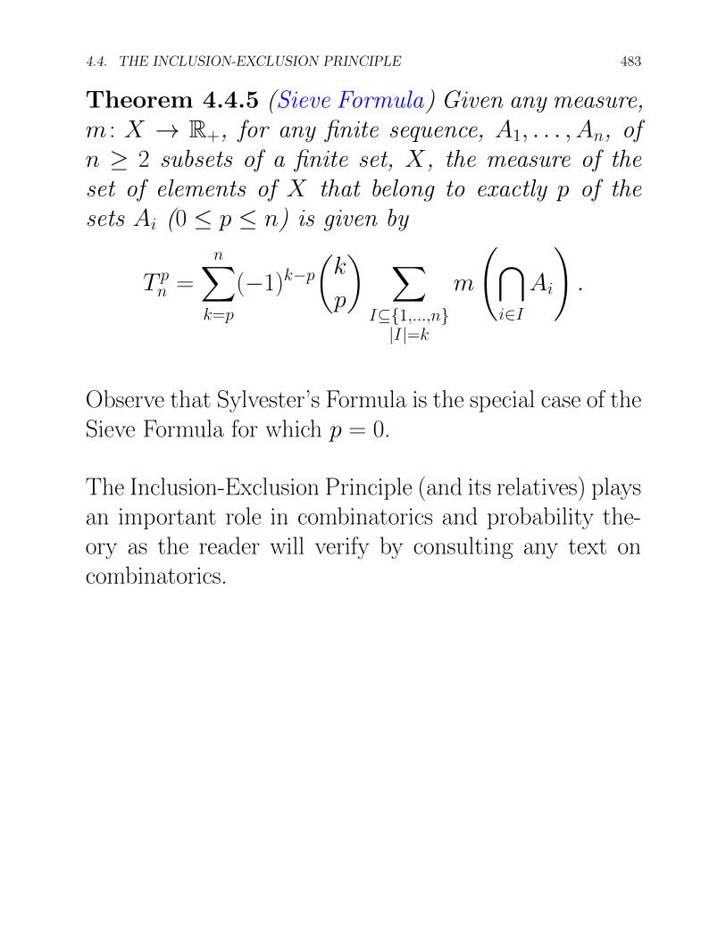
4.4. THE INCLUSION-EXCLUSION PRINCIPLE 483
Theorem 4.4.5 (Sieve Formula) Given any measure,m : X ! R+, for any finite sequence, A1, . . . , An, ofn � 2 subsets of a finite set, X, the measure of theset of elements of X that belong to exactly p of thesets Ai (0 p n) is given by
Tpn =
nX
k=p
(�1)k�p
✓k
p
◆ X
I✓{1,...,n}|I|=k
m
\
i2I
Ai
!.
Observe that Sylvester’s Formula is the special case of theSieve Formula for which p = 0.
The Inclusion-Exclusion Principle (and its relatives) playsan important role in combinatorics and probability the-ory as the reader will verify by consulting any text oncombinatorics.
484 CHAPTER 4. SOME COUNTING PROBLEMS; MULTINOMIAL COEFFICIENTS
A classical reference on combinatorics is Berge [1]; a morerecent is Cameron [3].
More advanced references are van Lint and Wilson [19],and Stanley [17].
Another great (but deceptively tough) reference coveringdiscrete mathematics and including a lot of combinatoricsis Graham, Knuth and Patashnik [9].
Conway and Guy [4] is another beautiful book that presentsmany fascinating and intriguing geometric and combina-torial properties of numbers in a very untertaining man-ner.
For readers interested in geometry with a combinatriolflavor, Matousek [13] is a delightful (but more advanced)reference.
We are now ready to study special kinds of relations:Partial orders and equivalence relations.