chapter 2 the diffusion equation and the steady state library/20041802.pdf · chapter 2 the...

Chapter 2

The Diffusion Equation and the Steady State

We shall now study the equations which govern the neutron field in a reactor. These equationsare based on the concept of local neutron balance, which takes int<:1 accounL the reaction rates in anelement of volume and the net leakage rates out of the volume. The reaction rates are written intenDS of the local cross sections, assumed known from a pre-processed data base (e.g., ENDF/BVI). The starting equation is the Maxwell-Boltzmann transport equation, in its integn:Hiifferentialfonn. The various approximations required to go from the transport equation to the neutrondiffusion equation will first be presented, because all finite-reactor calculations are based on thediffusion approximation. We shall then discuss the multi-group fonnalism of the diffusionequations and study the mathematical properties of these equations in steady state. That preliminarystep will allow liS to derive in a more accurate way, in the next chapter, the reactor point-kineticsequations.

In the diffusion approximation, neutrons diffuse from regions of high concentration to regionsof low concentration, just as heat diffuses from regions of high temperature to those of lowtemperature, or rather as gas molecules diffuse to reduce spatial variations in concentration.

While it is sufficiently accmate to treat the transport of gas molecules as a diffusion process,this approach is too limiting for neutron transport. In contrast to a gas, where collisions are veryfrequent, the cross sectioos for the interaction of neutrons with nuclei are relatively small, as wesaw in chapter 1 (of the order of bams, i.e., 10.24 cm2

). This implies that neutrons traverseappreciable distances (of the order of a centimetre) between collisions. This relatively long neutronmean free path, together with the heterogeneity of the physical medium, requires that a morecomplete treatment be carried out, taking account of variations in the angular distribution of neutronspeed in the vicinity of highly absorbing regions (such as t.'le fuel). The Boltzmann transportequation allows an accurate treatment of neutron leakage in the presence of large heterogeneities.While we shall not directly tackle the solution of the transport equations, the derivation of thediffusion equation from the tr3nsport equation will allow us to appreciate the degree ofapproximation of the methods used in finite-reactor calculations.

2.1 Neutron Balance in a Reactor

From a fundamental point of view, the individual fate of neutrons cannot be defined in adetenninistic manner. The Heisenberg uncertainty principle and quantum mechanics teach us thatonly the probability ofa given fate can be calculated. Thus, if the total number of neutrons in thesystem under observation is relatively small, fluctuations will be observed in the number andenergies of n~utronsat a given point. We shall assume here that the neutron density is sufficientlyhigh that one can neglect these statistical variations and predict the average behaviour 0/ the neutronfield in a deterministic manner. We shall assume in addition that the neutron density is not so highthat neutron-neutron interactions must be taken into account The starting equation for our analysiswill be that which describes detenninistically the interaction of the neutron field with the field ofnuclei., i.e., the Maxwell-Boltzmann neutron transport equation.

26

2.1.1 Transport Equation

Introduction to Nuclear Reactor Kinetics

The transport equation, in its integro-differential fonn, will allow us to describe the neutronbalance in an elel!!Cntal volume in phase spac~. The fundamental quantity is the angular density ofneutrons, n(r,E, n ,t) defined so that n(r,E, n ,t) d3r tfD dE represents the number of neutrons attime i in an element ofvolume tlr around point r. These neutrons have energies between E and E +dE; if a sphere of unit radius is drawn aIQ.und point r, IDe neutrons travel in a direction inside thesolid angle tfD around the radius vector n (the vector n is thus of unit length). The angular c0

ordinates are shown in Figure 2.1.

. Neutrons propagate at scalar speed v, function of E:

~E

v(E)= -mo

Given the direction of travel Q of ta'le neutrons, the velocity vector Vcan be written

v(E) =Qv(E)

(2-1)

(2-2)

- -The density n is continuous, which means that n(r+sn,E, Q ,t+s/v) must be a continuous

function ofs at all points r in the domain.

Fig. 2.1 Spherical Coordinates in Transport Calculations

~:-------------~y

2. The Diffusion Equation and the Steady State 27

We define f!lso the scalar angular-flux density f/J (r,E, {1,/), and the vector angular-currentdensity j (r,E, {1,/), as follows:

and

f/J (r,E, 0,1) = v n(r,E, O,t)

j (r,E,O,t) = OtIJ (r,E,O,t) = v n(r,E,O,t)

(2-3)

(2-4)

The other quantities related to the neutron density are defined in Table 2.1.

Consider now the neutron balance in an element of volume in the 7-dimensional phase spacewith co-ordinates x, y, z, E, {lj' {lB' and t. The rate of change of the neutron density in theelement of volume will of necessIty be the result of a difference between the rates of production andremoval of neutrons.

The removal of neutrons from the volume element comes about as the result of collisionsbetween the neutrons and the nuclei in the volume, or as the result of the leakage of neutrons out ofthe volume. Indeed, we assume that if there is a collision and the neutron is not captured by thetarget, the neutron's fmal velocity will be different from v and its energy will be different from E,so that the neutron exits from the "hypervolume" element Consequently, as soon as there is acollision, the neutron disappears from the element of volume.

On the other hand, the production of neutrons within the volume element can result either fromcollisions or from an independent (external) source q. In order to evaluate the production ofneutrons from collisions, one must integrate over all incidents~s and directions, and retain onlytlte collisions which lead to speed v (or energy E) and angle {1. The "collision source" thereforeincludes neutrons born from fISsions!. \Ve shall assume that all neutrons emerging from a collisionappear instantaneously. That is, we shall neglect delayed-neutron emission for the moment.

Using the notation of Table 2.1, the transport equation in the absence of delayed neutrons canbe written:

~ ~ ell (r,E, 0. ,t) = - I(r,E,r) f/J (r,E, 0. ,t) - 0.. Vf/J (r,E, 0. ,t)

+ I~E' I:ll"d 2Q' g(r,E'4E,0., 4 O)I(r,E',t) f/J(r,E',O',t)

+ q(r,E', Q ,t)

(2-5)

Some authors prefer to trealthe fISSion source separately, by including it for instance in the independent sourceterm.

28 Introduction to Nuclear Reactor Kinetics

Referring back to equation 2-3, we see that the left-hand side of equation 2-5 is the timevariation of the neutron density.

Let us now consider each tenn on dIe right-hand side.

1) Neutrons removed by collision

We have seen in chapter 1 (equation 1-5) that the rate of collisions per unit volume is equalto the product of the total cross section X and the flux. The total macroscopic cross sectionincludes neutron scattering and absorption, as in equation 1-7. We shall omit the index t inorder to simplify the notation and to avoid confusion with the time depepdence of the crosssections (due, for example, to a perturbation or to temperature variations). We shall assumethat cross sections have been averaged with respect to the motion of nuclei. TIledependence of the cross sections on E (the neutron energy, rather than the speed of neutronsrelative to the nuclei) will therefore have an implicit dependence on the temperature of themedium.

2) Neutrons removed by leaka&e

The second tenn measures neutron loss by leakage in direction_ n, by projecting thegradient of the angular-flux density on the direction of propagation n. This term gives thenumber of neutrons which escape from the element of volume without collision. Asmentioned previously, this term is large in neutron transport because of the relatively longmean free path of neutrons in matter.

3) Neutrons produced by collisions

Scattering cross sections give no information on the fate of the neutron after a collision. Inorder to track neutron histories, one needs more infonnation on the post-collision directiona'ld energy of neutrons. This information is provided by the differential cross section. Jleshall use a generalized form for the differential cross sections, viz. gx(r,p' -+E, n'-+ n),i.e., the probability that a neutron of energy E' moving in direction n, entering in aninteraction of type x at point r, will emerge from the collision in a solid angle tf-n aroundn and with an energy between E and E+dE. The normalization of gx is such that:

a) elastic collisions:

(2-6)

The probability of locating a neutron regardless of its energy E and its direction n isthus exactly unity, by definition of elastic (or inelastic) collision.

b) inelastic collisions

(2-7)

2. The Diffusion Equation and the Steady State

c) radiative capture (n;y):

rdEJo"lrd 20gtr; E'-+E,O' -+ 0) = 0

d) (n,2n), (n,3n), ..., reactions:

r r4lr - -o dEJo d 20g2n,3n...(r; E'-+E,O' -+ 0) = 2, 3...

e) fission:

29

(2-8)

(2-9)

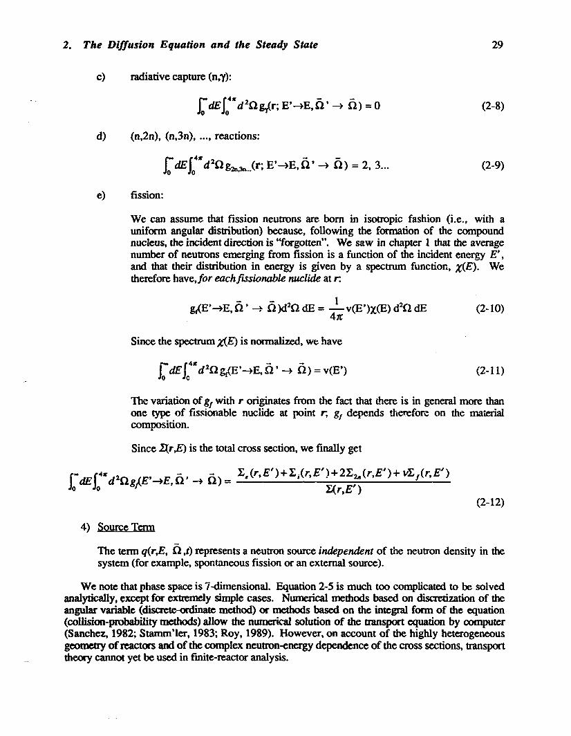
We can assume that fission neutrons are born in isotropic fashion (Le., with auniform angular distribution) because, following the formation of the compoundnucleus, the incident direction is "forgotten". We saw in chapter 1 that the averagenumber of neutrons emerging from fission is a function of the incident energy E',and that their distribution in energy is given by a spectrum function, X(E). Wetherefore have,for eachfLSsionable nuclide at r:

(2-10)

Since the spectrum x(E) is normalized, we have

(2-11)

The variation of g, with r originates from the fact that there is in general more thanone type of fissionable nuclide at point r; 8, depends therefore on the maierlalcomposition.

Since ~r,E) is the total cross section, we finally get

(2-12)

4) SQyrce Tenn

The term q(r,E, 0 ,t) represents a neutron source independent of the neutron density in thesystem (for example, spontaneous fission or an external source).

We note dlat phase space is 7-dimensional. Equation 2-5 is much too complicated to be solvedanalytically, except fOf extremely simple cases. Numerical methods based on discretization of theangular variable (disaete-oniinate method) or methods based on the integral form of the equation(collision-probability methods) allow the numerical solution of the transport equation by COmputef(Sanchez, 1982; Stamm'ler, 1983; Roy, 1989). However, on account of the highly heterogeneousgeometry ofreactors and of the complex neutron-energy dependence of the cross sections, transporttheory cannot yet be used in finite-reactor analysis.


It is therefore not possible in practice to study the space-time behaviour of neutrons in the entirereactor with transport theory. Instead, it will be necessary to use the Wigner-Seitz approximation,which consists in identifying unit cells in the reactor, in which it is possible to use transport theoryto generate average properties (homogeneous macroscopic cross sections). 1bese homogeneouscell properties are then used in diffusion theory to solve for the macroscopic distribution ofneutrons in the reactor. 1bat is, tIK, power distribution in a reactor of large size is calculatedaccurately with diffusion theory, using a pre-processing with transport theory to calculatehomogeneous properties (cell calculations).

The transition from transport to diffusion theory, and the condensation and homogenization ofcross sections, play a central role in reactor physics. These topics will not be discussed in detailhere (see the bibliography). We shall instead assume that homogeneous, macroscopic, multi-groupcross sections are known for all regions of the reactor (each fuel bundle, each control mechanism,etc.). This data will be the starting point for our analysis.

2.1.2 Continuity Equation

(2-13)

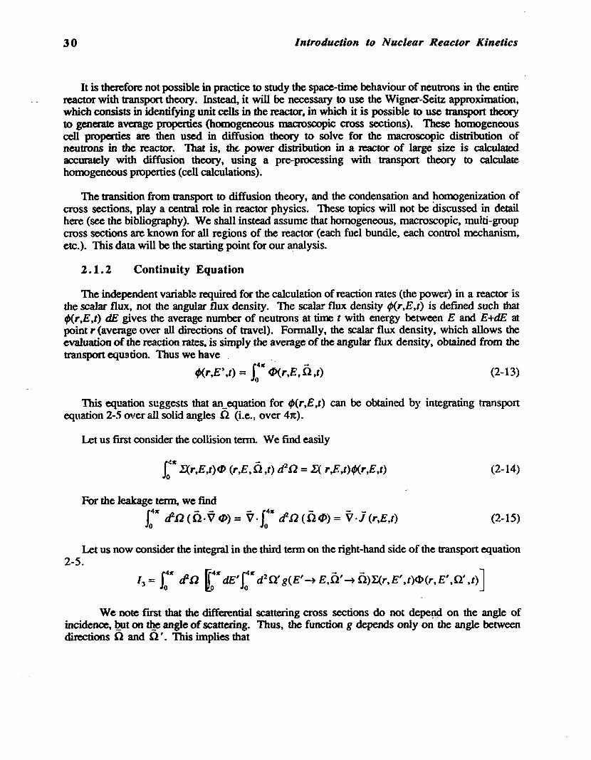
The independent variable required for the calculation of reaction rates (the power) in a reactor isthe scalar flux, not the angular flux density. The scalar flux density tP(r,E,t) is defined such thattP(r,E,t) dE gives the average number of neutrons at time t with energy between E and E+dE atpoint r (average over all directions of travel). Formally. the scalar flux density, which allows theevaluation of the reaction rates. is simply the average of the angular flux density, obtained from thetransport equation. Thus we have .

J.4lf· -

tP(r,E' ,t) = 0 c1J(r,E. 0. .t)

This equation suggests that an_equation for tP(r,E,t) can be obtained by integrating transponequation 2-5 over all solid angles n (i.e., over 41t).

Let us first consider the collision term. We find easily

r4lf- 2J

o1:(r.E.t)4J (r,E. 0. ,t) d Q = 1:( r,E,t)tP(r.E.t)

For the leakage tenD, we find

14lftfn (O.V 4» = V·J

0

4lftfn (04J) = V·j (r,E,t)

(2-14)

(2-15)

Let us now consider the integral in the third term on the right-hand side of the transport equation2-5.

/3= J:" £-n ~:lfdE'J: lf

d20.'g(E'~E.O'~Q)1:(r,E',t)<I>(r,E'.0."t)J

We note first that the differential scattering cross sections do not depe¢ on the angle ofincidence, ~t 011 tile angle of scattering. Thus. the function g depends only on the angle betweendirections 0. and n'. This implies that


I:1r cfa geE'~E, 0. '~ 0.) =2% fl dllogeE'~E, 1Jo)

=g(E'~E)

where, per Figure 2.1,

Jlo =cos 91) =n'· n

By changing the order of integration, we then get

13 = lodE' geE'~E) 1X..r,E',t) I:1r cPa 4J(r,E', 0. ,t)

= !odE' geE'~E) I,(r,E' ,t) ¢J(r,E' ,t)

31

(2-16)

(2-17)

"" If +1.

This term measures the production rate of all neutrons of energy E from all collisions, since thesummation is taken over all incident energies E'. We distinguish between neutrons emerging fromfission and those "produced" by (elastic or inelastic) scattering, I •.

As for this scattering term. we shall simplify the notation by writing

/. = /0. dE' E.(r,E'~E,t) ¢J(r,E' ,t) (2-18)

We can assume that the fission source is isotropic, as in equation 2-10. Let vpc.(E') be theaverage number ofprompt neutrons per fission of nuclide i induced by incident neutrons of energyE'. Let also Zpi(E) be the energy spectrum of these fission neutrons from nuclide i. We get

If = 4: %pi(E) So· dE' vpi(E')Xir,E' ,t) ¢J(r,E' ,t)•

(2-19)

We saw in chapter 1 that the prompt-neutron emission spectrum does not depend strongly onthe fissionable nuclide. If we neglect such dependence on the nuclide, we can simplify equation 219 and find

(2-20)

where the macroscopic cross section satisfies

(2-21)

The notation v17 will therefore henceforth, in the rest of this book, imply summation over allfissionable nuclides.


We know that a fraction of neutrons emerging from fission are delayed.. Similarly to prompt·neutrons, we can consider the delayed-neutron source to be isotropic. We shall suppose for themoment that there exists at time t a certain density S/..r,E,t) defined so that S/..r,E,t)dE gives thenumber of delayed neutrons appearing at time t with energy between E and E + dE. Therelationship between the delayed-neutron source and the scalar flux will be discussed later.

Ifwe use the equations above and gather all terms, we arrive at the continuity equation, whichdescribes neutron conservation in the system:

1i) - - 1- .v iJt tf>(r,E,t) = - I(r,E,t)tfJ(r,E,t) - V· J (r,E,t) + 0 dE' EIl(r,E'-+E,t) tfJ(r,E' ,t)

+ Xp(E) J; dE' vp(E')"Era(r,E' ,t) tf>(r,E' ,t) + S/..r,E,t) + S(r,E,t)

(2-22)where

r4~ -S(r,E,t) ::: Jo

tPn q(r,E' ,n ,t) (2-23)

v"e note that this equation now contains two unknowns, ,(r,E,t) and j (r,E,t), in contrastwith the tr'"cansport equation, which contained only one, the angular flux density fP(r,E ,t). Thepresence of dae leakage tenD in the transport equation has led to the appearance of a newindependent variable in the continuity equation, the net current J (r,E,t), itself related to the angulardensity:

J (r,£,t) = J:1r

tin n fP(r,E', n,t) (2-24)

This quantity is independent of q,(r,E ,r). It is re<n!ired to complete the information lost onintegrating the transport equation 2-5 over all directions .Q.

It is important to note that the continuity equation contains no approximation. It only expressesthe neutron balance in terms of the scalar flux and of the current, rather than in tenns of the angulardensity only. However, in order to obtain a solution we shall need to derive an additional relationbetween tf1(r,E,I) and j (r,E,t), to ~e into account the angular dependence of fP(r,E,t). Indeed,it is 1I0t sufficient to integrate over .Q to eliminate the effect ofdependence with angle.

It is in actual fact not possible to express J (r,E,t) as a function of q,(r,E,r) exactly. From thedefinition of the net current in equation 2-24, one.PQuld be tempted to try to obtain a relationjorJ (r,E,t) by multiplying the transport equation by n before integrating over all angles. Since.Q isa vector, one would need in fact to multiply the equation by each component of .Q, i.e., n", ny,and .oz, and dlen integrate over the 4x solid angle. One would obtain three equations, one for eachcomponent of the vector J (r,E,t) (Duderstadt, 1976).


Table 2.1 Independant Variables in Neutron Transport

33

Neutron Speed v = va

Angular Flux Density ~(f.E.ii.t) = v n(f.E.ii.t)

Angular Current Density 7(f.E.ii,t) = ii~ = vn

Scalar Flux Density 41(f.E.t) = f ~(f,E•.Q,t) d2{J = ( ~)ii(cm-2·s-1·eV-1) 4n

Net Current J(r.E.t) = (7)ii = (ii~)ii

Scalar Flux (group g) t (41).1Eg(cm-2·s-1) ¢g (f,t) = 41(f.E,t) dE =

Eg

_1

SCalar Flux (total)tP(',t) J:' ",(r,E' ,t)dE' = (41 )E (<I> )ii,E(crn-2·s-1) = =

Total Flux~(t) J4J(r.t)d3r {41 )E,V ( ~)ii,E,V(cm-s-1) = = =

Total Number of Neutrons n(t) .:!. ~(t) (n) ii,E,V= =(population) v

Average Neutron Speed v {vn}jj EV(cm-s-1) = ' ,

{n}jj,E,v


The problem with this approach is that the leakage term leads to the appearance of still anotherunknown, in addition to the current density J (r,E,t), viz. the tensorial product

n(r,E,t) = J:1f

d2n n n~(r,E,n,t) (2-25)

This variable is ~dependentof, and of the current J. It cohwns 9 components ~whereasthe current contains 3). The only way to close the system is to introduce an approximation for theangular variation of the solution, so as not to introduce a new variable each time one integrates theleakage term in the transport equation. It is precisely such an approximation which will lead to thediffusion equation.

2.2 Diffusion Equation

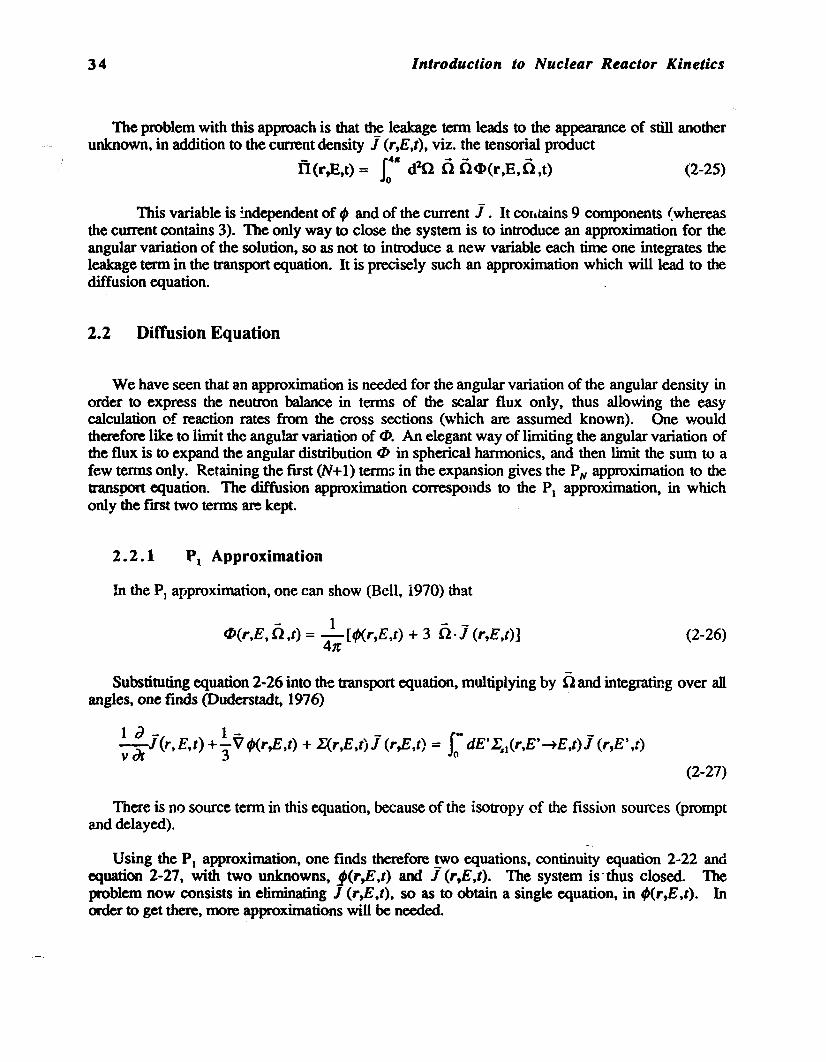
We have seen that an approximation is needed for the angular variation of the angular density inorder to express the neutron balance in terms of the scalar flux only, thus allowing the easycalculation of reaction rates from the cross sections (which a.re assumed known). One wouldtherefore like to limit the angular variation of 4>. An elegant way of limiting the angular variation ofthe flux is to expand the angular distribution 4> in spherical hannonics, and then limit the sum to afew terms only. Retaining the first (N+l) terms in the expansion gives the PN approximation to thetransport equation. The diffusion approximation corresponds to the PI approximation, in whichonly the fIrSt two terms are kept.

2.2.1 PI Approximation

In the PI approximation, one can show (Bell, 1970) that

- 1 - -4>(r,E,n,t) = -[~r,E,t) + 3 n·J (r,E,t)]

4n(2-26)

Substituting equation 2-26 into the transport equation, multiplying by n and integrating over allangles, one finds (Duderstadt, 1976) -

(2-27)

Tnere is no source term in this equation, because of the isotropy of the fission sources (promptand delayed).

Using the PI approximation, one finds therefore two equations, continuity equation 2-22 andequation 2-21. with two unknowns, l(r,E,t) and J (r,E,t). The system is"thus closed. Theproblem now consists in eliminating J (r,E,t), so as to obtain a single equation. in '(r,E,t). Inorder to get there, more approximations will be needed.


Consider first the tenn in the time derivative, v·1iJJ I iJt. This tenn will be negligible withrespect to the others if we can show that

(2-28)

This is equivalent to saying that the rate of change of the current density is much smaller thanthe frequency of collisions, vX. The latter being of the order of lOS S·I or greater, the rate of changeof the current would have to be extremely high to invalidate inequality 2-28. In fact one can show,in mon~nergetic transport theory (Weinberg, 1958), that in the absence of approximation 2-28one obtains not the diffusion equation, but rather a second-order equation (the "telegraph" equation)which displays the properties of a wave equation in addition to those of a diffusion equation.Hypothesis 2-28 is tantamount to neglecting the wavefront which propagates from a perturbation atspeed v, and to suppose that the perturbation is felt instantaneously throughout the reactor. Giventhe great speed of neutrons (thennal neutrons of energy 0.0625 eV travel at 2,200 mls) and therelatively small dimensions of reactors, it is in tact a very short delay time which is neglected.

With the neglect of the first tenn in equation 2-27, the latter can be rewritten

I(r,E,t) J (r,E,t) - roo dE'Ell (r,E'~E,t)J (r,E' ,t) = - !.V¢(r,E ,t)Jo 3

(2-29)

Other assumptions on the anisotropy of the collision law are necessary to isolate J (r,E ,t). Onecan then write (Duderstadt, 1976)

IJ (r,E,t) = - D(r,E) V¢(r,E,t) I(2-30)

where D is the diffusion coefficient, which can be expressed as

D(r,E,£) = r :. .] = 13LI:(r,E,t) - poE1('" E, t) 3E/r(r, E,t)

(2-31)

with Po the average cosine of the scattering angle. In this equation we have also introduced thetransport cross section, E/r.

We find thus that in certain situations the current density is proportional to the flux gradient.This result is analogous to many other phenomena in physics, and is known as Fick's Law. 1benegative sign in equation 2-30 indicates that neutrons tend to diffuse from high-density regions tolow-density regions, just a~ a gas through a porous partition.

Using equation 2-30 to eliminate J (r,E,t) in the continuity equation, we finally obtain theenergy- and time-dependent diffuswn equatwn


1 d - -v dt t/J{r,E,t) = - I( r,E,t)t/J{r,E,t) + V ·D(r,E)V t/J{r,E,t)

+ rdE' 'E.. (r,E'~ E,t)t/J{r,E',t)

+Z,(E) J: dE'v,(E')Ij.r,E' ,t)t/J(r,E',t)

+ Sj.,r,E,t) + S(r,E,t)(2-32)

We shall simplify the notation by making use of the following linear operators:

•

•

prompt-neutron production:

F,~ = Z,(E) J: dE' v,(E')IJr,E' ,t)t/J(r,E' ,t)

neutron removal (interactions and leakage):M ~ = - V. D(r, E)V t/J{r,E,t) + I( r,E,t)t/J{r,E,t)

-1-dE' 'E.. (r,E'~ E,t)t/J{r,E' ,t)

(2-33)

(2-34)

11te diffusion equation can then be cast in the foon •

1 a~- = (F, - M)~ + Sj.,r,E,t) + S(r,E,t)vdt

(2-35)

We note that M tP measures the net loss of neuttons. Indeed, by convention we include theelastic-scattering teon in the operator M, with a negative sign, indicating it is a gain of neuttons ofenergy E at point r.

The tam F,tp measures the rate of production of prompt neutrons at time t. It thus does notillclude the v" delayed neutrons due to fissions occurring at time t, these neutrons will appear later.Nor in fact does it include delayed neutrons from earlier fissions. The rate of production of delayedneutrons is taken into account via the teon Sj.,r,E,t), which we shall discuss in section 2.2.3.

2.2.2 Diffusion Approximation

Let us return for now to the diffusion approximation. The main approximations which weremade leading to the diffusion equation are the following:

• the angular flux has only one linear component of anisotropy (PI approximation, Eq. 2-26);• neutton sources, including fission, are isottopic; ...• the current density varies slowly, relative to the collision frequency (no neutron waves).


The first of these approximations is the most stringent. It is natural to ask in whatcircumstances the angular flux varies sufficiently slowly with angle to ensure the validity of thediffusion approximation. Comparisons with transport-theory solutions show that the assumptionof a weak angular dependence is invalidated in the following cases (Larsen, 1991; Rulko, 1991):

• near external boundaries of the domain, and near interfaces at which properties changesuddeuly;

• in the vicinity of localized sources;• in highly absorbing media.

This is illustrated in Figure 2.2, which shows the polar diagram of n(r,E, n) near an interfacebetween two materials. We assume that the region on the left is of weak absorption and largescattering cross section, while the region on the right is of high absorption.

let us look flfSt at region 2. Neutrons are strongly absorbed there. Consequently, fewneutrons will travel from region 2 to region 1, whereas a lar~e number of neutrons will travel from~gion 1 to region 2. Near the interface then, n(r,E, n) must Qe large for those directionsnpointing towards the interface (e.g., .01). The density n(r,E, n) will continue to decreaserapidly as one moves away from the interface. Also, the neutron current in the direction from left toright will continue to be greater than that in the opposite direction, even though both currents havediminished due to absorption.

In region 1, where X.. « X. neutron scattering will reduce the angular dependence of the currentand, at a distance of a few mean free paths, Fick's Law will become a good approximation.

In summary, the diffusion equation applies a few mean free paths inside regions where X,,(r,E)and X..(r,E) do not vary rapidly with position, and in which X..(r,E) « L.(r,E).

Fig. 2.2 Polar Plot of n(r,E,D ) near an Interface

Region 1 Region 2Xa1« Xi


It is natural then to wonder about the applicability of the diffusion equation to finite-reactor .calculations, with its strongly absorbing regions such as the fuel and the control mechanisms. Onemust however remember that the diffusion equation is used to calculate the macroscopic fluxdisttibution in the reactor, utilizing properties previously homogenized (by means of transport··theory calculations) over unit cells with dimensions much greater than the neutron mean free path.The goal of diffusion calculations is thus, by evaluating the neutron diffusion from cell to cell, tocompute the disttibution ofcell-average reaction rates throughout the reactor.

2.2.3 Delayed-Neutron Source

We note that the delayed-neutron source, 5/...r,E,t) in equation 2-35, is not~ly independent ofthe flux, since it depends on the earlier flux level in the reactor (t' <I).

We saw in chapter 1 that the delayed-neutron source is directly related to the concentration ofthe precursor fission products, and that a limited number of precursor groups is sufficient tocharacterise the source.

Let C,,(r,t) be the concentration of group-k precursors at point r and time t, and let K be the totalnumber of delayed-neutron-precursor groups used (generally 6 for each fissionable isotope and 9for the photoneutrons). As the delayed neutrons originate from the natural decay of the precursors,the delayed-neutron source can simply be written

IC

5/...r,E,t) = L A"Cir,t) XtA;(E)"=1

(2-36)

where X.(E) is the nonnallzed spectrum of group-k delayed neutrons. To simplify the notation,and without much error, we have neglected the dependence of the delayed-neutron spectrum Xci'"and of the decay constants A", on the isotope. In addition, we shall use a common set of decayconstants to ior all isotopes (the yields have to be defined accordingly). The data is found in Tables1.8, 1.9, and 1.10 of chapter 1.

In order to complete the system of equations, we must now write equations for the evolution ofthe precursors, which will allow us to calculate me C,,(r,t) in equation 2-36. Since each precursoryields only one neutron and each fission produces vel" precursors of group k, me evolution of theprecursors is governed by

iK:" = _ A" C,,(r,t) + r- dE' v.xl-r,E' ,t)t/J(r,E',t) (k = 1,2... K)at Jo

where the sum over fissionable isotopes i is implicit:

(2-37)

(2-38)

The diffusion equation 2-35 is coupled to the precursor evolution equations 2-37. The kineticsproblem then reduces to the solution of the system of (K+l) equations 2-35 and 2-37,supplemented by boundary conditions for, and initial conditions for, and the CIe.

2. The Diffusion EqUiltion and the Steady State 39

2.2.4 Boundary Conditions

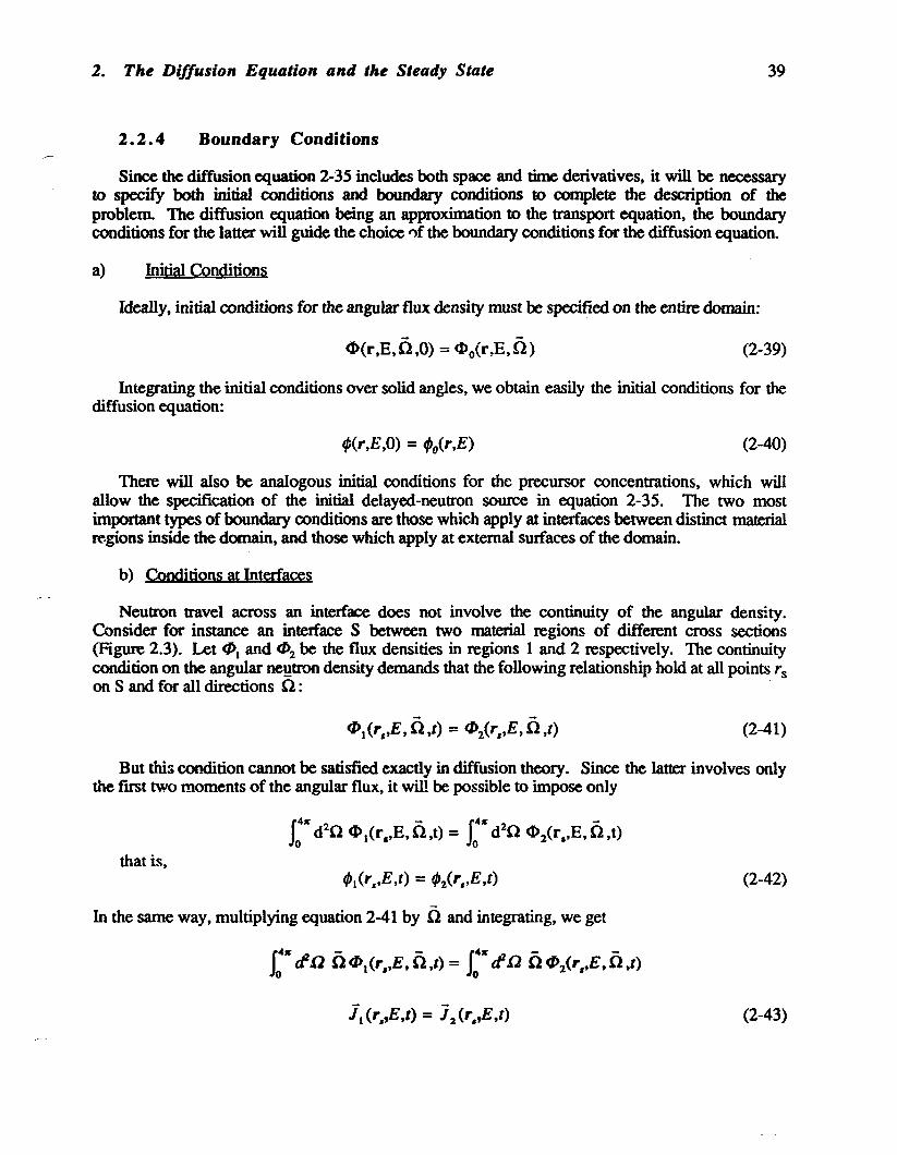
Since the diffusion equation 2-35 includes both space and time derivatives. it will be necessaryto specify both initial conditions and boundary conditions to complete the description of theproblem. The diffusion equation being an approximation to the transport equation. the boundaryconditions for the latter will guide the choice 'lf the boundary conditions for the diffusion equation.

a) Initial Conditions

Ideally. initial conditions for the angular flux density must be specified on the entire domain:

- -cIl(r.E.n.O) = cIlo(r.E.n) (2-39)

Integrating the initial conditions over solid angles, we obtain easily the initial conditions for thediffusion equation:

~(r,E.O) = tPo(r,E) (2-40)

There will also be analogous initial conditions for the precursor concentrations, which willallow the specification of the initial delayed-neutron source in equation 2-35. The two mostimportant types of boundary conditions are those which apply at interfaces between distinct materialregions inside the domain. and those which apply at external surfaces of the domain.

b) Conditions at Interfaces

Neutron travel across an interface does not involve the continuity of the angular density.Consider for instance an interface S between twO material regions of different cross sections(Figure 2.3). Let <,1)1 and <,1)2 be the flux densities in regions 1 and 2 respectively. The continuitycondition on the angular ne~trondensity demands that the following relationship hold at all points rson S and for all directions 0:

- -<,I)1(r"E,0,t) = <,I)2(r"E,0.t) (2-41)

But this condition cannot be satisfied exactly in diffusion theory. Since the latter involves onlythe first two moments of the angular flux. it will be possible to impose only

141( 2 - 141( 2 -o dOcllt(r••E.O.t)= 0 dOcll2(r.,E.0.t)

that is,(2-42)

In the same way, multiplying equation 2-41 by 0 and integrating, we get

(2-43)

40

Utilizing equation 2-30, we finally get


(2-44)

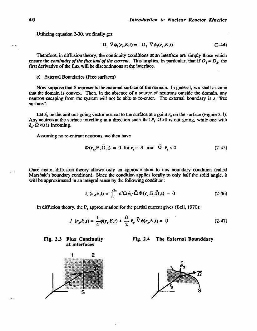
Therefore, in diffusion theory, the continuity conditions at an intetface are simply those whichensure the continuity ofthe flux and ofthe current. This implies, in particular, that if D1* D2, thefirst derivative of the flux will be discontinuous at the intetface.

c) External Boundaries (Free surfaces)

Now suppose that S represents the external surface of the domain. In general, we shall assumethat the domain is convex. Then, in the absence of a source of neutrons outside the domain, anyneutron escaping from the system will not be able to re-enter. The external boundary is a "freesurface".

Let is be the unit out-going vector normal to the sutface at a ~int rson the surface (Figure 2.4).Any neutron at the surface travelling in a direction such that is· 0>0 is out-going, while one wita'lis· 0<0 is incoming.

Assuming no re-entrant neutrons, we then have

~(r.,E,O,t) = 0 forr.E Sand O·e.<O (2-45)

Once again, diffusion theory allows only an approximation to this boundary condition (calledMarshak's boundary condition). Since the condition applies locally to only half the solid angle, itwill be approximated in an integral sense by the following condition:

In diffusion theory, the PI approximation for the partial current gives (Bell, 1970):

1 D-J_ (r.,E,t) = 4'tP(r.,E,t) + '2 e.· vtP(r.,E.t) = 0

(2-46)

(2-47)

Fig. 2.3 Flux Continuityat interfaces

1 2

Fig. 2.4 The External Bounddary


This boundary condition can be generalized in the form

- I(I-a)D(r.) e•. V ~r.,E,t) + - - q,(r.,E,t) = 02 I+a

41

(2-48)

where we have introduced the albedo a, a positive quantity. The -;ase a = 0 reverts to theprevious condition. Ifa = I, we get reflection boundary conditions; these can be used to limit thedomain when symmetry exists.

Another fonn of boundary condition is obtained by demanding that the flux vanish at acertain distance from the physical boundary. By starting from equation 2-47 and extrapolating theflux linearly in the out-going direction, we note that in one dimension it vanishes at theextrapolation distance

A more detailed treatment (Dudersiadt, 1979) gives a more correct value:

x. = x. + 0.7104Atr

(2-49)

(2-50)

Finally, it is important to note that the real flux does not go to zero either at the physicalboundary or at the extrapolation distance. In fact, in a vacuum, it remains non-zero over an infuiitedistance. Diffusion theoty, using a boundary coodition of type albedo (equation 2-48) or of typeextrapolation distance (equation 2-50), is valid only within the domain inside a few mean free pathsaway from the external surface.


2.2.5 Multigroup Formalism

An analytic solution to the time- and energy-dependent diffusion equation IS m practiceimpossible in the large majority of cases. In spite of all the simplifications incorporated in theenergy-dependent diffusion equation, the presence of the integral term makes the equation fearsomewhen applied to finite-reactor calculations. In order to obtain a system of algebraic equationsefficiently solvable by computer, it is necessary to further simplify the energy dependence of thediffusion equation, even before considering tile spatial discretizz:ion of the domain and theapplication of an appropriate numerical technique for treating differential operators.

We shall briefly describe the multigroup formalism for discretizing the neutron energy domain,which allows the transfonnation of the energy-dependent diffusion equation in~ a set of coupledequations in the various energy groups. In this formalism, the operators M and F, take a matrixform.

Since fISsion neutrons appear with an energy which can reach 10 MeV, and since they must beslowed to thermal energies (arbitrarily defined as energies E < 0.625 eV) before absorption in thefuel, the neutron energy domain spans at least 8 decades, within which cross sections vary in acomplex manner. The multigroup formalism consists of reducing the energy dependence to a fewenergy groups covering the entire domain. It will therefore first be necessary to condense the crosssections, in order to reduce their energy dependence to a few group constants.

We have also seen that the diffusion approximation is not valid in the vicinity of a stronglyabsorbing medium, such as the fuel. It will therefore be necessary to average the cross sectionsover a larger volume, by including the moderator region, to derive homogeneous cross sectionsallowing the use of diffusion theory.

The approach generally used to perform finite-reactor calculations consists of first effecting adecoupling at the Jattice-celllevel (with each cell centered around the repeating elements of thelattice, such as the fuel bundles in a CANDU or the fuel clusters in a PWR). Inside the lattice cells,a time-independent transport-theory calculation is perfonned, assuming reflection boundaryconditions (infinite lattice). This calculation provides the microscopic distribution of the neutronflux within the cell, IfI(r,E), which pennits the condensation and homogenization of the crosssections by conserving reaction rates within the unit cells.

Let us assume that the energy domain has been subdivided into G energy groups. Thus, therewill be G energy intervals .dE( ~panning the neutron energies in the reactor: Eo>...> E,>...>EG•

Typically, Eo = 0 md Eo = IS MeV. The unknown in the diffusion equation 2-35, the sCalar fluxdensity ;(r,E,t), is interpreted as being the product of a macroscopic scalar flux #/J(r,t), definedover the reactor, and of the microscopic flux 1fI{r,E), obtained from the eel! calculation:

scalar fluxdensity

~(r.~E,tj

macroscopicscalar flux~

= q,(r,t)

microscopicdistribution

A

(2-51)

(2-52)

The group flux, the solution of the equations to be derived in the multigroup fonnalism, isformally written -.

fEg- t

q,g(r,t) = de q,(r,E',t)E,

for Eg < E < Eg-l

2. The Diffusion Equation and the Sleady State 43

Recall that the group flux ',(r,t) is a scalar quantity, indicating the total nwnber of neutronswith energy between Ef. and E,ol' while ¢(r,E,t) is a density, with ¢<r,E,t)dE giving the number ofneutrons between E anc1 E+dE. The units of " are em-2s l

• In the following, we shall assume thatthe microscopic flux distribution within the unit cell has been nonnalized over the cell volume VC4U:

= 1.0 (2-53)

We write all the group fluxes in a column vector~ of length G (not to be confused with theangular flux):

(multigroup) (2-54)

In the multigroup fonnalism, the operators M and F, in equation 2-35 become GxG matrices.The neutron removal operator is

(2-55)

where the leakage operator L and the scattering operator A are

L=

o

o

oo -V·D VG

(2-56a)

o 01:2 0

(2-56b)

Note that in the general problem, the cross sections appearing in the matrix operators are allfunctions of position and of time. Also, the scattering matrix contains no up-scattering tenns, i.e.,it is assumed neutrons do not gain energy from elastic, or inelastic, collisions.

For the prompt-neutron-production operator, we get

(2-57)

where the column vector lt,.l and the row vector [F,.IT are

44

[z,J =


Zpl (r)

(2-58a)

Z pa(r)

and (2-58b)

We observe that the prompt fission source (equation 2-57) is the product of a scalar, the rate ofproduction of prompt neutrons, Rp and a vector, the spectrum Zp:

where

FptP = [zp] ·rpJ cI>.. ,R/(r/)"..-J.

G

Rf..r,t) = L Vp,Lj,(r,t)tP(r,t),=1

(2-59a)

(2-59b)

(2-61)

We show a spatial dependence for the spectrum to remember that the fission spectrum is afunction of the fuel composition (fissionable isotopes), which can vary with position. We note alsothat the fission-neutron spectrum is normalized in an analogous fashion with equation 1-15:

G

L Zp,(r) = 1.0 (2-60),=1

Substituting equation 2-51 into the energy-dependent diffusion equation (equation 2-35),and integrating over energy in each energy group in turn, we obtain the multigroup diffusionequations, here shown in matrix form:

I~[;~]~~-<I>-=-[F-~-!I!.---[-M]-!I!.-+-S-..J-+-s.-I

where the matrix [1/v] is simply1

0 0VI

-1 ] 0I

l-v- = Vz (2-62a)

0

0 01

vG

and where the delayed-neutron source s...a is the column vectorZIlI.

K

S-tt = L A.l,c1(r,t)1=1

Z41G

(2-62b)


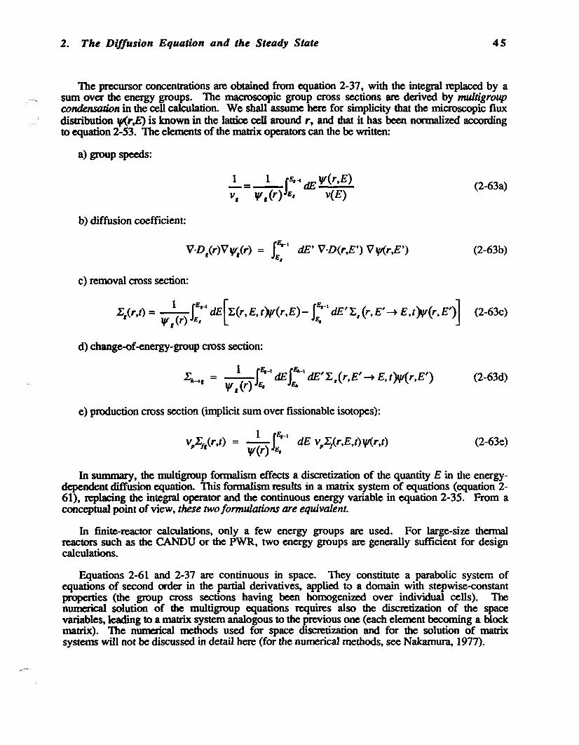
The precursor concentrations are obtained from equation 2-37, with the integral replaced by asum over the energy groups. The macroscopic group cross sections are derived by multigroupcondensation in the cell calculation. We shall assume here for simplicity that the microscopic fluxdistribution lp(r,E) is known in the lattice cell around r, and that it has been normalized accordingto equation 2-53. The elements of the matrix operators can the be written:

a) group speeds:

2..= 1 l~o{ dE 'If(r,E)v, VI,(r) E. v(E)

b) diffusion coefficient:

1Er-1

V·D,(r)V'I',(r) = dE' V·D(r,E') VtjI(r,E')E.

c) removal cross section:

(2-63a)

(2-63b)

X,(r,t) = I t'o{ dE[};(r,E,i)l'(r,E)- t·-I dE'};.(r,E'~ E,t)l'(r,E,)l (2-63c)VI,~) ~ ~ ~

d) change-of-energy-group cross section:

1 1~-1 lE.-1 , (' \lId'III-+1 = dE dE };. r,E ~E,t/'Y\r,E)

'If, (r) E, E"

e) production cross section (implicit sum over fissionable isotopes):

(2-63d)

(2-63e)

In summary, the multigroup formalism effects a discretization of the quantity E in the energydependent diffusion equation. This formalism results in a matrix. system of equations (equation 261), replacing the integral operator and the continuous energy variable in equation 2-35. From aconceptual point ofview, these twoformulations are equivalent.

In finite-reactor calculations, only a few energy groups are used. For large-size thermalreactors such as the CANDU or the PWR, two energy groups are generally sufficient for designcalculations.

Equations 2-61 and 2-37 are continuous in space. They constitute a parabolic system ofequations of second order in the partial derivatives, applied to a domain with stepwise-constantproperties (the group cross sections having been homogenized over individual cells). Thenumerical solution of the multigroup equations requires also the discretization of the spacevariables, leading to a matrix system analogous to the previous one (each element becoming a blockmatrix). The numerical methods used for space discretization and for the solution of matrix.systems will not be discussed in detail here (for the numerical methods, see Nakamura, 1977).


2.3 Time-Independent Equation and Eigenvalue Problem

The neutron balance in the reactor is described by the energy- and time-dependent diffusionequation 2-35. or else by the multigroup equation 2-61. This equation is coupled to the precursorevolution equations 2-37. which allow the tracking of the delayed-neutron source SiI which ispresent whenever the scalar flux , is non-zero and there is fission. Prior to studying the timedependent problem in the next chapter, let us now con~ider the neutron field in a reactor in steadystate. It will first be necessary to detennine whether a steady state is indeed possible, whether inthe presence or in the absence of the external source S in the balance equation. This will lead us tointroduce the concept ofreactor criticalitY .

2.3.1 Steady State and Criticality

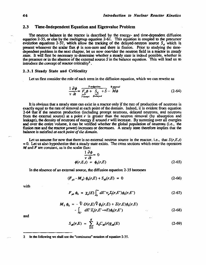
Let us first consider the role of each term in the diffusion equation, which we can rewrite as

(2-64)

It is obvious that a steady state can exist in a reactor only if the rate of production of neutrons isexactly equal to the rate of removal at each point of the domain. Indeed, it is evident from equation2-64 that if the neutron production (including prompt neutrons, delayed neutrons, and neutronsfrom the external source) at a point r is greater than the neutron removal (by absorption andleakage), the density of neutrons of energy E around r will increase. By summing over all energiesand over the entire volume, it can be verified whether the global population of neutrons (i.e., thefission rate and the reactor power) increases or decreases. A steady state therefore implies that thebalance is satistied at each point ofthe domain.

Let us assume for now that there is no external neutron source in the reactor, i.e., that S(r,E,t)= O. Let us also hypothesize that a steady state exists. The cross sections which enter the operatorsM and F are constant, as is the scalar flux:

1 a,-=0viJt

tP(r.E,t) = ifJo(r,E) (2-65)

In the absence of an external source, the diffusion equation 2-35 becomes

(2-66)

with

- -M 0 tPo = - V oD(r,E) V tPo(r,E) + X(r,E)tPo(r,E)

- r dE' E.(r,E' -+E)tPo(r,E')JE,

andK

S4J(r,E) = L A,PIttJ(r)x.(E)1:=1

2 In the following we shall use the "continuous" notation of equation 2-35.

(2-67)

(2-68)

(2-69)


The steady-state delayed-neutron source can be found by setting the derivative in equation 2-37to zero:

Substituting this result in equation 2-69, we get

K

StlO(r,E) = L ZIIk(E) f" dE'v~j..r,E')f/Jo(r,E')1:,.,1 0

= F tlOf/Jo

(2-70)

(2-71)

In order to simplify the notation, we shall drop the subscript 0, since all tenns are timeindependent. The fission-source term can then be written

Ftf' = (Fp + FJ f/J = ziE) J; dE'vpIj..r,E')f/J(r,E')K

+ L Z.JE) i- dE'v~j..r,E')f/J(r,E')1:=1 0

(2-72)

We can simplify further by writing the fission operator as a function of the total spectrum.Neglecting the dependence of vI' and vIlk on the energy E' of the incident neutron - but not theirdependence on the fissionable isotope, implicit in the previous equations 2-21 -we define t.lte totalspectrum:

Z(E) =

K

v pZp(E)+ LVtuZtu(E)l,.,l

v(2-73)

or, using the definition of delayed-neutron fraction,

K

z(E) = (l-{3)ZiE) + L f3tZl:(E)1:=1

(2-74)

The total steady-statefission source can therefore be expressed as follows in tenns of the totalspectrum and of the production cross section v..;:

Ff/J = Z(E) 1- dE'vIj.r,E')f/J(r,E') (2-75)

Note that the form of equation 2-75 has been simplified to lighten the notation. It is not anapproximation, as we could use the exact form 2-72 of the equation, in which we would show thesum over all fissionable isotopes.

In steady state and in the absence ofan externtJI source, the diffusion equation reduces to

ProdlJctioo= • Ff/J \ (2-76)


From the point of view of physics, this equation simply states the following:

• For a steady state to exist in a reactor in the absence of an external source ofneutrons, the number of neutrons produced at each point of the domain must beexactly equal to the number of neutrons removed, including leakage to other regionsor to the exterior of the domain. In such a case, the reactor is said to be critical.

The importance of equation 2-76 is that it allows us to verify th:s statement for a particular case-,to the extent that the geometry and the properties of the reactor are well known. Indeed, everythingwe have learned to this point is limited to counting neutrons according to the rules which govern thetranspott of neutrons in matter. A reactor will therefore be critical. in the absence of an externalsource, if the production of neutrons is equal to their removal. If the production. is greater than theremoval, the flux level will increase and equation 2-76 does not apply. In this case the reactor issupercritical, and the only way to predict the neutron behaviour will be to solve the time-dependentdiffusion equation 2-59. If in contrast the production is smaller than the removal, the reactor issubcritical.

From the mathematical point of view, the time-independent diffusion equation 2-76 is ahomogeneous equation which has only a trivial solution (IP = 0), unless the reactor is critical, thatis, unless its properties are such as to ensure neutron balance. Since the operators M and F arelinear, this critical condition translates mathematically to a discretized matri..x with a zerodeterminant. The linearity of the operators] also implies that the neutron flux level in a crilicalreactor is arbitrary. The criticality of a reactor is thus defined solely by its properties, in the absenceof an external source. It does not depend on the flux level in the reactor, although it is necessary tosolve the diffusion equation and calculate the flux distribution to ver..fy criticality.

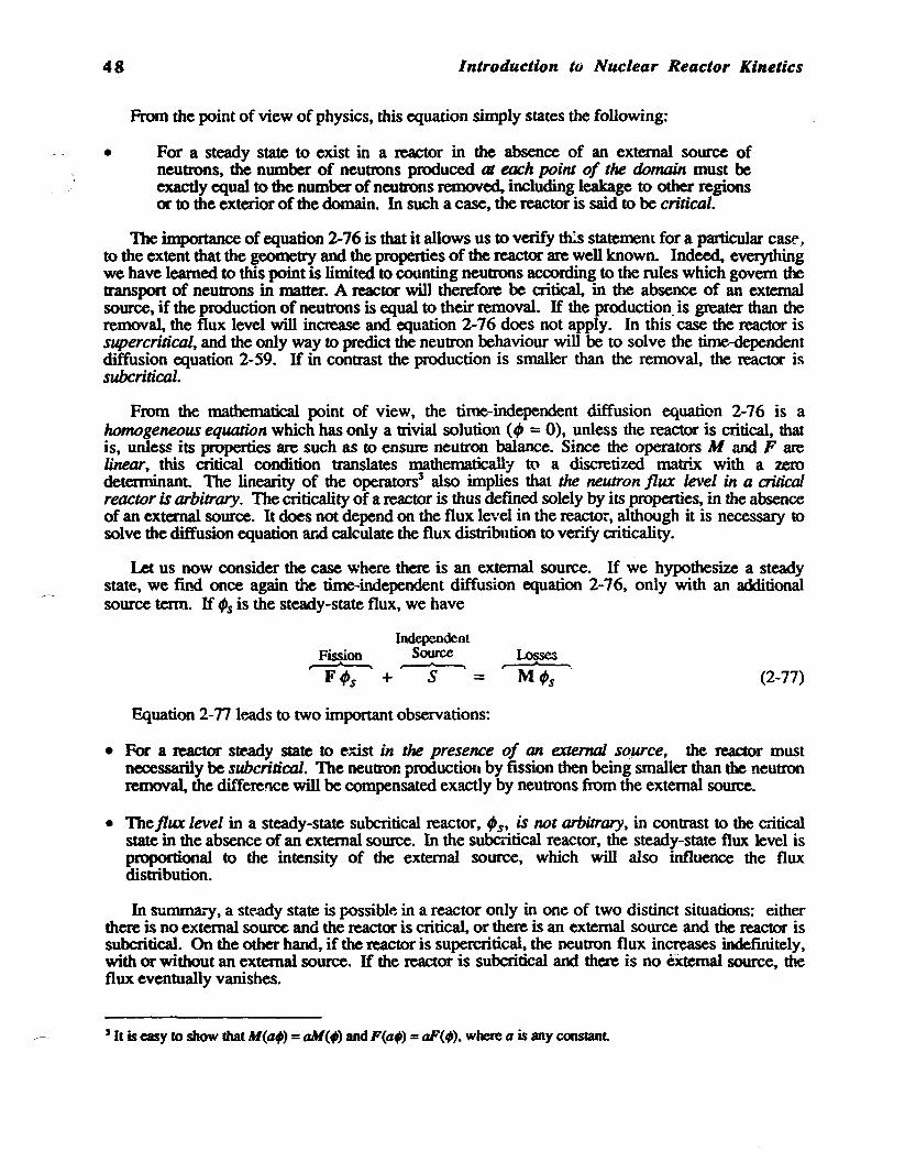
Let us now consider the case where there is an external source. If we hypothesize a steadystate, we find once again the time-independent diffusion equation 2-76, only with an additionalsource term. If IPs is the steady-state flux, we have

IndependentFission Source

" .. Losses.(2-77)

Equation 2-77 leads to two important observations:

• For a reactor steady state to exist in the presence of an external so.urce, the reactor mustnecessarily be subcritical. The neutron production by fission then being smaUer than the neutronremoval, the difference will be compensated exactly by neutrons from the external source.

• Theflux level in a steady-state subcritical reactor, IPs, is not arbitrary, in contrast to the criticalstate in the absence of an external source. In the subcritical reactor, the steady-state flux level isproportional to the intensity of the external source, which will also influence the fluxdistribution.

In sumnUll)', a steady state is possible in a reactor only in one of two distinct situations: eitherthere is no external source and the reactor is critical, or there is an external source and the reactor issubcritical. On the other hand, if the reactor is supercritical, the neutron flux increases indefinitely,with or without an external source. If the reactor is subcritical and there is no extelIUll source, theflux eventually vanishes.

, It is easy to show that M(a,) =aM(,) and F(a,) =aF'('>. where a is any constant


2.3.2 Effective Multiplication Constant and Static Reactivity

Power reactors generally do not use external neutron sources. Consequently. in normaloperation, power reactors are in general critical. It is then easy to understand the reactor designer'sdesire to be able to verify a priori (befo~ construction) that the configuration selected for the reactorcorresponds indeed to a critical state.

Let us consioa"' for examyle the calculation for a particular ~ctor. without an external source.This ~tor is characterized by a set of cross sections.lXr). One cannot know in advance whethercriticality will be satisfied, unless one solves equation 2-76 for this ~tor. Solving the timeindependent problem of equation 2-76 therefo~ implicitly assumes that the physical properties ofthe ~etor allow criticality. However, a small difference between the production and ~moval ofneutrons would lead to a neutron population changing with time. That small difference can indeedreflect a real situation. In such a case, either the model of the reactor is incomplete or the reactordesign is incorrect. Or else the difference could be due to uncertainties in the values of the crosssections, even if the reactor is in fact critical.

In order to ensure that we get a non-trivial solution whenever we solve equation 2-76, weintroduce a constant, A, called the eigenvalue, which will be used as a multiplier on the fissionsource ten1'_ We adjust this constant artificially so that the neutron balance corresponding tocriticality is satisfied. In practical tenns, this is equivalent to varying artificially the number ofneutrons emitted per fission until the neutron production is equal to the removal. Any systemcontaining fissionable material can be made critical by arbitrarily varying the number of neutronsemitted per fission. There must therefore always be a positive solution for , and for 11.. 1bemodified equation is thus

(2-78)

(2-79)

Note that the same constant II. is applied at all points of the domain, and that it is necessarilypositive (since the neutron flux must be positive).

Mathematically speaking, there may be a large number of distinct eigenvalues which satisfyequation 2-78. To these distinct eigenvalues are associated distinct eigenfunctions4

• For greatergenerality, we should thus write the time-independent diffusion equation as

M 'ell) = Aell)F 'ell) IHere the 'C!&) are the eigenvalues (harmonics) of the problem. Only the fundamental mode 'CO)

is everywhere positive, and it is the only one which ~presents a physical quantity (the scalar flux).In the following, the scalar flux of equation 2-78 thus corresponds to the fundamental mode ofequation 2-79:

¢(r,E) = 'eo)(r,E)

We note also that the hannonics appear in the following natural order.

41n the case of degeneracy. several eigenfunctions may possess the same eignevalue.

(2-80)

(2-81)


1beflux distribution in a critical reactor can therefore be obtained by solving equation 2-79 for~(II). Recall that this equation does not allow the determination of the absolute value of the flux.An additional condition is needed to nonnalize~. As far as the eigenvalue and the flux distributiongo, the normalization is arbitrary. To obtain the absolute flux value, one often uses normalizationto the total reactor power Po. To illustrate, if K is the average energy released per fission, thenonnalization condition would be written

where

H(r,E) = KIJ.r,E)

(2-82)

(2-83)

1be physical meaning of the eigenvalue 1 is important It can be shown that the eigenvalue issimply the inverse of the effective multiplication constant ke/I' a quantity which springs from theconsideration of successive generations of neutrons in fundaffiental reactor theory.

Intuitively, think of a reactor where the flux level is maintained constant in time, on average, bya chain reaction. Under such conditions, kelT is defined as the ratio of the number of neutrons insuccessive generations, with fission the event sep&-ating generations (Lamarsh, 1965). In a criticalreactor, the chain reaction is maintained on the strength of keJf being equal to 1.0. Let us now seehow the value of k", can be obtained from diffusion theory, using the approach employed by Bell(1970) with transport theory.

Consider a multiplying medium in which is introduced a pulse source S(r,E,t) at t=O. Weassume there are no neutrons in t'le system initially. If 0 represents the Dime delta function, wewrite

S(r,E,t) = Sl(r,E)l5(:) (2-84)

The neutrotls from the pulse source constitute the neutrons of the first generation, which weshall denote ~l(r,E.t). All the neutrons of each generation will disappear either by absorption(including tbat leading to fission) or by leakage out of the system. The neutrons produced byfissions induced by first-generation neutrons are the neutrons of the second generation, and so on.Thus. the rust-generation neutrons, ~l' will satisfy equation 2-64, where fission appears within theabsorption term:

1 ij~l~= S(r,£,t) - MtP(r,E,t) (2-85)v ot

Neutrons from the pulse source diffuse throughout the system and eventually disappear.Integrating equation 2-85 over all time, the left-hand side becomes

=0 (2-86)


Let fPl denote the total neutron flux in the first generation:

'Pl(r,E) = I; ~I(r,E,t)dt

Integration ofequation 2-85 over time thus gives

51

(2-87)

(2-88)

TIle neutton source in the second generation can be obtained by integrating appropriately overneuttons of the flISt generation:

Sz(r,E) = J: dt[Fp~I(r,E,t) + S.u(r,E,t)]

= F'Pt(r,E) (2-89)

Indeed, integrating the delayed-neutron source over all time gives the steady-state emissionspectrum (equation 1-28). This source can therefore be used to fmd the neuttons of the secondgeneration and those of the third generation. There is in fact here an iterative procedure whichallows the calculation of the neutton flux in any generation from the flux in the previous one:

(2-90)

From this recursion relation 2-90, we can expect that the neutton density will increase from onegeneration to the next if the system is supereritical. that it will decrease jf the system is subcritical,and will become constant if the system is critical. In LilY case. we can expect the ratio of densities(fluxes) in successive generations to become constant, independent of r and of E:

= constant

= k.//

Comparing equations 2-90 and 2-78, we find1

A. = k.n

(2-91)

(2-92)

Equations 2-90 and 2-91 serve in fact in general as an iterative procedure for the calculation ofthe eigenvalue (by the method of powers). It will thus be easy to verify whether the multiplyingsystem is critical by calculating the eigenvalue A. and comparing it to 1.0. The difference between Aand 1 is a measure of the non-criticality of the medium. This difference is called the staticreactivity, Ps:

(2-93)

TIle static reactivity is thus a measure of the degree ofadjustment which would have to made tothe system to make it critical (for instance, by the insertion of the reactor conttol mechanisms).This quantity is of great interest in reactor studies. In the following section, we shall study thesensitivity of this quantity to various perturbations or modifIcations which can be made to thesystem.

(; 0 Introduction to Nuclear Reactor Kinetics

2.4 Perturbation Theory and Flux Adjoint

Power reactors are highly heterogeneous. Let us consider for instance the CANDU 6. Thisreactor has 380 fuel channels (.... 10 em in diameter and 600 em long), arrayed in a square lattice ona 28.6-cm lattice pitch. 1be space between channels is tilled with heavy water, which serves as themoderator. Reactivity devices are inserted at various locations in the moderator, as part of thereactor regulating system. Each channel contains 12 fuel bundles, which can be moved axiallyalong the channel. The reactor is refuelled on-line, with a small fraction of the fuel load replacedeach day on the average. In view of the changes in fuel composition with bumup during reactoroperation, each fuel bundle can be considered to have different properties. Finally, the reactor coreis surrounded by a radial reflector of thickness :os 60~ consisting of heavy water only.

Cell calculations can give us homogenized cross sections in two neutron energy groups for eachlattice cell (fuel bundle and its surrounding moderator). Transport calculations in 3 dimensions canbe perfonned on supezcells defined around the reactivity mechanisms in order to homogenize theirproperties over the neighbouring lattice cells. The two-energy-group properties of the reflectorcomplete the data set which is used to carry out diffusion-theory calculations for the entire reactor.

The time-independent diffusion equation 2-78 is thus applied over a dOIl18ID containing a largenumber of material regionss, typically of the order of 10,000. In its multigroup form, it is in fact aset of G partial differential (elliptic) equations of second order, with G x N unknowns, N being thenumber of variables appearing from the spatial discretization. N is generally greater than thenumber of material regions, because many variables are introduced in discretizing the leakage term,which contains derivatives. 1be method used to satisfy the continuity equations 2-42 and 2-44 atthe interfaces between the finite elements (material regions) can also govem the number ofunknowns.

The number of equations for the discretized system can thus easily reach 50,000. In addition,the eigenvalue problem requires outer iterations on the eigenvalue, as seen earlier (equation 2-89).Even when using convergence acceleration techniques (Hebert, 1985), of the order of 50 iterationswill be required. While this type of calculation is easily perfonned on a computer, its cost (incomputer time) is not negligible. .

It is important to remember that a reactor design is the end product of a long process. For eachcore configuration, the diffusion calcuJation is perfonned to determine the power distribution thatwould be obtained if the reactor were critical (the reference distribution). This calculation also givesan eigenvalue for each configuration, which is a measure. as we saw earlier, of the reactivitydifference between the actual configuration and a'critical state. Taking into account the largenumber of design variables to be optimized, the detailed design of the reactor core can requireseveral thousand diffusion calculations.

In many cases, what is of interest are the variations in k.o due to "perturbations" (minor designvariations, small changes in device positions, etc.), whereas the perturbed flux is not reallyrequired, because the perturbations to the flux are considered localized or negligible. In thissection, we shall discuss pe!tlL.~tion theory, which allows the evaluation of changes in theeigenvalue without the needfor a new diffusion calculalionfor the perturbed system.

S In the context of a diffusion calculation, a material region is a sulrvolume within which thecross sections are uniform.


Such perturbation calculations give great computational savings. However, what is even moreimportant for us is that perturbation theory introduces intrinsic properties of a critical system whichwill influence the manner of defining kinetic parameters in the next chapters. Recall indeed thatmost transients studied in reactor kinetics are those of a reactor which differs only very slightlyfrom criticality.

A mathematical review will allow us to simplify the presentation which will follow.

MA1HEMATICAL REVIEW

The vectorial space to which the solutions to the diffusion equation belong consists of the set ofreal functions which are analytical on the domain (r e V, EG < E < Eo) and which satisfy the fluxand current continuity conditions (equations 2-42 and 2-44 respectively) at the interfaces betweenthe material regions which make up the reactor, and the boundary conditions (equation 2-48) at theexternal surface delimiting the reactor volume V.

Letf(r,E) and h(r,E) be two elements in this vectorial space. In the multigroup fonnalism(equation 2-61), the elements of the space are the column vectors [ and h., whose G componentsare group spatial distributions defined over volume V.

A function which defmes a correspondence between an element or set of elements of thevectorial space and a (real or complex) number is called a functional. One functional of interestisthe internal (or scalar) product of two elements, which is written

(t,h)= !vd3rIi(r, E)· h(r, E)

In matrix notation (multigroup formalism), this is written

(2-94)

(2-95)G r= ~ J fg(r)· hg(r) d3r

g=1 V

Let A be an operator which transfonns a vector into another in this vectorial space. 1beoperatorA • is the adjoint operator to A if the following relation is true for allf and h in the space:

(2-96)

• real matrix:A = [A]A· = [Af (transpose)

62

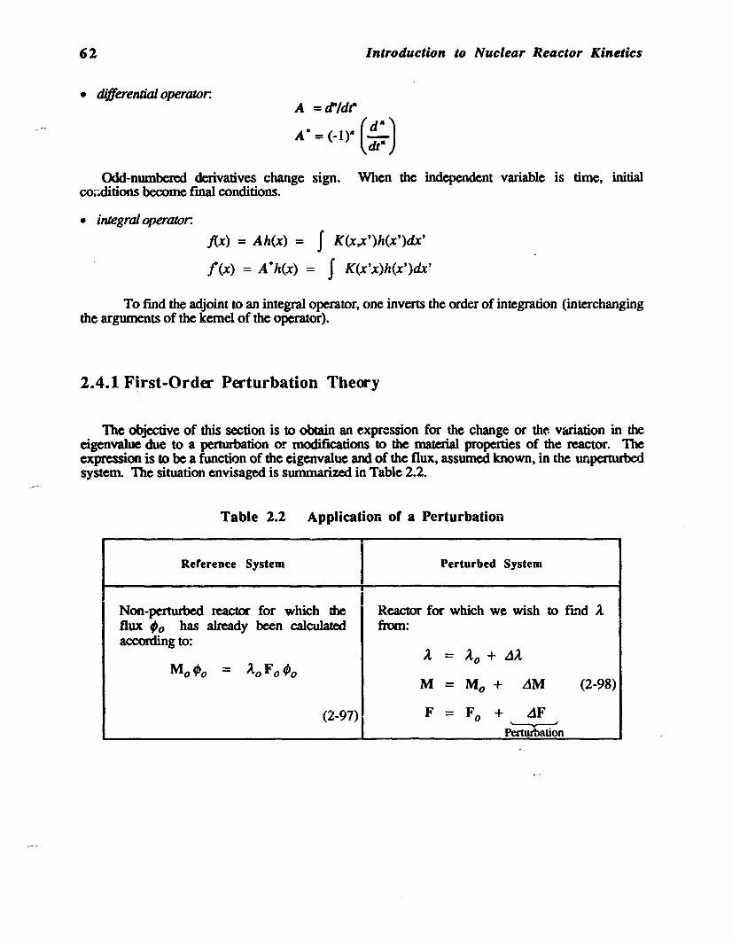
• differential operator.


A = tl'ldt"

AO = (-I)' (~:)

Odd-numbered derivatives change sign. When the independent variable is time, initialco~ditions become final conditions.

• integraloperalOr.

f(x) = Ah(x) = JK(x,x')h(x')dx'

!(x) = A·h(x) = J K(x'x)h(x')dx'

To find the adjoint to an integral operator, one inverts the order of integration (interchangingthe arguments of the kernel of the operator).

2.4.1 First-Order Perturbation Theory

The objective of this section is to obtain an expression for the change or th~ variation in theeigenvalue due to a perturbation or modifications to the material properties of the reactor. 'Theexpression is to be a function of the eigenvalue and of the flux, assumed known, in the unperturbedsystem. The situation envisaged is summarized in Table 2.2.

Table 2.2 Application of a Perturbation

Reference System Perturbed System

Non-perturbed reactor for which theI

Reactor for which we wish to fmd A

flux '0 has already been calculated from:according to:

At = Ao + LiAMotPo = AtoFo~o

M = Mo + LiM (2-98)

(2-97) F = Fo + LiF'---v--:-"'

Perturbauon


The change in the static reactivity which accompanies the perturbation is equal to the change itA..in the eigenvalue, but of opposite sign:

itA.. = A - Ao

= (1

- k.;.O) - (1- k~J

=

= -itp(2-99)

We would like to calculate itA without knowing the flux distribution in the perturbed system,that is, we would like to avoid solving the diffusion equation again for the perturbed system:

(2-100)

Note that the operator AM in equation 2-98 contains a perturbation to the differential operator- --V· DV _ For the leakage tenn, it wiil thus not be possible to express the perturbation with asimple difference ofcross sections only_ One will need to write

- -' - -t1L = -V-DV+V-DoV

The notation Ml must thus be understood as an abbreviation for the operator (M - M 0)' tPo isthe known unperturbed flux and f the unknown perturbed flux, solution to equation 2-100. Let uswrite

tf>(r,E) = 'o(r,E) + ittP(r,E) (2-101)

and let us substitute equation 2-101 into equation 2-100. Keeping in mind equation 2-99, we get

We also have

).Ffc = A(F°+ L1F),0

= A.F0'0 + loAF4'0 + AUF,0t.. '

",.,lDr4cr

... ).Fofo + A..p'0Substituting this into equation 2-102, we find

(2-102)

(2-103)

(2-104)


This relation is true (to first order) at each point of the domain. On the other hand, the quantity .we want. At. is a scalar. In order to preserve as much generality as possible, we shall use aU thepoints of the domain to calculate .1A, by integrating equation 2-104 over the entire domain (spaceand neutron energy).

The sensitivity of A to arbitrary perturbations is not necessarily the same for all points or allP.nergies of the domain. To preserve as much generality as possible in the calculation of .1A, wemultipll equation 2-104 by an arbitrary weighting function ;w before integreing over r and E.Thus ~ o(r.E) will weight the contribution of each point (r.E) in the integral. We assume also that;w belongs to the same vectorial space as the solution. Integrating the equation and ma.kir.g use ofdefinition 2-94, we find the following relation between the internal products:

(2-105)

From equation 2-97, we have

(2-106)

Subtracting this equation from 2-105, we get

(2-107)

Note that only the second term on the right is a function of the perturbed flux. The other tennsare in the known flux, '0" Since;w is arbitrary, there may be a particular choice which makes thesecond tenD on the right disappear, regardless of .1;. In such a case relation 2-107, from which.1A will be derived, will be a function of the known unperturbed flux ;0 only. Let us thereforeexamine the second term in equation 2-107. We note that

(;w ,(M -AF)l1;)= (;w,(Mo -AoFo)1;)+ (;w ,(LiM -A.o..1F- A~)1;) (2nd order)

- .1A(;w,LlF.14 (3rdorder) (2-108)

Since we limited equation 2-107 to first order, we shall keep only the first term on the right inequation 2-108. This last relation then tells us that we can eliminate the seCond term on the right inequation 2-107, ifwe can show that

(;w ,(Mo- A.oF;,)1 tfi) = 0 (2-109)

But there is indeed a particular choice for the weighting function ;w which satisfies equation 2109, regardless of .1;. This choice is the adjoint flux, solution to the adjoint equation for theunperturbed system:

(2-110)

Let us multiply equation 2-97 by ;0· and equation 2-110 by ;0' Then let.-us integrate bothequations over the entire domain and subtract. to find

(;;,MotPo)-(;o,M;;~)=(Ao-A~X;o,F:;;)= 0 (2-111)


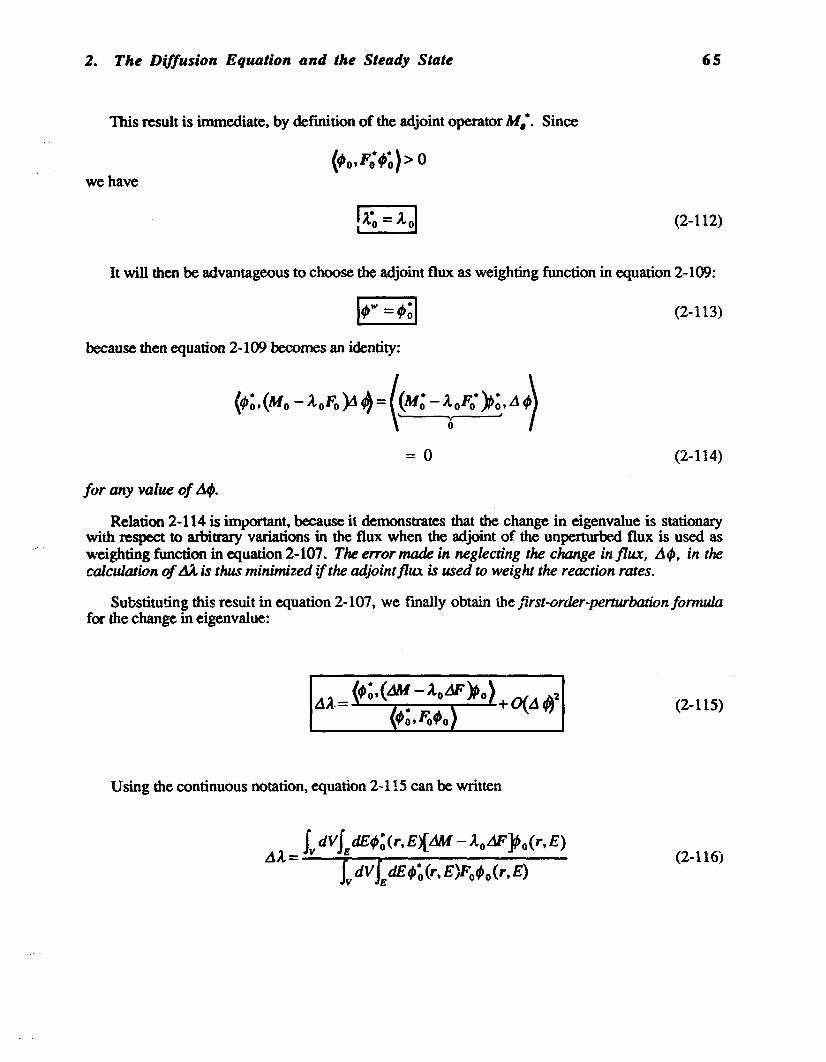
This result is immediate, by defmition of the adjoint operator M,·. Since

we have

6S

(2-112)

It will then be advantageous to choose the adjoint flux as weighting function in equation 2-109:

because then equation 2-109 becomes an identity:

(,;,(Mo-~oFo}1~=(M; -:oF,,');:M)

= 0

(2-113)

(2-114)

for any value of At/>.

Relation 2-114 is important, because it demonstrates that the change in eigenvalue is stationarywith respect to arbitrary variations in the flux when the adjoint of the unperturbed flux is used asweighting function in equation 2-107. The error made in neglecting the change influx, A~, in thecalculation ofLU. is thus minimized ijthe adjointflux is used to weight the reaction rates.

Substituting this result in equation 2-107, we finally obtain the first-order-pertwbation formulafor the change in eigenvalue:

(2-115)

Using the continuous notation, equation 2-115 can be written

(2-116)


2.4.2 Perturbation Formulas for the Reactivity

Let us consider a reactor in any state different from the reference (critical) state. This may betaken to be the perturbed state defined by equation 2-100. Multiplying equation 2-100 by fo· (thereference-state adjoint) and integrating over the entire domain, we readily find the followingexpression for the eigenvalue:

(2-117)

This expression is a much more exact defInition of the eigenvalue of the problem than wasequation 2-91. It is Rayleigh's quotient. We note that it is a homogeneous functional, the ratio oftwo bilinear functionals.

An interesting property of this functional was pointed out in the previous section. Since thefunctional is stationary with respect to arbitrary changes in the flux, it will have a minimum valuewhen the eXC',ct flux, solution of equation 2-100, is used. In fact, this property is often employed invariational methods for convergence acceleration, in the outer iterations of the flux calculation(Hebert, 1985).

Since the static reactivity is equal to (l - A), we obtain the exactformula for the static reactivity:

(2-118)

This formula is exact, because it contains the perturbed flux f, in addition to the perturbedoperators M and F.

It is possible in the same way to find an exact expression for LiA.. Let us multiply equation 2100 by '0· and equation 2-110 by" 2nd then integrate oyer the domain. -We find

(,~,M,)= A(,~,Ff)

("M~f~)= A.o(t/>,F;'~)

Transposing terms in this equation,

(,;,Mof)= '~o(q,;,Foq,)

= Ao(q,;, Fq,)- Ao(';' eq,)

(2-119)

(2-120)

(2-121)


Subtracting equation 2-121 from equation 2-119, we get for AA.:

Ll~XGC' =..J--__~-_+---L

Since Lip =-LU, the following exactformula for the reactivity change em....-rges:

67

(2-122)

(2-123)

This can be compared to thejirst-order-perturbationformula, taken from equation 2-115:

2-124)

The exact formula differs from the fIrst-order formula in the use of the perturbed flux, iP, in thebilinear products, and, in the denominator, of the perturbed operator, F. instead of F..

We note the following,

• The importance of dIe perturbation fonnula is that it allows the evaluation of changes inreactivity for a large number ofperturbations, without a calculation of the perturbed flux ineach case, and to order O(L1<fJ)2, where d<fJ repre~ntc; the flux error (when using theunperturbP...d flux).

• The importance of t.;e exact fannula 2-122 or 2-123 is that it allows a more preciseevaluation ofAA. than that obtained by taking the difference of the eigenvalues of equations2-97 and 2-100. TIais stems from the fact that Rayleigh's quotient is stationary with respectto arbitrary variations in iP. Thus, using the adjoint flux in equation 2-118 or 2-123, evenwith only an estimate for the perturbed (exact) flux, the en-or in p or in dp is minimizedwith respect to LiiP (error ... O(AiP)2).

68

2.4.3 Adjoint Equation


1be exact fannula or the perturbation formulas can be used to evaluate the static reactivity for alarge number of perturbations once the reference-system (unpenurbed) adjoint flux has beencalculated We shall now derive the adjoint diffusion equation, that is, find expressions for theoperators K and r which appear in equation 2-110.

From the definition of an adjoint operator in equation 2-96, we have

(if ,M4» = (4),M· 4>.)

(4)., F4» = (4). F·4>.)

Let us begin with the fission-source term.

IFISSION SOURCEl

(losses)

(fission source)

(2-125)

(2-126)

In its integral form, the total-fission-source term, weighted by the adjoint, is written

= f,Jv 4>(r, E)vEI (r, E)J£. x(E')f (r ,E'}tE'dEd 3r, --'

Ft~.

(2-127)

We can see, by inverting the order of integration in the operator, that the adjoint operator for thefission source can be written as follows in continuous notation:

In matrix notation (multigroup formalism), we get

= (cP .[FbrfJ!..)

(2-128)

(2-129)


Consequently we find, in matrix notation:

This result is in case immediate, from the observation

[FIxf = [fxIFrJLet us now obtain the adjoint operator for neutron loss_

rNEUTRON REMOVALI

69

(2-130)

(2-131)

The operator M consists of a leakage term, L, and a collision term, A, as we saw in equation 255:

(If ,M~)=(If, (L+ A)~)

= (~. ,Lt/J)+(f ,At/»where, in matrix notation:

Lt/> = -\7 -D(r,E)Vt/>(r,E)

At/> = I(r, E)f>(r,E) - IE' I.(r,E'~ E)p(r, E')

First consider the collision term. We see that

Iv IE t/>. (r, E)I(r,E}tft(r,E)dEd 3r = IvI~~(r, E)I(r,E)I>·(r, E)dEd 3r

SiInilih-Iy

= Iv IE' t/>(r, E')UE I.(r, E'~ E)f (r,E)dEp'd1r

=Iv IE t/>(r, E)UE' I. (r, E~ E'~· (r,E'}iE'pd3r

It is then evident that

(2-132)

(2-133a)

(2-133b)

(2-134)

(2-135)

(2-136)


The leakage operator L requires closer attention, because it contains derivatives. First, we notethe following vector identity, which holds at every point of the domain (r,E):

(2-137)

We therefore have

(2-138)

Let us apply the divergence (Gauss') theorem to the first term on the right-hand side of equation2-138:

(2-139)

where S is the external surface of volume Vand Ii is the unit vector is shown in Figure 2.4.

In order for the divergence theorem to apply to equation 2-139, the function (t/1*DV iP) must becontinuous everywhere in volume V. Let us assume the volume consists of sub-volumes Vi,material regions within which the diffusion constant is constant. We can then write

JvVo~·DVt/> )t3r = ~J., V.~·DViP)13r

= Ll ;'0 ~·DVt/>)Pr. Sl,

(2-140)

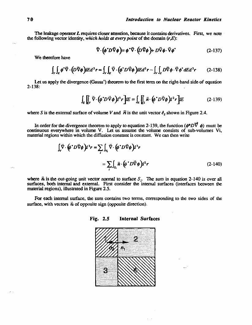
where iii is the out-going unit vector nonnal to surface Sj' The sum in equation 2-140 is over allsurfaces, boLlt internal and external. First consider the internal surfaces (interfaces between thematerial regions), illustrated in Figure 2.5.

For each internal surface, the sum contains two terms, corresponding to the two sides of thesurface, with vectors ;;; of opposite sign (opposite direction),

Fig. 2.5 Internal Surfaces

2. The Diffusion Equation and the Steady Sltlte

We can therefore write

Co..'i_it"'lc,.,.,....' Bo....t14ryollditiolV

Iv V.(fDV,)t3r = I, iii· f(niV'i ~D:V':)- I,iii ·'·~iv,i~~~ ~~

71

(2-141)

Conservation of neutrons across internal surfaces of the domain requires continuity of the

current J =-DV, . Consequently, if the solution satisfies the continuity conditions 2-42 and 2-44,the first term on the right-hand side in equation 2-141 vanishes. We then get

(2-142)

On the reactor's external surfaces, the boundary conditions (equation 2-48) can be written ingeneral fonn as

(2-143)

with { b = 0 => reflectionb = 1/2 => vacuwn

Analogous boundary conditions will be written for the adjoint flux:

(2-144)

Equation 2-138 then w.-omes

(2-145)

From this we see that , and ,. can be interchanged without affecting the value of the righthand~side term. We can thus write

and consequently

(2-146)

Combining equations 2-136 and 2-146, we finally find for the adjoint M· of the removaloperator

(2-147)


In the multigroup fonnalism (matrix notation) we easily find

1$:,[M~= <:P-* ,Q:L]+[AD!)

= (cI>,([Lt +[Atlt )

=~[Mr!!*) (2-148)

ITREATMENT OF TIIE LEAKAGE TERM IN TIIE PERnJRBAnON FORMULAS J

The perturbation fonnulas for the reactivity (equations 2-122, 2-123 and 2-124), which wehave derived in the preceding section, each contain a tenn in AM. Since M includes the leakageterm, it is necessary to apply the divergence theorem to all internal surfaces to evaluate theperturbation due to the variations in the diffusion coefficient

Consider the following functional:

(2-149)

On the other handM = L + A (2-150)

The LiA tenn poses no great difficulty since it contains no derivative. In contrast, the variationin the leakage term is

(2-151)

And using the vector identity 2-137

(2-152)

Now apply the divergence theorem to ~L:

(2-153)

If we select b* = b in equation 2-144, we can write LiM as a function of th~.-increments of thecross sections only:

(2-154)


2.4.4 Importance of Adjoint Weighting

73

We can understand the importance of adjoint weighting of reaction rates in reactivitycalculations by considering the simplified problem shown in Figure 2.6.

Assume we have a slab reactor of width L = 2a in the x direction (and of infinite extent in theother twO" directions). Assume also a single neutron-energy group, and that th~ unperturbed reactoris uniform. The reference flux disnibution, ~o(x), satisfies the equation

(2-155)

with the following boundary conditions:(Xb = ±a)

The above equation is of the form

(2-156)

The only solution which is positive throughout the domain and which satisfies the boundaryconditions is

Fig. 2.6 Localized Perturbation

(2-157)

-8 -Xp Xp

owith the following value for B2

, the geometric buckling:

8

(2-158)


Now assume that a perturbation is made in the centre olthe reactor, more specifically, that onlythe absorption cross section is perturbed, in the interval X=-Xp to x=+xp ' That is, only LiE.. :F. 0 inthe region of the perturbation.

The fundamental eigenvalue for the unpenurbed reactor is obtained by substituting tft/J/dx?' with_B2

; in equation 2-155. Since the reference state is unifonn, the same relation applies at all points.We find:

(2-159)

From the definition for the adjoint operator, it is easy to see that when a single energy group isused the adjoint equation is identical to the "direct" equation for the flux6

• We have therefore

(2-160)

Let us evaluate the change in the reactivity due to this perturbation in two different ways:

• t1(fO): assuming that all points in the domain have the same importance; there is no weighting(;-0 = 1);

• Ap(l): first-order approximation (equation 2-124).

If we neglect weighting, we find approximately (taking cos Bx ... 1) for -xp<.x< xp:

(2-161)

Using now the perturbation fonnula 2-124 and also equation 2-160, we find

(2-162)

The right-hand sides in fonnulas 2-161 and 2-162 each contain three factors. The secondfactor, -LiE/vEjO' is the contribution due to a uniform change in E... The third factor, x/a, is thefraction of the <somain affected by the perturbation. The fIrSt factor is greater than I, and takes intoaccount the fact that the perturbation is concentrated at the centre of the reactor, where the flux ishigher than on average. When we neglect weighting, this factor is 1C/2 =.: 1.57. But with adjointweighting, this factor becomes equal to 2. There is a difference 0127 %.

6 This is not the case when using more than one neutron energy group. In general ;-(r,E) :F.

;(r,E).

2. The Diffusion Equation and the Steady State 7S

This difference can be attributed to the fact that the neutron importance is not uniform in thereactor. In our example, the neutron importance in the central region is greater than the average by27 %. In contrast to a neutron born in the centre of the reactor, one born near the core peripheryhas a greater' chance of escaping from the system before being absorbed. Its contribution to theeffective multiplication constant will thus be smaller, and its importance reduced relative to aneutron at the centre.

This simplified example illustrates the necessity of taking into account the ~djoint-flux

distribution in reactivity calculations, because the spatial importance is not the same everywhere.Furthennore, heterogeneities in the energy domain make the use of the importance (adjoint) evenmore necessary when treating energy groups.

2.5 Conclusion

In LJtis chapter, we have presented the main approximations made to allow the calculation of thescalar-flux distribution in the reactor, using multigroup diffusion theory. We have introduced theconcept of criticality of a reactor, and given a rigorous definition of the critical steady state. 1bestatic reactivity has been defined relative to the eigenvalue It emerging from the steady-statediffusion calculation.

Using first-order perturbation theory, we have seen how to calculate the change in staticreactivity, L1p, due to a perturbation acting on the reactor, even without the knowledge of theperturbed flux. This calculation actually gives the change in reactivity to second order in the changein flux. Such precision is obtained by adjoint weigh.t!ng, and stems from the stationarity ofRayleigh's quotienL

When using a single neutron energy group, the adjoint is identical to the scalar flux, i.e., ~. =~ (the diffusion operator is hermitean). In reality, one should generally consider the variation offlux with E and adopt the multigroup approach in calculations. In that case

',·(r):I: ',(r)

'·(r,E) ~ q,(r,E)

i.e., the adjoint cannot be obtained from the flux itself, but only by actually solving the adjointequation. Note that the adjoint operator is constructed from a discretized form of the directoperator. The adjoint equation contains therefore the same number of groups, and the finitedifference is applied on the same mesh. The adjoint satisfies the same continuity conditions and thesame boundary conditions as the flux.

A complete description of a reactor in steady state thus requires the knowledge of the scalarflux, of the eigenvalue, and of the adjoint flux, which allows the evaluation of the sensitivity of theeigenvalue to perturbations. Since the starting point of a transient is generally a steady state, ourresults will have an impact on the exact fonnulation of the kinetics equations, to be presented in thenext chapter.

Finally, we note that the classical approach of perturbation theory can be generalized tofunctionals of the flux other than the eigenvalue It. By defming generalized adjoints, variationalmethods (Stacey, 1974) allow the evaluation of flux functionals with a precision of order O(Ll,)2.The generalized perturbation theory which is derived in that fashion finds application in fuel designand fuel management, where it is important to know the sensitivity of the characteristic functionalsof the system (Rozon, 1990).

chapter 2 the diffusion equation and the steady state library/20041802.pdf · chapter 2 the...

Documents