chapter 1: introduction and problem statement · invasive exotic pest from indonesia (sanford,...
TRANSCRIPT
1
Chapter 1: Introduction and Problem Statement
Bees are critical to the stability and persistence of many ecosystems, and
therefore, must be understood and protected (Allen-Wardell et al., 1998; Kearns, Inouye
& Waser, 1998; Michener, 2000; Cane, 2001; Kremen, Williams & Thorp, 2002;
LeBuhn, Droege & Carboni, in press). Their pollination services are responsible for
global biodiversity and maintenance of human food supplies (Allen-Wardell et al., 1998;
Kearns et al., 1998; Michener, 2000; Kremen et al., 2002). Over the past two decades,
bees have received increased attention by the scientific community because of population
declines (Allen-Wardell et al., 1998; Kearns et al., 1998). Scientific research has focused
primarily on honey bee (Apis mellifera) declines because this species is the most
commonly used pollinator in United States agriculture, but significant declines have also
occurred in native bees (Kevan and Phillips, 2001; Allen-Wardell et al., 1998). The
United States Department of Agriculture (USDA) Bee Research Laboratory has charted a
25% decline in managed honey bee colonies since the 1980s (Greer, 1999). Estimates on
native bee declines, on the other hand, are disputed and vary (Williams, Minckley &
Silveira, 2001). Nonetheless, increased anthropogenic effects and exotic pests are
impacting global bee populations (Kim, Williams & Kremen, 2006).
The specific consequences of the bee population decline on our food supply and
global biodiversity remain to be seen, but the effects will inevitably be negative (Allen-
Wardell et al., 1998). Fears of food, economic and biological losses have provoked a
surge of scientific literature that examines the associated problems. Recent
advancements in geography and landscape ecology suggest that landscape composition
and pattern are critical to population dynamics (Turner, Gardner & O’Neill, 2001). Work
2
by entomologists and agriculturalists reveal links between the landscape matrix and bee
populations, however, these landscape and regional scale links are not yet fully
understood (Kremen et al., 2004; Steffan-Dewenter et al., 2002a; Dauber et al., 2003)
This thesis explores the spatial components of native bee habitat in Montgomery
County, Virginia, by means of spatial analysis informed by a synthesis of
interdisciplinary research findings, field data and statistical analysis. The goal of this
study is to examine landscape scale components (topography, soils, and land cover) of
native bee habitat in Montgomery County, Virginia for the purpose of assessing: 1) the
usability of geographic information systems (GIS) analysis in bee research, 2) landscape
scale variables important to native bee populations in the region, and 3) the impact of
local site influence on bee populations. Specific objectives of this thesis are to:
1. Identify important spatial variables of bee habitat through an extensive
literature review.
2. Build and validate a GIS model that generates a landscape scale bee habitat
suitability index for Montgomery County, Virginia.
3. Evaluate the use of geographic methods in assessing the relationship between
bee population and habitat.
I correlate landscape variables and relate them to nesting and foraging
requirements to create a GIS habitat suitability index for native bees. The index, created
by incorporating findings from scientific literature, represents a quantitative estimate of
bee diversity and abundance at a given location. The index enables a landscape scale
3
assessment of variation in bee habitat, and therefore, fills an important gap in bee
research that can serve to inform land management practices by providing critical coarse
scale information on pollinators.
A key distinction between this research and the work of others is that it relies
heavily on Geographic Information Systems (GIS) to aid in the research on bees. GIS
has become a term that is intertwined with geography and can allow for flexibility and
error assessment in modeling, allowing for innovative and creative methods that
incorporate decision support, spatial statistic, and relational databases that can be very
useful in identifying scales appropriate for analysis (Turner et al., 2001).
1.1: Significance of Research
The importance of pollination services to ecosystem and economic health has
been a major concern of many scholars. As a result, honey bee pollination is widely used
and documented; pollination services by native bees, on the other hand, are less prevalent
and less understood. However, recent research claims some native bees, such as
bumblebees, are better than honey bees as pollinators, and this claim is driving new
research (Thomson & Goodell, 2001). In addition, bee researchers are expanding and
seeking out new methods for pollination because the current honey bee declines have
presented needs for alternative pollinators in agriculture.
Strong efforts are being taken to ensure continued pollination by bees, especially
in Europe where bee declines and extinctions predate North American declines. One
stumbling block in the research efforts for North American bees is that there have been
no spatially large, systematic surveys of pollinators and no long term datasets compiled
4
(Cane, 2001). This has lead to criticism of prior studies on population declines and is a
strong indication of a need for more research (Cane, 2001; Lebuhn et al., in press). My
work contributes to this need by adding to the North American literature on bees which
traditionally has been an area dominated by European research.
The need to quantify the temporal and spatial aspects of North America’s native
bees, demands an accurate means of conducting landscape scale bee population analyses
(Cane, 2001; Lebuhn et al., in press). This study will be one of the first of its kind
focusing on this, incorporating GIS and suitability indexing methods. It will fill an
important gap in bee research by studying native bee populations from a multiple scale
and geographic perspective, with a focus on GIS modeling.
This research also contributes to the North American Pollinator Protection
Campaign (NAPPC), designed to map and identify all pollinators in North America
(LeBuhn et al., in press). By addressing the campaign’s specific call for a landscape
scale analysis method for assessing pollinator populations this thesis further contributes
to bee population research. I focus on building a model that can potentially be used to
assess temporal change in pollinator populations, identify current population dynamics
and as a quantitative link between landscape pattern and biodiversity.
5
Chapter 2: Literature Review
The literature review is separated into two main sections to reflect the major focus
areas of this study. The first section, Pollination and Ecosystem Services, reviews
background on pollination services, and the biogeography of honey bees, native bees and
individual bee species. The purpose of this section is to provide important background
information on the species modeled in this research. The second section, Spatial
Components and Geographic Concepts, contextualizes the spatial components of native
bee habitat used in the GIS model, with emphasis on theory from landscape ecology and
geography. When the model is referred to in the literature review it relates to the GIS
model I build for bee habitat suitability which uses landscape variables as a predictor of
bee species abundance and diversity. The development of the model is explained in
Chapter 3: Methods.
2.1: Pollination and Ecosystem Services
Honey bees are recognized as contributors to the majority of pollination services
because current agricultural practices in North America and most of the world are
dependent on managed colonies of honey bees (Kevan & Phillips, 2001). However,
declining populations of honey bees has decreased their reliability as pollinators (Greer,
1999). New research is proving that native bees such as bumblebees (Bombus), digger
bees (Andrena, Colletes) and mason bees (Osmia) are more important than honey bees
for pollination (Chambers, 1946; Klein et al., 2003; Kremen et al., 2002).
Using native bees for agriculture is still rare and adoption of new pollination
techniques has been slow. Michener (2000) estimates that only 20% of cultivated plants
6
are pollinated by native bees. Lack of even a simple species list for most geographic
regions makes a change in managed pollinators even more difficult for farmers. If honey
bee populations don’t stabilize, there will be many hurdles to overcome in order to
maintain the current level of agricultural production.
The benefits from pollination are most notably important to crop production.
Klein et al., (2003) successfully correlated increased yields of fruit with increased
diversity and abundance of pollinators. Estimates in the 1980’s on the value of insect
crop pollination are as high as 18.9 billion dollars (Michener, 2000). Pollination not only
increases the number of seeds and size of fruit, it is also an important genetic provider,
needed to improve cultivated strains (Fell, 2005; Michener, 2000). O’Toole (1993)
reviews usage and trends of native bees and insect pollinated crops.
Pollinators’ essential role is to spread genetic information. At the most basic level
it is the transfer of pollen grains (male gametes) to the plant carpel, the structure that
contains the ovule (female gamete; Fell, 2005). This task produces ecosystem services
providing honey for food, improving crop production and improving biodiversity in
ecosystems (MEA, 2005). Ecosystem services are those that the natural environment
produces, from which humans benefit (Kremen et al., 2004).
Fruit crops are especially susceptible to the decline of pollinators (Fell, 2005).
Without pollinators, 110-150 crop species, such as apples, peaches, blueberries,
cranberries, squash, pumpkins, melons, strawberries, and almonds will be at risk with
limited gene pools, reduced seed quantities and reduced yields (Allen-Wardell et al.,
1998). Therefore, preservation of bees is critical to efficient, continued agriculture, and
biodiversity (Kremen et al., 2002).
7
2.2: Biogeography of the Honey Bee (Apis mellifera)
Honeybees belong to the old world genus Apis, of which no species are native to
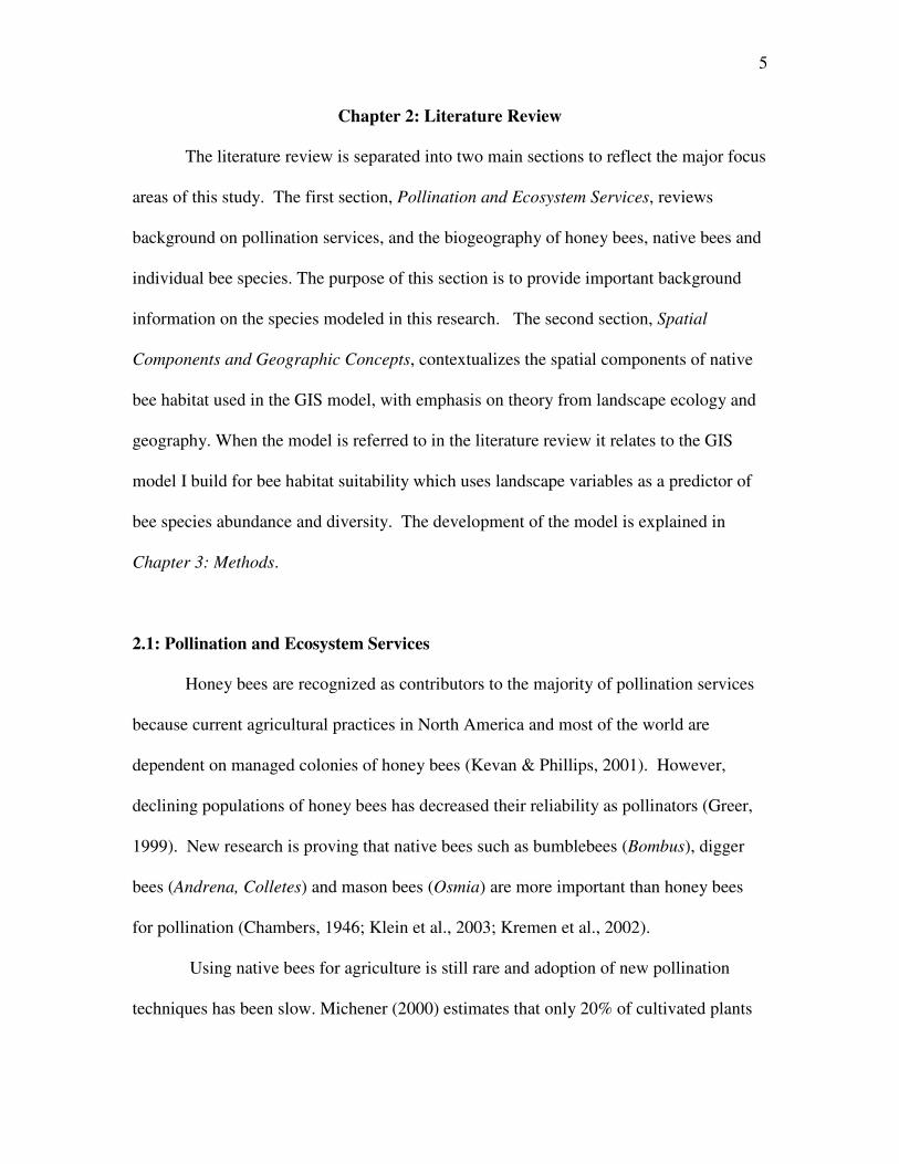
the Americas (Milner, 1996). There are four species of honeybees, but Apis mellifera, the
domesticated or Western Honeybee (Figure 2.1) was the species introduced to North
America and used for agriculture (Milner,
1996). The domesticated honeybee is
native to Europe, Africa and western Asia.
The Giant Honeybee (Apis dorsata) is
native to Southeast Asia. The Eastern
Honeybee (Apis cerana) is native to
eastern Asia, Korea & Japan and the Little
Honeybee (Apis florea) is native to Southeast Asia (Winston, 1987).
As opposed to the many annual species of native bees, the species of Apis have
perennially social colonies persisting over the winter from one season to the next for
periods of three or four years (Mitchell et al., 1985). There is no interaction between the
queen and the worker bees. Queens never engage in foraging activities or build nests
(Michener, 2000). Honey bees collect large amounts of honey used for over wintering,
which can also be used for economic benefit (Milner, 1996).
Honey Bee Decline
In the late 1980’s honeybee feral populations began disappearing and commercial
colonies in production dropped drastically due to the varroa mite (Varroa jacobonsi), an
invasive exotic pest from Indonesia (Sanford, 1987). In addition, Old World parasites,
8
larval diseases and the red imported fire ant have all weakened honeybee colonies (Allen-
Wardell et al., 1998). Furthermore, a new phenomenon labeled Colony Collapse
Disorder (CCD) has emerged that resulted in the disappearance of Western honey bee
colonies (Engelsdorp et al., 2006).
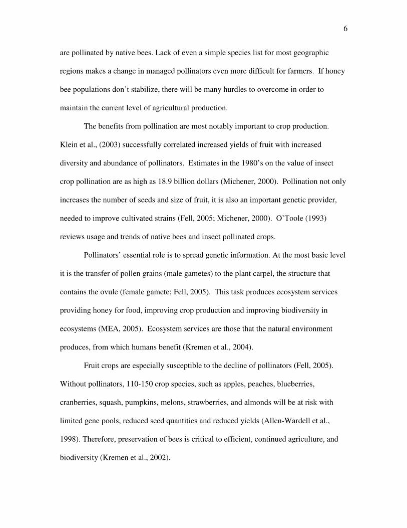
The exotic varroa mite (Figure 2.2) is considered to be the biggest threat to the
honeybee. It was hypothesized that the introduction of the exotic pest resulted from
shipping bio-contaminated material or illegal
cargo containing infected honeybees into the
U.S. (Sanford, 1987). The varroa mite was
first identified in Java in 1904. For roughly
40 years, it was not reported in many places
other than Indonesian neighboring islands.
Around 1960 there was a marked increase in the range of the varroa habitat moving to
Africa, Asia, Europe, South America and then finally North America in 1988
(Rademacher, 1991).
Varroa mites are estimated to have caused a 50-75% loss in commercial honey
bee populations, almost entirely destroying feral honey bee colonies (Allen-Wardell et
al., 1998; Gegner, 2003). All policies and eradication plans failed at containing the pest
(Sanford, 1989). The varroa mite is most destructive to the European honey bee because
of an undeveloped host parasite relationship. In developed host parasite relationships the
parasite typically does not kill the host. The introduction has been called a “nightmare
come true” (Sanford, 2003). Several states have already associated the honeybee decline
9
with reduced crop yields. For example, the California Almond has suffered decreased
yields and prices increases (Morse, 2002).
2.3: Biogeography of Native Bees
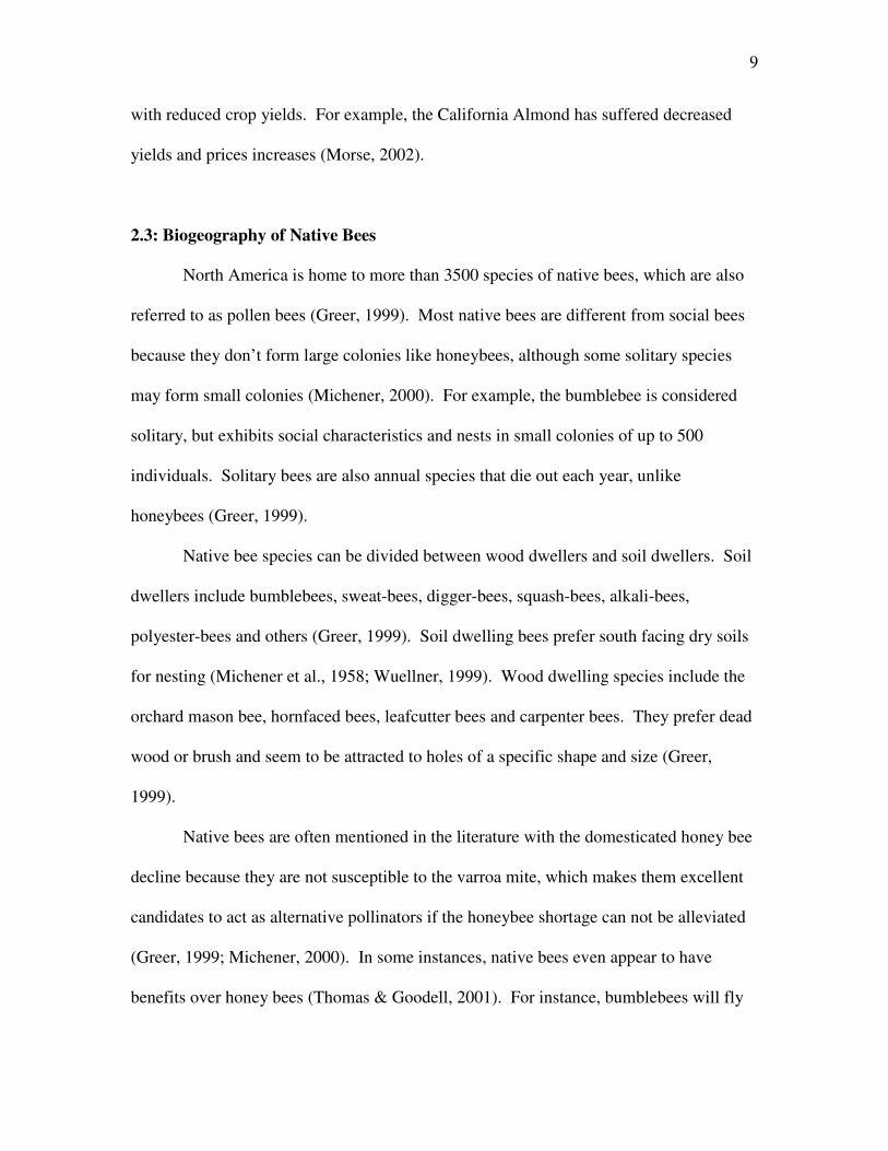
North America is home to more than 3500 species of native bees, which are also
referred to as pollen bees (Greer, 1999). Most native bees are different from social bees
because they don’t form large colonies like honeybees, although some solitary species
may form small colonies (Michener, 2000). For example, the bumblebee is considered
solitary, but exhibits social characteristics and nests in small colonies of up to 500
individuals. Solitary bees are also annual species that die out each year, unlike
honeybees (Greer, 1999).
Native bee species can be divided between wood dwellers and soil dwellers. Soil
dwellers include bumblebees, sweat-bees, digger-bees, squash-bees, alkali-bees,
polyester-bees and others (Greer, 1999). Soil dwelling bees prefer south facing dry soils
for nesting (Michener et al., 1958; Wuellner, 1999). Wood dwelling species include the
orchard mason bee, hornfaced bees, leafcutter bees and carpenter bees. They prefer dead
wood or brush and seem to be attracted to holes of a specific shape and size (Greer,
1999).
Native bees are often mentioned in the literature with the domesticated honey bee
decline because they are not susceptible to the varroa mite, which makes them excellent
candidates to act as alternative pollinators if the honeybee shortage can not be alleviated
(Greer, 1999; Michener, 2000). In some instances, native bees even appear to have
benefits over honey bees (Thomas & Goodell, 2001). For instance, bumblebees will fly
10
and forage in a broad range of weather conditions (Gathmann & Tscharnkte, 2002),
whereas, honeybees only perform pollination in a narrow weather conditions: sunny with
low winds and high temperatures (Gegner, 2003). Other species, such as digger-bees or
the blue orchard bee seem to be more effective at successfully transferring pollen grains,
which is critical for fertilization. For example, an acre of apples can be successfully
pollinated using a small percentage of blue orchard bees compared to the honeybees
needed to cover the same area (Wolf et al., 2002).
Native Bee Decline
Though resistant to the varroa mite, native bee populations have also been
declining, likely due to the combined influences of habitat fragmentation, urbanization
and pesticides (Aizen & Feinsinger, 1994; Cane, 2001; Roubik, 2001). However, a lack
of systematic large scale bee sampling and conflicting research results confound the truth
on native bee declines (Cane, 2001; Lebuhn et al., in press). For example, Packer (2001)
suggests that bees flourish in fragmented and disturbed habitats, even though the negative
effect of habitat fragmentation on species abundance and diversity of pollinators has been
well documented. To further complicate explanations, solitary bee populations can be
dynamic, exhibiting temporal and seasonal variability (Roubik, 2001). One potential
reason for confounded explanations is the use of simple linear regression and correlation
estimates to build models in many of these studies. Biological data is rarely linear and
transformations can change data, making the use of all linear modeling concerning and
possibly even explaining the drastic variations (Agresti, 1996).
11
Finally, the current state of native bee populations is largely unknown in North
America (Cane, 2001; Lebuhn et al., in press). Cane (2001) concluded that while
populations might be declining there was not strong enough evidence to support such
claims and that a better approach to understanding changes in bee populations might be
assessing habitat change. This approach may be facilitated with geographic methods
incorporating spatial analysis and GIS modeling, as spatial and temporal habitat change is
commonly modeled by geographers.
2.4: Biogeography of Bees Species of Interest
A major objective of this thesis was to develop a bee habitat suitability model
using the currently available research. This model was developed for solitary, soil
dwelling species such as digger bees, bumblebees, and sweat bees. Scale limitations in
the available GIS and remote sensing data meant that wood dwelling bees were omitted
from the model because of their fine scaled habitat requirements, which are identified
through wood debris composition and nesting hole diameter (Greer, 1999; Wolf et al.,
2002). It is difficult or impossible to detect these requirements with available resolution
imagery. Described below are the major
groups of bees to which the literature
refers that could be used in a GIS.
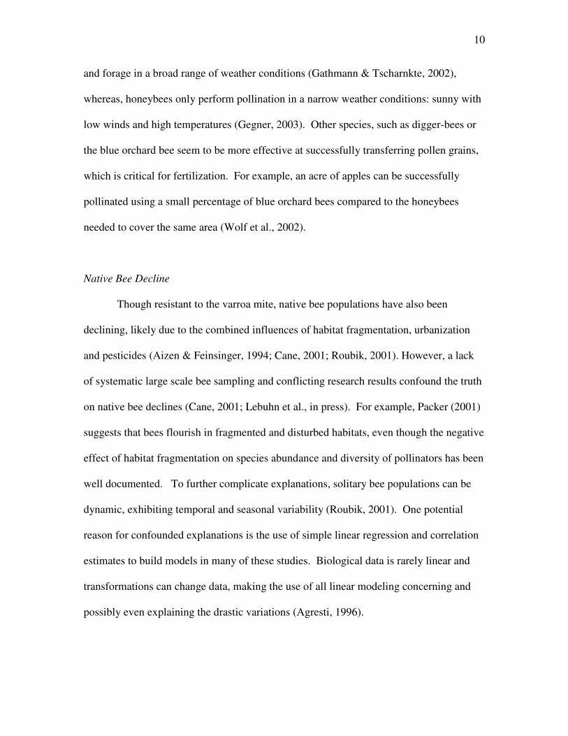
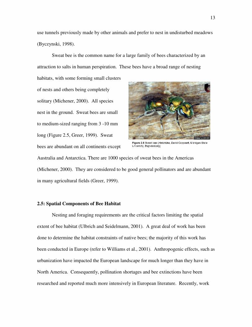
Digger bee is the common name
for a group of fast-flying, ground-nesting
bees with velvety fur (Figure 2.3). These
bees are a cosmopolitan species, meaning they are located throughout the world
12
(Michener, 2000). Several thousand species exist, of which more than 900 occur in the
United States and Canada. Digger bees are generalists, visiting a wide variety of flowers
(Greer, 1999). They form their nests in the ground, leaving small mounds of soils behind
(Wuellner, 1999). Although digger bees are solitary they sometimes nest together in
dense patches (Michener et al., 1958). Their size can vary considerably. Rarely noticed
digger bees are often the most abundant pollinator in the agricultural fields (Greer, 1999).
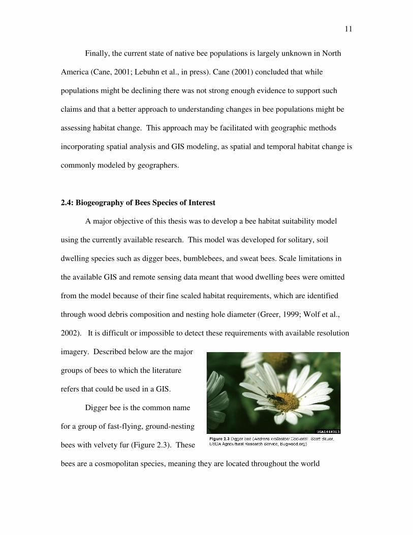
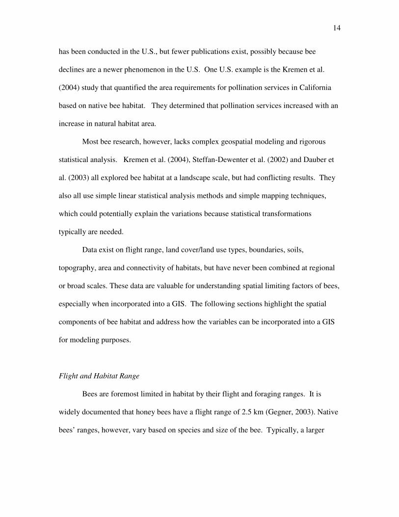
Bumblebee is the common name for a group of large, hairy, black and yellow,
social bees ranging in size from 9 - 22 mm long (Figure 2.4, Michener, 2000). They are
found in temperate regions of the northern
hemisphere, including alpine environments
(Michener, 2000). Bumblebees’ large size and
ability to regulate their own body temperature
allow the bees to live in a wide range of
habitats (Michener, 2000). This unique
characteristic also allows them to fly and
forage in harsh weather conditions. They are important pollinators that visit a wide
variety of floral hosts (Greer, 1999). The bumblebee pollinates important agricultural
crops such as tomatoes, eggplants, pepper, melons, raspberries, strawberries, blueberries,
cranberries, apples, etc (Smith-Heavenrich, 1998). They are also the only pollinators of
the potato flower (Reickenberg, 1994).
North America is home to fifty species of bumblebees (Michener, 2000). The
common bumble bee on the eastern landscape is Bombus impatiens. They form nests
much like honeybees except colony sizes are small and underground. Bumblebees often
13
use tunnels previously made by other animals and prefer to nest in undisturbed meadows
(Byczynski, 1998).
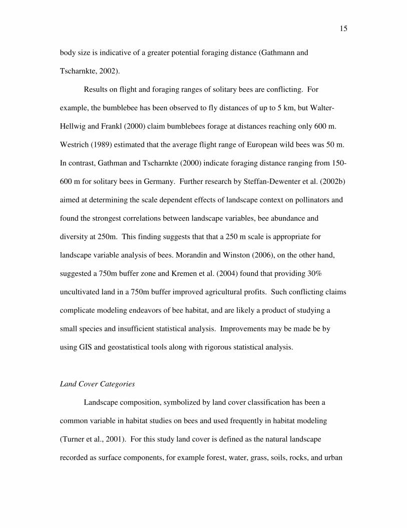
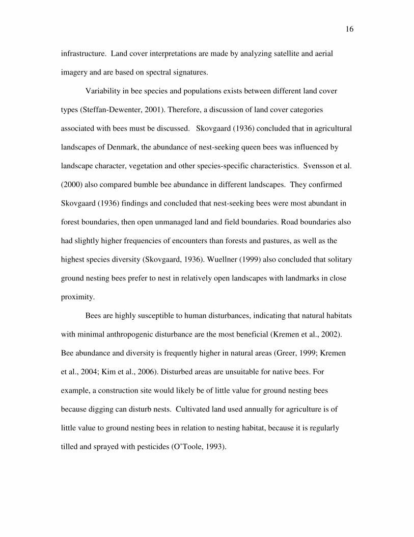
Sweat bee is the common name for a large family of bees characterized by an
attraction to salts in human perspiration. These bees have a broad range of nesting
habitats, with some forming small clusters
of nests and others being completely
solitary (Michener, 2000). All species
nest in the ground. Sweat bees are small
to medium-sized ranging from 3 -10 mm
long (Figure 2.5, Greer, 1999). Sweat
bees are abundant on all continents except
Australia and Antarctica. There are 1000 species of sweat bees in the Americas
(Michener, 2000). They are considered to be good general pollinators and are abundant
in many agricultural fields (Greer, 1999).
2.5: Spatial Components of Bee Habitat
Nesting and foraging requirements are the critical factors limiting the spatial
extent of bee habitat (Ulbrich and Seidelmann, 2001). A great deal of work has been
done to determine the habitat constraints of native bees; the majority of this work has
been conducted in Europe (refer to Williams et al., 2001). Anthropogenic effects, such as
urbanization have impacted the European landscape for much longer than they have in
North America. Consequently, pollination shortages and bee extinctions have been
researched and reported much more intensively in European literature. Recently, work
14
has been conducted in the U.S., but fewer publications exist, possibly because bee
declines are a newer phenomenon in the U.S. One U.S. example is the Kremen et al.
(2004) study that quantified the area requirements for pollination services in California
based on native bee habitat. They determined that pollination services increased with an
increase in natural habitat area.
Most bee research, however, lacks complex geospatial modeling and rigorous
statistical analysis. Kremen et al. (2004), Steffan-Dewenter et al. (2002) and Dauber et
al. (2003) all explored bee habitat at a landscape scale, but had conflicting results. They
also all use simple linear statistical analysis methods and simple mapping techniques,
which could potentially explain the variations because statistical transformations
typically are needed.
Data exist on flight range, land cover/land use types, boundaries, soils,
topography, area and connectivity of habitats, but have never been combined at regional
or broad scales. These data are valuable for understanding spatial limiting factors of bees,
especially when incorporated into a GIS. The following sections highlight the spatial
components of bee habitat and address how the variables can be incorporated into a GIS
for modeling purposes.
Flight and Habitat Range
Bees are foremost limited in habitat by their flight and foraging ranges. It is
widely documented that honey bees have a flight range of 2.5 km (Gegner, 2003). Native
bees’ ranges, however, vary based on species and size of the bee. Typically, a larger
15
body size is indicative of a greater potential foraging distance (Gathmann and
Tscharnkte, 2002).
Results on flight and foraging ranges of solitary bees are conflicting. For
example, the bumblebee has been observed to fly distances of up to 5 km, but Walter-
Hellwig and Frankl (2000) claim bumblebees forage at distances reaching only 600 m.
Westrich (1989) estimated that the average flight range of European wild bees was 50 m.
In contrast, Gathman and Tscharnkte (2000) indicate foraging distance ranging from 150-
600 m for solitary bees in Germany. Further research by Steffan-Dewenter et al. (2002b)
aimed at determining the scale dependent effects of landscape context on pollinators and
found the strongest correlations between landscape variables, bee abundance and
diversity at 250m. This finding suggests that that a 250 m scale is appropriate for
landscape variable analysis of bees. Morandin and Winston (2006), on the other hand,
suggested a 750m buffer zone and Kremen et al. (2004) found that providing 30%
uncultivated land in a 750m buffer improved agricultural profits. Such conflicting claims
complicate modeling endeavors of bee habitat, and are likely a product of studying a
small species and insufficient statistical analysis. Improvements may be made be by
using GIS and geostatistical tools along with rigorous statistical analysis.
Land Cover Categories
Landscape composition, symbolized by land cover classification has been a
common variable in habitat studies on bees and used frequently in habitat modeling
(Turner et al., 2001). For this study land cover is defined as the natural landscape
recorded as surface components, for example forest, water, grass, soils, rocks, and urban
16
infrastructure. Land cover interpretations are made by analyzing satellite and aerial
imagery and are based on spectral signatures.
Variability in bee species and populations exists between different land cover
types (Steffan-Dewenter, 2001). Therefore, a discussion of land cover categories
associated with bees must be discussed. Skovgaard (1936) concluded that in agricultural
landscapes of Denmark, the abundance of nest-seeking queen bees was influenced by
landscape character, vegetation and other species-specific characteristics. Svensson et al.
(2000) also compared bumble bee abundance in different landscapes. They confirmed
Skovgaard (1936) findings and concluded that nest-seeking bees were most abundant in
forest boundaries, then open unmanaged land and field boundaries. Road boundaries also
had slightly higher frequencies of encounters than forests and pastures, as well as the
highest species diversity (Skovgaard, 1936). Wuellner (1999) also concluded that solitary
ground nesting bees prefer to nest in relatively open landscapes with landmarks in close
proximity.
Bees are highly susceptible to human disturbances, indicating that natural habitats
with minimal anthropogenic disturbance are the most beneficial (Kremen et al., 2002).
Bee abundance and diversity is frequently higher in natural areas (Greer, 1999; Kremen
et al., 2004; Kim et al., 2006). Disturbed areas are unsuitable for native bees. For
example, a construction site would likely be of little value for ground nesting bees
because digging can disturb nests. Cultivated land used annually for agriculture is of
little value to ground nesting bees in relation to nesting habitat, because it is regularly
tilled and sprayed with pesticides (O’Toole, 1993).
17
Habitat Fragmentation
Habitat fragmentation is a reduction in area and connectivity of an organism’s
preferred habitat, creating discontinuous patches of habitat (Turner et al., 2001). Strong
negative effects on bees result from habitat fragmentation caused by urbanization,
expanding agriculture, deforestation and other geologic processes (Steffan-Dewenter &
Tscharntke, 1999; Aizen & Feinsinger, 1994; Powell & Powell, 1987). Powell and
Powell (1987) concluded that most euglossine bee species’ visitation rates declined with
fragment size. In addition, Aizen and Feinsinger (1994) also claim that frequency and
taxon richness of native pollinators declined with decreasing forest-fragment size.
Furthermore, Steffan-Dewenter and Tscharntke (1999) concluded habitat connectivity
was essential to maintain abundant and diverse bee communities.
Despite the scientific findings that habitat fragmentation is deleterious to bee
species, others have concluded differently. For example, Cane (2001) brings to light the
negations and importance of incorporating spatial and temporal scale into studies of
habitat fragmentation. Cane agrees that detrimental effects of fragmentation to bees are
scalar and species-specific. The challenge lies in determine the appropriate scale for
these type of analyses.
Though there are complications with determining the appropriate scale to measure
connectivity for a measure of fragmentation, predicting bee abundance and diversity is
less debated. Area of natural habitat appears to be the best predictor of pollinator
populations (Steffan-Dewenter, 2003). Increasing the area of natural habitat and floral
resources will increase bee abundance and diversity (Steffan-Dewenter, 2003; Kremen et
al., 2004; Kim et al., 2006).
18
Topography & Soils
Most native bees thrive in sun and dry soils, preferring south facing slopes to
slopes of other aspects (Greer, 1999). Dauber et al. (2003) also concluded that bees
preferred dry south facing slopes, but this preference was attributed to an increase in
floral resources in areas with more sunlight. Michener et al. (1958) provides specific
details on aspect and bee nesting abundance with statistical evidence. No research has
examined the influence of elevation gradients on changes in bee population variability.
Most species of native bees nest in the ground, but few studies aim at determining
the factors specific to soils that are most important for nesting habitat. Species richness
of wild bees was more abundant on dry soils then moist soils (Dauber et al., 2003). Sandy
soils are the preferred substrate because adequate drainage is necessary for bees (Cane,
1991; Cross & Bohart, 1960). In a study of eight nests in Utah, U.S.A., Cross and Bohart
(1960) found bees to nest in sandy loam, silt loam, clay loam and other sandy soils. Cane
(1991) also found bee species to have a preference for sandy soils.
2.6: Concepts from Geography and Landscape Ecology
Geography and landscape ecology are both concerned with understanding spatial
patterns to understand process, and process to understand pattern. Geography and
landscape ecology introduce fundamental questions on the concepts of scale, space and
place (Turner et al., 2001). The major difference between the two disciplines is that
landscape ecology is focused solely on ecological processes, whereas geography
encompasses all systems, including human, ecological, biological, and physical.
Ultimately, geography and landscape ecology are concerned with broad-scale
19
environmental issues and help provide insight on studies of ecological systems that
operate over various scales.
The systems provided and maintained by bees are inherently related to geography
and landscape ecology because of the importance of spatial scale and spatial pattern in
bee habitat. Bee distribution is geographic in nature because it is limited by climate,
topography, soils, and vegetation types (Michener, 2000). Thousands of species of bees
exist on our planet; their distributions limited by spatial variables, create great regional
diversity in bee populations.
Geography has also been on the forefront of GIS development, which may prove
to be an important data management solution for these spatial variables that effect bee
populations. It allows for many spatial variables to be modeled and statistically analyzed.
The benefits of using a GIS for modeling are that you can use large data sets and it is
easy to conduct multiple scale and temporal analysis. Vast quantities of historical data
exist that can be incorporated in models. Change detection algorithms and methods have
also been present in GIS analysis for a long time. GIS provides a prefect opportunity to
incorporate geography into modeling bee habitat at a landscape scale.
The most notable contribution of geography to research on bees was by Michener
(1979), in which he covered the distributional history of bees throughout the world. This
major biogeographic work encompassed the distribution of major groups of bees, and
speculated as to the historical and ecological explanations of such distributions.
Technological limitations at the time of publishing made it difficult for Michener to
quantify, and accurately map, bee populations. Additionally, in 2000 Michener authored
The Bees of the World, an update to his previous work. Other research is beginning to
20
incorporate GIS into bee research, primarily for the purpose of simple mapping and
linear-based modeling (Kremen et al., 2004; Dauber et al., 2003; Steffan-Dewenter et al.,
2004). Shortcomings of these approaches are the use of simple models to represent
complex systems that are rarely linear and can produce erroneous results; this topic is
discussed further in Agresti (1996).
Most research on bees has also neglected other key geography concepts such as
spatial autocorrelation. Spatial autocorrelation is foremost important in bee habitat
research because biological, ecological and landscape variables are most often spatially
autocorrelated. Bees are also small and dynamic, which complicates sampling measures
and statistical analysis. When spatial correlation is not accounted for, the results of
statistical tests can be inflated, increasing the chances of type I errors in hypothesis
testing (Davis, 1986). This can be misleading and makes standard significance test
inaccurate. There are techniques to work around this problem, but when possible it is
best to sample so that spatial autocorrelation is minimized. .
Spatial autocorrelation is defined as an assessment of the correlation of a variable
in reference to the spatial location of the variable (Turner et al., 2001). It tests for
whether a value of a variable at one locality is independent of the values of that variable
at neighboring localities. For example, the presence of some quantity of a given variable
in a county makes its presence in a neighboring counties more or less likely (Cliff and
Ord, 1973). In geographic applications there is most always positive spatial
autocorrelation, which suggests clustering of like values or variables. The spatial
autocorrelation association is always affected by scale, making it important to this study
and bee habitat research.
21
Landscape ecology is also important for understanding bee populations because of
the discipline’s focus on broad spatial scales and the ecological effects of the spatial
patterning of ecosystems (Turner et al., 2001). One theory common to landscape ecology
and important in the conceptualization of this research was percolation theory, which
addresses spatial pattern in random assembly. Applications of percolation theory have
brought to light questions of size, shape and connectivity of habitats (Turner et al., 2001).
Percolation theory has offered much insight into the nature of connectivity or inversely
fragmentation of landscapes (Gardner et al., 1992).
22
Chapter 3: Methods and Procedures
3.1: Study Area
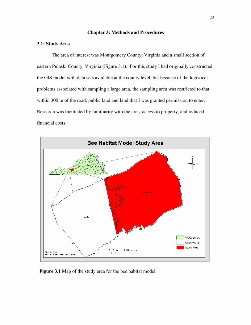
The area of interest was Montgomery County, Virginia and a small section of
eastern Pulaski County, Virginia (Figure 3.1). For this study I had originally constructed
the GIS model with data sets available at the county level, but because of the logistical
problems associated with sampling a large area, the sampling area was restricted to that
within 300 m of the road, public land and land that I was granted permission to enter.
Research was facilitated by familiarity with the area, access to property, and reduced
financial costs.
Figure 3.1 Map of the study area for the bee habitat model
23
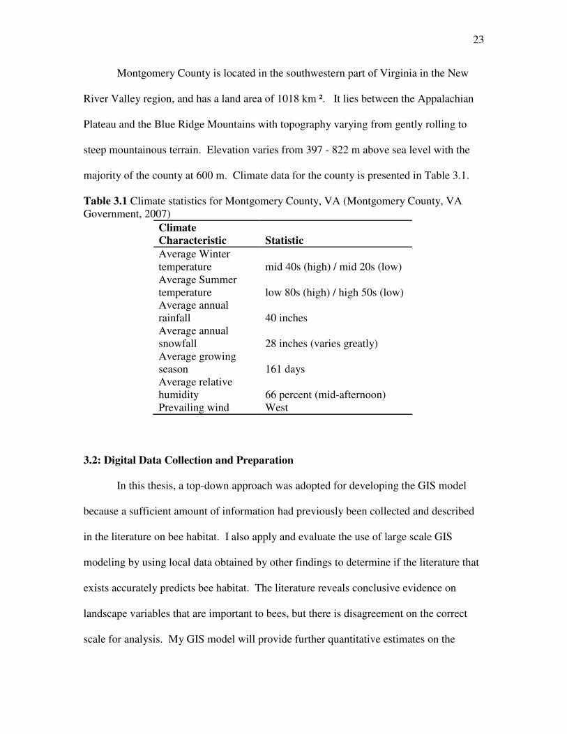
Montgomery County is located in the southwestern part of Virginia in the New
River Valley region, and has a land area of 1018 km ². It lies between the Appalachian
Plateau and the Blue Ridge Mountains with topography varying from gently rolling to
steep mountainous terrain. Elevation varies from 397 - 822 m above sea level with the
majority of the county at 600 m. Climate data for the county is presented in Table 3.1.
Table 3.1 Climate statistics for Montgomery County, VA (Montgomery County, VA Government, 2007)
Climate
Characteristic Statistic
Average Winter temperature mid 40s (high) / mid 20s (low) Average Summer temperature low 80s (high) / high 50s (low) Average annual rainfall 40 inches Average annual snowfall 28 inches (varies greatly) Average growing season 161 days Average relative humidity 66 percent (mid-afternoon) Prevailing wind West
3.2: Digital Data Collection and Preparation
In this thesis, a top-down approach was adopted for developing the GIS model
because a sufficient amount of information had previously been collected and described
in the literature on bee habitat. I also apply and evaluate the use of large scale GIS
modeling by using local data obtained by other findings to determine if the literature that
exists accurately predicts bee habitat. The literature reveals conclusive evidence on
landscape variables that are important to bees, but there is disagreement on the correct
scale for analysis. My GIS model will provide further quantitative estimates on the
24
validity of the current bee research and it will investigate the uncertainties in spatial scale
by using complex GIS modeling, decision support, and rigorous statistical analysis.
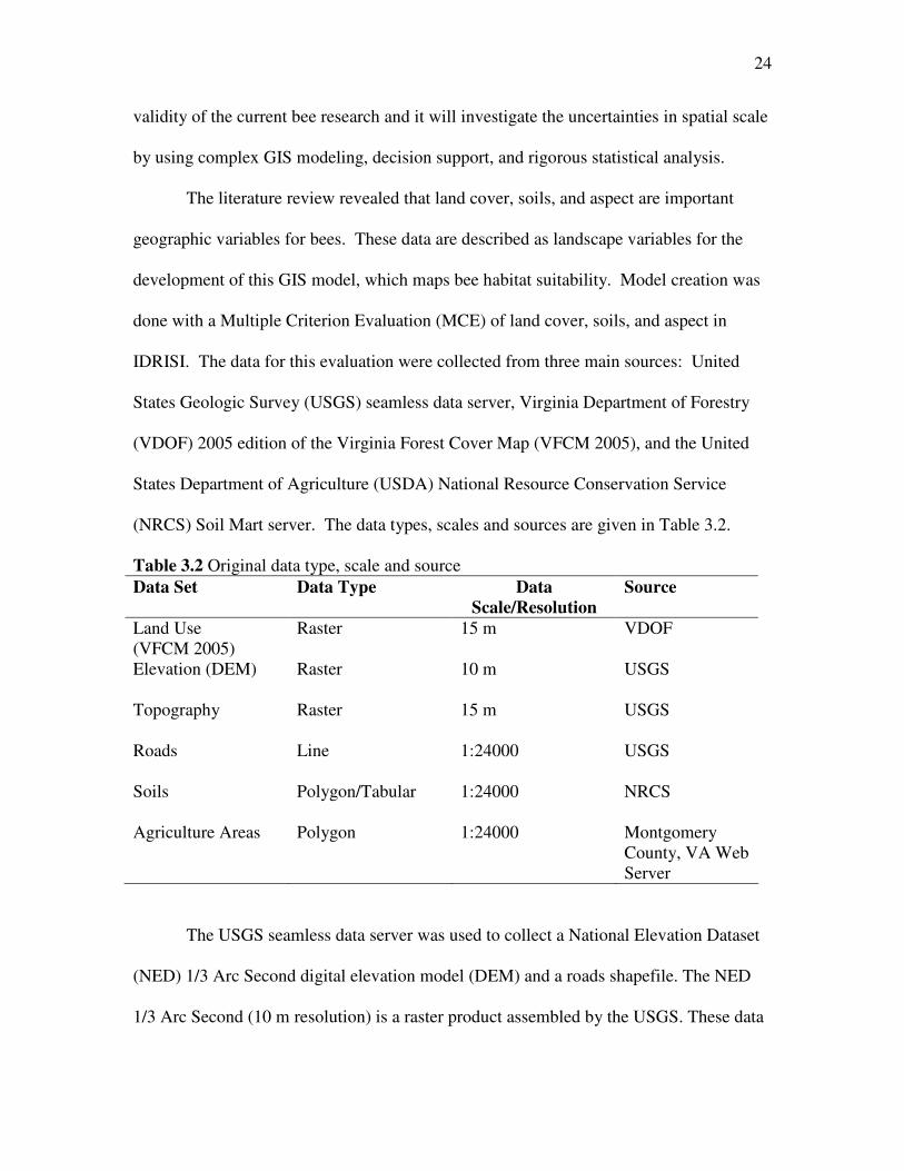
The literature review revealed that land cover, soils, and aspect are important
geographic variables for bees. These data are described as landscape variables for the
development of this GIS model, which maps bee habitat suitability. Model creation was
done with a Multiple Criterion Evaluation (MCE) of land cover, soils, and aspect in
IDRISI. The data for this evaluation were collected from three main sources: United
States Geologic Survey (USGS) seamless data server, Virginia Department of Forestry
(VDOF) 2005 edition of the Virginia Forest Cover Map (VFCM 2005), and the United
States Department of Agriculture (USDA) National Resource Conservation Service
(NRCS) Soil Mart server. The data types, scales and sources are given in Table 3.2.
Table 3.2 Original data type, scale and source Data Set Data Type Data
Scale/Resolution
Source
Land Use (VFCM 2005)
Raster 15 m VDOF
Elevation (DEM) Raster 10 m USGS
Topography Raster 15 m USGS
Roads Line 1:24000 USGS
Soils Polygon/Tabular 1:24000 NRCS
Agriculture Areas Polygon 1:24000 Montgomery County, VA Web Server
The USGS seamless data server was used to collect a National Elevation Dataset
(NED) 1/3 Arc Second digital elevation model (DEM) and a roads shapefile. The NED
1/3 Arc Second (10 m resolution) is a raster product assembled by the USGS. These data
25
were designed to provide national elevation data in a seamless form with a consistent
datum, elevation unit, and projection. There are corrections made to minimize artifacts,
perform edge matching, and fill sliver areas of missing data. The USGS roads were
obtained from the Bureau of Transportation Statistics (BTS) published in 2002. They
cover the 50 states, scaled 1:100,000.
The VDOF VFCM 2005 data was downloaded off the VDOF GIS web site. It was
developed to identify forests in Virginia as defined by the United States Forest Service
(USFS) Forest Inventory and Analysis (FIA) Program. VFCM 2005 was developed
through segment based classification of Landsat imagery spanning March 10, 2002 to
May 8, 2005. An accuracy assessment of water, forest, and non-forest land cover classes
was conducted by the USFS using over 120,000 points, which resulted in an overall
accuracy of 88.24%.
The NRCS Soil Mart server was used to download the soils data. This USDA
maintained site is an extensive data base with 1:12,000 soils maps and tabular data. One
additional data set produced by Montgomery County, VA was used obtained to error
check agricultural areas in the study site.
Preprocessing involving standardization of data was necessary before
incorporation into the model. Files were projected to the local UTM coordinate system,
and clipped to the same spatial extent to allow for proper spatial analysis. The VFCM
data classes were classified into similar classes used in research described in the literature
to ensure proper comparisons (Kremen et al., 2004; Dauber et al., 2003; Steffan-
Dewenter et al., 2004). The hardwood forest, pine forest and mixed forest classes were
reclassified to one class named forest, because forest type delineations have not been
26
made in previous research. Rooftops and pavement classes were also merged since they
represent impervious surfaces, which are equally detrimental to bees digging and habitat.
There were also very few rooftops pixels in the study area, making then statistically
insignificant. The USGS roads line file was rasterized and then overlaid with the
pavement raster class. A cross-tab calculation was done to determine the overlapping,
misclassified, or omitted roads and revealed the VFCM 2005 data mainly misclassified
small rural roads. Because these roads impact bee habitat the misclassified pixels were
corrected to represent pavement (Steffan-Dewenter et al., 2004).
An additional cross-tab calculation was conducted with the crops VFCM 2005
data and the grass/pasture class from the 2000 National Land Cover data set because I
suspected that the VFCM 2005 crops classification was misrepresenting crops as
pastures, grass, or land left fallow. The cross-tab revealed misrepresentation was the
case, indicating that the VFCM 2005 data poorly distinguishes between pastures/grass
and agriculture. For this reason, an agricultural districts polygon shapefile was obtained
from Montgomery County for the study area. This polygon was rasterized and overlaid
with the VFCM 2005 data. All pixels in the agricultural district and labeled as crop in the
FVCM 2005 data set were reclassified to agriculture. All other pixels were considered to
be pasture/grass. The study area contained no pixels classified as bare soil, salt marsh,
natural barren or mine.
Finally, a boundary detection algorithm in the FILTER module in IDRISI was
used to delineate forest, road and field boundaries because these edges have a significant
impact on bee habitat, as described in the literature review. The final result of numerous
cross-tab calculations and overlays was a land cover classification named VLC 2005
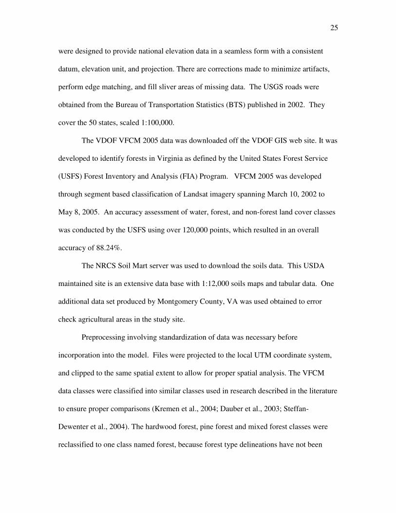
27
(Appendix A) that contained the following classes: water, pavement,
residential/industrial, forest, agriculture, pasture/grasses, forest boundary, field boundary
and road boundary (Table 3.3). The definitions other than the boundary classes are
analogous to the USGS land cover class definitions (Anderson et al., 1976).
Table 3.3 VLC 2005 class names and definitions
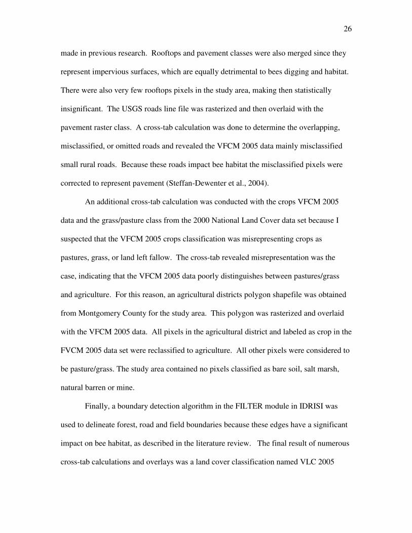
The NED 10 m DEM was resampled to 15 m resolution to allow for proper
overlays and to derive an aspect map (Appendix A), following the protocol outlined by
IDRISI. Aspect was separated into the five classes referred to in the literature and are
defined in Table 3.4 (Michener et al., 1958; Wuellner, 1999)
Table 3.4 Aspect derived from NED 10 m DEM
Class Name Class Name Definition
Water All areas of open water Pavement
> 75% asphalt, concrete, buildings and roads
Residential/Industrial Urban residential/Industrial areas 25-75 % asphalt, concrete, buildings, etc. with some vegetation, and areas of recent disturbance
Forest Areas dominated by trees where 75 % or more of the tree area is tree cover
Agriculture Areas used for the production of annual row and cover crops or used intensively for livestock grazing
Pastures/Grass Areas characterized by natural or semi-natural herbaceous vegetation; herbaceous vegetation accounts for 75-100 % of the cover
Forest Boundary Filter module output, area bordering forests Field Boundary Filter module output, area bordering fields Road Boundary Filter module output, area bordering roads
Class Name Class Definition
North East 0-90 degrees South East 90-180 degrees South West 180-270 degrees North West 270-360 degrees Flat -1 value

28
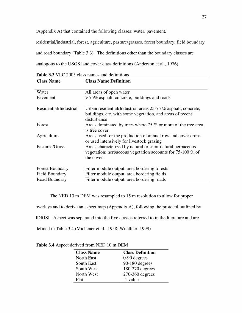
The soils spatial data set, a polygon shapefile, was joined with the soils tabular
data to attach more information to the spatial data. The soils polygons were merged with
the soil polygons that had the same hydrologic group classification. This process
produced polygons with values referencing the four hydrologic groups. Hydrologic
groups were used because they best represented characteristics such as water retention,
drainage and parent material, all important variables to bee habitat (Wuellner, 1999). A
hydrologic group represents soils with the similar runoff potential and drainage (USDA,
2002). The groups are derived from properties such as parent material, depth to water
table, intake rate, permeability after prolonged wetting, and depth to slowly permeable
layers (USDA, 2002). For analysis the soils data was converted to raster format
(Appendix A). The class names and definitions of the hydrologic groups were defined
following USDA (2002) (Table 3.5).
29
Table 3.5 Hydrologic group class names and definitions Class
Name
Class Definition
A Low runoff potential, high infiltration rate, Deep, well drained to excessively drained sands or gravels
B Moderate infiltration, moderately deep to deep, moderately well drained to well drained soils, moderately fine to moderately coarse textures
C Slow infiltration rate, have a layer that impedes downward movement of water or have moderately fine to fine texture
D High runoff potential very slow infiltration, clay soils that have a high swelling potential, soils that have a permanent high water table, soils that have a claypan or clay layer at or near the surface, and shallow soils over nearly impervious material
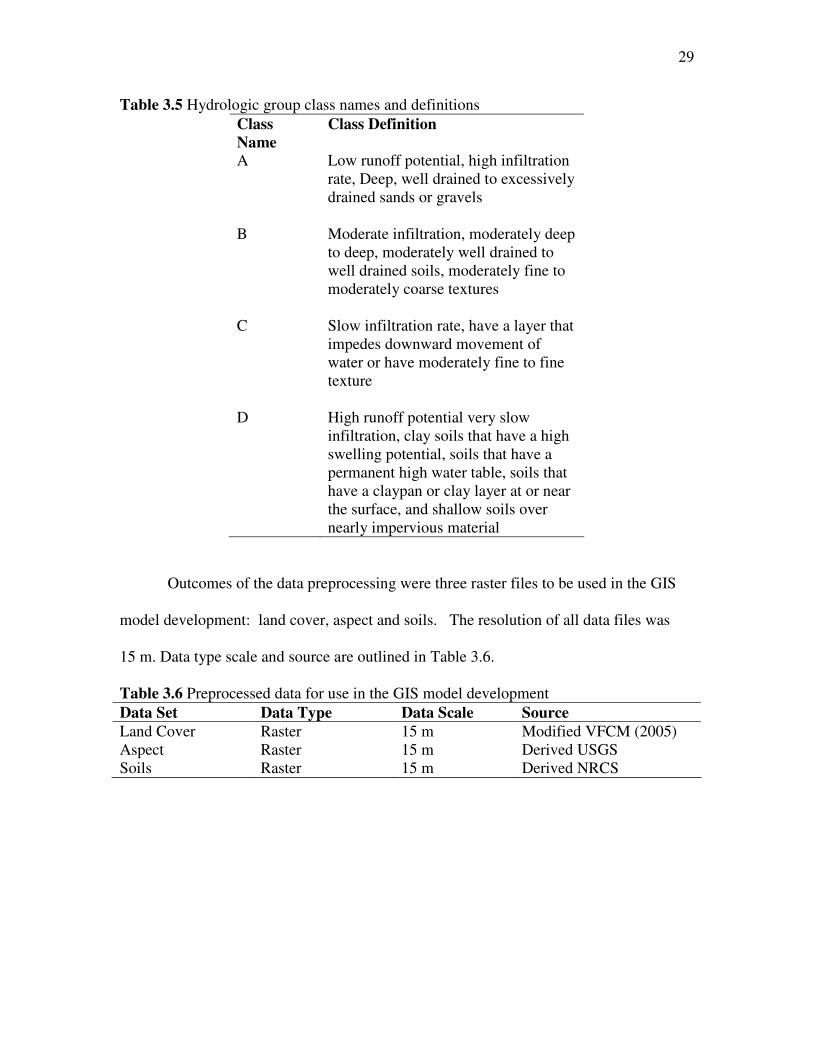
Outcomes of the data preprocessing were three raster files to be used in the GIS
model development: land cover, aspect and soils. The resolution of all data files was
15 m. Data type scale and source are outlined in Table 3.6.
Table 3.6 Preprocessed data for use in the GIS model development Data Set Data Type Data Scale Source
Land Cover Raster 15 m Modified VFCM (2005) Aspect Raster 15 m Derived USGS Soils Raster 15 m Derived NRCS
30
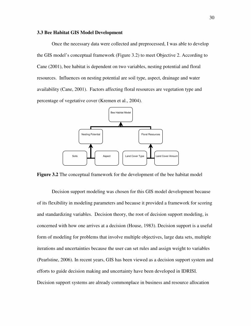
3.3 Bee Habitat GIS Model Development
Once the necessary data were collected and preprocessed, I was able to develop
the GIS model’s conceptual framework (Figure 3.2) to meet Objective 2. According to
Cane (2001), bee habitat is dependent on two variables, nesting potential and floral
resources. Influences on nesting potential are soil type, aspect, drainage and water
availability (Cane, 2001). Factors affecting floral resources are vegetation type and
percentage of vegetative cover (Kremen et al., 2004).
Figure 3.2 The conceptual framework for the development of the bee habitat model
Decision support modeling was chosen for this GIS model development because
of its flexibility in modeling parameters and because it provided a framework for scoring
and standardizing variables. Decision theory, the root of decision support modeling, is
concerned with how one arrives at a decision (House, 1983). Decision support is a useful
form of modeling for problems that involve multiple objectives, large data sets, multiple
iterations and uncertainties because the user can set rules and assign weight to variables
(Pearlstine, 2006). In recent years, GIS has been viewed as a decision support system and
efforts to guide decision making and uncertainty have been developed in IDRISI.
Decision support systems are already commonplace in business and resource allocation
Bee Habitat Model
Nesting Potential
Floral Resources
Soils
Aspect
Land Cover Type
Land Cover Amount
31
and are becoming increasingly popular in GIS and in habitat modeling (Armstrong &
Densham, 1990).
The three files were analyzed using a Weighted Linear Combination technique.
The MCE module in IDRISI allows for WLCs that produce one raster file with a score
for each cell. In this model the score signifies the suitability of that cell for native bees in
relation to land cover, soils, and aspect. This process involved separating the spatial
factors (land cover, soils, and aspect) into zero and one, using the BREAKOUT module
in IDRISI. The factors were then used in a pairwise comparison matrix to assign weights
for each factor. These comparisons were then implemented with WEIGHT, the IDRISI
module, which sets relative weights for a group of factors in the multi-criterion
evaluation. This is a scientific method for reclassing data from multiple sources, types
and scales.
Three separate comparisons were done for each group of factors because the
comparison matrix in IDRISI was too small to fit all of the combined factors. The factor
weights are developed by providing a series of pairwise comparisons of the relative
importance of factors to the suitability of pixels for the activity being evaluated, in this
case bee habitat suitability. These pairwise comparisons produce a set of weights that
sum to one. Comparisons were made based on the weight, importance and frequency of
the factors found in the literature. The weight and consistency ratios are provided in
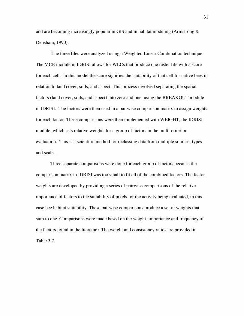
Table 3.7.
32
Table 3.7 Weight for aspect (consistency ratio = .04), land cover (consistency ratio = .07), soils (consistency ratio = .02), derived from a pairwise comparison. Consistency ratios all are acceptable.
Variable Weight
Aspect
Flat 0.0316
NW 0.0776 NE 0.1166 SW 0.2773 SE 0.4969
Land Cover
Forest Boundary 0.2788
Field Boundary 0.2449
Road Boundary 0.1661
Grass 0.1113
Forest 0.0803
Residential/Industrial 0.0547
Agriculture 0.0340
Water 0.0149
Soils
D 0.0618
C 0.2295
B 0.5825
A 0.1262
Once factor weights were determined they were used in the Multiple Criterion
Evaluation (MCE) module that provides a platform to perform the WLC. The method
of running the WLC in this study is different than a standard WLC because the factors are
weighted twice. Typically, a WLC works by multiplying each factor by its factor weight
and then adding the results. I used this technique, but in a hierarchical fashion, applying
33
weights to my factors listed in table 3.7, and then applying a second set of factor weights
to the groups of factors (i.e. land cover, aspect and soils) because the literature revealed
different weights for two habitat components. Most of the literature refers to land cover
and vegetation, and land cover relates specifically to floral resources, one of two
components critical to bee habitat. Thus, it was assigned a weight of 0.5. Aspect was
assigned a weight of 0.3 and soils 0.2 because they make up the nesting requirements.
Aspect was weighted higher than soils because more evidence supported the role of
aspect in bee habitat. In addition, there is more uncertainty in a soils map then in a
topographic map. This weighting assured that both floral resources and nesting
substrates were accounted for in the model, while still addressing uncertainty.
After the WLC was completed, the neighborhood averages of all the resulting
cells in a 250 m, 500 m, 750 m and 1000 m radius were computed to account for and
investigate the effects of scale. Bee habitat can not be defined by a single score of one
15 x 15 m cell because it is dependent on the surround landscape matrix (Steffan-
Dewenter et al., 2002b). The strongest correlation between landscape metrics and bee
populations was at 250 m, with correlations existing up to 1000 m for native bees
(Steffan-Dewenter et al., 2002b). Taking the neighborhood averages allowed for area
and type of the land cover to be part of the model. The MCE GIS model produced four
raster files with pixel values that represented the neighborhood averages of the
landscape’s bee habitat suitability. This score was used as the independent variable in
subsequent modeling to predict bee abundance and diversity.
34
3.4: Field Sampling
Bee abundance and diversity data were collected in the field to validate the bee
habitat suitability model. The field samples were taken to allow for statistical analysis
and model validation. The 250 m index was used to select locations for bee traps because
it had shown the strongest correlation with bee abundance and diversity in the literature
and could allow for a systematic means of obtaining equal samples in MCE class breaks
(Steffan-Dewenter, 2004).
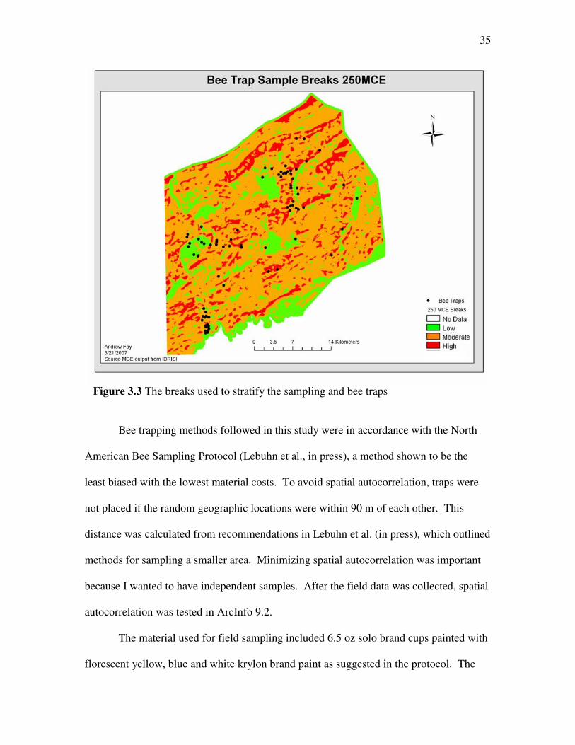
The MCE map was broken into three classes: High Suitability, Moderate
Suitability and Low Suitability (Figure 3.3). Class breaks were determined by using the
histogram of the model outputs. Breaks were set using standard deviations from the
mean. One standard deviation from the mean was used to represent Moderate Suitability.
Two standard deviations above the mean was High Suitability and two standard
deviations below the mean was Low Suitability. The 250 m MCE data x = 0.558 and σ =
0.094; physical breaks of the data are in Table 3.8.
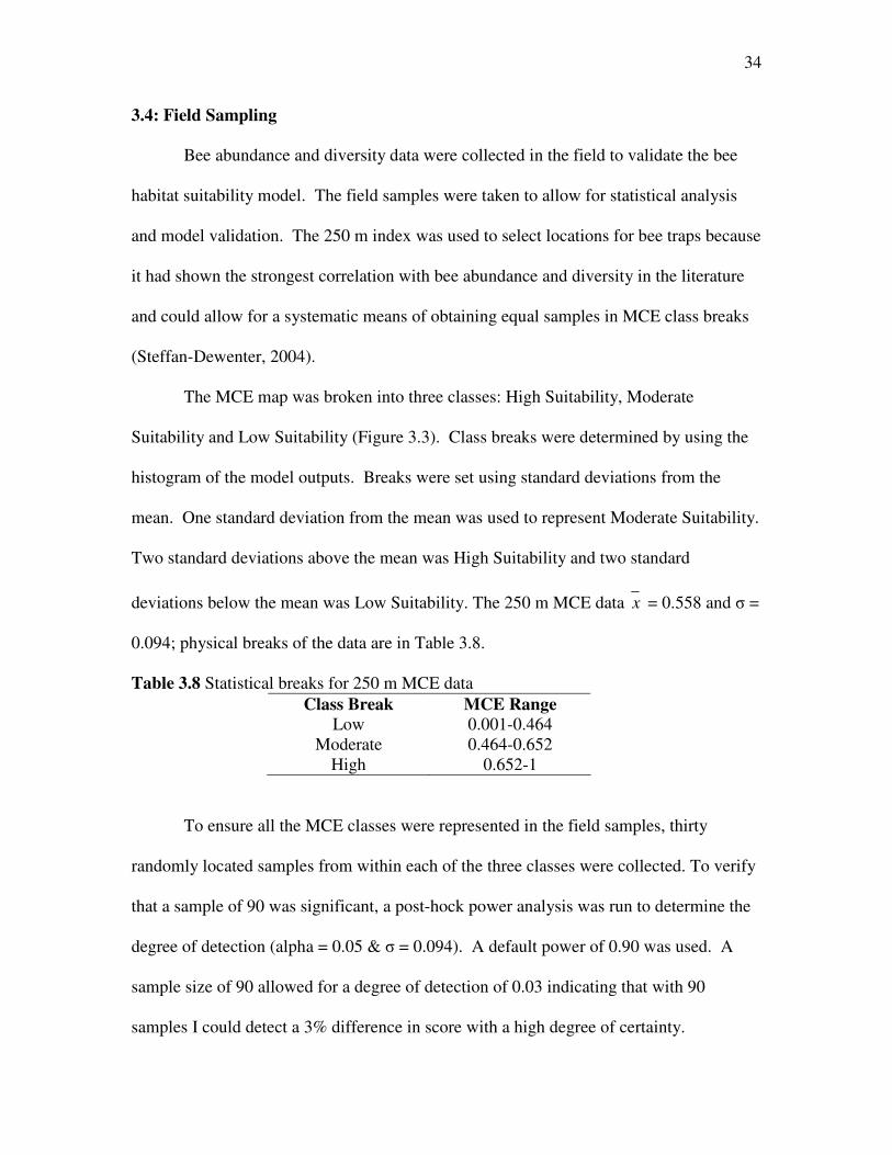
Table 3.8 Statistical breaks for 250 m MCE data Class Break MCE Range
Low 0.001-0.464 Moderate 0.464-0.652
High 0.652-1
To ensure all the MCE classes were represented in the field samples, thirty
randomly located samples from within each of the three classes were collected. To verify
that a sample of 90 was significant, a post-hock power analysis was run to determine the
degree of detection (alpha = 0.05 & σ = 0.094). A default power of 0.90 was used. A
sample size of 90 allowed for a degree of detection of 0.03 indicating that with 90
samples I could detect a 3% difference in score with a high degree of certainty.
35
Figure 3.3 The breaks used to stratify the sampling and bee traps
Bee trapping methods followed in this study were in accordance with the North
American Bee Sampling Protocol (Lebuhn et al., in press), a method shown to be the
least biased with the lowest material costs. To avoid spatial autocorrelation, traps were
not placed if the random geographic locations were within 90 m of each other. This
distance was calculated from recommendations in Lebuhn et al. (in press), which outlined
methods for sampling a smaller area. Minimizing spatial autocorrelation was important
because I wanted to have independent samples. After the field data was collected, spatial
autocorrelation was tested in ArcInfo 9.2.
The material used for field sampling included 6.5 oz solo brand cups painted with
florescent yellow, blue and white krylon brand paint as suggested in the protocol. The
36
cups were filled with a solution of blue Dawn brand soap and water at a ratio of one
tablespoon of soap to one gallon of water. The color of the cups attracts the bees and
when they hit the water they sink and drown because the soap reduces the surface tension
of the water.
Traps were set out before 9:00 am in the morning and collected after 3:00 pm in
the evening, the time period when bees are most active (Lebuhn et al., in press). They
were placed in random locations 90 m apart, within the selected location and stratified
classes (Figure 3.3.). These locations were selected using the RANDOM module in
IDRISI, on the area of interest. A GPS was used to navigate to the locations, set and
retrieve the traps. Location, time, date and temperature were recorded at trap setting. Cup
color was randomly chosen for a trap location within each class. This ensured that there
was equal representation of cup color within each bee habitat class.
Upon collection of the traps the water was drained and the bees were placed in an
alcohol solution and labeled based on the site number. Differences between bee species
were determined using a microscope, the Discover Life Identification Guide
(<http://www.discoverlife.org/20/q>) and Michener’s (2000) book Bees of the World.
Distinctions among bees that indicated a different species were easier to detect than
actual species, because of complexities in bee species identification. For this reason the
number of species present was recorded to use in statistical analysis. Bees in this thesis
are referred to at the genera level.
37
3.5: Statistical Analysis
Statistical analysis was conducted with the Fit Model Platform in JMP 6.0.2. To
achieve objective 2 of this study, the MCE GIS model was statistically validated. I used
three independent variables: 1) MCE score at 4 distance intervals, 2) color of bee traps
and 3) presence of flowers. The MCE score was used as a landscape variable because it
represented the combined suitability of land cover, soils and topography. The color of bee
traps and the presence of flowers were used as local site variables because these
characteristics were not part of the landscape matrix. The MCE sampling was conducted
with groups of the scored data explained in the methods. Analysis was conducted on the
raw neighborhood averaged MCE scores, scored between zero and one. Two
independent variables, bee abundance and bee species diversity, were fit to models
because bee abundance and diversity are related and are the most important indicators of
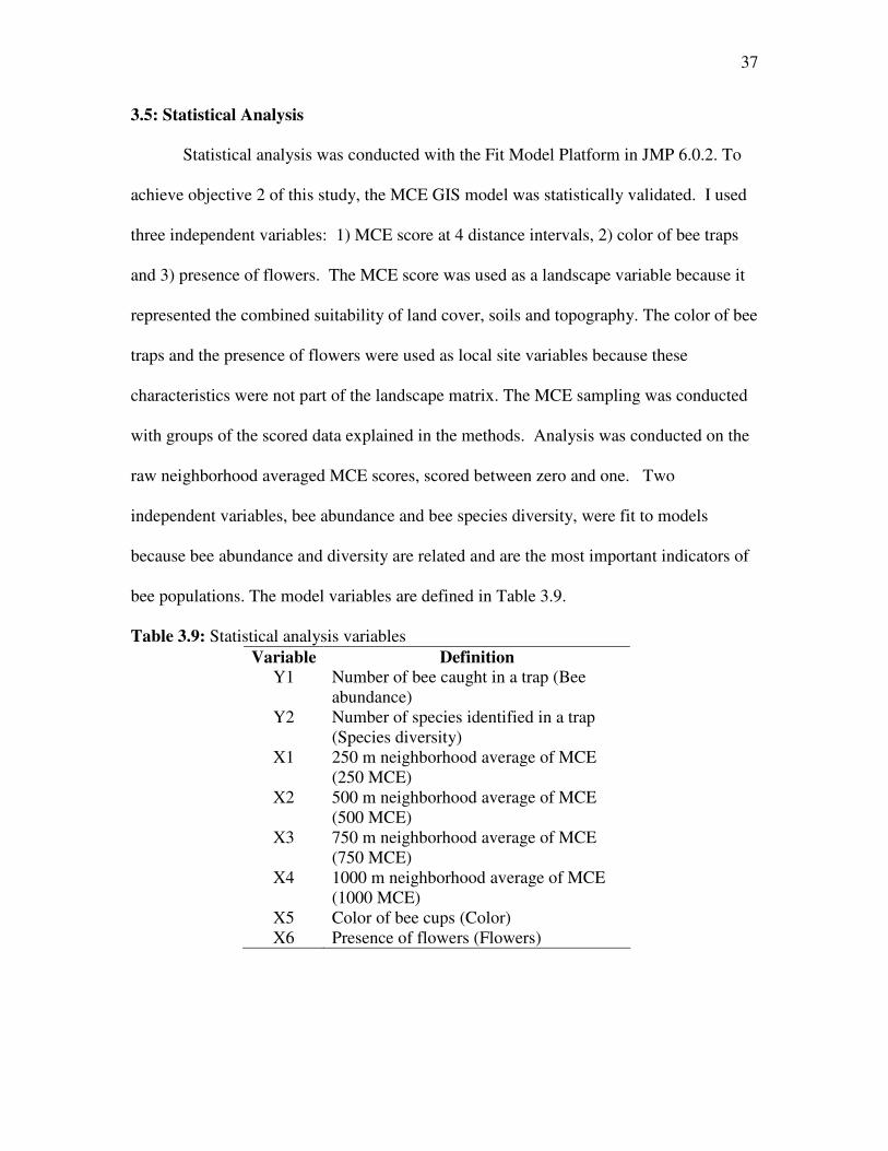
bee populations. The model variables are defined in Table 3.9.
Table 3.9: Statistical analysis variables Variable Definition
Y1
Number of bee caught in a trap (Bee abundance)
Y2 Number of species identified in a trap (Species diversity)
X1 250 m neighborhood average of MCE (250 MCE)
X2 500 m neighborhood average of MCE (500 MCE)
X3 750 m neighborhood average of MCE (750 MCE)
X4 1000 m neighborhood average of MCE (1000 MCE)
X5 Color of bee cups (Color) X6 Presence of flowers (Flowers)
38
A generalized linear model (GLM) was chosen for this work because a GLM
provides a way to fit responses that don't fit the usual requirements of least-squares fits.
Similarly to traditional linear models, fitted generalized linear models can be summarized
through statistics such as parameter estimates, standard errors, and goodness-of-fit
statistics. In addition, one can make statistical inference about the parameters using
confidence intervals and hypothesis testing.
Bee abundance data gathered in the field was grouped into classes to avoid
potential violation of the large sample chi-square theory because the data had excessive
zeros and counts less than five (Agresti, 1996). Data was grouped into 6 categories
following Agresti (1996) guidelines. The categories were separated by a difference of
two bees with the bottom class < 2 and the top class >10. The grouped bee abundance
distribution was tested for fit to a Poisson distribution using the Pearson’s goodness of fit
test. The tests indicated that the data fit a Poisson distribution (χ² = 15.46, p = 0.28). The
bee diversity data was not grouped because the structure of the data didn’t allow for
enough groups or counts in groups following Agresti (1996). The bee diversity count
data still fit a Poisson distribution indicated by the goodness of fit test (χ² = 4.16, p = 0.9).
A GLM with a Poisson distribution was determined to be an appropriate model
because both data distributions had Poisson distributions and were rare count data
(Agresti, 1996; Shaw & Wheeler, 1985). The assumptions of using this model are 1) the
data have a Poisson distribution, 2) the data are count data and 3) the data has a standard
deviation close to the mean. To properly conduct a GLM analysis multiple tests are
needed to confirm significance. For this statistical analysis I used the tests available in
39
JMP. A whole model test, goodness of fit test, effects test and parameter estimated test
were used. The null hypotheses and specifics of the tests are outlined below.
The whole model test determines if the model fits better than constant response
probabilities. It is a specific likelihood-ratio chi-square test that evaluates how well the
GLM fits the data using a likelihood-ratio statistic. Larger χ² and smaller p values
indicate more significance. It tests the null hypothesis that a reduced model without any
effects except the intercepts is better than the full model.
The goodness of fit test is analogous to a lack of fit test and tests for two things:
1) are the variables in the model accurate to describe the situation and 2) does the model
have the right form? A Pearson’s chi-square statistic (χ²), a deviance statistic, and an
overdispersion parameter indicate adequacy of the GLM. The null hypothesis was that
the model fits the data; it is good to not reject the null hypothesis in this case.
The effects test determines if the effects of a variable on the response were zero.
The null hypothesis is that variable has no effect as a predictor. The effects test uses joint
tests to determine if all the parameters for an individual effect are zero. If an effect has
only one parameter, for example, with simple regressors, then the tests are no different
from the tests in the parameter estimates. Large χ² and small p values indicate larger
effects.
The parameter estimates test gives estimates on standard errors, χ² and p values
analogous to the Wald statistic described in Agresti (1996). A Wald statistic is a
parameter estimate divided by its standard error and then squared. Larger χ² and small p
values are more significant.
40
Chapter 4: Results and Discussion
This section reviews the results from the field trapping, the MCE model and the
combined GLM model. First, I outline the bee trap data, discussing the basic descriptive
statistics on the abundance and diversity of bees. Then, the results of the landscape
variables and bee abundance fit to a GLM Poisson are given. Local site variable results
are also outlined, computed by adding the additional variables individually to the model.
Finally, the results for bee diversity are presented in the same order as bee abundance
results. The GLMs that incorporate only the landscape variables address the GIS MCE
model. The local site variables were added to the GLM to assess their impact on bee
populations and the appropriateness of using only landscape variables to model bees
4.1: Results
Bee Trap Results
A total of 98 bee traps were set in the field, and 81 were collected (Appendix B).
The loss was due to spilled, damaged, and lost traps. There were 25 samples collected for
MCE class Low, 31 for Moderate and 25 for High. The bee abundance count data
before grouping had a range of 0 - 29, x = 4.20 and σ = 4.24.
A total of 339 native bees were collected from the 81 traps, which represented 19
different species. Bees were separated by species and grouped by genera. The Halticid
bees and Lassioglossum spp. were the most abundant bees caught in the traps. The
Bombus genera were the most diverse followed by Halictus, Andrena and Lassioglossum.
The least abundant bee was Collettess spp.
41
No significant spatial autocorrelation was found for bee abundance or bee
diversity (Figure 4.1), as shown by the Moran's I Index = -0.01 for bee abundance, and
Moran's I Index = -0.03 for bee diversity. The scores indicate that the data is neither
clustered nor dispersed and suggest that field sampling was done in a way to reduce the
effect of spatial autocorrelation. This is an important finding because I was able to collect
independent samples at 90 m.
Bee Abundance and MCE (landscape variable) Results
To meet Objective 2 and determine if landscape scale factors influenced bee
population dynamics, the MCE score was first fitted to the data on bee abundance with a
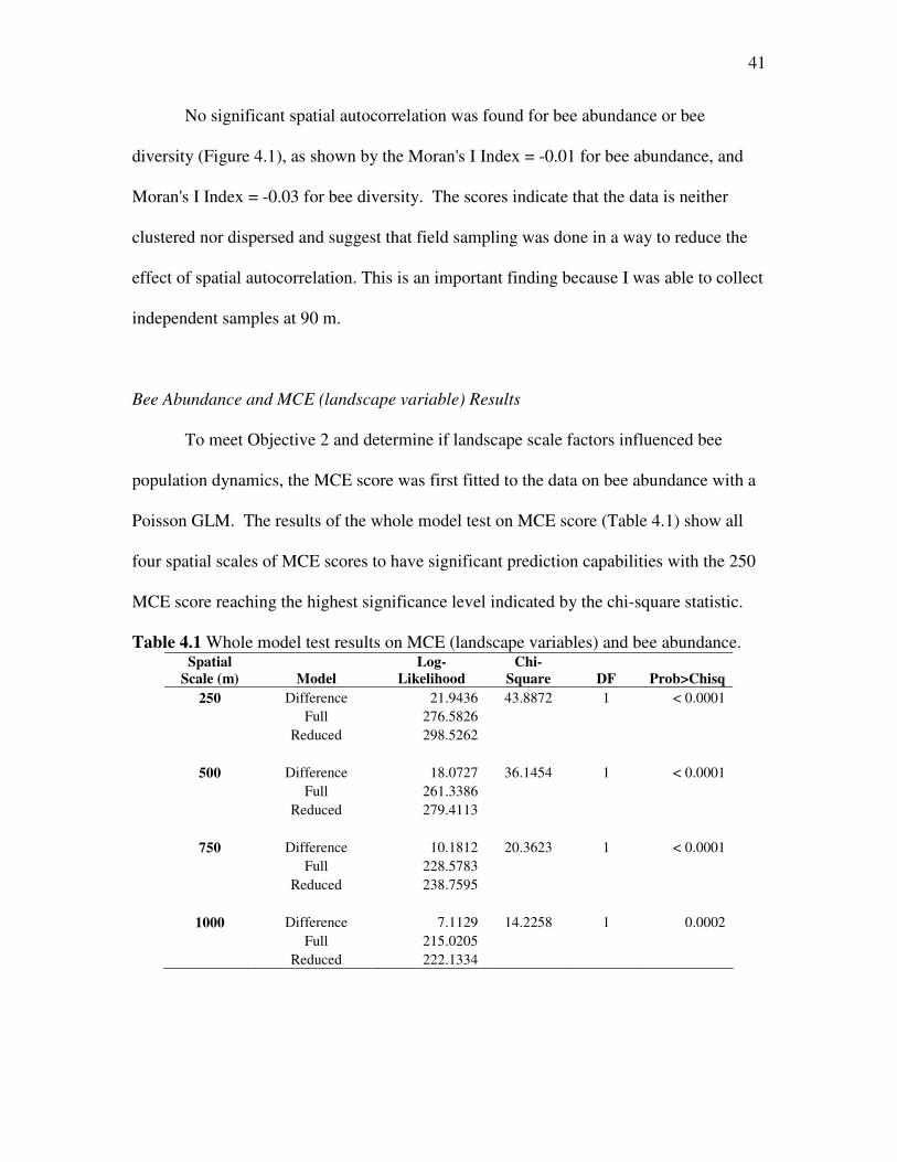
Poisson GLM. The results of the whole model test on MCE score (Table 4.1) show all
four spatial scales of MCE scores to have significant prediction capabilities with the 250
MCE score reaching the highest significance level indicated by the chi-square statistic.
Table 4.1 Whole model test results on MCE (landscape variables) and bee abundance. Spatial
Scale (m) Model
Log-
Likelihood
Chi-
Square DF Prob>Chisq
250 Difference 21.9436 43.8872 1 < 0.0001 Full 276.5826 Reduced 298.5262
500 Difference 18.0727 36.1454 1 < 0.0001 Full 261.3386 Reduced 279.4113
750 Difference 10.1812 20.3623 1 < 0.0001 Full 228.5783 Reduced 238.7595
1000 Difference 7.1129 14.2258 1 0.0002 Full 215.0205 Reduced 222.1334
42
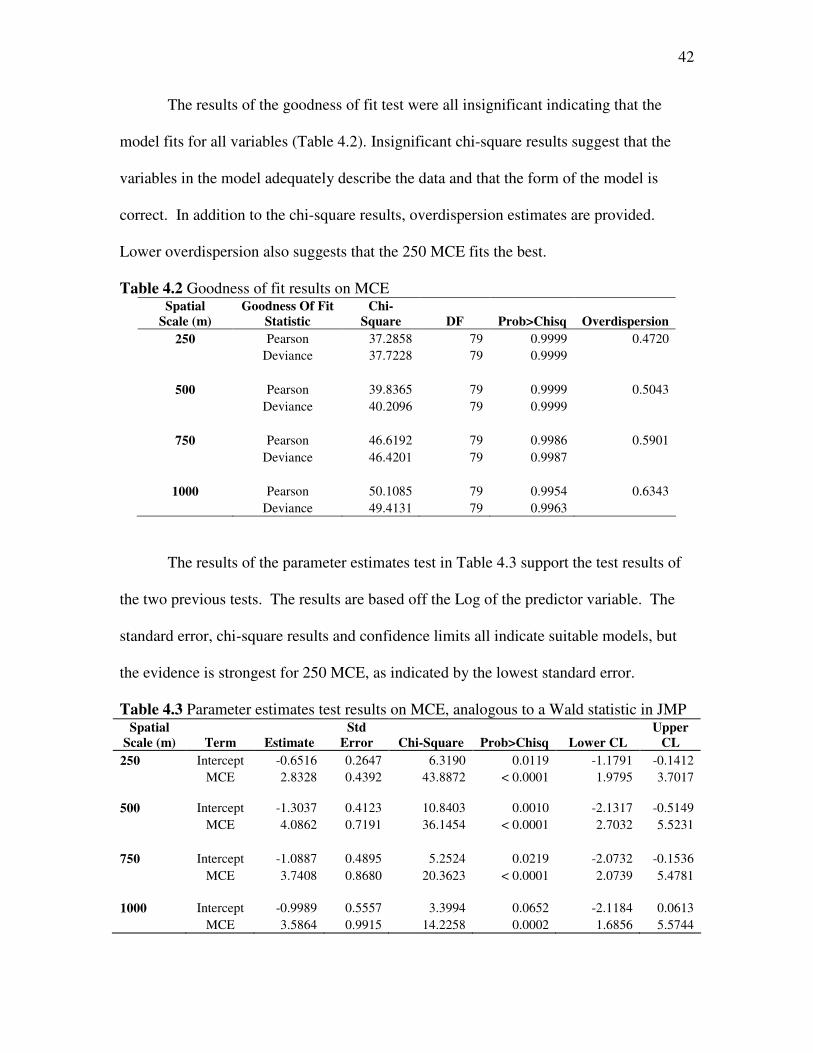
The results of the goodness of fit test were all insignificant indicating that the
model fits for all variables (Table 4.2). Insignificant chi-square results suggest that the
variables in the model adequately describe the data and that the form of the model is
correct. In addition to the chi-square results, overdispersion estimates are provided.
Lower overdispersion also suggests that the 250 MCE fits the best.
Table 4.2 Goodness of fit results on MCE Spatial
Scale (m)
Goodness Of Fit
Statistic
Chi-
Square DF Prob>Chisq Overdispersion
250 Pearson 37.2858 79 0.9999 0.4720 Deviance 37.7228 79 0.9999
500 Pearson 39.8365 79 0.9999 0.5043 Deviance 40.2096 79 0.9999
750 Pearson 46.6192 79 0.9986 0.5901 Deviance 46.4201 79 0.9987
1000 Pearson 50.1085 79 0.9954 0.6343 Deviance 49.4131 79 0.9963
The results of the parameter estimates test in Table 4.3 support the test results of
the two previous tests. The results are based off the Log of the predictor variable. The
standard error, chi-square results and confidence limits all indicate suitable models, but
the evidence is strongest for 250 MCE, as indicated by the lowest standard error.
Table 4.3 Parameter estimates test results on MCE, analogous to a Wald statistic in JMP Spatial
Scale (m) Term Estimate
Std
Error Chi-Square Prob>Chisq Lower CL
Upper
CL
250 Intercept -0.6516 0.2647 6.3190 0.0119 -1.1791 -0.1412 MCE 2.8328 0.4392 43.8872 < 0.0001 1.9795 3.7017 500 Intercept -1.3037 0.4123 10.8403 0.0010 -2.1317 -0.5149 MCE 4.0862 0.7191 36.1454 < 0.0001 2.7032 5.5231 750 Intercept -1.0887 0.4895 5.2524 0.0219 -2.0732 -0.1536 MCE 3.7408 0.8680 20.3623 < 0.0001 2.0739 5.4781 1000 Intercept -0.9989 0.5557 3.3994 0.0652 -2.1184 0.0613 MCE 3.5864 0.9915 14.2258 0.0002 1.6856 5.5744
43
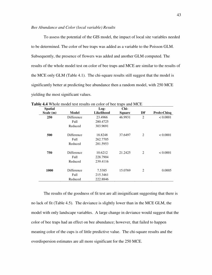
Bee Abundance and Color (local variable) Results
To assess the potential of the GIS model, the impact of local site variables needed
to be determined. The color of bee traps was added as a variable to the Poisson GLM.
Subsequently, the presence of flowers was added and another GLM computed. The
results of the whole model test on color of bee traps and MCE are similar to the results of
the MCE only GLM (Table 4.1). The chi-square results still suggest that the model is
significantly better at predicting bee abundance then a random model, with 250 MCE
yielding the most significant values.
Table 4.4 Whole model test results on color of bee traps and MCE Spatial
Scale (m) Model
Log-
Likelihood
Chi-
Square DF Prob>Chisq
250 Difference 23.4966 46.9931 2 < 0.0001 Full 280.4725 Reduced 303.9691
500 Difference 18.8248 37.6497 2 < 0.0001 Full 262.7705 Reduced 281.5953
750 Difference 10.6212 21.2425 2 < 0.0001 Full 228.7904 Reduced 239.4116
1000 Difference 7.5385 15.0769 2 0.0005 Full 215.3461 Reduced 222.8846
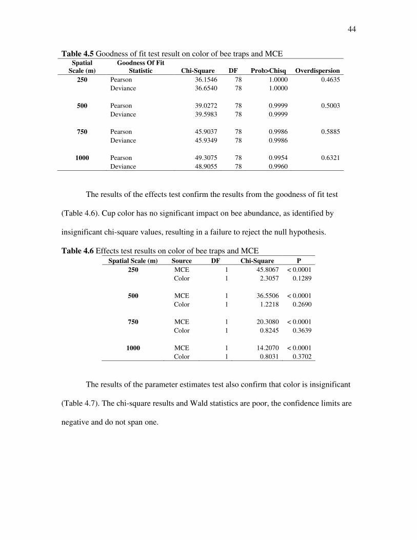
The results of the goodness of fit test are all insignificant suggesting that there is
no lack of fit (Table 4.5). The deviance is slightly lower than in the MCE GLM, the
model with only landscape variables. A large change in deviance would suggest that the
color of bee traps had an effect on bee abundance; however, that failed to happen
meaning color of the cups is of little predictive value. The chi-square results and the
overdispersion estimates are all more significant for the 250 MCE.
44
Table 4.5 Goodness of fit test result on color of bee traps and MCE Spatial
Scale (m)
Goodness Of Fit
Statistic Chi-Square DF Prob>Chisq Overdispersion
250 Pearson 36.1546 78 1.0000 0.4635 Deviance 36.6540 78 1.0000
500 Pearson 39.0272 78 0.9999 0.5003 Deviance 39.5983 78 0.9999
750 Pearson 45.9037 78 0.9986 0.5885 Deviance 45.9349 78 0.9986
1000 Pearson 49.3075 78 0.9954 0.6321 Deviance 48.9055 78 0.9960
The results of the effects test confirm the results from the goodness of fit test
(Table 4.6). Cup color has no significant impact on bee abundance, as identified by
insignificant chi-square values, resulting in a failure to reject the null hypothesis.
Table 4.6 Effects test results on color of bee traps and MCE Spatial Scale (m) Source DF Chi-Square P
250 MCE 1 45.8067 < 0.0001 Color 1 2.3057 0.1289
500 MCE 1 36.5506 < 0.0001 Color 1 1.2218 0.2690
750 MCE 1 20.3080 < 0.0001 Color 1 0.8245 0.3639
1000 MCE 1 14.2070 < 0.0001 Color 1 0.8031 0.3702
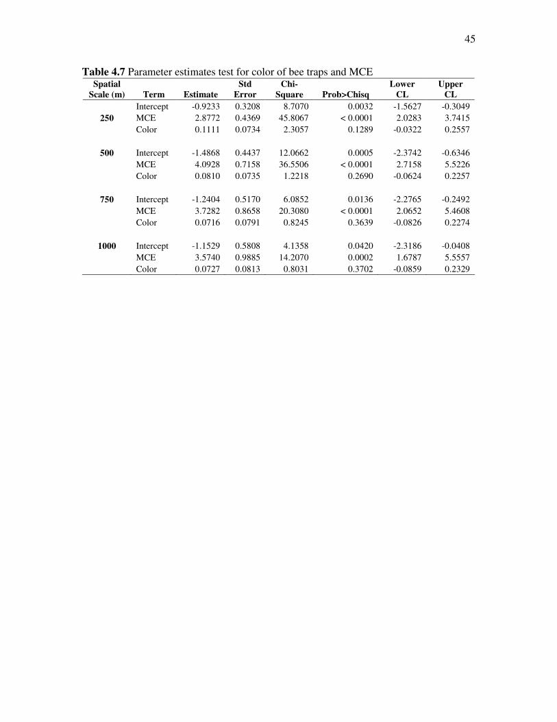
The results of the parameter estimates test also confirm that color is insignificant
(Table 4.7). The chi-square results and Wald statistics are poor, the confidence limits are
negative and do not span one.
45
Table 4.7 Parameter estimates test for color of bee traps and MCE Spatial
Scale (m) Term Estimate
Std
Error
Chi-
Square Prob>Chisq
Lower
CL
Upper
CL
Intercept -0.9233 0.3208 8.7070 0.0032 -1.5627 -0.3049 250 MCE 2.8772 0.4369 45.8067 < 0.0001 2.0283 3.7415
Color 0.1111 0.0734 2.3057 0.1289 -0.0322 0.2557
500 Intercept -1.4868 0.4437 12.0662 0.0005 -2.3742 -0.6346 MCE 4.0928 0.7158 36.5506 < 0.0001 2.7158 5.5226 Color 0.0810 0.0735 1.2218 0.2690 -0.0624 0.2257
750 Intercept -1.2404 0.5170 6.0852 0.0136 -2.2765 -0.2492 MCE 3.7282 0.8658 20.3080 < 0.0001 2.0652 5.4608 Color 0.0716 0.0791 0.8245 0.3639 -0.0826 0.2274
1000 Intercept -1.1529 0.5808 4.1358 0.0420 -2.3186 -0.0408 MCE 3.5740 0.9885 14.2070 0.0002 1.6787 5.5557 Color 0.0727 0.0813 0.8031 0.3702 -0.0859 0.2329
46
Bee Abundance and Flowers (local variable) Results
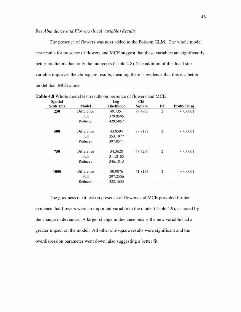
The presence of flowers was next added to the Poisson GLM. The whole model
test results for presence of flowers and MCE suggest that these variables are significantly
better predictors than only the intercepts (Table 4.8). The addition of this local site
variable improves the chi-square results, meaning there is evidence that this is a better
model than MCE alone.
Table 4.8 Whole model test results on presence of flowers and MCE Spatial
Scale (m) Model
Log-
Likelihood
Chi-
Square DF Prob>Chisq
250 Difference 49.7351 99.4703 2 < 0.0001 Full 379.8505 Reduced 429.5857
500 Difference 43.8594 87.7188 2 < 0.0001 Full 353.1977 Reduced 397.0571
750 Difference 34.3628 68.7256 2 < 0.0001 Full 311.8185 Reduced 346.1813
1000 Difference 30.9076 61.8153 2 < 0.0001 Full 297.2556 Reduced 328.1633
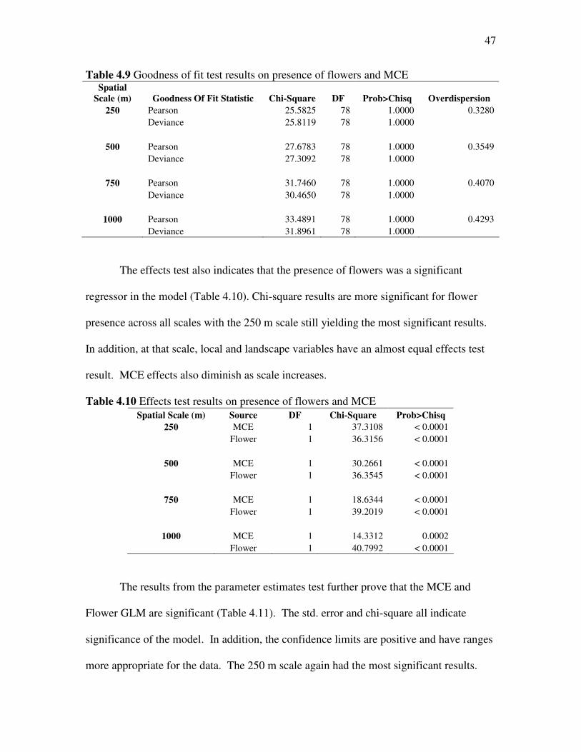
The goodness of fit test on presence of flowers and MCE provided further
evidence that flowers were an important variable in the model (Table 4.9), as noted by
the change in deviance. A larger change in deviance means the new variable had a
greater impact on the model. All other chi-square results were significant and the
overdispersion parameter went down, also suggesting a better fit.
47
Table 4.9 Goodness of fit test results on presence of flowers and MCE Spatial
Scale (m) Goodness Of Fit Statistic Chi-Square DF Prob>Chisq Overdispersion
250 Pearson 25.5825 78 1.0000 0.3280 Deviance 25.8119 78 1.0000
500 Pearson 27.6783 78 1.0000 0.3549 Deviance 27.3092 78 1.0000
750 Pearson 31.7460 78 1.0000 0.4070 Deviance 30.4650 78 1.0000
1000 Pearson 33.4891 78 1.0000 0.4293 Deviance 31.8961 78 1.0000
The effects test also indicates that the presence of flowers was a significant
regressor in the model (Table 4.10). Chi-square results are more significant for flower
presence across all scales with the 250 m scale still yielding the most significant results.
In addition, at that scale, local and landscape variables have an almost equal effects test
result. MCE effects also diminish as scale increases.
Table 4.10 Effects test results on presence of flowers and MCE Spatial Scale (m) Source DF Chi-Square Prob>Chisq
250 MCE 1 37.3108 < 0.0001 Flower 1 36.3156 < 0.0001
500 MCE 1 30.2661 < 0.0001 Flower 1 36.3545 < 0.0001
750 MCE 1 18.6344 < 0.0001 Flower 1 39.2019 < 0.0001
1000 MCE 1 14.3312 0.0002 Flower 1 40.7992 < 0.0001
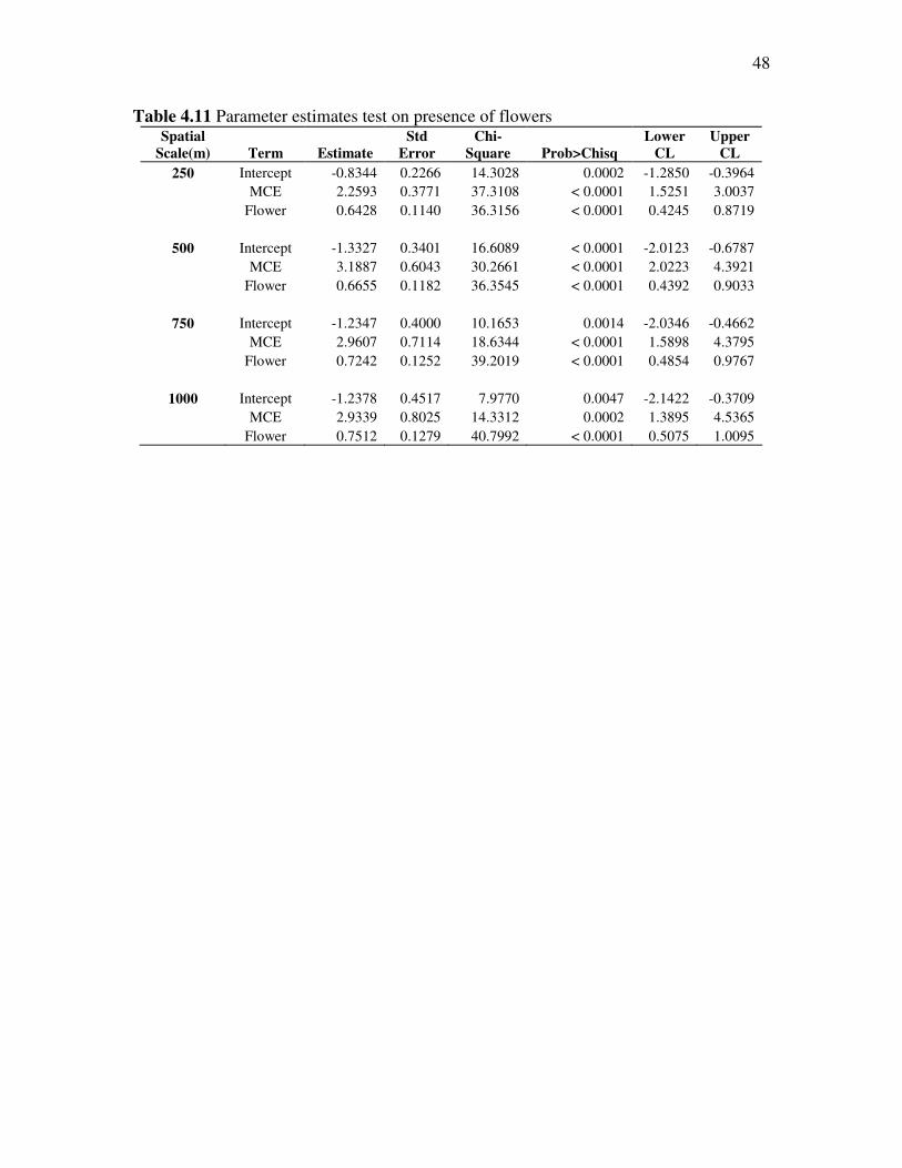
The results from the parameter estimates test further prove that the MCE and
Flower GLM are significant (Table 4.11). The std. error and chi-square all indicate
significance of the model. In addition, the confidence limits are positive and have ranges
more appropriate for the data. The 250 m scale again had the most significant results.
48
Table 4.11 Parameter estimates test on presence of flowers Spatial
Scale(m) Term Estimate
Std
Error
Chi-
Square Prob>Chisq
Lower
CL
Upper
CL
250 Intercept -0.8344 0.2266 14.3028 0.0002 -1.2850 -0.3964 MCE 2.2593 0.3771 37.3108 < 0.0001 1.5251 3.0037 Flower 0.6428 0.1140 36.3156 < 0.0001 0.4245 0.8719
500 Intercept -1.3327 0.3401 16.6089 < 0.0001 -2.0123 -0.6787 MCE 3.1887 0.6043 30.2661 < 0.0001 2.0223 4.3921 Flower 0.6655 0.1182 36.3545 < 0.0001 0.4392 0.9033
750 Intercept -1.2347 0.4000 10.1653 0.0014 -2.0346 -0.4662 MCE 2.9607 0.7114 18.6344 < 0.0001 1.5898 4.3795 Flower 0.7242 0.1252 39.2019 < 0.0001 0.4854 0.9767
1000 Intercept -1.2378 0.4517 7.9770 0.0047 -2.1422 -0.3709 MCE 2.9339 0.8025 14.3312 0.0002 1.3895 4.5365 Flower 0.7512 0.1279 40.7992 < 0.0001 0.5075 1.0095
49
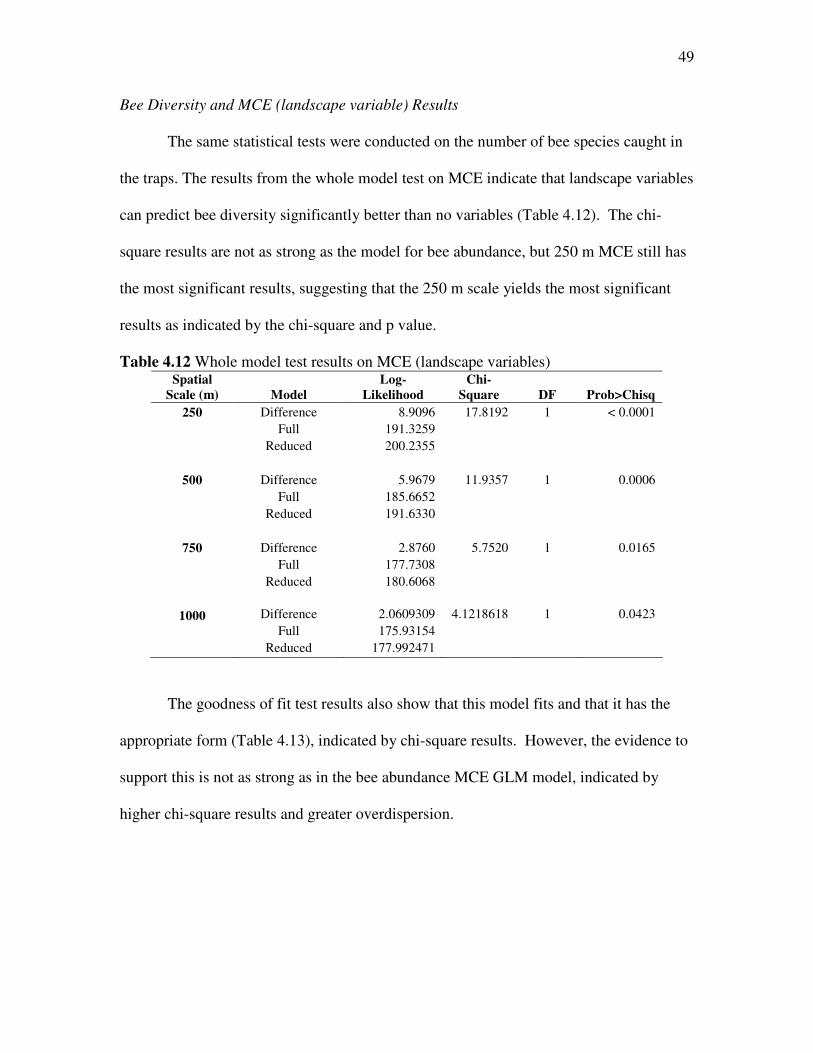
Bee Diversity and MCE (landscape variable) Results
The same statistical tests were conducted on the number of bee species caught in
the traps. The results from the whole model test on MCE indicate that landscape variables
can predict bee diversity significantly better than no variables (Table 4.12). The chi-
square results are not as strong as the model for bee abundance, but 250 m MCE still has
the most significant results, suggesting that the 250 m scale yields the most significant
results as indicated by the chi-square and p value.
Table 4.12 Whole model test results on MCE (landscape variables) Spatial
Scale (m) Model
Log-
Likelihood
Chi-
Square DF Prob>Chisq
250 Difference 8.9096 17.8192 1 < 0.0001 Full 191.3259 Reduced 200.2355
500 Difference 5.9679 11.9357 1 0.0006 Full 185.6652 Reduced 191.6330
750 Difference 2.8760 5.7520 1 0.0165 Full 177.7308 Reduced 180.6068
1000 Difference 2.0609309 4.1218618 1 0.0423
Full 175.93154
Reduced 177.992471
The goodness of fit test results also show that this model fits and that it has the
appropriate form (Table 4.13), indicated by chi-square results. However, the evidence to
support this is not as strong as in the bee abundance MCE GLM model, indicated by
higher chi-square results and greater overdispersion.
50
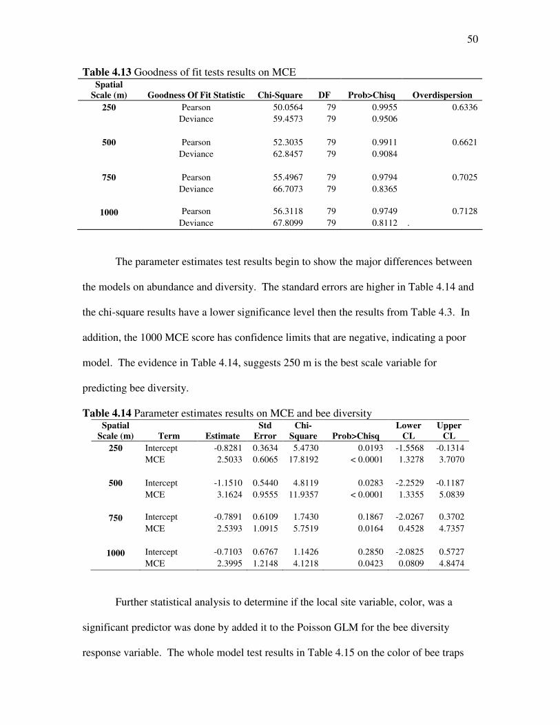
Table 4.13 Goodness of fit tests results on MCE Spatial
Scale (m) Goodness Of Fit Statistic Chi-Square DF Prob>Chisq Overdispersion
250 Pearson 50.0564 79 0.9955 0.6336 Deviance 59.4573 79 0.9506
500 Pearson 52.3035 79 0.9911 0.6621 Deviance 62.8457 79 0.9084
750 Pearson 55.4967 79 0.9794 0.7025 Deviance 66.7073 79 0.8365
1000 Pearson 56.3118 79 0.9749 0.7128
Deviance 67.8099 79 0.8112 .
The parameter estimates test results begin to show the major differences between
the models on abundance and diversity. The standard errors are higher in Table 4.14 and
the chi-square results have a lower significance level then the results from Table 4.3. In
addition, the 1000 MCE score has confidence limits that are negative, indicating a poor
model. The evidence in Table 4.14, suggests 250 m is the best scale variable for
predicting bee diversity.
Table 4.14 Parameter estimates results on MCE and bee diversity Spatial
Scale (m) Term Estimate
Std
Error
Chi-
Square Prob>Chisq
Lower
CL
Upper
CL
250 Intercept -0.8281 0.3634 5.4730 0.0193 -1.5568 -0.1314 MCE 2.5033 0.6065 17.8192 < 0.0001 1.3278 3.7070
500 Intercept -1.1510 0.5440 4.8119 0.0283 -2.2529 -0.1187 MCE 3.1624 0.9555 11.9357 < 0.0001 1.3355 5.0839
750 Intercept -0.7891 0.6109 1.7430 0.1867 -2.0267 0.3702
MCE 2.5393 1.0915 5.7519 0.0164 0.4528 4.7357
1000 Intercept -0.7103 0.6767 1.1426 0.2850 -2.0825 0.5727
MCE 2.3995 1.2148 4.1218 0.0423 0.0809 4.8474
Further statistical analysis to determine if the local site variable, color, was a
significant predictor was done by added it to the Poisson GLM for the bee diversity
response variable. The whole model test results in Table 4.15 on the color of bee traps
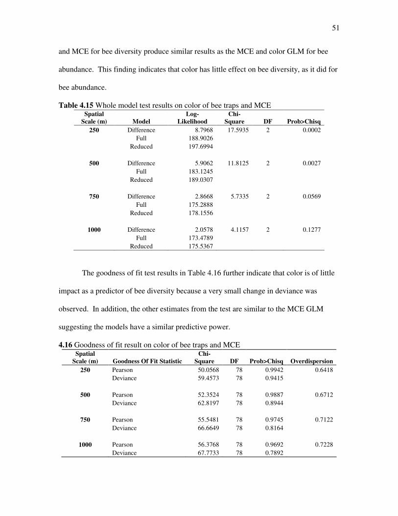
51
and MCE for bee diversity produce similar results as the MCE and color GLM for bee
abundance. This finding indicates that color has little effect on bee diversity, as it did for
bee abundance.
Table 4.15 Whole model test results on color of bee traps and MCE Spatial
Scale (m) Model
Log-
Likelihood
Chi-
Square DF Prob>Chisq
250 Difference 8.7968 17.5935 2 0.0002 Full 188.9026 Reduced 197.6994
500 Difference 5.9062 11.8125 2 0.0027 Full 183.1245 Reduced 189.0307
750 Difference 2.8668 5.7335 2 0.0569 Full 175.2888 Reduced 178.1556
1000 Difference 2.0578 4.1157 2 0.1277 Full 173.4789 Reduced 175.5367
The goodness of fit test results in Table 4.16 further indicate that color is of little
impact as a predictor of bee diversity because a very small change in deviance was
observed. In addition, the other estimates from the test are similar to the MCE GLM
suggesting the models have a similar predictive power.
4.16 Goodness of fit result on color of bee traps and MCE Spatial
Scale (m) Goodness Of Fit Statistic
Chi-
Square DF Prob>Chisq Overdispersion
250 Pearson 50.0568 78 0.9942 0.6418 Deviance 59.4573 78 0.9415
500 Pearson 52.3524 78 0.9887 0.6712 Deviance 62.8197 78 0.8944
750 Pearson 55.5481 78 0.9745 0.7122 Deviance 66.6649 78 0.8164
1000 Pearson 56.3768 78 0.9692 0.7228 Deviance 67.7733 78 0.7892
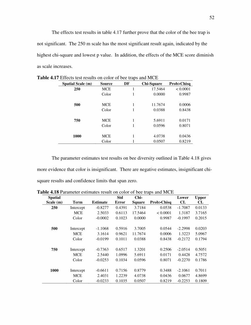
52
The effects test results in table 4.17 further prove that the color of the bee trap is
not significant. The 250 m scale has the most significant result again, indicated by the
highest chi-square and lowest p value. In addition, the effects of the MCE score diminish
as scale increases.
Table 4.17 Effects test results on color of bee traps and MCE Spatial Scale (m) Source DF Chi-Square Prob>Chisq
250 MCE 1 17.5464 < 0.0001 Color 1 0.0000 0.9987
500 MCE 1 11.7674 0.0006 Color 1 0.0388 0.8438
750 MCE 1 5.6911 0.0171 Color 1 0.0596 0.8071
1000 MCE 1 4.0738 0.0436 Color 1 0.0507 0.8219
The parameter estimates test results on bee diversity outlined in Table 4.18 gives
more evidence that color is insignificant. There are negative estimates, insignificant chi-
square results and confidence limits that span zero.
Table 4.18 Parameter estimates result on color of bee traps and MCE Spatial
Scale (m) Term Estimate
Std
Error
Chi-
Square Prob>Chisq
Lower
CL
Upper
CL
250 Intercept -0.8277 0.4391 3.7184 0.0538 -1.7087 0.0133 MCE 2.5033 0.6113 17.5464 < 0.0001 1.3187 3.7165 Color -0.0002 0.1023 0.0000 0.9987 -0.1997 0.2015
500 Intercept -1.1068 0.5916 3.7005 0.0544 -2.2998 0.0203 MCE 3.1614 0.9621 11.7674 0.0006 1.3223 5.0967 Color -0.0199 0.1011 0.0388 0.8438 -0.2172 0.1794
750 Intercept -0.7363 0.6517 1.3201 0.2506 -2.0514 0.5051 MCE 2.5440 1.0996 5.6911 0.0171 0.4428 4.7572 Color -0.0253 0.1034 0.0596 0.8071 -0.2270 0.1786
1000 Intercept -0.6611 0.7156 0.8779 0.3488 -2.1061 0.7011 MCE 2.4031 1.2239 4.0738 0.0436 0.0677 4.8699 Color -0.0233 0.1035 0.0507 0.8219 -0.2253 0.1809
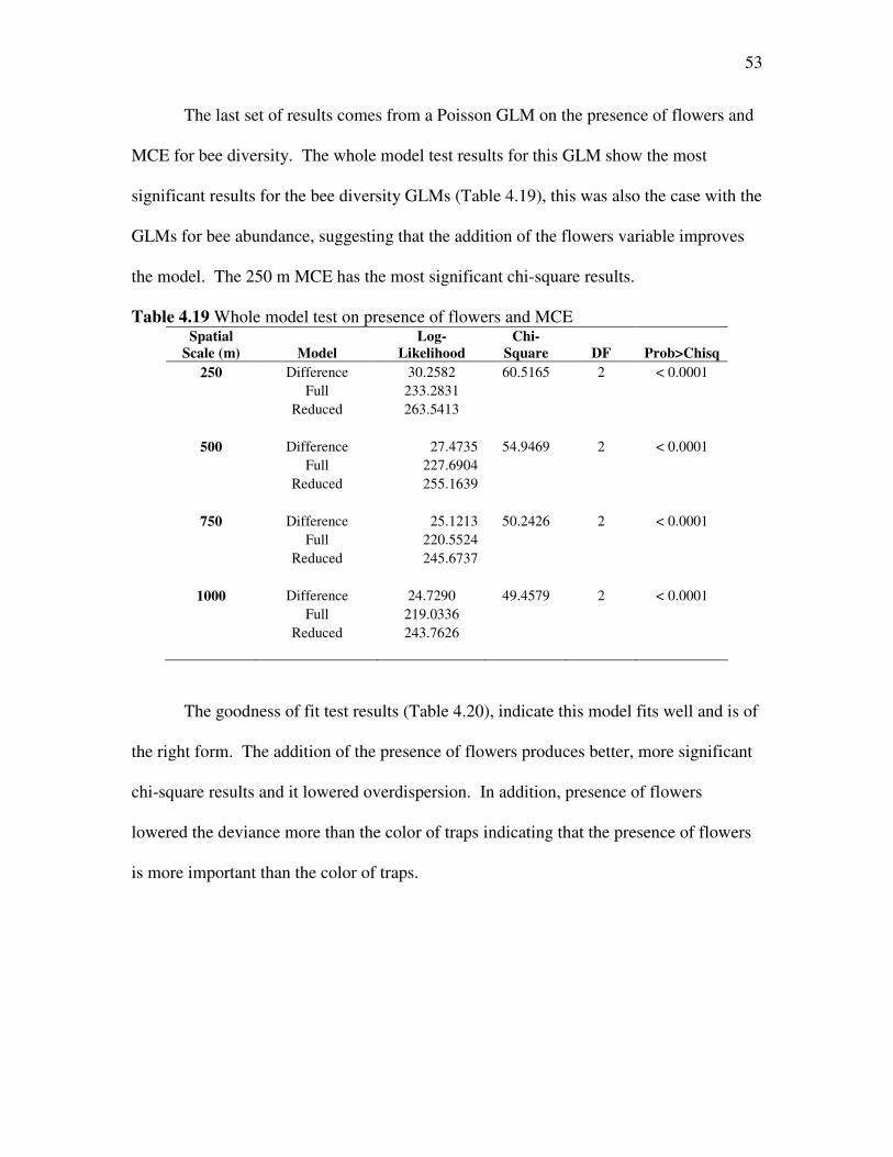
53
The last set of results comes from a Poisson GLM on the presence of flowers and
MCE for bee diversity. The whole model test results for this GLM show the most
significant results for the bee diversity GLMs (Table 4.19), this was also the case with the
GLMs for bee abundance, suggesting that the addition of the flowers variable improves
the model. The 250 m MCE has the most significant chi-square results.
Table 4.19 Whole model test on presence of flowers and MCE Spatial
Scale (m) Model
Log-
Likelihood
Chi-
Square DF Prob>Chisq
250 Difference 30.2582 60.5165 2 < 0.0001 Full 233.2831 Reduced 263.5413
500 Difference 27.4735 54.9469 2 < 0.0001 Full 227.6904 Reduced 255.1639
750 Difference 25.1213 50.2426 2 < 0.0001 Full 220.5524 Reduced 245.6737
1000 Difference 24.7290 49.4579 2 < 0.0001 Full 219.0336 Reduced 243.7626
The goodness of fit test results (Table 4.20), indicate this model fits well and is of
the right form. The addition of the presence of flowers produces better, more significant
chi-square results and it lowered overdispersion. In addition, presence of flowers
lowered the deviance more than the color of traps indicating that the presence of flowers
is more important than the color of traps.
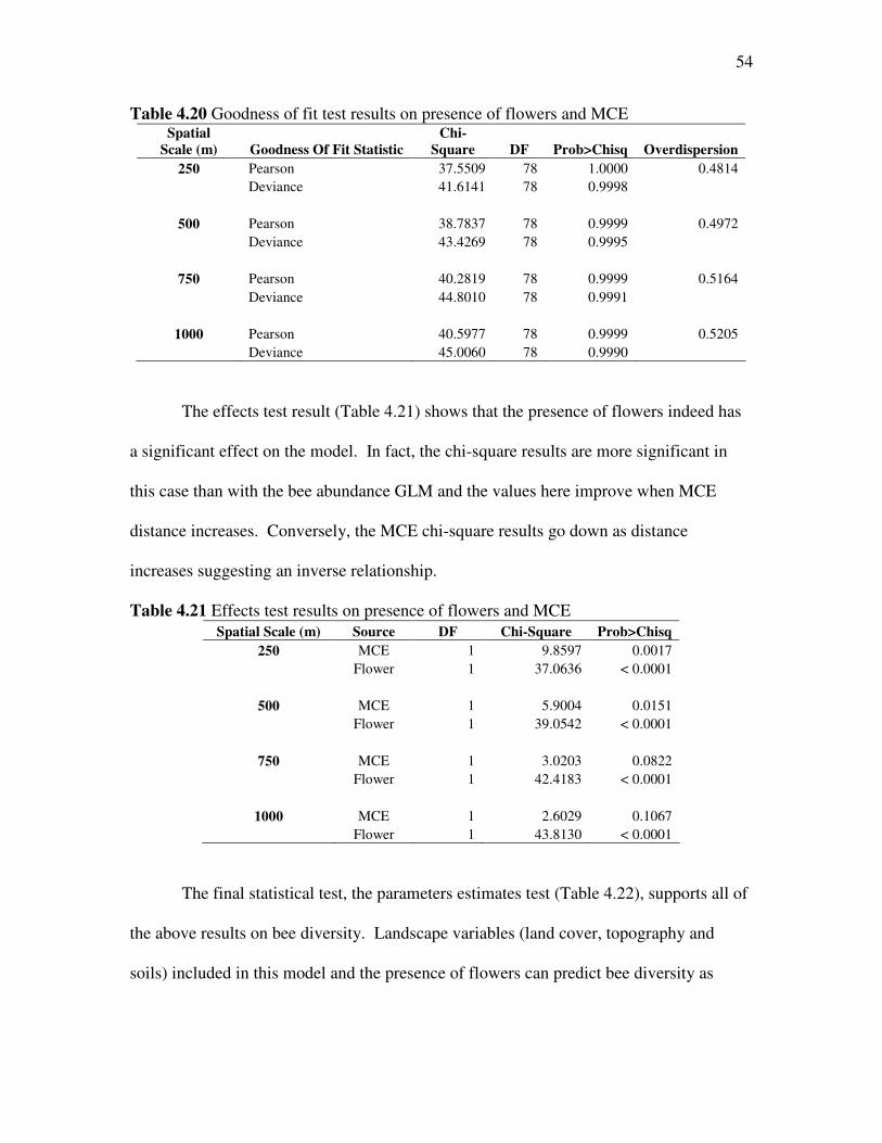
54
Table 4.20 Goodness of fit test results on presence of flowers and MCE Spatial
Scale (m) Goodness Of Fit Statistic
Chi-
Square DF Prob>Chisq Overdispersion
250 Pearson 37.5509 78 1.0000 0.4814 Deviance 41.6141 78 0.9998
500 Pearson 38.7837 78 0.9999 0.4972 Deviance 43.4269 78 0.9995
750 Pearson 40.2819 78 0.9999 0.5164 Deviance 44.8010 78 0.9991
1000 Pearson 40.5977 78 0.9999 0.5205 Deviance 45.0060 78 0.9990
The effects test result (Table 4.21) shows that the presence of flowers indeed has
a significant effect on the model. In fact, the chi-square results are more significant in
this case than with the bee abundance GLM and the values here improve when MCE
distance increases. Conversely, the MCE chi-square results go down as distance
increases suggesting an inverse relationship.
Table 4.21 Effects test results on presence of flowers and MCE
Spatial Scale (m) Source DF Chi-Square Prob>Chisq
250 MCE 1 9.8597 0.0017 Flower 1 37.0636 < 0.0001
500 MCE 1 5.9004 0.0151 Flower 1 39.0542 < 0.0001
750 MCE 1 3.0203 0.0822 Flower 1 42.4183 < 0.0001
1000 MCE 1 2.6029 0.1067 Flower 1 43.8130 < 0.0001
The final statistical test, the parameters estimates test (Table 4.22), supports all of
the above results on bee diversity. Landscape variables (land cover, topography and
soils) included in this model and the presence of flowers can predict bee diversity as
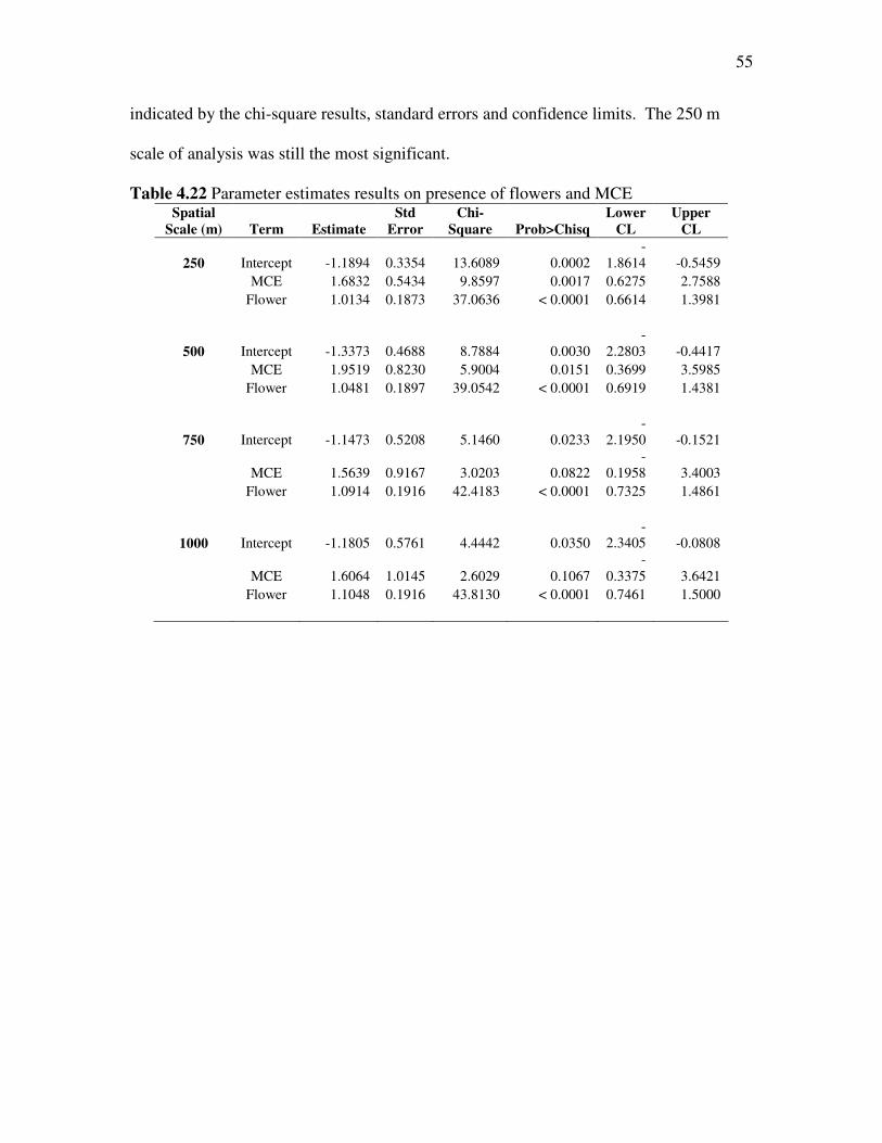
55
indicated by the chi-square results, standard errors and confidence limits. The 250 m
scale of analysis was still the most significant.
Table 4.22 Parameter estimates results on presence of flowers and MCE Spatial
Scale (m) Term Estimate
Std
Error
Chi-
Square Prob>Chisq
Lower
CL
Upper
CL
250 Intercept -1.1894 0.3354 13.6089 0.0002 -
1.8614 -0.5459 MCE 1.6832 0.5434 9.8597 0.0017 0.6275 2.7588 Flower 1.0134 0.1873 37.0636 < 0.0001 0.6614 1.3981
500 Intercept -1.3373 0.4688 8.7884 0.0030 -
2.2803 -0.4417 MCE 1.9519 0.8230 5.9004 0.0151 0.3699 3.5985 Flower 1.0481 0.1897 39.0542 < 0.0001 0.6919 1.4381
750 Intercept -1.1473 0.5208 5.1460 0.0233 -
2.1950 -0.1521
MCE 1.5639 0.9167 3.0203 0.0822 -
0.1958 3.4003 Flower 1.0914 0.1916 42.4183 < 0.0001 0.7325 1.4861
1000 Intercept -1.1805 0.5761 4.4442 0.0350 -
2.3405 -0.0808
MCE 1.6064 1.0145 2.6029 0.1067 -
0.3375 3.6421 Flower 1.1048 0.1916 43.8130 < 0.0001 0.7461 1.5000
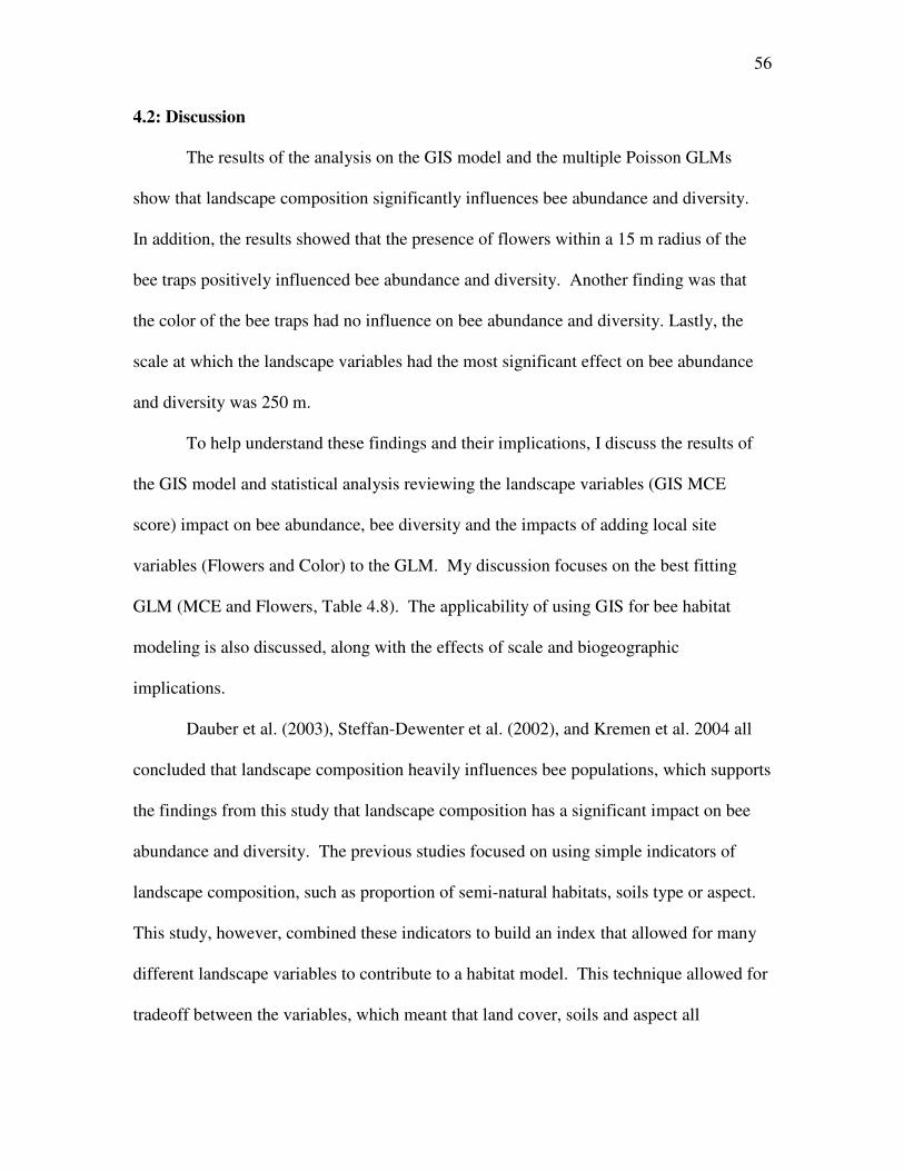
56
4.2: Discussion
The results of the analysis on the GIS model and the multiple Poisson GLMs
show that landscape composition significantly influences bee abundance and diversity.
In addition, the results showed that the presence of flowers within a 15 m radius of the
bee traps positively influenced bee abundance and diversity. Another finding was that
the color of the bee traps had no influence on bee abundance and diversity. Lastly, the
scale at which the landscape variables had the most significant effect on bee abundance
and diversity was 250 m.
To help understand these findings and their implications, I discuss the results of
the GIS model and statistical analysis reviewing the landscape variables (GIS MCE
score) impact on bee abundance, bee diversity and the impacts of adding local site
variables (Flowers and Color) to the GLM. My discussion focuses on the best fitting
GLM (MCE and Flowers, Table 4.8). The applicability of using GIS for bee habitat
modeling is also discussed, along with the effects of scale and biogeographic
implications.
Dauber et al. (2003), Steffan-Dewenter et al. (2002), and Kremen et al. 2004 all
concluded that landscape composition heavily influences bee populations, which supports
the findings from this study that landscape composition has a significant impact on bee
abundance and diversity. The previous studies focused on using simple indicators of
landscape composition, such as proportion of semi-natural habitats, soils type or aspect.
This study, however, combined these indicators to build an index that allowed for many
different landscape variables to contribute to a habitat model. This technique allowed for
tradeoff between the variables, which meant that land cover, soils and aspect all
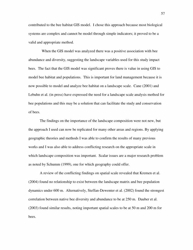
57
contributed to the bee habitat GIS model. I chose this approach because most biological
systems are complex and cannot be model through simple indicators; it proved to be a
valid and appropriate method.
When the GIS model was analyzed there was a positive association with bee
abundance and diversity, suggesting the landscape variables used for this study impact
bees. The fact that the GIS model was significant proves there is value in using GIS to
model bee habitat and populations. This is important for land management because it is
now possible to model and analyze bee habitat on a landscape scale. Cane (2001) and
Lebuhn et al. (in press) have expressed the need for a landscape scale analysis method for
bee populations and this may be a solution that can facilitate the study and conservation
of bees.
The findings on the importance of the landscape composition were not new, but
the approach I used can now be replicated for many other areas and regions. By applying
geographic theories and methods I was able to confirm the results of many previous
works and I was also able to address conflicting research on the appropriate scale in
which landscape composition was important. Scalar issues are a major research problem
as noted by Schumm (1999), one for which geography could offer.
A review of the conflicting findings on spatial scale revealed that Kremen et al.
(2004) found no relationship to exist between the landscape matrix and bee population
dynamics under 600 m. Alternatively, Steffan-Dewenter et al. (2002) found the strongest
correlation between native bee diversity and abundance to be at 250 m. Dauber et al.
(2003) found similar results, noting important spatial scales to be at 50 m and 200 m for
bees.
58
The results of this study suggest that the best scale for using landscape
composition to model bee habitat was 250 m, supporting Steffan-Dewenter et al. (2002)
results. This finding can be quickly identified from Table 4.1 because 250 MCE had the
most significant chi-square result within its model, from Table 4.2, by the least deviance
from the “perfect model” and from Table 4.3 because 250 MCE gives the most stable
parameter estimates (smallest standard error).
Another interesting finding, important to biogeography and the debates over
habitat fragmentation, was that the effects of landscape composition on bee abundance
and diversity dropped as spatial scale increased. This means that bees respond to
landscape composition on a small scale and that patches of 250 m size or a buffer of 250
m around farms could be adequate to preserve bees. This is opposite to many findings on
habitat fragmentation that have found small patches to be detrimental to species
abundance and diversity (Stefan-Dewenter & Tscharntke, 1999; Aizen & Feinsinger,
1994; Powell & Powell, 1987). However, the findings on habitat fragmentation are
supported by Cane (2001).
The addition of the presence of the flowers variable and the color of the bee traps
to the model was done to see if local site variables had an impact on bee abundance and
diversity because Williams et al. (2001) suggested that there is large variability between
bee populations on sites of a similar composition. To detect importance of these variables
they were added to the model and I looked for a large change in the tests results. The
addition of the color of bee traps had no impact on bee abundance and diversity at all
scales. According to Lebuhn et al. (in press) the developers of the North American bee
sampling protocol the color of bee traps is not supposed to effect the results of the
59
trapping. However, they advocated using colored cups to gather more data so that their
finding could be confirmed. The results from my study further proved that color is of
little importance in the trapping of bees.
Conversely, the addition of the presence of the flowers variable greatly improved
the GLM model. This was expected because flowers are the primary food source for bees.
If an area is void of flowering plants, then it is of little value for foraging, one critical
competent of bee habitat. Another interesting influence of the flowers variable on the
model was that as scale increased, so did the importance of flowers for bee diversity and
abundance. This means that large areas of flowering plants are more beneficial to bees
then small patches of flowers. With this in mind, it would seem that agricultural land has
a benefit to bees from a food standpoint. The differences in significance were also larger
for the bee diversity GLM, meaning the larger the area of flowering plants, the greater the
bee diversity. The combined finding on flowers were opposite of what I had expected; I
thought flower presence would affect bee populations at a localized scale.
The findings in this study suggest that bees require a large area of flowers or food
and need a small area with a specific landscape composition, which could advantageous
to agriculture because the agricultural landscape is highly managed. By conserving
patches or fringes of land for bees and providing floral resources, farmers may be able to
increase bee abundance and diversity, which would help with pollination services. The
idea of managing fringe agricultural land or patches was similar to Kremen et al. (2002),
but they recommended management using a larger area. The bottom line is that the
preservation of bees may be facilitated by conserving small areas for bees. Planting
dense floral resources could also improve the bee populations and ecosystem functions.
60
The results of this study show that bee habitat can be modeled with the included
landscape variables alone, but the importance and usability of the model drastically
improved with the addition of local site variables, such as flowers. The presence of
flowers is important to bees at a large scale and landscape composition important at a
small scale. However, there are limitations on the use and interpretations of this analysis
because of the Poisson tests used. Conducting analysis with data that is not normal
requires using the non-parametric alterative tests, which are not as unified, robust and
conclusive as parametric tests (Shaw and Wheeler, 1985). There are no meaningful r-
square values or root mean square errors associated with a Poisson regression, so
conclusions need to come from multiple tests (Agresti 1996). However, it was imperative
that I used the appropriate statistical test for this study because using statistics that don’t
meet all the assumptions can lead to improper conclusion and invalid results.
The problems with non-normal data and modeling local site variables create a
hurdle for the application of GIS to assessing bee habitat. It will be challenging to
incorporate the presence of local flowers into a GIS, unless intensive field research is
done. I am unaware of any remote sensing application that can detect flower presence;
however it is possible if ground truth information revealed flowering plants this could be
added to a GIS.
The problems associated with detecting flower presence should not discredit GIS
modeling for bee habitat. The GIS model proved to have an important predictive power,
identified by Table 4.1, but as indicated by the addition of flowers presence, there are
more variables impacting the bee populations. At this time, it is also difficult to model
61
pesticide levels, natural disturbances, and very small scale variables that could affect
bees.
The GIS model created in this project has several beneficial applications to the
study of bees. The spatial characteristics of the model allowed for systematic sampling
methods, which could be tailored to conduct bee trapping across larger landscapes. One
could insure that they were sampling a broad range of habitat levels to get an accurate
cross-section of the bee population. The structure of the model could also allow a user to
conduct habitat change analysis by building this model with historical data as opposed to
the 2005 data I used.
There are also applications for this model in agriculture and conservation. Land
owners could asses their property and farms to determine how many bees they likely
have. With further research bee population estimates could be made. Kremen et al.
(2004) has already made substantial progress into calculating the area requirement
needed for farms to ensure pollination. This model could possibly aid in that model
refinement.
62
4.3: Conclusions
The objectives of this research were to identify and use spatial variables important
to bee habitat to build a GIS model for bee populations and to evaluate the use of such a
model. The results lead to my conclusions that landscape composition is a significant
predictor of bee abundance and diversity. The landscape variables used were more
significant and a better fitting model for bee abundance than for diversity. The 250 m
scale model was the most significant. Cup color has no predictive power on bee
abundance and diversity. The presence of flowers, on the other hand, is a significant
predictor. The MCE score, the output from the GIS model and the flowers had similar
test results for bee abundance and the addition of flowers greatly improve the overall
model. Flower presence was more significant as scale increased and MCE score was less
significant as scale increased.
GIS modeling has its application for bee research because it provides a landscape
scale analysis method, can be used to model temporal change and can aid in systematic
sampling. It is always difficult to model complex systems, but this model provides
evidence that GIS can be suited to studying the habitat of these fascinating insects. Their
conservation is imperative to the continuation of our planets fragile existence. The model
and the associated methods have potential to be used in broad range of environments and
across large landscape to assist scientists. I hope that it can aid in the understanding of
one of Earth’s most precious ecosystem resources.
63
4.4: Future Research
Although this model proved to be significant there are ways in which it could be
improved. Logistical matters made field sampling challenging. With additional funding
and time I would like to have sampled every month of the bee season and to have take
samples spanning several years. 2007 was also climatically difficult for bees because of
a very late frost that could have killed some early risers and destroyed many flowers,
potentially causing fluctuations in the bee populations.
An objective of this model was to determine if the current literature allowed for a
model to be built. I was able to build a significant model, but if I were to do this research
again, I would break up the variables up to see if this model could be improved and if
regional differences exist. In addition, something as simple as forest type could be a
significant factor, not just forest.
One final hurdle to overcome is finding places to sample. Further research is
dependent on a large area to sample. This can be very difficult to find with increasing
urbanization and could potential impact future work.
64
References
Agresti. A. (1996). An Introduction to Categorical Data Analysis. John Wiley & Sons. New York, NY.
Aizen, M. A. & P. Feinsinger. (1994). Habitat fragmentation, natural insect pollination and feral honey bees in Argentine Chaco Serrano. Ecological Applications 4: 378-392.
Allen-Wardell, G., P. Bernhardt, R. Bitner, A. Burquez, S. L. Buchmann, J. H. Cane, P. A. Cox, V. Dalton, P. Feinsinger, D. Inouye, M. Ingram, C. E. Jones, K. Kennedy, P. Kevan, H. Koopowitz, R. Medellin, S. Medellin-Morales, G. P. Nabhan, B. Pavlik, V. J. Tepedino, P. Torchio & S. Walker. (1998). The potential consequences of pollinator declines on the conservation of biodiversity and stability of food crop yields. Conservation Biology 12: 8-17.
Anderson, J., E. Hardy, J. Roach & R. Witmer. (1976). A Land Use and Land Cover Classification System for Use with Remote Sensor Data: U.S. Government Printing Office, Washington, D.C.
Armstrong, M.P. and P.J. Densham. (1990). Database organization alternatives for spatial decision support systems. International Journal of Geographical Information Systems. 3: 1.
Buchmann, S.L. & G.P. Nabhan. (1996). The Forgotten Pollinators. Island Press, Washington, DC.
Byczynski, Lynn. (1998). Encourage native bees; increase your yields. Growing for Market. May.
Cane, J.H. (1991). Soils of ground-nesting bees (Hymneoptera: Apoidea): Texture, moisture, cell depth and climate. Journal of the Kansas Entomological Society 64:406-413.
Cane, J.H. (2001). Habitat fragmentation and native bees: a premature verdict? Conservation Ecology 5(1): 3. [online] URL: http://www.consecol.org/vol5/iss1/art3.
Chambers, V. H. (1946). An examination of the pollen loads of Andrena, the species that visit fruit trees. Journal of Animal Ecology 15: 9-21.
Cliff, A.D. & J.K. Ord. (1973). Spatial Autocorrelation. Pion Press. London.
Cross, E.A. & G. E. Bohart (1960). The Biology of Nomia (Epinomia) triangulifera with comparative notes on other species of Nomia. University of Kansas Science Bulletin, 41, 761-792.
Dauber, J., M. Hirsch, D. Simmering, R. Waldhardt, A. Otte & V. Wolters, (2003). Landscape structure as an indicator of biodiversity: matrix effects on species richness. Agriculture, Ecosystems & Environment 98: 321-329.
Davis, J. C. (1986). Statistics and data analysis in geology. 2nd Edition. John Wiley & Sons, New York
65
Engelsdorp, D., F. Diana, M. Frazier, N. Ostiguy & J. Hayes. (2006). Colony Collapse Disorder Preliminary Report, Mid-Atlantic Apiculture Research and Extension Consortium (MAAREC) - CCD Working Group: 22.
Fell, R.D. (2005). Mid-Atlantic Orchard Monitoring Guide, published by NRAES, 152 Riley-Robb Hall, Ithaca, New York. (607) 255-7654.
Gardner R.H., M. G. Turner, R. V. O’Neill, & S. Lavorel. (1992). Simulation of the Scale Dependent Effects of Landscape boundaries on species persistence and dispersal. The Role of Landscape Boundaries in the Management and Restoration of Changing Environments. pp. 76-89. Chapman and Hall, New York, NewYork, USA.
Gathmann, A. & T. Tscharntke. (2002). Foraging ranges of solitary bees. Journal of Animal Ecology 71(5):757-764.
Gegner, L. (2003). Beekeeping/Apiculture. [online] URL: www.attra.org.
Greer, L. (1999). Alternative Pollinators: Native Bees. ATTRA Publication, IP126, [online] URL: http://attra.ncat.org/attra-pub/PDF/nativebee.pdf.
House, W.C. (ed.), (1983). Decision Support Systems, Petrocelli, New York. Basic DSS text.
Ingram, M. G.P. Nabhan, S. Buchmann. (1996). Impending pollination crisis threatens biodiversity and agriculture. Tropinet 7:1.
Kearns, C. A., D. W. Inouye & N. M. Waser. (1998). Endangered mutualisms: the conservation of plant-pollinator interactions. Annual Review of Ecology and Systematics 29: 83-112.
Kevan, P. G. & T. Phillips, (2001). The economics of pollinator declines: assessing the consequences.ConservationEcology5(1):8[online]URL:http://www.consecol.org/vol5/iss1/art8.
Kim, J., Williams, N., & Kremen C. (2006). Effects of cultivation and the proximity to natural habitat on ground-nesting native bees in California sunflower fields. Journal of the Kansas Entomological Society, 79(4): 309-320.
Klein, A. M., I. Steffan-Dewenter & T. Tscharntke, (2003). Fruit set of highland coffee increases with the diversity of pollinating bees. Proceedings of the Royal Society of London, Series B – Biological Sciences 270(1518): 955-961.
Kremen, C., N. M. Williams & R. W. Thorp. (2002). Crop pollination from native bees at risk from agricultural intensification. Proceedings of the National Academy of Sciences 99(26): 16812-16818.
Kremen, C., N. M. Williams, R. L. Bugg, J. P. Fay & R. W. Thorp. (2004). The area requirements of an ecosystem service: crop pollination by native bee communities in California. Ecology Letters 7(11): 1109-1119.
LeBuhn, G., S. Droege, and M. Carboni. (in press). Monitoring methods for solitary bee species in North America. State of the Worlds’ Pollinators Report. UN-FAO.
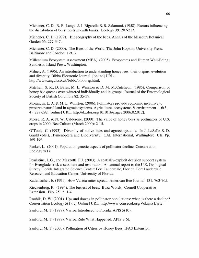
66
Michener, C. D., R. B. Lange, J. J. Bigarella & R. Salamuni. (1958). Factors influencing the distribution of bees’ nests in earth banks. Ecology 39: 207-217.
Michener, C. D. (1979). Biogeography of the bees. Annals of the Missouri Botanical Garden 66: 277-347.
Michener, C. D. (2000). The Bees of the World. The John Hopkins University Press, Baltimore and London: 1-913.
Millennium Ecosystem Assessment (MEA). (2005). Ecosystems and Human Well-Being: Synthesis. Island Press, Washington.
Milner, A. (1996). An introduction to understanding honeybees, their origins, evolution and diversity. Bibba Electronic Journal. [online] URL: http://www.angus.co.uk/bibba/bibborig.html.
Mitchell, S. R., D. Bates, M. L. Winston & D. M. McCutcheon. (1985). Comparison of honey bee queens over-wintered individually and in groups. Journal of the Entomological Society of British Columbia 82: 35-39.
Morandin, L. A. & M. L. Winston, (2006). Pollinators provide economic incentive to preserve natural land in agroecosystems. Agriculture, ecosystems & environment 116(3-4): 289-292. [online] URL: http://dx.doi.org/10.1016/j.agee.2006.02.012].
Morse, R. A. & N. W. Calderone. (2000). The value of honey bees as pollinators of U.S. crops in 2000. Bee Culture (March 2000): 2-15.
O’Toole, C. (1993). Diversity of native bees and agroecosystems. In J. LaSalle & D. Gauld (eds.), Hymenoptera and Biodiversity. CAB International, Wallingford, UK. Pp. 169-196.
Packer, L. (2001). Population genetic aspects of pollinator decline. Conservation Ecology 5(1). Pearlstine, L.G., and Mazzotti, F.J. (2003). A spatially-explicit decision support system for Everglades risk assessment and restoration: An annual report to the U.S. Geological Survey Florida Integrated Science Center: Fort Lauderdale, Florida, Fort Lauderdale Research and Education Center, University of Florida.
Rademacher, E. (1991). How Varroa mites spread. American Bee Journal. 131: 763-765.
Rieckenberg, R. (1994). The busiest of bees. Buzz Words. Cornell Cooperative Extension. Feb. 25. p. 1-4.
Roubik, D. W. (2001). Ups and downs in pollinator populations: when is there a decline? Conservation Ecology 5(1): 2 [Online] URL: http://www.consecol.org/Vol5/iss1/art2.
Sanford, M. T. (1987). Varroa Introduced to Florida. APIS 5(10). Sanford, M. T. (1989). Varroa Rule What Happened. APIS 7(6). Sanford, M. T. (2003). Pollination of Citrus by Honey Bees. IFAS Extension.

67
Shaw, H., & D. Wheeler. (1985). Statistical Techniques in Geographical Analysis. John Wiley & Sons. New York. Skovgaard O. S. (1936). Rødkloverens Bestøvning. Humlebier og Humleboer. Det Kongelige Danske Videnskabernes Selskabs Skrifter Naturvidenskabelig og Mathematisk Afdeling. 9, Raekke 6, 1–140.
Smith-Heavenrich, S. (1998). Going native with pollinators. Maine Organic Farmer & Gardener. March-May. p. 16-17.
Stauffer, D. & A. Aharony. (1992) Introduction to Percolation Theory (2nd Edition) Taylor and Francis, London, UK.
Steffan-Dewenter, I. (2001). Species richness and abundance of bees and wasps on orchard meadows: effects of habitat size, management and landscape complexity. Mitteilungen der Deutschen Gesellschaft fur allgemeine und angewandte Entomologie 13(1-6): 339-342.
Steffan-Dewenter, I. (2002). Landscape context affects trap-nesting bees, wasps, and their natural enemies. Ecological Entomology 27(5): 631-637.
Steffan-Dewenter, I., U. Munzenberg, C. Burger, C. Thies & T. Tscharntke. (2002). Scale-dependent effects of landscape context on three pollinator guilds. Ecology 83: 1421-1432.
Steffan-Dewenter, I. & T. Tscharntke. (1999). Effects of habitat isolation on pollinator communities and seed set. Oecologia 121: 432-440.
Svensson, B., Lagerlöf, J., and Svensson, B.G. (2000). Habitat preferences of nest-seeking bumble bees (Hymenoptera: Apidae) in an agricultural landscape. Agriculture, Ecosystems and Environment 77: 247-255.
Thomson, J. D. and K. Goodell. (2001). Pollen removal and deposition by honey bee and bumble bee visitors to apple and almond flowers. Journal of Applied Ecology. 38:1032-1044.
Turner, M.G., R. H. Gardner and R. V. O'Neill, R.V. (2001). Landscape Ecology in Theory and Practice. Springer-Verlag, New York, NY, USA.
Ulbrich, K. and Seidelmann, K. (2001). Modeling population dynamics of solitary bees in relation to habitat quality.Web Ecology 2: 57–64.
U.S. Department of Agriculture (USDA), Natural Resources Conservation Service, 2002. National Soil Survey Handbook, title 430-VI. [Online] URL: http://soils.usda.gov/procedures/handbook/main.htm.
Walter-Hellwig, K. & Frankl, R., (2000). Bombus spp. (Hym., Apidae), in an agricultural landscape. J. Applied Entomology 124, 299– 306.
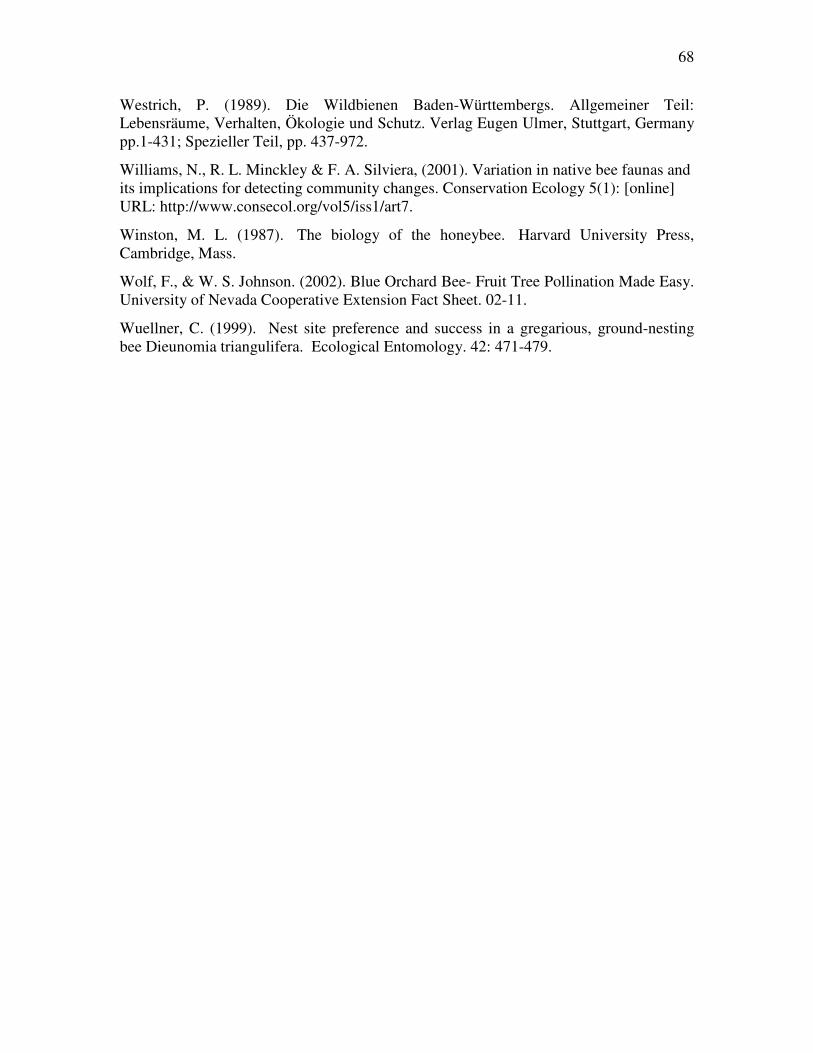
68
Westrich, P. (1989). Die Wildbienen Baden-Württembergs. Allgemeiner Teil: Lebensräume, Verhalten, Ökologie und Schutz. Verlag Eugen Ulmer, Stuttgart, Germany pp.1-431; Spezieller Teil, pp. 437-972.
Williams, N., R. L. Minckley & F. A. Silviera, (2001). Variation in native bee faunas and its implications for detecting community changes. Conservation Ecology 5(1): [online] URL: http://www.consecol.org/vol5/iss1/art7.
Winston, M. L. (1987). The biology of the honeybee. Harvard University Press, Cambridge, Mass.
Wolf, F., & W. S. Johnson. (2002). Blue Orchard Bee- Fruit Tree Pollination Made Easy. University of Nevada Cooperative Extension Fact Sheet. 02-11.
Wuellner, C. (1999). Nest site preference and success in a gregarious, ground-nesting bee Dieunomia triangulifera. Ecological Entomology. 42: 471-479.
69
Appendix A
70
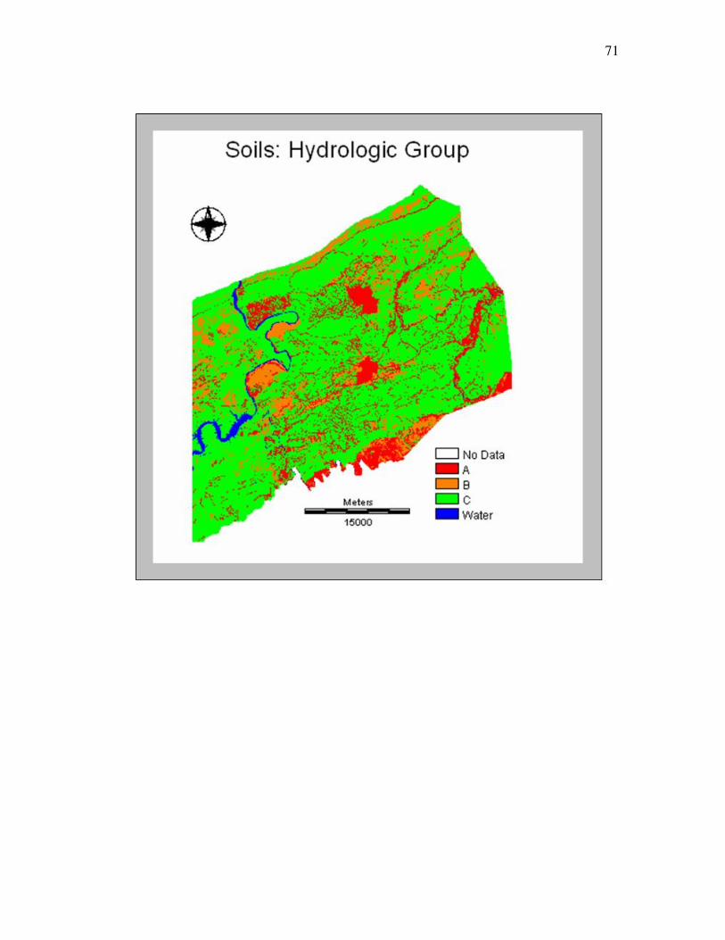
71
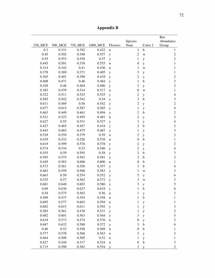
72
Appendix B
250_MCE 500_MCE 750_MCE 1000_MCE Flowers Species Num Color 2
Bee Abundance Group
0.3 0.331 0.392 0.422 n 1 b 1 0.45 0.502 0.548 0.557 y 2 w 2 0.55 0.553 0.558 0.57 y 1 y 2
0.445 0.501 0.538 0.555 n 0 y 1 0.314 0.342 0.41 0.436 n 1 w 1 0.378 0.369 0.371 0.405 y 3 y 1 0.365 0.401 0.398 0.419 y 2 y 2 0.408 0.471 0.46 0.484 y 1 b 2 0.428 0.46 0.464 0.486 y 2 y 2 0.383 0.479 0.514 0.517 n 0 w 1 0.522 0.511 0.525 0.525 y 2 y 4 0.585 0.542 0.542 0.54 y 3 b 3 0.611 0.569 0.56 0.542 y 2 y 2 0.677 0.615 0.587 0.565 y 1 y 4 0.463 0.449 0.461 0.494 y 2 b 2 0.521 0.523 0.495 0.481 n 2 y 2 0.627 0.55 0.531 0.527 y 3 y 4 0.427 0.465 0.457 0.434 y 2 b 2 0.443 0.465 0.475 0.467 y 1 y 3 0.539 0.559 0.579 0.59 n 2 y 2 0.439 0.532 0.526 0.539 n 0 b 1 0.619 0.599 0.576 0.578 y 2 y 2 0.574 0.534 0.53 0.546 y 2 y 4 0.555 0.59 0.595 0.58 y 2 b 3 0.595 0.575 0.563 0.581 y 2 b 2 0.445 0.563 0.606 0.606 n 0 b 1 0.573 0.561 0.556 0.557 y 3 b 4 0.462 0.559 0.568 0.583 y 1 w 3 0.663 0.59 0.554 0.552 y 5 y 6 0.525 0.57 0.562 0.572 y 3 w 3 0.681 0.648 0.603 0.586 y 3 y 5
0.69 0.636 0.627 0.618 y 1 b 6 0.58 0.575 0.562 0.56 n 1 y 2
0.509 0.537 0.554 0.558 n 1 b 1 0.695 0.577 0.603 0.594 n 1 y 1 0.682 0.615 0.611 0.592 y 1 y 3 0.585 0.561 0.538 0.531 y 1 y 2 0.682 0.601 0.563 0.564 y 3 y 5 0.618 0.573 0.574 0.576 n 0 y 2 0.687 0.632 0.588 0.572 y 3 b 6
0.46 0.52 0.548 0.569 n 0 b 1 0.577 0.578 0.566 0.563 n 2 y 2 0.464 0.509 0.505 0.52 n 1 y 1 0.627 0.549 0.517 0.524 n 0 b 3 0.715 0.598 0.582 0.554 y 3 y 2
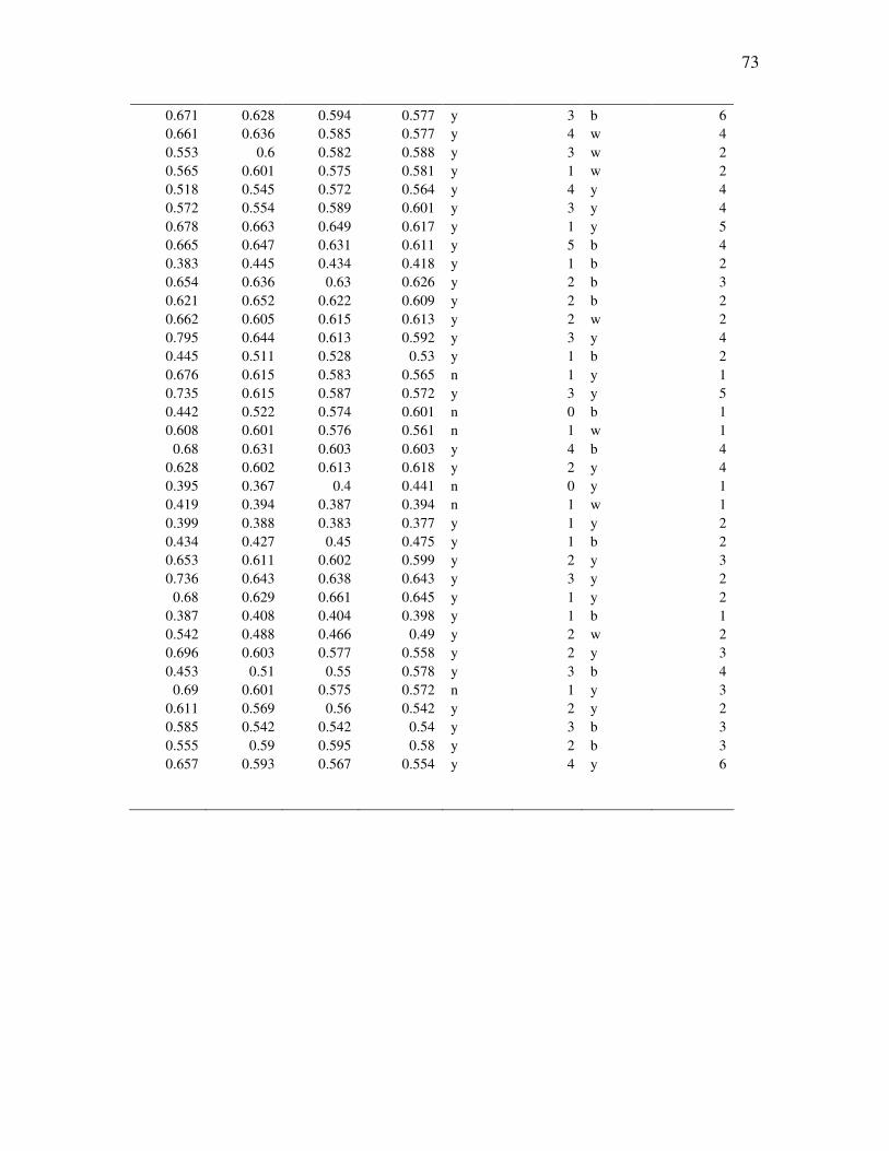
73
0.671 0.628 0.594 0.577 y 3 b 6 0.661 0.636 0.585 0.577 y 4 w 4 0.553 0.6 0.582 0.588 y 3 w 2 0.565 0.601 0.575 0.581 y 1 w 2 0.518 0.545 0.572 0.564 y 4 y 4 0.572 0.554 0.589 0.601 y 3 y 4 0.678 0.663 0.649 0.617 y 1 y 5 0.665 0.647 0.631 0.611 y 5 b 4 0.383 0.445 0.434 0.418 y 1 b 2 0.654 0.636 0.63 0.626 y 2 b 3 0.621 0.652 0.622 0.609 y 2 b 2 0.662 0.605 0.615 0.613 y 2 w 2 0.795 0.644 0.613 0.592 y 3 y 4 0.445 0.511 0.528 0.53 y 1 b 2 0.676 0.615 0.583 0.565 n 1 y 1 0.735 0.615 0.587 0.572 y 3 y 5 0.442 0.522 0.574 0.601 n 0 b 1 0.608 0.601 0.576 0.561 n 1 w 1
0.68 0.631 0.603 0.603 y 4 b 4 0.628 0.602 0.613 0.618 y 2 y 4 0.395 0.367 0.4 0.441 n 0 y 1 0.419 0.394 0.387 0.394 n 1 w 1 0.399 0.388 0.383 0.377 y 1 y 2 0.434 0.427 0.45 0.475 y 1 b 2 0.653 0.611 0.602 0.599 y 2 y 3 0.736 0.643 0.638 0.643 y 3 y 2
0.68 0.629 0.661 0.645 y 1 y 2 0.387 0.408 0.404 0.398 y 1 b 1 0.542 0.488 0.466 0.49 y 2 w 2 0.696 0.603 0.577 0.558 y 2 y 3 0.453 0.51 0.55 0.578 y 3 b 4
0.69 0.601 0.575 0.572 n 1 y 3 0.611 0.569 0.56 0.542 y 2 y 2 0.585 0.542 0.542 0.54 y 3 b 3 0.555 0.59 0.595 0.58 y 2 b 3 0.657 0.593 0.567 0.554 y 4 y 6
74
Vita
Andrew Scott Foy
Andrew was born in Tacoma, Washington in 1983. He spent a few years there and then his family moved to Massachusetts and finally to Virginia. Much of his interests in science developed while in rural Virginia, with ample room to explore as a kid. After high school, Radford University and then Virginia Tech were his other homes where he studied a variety of disciplines, eventually finding geography. The excellent faculty and resources provided focus and allowed many internship opportunities to arise. The hands-on work coupled with the two university educations was instrumental in his academic development. He has traveled, studied and worked both locally and abroad, for example Dinosaur National Monument and the Galapagos Islands. His broad academic interests focus on using GIS to solve every day, real world problems. Other passions are green development and alternative fuels, but everything biological and new technologies are always interesting. He plans to continue his education by beginning the PhD program in Geospatial and Environmental Analysis at Virginia Tech.