Chapter 1. Introduction

1. Generation of X-ray 1) X-ray: an electromagnetic wave with a wavelength of 0.1–100 Å. 2) Types of X-ray tubes a) A stationary-anode tube b) A rotating-anode tube

3) X-ray tube: price; $4,000–$5,000 a) Working hours; 5,000–10,000 h b) Cooling system; cold distilled water i) Mo target: 50 kV/30 mA (1,500 W) ii) Cu target: 40 kV/20 mA (800 W)

2. Characteristics of X-ray 1) White radiation versus characteristic lines 2) At energies of about 10,000 eV, 1s electrons in the K shell are removed. a) Kα1, Kα2: L → K b) Kβ1, Kβ2: M → K i) Wavelength: Kα > Kβ ii) Relative intensity: Kα1/Kα2 ≈ 2, Kα1/Kβ1 ≈ 3–6

λ

50 kV

40 kV

30 kV20 kV

I

Figure. Continuous X-ray spectra as a function of accelerating voltage.

Chapter 1-1

λ (angstrom)0.5 1.0 1.5

Cu

Kα

Kβ

I

Mo

KαKβ

Figure. X-ray spectra with characteristic peaks: Mo Kα, 50 kV; Cu Kα, 35 kV.

3) Monochromatization of X-ray: a β-filter or a monochromator a) Using a filter i) The absorption of X-ray by a solid I/Io = e–µτ µ; linear absorption coefficient

τ; path length ii) A plot of µ as a function of λ for a given element:

µ = kλ3 → Z ⇓ → E ⇓ → λ ⇑

I

λ

Kβ

Kα µ

Figure. X-ray spectrum showing characteristic peaks (I curve) and absorption

coefficients (µ curve) for the same element..

iii) The absorption edge of an element with an atomic number Z – 1 falls between the Kα and Kβ lines of the element with the atomic number Z.

Chapter 1-2

iv) If a target has Z, then a filter has Z – 1.

Mo X-ray tube: Nb filter Cu X-ray tube: Ni filter

I

λ

Kβ

KαI

λ

Kβ

Kα

µ for an element with Z - 1

Characteristic curvesfor an element with Z

Figure. X-ray spectra showing effects of a β filter. Mo radiation (50 kV) with a 0.001

inch Nb filter.

b) Using a monochromator The direct beam from the X-ray tube is reflected (diffracted) by a large single-crystal (e.g., graphite) of a suitable material before it is used.

3. Selection of radiation 1) Diffracted beams will be more separated on the detector if a longer wavelength is used. 2) here is a limiting sphere of a radius 2/λ that limits the volume of reciprocal space accessible to diffraction experiments. 3) Film is a better detector for Cu rather than Mo radiation. Diffractometer counters have a very high counting efficiency for the Mo Kα radiation. a) Cu Kα: cheap, good for photographs and for biological molecules b) Mo Kα: good for scintillation counters, but a low efficiency of recording for photographs.

c) The elements present in a crystal may play a role in the choice of radiation.

Chapter 1-3

4) Commonly used X-ray tubes Table. Target materials and associated constants

Cr Fe Cu Mo

Z 24 26 29 42

α1 (Å) 2.2896 1.9360 1.5405 0.70926

α2 (Å) 2.2935 1.9399 1.5443 0.71354

<α>a (Å) 2.2909 1.9373 1.5418 0.71069

β filter V, 0.4 min.b Mn, 0.4 min. Ni, 0.6 min Nb, 3 min.

Resolution (Å) 1.15 0.95 0.75 0.3

<α>a is the intensity-weighted average of α1 and α2 and is the figure usually used

for the wavelength when two lines are not resolved.

b1 min. = 0.001 in. = 0.025 mm.

Chapter 1-4

Chapter 2. Diffraction of X-ray

1. Lattices A point or space lattice is a three-dimensional periodic arrangement of points, and it is a purely mathematical concept. In contrast to a finite crystal, a space lattice is infinite.

(a) (b)

1) All of the points in a lattice should be able to be obtained by translations only. Dimensionality No. of lattices Lattice descriptor

1 1 row

2 5 net

3 14 Bravais

2) Each Bravais lattice can be specified by three non-coplanar vectors, a, b, and c, parallel to reference axes x, y, and z, respectively. a) From any point as an origin, any other point in a lattice has a vector distance ruvw from the origin given by

ruvw = Ua + Vb + Wc

where the integers U, V, and W are the coordinates of a lattice point.

Chapter 2-1

b) All lattices are centrosymmetric.

100

000 010

001

111

x

y

z

a

b

c

231101

110

Figure. Designation of a lattice point with the coordinates UVW that define the vector from

the origin to the lattice point, ruvw = Ua + Vb + Wc.

3) Designation of lines in a lattice a) The coordinates are placed in square brackets [231] to show that they represent the direction of a line.

b) The lattice lines X' and X may be referred to by the symbol [112]. c) The triple [UVW] describes not only a lattice line passing through the origin and the point UVW, but also an infinite set of lattice lines that are parallel to it and have the same lattice parameters.

Chapter 2-2

100

000

x

y

z

a

b

c

231

112

212 XX'

A

Figure. Designation of lattice lines with the coordinates [UVW] that define the vector from the

origin to the lattice point, ruvw = Ua + Vb + Wc (A: [231], X: [112]).

The following figure shows parallel sets of lines [110], [120], and [310].

a

b

x

[310] [110]

[120]

y

Chapter 2-3

The following figure shows a projection of a lattice along c-axis on the a,b-plane. The lattice line A intersects the points 210, 000, 210, and 420.

y

x

ab

[010]

[100]

210

210

420

130

130

[210]

A

B

a) Each point on the line has the different UVW values, but the ratio of U:V:W

remains constant. In this case, the smallest triple is used to define the lattice line.

b) Lines parallel to the a- and b-axis are defined as [100] and [010], respectively. The line B is given as [130] or [130]. Note that minus signs are placed above the numbers to which they apply;

this appears to all crystallographic triples.

4) Designation of planes in a lattice Consider a plane in a lattice that intersects the axes a, b, and c at the points a/h00, 0b/k0, and 00c/l. The reciprocals of these coordinates are used rather than the coordinates themselves.

The (hkl) values are called Miller indices, and they are defined as the smallest integral multiples of the reciprocals of plane intercepts on three axes.

Chapter 2-4

(230)

y

x

ab

H

A

BCDE

GF

(210)

Lattice plane a/h b/k c/l hkl

A a/(1/2) b/(1/4) c/0 1/2 1/4 0 (210)

B a/(2/3) b/(1/3) c/0 2/3 1/3 0 (210)

C a/(1) b/(1/2) c/0 1 1/2 0 (210)

D a/(2) b/(1) c/0 2 1 0 (210)

E – – – – – – –

F a/(–2) b/(–1) c/0 –2 –1 0 (210)

G a/(–1) b/(–1/2) c/0 –1 –1/2 0 (210)

H a/(1/3) b/(–1/2) c/0 1/3 –1/2 0 (230)

a) The lattice planes A to G belong to a set of equally spaced planes, parallel planes resulting in the same indices. Generally, they are all described by the triple (hkl), which represents an infinite set of parallel lattice planes.

b) (210) and (210) define the same set of parallel planes. 5) Because the lattice plane E intersects the origin, it cannot be indexed in the projection. a) The line H is the trace of the plane (230). e) The spacing between the planes decreases with increasing indices. f) Planes that are parallel to b- and c-axis and have intercepts only with the a-axis are indexed as (100).

g) (010) intersects only the b-axis, and (001) intersects only the c-axis.

Chapter 2-5

The following figure shows a projection of a lattice onto the ab-plane.

a

b

(410)

(210)

(100)

(110)

(010)

2. Unit cell: the smallest building block (a repeating unit) The most general lattice is represented in the figure, in which a ≠ b ≠ c and α ≠ β ≠ γ ≠ 90° or 120°.

xy

z

ab

c

ab

c

αβ

γ

x

y

z

There is no unique way to select a unit cell for a given crystal. 1) The symmetry at each point in a lattice is 1 (i). a) When a lattice possesses symmetry higher than 1 at each point, the

Chapter 2-6

vectors a, b, and c can be selected in a specialized manner. b) If a 2-fold symmetry axis passes through each point in the lattice, the symmetry at each point is 2/m (C2h):

c) The symmetry of a lattice is invariant under the selection of a unit cell. 2) A unit cell should show the symmetry of its lattice. 3) For the origin of a unit cell, a geometrically unique point is selected, with a priority given to a symmetry center. 4) The base vectors should be as short as possible. 5) When the angles between base vectors deviate from 90°, they are selected to be either all larger or all smaller than 90°. 3. Miller Index The intercept equation of the general plane:

(hX/a) + (kY/b) + (lZ/c) = 1

The equation of the parallel plane passing through the origin:

(hX/a) + (kY/b) + (lZ/c) = 0 1) The sets of parallel lattice planes can be constructed so that, for any given set, every lattice point can lie on some member of it. 2) A 3-D unit cell

a

b

c

1

2

Figure. An example of a lattice plane and an interleaving plane.

3) Intercepts of a plane (1/h, 1/k, 1/l) ⇒ hkl: Miller index 4) Planes parallel to one or more of the axes ⇒ Miller index is 0.

Chapter 2-7

5) Relationship between (h, k, l) and (nh, nk, nl) indices In general, the addition of n – 1 interleaving planes between each pair of the set (h, k, l) will give the family of planes with the indices (nh, nk, nl). 6) Three ways to use Miller indices a) A set of lattice planes (hkl): (010) b) A direction and line segment from the origin to the point [x, y, z] Example: the three cell axes are [100], [010], and [001].

c) A set of face planes that are equivalent due to the symmetry of the crystal. Such a set is called a crystal form. i) For a cubic crystal, {100} includes (100), (010), (001), (100), (010), and (001).

ii) For a triclinic crystal, {100} includes only (100).

4. X-ray diffraction 1) Historical backgrounds a) X-ray was discovered by Roentgen in 1895 b) X-ray diffraction by crystals was found by Laue in 1912 c) In 1912, Bragg found similarities between diffraction and ordinary reflection.

2) Scattering versus diffraction

1st EM

2nd EM

Σ(scattering)i = diffraction

Chapter 2-8

3) Bragg's law

1 1'

2 2'O

C

A B d

θθ

θθθθ

θ

2AC = nλ (for constructive interference)

2d sin θ = nλ

5. Reciprocal lattice 1) 2d sin θ = nλ ⇒ sin θ = (nλ/2) × (1/d) a) Structures with large d values will exhibit a compact diffraction pattern. b) Interpretation of X-ray data would be facilitated if the inverse relationship would become a direct one. ⇒ a reciprocal lattice.

2) Reciprocal lattice c) Two-dimensional case

O

0,1

1,12,13,1

0,11,1 2,1 3,1

⇒ The set of points is defined as a reciprocal lattice.

Chapter 2-9

d)

0

A/2

A

0*

1*

2*1kl

δ1

δ2

φ1

φ2

2kl

B

φ2

φ1

i) OA: a unit translation along the a-axis in a direct space ii) All planes having their h index 0 are parallel to OA, and their normals will lie in the plane perpendicular to OA through the origin O, the trace of which is labeled 0*.

iii) d1kl = OA sin φ1kl δ1kl = OB sin φ1kl OB = 1/d1kl = 1/[OA sin φ1kl] ∴ δ1kl = 1/OA In the same way, it can be shown that δ2kl = 1/(1/2OA) = 2(1/OA)

iv) and in general

δnkl = n(1/OA)

v) The various reciprocal lattice points are segregated according to the h indices into equally spaced parallel layers.

Chapter 2-10

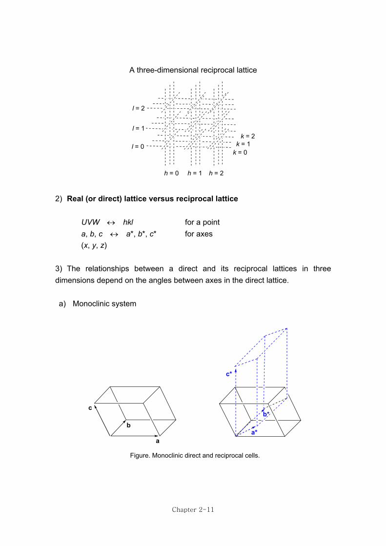
A three-dimensional reciprocal lattice

h = 1 h = 2h = 0

l = 1

l = 2

l = 0k = 0k = 1

k = 2

2) Real (or direct) lattice versus reciprocal lattice UVW ↔ hkl for a point a, b, c ↔ a*, b*, c* for axes (x, y, z) 3) The relationships between a direct and its reciprocal lattices in three dimensions depend on the angles between axes in the direct lattice. a) Monoclinic system

a

ba*

b*

c*

c

Figure. Monoclinic direct and reciprocal cells.

Chapter 2-11

a

c

d100

d001

β

β*

d100 = a sin (180 - β) = a sin βa* = 1/d100 = 1/(a sin β)

aa*

b

b*

ob

b*

c

c*

o

γ = γ* = 90o

b ⊥ a*, a ⊥ b*α = α* = 90o

b ⊥ c*, c ⊥ b* Table. Monoclinic direct–reciprocal relationships

a* = 1/(a sin β) a = 1/(a* sin β*) α = γ = α* = γ* = 90°

b* = 1/b b = 1/b* β* = 180 – β

c* = 1/(c sin β) c = 1/(c* sin β*) V* = 1/V = a*b*c* sin β*

V = 1/V* = abc sin β

b) Triclinic system

a

b

c

a*

b*

c*

Figure. Triclinic direct and reciprocal cells.

Table. Triclinic direct–reciprocal relationships

a* = (bc sin α)/V b* = (ac sin β)/V c* = (ab sin γ)/V

sin α* = V/(abc sin β sin γ) cos α* = (cos β cos γ – cos α)/(sin β sin γ)

sin β* = V/(abc sin α sin γ) cos β* = (cos α cos γ – cos β)/(sin α sin γ)

sin γ* = V/(abc sin α sin β) cos γ* = (cos α cos β – cos γ)/(sin α sin β)

V = 1/V* = abc(1 – cos2 α – cos2 β – cos2 γ + 2 cos α cos β cos γ)1/2

= abc sin α sin β sin γ* = abc sin α sin β* sin γ = abc sin α* sin β sin γ

Chapter 2-12

c) Some remarks i) The reciprocal vector, r* = ha* + kb* + lc*, is normal to the family of the lattice plane (hkl). If the h, k, and l have no common factor, then

|r*| = r* = 1/dhkl

Table. The algebraic expressions of dhkl for the various systems

System 1/dhkl

Cubic (h2 + k2 + l2)/a2

Tetragonal (h2 + l2)/a2 + l2/c2

Orthorhombic h2/a2 + k2/b2 + l2/c2

Hexagonal 4(h2 + k2 + hk) + l2

3a2 c2

Trigonal (R) (h2 + k2 + l2) sin2 α + 2(hk + hl + kl)(cos2 α – cos α)

a2 (1 + 2cos3 α – 3cos2 α)

Monoclinic h2 + k2 + l2 – 2hl cos b

a2 sin2 β b2 c2 sin2 β ac sin2 β

Triclinic (1 – cos2 α – cos2 β – cos2 γ + 2cos α cos β cos γ)–1[(h2/a2)sin2

α + (k2/b2)sin2 β + (l2/c2)sin2 γ + (2kl/bc)(cos β cos γ – cos α) +

(2hl/ac)(cos α cos γ – cos β) + (2hk/ab)(cos α cos β – cos γ)]

ii) Any direct axis has a family of reciprocal lattice planes perpendicular to it, each plane containing points with a constant index associated with that axis.

iii) A reciprocal lattice axis should be perpendicular to one face of the direct unit cell: a ⊥ b*c* b ⊥ a*c* c ⊥ a*b*, a* ⊥ bc b* ⊥ ac c* ⊥ ab

Chapter 2-13

c

a*

b*c*

l = 0

l = 1

l = 2

Figure. Reciprocal lattice levels a*b* perpendicular to a direct axis c.

6. Bragg's law in a reciprocal lattice 1)

X-ray

C

BP

O

c*

a*

C

DX-ray

O

θ

θθ

2θ

PB

Figure. Diffraction in terms of the reciprocal lattice.

a) X-ray beam parallel to the a*c* plane, a circle with a radius of 1/λ b) OP = OB sin θ

OP = 1/dhkl = (2/λ) × sin θ ⇒ 2d sin θhkl = λ (Bragg's law with n = 1)

2) Some remarks a) Whenever a reciprocal lattice point coincides with a circle, Bragg's law is satisfied and reflection occurs.

b) Because, experimentally, the diffraction is viewed from an approximately infinite distance, there is no practical difference between OD and CP.

3) Two kinds of spheres in the reciprocal lattice a) Sphere of reflection (reflection sphere or Ewald sphere): the sphere with a radius of 1/λ

Chapter 2-14

b) Limiting sphere: the sphere with a radius of 2/λ

Direct axis

short λ sphere

long λ sphere

c) If there is only one reciprocal lattice point per reciprocal unit cell, the total number of possible reflections, N, is approximately N = {4/3 × π(2/λ)3}/{vol. reciprocal cell} N = 33.5/(vol. reciprocal cell × λ3) N = (33.5 × vol. direct cell)/λ3 Example: A rectangular cell of dimensions 8 × 10 × 20 Å has a volume of 1600 Å3

if Cu Kα(1.5418 Å) N = 14,600 reflections if Mo Kα (0.7107 Å) N = 149,000 reflections

4) Quantities other than 1/dhkl are often used to describe the distances of the reciprocal lattice points from the origin. a) (sin θ)/λ = 1/2dhkl = 1/2(h2a*2 + k2b*2 + l2c*2 + 2hka*b*cos γ* + 2hla*c*cos β* + 2klb*c* cos α)1/2

b) Scattering vector: S This arises from a vector derivation of Bragg reflection and is the magnitude of the scattering vector normal to the reflecting plane. |S| = 1/dhkl = 2(sin θ)/λ

Chapter 2-15

5) Table. Limiting values of reciprocal measurements and resolution

Cu Kα Mo Kα

λ 1.5418 0.7107

[(sin θ)/λ]max 0.648–1 1.407–1

|S| = (1/dhkl)max 1.296 2.814

(dhkl)min = λ/2 0.7709 0.3554

Resolution 0.71 0.33

a) The maximum possible value of sin θ is 1. b) LR (limit of resolution): the minimum separation at which two atoms can be distinguished.

LR = 0.92 × dmin

6) Cones of diffracted rays for rotation about a direct axis

Rotationaxis

X-raybeam

Chapter 2-16

Chaper 3. Crystal symmetry and space groups

lattice + basis ⇒ crystal structure (basis: the arrangement of atoms)

1) A complete set of symmetry elements in a lattice or a crystal structure, or a group of symmetry elements including lattice translations is a called a space group. 2) Crystals are solid chemical substances with a three-dimensional periodic array of atoms, ions, or molecules. This array is called a crystal structure.

1. The 14 Bravais lattices: primitive and nonprimitive lattices 1) Symmetry in crystallography a) n-fold rotation: n (= Cn), rotation by 360º/n (n = 1, 2, 3, 4, 6) b) mirror plane (or a plane of symmetry): m (= σv), /m (= σh) c) inversion (or a center of symmetry): 1 (= i) d) rotary inversion axis: n = n + 1 Example: 4 (read: bar four) ⇒ 90º rotation (4) + inversion (1) In the following two rules, the presence of any two of the given symmetry elements will imply the presence of a third.

① Rule 1. A rotation axis of even order (n = 2, 4, 6), a mirror plane perpendicular to the rotation axis, and an inversion center at the position of their intersection (n, /m, and 1).

② Rule 2. Two mutually perpendicular mirror planes and a 2-fold rotation axis along the line of their intersection (m, /m, and 2).

Chapter 3 - 1

2) Primitive lattices (P): lattice points only at the corners of the unit cell (one lattice point per unit cell)

3) Nonprimitive lattices (A, B, C, F, or I): centered lattices Is it possible to add one or more lattice points to the primitive lattices without

destroying the symmetry?

a) Two or more lattice points per unit cell b) Side-centered lattices (A, B, C, F) and body-centered lattices (I) i) A-centered lattice: an additional lattice point on the bc plane ii) B-centered lattice: an additional lattice point on the ac plane iii) C-centered lattice: an additional lattice point on the ab plane iv) F-centered lattice: additional lattice points on all planes v) I-centered lattice: an additional lattice point on the body center

7 primitive lattices + 7 nonprimitive lattices ⇒ 14 Bravais lattices

The 14 Bravais lattices represent the 14 only ways of filling space with a three-dimensional periodic array of points. All crystals are built up on the basis of the 14 Bravais lattices. The crystal structure can be thought of as a combination of a lattice and a basis. Whereas the number of lattices is constant (14), there are many possible ways of arranging atoms in a unit cell. However, any crystal structure belongs to only one of the 14 Bravais lattices. Table. Space-group symbols for the 14 Bravais lattices

P C I F

Triclinic P 1

Monoclinic P 2/m C 2/m

Orthorhombic P 2/m 2/m 2/m C 2/m 2/m 2/m I 2/m 2/m 2/m F 2/m 2/m 2/m

Tetragonal P 4/m 2/m 2/m I 4/m 2/m 2/m

Trigonal P 6/m 2/m 2/m R 3 2/m

Hexagonal

Cubic P 4/m 3 2/m I 4/m 3 2/m F 4/m 3 2/m

Chapter 3 - 2

P1β

β

P2/m C2/m

a

bc

Pmmm Cmmm Immm Fmmm

R3m P4/mmm I4/mmm

120o

P6/mmm

Pm3m Im3m Fm3m

14 Bravais lattices

2. Seven crystal systems

All lattices, all crystal structures, and all crystal morphologies that can be defined by the same lattice parameters belong to the same crystal system.

3) The unit cell is characterized by six parameters. a) Unit cell (or lattice) parameters i) Axial lengths: a, b, c ii) Interaxial angles: α, β, γ

Chapter 3 - 3

ab

c

αβ

γ

x

y

z

b) Seven crystal systems A cardinal rule is to select a unit cell in such a way that it conforms to the symmetry actually present. Table 3.1. Seven crystal systems

Crystal Symbols of Parameters Lattice

system conventional Symmetry unit cells

Triclinic P a ≠ b ≠ c; α ≠ β ≠ γ 1 (Ci)

Monoclinic P, C a ≠ b ≠ c; α = γ = 90, β > 90° 2/m (C2h)

Orthorhombic P, C, I, F a ≠ b ≠ c; α = β = γ = 90° mmm (D2h)

Tetragonal P, I a = b ≠ c; α = β = γ = 90° 4/mmm (D4h)

Cubic P, I, F a = b = c; α = β = γ = 9o° m3m (Oh)

Hexagonal P a = b ≠ c; α = β = 90°, γ = 120° 6/mmm (D6h)

Trigonal R a = b = c; α = β = γ ≠ 90°, <120° 3m (D3d)

4) Some remarks a) The lattice symmetry is fundamental. b) Every lattice (or unit cell) is inherently centrosymmetric. c) In the monoclinic system, the b-axis is unique with β > 90°. d) In the tetragonal and hexagonal systems, the c-axis is unique.

5) Examples a) Triclinic system: 1 b) Monoclinic : 2/m (read “2 over m”, 1(a-axis) 2/m(b-axis) 1(c-axis)) a 2-fold axis with a mirror plane perpendicular to it.

c) Orthorhombic: 2/m (a-axis), 2/m (b-axis), 2/m (c-axis) ⇒ mmm

Chapter 3 - 4

**

**

**** * **

***

**

**β

(010)

(020)

triclinic monoclinic orthorhombic

d) Tetragonal: 4/m (c-axis), 2/m <a>, 2/m <110> ⇒ 4/mmm) e) Rhombohedral (or trigonal): 3m

4 3

tetragonal rhombohedral

f) Hexagonal: 6/m mm g) Cubic: m3m

120o

6

hexagonal cubic

Chapter 3 - 5

3. Conventions to select a standard unit cell 1) In the monoclinic lattices

c

ba

c

ba

c

b

a

c

b

a

(a) (b)

(c)(d)

Figure. Monoclinic lattices: (a) reduction of a B-centered cell to a P cell; (b) reduction of an I-

centered cell to an A-centered cell; (c) reduction of an F-centered cell to a C-centered cell; (d)

reduction of a C-centered cell to a triclinic P cell. 2) Tetragonal C and P lattices ⇒ No C-centered tetragonal lattice

c

a

a

Figure. A relationship between tetragonal C and P lattices.

Chapter 3 - 6

4. The 32 crystallographic point groups The space groups of the Bravais lattices are those with the highest possible symmetry for the corresponding crystal systems. Formally, a point group is defined as a group of point symmetry elements whose operations leave at least one point unchanged.

1) Rotation axes (n) + mirrors (m) + centers of symmetry (1) + rotary-inversion axes (n) ⇒ 32 point groups 2) The space group of the monoclinic P-lattice is P2/m, where it is conventional to select the b-axis parallel to 2 and perpendicular to m. The b-axis is called “symmetry direction”. Therefore, the a- and c-axis lie in the plane of m. Table. Symmetry directions in seven crystal systems

Position in the international symbol

1st 2nd 3rd

Triclinic – – –

Monoclinic b

Orthorhombic a b c

Tetragonal c <a>1 <110>2

Trigonal c <a> –

Hexagonal c <a> <210>

Cubic <a> <111> <110>

1 <a> a set of symmetry-equivalent axes (a1, a2; a1, a2, a3)

2 The symbol <UVW> denotes the lattice direction [UVW] and all directions equivalent to it.

3) The point group or groups derived from the space groups of lattices are the highest possible symmetry for the particular crystal system. 4) The point groups of the highest symmetry (the symmetry of a lattice point) in each crystal system all contain the symmetry elements of one or more point groups of lower symmetry (or subgroups).

Chapter 3 - 7

5) Molecular symmetry Molecular point groups are often called non-crystallographic point groups. 6) Determination of point groups

a) All rotation axes are polar. This means that they have distinct properties in parallel and antiparallel directions. Some symmetry elements can destroy this polarity. i) 1 ii) m (⊥ n) iii) 2 (⊥ n)

Table. Essential symmetry elements for crystal systems

Essential symmetry elements

Triclinic None

Monoclinic 2 or 2 axis along b

Orthorhombic Three mutually perpendicular m or 2 along a, b, and c

Tetragonal 4 or 4 along c

Trigonal 3 or 3 along c

Hexagonal 6 or 6 along c

Cubic Four 3 axes (4 C3)

b) Questions to use for point-group determination:

i) Are rotation axes are higher than 2 (3, 4, or 6)? ii) Are these axes are polar? Or, is an inversion center present?

7) Enantiomorphism The point group 1 (C1) is asymmetric. All other point groups with no symmetry elements other than rotation axes are called chiral or dissymmetric. The relevant point groups are: n: (1), 2, 3, 4, 6 Cn: (C1), C2, C3, C4, C6 n2: 222, 32, 422, 622 Dn: D2, D3, D4, D6 n3: 23, 432 T, O

Chapter 3 - 8

a) Asymmetric or dissymmetric crystals and molecules are those which are not superimposable on their mirror images by rotation or translation.

b) The mirror images are said to be enantiomorphs of each other. c) Enantiomorphic molecules are also called enantiomeric.

8) Because only rotations by 2π/n with n = 1, 2, 3, 4, and 6 can occur in 3-D lattices, only those point groups that comprise these and no other rotations are found in crystalline solids. Table. A list of the 32 point groups

Crystal Point groups Laue Lattice point

system Noncentrosym. Centrosym. class groups

triclinic 1(C1) 1(Ci) 1 1

monoclinic 2(C2), m(Cs) 2/m(C2h) 2/m 2/m

orthorhombic 222(D2), 2mm(C2v) mmm(D2h) mmm mmm

tetragonal 4(C4), 4(S4) 4/m(C4h) 4/m 4/mmm

422(D4), 4mm, 42m(D2d) 4/mmm(D4h) 4/mmm

trigonal 3(C3) 3(S6) 3 3m

32(D3), 3m(C3v) 3m(D3d) 3m

hexagonal 6(C6), 6(C3h) 6/m(C6h) 6/m 6/mmm

622(D6), 6mm, 6m2(D3h) 6/mmm(D6h) 6/mmm

cubic 23(T) m3(Td) m3 m3m

432(O), 43m(Td) m3m(Oh) m3m

9) The symbol on its own shows the relative orientation of symmetry elements. a) n2: rotation axis(n) and 2-fold axes perpendicular to it: 42(2) b) nm: n and mirror planes parallel to it: 3m c) n2: rotary-inversion axis (n) and 2-fold axes perpendicular to it: 42(m) d) nm: n and mirror planes parallel to it: 3m e) n/mm: n and mirror planes both parallel and perpendicular to it: 4/mm

Chapter 3 - 9

10) Crystal faces can be related to one another by point groups. 11) The point group C2v is described as mm, because two intersecting mirror planes generate a rotation axis along the line of their intersection. 12) The point group D2h is represented as mmm, indicating there are three different mirror planes. A 2-fold axis is necessarily generated along each of the three lines of intersection, as well as an inversion center where all planes and axes meet. 13) The point group D2 is a pure rotation group consisting of only three C2 (or 2) operations and the identity (1) operation. It is uniquely specified by the symbol 222. 5. Space groups Starting from the space groups with the highest symmetry in each crystal system, i.e., those of the 14 Bravais lattices, it is possible to derive all of their subgroups. However, you must keep in mind that screw axes can replace rotation axes and glide planes mirror planes. 2 ⇒ 21 3 ⇒ 31, 32 4 ⇒ 41, 42, 43 6 ⇒ 61, 62, 63, 64, 65 m ⇒ a, b, c, n, d 1) The ways in which identical objects can be arranged in an infinite lattice 2) Two ways to generate the space groups

i) 32 point groups + 14 Bravais lattices ⇒ 230 space groups ii) symmetry elements + translations ⇒ 230 space groups

3) Translational symmetry elements

Chapter 3 - 10

a) Screw axis i) nm: 360°/n rotation + m/n translation parallel to n ii) Characteristic of an n-fold screw axis: the position of the nth point laid down differs from the initial point by an integral number of unit translations

Screw axis 31

Unittranslation

1

23

1'

Unittranslation

1

23

1'

Unittranslation

1

2'3'

1'

Screw axis 32

b) Glide planes i) Reflection + translation along the edge or face diagonal of the unit cell ii) a glide: a/2 translation b glide: b/2 translation c glide: c/2 translation n glide: (a + b)/2, (b + c)/2, or (a + c)/2 translation d glide: (a + b)/4, (b + c)/4, or (a + c)/4 translation

i) Characteristic of a glide plane: after two glide operations (or four for d-glides) the position of the point laid down is identical to that of the initial point plus unit translations on one or two axes.

a

bc

Glide plane a

Chapter 3 - 11

Table. Some symmetry elements and their equivalent positions

Equivalent positions

Axis 2 Parallel to a x, y, z x, –y, –z

2 b x, y, z –x, y, –z

2 c x, y, z –x, –y, z

21 a x, y, z 1/2 + x, –y, –z

21 b x, y, z –x, 1/2 + y, –z

21 c x, y, z –x, –y, 1/2 + z

Plane m Perpendicular to a x, y, z –x, y, z

m b x, y, z x, –y, z

m c x, y, z x, y, –z

a b x, y, z 1/2 + x, –y, z

a c x, y, z 1/2 + x, y, –z

b c x, y, z x, 1/2 + y, –z

b a x, y, z –x, 1/2 + y, z

c a x, y, z –x, y, 1/2 + z

c b x, y, z x, –y, 1/2 + z

n b x, y, z 1/2 + x, –y, 1/2 + z

n c x, y, z 1/2 + x, 1/2 + y, –z

d a x, y, z –x, 1/4 + y, 1/4 + z

d b x, y, z 1/4 + x, –y, 1/4 + z

d c x, y, z 1/4 + x, 1/4 + y, –z

The space groups of the monoclinic system will be derived as an example for all crystal systems. Let's begin with the two monoclinic space groups with the highest symmetry: P2/m and C2/m. The monoclinic subgroups of the point group 2/m are 2 and m. The point-group symmetry elements 2 and m can be replaced by a 21 screw axis and a glide plane, respectively. Because m is perpendicular to the b-axis, only a-, c-, and n-glide planes are possible. The replacement of 2 and m by 21 and c results in the 13 monoclinic space groups.

Chapter 3 - 12

Table. The point and space groups of the monoclinic crystal system

Point groups Space groups

2/m P2/m C2/m

P21/m

P2/c C2/c

P21/c

m Pm Cm

Pc Cc

2 P2 C2

P21

4) International Tables for Crystallography a) A symmetry diagram shows the projection of a unit cell and the location of all its symmetry elements.

b) A cell diagram shows equivalent general points that are generated by applying symmetry operations to any initial point.

c) There is a list of positions of all possible types within the unit cell and the symmetry element that exists at each one.

d) Expression: Pbca e) Examples i) P21 ii) P21/c

+(1)

+

P21

+(1)

1/2-

1/2-

P21/c

b b

a a

(2)1/4

1/4

1/4

1/4

1/4

1/4

1/2+(3)

(2)(4)

,

,+

+

, +

, + , +

,

1/2+

Figure. P21: equivalent positions (1) x, y, z; (2) –x, 1/2 + y; –z

Figure. P21/c: equivalent positions (1) x, y, z; (2) –x, 1/2 + y, 1/2 – z; (3) x, 1/2 – y, 1/2 + z; (4) –x,

–y, –z.

Chapter 3 - 13

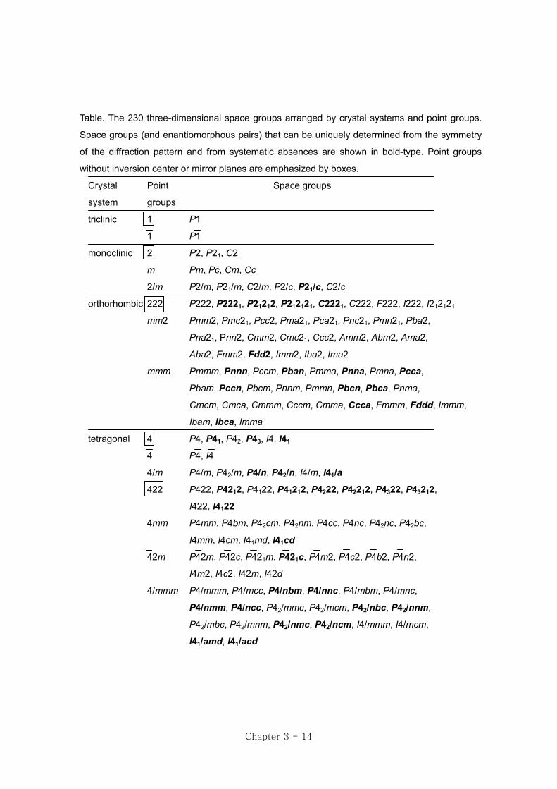
Table. The 230 three-dimensional space groups arranged by crystal systems and point groups.

Space groups (and enantiomorphous pairs) that can be uniquely determined from the symmetry

of the diffraction pattern and from systematic absences are shown in bold-type. Point groups

without inversion center or mirror planes are emphasized by boxes.

Crystal Point Space groups

system groups

triclinic 1 P1

1 P1

monoclinic 2 P2, P21, C2

m Pm, Pc, Cm, Cc

2/m P2/m, P21/m, C2/m, P2/c, P21/c, C2/c

orthorhombic 222 P222, P2221, P21212, P212121, C2221, C222, F222, I222, I212121

mm2 Pmm2, Pmc21, Pcc2, Pma21, Pca21, Pnc21, Pmn21, Pba2,

Pna21, Pnn2, Cmm2, Cmc21, Ccc2, Amm2, Abm2, Ama2,

Aba2, Fmm2, Fdd2, Imm2, Iba2, Ima2

mmm Pmmm, Pnnn, Pccm, Pban, Pmma, Pnna, Pmna, Pcca,

Pbam, Pccn, Pbcm, Pnnm, Pmmn, Pbcn, Pbca, Pnma,

Cmcm, Cmca, Cmmm, Cccm, Cmma, Ccca, Fmmm, Fddd, Immm,

Ibam, Ibca, Imma

tetragonal 4 P4, P41, P42, P43, I4, I41

4 P4, I4

4/m P4/m, P42/m, P4/n, P42/n, I4/m, I41/a

422 P422, P4212, P4122, P41212, P4222, P42212, P4322, P43212,

I422, I4122

4mm P4mm, P4bm, P42cm, P42nm, P4cc, P4nc, P42nc, P42bc,

I4mm, I4cm, I41md, I41cd

42m P42m, P42c, P421m, P421c, P4m2, P4c2, P4b2, P4n2,

I4m2, I4c2, I42m, I42d

4/mmm P4/mmm, P4/mcc, P4/nbm, P4/nnc, P4/mbm, P4/mnc,

P4/nmm, P4/ncc, P42/mmc, P42/mcm, P42/nbc, P42/nnm,

P42/mbc, P42/mnm, P42/nmc, P42/ncm, I4/mmm, I4/mcm,

I41/amd, I41/acd

Chapter 3 - 14

trigonal 3 P3, P31, P32, R3

3 P3, R3

32 P312, P321, P3112, P3121, P3212, P3221, R32

3m P3m1, P31m, P3c1, P31c, R3m, R3c

3m P3m1, P31m, P3c1, P31c, R3m, R3c

hexagonal 6 P6, P61, P65, P63, P62, P64

6 P6

6/m P6/m, P63/m

622 P622, P6122, P6522, P6222, P6422, P6322

6mm P6mm, P6cc, P63cm, P63mc

6m2 P6m2, P6c2, P62m, P62c

6/mmm P6/mmm, P6/mcc, P63/mcm, P63/mmc

cubic 23 P23, F23, I23, P213, I213

m3 Pm3, Pn3, Fm3, Fd3, Im3, Pa3, Ia3

432 P432, P4232, F432, F4132, I432, P4332, P4132, I4132

43m P43m, F43m, I43m, P43n, F43c, I43d

m3m Pm3m, Pn3n, Pm3n, Pn3m, Fm3m, Fm3c, Fd3m, Fd3c,

Im3m, Ia3d

3) The number of symmetry-equivalent positions in a unit cell is called its multiplicity. 4) General and special positions a) General positions: when they are not restricted to coincide with any symmetry element

b) Special positions: when two or more general positions coalesce on one or more symmetry elements of the space group.

The center of the molecule can be located on point-symmetry elements (symmetry elements without translation: a center of symmetry, a plane of symmetry, a rotation axis, and a rotary-inversion axis) or at their intersection.

Chapter 3 - 15

Example: P21/c: (1) General positions: (x, y, z), (–x, 0.5 + y, 0.5 – z), (x, 0.5 – y, 0.5 + z), (–x, –y, –z)

(2) Special positions: (0, 0, 0), (0, 0.5, 0.5)

5) An asymmetric unit of a space group is the smallest part of a unit cell, which generates the entire cell when symmetry operations applying to it. Its volume is given Vasymm, unit = Vunit cell/(multiplicity of the general position)

Example: P2/m An asymmetric unit: 0 ≤ x ≤ 1/2, 0 ≤ y ≤ 1/2, and 0 ≤ z ≤ 1.

Table. Positions of the space group P2/m.

Position degree of Multiplicity Site Coordinates of freedom symmetry equivalent positions

General 3 4 1 x, y, z

x, –y, z

–x, y, –z

–x, –y, –z

Special 2 2 m x, 1/2, z

–x, 1/2, –z

1 2 2 1/2, y, 1/2

1/2, –y, 1/2

0 1 2/m 1/2, 1/2, 1/2

6) Characteristics a) Centrosymmetric point groups ⇒ Centrosymmetric space groups b) Considerable simplification results by having the unit-cell origin coincided with a center of symmetry.

c) Any space group is related to the point group. Examples: I4/mcd, P42/nmc → 4/mmm → centrosymmetric Cmc21 → mm2 → non-centrosymmetric Fddd → mmm → centrosymmetric

Chapter 3 - 16

7) Space groups containing translational elements give diffraction patterns in which certain classes of reflections are absent. ⇒ Systematic absences (or space-group extinctions or simply extinctions) 8) There is no simple relationship between molecular and crystal symmetry. compound molecular symmetry space group

ethylene (C2H4) 2/m 2/m 2/m (mmm or D2h) P21/n 21/n 2/m (Pnnm)

benzene (C6H6) 6/mmm (D6h) Pbca

9) Molecules, crystals, and chirality a) There are several examples of optically active molecules without chiral centers.

R'

OH

R H

HO

RH

b) Chirality is not restricted to organic compounds.

1

35

64

21

3 5

64

2N

NN

NN

NN

N N

NN

N

c) Of 230 space groups, 165 have reflection symmetry or inversion symmetry. d) Twenty-two space groups (which are actually 11 enantiomeric space groups) have the property of being unable to accommodate anything but optically active forms of chiral molecules.

Chapter 3 - 17

P31 (P32), P3112 (P3212), P3121 (P3221), P41 (P43), P4122 (P4322), P41212 (P43212), P61 (P65), P62 (P64), P6122 (P6522), P6222 (P6422), P4132 (P4332). The (+) isomer of an optically active molecule crystallizes in one of the enantiomorphous space groups, the (–) isomer will crystallize in the other.

11) Common co-crystallized solvents Solvent Formula Total % Disorder %

Water H2O 8.8 24.7

Dichloromethane CH2Cl2 2.2 44.3

Methanol CH3OH 1.0 36.3

Benzene C6H6 1.0 24.4

Acetonitrile CH3C≡N 1.0 37.1

Toluene C6H5CH3 0.87 61.6

Tetrahydrofuran C4H8O 0.81 48.7

Chloroform CHCl3 0.70 40.9

Ethanol C2H5OH 0.62 54.0

Dimethylformide (DMF) Me2CHO 0.42 35.9

Diethyl ether Et2O 0.40 57.2

Phenol C6H5OH 0.30 21.1

Hexane C6H14 0.23 59.8

Pyridine C5H5N 0.19 34.1

Dimethylsulfoxide (DMSO) Me2SO 0.15 42.6

Dioxane O(CH2CH2)2O 0.14 26.5

Ethyl acetate MeCO2Et 0.11 48.4

Dichloroethane ClCH2CH2Cl 0.08 45.5

Carbon tetrachloride CCl4 0.07 47.9

Cyclohexane C6H12 0.06 58.8

Chlorobenzene C6H5Cl 0.06 47.5

Carbon disulfide CS2 0.03 30.9

1-Propanol n-PrOH 0.02 47.5

Ethylene glycol HOCH2CH2OH 0.02 59.3

Chapter 3 - 18

6. Matrix representation of symmetry operations (or operators) 1) A symmetry operation (or operation) ⇒ A matrix 2) a) Symmetry operations of 32 point groups ⇒ rotations b) Symmetry operations of 230 space groups ⇒ rotations + translations

3) Rx + t = x' a) R: a rotation matrix, a 3 × 3 square matrix b) t: a translation matrix, a 3 × 1 column matrix c) x: coordinate, a 3 × 1 column matrix d) x': transformed coordinate, a 3 × 1 column matrix Table. Symmetry operations and matrices

Symmetry Orientation Equivalent Rotation Translation

operations positions matrix vector

1 any x, y, z 1 0 0 0

0 1 0 0

0 0 1 0

1 any x, y, z –1 0 0 0

–x, –y, –z 0 –1 0 0

0 0 –1 0

2 [010] x, y, z –1 0 0 0

–x, y, –z 0 1 0 0

0 0 –1 0

21 [010] x, y, z –1 0 0 0

–x, 1/2 + y, –z 0 1 0 1/2

0 0 –1 0

m ⊥ to [010] x, y, z 1 0 0 0

x, –y, z 0 –1 0 0

0 0 1 0

c ⊥ to [010] x, y, z 1 0 0 0

x, –y, 1/2 + z 0 –1 0 0

0 0 1 1/2

Chapter 3 - 19

4) Example: P21/c a) 21 screw –1 0 0 x 0 –x

0 1 0 y + 1/2 = 1/2 + y

0 0 –1 z 0 –z

b) c-glide 1 0 0 x 0 x

0 –1 0 y + 0 = –y 0 0 1 z 1/2 1/2 + z

1 0 0 –x 0 –x

0 –1 0 1/2 + y + 0 = –1/2 – y

0 0 1 –z 1/2 1/2 – z

7. Intensity-weighted reciprocal lattice 1) A reciprocal lattice in which each lattice point has been assigned a weight equal to the intensity of the corresponding diffracted ray. 2) The possible symmetries of the intensity-weighted reciprocal lattice ⇒ Laue symmetry 3) Diffraction effects are inherently centrosymmetric.

Ihkl = Ihkl (Friedel's law)

Chapter 3 - 20

+b

-b

+a-a

r.l pointhkl

r.l pointhkl

Set of planes hkl

hkl

hkl hkl

hkl

Plane ofset hkl

Plane ofset hkl

(a) (b)

X-ray X-ray

Figure. Reciprocal lattice points hkl and hkl.

Figure. (a) Reciprocal lattice point hkl in position to reflect; (b) Reciprocal lattice point hkl in

position to reflect.

Both reciprocal lattice points hkl and hkl lie on the normal to the plane passing through the origin, but in opposite directions; the two positions correspond to reflections from opposite sides of the set of planes hkl. 4) 32 point groups + center of symmetry ⇒ 11 Laue symmetry (Number of unique data in data collection) a) Laue group 4/m

i) 4 + 1 ⇒ 4/m ii) 4 + 1 ⇒ 4/m

b) Laue group 4/m 2/m 2/m (4/mmm)

iii) 422 + 1 ⇒ 4/m 2/m 2/m iv) 4mm + 1 ⇒ 4/m 2/m 2/m v) 42m + 1 ⇒ 4/m 2/m 2/m

Chapter 3 - 21

Chapter 4. Crystals and their properties

1. Crystalline state 1) Crystal face Many crystals not only have smooth faces but also have regular shapes. 2) Cleavage Some crystals are split, and the resulting fragments have similar shapes with smooth faces. This phenomenon is referred to as cleavage. 3) Pleochroism When the absorption differs in three directions, the crystal is said to exhibit pleochroism.

bright yellow

blue-grey

blue

blue

bright yellow

blue-grey

Figure. Pleochroism as shown by a crystal face of cordenite.

4) Hardness When a crystal of kyanite (Al2OSiO4) is scratched parallel to its length by a steel needle, a deep indentation will be made on it, whereas a scratch perpendicular to the crystal length will leave no mark. The hardness of this crystal is thus different in the two directions.

Chapter 4-1

Figure. A crystal of kyanite, with a scratch illustrating the anisotropy of its hardness.

5) Isotropy and anisotropy a) Anisotropy: different values of a physical property in different directions b) Isotropy: the same value of a physical property in all directions

(010)

III

Figure. A crystal of gypsum covered with wax showing the melting front. The ellipse is an

isotherm and shows the anisotropy of the thermal conductivity.

2. Crystals The movement of molecules in a crystal consists of only vibrations about molecular centers.

A crystal is an anisotropic, homogeneous body consisting of a three-dimensional ordering of atoms, ions, or molecules.

Chapter 4-2

3. Morphology 1) Relationship between crystal structure and morphology

a

b

c

(100)(010)

(001)(011)

(111)(101)(111)

(110)(110)

(111) (101)(111) (011)

(a) (b) [110]

[101]

PbS

Figure. Correspondence between crystal structure (a) and morphology (b) in galena (PbS). In

(a), the atoms are reduced to their centers of gravity.

a) The faces of a crystal are parallel to the sets of lattice planes occupied by atoms.

b) The edges of a crystal are parallel to lattice lines occupied by atoms.

Because crystal faces lie parallel to lattice planes and crystal edges to lattice lines, Miller indices (hkl) may be used to describe a crystal face and [UVW] a crystal edge.

c) The morphology of a crystal gives no information about the size of a unit cell, but can in principle gives the ratio between one unit-cell edge and another.

d) Normally, the lattice parameters are known, so the angles between any pair of lattice planes can be calculated and compared with the observed angles between two crystal faces.

e) The crystal of galena in the figure has been indexed; i.e., the faces have been identified with (hkl).

Chapter 4-3

2) Fundamentals of morphology a) Form. A crystal form is defined as a set of symmetry-equivalent faces. b) Habit. This term is used to describe the relative sizes of faces of a crystal.

(a) (b) (c) Figure. Three basic habits: (a) equant, (b) planar or tabular, (c) prismatic or acircular (needle-

like) with the relative rates of growth in different directions shown by arrows.

c) Zone. A zone is defined as a set of crystal faces whose lines of intersection are parallel.

Zoneaxis

A plane of thenormals to the face

Figure. A zone is a set of crystal faces with parallel lines of intersection. The zone axis is

perpendicular to the plane of the normals to the intersecting face, and thus parallel to their

lines of intersection.

Chapter 4-4

i) Faces belonging to the same zone are called tautozonal. ii) The direction parallel to the lines of intersection is the zone axis. iii) Starting from any point inside the crystal, the normals to all crystal faces in a zone are coplanar, and the zone axis is perpendicular to the plane of the normals.

iv) The galena crystal shows several zones. For example, the face (100) belongs to the zones [(101)/101]] = [010], [(110)/(110)] = [001], [(111)/(111)] = [011], and [(111)/(111)] = [011].

v) All intersecting faces of a crystal have a zonal relationship with one another.

vi) Do the planes (hkl) belong to the zone [UVW]? The answer depends on whether the zone equation hU + kV + lW = 0 is fulfilled. For example, (112) lies in the zone [111], because (1) × (–1) + (–1) × (1) + (2) × (1) = 0

4. Crystallization 1) Nucleation 2) Growth of a nucleus to a crystal

(a) (b)

(c)(d) Figure. Nucleation and growth of the nucleus to a macrocrystal illustrated in two dimensions:

(a) Nucleus; (b) Atoms adhere to the nucleus; (c) Growth of a new layer on the face of a

Chapter 4-5

nucleus; (d) The formation of a macrocrystal by the addition of further layers of atoms.

a) Crystallization involves a dynamic equilibrium.

fluid ↔ solid

b) The rate of crystallization depends on the nature of forces at the crystal surface, on the concentration of a crystallizing substance, and on the nature of the medium in the vicinity of a growing crystal.

3) The following figure shows how crystals of different shapes can result from the same nucleus. The angles between normals to the crystal faces remain constant. A parallel arrangement of faces cannot change interfacial angles.

III

IIINormal to the face

Figure. Despite difference in rates of growth of different parts of a crystal, the angles between

corresponding faces remain equal.

a) The law of constancy of the angle. In different specimens of the same crystal, the angles between corresponding faces are the same.

b) The relative positions of normals to the crystal faces remain constant.

Chapter 4-6

Huggiler, J. "Chemistry and Crystal Growth", Angew. Chem. Int. Ed. Engl. 1994, 33, 143–162. 1) Types of chemical crystallization a) Large-scale production of small crystals b) Crystallization of individual single crystals (d less than 1 mm) c) Growth of single crystals (1 m ≥ d ≥ 1 mm)

2) Crystallization on the laboratory scale: crystallization from solution a) Complete (usually rapid) evaporation of the solvent (rotary evaporator) b) Slowly evaporating the solvent c) Slowly cooling a saturated solution d) Freezing the solvent e) Precipitation by adding reactive components or solvent components to reduce solubility (a layer method).

f) Salting out by adding a strong electrolyte g) Spray-drying by rapidly evaporating the solvent h) Freeze-drying i) Molten-salt synthesis j) Hydrothermal synthesis

5. Choosing a crystal 1) Two main requirements a) It must possess a uniform internal structure ⇒ a single crystal b) It must have a proper size and shape.

2) It should not be twinned or composed of microscopic subcrystals. a) Twinning: the existence of two different orientations of a lattice in what is often apparently one crystal.

b) Almost all real single crystals are, in a sense, imperfect, being composed of slightly misaligned minute regions ⇒ a mosaic structure

Chapter 4-7

3) It is known that the diffracted intensities from the crystal with a mosaic structure are much higher than those from the (unusual) perfect crystals.

A mosaic structure of a crystal (schematic)

4) Proper size and shape a) Proper size: d ≈ 0.5 mm (0.3–0.7 mm)

Proper shape: sphere > cylinder > block,… , thin plate > irregular shape

b) Absorption of X-rays by the crystal

I = Io exp(–µτ) ⇒ I = Io exp{–τρ(µ/ρ)λ} µ: linear absorption coefficient ρ: density of a crystal (µ/ρ)λ: mass absorption coefficient for the wavelength used i) The linear absorption coefficient, µ, depends on the wavelength of radiation and on the nature of an absorber. The mass absorption coefficient, (µ/ρ)λ, is found to be approximately independent of the physical state of a material.

ii) For a compound made up of P1% by mass of element E1, P2% of E2, and so on, and having a density ρ, the linear absorption coefficient for radiation of a specific wavelength λ is given.

(µ)λ = ρΣ{(Pn/100)(µ/ρ)λ}}, En

Chapter 4-8

6. Crystal mounting 1) Crystal mounting

crystaladhesive

glassfiber

brass pin

sealing wax

2) Air- or water-sensitive crystals are mounted in capillaries. 3) If a crystal is somewhat sensitive to the atmosphere, it can be covered with a drop of epoxy with very little impairment.

4) Crystals to be used for data collection at low temperature can even be frozen on the glass fiber or in the capillary.

5) A crystal of the shape of a needle is best mounted to rotate about its needle axis.

6) A crystal of the shape of a thin plate should be placed with the rotation axis in the plane of the plate and parallel to a well-defined edge if possible.

7) The crystal should be entirely bathed in the X-ray beam and should be centered as well as possible.

8) Today crystals are "aligned" automatically by diffractometer-setting programs.

Centeringof crystal

Peaksearching

Orientationmatrix

Datacollection

Unit cellparameters

Chapter 4-9

7. Measurement of crystal density 1) Floatation method: several crystals are needed. a) "International Table for X-ray Crystallography" 1995, Vol. C, 141–143. b) Roman, P. et al, J. Chem. Edu, 1985, 62, 167–168.

2) Z: the number of molecules per unit cell ρc = (mass of unit cell)/(volume of unit cell) = {Z × Mw × (1/NA)}/Vunit cell (a calculated density) 8. The stereographic projection 1) The principle of projection is shown in the following figure.

N

S Figure. A crystal of galena at the center of a sphere. The normals to the faces of the crystal

cut the sphere at their poles, which lie on great circles.

2) The normals to crystal faces cut the surface of the sphere through the indicated points, the poles of the crystal faces. The angle between the poles is taken to be the angle between the normals n, not the dihedral angle f between the crystal faces.

Chapter 4-10

n (angle of normals) = 180 – f (dihedral angle).

f

nF1 F2

zone circle

Great circle

A normalof face

f

Figure. A relationship between the angle of intersection of the normals (n) and the dihedral

angle (f) between the faces F1 and F2. The poles of the faces lie on a great circle, the zone

circle.

3) The poles will lie on a few great circles, i.e., circles whose radius is that of the sphere. The faces whose poles lie on a single great circle will belong to a single zone. The zone axis will lie perpendicular to the plane of the great circle. 4) Considering the sphere as a terrestrial globe, a line from each of the poles in the northern hemisphere is projected to the south pole, and its intersection with the plane of the equator is marked with a point • or a cross +. a) Lines from poles in the southern hemisphere are similarly projected to the north pole, and their intersections with the equatorial plane are marked with open circles (o).

b) For the poles lying exactly on the equator, a point or cross is used.

Chapter 4-11

N

S Figure. In a stereographic projection, lines are drawn between the poles of the faces in the

northern hemisphere and the south pole, and the intersection of these lines with the

equatorial plane is recorded.

5) The following figure shows the stereogram of the crystal (galena). The points resulting from the projections of the faces are indexed.

100

100

110

110

110

110

010 010

111

111111

111

001011011

101

101

Figure. A stereographic projection of a crystal.

5) The following figure shows the stereographic projections of a tetragonal prism and a tetragonal pyramid.

Chapter 4-12

(a) (b) Figure. A stereographic projection: (a) a tetragonal prism; (b) a tetragonal pyramid.

6) The stereographic projection is very useful in describing point groups. In this case, there is a deviation from the normal convention of plotting the stereogram. a) For rotation and rotary inversion axes, the symbols of these axes are used to indicate their intersection with the surface of the sphere of projection.

b) For mirror planes, the corresponding great circle of intersection is indicated.

a

b

c

a

c

a

b

Figure. Symmetry elements and stereograms of the point group 2/m.

Chapter 4-13

Chapter 5. Intensity data collection

1. Collection of diffraction (or intensity) data 1) Geometry of diffraction: size, shape, and symmetry of reciprocal and direct lattices 2) Indexing ⇒ an intensity-weighted reciprocal lattice 2. Camera versus diffractometer 1) Camera a) Weissenberg camera: oscillation/rotation/Weissenberg b) Burger camera: precession camera

2) Diffractometer: a scintillation counter 3. Weissenberg camera 1) To index diffracted reflections 2) To measure lattice parameters 3) Systematic absences ⇒ space-group determination 4) Structure determination is possible if the relative intensities of diffracted spots are measured. 4. Precession camera A two-dimensional reciprocal lattice plane ⇒ an undistorted record

Chapter 5-1

5. Diffractometer (a four-circle diffractometer) 1)

ω, 2θ

ψ

χ

2θω

Figure. 4-circle diffractometer.

2) Characteristics a) It possesses four arcs to adjust the orientation of a crystal and a counter to bring any desired plane into a reflecting position and detect this reflection.

b) 4-circles i) Crystal orienter: phi (φ), chi (χ) circles ii) Base: omega (ω), two theta (2θ) circles

6. Unique data 1) Not all of the points within a limiting sphere represent independent reflections. 2) An intensity-weighted reciprocal lattice ⇒ 11 Laue symmetry

Chapter 5-2

3) A limiting sphere can be thought of as being cut by three planes, each of which contains two of the three reciprocal lattice axes.

a*

b*

c*

Figure. Intersection of the principal reciprocal planes within a limiting sphere.

4) Symmetry-equivalent reflections a) Triclinic system: 1 ⇒ A half of the sphere is unique. b) Monoclinic system; 2/m ⇒ One quarter of the sphere is unique. I(h, k, l) = I(–h, –k, –l) = I(–h, k, –l) = I(h, –k, l) I(–h, k, l) = I(h, –k, –l) = I(h, k, –l) = I(–h, –k, l) I(h, k, l) ≠ I(–h, k, l)

a*

b*

c*

uniqueaxis

Figure. A unique volume in reciprocal space for a monoclinic crystal.

Chapter 5-3

c) Orthorhombic system: mmm ⇒ One eighth (1/8) of the sphere is unique.

a*

b*

c*

Figure. Unique volume in reciprocal space for an orthorhombic crystal.

5) Data collection

a) Triclinic one index running 0 → ∞ two indices running –∞ → ∞

b) Monoclinic k and one h or l running 0 → ∞ the second h or l running –∞ → ∞

c) Orthorhombic All indices running 0 → ∞

6) For space groups of higher symmetry, the equivalent reflections are best obtained from matrices describing symmetry operations. All equivalent reflections are related by

hR = h'

h: a row vector (a 1 × 3 matrix) h': a column vector (a 3 × 1 matrix) R: point group matrix (a 3 × 3 matrix)

Chapter 5-4

Example: monoclinic system: 2/m

(1) Identity (2) Center of symmetry

1 0 0 h –1 0 0 –h

[h k l] 0 1 0 = k [h k l] 0 –1 1 = –k

0 0 1 l 0 0 –1 –l

(3) 2-fold rotation axis (2) (4) Ｍirror plane (reflection)

–1 0 0 –h 1 0 0 h

[h k l] 0 1 0 = k [h k l] 0 –1 0 = –k

0 0 –1 –l 0 0 1 l

7. Space-group determination

Chapter 5-5

Table. Translational symmetry elements and their extinctions

Symmetry elements Affected reflection Systematic absences

2-fold screw (21) along a h00 h = 2n + 1

4-fold screw (42) along b 0k0 k = 2n + 1

6-fold screw (63) along c 00l l = 2n + 1

3-fold screw (31, 32) along c 00l l = 3n + 1, 3n + 2

6-fold screw (62, 64)

4-fold screw (41, 43) along a h00 h = 4n + 1, 2, or 3

along b 0k0 k = 4n + 1, 2, or 3

along c 00l l = 4n + 1, 2, or 3

6-fold screw (61, 65) along ca h00 l = 6n + 1, 2, 3, 4, or 5

Glide plane perpendicular to a

Translation b/2 (b glide) 0kl k = 2n + 1

Translation c/2 (c glide) l = 2n + 1

b/2 + c/2 (n glide) k + l = 2n + 1

b/4 + c/4 (d glide) k + l = 4n + 1, 2, or 3

Glide plane perpendicular to b

Translation a/2 (a glide) h0l h = 2n + 1

Translation c/2 (c glide) l = 2n + 1

a/2 + c/2 (n glide) h + l = 2n + 1

a/4 + c/4 (d glide) h + l = 4n + 1, 2, or 3

Glide plane perpendicular to c

Translation a/2 (a glide) hk0 h = 2n + 1

Translation b/2 (b glide) k = 2n + 1

a/2 + b/2 (n glide) h + k = 2n + 1

a/4 + b/4 (d glide) h + k = 4n + 1, 2, or 3

A-centered lattice (A) hkl k + l = 2n + 1

B-centered lattice (B) h + l = 2n + 1

C-centered lattice (C) h + k = 2n + 1

F-centered lattice (F) h + k = 2n + 1

k + l = 2n + 1

h + l = 2n + 1

Body-centered lattice (I) h + k + l = 2n + 1

a In the crystal classes in which 3- and 6-fold screws occur as cell axes, these are

conventionally assigned to be c, so only the 00l reflections need be considered.

Chapter 5-6

1) Problems

a) Only translational elements can be detected. b) There are many other space groups that are not fully determined by systematic absences. Table. Orthorhombic and lower space-group sets with identical extinctions

P1a, P1b Pmn2, Pmmmb

Pba2, Pbamb

P2a, Pm, P2/mb Pna2, Pnmab

P21a, P21/mb Pnn2, Pnnmb

Pc, P2/cb Cmc21, Ama2, Cmcmb

C2a, Cm, C2/mb Ccc2, Cccmb

P21/cb Abm2, Cmmab

Cc, C2/cb Aba2, Cmcab

Fdd2

P222a, Pmm2, Pmmmb Iba2, Ibamb

P2221a Ima2, Immab

P21212a Pnnnb

P212121a Pbanb

C2221a Pnnab

C222a, Cmm2, Amm2, Cmmmb Pccab

F222a, Fmm2, Fmmmb Pccnb

I222a, I212121a, Imm2, Immmb Pbcnb

Pmc21, Pma2, Pmmab Pbcab

Pcc2, Pccmb Cccab

Pca21, Pbcmb Fdddb

Pnc2, Pmnab Ibcab

a Possible for optically active compounds.

b Centrosymmetric

Space groups occurring singly are completely determined by their systematic

absences.

Chapter 5-7

2) Some useful informations Table. Percentage of common space groups found for 29,059 organic compounds

P21/c 36.0% P21 6.7%

P1 13.7% C2/c 6.6%

P212121 11.6%

a) Optically active compounds cannot crystallize in the space group containing either a mirror plane or a center of symmetry.

b) Z (the number of molecules in the unit cell) Each space group has a characteristic number of asymmetric units, depending on the point group and the presence or absence of centering.

Table. Asymmetric units per unit cell

Point group

1 1 2 m 2/m 222 mm2 mmm

P 1 2 2 2 4 4 4 8

A, B, C 4 4 8 8 8 16

F 16 16 32

I 8 8 16

c) Study of X-ray intensity distribution X-ray data can give a strong clue to the presence or absence of an inversion center if not only the symmetry of the diffraction pattern but also the distribution of diffraction intensities are taken into account.

d) If the lattice type turns out to be centered, which reveals itself by systematic absences in general reflections hkl, check whether the smallest cell has been selected with the conventions appropriate to the crystal system.

Chapter 5-8

3) Some examples a) Monoclinic system

Table. Limiting conditions for monoclinic space groups

Systematic absences Possible space groups

hkl: none

h0l: none P2, Pm, P2/m

0k0: none

hkl: none

h0l: none P21, P21/m

0k0: k = 2n + 1

hkl: none

h0l: l = 2n + 1 Pc, P2/c

0k0: none

hkl: none

h0l: l = 2n + 1 P21/c

0k0: k = 2n + 1

hkl: h + k = 2n + 1

h0l: (h = 2n + 1) C2, Cm, C2/m

0k0: (k = 2n + 1)

hkl: h + k = 2n + 1

h0l: l = 2n + 1 (h = 2n + 1) Cc, C2/c

0k0: k = 2n + 1

Chapter 5-9

b) Orthorhombic system i)

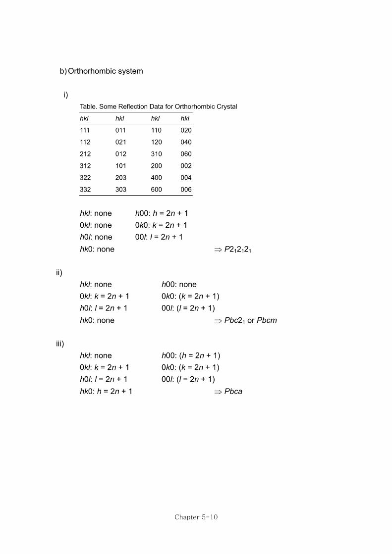
Table. Some Reflection Data for Orthorhombic Crystal

hkl hkl hkl hkl

111 011 110 020

112 021 120 040

212 012 310 060

312 101 200 002

322 203 400 004

332 303 600 006

hkl: none h00: h = 2n + 1 0kl: none 0k0: k = 2n + 1 h0l: none 00l: l = 2n + 1 hk0: none ⇒ P212121 ii) hkl: none h00: none 0kl: k = 2n + 1 0k0: (k = 2n + 1) h0l: l = 2n + 1 00l: (l = 2n + 1) hk0: none ⇒ Pbc21 or Pbcm iii) hkl: none h00: (h = 2n + 1) 0kl: k = 2n + 1 0k0: (k = 2n + 1) h0l: l = 2n + 1 00l: (l = 2n + 1) hk0: h = 2n + 1 ⇒ Pbca

Chapter 5-10

Appendix: Data collection in practice

1) Mount a goniometer head with a crystal and center it optically. 2) Search for reflections that will be used to determine the orientation matrix and unit-call parameters of the crystal. At this stage, it is easier to look for reflections at fairly low 2θ values.

3) Check the quality of the crystal by examining the profiles of some reflections. If at this point one suspects that a better crystal is available, it is wise to select it and repeat the steps (1) through (3).

4) Once a satisfactory number of reflections have been found, determine a preliminary orientation matrix and unit-cell parameters.

5) Using the result of (4), find reflections at high 2θ values that will give a better orientation matrix and more precise unit-cell parameters. If required, at this point, one is in a position to determine very accurate unit-cell parameters by using an adequate number of Friedel pairs at high 2θ values and least-squares refinement methods.

6) If possible, transform the unit cell that has been found into another of higher symmetry. Check its systematic absences.

7) Choose the scan mode, range, and speed by examining an adequate number of reflections carefully.

8) Select a subset of reflections to periodically check the orientation of the crystal and to monitor radiation damage.

9) Decide which reflections will be collected (one or more asymmetric units), in which order, and 2θ range.

10) Start data collection. 11) When data collection is finished, before removing the crystal, remember that an absorption correction is essential, and most probably record the data necessary for an empirical absorption correction.

Chapter 5-11

Chapter 6. Data reduction

Raw intensity data (Iobs) ⇒ structure factors (|F|rel)

1. Lorentz and polarization corrections

|F| ∝ I1/2

|F|: from the experiment or calculation from the known positions of atoms I: from the experiment

1) |Fhkl| = (KIhkl/Lp)1/2 a) L (Lorenz factor): It arises because the time required for a reciprocal lattice point to pass through the sphere of reflection is not constant. ⇒ L = 1/(sin 2θ)

b) p: polarization factor ⇒ p = (1 + cos2 2θ)/2 c) K: It depends on the crystal size, beam intensity, and a number of fundamental constants.

|Frel| = k'|Fhkl| = (Ihkl/Lp)1/2 (k': a scaling factor)

2) Polarization factor a) The normal X-ray beam is not polarized.

Figure. Electric vectors in an unpolarized X-ray beam.

Chapter 6-1

I⊥

I||

I||

I⊥

θ

θ

Figure. A partial polarization of X-ray due to reflection.

i) I|| (π beam): parallel to the surface of the reflecting plane depends on the electron density only (the greater efficiency of reflection compared to I⊥)

ii) I⊥ (σ beam) perpendicular to I|| depends on the electron density and cos2 2θ

b) The reflected beam will be partially polarized. p = {(1 + α cos2 2θ)/(1 + α)} ≈ {(1 + cos2 2θ)/2} α = I⊥/I||

c) When a crystal monochromator is used, this effect is high. ⇒ The partial polarization of X-ray beam from a monochromator must be taken into consideration.

2. Data reduction in practice 1) Absorption a) The theoretical absorption correction is extremely difficult. b) Empirical methods are usually applied. ⇒ ψ-scan or analytical corrections

Chapter 6-2

c) North method (psi (ψ) scan) i) This method includes setting χ to 90° and measuring the variation in the integrated intensity of several reflections as φ is rotated through 360°.

ii) The process rotates the reflecting plane about its normal and rotates the crystal about the axis (ψ-axis, in reciprocal space but not necessarily an reciprocal lattice axis) connecting the observed reciprocal lattice point to the reciprocal lattice origin.

iii) The observed variation can be readily converted to an approximate correction as a function of φ and applied to the entire data set.

d) Absorption corrections are less significant for a Mo target.

2) Deterioration A. ψ-scan curve

1.0

0.90 40 80 120 160 200 240 280 320 360

0.95

Angle ψ

Transmission

Figure. Relative transmission factor plotted as a function of the scanning angle φ = ψ for a

reflection with a χ value close to 90o.

Chapter 6-3

B. Deterioration (decay correction)

Intensitymeasured

Exposure (hours)0 8 16 24 32 40 48

Figure. Typical behavior of the relative intensities of three reflections of a protein crystal

monitored with a diffractometer at different times after exposure begins.

3. Unobserved reflections 1) Uncertainty (σ: standard deviation of intensity) σI = (I + rB+ r2B)1/2

I: the net integrated intensity B: background intensity r: the ratio of the time spent in measuring I to that in measuring B (1.5)

2) Immeasurably weak reflections ⇒ unobserved reflections A conventional criterion: I < x σ(I) x: 2–3 3) Unobserved reflections have little effects on the refinement of a structure for which the model fits the data well. However, they do provide extremely powerful information for improving partial structures and detecting errors in poor models. 4) A reflection of zero intensity is nearly as improbable as one of high intensity. 5) In the structure-refinement process, omitting weak reflections is theoretically inferior to using all reflections and weighting them by their uncertainties.

Chapter 6-4

4. Intensity statistics Wilson plot ⇒ Absolute scaling and temperature factors 1) Atomic scattering factor (fo) a) Assumption: spherical atoms i) The scattering power of an atom is a function of the atom identity and (sin θ)/λ.

ii) The scattering factor is independent of the position of an atom in a unit cell.

b) Scattering factor (fo): the scattering power of a given atom for a given reflection The scattering power of an equivalent number of electrons located at the position of the atomic nucleus. ⇒ International table

c) Scattering factor curve

0.1 0.3 0.5 0.7

2

4

6

(sin θ)/λ

fC

Figure. Scattering factor of a carbon as a function of (sin θ)/λ.

i) fo {(sin θ)/λ = 0} ⇒ a total number of electrons in an atom (Z) ii) As (sin θ)/λ increases, the scattering factor decreases.

Chapter 6-5

2) Temperature factor (B)

a) The effect of thermal motion is to spread the electron cloud over a larger volume and thus to cause the scattering power of a real atom to fall off more rapidly than that of an ideal, stationary atom.

b) From the theory

f = fo exp{–B(sin2 θ/)λ2} (B: temperature factor) B = 8π2u2 (u2: the mean-square amplitude of atomic vibration)

(sin θ)/λ0.1 0.3 0.5 0.7

0

0.5

1.0B = 0.0

B = 2.0

B = 4.0

B = 8.0

exp{(-B (sin2 θ)/λ2}

Figure. Temperature factor exp{–B(sin2 θ)/λ2} as a function of (sin θ)/λ.

0.1 0.3 0.5 0.7

2

4

6

(sin θ)/λ

fC xexp(-Bsin2 θ/λ2) B = 0.0

B = 4.0

Figure. The product fo exp{–B(sin2 θ)/λ2} as a .function of (sin θ)/λ.

Chapter 6-6

3) Absolute scaling factor and temperature factor (B) from a Wlison's plot a) Irel ≡ <|Frel|2>ave ⇐ from the experiment b) For a unit cell containing N atoms, it can be shown fairly easily that the theoretical average intensity is given by N Iabs ≡ Σ fi2 ⇐ from the theory i = 1 The average intensity depends merely on what is in the unit cell and not on

where it is. c) Ideally, the ratio of the Iabs to Irel should be the scaling factor required to place the individual Irel values on an absolute scale.

d) The f's (fi and fo) are functions of (sin θ)/λ, so that Iabs is also a function of (sin θ)/λ. This is normally avoided by dividing a reciprocal space into concentric shells, each thin enough that the variation of f's with (sin θ)/λ within the shell can be ignored. In addition, the Irel values of observed reflections are averaged within each shell. This Irel can then be compared to Iabs calculated from the f's appropriate to the shell.

N

e) Irel = CIabs = C Σ fj2 = C Σ foj2 exp{–2B(sin2 θ)/λ2}

j = 1 If B is assumed to be the same for all atoms {(sin θ)/λ) is assumed to be constant in each shell.), Irel = C exp{–2B(sin2 θ)/λ2} Σ foj

2 Irel/(Σ foj

2) = C exp{–2B(sin2 θ)/λ2} ln{Irel/(Σ foj

2)} = ln C – 2B(sin2 θ)/λ2

Chapter 6-7

(sin2 θ)/λ2

ln (Irel / Σ fj2)

slope = -2B

ln C

Figure. Wilson plot for determining scale and thermal parameters.

f) In practice, each concentric shell is taken to contain 50–100 reflections.

4) Symmetry information from intensity data a) Most space groups are not determined completely by systematic absences. i) If a crystal contains atoms heavier than sulfur, it is likely that there will be deviations from Friedel's law if the true space group is not centrosymmetric.

ii) Seemingly within experimental error, cell parameters sometimes appear to have values that suggest a higher lattice symmetry than is actually present.

b) It is safe to collect a data set rapidly over the entire sphere of data rather than a unique set more slowly. Check the Laue-symmetry-equivalent reflections.

Chapter 6-8

c) Although, in principle, the average reflection intensity depends only on what is in the unit cell and not on where it is, the same is not true of the distribution of individual intensities about the average.

i) A non-centrosymmetric crystal tends to have reflections bunched more tightly about their mean value than a centrosymmetric one.

ii) A centrosymmetric crystal tends to have relatively more weak or unobserved reflections than a non-centrosymmetric one.

b) Several quantitative tests have been devised to compare a distribution of observed intensities with that of calculated ones. i) |E| value test E2

hkl = |Fhkl|2/ {ε Σ fi2}

ε: an integer that is generally 1 but may assume other values for special sets of reflections in certain space groups. ⇒ International table.

Table. Theoretical values related to |E| values

Centrosymmetric Non-centrosymmetric

Average |E|2 1.000 1.000

Average |E2 – 1| 0.968 0.736

Average |E| 0.798 0.886

|E| > 1 32.0% 36.8%

|E| > 2 5.0% 1.8%

|E| > 3 0.3% 0.01%

Chapter 6-9

Howells, Phillips, and Rodges ⇒ Comparison between two intensity-distribution curves

0.2 0.4 0.8

Centrosymmetric

Noncentrosymmetric

1.0

N(z)

0.2

0.4

0.6

0.6

0.8

1.0

Z Figure. A distribution plot of reflection intensities: N(Z) is a fraction of reflections with I/<I> less

than Z; N(Z) is a fraction of the reflections less than a specified fraction of the average

intensity

Table 7.1. Theoretical intensity distribution

Z

0.0 0.1 0.2 0.3 0.4 0.5 0.6 0.7 0.8 0.9 1.0

1 0.0 0.248 0.345 0.419 0.479 0.520 0.561 0.597 0.629 0.657 0.683

1 0.0 0.095 0.181 0.259 0.330 0.394 0.451 0.503 0.551 0.593 0.632

Chapter 6-10

Chapter 7. Structure factors and Fourier synthesis

Fhkl (structure factor) ⇒ ρ(x, y, z) (electron density) 1. Simple harmonic motion

φ

A

B

O

π

2π

f cos φ

f φ

Figure. Cosine function as a representation of simple harmonic motion.

1) The point A moves on a circle at a constant angular velocity. 2) The point B is said to execute a simple harmonic motion. 3) Some remarks a) frequency: the number of cycles per second b) OB = f cos φ c) AB = f sin φ d) |f| = (OB2 + AB2)1/2

Chapter 7-1

2. Waves, vectors, and complex numbers 1) Wave

λ

f

δO φ

Figure. A wave with an amplitude f and a phase angle δ.

2) Vector

i

x

b

a

f

δ

Figure. A vector f in a complex plane with a modulus |f| and a phase angle δ.

a) f = a + ib (a: a real part; b: an imaginary part) ⇐ a rectangular form

f = feiδ = f(cos δ + isin δ) (δ = phase angle) ⇐ a polar or trigometric form

(f: a vector; f = |f|: amplitude, absolute value, or modulus of f)

b) a + ib ↔ a – ib (complex conjugate) |f|2 ≡ (a + ib)(a – ib) = a2 + b2

Chapter 7-2

3. Superposition of waves

1) Waves ⇒ vector representations ⇒ superposition 2) A vectorial sum

O O O O

f1 f2 f3δ1

δ2δ3 f1

f2

f3

(a) (b) Figure. (a) Vectors representing three waves of different amplitudes and phases. (b)

Resultant.

O

f1

f2

f3

δ1

δ2

δ3

Figure. Components of a sum of vectors on the coordinate axes are equal to the

sums of the components of the individual vectors.

Resulting components x = Σ fj cos δj, y = Σ fj sin δj α = tan–1 {(Σ fj sin δj)/(Σ fj cos δj)} 4. Structure factor: Fhkl A structure factor, Fhkl, is the resultant of N waves scattered in the direction of a reflection hkl by the N atoms in a unit cell. Each wave has an amplitude proportional to fj (atomic scattering factor) and a phase δj with respect to the origin of the unit cell.

Chapter 7-3

1) A set of planes hkl cuts the a-axis into h, b-axis into k, and c-axis into l divisions.

(x, y, z)

x

y

z

(x, y, 0)

a

b

c

x

y

z

2) The phase difference between reflections from the successive planes of any given set hkl is one cycle (2π radians, or 360°). 3) The phase differences for unit translations along the axes or along any lines parallel to those axes are 2πh, 2πk, and 2πl radians, separately. 4) The phase difference between the origin (0, 0, 0) and (x, y, z) for the set of hkl planes ⇒ δ = 2πhx + 2πky + 2πlz ⇒ 2π(hx + ky + lz) 5) Fhkl = |Fhkl| exp(iαhkl) = |Fhkl| (cos αhkl + isin αhkl) = Ahkl + iBhkl = Σ fj exp(iδj) = Σ fj exp[2πi(hxj + kyj + lzj)] = Σ fj [cos 2π(hxj + kyj + lzj) + isin 2π(hxj + kyj + lzj)] Ahkl = Σ fj cos 2π(hxj + kyj + lzj) Bhkl = Σ fj sin 2π(hxj + kyj + lzj) tan αhkl = Bhkl/Ahkl

Chapter 7-4

5. Fridel's law: Ihkl = Ihkl 1) Ihkl = |Fhkl|2 = |Fhkl(cos αhkl)|2 + |Fhkl(sin αhkl)|2 = Ahkl

2 + Bhkl2

2) Ihkl = |Fhkl|2 = |Fhkl(cos αhkl)|2 + |Fhkl(sin αhkl)|2 = Ahkl2 + Bhkl

2 = (Ahkl)2 + (–Bhkl)2 = Ihkl 3) Fhkl = Ahkl + iBhkl Fhkl = Ahkl + iBhkl = Ahkl – iBhkl

Fhkl

Fhkl

αhkl

αhkl

Bhkl

Bhkl

Figure. Vector representations of Fhkl and Fhkl .

6. The structure factor in an exponential form Fhkl = Σ fj exp(iδj) = Σ fj exp[2πi(hxj + kyj + lzj)] 7. The structure factor in a vector form 1) h = (hkl): a reciprocal-space vector r = (x, y, z): a direct-space vector ⇒ h·r ≡ hx + ky + lz 2) Fhkl = Σ fj exp[2πi(h·r)] = Σ fj (cos 2πh·r + isin 2πh·r)

Chapter 7-5

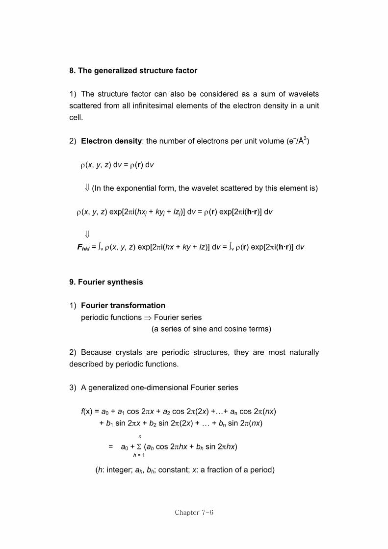
8. The generalized structure factor 1) The structure factor can also be considered as a sum of wavelets scattered from all infinitesimal elements of the electron density in a unit cell. 2) Electron density: the number of electrons per unit volume (e–/Å3) ρ(x, y, z) dv = ρ(r) dv

⇓ (In the exponential form, the wavelet scattered by this element is) ρ(x, y, z) exp[2πi(hxj + kyj + lzj)] dv = ρ(r) exp[2πi(h·r)] dv

⇓

Fhkl = ∫v ρ(x, y, z) exp[2πi(hx + ky + lz)] dv = ∫v ρ(r) exp[2πi(h·r)] dv 9. Fourier synthesis 1) Fourier transformation periodic functions ⇒ Fourier series (a series of sine and cosine terms) 2) Because crystals are periodic structures, they are most naturally described by periodic functions. 3) A generalized one-dimensional Fourier series f(x) = a0 + a1 cos 2πx + a2 cos 2π(2x) +…+ an cos 2π(nx) + b1 sin 2πx + b2 sin 2π(2x) + … + bn sin 2π(nx) n = a0 + Σ (ah cos 2πhx + bh sin 2πhx) h = 1 (h: integer; ah, bh; constant; x: a fraction of a period)

Chapter 7-6

a) Example: a four-term cosine approximation In this case, the series includes only cosine terms because the function to be fitted is centrosymmetric; that is, f(x) = f(–x), and the cosine function has this property.

(a)

(b)

(c)

(d)

(e)

(f)

y

y1 = π/4

y2 = cos 2πx

y3 = -1/3 cos 3(2π)x

y4= 1/5 cos 5(2π)x

y1 + y2 + y3 + y4

Figure. (a) A periodic step function; (b)–(e) Graphs of the first four terms of the

Fourier series representing (a); (f) Sum of terms represented by (b)–(e) as an

approximation to the function.

b) It is often convenient to represent the Fourier series in the exponential form. cos x = (eix + e–ix)/2, sin x = {-i(eix – e–ix)}/2 n f(x) = Σ Ch exp(2πihx) = Σ Ch (cos 2πhx + isin 2πhx) h = –n

[C0 = a0, Ch = (ah – ibh)/2, Ch = (ah + ibh)/2]

Chapter 7-7

4) Assumption A three-dimensional, periodic electron-density in a crystal can be

represented by a three-dimensional Fourier series. ρ(x, y, z) = Σ Σ Σ Ch'k'l' exp[2πi(h'x + k'y + l'z)] h ' k ' l' ⇓ Fhkl = ∫v ρ(x, y, z) exp[2πi(hx + ky + lz)] dv Fhkl = ∫v Σ Σ Σ Ch'k'l' exp[2πi(h + h') + (k + k')y + (l + l')z]] dv

h' k' l' (The exponential is periodic, and the integral over one period is zero for all terms except that one for which h' = –h, k' = –k, l' = –l.) Fhkl = ∫v Chkl dv = VChkl ∴ Chkl = (1/V)Fhkl

ρ(x, y, z) = 1/V Σ Σ Σ Fhkl exp[–2πi(hx + ky + lz)]

h k l = 1/V Σ Fhkl exp(–2iπh·r)

(An expression for the electron density in a direct space in terms of structure factors in a reciprocal space)

5) Summary a) Fhkl ⇔ ρ(x, y, z): FT-relationship (reciprocal space) (direct space)

b) Fhkl = ∫v ρ(x, y, z) exp[2πi(hx + ky + lz)] dv = Σ fj exp[2πi(h·r)]

= Σ fj exp[2πi(hxj + kyj + lzj)] = |Fhkl| exp(iδ) = |Fhkl| exp(2πiαhkl) c) ρ(x, y, z) = 1/V Σ Σ Σ Fhkl exp[–2πi(hx + ky + lz)] = 1/V Σ Σ Σ |Fhkl| exp(2πiαhkl) exp[–2πi(hx + ky + lz)] = 1/V Σ Σ Σ |Fhkl| exp[–2πi(hx + ky + lz– αhkl)] ⇒ Phase problem

Chapter 7-8

10. An example of structure factors and Fourier synthesis 1) A hypothetical one-dimensional structure

L = 10 A

C1 C2

a) Cu Kα, 25 reflections (h = –12 → +12)

b) Two carbon atoms at x1 = 1.833 Å and x2 = 8.167 Å ⇒ x1 = 1.833 Å, x2 = –1.833 Å ∴ x1 = 0.1833, x2 = –0.1833 = –x1 (centrosymmetric) c) Fh = Σ fj exp(2πihxj) 2 = Σ fj (cos 2πhxj + i sin 2πhxj) j = 1 = fC[cos 2πhxC1 + cos 2πh(xC2) + i sin 2πhxC1 + i sin 2πh(xC2)] = fC[cos 2πhxC1 + cos 2πh(–xC1) + i sin 2πhxC1 + i sin 2πh(–xC1)] = 2 fC[cos 2πhxC1] ∴ tan αh = 0 ⇒ αh = 0 or 180° (0 or π) Table. Data for a one-dimensional hypothetical structure with L = 10 Å

h sin θ Fh h sin θ Fh

0 0.000 12 ±7 0.539 –1

±1 0.077 5 ±8 0.616 –4

±2 0.154 –7 ±9 0.693 –2

±3 0.231 –8 ±10 0.770 2

±4 0.308 –1 ±11 0.847 3

±5 0.385 5 ±12 0.924 1

±6 0.462 4

Chapter 7-9

2) Fourier synthesis: 12 12

ρ(x) = 1/L Σ Fh exp(–2πihx) {or 1/L(F0 + 2 Σ Fh cos 2πhx)} h = –12 h = 1

Table. 2Fh cos 2πh(x)

x

h Fh 0.00 0.02 0.04 0.06 0.08 0.10 0.12 0.14 0.16 0.18 0.20 0.22 0.24

0 12 12.0 12.0 12.0 12.0 12.0 12.0 12.0 12.0 12.0 12.0 12.0 12.0 12.0

1 5 10.0 9.9 9.7 9.3 8.8 8.1 7.3 6.4 5.4 4.3 3.1 1.9 0.6

2 –7 –14.0 –13.6 –12.3 –10.2 –7.6 –4.3 –0.8 2.7 6.0 9.0 11.3 13.0 13.8

3 –8 –16.0 -14.8 –11.7 -6.9 –1.0 4.3 10.2 14.1 15.8 15.5 12.9 7.5 3.0

4 –1 –2.0 –1.8 -1.1 –0.1 0.8 1.6 2.0 1.9 1.3 0.4 –0.6 –1.5 –1.9

5 5 10.0 8.1 3.1 –3.1 –8.1 –10.0 –8.1 –3.1 3.1 8.1 10.0 8.1 3.1

6 4 8.0 5.8 0.5 –5.1 –7.9 –6.5 –1.5 4.3 7.8 7.0 2.5 –3.4 –7.4

7 –1 –2.0 –1.3 0.4 1.8 1.9 0.6 –1.1 –2.0 –1.5 0.1 1.6 1.9 0.9

8 –4 –8.0 –4.3 3.4 7.9 5.1 –2.5 –7.8 –5.8 1.5 7.4 6.5 –0.5 –7.0

9 –2 –4.0 –1.7 2.6 3.9 0.8 –3.2 –3.5 0.2 3.7 2.9 –1.2 –4.0 –2.2

10 2 4.0 1.2 –3.2 –3.2 1.2 4.0 1.2 –3.2 –3.2 1.2 4.0 1.2 –3.2

11 3 6.0 1.1 –5.6 –3.2 4.4 4.9 –2.6 –5.8 0.4 5.9 1.9 –5.3 –3.8

12 1 2.0 0.1 –2.0 –0.4 1.9 0.6 –1.9 –0.9 1.8 1.1 –1.6 –1.3 1.5

1/10 Σ 0.6 0.1 –0.4 0.3 0.2 1.0 0.5 2.1 5.4 7.5 6.2 3.0 0.9

⇓ Electron-density map

1.0 2.00

0.5

e/A

x

A Figure. An electron density of a carbon atom as a representation by a 13-term

Fourier series.

Chapter 7-10

11. Special structure-factor expressions (1) To save computing time and to point up phenomena such as systematic absences

(2) Special forms are obtained by modifying general structure-factor expressions to include explicitly the effects of symmetry elements. Q

1) Fhkl = Σ fj exp[2πi(hxj + kyj + lzj)] j n m = Σ fp {Σ exp[2πi(hxp,q + kyp,q + lzp,q)]} p=1 q The Q atoms are now divided into n unique atoms (per asymmetric unit), each of which is converted into a set of m symmetry-related atoms (m = the number of asymmetric units) by symmetry operations of the cell (Q = n × m). = Σ fp (Ehkl)p ⇒ (Ehkl)p = Σ exp[2πi(hxp,q + kyp,q + lzp,q)] p q Ehkl = Σ exp[2πi(hxq + kyq + lzq)] q 2) Examples a) 1 (inversion): (x, y, z), (–x, –y, –z) Ehkl = exp2πi(hx + ky + lz) + exp–2πi(hx + ky + lz)

= cos 2π(hx + ky + lz) + isin 2π(hx + ky + lz) + cos 2π(hx + ky + lz) – isin 2π(hx + ky + lz)

= 2 cos 2π(hx + ky + lz)

Fhkl = 2 Σ fn cos 2π(hx + ky + lz)

Chapter 7-11

b) 21 parallel to the c-axis: (x, y, z), (–x, –y, 1/2 + z) Ehkl = e2πi(hx + ky + lz)+ e–2πi(hx + ky – lz – 1/2) Ehkl = e2πi(hx + ky)e2πilz + e–2πi(hx + ky)e2πile2πil/2 Ehkl = e2πilz [e2πi(hx + ky) + e–2πi(hx + ky)eπil] In general, Ehkl ≠ 0 except in the case of the 00l reflections, when E00l = e2πilz [1 + eπil] E00l = 2 e2πilz for l = 2n E00l = 0 for l = 2n + 1

c) n-glide perpendicular to the b-axis: (x, y, z), (1/2 + x, –y, 1/2 + z) Ehkl = e2πi(hx + ky + lz) + e2πi(hx + h/2 – ky + lz + l/2) Ehkl = e2πi(hx + lz)e2πiky + e2πi(hx + lz)e–2πikye2πi(h/2 + l/2) Ehkl = e2πi(hx + lz)[e2πiky + e–2πikyeπi(h + l)] In general, Ehkl ≠ 0 except in the case of the h0l reflections, when

Eh0l = e2πi(hx + lz)[1 + eπi(h + l)] Eh0l = 2 eπi(h + l) for h + l = 2n Eh0l = 0 for h + l = 2n + 1 d) A-centered lattice (x, y, z), (x, 1/2 +y, 1/2 + z) Ehkl = e2πi(hx + ky + lz) + e2πi(hx + ky + k/2 + lz + l/2) Ehkl = e2πi(hx + ky + lz) [1 + eπi(k + l)] Ehkl = 2 e2πi(hx + ky + lz) for k + l = 2n Ehkl = 0 for k + l = 2n + 1

Chapter 7-12

12. Fast Fourier transformation (FFT) Example H

ρ(x) = Σ Fh exp(2πihx) 0 H/2 H/2

ρ(x) = Σ F2h exp(2πi(2h)x) + Σ F2h+1 exp(2πi(2h + 1)x) 0 0 H/2 H/2

ρ(x) = Σ F2h exp(2πi(2h)x) + exp(2πix) Σ F2h+1 exp(2πi(2h)x) 0 0 (Exponential forms are calculated once and used twice!)

1) As long as the number of terms in each series is evenly divisible into even and odd. 2) Computing time: H log2 H versus H2 3) The process of factorization is not limited to division by 2 but can be applied to any factor, although with greater complexity. 13. Anomalous scattering and its effect 1) Normal scattering factors (fj): real numbers This is generally the case for light atoms and the radiations commonly used in X-ray diffraction. 2) For atoms with Z near that of the element used to generate the incident X-rays. If the wavelength of the X-ray falls near the absorption wavelength of some atom, an anomalous phase change occurs on scattering by atoms of that type. ⇒ anomalous scattering (or dispersion) ⇒ foanom: a complex number

Chapter 7-13

3) foanom = fo + ∆f' + i∆f" = f' + i∆f" fo: a normal scattering factor ∆f': a real correction term (usually negative) ∆f": an imaginary correction term

An imaginary correction term (∆f") is rotated counterclockwise by 90° in the complex plane with respect to fo and ∆f', that is, to f'. The relationship between f' and ∆f" remains the same as the phase angle changes, that is, as the anomalous scatterer moves around the unit cell.

fo

f' ∆f'

∆f"(a)

δ

−δ

∆f"

∆f"

∆f'

∆f'f'

f'

(b) (c) Figure. Vector representations of f, ∆f', and ∆f" for an atom showing anomalous

scattering: (a) At the origin; (b), (c) at other positions in the unit cell.

4) (a), |Fhkl| = |Fhkl|. (b), |Fhkl| ≠ |Fhkl

Fhkl fA(hkl)

Fw(hkl)

(a)

Fhkl fA(hkl) fA(hkl)

Fw(hkl)

Fhkl fA(hkl)

Fw(hkl)

(b)

Fhkl

Fw(hkl)

∆f'∆f"

∆f"∆f'

Chapter 7-14

Table. Dispersion effects on scattering factors (sin θ)/λ = 0

Cr Kα Cu Kα Mo Kα

∆f' ∆f" ∆f' ∆f" ∆f' ∆f"

K 0.1 2.1 0.4 1.1 0.2 0.3

Br –0.2 2.6 –0.8 1.3 –0.4 2.5

Ag –0.9 8.2 –0.1 4.3 –1.1 1.1

I –5.9 12.8 –0.6 6.8 –0.7 1.8

Hg –4.8 14.1 –5.0 7.7 –3.1 9.2

5) The variations of ∆f' and ∆f” with Z for copper radiation.

20 23 26 29 32

-10

1234

Electrons

∆f"

∆f"

∆f'

∆f'

Ca V Fe Cu Ge Figure. ∆f' and ∆f" as a function of atomic number for Cu Kα radiation.

0 0.1 0.3 0.5 0.7

10

20

30

fCo

f'Co

∆f"Co-∆f'Co

f, electrons

(sin θ)/λ

Figure. fCo, f'Co, –∆f'Co, and ∆f"Co for Cu Kα radiation as functions of (sin θ)/λ.

Chapter 7-15

6) Characteristics a) Anomalous scattering effects are more significant for long-wavelength radiations.

b) The ∆f' and ∆f" values are almost independent of sin θ. c) For a given atom, the effects of dispersion are relatively greater at high sin θ than at low sin θ. ex) at (sin θ)/λ = 0 ⇒ ∆f"Co/f'Co = 3.6/24.5

at (sin θ)/λ = 0.6 ⇒ ∆f"Co/f'Co = 3.6/7.8

7) The effects of dispersion on Fc can be illustrated by a series of Argand diagrams. a) Centrosymmentric structure i) A number of normal atoms + a pair of anomalous atoms ii) Friedel's law still holds. ⇒ (|Fhkl| = |Fhkl|) iii) There are changes in both the phase angle and the magnitude of Fhkl.

⇒ Fhkl's are now complex numbers (αhkl ≠ 0 or π).

αhkl

Fhkl

Fw

f'

f'

∆f"∆f"

αhkl

Fhkl

Fwf'

f'

∆f"

∆f"

(a) (b) Figure. Vector representation showing anomalous scattering for a Friedel pair in a

centrosymmetric structure; Fhkl = Fhkl.

(Fw is the resultant of scattering from the atoms without dispersion; f' and ∆f" are the real and imaginary parts of the anomalous scattering atom, respectively.)

Chapter 7-16

d) Non-centrosymmetric structure i) A number of normal atoms + only one anomalous scattering atom.

ii) Friedel's law does not hold. ⇒ (|Fhkl| ≠ |Fhkl|) iii) The phase angle: αhkl ≠ αhkl

Fhklf'

∆f"

Fw

αhkl

f'∆f"

Fwαhkl Fhkl

Fhkl

Fhkl

(a) (b)

(c)

Figure. Vector representation showing anomalous scattering for a Fridel pair in a

non-centrosymmetric structure: Fhkl ≠ Fhkl. e) Some remarks i) The dispersion effect can be minimized by an appropriate selection of radiation.

ii) This effect is useful, particularly for phasing reflections and for determining the absolute molecular configurations.

8) A given set of atomic coordinates can be used to calculate |Fc| for a number of Friedel pairs, because the coordinates of the enantiomorph (or enantiomer) can be obtained, for example, by inversion through the origin.

Chapter 7-17

Table. Example of some Friedel pairs and corresponding |F| values

hkl |Fo| |Fc|(x, y, z) |Fc|(–x, –y, –z)

121 17.0 19.1 18.3

122 21.2 22.9 21.9

123 41.4 44.4 42.8

341 36.7 38.7 35.8

342 7.8 9.5 8.2

413 14.2 15.3 13.5 14. Other Fourier syntheses 1) |F|2 synthesis (Patterson method or Patterson function) ρ(x, y, z) = 1/V Σ Σ Σ |Fhkl|2 exp[–2πi(hx + ky + lz)] a) One of heavy atom methods b) |Fhkl|2 is a phaseless quantity

2) ∆F synthesis (Difference Fourier synthesis) ∆ρ(x, y, z) = 1/V Σ Σ Σ ∆Fhkl exp[–2πi(hx + ky + lz)] a) ∆F = (|Fo| – |Fc|) exp(iαc) b) To locate new atoms and to correct the positions of those already present.

c) phase αc ⇐ |Fc| 15. Some indices 1) LRS (Linear ReScale factor) LRS = Σ |Fc|/Σ |Fo| a) If the model used for calculations contains all of the atoms in a unit

Chapter 7-18

cell, this rescale factor is usually more accurate than the one obtained from the Wilson plot.

b) To check the overall agreement

2) R (Reliability factor or Residual factor) R = Σ|∆F|/Σ|Fo| = Σ||Fo| – |Fc||/Σ|Fo| a) To check the reflection-by-reflection agreement between the observations and the calculations.

b) If R < 0.06 (or 6%) ⇒ a reasonable (or publishable) structure. 16. A general scheme for structure refinements ① Overall isotropic vibration (temperature factor is B ⇐ Wilson plot) ② Individual isotropic vibration (spherical: isotropic thermal parameter) ③ Individual anisotropic vibration (ellipsoid: anisotropic thermal parameter)

17. Final comments 1) The F000 reflection is not an observable datum, which corresponds to a reflection in the line of the direct beam. 2) The average value of a trigometric function over one full cycle is zero. The average over one cycle of a Fourier series consisting only of trigometric forms is also zero. In order to have a nonzero average, a constant term, F000 , equal to this average, must be added to this series. F000 = Σ fj exp[2πi(hxj + kyj + lzj)] = Σ fj = Σ Zj (at (sin θ)/λ = 0) (A total number of electrons in a unit cell)

Chapter 7-19

Chapter 8. Phase Problem

1. Introduction 1)

Fhkl = ∫v ρ(x, y, z) exp[2πi(hx + ky + lz)] dv = Σ fj exp[2πi(h·r)]

= Σ fj exp[2πi(hxj + kyj + lzj)] = |Fhkl| exp(iδ) = |Fhkl| exp(2πiαhkl)

A point in a direct lattice: r = xa + yb + zc A point in a reciprocal lattice: h = ha* + kb* + lc* a·b* = a·c* = b·c* = b·a* = c·a* = c·b* = 0

2) ρ(x, y, z) = 1/V Σ Σ Σ Fhkl exp[–2πi(hx + ky + lz)]

= 1/V Σ Σ Σ |Fhkl| exp(2πiαhkl) exp[–2πi(hx + ky + lz)] = 1/V Σ Σ Σ |Fhkl| exp[–2πi(hx + ky + lz– αhkl)] ⇒ Phase problem 3) Methods to phase reflections (or structure factors) a) Direct method b) Heavy atom methods i) Patterson method (or Patterson synthesis) ii) Superposition method iii) Isomorphous replacement method (MIR: multiple isomorphous replacement)

iv) Anomalous scattering method

Chapter 8-1

2. Direct method 1) Mathematical techniques that attempt to solve the phase problem from observed amplitudes (|Fhkl|obs's) by purely mathematical techniques, with no recourse to structural and chemical information. 2) Direct method is now the method of choice, with the result that 80–90% of reported structures of small molecule are solved in this way. 3) Nobel prize in chemistry to Karle and Hauptman in 1985 4) Phase determination in practice a) Symbolic addition method b) MULTAN (Multiple Tangent Formula) c) Magic Integer method d) Probability method e) SHELX programs (SHELXS-86, SHELXL-97) f) XTAL g) TEXAN h) MolEN ⇐ SDP i) GX j) NRCVAX

5) Normalized structure factor: Ehkl A simplification in direct phase-determining formulas results from replacing |Fhkl| by the corresponding normalized structure factor |Ehkl|, which is given by the equation.

|Ehkl|2 = (K2|Fhkl|2)/(ε Σ fj2)

The summation in the denominator, which is θ-dependent through fj, may be obtained from a Wilson plot (K and B). The data must be on an absolute scale (K = 1), and ε is incorporated in setting up the Wilson plot.

Chapter 8-2

a) The E values have properties similar to those of the sharpened F values derived for a point-atom model. i) They are largely compensated for the fall-off of f with sin θ. ii) High-order reflections with comparatively small |Fhkl| values can have quite large |Ehkl| values, an important factor in the application of direct methods.

iii) <|Ehkl|2>average = 1 b) The ε factor The ε value depends on the crystal system.

Table. The ε factors for some crystal systems

hkl 0kl h0l hk0 h00 0k0 00l hhl hh0

Triclinic 1 1 1 1 1 1 1 1

1 1 1 1 1 1 1 1

Monoclinic 2 1 1 1 1 1 2 1

m 1 1 2 1 2 1 2 2/m 1 1 2 1 2 2 2

Orthorhombic 222 1 1 1 1 2 2 2

mm2 1 2 2 1 2 2 4

mmm 1 2 2 2 4 4 4

Tetragonal 4 1 1 1 1 1 1 4

4 1 1 1 1 1 1 2

4/m 1 1 1 2 2 2 4

42m 1 1 1 1 2 2 4 2 2

4mm 1 2 2 1 2 2 8 2 2 422 1 1 1 2 2 2 4 2 1

4/mmm 1 2 2 2 4 4 8 4 2

Chapter 8-3

c) |Ehkl|-value statistics Table. Some theoretical and experimental values related to |Ehkl|-value statistics

Theoretical values Experimental values and conclusions

Mean values P1 (C) P1 (A) Crystal 1 Crystal 2

|E|2 1.00 1.00 0.99 0.98

|E| 0.80 0.89 0.85 A/C 0.84 A/C

|E|2 – 1 0.97 0.74 0.91 C 0.82 A

Distribution % % % %

|E| > 3.0 0.30 0.01 0.20 C 0.05 A

|E| > 2.5 1.24 0.19 0.90 C 0.98 C |E| > 2.0 4.60 1.80 2.70 A/C 2.84 A/C |E| > 1.75 8.00 4.71 7.14 C 6.21 A/C |E| > 1.5 13.4 10.5 12.9 C 10.5 A |E| > 1.0 32.0 36.8 33.7 C 37.1 A 3. Patterson method In 1934, Patterson reported a new Fourier series, which could be calculated directly from the experimental intensity data. However, because phase information is not required in the Patterson series, the result cannot be interpreted as a set of atomic positions, but rather as a collection of interatomic vectors all taken to a common origin. 1) Patterson function or synthesis

ρ(u, v, w) = 1/V Σ Σ Σ |Fhkl|2 cos [2π(hu + kv + lw)]

2) a) Interatomic vectors

u = x1 – x2, v = y1 – y2, w = z1 – z2

Chapter 8-4

b) The weight of a Patterson peak is proportional to the product of its atomic numbers. i) A heavy–heavy atom pair ⇒ This easily locates the heavy atom. ii) A heavy–light atom pair iii) A light–light atom pair

c) In a structure with N atoms per unit cell, each atom forms vectors with the remaining (N – 1) atoms. Therefore, there are N(N – 1) peaks and one big peak at the origin in the Patterson cell (or space).

(d)(c)

(a)

(b) Figure. (a) Set of points; (b) Interatomic vectors; (c) Patterson peaks about the origin from

one set and (•) is an origin peak; (d) Patterson peaks in four unit cells,

A1 A2P

O

ν1

(a) (b)

ν12

ν2

ν3

ν4 ν4

ν3

Figure. (a) Two atoms; (b) A Patterson peak resulting from the atoms in (a), showing spread

of a vector peak (with an arbitrary height). An origin peak is not shown.

3) Sharpened Patterson function a) |Fpoint| or |Ehkl| values are used instead of |Freal|. b) Point atoms i) Atoms in which all of the scattering power is concentrated at the nucleus

Chapter 8-5

ii) One of the characteristics of a point atom is that its scattering power is not a function of (sin θ)/λ, but a constant equal to the atomic number Z, that is, equal to the usual scattering factor at (sin θ)/λ = 0.

Zj

fj

0.1 0.2 0.3 0.4 0.5 0.6(sin θ)/λ

fpoint atom

factual atom

Figure. Scattering factors for actual and point atoms.

Fhkl = Σ fj exp[2πi(h·r)] = Σ fj exp[2πi(hxj + kyj + lzj)]

⇓ For a cell containing only one kind of atom Fhkl = f Σ exp[2πi(hxj + kyj + lzj)] = f·E (E: phase)

an actual atom: f = fo exp[–B(sin2 θ)/λ2[ a point atom: f = Z ⇓ Fpoint/Freal = (ZE)/{fo exp[–B(sin2 θ)/λ2]}·E = (Z)/{fo exp[–B(sin2 θ)/λ2]}

⇓ For more general cases Fpoint = (Σ Zj) × Freal exp[–B(sin2 θ)/λ2 Σ fo,j]

c) A plot of the average value of |Fo|2 as a function of (sin θ)/λ for a typical set of data is shown in the following Figure.

Chapter 8-6

0

100

200

300

400

500

0.1 0.2 0.3 0.4 0.5 0.6(sin θ)/λ

<|Fo|2>shaprpened

unshaprpened

Figure. Effect of sharpening on the radial decrease of the local average intensity |Fo|2.

d) The origin peak can be removed. Patterson showed that it was possible to remove the origin peak from a vector map by subtracting the average value of |Fhkl|2 from each term in the summation. i) |F'hkl|2 = |Fhkl|2 – <|Fhkl|2> = |Fhkl|2 – Σ fj2 = |Fhkl|2 – Σ Zj

2 ii) If |Ehkl|'s are used, <|Ehkl|2> = 1. |Ehkl|2 – 1 is used instead of |Fhkl|2 in the Patterson synthesis to give a sharpened Patterson map.

0.2 0.4 0.8 u

0.1

0.2

0.3

0.4

w/2

w

v

(a) (b) Figure. (a) Asymmetric part of the u0w section of the Patterson map of a natural product; (b)

The same section after sharpening and removal of the origin peak.

Chapter 8-7

4) Patterson symmetry a) 230 space groups ⇒ 24 space groups in the Patterson map b) Characteristics i) All Patterson functions are centrosymmetric. ii) Their lattice type (P, C, F, etc.) is the lattice type of the original space group.

iii) Their space group is derived from the original space group by replacing all translational symmetry elements by the corresponding non-translational symmetry elements and adding a center of symmetry if it is not already present.

c) Examples (1) All triclinic crystals ⇒ P1 (2) Monoclinic crystals ⇒ 2/m (P2/m or C2/m, depending on the lattice type) (3) Orthorhombic crystals ⇒ mmm (Pmmm, Cmmm, Immm, or Fmmm)

d) Although symmetry elements of a space group do not necessarily appear as such in the Patterson map, they leave their traces in the form of particular concentrations of vector points. They arise because the vectors between corresponding atoms of molecules related by symmetry elements other than a center of symmetry have one or two constant coordinates. ⇒ Harker lines and Harker planes Example: Pm (A mirror is perpendicular to the b-axis) (x, y, z), (x, –y, z) ⇒ (u, v, w) = (0, 2y, 0) ⇐ Harker line Table. Some Harker lines and Harker planes

2-Fold axis || a, b, c 0vw; u0w; uv0

2-Fold screw axis || a, b, c 1/2 v w; u 1/2 w; u v 1/2

m plane ⊥ a, b, c u00; 0v0; 00w

a-glide plane ⊥ b, c 1/2 v 0; 1/2 0 w

b-glide plane ⊥ a, c u 1/2 0; 0 1/2 w

c-glide plane ⊥ a, b u 0 1/2; 0 v 1/2

Chapter 8-8

5) Atom finding in practice (Assumption: There is a single atom per asymmetric unit.) a) P1: (x, y, z) ⇒ the position of a heavy atom: (0, 0, 0)

b) P1: (x, y, z), (–x, –y, –z) ⇒ (u, v, w) = ± (2x, 2y, 2z) ⇒ the position of a heavy atom: (u/2, v/2, w/2)

c) P21/c: (x, y, z), (–x, –y, –z), (–x, 1/2 + y, 1/2 – z), (x, – y, 1/2 + z) ⇒ (u, v, w) = ± (2x, 2y, 2z) ⇒ (u, v, w) = ± (2x, 1/2, 2z) ⇐ a Harker plane ⇒ (u, v, w) = ± (0, 2y, 1/2) ⇐ a Harker line

Chapter 8-9

Chapter 9. Completing the structure

⇒ ∆F synthesis and structure refinements 1. ∆F synthesis

∆ρ(x, y, z) = 1/V ΣΣΣ (|Fo| – |Fc|) exp(iαc) exp[-2πi(hx + ky + lz)] (αc: the phase of Fc)

① To locate the missing atoms ② To refine the structure

1) Three limiting cases

|Fo|

|Fc|

|Fo|

|Fc| |Fo|

|Fc|

(a) (b) (c) Figure. (a) |Fo| ≈ |Fc|; (b) |Fo| > |Fc|; (c) |Fo| < |Fc|.

a) In case of |Fo| ≈ |Fc|.

i) If the phasing is a suitable one, there is a high probability that α is approximately the value corresponding to the true phase of Fo.

ii) On the other hand, the reflections for which |Fo| ≈ |Fc| tend to merely reproduce the model and add little new information.

b) In case of |Fo| >> |Fc|. |Fo| will make a significant contribution to the Fo Fourier series and should provide useful information. However, the probability of correspondence (or agreement) between αo and αc is small and diminishes as |Fo| approaches zero.

Chapter 9-1

c) In case of |Fo| << |Fc|. ||Fo| – |Fc|| will be large and will be a significant contributor to the ∆F synthesis. Furthermore, it can be shown that these terms will be more or less correctly phased regardless of differences between αo and αc. i) ∆F = Fo – Fc = |∆F| exp(iα∆) = |Fo| exp(iαo) – |Fc| exp(iαc)

FoFc Fo - Fc

(|Fo| - |Fc|)eiαc

= |∆F|eiαc

(a)

FoFc

Fo - Fc

(b)

FoFc

Fo - Fc

(c)

|∆F|eiαc

Figure. (a) Vectors for the case of |Fo| < |Fc|; (b) Vectors for the case if αo is taken as equal to

αc; (c) Comparison of vectors Fo – Fc and |∆F| exp(iαc).

These vectors are just the structure factors that would result from adding electron density where it is needed and subtracting it where it is in excess. However, as usual, αo is unknown and therefore the assumption is made that αo ≈ αc |∆F| exp(iα∆) = |Fo| exp(iαc) – |Fc| exp(iαo) ≈ |∆F| exp(iαc)

ii) Comparison The two vectors, ∆F and |∆F| exp(iαc), are in fact comparable in magnitude and phase.

2) The most valuable reflections for use in ∆F syntheses are those for which |Fo| is very small and |Fc| very large. Unobserved reflections meet this requirement and in an incomplete structure it is highly probable that some of them will calculate large.

Chapter 9-2

3) The difference synthesis has two main advantages. a) First, if the phases αc equal αo, it provides a direct measure of the errors between the model used and the true structure implied by the |Fo| values.

b) Second, even when the phases are moderately in error, the ∆F synthesis can provide useful information that is difficult or impossible to obtain from the Fo synthesis.

4) The difference synthesis corresponds to a point-by-point subtraction of an Fc Fourier map from an Fo Fourier map with the same phases. a) Incorrectly placed atoms correspond to regions of high electron density in ρc(x, y, z) and low electron density in ρo(x, y, z); therefore, ∆ρ(x, y, z) is negative in these regions.

b) A correctly placed atom with either too small an atomic number or too high a temperature factor shows up as a small positive area in ∆ρ.

c) An atom requiring a small positional correction tends to lie in a negative area at the side of a small positive peak. The correction is applied by moving the atom into the positive area.

d) Very light atoms, such as hydrogen, may be located by a ∆F synthesis when the phases are essentially correct, after least-squares refinement has been carried out.

e) As one final test of the validity of a refined structure, the ∆F synthesis should be effectively featureless within 2–3 times the standard deviation of the electron density.

5) Other ∆F syntheses a) (2|Fo| – |Fc|) exp(iαc) ⇒ This type of the difference Fourier map shows the input model as well as the implication of the difference Fourier synthesis.

b) (3|Fo| – 2|Fc|) exp(iαc) ⇒ To reduce the contribution of |Fo|.

6) Structure completion in practice a) Use your chemical senses b) The R factor should decrease steadily from its starting value.

Chapter 9-3

1) Introduction of weightings 2) Refinements by Fourier syntheses

(a) Fo synthesis (b) Differential synthesis

3) Series-termination error (a) Errors due to the omission of significant terms beyond the limit of observation.

(b) Booth's back-shift method. After the last refinement cycle, an Fc synthesis is carried out. Because of the effects of series termination, the peaks in this synthesis will not agree exactly with coordinates used for the structure-factor calculation. The differences are the termination errors.

4) Refinements by difference Fourier syntheses ρo(x, y, z) = 1/V ΣΣΣ Fo,hkl exp[–2πi(hx + ky + lz)] + R ρc(x, y, z) = 1/V ΣΣΣ Fc,hkl exp[–2πi(hx + ky + lz)] + R’ (R, R': remainders representing the omitted parts of the series, R ≈ R') ⇓ ∆ρ(x, y, z) = 1/V ΣΣΣ ∆Fhkl exp(iαc) exp[–2πi(hx + ky + lz)]

(Since R and R' virtually cancel, the parameters from ∆F syntheses are essentially free of series-termination error.)

a) The effects of errors solely in the coordinates

ρc ρo

ρo - ρc Figure. Line section through ρo – ρc synthesis showing effects of an error in position.

Chapter 9-4

b) The effects of errors solely in the thermal parameters

ρc

ρo

ρo - ρc

ρc

ρo

ρo - ρc

(a) (b) Figure. Line section through ρo – ρc synthesis. (a) Thermal parameter overestimated. (b)

Thermal parameter underestimated.

c) In general, the thermal motion of an atom is not spherically symmetric; that is, it is anisotropic and leads to the ellipsoidal distribution of electron density.

(a) (b) (c)

5) Temperature-factor expressions a) A general form of the temperature-factor expression contains six parameters that determine the magnitudes and orientations of three principal axes of the ellipsoidal electron distribution of an atom.

b) The temperature factor of an atom for any set of lattice planes (hkl) depends on the interplanar spacing d and on the magnitude of vibration perpendicular to the plane. For the isotropic case, the temperature factor of an atom for an given set of planes (hkl) is exp[–B(sin2 θhkl )/λ2] = exp{–B/4 × [(2sin θhkl )/λ]2} = exp[–B/4 × (1/dhkl )2]. For the general case (any crystal system), the length of 1/dhkl is 1/dhkl = (h2a*2 + k2b*2 + l2c*2 + 2hka*b* cos γ* + 2hla*c* cos β* + 2klb*c* cos α)1/2

Chapter 9-5

and the temperature factor must have a parameter for every term in this expression because each parameter represents a component perpendicular to the set of planes (hkl). The general temperature factor expression is therefore, exp[–1/4(B11h2a*2 + B22k2b*2 + B33l2c*2 + 2B12hka*b* cos γ* + 2B13hla*c* cos β* +

2B23klb*c* cos α*)] where the Bij are the thermal parameters in the same units as the conventional isotropic thermal-parameter B. An equivalent and preferable expression for the general temperature factor is exp[–2π2(U11h2a*2 + U22k2b*2 + U33l2c*2 + 2U12hka*b* cos γ* + 2U13hla*c* cos β* +

2U23klb*c* cos α*)] where the Bij are now the thermal parameters expressed in terms of mean-square amplitudes of vibration in angstroms (Å). Another expression for the anisotropic factor that will be encountered in the literature and in some computer programs is exp[–(β11h2a*2 + β22k2b*2 + β33l2c*2 + 2β12hka*b* cos γ* + 2β13hla*c* cos β*

+2β23klb*c* cos α*)]

Although this is a relatively compact expression, reporting of the thermal parameters as β's is to be discouraged because of the difficulty in comparing β values associated with axes of different lengths. c) An incorrectly placed atom may manifest itself in the least-squares refinement by an abnormally high temperature factor.

d) If absorption corrections are neglected, the overall effect is to make low-angle reflections too strong in comparison with high-angle ones, and this will be reflected in the temperature factors that are too low.

Chapter 9-6

6) Thermal motion

A

B

NP

Q

R

(a) (b) (a) Atom B vibrates most strongly in the plane perpendicular to the A–B bond.

(b) Atoms Q and R have a large amplitude of vibration than does atom P.

a) Bridging atoms often have lower temperature factors than terminal ones of the same kind.

b) Atoms in a cyclic molecule vibrate more vigorously in the direction perpendicular to the plane of the ring than in its plane.

c) The presence of strong hydrogen bonding or similar interaction in a structure reduces thermal motions in its vicinity.

7) Locating hydrogen atoms a) After refinements of both positional and thermal parameters of non-hydrogen atoms ⇒ ∆F synthesis

H1

H2

H3

H4

H5

H6

H7

H8 Figure. ∆F synthesis showing the 7 hydrogen atoms in a certain molecule.

Chapter 9-7

b) The peak densities ranges in 0.3–0.7 e–/Å3, with B's in the range 6–10 Å2. Values as high as 0.5 – 0.7 e–/Å3 are observed for data collected at room temperature, and much higher values for low-temperature data.

3. Least-squares refinement of crystal structure in practice 1) The Rietveld technique for the analysis of powder diffraction data. 2) A large number of modules, ||Fhkl|o's, are measured. Parameters are then refined in order to minimize the difference between the |Fhkl|o's and the |Fhkl|c's. A. Parameters usually refined are as follows. ① Overall scale factor (Observed intensities are usually on an arbitrary scale) ② A parameter defining chirality in non-centrosymmetric space groups. (Flack constant, Rodgers constant)

③ For each atom, a) Up to three coordinates (fewer if the atom is on a special position) b) Thermal parameters i) One parameter for isotropic motion ii) Six parameters for anisotropic motion

④ The site-occupation factor (sof) if an atomic position is statistically occupied because of some structural disorder.

B. Correlation coefficients A critical point in least-squares refinement is the occurrence of large correlation coefficients among parameters. This occurs when the following conditions occur. ① Two atomic sites nearly overlap because of some structural disorder (or some error).

② The symmetry of an actual structure is higher than the space-group symmetry in which refinement is made.

Chapter 9-8

③ Symmetry constraints are not introduced. ④ In some non-centrosymmetric space groups, the origin may float in some directions. The normal equation matrix will become singular if the coordinates of one atom along the free directions are not fixed (e.g., z in Pca21 or x and z in Pm). C. A list of errors that can affect the results of a structure analysis ① Experimental accidents a) Fluctuating power in the incident beam b) Crystals moving on their mounts

② Statistical fluctuations in quantum counts (scintillation counter) ③ Crystal damage by the incident beam ④ Errors in corrections for absorption, background radiation, thermal diffuse scattering, extinction, anomalous dispersion, anisotropic or anharmonic vibration, disorder, multiple reflections

⑤ Deviation from the isolated atom approximation ⑥ Incorrect symmetry assignment ⑦ Correlation among observations.

D. Constraints and restraints in crystallographic least-squares refinements. The accuracy of derived parameters is generally low when at least one of the following conditions occurs. ① A low ratio between the number of observed reflections and the number of parameters refined.

② Very heavy atoms and very light atoms coexist in a unit cell. ③ Too high thermal motion, presence of structural disorder, etc.

1) Rigid-body refinement (Constraints) a) If the structure contains somewhat rigid molecular fragments of well-established geometry (e.g., benzene), the number of parameters to refine may be considerably reduced.

b) For each rigid group of n atoms, the number of independent parameters reduces from 3n (positional parameters) to 6 parameters defining the position

Chapter 9-9

of some reference point and three angles for group orientation. c) Sometimes hydrogen atoms are geometrically located at the end of each round of the least-squares refinements, but more frequently hydrogen atom parameters ride upon those of a reference atom (riding model).

2) Use of restraints Soft, flexible constraints (say restraints) may be imposed to some functions of parameters in order to allow only realistic deviations of their values from standard ones. a) Interatomic distance b) The sum of atomic coordinates along a polar direction can be fixed to its current value in order to keep the center of gravity of a molecule fixed and so determine the origin.

c) van der Waals distances d) Planarity of groups e) Chirality f) Bond and torsion angles g) Thermal motion h) Positional and thermal parameters related by non-crystallographic symmetry

i) Potential energy functions j) The sum of site-occupation factors of two or more atoms can be restrained to some fixed value when a disorder problem occurs.

4. Atoms in special positions

If any symmetry operation of the space group of a structure leaves an atom invariant, the atom is on the special position.

Consider one molecule of a formula AB2 in a unit cell of the space group P2. The A atoms occupy the special positions (0, y, 0), and the B atoms occupy the general positions (x, y, z) and (–x, y, –z). Several important points arise. 1) The x and z coordinates of the atom A remain invariant at zero during refinement.

Chapter 9-10

2) In this space group, the origin is along the 2-fold axis (y–axis) and must be specified by fixing the y-coordinate of an atom; the heavier the atom, the better. It could be yA, in which case this parameter also remains invariant. 3) With respect to symmetry operations of the space group, the atom A must be given an atom-multiplicity factor (or a site-occupation factor) of 1/2 so to give a total of one A atom per unit cell. 4) In anisotropic refinements, one of the three 2-fold axes of the biaxial thermal ellipsoid must lie along the 2-fold axis (y–axis) of the space group. In this case, the U12 and U23 elements of U remain invariant at zero value. 5. Correctness of a structural analysis 1) There should be good agreement between |Fo| and |Fc|, expressed through the R factor. Ultimately, R depends on the quality of experimental data. 2) The electron-density map (Fo synthesis) should show neither positive nor negative density regions that are unaccountable, other than Fourier series-termination errors. 3) The difference-Fourier map (∆F synthesis) should be relatively flat. This map eliminates series-termination errors present in both ρo and ρc. Random errors may produce small fluctuations on a difference Fourier map, but they should be less than 2.5–3 times of the standard deviation of the electron density σ(ρo):

σ(ρo) = (1/Vc) × [ Σ (∆F)2]1/2 hkl

where ∆F = |Fo| – |Fc| and the sum extends over all symmetry-independent reflections. 4) The molecular geometry should be chemically sensible, within the limits of current structural knowledge. Normally, a deviation from less than three times of the corresponding standard deviation is not considered to be statistically significant.

Chapter 9-11

6. Limitations of X-ray structure analysis. 1) Liquids and gases lack 3-dimensional order, and therefore cannot be used in diffraction experiments in the same way as crystals. 2) It is not easy to locate light atoms in the presence of heavy atoms. a) Difference-Fourier maps alleviate the situation to some extent, but the atomic positions are not precise.

b) The least-squares refinement of light-atom parameters is not always successful.

3) Hydrogen atoms are particularly difficult to precisely locate because of their poor scattering power and the fact that the center of the hydrogen atom does not generally coincide with the maximum of its electron density. 4) In general, bond distances determined by X-ray diffraction indicate distances between the centers of gravity of the electron clouds, which may not be the same as the internuclear distances.

Chapter 9-12

Chapter 10. Miscellaneous topics

10.1. Hydrogen bonding: A–H···B To interact with the donor A–H bond, the acceptor B must have lone-

pair electrons or polarizable π electrons. Table. Properties of strong, moderate, and weak hydrogen bonds

Strong moderate weak

A–H···B interaction mostly covalent mostly electrostatic electrostatic

Bond lengths A–H ≈ H···B A–H < H···B A–H << H···B

H···B (Å) ~1.2–1.5 1.5–2.2 2.2–3.2

A···B (Å) 2.2–2.5 2.5–3.2 3.2–4.0

Bond angles (º) 175–180 130–180 90–150 Bond energy (kcal/mol) 14–40 4–15 < 4

IR ν(A–H) shift (cm–1) 25% 10–25% < 10%

NMR σ shift (ppm) 14–22 < 14 –

Examples Gas-phase Acids Gas-phase

dimers of strong Alcohols dimers of weak

acids and bases Phenols acids and bases

Proton sponges Hydrates of 3-center bonds

Pseudo hydrates All biological C–H···O/N bonds

HF complexes molecules O/N–H···π bonds

The failure to recognize these distinctions has led to some popular misconceptions in the past. ① Hydrogen bonds are almost linear. ② The distance between the donor A and acceptor B atoms should be less than the sum of the van der Waals radii of A and B.

1. Categories Hydrogen-bond energies extend from about 15–40 kcal/mol for strong bonds, to 4–15 kcal/mol for moderate bonds and 1–4 kcal/mol for weak bonds. 1) Strong hydrogen bonds are formed by groups in which there is a

Chapter 10-1

deficiency of electron density in the donor group (–O+–H or –N+–H) or an excess of electron density in the acceptor group (F–, O––H, O––C–, O––P, or N–R2). a) Ionic hydrogen bonds. b) Forced strong hydrogen bonds.

2) Moderate hydrogen bonds are formed generally by neutral donor (–O–H or –N–H) and acceptor (OR2, O=C, or NR2) groups. a) These are the most common hydrogen bonds. ⇒ normal hydrogen bonds.

b) They are important and essential components of the structures and functions of biological molecules.

3) Weak hydrogen bonds are formed when the hydrogen atom is covalently bonded to a slightly more electroneutral atom relative to hydrogen (C–H or Si–H) or when the acceptor group has no lone-pair electrons but has π electrons (C≡C or aromatic rings). 2. Important properties 1) Hydrogen bonds are group-pair properties. 2) Hydrogen bonds can be either intramolecular or intermolecular. a) When A and B are the same, ⇒ homonuclear H-bonds. b) When A and B are different, ⇒ heteronuclear H-bonds. c) In the gas phase, homonuclear bonds lead to the formation of hydrogen-bonded dimers. When A and B are different, the terms “hydrogen-bonded adducts or complexes” are used.

d) In liquids, hydrogen bonds can be formed between like molecules or between unlike molecules forming multicomponent systems.

e) In solids, they can form hydrogen-bonded clusters, or 1-, 2-, or 3-dimensional arrays of hydrogen-bonded molecules.

Chapter 10-2

Table. Functional groups that form hydrogen bonds

Strong hydrogen bonds Donor and acceptors

[F···H···F]– Symmetrical hydrogen difluoride ion [F–H–H]n– Anions in fluoride–HF adducts

[O–H···O–] Hydrogen phosphates and sulfates, hydrogen carboxylates

[O+–H···O] Hydroxonium ions, pseudo hydrates

[N+–H···N] Proton sponges

[N–H···N–]

Moderate hydrogen bonds Donor and acceptors

O–H, P–O–H Water, hydrates, alcohols, carboxylic acids, phenols, H–Ow–H carboxylates, oligo- and polysaccharides, nucleosides,

N–H 2º amines, amides, carbamates, hydrazides, purines

Donors only

[H3N+–H] Ammonium salts

[H2N+–H] Zwitterion amino acids

[R2HN+–H]

[S–H] Cysteine

[R–N(H)H] 1º amines, pyrimidines, purines, barbiturates

Acceptors only

[R2O] Ethers, carbohydrates, oligo- and polysaccharides

[R2C–=O] Carboxylates, Zwitterion amino acids

[R2C=O] Carboxylic acids, ketones, esters, N-oxides, pyrimidines

[S–H] Cysteine

[R–N(H)H] 1º amines, pyrimidines, purines, barbiturates

[X–=O] Oxyanions, nitrates, chlorates, sulfates, phosphates

[R3N] 3º amines

N=O Aromatic nitro compounds

[R2S] Methionine

Weak hydrogen bonds

Donors: C–H, Si–H

Acceptors: C≡C, C6H6, F–C

Chapter 10-3

3. Bonding parameters 1) Three scalar quantities are necessary to describe the geometry of a H-bond: the A–H covalent bond distance, H···B distance, and A···B distance. a) Only in strong H-bonds, the H-bond angle is close to 180º. b) In moderate and weak H-bonds, the angle easily deviates from 180º.

2) Bent hydrogen bonds are entropically favored.

It only for the strong H-bonds that the A–H···B distances are a reliable measure of the H-bond distances. In structure analyses where hydrogen-atom positions cannot be determined, as in proteins and nucleic acids, this feature is sometimes overlooked. 3) There are other systems such as M–H–B and B–H–B, which formally meet the operational definition of the H-bonding. Table. van der Waals distances and observed distances (pm) for some

common hydrogen bonds

A···B A···B H···B H···-B

Bond type (cal) (obs) (cal) (obs)

F–H–F 270 240 260 120

O–H···O 280 270 260 170

O–H···F 280 270 260 170

O–H···N 290 280 270 190

O–H···Cl 320 310 300 220

N–H···O 290 290 260 200

N–H···F 290 280 260 190

N–H···Cl 330 330 300 240

N–H···N 300 310 270 220

N–H···S 340 340 310 240

C–H···O 300 320 260 230

Chapter 10-4

4. Dihydrogen bonding: E–H···H–X (X = N, O) 1) Intramolecular dihydrogen bond: M–H···H–X

[1] Crabtree, et al., J. Am. Chem. Soc. 1994, 116, 11014. [2] Crabtree, et al., J. Am. Chem. Soc. 1995, 117, 3845.

The σ-electron pair of a transition-metal–hydride (M–H) bond is gives intramolecular N–H···H–M and O–H···H–M hydrogen bonds (dihydrogen bond). a) Bond strength: 4–6 kcal/mol b) H···H distance: 1.7–2.0 Å c) M–H···H–X fragment is always bent. d) This type of the hydrogen bond seems to play a role in proton transfer, fluxional process, and other reactions.

2) Intermolecular dihydrogen bond: B–H···H–N

[1] Crabtree, et al., J. Am. Chem. Soc. 1995, 117, 12875. a) Melting points of isoelectronic compounds H3C–CH3: –118 ºC H3B–BH3: +104 ºC ⇒ These data suggest the intermolecular H-bond!!

b) Crabtree's study on B–H···H–N i) Cambridge Structure Database (CSD) H···H distance: 1.7–2.2 Å (average: 1.96(13) Å) N–H···H–B angle: 90–180º (But majority fall in the range of 95–120º)

ii) Theoretical study by PCI-80/B3LYD method

Chapter 10-5

H

H N B

H

H

HH

H B

B

NH

N

BH

H H

H

N

HH

H

H

100o1.82 A

1

Figure. The structure of [H3BNH3]2 (1) from PCI-80/B3LYP studies and a structural

diagram for 1.

iii) Charge distribution (calculated) The boron is very negative and is at the negative end of the B–H dipole, so that a linear N–H···H–B arrangement would lead to an unfavorable (– +) (+ –) arrangement of the two dipoles.

N

B

H

N

H

H

B

H

H

H

-0.08e-0.26e

-0.09e

+0.27e

-0.32e

+0.25e

+0.25e

-0.04e Figure. The Mulliken charge distribution in [HB3NH3]2 (1) from PCI-80/B3LYP studies.

Chapter 10-6

10. 2. Disorder (or structural disorder) 1) Statistical disorder. Most of the unit cells having molecules are lined up in the preferred conformation, but a fraction of the unit cells have molecules in a different conformation of slightly higher energy. 2) Rotational disorder

If a molecule has a high rotational symmetry except for a small symmetry-breaking atom or group (R), molecules may pack in any of n-fold ways in which the R group has no effects on the packing but shows up as (1/n)R at each of the n possible positions.

N

NN

N

Fe

O1

N

N

O2O2O2 O2 1/4

1/2 Me

3) Symmetry-related disorder

If a molecule lies on a non-translational symmetry element (center of symmetry, rotation axis, or mirror plane) and does not itself possess that symmetry element, there will be a superposition of images. ⇒ Fe3(CO)12.

F

F

F

F

F

F

4) Compositional disorder

As a result of the cocrystallization of two closely related compounds,

Chapter 10-7

a crystal will not be pure. Often, the contaminant will be present at only a few mol percent. An example is found in the structure of cis,fac-(R3P)3Mo(=O)Cl2, which is now known to contain a small quantity of fac-(R3P)3MoCl3. 5) The thermal motion of an atom is represented by an ellipsoid with which the electrons of the atom have a probability of being there. This probability, which is usually 50%, should be noted on the plot. If an atom is disordered, a large thermal motion may either alert one to this possibility or serve to "smear out" the disordered components. 6) A few ions that are often disordered are Et4N+, ClO4

–, BF4–, and PF6

–. Some alternative counter ions that can be employed, and that are usually ordered, are triflate (OSO2CF3), BPh4

–, (Ph3P)2N+, and AsPh4+.

7) Protein structures. a) The molecules involved in protein analysis are very large, typically with more than 1000 non-hydrogen atoms in an asymmetric unit.

b) It is customary to severely limit the maximum θ value (θmax) during the course of a protein-structure analysis.

c) Corresponding to a given θmax, there is a minimum d value [dmin = λ/(2 sin θmax)], and it is customary to speak of the dmin of an analysis as the (normal) resolution.

d) The protein analysis may proceed through stages of progressively higher order (for example, 6 Å, 3 Å, 2.5 Å, 2 Å, and 1.5 Å).

e) During the crystallization process from solutions, solvent molecules (typically 40–60% by weight) are trapped in the structure; the protein molecules almost float in a solvated crystalline state, and consequently many regions of electron density in the protein structure may be subject to the type of disorder.

f) Even in a good high-resolution analysis, protein data rarely extend beyond 1.5 Å, and individual atoms in the protein molecule will not be revealed.

Chapter 10-8

10.3. Some derived results 1) Bond distances

For a triclinic lattice, the distance between two points in fractional coordinates (x1, y1, z1) and (x2, y2, z2) is given by the law of cosines.

l = {[(∆x)a]2 + [(∆y)b]2 + [(∆z)c]2 – 2ab∆x∆y cos γ – 2ac∆x∆z cos β – 2bc ∆y∆z cos α}1/2

2) Bond angles

If the lengths AB, AC, and BC are known, ⇒ angle calculation θ = cos–1 {[(AB)2 + (AC)2 – (BC)2]/[2(AB)(AC)]}

A

B

C

AB

AC

BC

θ

2) Least-squares planes A common question encountered in discussing the results of crystal structure determinations is whether a set of four or more atoms is planar within experimental error. It is usual to discuss planarity in terms of the least-squares plane through the set of atoms; that is, the plane that minimizes Σm dm

2, where dm's are perpendicular distances of the m atoms from the plane. 3) Hybridization of the central atom a) The sum of bond angles around an sp3-hybrid atom should be close to 328.5° (109.5 × 3).

b) The sum of bond angles around an sp2-hybrid atom should be close to 360° (120 × 3).

Chapter 10-9

4) Atomic volumes (Å3) 1st-row transition metals: 30 2nd- and 3rd-row transition metals: 40 H

(5.4)

B C N O F

(13) (14.4) (11) (10) (11.5)

Na P S Cl

(17) (29) (26) (25) K Br

(29) (31) 10.4. Extinction 1) Primary extinction

X-raybeam

Reflectingplanes

Primary extinction

The reflected rays are at the proper angles to reflect a second time from the bottom sides of the planes, and so on for multiple times. The directions of the reflected rays alternate between that of the incident and that of the once-reflected rays. a) Because a phase change of π/2 occurs on reflection, the doubly reflected ray has a phase-difference of π with respect to the incident beam.

b) The net effect of the multiple reflections is to reduce the intensity of the reflected ray in the limit to be proportional to |F| rather than |F|2.

Chapter 10-10

2) Secondary extinction

Consider a situation in which the first planes encountered by the X-ray beam reflect a high proportion of the incident beam. The deeper parallel planes thus receive less intensity and reflect less than might be expected. a) The magnitude of secondary extinction depends strongly on the size of the crystal.

b) Crystals with less well-aligned blocks will suffer less than those in which the alignment is more nearly parallel.

c) A mosaic crystal in which secondary extinction is negligible is said to be ideally imperfect.

d) Secondary extinction may be important even when blocks are small, if there are enough blocks in parallel orientation for the lower ones to be shielded from the total incident intensity because of diffraction by the upper ones.

3) Remarks a) Both primary and secondary extinction reduce the intensity of the incident radiation on the lower layers and consequently reduce the observed intensity of the diffracted beam.

b) The errors due to extinction are serious for strong reflections.

4) If reflections at low angles with large F values (intense reflections) have Fo consistently lower than Fc, they are assumed to be affected by extinction, and excluded from any further least-squares cycles or given zero weights.

Chapter 10-11

** Good References and Useful Data in X-ray Crystallography **

[1] International Tables for Crystallography: Volume A–C. [2] "Tables of Bond Lengths Determined by X-Ray and Neutron Diffraction. Part 1. Bond Lengths in Organic Compounds" J. Chem. Soc., Perkin Trans. II, 1987, S1–S19.

[3] "Tables of Bond Lengths Determined by X-Ray and Neutron Diffraction. Part 2. Organometallic Compounds and Coordination Complexes of the d- and f-Block Metals" J. Chem. Soc., Dalton Trans. 1989, S1–S83.

[4] " Atomic Radii in Crystals", J. Chem. Phys. 1964, 41, 3199–3204. [5] "Crystal Structure Determination: A Critical View" J. Chem. Soc. Rev. 1984, 13, 157–172.

[6] "Bond Valence Sum Analysis of Metal–Ligand Bond Lengths in Metalloezymes and Model Complexes" Inorg. Chem. 1992, 31, 1585–1588.

[7] "Bond-Stretch Isomerism in Transition Metal Complexes: A Reevaluation of Crystallographic Data" Chem. Rev. 1993, 93, 887–911.

[8] "Are Crystal Structures Predictable?" Acc. Chem. Res. 1994, 27, 309–314.

[9] "The Language of Lattices and Cells" J. Chem. Edu. 1997, 74, 461–465.

[10] "Teaching Space Group Symmetry through Problems" J. Chem. Edu. 1997, 74, 797–799.

[11] "Molecules, Crystals, and Chirality" J. Chem. Edu. 1997, 74, 800–805.

[12] "Hydrogen Bonding Interactions with the CO Ligand in the Solid State" F. Acc. Chem. Res. 1997, 30, 81–87.

[13] "Hydrogen bonding in organometallic crystals—a survey" J. Organomet. Chem. 1997, 548, 33–43.

[14] "Novel types of hydrogen bonding with transition metal-complexes and hydrides" J. Organomet. Chem. 1997, 536–537, 37–29.

Chapter 10-12