Chapter 1

1.1 Relations & Functions1.2 Composition of Functions1.3 Graphing Linear Equations1.4 Writing Linear Equations1.5 Equations of Parallel & Perpendicular Lines1.7 Piecewise Functions1.8 Graphing Linear Inequalities

1.1 Relations & Functions A relation is a set of ordered pairs. The domain

is the set of abscissas ( x – values) of the ordered pair and the range is the set of ordinates (y – values) of the ordered pair.

Example: (2,4) (3,5) (4,6) (-1,1) (0, 2)

These ordered pairs represent the relation {y = x + 2}.

The domain values are: {x: -1, 0, 2, 3, 4}

The range values are: {y: 1, 2, 3, 4, 5, 6}

1.1 Relations & Functions

Example: (2,4) (3,5) (4,6) (-1,1) (0, 2)

These ordered pairs represent the relation {y = x + 2}.

The domain values are: {x: -1, 0, 2, 3, 4}

The range values are: {y: 1, 2, 3, 4, 5, 6}

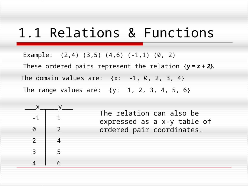
___x_____y___

-1 1

0 2

2 4

3 5

4 6

The relation can also be expressed as a x-y table of ordered pair coordinates.

1.1 Relations & Functions

Example: (2,4) (3,5) (4,6) (-1,1) (0, 2)

These ordered pairs represent the relation {y = x + 2}.

The domain values are: {x: -1, 0, 2, 3, 4}

The range values are: {y: 1, 2, 3, 4, 5, 6}

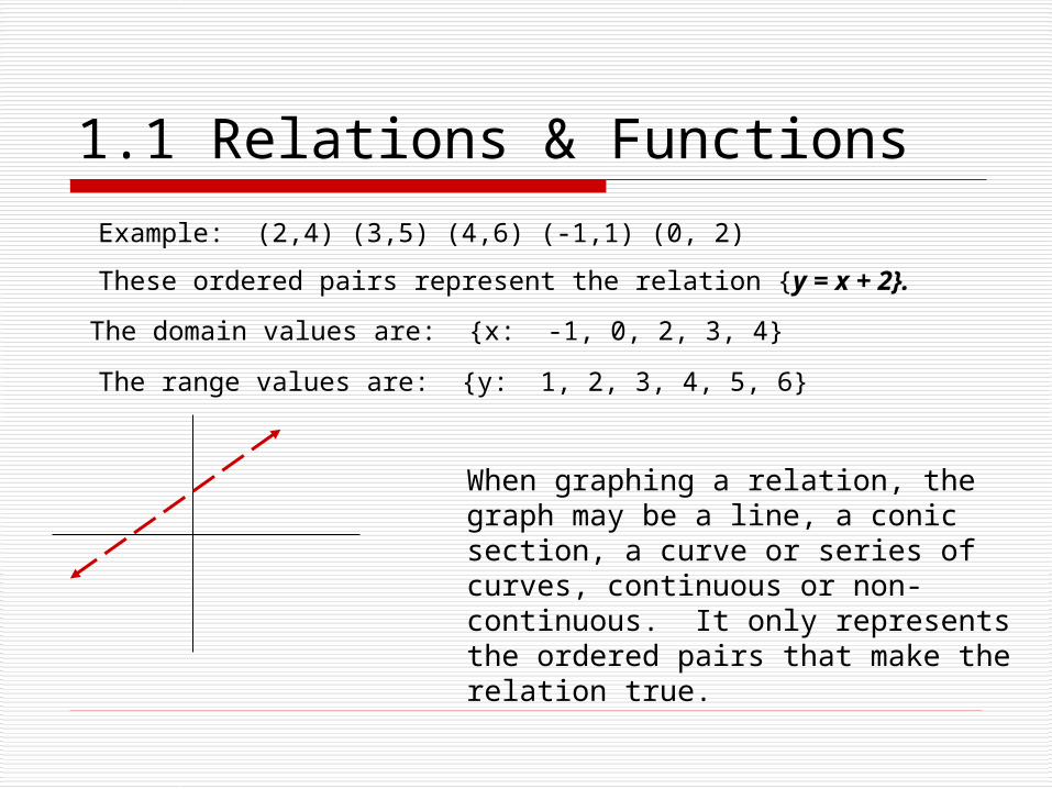
When graphing a relation, the graph may be a line, a conic section, a curve or series of curves, continuous or non-continuous. It only represents the ordered pairs that make the relation true.

1.1 Relations & Functions Function – A relation in which each element of

the domain is paired with exactly one element in the range.

Is a function Is a function Is not a function

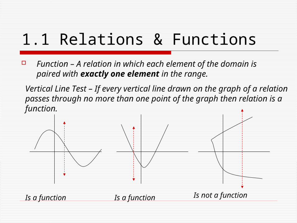
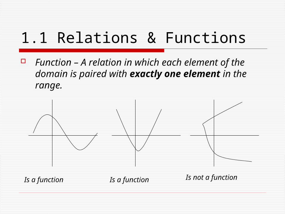
1.1 Relations & Functions Function – A relation in which each element of the domain

is paired with exactly one element in the range.

Is a function Is a function Is not a function

Vertical Line Test – If every vertical line drawn on the graph of a relation passes through no more than one point of the graph then relation is a function.

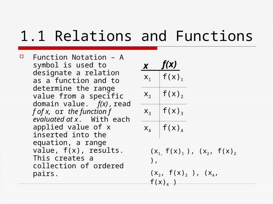
1.1 Relations and Functions Function Notation – A

symbol is used to designate a relation as a function and to determine the range value from a specific domain value. f(x) , read f of x, or the function f evaluated at x. With each applied value of x inserted into the equation, a range value, f(x), results. This creates a collection of ordered pairs.

x1 f(x)1

x2 f(x)2

x3 f(x)3

x4 f(x)4

x f(x)

(x1, f(x)1 ), (x2, f(x)2 ),

(x3, f(x)3 ), (x4, f(x)4 )

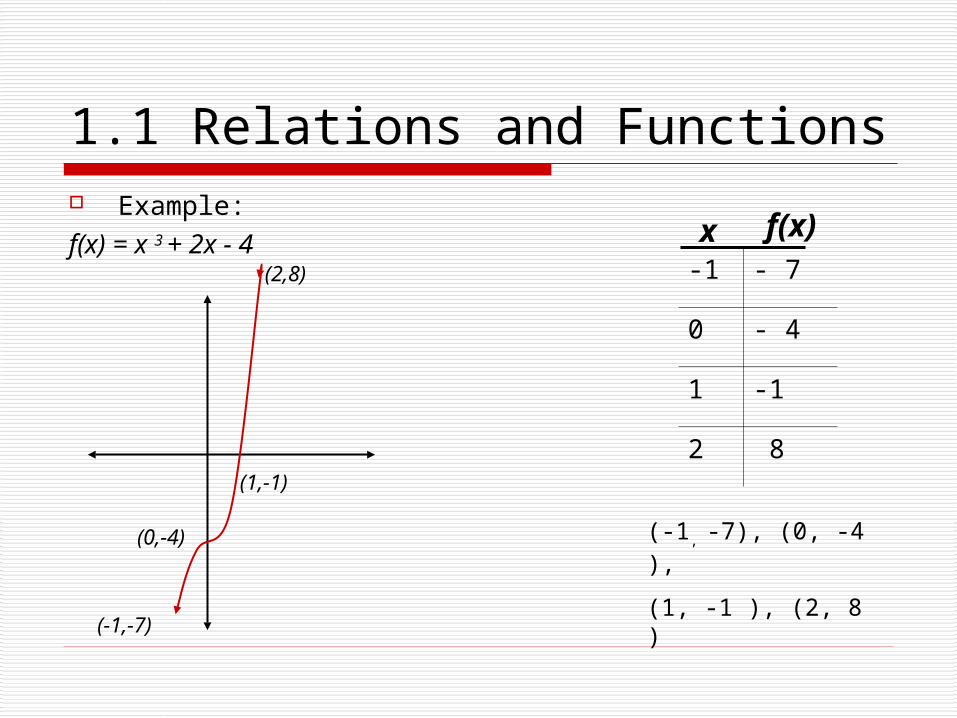
1.1 Relations and Functions Example:f(x) = x 3 + 2x - 4

-1 - 7

0 - 4

1 -1

2 8

x f(x)

(-1, -7), (0, -4 ),

(1, -1 ), (2, 8 )

(-1,-7)

(0,-4)

(2,8)

(1,-1)

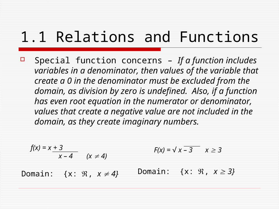
1.1 Relations and Functions Special function concerns – If a function includes

variables in a denominator, then values of the variable that create a 0 in the denominator must be excluded from the domain, as division by zero is undefined. Also, if a function has even root equation in the numerator or denominator, values that create a negative value are not included in the domain, as they create imaginary numbers.

f(x) = x + 3 x – 4 (x 4)

F(x) = √ x – 3 x 3

Domain: {x: , x 4} Domain: {x: , x 3}

1.1 Relations and Functions

Homework from Textbook Pages 10 – 11 Problems 17 – 51 odd problems

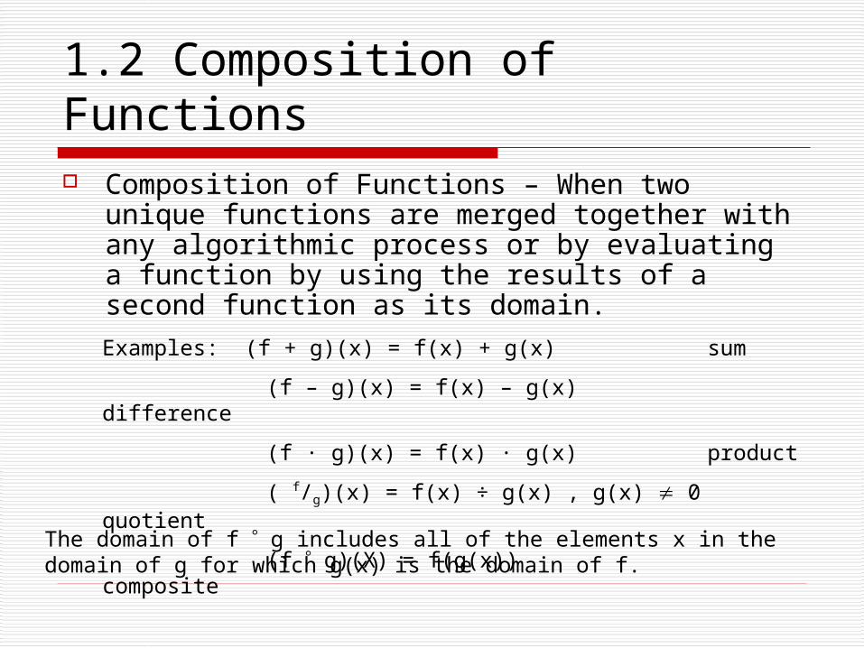
1.2 Composition of Functions Composition of Functions – When two unique

functions are merged together with any algorithmic process or by evaluating a function by using the results of a second function as its domain.Examples: (f + g)(x) = f(x) + g(x) sum

(f – g)(x) = f(x) – g(x) difference

(f · g)(x) = f(x) · g(x) product

( f/g)(x) = f(x) ÷ g(x) , g(x) 0 quotient

(f g)(X) = f(g(x)) compositeThe domain of f g includes all of the elements x in the domain of g for which g(x) is the domain of f.

1.2 Composition of Functions The domain of a composite function is

determined by the domains of f(x) and g(x). To determine the domain of a composite

function, begin by determining the domain of each function separately.

Any values for the inside function; g(x) in the relation f(g(x)) that are not defined will also be not defined in the composite.

Match the domain limitations of f(x) to the function g(x) to determine any other limitations.

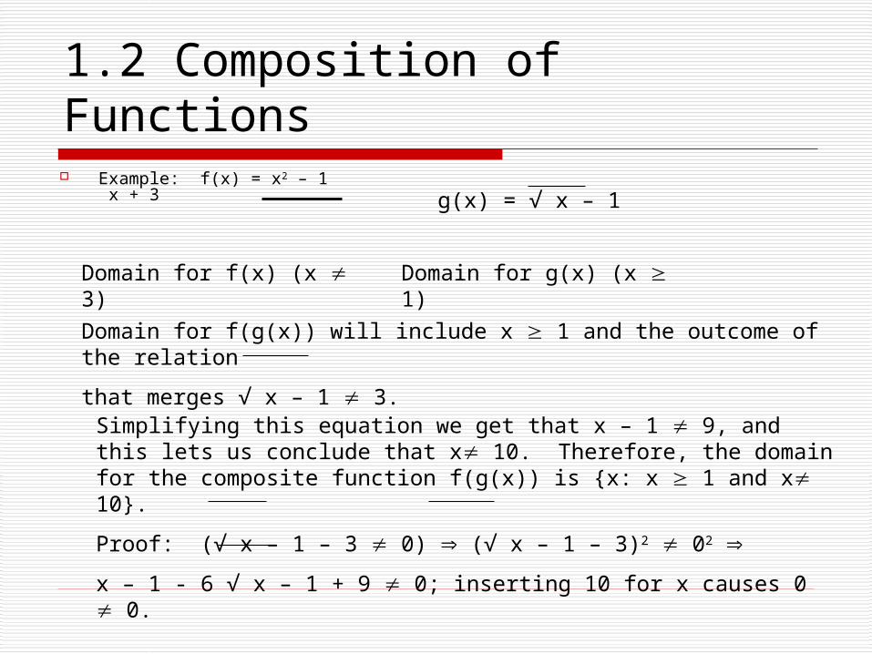
1.2 Composition of Functions Example: f(x) = x2 – 1

x + 3 g(x) = √ x – 1

Domain for f(x) (x 3) Domain for g(x) (x 1)

Domain for f(g(x)) will include x 1 and the outcome of the relation

that merges √ x – 1 3.

Simplifying this equation we get that x – 1 9, and this lets us conclude that x 10. Therefore, the domain for the composite function f(g(x)) is {x: x 1 and x 10}.

Proof: (√ x – 1 – 3 0) (√ x – 1 – 3)2 02

x – 1 - 6 √ x – 1 + 9 0; inserting 10 for x causes 0 0.

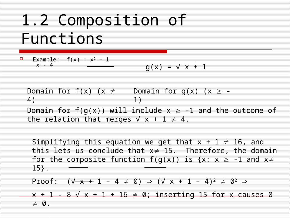
1.2 Composition of Functions Example: f(x) = x2 – 1

x - 4g(x) = √ x + 1

Domain for f(x) (x 4) Domain for g(x) (x -1)

Domain for f(g(x)) will include x -1 and the outcome of the relation that merges √ x + 1 4.

Simplifying this equation we get that x + 1 16, and this lets us conclude that x 15. Therefore, the domain for the composite function f(g(x)) is {x: x -1 and x 15}.

Proof: (√ x + 1 – 4 0) (√ x + 1 – 4)2 02

x + 1 - 8 √ x + 1 + 16 0; inserting 15 for x causes 0 0.

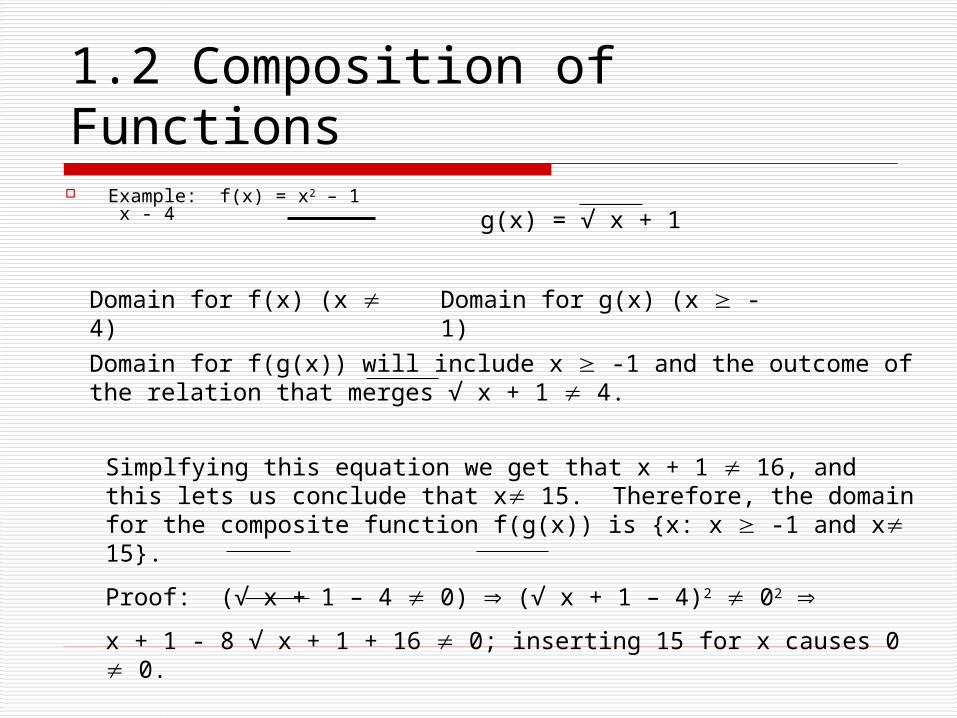
1.2 Composition of Functions Example: f(x) = x2 – 1

x - 4g(x) = √ x + 1

Domain for f(x) (x 4) Domain for g(x) (x -1)

Domain for f(g(x)) will include x -1 and the outcome of the relation that merges √ x + 1 4.

Simplfying this equation we get that x + 1 16, and this lets us conclude that x 15. Therefore, the domain for the composite function f(g(x)) is {x: x -1 and x 15}.

Proof: (√ x + 1 – 4 0) (√ x + 1 – 4)2 02

x + 1 - 8 √ x + 1 + 16 0; inserting 15 for x causes 0 0.

1.2 Composition of Functions The composite of a function with itself is called

an iteration. It is the expression (f f)(x) or otherwise stated as f(f(x)). When xo is inserted into the function f(x), the answer is the first iterate; i.e., f(xo) = x1, the first iterate. If we evaluate f(x1), we get the second iterate, x2. This process can continue to the specified iterate needed for the problem.

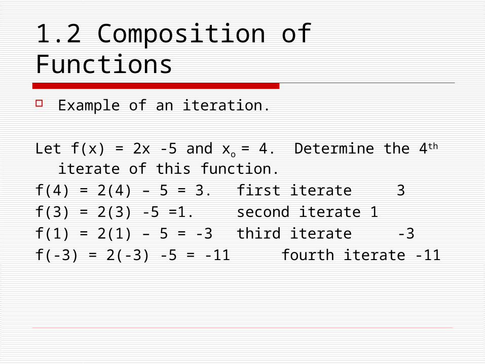
1.2 Composition of Functions Example of an iteration.

Let f(x) = 2x -5 and xo = 4. Determine the 4th iterate of this function.

f(4) = 2(4) – 5 = 3. first iterate 3f(3) = 2(3) -5 =1. second iterate 1f(1) = 2(1) – 5 = -3 third iterate -3f(-3) = 2(-3) -5 = -11 fourth iterate -11

1.2 Composition of Functions

Homework from TextbookPages 17 – 18Problems 11 – 27 odd problems

Graphing Linear Equations

Linear equations – these equations have a degree of 1 and take the general form of : Ax + By + C = 0, where A and B are not both 0 and where A, B, and C are real numbers. The graph for this type of equation is a line, hence the name linear.

1.3 Graphing Linear Equations

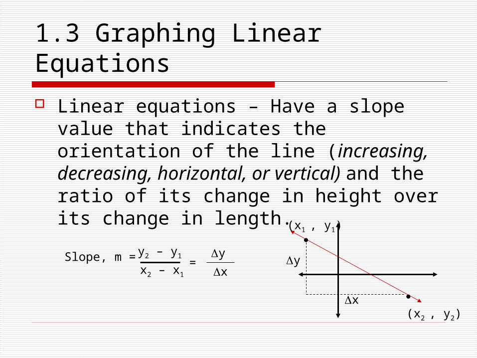
Linear equations – Have a slope value that indicates the orientation of the line (increasing, decreasing, horizontal, or vertical) and the ratio of its change in height over its change in length.Slope, m = y2 – y1

x2 – x1

(x1 , y1)

(x2 , y2)

y

x= y

x

1.3 Graphing Linear Equations

Forms for Linear Equations Standard form Ax + By + C = 0; the

value of slope, m = - A/B

Slope – Intercept form y = mx + b where m is the slope and b is the y-intercept value.

Slope is determined from the equation, from the intercept form, and from the standard form based upon what is known.

1.3 Graphing Linear Equations

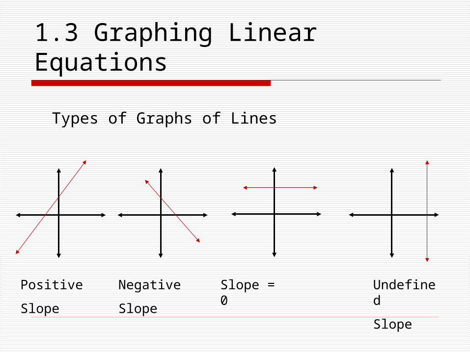
Types of Graphs of Lines

Positive

Slope

Negative

Slope

Slope = 0 Undefined

Slope

1.3 Graphing Linear Equations

Linear functions – defined by the equation f(x) = mx + b where m and b are real numbers. If we insert values for x that cause f(x) to equal 0, we call these values zeroes of the function f. The zeroes of the function are also known as the x-intercepts of the function f. Each line has exactly one zero of the function value.

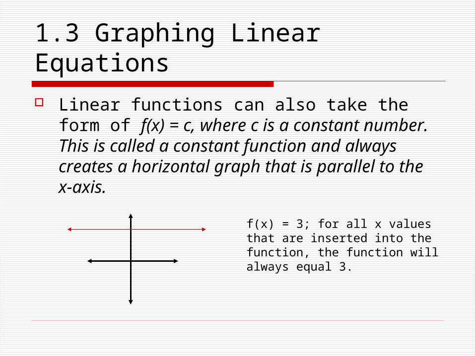
1.3 Graphing Linear Equations Linear functions can also take the form of

f(x) = c, where c is a constant number. This is called a constant function and always creates a horizontal graph that is parallel to the x-axis.

f(x) = 3; for all x values that are inserted into the function, the function will always equal 3.

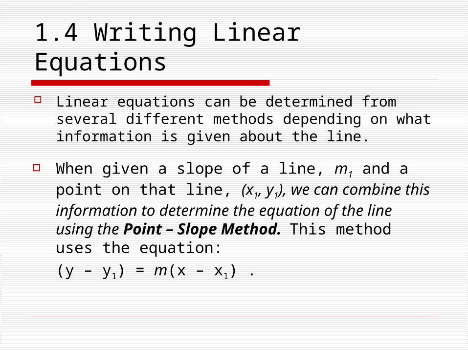
1.4 Writing Linear Equations Linear equations can be determined from

several different methods depending on what information is given about the line.

When given a slope of a line, m1 and a point on that line, (x1, y1), we can combine this information to determine the equation of the line using the Point – Slope Method. This method uses the equation: (y – y1) = m(x – x1) .

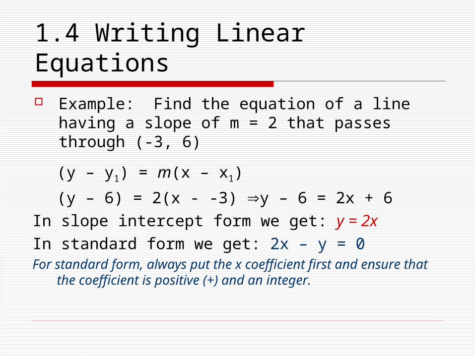
1.4 Writing Linear Equations Example: Find the equation of a line having a

slope of m = 2 that passes through (-3, 6)

(y – y1) = m(x – x1)

(y – 6) = 2(x - -3) y – 6 = 2x + 6In slope intercept form we get: y = 2xIn standard form we get: 2x – y = 0For standard form, always put the x coefficient first and

ensure that the coefficient is positive (+) and an integer.

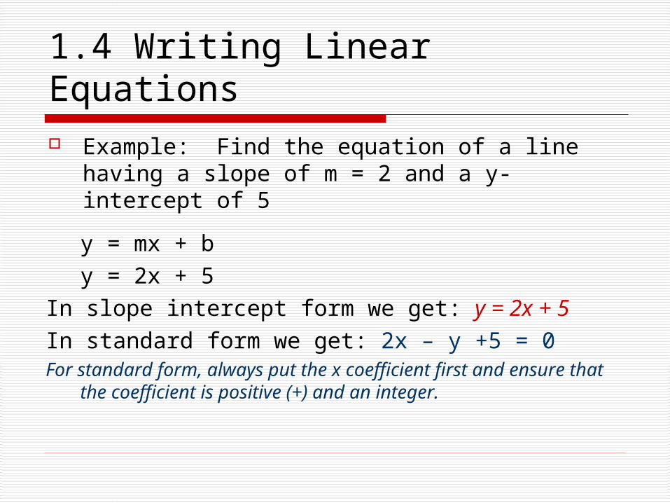
1.4 Writing Linear Equations Example: Find the equation of a line having a

slope of m = 2 and a y-intercept of 5

y = mx + by = 2x + 5

In slope intercept form we get: y = 2x + 5In standard form we get: 2x – y +5 = 0For standard form, always put the x coefficient first and

ensure that the coefficient is positive (+) and an integer.

1.3 Graphing Linear Equations1.4 Writing Linear Equations

Homework from Textbook Pages 24 – 25 Problems 13 – 39 odd

Page 30 Problems 11 – 23 odd

1.5 Writing Equations of Parallel and Perpendicular Lines

Parallel Lines – Two nonvertical lines in a plane are parallel if and only if their slopes are equal and they have not points in common. If the lines have the same slope and have points in common they are said to coincide.

Parallel Lines Lines of Coincidence

m1 = m2

1.5 Writing Equations of Parallel and Perpendicular Lines

Example : 3x – 4y = 12m1 = -(3/-4) = 3/4

9x – 12y = 72 m2 = -(9/-12) = 3/4

Put both equations into slope-intercept form.y = 3/4 x – 3 and y = 3/4 x – 6.

They have the same slope, ¾, but different intercepts. This means the lines must be parallel to each other.

1.5 Writing Equations of Parallel and Perpendicular Lines

Example : 15x + 12y = 36 m1 = -(15/12) = - 5/4

5x + 4y = 12 m2 = -(5/4) = - 5/4

Put both equations into slope-intercept form.y = -5/4 x + 3 and y = -5/4 x + 3.

They have the same slope, ¾, and the same intercepts. This means the lines must coincide with each other.

1.5 Writing Equations of Parallel and Perpendicular Lines

Perpendicular Lines – Two lines in a plane are perpendicular if and only if their slopes are opposite reciprocals. For slopes to be negative reciprocals m1 m2 = - 1.

Perpendicular Lines

Ex: m1 = ½ m2 = - 2

m1 m2 = -1

1.5 Writing Equations of Parallel and Perpendicular Lines

Example: Write the standard form of the equation of the line that passes through the point (4,-7) and is parallel to the graph of 2x – 5y + 8 = 0

Solution: m1 =-( 2/-5) = 2/5. Since the line is parallel, its slope, m2 = 2/5. We can now use the point – slope method to determine the equation of our line.

(y – y1) = m(x – x1) (y - -7) = 2/5(x – 4) (y+7) = 2/5(x – 4)

5y + 35 = 2x – 8 2x – 5y = 43

1.5 Writing Equations of Parallel and Perpendicular Lines

Example: Write the standard form of the equation of the line that passes through the point (4,-7) and is perpendicular to the graph of 2x – 5y + 8 = 0

Solution: m1 =-( 2/-5) = 2/5. Since the line is perpendicular, its slope, m2 = - 5/2. We can now use the point – slope method to determine the equation of our line.

(y – y1) = m(x – x1) (y - -7) = - 5/2(x – 4) (y+7) = - 5/2(x – 4)

2y + 14 = -5x + 20 5x + 2y = 6

1.5 Writing Equations of Parallel and Perpendicular Lines

Homework from Textbook Pages 36 – 37 Problems 13 – 33 odd problems