chap 5. solute transport in soil

7/31/2019 Chap 5. Solute Transport in Soil

http://slidepdf.com/reader/full/chap-5-solute-transport-in-soil 1/18

V. Solute Transport

Chap V. Solute Transport in Soils

5.1. Introduction

Soil water carries its solute load in its convective stream, leaving someof it behind to the extent that the component salts are absorbed, taken

up by plants, or precipitated whenever their concentration exceeds their

solubility (e.g. at the soil surface during evaporation).

Transport of solutes in porous materials such as soils is important in

understanding problems of chemical residue, salinity, availability of

solutes for plant uptake, leaching or redistribution within the vadose

zone to groundwater, runoff to surface water, and seepage from various

storage and waste disposal systems.

Solute transport in soil depends on H2O flow velocity, water content, soil

characteristics, solute species (mobile and immobile), solute reaction,

etc.

Transport of solutes in soil occurs by two physical processes; namely

Diffusion

Convective flow – mass flow

5.2. Diffusion

Diffusion is the movement of ions or molecules from areas of higher to

areas of lower concentration. This is generally proportional to the

concentration gradient, the cross sectional area available for diffusion,

and the time during which the transport process occurred.

Page V.1: AgEn 311: Soil Physics



V. Solute Transport

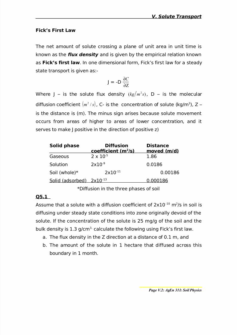
Fick’s First Law

The net amount of solute crossing a plane of unit area in unit time is

known as the flux density and is given by the empirical relation known

as Fick’s first law. In one dimensional form, Fick’s first law for a steady

state transport is given as:-

J = -DΖ ∂

∂C

Where J – is the solute flux density )( 2 smkg , D – is the molecular

diffusion coefficient ( ) sm /2 , C- is the concentration of solute (kg/m3), Z –

is the distance is (m). The minus sign arises because solute movement

occurs from areas of higher to areas of lower concentration, and it

serves to make J positive in the direction of positive z)

Solid phase Diffusion Distancecoefficient (m2/s) moved (m/d)

Gaseous 2 x 10-5 1.86

Solution 2x10-9 0.0186

Soil (whole)* 2x10-11 0.00186

Solid (adsorbed) 2x10-13 0.000186

*Diffusion in the three phases of soil

Q5.1

Assume that a solute with a diffusion coefficient of 2x10-10 m2/s in soil is

diffusing under steady state conditions into zone originally devoid of the

solute. If the concentration of the solute is 25 mg/g of the soil and the

bulk density is 1.3 g/cm3, calculate the following using Fick’s first law.

a. The flux density in the Z direction at a distance of 0.1 m, and

b. The amount of the solute in 1 hectare that diffused across this

boundary in 1 month.




V. Solute Transport

Fick’s Second Law

For transient – state conditions, the concentration of mass equation has

to be satisfied. In one dimension and without generation and

consumption, this equation is

t

C

∂∂

= - Z

J

∂∂

which implies that the rate of change of solute concentration equals the

net rate of flow over the boundary. Combining equation (2) and (4)

yields the transient form of the diffusion equation:

∂∂

∂∂

=∂∂

z

C D

z t

C

Which is known as Fick’s Second Law. If the solute diffusion coefficient isindependent of solute concentration and depth, equation above

simplifies to

2

2

z

C D

t

C

∂∂

=∂∂

This has been solved analytically and numerically for several initial and

boundary conditions.

Analytical Solution and Application

One analytical solution is given for situation:-

when a solute is uniformly broadcast on the soil surface in

quantities high enough to cause saturation in solution,

if the initial concentration of solute in the profile is negligible, and

if only diffusion transport occurs.

if there is no root water uptake by plant roots the solute will

diffuse downward into the soil profile.

The solute concentration distribution C(z, t) at some depth z and time t

after application can be estimated from

C(z, t) = Co erfc

5.0)(2 Dt

z




V. Solute Transport

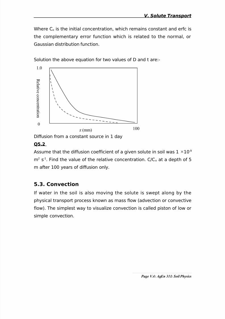
Where Co is the initial concentration, which remains constant and erfc is

the complementary error function which is related to the normal, or

Gaussian distribution function.

Solution the above equation for two values of D and t are:-

Diffusion from a constant source in 1 day

Q5.2

Assume that the diffusion coefficient of a given solute in soil was 1 ×10-9

m2 s-1. Find the value of the relative concentration. C/Co at a depth of 5

m after 100 years of diffusion only.

5.3. Convection

If water in the soil is also moving the solute is swept along by the

physical transport process known as mass flow (advection or convective

flow). The simplest way to visualize convection is called piston of low or

simple convection.


1.0

0100z (mm)

Relativecon

centration



V. Solute Transport

Steady state convection

Consider a column of soil with pure water uniformly moving through it

`

Assume that we quickly replace the water at the intake end of the

column with a solution containing a solute at some known concentration,

Co. In piston flow, the solute will travel through the column, at the some

rate as the flow of water and will not spread. At the outflow end of the

column, the concentration of the solute is zero until the front appears at

which time the concentration of the solute becomes the same as that at

the inflow end of the column.

The solute flow rate in the column can be described by the product of

the macroscopic flow rate of water (i.e. the Darcy flux density) and the

concentration of the solute in that water. In the Z dimension, this solute

flow rate is determined by

l z z C q J =

Where

Jz – is the solute flux density (kg, m-2 S-1) of soil in the Z direction (m)

qz – is the macroscopic water flow rate per unit area perpendicular to the

Z direction (m/s), and

Cl - is the concentration of the solute in that water (kg/m3)

The flux density of soil water is calculated by the Darcy equation for

steady state flow of water.




V. Solute Transport

Since in soil vq vθ = , we can also write l v z C v J θ = . Where v is the average

water velocity in the soil pores in the Z –direction (m/s) and vθ is the

average volumetric soil – water – content (m3 water per m3- soil)

Q5.3

If the soil water flux density is 0.045 cm/d downward, the soil water

content is 0.35 m3.m-3 and the soil solution concentration of nitrate –N is

3 l mg calculate the pore water velocity and the amount of nitrate –N

moved by convective flow per unit area below the plant root zone in 1

day.

Transient – state convection

Combining equations

Ζ ∂∂

−=∂∂ J

t

c, and l z C v J θ =

we obtain the one dimensional conservation equation for convective

flow.

( )

z

C v

t

c l v

∂∂

−=∂∂ θ

Solution of this gives a sharp concentration front in which on the

advancing side of the front, the solute concentration is equal to the

inflow Co and on the other side it is equal to the initial concentration C i.

This is known as piston (or plug) flow where all of the resident soil water

is replaced by the invading solute front. The sharp interface that results

from piston flow is shown


(Relativecon

centration)

1

0

oC C

Time



V. Solute Transport

It should be emphasized that piston flow very seldom, if ever occurs in

field soils, but it is a useful first approximation of the potential

movement of solutes. Non-uniform flow mechanism such as

hydrodynamic dispersion, preferential flow, and fingering lead to solute

concentration distributions that differ significantly from those predicted

by piston flow.

Fingering is the preferential movement of water in soil along a vertically

elongated path. These heterogeneous concentration distributions are

usually attributed to the influence of non-homogenous of soil properties

such as soil structure and biological channels resulting in water and

solute flowing more rapidly in large pores than in small pores.

Mechanical Dispersion

As a solute moves through the soil profile, it mixes with the soil solution,

which has a different chemical composition. Initially, there is a sharp

boundary or interface between the solute concentration of the new andold solutions. Eventually, a transition zone develops between the two

solutions where the solute concentration varies.

Assuming no interaction between the solute and soil surface (i.e no

sorption), the solute concentration curve varies with time and has the

shape of the S curve.

The tendency for solute molecules to become more diffuse with time

when water is moving is known as mechanical dispersion. Dispersion

occurs when a transition zone develops between two solutions of

differing chemical compositions. The change in width of the front is due

to both diffusion and mechanical dispersion. However, it is not

generally possible to separate the effects of the two processes.




V. Solute Transport

Hydrodynamic dispersion can be visualized as occurring in soil when the

water is moving. Its velocity distribution is not uniform because of three

boundary effects. Causes contributing to hydrodynamic dispersion of

solutes are:-

a. Zero velocity at the soil particle surface (capillary model).

Velocity inside the tube at any radius (r) is given by the equation

below

−=

a

r vv o

2

12

b. Variation in pore size

Causing different average flow

velocity between the pores of the

soil

c. Influence of microscopic flow direction

The mixing or dispersion that occurs along the direction of the flow path

is called longitudinal dispersion. The dispersion in directions normal

to the flow path is called transverse dispersion. Both of these

mechanical dispersion coefficients are the result of the product of the

linear velocity of the fluid in the principal direction of flow and a

property of the soil called the dispersivity.

The mathematical equation for the flux density of solutes by

hydrodynamic dispersion is

z

C D J

l

lhh

∂

∂−=




V. Solute Transport

Where lh D is the hydrodynamic dispersion coefficient (m2/s). The

magnitude of the dispersion coefficient depends on the pore water

velocity and the solute diffusion coefficient. Since the effects of diffusion

and dispersion on the concentration distribution are similar, they are

often combined even though the mechanisms of transport are different.

Miscible Displacement and Breakthrough curves

Miscible refers to the displacement of one fluid by another miscible fluid

in soil.

Steady- state flow conditions when the initial soil solution with a

solute concentration of Ci, is invaded and eventually displaced by a

second miscible solution with solute concentration Co.

No mixing of the two solutions should occur at the ends of the column

and side walls. Samples of the effluent are collected and analyzed for

the solute without disturbing the flow.

Let the volume of the soil column occupied by the resident solution

be Vo (m3) and the steady state rate of inflow and outflow of the

solution be t Q / (m3/s). The initial solute concentration, C1, is suddenly

displaced by an incoming solute concentration solution, Co. The

fraction of this incoming solute in the effluent at time (t) will be

CiCo

CiC

−−

or for an initial concentration (Ci) of zero, simplyCo

C .

Plot of the relative concentration ,Co

C at a fixed location (usually the

outlet of the column) versus pores volume of effluent, oV Q are called

Breakthrough curves (BTCs).

Pore volume[-] is defined as the ratio of the column effluent volume

to the total pore water volume in column.




V. Solute Transport

The parameter t is the time since the dissolved solute was introduced

to the effluent.

The BTCs describe the transport behavior of the solute in the soil and

provide information on interactions between the soil matrix and

solute.

Example of breakthrough curves for miscible displacement.

oC C is the relative concentration of the solute measured in the

effluent, and pore volume is the ratio of the volume of effluent to the

volume of fluid in the soil column. Curve number 1 is for no

dispersion, curve 2 is for dispersion with no sorption, and curve 3 is

dispersion with sorption.

If there is no dispersion – and the dissolved solute is conservative

(i.e. no sorption or microbial or chemical transformation), at 1 pore

volume the effluent break though relative concentration willinstantaneously reach 1.0, being zero until 1 pore volume is

displaced from the column.


3

2

1

oC C

Pore Volume



V. Solute Transport




V. Solute Transport

Derivation of the solute Transport Equation

The derivation (in complete form) of the equations used for the

prediction of solute transport in soils will be derived first by summing

the steady – state flow processes in the three phases. Then, with the aid

of the law of conservation of mass, the transient – state processes will

be accounted for.

Steady – state solute transport

Under steady- state conditions, the flux density of solutes in soil is the

sum of the flux densities in the three phases of soil. Mathematically, this

can be written as

a g l s J J J J ++=

Where Js is the total solute flux density in soil, Jl, is the flux density in the

liquid phase, Jg is the flux density in the gas phase and Ja – flux density in

the solid/adsorbed phase.

Values of Ja are usually considered negligible compared to the overall

macroscopic transport process of solutes and often ignored when long

distance transport is considered. For solute transport in the soil – air gas

phases the diffusion is the primary transport mechanism. We use Fick’s

first law to write

z

C D f J

g

g g g ∂

∂−=

Where f a – is the aeration porosity (m3

/m3

), Dg is the molecular diffusioncoefficient in the gas phase (m/s), and Cg is the concentration of the

solute in the gas phase (kg /m3 of soil air.

In the liquid phase, both diffusion and concoctive flow transport

processes operate. The convective flux density, Jl, can be represented by




V. Solute Transport

l

l lc ld v l v h

C J J J v C D v

z θ θ

∂= + = −

∂

Often, it is difficult to separate diffusion from dispersion, and these

terms are combined and collectively called diffusion- dispersion (and

taken as D).

The total solute flux density in the liquid phase, Jl, is the sum of the

diffusion and convective dispersion flux densities.

l v

l

vl C v z

C D J θ θ +

∂∂

−=

Where D is the diffusion- dispersion coefficient of the solute. The firstterm on the right hand side is the contribution of dispersion (molecular

diffusion and mechanical dispersion), and the second term is the

contribution of convective flow.

Neglecting the adsorbed (Ja) component, the steady – state solute flux

density in soil, Js, is written as

z

C D f C v

z C D J g

g al vv s ∂

∂−+∂∂−= θ θ 1

This combines the solute flux densities in both liquid and gaseous

phases of soil.

The general form of the mass balance equation for one dimensional

solute flow in the same direction as water and without generation and

consumption can be represented as

( ) z

J

t

C sl v

∂

∂−=

∂

∂ θ

Note that C C l v =θ and Js is expressed on a soil basis.




V. Solute Transport

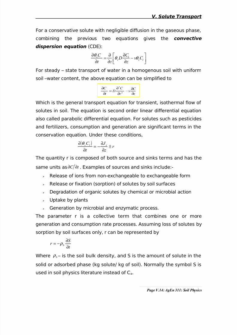
For a conservative solute with negligible diffusion in the gaseous phase,

combining the previous two equations gives the convective

dispersion equation (CDE):

v l

v v l

C C

D v C t z z

θ

θ θ

∂ ∂∂ = − ∂ ∂ ∂

For steady – state transport of water in a homogenous soil with uniform

soil –water content, the above equation can be simplified to

z

C v

z

C D

t

C

∂

∂−

∂

∂=

∂

∂

2

2

Which is the general transport equation for transient, isothermal flow of

solutes in soil. The equation is second order linear differential equation

also called parabolic differential equation. For solutes such as pesticides

and fertilizers, consumption and generation are significant terms in the

conservation equation. Under these conditions,

( )r

z

J

t

C sl v ±∂

∂−=

∂∂ θ

The quantity r is composed of both source and sinks terms and has the

same units as t C ∂∂ . Examples of sources and sinks include:-

Release of ions from non-exchangeable to exchangeable form Release or fixation (sorption) of solutes by soil surfaces

Degradation of organic solutes by chemical or microbial action

Uptake by plants

Generation by microbial and enzymatic process.

The parameter r is a collective term that combines one or more

generation and consumption rate processes. Assuming loss of solutes by

sorption by soil surfaces only, r can be represented by

t

S r b ∂

∂−= ρ

Where b ρ – is the soil bulk density, and S is the amount of solute in the

solid or adsorbed phase (kg solute/ kg of soil). Normally the symbol S is

used in soil physics literature instead of Ca.




V. Solute Transport

For a given unit volume of soil, the total concentration of a nonvolatile

solute (kg m-3) is represented by the sum of the amounts retained by soil

surfaces and that present in the solution phase. The total resident solute

concentration in soil is defined as the sum of the volume – weighted

concentrations in the three phases and is

g al vab C f C C C ++= θ ρ

The revised form of this equation is l vb C S C θ ρ +=

Differentiating with respect to t, assuming that b ρ is constant with t, and

substituting the result into

z C v

z C D

t C l l l

∂∂−

∂∂=

∂∂

2

2

Gives the following form of CDE:

( )

z

C v

z

C D

t

S

t

C l

v

l

vb

l v

∂∂

−∂

∂=

∂∂

+∂

∂θ θ ρ

θ 2

2

Using the chain rule, collecting t C ∂∂ terms and assuming that vθ does

not change with z or t, we define

l v

b

dC

dS R ×+= θ

ρ 1 =1 b

d K ρ

θ +

For no interaction between the solute and the soil K d = 0 and R=1. Here

R is called the retardation coefficient.

For organic and inorganic cations and neutral molecules, R will be

greater than 1. However, if there is no sorption of the solute by soil

surfaces, then the term l dC dS is zero and R becomes 1. This assumption

is often made of anionic and neutral tracers such as chloride, bromide,

and tritium. However, if there is ion exclusion, R may be less than 1.

Finally, the CDE that accounts for sorption of a conservative solute by

soil surfaces is written as




V. Solute Transport

z

C v

z

C D

t

C R l

∂∂

−∂

∂=

∂∂ 1

2

2

1

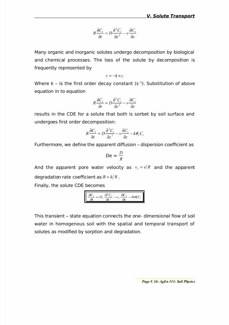
Many organic and inorganic solutes undergo decomposition by biological

and chemical processes. The loss of the solute by decomposition is

frequently represented by

ck r ×−=

Where k – is the first order decay constant (s -1). Substitution of above

equation in to equation

z

C v

z

C D

t

C R l

∂∂

−∂

∂=

∂∂ 1

2

2

1

results in the CDE for a solute that both is sorbet by soil surface and

undergoes first order decomposition:

l vl C k

z

C v

z

C D

t

C R θ −

∂∂

−∂

∂=

∂∂ 1

2

2

1

Furthermore, we define the apparent diffusion – dispersion coefficient as

De = R

D

And the apparent pore water velocity as Rvve = and the apparent

degradation rate coefficient as Rk B = .

Finally, the solute CDE becomes

l ve

l

eC B

z

C v

z

C D

t

C θ −

∂

∂−

∂

∂=

∂

∂1

2

2

1

This transient – state equation connects the one- dimensional flow of soil

water in homogenous soil with the spatial and temporal transport of

solutes as modified by sorption and degradation.




V. Solute Transport

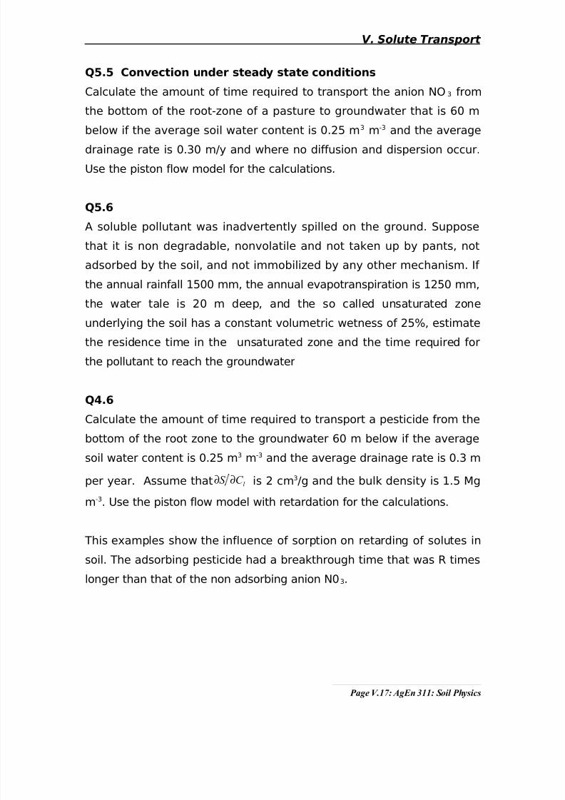
Q5.5 Convection under steady state conditions

Calculate the amount of time required to transport the anion NO3 from

the bottom of the root-zone of a pasture to groundwater that is 60 m

below if the average soil water content is 0.25 m3 m-3 and the average

drainage rate is 0.30 m/y and where no diffusion and dispersion occur.

Use the piston flow model for the calculations.

Q5.6

A soluble pollutant was inadvertently spilled on the ground. Suppose

that it is non degradable, nonvolatile and not taken up by pants, not

adsorbed by the soil, and not immobilized by any other mechanism. If

the annual rainfall 1500 mm, the annual evapotranspiration is 1250 mm,

the water tale is 20 m deep, and the so called unsaturated zone

underlying the soil has a constant volumetric wetness of 25%, estimate

the residence time in the unsaturated zone and the time required for

the pollutant to reach the groundwater

Q4.6

Calculate the amount of time required to transport a pesticide from thebottom of the root zone to the groundwater 60 m below if the average

soil water content is 0.25 m3 m-3 and the average drainage rate is 0.3 m

per year. Assume that l C S ∂∂ is 2 cm3/g and the bulk density is 1.5 Mg

m-3. Use the piston flow model with retardation for the calculations.

This examples show the influence of sorption on retarding of solutes in

soil. The adsorbing pesticide had a breakthrough time that was R timeslonger than that of the non adsorbing anion N03.




V. Solute Transport

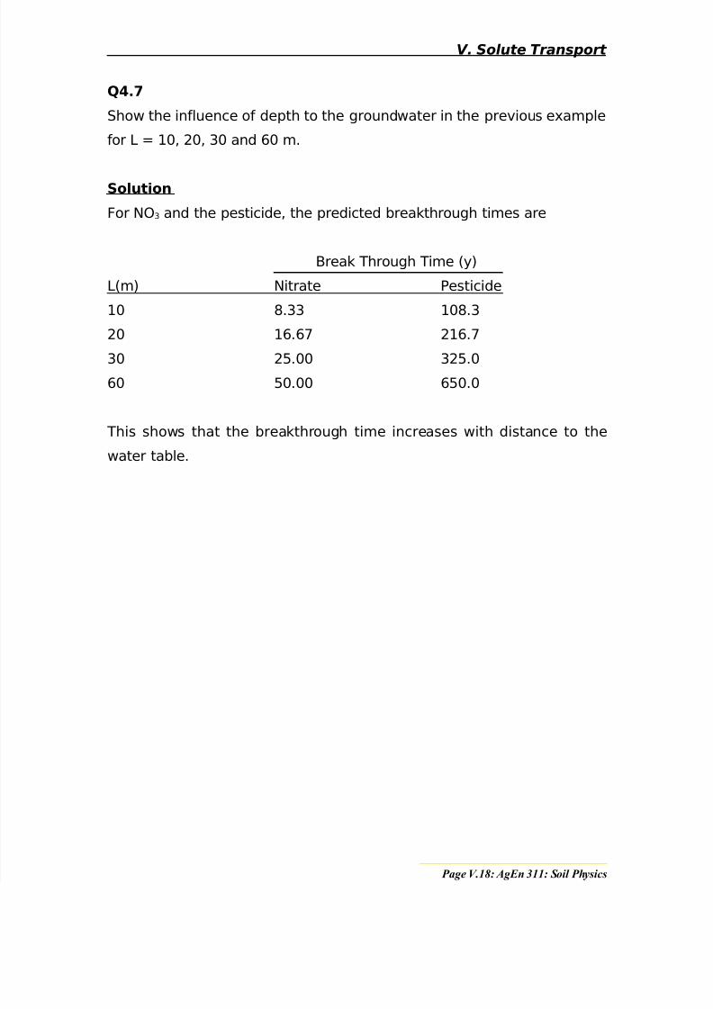
Q4.7

Show the influence of depth to the groundwater in the previous example

for L = 10, 20, 30 and 60 m.

Solution

For NO3 and the pesticide, the predicted breakthrough times are

Break Through Time (y)

L(m) Nitrate Pesticide

10 8.33 108.3

20 16.67 216.7

30 25.00 325.0

60 50.00 650.0

This shows that the breakthrough time increases with distance to the

water table.

chap 5. solute transport in soil

Documents