changes of coastal groundwater systems … · the direct impact of land reclamation on coastal...
TRANSCRIPT

In: New Topics in Water Resources Research… ISBN: 978-1-60021-974-8Editor: Henrik M. Andreassen, pp. 79-136 © 2007 Nova Science Publishers, Inc.
Chapter 2
CHANGES OF COASTAL GROUNDWATERSYSTEMS IN RESPONSE TO LARGE-SCALE
LAND RECLAMATION
Haipeng Guo and Jiu J. JiaoDepartment of Earth Sciences, The University of Hong Kong,
Hong Kong, P. R. China
Abstract
Most large urban centers lie in coastal regions, which are home to about 25% of theworld's population. The current coastal urban population of 200 million is projected to almostdouble in the next 20 to 30 years. This expanding human presence has dramatically changedthe coastal natural environment. To meet the growing demand for more housing and otherland uses, land has been reclaimed from the sea in coastal areas in many countries, includingChina, Britain, Korea, Japan, Malaysia, Saudi Arabia, Italy, the Netherlands, and the UnitedStates. Coastal areas are often the ultimate discharge zones of regional ground water flowsystems. The direct impact of land reclamation on coastal engineering, environment andmarine ecology is well recognized and widely studied. However, it has not been wellrecognized that reclamation may change the regional groundwater regime, includinggroundwater level, interface between seawater and fresh groundwater, and submarinegroundwater discharge to the coast.
This paper will first review the state of the art of the recent studies on the impact ofcoastal land reclamation on ground water level and the seawater interface. Steady-stateanalytical solutions based on Dupuit and Ghyben-Herzberg assumptions have been derived todescribe the modification of water level and movement of the interface between freshgroundwater and saltwater in coastal hillside or island situations. These solutions show thatland reclamation increases water level in the original aquifer and pushes the saltwaterinterface to move towards the sea. In the island situation, the water divide moves towards thereclaimed side, and ground water discharge to the sea on both sides of the island increases.After reclamation, the water resource is increased because both recharge and the size ofaquifer are increased.
This paper will then derive new analytical solutions to estimate groundwater travel timebefore and after reclamation. Hypothetical examples are used to examine the changes ofgroundwater travel time in response to land reclamation. After reclamation, groundwater flowin the original aquifer tends to be slower and the travel time of the groundwater from any

Haipeng Guo and Jiu J. Jiao80
position in the original aquifer to the sea becomes longer for the situation of coastal hillside.For the situation of an island, the water will flow faster on the unreclaimed side, but moreslowly on the reclaimed side. The impact of reclamation on groundwater travel time on thereclaimed side is much more significant than that on the unreclaimed side. The degree of themodifications of the groundwater travel time mainly depends on the scale of land reclamationand the hydraulic conductivity of the fill materials.
1. Introduction
Most of the large urban centers are coastal and population in coastal areas is expandingrapidly. This expanding human presence has dramatically changed the coastal naturalenvironment, which has made human as the most active geological agent in coastal areas.Coastal areas are faced with a challenge of lack of land due to increase in ecological,economic and social activities, which have led to an increase in pressure on coastal areas andin some cases led to the change of the coastal natural environment. Land reclamation, creatingof new land in areas that were initially covered with water, has been a common practice toreduce the increasing pressure in coastal areas (Seasholes, 2003; Lumb, 1976; Suzuki, 2003;Stuyfzand, 1995). Coastal areas are usually the ultimate discharge zones of regionalgroundwater flow systems. Human activities such as large-scale land reclamation may havesevere effect on coastal groundwater regimes.
In the early days, land was reclaimed by draining of swampy or seasonally submergedwetlands. In the coastal areas where intertidal zones have already been reclaimed, coastalreclamation usually means that shallow sea is landfilled extensively to create more usefulland area. The analytical studies in this paper focus on the latter case. Land reclamation canincrease the land for food production, create new investment into a city, and create new areasfor urban development, easing housing shortages. From 1949 to 2001, about 22, 000 km2
land, which is about half of the total tidal wetlands, along the coast of the Mainland China hasbeen reclaimed. One third of urban area in Hong Kong is reclaimed from the sea. Landreclamation has been also very popular in many other countries including Japan, Korea,Malaysia, USA etc. For example, 45% of Korea's population lives in areas reclaimed fromintertidal zone or shallow sea.
While reclamation satisfies the growing needs for land use, it also induces variousengineering, environmental and ecological problems such as modification of coastal sedimentdeposition and erosion, coastal flooding, loss of the coastal habitat and change of marineenvironment. These problems have been widely discussed (Barnes, 1991; Noske, 1995; Ni etal., 2002; Terawaki et al., 2003). Coastal areas are often the ultimate discharge zones ofregional ground water flow systems. Interaction between coastal groundwater and seawateralways occurs (Fetter, 1972; Jiao and Tang, 1999), and is expected to be modified by landreclamation. Because the response of a groundwater regime to land reclamation may be slowand not so obvious, this phenomenon has been largely ignored. Stuyfzand (1995) discussedthe impact of land reclamation on groundwater quality and future drinking water supply in theNetherlands. Mahamood and Twigg (1995) noted that the water table increased under areasrelated to reclaimed land in Bahrain Island of Saudi Arabia. A research team in theDepartment of Earth Sciences, the University of Hong Kong has carried out a research projectaiming to understand the impact of large-scale land reclamation on physical and chemicalprocess in coastal groundwater system. They conducted numerical modeling on the impact of

Changes of Coastal Groundwater Systems… 81
land reclamation on groundwater flow and contaminant migration in Penny’s Bay and Mid-Level areas, Hong Kong (Jiao, 2000; Jiao, 2002; Jiao et al., 2006). Jiao et al. (2001) presentedsome analytical solutions on the influence of reclamation on the water level changes incoastal unconfined aquifers. Jiao et al. (2005) hypothesized that there may be variousphysiochemical reactions between the fill materials and the original marine sediments in areclamation site and these processes may result in chemicals which may have adverse effectto the coastal plants and organisms. Guo and Jiao (2007) presented some analytical solutionson impact of land reclamation on both the ground water level and the sea water interface withunconfined ground water conditions.
Reclamation is expected to modify the groundwater travel time. Ground water travel timeis defined as the time required for a unit volume of ground water to travel between twolocations. The travel time is the length of the flow path divided by the velocity, wherevelocity is the average groundwater flux passing through the cross-sectional area of thegeologic medium through which flow occurs, perpendicular to the flow direction, divided bythe effective porosity along the flow path. If discrete segments of the flow path have differenthydrologic properties the total travel time will be the sum of the travel times for each discretesegment (Code of Federal Regulations, 1988). Groundwater travel times have importantimplications for the management of water resources, evaluation of the groundwateravailability and sustainability, and dating of groundwater. The assessment of groundwatertravel times can be used to determine spreading of contaminated plume. The origin ofgroundwater particles can be tracked if their ages are known. In coastal aquifers, largeamounts of dissolved and suspended materials are transported from the land to the seatogether with terrestrial groundwater. Discharge of terrestrial groundwater derived fromrainfall is a primary component of SGD (submarine groundwater discharge). Thus it isnecessary to investigate sensitivity of the groundwater travel time in coastal aquifers.
The ground water transit time is defined as the time interval of water flow from therecharge points to the discharge points (Etcheverry and Perrochet, 2000�Chesnaux et al.,2005; Cornaton and Perrochet, 2005). Groundwater transit times have important applicationsand their sensitivity has been well investigated. Fórizs and Deák (1998) compared transittimes calculated from stable oxygen isotope data and hydraulic modeling. They concluded atime series of groundwater sampling would be necessary when groundwater transit time wascalculated from isotope data. Florea and Wicks (2001) constructed laboratory-scale karsticmodels to investigate transit times by controlling the length of the flow paths, the gradient,the recharge rate, the size of the conduits, and the geomorphic pattern of conduit layout. Theirmodels provided reliable data that could be used in calibrating numerical models. A generaltheoretical framework to model complete groundwater age and transit time distributions ataquifer scale was presented by Cornaton and Perrochet (2005). The effect of aquifer structureand macro-dispersion on the distributions of age, life expectancy and transit time wasdiscussed by means of analytical and numerical analysis of one- and two-dimensionaltheoretical flow configurations.
While numerical solutions for determining groundwater age and travel times are available(e.g., Varni and Carrera, 1998), they need more computational efforts and may be applicablefor more complicated groundwater system. In many cases, analytical solutions can be used toassess travel times even though their application is limited by a certain number ofassumptions. Gelhar and Wilson (1974) developed an analytical solution to calculate thegroundwater transit time using the Dupuit assumption. Their analytical solution does not

Haipeng Guo and Jiu J. Jiao82
include the influence of the aquifer hydraulic conductivity. Amin and Campana (1996)presented a general lumped parameter mathematical model for estimating mean transit timesin hydrologic systems characterized by different mixing regimes. Etcheverry and Perrochet(2000) calculated transit-time distributions based on the reservoir theory without consideringthe case of surface recharge. More recently, Chesnaux et al. (2005) developed a closed-formanalytical solution for calculating groundwater transit times in unconfined aquifers, whichincluded the influence of the hydraulic conductivity of the aquifer. Numerical verificationwas conducted to testify their analytical solution and comparison was made between theirsolution and that from Gelhar and Wison (1974). Chesnaux et al. (2005) concluded that thederived closed-form analytical solution was in excellent agreement with the numericalsolution. Analytical solutions were also developed for computing the travel time for flow to apumping well in unconfined aquifer without recharge (Simpson et al., 2003; Chapuis andChesnaux, 2006).
An important class of ground water flow problems involves steady state, unconfinedinterface flow in coastal aquifers. Hydrologists have investigated the sea water interface formany decades. While analytical solutions do not directly solve “real-world” problems, theycan serve as instructional tools, be used for first-cut engineering analysis and be used asbenchmark problems for testing numerical algorithms (Bear et al., 1999). More than a centuryago, a relationship resulting from Ghyben (1888) and Herzberg (1901) described thatsaltwater occurred underground at a depth below sea level of about forty times the freshwaterhead above the sea level. This relationship, known as Ghyben-Herzberg relation, has beenwidely used (Bear et al., 1999). With the sharp-interface assumption, many classicalanalytical solutions have been presented (Henry 1964; Glover 1964; Bear and Dagan 1964;Fetter 1972; Strack 1976). Glover (1964) used the method of complex variables to calculatethe flow net and the position of the interface in an infinitely thick confined aquifer. Henry(1964) presented a solution for the position of the interface more precisely with thehodograph method. By comparing this solution with a model obtained under the Dupuitassumption (Fetter, 1994), Henry concluded that the use of the Dupuit assumption couldproduce sufficiently accurate results for most natural conditions. Fetter (1972) presented ageneral solution to determine the position of the saline interface under an oceanic island ofany shape. A single-potential solution for regional interface problems in coastal aquifers waspresented by Strack (1976), which was restricted to cases of steady flow with homogeneousisotropic permeability where the Dupuit assumption was valid.
Both Dupuit and Ghyben-Herzberg assumptions are also used in this paper. It is furtherassumed that the system is unconfined and all the ground water flow originates asprecipitation recharge. The paper concerns only the long-term impact of large-scale landreclamation on coastal groundwater flow system and it is assumed that the ground water flowbefore reclamation is in a steady state and achieves another steady state after reclamation.
This paper consists of two parts. Based on the recent studies by Jiao et al (2001) and Guoand Jiao (2007), Part one presents the analytical solutions to study the long-term impact ofland reclamation on both water level and saltwater interface in a coastal extensive land massand an island with unconfined ground water conditions. Steady-state analytical solutionshave been derived to describe the modification of water level and movement of the saltwaterinterface in coastal hillside or island situations. The derivation of the analytical solutions waspresented in terms of water head. A far more advanced method in terms of the potentialfunction (Strack, 1976) is also presented to obtain the analytical solutions (see appendix A

Changes of Coastal Groundwater Systems… 83
and B). Variable-density flow and solute transport simulations, conducted by the numericalcode FEFLOW, are used to evaluate the accuracy of the analytical solutions. A case studybased on a major reclamation site in Shenzhen, China is presented to demonstrate theapplicability of the analytical solutions.
Part two presents new analytical solutions for the travel time in coastal unconfinedaquifers before and after reclamation for cases of both an extensive land mass and an island.Hypothetical examples are utilized to examine the difference of the new analytical solutionand the solution developed by Chesnaux et al. (2005) which does not include the influence ofthe seawater-terrestrial groundwater interface. Sensitivity of travel times to the reclamationscale and hydraulic conductivity of the reclamation material is discussed. With the increase ofthe concern for pollution of aquifers, it becomes desirable to predict travel paths ofcontaminated water through the aquifer system. The streamline pattern will give a usefulinsight into spreading of contaminants. The impact of land reclamation on streamline patternin the aquifer is investigated. Furthermore, the changes of the flow-velocity distribution inresponse to land reclamation are discussed.
2. Impact of Land Reclamation in an Extensive Land Mass
Figure 1. Sketch of an unconfined aquifer system and the seawater-terrestrial groundwater interface in acoastal extensive land mass (a) before reclamation and (b) after reclamation (Guo and Jiao, 2007).

Haipeng Guo and Jiu J. Jiao84
Impact of land reclamation on groundwater flow in an extensive land mass was investigatedby Jiao et al. (2001) and Guo and Jiao (2007). Problems of combined shallow unconfinedinterface flow and unconfined flow often occur in coastal aquifers. Figure 1a shows a coastalunconfined ground water system receiving uniform vertical recharge w. The freshgroundwater and the sea water near the coast are separated by a saltwater interface. Thehydraulic conductivity of the unconfined aquifer is K1. The distances from the water divide tothe coastline and the tip of the saltwater tongue are represented as L1 and xt, respectively(Figure 1a). The head in the fresh water is h above the horizontal impermeable bottom of theaquifer, which is H0 below sea level. After reclamation (Figure 1b), the coastline movestoward the sea by a distance of L2, which is hereafter called reclamation length, and thehydraulic conductivity of the fill materials is K2 (the boundary between K1 and K2 isapproximated as vertical). The distance from the water divide to the post-reclamation tip isassumed to be xtr. This study focuses primarily on changes of coastal groundwater systems inresponse to large-scale land reclamation. In this case, it is assumed that the post-reclamationtip of the salt water tongue is located in the reclaimed land when steady-state flow conditionsare achieved. The conceptual models in Figure 1 are similar to those presented by Guo andJiao (2007).
2.1. Impact of Reclamation on Ground Water Level and Saltwater Interface
2.1.1. Solution for Ground Water Level and Saltwater Interface
According to Ghyben-Herzberg assumption (Bear et al. 1999), the seawater and freshgroundwater are assumed to be separated by a sharp interface rather than by a transition zone.The saltwater interface can be regarded as a fixed impermeable boundary at a distance belowsea level equal to
0( )f
s f
h Hz
ρρ ρ
−=
−(1)
where fρ and sρ are the densities of ground water and seawater. As showed in Figure 1a,
the depth of flow in the Dupuit equation, b, is
b h= (0 )tx x≤ ≤ (2)
00
( )s
s f
h Hb z h H ρρ ρ
−= + − =
− 1( )tx x L≤ ≤ (3)
The depth of the saltwater interface below sea level z is equal to 0H at tx x= , whichleads to
0s
f
h Hρρ
= ( )tx x= (4)

Changes of Coastal Groundwater Systems… 85
The Dupuit assumption, which states that equipotential surfaces are essentially verticaland the flow horizontal, is a most powerful tool for treating unconfined or unconfinedinterface flow. Ground water flow in the unconfined aquifer is assumed to satisfy Dupuitassumption and can be described as:
( ) 0d dhKb wdx dx
+ = (5)
where b is as defined by expressions (2) and (3), and K is the hydraulic conductivity of theaquifer. Guo and Jiao (2007) presented analytical solutions for the water level and thepositions of the saltwater interface before and after reclamation. The main solutions are asfollows:
(I) before reclamation
2 2 21 0
1
( ) (0 ) st
f
wh L x H x xK
ρρ
= − + ≤ ≤ (6)
2 21 0 1
1
( )( ) ( )s f
ts
wh L x H x x L
Kρ ρ
ρ−
= − + ≤ ≤ (7)
212 2
1 02
( ) s s f
tf
Kx L H
wρ ρ ρ
ρ−
= − (8)
(II) after reclamation
2 2 21 1 2 2 0 1
1 2
1 1( ) (2 ) (0 )s
f
h w L x L L L H x LK K
ρρ
⎡ ⎤= − + + + ≤ ≤⎢ ⎥
⎣ ⎦(9)
2 2 21 2 0 1
2
( ) ( )str
f
wh L L x H L x xK
ρρ
⎡ ⎤= + − + ≤ ≤⎣ ⎦ (10)
2 21 2 0 1 2
2
( )( ) ( )s f
t rs
wh L L x H x x L L
Kρ ρ
ρ−
⎡ ⎤= + − + ≤ ≤ +⎣ ⎦ (11)
222 2
1 2 02
( )( ) s s f
t rf
Kx L L H
wρ ρ ρ
ρ−
= + − (12)

Haipeng Guo and Jiu J. Jiao86
2.1.2. Numerical Verification and Comparison
Figure 2. Schematic diagram of the geometry and boundary conditions used in the numericalverification.
In reality, the seawater-terrestrial groundwater interface is a transition zone so that numericalexperiments with a variably-density flow model need to be conducted to check the validity ofthe derived analytical solutions. The analytical solutions for the water table and the seawater-freshwater interface are here tested numerically for a field-scale problem using the FEFLOWcode (Diersch, 2002).
Geometry, Aquifer Properties, Boundary Conditions, and Numerical Strategy
Figure 2 shows the geometry and boundary conditions that are considered to verify theprevious analytical solutions. It represents a vertical section through a typical coastalunconfined aquifer. The notations LL and LS are the landward and seaward lengths. LL and LS
were determined experimentally so that they didn’t influence the shape of the mixing zonesignificantly (Smith, 2004). The notation d is the distance from the sea level to the landsurface. The sea level is assumed to be H0 above the impermeable bottom boundary. Thecoordinate origin is set to be on the bottom boundary with the same x coordinate of theshoreline (see Figure 2).
The base of the aquifer at z = 0 is assumed to be a no-flow boundary. Neuman boundaryconditions are specified along the left model boundary and the landward portion of the topboundary, which respectively represent the terrestrial groundwater inflow and the localrecharge. The boundary conditions can be described as follows:
0 ( , ) 0 L fC L z C z H− = ≤ ≤ (13)
1 2 0 ( , ) ( ) 0 L LQ L z w L L L z H− = + − ≤ ≤ (14)
0( , ) - 0 f LC x H d C L x+ = ≤ ≤ (15)
0( , ) - 0 LN x H d w L x+ = ≤ ≤ (16)

Changes of Coastal Groundwater Systems… 87
where Cf is the salt concentration of the fresh groundwater, Q is the discharge per unit width(L2/T), N is the uniform recharge across land portion of the upper boundary (L/T), and w is theinfiltration rate used in the numerical solution (L/T). L1 and L2 are the distance from the waterdivide to the original coastline and the reclamation length, respectively (Figure 1).
The seabed is assumed to be horizontal in all simulations and the sea level static so thatinfluences of the tidal fluctuations, waves, and the seasonal water exchange between thefreshwater and the seawater are neglected. The simplification of the surface water body to benon-penetrating has been adopted in many works (Townley and Davidson, 1988; Nield etal.,1994; Smith and Turner, 2001, Smith, 2004). The boundary conditions along the seabedportion of the top boundary and the right boundary can be described as follows:
0( , ) 0 0 f SH x H x L= ≤ ≤ (17)
0( , ) 0 S SC x H C x L= ≤ ≤ (18)
0 0 ( , ) ( - ) 0 sf S
f
H L z z H z z Hρρ
= + ≤ ≤ (19)
0 ( , ) 0 S SC L z C z H= ≤ ≤ (20)
where Hf is the hydraulic head (L) expressed at the fresh groundwater density ρf (M/L3)�ρs isthe density of sea water, C is the salt concentration (M/L3), and CS is the salt concentration ofthe seawater. The so-called “boundary constraint” condition available in FEFLOW simulatoris utilized to achieve the described mass boundary.
Three hypothetical cases were simulated to verify the accuracy of the analytical solutions(Table 1). An iterative solution for steady flow and mass transport was obtained for case 1.However, the solutions could not converge for cases 2 and 3, then transient model runs wereperformed to achieve quasi-steady states.
The simulation parameters are presented in Table 2. These parameters are based on thoseused by Smith (2004) for similar coastal groundwater problems.
The numerical solution strategy adopted in the simulation is listed in Table 3. TheBoussinesq approximation is applied so that density variations are included by the buoyancyterm of the Darcy equation only. This approximation can also simplify the mathematicalmodel of the variable density flow. In addition, the so-called no-upwinding approach is usedto keep numerical dispersion as low as possible (Kolditz et al., 1998). Furthermore, theinfluence of the viscosity on the hydraulic conductivity is neglected in this study.
Table 1. FEFLOW Model Inputs for the Hypothetical Simulation Cases
Case K1
m/dayK2
m/dayLL
mLS
mw
m/dayL1
mL2
mH0
m Description
Case 1 3 --- 200 50 0.0005 1000 --- 20 Before ReclamationCase 2 3 5 200 50 0.0005 1000 500 20 After ReclamationCase 3 3 10 400 100 0.0005 1000 500 20 After Reclamation
Haipeng Guo and Jiu J. Jiao88
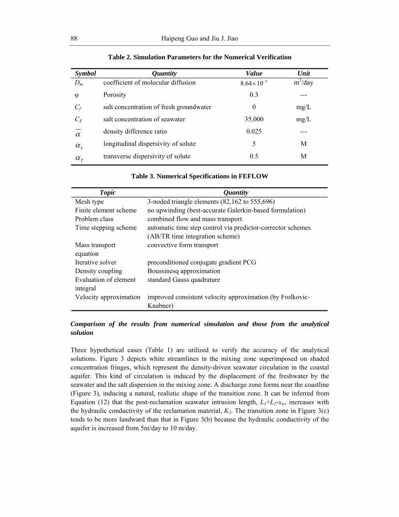
Table 2. Simulation Parameters for the Numerical Verification
Symbol Quantity Value UnitDm coefficient of molecular diffusion 58.64 10−× m2/day
φ Porosity 0.3 ---
Cf salt concentration of fresh groundwater 0 mg/L
CS salt concentration of seawater 35,000 mg/L
α density difference ratio 0.025 ---
Lα longitudinal dispersivity of solute 5 M
Tα transverse dispersivity of solute 0.5 M
Table 3. Numerical Specifications in FEFLOW
Topic QuantityMesh type 3-noded triangle elements (82,162 to 555,696)Finite element scheme no upwinding (best-accurate Galerkin-based formulation)Problem class combined flow and mass transportTime stepping scheme automatic time step control via predictor-corrector schemes
(AB/TR time integration scheme)Mass transportequation
convective form transport
Iterative solver preconditioned conjugate gradient PCGDensity coupling Boussinesq approximationEvaluation of elementintegral
standard Gauss quadrature
Velocity approximation improved consistent velocity approximation (by Frolkovic-Knabner)
Comparison of the results from numerical simulation and those from the analyticalsolution
Three hypothetical cases (Table 1) are utilized to verify the accuracy of the analyticalsolutions. Figure 3 depicts white streamlines in the mixing zone superimposed on shadedconcentration fringes, which represent the density-driven seawater circulation in the coastalaquifer. This kind of circulation is induced by the displacement of the freshwater by theseawater and the salt dispersion in the mixing zone. A discharge zone forms near the coastline(Figure 3), inducing a natural, realistic shape of the transition zone. It can be inferred fromEquation (12) that the post-reclamation seawater intrusion length, L1+L2-xtr, increases withthe hydraulic conductivity of the reclamation material, K2. The transition zone in Figure 3(c)tends to be more landward than that in Figure 3(b) because the hydraulic conductivity of theaquifer is increased from 5m/day to 10 m/day.

Changes of Coastal Groundwater Systems… 89
-100 -75 -50 -25 0 25 50Distance from the coastline (m)
0
5
10
15
20
25
Dis
tanc
e fro
m th
e bo
ttom
bou
ndar
y (m
)
Sea level
Recharge boundary
Seawater
Freshwater
(a)
-100 -75 -50 -25 0 25 50Distance from the coastline (m)
0
5
10
15
20
25
Dis
tanc
e fro
m th
e bo
ttom
bou
ndar
y (m
)
Seawater
Freshwater
(b)
-100 -75 -50 -25 0 25 50Distance from the coastline (m)
0
5
10
15
20
25
Dis
tanc
e fro
m th
e bo
ttom
bou
ndar
y (m
)
Seawater
Freshwater
(c)
Figure 3. Steady-state simulation results for the hypothetical examples. White streamlinessuperimposed on shaded concentration fringes show the seawater circulations. Only results of ahorizontal range of 150m besides the coastline are presented in order to compare the simulated mixingzones in different cases. (a) Hydraulic conductivity of the aquifer is 3m/day and no reclamation occurs.(b) Hydraulic conductivities of the original aquifer and the reclaimed aquifer are 3m/day and 5m/day,respectively. (c) Hydraulic conductivities of the original aquifer and the reclaimed aquifer are 3m/dayand 10m/day, respectively.

Haipeng Guo and Jiu J. Jiao90
-200 -150 -100 -50 0 50
0
5
10
15
20
25
Dis
tanc
e fro
m th
e bo
ttom
bou
ndar
y (m
)
Sea level
Recharge boundary
0.5Cs Isochlor
Analytical solution of the interface
Coastline before reclamation
Analytical solution of the water table
Numerical solution of the water table
K1 = 3 m/day
(a)
-200 -150 -100 -50 0 50
0
5
10
15
20
25
Sea level
0.5Cs Isochlor
Coastline after reclamationK1 = 3 m/day
K2 = 5 m/day
(b)
Sea level
0.5Cs Isochlor
Coastline after reclamation
-400 -300 -200 -100 0 100
Distance from the coastline
0
5
10
15
20
25
K1 = 3 m/dayK2 = 10 m/day
(c)
Figure 4. Steady state 0.5CS isochlors compared with saltwater interfaces obtained from the analyticalsolutions for three different cases. (a) Hydraulic conductivity of the aquifer is 3m/day and noreclamation occurs. (b) Hydraulic conductivity of the original aquifer and the reclaimed aquifer are3m/day and 5m/day. (c) Hydraulic conductivity of the original aquifer and the reclaimed aquifer are3m/day and 10m/day.
Figure 4 compares the 0.5Cs isochlors at steady state for the three cases in Table 1 withthe corresponding saltwater interfaces obtained from the analytical solutions. The accuracy ofthe analytical solution is somewhat limited by assumptions such as Dupuit-type flow and theGhyben-Herzberg relation. Because of these assumptions, the saltwater interfaces from the

Changes of Coastal Groundwater Systems… 91
analytical solutions do not completely agree with the 0.5Cs isochlors produced by thedensity-driven transport model. The 0.5 Cs isochlors are a little further seaward than the sharpinterface obtained from the analytical solutions. Comparisons of the water tables between thenumerical solutions and the analytical solutions show that the water tables calculated from theanalytical solutions are slightly higher than those from the numerical solutions. However,these differences are not very significant and the maximal difference is 0.5m, which is only2.5% of the elevation of the sea level in relation to the bottom boundary. Thus the simplifyingassumptions used in the analytical studies are testified to be reasonable.
2.1.3. Discussion of the Analytical Solutions
Change of the water level in the original aquifer
The change of the water table in the original aquifer between x = 0 and x = L1 induced byreclamation can be calculated from Equations (6), (7) and (9), which yields
2 2 2 2 2 21 1 2 2 0 1 0
1 2 1
1 1( ) (2 ) ( ) s s
f f
wh w L x L L L H L x HK K K
ρ ρρ ρ
⎡ ⎤Δ = − + + + − − +⎢ ⎥
⎣ ⎦(0 )tx x≤ ≤ (21)
2 2 2 2 21 1 2 2 0 1 0
1 2 1
( )1 1( ) (2 ) ( )s fs
f s
wh w L x L L L H L x H
K K Kρ ρρ
ρ ρ−⎡ ⎤
Δ = − + + + − − −⎢ ⎥⎣ ⎦
1( )tx x L< ≤ (22)
Equations (21) and (22) can be utilized to analyze sensitivity of the ground water tablechange to the hydraulic conductivity of the reclamation material and the scale of reclamation.The change of the water level at the original coastline, which is the maximum change in thedomain, can be readily obtained by setting 1x L= in Equation (22), which leads to
21 2 2 0 0
2
(2 ) s
f
wh L L L H HK
ρρ
Δ = + + − (23)
Equation (23) indicates the maximum buildup of the water level at the original coastlineis independent of K1, and increases with L1, L2, and the ratio between the recharge rate w andK2. For a specific coastal area, the parameters L1 and w are fixed so that the water levelbuildup at the original coastline mainly depends on the hydraulic conductivity of thereclamation material K2 and the reclamation length L2. The reclamation tends to have asignificant damming effect when L1 is great and K2 is low. This conclusion is the same as thatof the study by Jiao et al (2001) which ignored the seawater interface.

Haipeng Guo and Jiu J. Jiao92
Displacement of the tip of the saltwater tongue
Due to reclamation the position of the tip of the saltwater tongue moves towards the sea by adistance of tr tx x− , which can be obtained from Equations (8) and (12):
2 22 12 2 2 2
1 2 0 1 02 2
( ) ( )( ) s s f s s f
tr tf f
k kx x L L H L H
w wρ ρ ρ ρ ρ ρ
ρ ρ− −
− = + − − − (24)
For a particular coastal area, parameters L1, K1, w, and H0 are fixed, the change of the tipof the saltwater tongue depends mainly on L2 and K2. As mentioned early, this study assumesthat the tip of the saltwater tongue after reclamation is located in the reclaimed land whensteady state flow conditions are reached. In this case, the value tr tx x− is always positive,i.e. the tip of the saltwater interface will be pushed seaward after reclamation. Equation (24)shows that displacement of the tip, tr tx x− , is significant if the reclamation length L2 is great
and the hydraulic conductivity of the reclamation material K2 is low.
2.1.4. Hypothetical Example
The impact of the reclamation on the ground water level and the seawater-freshwaterinterface is discussed here with a hypothetical example. Assume that the saturated hydraulicconductivity K1 of the aquifer is 0.1 m/day and the distance from the ground water divide tothe original coastline, L1, is 1000m. The densities of seawater and freshwater are 1.025 g/cm3
and 1.000 g/cm3, respectively. The infiltration rate is 0.0005 m/day and H0 =20m.
0
5
10
15
20
25
0. 5 2. 5 4. 5 6. 5 8. 5
Hydr aul i c conduct i vi t y of r ecl amat i on mat er i al , K2( m/ day)
Wat
er le
vel c
hang
e (m
) L2 = 500 mL2 = 300 mL2 = 100 m
Figure 5. Change of ground water level at the original coastline with hydraulic conductivity of thereclamation materials when K1=0.1m/day, L1=1000m, sρ =1.025g/cm3, fρ =1.000g/cm3,
w=0.0005m/day, and H0=20m.

Changes of Coastal Groundwater Systems… 93
0
5
10
15
20
25
0 100 200 300 400 500 600 700 800 900 1000Di st ance f r om gr oundwat er di vi de ( m)
Wate
r le
vel
chan
ge(m
)
K2 = 0. 5 m/ dayK2 = 1 m/ dayK2 = 10 m/ day
Figure 6. Change of ground water level in the original unconfined aquifer with distance from theground water divide when K1=0.1m/day, L1=1000m, L2=500m, sρ =1.025g/cm3, fρ =1.000g/cm3,
w=0.0005m/day, and H0=20m.
The land reclamation will increase the water level in the original aquifer and push thesaltwater interface seaward. A comparison of predicted water levels at the original coastlineas a function of hydraulic conductivity and reclamation length shows that the water level riseat the original coastline after reclamation decreases with K2 and increases with L2 (Figure 5).The buildup of the water level at the original coastline can be great and is sensitive to K2
when K2 is low. When K2 is greater than 5 m/day, the water-level rise tends to be small andinsensitive to K2.
0
100
200
300
400
500
600
0. 1 1. 1 2. 1 3. 1 4. 1 5. 1 6. 1 7. 1 8. 1 9. 1 10. 1Hydr aul i c conduct i vi t y of t he r ecl amat i on mat er i al , K2( m/ day)
Disp
lace
ment
of
the
tip(
m)
L2 = 500 mL2 = 300 mL2 = 100 m
Figure 7. Displacement of the tip of the saltwater tongue with hydraulic conductivity of the reclamationmaterials for different reclamation lengths when K1=0.1m/day, L1=1000m, sρ =1.025g/cm3, fρ=1.000g/cm3, w=0.0005m/day, and H0=20m (Guo and Jiao, 2007).

Haipeng Guo and Jiu J. Jiao94
Figure 6 shows the change of ground water level in the original unconfined aquifer withdistance from the ground water divide when L2=500m. The rise of the water level increaseswith the distance from the ground water divide and decreases with hydraulic conductivity ofthe fill materials. For any fixed value of K2, the water level change is sensitive to distancefrom the water divide and can be significant at positions close to the original coastline. Thewater-level rise is much more sensitive to K2. With L2 = 500 m the increase is 20.7 m for K2 =0.5 m/day and only 1.7 m for K2 = 10 m/day. The maximum water level rise is located at theoriginal coastline.
Figure 7 shows the displacement of the tip of the saltwater tongue, which is defined asxtr-xt, as a function of L2 and K2. The displacement of the tip decreases with K2 and increaseswith L2, and is usually less than L2 when K2 > K1. The displacement is slightly greater than L2
when K2 =K1 because the tip is pushed much more seaward due to the increased recharge inthe reclaimed land. The displacement of the tip decreases almost linearly with K2, indicatingthat the post-reclamation saltwater tongue can be significantly longer than the initial onewhen K2 is great. After reclamation, the saltwater interface is pushed seaward, which maybenefit groundwater wells screened close to the saltwater interface.
2.1.5. Application: a Case Study in Shenzhen, China
The study site covers a major reclamation area to the southwest of Shenzhen, China (seeFigure 8). The rapid urban development has led to a sharp increase in the demand for usableland in this area during the past 20 years, and large-scale land reclamation by filling theshallow sea has been a common practice to ease this demand. Figure 8 shows the originalcoastline in 1983 and the coastline in 2000 around the Deep Bay, Shenzhen. The water divideis located about 4.2 km north of the reclamation area and lies along topographical peaks andridges. Between 1983 and 2000, the coastline has been pushed towards the sea by a distanceof approximately 700 m due to a series of reclamation projects.
Figure 8. Change of the coastline due to reclamation in Shenzhen, China between year 1983 and year2000.

Changes of Coastal Groundwater Systems… 95
The study area around Deep Bay is underlain mainly by weathered igneous rock. Ding(2006) analyzed the measured hydraulic conductivity values of the weathered granite andconcluded that average hydraulic conductivity value was of the order of 10-6 m/s. In theanalytical study, the hydraulic conductivity of the original aquifer K1 is assumed to be
6100.1 −× m/s. The approximate hydraulic conductivity of the fill material in this area is ofthe order of 10-4 m/s. The climate of this area is subtropical humid with hot wet summer andmild dry winter, and the average annual rainfall is about 1837 mm. The recharge coefficient ishere taken as 0.1 over a long-term basis, which leads to an annual infiltration rate of about184mm. The average reclamation thickness in Deep Bay is about 10 m. According toEquations (22) and (24), the estimated values are very sensitive to hydraulic conductivity ofthe fill material K2, which is uncertain in the field. If 4
2 100.2 −×=K m/s, the estimatedchange of the water level at the original coastline is 6.9m. Because of the reclamation, thesaltwater tongue will be pushed to the new coastline, and the displacement of the tip of thetongue is estimated to be 691m based on (24). The change of the water level at the originalcoastline and the displacement of the tip are estimated to be 3.3m and 677m when K2 isincreased to be 4100.5 −× m/s.
2.2. Impact of Reclamation on Ground Water Travel Time
According to the Dupuit theory, the flow in the unconfined aquifer is considered horizontaland one dimensional, and the ground water discharge per unit width of aquifer is defined as:
x xdhQ Kb q bdx
= − = (25)
where Qx is the ground water discharge per unit width (L2/T), K is the saturated hydraulicconductivity(L/T), b is the thickness of the fresh groundwater (L) , h is the hydraulic head (L),and qx is specific discharge or Darcy flux (L/T).
In the unconfined systems (Figure 1), infiltration occurs at a constant rate w along theentire upper boundary of the aquifer. The ground water discharge per unit width of aquiferaffected by a uniform recharge is
xQ w x= (26)
Since the vertical component of the flow velocity is neglected, the ground water velocityv (L/T) can be expressed as:
xx
e
d x qvd t n
= = (27)

Haipeng Guo and Jiu J. Jiao96
where ne is the effective porosity of the porous medium. Closed-form solutions for travel timet (T) of a water particle to move between two arbitrary positions xi (at time ti) and x (at time t)in the unconfined aquifer can be obtained by combining Equations (25), (26) and (27), whichleads to
( )i i
t xe
t x
n bd t dw
τ ττ
=∫ ∫ (28)
Based on Equation (28), Chesnaux et al. (2005) developed an analytical solution tocalculate ground water transit time in a Dupuit-type flow system bounded by lakes or rivers(Figure 9). Figure 9 shows the unconfined system used for developing the analytical solution.The left-hand boundary is groundwater divide, and ground water discharges through the right-hand fixed-head boundary. The solution of the transit time from an arbitrary point at which x= xi (assuming the travel path begins at the water table) can be expressed as:
2 2
' '
2' 1 1 1 1
'
2
1( ) ( ln )
1i
i ii e iL x
x xt x n L x
w KL L
ζ ζ
ζ ζζ
ζ ζ
+ −= − − − +
+ −
(29)
where 2 2'' /LL K h wζ = + , L’ represents the length of the unconfined aquifer
system, and hL’ is the fixed-head of the right-hand boundary.
Figure 9. The unconfined system used for developing the analytical solution by Chesnaux et al. (2005).The left-hand boundary is groundwater divide, and ground water discharges through the right-handfixed-head boundary.

Changes of Coastal Groundwater Systems… 97
2.2.1. Analytical Solution for the Ground Water Travel Time before Reclamation
Analytical Solution
When seawater-freshwater interface is considered, the thickness of the cross-sectional areathrough which flow occurs will not be always equal to the water head. Change of thickness offreshwater with distance towards the left boundary can be obtained from Equations (2), (3),(6) and (7). The final solutions are
2 2 21 0
1
( ) (0 ) st
f
wb h L x H x xK
ρρ
= = − + ≤ ≤ (30)
2 201 1
1
( ) ( ) ( )( )
s st
s f s f
h H wb L x x x LK
ρ ρρ ρ ρ ρ
−= = − ≤ ≤
− −(31)
Substituting Equations (30) and (31) into Equation (28), one has:
2 2
1i i
t xe
t x
n xd t d xxw K
ω −=∫ ∫ ( 0 )tx x≤ ≤ (32)
2 21
1 ( )i i
t xs
et xs f
L xd t n d x
w K xρρ ρ
−=
−∫ ∫ 1( )a x L≤ ≤ (33)
where 2 211 0
s
f
KL Hw
ρωρ
= +
The solution to Equations (32) and (33) leads to:
2 22 2 2 2
2 21
1 lni
ti
e iti
x xd t n x xw K xx
ω ωω ω ωω ω
⎡ ⎤⎛ ⎞+ −⎢ ⎥⎜ ⎟= − − − −⎜ ⎟⎢ ⎥+ −⎝ ⎠⎣ ⎦
∫
( 0 )tx x≤ ≤ (34)
2 22 2 2 2 1 1
1 1 1 2 21 1 1
ln( )i
ts i
e its f i
L L x xdt n L x L x LwK xL L x
ρρ ρ
⎡ ⎤⎛ ⎞+ −⎢ ⎥⎜ ⎟= − − − −
⎜ ⎟− ⎢ ⎥+ −⎝ ⎠⎣ ⎦∫
1( )tx x L≤ ≤ (35)

Haipeng Guo and Jiu J. Jiao98
Integrating Equations (34) and (35) with respect to x from x0 to x1 yields the travel timeof water flow from one position (x = x0) to another position (x = x1) in the unconfined aquiferbefore reclamation. If x1= L1, the resultant travel time is the transit time of a particle of wateroriginating at x = x0 before reclamation. The total travel time will be the sum of the traveltimes for each discrete segment if discrete segments of the flow path have different aquiferproperties.
Comparison of the solutions with and without considering seawater interface
A hypothetical example is used here to compare the new analytical solution with the transittime solution developed by Chesnaux et al. (2005), which didn’t include the influence ofseawater-freshwater interface and can be expressed as Equation (29). Assume the distancefrom the ground water divide to the coastline is 1000m, and the effective porosity of theaquifer is 0.3. The difference between the groundwater travel time with and without theseawater-freshwater interface is defined as
N e w C h e s n a u xt t tΔ = − (36)
where tNew and tChesnaux represent the groundwater travel time calculated from the newanalytical solution in this paper and from Equation (29) developed by Chesnaux et al. (2005),respectively.
Figure 10 shows the differences (defined by Equation 36) of transit times to the sea fromdifferent positions in the aquifer with distance from the water divide for different sea levelswhen w = 0.0005 m/day and K1 = 3 m/day. The calculated water level becomes higher whenthe impact of the seawater-freshwater interface is considered. Thus, the thickness of thefreshwater between the water divide and the tip of the saltwater tongue will be greater,thereby decreasing the flow velocity. However, the groundwater flow velocity tends to begreater in the area between the tip and the coastline due to decrease of the freshwaterthickness in this area. Therefore, as shown in Figure 10, differences of transit times decreasewith the distance from groundwater divide, and tend to be positive close to the water divideand negative near the coastline. When H0 is greater, differences of the transit times will bemore significant because the seawater intrusion length tends to be greater according toEquation (8). With H0 = 30 m the difference is 188.1 days for x = 50m and -424.8 days forx=950m.
Figure 11 shows differences of transit times to the sea from different positions in theaquifer with distance from the water divide for different infiltration rates when K1 = 3 m/dayand H0 =20m. The curves in Figure 11 show the similar trends as those in Figure 10.According to Equation (8), the influence of the seawater intrusion will be great when therecharge rate w is low. Therefore, differences of the transit times to the sea tend to be moresignificant when the recharge rate w is low. With w = 0.0005 m/day the difference is 260.1days for x = 50m and -118.5 days for x=950m.
Figure 12 shows differences of the transit times with distance from the water divide fordifferent hydraulic conductivities of the aquifer when w = 0.0005 m/day and H0 =20m.According to Equation (8), the seawater intrusion length, L1-xt , becomes longer when K1 isincreased. In this case, the flow-velocity increase due to decrease of the freshwater thickness

Changes of Coastal Groundwater Systems… 99
between the tip and the coastline will be more significant and be in a greater area. Thus,differences of transit times decrease with K1. With the distance from the groundwater divideincreasing, the impact of the flow-velocity increase close to the coastline on the transit timewill become stronger. At the same time, the influence of the flow-velocity decrease due torise of the water table away from the coastline will diminish. Therefore, differences of thetransit times decrease with the distance from the groundwater divide.
.
- 500
- 400
- 300
- 200
- 100
0
100
200
300
0 200 400 600 800 1000Di st ance f r om gr oundwat er di vi de ( m)
Diff
eren
ces
of t
rans
it t
imes
(day
s)
Ho=10 mHo=20 mHo=30 m
Figure 10. Differences of transit times to the sea from different positions in the aquifer with distancefrom the water divide for different sea levels when K1=3m/day, L1=1000m, sρ =1.025g/cm3, fρ=1.000g/cm3, and w=0.0005m/day.
- 200
- 100
0
100
200
300
0 200 400 600 800 1000Di st ance f r om gr oundwat er di vi de ( m)
Diff
eren
ces
of t
rans
it t
imes
(day
s)
w=0. 0005 m/ dayw=0. 001 m/ dayw=0. 0015 m/ day
Figure 11. Differences of the transit times to the sea from different positions in the aquifer with distancefrom the left water divide for different infiltration rates when K1=3m/day, L1=1000m, sρ =1.025g/cm3,
fρ =1.000g/cm3, and H0 =20m.

Haipeng Guo and Jiu J. Jiao100
- 500
- 400
- 300
- 200
- 100
0
100
200
300
0 200 400 600 800 1000Di st ance f r om gr oundwat er di vi de ( m)
Diff
eren
ces
of t
rans
it t
imes
(day
s)
K1=3 m/ dayK1=5 m/ dayK1=10 m/ day
Figure 12. Differences of the transit times to the sea from different positions in the aquifer with distancefrom the water divide for different hydraulic conductivities of the aquifer when L1=1000m, sρ=1.025g/cm3, fρ =1.000g/cm3, w = 0.0005 m/day, and H0 =20m.
2.2.2. Analytical Solution for the Ground Water Travel Time after Reclamation
Analytical solution
After reclamation the coastline is pushed seaward by a distance of L2 so that an additionalaquifer forms and rain recharge takes place over a larger area (Figure 1b). The change of thefreshwater thickness with distance from the left boundary can be obtained from Equations (9),(10) and (11) as follows:
2 2 21 1 2 2 0 1
1 2
1 1( ) (2 ) (0 )s
f
b h w L x L L L H x LK K
ρρ
⎡ ⎤= = − + + + ≤ ≤⎢ ⎥
⎣ ⎦(37)
2 2 21 2 0 1
2
( ) ( )str
f
wb h L L x H L x xK
ρρ
⎡ ⎤= = + − + ≤ ≤⎣ ⎦ (38)
2 201 2 1 2
2
( ) ( ) ( )( )
s st r
s f s f
h H wb L L x x x L LK
ρ ρρ ρ ρ ρ
− ⎡ ⎤= = + − ≤ ≤ +⎣ ⎦− −(39)
Equations (37), (38) and (39) can be used to describe relation between thickness of thevertical cross section through which water flow occurs and the distance towards the waterdivide. Substituting these equations to equation (28) respectively and integrating the derivedequations, the following equations are obtained:

Changes of Coastal Groundwater Systems… 101
2 22 2 2 2
2 21
1 lni
ti
e iti
x xd t n x xw K xx
ϕ ϕϕ ϕ ϕϕ ϕ
⎡ ⎤⎛ ⎞+ −⎢ ⎥⎜ ⎟= − − − −⎜ ⎟⎢ ⎥+ −⎝ ⎠⎣ ⎦
∫
1(0 )x L≤ ≤ (40)
2 22 2 2 2
2 22
1 lni
ti
e iti
x xd t n x xw K xx
λ λλ λ λλ λ
⎡ ⎤⎛ ⎞+ −⎢ ⎥⎜ ⎟= − − − −⎜ ⎟⎢ ⎥+ −⎝ ⎠⎣ ⎦
∫
1( )trL x x≤ ≤ (41)
2 22 2 2 2
2 22
ln( )i
ts i
e its f i
L L x xdt n L x L x LwK xL L x
ρρ ρ
⎡ ⎤⎛ ⎞+ −⎢ ⎥⎜ ⎟= − − − −⎜ ⎟− ⎢ ⎥+ −⎝ ⎠⎣ ⎦
∫
1 2( )trx x L L≤ ≤ + (42)
where 2
2 1 1 01 1 2 2
2
(2 ) s
f
K K HL L L LK w
ρϕρ
= + + + , 2
2 2 01 2( ) s
f
K HL Lw
ρλρ
= + + .
Discussion of the analytical solutions
The changes of groundwater travel times due to the coastal reclamation are herediscussed with a hypothetical example. Assume that the saturated hydraulic conductivity ofthe original aquifer is 3 m/day and the distance from the ground water divide to the originalcoastline is 1000m. The infiltration rate is 0.0005 m/day and H0 =20m.
0
5
10
15
20
25
30
35
0. 5 1. 5 2. 5 3. 5 4. 5 5. 5 6. 5 7. 5 8. 5 9. 5Hydr aul i c conduct i vi t y of t he r ecl amat i on mat er i al , K2( m/ day)
Cha
nges
of t
rans
it tim
es (y
ears
)
L2 = 500 mL2 = 300 mL2 = 100 m
Figure 13. Changes of transit times from a point at which x = 800m to the sea with hydraulicconductivity of the reclamation material for different reclamation lengths when K1 = 3 m/day, L1 = 1000m, sρ = 1.025 g/cm3, fρ = 1.000 g/cm3, w = 0.0005 m/day, and H0 = 20m.

Haipeng Guo and Jiu J. Jiao102
0
10
20
30
40
50
60
200 300 400 500 600 700 800 900Di st ance f r om gr oundwat er di vi de ( m)
Chan
ges
of t
rans
it t
imes
(ye
ars)
K2 = 1 m/ dayK2 = 5 m/ dayK2 = 10 m/ day
Figure 14. Changes of transit times to the sea from different positions in the original aquifer withdistance from the water divide for different hydraulic conductivity of the reclamation material when K1
= 3 m/day, L1 = 1000 m, L2=500m, sρ = 1.025 g/cm3, fρ = 1.000 g/cm3, w = 0.0005 m/day, and H0 =
20m.
Figure 13 shows changes of the transit times from a point at which x = 800m to the seawith hydraulic conductivity of the reclamation materials for different reclamation lengths.The increase of the transit times due to reclamation decreases when K2 increases and L2
decreases. This is easily understood because the damping effect due to reclamation will bemore significant when K2 decreases and L2 increases. With K2 = 0.5 m/day the change is 29.7years for L2 = 500 m and 5.5 years for L2 = 100 m, showing that changes of transit times arevery sensitive to the distance from the water divide. Changes of the transit times tend to below and insensitive to K2 when K2 is greater than 3m/day.
Figure 14 shows how transit times to the sea from different positions in the originalaquifer change with the distance from the water divide for different hydraulic conductivity ofthe reclamation materials when L2=500m. After reclamation, the water table in the wholeoriginal aquifer will increase so that the thickness of freshwater is increased and the waterwill flow more slowly. Therefore, as showed in Figure 14, the transit time changes increasefrom the original coastline to the water divide and tend to be more significant when K2
becomes low. With K2 = 1 m/day the change is 47.7 years for x = 200 m and 19.6 years for x= 950 m.
Figure 15 shows how ground water travel times from a point at which x = 800m to theoriginal coastline change with hydraulic conductivity of the reclamation materials fordifferent reclamation lengths. After reclamation groundwater flow in the original aquifertends to be slower so that the travel time becomes greater. This is because the reclamationincreases the water table so that the water will flow through a cross-sectional area of greaterheight. The influence of the reclamation on groundwater travel times in the original aquiferdiminishes gradually when K2 increases and L2 decreases, and becomes less sensitive to K2
when K2 is greater than 7 m/day. With L2 = 500 m the change is 7.7 years for K2 = 0.5 m/dayand 0.9 years for K2 = 10 m/day.

Changes of Coastal Groundwater Systems… 103
0
1
2
3
4
5
6
7
8
9
0. 5 1. 5 2. 5 3. 5 4. 5 5. 5 6. 5 7. 5 8. 5 9. 5Hydr aul i c conduct i vi t y of t he r ecl amat i on mat er i al , K2( m/ day)
Chan
ges
of t
rave
l ti
mes
(yea
rs)
L2 = 500 mL2 = 300 mL2 = 100 m
Figure 15. Changes of ground water travel times from a point at which x = 800m to the originalcoastline with different hydraulic conductivity of the reclamation materials for different reclamationlengths when K1 = 3 m/day, L1 = 1000 m, sρ = 1.025 g/cm3, fρ = 1.000 g/cm3, w = 0.0005 m/day, and
H0 = 20m.
0
5
10
15
20
25
30
35
200 300 400 500 600 700 800 900Di st ance f r om gr oundwat er di vi de ( m)
Chan
ges
of t
rave
l ti
mes(
year
s)
K2 = 1 m/ dayK2 = 5 m/ dayK2 = 10 m/ day
Figure 16. Changes of ground water travel times from different positions in the original aquifer to theoriginal coastline with distance from the water divide for different hydraulic conductivity of thereclamation material when K1 = 3 m/day, L1 = 1000 m, L2=500m, sρ = 1.025 g/cm3, fρ = 1.000 g/cm3,
w = 0.0005 m/day, and H0 = 20m.
Figure 16 shows the changes of ground water travel times from different positions in theoriginal aquifer to the original coastline with distance from the water divide for differenthydraulic conductivity of the reclamation materials when L2=500m. Since the ground water inthe whole original aquifer flows more slowly after reclamation, the increase of ground watertravel times decreases with the distance from the ground water divide, which is similar tocurves in Figure 14. When K2 is low, the influence of the reclamation on groundwater flowwill be more significant so that the changes of ground water travel times are greater. With K2

Haipeng Guo and Jiu J. Jiao104
= 1 m/day the change is 29.4 years for x = 200 m and 1.3 years for x = 950 m, indicating thatchanges of travel times are very sensitive to the distance towards the water divide.
2.3. Impact of Reclamation on Streamline Pattern and Flow Velocity
It is well known that recharge can cause the spreading of contaminants (e.g. plume diving),which should be considered when placing wells at sites. The streamlines originating at thelocations for the source of contaminants can be used to decide how much spreading ofcontaminants to expect at a point down gradient from the source.
Streamline calculation
The calculation method will be applicable for a case of one-dimensional shallow flow ina water table aquifer receiving an infiltration of a constant rate along the entire upperboundary (Figure 17). The base of the aquifer is assumed to be horizontal and impermeable.Water entering the aquifer due to recharge along the water table would move down gradientalong the streamline. In a Dupuit-type water table aquifer recharged by surface infiltrationand discharged by a down-gradient, fixed-head boundary, the flux is related to the recharge,w, by
)( 0x-xwQx = (43)
where Qx is the discharge per unit width (L2/T), and x0 is the location of the upgradient waterdivide. The total discharge in the x direction per unit width, through a vertical cross section ofheight b(x) is partitioned by the streamline originating at x = xs (Strack ,1984), which leads to
00 )()(
)()(
xxxx
xxwxxw
QQQ
xbxD
QQ ss
x
sx
x
tx
−−
=−−
=−
== (44)
Figure 17. The streamline in an unconfined system recharged only by infiltration and discharged by adown-gradient, fixed-head boundary.

Changes of Coastal Groundwater Systems… 105
where Qxt is discharge above the streamline, Qx is the total discharge, and D(x) is the depth of
the streamline below the water table. Note that (44) implies that Dupuit assumption applies,i.e., equipotential surfaces are vertical and the flow is essentially horizontal. In other words,the water head h(x) and the specific discharge q(x) are constant over the height of the aquifer.Thus the depth of the streamline below the water table, D(x), can be obtained as:
)()(0
xbxxxxxD s
−−
= (45)
Discussion of the analytical solutions
The streamlines can be calculated by combing Equations (30)-(31), (37) - (39), and (45).Assume that the saturated hydraulic conductivity K1 of the aquifer is 0.1 m/day and thedistance from the ground water divide to the original coastline, L1, is 1000m. The densities ofseawater and freshwater are 1.025 g/cm3 and 1.000 g/cm3, respectively. The infiltration rate is0.0005 m/day and H0 =20m. The hydraulic conductivity of the reclamation material, K2, is 0.5m/day and the reclamation length, L2, is 500 m.
Figure 18 shows that how the water table and the streamline originating at x = 500mchange before and after reclamation. One can see that the water table in the original aquiferincreases significantly after reclamation. The streamline originating at x=500m also increasesso that it may intersect the well (Figure 18). After reclamation the contaminants may entersome wells due to the increase of the elevation of the streamline originating from the sourceof contaminants, which should be considered when placing wells. One can also see that therecharged water will move across a vertical cross section of greater height so that the flowvelocity becomes slower.
Water table after reclamation
500 750 1000 1250 1500Distance from the water divide (m)
0
20
40
60
80
Dis
tanc
e fro
m th
e b
otto
m (m
)
Water table before reclamation
Streamline after reclamation
Streamline before reclamation
Well
Figure 18. The water table and streamline originating at x = 500 m before and after reclamation,respectively (K1=0.1m/day, K2=0.5m/day, L1=1000m, L2=500m, sρ =1.025g/cm3, fρ =1.000g/cm3,
w=0.0005m/day, and H0=20m).

Haipeng Guo and Jiu J. Jiao106
0 250 500 750 1000Distance from the left water divide (m)
0
0.01
0.02
0.03
Spe
cific
dis
char
ge (m
/day
)Specific discharge before reclamation
Specific discharge after reclamation
Figure 19. The specific discharge with distance from the water divide in the original aquifer before andafter reclamation (K1=0.1m/day, K2=0.5m/day, L1=1000m, L2=500m, sρ =1.025g/cm3, fρ=1.000g/cm3, w=0.0005m/day, and H0=20m).
Figure 19 shows how the specific discharge (Darcy flux) defined by Equation (25)changes before and after reclamation. The discharge per unit width will increase and thethickness of freshwater will decrease with distance from the water divide. Thus, as showed inFigure 19, the specific discharge increases with the distance from the water divide. Afterreclamation the height of the vertical cross section through which freshwater flows becomesgreater because the reclamation increases the water table in the original aquifer. Thedischarge defined by Equation (43) remains unchanged so that the specific dischargedecreases. As discussed previously, the maximal water level increase due to reclamation is atthe original coastline, and the flow velocity at the water divide is always zero. Therefore, afterreclamation the specific discharge becomes lower than that before reclamation especially inareas close to the original coastline.
3. Impact of Land Reclamation in an Island
When the reclamation scale is relatively small compared to the size of the originalgroundwater catchment, the previous assumption that the water divide remains unchanged(Figure 1) is valid. In the situation of an island the water divide may be moved when large-scale land reclamation occurs. In this case the reclamation on one side may change the groundwater flow on both sides of the island.
3.1. Impact of Reclamation on Ground Water Level and Saltwater Interface
Two kinds of islands are considered, both with ground water flow resulting from precipitationrecharge. In these two different kinds of islands, the unconfined flow system is bounded at thebottom by a horizontal impermeable layer (Figure 20) and by a saltwater-freshwater interface(Figure 27), respectively.
Changes of Coastal Groundwater Systems… 107
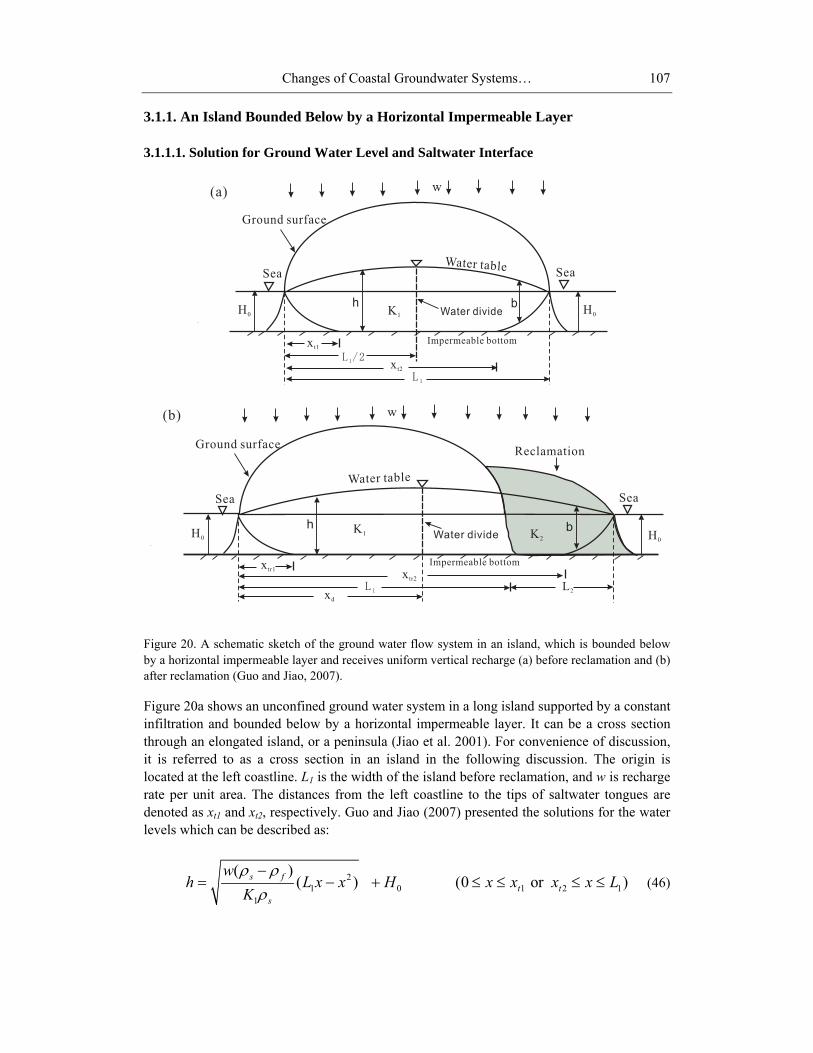
3.1.1. An Island Bounded Below by a Horizontal Impermeable Layer
3.1.1.1. Solution for Ground Water Level and Saltwater Interface
L1/2
Ground surface
Water tableSea
H0
Sea
H0
w
Impermeable bottomxt1
xt2
K1
(a)
h bWater divide
L1
L1
Ground surface
Water table
Sea
H0
Sea
H0
w
Impermeable bottomxtr1
K1
(b)
xtr2
K2
L2
Reclamation
h bWater divide
xd
Figure 20. A schematic sketch of the ground water flow system in an island, which is bounded belowby a horizontal impermeable layer and receives uniform vertical recharge (a) before reclamation and (b)after reclamation (Guo and Jiao, 2007).
Figure 20a shows an unconfined ground water system in a long island supported by a constantinfiltration and bounded below by a horizontal impermeable layer. It can be a cross sectionthrough an elongated island, or a peninsula (Jiao et al. 2001). For convenience of discussion,it is referred to as a cross section in an island in the following discussion. The origin islocated at the left coastline. L1 is the width of the island before reclamation, and w is rechargerate per unit area. The distances from the left coastline to the tips of saltwater tongues aredenoted as xt1 and xt2, respectively. Guo and Jiao (2007) presented the solutions for the waterlevels which can be described as:
21 0 1 2 1
1
( )( ) (0 or )s f
t ts
wh L x x H x x x x L
Kρ ρ
ρ−
= − + ≤ ≤ ≤ ≤ (46)
Haipeng Guo and Jiu J. Jiao108
2 21 0 1 2
1
( ) ( )st t
f
wh L x x H x x xK
ρρ
= − + ≤ ≤ (47)
At the tip of the saltwater tongue, the water head is equal to 0/s fHρ ρ (see Equation 4).
Set h equal to 0/s fHρ ρ in either (46) or (47), one has
212 2
1 02
( )0 s s f
f
Kx L x H
wρ ρ ρ
ρ−
− + = (48)
The locations of the tips of saltwater tongues can be readily obtained by solving Equation(48) for xt1 and xt2.
Figure 20b shows the unconfined ground water flow system in the island afterreclamation. The hydraulic conductivity of the reclamation material and the reclamationlength are denoted as K2 and L2, and the post-reclamation groundwater divide is locatedat dx x= . After reclamation, the distances from the left coastline to the tips of saltwatertongues are represented as xtr1 and xtr2, respectively. The solutions for the water level and theposition of the ground water divide are (Guo and Jiao, 2007):
2 21 2 1 1
1 2 2 1
( )2( )d
K L K K LxL K L K+ −
=+
(49)
20 1
1
( )( ) 0 s f
t rs
wh x x H x x
Kρ ρ
βρ−
= − + ≤ ≤ (50)
2 20 1 1
1
( ) str
f
wh x x H x x LK
ρβρ
= − + ≤ ≤ (51)
2 20 1 2
2
( 2 / ) str
f
wh x x w H L x xK
ρβ γρ
= − + + ≤ ≤ (52)
20 2
2
( )( 2 / ) s f
t rs
wh x x w H x x L
Kρ ρ
β γρ−
= − + + ≤ ≤ (53)
where 2 21 2 1 1 1 2 2 1= ( ) /( )K L K K L L K L Kβ ⎡ ⎤+ − +⎣ ⎦ and 1 2 2 1 1 2 2 1= ( ) /(2 2 )wL L L K K L K L Kγ − + .
Set h equal to 0/s fHρ ρ in either (50) or (51), one has

Changes of Coastal Groundwater Systems… 109
212 2
02
( )0 s s f
f
Kx x H
wρ ρ ρ
βρ−
− + = (54)
The distance from the left coastline to the tip of the saltwater tongue on the unreclaimedside, xtr1, is one root of equation (54). Similarly, set h equal to 0/s fHρ ρ in either (52) or (53),
the location of the tip of the saltwater tongue on the reclaimed side, xtr2, can be obtained as aroot of the following equation:
222 2
02
( )2 / 0 s s f
f
Kx x H w
wρ ρ ρ
β γρ−
− + − = (55)
Solving (54) and (55) for the tip locations is not difficult, but the process is cumbersomeand is not shown here.
An important influence of the reclamation on the ground water flow system is that thewater divide is displaced. The displacement of the water divide, dΔ , can be calculated as
1 1 2 1 2
1 2 2 1
( )2 2( )dL K L L Ld x
L K L K+
Δ = − =+
(56)
Equation (56) shows that the ground water divide will move toward the post-reclamationcoastline, implying that ground water discharge to the sea on the left is increased. Thedisplacement of the water divide is significant when K1 is great. For a particular coastal area,the parameters L1 and K1 are fixed. In this case, Equation (56) implies that he displacement ofthe water divide, dΔ , increases with L2 and decrease with K2. One can also see that thedisplacement of the water divide has nothing to do with the recharge rate w and the elevationof the sea level H0.
3.1.1.2. Discussion of the Analytical Solutions Using a Hypothetical Example
A hypothetical example is employed to study the influence of the reclamation on groundwater level and seawater-freshwater interface in an island bounded below by a horizontalimpermeable layer. Assume that the width of the island before reclamation L1 and thehydraulic conductivity of the original aquifer K1 are 2000m and 0.1 m/day, respectively. Theinfiltration rate is taken as 0.0005 m/day and H0 = 20m. The densities of seawater andfreshwater are 1.025 g/cm3 and 1.000 g/cm3, respectively.
Change of the water level in the original aquifer
A comparison of predicted water levels at the original coastline on the reclaimed side (Figure21) shows that the rise of the water level decreases with K2 and increases with L2. For a fixedvalue of L2, the water level change tends to be sensitive to K2 when K2 is low. With L2 = 500m the change is 20 m for K2 = 0.5 m/day and only 1.7 m for K2 = 10 m/day, which indicates

Haipeng Guo and Jiu J. Jiao110
that the water level change can be very sensitive to K2. The reclamation results in rise of thewater table throughout the island (Figure 22), thereby increasing the volume of thefreshwater. The water-table rise decreases with K2 and increases with distance towards the leftcoastline. The shape of the water table in the original aquifer tends to be asymmetric afterreclamation due to displacement of the water divide, as indicated by Equation (56). There isan obvious jump for the hydraulic gradient at the original coastline on the reclaimed side.
0
5
10
15
20
25
0. 5 1. 5 2. 5 3. 5 4. 5 5. 5 6. 5 7. 5 8. 5 9. 5Hydr aul i c conduct i vi t y of r ecl amat i on mat er i al , K2( m/ day)
Wate
r le
vel
chan
ge(m
) L2 = 500 m
L2 = 300 m
L2 = 100 m
Figure 21. Change of the water level at the original coastline with hydraulic conductivity of thereclamation material for different reclamation lengths when K1=0.1m/day, L1=2000m, sρ=1.025g/cm3, fρ =1.000g/cm3, w=0.0005m/day, and H0=20m.
20
40
60
80
0 500 1000 1500 2000 2500Di st ance f r om t he coast l i ne on t he unr ecl ai med si de ( m)
Grou
ndwa
ter
leve
l (m
)
K2 = 0. 5 m/ dayK2 = 1 m/ dayK2 = 3 m/ dayBef or e r ecl amat i on
Figure 22. Water tables in the island with the distance from the coastline on the unreclaimed side fordifferent hydraulic conductivity of the reclamation material when K1=0.1m/day, L1=2000m, L2=500m,
sρ =1.025g/cm3, fρ =1.000g/cm3, w=0.0005m/day, and H0=20m (Guo and Jiao, 2007).

Changes of Coastal Groundwater Systems… 111
Displacement of the tip of the saltwater tongue
0
100
200
300
400
500
600
0. 5 2. 5 4. 5 6. 5 8. 5
Hydr aul i c conduct i vi t y of r ecl amat i on mat er i al , K2( m/ day)
Disp
lace
ment
of
the
tip(
m)L2 = 500 mL2 = 300 mL2 = 100 m
Figure 23. Displacement of the tip of the saltwater tongue on the reclaimed side with hydraulicconductivity of the reclamation material when the reclamation lengths are 500m, 300m and 100m,respectively (K1=0.1m/day, L1=2000m, sρ =1.025g/cm3, fρ =1.000g/cm3, w=0.0005m/day, and
H0=20m).
Predicted displacement of the tip of the saltwater tongue on the reclaimed side as a functionof the hydraulic conductivity of the reclamation material and reclamation length is presentedin Figure 23, which shows the displacement of the tip decreases with K2 and increases withL2. After reclamation, the saltwater interface on the reclamation side is pushed toward thepost-reclamation coastline, which in turns increases the volume of the freshwater. Thedisplacement of the tip is similar to the results in Figure 7. For the sake of convenience, it isnot presented here the influence of the reclamation on the saltwater tongue on theunreclaimed side. After reclamation, the water divide moves toward the reclaimed side,increasing the ground water discharge to the sea on the unreclaimed side. Thus, the saltwaterinterface on the unreclaimed side will also move seaward. Therefore, for a large-scale landreclamation project, the changes of ground water flow and seawater-freshwater interface overthe whole island should be taken into account. Usually, reclamation will increase the volumeof the freshwater, a valuable water resource in the island situation.
Change of the discharge to the sea on the unreclaimed side
Based on Equation (56), the percentage increase in flow to the sea on the unreclaimed side( 1 1100 2 / 200 /w d wL d L× Δ = Δ ) is plotted with the ratio of the reclamation length (L2) toisland width (L1) (Figure 24). The percentage increase in flow increases with the ratio of thereclamation length to island width and decreases with K2. With L2 = 500 m, i.e., the ratio ofthe reclamation length to island width is 0.25, the percentage increase in flow to the sea onthe unreclaimed side is 6% for K2 = 0.5 m/day and 1% for K2 = 3 m/day, indicating that theincrease in discharge to the sea on the unclaimded side is very sensitive to K2.

Haipeng Guo and Jiu J. Jiao112
0
2
4
6
0 0. 05 0. 1 0. 15 0. 2 0. 25
Rat i o of t he r ecl amat i on l engt h t o i sl and wi dt h
Perc
enta
ge i
ncre
ase
in f
low
K2 = 0. 5 m/ dayK2 = 1 m/ dayK2 = 3 m/ day
Figure 24. Percentage increase in the freshwater discharge to the unreclaimed side of the island versusthe ratio of the reclamation length to island width for different K2 when K1=0.1m/day, L1=2000m, sρ=1.025g/cm3, fρ =1.000g/cm3, w=0.0005m/day, and H0=20m (Guo and Jiao, 2007).
Change of the streamline pattern and flow velocity
0
20
40
60
80
0 500 1000 1500 2000 2500
Di st ance f r om l ef t coast l i ne ( m)
Dist
ance
fro
m th
e bo
ttom
(m)
Wat er t abl e af t er r ecl amat i onSt r eaml i ne bef or e r ecl amat i onSt r eaml i ne af t er r ecl amat i onWat er t abl e bef or e r ecl amat i on
Figure 25. Change of the streamline pattern originating at x=500m and 1500m due to land reclamationwith distance from the coastline on the unreclaimed side when K1 = 0.1 m/day, K2 = 0.5 m/day, L1 =2000 m, L2 = 500 m, sρ = 1.025 g/cm3, fρ = 1.000 g/cm3, w = 0.0005 m/day, and H0 = 20 m.
Figure 25 shows streamlines originating at x=500m and 1500m before and after reclamation.One can see that the elevations of streamlines on both sides of the island increase. On theunreclaimed side the streamline increases slightly more greatly than the water table so that therecharged water moves through a vertical cross section of lower height and the flow velocityof ground water becomes greater. On the reclaimed side, however, the water will flow moreslowly because the increase of the streamline elevation is less than that of the water table.

Changes of Coastal Groundwater Systems… 113
Figure 26 shows how the specific discharge and the water divide change in the originalaquifer system before and after reclamation. Before reclamation the specific dischargedecreases from the left coastline to the water divide and then increases gradually towards thecoastline on the right. After reclamation, the specific discharge tends to increase on theunreclaimed side and decreases on the reclaimed side. The two curves intersect at a point inthe area between the original water divide and the post-reclamation water divide. Theinfluence of the reclamation on the flow velocity on the reclaimed side tends to be moresignificant than that on the unreclaimed side, and the influence increases with the distancefrom the left coastline.
Water divide after reclamation
0 250 500 750 1000 1250 1500 1750 2000Distance from the left coastline (m)
0
0.004
0.008
0.012
0.016
0.02
Spe
cific
dis
char
ge (m
/day
) Water divide before reclamation
Specific discharge before reclamation
Specific discharge after reclamation
Figure 26. The specific discharge and the water divide in the original aquifer before and afterreclamation (K1=0.1m/day, K2=0.5m/day, L1=2000m, L2=500m, sρ =1.025g/cm3, fρ =1.000g/cm3,
w=0.0005m/day, and H0=20m).
3.1.2. An Island Bounded Below by Saltwater-freshwater Interface
L1/2
Ground surface
Water table
SeaSea
w
x
K1
(a)
hf
Water divide
L1
Freshwater
z
Saltwater
Figure 27. Continued on next page.

Haipeng Guo and Jiu J. Jiao114
Ground surface
Water table
SeaSea
w
x
K1
(b)
h1f
Water divide
L1
Freshwater
z
Saltwater
d
h2f
K2
L2
x d
Figure 27. A schematic sketch of the ground water flow system beneath an oceanic island, which isbounded on the bottom by saltwater-freshwater interface and receives uniform vertical recharge :(a)before reclamation; (b) after reclamation.
3.1.2.1. Analytical Solution for Ground Water Level and Saltwater Interface
Figure 27a shows an approximate description of a long oceanic island supported by a constantrainfall infiltration rate. The freshwater lens, floating on top of sea water, is bounded aboveby a phreatic surface and below by a seawater-freshwater interface. The flow of the salt waterbeneath the interface may be neglected if the aquifer is thick. Here, x is the horizontaldistance which origins at the left shoreline, L1 is the original width of the island, w is theuniform vertical recharge rate per unit area, and K1 is the hydraulic conductivity of theaquifer. The ocean surface is taken as the datum for the water head of fresh water hf(x), andz(x) denotes the depth of the saltwater-freshwater interface below the sea level. The governingequation for freshwater flow based on Dupuit assumption and Ghyben-Herzberg relation is:
1 1( / 2) (1 ) ff
dhw x L K h
dxδ− = − + (57)
where /( )f s fδ ρ ρ ρ= − . The boundary conditions are hf = 0 at x = 0 ( or L1 ) and dhf / dx
= 0 at x = L1/2 . The solution to equation (57) is
21
1
( )(1 )fwh L x x
K δ= −
+(58)
The expression (58) is identical to the solution presented by Henry (1964) and Fetter(1972).

Changes of Coastal Groundwater Systems… 115
Figure 27b shows the unconfined ground water flow system after reclamation. Thereclamation length and the hydraulic conductivity of the reclamation material are denoted asL2 and K2, respectively. The water depth of the shallow sea is d. The water divide will shift tothe right due to reclamation because ground water cannot discharge to the sea on the right asfreely as it was before reclamation. Assuming that the water divide after reclamation is at x =xd, the mathematical model can be described as:
11 1( ) (1 ) f
d f
dhw x x K h
dxδ− = − +
1(0 )x L≤ ≤ (59)
2 22 2 1 2( ) ( ) ( )f f
d f f
dh dhw x x K h d K h d
dx dxδ− = − + − −
1 1 2( )L x L L≤ ≤ + (60)
with boundary conditions
1 (0) 0fh =(61)
2 1 2( ) 0fh L L+ =(62)
and the continuity conditions of ground water head and flux at the position where x = L1 are
1 1 2 1( ) ( )f fh L h L=(63)
1 1 2 1( ) ( )q L q L= , or
1 2 21 1 2 2 1 2(1 ) ( ) ( )f f f
f f f
dh dh dhK h K h d K h d
dx dx dxδ δ+ = + + −
(64)
where h1f and h2f are the water head of fresh water in the original aquifer and the reclamationarea, respectively. The solution of Equations (59) and (61) is
21
1
(2 )(1 )f dwh x x x
K δ= −
+ 1(0 )x L≤ ≤ (65)
The solution of Equations (60) and (62) is
22 12 2 1 2
2 21 2 1 2 1 1 2
( )2
( ) ( ) ( )2 2
f f
d d
K K h d K K h
w wwx x x L L wx L L L x L L
δ++ − =
− + + − + < ≤ +(66)

Haipeng Guo and Jiu J. Jiao116
The following equation can be obtained by combining Equations (63), (64), (65) and (66):
2 21 2 1( ) 0t t L L Lκ ν+ − + = (67)
where
21 1
1
(2 )(1 ) dwt x L L
K δ= −
+ , (68)
1 2 2 1 1 1 2
2
( )L K L K K L LwLδκ + + +
=(69)
1 2 1
2
2 ( )dL K KwL
ν −=
(70)
The solution to Equations (67) through (70) is
21 1
1
(1 )2 2dL K tx
wLδ+
= +(71)
2 21 2 14 ( )2L L L
tν κ ν
κ+ + −
=(72)
The solutions for ground water level and the seawater-freshwater interface afterreclamation can be obtained with the combination of Equations (65), (66), (71) and (72). Itshould be noted that the ocean level is not involved in all these equations, indicating that theocean level does not impact the shape and, thus, the volume of freshwater. However, asdiscussed previously, the volume of freshwater lens can be greatly impacted by the sea levelif the island is bounded below by a horizontal impermeable bottom.
Equation (71) shows the water divide moves towards the coastline on the reclaimed sideafter reclamation, the change in the water divide is calculated as
21 1
1
(1 )2 2dL K td x
wLδ+
Δ = − = (73)
The increased freshwater discharge to the sea on the unreclaimed side is calculated as:
21
1
(1 )2
K tw dLδ+
Δ =(74)

Changes of Coastal Groundwater Systems… 117
3.1.2.2. Discussion of the Analytical Solutions Using a Hypothetical Example
A hypothetical example is employed to study the influence of the reclamation on the groundwater flow pattern and the seawater-freshwater interface. Assume that the distance betweenthe coastlines before reclamation L1 and the hydraulic conductivity of the original aquifer K1
are 2000m and 0.1 m/day, respectively. The infiltration rate is taken as 0.0005 m/day. Thedensities of seawater and freshwater are 1.025 g/cm3 and 1.000 g/cm3, respectively.
Change of the water level at the original coastline and displacement of the water divide
Figure 28 shows how the water level at the original coastline changes with K2 for differentreclamation lengths when the reclamation depth d is 20m. The water-level rise decreases withK2 and increases with L2. The water level buildup is very sensitive to the reclamation lengthand the hydraulic conductivity of the reclamation material. The increase of the water table is9.3 m with K2 = 0.5 m/day and L2 = 500 m, and is only 0.3 m with K2 = 10 m/day and L2 =100m. Comparing the results in Figure 28 with those in Figure 21, one can see that theinfluence of reclamation on water-level change in the original aquifer in an island boundedbelow by a horizontal impermeable layer is more significant than that in an island boundedbelow by seawater-freshwater interface.
Based on Equation (73), the displacement of the water divide (Δd) with hydraulicconductivity of the reclamation material is showed in Figure 29. The displacement becomessmaller as K2 increases and L2 decreases. The curves show that the displacement becomesmore sensitive to L2 and K2 when K2 becomes low, and the displacement of the water dividecan be very significant. With K2 = 0.5 m/day and L2 = 500 m, the displacement of the waterdivide is 176.8 m, a great distance relative to the width of 2000 m of the island beforereclamation.
0
2
4
6
8
10
0.5 1.5 2.5 3.5 4.5 5.5 6.5 7.5 8.5 9.5
Hydraulic conductivity of the reclaimation material K 2 (m/day)
Chan
ge o
f wat
er le
vel (
m) L2=500m
L2=300mL2=100m
Figure 28. Change of the water level at the original coastline with the hydraulic conductivity of thereclamation material for different reclamation lengths when K1=0.1m/day, L1=2000m, sρ=1.025g/cm3, fρ =1.000g/cm3, w=0.0005 m/day, and d=20m.

Haipeng Guo and Jiu J. Jiao118
0
40
80
120
160
200
0.5 1.5 2.5 3.5 4.5 5.5 6.5 7.5 8.5 9.5
Hydraulic conductivity of the reclaimation material K 2 (m/day)
Disp
lace
men
t of w
ater
div
ide
m)
L2=500mL2=300mL2=100m
Figure 29. Displacement of ground water divide with hydraulic conductivity of the reclamation materialfor different reclamation lengths when K1=0.1m/day, L1=2000m, sρ =1.025g/cm3, fρ =1.000g/cm3,
w=0.0005 m/day, and d=20m.
Change of the seawater-freshwater interface and the freshwater resource
0 500 1000 1500 2000 2500Distance from left shoreline (m)
5
10
15
Wat
er le
vel (
m)
-500
-400
-300
-200
-100
0
The
saltw
ater
inte
rfac
e (m
)
Before reclamationK2 = 0.5 m/dayK2 = 1 m/dayK2 = 3 m/day
Figure 30. Changes of the water table and seawater-freshwater interface with distance from thecoastline on the unreclaimed side when K1 = 0.1 m/day, L1 = 2000 m, L2 = 500m sρ = 1.025g/cm3, fρ= 1.000g/cm3, w = 0.0005 m/day, and d = 20m.

Changes of Coastal Groundwater Systems… 119
Figure 30 shows changes of the water table (above the horizontal axis) and the seawater-freshwater interface (below the horizontal axis) with distance from the coastline on theunreclaimed side when L2 and d are 500m and 20m, respectively. After reclamation, both thewater table and the depth of the seawater-freshwater interface increase, thereby increasing thevolume of the freshwater lens, an important resource in coastal areas. The increases in watertable and the depth of the interface are more significant when K2 decreases. The hydraulicgradient jumps at the interface between the original aquifer and the reclamation area due tothe permeability contrast between the original aquifer and the reclamation material. When K2
becomes greater, the permeability contrast will increase accordingly, thereby increasing thejump of the hydraulic gradient at the original coastline.
Figure 31 shows how the water table and the seawater-freshwater interface change withdistance from the coastline on the unreclaimed side when L2 and K2 are 500m and 1m/day,respectively. The water table and the depth of the seawater-freshwater interface increasewhen the reclamation depth d decreases because K2 (1m/day) is greater than K1 (0.1m/day). IfK2 is lower than K1, the water table and the depth of the seawater–freshwater interface can beexpected to increase with the reclamation depth d.
For simplicity, it is not presented here how the water table and the seawater-freshwaterinterface change with distance from the left coastline for different reclamation lengths. Theprevious analysis (Figure 28) shows that the water table and the depth of the seawater-freshwater interface will increase when the reclamation length L2 becomes great. The volumeof the freshwater lens (Figure 27b), therefore, is increased.
0 500 1000 1500 2000 2500Distance from left shoreline (m)
5
10
15
Wat
er le
vel (
m)
-500
-400
-300
-200
-100
0
The
saltw
ater
inte
rfac
e (m
)
Before reclamationd = 5 md = 10 md = 20 m
Figure 31. Change of the water table and the seawater-freshwater interface with distance from thecoastline on the unreclaimed side when K1 = 0.1 m/day, K2 = 1 m/day, L1 = 2000 m, L2 = 500m sρ =
1.025g/cm3, fρ = 1.000g/cm3, w = 0.0005 m/day.

Haipeng Guo and Jiu J. Jiao120
Change of the discharge to the sea on the unreclaimed side
0
5
10
15
20
0 0.05 0.1 0.15 0.2 0.25
Ratio of the reclamation length to island width
Perc
enta
ge in
crea
se in
flow
K2 = 0.5 m/dayK2 =1 m/dayK2 = 3 m/day
Figure 32. Percentage increase in the freshwater discharge to the unreclaimed side of the island versusthe ratio of the reclamation length to island width for different K2 when K1=0.1m/day, L1=2000m, sρ=1.025g/cm3, fρ =1.000g/cm3, w=0.0005 m/day, and d =20m.
Equation (74) shows that the freshwater recharge to the sea on the unreclaimed side will beincreased. Using Equation (74), the percentage increase in the flow to the sea on theunreclaimed side ( 1 1100 2 / 200 /w d wL d L× Δ = Δ ) is plotted with the ratio of thereclamation length (L2) to island width (L1) (Figure 32). The percentage increase in flowincreases with the ratio of the reclamation length to island width and decreases with K2, whichis similar to the results in an island bounded below by an impermeable layer (Figure 24).When ratio of the reclamation length to island width is low and K2 is great, the increase inflow to the left sea is minor and insensitive to K2. The increase in flow, however, tends to besignificant and sensitive to K2 when ratio of the reclamation length to island width is greatand K2 is low, and increases almost linearly with ratio of L2 to L1. Comparing the results inFigure 32 with those in Figure 24, one can see that the increase in discharge to the sea on theunreclaimed side, and thus the displacement of the water divide (see Equation 74), is moresignificant in an island bounded below by seawater-freshwater interface than that in an islandbounded below by a horizontal impermeable layer. With L2 = 500 m, i.e., the ratio of thereclamation length to island width is 0.25, the percentage increase in flow to the sea on theunreclaimed side is 6% in an island bounded below by a horizontal impermeable layer, and17% in an island bounded below by seawater-freshwater interface.
Change of the streamline pattern and the flow velocity
Figure 33 shows the streamlines originating at x=500m and 1500m in the original aquiferbefore and after reclamation. After reclamation the elevation of the streamline on theunreclaimed side becomes higher but that on the reclaimed side becomes lower. The post-reclamation water table on the unreclaimed side will increase, but the rise of the water table isless than that of the streamline elevation (Figure 33). Therefore, the infiltrated water will

Changes of Coastal Groundwater Systems… 121
move across a vertical cross section of lower height, which leads to a greater flow velocity.Similarly, the water will flow through a vertical cross section of greater height and the flowvelocity becomes slower on the reclaimed side.
0 400 800 1200 1600 2000
Distance from left shoreline (m)
5
10
15W
ater
leve
l (m
)
-500
-400
-300
-200
-100
0
The
saltw
ater
inte
rfac
e (m
)
Before reclamationAfter reclamationStreamline before reclamationStreamline after reclamation
Figure 33. Change of streamlines originating at x=500m and 1500m in the original aquifer due to landreclamation with distance from the left shoreline when K1 = 0.1 m/day, K2 = 0.5 m/day, L1 = 2000 m, L2
= 500m sρ = 1.025g/cm3, fρ = 1.000g/cm3, w = 0.0005 m/day and d = 20 m.
Water divide after reclamation
0 250 500 750 1000 1250 1500 1750 2000Distance from the left coastline (m)
0
0.002
0.004
0.006
0.008
Spe
cific
dis
char
ge (m
/day
) Water divide before reclamation
Specific discharge before reclamation
Specific discharge after reclamation
Figure 34 The specific discharge and the water divide in the original aquifer of the island before andafter reclamation when K1 = 0.1 m/day, K2 = 0.5 m/day, L1 = 2000 m, L2 = 500m sρ = 1.025g/cm3, fρ= 1.000g/cm3, w = 0.0005 m/day and d = 20 m.

Haipeng Guo and Jiu J. Jiao122
Figure 34 shows how the specific discharge and the water divide change in the originalaquifer before and after reclamation. The specific discharge decreases from the coastline onthe unreclaimed side to the water divide and then increases gradually towards the coastline onthe right, which is similar to that in the island bounded below by an impermeable bottom(Figure 26). With the same parameter setting, the specific discharge (Figure 34) is much lessthan that in an island with a horizontal impermeable bottom. This is because the freshwaterthickness is overall bigger so that the available surface for flow per unit width of aquifer isgreater in an island bounded below by saltwater interface. After reclamation, the specificdischarge tends to increase on the unreclaimed side and decrease on the reclaimed side, andthe water divide moves towards the coastline on the reclaimed side. The displacement of thewater divide is more significant than that in an island with a horizontal impermeable bottom(Figure 26) for the same parameter setting.
3.2. Impact of Land Reclamation on Ground Water Travel Time
In this section, analytical solutions are developed to estimate ground water travel times inunconfined aquifers located in an island bounded on the bottom by a horizontal impermeablelayer, and the influence of the reclamation on ground water travel time is presented.
3.2.1. Analytical Solution
Before reclamation, Equation (34) remains valid in the portion between the water divide andthe tip of the saltwater tongue. Equation (35) remains valid in the portion between the tip ofthe saltwater tongue and the corresponding coastline. In the coordinate system of the islandsetting, however, L1 in Equations (34) and (35) should be replaced by L1/2 , x by 1 / 2x L− ,
and xi by 1 / 2ix L− . The solutions are:
22 2 1 11 1
1 1 21 11 1
/ 2 / 2ln( ) 2 / 2/ 2i
ts i
e i its f i i
L L x xL x Ldt n L x x L x xwK x LL L x x
ρρ ρ
⎡ ⎤⎛ ⎞+ − −⎢ ⎥⎜ ⎟= − − − −⎜ ⎟− −⎢ ⎥+ −⎝ ⎠⎣ ⎦
∫
1 2 1( 0 )t tx x o r x x L≤ ≤ ≤ ≤ (75)
2 22 2 2 2 1 1
1 1 2 21 11
( /2)1 /2( /2) ( /2) ln/2( /2)i
ti
e it
x L x Ldt n x L x LwK x Lx L
χ χχ χ χ
χ χ
⎡ ⎤⎛ ⎞+ − − −⎢ ⎥⎜ ⎟= − − − − − −⎜ ⎟−⎢ ⎥+ − −⎝ ⎠⎣ ⎦
∫
1 2( )t tx x x≤ ≤ (76)
where 2 211 0/ 4 s
f
KL Hw
ρχρ
= +

Changes of Coastal Groundwater Systems… 123
Integrating Equations (75) and (76) with respect to x from x0 to x1 yields the travel timeof water flow from one position (x = x0) to another position (x = x1) before reclamation. If x1 =0 (or L1), the obtained travel time is the transit time of a particle of water originating at x = x0.
After reclamation, Equation (34) remains valid in the portion between the water divideand the tip of the saltwater tongue on the unreclaimed side but with xd in place of L1 and x-xd
in place of x in the coordinate system of the island setting. Equation (35) remains valid in theportion between the tip of the saltwater tongue on the unreclaimed side and the correspondingcoastline and the same substitutions of symbols are made. Similarly, Equation (40) remainsvalid in the portion between the water divide and the original coastline on the reclaimed side,Equation (41) remains valid between the original coastline and the tip of the saltwater tongueon the reclaimed side, and Equation (42) remains valid between the tip of the saltwater tongueand the coastline on the reclaimed side. However, the symbol L1 should be replaced by
1 - dL x and x replaced by x-xd. The final solutions are:
22 2
21
22 2 ln
( ) 2i
t d ds i de d d i i dt
s f dd d i i
x x x x x xdt n x x x x x x xwK x xx x x x
ρρ ρ
⎡ ⎤⎛ ⎞+ − −⎢ ⎥⎜ ⎟= − − − −⎜ ⎟− −⎢ ⎥+ −⎝ ⎠⎣ ⎦
∫
1(0 )t rx x≤ ≤ (77)
2 22 2 2 2
2 21
( )1 ( ) ( ) ln( )i
t d i de d i dt
di d
x x x xdt n x x x xwK x xx x
ε εε ε ε
ε ε
⎡ ⎤⎛ ⎞+ − − −⎢ ⎥⎜ ⎟= − − − − − −⎜ ⎟−⎢ ⎥+ − −⎝ ⎠⎣ ⎦
∫
1 1( )trx x L≤ ≤ (78)
2 22 2 2 2
2 22
( )1 ( ) ( ) ln( )i
t d i de d i dt
di d
x x x xdt n x x x xwK x xx x
η ηη η η
η η
⎡ ⎤⎛ ⎞+ − − −⎢ ⎥⎜ ⎟= − − − − − −⎜ ⎟−⎢ ⎥+ − −⎝ ⎠⎣ ⎦
∫
1 2( )trL x x≤ ≤ (79)
2 2 2 2
2
2 2
2 2
( ) ( ) ( ) ( )( )
( ) ( ) ( ) ln
( ) ( )
i
ts
e d d d i dts f
d d d i dd
dd d i d
dt n L x x x L x x xwK
L x L x x x x xL xx xL x L x x x
ρρ ρ
⎡= − − − − − − −⎣−
⎤⎛ ⎞− + − − − − ⎥⎜ ⎟− −⎜ ⎟− ⎥− + − − −⎝ ⎠⎦
∫
2( )t rx x L≤ ≤ (80)
Where [ ]2 21 2 1 1 1 2 2 1( ) / 2( )dx K L K K L L K L K⎡ ⎤= + − +⎣ ⎦ ,
2 210
sd
f
Kx Hw
ρερ
= + , and 2
2 2 01 2( ) s
df
K HL L xw
ρηρ
= + − + .
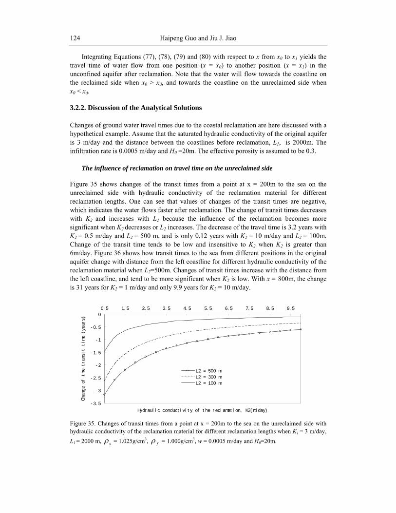
Haipeng Guo and Jiu J. Jiao124
Integrating Equations (77), (78), (79) and (80) with respect to x from x0 to x1 yields thetravel time of water flow from one position (x = x0) to another position (x = x1) in theunconfined aquifer after reclamation. Note that the water will flow towards the coastline onthe reclaimed side when x0 > xd, and towards the coastline on the unreclaimed side whenx0 < xd.
3.2.2. Discussion of the Analytical Solutions
Changes of ground water travel times due to the coastal reclamation are here discussed with ahypothetical example. Assume that the saturated hydraulic conductivity of the original aquiferis 3 m/day and the distance between the coastlines before reclamation, L1, is 2000m. Theinfiltration rate is 0.0005 m/day and H0 =20m. The effective porosity is assumed to be 0.3.
The influence of reclamation on travel time on the unreclaimed side
Figure 35 shows changes of the transit times from a point at x = 200m to the sea on theunreclaimed side with hydraulic conductivity of the reclamation material for differentreclamation lengths. One can see that values of changes of the transit times are negative,which indicates the water flows faster after reclamation. The change of transit times decreaseswith K2 and increases with L2 because the influence of the reclamation becomes moresignificant when K2 decreases or L2 increases. The decrease of the travel time is 3.2 years withK2 = 0.5 m/day and L2 = 500 m, and is only 0.12 years with K2 = 10 m/day and L2 = 100m.Change of the transit time tends to be low and insensitive to K2 when K2 is greater than6m/day. Figure 36 shows how transit times to the sea from different positions in the originalaquifer change with distance from the left coastline for different hydraulic conductivity of thereclamation material when L2=500m. Changes of transit times increase with the distance fromthe left coastline, and tend to be more significant when K2 is low. With x = 800m, the changeis 31 years for K2 = 1 m/day and only 9.9 years for K2 = 10 m/day.
- 3. 5
- 3
- 2. 5
- 2
- 1. 5
- 1
- 0. 5
00. 5 1. 5 2. 5 3. 5 4. 5 5. 5 6. 5 7. 5 8. 5 9. 5
Hydr aul i c conduct i vi t y of t he r ecl amat i on, K2( m/ day)
Chan
ge o
f th
e tr
ansi
t ti
me (
year
s)
L2 = 500 mL2 = 300 mL2 = 100 m
Figure 35. Changes of transit times from a point at x = 200m to the sea on the unreclaimed side withhydraulic conductivity of the reclamation material for different reclamation lengths when K1 = 3 m/day,L1 = 2000 m, sρ = 1.025g/cm3, fρ = 1.000g/cm3, w = 0.0005 m/day and H0=20m.

Changes of Coastal Groundwater Systems… 125
- 35
- 30
- 25
- 20
- 15
- 10
- 5
00 100 200 300 400 500 600 700 800
Di st ance f r om gr oundwat er di vi de ( m)
Chan
ge o
f th
e tr
ansi
t ti
me (
year
s)
K2 = 1 m/ day
K2 = 5 m/ day
K2 = 10 m/ day
Figure 36. Changes of transit times to the sea on the unreclaimed side from different positions in theoriginal aquifer with distance from the left coastline for different hydraulic conductivity of thereclamation materials when K1 = 3 m/day, L1 = 2000 m, L2=500m sρ = 1.025g/cm3, fρ = 1.000g/cm3,
w = 0.0005 m/day and H0=20m.
The influence of reclamation on travel time on the reclaimed side
Figure 37 shows changes of travel times from a point at x = 1800 m to the original coastlineon the reclaimed side with hydraulic conductivity of the reclamation material for differentreclamation lengths. One can see that values of changes of travel times are positive, whichindicates that the water flows more slowly after reclamation. The increase of the travel timedecreases with K2 and increases with L2. Changes of travel times tend to be low andinsensitive to K2 when K2 is greater than 5m/day. Comparision of Figures 35 and 37 showsthat the influence of reclamation on ground water travel time is much more significant on thereclaimed side than that on the unreclaimed side. With K2 = 0.5m/day and L2 = 500 m, changeof travel time over the last 200 m of the original aquifer is 72.8 years on the reclaimed side,and only 3.2 years on the unreclaimed side
Figure 38 shows how transit times from a point at x = 1800m to the sea on the reclaimedside change with hydraulic conductivity of the reclamation materials for different reclamationlengths. Ground water flow in the original aquifer tends to be slower so that the travel timebecomes longer after reclamation (Figure 37). Also, the travel path of ground water becomeslonger due to land reclamation. Therefore, transit times become greater than those beforereclamation. The influence of the reclamation on groundwater transit time diminishesgradually when K2 increases and L2 decreases. For a fixed reclamation length, the impact ofreclamation becomes less sensitive to K2 when K2 becomes great. Chang of transit times froma point at x = 1800 m can range from several years to more than one hundred years when K2
and L2 are combined differently. With K2 = 0.5 m/day the change is 10.4 years for L2 = 100 mand 123 years for L2 = 500 m.

Haipeng Guo and Jiu J. Jiao126
0
10
20
30
40
50
60
70
80
0. 5 1. 5 2. 5 3. 5 4. 5 5. 5 6. 5 7. 5 8. 5 9. 5Hydr aul i c conduct i vi t y of t he r ecl amat i on, K2( m/ day)
Chan
ge o
f th
e tr
avel
tim
e (y
ears
)
L2 = 500 mL2 = 300 mL2 = 100 m
Figure 37. Changes of travel times from a point at x = 1800m to original coastline on the reclaimed sidewith hydraulic conductivity of the reclamation material for different reclamation lengths when K1 = 3m/day, L1 = 2000 m, sρ = 1.025g/cm3, fρ = 1.000g/cm3, w = 0.0005 m/day and H0 = 20 m.
0
20
40
60
80
100
120
140
0. 5 1. 5 2. 5 3. 5 4. 5 5. 5 6. 5 7. 5 8. 5 9. 5Hydr aul i c conduct i vi t y of t he r ecl amat i on, K2 ( m/ day)
Chan
ge o
f th
e tr
ansi
t ti
me (
year
s)
L2 = 500 mL2 = 300 mL2 = 100 m
Figure 38. Changes of the transit times from a point at x = 1800 m to the sea on the reclaimed side withhydraulic conductivity of the reclamation materials for different reclamation lengths when K1 = 3m/day, L1 = 2000 m, sρ = 1.025g/cm3, fρ = 1.000g/cm3, w = 0.0005 m/day and H0=20m.
4. Summary and Conclusions
The impact of land reclamation on ground water level and saltwater interface in an extensiveland mass and an island are discussed. After reclamation, the water level in the originalaquifer is increased and the saltwater interface moves seaward. The recharge can occur in agreater area so that the size of aquifer, and therefore the water resource, is increased. In theisland situation, large-scale reclamation can result in the displacement of the water dividetowards the reclaimed side, thereby increasing ground water discharge to the sea on both

Changes of Coastal Groundwater Systems… 127
sides of the island. In all the cases, the impact of the reclamation on the water level and thesaltwater interface mainly depends on the reclamation scale and the hydraulic conductivity ofthe reclamation material. For the case of an extensive land mass, the analytical solutions arechecked against the results of a numerical code, which shows that only minor differenceoccurs.
Analytical solutions have been obtained to describe ground water travel time before andafter reclamation for an extensive land mass and an island bounded below by a horizontalimpermeable layer. Comparisons have been made between the solution in this paper and thatdeveloped by Chesnaux et al. (2005), which doesn’t include the influence of seawater-freshwater interface. It is concluded that difference of these two solutions depends mainly onthe elevation of the sea level, the infiltration rate and the hydraulic conductivity of theaquifer. The impact of reclamation on groundwater travel time is discussed detailedly basedon the hypothetical examples. The groundwater travel time tends to be longer, and waterflows more slowly in the original aquifer after reclamation. In the island situation, the groundwater will flow more slowly in the original aquifer on the reclaimed side. However, theground water travel time becomes shorter and water flows faster in the unreclaimed side. Theimpact of the coastal reclamation on ground water travel time is mainly controlled by thereclamation scale and hydraulic conductivity of the reclamation material. For the samereclamation scale and hydraulic conductivity of the reclamation material, the reclamationtends to have more significant impact on ground water flow on the reclaimed side than that onthe unreclaimed side.
The impact of reclamation on flow velocity and streamline pattern is also presented. Insome cases, the elevation of streamline increases after reclamation, which may impactspreading of contaminants and should be noted when placing wells. After reclamation theflow velocity will decrease especially in areas close to the original coastline for the situationof an extensive landmass. For the island setting, the flow velocity will decrease on thereclaimed side and increase on the unreclaimed side.
The analytical study in this paper is based on Dupuit and Ghyben-Herzberg assumptions.There exist some shortcomings in these assumptions such as no seepage face at the coastlineand neglect of the vertical flow. In addition, the conceptual models considered here don notinclude the heterogeneity of the aquifer system, complicated topography at the coast, and thetransient process immediately after the reclamation (Guo and Jiao, 2007). However, this studypresents very useful insight into change of coastal ground water system in response to landreclamation.
Appendix A
A single-potential solution for regional interface problems in coastal aquifers was presentedby Strack (1976), which was restricted to cases of steady flow with homogeneous isotropicpermeability where the Dupuit assumption was valid. This approach is a more advanced andgeneral method to handle combined unconfined flow, unconfined interface flow. In thisAppendix, we describe the derivation of the analytical solution for groundwater level andseawater-freshwater interface in an extensive land mass in terms of the potential functioninstead of water head, and all symbols used are as defined previously.

Haipeng Guo and Jiu J. Jiao128
Solutions for water level and saltwater interface before reclamation
Figure 1a shows a coastal unconfined ground water system receiving uniform verticalrecharge. According to Strack (1976), the potentials for combined unconfined flow andunconfined interface flow are
21
12 uK h CΦ = + 0
s
f
h Hρρ
≥ (A1)
21 0
1 ( )2
sui
s f
K h H Cρρ ρ
Φ = − +− 0
s
f
h Hρρ
≤ (A2)
21 0
12
sui u
f
C C K Hρρ
− = (A3)
where fρ and sρ are the densities of fresh ground water and seawater. Cui and Cu stand for
two constants and the subscripts ui and u refer to unconfined interface flow and unconfinedflow, respectively. Choosing Cu = 0, one obtains
21 0
10 2
su ui
f
C C K Hρρ
= = (A4)
The boundary conditions of the unconfined aquifer before reclamation (Figure 1a) are
0 0xx Qx
∂Φ= = − =
∂(A5)
and
21 0 1 0
1 =2
s
f
x L h H K Hρρ
= = Φ (A6)
where Qx is the discharge vector defined as pointing in the direction of flow and having amagnitude equal to the discharge flowing through a surface perpendicular to the direction offlow, of unit width and of a height equal to the thickness of the flow region (Strack, 1976).The governing differential equation for the case of rainfall is
2 w∇ Φ = − (A7)

Changes of Coastal Groundwater Systems… 129
The solution of Equations (A5) through (A7) is
2 2 21 1 0
1 1= ( )2 2
s
f
w L x K Hρρ
Φ − + (A8)
The heads in the aquifer can be obtained from (A1), (A2), and (A8):
2 2 21 0
1
( ) 0 st
f
wh L x H x xK
ρρ
= − + ≤ ≤ (A9)
2 21 0 1
1
( )( ) s f
ts
wh L x H x x L
Kρ ρ
ρ−
= − + ≤ ≤ (A10)
The expression for the location of the tip of the saltwater tongue can be obtained bysetting h equal to 0/s fHρ ρ in either (A1) or (A2) and then solving for x after substitution of
this value of the potential in (A8), which yields
212 2
1 02
( ) s s f
tf
Kx L H
wρ ρ ρ
ρ−
= − (A11)
Solutions for water level and saltwater interface after reclamationAfter reclamation (Figure 1b), the potentials in the reclaimed portion of the aquifer can
be defined as
22
12
K hΦ = 0s
f
h Hρρ
≥ (A12)
2 22 0 2 0
1 1( )2 2
s s
s f f
K h H K Hρ ρρ ρ ρ
Φ = − +− 0
s
f
h Hρρ
≤ (A13)
The condition (A5) remains valid for the left boundary but the boundary condition at
1 2 ,x L L L= = + is changed as:
20 2 0
1 =2
s
f
x L h H K Hρρ
= = Φ (A14)

Haipeng Guo and Jiu J. Jiao130
The governing equation for the potential throughout the flow region is the same as (A7).The solution is
2 2 22 0
1 1= ( )2 2
s
f
w L x K Hρρ
Φ − + (A15)
If the hydraulic conductivity jumps at 1x L= then (A15) remains valid, but the potentialjumps:
1 2/ = /K K− +Φ Φ (A16)
In order to have a continuous potential, the potential in the original aquifer is redefined as
21
12
K h ξΦ = + (A17)
where 2 1
2
= K KK
ξ + − +−= Φ −Φ Φ .
Now that the new potential is continuous throughout the flow region. The unknown valueξ can be obtained from (A15) by computing Φ at 1x L= :
2 2 22 1 2 11 1 2 0
2 2
( ) ( )2
s
f
K K K KL w L L K HK K
ρξρ
⎡ ⎤− −= Φ = − +⎢ ⎥
⎢ ⎥⎣ ⎦(A18)
The solution throughout the flow domain is now obtained. The head in the originalaquifer can be computed from (A15) and (A17), and heads in the reclaimed portion of theaquifer can be obtained from (A12), (A13), and (A15):
2 2 21 1 2 2 0 1
1 2
1 1( ) (2 ) 0s
f
h w L x L L L H x LK K
ρρ
⎡ ⎤= − + + + ≤ ≤⎢ ⎥
⎣ ⎦(A19)
2 2 21 2 0 1
2
( ) str
f
wh L L x H L x xK
ρρ
⎡ ⎤= + − + ≤ ≤⎣ ⎦ (A20)
2 21 2 0 1 2
2
( )( ) s f
t rs
wh L L x H x x L L
Kρ ρ
ρ−
⎡ ⎤= + − + ≤ ≤ +⎣ ⎦ (A21)

Changes of Coastal Groundwater Systems… 131
The expression for the location of the tip of the saltwater tongue can be obtained bysetting h equal to 0/s fHρ ρ in either (A12) or (A13) and then solve for x after substitution of
the derived potential in (15), which yields
222 2
1 2 02
( )( ) s s f
t rf
Kx L L H
wρ ρ ρ
ρ−
= + − (A22)
Appendix B
In this Appendix, we describe the derivation of the analytical solution for groundwater leveland seawater-freshwater interface in an island, bounded below by and horizontal impermeablebottom, in terms of the potential function instead of water head, and all symbols used are asdefined previously.
Solutions for water level and saltwater interface before reclamation
Figure 20a shows the unconfined ground water flow system before reclamation. Thepotentials in the whole flow region may be obtained by setting Cui equal to 0 in (A1) and(A2), which yields
2 21 1 0
1 12 2
s
f
K h K Hρρ
Φ = − 0s
f
h Hρρ
≥ (B1)
21 0
1 ( )2
s
s f
K h Hρρ ρ
Φ = −− 0
s
f
h Hρρ
≤ (B2)
The boundary conditions of the unconfined system before reclamation are
0 1 0 when 0 or h H x L= Φ = = (B3)
The governing equation (A7) for the potential throughout the flow region remains valid.The solution is
21
1= ( )2
w L x xΦ − (B4)
The heads in the aquifer may be obtained from (B1), (B2), and (B4):
21 0 1 2 1
1
( )( ) 0 s f
t ts
wh L x x H x x or x x L
Kρ ρ
ρ−
= − + ≤ ≤ ≤ ≤ (B5)

Haipeng Guo and Jiu J. Jiao132
2 21 0 1 2
1
( ) st t
f
wh L x x H x x xK
ρρ
= − + ≤ ≤ (B6)
Set h equal to 0/s fHρ ρ in either (B1) or (B2) and then substitute this value of the
potential in (B4), one has
212 2
1 02
( )0 s s f
f
Kx L x H
wρ ρ ρ
ρ−
− + = (B7)
The locations of the tips of saltwater tongues can be readily obtained by solving for xt1
and xt2 in equation (B7).
Solution for ground water level and saltwater interface after reclamation.
Figure 20b shows the ground water flow system after reclamation. The potentials in thereclaimed portion of the aquifer are defined as
2 22 2 0
1 12 2
s
f
K h K Hρρ
Φ = − 0s
f
h Hρρ
≥ (B8)
22 0
1 ( )2
s
s f
K h Hρρ ρ
Φ = −− 0
s
f
h Hρρ
≤ (B9)
If the hydraulic conductivity jumps at 1x L= then the potential jumps:
1 2/ = /K K− +Φ Φ (B10)
In order to make the potential continuous throughout the flow region, the potentials in theoriginal aquifer are redefined as
2 21 1 0
1 12 2
s
f
K h K Hρ γρ
Φ = − + 0s
f
h Hρρ
≥ (B11)
21 0
1 ( )2
s
s f
K h Hρ γρ ρ
Φ = − +− 0
s
f
h Hρρ
≤ (B12)
where 2 1
2
= K KK
γ + − +−= Φ −Φ Φ .

Changes of Coastal Groundwater Systems… 133
The boundary conditions at x=0 and x=L=L1+L2, are
00 x h H γ= = Φ = (B13)
0 0x L h H= = Φ = (B14)
The governing equation (A7) for the domain remains valid. The solution is
21= ( )2 2
wLwx xLγ γΦ − + − + (B15)
The unknown value γ can be obtained from (B15) by computing Φ at 1x L= :
22 1 2 11 1 1
2 2
1= ( ) ( )2 2
K K K K wLL wL LK K L
γγ γ− − ⎡ ⎤Φ = − + − +⎢ ⎥⎣ ⎦
The solution is:
1 2 2 1
1 2 2 1
( )=2( )
wL L L K KL K L K
γ −+
(B16)
The heads in the aquifer can be obtained from (B8), (B9), (B11), (B12), and (B15):
20 1
1
( )( ) 0 s f
t rs
wh x x H x x
Kρ ρ
βρ−
= − + ≤ ≤ (B17)
2 20 1 1
1
( ) str
f
wh x x H x x LK
ρβρ
= − + ≤ ≤ (B18)
2 20 1 2
2
( 2 / ) str
f
wh x x w H L x xK
ρβ γρ
= − + + ≤ ≤ (B19)
20 2
2
( )( 2 / ) s f
t rs
wh x x w H x x L
Kρ ρ
β γρ−
= − + + ≤ ≤ (B20)
where 2 21 2 1 1 1 2 2 1= ( ) /( )K L K K L L K L Kβ ⎡ ⎤+ − +⎣ ⎦ , and γ is obtained from (B16).

Haipeng Guo and Jiu J. Jiao134
Set h equal to 0/s fHρ ρ in either (B11) or (B12) and then substitute the derived potential
in (B15), one has
212 2
02
( )0 s s f
f
Kx x H
wρ ρ ρ
βρ−
− + = (B21)
The distance from the left coastline to the tip of the left saltwater tongue, xtr1, is one rootof equation (B21). Similarly, the location of the tip of the right saltwater tongue, xtr2, can beobtained as a root of the follow equation:
222 2
02
( )2 / 0 s s f
f
Kx x H w
wρ ρ ρ
β γρ−
− + − = (B22)
Acknowledgements
The study was supported by the Research Grants Council of the Hong Kong SpecialAdministrative Region, China (HKU 7105/02P).
References
Amin, I. E. and Campana, M. E. (1996), A general lumped parameter model for theinterpretation of tracer data and transit time calculation in hydrologic systems. Journal ofHydrology, 179(1-4): 1-21.
Barnes RSK (1991), Dilemmas in the theory and practice of biological conservation asexemplified by British coastal lagoons, Biological Conservation 55(3): 315-328.
Bear, J., A.H.-D. Cheng, S. Sorek, D. Ouazar, and I. Herrera, ed. (1999), Seawater Intrusionin Coastal quifers-Concepts, Methods and Practices. Dordrecht, The Netherlands:Kluwer Academic Publishers.
Bear, J., and G. Dagan (1964), Some exact solutions of interface problems by means of thehodograph method, J. Geophys. Res., 69(8): 1563-1572.
Code of Federal Regulations (1988), Title 10--Energy: Department of Energy (Part 960.2).Miamisburg, OH : LEXIS-NEXIS, Division of Reed Elsevier.
Chapuis, R. P., R. Chesnaux. (2006). Travel time to a well pumping an unconfined aquiferwithout recharge. Ground Water 44 (4): 600-603.
Chesnaux, RE, JW Molson, and RP Chapuis (2005), An analytical solution for ground watertransit time through unconfined aquifers. Ground Water, 43(4): 511 -517.
Cornaton F., Perrochet P. (2005), Groundwater age, life expectancy and transit timedistributions in advective–dispersive systems; 1.Generalized reservoir theory. Advancesin Water Resources, 29(9), 1267-1291.
Diersch, H.-J.G.. (2002), FEFLOW finite element subsurface flow and transport simulationsystem reference manual, WASY Inst. for Water Resour. Plann. and Syst. Res., Berlin.

Changes of Coastal Groundwater Systems… 135
Ding Guoping (2006), Impact of deep building foundations on coastal groundwater flowsystems, Ph.D thesis, Univ. of Hong Kong, China.
Etcheverry, D., and P. Perrochet (2000), Direct simulation of groundwater transit-timedistribution using the reservoir theory, Hydrogeol. J., 8: 200-208.
Fetter, C. W. (1972), Position of the saline water interface beneath oceanic islands. WaterResources Research 8 (5): 1307-1315.
Fetter, C.W. (1994), Applied Hydrogeology. New York: Prentice-Hall.Fórizs, I., and Deák, J. (1998), Origin of bank filtered groundwater resources covering the
drinking water demand of Budapest, Hungary. In: Application of isotope techniques toinvestigate groundwater pollution, IAEA-TECDOC-1046, Vienna, pp.133-165.
Gelhar, L.W., and J.L. Wilson (1974), Ground-water quality modeling. Ground Water 12(6):399–408.
Glover, R.E. (1964), The pattern of fresh water flow in coastal aquifer. In Sea Water inCoastal Aquifers. USGS Water-Supply Paper 1613-C. Reston, Virginia: USGS.
Henry, H.R. (1964), Interfaces between salt water and fresh water in coastal aquifers. In SeaWater in Coastal quifers. USGS Water-Supply Paper 1613-C. Reston, Virginia: USGS.
Jiao, J. J. (2000), Modification of regional groundwater regimes by land reclamation. HongKong Geologist 6, 29-36.
Jiao, J. J., S. Nandy, and H. Li. (2001), Analytical studies on the impact of reclamation ongroundwater flow. Ground Water 39(6): 912-920
Jiao, J.J. (2002), Preliminary conceptual study on impact of land reclamation on groundwaterflow and contaminant migration in Penny's Bay, Hong Kong Geologist, 8: 14-20.
Jiao, J. J., and Z. Tang. (1999), An analytical solution of groundwater response to tidalfluctuation in a leaky confined aquifer. Water Resources Research 35(3): 747-751.
Jiao JJ, C Leung, KP Chen, JM Huang, and RQ Huang (2005), Physical and chemicalprocesses in the subsurface system in the land reclaimed from the sea, in Collections ofCoastal Geo-Environment and Urban Development, P399-407, China Dadi PublishingHouse, Beijing, China.
Jiao, J. J., XS Wang and S Nandy (2006), Preliminary assessment of the impacts of deepfoundations and land reclamation on groundwater flow in a coastal area in Hong Kong,China, Hydrogeology Journal, 14 (1-2): 100-114.
Kolditz, O., R. Ratke, H.-J. G. Diershch, and W. Zielke (1998), Coupled Groundwater flowand. transport: 1. Verification of variable density flow and transport models. Advances inwater. resources 21: 27–46.
Lee J. Florea and Carol M. Wicks (2001), Solute transport through laboratory-scale karsticauifers. Journal of Cave and Karst Studies, 63(2): 59-66.
Lumb P. (1976), Land reclamation in Hong Kong. In Proceedings of Residential Workshopon Materials and Methods for Low Coast Road, Rail and Reclamation Works, Leura,Australia, 299-314.
Mahamood, H. R., and D. R. Twigg (1995), Statistical analysis of water table variations inBharain. Quarterly Journal of Engineering Geology 28: s63-s74.
Nield, S.P., L. R. Townley, and A. D. Barr (1994), A framework for quantitative analysis of.surface water-groundwater interaction: Flow geometry in vertical section. WaterResources. Research, 30(8): 2461-2475.

Haipeng Guo and Jiu J. Jiao136
Ni JR, Borthwick AGL, and Qin HP (2002), Integrated approach to determiningpostreclamation coastlines, Journal Of Environmental Engineering-Asce, 128 (6):543-551.
Noske R. A. (1995), The ecology of mangrove forest birds in peninsular malaysia, IBIS 137(2): 250-263.
Seasholes, N. S. (2003), Gaining ground: a history of landmaking in Boston. Cambridge,Mass. : MIT Press.
Simpson, M. J., T. P. Clement, and F. E. Yeomans (2003), Analytical model for computingresidence times near a pumping well. Ground water 41(3): 351-354.
Smith, A. J., and J. V. Turner (2001), Density-dependent surface water-groundwaterinteraction and nutrient discharge in the Swan-Canning Estuary, Hydrol. Processes, 15,2595-2616.
Smith, A. J. (2004), Mixed convection and density-dependent seawater circulation in coastalaquifers, Water Resour. Res., 40, W08309, doi:10.1029/2003WR002977.
Strack, O.D.L. (1976), A single-potential solution for regional interface problems in coastalaquifers. Water Resources Research 12(6): 1165-1174.
Strack, O. D. L. (1984), Three-dimensional streamlines in Dupuit-Forchheimer models. WaterResources Research 20(7): 812-822.
Stuyfzand, P. J. (1995), The impact of land reclamation on groundwater quality and futuredrinking water supply in the Netherlands. Wat. Sci. Tech. 31(8): 47-57.
Suzuki, T. (2003), Economic and geographic backgrounds of land reclamation in Japaneseports. Marine Pollution Bulletin 47:226-229.
Terawaki T, Yoshikawa K, Yoshida G, Uchimura M, and Iseki K (2003), Ecology andrestoration techniques for Sargassum beds in the Seto Inland Sea, Japan, MarinePollution Bulletin 47 (1-6): 198-201.
Townley, L.R., and M.R. Davidson (1988), Definition of a capture zone for shallow watertable lakes, Journal of Hydrology, 104: 53-76.
Varni, M., and J. Carrera (1998), Simulation of groundwater age distributions,. Water Resour.Res., 34: 3271–3281.