Double parton distributions for a positronium-like bound state

using light-front wave functions

Chandan Mondala, Asmita Mukherjeeb and Sreeraj Naira

a Institute of Modern Physics, Chinese Academy of Sciences, Lanzhou 730000, China

b Department of Physics, Indian Institute of Technology Bombay,Powai, Mumbai 400076, India.

Abstract

We investigate the double parton distributions (DPDs) for a positronium-like bound state using

light-front QED. We incorporate the higher Fock three particle component of the state, that includes

a photon. We obtain the overlap representation of the DPDs in terms of the three-particle light-

front wave functions (LFWFs). Our calculation explores the correlations between the momentum

fractions of the particles probed and the transverse distance between them, without any assumption

of factorization between them. We also investigate the behavior of the DPDs near the kinematical

boundary when the sum of the momentum fractions is close to one.

1

arX

iv:1

906.

1090

3v1

[he

p-ph

] 2

6 Ju

n 20

19

I. INTRODUCTION

As the flux of partons increases in high energy hadronic collision experiments, the probabil-

ity of having more than one independent hard scattering interaction also increases and a proper

description of final states in hadronic collisions requires the inclusion of multiple partonic inter-

actions (MPIs). The MPIs in hadronic collision have been predicted a long ago [1–5]. The most

probable and the simplest of these MPIs are the double parton scattering (DPS) events. In

DPS two partons from each hadron participate in separate hard interactions. In such a process,

a large momentum transfer is involved in both scattering. The first experimental evidence of

DPS was found at CERN-ISR [6] in p-p collision. DPS are indeed relevant at LHC because

of the high density of partons. The ATLAS collaboration had reported their first results on

DPS a while ago [7] and DPS also contributes to the Higgs production background in several

channels at LHC.

DPS can be factorized in terms of the hard interactions which are calculable in perturbation

theory and the double parton distribution (DPDs) functions. The DPDs depend on two-body

quantities encoding the non-perturbative dynamics of the partons. Factorization of DPS usually

assumes the simplest case wherein there are no correlations between the two partons [8–11].

The DPDs are interpreted as the number densities of parton pair at a given transverse distance

y⊥ and carrying longitudinal momentum fractions (x1, x2) of the composite system [2, 10, 12].

Since the DPDs depend on the partonic inter-distance [12], they contain information on the

hadronic structure which compliments the tomographical information encoded by the one-body

distributions such as generalized parton distributions (GPDs) [13] and transverse momentum

dependent distributions (TMDs) [14]. Therefore, DPDs represent a novel tool to access the

three-dimensional hadron structure. Despite the wealth of information provided by the DPDs,

the present experimental knowledge is mainly accessible through the DPS cross section which

has been accumulated into the effective cross section, σeff . For the recent results we refer to

the articles [15–20].

DPDs being nonperturbative in nature are always very difficult to evaluate from QCD first

principles and there have been numerous attempts to gain insight into them by studying QCD

inspired models. Model calculations of DPDs are important and interesting to understand the

2

properties as well as for predictions of experimental observables. Several phenomenological

models such as bag model [21], constituent quark model [22–25], generalized valon model [26],

soft-wall AdS/QCD model [27], dressed quark model [28] etc. have been used to obtain the basic

information on DPDs and to gauge the phenomenological impact of transverse and longitudinal

correlations, along with spin correlations [23, 29–32]. The transverse structure of of the proton

from the DPDs and the effective cross section has been investigated in [12, 33, 34]. Recently, the

matching of both the position and momentum space DPDs onto ordinary parton distribution

functions at the next-to-leading order (NLO) in perturbation theory has been reported in [35],

where the authors have also discussed about the sum rules for DPDs [36]. The quantities related

to DPDs, and encoding double parton correlations, have been evaluated for the pion in lattice

QCD [37].

As very little is known so far on the DPDs F (x1, x2, y⊥), there are several approaches to

parameterize or model them. A common approach is based on a factorized ansatz, which

assumes that the y⊥ dependence is factored out from the dependence on x1 and x2, which

are the momentum fractions of the partons probed. In addition, it is sometimes also assumed

that x1 and x2 dependences are factored out, in terms of single parton distributions (pdfs)

and neglecting any correlations between them [21]. In [38] an approach was used based on

[39] where the DPDs were written as a convolution of two impact parameter dependent pdfs

which are obtained from GPDs. A Gaussian form of the impact parameter dependent pdfs were

used. However it was concluded that the factorized ansatz fails in the valence region and the

authors also observed that a Gaussian dependence on y⊥ is rather arbitrary. It is thus relevant

to investigate the DPDs without such assumptions. The model calculations can be thought of

as a parameterization of the DPDs at a low momentum scale and one then evolves them to a

higher scale of the experiments using evolution equation, such evolution equations have been

obtained by now and discussed in detail [40]. Another interesting aspect of model calculation

of the DPDs is the behavior near the kinematical bound x1 +x2 = 1. The DPDs should vanish

in the unphysical region x1 + x2 > 1. In some early model calculations this support property

was violated, due to non-conservation of momentum of the constituents. In later calculations,

a phenomenological factor is included to improve the behavior in this kinematical limit.

A widely used method to calculate the DPDs is by expressing them in terms of overlaps of

3

light-front wave functions (LFWFs). In the light-front formalism, the proton state is expanded

in Fock space in terms of multi-parton LFWFs. The LFWFs satisfy the bound state equation

in light-front(LF) QCD. One then truncates the Fock space to a few particle sector; such

truncation is boost invariant in light-front framework. As it is very difficult to solve the light-

front bound state equation, in particular to obtain the wave functions of the higher Fock sector,

most model calculations are restricted to using the three quark valence LFWF for the proton. In

a previous work [28], in order to calculate the quark-gluon DPDs, a different approach was used;

namely instead of a proton state a relativistic spin 1/2 composite state of a quark dressed with

a gluon was used. The LFWFs of the two-particle state was calculated in perturbation theory.

This may be thought of as a field theory based perturbative model, to investigate the quark-

gluon correlations in the DPDs. However, the kinematics of a two-particle system are rather

constrained. In this work, we use the overlap approach in terms of LFWFs for a two-particle

bound state like a positronium in QED, in the weak coupling limit. We include the effect of

the three particle e+e−γ component of the LFWF. As solving the LF bound state equation is

rather difficult in QED as well, we use a simpler but nevertheless interesting approach earlier

followed in [41], to calculate the twist-four structure function of positronium and verifying a

sum rule. We use an analytic form of the two-particle LFWF in the weak coupling limit.

The three-particle LFWF is then expressed in terms of the two-particle LFWF using LF QED

Hamiltonian. This calculation illustrates the formalism which can also be applied to a QCD

mesonic system; in fact in the weak coupling limit, the LFWFs are expected to mimic those of

a meson. Our approach allows us to calculate them without any assumption on factorization

of the x1, x2 and y⊥ dependence, and we can investigate the interplay between these variables

in full form. Thus, our calculation may be thought of as an exploratory analysis on the explicit

x1, x2 and y⊥ dependence of the DPDs in a three-particle system. We also discuss the behavior

of the DPD in the limit x1 + x2 → 1.

The paper is organized as follows: In section II we discuss the DPDs for the {e−e+} pair

and their overlap representation in the light-front dressed positronium model. We present the

numerical results in section III. Conclusions are given in section IV.

4

II. DOUBLE PARTON DISTRIBUTIONS

The double parton distributions (DPDs) for unpolarized quarks can be defined as [10, 11]

Fa1a2(x1, x2,y⊥) = 2p+

∫dz−12π

dz−22π

dy− ei(x1z−1 +x2z

−2 )p+

× 〈p| Oa2(0, z2)Oa1(y, z1) |p〉 , (1)

where | p〉 is the target system with momentum p. x1 and x2 are momentum fractions of the

partons and y⊥ is the relative transverse distance between them.

The fermionic operators are given by [10] (see the appendix)

Oai(y, zi) = ψi

(y − zi

2

)Γaiψi

(y − zi

2

) ∣∣∣z+i =y+i =0,z⊥i =0

(2)

where Γai are various Dirac γ matrices projecting onto the corresponding polarization states

given by

Γq =1

2γ+, Γ∆q =

1

2γ+γ5, Γjδq =

1

2iσj+γ5 (3)

for the unpolarized fermion (q), longitudinally polarized fermion (∆q) or transversely polarized

fermion (δq) respectively. We choose the light-cone gauge and the gauge link in the operator

structure is set to unity.

A. Overlap Representation for the DPD

As discussed in the Introduction, we consider our target state to be a positronium-like bound

state in LF QED. We use the two-component form of the LF QED in the line of [42, 43]. In

this section, we present a calculation of the unpolarized fermion DPDs for such a state. This

means Γq = 12γ+ in Eq. 2. The state can be expanded in Fock space in terms of LFWFs as

| P 〉 =∑σ1,σ2

∫dp+

1 d2p⊥1√

2(2π)3p+1

∫dp+

2 d2p⊥2√

2(2π)3p+2

φ2(P | p1, σ1; p2, σ2)√

2((2π)3P+δ3(P − p1 − p2)b†(p1, σ1)d†(p2, σ2) | 0〉

+∑σ1,σ2,λ

∫dp+

1 d2p⊥1√

2(2π)3p+1

∫dp+

2 d2p⊥2√

2(2π)3p+2

∫dp+

3 d2p⊥3√

2(2π)3p+3

φ3(P | p1, σ1; p2, σ2; p3, λ)√

2(2π)3P+δ3(P − p1 − p2 − p3)

b†(p1, σ1)d†(p2, σ2)a†(p3, λ) | 0〉, (4)

5

where the first term corresponds the two particle Fock sector, | e+e− 〉 with the two particle

LFWF φ2 and the second term is the three particle Fock component | e+e−γ 〉 wherein φ3 is

the three particle LFWF. σ1, σ2 and λ are the helicities of the electron, positron and photon

respectively. The LFWF are written in terms of the Jacobi momenta (xi, q⊥i ) defined as

p+i = xip

+, p⊥i = q⊥i + xip⊥ (5)

where∑

i xi = 1 and∑

i q⊥i = 0. The contribution coming from the three particle sector of the

Fock space can then be written in term of overlap of LFWFs,

Fe−e+(x1, x2,y⊥) =

(p+)2

2π2

∑σ1,σ′1,σ2,σ

′2,λ

∫d2k⊥1 d2k⊥2 d2k′⊥1 φ3∗

σ1,−σ′2,λ(p, k1, k

′1, p− k1 − k′1)

φ3σ′1,−σ2,λ

(p, k1 + k′1 − k2, p− k1 − k′1) ei(k⊥1 −k′⊥1 ).y⊥ (6)

with p+φ3σ1σ2λ

(k+i , k

⊥i ) = ψ3

σ1σ2λ(xi, q

⊥i ). The Eq.(6) can be rewritten as

Fe−e+(x1, x2,y⊥)

=1

2π2

∑σ1,σ′1,σ2,σ

′2,λ

∫d2k⊥1 d2k⊥2 d2k′

⊥1 ψ3∗

σ1,−σ′2,λ(x1, k

⊥1 ;x2, k

′⊥1 + k⊥2 − k⊥1 ; 1− x1 − x2, k

⊥3 )

× ψ3σ′1,−σ2,λ

(x1, k′⊥1 ;x2, k

⊥2 ; 1− x1 − x2, k

⊥3 ) ei(k

⊥1 −k′

⊥1 ).y⊥ (7)

where k⊥3 = p⊥ − k′⊥1 − k⊥2 , we consider the frame where p⊥ = 0. The amplitudes or LFWFs

ψ2 and ψ3 are boost invariant and are functions of the Jacobi momenta. These can be written

as [43, 44],

ψ3σ1,σ2,λ3

(x1, k1;x2, k2; 1− x1 − x2, k3) =M1 +M2, (8)

where the amplitudes are given by [41] :

M1 =1

E(−)

e√2(2π)3

1√1− x1 − x2

V1 ψ2s1,σ2

(1− x2,−k⊥2 ;x2, k⊥2 ),

M2 =1

E

e√2(2π)3

1√1− x1 − x2

V2 ψ2σ1,s2

(x1, k⊥1 ; 1− x1,−k⊥1 ) (9)

with the energy denominator

E(x1, x2) =[M2 − m2 + (k⊥1 )2

x1

− m2 + (k⊥2 )2

x2

− (k⊥3 )2

1− x1 − x2

],

6

and the vertices

V1(x1, k⊥1 ;x2, k

⊥2 ) = χ†σ1

∑s1

[2k⊥3

1− x1 − x2

− (σ⊥.k⊥1 − im)

xσ⊥ + σ⊥

(σ⊥.k⊥2 − im)

1− x2

]χs1 .(ε

⊥λ1

)∗,

V2(x1, k⊥1 ;x2, k

⊥2 ) = χ†−σ2

∑s2

[2k⊥3

1− x1 − x2

− σ⊥ (σ⊥.k⊥2 − im)

x2

+(σ⊥.k⊥1 − im)

1− x1

σ⊥]χ−s2 .(ε

⊥λ1

)∗.

(10)

The above expressions are obtained using the light-front Hamiltonian for QED in a similar line

as in light-front QCD [43]. Following Eqs.(8− 10) we can rewrite the Eq.(7) in terms of ψ2 as

Fe−e+(x1, x2,y⊥) =

e2

(2π)5

1

[E(x1, x2)]21

1− x1 − x2

∑σ1,σ′1,σ2,σ

′2,λ

∫d2k⊥1 d2k⊥2 d2k′

⊥1

× [P11 + P12 + P21 + P22] ei(k⊥1 −k′

⊥1 ).y⊥ (11)

where

P11 = [V1(x1, k⊥1 ;x2, k

′⊥1 + k⊥2 − k⊥1 ) ψ2

s1,−σ′2(1− x2,−k′⊥1 − k⊥2 + k⊥1 ;x2, k

′⊥1 + k⊥2 − k⊥1 )]†

× [V1(x1, k′⊥1 ;x2, k

⊥2 ) ψ2

s1,−σ2(1− x2,−k⊥2 ;x2, k⊥2 )]

P22 = [V2(x1, k⊥1 ;x2, k

′⊥1 + k⊥2 − k⊥1 ) ψ2

σ1,s2(x1, k

⊥1 ; 1− x1,−k⊥1 )]†

× [V2(x1, k′⊥1 ;x2, k

⊥2 ) ψ2

σ′1,s2(x1, k

′⊥1 ; 1− x1,−k′⊥1 )]

P12 = [V1(x1, k⊥1 ;x2, k

′⊥1 + k⊥2 − k⊥1 ) ψ2

s1,−σ′2(1− x2,−k′⊥1 − k⊥2 + k⊥1 ;x2, k

′⊥1 + k⊥2 − k⊥1 )]†

× [V2(x1, k′⊥1 ;x2, k

⊥2 ) ψ2

σ′1,s2(x1, k

′⊥1 ; 1− x1,−k′⊥1 )]

P21 = [V2(x1, k⊥1 ;x2, k

′⊥1 + k⊥2 − k⊥1 ) ψ2

σ1,s2(x1, k

⊥1 ; 1− x1,−k⊥1 )]†

× [V1(x1, k′⊥1 ;x2, k

⊥2 ) ψ2

s1,−σ2(1− x2,−k⊥2 ;x2, k⊥2 )]. (12)

The above expression is evaluated using Mathematica to calculate the spinor products. The

final expressions are given below.

P11 =8(1 + x1 − x2)2

(k′y1 (1− x2) + ky2x1

)((k′y1 + ky2)x1 − ky1(x1 + x2 − 1)

)x2

1(x2 − 1)2(x1 + x2 − 1)2×

ψ2(x2, k

⊥1 − k′⊥1 − k⊥2

)ψ2(x2, k

⊥2 ) (13)

7

P22 =−8(1− x1 + x2)2

(ky2(x1 − 1) + k′y1 x2

)(ky1(x1 + x2 − 1)− (k′y1 + ky2)(x1 − 1)

)x2

2(x1 − 1)2(x1 + x2 − 1)2×

ψ2(x1, k

⊥1

)ψ2(x1, k

′⊥1 ) (14)

P12 =8((x1 − x2)2 − 1)

(ky2(1− x1) + k′y1 x2

)(ky1(x1 + x2 − 1)− (k′y1 + ky2)x1

)x1(x1 − 1)x2(x2 − 1)(x1 + x2 − 1)2

×

ψ2(x2, k

⊥1 − k′⊥1 − k⊥2

)ψ2(x1, k

′⊥1 ) (15)

P21 =8((x1 − x2)2 − 1)

(k′y1 (1− x2) + ky2x1

)((k′y1 + ky2)(x1 − 1)− ky1(x1 + x2 − 1)

)x1(x1 − 1)x2(x2 − 1)(x1 + x2 − 1)2

×

ψ2(x1, k

⊥1

)ψ2(x2, k

⊥2 ) (16)

Motivated by [41, 45], we take the two-particle wave-function ψ2 in the weak coupling limit

as :

ψ2(x, k⊥) =

√m

π2

4(e1)5/2[(e1)2 −m2 + 1

4(k⊥)2+m2

x(1−x)

]2 , (17)

with m is the electron mass and e1 = m/2.

III. NUMERICAL RESULTS

In this section we present the numerical results for the unpolarized DPDs for the correlation

between e− and e+. In order to do the numerical calculations, a cut-off kmax = 20 MeV has been

introduced for the upper limit of all the integrations over k⊥. We notice that for higher vales of

kmax the results do not change. The electron (positron) mass has been taken as m = 0.50 MeV.

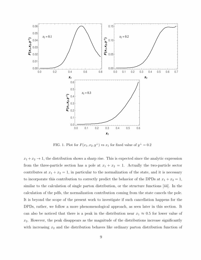
In Fig 1, we show the DPD for e− and e+ pair in the positronium-like bound state as a function

of x1 for different values of x2 and fixed value of y⊥ = 0.2 MeV−1. In this figure, we present the

contribution evaluated from the |e−e+γ〉 Fock sector. In our calculation, we have chosen the

physical kinematical region in the three-particle sector, that is, x1 +x2 < 1. We observe that as

8

0.0 0.2 0.4 0.6 0.8

0.00

0.01

0.02

0.03

0.04

0.05

0.06

x1

F(x

1,x

2,y

⊥) x2 = 0.1

0.0 0.1 0.2 0.3 0.4 0.5 0.6 0.7

0.00

0.05

0.10

0.15

x1

F(x

1,x

2,y

⊥) x2 = 0.2

0.0 0.1 0.2 0.3 0.4 0.5 0.6

0.0

0.1

0.2

0.3

0.4

0.5

0.6

x1

F(x

1,x

2,y

⊥) x2 = 0.3

FIG. 1. Plot for F (x1, x2, y⊥) vs x1 for fixed value of y⊥ = 0.2

x1 +x2 → 1, the distribution shows a sharp rise. This is expected since the analytic expression

from the three-particle section has a pole at x1 + x2 = 1. Actually the two-particle sector

contributes at x1 + x2 = 1, in particular to the normalization of the state, and it is necessary

to incorporate this contribution to correctly predict the behavior of the DPDs at x1 + x2 = 1,

similar to the calculation of single parton distribution, or the structure functions [44]. In the

calculation of the pdfs, the normalization contribution coming from the state cancels the pole.

It is beyond the scope of the present work to investigate if such cancellation happens for the

DPDs, rather, we follow a more phenomenological approach, as seen later in this section. It

can also be noticed that there is a peak in the distribution near x1 ≈ 0.5 for lower value of

x2. However, the peak disappears as the magnitude of the distributions increase significantly

with increasing x2 and the distribution behaves like ordinary parton distribution function of

9

the bare electron in a physical electron system [46]. In Fig 1 the peak is present only for

x2 = 0.1 because of the term (x1 − 1) 2x22 (x1 + x2 − 1) 2 present in the denominator of the term

P22 which suppress the peak value for x2 > 0.1.

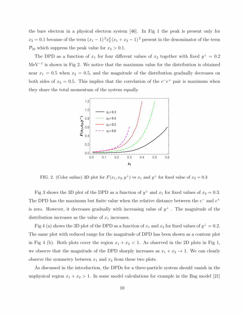
The DPD as a function of x1 for four different values of x2 together with fixed y⊥ = 0.2

MeV−1 is shown in Fig 2. We notice that the maximum value for the distribution is obtained

near x1 = 0.5 when x2 = 0.5, and the magnitude of the distribution gradually decreases on

both sides of x2 = 0.5. This implies that the correlation of the e−e+ pair is maximum when

they share the total momentum of the system equally.

x2= 0.3

x2= 0.4

x2= 0.5

x2= 0.6

0.0 0.1 0.2 0.3 0.4 0.5 0.6

0.0

0.2

0.4

0.6

0.8

1.0

1.2

x1

F(x

1,x

2,y

⊥)

FIG. 2. (Color online) 3D plot for F (x1, x2, y⊥) vs x1 and y⊥ for fixed value of x2 = 0.3

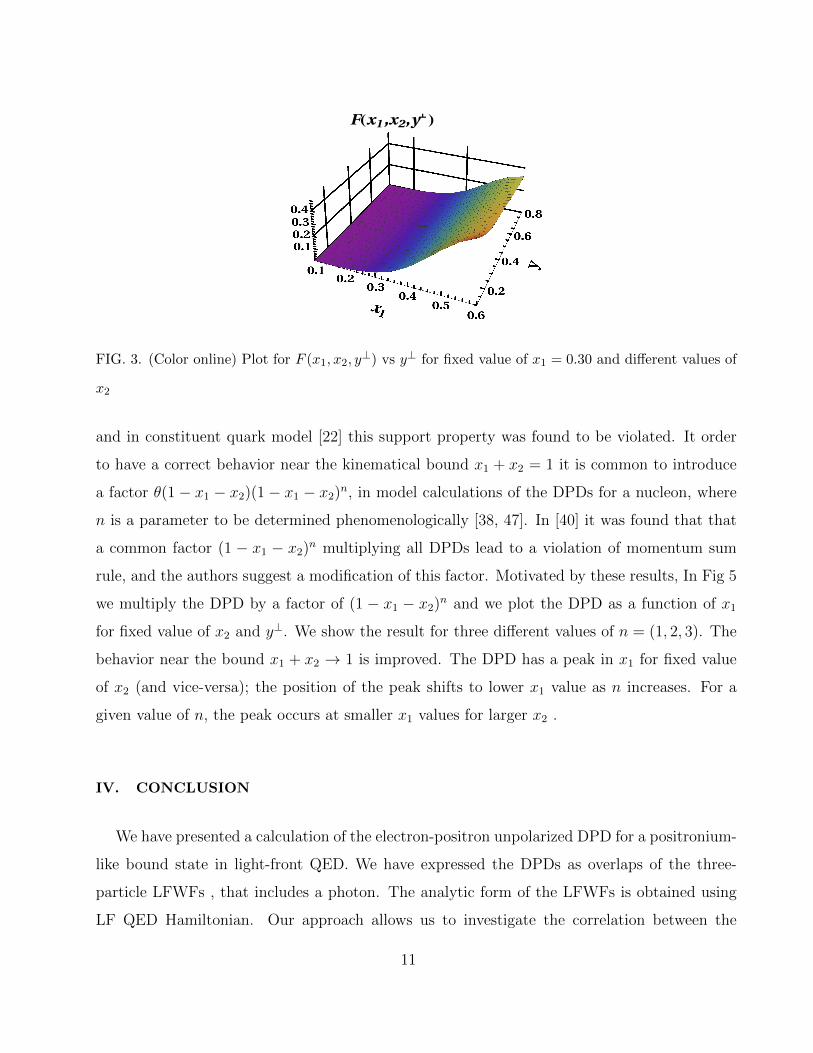
Fig 3 shows the 3D plot of the DPD as a function of y⊥ and x1 for fixed values of x2 = 0.3.

The DPD has the maximum but finite value when the relative distance between the e− and e+

is zero. However, it decreases gradually with increasing value of y⊥ . The magnitude of the

distribution increases as the value of x1 increases.

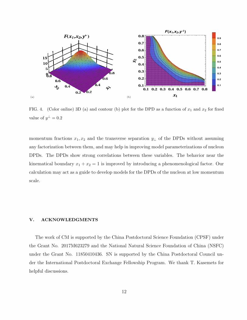
Fig 4 (a) shows the 3D plot of the DPD as a function of x1 and x2 for fixed values of y⊥ = 0.2.

The same plot with reduced range for the magnitude of DPD has been shown as a contour plot

in Fig 4 (b). Both plots cover the region x1 + x2 < 1. As observed in the 2D plots in Fig 1,

we observe that the magnitude of the DPD sharply increases as x1 + x2 → 1. We can clearly

observe the symmetry between x1 and x2 from these two plots.

As discussed in the introduction, the DPDs for a three-particle system should vanish in the

unphysical region x1 + x2 > 1. In some model calculations for example in the Bag model [21]

10

F(x1,x2,y⊥)

FIG. 3. (Color online) Plot for F (x1, x2, y⊥) vs y⊥ for fixed value of x1 = 0.30 and different values of

x2

and in constituent quark model [22] this support property was found to be violated. It order

to have a correct behavior near the kinematical bound x1 + x2 = 1 it is common to introduce

a factor θ(1− x1 − x2)(1− x1 − x2)n, in model calculations of the DPDs for a nucleon, where

n is a parameter to be determined phenomenologically [38, 47]. In [40] it was found that that

a common factor (1 − x1 − x2)n multiplying all DPDs lead to a violation of momentum sum

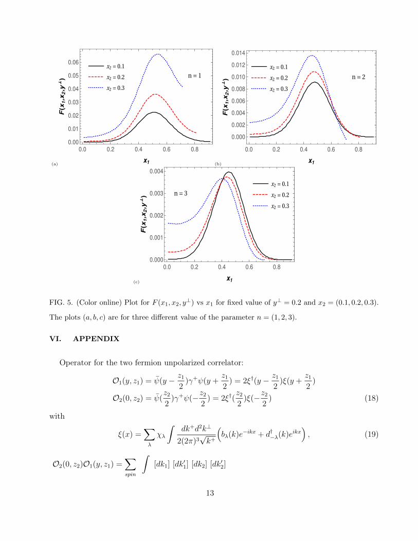
rule, and the authors suggest a modification of this factor. Motivated by these results, In Fig 5

we multiply the DPD by a factor of (1 − x1 − x2)n and we plot the DPD as a function of x1

for fixed value of x2 and y⊥. We show the result for three different values of n = (1, 2, 3). The

behavior near the bound x1 + x2 → 1 is improved. The DPD has a peak in x1 for fixed value

of x2 (and vice-versa); the position of the peak shifts to lower x1 value as n increases. For a

given value of n, the peak occurs at smaller x1 values for larger x2 .

IV. CONCLUSION

We have presented a calculation of the electron-positron unpolarized DPD for a positronium-

like bound state in light-front QED. We have expressed the DPDs as overlaps of the three-

particle LFWFs , that includes a photon. The analytic form of the LFWFs is obtained using

LF QED Hamiltonian. Our approach allows us to investigate the correlation between the

11

(a)

F(x1,x2,y⊥)

(b)

0.1 0.2 0.3 0.4 0.5 0.6 0.7 0.8

0.1

0.2

0.3

0.4

0.5

0.6

0.7

0.8

x1

x2

F(x1,x2,y⊥)

0.1

0.2

0.3

0.4

0.5

0.6

0.7

0.8

0.9

FIG. 4. (Color online) 3D (a) and contour (b) plot for the DPD as a function of x1 and x2 for fixed

value of y⊥ = 0.2

momentum fractions x1, x2 and the transverse separation y⊥ of the DPDs without assuming

any factorization between them, and may help in improving model parameterizations of nucleon

DPDs. The DPDs show strong correlations between these variables. The behavior near the

kinematical boundary x1 + x2 = 1 is improved by introducing a phenomenological factor. Our

calculation may act as a guide to develop models for the DPDs of the nucleon at low momentum

scale.

V. ACKNOWLEDGMENTS

The work of CM is supported by the China Postdoctoral Science Foundation (CPSF) under

the Grant No. 2017M623279 and the National Natural Science Foundation of China (NSFC)

under the Grant No. 11850410436. SN is supported by the China Postdoctoral Council un-

der the International Postdoctoral Exchange Fellowship Program. We thank T. Kasemets for

helpful discussions.

12

(a)

x2 = 0.1

x2 = 0.2

x2 = 0.3

0.0 0.2 0.4 0.6 0.8

0.00

0.01

0.02

0.03

0.04

0.05

0.06

x1

F(x

1,x

2,y

⊥) n = 1

(b)

x2 = 0.1

x2 = 0.2

x2 = 0.3

0.0 0.2 0.4 0.6 0.8

0.000

0.002

0.004

0.006

0.008

0.010

0.012

0.014

x1

F(x

1,x

2,y

⊥) n = 2

(c)

x2 = 0.1

x2 = 0.2

x2 = 0.3

0.0 0.2 0.4 0.6 0.8

0.000

0.001

0.002

0.003

0.004

x1

F(x

1,x

2,y

⊥) n = 3

FIG. 5. (Color online) Plot for F (x1, x2, y⊥) vs x1 for fixed value of y⊥ = 0.2 and x2 = (0.1, 0.2, 0.3).

The plots (a, b, c) are for three different value of the parameter n = (1, 2, 3).

VI. APPENDIX

Operator for the two fermion unpolarized correlator:

O1(y, z1) = ψ(y − z1

2)γ+ψ(y +

z1

2) = 2ξ†(y − z1

2)ξ(y +

z1

2)

O2(0, z2) = ψ(z2

2)γ+ψ(−z2

2) = 2ξ†(

z2

2)ξ(−z2

2) (18)

with

ξ(x) =∑λ

χλ

∫dk+d2k⊥

2(2π)3√k+

(bλ(k)e−ikx + d†−λ(k)eikx

), (19)

O2(0, z2)O1(y, z1) =∑spin

∫[dk1] [dk′1] [dk2] [dk′2]

13

×[b†σ2(k2)bσ′2(k

′2)b†σ1(k1)bσ′1(k

′1) eik1.(y−

z12

)e−ik′1.(y+

z12

)ei2k′2.z2e

i2k2.z2

+ b†σ2(k2)bσ′2(k′2)d−σ1(k1)d†−σ′1(k

′1) e−ik1.(y−

z12

)eik′1.(y+

z12

)ei2k′2.z2e

i2k2.z2

+ b†σ2(k2)d†−σ′2(k′2)d−σ1(k1)bσ′1(k

′1) e−ik1.(y−

z12

)e−ik′1.(y+

z12

)e−i2k′2.z2e

i2k2.z2

+ d−σ2(k2)bσ′2(k′2)b†σ1(k1)d†−σ′1(k

′1) eik1.(y−

z12

)eik′1.(y+

z12

)ei2k′2.z2e−

i2k2.z2

+ d−σ2(k2)d†−σ′2(k′2)b†σ1(k1)bσ′1(k

′1) eik1.(y−

z12

)e−ik′1.(y+

z12

)e−i2k′2.z2e−

i2k2.z2

+ d−σ2(k2)d†−σ′2(k′2)d−σ1(k1)d†−σ′1(k

′1) e−ik1.(y−

z12

)eik′1.(y+

z12

)e−i2k′2.z2e−

i2k2.z2

](20)

[1] C. Goebel, F. Halzen and D.M. Scott, Phys. Rev. D 22, 2789 (1980).

[2] N. Paver and D. Treleani, Nuovo Cimento A 70, 215 (1982).

[3] B. Humpert, Phys. Lett. B 131, 461 (1983).

[4] M. Mekhfi, Phys. Rev. D 32, 2371 (1985).

[5] T. Sjostrand and M. Van Zijl, Phys. Rev. D 36, 2019 (1987).

[6] T. Akesson et. al. [Axial Field Spectrometer Collaboration], Z.Phys. C 34, 163 (1987).

[7] G. Aad et. al. [ATLAS Collaboration], New J. Phys. 15, 033038 (2013).

[8] M. Diehl, J. R. Gaunt, D. Ostermeier, P. Pll, and A. Schafer, JHEP 01, 076 (2016).

[9] A. V. Manohar and W. J. Waalewijn, Phys.Rev. D 85, 114009 (2012).

[10] M. Diehl and A. Schafer, Phys. Lett. B 698, 389 (2011).

[11] M. Diehl, D. Ostermeier and A. Schafer JHEP 03, 089 (2012).

[12] G. Calucci and D. Treleani, Phys. Rev. D 60, 054023 (1999).

[13] For reviews on generalized parton distributions and DVCS, see M. Diehl, Phys. Rep.388, 41

(2003); A. V. Belitsky and A. V. Radyushkin, Phys. Rep.418, 1 (2005); K. Goeke, M. V. Polyakov,

and M. Vanderhaeghen, Prog. Part. Nucl. Phys.47, 401 (2001).

[14] P. J. Mulders and R. D. Tangerman, Nucl. Phys. B461, 197 (1996); V. Barone, A. Drago and

P. G. Ratcliffe, Phys. Rept. 359, 1 (2002); A. Bacchetta, M. Diehl, K. Goeke, A. Metz, P. J.

Mulders and M. Schlegel, JHEP 0702, 093 (2007).

[15] M. Aaboud et. al. [ATLAS Collaboration], JHEP 11, 110 (2016).

14

[16] R. Aaij et. al. [LHCb Collaboration], JHEP 06, 047 (2017) Erratum: [JHEP 10, 068 (2017)].

[17] S. Chatrchyan et. al. [CMS Collaboration], JHEP 03, 032 (2014).

[18] A. M. Sirunyan et. al. [CMS Collaboration], JHEP 02, 032 (2018).

[19] M. Aaboud et. al. [ATLAS Collaboration], Eur. Phys. J. C 77, no. 2, 76 (2017).

[20] J. P. Lansberg and H. S. Shao, Phys. Lett. B 751, 479 (2015).

[21] H. M. Chang, A. V. Manohar and W. J. Waalewijn, Phys. Rev. D 87, no. 3, 034009 (2013).

[22] M. Rinaldi, S. Scopetta and V. Vento, Phys. Rev. D 87, 114021 (2013).

[23] M. Rinaldi, S. Scopetta, M. Traini and V. Vento, JHEP 12, 028 (2014).

[24] M. Rinaldi and F. A. Ceccopieri, Phys. Rev. D 95, 034040 (2017).

[25] W. Broniowski and E. Ruiz Arriola, Few Body Syst. 55, 381 (2014).

[26] W. Broniowski, E. Ruiz Arriola and K. Golec-Biernat, Few Body Syst. 57, no. 6, 405 (2016).

[27] M. Rinaldi, S. Scopetta, M. Traini and V. Vento, Eur. Phys. J. C 78, 781 (2018).

[28] T. Kasemets and A. Mukherjee, Phys. Rev. D 94, no. 7, 074029 (2016).

[29] S. Cotogno, T. Kasemets and M. Myska, arXiv:1809.09024 [hep-ph].

[30] M. G. Echevarria, T. Kasemets, P. J. Mulders and C. Pisano, JHEP 04, 034 (2015)

[31] M. Diehl and T. Kasemets, JHEP 05, 150 (2013)

[32] T. Kasemets and M. Diehl, JHEP 01, 121 (2013).

[33] M. Rinaldi and F. A. Ceccopieri, arXiv:1812.04286 [hep-ph].

[34] M. Rinaldi, S. Scopetta, M. Traini and V. Vento, Phys. Lett. B 752, 40 (2016).

[35] M. Diehl, J. R. Gaunt, P. Ploessl and A. Schafer, arXiv:1902.08019 [hep-ph].

[36] M. Diehl, P. Pll and A. Schfer, arXiv:1811.00289 [hep-ph].

[37] G. S. Bali et. al., arXiv:1807.03073 [hep-lat].

[38] M. Rinaldi, S. Scopetta, M.Traini and V. Vento, JHEP 10, 063 (2016).

[39] M. Diehl, T. Kasemets and S. Keane, JHEP 05, 118 (2014).

[40] J. Gaunt and W-J. Stirling, JHEP 03, 005 (2010).

[41] A. Mukherjee, Phys. Lett. B 517, 109 (2001).

[42] S. J. Brodsky, D. Chakrabarti, A. Harindranath, A. Mukherjee, and J. P. Vary, Phys. Rev. D

75, 014003 (2007); Phys. Lett. B 641, 440 (2006).

[43] W-M. Zhang and Harindranath, Phys. Rev. D 48, 4881 (1993).

15

[44] A. Harindranath, R. Kundu and W-M Zhang, Phys. Rev. D 59, 094013 (1999).

[45] Billy D. Jones, Ph. D. Thesis, Ohio State University, hep-ph/9709463.

[46] D. Chakrabarti, X. Zhao, H. Honkanen, R. Manohar, P. Maris and J. P. Vary, Phys. Rev. D 89,

116004 (2014).

[47] V. L. Korotkikh and A. M. Snigirev, Phys. Lett. B 594, 171 (2004).

16